Investigation Of Several Critical Issues In Screen Mesh Heat ...

Investigation Of Several Critical

Issues In Screen Mesh Heat Pipe

Manufacturing And Operation

Andreas Engelhardt, MEng (Hons),

Dipl. Ing. (FH)

Thesis submitted to

for the Degree of Doctor of Philosophy

February 2010

- i -

Abstract PhD Thesis Andreas Engelhardt

The PhD thesis with the title “Investigation of several critical issues in screen

mesh heat pipe manufacturing and operation” presented hereafter describes

work carried out in four main areas. Initially the relevant literature is reviewed

and presented, followed by the presentation of theoretical work regarding

screen mesh heat pipe fill calculations, heat pipe processing and an

investigation into the capillary or lifting height for screen mesh heat pipes.

Further, the possibility of tailoring screen mesh heat pipes towards certain

applications was investigated and it was found that further work is required in

this area to allow a conclusive judgement whether a coarser or finer wick at

the wall provides a distinguish advantage over two wraps of a medium coarse

type. Within this approach a calculation method for the determination of the

optimum working fluid fill of a screen mesh heat pipe based on geometrical

parameters of the wick was developed and successfully implemented for the

production of the later tested samples.

The investigation into the effects of bending on the heat pipe performance,

both using single phase flow CFD as well as experimentation, was performed

using five different geometrical cases, each with five samples. These were

tested in order to minimise the effects of sample variation. The test cases

investigated contained the deformation angles of 0° (straight), 45°, 90°, 135°

and 180°. During all test cases the orientation of the samples was kept

constant at 0° to minimise additional influences like the effects of gravity on

the reduction of available power handling capability. The test results show in

deviation from CFD results that screen mesh heat pipe performance is

- ii -

significantly affected when bends are introduced and the reduction in power

handling capability can be up to nearly 50% of a straight heat pipe value.

Finally this thesis advances into the field of water heat pipe freeze thaw and

the possibility of screen mesh heat pipes with changed shapes to withstand

multiple freeze thaw cycles. It was found that correctly engineered screen

mesh copper water heat pipes can be used in applications where they are

subjected to multiple freeze thaw cycles. The fluid charge for water heat pipes

subjected to these conditions needs to be adjusted in such a way, that

accumulation of working fluid in certain areas, regardless of orientation or

process variation during filling, is avoided.

- iii -

ACKNOWLEDGEMENTS

The author would like to take the opportunity to thank Xudong Zhao of the

School of Built Environment at the University of Nottingham and David

Mullen of Thermacore Europe for their continuous support and offering of

advice when required over the entire duration of this PhD.

Further thanks have to go to Saffa Riffat of the School of Built Environment at

the University of Nottingham and Kevin Lynn of Thermacore Europe for their

understanding and their support during the period of the work conducted.

Since most of the experimental work was carried out at the sponsoring

company, Thermacore Europe, an additional large thank you has to go to all

the co-workers there for their support and help. But a special thank you has to

go to Ian Davies for the production of the test samples and advice when

required. Without his knowledge and skills the production of test samples with

certain characteristics would have been more time consuming and less

successful then it was.

Last but not least the author would like to thank the EPSRC (Engineering and

Physical Sciences Research Council), which made this PhD thesis possible

through their financial support under the Grant number EP/P501733/1.

- iv -

COPYWRITER DECLARATION

I declare that this thesis is the result of my own work and has not, whether in

the same or a different form, been presented to this or any other university in

support of an application for any degree other than that of which I am now a

candidate.

- v -

TABLE OF CONTENTS

Abstract i

Acknowledgements iii

Copyright Declaration iv

Nomenclature xi

List of Figures xv

List of Tables xxiii

CHAPTER 1 – INTRODUCTION . . . . . . . . . . . . . . . . . . . . . . . 1

1.1 BACKGROUND . . . . . . . . . . . . . . . . . . . . . . . . . . . . . . . . . . . . . . . . 1

1.2 DESCRIPTION OF THE RESEARCH . . . . . . . . . . . . . . . . . . . . . 4

1.3 WORK INVOLVED IN THE RESEARCH. . . . . . . . . . . . . . . . . . . 7

CHAPTER 2 - LITERATURE REVIEW HEAT PIPE

TECHNOLOGY . . . . . . . . . . . . . . . . . . . . . . . . . . . . . . . . . . . . 11

2.1 HEAT PIPE CONSTRUCTION . . . . . . . . . . . . . . . . . . . . . . . . . 12

2.1.1 Container Materials . . . . . . . . . . . . . . . . . . . . . . . . . . . . . . . 12

2.1.2 Working Fluids . . . . . . . . . . . . . . . . . . . . . . . . . . . . . . . . . . 20

2.1.3 Performance Limits Of Heat Pipes . . . . . . . . . . . . . . . . . . 24

2.1.4 Types Of Heat Pipes . . . . . . . . . . . . . . . . . . . . . . . . . . . . . . . 26

2.2 HEAT PIPE APPLICATIONS . . . . . . . . . . . . . . . . . . . . . . . . . . 36

2.2.1 Typical Heat Pipe Applications . . . . . . . . . . . . . . . . . . . . . 36

- vi -

2.2.2 Detail Focused Investigation Of Heat Pipe Behaviour (Start-

Up; Freeze- Thaw) . . . . . . . . . . . . . . . . . . . . . . . . . . . . . . . . 40

2.3 MATHEMATICAL MODELLING OF HEAT PIPES . . . . . . . . 44

2.3.1 General Approaches To Heat Pipe Performance Modelling

. . . . . . . . . . . . . . . . . . . . . . . . . . . . . . . . . . . . . . . . . . . . . . . . . 44

2.3.2 Heat Pipe Modelling Using Commercial CFD Codes . . . 52

2.3.3 Modelling Of Multiphase Flow Using Commercial CFD

Codes . . . . . . . . . . . . . . . . . . . . . . . . . . . . . . . . . . . . . . . . . . . 54

2.3.4 Numerical Investigation Of The Effects Of Bends And

Shape-Changes In Related Areas . . . . . . . . . . . . . . . . . . . . 57

2.4 EXPERIMENTAL TECHNIQUES WITH FOCUS ON HEAT

PIPES. . . . . . . . . . . . . . . . . . . . . . . . . . . . . . . . . . . . . . . . . . . 61

2.4.1 Test Rig Design . . . . . . . . . . . . . . . . . . . . . . . . . . . . . . . . . . . 61

2.4.2 Temperature Measurement Techniques . . . . . . . . . . . . . . 66

2.4.3 Previous Experimental Work On The Subject Of Bending .

. . . . . . . . . . . . . . . . . . . . . . . . . . . . . . . . . . . . . . . . . . . . . . . . . 67

2.5 LATEST TECHNOLOGY DEVELOPMENTS IN THE HEAT

PIPE AREA . . . . . . . . . . . . . . . . . . . . . . . . . . . . . . . . . . . . . . . . . . 68

2.6 SCOPE OF THE WORK OF THIS THESIS AND ITS NOVEL

ASPECTS TO THE SCIENTIFIC COMMUNITY . . . . . . . . . . . .70

2.7 AREAS OF FURTHER RESEARCH REQUIRED . . . . . . . . . . . 73

CHAPTER 3 – INVESTIGATIONS OF HEAT PIPE FILLING

AND VENTING TECHNIQUES . . . . . . . . . . . . . . . . . . . . . . . 75

- vii -

3.1 INTRODUCTION . . . . . . . . . . . . . . . . . . . . . . . . . . . . . . . . . . . . . . 75

3.2 MESH HEAT PIPE FILL CALCULATIONS . . . . . . . . . . . . . . . 77

3.2.1 Weight Of Water Required For Generating Saturated

Steam Within The Vapour Space . . . . . . . . . . . . . . . . . . . . 80

3.2.2 Mathematical Foundations Of The Porosity Calculation For

Screen Meshes Used As Heat Pipe Wicks . . . . . . . . . . . . . 83

3.2.3 Development And Implementation Of VB Based Screen

Mesh Wick Heat Pipe Fill Calculation Software . . . . . . . . 88

3.3 ANALYTICAL INVESTIGATION OF THE CAPILLARY OR

LIFTING HEIGHT FOR DIFFERENT WICK STRUCTURES . . .

. . . . . . . . . . . . . . . . . . . . . . . . . . . . . . . . . . . . . . . . . . . . . . . . . . . . . . . 94

3.4 VENTING OR PROCESSING OF HEAT PIPES. . . . . . . . . . . . 100

3.4.1 Venting Techniques . . . . . . . . . . . . . . . . . . . . . . . . . . . . . . .100

3.4.2 Venting Technique Applied To The Heat Pipes Used For

This Study . . . . . . . . . . . . . . . . . . . . . . . . . . . . . . . . . . . . . . 105

3.4.3 Most Common Venting Failure Modes . . . . . . . . . . . . . . 107

3.5 SUMMARY AND CONCLUSIONS . . . . . . . . . . . . . . . . . . . . . . .113

CHAPTER 4 – INVESTIGATION OF THE USE OF

DISSIMILAR SCREEN MESHES AS HEAT PIPE WICKS . .

. . . . . . . . . . . . . . . . . . . . . . . . . . . . . . . . . . . . . . . . .. . . . . . . . . . . . . . . . . . . 115

4.1 INTRODUCTION . . . . . . . . . . . . . . . . . . . . . . . . . . . . . . . . . . . . 116

4.2 DISSIMILAR SCREEN MESH WICK HEAT PIPE

INVESTIGATIONS . . . . . . . . . . . . . . . . . . . . . . . . . . . . . . . . . . . . 117

- viii -

4.2.1 Design And Manufacturing Considerations For Dissimilar

Mesh Wick Heat Pipes . . . . . . . . . . . . . . . . . . . . . . . . . . . . 117

4.2.2 Experimental Results And Analysis Of Dissimilar Mesh

Wick Heat Pipe Investigations. . . . . . . . . . . . . . . . . . . . . . 121

4.3 CONCLUSIONS . . . . . . . . . . . . . . . . . . . . . . . . . . . . . . . . . . . . . . . 129

CHAPTER 5 – BENDING OF SCREEN WICK HEAT PIPES .

. . . . . . . . . . . . . . . . . . . . . . . . . . . . . . . . . . . . . . . . . . . . . . . . . . . 130

5.1 FLOW SIMULATION THROUGH PIPE BENDS USING CFD

SOFTWARE . . . . . . . . . . . . . . . . . . . . . . . . . . . . . . . . . . . . . . . . . .131

5.1.1 Introduction Into Separate Phase Modelling Theory . . . 132

5.1.2 Separate Phase Modelling . . . . . . . . . . . . . . . . . . . . . . . . . .134

5.1.3 Calculation Of Flow Parameters . . . . . . . . . . . . . . . . . . . .135

5.1.3.1 Liquid Film Height Calculation . . . . . . . . . . . . . . . . . . . . 135

5.1.3.2 Reynolds Number Calculation . . . . . . . . . . . . . . . . . . . . . .137

5.1.4 Theory Used For Obtaining The CFD Settings . . . . . . . . 141

5.1.4.1 Flow Models and Boundary Conditions used . . . . . . . . . . 145

5.1.4.2 Settings as per Heat Pipe Theory disregarding Validity of

Mathematical Models for certain Flow Conditions . . . . . .145

5.1.5 CFD Results And Result Plots . . . . . . . . . . . . . . . . . . . . . . 150

5.1.5.1 Results And Plots From Runs Of Annular Flow Per Heat

Pipe Theory . . . . . . . . . . . . . . . . . . . . . . . . . . . . . . . . . . . . . 150

5.1.5.2 Results And Plots From Runs Of Full Pipe Flow At Flow

Velocity From Heat Pipe Theory. . . . . . . . . . . . . . . . . . . . . 152

- ix -

5.1.6 Creating The Link Between The Pressure Results From The

CFD Model And The Experimental Results . . . . . . . . . . 155

5.2 TEST RIG DESIGN FOR BENT HEAT PIPES . . . . . . . . . . . . . 161

5.2.1 Purpose Of The Test Rig And Introduction To The Principle

. . . . . . . . . . . . . . . . . . . . . . . . . . . . . . . . . . . . . . . . . . . . . . . . 161

5.2.2 Instrumentation Used . . . . . . . . . . . . . . . . . . . . . . . . . . . . . 162

5.2.3 Water Side And Cold Plates . . . . . . . . . . . . . . . . . . . . . . . 164

5.2.4 Test Side And Heater Blocks . . . . . . . . . . . . . . . . . . . . . . .166

5.2.5 Adaptability For Different Heat Pipe Diameters And

Shapes . . . . . . . . . . . . . . . . . . . . . . . . . . . . . . . . . . . . . . . . . 168

5.3 EXPERIMENTAL TRIALS WITH BENT HEAT PIPES . . . . . 169

5.3.1 Experimental Methodology . . . . . . . . . . . . . . . . . . . . . . . 170

5.3.2 Figures Of Experimental Procedure For One Single Heat

Pipe . . . . . . . . . . . . . . . . . . . . . . . . . . . . . . . . . . . . . . . . . . .

172

5.3.3 Failure Mode Analysis . . . . . . . . . . . . . . . . . . . . . . . . . . . . 185

5.3.4 Analysis Of The Thermal Load Transmitted By The Heat

Pipes . . . . . . . . . . . . . . . . . . . . . . . . . . . . . . . . . . . . . . . . . . . 186

5.3.5 Comparison Of The CFD Simulation Results To

Experimental Results . . . . . . . . . . . . . . . . . . . . . . . . . . . . . 190

5.4 DEVELOPMENT OF A MATHEMATICAL APPROXIMATION

FOR PERFORMANCE LOSSES DUE TO THE BEND ANGLE . .

. . . . . . . . . . . . . . . . . . . . . . . . . . . . . . . . . . . . . . . . . . . . . . . . . . . . . . 192

- x -

5.5 CONCLUSIONS . . . . . . . . . . . . . . . . . . . . . . . . . . . . . . . . . . . . . . 194

CHAPTER 6 – FREEZE - THAW BEHAVIOUR

INVESTIGATION OF HEAT PIPES . . . . . . . . . . . . . . . . . . 198

6.1 INTRODUCTION . . . . . . . . . . . . . . . . . . . . . . . . . . . . . . . . . . . . . .198

6.2 FROZEN START-UP MODELS OF HEAT PIPES . . . . . . . . . . 199

6.3 PREVIOUS PRACTICAL WORK . . . . . . . . . . . . . . . . . . . . . . . 202

6.4 PRACTICAL INVESTIGATIONS OF FREEZE-THAW

EFFECTS ON SCREEN WICK WATER HEAT PIPES . . . . . 204

6.5 CONCLUSIONS . . . . . . . . . . . . . . . . . . . . . . . . . . . . . . . . . . . . . . . 217

CHAPTER 7 – CONCLUSIONS & FURTHER WORK

REQUIRED . . . . . . . . . . . . . . . . . . . . . . . . . . . . . . . . . . . . . . . 220

7.1 CONCLUSIONS . . . . . . . . . . . . . . . . . . . . . . . . . . . . . . . . . . . . . . . 220

7.2 FURTHER WORK REQUIRED . . . . . . . . . . . . . . . . . . . . . . . . . 226

REFERENCES . . . . . . . . . . . . . . . . . . . . . . . . . . . . . . . . . . . . . 231

PAPERS PUBLISHED BY AUTHOR . . . . . . . . . . . . . . . . . . . . . . . . . . . 242

APPENDICES . . . . . . . . . . . . . . . . . . . . . . . . . . . . . . . . . . . . . 243

Appendix 1 – Data Table for Temperature Dependence of Fill

Calculations . . . . . . . . . . . . . . . . . . . . . . . . . . . . . . . . . . . . . . . . . . . . . . . . . 244

Appendix 2 – Result Plots obtained from the CFD Runs . . . . . . . . . . . . 247

Appendix 3 - Thermocouple Fabrication and Calibration . . . . . . . . . . . 258

Appendix 4 – Graphs of the Experimental Measurements and Analysis . .

. . . . . . . . . . . . . . . . . . . . . . . . . . . . . . . . . . . . . . . . . . . . . . . . . . . . . . . . . . . . 269

- xi -

NOMENCLATURE

Symbol:

a, b Geometrical constants [m]

A Area of wick [m2]

A’w Cross Sectional Area of the Working Fluid in the Wick [m2]

c Clearance [m]

C Specific Heat Capacity per unit length of pipe wall [J/(m*K)]

cp Specific heat capacity [J/(kg*K)]

d Screen wire diameter [m]

dh Hydraulic diameter [m]

di Here: vapour core diameter of Pipe [m]

do Internal diameter of pipe [m]

DNF Does Not Function

H Capillary or Lifting Height [m]

hfg Latent heat of Evaporation [J/kg]

g Gravity constant [m/s2]

K Permeability [m2]

leff Heat pipe effective length [m]

m Mass flow rate [kg/s]

MS Mass of Screen Wire Sample [kg]

N Number of Screen Openings per unit length [1/m]

Q Heat Load (Power) [W]

- xii -

r1 Maximum aperture, warp wires [m]

r2 Maximum aperture, shoot wires [m]

rc Capillary Radius [m]

Re Reynolds number

rv Vapour Core Radius [m]

rw Internal Radius of the Pipe [m]

RW Radius of curvature, warp wire [m]

RS Radius of curvature, shoot wire [m]

S Crimping Factor of Screen, dimensionless

s, w Indexes used as subscripts for Shoot and Warp Wire

Tmel Melting Temperature of the Working Fluid [K]

T∞ Initial or ambient Temperature of the Working Fluid [K]

ul Velocity of liquid within the wick [m/s]

V Volume of Wick [m3]

VS Volume of Screen Wire [m3]

w Screen opening (Aperture) [m]

- xiii -

Greek Symbols:

α Gap of the single screen layer, dimensionless

γ Liquid Air Surface Tension [N/m]

δl Thickness of Screen [m]

ΔPc Capillary Pressure within the heat pipe wick [bar or Pa]

ΔPl Differential Pressure in liquid phase [bar or Pa]

ΔPv Differential Pressure in vapour phase [bar or Pa]

ΔT Temperature difference [K]

ε Surface roughness (Fig. 5.4 only) [m]

ε Porosity, dimensionless

εl Porosity, dimensionless

θ Contact Angle Working Fluid [°]

Θ Bend Angle in the Heat Pipe [° or rad]

µl Dynamic viscosity of liquid [kg/(m*s)]

ν Kinematic viscosity [m2/s]

υg Specific volume of vapour [m3/kg]

π Pi

1 Geometrical Angle used for Warp Wires [rad]

2 Geometrical Angle used for Shoot Wires [rad]

'W Additional Angle used for Warp Wire [rad]

- xiv -

'S Additional Angle used for Shoot Wire [rad]

Φ Geometrical Angle used for Shot and Warp Wires [rad]

ρl Liquid density [kg/m3]

ρS Density of Screen Wire [kg/m3]

8800 kg/ m3

for Phosphor Bronze (ISO 4783-1, 1989)

ρv Vapour density [kg/m3]

ζ Surface tension [N/m]

- xv -

LIST OF FIGURES

Figure 1.1: Picture showing internal construction of a screen mesh heat

pipe . . . . . . . . . . . . . . . . . . . . . . . . . . . . . . . . . . . . . . . . . . . . . . . . . . . . . . . . . . 3

Figure 2.1: Useful Temperature Range of Working Fluids

(Reay & Kew, 2006) . . . . . . . . . . . . . . . . . . . . . . . . . . . . . . . . . . . . . . . . . . . .22

Figure 2.2: Internal Structure of a Grooved Heat Pipe (Thermacore, 2008) 27

Figure 2.3: Screen Mesh as used for wicks inside Heat Pipes

(Thermacore, 2008) . . . . . . . . . . . . . . . . . . . . . . . . . . . . . . . . . . . . . . . . . . . . .27

Figure 2.4: View into Sintered Heat Pipe (Thermacore, 2008) . . . . . . . . . . . .28

Figure 2.5: Loop Heat Pipe Schematic (Maydanik, 2006) . . . . . . . . . . . . . . . 29

Figure 2.6: Capillary Pumped Loop (CPL) Schematic (Hoang, 1997) . . . . . .30

Figure 2.7: View of a Vapour Chamber (Flat Plate Heat Pipe)

(Thermacore, 2008) . . . . . . . . . . . . . . . . . . . . . . . . . . . . . . . . . . . . . . . . . . . . .32

Figure 2.8: Schematic of a Loop Thermosyphon (LTS) (McGlen, 2007) . . . 34

Figure 2.9: Schematic of a Variable Conductance Heat Pipe

(Sarraf, Bonner & Colahan, 2006) . . . . . . . . . . . . . . . . . . . . . . . . . . . . . . . . . 35

Figure 2.10: Heat Pipe Resistance Model (Peterson, 1994, p.147) . . . . . . . . .46

Figure 2.11: Analytical model of Zhu and Vafai (1999) . . . . . . . . . . . . . . . . .49

Figure 2.12: Network model of Zuo and Faghri (1998) . . . . . . . . . . . . . . . . . 51

- xvi -

Figure 2.13: Schematic of the SINDA/FLUINT node model

(C&R Technologies, 2008) . . . . . . . . . . . . . . . . . . . . . . . . . . . . . . . . . . . . . . .52

Figure 2.14: Schematic of different Two-Phase patterns

(Lun, Calay & Holdo, 1996) . . . . . . . . . . . . . . . . . . . . . . . . . . . . . . . . . . . . . .56

Figure 2.15: Schematic of different heat input methods (Faghri, 1995) . . . . .62

Figure 2.16: Schematic of different heat output methods (Faghri, 1995) . . . .63

Figure 2.17: Brief Schematic of a typical Test Rig (Reay & Kew, 2006) . . . 63

Figure 2.18: Schematic of the Test Rig used by Kempers, Ewing and Ching

(2006) . . . . . . . . . . . . . . . . . . . . . . . . . . . . . . . . . . . . . . . . . . . . . . . . . . . . . . . 64

Figure 2.19: Schematic of the Test Rig used by Maziuk et al. (2001) . . . . . . 65

Figure 2.20: Schematic of the Test Rig used by Murer et al. (2005) . . . . . . . 66

Figure 3.1: Average Percentage Overfill . . . . . . . . . . . . . . . . . . . . . . . . . . . . .78

Figure 3.2: Steam (red) and Liquid (blue) Density vs. Temperature

(Wikipedia, 2008) . . . . . . . . . . . . . . . . . . . . . . . . . . . . . . . . . . . . . . . . . . . . . . 81

Figure 3.3: Pressure inside a heat pipe during venting . . . . . . . . . . . . . . . . . . 83

Figure 3.4: Layout of the Calculation Software . . . . . . . . . . . . . . . . . . . . . . . 89

Figure 3.5: Screen Mesh Wick Heat Pipe Fill Calculation Software

Flowchart . . . . . . . . . . . . . . . . . . . . . . . . . . . . . . . . . . . . . . . . . . . . . . . . . . . . .92

Figure 3.6: Fill for various Screen Mesh Heat Pipe Configurations . . . . . . . .94

Figure 3.7: Definition of screen mesh parameters (ISO 4783-2, 1989) . . . . . 95

- xvii -

Figure 3.8: Scheme of a Heat Pipe containing a Source of Contamination . 108

Figure 3.9: Scheme of a Heat Pipe containing Non Condensable Gas . . . . .109

Figure 3.10: Scheme of a dried out Heat Pipe . . . . . . . . . . . . . . . . . . . . . . . .110

Figure 3.11: Scheme of a Heat Pipe with excess Working Fluid . . . . . . . . . 111

Figure 3.12: Scheme of a good Heat Pipe . . . . . . . . . . . . . . . . . . . . . . . . . . .112

Figure 4.1: Scheme of the Screen Mesh used in Heat Pipes

(ISO 4783-1, 1989) . . . . . . . . . . . . . . . . . . . . . . . . . . . . . . . . . . . . . . . . . . . . 115

Figure 4.2: Wick with vapour leaving freely (150 Mesh with q =52kW/m2)

(Brautsch & Kew, 2002) . . . . . . . . . . . . . . . . . . . . . . . . . . . . . . . . . . . . . . . .119

Figure 4.3: Wick with vapour collecting in patches and depleting the wick

of working fluid in the top right corner (150 Mesh with q =137kW/m2)

(Brautsch & Kew, 2002) . . . . . . . . . . . . . . . . . . . . . . . . . . . . . . . . . . . . . . . .120

Figure 4.4: Close-up of a bursting vapour bubble (150 Mesh with q

=137kW/m2) (Brautsch & Kew, 2002) . . . . . . . . . . . . . . . . . . . . . . . . . . . . .120

Figure 4.5: Wick with dried out Areas on the top right side (150 Mesh

with q =152kW/m2) (Brautsch & Kew, 2002) . . . . . . . . . . . . . . . . . . . . . . . 120

Figure 4.6: Entire Test Rig Setup . . . . . . . . . . . . . . . . . . . . . . . . . . . . . . . . . 123

Figure 4.7: Schematic of Test Rig including Instrumentation used . . . . . . . 123

Figure 4.8: Thermal load transmitted per sample and wick structure . . . . . .125

Figure 4.9: Average thermal load transmitted per wick structure . . . . . . . . .126

- xviii -

Figure 4.10: ΔT Results for all Heat Pipe samples including limit . . . . . . . .129

Figure 5.1: Scheme of Liquid Film Height (Fu & Klausner, 1997) . . . . . . . 136

Figure 5.2: Error in dependence of the Reynolds number

(Romeo, Royo & Monzó, 2002) . . . . . . . . . . . . . . . . . . . . . . . . . . . . . . . . . . 140

Figure 5.3: Comparison of the models including and excluding interfacial

effects (Zhu & Vafai, 1999) . . . . . . . . . . . . . . . . . . . . . . . . . . . . . . . . . . . . . .142

Figure 5.4: Definition of Surface Roughness Height

(Engineer’s Edge, 2006) . . . . . . . . . . . . . . . . . . . . . . . . . . . . . . . . . . . . . . . . 143

Figure 5.5: Mesh quality and Prism Layer number . . . . . . . . . . . . . . . . . . . .144

Figure 5.6: Meshing models and Physics models used . . . . . . . . . . . . . . . . .146

Figure 5.7: Differential Pressure inside the Pipe including the Error bars . . 151

Figure 5.8: Total Deviation from Straight Pipe Value . . . . . . . . . . . . . . . . . 151

Figure 5.9: Differential Pressure inside the Pipe including the Error bars . . 153

Figure 5.10: Total Deviation from Straight Pipe Value 154

Figure 5.11: Entire Test Rig Setup . . . . . . . . . . . . . . . . . . . . . . . . . . . . . . . . 162

Figure 5.12: Scheme of Test Rig Setup including data- logging and

controls . . . . . . . . . . . . . . . . . . . . . . . . . . . . . . . . . . . . . . . . . . . . . . . . . . . . . 162

Figure 5.13: Cold Plate used . . . . . . . . . . . . . . . . . . . . . . . . . . . . . . . . . . . . .165

Figure 5.14: Function Scheme Cold Plate . . . . . . . . . . . . . . . . . . . . . . . . . . .165

Figure 5.15: Cold Plate Arrangement . . . . . . . . . . . . . . . . . . . . . . . . . . . . . . 165

- xix -

Figure 5.16: Embedded Thermocouples . . . . . . . . . . . . . . . . . . . . . . . . . . . .165

Figure 5.17: Filter, Bypass & Needle Valve . . . . . . . . . . . . . . . . . . . . . . . . .165

Figure 5.18: Test Chamber and Insulation . . . . . . . . . . . . . . . . . . . . . . . . . . 166

Figure 5.19: Heater Block . . . . . . . . . . . . . . . . . . . . . . . . . . . . . . . . . . . . . . .166

Figure 5.20: Heater Block Assembly . . . . . . . . . . . . . . . . . . . . . . . . . . . . . . 167

Figure 5.21: Adiabatic Section and Thermocouple Positions . . . . . . . . . . . .167

Figure 5.22: 8mm Adaptor Block . . . . . . . . . . . . . . . . . . . . . . . . . . . . . . . . . 168

Figure 5.23: Hinge Arrangement . . . . . . . . . . . . . . . . . . . . . . . . . . . . . . . . . .169

Figure 5.24: 70W Run Straight Heat Pipe 3 Raw Data . . . . . . . . . . . . . . . . .172

Figure 5.25: 70W Run Straight Heat Pipe 3 Analysed Data . . . . . . . . . . . . .172





Figure 5.30: 100W Run Straight Heat Pipe 3 Raw Data . . . . . . . . . . . . . . . .174

Figure 5.31: 100W Run Straight Heat Pipe 3 Analysed Data . . . . . . . . . . . .174

Figure 5.32: 90WRamp Up Run Straight Heat Pipe 3 Raw Data . . . . . . . . .174

Figure 5.33: 90WRamp Up Run Straight Heat Pipe 3 Analysed Data . . . . . 174

- xx -

Figure 5.34:100W Run Straight Heat Pipe 3 Raw Data with Phenomena

Explained . . . . . . . . . . . . . . . . . . . . . . . . . . . . . . . . . . . . . . . . . . . . . . . . . . . .177

Figure 5.35:100W Run Straight Heat Pipe 3 Analysed Data . . . . . . . . . . . . 177

Figure 5.36:92W Ramp Up Run Straight Heat Pipe 3 Raw Data . . . . . . . . .178

Figure 5.37:92W Ramp Up Run Straight Heat Pipe 3 Analysed Data . . . . . 178

Figure 5.38:50W Run 1 90° Heat Pipe 1 Analysed Data . . . . . . . . . . . . . . . 179

Figure 5.39:50W Run 2 90° Heat Pipe 1 Analysed Data . . . . . . . . . . . . . . .179

Figure 5.40: 60W Run 200 Mesh at the Wall Heat Pipe Analysed Data . . . 180

Figure 5.41: 70W Run 200 Mesh at the Wall Heat Pipe Analysed Data . . . 181

Figure 5.42: 60W Run Heat Pipe 4 45° Bend Analysed Data . . . . . . . . . . . .182

Figure 5.43:70W Run 200 Run Heat Pipe 4 45° Bend Analysed Data . . . . .182

Figure 5.44:80W Run Heat Pipe 4 45° Bend Analysed Data . . . . . . . . . . . . 182

Figure 5.45: 90W Run Heat Pipe 4 45° Bend Analysed Data . . . . . . . . . . . 183

Figure 5.46: Thermal Performance transmitted in Watts averaged per

Bend Angle . . . . . . . . . . . . . . . . . . . . . . . . . . . . . . . . . . . . . . . . . . . . . . . . . .188

Figure 5.47: Reduction in Thermal Performance in Watt averaged per

Bend Angle . . . . . . . . . . . . . . . . . . . . . . . . . . . . . . . . . . . . . . . . . . . . . . . . . . 189

- xxi -

Figure 5.48: Reduction in Thermal Performance in Percent averaged per

Bend Angle . . . . . . . . . . . . . . . . . . . . . . . . . . . . . . . . . . . . . . . . . . . . . . . . . .189

Figure 5.49: Pressure Degradation in % from Straight Heat Pipe obtained

through Experimental Analysis . . . . . . . . . . . . . . . . . . . . . . . . . . . . . . . . . . .190

Figure 5.50: Comparison Pressure Deviation from Straight Heat Pipe CFD

Runs and Experiments . . . . . . . . . . . . . . . . . . . . . . . . . . . . . . . . . . . . . . . . . .191

Figure 5.51: Remaining Thermal Performance in Percent vs. Bend Angle . 193

Figure 6.1: Heat Pipe Failure during operational Freeze Thaw Cycling

(Cheung, 2004) . . . . . . . . . . . . . . . . . . . . . . . . . . . . . . . . . . . . . . . . . . . . . . . 203

Figure 6.2: Heat Pipe with good Mesh Distribution . . . . . . . . . . . . . . . . . . .205

Figure 6.3: Heat Pipe with two Bubbles in the Mesh wick due to Freeze

Thaw Cycling . . . . . . . . . . . . . . . . . . . . . . . . . . . . . . . . . . . . . . . . . . . . . . . . 204

Figure 6.4: Heat Pipe with very slight Wick distortion due to Freeze Thaw

Cycling . . . . . . . . . . . . . . . . . . . . . . . . . . . . . . . . . . . . . . . . . . . . . . . . . . . . . 204

Figure 6.5: Heat Pipe Sample with Wick distortion due to Freeze Thaw

Cycling . . . . . . . . . . . . . . . . . . . . . . . . . . . . . . . . . . . . . . . . . . . . . . . . . . . . .207

Figure 6.6: Heat Pipe with very slight Wick distortion due to Freeze Thaw

Cycling . . . . . . . . . . . . . . . . . . . . . . . . . . . . . . . . . . . . . . . . . . . . . . . . . . . . . 207


Cycling . . . . . . . . . . . . . . . . . . . . . . . . . . . . . . . . . . . . . . . . . . . . . . . . . . . . . 208

- xxii -


Cycling . . . . . . . . . . . . . . . . . . . . . . . . . . . . . . . . . . . . . . . . . . . . . . . . . . . . . 208


Cycling . . . . . . . . . . . . . . . . . . . . . . . . . . . . . . . . . . . . . . . . . . . . . . . . . . . . . 209


Cycling . . . . . . . . . . . . . . . . . . . . . . . . . . . . . . . . . . . . . . . . . . . . . . . . . . . . . 209

Figure 6.11: Picture of the Test Rig and Instrumentation used for the

Thermal Testing . . . . . . . . . . . . . . . . . . . . . . . . . . . . . . . . . . . . . . . . . . . . . . 212

Figure 6.12: Schematic of the Test Rig and Instrumentation used for the

Thermal Testing . . . . . . . . . . . . . . . . . . . . . . . . . . . . . . . . . . . . . . . . . . . . . . 212

Figure 6.13: Heat Pipe Fill vs. Bulging Trend Graph . . . . . . . . . . . . . . . . . .216

- xxiii -

LIST OF TABLES

Table 2.1: Compatibility Matrix Working Fluids- Materials [22] . . . . . . . . . 21

Table 3.1: Calculated Porosity, Effective Pore Radius and Lifting Height

[last two m] . . . . . . . . . . . . . . . . . . . . . . . . . . . . . . . . . . . . . . . . . . . . . . . . . . . 98

Table 4.1: ΔT Results for all Heat Pipe samples including Standard

Deviation . . . . . . . . . . . . . . . . . . . . . . . . . . . . . . . . . . . . . . . . . . . . . . . . . . . .127

Table 5.1: Models and Boundary Conditions used for CFD investigation . .147

Table 5.2: Pressure values for annular flow as given by the CFD Software .150

Table 5.3: Pressure values for full flow as given by the CFD Software . . . .153

Table 5.4: Set of Experiments conducted . . . . . . . . . . . . . . . . . . . . . . . . . . . 170

Table 5.5: Monitored Channels . . . . . . . . . . . . . . . . . . . . . . . . . . . . . . . . . . .175

Table 5.6: Failure Modes and Heat Fluxes per Heat Pipe tested . . . . . . . . . 185

Table 5.7: Thermal Load in Watt transmitted per Heat Pipe and averaged

per Bend Angle. . . . . . . . . . . . . . . . . . . . . . . . . . . . . . . . . . . . . . . . . . . . . . . .186

Table 5.8: Reduction in Thermal Performance in Watt and Percents . . . . . . 187

Table 5.9: Capillary Pressure Comparison Results . . . . . . . . . . . . . . . . . . . .191

Table 6.1: Geometrical Data Compared to Fill Information of 16 Heat Pipe

Samples . . . . . . . . . . . . . . . . . . . . . . . . . . . . . . . . . . . . . . . . . . . . . . . . . . . . . 215

- 1 -

CHAPTER 1 – INTRODUCTION

1.1 BACKGROUND

“A heat pipe is an evaporative- condensation device for transferring heat in

which latent heat of vaporization is exploited to transport heat over long

distances with a corresponding small temperature gradient. The heat transport

is realized by means of evaporating a liquid in the heat inlet region (called the

evaporator) and subsequently condensing the vapour in a heat rejection region

(called the condenser). Closed circulation of the working fluid is maintained

by capillary action and/ or bulk forces. The heat pipe was originally invented

by Gaugler of the General Motors Corporation in 1944, but did not truly

garner any significant attention within the heat transfer community until the

space program resurrected the concept in the early 1960’s. Early development

of terrestrial applications of heat pipes proceeded slowly; however due to the

high cost of energy, the industrial community has begun to appreciate the

significance of heat pipes in energy savings and design improvements in

various applications. Most recently, with heat density of electronic

components continually increasing, there is a growing interest in using heat

pipes for transferring and spreading heat in conjunction with cooling these

components.

A simple constant conductance heat pipe consists of a sealed case lined with

an annular porous wicking material. The wick is filled with a working fluid in

the liquid state. A heat load is placed in contact with the casing at the

evaporator end. Heat is transferred radially through the case and into the wick.

This causes the liquid to evaporate, transferring mass from the wick to the

- 2 -

vapour core. This addition of mass in the vapour core increases the pressure of

the vapour at the evaporator end of the pipe, thus creating a pressure

differential that drives vapour flow to the condenser end of the heat pipe. Heat

is removed via a suitable heat sink attached to the outside of the casing at the

condenser end of the heat pipe. This causes the vapour to condense, replacing

previously evaporated liquid mass to the wick. In absence of bulk forces

(gravity, centrifugal, etc) in the axial direction, capillary forces “pump” the

liquid axially through the wick, feeding liquid back to the evaporator. An

advantage of a heat pipe over other conventional methods to transfer heat such

as a finned heat sink, is that a heat pipe can have an extremely high thermal

conductance in steady state operation. Hence, a heat pipe can transfer a high

amount of heat over a relatively long length with a comparatively small

temperature differential. Heat pipes with liquid metal working fluids can have

a thermal conductance of a thousand or even tens of thousands times greater

than the best solid metal conductors, silver or copper. Heat pipes, that utilize

water as the working fluid, can have a thermal conductance tens of times

greater than the best metallic conductors. This is because the heat transfer in a

heat pipe utilizes the phase change of the working fluid, where a high amount

of heat can be transferred with very little temperature difference between the

source and the sink.

There are generally at least five physical phenomena that will limit, and in

some cases catastrophically limit, a heat pipe’s ability to transfer heat. They

are commonly known as the sonic limit, the capillary limit, the viscous limit,

the entrainment limit and the boiling limit.”

- 3 -

These descriptions have been found in a journal paper of Williams and Harris

(2005) and very well describe the heat pipe itself; the functional principles of

it and the motivation behind its application. Within the following chapters of

this thesis the oldest of the three conventional heat pipe types, which are

sintered, screen mesh wick and grooved heat pipes, is investigated. Screen

mesh wick heat pipes utilize a single or multiple layers of woven wire cloth

inside the heat pipe container as the wick structure providing capillary forces

to return the working fluid to the evaporation section in absence of

gravitational support. For all the work presented the most common, and the

one with the highest heat transfer capabilities within the low temperature

region, working fluid is used, which is water.

Figure 1.1: Picture showing internal construction of a screen mesh heat pipe

Screen mesh wick heat pipes are not only one of the oldest heat pipe types, but

also one which is lacking a distinctive use for real life applications and are

subject to common misconceptions that they cannot be used for anti-

gravitational operations or are unable to withstand freeze- thaw. These

- 4 -

misconceptions are tried to be removed during the work presented within this

thesis on the basis of scientific evidence found in existing literature sources as

well as own analysis and experimentation.

The following questions have arisen and require solving for a deeper

understanding of screen mesh wick heat pipes:

Can the fluid charge/ fill level for a screen mesh wick heat pipe be

analytically determined based on screen mesh wick geometry?

How can the filling and venting/ charging processes be improved in

order to reduce production variation?

What are the limitations of screen mesh heat pipes in terms of

capillary/ lifting height and can they used for anti-gravitational

operation?

Can screen mesh wicks be tailored for certain application conditions;

for example high heat fluxes or low ΔTs along the heat pipes by

implementing different screen mesh types?

Are screen mesh heat pipes affected by bends and if so how severe are

the effects on overall performance?

How are screen mesh wicks affected by multiple freeze thaw cycles

and if they are affected, what are the mechanisms inside the heat pipes

which cause failure?

1.2 DESCRIPTION OF THE RESEARCH

Despite the time which has passed since heat pipe technology was first

developed, and the fact that most of the phenomena around heat pipes are

scientifically described, there are still many areas, and in particular, when it

- 5 -

comes to application specific and manufacturing considerations, which are not

fully scientifically described and require further attention to obtain a deeper

understanding of screen mesh heat pipe applications. The following areas

addressed present novel and additional factors to the common knowledge of

screen mesh wick heat pipes:

Venting/ Charging Processes And Screen Mesh Wick Fill Calculations

One area which is addressed would be the fluid charge for screen mesh heat

pipes. Whilst reviewing existing literature as well as preliminary test results, it

was found that the calculation of the amount of working fluid for screen mesh

heat pipes as well as failure modes during the venting or charging process

(despite their paramount importance on the overall heat pipe performance)

have largely been neglected. This work was seen as too significant in terms of

the impact on the aim to investigate the effects of bends on screen mesh wick

heat pipes to remain unsolved. Therefore, as a first step a calculation software

has been developed which allows the calculation of the fluid charge for screen

mesh heat pipes whilst being able to compensate for venting losses and cater

for different venting temperatures which influence the amount of fluid charge

required inside the heat pipe. However the software did not only compensate

for losses and process temperature differences, it also allowed the calculation

of the fluid charge for each heat pipe type based on the screen wick

parameters. It indicated that significant improvements could be made over

previous methods using tables and the amount of experimentation and time for

proving certain fill levels has been reduced to a great degree, as well as

improving the first time process yield. Based on the new calculation software

- 6 -

the design process for screen mesh wick heat pipes could be accelerated and

made more precise.

Investigations of Performance Issues based on Screen Mesh Wick

Geometries

Most people within the heat pipe community still believe that screen mesh

heat pipes cannot be used for applications where gravitational support or at

least horizontal operation can be ensured. An investigation into a

mathematical model for the capillary or lifting height is presented and from

there it can be shown that screen mesh heat pipes can be used for applications

that do not depend on the gravitational support. The mathematical model also

indicates the actual limitations of the screen mesh wick heat pipe. Apart from

the experimental validation, additional literature resources have been used as a

background source to discuss novel aspects to the statement and support the

two different opinions prior to conducting the practical experimentations.

Bent Heat Pipe Performance Trials

The developed fill calculation software was used for the manufacturing of the

bending test samples. These samples were then used to conduct research into

the field of heat pipe bending. Whilst bends occur in most industrial heat pipe

applications, they have been neglected by the scientific community. Only one

source (Quick Cool Heat Transfer GmbH, 2008) was found stating that bends

in heat pipes do have negative effects on performance. In order to investigate

the effects of bends on the overall heat pipe performance, detailed

experimentation investigating multiple bend angles has been carried out.

Based on the results, an equation for the performance losses has been derived

and can now be used to assess the performance losses of heat pipes of a

- 7 -

similar type but with different bend angles. The use of this performance

reduction equation, whilst linked to the straight heat pipe performance allows

adjustments to heat pipe designs accordingly and avoids the risk of prototype

failure in the application. This does not only help to reduce costs during the

development process of heat pipe based cooling solutions, but it further

reduces the time for the development of such solutions.

Multiple Freeze Thaw Cycling of Screen Mesh Heat Pipes

Furthermore, the developed software also gave the capability of solving freeze

thaw issues of screen mesh wick heat pipes where destructive mechanisms

linked to excess working fluid caused the heat pipe container to change its

shape and created a risk of losing the vacuum inside the heat pipe through

mechanical breakage. For the visualisation of the freeze thaw related

phenomena, X-ray imaging technology was used and presented a novel way of

showing the phenomena occurring inside the heat pipes. Being able to resolve

these issues and avoid these phenomena allows the successful application of

screen mesh heat pipes into areas which previously would have required a

different type of heat pipe or technology altogether.

1.3 WORK INVOLVED IN THE RESEARCH

Work presented within this thesis contains five different technical parts, of

which some are broken down into two or more sub-sections:

Part 1: The first part contains a review of existing research presented in

literature. This review is presented in Chapter 2 and contains numerous topics

related to heat pipes. Different types of heat pipes are presented as well as the

- 8 -

components required to construct heat pipes in general, their performance

limits, mathematical models to describe them and techniques to simulate heat

pipes using different numerical techniques. Further typical applications and

their behaviour during start-up from conditions below zero degrees Celsius are

described. All of these aspects were used as a foundation for the research

presented and used as a point to evolve new approaches from.

Part 2: The second part of this work is presented in Chapter 3, where

manufacturing issues around the production of high quality heat pipes are

discussed. A high quality of heat pipe is required in order to be able to

investigate certain parameters of the heat pipes rather than compairing

manufacturing variations. Therefore, in the first section of this part, existing

literature resources have been carefully reviewed with the aim to be able to

obtain a mathematical model for the calculation of the required fill or working

fluid charge depending on the screen mesh wick geometry. Once this model

was established, existing data about fluid charges for different heat pipe

diameters and length has been reviewed and compared with the new

calculation software. As a second section of this part, venting techniques for

heat pipes are presented and the most suitable one for the production of the

test samples is identified. Further failure modes during the heat pipe venting or

charging process, which have the most significant impact on heat pipe

performance, have been analysed with their effects on the performance of the

finished heat pipe and visually presented in order to be able to avoid these

during the manufacturing of the heat pipe test samples.

- 9 -

Part 3: The third part of this work is introduced in Chapter 4, which is broken

down into two sub-sections evolving around design parameters for screen

mesh heat pipes. As a first section of this part a mathematical model for the

calculation of the capillary or lifting height based on the screen mesh wick

geometry is derived and then analysed with respects of available screen mesh

wick types and their ability to be operated without gravitational support for the

working fluid. The second sub section of this part presents an approach to use

screen mesh wick properties to tailor particular screen mesh wick heat pipes

towards certain applications like a low ΔT along the heat pipe length or their

ability to handle high heat fluxes at the evaporator end. This work involved the

use of different screen mesh types within the same heat pipe as well as

different locations for these wick types within the heat pipe towards the

container wall and was practically investigated using experimental techniques.

Part 4: The forth part of this work is presented in Chapter 5 of this thesis,

where as a first sub section the difference in pressure drop for a single phase

flow in a tube was investigated using commercially available CFD packages.

These results were then linked to potential heat pipe heat transfer limitations

due to the capillary limit which is seen as the main limit when heat pipes are

bent. Moving on from there the construction of a dedicated test rig for

horizontal heat pipe tests of the type described in Chapter 3 was presented as a

second sub section and carefully discussed including all the components and

instrumentation involved. This test rig was then used to obtain the test results

which were analysed within the third subsection. Since no suitable correlation

between the pressure drop work and the experimental results was found, a

- 10 -

second order mathematical equation to describe the performance degradation

has been developed and is presented.

Part 5: The fifth part of this research contains work around the freeze thaw

behaviour of screen wick heat pipes and how the screen wick is affected by

multiple freeze thaw cycles. This can be found in Chapter 6, where an in depth

investigation of the behaviour of screen mesh wick heat pipes when subjected

to multiple non-operational freeze thaw cycles has been launched. This work

was aimed to resolve the issue of destructive mechanisms not allowing the

screen mesh heat pipes to withstand these cycles without showing geometrical

distortions of the container and used X-ray techniques as well as thermal

cycling and geometrical measurements to prove that these problems can be

overcome. A link to work presented earlier during the fill calculations has

been established and proved to be the solution to this additional task.

Finally within Chapter 7 of this work, the results of all the technical parts were

critically discussed and the novelty and the benefits obtained from the results

of this research are presented in a summarised form. Additionally, areas where

further in depth research would be beneficial are introduced.

All the work carried out within this thesis has been aimed to give the screen

mesh wick heat pipe its position amongst other wick structures and more

advanced heat pipe types they deserve. It will be shown that screen mesh wick

heat pipes still have despite their technological age, spare potential which

could be used to give them unique advantages when applied correctly for

certain applications.

- 11 -

CHAPTER 2 - LITERATURE REVIEW HEAT PIPE

TECHNOLOGY

INTRODUCTION TO HEAT PIPE TECHNOLOGY:

What is a heat pipe? A heat pipe is a two phase device which allows heat to be

transported over a certain length with very little temperature difference, at

great speed, and is often referred to as superconductor (Shankara Narayanan,

2005). It consists of three main sections, the evaporator section, the adiabatic

section and the condenser section. A heat pipe’s basic functional principles are

the evaporation of the working fluid in the evaporator, the transport of the

working fluid as vapour along the adiabatic section with little temperature loss

and the condensation of the working fluid at the condenser section. In order to

be able to complete the two phase cycle, the liquid return to the evaporator

section is provided by a wick structure within the heat pipe. In order to have a

heat pipe fulfilling its designated job without problems over many years,

particular interest needs to be paid to the three components in a heat pipe, such

as container material, wick structure and working fluid, in order to find the

most suitable combination for a required application without having any

material compatibility issues. Within the following chapter a brief overview of

heat pipe construction, heat pipe performance limits as well as typical and

more specific heat pipe applications will be provided. This work has been

conducted as part of a PhD thesis and is aimed to provide an overview leading

towards the chapters which deal with the investigation of novel approaches to

existing problems and offering new combinations or view points on problems

not fully addressed previously.

- 12 -

2.1 HEAT PIPE CONSTRUCTION

2.1.1 Container Materials

The container is the envelop which forms the heat pipe once it has been

evacuated and sealed. Container materials can be of different types, metals,

glass, plastic, even ceramics and many others (Groll et al., 1998). Due to their

high thermal conductance and the possibility to reliably seal them and change

their shape, metals, and in particular copper, are the most common container

materials.

A very comprehensive overview about heat pipes used for cooling electronic

components especially with regards of material selection and possible material

combinations has been given by Groll et al. (1998) and was seen as a good

starting point for this literature review.

This paper states that typical wall materials are carbon steel, stainless steel,

and copper as well as their alloys. It confirms what was already said in the

introduction of this chapter that copper is the most common wall material for

low temperature heat pipes. The main advantage of copper is its compatibility

with water and other low temperature working fluids as well as having a high

thermal conductivity. The main advantages of aluminium are its low density

and therefore low weight and its compatibility with ammonia which makes it

the standard heat pipe for satellite thermal control. A further advantage is the

possibility to manufacture various profiles of very complex shapes by

extrusion (Groll et al., 1998).

- 13 -

Reay and Kew (2006) provide a statement about the function of the container

which is to isolate the working fluid from the outside environment. Therefore

it is emphasised that it has to be leak-proof as well as maintain the pressure

differential across its wall and to enable the transfer of heat to take place into

and away from the working fluid. According to them, the most common three

container materials used are copper, aluminium and stainless steel. Copper is

eminently the preferred choice for electronics cooling applications with

working temperatures in the range between 0°C and 200°C. When

commercially available tube is used, the oxygen-free high-conductivity type

should be preferred. Aluminium is the next common container material but by

far less often used in commercial heat pipe applications. The main area of use

is by the aerospace industry with its more rigorous weight constrains and is

generally used in alloy form. These alloys are then either drawn to suit the

applications requirements or extruded into a suitable shape, to incorporate a

grooved wick for example. Stainless steel is the third common container

material but as with aluminium cannot be used with water as a working fluid

due to gas generation problems. On the other hand, stainless steel is

compatible with many other working fluids and can be, in many cases, the

only suitable container material. These cases include the use of liquid metals

such as mercury, sodium and potassium. Reay and Kew (2006) are amongst

the few who present a use for mild steel as a container material utilizing

organic working fluids.

Recent advances in materials for heat pipe container materials can be found in

conference proceedings or journals such as “Applied Thermal Engineering” or

many others. Most new materials investigated are aiming to either enhance the

- 14 -

temperature range of heat pipes, or save weight and costs in comparison to

other known container materials.

Hwang et al. (2007) proposed the use of titanium as a container material for a

heat pipe with water as the working fluid. The main reason for the use of

titanium was its higher structural strength, and therefore, its capability to

operate the water heat pipe at higher temperatures than a copper version,

without risking the container rupturing due to the vapour pressure. Doing so

still enables the benefits of good heat transfer properties of water as a working

fluid.

Very recent industrial research at Thermacore Inc. through Rosenfeld (2006)

investigates the use of magnesium and magnesium alloys as container material

for heat pipes. The use of these materials is seen beneficial due to low density

and high structural strength of the material, which makes it particular

interesting for the aerospace industry as well as consumer products such as

laptop computers. The major challenges with the use of magnesium and its

alloys are the sealing processes, and to find suitable combinations of container

materials, wick structures and working fluid which will give these heat pipes

the desired lifetime of up to 25 years. Once this is successfully resolved

magnesium offers weight savings up to 35% by replacing aluminium within

grooved heat pipe applications.

Wicks

A wick is the material inside a heat pipe which forms the capillary structure in

order to provide liquid return to the evaporation section. Along with the

container material it is also exposed to the working fluid and therefore

compatibility between wall and wick, as well as wick and working fluid, needs

- 15 -

to be ensured. Throughout the literature three main categories of wicks can be

found, screen mesh heat pipes, sintered powder heat pipes and grooved heat

pipes. Whilst there are other sub categories of wicks these can be more or less

related to one of the three main categories.

Groll et al. (1998) states that a wick structure for conventional heat pipes as

investigated in this study and mostly implemented in electronics cooling

applications can be made out of sintered metal powders, screens and wire

meshes. In more advanced wicks, woven fibre glass or carbon fibres can also

be employed into the heat pipe.

Analysing the three main books on the topic of heat pipes authored by Faghri

(1995), Peterson (1994) and Reay and Kew (2006), they contain information

about wicks but only one will be presented.

Reay and Kew (2006) probably provide the most comprehensive section on

the wick selection and are the only ones which specify materials for screen

wicks. They state that meshes and twills are the most common wick form,

which can be manufactured from a range of materials including stainless steel,

nickel, copper and aluminium as well as alloys of the above. Further, metal

foams and felts can be used as well. Within their work they provide very

detailed information about different pore radii for different mesh types. In

total, they divide the wicks into five categories including a sixth sub category

which is derived from the first five categories. The five categories are meshes,

sintered wicks, grooved wicks, concentric annulus wicks and sintered metal

fibres whilst the sixth sub category is the arterial wick. This category also

contains the monogrooved heat pipe.

- 16 -

More recent research has been conducted by various authors and has been

published in various technical journals such as “Applied Thermal

Engineering”, “Experimental Thermal and Fluid Sciences”, “International

Journal of Heat and Mass Transfer” and many more. This review has been

focused on the two categories of wicks used for electronics thermal

management applications which are sintered wicks and screen mesh wicks.

Sintered Wicks:

Leong, Liu and Lu (1997) did a very detailed metallurgical analysis of

sintered copper wicks to be used in heat pipes. Within their paper they state

the main advantage of sintered copper wicks to be the existence of smaller

pores when compared to wire mesh and the better controllability of porosity

and pore size to optimize heat pipe performance. Within their experiments

they compared a constant sphere size copper powder when sintered at

different temperatures and durations in the sinter oven. One of their main

findings was that the sintering temperature, whether it is 800°C or 1000°C has

less of an effect on the overall porosity of the wick than the sintering time

which when extended can lower the porosity quite significantly. The sintering

temperature on the other hand does significantly influence the pore size

distribution in the wick. Only at the lower temperature of 800°C are there

significant numbers of pores below the size of 0.35μm, whilst this is not seen

at the higher temperature. Finally they confirm the achievable range of heat

fluxes for high performance sintered heat pipes to be between 50 and 100

W/cm2.

Another interesting approach in order to raise the achievable heat flux in a

sintered wick has been undertake by Semenic et al. (2008), who promote the

- 17 -

use of biporous wicks in order to remove high heat fluxes. With their wick,

which consists of clusters of sintered material of finer pores within the cluster,

they manage to achieve heat fluxes up to 494 W/cm2, which is almost 2.5

times what is believed to be the critical heat flux limit for sintered heat pipes.

The approach of Hwang et al. (2007) is similar to the one mentioned above

but points into a different direction, rather than changing the structure of the

wick, in their approach the shape of the wick has been changed and extensive

research on the optimum shape of the wick has been conducted. In general,

they are mimicking the shape of a grooved heat pipe through a sintered

structure within a plain tube which forms the grooves. This approach has the

advantage that it provides extra capillary forces through the stacks which form

the grooves for the working fluid to return to the evaporator and still have low

resistance against vaporisation in the evaporation section. For their wick they

used titanium as material whilst the other papers presented used copper

powder. The approach of Mwaba, Huang and Gu (2006) presented under the

screen mesh wick section following, also uses copper powder as part of their

composite wicks.

Screen Mesh Wicks:

Canti et al. (1998) provide an overview of stainless steel as a wick material for

a heat pipe as well as provide a good definition for having a wick inside a heat

pipe, which states, that heat pipe design and manufacturing requires the

knowledge of the thermal hydraulics of the wick. They present work on

stainless steel, which is not the most common material for either sintered

wicks or mesh wicks. This review is merely focused on the screen mesh part

of their work. Through using very simple apparatus they provide a detailed

- 18 -

analysis of the properties, like the capillary height/ head, permeability and the

heat fluxes possible. An interesting part of their work is that they actually

achieve heat fluxes between 55 and 70 W/cm2 for a composite wick, made out

of a combination between sintered and mesh wicks, which is by some degree

higher what is assumed to be the critical heat flux for screen meshes. Further

their paper presents the mathematical foundations for further work and

descriptions around screen mesh wicks which are utilized in later sections of

this thesis.

Kozai, Imura and Ikeda (1991) have also presented very interesting

fundamental research around screen meshes. Their work shows how to obtain

the porosity of a certain screen mesh directly from using its geometrical data

like wire diameter, aperture and crimping factor. They provide a correlation

between their experimental work and their analytical work showing a very

small difference of around 3%, as well as providing information on how to

treat multilayer screen wicks which are commonly used in heat pipes with

regards of overall porosity. This is of paramount importance for carrying out

work on fill/ fluid charge calculations of heat pipes.

Kempers, Ewing and Ching (2006) have worked on the problems of fluid

loading as well as investigating the effects of different numbers of wick layers

within the screen mesh heat pipe. Their most significant findings were that the

overall thermal resistance of the heat pipe does not increase in a linear way

with an increasing number of mesh layers, but almost reaches a stable state

once three layers are implemented. But, the number of mesh layers has a

positive effect on the other side on the maximum overall thermal resistance

prior to failure of the heat pipe. The next phenomenon they investigated was

- 19 -

the amount of working fluid required. Their results coincide with what has

been stated by Peterson (1994). They found that the heat pipes with less fluid

load had a lower overall thermal resistance but a reduced maximum heat

transfer rate as well. The ideal heat pipe has a saturate wick and no excess

working fluid whilst the heat pipes with excess working fluid have in nearly

all orientations, apart from the vertical one, a higher maximum heat transfer

rate but also a higher overall thermal resistance.

The work of Brautsch and Kew (2002) directly investigating the heat transfer

capabilities of the wick is very interesting as the work compares the heat

transfer capabilities of each wick type investigated. The wick types

investigated coincides very nicely with wick geometries available for uses in

heat pipes as well, and are 50 mesh, 100 mesh, 150 mesh and 200 mesh.

Within the work conducted and presented as part of this thesis, all three, 100

mesh, 150 mesh and 200 mesh have been used and therefore there is a great

relevance of their work to this work. Their work clearly indicates that for the

transmission of high heat fluxes a great amount of evaporation surface needs

to be provided, and therefore, the finer meshes with higher numbers are

capable of handling higher heat fluxes, which can even be increased further by

providing more than one layer of wick.

The final study to be mentioned with regards of screen mesh heat pipes is the

one of Mwaba, Huang and Gu (2006). Firstly their definition of heat pipes

needs to be mentioned, which states that in its conventional form, a heat pipe

consists of a sealed tube that is partially filled with a working fluid. A wick,

saturated with a working fluid, lines the inner sides of the tube. Within their

study, they have investigated three different wick types, first a coarse screen

- 20 -

mesh type of 100 copper mesh, secondly a fine sintered copper wick and third

a combination between the two where the sintered wick is used in the

evaporator, whilst the screen is used in the adiabatic section as well as the

condensation section. Their conclusions are that the combined wick performs

best of all three and can enhance the performance of the heat pipe up to a

factor of two when all the other conditions like heat load and cooling

conditions are kept the same. Their combined wick combines a high surface

area for evaporation in the evaporation section with a low thermal resistance

in the condenser section.

2.1.2 Working Fluids

The working fluid is the medium inside a heat pipe which gets evaporated,

transports the heat and condenses at the condenser section prior to being

returned either through gravitational or capillary forces to the evaporation

section. Its latent heat of evaporation as well as other thermodynamic

properties has a paramount influence on the heat pipe’s overall performance.

- 21 -

Table 2.1: Compatibility Matrix Working Fluids- Materials (Groll et al., 1998)

Apart from compatibility issues with the container material and the wick, the

working fluid is also of paramount importance when the classification due to

the operating temperature of the heat pipe needs to be conducted. An overview

of working temperature ranges for working fluid is provided in Figure 2.1

below which is providing information based on information of Reay and Kew

(2006) and is presented in a similar manner and coincides with information

provided by Groll et al. (1998).

Table VI

List of subjects

Fluid Compatible Incompatible

Freon 11

Freon 22

Freon 113

Aluminium

Aluminium

Aluminium

Ammonia Aluminium (+ alloys)

Stainless steel

Nickel

Copper

Acetone Aluminium (+ alloys)

Copper (+ alloys)

Stainless steel

Nickel

Methanol Copper (+ alloys)

Stainless steel

Nickel

Aluminium

Ethanol Copper (+ alloys)

Stainless steel

Nickel

Aluminium

Water Copper (+ alloys)

Stainless steel

Nickel

Titanium

Aluminium

(Inconel)

- 22 -

Figure 2.1: Useful Temperature Range of Working Fluids (Reay & Kew, 2006)

In general, heat pipes can be classified into the following 4 categories

depending on their operational range: Cryogenic heat pipes; low temperature

heat pipes; medium temperature and high temperature heat pipes. The total

number of categories is totally depending on which author of the three leading

books about heat pipes, Reay and Kew (previously Reay and Dunn) (2006),

Faghri (1995) and Peterson (1994) is followed and may vary between three to

four depending on the author.

The review of operational ranges presented is the one of Faghri (1995), who

provided the most detailed information on temperature ranges and promotes

the use of four different categories for heat pipe classification: First there is

the cryogenic heat pipe which has a useful temperature range between -270°C

and -75°C. This type of heat pipe uses either helium or argon, oxygen and

krypton as working fluid and is capable only of transporting minimal amounts

of heat due to the small heat of vaporisation.

- 23 -

The second category according to him is the low temperature category which

has a temperature range between -75°C and 275°C and is the category into

which most electronics cooling and heat pipe applications generally fall. This

category houses the most common working fluids, like water, ammonia,

acetone, the Freons along with ethanol and methanol. The use of these

category boundaries coincides as well with the statements of Sarraf and

Anderson (2007) which use water as a working fluid with titanium and Monel

as container materials within the same temperature range.

The third category proposed by Faghri (1995) contains the medium

temperature heat pipe with an operational range between 275°C and 475°C.

Heat pipes within this category are already liquid metal heat pipes using

sulphur and mercury as working fluids. Mercury is an attractive working fluid

due to its high thermal conductivity but is rarely used in applications due to

wetting problems with the wick and the fact that it is a toxic heavy metal.

The fourth category announced by Faghri (1995), the high temperature heat

pipe contains the liquid metal heat pipes with an operational range between

475°C and 2725°C. Heat pipes within this category use sodium, lithium, silver

and potassium and their compounds as working fluids and offer therefore

much higher heat transport rates than heat pipes of the other temperature

ranges (Faghri, 1995).

More recently research has been conducted on mixtures of water with either

ethanol or methanol in order to increases the heat transport properties of the

alcohol without the possibility of separating the combination by distillation

again. These mixtures are called azeotropic mixtures and are merely aimed at

applications where freezing of the working fluid as well as thermal

- 24 -

performance with weight restrictions such as onboard of satellites are

problematic (Savino, Abe & Fortezza, 2008; Savino et al., 2009 and di

Francescantonio, Savino and Abe, 2008). This research has been conducted

very recently and has not been introduced into heat pipes on a wider scale yet.

Therefore it is not explained further in this review.

2.1.3 Performance Limits Of Heat Pipes

The main performance limits of heat pipes are very well described and could

justify a full scale review themselves. Since the main focus of this PhD thesis

is aimed to a different area, only a short descriptive section is dedicated to the

performance limits of heat pipes. Due to the extent of work presented; only the

three main books on heat pipes are reviewed with regards of that topic. It has

to be mentioned that the dry-out limit and the entrainment limits are seen most

critical to the work presented at a later stage.

A book to be mentioned out of the three reviewed is the one of Faghri (1995),

which provides the most comprehensive review on the topic. In total eight

different limitations are described, which are the capillary limitation; the

boiling limitation; the sonic limitation; the entrainment limitation; the viscous

limitation; the condenser limitation; the continuum flow limitation and the

frozen start-up limitation.

A very brief description is provided onto each limitation and more details can

be found in the source itself whilst only the brief ones are cited here.

1. Capillary Limitation: “For a given capillary wick structure and working

fluid combination, the pumping ability of the capillary structure to provide the

- 25 -

circulation for a given working medium is limited. This limit is usually called

the capillary or hydrodynamic limit.”

2. Boiling Limitation: “If the radial heat flux or the heat pipe wall

temperature becomes excessively high, boiling of the working fluid in the

wick may severely affect the circulation of the working fluid and lead to the

boiling limit.”

3. Sonic Limitation: “For some heat pipes, especially those operating with

liquid metal working fluids, the vapour velocity may reach sonic or supersonic

values during the start-up or steady state operation. This choked working

condition is called the sonic limit.”

4. Entrainment Limitation: “When the vapour velocity in the heat pipe is

sufficiently high, the shear force existing at the liquid-vapour interface may

tear the liquid from the wick surface and entrain it into the vapour flow

stream. This phenomenon reduces the condensate return to the evaporator and

limits the heat transport capability.”

5. Viscous Limit: “When the viscous forces dominate the vapour flow, as for

a liquid-metal heat pipe, the vapour pressure at the condenser end may reduce

to zero. Under this condition the heat transport of the heat pipe may be

limited. A heat pipe operating at temperatures below its normal operating

range can encounter this limit, which is also known as the vapour pressure

limit.”

6. Condenser Limitation: “The maximum heat rate capable of being

transported by a heat pipe may be limited by the cooling ability of the

condenser. The presence of non-condensable gases can reduce the

effectiveness of the condenser.”

- 26 -

7. Continuum Flow Limitation: “For small heat pipes, such as micro heat

pipes and for heat pipes with very low operating temperatures, the vapour

flow in the heat pipe may be in the free molecular or rarefied condition. The

heat transport capability under this condition is limited because the continuum

vapour state has not been reached.”

8. Frozen Start-Up Limitation: “During the start-up process from frozen

state, vapour from the evaporation zone may be refrozen in the adiabatic or

condensation zones. This may deplete the working fluid from the evaporation

zone and cause dry out of the evaporator.

A more detailed review on that limitation will be provided in section 2.2.2 of

this literature review and therefore no more details are provided here.

2.1.4 Types Of Heat Pipes

The first three types of heat pipes are already described in greater detail in

section 2.1 under wick structures. Therefore the focus here will be on the

unique application of these three heat pipes and the section on advanced heat

pipe types will provide further details of those heat pipe types which are not

investigated further at a later stage for this PhD thesis.

1. Grooved Heat Pipes:

Grooved Heat Pipes are primarily used for space applications. The advantages

of these devices have been pointed out by Hoa, Demolder and Alexandre

(2003).They state: “Most of heat pipes for space applications have axial

grooves and are made of extruded aluminium 6063. The common working

- 27 -

fluid is ammonia as its operational temperature is well suited to space

applications (-40, 80°C). Axially grooved heat pipes offer relatively simple

industrial fabrication and greater reliability than other wick designs, such as

artery heat pipes.”

Figure 2.2: Internal Structure of a Grooved Heat Pipe (Thermacore, 2008)

2. Mesh Wick Heat Pipes

Screen mesh heat pipes are one of the older types and have been in the market

place since the mid 1960’s when heat pipes where mentioned by Cotter,

Grover and Erickson (1964). They can be used in various applications but lack

a distinctive market.

Figure 2.3: Screen Mesh as used for wicks inside Heat Pipes (Thermacore, 2008)

3. Sintered Heat Pipes

Sintered heat pipes have the highest proportion amongst all heat pipes

manufactured. They can be found in all sorts of electronic cooling applications

including laptops, personal computers and many more.

- 28 -

Figure 2.4: View into Sintered Heat Pipe (Thermacore, 2008)

4. Advanced Heat Pipe Types: Loop Heat Pipes; Capillary Pumped

Loops; Vapour Chambers, Thermosyphons; Loop Thermosyphons

and Variable Conductance Heat Pipes:

Loop Heat Pipes:

When it comes to the topic of loop heat pipes, one name has to be mentioned

and that is the one of Yury Maydanik. He provides a very comprehensive

review on the topic of loop heat pipes in his paper “Loop Heat Pipes”

(Maydanik, 2006) as well as the typical applications for loop heat pipes. He

describes a loop heat pipe the following way: “Loop heat pipes (LHPs) are

two-phase heat-transfer devices with capillary pumping of a working fluid.

They possess all the main advantages of conventional heat pipes, but owing to

the original design and special properties of the capillary structure are capable

of transferring heat efficiency for distances up to several meters at any

orientation in the gravity field, or to several tens of meters in a horizontal

position. Besides, the LHP conception allows a wide variety of different

design embodiments, which essentially extends the sphere of functional

possibilities and practical application of these devices.”

- 29 -

Figure 2.5: Loop Heat Pipe Schematic (Maydanik, 2006)

Due to the loop heat pipes ability to overcome gravitational effects and their

high cost, he describes their main application in space technology. Another

interesting application is proposed in the paper of Pastukhov and Maydanik

(2006). They describe the use of miniature loop heat pipes for the cooling of

personal computers (PCs). The main advantage is seen in the superior power

handling ability of the loop heat pipe in comparison to normal heat pipes.

Therefore they are capable of transporting the higher power provided by

modern CPUs within the same space envelop.

Further work on Loop Heat Pipes has been presented by Zan et al. (2004),

where particular interest is paid to the sintered evaporator wick and the

material used for creating it. They investigated both, different porosities of the

dendritic nickel powder as well as two different manufacturing methods for

sintering the wick. Based on these and the experimental results of trials run for

four different porosities, it was found that there is an optimum composition of

the wick to maintain maximum power handling at a minimum overall thermal

resistance.

- 30 -

Capillary Pumped Loops:

Capillary pumped loops (CPL) are very similar to loop heat pipes but still

different in a multiple of ways. According to Faghri (1995), the CPLs were

invented five years earlier than the LHPs, in the United States in 1966 versus

the LHP in 1971 in Russia. They consist of the same components, an

evaporator, a condenser, transport lines, in case of the CPL, a sub-cooler to

liquefy the working fluid and avoid bubbles prior to entering the evaporator

and a liquid-vapour reservoir.

Figure 2.6: Capillary Pumped Loop (CPL) Schematic (Hoang, 1997)

The major difference between a LHP and a CPL is the location of the

reservoir. In a LHP, the reservoir is part of the evaporator (compensation

cavity), whilst the CPL has a separate component, which is a two-phase

accumulator. The temperature of the reservoir is controlled through electrical

heaters and changing conditions anywhere in the loop will cause either liquid

to move in or out of the reservoir until the loop has reached stable conditions

again. The main applications are similar to the ones of LHP’s, including

spacecraft, space stations and satellites as well as electronic cooling.

- 31 -

Chen and Lin (2001) have investigated the possibility of using CPL’s for the

cooling of electronic components such as CPUs in personal computers and

notebooks. They positively describe the ability of using CPL’s for the

proposed application even though their tested power levels are not up to the

ones recently seen for the application and are below the ones proposed by

Pastukhov and Maydanik (2006).

According to Faghri (1995), CPL’s are structurally more complex than LHP’s

but offer the ability to transport higher amounts of heat over long distances

which gives them a slight advantage over LHP’s.

Vapour Chambers and Flat Plate Heat Pipes:

Vapour chambers and flat plate heat pipes are very popular in electronics

cooling application, since their flat shape allows components to be directly

attached to them without having to have special connector plates. The main

difference between vapour chambers and flat plate heat pipes is seen as their

fabrication. Flat plate heat pipes can be stamped from originally round

material, whilst the vapour chambers are formed through a welding or brazing

operation and originally consist of a separate evaporator and condenser where

only the evaporator has a wick structure.

Groll et al. (1998) proposed various uses of flat plate heat pipes which range

from the direct attachment of flat heat pipes directly to the back of printing

wiring boards. These applications can be extended to avionics applications as

well.

Faghri (1995) provides the following description for a flat plate heat pipe:

“The flat-plate heat pipe is capillary driven and has a rectangular shape with a

- 32 -

small aspect ratio. Additional wick blocks between evaporator and condenser

aid in condensate return, especially when the condenser is below the

evaporator in a gravity field. If the condenser is above the evaporator, there is

no need to have a wick in the condenser section, since the working fluid will

drip back to the evaporator.”

Figure 2.7: View of a Vapour Chamber (Flat Plate Heat Pipe) (Thermacore, 2008)

Further it was stated, that “a wick is needed over the evaporator section,

however, in order to uniformly distribute the liquid over the entire surface so

that dry-out is prevented. The flat-plate heat pipe is an excellent candidate for

use in electronics cooling applications. Small semiconductors or transistor

packages can be mounted in arrays onto the flat heat pipe for cooling and/ or

temperature flattening.”

More practical work with regards to vapour chambers can be found in a paper

of Haddad, Boukhanouf and Buffone (2006), where a small vapour chamber

of 40x40mm is experimentally investigated. Within the work, different wick

structures inside the vapour chamber, screen mesh and sintered powder are

compared and it was found that for vapour chambers, sintered wicks are the

- 33 -

superior choice over screen mesh due to the higher heat flux handling

capabilities and the lack of sensitivity to gravitational orientation.

Thermosyphons and Loop Thermosyphons:

Thermosyphons and Loop Thermosyphons are a simplified version of their

heat pipe equivalents and therefore require gravitational aid for the liquid to

return to the condenser.

A description of a two-phase closed thermosyphon can be found in the book

of Faghri (1995) and the following one is given: “A two-phase thermosyphon

is a gravity-assisted wickless heat pipe. The condenser section is located

above the evaporator so that the condensate is returned by gravity. The sonic

and vapour pressure limits are constraints of the thermosyphon as with

capillary driven heat pipes. The entrainment limit is more profound in the

thermosyphon than in capillary driven heat pipes due to the free liquid surface.

The counterpart of the entrainment limit in thermosyphons is called flooding,

which is the most severe limitation in the operation of these systems.”

Loop Thermosyphons are very similar to the loop heat pipes and a description

can be found in the work of McGlen (2007).

A loop thermosyphon consists of two large chambers which act as the

evaporator and the condenser and are connected by two liquid lines. The

functional principle is based on the vapour generated through the evaporation

of the working fluid in the evaporator, travelling up the vapour line, prior to

condensing in the condensation chamber and returned to the evaporator down

the liquid line with the help of gravity. The main advantage is seen as that the

liquid does not have to overcome the pressure drop of the vapour and hence an

increased return flow rate can be achieved. Further, in comparison to a

- 34 -

standard heat pipe, the LTS’s larger area in the evaporator section allows

higher heat inputs and the condenser section offers a lower dT due to the lack

of a wick there.

Figure 2.8: Schematic of a Loop Thermosyphon (LTS) (McGlen, 2007)

Joudi and Witwit (2000) conducted some very interesting work where they

worked on numerous topics, gravity assisted heat pipes, which are effectively

thermosyphons and thermosyphons with partially wicked evaporators as well

as heat pipes with seperators, internal tubes separating the liquid and vapour

phase, were also investigated. Within their investigation, they investigated

both, different fill levels as well as multiple orientations. The interesting

remark to be made is that they can see notable reductions in the heat pipe wall

temperatures at the same external conditions whilst having a 35% increase in

the heat transfer coefficient. There has been very little work trying to combine

both types, the thermosyphon and the screen wick heat pipe, in order to tailor

the thermal solution towards a particular application. Their work is very

similar to the approach of the author trying to tailor screen wick heat pipes

towards particular applications which can be found in chapter 4 of this thesis.

- 35 -

Variable Conductance Heat Pipes:

Variable conductance heat pipes are heat pipes capable of maintaining the

temperatures at a heat source or electrical component attached to them. Since

they are not the key part of this work but worthwhile mentioning only the very

good brief description of Sauciuc, Akbarzadeh and Johnson (1996) is

provided. They state that most important feature of a variable conductance

heat pipe is the NCG pressure and working fluid composition to enable

temperature control of a hot source. The length of the condensing section or

heat transfer in general starts when the saturated partial vapour pressure equals

the NCG pressure inside the heat pipe. The NCG is carried to the condenser

section by the working fluid vapour where it is becoming trapped.

Figure 2.9: Schematic of a Variable Conductance Heat Pipe (Sarraf, Bonner & Colahan,

2006)

The condenser length is varied during operation with the increase in vapour

temperature and corresponding larger increase of operating pressure.

Therefore, when designed properly, the heat source temperature can remain

- 36 -

constant whilst the heat transfer rates vary during the operation of Variable

Conductance Heat Pipes.

2.2 HEAT PIPE APPLICATIONS

2.2.1 Typical Heat Pipe Applications

Heat Pipes have been employed in various applications apart from the typical

electronics cooling ones. They can be found in various other applications like

solar collectors, drill bits, medical applications and military applications as

well as various other ones. The number and area of heat pipe applications

extends on a daily basis.

All three major books on the topic of heat pipes have sections about the

applications of heat pipes in them as well as quite a few review journal papers

deal with that topic. For length reasons, only a few major ones will be quoted

here.

Faghri (1995) provides a chapter in his book about heat pipe applications

which is divided into the areas of applications as well as groups. In total three

groups are mentioned which contain i) separation of heat source and sink; ii)

temperature equalisation and iii) temperature control.

The first area mentioned is the area of aerospace, containing both conventional

aerospace applications as well as space craft. For spacecraft heat pipes are

used for satellite thermal control as well as isothermalisation of the effects of

solar radiation from the sun around the structure. In conventional aerospace

applications the use is described as heat pipe laser mirrors where heat pipes

- 37 -

are used to overcome the effects of distortion through overheating and extend

the lifetime of these mirrors.

The second area is the area of heat exchangers where the use of heat pipe heat

exchangers is described as cheaper due to reduced size as well as being more

efficient due to a higher grade of isothermalisation in comparison to

conventional tubular heat exchangers. Furthermore, three groups of heat pipe

heat exchangers are provided, which are described as gas-gas, gas-liquid and

liquid-liquid heat exchanger units. The first group finds the widest usage

amongst the three types.

The third area of applications is the one of electrical and electronic equipment

cooling. Applications described here range from cooling of hot spots where

cables cross other hot pipes, to the increase of the life of bearings in electrical

motors and electrical components. Due to the use of heat pipes these can be

operated for longer because of the reduce temperatures they are facing. This

area includes the application in computers such as laptops and desktop PCs as

described by Kim et al. (2003).

The fourth area is also one where heat pipes or their predecessors were first

used at the middle of the 19th

century and contains ovens and furnaces. Heat

pipes and thermosyphons were used to transport heat from a separate fire box

into the baking chamber offering up to 25% fuel savings at a higher

temperature. More recent applications of heat pipes in that area are high

temperature furnaces and calibration furnaces for temperature measurement

equipment.

The fifth area described are production tools and contain primarily injection

moulding tools where heat pipes are used to spread the heat across the tool as

- 38 -

well as cool the die and prevent it from overheating, as well as cool the cast

material.

The sixth area mentioned is medicine and human body temperature control,

where heat pipes are used for surgical instruments as well as for clothing and

blankets which are used to either cool large regions of the body or prevent

extremities from under cooling.

The seventh area proposed for heat pipe applications is transportation systems

and de-icing where heat pipes and waste energy, either from a natural source,

like the ground or sea, or an external source like a ships engine, are used to

melt snow and ice on pavements, airfield runways, roads, bridges, handrails

on ships and other seaborne and land bound structures which are suffering

from icing problems.

As an eighth area of heat pipe applications, engines and the automotive

industry are proposed. This mainly includes Stirling engines with incorporated

heat pipes as well as automotive brake discs and pads, where heat pipes are

used to reduce the thermal stresses within these components.

An area which is described in ninth place is Permafrost stabilisation and the

case mentioned, in particular the Trans Alaska pipeline and her “Cryo-

Anchors” have been described by Reay and Kew (2006) as well.

The tenth area of applications is solar systems, in which inclined banks of heat

pipes or thermosyphons collect solar energy and either transport it into water

storage tanks or convert it into heat which is used to heat up internal spaces.

The eleventh and final area is the one of manufacturing where liquid metal

heat pipes can be used to increase the dipping frequency and decrease the

- 39 -

waste during the manufacturing of glass bottles by isothermalising the steel

piston used to make the billets which are later blown into bottle shape.

An interesting paper describing rather unusual heat pipe application was

written by Vasiliev (1998) and deals with heat pipe applications in the former

Soviet Union. Within the paper the usage of flexible heat pipes (FHP) for

heating of greenhouses and railway points as well as cooling electric cables is

described. Further a solar cooker based on a long thick heat pipe is mentioned,

which provides a hot plate to cook on within a building. In terms of residential

heating, a system named BETA, was developed and is based on heat pipes and

an electric heat ceramic storage block. In this system, a control valve is used

to start the release of the stored energy through the heat pipe and allows

precise control of the ambient temperature. In terms of medical applications,

an apparatus was described, which allows the cooling of cavities within the

human body through heat pipes and peltier elements.

Zhang and Zhuang (1998) present a similar approach for heat pipe

applications in China and emphasise on the use of heat pipes in industrial

process applications. They are amongst very few who work on carbon steel

water heat pipes which are not widely used due to corrosion issues, but in their

case, they report successes for heat pipe heat exchangers.

Many other applications have been described in great detail as well but are

very similar to applications described earlier in this section and are therefore

not mentioned in greater detail, which does not reflect any critics of the

descriptions provided.

- 40 -

2.2.2 Detail Focused Investigation Of Heat Pipe Behaviour (Start-Up;

Freeze- Thaw)

One of the most interesting parts of heat pipe operation is the start up and the

start-up from frozen state, when non liquid metal working fluids are used.

Further, the behaviour of the heat pipe container during frozen state, whether

it is suffering from any influences of the working fluid directly or if the

working fluid is gathered in frozen state in a different location than the

evaporator which will prevent the heat pipe from working are well worth

investigating. Unfortunately the topic of frozen start-up and heat pipe freeze

thaw are not very well investigated and only very few publication are

available.

Successfully starting up a heat pipe can prove to be not straight forward, the

two-phase cycle needs to be successfully started and that can depend on

various factors like orientation and length of the heat pipe, the system mass

the heat pipe is integrated in, ambient conditions etc.

This coincides with the statement provided by Reay and Kew (2006), which is

that “heat pipe start-up behaviour is difficult to predict and may vary

considerably depending upon many factors.” Further, the start-up conditions

are described in great detail and it is stated that vapour must travel at a

relatively high velocity from the evaporator to the condenser with a large

pressure drop along the vapour space. The temperature gradient along the wall

is determined by the vapour pressure drop, therefore the temperature at the

evaporator is much higher than at the condenser during start-up. Once the heat

input has reached a certain level, the temperature front will move and the pipe

- 41 -

will behave near isothermal. This process and the duration of the transient

period are determined by the wick structure and the working fluid used.

The book that particular deals with start-up of heat pipes is the one of Faghri

(1995). He states that most heat pipe design parameters deal with the heat

pipe’s steady state operation and the related temperature rather than start-up

from ambient. Depending on the heat pipe type, this can be either higher or

lower than the operational temperature. If the heat input during start-up is

happening too fast, the evaporation section can be overheated and cause

damage to the heat pipe. Faghri (1995) proposes a start up procedure where

the entire heat pipe is taken to its operational temperature. This can either be

an increase or a decrease of temperature depending on the heat pipe type.

Then the power should slowly be ramped up from zero to operational whilst

maintaining a uniform temperature along the pipe. Due to the fact that this

condition cannot always be maintained in reality, where the power input

happens suddenly, he describes an additional three real start up scenarios,

which are uniform start-up; gas loaded start-up and frozen start-up. Uniform

start-up is happening when the heat pipe has a uniform axial temperature and

the working fluid in the wick is in a liquid state with the vapour at continuum

state. A practical example would be the start-up of a copper-water heat pipe

started from an above 0°C ambient to its higher operating temperature without

any problem. The next one would be the gas-loaded heat pipe start-up, which

is very similar to what Peterson (1994) describes as frontal start-up with NCG

present. The working fluid is in the wick and the vapour space is filled with

the gas. Once the evaporation is started, the working fluid vapour drives the

gas to the condenser end of the heat pipe. Since the gas is blocking the

- 42 -

condenser, this phenomenon can be seen on the axial temperature gradient

along the pipe. Once sufficient heat is inserted to build up a vapour pressure

which is higher than the gas pressure, the NCG is driven further to the end of

condenser with reduction of its effect. Once the pressure is high enough to

ensure normal operation, it can be seen by the temperature along the pipe

where the sudden drop of temperature gets moved further along the pipe till it

reaches the condenser end. The final mode of start-up is the frozen start-up.

Here the working fluid within the wick structure is frozen and the vapour

space is evacuated of any working fluid vapour. This is referred to be a mode

of frontal start-up and is normal for liquid metal heat pipes. The principles of

frozen start-up are described as following: First heat is conducted through the

container material into the wick structure, which raises the temperature in the

evaporator section only. This first changes the phase of the working fluid into

liquid and then evaporates it. This vapour then travels and condenses in the

adiabatic section where the temperature gets raised. This cycle gets repeated

until the condenser region is reached and the temperature gradient along the

pipe is uniform and the start-up process is completed. If a large temperature

gradient is seen during start-up the sonic limit is reached during frozen start-

up.

The start-up of heat pipes which are classified as low temperature from frozen

state has been investigated by some researchers but still not a great number.

Certainly Faghri (1995) has provided a great deal of work and is one of the

few who actually provide some advice on how to investigate the start-up of a

heat pipe prior to conducting experiments. He proposes a frozen start-up limit

(FSL):

- 43 -

1)T(T*C

hAρεFSL

mel

fgWll

(Eq. 2.1)

This equation requires the porosity of the wick, the density of the working

fluid, the area of the wick, which is covered by the working fluid, the latent

heat of evaporation of the working fluid, the heat capacity per unit length, the

melting temperature and the initial ambient temperature. If this condition is

fulfilled, the heat pipe should start up successfully. But if this limit is seen,

then more working fluid is evaporated than can be returned by the wick

structure. A possible reason for that is that the working fluid is totally frozen

in the adiabatic and condenser section whilst the evaporator is overheating due

to the lack of working fluid and actually drying out.

A very interesting phenomenon is described by Vukovic and Watkins (1999),

where heat pipes under operational conditions were freeze thaw cycled. In

order to simulate conditions as to be seen, by for example telecommunication

base stations, which can have a heat pipe based cooling solution, fully

thermally loaded finned assemblies were used. It was seen that the working

fluid can freeze and the heat pipe will cease operation. Then a large

temperature gradient occurs which will overheat the components attached.

That phenomenon is called suction- freezing and was envisaged by other

researchers like Cheung (2004) as well. In order to overcome the phenomenon

of suction freezing, he proposed the usage of electrical heaters to keep the

condenser section above the freezing point of the working fluid.

Some researchers like Tournier and El-Genk (1996) describe the frozen start-

up of liquid metal heat pipes. The temperature range they claim the frozen

start-up is happening is at 290K, which is equal to around 17°C. The working

- 44 -

fluid is a solid state at that temperature and it is at solid state as well when it

gets filled into the heat pipe prior to charging/ venting of the heat pipe.

Therefore it can not really be compared with the frozen start-up of low

temperature heat pipes, for example with water as working fluid, where the

working fluid has changed phase from its initial liquid state to a solid frozen

state due to the reduction in ambient temperature.

2.3 MATHEMATICAL MODELLING OF HEAT PIPES

Heat Pipe modelling in CFD can be undertaken to different degrees. But so

far, the two phase models are not seen accurate enough to be considered for

industrial applications. Further the computational power requirements will

increase dramatically when the two-phase simulations are used in general.

2.3.1 General Approaches To Heat Pipe Performance Modelling

Heat pipe performance can be simulated with a multitude of options.

First, the type of model has to be determined, this could either be a steady

state model which requires fairly little computational efforts, to the more

complex and less accurate transient start-up models. Generally Models can

range from 1D and 2D to the most complex 3D models. Sections about

different modelling approaches can be found in two of the three main books

on the topic of heat pipes.

Peterson (1994) dedicated an entire chapter in his book to the performance

modelling of heat pipes, for both, steady state conditions and transient

- 45 -

conditions. For steady state conditions he promotes two different approaches,

one is for the heat pipe performance limits depending on temperature whilst

the other is the based on the heat pipe thermal resistance. The performance

limit approach means that each performance limit will be calculated separately

starting with the capillary limit. Once the capillary limit is determined

iteratively as a function of the operating temperature, the other limits like

viscous, sonic, entrainment and boiling limitations have to be calculated.

These are dependent on operating temperatures as well. Once all limitations

are calculated, the heat pipe performance map can be drawn and the maximum

power handling capability at a certain orientation and operating temperature

can be found. The second approach, through a heat pipes thermal resistance, is

a network approach, where various resistances around the heat pipe are

determined in order to be able to calculate the overall temperature gradient

between heat source and heat sink. Therefore the various separate resistances,

like radial resistance of the pipe wall at the evaporator; resistance of the

liquid-wick at the evaporator etc. will be determined alone. There are nine

resistances in total for the heat pipe itself plus possibly more when a thermal

system with evaporator plate and condenser attached to a heat pipe are to be

considered. These resistances can be found in figure 2.6 below.

- 46 -

Heat Pipe Wall

Wick

Vapour Space

CondenserEvaporator

Rpa

Rwa

Rva

RpcRpe

Rwe

Ric

Rie

Rwc

Figure 2.10: Heat Pipe Resistance Model (Peterson, 1994, p.147)

Nine Resistances as per Figure 2.6 above:

1. Rp,e: Radial resistance of the pipe wall at the evaporator

2. Rv,e: Resistance of the liquid-wick combination at the evaporator

3. Ri,e: Resistance of the liquid-vapour interface at the evaporator

4. Rv,a: Resistance of the adiabatic vapour section

5. Rp,a: Axial Resistance of the heat pipe wall

- 47 -

6. Rw,a: Axial Resistance of the liquid- wick combination

7. Ri,c: Resistance of the liquid-vapour interface at the condenser

8. Rv,c: Resistance of the liquid-wick combination at the condenser

9. Rp,c: Radial resistance of the pipe wall at the condenser

Once these are all obtained, they will be summed up and give the total

temperature gradient between heat source and heat sink. This has to be seen in

conjunction with the performance map of a heat pipe in order to find its

suitability for a certain application. The thermal resistance network approach

is applied mostly when heat pipes are used for cooling electronic components.

Transient modelling is only touched very briefly in his book and it is

mentioned that heat pipes can be modelled using a lumped capacitance

method when analysing an entire thermal system. Further, particular interest

needs to be paid to the situation when the heat pipe and system are subjected

to freeze thaw etc.

Faghri (1995) presents the most comprehensive analysis on modelling of heat

pipes. He has dedicated two separate chapters in his book, one very long one

to steady state condition modelling of various orders and a slightly shorter one

on transient conditions including the transient start- up from frozen state.

Further special modelling attempts for non standard heat pipes can be found in

the relevant chapters dealing with each type. Since transient start-up is not the

focus point of this investigation and the frozen start-up is described at an

earlier stage in this review, the main described focus here will be on steady

state modelling. The modelling effort for steady state is based around the

attempt to determine the maximum heat capacity transmittable through a heat

pipe. In order to be able to do so, it is necessary to know the heat pipe’s liquid

- 48 -

and vapour pressure losses in each separate segment. Within the heat pipe the

thermal fluid phenomena occurring can be divided into three different

categories, which are the vapour flow in the core region, the liquid flow in the

wick and the interaction between the liquid and vapour flows. Faghri (1995)

further states that most research of analytical and numerical nature has been

conducted around the vapour core because the liquid flow is hard to describe

with an exact theoretical model due to the presence of different wick

structures. The attraction to work on the vapour core can be seen because of

the differences in geometry and boundary conditions for each different type of

non conventional heat pipes whilst the phenomena related to the liquid return

in the wick and the boundary conditions at the liquid vapour interface are seen

to be similar. In order to be able to predict effects related to the wick structure

and the interface between liquid and vapour in a heat pipe accurately, both

need to be based on some empirical data obtained through experimentation.

Zhu and Vafai (1999) present a two dimensional analytical model for low

temperature cylindrical heat pipes. Their solution method contains a closed

form solution which incorporates liquid and vapour interfacial hydrodynamic

coupling and non Darcian transport through the porous wick. Further their

model allowed them to predict the pressure distributions, vapour and liquid

velocities as well as steady state wall and vapour temperatures that could be

obtained for given heat input in the evaporator region and a known convective

boundary condition in the condenser region. Reviewing work of other

researchers, Zhu and Vafai (1999) found that most numerical models dealing

with overall heat pipe operation, when they are dealing with both, liquid and

vapour flow, made the coupling of the liquid and vapour interface through

- 49 -

applying either the Laplace- Young equation or the momentum jump

condition. Both neglect interfacial drag caused by velocity and shear stress at

the liquid-vapour interface and assume a non-slip condition. This was the

starting point for their mathematical modelling and they developed their

model as seen in Figure 2.3 below based on the following assumptions for the

functional principle of a heat pipe: The heat entering the heat pipe in the

evaporator section causes vaporisation and therefore subsequent pressurization

of the working fluid. This makes the vapour flow to the condenser section and

causes the vapour to condense. During the condensation the latent heat is

released. In their analysis, the flow regimes for liquid and vapour were

considered to be steady, incompressible and laminar. For the wick, isotropic

behaviour was assumed as well as full saturation of the cavities with working

fluid. Both phases in the model, liquid and vapour, are coupled with each

other at the liquid-vapour interface. The rates of vapour injection and suction

are assumed to be uniform at the liquid-vapour interface.

Figure 2.11: Analytical model of Zhu and Vafai (1999)

They see their work as the first comprehensive closed solution, which

provides information about the vapour and liquid flow as well as operating

temperatures and maximum heat removal rate.

- 50 -

Generally they found good agreement between their analytical model and

numerical as well as experimental results. Therefore they see their closed form

analytical solution as a quick and accurate prediction method for low

temperature operation. Further they found that the interfacial effects on the

boundary between the liquid and vapour phase are very small and can

therefore be neglected.

Zuo and Faghri (1998) present a thermal network model which was aimed to

be a simplified engineering model of the heat pipe and therefore reduce the

required computing resources. In order to be able to do so, the thermodynamic

cycle approach was used to analyse the working fluid and its circulation

within the heat pipe. This model was extended to transient heat pipe analysis

and within the network there were various components with different thermal

resistances and dynamic responses as to be seen in Figure 2.4 below. These

were represented in a simplified form through first order, linear, ordinary

differential equations.

- 51 -

Figure 2.12: Network model of Zuo and Faghri (1998)

In order to be able to compare the accuracy with experimental data present,

they used a screen mesh heat pipe with two layers of 150 mesh wick and an

outside diameter of 19.1mm. They started their experiments when the heat

pipe was at equilibrium with the ambient. Then they applied uniform heat

fluxes to the evaporator side and convective cooling to the condenser side.

Doing so, they found that their model slightly over-predicted the vapour

temperature in a heat pipe, especially during the early transient stages. They

explained these over-predictions through the lack of heat losses to the ambient

in their model and also that the model does not consider any heat capacities

such as insulation layers and cooling water jackets. This has produced slightly

faster heat pipe transients than measured but the overall the largest deviation

between measurements and prediction was not bigger than 5%.

- 52 -

2.3.2 Heat Pipe Modelling Using Commercial CFD Codes

One approach on how to model a heat pipe was undertaken by C&R

Technologies (2008), where a 1D heat pipe model consisting of different wall

and vapour nodes is proposed. This model is implemented into their software

SINDA/ FLUINT and a scheme of their model can be found in Figure 2.5

below.

Figure 2.13: Schematic of the SINDA/FLUINT node model (C&R Technologies, 2008)

The key components of their model can be seen as the vapour nodes to which

the wall nodes are attached via linear conductance and resistances. The vapour

nodes represent the saturation conditions in the heat pipe whilst the wall nodes

represent the wall, wick and liquid vapour interface. In some cases the wick

and the wall can be neglected for the “wall” nodes. But their model requires

some data input from the heat pipe vendor like the power length coefficient at

a certain temperature and tilt angle. This means that the maximum heat pipe

performance is not totally determined using their method as the method is not

entirely empirical.

However, the more conventional approach of modelling heat pipes, which was

advised not to be used for heat pipe modelling, can still be valid and worth

- 53 -

using for many applications where complex two phase solutions are not

required. But there are tight restrains and more input parameters required than

just to undertake a general approach. It has to be ensured that the heat pipes

used for the applications are actually meeting the assumptions made during

the modelling of the thermal system such as that they can handle the power

subjected to in the application. This is only possible for heat pipe

manufacturers or when the actual performance limitations of the heat pipes

used are very well known. In these cases it is possible to use a high thermal

conductivity for a heat pipe but this requires that each heat pipe is meeting the

assumed thermal conductivity i.e. is 100% tested to a certain limit prior to

being used for any products. This measured temperature gradient along the

pipe/ heat pipe ΔT limit can then be used to calculate the overall heat pipe

thermal conductivity for that orientation and this can be used as a single high

conductivity cylinder in a CFD model. This method is only valid if the heat

pipes are tested in the same orientation as they will be used in the final

application, otherwise the model might represent either a too high or too low

thermal conductivity. All other interfaces around the cylinder need to be

modelled as they are in the real application. A weak point of this method is

that for any heat pipes performing better than the heat pipe performance limit,

the advantage will not be represented by the CFD model. In reality, if the

maximum allowable ΔT limit for a heat pipes is used for the calculation of the

thermal conductivity, the vast majority of all heat pipes produced may exceed

the performance assumed in the CFD model, depending on the process

capabilities of the heat pipe manufacturer.

- 54 -

2.3.3 Modelling Of Multiphase Flow Using Commercial CFD

Codes

A comparison of different two phase models is provided by Banjeree et al.

(2002). But, generally they state that the modelling of two phase problems

with fluids comprising water or gasoline, as in their case for a fuel tank filler

pipe as the liquid phase and air vapour for the gas phase, poses several

challenges for the CFD engineer. The models available for the governing

equations contain the volume-of-fluid (VOF) model, the cavitation model and

the algebraic slip model. All three models are available in Fluent, the CFD

software used for their analysis for multiphase simulations. Further they state

that the choice of a certain model is dependent on several factors but also

often guided by experience of the particular CFD engineer. For their study the

VOF model was chosen for the presented simulations and this model is

designed for tracking the interface between the immiscible fluids. In the

model, a single set of momentum equations is shared by the fluids and the

volume fraction of each fluid in each computational cell in the domain is

tracked during the solution. Apart from the direct choice of the two phase

model, they put further emphasis onto the correct choice of the turbulent

model used for the simulation. Within Fluent, they described four different

models to be available. These models are the standard k-ε model; its variant

the RNG (renormalisation group) k-ε model; the Reynolds stress model

(RSM) and the large eddy simulation (LES) model. Each model has its own

advantages. The k-ε model is described as the most widely used model, whilst

the RNG k-ε model has an improved accuracy for rapidly strained flows and

- 55 -

seems to be better for predicting flows with swirl. The RSM model solves

individually all the terms of the Reynolds stress tensor, but the additional

required computational time could not be justified since the differences

between the RNG k-ε model and the RSM models were less than 5% for the

two direct comparison cases. The LES model was not supported in Fluent for

the multi phase option and could therefore not been investigated.

Sussman, Smereka and Osher (1994) worked on a level set approach for

incompressible two-phase flow. They have considered the interface between

the two fluids as sharp and described it as the zero level set of a smooth

function. The medium they used was water and air for their simulation where

water is not treated as a perfect gas. Even though they are not treating water as

a perfect gas, they solve the equations for both, water and air as perfect gas,

and found that that approximation has proved to be very good for cases where

the fluid velocities are much smaller than the speed of sound in that medium.

Finally they propose the use of a second order accurate algorithm for tracking

the interface of two incompressible fluids, where the interface remains sharp

due to the high density ratio of the two fluids of 1000.

Lun, Calay and Holdo (1996) have presented a fairly general approach to two-

phase modelling in CFD. They state that two phase flows can be found in a

wide range of industrial applications and natural situations.

As a general description, two phase flow is seen as the interacting flow of two

phases where the interface between the phases is influenced by their motion.

The complexity of these flows made experimental and analytical

investigations the only options. Only recently, with the broader availability of

computational resources of sufficient speed, has computational analysis been

- 56 -

made an attractive alternative to the building of large scale prototypes and

expensive test rigs. When using CFD, the quality of mesh is important for the

modelling of two- phase flow in horizontal pipelines which means that

additional computing power is required. But even with sufficient

computational power available, the accuracy of the simulations may vary

dramatically, depending on the modelling input parameters like grid or mesh

density for the numerical solution method. If these parameters are chosen

incorrectly, this might help to solve the solution in a smooth way but guide to

physically inaccurate results. During previous experimentations it was found

that two-phase flow can take many different forms at the interface between the

two phases. Especially in horizontal and inclined pipes, where gravity causes

an asymmetric distribution of the phases, the flow patterns get more complex.

Figure 2.6 below describes several different flow patterns which can occur in

pipes. Particular interest has to be paid to flow pattern f) which is very similar

to the flow pattern in a thermosyphon or heat pipe.

Figure 2.14: Schematic of different Two-Phase patterns (Lun, Calay & Holdo, 1996)

- 57 -

2.3.4 Numerical Investigation Of The Effects Of Bends And

Shape-Changes In Related Areas

The effects of bends are not only to be considered when investigating the

effects of bends within heat pipes but there are many other areas where bends

can influence the flow characteristics of fluids. These fluids can either be

liquids or gases or even a combination of both so the flow is two phase as in a

heat pipe. In the following pages a brief overview will be given about

literature found on these investigations.

Supa-Amornkul, Steward and Lister (2005) present a comparison between

simulations and experimental results of a water- air mixture. Their study was

started when corrosion was found in feeder pipes of reactors which were filled

with an air water mixture of a temperature below 55°C. As their research

sample, a 73° bend in a 5.9cm diameter pipe filled with water in a turbulent

flow regime was investigated. Later this was expanded to two phase flow with

air voids between 5 and 50%. For the single phase flow it was found that

Fluent, the CFD software used, was able to predict the single phase flow and

pressure drop accurately. Later the two phase model was used. This model

solves both sets of transport equations, for the liquid phase and the vapour

phase, separately and both phases are treated as homogenous. Once these

equations were solved, they were coupled through pressure and interface

exchange coefficients. It was found that this CFD model predicts the pressure

drop less accurate than the single phase model and requires further

development work to raise accuracy. The higher rate of voidage in the two

phase flow combined with curved pipe geometry will guide towards an

- 58 -

inhomogeneous phase distribution, flow reversal, flooding and secondary

flow. Further it was stated the evolution of bubbles in two phase flow is not

considered in the CFD model which might be the case of finding less accuracy

in the pressure drop and flow results.

Banerjee et al. (2002) investigated the two phase flow in an automotive fuel

tank filler pipe numerically as well as experimentally. For their experiments

they used an air water mixture running through a glass pipe of the shape of the

filler tube investigated. This setup allowed them to visualize the problems

occurring within the flow and especially after bends. One thing noticed was

that they are amongst very few who are actually presenting results for three-

dimensional bends. Most people concentrate on just two-dimensional bends

which are following the axis of the co-ordinate system, this means that the

pipe is either horizontally or vertically orientated. Generally they found a good

correlation between their simulations and their experiments. Even so, the

design rules for fuel filler pipes state that the radii of curvature should be large

for bends to minimise the flow losses in them, they found that swirl occurred.

This was found in both the simulations as well as the experiments. In the

simulations section it was stated that due to the swirl being introduced in out-

of-plane bends, the misalignment of the flow along the grid can increase

numerical diffusion. During their experiments it was found that swirls

introduced in one bend can be enhanced after another later bend, but this is

depending on the flow rate as well. It was found swirls can be so strong that

they enhance air entrainment which is often referred to as dynamic seal.

Spedding and Benard (2007) investigated the two phase air-water flow

through a vertical to horizontal 90° bend with an inner diameter of 26mm, and

- 59 -

also review work of others on the topic of single and two phase flow and

pressure drop predictions in pipe bends. Generally they found that the

calculation of the pressure drop in elbows with two phase flow is more

complicated than within single phase flow. Unlike single phase flow the

orientation of the bend plane plays a role, and the method of calculating the

straight pipes frictional losses can not be used. It was found that the two phase

bend pressure drop is independent of the pipe diameter itself but highly

dependent on the ratio between the bend radius and the pipe diameter. This is

similar to what can be found for single phase flow. For some flow regimes

they found that the inflow can even be partially choked by the elbow and this

leads towards a build up of pressure and liquid in the vertical riser, but this can

be seen unique to the orientation of their experimental setup.

Harris and Goldschmidt (1999) have investigated the external heat transfer

coefficient in 180° U-shaped bends. They have investigated a geometry which

is commonly found in tubular or serpentine heat exchangers and their

investigated tube diameter ranges from 12.5 to 44.5 mm. All their experiments

were carried out in the horizontal plane, which means that the air flow on the

outside of the tube is running parallel to the bend plane. It was found that the

Nusselt number for the u-bend was about four times higher than for straight

pipes of identical diameter and that the external heat transfer coefficient for

bent pipes was considerably increased. Further a strong dependence of the

performance enhancement on the curvature ratio was discovered and the

optimum value for this relation was found to be 0.23. This means that their

ideal bend radius is about 4.3 times the pipe radius.

- 60 -

Barletta and Rossi di Schio (2001) have investigated stadium shaped ducts as

applied for liquid-gas heat exchangers. This shape can be found in flattened

heat pipes as well. The authors of that study state that some authors reporting

on similar cases have found conditions in non- circular cross sections of either

elliptical or stadium shape, where the losses in the flow on the gas side are

reduced whilst the heat exchanging surface on the gas side is increased. The

flow regime they investigated was always laminar and they investigated three

different wall boundary conditions, uniform wall temperature distribution,

axially uniform wall heat flux distribution with peripherally uniform wall

temperature distribution and finally axially and peripherally uniform wall heat

flux distribution. These cases were investigated with FlexPDE and PDEase

2D, two different software types used to solve partial differential equations.

With all software versions, it was found that for any given value of β, which is

the ratio between the heights of the duct to the widths of the duct, a stadium

shape gives an increased Nusselt number in comparison to a normal round

shape.

Ismail and Zanardi (1996) developed a general analytical numerical heat pipe

model which could be used with two different co-ordinate systems and cater

for both, circular shapes and rectangular shapes of heat pipe container cross

sections. That model is based on two dimensional equations and would still

not be suitable for being modified for the investigation of bends. But the

approach of postulating certain assumptions prior to the setup of the model has

been used for CFD models described in later sections of this work.

- 61 -

2.4 EXPERIMENTAL TECHNIQUES WITH FOCUS ON HEAT

PIPES

While reviewing the literature it was found that most heat pipe test rigs are

more or less of the same design and are only modified and improved in

different areas. These improvements are mostly the areas where people want

to carry out their particular research, but the overall layout does only deviate

slightly and was therefore seen applicable for the practical studies at a later

part of the PhD. Following the sub- topics this will be reviewed in greater

detail.

2.4.1 Test Rig Design

Test rigs can be seen as consisting of two different large component groups,

the test rig itself and the instrumentation. Both groups could become the main

focus of the experiment but generally the test rig itself is the main focus. For

heat pipe testing the test rig consists of a heater attached to the heat pipe and a

condenser. The condenser can either be natural convection through fins or

forced convection through fins with forced airflow or liquid cold plates. With

liquid cold plates it is fairly easy to determine the experimental error through

the flow rate, electrical power supplied and the temperature difference

between the inlet and outlet water temperature. Therefore, as it can be seen

from the following referenced books and papers, this seem to have become the

most favoured option amongst heat pipe researchers.

- 62 -

Starting with the evaporator side, Faghri (1995) provides with Figure 2.7 a

very comprehensive guide about different heater block designs. According to

him, there are six different types: a) A heater wire which needs to be cemented

in place after being wrapped around the pipe; b) heater tape or c) a heater rod,

which are as well wrapped around the pipe. Some more flexibility in terms of

Watt density is offered by d) the flexible etched foil heater. Cartridge heaters,

as proposed in e) require mechanical attachment in terms of heater blocks, but,

can provide through their multiplication quite a high heat load. Only where

very high heat fluxes are required, the usage of Eddy current heaters (f) is

promoted as they are very cost intensive.

Figure 2.15: Schematic of different heat input methods (Faghri, 1995)

For the condenser side, Faghri (1995) provides six different types as well

which are: Open bath (a); direct fluid contact (b); tube calorimeter (c); fins,

either forced or natural convection (d); spray evaporative cooling (e), which is

- 63 -

very advanced and not easy to realise for a simple and quick test setup and

finally a gas gap calorimeter as used for high temperature heat pipes.

Figure 2.16: Schematic of different heat output methods (Faghri, 1995)

Reay and Kew (2006) shows in their book as seen in Figure 2.9 a typical brief

test setup with very minor experimentation but the main principles including

thermocouple positions can be seen.

Figure 2.17: Brief schematic of a typical Test Rig (Reay & Kew, 2006)

- 64 -

Figure 2.10 below shows the test setup as used by Kempers, Ewing and Ching

(2006). As a unique point the full instrumentation set is shown as well in great

detail. This includes the water loop with flow meter, chiller and temperature

measuring and logging equipment in that loop. Further the separate

temperature measurement and logging equipment for the pipe temperature

itself are shown and finally the heater circuit including the power

measurement equipment.

Figure 2.18: Schematic of the test rig used by Kempers, Ewing and Ching (2006)

Below in Figure 2.11 a very similar setup used by Maziuk et al. (2001) can be

found. Apart from the similar instrumentation used and a similar heater and

condenser setup, a unique point found on that rig is a platform which allows

the testing of heat pipes under a changed orientation. This platform is

indicated in Figure 2.11 No. 3 and this allows the rotation of the test rig by full

180°. Both vertical orientations, evaporator above condenser and condenser

above evaporator can be tested.

- 65 -

Figure 2.19: Schematic of the Test Rig used by Maziuk et al. (2001)

A particular focus on the test rig’s main or core part is shown in Figure 2.12

below. This setup was used by Murer et al. (2005) and shows in a very

detailed way even the smallest components like thermal interface materials

and the exact locations of thermocouples. Unique is the usage of adaptor

blocks, highlighted in Copper colour on the heater and condenser side, which

allow the attachment of different shapes and diameters to the existing heater

and cold plates. This allows the testing of the three different diameters of the

round miniature heat pipes (2, 3 and 4mm) as well as the use of a flat shape

miniature heat pipe with a greater width. Therefore this rig design will not be

the most responsive one but offers a great amount of flexibility.

- 66 -

Figure 2.20: Schematic of the Test Rig used by Murer et al. (2005)

Most of the experimental results and test rig designs described above were used for

steady state experimentation. Legierski, Wiecek and de Mey (2006) present an

approach using two controlled temperature water baths to investigate the transient

characteristics of heat pipe. This is a rather unusual approach but seems reasonable to

be able to determine the heat pipes effective thermal conductivity during start-up of

the heat pipe.

2.4.2 Temperature Measurement Techniques

There are three main temperature measurement techniques used generally for

obtaining temperatures in the normal range. First there are wire thermocouples

of different types, and suitable for different temperature ranges, and secondly

there are RTD’s, which are resistance thermal detectors and provide greater

accuracy than normal wire thermocouples. The last group is infrared

thermography, which is a very powerful tool to visualize heat transfer,

especially for natural convection assemblies like finned heat pipes.

- 67 -

Faghri (1995) presents advice on how to measure heat pipe wall temperatures

and what will have to be considered when attaching a thermocouple to a

surface. The chosen thermocouple diameter should not be too large so that the

thermocouple is acting as a heat sink itself and good contact to the measured

surface is mandatory. Further, if the thermocouples are permanently attached

through epoxy or a strap, mechanical or thermally resistant tape like Kapton,

calibration is required prior to attachment to the heat pipe. Only when the

thermocouple is welded to the heat pipes, is calibration not required, as the

weld changes the bead resistance.

2.4.3 Previous Experimental Work On The Subject Of Bending

During the search of the literature, hardly any information and references on

bending of heat pipes was found. Any information found was contradictory.

First there is information found on a heat pipe producer’s website. Noren Inc.

(2008) claims that bending does not have any effects on the heat pipe

performance if it is done with quite elaborate factory tooling, and that even the

shape of the bends and the amount of them will not change that fact. But here

they lack to prove that statement through test results. Cheung (2004) has

found out that heat pipes can be bent moderately when required for the

application. There, two 90° angle bends were introduced into the pipe and no

degradation in performance or conductance was found. It was noticed that the

bend radius was chosen in accordance with the industrial standard of three

times the diameter and that the power of max. 1W was probably too low to

realize any degradation in performance. Finally there was Quick Cool (2008)

- 68 -

in Germany who promoted that bends, even if carried out to a high standard

with a required tool will cause degradation in performance of up to 30%.

Further they recommend that the bend angle should not exceed 120° in total.

Again, no test data is supplied to back up any of these statements even though

they sound reasonable logical.

2.5 LATEST TECHNOLOGY DEVELOPMENTS IN THE HEAT

PIPE AREA

Even within a well proven technology like a heat pipe there are still plenty of

non investigated areas which would require further research. The motivation

for doing this research might be very different, and recently with raising

energy and material prices, a huge drive is on either energy conservation or

renewable and alternative energy, in general, as well as minimising the usage

of material. So, each unique application or market has their own needs to drive

further research. In the following section a more detailed review of the driving

forces will be provided.

Driving Forces For New Technology Developments On Heat Pipes

The particular driving forces on heat pipe development are highly dependent

on the certain markets or areas where heat pipes are used. For example there is

the energy conservation area where heat pipes are used to either conserve

existing energy or transport waste process energy from the place where it is

produced to a place where it can be re-used. This has become particularly

- 69 -

more attractive recently, when energy prices have risen quite dramatically.

Work on that subject was presented very recently at various international

conferences on the topic of heat pipes. One example to be mention in that area

is the work presented by Pereira (2008) where the usage of heat pipes for

industrial processes is suggested and particular interest was pointed towards

the energy sector like oil and gas refineries.

Another sector to be mentioned is the one of renewable/ sustainable energy.

Apart from the well known application for heat pipes as solar collectors, some

new uses to reduce energy costs were proposed with emphasises on the

reduced cost due to the heat pipe. Aleksandravicius (2008) proposed the usage

of ground source heat pumps in order to reduce the total costs of energy for

heating the house by 75% for the same period of time.

The consumer products market containing mobile computer devices currently

drives the technological development for different reasons, but primarily to

reduce cost. A further drive is to produce notebook and laptop products

thinner and therefore reduce the height of the heat pipe solution. This has to be

done in the existing low cost envelop and also not to compromise the thermal

performance of the product. As stated by Mongia (2007), further factors like

the skin temperature on the outside of the casing have to be considered as well

and the thermal challenge of cooling the chips has to coincide with human

comfort factors like a relatively low casing temperature.

The final market which is always driving heat pipe technology in terms of

reducing weight whilst increasing the performance are military and space

applications. That market is different from the others since the quality of the

solution and the fact that it fulfils the requirements as perfectly as possible is

- 70 -

the priority whilst costs are only of secondary importance. Here the ambient

conditions and tight weight constrains push the development of new lighter

container materials, different heat pipe types which perform better than

existing ones and working fluid which can meet contradicting ambient

temperature ranges. The military market is less challenging than the space one

but still a big enough driver to revise existing technologies and either improve

them or come up with new uses for them.

2.6 SCOPE OF THE WORK OF THIS THESIS AND ITS NOVEL

ASPECTS TO THE SCIENTIFIC COMMUNITY

The work presented in this PhD thesis was undertaken in order to investigate

and tackle a multitude of issues. One issue was to reduce the process variation

during the charging process in order to be able to investigate the effects of

bends in heat pipes.

The main focus of the work presented in this thesis was initially focussed on

the performance changes due to these bends but broadened to the

manufacturing process very soon, due to the linkage between the phenomena

of performance handling and production accuracy. Generally bends are

application specific requirements and therefore worth investigating in order to

gain a more in depth knowledge about them. So far, only a minor industrial

reference was found (Quick Cool Heat Transfer GmbH, 2008), which states

that heat pipe bending requires particular attention and that bending angles of

more than 120° should not been realised. Further it was stated that even minor

bends introduced into the heat pipe, even when done correctly, can influence

- 71 -

the performance of heat pipes of up to 30%. Apart from this single reference,

no further ones have been found on the topic of bending and flattening of heat

pipes.

In order to be able to investigate the effects of bends on heat pipe performance

and minimise existing production variations, the fill and charging/ venting

operations need to be optimised. Fill calculations for certain wick structures

have only been described very briefly and require a more detailed

investigation as the performance of a heat pipe can be highly influenced by the

amount of working fluid present in the pipe as well as the degree of

evacuation of air and non condensable gas. From previous experiments it

became clear that the accuracy of fill and also quality of vent have a very big

influence on the overall performance as well as the start-up performance of a

heat pipe and therefore require a high degree of attention prior to investigation

of any other phenomena on heat pipes. This was then taken as a starting point

for the theoretical work and a more detailed insight of these areas is presented

at a later stage together with the conclusions drawn from these investigations.

Based on the theoretical value of the fill calculated, the experimental samples

were then produced to the highest manufacturing standard possible and tested.

These tests have proved to be successful and clear correlations in performance

for different bending angles at a radius close to the tightest achievable one

could be seen. Even so the fill used was contradicting that mentioned in well

known literature (Faghri, 1995; Peterson, 1994 and Reay&Kew, 2006) about

heat pipes. In general it was seen during heat pipe experiments that leaving the

standard procedure and not adhering to common prediction not only helped to

investigate the effects required but also very clearly showed that further

- 72 -

optimisation on performance can be achieved. In order to be able to improve

the performance of a heat pipe, the direction of optimisation needs to be

known. A heat pipe can be either optimised for performance or low thermal

resistance and only very few heat pipes will fulfil both criteria at the same

time. Different screen mesh wicks were investigated theoretically and

experimentally and brought to a new non described use. This use is opposing

that mentioned by Reay and Kew (2006) in their book about how to use coarse

and fine wicks within the same heat pipe and new theoretical considerations

are proposed for further considerations and investigation within the scientific

community.

Carrying out additional work on freeze thaw phenomena of screen wick heat

pipes have created an extra emphasis on the importance of having the correct

amount of working fluid inside the heat pipe and to have a repeatable charging

/ venting process. Further it will be proven that there is a direct link between

the amount of working fluid inside the heat pipe and its likelihood of being

affected by freeze- thaw phenomena.

Despite the fact that all the work presented in this thesis was carried out on

screen wick heat pipes, the importance of correct amounts of working fluids

and the choice of a reliable venting method apply to any kind of heat pipe, not

just screen mesh heat pipes and/ or heat pipes subjected to bending or

flattening. For that reason the outcome of the work presented in this thesis is

seen beneficial for a broad range of heat pipe applications.

- 73 -

2.7 AREAS OF FURTHER RESEARCH REQUIRED

There are still various areas related closely to the area investigated in this

thesis where further research is required. One aspect would be on the

development of new lighter materials which are not as widely used and

therefore not subject to high world market fluctuations in price. Research in

that area for example has been carried out by Rosenfeld (2006) at Thermacore

Inc. on Magnesium heat pipes. There the compatibility of the container

material with various wick structures and working fluids has been

investigated. Further research in the area of materials for example is being

conducted by Intel Inc, where aluminium as a container material is

investigated. All research does not only contain the material to be used for the

heat pipe (container) itself and their compatibility with wick structures and

working fluid itself but also the related manufacturing processes. Each

material has its own characteristics and therefore requires its specialised

manufacturing processes in order to allow a successful break through into the

mass market. But new materials research is not only limited to metals,

alternative materials from the plastics sector and composites are investigated

for the usage as container materials as well. Unfortunately, this research is at

very early stages and therefore referenceable publications are rare.

Some new approaches to experimental techniques have been presented by

Vasiliev Jr. et al. (2008). There, the entire test rig has been placed inside a

vacuum chamber in order to have the heat losses towards the ambient kept to

an absolute minimum. An advanced condenser design has been presented as

well which could be used for R&D type experiments.

- 74 -

But even in the field of conventional heat pipes, further research is required.

Currently there are various fields where big improvements can be made to the

pipe performance and therefore would benefit the application industries. Areas

of improvements would be calculations of fill/ fluid charge for various wick

structures, investigations on bending of heat pipes and the effects on wick

structures and container materials. This would help the application industries

to minimise the usage of materials and improve on the design time as well as

reduce the amount of practical experimentations required in order to provide

an optimised product design. There is a high demand on that topic with raw

material prices high at the present point of time.

Further work on optimising the wick structure has been presented as well by

Vasiliev Jr. et al. (2008), where characteristics from very specialised high heat

flux heat pipe wicks have tried to be mimicked in low cost parts by using a

binding/ separating agent which evaporate during the sintering process and

allows the production of grooves which will help to reduce the thermal

resistance along the heat pipe. There is an opportunity to improve heat pipe

performance and save mass on the wick but this technology needs further

development in terms of manufacturability. Life tests also have to be

conducted in order to determine whether the agent has any effects on the pipe

in terms of contamination and the occurrence of NCG inside the pipe which

could reduce performance.

- 75 -

CHAPTER 3 – INVESTIGATIONS OF HEAT PIPE

FILLING AND VENTING TECHNIQUES

Within this chapter, theoretical investigations leading towards the finalized

design of the tested heat pipes and the results thereof are presented in Chapter

5. This chapter contains three major sub-sections, the first section starts with

some preliminary work carried out, which identifies areas of improvement

within the manufacturing process for heat pipes and in particular the screen

mesh heat pipe fill calculations. The second sub section continues work from

the first sub-section by expanding it into a theoretical investigation of the

possibility of using screen mesh heat pipes without gravitational support for

the liquid return and the possibility of predicting the actual capillary or lifting

height based on the screen mesh wick geometry. The third sub-section then

focuses on venting techniques and the most common errors occurring during

the venting process and was seen as essential for the production of high

quality test samples used for the experimentation presented in the later

chapters of this thesis.

3.1 INTRODUCTION

Despite their paramount influence on the performance of heat pipes, both fill

calculations and venting techniques are rarely quantified in work investigating

heat pipe performance. It seems that the heat pipes to be tested were

introduced with no background information about the fill levels, unless the

work was specific to the investigation of different fluid charges. Reviewing

- 76 -

existing literature about this topic, different techniques are used and

information is very limited about how to determine the fill and statements are

made that heat pipe manufacturers are spending considerable amounts of time

on determining the fill for each wick structure (Peterson, 1994) but no more

useful details appear to exist. Information on venting and subsequent failures

during venting or information on process yield is even rarer than information

on heat pipe fill.

Based on that lack of information about fills, addressing this issue was seen as

very beneficiary for the experimental investigation presented at a later stage in

this thesis. Therefore, some time was spent developing a numerical calculator

rather than rely on empirically determined fill levels. There are two different

ways of determining the optimum fluid charge for heat pipes, both of which

are very similar and both require some experimentation at the end to prove the

developed fill. The major difference between the two methods is the amount

of experimentation required. The first method would be to produce large

amounts of heat pipes, split them into equally sized batches and then fill and

vent them with different amounts of working fluid. The amount of working

fluid needs to be increased in equal small steps and then tested until the heat

pipe batch with the lowest dT and most consistent performance for a certain

power level is found. The second method would be a more analytical way

where the porosity of the wick structure is determined analytically and then a

fill calculated to saturate the openings in the wick plus the vapour space with

vaporised working fluid. This will still require some experimentation running

trials with 90%, 95%, 100%, 105% and 110% fill in order to avoid

mathematical inaccuracies. The amount of experimentation in this method is

- 77 -

considerably less and the main advantage is that a change in wick structure

can be catered for relatively easily, rather than having to start from a blank

sheet every time again. In the next section of this chapter an approach to

develop a calculator following the second approach for screen wick heat pipes

will be described in greater detail and some reasons why the first approach is

seen as inappropriate.

3.2 MESH HEAT PIPE FILL CALCULATIONS

Previous work carried out for the sponsoring company Thermacore Europe

lead into this theoretical investigation. During this work it was determined that

the different pipes of a single batch were exhibiting a lot of variation. Even

testing of the same heat pipe showed differing performances after starting the

test again with the same start conditions. This was due to different thermal

contact areas in the collars of the rig and highlighted that further attention

would be needed in order to investigate a single parameter, for example, the

effects of bending of the heat pipes which is one subject of this PhD thesis.

The uncovered facts were than the starting point of further investigations to

resolve these matters.

An area where more attention was needed in order to determine accurate fluid

charges was the fill of screen mesh heat pipes and manual filling process used

at Thermacore Europe. The fill for screen mesh heat pipes was determinated

using tables produced some time ago within Thermacore Europe and has been

used ever since. This method was seen as very inaccurate especially when the

number of wraps of the internal wick structure and the mesh count of the wick

- 78 -

itself were changed. This guided to a different free volume available in the

wick and was not taken into consideration within the previous fill calculations.

The venting temperature, which has an influence on the amount of water

required for saturation of the vapour space with working liquid, was also not

taken into account. Based on these findings, every heat pipe length outside of

the tabled ones and a different wire mesh wick count used as a wick structure

in order to achieve a different performance was leading towards an even more

inaccurate fill due to interpolation errors. Starting from these facts the tables

(Thermacore, 2008) were analysed in order to gather information about the

percentage of water applied to the available free volume in the wick. It was

determined that there was no analysable trend after averaging out the

percentage of overfill per pipe diameter and then showing the percentage of

overfill over the pipe diameter. The results of this work are presented in

Figure 3.1 below:

Figure 3.1: Average Percentage Overfill (Thermacore, 2008)

- 79 -

These results guided towards a much more theoretical analysis of the wick

structure in terms of free volumes and ways to work out how much working

liquid can be held by certain wick structures and how it was the appropriate

way to calculate it. A review of literature shows that Reay and Kew (2006)

recommend that further work needs to be undertaken in this particular area.

The approach of filling pipes with a certain fluid charge and calculate it as

described by Reay and Kew (2006) comes with a major disadvantage as the

performance is dependent upon the power level and can therefore not be seen

appropriate for industrial heat pipe production. The major problem is that the

heat pipe performance is dependent upon not only on the power level, but also

on the orientation. Therefore the fill should enable a stable operating condition

for the heat pipe in all operation conditions, rather than give a much more

optimized performance in one orientation. Taking it further from this approach

a fill saturating the wick was seen to be a good starting point. Due to the high

inaccuracy within the overfill values as well as the manual venting process

and due to the fact that heat pipes operate over a wide filling range, the

saturation of the available cavities in the wick as well as creating saturated

steam within the vapour space was seen sufficient. Additional water is not

seen as beneficial from a thermal point of view as it could increase the

temperature gradient along the heat pipe.

- 80 -

3.2.1 Weight Of Water Required For Generating Saturated Steam

Within The Vapour Space

In order to be able to saturate the wick as well as the vapour space in a heat

pipe, the venting temperature should be higher than the operational

temperature. This is due to the fact that the amount of water which can be

diluted as saturated steam into a certain amount of air is dependent upon

temperature and can vary by quite a significant amount. Therefore at least

saturation of wick, as well as having sufficient water molecules to generate

saturated steam in the vapour space should be targeted at the maximum

operational temperature and the amount of excess liquid should be kept as low

as possible.

Figure 3.2 below shows the amount of water possible to be diluted as vapour

in the gaseous phase in the heat pipe as a function of temperature and density

g/m3

(Wikipedia, 2008). The data on this graph is supported by a reference in

a book which reports that the specific volume, is an inversion of the specific

density for both phases, the liquid phase as well as the vapour phase (Lucas,

2000). In the reference table, which can be found in Appendix A-2, v’ displays

the specific volume for the liquid phase whilst v” displays the specific volume

for the vapour phase. Inverting the actual value from the table for a certain

temperature will generate the amount of liquid substituted into the air at that

temperature.

- 81 -

Figure 3.2: Steam (red) and Liquid (blue) Density vs. Temperature (Wikipedia, 2008)

On the graph the red line shows the density of the vapour phase, whilst the

blue line shows the density for the liquid water at equilibrium conditions. Both

lines merge at the critical temperature of 374.1°C. When closing in to the

critical temperature the difference between both densities decreases to

equilibrium at the critical temperature.

From this graph it can be clearly seen that the density of the vapour rises

significantly above the 200°C mark. This coincides with the fact that the

pressure due to the much higher saturation pressure within the heat pipe rises

dramatically. Due to the limited mechanical strength of the pipe wall it was

seen as appropriate from a Health and Safety point of view to limit the

calculation software to a maximum temperature of 200°C. For heat transfer

reason, the walls of the container of a heat pipe are designed to be as thin as

possible and therefore have as low a thermal resistance as possible. During

venting at a higher temperature, the pressure inside a pipe can overcome the

structural strength and lead to a burst of the pipe wall. Therefore it was seen as

appropriate together with other precautions during the venting process to keep

- 82 -

this risk low. Figure 3.3 below shows the pressure build up within a heat pipe

demonstrating all the elements involved in the total pressure. A heat pipe

during the venting process is a sealed container with air trapped inside it. This

air is expanding at constant volume (isochoric), but there is also the water

introduced which vaporises and can achieve a pressure up to the saturation

pressure. Since heat pipe filling and charging is aimed at saturation of the

wick and the vapour space, it has to be ensured that this state is reached. Both

lines as well as the original ambient pressure are shown. It has to be

mentioned that an extension of the temperature is guiding to a very high

increase in the scale of the y-axis and pressures above 200bar can be reached

at the temperature of 374.1°C.

Figure 3.3 below shows the saturation pressure for steam (Pvapor), the ambient

pressure, the air pressure for isochoric expansion of trapped volumes (Pair) and

then the total pressure, which is a superposition of the saturation and the

isochoric expansion pressure and is represented through the purple line.

The isochoric expansion pressure is calculated using equation 3.1 below:

ambient

ambientT

TPP 2

2 * (Eq. 3.1)

- 83 -

Figure 3.3: Pressure inside a heat pipe during venting

Once the results of the calculation of the amount of water molecules to

saturate the vapour space have been achieved, the next step is to calculate the

volume of water required to saturate the wick. Again this volume is

temperature dependant and it has to be taken into consideration that the

density of water at a temperature between 20 and 25°C when it is injected into

the heat pipe is different from the one at venting temperature and has to be

compensated for.

3.2.2 Mathematical Foundations Of The Porosity Calculation For

Screen Meshes Used As Heat Pipe Wicks

The most critical part of the heat pipe fill calculation for a screen mesh wicked

heat pipe is the calculation of the screen porosity, as this represents the largest

- 84 -

proportion of the working fluid contained within the wick’s cavities. Apart

from the two experimental methods described by Kozai, Imura and Ikeda

(1991) and Canti et al. (1998) the calculation of the screen porosity is the only

other logical method to obtain porosity for a certain screen type.

Experimentally there are two methods which allow the evaluation of the

screen in use. One is based on the void volume of the screen and the

immersion of a certain amount of screen into a measurement cylinder filled

with either water or ethyl alcohol. From the volume displaced by the

immersion the volume of screen wires Vs can be determined. Subtracting this

volume from 1 after divided it by the theoretical volume of a plate with the

same thickness and size as the screen immersed gives the porosity (Kozai,

Imura & Ikeda, 1991; Canti et al., 1998).

The second method is based on mass measurements of the mass of the screen

wires on electronic scales. Therefore, a sample of a certain size will be applied

to the scales and later divided by the volume of a plate of the same material at

the same thickness than the screen multiplied by the density of that material.

Subtracting that figure from 1 gives the porosity as well:

V

M

V

V

s

SSi

11 (Eq. 3.2)

Both methods are well known but come with a number of disadvantages and

therefore a third method is seen as more appropriate as it is entirely

mathematical and delivers results within +- 3% from the other two. This is

seen as sufficient when considering the process inaccuracies of the venting

process. The major disadvantages of the two experimental methods are that

they are based on readings obtained from manual instruments like

micrometers or measuring microscopes which come with an error and

- 85 -

therefore that error carries through to the final calculation. Further

inaccuracies can incur when the reading of the volume of the immersed screen

is taken and the weight of the screen on the scales is obtained. This is due to

inaccuracies of the human eye as well as the possibility that the scales are

effected by a lack of level arrangements.

Further, whenever a new mesh type with different wire diameters or mesh

numbers is used, new experiments have to be conducted, which is a lengthy

and costly procedure. Therefore and with contemplation that all results for the

porosity are within a 3% range of each other (Kozai, Imura & Ikeda, 1991) the

numerical method described below is seen as the most appropriate.

For this method first a couple of parameters need to be obtained, generally

from the source of the screen wick like the mesh supplier or distributor. These

are the wire diameter as well as the mesh number, which could be calculated

following a route described in the International Standard ISO 4783-2 (1989)

but are generally available when screen mesh is purchased.

First the clearance c has to be calculated via the following formula (Eq. 3.3):

dc *21 (Eq. 3.3)

Considering that the total thickness of a wick layer is nominal 2.2 *d (Eq. 3.4)

this works out to be 0.2*d.

d*2.21 (Eq. 3.4)

Now the aperture (number of openings per unit length) of the screen wick is

required. There are two possible methods, which will guide to the same

results: First the mesh number (for example 150) is the number of openings

per inch, so this one can be converted mathematically into openings per meter

and gives the required aperture which is then used in a number of equations.

- 86 -

This, like the wire diameter, is a unique characteristic of the wick and

available at the point of purchasing the wick. The second approach is

described in ISO 4373-2 (1989) and shows how to experimentally/

mathematically obtain this number (Eq. 3.5).

dwN

1(Eq. 3.5)

For this calculation it was seen as more appropriate to use the mesh number

and then convert it but both ways have been checked and the difference is

negligible. Once this value is determinated the warp and the shoot angles can

be calculated following equations 3.6 and 3.7:

dwcdw /tan*2 1 (Eq. 3.6)

dwcds /tan*2 1 (Eq. 3.7)

These two angles, which are received as a rad value are then implemented into

the calculation for the radius of curvature for the warp and shoot wire (Eq. 3.8

and Eq. 3.9). These are then needed to calculate the crimping factors for the

shoot and warp wire.

ww dwR sin*2/ (Eq. 3.8)

ss dwR sin*2/ (Eq. 3.9)

After obtaining these two radii the crimping factors for the two wires can be

obtained directly from the following two linear equations (Eq. 3.10 and Eq.

3.11).

dw

RS ww

w

*2

(Eq. 3.10)

dw

RS ss

s

*2

(Eq. 3.11)

- 87 -

These two crimping factors are then combined into one general crimping

factor for the screen mesh disregarding the weaving technique of having a

shoot and a warp wire (Eq. 3.12).

2

swm

SSS

(Eq. 3.12)

At this stage it has to be mentioned that it can be seen as clearly advantageous

of the work of Kozai, Imura and Ikeda (1991) to provide empirical data as

well as more in depth explanations of factors and parameters used and

involved in comparison to the work of Mwaba, Huang and Gu (2006) which

promotes a simpler model for obtaining the porosity of screen wicks. This

model can be found in Equation 3.13 but is not used for these calculations as

the use of the model of Kozai, Imura and Ikeda (1991) is seen as superior.

4

***1

SdNi

(Eq. 3.13)

The main difference between both models, as can be seen later in equation

3.15, is the addition of the term for the dimensionless gap of the single layer

screen into the denominator of Equation 3.15. This term is defined in

equation 3.14 and its existence was confirmed when a supplier of screen

meshes within the United Kingdom specified the thickness of its weave as

2.2*d nominal rather than 2*d nominal as assumed by Mwaba, Huang and Gu

(2006). Further, it was assured that this factor is closely monitored and

recorded as part of their production quality control and therefore seen as valid.

The extra 0.2*d is taken up by the clearance c as well as the dimensionless gap

α, which justifies the existence of the extra thickness of the wick.

d

c

*2 (Eq. 3.14)

- 88 -

Once all the parameters are calculated the porosity can be determined using

the method of Kozai, Imura and Ikeda (1991) through the derivation of the

following equation (Eq. 3.15).

14

***1 m

i

SdN(Eq. 3.15)

This porosity is then directly looked up through a software function for that

particular type of screen rather than being calculated directly. This will be

described in greater detail in the next paragraph.

3.2.3 Development And Implementation Of VB Based Screen Mesh

Wick Heat Pipe Fill Calculation Software

As mentioned earlier, the heat pipe fill calculations are temperature dependent

and superimpose the amount of water required to saturate the wick and the

vapour space with water molecules at a certain temperature. Figure 3.4 shows

the layout of the input screen of the calculation software and indicates the

required input parameters as well as the values looked up from datasets behind

the calculation software. They will be explained in greater detail later on, first

in written from explaining the details and then in form of a flow chart in

Figure 3.5.

- 89 -

Figure 3.4: Layout of the Calculation Software

The first input required is the length of pipe. This will be used at a later stage

to determine the volume of the wick to be saturated as well as the volume of

the vapour space. Due to the fact that the length of the pipe is significantly

longer than double the wall thickness of the wick which could be used at the

end form of the heat pipes, the amount of wick possibly located within the end

form is neglected.

The next two inputs are the outside diameter and the wall thickness of the heat

pipe. These two parameters are used to determine the internal pipe diameter

which is the outside diameter of the wick. Further, the number of wraps is

used to ultimately determine the vapour space diameter, but first the wick

thickness which is then used to determine the wick volume combined with the

length of the pipe. Using the drop down box to select the Mesh No is used to

look up the relevant wire diameter. This wire diameter is then automatically

introduced into the box below and used together with a factor of 2.2 to

determine the thickness of the wick layer. The factor of 2.2 was given by the

supplier of the wick and is regularly checked during the manufacture of the

wick in order to maintain a constant thickness weave. It has to be considered

that the factor of 2.2 is only valid for the type of plain weave as shown in

- 90 -

figure 3.7 below, which is the most common one used in heat pipes. For other

types as show in the International Standard ISO 4783-2 (1989) and other

references like manufacturers’ data this factor has to be obtained separately

and implemented prior to calculating the thickness of the wick layer and the

resulting overall thickness of the wick.

The overall thickness of the wick layers when multiplied by the number of

wraps will then give the thickness of the wick and once the area of the circular

ring being occupied by the wick inside the heat pipe is calculated, multiplying

this by the length will give towards the total volume of the wick. The use of

the drop down boxes has only been programmed for ease of use for the wicks

shown as they are widely available and are considered as “standard wicks”,

but it could be expanded to be a more generic type. The limited amount of

“standard wicks” also allows for the porosity to be looked up from a table

rather than be calculated directly and this will save valuable computational

resources.

Further, the thickness of the wick is used to determine the diameter of the

vapour space which will then be used to determine the volume of the vapour

space. From the law of mass conservation, which says that the product of

density and volume remains constant unless there is mass transfer out of the

system, it can be derived that the volume shown as a result in the calculation

software is required for saturation of the vapour space with water molecules

and is obtained from dividing the density for the higher temperature by the

one for the lower and multiplying it by the volume determined for the higher

temperature.

- 91 -

The other calculated parameter is the amount of working fluid required for

saturation of the wick. This amount is obtained by multiplying the volume of

the wick with its porosity. The calculation of the porosity has been described

in greater detail in an earlier section and the value will not change unless

physical parameters of the wick are changed, e.g. wire diameter or mesh

number. Therefore a look up function has been seen as sufficient for the

calculation software. In order to avoid a heat pipe which has too little fluid

charge during operation, it is of significant importance that the heat pipe is

vented at a temperature higher than the planned operating temperature.

Depending on the difference between the venting and operating temperature,

this approach might even almost be sufficient to give the 10 to 20% of overfill

Peterson (1994) is suggesting.

A flow chart detailing the equations and order of these used to determine the

required amount of working fluid for a screen mesh wick heat pipe with a

certain wick structure including the saturation of the vapour space can be

found below in Figure 3.5:

- 92 -

Inputs:

· Heat Pipe Length

· Heat Pipe Diameter

· Wall Thickness used

· Number of Screen Mesh Wraps used

· Screen Mesh Type (Number)

· Venting Temperature

Calculation of Heat Pipe Internal

Diameter:

di=do- 2*t wall

do: Heat Pipe Outer Diameter

t wall: Wall Thickness used

Calculation of Wick and Vapour Core

Area:

Aw=π/4*(di^2- dv^2)

Av=π/4*dv^2

Calculation of Vapour Core Diameter:

dv=di- 2*(No. of Wraps*2.2*d)

No. Of Wraps: Number of Screen

Layers

d: Wire Diameter for Screen Type used

Calculation of Wick and Vapour Core

Volume:

Vw=Aw*Heat Pipe Length

Vv=Av*Heat Pipe Length

Calculation of Working Fluid Amount to

saturate the Wick in cc:

Vwfw=Vw*ε*1E6

ε:Porosity of Screen Mesh Type Used

Calculation of Working Fluid Amount to

saturate the Vapour Space in cc:

Vwfv=Vv*ρv,max/ρw,20°C*1E6

ρv,max: Max. Vapour Density at Venting

Temperature

ρw,20°C: Density of Water at 20°C

(RoomTemperature for Filling)

Calculation Flow Chart Screen Mesh Heat Pipe Fill Calculation

Software

Additional Input (optional):

Vwfvl: Additional Volume of Working

Fluid to overcome Process Losses and

Inaccuracies

Calculation of Total Fill Volume in cc:

Vwft=Vwfw+ Vwfv+ Vwfvl

Final Output:

Heat Pipe Fill for Production in cc

(1cc = 1ml)

Figure 3.5: Screen Mesh Wick Heat Pipe Fill Calculation Software Flowchart

One thing which has not been taken into consideration is the effect of

intermeshing between the relevant numbers of mesh layers (Reay&Kew,

2006). Any gaps between layers of wick could add up as an extra capillary

- 93 -

space, but is a unique feature of each pipe and are therefore hard to be taken

into account using theoretical fill calculations. One way proposed by Reay and

Kew (2006) is to measure the actual thickness of the wick. This is not seen as

an appropriate way for medium to large batch size manufacturing. There are

various reasons for this, first it is not possible to measure the thickness of the

wick and neither appropriate to change the fill prior to filling each pipe.

Secondly this method assumes a similar thickness of the gap around the

circumference of the wick which cannot actually be realised. Chapter 6 of this

PhD thesis work will show some X-Ray pictures to prove this statement and

show the distribution of the wick around the container wall. Finally the

measurement and the venting operation are subject to errors as well as process

variations which have a bigger effect than the adjustment volume of the fill

and therefore the approach is seen as inappropriate for industrial applications.

Figure 3.6 shows a diagram, where heat pipes with a length of 230mm, such

as used for the later experimentation as presented in chapters 4 and 5 were

used to calculate the fill depending on the screen mesh wick type used inside.

For all of these pipes two wraps of screen mesh was used and for the lower

three diameters, 0.5mm wall thickness was used, whilst for the largest

diameter of 19.05mm 0.8mm was used to use container material diameters,

which are available in reality. Once the diameter, wall thickness and number

of wraps was chosen, the fill for each of the four wick structures/ screen mesh

types included in the calculation software was calculated and plotted. From

the lines it can be clearly seen that the coarser wicks with lower numbers have

a significantly high fluid charge than the finer wicks where the overall

thickness of the wick is less due to the thinner wire used.

- 94 -

Figure 3.6: Fill for various Screen Mesh Heat Pipe Configurations

3.3 ANALYTICAL INVESTIGATION INTO THE CAPILLARY OR

LIFTING HEIGHT FOR DIFFERENT WICK STRUCTURES

For screen wick heat pipes the same basic design considerations apply as for

any other heat pipe type. Primarily the compatibility between the container

material, wick material and the working fluid has to be ensured in order to

avoid out-gasing (the production of non-condensable gases inside the heat

pipe due to material incompatibility), and the loss of the vacuum seal. A very

comprehensive guide on the selection of material working fluid combinations

can be found in Groll et al. (1998). The operational limits of heat pipes as

presented by Garner (1996) and are valid for each of the three different wick

structures. Zaghdoudi, Tantolin and Godet (2004) provide a more recent

overview of heat pipe applications in the electronics cooling industry. They

give the impression that the lifting height of the mesh heat pipe is inherently

- 95 -

less than that of sintered heat pipes. However, this is only true when relatively

coarse meshes are used.

The work in this section explores the relationship of mesh size to lifting height

and shows that the lifting height can be significantly increased with the use of

finer meshes. There are various screen mesh types which can be used as a

wick for a heat pipe. The main screen mesh wick characteristics are the mesh

number and the wire diameter. But screen mesh wicks are limited by the

capabilities of manufacturing techniques, and the finest achievable mesh

available has a mesh number of 625, which means 625 openings per inch. The

type of mesh limits the achievable porosity to around 0.6- 0.7 and the

minimum pore radius to around 40 μm (Williams & Harris, 2005).

Based on the wire diameter and the mesh number, the aperture (opening

width) can be obtained either by information from the manufacturer or by

calculation.

Figure 3.7: Definition of screen mesh parameters (ISO 4783-2, 1989)

- 96 -

Work presented in section 3.2 within this chapter can be expanded to obtain an

equation for the capillary or lifting height and this approach is presented

within this section. Within equations 3.8 and 3.9 the mathematical foundations

for the calculations of the radii of curvature for the warp and shoot wire are

presented. These radii can then be used to calculate an additional angle for

both the warp and shoot wire between the vertical and the radius for the

particular wire at the position of half the wire diameter on the other type of

wire:

)*2/(sin*2' 1

Ww Rd (Eq. 3.16)

Ss Rd *2/sin*2' 1 (Eq. 3.17)

Once obtained, these angles can then be used to determine additional

geometrical offsets required to determine the next calculation steps, which are

the angles between two warp or shoot wires on the top and bottom side of the

screen wick and the horizontal:

)cos1(*2/ '

WWRda (Eq. 3.18)

)cos1(*2/*3 '

SSRdb (Eq. 3.19)

Once these offsets are obtained, the angles between the warp or shoot wires

and the horizontal can be calculated whereas θ1 is the angle for two warp

wires and the horizontal and θ2 respectively for two shoot wires and the

horizontal:

]}2/)/[()2/{(tan 1

1

1 dwa (Eq. 3.20)

]}2/)/[()2/{(tan 1

1

2 dwb (Eq. 3.21)

These angles are then used to be able to determine the radius of a circle which

could be fitted in between two adjacent warp or shoot wires on the top and

- 97 -

bottom side of the wick. Again, the index 1 is used for the warp wires whilst

the index two is reserved for the shoot wires:

2cos*2

)(

1

1

ddwr

(Eq. 3.22)

2cos*2

)(

2

2

ddwr

(Eq. 3.23)

These two radii finally enable the calculation of the average capillary radius or

the effective pore radius as Imura, Kozai and Ikeda (1994) are referring to,

which is a unique characteristic for each screen mesh type, using the

relationship below:

)(

**2

21

21

rr

rrrc

(Eq. 3.24)

From the average pore radius, the lifting or capillary height for a certain wick/

working fluid combination can be obtained. The derivation of the equation

above is based on the assumption of constant wick properties along the heat

pipe in an ideal case with no voids between wick and wall.

Equation 3.25 below shows how the lifting or capillary height can be obtained

from the average capillary radius whilst Table 3.1 shows a comparison of

results for the lifting / capillary height for six different wick types; four

different screen meshes and two different sinter powder types, which are

available at Thermacore Europe. In all six cases, water was used as working

fluid. Other working fluids could be used, but would only offset the results

obtained for water.

grH

lc **

cos**2

(Eq. 3.25)

- 98 -

Within this equation, H is the capillary or lifting height, whilst γ is the surface

tension [N/m], which is a unique characteristic for each working fluid at

certain temperatures. Furthermore, the contact angle θ [rad] differs for each

working fluid, whilst rc, the effective capillary radius[m] is a unique

characteristic of the wick type used and the way to obtain the radius for screen

wicks is described above. The gravitational support g [m/s2] can be assumed

as constant for this equation, whilst the working fluid density ρl [kg/m3] is

dependent upon application conditions like the operating temperature and the

type of working fluid used. Using the equations presented above, as well as

proprietary information (Thermacore Inc., 2008) for the two different sintered

powders the table 3.1 below shows the results. These are valid for heat pipes

of any diameter with these wick structures and could be expanded for and

porous material used as a wick structure inside a heat pipe as long as a

capillary radius can be obtained.

Screen Mesh Sintered Powder

Mesh Type 100 Mesh 150 Mesh 200 Mesh 250 Mesh Powder Type 1 Powder Type 2

Calculated

Porosity 0.690 0.709 0.690 0.691 n.a. n.a.

Effective

Pore Radius 7.93E-05 5.46E-05 3.96E-05 3.19E-05 n.a. n.a.

Lifting/

Capillary

Height

0.171 0.248 0.342 0.425 0.499 0.560

Table 3.1: Calculated Porosity, Effective Pore Radius and Lifting Height [last two m]

(Thermacore Inc., 2008)

From the last row of Table 3.1, it can be seen that screen mesh wicks provide

a lifting height and therefore can work without gravitational support. These

results do not only correlate very well with the experience of the author, where

screen mesh heat pipes of a higher mesh number were the only solution to

transport a certain quantity of heat within a small space, but also with work

presented by Reay and Kew (2006).

- 99 -

A corrected statement therefore has to be: “Screen mesh heat pipes work

against gravity as long as the pipe is reasonably short and its vertical length/

height when tilted is below the lifting/ capillary height for the particular mesh

deployed.”

The main advantage which makes screen mesh wick heat pipes attractive is

their ability to handle higher power levels when the same container diameter is

used. This advantage is obtained from the larger vapour space available due to

the thinner wick within the screen mesh wick heat pipe compared to a sintered

heat pipe. But screen mesh wick heat pipes can only be used when the heat

fluxes at the evaporator and condenser length kept below the critical values for

the wick type used. For standard sintered heat pipes the heat flux limit is

typically around 50W/cm2 whilst with more specialised design approaches

combining special powder types with a particular shape of wick structure, heat

fluxes up to 250W/cm2

can be achieved. For grooved heat pipes the heat flux

limit is relatively low due to less surface area available for evaporation

(around 5W/cm2). Screen mesh wicks can typically handle between 10 and

15W/cm2 so the evaporator and condenser design needs to allow the use of

this type of heat pipe (Zaghdoudi, Tantolin & Godet, 2004; Peterson, 1994).

- 100 -

3.4 VENTING OR PROCESSING OF HEAT PIPES

Venting or processing is the process in which the working fluid is introduced

into the heat pipe and the vacuum is then generated prior to sealing the heat

pipe container and finishing the transition from a copper tube to a heat pipe.

The accuracy of the vent itself, apart from the amount of working fluid

introduced into the heat pipe has a very significant influence on the

performance and the characteristics of the heat pipe and therefore needs to be

considered very carefully. Common errors or shortfalls during the

manufacturing and venting process are described at a later stage of this section

and also graphically represented.

3.4.1 Venting Techniques

When the venting process of a heatpipe is carried out manually, it is highly

inaccurate and one of the major reasons for introducing variations in the heat

pipe performance of a batch. This is due to the different ways the heat pipes

are vented on a production run. The pipes are heated beyond evaporation

temperature of the working fluid at the top of the pipe after the required

amount of fill has been introduced into the pipe using a syringe and a needle.

The opening is then sealed using a brass pin. There are two pin sizes regularly

used for heat pipes, so the opening of the pin hole varies between 0.9mm and

1.2mm. Depending upon the time the pin is removed from the pipe, the

amount of water escaping in a vaporized state varies. In order to overcome this

production inaccuracy, an approach to calculate the pressure inside the pipe

- 101 -

and from there being able to get information on the escaping water was

undertaken. This will guide towards a more accurate fill calculation, as well as

identifying a compensation factor to overcome the venting losses.

The major problem for calculating the losses during the venting process is the

two-phase phase change during the venting process. From theory, the process

is an isochoric process, but due to the phase change, the pressure built up

before the removal of the pin is always higher than in a pure isochoric process.

This has to be considered because in the next calculation the exact relationship

between the quantity of water and the quantity of air is required in order to

predict the pressure inside the pipe and from there being able to predict the

amount of water escaping. The removal of the pin will allow the hot trapped

air in the pipe to be pushed out by the vapour and therefore, once cooled,

create the vacuum inside the pipe which is required for heat pipe operation.

The ratio of dispensed water and trapped air is a characteristic of a single pipe,

therefore a general rule is hard to achieve as the pressure inside the pipe varies

with size, length and wick structure which influences the available vapour

space whilst the pure isochoric approach of treating the fluid as an ideal gas

would be a linear function of initial pressure, and the temperatures at starting

and pin removal conditions. The isochoric part of the overall pressure is not

seen critical during production, as a high risk of mechanical distortions can be

seen on short thick pipes, whilst the isochoric pressure rise would only be one

bar above ambient and therefore not sufficient to mechanically expand the

pipe. This feature can be used to mechanically create a good thermal interface

whilst embedding the pipes into cavities, but during the venting process it is

- 102 -

an unwanted side effect, which needs further theoretical investigation to be

resolved.

Once the internal pressure is calculated the outflow from a pressure vessel can

be calculated taking nozzle shape and internal pressure into account. From the

calculated outflow speed, the mass flow rate out of the venting hole can be

determined and from there the amount of escaping liquid through the venting

hole over a set period of time can be obtained. This work has proved to be

hard to carry out due to the fact that the outflow speed of the vapour is close

or above the critical speed of sound and therefore even if the critical pressure

ratio is implemented directly, mathematical inaccuracies during calculation

and checking of results guide towards a vapour speed which is higher than the

critical one. Therefore a closer investigation of this phenomenon is suggested

to be undertaken later. From experiments carried out at Thermacore Europe, it

has been proven that typical vent losses on venting technique 2, as described

in a later section of this chapter for small pipes in the 6 to 8mm diameter range

and 150 to 250mm length are in an order of magnitude of 0.1-0.15cc and can

therefore be manually added into the calculation software to counteract the

loss of working fluid.

There are four venting techniques which are commonly used to produce heat

pipes.

Some of the techniques seem to be laboratory based whilst others can be

modified to suit industrial scales and needs of through-put whilst still offering

the required fill and geometrical accuracies. Another criterion not to be

neglected is the temperature range of the working fluid. Generally low to

- 103 -

moderate temperature range working fluids like water, ammonia and methanol

are easier to handle and more commonly used in industrial heat pipe

applications. Therefore, in later sections of this chapter only low temperature

venting techniques will be dealt with. The four venting techniques are

(Peterson, 1994):

1. Use of an evacuation and back-filling technique

2. Use of a liquid fill and vapour generation technique

3. Use of a solid fill and sublimation technique, and

4. Charging using a supercritical vapour technique

These venting techniques coincide with techniques presented by Faghri

(1995), but due to the greater extend of work presented here, the focus in the

following section will be on the work of Peterson (1994).

Depending on the amount of automation required, not all the venting

techniques offer much of flexibility and therefore can not be seen as

applicable for small to medium batch sizes of pipes to be produced. For low to

medium temperature heat pipes used in electronic cooling, the two most

common techniques are the evacuation and back-filling technique and the

liquid fill and vapour generation technique. Both techniques are compatible

with the more standard working fluids like water, methanol and ammonia,

whilst ammonia due to its low boiling point hardly needs any additional heat

input with the liquid fill and vapour generation technique.

The evacuation and back filling technique consist of a vacuum pump as well

as a set of valves. The vacuum pump is used to generate a vacuum down to a

pressure of 1.3332237e-7 bar (Reay & Kew, 2006). Once this pressure is

achieved the valves towards the pump are shut and the valves towards the

- 104 -

container with the working fluid are opened. A controlled amount of working

fluid is injected into the heat pipe. Then the valves towards the heat pipe are

shut and the unit is heated up to desired venting temperature. Then the valve

towards the heat pipe is opened again and any air or gases left in the heat pipe

is forced out into the venting system. This step is similar to the liquid and

vapour generating technique and is essential because the vacuum achieved by

the pump is not strong enough to get rid off all the air in the system. Any air

remaining in the heat pipe will act as a non condensable gas and can shorten

the active pipe length due to a gas pocket in the condenser section which can

not be used for active heat transfer into any sort of heat sink.

The liquid fill and vapour generation technique will be described in greater

detail in section 3.4.2 of this chapter where the charging of the heat pipes used

for this PhD thesis work is described.

A solid fill and sublimation technique is applicable for heat pipes where the

working fluid is solid at room temperature, e.g. liquid metal heat pipes. This

technique is similar to the liquid fill and vapour generation technique. The

working fluid is heated up to its evaporation temperature and the air or Non

Condensable Gases (NCG) are removed from the inside of the heat pipe

container by the pressure of the vapour from the working fluid.

The fourth process is the most complicated and is described in Peterson’s

work (1994). This technique certainly requires the highest amount of

equipment and automation. The process is based on the evacuation of a high

pressure chamber down to a certain pressure and then a controllable amount of

working fluid is injected into the chamber. This amount has to be sufficient to

saturate the vacuum in the entire chamber at a temperature higher than the

- 105 -

critical temperature of the working fluid. The entire chamber has to be taken

to a temperature higher than the critical temperature of the working fluid.

Another alternative is to allow repetitive injections of working fluid amounts

less than the saturation amount in the chamber and therefore give a better

control on how much working fluid is applied. This technique relies mostly on

the precise control of the temperature of the pressure vessel and quantity of

working fluid applied after the initial evacuation. It is seen that this gives a

good control for every heat pipe within the batch.

3.4.2 Venting Technique Applied To The Heat Pipes Used For This

Study

The heat pipes to be tested for this study were produced using the liquid fill

and vapour generation technique. This technique can be used to produce pipes

as well as to achieve what is referred by Peterson (1994) as “burping the

pipe”, a final attempt to get rid of traces of Non Condensable Gas (NCG),

where the heated heat pipe is opened for a short period of time to the ambient

in order to force any NCG out of the pipe.

Since the samples used for this PhD are relatively small, the technique was

adapted to deal with the reduced size. Therefore, a brass pin was used rather

than a fill tube which requires crimping, opening etc, whilst a pin can be

released from the hole during the venting process and applied back in before

being soldered in place.

The venting of a heat pipe starts with the injection of the correct amount of

working fluid determined as described earlier in this chapter into the pipe and

- 106 -

the sealing of it through either a pin used to fill the hole or a crimp of the fill

tube. The pipe is then inserted into a venting rig which contains a heating

element and an insert with the same diameter to the heatpipe to be vented.

This rig is set then to a controlled temperature between 100°C and 200°C for

water as a working fluid for safety reasons. Another important parameter is

the insertion depth of the pipe into the rig as this determines the amount of

heat directly transferred into the pipe. There are two different methods widely

used to evaluate the temperature of the top end of the heat pipe. One uses

thermocouples and therefore allows the temperature to be read at the top end

of the heat pipe directly. This temperature has to be higher than the

evaporation temperature of the working fluid and lower than the temperature

of the venting rig in order to give a pressure gradient along the pipe and make

sure that the NCG’s are collected at the top end of the pipe and being forced

out of the system by the vaporised working fluid. This method, as well as the

second one relies on the fact that the point where the pipe is opened is the

highest point.

The second method is more practical and less scientific and can only be

applied to working fluids which have no major hazardous effects to the

surrounding. For this method a small amount of working fluid is applied to the

outside of the container at the point where it is vented. Once this amount of

working fluid on the outside of the top end of the pipe has reached its boiling

temperature, it starts to evaporate and the person processing the pipe knows

that the correct venting temperature has been achieved and NCG’s are ready to

be forced out of the pipe. This also indicates that the working fluid within the

pipe has already reached its boiling point beforehand and is available as

- 107 -

vapour in the pipe. Therefore, at this point the pipe is opened and the NCG’s

are let out. The heat pipe is now sealed and after mechanical preparations, like

removal of excess pin length, is now ready to be used for tests, applications,

etc.

3.4.3 Most Common Venting Failure Modes

During the Venting or Processing of a Heat Pipe there are various reasons

which can cause a heat pipe to incorrectly function. There are four main

failure modes as well as combinations of these four failure modes which can

cause a heat pipe not to perform as designed. All these venting failure modes

have been anticipated during initial work for this thesis and it was found that

very little consideration was given to them by the scientific community as

hardly any work dealing with issues during the venting process has been

presented.

In this work the main four failure modes are illustrated below in Figures 3.8 to

3.11 with a description of how these failure modes can be identified during

heat pipe testing. Finally an illustration of a heat pipe vented to a desired

condition on the venting rig is shown as a comparison in Figure 3.12.

- 108 -

1. Contamination:

Figure 3.8: Scheme of a Heat Pipe containing a Source of Contamination

Contamination inside a heat pipe can be anything which will create or assist to

create the formation of Non-Condensable-Gas (NCG), or will limit the

performance of the heat pipe by other means. NCG’s are normally caused by

chemical impurities left inside a heat pipe, like greases, etc, which will then

form gas during heat pipe operations and therefore shorten the active length of

the condenser. NCG’s can also be formed through the oxidization of metals

other than the container material. This can be either metals mistakenly left

over during the manufacturing process like snapped drill bits or can occur

through a non-suitable working fluid/ wick and container combination.

The NCG’s collect during the operation of the heat pipe in the condenser

section due to the lower pressure at this end and shorten its active length.

- 109 -

A Heat Pipe like this will show up during testing with having a high ΔT

between the evaporator and the condenser and will not handle the power very

well.

2. Dry out with NCG left

Figure 3.9: Scheme of a Heat Pipe containing Non Condensable Gas

Dry out with NCG left occurs if the working fluid charge to start the venting/

processing is very low and insufficient to force the NCG’s out of the pipe

whilst the pipe is opened to the ambient. This failure mode is the most

catastrophic one and will results in a “dead” or non-operational heat pipe. This

pipe will not even perform in a simple water test and will not warm up from

top to bottom. Therefore, this failure mode is the easiest to identify.

Furthermore, the pipe will show a very high ΔT on a power test on a test rig

and the temperatures of the heat input rig components will carry on rising until

the steady state temperature is reached. This will take longer than a standard

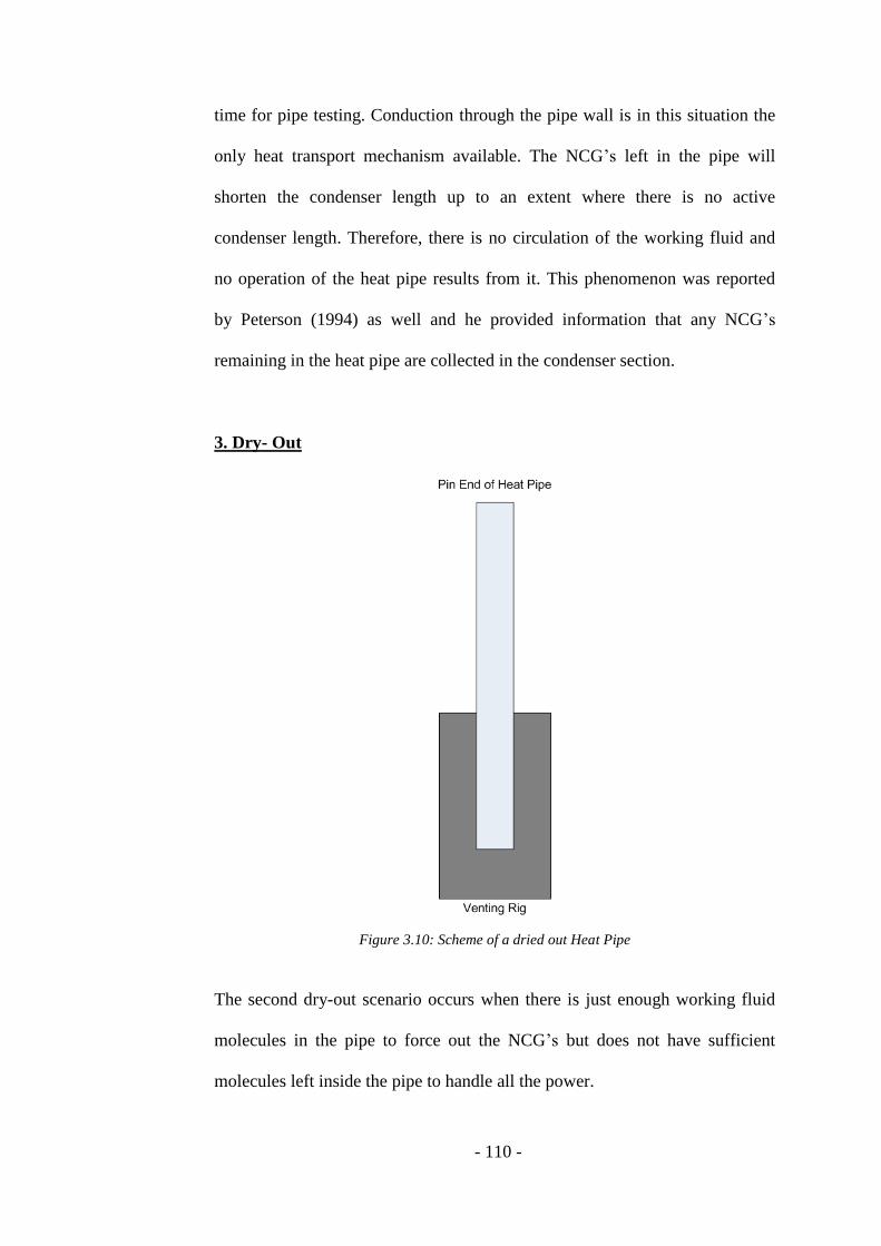
- 110 -

time for pipe testing. Conduction through the pipe wall is in this situation the

only heat transport mechanism available. The NCG’s left in the pipe will

shorten the condenser length up to an extent where there is no active

condenser length. Therefore, there is no circulation of the working fluid and

no operation of the heat pipe results from it. This phenomenon was reported

by Peterson (1994) as well and he provided information that any NCG’s

remaining in the heat pipe are collected in the condenser section.

3. Dry- Out

Figure 3.10: Scheme of a dried out Heat Pipe

The second dry-out scenario occurs when there is just enough working fluid

molecules in the pipe to force out the NCG’s but does not have sufficient

molecules left inside the pipe to handle all the power.

- 111 -

During tests, these pipes will perform very well at lower power input levels

with a low ΔT and stable operation at various inclination angles. At higher

power input levels, close to the design power, these pipes will start to show a

rising ΔT and eventually dry out. This dry out will cause components attached

to it, like heater blocks, to overheat and the heat pipes will not being able to

handle any power and will stop operating. However, the heat pipes will be

able to operate again after a complete cool down period.

4. Excess Fluid Charge

Figure 3.11: Scheme of a Heat Pipe with excess Working Fluid

An excess fluid charge occurs when the fill volume of the Heat Pipe was not

calculated correctly or there were less losses of the working fluid during the

venting process than anticipated. Also, the introduction of extra working fluid

- 112 -

due to inaccurate dispensing equipment or operator error during the charging

process will have the same effect as a high calculated fill volume. Upon

testing, the heat pipe will be capable of carrying the power as designed, but it

will have a high ΔT. When aligned at an angle, the pipe will show a high ΔT

and might even have erratic temperature behaviour at the evaporator section if

the pipe wall temperature is measured directly. Overall this scenario is less

critical than a drying out pipe, but still far away from a good performing pipe.

5. Ideal State

Figure 3.12: Scheme of a good Heat Pipe

The ideal state for a heat pipe filled normally shows a little bit of excess water

at the bottom of the pipe, but not too significant. This follows the guidelines as

proposed by Peterson (1994) to introduce between 10 and 20% overcharge,

although it is believed that this figure is too high for certain applications

- 113 -

where the pipes are subject to freeze/ thaw cycles, as well as shape changes

and angle inclinations. It can clearly be seen that there is no contamination or

any NCG’s left in the pipe. It is believed that this pipe which has full

saturation of the wick will perform well on the test rig and in applications.

3.5 SUMMARY AND CONCLUSIONS

Three different subjects were investigated within this chapter and are

presented above. Firstly the theory behind a calculation software for

calculating the fill for screen wick heat pipes based on geometrical wick

properties and venting temperature has been presented. The geometrical

properties of the screen wick are directly used to calculate the porosity of

screen mesh wick using equation 3.15 and combining that with the number of

wraps used and the venting temperature leads towards the required fluid

charge. This approach is seen as being quite novel as this has not been

presented in a similar form before and so has not been used before for larger

production batches of heat pipes and comparison with previous methods. Both

the material presented above and other work which has not been presented in

this section, indicates an accuracy of 7% between the theoretically determinate

fill and the experimentally concluded fill. That accuracy is seen as a vast

improvement and helps considerably to reduce the amount of experimentation

required to produce well performing heat pipes with significantly reduced

development time. Continuing this work has led within the second sub-section

towards the possibility of calculating the capillary or lifting height for a

particular screen mesh wick type and its ability to be used for operations

- 114 -

against gravity. That approach is based on the calculation of the capillary

radius (Eq. 3.24) and proposes that screen mesh wick heat pipes can be used

against gravity. From these results presented in Table 3.1 and practical

experience of the author it was concluded that screen mesh heat pipes can be

used for anti- gravitational operation as long as the heat pipe is not utilized to

a greater vertical length than its capillary or lifting height. Furthermore, these

calculations can be used to prevent the detrimental effects of “puddling”, the

collection of working fluid at the bottom of heat pipes operated with gravity,

on the ΔT observed during operation of the heat pipe.

Within the third sub-section, the most common errors during the venting

process, which is one of the most influential processes with regards to heat

pipe performance, have been described. This information is new to the

scientific community as most heat pipes just seem to appear from an

“unknown source” and the process variation effects on the performance of

heat pipes, even within the same batch, have either not been presented before

or are not considered at all due to the relatively small batch sizes that have

been investigated previously. This work can be used to explain the occurrence

of certain failure modes described in literature. Only the existence of these

failure modes has been described previously, but not the reasons why they

occur and how they are caused by the manufacturing process. From this point

of view it was extremely valid to undertake this work in order to be able to

produce heat pipes of the highest quality to then be subsequently investigated

with regards to the effects of bending upon heat pipes.

- 115 -

CHAPTER 4 – INVESTIGATION OF THE USE OF

DISSIMILAR SCREEN MESHES AS HEAT PIPE WICKS

This chapter reviews existing literature with respect to a single important

parameter of screen mesh wick heat pipes, the mesh count or number of

openings and tries to link changes to this parameter and mixing of different

layers of screen mesh wick to advantages in performance for certain industrial

applications, such as the ability to manufacture heat pipes with screen mesh

wicks with a particular low ΔT across the wick structure or to overcome

maximal operational angles for the application.

Figure 4.1: Scheme of the Screen Mesh used in Heat Pipes (ISO 4783-1, 1989)

Equation 4.1 below shows a relationship between the Mesh number per inch

and the wire diameter and aperture of the screen used (Brautsch & Kew,

2002):

dwN

1(Eq. 4.1)

- 116 -

Based on this definition, the use of dissimilar screen mesh types for multiple

layers of the wick was investigated. This work includes a review of existing

work on dissimilar screen mesh wick heat pipes, which is quite rare, followed

by a discussion of screen mesh parameters vital for the function of heat pipes.

These parameters are then compared with a statement found in literature

advising on the use of a certain combination of layers of screen mesh. Finally

the author’s own experimental results are used to validate or disproof the

content of the statement where the position of the finer screen mesh towards

the vapour space is promoted (Reay & Kew, 2006). From the results of the

experimentation it is also shown that the use of dissimilar screens meshes

inside heat pipes is not totally free of manufacturing barriers and that this part

needs consideration as well.

4.1 INTRODUCTION

Screen mesh is one of the oldest types wick structure used within heat pipes

and has been used since 1964 when Cotter, Grover and Erickson (1964) first

published articles about heat pipes as they are known today. However, with

today’s requirements of higher power handling and reduced space available,

screen mesh heat pipes are becoming a more attractive option for certain

demanding applications. Work presented here will show an investigation of

whether it is possible to engineer screen mesh wick heat pipes towards any

application by using a different composition of the screen wick itself or use

multiple layers of different types of screen wicks.

- 117 -

4.2 DISSIMILAR SCREEN MESH WICK HEAT PIPE

INVESTIGATIONS

This section of work can be seen as an expansion of the work presented in

chapter 3 and goes more into the detail of screen wick theory. Investigations

will review published work as well as own experimentation and determine

whether it is possible to tailor make heat pipes with screen mesh wicks to meet

the demands of certain applications like low ΔT along the heat pipes rather

than produce general “all-round” heat pipes suitable for most applications.

4.2.1 Design And Manufacturing Considerations For Dissimilar

Mesh Wick Heat Pipes

The point starting for this work was a paragraph in Reay and Kew’s book

(2006), which deals with the usage of dissimilar meshes within heat pipes. In

the book it is stated “In instances where two mesh sizes may be used in the

heat pipe say two layers of 200 mesh and one layer of 100 mesh, the liquid-

vapour layer must always be in the 200 mesh to achieve maximum capillary

rise. It is therefore advisable to wrap the 200 mesh over the end of the 100

mesh as shown in Figure 5.9. It is possible to locate the fine mesh against the

wall, where it will suppress boiling.”

The above statement has provoked various comments and discussions from

others involved in the heat pipe industry, these comments sometimes varied

significantly. Some agreed with the statement in the book whilst others were

to dispute it. Those disputing the statement stated two main objections against

having the finer mesh towards the liquid vapour interface. The finer mesh

certainly reduces the entrainment forces acting on the liquid returning to the

- 118 -

evaporation section of the heat pipe, however, there were concerns over the

statement. Firstly, the finer wick structure at the wall will positively support

the evaporation of the working fluid by providing a greater heated surface

area. Secondly, having the coarser mesh towards the liquid vapour interface is

seen to present less resistance to the evaporated working fluid vapour leaving

the wick structure due to the larger pore size and it offers better alignment of

fine wick to the wall due to the higher spring force provided for pressing the

wick against the wall due to the thicker wire diameter utilised. The likelihood

of vapour being trapped within the wick was reported as a major cause for heat

pipe failure and premature dry-out of the evaporator section, preventing the

liquid from returning into the evaporator, by Williams and Harris (2005)

investigating step-graded metal felt as wicks for heat pipes. Furthermore, they

have identified two limits to be critical to heat pipe operation, both of which

are directly linked to the wick. These limits are the capillary limit, which is the

ability of the wick to return the working fluid to the evaporator section and the

boiling limit, which is the wick’s ability to evaporate working fluid and allow

the two-phase heat transfer to happen. The second limit is influenced by the

wick’s pore size allowing the working fluid vapour to leave and the amount of

evaporation surface provided to reach its vaporisation temperature.

Brautsch and Kew (2002) present very interesting work on the two limits

mentioned by Harris and Williams (2005) and confirm their findings in a more

detailed way for heat pipe screen mesh wicks even using the same mesh

numbers as during the experimentation presented in a later section of this

work. They investigate the boiling and the wicking/ capillary limit as the main

limitations for screen mesh wicks and state that local dry-out is encouraged by

- 119 -

trapped vapour bubbles within the wick and this leads to a decrease in the

achievable heat transfer coefficient. This issue is caused by the reduced

available cross section of the wick and thus reduces the amount of returning

working fluid whilst at the same time increasing the pressure drop through the

wick structure. The finer the top structure, the more likely they found it to be

an obstacle for the bubbles to leave and therefore act as a vapour trap.

Additionally, they also confirmed that a fine wick structure applied to the wall

of a heat pipe enhances the heat transfer coefficient in comparison to the bare

surface. Depending on the temperature, the enhancement for a fine mesh is

greater than a coarser one, but the configuration is then more likely to suffer

from burnout or local dry-out. Interestingly, for the work presented here is

their use of high speed video equipment in conjunction with a dedicated

evaporation test rig visualising the evaporation process within screen mesh

wicks. Some examples of the visualisation at different heat fluxes are

presented in the Figures 4.2 – 4.5 below. The lighter the area of the

investigated screen wick behind the coarse carrier wick is, the less liquid is

contained within the wick, where the picture is white and shinny, it indicates

the wick is depleted of working fluid, whilst the grey shows vapour and the

darker patches are working fluid in its liquid phase. The exit of a vapour out of

the wick through bursting bubbles can be seen in Figure 4.4.

Figure 4.2: Wick with vapour leaving freely (150 Mesh with q =52kW/m2) (Brautsch & Kew,

2002)

- 120 -

Figure 4.3: Wick with vapour collecting in patches and depleting the wick of working fluid in

the top right corner (150 Mesh with q =137kW/m2) (Brautsch & Kew, 2002)

Figure 4.4: Close-up of a bursting vapour bubble (150 Mesh with q =137kW/m2) (Brautsch &

Kew, 2002)

Figure 4.5: Wick with dried out Areas on the top right side (150 Mesh with q =152kW/m2)

(Brautsch & Kew, 2002)

Based on all the findings from literature presented above it was concluded that

the only way to resolve the various differences would be to build some sample

heat pipes of each design and then test them. Based on work presented by

Kempers, Ewing and Ching (2006) stating that a higher number of mesh layers

does not in all cases support the heat transfer rate and general manufacturing

experience, two layers of mesh were chosen for the test sample. Further

calculation software developed by the author as part of previous work, has

been utilized to determine the theoretical optimum fill, and was used to

- 121 -

determine the fill for each design. The fill of each heat pipe was calculated to

ensure that the wick is saturated with working fluid. This method has been

based on work presented by Imura et al. (1988) and Imura, Kozai and Ikeda

(1994) but no provisions were made for over- charging as suggested by

Peterson (1994) by 10 to 20%. The main aim of this research was to determine

the influence of the wick and optimum thermal performance rather than aim

for high yield production heat pipes. All four papers, Kozai, Imura and Ikeda

(1991), Imura et al. (1988), Imura, Kozai and Ikeda (1994) and Kempers,

Ewing and Ching (2006) state, that they have found very little evidence of

negative effect of intermeshing between different layers of screen wicks. That

assumption was used for the fill calculations for these heat pipes as well as the

assumption that intermeshing is unique to each heat pipe and therefore cannot

be considered in theoretical calculations. When carrying out the calculations

with these parameters, it was found that the difference in fill between having

the 100 mesh wick at the wall and at the liquid vapour interface was minor and

only in the range of one thousand of a cc. That value is below the known

processing parameters for filling accuracy and venting of around 0.05cc and

therefore both sets of heat pipes were produced using the working fluid fill.

4.2.2 Experimental Results And Analysis Of Dissimilar Mesh Wick

Heat Pipe Investigations

The results presented below were obtained using a water cooled test rig with

two heater blocks and cold plates of the same design as shown in Figure 4.7

and a schematic indicating the instrumentation used in Figure 4.8. The heater

blocks and cold plates were transferring heat into and out of the heat pipe at

- 122 -

the top and bottom face in the horizontal orientation. In order to minimise the

number of variables for all the experiments, the heat pipe orientation was kept

constant at an angle of 0° (0° tilt angle). On the condenser end of the heat pipe

a Lytron RC006 recirculating chiller was used to supply the two cold plates of

1.5” x 2“ with a uniform cooling water flow of 25°C inlet temperature and a

flow rate of 0.001l/s. The thermal load was introduced into the heat pipe using

four electrical DC heater cartridges with a total capacity of 200W. These

cartridges were equally spread within the two copper heater blocks in order to

maintain an even heat flux at an acceptable level into the heat pipe. The

electrical power was monitored using a calibrated power meter whilst the

water flow was monitored using a contactless magnetic flow meter which is

directly logged via the same software which is used to log the temperatures.

Further details of the test rig used as well as some pictures and design

considerations can be found at a later stage of this thesis in Chapter 5, where

the results of the primary experiments are presented.

- 123 -

Figure 4.6: Entire Test Rig Setup

Figure 4.7: Schematic of Test Rig including Instrumentation used Flowmeter

Reciprocating

Chiller

Test PC Data

Logger

Test

Chamber

Power Supply

& Power Meter

Flow

Meter

Flow Bypass

System

- 124 -

In total eight different temperatures on the heat pipe external surfaces as well

as heater and condenser block and inlet and outlet water temperature were

monitored. These temperatures were the water in and outlet temperatures, the

test chamber ambient temperature, the heater and condenser diameter specific

adaptor block temperatures and the temperature on the heat pipe itself right in

front of the heater adaptor block, in front of condenser adaptor block and at

the heat pipe middle. Wherever in this work references to a ΔT of the heat

pipe are made, the temperature difference between the heat pipe temperature

right in front of the heater adaptor block and right in front of the condenser

block is considered. All heat pipes tested have been subjected to a single pass

test where the test conditions bar the heat load were maintained constant. The

tests took place in an insulated test chamber as shown without the front and

top insulation in Figure 4.6 and the incoming water temperature was

maintained at 25°C whilst the outgoing water temperature was measured and

used for the calculation of the heat load as described below. In order to be

independent form production variations, a batch size of 5 was tested for each

design as a single pass test per heat pipe. The results presented in Figures 4.8

are the thermal loads actually transferred by the heat pipes into the water and

are calculated using the energy equation (Faghri, 1995):

TcmQ p ** (Eq.4.18)

All the results presented are clear of any heat losses to the ambient and losses

across interfaces. Therefore, the thermal load results are lower than the values

for the electrical loads applied to the heater cartridges. The results presented in

Figure 4.9 show the average values per heat pipe type obtained from the

individual results presented in Figure 4.8.

- 125 -

Figure 4.8: Thermal load transmitted per sample and wick structure

From the results presented in Figure 4.8 above it can be seen that the

conventional two layers of 150 screen mesh wick heat pipes have, apart from

one exceptionally good pipe, a very consistent performance over the entire

batch size, whilst the other two designs appear to be more susceptible to

process variations. The sample 2 with 2 wraps of 150 Mesh seemed to be

performing significantly better than the other samples of that particular design.

The recorded transmitted thermal load is about 70% higher than the average

obtained from the rest of the results for that design and has therefore a

significant influence on the average thermal load value for that design. This

fact cannot be neglected and makes that design type look particular attractive

whilst in reality this may not be constantly maintainable for larger batch sizes

of that heat pipe type.

Both dissimilar screen mesh wick combination heat pipe types would need

some more process refinements to achieve their performance consistently. For

the 200 screen mesh wick at the wall design, only three heat pipes out of the

batch of five could be tested and judged using conventional criteria whilst heat

- 126 -

pipes 2 and 4 appeared to have Non-Condensable Gas (NCG) present. This

has resulted in a ΔT along the adiabatic section of around 10- 12°C and was

lowered towards 7°C for higher power levels when the dry-out of the

evaporator section occurred. The reduction of ΔT with rising power levels was

seen as being linked to the extension of the condenser length where the NCG

is compressed by the rising vapour pressure and therefore more thermal load

can be transferred out of the pipe at a risen power level.

Figure 4.9: Average thermal load transmitted per wick structure

From Figure 4.9 above, it can be seen that the 200 screen mesh wick at the

wall combination offers a marginally superior performance over the 100 mesh

at the wall combination but both are still below the performance of the well

established two layers of 150 screen mesh wick heat pipes. The reason for that

is seen due to the fact that heat pipes with two layers of the same screen mesh

have been produced in volumes of several hundred thousand to millions,

whilst the combination of two different screen wicks is still in its infant stage

and has not left the area of R&D applications yet. Furthermore, a statement by

Imura, Kozai and Ikeda (1994), states that the effects of intermeshing between

- 127 -

two screen layers has to be proved for heat pipes with two different screen

mesh layers inside.

The results presented above do not emphasise the fact that all the working heat

pipes with 200 screen mesh wick at the wall had a significantly lower ΔT

between the evaporator and condenser section and would therefore present an

advantage over the 100 screen mesh wick at the wall.

The results of the experimental analysis with respect to ΔT can be found in

table 4.1 below, which represents the analysis of the runs at a power level

which has been successfully completed as a stabilized run (1h duration) by all

heat pipe samples. For all of the 100 Mesh at the Wall samples the power

levels for these runs were lower by one 10W increment than for the heat pipe

with two wraps of 150 Mesh and the 200 Mesh at the Wall samples bar one

containing NCG.

Heat Pipe ΔT 150 Mesh 200 @ Wall 100 @ Wall

Sample 1 [°C] 0.25 2.52 5.58

Sample 2 [°C] 0.32 7.38 5.80

Sample 3 [°C] 2.12 4.82 12.96

Sample 4 [°C] 0.78 9.9 10.78

Sample 5 [°C] 0.15 2.10 6.28

Average [°C] 0.72 5.34 8.28

STD [°C] 0.82 3.30 3.38

Table 4.1: ΔT Results for all Heat Pipe samples including Standard Deviation

The results of table 4.1 can be found in graphical form below as figure 4.10. It

has to be pointed out that all samples with dissimilar wick inside have a higher

ΔT than the conventional benchmark samples with two wraps of 150 Mesh,

however non- NCG samples (1; 3; 5) of the 200 Mesh at the Wall type have a

lower ΔT than the 100 Mesh at the Wall type. Further it can be clearly seen

that these samples of the 200 Mesh at the Wall type as well as all conventional

benchmark samples remain below the 5°C limit used for the experimental

- 128 -

analysis in chapter 5; whilst all samples of the 100 Mesh at the wall have ΔT

values above this limit.

Figure 4.10: ΔT Results for all Heat Pipe samples including limit

The reasons for this trend and the fact that the 200 Mesh at the Wall samples

are performing better than their 100 Mesh at the Wall counter parts are

relatively hard to prove as the amount of produced and correctly working heat

pipes of the 200 Mesh at the Wall design was low, whilst the failure rate out of

that batch was very high at 40%. Further the failure modes of all the heat pipes

tested were different and could not be compared directly. For more definitive

proof, additional process and fill optimisation tests as well as experimentation

is required to clearly outline the advantages of having the finer wick aligned

on the wall. The additional direct comparisons of results of experiments for

heat pipes with two layers of the 100 screen mesh wick and 200 screen mesh

wick would complete this work and might be presented at a later stage in a

different format.

- 129 -

4.3 CONCLUSIONS

In this chapter, different combinations of screen mesh wick types were

experimentally compared and some potential for screen mesh wicks with

higher mesh numbers was found. Based on these findings and additional work

optimising the fill and manufacturing processes the possibility of tailoring

screen wick heat pipes towards certain industrial applications is envisaged.

However, there has to be a significant amount of additional work to be

undertaken, before dissimilar screen mesh heat pipes can reach the same

maturity as “normal” screen mesh heat pipes with layers of the same mesh

inside. This can be seen through the fact that, despite all the theoretical

considerations presented within this chapter, the performance in terms of

power handling for both types of dissimilar screen wicks was very close

together and no significant conclusions can be drawn from that yet. Further it

has to be considered, that only three of the 200 Mesh at the wall samples could

be used for the analysis of the test results as the other two had shown the

presence of NCG and no definite failure power level could be determined.

Therefore these results are seen as a bit weaker than for the batch of five heat

pipes with the 100 Mesh at the wall. Despite the drawn back and lack of

distinctive results at this very early stage, it should not be concluded that

screen mesh wick heat pipes with dissimilar mesh wicks inside do not have

potential but it should be aimed to prove their potential through continuation

of this work.

- 130 -

CHAPTER 5 – BENDING OF SCREEN WICK HEAT PIPES

Within this chapter theoretical investigations guiding towards the finalized

design of the heat pipes tested, and the results obtained during the

experimentation, will be presented. This chapter contains four major sub-

sections, the first one starts with some prelimary work carried out to identify

the setup parameters for the CFD runs and theoretical investigation on the

effects of bending on heat pipe performance, whilst the second sub section is

focused on the design of the test rig used to obtain the test results presented in

analysed form within the third sub section of this chapter. Within the first

section, various approaches on how to numerically capture the effects of

bending on the reduction of heat pipe performance are described. The second

section describes the design process of the test rig used for the

experimentation in great detail. The third section contains a detailed analysis

of the experimental results including failure modes seen during the

experimentation, plus the trends of performance reduction obtained from the

experimental runs. Further these results were compared to the CFD results

obtained in the first sub section. The fourth sub section is presenting an

approach to utilize the experimental results to develop an equation to predict

the performance of bent heat pipes.

The conclusions will describe why a numerical approach alone will never fully

capture the phenomena that can occur within a heat pipe which has been

subjected to bending, and in particular when the wick structure is a screen

mesh.

- 131 -

5.1 FLOW SIMULATION THROUGH PIPE BENDS

USING CFD SOFTWARE

This section presents an approach to simulate the effects of bends in heat

pipes. This work was undertaken after other approaches using different

commercial codes as well as self- programmed codes failed. All the

undertaken approaches failed to prove the capability of providing the required

accuracy. A number of different pipe geometries were investigated using the

same settings and models as used by the commercial CFD software. In total,

five different geometries were investigated. They were a straight pipe and

pipes with bend angles of 45°, 90°, 135° and 180°.

A commercially available CFD software named Star- CCM+ from cd-adapco,

a competitor of FLUENT, was used to carry out the investigation. This

software had to face the same challenges that other software like Fluent and

ICEPAK also struggled to compute. Star- CCM+ has its origin in the

automotive and oil and gas as well as offshore industry and offers in

comparison to FLUENT enhanced meshing and CAD geometry import

capabilities. The initial shape of the flow body (water film) investigated was

modelled using a CAD software called SolidWorks and then introduced into

Star-CCM+ via STEP CAD files, which could then be directly imported and

converted into solvable flow domains.

The main challenge was not the geometrical shape, but more the very thin

thickness of the water layer used in heat pipes. In order to be able to compute

- 132 -

the solution, theoretical assumptions simplifying the geometry had to be

undertaken. These followed well know heat pipe theory and will be described

in greater detail in the following sections of the chapter.

Through the progression of this chapter it will be outlined why CFD on a thin

film layer is very complicated and the results have to be reviewed carefully.

The various reasons why this is the case will be shown clearly.

Multiple CFD runs with various geometries and different model settings, as

well as different flow speeds, have been conducted in order to present a

rounded work package and validate the various models. It was found difficult

to model all the flow conditions to include all the required settings. In this

report only selected cases are presented, along with the theoretical part of

work carried out regardless of whether it was finally implemented into the

CFD software or not. This is included as it provided vital information required

for understanding the flow regime within a heat pipe.

5.1.1 Introduction Into Separate Phase Modelling Theory

In order to investigate the influence of bends on the performance of heat pipes,

a separate phase modelling approach was taken as currently there is no

mathematical model available representing the countercurrent liquid –vapour

interaction accurately.

It was assumed that the bend will occur in the adiabatic section of the pipe so

no heat transfer with the external environment occurs. Deriving from first

principles, the liquid film height was calculated for a certain operating

- 133 -

condition, and from there further calculations of the flow conditions like the

Reynolds number, Fanning friction Factor were taken. Attempts were then

conducted to accurately convert the results into an equivalent surface

roughness to represent an interface wall for the CFD model.

This was then used to calculate the power handling performance using the

results obtained from commercial CFD code based on the Star-CCM+ solver

engine from cd-adapco. The newly obtained results were then used to compare

the actual heat pipe limits with the mathematical model presented by Riffat et

al. (2004). This model allows the prediction of the operational limits in a

steady state condition, whilst transient start-ups of the investigated heat pipes

are much more complicated. From these limits a performance degradation

trend was hoped to be achieved.

For reasons of simplicity plain copper tube with no wick was modelled to

easily obtain a trend reflecting the effect of bends in a heat pipe. An attempt

was made to replicate the vapour- water interface using a wall including a

friction factor, which had to be determined before being used. This did not

prove to be successful since both roughness heights combined were found to

be greater than the actual film thickness obtained. This was due to

inaccuracies in the mathematical models used. Therefore a slip wall approach

was then undertaken. A separate phase modelling approach is a fairly common

technique used by the chemical industry but does not appear to have been

applied to this particular area of research.

- 134 -

5.1.2 Separate Phase Modelling

Separate Phase modelling is a widely used approach to investigate certain

areas of interest in fluid flow as well as utilizing the limited capabilities of

today’s CFD code on Two Phase Flow, especially if it is in countercurrent.

The most common approach to solve the thermo-hydraulics of single phase,

and especially the more complicated two-phase, flow models is separate phase

modelling. Typical characteristics of two-phase flow models are that they treat

the flow as steady, with a simplified geometry of the investigated flow

structure. They also use the conservation of mass, momentum and energy to

predict the thermodynamic properties of the flow.

The attractiveness of this type of model is their broad applicability as well as

being able to be used with 1-D models as well as 2-D models (Fu & Klausner,

1997). Further to this the 1D- model approach has been known for some time

and was introduced by Hewitt and Hall-Taylor (1970 cited in Fu & Klausner,

1997), who widely discussed the ability of these models.

The approach taken for this work was one of separated flow 1-D models for

the vapour core and liquid film and then coupled through closure relations

applied to the liquid vapour interface. This was attempted and shown as a wall

in the CFD model.

In many cases of previous works the interface between the liquid and the

vapour of air are treated as hydraulically smooth which means that they are

considered not to add any additional friction to the flow. It will be shown later

in this work why this had to be adapted, as had been done by fellow

researchers.

- 135 -

The ultimate aim of the work carried out was to develop a simple easy-to-use

tool to predict the performance, and performance degradation, of heat pipes

under various operating conditions as well as being subjected to shape

changes.

5.1.3 Calculation Of Flow Parameters

5.1.3.1 Liquid Film Height Calculation

In order to predict the liquid height/ film thickness in the adiabatic section,

where the bends are assumed to take place, it was assumed that the heat input

in the evaporator section is only through the wall of the tube. Following well

established models the assumptions were made that the liquid film thickness is

uniform around the wall as well as the flow is steady. Further, no change of

thermodynamic properties, like extra evaporation within the adiabatic section

and a uniform radial pressure, are assumed.

- 136 -

Figure 5.1: Scheme of Liquid Film Height (Fu & Klausner, 1997)

The starting point for this calculation was the Conservation of Energy

equation which states that vl QQ . From there, the Continuity equation was

introduced to this which states 222111 **** uAuA (Hewitt, Shires &

Bott, 1994). In order to be able to resolve this equation, further assumptions

were required in absence of known operating conditions for the heat pipe.

Therefore, it was assumed for simplicity reasons that the velocity of the

vapour is equal to the velocity of the liquid, gl uu . This supports the closed

loop system theory for a heat pipe and allows the use of the separate phase

modelling theory, which was used to determine the pressure drop difference

due to a change of geometry.

Introducing these two statements into the continuity equation, plus applying it

to the two fluids involved in the problem investigated, guides towards the

derivation of equation 5.1 shown below.

- 137 -

)(*

vl

loi dd

(Eq. 5.1)

In order to be able to obtain accurate data for the previous equation, the

equation 5.2 below has to be applied to data from the reference books

(Houghton & Brock, 1975; Rogers & Mayhem, 1995).

g

v

1

(Eq. 5.2)

Applying these two equations guides towards a liquid film height, which is

dependent on the temperature of the surrounding wall. Therefore it is shown

that the liquid film height for a given diameter of tubing is dependent on the

wall temperature and that the flow regime is largely depending on that input,

as well as the assumed velocity in the pipe. It was proved that this liquid film

height is below the peak height of the surface roughnesses and can therefore

not be used for numerical computation. Instead, the wick thickness where the

working fluid returns was intended to be used for computation of the pressure

required to overcome the bend. This will be described in greater detail in

section 5.1.4 of this chapter.

5.1.3.2 Reynolds Number Calculation

The dimensionless Reynolds number used in fluid mechanics is an indicator

for the flow regime applicable to a certain set of conditions in pipe flow.

Being one of the most important dimensionless numbers used in fluid flows, it

provides a criterion to determine dynamic similitude of different flows.

Unequal flows of different liquids can have the same Reynolds numbers,

- 138 -

whilst the liquid velocity and the pipe diameter are different, but the behaviour

is judged dynamically similar.

The Reynolds number is physically the ratio of inertial forces to viscous forces

and therefore consequently quantifies the relative contribution of these two

types of forces to a certain flow regime. Inertial forces in pipe flow are

represented by mean fluid velocity multiplied by density of fluid whilst the

viscous forces are incorporated through the ratio dynamic fluid velocity

divided by the hydraulic diameter. As heat pipes are most commonly round

and the hydraulic diameter for that geometry is equal to round pipe diameter,

this was used. Further considerations need to be taken into account for other

shapes like stadium shaped pipes.

There are three main flow regimes occurring within pipes: For very low

Reynolds numbers, which are smaller than 2300, the flow is laminar. Laminar

flow is characterized through smooth, constant fluid motion. At this flow

regime, viscous forces are the dominant ones. The more common flow regime

in pipes potentially used as evacuated containers such as heat pipes, is the

turbulent flow regime. This is considered for Reynolds numbers bigger than

3000 where inertial forces dominate the flow. Within this flow all sorts of flow

fluctuations like vortices and random eddies can occur. This flow regime can

be completely described mathematically. The most complicated flow to

describe scientifically is the transient flow for Reynolds number regions

between 2300 and 4000. The exact transition can only be determined through

experiments of the flow conditions for each particular case. In order to avoid

- 139 -

that sort of problem the Reynolds number range between 2300 and 4000

where the flow is neither fully laminar nor fully turbulent is generally avoided

when designing a system. For circular pipes as often used for heat pipe

applications the transition is around 2300. At this point the flow is dependent

on the pipe diameter as well as the mean velocity in the pipe. Deriving of this

equation will guide towards the equation (Eq. 5.3) used below for calculating

the Reynolds number for the application simulated.

The Calculation of Reynolds number is a straight forward calculation

following the equation proposed by Osborne Reynolds (1883):

l

hll du

**Re (Eq. 5.3)

In order to use the available data for the two liquids involved in the

simulation, the properties of water and air were assumed in order to simulate

the vapour. Where properties like kinematic and dynamic viscosity are not

both available at the same time, the missing parameter can be calculated using

the following equation:

lll v* (Eq. 5.4)

The density of the working fluid as a temperature dependent variable is

obtained from the following reference data books (Houghton & Brock, 1975;

Rogers & Mayhem, 1995). The tables of Rogers and Mayhem (1995) are

widely used in any thermodynamic area and were applied as source for the

base material data for that very reason. As the average velocity was seen as an

unknown value, which can vary from very low values up to sonic velocity for

the vapour flow, a velocity was chosen which places both flows into the area

- 140 -

of turbulent flow. In order to keep the thermodynamic cycle working and to

justify the assumption that the separated flow modelling the vapour velocity

was equal to the velocity of the water travelling into a countercurrent

direction.

For the calculation of the Reynolds numbers of the flow an average surface

roughness for drawn Copper tubing, which is widely used as container

material for heat pipes, was assumed to be 0.0015mm (Anon, 2005). As shown

by Romeo, Royo and Monzó (2002), this might introduce an error into the

calculation, but this error seems to be negligible in consideration of the

accuracy of currently available CFD codes.

Further percentages of the error introduced can be found in Fig. 5.2 below.

Figure 5.2: Error in dependence of the Reynolds number (Romeo, Royo & Monzó, 2002)

It can be seen clearly from this figure that the introduced error is less than

0.1% and so small that it will not have a significant influence on the overall

error occurring when carrying out this numerical iteration. Due to different

definitions of the different parameters, it has proved to be impossible to finally

convert the equivalent surface roughness of Romeo, Royo and Monzó (2002)

- 141 -

into an equivalent surface roughness as per definition of Figure 5.4 of this

chapter, where it is a geometrical value of the boundary of the fluid passing

along it.

5.1.4 Theory Used For Obtaining The CFD Settings

In order to be able to obtain the CFD boundary settings for Star – CCM+, the

following theoretical approach was undertaken to gain the values used as

inputs:

1. The maximum axial velocity in the adiabatic section, where the bend

is, was obtained following a method proposed by Zhu and Vafai

(1999). The use of this method has guided towards the following

equation:

22***)(

vwfgl

lrrh

Qxu

(Eq. 5.5)

This equation was derived by implementing equation (9) and (23) into

equation (21) of the work of Zhu and Vafai (1999). In order to be able

to solve the equation, the maximum transmittable power Q was

obtained through the use of Thermacore priority software and has

worked out to be 176 W for a pipe of the same geometry and

orientation. Implementing this as well as all the other parameters leads

towards a maximum axial liquid velocity of 0.0122m/s. In order to deal

best with the settings in the CFD software this was converted into a

mass flow rate of 0.000179kg/s, which was set as a boundary condition

in the mass flow inlet face for the first case with annular flow.

- 142 -

For second case with full flow the same liquid velocity was used but

due to the changed geometry it has guided towards a new mass flow

rate of 0.001241kg/s. For all cases, the interfacial effects between

liquid and vapour have been neglected.

From Figure 5.3 it can be seen that the accuracy of that assumption is

seen appropriate for settings implemented into CFD code:

Figure 5.3: Comparison of the models including and excluding interfacial effects

(Zhu & Vafai, 1999)

Following these results the internal wall boundary has been set to be a

friction-less slip wall and has no significant influence on the flow,

apart from guiding the liquid along the geometry. This setting is a

standard within CFD code like Star- CCM+ for investigating pressure

drops within geometries.

2. The outlet is set to be a pressure outlet and the pressure at the outlet

was set to be 0.2501bar. This is equal to the saturation pressure for

- 143 -

65°C temperature. Assuming a perfect vacuum in the pipe this is the

minimum pressure in a fully operational pipe at that temperature.

Therefore this assumption can be seen as perfectly valid following the

theory of heat pipes.

3. The external wall is set to be a rough wall with a surface roughness of

0.0015mm which is a common value for drawn copper pipe as used for

heat pipe container material. The surface roughness was obtained from

an engineering web source for drawn copper pipe (Anon, 2005). In this

application a constant surface roughness as per definition of Engineer’s

Edge (2006), flat along the length of the wall, is assumed.

Figure 5.4: Definition of Surface Roughness Height (Engineer’s Edge, 2006)

The effects of different surface roughness have been investigated by

Romeo, Royo and Monzó (2002) but this investigation was only

conducted on straight pipe samples with a full flow regime rather than

only a thin layer of water along the wall. Therefore, their approach

cannot really be seen representative for heat pipe applications.

- 144 -

4. In order to take the different evaporation and condensation rates along

the evaporator and condenser length into account, the theory of the

effective length was used. This means that only half of the evaporator

and half of the condenser length will be added to the adiabatic length

of the heat pipe. This theory is widely used in heat pipe applications

(Reay & Kew, 2006) and was used in this application in order to get rid

of the very sharp edged triangular feature as shown in Figure 5.1 at the

evaporator and condenser end of the pipe. This allowed a far more

solid and solvable geometry for the CFD software before meshing. It

also guided towards a far better grid, as it limited the number of cell

types down in that area towards rectangular ones which can be much

easier solved than others. Figure 5.5 shows the achieved grid as well as

the prism layers.

Figure 5.5: Mesh quality and Prism Layer number

- 145 -

5.1.4.1 Flow Models and Boundary Conditions used

In order to obtain meaningful results multiple runs with different settings were

performed. These varied from the theoretical settings in order to overcome the

lack of mathematical models of dealing with the real time situation in the heat

pipes.

5.1.4.2 Settings as per Heat Pipe Theory disregarding Validity of

Mathematical Models for certain Flow Conditions

For the simulations carried out, all different geometries replicating the bent

heat pipes were investigated using the same settings and models in the CFD

software, allowing a direct comparison of the results and show the

performance difference due to the bends. The only variation between the

different simulation cases was the freshly imported CAD geometry. This was

introduced into the CFD software via STEP files.

- 146 -

Figure 5.6: Meshing models and Physics models used

Figure 5.6 shows the actual models used for the simulation, both the Physics

models specifying the fluid used for the simulation, as well as the meshing

models, used to create the grid. The grid generated is shown in Figure 5.5,

whilst all the settings used can be found in a table format below as table 5.1.

- 147 -

Common CFD Settings used for both Flow Types

Meshing Models:

Surface Remesher

Trimmer

Prism Layer Mesher ( Setting 5 Prism layers at T=0.1mm

max)

Physics Models:

Three Dimensional

Stationary (instead of moving Coordinate System)

Liquid (H2O) as per Working Fluid in Heat Pipe Samples

Segregated Flow

Constant Density

Steady (instead of Transient)

Turbulent

Reynolds- Averaged Navier- Stokes

K-Epsilon Turbulence

Realizable K-Epsilon

High y+ Wall Treatment

Boundary

Conditions:

Inlet:

Inlet Temperature set at 65°C

Constant Mass Flow set to reflect Mass Flow Rates for:

Annular Flow: 0.00018kg/s; Full Flow: 0.00124kg/s

Inlet Pressure is the obtained Parameter

Outlet:

Pressure Set to be 25010Pa (Saturation Pressure at 65°C)

Outside Wall:

Surface Roughness: 0.0015mm (for Drawn Copper Tube)

Wall Temperature to be set at 65°C

Inside Wall: Annular Flow only

Set to be a frictionless "Slip Wall" used for Fluid

Guidance

Table 5.1: Models and Boundary Conditions used for CFD investigation

- 148 -

Table 5.1 above lists all the models and boundary conditions used to obtain the

results for the two different flow types run and presented at a later stage of this

chapter. The meshing models used were the Trimmer type in order to improve

and make the imported CAD geometry more handlable. The Surface

Remesher was used to improve the initially generated surface mesh before the

volume mesh was generated. The Prism Layer Mesher was an essential tool to

be used for this simulation due to this part geometry.

As the emphasises of this investigation was on the effects of the bends onto

pipe performance, it was seen vital to have a high number of prism layers in

order to be able to get accurate results of the pressure required in the inlet

section. This pressure was required in order to overcome the effects of the wall

surface roughness, as well as the effects of the bend itself. Even if the flow is

laminar, a turbulent model has to be used in order to be able to set up a wall

surface roughness, as the laminar model does not allow any wall roughness to

be set up. From the available models the k-ε turbulence model was chosen. In

accordance with the work of Lacasse, Turgeon and Pelletier (2004), this model

is capable of delivering adequate results as long as the geometry is not too

complicated.

Even with geometry to be seen relatively simple, due to the bends, a Three-

dimensional model had to be used. A large proportion of the remaining

Physics models guided towards themselves with regards of the conditions

within the heat pipe to be investigated. As the most common working fluid

used for heat pipes is water, the liquid investigated representing the working

fluid had to be water. Per heat pipe theory, no heat transfer takes place in the

adiabatic section, where the bends are located. Therefore the use of a constant

- 149 -

density model with changing geometries replicating the bent heat pipes was

seen adequate for these simulations. As per separate phase modelling theory, it

was entirely focussed on the liquid phase (water flow along the heat pipe wall)

and circulation as occurring inside a heat pipe was represented through the

constant mass flow rate into and out of the control volume (geometry used).

Further the choice of the k-ε turbulence model has led itself towards more

settings in the software which were exclusive defaults for the model used.

Assumptions made previously have been used in the same way as CFD

analysis of flows in pipes has been conducted by Fu and Klausner (1997). The

main difference was the geometry and diameter of the pipe. Most applications

previous investigated are from the field of chemical engineering. Therefore the

pipe diameters investigated as well as the flow regimes can not be directly

linked to heat pipe applications since in chemical engineering pipe diameter

are rather large and flow regimes are mostly turbulent .

In order to improve the run time and the accuracy, this model setup followed

and approach by Löhner et al. (2006), where it was emphasised to use the

steady state solver as well as reduce the pressure iterations. As the inlet

pressure required for overcoming the wall resistance was the criteria

investigate, this step towards run time reduction of the model has not been

undertaken. But already the use of a steady state solvers, as well as different

other setups reduced the runtime of the model down to about 45min. This can

be seen as adequate for a model with a similar mesh count used on a standard

PC (Cd-adapco, 2007). A further reduction of the runtime was achieved

though a reduction of iterations from 1000 down to 500. This was seen

adequate as the model converges, depending on the geometry, between 80 and

- 150 -

100 iteration steps. Therefore 500 iterations will give sufficient time to let the

model fully reach steady state as well as achieve the engineering values like

pressure, to be solved satisfactorily.

Star-CCM+ 2.06 offers a multiphase solver but as the accuracy of the single-

phase solver already reaches the limits for a very thin featured object like the

one investigated. The use of a multiphase model would have only added

towards the results inaccuracies. Added to this there are no accurate

predictions of the interfacial friction factors available. Therefore the use of

that model has not been seen beneficial and therefore not performed.

5.1.5 CFD Results And Result Plots

5.1.5.1 Results And Plots From Runs Of Annular Flow Per Heat Pipe

Theory

Results from Initial Runs in Accordance to Heat Pipe Theory:

Plots for the pressure distribution and velocity of the fluid can be found in

appendix A of this thesis whilst the numerical results for the annular flow are

presented in the Table 5.2 below:

Analysis of Initial Runs:

Pressure at Outlet Ps 25010 Pa

Bend Angle

Pressure required at Pipe Inlet dP

Deviation

0° (0) 25744.07 Pa 734.07 Pa 0.00 %

45° (π/4) 25732.97 Pa 722.97 Pa 1.51 %

90° (π/2) 25732.2 Pa 722.2 Pa 1.62 %

135° (3π/4) 25719.84 Pa 709.84 Pa 3.30 %

180° (π) 25728.15 Pa 718.15 Pa 2.17 %

Table 5.2: Pressure Values as given by the CFD Software

- 151 -

Figure 5.7: Differential Pressure inside the Pipe including the Error bars

Figure 5.8: Total Deviation from Straight Pipe Value

This analysis and the later one were performed in a way that the deviation

within the pipe was assumed to be added to the pressure available on the outlet

end of the pipe. This is equal to the saturation pressure for water vapour at the

- 152 -

set temperature of 65°C. For analysis purposes, the value of 0.2501bar or

25010Pa was subtracted after the results of the simulation were obtained. The

internal resistance value for the straight pipe was then taken as a 100%

benchmark value. All results for bent pipes were then compared to the value of

the straight heat pipe and the absolute deviation was obtained. A significant

outcome from this was that all the results for the bent pipes were lower than

the result for the straight pipe. Numerous re-iterative runs even with new

models have been conducted and have proved that result. Therefore it was

assumed that the initial geometry cannot be investigated using current CFD

software. In order to obtain meaningful results, an approach investigating a

full pipe flow with the same liquid velocity was undertaken. These results can

be seen in the next section of this report.

5.1.5.2 Results And Plots From Runs Of Full Pipe Flow At Flow Velocity

From Heat Pipe Theory

The runs presented are performed with a flow velocity which is obtained from

the heat pipe theory but the flow rate is adapted to cater for the larger cross

section area that the water is going through. Therefore the mass flow rate was

adapted adequately to maintain a velocity of 0.0122m/s and the increased open

area of the liquid. Plots for the pressure distribution and velocity of the fluid

can be found in appendix A of this thesis whilst the numerical results for the

annular flow are presented in the table 5.3 below:

- 153 -

Analysis of Runs with Full Pipe Flow and Flow Velocity from Heat Pipe

Theory:

Pressure at Outlet Ps 25010 Pa

Bend Angle

Pressure required at Pipe Inlet dP

Deviation

0° (0) 25014.16 Pa 4.16 Pa 0.00 %

45° (π/4) 25014.24 Pa 4.24 Pa 1.92 %

90° (π/2) 25014.36 Pa 4.36 Pa 4.81 %

135° (3π/4) 25014.43 Pa 4.43 Pa 6.49 %

180° (π) 25014.5 Pa 4.5 Pa 8.17 %

Table 5.3: Pressure Values as given by the CFD Software

Figure 5.9: Differential Pressure inside the Pipe including the Error bars

- 154 -

Figure 5.10: Total Deviation from Straight Pipe Value

This analysis shown in Fig. 5.10 indicates that the effects of bends in heat

pipes can be investigated using commercial CFD and separate phase

modelling but also shows that the performance deviation from a normal round

pipe due to changed geometry is very minor. It is in total a deviation of a

maximum of 0.34 Pa from a straight pipe to a 180° bent pipe. The results

presented in figure 5.9 oppose in a direct way the results presented in figure

5.7, which are seen as unrealistic and conflictive to well known hydraulics

theory where bends or elbows increase the pressure drop of the system and

should be avoided. Therefore it can only be concluded that the results

presented in figure 5.7 suffer from the lack of the ability of current CFD

software to cope with the simulation of thin liquid films and can therefore be

seen as error loaded. Based on that, the full flow case was used to investigate

the effects of bends on the overall pressure required.

- 155 -

Figure 5.9 clearly indicates through the use of 10% error bars that the pressure

changes, due to shape changes of the geometry investigated, are minor in

comparison to the total achievable accuracy of CFD (Shao & Riffat, 1995).

In reality these effects might be much bigger due to effects described later in

the conclusions.

5.1.6 Creating The Link Between The Pressure Results From The CFD

Model And The Experimental Results

The key to comparison of the simulation results with the experimental results

is the link in between them. In order to create this link and validate the

separate phase modelling theory applied for the CFD runs presented above, the

heat pipe theory needs to be fulfilled. The key parameter seen responsible for

the degradation of the performance in a heat pipe due to bends is the capillary

limit or more specially the capillary pressure. The capillary pressure allows the

working fluid to return to the evaporator and be available for further

evaporation. A reduction in capillary pressure due to a bend would result in

less liquid in the evaporator and therefore reduce directly the maximum

transmittable power.

Starting this work on the theoretical side guides towards a minimum condition,

which needs to be fulfilled in all cases to allow the heat pipe to function, that

is the capillary pressure condition (Reay & Kew, 2006):

PgPPP vlc max (Eq. 5.6)

Applying the test conditions of 0° operational angle for the experiments allows

the following simplification of Equation 5.6:

- 156 -

vlc PPP max (Eq. 5.7)

This simplification is seen suitable for both, the CFD runs and the experiments

where the conditions were always horizontal. Therefore the wick inside the

heat pipe did not have to overcome any gravitational heads. In the horizontal

orientation of the heat pipes tested the screen mesh wick only needed to

overcome the liquid resistance in the wick and the resistance of the vapour

pressure preventing the liquid from returning to the evaporator.

In order to establish the maximum condition rather than the real condition,

heat pipe theory has been consulted once more. Starting from equation 5.7

above, the maximum available capillary pressure needs to be known in order

to be compared to the liquid pressure and vapour pressure produced. Peterson

(1994) states the maximum condition for the capillary pressure to be obtained

when the contact angle is zero, this guides towards the following equation:

c

Cr

P2

max (Eq. 5.8)

The value for the surface tension can be obtained from the National Physics

laboratory for air to water and are available in the nomenclature. Instead of

using the description for the capillary radius provided with the equation, the

later and more accurate description for the capillary radius of Kozai, Imura

and Ikeda (1991), which has been already used in chapter 3 of this thesis, is

used. This guides towards a maximum available capillary pressure for the used

wick structure and water as a working fluid at 60˚C of 2423.19Pa.

For the liquid pressure drop ΔPl a form of Darcy’s law can be used in

accordance to the heat pipe book of Reay and Kew (2006):

- 157 -

KA

mlP

l

effl

l

(Eq. 5.9)

Equation 5.9 above is seen valid for homogeneous wicks such as screen mesh

wicks and is linked to fluid parameters such as the dynamic viscosity, the mass

flow rate and the density of the working fluid. These fluid parameters are

temperature dependent, but for comparison between CFD results and

experimental results a constant temperature of 60˚C was chosen to obtain the

values, and that assumption was maintained throughout the analysis. The mass

flow rate was chosen to be the same as in the separate phase flow model. This

was used to obtain the pressure difference in order to be able to have a direct

link or chance of comparison between experiments and CFD runs, rather than

relating back to the heat pipe theory. Further, there is only one additional

parameter, which is the permeability K, required in Equation 5.9 above, which

can be obtained from the empirically analysed data presented in chapter 3 of

this thesis. The permeability K is defined (Faghri, 1995; Peterson, 1994) as:

2

32

)1(122

*

dK (Eq. 5.10)

Both, the wire diameter of the screen wick used and the way the porosity of

the screen wick is calculated have been presented earlier leaving only

additional constants to be added into the equation.

Using the mass flow rate of 0.000179kg/s for the annular flow case guides

towards a maximum capillary pressure of 4891.83Pa. For the full flow case the

mass flow rate is 0.001241kg/s leads to a maximum available capillary

pressure of 33920.31Pa. Since the second value is obtained for a simplified

model to increase accuracy of CFD software, this condition cannot be seen as

realistic in terms of heat pipe theory and is therefore discarded.

- 158 -

A further description of the liquid pressure inside the wick dependent on the

heat load (power) transmitted can be found at equation 2.30 in Reay and

Kew’s book (2006), which states:

fglcvw

effl

lhrrr

QlP

222 )(

8

(Eq. 5.11)

All parameters within the equation are either known or their derivations have

been earlier described. In comparison to Equation 5.10, this equation is

depending on the transmittable power rather than the mass flow rate inside the

heat pipe. Through the link shown in the equation towards the transmittable

power, it can be used in two different ways. One is to gain from the flow/

pressure drop CFD analysis, a maximum transmittable power for that heat pipe

configuration, and the second would be to obtain the liquid pressure inside the

pipe from analysis of experimental results. Due to the assumptions made,

despite their better logical correlation, the full flow results have not proved to

be realistic and do not coincide with the heat pipe theory. Their sole purpose

was for increased computational accuracy. However, the pressure drops along

the heat pipe wall are unrealistically low with a range increasing from 4.1 to

4.5 Pa obtained through the CFD software. This indicates a transmittable

power around 0.75 W, which is not realistic.

Since the calculated differential pressure inside the wick and the maximum

available pressure drop are know, only the vapour pressure drop needs to be

known in order to be able to quantify if Equation 5.7 is fulfilled. For the

vapour pressure Faghri (1995) provides the following expression for the total

vapour pressure drop occurring using a “generalised similarity closed-form

approximation”:

- 159 -

eff

vfgv

vav l

rh

QP *

84

(Eq. 5.12)

Using values for the vapour constants assuming full saturation from Rogers

and Mayhem (1995) guides towards a vapour pressure of less than 1 Pa for all

the experimental cases described at a later stage. Therefore the vapour

pressure drop was seen negligible to the overall result for this investigation

and the condition from equation 5.7 seems to be fulfilled at any point of the

experiments conducted.

Deriving the equation towards heat load leads to the following equation:

effl

fglcvwl

l

hrrrPQ

8

)( 222 (Eq. 5.13)

Using the equation above in combination with the pressure results for the

differential pressure obtained from the annular flow run, which range from

709 to 734Pa guide towards a maximum transmittable power of 122W. That

correlates approximately with the maximum thermal power transmitted within

the experiments of 87.34W for the straight sample 2.

Unfortunately, these equations are all one dimensional and do not allow to

compensate or cater for any bends etc. Therefore, only direct correlation could

be made between the results of the equations and the experimental results for

the straight heat pipe cases.

Both methods described either relied on an assumed input or empirical or

experimentally obtained results.

Using the equation stated by Reay and Kew (2006) presented above for the

pressure drop gives good correlation for the straight heat pipe case between

the thermal power transmitted by the heat pipe, and the pressure drop obtained

- 160 -

for the annular run. The accuracy is within 33% of each other. It was not seen

appropriate to compare the results of any other cases apart from the straight

heat pipe as the equation used for the pressure drop does not have any

provisions for bend angles. Overall the correlation between the CFD results

for the straight case with annular flow and the experimental results for the

same pipe geometry differ by a factor of 2. That factor could be reduced by

lowering the flow rate or velocity and introducing an appropriate porosity into

the CFD model. Further, the accuracy of the CFD correlation could be

improved if scaling along a non straight axis were possible in the CFD

package used, as more cells along the perimeter could be introduced.

- 161 -

5.2 TEST RIG DESIGN FOR BENT HEAT PIPES

5.2.1 Purpose Of The Test Rig And Introduction To The Principle

A test rig specially designed for the characterization of heat pipes and testing

of bent and/ or flattened heat pipes was commissioned and can be found in

Figure 5.11 below. The test rig contained a number of DC cartridge heaters

evenly distributed through the top and bottom heater block capable of

providing 200W of heat on the heat input side. On the cooler side two standard

Thermacore Porous Metal cold-plates were provided to remove the heat.

These cold plates are normally used for CPU cooling and therefore are capable

of removing 75W each. Their size is 1.5” x 2”. The coolant flow was

provided by a re-circulating chiller combined with an electro-magnetic flow

meter as well as a bypass system to compensate for excess liquid to be

pumped through the cold plates. This was necessary as a too high pressure

drop through the system would stop the chiller from working. Further a paper

cartridge filter was implemented in the system to collect any occurring

particles in a set location and prevent the cold plates from becoming clocked

up. Two thermocouples, one in the inlet stream and one in the outlet stream of

the cold plates were put in place in order to get the energy balance controlled

and to obtain a failure rate between heat input and output.

- 162 -

Figure 5.11: Entire Test Rig Setup

5.2.2 Instrumentation Used

Computer

Bypass System

Test Rig Scheme PhD Test Rig

Power

Meter

DC

Flow Meter

Reciprocating Chiller

Data Logger

Heat Pipe

Filter

Test Chamber

Cold PlatesHeater Blocks

Figure 5.12: Scheme of Test Rig Setup including data- logging and controls Flowmeter

Reciprocating

Chiller

Test PC Data

Logger

Test

Chamber

Power Supply

& Power Meter

Flow

Meter

Flow Bypass

System

- 163 -

Figure 5.12 shows a schematic test rig setup including the instrumentation,

data logging equipment, thermocouple positions as well as controls applied.

The data logging of the temperatures on the rig is performed by one single

eight channel USB data logger (Pico TC-08 USB) onto a PC dedicated for this

experiment. The initial data including the separate signal from the flow meter

is transferred into Microsoft Excel for further post processing and analysis.

The data logging logs temperature readings directly whilst the flow meter

input is in micro-volts which is re-converted into a volumetric flow rate by the

data logging software.

The heat input is conducted via a DC power supply being capable of

transmitting 200 W and the power level is controlled in addition to the

numerical displays on the instrument itself, via a Power meter, which can also

be fed into the PC via a serial cable. The control level allows monitoring at

two decimal places which can be seen as accurately enough. The flow rate is

automatically recorded during the test duration via a serial input after the

signal has been transformed into a readable format of micro-volts via a data

converter. The flow rate will be determined by the pressure drop through the

cold plates and therefore a pressure drop free flow meter as the

electromagnetic one used is seen to be beneficial.

For heat pipe performance monitoring as well as obtaining temperature

readings of ambient and water inlet and outlet temperatures T-type

thermocouples are used as standard sensor probes. These are manufactured on

site and calibrated using thermocouple calibration equipment. For the

temperature range monitored, T-type thermocouples with a maximum

measuring junction temperature of 300°C are seen to be sufficiently accurate

- 164 -

and offer less deviation than other thermocouples. T-type thermocouples only

a have a tolerance of +/- 0.5°C whilst the accuracy of K-type thermocouples is

three times as low with a tolerance of +/-1.5°C. There are no standard

thermocouples available offering a greater accuracy apart from Platinum

resistance ones which are seen as too expensive for this purpose.

5.2.3 Water Side And Cold Plates

The water side of the test rig consists of a recirculating chiller providing

coolant flow through an electro-magnetic flow meter (Promag 30A) into two

porous metal cold plates which are a standard Thermacore product designed

for CPU cooling capable of removing 75W each. The cold plate itself is shown

in Figure 5.13 below, whilst Figure 5.14 visualises the function principle and

inner structure of the cold plate. At a later stage, within Figure 5.15 below, the

arrangement within the rig, containing the two cold plates and their

surrounding insulation and mounting blocks are shown.

Further the system is equipped with a bypass system allowing excess water to

get into the return stream and therefore keeping the systems pressure on the

inlet side at a lower level and preventing the chiller from operating the

overpressure/ blocked- system switch. Ultimately the achievable flow rate of

the given system is determined by the pressure drop through the cold plates.

The flow through the cold plates can be controlled in a very accurate manner

through a needle valve directly inserted in the inlet pipe upstream from the

paper filter prior to the cold plates. The exact flow arrangement has been

shown in the Figure 5.17.

- 165 -

The temperature of the inlet and outlet stream is measured through two

thermo-couples, one embedded directly into each liquid stream. The

arrangement of the flow thermocouples is shown in Figure 5.16 below. Due to

the operating temperature range of the cooling system and the capabilities of

the chiller as well as the absence of any materials like Aluminium, which

would require corrosion protection, pure DI water is used. This also allows a

higher heat transport capacity than a coolant containing additives. The water

flow is run through a paper cartridge filter in order to protect the pump and the

cold plates from damage or pollution from randomly occurring debris particles

and dirt left in the system.

Figure 5.13: Cold plate used Figure 5.14: Function Scheme Cold Plate

Figure 5.15: Cold Plate

Arrangement

Figure 5.16: Embedded

Thermocouples

Figure 5.17: Filter, Bypass &

Needle Valve

- 166 -

5.2.4 Test Side And Heater Blocks

The testing of the various heat pipes takes place in a test chamber which is

isolated by 2” polystyrene foam. This test chamber is shown in Figure 5.18

below. For clarity purposes the front cover as well as the insulation were

removed. Further woollen insulation and Rockwool is used to cover the pipe

itself and minimize heat losses to the environment.

The heat input is performed via two copper blocks as shown in Figure 5.19

above containing in total, four heater cartridges. These DC heater cartridges

are evenly distributed through both heater blocks, which are both the same

design for cost purposes. In total, 200W of power can be introduced, which is

more than sufficient for the heat pipe sizes to be tested. Each heater cartridge

has a length of 1.5” and a diameter of ¼” and is capable of delivering 50W.

The heater blocks have a size of 2” square and a thickness of 8mm. In order to

secure good thermal contact between the heater blocks and the heater

cartridges, thermal grease is applied around the heater cartridges. The same

thermal grease is applied on the pipe/ heater block interfaces. For safety

reasons as well as to prevent electrical noise visible on the thermocouple

readings, both heater blocks are earthed separately.

Figure 5.18: Test Chamber and

Insulation

Figure 5.19: Heater Block

- 167 -

For the mounting brackets, a general purpose engineering plastic called Delrin

was used. The heater block covered in Delrin, is shown in Figure 5.20 below.

The material was chosen due to its thermal properties as it does not act as a

thermal conductor, so heat transfer into the test sample is ensured. The use of a

metal like Aluminium would act as a heat sink and is therefore not

appropriate. Delrin is widely available and provides good machining

capabilities and has become first choice due to the properties mentioned

before. Unfortunately, Delrin is only capable of withstanding maximum

temperatures between 150°C and 180°C. Therefore during the experiments,

the temperature of the heater block close to the pipe had to be limited to

120°C. This lower threshold was required as the additional interface between

the pipe adapter and the heater block can raise the temperature at the block

very close to its limits and cause fatal test rig damage.

Along the adiabatic length of the tested heat pipe, T-type thermocouples are

attached using Kapton tape. Indications of the positions can be found in Figure

5.21 above. This allows a very flexible thermocouple adjustment and provides

good contact of the thermocouple tip with the pipe outer wall which is used as

the point of temperature measurement.

Figure 5.20: Heater Block

Assembly

Figure 5.21: Adiabatic Section and

Thermocouple Positions

Thermocouple Positions

Delrin Material

- 168 -

5.2.5 Adaptability For Different Heat Pipe Diameters And Shapes

In order to be able to use the test rig for testing round as well as flattened

stadium shaped heat pipes without major mechanical modifications, some

adaptor blocks for round pipes were made. Their design as well as the location

of the thermocouple in the heater and condenser block is shown in the Figure

5.22 below. Due to the higher thermal mass, the test duration for a round pipe

had to be increased to fulfil the stability criterion as well as achieve the same

operating conditions. For monitoring purposes, 2mm holes allowing

thermocouples to be greased in are implemented in the blocks. Introducing

thermocouples in these holes will give accurate feedback about the block

temperature. Extra time had to be added to the test duration until these two

temperatures have reached the same values as the respective block and cold

plate values. The blocks are produced using standard 12mm square copper

C101 bar and the centre hole has a diameter of 8mm in order to accommodate

the 8mm heat pipes solely focused on for this PhD.

Inside the test chamber a Bosch Rexroth strut profile system was used to allow

multiple shape adjustments. The heater and the chiller blocks can be moved

along the profile. Further, there are two more possibilities of adjusting the test

angles within the rig in order to accommodate the different heat pipe

Figure 5.22: 8mm Adaptor Block

Thermocouple Hole

Heat Pipe Hole

- 169 -

geometries. This arrangement is shown in Figure 5.23 below. There is a large

hinge allowing the entire arm to be articulated as well as a small hinge

allowing the length of the arm to be bent further. This will give a great deal of

flexibility and multiple heat pipe designs can be tested with a very little

amount of physical modification on the test rig required. The proposed designs

included in the experimentation list are all suitable to be used in the test

chamber.

Figure 5.23: Hinge Arrangement

5.3 EXPERIMENTAL TRIALS WITH BENT HEAT PIPES

The previously described trials were carried out with a set of 5 heat pipes per

shape in order to minimize the effects of production variations. All heat pipes

tested have a wall thickness of 0.5mm and the length of the heat pipes is

235mm. As a wick structure two wraps of 150 Mesh count Phosphor Bronze

screen wire mesh with a wire diameter of 0.063mm were applied to all heat

pipes. The fill volume per heat pipe is fixed to 0.57cc for a diameter of 8mm

using the fill calculation software developed and described in chapter 3 of this

thesis. The pulley diameter used for bending the heat pipes into the different

Small Hinge

Large Hinge

- 170 -

geometric shapes was kept constant at the minimum advisable bend radius of

three times the diameter of the heat pipes. During all experiments, the

orientation of the test rig was kept constant at 0° and no further orientation

angles were tested. Adding different orientational angles can be performed at a

later stage outside of the work presented here.

For the given condition the maximum transmittable power Qmax of the heat

pipe is measured. Changes in the power levels transmittable are seen as a

measurement of performance degradation due to the shape changes.

Heat Pipe Shape Heat Pipe Diameter

Round pipe straight 8mm

Round Pipe 45° Bend 8mm




Table 5.4: Set of Experiments conducted

5.3.1 Experimental Methodology

Within this section the methodology of the experiments carried out as

described above is shown, and the raw data obtained is systematically

analysed and presented. First the methodology of the tests is presented and at

the latter stage the obtained results are thoroughly analysed and presented in

an understandable manner.

The following methodology was applied to obtain the results presented in this

section of the thesis: First the power was ramped up to a dry out stage in 10W

steps. For each of these 10W levels a run time of 3600seconds was used. Once

severe dry out up to the critical heater block temperature, was occurring within

runs, where further power input would damage the test rig, the power was

- 171 -

switched off and the rig allowed to cool down to its starting conditions. Once

these starting conditions were achieved, the power was switched on at the

lower stable power level where the 10W increment test had been run for its

entire duration successfully before. For example, if a heat pipe was drying out

at 80W, but has successfully withstood the 70W test without any signs of

performance loss, the ramp up test was started at 70W and then run for 10

minutes in order to double check the conditions observed in previous tests.

After 10 minutes or 600 seconds, the power was ramped up to the next level in

2W increments. The 2W increment was chosen because of electrical mains

instability of up to about 0.6W. It was seen as unsuitable to choose a smaller

ramp up increment as the uncertainties would cater for more than 50% of the

next power level. So after 600 seconds the power was ramped up to 72Watts

and left at that level to stabilise for 600 seconds. After the second segment of

600 seconds, assuming that there were no anomalies envisaged, the power was

ramped up to the next 2W increment. This procedure was repeated until the

heat pipe on test showed signs of dry out or other performance limiting

failures were observed. If issues were found, it was decided on an individual

test basis to extend the previous 600 seconds segment by another 600 seconds.

This was carried out in order to eliminate any possibility of dry out occurring

during the later stage of the test, and pass by unnoticed. If the heat pipe had

reached the next higher 10W increment without drying out, during the ramp

up runs, the power level of the previous 1 hour or 3600 seconds run was

assumed as the dry out power level. Within the following Figures 5.24 – 5.33,

one set of a typical test with multiple runs is presented. Afterwards, only the

values of the dry out power/ load will be reported, unless the graphs show

- 172 -

some anomalies or phenomena which were considered worthwhile. In that

case more detailed explanation differing from the dry-out phenomenon

explained previously is presented.

5.3.2 Figures Of Experimental Procedure For One Single Heat Pipe

The following Figures 5.24 – 5.33 represent the test runs of the Straight Pipe

3, and is used as an example to describe the experimental procedure. The other

results produced have similar curves and their addition would add no value.

Figure 5.24: 70W Run Straight Heat Pipe 3 Raw Data

Figure 5.25: 70W Run Straight Heat Pipe 3 Analysed Data

- 173 -





- 174 -



Figure 5.32: 90WRamp Up Run Straight Heat Pipe 3 Raw Data

Figure 5.33: 90WRamp Up Run Straight Heat Pipe 3 Analysed Data

- 175 -

Above a full set of test results for one heat pipe can be found. The figures with

the even numbers present the raw test data as recorded and contain the results

for all nine channels, one flow rate and eight temperatures, which are:

Channel:

Logged

Parameter: Comments:

Channel 1 Heater Block

Temperature To be maintained below 120°C to prevent

permanent test rig damage

Channel 2 Pipe 60mm In Temperature on the heat pipe in front of

the heater block

Channel 3 Pipe Middle Temperature on the heat pipe in the middle

Channel 4 Pipe 60mm from

End Temperature on the heat pipe in front of

the condenser block

Channel 5 Test Chamber

Ambient

Chamber temperature close to the test

sample but underneath the insulation

blanket

Channel 6 Condenser Block Condenser block temperature

Channel 7 Water In Water temperature when entering the cold

plates

Channel 8 Water Out Water temperature when leaving the cold

plates and returning to the chiller

Calculated

Parameter

Heat Pipe ΔT Difference between Channel 2 and

Channel 5, indicating heat pipe

performance

Channel 9 Flow Rate Coolant Flow measured separately

Table 5.5: Monitored Channels

The odd figures represent the analysed data, particlularly the water ΔT which

is the difference between the water inlet and water outlet temperature, and the

heat pipe ΔT. Taking the water ΔT and the flow rate plus the values for the

flow rate, the power transmitted by the heat pipe itself transported into the

water can be detrmined using the following equation (Faghri, 1995):

TcmQ p ** (Eq. 5.14)

The flow rate had to be converted from a volumetric flow rate as provided

from the flow meter and logged by a data logger into a mass flow rate, which

could then be used in the equation above. For the equation above, the flow

- 176 -

rate was converted by using the constant density for water at 25°C, 997.1

kg/m^3 and the cp of 4181 J/(kgK) was used for 25°C water temperature. This

approach was undertaken due to the very minor deviation between the cp and

water density values for 25°C and 35°C and interpolation on an individual

case was not seen necessary. It obviously has to be considered that the power

transmitted into the water is slightly lower than the electrical power applied to

the heater cartridges. The total deviation contains a number of accountable

experimental errors, which are heat losses in the interfaces between heater

cartridges and heater plate, the heater plates into the pipe specific heater block

and from there into the pipe itself, heat radiated off the free heater surfaces,

which are required in order to accommodate all the different heat pipes. On the

condenser end, there are two cold plates used instead of the heater plates but

the design is similar. Therefore similar errors are seen at the condenser end.

As there are similar errors on both ends, the overall deviation between the

electrical power of the system and the thermal power transmitted could be

considered significant.

During the following section below the detailed phenomena within the

particular data set is explained in greater detail.

First the dry out phenomenon will be described using straight heat pipe

number 3, which is presented above and in particular the 100W run.

- 177 -

Figure 5.34:100W Run Straight Heat Pipe 3 Raw Data with Phenomena explained

Figure 5.35:100W Run Straight Heat Pipe 3 Analysed Data

It can be clearly seen from Figure 5.35 that the significant rise of temperature

of the heater block is linked to the dry out of the heat pipe. Both of them occur

at the same time and are the starting point of the significant rise of the heat

pipe ΔT as well. The power handling capability drops at exactly the same

point of time when the heater block temperature runs away. This is seen as a

temporary failure of operation of the heat pipe and is presented through Figure

5.36, where the heater block temperature is shown, and Figure 5.37 where the

analysed power through the water is presented. The following heat pipe ramp

up run, to determine the 2W increment at which the dry-out occurs, is

presented below. The phenomenon observed is similar to the 100W run where

the heat pipe dried out and is presented above. Therefore only the new

phenomena observed are described.

Heat Pipe Temperatures

drop and start to separate

Power off

Power Handling drops

- 178 -

Figure 5.36:92W Ramp Up Run Straight Heat Pipe 3 Raw Data

Figure 5.37:92W Ramp Up Run Straight Heat Pipe 3 Analysed Data

The colours of the series on these graphs are exactly the same as the ones for

the full runs presented previously. The next interesting phenomenon observed

was the one of either an out-gasing heat pipe or a heat pipe containing NCG

(Non Condensable Gas). Figures 5.38 and 5.39 show the performance of that

heat pipe reducing with each run. The power level of the run, the heat pipe had

successfully finished, was assumed as the limit. Further investigations could

not be conducted as the heat pipe seemed to have lost its mechanical integrity

- 179 -

and could not add any value to the investigation of the effects of bends within

the adiabatic section of heat pipe.

Figure 5.38:50W Run 1 90° Heat Pipe 1 Analysed Data

Figure 5.39:50W Run 2 90° Heat Pipe 1 Analysed Data

It should be noted that with each of the two runs under exactly the same

conditions, the heat pipe performance had deteriorated and the characteristics

had been changed. A very slow deterioration in performance over repeated

runs can be an indication for a slow loose of the vacuum inside the heat pipe.

One cause for a slow loose of vacuum could be the presence of micro cracks,

which allow portions of air to penetrate into the heat pipe envelope with time

and working fluid vapour to escape during each run and therefore the

performance reduces gradually until total failure. The escape of working fluid

is called “outgasing”, but for this study the heat pipe was considered damaged

and no further investigation into the root cause of the damage were launched.

- 180 -

Indications for the phenomenon of “outgasing” can be seen on the graphs

above, during the first run (Fig 5.38), the power handling capability dropped at

around 1300 seconds from 27W to round about 25W. At the same time the ΔT

rose above the 5°C limit. During the second run presented in Figure 5.39, the

5°C limit was already passed at 300 seconds and the power handling

capability is significantly slower than during the previous run presented in

Figure 5.38. It was observed that the maximum value of round about 25W was

only reached at a very late stage during the test when the heater block

temperature was at a temperature level where the power had to be switched off

to prevent the rig from overheating.

The next interesting phenomenon noted was the presence of NCG. This

phenomenon can be found when the heat pipe ΔT reduces from a high level

down to a lower level within a raising power level transmitted through the

pipe. The higher internal pressure reduces the length of the NCG cylinder in

the condenser section of the pipe and the active length of the condenser is

increased, reducing the heat flux within that region and therefore the ΔT of the

heat pipe. This can be seen in the Figures 5.40 and 5.41 below.

Figure 5.40: 60W Run 200 Mesh at the Wall Heat Pipe Analysed Data

- 181 -

Figure 5.41: 70W Run 200 Mesh at the Wall Heat Pipe Analysed Data

From the two graphs (Figures 5.40 and 5.41) above it can be clearly seen that

despite the fact that the power level is higher during the second run, the heat

pipe ΔT, which is the red line, is significantly lower and stays below the 10°C

marker. During the first run the heat pipe ΔT is above the 10°C marker whilst

the water temperature rise is lower than during the second run with 70W. The

most logical explanation, as mentioned above, is the change of internal

pressure and therefore reduced length of the NCG cylinder within the

condenser area.

The next phenomenon observed was related to the entrainment limit and

described below as well as in the section where the table of the failure modes

of each test set is presented. The following four graphs (Figure 5.42- 5.45)

taken from runs at different power levels for the same heat pipe (45° Bend

Heat Pipe 4) describe in greater detail why it is believed that this particular

limit is observed. Other heat pipes with bent angles beyond 45°, but certainly

not all heat pipes tested, show the same symptoms but are less distinctive than

for the case presented. For this reason this case was chosen to be presented.

- 182 -

Figure 5.42:60W Run Heat Pipe 4 45° Bend Analysed Data

Figure 5.43:70W Run 200 Run Heat Pipe 4 45° Bend Analysed Data

Figure 5.44:80W Run Heat Pipe 4 45° Bend Analysed Data

Point where Pipe Middle Temperature falls

below Temperature close to Evaporator





- 183 -

Figure 5.45: 90W Run Heat Pipe 4 45° Bend Analysed Data

The figures 5.42 to 5.45 above clearly indicate the same phenomenon on all of

them independent of the power level introduced into the heat pipe. The power

introduced into the system was varied in 10W increments from 60W up to

90W. All four graphs clearly indicate the point where the temperature in the

middle of the bend in the adiabatic section sinks below the temperature taken

directly on the heat pipe in front of the heater block. This reverts back into

logical order of the temperatures according to traditional conduction

understanding, as the test progressed. It is believed that the middle

temperature is raised due to entrainment phenomenon where the working fluid

vapour is subjected to friction against the wick within the heat pipe. This can

cause performance reductions when very high vapour velocities are present

within the heat pipe or when the geometry of the heat pipe is changed. In case

of changed geometries, vapour velocities of lower magnitude can produce the

same phenomenon. At a point during the test runs, the temperature conducted

through the copper of the heat pipe container was observed to be the same as

the one in the middle of the adiabatic section. This instant rise of the

temperature is seen as linked to the working fluid vapour travelling past the

point of the bend, and cause local heating of the wick and the container wall.



- 184 -

At later stages of the test the temperature close to the heater, represented

through the pink line on the graph, rises and passes above the temperature in

the middle of the adiabatic section. The temperature in the middle of the

adiabatic section, represented through the light green line, in Figures 5.44 and

5.45 can clearly be seen to close in on the purple line representing the

temperature close to the condenser block. The closing together of both lines at

one point in the test is seen as linked to the entrainment limit rather than the

presence of NCG within the heat pipe. NCG would still have a negative effect

on the ΔT of the heat pipe at lower power levels, which could not be found

within these tests.

Due to the amount of data available and due to the absence of phenomena

which would justify presenting further graphs, only the absolute results in

terms of power handling capabilities, as well as the deviation from the power

handling capability, in both W and % are presented as tables and graphs.

Where appropriate, an entire series has been presented as a graph but mostly it

is referred to as an average value per geometrical design. This method has

been chosen to ensure that the results are not solely dependent on a single heat

pipe and its process and performance variation. For every case, apart from the

dissimilar mesh investigation, the results were averaged out over the entire

batch size of five units.

- 185 -

5.3.3 Failure Mode Analysis

8mm

Straight

(0) 45° (π/4) 90° (π/2)

135°

(3π/4) 180° (π)

Sample 1

Heat flux [W/cm2]

DT / DO

6.58

DO

5.49

EN / DT

3.38

DO / DT

4.40

DT & DO

3.28

Sample 2

Heat flux [W/cm2]

Rig Limit

10.92

DO

4.37

DO / DT

4.87

DT

3.28

DO & DT

2.77

Sample 3

Heat flux [W/cm2]

DO

6.59

DO

4.68

DT / DO

3.75

DT

3.14

DT

3.99

Sample 4

Heat flux [W/cm2]

DO

6.27

EN

5.39

DT

2.69

DO / DT

2.78

DT & DO

2.79

Sample 5

Heat flux [W/cm2]

DO

6.24

DO / DT

6.35

DT / DO

3.50

DO & DT

2.48

DT / DO

2.79

Average Heat Flux

[W/cm2] 7.32 5.26 3.64 3.21 3.11

Table 5.6: Failure Modes and Heat Fluxes per Heat Pipe tested

Table 5.6 above shows the failure modes which are related to each individual

pipe tested. The following failure modes were used for the table above:

DT: Heat Pipe ΔT has exceeded 5°C and therefore the test was

stopped.

DO: Dry-out of the Heat Pipe occurred and the heater block

temperature ran away. The test was abandoned at that stage to

prevent the test rig from permanent damage.

EN: The heat pipe had reached its entrainment limit and the vapour

flow had slowed down. This can be seen when the three heat

pipe temperatures cross from their normal order with the one

closest to the heater being the highest, to the middle

temperature taking over that position. The symptoms for that

limit are very similar to dry-out, apart from the phenomenon

mentioned above.

- 186 -

Rig Limit: The power supply used was capable of providing 200W at a

certain Voltage and Current combination. When connected to

the heater cartridges within the rig, this limit dropped to a

maximum of 129W and was only achieved for one case.

Further, the heat fluxes, at which the failure modes occurred, are included in

the table. It can be seen that in all cases the heat fluxes remain below the limit

of 15W/cm2 for screen mesh wicks as proposed by Reay and Kew (2006) and

Zaghdoudi; Tantolin and Godet (2004). This can be ssen as an indication that

the dry out phenomena envisaged are related to return of the working fluid

rather than critical heat flux at the heat input area.

5.3.4 Analysis Of The Thermal Load Transmitted By The Heat Pipes

Maximum

Power

Straight

(0)

45°

(π/4)

90°

(π/2)

135°

(3π/4)

180°

(π)

Sample 1 [W] 52.61 43.94 27.01 35.23 26.26

Sample 2 [W] 87.34 34.98 38.94 26.22 22.14

Sample 3 [W] 52.74 37.44 30.02 25.10 31.89

Sample 4 [W] 50.15 43.11 21.51 22.22 21.76

Sample 5 [W] 49.94 50.82 27.97 19.80 22.35

Average [W] 58.56 42.06 29.09 25.71 24.88

St. Dev. [±W] 16.14 6.18 6.34 5.88 4.32

Table 5.7: Thermal Load in Watt transmitted per Heat Pipe and averaged per Bend Angle

Table 5.7 above presents the thermal loads which were transported into the

water of the chiller at the dry out point and raised the water temperature within

the cold plates above the set temperature of 25°C for the water inlet

temperature. These values were numerically obtained by using Equation 5.13

- 187 -

presented above and were influenced by all errors and heat losses occurring

within the system. It can be noted that for the Straight heat pipes and the heat

pipes with the 90° bends and 135° bends that each set had one pipe with a

significantly higher performance. In the case of the straight pipes, the heat

pipe with the highest power handling capability was sample 2, for the 90°

bend it was the heat pipe sample 2 again and for the 135° set it was sample 1.

These are seen as the heat pipes with the performance close to the theoretical

performance limit whilst the other heat pipes are subject to normal production

variation. The variation seen is still one of the reasons mass produced heat

pipes are 100% sample tested.

The standard deviation for each heat pipe geometry investigated can be found

in the last row of table 5.7 above. The standard deviation varies from 4.3°C for

the 180° case to 16.1 for the 0° (Straight) heat pipe case. The values outside

the average value for each case plus or minus the standard deviation are

highlighted through orange cells. Particularly for sample 2 of the straight heat

pipe the result is about 70% higher than the average obtained from the rest of

the results for that design and has therefore a significant influence on the

average thermal load value for that design. Reducing this value towards 50W

would not only reduce the standard deviation by a factor of 10, it would also

lower the average value by about 10%.

Bend Angle

[°/ (rad)]

Thermal

Load [W]

%

Qmax

Reduction in

Qmax [%]

Reduction in

Qmax [W]

0/ (0) 58.56 100.00 0.00 0.00

45/ (π/4) 42.06 71.82 28.18 16.50

90/ (π/2) 29.09 49.68 50.32 29.47

135/ (3π/4) 25.71 43.91 56.09 32.84

180/ (π) 24.88 42.49 57.51 33.68

Table 5.8: Reduction in Thermal Performance in Percents and Watt

- 188 -

Table 5.8 above shows the average reduction in performance against the

performance of a straight heat pipe set in percent as well as in Watt. Column 1

presents the bend angle, column 2 presents the average transmitted thermal

load, column 3 presents the performance in percent of Qmax, and column 4

presents the reduction in percent from the straight case whilst column 5

presents the reduction in performance in Watts from the straight case. The data

presented above was used to generate Figures 5.46, 5.47 and 5.48. They are

based on the more accurate measurement of the properties within the water

circuit of the chiller and are therefore independent from the electrical input

parameters. The electrical parameters are subject to mains fluctuation and

were not recorded electronically, but the data was taken manually. The data

presented above was 100 percent recorded or calculated and therefore

independent of human error.

Figure 5.46: Thermal Performance transmitted in Watts averaged per Bend Angle

Figure 5.46 above shows the thermal load transmitted by the heat pipes into

the water. The thermal performance transmitted into the water of the chiller

starts with 58Watts for the straight pipe configuration and ends with about

- 189 -

25Watt transmitted for the horse shoe shaped pipe with a 180° bend. The

figure clearly indicates that the heat pipe performance is reduced. Within the

next two figures the analysis of reduction in thermal performance is presented.

Firstly the reduction in Watts is presented whilst the second figure shows the

reduction in percent from the straight performance. Again it can be seen that

bends with angles greater than 90° do not much further reduce the

performance handling capabilities of the heat pipes.

Figure 5.47: Reduction in Thermal Performance in Watt averaged per Bend Angle

Figure 5.48: Reduction in Thermal Performance in Percent averaged per Bend Angle

- 190 -

5.3.5 Comparison Of The CFD Simulation Results To Experimental

Results

Figure 5.49: Pressure Degradation in % from Straight Heat Pipe obtained through

Experimental Analysis

Figure 5.49 shows the results of the analysis of the experimental results

towards pressure deviation from the straight heat pipe value. In order to be

able to obtain this deviation, the experimental results have been analysed

towards the heat pipe middle temperature at the failure point. These results

were then averaged over the total batch size of five samples and for the

obtained average, the saturation pressure was looked up from a reference table

(Rogers & Mayhem, 1995). Once the saturation pressure per invested

geometry was obtained, it was compared towards the value for the straight

heat pipe and the deviation from it was calculated. Table 5.9 below presents

- 191 -

the absolute results for the deviation in this case as well as the pressure

deviation results obtained from the CFD analysis carried out and presented

earlier in this chapter.

Pressure Deviation Analysis

Temperature assumed for CFD: 65 °C

Corresponding Saturation Pressure: 25010 Pa

Bend Angle

[°/ rad]

Annular Flow

CFD [Pa]

Deviation

[%]

Full Flow

CFD [Pa]

Deviation

[%]

Experiment.

Results [Pa]

Deviation

[%]

0/ 0 25744.07 0.00 25014.16 0.00 14717 0.00

45/ π/4 25732.97 1.51 25014.24 1.92 10791.12 26.68

90/ π/2 25732.2 1.62 25014.36 4.81 7551.56 48.69

135/ 3π/4 25719.84 3.30 25014.43 6.49 8743.34 40.59

180/ π 25728.15 2.17 25014.5 8.17 7816.4 46.89

Table 5.9: Capillary Pressure Comparison Results

Figure 5.50: Comparison Pressure Deviation from Straight Heat Pipe CFD Runs and

Experiments

- 192 -

Figure 5.50 shows the comparison of the pressure deviations from the straight

heat pipe geometry for each investigated geometry in percent due to the wall

friction for the CFD cases with full flow, annular flow as well as the analysed

experimental results. The experimental results are the average values for each

geometrical set as described earlier.

The deviation between the simulated performance reduction in percent and the

experimentally obtained performance reduction is of the magnitude of a factor

of 5, so it can be seen clearly that there are other factors influencing the

performance handling capability other than only the friction caused by the

working fluid passing along the wall at the bend in the heat pipe. There are

more reasons that can cause performance reduction than only single phase

flow. This was simulated as a starting point for the investigation of bending

phenomena. In reality there is the liquid vapour interface which has to be

investigated with the respect of the area of the bend.

Since no real correlation could be found between the two different CFD

settings used and the experimental results, an equation was developed to

predict the performance of heat pipes of a similar design with bend angles

anywhere between the tested ones. This approach is shown in section 5.4

below.

5.4 DEVELOPMENT OF A MATHEMATICAL APPROXIMATION

FOR PERFORMANCE LOSSES DUE TO THE BEND ANGLE

Based on the average data for the bend angles experimentally tested and

presented, the following second order polygon has been found to match the

- 193 -

graph. The use of that equation allows the estimation of performance losses

for other bending angles apart from the ones tested.

Figure 5.51: Remaining Thermal Performance in Percent vs. Bend Angle

From Figure 5.51 above and the trend line presented the following second

order equation can be developed to link the performance of a straight heat pipe

of the mesh wick structure investigated to the performance of a heat pipe of

the same wick structure and geometry with a bend in the middle of any angle

between 0 and π(180°):

StraightBent QQ *100

)15.100621.43*0923.8( 2 (Eq. 5.15)

Within that equation Θ is the value of the bend angle in rad and the outcome is

a performance figure based on the maximum straight performance of that heat

pipe. This approach should allow an easy to use approximation for the

performance of a bent heat pipe and gives, as it can be seen from the error bars

applied to the graph, a correlation within 5%. That value is seen reasonable for

an initial development.

- 194 -

5.5 CONCLUSIONS

Work presented in this chapter compares two different approaches to the

investigation of the effect of bends within heat pipes. One was a theoretical

approach using CFD software and empirical equations to describe the effects

of bends within heat pipes whilst the second one was a practical approach

where experimentation with different heat pipe geometries was carried out. It

is known that performance changes occur through bending of heat pipes but

the total influence of shape changes has not been closely investigated so far.

One reason is that commercially available CFD code as well as self written

ones do not provide the required accuracy or are not solvable on normal PCs.

This is due to the very small thickness of the water layers within heat pipes, as

well as the difficulty of replicating actual geometries as used in heat pipes

used for general applications. Neither do they follow the guidelines as

proposed by Shao and Riffat (1995) for modelling inlet length etc. It is also

known that there are large discrepancies in the accuracy of the numerical

solutions when changing geometry. Shao and Riffat proposed an accuracy of

around 10% for bends on HVAC ducting, whilst the worst total deviation in

this case is only around 10% from the straight pipe case for full flow and

around 3.2% for the annular flow case. Experimental results indicate a totally

different outcome as can be seen in Figures 5.49, 5.50 and 5.51 where a clear

reduction in performance for bent heat pipes, and in particular for greater bend

angles over 90°, is reduced by a magnitude of up to more than 50% and is

therefore far more severe than predicted by any CFD models.

- 195 -

It is believed that the performance changes on test samples are more related to

conditions unique to each pipe like the overlapping conditions of the wick

inside the pipe, and where two cavities of the wick are on top of each other, or

where a cavity and a wire are overlaid. This will influence the capillary forces

provided by the wick and therefore a decrease of this limit may make it the

ultimate one for that particular pipe. This will be more related to production

variation within the pipe making process. Further the radius of the bend has an

influence on the integrity and smoothness of the wall, too tight a bend will

guide towards a bowing and wrinkling effect of the container material at the

inner radius of the bend and therefore the wick will be separated from the

wall. This will have an effect on the capillary force caused by that effect. A

similar effect can be seen on sintered heat pipes where the wick follows the

wrinkling of the wall and therefore has an influence on the pore shape as well

as the liquid-vapour interface.

The simulation approach has proved that the effects of bends on the

performance of heat pipes are hard to investigate theoretically as most of the

factors influencing the heat pipe performance are difficult to describe

theoretically and are likely to differ from heat pipe to heat pipe. It is seen that

the only way of investigating the effects of bends in heat pipes is the use of

practical experimentation with a suitable number of heat pipes. These results

will then guide towards a more conclusive picture about the real effects of

bends and can be used for the proposal of a power law such as equation 5.15.

This equation can then be used as an indication for the performance changes

of heat pipes of similar geometrical constraints within future applications.

- 196 -

In addition to the reasons presented above there is the possibility that the heat

pipe wick becomes mechanically distorted within the bend itself and

negatively influence the liquid return to the evaporator end of the heat pipe.

This is a condition which can occur to both sintered and screen mesh wicked

heat pipe but this has a higher influence in the non bound two material wick-

wall combination within the screen mesh wick heat pipe where a gap between

the wire mesh and the wall can be formed. This gap, depending onto its

location around the circumference of the wick can have a negative effect on

the liquid return to the evaporator end of the heat pipe and lead to reduced

power handling capabilities, plus the likelihood of earlier dry-out of the heat

pipe. So far there are no real time fluid flow models which deal with all

aspects of the two phase circle occurring in a heat pipe, even if the heat pipe

were simulated in all details including evaporation, condensation, vapour flow

and liquid return through the porous material in the wick. As far as the author

of this thesis is concerned, such models do not consider any phenomena as

seen in practical applications such as collapsing pores within the bend area due

to the bends in sintered pipes, or separation from the wall for screen mesh heat

pipes. From an equivalent porosity point of view the screen mesh is seen as

more uniform than the sintered wick which is subject to variation in the grain

size and grain size distribution of the copper powder used. Screen mesh heat

pipes are seen to be more affected by bends. If such a model were available, at

the current time it would require a vast amount of computational power to

solve and such a model would still require manual inputs for the refined

porosity in the region of the bend. This reduction in porosity would still need

to be based on experimental results. Therefore it is seen that investigating the

- 197 -

effects of bending is neither an easy task numerically or empirically, but the

performance losses need to be considered when designing heat pipe based

cooling solutions. One outcome of this study is that heat pipes, even when

manufactured to the highest standard possible, suffer from the effects of bends

within them. The severity of the deterioration is dependent on multiple factors,

these are the operating conditions such as operating temperatures influencing

the vapour speed within the heat pipe, the wick structure used within the heat

pipe, the bend radius used to create the geometry, as well as the number of

bends. From the reasons presented above, it is clear that to design a heat pipe

system with numerous bends and have it operating in very close proximity of

one of its performance limits calculated for straight heat pipes, and not

considering any deviation in performance due to bends introduced is not

desirable. Due to the spread in performance in production batches, as well as

inaccuracy in the models predicting these performance limits, there is a very

high likelihood that such a system will not meet the set expectations of the

designing engineer using straight heat pipe parameters.

- 198 -

CHAPTER 6 – FREEZE - THAW BEHAVIOUR

INVESTIGATION OF HEAT PIPES

The sixth chapter of this thesis contains work regarding the investigation of

copper water screen mesh heat pipe behaviour when subjected to freeze- thaw

cycles which can occur in automotive and airborne applications, as well as in

other harsh environments. In addition, the effects the low ambient temperature

can have on function and performance of the heat pipes is also documented.

6.1 INTRODUCTION

Freeze Thaw behaviour of heat pipes is an area where very little work has

been reported, whilst it is an area which gets more important to be considered

with heat pipes entering new market segments like the automotive or

aerospace market. In addition to in these markets, the telecommunications

market with its outdoor applications and water heat pipes will be frequently

subjected to temperatures below the freezing point of the working fluid due to

either ambient temperature below 0°C or high altitudes where the

temperatures are lower.

Work reported so far dealt with the start up of heat pipes where the working

fluid is frozen in the wick and its relevant phenomena. A tremendous amount

of work was reported on the development of start-up simulation models whilst

only very few reported experimental results or practical investigations. Three

people mentioned in this context are Ochterbeck and Peterson who have

published three articles and a chapter in a book. Third, Faghri conducted some

further work including the development of a mathematical model. Initially

- 199 -

frozen start-up models of heat pipes are reviewed in this chapter, whilst at a

later stage will be concentrated on reviewing more of the practical work.

It has to be separated at the very beginning of this work the difference between

the two most common mesh types, sinter and screen mesh, since both types

have different failure behaviours. This is due to the different mechanical

properties of the wicks having different restrains. Sintered wicks are a lot less

susceptive to wick separation off the wall and therefore their changes are

solely due to excess water accumulating in certain regions and forming the

container material back to round shapes. Neither in reports of other work or in

practical experience has it been found that the force provided by the frozen

water was strong enough to either overcome the resistance of sintered powder

grains towards each other or between the sinter powder and the wall, assuming

that the sintering process has been performed in a suitable and professional

manner. This will be shown in greater detail in section 6.3 of this chapter.

Section 6.4 then takes the theoretical work and links it to own investigations

with regards to a particular screen mesh heat pipe design where a flattened

section was subjected to bulging or geometrical distortion during thermal

storage cycling.

6.2 FROZEN START-UP MODELS OF HEAT PIPES

Amongst numerous start-up models for transient start-up of heat pipes, models

for frozen start-up are a rather rare exception since work on this topic is

limited to very few people. This PhD thesis work is concentrated on more

common working fluids like water and methanol, which does not freeze during

- 200 -

normal operation, liquid metal start- up is only mentioned as an aside and not

further investigated since liquid metal is already at a solid state during normal

ambient temperatures.

Chapters on frozen start-up behaviour can be found in both books dealing with

heat pipes, Peterson’s (1994) and Faghri’s (1995) whilst Faghri has further

publications dealing with modelling of heat pipes during frozen start-up (Jang

et al., 1989; Faghri, 1992).

Peterson describes in great detail work previously conducted and also

indicates three types of freezing that can occur in a heat pipe: suction freezing,

freezing blowby and diffusion freezeout. The third phenomenon, diffusion

freezeout, requires the presence of NCG (Non Condensable Gas) and is

therefore not further described as it is not applicable to normal copper water

heat pipes. The first phenomenon is what Cheung (2004) envisaged and is

described in section 3 of this chapter. Further it is described by Peterson where

the heat pipe will eventually start working even with the water frozen out in

the condenser section, however this used a large gradient along the pipe in the

magnitude of around 100°C between evaporator and condenser. Here

conduction through the heat pipe container was the mechanism which

eventually caused the working fluid in the condenser section to thaw. This

cannot be seen as an appropriate start up by any means for technical

applications as most components to be cooled by heat pipes are not able to

withstand that temperature. Depending on the length of the heat pipe, this can

be a very time consuming start-up condition to solely rely on conduction

through the pipe wall.

- 201 -

The second phenomenon freezing blowby was investigated by Ochterbeck and

Peterson (1992, 1995) and is described in great detail as well in a later section

of this chapter.

The work of Amir Faghri in his book (Faghri, 1995) seems to be the most

comprehensive one on the topic of frozen start up and mathematical modelling

of that phenomenon and the only one which gives a very practical explanation

in the shape of a Frozen Start-Up Limit on how to deal with start- up of low

temperature heat pipes. Further work was published by him as well as

together with others previously (Jang et al., 1989; Faghri, 1992) and backs his

work in the book. His definition of the Frozen Start-Up Limit (FSL) can be

used as an indication whether any problems during the start-up of a heat pipe

are likely to occur and if further precautions are required. The derivation is

described in great detail in Chapter 5 of his book (Faghri, 1995) but here only

the final equation can be found below (Eq. 6.1):

1)(*

TTC

hAFSL

mel

fgWll (Eq. 6.1)

For uniformity reasons the nomenclature of this equation was changed so that

the porosity of the wick remains in all cases mentioned within this work εl

rather than staying with Faghri’s nomenclature. The term A’w is the cross

sectional area of the working fluid in the wick, which is unequal to the wick

cross sectional area. Even with a fully saturated wick, these values cannot be

equal as working fluid and wick material share the same space.

The Frozen Start-Up Limit was then tested against certain test samples where

data was available and this criterion was always satisfied when a heat pipe had

been started up successfully.

- 202 -

6.3 PREVIOUS PRACTICAL WORK

The main focus of this work is on screen mesh heat pipes but sintered heat

pipes have been briefly investigated theoretically as well. It became quickly

obvious that there are contradicting opinions about freeze thaw behaviour of

sintered heat pipes. Zaghoudi, Tantolin and Godet (2004) state that sintered

heat pipes only have sufficient fluid charge to saturate the wick and therefore

can be subjected to freeze thaw cycling without any degradation of

performance. This statement is theoretically true but as stated by Peterson

(1994) heat pipes can have a 10- 20% overfill in order to ensure their

performance. For batch produced heat pipes it has to be ensured that these

pipes, subjected to process accuracies, maintain at least the required minimum

fill rather than being underfilled. Therefore there is a chance that the pipes

contain excess liquid which can support effects as reported by Cheung (2004).

Here a failure mode due to a forced temperature gradient along the pipe was

seen. This has caused the water within the relatively long pipe (305mm) in

comparison to the thin diameter of 4mm to be frozen in the condenser section

and caused the container to rupture and loose its vacuum. This failure can be

seen in Figure 6.1 which also presents thermal conductance measurements in

between cycles.

- 203 -

Figure 6.1: Heat Pipe Failure during operational Freeze Thaw Cycling (Cheung, 2004)

The major concern with pure freeze thaw cycling is that the heat pipe during

these tests is actually operational and therefore forces its working fluid to

accumulate at the cold end and freeze there. In this test a dry out of the

evaporator end is ultimately achieved and the heat pipe stopped operating due

to the lack of working fluid in the evaporator section whilst the condenser

section is frozen and fails due to a burst container. Overall the failure mode is

more related to work performed by Ochterbeck and Peterson (1991, 1992 &

1995). Already during the introduction of an article by Ochterbeck and

Peterson (1991) it is stated that “If enough liquid is transported into the

condenser region, depletion of liquid in the evaporator wicking structure and

dryout can result.” Further the paper states that the depletion of available

working fluid inventory by mass freezeout in the frozen or freezing condenser

region. This is the phenomenon Cheung (2004) has envisaged in Figure 6.1

where vapour freeze out in the condenser region happened and there for

caused the container to rupture.

- 204 -

Ochterbeck and Peterson’s investigation of the Freeze Blowby phenomenon

(1992, 1995) clearly allows visualisation of the blockage of the vapour path

with solid frozen working fluid and also shows the effects of start-up

behaviour. However, the sheer scale of this experiment (2m length) will not

show certain phenomena like screen wicks moving away from the wall etc.

Therefore its overall validity for start-up investigation for normal scale heat

pipes (Round shape with a diameter up to25.4mm and a length up to 1000mm)

is doubted. These experiments should be performed on a smaller scale closer

to the actual investigation sample.

6.4 PRACTICAL INVESTIGATIONS OF FREEZE-THAW

EFFECTS ON SCREEN WICK WATER HEAT PIPES

In this section the physical effects of repetitive freeze- thaw cycling on screen

mesh heat pipes is described. X-Ray images of heat pipes which have been

subjected to freeze thaw thermal cycling in an orientation where any excess

liquid collects in the bottom section of the evaporator are included. The heat

pipe cross section is D-shaped which means that it has been flattened from its

round shape with a diameter of 6.35mm (1/4”) down to 4.25mm nominal for

application related reasons. The heat pipe has an overall length of 153mm with

93mm being flattened down to 4.25mm where the heat input is and 52mm

remaining round at the original diameter of 6.35mm. The remaining length is

the transitional area. Within the heat pipe a 200mesh screen wick has been

utilized to ensure the working fluid return to the evaporator section in all

operations. All the heat pipes, X-Ray images and thermal results are presented

- 205 -

of within this chapter, have undergone the same test routine. First they were

thermally tested at a fixed power level to ensure their function and were found

to be working to a ΔT of less than 6˚C between evaporator and condenser and

then assembled into a mechanical structure, which was then subjected to a

HALT/ HASS qualification for the electronics attached to the mechanical

structure. This procedure is described in greater detail at a later stage in this

chapter. After this test, bulging was found on most heat pipes and an

investigation into the root causes of this phenomenon was launched. During

these tests the orientation was kept constant at 90° towards the horizontal,

which is a worst case scenario for heat pipes.

At that orientation, bulges in the area of the flattening were found in numbers

of one or two up to a height gain of 1.6mm above the nominal height. It was

found that excess liquid gathered in that area has caused this and therefore an

approach of fill optimisation and fill calculations improvements had to be

undertaken in order to overcome this problem. The X-ray images taken after

the thermal cycling clearly indicate the failure modes and a good distributed

wick is shown for comparison as well.

Figure 6.2: Heat Pipe with good Mesh Distribution

- 206 -

Figure 6.3: Heat Pipe with two Bubbles in the Mesh wick due to Freeze Thaw Cycling

Figure 6.4: Heat Pipe with very slight Wick distortion due to Freeze Thaw Cycling

Distortions of Wick

Distortion of Wick

- 207 -

Figure 6.5: Heat Pipe Sample with Wick distortion due to Freeze Thaw Cycling

Figure 6.6: Heat Pipe with very slight Wick distortion due to Freeze Thaw Cycling

Distortion of Wick

Distortion of Wick

- 208 -



Distortion of Wick

Distortion of Wick

- 209 -



Distortion of Wick

Distortion of Wick

- 210 -

Figure 6.2 above shows a merged image out of three different x-ray shots

along the length of the pipe and displays a wick as it should be in a screen

mesh heat pipe produced to a good quality standard. Figure 6.3 and 6.4 show

merged images out of three x-rays along the length of heat pipes where

distortions of the wick due to repetitive freeze thaw cycling are visible. The

pipes in Figure 6.3 and 6.4 as well as the pipes in Figures 6.5 to 6.10 were

subject to 300 freeze thaw cycles between -20°C and +20°C in an upright

position (90° towards the horizontal) and all show significant distortions of the

wick in regions where mechanical deformation of the flattened container took

place. Figure 6.3 shows two positions where the wick is removed from the

wall due to water collecting between the wall and screen mesh and the

expansion of the water due to freezing has caused the mesh to move as well.

The pipe from Figure 6.3 shows two bulges, whilst the pipe of figure 6.4 only

shows one bulge a long way up the pipe.

The Figures 6.5 to 6.10 belong to heat pipes which were previously

implemented into a mechanical structure containing 16 heat pipes in total

combined in four separated fin stacks and underwent a reverse engineering

exercise after a mechanical deformation due to freeze thaw cycling was found.

They are only exemplary for the sixteen pipes in total which were x-rayed and

then retested thermally after removal from the mechanical structure. But all of

these figures show a characteristic distortion of the wick where mechanical

deformation of the D-shape has happened. Therefore it can be concluded that

the freezing water at the bottom of the heat pipe is removing the wick from the

wall. Once that phenomenon is started it gradually increases as the progressing

cavity supports the problem through being filled by water. This water then

- 211 -

freezes during the next freeze cycle and the wick is moved further away from

the wall. In extreme cases a total blockage of the vapour path can occur and

the formation of a secondary bulge is possible. Yet this problem was

supported by the fact that the heat pipes were not operational during these tests

and the tests more related to storage conditions. Operating the heat pipes

would have positively prevented the growing of the bulges and removal of the

wick from the wall as it would have redistributed the working fluid inside the

wick and prevented it’s accumulation in areas where the wick is already

misaligned from the wall. Once all the X-Ray images were taken of the heat

pipes within the mechanical structure, they were removed and subjected to an

additional thermal function test with a fixed heat load prior to a destructive

test where the amount of working fluid within the heat pipe was determined.

The results of these tests as well as geometrical measurements are presented

within the next section of this chapter.

Description of Experimental Procedure:

After removal of the pipes from the mechanical structure these pipes have

been power tested in a horizontal orientation and the ΔT value of the pipe

between the evaporator and condenser for a fixed power level of 16.5W was

reported. In order to be able to conduct these tests, a purposefully designed

and built test rig with two separate test stations has been used for conducting

the single pass test. A picture of the test rig can be found in Fig. 6.11 below

whilst the schematic diagram of the test rig and the instrumentation used can

be found in Fig. 6.12, both below.

- 212 -

Figure 6.11: Picture of the Test Rig and Instrumentation used for the Thermal Testing

Computer

Bypass System

Test Rig Scheme Two Station

Heat Pipe Tester

DC

Power

Meter

DC

Power

Meter

Flow Indicators

Reciprocating Chiller

Data Logger

Station 2

Station 1 Heat Pipe 1

Heat Pipe 2

Figure 6.12: Schematic of the Test Rig and Instrumentation used for the Thermal Testing

- 213 -

For the tests, the thermal results can be found in the last column of Table 6.1

below, the heat load of the components was simulated using two DC heater

cartridges capable of providing a maximum heat load of 25W each which were

independently connected to a dual channel power supply. For the tests

conducted a TTI CPX 200 power supply was used. The power level was set to

16.5W which was 110% of the system heat load per heat pipe and the power

per heat pipe was independently monitored through two calibrated HAMEG

power meters allowing the power to be set to two decimal places.

The cooling of the heat load introduced into the heat pipes is performed

through a Lytron recirculating chiller with a set water temperature of 6°C and

the flow is evenly distributed to two pairs of purposefully designed cold plates

through adjustable gauge style flow indicators. The cold plates contain half

circular grooves for the heat pipes round ends to rest in and to optimize

thermal contact between the cold plates and the heat pipes. The flow indicators

used for matching each of the cold plate pairs flow consist of a calibrated float

and have their own adjuster valve to match each other’s flow rate. Further the

coolant circle consisted of a bypass system consisting of three valves, one one-

way valve in the return path of the coolant from the cold plates and one shut

off valve in the coolant feeding side to be able to close the liquid loop in the

case of a leak within the test side of the rig. Finally there was an adjuster valve

connecting both paths and allowing adjustment of the flow rate through the

test rig and to minimize the pressure drop the chiller has to cope with to a

sustainable level. A sketch of the bypass system layout can be found in the

bottom right half of the test rig schematic shown in Figure 6.12 above.

- 214 -

The data logging of the measured temperatures was done at a sampling rate of

1 sample per second over the entire test duration of 300 seconds using an 8

channel Pico TC08-USB data logger connected to a standard PC. In total three

thermocouples were used per test station, leaving the data logger with two

unused connector places. The layout of both test stations was exactly the

same; one thermocouple was placed within the heater block as a pure

monitoring device to ensure the functionality of the interface between the

heater block and the heat pipe and to prevent the rig from overheating whilst

the other two were placed directly on the heat pipe. The heat input in the

evaporator region was realized solely from the top of the heat pipe in order to

mimic the application as close as possible. The evaporator thermocouple was

embedded into a Delrin block which is a good thermal insulator and therefore

seen as suitable to prevent the thermocouple mount or mechanical stop from

acting as a heat sink itself. Its location was in the middle of the evaporator

section, which had a length of 38.5mm from the flattened end of the heat pipe.

The condenser thermocouple was of a split wire type were the temperature is

measured at the point where the Constantan wire of the T-type thermocouple

is touching the copper container of the heat pipes. The two wires of that

thermocouple were located on a leaf spring at the very end of the heat pipe

past the cold plate pairs. That location was chosen as it is the most stringent

test method for a heat pipe detecting even traces of NCG (Non-Condensable

Gas) in the heat pipe and would result in a thermal failure of the heat pipe.

The ΔT reported in the final column of Table 6.1 below was obtained from

deducting the condenser temperature from the evaporator temperature as a

single point measurement at the end of the 300seconds test interval.

- 215 -

After the thermal tests have been carried out the heat pipes samples were

labelled and weighed on high precision scales and afterwards the pipe

containers were mechanically opened without removing any material and the

pipe was subjected to a temperature of 120°C for duration of 2h. This is

proved to be sufficient to cause all the working fluid in the container to

evaporate and remove to the ambient of the oven. Afterwards the heat pipe

samples were weight again and through the weight difference the fill volume

at the filling temperature of 20°C was determined.

One thing to be mentioned is the fact that the distorted wick did not cause

sufficient problems within the heat pipe structure to stop it from functioning.

Only one pipe failed due to mechanical damage during removal from its

surrounding mechanical structure.

Table 6.1 below shows the combined data of the destructive reverse

engineering exercise as well as previous thermal tests the 16 heat pipe samples

have under gone as well as geometrical measurements taken after removal.

Point 1

w [mm]

Point 1

h[mm]

Weight

2[g]

Weight

dry [g] Fill [cc] ΔT [° C]

Sample 8 7.76 4.2 14.52 14.05 0.476 5.63

Sample 14 7.62 4.29 14.56 14.08 0.486 5.19

Sample 6 7.67 4.35 14.64 14.09 0.557 3.27

Sample 5 7.7 4.51 14.78 14.05 0.739 3.14

Sample 15 7.64 4.57 14.61 14.06 0.557 7.14

Sample 4 7.6 4.62 14.6 13.94 0.668 DNF

Sample 11 7.46 5.15 14.76 14.05 0.718 5.01

Sample 2 7.36 5.19 14.14 13.46 0.688 4.93

Sample 13 7.35 5.27 14.2 13.48 0.729 7.23

Sample 3 7.46 5.28 14.84 14.07 0.779 7.17

Sample 1 7.22 5.36 14.19 13.49 0.708 4.75

Sample 10 7.3 5.36 14.84 14.07 0.779 5.57

Sample 7 7.34 5.38 14.88 14.09 0.799 8.61

Sample 9 7.09 5.44 14.17 13.43 0.749 10.94

Sample 16 7.17 5.7 14.8 14.03 0.779 10.59

Sample 12 7.16 5.79 14.81 14.02 0.799 7.55

Table 6.1: Geometrical Data Compared to Fill Information of 16 Heat Pipe Samples

- 216 -

The test results obtained were higher than the original failure limit of 6°C for

that test rig but the deviation of the performance was not seen as solely related

to the reduction in performance due to freeze thaw cycling but also to the fact

that the heat pipes had been mechanically removed from a structure and

therefore the interface surfaces were not as smooth as it would be

representative from a thermal point of view.

In the table the data is sorted by the amount of mechanical distortion in the D-

section of the pipe which is in the column 3 of the table and is a height of

4.25mm nominal. A direct link between that data and the amount of overfill

can be concluded since the data clearly shows the trend that the higher the fill

the higher the amount of bulging/ mechanical distortion is likely to happen in

that area. This trend is shown in Figure 6.13.

Figure 6.13: Bulging Trend vs. Heat Pipe Fill Graph

Even though the graph shows some anomalies, the trend can be clearly found

that with a higher fill the risk of a bulge is increasing. It has to be considered

that these pipes were in a mechanical structure as well and the data obtained is

- 217 -

entirely empirical and is subject to measurement errors and instruments

accuracies as well as other restrains which were not closer investigated in this

study.

Comparing this fill data with a fill calculated for these pipes by a software

program calculating the heat pipe fill for screen wick heat pipes developed for

this PhD thesis work has shown that the pipes where overfilled between 25%

and 110%. This excess working fluid will form a free water column at the

bottom of the heat pipe and therefore cause distortion of the heat pipe

container during freezing.

It has to be pointed out that this failure mode is purely due to storage thermal

cycling of the heat pipe and the failure mode being very similar is not directly

linked to operational suction freezing mentioned by Peterson (1994) and

envisaged by Cheung (2004). It is mostly related to excess working fluid not

entirely contained in the wick.

6.5 CONCLUSIONS

When water heat pipes are exposed to lower temperatures than the freezing

point of their working fluid, special attention has to be paid to a great amount

of details. For example the orientation is of vast importance as it will

determine where excess working fluid within the heat pipe is collecting. If the

fact that any working fluid not contained in the wick coincides with an area

where a shape change of the heat pipe has taken place, permanent distortions

are possible up to the pipe trying to regain its original round shape or the

container material ruptures. For this repetitive thermal cycling down to low

- 218 -

temperatures has to take place in an orientation with parts of the heat pipe

facing downwards and the excess water column needs to be severe enough to

leave the region where the pipe end is formed. No distortion takes places near

the endform due to the fact that the endform itself hardens the pipe material

and therefore helps to prevent further shape changes. Both mesh types

investigated, sinter and screen mesh are subject to shape changes due to

freezing if there is excess water available but the mechanisms working are

very different. Within a screen mesh heat pipe it is possible that the wick is

removed from the wall due to water trapped in between wall and wick, whilst

in a sintered wick pipe the walls are moved outwards due to the expansion of

the water column formed in the vapour space. Investigations have proved that

these effects do in general not fatally reduce the thermal performance of a heat

pipe and even a mechanically distorted heat pipe can carry the required power

assuming that the heat transfer interfaces are still intact. This statement is seen

valid for the tests described above where the heat pipes were subjected to one

single set power level for an application type and not been tested to their

failure power. If the test accuracy with regards to interfaces and repeatability

would be high enough and the test scheme would be to measure fatal failure, it

might have been found that the bulges and the wick distortions inside the heat

pipe would have been severe enough to cause a reduction in the returning

liquid inside the heat pipe and therefore reduce the power handling capability

of the distorted heat pipes.

Further the use of X-Ray images has proved a very valuable tool to investigate

the distortion of screen wick or any other anomalies within the screen wick

which affect the heat pipe performance. The use of X-Ray technology for wick

- 219 -

investigations has not been reported to be used very often for the investigation

of heat pipes despite its proven tremendous value.

- 220 -

CHAPTER 7 – CONCLUSIONS AND FURTHER WORK

REQUIRED

Within this chapter the work presented previously in this thesis is reviewed

and the most significant findings are summarised. Further areas are identified

where additional work would be required or is seen as beneficial to the

understanding of the subject are identified.

7.1 CONCLUSIONS:

The theoretical part of this work started by reviewing existing literature with

relevance to the topic of screen mesh wick heat pipes and additional aspects to

their performance and operation; for example the effects of bending but also

the use of advanced wick structures and the effects of freeze- thaw behaviour.

Whilst conducting that review, which is presented in chapter 2 of this thesis, it

was found that only very little work had been presented on the subject of

bending of heat pipes, in fact only one minor industrial reference was found.

Therefore the work presented in this thesis can be seen as a starting point to

gain more detailed knowledge of the effects of bending heat pipes to match

applications needs and provide topics for further research in narrower areas.

But the review was not limited to the effects of bending heat pipes; it also

presented a general overview of heat pipe construction and the materials used

for heat pipes, types of heat pipes available and their application ranges.

Furthermore, the limitations of heat pipes are explained in detail and more

specialised heat pipe types like loop heat pipes, capillary pumped loops and

vapour chambers plus many others are described. Beyond the heat pipe types,

suitable material combinations for successful lasting heat pipe operation and

- 221 -

working fluids for a wider range of temperatures than the low temperature

heat pipes with water as the working fluid investigated in the later chapters of

this thesis were introduced.

The third chapter started from some preliminary work where significant

process and performance variations were identified and seen unsuitable for a

scientific investigation of certain aspects of heat pipe operation. Based on

these identified variations, the manufacturing processes involved in the

production of heat pipes were reviewed and the area of filling and venting was

identified through initial experimentation to be one of the key sources of

performance variation. Firstly, it was found that for screen mesh wick heat

pipes which were to be used as the core heat pipes for the investigations, no

suitable calculation software for the fill was available. From that shortfall,

literature was reviewed again and suitable mathematical models were found.

Previous fill calculations seemed to have been done on a rather experimental

basis where tables were consulted to determine the amount of working fluid

required. That method was seen as problematic as it was not easy to determine

the fill for different screen mesh types than the ones the tables were based on

or for heat pipes with different amounts of layers of screen mesh. The tables

did not consider the screen geometry such as wire diameter and opening width

and therefore additional experimentation was always required. But not only

were existing mathematical models used, this work was then extended and the

temperature dependence of the amount of working fluid required to be able to

have sufficient water molecules in the vapour space to create saturated steam

was introduced. From there process improvements were identified and

implemented. The fill calculation software was not only used for the heat

- 222 -

pipes experimentally investigated in chapters 4 and 5 but was employed to

solve the problems envisaged during the freeze- thaw work presented in

chapter 6 as well. During other occasions the calculation software has proved

valuable by being able to theoretically determine the fill with an accuracy of

7% of the experimentally determined optimum fill amount and therefore

significantly reduces the quantity of required experimentation.

The second part of the work presented within chapter 3 was conducted in

order to be able to realise the ability of the screen mesh wick heat pipe of

having a higher power handling capability when the same container diameter

is used as would be used for a sintered heat pipe. So far a common

misconception that screen mesh heat pipes cannot be used for anti-

gravitational operation and working fluid would collect at the bottom.

Therefore, it was seen as invaluable to have an in-depth knowledge of the

boundaries of anti-gravitational operation. Literature was reviewed and

mathematical models leading towards an expression for the capillary or lifting

height for different screen mesh wick types were presented. The theoretical

work clearly shows that screen mesh wick heat pipes do have capillary or

lifting height performance and can therefore be used for anti-gravitational

operation without any problems as long as their capillary or lifting height is

not exceeded.

Within the third part of chapter 3 the most common failure modes during heat

pipe venting were graphically illustrated and described in detail. Furthermore,

it was proposed that the heat pipe venting or charging temperature on heat

pipes with an optimised fill should always be higher than the continuous

operating temperature to ensure that there are always sufficient water

- 223 -

molecules available to create saturated steam in the vapour space rather than

to overcharge the heat pipes by a fixed percentage of the working fluid.

Work based around screen mesh geometries and their usability for heat pipe

wicks was extended into chapter 4. Within that chapter the use of different

types of screen mesh wicks within the same heat pipe and the effects, the

different types of screen mesh wicks used either towards the vapour space or

the heat pipe wall have on the overall heat pipe performance, is presented.

Based on a statement from Reay and Kew (2006), the work was carried out as

serious objections against that statement were raised. It was aimed to validate

the statement that a finer wick towards the vapour space would be beneficial

for the overall heat pipe performance. A review of the literature available on

the subject of capillary or wicking and boiling limits for screen mesh wicks

confirmed the issues, experimentation carried out during this PhD study did

not quite manage to do the same. The improvement seen with the coarser wick

towards the vapour space, combined with the higher failure rate of that design

over the finer wick towards the vapour space was too marginal to conclude

with confidence that this combination is superior. The doubts were further

confirmed by the fact that both designs fell short of the performance of the

well established two layer of the same screen mesh wicked heat pipe. In order

to be able to definitely prove or disprove the statement from literature,

additional work would be required and could prove beneficial to obtain new

valuable screen mesh wicked heat pipes tailored for certain applications.

In chapter 5, the effects of bending on screen mesh wick heat pipe

performance are investigated. Firstly, investigation were carried out using

CFD software, but unfortunately the accuracy of the CFD software available

- 224 -

made it difficult to have confidence in the results and the results differed

significantly from the experimental results. At the current stage, even with

techniques like separate phase modelling, CFD software and available

mathematical models fall short of being useful in investigating two-phase

phenomena occurring inside a heat pipe when combined with a shape change

like a bend at the microscopic level. It is seen that each model is too

inaccurate to make results obtained for the combination of the multiple models

meaningful. 1 and 2D models can accurately predict the performance of heat

pipes but cannot be used to investigate the effects of 3D bends.

During a later section of that chapter the design of a test rig used for the heat

pipe experimentation is described. This design has proved to be suitable and

accurate enough for the experimental work that was conducted.

Finally, experimentation was been carried out with five different sets of heat

pipes with bend angles of 0°, 45°, 90°, 135° and 180° and a batch size of five

heat pipes per set. The tests for each heat pipe were carried out under equal

conditions and the power level introduced to each heat pipe was the only

parameter varied. The results were averaged per design in order determine the

performance achievable for a certain design rather than relying on a single

heat pipe performance. Depending on the geometrical shape the process

variation varied in intensity, but a clear trend for the effects of the bends could

be developed. The trend indicates that the performance of screen mesh wick

heat pipes is reduced significantly when bent, but once the bend angle has

reached 90°, the performance reduction for higher bend angles is almost

negligible. Up to a bend of 90° the performance is reduced significantly to

around 50% of the straight heat pipe performance.

- 225 -

A second order equation based on the experimental results has been developed

and is able to calculate the expected performance of heat pipes of the same

design and length but with bend angles other than the ones experimentally

investigated. Based on the calculated straight heat pipe performance, the

performance of the heat pipe design with the bend angle can be determined

and considered for more accurate application designs.

Chapter 6 presents work investigating the effects of freeze- thaw on heat pipes

and in particular multiple freeze- thaw cycling. Starting with an application

specific problem the root cause of the problem was linked to the fill and

amount of working fluid within the heat pipes. That link could further proven

as the problem became more apparent during orientations where the heat pipes

were vertical and excess working fluid was allowed to accumulate in the

bottom of the heat pipes where the normal shape changed. That excess

working fluid caused the container material to bulge and remain plastically

deformed. Since this phenomenon was a growing one and the bulges became

more severe with each cycle, there was concern that the freezing of working

fluid, in this case water, would be able to rupture the container material and

therefore cause the heat pipe to cease operation. Finding a solution to this

problem was therefore vital to ensure that the heat pipes remained suitable for

this particular application. During the investigation of the already deformed

heat pipes, X-ray imaging technology has proved to be an invaluable tool to

visualise the effects inside the heat pipe and the fact that it is a non-destruction

test was of great value. The visualisation confirmed that working fluid was

trapped in pockets of the wick and therefore was able to expand locally and

cause the container material to move outwards. So far very little further use of

- 226 -

X-ray technology to investigate heat pipes as an entire assembly has been

reported. After identifying the root cause of this issue, the elimination was

rather straight forward and offered the first proof for the value of the

calculation software developed and presented in chapter 3 of this thesis. The

calculation software was successfully used to determine a fill which accurately

coincided with experimentally obtained results. Through a suitable fill, which

was considerably less than at the beginning of the investigation, the problem

could be eliminated. Copper water screen mesh wick heat pipes proved to be

able to withstand temperatures below the freezing point of water without any

geometrical deformation of the heat pipe container.

7.2 FURTHER WORK REQUIRED:

Within this thesis, work was predominantly focussed on screen mesh heat

pipes and parameters associated with their wick structure. Therefore, an

expansion of the work presented in this thesis can be undertaken in different

directions, either to broaden the work and expand it to cover other wick

structures like sintered heat pipes and grooved heat pipes or going into more

detail and improving manufacturing processes and conducting further

experimentation with different screen mesh types and multiple combinations

of different screen mesh layers within a heat pipe.

Starting in a chronological order to review where additional work would be

beneficial, it was found that very little work is reported into the investigation

of bending and shape changes of heat pipes. Both theoretical investigations

and practical experimentation into bending and shape changes of heat pipes

- 227 -

are not existent. It would have been beneficial to have a comparison of work

presented by others as a benchmark, but since there is none, the work

presented in this thesis will fill that gap and be available to others as a

benchmark.

From the manufacturing aspect it was found that that process parameters like

the fill for screen mesh heat pipes were partially described mathematically, but

the work is very fragmented and therefore hard to collect and combine in a

useful manner. Based on this experience, a review paper with emphasis on the

manufacturing processes and process parameters would be seen beneficial as

in order to create a link between academia and the heat pipe manufacturing

industry. That link seems to be non-existent at the present moment as most

information concerns experimental results on entire heat pipes and does not

investigate certain wick structures or fill parameters. The heat pipes used for

tests appear to just appear and very little consideration or explanation on the

manufacturing process is provided.

Within chapter 4 the aim was to advance the use of screen mesh wicks for heat

pipes and whilst doing so it was found that the work is not totally free of

obstacles. Additional experimental work with different screen mesh wicks and

different screen wick compositions within the same heat pipes would round up

the overall results. In particular testing a batch of heat pipes with two layers of

a rather coarse 100 screen mesh as a wick and a similar batch of heat pipes

with two layers of the finer 200 screen mesh would be beneficial, not only

would it give additional data to compare, but also to judge the manufacturing

issues envisaged during the work with dissimilar meshes. Furthermore this

- 228 -

would allow a benchmark of the accuracy of the calculation software

developed in an earlier part of this thesis.

Once these results are obtained for the horizontal heat pipe orientation they

could then be expanded to include vertical heat pipe orientation. This work

would then be used to validate the empirical findings presented in the first part

of that chapter.

Work presented in chapter 5 of this thesis compromises of a number of

different tasks. One task attempted to use commercial available CFD software

to investigate the effects of bends on the pressure drop of a thin film flow like

the liquid return in a heat pipe. During the use of the software it was found

that at the present moment the commercially available CFD software is not

able to provide accurate pressure drop results and a review of the results for

the entire set of bend angles was found to be incorrect. The main problem was

the amount of mesh cells required. Due to the thin feature and the 3D

geometry, a very large number of cells were required and this caused

problems to be run on a standard CFD PC. One solution to the problem would

be the scaling function along a heat pipe axis rather one of the three coordinate

axis or improved mathematical models for thin features. With currently

available software, the model had to be amended to such a high degree it was

no longer an accurate representation of the conditions within a heat pipe.

On the experimental side of the presented work there are two main parts, into

which the work could be expanded, the first would be to broaden the work to

additional wick structures or different geometries. So far, work presented in

this thesis has been limited to screen mesh wick heat pipes whilst the most

common heat pipe in terms of quantities produced worldwide is the heat pipe

- 229 -

with a sintered wick structure. Therefore expanding the work to sintered heat

pipes would be the next logical step in order to obtain a full picture of the

effects of bending on heat pipe performance. Sintered heat pipe wicks are seen

as less susceptible to the effects of bending as the wick is in permanent contact

with the container wall and if certain parameters like correct sintering

temperature and minimum bend angle are considered, the wick should not

separate from the wall. Therefore the liquid return should be less affected than

in a screen wick heat pipe and the effects should be less severe. Further the

work of the production optimisation for sintered heat pipes is seen as being

easier as the heat pipe type is a lot more common and therefore the parameters

to be considered like porosity and pore size within the wick structure are

better described mathematically.

Additionally, to the work suggested above, the experimentation and

theoretical work could be expanded to investigate the effects of flattening heat

pipes and how the performance will change. This would then guide towards

understanding all the shape changes which could be carried on a heat pipe in

real life applications and allow the prediction of potential performance losses

for both shape changes occurring alone as well as combined. Having an

indication of these performance losses available would be well appreciated by

the industries applying heat pipes to their products. As a second part, the work

could be expanded to different diameters of screen mesh wick heat pipes and

different types of screen wicks in order to validate the expression found for

the performance losses due to bends. Using different types of screen wicks

might guide towards a different set of results which would either require a

new expression or an offset for the existing expression.

- 230 -

For the work carried out in chapter 6, it would be beneficial to define a

method of testing which could accommodate the existence of bulges in the

heat transfer surface or have a means to test heat pipes incorporating bulges

allowing the comparison of prior results and past bulging and not having to re-

flatten the heat pipes prior to the tests. Furthermore, it would have been

beneficial to have the initial results of the heat pipes tested prior to the freeze-

thaw cycling, but this was not available in this case. These results would then

allow the assessment of performance degradation due to the screen mesh

wicks being locally removed from the wall and therefore reducing the

available heat transfer surface and influencing the liquid return to the

evaporator.

- 231 -

REFERENCES

Aleksandravicius, T. A., (2008). Investigation of the Results of a Heat Pump

in a real House. Proceedings of the 7th

Minsk International Seminar “Heat

Pipes, Heat Pumps, Refrigerators, Power Sources”, Minsk, Belarus.

Amili, P. and Yortsos, Y. C., (2004). Stability of heat pipes in vapour-

dominated systems. Int. J. Heat Mass Transfer, Vol.47, pp. 1223-1246.

Anon., (2005). Major loss in Ducts, Tubes and Pipes. Engineering Toolbox,

http://www.engineeringtoolbox.com/major-loss-ducts-tubes-d_459.html,

(Accessed 20 October 2006).

Banerjee, R.; et al., (2002). Features of Automotive Gas Tank Filler Pipe

Two-Phase Flow: Experiments and Computational Fluid Dynamics

Simulations. Journal of Engineering for Gas Turbines and Power,

Transactions of the ASME, Vol. 124, pp. 412-420.

Barletta, A. and Rossi di Schio, E., (2001). Analysis of the Effects of Viscous

Dissipation for Laminar Flow in Stadium Shaped Ducts. Int. Comm. Heat

Mass Transfer, Vol.28, pp. 449-459.

Brautsch, A. and Kew, P., (2002). Examination and visualisation of heat

transfer processes during evaporation in capillary porous structures, Appl.

Thermal Eng., Vol. 22, pp. 815-824.

C&R Technologies, (2008). How to model a Heat Pipe.

http://www.crtech.com , (Accessed 22 September 2008)

Canti, G.; et al., (1998). Thermal hydraulic characterisation of stainless steel

wicks for heat pipe applications. Rev. Gén. Therm., Vol. 37, pp. 5-16.

http://www.engineeringtoolbox.com/major-loss-ducts-tubes-d_459.html

http://www.crtech.com/

- 232 -

Canti, G.; et al., (2002). Thermal hydraulic characterisation of a heat pipe with

extracapillary circulation. Int. J. Therm. Sci., Vol. 41, pp. 115-123.

CD-adapco, (2007). Star-CCM+/Design v.2.06 Training Handbook, London.

Chen, P.C. and Lin, W. K., (2001). The application of capillary pumped loop

for cooling of electronic components. Appl. Thermal Eng., Vol. 21, pp. 1739-

1754.

Cheung, K., (2004). Qualification of Copper Water Heat Pipes for Space

Applications. US Naval Research Laboratory,

http://www.nrl.navy.mil/content.php?P=04REVIEW153, (Accessed 20

February 2008).

Cole, J.S.; Donnelly, G.F. and Spedding, P.L., (2004). Friction Factors in Two

Phase Horizontal Pipe Flow. Int. Comm. Mass. Transfer, Vol. 31, pp. 909-

917.

Cotter, T.P.; Grover, G.M., and Erickson, G.F., (1964). Structures of very high

thermal conductance. Journal of Applied Physics, Vol. 35, pp. 1990-1991.

di Francescantonio, N.; Savino, R. and Abe, Y., (2008). New alcohol solutions

for heat pipes: Marangoni effect and heat transfer enhancement. Int. J. Heat

Mass Transfer, Vol. 51, pp. 6199-6207.

Engineer’s Edge, (2006). Def. Roughness Height: URL:

http://www.engineersedge.com/surface_finish.htm, (Accessed 4 October

2006)

European Cooperation for Accreditation of Laboratories, (1997). EAL-G31:

Calibration of Thermocouples.

http://www.nrl.navy.mil/content.php?P=04REVIEW153

http://www.engineersedge.com/surface_finish.htm

- 233 -

Faghri, A., (1992). Frozen start-up behaviour of low-temperature heat pipes.

Int. J. Heat Mass Transfer, Vol. 35, pp. 1681-1694.

Faghri, A., (1995). Heat Pipe Science and Technology. 1st Edition, Taylor and

Francis Group, Oxon.

Fu, F. and Klausner, J.F., (1997). A separated Flow model for predicting two-

phase pressure drop and evaporative heat transfer for vertical annular flow.

Int. J. Heat and Fluid Flow, Vol. 18, pp. 541-549.

Garner, S.D., (1996). Heat Pipes for Electronics Cooling Applications.

Electronics Cooling, Vol. 2. http://electronics-cooling.com. (Accessed 12

December 2007).

Groll, M.; et al., (1998). Thermal control of electronic equipment by heat

pipes. Rev. Gén. Therm., Vol. 37, pp. 323-352.

Haddad, A.; Boukhanouf, R. and Buffone, C., (2006). Testing of vapour

chamber used in electronics cooling. Proceedings of the 9th

International

Conference on Advanced Computational and Experimental Measurements in

Heat and Mass Transfer, The New Forrest, United Kingdom.

Harris, D.K. and Goldschmidt, V.W., (1999). An empirical investigation into

the external heat transfer of a U-bend in cross-flow. Int. J. Heat Mass

Transfer, Vol.42, pp. 1957-1968.

Hewitt, G.F.; Shires, G.L. and Bott, T.R., (1994). Process Heat Transfer.

1st Edition, CRC Press, London.

Hoa, C.; Demolder, B. and Alexandre, A., (2003). Roadmap for developing

heat pipes for ALCATEL SPACE’s satellites. Appl. Thermal Eng., Vol. 23,

pp. 1099-1108.

http://electronics-cooling.com/

- 234 -

Hoang, T. T., (1997), Development of an Advanced Capillary Pumped Loop.

Proceedings of the 27th

International Conference on Environmental Systems,

Lake Tahoe, USA

Houghton, E.L. and Brock, A.E., (2001). Tables for Compressible Flow.

3rd

Edition, Butterworth Heinemann, Oxford.

Hwang, G.S.; et al., (2007). Modulated wick heat pipe. Int. J. Heat Mass

Transfer, Vol.50, pp. 1420-1434.

Imura, H., et al., (1988). Heat-Transfer Characteristics of Screen-Wick Heat

Pipes. JSME International Journal, Vol.31, pp. 88-97.

Imura, H.; Kozai, H. and Ikeda, Y., (1994). The effective Pore Radius of

Screen Wicks. Heat Transfer Engineering, Vol.15, pp. 24-32.

International Standard ISO 4783-1:1989. Choice of aperture size and wire

diameter combinations for industrial wire screens and woven wire cloth –

Part 1: General. ISO, London.

International Standard ISO 4783-2:1989. Choice of aperture size and wire

diameter combinations for industrial wire screens and woven wire cloth –

Part 2: Preferred combinations for woven wire cloth. ISO, London.

Ismail, K. A. R. and Zanardi, M. A., (1996). A steady-state model for heat

pipes of circular or rectangular cross-sections. Appl. Thermal Eng., Vol.16,

pp. 753-767.

Jang, J. H.; et al., (1989). Mathematical Modelling and Analysis of Heat Pipe

Start-Up from the Frozen State. NASA Contractor Report 185132.

- 235 -

Joudi, K. A. and Witwit, A. M., (2000). Improvements of gravity assisted

wickless heat pipes. Energy Conversion & Management, Vol.41, pp. 2041-

2061.

JEDEC Publications, (2006). JEP140: Beaded Thermocouple Temperature

Measurements of Semiconductor Package.

Kempers, R.; Ewing, D. and Ching, C.Y., (2006). Effects of number of mesh

layers and loading on the performance of screen mesh wicked heat pipes.

Appl. Thermal Eng., Vol. 26, pp. 589-505.

Kim, K S.; et al., (2003). Heat pipe cooling technology for desktop PC CPU.

Appl. Thermal Eng., Vol. 23, pp. 1137-1144.

Kozai, H.; Imura, H. and Ikeda, Y., (1991). The Permeability of Screen

Wicks. JSME International Journal, Vol. 34, pp. 212- 219.

Lacasse, D.; Turgeon, E. and Pelletier, D., (2004). On the judicious use of the

k–ε model, wall functions and adaptivity. Int. J. Therm. Sci., Vol. 43, pp. 925-

938.

Legierski, J.; Wiecek, B. and de Mey, G., (2006). Measurements and

simulations of transient characteristics of heat pipes. Microelectronics

Reliability, Vol.46, pp. 109–115.

Leong, K.C.; Liu, C.Y. and Lu, G.Q., (1997). Characterisation of Sintered

Copper Wicks used in Heat Pipes. Journal of Porous Materials, Vol. 4, pp.

303-308.

Löhner, R.; et al., (2006). Improving the speed and accuracy of projection-

type incompressible flow solvers. Comput. Methods Appl. Mech. Engrg., Vol.

195, pp. 3087-3109.

- 236 -

Lu, G. and Wang, J., (2008). Experimental investigation on heat transfer

characteristics of water flow in a narrow annulus. Appl. Therm. Eng., Vol. 28,

pp. 8-13.

Lucas, K., (2000). Thermodynamik - Die Grundgesetze der Energie- und

Stoffumwandlung. (in German), 2nd

Edition, Springer, Berlin.

Lun, I.; Calay, R. K. and Holdo, A. E., (1996). Modelling Two-Phase Flows

using CFD. Applied Energy, Vol.53, pp. 299-314.

Ma, H. B.; Peterson, G. P. and Peng, X.F., (1996). Experimental Investigation

of countercurrent Liquid-Vapour Interactions and their Effect on the Friction

Factor. Experimental Thermal and Fluid Science, Vol. 12, pp.25-32.

Maydanik, Y.F., (2006). Loop Heat Pipes. Appl. Thermal Eng., Vol. 25, pp.

635-657.

Maziuk, V.; et al., (2001). Miniature heat-pipe thermal performance prediction

tool – software development. Appl. Thermal Eng., Vol. 21, pp. 559-571.

McGlen, R. J., (2007). Advanced Thermal Management Techniques for High

Power Electronic Devices. PhD thesis, University of Newcastle upon Tyne.

McKeon, B.J.; Zagarola, M.V. and Smits, A.J., (2005). A new Friction Factor

Relationship for fully developed Pipe Flow. J. Fluid. Mech., Vol. 538, pp.

429-443.

Moffat, R. J., (1997). Notes on using Thermocouples. Electronics Cooling,

Vol. 3. www.electronics-cooling.com, (Accessed 19 November 2007).

Mongia, R. K., (2007). Heat Pipe in Future Mobile Platforms. Proceedings of

the 14th

International Heat Pipe Conference, Florianopolis, Brazil

http://www.electronics-cooling.com/

- 237 -

Moon, S. H.; et al., (2004). Experimental study on the thermal performance of

micro-heat pipe with the cross-section of polygon. Microelectronics

Reliability, Vol.44, pp. 315-321.

Murer, S.; et al., (2005). Experimental and numerical analysis of the

transient response of a miniature heat pipe. Appl. Thermal Eng., Vol. 25, pp.

2566-2577.

Mwaba, M.; Huang, X. and Gu, J., (2006). Influence of wick characteristics on

heat pipe performance. Int. J. Energy Research, Vol. 30, pp. 489-499.

Noren Products Inc., (2008). Guide to Designing.

http://www.norenproducts.com, (Accessed 22 September 2008).

Ochterbeck, J.M. and Peterson, G.P., (1991). Visualisation of the Freeze/

Thaw Characteristics of a Copper/ Water Heat Pipe: Effects of Non-

Condensable Gas Charge. AIAA Paper 91-1402.

Ochterbeck, J.M. and Peterson, G.P., (1992). Experimental Investigation of

Freezing Blowby on a Copper/ Water Heat Pipe”, AIAA Paper 92-2909.

Ochterbeck, J.M. and Peterson, G.P., (1995). Investigation of the Freezing

Blowby Phenomenon in Heat Pipes. Journal of Thermophysics and Heat

Transfer, Vol. 9, pp. 314-321.

Pastukhov, V.G. and Maydanik, Y.F., (2006). Low-noise cooling system for

PC on the base of loop heat pipes. Appl. Thermal Eng., Vol. 27, pp. 894-901.

Pereira, C. A., (2008). Back to Earth and real big business: Heat Pipes from

Satellites and Microchips to Industry. Proceedings of the 7th

Minsk

International Seminar “Heat Pipes, Heat Pumps, Refrigerators, Power

Sources”, Minsk, Belarus.

http://www.norenproducts.com/

- 238 -

Peterson, G. P., (1994). An Introduction to Heat Pipes: Modelling, Testing

and Applications. 1st Edition, John Wiley & Sons, Inc., New York.

Peterson, G.P. and Ma, H.B., (1996). Analysis of Counter-current Liquid-

Vapour Interactions and the Effect on the Liquid Friction Factor.

Experimental Thermal and Fluid Science, Vol. 12, pp.13-24.

Pico Technology, (2007). Thermocouple Application Note.

www.picotech.com, (Accessed 20 November 2007).

Quick Cool Heat Transfer GmbH, (2008). Einbauhinweise Heat Pipes. (In

German), http://www.quick-cool.de/index.html , (Accessed 17 October 2008).

Reay, D. and Kew, P., (2006). Heat Pipes, 5th Edition, Elsevier, London.

Reynolds, O., (1883). An experimental investigation of the circumstances

which determine whether the motion of water shall be direct or sinuous, and of

the law of resistance in parallel channels. Philosophical Transactions of the

Royal Society, Vol. 174, pp. 935–982

Riffat, S.B.; et al., (2004). Development of a simplified heat pipe numerical

model and case study/experimental validation using a long ‘wicked’ heat pipe.

Int. J. Energy Res, Vol. 28, pp.1293-1311.

Rogers, C.F.C. and Mayhem, Y.R., (1995). SI Units. 5th Edition, Blackwell

Publishing, Oxford.

Romeo, E.; Royo, C. and Monzó, A., (2002). Improved explicit equations for

estimation of the friction factor in rough and smooth pipes. J. Chem. Eng.,

Vol. 86, pp. 369-374.

Rosenfeld, J., (2006). Ultra-Lightweight Magnesium Heat Pipes for Spacecraft

Thermal Management. Internal Documentation, Thermacore Inc.

http://www.picotech.com/

http://www.quick-cool.de/index.html

- 239 -

Sarraf, D. B.; Bonner, R. W. and Colahan, D., (2006), Passive Thermal

Management for a Fuel Cell Reforming Process. Proceedings of the 4th

International Energy Conversion Engineering Conference, San Diego, USA

Sarraf, D.B. and Anderson, W.G., (2007). Heat Pipes for High Temperature

Thermal Management, Proceedings of IPACK2007, ASME InterPACK’07,

Vancouver, Canada.

Sauciuc, I.; Akbarzadeh, A. and Johnson, P., (1996). Temperature control

using variable conductance closed two-phase heat pipe. Int. Comm. Mass.

Transfer, Vol. 23, pp. 427-433.

Savino, R.; Abe, Y. and Fortezza, R., (2008). Comparative study of heat

pipes with different working fluids under normal gravity and microgravity

conditions. Acta Astronautica, Vol. 63, pp. 24-34.

Savino, R.; et al., (2009). Marangoni heat pipe: An experiment on board

MIOsat Italian microsatellite. Acta Astronautica, Vol. 65, pp. 1582-1592.

Semenic, T.; Lin, Y.Y., Catton, I. and Sarraf, D.B., (2008). Use of biporous

wicks to remove high heat fluxes. Appl. Thermal Eng., Vol. 28, pp. 278-283.

Shankara Narayanan, K.R., (2005). What is a Heat Pipe? Cheresources.com,

www.cheresources.com, (Accessed 17 November 2005)

Shao, L. and Riffat, S.B., (1995). Accuracy of CFD for Predicting Pressure

Losses in HVAC Duct Fittings. Applied Energy, Vol. 51, pp. 233-248.

Spedding, P.L. and Benard, E., (2007). Gas-liquid two phase flow through a

vertical 90° elbow bends. Experimental Thermal and Fluid Sciences, Vol. 31,

pp. 761-769.

http://www.cheresources.com/

- 240 -

Spiga, M. and Dall’Olio, R., (1995). Friction Factor and Nusselt Number in

Flat Tubes with round Edges. Int. J. Heat and Fluid Flow, Vol. 16, pp. 307-

310.

Suman, B.; De, S. and DasGupta, S., (2005). A model of the capillary limit of

a micro heat pipe and prediction of the dry-out length. Int. J. Heat and Fluid

Flow, Vol. 26, pp. 495-505.

Supa-Amornkul, S.; Steward, F. R. and Lister, D. H., (2005). Modelling Two-

Phase Flow in Pipe Bends. Journal of Pressure Vessel Technology,

Transactions of the ASME, Vol. 127, pp. 204-209.

Sussman, M.; Smereka, P. and Osher, S., (1994). A Level Set Approach for

Computing Solutions to Incompressible Two-Phase Flow. Journal of

Computational Physics, Vol. 114, pp. 146-159.

Thermacore Inc., (2008). Internal Process Documentation. Lancaster, USA

Tournier, J.M. and El-Genk, M.S., (1996). A vapour flow model for analysis

of liquid metal heat pipes from frozen state. Int. J. Heat Mass Transfer,

Vol.39, pp. 3767- 3780.

Vasiliev, L.L., (1998). State-of-the-Art on Heat Pipes Technology in the

former Soviet Union. Appl. Thermal Eng., Vol. 18, pp. 507-551.

Vasiliev, L. Jr.; et al., (2008). An Advanced Miniature Copper Heat Pipes

Development for Cooling systems of mobile PC platforms. Proceedings of the

7th

Minsk International Seminar “Heat Pipes, Heat Pumps, Refrigerators,

Power Sources”, Minsk, Belarus

Vukovic, M. and Watkins, J., (1999). Reliability Characterization of

Copper/Water heat pipe below 0°C. Advances in Electronic Packaging,

ASME, Vol. 26, pp. 1979-1987.

- 241 -

Wikipedia, (2008). http://de.wikipedia.org/wiki/Dampfdruck (in German)

(Accessed 5 February 2008).

Wiliams, R. R. and Harris, D. K., (2005). The heat transfer limit of step-

graded metal felt heat pipe wicks. Int. J. Heat Mass Transfer, Vol.48, pp.

293-305.

Wongwises, S., (1998). Interfacial Friction Factors in counter-current

stratified Two-Phase Flow in a nearly-horizontal circular Pipe. Int. Comm.

Mass. Transfer, Vol. 25, pp. 369-377.

Yao, G.F. and Ghiaasiaan, S.M., (1996). Wall friction in annular dispersed

two-phase flow. Nuclear Engineering and Design, Vol.163, pp.149-161.

Zaghdoudi, M.C.; Tantolin, C. and Godet, C., (2004). Use of Heat Pipe

Cooling Systems in the Electronics Industry”, Electronics Cooling, Vol. 10.

http://electronics-cooling.com, (Accessed 14 February 2008).

Zan, K. J.; et al., (2004). Analysis of the parameters of the sintered loop heat

pipe. Heat Transfer- Asian Research, Vol.33, pp. 515-526.

Zhang, H. and Zhuang, J., (1998). Research, development and industrial

application of heat pipe technology in China. Appl. Thermal Eng., Vol. 23,

pp. 1067-1083.

Zhu, N. and Vafai, K., (1999). Analysis of cylindrical heat pipes incorporating

the effects of liquid-vapour coupling and non-Darcian transport- a closed form

solution. Int. J. Heat Mass Transfer, Vol.42, pp. 3405-3418.

Zuo, Z. J. and Faghri, A., (1998). A network thermodynamic analysis of the

heat pipe. Int. J. Heat Mass Transfer, Vol.41, pp. 1473-1484.

http://de.wikipedia.org/wiki/Dampfdruck

http://electronics-cooling.com/

- 242 -

LIST OF PUBLICATIONS ANDREAS ENGELHARDT

1. Engelhardt, A., Buffone, C., Riffat, S. and Zhao, X., Experimental

study of a novel thermoelectric/ heat-pipe assembly for probe cooling

of the surface analysing machine, Proceedings of the 14th

International

Heat Pipe Conference, Florianopolis, Brazil, April 2007

2. Engelhardt, A., Passive Heat Sinks Designed to Out-perform Active

Solutions, Bodo’s Power, www.bodospower.com, April 2008

3. Engelhardt, A., Lynn, K.V., Riffat, S. and Zhao, X., Theoretical and

experimental study of a copper-water screen mesh heat pipe for an

airborne application with particular Focus on the effects of multiple

freeze thaw cycles, Proceedings of the 8th

Minsk International Seminar

“Heat Pipes, Heat Pumps, Power Sources and Refrigeration”, Minsk,

Belarus, September 2008

4. Engelhardt, A., Pushing the Boundaries of Heat Pipe Operation,

Electronics Cooling Magazine, www.electronics-cooling.com,

November 2008

5. Engelhardt, A., Poebl, M., Mitic, G., Broadbent, J., Riffat, S. and Zhao,

X., Water-methanol based heat pipe array for automotive application,

Submitted to Appl. Thermal Engineering for Correction, February

2009

http://www.bodospower.com/


- 243 -

APPENDICES

The appendices for this thesis contain four parts, first a table from a book

which was used as the basis for the temperature dependant fluid charge/ fill

level calculation is reproduced. The second part presents the images for the

flow characteristics like velocity vectors and pressure distributions for the

cases investigated using CFD software. The results were presented earlier but

this gives the chance to observe how these results were obtained. As a third

part, the results of the thermocouple calibration for the thermocouples used for

the experiments are presented to allow accessing the quality of the

thermocouples used. Finally as a fourth part the additional graphs for the

bending and additional heat pipe experiments are presented as analysed and

recorded.

- 244 -

Appendix 1 – Data Table for Temperature Dependence of Fill

Calculations

Due to the relevance of the data presented by Lucas [45] as Table A1.1

“Properties of Water and Steam – Saturation Phase – Temperature Table” for

the fill calculation work presented in chapter 3 of this thesis, the most relevant

data is reproduced and shown here. Additional data can be found within the

original source but has had little used during the work presented and is

therefore not reproduced.

Within the following table A1.1, v‟ represents the specific volume of the

liquid phase for water. The specific volume is the inverse of the density for the

fluid in a certain phase. The second half of the third column, v‟‟, represents

the specific volume of water vapour in the saturated state. That is the state

where the maximum possible amount of water molecules is held by the vapour

and that is the state to be aimed for to achieve in a heat pipe at a certain

temperature and therefore these values are used for the look-up function

within the heat pipe fill calculation software developed.

- 245 -

Spec. Volume

t p v' v''

°C kPa m3/kg

0.01 0.6113 0.001 206.14

5 0.8721 0.001 147.12

10 1.2276 0.001 106.38

15 1.7051 0.001 77.93

20 2.339 0.001 57.79

25 3.169 0.001 43.36

30 4.246 0.001 32.89

35 5.628 0.00101 25.22

40 7.384 0.00101 19.52

45 9.593 0.00101 15.26

50 12.349 0.00101 12.03

55 15.758 0.00102 9.568

60 19.94 0.00102 7.671

65 25.03 0.00102 6.197

70 31.19 0.00102 5.042

75 38.58 0.00103 4.131

80 47.39 0.00103 3.407

85 57.83 0.00103 2.828

90 70.14 0.00104 2.361

95 84.55 0.00104 1.982

100 0.10135 0.00104 1.6729

105 0.12082 0.00105 1.4194

110 0.14327 0.00105 1.2102

115 0.16906 0.00106 1.0366

120 0.19853 0.00106 0.8919

125 0.2321 0.00107 0.7706

130 0.2701 0.00107 0.6685

135 0.313 0.00108 0.5822

140 0.3613 0.00108 0.5089

145 0.4154 0.00109 0.4463

150 0.4758 0.00109 0.3928

155 0.5431 0.0011 0.3468

160 0.6178 0.0011 0.3071

165 0.7005 0.00111 0.2727

170 0.7917 0.00111 0.2428

- 246 -

Spec. Volume

t p v' v''

°C kPa m3/kg

175 0.892 0.00112 0.2168

180 1.0021 0.00113 0.19405

185 1.1227 0.00113 0.17409

190 1.2544 0.00114 0.15654

195 1.3978 0.00115 0.14105

200 1.5538 0.00116 0.12736

205 1.723 0.00116 0.11521

210 19062 0.00117 0.10441

215 2.104 0.00118 0.09479

220 2.318 0.00119 0.08619

225 2.548 0.0012 0.07849

230 2.795 0.00121 0.07158

235 3.06 0.00122 0.06537

240 3.344 0.00123 0.05976

245 3.648 0.00124 0.05471

250 3.947 0.00125 0.05013

255 4.319 0.00126 0.04598

260 4.688 0.00128 0.04221

265 5.081 0.00129 0.03877

270 5.499 0.0013 0.03564

275 5.942 0.00132 0.03279

280 6.412 0.00133 0.03017

285 6.909 0.00135 0.02777

290 1.436 0.00137 0.02557

295 7.993 0.00138 0.02354

300 8.581 0.0014 0.02167

350 9.202 0.00143 0.01995

310 9.856 0.00145 0.01835

315 10.547 0.00147 0.01687

320 11.274 0.0015 0.01549

330 12.845 0.00156 0.013

340 14.586 0.00164 0.0108

350 16.513 0.00174 0.00881

360 18.651 0.00189 0.00695

370 21.03 0.00221 0.00493

374.14 22.09 0.00316 0.00316

- 247 -

Appendix 2 – Result Plots obtained from the CFD Runs

Within the second part of the appendices the result plots from the CFD runs

are presented. Within the part there are two section representing different CFD

models run. First a model investigating the effects of bends within heat pipes

when subjected to an annular single phase flow using separate flow modelling

techniques is presented with all five bending cases.

The second part contains the result plots for a full flow where the flow rate

was adapted to cater for the increased space available. The flow velocity

entering the pipes at the front end was maintained at the same level as during

the annular flow cases. For both of the two sections, five cases with bend

angles starting from 0° (Straight) and the continuing with 45°, 90°, 135° and

finally 180° were simulated.

- 248 -

A2.1 Annular Flow Cases

A2.1.1 Straight Pipe

Figure A2-1: Pressure Distribution for Straight Pipe

Figure A2-2: Velocity Vectors for Straight Pipe

- 249 -

A2.1.2 Pipe with 45° Bend

Figure A2-3: Pressure Distribution for Pipe with 45° Bend

Figure A2-4: Velocity Vectors for Pipe with 45° Bend

- 250 -




- 251 -




- 252 -




- 253 -

A2.2 Full Flow Cases with Flow Velocity from Heat Pipe Theory

A2.2.1 Straight Pipe with Full Pipe Flow and Flow Velocity from Heat

Pipe Theory

Figure A2-11: Pressure Distribution for Straight Pipe

Figure A2-12: Velocity Vectors for Straight Pipe

- 254 -

A2.2.2 Pipe with 45° Bend and Full Pipe Flow and Flow Velocity from

Heat Pipe Theory



- 255 -

A2.2.3 Pipe with 90° Bend and Full Pipe Flow and Flow Velocity from

Heat Pipe Theory



- 256 -

A2.2.4 Pipe with 135° Bend and Full Pipe Flow and Flow Velocity

from Heat Pipe Theory



- 257 -

A2.2.5 Pipe with 180° Bend and Full Pipe Flow and Flow Velocity

from Heat Pipe Theory



- 258 -

Appendix 3 - Thermocouple Fabrication and Calibration

Thermocouples are the most widely used temperature sensor in test and

development work. Therefore some time will be spend during the following

sub-section to explain their function and what precautions were undertaken to

ensure their accuracy for the experiments carried out for this study. During the

experimentation carried, T-type thermocouples were used due to the suitability

of temperature range and highest accuracy amongst the different thermocouple

types.

A3 – 1: Definition of a Thermocouple

A temperature measurement sensor that that consists of two dissimilar metals

intimately joined together in a bead at one end (a junction) that produces a

small thermoelectric voltage, corresponding to a temperature, when the

junction is heated (JEDEC Publications, 2006).

The physical effects thermocouples are relying on is the Seebeck effect. This

effect was named after the Estonian physician Thomas Seebeck who

accidentally discovered in 1822 that in a junction between two metals a

voltage is generated which is a function of temperature (Pico Technology,

2007). This was than used for wire thermocouples which became increasingly

popular with the availability of electronic instruments and data logging

equipment and ever since the wire thermocouple is the most common

thermometric tool in component thermometry. Thermocouples are relatively

- 259 -

inexpensive, have a fast response time and are well supported by electronic

instrumentation and computing infrastructure. They are interchangeable, have

standard connectors and can measure a wide range of temperatures (JEDEC

Publications, 2006). Data logging equipment supporting channels from four up

to 60 channels is available. The thermocouples‟ thermal effects on the

apparent temperature of the test point are minimized when:

a) The thermocouple is fabricated with fine wire

b) The junction of the metallic couple or “bead” is small

c) The junction is in good thermal contact with or is well coupled to the

surface to be measured

d) The attached medium is not too thick

e) The attached medium has an emissivity not significantly different

from the one of the surface being measured

f) The wire lie flat against the surface of interest, for a distance of >20x

the diameter of the wire (JEDEC Publications, 2006).

Figure A3 -1: Scheme of a Wire Thermocouple (K-type) (Pico Technology, 2007)

Type K (chromel-alumel) or Type T (copper-constantan) thermocouple

materials are generally used for peak temperature ranges form 200°C to 400°C

- 260 -

and in either oxidizing or neutral atmosphere. Three grades of wire are

available in each type based on calibration accuracy: Precision, Standard and

Lead wire. The calibration of Precision grade thermocouple is the highest one

available and guaranteed within +/- 3.8% or 1°C(2°F), which ever is largest

(Moffat, 1997). Considering the low cost and little difference between grades

precision grade was used for this experimentation.

A3 – 2: Thermocouple Fabrication

Three techniques are the most common ones for fabricating thermocouples

from thermocouple wire supplied on a reel:

1. The simplest method of generating a thermocouple junction is simply

by twisting or crimping the two wires together at one end.

Unfortunately this is also the method which has the least defined

junction as it is hard to predict on which of the twists the temperature

is measured.

2. The second way is by simply soldering the two different metals of the

wire together as the solder will not affect the reading.

3. The third way which is used for the fabrication of most commercially

made thermocouples is by welding the ends together. This welding

process can be done in two ways, either through the use of a finer

oxygen – hydrogen welding torch or more widely used is a capacitive

discharge micro spot welding thermocouple welder. The main

advantages of that technique are that it forms the wire into a

- 261 -

homogenous bead as well as does not limit its performance to the

melting point of the solder used (JEDEC Publications, 2006).

The thermocouple response time is proportional to the surface area of the

active junction to the diameter of the round of which the thermocouple is

formed. A spherical or ball-shaped thermocouple junction has the smallest

ratio. Response time of round wire thermocouples are typically in the range of

milliseconds to seconds, dependent on the thermocouple gauge and attachment

technique, with finer wire and more refined attachment having the faster

response time (JEDEC Publications, 2006).

Poor joining techniques could result in monitoring errors and/ or performance

instabilities. Therefore the resistance of the thermocouple assembly should be

measured before using and must be compatible with the measuring device

input specifications since thermocouple wire can change can change resistance

at high temperature and thus induce error in measurement (JEDEC

Publications, 2006)

.

For the fabrication of the thermocouples used for this experimentation a

thermocouple welder was used and can be seen on Figure A3-2 below. This

welder was of a Labfacility L60+ type and allows adjustments of power as

well as current level. The quality of the welds was inspected only visually.

- 262 -

Figure A3-2: Thermocouple Welder inc manufactured TC

A3 – 3: Thermocouple Calibration

Thermocouple calibration is an important measure to improve accuracy of

temperature measurements. According the well recognized European standard

EAL-G31, effective measurements and calibrations are possible only if the hot

and cold junction are maintained in isothermal regions and at a depth

sufficient to overcome heat losses (or gains), thereby ensuring that each

junction actually reaches the temperature of its environment (European

Cooperation for Accreditation of Laboratories, 1997).

Further this standard text advices that with time and use, degradation of the

thermocouple and its calibration is inevitable and, in the long term, therefore a

- 263 -

scheme of regular checks and eventual replacement should be established and

maintained.

The following advice was given with regards to the direct calibration: Every

thermocouple which shall be calibrated should be homogenous. Further heat

treatment/ annealing of a thermocouple should be seen as a kind of

„adjustment‟ (European Cooperation for Accreditation of Laboratories, 1997).

In terms of direct calibration, thermocouples are calibrated by measurement

either at a series of fixed point temperatures, e.g. melting/ freezing points or,

by comparison with reference/ standard thermometers, in thermally stabilized

baths or furnaces suitable for the calibration, or by a combination of

techniques, e.g. comparisons and fixed-point temperatures (European

Cooperation for Accreditation of Laboratories, 1997).

A thermally stabilised bath or furnace suitable for calibration is one in which

the spatial temperature profiling using two or more standard thermometers at

usually the midpoint and both ends of the working temperature range and

within the working volume has been shown to be within required limits

(European Cooperation for Accreditation of Laboratories, 1997).

Temperature gradients within thermally stabilized baths or furnaces can be

reduced or minimised by the insertion of a metal equalising block drilled with

thermowells to receive the standard and test instruments. Such a block is not

always necessary for example in multi-zone controlled furnaces and without a

block, stabilisation may be achieved more quickly (European Cooperation for

- 264 -

Accreditation of Laboratories, 1997).

For the calibration of the six thermocouples used in direct contact with the

pipe as well as for measuring the temperature within the test chamber in close

proximity to the test sample a commercially made thermocouple calibrator

using a metal equalizing block was used. This calibrator was manufactured by

ISOTECH and was of an ISOCAL-6 Venus Plus

2140 type. A metal equalising

block was used to avoid temperature gradients within the calibration chamber.

A picture of the thermocouple calibrator whilst being used in the lab can be

seen below in Fig. A3-3.

Figure A3-3: Thermocouple Calibrator inc TCs

For this PhD experimentation a four point calibration up to a 100°C was run.

The monitored temperature points are 25°C, 50°C, 75°C and 100°C. This was

seen sufficient since the simulation of performance was done for a set

temperature of 65°C. Tests at much higher temperatures than 100°C can not be

performed because it will guide towards melting of the insulation/ carrier

around the heater blocks which are made out a thermo plastic. The obtained

- 265 -

results for deviations between readings of the logger and the reference

thermocouple/ temperature from the calibrations were used as inputs for the

table look up functions within the Pico software used for the data logging of

the temperatures. Results of the calibration can be found below.

A3-3.1 Results of the Calibration Runs:

Figure A3-4: Thermocouple Readings prior to Calibration

- 266 -

Figure A3-5: Thermocouple Readings after Calibration

Figure A3-6: Offsets prior to Calibration

- 267 -

Figure A3-7: Offsets after Calibration

For values above 0.15°C nominal offsets marked in yellow the new gained

results were introduced in the look-up table and no further verifications

undertaken. This approach was seen accurate enough and in this case it was

obtained to get down the accuracy of the thermocouple wire down to around

one third of the precision grade thermocouple wire with 0.5°C. Therefore this

accuracy is seen as a good result and good enough for experimentation using

thermocouples. Furthermore only three out of the 24 data points required this

step whilst after calibration every other data point was below that threshold or

better. The total values of the offsets prior to and after calibration can be found

in table A3-1 and A3-2 below.

Points used for

Re-Calibration

- 268 -

RUN 1 TC 1 TC 2 TC 3 TC 4 TC 5 TC 6

25° C 0.41 0.04 0.15 -0.07 -0.27 0.02

50° C 0.47 0.42 0.27 -0.02 -0.32 0.07

75° C 0.51 0.44 0.26 -0.06 -0.39 0.07

100° C 0.55 0.49 0.29 -0.04 -0.40 0.11 Table A2-1: Offsets prior to Calibration

RUN 2 TC 1 TC 2 TC 3 TC 4 TC 5 TC 6

25° C 0.12 0.45 0.02 -0.08 0.03 0.08

50° C 0.13 0.07 0.00 -0.02 0.17 0.01

75° C 0.03 0.02 -0.02 -0.03 0.20 0.15

100° C -0.14 -0.09 -0.10 -0.05 0.14 0.01 Table A3-2: Offsets past first Calibration Run

References:

European Cooperation for Accreditation of Laboratories, 1997. EAL-G31:

Calibration of Thermocouples.

JEDEC Publications, 2006. JEP140: Beaded Thermocouple Temperature

Measurements of Semiconductor Package.

Moffat, R. J., 1997. Notes on using Thermocouples. Electronics Cooling, Vol.

3. www.electronics-cooling.com, (Accessed 19 November 2007).

Pico Technology, 2007. Thermocouple Application Note. www.picotech.com,

(Accessed 20 November 2007).


http://www.picotech.com/

- 269 -

Appendix 4 – Graphs of the Experimental Measurements and

Analysis

Within the fourth section of this appendix, the additional experimental results,

which have not previously been shown within the main body of this PhD

thesis, are presented. First the analysed results, only presenting the heat pipe

ΔT as well as the water ΔT (red and blue line, both ºC) and the heat load

transferred into the water (W) over time are shown for each test run. Then as a

second graph per test run, the original recording, which are the eight

temperatures measured and described earlier in chapter 5 of this thesis, as well

as the flow rate recorded in l/s over time, are shown. If certain graphs are not

presented in this appendix, they have been used to indicate certain phenomena

within the main body of the thesis and are therefore not replicated within the

appendix and no additional comments are added to the graphs presented. The

order of the runs is presented as recorded, the 10W increment runs first and

then the ramp-up runs establishing the failure within the nearest 2 W

increment are shown at the end of the test results set.

- 270 -

A4-1 Straight Heat Pipes:

Heat Pipe 1:

Figure A4-1: Analysed Results Heat Pipe 1 60W Run

Figure A4-2: Recorded Results Heat Pipe 1 60W Run


- 271 -




- 272 -



Figure A4-9: Analysed Results Heat Pipe 1 80W Ramp-Up Run

- 273 -

Figure A4-10: Recorded Results Heat Pipe 1 80W Ramp-Up Run

Heat Pipe 2:



- 274 -




- 275 -




- 276 -




- 277 -




Heat Pipe 3:

The results for the straight heat pipe 3 are presented and described within

chapter 5 of this PhD thesis.

- 278 -

Heat Pipe 4:




- 279 -




- 280 -



Heat Pipe 5:


- 281 -




- 282 -




- 283 -




- 284 -

A4-2 45º Bent Heat Pipes:

Heat Pipe 1:




- 285 -




- 286 -

Heat Pipe 2:




- 287 -




- 288 -

Heat Pipe 3:




- 289 -




- 290 -



Heat Pipe 4:


- 291 -




- 292 -




- 293 -


Heat Pipe 5:



- 294 -




- 295 -




- 296 -


Heat Pipe 1:



Figure A4-81: Analysed Results Heat Pipe 1 50W Run 1

- 297 -

Figure A4-82: Recorded Results Heat Pipe 1 50W Run 1

Figure A4-83: Analysed Results Heat Pipe 1 50W Run 2

Figure A4-84: Recorded Results Heat Pipe 1 50W Run 2

- 298 -

Heat Pipe 2:




- 299 -




- 300 -



Heat Pipe 3:


- 301 -




- 302 -



Heat Pipe 4:


- 303 -




- 304 -




- 305 -




- 306 -

Heat Pipe 5:




- 307 -




- 308 -




Heat Pipe 1:


- 309 -




- 310 -




- 311 -




- 312 -

Heat Pipe 2:




- 313 -




- 314 -

Heat Pipe 3:




- 315 -




- 316 -

Heat Pipe 4:




- 317 -




- 318 -

Heat Pipe 5:




- 319 -




- 320 -


Heat Pipe 1:




- 321 -




- 322 -



Heat Pipe 2:


- 323 -




- 324 -



Heat Pipe 3:


- 325 -




- 326 -



Heat Pipe 4:


- 327 -


Figure A4-173: Analysed Results Heat Pipe 4 30W Ramp-Up Run 1

Figure A4-174: Recorded Results Heat Pipe 4 30W Ramp-Up Run 1

- 328 -



Heat Pipe 5:


- 329 -




- 330 -



A4-6 100 Mesh at Wall Heat Pipes:

Heat Pipe 1:


- 331 -




- 332 -




- 333 -


Heat Pipe 2:



- 334 -




- 335 -




- 336 -



Heat Pipe 3:


- 337 -




- 338 -




- 339 -


Heat Pipe 4:



- 340 -




- 341 -




- 342 -

Heat Pipe 5:




- 343 -




- 344 -

A4-7 200 Mesh at Wall Heat Pipes:

Heat Pipe 1:




- 345 -




- 346 -

Heat Pipe 2:




- 347 -




- 348 -

Heat Pipe 3:




- 349 -




- 350 -

Heat Pipe 4:




- 351 -




- 352 -



Heat Pipe 5:


- 353 -




- 354 -




- 355 -




Investigation Of Several Critical Issues In Screen Mesh Heat ...

Documents

Transcript of Investigation Of Several Critical Issues In Screen Mesh Heat ...