INVESTIGATING OUR DYNAMIC SOLAR CORONA FROM ...

INVESTIGATING OUR DYNAMIC

SOLAR CORONA FROM NEAR SUN

TO 1 AU

Jaz Pearson

A thesis submitted in partial fulfilment

of the requirements for the degree of

Doctor of Philosophy

Jeremiah Horrocks Institute for Astrophysics and Supercomputing

University of Central Lancashire

March 2011

Declaration

The work presented in this thesis was carried out in the Jeremiah Horrocks Institute

for Astrophysics and Supercomputing, University of Central Lancashire.

I declare that while registered as a candidate for the research degree, I have not

been a registered candidate or enrolled student for another award of the University

or other academic or professional institution.

I declare that no material contained in the thesis has been used in any other

submission for an academic award and is solely my own work.

2

Abstract

In this thesis, we study two areas of high interest in solar physics: the propagation

of coronal mass ejections (CMEs); and the heating and thermal evolution of coronal

loops.

In our study of CMEs, two separate techniques are employed to derive the three-

dimensional (3-D) position angles and kinematic profiles of three separate CME

events as they propagate through the heliosphere and into interplanetary space.

By analysing observations from two vantage points of Sun-centred, and corona-

graph stereoscopic data, provided by the NASA STEREO spacecraft, a triangulation

technique is used to pin-point the location of the CME’s leading edge in 3-D space.

The resulting direction of the CME is compared with that derived from a method

which employs the construction of “j-maps”; continuous running-difference height-

time maps of coronal ejecta displaying solar transients along a selected radial path

as they propagate from the Sun. This technique uses the assumption that a CME

will experience no change in velocity or direction once it has reached the field of view

of STEREO’s Heliospheric Imager (HI). It is found that the two methods agree well

for fast CMEs (propagating faster than the ambient solar wind speed), but there is a

large discrepancy in the slow CME (propagating slower than the ambient solar wind

speed), which is due to the longitudinal deflection of the CME by the interplanetary

magnetic field. Also, the analyses show that the CME experiences both a latitudinal

and longitudinal deflection early in its acceleration / propagation phase.

3

The study of coronal loops consists of two parts; hydrodynamics and hydrostat-

ics.

Firstly, a 1-D hydrodynamic Lagrange re-map code is employed to numerically

model a 10 Mm coronal loop which is split into many sub-resolution strands. Each

strand is heated impulsively, by localised discrete energy bursts, and the strands

are then amalgamated to form a global loop system. The effects of changing the

parameters of the simulation upon the temperature and velocity profiles of the loop

are examined and compared to observations. It is found that the multi-strand model

can accurately match synthetic velocity observations to those from spectroscopic

satellite observations from Hinode EIS, say.

Finally, a phase plane analysis is introduced to study the temperature structure

along 1-D hydrostatic coronal loops. Using a new four-range optically thin radiative

loss function, it is possible to analytically solve the thermal equilibrium equation

and investigate the resulting solution space. It is found that the new radiative

function produces many new solutions to the phase plane with a subsequent impact

on coronal loop thermal equilibria.

4

Contents

Declaration 2

Abstract 3

Acknowledgements 24

1 Introduction 26

1.1 Solar Atmosphere . . . . . . . . . . . . . . . . . . . . . . . . . . . . . 26

1.2 Coronal Loops . . . . . . . . . . . . . . . . . . . . . . . . . . . . . . . 28

1.2.1 Coronal Heating . . . . . . . . . . . . . . . . . . . . . . . . . 31

1.3 Other Features on the Solar Disk . . . . . . . . . . . . . . . . . . . . 32

1.3.1 Sunspots . . . . . . . . . . . . . . . . . . . . . . . . . . . . . . 32

1.3.2 Filaments and Prominences . . . . . . . . . . . . . . . . . . . 33

1.3.3 Coronal Holes . . . . . . . . . . . . . . . . . . . . . . . . . . . 33

1.4 Hydrostatics . . . . . . . . . . . . . . . . . . . . . . . . . . . . . . . . 34

1.5 Hydrodynamics . . . . . . . . . . . . . . . . . . . . . . . . . . . . . . 35

1.6 Explosive Events . . . . . . . . . . . . . . . . . . . . . . . . . . . . . 36

1.6.1 Coronal Mass Ejections . . . . . . . . . . . . . . . . . . . . . . 36

1.6.2 Flares . . . . . . . . . . . . . . . . . . . . . . . . . . . . . . . 36

2 Instrumentation 38

2.1 STEREO . . . . . . . . . . . . . . . . . . . . . . . . . . . . . . . . . 38

5

2.1.1 SECCHI . . . . . . . . . . . . . . . . . . . . . . . . . . . . . . 39

2.1.2 PLASTIC and IMPACT . . . . . . . . . . . . . . . . . . . . . 64

2.2 SOHO . . . . . . . . . . . . . . . . . . . . . . . . . . . . . . . . . . . 64

2.2.1 LASCO . . . . . . . . . . . . . . . . . . . . . . . . . . . . . . 64

2.2.2 MDI . . . . . . . . . . . . . . . . . . . . . . . . . . . . . . . . 64

2.2.3 EIT . . . . . . . . . . . . . . . . . . . . . . . . . . . . . . . . 65

2.3 OMNI Combined Data . . . . . . . . . . . . . . . . . . . . . . . . . . 66

2.4 TRACE . . . . . . . . . . . . . . . . . . . . . . . . . . . . . . . . . . 68

2.5 Yohkoh (SXT) . . . . . . . . . . . . . . . . . . . . . . . . . . . . . . . 68

2.6 Hinode . . . . . . . . . . . . . . . . . . . . . . . . . . . . . . . . . . . 69

3 The Theory of Coronal Mass Ejections: Initiation and Propagation 72

3.1 CME Inititation . . . . . . . . . . . . . . . . . . . . . . . . . . . . . . 73

3.2 CME Acceleration and Propagation . . . . . . . . . . . . . . . . . . . 82

4 STEREO Observations of Coronal Mass Ejections 87

4.1 CME Observations . . . . . . . . . . . . . . . . . . . . . . . . . . . . 87

4.1.1 Solar Coordinate Systems . . . . . . . . . . . . . . . . . . . . 88

4.1.2 Geometry . . . . . . . . . . . . . . . . . . . . . . . . . . . . . 92

4.1.3 Stereoscopic Triangulation . . . . . . . . . . . . . . . . . . . . 98

4.1.4 J-maps . . . . . . . . . . . . . . . . . . . . . . . . . . . . . . . 104

4.2 3rd December 2007 CME . . . . . . . . . . . . . . . . . . . . . . . . . 107

4.2.1 Observations . . . . . . . . . . . . . . . . . . . . . . . . . . . 108

4.2.2 Triangulation method with COR-1 and COR-2 data . . . . . . 113

4.2.3 Calculating β from the HI-1 and HI-2 j-map data . . . . . . . 116

4.2.4 Kinematics . . . . . . . . . . . . . . . . . . . . . . . . . . . . 116

4.2.5 Discussion . . . . . . . . . . . . . . . . . . . . . . . . . . . . . 119

4.3 25th March 2008 CME . . . . . . . . . . . . . . . . . . . . . . . . . . 124

6

4.3.1 Observations . . . . . . . . . . . . . . . . . . . . . . . . . . . 129

4.3.2 Triangulation method with EUVI, COR-1 and COR-2 data . . 130


4.3.4 Kinematics . . . . . . . . . . . . . . . . . . . . . . . . . . . . 133

4.3.5 Discussion . . . . . . . . . . . . . . . . . . . . . . . . . . . . . 133

4.4 3rd April 2010 CME . . . . . . . . . . . . . . . . . . . . . . . . . . . 138

4.4.1 Observations . . . . . . . . . . . . . . . . . . . . . . . . . . . 141

4.4.2 Triangulation method with COR-1 and COR-2 data . . . . . . 143


4.4.4 Kinematics . . . . . . . . . . . . . . . . . . . . . . . . . . . . 147

4.4.5 Discussion . . . . . . . . . . . . . . . . . . . . . . . . . . . . . 151

4.5 Results and Discussion . . . . . . . . . . . . . . . . . . . . . . . . . . 153

5 Multi-strand 1-D Hydrodynamic Coronal Loop Simulations 156

5.1 Single Strand Model . . . . . . . . . . . . . . . . . . . . . . . . . . . 158

5.1.1 Numerical Model of a Single Strand . . . . . . . . . . . . . . . 158

5.1.2 Plasma Response in a Single Strand to a Discrete Energy Burst161

5.2 125 Multi-Strand Model - Varying the Spatial Distribution of the

Discrete Energy Bursts . . . . . . . . . . . . . . . . . . . . . . . . . . 162

5.2.1 Effect on Loop Temperature . . . . . . . . . . . . . . . . . . . 167

5.2.2 Effect on Loop Line-of-Sight Velocity . . . . . . . . . . . . . . 169

5.2.3 Discussion . . . . . . . . . . . . . . . . . . . . . . . . . . . . . 177

5.3 Changing ETotal . . . . . . . . . . . . . . . . . . . . . . . . . . . . . . 179



5.3.3 Discussion . . . . . . . . . . . . . . . . . . . . . . . . . . . . . 187

5.4 Changing the Number of Strands . . . . . . . . . . . . . . . . . . . . 188


7


5.4.3 Discussion . . . . . . . . . . . . . . . . . . . . . . . . . . . . . 192

5.5 Changing the Number of Discrete Energy Bursts Per Strand . . . . . 197



5.5.3 Discussion . . . . . . . . . . . . . . . . . . . . . . . . . . . . . 205

5.6 Conclusions . . . . . . . . . . . . . . . . . . . . . . . . . . . . . . . . 206

6 Phase Plane Analysis of the Temperature Structure Along 1-D Hy-

drostatic Coronal Loops 209

6.1 Basic Equations . . . . . . . . . . . . . . . . . . . . . . . . . . . . . . 211

6.2 Analytical Solutions to the Phase Plane . . . . . . . . . . . . . . . . . 221

6.2.1 Thermal Equilibrium and the Four Range Radiative Loss Func-

tion . . . . . . . . . . . . . . . . . . . . . . . . . . . . . . . . 221

6.2.2 Dependence of the summit temperature upon the length of

the loop . . . . . . . . . . . . . . . . . . . . . . . . . . . . . . 236

6.3 Conclusions . . . . . . . . . . . . . . . . . . . . . . . . . . . . . . . . 240

7 Future Work 242

7.1 CME Observations . . . . . . . . . . . . . . . . . . . . . . . . . . . . 242

7.2 Multi-Strand Coronal Loop Simulations . . . . . . . . . . . . . . . . . 243

7.3 Phase Planes . . . . . . . . . . . . . . . . . . . . . . . . . . . . . . . 243

Appendices 247

A Critical Point Analysis 247

A.1 Analysis of y = ycrit1 and y = ycrit3 . . . . . . . . . . . . . . . . . . . 248

A.2 Analysis of y = ycrit2 and y = ycrit4 . . . . . . . . . . . . . . . . . . . 248

8

B Analytical Solutions for the Dependence of the Summit Tempera-

ture upon the Length of the Loop 250

B.1 Region 1: T0 ≤ Ta . . . . . . . . . . . . . . . . . . . . . . . . . . . . 250

B.1.1 For T ≤ Ta . . . . . . . . . . . . . . . . . . . . . . . . . . . . 250

B.2 Region 2: Ta ≤ T0 ≤ Tb . . . . . . . . . . . . . . . . . . . . . . . . . 253

B.2.1 For Ta ≤ T ≤ Tb . . . . . . . . . . . . . . . . . . . . . . . . 253

B.2.2 For T ≤ Ta . . . . . . . . . . . . . . . . . . . . . . . . . . . . 256

B.3 Region 3: Tb ≤ T0 ≤ Tr . . . . . . . . . . . . . . . . . . . . . . . . . 258

B.3.1 For Tb ≤ T ≤ Tr . . . . . . . . . . . . . . . . . . . . . . . . . 258

B.3.2 For Ta ≤ T ≤ Tb . . . . . . . . . . . . . . . . . . . . . . . . 259

B.3.3 For T < Ta . . . . . . . . . . . . . . . . . . . . . . . . . . . 260

B.4 Region 4: T0 ≥ Tr . . . . . . . . . . . . . . . . . . . . . . . . . . . . 263

B.4.1 For T ≥ Tr . . . . . . . . . . . . . . . . . . . . . . . . . . . . 263

B.4.2 For Tb ≤ T ≤ Tr . . . . . . . . . . . . . . . . . . . . . . . . . 265

B.4.3 For Ta ≤ T ≤ Tb . . . . . . . . . . . . . . . . . . . . . . . . 267

B.4.4 For T ≤ Ta . . . . . . . . . . . . . . . . . . . . . . . . . . . 269

9

List of Tables

1.1 From Reale (2010): Typical X-ray coronal loop parameters . . . . . . 29

1.2 From Reale (2010): Thermal coronal loop classification . . . . . . . . 29

2.1 Main EUVI telescope properties . . . . . . . . . . . . . . . . . . . . . 41

2.2 Main COR-1 performance properties . . . . . . . . . . . . . . . . . . 49

2.3 COR-1 comparison with LASCO C2 and MLSO Mk4 . . . . . . . . . 51

2.4 COR-2 Performance Characteristics . . . . . . . . . . . . . . . . . . . 56

2.5 HI Performance Characteristics . . . . . . . . . . . . . . . . . . . . . 59

2.6 From Delaboudiniere et al. (1995): EIT Bandpasses . . . . . . . . . . 67

2.7 Key Science Parameters for the TRACE satellite . . . . . . . . . . . . 68

2.8 Key Science Parameters for EIS . . . . . . . . . . . . . . . . . . . . . 71

4.1 Table indicating the times the leading edge of the CME is visible in

the SECCHI instruments . . . . . . . . . . . . . . . . . . . . . . . . . 109

4.2 Table showing the Stonyhurst and Heliocentric Earth Ecliptic (HEE)

positions of STEREO-A, STEREO-B and the Earth on 3rd December

2007 at 22:00:00UT . . . . . . . . . . . . . . . . . . . . . . . . . . . 110

4.3 Table comparing results from this analysis and previous author’s. . . 121

4.4 Table indicating the times the leading edge is visible in each instrument126


positions of STEREO-A, STEREO-B and the Earth on 25th March

2008 at 18:42:15UT . . . . . . . . . . . . . . . . . . . . . . . . . . . . 127

10

4.6 Table comparing results from this analysis and previous author’s. . . 136

4.7 Table indicating the times the leading edge of the CME is visible in

the SECCHI instruments . . . . . . . . . . . . . . . . . . . . . . . . . 139


positions of STEREO-A, STEREO-B and the Earth on 3–Apr–2010

at 00:00:00UT . . . . . . . . . . . . . . . . . . . . . . . . . . . . . . . 140

4.9 Table summarising the results found from all three CME examples . . 154

5.1 Chianti contribution lines . . . . . . . . . . . . . . . . . . . . . . . . 172

5.2 Changing ETotal: simulation parameters . . . . . . . . . . . . . . . . . 181

5.3 Changing the number of strands: simulation parameters . . . . . . . 189

5.4 Changing the number of energy bursts: simulation parameters . . . . 197

5.5 Summary of results in Chapter 5 . . . . . . . . . . . . . . . . . . . . 208

11

List of Figures

1.1 Figure showing the solar atmospheres and features on the solar disk. . 27

1.2 Coronal loops shown in X-ray (left) from Yohkoh SXT, and in EUV

(right) from TRACE. . . . . . . . . . . . . . . . . . . . . . . . . . . . 28

1.3 Loop apex temperature and velocity profile for a 1 stranded loop . . . 30

1.4 Figure showing a large sunspot group on the 29th March 2001, taken

by MDI on-board the SOHO spacecraft . . . . . . . . . . . . . . . . . 32

1.5 Figure showing a filament and a prominence . . . . . . . . . . . . . . 33

1.6 Figure showing a large coronal hole, as the dark feature running from

the north pole, near the middle of the image, towards the equator.

(From http://jtintle.wordpress.com/category/planets/sun/page/2/ ) . . 34

1.7 Standard flare model diagram (Hirayama, 1974) . . . . . . . . . . . . 37

2.1 EUVI telescope cross-section (Wuelser et al., 2004) . . . . . . . . . . 40

2.2 EUVI effective area . . . . . . . . . . . . . . . . . . . . . . . . . . . . 42

2.3 EUVI response function . . . . . . . . . . . . . . . . . . . . . . . . . 43

2.4 Layout of the COR-1 instrument (Thompson and Reginald, 2008) . . 44

2.5 COR-1 vignetting . . . . . . . . . . . . . . . . . . . . . . . . . . . . . 47

2.6 COR-1 scattered light and average radial profiles . . . . . . . . . . . 48

2.7 Estimated signal-to-noise ratios for a modeled K corona for an ex-

posure time of 1 second, with 2 x 2 pixel binning (Howard et al.,

2008) . . . . . . . . . . . . . . . . . . . . . . . . . . . . . . . . . . . . 49

12

2.8 COR-1 total brightness comparison with LASCO C2 . . . . . . . . . 52

2.9 COR-1 polarized brightness comparison with MLSO Mk4 . . . . . . . 53

2.10 Layout of the COR-2 instrument (Howard et al., 2008) . . . . . . . . 54

2.11 COR-2 flat field response and vignetting pattern . . . . . . . . . . . . 55

2.12 COR-2 stray light performance . . . . . . . . . . . . . . . . . . . . . 56

2.13 The HI design concept (Howard et al., 2008) . . . . . . . . . . . . . . 58

2.14 HI schematic side view of the optical configuration . . . . . . . . . . . 59

2.15 The geometrical layout of the HI fields of view and the major intensity

contributions (based upon a figure from Socker et al., 2000). . . . . . 60

2.16 HI-1A pointing . . . . . . . . . . . . . . . . . . . . . . . . . . . . . . 61

2.17 Schematic cross section of the Guide Telescope (Howard et al., 2008) 62

2.18 Example of a LASCO C3 image. A CME is clearly visible. . . . . . . 65

2.19 Example of an MDI magnetogram. . . . . . . . . . . . . . . . . . . . 66

2.20 Example EIT image of the Sun in 304 A . . . . . . . . . . . . . . . . 67

2.21 Example of a TRACE image, displaying coronal loops at 171 A . . . 69

2.22 Yohkoh SXT image of the solar corona from the 12th November 1991

11:28:20 UT. . . . . . . . . . . . . . . . . . . . . . . . . . . . . . . . . 70

2.23 Example EIS image . . . . . . . . . . . . . . . . . . . . . . . . . . . . 71

3.1 Mechanical analogue of the thermal blast model. Figure taken from

UCLan course notes. . . . . . . . . . . . . . . . . . . . . . . . . . . . 74

3.2 Mechanical analogue of the dynamo model. Figure taken from UCLan

course notes. . . . . . . . . . . . . . . . . . . . . . . . . . . . . . . . . 75

3.3 Mechanical analogue of the mass loading model. Figure taken from


3.4 Mechanical analogue of the tether release model. Figure taken from


3.5 Forbes and Isenberg (1991) CME model . . . . . . . . . . . . . . . . 79

13

3.6 Mechanical analogue of the tether straining model. Figure taken from


3.7 Magnetic breakout model . . . . . . . . . . . . . . . . . . . . . . . . . 81

3.8 Sheeley et al. (1999) CME acceleration and propagation profiles . . . 82

3.9 Parker spiral configuration . . . . . . . . . . . . . . . . . . . . . . . . 84

3.10 Current sheet in the inner heliosphere, illustrating the ballerina skirt

effect . . . . . . . . . . . . . . . . . . . . . . . . . . . . . . . . . . . . 84

3.11 From Wang et al. (2004): Schematic pictures of (a) slow and (b) fast

CME propagation in the interplanetary medium. . . . . . . . . . . . . 86

3.12 From Wang et al. (2004): The deflection angle (δφ) in the ecliptic

plane at 1 AU versus the radial speed (Vr) of CMEs. . . . . . . . . . 86

4.1 Solar coordinates: heliocentric Cartesian, and Stonyhurst . . . . . . . 89

4.2 HEE and HEEQ coordinates example . . . . . . . . . . . . . . . . . . 90

4.3 Heliocentric-radial coordinates . . . . . . . . . . . . . . . . . . . . . . 90

4.4 HI-1A image with HPC (left) and HPR (right) contours . . . . . . . . 91

4.5 HI-2A image, highlighting the spherical nature of the observations. . . 92

4.6 Triangulation geometry from Aschwanden et al. (2008) . . . . . . . . 99

4.7 Epipolar geometry . . . . . . . . . . . . . . . . . . . . . . . . . . . . 102

4.8 Screenshot of scc measure . . . . . . . . . . . . . . . . . . . . . . . . 103

4.9 HI-1 and HI-2 combined j-map, from the 25th March 2008. . . . . . . 105

4.10 EUVI 304 A data from the 3rd December 2007 . . . . . . . . . . . . 107

4.11 MDI magnetogram data for the 4th December 2007 . . . . . . . . . . 108

4.12 Location of the STEREO spacecraft in HEEQ coordinates in the 4th

December 2007 . . . . . . . . . . . . . . . . . . . . . . . . . . . . . . 111

4.13 Running difference images of COR-1 data (left: STEREO-B, right:

STEREO-A). Contours of elongation are drawn at intervals of 0.25◦ . 112

14


STEREO-A). Contours of elongation are drawn at intervals of 1◦ . . . 112

4.15 Running difference images of HI-1B (left) and HI-2B (right) data,

with contours of PA and elongation. Contours of elongation are drawn

at intervals of 5◦ and 20◦ for HI-1B and HI-2B respectively. . . . . . . 114

4.16 Latitude and longitude of the CME’s leading edge. The solid line (if

present) shows a best fit of the form f(x) = aebx + c . . . . . . . . . . 115

4.17 Figure showing the 3-D leading edges from COR-1 and COR-2 tri-

angulated data. The HEEQ Y-X plane is shown (bottom) and the

HEEQ Y-Z plane (top), with the projected CME direction indicated

by the red line. . . . . . . . . . . . . . . . . . . . . . . . . . . . . . . 115

4.18 J-map from STEREO-B HI-1 (4− 24◦) and HI-2 (24− 60◦) from the

4th December 2007 00:00UT to 10th December 2007 00:00UT, along

a constant PA of 273◦. The red line shows the track being analysed. . 117

4.19 Elongation (top-left) and distance (top-right) plots, along a PA of

ψ = 273◦, as a function of time. The stars represent the data taken

from the associated j-map, and the solid line represents the fitted data

from Section 4.2.3. Velocity (bottom-left) and acceleration (bottom-

right) plots of the CME’s leading edge, along a PA of ψ = 273◦, as

a function of radial distance. The solid line represents an angle of

β = 62◦, and the dashed line an angle of β = 97◦. . . . . . . . . . . . 118

4.20 In-situ data from STEREO-B (blue), OMNI (green), and STEREO-A

(red), displaying (from top to bottom): solar wind speed; proton den-

sity; temperature; magnetic field magnitude; elevation angle; azimuth

angle. . . . . . . . . . . . . . . . . . . . . . . . . . . . . . . . . . . . 120

4.21 EIT image from SOHO on the 8th December 2007 11:48:09 UT, dis-

playing an equatorial coronal hole. . . . . . . . . . . . . . . . . . . . 122

15

4.22 MDI magnetogram data for the 25th March 2008 . . . . . . . . . . . 124

4.23 Plot showing the location of the STEREO spacecraft in relation to

the Sun and Earth, in HEEQ coordinates at 18:42:15UT. The dotted

lines indicate the HI FOV for each spacecraft. . . . . . . . . . . . . . 125

4.24 Running difference images of EUVI 171 A data (left: STEREO-B,

right: STEREO-A). Contours of elongation are drawn at intervals of

0.1◦ . . . . . . . . . . . . . . . . . . . . . . . . . . . . . . . . . . . . . 125


STEREO-A). Contours of elongation are drawn at intervals of 0.25◦.

The red circle outlines the solar limb. . . . . . . . . . . . . . . . . . . 127


STEREO-A). Contours of elongation are drawn at intervals of 1◦.


4.27 Running difference images of HI-1A (left) and HI-2A (right) data.

Contours of elongation are drawn at intervals of 5◦ and 20◦ respectively.128

4.28 Latitude and longitude of the CME’s leading edge. The solid line (if

present) shows a best fit of the form f(x) = aebx + c . . . . . . . . . . 131

4.29 Figure showing the 3-D leading edges from EUVI, COR-1 and COR-

2 triangulated data. The HEEQ Y-X plane is shown (top) and the

HEEQ Y-Z plane (bottom), with the longitudinal and latitudinal pro-

jected CME direction indicated by the arrows, respectively. . . . . . . 132

4.30 J-map from STEREO-A HI-1 (4 − 24◦) and HI-2 (24 − 50◦) from

the 25th March 2008 00:00UT to 29th March 2008 00:00UT, along a

constant PA of 102◦ . . . . . . . . . . . . . . . . . . . . . . . . . . . . 132

16

4.31 Elongation (top-left) and distance (top-right) plots, along a PA of

ψ = 102◦, as a function of time. The stars represent the data taken

from the associated j-map, and the solid line represents the fitted data

from Section 4.3.3. Velocity (bottom-left) and acceleration (bottom-

right) plots of the CME’s leading edge, along a PA of ψ = 102◦, as

a function of radial distance. The dashed line represents an angle of

β = −109◦, and the solid line represents an angle of β = −114◦ . . . . 134

4.32 MDI Magnetogram Data for the 3rd April 2010 . . . . . . . . . . . . 138

4.33 Plot showing the location of the STEREO spacecraft in relation to

the Sun and Earth, in HEEQ coordinates on 3rd April 2010 09:15:00

UT. The dotted lines indicate the HI FOV for each spacecraft . . . . 140

4.34 Running difference images of EUVI 195A data, with contours of PA

and elongation. Contours of elongation are drawn at 0.1◦ intervals. . 141


STEREO-A). Contours of elongation are drawn at intervals of 0.25◦ . 142


STEREO-A). Contours of elongation are drawn at intervals of 1◦.


4.37 Running difference images of HI-1 data (left: STEREO-B, right:

STEREO-A). Contours of elongation are drawn at intervals of 5◦ . . . 144

4.38 Running difference images of HI-2 data (left: STEREO-B, right:

STEREO-A).. Contours of elongation are drawn at intervals of 20◦. . 144

4.39 Latitude and longitude of the CME’s leading edge . . . . . . . . . . . 145

4.40 Figure showing the 3-D leading edges from COR-1 and COR-2 stereo-

scopic triangulated data. The HEEQ Z-X plane is shown (right) and

the HEEQ Y-X plane (left), with the longitudinal and latitudinal

projected CME direction indicated by the arrow. . . . . . . . . . . . 146

17

4.41 STEREO-A J-map for PA = 105◦ . . . . . . . . . . . . . . . . . . . . 148

4.42 STEREO-B J-map for PA = 257◦ . . . . . . . . . . . . . . . . . . . . 148

4.43 STEREO-A elongation (top-left) and distance (top-right) plots, along

a PA of ψ = 105◦, as a function of time. The stars represent the

data taken from the associated j-map, and the solid line represents

the fitted data from the j-map analysis. Velocity (bottom-left) and

acceleration (bottom-right) plots of the CME’s leading edge, as a

function of radial distance. The dashed line represents an angle of

β = 71◦, and the solid line represents an angle of β = 68◦ . . . . . . . 149

4.44 STEREO-B elongation (top-left) and distance (top-right) plots, along

a PA of ψ = 257◦, as a function of time. The stars represent the

data taken from the associated j-map, and the solid line represents

the fitted data from the j-map analysis. Velocity (bottom-left) and

acceleration (bottom-right) plots of the CME’s leading edge, as a

function of radial distance. The dashed line represents an angle of

β = 73◦, and the solid line represents an angle of β = 72◦ . . . . . . . 150

4.45 In-situ data taken from the OMNI data. From top-to-bottom: solar

wind speed, proton density, temperature, magnetic field magnitude,

elevation, and azimuth. . . . . . . . . . . . . . . . . . . . . . . . . . . 152

5.1 Snapshots of the strand evolution in temperature (left) and velocity

(right) in response to a discrete energy burst containing 1.049× 1024

erg of energy being deposited at a position s = −2.5 Mm. . . . . . . . 163

5.2 Evolution of the strand apex temperature (left) and density (right)

after the discrete energy burst . . . . . . . . . . . . . . . . . . . . . . 164

5.3 Histogram showing the spatial energy distribution for ADH (blue),

SUH (green) and FDH (red) heating. . . . . . . . . . . . . . . . . . . 165

18

5.4 Energy histograms for the three different cases of spatial heating, with

straight lines fitted to show the power-law slope, which has a value

of α = 2.3 in all cases. . . . . . . . . . . . . . . . . . . . . . . . . . . 166

5.5 Line of sight velocity . . . . . . . . . . . . . . . . . . . . . . . . . . . 168

5.6 Time evolution of the emission measure weighted temperature at the

loop apex for 125 stranded loop with apex (left), footpoint (right)

and uniform (bottom) heating. . . . . . . . . . . . . . . . . . . . . . . 168

5.7 Average temperature of the loop for each of the spatial heat inputs

(0 Mm = loop apex). . . . . . . . . . . . . . . . . . . . . . . . . . . . 170

5.8 From Del Zanna (2008): Monochromatic (negative) images and dopp-

lergrams (km s−1) of NOAA 10926 in Fe VIII, Fe XII, Fe XV . . . . . 170

5.9 Chianti contribution functions for Si VII, Fe XI, and Fe XV . . . . . 172

5.10 Si VII line-of-sight blue/red shifts for the three cases of spatial heating

(left), their corresponding histograms (centre), and the time-averaged

mean blue/red Vcf along the loop (right). . . . . . . . . . . . . . . . . 174

5.11 Fe XI line-of-sight blue/red shifts for the three cases of spatial heating



5.12 Fe XV line-of-sight blue/red shifts for the three cases of spatial heat-

ing (left), their corresponding histograms (centre), and the time-

averaged mean blue/red Vcf along the loop (right). . . . . . . . . . . 176

5.13 Comparison of Tripathi et al. (2009) average footpoint velocities (left)

and the average simulation Vcf at s = 4.5 Mm (right). . . . . . . . . . 177

5.14 Energy histograms for three different total energy ranges, with straight

lines fitted to show the power-law slop, which has a value of α = 2.3

in all cases. . . . . . . . . . . . . . . . . . . . . . . . . . . . . . . . . 180

19

5.15 Emission measure weighted temperature at loop apex for different

levels of ETotal: 0.001ETotal, 0.1ETotal and 10ETotal (SUH). . . . . . . 181

5.16 Average emission measure weighted temperature of the loop for dif-

ferent levels of ETotal: 0.001ETotal, 0.1ETotal and 10ETotal (SUH). . . . 182

5.17 Average emission measure weighted temperature at the loop apex

(left), and the average deviation of the temperature along the loop

apex, over a range of total energy inputs . . . . . . . . . . . . . . . . 182

5.18 Si VII line-of-sight blue/red shifts for the three selected cases of ETotal


mean blue/red Vcf along the loop (right). For SUH only. . . . . . . . 184

5.19 Fe XI line-of-sight blue/red shifts for the three selected cases of ETotal


mean blue/red Vcf along the loop (right). The top row of diagrams

can be ignored, but are included for completeness. For SUH only. . . 185

5.20 Fe XV line-of-sight blue/red shifts for the three selected cases of ETotal


mean blue/red Vcf along the loop (right). The top row of diagrams

can be ignored, but are included for completeness. For SUH only. . . 186

5.21 Percentage of red shifted pixels (left column), maximum mean ve-

locity ranges (centre column), and average velocity deviation (right

column) over a range of total energy inputs, and line filters. From

top-to-bottom: Si VII, Fe XI, Fe XV . . . . . . . . . . . . . . . . . . 187

5.22 Comparison of Tripathi et al. (2009) average footpoint velocities (left)

and the average simulation Vcf at s = 4.5 Mm (right) for 0.1 and 0.5

ETotal . . . . . . . . . . . . . . . . . . . . . . . . . . . . . . . . . . . 188

5.23 Energy histograms for three different cases of strand number, with

straight lines fitted to show the power-law slope (α). . . . . . . . . . 190

20

5.24 Emission measure weighted temperature of the loop apex for 5 strand

(left), 125 strand (right) and 2000 strand (bottom) loop. . . . . . . . 190

5.25 Average temperature along the loop of a 5, 125 and 2000 strand loop. 191

5.26 Average apex emission measure weighted temperature (left) and the

average deviation of the apex temperature (right) as a function of

strand number. . . . . . . . . . . . . . . . . . . . . . . . . . . . . . . 192

5.27 Si VII line-of-sight blue/red shifts for the three selected cases of strand

number (left), their corresponding histograms (centre), and the time-


5.28 Fe XI line-of-sight blue/red shifts for the three selected cases of strand

number (left), their corresponding histograms (centre), and the time-


5.29 Fe XV line-of-sight blue/red shifts for the three selected cases of

strand number (left), their corresponding histograms (centre), and

the time-averaged mean blue/red Vcf along the loop (right). . . . . . 195

5.30 Percentage of red shifted pixels (left column), maximum mean ve-

locity ranges (centre column), and average velocity deviation (right

column) over a range of number of strands, and line filters. From


5.31 Energy histograms for 11, 114 and 1140 energy bursts per strand. . . 198

5.32 Emission measure weighted temperature of the loop apex for 11 en-

ergy bursts (left), 114 energy bursts (right) and 1140 energy burst

(bottom) per strand in a 125 strand loop. . . . . . . . . . . . . . . . . 198

5.33 Average temperature along a 125 strand loop with 11, 114 and 1140

discrete energy bursts per strand . . . . . . . . . . . . . . . . . . . . 199

21

5.34 Average apex emission measure weighted temperature (left) and the

average deviation of the apex temperature (right) as a function of

number of energy bursts per strand. . . . . . . . . . . . . . . . . . . . 200

5.35 Si VII line-of-sight blue/red shifts for the selected cases of number of

energy bursts per strand (left), their corresponding histograms (cen-

tre), and the time-averaged mean blue/red Vcf along the loop (right). 201

5.36 Fe XI line-of-sight blue/red shifts for the three cases of spatial heating



5.37 Fe XV line-of-sight blue/red shifts for the three cases of spatial heat-

ing (left), their corresponding histograms (centre), and the time-


5.38 Percentage of red shifted pixels (left column), the minimum and max-

imum velocity (centre column), and the average deviation of the ve-

locity (right column) as a function of energy bursts per strand. From


6.1 Comparison of the radiative loss function Q(T ) from Hildner (1974),

Rosner et al. (1978), and Cook et al. (1989). . . . . . . . . . . . . . . 216

6.2 An example of a magnetic flux tube through surfaces S1 and S2. . . . 217

6.3 Colgan et al. (2008) radiative losses . . . . . . . . . . . . . . . . . . . 222

6.4 Figure showing the non-dimensional four-range radiative loss function

(solid line), Walsh et al. (1995) (dot-dash line) and Hildner (1974)

(dashed line) optically thin radiative loss functions, with temperature

(T ) displayed in dimensionless units. . . . . . . . . . . . . . . . . . . 224

6.5 Levels of uniform heating for the phase planes displayed in Figures

6.6 to 6.13, for Ta = 0.07, Tb = 0.1, Tr = 0.15. . . . . . . . . . . . . . . 226

6.6 Phase planes for H0 = 5. . . . . . . . . . . . . . . . . . . . . . . . . . 227

22

6.7 Phase planes for H0 = 6.69. . . . . . . . . . . . . . . . . . . . . . . . 230

6.8 Phase planes for H0 = 7.5. . . . . . . . . . . . . . . . . . . . . . . . . 231

6.9 Phase plane for H0 =

√

√

√

√

√

3

(

y1/2

a −y1/2

b

)

y3

b(

y3/2

a −y3/2

b

)

y3r

. . . . . . . . . . . . . . . . . . 232

6.10 Phase planes for H0 = 10 . . . . . . . . . . . . . . . . . . . . . . . . . 233

6.11 Phase plane for H0 = 12.49. . . . . . . . . . . . . . . . . . . . . . . . 234

6.12 Phase plane for H0 = 15. . . . . . . . . . . . . . . . . . . . . . . . . . 235

6.13 Phase plane for H0 = 27.66. . . . . . . . . . . . . . . . . . . . . . . . 235

6.14 Variation of length of loop parameter, L, for the case with the double

separatrix at H0 ∼ 8.58. . . . . . . . . . . . . . . . . . . . . . . . . . 236

6.15 Summit temperature for increasing H0 for loops with a footpoint tem-

perature of Te = 0.01 MK, and L = 2, with Ta = 0.07, Tb = 0.1, Tr =

0.15. . . . . . . . . . . . . . . . . . . . . . . . . . . . . . . . . . . . . 237

6.16 Dependence of the summit temperature T0 (in units of 106K upon the

parameter L for different values of H0, for a footpoint temperature of

Te = 0.01 MK . . . . . . . . . . . . . . . . . . . . . . . . . . . . . . . 241

7.1 Si VII (top row), Fe XI (middle row) and Fe XV (bottom row) line-

of-sight blue/red shifts for a 1125 strand loop, with 57 energy bursts

per strand and 0.1ETotal (left column), their corresponding histograms

(centre column), and the time-averaged mean blue/red Vcf along the

loop (right column). . . . . . . . . . . . . . . . . . . . . . . . . . . . 244

7.2 Phase volume displaying the separatrix curve for increasing H0 with

L = 1, Ta = 0.07, Tb = 0.1, and Tr = 0.15. The double separatrix is

illustrated by the blue contours. . . . . . . . . . . . . . . . . . . . . . 246

23

Acknowledgements

I would like to express my extreme gratitude towards my supervisor, Robert Walsh,

whose incredible enthusiasm and support was truely appreciated, and to the rest of

my supervisory team; Danielle Bewsher and Dan Brown. With wonderful support

also from Jackie Davies, who spent countless hours helping me through my struggles,

and also to Aveek Sarker.

To my father, Roger, who has given me fantastic support throughout my life,

and in particular this last year, offering me accommodation and financial support

when I have needed it most. I can never thank you enough. To my mother, whose

unquestionable love and faith shown in me, will never be forgotten, and to my step-

father, Geoff, who has been an amazing role model. You have all given me so much,

and yet asked for nothing in return. Words cannot express the gratitude I have, and

I could not have wished for better parents. My only wish is to make you all proud.

To my girlfriend, Sheila, who has had to endure me at my worst, showing me

wonderful patience, love, and understanding. During times when I have needed

someone the most, you have been there.

To my wonderful family: Cherry and Harris; Fran and Lindsey; Sue and Keith;

Sheila and Ray. Whether it be financial support, emotional support, or just a

friendly word of advice; you have always been there for me and I know you always

will. Your support has meant so much.

To all my friends who I have neglected whilst undertaking this project.

My thanks go to the staff at the University of Central Lancashire, where I have

24

spent over eight years, having arrived with barely any qualifications. The time I

have spent there has been amongst my most enjoyable and fulfilling, throughout

both my under-graduate and post-graduate studies. I have achieved things I never

thought possible, and leave with great pride and wonderful memories.

I would like to thank my institution, the Jeremiah Horrocks Institute for Astro-

physics and Supercomputing, for funding me for three years of my research, and for

helping fund trips, in particular, to the USA and China, and for providing me with

the chance to reach my academic potential.

Finally, to my dearly missed grandparents; Nan Irene, Nanna Pickles, and Grandad

Ramsden. You never stopped believing in me, never stopped supporting me, and

gave me joy throughout my life. I write this thesis for you. I only wish you were

here to read it.

25

Chapter 1

Introduction

This thesis concerns two topics of high interest in the field of solar physics: the role

of coronal loops in heating up the corona; and the 3-D propagation of coronal mass

ejections (CMEs) into the heliosphere.

The Sun is our nearest star and contains ∼ 99.8% of the total mass in the Solar

System. It has been the subject of our attention for centuries, with the earliest

known observations of sunspots made by the Chinese in 364 BC. In 1610, sunspots

were first observed by Galileo with the use of a telescope. From this simple in-

strument, a wide range of earth-based and space-based instruments has evolved,

which provide data covering a wide range of particle energetics and electromagnetic

wavelengths.

1.1 Solar Atmosphere

The photosphere is the visible surface of the Sun, and is one of four layers of the solar

atmosphere. It has an average temperature of ∼ 5800 K, while dropping to ∼ 4500

K in sunspot regions. It is approximately 0.5 Mm in depth, and has a number

density of ∼ 1017 cm−3. Immediately above the photosphere, lies the ∼ 2 Mm thick

chromosphere. The density number drops to ∼ 1011 cm−3, while the temperature

26

CHAPTER 1

Figure 1.1: Figure showing the solar atmospheres and features on the solar disk.

rises slowly to ∼ 20, 000 K. There is then a sudden jump in temperature, in an

area < 100 km thick, known as the transition region. The temperature increases

significantly, from chromospheric temperatures up to 2 MK, into the Sun’s outer

atmosphere, known as the corona. The corona extends for millions of kilometres

into interplanetary space, and has an average number density of ∼ 109 cm−3 in the

lower corona.

The corona is the laboratory within which the research in this thesis is predom-

inantly based. It is a low plasma-beta (β) environment, where β is the ratio of the

plasma pressure to the magnetic pressure. A low β (i.e. β < 1) indicates that the

magnetic pressure force is greater than the plasma pressure force, and therefore the

plasma follows the motion of the magnetic field.

27

CHAPTER 1

Figure 1.2: Coronal loops shown in X-ray (left) from Yohkoh SXT, and in EUV

(right) from TRACE.

1.2 Coronal Loops

X-ray observations of the Sun’s million degree outer atmosphere, the corona, show

that it is made up almost entirely of loop-like structures which typically follow the

Sun’s magnetic field topology (see Figure 1.2, left). These coronal loops can also be

observed in fine detail in the EUV band (see Figure 1.2, right), but the majority

of loops are observed in the X-ray band, at temperatures of over 2 MK. Extensive

research has gone into understanding the dynamical system of coronal loops, because

it is believed that they hold a big key in solving the coronal heating problem, for

example.

Coronal loops are characterised by an arch-like shape which are seen over a

wide range of dimensions, and can be split into four categories (in terms of size):

giant arches (∼ 1011 cm); active region loops (∼ 1010 cm); small active region

loops (∼ 109 cm); and bright points (∼ 108 cm). Table 1.1 describes typical loop

parameters, dependent upon the length of the loop. Most of the thermal energy is

28

CHAPTER 1

Table 1.1: From Reale (2010): Typical X-ray coronal loop parameters

Type Length Temperature Density Pressure

(109 cm) (MK) (109 cm−3) (dyne cm−2)

Bright points 0.1 - 1 2 5 3

Active region 1 - 10 3 1 - 10 1 - 10

Giant arches 10 - 100 1-2 0.1 - 1 0.1

Flaring loops 1 - 10 > 10 > 50 > 100

Table 1.2: From Reale (2010): Thermal coronal loop classification

Type Temperature (MK)

Cool 0.1 - 1

Warm 1-1.5

Hot ≥ 2

conducted along the magnetic field lines by the magnetised plasma. As a result of

high thermal insulation, coronal loops can have varying temperatures, with loops

classed thermally as: cool (0.1 - 1 MK); warm (1 - 1.5 MK); and hot (≥ 2MK).

This thermal classification is displayed in Table 1.2.

It is widely believed that these features coincide with magnetic flux tubes, and

occur because plasma and thermal energy flow along the magnetic field (Sarkar

and Walsh, 2008). However, at this time, it is still not clear whether or not a

coronal loop is one single loop, or in fact contains an amalgamation of many sub-

resolution strands within one bright uniform structure, as investigated by Cargill

(1994) and Cargill and Klimchuk (1997). Each strand could have a wide range of

temperatures occurring across the structure, and could operate in thermal isolation

from each other. Figure 1.3 displays the apex temperature and the line-of-sight

29

CHAPTER 1

Figure 1.3: Loop apex temperature (left) and the Si VII line-of-sight velocities

(right) from a 1 stranded loop heated by 57 discrete energy bursts. Taken from

preliminary work in Chapter 5.

velocities of a 1 stranded loop, heated by 57 discrete energy bursts. It is clear to

see, that a 1 stranded loop heated in this manner does not accurately reproduce

loop observations found from satellite data. If we examine the apex temperature,

we see that the loop apex temperature has huge variation as it is continually heated

and then cooled, which do not accurately match the observations since we would

see constant flashing and dimming over the time scales presented here. If we now

examine the loop line-of-sight velocity, we see that there is no predomination of red

or blue shift, which we would expect to see (Del Zanna, 2008; Hara et al., 2008;

Tripathi et al., 2009). However, upon splitting up the loop into many strands, and

combining them to form a global loop, it is possible to reproduce more accurately

the temperature and velocity profiles (Sarkar and Walsh, 2008, 2009).

In Chapter 5, we take a 10 Mm long coronal loop, and split it into many, ther-

mally isolated, strands, heated by localised discrete energy bursts. We then combine

all the strands together, to form one single loop, and investigate the temperature

and velocity profiles associated with the simulation parameters employed.

30

CHAPTER 1

1.2.1 Coronal Heating

The coronal heating problem is one of the biggest mysteries in solar physics. Whilst

the temperature of the Sun’s surface, the photosphere, is ∼ 6000 K, the corona is

over a million degrees hotter. By the laws of thermodynamics, the temperature of

the corona should be lower than that of the photosphere. So the question is posed:

what is heating the corona?

It is widely accepted that the source of the energy must come from mechanical

motions in and below the photosphere. From these motions, the footpoints of a

coronal loop are displaced. Magnetic disturbances propagate from the photosphere

to the corona at the Alfven speed. If the time-scale of the motions is much longer

than the Alfven travel time, the loop is able to adjust to the changing conditions in

a quasi-static way. This dissipation of magnetic stresses is known as direct current

(DC) heating. Conversely, if the time-scale of the motions is much shorter, then the

loop experiences, for example, wave dissipation referred to as alternating current

(AC) heating.

AC Heating

p (eg. Alfven, acoustic, fast and slow magnetosonic waves) are generated in the

photosphere, and propagate upwards into the corona. The waves are able to transfer

energy, and thus heat, into coronal loops. AC heating is not considered in this thesis.

DC Heating

Heating by nanoflares is one possible mechanism to explain the heating of the corona

(eg. Parker 1988). Here, the plasma is heated by the cumulative effects of many

random time distributed pulses, deposited in the loop. In Chapter 5, a 1-D hydro-

dynamic simulation is used, which uses the principles of this type of DC heating,

to investigate the temperature structure, and the line-of-sight Doppler velocities

31

CHAPTER 1

Figure 1.4: Figure showing a large sunspot group on the 29th March

2001, taken by MDI on-board the SOHO spacecraft. (Taken from

http://sohowww.nascom.nasa.gov/gallery/images/bigspotfd.html)

associated with the random energy bursts.

1.3 Other Features on the Solar Disk

As well as coronal loops, several other solar features exist on the solar disk, and

some of these are discussed here.

1.3.1 Sunspots

Sunspots appear on the photosphere as a dark spot, because they are cooler than

their surroundings. They vary greatly in size, ranging from around 600 to 12,000

km in diameter, and can last from anything from 1 hour to half a year. Sunspot

numbers also vary with the solar cycle, which has an average periodicity of about 11

years. During solar maximum, when the Sun’s activity is at its peak, more sunspots

are observed. Conversely, during solar minimum, the number of sunspots decreases.

The latitudinal variation of sunspots also changes with the solar cycle. At the start

of the solar cycle, sunspots will appear as low/high as 40◦ latitude, but new sunspots

32

CHAPTER 1

Filament

Figure 1.5: Figure showing a filament (left) observed on the solar disk,

and a prominence (right) observed off the solar limb. Images taken from

http://www.universetoday.com/wp-content/uploads/2009/12/SolarFilament.jpg

(left image), and http://sdo.gsfc.nasa.gov/gallery/ (right).

will emerge at latitudes closer to the equator as the cycle progresses. An example

of several sunspots and sunspot groups is shown in Figure 1.4.

1.3.2 Filaments and Prominences

Filaments and prominences are large regions of very dense, cool gas, which are

held in place by the Sun’s magnetic field. Filaments will appear long, thin, and

darker than the surrounding material (see Figure 1.5 (left). They appear darker

because they are cooler than their surroundings. A prominence is the same thing as

a filament, but from the observer’s perspective is seen off-disk, and as such appears

extremely bright against the darker background (see Figure 1.5).

1.3.3 Coronal Holes

Coronal holes are areas of the Sun, when observed in EUV and X-ray, that appear

darker than the surrounding coronal material. These darker regions are slightly

cooler than the surrounding plasma, and are dominated by open magnetic field

33

CHAPTER 1

Figure 1.6: Figure showing a large coronal hole, as the dark feature running

from the north pole, near the middle of the image, towards the equator. (From

http://jtintle.wordpress.com/category/planets/sun/page/2/ )

lines, and are the source of the fast solar wind. Figure 1.6 displays a large coronal

hole.

1.4 Hydrostatics

The physics of hydrostatics provides a description of the density and pressure vari-

ation with height, and this strongly depends upon the temperature of the coronal

plasma. Strictly speaking, hydrostatics is only applicable to static (or quasi-static)

structures. This indeed does apply to most dynamic solar features, since they spend

most of their time in a quasi-stationary state, evolving from a stable equilibrium.

Chapter 6 uses a phase plane analysis to explore the temperature structure of a 1-D

hydrostatic coronal loop.

34

CHAPTER 1

A phase plane displays a visual representation of solutions to a differential equa-

tion. In Chapter 6, the hydrostatic equation for thermal equilibrium is solved an-

alytically, with possible solutions illustrated within phase plane diagrams, and in

phase volumes (a 3-D form of a phase plane).

1.5 Hydrodynamics

It is currently believed that most coronal structures which appear to be static are

probably controlled by plasma flows. However, it is not a trivial task to observe,

measure, and track these flows. A moving plasma blob travelling along a coronal

loop may be easy to track, because it is a turbulent flow, and has increased contrast

to that of the surroundings. Most flows in a coronal loop are thought to behave as

a laminar flow, where a fluid flows in parallel layers and with no disruption between

the layers. This makes a laminar type flow very difficult to measure. It is possible,

though, to measure the line-of-sight Doppler shift velocities of the flows. Therefore,

it is appropriate to consider hydrodynamics applied to coronal plasma.

Chapter 5 takes 1-D hydrodynamic equations, using a 1-D Lagrange re-map

(Arber et al., 2001) code, to simulate plasma flows along individual plasma strands,

within a global loop system. Random, localised heating events (eg. nanoflares) are

released into the loop, and the temperature, density and Doppler shift line-of-sight

velocities are recorded and compared to observations.

The Lagrange re-map code is particularly useful because it deals very well with

shock fronts, which are important in fluid dynamics. The code solves the Euler

equations, updating the variables in time and space on a Lagrangian grid, automat-

ically conserving mass, momentum, and thermal energy, before remapping back on

to a standard Eulerian grid.

35

CHAPTER 1

1.6 Explosive Events

1.6.1 Coronal Mass Ejections

Coronal mass ejections (CMEs) are huge eruptions of plasma from the corona into

interplanetary space, typically ejecting 1014 − 1016 g of coronal materal at speeds of

100 − 2000 km s−1. When directed towards the Earth, they can have very serious

implications; causing damage to satellites, be potentially fatal to astronauts, and

cause severe magnetic storms, so it is very important to understand what are the

largest eruptive events in the solar system. CME initiation, acceleration and prop-

agation theory is discussed in more detail in Chapter 3, whilst three separate CME

events are analysed and discussed in Chapter 4.

1.6.2 Flares

Many CMEs are associated with solar flares, and as such, several CME models

require a solar flare as part of the initiation process. The most widely accepted

flare model, is the CSHKP model, which has evolved from the work of Carmichael

(1964); Sturrock (1966); Hirayama (1974); Kopp and Pneuman (1976), and this is

briefly described here.

A flare is defined as a sudden increase in brightness, and occurs when magnetic

energy is suddenly released in the solar atmosphere. Radiation is emitted through

much of the entire electromagnetic spectrum, from radio waves, through optical,

X-rays, and gamma rays.

A rising prominence above the neutral line is the initial driver of the flare process,

shown in Figure 1.7a. This then stretches a current sheet above the neutral line,

and magnetic reconnection is thought to occur at the X-point. This X-point recon-

nection region is assumed to be the location of major magnetic energy dissipation,

accelerating particles and heating the nearby plasma.

36

CHAPTER 1

X-point

Figure 1.7: From Aschwanden (2005): Temporal evolution of a flare according to

the model of Hirayama (1974), which starts from a rising prominence (a), triggers

X-point reconnection beneath an erupting prominence (b), shown in side-view (b’),

and ends with the draining of chromospheric evaporated, hot plasma from the flare

loops (c).

37

Chapter 2

Instrumentation

The research conducted in this thesis has been assisted by several instruments, and

these are discussed in this chapter. By far, the most significant research has been

conducted in collaboration with the STEREO satellite pair.

2.1 STEREO

The pair of near-identical NASA Solar Terrestrial Relations Observatory (STEREO)

spacecraft were launched in October 2006 into a near-ecliptic heliocentric orbit of

1 AU. STEREO-B (Behind) lags behind the Earth in its orbit, while STEREO-A

(Ahead) leads the Earth in its orbit, providing us with a unique view of the Sun.

The spacecraft separate from Earth at around 22◦ each year.

Each STEREO spacecraft consists of range of four instrument suites, including:

the Sun Earth Connection and Heliospheric Investigation (SECCHI); Plasma and

Supra-Thermal Ion Composition Investigation (PLASTIC); In-situ Measurements

of Particles and CME Transients (IMPACT); and SWAVES (this instrument is not

used in the work presented in this thesis).

38

CHAPTER 2

2.1.1 SECCHI

The Sun Earth Connection and Heliospheric Investigation (SECCHI) (Howard et al.,

2008) instruments are a suite of five telescopes on-board the Solar TErrestrial REla-

tions Observatory (STEREO), that observe the solar corona and inner heliosphere,

out to 1 AU, and consists of an EUV imager, two white-light coronagraphs, and two

heliospheric imagers which observe along the Sun-Earth line. As the name suggests,

one of SECCHI’s main objectives is to advance our understanding of the Sun-Earth

connection. The STEREO mission hopes to learn more about the origin and evo-

lution of CMEs, and their interaction, in particular, with the Earth. The SECCHI

suite of instruments is now providing unique observations of CMEs, from multiple

vantage points. The work presented here, uses the full range of SECCHI observa-

tions, and tries to provide evidence to further understand the 3-D propagation and

evolution of these huge events. This section draws heavily upon the work presented

in Howard et al. (2008).

Extreme UltraViolet Imager (EUVI)

The Extreme UltraViolet Imager (EUVI) (Wuelser et al., 2004) is a normal incidence

extreme ultraviolet (EUV) Sun-centred telescope, which observes the chromosphere

and low corona at four distinct EUV emission lines; Fe IX (171 A), Fe XII (195 A),

Fe XV (284 A) and He II (304 A), out to 1.7R⊙, and spans a temperature range

from 0.1 to 20MK. The instrument also offers a substantial improvement in image

resolution and cadence over its predecessor EIT on-board the SOHO spacecraft.

EUV radiation enters the telescope through a thin (150 nm) metal film filter of

aluminium, which helps to suppress most of the UV, visible, and IR radiation, and

also helps to keep any heat out of the telescope. The radiation then passes through

the quadrant sector, to one of the four quadrants of the optics. Each quadrant

of the primary and secondary mirror is coated with a multi-layered, narrow-band

39

CHAPTER 2

Figure 2.1: EUVI telescope cross-section (Wuelser et al., 2004)

reflective coating, optimised for one of the four EUV lines. The radiation bounces

off the primary and secondary mirror, before passing through a filter wheel, which

has redundant thin-film aluminium filters to remove the remainder of the visible and

IR radiation. The rotating shutter blade is responsible for controlling the exposure

times, and the image is formed on a charge-coupled device (CCD) detector. Figure

2.1 shows a cross section through the telescope, and the main properties of the

telescope are featured in Table 2.1.

Calibration and Predicted Response to Solar Phenomena

The EUVI mirrors were calibrated at the synchrotron of the Institut d’Astrophysique

Spatiale in Orsay, as pairs. In the same geometry as the EUVI telescope, the mirrors

were arranged, and illuminated by a nearly collimated beam from a monochromator

attached to the synchotron, and each telescope quadrant was measured individu-

ally. Wavelength scans were performed with the telescope in the beam, and also

without, with the absolute total reflectivity of the mirror pairs being provided by

the measured ratio of these wavelength scans. Each coating performed well both

in terms of high reflectivity and proper wavelength of peak reflectivity. For 284 A,

the coating was optimised for rejecting the strong He II line at 304 A. The result of

this, is that it produces a lower peak reflectivity. The CCDs were calibrated at the

40

CHAPTER 2

Table 2.1: Main EUVI telescope properties

Instrument type Normal incidence EUV telescope (Ritchey-Chretien)

Wavelengths He II 304 A; Fe IX 171 A; Fe XII 195 A; Fe XV 284 A

Characteristic Temperature 0.06-0.08 MK; 1 MK; 1.4 MK; 2.2 MK

(in relative order of

wavelengths above)

Aperture 98 mm at primary mirror

Effective focal length 1750 mm

Field of view Circular full sun field of view to ±1.7R⊙

Spatial resolution 1.6 arc second pixels

Detector Backside illuminated CCD, 2048 x 2048 pixels

41

CHAPTER 2

Figure 2.2: EUVI effective area (Howard et al., 2008). The solid lines are for the

EUVI-A, the dashed lines for the EUVI-B.

Brookhaven synchrotron and at the LMSAL XUV calibration facility. The entrance

and focal plane filters were also calibrated at the LMSAL XUV calibration facility.

The results of those measurements were used to fit CCD and filter response models.

The calibration curves of the individual components were combined to obtain the

EUVI effective area as a function of wavelength. The effective area is defined by

the product of the optical efficiency and the telescope area. The results are shown

in Figure 2.2. The two telescopes (EUVI-A and EUVI-B) were found to have very

similar responses.

Using the calibration results, the response of the EUVI to typical solar plas-

mas was then predicted. Using typical differential emission measure distributions

(DEMs), the resulting solar spectral line emission was predicted using the CHIANTI

software (Dere et al., 1997; Young et al., 2003), and the results were combined with

the calibration data. Figure 2.3 shows count rates (in photons per pixel per second)

predicted for isothermal plasmas (for an EM of 1011 cm−5) as a function of plasma

42

CHAPTER 2

Figure 2.3: The response of the EUVI as a function of solar plasma temperature

(Howard et al., 2008). The solid lines are for the EUVI-A, the dashed lines for the

EUVI-B.

temperature.

Coronagraphs

There are two coronagraphs on-board each STEREO spacecraft; the inner coro-

nagraph (COR-1), and the outer coronagraph (COR-2). These visible light Lyot

(Lyot, 1939) instruments measure the weak light from the solar corona originating

from scattered light from the solar photosphere, allowing observations of the inner

and outer corona from 1.4R⊙ to 15R⊙. Due to the large radial gradient of coronal

brightness in this height range, two different types of coronagraphs are required in

order to fully exploit the potential observations.

The coronagraphs on STEREO owe much to the huge success of the LASCO

coronagraphs on-board SOHO.

43

CHAPTER 2

Figure 2.4: Layout of the COR-1 instrument (Thompson and Reginald, 2008)

Inner Coronagraph (COR-1)

COR-1 (Thompson and Reginald, 2008) is the inner of the two coronagraphs, observ-

ing the corona from 1.4R⊙ to 4R⊙. It is a classic Lyot internally occulting refractive

coronagraph, and is the first internally occulting coronagraph of its kind currently

in space. The internal occultation enables a better spatial resolution closer to the

limb than an externally occulted design, as it eliminates more sources of stray light.

The COR-1 signal is dominated by instrumentally scattered light, which is removed

to measure the underlying coronal signal. This stray light cannot be removed by the

Lyot principles but is largely unpolarised and is therefore greatly reduced by mak-

ing polarised observations in three states of linear polarisation and calculating the

polarised brightness (pB). To achieve this separation, there must be a high enough

signal to noise ratio, even in the presence of the large scattered light noise, and this

is partly achieved by performing on-board binning of the pixels.

The instrument layout is shown in Figure 2.4. Sunlight enters through the front

44

CHAPTER 2

aperture, and is focused onto the internal occulter, by the objective lens, to remove

the direct photospheric light. As a result of the occulter being mounted onto the

field lens, no occulter stem appears in the image. The field lens re-images the front

aperture onto a Lyot stop to remove any diffracted light, and a series of lenses refocus

the coronal light onto a cooled CCD detector. Diffracted light is removed from the

first occulter by a secondary occulter, known as the focal plane mask, which sits just

in front of the detector. This has the net effect of giving a field of view which ranges

from 1.4 to 4R⊙. A bandpass filter restricts the wavelength range to a region 22.5 nm

wide, centred on the Hα line at 656 nm. A Corning Polarcor linear polariser within

the beam allows one to derive both total and polarised brightness. The polariser

is always in the optical path, and is rotated to sample different polarisation states.

A contrast ratio in excess of 10,000:1 provides completely polarised images to all

practical purposes, as was confirmed during ground testing. Three images are taken

in rapid sequence at polarizer angles of 0◦, 120◦, and 240◦. The total brightness

(B) and polarised brightness (pB) can then be derived via Equations 2.1 and 2.2

(Thompson and Reginald, 2008)

B =2

3(I0 + I120 + I240) (2.1)

pB =4

3

√

(I0 + I120 + I240)2 − 3 (I0I120 + I0I240 + I120I240) (2.2)

which are adopted from Billings (1966).

To produce calibrated data, the following steps are taken with each COR-1 image:

1. A correction is done for certain numerical operations applied on board the

spacecraft to keep the data within the valid range of the compression algorithm.

45

CHAPTER 2

2. A CCD bias derived from the overscan pixels is subtracted, and the data are

divided by the exposure time.

3. A flat field image, which includes vignetting effects, is divided into the image,

and is derived from observations using an opal window built into the aperture

door.

4. The data are multiplied by a calibration factor to convert from data numbers

per second (DN s−1) to mean solar brightness (MSB) units. These factors are

applied to each of the individual polarisation components I0, I120, and I240 in

Equations 2.1 and 2.2.

Vignetting occurs near the edge of the occulter. The same calibration factor

is used regardless of the polarisation angle, since the polariser never leaves the

beam; it rotates about the optical axis. All of these calibration factors are applied

through the IDL routine secchi prep.pro in the SolarSoft (Freeland and Handy,

1998) library. COR-1 is internally occulted, and as such, the images are dominated

by light scattered from the front objective. To derive useful data, additional steps

must be taken to remove the background. Throughout the work presented in this

thesis, running difference images are used, as described in Section 4.1.

Pointing Calibration

The simultaneous images from each STEREO spacecraft must be co-aligned in order

to compare the data correctly. The SECCHI Guide Telescope, the star tracker, and

the Inertial Measurement Unit (IMU) (Driesman et al., 2008) control the attitude of

the STEREO spacecraft. The Guide Telescope provides the primary Sun pointing

information, and this is mounted on the same optical bench as EUVI, COR-1, and

COR-2. The spacecraft roll is controlled by the star tracker and IMU. The SECCHI

FITS headers contain the attitude information, and is based upon telemetry from

46

CHAPTER 2

Figure 2.5: Flat field response and vignetting function of the COR-1A instrument

(Howard et al., 2008)

the Guide Telescope, and the STEREO Mission Operations (SMO) which provides

the attitude history data based on the star tracker and IMU.

Calibration and Performance Results

The vignetting function and flat field response of the instrument is demonstrated in

Figure 2.5. The field is unvignetted except for a small area around the edge of the

occulter, and near the field stop in the corners of the image. (The dim spot in the

center of the occulter shadow is caused by scattering within the instrument.) Only

the Ahead data are shown, as the Behind response is virtually identical.

Figure 2.6 shows the measured COR1 scattered light performance for the Ahead

and Behind instruments. The average radial profile is well below 10−6B/B⊙ for

both instruments. There are discrete ring-shaped areas of increased brightness,

which can climb to as high as 1.4 x 10−6B/B⊙ for the Behind instrument. It has

been determined that these are caused by features on the front surface of the field

lens. However, after the thermal vacuum testing of the STEREO spacecraft, some

47

CHAPTER 2

contamination was found on the COR-1 Behind objective lens. As a result, the

objective was cleaned and re-installed, and may therefore have a slightly different

performance to that shown in Figure 2.6

Figure 2.6: Measured scattered light images and average radial profiles for the COR-

1 Ahead (solid) and Behind (dashed) instruments (Howard et al., 2008)

Using a model of the K corona polarised brightness, based upon the model found

in Gibson (1973), with the data from Figures 2.5 and 2.6, allows one to estimate

the signal-to-noise ratios seen during the mission, and the results of this, is shown

in Figure 2.7 The coronal model, which is valid from 1.4 to 4⊙ has the functional

form:

log10(pB) = −2.65682 − 3.55169(R/R⊙) + 0.459870(R/R⊙)2 (2.3)

The main performance properties of the COR-1 instruments are shown in Table

48

CHAPTER 2

Figure 2.7: Estimated signal-to-noise ratios for a modeled K corona for an exposure

time of 1 second, with 2 x 2 pixel binning (Howard et al., 2008)

Table 2.2: Main COR-1 performance properties

Property Units Ahead Behind

Pixel size, full resolution arcsec 3.75 3.75

Pixel size, 2 × 2 binned arcsec 7.5 7.5

Planned exposure time s 1 1

Polariser attenuation - 10−4 10−4

Photometric response B⊙/DN 7.1 × 10−11 5.95 × 10−11

Time to complete pB sequence s 11 11

Image sequence cadence min 8 8

49

CHAPTER 2

2.2. To increase the signal to noise ratio, the full resolution 3.75 arcsec square pixels

are summed together into 2 × 2 bins, to form 7.5 arcsec pixels.

Due to dynamic changes in the corona, it is essential to take the three images

in a polarisation sequence as quickly as possible, so that any changes are kept to

a minimum. Each set of three images makes up a complete observation, and the

cadence of observations is the time between each polarisation set and the next.

Comparison with other Coronagraphs

The coronagraphs on STEREO, above all, offer continuous observations of the solar

corona, from a different vantage than the Earth. COR-1, LASCO C2 and MLSO

Mk4 all observe a similar region of the solar corona, and Table 2.3 presents a com-

parison in cadence, pixel resolution, field of view, and CCD size. COR-1 offers

a higher cadence, and better pixel resolution than LASCO C2, and observes the

corona at a lower height. LMSO MK4 has a higher cadence and pixel resolution

than COR-1, but has a smaller field of view. Mk4 is also based upon Earth, and

so cannot observe 24 hours a day like COR-1 and C2. Being on Earth has other

disadvantages too, such as having to deal with the Earth’s atmosphere, weather and

other such phenomena.

Figures 2.8 and 2.9 show a comparison of the COR-1 telescopes with two pre-

viously existing coronagraphs; the LASCO (Brueckner et al., 1995) C2 telescope

on-board SOHO, and the Mk4 K-coronameter at the MLSO (Elmore et al., 2003).

C2 observes total brightness, and Mk4 polarised brightness, and thus comparisons

are made with COR-1 in their respective observed total / polarised brightness.

Figure 2.8 shows the comparison of COR-1 with the LASCO C2 telescope for

two strong CMEs that occurred on the 24th and 30th of January 2007, when the

two STEREO spacecraft were only 0.5◦ to 0.6◦ apart. Evidently the co-alignment

of the three telescopes is quite good. The bottom two panels show the signal as a

50

CHAPTER 2

Table 2.3: COR-1 comparison with LASCO C2 and MLSO Mk4

Instrument Cadence Pixel Resolution Field of View CCD size

(mins) (arcsec) (R⊙)

COR-1 8 7.5 1.4 to 4.0 2048 × 2048

LASCO C2 20 23.8 2 to 6 1024 × 1024

LMSO Mk4 3 5.95 1.14 to 2.86 960 × 960

function of position angle, averaged between 2.5R⊙ and 2.7R⊙ to reduce the noise.

The COR-1 Ahead and Behind telescopes follow each other extremely closely and

are practically indistinguishable from each other. The LASCO C2 data is ∼ 20%

lower than the COR-1 data.

The MLSO Mk4 is compared with COR-1, with a CME from 9 February 2007,

when the spacecraft were separated by 0.7◦. The results of this are shown in Figure

2.9. The overall appearance is the same from all three telescopes, but the Mk4 data

is ∼ 50% higher than the COR-1 data, and there may also be a slight offset in

position angle between the Mk4 data and COR-1. Overall though, the COR-1 and

Mk4 observations are in good agreement.

Outer Coronagraph (COR-2)

The outer coronagraph, known as COR-2 is an externally occulted Lyot coronagraph,

observing the weak coronal signal in visible light. The externally occulted design

shields the objective lens from direct sunlight, and therefore enables a lower stray

light level than COR-1, thus achieving observations to further distances from the

Sun. COR-2 is complementary to COR-1; while COR-1 observes closer to the Sun,

51

CHAPTER 2

Figure 2.8: Comparison of COR-1 total brightness measurements with LASCO C2.

The left panels show observations of a CME that occurred on the east limb on 24

January 2007, and the right panels show a CME from 30 January 2007 on the west

limb (Thompson and Reginald, 2008)

52

CHAPTER 2

Figure 2.9: Comparison of COR-1 polarized brightness measurements with the

MLSO Mk4 (second panel) for a CME on the east limb on 9 February 2007. Some

smoothing has been applied to the Mk4 data to reduce the noise (Thompson and

Reginald, 2008)

53

CHAPTER 2

Figure 2.10: Layout of the COR-2 instrument (Howard et al., 2008)

COR-2 observes at longer distances, from 2 to 15R⊙. There is thus an overlap with

COR-1, between the region of 2 to 4R⊙. COR-2 was designed so that it would build

upon the success of the LASCO C2 and C3 coronagraphs. In order to accomplish

this, COR-2 has a better spatial resolution, a higher cadence, and a shorter exposure

time than either of C2 and C3, whilst observing similar fields of view.

Figure 2.10 displays the layout of the COR-2 instrument. As radiation enters

into the coronagraph through the A0 aperture, a three-disk external occulter keeps

the objective lense shaded from direct solar radiation, and creates a deep shadow at

the objective lens aperture. Any incident solar radiation is reflected back through

the entrance aperture by a heat rejection mirror.

Calibration and Performance Results

The flat field response and vignetting pattern for the COR-2 Ahead telescope is

shown in Figure 2.11. Each image is vignetted throughout the field of view, reaching

a minimum of 20% at about 10R⊙, before increasing again towards the edge. Around

54

CHAPTER 2

Figure 2.11: Flat field response and vignetting pattern (left) for COR-2A. The plot

on the right is an intensity cut diagonally from the lower left to the upper right,

through the pylon (Howard et al., 2008)

the occulter pylon, the vignetting is about 40 - 50%, which means the pylon is

invisible in the images. The COR-2 Behind instrument has similar results.

During stray light tests, the instrument performance exceeded the design re-

quirements, and allows detailed images of the extended corona, as shown in Figure

2.12. The image on the left of Figure 2.12 shows back-reflections onto baffles in the

chamber, taken during the stray light test. The plot on the right shows the intensity

along the radial track (the line in the lower right of Figure 2.12 (left), compared to

the K- and F-coronae and stray light recorded by LASCO C2, and for the Saito

et al. (1977) (SPM) model of the K-corona.

The general performance characteristics of the COR-2 instruments are shown in

Table 2.4.

COR-2 only acquires polarised images of the corona because the polariser is al-

ways in the beam, and takes three sequence images, similar to COR-1. These images

are transmitted to the ground, and then processed to produce total and polarised

brightness, as described previously with COR-1. Also, an alternative observation

mode is used, which takes two images at 0◦ and 90◦ in quick succession, without

reading out the CCD in between exposures. This produces a “double” exposure im-

age, corresponding to a total brightness image. These images are sent to the ground

55

CHAPTER 2

Figure 2.12: Stray light performance of the COR-2A instrument. The image on

the left is an image taken during the stray light test, whilst the plot on the right

shows the intensity along the radial track along the line in the in the lower right of

the image as a dot-dash. The brightness is given in units of Mean Solar Brightness

(Howard et al., 2008)

Table 2.4: COR-2 Performance Characteristics

Property Units Ahead Behind

Field of View R⊙ 2-15R⊙ 2-15R⊙

Pixel size, full resolution arcsec 14.7 14.7

Planned Exposure Time sec < 4 < 4

Photometric Response B⊙/DN 1.35 × 10−12 1.25 × 10−12

Time to complete pB sequence sec 11 11

Image sequence cadence min 15 15

56

CHAPTER 2

as a single image, which helps to reduce telemetry, and increase image cadence for

special observations.

The Heliospheric Imagers

The Heliospheric Imager consists of two wide-angle telescopes, pointing off-limb

(with a combined field of view of about 4 to 89◦ elongation), meaning that the Sun

is not in the instrument’s field of view. It is mounted on the side of each STEREO

spacecraft, viewing the region between the Sun and the Earth; the so-called Sun-

Earth line. HI-1 is the inner-most of the imagers, and has a field of view extending

from 4 to 24◦, whilst HI-2 has a field of view extending from about 17 to 89◦. The

concept behind the HI instrument was originally derived from laboratory measure-

ments of Buffington et al. (1996), who determined that the scattering rejection was

a function of the number of occulters and the angle below the occulting edge. This

suggested that a simple telescope in a small package could achieve the required levels

of rejection by proper occulting and by putting the telescope aperture sufficiently in

the shadow of the occulter; a similar method can be used when observing the night

sky once the Sun has dipped below the horizon.

So far, two similar instruments (previous to HI) have been used before, and

have validated the ability to measure the electron scattered component against the

strong stellar background and zodiacal light; the Zodiacal Light Photometer (Pitz

et al., 1976) on-board the Helios spacecraft (launched 1974), and from the Solar

Mass Ejection Imager (SMEI) instrument (Eyles et al., 2003) on-board the Coriolis

spacecraft (launched 2003). Both of these instruments have demonstrated that a

properly baffled instrument can detect CMEs against the more intense background

(Tappin et al., 2004), and it is the primary objective of HI to study CMEs, as they

propagate out into the heliosphere. HI is also capable of providing measurements

of the F and K corona, interplanetary dust, comets, near-Earth objects, and stellar

57

CHAPTER 2

Figure 2.13: The HI design concept (Howard et al., 2008)

variability studies.

The design concept for HI can be seen in Figure 2.13. The instrument is a box

shape, about 0.7 m long. During launch, and the initial cruise phase activities, a

door covers the optical and baffle systems. Once HI reached its heliocentric orbit,

the door was permanently opened. The HI telescopes are buried within the baffle

system, as shown in Figures 2.13 and 2.14. The direction of sunlight is shown, and

the design results in the Sun keeping below the vanes of the forward baffle system.

The detectors are CCD devices, and are passively cooled by radiating the heat into

deep space.

Table 2.5 shows the performance specifications for HI. The HI-1 and HI-2 tele-

scopes are directed to angles of about 13◦ and 53◦ from the principal axis of the

instrument, which in turn is tilted upwards by 0.33◦ to ensure that the Sun is suf-

ficiently below the baffle horizon. Thus, the two fields of view are nominally set to

about 14◦ and 54◦ from the Sun, along the ecliptic line, with fields of view of 20◦

and 70◦, respectively, which means there is an overlap of approximately 5◦.

The top-half of Figure 2.15 shows the geometrical layout of the fields of view

HI instruments, as shown by the respective circles, and provides a view along the

58

CHAPTER 2

Figure 2.14: A schematic side view of the optical configuration, demonstrating the

two fields of view of the instrument. (Howard et al., 2008)

Table 2.5: HI Performance Characteristics

Units HI-1 HI-2

Direction of centre of field of view degrees 13.98 53.68

Angular field of view degrees 20 70

Angular range degrees 3.98 − 23.98 18.68 − 88.68

Image array (2 × 2 binning) pixels 1024 × 1024 1024 × 1024

Image pixel size 70 arcsec 4 arcmin

Spectral bandpass nm 630 − 730 400 − 1000

Nominal exposure time sec 12 − 20 60 − 90

Typical exposures per image 150 100

Nominal image cadence min 60 120

Brightness sensitivity B⊙ 3 × 10−15 3 × 10−16

59

CHAPTER 2

Figure 2.15: The geometrical layout of the HI fields of view and the major intensity

contributions (based upon a figure from Socker et al., 2000).

Sun-Earth line, extending from the COR-2 outer limit. The bottom-half of Figure

2.15 shows the major contributions to the observed intensities, as a function of

elongation. As shown, the brightness of a CME is some two orders of magnitude

dimmer than the sum of the F-corona and K-corona. In order to extract the CME

signal, the signal-to-noise ratio must be increased over a single exposure, and is

accomplished by summing individual exposures on-board. Prior to this summing,

and to the 2×2 pixel binning, the individual exposures must be scrubbed for cosmic

rays. Also, during the readout, a smearing occurs because there is no shutter. This

is accounted for in secchi prep.

Calibration and Pointing

The calibration of the pointing and optical parameters is derived by comparing the

locations of stars identified in each HI image, with known star positions predicted

from the star catalogue “NOMAD”, the Naval Observatory Merged Astrometric

60

CHAPTER 2

Figure 2.16: HI-1A images from May 2007 with catalogue stars overplotted as di-

amonds, Ideally, each diamond should contain a “dot” representing a star in the

image. Image (a) uses the nominal pointing to find star locations, and image (b)

uses the optimised pointing. For both images, the F corona has been subtracted

Brown et al. (2009)

Dataset, by Brown et al. (2009). The pointing and optical parameters are varied in

an autonomous way, in order to minimise the discrepancy between the observed and

predicted positions of the stars. In order to determine the location of a solar tran-

sient, such as a CME, the pointing attitudes of the HI cameras must be accurately

determined.

Attempts were initially made with the nominal preflight offsets between the HI

cameras and spacecraft coordinates, together with the provided spacecraft attitude

solutions. These spacecraft attitude solutions are derived from the error signals

from the Guide Telescope, and the roll angle from the spacecraft star trackers.

However, Brown et al. (2009) show in Figure 2.16a, that over-plotting the expected

star positions on a HI image using the attitude solutions derived in this manner,

shows an obvious discrepancy with the background star field observed by HI.

Inaccuracies in the attitude solutions can be contributed by many factors, such as

errors in the spacecraft pointing solutions of the yaw, pitch and roll, and deviations

61

CHAPTER 2

Figure 2.17: Schematic cross section of the Guide Telescope (Howard et al., 2008)

of the nominal instrument offsets from the spacecraft axes, and from any changes

in the offsets since the spacecraft was launched. Brown et al. (2009) use an alterna-

tive method for deriving the attitude solutions, by matching known catalogue stars

with those identified in the background star field, and by perturbing the pointing

parameters to optimise the fit between the predicted and observed star positions.

Figure 2.16(b) shows that this method shows an excellent correspondence be-

tween the background stars and the catalogue stars. The photometric calibration

and large scale flat field of HI-1 is discussed in Bewsher et al. (2010).

The Guide Telescope

The Guide Telescope (GT) is mounted on the SCIP, and has two many functions; to

act as the spacecraft fine Sun sensor, and to provide the error signal for the EUVI

fine pointing system.

The concept of the GT is based upon the guide telescope from the TRACE

mission. The GT images the Sun onto an occulter. Due to the size of this occulter,

most of the solar disk is blocked, with only the limb just being passed, and the

intensity of the limb is measured by photodiodes. These intensities are then used to

calculate pitch and yaw pointing error signals.

62

CHAPTER 2

Flight Software

The SECCHI flight software runs on a multi-tasking, real-time, VxWorks operating

system. This provides all the software services for all the instruments, including the

image processing tasks. The flight software also includes handling commands from

the spacecraft, heater control, guide telescope control, housekeeping and science

telemetry to the spacecraft, instrument control, and image scheduling.

Image Processing

After an image is taken, it requires processing before downlink. It is moved from

the camera buffer memory to the computer, and into a queue of images ready to

be processed. There are 27 camera buffers, and so it is possible for image taking to

take data faster that it can be processed.

The image processing comprises of 120 different functions, including cosmic ray

scrubbing, automatic compression control, automatic exposure control, image com-

pression, event detection and reporting, occulter and region of interest masks, adding

and subtracting images, and the ability to send images down any four channels (real-

time, space weather, solid state recorder 1, solid state recorder 2).

Of these procession, the image compression is the most important feature. Four

types of compression are used, including no compression. The Rice method is a loss-

less compression providing about a factor of 2.2 times compression. H-Compression

is a lossy wavelet image compression with a variable image compression. ICER is a

lossy wavelet image compression, which has the advantage of being able to specify

the desired output size, and can produce useful images with a compression factor of

up to 20 times.

63

CHAPTER 2

2.1.2 PLASTIC and IMPACT

In-situ data is collected from both STEREO spacecraft from a range of two instru-

ment suites. PLASTIC measures the density, speed, flow, and material of the solar

wind, while IMPACT measures its electrons, embedded magnetic fields, and more

energetic particles.

2.2 SOHO

The STEREO spacecraft owes much of its heritage to the success of the Solar and

Heliospheric Observatory (SOHO). SOHO is a satellite observing the Sun, based

at the L1 Lagrangian point, and was launched on the 2nd December 1995. The

satellite consists of a suite of twelve instruments, including: the Large Angle and

Spectrometric Coronagraph (LASCO); the Michelson Doppler Imager (MDI); and

the Extreme ultraviolet Imaging Telescope (EIT).

2.2.1 LASCO

The LASCO instrument consists of three coronagraphs: C1 (no longer operational),

which observed in the range 1.1 to 3R⊙; C2, which observes from 1.5 to 6R⊙; C3,

which observes from 3.5 to 30R⊙.

Figure 2.18 shows an example of a LASCO C3 image, and clearly shows a CME.

The COR instrument on-board STEREO offers similar imaging capabilities and

FOV, but has an increased cadence and pixel resolution.

2.2.2 MDI

CMEs are often associated with regions of intense magnetic field, called active re-

gions. It can therefore be useful to locate the source region of a CME. A useful way

of detecting an active region is through the use of magnetogram data.

64

CHAPTER 2

Figure 2.18: Example of a LASCO C3 image. A CME is clearly visible.

Magnetograms measure the line-of-sight magnetic field in the solar atmosphere,

and are produced by the MDI instrument (Scherrer et al., 1995). This is done by

measuring the spectral line splitting, known as the Zeeman effect. In a magnetogram,

grey areas indicate regions with closely packed positive and negative small-scale

magnetic fields. Black and white areas indicate regions where there is a strong

negative and positive magnetic field, respectively. Figure 2.19 shows an example of

a magnetogram, where there appears to be two active regions on the solar disk. The

dark areas are regions of inwardly directed magnetic field, and the whiter regions

are outwardly directed magnetic field.

If an active region is identified as the source region of a particular CME, it can

then be used to give Stonyhurst coordinates, for example, for the source region of

the CME; a useful tool for the analysis of the close-to-Sun propagation of CMEs.

2.2.3 EIT

The EIT (Delaboudiniere et al., 1995) provides wide-field images of the solar corona

and transition, from the solar disk, to 1.5R⊙. It observes in a range of spectral

65

CHAPTER 2

Figure 2.19: Example of an MDI magnetogram.

lines: Fe IX (171 A); Fe XII (195 A); Fe XV (284 A); He II (304 A), which provide

observations in a temperature range of 80,000 - 2,000,000 K (see Table 2.6). The

telescope provides a spatial resolution of approximately 5 arcsecs, with a 45x45

arcmin field of view. The EUVI instrument on-board STEREO provides data from

the same range of wavelengths, but offers increased cadence and resolution over EIT.

Figure 2.20 shows an EIT image of the Sun (with a large erupting prominence)

taken from September 1999, in 304 A.

2.3 OMNI Combined Data

OMNI combined data is a collaboration of near-Earth satellite data, which includes

satellites such as the Advanced Composition Explorer (ACE) and WIND. These

satellites contain instruments which measure properties of energetic particles near

the Earth. The majority of the energetic particles come from the solar wind. If a

CME is directed towards Earth, OMNI in-situ measurements of the CME are able

to be recorded.

66

CHAPTER 2

Table 2.6: From Delaboudiniere et al. (1995): EIT Bandpasses

Wavelength Ion Peak Temperature Observational Objective

304 A He II 8.0 × 104 K chromospheric network; coronal holes

171 A Fe IX-X 1.3 × 105 K corona / transition region boundary;

structures inside coronal holes

195 A Fe XII 1.6 × 106 K quiet corona outside coronal holes

284 A Fe XV 2.0 × 106 K active regions

Figure 2.20: Example EIT image of the Sun in 304 A

67

CHAPTER 2

Table 2.7: Key Science Parameters for the TRACE satellite

Wavelength 171 A (Fe IX); 195 A (Fe XII); 284 A (Fe XV);

1216 A (H I); 1550 A (C IV); 1600 A(continuum)

Spatial Resolution 1 arc second; 0.5 arc second pixels

Temporal Resolution < 1 s; 0.5 arc second pixels

Exposure Time 2 ms - 260 s

Field of View 8.5.5 arc minutes

2.4 TRACE

The Tansition Region And Coronal Explorer (TRACE) was launched on the 2nd

April 1988 (Strong et al., 1994). It was designed to investigate the relationship

between diffusion of the surface magnetic fields and the changes in heating and

structure throughout the transition region and corona, by providing high resolution

images. Table 2.7 describes the key science parameters, and Figure 2.21 shows an

example image of coronal loops, taken by TRACE.

2.5 Yohkoh (SXT)

Yohkoh (also known as Sunbeam) is a Japanse satellite that was launched on the

31st August 1991 (Ogawara, 1987). The scientific objective was to observe the

energetic phenomena taking place on the Sun, specifically solar flares in X-ray and

68

CHAPTER 2

Figure 2.21: Example of a TRACE image, displaying coronal loops at 171 A

gamma-ray emissions, and contains a range of four instruments, including the Soft

X-ray Telescope (SXT)

The SXT imaged X-rays in the 0.25 - 4.0 keV range. It used thin metallic filters

to acquire images in restricted portions of this energy range. Information about the

temperature and density of the plasma emitting the observed X-rays was obtained by

comparing images acquired with the different filters. Flare images could be obtained

every 2 seconds. Smaller images with a single filter could be obtained as frequently

as once every 0.5 seconds.

Figure 2.22 shows an SXT image of the solar corona from the 12th November

1991.

2.6 Hinode

Hinode (also known as Sunrise) is a Japanese satellite, and was launched on the

22nd September 2006 (Kosugi et al., 2007). It is a follow-on to the Yohkoh mission.

Hinode consists of a coordinated set of optical, EUV, and X-ray instruments that

69

CHAPTER 2

Figure 2.22: Yohkoh SXT image of the solar corona from the 12th November 1991

11:28:20 UT.

investigates the interaction between the Sun’s magnetic field and its corona. In

particular, and of interest to the research presented in Chapter 5, it contains the

EUV imaging spectrometer (EIS) providing monochromatic images of the transition

region and corona at high cadence, and high spectral resolution images. Table 2.8

displays the EIS science parameters.

70

CHAPTER 2

Figure 2.23: Taken from http : //msslxr.mssl.ucl.ac.uk : 8080/SolarB/Solar −

B.jsp: EIS intensity map (left) vs velocity map (right) on the 11th December 2007,

of active region coronal loops Credit: K Dere.

Table 2.8: Key Science Parameters for EIS

Wavelength Range 170 − 210 A and 250 − 290 A

Spatial Resolution 2 arc seconds. Four slit/slot positions are available:

1 and 2 arc second slits; 40 and 266 arc second slots

Velocity Resolution 3 km/s for Doppler velocities; 20 km/s for line widths

Temporal Resolution In spectroscopy mode: < 1 s in dynamic events

∼ 10 s in active regions

In imaging mode: monochromatic imaging of an active

region ( 4x4 arc min) in 3 s for dynamic events, 10 s

otherwise

Field of View 360 × 512 arc seconds

71

Chapter 3

The Theory of Coronal Mass

Ejections: Initiation and

Propagation

As stated in Chapter 1, CMEs are huge eruptions of plasma and magnetic field

from the solar corona, and play an important part in the role in space weather.

In Chapter 4, we observe and analyse the acceleration and propagation phase of 3

CMEs. Firstly, though, we give a brief overview of the CME initiation models in

Section 3.1.

Sheeley et al. (1999) propose two types of CME:

1. impulsive CMEs, which are often associated with a flare, and have speeds in

excess of 750 km s−1, and are observed to have a constant velocity or decelerate

at distances greater than 2R⊙

2. gradual CMEs, which appear to form from prominences whose cavities rise

up from below coronal streamers (a wisp-like stream of particles travelling

through the solar corona), with speeds typically in the range 400 - 600 km s−1,

and gradual acceleration up to distances of 30R⊙

72

CHAPTER 3

However, Moon et al. (2004); Vrsnak et al. (2005); Zhang et al. (2004), amongst

others, provide evidence for the continuity between slow and fast CMEs, thus arguing

against the existence of two such distinct CME classes.

Zhang et al. (2001) describes the evolution of a CME in three phases: the initi-

ation; the acceleration; and the propagation phases.

3.1 CME Inititation

The subject of how a CME is initiated is a topic of hot debate. There are five

major CME models; the thermal blast model, the dynamo model, the mass loading

model, the tether release model, and the tether straining model. These are briefly

discussed here, with these discussions drawing upon those in Klimchuk (2001) and

Aschwanden (2005).

Thermal Blast Model

The thermal blast model proposes that the main mechanism for the driving force of

a CME is produced by a flare.

In this model the coronal magnetic field is rooted deep in the photosphere, and

the thermal pressure force of a resulting flare event destabilises the magnetic field,

and the plasma can no longer be contained, and thus a CME is quickly formed and

able to propagate into the heliosphere.

Figure 3.1 shows a mechanical analogue to the thermal blast model, where a

bomb explosion (i.e. a flare) causes an overpressure, and forces the spring to recoil

outwards.

However, many CMEs have been recorded without a flare having occurred, or

even where a CME has launched first before a flare has happened, as discovered in

Harrison (1986), amongst others.

73

CHAPTER 3

Figure 3.1: Mechanical analogue of the thermal blast model. Figure taken from

UCLan course notes.

Dynamo Model

The dynamo model proposes that the main mechanism of a dynamo-driven CME

is due to a rapid generation of magnetic flux by the stressing of the magnetic field.

Extra magnetic field is added to the existing field from an external source, such as

from the emergence of more magnetic field through the photosphere into an active

region. This injection of magnetic flux would therefore increase the strength of the

magnetic field, inflating it outwards.

A mechanical analogue is displayed in Figure 3.2, and shows how through some

external source, extra tension is added to the spring, stretching the spring outwards.

A theoretical study by Klimchuk (1990) showed that shearing of a coronal loop

arcade always leads to an inflation of the entire magnetic field. A fast enough

driver would therefore mean it would be possible to produce a CME through this

mechanism. In simulations, such as those undertaken in Chen (2001), such a driver

mechanism is called a flux injection, which can correspond to either:

1. pre-existing coronal field lines become twisted. However, Krall et al. (2000)

show that the required footpoint motion needs to be at least two orders of

magnitude faster than what is observed.

74

CHAPTER 3

Figure 3.2: Mechanical analogue of the dynamo model. Figure taken from UCLan

course notes.

2. new ring-shaped field lines detach from the photosphere and rise upward into

the corona. This is unlikely, since the amount of entrained mass has never

been observed, whilst there is no obvious force that is known to exist that can

lift the mass.

3. new arch-shaped field lines stay anchored in the photosphere and emerge into

the corona. This emerging flux is theoretically more plausible, but there are

issues arising when trying to match this theory with the observations, and

whether or not the required increase in vertical flux through the photosphere

can be matched.

Mass Loading Model

The main mechanism of the mass loading model is the loading of the magnetic field

with a large mass, such as a prominence, straining the magnetic field in the process.

A magnetic instability can then move (drain) the prominence, and the surrounding

field erupts, expelling any remaining prominence material.

75

CHAPTER 3

Figure 3.3: Mechanical analogue of the mass loading model. Figure taken from

UCLan course notes.

A mechanical analogue is displayed in Figure 3.3, and shows a heavy mass being

placed upon the spring, which explosively recoils when this mass is moved to one

side.

Theoretical studies, such as Low (1996), Guo and Wu (1998) and Wolfson and

Saran (1998), have demonstrated this possible transition from a higher to a lower

state, by comparing the total magnetic energy in pre-eruption and post-eruption

equilibrium configurations. Mass loading can come in two forms:

1. by prominences, which have a chromospheric temperature, are extremely dense

and are contained in a compact volume. This is supported by observations,

for example, in Low (1996), with coincident starts of prominence eruptions

and CMEs. Zhang and Low (2004) show that the mass of the prominence is

crucial.

2. by a relatively higher electron density distributed over a large volume, which

is unstable to the Kruskal-Schwarzschild or Rayleigh-Taylor instability, if it

overlays a volume of lower density. This is supported by observations of CMEs

from helmet streamers, which contain lower density cavities, such as those

discussed in Hundhausen (1999). However, there are many examples where

76

CHAPTER 3

Figure 3.4: Mechanical analogue of the tether release model. Figure taken from

UCLan course notes.

this is not the case, with CMEs launching without any signs of internal low-

density regions.

Tether Release Model

The tether release model proposes that the main mechanism is the gradual releasing

of magnetic field lines, which are acting as tethers, in a downward-directed force of

magnetic tension, and are holding down the upward-directed force of magnetic pres-

sure. Once the tethers are released, one after another, the tension on the remaining

tethers increases, until the strain becomes too much, and the remaining tethers start

to release. It must be noted, however, that once a pair of field lines become free,

they reconnect at a point of contact to produce two new field lines with a different

topology from the original pair. Mass plays no significant role.

A mechanical analogue is displayed in Figure 3.4. This shows a spring compressed

by tethers, and as each tether is cut, the tension on the remaining tethers increases,

until all the tethers have broken, and the spring is allowed to recoil outwards.

The 2.5-D translationally-symmetric model of Forbes and Isenberg (1991) is an

example of a tether release model, which consists of an infinitely long flux rope

and an overlying arcade. The arcade field lines act as tethers and thus prevent

the flux rope from rising. By converging flow in the photosphere, the opposite

77

CHAPTER 3

magnetic polarity foot points are slowly brought together, and when they meet at

the neutral line, they reconnect to form a short loop between the nearest foot points,

which may submerge, and a long helical field line which is disconnected from the

photosphere, as shown in Figure 3.5. In this model, there is a transition through a

sequence of equilibria, which is driven by converging footpoint motion, until there

is a sudden loss of equilibrium, and the X-point jumps discontinuously upward into

a new equilibrium position. During this loss-of-equilibrium stage, a break-off of the

tethers would result (in a non-ideal MHD situation), resulting in the launch of a

CME (eg. Amari et al., 2000)

For a full eruption, however, the reconnection necessary has an important obser-

vational consequence, producing closed loops below the erupting flux rope. However,

in many examples, only post-eruption arcades are observed.

Tether Straining Model

The tether straining model is a slight adaptation to the tether release model. In the

tether release model, the force upon the tethers remains approximately constant,

but this force becomes distributed to fewer and fewer tethers, as the tethers break.

However, in the tether straining model, the number of tethers remains the same,

but the total stress increases, until the tethers eventually break.

A mechanical analogue is displayed in Figure 3.6. Here a spring is held on a

platform, and is held down by the tethers. As the platform is gradually raised, the

strain on the tethers increases, until they finally break.

Magnetic Breakout Model

The magnetic breakout model of Antiochos et al. (1999) is one such physical model

of tether straining, and is described by Figure 3.7, where there are four distinct

flux systems which are quadrupolar in nature. The blue lines indicate the central

78

CHAPTER 3

Figure 3.5: From Forbes and Isenberg (1991): Contours of the vector potential

for the normalised filament radius of 10−5. The six different configurations shown

correspond to different locations on the equilibrium curve. The contour levels are

not the same for all panels, and the field lines near the current filament are omitted.

The parameter φ is the flux between the filament and the base. In (a) the dipole

background field completely dominates. Reconnection in the photosphere causes

φ to continually increase in (b) and (c), and this increase eventually leads to the

formation of a neutral line in (d) and a current sheet in (e). However, when φ reaches

11.23, the equilibrium height jumps discontinuously from h = 1, 1 to h = 4.90, as

shown in (e) and (f).

79

CHAPTER 3

Figure 3.6: Mechanical analogue of the tether straining model. Figure taken from

UCLan course notes.

arcade, the red is the overlying field, and the green are two side arcades. Near to

the equator, shearing motions stretch the inner field lines of the central arcade in

an east-west direction, as shown by the thicker blue lines, which could be associated

with a prominence. The core of the central arcade inflates as a result of enhanced

magnetic pressure due to the shear. The overlying field and unsheared central arcade

help to counter this effect. However, as the system becomes gradually more and

more stressed, the magnetic X-point above the central arcade distorts, and forms a

horizontal region of enhanced electric current. As the stress keeps building, and the

current layer becomes thinner, the adjacent overlying field and central arcade field

lines reconnect to form side arcades which pull away from the X-point, resulting in

fewer tethers. This causes the central arcade to bulge, and so an eruption ensues.

80

CHAPTER 3

Figure 3.7: Magnetic breakout model showing the evolution of a quadrupolar system

in which the inner part of the central arcade are sheared by antiparallel footpoint

motions near the neutral line (equator). The field bulges slowly, until the red and

blue field lines begin to reconnect, and a runaway eruption ensues (Klimchuk, 2001)

81

CHAPTER 3

Figure 3.8: From Sheeley et al. (1999): Height-time plot (top), velocity (middle)

and acceleration profiles (bottom) shown for the two different classes of CME: grad-

ual CME (left), and an impulsive CME (right), taken from C2 and C3 LASCO

observations.

3.2 CME Acceleration and Propagation

By calculating the height, velocity and acceleration profiles of a CME, it may be

possible to shed some light upon the drivers of a CME, and it is the acceleration

phase which can help do this. By calculating when the acceleration phase ends

(when the CME is no longer experiencing any acceleration), this will indicate at

what height range the acceleration forces operate. Figure 3.8 attempts to show this,

and suggests that the acceleration profile of a CME can be approximated by either

an exponentially increasing or decreasing function.

Liu et al. (2010) report that all CMEs should undergo a west-ward deflection

during their acceleration phase. This westward motion can be explained by the

82

CHAPTER 3

magnetic field connection the Sun and the CMEs. The magnetic field is frozen in

the CME plasma, and so the Sun and CME are coupled together by the magnetic

field, out to a distance. Therefore, the westward deflection of CMEs is caused by

the rotation of the Sun when the motion of CMEs is still heavily influenced by the

magnetic field. The force is known as the Lorentz force. The distance at which

this occurs is known as the Alfven radius, and is found to occur at distances of

10 − 20R⊙.

In terms of latitudinal deflections, Gopalswamy et al. (2003) and Byrne et al.

(2010) report that CMEs experience a deflection from high latitude source regions,

into regions of lower latitude, particularly during solar minimum. This has been

attributed to the magnetic field from polar coronal holes guiding the CMEs towards

the equator, although other models may indicate otherwise. For example, Cremades

and Bothmer (2004) show that the internal configuration of the erupting flux rope

will determine where magnetic reconnection is more likely to occur, thus having a

significant effect on its propagation through the corona. The magnetic configuration

will therefore guide the CME towards the equator or towards the pole.

Once a CME leaves the acceleration phase (if indeed it actually does), it then

enters the propagation phase. During the propagation phase one important question

is left to be answered: does a CME travel in a constant direction, or will it be affected

by the interplanetary magnetic field (IMF)?

The IMF is defined by the flow of the solar wind between the planets near the

ecliptic plane, and has the form of a spiral shape, as defined in Parker (1958), and

this is displayed in Figure 3.9. The resulting spirals cross the orbit of the Earth at

an angle ≈ 45◦.

Measurements of the magnetic field direction at Earth orbit reveal a four-sector

pattern during solar minimum, and a two-sector pattern during the period of de-

clining solar activity, with oppositely directed magnetic field vectors in each sector.

83

CHAPTER 3

Figure 3.9: From Kivelson and Russell (1995): A sketch of the Parker spiral con-

figuration of the IMF. The footpoints of the field lines stay attached to the Sun,

and the field lines and plasma are carried away from the Sun, and are wound into a

spiral by the Sun’s rotation.

Figure 3.10: From Kivelson and Russell (1995): Current sheet in the inner helio-

sphere where the effect of the tilt of the solar magnetic axis with respect to the

rotation axis produces the “ballerina skirt” effect.

84

CHAPTER 3

Figure 3.10 shows an ecliptic cut of the warped heliospheric current sheet, which

shows the shape to be like a ballerina skirt. The strength of the IMF depends on the

solar cycle, where the IMF is stronger during solar maximum, and weakest during

solar minimum.

The IMF can be heavily disturbed by CMEs propagating into the heliosphere.

However, it is not well understood how the IMF affects the propagation of a CME.

Wang et al. (2004) provide evidence for the longitudinal deflection of CMEs in

the IMF. Figure 3.11 displays a schematic diagram showing how slow CMEs (where

a slow CME is a CME propagating at speeds slower than the solar wind) can be

expected to experience a west-ward deflection. Conversely, a fast CME (where a

fast CME is a CME travelling at speeds faster than the solar wind) can be expected

to experience an east-ward deflection. Figure 3.12 shows the predicted deflection

angle for a CME as a function of the CME’s speed.

85

CHAPTER 3

Figure 3.11: From Wang et al. (2004): Schematic pictures of (a) slow and (b) fast

CME propagation in the interplanetary medium.

Figure 3.12: From Wang et al. (2004): The deflection angle (δφ) in the ecliptic plane

at 1 AU versus the radial speed (Vr) of CMEs.

86

Chapter 4

STEREO Observations of Coronal

Mass Ejections

4.1 CME Observations

The SECCHI data was calibrated using secchi prep.pro from the SolarSoft library

(Freeland and Handy, 1998). The COR-1 and COR-2 data was further reduced by

taking three polarized brightness images for each particular time stamp and creating

a single, total brightness image. This was done by using the keyword polariz on

within secchi prep.pro. Also, for COR-2, the “img” files were used, as well as the

total brightness images. A standard running difference technique was employed

for the EUVI, COR-1 and COR-2 data sets only, such that the previous image is

subtracted from the current image. Where the image appears back or dark grey

implies a reduction of intensity with respect to the previous image. Conversely,

white and light grey areas show an increase in intensity. A somewhat modified

running difference technique was used with the HI data, in which the contribution

from the background star-field was reduced (as discussed by Davies et al. 2009). A

star will move approximately one pixel to the right, in each subssequent HI image.

87

CHAPTER 4

Therefore, the modified running difference technique takes this account, and shifts

each image to be subtracted by one pixel to the left. The pointing calibration of

Brown et al. (2009) was used to provide the accurate pointing information necessary

to perform a successful star-field removal.

4.1.1 Solar Coordinate Systems

There are many different coordinate systems employed throughout the fields of solar

and space physics, so it is important to understand and use the most suitable one

for the task at hand. Throughout this thesis, angles are presented in Stonyhurst

coordinates, but the conversion from pixel coordinates from the observations into

Stonyhurst coordinates is not a trivial matter, and this is discussed in Section 4.1.2.

Heliocentric Cartesian Coordinates

Heliocentric Cartesian coordinates (x,y,z) provide the spatial position of a feature

in physical units from the centre of the Sun. In this coordinate system, the y-axis

is defined along the central meridian, pointing towards the north-pole. The z-axis

runs along the Sun-observer line, pointing towards the observer, whilst the x-axis is

perpendicular to both the y and z-axis, pointing towards the western limb. This is

displayed in Figure 4.1 (left).

Heliocentric Earth Equatorial (HEEQ) coordinates are an example of heliocentric

Cartesian coordinates. In this coordinate system, the y-axis lies along the solar

equatorial plane, pointing towards the western limb. The z-axis lies along the central

meridian as seen from Earth, pointing towards the north-pole, and the x-axis is

perpendicular to the y and z-axis, pointing towards the observer. Figure 4.2 (left,

top-right panels) displays the location of the Sun, Earth and STEREO satellites on

the 24th October 2008 in HEEQ coordinates.

Stonyhurst coordinates are the spherical polar equivalent of HEEQ, and are

88

CHAPTER 4

Figure 4.1: From Thompson (2006): Left - A diagram of the Sun, with lines of

constant heliocentric Cartesian position (x; y) overlayed. The z axis points out

of the page. Right - A diagram of the Sun, showing lines of constant Stonyhurst

heliographic longitude and latitude on the solar disk. The origin of the coordinate

system is at the intersection of the solar equator and the (terrestrial) observers

central meridian. This representation is also known as a Stonyhurst grid.

displayed in Figure 4.1 (right). Angles are given in terms of Stonyhurst longitude

(Φ) and latitude (Θ).

Figure 4.2 (bottom-right panel) displays the location of the Sun and Earth in

X-Z heliocentric Earth ecliptic (HEE) coordinates. In this coordinate system, the

X-axis lies along the Sun-Earth line, pointing towards the Earth. The Z-axis points

towards ecliptic north, and the Y-axis lies along the ecliptic plane, as seen from

Earth.

Heliocentric Radial Coordinates

An alternative to the Cartesian coordinate system is the heliocentric-radial (HCR)

system. Position angle (ψ) is measured in degrees, anti-clockwise from the projection

of the north-pole. The z-axis points towards the observer, and ρ is a measure of

radial distance from the z-axis. This is displayed in Figure 4.3.

89

CHAPTER 4

Solar Equatorial Plane

Ecliptic Plane

Figure 4.2: Figure displaying the positions of the Sun, Earth and STEREO satellites

on the 24th October 2008. The HEEQ Y-X (left) and X-Z (top-right) positions are

displayed, along with the X-Z HEE positions of the Earth and Sun (bottom-right).

Figure 4.3: A diagram of the Sun demonstrating heliocentric-radial coordinates,

with lines of constant impact parameter (ρ) and position angle (ψ) overlayed. The

value of ψ at each of the four compass points is also shown. The z axis points out

of the page.

90

CHAPTER 4

Figure 4.4: HI-1A image with HPC (left) and HPR (right) contours

Helioprojective Coordinates

If only two of the positions (x,y) are known, then projected coordinates are more

suitable. In helioprojected coordinate systems, the origin is located at the observer,

with the z-axis along the Sun-observer line. The projective equivalent of heliocen-

tric Cartesian coordinates, are helioprojected Cartesian coordinates (HPC). The

distance parameters (x,y) are replaced by the angles θx (which is HPC longitude),

and θy (which is HPC latitude), respectively. Figure 4.4 (left) shows contours of

HPC overlayed.

The projected equivalent of HCR is helioprojective-radial (HPR) coordinates.

ρ is replaced by θp, and is a measure of angular distance from Sun-centre (by the

observer), also known as elongation. Constant values of θp are shown in Figure

4.4 (right) as the (∼) circles. ψ is a measure of position angle, which is shown in

Figure 4.4 (right) as the radial lines, originating from Sun-centre. ψ is measured

anti-clockwise from the projection of the north-pole.

91

CHAPTER 4

Figure 4.5: HI-2A image, highlighting the spherical nature of the observations.

4.1.2 Geometry

It is important to fully understand the 3-dimensional nature of the STEREO ob-

servations undertaken. When observing features close to the Sun, projection effects

are minimal, and plane-of-sky assumptions are often made. However, when deal-

ing with the propagation of CMEs into the heliosphere, and in particular, using HI

observations, plane-of-sky assumptions no longer hold. Figure 4.5 shows how, for

example, constant lines of PA are not straight lines; this is mainly due to the spheri-

cal nature of the coordinate system. Therefore, full 3-D angles must be calculated in

order to derive solar transient properties. HI observations are spherically projected,

and so when converting from pixel coordinates into solar coordinates, such as the

Stonyhurst coordinate system, this needs to be accounted for. This is done with use

of the FITS World Coordinate System (WCS), as disussed in Thompson and Wei

(2010).

EUVI, COR-1 and COR-2 pixels are converted into WCS coordinates via a multi-

step process. The simplest spherical projection is the TAN (also known as Gnomic

92

CHAPTER 4

projection) projection, which is where the pixel position scales as the tangent of the

angle away from a central reference point. Firstly, pixel coordinates are transformed

into a measure of distance (eg. degrees), and thus into intermediate coordinates

(Maloney et al., 2009), given by

xi = si

N∑

j=1

mij(pj − rj) (4.1)

where rj is the reference pixel, mij is a linear transformation matrix, pj are the pixel

coordinates, and si is a scale function, where i refers to pixel axes and j refers to

coordinate axes. To convert to Helioprojective-Cartesian (HPC) coordinates (where

θx is HPC longitude, and θy is HPC latitude), a reference coordinate, ci is introduced

into the intermediate coordinates, such that xi = xi + ci, where (x0 = θx and

x1 = θy). The HPC coordinate system can thus be described as

θx ≈(

180◦

π

)

x

D⊙≈

(

180◦

π

)

x

d(4.2)

θy ≈(

180◦

π

)

y

D⊙≈

(

180◦

π

)

y

d(4.3)

where d is the observer-feature distance, and D⊙ is the Sun-observer distance.

However, when observing out to much larger distances, the TAN projection is

insufficient to properly describe the coordinates. The transformation of pixel coor-

dinates into HPC coordinates for HI images is more complicated, and relies on the

azimuthal (or zenithal) perspective (AZP) projection, where an additional parame-

ter, µ, measuring the distortion, or the deviation away from TAN is introduced. To

convert from pixel coordinates, into HPC, the pixel coordiates are converted into

intermediate coordinates as described by Equation 4.1, and then by the following

(Maloney et al., 2009):

φ = tan−1(x/ − y cos(γ)) (4.4)

θ =

ψ − ω

ψ + ω + 180◦(4.5)

93

CHAPTER 4

where

ψ = tan−1(1/ρ) (4.6)

ω = sin−1

(

ρµ√ρ2 + 1

)

(4.7)

ρ =R

180◦

π(µ + 1) + y sin(γ)

(4.8)

R =√

x2 + (y cos(γ))2 (4.9)

where γ is the look-angle. Once θ and φ are calculated, they can then be ro-

tated into HPC. This can be done by converting each SECCHI header into a WCS

(Thompson, 2006) structure with the use of fitshead2wcs.pro. Using this WCS

structure, together with the pixel positions, one is able to use wcs get coord.pro to

convert the pixel position into HPC coordinates easily. The conversion into HPR

coordinates is obtained through Equations 4.10 and 4.11.

θp = arg(

cos θy cos θx,√

cos2 θy sin2 θx + sin2 θy

)

(4.10)

ψ = arg (sin θy,− cos θy sin θx) (4.11)

where arg(x, y) =

tan−1(y/x), if x > 0

π + tan−1(y/x), if x < 0 and y ≥ 0

tan−1(y/x) − π, if x < 0 and y < 0

π/2, if x = 0 and y > 0

−π/2, if x = 0 and y < 0

undefined, if x = 0 and y = 0

However, in order to calculate the full 3-D position of the CME, we need a further

94

CHAPTER 4

parameter; d.

d =D⊙ sin β

sin (β + θp)(4.12)

where d is the distance from the observer to the leading edge. The angle β

is the angle between the transient and the Sun-observer line, and is a convolution

of Stonyhurst longitude difference (ΦD), latitude (Θ) and the heliographic latitude

of the observer (B0), where ΦD is the Stonyhurst longitude difference between the

observer and the leading edge (Rouillard et al., 2009) .

sin2 β = cos2 Θ sin2 ΦD + [sin Θ cos B0 − cos Θ cos ΦD sin B0]2 (4.13)

It is also possible to directly calculate the position angle (PA or ψ) from the

heliographic latitude and longitude difference of the leading edge and heliographic

latitude of the observer (Rouillard et al., 2009)

ψ = arg (sin Θ cos B0 − cos Θ cos ΦD sin B0, cos Θ sin ΦD) (4.14)

Solutions to Equations 4.13 and 4.14, are given by Equations 4.15 and 4.16.

Θ = sin−1 (cos B0 cos δ cos ψ + sin B0 sin δ) (4.15)

ΦD = arg(cosB0 sin δ − cos δ cos ψ sin B0, sin ψ cos δ) (4.16)

where δ is the angle of the transient out of the sky plane, as seen by the observer.

If the transient is travelling in the plane of the sky, in relation to the observer, then

δ = 0◦. For δ = 90◦, this indicates the transient is travelling directly towards the

observer, and conversely, for δ = −90◦, the transient is travelling directly away from

the observer.

The conversion from Stonyhurst longitude and latitude into HEEQ is then given

by Thompson (2006):

XHEEQ = r cos Θ cos Φ (4.17)

95

CHAPTER 4

YHEEQ = r cos Θ sin Φ (4.18)

ZHEEQ = r sin Θ (4.19)

where r is the radial distance from Sun-centre, and can be derived by:

r =D⊙ sin θp

sin(θp + β)(4.20)

The conversion back in Stonyhurst coordinates from HEEQ is thus given by

Thompson (2006):

Θ = tan−1(

ZHEEQ/√

X2HEEQ + Y 2

HEEQ

)

(4.21)

Φ = arg (XHEEQ, YHEEQ) (4.22)

r =√

X2HEEQ + Y 2

HEEQ + Z2HEEQ (4.23)

Coordinate Transformation

Due to the dynamic nature of the solar system, and the many different sun-centred

coordinate systems in use, it is essential that when comparing similar work, that

one must be able to directly compare one set of results to another. If the coordinate

systems differ, then it is necessary to rotate the coordinate systems accordingly.

Since the results presented in this work use HEEQ coordinates, we describe how

to transform from HEEQ into other solar coordinate systems, such as Heliocentric

Earth Ecliptic (HEE), by using the 3-D rotation matrices in Equations 4.24 to 4.29

Rx =

1 0 0

0 cos a − sin a

0 sin a cos a

(4.24)

96

CHAPTER 4

Ry =

cos b 0 sin b

0 1 0

− sin b 0 cos b

(4.25)

Rz =

cos c − sin c 0

sin c cos c 0

0 0 1

(4.26)

These matrices represent anti-clockwise rotations of an object relative to fixed

coordinate axes, by an angle of a, b and c. Rx rotates the ZHEEQ axis towards the

XHEEQ axis (where a represents the latitudinal rotation), Ry rotates the XHEEQ

axis towards the YHEEQ axis (where b represents the longitudinal rotation), and Rz

rotates the YHEEQ axis towards the ZHEEQ axis (where c represents the roll-angle

rotation).

Finally, to put into the HEE coordinate system, for example, we use Equations

4.27 - 4.29 to rotate the system accordingly. Information on the position of the

spacecraft is held in the WCS structure file.

A = RzRyRx (4.27)

v =

XHEEQ

YHEEQ

ZHEEQ

(4.28)

vnew = Av (4.29)

where vnew =[

XHEE YHEE ZHEE

]T

.

97

CHAPTER 4

4.1.3 Stereoscopic Triangulation

The STEREO spacecraft gives us a unique opportunity to observe solar phenomena

from two separate vantage points. As a result of this, it is possible to stereoscopically

triangulate a solar feature, such as the leading edge of a CME, to give its full 3-D

coordinates. This section relies heavily on the work presented in Aschwanden et al.

(2008).

Firstly, it is practical to co-align the image pair. This is done by co-aligning,

rescaling, and rotating the images, into the STEREO spacecraft-plane, which is de-

fined by the positions of the two spacecraft and Sun-centre, using the information

stored within the SECCHI header structure files of each image. Each image is cen-

tred on Sun-centre, and the pixels are rebinned to an equal size, which is dependent

on the distance of each spacecraft from the Sun (1/D⊙). The images are then ro-

tated by the spacecraft roll angles into the plane defined by the STEREO spacecraft

and Sun centre.

The separation angle between the two spacecraft (αsep) can also be derived from

the heliographic longitudes and latitudes:

αsep = cos−1 [cos(lA − lB) cos(bA − bB)] (4.30)

Once the image-pair are properly co-aligned, it is possible to obtain the 3-D

position of a solar feature through stereoscopic triangulation, also known as tie-

pointing.

A coordinate system that has an origin O at Sun centre, a Z-axis which is the

line of sight from STEREO-A to Sun centre, an X-Z plane which is the plane of the

two spacecraft (as shown in Figure 4.6) is defined as (X,Y,Z).

The point P has 3-D coordinates (x,y,z), or heliographic longitude γ and latitude

difference b, with respect to the central meridian defined by the line-of-sight from

STEREO-A.

98

CHAPTER 4

Figure 4.6: Taken from Aschwanden et al. (2008): Geometry of triangulation or

projecting a point P from spacecraft A and B, where the X-Z plane is coincident

with the Sun centre position O, and the two spacecraft positions A and B (left),

while the vertical Y-Z plane is perpendicular (right). The distances of the spacecraft

from the Sun are dA and dB, the observed angles of point P with respect to the Sun

centre O are αA and αB, intersecting the X-axis at positions xA and xB with the

angles γA and γB. The spacecraft separation angle is αsep. The point P has 3-D

coordinates (x,y,z) and heliographic longitude γ and latitude b.

99

CHAPTER 4

The distance of the spacecraft from Sun centre is defined as dA and dB, and they

observe P at an angle of αA and αB in the X-direction from Sun centre, and at an

angle of δA and δB in the Y-direction from Sun centre.

xA and xB are the projected positions of the point P on the X-axis.

Thus, the requirement is to solve for (x,y,z), using the angles which are already

known.

Firstly, the angles γA and γB are easily calculated as:

γA =π

2− αA (4.31)

γB =π

2− αB − αsep (4.32)

From the sine rule, we can derive xA and xB:

xA = dA tan(αA) (4.33)

xB = dBsin αB

sin γB

(4.34)

Basic trigonometry allows the derivation of γA and γB:

tan γA =z

xA − x(4.35)

tan γb =z

xB − x(4.36)

Similarly, we can derive the x, y and z coordinates1:

x =xB tan γB − xA tan γA

tan γB − tan γA

(4.37)

y = (dA − z) tan δA (4.38)

z = (xA − x) tan γA (4.39)

1the x-coordinate should be derived first, then the z-coordinate, and finally the y-coordinate

100

CHAPTER 4

The point P can then be described in heliographic coordinates (r, b, γ) as:

r =√

x2 + y2 + z2 (4.40)

b = tan−1(

y

z

)

(4.41)

γ = tan−1(

x

z

)

(4.42)

where r is the radius of the point from Sun centre, b is the heliographic latitude,

and γ is the heliographic longitude.

Procedure “scc measure”

There exists a procedure in SolarSoft called scc measure.pro which conveniently

allows the user to select, by eye, a particular feature from a pair of simultaneous

STEREO images (see Figure 4.8). The user selects a point from the STEREO-A

image, and the tool then computes an approximate epipolar line (Inhester, 2006),

as shown in Figure 4.8, which constrains the user to select from a point along this

epipolar line.

An epipolar line is the projection of the plane containing the two spacecraft

positions and the feature to be triangulated, onto the opposing observer’s field of

view. From Figure 4.7, if a point P is observed from STEREO-B, it is projected onto

STEREO-B’s image plane as P’. The point A’ is the projection onto STEREO-B’s

image plane of the position of STEREO-A. The plane containing the positions of

STEREO-B, P’ and A’ is known as the epipolar plane, and the projection of this

plane onto the STEREO-A image plane is known as the epipolar line. Therefore,

upon picking the same feature (P) from STEREO-A, the feature will be positioned

along the epipolar line, and so the problem of picking the same feature from both

vantage points becomes a 1-D problem, rather than a 2-D problem.

This software was used to stereoscopically triangulate the leading edge of the

101

CHAPTER 4

B A

P

P’

A’

B’

P’’Epipolar Plane

Epipolar LineEpipole

Figure 4.7: The points A and B denote STEREO-A and STEREO-B, respectively.

The points P’ and P” are the projection onto STEREO-A’s and STEREO-B’s image

plane, respectively, of point P. The point A’ is the projection onto STEREO-B’s

image plane of STEREO-A. Similarly, the point B’ is the projection onto STEREO-

A’s image plane of STEREO-B.

CMEs analysed in this thesis. Datasets from EUVI, COR-1, COR-2 and HI-1 were

used, when the data was available.

The error in the 3-D triangulation decreases as the separation angle between the

two spacecraft increases, for a constant error (Liewer et al., 2009). If the feature

can be picked out to within a certain number of pixels (∆x), then this leads to an

error in the height of ∆h ≈ ∆x/ sin αsep, where αsep is the separation angle of the

two spacecraft. For each instrument, the error will also rely upon the pixel radius of

the Sun, so that an error of 1 pixel is given by ∆h/R⊙. Using EUVI as an example,

R⊙ ≈ 700 pixels, and assuming a separation angle of 30◦, would give an error in

height of ∼ 0.3%.

However, the ability to identify the same feature, within one pixel, is difficult.

Since there are two different vantage points, features may appear different, and any

changes in intensity could be a result of a line-of-sight integration effect, for example.

The leading edge of a CME does not have a clearly defined boundary which negates

any such effects, so there must be some degree of error in picking the location of the

leading edge. In this work, to give an estimation of error, a 3 pixel margin of error

102

CHAPTER 4

Epipolar Line

Figure 4.8: Screenshot of scc measure. Points are selected on the STEREO-B image

(left, indicated by the black crosses), and the epipolar line, corresponding to the

largest black cross from the STEREO-B image, is displayed on the STEREO-A

image (right).

103

CHAPTER 4

for EUVI, COR-1 and COR2 images has been assumed, whilst a 5 pixel margin of

error is assumed for HI. There is a larger error associated with HI, as the leading

edge becomes more diffuse, and therefore harder to pick out.

Errors in latitude and longitude are found by calculating the maximum difference

in longitude and latitude when triangulating from a derived point ± the pixel error.

For example, a point Q is selected from the STEREO-A image, and then triangu-

lated by selecting the appropriate point on the corresponding STEREO-B image.

The error is then found by altering the pixel position found from the STEREO-B

image by the pixel errors, and those points then triangulated. The error is then the

maximum difference between the original and the altered.

4.1.4 J-maps

The concept of the so-called j-map was originally devised by Sheeley et al. (1999),

for use in tracking white-light coronal intensity features, by constructing continuous

running difference height-time maps of coronal ejecta, from LASCO data. These

height-time maps display solar transients along a selected radial path, as they prop-

agate from the Sun. The work presented in this chapter uses this philosophy, but

extends the observable range vastly, into the HI FOV.

Rouillard et al. (2008, 2010), and Davies et al. (2009), amongst others, apply

the concept of the j-map to characterise outward-moving solar transients in HI data.

Briefly, j-maps are usually created by extracting running difference HI-1 and HI-2

observations (in HPR coordinates) along a fixed solar radial (ie. along a constant PA

- see Figure 4.4, right) from a series of HI images from a single STEREO spacecraft,

and plotting them as a function of elongation (y-axis) and time (x-axis).

Such a plot format clearly identifies outward-propagating transient features, such

as the leading edge of the CME (see Figure 4.30). A j-map instantly shows where

a particular feature is in terms of its elongation at a certain time. There exists

104

CHAPTER 4

Figure 4.9: HI-1 and HI-2 combined j-map, from the 25th March 2008.

software within the SolarSoft library to create single instrument j-maps (v2a.pro),

to combine these j-maps together (wjmap combine.pro), and to take height-time

points from the j-maps (tool2a.pro). It is then possible to use jgraph.pro which

applies a similar fitting to that as described in Rouillard et al. (2009). To calculate

the spacecraft-based longitudinal direction of the CME from these j-maps, via the

Rouillard technique, requires the assumption that by the time the leading edge has

entered the HI FOV, it is travelling at a constant radial velocity. This is achieved by

applying a constant velocity to the HI data and fitting this with a constant radial

direction, as described in Equation 4.43, which is derived from Equation 4.12.

α(t) = tan−1

(

Vr(t) sin β

D⊙(t) − Vr(t) cos β

)

(4.43)

where α(t) is the elongation variation, Vr is the radial velocity, D⊙ is the radial

distance of the spacecraft, and β is the angle of the CME relative to the observer-

Sun line.

105

CHAPTER 4

A point and click method is used to select points on the j-map to determine

its elongation variation with time. From the j-map, it is possible to extract the

elongation of the leading edge of the CME, at any particular time. An example

j-map is shown in Figure 4.9 for data from HI-1 from around 4◦−24◦ and data from

HI-2 from around 24◦ − 88◦.

Using the longitude difference (ΦD) and latitude (Θ) with Equation 4.14 allows

the PA to be derived. This is a useful check to compare the PA calculated via the

triangulation technique to the HI observation.

Once δ is known, Equations 4.15 and 4.16 can be used to calculate the Stonyhurst

longitude and latitude.

Williams et al. (2009) state that a user should be able to pick out the leading

edge of a CME from a j-map to within 1◦ elongation for HI-1 data, and 2◦ for HI-2

data. Therefore, to calculate errors from the j-maps, the height-time points are

randomly adjusted within the accuracy declared by Williams et al. (2009), and the

fitting process is repeated. The errors are then the difference between the original

fitted data, and those of the adjusted fitted data.

Any apparent acceleration shown within the j-maps is likely to be a cause of

projection geometry.

The basis of this technique makes two very large assumptions: that the CME

propagates radially, and does not have any sort of deflection (within the HI FOV),

thus maintaining a constant longitude and latitude; and that the CME experiences

no acceleration within the HI FOV. If either of these two assumptions is incorrect,

then this technique fails. However, there has been confirmation of the validity of

this technique by comparing the velocities and angles calculated with in-situ data,

in Rouillard et al. (2010).

106

CHAPTER 4

Figure 4.10: EUVI 304 A STEREO-A (top) and STEREO-B (bottom) data on the

3rd December 2007 at 23:36UT. The circle highlights a prominence feature believed

to be material from the CME as it leaves the Sun.

4.2 3rd December 2007 CME

A CME was launched from an unknown source region, from the western limb, at

high latitude at a time between 12:00UT and 22:00UT on the 3rd December 2007.

Figure 4.10 displays two snapshots of the solar disk in 304 A. Circled, is a prominence

type feature which starts to propagate outwards from the Sun, and it is this which

is believed to be material from the CME subsequently tracked in the coronagraphs

and heliospheric imagers. A magnetogram is shown in Figure 4.11, and this shows

there to be no viable strong-field source region associated with a CME at this time.

Figure 4.12 displays the location of the STEREO spacecraft in relation to the

Earth and Sun, in HEEQ coordinates. The CME is not observed in either HI-

1A or HI-2A, but can be seen in HI-1B and HI-2B. As such, the CME must be

propagating in the region marked “HI-B FOV” in Figure 4.12. Table 4.1 shows the

time at which the CME leading edge enters and exits each instrument’s FOV, and

107

CHAPTER 4

Figure 4.11: MDI magnetogram data for the 4th December 2007

Table 4.2 displays the location of the STEREO spacecraft and the Earth, in HEEQ

coordinates.

4.2.1 Observations

EUVI

In the EUVI observations, what appears to be a flux rope (containing the promi-

nence) is observed in 171 A and 195 A leaving the solar disk, at a high latitude, and

at a time consistent with the observations in the subsequent COR-1 observations.

Material is shown leaving the disk in 304 A, which is consistent with the other EUVI

observations. 284 A does not appear to show any prominence type features, but does

show very small flare-like events on the solar disk, which could be associated with

the site of initiation. There is no well defined leading edge in the EUVI observations.

108

CHAPTER 4

Table 4.1: Table indicating the times the leading edge of the CME is visible

in the SECCHI instruments

Instrument Leading Edge Leading Edge Leading Edge Leading Edge

Enters FOV Leaves FOV Enters FOV Leaves FOV

BEHIND BEHIND AHEAD AHEAD

EUVI - - - -

COR-1 3–Dec–2007 4–Dec–2007 4–Dec–2007 4–Dec–2007

22:00:00UT 08:50:30UT 02:30:00UT 09:40:00UT

COR-2 4–Dec–2007 4–Dec–2007 4–Dec–2007 4–Dec–2007

06:52:31UT 18:52:30UT 07:52:00UT 19:52:00UT

HI-1 4–Dec–2007 6–Dec–2007 - -

19:29:31UT 21:29:31UT - -

HI-2 6–Dec–2007 9–Dec–2007 - -

04:09:21UT 08:09:21UT1 - -

1 Time the leading edge becomes too faint to track

109

CHAPTER 4

Table 4.2: Table showing the Stonyhurst and Heliocentric Earth Eclip-

tic (HEE) positions of STEREO-A, STEREO-B and the Earth on 3rd

December 2007 at 22:00:00UT 1

STEREO-B Earth STEREO-A

Heliocentric distance (AU) 1.028625 0.985649 0.966430

Stonyhurst longitude −21.249◦ 0.000◦ 20.558◦

Stonyhurst latitude 3.408◦ 0.527◦ −2.166◦

Earth Ecliptic (HEE) longitude −21.427◦ 0.000◦ 20.729◦

Earth Ecliptic (HEE) latitude 0.283◦ 0.000◦ −0.105◦

Roll from ecliptic north 0.726◦ 0.278◦

Roll from solar north 7.274◦ 7.233◦

1 Note, these numbers change as the spacecraft orbit the Sun

110

CHAPTER 4

Figure 4.12: Plot showing the locations of the STEREO spacecraft in relation to the

Sun and Earth, in HEEQ coordinates on 4th December 2007 05:55UT. The dotted

lines indicate the HI FOV for each spacecraft

COR-1 and COR-2

The CME leading edge is first seen by COR-1 on STEREO-B on the 3rd December

2007 at 22:00:00UT, four and a half hours before it is seen by the COR-1 instrument

on-board STEREO-A. The CME remains in the COR-1B FOV for nearly eleven

hours, and in the COR-1A for about seven hours, as it slowly propagates outwards

from the Sun. The leading edge has a near semi-circular profile, with a flux rope

which appears to twist as it follows, resulting in an appearance similar to a light

bulb, as shown in Figure 4.13.

The leading edge enters the COR-2B FOV at 06:52:31UT on the 4th December

2007, where the leading edge remains in the FOV for twelve hours before exiting.

The COR-2A observations show similar results but with a discrepancy of one hour,

which is consistent with the COR-1 observations, and is due to the direction of

the CME and the relative longitude of the two spacecraft. Figure 4.13 displays a

snapshot of the CME in the COR-2 FOV.

111

CHAPTER 4

Figure 4.13: Running difference images of COR-1 data (left: STEREO-B, right:

STEREO-A). Contours of elongation are drawn at intervals of 0.25◦


STEREO-A). Contours of elongation are drawn at intervals of 1◦

112

CHAPTER 4

HI-1 and HI-2

Figure 4.15 displays modified running difference images for HI-1 and HI-2 from

STEREO-B only. Given the fact that the CME is not observed in HI by STEREO-

A, we already know that the CME is propagating at an angle that takes it beyond

the Sun – STEREO-A line in the HI-B FOV.

The leading edge is first observed by HI-1B on the 4th December 2007 at

19:29:31UT, and can be observed for a further 50 hours until it exits the HI-1B

FOV. During this stage of its evolution, the CME’s leading edge appears to lose its

more uniform shape, and spread out more. There also appears to be another loop-

like structure emerging at higher latitudes, in conjunction with the original leading

edge. The CME core is still visible but is travelling at a latitude that appears to

run parallel to the ecliptic plane.

As the leading edge enters the HI-2B FOV at 04:09:21UT on the 6th December

2007, the intensity of the leading edge begins to drop off, as it passes over Venus,

until it becomes too faint to be detected by 08:09:21UT on the 9th December 2007.

4.2.2 Triangulation method with COR-1 and COR-2 data

Nine COR-1 and COR-2 stereoscopic triangulations were performed to reconstruct

the 3-D geometric properties of the CME.

Figure 4.16 displays the latitude and longitude of the CME’s leading edge, and

clearly shows a trend in both latitude and longitude, and has been fitted with a curve

of the form f(x) = a exp(bx)+c. There is a deflection of the CME in latitude; during

the early phases of its evolution, in the COR-1 FOV, the central part of the leading

edge deflects from an initial angle of ∼ 13◦ and rapidly drops to ∼ 4◦ latitude, where

it would appear to plateau within 5R⊙, although without stereoscopic observations

from the HI instruments, this is not certain.

113

CHAPTER 4

VenusEarth

Figure 4.15: Running difference images of HI-1B (left) and HI-2B (right) data, with

contours of PA and elongation. Contours of elongation are drawn at intervals of 5◦

and 20◦ for HI-1B and HI-2B respectively.

A rapid deflection in longitude also seems to exist, with the leading edge deflect-

ing rapidly from ∼ 69◦ to approximately 76◦ where it again appears to plateau at

around 4R⊙.

Single HI-1B and HI-2B observations show that the CME’s leading edge follows

along a central PA of ∼ 273◦, which would agree with the longitude and latitude

estimations.

Assuming a constant radial direction of the CME (after the initial deflections),

the following Stonyhurst coordinates are derived:

Θ = 4◦ ± 1◦

Φ = 76◦ ± 2◦

To calculate the error from these angles, the average deviation was used:

1

n

n∑

i=1

|xi − m(x)|

114

CHAPTER 4

Figure 4.16: Latitude and longitude of the CME’s leading edge. The solid line (if

present) shows a best fit of the form f(x) = aebx + c

Figure 4.17: Figure showing the 3-D leading edges from COR-1 and COR-2 trian-

gulated data. The HEEQ Y-X plane is shown (bottom) and the HEEQ Y-Z plane

(top), with the projected CME direction indicated by the red line.

115

CHAPTER 4

where m(x) is the chosen “mean”

Figure 4.17 displays the leading edge of the CME at different time intervals,

in HEEQ coordinates. The functions fitted from the latitude and longitude are

displayed as the red line.

4.2.3 Calculating β from the HI-1 and HI-2 j-map data

Figure 4.18 displays a j-map created from HI data from the 4th - 10th December

2007, along a constant PA of 273◦. The leading edge can be seen entering the HI-1

FOV on the 4th December, and can be seen out to about 46◦ by the 9th December

2007.

Using the fitting technique discussed in Section 4.1.4, this CME track is found to

be travelling at a constant speed of 290 ±10 km s−1, at a constant radial direction

of β = 62◦ ± 5◦, along a PA of 273◦.

This gives the following Stonyhurst coordinates:

Θ = 5◦ ± 1◦

Φ = 41◦ ± 5◦

4.2.4 Kinematics

Height-time points taken from the j-map are shown in Figure 4.19 (top-left). The

best-fit data is plotted top-right, with a constant angle of β = 62◦ and velocity of

291 km s−1, and from this angle, the CME is tracked out to ∼ 170 R⊙.

When the data is fitted with an angle of β = 97◦ there is a significant change in

the velocity profile of the CME. With this angle, the CME has an initial velocity of

∼ 200 km s−1 and accelerates at a constant rate of 4.2 m s−2 for the duration of the

observations, with the CME being tracked out to 240 R⊙.

116

CHAPTER 4

2007-12-4 to 2007-12-10

5 6 7 8 9 10Time (day of month)

9

18

27

36

45

54

Elo

nga

tio

n (

deg

rees

)

PA

= 2

73

Figure 4.18: J-map from STEREO-B HI-1 (4 − 24◦) and HI-2 (24 − 60◦) from the

4th December 2007 00:00UT to 10th December 2007 00:00UT, along a constant PA

of 273◦. The red line shows the track being analysed.

117

CHAPTER 4

Figure 4.19: Elongation (top-left) and distance (top-right) plots, along a PA of

ψ = 273◦, as a function of time. The stars represent the data taken from the

associated j-map, and the solid line represents the fitted data from Section 4.2.3.

Velocity (bottom-left) and acceleration (bottom-right) plots of the CME’s leading

edge, along a PA of ψ = 273◦, as a function of radial distance. The solid line

represents an angle of β = 62◦, and the dashed line an angle of β = 97◦.

118

CHAPTER 4

There is a discrepancy in the β angle of 35◦ calculated by the two different

methods; a significant discrepancy which results in a totally different velocity and

acceleration profile (see Figure 4.19, bottom panels) for the CME.

4.2.5 Discussion

The 3rd December 2007 CME was launched from an unknown source region from the

western limb, and was tracked out to 46◦ elongation, over a duration of 105 hours.

The stereoscopic triangulation produced a Stonyhurst latitude of Θ = 4◦ ± 1◦, and

a longitude of Φ = 76◦ ± 2◦. The j-map tracking technique produces a Stonyhurst

latitude of Θ = 5◦ ± 1◦ and a longitude of Φ = 41◦ ± 5◦.

This significant discrepancy, of 35◦ in the longitude, results in a very different

velocity profile for the CME, and raises several questions as to why this discrepancy

exists.

The j-map fitting technique relies on the assumption that the CME has a constant

radial direction. If this assumption is false, and the CMEs direction is influenced by,

for example, the IMF, then the results from this fitting technique will be inherently

flawed. The stereoscopic triangulation technique is very unlikely to produce errors

> 30◦ longitude.

Wang et al. (2004) discuss the deflection of CMEs in the heliosphere, and predict

that CMEs with a velocity slower than the solar wind should have a west-ward

deflection. The amount of deflection depends upon the velocity of the CME, and of

the solar wind. As a general guide line, Wang et al. (2004) estimate that a CME

travelling around 300 km s−1 should be deflected by ∼ 25◦ in a west-ward direction.

However, if the j-map fitting technique is to be believed, the deflection would be

east-wardly and there appears to be no plausible explanation for this to happen.

In-situ data covering the 1st - 26th December 2007 is displayed in Figure 4.20

from the STEREO-A, STEREO-B and OMNI-combined spacecraft. Although there

119

CHAPTER 4

Figure 4.20: In-situ data from STEREO-B (blue), OMNI (green), and STEREO-A

(red), displaying (from top to bottom): solar wind speed; proton density; tempera-

ture; magnetic field magnitude; elevation angle; azimuth angle.

appears to be a change in the solar wind speed, proton density, and magnetic field

magnitude at approximately the estimated time of arrival of the CME at 1AU on

the 9th-10th December in first STEREO-B, then OMNI-combined on the 11th De-

cember, and then STEREO-A on the 13th December, this is most certainly not from

this CME. It is far more likely as a result of the fast solar wind originating from the

equatorial coronal hole, displayed in Figure 4.21 on the 8th December 2007 11:48:09

UT. From the in-situ data, the solar wind speed increases to ∼ 650 km s−1. At this

constant speed, it would take ∼ 2.5 days to travel 1 AU, which would indicate this

to be the case.

Several other authors have produced results for this particular event, and these

120

CHAPTER 4

Table 4.3: Table comparing results from this analysis and previous author’s.

Author Data Set Stonyhurst Stonyhurst Velocity

Longitude Latitude (km s−1)

Davis et al. (2009) HI-1, HI-2 55◦ ± 2◦ −7◦ 339 ± 8

Temmer et al. (2009) COR-1, COR-2, 62◦ - 215

C2, C3 1

Thernisien et al. (2009) COR-2 71◦ 4◦ 260

This work COR-1, COR-2 76◦ ± 2◦ 4◦ ± 1◦ 200 − 300 2

This work HI-1, HI-2 41◦ ± 5◦ 5◦ ± 1◦ 291 ± 21

1 from LASCO

2 velocity range from COR-1 and COR-2 data

121

CHAPTER 4

Figure 4.21: EIT image from SOHO on the 8th December 2007 11:48:09 UT, dis-

playing an equatorial coronal hole.

are displayed in Table 4.3.

Davis et al. (2009) use HI-1 and HI-2 data, to produce j-maps along the ecliptic

(Θ ∼ −7◦), and then use a similar fitting technique to that in Section 4.1.4. With

this technique, they produce a Stonyhurst longitude of φ = 55◦ ± 2◦. There is a

14◦ discrepancy here, with the j-map technique used in this work. However, the

discrepancy is likely to be caused by a different part of the leading edge being

tracked.

Triangulation techniques are used by Temmer et al. (2009), with COR-1, and

COR-2 data, as well as LASCO C2 and C3 data, so incorporating three separate

vantage points. Temmer et al. (2009) record a Stonyhurst longitude of 62◦ using

their triangulation method, and this compares to a longitude of 76◦ ± 2◦ with the

triangulation technique applied from Section 4.1.3. However, rather than tracking

the leading edge, Temmer et al. (2009), in this case, track a feature behind the

leading edge. This could result in the 14◦ discrepancy, since the same features are

not being tracked. However, Temmer et al. (2009) triangulate with different pairs,

122

CHAPTER 4

choosing LASCO/STEREO-A and LASCO/STEREO-B. Since the angle between

the two spacecraft is smaller, then the error is likely to be larger. Also, the image

cadence of LASCO is smaller than that of STEREO, and so the number of images

with a similar time-stamp will be smaller.

Thernisien et al. (2009) calculate a longitude of φ = 71◦ and a latitude of θ =

4◦, from a forward modelling technique with COR-2 data. This compares more

favourably with the longitude and latitude calculated from the COR-1 and COR-2

data calculated here, with only a discrepancy of 5◦ in the longitude.

There have been five separate analyses of this CME event, and all five results

differ somewhat from each other. The techniques that have used COR data have

found longitudes between 62◦ and 76◦, whilst the j-map fitting techniques which use

the HI data have found longitudes between 41◦ and 55◦.

123

CHAPTER 4

AR10989

Figure 4.22: MDI magnetogram data for the 25th March 2008

4.3 25th March 2008 CME

On the 25th March 2008 (25-Mar-2008), a CME erupted from active region AR10989

(see Figure 4.22). Running difference images of the CME are presented, in each

available SECCHI instrument in Figures 4.24 to 4.27, covering the CME’s evolution

from initiation at 18:42UT on 25-Mar-2008 in EUVI, through to ∼ 00:09UT on

28-Mar-2008 when it becomes too faint to track by HI.

Table 4.4 shows the times at which the CME leading edge enters and exits

the FOV of each instrument, and Table 4.2 displays the location of the STEREO

spacecraft and the Earth, in HEEQ coordinates.

The CME leading edge has a nearly semi-circular profile during its evolution,

consisting of a loop-like structure throughout. We do not observe the CME in HI

on STEREO-B, and this already gives us an idea of the CME’s direction. The CME

must have been propagating in the region marked “HI-1A FOV” (see Figure 4.23).

124

CHAPTER 4

Figure 4.23: Plot showing the location of the STEREO spacecraft in relation to the

Sun and Earth, in HEEQ coordinates at 18:42:15UT. The dotted lines indicate the

HI FOV for each spacecraft.

Figure 4.24: Running difference images of EUVI 171 A data (left: STEREO-B,

right: STEREO-A). Contours of elongation are drawn at intervals of 0.1◦

125

CHAPTER 4

Table 4.4: Table indicating the times the leading edge is visible in each instru-

ment




EUVI 25–Mar–2008 25–Mar–2008 25–Mar–2008 25–Mar–2008

18:42:37UT 18:57:37UT 18:42:15UT 18:54:45UT

COR-1 25–Mar–2008 25–Mar–2008 25–Mar–2008 25–Mar–2008

18:55:22UT 19:45:22UT 18:55:00UT 19:55:00UT

COR-2 25–Mar–2008 25–Mar–2008 25–Mar–2008 25–Mar–2008

19:38:16UT 22:08:16UT 19:07:54UT 22:07:54UT

HI-1 - - 25–Mar–2008 26/03/2008

- - 20:49:01UT 20:49:01UT

HI-2 - - 26/03/2008 28/03/2008

- - 10:09:21UT 00:09:21UT 1


126

CHAPTER 4

Table 4.5: Table showing the Stonyhurst and Heliocentric Earth Ecliptic (HEE) po-

sitions of STEREO-A, STEREO-B and the Earth on 25th March 2008 at 18:42:15UT




Stonyhurst latitude −7.260◦ −6.828◦ −5.300◦


Earth Ecliptic (HEE) latitude −0.027◦ 0.000◦ −0.013◦

Roll from ecliptic north −0.063◦ 0.027◦

Roll from solar north 0.454◦ −4.942◦


STEREO-A). Contours of elongation are drawn at intervals of 0.25◦. The red circle

outlines the solar limb.

127

CHAPTER 4


STEREO-A). Contours of elongation are drawn at intervals of 1◦. The red circle


Figure 4.27: Running difference images of HI-1A (left) and HI-2A (right) data.

Contours of elongation are drawn at intervals of 5◦ and 20◦ respectively.

128

CHAPTER 4

4.3.1 Observations

EUVI 171 A

Figure 4.24 displays an EUVI snapshot from both STEREO-A and STEREO-B

during the initial phase of propagation of the CME through the lower corona, shortly

after its eruption. A very clearly defined expanding leading edge, with a trailing

cavity, is first viewed by the EUVI instruments at ∼ 18:42UT. It takes only ∼ 15

minutes for the expanding CME leading edge to pass through the EUVI FOV. At

this stage, it is already clear that the different viewing angles of STEREO-A and

STEREO-B have a distinctly noticeable effect; from STEREO-A the CME appears

to originate from close to or behind the limb, but from STEREO-B the CME appears

to be front-sided. EUVI 171 A observations were only used due to the high cadence

at the time in this bandpass.

COR-1 and COR-2

The CME leading edge enters the COR-1A FOV first and then the COR-1B FOV.

The same is true for COR-2 where the leading edge emerges from behind the occulter,

first in COR-2A (at 19:07UT) and then later in COR-2B (at 19:38UT). The CME

propagates outwards with the leading edge exiting the FOV of COR-1A by 19:55UT,

and in COR-2A by 22:07UT. Figures 4.25 and 4.26 show a snapshot of the CME as

the leading edge passes through the COR-1 and COR-2 FOV.

HI-1 and HI-2

Figure 4.27 displays running difference images for HI-1 and HI-2 from STEREO-A

only. Given the fact the the CME is not observed in HI on STEREO-B, we already

know that the CME is propagating at an angle that takes it beyond the Sun -

STEREO-B line in the HI-A FOV.

The CME leading edge enters the HI-1A FOV at 20:49UT on 25-Mar-2008 and it

129

CHAPTER 4

propagates radially through the HI-1A FOV before leaving twenty four hours later.

Correspondingly, the CME leading edge is observed entering the HI-2A FOV at ∼

10:09 on 26-Mar-2008 before it becomes too faint to identify unambiguously at ∼

00:09 on 28-Mar-2008.

4.3.2 Triangulation method with EUVI, COR-1 and COR-2

data

Nine EUVI, COR-1 and COR-2 stereoscopic triangulations were performed to re-

construct the 3-D geometric properties of this CME. Figure 4.28 shows the longitude

and latitude of the leading edge.

Figure 4.28 shows a trend in both latitude and longitude, and has been fitted

with a curve, of the form f(x) = a exp(bx) + c. There appears to be a deflection of

the CME in latitude; during the initial phases of its evolution, in the EUVI, from an

initial angle of ∼ −16◦, up to 10◦ in the COR-2 FOV, where it appears to plateau

after ∼ 5R⊙. There also appears to be a rapid deflection in longitude, with the

longitude ranging from −78◦ in the first EUVI observation, to −86◦ after 3R⊙.

Single HI-1A and HI-2A observations show that the CME’s leading edge follows

along a central PA of ∼ 102◦, which agree well with the longitude and latitude

estimations calculated here.

Assuming a constant radial direction of the CME (after the initial deflectons),

the following Stonyhurst coordinates are used:

Θ = −10◦ ± 1◦ (4.44)

Φ = −86◦ ± 1◦ (4.45)

Figure 4.29 displays the leading edge of the CME at different time intervals,

in HEEQ coordinates. The functions fitted from the latitude and longitude are

130

CHAPTER 4

Figure 4.28: Latitude and longitude of the CME’s leading edge. The solid line (if

present) shows a best fit of the form f(x) = aebx + c

displayed with a red line.


Figure 4.31 displays a j-map created from the HI data from the 25th - 29th March

2008, along a constant PA of 102◦. The leading edge can be seen entering the HI-1

FOV on the 25th March, and can be seen propagating out to an elongation of ∼ 36◦

by the start of the 28th March.

Using the fitting technique discussed in Section 4.1.4, this CME track is found to

be travelling at a constant speed of 940 ± 90 km s−1, at a constant radial direction

of β = −114◦ ± 2◦, along a PA of 102◦.

This yields the following Stonyhurst coordinates:

Θ = −10◦ ± 1◦ (4.46)

Φ = −91◦ ± 2◦ (4.47)

131

CHAPTER 4

Figure 4.29: Figure showing the 3-D leading edges from EUVI, COR-1 and COR-2

triangulated data. The HEEQ Y-X plane is shown (top) and the HEEQ Y-Z plane

(bottom), with the longitudinal and latitudinal projected CME direction indicated

by the arrows, respectively.

Figure 4.30: J-map from STEREO-A HI-1 (4 − 24◦) and HI-2 (24 − 50◦) from the

25th March 2008 00:00UT to 29th March 2008 00:00UT, along a constant PA of

102◦

132

CHAPTER 4

4.3.4 Kinematics

J-maps were created for the EUVI-A, COR-1A and COR-2A data together, and

time-elongation points were taken from these, as well as those taken from HI-1A

and HI-2A. After calculating the constant velocity and longitudinal angle from the

single spacecraft fitting technique based on HI data, ψ = 102◦ and β = −114◦ were

used, from all the j-map data to calculate true distances, true velocity, and true

acceleration (see Figure 4.31), which is shown by the solid line.

A square root function was fitted to the velocity and acceleration (see Figure

4.31, bottom panels), to show an overall decrease in velocity of ∼ 1400 km s−1 from

its initiation until it reaches the HI FOV where the velocity then remains constant,

at ∼ 950 km s−1. From the initial eruption, the CME decelerates until ∼ 30R⊙,

which corresponds to the end of the acceleration phase as noted in Sheeley et al.

(1999). However, this indicates that the acceleration phase, in this instance, has not

ended until approximately 7◦ elongation, which is well into the HI-1 FOV. As such,

the j-map analysis was repeated, with elongations lower than 7◦ neglected, with the

results agreeing within 0.5◦ of the full elongation analysis.

Similarly, the propagation angles calculated in Section 4.3.2 were applied, and

the velocity and acceleration profiles were calculated, as shown by the dashed line

in Figure 4.31. The PA remains the same, but β = −109◦. Due to this different

angle, a different velocity and acceleration profile is seen, and a shorter distance is

travelled. For β = −109◦, the CME has an initial velocity of ∼ 1300 km s−1, before

it decelerates and converges towards ∼ 750 km s−1.

4.3.5 Discussion

A CME is observed by STEREO, and is tracked from its initiation, as observed by

EUVI, and is followed through its evolution as it propagates through COR-1 and

COR-2, and into HI-1 and HI-2.

133

CHAPTER 4

Figure 4.31: Elongation (top-left) and distance (top-right) plots, along a PA of

ψ = 102◦, as a function of time. The stars represent the data taken from the

associated j-map, and the solid line represents the fitted data from Section 4.3.3.

Velocity (bottom-left) and acceleration (bottom-right) plots of the CME’s leading

edge, along a PA of ψ = 102◦, as a function of radial distance. The dashed line

represents an angle of β = −109◦, and the solid line represents an angle of β = −114◦

134

CHAPTER 4

The results from the 3-D triangulation technique give a Stonyhurst longitude

of Φ = −86◦ ± 1◦ and latitude of Θ = −10◦ ± 1◦. The j-map technique provided

estimates of Φ = −91◦±2◦ and Θ = −10◦±1◦. The latitude angles are in agreement.

However, the longitudinal directions differ by 5◦. This could be attributed to a

number of things. It is possible there could be an east-ward deflection of the CME

in the HI observations compared to the close-to-the-Sun observations, as discussed

in more detail in Wang et al. (2004). Williams et al. (2009) state that the accuracy

of the technique employed in Section 4.3.3 deteriorates at elongations less than 40◦,

and as this CME is only observed out to 36◦ some caution must be attributed to

this result. It must also be noted how the accuracy relies heavily on the number of

data points taken from the j-map.

There have been a number of papers that have already obtained results for this

particular event, and these are discussed, with reference to Table 4.6.

For the 25th March 2008 CME event, Davis et al. (2010) used HI data to create j-

maps (along the ecliptic), to derive a constant velocity and direction. A Stonyhurst

longitude angle of −93◦ ± 3◦ from the Sun-Earth line, is derived by the authors,

together with a velocity of 1021±96 km s−1, which is in agreement with the longitude

and velocity derived in this work. The ecliptic corresponds to a STEREO-A PA of

95◦ for this interval, an offset of some 7◦ to the PA we have used, which may account

for some of the slight discrepancy between the latitude results from this work, and

those of Davis et al. (2010).

For the same event, Maloney et al. (2009) use 3-D COR-1 and COR-2 triangu-

lated data to calculate a latitude of −26◦. This is a significant difference from the

latitudinal angle calculated in this work, with a difference of 16◦. We assume that

Maloney et al. (2009) follow the bright “plasma-blob” which appears along a PA

of 120◦ in the STEREO-A observations. The latitudinal angle found in this work

135

CH

AP

TE

R4

Table 4.6: Table comparing results from this analysis and previous author’s.

Author Data Set Stonyhurst Stonyhurst Velocity

Longitude (◦) Latitude (◦) (km s−1)

Aschwanden (2009) EUVI −79 ± 1 −9 ± 1

Colaninno and Vourlidas (2009) COR-2 −78

Davis et al. (2009) HI-1, HI-2 −93 ± 3 −7◦ 1021 ± 96

Maloney et al. (2009) COR-1, COR-2 −77 −26 1020

Mierla et al. (2010) COR-1 -58 to -97 -12 to -15

COR-2 -50 to -92 -2 to -11

Temmer et al. (2009) COR, LASCO −82 ± 7 −10 ± 0 1095 ± 5

Thernisien et al. (2009) COR-2 −83 −12 1127

EUVI, COR-1, −85 ± 4 −10 ± 4 1310 ± 70

COR-2 (initial)

This work

HI-1, HI-2 −91 ± 6 −9 ± 5 950 ± 90

(final)

136

CHAPTER 4

follows the furthest point of the leading edge. Similarly, with the longitudinal direc-

tion, there are some discrepancies. Maloney et al. (2009) calculate their angle to be

−74◦, which differs from our closest calculation angle of −86◦. They use a similar

technique, using 3-D triangulated COR data, but calculate their angle from a single

point along each front (which we believe to be the plasma-blob). It would seem

likely that selecting only a single point would result in a greater need for accuracy,

and could thus be a reason for any discrepancy, or that the plasma-blob may simply

be traveling at a different longitude than the leading edge.

Thernisien et al. (2009) also present results from the COR-2 data set. They use

a forward modeling method that calculates the direction of propagation, velocity

and acceleration, by matching COR-2 observations to an assumed distribution of

electrons around a flux rope. Both their longitudinal and latitudinal angles agree

well.

Mierla et al. (2010) use a variety of techniques with COR data, including forward

modeling, stereocopic triangulation, and techniques based on the Thomson scatter-

ing properties. Mierla et al. (2010) produce results which have longitudes ranging

from −50◦ up to −97◦, and latitudes ranging from −2◦ to −15◦. Aschwanden (2009),

use stereoscopic EUVI data to derive Stonyhurst coordinates of the CME leading

edge, while Temmer et al. (2009) use LASCO data with COR data to derive true

propagation angles and velocities. Colaninno and Vourlidas (2009) use the Thomson

scattering function to calculate the mass of the CME with COR-2 data, and deduce

the longitudinal angle by comparing mass results from each image pair.

137

CHAPTER 4

AR11059

Figure 4.32: MDI Magnetogram Data for the 3rd April 2010

4.4 3rd April 2010 CME

A CME was launched from AR11059 (see Figure 4.32) on the 3rd April 2010 at

approximately 08:30UT as observed in both STEREO spacecraft with the EUVI

instrument at 195 A, and then progressively into each SECCHI instrument as the

CME propagates outwards from the Sun. The CME can be tracked until 5–Apr–

2010 18:09:41UT by HI-2B out to approximately 32◦, before it becomes too faint to

track, but can be seen through the entire FOV of HI-2A.

Figure 4.33 displays the location of the STEREO spacecraft in relation to the

Earth and Sun, in HEEQ coordinates. Table 4.7 shows the times at which the CME

leading edge enters and exits the FOV of each instrument, and Table 4.8 displays

the location of the STEREO spacecraft and the Earth, in HEEQ coordinates.

The CME is observed in both STEREO HI cameras, and so the CME must be

propagating in the region marked “Combined FOV” (see Figure 4.33).

138

CHAPTER 4

Table 4.7: Table indicating the times the leading edge of the CME is visible

in the SECCHI instruments




EUVI 1 - - - -

- - - -

COR-1 3–Apr-2010 3–Apr-2010 3–Apr-2010 3–Apr-2010

09:10:20UT 10:05:20UT 09:10:00UT 10:05:00UT

COR-2 3–Apr-2010 3–Apr-2010 3–Apr-2010 3–Apr-2010

10:08:35UT 12:39:20UT 10:08:15UT 12:24:00UT

HI-1 3–Apr–2010 4-Apr-2010 3–Apr–2010 4–Apr–2010

12:49:21UT 03:29:21UT 12:49:01UT 03:29:01UT

HI-2 4–Apr–2010 5–Apr–2010 4–Apr–2010 6–Apr–2010

00:09:41UT 18:09:41UT 2 00:09:21UT 14:09:21UT

1 No discernible leading edge seen by EUVI


139

CHAPTER 4

Figure 4.33: Plot showing the location of the STEREO spacecraft in relation to the

Sun and Earth, in HEEQ coordinates on 3rd April 2010 09:15:00 UT. The dotted

lines indicate the HI FOV for each spacecraft

Table 4.8: Table showing the Stonyhurst and Heliocentric Earth Ecliptic (HEE)

positions of STEREO-A, STEREO-B and the Earth on 3–Apr–2010 at 00:00:00UT




Stonyhurst latitude −5.045◦ −6.444◦ 0.675◦


Earth Ecliptic (HEE) latitude 0.0168◦ 0.000◦ −0.013◦

Roll from ecliptic north −0.063◦ 0.027◦

Roll from solar north 0.454◦ −4.942◦

140

CHAPTER 4

Figure 4.34: Running difference images of EUVI 195A data, with contours of PA

and elongation. Contours of elongation are drawn at 0.1◦ intervals.

4.4.1 Observations

EUVI 195A

Figure 4.34 displays an EUVI snapshot from both STEREO-A and STEREO-B. A

CME-type disturbance can be seen (although no discernible leading edge can be

seen) on the south-western limb of STEREO-B, and on the south-eastern limb of

STEREO-A.

COR-1 and COR-2

The CME leading edge is first observed by COR-1 on 3–Apr–2010 at 09:10UT by

both STEREO spacecraft, and stays within the COR-1 FOV for 55 minutes. The

features, and shape of the CME appear to be similar, from both vantage points, in an

almost symmetrical fashion, as shown by Figure 4.35. The leading edge is then seen

by both COR-2 instruments at 10:08UT, until 12:24:00UT by COR-2A, and 12:39:20

by COR-2B. The CME leading edge appears as if it is being slightly deflected in a

141

CHAPTER 4


STEREO-A). Contours of elongation are drawn at intervals of 0.25◦

northerly direction in COR-2A, as shown by Figure 4.36. This deflection is not as

noticeable in the COR-2B observations.

HI-1 and HI-2

At 12:49UT on 3–Apr–2010, the leading edge of the CME enters both the HI-1B

and HI-1A FOV. Again, the CME appears almost symmetrical, and can be seen

until 03:29UT the next day. There also appears to be a second edge, which appears

to be travelling at a similar velocity, but it is travelling at a higher PA, and has a

fainter boundary than the leading edge being tracked in this study. This could be

an associated shock-front. Mercury can be seen in HI-1A, as the bright saturated

object.

The leading edge enters both HI-2 FOV at 00:09UT on 4–Apr–2010. However,

the Milky Way is visible in HI-2B, and as a result, it becomes much more difficult to

pick out the leading edge. In HI-2A, however, this is not the case, and the leading

142

CHAPTER 4


STEREO-A). Contours of elongation are drawn at intervals of 1◦. The red circle


edge is seen across almost the entire FOV, passing over Earth as it does so.

4.4.2 Triangulation method with COR-1 and COR-2 data

Although there are clear signs of CME-type activity from the EUVI observations,

no clear leading edge is observed, and so no stereoscopic EUVI data is presented.

Although the leading edge can be seen in both HI-2 cameras, it is quite diffuse. Since

the Milky Way lies in the background of the HI-2B observations, no stereoscopic HI-2

data is presented.

Figure 4.39 shows the longitude and latitude of the leading edge. There appears

to be a clear trend in the change in latitude and longitude; from low latitude, the

CME appears to deflect north-wards by around 10◦, towards the ecliptic, and around

another 10◦ westward deflection in the CME’s longitude, by 50R⊙.

143

CHAPTER 4

Mercury

Figure 4.37: Running difference images of HI-1 data (left: STEREO-B, right:

STEREO-A). Contours of elongation are drawn at intervals of 5◦

EarthEarth

Figure 4.38: Running difference images of HI-2 data (left: STEREO-B, right:

STEREO-A).. Contours of elongation are drawn at intervals of 20◦.

144

CHAPTER 4

Figure 4.39: Latitude and longitude of the CME’s leading edge

By fitting an exponential function to the latitude, it would appear that the lati-

tude may converge to around 8◦ (if the function is extrapolated), and the longitude

at around −3◦. This would give a PA of 99◦ and 263◦ for STEREO-A and STEREO-

B respectively. From the HI observations, these PAs seem incorrect, as can be seen

in Figure 4.38, where the central point of the leading edge appears to be travelling

along PAs of 105◦ and 257◦ for STEREO-A and STEREO-B respectively.

Assuming the longitude remains approximately the same, then a latitude of −14◦

would appear to give more suitable PAs from the HI observations. Indeed, the data

points from Figure 4.39 (left) appear to be converging towards this figure, rather

than that predicted by the fitted exponential curve.

Therefore, for this dataset, the following angles are given:

Θ = −14◦ ± 2◦ (4.48)

Φ = −3◦ ± 3◦ (4.49)

Figure 4.40 displays the stereoscopic triangulated data for the CME’s leading

edge, taken at different time points, in HEEQ coordinates. The data includes COR-

1, COR-2, and HI-1. From the Y-X plane, the leading edge itself appears to rotate

somewhat, in a clock-wise direction. This could be due to the affects of the Parker

Spiral, or may be due to the higher errors with the HI data. The red line shows the

145

CHAPTER 4

Figure 4.40: Figure showing the 3-D leading edges from COR-1 and COR-2 stereo-

scopic triangulated data. The HEEQ Z-X plane is shown (right) and the HEEQ Y-X

plane (left), with the longitudinal and latitudinal projected CME direction indicated

by the arrow.

fitted exponential curve.


Figure 4.41 displays j-maps from STEREO-A HI data and Figure 4.42 STEREO-B

HI data.

The leading edge can be seen entering the HI-1A FOV at 12:49UT on the 4–

Apr–2010, and is tracked along a PA of 105◦, out to 75◦ elongation, at 14:09 on the

6–Apr–2010, before the leading edge becomes too faint to track.

Using the fitting technique discussed in Section 4.1.4, the CME is travelling at a

constant speed of 770±70 km s−1, and at a constant radial direction of β = 68◦±3◦,

146

CHAPTER 4

along a PA of 105◦, which yields the following Stonyhurst coordinates2:

Θa = −14◦ ± 1◦ (4.50)

Φa = 0◦ ± 2◦ (4.51)

Similarly, the leading edge can be seen entering the HI-1B FOV at 12:49UT on

the 4–Apr–2010. It is tracked along a PA of 257◦, until it becomes too faint to track

at around 32◦, at 18:09UT on the 5–Apr–2010. The constant speed is found to be

810 ± 110 km s−1, travelling at a constant radial direction of β = 72◦ ± 6◦. This

yields the following Stonyhurst coordinates3:

Θb = −14◦ ± 2◦ (4.52)

Φb = −1◦ ± 6◦ (4.53)

4.4.4 Kinematics

Height-time points taken from Figure 4.41 are shown in Figure 4.43 (top-left). The

best fit data is plotted top-right, to show distance as a function of time, and is

tracked out to ∼ 320R⊙. The CME has an initial velocity of 950 km s−1, before

decelerating to 870 km s−1 after 40R⊙, as shown by the solid line (bottom-left). The

dashed line shows the velocity profile of the CME when the β angle calculated in

Section 4.4.2 is imposed; there is negligible difference between the two profiles.

Similarly, height-time plots are taken from Figure 4.42, and are shown in Figure

4.44. The leading edge is only tracked out to ∼ 32◦ and this equates to a distance

of ∼ 115R⊙. It has an initial velocity of 1000 km s−1, before decelerating to 800 km

s−1 at 20R⊙. Imposing the β angle calculated in Section 4.4.2 produces a slightly

different velocity and acceleration profile, with the acceleration phase ending by

12R⊙, and with a faster final velocity of 860 km s−1.

2Θa and Φa refer to the Stonyhurst latitude and longitude derived from STEREO-A jmapsrespectively

3Θb and Φb refer to the Stonyhurst latitude and longitude derived from STEREO-B jmapsrespectively

147

CHAPTER 4

2010-4-3 to 2010-4-7

4 5 6 7Time (day of month)

14

28

42

56

70

84

Elo

nga

tio

n (

deg

rees

)

PA

= 1

05

Figure 4.41: STEREO-A J-map for PA = 105◦

2010-4-3 to 2010-4-6

8 16 0 8 16 0 8 16 0Time (hr)

7

14

21

28

35

42

Elo

nga

tio

n (

deg

rees

)

PA

= 2

57

Figure 4.42: STEREO-B J-map for PA = 257◦

148

CHAPTER 4

Figure 4.43: STEREO-A elongation (top-left) and distance (top-right) plots, along

a PA of ψ = 105◦, as a function of time. The stars represent the data taken from

the associated j-map, and the solid line represents the fitted data from the j-map

analysis. Velocity (bottom-left) and acceleration (bottom-right) plots of the CME’s

leading edge, as a function of radial distance. The dashed line represents an angle

of β = 71◦, and the solid line represents an angle of β = 68◦

149

CHAPTER 4

Figure 4.44: STEREO-B elongation (top-left) and distance (top-right) plots, along

a PA of ψ = 257◦, as a function of time. The stars represent the data taken from

the associated j-map, and the solid line represents the fitted data from the j-map

analysis. Velocity (bottom-left) and acceleration (bottom-right) plots of the CME’s

leading edge, as a function of radial distance. The dashed line represents an angle

of β = 73◦, and the solid line represents an angle of β = 72◦

150

CHAPTER 4

4.4.5 Discussion

The 3rd April 2010 CME was observed erupting by the STEREO EUVI instru-

ments at approximately 08:30UT, and is subsequently tracked by the entire suite of

SECCHI instruments out into the heliosphere to a distance of 320R⊙ by HI-2A.

The two techniques used to derive the 3-D direction of the CME give similar

results to each other, and imply that the CME is Earth-directed. Although the

latitude of the leading edge is calculated to be Θ = −14◦, this is only the central

part of the leading edge, and as such, other parts of the leading edge (at higher

latitudes) will pass over the Earth, and thus in-situ data is able to be taken, and

the velocity and angular estimations can be verified.

Figure 4.45 shows in-situ data taken from OMNI. There is a significant change

in the magnetic field strength, the plasma velocity, proton density, temperature,

at around 08:00UT on the 5–Apr–2010. This concurs with the HI-2 observations,

where the leading edge can be seen passing over Earth at a comparable time. This

confirms that the longitude calculations from the two techniques agree well with the

in-situ data, and verifies the applicability of using the j-map fitting technique has a

tool for CME propagation.

The plasma velocity recorded by WIND increases from 500 km s−1 to around

750 km s−1 which again agrees well with the velocity derived within this work. From

this particular CME event, the analytical methods used here have been verified by

in-situ data.

One topic of interest is the deflection of the CME leading edge, which is illus-

trated in Figure 4.40. Within the HI-1 FOV, the leading edge appears to have

rotated almost 90◦ by 48R⊙. Since the errors are much larger, due to difficulties in

picking out the same feature, and due to the leading edge becoming more diffuse, it

cannot be assumed that this particular feature is a true event. More CME events

will be needed to fully analyse whether this particular rotation feature exists.

151

CHAPTER 4

Figure 4.45: In-situ data taken from the OMNI data. From top-to-bottom: solar

wind speed, proton density, temperature, magnetic field magnitude, elevation, and

azimuth.

There has not been any other reported work done for this particular CME event,

so no angular comparisons can be made.

152

CHAPTER 4

4.5 Results and Discussion

Three CME events were analysed in this thesis, bringing together two separate

techniques to calculate the 3-D propagation angle, and the kinematic profiles of

each CME.

Firstly, each CME’s leading edge was stereoscopically triangulated (when possi-

ble), and the 3-D position of the furthest point of the leading edge in each sequence

recorded.

In each example, the leading edge would deflect from regions of high or low

latitude towards the equatorial plane. This agrees well with the work presented in

Gopalswamy et al. (2003); Byrne et al. (2010), who suggest that the over-expanding

magnetic field from polar coronal holes guide a CME towards the equator. In two

of the three examples, this latitudinal deflection occurs within 3 − 4R⊙, when the

Sun is at solar minimum. In the 3rd April 2010 CME, this latitudinal deflection is

found at a distance up to 40R⊙. However, in this case, HI-1 data was also used,

and therefore the stereoscopic data was obtained for much longer distances than the

previous two examples.

Each CME shows close-to-Sun (< 4R⊙) longitudinal deflections. The 2007 and

2010 CME examples experience rapid westward deflections due to the magnetic field

connecting the Sun and the ejecta, as predicted by Liu et al. (2010). However, the

2008 CME experiences an eastward deflection which contradicts Liu et al. (2010).

The predictions made by Wang et al. (2004) for fast CMEs indicate an overall

eastward deflection at 1 AU, and this is the case for the two fast CMEs presented in

this thesis, although the actual deflection is smaller in each case than that predicted

by Wang et al. (2004).

Secondly, j-maps were created for each CME example. With the 2007 CME,

there was a major discrepancy between the longitudes calculated between the two

techniques; it is believed in this case that the j-map fitting technique did not produce

153

CHAPTER 4

Table 4.9: Table summarising the results found from all three CME examples

Date Speed Region Early Θ Early Φ 2 Methods

Deflection Deflection Agree?

3-Dec-2007 slow Western limb High → Equator Westward ×

25-Mar-2008 fast Eastern limb Low → Equator Eastward√

3-Apr-2010 fast Earth-directed Low → Equator Westward√

accurate results. The technique relies upon the assumption that the CME undergoes

no acceleration in the heliosphere, and also travels in a constant radial direction.

But, if the CME interacts with the faster solar wind, it is likely to be deflected (in

a westward direction) to some extent, and also experience some acceleration. If this

happens, then the assumptions needed for the technique to work become invalid.

Also, the rotation of the spacecraft around the Sun is not taken into account. For

slow CMEs, such as this example, this is likely to have a larger impact upon the

analysis since the CME stays in the FOV for much longer, than for a much faster

CME. There have been other examples, although none published to date, where

slow CMEs do not work well with the j-map fitting method. However, for the fast

CMEs (the 2008 and 2010 CMEs), the directions agreed well with the stereoscopic

triangulation method.

These results are summarised in Table 4.9.

From these results alone, it can be seen that there is no one model that fits all.

Each CME has brought up at least one contradiction from predictions in previous

154

CHAPTER 4

research.

The assumption that a CME will propagate in a constant direction and constant

velocity appears to have been validated, at least once the CME leaves the acceler-

ation phase, by in-situ data. In-situ data is the only way of validating any results,

and where it has been available, it has been in agreement, both in this work, and

other’s (eg. Rouillard et al. 2010).

Summary

• CMEs will experience rapid latitude and longitude deflections close-to-the-Sun

(< 4R⊙)

• Fast CMEs work well with the j-map method; slow CMEs do not

• In-situ data verfies that fast CMEs approximately propagate in a constant

direction at a constant velocity

155

Chapter 5

Multi-strand 1-D Hydrodynamic

Coronal Loop Simulations

Coronal loops are the basic structural elements of the solar corona, and considerable

effort has gone into the research to understand these phenomena. Of particular

interest is the temperature structure along these plasma loops, and the heat input

associated with that.

In order to reach the observed temperatures in coronal loops (1 MK+), a heating

mechanism is required. Parker (1988) suggests the concept of nanoflares as one

possible mechanism, where the plasma is heated by the cumulative effect of numerous

small-scale, time-dependent, localised energy bursts of ∼ 1024 erg per event.

The frequency of occurrence (f) of larger solar flares has a dependence on their

energy content (E), and it follows the power law:

df

dE= E0E

−α (5.1)

where α ∼ 1.8. However, for the corona to be predominantly heated by nanoflare

events, Hudson (1991) calculated that the power law slope should be steeper, with

α > 2. This steeper distribution has been noted from observed brightening in X-ray

156

CHAPTER 5

and EUV by several authors, including Parnell and Jupp (2000) and Pauluhn and

Solanki (2007).

In the studies by Cargill (1994); Cargill and Klimchuk (1997); Klimchuk and

Cargill (2001); Cargill and Klimchuk (2004), the authors assumed that a coronal loop

could be made out of many sub-resolution strands. Each strand could be represented

by a single temperature and density value only, in a 0-D hydrodynamic simulation.

In these simulations, each strand experiences impulsive nanoflare heating, where

the energy deposition occurs on timescales much shorter than the plasma cooling

time. The heated plasma is cooled firstly by conduction, and then by radiation.

In this method, a loop consisting of many strands (500-5000) and its observables

were calculated. The results indicated that by increasing the number of strands, the

overall average temperature increases slightly, but the emission measure remains

almost unaffected.

Patsourakos and Klimchuk (2005) used their multi-stranded, nanoflare-heated

model to show that TRACE and Yohkoh SXT emission was only weakly affected

by changing the location of the heat-inputs (i.e. apex dominated heating (ADH),

spatially uniform heating (SUH), or footpoint dominated heating (FDH)). However,

throughout this chapter, this suggestion is investigated and discussed.

The research in this chapter relies heavily upon, but extends further, the works of

Sarkar and Walsh (2008), and Sarkar and Walsh (2009). However, during the course

of the research undertaken in this chapter, an error in the work of Sarkar and Walsh

(2008) and Sarkar and Walsh (2009) was discovered. This error was located in a

part of the simulation which incorrectly interpreted the Rosner et al. (1978) radiative

loss function. This was due to the radiation being undefined for temperatures lower

than 20,000 K, and with a temperature at the footpoints set at 10,000 K, there

was this large, and important, temperature range where there was no radiation.

This error was the source of the large quantity of high-density, low-temperature

157

CHAPTER 5

“plasmoids” found to occur throughout the loop structure. These plasmoids affected

the temperature, velocity and density profiles of the loop. The work presented

throughout this chapter uses the Hildner (1974) radiative loss function to correct

for this error.

The work in this chapter further investigates the effects of changing the location

of the energy bursts, upon the loop temperature. Furthermore, line-of-sight Doppler

velocities are calculated along the loop, using a selection of CHIANTI emission lines.

Also, the effects of changing the energy content of each energy burst, and therefore

the effect of changing the overall total energy deposited in the system, is investigated

and discussed, as well as investigating changing the number of strands in the loop

system and the number of energy bursts per strand. These are then compared with

observations to discuss the implications of the findings, and provide further evidence

that loops can indeed be split into many sub-resolution strands. This is important

to increase understanding of the underlying physics of coronal loops, and to match

theory to observation.

5.1 Single Strand Model

The model in this chapter follows that of Sarkar and Walsh (2008). Consider a loop

10 Mm in length, with a cross-sectional radius of 1.1 Mm. Let us assume that the

loop consists of 125 individual plasma strands that fill the loop volume, so that each

strand radius is 0.098 Mm. Each strand is thermally independent, so therefore the

dynamics along one strand do not affect any other.

5.1.1 Numerical Model of a Single Strand

1-D hydrodynamics can be used to simulate the plasma in each strand. It is assumed

that the corona is a highly conducting, low-β medium, and therefore the magnetic

158

CHAPTER 5

field confines the plasma along flux tubes. A Lagrange remap 1-D hydrodynamic

code, adapted from Arber et al. (2001), is employed for the purpose of solving the

following time-dependent 1-D differential equations of mass, momentum, and energy

conservation:

Dρ

Dt+ ρ

∂

∂sv = 0 (5.2)

ρDv

Dt= −∂p

∂s+ ρg + ρν

∂2v

∂s2(5.3)

ργ

γ − 1

(

p

ργ

)

=∂

∂s

(

κ∂T

∂s

)

− n2Q(T ) + H(s, t) (5.4)

p =R

µρT (5.5)

whereD

Dt≡ ∂

∂t+ v

∂

∂s

Where,

• ρ : is the mass density

• p : is the pressure

• n : is the particle density

• v : is the velocity

• T : is the temperature of the plasma

• ν : is the coefficient of kinematic viscosity, assumed to be uniform throughout

the plasma

159

CHAPTER 5

• g : is assumed to be a constant, with g = 2.74 × 104 s−2 for all points along

the loop

• s : is the spatial coordinate along a 10 Mm strand so that −5 < s < 5, and is

assumed to semi-circular.

• γ : is the adiabatic index of the medium, with γ = 5/3

• κ : is the conductivity of the plasma in the direction of s, with

κ = 9.2 × 10−7 T5/2 erg s−1 cm−1 K−1

• R : is the molecular gas constant, with R = 8.3 × 107 erg mol−1 K−1

• µ : is the mean molecular weight, with µ = 0.6 mol−1

• H(s, t) : is the spatially and temporally dependent coronal heating term

• Q(T ) : is the Hildner (1974) optically thin radiative loss function (see Figure

6.1)

where Q(T ) ≈

5.51 × 10−30T−1, T ≥ 8 × 105 K

3.94 × 10−21T−2.5, 8 × 105 > T ≥ 3 × 105 K

8 × 10−35T 0, 3 × 105 > T ≤ 8 × 104 K

1.2 × 10−43T 1.8, 8 × 104 > T ≤ 1.5 × 104 K

4.92 × 10−27T 7.4, T < 1.5 × 104

The loop is assumed to be symmetrical, and at the loop apex (s = 0), initially:

∂T

∂s=

∂p

∂s= 0 (5.6)

The boundary conditions are:

T (−5, t) = T (5, t) = Tch = 104 K (5.7)

p(−5, t) = p(5, t) = pch = 0.314 Pa (5.8)

160

CHAPTER 5

which describe the temperature and pressure at the loop footpoints deep in the

chromosphere (where Tch and pch are the chromospheric temperature and pressure,

respectively). The chromosphere has a depth of 0.4 Mm at the footpoint of each

loop end. At the start of the simulation, the temperature along the strand is kept

at 104 K (chromospheric value), and the velocity along the strand is set to zero.

The density and pressure decrease exponentially towards the strand apex. As a

result, the plasma is gravitationally stratified, and higher density plasma in the

chromosphere is available for chromospheric evaporation.

The sudden release of nano-flare events produces a travelling shock front through-

out the strand plasma. The Lagrange remap code (Arber et al., 2001) has been

shown to cope well with resolving this type of front. To optimise the simulation in

terms of a reasonable simulation run time, and the required resolution to track the

dynamic features in the strand, an average grid spacing of 0.037 Mm was employed.

5.1.2 Plasma Response in a Single Strand to a Discrete En-

ergy Burst

The response of the plasma in a single strand due to a single discrete energy burst

(containing 1.049 × 1024 erg) is examined in Figure 5.1; this displays snapshots of

the temperature and the density at different stages of the plasma evolution. The

energy burst takes place after 50 seconds of the start of the simulation, and has a

lifetime of τ = 50 seconds, at which point the heating is switched off. The heating

is localised at s = −2.3 Mm (which is 2.3 Mm to the left of the loop apex), and

occurs over a length scale of 0.2 Mm.

The temperature of the strand firstly increases to ∼ 4 MK where the heating is

localised, as shown by the snapshot at 51.75 seconds in Figure 5.1. The heat is then

conducted throughout the rest of the strand, which reaches an overall temperature

of up to 5 MK. As a result of this sudden heating, a shock front develops that

161

CHAPTER 5

propagates along the strand with a velocity of up to 160 km s−1, as shown in the

velocity snapshots in Figure 5.1. A slight increase in temperature is observed with

the propagation of the front, as expected from basic acoustic shock front physics

where there is always an extremely rapid rise in pressure, temperature and density

of the flow in front of the shock.

After 100 seconds, the heating is switched off. Sound waves bounce back and

forth along the strand, reflecting off the high-density boundary of the chromosphere.

Subsequently, the overall temperature starts to decrease, and the shock front begins

to decay.

The dominant cooling mechanisms of conduction and radiation is determined

automatically by solving the set of hydrodynamic equations. The model is also

capable of transporting localised extra heat by means of mass flow through enthalpy

flux. Figure 5.2 shows the evolution of the strand temperature and density at the

strand apex (s = 0) after the energy burst. The density evolution clearly shows

chromospheric evaporation taking place at until approximately 350 seconds. The

density then begins to decline as the plasma condenses back to the chromosphere.

Small scale structures exist due to the flow of material along the loop as the plasma

cools, and the evolution of this plasma flow is shown in Figure 5.1.

5.2 125 Multi-Strand Model - Varying the Spatial

Distribution of the Discrete Energy Bursts

In this section, a loop consisting of 125 individual strands, which evolve hydrody-

namically independently of each other is considered. However, it is important to

note that the strands are related through the frequency distribution of the total

energy input across the loop.

There are a number of fundamental aspects to the multi-strand heat deposition

162

CHAPTER 5

Figure 5.1: Snapshots of the strand evolution in temperature (left) and velocity

(right) in response to a discrete energy burst containing 1.049 × 1024 erg of energy

being deposited at a position s = −2.5 Mm.

163

CHAPTER 5

Figure 5.2: Evolution of the strand apex temperature (left) and density (right) after

the discrete energy burst

mechanism that must be considered. The localised heat input H(s, t) from a dis-

crete energy burst, which has a given amount of energy E, over an event lifetime τ is

chosen randomly in time, with constraints 1.00×1023 erg ≤ E ≤ 5.38×1024 erg, and

50 s ≤ τ ≤ 150 s. The location of the heat input (SL) is kept in the range -4.44 Mm

≤ SL ≤ 4.44 Mm so as to avoid the chromospheric part of the structure, while the

events are released in an element length of 0.2 Mm. However, three spatial (H(s))

cases of heat input are used separately throughout this section, namely: apex dom-

inated heating (ADH), where the discrete energy bursts are concentrated towards

the apex of each strand; spatially uniform heating (SUH), where the energy bursts

are spread evenly over the length of the loop (excluding the chromospheric foot-

points); footpoint dominated heating (FDH), where the energy bursts are located

predominantly towards the loop footpoint, but outside of the chromospheric part of

the loop. Figure 5.3 displays a histogram illustrating the spatial distribution of the

energy bursts. Each strand experiences 57 energy bursts. The results in this chapter

will investigate, amongst others, the impact of changing the spatial distribution of

the energy bursts, upon the resulting thermal and velocity profiles.

The overall energy-release profile follows the power-law given in Equation 5.1,

164

CHAPTER 5

Figure 5.3: Histogram showing the spatial energy distribution for ADH (blue), SUH

(green) and FDH (red) heating.

with a value of α kept fixed at 2.3, as can be seen in Figure 5.4. The total energy

input into the loop is also kept fixed throughout this section, with a value of 4.5×1027

erg; we will refer to this as ETotal.

All 125 strands are combined to form a global loop. Since individual strands are

unresolved, the observed temperature is affected by the composite emission of all

the strands together (Sarkar and Walsh, 2008). Therefore, it is important to include

a weighting to the derived temperature, which depends upon the emission measure

(EM). The emission measure is defined as:

EM =∫

Vn2dV (5.9)

where V is the plasma volume.

The emission measure weighted temperature (Tem), is therefore defined as:

Tem(s, t) =

r∑

i=1n2

i (s, t)Ti(s, t)dl(s)

r∑

i=1n2

i (s, t)dl(s)(5.10)

where r is the number of strands in the loop, n(s, t) is the density evolution in

165

CHAPTER 5

Figure 5.4: Energy histograms for the three different cases of spatial heating, with

straight lines fitted to show the power-law slope, which has a value of α = 2.3 in all

cases.

166

CHAPTER 5

space (s) and time (t), T is the strand temperature, and dl(s) is the grid resolution.

Similarly, a line filtered emission measure weighted velocity (Vcf ) is also calcu-

lated, and this is defined as:

Vcf (s, t) =

r∑

i=1n2

i (s, t)C(T )vi(s, t)dl(s)

r∑

i=1n2

i (s, t)C(T )dl(s)(5.11)

where v(s, t) is the velocity evolution, and C(T ) is the contribution function

of a particular spectral line. If one were to observe the plasma flow velocity in a

coronal loop from a spacecraft observation, the line-of-sight velocity is what would

be observed, and as such, this is used throughout this work. Any values with a

positive value are thus travelling away from the observer (and towards the loop

footpoints), and appear red-shifted. Conversely, values of a negative value would be

travelling towards the observer (and towards the loop apex), and so would appear

to be blue-shifted. Figure 5.5 illustrates this. The line-of-sight velocity is therefore

calculated by multiplying the derived velocities by sinφ, so that at the loop apex,

sin(φ = 0◦) = 0, and at the footpoints, sin(φ = 90◦) = 1.

The effect on the loop apex temperature by altering the spatial distribution of

the energy bursts is analysed in Section 5.2.1, while the impact on the loop line-of-

sight velocity is discussed in Section 5.2.2. In each simulation, the discrete energy

bursts will release the same amount of energy, and at the same time during the

simulation. The only difference is the locality of the energy bursts.

5.2.1 Effect on Loop Temperature

Figure 5.6 shows the time evolution of the emission measure weighted temperature

at the loop apex for the three different cases of spatial heating. A period of 25

minutes is selected in all simulations (9900 ≤ t ≤ 11400 s), and from this period,

the mean temperature is calculated.

167

CHAPTER 5

Figure 5.5: Line of sight velocity

Figure 5.6: Time evolution of the emission measure weighted temperature at the

loop apex for 125 stranded loop with apex (left), footpoint (right) and uniform

(bottom) heating.

168

CHAPTER 5

Figure 5.7 presents the time-averaged emission measure weighted temperature of

the half-loop system. This shows there to be a notable difference in the temperature

gradient from ∼ −4 Mm upwards, dependent on the location of the heat input. For

the case with ADH, the apex temperature reaches a mean of 2.59 MK. The energy

bursts occur at the loop apex, where thermal conduction dominates as the energy

mechanism. As a result, the average temperature and the temperature gradient has

to increase in order to account for the deposited heat, since radiation is so low. The

SUH simulation presents a lower mean apex temperature of 2.31 MK. The energy

bursts occur along the whole structure, and since there is a relatively flat coronal

temperature gradient, there must be a balance between heating, conduction and

radiation. FDH produces the lowest mean apex temperature of 2.23 MK. All the

energy bursts are located towards the footpoint, where there is also high density,

and so both radiation and conduction balance the heating. For the coronal part of

the loop, the temperature gradient is very flat, and so therefore thermal conduction

is negligible.

5.2.2 Effect on Loop Line-of-Sight Velocity

Observations of plasma up-flows and down-flows in coronal loop system, from satel-

lites such as Hinode, with EIS (eg. Del Zanna, 2008) have shown clear evidence

of:

1. red-shifted velocities in cooler lines, with typical speeds of 20 − 30 km s−1 in

Fe VIII. Also, in the hotter Fe XII line, typical velocities reach 5− 10 km s−1

(hot loop).

2. blue shifted velocities in the same locations, being predominantly seen in hotter

lines, with typical ranges of 5− 20 km s−1 in Fe XII (cooler loop) and 10− 30

km s−1 in Fe XV.

169

CHAPTER 5

Figure 5.7: Average temperature of the loop for each of the spatial heat inputs (0

Mm = loop apex).

Figure 5.8: From Del Zanna (2008): Monochromatic (negative) images and dopp-

lergrams (km s−1) of NOAA 10926 in Fe VIII, Fe XII, Fe XV

170

CHAPTER 5

Del Zanna (2008) agree with previous observations that red shifts are greater

in cooler lines. However, Del Zanna (2008) states that blue-shifts are located in

boundary sharp regions and that the shifts are higher in higher-temperature coronal

lines. The strongest blue shifts are in regions of low density, and are therefore

difficult to observe.

Hara et al. (2008) observe moderate (5-10 km s−1) blue shifts in coronal lines at

the footpoints with EIS observations, whilst Tripathi et al. (2009) find that:

1. down-flows are predominantly seen in the core of the active region, and that up-

flows are seen at the boundary of the active region in the low emission regions.

As the temperature is increased, the regions showing red-shifted emission turn

towards blue-shifted emission.

2. down-flows are observed all along the loop at all temperatures. In Si VII, the

down-flows are seen only towards the foot-points, with velocities reaching ≈ 60

km s−1. In the higher temperature lines of Fe X and Fe XII, the down-flows

are localised towards the loop apex.

With the above in mind, the work presented in this section uses contribution

functions, obtained from the CHIANTI database (Dere et al., 1997), for three emis-

sion lines spread over a range of (characteristic) temperatures, from 0.63− 2.0 MK.

In doing so, observables are produced from the simulation results, and line-of-sight

velocities from each emission line are compared with each heating case, from the

same 25 minute period previously used: 9900 ≤ t ≤ 11400 s. The contribution

functions are plotted in Figure 5.9, and are also presented in Table 5.1.

Si VII 275.36 A

The coolest of the three lines, Si VII, has a characteristic temperature of 0.63 MK.

Along the length of the loop, it is predominantly red shifted, as can be seen from

171

CHAPTER 5

Figure 5.9: Chianti contribution functions for Si VII, Fe XI, and Fe XV

Table 5.1: Chianti contribution lines

Emission Line Wavelength Characteristic Temperature

(A) Temperature (MK) Range (MK)

Si VII 275.36 0.63 0.16 - 2.51

Fe XI 188.23 1.26 0.40 - 3.16

Fe XV 284.16 2.00 1.00 - 12.59

172

CHAPTER 5

Figure 5.10 (left-hand-side). Towards the loop apex, only red shifts are seen in the

ADH case, whilst a small number of blue shifted pixels are seen in the SUH case,

and more so in the footpoint case.

This line filter has the highest predominance of red shift of all the line filters

used, with 96.10%, 92.94%, and 91.23% of pixels red shifted for the ADH, SUH,

and FDH cases in Figure 5.10 (left-hand-side), respectively. Figure 5.10 (middle

row) shows their respective histograms, which details the predominance of red shift.

There is a bump in the red shifted data, which is caused by the line-of-sight effect.

The higher velocities are located toward the footpoint, where the line-of-sight effect

has less impact, and as a result we see this bump in the data.

Figure 5.10 (right-hand-side) displays the average blue and red shift velocities

along the length of the loop. The mean velocity profiles show no blue shift in any of

the three cases, whilst reaching a mean red shift velocity of 2.3−2.6 km s−1 towards

each footpoint.

Fe XI 188.23 A

The Fe XI line filter has a characteristic temperature of 1.26 MK. The loop is slightly

more blue shifted than the Si VII line, with 92.77%, 80.97% and 81.20% of the pixels

being red shifted in the ADH, SUH and FDH cases respectively. The increase in

blue shift is due to an increase in the temperature range of the line filter, with the

majority of the blue shifts occurring towards the loop apex.

The mean velocity profiles (see Figure 5.11) show only red shifted velocities, in

the range 1.5 − 2 km s−1.

Fe XV 284.16 A

The hottest of the line filters, Fe XV, has a characteristic temperature of 2.00 MK.

The loop is now predominantly blue shifted, with 56.62%, 55.72%, and 53.18% of

173

CHAPTER 5

Figure 5.10: Si VII line-of-sight blue/red shifts for the three cases of spatial heating

(left), their corresponding histograms (centre), and the time-averaged mean blue/red

Vcf along the loop (right).

174

CHAPTER 5

Figure 5.11: Fe XI line-of-sight blue/red shifts for the three cases of spatial heating



175

CHAPTER 5

Figure 5.12: Fe XV line-of-sight blue/red shifts for the three cases of spatial heating



pixels being blue shifted, in Figure 5.12 (left-hand-side) for the ADH, SUH, and

FDH cases, respectively. The footpoints show a predominance of blue shift, while

red and blue shifts are seen along the rest of the loop. Again, this increase in blue

shift is due to the increase in temperature of the line filter, where hotter plasma is

being evaporated towards the loop apex.

The mean velocity profiles show that footpoints are predominantly blue shifted

with velocities reaching an average blue shift of 4.5− 5 km s−1. On either side, and

close to the loop apex, the ADH case is red shifted on both sides. In the SUH and

FDH cases, the loop apex is red shifted only on the left-hand-side, whilst slightly

176

CHAPTER 5

Figure 5.13: Comparison of Tripathi et al. (2009) average footpoint velocities (left)

and the average simulation Vcf at s = 4.5 Mm (right).

blue shifted on the right-hand-side. This discrepancy is likely to be caused by a

slight asymmetry in the energy deposition throughout the loop, with fractionally

more energy deposited on the right-hand-side of the loop.

5.2.3 Discussion

In this section, the effects of altering the localisation of the discrete energy bursts

in a 10 Mm, 125 stranded loop was investigated. Patsourakos and Klimchuk (2005)

suggest that the localisation of the heating has little effect on the emission. How-

ever, the work presented in this chapter suggests that it may not be quite so straight

forward. FDH has a much flatter coronal temperature profile than that from ADH,

where the temperature gradient is much steeper. However, with the current instru-

ment resolution this difference may be difficult to detect.

Figure 5.13 shows a comparison between the average (weighted) footpoint veloc-

ities found in Tripathi et al. (2009) (left), and the average velocity at s = 4.5 Mm

from the Si VII, Fe XI and Fe XV lines. There is a clear shift towards blue-shift

with increasing temperature with both the observations and the synthetic results.

However, Tripathi et al. (2009) observe blue shift velocities in the Fe XI filter, whilst

177

CHAPTER 5

red shifted velocities are obtained from the simulation results. The loop analysed in

Tripathi et al. (2009) is slightly cooler, with a temperature range of 0.8 − 1.5 MK

from the base of the loop to close to the apex. Since the red and blue shift veloc-

ities are heavily influenced by temperature, the effect of lowering the average loop

temperature, by changing the energy content of each energy burst is investigated in

the next section.

However, Del Zanna (2008) observe both red and blue shift velocities from their

observations in the Fe XII, which has a characteristic temperature very similar to Fe

XI. With Fe XII, red shifts are seen in the hot (3 MK) loops. The loops simulated

in this section are approximately 2.2−2.6 MK, and are therefore also classed as hot

loops, and so the red shifts we produce with the Fe XI filter, match those in Del

Zanna (2008), although the actual values of the velocity disagree by several factors.

But it is important to note, that where red shifts are expected, we have produced

red shifts, and where blue shifts are expected blue shifts are also produced.

It must be remembered that the results from the simulations are for one partic-

ular coronal loop, with a number of parameters that are unknown, and are being

compared with much longer loops, that have different temperature profiles. There-

fore, it is important to understand that although the values of the velocities do not

match accurately, the general relationship of the simulation results to the observa-

tions is in agreement; generally, where one expects to see red shifts, red shifts are

seen, with the same also applicable to blue shifts. Using this multi stranded hy-

drodynamic approach is therefore a useful tool to investigate the physics of coronal

loops. A single strand model would not produce results consistent with observations.

Figure 1.3 (left) illustrates the apex temperature of a single strand as it evolves over

time. There are large fluctuations in temperature as the strand is heated and cooled.

From an observer’s point-of-view, this would mean that the loop apex would keep

brightening, and then dimming, as the loop is being heated and cooled. But this is

178

CHAPTER 5

not the case, since a loop is observed to have a quasi-constant temperature during

its observable lifetime (excluding large flare type events). Figure 1.3 (right) also

shows the Si VII line-of-sight velocities from a single stranded loop. There is no

clear predominance of red or blue shift, which we would expect to see from any

line filtered velocities. However, by amalgamating all of the strands together, we

have shown that we can reproduce expected temperature and velocity profiles which

closely match observations.

As previously mentioned, we are investigating the heating of coronal loops through

localised energy bursts. There are a number of parameters which are unknown, such

as the number of strands in a loop, the number of discrete energy bursts in each

strand, the spatial distribution of the energy bursts, and the energy content in each

energy burst. Therefore, in the following sections, we will investigate each parame-

ter, and see how this effects the temperature and velocity profiles of the global loop

system.

5.3 Changing ETotal

So far, the total energy input has been kept fixed for all simulations. This section

will investigate how altering the energy of each discrete energy burst, and thus ETotal

affects the loop apex temperature for the three spatial heating cases. Logically, it

would be expected that as more energy is released into the loop that the temperature

will rise. Conversely, as energy is removed, the temperature will be expected to drop.

In this section, the number of strands is kept fixed at 125, α (the power law index

from Equation 5.1) is kept fixed at α = 2.3, and the timing and locations of the

energy bursts are kept the same. The only difference to the simulations in Section

5.2 is the energy content of each burst, thus meaning a change in ETotal. Only

SUH is considered. Figure 5.14 displays the energy distributions for three ranges of

ETotal from a slection of the simulations undertaken. The results of the same three

179

CHAPTER 5

Figure 5.14: Energy histograms for three different total energy ranges, with straight

lines fitted to show the power-law slop, which has a value of α = 2.3 in all cases.

simulations are shown throughout this section, with results for 0.001ETotal, 0.1ETotal

and 10ETotal. Table 5.2 displays the simulation parameters used throughout this

section.


Figure 5.15 displays the emission measure weighted apex temperature for the three

different ETotal cases, whilst Figure 5.16 displays the mean temperature profile along

the half-loop. With a total energy input of 0.001ETotal, the mean apex temperature

reaches approximately 0.3 MK. As the energy is increased to 0.1ETotal, the mean

apex temperature increases to 1.23 MK, and further to 3.69 MK for 10ETotal.

So far in this section, only three different cases of total energy have been dis-

cussed. However, Figure 5.17 (left) displays the average loop apex temperature for

a far greater number of simulations for the three spatial heating cases, in the range

0.001ETotal ≤ Total Energy ≤ 10ETotal. This plot clearly identifies how the average

loop apex temperature changes, as the total amount of energy deposited in the loop

180

CHAPTER 5

Table 5.2: Changing ETotal: simulation parameters

No. No. Total Energy Energy Range Power Law

Strands Bursts (×ETotal erg) (erg) Index (α)

125 57 0.001 1.00 × 1020 − 5.38 × 1021 -2.30

125 57 0.005 5.00 × 1020 − 2.69 × 1022 -2.30

125 57 0.01 1.00 × 1021 − 5.38 × 1022 -2.30

125 57 0.05 5.00 × 1021 − 2.69 × 1023 -2.30

125 57 0.1 1.00 × 1022 − 5.38 × 1023 -2.30

125 57 0.5 5.00 × 1022 − 2.69 × 1024 -2.30

125 57 1.0 1.00 × 1023 − 5.38 × 1024 -2.30

125 57 5.0 1.00 × 1023 − 2.69 × 1025 -2.30

125 57 10.0 1.00 × 1024 − 5.38 × 1025 -2.30

Figure 5.15: Emission measure weighted temperature at loop apex for different levels

of ETotal: 0.001ETotal, 0.1ETotal and 10ETotal (SUH).

181

CHAPTER 5

Figure 5.16: Average emission measure weighted temperature of the loop for different

levels of ETotal: 0.001ETotal, 0.1ETotal and 10ETotal (SUH).

Figure 5.17: Average emission measure weighted temperature at the loop apex (left),

and the average deviation of the temperature along the loop apex, over a range of

total energy inputs

182

CHAPTER 5

varies. The average absolute deviation (or average deviation) is used as a method

to quantify the fluctuations in the mean temperature (and later, the mean velocity).

As can be seen in Figure 5.15, the apex temperature corresponding to 10ETotal has

a much higher degree of variation than the the cooler temperatures displayed. At

higher temperatures, the loop will cool at a much faster rate, whilst the higher en-

ergy content of the energy bursts will also heat the loop more rapidly, causing the

higher level of fluctuations observed. Figure 5.17 (right) illustrates this, showing an

increase in average deviation with increasing energy.


Si VII 275.36 A

In the Si VII line filter, the 0.001ETotal case is predominantly blue shifted (see Figure

5.18). We believe that this is caused because the loop is not being heated sufficiently

by the low energy bursts, and a “one-way-traffic” situation occurs. Also, at this lower

temperature, the density is much lower, and, as Del Zanna (2008) suggests, it is

much easier to see blue shifts at lower densities. As the energy is increased, the loop

becomes increasingly more red shifted, going from 20% red shifted at 0.001ETotal to

95% at 10ETotal.

The mean velocity moves from a blue shift of 4 km s−1 up to a red shift of 3.5

km s−1.

Fe XI 188.23 A

The Fe XI line filter has a temperature range of 0.4 − 3.16 MK, and therefore the

0.001ETotal case is not within this range. At 0.1ETotal, the footpoints are predom-

inantly blue shifted, with red and blue shifts occurring along the rest of the loop

length, with average blue shift velocities reaching 3.5 km s−1. As the energy is in-

creased further, the loop becomes predominantly red shifted (90%), with red shift

183

CHAPTER 5

Figure 5.18: Si VII line-of-sight blue/red shifts for the three selected cases of ETotal


Vcf along the loop (right). For SUH only.

184

CHAPTER 5

Figure 5.19: Fe XI line-of-sight blue/red shifts for the three selected cases of ETotal


Vcf along the loop (right). The top row of diagrams can be ignored, but are included

for completeness. For SUH only.

185

CHAPTER 5

Figure 5.20: Fe XV line-of-sight blue/red shifts for the three selected cases of ETotal


Vcf along the loop (right). The top row of diagrams can be ignored, but are included

for completeness. For SUH only.

velocities reaching 2 km s−1.

Fe XV 284.16 A

Again, the 0.001ETotal temperature falls below the temperature range of the Fe

XV filter. At 0.1ETotal, the loop is predominantly blue shifted (82%), with mean

velocities reaching 9 km s−1 at the footpoints. As the energy is increased to 10ETotal,

the loop becomes more red shifted, although still has a predominance of blue shift

at 59%, and mean blue shift velocities of 1 km s−1 at the footpoint.

186

CHAPTER 5

Figure 5.21: Percentage of red shifted pixels (left column), maximum mean velocity

ranges (centre column), and average velocity deviation (right column) over a range

of total energy inputs, and line filters. From top-to-bottom: Si VII, Fe XI, Fe XV

5.3.3 Discussion

Figure 5.21 (left column) displays the percentage of red shift in the loop for each line

filter. For all three line filters there is a trend of increasing red shift with increasing

energy. The Si VII and Fe XI filters show an increase in red shift velocities and a

decrease in blue shift velocities with increasing energy. The Fe XV shows an decrease

in both red and blue velocities with increasing temperature. The average deviations

show similar trends to the maximum mean velocities.

Figure 5.22 shows another comparison between the simulation velocities and the

Tripathi et al. (2009) velocities. The 0.1 and 0.5ETotal cases represent the closest

187

CHAPTER 5

Figure 5.22: Comparison of Tripathi et al. (2009) average footpoint velocities (left)

and the average simulation Vcf at s = 4.5 Mm (right) for 0.1 and 0.5 ETotal

matches to the observations. The velocities do not match exactly, but are within a

reasonable limit, and show red shifts where red shifts are expected, and blue shifts

where blue shifted are expected. The temperature of the loop at 0.1 and 0.5ETotal

matches closely to that of the observed loop. The cool loops (1 MK) observed in Del

Zanna (2008) are blue shifted in the footpoints in the Fe XII line filter, matching

well with the 1 MK (0.1ETotal) loop in the Fe XI filter.

5.4 Changing the Number of Strands

In this section, the effects of changing the number of strands from 5 up to 2000 will

be investigated. The total energy is kept at approximately ETotal(= 4.5× 1027 erg),

and α, the power law index, is kept approximately fixed at α = 2.3. Due to the

generation of random numbers within the simulation, this is not always possible, but

efforts have been made to keep to these figures. Table 5.3 displays the parameters

used throughout this section. The number of discrete energy bursts is kept fixed

at 57 per strand, but since the number of strands in the loop changes, the energy

content of each burst is adjusted accordingly to keep the total energy deposited over

the course of the simulation the same. In a 5 stranded loop, the energy released

188

CHAPTER 5

Table 5.3: Changing the number of strands: simulation parameters



1 57 1.06 5.28 × 1025 − 1.92 × 1026 -2.37

5 57 0.96 1.00 × 1025 − 5.41 × 1025 -3.31

45 57 1.01 4.50 × 1023 − 1.35 × 1025 -2.37

125 57 1.00 1.00 × 1023 − 5.38 × 1024 -2.30

500 57 0.98 5.00 × 1021 − 4.39 × 1023 -2.24

1125 57 1.01 3.31 × 1021 − 7.34 × 1023 -2.28

2000 57 1.00 1.26 × 1021 − 4.80 × 1023 -2.34

by each burst is therefore greater than the energy release by a burst from a 2000

stranded loop. SUH is used in each case.

Figure 5.23 shows the energy distribution histograms for three selected cases of

strand number.


Figure 5.24 shows the emission measure weighted temperature of the loop apex for

the selected cases. As the number of strands increases from 5 to 125 and 2000, the

variation in the temperature decreases. Since more energy bursts are occurring with

increasing strand number, the loop has less time to cool, than when there are far

fewer energy bursts.

The mean temperature along the loop for the three selected cases is displayed

in Figure 5.25. This shows an increase in loop temperature as the strand number

is increased, and also shows that the temperature gradient along the coronal part

of the loop is very similar. The 5 stranded loop profile is somewhat lower than the

189

CHAPTER 5

Figure 5.23: Energy histograms for three different cases of strand number, with

straight lines fitted to show the power-law slope (α).

Figure 5.24: Emission measure weighted temperature of the loop apex for 5 strand

(left), 125 strand (right) and 2000 strand (bottom) loop.

190

CHAPTER 5

Figure 5.25: Average temperature along the loop of a 5, 125 and 2000 strand loop.

125 and 2000 strand loops. This is in part due to the lower energy deposited in the

simulation of 0.96ETotal. However, if we take this lower energy into account, and

also the error bars (the average deviation), then the average temperature profiles,

from all the strand numbers, could quite easily match one another.

The increase in mean apex temperature is again illustrated in Figure 5.26 (left)

with the decreasing average deviation shown in Figure 5.26 (right).


The effects of increasing the number of strands upon the loop velocities can be seen

in Figures 5.27 to 5.28. In the Si VII and Fe XI case, increasing the strand number

has the effect of increasing the red shift up to close to 100%, and has the effect of

smoothing out the appearance of the red shifts. With the Fe XV line filter, the

footpoints become more blue shifted with increasing strand number, and again has

the effect of smoothing out the appearance. The velocity profiles in the Si VII and

Fe XI line filters for the three selected cases show very little change with increasing

strand number, however in the Fe XV filter, there appears to be an increase in blue

191

CHAPTER 5

Figure 5.26: Average apex emission measure weighted temperature (left) and the

average deviation of the apex temperature (right) as a function of strand number.

shift velocity.

Figure 5.30 displays the percentage of red shifted pixels (left column), the mean

maximum velocity ranges for the three line filters (central column) and the average

velocity deviation (right column) , as a function of strand number. Again, this

illustrates that with increasing strand number, Si VII and Fe XI show a general

increase towards red shift.

5.4.3 Discussion

The effect of increasing strand number has the effect of increasing the loop tem-

perature slightly, and smoothing over the velocity profiles. Where something is

particularly red (blue) shifted, increasing the number of strands will have the effect

of making it more red (blue) shifted. This can also lead to an increase in the ve-

locity, since any blue (red) shift velocities removed by the smoothing will therefore

increase the mean red (blue) velocity.

192

CHAPTER 5

Figure 5.27: Si VII line-of-sight blue/red shifts for the three selected cases of strand

number (left), their corresponding histograms (centre), and the time-averaged mean

blue/red Vcf along the loop (right).

193

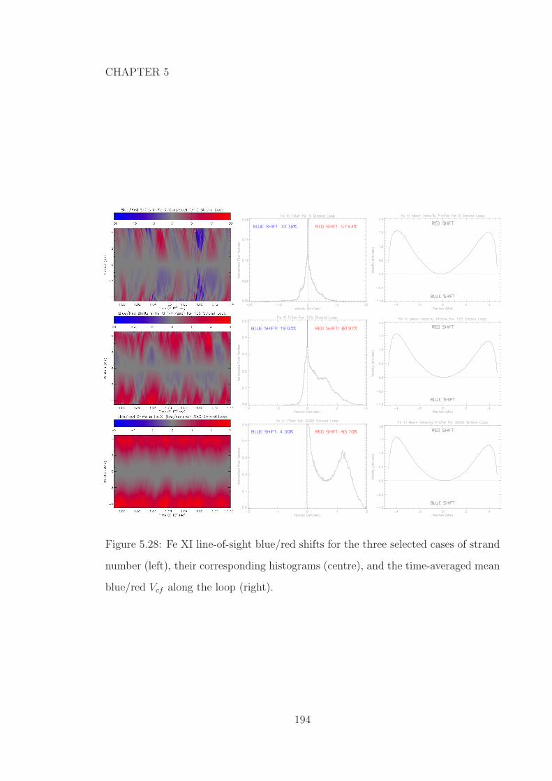
CHAPTER 5

Figure 5.28: Fe XI line-of-sight blue/red shifts for the three selected cases of strand



194

CHAPTER 5

Figure 5.29: Fe XV line-of-sight blue/red shifts for the three selected cases of strand



195

CHAPTER 5

Figure 5.30: Percentage of red shifted pixels (left column), maximum mean velocity

ranges (centre column), and average velocity deviation (right column) over a range

of number of strands, and line filters. From top-to-bottom: Si VII, Fe XI, Fe XV

196

CHAPTER 5

Table 5.4: Changing the number of energy bursts: simulation parameters



125 11 1.07 1.11 × 1024 − 2.37 × 1025 -2.36

125 57 1.0 1.00 × 1023 − 5.38 × 1024 -2.30

125 114 1.00 3.76 × 1022 − 2.81 × 1024 -2.34

125 570 1.01 2.65 × 1021 − 6.46 × 1023 -2.26

125 1140 1.01 8.56 × 1020 − 3.38 × 1023 -2.31

5.5 Changing the Number of Discrete Energy Bursts

Per Strand

In the previous section, the number of strands in the loop was changed, whilst

keeping the number of energy bursts fixed at 57 per strand. In essence this meant

that the number of energy bursts in the global loop system also changed, even though

the number of bursts per strand did not. Therefore, in this section, we investigate

how changing the number of energy bursts per strand affects the loop temperature

and velocity profiles.

Once more, SUH is used, the total energy is kept fixed at approximately ETotal(=

4.5 × 1027 erg) and α is kept as close to −2.3 as possible (see Figure 5.31 for the

three selected cases illustrating the power law slope). Since the number of bursts per

strand is changing, the energy of each particular burst must also change in order to

keep the total energy the same. Table 5.4 displays the simulation parameters used

in this section.

197

CHAPTER 5

Figure 5.31: Energy histograms for 11, 114 and 1140 energy bursts per strand.

Figure 5.32: Emission measure weighted temperature of the loop apex for 11 energy

bursts (left), 114 energy bursts (right) and 1140 energy burst (bottom) per strand

in a 125 strand loop.

198

CHAPTER 5

Figure 5.33: Average temperature along a 125 strand loop with 11, 114 and 1140

discrete energy bursts per strand


Figure 5.32 shows the emission measure weighted temperature of the loop apex for

the three selected cases. With only 11 energy bursts per strand, there are large

deviations in the apex temperature compared to that of the 114 and 1140 energy

bursts per strand cases. With fewer bursts, in order to maintain the same overall

energy in the strand, each particular burst contains more energy than that with more

bursts. As such, the loop will be heated more intensely, but also has more time to

cool in-between the next burst, thus causing the larger deviations. Conversely, with

more energy bursts, each burst contains less energy, but will have less time to cool,

since the time between energy bursts is much less. On the other hand, much like in

Section 5.4, the error bars show that the average profiles all lie within each other.

Figure 5.33 shows the time-average temperature profile along the loop. The 11

energy bursts per strand loop has the highest average apex temperature of 2.53 MK,

although the error on this value is far larger than the other two examples. Also, the

199

CHAPTER 5

Figure 5.34: Average apex emission measure weighted temperature (left) and the

average deviation of the apex temperature (right) as a function of number of energy

bursts per strand.

11 bursts per strand loop has a larger amount of energy deposited than in any of

the other simulations. The temperature gradient of the 11 energy burst per strand

loop is also significantly different. This is because there are only 11 energy bursts

along the length of each strand, and will not have as many being released in the

footpoint regions as the other examples.

The average apex temperature of the loop as a function of number of bursts per

strand is displayed in Figure 5.34 (left). Apart from the 11 energy bursts per strand

simulation, there is a general trend of increasing apex temperature with increasing

number of energy bursts per strand. Figure 5.34 (right) shows the average deviation

of the apex temperature as a function of increasing energy bursts per strand. There

is a very clear trend showing a smaller deviation with increasing number of events.

This because although the loop is heated more frequently, the energy released is

much less, and so there are no big spikes in temperature, whilst the frequency of the

bursts is such that there is also much less time to cool between each heating event.

200

CHAPTER 5

Figure 5.35: Si VII line-of-sight blue/red shifts for the selected cases of number of

energy bursts per strand (left), their corresponding histograms (centre), and the

time-averaged mean blue/red Vcf along the loop (right).

201

CHAPTER 5

Figure 5.36: Fe XI line-of-sight blue/red shifts for the three cases of spatial heating



202

CHAPTER 5

Figure 5.37: Fe XV line-of-sight blue/red shifts for the three cases of spatial heating



203

CHAPTER 5

Figure 5.38: Percentage of red shifted pixels (left column), the minimum and max-

imum velocity (centre column), and the average deviation of the velocity (right

column) as a function of energy bursts per strand. From top-to-bottom: Si VII, Fe

XI, Fe XV


In the SI VII and Fe XI line filters (see Figure 5.35 and 5.36), the loop is significantly

red shifted with the 11 and 114 bursts per strand. However, with 1140 bursts

the loops become more blue shifted, and there appear to be lots of flows from

one footpoint to another. In the Fe XV filter, the 1140 bursts per strand creates

a predominantly blue shifted left-hand-side of the loop, and a predominantly red

shifted right-hand-side of the loop.

Figure 5.38 quantifies the change in red shift, the change in velocity, and the

204

CHAPTER 5

change in the average deviation of the velocity for each line filter. In both the Si

VII and Fe XI, there is a clear trend of increasing blue shift with increasing number

of bursts per strand. With the Fe XV filter there is no clear trend in change in red

shift, with the 1140 bursts per strand loop being a notable difference to the results

obtained with fewer bursts per strand.

The Si VII and Fe XI line filters show a decrease in red shift velocities, which

would be expected with the decrease in the number of red shifted pixels. Therefore,

with the increase in the number of blue shifted pixels, it comes as no surprise that

the blue shift velocities show an increase with an increasing number of energy bursts

per strand. With Fe XV, there appears to be no clear trend in the change in red shift

velocities, but there is a decrease in blue shifted velocities with increasing number

of events.

The average deviation of the Si VII velocities appear to be show a trend of

increasing deviation of both red and blue shift velocities with increasing burst num-

ber, whilst the Fe XI and Fe XV line filters show a trend of decreasing red and blue

velocity deviations.

5.5.3 Discussion

Changing the number of energy bursts per strand throws up some interesting co-

nundrums, particularly where the line filtered velocities are concerned. In terms of

the temperature profile, there is a similar pattern to that of changing the number

of strands.

In the Si VII and Fe XI line filters, there is a clear trend of increasing blue

shift with increasing burst number. In the previous section, the number of strands

was changed, which meant that the total number of energy bursts also changed.

However, unlike the smoothing effect found from increasing the number of strands,

there is a somewhat lack of smoothing. The increase in blue shift could be due to

205

CHAPTER 5

a number of things. Firstly, it has been shown previously in Section 5.3, that the

loop is predominantly blue shifted in the Si VII filter with a total energy of 0.001

- 0.01ETotal. During these simulations, the bursts released energy in the range of

1 × 1020 − 5 × 1022 erg per event, which are similar to the values used in the 1140

bursts case. However, it is more likely that the increase in blue shift is because

each strand is being continually heated to a point where there is no, or very little,

time when there is not an energy burst being released. The simulation lasts 17,250

seconds, and there are 1140 energy bursts, each lasting between 50 and 150 seconds

each, which means there is likely to always be a time where each strand is being

continually heated, thus causing more evaporation, and therefore more blue shifts.

5.6 Conclusions

The multi stranded coronal loop simulations investigated throughout this chapter

have shown some interesting results, and important implications to understanding

the general physics of the coronal loop environment. We have shown that by dividing

a loop into multiple, thermally isolated strands, and amalgamating to form a single,

global loop system, we can produce results which can closely match the properties

obtained from loop observations.

The temperature profile of a loop can be simulated efficiently with a multi-strand

model heated by discrete energy bursts, where a single stranded model cannot.

In addition, we have also shown that the line-of-sight Doppler velocities can also

be reproduced with the use of the multi-strand model employed. We have used

three line filters, to show that red shifts and blue shifts can be produced, which

match general coronal loop observations. Where red shifts are seen from satellite

observations, we have shown we can reproduce these red shifts, and similarly for the

blue shifts. It must be noted however, that the derived velocities are often lower

than the observed velocities by several factors in some cases, although we do show

206

CHAPTER 5

good agreement with the velocities observed in Tripathi et al. (2009).

We have simulated a short, 10 Mm loop, and we believe that a longer loop could

produce higher velocities. This is discussed in more detail in Chapter 7.

Finally, Table 5.6 summarises the results from this chapter.

207

CH

AP

TE

R5

Table 5.5: Summary of results in Chapter 5

Parameter Si VII Si VII Fe XI Fe XI Fe XV Fe XV Vcf Temperature Temperature

Vcf % Red Vcf % Red Vcf % Red Deviation Deviation

(blue, red) Shift (blue, red) Shift (blue, red) Shift (blue, red)

Increasing decrease, increase, decrease, increase decrease, no trend decrease, increase increase

ETotal increase increase no trend increase

Increasing n/a, increase n/a, 1 increase 1 increase, decrease decrease, increase decrease

No. Strands increase no trend no trend decrease

Increasing increase, decrease increase, decrease decrease, no trend decrease, 2 increase decrease

No. Bursts decrease decrease no trend decrease 2

1 At cooler temperatures, blue shifts are seen, and are expected to behave similarly to the red shift

2 Si VII shows an increase in deviation

208

Chapter 6

Phase Plane Analysis of the

Temperature Structure Along 1-D

Hydrostatic Coronal Loops

The concept of the phase plane to study the thermal equilibrium of solar coronal

loops has been previously introduced by several authors, including Hood and Priest

(1979), Hood and Anzer (1988), Steele and Priest (1990), Steele and Priest (1991),

Walsh et al. (1995), and Mendoza-Briceno and Hood (1997).

In the absence of gravity, and with a loop footpoint temperature of 1 MK, Hood

and Priest (1979) solved the equations of thermal equilibrium. They concluded that

when the radiative term dominated the uniform heating along the loop, a lack of

equilibrium occurred, and solutions with cool summit temperatures were possible.

The equations of thermal equilibrium were re-examined in Hood and Anzer (1988)

to find conditions under which cool condensations could form in the corona. Steele

and Priest (1990) extended this work, using the Hildner (1974) radiative losses to

numerical solve the thermal equilibrium equations. It was shown that a number of

solutions existed:

209

CHAPTER 6

1. Hot loops: which have hot summits (0.4 − 3.0 MK), and cool footpoint (0.02

MK).

2. Hot-cool loops: which have footpoints at 0.2 MK, and a similar summit tem-

perature, or possibly even lower, but with sections of the loop at coronal

temperatures.

3. Cool loops: which have temperatures of ∼ 0.8 MK along their entire length.

4. Warm loops: which are similar to cool loops, but have summit temperatures

in the region of 0.08 − 0.4 MK.

Steele and Priest (1990) suggest that the cool loops could be associated with

active region prominences where the magnetic field line lies mainly along the plane

of the prominence, and that the global differential emission measure (DEM) can be

explained by the hot-cool loop solution. Later, by including changes in the cross-

sectional area of the coronal loop, by increasing the area towards the loop apex,

Steele and Priest (1991) showed that:

1. the summit temperature of hot-cool loops increased significantly

2. the summit temperature of the warm loops remained unchanged

3. the summit temperature of the hot and cool loops increased slightly

Steele and Priest (1994) then went on to include gravity in the thermal equilib-

rium equation, meaning that the pressure along the loop fell from the footpoint to

the summit. As such, this means that the pressure was now a free parameter, and

so rather than a 2-D phase plane, a 3-D phase volume was introduced. The effects

of this, meant that the hot-cool loop solutions no longer existed, thus reducing the

number of solutions.

210

CHAPTER 6

Walsh et al. (1995) also investigated the solution space to analytically solve the

thermal equilibrium equation, using a simplified, optically thin, two-range radiative

loss function. Again, using a phase plane analysis, Walsh et al. (1995) produced

solution where hot, cool, warm and hot-cool solutions are possible, depending on

the length of the loop, the footpoint temperature, the base conductive flux and the

value of the unknown coronal heating term. This unknown coronal heating term,

previously just assumed to be constant along the length of the loop, was investigated

in Mendoza-Briceno and Hood (1997), by varying the heating term as a function

of the length of the loop. Mendoza-Briceno and Hood (1997) found that there is a

critical decay length of the heating below which a hot coronal loop can not exist,

and it is thought that this allows the existence of catastrophic cooling after thermal

non-equilibrium occurs.

With the above in mind, the work presented in this chapter builds upon the work

of Walsh et al. (1995), by analytically solving, and investigating, the solution space

of the thermal equilibrium equation, in the absence of gravity, but introduces a new

four-range, optically thin, radiative loss function.

6.1 Basic Equations

This section will outline the MHD equations, and how with certain assumptions,

these can be used to produce the thermal equilibrium equation from which to explore

the temperature structure along 1-D hydrostatic coronal loops.

Maxwell’s Equations

∇× B = µj +1

c2

∂E

∂t(6.1)

∇ · B = 0 (6.2)

∇× E = −∂B

∂t(6.3)

211

CHAPTER 6

∇ · E =ρe

ǫ(6.4)

where B is the magnetic field strength, E is the electric field strength, j is the

current density, µ is the magnetic permeability, t is the time, ρe is the charge density,

c is the speed of light in a vacuum, and ǫ is the permittivity of free space. These

equations can then be simplified under certain assumptions, as discussed in Priest

(1982):

• The plasma is assumed to be in thermal equilibrium.

• The plasma is treated as a continuous medium. This assumption is held if the

length-scales considered greatly exceed any internal plasma lengthscales.

• The plasma is treated as a single fluid system

• The plasma is assumed to be isotropic, except for the thermal conduction,

which is greatest along the magnetic field line.

• Rotational effects of the Sun are neglected, and so an inertial frame of reference

is used. The rotational effects can become important when considering very

large structures.

• A simplified Ohm’s Law is applied:

j = σ (E + v × B) (6.5)

where σ is the electrical conductivity and v is the plasma velocity.

• ǫ and µ are assumed to be constant, with values taken from a vacuum in the

solar context: ǫ0 = 8.854 × 10−12 F m−1; µ0 = 4π × 10−7 H m−1

• Relativistic effects can be ignored, since the sound, Alfvenic and flow velocities

are much smaller than the speed of light. Thus, consider

v0 = l0/t0,

212

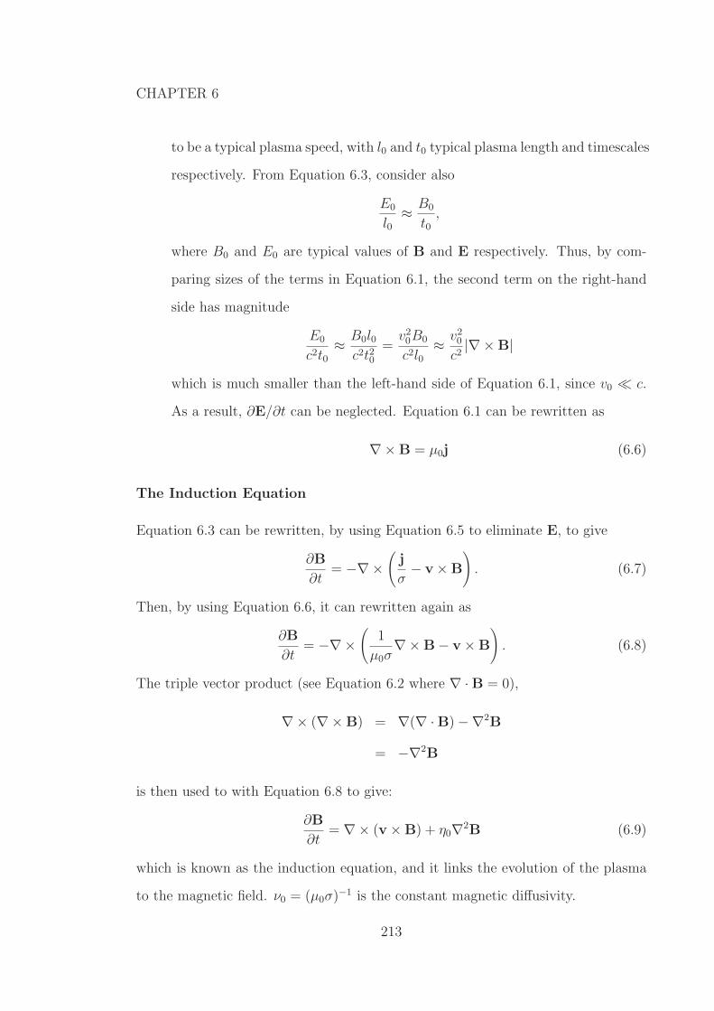
CHAPTER 6

to be a typical plasma speed, with l0 and t0 typical plasma length and timescales

respectively. From Equation 6.3, consider also

E0

l0≈ B0

t0,

where B0 and E0 are typical values of B and E respectively. Thus, by com-

paring sizes of the terms in Equation 6.1, the second term on the right-hand

side has magnitude

E0

c2t0≈ B0l0

c2t20=

v20B0

c2l0≈ v2

0

c2|∇ × B|

which is much smaller than the left-hand side of Equation 6.1, since v0 ≪ c.

As a result, ∂E/∂t can be neglected. Equation 6.1 can be rewritten as

∇× B = µ0j (6.6)

The Induction Equation

Equation 6.3 can be rewritten, by using Equation 6.5 to eliminate E, to give

∂B

∂t= −∇×

(

j

σ− v × B

)

. (6.7)

Then, by using Equation 6.6, it can rewritten again as

∂B

∂t= −∇×

(

1

µ0σ∇× B − v × B

)

. (6.8)

The triple vector product (see Equation 6.2 where ∇ · B = 0),

∇× (∇× B) = ∇(∇ · B) −∇2B

= −∇2B

is then used to with Equation 6.8 to give:

∂B

∂t= ∇× (v × B) + η0∇2B (6.9)

which is known as the induction equation, and it links the evolution of the plasma

to the magnetic field. ν0 = (µ0σ)−1 is the constant magnetic diffusivity.

213

CHAPTER 6

The Plasma Equations

The motion of the magnetic field is coupled to the behaviour of the plasma by

the presence of the velocity term in Equation 6.9 and in the equations for mass

continuity, motion, and energy.

Mass Continuity

In an MHD system, the mass must be conserved:

Dρ

Dt+ ρ∇ · v = 0, (6.10)

where ρ is the plasma density and

D

Dt=

∂

∂t+ v · ∇

is the total derivative.

Motion

The equation of motion for the plasma can be written as

ρDv

Dt= −∇p + j × B + ρg + ρν∇2v, (6.11)

where p is the plasma pressure. The terms on the right-hand side of the equation

can be separated as:

• ∇p is the plasma pressure gradient.

• j × B is the Lorentz force. Using Equation 6.6,

j × B =1

µ0

(∇× B) × B

which becomes

j × B = (B · ∇)B

µ0

−∇(

B2

2µ0

)

214

CHAPTER 6

when using the triple vector product. The first term on the right-hand side of

the equation is a magnetic tension force that is proportional to B2. The second

term on the right-hand side is a magnetic pressure force, with the magnetic

pressure given by B2/2µ0.

• ρg is the effect of gravity, where g is the local gravitational acceleration at the

surface of the Sun. g ∼ 274 m s−2.

• ρν∇2v is the effect of viscosity on an incompressible flow. ν is the coefficient

of kinematic viscosity which is assumed to be uniform throughout the plasma.

Spitzer (1962) gives

ρν = 2.21 × 10−16 T5/2

LnΛkg m−1 s−1,

where LnΛ is the Coulomb Logarithm, taken to be ∼ 20 for the solar corona.

The Energy Equation

The fundamental energy is expressed as:

ργ

γ − 1

D

Dt

(

p

ργ

)

= ∇ · (K∇T ) − L (6.12)

where γ is the ratio of specific heats (γ = 5/5), and T is the temperature of the

plasma. K is the tensor of thermal conduction. This can be split into components

across and along the magnetic field:

∇‖ · (κ‖∇‖T ) + ∇⊥ · (κ⊥∇⊥T ).

Conduction along the magnetic fieldlines is mainly by electrons. Braginski (1965)

gives κ‖ = κ0T5/2 W m−1 deg−1 with κ0 = 10−11 for the corona. Across the fieldlines,

conduction is mainly by ions. At coronal temperatures:

κ⊥κ‖

≈ 10−12.

215

CHAPTER 6

Figure 6.1: Comparison of the radiative loss function Q(T ) from Hildner (1974),

Rosner et al. (1978), and Cook et al. (1989).

Therefore, the vast majority of conducted heat occurs along the magnetic field, and

as such, the conduction term can be written as:

κ‖ · (κ‖∇T ) = κ0∇‖ · (T 5/2∇‖T ). (6.13)

The loss-gain function, W , has the form:

W (ρ, T ) = ρ2Q(T ) − H (6.14)

where H is the unknown coronal heating term, and Q(T ) is the optically thin ra-

diative loss function, approximated by a piece-wise continuous function:

Q(T ) = χT α (6.15)

where α and χ are constant within a particular temperature range of the piecewise

fit, and is illustrated, by three examples, in Figure 6.1.

Perfect Gas Law

The perfect gas law is used:

p =R

µρT (6.16)

216

CHAPTER 6

Figure 6.2: An example of a magnetic flux tube through surfaces S1 and S2.

where R = 8.3 × 103 m2 s−2 K−1 is the molar gas constant, and µ = 0.6 in the

ionised corona.

Summary of Equations

Thus, summarising the equations considered so far, we have:

∂B

∂t= ∇× (v × B) + η0∇2B (6.17)

Dρ

Dt+ ρ∇ · v = 0 (6.18)

ρDv

Dt= −∇p + j × B + ρg + ρν∇2v (6.19)

ργ

γ − 1

D

Dt

(

p

γρ

)

= κ0∇‖ ·(

T 5/2∇‖T)

− ρ2χT α + H (6.20)

p =R

µρT (6.21)

Magnetic Flux Tubes

The volume generated by a set of fieldlines, which intersect a simple, closed curve, is

called a magnetic flux tube. Figure 6.2 shows a simple diagram illustrating a typical

flux tube. The strength of a flux tube, Fs is the amount of magnetic flux B crossing

a particular section, S1, of the tube:

Fs =∫

S1

B · dS =∫

S1

BndS (6.22)

where Bn is the normal component of the field through the section S1.

217

CHAPTER 6

Coronal loops outline the magnetic field, and are examples of flux tubes. Through-

out this chapter, it is assumed that the coronal loops have a constant cross-sectional

area, and that the loop structure remains rigid due to the strong magnetic field (i.e.

the coronal plasma-β is very small).

This also means that Equation 6.17, the induction equation, is no longer required.

Also, this means that j × B = 0, and thus can be omitted from Equation 6.19. All

plasma motions are assumed to be along the coronal loop length, and this therefore

allows the analysis to be restricted to one-dimensional dynamics. As such, Equations

6.18 to 6.21 are reduced to:

Dρ

Dt+ ρ

∂v

∂x= 0 (6.23)

ρDv

Dt= −∂p

∂x+ ρg + ρν

∂2v

∂x2(6.24)

ργ

γ − 1

D

Dt

(

p

ργ

)

= κ0∂

∂x

(

T 5/2∂T

∂x

)

− ρ2χT α + H (6.25)

p =R

µρT (6.26)

where all quantities are along the magnetic field, and x is the distance along the

field line.

The Isobaric Assumption

Walsh et al. (1996) investigate the validity of the isobaric assumption, by including

the inertial terms in the fluid equations. It was found that the temperature structure

can be approximated to a high degree, by assuming an isobaric environment, since

the temperature changes along a loop are generally governed by the variations in

the heating.

So, using Equations 6.23 to 6.26, and neglecting gravity and viscosity, Equation

6.23 (mass continuity) can be rewritten as:

∂ρ

∂t+ v

∂ρ

∂x+ ρ

∂v

∂x= 0.

218

CHAPTER 6

Thus,

∂ρ

∂t+

∂(ρv)

∂x= 0. (6.27)

Equation 6.24 (motion) can be expressed as:

ρ

(

∂v

∂t+ v

∂v

∂x

)

= −∂p

∂x, (6.28)

whilst the left-hand side of Equation 6.25 (energy) can be be rewritten as:

ργ

γ − 1

D

Dt

(

p

ργ

)

=1

γ − 1

Dp

Dt− γp

(γ − 1)ρ

Dρ

Dt

=1

γ − 1

Dp

Dt+

γp

γ − 1

∂v

∂x

=1

γ − 1

(

∂p

∂t+ v

∂p

∂x

)

+γp

(γ − 1)

∂v

∂x(6.29)

by expanding the total derivative. These equations can then be made dimensionless,

against typical coronal values, so that:

t = tct, x = lx, v = vcv =lv

tc, ρ = ρcρ, T = TcT , p = pcp

where l is the length of the field line, vc = l/tc is the conductive velocity, Tc = 106

K, ρc = 8.35 × 10−13 kg m−3, and pc = RρcTc/µ. The timescale, tc is defined as the

conduction timescale:

tc =γpcl

2

κ0(γ − 1)T7/2c

(6.30)

Substituting into Equations 6.26 to 6.29, gives:

∂ρ

∂t+

∂(ρv)

∂x= 0 (6.31)

ρcργv2c

c2s

(

∂v

∂t+ v

∂v

∂x

)

+∂p

∂x= 0 (6.32)

1

γ

(

∂p

∂t+ v

∂p

∂x

)

+ p∂v

∂x=

∂

∂x

(

T 5/2∂T

∂x

)

− L[

χp2Tα−2 − H]

(6.33)

p = ρT (6.34)

where the sound speed squared is defined as c2s = γpc/ρc, and H = HcH, with

Hc = ρ2cχcT

αcc (χc and αc are the values of the temperature dependent parameters

when T = Tc).

219

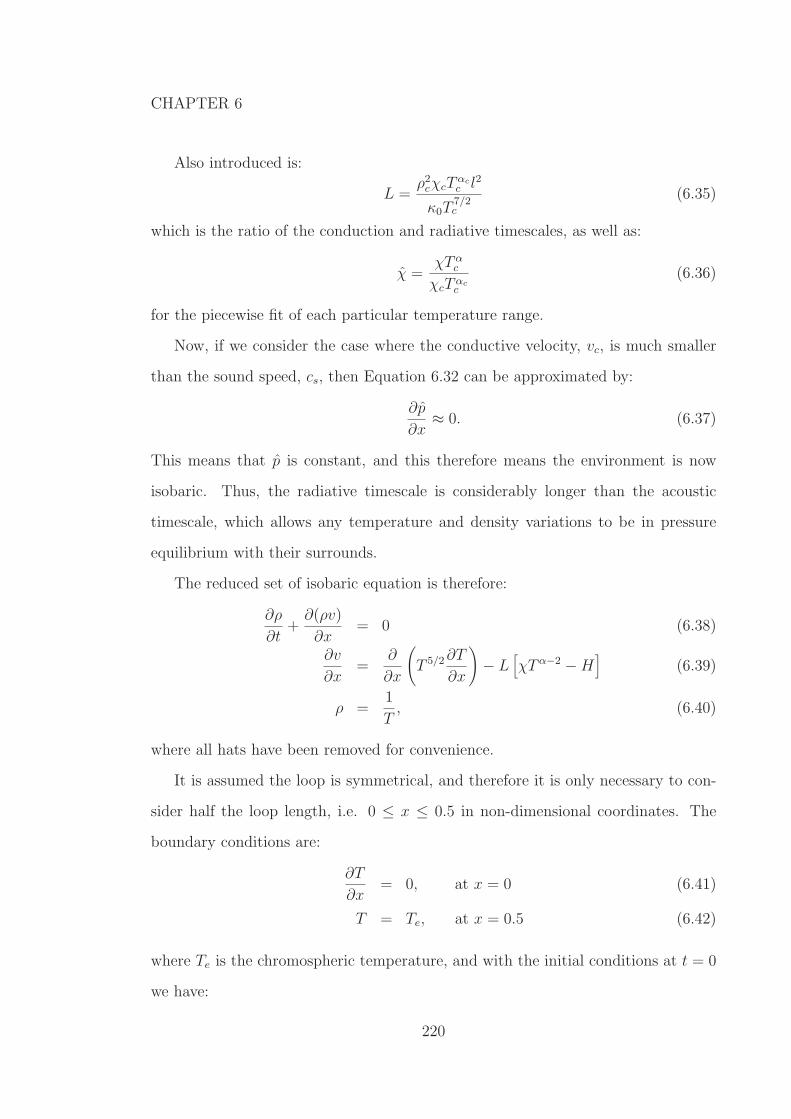
CHAPTER 6

Also introduced is:

L =ρ2

cχcTαcc l2

κ0T7/2c

(6.35)

which is the ratio of the conduction and radiative timescales, as well as:

χ =χT α

c

χcTαcc

(6.36)

for the piecewise fit of each particular temperature range.

Now, if we consider the case where the conductive velocity, vc, is much smaller

than the sound speed, cs, then Equation 6.32 can be approximated by:

∂p

∂x≈ 0. (6.37)

This means that p is constant, and this therefore means the environment is now

isobaric. Thus, the radiative timescale is considerably longer than the acoustic

timescale, which allows any temperature and density variations to be in pressure

equilibrium with their surrounds.

The reduced set of isobaric equation is therefore:

∂ρ

∂t+

∂(ρv)

∂x= 0 (6.38)

∂v

∂x=

∂

∂x

(

T 5/2 ∂T

∂x

)

− L[

χT α−2 − H]

(6.39)

ρ =1

T, (6.40)

where all hats have been removed for convenience.

It is assumed the loop is symmetrical, and therefore it is only necessary to con-

sider half the loop length, i.e. 0 ≤ x ≤ 0.5 in non-dimensional coordinates. The

boundary conditions are:

∂T

∂x= 0, at x = 0 (6.41)

T = Te, at x = 0.5 (6.42)

where Te is the chromospheric temperature, and with the initial conditions at t = 0

we have:

220

CHAPTER 6

v(x) = 0

T = Ts(x)

where Ts(x) is the static temperature profile obtained for a constant value of the

heating (H = H0).

6.2 Analytical Solutions to the Phase Plane

From the reduced set of isobaric equations, it is now possible to study the thermal

equilibrium equation, and introduce a simplified radiative loss function. This allows

solutions of the thermal equilibrium equation to be found, by a powerful technique

known as phase plane analysis. A phase plane analysis will therefore investigate the

solution space to the thermal equilibrium equation.

6.2.1 Thermal Equilibrium and the Four Range Radiative

Loss Function

By setting the time derivatives and velocity of Equations 6.38 to 6.40 to zero, one

is able to obtain the equation of thermal equilibrium. What is left, is a balance

between conduction, radiation, and heating:

d

dx

(

T 5/2dT

dx

)

= L[

χT α−2 − H0

]

, (6.43)

and this chapter will investigate the solution space to this equation.

This is a complicated problem, particularly when considering the radiative losses.

Colgan et al. (2008) present the latest optically thin radiative loss calculations in

Figure 6.3. Hildner (1974); Rosner et al. (1978); Cook et al. (1989) have previously

created the piecewise radiative loss functions, as discussed earlier and shown in

221

CHAPTER 6

Figure 6.3: From Colgan et al. (2008): Radiative losses from a coronal plasma

containing 15 elements. Colgan et al. (2008) compare their ATOMIC calculations

(solid line) with those of Landi and Landini (1999) (dashed line) and a calculation

made using the most recent version of CHIANTI (dot-dashed line). Also shown

is an ATOMIC calculation obtained by solving the full set of collisional-radiative

equations, (dashed line with small squares). Losses are given in W cm3, where 1

W= 107 erg s−1. The red circle highlights the significant bump.

222

CHAPTER 6

Figure 6.1. Walsh et al. (1995) devised a simplified, two-range radiative loss function.

However, these previous functions do not take into consideration the significant

bump that is shown at cooler temperatures in Figure 6.3. Therefore, a new four-

range radiative loss function is introduced, to investigate the properties of including

this extra bump. Also, it can be argued that there are many more dips and rises in

the radiative loss function than just the feature being included in this work. But, by

just including the one feature, the results of this will have important implications

for a fuller treatment of the radiative loss function.

The analytical solutions for the equilibrium states are derived by using this new

four-range radiative loss function:

where χT α−2 =

T−7/4, T > Tr, α = 1/4

T 7/2

T21/4

r

, Tb ≤ T < Tr, α = 7/2

T21/4

b

T21/4

r T 7/4, Ta ≤ T < Tb, α = 1/4

T21/4

bT 7/2

T21/4

r T21/4

a

, T < Ta, α = 7/2

where Ta is the temperature at the first peak (∼ 0.016 MK), Tb is the temperature

at the proceeding trough (∼ 0.035 MK), and Tr is the value at the highest value of

the radiation (∼ 0.06 MK). Each temperature interval has a specific value of α and

χ, as indicated in the above equation. The four-range function is compared to the

two-range function in Walsh et al. (1995), and Hildner (1974) in Figure 6.4.

This simplified function has similar properties to that of the original radiative

losses, but allows for simpler, analytical solutions to be calculated, and presented in

the form of a phase plane. The radiative losses can only be considered down to chro-

mospheric temperatures (0.01 MK) as at lower temperatures, optically thick effects

become important, and so solutions below this temperature will not be considered.

For mathematical ease, Equation 6.43 can now be rewritten as:

y′′ =7L

2

[

χy[2(α−2)]/7 − H0

]

(6.44)

223

CHAPTER 6

Figure 6.4: Figure showing the non-dimensional four-range radiative loss function

(solid line), Walsh et al. (1995) (dot-dash line) and Hildner (1974) (dashed line) op-

tically thin radiative loss functions, with temperature (T ) displayed in dimensionless

units.

224

CHAPTER 6

where y = T 7/2. The boundary conditions (Equations 6.41 and 6.42) are now defined

as:

dy

dx= 0, at x = 0 (6.45)

y = ye, at x = 0.5 (6.46)

Furthermore, there exist critical points, which are inherent to the solutions avail-

able. By setting:

dy

dx= Ψ (6.47)

dΨ

dx=

7L

2

[

χy[2(α−2)]/7 − H0

]

(6.48)

then the critical points exist when the two derivatives are zero. Therefore, the

critical points exist at:

y = ycrit =

(

H0

χ

)7/[2(α−2)]

, Ψ = 0 (6.49)

Depending on the value of H0, there may be up to four critical points. If we

define:

1. Tcrit1 being the critical temperature for T < Ta.

2. Tcrit2 being the critical temperature for Ta < T < Tb.

3. Tcrit3 being the critical temperature for Tb < T < Tr.

4. Tcrit4 being the critical temperature for T > Tr.

and so we have:

ycrit1 =H0y

3/2a y3/2

r

y3/2b

(6.50)

ycrit2 =

(

H0y3/2r

y3/2b

)−2

(6.51)

225

CHAPTER 6

Figure 6.5: Levels of uniform heating for the phase planes displayed in Figures 6.6

to 6.13, for Ta = 0.07, Tb = 0.1, Tr = 0.15.

ycrit3 = H0y3/2r (6.52)

ycrit4 = H−20 (6.53)

A critical point analysis gives (ycrit1, 0) and (ycrit3, 0) as saddle points, and

(ycrit2, 0) and (ycrit4, 0) as centre points (see Appendix A).

Figure 6.5 displays the four-range radiative loss function for values of Ta =

0.07, Tb = 0.1 and Tr = 0.15. Changing the value of these parameters helps to

display the different solutions to the phase plane more clearly, without affecting the

physics of the system. The different coloured lines represent the values of H0 used

in the subsequent phase planes, with the colours matching the chosen colours of the

separatrix curves.

Figures 6.6 to 6.13 display the phase planes for a variety of values of H0. L = 2

is used throughout, for analytical expediency.

If we first examine Figure 6.6, the most significant solution is the separatrix

226

CHAPTER 6

(a) Full solution space.

(b) Zoomed-in cool region.

Figure 6.6: Phase planes for H0 = 5.

227

CHAPTER 6

curve, which in this diagram is coloured blue. The separatrix curve is fundamental

to the solutions in the phase plane, since it separates areas of different topological

solutions. This phase plane, for H0 = 5, has only two critical points; Tcrit1 and

Tcrit4. For example, if we have a loop with a footpoint temperature that lies along

the line L1, then three unique solution types exist. Firstly, there is the separatrix

curve itself, which has the saddle point at T = Tcrit1. Secondly, there is the situation

where the footpoint (or base) conductive flux is greater than that of the separatrix

curve (so that it lies outside of the separatrix curve), then only a hot solution exists.

Starting at A1, and following the contour clockwise, the contour A1G1A2 gives a

loop with a hot summit. Finally if the base conductive flux is less than that of the

separatrix curve (and thus lies inside it), then we get the contour E1E2 which has a

cool summit.

Now, if we have a loop with a footpoint temperature along L2 and a base con-

ductive flux greater than the separatrix curve, we have the solution G1A2, which is

again a hot solution. But, if the base conductive flux is lowered to less than that

of the separatrix curve then we get a loop such as B1B2, making sure to follow the

contour clockwise. This gives a loop with a hot summit, that is thermally isolated,

since the base conductive flux is zero. The summit temperature of the loop is the

minimum value for a hot loop solution with this particular footpoint temperature. It

is also possible to continue along the contour (e.g. B1B2B1), to give a cool summit

temperature. This type of a loop is a hot-cool loop, since it is hot along most of its

length, but it has a cool summit. The contour C1C2 has a hot summit temperature,

whilst if the base conductive flux is negative, then cool solutions can occur, such

as C3C4, although these cool solutions are normally rejected for being non-physical

since the summit temperature is lower than the footpoint temperature.

Figure 6.7 displays the phase plane for H0 ∼ 6.69. It is at this point that

Tcrit2 and Tcrit3 suddenly appear at the point T = Tb. As H0 is increased past

228

CHAPTER 6

this point, four critical points are now observed, with two saddle points, and two

centre points. There are therefore now two separatrix curves, as can be seen in

Figure 6.8. As H0 is increased further, there is a point at which the two separatrix

curves join together, to form a “double separatrix”, as shown in Figure 6.9, where

H0 =

√

3(y1/2

a −y1/2

b)y3

b

(y3/2

a −y3/2

b)y3

r

∼ 8.58. As H0 is again increased, the double separatrix splits

into two separate curves, with an example shown for H0 = 10 in Figure 6.10, which

shows the existence of the two separatrix curves, but which offer different properties

to those found in Figure 6.8. Increasing H0 again, begins to merge Tcrit1 and Tcrit2

together, which occurs at T = Ta for H0 ∼ 12.49, as shown in Figure 6.11, at which

point they disappear, and a single separatrix curve remains. This can be seen in

Figure 6.12 for H0 = 15. As H0 is increased further, the two critical points Tcrit3 and

Tcrit4 being to move towards each other, until they reach T = Tr, at H0 ∼ 27.66. At

this point all the critical values have disappeared, and no separatrix curves exist.

If we now examine the different contours of the phase planes, we notice that

there exists different solutions, depending on the value of H0. If we take a footpoint

temperature along the line L1, then we notice that there exists hot solutions in

each phase plane, such that the contours A1G1A2, and E1E2 are always possible.1

Similarly, the same solutions exist in phase planes, until we see in Figure 6.13 at H0 =

27.66, where the contours C1C2 and B1B2, which include the hot-cool solutions, no

longer exist.

When we examine the phase planes, for footpoint temperatures lying along the

line L3, we now also see some of the solutions such as F1A22 which are capable of

the hot-cool and thermally isolated solutions.

Figure 6.14 shows how the phase plane diagram changes with increasing values

of L, which scales as L1/2. Figure 6.15 shows the maximum and minimum summit

temperatures with increasing H0. In Region 1, the summit temperature represented

1the contours show topologically similar solutions, but the actual solutions are different in eachphase plane

2in this case, the point A2 lies directly inside the separatrix curve

229

CHAPTER 6


(b) Zoomed in cool region.

Figure 6.7: Phase planes for H0 = 6.69.

230

CHAPTER 6



Figure 6.8: Phase planes for H0 = 7.5.

231

CHAPTER 6



Figure 6.9: Phase plane for H0 =

√

√

√

√

√

3

(

y1/2

a −y1/2

b

)

y3

b(

y3/2

a −y3/2

b

)

y3r

232

CHAPTER 6



Figure 6.10: Phase planes for H0 = 10

233

CHAPTER 6



Figure 6.11: Phase plane for H0 = 12.49.

234

CHAPTER 6

Figure 6.12: Phase plane for H0 = 15.

Figure 6.13: Phase plane for H0 = 27.66.

235

CHAPTER 6

Figure 6.14: Variation of length of loop parameter, L, for the case with the double

separatrix at H0 ∼ 8.58.

is the maximum summit temperature that can exist, and is the location of the

saddle point (Tcrit1). In Region 2, the minimum possible summit temperature is

displayed, which represents the summit temperature of the separatrix curve. In

Region 3, the maximum summit temperature is displayed, corresponding to Tcrit3,

whilst the minimum summit temperature in Region 4 is displayed, corresponding to

the summit temperature of the separatrix curve in Region 4.

6.2.2 Dependence of the summit temperature upon the length

of the loop

The two-range radiative loss function (Walsh et al., 1995) was chosen, so that the

analytical solutions to the thermal equilibria could be derived. As such, this is the

reason that the four-range radiative loss function introduced in this chapter was

adapted from this. It is also possible to derive an analytical expression for the

236

CHAPTER 6

Region 1

Region 4

Region 3

Region 2

Figure 6.15: Summit temperature for increasing H0 for loops with a footpoint tem-

perature of Te = 0.01 MK, and L = 2, with Ta = 0.07, Tb = 0.1, Tr = 0.15.

dependence of the summit temperature (T0), upon the length of the loop variable,

L, for different values of H0. There are four sets of solutions, depending upon which

temperature region the summit is located at.

Region 1: For T < Ta

L =8

7w

(

cosh−1

(

ye − γ

y0 − γ

))2

(6.54)

where:

w =y

3/2b

y3/2r y

3/2a

γ =H0

w

237

CHAPTER 6

Region 2: For Ta ≤ T < Tb

L =2

7

[

[

(

H0y1/20 − z

)2 −(

z − H0y1/2a

)2]1/2

+ z

[

sin−1

(

z − H0y1/2a

H0y1/20 − z

)

+π

2

]

+2√w

ln

C3 −√

C23 − 4 (C2

2 − C21)

2 (C2 − C1)

]2

(6.55)

where z =y3/2

b

y3/2

r

, and:

C1 =1√

2H0w

[

(

z − H0y1/20

)2 −(

H0y1/2a − z

)2]1/2

C2 =1

2

(

ya −H0

w

)

C3 = ye −H0

w

Region3: For Tb ≤ T < Tr

L =2

7

[

2√w

ln

C6 −√

C26 − 4 (C2

5 − C24)

2 (C5 − C4)

+2√

2√

H30

[

z (θc − θd) +√

E (cos θc − cos θd)]

+ 4y3/4r cosh−1

(

yb − H0y3/2r

y0 − H0y3/2r

) ]2

(6.56)

where:

θc = sin−1

[

z − H0y1/2a√

E

]

θd = sin−1

z − H0y1/2b√

E

D = H0y0 −y2

0

2y3/2r

− 3y2b

2y3/2r

E = H0D + z2

238

CHAPTER 6

C4 =1√

2H0w

[

E −(

z − H0y1/2a

)2]1/2

C5 =1

2

(

ya −H0

w

)

C6 = ye −H0

w

Region 4: For T > Tr

L =2

7

[

2√

2√

H30

(

sin−1

(

1 − H0y1/2r√

G

)

+π

2+

[

G −(

1 − H0y1/2r

)2]1/2

)

+ 4y3/4r ln

C9 −√

C29 − 4 (C2

8 − C27)

2 (C8 − C7)

+2√

2√

H30

[

z (θe − θf ) +√

M (cos θe − cos θf )]

+2√w

ln

C12 −√

C212 − 4 (C2

11 − C210)

2 (C11 − C10)

]2

(6.57)

where:

F = H0y0 − 2y1/20

G =(

H0y1/20 − 1

)2

J =3

2y1/2

r + F

K = J − 3y2b

2y3/2r

M = H0K + z2

θe = sin−1

[

z − H0y1/2a√

M

]

θf = sin−1

z − H0y1/2b√

M

239

CHAPTER 6

C7 =y3/4

r√2H0

[

(

1 − H0y1/20

)2 −(

1 − H0y1/2r

)2]1/2

C8 =1

2

(

yr − H0y3/2r

)

C9 = yb − H0y3/2r

C10 =1√

2H0w

[

M −(

z − H0y1/2a

)2]1/2

C11 =1

2

(

ya −H0

w

)

C12 = ye −H0

w

The derivation of these expressions can be found in Appendix B. All four cases

are shown in Figure 6.16 for a range of values of H0, where it can be seen that the

value of H0 has a large affect on the solution space.

6.3 Conclusions

In this chapter, we have analytically solved the thermal equilibrium equation, to pro-

duce a phase plane analysis for the temperature structure along hydrostatic coronal

loops. Landi and Landini (1999), and Colgan et al. (2008) present optically thin ra-

diative losses which include a significant bump at cooler temperatures, not observed

in previous studies by Hildner (1974), Rosner et al. (1978) and Cook et al. (1989).

As such, the two-range radiative loss function of Walsh et al. (1995) was adapted

to take into account this bump, and a new four-range radiative loss function was

introduced.

With this new four-range function, the thermal equilibrium equation was an-

alytically solved, and a new set of solutions to the solution space was observed.

The Colgan et al. (2008) radiative losses also show several more dips and peaks

(although not quite as prominent), and so the implications are that with a more

complex radiative loss function, many more solutions may be possible.

240

CHAPTER 6

Figure 6.16: Dependence of the summit temperature T0 (in units of 106K upon the

parameter L for different values of H0, for a footpoint temperature of Te = 0.01 MK.

The dashed lines (from the bottom upwards) represent where T0 = Ta, T0 = Tb and

T0 = Tr.

241

Chapter 7

Future Work

In this chapter, we outline the work we would like to do, to further increase our

understanding of each particular subject.

7.1 CME Observations

We would like to analyse many more CME events, and in particular, more slow

CMEs, which we are able to obtain in-situ data for, in order to fully understand

the propagation of slow CMEs as they travel through the heliosphere. This would

hopefully answer some of the questions regarding CME deflections in the heliosphere.

We would also like to use other methods to derive the 3-D position angles, such

as using forward modelling, to build up a better understanding of which method

works best, with which particular CME type.

Once the 3-D position angles of a CME are known, a plethora of kinematic,

energetic, and geometric analysis can be done accurately. We would also strive to

include any Thompson scattering effects, which we have so far neglected.

For example, the CME cone models of Michalek et al. (2009) use LASCO CME

observations, and derive velocities based upon the latitudinal expansion angle of a

CME, using a plane-of-sky assumption. However, if this expansion angle deviates

242

CHAPTER 7

away from the plane-of-sky, the expansion angle is greatly affected by the angle at

which it is propagating, and will therefore have a large impact upon the results.

7.2 Multi-Strand Coronal Loop Simulations

Work has already begun on a preliminary investigation to see if it is possible to obtain

more accurate velocity results to compare with Tripathi et al. (2009). Figure 7.1

displays the red/blue shifts, their corresponding histograms, and the average velocity

profile, for a 1125-strand loop, with 57 energy bursts per strand, for 0.1ETotal. We

would like to further this work, by increasing the length of the loop to those from the

observations. In Tripathi et al. (2009), they observe loops with projected heights

of at least 75 Mm, meaning a loop length of ∼ 250 Mm. Such a long loop will

likely provide different results. For example, the temperature profile may change

significantly, since it will take far longer for the heat released by the energy burts

to reach the loop apex. The loop velocities are also expected to change, since the

effects of gravity will have a far larger impact upon the plasma in a longer loop.

7.3 Phase Planes

We would like to further extend the four-range radiative loss function, into a six-

range or even an eight-range function, to investigate the new solution space. We

have already seen an increase in the number of solutions when increasing from a

two-range to a four-range, so it would be expected that more solutions would indeed

exist with a more complex radiative loss function.

At present, gravity is assumed to be constant along the length of the loop.

Therefore, we would like to investigate the effects of including gravity upon the

thermal equilibrium equation. In doing so, the pressure will be at its greatest at the

base of the loop, whilst it will be the least at the loop apex. In order to investigate

243

CHAPTER 7

Figure 7.1: Si VII (top row), Fe XI (middle row) and Fe XV (bottom row) line-of-

sight blue/red shifts for a 1125 strand loop, with 57 energy bursts per strand and

0.1ETotal (left column), their corresponding histograms (centre column), and the

time-averaged mean blue/red Vcf along the loop (right column).

244

CHAPTER 7

this solution space, a phase volume will need to be constructed, since there is now

an extra varaible to consider. We believe that the inclusion of gravity will push the

critical points together, possibly making them merge together and disappear.

Also, we would like to further investigate the effects of changing the spatial

distribution of the coronal heating parameter. Currently, we have only assumed

uniform heating, and therefore we would like to investigate using footpoint and

apex dominated heating.

A phase volume, consisting of layers of phase planes stacked on top of each

other, is presented in Figure 7.2, and shows the separatrix curve for each value of

H0 within the plotted range. When there are two separatrix curves available, only

the separatrix curve with the highest summit temperature is plotted.

By taking an angled slice out of the x-y (temperature-conductive flux) plane,

it is possible to produce phase plane solutions with heating that varies along the

length of the loop (e.g. footpoint or apex dominated heating), dependent upon the

gradient of the slice. A slice with a positive gradient with respect to the z-axis, will

produce apex heating, whilst a slice with a negative gradient will produce footpoint

heating.

245

CHAPTER 7

Figure 7.2: Phase volume displaying the separatrix curve for increasing H0 with

L = 1, Ta = 0.07, Tb = 0.1, and Tr = 0.15. The double separatrix is illustrated by

the blue contours.

246

Appendix A

Critical Point Analysis

Here, we investigate the nature of the critical points, in the (y, Ψ) space of the

following equations1:

dy

dx= Ψ (A.1)

dΨ

dx=

7L

2

[

χy2(α−2)/7 − H0

]

(A.2)

and we have the following critical points:

ycrit1 =H0y

3/2a y3/2

r

y3/2b

ycrit2 =

(

H0y3/2r

y3/2b

)−2

ycrit3 = H0y3/2r

ycrit4 = H−20

and for convenience, let:

χa =y3/2

a y3/2r

y3/2b

χb =y3/2

r

y3/2b

(A.3)

1note: the critical points exist only for certain values of H0. For H0 > y−1/2

r there exist nocritical points.

247

CHAPTER A

A.1 Analysis of y = ycrit1 and y = ycrit3

To investigate the local behaviour near y = ycrit1 let (ycrit1, 0) ≈ (H0χa + ǫ1, ǫ2),

where ǫ1 and ǫ2 are small quantities. Then, approximate Equations A.1 and A.2 by:

ǫ1 ∼ ǫ2 (A.4)

ǫ2 ∼ 7L

2

[

1

χa

(H0χa + ǫ1) − H0

]

(A.5)

A Taylor series expansion of the right-hand-side of Equation A.5 about the point

ǫ1 = 0 gives:

ǫ2 ∼7L

2χa

ǫ1 (A.6)

and dividing Equation A.6 by A.4 we get:

dǫ2

dǫ1

∼ 7L

2χa

ǫ1

ǫ2

(A.7)

Finally, if we now integrate, we get:

ǫ22 −

7L

2χa

ǫ21 = C (A.8)

which is the equation of a hyperbola. Hence, the critical value at y = ycrit1 is a

saddle point.

Similarly, at y = ycrit3, we get:

ǫ24 −

7L

2y3/2r

ǫ23 = C (A.9)

A.2 Analysis of y = ycrit2 and y = ycrit4

To investigate the local behaviour near y = ycrit2 let (ycrit2, 0) ≈(

(H0χb)−2 + ǫ5, ǫ6

)

,

where ǫ5 and ǫ6 are small quantities. Then, approximate Equations A.1 and A.2 by:

ǫ5 ∼ ǫ6 (A.10)

ǫ6 ∼ 7L

2

[

1

χb

(

(H0χb)−2 + ǫ5

)−1/2 − H0

]

(A.11)

248

CHAPTER A

A Taylor series expansion of the right-hand-side of Equation A.11 about the point

ǫ5 = 0 gives:

ǫ6 ∼ −7L (H0χb)3

4ǫ5 (A.12)

and dividing Equation A.12 by A.10 we get:

dǫ6

dǫ5

∼ −7L(H0χb)3

4

ǫ5

ǫ6

(A.13)

Finally, i f we integrate, we get:

ǫ26 +

7L(H0χb)3

4ǫ25 = C (A.14)

which is the equation of an ellipse. Therefore, the critical point at y = ycrit2 is a

centre point.

The direction of rotation of the closed trajectory around the centre is obtained

by setting ǫ6 = 0 and ǫ5 > 0 and checking to see if ǫ6 is positive or negative. In this

particular instance, ǫ6 is negative, and therefore the rotation is clockwise.

Similarly, for y = ycrit4, we get:

ǫ28 +

7LH30

4ǫ27 = C (A.15)

249

Appendix B

Analytical Solutions for the

Dependence of the Summit

Temperature upon the Length of

the Loop

B.1 Region 1: T0 ≤ Ta

Here, we derive the analytical solutions for the dependence of the summit tem-

perture, T0, upon the length of the loop parameter, L. There are four solutions,

depending upon the temperature region of the loop.

B.1.1 For T ≤ Ta

Our starting equation is:

y′′ =7L

2

y3/2b y

y3/2r y

3/2a

− H0

(B.1)

We can solve this equation by finding the complimentary function (ycf ) and the

250

CHAPTER B

particular integral (ypi) :

ycf1= A1e

λx + B1e−λx (B.2)

Where λ =√

7Lw2

, and w =y3/2

b

y3/2

r y3/2

a

And we have

ypi1 =H0

w(B.3)

And thus we have the general solution

y = A1eλx + B1e

−λx +H0

w(B.4)

We have the boundary condition that y′ = 0 at x = 0. Thus, since we are

starting at this lower temperature range, we have

y′ = 0 = λA1 − λB1

And so we have that

A1 = B1 (B.5)

To leave us with

y = A1eλx + A1e

−λx +H0

w

= 2A1 cosh(λx) +H0

w(B.6)

We also have the condtion that y(0) = y0, which allows us to write

y0 = 2A1 +H0

w

Thus

251

CHAPTER B

A1 =1

2

(

y0 −H0

w

)

(B.7)

The final boundary condition also states that y(1/2) = ye, which gives

ye = 2A1 cosh(λ/2) +H0

w

=(

y0 −H0

w

)

cosh(λ/2) +H0

w(B.8)

And by rearranging, we have

λ = 2 cosh−1

(

ye − γ

y0 − γ

)

(B.9)

Where γ = H0/w

and since y(1/2) = ye we have

λ = 2 cosh−1

(

ye − γ

y0 − γ

)

=

√

7Lw

2(B.10)

To give

L =8

7w

(

cosh−1

(

ye − γ

y0 − γ

))2

(B.11)

252

CHAPTER B

B.2 Region 2: Ta ≤ T0 ≤ Tb

B.2.1 For Ta ≤ T ≤ Tb

Our starting equation is

y′′ =7L

2

[

z

y1/2− H0

]

(B.12)

where z =y3/2

b

y3/2

r

Now, if we multiply both sides by y′ and integrate, we get

(y′)2 = 7L(

2y1/2z − H0y + C)

(B.13)

where C is a constant of integration. Now we know that when y′ = 0, y(0) = y0,

and this gives us

C = H0y0 − 2y1/20 z

to give

(y′)2 = 7L(

2y1/2z − H0y + H0y0 − 2y1/20 z

)

(B.14)

and this can be rewritten in the form

y′ = −√

7L

H0

[

(

z − H0y1/20

)2 −(

z − H0y1/2

)2]1/2

(B.15)

and it is the negative root we require, since the temperature gradient is always

negative. However, we must notice that

(

z − H0y1/20

)2 −(

z − H0y1/2

)2> 0

which implies that

y > y0

253

CHAPTER B

which is not possible, and so we must rewrite (B.15) in the form

y′ = −√

7L

H0

[

(

H0y1/20 − z

)2 −(

z − H0y1/2

)2]1/2

(B.16)

which we then integrate in the form

−√

7L

H0

xa =∫ ya

y0

dy[

(

H0y1/20 − z

)2 − (z − H0y1/2)2]1/2

(B.17)

where ya = y(xa). There is a removable singularity in the denominator on the

right hand side of (B.17). So set

z − H0y1/2 =

(

H0y1/20 − z

)

sin θ = A2 sin θ (B.18)

and so we have

A2 = H0y1/20 − z (B.19)

sin θ =z − H0y

1/2

H0y1/20 − z

(B.20)

and so we have that

[

(

H0y1/20 − z

)2 −(

z − H0y1/2

)2]1/2

=[

A22 − A2

2 sin2 θ]1/2

= A2 cos θ (B.21)

Now, we need to find dydθ

= dydu

dudθ

. So letting u = A2 sin θ we have

du

dθ= A2 cos θ

and from (B.18), we have that

y =(

z − u

H0

)2

254

CHAPTER B

thus

dy

du=

−2(z − A2 sin θ)A2 cos θ

H20

and so

dy =−2A2(z − A2 sin θ) cos θ

H20

dθ (B.22)

So, if we substitute (B.21) and (B.22) into (B.17) we get

−√

7L

H0

xa = − 2

H20

∫ θa

−π/2(z − A2 sin θ) dθ

= − 2

H20

(

A2 cos θa + z(

θa +π

2

))

(B.23)

From (B.19) and (B.20), and by using Pythagoras, we have

cos θa =

[

A22 −

(

z − H0y1/2a

)2]1/2

A2

(B.24)

and also

θa = sin−1

(

z − H0y1/2a

A2

)

(B.25)

and so we have

xa = 2√7LH3

0

[

[

A22 −

(

z − H0y1/2a

)2]1/2

+z[

sin−1(

z−H0y1/2

a

A2

)

+ π2

]

]

(B.26)

255

CHAPTER B

B.2.2 For T ≤ Ta

Our equation for this section is

y′′ =7L

2[yw − H0] (B.27)

where w =y3/2

b

y3/2

r y3/2

a

, and this has the general solution

y = A3eλx + B3e

−λx +H0

w(B.28)

We know that, y(0) = ya for this lower temperature region, and so we have

ya = A3 + B3 +H0

w

and so we can define B3 as

B3 = ya − A3 −H0

w(B.29)

and substituting this into B.28 gives us

y = A3eλx +

(

ya − A3 −H0

w

)

e−λx +H0

w(B.30)

We now need to match the gradient of (B.30) to (B.16), and so differentiating

(B.30) yields

y′ = 2λA3 − λ(

ya −H0

w

)

(B.31)

and we need to match this at y = ya to (B.16) which gives

2λA3 − λ(

ya −H0

w

)

= −√

7L

H0

[

(

z − H0y1/20

)2 −(

H0y1/2a − z

)2]1/2

and thus we can specify A3, and thus also B3

A3 =−1√2H0w

[

(

z − H0y1/20

)2 −(

H0y1/2a − z

)2]1/2

+1

2

(

ya −H0

w

)

(B.32)

256

CHAPTER B

And so if we let

C1 =1√

2H0w

[

(

z − H0y1/20

)2 −(

H0y1/2a − z

)2]1/2

(B.33)

C2 =1

2

(

ya −H0

w

)

(B.34)

Then we have that

A3 = C2 − C1 (B.35)

B3 = C2 + C1 (B.36)

Now, we have our final boundary condition that y(xe) = ye, we can use (B.28)

to write

ye = (C2 − C1)eλxe + (C2 + C1)e

−λxe +H0

w(B.37)

Now if we multiply both sides by eλxe , we get

(C2 − C1)e2λxe − C3e

λxe + (C2 + C1) = 0 (B.38)

where

C3 = ye −H0

w(B.39)

and so (B.38) can be solved by the quadratic formula, (needing only the negative

root) to produce

xe =

√

2

7Lwln

C3 −√

C23 − 4 (C2

2 − C21)

2(C2 − C1)

(B.40)

Now, since only half the length of the loop is calculated, we have that

xa + xe =1

2(B.41)

257

CHAPTER B

And solving for L gives

L =2

7

[

[

(

H0y1/20 − z

)2 −(

z − H0y1/2a

)2]1/2

+ z

[

sin−1

(

z − H0y1/2a

H0y1/20 − z

)

+π

2

]

+2√w

ln

C3 −√

C23 − 4 (C2

2 − C21)

2 (C2 − C1)

]2

(B.42)

B.3 Region 3: Tb ≤ T0 ≤ Tr

B.3.1 For Tb ≤ T ≤ Tr

Our starting equation is:

y′′ =7L

2

[

y

y3/2r

− H0

]

(B.43)

Like before, we solve this via a complimentary function and a particular integral.

ycf2= A4e

λx + B4e−λx (B.44)

where λ =√

7L/2y3/2r to give

y = A4eλx + B4e

−λz + H0y3/2r (B.45)

Now we have that y′ = 0 at x = 0, which gives A4 = B4 giving

y = 2A4 cosh (λx) + H0y3/2r (B.46)

We also know that y(0) = y0 which yields

A4 =1

2

(

y0 − H0y3/2r

)

(B.47)

258

CHAPTER B

This is true for up to y = yb, where it must match the gradient discussed in

subsubsection 3.2. Thus, using (B.46) and substituting y(xb) = yb and rearranging,

we have

xb =

√

√

√

√2y

3/2r

7Lcosh−1

(

yb − H0y3/2r

y0 − H0y3/2r

)

(B.48)


For this region, we are now dealing with the equation

y′′ =7L

2

y3/2b

y1/2y3/2r

− H0

(B.49)

which we will rewrite for convenience as

y′′ =7L

2

[

2y−1/2z − H0

]

(B.50)

where z =y3/2

b

y3/2

r

As in subsubsection 2.1, we multiply both sides by y′ and integrate to get

(y′)2

= 7L[

2y1/2z − H0y + D]

(B.51)

where D is a constant of integration. This needs to match the gradient at y = yb

from the previous subsubsection. Thus we get

D = H0y0 −y2

0

2y3/2r

− 3y2b

2y3/2r

Thus, by rearranging (B.51), as in subsubsection 2.1, we have

y′ = −√

7L

H0

[

E −(

z − H0y1/2

)2]1/2

(B.52)

259

CHAPTER B

and we then put it in the form

−√

7L

H0

∫ xa

xb

dx =∫ ya

yb

dy[

E − (z − H0y1/2)2]1/2

(B.53)

where E = H0D + z2. Now this is in the same form as (B.15) and so if we

approach this in a similar way we get

sin θ =z − H0y

1/2

√E

dy = −2√

E(

z −√

E sin θ)

cos θ

H20

dθ

[

E −(

z − H0y1/2

)2]1/2

=[

E −(√

E sin θ)2

]1/2

=√

E cos θ

and so substituting these into (B.53) we have

−√

7L

H0

∫ xa

xb

dx = − 2

H20

∫ θa

θb

(

z −√

E sin θ)

dθ (B.54)

which can be solved to give

xa =2

√

7LH30

[

z (θa − θb) +√

E (cos θa − cos θb)]

+ xb (B.55)

with θb = sin−1[

z−H0y1/2

b√E

]

, and θa = sin−1[

z−H0y1/2

a√E

]

B.3.3 For T < Ta

Now, our equation is

y′′ =7L

2[yw − H0] (B.56)

where w =y3/2

b

y3/2

r y3/2

a

and this has the general solution

260

CHAPTER B

y = A5eλx + B5e

−λx +H0

w(B.57)

where λ =√

7Lw2

, and we have that y(0) = ya to give

B5 =(

ya − A5 −H0

w

)

(B.58)

Thus substituting this into (B.57) gives

y = A5eλx +

(

ya − A5 −H0

w

)

e−λx +H0

w(B.59)

This now has to match the gradient of equation (B.52) at the point y = ya, so

first we differentiate (B.59) and then set (B.52) equal to this, at y = ya, which gives

−√

7L

H0

[

E −(

z − H0y1/2a

)2]1/2

= 2λA5 − λ(

ya −H0

w

)

(B.60)

and thus rearranging, we can now specify A5 as

A5 = − 1√2H0w

[

E −(

z − H0y1/2a

)2]1/2

+1

2

(

ya −H0

w

)

(B.61)

So, if we let

C4 =1√

2H0w

[

E −(

z − H0y1/2a

)2]1/2

C5 =1

2

(

ya −H0

w

)

Then

A5 = C5 − C4

B5 = C5 + C4

261

CHAPTER B

Now, our final boundary condition states that y(xe) = ye, thus if we substitute

this into (B.57) we get

ye = A5eλxe + B5e

−λxe +H0

w

Multiplying by eλxe , and substituting for A5 and B5 respectively gives

(C5 − C4) e2λxe − C6eλxe + (C5 + C4) = 0 (B.62)

where

C6 = ye −H0

w

Thus (B.62) is now solvable by the quadratic formula, to give

xe =

√

2

7Lw

C6 −√

C26 − 4 (C2

5 − C24)

2 (C5 − C4)

(B.63)

We can now specify L, since we know that

xb + xa + xe = 1/2

Thus we have

L =2

7

[

2√w

ln

C6 −√

C26 − 4 (C2

5 − C24)

2 (C5 − C4)

+2√

2√

H30

[

z (θa − θb) +√

E (cos θa − cos θb)]

+ 4y3/4r cosh−1

(

yb − H0y3/2r

y0 − H0y3/2r

) ]2

(B.64)

262

CHAPTER B

B.4 Region 4: T0 ≥ Tr

B.4.1 For T ≥ Tr

Our starting equation is

y′′ =7L

2

[

y−1/2 − H0

]

(B.65)

Using the same approach as in subsubsection 2.1, we multiply both sides by y′

and integrate with respect to y, yielding

(y′)2 = 7L(

2y1/2 − H0y + F)

(B.66)

where F is a constant of integration;

F = H0y0 − 2y1/20

since we know that y′ = 0 when y = y0

Rearranging (B.66) we get

y′ = −√

7L

H0

[

(

1 − H0y1/20

)2 −(

1 − H0y1/2

)2]1/2

(B.67)

However, this implies that y > y0, and so we must rewrite (B.67) as

y′ = −√

7L

H0

[

(

H0y1/20 − 1

)2 −(

1 − H0y1/2

)2]1/2

(B.68)

Now, if we let

G =(

H0y1/20 − 1

)2

263

CHAPTER B

then we can integrate in the form

−√

7L

H0

∫ xr

x0

dx =∫ yr

y0

dy[

G − (1 − H0y1/2)2]1/2

(B.69)

Now, there is again a removable singularity;

1 − H0y1/2 =

√G sin θ

Now, exactly as in subsubsection 2.1, we apply the same method to get

dy =−2

√G

(

1 −√

G sin θ)

cos θ

H20

dθ (B.70)

[

G −(√

G sin θ)2

]1/2

=√

G cos θ (B.71)

So, when we substitute (B.70) and (B.71) into (B.69), we get

−√

7L

H0

xr = − 2

H20

∫ θr

−π/2

(

1 −√

G sin θ)

dθ

= − 2

H20

(√G cos θr + θr +

π

2

)

(B.72)

where

θr = sin−1

(

1 − H0y1/2

√G

)

cos θr =

[

G −(

1 − H0y1/2r

)2]1/2

√G

and thus we have

xr =2

√

7LH30

[

sin−1

(

1 − H0y1/2r√

G

)

+π

2+

[

G −(

1 − H0y1/2r

)2]1/2

]

(B.73)

264

CHAPTER B

B.4.2 For Tb ≤ T ≤ Tr

In this subsubsection, we are dealing with the equation

y′′ =7L

2

[

y

y3/2r

− H0

]

(B.74)

which has the general solution

y = A6eλx + B6e

−λx + H0y3/2r (B.75)

where λ =√

7L/2y3/2r . Now, for this subsubsection, we know that y(0) = yr

which therefore allows us to write

A6 + B6 + H0y3/2r = yr

thus we can now specify B6;

B6 = yr

(

1 − H0y1/2r

)

− A6 (B.76)

Thus, substituting (B.76) into (B.75) gives

y = A6eλx − A6e

−λx + yr

(

1 − H0y1/2r

)

e−λx + H0y3/2r (B.77)

We now need to differentiate (B.77), so as to match the gradient at (B.68), and

so we have

y′ = λA6

(

eλx + e−λx)

− λyr

(

1 − H0y1/2r

)

e−λx

265

CHAPTER B

Thus, matching this to (B.68) where we know that y(0) = yr. This gives

2λA6 − λyr

(

1 − H0y1/2r

)

= −√

7L

H0

[

(

1 − H0y1/20

)2 −(

1 − H0y1/2r

)2]1/2

Rearranging, and substituting in λ =√

7L/2y1/2r we get

A6 = − y3/4r√2H0

[

(

1 − H0y1/20

)2 −(

1 − H0y1/2r

)2]1/2

+1

2

(

yr − H0y3/2r

)

(B.78)

So, if we let

C7 =y3/4

r√2H0

[

(

1 − H0y1/20

)2 −(

1 − H0y1/2r

)2]1/2

(B.79)

C8 =1

2

(

yr − H0y3/2r

)

(B.80)

Thus

A6 = C8 − C7

B6 = C8 + C7

Since y (xb) = yb, we can use (B.75) to write

yb = A6eλxb + B6e

−λxb + H0y3/2r

Multiplying both sides by eλxb , and rearranging, we have

(C8 − C7) e2λxb − C9eλxb + (C8 + C7) = 0 (B.81)

where C9 = yb − H0y3/2r

and we can now use the quadratic forumla to give us xb;

266

CHAPTER B

xb =

√

√

√

√2y

3/2r

7Lln

C9 −√

C29 − 4 (C2

8 − C27)

2 (C8 − C7)

(B.82)


For this particular region, we are using

y′′ =7L

2

[

z

y1/2− H0

]

(B.83)

where z = y3/2b /y3/2

r , and we will use the same approach as in subsubsection 3.2.

So, if we multiply both sides of (ref4.3start) and integrate, we get

(y′)2

= 7L[

2y1/2z − H0y + K]

(B.84)

where K is a constant of integration. We can now find K, by matching the

gradient from (B.74) at y = yb. This means first of all, that we must multiply both

sides of (B.74) by y′ and integrate, and match that gradient to that of (B.66) at

y = yr.

So, first of all, multiplying both sides of (B.74) by y′ and integrating yields

(y′)2

= 7L

[

y2

2y3/2r

− H0y + J

]

(B.85)

and thus if we match this to (B.66) at y = yr we get

J =3

2y1/2

r + F

=3

2y1/2

r − 2y1/20 + H0y0

267

CHAPTER B

where F = H0y0 − 2y1/20

Thus we can now sepcify K by matching the gradients of (B.85) and (B.84) at

y = yb to give us

K = J − 3y2b

2y3/2r

=3

2y1/2

r − 2y1/20 + H0y0 −

3y2b

2y3/2r

Thus we can rewrite (B.84) as

y′ = −√

7L

H0

[

(

H0K + z2)

−(

z − H0y1/2

)2]1/2

(B.86)

or, more conveniently as

y′ = −√

7L

H0

[

M −(

z − H0y1/2

)2]1/2

(B.87)

where M = H0K + z2.

This is now in exactly the same form as (B.52), and thus we can therefore write

xa =2

√

7LH30

[

z (θc − θd) +√

M (cos θc − cos θd)]

+ xb (B.88)

268

CHAPTER B

where

θc = sin−1

[

z − H0y1/2a√

M

]

θd = sin−1

z − H0y1/2b√

M

B.4.4 For T ≤ Ta

Finally, we are looking at

y′′ =7L

2[yw − H0] (B.89)

where w =y3/2

b

y3/2

r y3/2

a

If we now follow the same method as in subsubsection 3.3, we get

C10 =1√

2H0w

[

M −(

z − H0y1/2a

)2]1/2

C11 =1

2

(

ya −H0

w

)

C12 = ye −H0

w

and therefore

xe =

√

2

7Lwln

C12 −√

C212 − 4 (C2

11 − C210)

2 (C11 − C10)

(B.90)

We can now specify L for this region since

269

CHAPTER

xr + xb + xa + xe =1

2(B.91)

Finally, we therefore have

L =2

7

[

2√

2√

H30

(

sin−1

(

1 − H0y1/2r√

G

)

+π

2+

[

G −(

1 − H0y1/2r

)2]1/2

)

+ 4y3/4r ln

C9 −√

C29 − 4 (C2

8 − C27)

2 (C8 − C7)

+2√

2√

H30

[

z (θc − θd) +√

M (cos θc − cos θd)]

+2√w

ln

C12 −√

C212 − 4 (C2

11 − C210)

2 (C11 − C10)

]2

(B.92)

270

Bibliography

Amari, T., J. F. Luciani, Z. Mikic, and J. Linker (2000). A Twisted Flux Rope

Model for Coronal Mass Ejections and Two-Ribbon Flares. Astrophys. J., 529,

L49–L52.

Antiochos, S. K., C. R. DeVore, and J. A. Klimchuk (1999). A Model for Solar

Coronal Mass Ejections. Astrophys. J., 510, 485–493.

Arber, T. D., A. W. Longbottom, C. L. Gerrard, and A. M. Milne (2001). A

staggered grid, lagrangian-eulerian remap code for 3-d mhd simulations. Journal

of Computational Physics 171 (1), 151 – 181.

Aschwanden, M. J. (2005, December). Physics of the Solar Corona. An Introduction

with Problems and Solutions (2nd edition).

Aschwanden, M. J. (2009, August). 4-D modeling of CME expansion and EUV

dimming observed with STEREO/EUVI. Annales Geophysicae 27, 3275–3286.

Aschwanden, M. J., J. Wulser, N. V. Nitta, and J. R. Lemen (2008, May). First

Three-Dimensional Reconstructions of Coronal Loops with the STEREO A and

B Spacecraft. I. Geometry. Astrophys. J., 679, 827–842.

Bewsher, D., D. S. Brown, C. J. Eyles, B. J. Kellett, G. J. White, and B. Swin-

yard (2010, July). Determination of the Photometric Calibration and Large-Scale

Flatfield of the STEREO Heliospheric Imagers: I. HI-1. Solar Phys., 264, 433–460.

271

CHAPTER

Billings, D. E. (1966). A guide to the solar corona.

Braginski, S. I. (1965). Transport processes in a plasma. Reviews of Plasma

Physics 1, 205–311.

Brown, D. S., D. Bewsher, and C. J. Eyles (2009). Calibrating the Pointing and

Optical Parameters of the STEREO Heliospheric Imagers. Solar Phys., 254, 185–

225.

Brueckner, G. E., R. A. Howard, M. J. Koomen, C. M. Korendyke, D. J. Michels,

J. D. Moses, D. G. Socker, K. P. Dere, P. L. Lamy, A. Llebaria, M. V. Bout,

R. Schwenn, G. M. Simnett, D. K. Bedford, and C. J. Eyles (1995). The Large

Angle Spectroscopic Coronagraph (LASCO). Solar Phys., 162, 357–402.

Buffington, A., B. V. Jackson, and C. M. Korendyke (1996). Wide-angle stray-

light reduction for a spaceborne optical hemispherical imager. Appl. Opt. 35 (34),

6669–6673.

Byrne, J. P., S. A. Maloney, R. T. J. McAteer, J. M. Refojo, and P. T. Gallagher

(2010, October). Propagation of an Earth-directed coronal mass ejection in three

dimensions. ArXiv e-prints.

Cargill, P. J. (1994, February). Some implications of the nanoflare concept. Astro-

phys. J., 422, 381–393.

Cargill, P. J. and J. A. Klimchuk (1997, March). A Nanoflare Explanation for the

Heating of Coronal Loops Observed by YOHKOH. Astrophys. J., 478, 799–+.

Cargill, P. J. and J. A. Klimchuk (2004, April). Nanoflare Heating of the Corona

Revisited. Astrophys. J., 605, 911–920.

Carmichael, H. (1964). A Process for Flares. NASA Special Publication 50, 451–+.

272

CHAPTER

Chen, J. (2001). Physics of Coronal Mass Ejections: A New Paradigm of Solar

Eruptions. Space Sci. Rev., 95, 165–190.

Colaninno, R. C. and A. Vourlidas (2009, June). First Determination of the True

Mass of Coronal Mass Ejections: A Novel Approach to Using the Two STEREO

Viewpoints. Astrophys. J., 698, 852–858.

Colgan, J., J. Abdallah, Jr., M. E. Sherrill, M. Foster, C. J. Fontes, and U. Feldman

(2008, December). Radiative Losses of Solar Coronal Plasmas. Astrophys. J., 689,

585–592.

Cook, J. W., C. Cheng, V. L. Jacobs, and S. K. Antiochos (1989, March). Effect of

coronal elemental abundances on the radiative loss function. Astrophys. J., 338,

1176–1183.

Cremades, H. and V. Bothmer (2004, July). On the three-dimensional configuration

of coronal mass ejections. Astron. Astrophys., 422, 307–322.

Davies, J. A., R. A. Harrison, A. P. Rouillard, N. R. Sheeley, C. H. Perry, D. Bew-

sher, C. J. Davis, C. J. Eyles, S. R. Crothers, and D. S. Brown (2009). A synoptic

view of solar transient evolution in the inner heliosphere using the Heliospheric

Imagers on STEREO. Geophys. Res. Lett., 36, 2102–+.

Davis, C. J., J. A. Davies, M. Lockwood, A. P. Rouillard, C. J. Eyles, and R. A.

Harrison (2009). Stereoscopic imaging of an Earth-impacting solar coronal mass

ejection: A major milestone for the STEREO mission. Geophys. Res. Lett., 36,

8102–+.

Davis, C. J., J. Kennedy, and J. A. Davies (2010). Assessing the Accuracy of

CME Speed and Trajectory Estimates from STEREO Observations Through a

Comparison of Independent Methods. Solar Phys.,, 61–+.

273

CHAPTER

Del Zanna, G. (2008, April). Flows in active region loops observed by Hinode EIS.

Astron. Astrophys., 481, L49–L52.

Delaboudiniere, J., G. E. Artzner, J. Brunaud, A. H. Gabriel, J. F. Hochedez,

F. Millier, X. Y. Song, B. Au, K. P. Dere, R. A. Howard, R. Kreplin, D. J. Michels,

J. D. Moses, J. M. Defise, C. Jamar, P. Rochus, J. P. Chauvineau, J. P. Marioge,

R. C. Catura, J. R. Lemen, L. Shing, R. A. Stern, J. B. Gurman, W. M. Neupert,

A. Maucherat, F. Clette, P. Cugnon, and E. L. van Dessel (1995, December). EIT:

Extreme-Ultraviolet Imaging Telescope for the SOHO Mission. Solar Phys., 162,

291–312.

Dere, K. P., E. Landi, H. E. Mason, B. C. Monsignori Fossi, and P. R. Young (1997).

CHIANTI - an atomic database for emission lines. Astron. Astrophys. Suppl., 125,

149–173.

Driesman, A., S. Hynes, and G. Cancro (2008, April). The STEREO Observatory.

Space Sci. Rev., 136, 17–44.

Elmore, D. F., J. T. Burkepile, J. A. Darnell, A. R. Lecinski, and A. L. Stanger

(2003). Calibration of a ground-based solar coronal polarimeter. In S. Fineschi

(Ed.), Society of Photo-Optical Instrumentation Engineers (SPIE) Conference Se-

ries, Volume 4843 of Society of Photo-Optical Instrumentation Engineers (SPIE)

Conference Series, pp. 66–75.

Eyles, C. J., G. M. Simnett, M. P. Cooke, B. V. Jackson, A. Buffington, P. P. Hick,

N. R. Waltham, J. M. King, P. A. Anderson, and P. E. Holladay (2003). The

Solar Mass Ejection Imager (Smei). Solar Phys., 217, 319–347.

Forbes, T. G. and P. A. Isenberg (1991). A catastrophe mechanism for coronal mass

ejections. Astrophys. J., 373, 294–307.

274

CHAPTER

Freeland, S. L. and B. N. Handy (1998). Data Analysis with the SolarSoft System.

Solar Phys., 182, 497–500.

Gibson, E. G. (1973). The quiet sun.

Gopalswamy, N., M. Shimojo, W. Lu, S. Yashiro, K. Shibasaki, and R. A. Howard

(2003, March). Prominence Eruptions and Coronal Mass Ejection: A Statistical

Study Using Microwave Observations. Astrophys. J., 586, 562–578.

Guo, W. P. and S. T. Wu (1998). A Magnetohydrodynamic Description of Coronal

Helmet Streamers Containing a Cavity. Astrophys. J., 494, 419–+.

Hara, H., T. Watanabe, L. K. Harra, J. L. Culhane, P. R. Young, J. T. Mariska,

and G. A. Doschek (2008, May). Coronal Plasma Motions near Footpoints of

Active Region Loops Revealed from Spectroscopic Observations with Hinode EIS.

Astrophys. J., 678, L67–L71.

Harrison, R. A. (1986). Solar coronal mass ejections and flares. Astron. Astro-

phys., 162, 283–291.

Hildner, E. (1974, March). The Formation of Solar Quiescent Prominences by Con-

densation. Solar Phys., 35, 123–136.

Hirayama, T. (1974, February). Theoretical Model of Flares and Prominences. I:

Evaporating Flare Model. Solar Phys., 34, 323–338.

Hood, A. and U. Anzer (1988, March). Thermal condensations in coronal magnetic

fields. Solar Phys., 115, 61–80.

Hood, A. W. and E. R. Priest (1979, August). The equilibrium of solar coronal

magnetic loops. Astron. Astrophys., 77, 233–251.

Howard, R. A., J. D. Moses, A. Vourlidas, J. S. Newmark, D. G. Socker, S. P. Plun-

kett, C. M. Korendyke, J. W. Cook, A. Hurley, J. M. Davila, W. T. Thompson,

275

CHAPTER

O. C. St Cyr, E. Mentzell, K. Mehalick, J. R. Lemen, J. P. Wuelser, D. W. Dun-

can, T. D. Tarbell, C. J. Wolfson, A. Moore, R. A. Harrison, N. R. Waltham,

J. Lang, C. J. Davis, C. J. Eyles, H. Mapson-Menard, G. M. Simnett, J. P. Ha-

lain, J. M. Defise, E. Mazy, P. Rochus, R. Mercier, M. F. Ravet, F. Delmotte,

F. Auchere, J. P. Delaboudiniere, V. Bothmer, W. Deutsch, D. Wang, N. Rich,

S. Cooper, V. Stephens, G. Maahs, R. Baugh, D. McMullin, and T. Carter (2008).

Sun Earth Connection Coronal and Heliospheric Investigation (SECCHI). Space

Science Reviews 136, 67–115.

Hudson, H. S. (1991, June). Solar flares, microflares, nanoflares, and coronal heating.

Solar Phys., 133, 357–369.

Hundhausen, A. (1999). Coronal Mass Ejections. In K. T. Strong, J. L. R. Saba,

B. M. Haisch, & J. T. Schmelz (Ed.), The many faces of the sun: a summary of

the results from NASA’s Solar Maximum Mission., pp. 143–+.

Inhester, B. (2006, December). Stereoscopy basics for the STEREO mission. ArXiv

Astrophysics e-prints.

Kivelson, M. G. and C. T. Russell (1995, April). Introduction to Space Physics.

Klimchuk, J. A. (1990). Shear-induced inflation of coronal magnetic fields. Astro-

phys. J., 354, 745–754.

Klimchuk, J. A. (2001). Theory of Coronal Mass Ejections. Space Weather (Geophys-

ical Monograph 125), ed. P. Song, H. Singer, G. Siscoe (Washington: Am. Geo-

phys. Un.), 143 (2001) 125, 143–+.

Klimchuk, J. A. and P. J. Cargill (2001, May). Spectroscopic Diagnostics of

Nanoflare-heated Loops. Astrophys. J., 553, 440–448.

Kopp, R. A. and G. W. Pneuman (1976, October). Magnetic reconnection in the

corona and the loop prominence phenomenon. Solar Phys., 50, 85–98.

276

CHAPTER

Kosugi, T., K. Matsuzaki, T. Sakao, T. Shimizu, Y. Sone, S. Tachikawa,

T. Hashimoto, K. Minesugi, A. Ohnishi, T. Yamada, S. Tsuneta, H. Hara, K. Ichi-

moto, Y. Suematsu, M. Shimojo, T. Watanabe, S. Shimada, J. M. Davis, L. D.

Hill, J. K. Owens, A. M. Title, J. L. Culhane, L. K. Harra, G. A. Doschek, and

L. Golub (2007, June). The Hinode (Solar-B) Mission: An Overview. Solar

Phys., 243, 3–17.

Krall, J., J. Chen, and R. Santoro (2000). Drive Mechanisms of Erupting Solar

Magnetic Flux Ropes. Astrophys. J., 539, 964–982.

Landi, E. and M. Landini (1999, July). Radiative losses of optically thin coronal

plasmas. Astron. Astrophys., 347, 401–408.

Liewer, P. C., E. M. de Jong, J. R. Hall, R. A. Howard, W. T. Thompson, J. L.

Culhane, L. Bone, and L. van Driel-Gesztelyi (2009). Stereoscopic Analysis of the

19 May 2007 Erupting Filament. Solar Phys., 256, 57–72.

Liu, Y., A. Thernisien, J. G. Luhmann, A. Vourlidas, J. A. Davies, R. P. Lin,

and S. D. Bale (2010, October). Reconstructing Coronal Mass Ejections with

Coordinated Imaging and in Situ Observations: Global Structure, Kinematics,

and Implications for Space Weather Forecasting. Astrophys. J., 722, 1762–1777.

Low, B. C. (1996). Solar Activity and the Corona. Solar Phys., 167, 217–265.

Lyot, B. (1939). The study of the solar corona and prominences without eclipses

(George Darwin Lecture, 1939). Mon. Not. Roy. Astron. Soc., 99, 580–+.

Maloney, S. A., P. T. Gallagher, and R. T. J. McAteer (2009). Reconstructing the

3-D Trajectories of CMEs in the Inner Heliosphere. Solar Phys., 256, 149–166.

Mendoza-Briceno, C. A. and A. W. Hood (1997, September). The effect of spatially

dependent heating on the thermal equilibria of coronal loops. Astron. Astro-

phys., 325, 791–802.

277

CHAPTER

Michalek, G., N. Gopalswamy, and S. Yashiro (2009, December). Expansion Speed

of Coronal Mass Ejections. Solar Phys., 260, 401–406.

Mierla, M., B. Inhester, A. Antunes, Y. Boursier, J. P. Byrne, R. Colaninno,

J. Davila, C. A. de Koning, P. T. Gallagher, S. Gissot, R. A. Howard, T. A.

Howard, M. Kramar, P. Lamy, P. C. Liewer, S. Maloney, C. Marque, R. T. J.

McAteer, T. Moran, L. Rodriguez, N. Srivastava, O. C. St. Cyr, G. Stenborg,

M. Temmer, A. Thernisien, A. Vourlidas, M. J. West, B. E. Wood, and A. N.

Zhukov (2010, January). On the 3-D reconstruction of Coronal Mass Ejections

using coronagraph data. Annales Geophysicae 28, 203–215.

Moon, Y., K. S. Cho, Z. Smith, C. D. Fry, M. Dryer, and Y. D. Park (2004, Novem-

ber). Flare-Associated Coronal Mass Ejections with Large Accelerations. Astro-

phys. J., 615, 1011–1020.

Ogawara, Y. (1987). The Solar-A mission. Solar Phys., 113, 361–370.

Parker, E. N. (1958, November). Dynamics of the Interplanetary Gas and Magnetic

Fields. Astrophys. J., 128, 664–+.

Parker, E. N. (1988, July). Nanoflares and the solar X-ray corona. Astrophys.

J., 330, 474–479.

Parnell, C. E. and P. E. Jupp (2000, January). Statistical Analysis of the Energy

Distribution of Nanoflares in the Quiet Sun. Astrophys. J., 529, 554–569.

Patsourakos, S. and J. A. Klimchuk (2005, August). Coronal Loop Heating by

Nanoflares: The Impact of the Field-aligned Distribution of the Heating on Loop

Observations. Astrophys. J., 628, 1023–1030.

Pauluhn, A. and S. K. Solanki (2007, January). A nanoflare model of quiet Sun

EUV emission. Astron. Astrophys., 462, 311–322.

278

CHAPTER

Pitz, E., C. Leinert, H. Link, and N. Salm (1976). HELIOS zodiacal light experi-

ment. In H. Elsaesser & H. Fechtig (Ed.), Interplanetary Dust and Zodiacal Light,

Volume 48 of Lecture Notes in Physics, Berlin Springer Verlag, pp. 19–23.

Priest, E. R. (1982). Solar magneto-hydrodynamics.

Reale, F. (2010, November). Coronal Loops: Observations and Modeling of Confined

Plasma. Living Reviews in Solar Physics 7, 5–+.

Rosner, R., W. H. Tucker, and G. S. Vaiana (1978, March). Dynamics of the

quiescent solar corona. Astrophys. J., 220, 643–645.

Rouillard, A. P., J. A. Davies, R. J. Forsyth, A. Rees, C. J. Davis, R. A. Harrison,

M. Lockwood, D. Bewsher, S. R. Crothers, C. J. Eyles, M. Hapgood, and C. H.

Perry (2008). First imaging of corotating interaction regions using the STEREO

spacecraft. Geophys. Res. Lett., 35, 10110–+.

Rouillard, A. P., J. A. Davies, B. Lavraud, R. J. Forsyth, N. P. Savani, D. Bewsher,

D. S. Brown, N. R. Sheeley, C. J. Davis, R. A. Harrison, R. A. Howard, A. Vourl-

idas, M. Lockwood, S. R. Crothers, and C. J. Eyles (2010). Intermittent release

of transients in the slow solar wind: 1. Remote sensing observations. Journal of

Geophysical Research (Space Physics) 115, 4103–+.

Rouillard, A. P., B. Lavraud, J. A. Davies, N. P. Savani, L. F. Burlaga, R. J. Forsyth,

J. Sauvaud, A. Opitz, M. Lockwood, J. G. Luhmann, K. D. C. Simunac, A. B.

Galvin, C. J. Davis, and R. A. Harrison (2010). Intermittent release of transients

in the slow solar wind: 2. In situ evidence. Journal of Geophysical Research (Space

Physics) 115, 4104–+.

Rouillard, A. P., N. P. Savani, J. A. Davies, B. Lavraud, R. J. Forsyth, S. K. Morley,

A. Opitz, N. R. Sheeley, L. F. Burlaga, J. Sauvaud, K. D. C. Simunac, J. G.

Luhmann, A. B. Galvin, S. R. Crothers, C. J. Davis, R. A. Harrison, M. Lockwood,

279

CHAPTER

C. J. Eyles, D. Bewsher, and D. S. Brown (2009). A Multispacecraft Analysis of

a Small-Scale Transient Entrained by Solar Wind Streams. Solar Phys., 256,

307–326.

Saito, K., A. I. Poland, and R. H. Munro (1977). A study of the background corona

near solar minimum. Solar Phys., 55, 121–134.

Sarkar, A. and R. W. Walsh (2008, August). Hydrodynamic Simulation of a

Nanoflare-heated Multistrand Solar Atmospheric Loop. Astrophys. J., 683, 516–

526.

Sarkar, A. and R. W. Walsh (2009, July). Extreme-Ultraviolet Observational Con-

sequences of the Spatial Localization of Nanoflare Heating within a Multistranded

Atmospheric Loop. Astrophys. J., 699, 1480–1486.

Scherrer, P. H., R. S. Bogart, R. I. Bush, J. T. Hoeksema, A. G. Kosovichev,

J. Schou, W. Rosenberg, L. Springer, T. D. Tarbell, A. Title, C. J. Wolfson,

I. Zayer, and MDI Engineering Team (1995, December). The Solar Oscillations

Investigation - Michelson Doppler Imager. Solar Phys., 162, 129–188.

Sheeley, N. R., J. H. Walters, Y. Wang, and R. A. Howard (1999). Continuous

tracking of coronal outflows: Two kinds of coronal mass ejections. J. Geophys.

Res., 104, 24739–24768.

Socker, D. G., R. A. Howard, C. M. Korendyke, G. M. Simnett, and D. F.

Webb (2000). NASA Solar Terrestrial Relations Observatory (STEREO) mis-

sion heliospheric imager. In S. Fineschi, C. M. Korendyke, O. H. Siegmund,

& B. E. Woodgate (Ed.), Society of Photo-Optical Instrumentation Engineers

(SPIE) Conference Series, Volume 4139 of Society of Photo-Optical Instrumenta-

tion Engineers (SPIE) Conference Series, pp. 284–293.

Spitzer, L. (1962). Physics of Fully Ionized Gases.

280

CHAPTER

Steele, C. D. C. and E. R. Priest (1990, May). Thermal equilibria of coronal magnetic

arcades. Solar Phys., 127, 65–94.

Steele, C. D. C. and E. R. Priest (1991, April). Thermal equilibria of coronal

magnetic loops with non-constant cross-sectional area. Solar Phys., 132, 293–306.

Steele, C. D. C. and E. R. Priest (1994, December). Thermal equilibria in solar

coronal magnetic loops: Gravitational considerations. Astron. Astrophys., 292,

291–303.

Strong, K., M. Bruner, T. Tarbell, A. Title, and C. J. Wolfson (1994, October).

Trace - The transition region and coronal explorer. Space Sci. Rev., 70, 119–122.

Sturrock, P. A. (1966, August). Model of the High-Energy Phase of Solar Flares.

Nature, 211, 695–697.

Tappin, S. J., A. Buffington, M. P. Cooke, C. J. Eyles, P. P. Hick, P. E. Holladay,

B. V. Jackson, J. C. Johnston, T. Kuchar, D. Mizuno, J. B. Mozer, S. Price,

R. R. Radick, G. M. Simnett, D. Sinclair, N. R. Waltham, and D. F. Webb

(2004). Tracking a major interplanetary disturbance with SMEI. Geophys. Res.

Lett., 31, 2802–+.

Temmer, M., S. Preiss, and A. M. Veronig (2009, May). CME Projection Effects

Studied with STEREO/COR and SOHO/LASCO. Solar Phys., 256, 183–199.

Thernisien, A., A. Vourlidas, and R. A. Howard (2009). Forward Modeling of Coro-

nal Mass Ejections Using STEREO/SECCHI Data. Solar Phys., 256, 111–130.

Thompson, W. T. (2006). Coordinate systems for solar image data. Astron. Astro-

phys., 449, 791–803.

Thompson, W. T. and N. L. Reginald (2008). The Radiometric and Pointing Cali-

bration of SECCHI COR1 on STEREO. Solar Phys., 250, 443–454.

281

CHAPTER

Thompson, W. T. and K. Wei (2010, January). Use of the FITS World Coordinate

System by STEREO/SECCHI. Solar Phys., 261, 215–222.

Tripathi, D., H. E. Mason, B. N. Dwivedi, G. del Zanna, and P. R. Young (2009,

April). Active Region Loops: Hinode/Extreme-Ultraviolet Imaging Spectrometer

Observations. Astrophys. J., 694, 1256–1265.

Vrsnak, B., D. Sudar, and D. Ruzdjak (2005, June). The CME-flare relationship:

Are there really two types of CMEs? Astron. Astrophys., 435, 1149–1157.

Walsh, R. W., G. E. Bell, and A. W. Hood (1995, October). Time-Dependent

Heating of the Solar Corona. Solar Phys., 161, 83–102.

Walsh, R. W., G. E. Bell, and A. W. Hood (1996, November). Validity of the

Isobaric Assumption to the Solar Corona. Solar Phys., 169, 33–45.

Wang, Y., C. Shen, S. Wang, and P. Ye (2004). Deflection of coronal mass ejection

in the interplanetary medium. Solar Phys., 222, 329–343.

Williams, A. O., J. A. Davies, S. E. Milan, A. P. Rouillard, C. J. Davis, C. H.

Perry, and R. A. Harrison (2009). Deriving solar transient characteristics from

single spacecraft stereo/hi elongation variations: a theoretical assessment of the

technique. Annales Geophysicae 27 (12), 4359–4368.

Wolfson, R. and S. Saran (1998). Energetics of Coronal Mass Ejections: Role of the

Streamer Cavity. Astrophys. J., 499, 496–+.

Wuelser, J., J. R. Lemen, T. D. Tarbell, C. J. Wolfson, J. C. Cannon, B. A. Car-

penter, D. W. Duncan, G. S. Gradwohl, S. B. Meyer, A. S. Moore, R. L. Navarro,

J. D. Pearson, G. R. Rossi, L. A. Springer, R. A. Howard, J. D. Moses, J. S. New-

mark, J. Delaboudiniere, G. E. Artzner, F. Auchere, M. Bougnet, P. Bouyries,

F. Bridou, J. Clotaire, G. Colas, F. Delmotte, A. Jerome, M. Lamare, R. Mercier,

282

CHAPTER

M. Mullot, M. Ravet, X. Song, V. Bothmer, and W. Deutsch (2004). EUVI: the

STEREO-SECCHI extreme ultraviolet imager. In S. Fineschi & M. A. Gummin

(Ed.), Society of Photo-Optical Instrumentation Engineers (SPIE) Conference Se-

ries, Volume 5171 of Society of Photo-Optical Instrumentation Engineers (SPIE)

Conference Series, pp. 111–122.

Young, P. R., G. Del Zanna, E. Landi, K. P. Dere, H. E. Mason, and M. Landini

(2003). CHIANTI-An Atomic Database for Emission Lines. VI. Proton Rates and

Other Improvements. Astrophys. J., 144, 135–152.

Zhang, J., K. P. Dere, R. A. Howard, M. R. Kundu, and S. M. White (2001, Septem-

ber). On the Temporal Relationship between Coronal Mass Ejections and Flares.

Astrophys. J., 559, 452–462.

Zhang, J., K. P. Dere, R. A. Howard, and A. Vourlidas (2004, March). A Study of

the Kinematic Evolution of Coronal Mass Ejections. Astrophys. J., 604, 420–432.

Zhang, M. and B. C. Low (2004). Magnetic Energy Storage in the Two Hydromag-

netic Types of Solar Prominences. Astrophys. J., 600, 1043–1051.

283

INVESTIGATING OUR DYNAMIC SOLAR CORONA FROM ...

Documents

Transcript of INVESTIGATING OUR DYNAMIC SOLAR CORONA FROM ...