Introduction to path-integral Quantum Field Theory - SciELO

Revista Brasileira de Ensino de Física, vol. 43, e20210170 (2021) Artigos Geraiswww.scielo.br/rbef cb

DOI: https://doi.org/10.1590/1806-9126-RBEF-2021-0170 Licença Creative Commons

Introduction to path-integral Quantum Field Theory –A toolbox

Roland Koberle*1

1Universidade de São Paulo, Departamento de Física e Informática, São Carlos, SP, Brasil.

Received on May 06, 2021. Revised on July 09, 2021. Accepted on August 04, 2021.

Lecture notes on path-integrals, suitable for an undergraduate course with prerequisites such as: ClassicalMechanics, Electromagnetism and Quantum Mechanics. The aim is to provide the reader, who is familiar withthe major concepts of Solid State Physics, to study these topics couched in the language of path integrals. Weendeavor to keep the formalism to the bare minimum.Keywords: Path-integrals, Quantum Field Theory, Solid State Models.

1. Introduction

If you are familiar with some of the major conceptsof Solid State Physics, but want to dive into moderntopics using the language of Quantum Field Theorythese notes are for you. As stated in the subtitle, thenotes are only a toolbox and not a complete set of lecturenotes. Therefore they are actually a sort of manual,as required for any box containing moderately complextools. It is a common phenomenon, that students oftenhave problems with the mathematical techniques and thenotes are supposed to address this and only this issue.We have endeavored to keep them as short as possible,refraining e.g. to include many references, so that thestudent may dive into the tricks of the trade withoutdistraction. As such the notes are like a skeleton ontowhich the instructor/student is supposed to attach theflesh.The material was used in a one-semester, four hours

per week, undergraduate course in our institute. Prereq-uisites being mainly Classical, Statistical and QuantumMechanics. After digesting the material, you shouldbe able to read books like [6], [7] etc. Of course allthese books also present the mathematical techniqueswe discuss, but the exposition is often incomplete or toocomplete.Our journey starts with Gaussian integrals in sec-

tion 2, since these are essentially the only integralswe need to set up the path-integrals used below. Sec-tions 2.4 and 2.5 on stochastic processes are not pre-requisites for the subsequent material, but are includedto highlight the unity of the mathematical structure.We introduce path-integrals in section 3, generalizingthe Gaussian processes of section 2.2 from the 3-dimensional euclidean space to four dimensions. Uponanalytic continuation in the time variable, we obtain

* Correspondence email address: [email protected]

a relativistically invariant theory in Minkowski-spacein section 3.3 and show that this theory is identicalto the one obtained using the operator-quantum-field-theory formalism. This is too good a bonus to leaveout, although our subsequent models are mainly non-relativistic. This formalism is extended to interactingtheories in section 3.5, where we also introduce inte-grals over fermionic variables. Section 4 rewrites quan-tum mechanical expectation values as path-integrals andsection 5 uses this to express statistical mechanics inthe path-integral formalism. Finally section 6 presentsmodels for ferro-magnetism and superconductivity withemphasis on spontaneous symmetry breaking.

The only possibly new result is the behavior of theorder-parameter near criticality within the BCS-modelEq. (354). I added pointers, indicated as , which shouldhelp you brush up on the physical underpinnings ofthe math used. To get a flavor of Feynman’s originalthoughts, you may look at Feynman & Hibbs[1].

2. Gaussian Integrals and GaussianProcesses

Gaussian integrals are the basic building blocks for thesubsequent material.

2.1. Gaussian integrals in n dimensions

Let us start with the basic 1-dimensional integral1

I00 =∫ ∞−∞

dxe−ax2/2 =

√2πa. (1)

For complex a the integral may be defined by analyticcontinuation. For this to be possible a needs a positive

1 In case you forgot, recall I200 =

∫∞−∞ dxdye−a(x2+y2)/2 =∫ 2π

0 dϕ∫∞

012dr

2ear2/2 etc.

Copyright by Sociedade Brasileira de Física. Printed in Brazil.

www.scielo.br/rbef

https://orcid.org/0000-0003-4673-1856

emailto:[email protected]

e20210170-2 Introduction to path-integral Quantum Field Theory – A toolbox

real part for the integral to be convergent. Complete thesquare in the exponential to get

I0 =∫ ∞−∞

dxe−(ax2/2+bx) =√

2πae+b2/2a (2)

and use the derivative-trick to integrate powers of x

I0n(a, b) =∫ ∞−∞

dxxne−ax2/2−bx

=∫ ∞−∞

dx∂n

∂bne−ax

2/2−bx

=√

2πa

∂n

∂bneb

2/2a. (3)

Here we may set b = 0 after taking derivatives to obtainI0n(a, 0).

The generalization to n dimensions is straightforward.x becomes a vector x = [x1, x2, . . . xn] ∈ Rn and theexponent ax2/2 + bx is replaced by

Q(x) = 12

n∑i,j=1

xiAijxj +n∑i=1

bixi (4)

with A a symmetric, positive matrix and b ∈ Rn anauxiliary vector. It is convenient to introduce the innerproduct notation

Q(x) ≡ 12(x | A | x) + (b | x) (5)

The minimum of Q(x) is at x = −A−1b. We thus have

Q(x) = Q(x) + 12(x− x | A | x− x), (6)

with

Q(x) = −12(b | A−1 | b). (7)

After shifting x−x→ x, we have to compute the integral∫ ∞−∞

Dxe− 1

2

∑n

i,j=1xiAijxj , Dx ≡ dnx, (8)

which is invariant under unitary transformations Uor orthogonal transformations for real matrices. Wetherefore change to a new basis x → z = Ux,which diagonalises the matrix A. A being diagonal,the integral

∫Dnz becomes a product of n integrals

∼∫dzie

−z2i ai =

√2π/ai, where ai is an eigenvalue of

1A. This yields∫ ∞−∞

Dze−12 (z|A|z) =

∏i

(2π/ai)1/2

= (2π)n/2(detA)−1/2. (9)

Here we wrote the product of the eigenvalues as adeterminant. Since the determinant is invariant under

orthogonal transformations, the result holds true in theoriginal basis x.Thus we obtain∫ ∞

−∞Dxe−

12 (x|A|x)−(b|x)

= (2π)n/2(detA)−1/2e12 (b|A−1|b). (10)

It will be convenient to include the determinant in theexponential as

(detA)−1/2 = e−1/2 ln detA.

Using the identity2 ln detA = Tr lnA, where the traceoperation instructs us to sum over the diagonal elements,we get ∫ ∞

−∞Dxe−

12 (x|A|x)−(b|x)

= (2π)n/2e 12 [ (b|A−1|b)−Tr lnA ]. (11)

Using

xje12

∑xiAijxj+

∑bixi = ∂

∂bje

12

∑xiAijxj+

∑bixi , (12)

we conveniently compute integrals with a polynomialP (x) in the integrand as∫

DxP (x)e−Q(x) =∫DxP

[∂

∂b

]e−Q(x)

= P

[∂

∂b

] ∫Dxe−Q(x)

= (2π)n/2(detA)−1/2P

×(∂

∂b

)[e 1

2 (b|A−1|b))]. (13)

For example∫ ∞−∞

Dxxie− 1

2 (x|A|x)

= (2π)n/2(detA)−1/2A−1bi |bi=0= 0 (14)

and

〈xixj〉 ≡∫∞−∞Dxxixje

− 12 (x|A|x)

(2π)n/2(detA)−1/2

= ∂

∂bj(A−1bi) |b=0= A−1

ji = A−1ij . (15)

2 This is easy to verify in a base, where A is diagonal. Functionswith matrix entries, such as logA, expA, are defined by their powerseries expansions and we gloss over questions of convergence.

Revista Brasileira de Ensino de Física, vol. 43, e20210170, 2021 DOI: https://doi.org/10.1590/1806-9126-RBEF-2021-0170

Koberle e20210170-3

Exercise 2.1Show that all Gaussian means with even powers of〈x1, x2, . . . , xn〉, n = 1, 2, 3 . . ., can be expressed interms of one mean 〈xaxb〉 only.

2.2. Gaussian processes

A deterministic process X may be the evolution of adynamical system described by Newton’s laws like thetrajectory of a point particle X = x(t), i.e. at each timethe particle has a precise position.In a stochastic process3 q we would allow the position

of the particle to be random, i.e. at each time we haveq = f(X, t), where X is a stochastic variable chosenfrom some probability density P (x). There are now manypossible trajectories for the particle and we can computea mean over all of them as

〈q(t)〉 =∫f(x, t)P (x)dx. (16)

We will study systems described by a variable q(t), ormany variables qi(t), with P (x) a Gaussian distribution.If the process is Gaussian, we may define it either by

its probability distribution, as any stochastic process, orby its two correlation functions: the one-point function

〈q(t)〉 = 0, (17)

set to zero for simplicity4 and the two-point function

〈q(t1)q(t2)〉 = g(t1, t2). (18)

Here g(t1, t2) may be regarded as an infinite, positivelydefined matrix, since t1 and t2 may assume any realvalues.5 Yet if we want this process to represent aphysically realizable one, such as a one-dimensionalrandom walk, the time variables have to satisfy thefollowing obvious ordering

t1 ≤ t2. (19)

For a Gaussian process all other N -point functionscan be expressed in terms of the one- and two-pointfunctions.Supposing the process to be time-translationally

invariant, the two-point function satisfies

g(t1, t2) = g(t2 − t1). (20)

We now verify that the probability distribution is givenin terms of the two-point function as:

P [q(t)] = 1Ze−

12

∫q(t2)g−1(t2−t1)q(t1)dt1dt2 . (21)

3 See [3], III.4 for a detailed definition.4 Otherwise just consider the process q − 〈q(t)〉.5 We use the letter g, since this function will become a Greenfunction.

Here g−1(t1, t2) is the inverse of the matrix g(t1, t2),defined as∫

dtg(t1, t)g−1(t, t2) =∫dtg−1(t1, t)g(t, t2) = δ(t1−t2).

(22)The factor Z is responsible for the correct normalizationof P [q(t)]:∫

DQP [q(t)]

≡∫ ∏

t

dq(t) 1Ze−

12

∫q(t1)g−1(t1−t2)q(t2)dt1dt2 = 1.

(23)

The distribution P [q(t)] is a functional, since it dependson the function q(t). In order to perform explicit compu-tations, like the normalization factor Z, we will discretizethe continuous time variable in the next section. Thiswill turn the functional into a function of many variables.

2.3. Discretizing and taking the limit N →∞

To make sense of integrals over in infinite number ofintegration variables, we have to discretise our continu-ous time axis as

t→ i

with i = 1, 2 . . . , N . Thus t becomes an integer indexand g(t) an N -dimensional matrix

q(t) → qi,g(t1 − t2) → g(i, j) ≡ gi−j .

(24)

The integral in Eq. (23) is now approximated by anintegral over the N variables qi as∫DQP [q(t)] ∼

∫dq1dq2 . . . dqNe

− 12

∑N

i,j=1q(i)g−1(i−j)q(j)

(25)

After effecting the matrix computations, we will take thecontinuum limit∏

t

dq(t) ≡ DQ = limN→∞

N∏i

dqi (26)

The exponent becomes

12

∫q(t1)g−1(t1 − t2)q(t2)dt1dt2

= limN→∞

12

N∑i,j=1

q(i)g−1(i− j)q(j), (27)

yielding for Eq. (21)

P [q(t)] = limN→∞

N∏i

dqi1ZN

e− 1

2

∑N

i,j=1q(i)g−1(i−j)q(j)

,

(28)

DOI: https://doi.org/10.1590/1806-9126-RBEF-2021-0170 Revista Brasileira de Ensino de Física, vol. 43, e20210170, 2021


where ZN is the normalization factor for finite N . Againit is convenient to introduce the auxiliary vector bto compute correlation functions as derivatives ∂

∂b(i)applied to

Pb[q(t)] = limN→∞

N∏i

dqi1ZN

× e−12

∑N

i,j=1q(i)g−1(i−j)q(j)−

∑N

i=1b(i)q(i)

.(29)

The correct 2-point function can be read off Eq. (15),yielding Eq. (18), albeit for finite N , with

ZN = (2π)N/2(det g)1/2. (30)

Let us verify in detail, that Eqs. (17) e (18) follow fromEq. (21), when we take the limit N → ∞. Eq. (17) istrivially true, since Gaussian integrals of odd powers arezero. Now compute 〈q(t1)q(t2)〉 in two steps.

1. Calculate first the exponent in Eq. (21), i.e.∫q(t2)g−1(t2 − t1)q(t1)dt1dt2 ≡ 〈q|g−1|q〉,

(31)

directly in the continuum limit. Due to transla-tional invariance the Fourier-transform (FT)6

q(t) =∫ ∞−∞

dωe−ıωtq(ω), dω ≡ dω√2π. (32)

is the road to take.

The exponent is∫q(t2)g−1(t2 − t1)q(t1)dt1dt2

=∫dω1dω2dω3e

−ıω1t2e−ıω2(t2−t1)e−ıω3t1

q(ω1)q(ω2)q(ω3)g−1(ω2)dt1dt2

=∫dω1dω2dω32πδ(ω1 + ω2)δ(ω2 − ω3)

× q(ω1)q(ω3)g−1(ω2)

=∫dω | q(ω) |2 g−1(ω). (33)

q(ω) are complex variables satisfying q(ω) =q?(−ω), since q(t) is real.

6 This is the orthogonal transformation mentioned to get Eq. (9).

g(.) depends only on the difference t1 − t2. There-fore g is a function of one variable only. Since g isa diagonal matrix7, we get for its inverse

g−1(ω) = 1g(ω) . (34)

The diagonal matrix g(ω) does not couple vari-ables with different ω′s, therefore the q(ω) areindependent random variables with probabilitydistribution given by

P [q(ω)] = 1Ze−1/2

∫dω|q(ω)|2g(ω) . (35)

2. Let us compute the correlation function

〈q(t1)q(t2)〉 =∫DQ · q(t2) · q(t2)

× 1Ze−1/2

∫q(t2)g−1(t2−t1)q(t1)dt1dt2

(36)

We discretize as Eq. (24), but now in Fourier space.Instead of continuous variables q(ω), due to thediscretization we now have discrete variables qa,where a is an integer index

q(ω)→ qa, q(ω′)→ qb.

Thus we get

〈q(ω)q(ω′)〉 → 〈qaqb〉

= 1Z

limN→∞

×

∫qaqb [

N∏k=−N

dqk] e−1/2∑N

k=−Nq?k

1gkqk

= 1Z

limN→∞

N∏

k=−N

∫dqkqaqbe

−1/2q?k 1gkqk

,

(37)

Here we used that the Jacobian t→ ω equals unityand replaced the sum

∑Nk=−N in the exponent by

the product∏Nk=−N .

Since∫∞−∞ xne−cx

2dx = 0 (n = odd) we get a non-

zero result only if qa = q−b or qb = q−a:

〈qaq−b〉 = [〈q−aqb〉]?

= 1Z

[∫dqa |qa|2e−1/2|qa|2/ga

]

× limN→∞

N∏|k|6=a

[∫dqk e

−1/2|qk|2/gk]

7 Such as A(i, j) = a(i− j)δi,j .


Koberle e20210170-5

Performing the Gaussian integrals8 yields

〈qaq−b〉 = limN→∞

(2π)N/2ZN

[ga]1/2ga

?

N∏k 6=a

[gk]1/2

= limN→∞

(2π)N/2ZN

ga

N∏k=−N

[gk]1/2 (38)

Here we encounter our first problem withthe continuum limit. The infinite productlimN→∞

∏∏∏Nk .

Yet performing the same computation without thefactors qaq−b, we compute Z as

Z = limN→∞

(2π)N/2(det g)1/2 (39)

in agreement with Eq. (30). This factor guaranteesthe equality∫

P [q(t)]DQ = 1 =∫P [q(ω)]DQ (40)

with DQ ≡ dq1dq2 . . . .dqN and cancels out inthe correlation function, leaving a finiteresult.We are left only with the factor ga in Eq. (38) andtherefore get

〈qaq−a〉 = ga (41)

or

〈qaq−b〉 = δa,bga. (42)

The continuum limit results in

〈q(ω)q(−ω′)〉 = δ(ω − ω′)g(ω). (43)

Using q(−ω) = q?(ω), since q(t) is real, we get itsFT as

〈q(t1)q(t2)〉

=∫Dω1Dω2e

−ı(ω1t1+ıω2t2)〈q(ω1)q(ω2)〉

=∫Dω1e

−ıω1(t2−t1)g(ω1) = g(t2 − t1).

(44)8 q = x + ıy is a complex number. The reality of q(t) impliesqk = q?−k, so that we do not double the number of degrees offreedom, even though k runs over positive and negative values.Since only half of the degrees of freedom of q are independent, weintegrate as Dq(ω) ≡

∏n/2k=1 dxkdyk.

For a complex variable this results in∫dqe−c|q|

2 ≡∫dxe−c|x|

2 ∫dye−c|y|

2 = [√

πc

]2,∫x2dqe−c|q|

2 =∫y2dqe−c|q|

2 = π2c2 ,

∫|q|2dqe−c|q|2 = π

c2,∫q2dqe−c|q|

2 = 0.

We realize that the two-point function is the inverse ofthe function, which couples the variables in the exponentof the Gaussian distribution Eq. (21).Using Eq. (13) we obtain the n-point functions as

〈q(t1)q(t2) . . . q(tn)〉 = ∂b1 . . . ∂bn [e 12 〈b|g|b〉]

e12 〈b|g|b〉

∣∣∣∣∣b=0

. (45)

Exercise 2.2Show that all the n-point functions can be expressed interms of the one- and two-point functions, if the processis Gaussian.Exercise 2.3Using a dice, propose a protocol to measure the corre-lation function 〈q(t1)q(t2)〉. What do you expect to get?Perform a computer experiment to compute this 2-pointfunction. Can you impose some correlations withoutspoiling time-translation invariance?Exercise 2.4 (The law of Large Numbers)In an experiment O an event E is given by

P (E) = p, P (E) = 1− p ≡ q.

Repeating the experiment n times, the probability ofobtaining E k times is

pn(k) =(n

k

)pkqn−k,

assuming the events E to be independent. Show that(n

k

)pkqn−k ∼ 1√

2πnpq e−(k−np)2/2npq, npq 1.

Verify the weak law of large numbers

P|kn− p| ≤ ε → 1 as n→∞.

The strong law of large numbers states that the aboveis even true a.e. (a.e.==almost everywhere).What is the difference between the weak and stronglaws? For a delightful discussion of these non-trivialissues see [2], pg.18, Example 4.Exercise 2.5 (The Herschel-Maxwell distribution)Suppose that a joint probability distribution ρ(x, y)satisfies (Herschel 1850)1 - ρ(x, y)dxdy = ρ(x)dxρ(y)dy2 - ρ(x, y)dxdy = g(r, θ)rdrdθ with g(r, θ) = g(r).Show that this distribution is Gaussian.Exercise 2.6 (Maximum entropy)Show that the Gaussian distribution has maximumentropy S = −

∑i pi ln pi for a given mean and variance.

2.4. *The Ornstein-Uhlenbeck process

We define the Ornstein-Uhlenbeck process as a Gaus-sian process with one-point function 〈q(t)〉 = 0 and two-point correlation function as

〈q(t1)q(t2)〉 = e−γ(t2−t1) ≡ κ(τ) (46)



with t2 − t1 = τ > 0. τou ≡ 1/γ is a characteristicrelaxation time.This process was constructed to describe the stochas-

tic behavior of the velocity of particles in Brow-nian motion. It is stationary, since it depends only onthe time difference9

〈q(t1)q(t2)〉 = 〈q(t1 + τ)q(t2 + τ)〉.

Write the probability distribution P [q2, q1] to observeq at instant t1 and at instant t2 as P [q2, q1] ≡P [q(t1), q(t2). It is convenient to condition this distri-bution on q1, decomposing it as

P [q2, q1] ≡ Tτ [q2|q1]P [q1]. (47)

Here P [q1] is the probability to observe q at time t1 andTτ (q2|q1) is the transition probability to observe q2 atinstant t2 given q1 at instant t1 with τ = t2 − t1 > 0.Note that Tτ (q2|q1) does not depend on the two times,but only on the time difference τ .The Gaussian distribution P [q2, q1], which depends

only on two indices [t1, t2]→ [i, j], is of the form

P [q2, q1] ∼ e−12

∑2i,j=1

qiAijqj .

To obtain the matrix A, we insert Eq. (46) into Eq. (15)to get

κ(τ) = A−112 = A−1

21 . (48)

In the limit t2 → t1 we have κ(0) = 1, implying

〈|q21 |〉 = A−1

11 = 〈|q22 |〉 = A−1

22 = 1,

i.e

A−111 = A−1

22 = 1. (49)

The matrix A−1 is therefore

A−1 =(

1 κκ 1

)(50)

with the inverse

A = 11− κ2

(1 −κ−κ 1

). (51)

Requiring the correct normalization∫P [q2, q1]dq1dq2 = 1. (52)

we get

P [q2, q1] = 12π√

detAe−〈q2,q1|A|q2,q1〉. (53)

9 It is the only Gaussian, stationary, markovian process (Doob’sTheorem). For markovian see Eq. (55).

To compute P [q1] and Tτ [q2|q1], note that we mayfactor the exponential in Eq. (53) as follows

e−12 〈q2,q1|A|q2,q1〉 = e

−q22−2κq2q1+q21

2(1−κ2) = e− (q2−κq1)2

2(1−κ2) e−12 q

21 ,

allowing us to identify

P [q1] = 1√2πe−

12 q

21 ,

∫dq1P [q1] = 1. (54)

and

Tτ [q2|q1] ≡ 1√2π(1− κ2)

e− (q2−κq1)2

2(1−κ2) . (55)

You may verify that∫Tτ [q2|q1]dq2 = 1,

∫Tτ [q2|q1]P [q1]dq1 = P [q2]. (56)

Since all other correlation functions can be reconstructedfrom P [q1] and Tτ [q2|q1], the Ornstein-Uhlenbeck pro-cess is Markovian. For example, taking t3 > t2 > t1,

P [q3, q2, q1] = P [q3|q2, q1]P [q2, q1]

= Tτ ′ [q3|q2]Tτ [q2|q1]P [q1]

with τ ′ = τ3 − τ2. Here we used the fact that thetransition probability depends only on one previoustime-variable, i.e. P [q3|q2, q1] = P [q3|q2].We now model the velocity distribution of Brownian

particles at temperature T introducing the velocity V (t)of a particle as

q(t) =√

m

kBTV (t). (57)

Noticing that P [q]dq = P [V ]dV , this results in thecorrect Maxwell-Boltzmann distribution at the initialtime t = t1

P [V1] =√

m

2πkBTe−mV 2

12kBT with

∫dV1P [V1] = 1. (58)

The transition probability becomes

Tτ [V2|V1] =√

m

2πkBT (1− κ2)e− mkBT

(V2−κV1)2

2(1−κ2) . (59)

The correlation functions are

〈V (t2)V (t1)〉 = kBT

me−γ(t2−t1), 〈V (t)〉 = 0. (60)

Exercise 2.7Generate an Ornstein-Uhlenbeck process and measurethe 2-point function using a random-number generator.Use the Yule-Walker equations. You need only twoequations.


Koberle e20210170-7

Exercise 2.8Convince yourself, that the transition probabilityTτ [V2|V2] satisfies

limτ→0

Tτ [V2|V2] = δ(V2 − V1). (61)

Exercise 2.9Show that the transition probability P (V, τ) ≡ Tτ [V |V0]satisfies the Fokker-Planck equation

∂P

∂τ= γ

∂ V P

∂V+ kBT

m

∂2P

∂V 2

. (62)

Exercise 2.10Using the transition probability Tτ [V |V0] compute theone and two-point correlation functions for a fixed initialvelocity V0, i.e.

P [V1] = δ(V1 − V0).

Since the initial distribution is not Gaussian with meanzero, the correlation functions are only stationary fort 1/γ.Exercise 2.11Use Eq. (60) to show that

〈(V (t+ ∆t)− V (t))2〉 → 2kBTm

γ∆t as ∆t→ 0.

Conclude that V (t) is not differentiable.

2.5. *Brownian motion X(t)

Imagine a bunch of identical and independent particles,initially at X = 0 with the equilibrium velocity distri-bution given by the Ornstein-Uhlenbeck process Eq. (58,59). Now define the Brownian process by

X(t) =∫ t

0V (t′)dt′. (63)

This equation is understood as an instruction to com-pute averages 〈·〉, since we have not defined V (t) by itself.As the sum of Gaussian processes X(t) is also Gaus-

sian.10 The mean vanishes, since

〈X(t)〉 =∫ t

0〈V (t′)〉dt′ = 0 (64)

and the correlation function is

〈Xt1)X(t2)〉 =∫ t1

0dt′∫ t2

0dt′′〈V (t′)V (t′′)〉. (65)

We get from Eq. (60) for t2 > t1

〈X(t1)X(t2)〉 = kBT

m

∫ t1

0dt′∫ t2

0dt′′e−γ|t

′−t′′|

10 Consider two independent Gaussian processes. The probabilityfor the sum Y = X1 + X2 is P (Y ) =

∫ ∫P1(X1)P2(X2)δ(X1 +

X2−Y )dX1dX2 =∫P1(X1)P2(Y −X1)dX1. This convolution of

two Gaussians is again Gaussian.

To compute the above integral I(t), compute first theintegral

I1(t) =∫ t

0dt1

∫ t

0dt2e

−γ|t1−t2|

=∫ t

0dt1

∫ t1

0dt2e

−γ(t1−t2)

+∫ t

0dt2

∫ t2

0dt1e

+γ(t1−t2)

= 2γ2 (γt+ e−γt − 1).

Now use I1(t) to compute I(t) for 0 ≤ t1 ≤ t2 as

I2 =∫ t1

0dt′∫ t2

0dt′′e−γ|t

′−t′′|

=∫ t1

0dt′(∫ t1

0dt′′ +

∫ t2

t1

dt′′)e−γ|t

′−t′′|

= I1(t1) +∫ t1

0dt′∫ t2

t1

dt′′eγ(t′−t′′)

= I1(t1) + 1γ2 (eγt1 − 1)(e−γt1 − e−γt2)

= 1γ2

(2γt1 − 1 + e−γt1 + e−γt2 − e−γ(t2−t1)

).

We obtain the correlation function for 0 ≤ t1 ≤ t2 as

〈X(t1)X(t2)〉 = kBT

mγ2

[2γt1−1+e−γt1+e−γt2−e−γ(t2−t1)

].

(66)Now this Gaussian process is fully specified, since weknow the first two correlation functions. But notice thatX(t) is neither stationary nor markovian! Yet for largetimes

t1 1/γ, t2 − t1 1/γ (67)

this process reduces to the markovianWiener process11

with

〈W (t1)W (t2)〉 = 2kBTmγ

t1 = 2kBTmγ

min(t1, t2) (68)

and

〈W 2(t)〉 = 2kBTmγ

t ≡ 2Dt. (69)

Here D with dimension [m2

sec ] is the diffusion coefficient(Einstein 1905)

D = kBT

mγ. (70)

11 The sample paths of this process, as of the Ornstein-Uhlenbeckprocess, are very rough: they are continuous, but nowhere ( almostnever) differentiable. In fact from Eq. (69) we get 〈(W (t+ ∆t)−W (t))2〉 = 2kBT

mγ∆t, so that the increments ∆W over a time-

interval ∆t behave as ∆W ∼√

∆t. Thus ∆W∆t ∼ ∆t−1/2, which

diverges as ∆t→ 0.



This equation says: to reach thermal equilibrium, therehas to be a balance between fluctuations kBT anddissipation mγ, i.e. kBT ∼ mγ.Inspired by Einstein’s paper on Brownian motion, J.B.

Perrin measured 〈X2(t)〉 to obtain D and therefore thevalue of the Boltzmann constant

kB = mγD

T.

For γ Einstein used Stoke’s formula γ = 6πηa for amolecule with radius a immersed in a stationary mediumwith viscosity η. From the perfect gas law pV = RT =NAkBT , we know R = NAkB , yielding a value forAvogadro’s number NA

NA = RT

Dmγ. (71)

This equation has been verified by Perrin.12 For themeasurement of NA he received the Nobel price in 1926.His work provided the nail in the coffin enclosing thedeniers of the existence of atoms: Boltzmann was finallyvindicated.

Exercise 2.12The Ornstein-Uhlenbeck and the Wiener processes arerelated as

W (t) =√

2t V (ln t/2γ), t > 0. (72)

Verify that√

2tV (ln t/2γ) is also Gaussian and showthat Eq. (60) go over into 〈W (t)〉 = 0 and Eq. (68).Exercise 2.13Show that the Ornstein-Uhlenbeck transition probabilityTτ in Eq. (55) becomes the Wiener transition probability

Wτ [q|q0] = 1√4πDτ

e−(q−q0)2

4Dτ , limτ→0

Wτ [q|q0] = δ(q − q0),

(73)when we rescale the variables as follow Tτ →√β/DTτ , q → αq, τ → βτ, β = 2Dα2 → 0. Show that it

satisfies the diffusion equation

∂Wτ

∂τ= D

∂2Wτ

∂q2 . (74)

Exercise 2.14V (t) being the Ornstein-Uhlenbeck process given byEq. (60), use Eq. (66) for X(t), show that

〈(X(t+s)−X(t))2〉 = 2Dγ

(e−γs2

+γs−1), s > 0. (75)

Therefore

〈(X(t+ ∆t)−X(t))2〉 ∼ Dγ∆t2, ∆t→ 0. (76)

From its definition, we expect X(t) to be differentiable(almost everywhere). This is born out due to the (∆t)2

12 For a discussion of this point see ref. [4], pg. 51.

in Eq. (76), as opposed to the Wiener process, in whichwe have a (∆t)1. Yet for large t, X(t) goes over into thenon-differentiable Wiener process. Clarify!Exercise 2.15For the Langevin approach to Brownian motion see [3],chapt. VIII,8.

3. Path Integrals

The integral∫DQ in the correlation function Eq. (36)

〈q(t1)q(t2)〉 =∫DQ · q(t1) · q(t2)P [q(t)] = g(t2 − t1)

(77)with

P [q(t)] = 1Ze−1/2

∫dt1q(t2)g−1(t2−t1)q(t1)dt2 (78)

is in fact a sum over all trajectories, a path integral. InFig. 1 we show two possible paths for a discrete time axisand discrete q(t). The probability distribution P [q(t)] isa functional, since it depends13 on a whole function q(t).We define the Generating Function as

Z[j] ≡ 1Z

∫DQ

× e−1/2∫dt2q(t2)g−1(t2−t1)q(t1)dt1+

∫dt1j(t1)q(t1)

(79)

and using Eq. (10) to integrate over DQ

Z[j] = e1/2∫dt2j(t2)g(t2−t1)j(t1)dt1 . (80)

Figure 1: The integral DQ is discretized into a sum. Summingover all paths means adding the contribution of possible lineswith the proper weight. Here we show only two paths fordiscretized time t = 0, 1, 2, . . . , 20 . The dynamical variable q isalso discretized 0 ≤ q(t) < 10.

13 Notice the difference to section 2.4, where P [q1] there dependsonly on the real number q1.


Koberle e20210170-9

Here we chose the normalization factor Z such thatZ(j = 0) = 1.Use Eq. (45) with bi replaced by j(t), to obtain the

correlation functions as14

〈q(t1) . . . q(tN )〉 = δNZ[j]δj(t1) . . . δj(tN ) |j=0 . (81)

All correlation functions are actually compositions of the2-point function g(t) (See exercise 2.1).

3.1. A Gaussian field in one dimension

Consider an Ornstein-Uhlenbeck type process with thecorrelation function

gt2,t1 = g(t2 − t1) = e−|t2−t1|/τ .

Due to the absolute value in the exponent, the cor-relation function 〈q(t2)q(t1)〉 is defined for any time-ordering, although only for t1 < t2 does it describe theBrownian motion of particles.Let us compute the matrix-inverse g−1

t2,t1 . This willdeliver a convenient operator expression for g−1(t),easily generalizable to higher dimensions.The Fourier transform g(t) ≡

∫dω2π e−ıωtg(ω) of g(t) is

g(ω) =∫ ∞

0dte−ıωt−t/τ +

∫ 0

−∞dte−ıωt+t/τ

= 1−ıω + 1/τ −

1−ıω − 1/τ = 2

τ

1ω2 + τ−2 . (82)

Since this is a diagonal matrix, the inverse is

g−1(ω) = τ

2 (ω2 + τ−2). (83)

In t-space we get

g−1(t) =∫dω

2π e+ıωt τ

2 (ω2 + τ−2).

Using δ(t) =∫∞−∞

dω2π e

ıωt, this results in15

g−1(t) = τ

2

(− d2

dt2+ τ−2

)δ(t). (84)

We check this equation using partial integration withvanishing boundary terms and respecting the symmetry

14 The definition of the functional derivative of the functionalF [ϕ(x)], generalizing the index i in ∂/∂bi to a continuous variable,is

∂F [ϕ(x)]∂ϕ(y)

≡ limε→0

F [ϕ(x) + εδ(x− y)]− F [ϕ(x)]ε

.

In particular we have ∂ϕ(x)∂ϕ(y) = δ(x − y), generalizing the discrete

Kronecker δij .15 This identity is easily shown using θ(t) =

∫∞−∞

dω2π

eıωt

ıω+ε andtaking the derivative d/dt before the limit ε ↓ 0.

g(t) = g(−t)16:∫ ∞−∞

dtg−1(t1 − t)g(t− t2)

= τ

2

∫ ∞−∞

dt

(− d2

dt21+ τ−2

)δ(t1 − t)

e−|t−t2|/τ

= τ

2

∫ ∞−∞

dtδ(t1 − t)(− d2

dt2+ τ−2

)× θ(t− t2)e−(t−t2)/τ + θ(t2 − t)e+(t−t2)/τ

= τ

2

∫ ∞−∞

dtδ(t1 − t)τ−2e−|t−t2|/τ

−(

12δ′t(t− t2)− 1

22δ(t− t2)/τ + θ(t− t2)/τ2)

× e−(t−t2)/τ

−(

12δ′t(t2 − t)−

122δ(t2 − t)/τ + θ(t2 − t)/τ2

)

× e+(t−t2)/τ

= δ(t1 − t2),

i.e. ∫dtg−1(t1 − t)g(t− t2) = δ(t1 − t2). (85)

Recognize g(t) ≡ gOU (t) as the Green function of thedifferential operator OOU [t] (also called the resolvent)with Dirichlet boundary conditions at t = ±∞

OOU [t] ≡ τ

2

(− d2

dt2+ τ−2

), (86)

satisfying17

OOU [t]g(t− t′) = τ

2

(− d2

dt2+ τ−2

)g(t− t′)

= δ(t− t′). (87)

For the physically realizable process the time-variablesare restricted to t2 > t1. The corresponding retardedGreen function

gt2,t1 = g(t2 − t1) = e−(t2−t1)/τθ(t2 − t1) (88)

is the solution of the diffusion equation

OOU (t)g(t) ≡(τd

dt+ 1)g(t) = δ(t).

16 This means in particular,that the singularities generated byd/dt applied to the θ-functions are equally distributed, acquiringeach a factor 1/2 to avoid double counting.17 The matrix product is

∫dt1g−1(t − t1)g(t1 − t′) =

∫dt1

τ2(

− d2

dt21+ τ−2

)δ(t− t1)g(t1 − t′) = δ(t− t′), the δ(t− t1) eating

up the integral to get Eq. (87).



Writing g(t) asg(t) = g(t) + g(−t) = e−t/τθ(t) + e+t/τθ(−t). (89)

Up to boundary conditions, this shows this expressionto be a one-dimensional analog of the Feynman propa-gator – to be introduced below Eq. (133).

3.2. Gaussian field in Euclidean 4-dimensionalspace

Let us extend the path integral formalism to fourdimensions. Consider a field φ(x, y, z, t) living in thisfour-dimensional space and suppose it to be random.An example could be the surface of a wildly perturbedocean and the field φ(x, y, z, t) would be the height ofthe ocean’s surface at point x, y, z at time t. Notice thethe height φ is a random variable, whereas x, y, z, t arecoordinates, which under discretisation become integerindices.We generalize the 1-dimensional operator in Eq. (86)

to four Euclidean dimensions [x1, x2, x3, x4], renamingτ−1 ≡ m

O′OU (t) ≡ − d2

dt2+ τ−2

→ − ∂2

∂x21− ∂2

∂x22− ∂2

∂x23− ∂2

∂x24

+m2

≡ −2x +m2.

The one-dimensional field q(t) becomes a four-dimensional euclidean field ϕ(x1, x2, x3, x4)

q(t)→ ϕ(x1, x2, x3, x4) (90)with a mass-type parameter m. Denote x =[x1, x2, x3, x4] the coordinate in the four-dimensionaleuclidean space E4.Applying the substitution

O′OU (t) = −d2

dt2+ τ−2 → OE(x) = 2

x −m2 (91)

to Eq. (87), requires the 2-point function DE(x) ofthe Euclidean theory to satisfy the four-dimensionalequation

(2x −m2)DE(x) = δ(4)(x). (92)

We therefore have the following correspondencesq → φ

t → x = [x1, x2, x3, x4]〈q(t2)q(t1)〉 → 〈ϕ(y)ϕ(z)〉O′OU (t)δ(t) → OE(x)δ(4)(x). (93)

We now define the Euclidean generating functional, as

ZE [J ] = 1Z

∫E

Dϕ

e1/2∫d4xϕ(x)(x−m2)δ(4)(x−y)ϕ(y)d4y+

∫d4xJ(x)ϕ(x).

(94)

where the subscript E reminds us that we are inEuclidean space.In the next section we will relate our Euclidean theory

to a relativistic Minkowskian one. The variable x4 willgo over into a time variable as x4 → ct with c the lightvelocity. Without the δ(4)(x− y) in Eq. (94), this wouldlead to a non-local Lagrangian density, which for a localrelativistic field theory an unacceptable situation. Suchthings as action-at-a-distance potentials as ∼ 1/r wouldviolate special relativity. Using δ(4)(x − y) to eliminateone integral, we get

ZE [J ] = 1Z

∫E

Dϕe1/2∫d4xϕ(x)(x−m2)ϕ(x)+

∫d4xJ(x)ϕ(x) .

(95)

We now trade∫d4xϕ(x)xϕ(x) for −

∫d4x∂µϕ(x)

∂µϕ(x) by a partial integration and use Gauss’s theoremunder the assumption that the boundary terms vanish.This is true, if the field ϕ(x) and its first derivatives van-ish at the boundary or for periodic boundary conditions.We get

ZE [J ] = 1Z

∫E

Dϕ

e1/2∫d4x(−∂νϕ(x)∂νϕ(x)−m2)ϕ2(x)

)+∫d4xJ(x)ϕ(x)

with ∂ν ≡ ∂/∂xν ≡ [∂x1 , ∂x2 , ∂x3 , ∂x4 ] and sum over ν =1, 2, 3, 4 implied,The generating functional can the expressed in terms

to the Euclidean Lagrangian density

LE(ϕ) ≡ 12 [∂νϕ(x)∂νϕ(x) +m2ϕ2(x)] (96)

as

ZE [J ] = 1Z

∫E

Dϕe−∫d4xLE(ϕ)+

∫d4xJϕ (97)

Integrating out Dϕ as in Eq. (80), we obtain thegenerating functional defining our theory

ZE [J ] = e1/2∫Ed4xJ(x)[x−m2]−1J(x)

. (98)

Again normalized as Z(0) = 1. We have constructed alocal theory, involving only fields and their derivativesat the single point x.Notice that the above construction works for any

Green function, not only for the relativistic case. In factwe will use non-relativistic models of electrons in theapplications sects.(6.1,6.3) with

O = ı~∂t −~2∇2

2m − µ. (99)

We constructed a field theory in four dimensions basedon a Gaussian probability distribution and the questionarises: What does it describe? To answer this ques-tion we will


Koberle e20210170-11

1. Morph one of its coordinates into a time variable,so that the resulting theory lives in Minkowskispace.

2. Show that this theory equals the usual OperatorQuantum Field Theory (OQFT) of a free bosonicquantum field.

3. Show that this equivalence carries over to interact-ing fields.

3.3. Wick rotation to Minkowski space

Start from a 4-dimensional Euclidean space E4 withpoints being indexed as xµ = [x1, x2, x3, x4] and metric

ds2E = dx2

1 + dx22 + dx2

3 + dx24. (100)

Although we could have defined our theory directlyin Minkowski space M4, it is instructive to go fromE4 to M4 by an analytic continuations18 in x4, sincethis automatically yields the 2-point function with thecorrect boundary condition. In fact to go from anEuclidean theory with metric ds2

E to a Minkowskiantheory with metric

− ds2M = dx2

1 + dx22 + dx2

3 − dt2 ≡ −dxµdxµ (101)

we perform the analytic continuation

t ≡ x0 = −ıx4, (102)

where t is now our time-variable.19

In the case of a Gaussian theory it is sufficientto perform this for the 2-point function, also calledthe propagator. The Fourier transform of the definingEq. (92) in 4-dimensional Euclidean space, is

− (p2 +m2)DE(p) = 1, p2 = p21 +p2

2 +p23 +p2

4 = p2 +p24,

(103)i.e.

DE(p) = −1p2 +m2 . (104)

Therefore going to x-space yields

DE(x) =∫

d3p

(2π)3dp4

2πe−ıp·x

p2 + p24 +m2 . (105)

This integral is well defined and is the unique solutionof Eq. (92).To obtain a theory living in Minkowski space analyt-

ically20 continue DE(p) to complex momentum p4. The

18 The Osterwalder-Schrader theorem states the very generalconditions under which this analytic continuation is possible.19 Whenever a time variable has the same dimension as a spacevariable, it means that we are using unities in which c = 1.20 For our Gaussian theory there are no problems with analyticcontinuation.

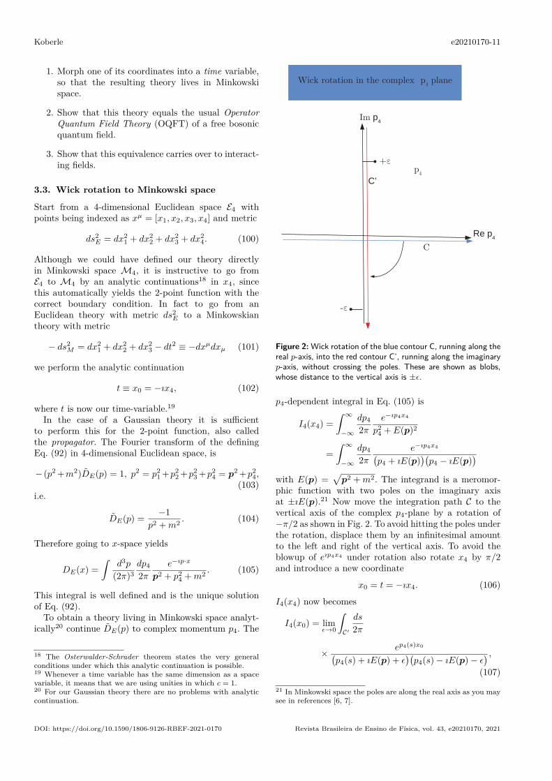
Figure 2: Wick rotation of the blue contour C, running along thereal p-axis, into the red contour C’, running along the imaginaryp-axis, without crossing the poles. These are shown as blobs,whose distance to the vertical axis is ±ε.

p4-dependent integral in Eq. (105) is

I4(x4) =∫ ∞−∞

dp4

2πe−ıp4x4

p24 + E(p)2

=∫ ∞−∞

dp4

2πe−ıp4x4(

p4 + ıE(p))(p4 − ıE(p)

)with E(p) =

√p2 +m2. The integrand is a meromor-

phic function with two poles on the imaginary axisat ±ıE(p).21 Now move the integration path C to thevertical axis of the complex p4-plane by a rotation of−π/2 as shown in Fig. 2. To avoid hitting the poles underthe rotation, displace them by an infinitesimal amountto the left and right of the vertical axis. To avoid theblowup of eıp4x4 under rotation also rotate x4 by π/2and introduce a new coordinate

x0 = t = −ıx4. (106)

I4(x4) now becomes

I4(x0) = limε→0

∫C′

ds

2π

× ep4(s)x0(p4(s) + ıE(p) + ε

)(p4(s)− ıE(p)− ε

) ,(107)

21 In Minkowski space the poles are along the real axis as you maysee in references [6, 7].



where s is a real coordinate running along the contourC′. Since along this contour p4(s) is purely imaginarydefine the real variable k0 as

k0 = ıp4 (108)

and trade s for k0 as integration variable. With thischange of variables, the integral along the new path C′becomes22

I4(x0) = limε→0

∫ ∞−∞

dk0

2πe−ık0x0(

k0 + E(k)− ıε)(k0 − E(k) + ıε

)= limε→0

∫ ∞−∞

dk0

2πe−ık0x0

k2 −m2 + ıε, (109)

where

k2 ≡ k20 − k2. (110)

After this analytic continuation of the Euclidean prop-agator DE(x) of Eq. (105) becomes the Feynmanpropagator

DF (x) =∫ ∞−∞

d4k

(2π)4e−ık·x

k2 −m2 + ıε, (111)

the scalar product in Minkowski space being defined ask · x ≡ k0x0 − k · x. The propagator satisfies

(∂2 +m2)DF (x− y) = −δ(4)(x− y),

∂2 ≡ ∂ν∂ν = ∂2t −∇2 (112)

where ∂ν ≡ ∂/∂xν ≡ [∂t, ∂x1 , ∂x2 , ∂x3 ], ∂ν ≡[∂t,−∂x1 ,−∂x2 ,−∂x3 ], repeated indices ν = [0, 1, 2, 3]being summed over.To explicitly compute I4(x0), we close the integration

path by a contour in the complex plane, choosing alwaysthe decreasing exponential in Eq. (109) to get

I4(x0) = ı

e−ıx0E(k)

2E(k) , x0 > 0

eıx0E(k)

2E(k) , x0 < 0(113)

with E(k) =√k2 +m2.

In the following section we show, that the Feynmanpropagator obtained by the the analytic continuationof the euclidean one, is identical to the Feynmanpropagator of the Operator Quantum Field Theory(OQFT). This great advantage is the reason we startedfrom the Euclidean formulation.Apply now the substitution∫

E

d4x→ ı

∫d4x, → −∂2, (114)

22 Since E(p) > 0, 2E(p)ε is an equivalent stand-in for the limitε→ 0.

to the Euclidean functional Eq. (97), to get the generat-ing functional for the Minkowskian theory as

Z[J ] = 1Z

∫Dϕeı

∫d4x(L0(ϕ)+Jϕ

)(115)

with

L0(ϕ) ≡ 12(∂νϕ∂

νϕ−m2ϕ2) . (116)

and d4x = dxdydzdt. Notice that whenever an ı appearsin the exponent multiplying L0, we are in Minkowskispace M4. Integrating over ϕ we get in analogy toEq. (98)

Z[J ] = 1Z

∫Dϕe

ı2

∫d4x(ϕ(−∂2−m2)ϕ+Jϕ

)= e−

ı2

∫d4xJ(x)[∂2+m2]−1J(x)

= e− ı

2

∫d4xd4yJ(x) δ

(4)(x−y)∂2+m2 J(y)

where we set the normalization factor Z such thatZ(0) = 1. Upon using Eq. (112) this yields

Z[J ] = eı2

∫d4xd4yJ(x)DF (x−y)J(y). (117)

The Minkowskian generating functional Eq. (115) pro-duces the correct correlation function as

〈ϕ(x1) . . . ϕ(xn)〉 = δnZ[j]ınδJ(x1) . . . δJ(xn) |J=0. (118)

In particular for n = 2 we get

〈ϕ(x1)ϕ(x2)〉 = ıDF (x1 − x2). (119)

Since the equation of motion Eq. (92) is linear, itdescribes a free field propagation in space-time. To getsome interesting physics we will have to turn interactionson in Sect. 3.5.

3.4. Quantizing a complex scalar field

In this section we will compute the two-point function ofa free complex scalar field using the operator approachof Quantum Field Theory (OQFT) in order to show thatthis yields the same Feynman propagator. In this sectionwe will always work in Minkowski space with coordinate[x1, x2, x3, x0 = t].In OQFT the propagator is defined to be the vacuum

expectation value of the following time-ordered 2-pointfunction

ıD(OQFT )F (x− y) = 〈Ω|Tφ(x)φ?(y)|Ω〉 (120)

of the quantized operator field φ(~x, t) – actually anoperator valued distribution. Here |Ω〉 is the vacuumstate and T means time-ordered – see Eq. (133). Thequantized field φ(~x, t) will turn out to be a collection ofharmonic operators.



Consider a complex scalar field, whose Lagrangiandensity is

L0(φ) ≡ 12(∂αφ

?∂αφ−m2φ?φ), (121)

where ∂α ≡ [∂t, ∂x1 , ∂x2 , ∂x3 ], ∂α ≡ [∂t,−∂x1 ,−∂x2 ,−∂x3 ]and we sum over the repeated indices α, so that

L0(φ) = 12(∂0φ

?∂0φ−∇φ? · ∇φ−m2φ?φ).

The equations of motion are

∂

∂xα∂L0

∂(∂φ/∂xα) −∂L0

∂φ= 0,

∂

∂xα∂L0

∂(∂φ?/∂xα) −∂L0

∂φ?= 0

i.e.

(∂2 +m2) φ(x)φ?(x)

= 0 (122)

with ∂2 ≡ ∂2t − ∂2

x1− ∂2

x2− ∂2

x2. This so called Klein-

Gordon equation, is a four-dimensional wave equationfamiliar from the study of Maxwell’s equations, in whichcase m = 0.The canonical quantization rules are – in units where

c = ~ = 1 –

[φ(x, t), φ(x′, t)] = 0, [π(x, t), π(x′, t)] = 0

φ(x, t), π(x′, t)] = −ıδ(3)(x− x′) (123)

with the conjugate momenta

π = ∂L0/∂φ = φ? and π? = ∂L0/∂φ? = φ.

Expand this field in energy-momentum eigenstates,23

satisfying Eq. (122)

φ(x, t) =∫

d3k√(2π)32Ek

× [a+(k)eık·x−ıEkt + a†−(k)e−ık·x+ıEkt]

≡∫d3k[a+(k)fk(x) + a−(k)†f?k(x)], (124)

where

Ek =√

k2 +m2, fk(x) = e−ık·x√(2π)32Ek

with k = k = [k1, k2, k3], k0 = Ek and k · x = Ekx0 −k · x. Here a†−(k) is the hermitian conjugate of a−(k),since we are dealing with operators.

23 The factor√

2Ek is included, so that e.g. the commutationrelations Eq. (128) are the usual harmonic oscillator ones.

We easily solve for a±(k). For this we use the orthog-onality relations

ı

∫d3xf?k(x, t)

↔∂t fl(x, t) = δ3(k− l) (125)∫

d3xfk(x, t)↔∂t fl(x, t) = 0, (126)

where

f(t)↔∂t g(t) ≡ f(t)dg

dt− df

dtg(t),

such that, inter alia, the↔∂t kills the Ek factors from

fk(x) and allows the cancellation necessary for Eq. (126)to be true. Using these in Eq. (124) we get

a+(k) = ı

∫d3xf?k(x, t)

↔∂t φ(x, t),

a−(k) = ı

∫d3xf?k(x, t)

↔∂t φ

?(x, t).

Executing the operation↔∂t we get

a+(k) =∫d3xf?k(x, t)[Ekφ(x, t) + ıφ(x, t]

and using Eq. (123), this yields the commutator

[a+(k), a†+(l)]

= −∫d3xd3y[f?k(x, t)

↔∂t φ(x, t), fl(y, t)

↔∂t φ

?(y, t)

= ı

∫d3xf?k(x, t)

↔∂t fl(x, t) = δ(3)(k− l). (127)

Proceeding analogously, we get for the whole set

[a+(k), a†+(k′)] = [a−(k), a†−(k′)] = δ(3)(k− k′)),

[a±(k), a±(k′)] = 0, [a†±(k), a†±(k′)] = 0,

[a+(k), a†−(k′)] = 0, [a−(k), a†+(k′)] = 0. (128)

These commutation relations show, that we have twoindependent harmonic oscillators a±(k) for eachmomentum k. Defining the vacuum for each k as

a±(k)|0k〉 = 0,∀k, (129)

we build a product-Hilbert space applying the creationoperators a†±(k) to the ground state |Ω〉 =

∏k |0k〉.

We have the usual harmonic oscillator operators likeenergy, momentum etc, but here just highlight thecharge operator. Due to the symmetry

φ(x)→ eıηφ(x) (130)

for constant η, Noether’s theorem tells us that thecurrent

jµ = ı(φ?∂µφ− φ∂µφ?) (131)



is conserved: ∂µjµ = 0. The conserved charge is24

Q = ı

∫d3xj0 =

∫d3k[a†+(k)a+(k)− a†−(k)a−(k)],

(132)the operator a†+(k) creating a positively charged particleof mass m and the a†−(k) a negatively charged one.

Now compute the time-ordered product

〈Ω|Tφ(x′)φ?(x)|Ω〉

≡ θ(t′ − t)〈0|φ(x′)φ?(x)|0〉

+ θ(t− t′)〈0|φ?(x)φ(x′)|0〉. (133)

Both terms above create a charge Q = +1 at (x, t) anddestroy this charge at (x′, t′ > t). The first term does theobvious job, whereas the second term creates a chargeQ = −1 at (x′, t′) and destroys it at (x, t > t′). Thisjustifies the name propagator, since it propagates stufffrom x to x′ and vice-versa.25 Since the fields φ(x), φ?(x′)commute for space-like distances x− x′, the θ-functionsdon’t spoil relativistic invariance.Inserting the expansions Eq. (124) into Eq. (133),

we get

〈Ω|Tφ(x′)φ?(x)|Ω〉

=∫d3k[fk(x′)f?k(x)θ(t′ − t)

+ f?k(x′)fk(x)θ(t− t′)]

=∫

d3k

(2π)32Ek[θ(t′ − t)e−ık·(x

′−x)

+ θ(t− t′)eık·(x′−x)]

The time-dependent part of the integrand in squarebrackets equals the rhs of Eq. (113).26 Using Eq. (109)we get

〈Ω|Tφ(x)φ?(y)|Ω〉 = ı

∫d4k

(2π)4e−ık·(x−y)

k2 −m2 + ıε. (134)

Therefore conclude with Eq. (111), that

〈Ω|Tφ(x)φ?(y)|Ω〉

= ıD(OQFT )F (x− y)

= ıDF (x− y) = 〈ϕ(x)ϕ?(y)〉. (135)

24 Going from Eq. (131) to Eq. (132) we actually subtracted ininfinite constant. The presence of an infinite number of oscillatorsrequires this redefinition of the charge! This simple subtraction issufficient for a free theory. The interacting case requires a wholenew machinery called renormalization.25 To be able to follow the propagating charge, was to reason touse a complex field and not a real, neutral field.26 Although this equation was computed for a real scalar field, theintegrand is the same for our complex field.

The other time-ordered products are

〈Ω|Tφ(x)φ(y)|Ω〉 = 〈Ω|Tφ?(x)φ?(y)|Ω〉 = 0. (136)

Upon expanding in terms of real, hermitian fieldsφ1, φ2 as

φ(x) = 1√2(φ1(x) + ıφ2(x

),

yields

〈Ω|Tφi(x)φj(y)|Ω〉 = ıδijD(OQFT )F (x− y)

= ıδijDF (x− y). (137)

Thus Eqs. (115, 119) show, that the path-integral yieldsthe time-ordered correlation functions of OQFT

〈Ω|Tφ(x1)φ(x2)|Ω〉 =∫Dϕϕ(x1)ϕ(x2)eı

∫d4xL0(ϕ).

(138)Since our theory is Gaussian, this is all we need to specifythe whole theory and we therefore have for any numberof fields

〈Ω|Tφ(x1)φ(x2) . . . φ(xN )|Ω〉

=∫Dφϕ(x1)ϕ(x2) . . . ϕ(xN )

× eı∫d4xL0(ϕ). (139)

We have therefore shown, that the path-integral for-mulation is equivalent to the OQFT description.In section 3.5 we will extend this to a theory withinteractions.

Aside: On- & Off-shellA field is called on-shell, if its energy-momentum operator eigenvalues satisfyEk = +

√k2 +m2. If this is not true, the

field is off-shell.27

Explicit relativistic invariance is a mustin QFT, especially in the old days, whennon-invariant cut-offs abounded to tameultraviolet divergences. If we use tradi-tional non-relativistic perturbation theory,we maintain conservation of momentum,but abandon conservation of energy, toallow the appearance of intermediate states.This results in the ubiquitous presenceof energy denominators. This procedure,although yielding correct results, breaksexplicit relativistic invariance. In QFT we

27 We may impose the on-shell condition with positive energy ina manifestly relativistic invariant way as∫

d3k

(2π)32Ek=∫

d4kδ(k2 −m2)2πθ(k0).

.



want to maintain explicit invariance andtherefore impose conservation of energy andmomentum. But now, in order to allow theappearance of intermediate states, we haveto place the particles off-shell.

Exercise 3.1For a discussion of Feynman’s propagator theory BD1[8], Section 6.4. What is the difference betweenretarded, advanced and Feynman propagators, all ofwhich satisfy Eq. (112)?

3.5. Generating functional for interactingtheories

We turn interactions on28 adding an interaction term tothe free quadratic Lagrangian L0(ϕ) in Eq. (115)

L0(ϕ)→ L(ϕ) = L0(ϕ) + Lint(ϕ) (140)

and define our interacting theory via the generatingfunctional

Z[J ] =∫Dϕeı

∫d4x(L0(ϕ)+Lint(ϕ)+Jϕ

)(141)

with the normalization factor∫Dϕeı

∫d4x(L0(ϕ)+Lint(ϕ)

)included into the measure Dϕ, so that Z(0) = 1.Equation (139) written now for interacting fields

becomes

〈Ω|Tφ(x1)φ(x2) . . . φ(xN )|Ω〉

=∫Dφϕ(x1)ϕ(x2) . . . ϕ(xN )eı

∫d4x(L0(ϕ)+Lint(ϕ)

).

(142)

This looks, but only looks, similar to the Gell-MannLow formula of OQFT

〈Ω|Tφ(x1)φ(x2) . . . φ(xN )|Ω〉

= 1Z〈0|Tφ0(x1)φ0(x2) . . . φ0(xN )

× eı∫d4x(Lint(φ0)+Jφ0)|0〉, (143)

where φ, |Ω〉 are the operator field and the vacuum ofthe interacting theory, |0〉, φ0 the corresponding free fieldquantities29 and Z, as usual, equals the numerator withJ = 0. But here we deal with time-ordered products,as in Eq. (133), of operator-valued-distributions. In the

28 This process often leads to misunderstandings. We startedwith a chimera: a free charged field, which is not the source ofan electromagnetic field. The interaction now has to change thischimera into a real-world particle with a new mass, charge etc. Avery non-trivial process indeed, which we don’t discuss here.29 Like the free scalar field of Eq. (124).

rhs of Eq. (142) the operator-valued-distributions havemorphed into mere integration variables at the price ofperforming path-integrals.Generally we are unable to perform the

∫Dϕ integral,

since the interaction Lagrangian is not quadratic in thefield variables. But we may rewrite Z[j] using our oldtrick equ(15). Expand the exponential eı

∫d4xLint(ϕ) in

powers of ϕ(y). A linear term would be∫Dϕϕ(y) eı

∫d4x(L0(ϕ)+Jϕ

)Replace ϕ(y) by the operation 1

ıδ

δJ(y) as∫Dϕϕ(y) eı

∫d4x(L0(ϕ)+Jϕ

)=∫Dϕ

1ı

δ

δJ(y)eı∫d4x(L0(ϕ)+Jϕ

)= 1ı

δ

δJ(y)

∫Dϕeı

∫d4x(L(ϕ)+Jϕ

)We can perform this substitution for all the powers ofϕ(y) and reassemble the exponential to get

Z[j] =∫Dϕeı

∫L(ϕ)+ı

∫Jϕ

= eı∫Lint( 1

ıδδJ )∫Dϕeı

∫L0(ϕ)+ı

∫Jϕ. (144)

Performing the Gaussian integral over Dϕ we obtain

Z[J ] = eı∫Lint( 1

ıδδJ )e

ı2

∫d4xJ(x)∆F (x−y)J(y)d4y (145)

and correlation functions as

〈ϕ(x1)ϕ(x2) . . . ϕ(xn)〉

= δnZ[J ]ınδJ(x1)δJ(x2) . . . δJ(xn)

∣∣∣∣∣J=0

(146)

Eq. (145) is a closed formula for the fully inter-acting theory. Yet it is in general unknown how tocompute

eLint(1ıδδJ )〈. . .〉,

except expanding the exponential.Furthermore our manipulations are formal and the

integrals in general turn out to be divergent! Yet thereis a well-defined mathematical scheme – not somemysteriously dubious instructions – to extract finiteresults for renormalizable field theories e.g. the BPHZ30

renormalization scheme [16]. Renormalizable roughly

30 The acronym stands for N. Bogoliubov and O. Parasiuk, whoinvented it; K. Hepp, who showed its correctness to all orders inperturbation theory and W. Zimmerman, who turned it into ahighly efficient machinery.



means that the Lagrangian contains only products offields, whose total mass-dimension is less or equal to thespace-time dimension D = 4 and the theory includesall interactions of this type. The symmetries of the thusconstructed quantum field theory may be different fromthe classical version. In particular it may have evenmore or less conservation laws – in which case anomaliesare said to arise.Let us obtain the path-integral version of the

equation of motion like Eq. (122). For this purposeuse the following simple identity∫

Dϕδ

δϕ= 0, (147)

assuming as usual boundary conditions with vanishingboundary terms. Applying this to the integrand of thegenerating functional Z[j] of Eq. (144)

Z[J ] =∫Dϕeı

∫d4x(L(ϕ)+Jϕ) =

∫DϕeıS(ϕ)+ı

∫d4xJϕ,

we get∫Dϕ

δ

δϕeıS(ϕ)+ı

∫d4xJϕ

=∫Dϕ ı

[δS(ϕ)δϕ

+ J]eıS(ϕ)+ı

∫d4xJϕ = 0.

(148)Remember that

δS(ϕ)δϕ

= ∂L∂ϕ− ∂µ

∂L∂∂µϕ

, (149)

which set to 0 yields the classical equation of motion.In fact, since the action depends both onϕ(x) and its derivative ϕ′(x) = dϕ(x)/dx,we have

δS = δ

∫dyL[ϕ(y), ϕ′(y)]

=∫dy

[∂L∂ϕ(y)δϕ+ ∂L

∂ϕ′(y)δϕ′]

=∫dy

[∂L∂ϕ(y) −

d

dy

∂L∂ϕ(y)

]δϕ(y),

(150)where we performed a partial integration,assuming that the boundary terms vanish.Thus

δS

δϕ(x) = ∂L∂ϕ(x) −

d

dx

∂L∂ϕ(x) (151)

with Eq. (149) its four-dimensional version.Setting J = 0 in Eq. (148) yields the equation of

motion∫DϕeıS(ϕ) δS

δϕ(y)

=∫DϕeıS(ϕ)

(∂L∂ϕ− ∂µ

∂L∂∂µϕ

)= 0. (152)

Here the classical equation of motion shows up in theintegrand.Taking one derivative of Eq. (148) with respect to J ,

we get

0 = δ

δJx1

∫DϕeıS(ϕ)+ı

∫d4xJ(x)ϕ(x)

(δS

δϕ(y) + J(y))

= ı

∫Dϕϕ(x1)eıS(ϕ)+ı

∫d4xJ(x)ϕ(x)

(δS

δϕ(y) + J(y))

+∫DϕeıS(ϕ)+ı

∫d4xJ(x)ϕ(x)δ(4)(y − x1)

Setting J = 0 yields∫DϕeıS(ϕ)

(ϕ(x1) δS

δϕ(y) − ıδ(4)(y − x1)

)= 0.

(153)

Exercise 3.2Taking two derivatives of Eq. (148) with respect to J ,show that∫

Dϕϕ(x2)ϕ(x1)eıS(ϕ)( δS

δϕ(y)

)= ı

∫DϕeıS(ϕ)

×(ϕ(x1)δ(4)(y − x2) + ϕ(x2)δ(4)(y − x1)

).

(154)

Exercise 3.3Write Eq. (148) as[

δS′(−ı δδJ

) + J]Z[j] = 0. (155)

This Schwinger-Dyson equation is an exact equation.Z[j] may now be expanded in a power series to obtainperturbation theory results.

3.6. Connected correlation functions and theeffective action

We have been using the auxiliary source field J(x) togenerate correlation functions from Z[j] via Eq. (146).As such J(x) actually is a sort of outsider, since weare really interested in the field ϕ(x). It is thereforeextremely useful to have a generating functional, whichpermits direct access to the field ϕ(x).For this purpose we first define a new generating

functional W (J) as

Z[J ] = eıW [J], W [J ] = −ı lnZ[J ]. (156)

Using the cumulant expansion of exercise 3.3 or by directcomputation, it is straightforward to verify, that W [J ]



generates the connected correlation functions

〈ϕ(x1)ϕ(x2) . . . ϕ(xn)〉c = ıδnW [J ]ınδJ(x1)δJ(x2) . . . δJ(xn)

∣∣∣∣∣J=0

(157)E.g.

〈ϕ(x)〉c = 〈ϕ(x)〉,

〈ϕ(x1)ϕ(x2)〉c = δ2W [J ]ıδJ(x1)δJ(x2) |J=0

=[− 1Z[j]

δ2Z[j]δJ(x1)δJ(x2)

+ 1Z[j]2

δZ[j]δJ(x1)

δZ[j]δJ(x2)

]J=0

= 〈ϕ(x1)ϕ(x2)〉 − 〈ϕ(x1)〉〈ϕ(x2)〉,(158)

where we used Eq. (146). Now trade the auxiliary sourceJ(x) for the one-point correlation function31

ϕ(x) ≡ 〈ϕ(x)〉 = 〈ϕ(x)〉c = δW

δJ(x) (159)

by a functional Legendre transformation

Γ[ϕ] ≡W [J ]−∫d4xJ(x)ϕ(x) (160)

and use ϕ(x) as the independent field. The field ϕ(x)is directly related to physical properties as opposed toauxiliary field J(x).As Eq. (156) shows, Γ[ϕ] is an effective action. J(x)

is now a variable dependent of ϕ(x), given by

δΓ[ϕ]δϕ(x) = −J(x). (161)

Using Eq. (159) it also follows that

δΓ[ϕ]δJ(x) = 0.

Differentiating Eqs. (159, 161), we get

〈ϕ(x)ϕ(y)〉c = −ıδ2WδJ(x)δJ(x) = −ı δϕ(x)

δJ(y)

Γ(2)(x, y) ≡ δ2Γδϕ(x)δϕ(x) = − δJ(y)

δϕ(x) . (162)

The functional Γ[ϕ] is useful, inter alia, for the study ofphase transitions. If ϕ(x) is not zero, even if J(x) = 0,spontaneous symmetry breaking32 occurs. Due toEq. (161), this means

δΓ[ϕ]/δϕ(x) = 0. (163)

31 In the presence of the external source J(x) the one-pointcorrelation functions 〈ϕ(x)〉 does not vanish!32 See e.g. [11], Eq. (3.18) for details, after reading section 6.1.

Exercise 3.4 (The cumulant expansion)Show that

ln〈e−x〉 =∞∑n=0

(−1)nn! 〈x

n〉c, (164)

where the subscript c stands for connected. We have

〈x〉c = 〈x〉, 〈x2〉c = 〈x2〉 − 〈x〉2, . . .

Exercise 3.5 (Proper vertex functions)The functions

Γ(n)(x1, x2, . . . xn) ≡ δnΓ[ϕ]δϕ(x1) . . . δϕ(xn)

∣∣∣ϕ=0

(165)

are called proper vertex functions. Verify, that for thefree field case the only proper vertex is

Γ(2)0 (x, y) = −(∂2 +m2)δ(4)(x− y), Γ(2)

0 (p) = p2 −m2.(166)

Exercise 3.6Show that∫

d4yΓ(2)0 (x, y)DF (y − z) = δ(4)(x− z), (167)

i.e. the Feynman propagator is the Green function of theproper vertex Γ(2)

0 . Show that the analogous relation∫d4yΓ(2)(x, y) [−ı〈ϕ(y)ϕ(z)〉c] = δ(4)(x− z) (168)

holds for the interacting case. Multiply Eqs. (162)like matrices, paying attention to the repeated indicessummed/integrated over.Exercise 3.7 (The free field case)Eq. (117) states

W0[J ] = 12

∫d4xd4yJ(x)DF (x− y)J(y).

Verify

ϕ0(z) =∫d4z′DF (z − z′)J(z′). (169)

Insert this in Eq. (160) to get

Γ0[ϕ] = −∫d4yJ(y)ϕ0(y)

=∫d4xd4yJ(x)

(− δ(4)(x− y)

)ϕ0(y).

Use the equation for the Feynman propagator(Eq. (112))

(∂2x +m2)DF (x− y) = −δ(4)(x− y)

to get rid of the(− δ(4)(x − y)

)-factor. Show using

Eq. (169), that

Γ0[ϕ] = −12

∫d4xϕ0(x)(∂2 +m2)ϕ0(x), (170)

J(x) = (∂2 +m2)ϕ0(x).



You will perform usual matrix multiplications withcontinuous indices and perform a partial integration.

Apply a partial integration on the ∂2ϕ-term33 to showthat the effective action Γ0[ϕ] coincides with the classicalfree action S0(ϕ) =

∫L0(ϕ).

At this point notice, that we had to execute the path-integral

∫Dϕ in Eq. (95) with the classical action S0(ϕ)

figuring in the integrand, to obtain Γ0[ϕ] = S0(ϕ).In the interacting case Γ[ϕ] is very different from theinteracting classical action S(ϕ) =

∫L(ϕ)!

Exercise 3.8(The effective potential)Let us compute the first order quantum correction to theclassical action[11, 13, 18]. For this purpose we expandaround the classical saddle point Eq. (149), whereφ(x)|saddle point = φ0. The saddle-point equation is

δ(S[φ] +∫Jφ)

δφ|φ=φ0 = 0 (171)

orδS[φ]δφ(x) |φ=φ0 = −J(x), (172)

which expresses φ0 as a functional of J → φ0[J ].Expanding about the saddle-point, we have up to secondorder

S[φ] = S[φ0]−∫d4xJ(x)∆φ(x)

+ 12

∫d4xd4y∆φ(x)A∆φ(y) (173)

with ∆φ = φ − φ0 and the expansion coefficient A is afunctional of φ0:

A[φ] = δ2S[φ]δφ(x)δφ(y) |φ=φ0 . (174)

To simplify notation write this as

S[φ] = S[φ0]− (J,∆φ) + 12(∆φ, A∆φ). (175)

Eq. (156) tells us to compute

Z[J ] =∫Dφeı

(S[φ]+(J,φ)

)= eıW [J]. (176)

We perform this in the Euclidean version

ZE [J ] =∫Dφe−

(SE [φ]+(J,φ)

)= e−WE [J], (177)

where (, ) are now Euclidean integrals. Shifting φ toφ+ φ0, we have

ZE [J ] =∫Dφe−

(SE [φ0]+(J,φ0)+ 1

2 (φ,Aφ))

= e−SE [φ0]−(J,φ0)∫Dφe−

12 (φ,Aφ) (178)

33 See the comments after Eq. (97).

Integrate over φ, to get

WE [J ] = SE [φ0] + (J, φ0) + 12 log detA. (179)

The corresponding effective action is

ΓE [φ] = WE [J ]− (J, φ)

= SE [φ0] + (J, (φ0 − φ)) + 12 log detA. (180)

We still have to trade J for φ0. This means solvingthe implicit Eq. (172) and Eq. (159). Fortunately it isonly necessary to expand SE to first order to get withEq. (172)

SE [φ] = SE [φ0] +∫

(φ− φ0)δSEδφ|φ=φ0

= SE [φ0]−∫

(φ− φ0)J.

Therefore we find the effective action including a firstorder quantum correction as

ΓE [φ] = SE [φ] + 12 log detA[φ]. (181)

Reinstating the factors of ~, convince yourself that theadditional term is first order in ~.To get some feeling for this formula, we compute the

effective potential Veff , which is the effective actionΓ[φ] computed for constant φ. Since Γ[φ] is an extensivequantity, we also will extract the space-time volume Ωto obtain an intensive quantity for Veff . Computing inEuclidean space we get for the action

SE [φ] =∫d4x

[12(∂φ)2 + V (φ)

](182)

and expand it to second order in η with φ = v + η(x)and v constant. After a partial integration we get

SE [φ] =∫d4x

[12(∂η)2 + V (v) + ηV ′(v) + 1

2η2V ′′(v)

]= ΩV (v) +

∫d4x

×ηV ′(v) + 1

2η[− ∂2 + V ′′(v)

]η

. (183)

Eq. (172) and Eq. (174) now yield at the saddle-pointφ = v

V ′(v) = −J

A[x, y] = [−∂2 + V ′′(v)]δ(4)(x− y). (184)

Thus integrating over η, we obtain from Eq. (179)

WE [J ] = ΩV (v) + (J, v) + 12Tr logA[v].



In Fourier space the trace is

Tr logA[φ] = Ω∫

d4k

(2π)4 log[k2 + V ′′(v)]. (185)

Now expand the effective action in powers of momentumaround a constant φ = v as

Γ[φ] ≡∫d4x

[Veff (v) + 1

2(∂φ)2Z(v) + · · ·], (186)

where Veff is now a function of v, not a functional.Thus we finally get from Eq. (181)

Veff (v) = V (v) + 12

∫d4k

(2π)4 log[k2 + V ′′(v)]. (187)

This integral is ultraviolet divergent for large k. Inte-grating up to a cut off at Λ, one obtains neglecting anirrelevant constant

Veff (v) = V (v) + Λ2

32π2V′′(v)

+(V ′′(v)

)264π2

(log(V ′′(v)

)2Λ2 − 1

2

). (188)

If we choose for the potential the expression

V (φ) = λ

4!φ(x)4 (189)

our model is renormalizable,34 allowing us to obtain acut-off independent result. It has the symmetry

φ(x)→ −φ(x). (190)

After the dust of the renormalization has settled, weare left with the following effective potential

Veff (v) = λ

4!v4 + (a1λ

2 + a2)v4(

log v2

M2 − a3

),

(191)

where ai, i = 1, 2, 3 are numerical constants. Noticethat the action SE [φ] does not contain any dimensionalparameter. Yet in order to obtain a non-trivial resultwhen implementing the renormalization, one is obligedto introduce a mass-parameterM in order to avoid infra-red divergencies at k = 0.Although V (φ) has a minimum at φ = 0, Veff (v) has

a maximum there and two minima at ±vmin∂Γ[v]∂v|vmin = ∂V [v]

∂v|vmin = 0, v2

min > 0. (192)

In accordance with Eq. (163), the quantum correctionsinduce the spontaneous breaking of the symmetryEq. (190) in the limit35 Ω→∞ – see sect. 6 explainingthis concept.

34 See the comments after Eq. (146).35 For finite Ω the two states centered at ±vmin would overlap,creating either a symmetric or an anti-symmetric state. For infiniteΩ the overlap vanishes exponentially and we have to choose either+vmin or −vmin with identical physics.

4. Path Integrals in Quantum Mechanics

We now rewrite the usual formulation of non-relativistic Quantum Mechanics in terms of path-integrals. Although this is just a special 1-dimensionalcase of sect. 3.3, it is instructive, because we start fromscratch and obtain the path-integral formulation also forthe interacting case.

Consider the hamiltonian

H = 12mP 2 + V (Q) (193)

with

[Q,P ] = ı~. (194)

Time evolution is given by

〈b(t′)|a(t)〉 = 〈b|e−ıH(t′−t)/~|a〉 (195)

Using the usual non-normalizable states, we have

Q|q〉 = q|q〉, P |p〉 = p|p〉, (196)

〈q′|q〉 = δ(q′ − q), 〈p′|p〉 = δ(p′ − p) (197)

〈q|p〉 = 〈p|q〉? = eıpq√2π

(198)

〈q|P |p〉 = p〈q|p〉 = 1ı

∂

∂q〈q|p〉. (199)

The completeness relation is

I =∫ ∞−∞

dq|q〉〈q|. (200)

We have in the Heisenberg representation

qH(t)|q, t〉 = eıtH/~qe−ıtH/~eıtH/~|q〉 = q|q, t〉. (201)

For a time-dependent Hamiltonian the Heisenberg oper-ators qH(t1) and qH(t2) do in general not commute fort1 6= t2. Therefore, if we want to use completeness fordifferent times, we have to choose a different basis |q, t〉for each t in which q(t) is diagonal.Use the unitary time evolution operator U(tI , tF ) to

propagate the wave function as

ψ(tF ) = U(tf , tI)ψ(tI). (202)

Therefore U(tF , tI) has to satisfy the Schrödinger equa-tion

ı~∂U(tF , tI)

∂tF= H(tF )U(tF , tI) (203)

with the initial condition U(tI , tI) = I. For a time-independent Hamiltonian H the evolution operatorU(tI , tI) is given by

U(tF , tI) = e−ı/~(tF−tI)H , (204)



whereas for a time-dependent Hamiltonian it isexpressed in terms of the time-ordered exponential as

U(tF , tI) = Te−ı/~

∫ tFtI

dt′H(t′). (205)

We can decompose the time-evolution into steps due to

U(tF , tI) = U(tF , t)U(t, tI), for tF > t > tI . (206)

The matrix elements

K(qF , qI ; tF − tI) ≡ 〈qF |U(tF , tI)|qI〉 ≡ 〈qF , tF |qI , tI〉(207)

are called the kernel. We will compute it in the position-space representation in order to express it in terms ofPath-integrals. Use Eq. (206) to evolve from tI to tF inN consecutive steps (for notational simplicity only forthe time-independent case)

K(qF , qI ; tF − tI)

= 〈qF |U(tF , tN−1)U(tN−1, tN−2) . . . U(t1, tI)|qI〉.(208)

Insert the identity Eq. (200) N times splitting our timeinterval into N small intervals ∆t = (tF − tI)/N to get

K(qF , qI ; tF − tI) =N−1∏i=1

∫ ∞−∞

dqi

N−1∏i=0

K(qi+1, qi; ∆t)

(209)with t0 = tI , tN = tF and we do not integrate overq0 = qI and qN = qF ! Now compute the kernel for asmall time step (with ~ = 1)

K(qi+1, qi; ∆t) = 〈qi+1|e−ıH∆t|qi〉 (210)

with

K(qi+1, qI ; ∆t)→ δ(qi+1 − qi) for ∆t→ 0.

Although q does not commute with p, for small ∆t wemay ignore36 this and write

e−ıH∆t = e−ıp22m∆te−ıV (q)∆t (211)

Therefore

〈qi+1e−ıH∆t|qi〉 = 〈qi+1|e−ı

p22m∆te−ıV (q)∆t|qi〉

= 〈qi+1|e−ıp22m∆t|qi〉e−ıV (qi)∆t

=∫dpi〈qi+1|pi〉e−ı

p2i

2m∆t〈pi|qi〉e−ıV (qi)∆t

= 12π

∫dpie

ıpi(qi+1−qi)−ı∆t[p2i

2m+V (qi)].

(212)

36 The commutant of the kinetic and potential energy is of orderO(ε2). If this were untrue, and if [H(t), H(t′] 6= 0 we would haveto use the Baker-Haussdorf formula – see [5], section 10.2.5 andWikipedia.

Here we chose to replace 〈qi+1|e−ıV (q)∆t|qi〉 bye−ıV (q=qi)∆t. For eventual problems with this choice see[5], section 4.

Performing the p-integrals, we get

12π

∫dpie

ıpi(qi+1−qi)−ı(p2i

2m )∆t

=( m

2πı∆t

)1/2eım(qi+1−qi)2/(2∆t). (213)

Therefore the small time-step kernel is

K(qi+1, qi; ∆t) =( m

2πı∆t

)1/2

× exp(ım

2(qi+1 − qi)2

∆t − ı∆tV (qi))

(214)

For qi+1 = q(t+∆t), qi = q(t) and ∆t ∼ 0 we manipulateas37 Thus

m

2

(q(t+ ∆t)− q(t)

)2

∆t = m

2

(q(t+ ∆t)− q(t)

∆t

)2∆t

= m

2

∫ t+∆t

t

dtq2. (215)

Therefore we get

m

2

(q(t+ ∆t)− q(t)

)2∆t −∆tV (q1) =

∫ t+∆t

t

dtL(q, q),(216)

where the systems Lagrangian is

L(q, q) = 12mq

2 − V (q). (217)

This yields

〈q(t+ ∆t|q(t)〉 =( m

2πı∆t

)1/2eı∫ t+∆t

tdtL(q,q)

. (218)

Inserting this into Eq. (209) (now with ~ inserted),

〈qF , tF |qI , tI〉

= K(qF , qI ; tF − tI)

= limN→∞

( m

2πı~∆t

)N/2×[ΠN−1k=1

∫ ∞−∞

dqk

]eı∫ tFtI

dtL(q,q). (219)

With the notation

limN→∞

[ΠN−1k=1

∫ ∞−∞

dqk

]=∫ q(tF )

q(tI)D[q(t)] =

∫Dq,

(220)

37 Regarding the differentiability of q(t), refer to the discussionat Eq. (68) of the Wiener process. Thus our manipulations areformal, but we know how to compute before the limit N →∞.



we have

〈qF , tF |qI , tI〉 =∫ q(tF )

q(tI)D[q(t)]eı/~

∫dtL(q,q)

=∫DqeıS/~, (221)

with the action

S =∫ tF

tI

L(q, q)dt. (222)

This equation is the one-dimensional version of Eq. (141)with J = 0.Although we have shown Eq. (221) to be true for a

non-relativistic one-body Hamiltonian with a potentialV (q), Eq. (221) does not make any reference to thisparticular form and it is in fact true generally.We can also leave the p-integrals undone38 in Eq. (213)

and write

〈qF , tF |qI , tI〉 = limN→∞

[ΠN−1k=1

∫ ∞−∞

dqk

] [ΠN−1k=1

∫ ∞−∞

dpk

]eı/~

∫dt(p(t)q(t)−H(p(t),q(t))).

or

〈qF , tF |qI , tI〉 =∫ q(tF )

q(tI)D[q(t)]

∫D[p(t)]

2π~

× eı~

∫ tFtI

dt[p(t)q(t)−H(p(t),q(t)). (223)

This formulation is called the phase space integral,since the integration measure is the Liouville measureD[q(t)]D[p(t)].In our computation it was necessary that tF > tI ,

so that we could use the kernel-decomposition propertyEq. (206) in Eq. (208). Suppose, we want to computethe expectation value of two operators, e.g. q(t1), q(t2).In their path-integral computation we would necessarilyhave to insert q(t1), q(t2) in their correct ∆t-interval,the later operator to the left and the earlier to the right.Therefore the path-integral∫

Dq q(t1)q(t2)eıS/~

always represents the expectation value of the time-ordered operators∫

Dq q(t1)q(t2)eıS/~ = 〈qF , tF |T q(t1)q(t2)|qI , tI〉.

One outstanding property of the path integral repre-sentation Eq. (221) is the ease in obtaining the classical

38 The first and last p-integrals are different, but we have notindicated this.

limit, which means taking ~ → 0. For small ~ theexponent fluctuates wildly and the integrals will vanish,unless the action S assumes its minimum, implying

δS[q(t), q(t)]/δq = 0, (224)

which yields the classical equations of motion, to becompared with the exact equation (152).

We quote several relevant properties of K

1. The kernel K(qF , qI , tF − tI) satisfies theSchrödinger equation

[ı~∂tF −H(qF , pF )]K(qF , qI , tF − tI) = 0. (225)

2. We can expand the kernel using energy eigenstatesψn(x) ≡ 〈x|n〉

K(qF , qI , tF − tI) = 〈qF |e−ı(tF−tI)H |qI〉

=∑n

〈qF |e−ı(tF−tI)H |n〉〈n|qI〉

=∑n

e−ı(tF−tI)Enψ?n(qF )ψn(qI)

(226)

3. The kernel is also called propagator, since it prop-agates the system from tI to tF . We can constructthe retarded propagator as

KR(qF , qI ; tF − tI) = θ(tF − tI)K(qF , qI ; tF − tI)(227)

where θ(t) = 1 for t > 0 and zero elsewhere. Sincedθ(x)/dx = δ(x), the retarded propagator satisfies

[ı~∂tF −H(qF , pf , tF )]KR(qF , qI ; tF − tI)

= ı~δ(tF − tI)δ(qF − qI), (228)

i.e. the retarded propagator is the Green functionof the Schrödinger equation.

Exercise 4.1Obtain Eq. (205) for a time-dependent Hamiltonian.To show this rewrite Eq. (203) as an integral equation,using the identity∫ t

tI

dt′∂t′U(t′, tI) = U(t, tI)− U(tI , tI)

= −ı/~∫ t

tI

dt′H(t′)U(t′, tI).

Therefore

U(t, tI) = 1− ı/~∫ t

tI

dt′H(t′)U(t′, tI).



Now we iterate this as

U(t, tI) = 1− ı/~∫ t

tI

dt′H(t′)

×(

1− ı/~∫ t′

tI

dt′′H(t′′)U(t′′, tI))

+ · · ·

= 1 + (−ı/~)∫ t

tI

dt′H(t′)

+ (−ı/~)2∫ t

tI

dt′∫ t′

tI

dt′′H(t′)H(t′′) + · · ·

We express the integrands in terms of the time-orderedproducts defined as

T [H(t1)H(t2) . . . H(tn)]

≡ θ(t1 − t2)θ(t2 − t3) . . . θ(tn−1 − tn)

H(t1)H(t2) . . . H(tn)

+ n! permutations.

Show that

12

∫ t

tI

dt1

∫ t

tI

dt2T [H(t1)H(t2)]

=∫ t

tI

dt1

∫ t1

tI

dt2H(t2)H(t1)

Therefore

U(t, tI) = 1 + (−ı/~)∫ t

tI

dt1T [H(t1)]

+ (−ı/~)2

2!

∫ t

tI

dt1

∫ t

tI

dt2T [H(t1)H(t2)] + · · ·

Going on like this get Eq. (205).Exercise 4.2Obtain the kernel for the free particle with H = p2

2m

K0(qF , qI , tF − tI) =√

m

2πı~(tF − tI)eı~m(qF−qI )2

2(tF−tI ) ,

(229)using its path-integral representation Eq. (221). This canalso easily obtained directly as

K0(qF , qI , tI − tI) = 〈qf |e−ıH(tF−tI)/~|qI〉

= 〈qf |∫

dp

2π e−ıH(tF−tI)/~|p〉|p〈|qI〉

=∫

dp

2π e−ı[ p

22m ](tF−tI)/~〈qf |p〉〈p|qI〉

=∫

dp

2π e−ı[ p

22m ](tF−tI)/~+ı(qF−qI)p/~.

Performing this Gaussian integral yields Eq. (229).

Exercise 4.3Show that the kernel for the harmonic oscillator withaction

Sh[q] = m

2

∫ tF

tI

dt[q(t)2 − ω2hq(t)2] (230)

is given by

Kh(qF , qI , T = tI − tI) =√

mωh2πı~ sinωhT

eıSh[qc(T )]/~,

(231)where qc is the classical path and

Sh[qc(T )] = mωh2 sinωhT

[(q2F + q2

I ) cosωhT − 2qfqI ].

(232)For details see e.g. [1], Problem 3-8.

5. Statistical Mechanics in Terms ofPath Integrals

The statistical partition function is

Z(β) =∑n

e−βEn ≡ Tre−βH , β = 1kBT

. (233)

For systems to be in thermal equilibrium, the Hamil-tonian has to be time-independent. This looks like thequantum mechanical TrU(tF − tI) of Sect. 4, afterreplacing β by ı(tF − tI)/~. We will therefore usethe quantum-mechanical path-integral formulation forU(tF − tI) and after that introduce a fictitious timevariable τ to label our paths.To start with write

Z(tF − tI) ≡ Tre−ı~ (tF−tI)H (234)

in terms of the position-representation using Eq. (226).The trace operation becomes an integral over |x〉 stateswith xF = xI = x, i.e. we do not integrate over all paths,but only over all closed loops coming back to x and thenintegrate over x

Z(tF − tI) =∫ ∞−∞

dx〈x|U(tF , tI)|x〉

=∫ ∞−∞

dxK(x, x, tF − tI). (235)

Using Eq. (219) with x(tF ) = x(tI), i.e. periodicboundary conditions and the product now runningup to k = N , we get

Z(tF − tI) = limN→∞

( m

2πı~∆t

)N/2×[ΠNk=0

∫ ∞−∞

dqk

]e

(ı/~)∫ t+∆t

tdtL(x,x)

=∫ ∞−∞

dx

∫ x(tF )=x

x(tI)=xD[x(t)]eı/~S[x(t)]



or

Z(tF − tI) =∫pbc

D[x(t)]eı/~S[x(t)]. (236)

We now set tI = 0 and tF = ı~β and t = −ıτ . Theexponent becomes for a particle subject to a potential

ıS[x(t)] = ı

∫dt

[m

2

(dx

dt

)2− V (x)

]

= −∫ ~β

0dτ

[m

2

(dx

dτ

)2+ V (x)

]with the Euclidean Lagrangian

LE [x] ≡ m

2

(dx

dτ

)2+ V (x). (237)

In terms of the Euclidean Lagrangian density in fourdimensions as in Eq. (96), we get

Z(β) =∫pbc

Dϕe−∫ ~β

0dτ∫d3xLE(ϕ,∂ϕ)

. (238)

The imposition of periodic boundary conditionsimposes a constraint on the Fourier transforms g(t) =∫∞−∞

dω2π g(ω)e−ıωt. Requiring g(t) = g(t + β) implies

eıωβ = 1 or

ωn = 2πnβ

(bosons) (239)

for integer n. The integral becomes a Matsubara sum∫dω

2π g(ω)→ 1β

∞∑n=−∞

g(ωn). (240)

5.1. Fermions

For fermionic fields we have to impose anti-periodicboundary conditions. We therefore need to set eıωβ =−1 or

ωn = (2n+ 1)πβ

, (fermions). (241)

To get this tricky point clear, we will look at a one-dimensional fermionic oscillator. We will computethe trace e−ıHt using elementary quantum mechanicsand path-integrals to compare the results. But first wehave to learn how to integrate over fermionic variables!

5.1.1. Fermionic integrals

We need a fermionic path-integral formalism analogousto the bosonic case. Since we don’t have the least ideahow to get this, we proceed the following way.For a quadratic Lagrangian we know how to perform

the path-integral. We will therefore invent integrationrules, which for the known free quadratic case give the

same results as OQFT. Then we will use these rulesfor interacting Lagrangians, guaranteeing that they givethe OQFT results in perturbation theory. We may ofcourse then use our path-integral formalism to obtainnon-perturbative results.Consider real-valued quantities obeying the following

anti-commutation rules

θi, θj = 0→ θ2i = 0, i, j = 1, 2, . . . , N. (242)

Thus any function of one variable is at most linear in θ

g(θ) = g0 + g1θ (243)

and for two variables

g(θ1θ2) = g0 + g1θ + g2θ2 + g12θ1θ2.

E.g. for the exponential we have

eAθ1θ2 = 1 +Aθ1θ2.

The variables θi are called Grassmann fermions.Define differentiation and integration rules as

d

dθiθj = δij ,

∫dθi = 0,

∫θj dθi = δi.j , (244)

where dθi are also anti-commuting Grassmann variables,anti-commuting also with θj . Although differentiationand integration rules are the same39, therefore redun-dant, having both is still convenient in order to maintainsimilarity to the bosonic calculations. We will go on anduse most of the usual calculus rules without provingthem.

The only big difference will be the rule for changingvariables40. In fact we have with Eq. (243)∫

g(θ)dθ = g1

and for a real number a using linearity

g(aθ) = g0 + ag1θ.

Therefore∫g(aθ)dθ =

∫(g0 + ag1θ)dθ = ag1 =

a∫g(θ)dθ i.e. ∫

g(aθ)dθ = a

∫g(θ)dθ. (245)

For the bosonic case we would have instead∫f(ax)dx = 1

a

∫f(x)dx.

The ubiquitous determinant also moves to the numer-ator. Consider a real, positive definite matrix Ai,j

39 It necessarily follows, that there is no geometric interpretationfor∫dθ and no integration limits etc.

40 The Jacobian in a transformation of variables also changesplace.



composed of four sets of all anti-commuting variablesθi, θ

?j , ηi, η

?i with i, j = 1, 2, . . .M and the quadratic form

Q(θ, θ?) ≡M∑

[i,j]=1

θ?iAi,jθj −M∑i=1

η?i θi −M∑i=1

θ?i ηi

≡ Q(θ, θ?) = θ?Aθ − η?θ − θ?η, (246)

where the ? just distinguishes different independent anti-commuting sets.Notice that

∂eQ

∂θi= −θieQ,

∂eQ

∂θ?i= +θ?i eQ.

With the convention∫[DθDθ?]θ?1θ1θ

?2θ2 . . . θ

?MθM = +1, (247)

where DθDθ? = dθ1dθ?1dθ2dθ

?2 . . . dθMdθ

?M , we have the

following identity

IF =∫DθDθ?eQ(θ,θ?) = detAe−η

?A−1η. (248)

This can be shown with some combinatorics. To compute

IF =∫

[DθDθ?]e∑M

[i,j]=1θ?iAi,jθj

for the case η = 0, η? = 0, we go to the diagonalrepresentation of A

IF =∫

[DθDθ?]e∑M

i=1θ?i aiθi .

Expand the exponential and notice that one factor ofθ, θ? is needed for each dθ, dθ? to get a non vanishingresult after integration. Thus only the term

a1θ?1θ1a2θ

?2θ2 . . . .aMθ

?MθM

survives in the integral. But there areM ! ways to obtainthis term and all have the same sign, since the pairθ?i θi commutes with all other pairs. Thus we get41 withEq. (247)

IF =∫

[DθDθ?]e∑M

[i,j]=1θ?iAi,jθj =

M∏i=1

ai = detA.

For η, η? nonzero we complete the square as in thebosonic case.We will generate correlation functions applying ∂/∂ηi

as in the bosonic case.

41 Had we integrated only over∫dθ with an anti-symmetric matrix

A – therefore with purely imaginary eigenvalues – and an evennumber of variables, the result would be the Pfaffian of A withPf(A) =

√detA.

Exercise 5.1Show that the definition of the integral as

∫dθ = 0 is

required by shift invariance, which we of course wantto maintain. For this purpose consider g(θ) = g0 + g1θand compute

∫g(θ + η)dθ, assuming

∫θdθ = 1. Invoke

linearity to conclude that∫g(θ)dθ =

∫g(θ + η)dθ

requires (f1η)∫dθ = 0.

Exercise 5.2Show that the Jacobian’s position is inverted, whencompared to the bosonic case.

5.1.2. The fermionic harmonic oscillator

To compute path-integrals we need the classical descrip-tion of the oscillator for a fermionic field ψ(t). Define itsLagrangian density to be

L(ψ,ψ?) = ψ?ı∂tψ − ωψ?ψ, (249)

where ω is some constant parameter and we set~ = 1. Here ψ and ψ? are independent fields. ThisLagrangian is the one-dimensional version of the rela-tivistic 3-dimensional Dirac Lagrangian, see e.g. [12],chapter 3.Since L(ψ,ψ?) is independent of ∂tψ?, the equation

motion for ψ reduces to ∂L∂ψ? = 0, i.e.

ı∂tψ − ωψ = 0 → ψ(t) = beıωt. (250)

The equation of motion for ψ? yields

ψ?(t) = b†e−ıωt, (251)

where the peculiar naming of the initial condition as b†for ψ?(t) foreshadows its role as creation operator. Hereit is just another constant.The momentum conjugate to ψ is πψ = ∂L/∂ψ = ıψ?

and we compute the Hamiltonian as

HF = πψψ − L = ωψ?ψ. (252)

Now quantize this fermionic system. In accordancewith Pauli’s principle b becomes an anti-commutingoperator satisfying

b, b† = 1, b, b = 0 b†, b† = 0,

where now b† is the hermitian conjugate of b.This one-dimensional fermionic system has only two

eigenstates: the fermionic state being either empty oroccupied

b|0〉 = 0, |1〉 = b†|0〉.

We thus have a two-dimensional Hilbert space withHamiltonian

HF = ωb†b+ constant,



where we used the equations of motion Eq. (250).Hermiticity of HF correctly identifies b† as the hermitianconjugate of b. Due to possible operator ordering ambi-guities, when going from the classical to the quantumhamiltonian, the energy levels are only given up to anarbitrary off-set. We set the constant so that

HF = ω(b†b− 1/2). (253)

Compare HF with the bosonic Hamiltonian HB =ω(a†a+ 1/2).The two energy eigenvalues of HF are

ε0 = 〈0|HF |0〉 = −ω/2, ε1 = 〈1|HF |1〉 = +ω/2.

We now compute the normalized trace of e−ıHFT forsome time variable T , summing over the two eigenvalues

tr[e−ıHFT ] =∑1i=0 e

−ıεiT

Z

= eıωT/2 + e−ıωT/2

2 = cos ωT2 , (254)

where the normalization factor Z = 2 has been chosenas to satisfy the normalization condition

tr[e−ıHFT ]ω=0 = 1. (255)

Now compute the same trace with the path-integralmethod. Use Eq. (236), integrating over the anti-commuting Grassmann variables ψ,ψ?. The normalizedtrace with normalization factor Z is

tre−ıHT = 1Z

∫DψDψ?e

ı∫ T

0Ldt

Inserting Eq. (249) we have

tre−ıHT = 1Z

∫DψDψ?eı

∫dτψ?(t) [ıdt−ω]ψ(t)

= 1Z

det[ıd/dt− ω].

Adopting the same normalization Eq. (255) we get

Z = det[ıd/dt− ω]|ω=0 = det[ıd/dt],

yielding

tre−ıHT = det[ıd/dt− ω]det[ıd/dt] ≡ det[Dω]

det[ıd/dt] . (256)

We compute the determinants in momentum-space,where the operators are diagonal and the determinantis the product of the eigenvalues en(ω). Compute themsolving the classical equations of motion to get a com-plete set of eigenfunctions

Dωfn(t) ≡ [ıd/dt− ω]fn(t) = en(ω)fn(t).

With the appropriate anti-periodic boundary conditionsfn(t+ T ) = −fn(t) the eigenvalues are

en(ω) = − (2n+ 1)πT

− ω ≡ −ωn − ω, n = 0,±1,±2, . . .

This yields

tre−ıH(ω)T =∞∏

n=−∞

en(ω)en(0) =

∞∏n=0

(1− ω2

ω2n

).

The product is∞∏n=0

(1− ω2T 2

(2n+ 1)2π2

)= cos ωT2 . (257)

This agrees with the fermionic partition functionEq. (254)

ZF (ω) = cos ωT2 , (258)

vindicating the use of anti-periodic boundary condi-tions. Although we used the proverbial slash-hammerto kill the fly Eq. (254), path-integrals prove to beextremely expedient in the field-theoretical case.

Remember that we had to use particular bound-ary conditions to write the path-integral in terms ofthe Lagrangian in Eq. (96). This is not necessary forfermionic Lagrangians linear in the derivatives, so thatanti-periodic boundary conditions are no roadblock here.

Exercise 5.3Repeat the computation of the trace for the bosonicoscillator.Exercise 5.4Show that Matsubara-sums may be evaluated as∑

n

f(ωn) =∑Resf

f(−ız)g(z) (259)

with

g(z) =

+ βeβz−1 bosons

− βeβz+1 fermions

(260)

and Resf instructs us to sum over the residues of thepoles of f(−ız). If f(z) has cuts, we have to include thediscontinuity across them.For ωn=fermionic and ωm=bosonic show

1β

∞∑n=−∞

1ıωn − ε

= 1eβε + 1 ,

1β

∞∑m=−∞

1ıωm − ε

= − 1eβε − 1

The bosonic sum has limε→0 → −∞, so we may use thislimit to check the sign.



If you use the function g(z) = −π2 tanh(πz2 ) forfermions or g(z) = π

2 coth(πz2 ) for bosons, do you getthe same result?Exercise 5.5Show the following identities for fermions

1β

∑n

1(ıωn − εq)(ıωn + ıω − εp+q)

= −nF (εq)− nF (εq+p)ıω + εp − εq+p

(261)

and

1β

∑n

1(ıωn − εq)(ıωn − ıωm − εp−q)

= 1− nF (εq)− nF (εp−q)ıω + εp − εp−q

,

using nF (−x) = 1− nF (x), nF (x+ ıω) = nF (x).Exercise 5.6For ωn=fermionic and ωm=bosonic frequencies show

1β

∑n

1(ıωn − εq)(ıωn + ıωm − εq+p)

= nF (εq)− nF (εq+p)ıωm − εq+p + εq

. (262)

6. Non-relativistic Electron Models

Let us consider non-relativistic electrons coupled by a 4-fermion interaction. This is one of the simplest models,yet sufficiently rich to contain extremely interestingphysics, such as spontaneous symmetry breaking.

Since this model includes fermions, we will use twoindependent set of Grassmann variables: ψ(x) and ψ?(x)with x = [x1, x2, x3, t]. We append a binary variableto describe the electron’s spin ψ?i (x), ψi(x), i = ±. Wewill integrate over ψ and ψ?, indicating the measure asD[ψ,ψ?], using the results of Sect. (5.1.1), in particularEq. (248). As usual path-integrals will be performed intheir discrete version. A finite hyper-cube inR4 of lengthL = N , we will have N4 space-time points with twovariables at each point, yielding M = 2 ∗N4 degrees offreedom in e.g. Eq. (248).The total Lagrangian density is the sum of the free

density42 and an additional 4-fermion interaction

L =∑i=±

ψ?i(ı∂t + 1

2m∇2 + µ

)ψi +Gψ?+ψ

?−ψ−ψ+

(263)

where µ is the chemical potential and G is a couplingconstant.

42 We will set ~ = 1 in the following.

With one electron per site, a half-filled band, thisinteraction is the only local four-fermion interactionpossible. Yet this simple model is rich enough to describeseveral important systems undergoing phase transitions.The free parameter G is a coupling constant withdimension ∼ m−2, supposed to encapsulate all physics,such as non-local effects due to some potential V (r−r′),which are swept under the rug by our simple 4-fermioninteraction. Of course this model cannot describe situ-ations, where particular properties of the Fermi-surfaceare important like high temperature superconductors,graphene etc.The generating functional

Z =∫D[ψ,ψ?]eı

∫d4xL (264)

with d4x = dtd3x. The generating functional is trans-lationally and rotationally invariant, although in con-densed matter physics we typically want to describecrystals. In crystals these symmetries are broken downto sub-symmetries and we have invariance only tosubgroups, depending on the crystal’s symmetry. Sincewe will concentrate on phase transitions, these detailsare not relevant.In the following sections we will manipulate this

Lagrangian in several ways, each one exposing thefeature we are looking for. In other words, we will finddifferent minima of the generating functional above – [7], chapter 6. This of course means, that we knowwhat we want to get: how to introduce additional fieldsm(x),∆(x) to tame the 4-fermion interaction, morphingit to a bilinear form. This will allow us to exactlyintegrate over the fermions, leaving an action involvingonly these new fields m(x) and ∆(x).

6.1. Ferromagnetism

We will rewrite the generating functional Eq. (264)to extract a model describing the ferromagnetic phasetransition.In order to describe spin, we need the three traceless

Pauli matrices

σ1 =(

0 1−1 0

), σ2 =

(0 −ı

+ı 0

),

σ3 =(

1 00 −1

), (265)

satisfying the identity

σαijσβkl = δαβ

3 [2δilδjk − δijδkl] + ıεαβγ [δjkσγil − δikσγjl]

(266)with α, β = 1, 2, 3 and i, j, k, l = ±. In particular we setα = β and sum to get

σij · σkl = 2δilδjk − δijδkl. (267)



Use it to rewrite the 4-fermion interaction as43

ψ?+ψ?−ψ−ψ+ = −2s(x) · s(x) (268)

with

s(x) =∑ij=±

ψ?i σijψj . (269)

The action becomes

S[ψ, s] =∫d4xL

=∫d4x

(∑i=±

ψ?i(ı∂t + 1

2m∇2 + µ

)ψi

− 2Gs(x) · s(x)). (270)

Now linearize the s(x) · s(x) term introducing the fieldm, called magnetization. The name is justified, since mcouples with the spin-density s(x) due to the termm ·s.In fact, with g =

√G, use∫

D[m]eı∫d4x(m2−2gm·s) (271)

=∫D[m]eı

∫d4x(m−gs)2

e−ı∫d4xGs2

=[∫

D[m′]eı∫d4xm′2

]e−ıG

∫d4x s·s.

The integral overm′ yields the constant determinant Nand we get the identity

e−ıG∫d4x s(x)·s(x) = 1

N

∫D[m]eı

∫d4x(m2−2gm·s).

(272)Using m · s = m · ψ?i σijψj , the generating functionalbecomes

Zψ,m = 1N

∫D[ψ,ψ?]D[m]

× eı∫d4x

∑i,jψ?i [(ı∂t+ 1

2m∇2+µ)δij−2gm·σij ]ψj+m2

(273)

Now use Eq. (248) to integrate over the bilinear fermions,to get

Z[m] = 1N

∫D[m]

(detO[m]

)eı∫d4xm2],

where

O[m] = (ı∂t + 12m∇

2 + µ)δij − 2gm(x)·σ. (274)

43 Remember the anti-commutativity of ψ!

Putting the determinant into the exponent with detO =eTr lnO, we get for the generating functional in terms ofthe action S[m]

Z[m] = 1N

∫D[m]eıS[m]

= 1N

∫D[m]eı

∫d4xgm2+Tr lnO[m]. (275)

O is the infinite-dimensional matrix with indices [x, i],so that the trace is to be taken over all the indices x inx-space and i in σ-space: Tr ≡ Tr[x,σ]. Eventually wewill have to expand the log and we therefore factor outO[0] to get a structure like ln(1− x)

Tr lnO[m]) = Tr lnO[0](1− 2DSgm · σ

)(276)

with

D−1S ≡ O[0] = (ı∂t + 1

2m∇2 + µ)δij .

(277)

To ease the notation we renamed O−1[0] asDS, which isthe Schrödinger propagator of the free fermionic theory.Let us flesh out the structure of the above equation,

writing out the indices. As a matrix O[m] needs twoindices a and c

O[m]ac = O[0]a,b(δb,c − 2g[DS ]b,c[m · σ]b,c

), (278)

where Latin indices are compound indices as a, b, . . . ≡[x, i], [y, j], . . .. The δb,c is a product of a Kroneckerdelta in σ-space and a Dirac delta in x-space. O[0]is a local operator – see Eq. (86) for a 1-dimensionalexample. But an operator containing derivatives willbecome non-local in the discrete/finite version of thepath-integral, since derivatives have support in neigh-boring bins. Its inverse, the propagator DS , due totranslational invariance depends only on the differencein x-space, as g(t2 − t1) in Eq. (87). It is diagonal inσ-space: DS ≡ DS(x− y)δij . m is a diagonal matrix inx-space: mx,y = m(x)δ(x − y). Products of m(x) arelocal in x-space, but non-local in momentum space.We now compute the trace trσ in spin-space. In order

to get rid of the logarithm, we use a convenient trick.Take the derivative of

Tr lnO[m] = Tr lnO[0](1− 2gDSσ ·m

)as

∂Trx,σ lnO[m]∂g

Trx,σ

−2DSσ ·m

1− 2gDSσ ·m

, (279)

where we have displayed the matrix-inverse as a fractionto emphasize, that positions don’t matter. Using

[1−B · σ]−1 = 1 +B · σ1−B2 ,



we compute

trσ2DSσ ·m

1− 2gDSσ ·m] = trσ2DSσ ·m[1 + 2gDSm · σ]

(1− 4g2[DSm]2)

= 8gDSm ·DSm

1− 4g2DSm ·DSm, (280)

where we used trσ = 0. Inserting this into the derivativeof Eq. (275), we get

∂S[m]∂g

= trx−8gDSm ·DSm

1− 4g2DSm ·DSm. (281)

Integrating we get the action with the trσ already taken

S[m] = ı

∫d4xm2(x)

+ trx lnO[0]

[1− 4GDSm ·DSm

](282)

where we adjusted the g-independent constant to cor-rectly reproduce the limit G→ 0.Up to here we have not made any approximations,

but only rewritten Eq. (264). Yet it is not known howto compute the trx or compute the integral

∫D[m]

without some approximation, such as expanding the ln.Eq. (282) shows that our system is rotationally

invariant. In fact the measure D[m] and∫d3x, d3k are

invariant and S[β,m] depends only on scalar products ofbona fide vectors.44 Therefore any mathematicallycorrect result deduced from this action has torespect this symmetry. Dear reader: please neverforget this statement!When describing phase-transitions, we are looking

for an order parameter, in the present case the magneti-zation, which is zero in the paramagnetic and non-zeroin the ferromagnetic phase. As mentioned in Eq. (163)we require, that

δΓ[m(x)]δm(x) = 0 (283)

for some non-zero m(x) ≡ 〈m(x)〉. We do want topreserve translational invariance, so that momentumconservation is not spontaneously broken. Therefore werequire Eq. (283) to hold for a constant non zero valueof the magnetization m

〈m(x)〉 = m 6= 0. (284)

Since we did not compute Γ[m(x)], we will resort tothe mean field approximation or Ginzburg-Landaueffective action in the next section.

6.2. The Ginzburg-Landau effective action:ferromagnetic spontaneous symmetrybreaking

To model a simple ferromagnetic phase transition, wewill expand the logarithm of S[m] in Eq. (282). It is

44 We actually should show that m transforms as a vector: seeexercise 6.1 below.

sufficient to keep terms up to g4. We therefore compute

tr ln

1− 4g2DSm ·DSm

=∞∑n=1

(−4g2)nn

tr[DSm ·DSm

]n.

Thus S[m] is given up to order g4 by

S4[m] =∫ β

0dτ

∫d3xm2(x)− 4g2tr

DSm ·DSm

+ 8g4tr

[DSm

]4. (285)

In the instruction to take the trace trx, x is anintegration variable and we may therefore change toany other convenient variables, but let us not forgetthe Jacobian J of the transformation. We will computethe determinants/traces in momentum-space, using theirinvariance under this unitary transformation, whichguarantees J = 1

detx(A) = detxUU−1AUU−1

= detxUdetxU−1AUdetxU−1

= detxUdetxU−1detxU−1AU

= detxUU−1detxU−1AU = detkA.

With t = −ıτ and taking the Fourier transform as

m(ω,k) =∫d4xeı(ωτ+k·x)m(τ,x),

we get for the free propagator from Eq. (277)

DS(k) = 1ıω − ε(k) (286)

with ε(k) = k2

2m − µ.We compute the g2-term as

trx

DSmi ·DSmi

= Trx

miDS ·miDS

(287)

=∫d4xd4ymi(x)DS(x− y)mi(y)DS(y − x)

=∫d4xd4y

d4k1

(2π)4d4k2

(2π)4d4k3

(2π)4d4k4

(2π)4

? eı[k1·x+k2·(x−y)+k3·y+k4·(y−x)]mi(k1)

DS(k2)mi(k3)DS(k4)

=∫

d4k1

(2π)4d4k2

(2π)4d4k3

(2π)4d4k4

(2π)4



? δ(k1 + k2 − k4)δ(−k2 + k3 + k4))mi(k1)

DS(k2)mi(k3)DS(k4)

=∫

d4k1

(2π)4d4k2

(2π)4mi(k1)

DS(k2)mi(−k1)DS(k1 + k2). (288)

Thus

trDSmiDSmi

=∫

d4k

(2π)4mi(k) Π2(k) mi(−k).

(289)with the polarization function

Π2(k) =∫

d4q

(2π)4DS(q)DS(k + q). (290)

This process is illustrated in Fig. 3. We can easily readoff the resulting Eq. (289) without tedious Fourier trans-forms. Notice that translational invariance in x-spaceimplies energy-momentum conservation.To describe statistical mechanics, the ω-integral in∫d4q has to morph into a sum over Matsubara frequen-

cies Eq. (240) for fermions as∫dω

2π g(ω)→ 1β

∞∑n=−∞

g(ωn), ωn = (2n+ 1)πβ

.

Remembering from Eq. (277) that ωn are fermionic,whereas ω are bosonic frequencies coming from mi(k),we get from Eq. (262)

1β

∑n

DS(q)DS(k + q)

= 1β

∑n

1(ıωn − εq

)(ıωn + ıω − εk+q

)= nF (εq)− nF (εk+q)

ıω − εk+q + εq(291)

Below we will need the expansion of Π(k2, ω) to firstorder in k2

Π2(k, ω) ∼ Π2(0, 0) + α2k2, (292)

k

k+q

q

k

Figure 3: Π2(k): second order contribution to the trace. Thethin lines stand for the propagators DS . Notice momentumconservation at the vertices.

with e.g.

Π2(0, 0) = limk→0

∫d3q

(2π)3

∑n

DS(q)DS(k + q)

=∫

d3q

(2π)3eβεq(εq + 1

)2 .Similarly we get for the g4 term - indicating convolutionsby the symbol ⊗,

tr

(DSm ·DSm)2 = a4(β)m⊗

4. (293)

Hence we get to order g4 or G2

S4[m] = 8G2α4m⊗

4 +∫

d4k

(2π)4mi(k)

×[1− 4G

(Π2(0, 0) + α2k

2)] mi(−k). (294)

This model is supposed to describe the Fe-phasetransition occurring at some critical temperature Tc.The magnetization vanishes above Tc and is non-zerobelow Tc. Therefore it is called order parameter. Theparticular value of Tc depends on the physical detailsof the ferro-magnetic material. We will not model someparticular system, but rather leave Tc as well as asα2,Π2(0, 0) and α4 as free parameters.Yet in the vicinity of the critical point a universal

behaviour of the order parameter sets in. Universal quan-tities do not depend on the details, but only on stuff likethe spatial dimension (d = 3 in our case), the symmetryof the order parameter (rotational symmetry in our case)etc. Which properties are universal has to be discoveredin each case and it is those our model has a chanceto describe. We therefore simply dump non-universalproperties into the free parameters [G,α2,Π2(0, α4] andhope for the best.45 We will expand all the temperature-dependent variables around the critical temperature Tc.As we will see, the value of Tc is determined by thevanishing of the coefficient of the m2-term.All this can be subsumed into theGinzburg-Landau

effective action as an approximation to Γ[m] ofEq. (160). Notice that at this point we have abandonedperforming the path integral

∫D[m], neglecting the

associated quantum effects. We therefore drop the meanvalue symbol and set 〈m(x)〉 ∼ m(x). TransferringS4[m] to Euclidean τ,x-space, we get the Ginzburg-Landau effective action

ΓGL[m] =∫dτd3x[c1∇m ·∇m+ c2m

2 + c4m4].

(295)with some free parameters c2, ci > 0, i = 1, 4. The gra-dient term damps out high frequency spatial variationsof the order-parameter.

45 For more details see [13], sect. 15.2.



Using Eq. (283) we get the gap equation for m(x)

δΓGL[m]δm(y) = [−2c1∇2m+ 2c2m+ 4c4m3] = 0. (296)

As a first approximation, we neglect fluctuations andlook for constant

m(x) = m 6= 0 (297)

as required by Eq. (284). The magnetization m becomesthe order parameter of the ferromagnetic phasetransition. Since our model is rotationally invariant, itis of course unable to provide a particular direction forthe magnetization to point to! At most it may yield anon-zero value for the length of the magnetization vec-tor. This is called Spontaneous Symmetry Breaking(SSB). In fact under a rotation the magnetizationvector m transforms as

mi → Rijmj , summed over j, (298)

where R is a anti-symmetric 3 × 3 - matrix. It satisfiesRijRik = δjk, so that the original vector and the rotatedone have the same length. This means that the angle ofm is arbitrary, the partition function being independentof this angle! We have now two possibilities

1. Either m = 0, in which case the angle is irrelevant.2. Or m 6= 0, in which case we have identical physics

for all values of the angle, i.e. SSB. The theory onlytells us thatm lies on a sphere of radius |m| 6=0. If the reader needs a bona fide magnetizationvector with a direction, it is up to him to choosethis direction. Due to the symmetry, all eventuallychosen directions will produce identical results!

Comment 1

Symmetry arguments like the one usedat Eq. (298) are millennia old. Aristotelesresorted to symmetry to prove that thevacuum does not exist. In the middle agesthis was called horror vacui - nature abhorsthe vacuum.The argument goes as follows: If the vacuumexisted, a body travelling in it with constantvelocity would never stop! Due to transla-tional invariance this is true, since all theplaces are equivalent and the body can’tdo anything except going on[20]. Now heconcludes: but this is absurd, therefore thevacuum does not exist46.Notice that Aristoteles lived ∼ 2000 yearsbefore Galileo! If you want the body to stop,you have to somehow break translational

46 Do you agree or do you feel cheated?

invariance. In our system you have to some-how break rotational invariance. You couldtake resource to some magnetic field point-ing in a particular direction and adding acorresponding interaction to our model. Thiswould be explicit symmetry breaking.But SSB is much more subtle!

For a constant order parameter the gap equationEq. (296) becomes

2mc2 + 4c4m2 = 0. (299)

If m2 6= 0, we say that the system undergoes sponta-neous symmetry breaking. This requires c2 to changesign at some T = Tc. The simplest assumption is

c2 = a(T − Tc), a > 0

such that

m2 = a(Tc − T )4c4

. (300)

The solutions of our gap-equation are then

|m| =a′[Tc − T ]1/2, T ≤ Tc

0 T > Tc(301)

with the constant a′ =√a/(4c4).

Here we encounter the critical index γ, whichcontrols how the magnetization vanishes at the criticaltemperature

m ∼ (Tc − T )γ (302)

with γ = 1/2. We also notice that the derivativedm/dT diverges at the critical temperature, signalinga singularity.Now we observe

1. The critical temperature Tc depends on the detailsof the physics to be described. Since this would bea tall order for our model to live up to, we left Tca free, unknown parameter.

2. Unless forbidden by some special requirement, thelowest order terms in the expansion of the determi-nant arem(x) ·m(x), [m(x) ·m(x)]2. These termsare required by the rotational symmetry ofour model, which excludes all the odd powers ofm(x). This fixes the value of critical exponent γto be 1

2 . We therefore trust this value to have arather general validity: it is called universal. See [7], pgs. 285, 351.

We now include fluctuations to compute the x-dependence of the 2-point correlation function. Thisis actually an inconsistent procedure. We first neglectfluctuations, which forced us to set 〈m(x)〉 ∼ m(x) =m. But we include them now, to compute 〈m(x)m(0)〉.



Yet the results provide valuable insights into the physicsof phase transitions.In analogy to Eq. (92), we use Eq. (168) – with no

factor of ı since our setting is in our Euclidean. Thisshows, that the two point correlation function gGL(x) =〈m(x)m(0)〉 − m2 satisfies the equation

2c2 + 4c4m(x)2 − 2c1∇2gGL(x) = δ(3)(x). (303)

Inserting m(x) from Eq. (301), we get−2c1∇2 + 2λa′(Tc − T )

gGL(x) = δ(3)(x) (304)

with λ = 2 for T < Tc and λ = −1 for T > Tc. Thesolution with the boundary condition gGL(∞) = 0 is

gGL(x) = 18πc1

e−|x|/ξ

|x| (305)

with

ξ =a+(T − Tc)−1/2, T > Tca−(Tc − T )−1/2, T < Tc

(306)

where a+ =√c1/a′, a− =

√c1/2a′. ξ is called

correlation length. It diverges at T = Tc with theuniversal critical exponent ν = 1

2 . The ratio a+/a− isalso a universal parameter.If you want to go beyond the mean-field picture, use

e.g. the Renormalization Group approach, which isbeyond this note. You may check out [10, 17], besidesthe books already mentioned.

Exercise 6.1Consider a massless boson in d = 2 euclidean dimen-sions. In analogy to Eq. (92) its propagator satisfies

∇2DE2(x) = δ(2)(x). (307)

Solve this equation and notice divergences for bothsmall and large distances. The small distance behavioris not relevant, if the system lives on a solid lattice.The large distance divergence illustrates, why SSB ofa continuous symmetry does not exist in two dimen-sions. The small number of neighbors is insufficient toprevent the large distance fluctuations from destroyingthe coherence in the ordered phase. d = 1 is even worsein this respect. d = 2 is the lower critical dimensionfor spontaneously breaking a continuous symmetry ata temperature T > 0. Yet a discreet symmetry may bebroken in d=2, but not in d=1.Exercise 6.2Show that c4 > 0.Exercise 6.3Show that m transforms as a vector under rotations.Choose a coordinate system, whose z-axis coincides withthe rotation axis. By definition ψ transforms under arotation around this axis by an angle ϕ as

ψ′(x′) = S3ψ(x),

with

S3 = eıσ32 ϕ

and the vector x transforms as

x′ = Ax

A =

cosϕ sinϕ 0sinϕ cosϕ 0

0 0 1

Show that m transforms as x, i.e.

m′i(x′) = (ψ?)′(x′)σiψ′(x′)

= Aijψ?(x)σjψ(x) = Aijmj(x). (308)

6.3. Superconductivity

Consider again the Lagrangian density Eq. (263)

L =∑i=±

ψ?i(ı∂t −

12m∇

2 − µ)ψi +Gψ?+ψ

?−ψ−ψ+.

(309)

with the partition function

Z =∫D[ψ,ψ?]eı

∫d4xL. (310)

We will again integrate over the fermions, but now ina way different from the previous section. The orderparameter will be a charged field! In the OQFTlanguage, instead of the Hartree-Fock approximationwith the charge-conserving break-up

〈ψ†+ψ†−ψ+ψ−〉 ∼ 〈ψ†+ψ−〉〈ψ

†−ψ+〉,

Bardeen-Cooper-Schrieffer(BCS) took the revolu-tionary step to decouple the 4-fermion interaction as

〈ψ†+ψ†−ψ+ψ−〉 ∼ 〈ψ†+ψ

†−〉〈ψ+ψ−〉,

requiring the introduction of a complex charged orderparameter ∆(x).First convert the quartic fermion interaction to a bilin-

ear one, a little different from the analogous computationin Eq. (272). Notice that the integral∫

D∆D∆?e−G∆∆?

= CG

where ∆,∆? are two independent bosonic fields, is theG-dependent irrelevant constant CG. Shifting the fields∆,∆? as

∆→ ∆−Gψ+ψ−, ∆? → ∆? −Gψ?−ψ?+, (311)



and noticing that this leaves the measure invariant, weget,

CGeG∫d4xψ?+ψ

?−ψ−ψ+

=∫D[∆,∆?]e

∫d4x[−∆?∆

G +∆?ψ+ψ−+∆ψ?−ψ?+].

(312)

Inserting Eq. (312) into Eq. (310) yields

Z =∫D[ψ,ψ?]D[∆,∆?]eı

∫d4xL[ψ,∆] (313)

with the Lagrangian density

L[ψ,∆] =∑i=±

ψ?i(ı∂t −

12m∇

2 − µ)ψi

+ ∆?ψ+ψ− + ∆ψ?−ψ?+ −∆?∆G

. (314)

From their coupling to the electrons, we infer that∆(x),∆?(x) have spin zero and electric charge

Q∆ = −2, Q∆? = 2. (315)

From Eq. (309) it easily follows that our theory doesconserve the electric charge

∂tρ+∇ · j = 0 (316)

with ρ =∑σ ψ

?σψσ, j =

∑σ ψ

?σ∇ψσ. This conservation

law also follows from symmetry arguments. The classicalNoether theorem tells us: To every continuous symme-try there corresponds a conservation law. Although thisis true in classical physics it may fail in the quantumdomain. Yet in our case it is true. Our Lagrangiandensity L[ψ,∆] Eq. (314) is invariant under the followingU(1) transformations

∆i → e2ıα∆i

∆?i → e−2ıα∆?

i

ψi → eıαψiψ?i → e−ıαψ?i ,

(317)

the starred variables transforming as complex conjugatesof the un-starred ones.To address the statistical-mechanical description of

superconductivity, perform the analytic continuation t =−ıτ to obtain the finite temperature partition functionusing Eq. (238)

Z(β) =∫D[ψ,ψ?]D[∆,∆?]e−S[β,ψ,∆] (318)

with the action

S[β, ψ,∆] =∫ β

0dτ

∫d3xLE [ψ,∆], (319)

where

LE [ψ,∆] =∑i=±

ψ?i(∂τ + 1

2m∇2 + µ

)ψi

−∆?ψ+ψ− −∆ψ?−ψ?+ + ∆?∆G

. (320)

Assemble the fermions into Nambu-spinors, as

Ψ = (ψ?+, ψ−),Ψ =( ψ+ψ?−

). (321)

In terms Ψ,Ψ we get

S[β, ψ,∆] =∫ β

0dτ

∫d3x

[ΨOΨ + ∆?∆

G

](322)

with

O(τ,x) =(O+ ∆

∆? O−

), (323)

where

O+ = ∂τ +(∇2

2m + µ

)O− = ∂τ −

(∇2

2m + µ

).

With respect to O− notice that

ψ?−∂τψ− = ∂τ (ψ?−ψ−)− (∂τψ?−)ψ−µψ?−ψ− = −µψ−ψ?−

ψ?−∇2ψ− = ∇(ψ?−∇ψ−)− (∇ψ?−)(∇ψ−)

= ∇(ψ?−∇ψ−) + (∇2ψ?−)ψ− −∇(∇ψ?−)ψ−

)Although the ψ’s satisfy anti-periodic boundary condi-tion, the ψψ?-terms satisfy periodic ones. Therefore thetotal derivative terms cancel in the action and we get

ψ?−(∂τ + 1

2m∇2 + µ

)ψ−

= ψ−∂τ − ( 1

2m∇2 + µ)

ψ?− = O−.

Since S[β, ψ,∆] is quadratic in the fermion variables,we integrate them out using Eq. (248) and include thedeterminant in the exponent to get

Z[β] =∫D[∆,∆?]e−S[β,∆] (324)

with the action

S[β,∆] =∫ β

0dτ

∫d3x|∆|2G− ln detO[∆]. (325)

From here proceed as in the previous ferromagneticsection, except for the different O[∆]. In the Fe-case the



system had rotational symmetry in R3, whereas now wehave rotational symmetry in a two-dimensional complexplane, as seen from Eqs. (317). We again factor out O[0],which now involves σ3, as

O[0] = ∂τ +(∇2

2m + µ

)σ3, (326)

to get

O[∆] = O[0] + σ ·∆ = O[0](1 +O[0]−1σ ·∆

),

(327)

where for notational convenience we changed

∆→∆ = [Re∆,−Im∆, 0]. (328)

The propagator

DS = O[0]−1 =[∂τ +

(∇2

2m + µ

)σ3

]−1

(329)

has the momentum-space representation DS(k) =∫d4xeı(ωτ+k·x)DS(x)

DS(k) = −ıω − εkσ3

ω2k + ε2k

(330)

with εk = k2

2m − µ.There is no closed form available for the generating

functional Z(β) Eq. (324). We therefore have to resortto a perturbation analysis or some other approximation.Before discussing these, we add the following comments

• ∆ = ρeıφ is complex and therefore not an observ-able quantity.

• Using OQFT-parlance: since ∆ has charge two,yet the Hamiltonian conserves charge, it followsthat ∆ does not commute with the Hamiltonian.Therefore there does not exist a common set ofeigenvectors.

• If we select a particular value for ∆, we have alsohave to choose a particular value for its phase: weare spontaneously breaking charge conser-vation. Yet any value for the phase will giveequivalent results! Due to the symmetry, theaction does not depend on the phase φ.

• In the ferromagnetic case we had to choose a par-ticular value for the direction of the magnetization,thereby breaking rotational symmetry. We are usedto a ferromagnet pointing in a particular direction,blaming all kinds of small external fields for thebreaking. Yet in the present case, who is supplyingthe charge, since charge conservation is broken?We can argue as follows. SSB occurs only in thethermodynamic limit M → ∞. Nature may bevery large, yet she is finite.47 In real life, we maytherefore approximate to any precision the SSB-state by a superposition of charge-conserving statesand nobody will create charges from the vacuum!

47 For small enough samples one observes finite-size effects!

6.4. The BCS model for spontaneous symmetrybreaking

We will study the phase transition, using a saddle-point approximation for Z(β). Thus we look forextrema of the action S[β,∆], where the integranddominates the integral

∫D[∆]. This selects the ∆(x)’s,

which satisfyδS[β,∆]δ∆(y) = 0. (331)

Here S[β,∆] is given by Eq. (325)

S[β,∆] =∫ β

0dτ

∫d3x|∆(x)|2G

−Trx,σ lnO[∆]. (332)

The derivative of the first term as∫d4y|∆(y)|2/G∂∆(x) = 2∆?(x)/G.

To illustrate, how to compute the derivative of a termlike trx ln (1 +A[z]) with z = ∆(x), take an arbitraryfunction f(A[z]), expand it in a Taylor series and takethe derivative dz ≡ d/dz term by term

dztr(f(A)

)= dz

∞∑n=0

f(0)(n)

n! tr(An)

=∞∑n=1

f (n)(0)n! tr[dzAA . . .A

+AdzA . . .A+ · · · AA . . . dzA].

Now use the circular property of the trace get

dztr(f(A)

)=∞∑n=1

f (n)(0)(n− 1)! tr

An−1dzA

= tr

(f ′(A)dzA

), (333)

where f ′(A)dzA is a matrix product with a sum/integralover common indices!Thus we obtain – with ∆(x) ≡ ∆x for notational

simplicity – for the functional derivativeδ

δ∆xtry

ln(A[∆y]

= try

(A[∆y]

)−1 ∂A[∆y]∂∆x

.

(334)

This yields with the trace taken in x- and σ-spaceδ

δ∆xTr

ln(O[∆y]

= δ

δ∆(x)Tr ln [O[0] + ∆(y) · σ]

= Tr

(O[0] + ∆(y) · σ

)−1(

0 δ(4)(x− y)0 0

)= Tr

(O[0] + ∆(x) · σ

)−1(

0 10 0

). (335)



to get the gap-equation

2∆?(x)G

= Tr

(O[0] + ∆(x) · σ

)−1(

0 10 0

).

(336)

We first seek solutions for constant ∆(x) = ∆. Tocompute the trace in the rhs, we go to Fourier space anduse Eq. (330) for DS(k). The matrix O[∆] in the traceto be inverted is block diagonal in momentum space, sothat the inversion replaces the 2 × 2 blocks by theirinverses. We have recalling Eq. (323)

Trxσ

(O[0] + ∆ · σ

)−1(

0 10 0

)= Trkσ

(O[0] + ∆ · σ

)−1(

0 10 0

)

= Trkσ

(ıω − εk ∆

∆? ıω + εk

)−1(0 10 0

)

= Trkσ

(ıω + εk −∆−∆? ıω − εk

) ∣∣∣21

−1ω2 + ε2k + |∆|2

= trk∆?

ω2 + ε2k + |∆|2, (337)

where the indices i = 1, j = 2 label the matrix element inthe 2×2 matrix selecting −∆. The expression ξ2

k = ε2k+|∆|2 is called the dispersion relation for the Bogoliubovquasi-particles [7], pg. 272.

Thus the mean-field gap equation is

2∆

G= trk

∆

ω2 + ξ2k

(338)

The ω-integral in the trk ≡∫dω∫d3k is actually a

fermionic Matsubara sum48. With ω → ωn = π(2n+1)β

we get

trk →1β

∞∑n=−∞

∫d3k

(2π)3 .

If we want to describe the phase transition occurringin some real material, we have to inject here someinformation about its physical details. They are thusnon-universal inputs. To execute the

∫d3k, recall that

the attractive phonon-mediated interaction responsiblefor the BCS superconductivity, occurs only in a thin shellof the order of the Debye frequency ωD εF around theFermi surface – [7], pg. 269. Therefore we have∫

d3k

(2π)3 ≡∫ν(ε)dε ∼ ν(εF )

∫ ωD

−ωDdε, (339)

where ν(εF ) is the electron density of states at the Fermisurface.

48 Remember that O[0] and therefore DS are fermionic operators!

The gap-equation in this saddle-point or mean fieldapproximation is

0 = ∆

− 1G′

+ kBTν(εF )∫ ωD

−ωDdε

∞∑n=−∞

(1

ω2n + ξ2

k

)(340)

with G′ = G/2 required to be positive and ξ2k = ε2k +

|∆|2. The solution of this non-linear integral equationyields the temperature dependence ∆(T ) of the orderparameter. Concerning the phase of ∆, we again havenow two possibilities

1. Either ∆ = 0, in which case the phase is irrelevant.2. Or ∆ = ρeıφ 6= 0, in which case we have identical

physics for all values of the phase φ. The theoryonly tells us that ∆ lies on a circle of radiusρ 6= 0. In the jargon of the trade we say: theselection of a particular phase φ spontaneouslybreaks charge conservation! We choose thephase of ∆ to be zero for convenience.

Choosing the solution with ∆ 6= 0, we have

1G′

= kBTν(εF )∫ ωD

−ωDdε

∞∑n=−∞

1ω2n + ε2 + |∆|2

Using

∞∑k=−∞

1x2 + (2k − 1)2 = π tanh(πx/2)

4x , (341)

yields with g = ν(εF )G′

1 = g

∫ ωD

0dε

tanh(√

ε2+|∆|22kBT

)2√ε2 + |∆|2

. (342)

The superconducting phase is characterized by ∆ 6= 0and it vanishes at the critical temperature Tc.Setting ∆ = 0 in Eq. (342) we get an equation for the

critical temperature

1 = g

∫ ωD

0dε

tanh( ε2kBTc )

2ε . (343)

Since in many cases of interest ωD is large, we would liketo make our life easier setting ωD =∞. But the integralin Eq. (343) would be divergent. In order to extractthe offending term, we integrate by part obtaining atame log-term and an exponentially convergent 1/ cosh2

term as∫ ωD

0dxthx

x= lnωD tanhωD −

∫ ωD

0dx

ln xcosh2 x

.

(344)



We approximate the second term, extending the integralto ∞ to get for large ωD∫ ωD

0dx

ln xcosh2 x

∼=∫ ∞

0dx

ln xcosh2 x

= − log(4B),

(345)

with B = eC/π. Further using tanh(ωD) ' tanh(∞) = 1we obtain∫ ωD

0dxthx

x∼= lnωD + ln(4B) ' ln(4ωDB). (346)

This yields

Tc ∼=2eCπ

~ωDe−1g , (347)

with ~ reinstated to highlight the quantum effect. Noticethe non-analytic dependence on g. This equation for Tcexplicitly shows its non-universal characteristic.To obtain the zero-temperature gap ∆(0) set T =) in

Eq. (342)

1 = g

∫ ωD

0

dε

2√ε2 + ∆2(0)

= 12 ln

ωD +√ω2D + ∆2(0)

∆(0). (348)

or

∆(0)eg/2 = ωD +√ω2D + ∆2(0). (349)

Comparing with Eq. (349) we get for large ωD

∆(0) ' kBTcB

. (350)

We now extract the critical behavior of the order param-eter straightforwardly and without approximations[21].For this purpose we choose ∆ real and parametrize as49

∆(β) = a

(β − βcβc

)α; β ∼ βc. (351)

This yields for the derivative ∂β∆2 ≡ ∂∆2

∂β as

limT→Tc

∂β∆2 =

0 α > 1/2a2/βc α = 1/2∞ α < 1/2

(352)

The non-linear integral equation Eq. (342) for theorder parameter has the solution ∆(β, ωD, g), dependingon three parameters. Substituting this solution into

49 Although the standard nomenclature for the order parameter’scritical exponent is β, we use α to avoid confusion with β = 1/kBT .

Eq. (342) yields an identity. Differentiating this identitywith respect to β easily yields the following relation

∂β∆2(β, ωD, g) =

∫ ωD0

dε

cosh2 βE2∫ ωD

0dεE3

(tanh βE

2 −βE

2 cosh2 βE2

)(353)

with E =√ε2 + ∆2.

Taking the limit T → Tc,∆→ 0, we obtain

0 < a2 =2(kBTc)2 tanh ωDβc

2∫ ωDβc0

dxx3

(tanh x

2 −x

2 cosh2 x2

) <∞(354)

implying α = 1/2, as is to be expected for a mean-fieldtheory. Notice that the above integrand is finite at x = 0.As illustration we evaluate the integral for ωDβc = 10to get

∆(T ) = 3.10 · kBTc(

1− T

Tc

) 12, T ∼ Tc. (355)

We therefore obtain the same universal critical expo-nents as in the Fe-case as is expected for mean-fieldmodels.

Also for the superconducting case, we can writean effective action analogous to Eq. (295), whichincludes lowest order spatial derivatives of ∆(x). Usingln detO = Tr lnO, we expand the log in Eq. (325) as

Tr ln(1 +DS(x)∆ · σ

)=∞∑n=1

1nTr[DS(x)∆ · σ

]n. (356)

Due to the tracelessness of σ - or just by symmetry -all odd terms are forbidden. We therefore get includingonly the even terms

Tr ln(1 +DS(x)∆ · σ

)= 1

2

∞∑n=1

1nTr[DS∆ · σDS∆ · σ

]n. (357)

Reintroducing the log, the action is

S[β,∆] =∫ β

0dτ

∫d3x|∆(x)|2G

− 12Trx,σ ln

O[0]

×[1 +

(DS∆ · σDS∆ · σ

)(x)]. (358)

Here we only compute the second order term in the log.



Referring to Eq. (289), we tradem(k) for σ ·∆(k) to get

Trk,σ[DSσ ·∆DSσ ·∆

]= trσ

∫d4k

(2π)4

×[∫

d4q

(2π)4σ ·∆?(k)DS(q + k)σ ·∆(k)DS(q)

].

Here we have replaced σ ·∆(−k) by σ ·∆?(k) to exposecharge conservation. In Fig.(3) σ ·∆?(k) creates acharge Q∆? = 2 at the left vertex, which is destroyed byσ ·∆(k) at the right vertex.Inserting the momentum-space propagator DS(q)

from Eq. (330) yields

DS(q)σ ·∆?(k)DS(q + k)σ ·∆(k)

=∫

d4q

(2π)4

−ıωq − εqσ3

ω2q + ε2q

σ

·∆?(k)−ıωq+k − εk+qσ3

ω2q+k + ε2k+q

σ ·∆(k). (359)

To take the trσ, we choose axes such that Im∆ =0 and only ∆1-terms survive.50 Using σ3σiσ3σj =−1 for i = j = 1 we get[

DSσ ·∆?DSσ ·∆](k)

= −∫

d4q

(2π)4∆?i (k)∆j(q)

(ω2q + ε2q)(ω2

q+k + ε2q+k)

×(δij(ωqωq+k + εqεq+k)

+ ı[σ3][ij](εqωq+k − ωqεq+k)).

The trace over σ kills the σ3-term, resulting in

Trk,σ[DSσ ·∆DSσ ·∆

]= −

∫d4k

(2π)4 ∆?i (k) Π(2)

ij (k) ∆j(k) (360)

with the polarization tensor up to second order

Π(2)ij (k) = δij

∫d4q

(2π)4ωqωq−k + εqεq−k

(ω2q + ε2q)(ω2

q−k + ε2q−k) . (361)

Expanding Π(2)(k) to second order in k, we get thequadratic terms |∆|2, |∇∆|2 in a Ginzburg-Landauaction for ∆, analogous to Eq. (295). We complete theGinzburg-Landau action adding the zero-momentumfourth order term |∆|4.

50 At any time we may invoke rotational symmetry to restoregeneral axes.

Comment 2

Here we are dealing with equilibrium statis-tical mechanics, so that we have no time-dependence. Therefore the absence of time-dependence is not a shortcoming of thesaddle point, as is sometimes implied in theliterature. For example the classical saddlepoint in Eq. (149) obviously does not excludetime-dependent dynamics.The gap equation Eq. (336) selects oneparticular trajectory, meaning we aban-don doing the path integral. Since in ourapproach quantisation is effected by pathintegrals, the gap equation is always a clas-sical statement and we neglect quantumeffects associated with the path-integral over∆. Quantum effects associated with ψ weretreated exactly.So you may ask yourself how we got aquantum result with ~ showing up explicitlyin e.g. the critical temperature Eq. (347)?Recall, that an enormous amount of physicswas smuggled in, when we were required todo the integral in Eq. (347) over d3k. Stufflike the Fermi surface, Debye frequencies etc.All of these are quantum effects.Why in contrast to this in our modelingferromagnetism Eqs. (296) no quantum ves-tige shows up? The quantum effects thereare hidden in the non-universal quantitiesc1, c2, c4.

Exercise 6.4Expand Π(2)(k) to second order in ∇k. Extract the ∆4-term in the ln to obtain the Ginzburg-Landau action.Exercise 6.5 (The Meissner effect)We use the Ginzburg-Landau model for the doublycharged field ∆(x), renamed ϕ to unclutter notation, ofthe previous exercise to study how an applied magneticfield penetrates the superconducting region.As we are dealing with equilibrium statistical mechan-

ics, there is no time-coordinate. Thus we take as oureffective superconducting Euclidean Lagrangian for thedoubly charged field ϕ

LGL = 12M |ı∇ϕ|

2 + V (ϕ),

V (ϕ) = −12a(T )|ϕ|2 + 1

4b(T )|ϕ|4, (362)

where M = 2m. The coefficients a, b are non-universal,but obey

a(T ) = a′(Tc − T ), a′ > 0, b(T ) > 0.

LGL is invariant under the U(1)-symmetry

ϕ(x)→ ϕ(x)eıqθ, θ = constant. (363)



The standard way to couple an electromagnetic fieldto charged matter, e.g. the charged field of sect. 3.4,is the minimal coupling. This replaces the ordinaryderivative51 ∂µ by the covariant derivative

∂µ → Dµ = ∂µ + ıqAµ, (364)

where q is the charge of the matter field. Here we onlyuse the spatial part ∇ → ∇+ ıqA.Show that under the gauge transformation

Aα(x)→ Aα(x)− ∂αη(x), ϕ(x)→ ϕ(x)eıqη(x)

(365)

Dµϕ transforms as ϕ(x) and therefore the combination|Dµϕ|2 is invariant. This extends the symmetry ofEq. (130) to the local gauge symmetry as required by theelectromagnetic Maxwell Lagrangian L = − 1

4FµνFµν =

12 (E2−B2) with Fµν = ∂µAν − ∂νAµ and its Euclideanversion LE = 1

2 (E2 +B2).Under minimal coupling our Euclidean Lagrangian

Eq. (362) becomes

Ls = 12M |(ı∇− qA)ϕ|2 + V (ϕ) + 1

2(∇×A)2,

(366)

where M = 2m, q = 2e and B = ∇×A and we added amagnetic, but not an electric term.We now make two comments.

Comment 3

Whatever transformation or field expansionswe perform, the gauge invariance Eq. (365)will always hold. Otherwise we would noteven be able to compute the gauge-invariantmagnetic field as B = ∇×A. A gauge trans-formation just changes the way we describethe system, leaving the physics invariant.

Comment 4

We will use our gauge freedom to chooseparticular gauges for our convenience. Recallthat choosing the Coulomb gauge ∇ ·A = 0,instead of the relativistically invariant gauge∂µA

µ = 0, is convenient, because the fieldA will be transversal in this gauge. Yet thisdoes not mean that we are obliged to breakrelativistic invariance.Only gauge-invariant quantities are observ-ables. Statements involving gauge dependentfields likeA, ϕ, may be true in one gauge, butnot in another: they are gauge dependent andmay therefore be misleading.

51 We are using units c = ~ = 1.

Show that the equation of motion for A is

∇2A−∇(∇ ·A) = −∇×B = −j (367)

with the gauge invariant current

j = ıq

2 (ϕ?∇ϕ− ϕ∇ϕ?)− q2

M|ϕ|2A. (368)

For T > Tc the potential V (ϕ) has a minimum at |ϕ| =0, but for T < Tc the minimum is at

|ϕ|2 = a/b = ns,

where ns is the density of the superconducting carriers.This minimum condition leaves the phase θ(x) of thecomplex field ϕ(x) = ρ(x)eıθ(x) undetermined.To simplify our life, we choose the particular gauge

in which ϕ(x) is real, i.e. we set θ(x) = 0. Choosingthis phase for ϕ(x), we have spontaneously broken theU(1)-symmetry Eq. (363), although this is a gauge-dependent statement. For T < Tc we expand aroundthe minimum as

ϕ(x) = √ns + χ(x), χ=real. (369)

The Lagrangian now becomes

Ls = 12M

[(∇χ)2 + q2(√ns + χ

)2A2]

− V(√ns + χ

)+ 1

2(∇×A)2

= 12M (∇χ)2 + a(T )χ2 + m2

2 A2 + 12(∇×A)2

+ q2

2M(2√nsχ+ χ2)A2 + (higher order χ terms)

(370)

with m2 = q2aMb = q2ns

M .Taking the rotational of Eq. (367) yields, upon

neglecting fluctuations of the field χ

∇2B = m2B. (371)

Consider a superconducting material confined to thehalf-space z > 0 with a magnetic field applied parallel tothe bounding surface, e.g. B = Bx. Show that inside thesuperconducting medium, the magnetic field decreasesexponentially with magnetic length

ξB = 1m2 =

√bM

aq2 =

√bM

a′q2 (Tc − T )−1/2. (372)

The χ-dependent quadratic part of Ls shows, that thecoherence length of the order parameter field χ is

ξχ = [2Ma′(Tc − T )]−1/2. (373)

Show that the equation of motion for ϕ is1

2M (ı∇− qA)2ϕ− a(T )ϕ+ b(T )|ϕ|2ϕ = 0. (374)



Using this equation show that

∇ · j = −q2|ϕ|2

M∇ ·A. (375)

In our gauge Eq. (368) becomes London’s equation

j = − q2

M(√ns + χ)2A. (376)

To check what happens, if we keep the θ-field, let usneglect fluctuations in ρ and set ρ = √ns

ϕ(x) = √nseıθ(x). (377)

The Lagrangian then becomes, up to a constant

Ls = ns2M (∇θ − qA)2 + 1

2(∇×A)2. (378)

We define a new gauge-invariant field A as

qA = qA−∇θ (379)

to get

Ls = m2

2 A2 + 12(∇× A)2. (380)

The θ-field has disappeared into the massive A-field andthere is no trace left of gauge transformations.Exercise 6.6Obtain the Lagrangian analogous to Eq. (378), keepinga fluctuating ρ-field.Exercise 6.7 (Resistance conduction)The designation superconductor calls to mind theabsence of resistance to current flow. Current flow, unlessstationary, is a time-dependent phenomenon, outside ofequilibrium statistical mechanics. Yet, let us supposeEq. (368) to be true for slowly varying time-dependentphenomena. Consider the situation, when the orderparameter is ϕ is constant – ∇ϕ = 0 – and take thetime-derivative of Eq. (368)

dj

dt= −q

2nsM

dA

dt. (381)

Since we have not included the scalar potential A0 inour formulation, we are obliged to use a gauge in whichA0 = 0 yielding E = −∂tA. Hence we get

dj

dt= q2ns

ME. (382)

Check that from Newton’s equation F = qE = M ∂v∂t

and J = qnsv, we get exactly Eq. (382): currentflows without resistance! Resistive flow would modifyNewton’s equation as

M∂v

∂t= −M/τv +E, (383)

where τ is a time constant characterizing the friction.

Comment 5

Suppose we include a τ dependence in ourGL model Eq. (366), adding the terms52

12M |(∂τ − qA0)ϕ|2, 1

4F0iF0i,

which are dictated by gauge-invariance. Onethen argues that this leads to the appearanceof an electric field through E = −ı∂τA andtaking the τ -derivative of Eq. (368) one gets

−ı∂τJ = q2nsM

E.

Then, appealing to analytic continuation,use −ı∂τ = ∂t to recover Eq. (382).But notice, that we started from a the-ory indexed by [t, x, y, z] and analyticallycontinued to [τ, x, y, z], having traded timefor temperature: we cannot have both! Infact, if we now continue back reinstating atime variable, we would describe a theory,where our potential V (ϕ) would have time-dependent coefficients a, b. This is not whatyou want!You may see many papers in the literatureabout GL models including time depen-dence, quantising them etc. Nothing wrongwith this, but this is not supported byour microscopic model (which actually maynot mean that much, given that our modelis extremely simple, probably as simple aspossible with a lot of physics injected byhand).

Exercise 6.8 (The Higgs Mechanism)The Higgs mechanism is the relativistic analog of theMeissner effect of the previous exercises. To illustrateit, we will use our singly charged complex scalar field ϕwith Lagrangian

LM = 12(∂αϕ)∗(∂αϕ)− V (ϕ) (384)

where V (ϕ) = − 12µ

2ϕ∗ϕ + 14λ(ϕ∗ϕ)2, λ > 0. LM is

invariant under the U(1) symmetry given by Eq. (130),namely

ϕ→ ϕeıη (385)

with constant η. Minimally coupling ϕ to an electromag-netic field with the substitution

∂α → Dα = ∂α + ıqAα, (386)

52 Notice that these time-dependent terms are unrelated the non-commutativity of q and p. In fact in Eq. (211) we chose ∆t smallenough, in order to be able to ignore this effect.



we get

L = −14FαβF

αβ + 12(Dαϕ)∗(Dαϕ)− V (ϕ).

(387)

L is now invariant under the gauge transformation (365).For µ2 < 0 the potential V (ϕ) has a minimum at

ϕ = 0, but for µ2 > 0 the minimum is at the constantnon-zero value

|ϕ|2 = µ2

λ≡ v2. (388)

We therefore expand the field ϕ(x) around this mini-mum as

ϕ(x) = eıχ(x)/v (v + σ(x)) = v + σ + ıχ(x) + · · · .(389)

The field χ(x) is called Nambu-Goldstone and σ(x) theHiggs boson. Obviously we explicitly maintain gaugeinvariance.Show that the Lagrangian becomes

L = −14 FαβF

αβ

+ ∂ασ∂ασ + (v + σ)2(qAα + ∂αχ/v)2 − V (v + σ).

(390)

As before we introduce the gauge-invariant field Aα as

qAα = qAα −1v∂αχ. (391)

This absorbs the Nambu-Goldstone boson into theAα-field and the Lagrangian becomes

L = −14 FαβF

αβ + m2A

2 AαAα

+ 12∂ασ∂

ασ − 12m

2σσ

2

+ 12e

2σ(2v + σ)AαAα − λvσ3/16− λσ4/4,

(392)

with the vector and boson field’s masses

m2A = (ev)2 = e2µ2/λ,

m2σ = µ2 + 3λv2/4 = 7µ2/4. (393)

The Nambu-Goldstone boson has disappeared from theLagrangian and we are left with a massive vector fieldand no gauge freedom.Exercise 6.9Repeat the previous exercise using the gauge in which ϕis real.

References

[1] R.P. Feynman and A.R. Hibbs, Quantum Mechanics andPath Integrals (McGraw Hill Book Company, New York,1965).

[2] M. Kac, Probability and related topics in Physical Sci-ences (Interscience Publishers, London, 1959).

[3] N.G. van Kampen, Stochastic Processes in Physicsand Chemistry (North-Holland Publishing Company,Amsterdam, 1981).

[4] S. Chandrasekhar, Rev. Mod. Physics. 15 (1943).[5] C.W. Gardiner, Handbook of Stochastic Methods

(Springer-Verlag, Berlin, 2002).[6] E.C. Marino, Quantum Field Theory Approach to Con-

densed Matter Physics (Cambridge University Press,Cambridge, 2017).

[7] A. Atland and B. Simon, Condensed Matter Field The-ory (Cambridge University Press, Cambridge, 2010).

[8] J.D. Bjorken and S. Drell, Relativistic QuantumMechanics (Mc Graw Hill Book Company, Nova York,1965).

[9] J.D. Bjorken and S. Drell, Relativistic Quantum Fields(Mc Graw Hill Book Company, New York, 1965).

[10] A.M. Tsvelick, Quantum Field Theory in Con-densed Matter Physics (Cambridge University Press,Cambridge, 2003).

[11] S. Coleman, Secret symmetry: an introduction to sponta-neous symmetry breakdown and gauge fields ( CambridgeUniversity Press, Cambridge, 2010).

[12] J.J. Sakurai, Advanced Quantum Mechanics (AddisonWesley, Boston, 1965).

[13] K. Huang, Quantum Field Theory: From Operators toPath Integrals (John Wiley & Sons, New Jersey, 1998).

[14] C. Kittel, Quantum Theory of Solids (John Wiley &Sons, Nova Jersey, 1987).

[15] http://matrixcookbook.com.[16] http://www.scholarpedia.org/article/Bogoliubov-Para

siuk-Hepp-Zimmermann_renormalization_scheme.[17] J. Zinn-Justin, Quantum Field Theory and Critical

Phenomena (Clarendon Press, Oxford, 2002).[18] R. Jackiw, Phys. Rev. 9, 1686 (1974).[19] S. Coleman and E.J. Weinberg, Phys. Rev. D 8, 1888

(1973).[20] Aristotle, Physics, (Encyclopedia Britannica,

Edinburgh, 1952), v. I.[21] R. Köberle, Rev. Bras. Ens. Física, 43, e20210133

(2021).


http://www.scholarpedia.org/article/Bogoliubov-Parasiuk-Hepp-Zimmermann_renormalization_scheme

http://www.scholarpedia.org/article/Bogoliubov-Parasiuk-Hepp-Zimmermann_renormalization_scheme

Introduction to path-integral Quantum Field Theory - SciELO

Documents

Transcript of Introduction to path-integral Quantum Field Theory - SciELO