INTRODUCTION TO MODELING AND SIMULATION - Johns ...

Introduction to Modeling and Simulation

William A. Menner

MOdeling and simulation constitute a powerful method for designing and evaluating complex systems and processes, and knowledge of modeling and simulation principles is essential to APL's many analysts and project managers as they engage in state ,~f,the,art research and development. This article presents an end,to,end description of these principles, taking the reader through a series of steps. The process begins with careful problem formulation and model construction and continues with simulation experiments, interpretation of results, validation of the model, documenta, tion of the results, and final implementation of the study's conclusions. Each step must be approached systematically; none can be safely omitted. Critical issues are identified at each step, and guidelines are presented for the successful completion of modeling and simulation studies.

INTRODUCTION Constructing abstractions of systems (models) to

facilitate experimentation and assessment (simula, tion) is both art and science. The technique is partic, ularly useful in olving problems of complex systems where easier solutions do not present themselves. Modeling and simulation methods also allow experi, mentation that otherwise would be cumbersome or impossible. For example, computer simulations have been responsible for many advancements in such fields as biology, meteorology, cosmology, population dy, namics, and military effectiveness. Without simula, tion, study of these subjects can be inhibited by the lack of accessibility to the real system, the need to study the system over long time periods, the difficulty of recruiting human subjects for experiments, or all of these factors. Because the technique offers solutions to

these problems, it has become a tremendously powerful tool for examining the intricacies of today's increasing, ly complex world.

As powerful as modeling and simulation methods can be, applying them haphazardly can lead to errone' ous conclusions. This article presents a structured set of guidelines to help the practitioner avoid the pit, falls and successfully apply modeling and simulation methodology.

Guidelines are all that can be offered, however. Despite a firm foundation in mathematics, computer science, probability, and statistics, the discipline re' mains intuitive. For example, the issues most relevant in a cardiology study may be quite different from those most significant in a military effectiveness study. Therefore, this article offers few strict rules; instead, it

6 JOHNS HOPKINS APL TECHNICAL DIGEST, VOLUME 16, NUMBER 1 (1995)

attempts to create awareness of critical issues and of the existing methods for resolving potential problems.

SYSTEMS, MODELS, AND SOLUTIONS Modeling and simulation are used to study systems.

A system is defined as the collection of entities that make up the facility or process of interest. To facilitate experimentation and assessment of a system, a repre, sentation- called a model-is constructed. Physical models represent systems as actual hardware, whereas mathematical models represent systems as a set of computational or logical associations. Models can also be static, representing a system at a particular point in time, or dynamic, representing how a system changes with time. The set of variables that describes the system at any particular time is called a state vector. In general, the state vector changes in response to system events. In continuous systems state vectors change constantly, but in discrete systems they change only a finite num, ber of times. When at least one random variable is present, a model is called stochastic; when random variables are absent, a model is called deterministic. Sometimes the mathematical relationships describing a system are simple enough to solve analytically. An, alytical solutions provide exact information regarding model performance. When the model cannot be solved analytically, it can often imitate system operationsa process called simulation-enabling performance to be estimated numerically.

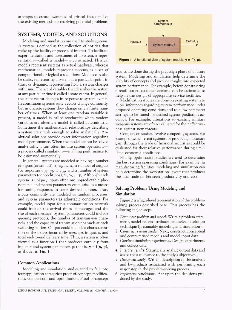
In general, systems are modeled as having a number of inputs (or stimuli), xl. X2, ••• , Xr; a number of outputs (or responses), Yb Y2, ... , Ys; and a number of system parameters (or conditions), Pb P2,···, Pc. Although each system is unique, inputs often are unpredictable phe, nomena, and system parameters often arise as a means for tuning responses in some desired manner. Thus, inputs commonly are modeled as random processes, and system parameters as adjustable conditions. For example, model input for a communication network could include the arrival times of messages and the size of each message. System parameters could include queuing protocols, the number of transmission chan, nels, and the capacity of transmission channels at each switching station. Output could include a characteriza, tion of the delays incurred by messages in queues and total end,to,end delivery time. Thus, a system is often viewed as a function f that produces output y from inputs x and system parameters p; that is, y = f(x, p), as shown in Fig. 1.

Common Applications

Modeling and simulation studies tend to fall into four application categories: proof,of,concept, modifica, tion, comparison, and optimization. Proof,of,concept

Inputs, x

System parameters, p

1 System model, f

Output, Y

Figure 1. A functional view of system models, Y = f(x, p).

studies are done during the predesign phase of a future system. Modeling and simulation help determine the viability of concepts and provide insight into expected system performance. For example, before constructing a retail outlet, customer demand can be estimated to help in the design of appropriate service facilities.

Modification studies are done on existing systems to allow inferences regarding system performance under proposed operating conditions and to allow parameter settings to be tuned for desired system prediction ac, curacy. For example, alterations to existing military weapons systems are often evaluated for their effective, ness against new threats.

Comparison studies involve competing systems. For example, two different systems for producing monetary gain through the trade of financial securities could be evaluated for their relative performance during simu, lated economic conditions.

Finally, optimization studies are used to determine the best system operating conditions. For example, in manufacturing facilities, modeling and simulation can help determine the workstation layout that produces the best trade, off between productivity and cost.

Solving Problems Using Modeling and Simulation

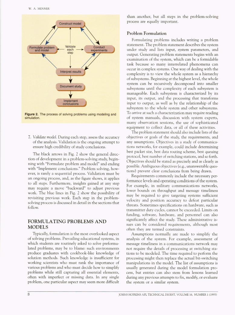
Figure 2 is a high, level representation of the problem, solving process described here. This process has the following major steps:

1. Formulate problem and model. Write a problem state' ment, model system attributes, and select a solution technique (presumably modeling and simulation).

2. Construct system model. Next, construct conceptual and computerized models and model input data.

3. Conduct simulation experiments. Design experiments and collect data.

4. Interpret results. Statistically analyze output data and assess their relevance to the study's objectives.

5 Document study. Write a description of the analysis and by, products associated with performing each major step in the problem,solving process.

6. Implement conclusions. Act upon the decisions pro' duced by the study.

JOHNS HOPKINS APL TECHNICAL DIGEST, VOLUME 16, NUMBER 1 (1995) 7

W. A. MENNER

Validate each ~ step '-""""'!l .... ..,...--,

1

Implement conclusions

Figure 2. The process of solving problems using modeling and simulation.

7. Validate model. During each step, assess the accuracy of the analysis. Validation is the ongoing attempt to ensure high credibility of study conclusions.

The black arrows in Fig. 2 show the general direc, tion of development in a problem,solving study, begin, ning with "Formulate problem and model" and ending with "Implement conclusions." Problem solving, how, ever, is rarely a sequential process. Validation must be an ongoing process, and, as the figure shows, it applies to all steps. Furthermore, insights gained at any step may require a move "backward" to adjust previous work. The blue lines in Fig. 2 show the possibility of revisiting previous work. Each step in the problem, solving process is discussed in detail in the sections that follow.

FORMULATING PROBLEMS AND MODELS

Typically, formulation is the most overlooked aspect of solving problems. Prevailing educational systems, in which students are routinely asked to solve preformu, lated problems, may be to blame: such environments produce graduates with cookbook,like knowledge of solution methods. Such knowledge is insufficient for working scientists who must rank the importance of various problems and who must decide how to simplify problems while still capturing all essential elements, often with imperfect or missing data. In any single problem, one particular aspect may seem more difficult

than another, but all steps in the problem,solving process are equally important.

Problem Formulation

Formulating problems includes wntmg a problem statement. The problem statement describes the system under study and lists input, system parameters, and output. Generating problem statements begins with an examination of the system, which can be a formidable task because so many interrelated phenomena can occur in complex systems. One way of dealing with the complexity is to view the whole system as a hierarchy of subsystems. Beginning at the highest level, the whole system can be recursively decomposed into smaller subsystems until the complexity of each subsystem is manageable. Each subsystem is characterized by its input, its output, and the processing that transforms input to output, as well as by the relationship of the subsystem to the whole system and other subsystems. To arrive at such a characterization may require reading of system manuals, discussion with system experts, many observation sessions, the use of sophisticated equipment to collect data, or all of these activities.

The problem statement should also include lists of the objectives or goals of the study, the requirements, and any assumptions. Objectives in a study of communica, tions networks, for example, could include determining best packet size, best data routing scheme, best queuing protocol, best number of switching stations, and so forth. Objectives should be stated as precisely and as clearly as possible. Ambiguous objectives (e.g., unanswerable ques, tions) prevent clear conclusions from being drawn.

Requirements commonly include the necessary per, formance levels and operating conditions of the system. For example, in military communications networks, lower bounds on throughput and message timeliness may be required to give targeting systems sufficient velocity and position accuracy to defeat particular threats. Sometimes specifications on hardware, such as transmitter duty cycles, cannot be exceeded. Limits on funding, software, hardware, and personnel can also significantly affect the study. These administrative is, sues can be considered requirements, although most often they are termed constraints.

Assumptions normally are made to simplify the analysis of the system. For example, assessment of message timeliness in a communications network may not require the details of processing at switching sta' tions to be modeled. The time required to perform the processing might then replace the actual bit,switching manipulations in the model. The list of assumptions is usually generated during the model formulation pro, cess, but entries can also stem from lessons learned during any previous attempts to fix, modify, or evaluate the system or a similar system.


Model Formulation

Modeling involves constructing an abstract repre, sentation of a system. The modeler must determine what system elements are essential- often a difficult challenge. Leaving out essential elements leads to an invalid model, but including unnecessary elements unduly complicates the model and adds to the cost of assessment.

Because each system is unique, only three broad guidelines can be offered for the intuitive and artful process of formulating models. First, the analyst should gain experience through exposure to the modeling literature. Most of this literature contains particular models and specific techniques, only some of which may be useful in future modeling projects. 1,2 A smaller portion contains helpful lists of issues that a modeler should always consider.3

-5 Second, the analyst should

cultivate the use of both right,brain (imaginative and creative) and left,brain (rational and disciplined) thinking. Modeling is most successful when both are used. Third, the analyst should start with a simple model and add details only as the validation process shows they are needed.

Selection of an Appropriate Solution Technique

The last part of the formulation step involves the search for an appropriate solution technique. This search should be exhaustive, and the technique chosen should exhibit the highest benefit,to,cost ratio. Ana, lytical solutions generally are preferred because they are exact. Unfortunately, the vast complexity of many systems precludes the use of analytical solution tech, niques. For such systems, simulation may be the only effective solution method.

CONSTRUCTING SYSTEM MODELS After the decisions and by,products of the formula,

tion step are validated, attention turns to the software engineering aspects of developing conceptual and com, puterized models of the system. Input data processes must also be modeled. Because software engineering is a well, documented subject separate from modeling and simulation, this aspect is given only cursory treat, ment here.

The Conceptual Model

The conceptual model is a structured description that provides a common understanding of system orga, nization, behavior, and nomenclature. Its purpose is to provide analysts with a way to think about the system. The conceptual model can be developed using any combinations of standard techniques, such as data flow

INTRODUCTION TO MO DELING AND SIMULATION

diagrams, structured English, pseudocode, decision ta, bles, Nassi-Schneiderman charts, flowcharts, and any of numerous graphical or textual methods.6

The Computerized Model

The computerized model should be developed ac, cording to the accepted conventions of software engi, neering. This means using a structured approach to analysis, design, coding, testing, and maintenance. A structured development approach focuses on three as, pects of software quality-its operational attributes, its accommodation of change, and its capacity to adapt to new environments. 7 The development team should address at least the following list of software quality factors:

• Auditability • Maintainability • Consistency • Modularity • Correctness • Portability • Data commonality • Reliability • Efficiency • Reusability • Expandability • Robustness • Flexibility • Security • Integrity • Testability • Interoperability • Usability

The matter of selecting a programming language also commands considerable coverage in the modeling and simulation literature.8 General,purpose languages such as Ada, C++, and Fortran are usually praised for flex, ibility, availability, and low purchase price, but the resulting software can require more development time and be more difficult to maintain than software con, structed with specialized simulation languages. There are two types of simulation languages: general, purpose languages, which can be applied to any system (GPSS, SIMSCRIPT, and SLAM are examples), and applica, tion,specific languages (AutoMod and SIMFACTORY for manufacturing; also COMNET II.S and NETWORK II.S for communications networks). Simulation lan' guages provide preprogrammed means for satisfying many anticipated simulation needs, such as numerical integration, random number generation, and statistical data analysis. Many simulation languages also provide animation capabilities. Their built,in conveniences can reduce development time, enhance software quality, and increase model credibility. Spreadsheets are a third option for computerizing some models.9

Ultimately the choice of a computer language should account for (1) the technical background of the soft, ware development team, (2) the appropriateness of the language for describing the model, and (3) the extent to which the language supports the listed software quality factors.

JOHNS HOPKINS APL TEC HNICAL DIGEST, VOLUME 16, NUMBER 1 (1995) 9

w. A. MENNER

Modeling the Input Data

The problem of modeling input data has two parts. First, appropriate input models must be selected to represent the random elements of the system. Second, a mechanism must be constructed for generating ran, dom variates according to the input model.

With respect to input data, simulation models are categorized as trace,driven or distribution,driven mod, els. Trace,driven models use the data that were collect, ed during measurements of the real system. (The real system must exist and be measurable.) Distribution, driven models use probability distributions (for exam, pIe, exponential, normal, or Poisson distributions) derived from the trace data, or from assumptions when trace data are not available.

The process of deriving probability distributions in' volves selecting a distribution type, estimating values for all distribution parameters, and evaluating the resulting distribution for agreement with the trace data. The selection of an appropriate distribution type is aided by visual assessment of graphs and the use of statistical attributes, including coefficients of variation (the ratio of the square root of the variance to the mean for con, tinuous random variables) and lexis ratios (the ratio of the variance to the mean for discrete random vari, ables).10 The reason for using a particular distribution can be compelling, as it is when arrival times are mod, eled as a Poisson process. Distribution parameter values are often estimated using the maximum likelihood method.10 This method involves finding the values of one or more distribution parameters that maximize a joint probability (likelihood) function formed from the trace data. Assessing the resulting distribution for agree' ment with trace data involves visual assessment of graphs and goodness,of,fit tests. Goodness,of,fit tests are special statistical hypothesis tests that attempt to assess the agreement between trace data and derived distribu, tions. Some of the more common goodness,of,fit tests are the chi,squared test, the Kolmogorov-Smimov test, and the Anderson-Darling test. 10

In some cases (proof,of,concept studies, for exam, pie), collecting trace data is impossible. When data are unavailable, theoretical distributions should be select, ed that can capture the full range of system behavior. Law and Kelton 10 suggest querying experts for estimates of parameter values in triangular or beta distributions. The simulation should be run for multiple distribution parameter settings, and results should be stated with an appropriate degree of uncertainty.

Random Number Generation

The term "random number" typically denotes a random variable uniformly distributed on the interval (0, 1). The term "random variate" denotes all other random variables. Random variates commonly are

generated from some mathematical combination of random numbers. Thus, having a good mechanism for generating random numbers is extremely important.

True randomness is a difficult concept to define. 11 Despite the availability of many tests for satisfactory randomness,12 random number generators typically are based on a deterministic formula. Using the formula, the next number in the "random" sequence can always be predicted, which means the numbers are not truly random. The numbers produced by such generators are generally called pseudorandom numbers.

The most commonly used pseudorandom number generators are linear congruential or multiple recursive. Linear congruential generators have the following form:

Xn = (exxn-l + (3)(mod m), (1)

where Xn is the (n + l)th pseudorandom number in the sequence, x 0 (the first member of the sequence) is called the seed, m is the constant modulus, ex and (3 are also constants, and the Xn values are divided by m to produce values in the interval (0, 1). Multiple recursive generators avoid the addition operation by setting (3 = ° in Eq. 1. For either type of generator, once Xn = Xj for some j < n, an entire sequence of previously generated values is regenerated and this cycle repeats endlessly. The length of this cycle is called the period of the generator. When the period is equal to the modulus m, a generator is said to have full period. Maximum period is equal to the largest integer that can be represented, which on many machines is 2b

, where b is the number of bits used to store or represent nu' meric data in a computer word. (The value of b is 31 on many mini, and microcomputers in current use, providing a maximum period of over 2.1 billion.)

A good pseudorandom number generator is compu, tat ion ally fast, requires little storage, and has a long period. Conditions for achieving full period are given by Law and Kelton. 10 Good generators should produce numbers that pass goodness,of,fit tests when compared with the uniform distribution. They also should not exhibit correlation with each other. A generator's ca, pacity to exactly reproduce a stream of numbers is also important, particularly for subjecting different models of the same system to the same input stimuli for comparison. Changing the scalar notation of Eq. 1 to matrix or vector notation also allows several separate streams of pseudorandom numbers to be generated, which is important when more than one source of randomness is being modeled.

A pseudorandom number generator should be cho, sen with the preceding criteria in mind. In addition to the types of generators already described, many other excellent generator types are available, such as


lagged~Fibonacci, generalized feedback shift register, and Tausworthe. 11 Because a number of poor generators are also on the market,13 the modeling and simulation community has developed a general distrust of the library generators that come packaged with many soft~ ware products. Therefore, analysts should choose generators for which descriptions and favorable test results have been published in reputable literature. When this strategy is not possible, output from a cho~ sen generator should be tested for independence, cor~ relation, and goodness of fit using statistical hypothesis testing procedures.

Random Variate Generation

The inverse~transform method for generating ran~ dom variates relies on finding the inverse of the cumu~ lative distribution function (CDF) that represents the desired distribution of variates. The CDF, F(x), is either an empirical distribution or a theoretical distribution that has been fitted to trace data. Empirical CDFs are formed by sorting trace data into increasing order and forming a continuous, piecewise~linear interpolation function through the sorted data. With either theoret~ ical or empirical distributions, a variate Y having the CDF F(x) is generated as Y = F- 1(U), where U is a random number uniformly distributed on the interval (0, 1) generated according to the criteria just described.

The composition method is used when the CDF F(x) can be expressed as

]

F(x)= LPjF/x), j=l

(2)

where {Pj} represents a discrete probability distribution, and each Fj is a CDE A positive random integer k, where 1 :s k :S j, is generated from the {Pj} distribution, and the final random variate Y is generated from the distribution Fk•

Sometimes random variates can be generated by taking advantage of special relationships between prob~ ability distributions. For example, if Y is normally dis~ tributed with a mean of zero and a variance of one, then yZ has a chi~squared distribution with 1 degree of free~ dom. Several other advanced techniques are also available for random variate generation, including acceptance-rejection14 and the alias method. 15,16

CONDUCTING SIMULATION EXPERIMENTS

Once the computerized model is finished, it is tempting to consider the most important work finished and to believe that turning on the computer will start

INTRODUCfION TO MODELING AND SIMULATION

the answers coming. Modeling is not that simple, however. It is a big mistake simply to run the model once, compute averages for output data, and conclude that the averages are the correct set of values with which to operate the system. To support accurate and useful decisions, data must be collected and character~ ized with much greater fidelity. Effective design of experiments begins this process.

The experimentation step involves building a com~ puterized shell to drive the computerized model and collect data in a manner that supports the study objec~ tives. Thus, in designing the experiments, the analyst should look back at the study objectives and look for~ ward to the methods for analyzing output data. T ypi~ cally the shell manages such things as pseudorandom number seeds and streams, warm~up periods, sample sizes, precision of results, comparison of alternatives, collection of data, variance reduction techniques, and sensitivity analysis. Variance reduction techniques and sensitivity analysis are treated in the following para~ graphs; the other items either were discussed in the preceding sections or are considered later in the article.

Variance Reduction Techniques

In some cases, the precision of results produced by simulation is unacceptably poor. The most common remedy for poor precision is to collect more data during additional simulation runs, even though computational costs can limit both the number of simulation runs and the amount of data that can be gathered. Regardless of circumstances, variance reduction techniques often can improve simulation efficiency, allowing higher~ precision results from the same amount of simulation.

Two of the most common variance reduction tech~ niques, common random numbers and antithetic vari~ ates, are based on the following statistical definitions17:

var[aX + bY]=a2var[X]+b2var[Y] + 2ab cov[X, Y], (3)

where

cov[U, V]=E[(U - E[U]) (V - E[V])] , (5)

and E is the expected value. The common random number technique is used when alternative systems are being compared. Simulations are run for two different models of the same system. Model X produces obser~ vat ions Xl> Xz, ... , Xn for a particular output variable, and model Y produces observations Yl> Yz, ... , Yn for


w. A. MENNER

the same output variable. A point estimate for the difference between corresponding output from the two models is

(6)

The width of the confidence interval for this point estimate depends on var[X - V], which, using Eq. 3 with a = 1 and b = - 1, is

var[X - Y]=var[X]+var[Y]- 2 cov[X, YJ. (7)

Therefore, if the output data from the two models can be positively correlated (i.e., cov[X, V]> 0), the vari~ ance of the difference between the two outputs will be smaller than if the output data were independently generated. Positive correlation can often be induced by using common p eudorandom number streams in the two models. It is reasonable to expect the models to

respond in roughly the same way to the same inputs. For example, if two different (and reasonable) routing schemes were being compared within the same com~ munication network, despite any inherent superiority of one routing scheme over the other, delays would be expected to increase in both model when input mes~ sage traffic increases. Such insights can lead to more precise characterizations of competing output data, showing what differences result from actual system dif ferences rather than from the effect of random inputs.

Nevertheless, a risk is associated with applying this technique. If the pseudorandom number streams are not synchronized properly (that is, if they are not used for the same purposes in each model), output from the two models can become negatively correlated. In this case, cov[X, Y]< 0, and the precision of the estimated difference between the two models will be worse than if independent pseudorandom number streams had been u ed.

The antithetic variates variance reduction tech~ nique increases the precision of results obtained from the simulation of a ingle system. First, the simulation is run using pseudorandom numbers U[! U2, •.• , Urn to

produce observations Xl! X2, ••• , Xn for a particular output variable. Then, the simulation is run using pseu~ dorandom numbers 1 - U1, 1 - U2, ... , 1 - Urn to produce output observations Y1, Y2, ... , Yn for the same output variable. The observations are then averaged to produce the following point estimate for the output variable:

X+Y 1 n --=-IJXi+Y).

2 2n i= l (8)

The width of the confidence interval for this point estimate depends on var[(X + Y)/2], which, using Eq. 3 with a = 1/2 and b = 1/2, is

Therefore, when the output data from the two models are negatively correlated (that is, cov[X, Y]< 0), the variance of the average of the two different output data sets is less than if the output data were independently generated. The opposing nature of the antithetic variates is often sufficient to provide this negative correlation.

As with common random numbers, a risk is associ~ ated with applying antithetic variates. If the pseudoran~ dom number streams are not synchronized properly, output from the two runs can become positively cor~ related. In this case, cov[X, V]> 0, and the e timated average of the two different output data sets exhibits worse precision than if independent pseudorandom number streams had been used.

Other methods for variance reduction include con~ trol variates, indirect e timation, and conditioning. IS

All of these methods attempt to increase the precision of estimates by exploiting relationships between esti~ mates and random variables.

Sensitivity Analysis

As mentioned in the introduction and shown in Fig. 1, output variables yare often modeled as a func~ tion of inputs x and system parameters p. In addition, inputs are often modeled as random processes that have distribution parameters 8. Thu , a particular output variable y can be viewed as the function y = j [x(8), p], and knowing how small changes in 8 and p affect the output y is desirable. Sensitivity analysis (al 0 called gradient estimation) involves forming the following ratios after conducting simulation runs at various parameter values: ~y / ~p and ~y/ ~(), where y common~ ly represents the mean or variance of the output variable, and p and () represent particular sy tem and di tribution parameters. The magnitude of the e ratios is an indicator of output sensitivity. This technique is called the finite~difference method of sensitivity analysis.

Another sensitivity analysis method is the likelihood ratio (or score function) method, which is based on the following ideas. If X is a random variable with distri~ bution parameter () and continuous probability density function (PDF) j, then the expected value E of X is

E[X]= f xj(x, ()) dx, (10) all x


and, using the usual continuity assumptions regarding the interchange of integration and differentiation, it follows that

dE[X] d --=- f xf(x,O) dx

dO dO all x

= f x~ f(x,O) dx. all x dO

(11)

Thus, the sensitivity of the expected mean of X with respect to changes in the distribution parameter ° is estimated using samples of X as follows:

(12)

Other sensitivity analysis methods include infinites~ imal perturbation analysis, cut~and~paste methods, and standard clock methods. 19 All of these methods involve the simultaneous tracking of variants of the same out~ put variable, each corresponding to a slightly different parameter value. For example, in infinitesimal pertur~ bation analysis, a time is chosen for a simulation pa~ rameter to be perturbed. From then on, the simulation tracks not only how the model behaves, but also how the model would have behaved if the parameter had not been perturbed.

INTERPRETING RESULTS When a computerized model is driven with random

variables, the output data are also random variables. Output data therefore should be characterized using confidence intervals that include both mean and vari~ ance. If classical statistical data analysis methods are to be used, however, independent and identically distrib~ uted (lID) data must be collected from simulation runs.

Approaches for collecting IID data depend on the type of system being studied. Terminating (or transient) systems have definite start and stop times. For example, a business that opens at 10:00 a.m. and closes at 5:00 p.m. would usually be modeled as a terminating system. The analyst is interested in characterizing data collected between the start and stop times of the sys~ tern, such as the distribution of service times for busi~ ness clients. Nonterminating (or steady~state) systems have no definite start and stop times. Output from these systems eventually becomes stationary- a pat~ tern in which random fluctuations are still observed, but system behavior is no longer influenced by initial conditions. For example, a manufacturing facility that operates continuously would usually be modeled as a

I TRODUCTION TO MODELING AND SIMULATION

nonterminating system. The analyst is interested in characterizing the distributions of output processes once they have become invariant to the passage of time.

Terminating Systems

Initial conditions definitely influence the output distributions of terminating systems. For instance, the average wait at a ticket window depends on the number of people in line when the ticket window opens. Therefore, the same initial conditions must be used to begin each simulation run. If Xi represents a particular result (e.g., average wait in line) for the ith simulation run, then n runs of the simulation produce data {Xl, X2, .•• , XJ. These data are independent when an independent set of random number seeds is used. They are also identically distributed because the model was not changed between runs. Therefore, the statistical techniques for IID data can be applied.

A point estimate for the mean is calculated as

(13)

and the 100(1 - a) percent confidence interval for the mean is

- [2 X±ta /2,n-l ~ ~, (14 )

where tex/2,n-l represents the value of the t distribution with n - 1 degrees of freedom that excludes a/2 of the probability in the upper tail, and where the sample variance is

2 1 n - 2 S =-IJXi -X) .

n-1 i=l (15)

The second term in Expression 14 is called the haIr width or absolute precision of the confidence inter~ val, and the ratio of the second term to the first term is called the relative precision of the confidence interval.

This method is called the method of independent replications. It is applied to each output process to produce confidence intervals for all random output variables.

Nonterminating Systems

Nonterminating simulations are commonly started in an "empty" state and proceed to achieve a steady state. The period of time between these states is known as the warm~up period. Because the system state chang~ es, data collected during the warm~up period are


w. A. MENNER

unlikely to be independent. This problem, called initialization bias, is typically solved by ignoring data collected during the warm~up period.

Many procedures exist for determining when a sim~ ulation has achieved a steady state.20 One of the most effective involves plotting moving averages of each frequently sampled output variable during many inde~ pendent replications.21

,22 The time at which steady state occurs is chosen a the time beyond which the moving average sequences converge, provided the plots are reasonably smooth. Plot smoothness is sensitive to moving average window size and may need to be ad~ justed-a process similar to finding acceptable interval widths for histograms.

If a good estimate of steady,state time is available, nonterminating systems can be treated much like ter~ minating systems by using a method called indepen, dent replications with truncation. In this method, independent pseudorandom number streams are used for each simulation run, and output data collection is truncated during the warm~up period. The moving average values of each output variable are recorded as point estimates once steady state is achieved. This method produces IID data, but it has the disadvantage of "throwing away" the warm~up period during each run. If simulation runs are costly, one~long~run meth~ ods may be preferred, but these methods force the analyst to deal with the problem of autocorrelation.

Autocorrelation means that consecutively collected data points exhibit correlation with one another; they are not independent. For example, two cars arriving consecutively to a car wash both must wait for all cars ahead of them. Compounding this problem is the tendency for simulation output to be positively auto~ correlated. Change occurs more slowly under such conditions, resulting in confidence intervals that un, derestimate the amount of error in output data.

Autocorrelation effects can be defeated in many ways. The batch means method is perhaps the most common. With this method, data collected during steady state are grouped into batches and the sample mean is computed for each batch. For large enough batch sizes, the batch means are sufficiently uncorre~ lated that they can be treated as IID data for compu~ tation of a confidence interval. Methods for determin~ ing batch size generally use one of the many hypothesis testing procedures for independence, such as the runs test, the flat spectrum test, and correlation tests. 23

Other methods for output data analysis include the autoregressive method, the regenerative method, the spectral estimation method, and the standardized time series method.24

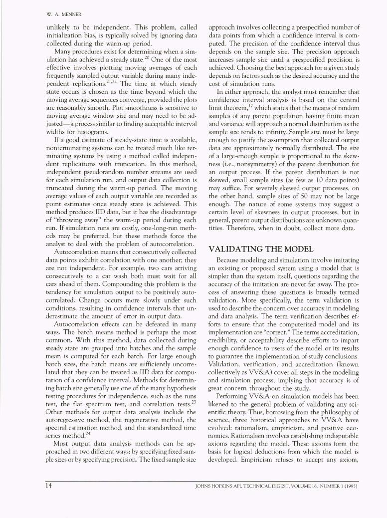
Most output data analysis methods can be ap~ proached in two different ways: by specifying fixed sam~ pIe sizes or by specifying precision. The fixed sample size

approach involves collecting a prespecified number of data points from which a confidence interval is com~ puted. The precision of the confidence interval thus depends on the sample size. The precision approach increases sample size until a prespecified precision is achieved. Choosing the best approach for a given study depends on factors such as the desired accuracy and the cost of simulation runs.

In either approach, the analyst must remember that confidence interval analysis is based on the central limit theorem, 17 which states that the means of random samples of any parent population having finite mean and variance will approach a normal distribution as the sample size tends to infinity. Sample size must be large enough to justify the assumption that collected output data are approximately normally distributed. The size of a large~enough sample is proportional to the skew~ ness (i.e., nonsymmetry) of the parent distribution for an output process. If the parent distribution is not skewed, small sample sizes (as few as 10 data points) may suffice. For severely skewed output processes, on the other hand, sample sizes of 50 may not be large enough. The nature of some systems may suggest a certain level of skewness in output processes, but in general, parent output distributions are unknown quan~ tities. Therefore, when in doubt, collect more data.

VALIDATING THE MODEL Because modeling and simulation involve imitating

an existing or proposed system using a model that is simpler than the system itself, questions regarding the accuracy of the imitation are never far away. The pro~ cess of answering these questions is broadly termed validation. More specifically, the term validation is used to describe the concern over accuracy in modeling and data analysis. The term verification describes efforts to ensure that the computerized model and its implementation are "correct." The terms accreditation, credibility, or acceptability describe efforts to impart enough confidence to users of the model or its results to guarantee the implementation of tudy conclusions. Validation, verification, and accreditation (known collectively as VV&A) cover all teps in the modeling and simulation process, implying that accuracy is of great concern throughout the study.

Performing VV &A on simulation models has been likened to the general problem of validating any sci~ entific theory. Thus, borrowing from the philosophy of science, three historical approaches to VV &A have evolved: rationalism, empiricism, and positive eco~ nomics. Rationalism involves establishing indisputable axioms regarding the model. These axioms form the basis for logical deductions from which the model is developed. Empiricism refuses to accept any axiom,


deduction, assumption, or outcome that cannot be substantiated by experiment or the analysis of empirical data. Positive economics is concerned only with the model's predictive ability. It imposes no restrictions on the model's structure or derivation.

Practical efforts to validate simulation models should attempt to include all three historical VV &A approaches. Including all approaches can be difficult, because situations do exist in which high predictability goes hand,in,hand with illogical assumptions, as in the case of studying celestial systems or amoebae aggrega, tion using continuum models. 25 Empirically validating a model of a nonexistent system is also a problem. Despite these difficulties, some subset of available validation techniques must be systematically applied to every modeling and simulation study if conclusions are to be accepted and implemented.

The modeling and simulation team must first decide who will conduct VV &A. The team can perform this task itself or can use an independent party of experts. If the team performs VV&A, few new perspectives are generally brought to bear on the study. The use of independent peer assessment can be costly, however, and can involve repetition of previous work. In either case, the VV&A team should be familiar with model, ing and simulation methods and their potential pitfalls. The VV &A team's first step should be comparing the methods used by the modeling and simulation team to the accepted methods outlined in any of the standard texts on the subj ect.

Validation techniques typically are categorized as statistical or subjective. Statistical techniques are used in studies of existing systems from which data can be collected. They are particularly useful for assessing the validity of input data models, analyzing output data, comparing alternative models, and comparing model and system output. Statistical techniques include, but are not limited to, analysis of variance, confidence intervals, goodness,of,fit tests, hypothesis tests, regres, sion analysis, sensitivity analysis, and time series anal, ysis. In contrast, subjective techniques generally are used during proof,of,concept studies or to validate systems that cannot be observed and from which data cannot be collected. Subjective techniques include, but are not limited to, event validation, field tests, hypothesis validation, predictive validation, submodel testing, and Turing tests. 26

Verifying the correctness of the computerized model and its implementation has two main components: technical reviews and software testing. Technical re' views include structured walk,throughs of the software requirements, design, code, and test plan. Software re, quirements are assessed for their ability to support the objectives of the modeling and simulation study. The software design is reviewed in two phases. Phase 1, a

INTRODUCTION TO MODELING AND SIMULATION

preliminary design review, evaluates the transformation of requirements into data and code structures; phase 2, a critical design review, walks through the details of the design, assessing such things as algorithm correctness and error handling. A structured walk, through of the software code checks for such things as coding errors and adherence to coding standards and language conventions.

Software testing is designed to uncover errors in the computerized implementation and includes white, and black, box testing. White,box tests ensure that all coded statements have been exercised and that all possible states of the model have been assessed. Black,box tests explore the functionality of software components through the design of scenarios that exhaustively ex, amine the cause and effect relationships between in, puts and outputs. All of these software verification techniques are applied with respect to the list of soft, ware quality factors given in the Constructing System Models section.

Most software systems provide tools to assist the VV &A process. Among the more important are graph, ics and animation, interactive debuggers, and the automated production of logic traces. Graphics and animation involve the visual display of model status and the flow of entities through the model. These tools are extremely useful, particularly for spotting gross errors in computerized model output and for enhancing model credibility through demonstrations. Interactive debuggers help pinpoint problems by stopping the sim, ulation at any desired time to allow the value of certain program variables to be examined or changed. A logic trace is a chronological, textual record of changes in system states and program variables. It can be checked by hand to determine the specific nature of errors. Typically, the logic trace can be tuned to focus on a particular area of the model.

Ultimately, for each step of modeling and simula, tion, the goal of VV &A is to avoid committing three types of errors. A type I error (called the model builder's risk) results when study conclusions are rejected despite being sufficiently credible. A type II error (called the model user's risk) results when study conclusions are accepted despite being insufficiently credible. A type III error (called solving the wrong problem) results when significant aspects of the system under study are left unmodeled. Many methods besides the techniques described here are available for avoiding these errors and producing a model that is accepted as reasonable by all people associated with the system under study. These methods include the use of existing theory, com' parisons with similar models and systems, conversa, tions with system experts, and the active involvement of analysts, managers, and sponsors in all steps of the process.


w. A. MEN ER

DOCUMENTING THE STUDY Documentation is critical to the success of a mod,

eling and simulation study. If it's not written down, it didn't happen. Done properly, documentation fosters credibility and facilitates the long, term maintainability of the computerized model. Credibility is extremely important if the conclusions and recommendations of the study are to be taken seriously. Maintainability is important because software, hardware, and personnel change. Technological advances in the computer field may necessitate changes in the parts of the computer, ized model that interface with new hardware or soft, ware. Personnel levels also can change during or after a study. Required model changes and education of new people are much easier if good documentation is available.

Several tendencies conspire against the generation of good documentation. Preparing good documenta, tion consumes a significant amount of time during and after development work. One tendency is to lose sight of how time,consuming preparing documentation can be and to push for quick results. Another temptation is to view the documentation as relatively unimportant during and shortly after model development and simulation studies. During this time, the development team usually understands the model quite well, so changes are less likely to require complete documenta, tion. Finally, analysts tend to dislike the documentation task; they would rather devote time to the modeling and simulation work itself. To counteract these tenden, cies, the entire development team should agree on the importance of good documentation. Managers and sponsors should support documentation with adequate schedules and funding.

Good documentation includes a written description of the analysis and by,products associated with per, forming all major steps in the process. Documentation is best written at the peak of understanding. For some items, the peak of understanding occurs at the end of the study, but other items are better documented earlier. As a minimum, final documentation should include the following:

1. A statement of objectives, requirements, assump, tions, and constraints

2. A description of the conceptual model 3. Analysis associated with modeling input data 4. A description of the experiments performed with the

computerized model 5. Analysis associated with interpreting output data 6. Conclusions 7. Recommendations 8. Reaso~s for rejecting any alternatives

The conceptual and computerized models should be documented according to the standards of whatever

software engineering methodology was employed. If the simulation is designed for use by a broad audience, a user's manual may also be necessary.

Often a visual presentation is also part of the doc, umentation step. Presenters address the same topics listed for written documentation but use a different format. Animation, which allows visual observation of system operations as predicted by the computerized model, is extremely useful for illustrating system idiosyncrasies that support the study's conclusions, aI, though it can be quite costly. For physical models, videotape can often serve the same purpose. If anima, tion cannot be used, presenters should make maximum use of charts, graphs, pictures, and diagrams. Presenters also should try to anticipate questions and prepare visual aids to answer them.

IMPLEMENTING THE CONCLUSIONS The implementation of conclusions culminates the

successful modeling and simulation study. Conversely, the failure to implement conclusions is usually a sign that the study has lost credibility with its sponsor. The best way to influence the implementation of conclu, sions is to follow a structured set of guidelines, such as those presented here, throughout the study. Perhaps the most important guideline, however, is to commu, nicate all major decisions to every participant. A high level of involvement from all participants throughout the process is a major hedge against credibility failure.

Once results are implemented, the system should be studied to verify that the predicted performance is indeed realized. Discrepancies between predicted and observed performance can indicate that aspects of the real system were incorrectly modeled or left entirely unmodeled.

SUMMARY The following list summarizes this article's major

suggestions for successful problem solving using mod, eling and simulation:

1. Define specific objectives. 2. Start with a simple model, adding detail only as

needed. 3. Follow software engineering quality standards when

developing the computerized model. 4. Model random processes according to accepted

criteria. 5. Design experiments that support the study obj ecti ves. 6. Provide a complete and accurate characterization of

random output data. 7. Validate all analysis and all by, products of the

problem,solving process. 8. Document and implement conclusions.


Also, over the course of the study, the modeling and simulation team should systematically communicate all major decisions to every participant. This step helps ensure that the model retains credibility from the start of the work through the final stages of the study.

Unfortunately, one short article cannot present all issues relevant to modeling and simulation. Readers interested in further study of the issues presented here are encouraged to consult the many excellent modeling and simulation textbooks available, such as Banks and Carson27 ; Bratley, Fox, and Schrage28

; Fishman23; Law

and Kelton1O; Lewis and Orav29

; and Pritsker.30

REFERENCES

1 Haberman, R., Mathematical Models, Prentice-Hall, Englewood Cliffs, NJ (1977).

2 Maki, D. P., and Thompson, M., Mathematical Models and Applications, Prentice-Hall, Englewood Cliffs, NJ (1973).

J Polya, G., How To Solve It , 2nd Ed., Princeton Press, Princeton, NJ (1957) . 4 Saaty, T. L., and Alexander, J. M., Thinking with Models, Pergamon Press,

New York (1981). 5 Starfield, A M., Smith, K. A, and Bleloch, A L., How To Model It-Problem

Solving for the Computer Age, McGraw-Hill, New York (1990). 6 Sommerville, 1., Software Engineering, 3rd Ed., Addison-Wesley, Reading, MA

(1989). 7 Pressman, R. S., Software Engineering, 3rd Ed., McGraw-Hill, ew York

(1992). S Banks, J., "Software for Simulation," in 1987 Winter Simul. Conf. Proc.,

Theson, A, Grant, H., and Kelton, W. D. (eds.), pp. 24-33 (1993). 9 Savage, S. L. , "Monte Carlo Simulation," in IEEE Videoconference on

Engineering Applications for Monte Carlo and Other Simulation Analyses, IEEE, Inc., New York (1993).

IOLaw, A M., and Kelton, W. D., Simulation Modeling and Analysis, 2nd Ed. , McGraw-Hill, New York (1991).

11 L'Ecuyer, P., "A Tutorial on Uniform Variate Generation," in 1989 Winter Simul. Conf. Proc., MacNair, E. A, Musselman, K. J., and Heidelberger, P. (eds.), pp. 40-49 (1989).

THE AUTHOR

INTRODUCTION TO MODELING AND SIMULATION

12Morgan, B. J. T., Elements of Simulation, Chapman and Hall, London (1984) . 13Park, S. K., and Miller, K. W., "Random Number Generators: Good Ones Are

Hard to Find," Commun. ACM 31, 1192-1201 (1988). 14Schmeiser, B. W., and Shalaby, M. A, "Acceptance/Rejection Methods for

Beta Variate Generation," J. Am. Stat. Assoc. 75 ,673-678 (1980). lSWalker, A. J., "An Efficient Method of Generating Discrete Random

Variables with General Distributions," ACM Trans. Math. Software 3, 253-256 (1977).

16Kronmal, R. A, and Peterson, A V., "On the Alias Method for Generating Random Variables from a Discrete Distribution," Am. Stat. 33 , 214-218 (1979).

17Hamen, D. L., Statistical Methods, 3rd Ed., Addison-Wesley, Reading, MA (1982) .

1SNelson, B. L., "Variance Reduction for Simulation Practitioners," in 1987 Winter Simul. Conf. Proc. , Theson, A, Grant, H., and Kelton, W. D. (eds.), pp. 43- 51 (1987).

19Strickland , S. G., "Gradient/Sensitivity Estimation in Discrete-Event Simulation," in 1993 Winter Simul. Conf. Proc., Evans, G. W., Mollaghasemi, M., Russell, E. c., and Biles, W. E. (eds.), pp. 97-105 (1993).

20Schruben, L. W., "Detecting Initializa tion Bias in Simulation Output," Opel'. Res . 30, 569-590 (1982).

21 Welch, P. D., On the Problem of the Initial Transient in Steady State Simulations, Technical Report, IBM Watson Research Center, Yorktown Heights, NY (1981).

22Welch, P. D., "The Statistical Analysis of Simulation Results," in The Computer Perfonnance Modeling Handbook, S. Lavenberg (ed.), pp. 268-328, Academic Press, New York (1983).

2JFishman, G. S., Principles of Discrete Event Simulation, John Wiley & Son, New York (1978).

24Alexopoulos, c., "Advanced Simulation Output Analysis for a Single System," in 1993 Winter Simul. Conf. Proc., Evans, G. W., Mollaghasemi, M., Russell , E. c., and Biles, W. E. (eds.), pp. 89-96 (1993).

2SUn, C. c., and Segel, L. A, Mathematics Applied to Detenninistic Problems in the Natural Sciences, Macmillan, New York, pp. 3-31 (1974).

26Sargent, R. G., "Simulation Model Verification and Validation," in 1991 Winter Simul. Conf. Proc., Nelson, B. L., Kelton, W. D., and Clark, G. M. (eds.), pp. 37-47 (1991).

27Banks, J., and Carson, J. S., Discrete-Event System Simulation, Prentice-Hall , Englewood C liffs, NJ (1984).

2SBratley, P., Fox, B. L., and Shrage, L. E., A Guide to Simulation, 2nd Ed., Springer-Verlag, New York (1987).

29Lewis, P. A. W., and Orav, E. J. , Simulation Methodology for Statisticians, Operations Analysts, and Engineers, Vol. I, Wadsworth, Pacific Grove, CA (1989).

JOPritsker, A A B., Introduction to Simulation and SLAM II, John Wiley & Sons, New York (1986).

WILLIAM A. MENNER received a B.S. degree in 1979 from Michigan Technological University and an M.S. degree in 1982 from Rensselaer Polytechnic Institute; both degrees are in applied mathematics. From 1979 to 1981, Mr. Menner worked at Pratt & Whitney Aircraft as a numerical analyst. Since 1983, when he joined APL's Fleet Systems Department, he has completed modeling, simulation, and algorithm development tasks for the Tomahawk Missile Program, the Army Battlefield Interface Concept, the SSN21 ELINT Correlation Program, the Marine Corps Expendable Drone Program, and the Cooperative Engagement Capability. Mr. Menner supervises a computer systems section and is currently working on the Defense Satellite Communications system. He also has taught a course in mathematical modeling and simulation for APL's Associate Staff Training Program.


INTRODUCTION TO MODELING AND SIMULATION - Johns ...

Documents

Transcript of INTRODUCTION TO MODELING AND SIMULATION - Johns ...