Introduction to Actor-Based Modelsfor Network Dynamics∗

Tom A.B. Snijders†

Christian E.G. Steglich‡

Gerhard G. van de Bunt§

June 4, 2008

Abstract

Stochastic actor-based models are a class of statistical models for net-work dynamics. The nodes in the network represent social actors, and thecollection of ties represents a social relation. Such models can be used toanalyze longitudinal data on social networks, studying the array of tie indi-cators in the network as dependent variables. The assumptions posit that thenetwork evolves as a stochastic process ‘driven by the actors’, and that thechange probabilities are in part endogenously determined, i.e., as a functionof the current network structure itself, and in part exogenously, as a func-tion of characteristics of the nodes (‘actor covariates’) and of characteristicsof pairs of nodes (‘dyadic covariates’). The latter can be regarded as valuednetworks, on the same set of nodes, having the role of independent variables.In an extended form, stochastic actor-based models can be used to analyzelongitudinal data on social networks jointly with changing attributes of theactors: dynamics of networks and behavior.

This paper gives an introduction to stochastic actor-based models usingonly a minimum of mathematics. The focus is on understanding the basicprinciples of the model, understanding the results, and on sensible rules formodel selection.

Keywords: social networks, statistical modeling, endogenous feedback model,Markov chain.∗Draft article for special issue of Social Networks on Dynamics of Social Networks.†University of Oxford and University of Groningen‡University of Groningen§Free University, Amsterdam

1

1 IntroductionSocial networks are dynamic by nature. Ties are established, they may flourishand perhaps evolve into close relationships, and they can also dissolve quietly, orsuddenly turn sour and go with a bang. These relational changes are not random,but may be considered the result of the structural positions of the actors concernedwithin the network – e.g., when friends of friends become friends–, characteristicsof the actors (‘actor covariates’), and characteristics of pairs of actors (‘dyadiccovariates’). Network research has in recent years paid increasing attention tonetwork dynamics, as is shown by the three special issues devoted to this topic inJournal of Mathematical Sociology edited by Patrick Doreian and Frans Stokman(1996, 2001, and 2003). The three issues shed light on the underlying theoreticalmicro mechanisms that induce the evolution of social network structures on themacro level. Network dynamics is important for domains ranging from friendshipnetworks (e.g., Pearson & Michell, 2000; Burk, Steglich, & Snijders, 2007) to, forexample, inter-organizational networks (see the review articles Borgatti & Foster,2003; Brass, Galaskiewicz, Greve & Tsai, 2004).

This article gives a tutorial introduction to what we call here actor-based mod-els for network dynamics, and their use as statistical models for data sets wheretwo or more repeated observations of a social network on a given set of actorsare available; one could call this network panel data. Ties are supposed to be thedyadic constituents of positive relations (e.g. friendship, trust, or cooperation).In our examples social actors are individuals, but they could also be firms, coun-tries, etc. Actor covariates may be constant like sex or ethnicity, or subject tochange like opinions, attitudes, or lifestyle behaviors. Actor covariates often areamong the determinants of actor similarity (e.g., same sex or ethnicity) or spatialproximity between actors (e.g., same neighborhood). Dyadic covariates likewisemay be constant, such as determined by kinship or formal status in an organiza-tion, or changing over time, like friendship between parents of children or taskdependencies within organizations.

Some historyDespite the evident importance of relation dynamics, the network literature does

not provide many statistical network models that are suitable for analyzing thedynamic aspects of social networks. The main reason is the complexity generatedby the fact that network data structures do not consist of independent observations.Indeed, it is the dependencies among actors and among their relational ties thatmake network analysis the fascinating research discipline that it is.

The prehistory of statistical modeling for longitudinal network data is Katz andProctor’s (1959) Markov chain model. Their model assumed independent tie vari-ables that could change randomly at each next observation. Later on, Wasserman

2

(1987) and Wasserman & Iacobucci (1988) proposed models extending Holland& Leinhardt’s p1-model (1981) to longitudinal data, retaining the (unattractive)assumption of independent dyads. Robins & Pattison (2001) proposed a longitu-dinal version of the exponential random graph model of Frank & Strauss (1986)and Wasserman & Pattison (1996). All these models have the property that theyare Markov chains in discrete time, which means that the transition of one obser-vation to the next is proposed as one ‘jump’. If, for example, three actors who attime 1 are mutually disconnected form at time 2 a closed triad, where everybodyis connected to everybody else, then such a model has to account for the fact thatthis structure is formed ‘out of nothing’. However, it is often intuitively morereasonable to assume that the closed triad has been formed tie by tie, as a conse-quence of reciprocation and triadic closure. Models expressing the dynamics ofnetworks as processes where ties change one by one were initially proposed byHolland & Leinhardt (1977) as continuous-time Markov processes.

When modeling network dynamics as a continuous-time process, it is assumedthat, although the observations are made at discrete moments in time, the networkchange process itself is continuous, and proceeds in small steps. Holland & Lein-hardt (1977) proposed to make this assumption, and further to assume that tieschange only one by one, and that the probability of each tie change may dependon the entire current network, but not on earlier states of the network. The latterassumption means that the observed network is the outcome of a continuous-timeMarkov chain. This was elaborated by Wasserman (1979 and other publications)and Leenders (1995 and other publications). These models still assumed thatdyads evolve independently, which excludes the modeling, for example, of tran-sitive closure. Continuous-time models that allow triadic and other higher-orderdependencies were proposed by Snijders (1996, 2001) and Snijders & Van Duijn(1997). These are the actor-based models treated in the current article. Some ap-plications are presented in Van de Bunt, Van Duijn & Snijders (1999), Van Duijn,Zeggelink, Huisman, Stokman & Wasseur (2003), and Van de Bunt, Wittek & DeKlepper (2005).

More recently, these models were extended to simultaneously model changesin ties and changes in individual behavior, thus permitting to model social se-lection and social influence simultaneously (see Snijders, Steglich, and Schwein-berger, 2007; Steglich, Snijders, and Pearson, 2008). This makes it possible toanswer not only a question like ‘did actor i initiate a friendship with actor j be-cause they were both smokers?’, but also related questions such as ‘did actor ibecome a smoker because of his friendship with a smoker’ and ‘are actors morestrongly influenced in their behavior by friends who are more popular?’ – wherethe ‘because’ has to be understood, of course, in the limited sense of statisticalassociations over time.

This paper is organized as follows. In the next section, we present the as-

3

sumptions of the actor-based model. The heart of the model is the so-called ob-jective function, which determines probabilistically the tie changes made by theactors, and captures all theoretically relevant information the actors need to ‘eval-uate’ their relations. Some of the components of this function are structure-based(endogenous effects), such as the assumed tendency to form reciprocal relations,others are attribute-based such as the preference for similar others (exogenous ef-fects). In Section 3 we discuss several statistical issues, such as data requirementsand how to test and select the appropriate model. Following this we present anexample (about friendship dynamics) that focuses on the interpretation of the pa-rameters. Section 4 proposes some more elaborate models. In Section 5, modelsfor the coevolution of networks and behavior are introduced. Finally, in Section 6,several new developments are presented.

2 Model assumptionsA dynamic network is formed by ties between actors that change over time. Afoundational assumption of the models discussed in this paper is that the networkties are not brief events, but can be regarded as states with a tendency to endureover time. Many relations commonly studied in network analysis naturally satisfythis requirement of slow change, such as friendship, trust, and cooperation. Othernetworks more strongly resemble ‘event data’, e.g., the set of all telephone callsamong a group of actors at any given time point, or the set of all e-mails beingsent at any given time point. While it is meaningful to interpret these networksas indicators of communication, it is not plausible to treat their ties as enduringstates, and aggregation of event intensity over a certain period may be necessaryto approximate this requirement.

Given that the network ties under study denote states, it is further assumed, asan approximation, that the changing network can be interpreted as the outcome ofa Markov process, i.e., that for any point in time, the probability distribution of thefuture network given current and past states of the network is a function only ofthe current network. All relevant information is therefore assumed to be includedin the current state. This is a strong assumption, which often can be made moreplausible by choosing meaningful explanatory variables that incorporate relevantinformation from the past. The researcher will have to check that the Markovassumption is reasonable given the definition of the relation under study and thelimitations of the available data.

This paper gives a non-technical introduction into actor-based models for net-work dynamics. More precise explanations can be found in Snijders (2001, 2005).However, a modicum of mathematical notation cannot be avoided. The tie vari-ables are binary variables, denoted by xij . A tie i → j is either present or absent

4

(values 1 and 0, respectively). Although this is in line with traditional networkanalysis, an extension to valued networks would be theoretically more sound, andcould make the Markov assumption more plausible. This is one of the topics ofcurrent research. The tie variables constitute the network, represented by its n×nadjacency matrix x =

(xij

)(self ties are excluded), where n is the total number

of actors in the network. These tie variables are the dependent variables in theanalysis. The observed ties are assumed to be the result of time-dependent ran-dom variables Xij(t) which are represented in the time-dependent random matrixX(t). Explanatory variables (which also can be called independent or exogenousvariables) are distinguished in actor covariates vi and dyadic covariates wij .

2.1 Basic assumptionsThe model is about directed relations, where each tie i → j has a sender i, whowill be referred to as ego, and a receiver, referred to as alter. The followingassumptions are made.

1. The underlying time parameter t is continuous. The parameter estimationprocedure, however, assumes that the network is observed only at two ormore discrete points in time.

2. The changing network is the outcome of a Markov process (as explainedabove).

3. The actors control their out-going ties. This is the reason for using the term‘actor-based model’. This approach to modeling agrees very well with themethodological approach of structural individualism (Udehn, 2002; Hed-strom, 2005), where actors are assumed to be purposeful and to behavesubject to structural constraints. The assumption of purposeful actors is notrequired, however, but a question of model interpretation (see below).

4. At a given moment one probabilistically selected actor – ‘ego’ – may get theopportunity to change one out-going tie. No more than one tie can changeat any moment – a principle first proposed by Holland & Leinhardt (1977).This implies that tie changes are not coordinated, and depend on each otheronly sequentially, via the changing configuration of the whole network.

The actor-based network change process is decomposed into two sub-processes,both of which are stochastic.

5. The change opportunity process, modeling the frequency of tie changes byactors. The change rates may depend on the network positions of the actors(e.g., centrality) and on actor covariates (e.g., age and sex).

5

6. The change determination process, modeling the precise tie changes madewhen an actor has the opportunity to make a change. The probabilities oftie changes may depend on the network positions, as well as covariates, ofego and the other actors (‘alters’) in the network. This is explained below.

The actor-based model can be regarded as an agent-based simulation model (Macy& Willer 2002). It does not deviate in principle from other agent-based models,only in ways deriving from the fact that the model is to be used for statistical in-ference, which leads to requirements of flexibility (enough parameters that can beestimated from the data to achieve a good fit between model and data) and par-simony (not more fine detail in the model than what can be estimated from thedata). The word ‘actor’ rather than ‘agent’ is used, in line with other sociolog-ical literature (e.g., Hedstrom 2005), to underline that actors are not regarded assubservient to others’ interests in any way.

The actor-based model, when elaborated for a practical application, containsunknown parameters that have to be estimated from observed data by a statisticalprocedure. Since the proposed stochastic models are too complex for the straight-forward application of classical estimation methods such as maximum likelihood,Snijders (1996, 2001) proposed a procedure using the method of moments imple-mented by computer simulation of the network change process. This procedureuses the following basic principle.

• The first observed network is itself not modeled but used only as the startingpoint of the simulations (in statistical terminology: the estimation procedureconditions on the first observation).

This approach circumvents the necessity to require, for example, that the processobserved is in stochastic equilibrium.

2.2 Change determination modelOnce the focal actor (ego) who gets the opportunity to make a change is chosen bysome stochastic process, he/she may change one out-going tie (i.e. either initiateor withdraw a tie) or do nothing (i.e. keep the present status quo). This meansthat the set of admissible actions contains n elements: n−1 changes and one non-change. The probabilities for this choice depend on the so-called objective func-tion. This name was chosen because it can be interpreted as the representation ofthe short-term objectives (net result of preferences, constraints, and perceptions)of the actor. Informally, the objective function measures how attractive it is forthe focal actor to change her/his network in a particular way. This is the core ofmodel and it must represent the research questions and relevant theoretical andfield-related knowledge.

6

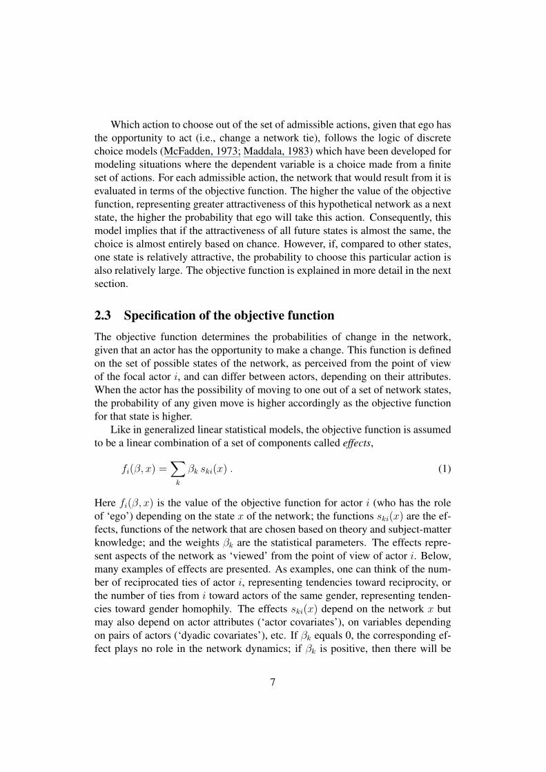
Which action to choose out of the set of admissible actions, given that ego hasthe opportunity to act (i.e., change a network tie), follows the logic of discretechoice models (McFadden, 1973; Maddala, 1983) which have been developed formodeling situations where the dependent variable is a choice made from a finiteset of actions. For each admissible action, the network that would result from it isevaluated in terms of the objective function. The higher the value of the objectivefunction, representing greater attractiveness of this hypothetical network as a nextstate, the higher the probability that ego will take this action. Consequently, thismodel implies that if the attractiveness of all future states is almost the same, thechoice is almost entirely based on chance. However, if, compared to other states,one state is relatively attractive, the probability to choose this particular action isalso relatively large. The objective function is explained in more detail in the nextsection.

2.3 Specification of the objective functionThe objective function determines the probabilities of change in the network,given that an actor has the opportunity to make a change. This function is definedon the set of possible states of the network, as perceived from the point of viewof the focal actor i, and can differ between actors, depending on their attributes.When the actor has the possibility of moving to one out of a set of network states,the probability of any given move is higher accordingly as the objective functionfor that state is higher.

Like in generalized linear statistical models, the objective function is assumedto be a linear combination of a set of components called effects,

fi(β, x) =∑

k

βk ski(x) . (1)

Here fi(β, x) is the value of the objective function for actor i (who has the roleof ‘ego’) depending on the state x of the network; the functions ski(x) are the ef-fects, functions of the network that are chosen based on theory and subject-matterknowledge; and the weights βk are the statistical parameters. The effects repre-sent aspects of the network as ‘viewed’ from the point of view of actor i. Below,many examples of effects are presented. As examples, one can think of the num-ber of reciprocated ties of actor i, representing tendencies toward reciprocity, orthe number of ties from i toward actors of the same gender, representing tenden-cies toward gender homophily. The effects ski(x) depend on the network x butmay also depend on actor attributes (‘actor covariates’), on variables dependingon pairs of actors (‘dyadic covariates’), etc. If βk equals 0, the corresponding ef-fect plays no role in the network dynamics; if βk is positive, then there will be

7

a higher probability of moving into directions where the corresponding effect ishigher, and the converse if βk is negative.

For the model selection, an essential part is the choice of effects to includein the objective function. These effects should be sufficient to understand thenetwork process given the scientific objectives of the study, and to give a good fitto the observed data, but one should not include in the model more effects thannecessary given these two conditions.

In the following we give a number of effects that may be considered for in-clusion in the objective function. They are described here only conceptually; theformulae are given in the appendix. Effects depending only on the network arecalled structural or endogenous effects, while effects depending only on exter-nally given attributes are called covariate or exogenous effects. The complexityof networks is such that an exhaustive list cannot meaningfully be given. To sim-plify formulations, the presentation shall assume that the relation under study isfriendship, so the existence of a tie i→ j will be described as i calling j a friend.Higher values of the objective function, leading to higher tendencies to form ties,will sometimes be interpreted in shorthand as preferences.

Basic effectsThe most basic effect is defined by the out-degree of actor i, and this will be

included in all models. It represents the basic tendency to have ties at all, and ina decision-theoretic approach its parameter could be regarded as the balance ofbenefits and costs of an arbitrary tie. Most networks are sparse (i.e., they have adensity well below 0.5) which can be represented by saying that for a tie to anarbitrary other actor – arbitrary meaning here that the other actor has no charac-teristics or tie pattern making him/her especially attractive to i –, the costs willusually outweigh the benefits. Indeed, in most cases a negative parameter is ob-tained for the out-degree effect. Note that in many data collection designs, thereare restrictions on the number of nominated alters, which may make it technicallyimpossible to ever obtain a density of 0.5 (or higher). If the data were collectedby a name generator restricting the number of possible nominations, a negativeoutdegree parameter value will be implied by the data collection, and not pointtowards any cost-benefit considerations.

Another quite basic effect is the tendency toward reciprocity, represented bythe number of reciprocated ties of actor i. This is a basic feature of most socialnetworks (cf. Wasserman and Faust, 1994, Chapter 13) and usually we obtainquite high values for its parameter, e.g., between 1 and 2.

Transitivity and other triadic effectsNext to reciprocity, an essential feature in most social networks is the tendency

toward transitivity, or transitive closure (sometimes called clustering): friends offriends become friends, or in graph-theoretic terminology: two-paths tend to be,

8

or to become, closed (e.g., Davis 1970, Holland and Leinhardt 1971). In Figure1.a, the two-path i→ j → h is closed by the tie i→ h.

Figure 1. a. Transitive triplet b. Three-cycle

i

h

j

i

h

j

The transitive triplets effect measures transitivity for an actor i by counting thenumber of pairs j, h such that there is the transitive triplet structure of Figure 1.a.However, this is just one way of measuring transitivity. Another one is the transi-tive ties effect, which measures transitivity for actor i by counting the number ofother actors h for which there is at least one intermediary j forming a transitivetriplet of this kind. The transitive triplets effect postulates that more intermediarieswill add proportionately to the tendency to transitive closure, whereas the transi-tive ties effect expects that given that one intermediary exists, extra intermediarieswill not further contribute to the tendency to forming the tie i→ h.

An effect closely related to transitivity is balance (cf. Newcomb, 1962) orstructural equivalence with respect to out-ties (cf. Burt, 1982), which is the ten-dency to have and create ties to other actors who make the same choices as ego.The extent to which two actors make the same choices can be expressed simply asthe number of choices and of non-choices that they have in common.

Transitivity can be represented by still more effects: e.g., negatively, by thenumber of others to whom i is indirectly tied but not directly (geodesic distanceequal to 2). The choice between these representations of transitivity may dependboth on the degree to which the representation is theoretically convincing, and onwhat gives the best fit.

Another triadic effect is the number of three-cycles that actor i is involved in(Figure 1.b). Davis (1970) found that in many social network data sets, there isa tendency to have relatively few three-cycles, which can be represented here bya negative parameter βk for the three-cycle effect. The transitive triplets and thethree-cycle effects both represent closed structures, but whereas the former is inline with a hierarchical ordering, the latter goes against such an ordering. If thenetwork has a strong hierarchical tendency, one expects a positive parameter fortransitivity and a negative for three-cycles. Note that a positive three-cycle effectcan also be interpreted, depending on the context of application, as a tendencytoward generalized exchange (Bearman, 1997).

9

Degree-related effectsIn- and out-degrees are primary characteristics of nodal position and can be im-

portant driving factors in the network dynamics.One pair of effects is degree-related popularity based on in-degree or out-

degree. If these effects are positive, nodes with higher in-degree, or higher out-degree are more attractive for others to send a tie to. This can be measured by thesum of in-degrees of i’s friends, and the sum of their out-degrees, respectively.A positive in-degree popularity effect implies that high in-degrees reinforce them-selves, which will lead to a relatively high dispersion of the in-degrees (a Mattheweffect in popularity, as measured by in-degrees, cf. Price, 1965). A positive out-degree related popularity effect will increase the association between in-degreesand out-degrees.

Another pair of effects is degree-related activity for in-degree or out-degree:when these effects are positive, nodes with higher in-degree, or higher out-degreerespectively, will have an extra propensity to form ties to others. These effects canbe measured by the in-degree of i times i’s outdegree; or the out-degree of i timesi’s outdegree, that is, the square of the out-degree. The out-degree related activityeffect again is a self-reinforcing effect: a positive parameter will lead to increaseddispersion of out-degrees. The in-degree related activity effect has the same con-sequence as the out-degree related popularity effect: positive parameters lead toa higher association between in-degrees and out-degrees. Therefore these two ef-fects are difficult to distinguish empirically (and they cannot be distinguished atall when estimation is carried out by the method of moments).

Experience has shown that for the degree-related effects, often the ‘drivingforce’ is measured better by the square roots of the degrees than by raw degrees.(Quite often counts, of which degrees are a special case, have consequences whichare better approximated in linear models by their square roots than by the countsthemselves.) See the formulae in the appendix.

Other degree-related effects are assortativity-related: actors might have pref-erences for other actors based on their own and the other’s degrees. This givesfour possibilities, depending on in- and out-degree of the focal actor (i) and thepotential friend.

Covariates: exogenous effectsFor an actor variable V , there are three basic effects: the ego effect, measuring

whether actors with higher V values tend to nominate more friends and hencehave a higher outdegree (which also can be called covariate-related activity effector sender effect); the alter effect, measuring whether actors with higher V val-ues will tend to be nominated by more others and hence have higher in-degrees(covariate-related popularity effect, receiver effect); and the similarity effect, mea-suring whether ties tend to occur more often between actors with similar values

10

on V (homophily effect). Tendencies to homophily constitute a fundamental char-acteristic of many social relations, see McPherson, Smith-Lovin, & Cook (2001).When the ego and alter effects are included, instead of the similarity effect onecould use the ego-alter interaction effect, which expresses that actors with higherV values have a greater preference for other actors who likewise have higher Vvalues.

For categorical actor variables, the same V effect measures the tendency tohave ties between actors with exactly the same value of V .

For a dyadic covariate, i.e., a variable defined for pairs of actors, there is onebasic effect, expressing the extent to which a tie between two actors is more likelywhen the dyadic covariate is larger.

InteractionsLike in other statistical models, interactions can be important to express theo-

retically interesting hypotheses. The diversity of functions that could be used aseffects makes it difficult to give general expressions for interactions. The ego-alter interaction effect for an actor covariate, mentioned above, is one example.Another example is the interaction of a covariate effect, for example for a dyadiccovariate W , with reciprocity, for which the parameter value can be interpreted asfollows. It gives the additional effect ofW on the propensity to create, or maintaina tie, that operates only if the reciprocated tie already exists; and equivalently itgives the part of the reciprocity effect that depends on the value of W .

In the actor-based framework it may be natural to hypothesize that the strengthof certain effects depends on attributes of the focal actor. For example, girls mighthave a greater tendency toward transitive closure than boys. This can be modeledby the interaction of the ego effect of the attribute and the transitive triplets, ortransitive ties effect.

Other interactions (and still other effects) are discussed in Snijders et al. (2008).As the selection presented here already illustrates, the portfolio of possible effectsin this modeling approach is very big, naturally reflecting the multitude of pos-sibilities by which networks can evolve over time. Therefore, the selection ofmeaningful effects for the analysis of any given data set is vital. This will bediscussed now.

3 Issues arising in statistical modelingWhen employing these models, important practical issues are the question how tospecify the model – boiling down mainly to the choice of the terms in the objectivefunction – and how to interpret the results. This is treated in the current section.

11

3.1 Data requirementsTo apply this model, the assumptions should be plausible in an approximate sense,and the data should contain enough information. Although rules of thumb alwaysmust be taken with many grains of salt, we here give some numbers to indicatethe sizes of data sets which might be well treated by this model.

The amount of information depends on the number of actors, the number ofobservation moments (‘panel waves’), and the total number of changes betweenconsecutive observations. The number of observation moments should be at least2, and is usually much less than 10. There are no objections in principle againstanalyzing a larger number of time points, but then one should check the assump-tion that the parameters in the objective function are constant over time, or thatthe trends in these parameters are well represented by their interactions with timevariables (see point 10 below).

The number of actors will usually be larger than 20 – but if the data containsmany waves, a smaller number of actors could be acceptable. The number of ac-tors will usually not be more than a few hundred, because the implicit assumptionthat each actor is a potential network partner for any other actor might be implau-sible for networks with so many actors that not all actors are aware of each others’existence.

The total number of changes between consecutive observations should be largeenough, because these changes provide the information for estimating the param-eters. A total of 40 changes (cumulated over all successive panel waves) is onthe low side. Between any pair of consecutive waves, the number of changesshould not be too high, because this would call into question the assumption thatthe waves are consecutive observations of a slowly changing network; or, if theywere, the consecutive observations would be too far apart. The amount of changebetween consecutive waves can be measured by the Jaccard index (Batagelj andBren, 1995) applied to the tie variables. This is defined as

N11

N11 +N01 +N10

where N11 is the number of ties present at both observation moments, N01 is thenumber of ties newly created, and N10 is the number of ties terminated. Jaccardvalues should preferably be higher than .3, and – unless the first wave has a muchlower density than the second – values less than .2 would lead to doubts aboutthe applicability of this model. If the network is in a period of growth and thesecond network has many more ties than the first, one may look instead at the pro-portion, among the ties present at a given observation, of ties that have remainedin existence at the next observation (N11/(N10 +N11) in the preceding notation).Proportions higher than .6 are preferable, between .3 and .6 would be low but

12

might still be acceptable. If the data collection was such that tie values (rangingfrom weak to strong) were collected, then these numbers may give some guidancefor the decision where to dichotomize the tie values – although, of course, sub-stantive concerns related to the interpretation of the results have primacy for suchdecisions.

3.2 Testing and model selectionIt turns out (supported by computer simulations) that the distributions of the esti-mates of the parameters βk in the objective function (1), representing the impor-tance of the various terms mentioned in Section 2.3, are quite close to normallydistributed. Therefore these parameters can be tested by referring the t-ratio, de-fined as parameter estimate divided by standard error, to a standard normal distri-bution.

For actor-based models for network dynamics, information-theoretic modelselection criteria have not yet generally been developed, although Koskinen (2004)presents some first steps for such an approach. Currently the best possibility isto use ad hoc stepwise procedures, combining forward steps (where effects areadded to the model) with backward steps (where effects are deleted). The stepscan be based on significance test for the various effects that may be included in themodel. Guidelines for such procedures are the following. We prefer not to givea recipe, but rather a list of considerations that a researcher might have in mindwhen constructing a strategy for model selection.

1. Like in all statistical models, exclusion of one effect may mask the existenceof another effect, so that pure forward selection may lead to overlookingsome effects.

2. Fitting complicated models may be time-consuming and lead to instability(and hence, non-convergence) of the algorithm. Therefore, forward selec-tion is technically easier than backward selection, which is unfortunately atvariance with the preceding remark.

3. The estimation algorithm (Snijders, 2001) is iterative, and the initial valuecan determine whether or not the algorithm converges. For relatively simplemodels, a simple standard initial value usually works fine. For complicatedmodels, however, the algorithm may converge more easily if started froman initial value obtained as the estimate for a somewhat simpler model. Es-timates obtained from a more complicated model by simply omitting thedeleted effects sometimes do not provide good starting values. Therefore,forward selection steps often work better from the algorithmic point of viewthan backward steps. This implies that, to improve the performance of the

13

algorithm, it is advisable to retain copies of the parameter values obtainedfrom good model fits, for use as possible initial values later on.

4. Network statistics can be highly correlated just because of their definition.This also implies that parameter estimates can be rather strongly correlated,and high parameter correlations do not necessarily imply that some of theeffects should be dropped. For example, the parameter for the out-degreeeffect often is highly correlated with various other structural parameters.This tells us that there is a trade-off between these parameters and it willlead to increased standard errors of the parameter for the out-degree effect,but it is not a reason for dropping this effect from the model.

5. Parameters can be tested by a score-type test (Schweinberger 2008) withoutestimating them. Since estimating many parameters can make the algorithminstable, and in forward selection steps it may be necessary to have testsavailable for several effects to choose the most important one to include,the score-type tests can be very helpful in model selection.

6. It is important to let the model selection be guided by theory, subject-matterknowledge, and common sense. Often, however, theory and prior knowl-edge are stronger with respect to effects of covariates – e.g., homophilyeffects – than with respect to structure. Since a satisfactory fit is importantfor obtaining generalizable results, the structural side of model selectionwill of necessity often be more of an inductive nature than the selection ofcovariate effects.

7. Among the structural effects, the out-degree and reciprocity effect should beincluded by default. In almost all longitudinal social network data sets, therealso is an important tendency toward transitivity (Davis 1970). This shouldbe modeled by one, or several, of the transitivity-related effects describedabove.

8. Often, there are some covariate effects which are predicted by theory; thesemay be control effects or effects occurring in hypotheses. It is good prac-tice to include control effects from the start. Non-significant control effectsmight be dropped provisionally and then tested again as a check in the pre-sumed final model; but one might also retain control effects independent oftheir statistical significance. We do not think there are unequivocal ruleswhether or not to include from the start the effects representing the mainhypotheses in a given study.

9. The degree-based effects (popularity, activity, assortativity) can be impor-tant structural alternatives for actor covariate effects, and can be important

14

network-level alternatives for the triad-level effects. It is advisable, at somemoment during the model selection process, to check these effects; note thatthe square-root specification usually works best.

10. If the data has three or more waves and the model does not include time-changing variables, then the assumption is made that the time dynamics ishomogeneous, which will lead to smooth trajectories of the main statisticsfrom wave to wave. It is good as a first general check to consider how aver-age degree develops over the waves, and if this development does not followa rather smooth curve (allowing for random disturbances), to include time-varying variables that can represent this development. Another possibilityis to analyze consecutive pairs of waves first, which will show the extent ofinhomogeneity in the process (cf. the example in Snijders, 2005).

11. The model assumes that the ‘rules for behavior’ of the actors are the same,except for differences implied by covariates. This leaves only moderateroom for outlying actors, such as are indicated by relatively very large out-degrees or in-degrees. Outliers should be ‘explainable’ from the covariates,or else have a tendency to regress toward the mean. It is good as a firstgeneral check to inspect the in-degrees and out-degrees for outliers. If thereare strong outliers then it is advisable to seek for actor covariates which canhelp to explain the outlying values. If these cannot be found, then one so-lution is to use dummy variables for the actors concerned, to represent theiroutlying behavior. Such an a hoc model adaptation, which may improve thefit dramatically, is better than the alternative of working with a model witha large unexplained heterogeneity.

3.3 Example: friendship dynamicsBy way of example, we analyze the evolution of a friendship network in a Dutchschool class. The data were collected between September 2003 and June 2004as part of a study reported in Knecht (2008). The 26 students in this class werefollowed over their first year at secondary school, during which friendship net-works as well as other data were assessed at four time points at intervals of threemonths. There were 17 girls and 9 boys in the class, aged 11-13 at the beginningof the school year. Network data were assessed by asking students to indicatethe code numbers of up to twelve classmates which they considered good friends.The average number of nominated classmates ranged between 3.6 and 5.7 overthe four waves, showing a moderate increase over time. Jaccard coefficients forsimilarity of ties between waves are between .4 and .5, which is on the low side.The Jaccard values imply that turnover between waves is fairly high, but not too

15

high for the applicability of the model.Considering point 1 above, an initial model for these data should be suffi-

ciently broad to allow effects to show up in the data. Effects known to play a rolein the data, such as basic structural effects and effects of basic covariates, shouldbe included in this model. From earlier research, it is known that friendship forma-tion tends to be reciprocal, shows tendencies towards network closure, and in thisage group is strongly segregated according to the sexes. For each of these tenden-cies, there are corresponding effects. Structural effects included are reciprocity;transitive triplets and transitive ties, measuring closure that is compatible with aninformal hierarchy in the friendship network; and the three-cycles effect measur-ing anti-hierarchical closure. Homophily based on the sexes is included as thesame sex effect. As exogenous control variables, we include sender and receivereffects of sex, and a dyadic covariate indicating friendship in primary school asan effect of relationship history. In addition, several degree-related endogenouseffects are included as control effects: in- and out-degree related popularity, andout-degree related activity, explained above. Estimates for this model are given inTable 1 as Model 0. All calculations were done using Siena version 3.2 (Snijderset al., 2008). The basic rate parameters are the expected frequencies, between anypair of successive waves, with which actors get the opportunity to change a net-work tie. For these parameters no p-values are given in the tables, as testing thatthey are zero is meaningless (if these would be zero there would be no change atall).

Table 1 about here

This analysis confirms, for this data set, several of the known properties offriendship networks: there is a high degree of reciprocity, as seen in the signif-icant reciprocity parameter; there is segregation according to the sexes, as seenin the significant same sex parameter; there is an almost equally strong effect ofhaving been friends at primary school already, and there is evidence for transitiveclosure, as seen in the significant effects of transitive triplets and transitive ties.A direct comparison of the size of parameter estimates is possible, given that theyoccur in the same linear combination in the objective function, but it should bekept in mind that these are unstandardized coefficients. Other significant effectsare the negative 3-cycles parameter, which indicates that the tendencies towardclosure are not completely egalitarian (as one might think based on the recipro-city parameter), but do show some evidence for local hierarchization in the net-work. This also is suggested by the marginally significant negative effect of theout-degree related popularity which indicates that active pupils, i.e., those whonominate particularly many friends, are less likely to be chosen as friends – thiscould be a status difference based on nomination activity. Also significant is the

16

sender effect of sex (sex (M) ego), which in our coding of the variable means thatthe boys tend to be more active in the classroom friendship network than the girls.

Rate parameters, finally, suggest that the amount of friendship change seemsto peak in the second period (maybe due to a higher friendship turnover afterthe Christmas break) and slow down towards the end of the school year. Thesedifferences are small, however.

In a subsequent model (Model 1 in Table 1), more parsimony is obtained byeliminating the non-significant effects in a backward selection procedure. Thesex alter effect was retained in spite of its non-significance, because the threesex-related effects belong together as a representation of sex-related friendshippreferences. One by one, the least significant of the insignificant effects weredropped from the model. While doing so, score-type tests were made for the ear-lier omitted parameters (now constrained to zero) to check whether the parameterdoes not become significant upon dropping other effects from the model. Thisis possible in models with correlated effects like ours, but it did not occur forour data set. Estimates of Model 1 give the same qualitative results as those ofModel 0. The parameters dropped due to insignificance were the out-degree re-lated activity effect (suggesting that the value of an individual friendship does notdepend on how many other friends the alter currently has) and the in-degree re-lated popularity effect (suggesting that receiving many friendship nominations isnot a self-reinforcing process).

3.4 Parameter interpretationFor the general understanding of the numerical values of the parameters, it may bekept in mind that the parameters βk in the objective function are unstandardizedcoefficients of the statistics of which the mathematical formulae are given in theappendix.

The parameters in the objective function can be interpreted in two ways. Inthe first place, by interpreting this function as the “attractiveness” of the networkfor a given actor. For getting a feeling of what are small and large values, notethat the objective functions are used to compare how attractive various differenttie changes are, and for this purpose random disturbances are added to the valuesof the objective function with standard deviations equal1 to 1.28.

A second interpretation is that when actor i is making a ‘ministep’, i.e., asingle change in her out-going ties (where no change also is an option), and xa

and xb are two possible results of this ministep, then fi(xb, β) − fi(xa, β) is thelog odds ratio for choosing between these two alternatives – so that the ratio of

1More exactly, the value is√π2/6, the standard deviation of the Gumbel distribution; see

Snijders (2001).

17

the probability of xb and xa as next states is

exp(fi(xb, β)− fi(xa, β)

).

Note that, when the current state is x, the possibilities for xa and xb are x itself(no change), or x with one extra out-going tie from i, or x with one less out-goingtie from i. Explanations about log odds ratios can be found in texts about logisticregression and loglinear models, e.g., Agresti (2002).

The objective function is a weighted sum of effects sik(x); their mathematicaldefinitions are given in the appendix. In most cases the contribution of a single tievariable xij is just a simple component of this formula.

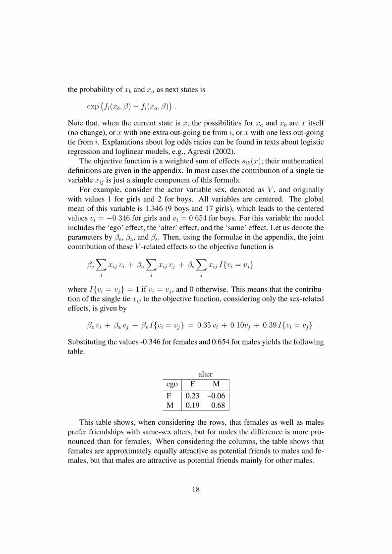
For example, consider the actor variable sex, denoted as V , and originallywith values 1 for girls and 2 for boys. All variables are centered. The globalmean of this variable is 1.346 (9 boys and 17 girls), which leads to the centeredvalues vi = −0.346 for girls and vi = 0.654 for boys. For this variable the modelincludes the ‘ego’ effect, the ‘alter’ effect, and the ‘same’ effect. Let us denote theparameters by βe, βa, and βs. Then, using the formulae in the appendix, the jointcontribution of these V -related effects to the objective function is

βe

∑j

xij vi + βa

∑j

xij vj + βs

∑j

xij I{vi = vj}

where I{vi = vj} = 1 if vi = vj , and 0 otherwise. This means that the contribu-tion of the single tie xij to the objective function, considering only the sex-relatedeffects, is given by

βe vi + βa vj + βs I{vi = vj} = 0.35 vi + 0.10vj + 0.39 I{vi = vj}

Substituting the values -0.346 for females and 0.654 for males yields the followingtable.

alterego F M

F 0.23 –0.06M 0.19 0.68

This table shows, when considering the rows, that females as well as malesprefer friendships with same-sex alters, but for males the difference is more pro-nounced than for females. When considering the columns, the table shows thatfemales are approximately equally attractive as potential friends to males and fe-males, but that males are attractive as potential friends mainly for other males.

18

4 More complicated modelsThis section treats two generalizations of the model sketched above.

4.1 Differential rates of change: the rate functionThe rate at which actors get the opportunity to change their out-going ties coulddiffer systematically between actors. Depending on actor attributes or on posi-tional characteristics such as in-degree or out-degree, actors might change theirties at differential frequencies. This can be the case, e.g., in networks betweenorganisations with clear differences in degrees, where the out-degrees reflect theimportance to the organizations of the network under study, and the resources theydevote to positioning themselves in it.

Model 2 in Table 1 gives an example of such an analysis. It extends Model 1 byadding an effect of sex on the rate function. The estimated negative effect indicatesthat in the data set under study, boys change their network ties less frequentlythan girls, although the difference is not significant (p = 0.13). To interpret theparameter values, it must be kept in mind that an exponential link function isused (Snijders, 2001; Snijders et al., 2008) and that the values of the variable‘sex’ are, still centered, vi = −0.346 for females and vi = 0.654 for males. Theparameter estimate of –0.42 implies that the estimated rate function is the base ratemultiplied by exp(−0.42 vi). Thus, for period 1, for girls the expected number ofopportunities for change is 9.75 × exp(−0.42 × (−0.346)) = 11.3, and for boysit is 9.75× exp(−0.42× (0.654)) = 7.4. The difference seems rather large but isnot significant in view of the small ‘sample size’.

4.2 Differences between creating and terminating ties: the en-dowment function

In the treatment given above, terminating a tie is just the opposite of creatingone. This is not always a good representation of reality. It is conceivable, forexample, that the loss when terminating a reciprocal tie is greater than the gainin creating one; or that transitive closure works especially for the creation of newties, but hardly guards against termination of existing ties. This can be modeled byhaving two components of the objective function: the evaluation function, whichconsiders only the network that will be the case as a result of the change to bemade; and the endowment function, which is a component that operates only forthe termination of ties and not for their creation. Everything discussed above aboutthe objective function concerned the evaluation function – in other words, in thosediscussions and the example, the endowment function was nil. The endowment

19

function gives contributions to the objective function that do not play a role whencreating ties, but that are lost when dissolving ties.

Model 3 in Table 1 gives the results of an analysis that includes, in addi-tion to the effects of Model 1, also an endowment effect related to reciprocity.It was estimated as significant and positive, while the corresponding evaluationfunction effect of reciprocity dropped in size and significance. To interpret thisresult, jointly consider the reciprocity evaluation effect with parameter 0.71 andthe reciprocity endowment effect with parameter 1.42. The contribution of a tiebeing reciprocated then is 0.71 for the creation of the tie and 0.71 + 1.42 = 2.13against the termination of the tie. Thus, reciprocity here is more important againstterminating friendships – that is, for maintaining friendships – than for creatingfriendships.

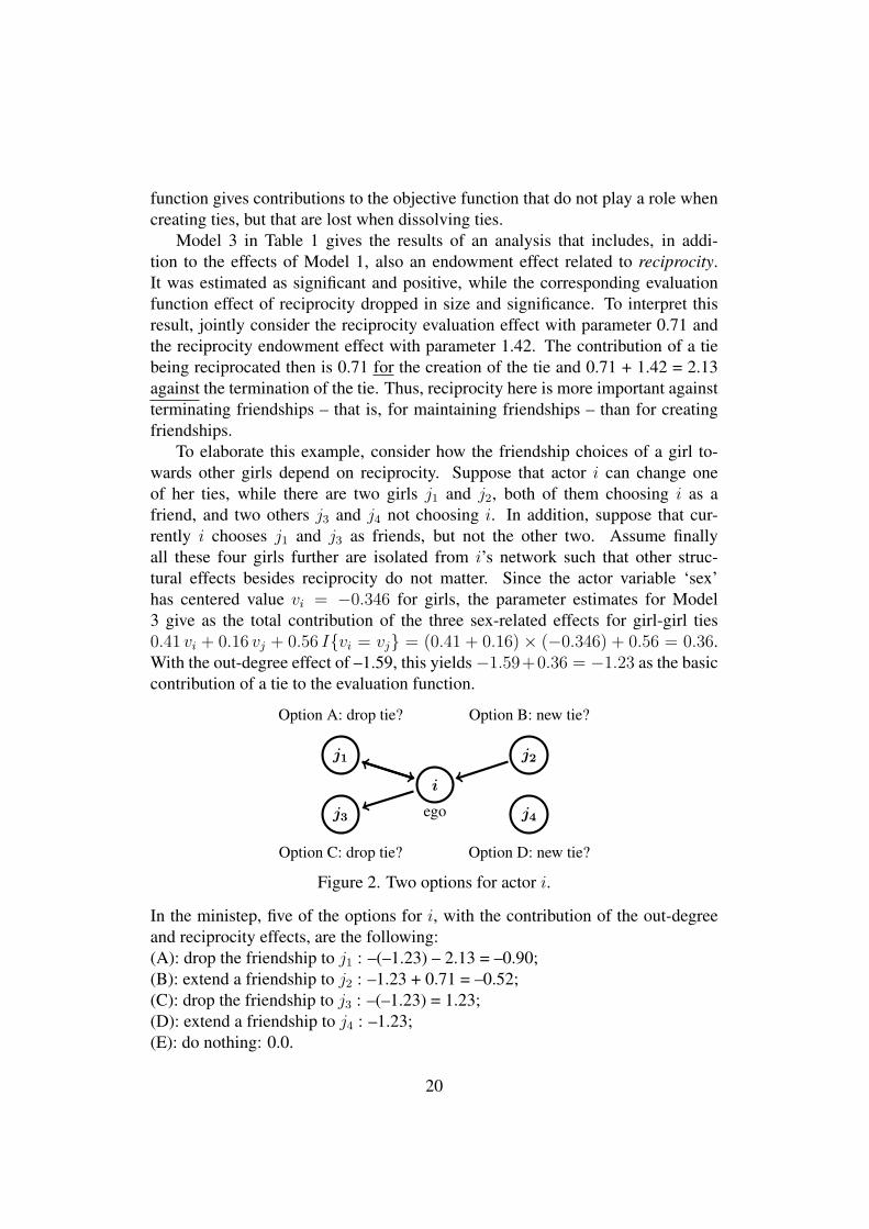
To elaborate this example, consider how the friendship choices of a girl to-wards other girls depend on reciprocity. Suppose that actor i can change oneof her ties, while there are two girls j1 and j2, both of them choosing i as afriend, and two others j3 and j4 not choosing i. In addition, suppose that cur-rently i chooses j1 and j3 as friends, but not the other two. Assume finallyall these four girls further are isolated from i’s network such that other struc-tural effects besides reciprocity do not matter. Since the actor variable ‘sex’has centered value vi = −0.346 for girls, the parameter estimates for Model3 give as the total contribution of the three sex-related effects for girl-girl ties0.41 vi + 0.16 vj + 0.56 I{vi = vj} = (0.41 + 0.16) × (−0.346) + 0.56 = 0.36.With the out-degree effect of –1.59, this yields−1.59+0.36 = −1.23 as the basiccontribution of a tie to the evaluation function.

Option A: drop tie? Option B: new tie?

Option C: drop tie? Option D: new tie?

ego

i

j1 j2

j3 j4

Figure 2. Two options for actor i.

In the ministep, five of the options for i, with the contribution of the out-degreeand reciprocity effects, are the following:(A): drop the friendship to j1 : –(–1.23) – 2.13 = –0.90;(B): extend a friendship to j2 : –1.23 + 0.71 = –0.52;(C): drop the friendship to j3 : –(–1.23) = 1.23;(D): extend a friendship to j4 : –1.23;(E): do nothing: 0.0.

20

Since these are contributions to logarithms of probabilities, the proportionalityfactors between the probabilities of these events must be calculated as the expo-nential transformations of these values, which are, respectively, e−0.90 = 0.41,0.59, 3.42, 0.29, and 1. Thus, for instance, the probability of dropping the re-ciprocated friendship (A) is 0.41 times the probability of not changing any tie(E), and 0.41/3.42 = 0.12 times the probability of dropping the non-reciprocatedfriendship (C).

5 Dynamics of networks and behaviorThe scientific importance of social networks often is related to the fact that net-works are relevant for behavior and outcomes of actors: related actors may in-fluence one another (e.g., Friedkin, 1998), and ties will be selected in part basedon the similarity between ego and potential relational partners (homophily, seeMcPherson, Smith-Lovin, and Cook, 2001). This means that the network togetherwith such actor variables will be endogenous, i.e., the network is changing as afunction of itself and of the actor variables, and likewise the actor variables arechanging as a function of themselves and of the network. We use the term behav-ior as shorthand for endogenously changing actor variables, although they couldalso refer to attitudes, performance, etc.; there could be one or more of such vari-ables. It is assumed here that the behavior variables are ordinal discrete variables,with values 1, 2, etc., up to some maximum value, for instance, several levelsof petty crime, several levels of smoking, etc. The dependence of the networkdynamics on the total network-behavior configuration will be also called the so-cial selection process, while the dependence of the behavior dynamics on the totalnetwork-behavior configuration will be called the social influence process. Bothsocial influence and social selection can lead to similarity between tied actors,which is often observed. A fundamental question then is whether this similarityis caused mainly by influence or mainly by selection, as discussed by Ennett &Bauman (1994) for smoking behavior and Haynie (2001) for delinquent behavior.

This combination of selection and influence can be modeled by an extensionof the actor-based model to a structure where the dependent variables consist notonly of the tie variables but also of the actors’ behavior variables, as specified inSnijders, Steglich and Schweinberger (2007) and Steglich, Snijders and Pearson(2008). Of course there usually will be, in addition, also exogenous actor and/ordyadic variables which purely have the role of independent variables.

The assumptions for the actor-based model for the dynamics of networks andbehavior are rather direct extensions of the assumptions for network dynamics.The extended formulations of assumptions 2–6 are as follows.

21

2. The changing system consisting of network and behavior is the outcome ofa Markov process.

3. At a given moment either one probabilistically selected actor may change atie, or one actor may change his/her behavior by going one unit up or down(recall that the behavior variables are assumed to be integer-valued). Thisexcludes coordination between changes in the network and in the behavior.

4. The actors control their out-going ties as well as their own behavior.

5. There are distinct change opportunity processes for tie changes and behaviorchanges.

6. There are distinct change determination processes for tie changes and be-havior changes, conditional on the possibility to make the respective type ofchange.

The changes in behavior depend on an objective function similar to the objectivefunction for network changes. However, this function will be different becauseit needs to represent primarily the actor’s behavior rather than his/her networkposition, and because choices of behavior changes may be framed differently fromchoices of tie changes, depending on different goals and restrictions.

5.1 The objective function for behaviorIf the objective function is such that increasing the behavior variable is just theopposite of decreasing it, then it is called an evaluation function. It can be repre-sented, analogously to (1), as

fZi (β, x, z) =

∑k

βZk s

Zki(x, z) , (2)

where sZki(x, z) are functions depending on the behavior of the focal actor i, but

also on the behavior of his network partners, his network position, etc. Thestrength of the effects of these functions on behavior choices are represented bythe parameters βZ

k . The main possible terms of the evaluation function are asfollows.

Basic shape effectsTo represent the basic tendencies to change the behavior, discussed here first in-

dependent of actor attributes and network position, the evaluation function will bea curve that can be loosely interpreted as the relative preference for the possiblevarious values of the behavior. When the behavior variable is dichotomous, then a

22

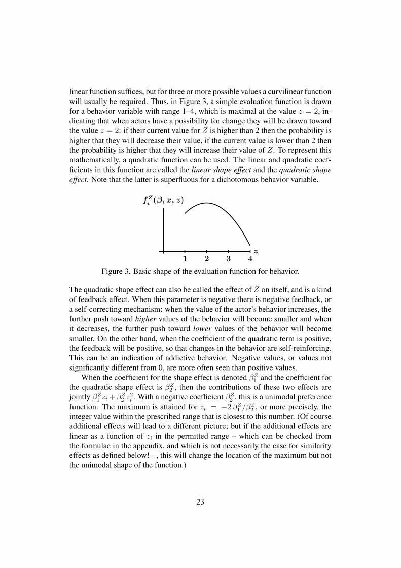
linear function suffices, but for three or more possible values a curvilinear functionwill usually be required. Thus, in Figure 3, a simple evaluation function is drawnfor a behavior variable with range 1–4, which is maximal at the value z = 2, in-dicating that when actors have a possibility for change they will be drawn towardthe value z = 2: if their current value for Z is higher than 2 then the probability ishigher that they will decrease their value, if the current value is lower than 2 thenthe probability is higher that they will increase their value of Z. To represent thismathematically, a quadratic function can be used. The linear and quadratic coef-ficients in this function are called the linear shape effect and the quadratic shapeeffect. Note that the latter is superfluous for a dichotomous behavior variable.

z

fZi (β, x, z)

1 2 3 4

Figure 3. Basic shape of the evaluation function for behavior.

The quadratic shape effect can also be called the effect of Z on itself, and is a kindof feedback effect. When this parameter is negative there is negative feedback, ora self-correcting mechanism: when the value of the actor’s behavior increases, thefurther push toward higher values of the behavior will become smaller and whenit decreases, the further push toward lower values of the behavior will becomesmaller. On the other hand, when the coefficient of the quadratic term is positive,the feedback will be positive, so that changes in the behavior are self-reinforcing.This can be an indication of addictive behavior. Negative values, or values notsignificantly different from 0, are more often seen than positive values.

When the coefficient for the shape effect is denoted βZ1 and the coefficient for

the quadratic shape effect is βZ2 , then the contributions of these two effects are

jointly βZ1 zi +βZ

2 z2i . With a negative coefficient βZ

2 , this is a unimodal preferencefunction. The maximum is attained for zi = −2 βZ

1 /βZ2 , or more precisely, the

integer value within the prescribed range that is closest to this number. (Of courseadditional effects will lead to a different picture; but if the additional effects arelinear as a function of zi in the permitted range – which can be checked fromthe formulae in the appendix, and which is not necessarily the case for similarityeffects as defined below! –, this will change the location of the maximum but notthe unimodal shape of the function.)

23

Influence and position-dependent effectsThe tendencies expressed in the shape parameters express affect everyone in the

group under study in the same way, irrespective of his/her characteristics or net-work position. To capture social network effects, additional terms in the behaviorevaluation function are needed.

The actor-based model can represent social influence, i.e., influence from al-ters’ behavior on ego’s behavior, in various ways, because there are several dif-ferent ways to measure and aggregate the influences from different alters. Threedifferent representations are as follows.

1. The average similarity effect, expressing the preference of actors to be sim-ilar in behavior to their alters, in such a way that the total influence of thealters is the same regardless of the number of alters (i.e., ego’s out-degree).

2. The total similarity effect, expressing the preference of actors to be similarin behavior to their alters, in such a way that the total influence of the altersis proportional to the number of alters.

3. The average alter effect, expressing that actors whose alters have a higheraverage value of the behavior, also have themselves a stronger tendencytoward high values on the behavior.

The choice between these three will be made on theoretical grounds and/or on thebasis of statistical significance.

The existence of various different ways of aggregating across alters impliesthat it may be important to control also for the effect of the out-degree of thefocal actor – the total number of alters. The out-degree and in-degree effectson behavior can also be interesting in themselves, expressing that those who aremore active (higher out-degree) or more popular (higher in-degree) have a highertendency to display higher values of the behavior.

Effects of other actor variablesFor each actor-dependent covariate as well as for each of the other dependent

behavior variables (if any), a main effect on the behavior can be included. Inaddition, it is possible that such a variable will moderate the influence effect,leading to an interaction between the variable and the influence effect.

24

5.2 Specification of models fordynamics of networks and behavior

There is a natural advantage of the network part over the behavior part in termsof the amount of information available on the two dimensions. For n actors, thereare n measurements of the behavior variable, while there are as many as n(n− 1)measurements of network tie variables. Typically, this asymmetry also affects theability to detect dynamic patterns and identify effects on the two types of depen-dent variables. In statistical terms, there will be less power to detect the determi-nants of behavioral evolution than there is to detect the determinants of networkevolution. Therefore, backward model selection is not a good route to follow forspecifying a model of network-behavior co-evolution: weak and unsystematic ef-fects on behavioral change, when estimated, subtract from the ability to identifythe stronger and more systematically occurring ones. Instead of starting with anextensive model, it is better to start with a small one, and proceed by way offorward model selection to arrive at a good model.

Since it is more difficult to estimate a model of network-behavior co-evolutionthan to estimate a model of only network evolution, it makes sense first to estimatea good model for the dynamics of only the network according to the approach ofthe preceding section, and to use this as a baseline for the network part of thenco-evolution model.

It has become clear above that there are several specifications of the socialselection part, such as Z-similarity and Z - ego × alter; like for any actor vari-able, also for behavior variable Z the ego and alter effects may be relevant. Thesimilarity effect in the network dynamics part is directly interpretable, whereasthe Z - ego × alter interaction effect needs also the ego and alter effects to bewell interpretable. For the social influence part likewise there are several possiblespecifications, such as average similarity, total similarity, and average alter.

A difficulty is that we usually have no clear theoretical clue as to which spec-ification is better in a particular case; the alternative specifications are definedby effects that may be highly mutually correlated and therefore are not readilyestimated jointly in the same model; and the power of detecting selection and in-fluence will depend on the specification chosen. If we do have prior informationas to the best specification, then it is preferable to work with this specification. Ifwe do not have such information, and we wish to evade the chance capitalizationinherent in using the ‘most significant’ effect without taking into account that itwas chosen exactly because it was the most significant, then we could proceedalong something like the following lines. An example of this approach is given inthe next subsection. This procedure uses score-type tests (Schweinberger, 2008)for several parameters simultaneously, which are chi-squared tests with numberof degrees of freedom equal to the number of tested effects.

25

1. Specify and estimate a baseline model ‘BM’ for network-behavior co-evolutionin which the network and behavior dynamics are independent; that is, themodel for network dynamics contains no effects dependent on the behaviorvariable, and vice versa.

2. Choose a number of candidate social selection effects ‘SEL’ and a numberof candidate social influence effects ‘INF’ on theoretical grounds, withoutconsidering the data.

3. Test the effects in the sets SEL and INF by score-type tests in the baselinemodel BM. Select the effects that are individually most significant in eitherset, and denote these effects by SEL1 and INF1.(In this formulation, the effects are selected based on their significance whenhypothesized to be added to the baseline model. Another possibility is toselect the effects based on the following two models.)

4. To test influence effects while controlling for selection, estimate the modelBM + SEL1 (i.e., the baseline model extended with the most significantselection effect) and within this model test all of the effects INF jointly bya score-type test.

5. To test selection effects while controlling for influence, estimate the modelBM + INF1 and test all of the effects SEL jointly by a score-type test.

6. To estimate a model with influence and selection, estimate the model BM +SEL1 + INF1.

7. It often will be sensible to conduct some further checks to guard againstthe danger of overlooking important effects. This can be done again withscore-type tests. Candidate effects to be checked include the in-degree andout-degree effects on the behavior variable.

5.3 Example: dynamics of friendship and delinquencySubstantively, what we address is again the dynamics of the friendship networkinvestigated also above, now co-evolving with the students’ delinquency (Knecht,2008). This variable is defined as a rounded average over four types of minordelinquency (stealing, vandalism, graffiti, and fighting), measured in each of thefour waves of data collection. The five-point scale ranged from ‘never’ to ‘morethan 10 times’, and the distribution is highly skewed, most students reporting nodelinquency. In a range of 1–5, the mode was 1 at all four waves, the average roseover time from 1.4 to 2.0, and the value 5 was never observed.

26

The analyses address the question whether the data provide evidence for net-work influence processes playing a role in the spread of delinquency through thegroup defined by the classroom. The results of the statistical procedures are proba-bilistic because of the randomness inherent in the MCMC procedure. Certainly inthis data set which is rather small for the model that is being fitted, results can dif-fer somewhat between different calculation runs. Reported results all were takenfrom runs in which all ‘t-ratios for convergence’ (see the Siena manual) were lessthan 0.1 in absolute value, indicating good convergence of the algorithm.

For the model selection we follow the steps laid out in the preceding section.The baseline model is the model which for the friendship dynamics is model 3in Table 1, and for the delinquency dynamics includes the linear and quadraticshape effects and the effect of sex (as a control variable). The effects potentiallymodelling social selection based on delinquency (the set SEL in the precedingsection) are delinquency ego, delinquency alter, delinquency similarity, and delin-quency ego × alter. Delinquency ego and delinquency alter are included here ascontrol variables for delinquency ego × delinquency alter. The effects potentiallymodelling social influence with respect to delinquency (the set INF) are averagesimilarity, total similarity, and average delinquency alter. Score tests for the se-lection and influence effects tested with the baseline model as the null hypothesisyielded the following p-values.

Effect pFriendship dynamicsdelinquency alter 0.32delinquency ego < 0.001delinquency similarity < 0.001delinquency ego × delinquency alter 0.02Delinquency dynamicsaverage similarity 0.03total similarity 0.12delinquency average alter 0.48

This suggests that strongest effects are delinquency similarity for the networkdynamics and average similarity for the behavior dynamics. These are the effectsdenoted above as SEL1 and INF1, respectively.

To test selection while controlling for influence, the baseline model was ex-tended with influence operationalized as average similarity, and the three selectioneffects (delinquency ego, delinquency alter, delinquency similarity, and delin-quency ego × delinquency alter) where jointly tested by a score-type test. Thetest result was highly significant, p < 0.001.

To test influence while controlling for selection, the baseline model was ex-tended with selection operationalized as delinquency similarity, and the three in-

27

fluence effects (average similarity, total similarity, and average delinquency alter)where jointly tested by a score-type test. This led to p = 0.04. Thus, there is inthis classroom clear evidence (p < 0.001) for delinquency-based friendship selec-tion, and weak evidence (p = 0.04) for influence from pupils on the delinquentbehavior of their friends.

To estimate a model incorporating selection and influence, the baseline modelwas extended with delinquency similarity for the network dynamics and averagesimilarity for the behavior dynamics. This model is estimated and presented inTable 2. The delinquency ego and delinquency alter effects were also tested forinclusion in the network dynamics model, and the in-degree and out-degree effectswere tested for inclusion in the behavior dynamics model, but none of these weresignificant.

Table 2 about here

It can be concluded that there is in this data set evidence for delinquency-based friendship selection, expressed most clearly by the delinquency similaritymeasure; and for influence from pupils on the delinquent behavior of their friends,expressed best by the average similarity measure. The delinquent behavior doesnot seem to be influenced by sex. The model for network dynamics yields es-timates that are quite similar to those for the model without the simultaneousdelinquency dynamics, except that the reciprocity effect has shifted more stronglytowards the endowment effect.

6 DiscussionThis paper has given a tutorial introduction in the use of actor-based modeling ofthe dynamics of networks, and of the joint interdependent dynamics of networksand behavior. Here ‘behavior’ is an actor variable which may refer to behavior,attitudes, performance, etc. In the models treated, the network is represented bya directed graph while the behavioral variable is assumed to be an ordinal dis-crete variable. A first fundamental assumption is that it is meaningful to approx-imate the dynamics of the network, or of the network together with behavior, bya Markov process in continuous time – even though it is observed only at two ormore discrete observation moments. A second fundamental assumption is that thenetwork dynamics can be represented as an actor-based model, where tendenciesof ties to change are described as depending on the actor who is the ‘sender’ of theties, both on the attributes and the network position of this actor and of potential‘targets’ of the ties. Likewise, in models of dynamics of network and behavior, itis assumed that the dynamics of an actor’s behavior can depend on the attributes

28

and the network position of the actor as well as on the behavior of the other ac-tor to which this actor is tied. These models can be estimated by software calledSiena (‘Simulation Investigation for Empirical Network Analysis’), of which themanual is Snijders et al. (2008). Program and documentation can be downloadedfree from the Siena web-page, http://www.stats.ox.ac.uk/siena/.The model and software have many more possibilities than can be treated in thecontext of this paper. Some of these are briefly mentioned here.

Some special issues concerning the treatment of the data in the example areas follows. In the data set used, some data were missing due to absence of pupilsat the moment of data collection, treated by ad-hoc model-based imputation asexplained in Huisman and Steglich (2008). One pupil left the classroom. Suchchanges in network composition can be treated by the methods of Huisman andSnijders (2003), but were treated here as structural zeros: tie variable that arenot allowed to change, in this case fixed to zero starting with the first observationmoment where this pupil was not a member of the classroom any more.

Various extensions of the model are the topic of recent and current research.Models for the dynamics of non-directed networks, e.g., alliance networks, havebeen developed and were applied already in Van de Bunt and Groenewegen (2007).Extensions to valued ties will be presented soon. Standardized parameters may bemore readily interpretable than the non-standardized parameters treated here, andwork to define standardized parameters is under way. Other estimation proce-dures have been proposed: Bayesian inference by Koskinen and Snijders (2007)and Schweinberger (2007), Maximum Likelihood estimation by Snijders, Koski-nen and Schweinberger (2008). Further applications of these models can be foundin some of the papers in this special issue.

AppendixThis appendix contains some formulae to support the understanding of the verbaldescriptions in the paper.

Objective functionWhen actor i has the opportunity to make a change, he/she can choose betweensome set C of possible new states of the network. Normally this will be set consist-ing of the current network and all other networks where one out-going tie variableof i is changed. The probability of going to some new state x in this set is givenby

exp(fi(β, x)

)∑x′∈C exp

(fi(β, x′)

) . (3)

29

Similarly, when actor i can make a change in the behavior variable z and thecurrent value is z0, then the possible new states are z0 − 1, z0, and z0 + 1 (unlessthe first or last of these three falls outside the range of the behavior variable).Denoting this allowed set also by C, the probability of going to some new state zin this set is given by

exp(fZ

i (βZ , x, z))∑

z′∈C exp(fZ

i (β, x, z′)) . (4)

These are the same formulae used in multinomial logistic regression.

EffectsSome formulae for effects sik(x) are as follows. Replacing an index by a + signdenotes summation over this index.

reciprocity∑

j

xij xji (5)

transitive triplets∑j,h

xih xij xjh (6)

transitive ties∑

h

xih maxj

(xij xjh) (7)

three-cycles∑j,h

xij xjh xhi (8)

balance1

n− 2

n∑j=1

xij

n∑h=1h6=i,j

(b0− | xih − xjh |) (9)

where b0 is the mean of | xih − xjh |;

in-degree popularity (sqrt)∑

j

xij√x+j (10)

out-degree popularity (sqrt)∑

j

xij√xj+ (11)

in-degree activity (sqrt)√x+i xi+ (12)

out-degree activity (sqrt) x1.5i+ (13)

30

out-outdegree assortativity (sqrt)∑

j

xij√xi+ xj+ (14)

(other assortativity effects similar)

V - ego∑

j

xij vi (15)

V - alter∑

j

xij vj (16)

V - similarity∑

j

xij (simij − sim) , (17)

where simij =(1− |vi − vj|/∆

); with ∆ = maxij |vi − vj|

same V∑

j

xij I{vi = vj} , (18)

where I{vi = vj} = 1 if vi = vj , and 0 otherwise;

V - ego × alter∑

j

xij vi vj (19)

dyadic covariate W∑

j

xij wij (20)

dyadic cov. W × reciprocity∑

j

xij xjiwij (21)

actor cov. V × transitive triplets vi

∑j,h

xij xjh xih . (22)

Some formulae for behavior effects sZik(x, z) are the following.

linear shape zi (23)quadratic shape z2

i (24)out-degree zi xi+ (25)in-degree zi x+i (26)

average similarity x−1i+

∑j

xij(simzij − simz) (27)

31

where simzij =

(1− |zi − zj|/∆Z

)with ∆Z = maxij |zi − zj|

total similarity∑

j

xij(simzij − simz) (28)

average alter zi

(∑j

xij zj

)/(∑

j

xij

)(29)

main effect covariate V zi vi . (30)

References

Agresti, Alan. 2002. Categorical data analysis. New Jersey: Wiley.

Batagelj, V., and M. Bren. 1995. Comparing resemblance measures. Journal ofClassification, 12, 73–90.

Bearman, P.S. (1997) Generalized exchange, American Journal of Sociology,102, 1383–1415.

Burk, William J., Steglich, Christian E.G., and Snijders, Tom A.B. (2007). Be-yond dyadic interdependence: Actor-oriented models for co-evolving socialnetworks and individual behaviors. International Journal of Behavioral De-velopment, 31: 397–404.

Burt, R.S. (1982) Toward a Structural Theory of Action. New York: AcademicPress.

Checkley, Matthew, and Steglich, Christian E.G. (2007). Partners in Power:Job Mobility and Dynamic Deal-Making. European Management Review 4(2007), 161–171.

Davis, James A. 1970. Clustering and Hierarchy in Interpersonal Relations: Test-ing Two Graph Theoretical Models on 742 Sociomatrices. American Sociolog-ical Review 35: 843–852.

Davis, James A., and Samuel Leinhardt. 1972. The Structure of Positive In-terpersonal Relations in Small Groups. In Joseph Berger (ed.), SociologicalTheories in Progress. Volume 2. Boston: Houghton-Mifflin.

Doreian, Patrick and Frans N. Stokman (Eds.). 1997. Evolution of Social Net-works. Amsterdam: Gordon and Breach Publishers.

Ennett, Susan T., and Karl E. Bauman. (1994). The Contribution of Influence andSelection to Adolescent Peer Group Homogeneity: The Case of AdolescentCigarette Smoking. Journal of Personality and Social Psychology 67, 653–63.

32

Frank, O., Strauss, D. (1986) Markov graphs, Journal of the American StatisticalAssociation, 81, 832–842.

Friedkin, N.E. (1998) A Structural Theory of Social Influence. Cambridge:Cambridge University Press.

Haynie, Dana L. 2001. Delinquent Peers Revisited: Does Network StructureMatter? American Journal of Sociology 106, 1013–57.

Peter Hedstrom. Dissecting the Social: On the Principles of Analytical Sociology.Cambridge University Press, 2005.

Holland, Paul W. and Samuel Leinhardt (1971). Transitivity in structural modelsof small groups. Comparative Groups Studies, 2: 107–124.

Holland, P.W., Leinhardt, S. (1977) A dynamic model for social networks, Jour-nal of Mathematical Sociology, 5, 5–20.

Holland, P.W. and Leinhardt, S. (1981) An exponential family of probability dis-tributions for directed graphs (with discussion). Journal of the American Sta-tistical Association, 76, 33–65.

Huisman, M.E., and T.A.B. Snijders. (2003). Statistical analysis of longitudinalnetwork data with changing composition. Sociological Methods & Research,32, 253 – 287.

Huisman, M., and C. Steglich (2008). Treatment of non-response in longitudinalnetwork data. Social Networks, in press, doi:10.1016/j.socnet.2008.04.004.

Katz, L., and C.H. Proctor. 1959. The configuration of interpersonal relationsin a group as a time-dependent stochastic process. Psychometrika 24: 317 –327.

Knecht, A. (2008). Friendship selection and friends’ influence. Dynamics of net-works and actor attributes in early adolescence. PhD dissertation, Universityof Utrecht.

Koskinen, J. 2004. Essays on Bayesian Inference for Social Networks. PhDDissertation. Department of Statistics, Stockholm University.

Koskinen, J.H., and T.A.B. Snijders. 2007. Bayesian inference for dynamic net-work data. Journal of Statistical Planning and Inference. Journal of StatisticalPlanning and Inference 13: 3930–3938.

Leenders, R.T.A.J. (1995). Models for network dynamics: A Markovian frame-work, Journal of Mathematical Sociology, 20, 1–21.

Macy, M.W., and Robb Willer. (2002). From factors to actors: ComputationalSociology and agent-based modelling, Annual Review of Sociology, 28, 143–166.

33

Maddala, G.S. (1983) Limited-dependent and Qualitative Variables in Econo-metrics (third ed.), Cambridge: Cambridge University Press.

McFadden, D. (1973), Conditional logit analysis of qualitative choice behavior,in Frontiers in econometrics, P. Zarembka (ed.), New York: Academic Press.

McPherson, Miller, Lynn Smith-Lovin, and James M. Cook. 2001. Birds of aFeather: Homophily in Social Networks. Annual Review of Sociology, 27,415–44.

Newcomb, Theodore M. 1962. Student Peer-Group Influence. In Nevitt Sanford(Ed.): The American College : A Psychological and Social Interpretation ofthe Higher Learning. New York, Wiley.

Pearson, M.A., and Michell, L. (2000) Smoke Rings: Social network analysisof friendship groups, smoking and drug-taking. Drugs: education, preventionand policy, 7, 21–37.

Pearson, Michael, Steglich, Christian, and Snijders, Tom (2006) Homophilyand assimilation among sport-active adolescent substance users. Connections27(1), 47–63.

Price, Derek de Solla (1965). Networks of scientific papers. Science 149, 510–515.

Robins, G., and Pattison, P. 2001. Random graph models for temporal processesin social networks. Journal of Mathematical Sociology 25: 5–41.

Schweinberger, M. 2008. Statistical Modeling of Network Dynamics Given PanelData: Goodness-of-fit Tests. Submitted for publication.

Snijders, T.A.B. (1996) Stochastic actor-oriented dynamic network analysis,Journal of Mathematical Sociology, 21, 149–172.

Snijders, T.A.B. (2001) The statistical evaluation of social network dynamics, in:Sobel, M., Becker, M. (Eds.), Sociological Methodology, Boston and London:Basil Blackwell, 361–395.

Snijders, T.A.B. (2005) Models for longitudinal network data, in: Carrington,P.J., Scott, J., Wasserman, S. (Eds.), Models and Methods in Social NetworkAnalysis. New York: Cambridge University Press.

Snijders, T.A.B., J.H. Koskinen, and M. Schweinberger. (2008). MaximumLikelihood Estimation for Social Network Dynamics. Submitted.

Snijders, Tom A.B., Steglich, Christian E.G., and Schweinberger, Michael. 2007.Modeling the co-evolution of networks and behavior. In Longitudinal modelsin the behavioral and related sciences, edited by Kees van Montfort, Han Oudand Albert Satorra, pp. 41–71. Mahwah, NJ: Lawrence Erlbaum.

34

Snijders, T.A.B., Steglich, C.E.G., Schweinberger, M., Huisman, M. (2008) Man-ual for SIENA version 3.2, Groningen: ICS, University of Groningen; Oxford:Department of Statistics, University of Oxford,http://stat.gamma.rug.nl/snijders/siena.html.

Steglich, C.E.G., Snijders, T.A.B., Pearson, M. (2008) Dynamic networks andbehavior: Separating selection from influence, Submitted for publication.

Steglich, Ch.E.G., Snijders, T.A.B., and West, P. 2006. Applying SIENA: AnIllustrative Analysis of the Coevolution of Adolescents’ Friendship Networks,Taste in Music, and Alcohol Consumption. Methodology, 2, 48–56.

Udehn, L. (2002) The changing face of methodological individualism, AnnualReview of Sociology, 8, 479–507.

van de Bunt, G.G. and Groenewegen, P. (2007). An Actor-Oriented DynamicNetwork Approach: The Case of Interorganizational Network Evolution. Or-ganizational Research Methods 10: 463–482.

van de Bunt, G.G., Van Duijn, M.A.J., and Snijders, T.A.B. (1999) Friendshipnetworks through time: An actor-oriented statistical network model. Compu-tational and Mathematical Organization Theory, 5: 167–192.

van de Bunt, G.G., Wittek, R.P.M., and de Klepper M.C. (2005) The Evolutionof Intra-Organizational Trust Networks; The Case of a German Paper Factory:An Empirical Test of Six Trust Mechanisms. International Sociology 20: 339–369.

van Duijn, M.A.J., Zeggelink, E.P.H., Huisman, M., Stokman, F.N., and Wasseur,F.W. (2003) Evolution of Sociology Freshmen into a Friendship Network.Journal of Mathematical Sociology 27: 153–191.

Wasserman, S. 1979. A stochastic model for directed graphs with transition ratesdetermined by reciprocity. Pp. 392 – 412 in Sociological Methodology 1980,edited by K.F. Schuessler. San Francisco: Jossey-Bass.

Wasserman, S. 1987. The conformity of two sociometric relations. Psychome-trika 53: 261–282.

Wasserman, S., and K. Faust. 1994. Social Network Analysis: Methods andApplications. New York and Cambridge: Cambridge University Press.

Wasserman, S., and D. Iacobucci. 1988. Sequential social network data. Psy-chometrika 53: 261–282.

Wasserman, S., Faust, K. (1994) Social Network Analysis: Methods and Appli-cations, Cambridge: Cambridge University Press.

Wasserman, S., and Pattison, P.E. 1996. Logit models and logistic regression forsocial networks: I. An introduction to Markov graphs and p∗. Psychometrika61: 401 – 425.

Tabl

e1:

Para

met

eres

timat

esof

frie

ndsh

ipev

olut

ion

mod

els,

with

stan

dard

erro

rsan

dtw

o-si

dedp-

valu

es.

Mod

el0

Mod

el1

Mod

el2

Mod

el3

estim

.s.

e.p

estim

.s.

e.p

estim

.s.

e.p

estim

.s.

e.p

obje

ctiv

efu

nctio

nou

tdeg

ree

−1.

410.

43<

0.00

1−

1.67

0.38

<0.

001−

1.62

0.34

<0.

001−

1.59

0.33

<0.

001

reci

proc

ity(e

valu

atio

n)1.

340.

22<

0.00

11.

420.

20<

0.00

11.

450.

20<

0.00

10.

710.

480.

14re

cipr

ocity

(end

owm

ent)

1.42

0.80

0.07

6tr

ansi

tive

trip

lets

0.23

0.03

<0.

001

0.21

0.03

<0.

001

0.21

0.03

<0.

001

0.20

0.03

<0.

001

tran

sitiv

etie

s0.

740.

21<

0.00

10.

740.

230.

001

0.78

0.22

<0.

001

0.67

0.20

<0.

001

3-cy

cles

−0.

320.

10<

0.00

1−

0.26

0.09

0.00

5−

0.25

0.09

0.00

7−

0.22

0.10

0.02

8in

-deg

ree

popu

lari

ty(s

qrt)

−0.

180.

120.

130.

230.

230.

29ou

t-de

gree

popu

lari

ty(s

qrt)−

0.40

0.24

0.09

3−

0.56

0.23

0.01

3−

0.62

0.20

0.00

2−

0.61

0.20

<0.

001

out-

degr

eeac

tivity

(sqr

t)0.

010.

070.

930.

180.

120.

19se

x(M

)ego

0.35

0.13

0.00

80.

390.

130.

002

0.44

0.14

0.00

20.

410.

13<

0.00

1se

x(M

)alte

r0.

100.

130.

460.

150.

130.

240.

180.

140.

200.

160.

140.

25sa

me

sex

0.49

0.13

<0.

001

0.54

0.12

<0.

001

0.56

0.14

<0.

001

0.56

0.13

<0.

001

prim

ary

scho

ol0.

370.

130.

006

0.35

0.14

0.01

30.

340.

140.

016

0.35

0.15

0.02

0

rate

func

tion

rate

peri

od1

10.0

12.

059.

761.

919.

691.

9610.9

32.

26ra

tepe

riod

210.6

71.

8510.4

41.

8310.2

81.

8211.1

31.

93ra

tepe

riod

39.

511.

538.

911.

398.

811.

379.

381.

52ef

fect

sex

(M)o

nra

te−

0.42

0.28

0.13

Thep-

valu

esar

eba

sed

onap

prox

imat

eno

rmal

dist

ribu

tions

ofth

et-

ratio

s(e

stim

ate

divi

ded

byst

anda

rder

ror)

.W

hen

rend

ered

for

non-

incl

uded

para

met

ers,

they

refe

rto

scor

e-ty

pete

sts.

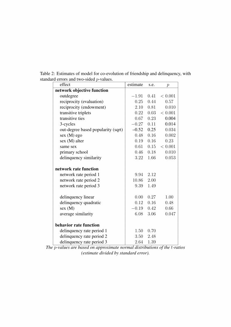
Table 2: Estimates of model for co-evolution of friendship and delinquency, withstandard errors and two-sided p-values.

effect estimate s.e. pnetwork objective function

outdegree −1.91 0.41 < 0.001reciprocity (evaluation) 0.25 0.44 0.57reciprocity (endowment) 2.10 0.81 0.010transitive triplets 0.22 0.03 < 0.001transitive ties 0.67 0.23 0.0043-cycles −0.27 0.11 0.014out-degree based popularity (sqrt) –0.52 0.25 0.034sex (M) ego 0.48 0.16 0.002sex (M) alter 0.19 0.16 0.23same sex 0.61 0.15 < 0.001primary school 0.46 0.18 0.010delinquency similarity 3.22 1.66 0.053

network rate functionnetwork rate period 1 9.94 2.12network rate period 2 10.86 2.00network rate period 3 9.39 1.49

delinquency linear 0.00 0.27 1.00delinquency quadratic 0.12 0.16 0.48sex (M) −0.19 0.42 0.66average similarity 6.08 3.06 0.047

behavior rate functiondelinquency rate period 1 1.50 0.70delinquency rate period 2 3.50 2.48delinquency rate period 3 2.64 1.39

The p-values are based on approximate normal distributions of the t-ratios(estimate divided by standard error).