Introducing regulation in the measurement of efficiency, with an application to the Canadian air...
28
Introducing Regulation in the Measurement of Efficiency, with an application to the Canadian Air Carriers Industry Pierre Ouellette a , Patrick Petit b Louis-Philippe Tessier-Parent a and Stéphane Vigeant c a Dept. of Economics, Université du Québec à Montréal b Analysis Group, Montréal, Canada c Médée, Institut des sciences économiques et du management, Université de Lille 1 October 2005 Correspondance should be sent to Stéphane Vigeant, Bureau 104, Bâtiment SH2, MÉDÉE, Faculté des sciences économiques et sociales, Université des sciences et technologies de Lille, F59655 Villeneuve d’Ascq Cédex, France.
-
Upload
independent -
Category
Documents
-
view
0 -
download
0
Transcript of Introducing regulation in the measurement of efficiency, with an application to the Canadian air...
Introducing Regulation in the Measurement of Efficiency, with an
application to the Canadian Air Carriers Industry
Pierre Ouellettea,
Patrick Petitb
Louis-Philippe Tessier-Parenta
and
Stéphane Vigeantc
a Dept. of Economics, Université du Québec à Montréal
b Analysis Group, Montréal, Canada
c Médée, Institut des sciences économiques et du management, Université de Lille 1
October 2005
Correspondance should be sent to Stéphane Vigeant, Bureau 104, Bâtiment SH2, MÉDÉE, Faculté des sciences économiques et sociales, Université des sciences et technologies de Lille, F59655 Villeneuve d’Ascq Cédex, France.
ii
Abstract
This paper proposes a method to measure efficiency in highly regulated capital-intensive
industries in the presence of state-owned enterprises. We generalize the DEA method so that
regulation is included in the model, and the quasi-fixed nature of capital and its links with the
firms’ investment decisions is explicit. The framework is then applied to the Canadian air
carriers industry to study the impact of regulation changes between 1960 and 1999 on the
efficiency of the various carriers. Our results show that deregulation explains a large part of the
measured inefficiency when regulation is not included in the model. This is consistent with the
aforementioned wisdom: inefficiency is a measure of our ignorance.
1
Introduction
Technological change is a key ingredient of improved standards of living and measuring it has
been a key preoccupation of economists for decades, if not centuries. Research in this field has
grown tremendously following the work of Shephard (1953) who showed that primal measures of
technology such as returns to scale and technical progress could be retrieved in the dual space of
price and costs with standard economic data, assuming the firm maximized profits or minimized
its costs of producing a given output. This resulted in many subsequent refinements in the tools
to study technological change, and in a surge in productivity analysis studies. Many of these
studies have had a major role in public policy debates, such as in the case of airline deregulation
in the 1970’s.
In spite of these tremendous advances, this approach to measuring technology has proven difficult
to adapt to the specific setting of regulated firms solving dynamic optimization problems: how do
we measure the technology of regulated firms of firms that optimize over many periods? Most
importantly, the dual approach has remained dependent on the strength of its underlying
assumption, i.e., the optimizing behavior of the firm. Do state-owned enterprises minimize costs?
How do we measure the technology of organizations with goals not direct profit maximization or
cost minimization, as it is the case in institutions such as many hospitals, schools etc.? The study
of such organizations, of which many operate in the public sector, has forced economists to return
to the primal approach and to measure technology directly in the input-output space. Data
envelopment analysis (DEA) for example, has become a prime tool to investigate the issue of
public sector productivity. Not only can DEA apply to cases of non-optimizing firms, it is also a
non-parametric technique, i.e., it does not have to rely on specific and potentially constraining
functional forms for estimation.
As for duality theory, DEA has undergone many improvements to adapt it to the specific context
of studied firms, such as the inclusion of quasi-fixed inputs. However, a major feature of all
2
industries of modern economies remains excluded from DEA models: regulation. As a matter of
fact, the presence of governments in the economy is mostly felt through regulation as opposed to
any other form of intervention such as spending, state-owned enterprises, etc. (Viscusi et al.,
2000). Governments intervene in the field of the environment, safety, intellectual property, as
well as in many other aspects of economic life. Another key area of intervention is competition
policy: do governments restrict the entry of competing firms? Do they let losers go bankrupt? Do
they allow firms to merge? This type of regulation has been present in many capital intensive
industries where highly-regulated public firms are often present, with or without private sector
competitors. Measuring technology in such a setting is very difficult without many adjustments
to standard models.
This paper proposes to integrate economic regulation to the DEA approach to measuring
technology. Although the impact of regulation on technological change can be measured in an ad
hoc fashion by comparing technical progress of regulated and non-regulated firms after
measuring their technology, such comparisons do not fully capture the interaction of regulation
and technology because there is no explicit representation of regulation in the model. Properly
including regulation, as well as other industry characteristics such as quasi-fixed inputs thus
requires solid theoretical foundations. Specifically, these elements should be analytically
included in the linear programming problem to be solved to obtain technological measures. The
model we propose builds on previous work in this area and includes quasi-fixed inputs and
regulation, which takes the form of a very general representation that can be adapted to many
types of governmental intervention. The model is tested with a Canadian dataset on airline
carriers between 1960 and 1999 and key technological parameters are calculated.
The airline industry is a highly interesting application for the model. It has been studied for
decades with many different methods, hence the possibility to compare and replicate results with
this new technique quite easily. It is also a capital-intensive industry that has been characterized
3
by sweeping changes in its size, technology and regulation. Finally, the Canadian industry has
been characterized by the presence of Air Canada, a dominant and eventually single carrier, and
that was publicly owned for many years.
The next section describes the model and derives the main technological measures. For clarity,
we first describe the model with quasi-fixed inputs only, and then we include regulation in a
second model. The Canadian airline industry is described in Section 2, where we focus on its
historical trends towards integration and concentration, and its complex regulation. This section
is completed by a description of the dataset. Results, including the calculation of efficiency and
returns to scale, are presented in Section 3. The last section discusses the main conclusion of the
model and the importance of adopting an appropriate methodology to reaching such conclusions.
1. The model
1.1 DEA model with quasi-fixed inputs in the presence of cost of adjustment
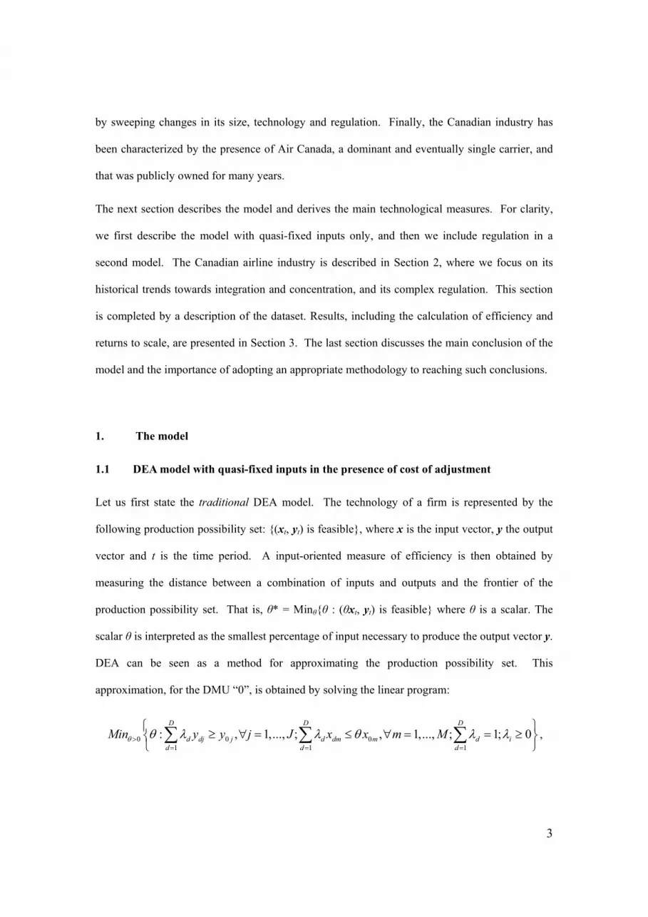
Let us first state the traditional DEA model. The technology of a firm is represented by the
following production possibility set: {(xt, yt) is feasible}, where x is the input vector, y the output
vector and t is the time period. A input-oriented measure of efficiency is then obtained by
measuring the distance between a combination of inputs and outputs and the frontier of the
production possibility set. That is, θ* = Minθ{θ : (θxt, yt) is feasible} where θ is a scalar. The
scalar θ is interpreted as the smallest percentage of input necessary to produce the output vector y.
DEA can be seen as a method for approximating the production possibility set. This
approximation, for the DMU “0”, is obtained by solving the linear program:
0 0 01 1 1
: , 1,..., ; , 1,..., ; 1; 0D D D
d dj j d dm m d id d d
Min y y j J x x m Mθ θ λ λ θ λ λ>= = =
≥ ∀ = ≤ ∀ = = ≥
∑ ∑ ∑ ,
4
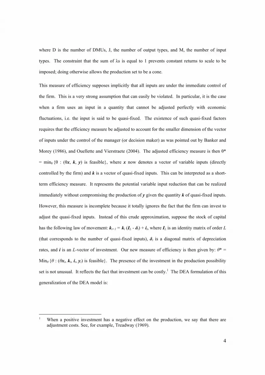
where D is the number of DMUs, J, the number of output types, and M, the number of input
types. The constraint that the sum of λs is equal to 1 prevents constant returns to scale to be
imposed; doing otherwise allows the production set to be a cone.
This measure of efficiency supposes implicitly that all inputs are under the immediate control of
the firm. This is a very strong assumption that can easily be violated. In particular, it is the case
when a firm uses an input in a quantity that cannot be adjusted perfectly with economic
fluctuations, i.e. the input is said to be quasi-fixed. The existence of such quasi-fixed factors
requires that the efficiency measure be adjusted to account for the smaller dimension of the vector
of inputs under the control of the manager (or decision maker) as was pointed out by Banker and
Morey (1986), and Ouellette and Vierstraete (2004). The adjusted efficiency measure is then θ*
= minθ {θ : (θx, k, y) is feasible}, where x now denotes a vector of variable inputs (directly
controlled by the firm) and k is a vector of quasi-fixed inputs. This can be interpreted as a short-
term efficiency measure. It represents the potential variable input reduction that can be realized
immediately without compromising the production of y given the quantity k of quasi-fixed inputs.
However, this measure is incomplete because it totally ignores the fact that the firm can invest to
adjust the quasi-fixed inputs. Instead of this crude approximation, suppose the stock of capital
has the following law of movement: kt+1 = kt (IL - δt) + it, where IL is an identity matrix of order L
(that corresponds to the number of quasi-fixed inputs), δt is a diagonal matrix of depreciation
rates, and i is an L-vector of investment. Our new measure of efficiency is then given by: θ* =
Minθ {θ : (θxt, kt, it, yt) is feasible}. The presence of the investment in the production possibility
set is not unusual. It reflects the fact that investment can be costly.1 The DEA formulation of this
generalization of the DEA model is:
1 When a positive investment has a negative effect on the production, we say that there are
adjustment costs. See, for example, Treadway (1969).
5
0 0 0 01 1 1
: , 1,..., ; , 1,..., ; , 1,..., ;D D D
d dj j d dm m d dl ld d d
Min y y j J x x m M k k l Lθ θ λ λ θ λ>= = =
≥ ∀ = ≤ ∀ = ≤ ∀ =
∑ ∑ ∑
01 1
, 1,..., ; 1; 0D D
d dl l d id d
i i l Lλ λ λ= =
≥ ∀ = = ≥
∑ ∑ .
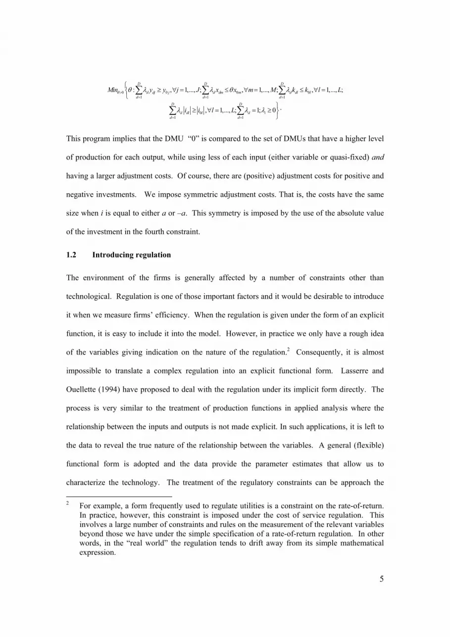
This program implies that the DMU “0” is compared to the set of DMUs that have a higher level
of production for each output, while using less of each input (either variable or quasi-fixed) and
having a larger adjustment costs. Of course, there are (positive) adjustment costs for positive and
negative investments. We impose symmetric adjustment costs. That is, the costs have the same
size when i is equal to either a or –a. This symmetry is imposed by the use of the absolute value
of the investment in the fourth constraint.
1.2 Introducing regulation
The environment of the firms is generally affected by a number of constraints other than
technological. Regulation is one of those important factors and it would be desirable to introduce
it when we measure firms’ efficiency. When the regulation is given under the form of an explicit
function, it is easy to include it into the model. However, in practice we only have a rough idea
of the variables giving indication on the nature of the regulation.2 Consequently, it is almost
impossible to translate a complex regulation into an explicit functional form. Lasserre and
Ouellette (1994) have proposed to deal with the regulation under its implicit form directly. The
process is very similar to the treatment of production functions in applied analysis where the
relationship between the inputs and outputs is not made explicit. In such applications, it is left to
the data to reveal the true nature of the relationship between the variables. A general (flexible)
functional form is adopted and the data provide the parameter estimates that allow us to
characterize the technology. The treatment of the regulatory constraints can be approach the
2 For example, a form frequently used to regulate utilities is a constraint on the rate-of-return.
In practice, however, this constraint is imposed under the cost of service regulation. This involves a large number of constraints and rules on the measurement of the relevant variables beyond those we have under the simple specification of a rate-of-return regulation. In other words, in the “real world” the regulation tends to drift away from its simple mathematical expression.
6
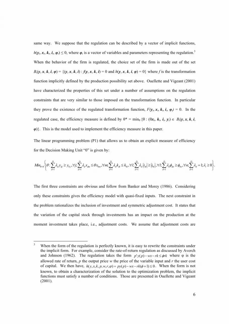
same way. We suppose that the regulation can be described by a vector of implicit functions,
h(yt, xt, kt, it, φt) ≤ 0, where φt is a vector of variables and parameters representing the regulation.3
When the behavior of the firm is regulated, the choice set of the firm is made out of the set
Bt(y, x, k, i, φ) = {(y, x, k, i) : f(y, x, k, i) = 0 and h(y, x, k, i, φ) = 0} where f is the transformation
function implicitly defined by the production possibility set above. Ouellette and Vigeant (2001)
have characterized the properties of this set under a number of assumptions on the regulation
constraints that are very similar to those imposed on the transformation function. In particular
they prove the existence of the regulated transformation function, F(yt, xt, kt, it, φt) = 0. In the
regulated case, the efficiency measure is defined by θ* = minθ {θ : (θxt, kt, it, yt) ∈ Bt(y, x, k, i,
φ)}. This is the model used to implement the efficiency measure in this paper.
The linear programming problem (P1) that allows us to obtain an explicit measure of efficiency
for the Decision Making Unit “0” is given by:
0 0 0 0 0 01 1 1 1 1 1
: , ; , ; , ; , ; , ; 1; 0 .D D D D D D
d dj j d dm m d dl l d dl l d dn n d id d d d d d
Min y y j x x m k k l i i l nθ θ λ λ θ λ λ λ φ φ λ λ>= = = = = =
≥ ∀ ≤ ∀ ≤ ∀ ≥ ∀ ≥ ∀ = ≥ ∑ ∑ ∑ ∑ ∑ ∑
The first three constraints are obvious and follow from Banker and Morey (1986). Considering
only these constraints gives the efficiency model with quasi-fixed inputs. The next constraint in
the problem rationalizes the inclusion of investment and symmetric adjustment cost. It states that
the variation of the capital stock through investments has an impact on the production at the
moment investment takes place, i.e., adjustment costs. We assume that adjustment costs are
3 When the form of the regulation is perfectly known, it is easy to rewrite the constraints under
the implicit form. For example, consider the rate-of-return regulation as discussed by Averch and Johnson (1962). The regulation takes the form rkrkwxpyp φ≤−−)(' where φ is the allowed rate of return, p the output price w the price of the variable input and r the user cost of capital. We then have, 0)1()(),,,,,,( ≤+−−= φϕ rkwxppyrwpkxyh . When the form is not known, to obtain a characterization of the solution to the optimization problem, the implicit functions must satisfy a number of conditions. Those are presented in Ouellette and Vigeant (2001).
7
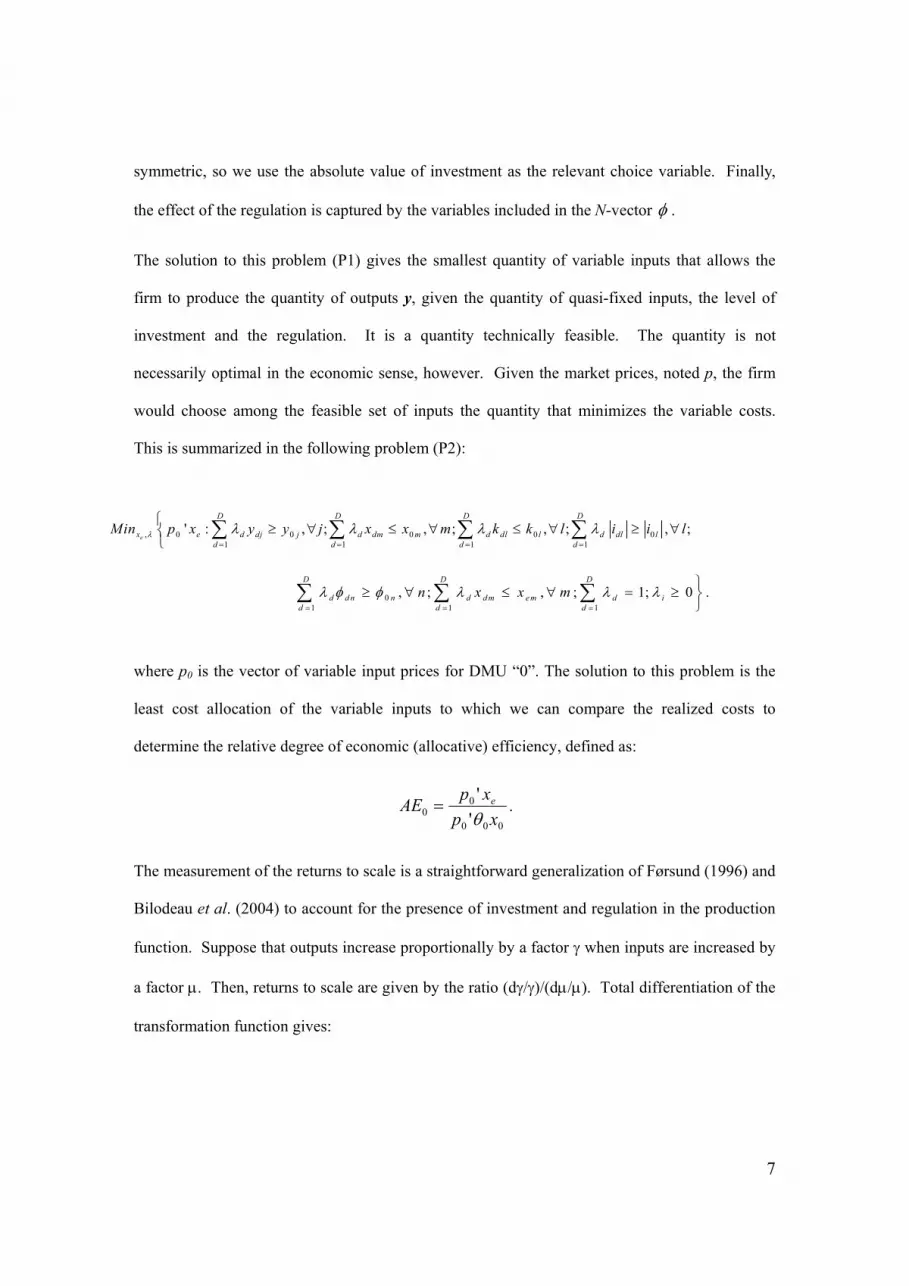
symmetric, so we use the absolute value of investment as the relevant choice variable. Finally,
the effect of the regulation is captured by the variables included in the N-vector φ .
The solution to this problem (P1) gives the smallest quantity of variable inputs that allows the
firm to produce the quantity of outputs y, given the quantity of quasi-fixed inputs, the level of
investment and the regulation. It is a quantity technically feasible. The quantity is not
necessarily optimal in the economic sense, however. Given the market prices, noted p, the firm
would choose among the feasible set of inputs the quantity that minimizes the variable costs.
This is summarized in the following problem (P2):
where p0 is the vector of variable input prices for DMU “0”. The solution to this problem is the
least cost allocation of the variable inputs to which we can compare the realized costs to
determine the relative degree of economic (allocative) efficiency, defined as:
000
00 '
'xp
xpAE e
θ= .
The measurement of the returns to scale is a straightforward generalization of Førsund (1996) and
Bilodeau et al. (2004) to account for the presence of investment and regulation in the production
function. Suppose that outputs increase proportionally by a factor γ when inputs are increased by
a factor µ. Then, returns to scale are given by the ratio (dγ/γ)/(dµ/µ). Total differentiation of the
transformation function gives:
, 0 0 0 0 01 1 1 1
' : , ; , ; , ; , ;e
D D D D
x e d dj j d dm m d dl l d dl ld d d d
Min p x y y j x x m k k l i i lλ λ λ λ λ= = = =
≥ ∀ ≤ ∀ ≤ ∀ ≥ ∀
∑ ∑ ∑ ∑
01 1 1
, ; , ; 1; 0 .D D D
d d n n d d m em d id d d
n x x mλ φ φ λ λ λ= = =
≥ ∀ ≤ ∀ = ≥
∑ ∑ ∑
8
( )
0.
hj m
j mh hj mj j m m
ll nl l n
l l nl l l l n n
dy d xF Fy xy y x x
d Idk dF F Fk Ik k I I
θθθ θ
φφφ φ
∂ ∂+ ∂ ∂
∂ ∂ ∂+ + + = ∂ ∂ ∂
∑ ∑
∑ ∑ ∑
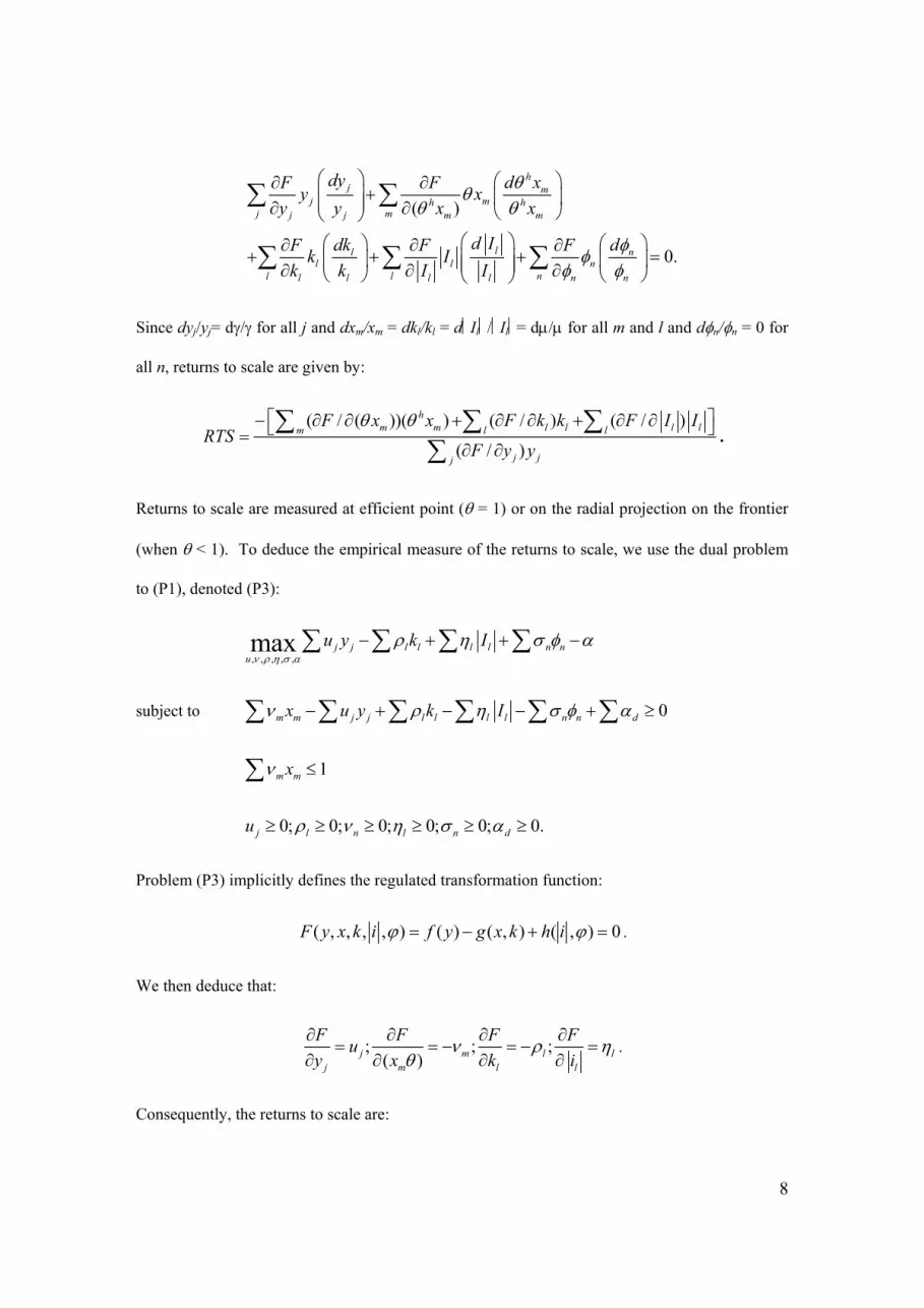
Since dyj/yj= dγ/γ for all j and dxm/xm = dkl/kl = dIl/Il= dµ/µ for all m and l and dφn/φn = 0 for
all n, returns to scale are given by:
( / ( ))( ) ( / ) ( / )
( / )
hm m l l l lm l l
j jj
F x x F k k F I IRTS
F y y
θ θ − ∂ ∂ + ∂ ∂ + ∂ ∂ =∂ ∂
∑ ∑ ∑∑
.
Returns to scale are measured at efficient point (θ = 1) or on the radial projection on the frontier
(when θ < 1). To deduce the empirical measure of the returns to scale, we use the dual problem
to (P1), denoted (P3):
, , , , ,max j j l l l l n n
uu y k I
ν ρ η σ αρ η σ φ α− + + −∑ ∑ ∑ ∑
subject to 0m m j j l l l l n n dx u y k Iν ρ η σ φ α− + − − + ≥∑ ∑ ∑ ∑ ∑ ∑
1m mxν ≤∑
0; 0; 0; 0; 0; 0.j l n l n du ρ ν η σ α≥ ≥ ≥ ≥ ≥ ≥
Problem (P3) implicitly defines the regulated transformation function:
( , , , , ) ( ) ( , ) ( , ) 0F y x k i f y g x k h iϕ ϕ= − + = .
We then deduce that:
; ; ;( )j m l l
j m l l
F F F Fuy x k i
ν ρ ηθ
∂ ∂ ∂ ∂= = − = − =
∂ ∂ ∂ ∂.
Consequently, the returns to scale are:
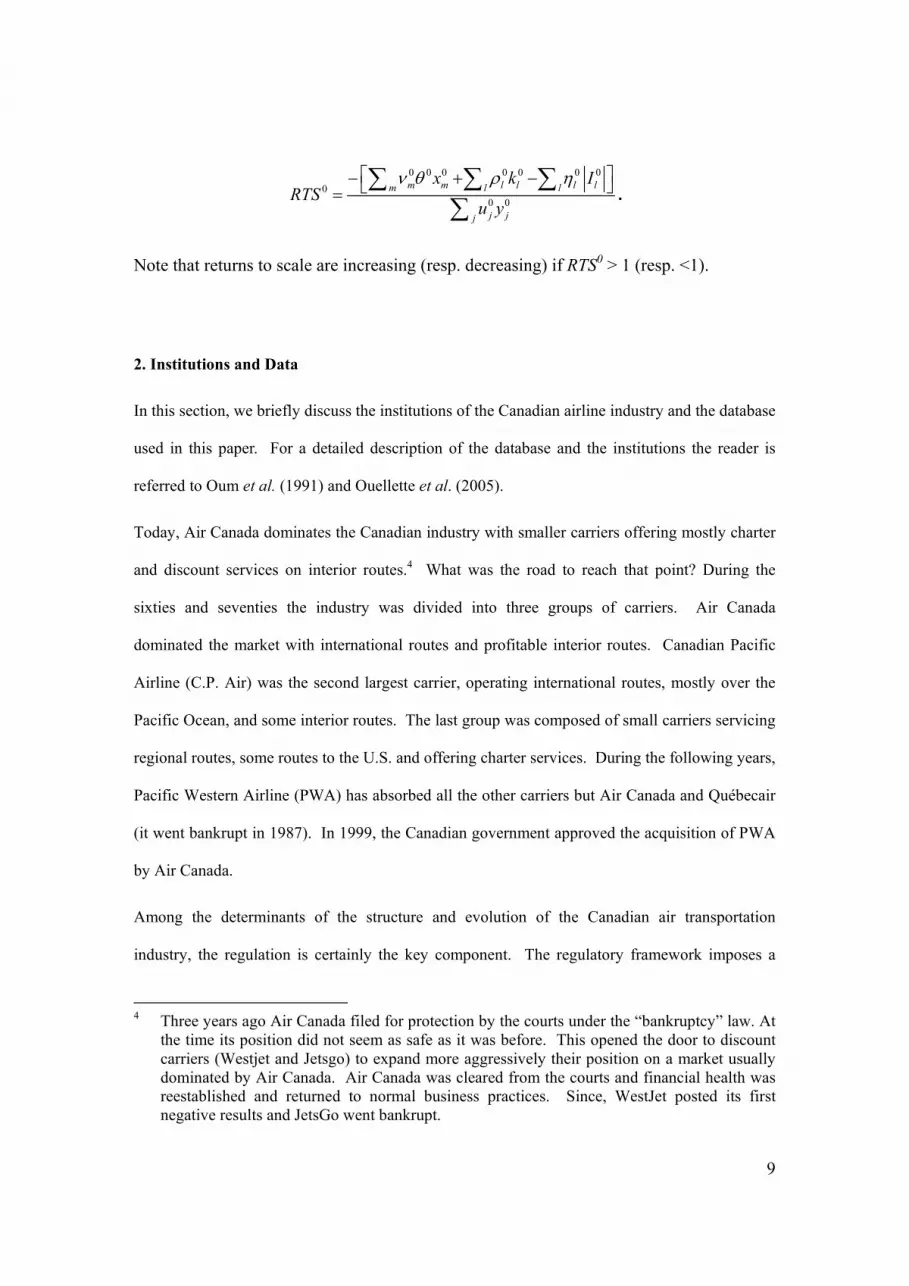
9
0 0 0 0 0 0 00
0 0
m m l l l lm l l
j jj
x k IRTS
u y
ν θ ρ η − + − =∑ ∑ ∑
∑.
Note that returns to scale are increasing (resp. decreasing) if RTS0 > 1 (resp. <1).
2. Institutions and Data
In this section, we briefly discuss the institutions of the Canadian airline industry and the database
used in this paper. For a detailed description of the database and the institutions the reader is
referred to Oum et al. (1991) and Ouellette et al. (2005).
Today, Air Canada dominates the Canadian industry with smaller carriers offering mostly charter
and discount services on interior routes.4 What was the road to reach that point? During the
sixties and seventies the industry was divided into three groups of carriers. Air Canada
dominated the market with international routes and profitable interior routes. Canadian Pacific
Airline (C.P. Air) was the second largest carrier, operating international routes, mostly over the
Pacific Ocean, and some interior routes. The last group was composed of small carriers servicing
regional routes, some routes to the U.S. and offering charter services. During the following years,
Pacific Western Airline (PWA) has absorbed all the other carriers but Air Canada and Québecair
(it went bankrupt in 1987). In 1999, the Canadian government approved the acquisition of PWA
by Air Canada.
Among the determinants of the structure and evolution of the Canadian air transportation
industry, the regulation is certainly the key component. The regulatory framework imposes a
4 Three years ago Air Canada filed for protection by the courts under the “bankruptcy” law. At
the time its position did not seem as safe as it was before. This opened the door to discount carriers (Westjet and Jetsgo) to expand more aggressively their position on a market usually dominated by Air Canada. Air Canada was cleared from the courts and financial health was reestablished and returned to normal business practices. Since, WestJet posted its first negative results and JetsGo went bankrupt.
10
series of constraints on the behavior of the firms in a very complex way. The challenge consists
in isolating the relevant components of the regulation. Economic and safety regulations are the
components we will consider in this paper. The economic regulation imposes specific restrictions
on the design of route, the frequency of flights, fare prices, the extent of the competition in
specific markets, and even the type of equipment used. These restrictions are often firm specific,
but overall they tend to affect the entire industry. The safety standard the carriers must maintain is
similar to the North American code of conduct. Because of the reputation effect and the degree
of monopolization of the markets, this aspect is sensitive to the size of the firms. Safety
regulation addresses problems related to the conditions of planes, the flight distance, airport
capacity, etc.
The database includes seven air carriers that operated during the period starting in 1960 ending in
1999. The carriers are (with the sample period in brackets): Air Canada (1960-1999), CPAir
(1960-1986), Pacific Western Airlines (PWA) (1964-1999), Québecair (1960-1987), Eastern
Provincial Airways (1964-1986), Transair (1964-1979) and Nordair (1970-1986). This is not an
exhaustive covering of the carriers that operated during that period, however. There is no
complete dataset on those carriers available. These carriers represent almost the entire industry,
however.
Most of the data are from Statistics Canada. They are the accounting data and operation statistics
that all carriers must report to Transport Canada. Interest rates and prices are also taken from
Statistics Canada. Some of the data are from the International Civil Aviation Organization
(ICAO), especially those concerning charter output, capital gains (for the entire period) and part
of the output (flight distance, flight departure, etc.). We constructed two outputs, unit toll (YR)
and charter (YN). The inputs are: capital (K), and investment (I), labor (L), energy (E) and
materials (M).
11
Because of the importance played by the regulation, the following describes the construction of
the two indices we used. The construction of the index should reflect the regulation and rely on
the information available to capture as perfectly as possible the state of the competition and the
bounds provided by the regulation to influence firms’ behavior. Advertising effort provides this
sort of compromise as it synthesizes the presence of competition for a given market, something
only allowed when the regulation is weakened. The index is an inverse function of the resources
devoted by each carrier to promotions and sales. It is defined as ERt = 1 / [ PSt / [ (AYt / PKMt ) *
FDt ] ], where ERt denotes the economic regulation, PSt is promotion and sales, AYt the available
output multilateral index, PKMt the total distance flown (plane-kilometers), and FDt the number
of flight departures. A decline in the index shows a relief in the regulation. The decrease of the
index for Air Canada and CP Air around the mid-70s corresponds to a greater competition on the
international market and the beginning of the relaxation of the regulation. This downward
slopping trend in the stringency of the regulation is observable for the small carriers few years
later (end of the 70s) when the charter service is deregulated and the regular service is partially
deregulated
Safety regulation aims at reducing the number of accidents. Ceteris paribus, more interventions
will lead to fewer accidents (e.g., higher competence standards, more inspections, more stringent
maintenance criteria, etc.). The inverse of the number of accidents per 100,000 hours of flight is
the best available index capable of grasping with a fair weight all safety-related interventions.
Our index is the same for each company, since firm-level data on accidents are not available.
Deviation by one firm will be monitored more closely, thus bringing back the number of accident
in line with the performance of the other carriers. Thus, we consider a common index for all
firms as acceptable. The index is increasing over the period covered by this analysis, meaning
that safety has increased.
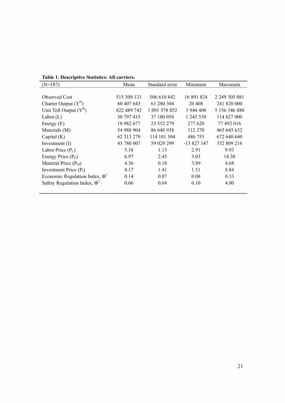
Table 1 presents descriptive statistics of the variables in the dataset.
12
[Insert Table 1 here]
3. Results
In this section, we present the results of our estimation of the efficiency of the Canadian Air
Carriers. Three models are estimated. The standard DEA model presented in the Section 1 is
implemented first. It serves as a reference to contrast our model’s results. The second model
includes quasi-fixed capital in a framework similar to Banker and Morey (1986). When
compared to our model, it shows that quasi-fixed capital is not enough to characterize entirely the
inefficiencies. Finally the third one is the model we proposed in Section 1; it adds adjustment
costs and regulation to the quasi-fixed capital model. As we will see, this model comparison
explicitly shows that efficiency measures can be misleading when the model is incompletely
specified. Regulation and costs associated to investments are real constraints on the behavior and
choices of the firms. Firms are not passive with respect to their environment and this shows in
business practices.
The estimation procedure includes two output free disposal constraints (unit toll and charter),
three variable input free disposal constraints (energy, labor and materials), one for the quasi-fixed
input (capital), two constraints to account for the economic and safety regulations and finally one
constraint for the cost of adjustment.
The solution to problem (P1) gives the technical efficiency parameters (θ). The observed cost is
simply the product of the prices and the input vector, p0’x0, and the technically efficient cost is
given by p0’(θ0 x0) = θ0 p0’x0, so that θ can be interpreted as the ratio of the technically efficient
cost over the observed cost. Then, the cost of the technical efficiency is (1- θ0)p0’x0.
The solution to the cost minimization problem (P2) allows us to find the allocatively efficient cost
in dollar units. The allocative efficiency ratio, AE, measures the distance in percentage between
13
the allocatively efficient cost, p0’xe, and the technically efficient cost, θ0 p0’x0. Total inefficiency
is measured as the ratio between the cost efficient allocation and the observed cost. That is:
0 0 0 0 00 0 0
0 0 0 0 0 0 0
' ' '' ' '
e ep x p x p xTI AEp x p x p x
θθθ
= × = × = .
Returns to scale are measured as shown in Section 2.
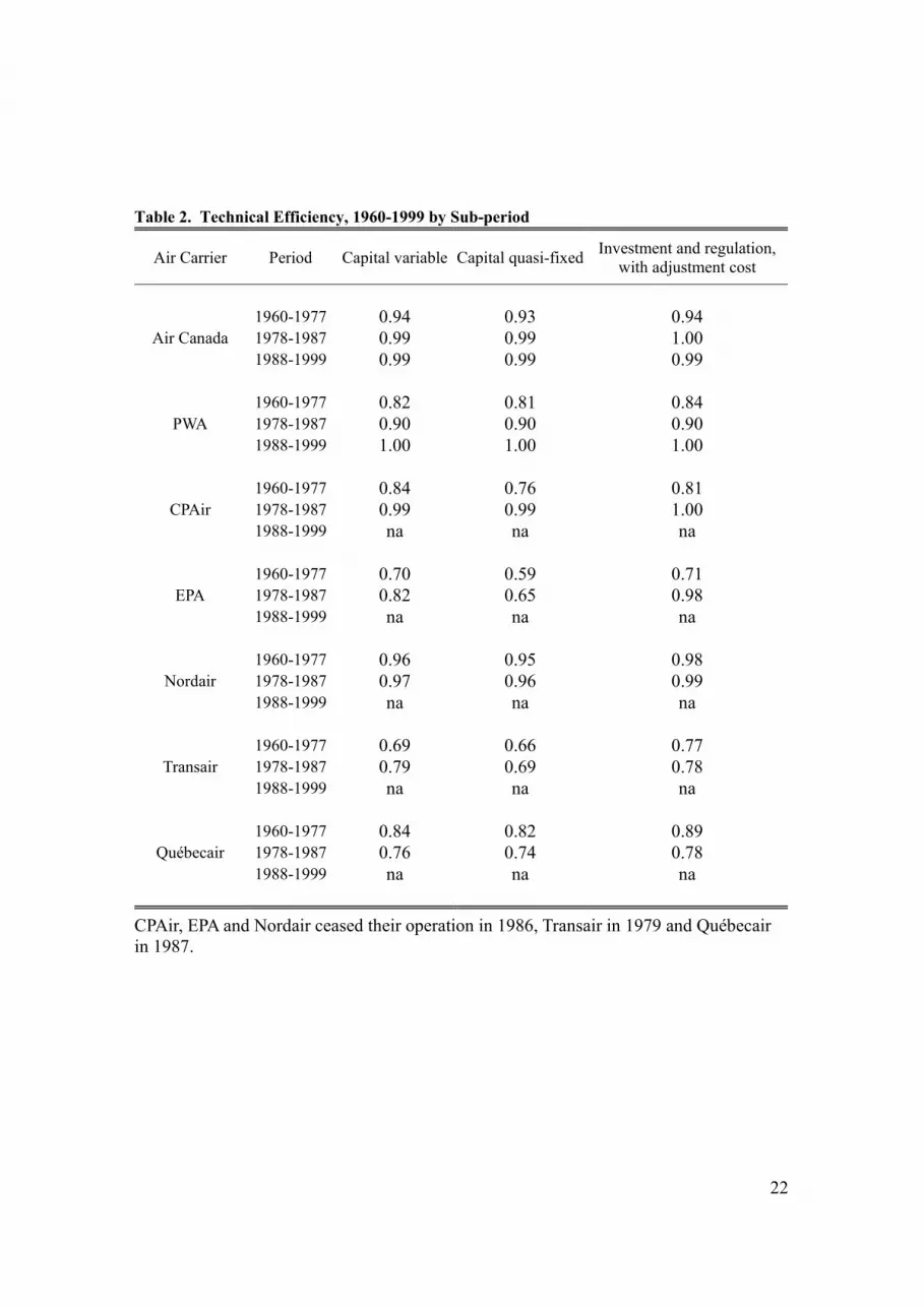
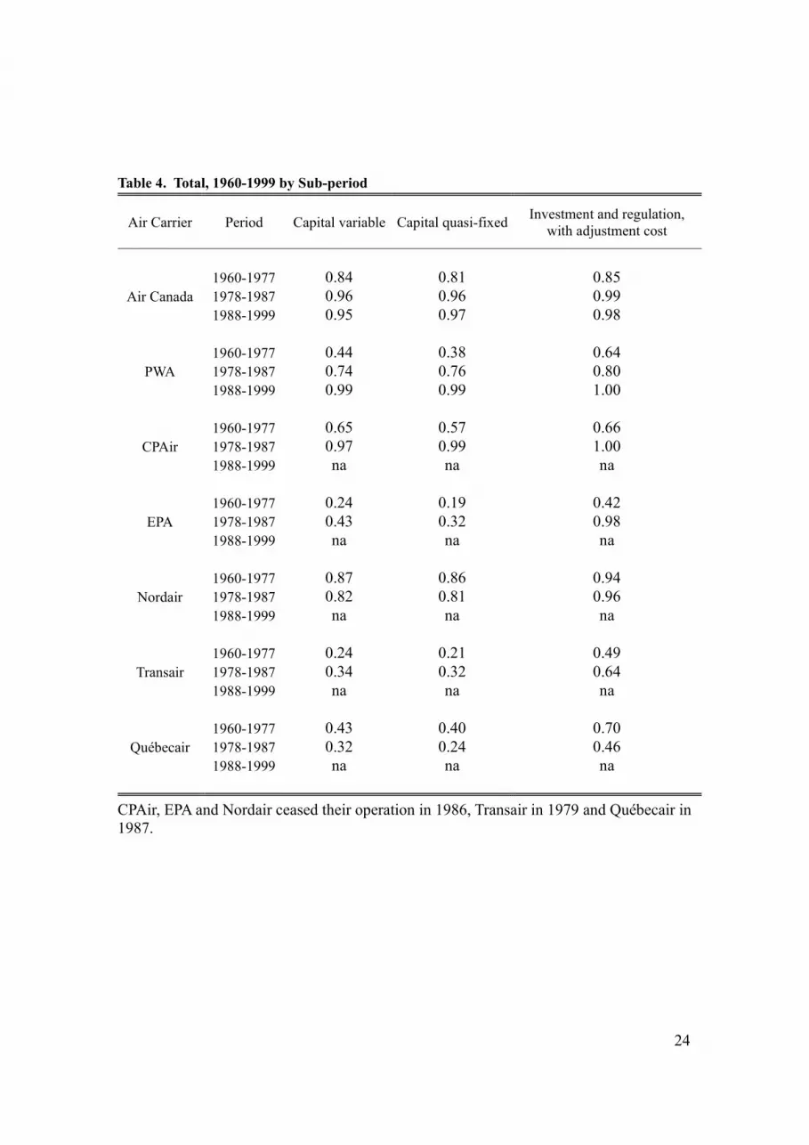
Tables 2 to 4 present the efficiency ratios for all three models. We have decomposed the sample
in three sub-periods: the period of strong regulation (1960-1977), the deregulation (or transition)
period (1978-1987) and the deregulated period (1988-1999). In our sample, the total number of
DMUs (Decision-Making Units) is 187.
As the model is refined, the number of firms5 diagnosed as inefficient tends to decrease. That is,
in the simplest model the number of efficient DMUs was 74, it increased to 99 in the model with
quasi-fixed capital, and to 112 in the model with the full set of constraints.6
[Insert Tables 2, 3 and 4 here]
The choice of model has a non neutral impact on the efficiency scores. That is, the scores
increase with the refinements so that, when the environment of the firm is taken into account
(regulation and adjustment costs), the firms exhibit relatively more efficient behaviors. This
suggests that an inadequate or too simple model might bias the results toward higher
inefficiencies then there really are. In other words, the regulation and other institutions represent
real constraints on the firm and this shows that firms’ decisions are mostly adequate response to
the circumstances they face. There are binding constraints beyond the technology that should be
taken into account in the firms’ decision process. To conclude that a firm is inefficient when the
5 We will equivalently use either DMU or firm. In this context, a “firm” is an observation at a
given date for a given firm. Then a firm may be composed of many DMUs or “firms”, one at each date a decision was made.
6 The firms not showing efficiency improvements are comparatively getting substantially worse when passing from the first model to the second as the averages of the efficiency measures for the sub-periods tend to decrease.
14
institutional specification of a model is incomplete can be a serious misrepresentation of firms’
behavior. It also means that we cannot compare the behavior of regulated firms to unregulated
firms without including the regulatory constraint because the notion of efficiency does not
include the same components simply because the model without regulatory constraints allows a
freedom of choice that the firm does not have.
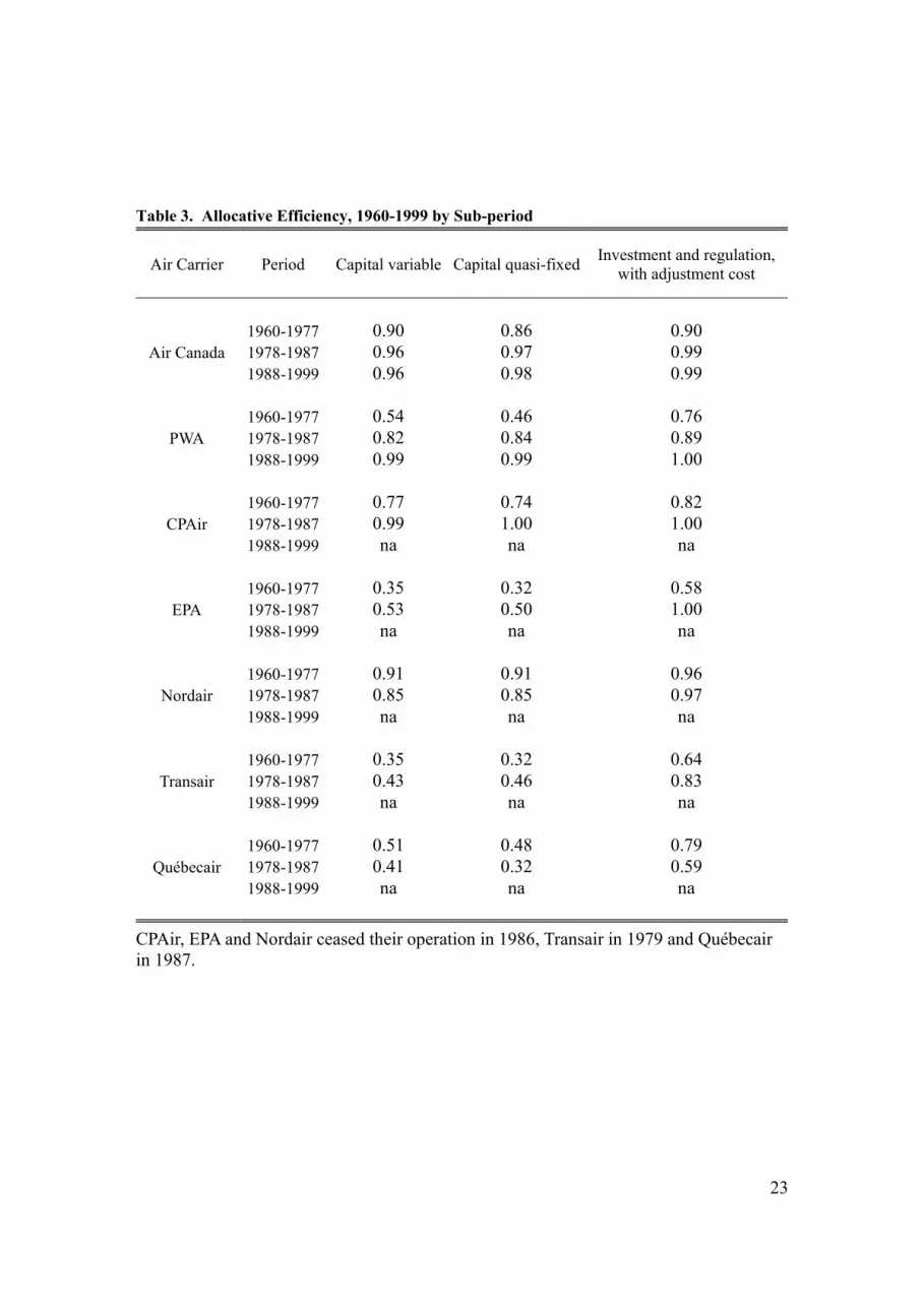
In all cases, the efficient allocation ratio is smaller than the technical efficiency ratio, for all
carriers and all periods. The carriers show that they have more difficulties to adapt to relative
price incentives than to use the resources available. The immediate conclusion would be to say
that they are technically more capable. This phenomenon can be related to the regulation,
however. Economic regulation is fairly explicit on what the firm can or cannot do, limiting their
responsiveness to prices. So we might be brought to think that with deregulation, the
responsiveness to price changes increase and so the firms should become less allocatively
inefficient. This is precisely what our results are showing. Furthermore, total efficiency has been
increasing over time in general, except for Québecair (and Nordair in the first two models).7
By contrasting these three models, we show that the improvement obtained from the introduction
of a more realistic environment helps to understand intricacies behind inefficiency scores. Model
refinements show non-trivial efficiency improvements as the number of inefficient firms decrease
when the model includes regulation and adjustment costs. A possible explanation is that
inefficiencies are simply the result of a misspecification and reflects “ignorance” of firms’
conditions. When using a complete set of constraints in a regulated industry the results are
consistent with the fact that firms internalize their environment: they behave much more
efficiently then it appears in a model where the regulation has been omitted. In other words,
firms do take into account costs of adjusting capital and the regulation in their decision process.
It also means that comparisons of efficiency measures between periods of regulated and
7 Note that Québecair is the only carrier in our sample that went bankrupt.
15
deregulated activities cannot be done without an explicit introduction of the regulation into the
model.
When the results are grouped according to the three regulatory regimes, the improvement of the
efficiency indicators is striking. There is a direct correlation between the relaxation of the
regulation and the improvement of the efficiency of the carriers. The total efficiency measure of
all carriers but Québecair increases from one regulatory period to the other. We can also identify
that the lack of efficiency during the period of stringent regulation (1960-1977) is attributable to
the allocative inefficiencies rather than technical efficiency. Thus, it is the capacity of the carriers
to respond adequately to price signals that is of concerns here. In fact, this is not so surprising
since the regulation specified a large share of the operation procedure (equipment, stopovers, etc.)
and it did not allow the carriers to choose the least expensive way to providing the service. When
the model already includes regulation and adjustment costs, the efficiency improvement
following deregulation is not as dramatic as it is when these constraints are not included. This
comes from the fact that firms already internalize those constraints, thus the relaxation of the
stringency of the regulation translates into a reallocation of the resources, not into an apparent
gain of efficiency. In the full model, the firms have similar performances. (There is a smaller
dispersion of the efficiency measure.) The large inefficiencies that we observe in the first two
setups again are mostly reflections of our ignorance; the incomplete specification tends to be
captured by the estimate of the inefficiency parameter and biases downward the real performance
of the firms.
We also note that during the deregulation phase and after, the firms in the third model tend to
perform better than in the first two. This will tend to corroborate the fact that the cost of
adjusting capital is not the same for all firms and that it is a real constraint for the firms. In other
words, adjusting capital is costly and takes firm’s resources away from productive activity.
16
Therefore, when this constraint is included in the model, the firms tend to exhibit a better
performance in its productive activities.
With deregulation, the firms were probably more able to respond to price incentives and thus to
adjust their input mix. This shows up in the results with a strong improvement of the allocative
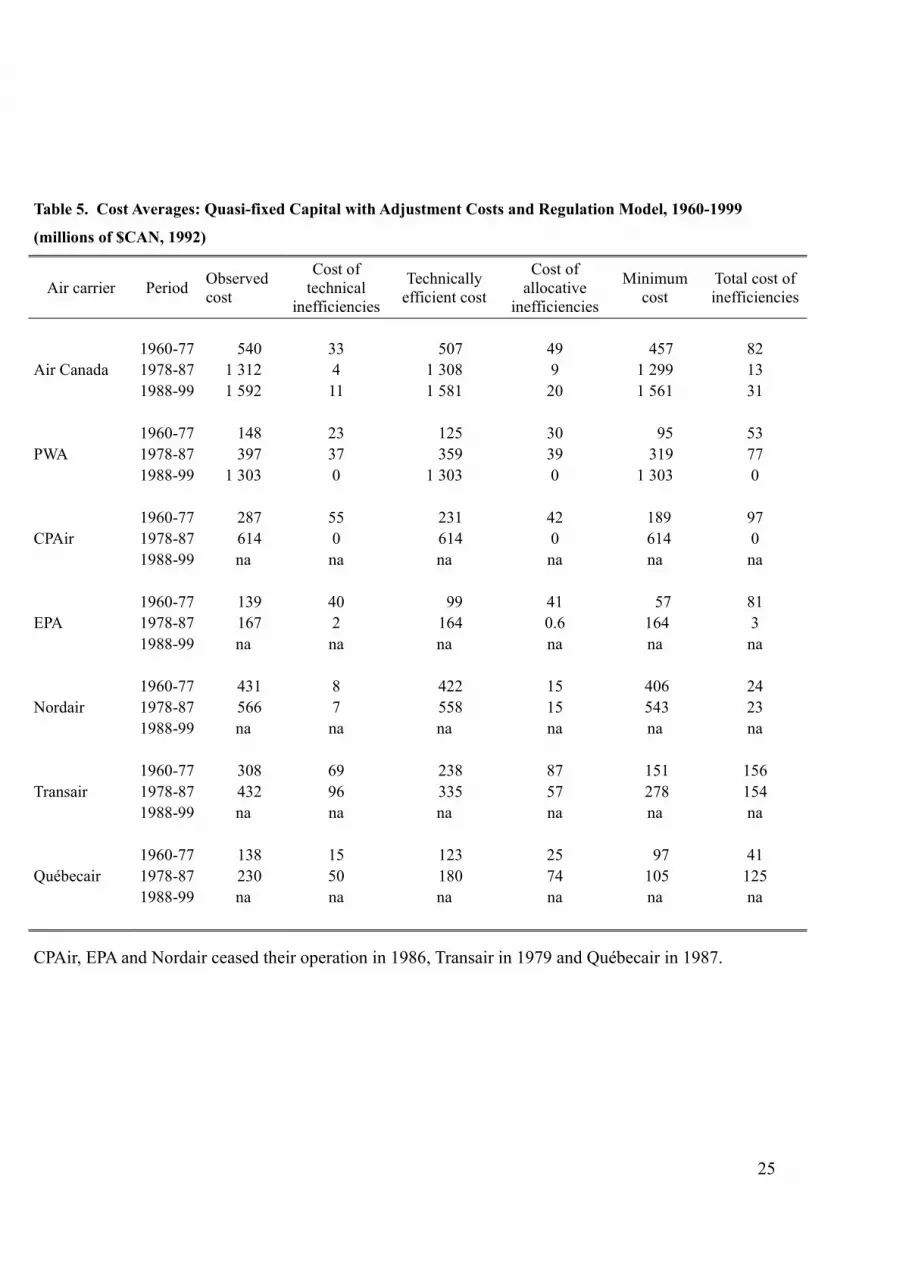
efficiency indicator during the transition period (1978-1987). These results are summarized in
Table 5 where we present dollar estimates of the inefficiency costs in 1992 Canadian dollars. As
expected, between the first and last sub-period, we observe that the total cost associated to
inefficiency decreases for all carriers but Québecair.8 In general, the costs associated to the
allocative inefficiency are larger than the costs associated to the technical inefficiency.
[Insert Table 5 here]
The relationship between regulation and returns to scale is extensively discussed in Ouellette et
al. (2005). The results we obtain here are very close to those in that article. (Those results were
obtained from a fully parametric econometric model.) The reader is referred there for a complete
discussion. Efficiency considerations bring something not taken into account in this article that
complements the parametric analysis, however. To conclude this section, we briefly discuss the
relationship between regulation, returns to scale, and efficiency.
Firms exhibiting increasing returns to scale try to exploit them by expanding the size of their
operations. Doing so, the resources will be used by the firm at their optimal level. However, a
firm may have difficulties to adjust adequately the technology to the size of the market. In our
case, the Canadian regulation is doing this. As explained above, the regulation has created
regional monopolies, artificially isolating them from direct competition, and often imposing the
technology to be used. It made it difficult for the firms to exploit those returns to scale by
expanding operations. The regulation was devised to limit the competition on a given territory
8 This observation is certainly compatible with the fact that Québecair went bankrupt. All the
other carriers, but Air Canada, were absorbed by PWA.
17
and restrict the access to other routes. Consequently, it was virtually impossible for the existing
carriers to exploit their increasing returns to scale. A limited freedom to adjust the technology
and to exploit returns to scale provides intuitive conditions for some persistent levels of
inefficiency. Relaxing the regulatory constraint would likely lead to inefficiency reduction and
lower returns to scale. What does our model tell us about this?
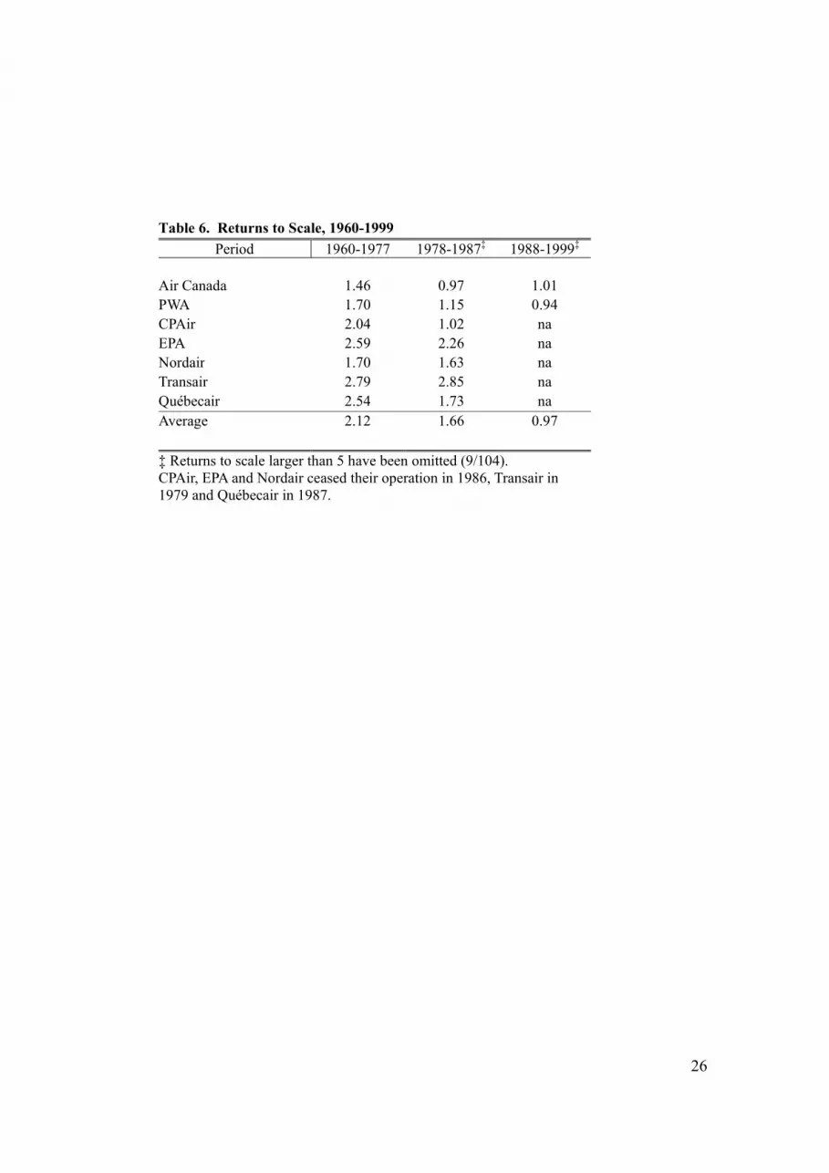
[Insert Table 6 here]
The picture of the returns to scale is as follows. First, during the period of strong regulation, all
firms evolved in a situation of important increasing returns to scale. On average they were of the
order of 2.38, with some important peaks for Québecair. During the deregulation phase, 1978-
1988, the returns to scale tended to decrease, even though they remained significantly above one
in the majority of the cases. There are two exceptions, however. Air Canada had decreasing
returns to scale during the period, while Transair saw its returns to scales increase. Finally, when
the deregulation was finalized, the returns to scale were very close to one, 0.97 on average for the
period, with Air Canada’s RTS close to one and PWA’s slightly below one. The returns to scale
of the large carriers are significantly different from those of the small ones.
Our results show clearly that returns to scale decreased for all firms following deregulation. So,
returns to scale and regulation are positively correlated: The size of the returns to scale has
increased with the strength of the regulation.
It is also the case that as deregulation took place and returns to scale decreased toward one, the
efficiency scores increased. Since the design of the regulation was such that it prevented the
exploitation of returns to scale, it also created inefficiencies directly associated to those increasing
returns to scale. Increasing returns to scale in the industry were probably just another
manifestation of the inefficiencies created by the regulation. Inefficiencies and returns to scale are
both symptoms of the same disease. Relaxing the regulatory constraint led to the already
observed increase of the efficiency and also to a significant reduction of the returns to scale.
18
Conclusion
In this paper we have developed a DEA model with adjustment costs and regulatory constraints.
We show that an incomplete specification of a DEA model can lead to the wrong conclusion that
firms are inefficient and to serious misinterpretations of firms’ behavior. The inclusion of the
regulatory constraints allowed us to show that the performance of the firms can be understated
when the model is incompletely formulated. Firms have the ability to adapt to circumstances and
use it even when the environment is regulated. Our results show higher technical efficiency when
the environment of the firm included adjustment costs and regulatory constraints. This means
that firms internalize the environmental constraints and those are important to correctly assess the
performance of the firm. This model allows us to raise the veil of our ignorance to capture the
real operating conditions of firms.
One could probably call for other factors that might have contributed to this efficiency
improvement. In the case of the airline industry, an increase in the population density can
substantially help firms to reduce costs. This is not a factor in Canada, however. Another factor
is the improvement of the technology. According to other studies of the industry, the economic
deregulation did not trigger the expected movement to renew fundamentally the technology used
(Ouellette et al., 2005). In fact, most of the technological improvements, especially those
concerning the planes, were already assimilated in the capital measure. It is then possible that the
liberalization of the skies explains almost all the performance improvement of the air carriers.
The challenge of regulators is to design rules that set the right incentives and allow firms to
develop and perform adequately. The results in this paper show that the federal transport
regulation failed to reach these objectives. Despite the fact that firms faired well considering the
regulatory constraints they faced during the sixties and seventies, it is also clear that their
performance improved with deregulation of the economic practices. However, the design of the
regulation led to unnecessary (allocation) inefficiencies and long lasting increasing returns to
19
scale. Following the phase of deregulation and the creation of a liberalized market in the
industry, the concentration increased in order to exploit the existing returns to scale and firms
were able to exploit relative price incentives in the choice of the input mix. This led to an
improvement of the allocative efficiency. Before the merger between Air Canada and PWA
(renamed later Canadian Airlines) the firms were virtually efficient and returns to scale were very
close to one. The deregulation process then led to millions of dollars in saved inefficiencies.
20
References
Averch, H., and L.R. Johnson, (1962), "Behavior of the Firm under Regulatory Constraint",
American Economic Review, 52, pp. 1053-1069
Banker, R.D., and R.C. Morey (1986), “The Use of Categorical Variables in Data Envelopment
Analysis”, Management Science, 32 (12), pp. 1613-1627.
Bilodeau, D., P.-Y. Crémieux, B. Jaumard, P. Ouellette, T. Vovor (2004), “Measuring Hospital
Performance in the Presence of Quasi-Fixed Inputs: An Analysis of Québec Hospitals”,
Journal of Productivity Analysis, 21, pp. 183-199.
Førsund, F.R. (1996), “On the Calculation of the Scale Elasticity in DEA Models”, Journal of
Productivity Analysis, 7, pp. 283-302.
Lasserre, P., and P. Ouellette, (1994), "Factor Demands, Cost Functions, and Technology
Measurements for Regulated Firms", Canadian Journal of Economics, 27 (1), pp. 218-
242.
Ouellette, P., and V. Vierstraete (2004), “Measuring Technological Change and Efficiency in the
Hospital Sector in the Presence of Quasi-Fixed Inputs”, European Journal of Operation
Research 154 (3), pp. 755-763.
Ouellette, P., and S. Vigeant (2001), “On the Existence of a Regulated Production Function”,
Journal of Economics, 73(2), pp. 193-200.
Ouellette, P., P. Petit, and S. Vigeant (2005), “Investment and Regulation: The Case of Canadian
Air Carriers”, Transportation Research Part E, 41, pp. 93-113.
Oum, T.H., W. Stanbury and M.W. Tretheway (1991), “Airline Deregulation In Canada”, in
Airline Deregulation: International Experiences, Kenneth Button (Ed.), New York,
University Press.
Shephard, R.W., (1953), Cost and Production Functions, Princeton University Press, Princeton,
N.J.
Treadway, A. B. (1969), "On Rational Entrepreneurial Behaviour and the Demand for
Investment." Review of Economic Studies, 36, pp. 227-39.
Viscusi, W.K., J,M, Vernon and J.E. Harrington, Jr., (2000), Economics of Regulation and
Antitrust, The MIT Press, Cambridge, Massachusetts, 864 pages.
21
Table 1. Descriptive Statistics: All carriers. (N=187) Mean Standard error Minimum Maximum
Observed Cost 515 308 131 506 610 842 16 891 824 2 249 305 081 Charter Output (YN) 60 407 643 61 280 304 20 408 241 820 000 Unit Toll Output (YR) 822 489 742 1 091 578 852 3 944 408 5 156 346 880 Labor (L) 30 797 415 37 180 058 1 245 530 114 827 000 Energy (E) 18 982 677 23 552 279 277 620 77 492 016 Materials (M) 54 988 904 86 640 938 112 270 465 645 632 Capital (K) 62 313 279 114 101 504 486 755 672 640 640 Investment (I) 43 780 007 59 029 299 -13 827 147 332 809 216 Labor Price (PL) 5.38 1.13 2.91 9.93 Energy Price (PE) 6.97 2.45 3.03 14.38 Material Price (PM) 4.36 0.18 3.89 4.68 Investment Price (PI) 4.17 1.41 1.51 8.84 Economic Regulation Index, Φ1 0.14 0.07 0.08 0.33 Safety Regulation Index, Φ2 0.66 0.64 0.10 4.00
22
Table 2. Technical Efficiency, 1960-1999 by Sub-period
Air Carrier Period Capital variable Capital quasi-fixed Investment and regulation, with adjustment cost
1960-1977 0.94 0.93 0.94
Air Canada 1978-1987 0.99 0.99 1.00 1988-1999 0.99 0.99 0.99 1960-1977 0.82 0.81 0.84
PWA 1978-1987 0.90 0.90 0.90 1988-1999 1.00 1.00 1.00 1960-1977 0.84 0.76 0.81
CPAir 1978-1987 0.99 0.99 1.00 1988-1999 na na na 1960-1977 0.70 0.59 0.71
EPA 1978-1987 0.82 0.65 0.98 1988-1999 na na na 1960-1977 0.96 0.95 0.98
Nordair 1978-1987 0.97 0.96 0.99 1988-1999 na na na 1960-1977 0.69 0.66 0.77
Transair 1978-1987 0.79 0.69 0.78 1988-1999 na na na 1960-1977 0.84 0.82 0.89
Québecair 1978-1987 0.76 0.74 0.78 1988-1999 na na na
CPAir, EPA and Nordair ceased their operation in 1986, Transair in 1979 and Québecair in 1987.
23
Table 3. Allocative Efficiency, 1960-1999 by Sub-period
Air Carrier Period Capital variable Capital quasi-fixed Investment and regulation, with adjustment cost
1960-1977 0.90 0.86 0.90
Air Canada 1978-1987 0.96 0.97 0.99 1988-1999 0.96 0.98 0.99 1960-1977 0.54 0.46 0.76
PWA 1978-1987 0.82 0.84 0.89 1988-1999 0.99 0.99 1.00 1960-1977 0.77 0.74 0.82
CPAir 1978-1987 0.99 1.00 1.00 1988-1999 na na na 1960-1977 0.35 0.32 0.58
EPA 1978-1987 0.53 0.50 1.00 1988-1999 na na na 1960-1977 0.91 0.91 0.96
Nordair 1978-1987 0.85 0.85 0.97 1988-1999 na na na 1960-1977 0.35 0.32 0.64
Transair 1978-1987 0.43 0.46 0.83 1988-1999 na na na 1960-1977 0.51 0.48 0.79
Québecair 1978-1987 0.41 0.32 0.59 1988-1999 na na na
CPAir, EPA and Nordair ceased their operation in 1986, Transair in 1979 and Québecair in 1987.
24
Table 4. Total, 1960-1999 by Sub-period
Air Carrier Period Capital variable Capital quasi-fixed Investment and regulation, with adjustment cost
1960-1977 0.84 0.81 0.85
Air Canada 1978-1987 0.96 0.96 0.99 1988-1999 0.95 0.97 0.98 1960-1977 0.44 0.38 0.64
PWA 1978-1987 0.74 0.76 0.80 1988-1999 0.99 0.99 1.00 1960-1977 0.65 0.57 0.66
CPAir 1978-1987 0.97 0.99 1.00 1988-1999 na na na 1960-1977 0.24 0.19 0.42
EPA 1978-1987 0.43 0.32 0.98 1988-1999 na na na 1960-1977 0.87 0.86 0.94
Nordair 1978-1987 0.82 0.81 0.96 1988-1999 na na na 1960-1977 0.24 0.21 0.49
Transair 1978-1987 0.34 0.32 0.64 1988-1999 na na na 1960-1977 0.43 0.40 0.70
Québecair 1978-1987 0.32 0.24 0.46 1988-1999 na na na
CPAir, EPA and Nordair ceased their operation in 1986, Transair in 1979 and Québecair in 1987.
25
Table 5. Cost Averages: Quasi-fixed Capital with Adjustment Costs and Regulation Model, 1960-1999
(millions of $CAN, 1992)
Air carrier Period Observed cost
Cost of technical
inefficiencies
Technically efficient cost
Cost of allocative
inefficiencies
Minimum cost
Total cost of inefficiencies
1960-77 540 33 507 49 457 82 Air Canada 1978-87 1 312 4 1 308 9 1 299 13 1988-99 1 592 11 1 581 20 1 561 31 1960-77 148 23 125 30 95 53 PWA 1978-87 397 37 359 39 319 77 1988-99 1 303 0 1 303 0 1 303 0 1960-77 287 55 231 42 189 97 CPAir 1978-87 614 0 614 0 614 0 1988-99 na na na na na na 1960-77 139 40 99 41 57 81 EPA 1978-87 167 2 164 0.6 164 3 1988-99 na na na na na na 1960-77 431 8 422 15 406 24 Nordair 1978-87 566 7 558 15 543 23 1988-99 na na na na na na 1960-77 308 69 238 87 151 156 Transair 1978-87 432 96 335 57 278 154 1988-99 na na na na na na 1960-77 138 15 123 25 97 41 Québecair 1978-87 230 50 180 74 105 125 1988-99 na na na na na na
CPAir, EPA and Nordair ceased their operation in 1986, Transair in 1979 and Québecair in 1987.
26
Table 6. Returns to Scale, 1960-1999 Period 1960-1977 1978-1987‡ 1988-1999‡
Air Canada 1.46 0.97 1.01 PWA 1.70 1.15 0.94 CPAir 2.04 1.02 na EPA 2.59 2.26 na Nordair 1.70 1.63 na Transair 2.79 2.85 na Québecair 2.54 1.73 na Average 2.12 1.66 0.97 ‡ Returns to scale larger than 5 have been omitted (9/104). CPAir, EPA and Nordair ceased their operation in 1986, Transair in 1979 and Québecair in 1987.