Intervention in Power Control Games With Selfish Users

arX

iv:1

104.

1227

v2 [

cs.IT

] 25

Nov

201

11

Intervention in Power Control Games

With Selfish UsersYuanzhang Xiao, Jaeok Park, and Mihaela van der Schaar,Fellow, IEEE

Abstract

We study the power control problem in single-hop wireless adhoc networks with selfish users.

Without incentive schemes, selfish users tend to transmit attheir maximum power levels, causing excessive

interference to each other. In this paper, we study a class ofincentive schemes based on intervention

to induce selfish users to transmit at desired power levels. In a power control scenario, an intervention

scheme can be implemented by introducing an intervention device that can monitor the power levels

of users and then transmit power to cause interference to users if necessary. Focusing on first-order

intervention rules based on individual transmit powers, wederive conditions on the intervention rates

and the power budget to achieve a desired outcome as a (unique) Nash equilibrium with intervention and

propose a dynamic adjustment process to guide users and the intervention device to the desired outcome.

We also analyze the effect of using aggregate receive power instead of individual transmit powers. Our

results show that intervention schemes can be designed to achieve any positive power profile while using

interference from the intervention device only as a threat.Lastly, simulation results are presented to

illustrate the performance improvement from using intervention schemes and the theoretical results.

Index Terms

Game theory, incentives, intervention, power control, wireless networks

I. INTRODUCTION

Power control is an essential resource allocation scheme tocontrol signal-to-interference-and-noise

ratios (SINRs) for efficient transmission in wireless networks. Extensive studies have been done on

Manuscript received March 31, 2011; revised August 15, 2011; accepted November 08, 2011.

Y. Xiao and M. van der Schaar are with the Electrical Engineering Department, University of California, Los Angeles, CA

90095 USA (e-mail: [email protected]; [email protected]).

J. Park is with the School of Economics, Yonsei University, Seoul 120-749, Korea (e-mail: [email protected]). He was

previously with the Electrical Engineering Department, University of California, Los Angeles, CA 90095 USA.

November 28, 2011 DRAFT

http://arxiv.org/abs/1104.1227v2

2

power control (see [1] and references therein for an overview of the literature in this topic). In many

earlier works on power control, each user has a fixed minimum SINR requirement and then minimizes its

transmit power subject to the SINR requirement [1, Ch. 2][2][3]. This approach is suitable for fixed-rate

communications with voice applications. However, with thegrowing importance of data and multimedia

applications, users are no longer satisfied with a fixed SINR requirement, but they seek to maximize their

utility reflecting the quality of service (QoS). To this end,most recent works formulate the problem in

the network utility maximization framework. In this framework, a central controller can compute optimal

transmit power levels when the utility functions are such that the network utility maximization problem

is convex, and then assigns the optimal power levels to users. Assuming that users areobedientto the

central controller, the problem can also be solved in a distributed manner [1, Ch. 4][4][5].

Besides the network utility maximization framework, many works use noncooperative games to model

the distributed power control problem, in which each user maximizes its own utility, instead of maximizing

the network utility. In a noncooperative game model with a single frequency channel, each user tends to

transmit at its maximum power level to obtain high throughput, causing excessive interference to other

users. This outcome may be far from the global optimality of social welfare [1][4][6], especially when

interference among users is strong [7]. To improve the noncooperative outcome, various power control

schemes have been proposed based on pricing [8]–[12], auctions [13], and mechanism design [14][15].

These works aim to achieve a better outcome by modifying the objective functions of users using taxation

and developing a distributed method based on the optimization of the modified objective functions. Users

are assumed to be obedient in that they accept the objective functions and follow the rule prescribed by

the designer, and prices are used as control signals to guideusers to a desired outcome. However,selfish

users may have their own innate objectives which are different from the assigned objectives and may

ignore control signals and deviate from the prescribed ruleif they are better off by doing so.

In summary, the methods in most existing works are not suitable for power control with selfish users.

Selfish behavior of users can arise in many practical scenarios without central controllers, such as wireless

ad hoc networks, where each user transmits information fromits own transmitter to its own receiver,

and multi-cell cellular networks, where the base station cannot control the interfering mobile stations

in other cells. Hence, it is important to design an incentivescheme to induce selfish users to achieve

a desirable outcome in power control scenarios. One method to provide incentives for selfish users is

to impose taxation as real money payment. However, in order to achieve a desired outcome with a

pricing scheme, the designer needs to know how payment affects the payoffs of users, which is often

the private information of users. The designer may use a mechanism design approach as in [14][15] to


3

elicit private information, but it generally requires heavy communication overheads.1 Another method

to provide incentives is to use repeated games [16][17]. However, effective incentive schemes based on

repeated games require users to have long-run frequent interactions and to be sufficiently patient [18].

Recently, a new class of incentive schemes has been proposedbased on the idea of intervention [19]–

[21]. To implement an intervention scheme, we need anintervention devicethat can monitor the actions of

users and intervene in their interaction if necessary. Themonitoring technologyof the intervention device

determines what it can observe about the actions of users, while its intervention capabilitydetermines

the extent to which it can intervene in their interaction. Anintervention ruleprescribes the action that the

intervention device should take as a function of its observation. Among existing works on intervention

schemes, [19] and [20] applied intervention schemes to contention games in the medium access control

(MAC) layer, while [21] studied the impact of the monitoringtechnology and the intervention capability

on the system performance in an abstract model. We also note that [22] proposed a packet-dropping

mechanism for queueing games using an idea similar to intervention. In this paper, we focus on a power

control scenario and study intervention schemes in this particular scenario.

In the power control scenario considered in this paper, the intervention device estimates the individual

transmit power of each user or the aggregate receive power atits receiver and then transmits at a certain

power level following the intervention rule prescribed by the designer. In order to achieve a target

operating point, the designer can use an intervention rule such that the intervention device transmits

minimum, possibly zero, power if users are transmitting at the desired power levels, while transmitting

at a high power level to reduce the SINRs of users if a deviation is detected. In this way, an intervention

scheme can punish the misbehavior of users and regulate the power transmission of selfish users. We

first consider a monitoring technology with which the intervention device can estimate the individual

transmit power of each user without errors. While focusing on a simple class of intervention rules called

first-order intervention rules, we study the requirements for the parameters of first-order intervention

rules to achieve a given target power profile as a (unique) Nash equilibrium (NE). We propose a

dynamic adjustment process that the designer can use to guide users to the target power profile through

intermediate targets. We then relax the monitoring requirement and consider a monitoring technology

with which the intervention device can estimate only the aggregate receive power. We show that with

aggregate observation, intervention rules can be designedto achieve a given target as a NE but rarely as

1Another drawback of [14] and [15] is the assumption that eachuser’s utility function is jointly concave in all the users’

power levels, which seems to be unrealistic in power controlscenarios.


4

a unique NE. Our results provide a systematic design principle based on which a designer can choose

an intervention scheme (an intervention device and an intervention rule) to achieve a desired outcome.

Our analysis suggests that, unlike pricing schemes, it is possible for the designer to design effective

intervention schemes without having knowledge about how users value their SINRs, as long as their utility

is monotonically increasing with their own SINRs. We also propose a method based on intervention for

the designer to estimate the cross channel gains, the noise powers, and maximum transmit power levels of

users without any cooperative behavior of users such as sending pilot signals for channel estimation and

reporting the estimates to the designer. After obtaining relevant information, the designer can configure

an intervention rule to achieve a target operating point as NE.

The rest of the paper is organized as follows. In Section II, we describe the system model of power

control with intervention. In Section III, we propose design criteria for intervention rules, performance

characteristics to evaluate intervention rules, and classes of intervention rules. In Section IV, we study

the design of first-order intervention rules to achieve a target power profile. In Section V, we discuss

implementation issues related to intervention. Simulation results are presented in Section VI. Finally,

Section VII concludes the paper. For the ease of reference, we summarize major notation used in this

paper in Table I.

II. M ODEL OF POWER CONTROL WITH INTERVENTION

We consider a single-hop wireless ad hoc network, where a fixed set ofN users and an intervention

device transmit in a single frequency channel. The set of theusers is denoted byN , {1, 2, . . . , N}. Each

user has a transmitter and a receiver. Each useri chooses its transmit powerpi in the setPi , [0, Pi], where

Pi > 0 for all i ∈ N . The power profile of all the users is denoted byp = (p1, . . . , pN ) ∈ P ,∏N

i=1 Pi,

and the power profile of all the users other than useri is denoted byp−i.

In the network, there is an intervention device, sometimes referred to as user0, that consists of a

transmitter and a receiver. The receiver of the intervention device can monitor the power profile of the

users, while the transmitter can create interference to theusers by transmitting power. Once the users

choose their power profile, the intervention device obtainsa signaly ∈ Y, whereY is the set of all

possible signals. We assume that the signal is realized deterministically given a power profile and use the

signal determination functionρ : P → Y to denote the signal given the power profilep.2 After observing

2More generally, we can assume that the signal is realized randomly given a power profile and useρ(p) to represent the

probability distribution of signals givenp. We leave the analysis of this general case for future research.


5

TABLE I

SUMMARY OF MAJOR NOTATION.

Symbol Description

N Number of (regular) users in the network

N Set of users,N , {1, . . . , N}

Pi Maximum transmit power level of useri; i ∈ N

P0 Power budget of the intervention device, or the intervention capability

Pi User i’s action spacePi , [0, Pi]; i ∈ N ∪ {0}

pi Transmit power level of useri, pi ∈ Pi; i ∈ N ∪ {0}

p Power profile of the users,p = (p1, . . . , pN) ∈ P ,∏N

i=1Pi

p⋆ Target power profile,p⋆ = (p⋆1, . . . , p⋆N )

P Profile of the maximum power levels,P = (P1, . . . , PN)

hij Channel gain from userj’s transmitter to useri’s receiver;i, j ∈ N ∪ {0}

ni Noise power at useri’s receiver

γi SINR at useri’s receiver

Y Set of all possible signals obtained by the intervention device

ρ Signal determination function,ρ : P → Y

f Intervention rule,f : Y → P0

E(f) Set of power profiles sustained byf

FK(p⋆) Set ofKth-order intervention rules with target power profilep⋆

PBK(p⋆) Minimum power budget to sustainp⋆ usingKth-order intervention rules

PBsK(p⋆) Minimum power budget to strongly sustainp⋆ usingKth-order intervention rules

fI1 First-order intervention rule based on individual transmit powers

αi Intervention rate for useri in fI1 ; i ∈ N

fA1 First-order intervention rule based on aggregate receive power

α0 Aggregate intervention rate infA1

N (p⋆) Set of users whose target powers are less than the maximum power levels,N (p⋆) = {i ∈ N : p⋆i < Pi}

N ′ Number of users whose target powers are less than the maximumpower levels,N ′ = |N (p⋆)|

{(f t,pt)}Tt=1 Sequence of intervention rules and power profiles in the dynamic adjustment process

{pt}Tt=1 Sequence of intermediate target power profiles in the dynamic adjustment process

d(p,p′) Relative distance between two power profilesp andp′, d(p,p′) =∑N

i=1(pi − p′i)/pi

T ⋆(p⋆) Minimum convergence time (in steps) for the dynamic adjustment process to reachp⋆


6

a signal, the intervention device chooses its own transmit powerp0 in the setP0 , [0, P0], whereP0 > 0.

We call(Y, ρ) the monitoring technology of the intervention device, and call P0 its intervention capability.

The ability of an intervention device is characterized by its monitoring technology and intervention

capability. We call the transmit powers of the interventiondevice and the users(p0,p) ∈ P0 × P an

outcome.

The QoS obtained by useri is determined by its SINR, denoted byγi. We use a block-fading channel

model with sufficiently long fading blocks, as in [2]–[5],[7]–[17]. In one block, fori, j ∈ N ∪{0}, let hij

be the channel gain from userj’s transmitter to useri’s receiver, and letni be the noise power at useri’s

receiver. If code-division multiple accessing (CDMA) is used, the channel gain is defined as the effective

channel gain taking into account the spreading factor. In one block, the users and the intervention device

transmit at constant power levelsp andp0, respectively.3 Then the SINR of useri ∈ N is given by

γi(p0,p) =hiipi

hi0p0 +∑

j 6=i hijpj + ni.4 (1)

We assume that each useri ∈ N has monotonic preferences on its own SINR in the sense that itweakly

prefersγi to γ′i if and only if γi ≥ γ′i. Our analysis does not require any other properties of preferences

(for example, preferences do not need to be represented by a concave utility function).5

In our setting, the intervention device has a receiver to measure the aggregate receive power from all

the users. Furthermore, if the receiver moves and takes measurement at different locations, it can estimate

the individual transmit power of each user as well. Thus, in this paper we will focus on two types of

monitoring technology with which the intervention device can estimate individual transmit powersp or

an aggregate receive power∑N

i=1 h0ipi. In other words, we consider two signal determination functions,

ρ(p) = p andρ(p) =∑N

i=1 h0ipi.

3In practice, there is a time lag between when the users transmit and when the intervention device transmits because the

intervention has to monitor the users’ power profile in orderto decide its transmit power level. In this paper, we assume that

this time lag is short and negligible compared to the length of fading blocks, although in principle we can take into account the

time lag in the users’ utility functions. See, for example, [20] for a model that takes into account the time lag explicitly.

4Throughout the paper, we usej 6= i with the summation operator to meanj ∈ N \ {i}, not j ∈ N ∪ {0} \ {i}.

5The preferences of a user may be defined on dimensions other than its SINR. For example, a user may use the ratio of SINR

to transmit power as the utility function, as in [9], becauseit may care about its energy consumption as well. Our approach can

be applied to such a scenario if utility functions representing the users’ preferences are known to the designer.


7

III. D ESIGN OFINTERVENTION RULES

A. Design Criteria

Since the intervention device transmits its power after it obtains a signal, its strategy can be represented

by a mappingf : Y → P0, which is called an intervention rule. The SINR of useri when the intervention

device uses an intervention rulef and the users choose a power profilep is given byγi(f(ρ(p)),p). With

an abuse of notation, we will usef(p) to meanf(ρ(p)). Given an intervention rulef , the interaction

among the users that choose their own power levels selfishly can be modeled as a non-cooperative game,

whose strategic form is given by

Γf = 〈N , (Pi)i∈N , (γi(f(·), ·))i∈N 〉. (2)

We can predict the power profile chosen by the users given an intervention rule using the concept of

Nash equilibrium.

Definition 1: A power profilep∗ ∈ P is a Nash equilibrium of the gameΓf if

γi(f(p∗),p∗) ≥ γi(f(pi,p

∗−i), pi,p

∗−i) (3)

for all pi ∈ Pi and all i ∈ N .

When a power profilep∗ is a NE of Γf , no user has the incentive to deviate fromp∗ unilaterally

provided that the intervention device uses intervention rule f . Moreover, ifp∗ is a unique NE ofΓf ,

intervention has robustness in that the designer does not need to worry about coordination failure (i.e.,

the possibility that the users get stuck in a “wrong” equilibrium).

Definition 2: An intervention rulef (strongly) sustainsa power profilep∗ if p∗ is a (unique) NE of

the gameΓf .

We useE(f) to denote the set of all power profiles sustained byf . Suppose that the designer has a

welfare functionU0(γ1, . . . , γN ), defined on the users’ SINRs. Then the objective of the designer is to

find a target power profile that maximizes the welfare function and an intervention rule that (strongly)

sustains the target power profile. Formally, the design problem solved by the designer can be written as

maxp

maxf{U0(γ1(f(p),p), . . . , γN (f(p),p)) : p ∈ E(f)}. (4)

If uniqueness is desired, we can replacep ∈ E(f) in (4) with {p} = E(f). Note that a solution to the

design problem (4),p⋆ andf∗, must satisfyf∗(p⋆) = 0, namely no intervention if the users choose the

target power profile. Based on this observation, the design problem (4) can be solved in two steps. In


8

the first step, we obtain a target power profilep⋆ by solving

maxp{U0(γ1(0,p), . . . , γN (0,p)) : p ∈ P}. (5)

There always exists a solution to the optimization problem (5) as long as the welfare functionU0 is

continuous inγ1, . . . , γN . Under some welfare functions, e.g.U0(γ1, . . . , γN )∑N

i=1 log(γi) as in [4][5],

the optimization problem (5) is convex, and thus easy to solve. If (5) is solved off-line, the designer

can choose other welfare functions even though the resulting optimization problem is nonconvex. In the

second step, we look for an intervention rulef such thatf(p⋆) = 0 andp⋆ ∈ E(f) (or {p⋆} = E(f)),

given the target power profilep⋆ obtained in the first step.

The first step of solving the design problem (4), namely finding the target power profilep⋆, requires

knowledge about the parameters in the model,hij , ni, andPi for all i, j ∈ N ∪ {0}. In Section V-A,

we propose a method for the designer to estimate the relevantsystem parameters needed to solve (5)

based on intervention. Note, however, that solving the problem (5) does not require the designer to know

the details of the users’ preferences on their SINRs since knowing the expressions for SINRs suffices

to evaluate the welfare function and to check the incentive constraints. To highlight the informational

advantage of our approach, let us consider a pricing scheme,in which each useri is chargedπi(p) when

the users choose a power profilep. Suppose that each useri has quasilinear preferences on its own SINR

and payment which are represented by a utility function of the form ui(γi)− πi. Then in order to find

a pricing scheme that sustains a target profilep⋆, the designer needs to knowui for all i ∈ N . Since a

pricing scheme uses an outside instrument to influence the decisions of the users, the designer needs to

know how the users value SINRs relative to payments, which issubjective and thus hard to measure. On

the contrary, an intervention scheme affects the users through their SINRs, and thus the designer does

not need to know how the users value their SINRs.

In the subsequent discussion of this paper, we focus on the second step of solving the design problem

(4), assuming that a target power profilep⋆ has been found. That is, we aim to find an intervention rulef

that (strongly) sustainsp⋆, namelyp⋆ ∈ E(f) (or {p⋆} = E(f)), and that satisfiesf(p⋆) = 0. Since user

i can guarantee a positive SINR by choosing a positive power, it is impossible to provide an incentive

for useri to choosepi = 0 using any intervention rule. Thus, we assume thatp⋆ ∈∏

i(0, Pi]. We say

that (f,p⋆) is an (intervention) equilibriumif p⋆ ∈ E(f) andf(p⋆) = 0. At an equilibrium, no user has

an incentive to deviate unilaterally while the designer fulfills his design criteria. Thus, an equilibrium

can be considered as a stable configuration of an intervention rule and a power profile. An equilibrium

can be achieved following the procedure described below.


9

1) The designer chooses a target power profilep⋆ and an intervention rulef .

2) The users choose their power profilep, knowing the intervention rule chosen by the designer.6

3) The intervention device obtains a signalρ(p) and chooses its powerp0 = f(p).

To execute the above procedure, we may consider an adjustment process (e.g., one based on best-response

updates) for the users and the intervention device to reach an equilibrium (see Section IV-B), as well as

an estimation process for the intervention device to obtaina signal (see Section V-A). It is an implicit

underlying assumption of our analysis that the time it takesto reach a final outcome (i.e., the duration

of the procedure) is short relative to the time for which the final outcome lasts. This justifies that in

our model, the users fully take into account interference from the intervention device that is realized

at the final outcome when they make decisions about their powers. When a network parameter changes

(e.g., some users leave or join the network, or move to different locations), a new target is chosen

and the procedure is repeated to achieve a new equilibrium. Thus, our analysis holds as long as network

parameters do not change frequently, whereas providing incentives using a repeated game strategy usually

requires an infinite horizon and sufficiently patient players.

Another important underlying assumption in our analysis isthat the designer can commit to the

intervention rule it chooses. SinceU0 is increasing in eachγi and eachγi is decreasing inp0, the

designer prefers not to intervene at all, i.e., it prefers tochoosep0 = 0. However, ifp0 is held fixed at0,

the users will chooseP. The role of the intervention device is to provide a punishment mechanism for

the users to choose a desired power profile other thanP; the device should choose a high power level if

a deviation is detected. Without the designer’s commitmentto the intervention rule, the designer would

choosep0 = 0 (e.g., by disabling the intervention device) regardless ofthe power profile chosen by the

users. Predicting this behavior of the designer, the users would chooseP, resulting in the same outcome

as with no intervention. Therefore, in order for the proposed intervention schemes to provide incentives

successfully, it is critical that the designer executes punishment as promised to make punishment credible.

In practice, credibility can be achieved by programming theintervention rule in the intervention device

and making the program difficult to manipulate.

Finally, the benchmark is the welfare when there is no intervention device in the network, i.e.,p0 is

held fixed at0. In this case,γi is always strictly increasing inpi, and thusP , (P1, . . . , PN ) is the

6The intervention rule can be broadcast to the users, or learned by the users from experimentation.


10

unique NE of the game〈N , (Pi)i∈N , (γi(0, ·))i∈N 〉.7 Thus, the case ofp⋆ = P is trivial, because there

is no need to use an incentive scheme in order to achieve the power profileP. Hence, our main interest

lies in the case ofp⋆ 6= P, although our analysis does not exclude the case ofp⋆ = P. The case of

p⋆ 6= P arises in many situations, for example, when interference among users is strong and welfare is

measured by the sum of utilities or the minimum of utilities [1][4][6][7].

B. Performance Characteristics

Given a target power profilep⋆, there are potentially many intervention rulesf that satisfy the design

criteria p⋆ ∈ E(f) and f(p⋆) = 0. Thus, below we propose several performance characteristics with

which we can evaluate different intervention rules satisfying the design criteria.

1) Monitoring requirement: The minimum amount of information about the power profile that is

required for the intervention device to execute a given intervention rule (assuming perfect estimation).

2) Intervention capability requirement: The minimum intervention capability needed for the intervention

device to execute a given intervention rule, i.e.,supp∈P f(p). (Even though there is no intervention at an

equilibrium, the intervention device should have an intervention capabilityP0 ≥ supp∈P f(p) in order

to make the intervention rulef credible to the users.)

3) Strong sustainment: Whether a given intervention rule strongly sustains the target power profilep⋆.

4) Complexity: The complexity of a given intervention rule in terms of design, broadcast/learning, and

computation.

C. Classes of Intervention Rules

Without loss of generality, we can express an intervention rule f satisfyingf(p⋆) = 0 as f(p) =

[g(p)]P0

0 , where [x]ba = min{max{x, a}, b}, for some functiong : P → R such thatg(p⋆) = 0. Also,

since the designer desires to achievep⋆, it is natural to consider functionsg that increase as the users

deviate fromp⋆. Hence, we consider the following classes of intervention rules,

FK(p⋆) =

f : f(p) =

[N∑

i=1

K∑

k=1

αi,k|pi − p⋆i |k

]P0

0

for someαi,k ≥ 0 andP0 > 0

, (6)

for K = 1, 2, . . .. We call an intervention rulef ∈ FK(p⋆) a Kth-order intervention rule with target

power profilep⋆. As K becomes larger, the setFK(p⋆) contains more intervention rules, but at the

7This is true for any constant intervention rule, wherep0 is chosen independently of the observation of the intervention device.

This shows the inability of traditional Stackelberg games,where the leader (the intervention device) takes an action before the

followers (the users) do, to provide incentives in our setting.


11

same time complexity increases. Simple intervention rulesare desirable for the designer, the users, and

the intervention device. AsK is smaller, the designer has less design parameters and lessburden of

broadcasting the intervention rule; the users can more easily learn the intervention rule and find their

best responses during an adjustment process; and the intervention device can more quickly compute the

value of the intervention rule at the chosen power profile. Thus, our analysis mainly focuses on first-order

intervention rules, the simplest among the above classes.

Let FK(p⋆) (FsK(p⋆)) be the set of allKth-order intervention rules that (strongly) sustainsp⋆, i.e.,

FK(p⋆) = {f ∈ FK(p⋆) : p⋆ ∈ E(f)} and FsK(p⋆) = {f ∈ FK(p⋆) : {p⋆} = E(f)}. We define the

minimum power budget8 for a Kth-order intervention rule to (strongly) sustainp⋆ by

PBK(p⋆) = inff∈FK(p⋆)

supp∈P

f(p), and PBsK(p⋆) = inf

f∈FsK(p⋆)

supp∈P

f(p). (7)

Thus, with an intervention capabilityP0 > PBK(p⋆) (P0 > PBsK(p⋆)), there exists aKth-order

intervention rule that (strongly) sustainsp⋆. We setPBK(p⋆) = +∞ (PBsK(p⋆) = +∞) if there

is no Kth-order intervention rule that (strongly) sustainsp⋆ (i.e., FK(p⋆) (FsK(p⋆)) is empty). Since

FK(p⋆) ⊂ FK ′(p⋆) for all K,K ′ such thatK ≤ K ′, both PBK(p⋆) and PBsK(p⋆) are weakly

decreasing inK for all p⋆. This suggests a trade-off between complexity and the minimum power

budget. Also, sinceFsK(p⋆) ⊂ FK(p⋆), we havePBK(p⋆) ≤ PBs

K(p⋆) for all K andp⋆. The difference

PBsK(p⋆) − PBK(p⋆) can be interpreted as the price of strong sustainment in terms of the minimum

power budget.

IV. A NALYSIS OF FIRST-ORDER INTERVENTION RULES

A. Design of Intervention Rules

We consider first-order intervention rules of the form

f I1 (p) =

[N∑

i=1

αi|pi − p⋆i |

]P0

0

. (8)

Under a first-order intervention rule, the intervention device increases its transmit power linearly with

the deviation of each user from the target power,|pi− p⋆i |, in the range of its intervention capability. We

call αi the intervention ratefor useri, which measures how sensitive intervention reacts to a deviation

of useri. Let N (p⋆) = {i ∈ N : p⋆i < Pi}. Without loss of generality, we label the users in such a way

8As to be shown later, for strong sustainment, we needP0 to exceed a certain value. Thus, we actually mean “infimum”

power budget by minimum power budget.


12

that i ∈ N (p⋆) if and only if i ≤ N ′, whereN ′ = |N (p⋆)|. Since the users have natural incentives to

choose their maximum powers in the absence of intervention,we need to provide incentives only for the

users inN (p⋆). The following theorem shows that when the intervention capability is sufficiently large,

the designer can always find intervention rates to have a given target power profilep⋆ sustained by a

first-order intervention rule.

Theorem 1:For anyp⋆ ∈∏

i(0, Pi], p⋆ ∈ E(f I1 ) if and only if

αi ≥

∑j 6=i hijp

⋆j + ni

p⋆ihi0(9)

and

P0 ≥(Pi − p

⋆i )(∑

j 6=i hijp⋆j + ni)

p⋆ihi0(10)

for all i ∈ N (p⋆).

Proof: See [23, Appendix B].

We can interpret Theorem 1 as follows. Ashi0 is larger, intervention causes more interference to user

i with the same transmit power, and thus the intervention rateαi can be chosen smaller to yield the

same interference. When∑

j 6=i hijp⋆j + ni is large, interference to useri from other users and its noise

power are already strong, and thus the intervention rateαi should be large in order for intervention to be

effective. Hence,hi0/(∑

j 6=i hijp⋆j + ni) can be interpreted as the effectiveness of intervention to useri.

Without intervention, users have natural incentives to increase their transmit powers. Thus, as the target

power for useri, p⋆i , is smaller, the incentive for useri to deviate is stronger, and thus a larger intervention

rateαi is needed to prevent deviation. Note that(Pi − p⋆i ) is the maximum possible deviation by user

i (in the direction where it has a natural incentive to deviate). The minimum intervention capability in

the right-hand side of (10) is increasing with the maximum possible deviation and the strength of the

incentive to deviate while decreasing with the effectiveness of intervention.

A first-order intervention rulef I1 satisfying the conditions in Theorem 1 may have a NE other than the

target power profilep⋆. For example, ifP0 ≤∑

j 6=i αj(Pj − p⋆j) for all i ∈ N (p⋆), P is also sustained

by f I1 . The presence of this extra NE is undesirable since it bringsa possibility that the users still choose

P while the intervention device causes interference to the users by transmitting its maximum power

P0. Obviously, this outcome(P0,P) is worse for every user than the outcome at the unique NE without

intervention(0,P). In order to eliminate this possibility, the designer may want to choose an intervention

rule that strongly sustains the target power profile. The following theorem provides a sufficient condition

for a first-order intervention rule to strongly sustain a given target power profile.


13


i(0, Pi], {p⋆} = E(f I1 ) if

αi >1

p⋆i

∑

j>i

αj(Pj − p⋆j) +

∑j<i hijp

⋆j +

∑j>i hijPj + ni

p⋆ihi0(11)

and

P0 >Pi

p⋆i

∑

j>i

αj(Pj − p⋆j) +

(Pi − p⋆i )(∑

j<i hijp⋆j +

∑j>i hijPj + ni)

p⋆ihi0(12)

for all i ∈ N (p⋆).9

Proof: See [23, Appendix C].

By comparing Theorems 1 and 2, we can see that the requirements for the intervention rates and the

intervention capability is higher when we impose strong sustainment. For any given power profile, the

intervention rates can be chosen sequentially to satisfy the condition (11) starting from userN ′ down

to user1. We can setαi = 0 for all i /∈ N (p⋆). Unlike Theorem 1, the choice of the intervention rates

affects the minimum required intervention capability. Forstrong sustainment, the intervention capability

is required to be larger as the designer chooses larger intervention rates. A main reason for the existence

of an extra NE is that the region of power profiles on which the maximum intervention power is applied

is so wide that the users cannot escape the region by unilateral deviation. Thus, a larger intervention

capability is needed to reduce the region and guarantee the uniqueness of NE.

From Theorem 1, we obtain

PB1(p⋆) = max

i

(Pi − p⋆i )(∑


p⋆i hi0. (13)

Since Theorem 2 gives a sufficient condition for strong sustainment, we obtain an upper bound on

PBs1(p

⋆),

PBs

1(p⋆) =

N∑

i=1

i−1∏

j=1

Pj

p⋆j

(Pi − p

⋆i )(∑

j<i hijp⋆j +

∑j>i hijPj + ni)

p⋆ihi0

. (14)

Note thatPB1(p⋆) ≤ PB

s

1(p⋆) with equality if and only ifN ′ ≤ 1. Combining these results, we can

boundPBs1(p

⋆) by

PB1(p⋆) ≤ PBs

1(p⋆) ≤ PB

s

1(p⋆). (15)

By Theorems 1 and 2, we know that first-order intervention rules can sustain the set∏

i(0, Pi]. Note

that among all the efficient power profiles, those withpi = 0 for somei have probability measure zero.

9We define∑

j∈Jxj = 0 if J is empty. Similarly, we define

∏j∈J

xj = 1 if J is empty.


14

Hence, we obtain almost the entire set of feasible payoffs byusing first-order intervention rules. As

argued in Section III, it is impossible to provide an incentive for useri to choosepi = 0 by intervention

rules of any orders. Thus, we actually obtain the largest setof sustainable payoffs by using first-order

intervention rules. This discussion suggests that the potential gain from using higher-order intervention

rules is not from what they can sustain but how they sustain a target power profile.

Remark 1:An extreme intervention rulef Ie [21], defined by

f Ie (p) =

0, if p = p⋆,

P0, if p 6= p⋆,

(16)

can be considered as the limiting case of first-order intervention rules as eachαi goes to infinity in that the

area of the region{p : f Ie (p) 6= f I1 (p)} approaches zero in the limit. With this class of intervention rules,

we haveE(f Ie ) = {p⋆,P} if P0 ≥ PB1(p⋆) and E(f Ie ) = {P} otherwise. Therefore, it is impossible

to construct an extreme intervention rule that strongly sustains a target power profile, except in the

uninteresting casep⋆ = P. This motivates us to study intervention rules other than extreme intervention

rules.

B. Dynamic Adjustment Processes

Previously, we have derived the conditions under which a target power profile is (strongly) sustained.

Now we propose a dynamic adjustment process, in order to guide the intervention device and the users to

achieve the target power profile as NE. The adjustment occursat discrete steps, labeled ast = 1, 2, . . ..

We allow the use of different intervention rules in different steps. Thus, the beginning of each step is

triggered by the intervention device’s announcement of theintervention rule to be used in that step. Users

are synchronized by the announcement of the intervention rules. The adjustment process is based on the

myopic best-response updates of the users and is described in Algorithm 1.

During the adjustment process, the designer may use different intervention rules, as well as intermediate

target profiles different from the final targetp⋆. That is, we havef t ∈ F1(pt), wherept is the intermediate

target power profile at stept. In the adjustment process, the designer chooses a sequenceof intervention

rules. Suppose that the designer uses an update ruleψ : P → F1 to determine an intervention rule based

on the power profile in the previous step. Then given an initial power profilep0, an update rule yields

a sequence of intervention rules and power profiles{(f t,pt)}∞t=1.10 We can evaluate an update rule by

10Since the best response correspondence is non-singleton only in knife-edge cases, we focus on update rules that yield a

deterministic sequence.


15

Algorithm 1 A dynamic adjustment process.1: Initialization: t = 0

2: The users choose an initial power profilep0.

3: The designer announces the use of first-order intervention rulesf t ∈ F1 with power budgetP0.

4: while pt 6= p⋆ or f t(pt) 6= 0 do

5: t← t+ 1

6: Given pt−1, the designer chooses and broadcasts the intervention rates αti and the target power

profile pt for the current time slott.

7: Given f t(p) =[∑N

i=1 αti

∣∣pi − pti∣∣]P0

0, each useri chooses a best response topt−1

−i :

8: pti ∈ BRi(ft,pt−1

−i ) , argmaxpi∈Piγi(f

t, pi,pt−1−i ).

9: end while

the following two criteria.

1) Convergence:Does the induced sequence reach an equilibrium(f,p⋆)? If so, how many steps are

needed?

2) Minimum power budget:How much power budget is needed to execute{f t}∞t=1, i.e.,supt supp∈P ft(p)?

The following theorem shows that when the target power profile p⋆ is close to the maximum power

profile P and the intervention capabilityP0 is large, we can obtain fast convergence as well as strong

sustainment.


i(0, Pi] such that∑N

i=1(Pi−p⋆i )/Pi < 1, there exists(α1, . . . , αN ) ∈ R

N+

such that

αi >1

p⋆i

∑

j 6=i

αj(Pj − p⋆j) +

∑j 6=i hijPj + ni

p⋆ihi0(17)

for all i ∈ N (p⋆). Suppose thatf s1 ∈ F1(p⋆) satisfies (17) and

P0 >Pi

p⋆i

∑

j 6=i

αj(Pj − p⋆j) +

(Pi − p⋆i )(∑

j 6=i hijPj + ni)

p⋆ihi0(18)

for all i ∈ N (p⋆). Then{p⋆} = E(f s1 ). Moreover, starting from an arbitrary initial power profilep0 6= p⋆,

the adjustment process withf t = f s1 for all t = 1, 2, . . . reaches(f s1 ,p⋆) in at most two steps (and in

one step ifp0 ∈∏

i[p⋆i , Pi]).

Proof: See [23, Appendix D].


16

The minimum power budget required to execute an intervention rule described in Theorem 3 is given

by

PBs

1(p⋆) =

1

1−∑N

i=1Pi−p⋆

i

Pi

N∑

i=1

(Pi − p⋆i )(∑

j 6=i hijPj + ni)

Pihi0. (19)

Since the requirement forαi in (17) is more stringent than that in (11), we havePBs

1(p⋆) ≥ PB

s1(p

⋆)

with equality if and only ifN ′ ≤ 1. The differencePBs

1(p⋆) − PB

s

1(p⋆) can be considered as the

price of fast convergence top⋆ in terms of the minimum power budget. In addition to requiring a larger

power budget, Theorem 3 imposes a restriction on the range oftarget profiles. That is, the target should

be close enough toP for the result of Theorem 3 to hold. However, the target may not satisfy the

restriction∑N

i=1(Pi − p⋆i )/Pi < 1. In this case, the designer needs to use intermediate targetpower

profiles that are successively close to one another in order to guide the users to the final target. The

use of intermediate target power profiles is also necessary when the intervention device does not have a

large enough power budget to strongly sustain a target powerprofile. In this case, the designer can use

a sequence of intervention functions to drive the users to reach the target power profile as the unique

outcome. This process requires smaller power budget than that required by strong sustainment, but may

take longer time for the system to reach the target power profile.

Define the relative distance fromp to p′ by

d(p,p′) =

N∑

i=1

pi − p′i

pi. (20)

Using the proofs of Theorems 2 and 3, we can show that, givenpt−1, the designer can achieve the

intermediate target at stept, i.e., pt = pt only if pt satisfiesd(pt−1, pt) < 1. This imposes a bound

on the relative distance between two successive intermediate targets. Below we provide two different

methods for the designer to generate intermediate targets.The first method, which is summarized in

Algorithm 2 and analyzed in Theorem 4, produces a sequence ofintermediate targets reaching the final

target whose successive elements have a relative distance of δ ∈ (0, 1) while requiring the minimum

power budget in each step. This method can be used in a scenario where the power constraint of the

intervention device does not bind; the designer can fixδ sufficiently close to 1, and the method will

allow the system to reach the final target in the minimum number of steps. The second method, which is

summarized in Algorithm 3 and analyzed in Theorem 5, yields asequence of intermediate targets with

the largest relative distance in each step while satisfyingthe power constraint. Thus, this method will

allow the manager with a limited power budget to reach the final target as fast as possible.


17

Now suppose that a fixed relative distance between two successive targets is given. Algorithm 2 provides

a method for the designer to generate intermediate targets in the most power-budget efficient way.

Algorithm 2 An algorithm that generates a sequence of intermediate target power profiles with a fixed

relative distance.Require: Fix δ ∈ (0, 1) close to 1

1: Initialization (t = 1): Set p1 = P {This step can be skipped ifp0 = P} andM = N

2: Setµi = p⋆i /p1i for all i ∈ N

3: while∑N

i=1(pti − p

⋆i )/p

ti ≥ 1 do

4: t← t+ 1

5: while∑N

i=1 µi < N − δ do

6: Choosei∗ ∈ argmaxi∈M

∑j 6=i

hij pt−1j +ni

hi0

7: Setµi∗ = min{1, N − δ −∑

j 6=i∗ µj} andM←M\ {i∗}

8: end while

9: Set pti = p⋆i /µi for all i ∈ N

10: end while

11: Set pt = p⋆

The following theorem shows that the designer can lead the users to the final target by using interme-

diate targets generated by Algorithm 2 provided that the intervention capability is sufficiently large.


i(0, Pi], if δ ≥ 1 −mini(p⋆i /Pi), then Algorithm 2 terminates at a finite

stepT with T ≤ N ′ +1. Let (pt)Tt=1 be the sequence of power profiles generated by Algorithm 2. Then

there exists a sequence of intervention rules(f t)Tt=1 with f t ∈ F1(pt) such that the adjustment process

with (f t)Tt=1 yieldspt = pt for all t = 1, . . . , T starting from anyp0 ∈ P.

Proof: See [23, Appendix F].

Now we consider a scenario where the intervention capability P0 should be taken into consideration

while generating intermediate targets11. In this scenario, in order to induce the users to follow intermediate

targets during the adjustment process, the intermediate targets(pt)Tt=2 should satisfy not only

N∑

i=1

pt−1i − ptipt−1i

< 1 (21)

11Note that to sustainp⋆ as the NE, we requireP0 to satisfy the conditions in Theorem 1.


18

but also

P t0 , max

i∈N (pt)

Pi

pt−1i

∑Nj=1

(pt−1j −pt

j)(∑

k 6=jhjk p

t−1k +nj)

pt−1j hj0

1−∑N

j=1pt−1j −pt

j

pt−1j

+(Pi − p

t−1i )(

∑j 6=i hij p

t−1j + ni)

pt−1i hi0

< P0 (22)

for all t = 2, . . . , T . In order to reach the final target in the minimum number of steps, we need to

maximize the relative distance between successive targetswhile satisfying the constraints (21) and (22).

Thus, the problem to obtainpt given pt−1 can be written as

maxpt

N∑

i=1


(23)

s.t. maxi∈N (pt)

Pi

pt−1i

∑Nj=1

pt−1j −pt

j

pt−1j

bt−1j

1−∑N

j=1pt−1j −pt

j

pt−1j

+Pi − p

t−1i

pt−1i

bt−1i

≤ P0 − ε1 (24)

N∑

i=1


≤ 1− ε2 (25)

p⋆ ≤ pt ≤ pt−1 (26)

for small ε1, ε2 > 0. Algorithm 3 formalizes the method to generate a sequence ofintermediate target

power profiles, which has maximal relative distances (MRD) between successive target power profiles

given an intervention capabilityP0. We call the sequence generated by Algorithm 3 the MRD sequence.

Note that the major complexity in solving the above problem is line 10 in Algorithm 3. This search on

pti∗ can be done efficiently by bisection method, becauseP t0 is decreasing withpti∗ .

Given the power budgetP0, we are interested in the minimum convergence time for the dynamic

adjustment process to reach the target power profilep⋆, defined byT ⋆(p⋆) = inf{T : pT = p⋆

}, where

the infimum is taken over the set of sequences satisfying (21)and (22) starting fromp1 = P. In order

to obtain an upper bound forT ⋆(p⋆), we use an upper bound for the convergence time of a geometric

sequence ofT intermediate target power profiles in the following form:

pti = (ηi)t−1Pi, ∀ i, t = 1, . . . , T, (27)

whereηi = (p⋆i /Pi)1

T−1 , i = 1, . . . , N .

Theorem 5:If p0 6= p⋆,∑N

i=1(Pi − p⋆i )/Pi ≥ 1, and

P0 >

(max

i

Pi

p⋆i− 1

)max

i

∑j 6=i hijp

⋆j + ni

hi0, (28)

thenT ⋆(p⋆) > 2 andT ⋆(p⋆) satisfiesN∑

i=1

(p⋆iPi

) 1

T⋆(p⋆)−2

< N − 1 +1

C, (29)


19

Algorithm 3 An algorithm that generates a sequence of intermediate target power profiles with maximal

relative distances given an intervention capability.

Require: Small ε1 ∈ (0, 1) andε2 ∈ (0, 1); P0 − ε1 > maxi

{Pi − p

⋆i

p⋆i·

∑j 6=i hijPj + ni

hi0

}

1: Initialization (t = 1): Set p1 = P {This step can be skipped ifp0 = P}

2: while pt 6= p⋆ do

3: t← t+ 1, M = {i : pt−1i > p⋆i }, pt = pt−1

4: repeat

5: i∗ = mini∈M bt−1i , pti∗ = max

{p⋆i∗ , (N − 1 + ε2 −

∑i 6=i∗ p

ti/p

t−1i ) · pt−1

i∗

}

6: calculateP t0 by (22)

7: if P t0 < P0 − ε1 then

8: M←M\{i∗}

9: else if P t0 > P0 − ε1 then

10: find pti∗ ∈[max

{p⋆i∗ , (N − 1 + ε2 −

∑i 6=i∗ p

ti/p

t−1i ) · pt−1

i∗

}, pt−1

i∗

]such thatP t

0 = P0 − ε1

11: end if

12: until P t0 = P0 − ε1 or M = ∅

13: end while

14: Set pt = p⋆

where

C =P0

maxi

∑j 6=i

hijp⋆j+ni

hi0·maxi

Pi

p⋆i

+1

maxiPi

p⋆i

. (30)

Proof: See [23, Appendix G].

The inequality (29) provides an upper bound forT ⋆(p⋆), since the left-hand side of (29) increases

in T ⋆(p⋆) and approachesN asT ⋆(p⋆) → ∞ while the right-hand side is smaller thanN given (28).

From Theorem 5, we can see that the convergence time is small if the power budgetP0 is large, the

target power profile is close to the maximum power (i.e.maxiPi

p⋆i

is small), or SINR is relatively small

compared to the channel gain from the intervention device (i.e.maxi

∑j 6=i

hijp⋆j+ni

hi0is small).

C. Relaxation of Monitoring Requirement

The results in this section so far relies on the ability of theintervention device to estimate individual

transmit powers. However, estimating individual transmitpowers requires larger monitoring overhead for


20

the intervention device than estimating aggregate receivepower. In order to study intervention rules that

can be executed with the monitoring of aggregate receive power, we consider a class of intervention rules

that can be expressed as

fA1 (p) =

[α0

∣∣∣∣∣

(N∑

i=1

h0ipi

)− p⋆A

∣∣∣∣∣

]P0

0

(31)

for someα0 ≥ 0, P0 > 0, andp⋆A. We call an intervention rule in this class a first-order intervention rule

based on aggregate receive power or, in short, an intervention rule based on aggregate power. We call

α0 the aggregate intervention rate, and callp⋆A the target aggregate power, which is set as the aggregate

receive power at the target power profile, i.e.,p⋆A =∑N

i=1 h0ip⋆i . We first give a necessary and sufficient

condition for an intervention rule based on aggregate powerto sustain a target power profile.


i(0, Pi], p⋆ ∈ E(fA1 ) if and only if

α0 ≥ maxi∈N (p⋆)

∑j 6=i hijp

⋆j + ni

h0ip⋆ihi0(32)

and

P0 ≥ maxi∈N (p⋆)

(Pi − p⋆i )(∑


p⋆ihi0. (33)

Proof: See [23, Appendix H].

The minimum intervention capability required to sustain a target profile is not affected by using

aggregate receive power instead of individual transmit powers. However, the aggregate intervention rate

should be chosen high enough to prevent a deviation of any user, whereas with the monitoring of individual

transmit powers the intervention rates can be chosen individually for each user. This suggests that strong

sustainment is more difficult with intervention rules basedon aggregate power. For example,P is also

sustained byfA1 if P0 ≤ α0∑

j 6=i(h0jPj−p⋆j) for all i ∈ N (p⋆), which is weaker than the corresponding

condition in the case of intervention rules based on individual powers,P0 ≤∑

j 6=i αj(Pj − p⋆j) for all

i ∈ N (p⋆). With the monitoring of individual powers, a deviation of each user can be detected and

punished. This leads to the property that the best response of user i is almost always eitherp⋆i or

Pi under first-order intervention rules based on individual powers. This implies that a power profile

sustained by a first-order intervention rule based on individual powers almost always belongs to the set∏

i{p⋆i , Pi}. In contrast, with the monitoring of aggregate power, only an aggregate deviation can be

detected. This yields a possibility that an intervention rule based on aggregate power sustains a power

profile that is different from the target but yields the same aggregate power. This possibility makes the

problem of coordination failure more worrisome because if the users are given only the target aggregate


21

powerp⋆A they may not know which power profile to select among those that yield the aggregate power

p⋆A.12 The problem arising from the increased degree of non-uniqueness can be considered as the cost

of reduced monitoring overhead. To state the result formally, let αi0 = (

∑j 6=i hijp

⋆j + ni)/(h0ip

⋆ihi0)

andP i0 = (Pi − p

⋆i )(∑

j 6=i hijp⋆j + ni)/(p

⋆i hi0) for all i ∈ N (p⋆). Also, let α0 = maxi∈N (p⋆) α

i0 and

P0 = maxi∈N (p⋆) Pi0.

Theorem 7:Suppose that, forp⋆ ∈∏

i(0, Pi], there existi, j ∈ N (p⋆) such that (i)α0 = αi0 > αj

0 or

αi0, α

j0 < α0, and (ii) P0 = P i

0 > P j0 or P i

0, Pj0 < P0. Then for anyfA1 such thatp⋆ ∈ E(fA1 ) and for

any ǫ > 0, there existsp 6= p⋆ such thatp ∈ E(fA1 ),∑N

i=1 h0ip⋆i =

∑Ni=1 h0ipi, and |p− p⋆| < ǫ.

Proof: See [23, Appendix I].

Theorem 7 provides a sufficient condition under which the strong sustainment of a given target power

profile is impossible with intervention rules based on aggregate power. We argue that the sufficient

condition is mild. First, note that, for almost allp⋆ ∈∏

i(0, Pi], αi0’s andP i

0’s can be ordered strictly.

With strict ordering ofαi0’s andP i

0 ’s, we can always find a pair of usersi, j ∈ N (p⋆) satisfying the

condition in Theorem 7 if there are at least three users inN (p⋆). That is, strong sustainment is generically

impossible with intervention rules based on aggregate power when |N (p⋆)| ≥ 3.

V. IMPLEMENTATION ISSUES

In this section, we discuss some implementation issues. First, we provide algorithms for the intervention

device to estimate the system parameters and individual transmit powers without user cooperation. Then

we compare the communication overhead of the intervention scheme with that of other incentive schemes.

A. Estimation of System Parameters and Individual TransmitPowers

As we have seen from previous results (e.g. Theorems 1–3), inorder to determine the intervention

rates and the power budget requirement, the designer needs to know the normalized cross channel gains

{hij

hi0}Nj=1,j 6=i,∀i ∈ N , the normalized noise powersni

hi0,∀i ∈ N , the maximum power levelsPi,∀i ∈ N ,

and the target power profilep⋆. We propose a method to estimate the normalized cross channel gains,

normalized noise powers, and the maximum power levels without user cooperation. Based on the above

parameters, the designer can determine the target power profile p⋆ by solving (4). In addition, we propose

a method to estimate the individual transmit powers withoutuser cooperation.

12A way to overcome this problem is to broadcast the target power profile p⋆ to the users in order to makep⋆ as a focal

point [24].


22

1) Normalized cross channel gains and noise powers:The designer estimates the normalized cross

channel gains and the normalized noise powers by adjusting the intervention rules and observing the

reaction of the users. First, the designer broadcast the intervention capabilityP0 and a temporary target

power profilep < P. Then it makesN rounds of measurements atN different locations. We assume

that during the measurements, the users always choose the power levels that maximize their SINRs given

the intervention rule. Thus, we exclude the strategic behavior of the users to influence the measurements

in their favor. We also assume that the intervention device can move its receiver toN different locations,

or it hasN receivers located at different locations.

Algorithm 4 Thenth round of measurement performed by the intervention device.Require: Error toleranceε > 0

1: Initialization: Broadcastαj = 0, ∀j ∈ N

2: for index = 0 to N − 1 do

3: Set i = (n+ index) mod N , αi = 0, αi = 0, αi any positive value (preferably large)

4: Measure the aggregate receive powerRi and set the current aggregate receive powerRi = Ri

5: while αi = 0 or αi − αi > ε do

6: if αi = 0 and Ri = Ri then

7: αi ← 2 · αi

8: else if Ri = Ri then

9: αi ← αi, αi ← (αi + αi)/2

10: else

11: αi ← αi, αi ← (αi + αi)/2

12: end if

13: Broadcast the indexi and the newαi, and measure the current aggregate receive powerRi

14: if Ri < Ri then

15: SetRi = Ri

16: end if

17: end while

18: end for

In roundn, the designer adjusts the intervention rates one by one, starting from αn to αN , then from

α1 to αn−1. All measurements are made at the receiver at locationn. When adjustingαi, the aim is to


23

find α∗i , the minimum intervention rate at which useri’s best response ispi. We can calculateα∗

i as

α∗i =

∑i−1j=1 hij pj+

∑n−1j=i+1 hijPj+

∑N

j=nhij pj+ni

hi0, i < n

∑n−1j=1 hijPj+

∑i−1j=n

hij pj+∑

N

j=i+1 hijPj+ni

hi0, i ≥ n

. (34)

The designer tunesαi to findα∗i according to the change of the aggregate receive power. Whenαi > α∗

i ,

useri’s best response isPi, and the aggregate receive power at locationn is

Rni =

∑i−1j=1 h

n0j pj +

∑n−1j=i h

n0jPj +

∑Nj=n h

n0j pj + n0, i < n

∑n−1j=1 h

n0jPj +

∑i−1j=n h

n0j pj +

∑Nj=i h

n0jPj + n0, i ≥ n

, (35)

wherehn0j is the channel gain from userj’s transmitter to the intervention device’s receiver at location

n. Whenαi > α∗i , useri’s best response is the target power profilepi, and the aggregate receive power

decreases to

Rni =

∑ij=1 h

n0j pj +

∑n−1j=i+1 h

n0jPj +

∑Nj=n h

n0j pj + n0, i < n

∑n−1j=1 h

n0jPj +

∑ij=n h

n0j pj +

∑Nj=i+1 h

n0jPj + n0, i ≥ n

. (36)

During the measurement, the designer maintains an upper bound αi, at which the aggregate receive

power isRi, and a lower boundαi, at which the aggregate receive power isRi. By bisection methods,

an estimate ofα∗i , denoted bymni, is obtained within the error toleranceε. Thenth–round measurement

is summarized in Algorithm 4.

Roundn returns a set of measurements{Rni , R

ni }

Ni=1, from which we obtain maximum power levels

{Pi}Ni=1. Note thatRn

i −Rni = hn0i · (Pi − pi) for all i, n ∈ N . Thus, we have

hn0i = h10i ·Rn

i −Rni

R1i −R

1i

, ∀i, n ∈ N . (37)

SinceRnn−1 =

∑Nj=1 h

n0j pj (R1

0 = R1N whenn = 1), using the above relationship betweenhn0i andh10i,

we have the followingN linear equations

N∑

j=1

h10j ·

(Rn

j −Rnj

R1j −R

1j

pj

)= Rn

n−1, n = 1, . . . , N, (38)

which we can solve for{h10j}Nj=1. Given {h10j}

Nj=1, we can calculate{Pi}

Ni=1 by using R1

i − R1i =

h10i · (Pi − pi),∀i ∈ N .

Roundn also returns another set of measurementsmn = [mn1, . . . , mni, . . . , mnN ], where we

assumemni = α∗i . Given the measurements{mn}

Nn=1, we can obtain the normalized cross channel gains

and the normalized noise powers. Specifically, frommn andmn+1,∀ n < N , we have

mn+1,i −mni =hinPn − hinpn

hi0, ∀ i 6= n, (39)


24

from which we can gethin

hi0= (mn+1,i −mni)/(Pn − pn),∀ i 6= n.

To sum up, we can get{hin

hi0}i 6=n according tomn andmn+1 for all n < N , and get{hiN

hi0}i 6=N according

to mN andm1. Now that we know all the normalized channel gains, we can getthe normalized noise

powers ni

hi0from (34).

2) Individual Transmit Powers:The byproduct of the above estimation is the channel gains from

the users to the intervention device atN different locations:{hn0i}Ni=1, n = 1, . . . , N . At any time, the

intervention device can measure the aggregate received power at all theN locations

N∑

j=1

hn0jpj + nn0 , (40)

wherenn0 is the noise power known to the intervention device. Since the designer knows the values of

N different linear combinations of theN individual transmit powers, it can solve the group ofN linear

equations to obtain the individual transmit powers. The complexity of this operation is of the orderN3.

B. Comparison of Communication Overhead

Now we compare the communication overhead of the intervention scheme with that of other frame-

works, including network utility maximization [4][5], game theoretic control based on taxation [8]–[13],

and mechanism design [14][15]. Before the comparison, we would like to emphasize that the intervention

scheme works for selfish users, who have no incentive to provide any information to anyone else. As

shown in Table II, intervention requires no information flowfrom the users to the designer. On the

contrary, the other works assume that the users are obedientto exchange information with the designer

or among each other according to some prescribed rules.

The communication overhead is measured by the total amount of information flow before the system

reaches the desired operating point. Specifically, the amount of information flow is measured by the

number of real numbers broadcast by the users and the intervention device, ignoring quantization and

coding. The communication overhead can be further categorized into the communication overhead on the

users and that on the designer. We summarize the comparison in Table II. In each framework, we select

representative algorithms to calculate the communicationoverhead. Hence, the numbers in the table are

not precise for all the algorithms, but are correct in terms of the order.

We can see from Table II that in intervention, users have zerocommunication overhead. In other words,

the intervention device does not rely on the users to provideinformation. While in other frameworks,

users may be required to broadcast some information. Hence,intervention is more suitable when users

are selfish and unwilling to provide information truthfully. Another advantage of intervention is that its


25

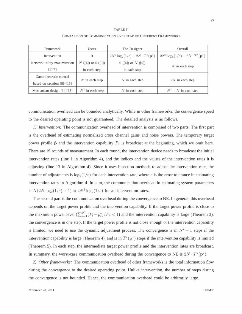
TABLE II

COMPARISON OFCOMMUNICATION OVERHEAD OF DIFFERENTFRAMEWORKS

Framework Users The Designer Overall

Intervention 0 2N2 log2(1/ε) + 2N · T ⋆(p⋆) 2N2 log

2(1/ε) + 2N · T ⋆(p⋆)

Network utility maximization N ([4]) or 0 ([5]) 0 ([4]) or N ([5])N in each step

[4][5] in each step in each step

Game theoretic controlN in each step N in each step 2N in each step

based on taxation [8]–[13]

Mechanism design [14][15] N2 in each step N in each step N2 +N in each step

communication overhead can be bounded analytically. Whilein other frameworks, the convergence speed

to the desired operating point is not guaranteed. The detailed analysis is as follows.

1) Intervention:The communication overhead of intervention is comprised oftwo parts. The first part

is the overhead of estimating normalized cross channel gains and noise powers. The temporary target

power profilep and the intervention capabilityP0 is broadcast at the beginning, which we omit here.

There areN rounds of measurement. In each round, the intervention device needs to broadcast the initial

intervention rates (line 1 in Algorithm 4), and the indices and the values of the intervention rates it is

adjusting (line 13 in Algorithm 4). Since it uses bisection methods to adjust the intervention rate, the

number of adjustments islog2(1/ε) for each intervention rate, whereε is the error tolerance in estimating

intervention rates in Algorithm 4. In sum, the communication overhead in estimating system parameters

is N(2N log2(1/ε) + 1) ≈ 2N2 log2(1/ε) for all intervention rates.

The second part is the communication overhead during the convergence to NE. In general, this overhead

depends on the target power profile and the intervention capability. If the target power profile is close to

the maximum power level (∑N

i=1(Pi− p⋆i )/P i < 1) and the intervention capability is large (Theorem 3),

the convergence is in one step. If the target power profile is not close enough or the intervention capability

is limited, we need to use the dynamic adjustment process. The convergence is inN ′ + 1 steps if the

intervention capability is large (Theorem 4), and is inT ⋆(p⋆) steps if the intervention capability is limited

(Theorem 5). In each step, the intermediate target power profile and the intervention rates are broadcast.

In summary, the worst-case communication overhead during the convergence to NE is2N · T ⋆(p⋆).

2) Other frameworks:The communication overhead of other frameworks is the totalinformation flow

during the convergence to the desired operating point. Unlike intervention, the number of steps during

the convergence is not bounded. Hence, the communication overhead could be arbitrarily large.


26

T1

T2

R1

R2T2

1.0

0.5

0.5

h11

h22

h20

h10 h12

I

h01

h02

h21

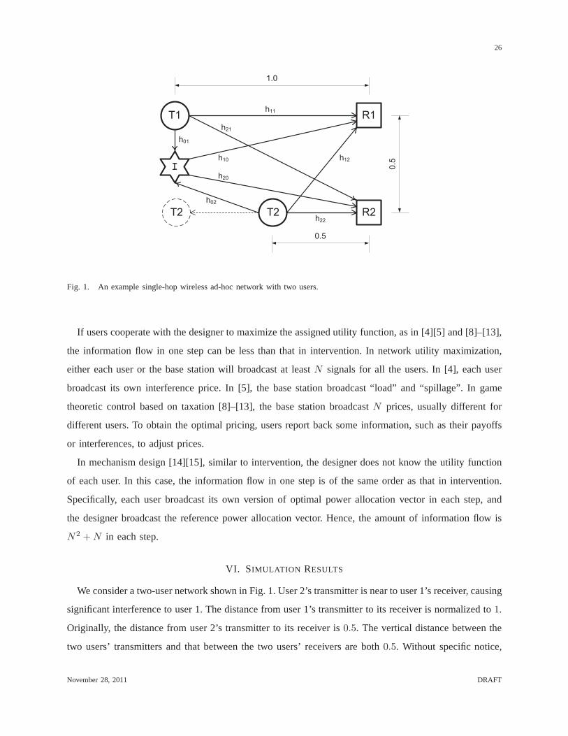
Fig. 1. An example single-hop wireless ad-hoc network with two users.

If users cooperate with the designer to maximize the assigned utility function, as in [4][5] and [8]–[13],

the information flow in one step can be less than that in intervention. In network utility maximization,

either each user or the base station will broadcast at leastN signals for all the users. In [4], each user

broadcast its own interference price. In [5], the base station broadcast “load” and “spillage”. In game

theoretic control based on taxation [8]–[13], the base station broadcastN prices, usually different for

different users. To obtain the optimal pricing, users report back some information, such as their payoffs

or interferences, to adjust prices.

In mechanism design [14][15], similar to intervention, thedesigner does not know the utility function

of each user. In this case, the information flow in one step is of the same order as that in intervention.

Specifically, each user broadcast its own version of optimalpower allocation vector in each step, and

the designer broadcast the reference power allocation vector. Hence, the amount of information flow is

N2 +N in each step.

VI. SIMULATION RESULTS

We consider a two-user network shown in Fig. 1. User 2’s transmitter is near to user 1’s receiver, causing

significant interference to user 1. The distance from user 1’s transmitter to its receiver is normalized to1.

Originally, the distance from user 2’s transmitter to its receiver is0.5. The vertical distance between the

two users’ transmitters and that between the two users’ receivers are both0.5. Without specific notice,


27

0.5 0.55 0.6 0.65 0.7 0.75 0.8 0.85 0.9 0.95 10

1

2

3

4

5

6

Distance between the transmitter and receiver of user 2

Soc

ial w

elfa

re

Sum rate − optimal achievable by interventionSum rate − at NE without interventionFairness − optimal achievable by interventionFairness − at NE without intervention

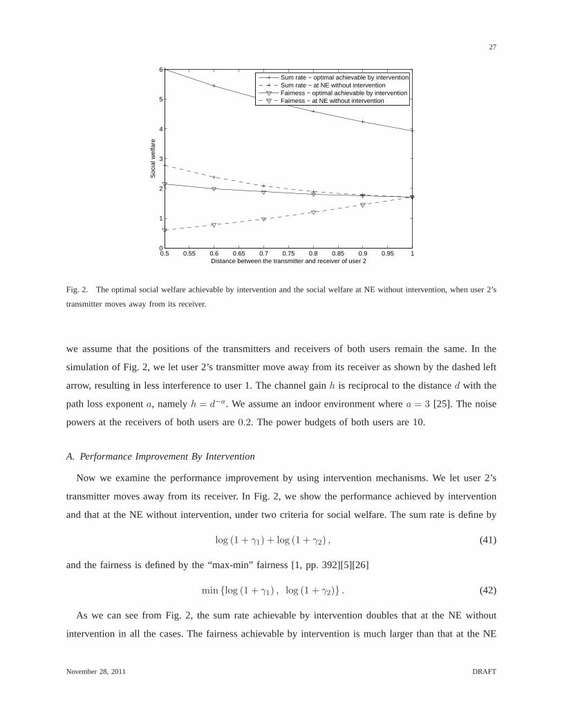
Fig. 2. The optimal social welfare achievable by intervention and the social welfare at NE without intervention, when user 2’s

transmitter moves away from its receiver.

we assume that the positions of the transmitters and receivers of both users remain the same. In the

simulation of Fig. 2, we let user 2’s transmitter move away from its receiver as shown by the dashed left

arrow, resulting in less interference to user 1. The channelgainh is reciprocal to the distanced with the

path loss exponenta, namelyh = d−a. We assume an indoor environment wherea = 3 [25]. The noise

powers at the receivers of both users are0.2. The power budgets of both users are 10.

A. Performance Improvement By Intervention

Now we examine the performance improvement by using intervention mechanisms. We let user 2’s

transmitter moves away from its receiver. In Fig. 2, we show the performance achieved by intervention

and that at the NE without intervention, under two criteria for social welfare. The sum rate is define by

log (1 + γ1) + log (1 + γ2) , (41)

and the fairness is defined by the “max-min” fairness [1, pp. 392][5][26]

min {log (1 + γ1) , log (1 + γ2)} . (42)

As we can see from Fig. 2, the sum rate achievable by intervention doubles that at the NE without

intervention in all the cases. The fairness achievable by intervention is much larger than that at the NE


28

10

10

10

10

20

20

20

20

20

20

40

40

40

4040

40

6060

60

60

60

60

8080

80

80

80

80

100100

100

100

100

100

200

200

200

200 200 200

Target power for user 1

Tar

get p

ower

for

user

2

1 2 3 4 5 6 7 8 9 10

1

2

3

4

5

6

7

8

9

10

(a)

10

1020

20

20

40 40

40

40

40

60

6060

60

60

80

8080

8080

100

100100

100100

200200

200 200 200

400400

400 400 400


Tar

get p

ower

for

user

2

1 2 3 4 5 6 7 8 9 10

1

2

3

4

5

6

7

8

9

10

(b)

10

10

20

20

20

40

40

40

40

6060

60

60

8080

8080

100100

100

100

200200

200

200 200

400400

400 400 400


Tar

get p

ower

for

user

2

1 2 3 4 5 6 7 8 9 10

1

2

3

4

5

6

7

8

9

10

(c)

10

10

20

20

40

40

40

60

60

60

80

80

80

80

100

100

100

100

200

200

200

200400

400

400

400


Tar

get p

ower

for

user

2

0 1 2 3 4 5 6 7 8 9 100

1

2

3

4

5

6

7

8

9

10

N/A

(d)

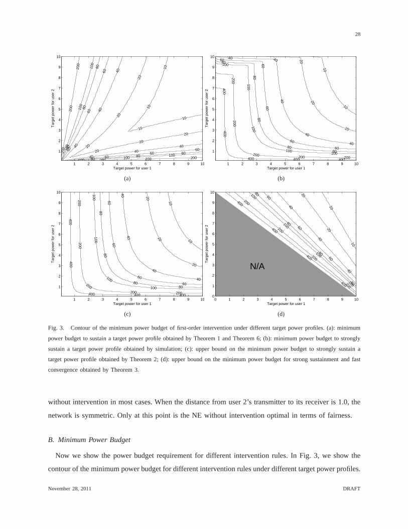
Fig. 3. Contour of the minimum power budget of first-order intervention under different target power profiles. (a): minimum

power budget to sustain a target power profile obtained by Theorem 1 and Theorem 6; (b): minimum power budget to strongly

sustain a target power profile obtained by simulation; (c): upper bound on the minimum power budget to strongly sustain a

target power profile obtained by Theorem 2; (d): upper bound on the minimum power budget for strong sustainment and fast

convergence obtained by Theorem 3.

without intervention in most cases. When the distance from user 2’s transmitter to its receiver is 1.0, the

network is symmetric. Only at this point is the NE without intervention optimal in terms of fairness.

B. Minimum Power Budget

Now we show the power budget requirement for different intervention rules. In Fig. 3, we show the

contour of the minimum power budget for different intervention rules under different target power profiles.


29

0.1 0.2 0.3 0.4 0.5 0.6 0.7 0.8 0.9 10

10

20

30

40

50

60

Relative distance between adjacent target power profiles

Converg

ence t

ime in t

he n

um

ber

of

ste

ps

Geometric sequence

MRD sequence

(a)

0 0.1 0.2 0.3 0.4 0.5 0.6 0.7 0.8 0.9 10

10

20

30

40

50

60

Relative distance between adjacent target power profiles

Pow

er

budget

in d

B

Geometric sequence

MRD sequence

Minimum power budget that sustains the

target power profile

Minimum power budgetthat strongly sustains

the target power profile

(b)

Fig. 4. Given the relative distance between adjacent targetpower profiles, the convergence time and the power budget requirement

of different sequences of intermediate target power profiles in a five-user network. The relative distance between the maximum

power profile and the target power profile is∑

5

i=1

Pi−p⋆iPi

= 3.6 > 1. (a): convergence time; (b): power budget requirement.

Fig. 3(a) shows minimum power budget to sustain a target power profile using first-order intervention

based on individual transmit powers obtained by Theorem 1 and that using first-order intervention based

on aggregate receive power obtained by Theorem 6. Since the power budget requirements are the same

for these two intervention rules, we show them in the same figure. Fig. 3(b) shows the minimum power

budget to strongly sustain a target power profile obtained bysimulation. As we expect, the power budget

requirement for strong sustainment is higher. Fig. 3(c) shows the upper bound on the minimum power

budget to strongly sustain a target power profile obtained byTheorem 2. We can see that the result in

Theorem 2 serves as a good upper bound. Finally, Fig. 3(d) shows the upper bound on the minimum

power budget for strong sustainment and fast convergence obtained by Theorem 3. In this case, the system

reaches NE in at most two time slots. To achieve this fast convergence, the intervention device needs

a much higher power budget. In addition, not all the target power profiles can be sustained. The target

power profiles that cannot be sustained lie in the shadow areain the figure.

C. Power Budget and Convergence Time Tradeoff In Dynamic Adjustment Process

Now we study the tradeoff between the power budget and the convergence time in the dynamic

adjustment process. Here the convergence time is measured as the number of steps in the adjustment

process. To better illustrate the tradeoff, we use a five-user network in the simulation for Fig. 4 and Fig. 5.


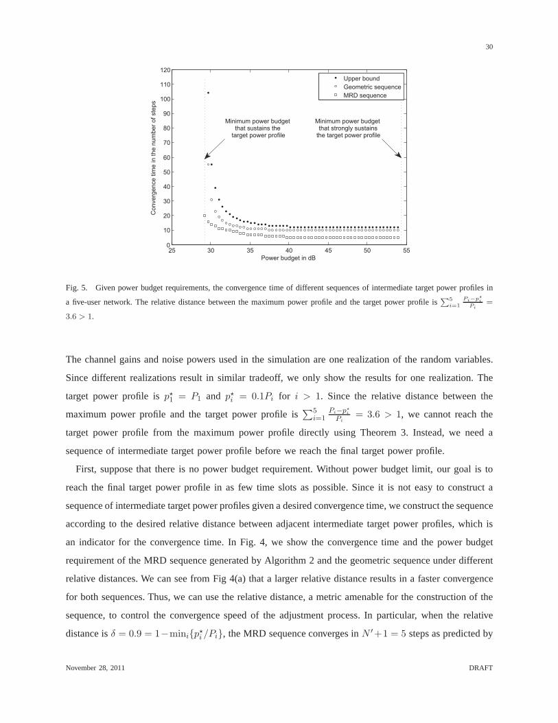
30

25 30 35 40 45 50 550

10

20

30

40

50

60

70

80

90

100

110

120

Power budget in dB

Converg

ence t

ime in t

he n

um

ber

of

ste

ps

Upper bound

Geometric sequence

MRD sequence

Minimum power budget that sustains the

target power profile

Minimum power budget that strongly sustains

the target power profile

Fig. 5. Given power budget requirements, the convergence time of different sequences of intermediate target power profiles in

a five-user network. The relative distance between the maximum power profile and the target power profile is∑

5

i=1

Pi−p⋆iPi

=

3.6 > 1.

The channel gains and noise powers used in the simulation areone realization of the random variables.

Since different realizations result in similar tradeoff, we only show the results for one realization. The

target power profile isp⋆1 = P1 and p⋆i = 0.1Pi for i > 1. Since the relative distance between the

maximum power profile and the target power profile is∑5

i=1Pi−p⋆

i

Pi= 3.6 > 1, we cannot reach the

target power profile from the maximum power profile directly using Theorem 3. Instead, we need a

sequence of intermediate target power profile before we reach the final target power profile.

First, suppose that there is no power budget requirement. Without power budget limit, our goal is to

reach the final target power profile in as few time slots as possible. Since it is not easy to construct a

sequence of intermediate target power profiles given a desired convergence time, we construct the sequence

according to the desired relative distance between adjacent intermediate target power profiles, which is

an indicator for the convergence time. In Fig. 4, we show the convergence time and the power budget

requirement of the MRD sequence generated by Algorithm 2 andthe geometric sequence under different

relative distances. We can see from Fig 4(a) that a larger relative distance results in a faster convergence

for both sequences. Thus, we can use the relative distance, ametric amenable for the construction of the

sequence, to control the convergence speed of the adjustment process. In particular, when the relative

distance isδ = 0.9 = 1−mini{p⋆i /Pi}, the MRD sequence converges inN ′+1 = 5 steps as predicted by


31

Theorem 4. In Fig 4(b), we can see that for both sequences, thepower budget requirement is decreasing

with the relative distances in most cases. The power budget is lower for the MRD sequence. For both

sequences, it requires much less power by the dynamic adjustment process than by the strong sustainment

condition in Theorem 2.

Second, suppose that there is a power budget requirement. Given different power budget requirements,

we show the convergence time of MRD and geometric sequences and the upper bound on the convergence

time in Fig. 5. We can see from the figure that under most power budget requirements, the convergence

time of MRD sequence is roughly half of that of the naive geometric sequence. When the power budget

is small (near to the minimum power budget that sustains the target power profile), the fast convergence

of MRD sequence is even more significant compared to that of the geometric sequence. When the

power budget approaches the minimum requirement that strongly sustains the target power profile, the

convergence time of MRD sequence is 5, which is half of that ofthe geometric sequence.

VII. C ONCLUSION

In this paper, we proposed incentive schemes based on intervention for power control in single-

hop wireless ad hoc networks with selfish users. We formulated a game-theoretic model of power

control with an intervention device and proposed design criteria that desirable intervention rules should

satisfy. Focusing on a simple class of intervention rules called first-order intervention rules, we provided

requirements for intervention rules to sustain a target power profile when the intervention device estimates

individual transmit powers or aggregate receive power. We also proposed dynamic adjustment processes

to guide users to a target power profile through intermediatetargets. We discussed implementation issues

and presented simulation results. To the best of our knowledge, this work is the first to investigate

intervention schemes in a power control scenario. For future research, we can apply intervention schemes

to different power control scenarios, for example, a scenario where users can allocate their power budgets

across multiple channels and a scenario where users care about their energy consumption as well as their

data rates.

REFERENCES

[1] M. Chiang, P. Hande, T. Lan, and C. W. Tan, “Power control in wireless cellular networks,”Foundations and Trends in

Networking, vol. 2, no. 4, pp. 381–533, Apr. 2008.

[2] R. D. Yates, “A framework for uplink power control in cellular radio systems,”IEEE J. Sel. Areas Commun., vol. 13, no.

7, pp. 1341–1347, Sep. 1995.


32

[3] E. Altman and Z. Altman, “S-modular games and power control in wireless networks,”IEEE Trans. Autom. Control, vol.

48, no. 5, pp. 839–842, May 2003.

[4] J. Huang, R. A. Berry, and M. L. Honig, “Distributed interference compensation for wireless networks,”IEEE J. Sel. Areas

Commun., vol. 24, no. 5, pp. 1074–1084, May 2006.

[5] P. Hande, S. Rangan, M. Chiang, and X. Wu, “Distributed uplink power control for optimal SIR assignment in cellular

data networks,”IEEE/ACM Trans. Netw., vol. 16, no. 6, pp. 1420–1433, Dec. 2008.

[6] E. Altman, T. Boulogne, R. El-Azouzi, T. Jimenez, and L. Wynter, “A survey on networking games in telecommunications,”

Computers and Operations Research, vol. 33, no. 2, pp. 286–311, Feb. 2006.

[7] E. G. Larsson, E. A. Jorswieck, J. Lindblom, and R. Mochaourab, “Game theory and the flat-fading gaussian interference

channel,”IEEE Signal Process. Mag., vol. 26, no. 5, pp. 18–27, Sep. 2009.

[8] T. Alpcan, T. Basar, R. Srikant, and E. Altman, “CDMA uplink power control as a noncooperative game,”Wireless

Networks, vol. 8, pp. 659–670, 2002.

[9] C. U. Saraydar, N. B. Mandayam, and D. J. Goodman, “Efficient power control via pricing in wireless data networks,”

IEEE Trans. Commun., vol. 50, no. 2, pp. 291–303, Feb. 2002.

[10] M. Xiao, N. B. Shroff, and E. K. P. Chong, “A utility-based power control scheme in wireless cellular systems,”IEEE/ACM

Trans. Netw., vol. 11, no. 2, pp. 210–221, Apr. 2003.

[11] G. Scutari, S. Barbarossa, and D. P. Palomar, “Potential games: A framework for vector power control problems with

coupled constraints,” inProceeding of ICASSP 2006, pp. 241–244, 2006.

[12] U. O. Candogan, I. Menache, A. Ozdaglar, and P. A. Parrilo, “Near-optimal power control in wireless networks: a potential

game approach,” inProceedings of IEEE INFOCOM 2010, pp. 1–9, 2010.

[13] J. Huang, R. A. Berry, and M. L. Honig, “Auction-based spectrum sharing,”Mobile Networks and Applications, vol. 11,

pp. 405–418, 2006.

[14] S. Sharma and D. Teneketzis, “An externalities-based decentralized optimal power allocation algorithm for wireless

networks,” IEEE/ACM Trans. Netw., vol. 17, no. 6, pp. 1819–1831, Dec. 2009.

[15] S. Sharma and D. Teneketzis, “A game-theoretic approach to decentralized optimal power allocation for cellular networks,”

Telecommunication Systems, pp. 1–16, 2010.

[16] Y. Wu, B. Wang, K. J. R. Liu, and T. C. Clancy, “Repeated open spectrum sharing game with cheat-proof strategies,”

IEEE Trans. Wireless Commun., vol. 8, no. 4, pp. 1922–1933, Apr. 2009.

[17] C. Long, Q. Zhang, B. Li, H. Yang, and X. Guan, “Non-cooperative power control for wireless ad hoc networks with

repeated games,”IEEE J. Sel. Areas Commun., vol. 25, no. 6, pp. 1101–1112, Aug. 2007.

[18] G. Mailath and L. Samuelson,Repeated Games and Reputations: Long-run Relationships. Oxford, U.K.: Oxford Univ.

Press, 2006.

[19] J. Park and M. van der Schaar, “Stackelberg contention games in multiuser networks,”EURASIP Journal on Advances in

Signal Processing, vol. 2009, pp. 1–15, 2009.

[20] J. Park and M. van der Schaar, “Designing incentive schemes based on intervention: The case of imperfect monitoring,”

in Proceedings of GameNets 2011. Available: http://medianetlab.ee.ucla.edu/papers/gamenets2011jaeok.pdf.

[21] J. Park and M. van der Schaar, “The theory of intervention games for resource sharing in wireless communications,”

Accepted byIEEE J. Sel. Areas Commun.Available: http://arxiv.org/abs/1101.3052.

[22] Y. Gai, H. Liu, and B. Krishnamachari, “A packet dropping-based incentive mechanism for M/M/1 queues with selfish

users”, inProceedings of IEEE INFOCOM 2011, pp. 2687–2695, 2011.


http://medianetlab.ee.ucla.edu/papers/gamenets2011_jaeok.pdf

http://arxiv.org/abs/1101.3052

33

[23] Y. Xiao, J. Park, and M. van der Schaar, “Intervention inPower Control Games With Selfish Users,”Tech. Rep.Available:

http://arxiv.org/abs/1104.1227v1.

[24] D. Fudenberg and J. Tirole,Game Theory. Cambridge, MA: MIT Press, 1991.

[25] T. S. Rappaport,Wireless Communications: Principles and Practice. Upper Saddle River, N.J.: Prentice Hall PTR, 2002.

[26] M. Schubert and H. Boche, “Solution of the multiuser downlink beamforming problem with individual SINR constraints,”

IEEE Trans. Veh. Technol., vol. 53, no. 1, pp. 18–28, Jan. 2004.

[27] R. A. Horn and C. R. Johnson,Matrix Analysis. Cambridge, U.K.: Cambridge Univ. Press, 1985.

PLACE

PHOTO

HERE

Yuanzhang Xiao received the B.E. and M.E. degree in electrical engineeringfrom Tsinghua University,

Beijing, China, in 2006 and 2009, respectively. He is currently pursuing the Ph.D. degree in the Electrical

Engineering Department at University of California, Los Angeles. His research interests include game

theory, optimization, communication networks, and network economics.

PLACE

PHOTO

HERE

Jaeok Park received the B.A. degree in economics from Yonsei University, Seoul, Korea, in 2003, and

the M.A. and Ph.D. degrees in economics from the University of California, Los Angeles, in 2005 and

2009, respectively.

He is currently an Assistant Professor in the School of Economics at Yonsei University, Seoul, Korea.

From 2009 to 2011, he was a Postdoctoral Scholar in the Electrical Engineering Department at the

University of California, Los Angeles. From 2006 to 2008, heserved in the Republic of Korea Army. His

research interests include game theory, mechanism design,network economics, and wireless communication.

Mihaela van der Schaar is Chancellor’s Professor of Electrical Engineering at University of California, Los Angeles. She

is an IEEE Fellow, a Distinguished Lecturer of the Communications Society for 2011-2012 and the Editor in Chief of IEEE

Transactions on Multimedia. She received an NSF CAREER Award (2004), the Best Paper Award from IEEE Transactions

on Circuits and Systems for Video Technology (2005), the Okawa Foundation Award (2006), the IBM Faculty Award (2005,

2007, 2008), the Most Cited Paper Award from EURASIP: Image Communications Journal (2006), the Gamenets Conference

Best Paper Award (2011) and the 2011 IEEE Circuits and Systems Society Darlington Award Best Paper Award. She holds 33

granted US patents. For more information about her researchvisit: http://medianetlab.ee.ucla.edu/


http://arxiv.org/abs/1104.1227v1

http://medianetlab.ee.ucla.edu/

Intervention in Power Control Games With Selfish Users

Documents

Transcript of Intervention in Power Control Games With Selfish Users