INTERROGATION UNIT AND SAW RDL SENSOR DESIGN ...
78
Department of Electrical and Computer Engineering INTERROGATION UNIT AND SAW RDL SENSOR DESIGN FOR AUTOMATIC MEASUREMENT OF TEMPERATURE AND STRESS by ALEJANDRO MORA MARTINEZ 2018
-
Upload
khangminh22 -
Category
Documents
-
view
0 -
download
0
Transcript of INTERROGATION UNIT AND SAW RDL SENSOR DESIGN ...
Department of Electrical and Computer Engineering
INTERROGATION UNIT AND SAW RDL SENSOR
DESIGN FOR AUTOMATIC MEASUREMENT OF
TEMPERATURE AND STRESS
by
ALEJANDRO MORA MARTINEZ
2018
INTERROGATION UNIT AND SAW RDL SENSOR DESIGN FOR
AUTOMATIC MEASUREMENT OF TEMPERATURE AND STRESS
Independent study conducted at University of Colorado at Colorado Springs
during the spring semester of 2018
and directed by Dr. T. S. Kalkur, Chair of the department
© 2018
ALEJANDRO MORA MARTINEZ
ALL RIGHTS RESERVED
iii
ABSTRACT
Technology advances towards the concept of IoT (Internet of Things), which is the idea
of a global network that integrates electronics and computer-based systems on physical devices
continuously sharing data, resulting in efficiency improvements and other benefits. Another
branch of engineering developments is directed towards automation and artificial intelligence,
which are being increasingly implemented in today’s world, and predictably will play a very
important role in the years to come.
What all these concepts have in common is the necessity gathering information of their
surroundings, or in other words, the incorporation of sensors. The monitorization of physical
parameters such as temperature or the concentration of a certain substance in the air are of vital
importance, because they may trigger actions that need to be taken to avert dangerous situations.
A sensor is a device that transforms a physical parameter into an electrical variable, which
can be measured and quantified. Throughout the years, many sensing devices have been studied
and developed; however, Surface Acoustic Waves (SAW) technology specifically presents
various attractive qualities for the current sensor market.
SAW sensors are solid state devices based in piezoelectric materials, which transform
electrical energy into mechanical waves. These are affected by multiple physical parameters, like
temperature, pressure, stress, concentration of a gas, etc., which modify the waveform traveling
through the material substrate (its amplitude, its frequency and / or its transversal speed). These
changes can be measured by a radio-frequency unit, and the information about the physical
parameters affecting the sensor can be extracted.
An interesting benefit of these devices is that they are passive, and as such don’t need any
kind of power supply. Adding the fact that they can be interrogated wirelessly, offer higher
protection against electromagnetic interference and their small size and low cost, SAW devices
are a very interesting alternative for IoT applications. The available computerized units in the
market needed to extract the information acquired by these sensors, however, are still expensive
and specialized.
This is the motivation for this project: the development of a low-cost, multi-purpose,
automatic interrogation unit, based in software-designed radio (SDR), that can extract information
from SAW devices response to an excitation signal. It is also a goal to accomplish this task in
real-time. The focus will be put on reflective delay line (RDL) SAW devices. To this end, the
software toolkit GNU Radio will be used, in conjunction with an Ettus B200 board that enables
the implementation of an SDR.
iv
At the same time, novel SAW devices that incorporate orthogonal frequency coding
(OFC) will be designed, due to their appealing lower insertion power loss and broader possibilities
of post-processing techniques to be applied. The numerical computation suite GNU Octave and
the drawing software AutoCAD will be used to simulate the devices behavior and create their 2D
model layout, respectively.
Before describing the core topics of this project, a brief introduction about SAW theory
and state-of-the-art sensor devices and interrogation techniques will be presented. Finally, the
tests conducted to prove SAW sensors functionality and their change with physical variables, like
temperature and stress, will be described, as well as the processing implemented to extract that
information and the material used in said tests.

v
To my family and Ana

vi
ACKNOWLEDGEMENTS
First and foremost, I would like to thank the Balsells Program and its creator, Mr. Pete
Balsells, as well as the coordination between the University of Colorado at Colorado Springs and
the Universitat Politècnica de Catalunya, for granting me the opportunity of studying and
conducting research in the United States of America. It has been a life-changing experience, and
I will be forever thankful for this.
I would like to thank my advisor, Dr. T.S. Kalkur, for his help and supervision while
developing this project. I would also like to thank Mr. Fran Soler, a former Balsells student
graduated at the University of Colorado at Colorado Springs, for his assistance.
Thanks to Mr. Roger Perkins, for arranging the necessary material at the laboratory to
conduct tests.
Thanks to my family, specially my parents Mariano and Lola, and my brother Enrique,
for being my emotional pillar and supporting me in my decision to study abroad, with all that it
entails.
Finally, thanks to my girlfriend, Ana, for being a constant source of motivation and
support regardless of the circumstances.
vii
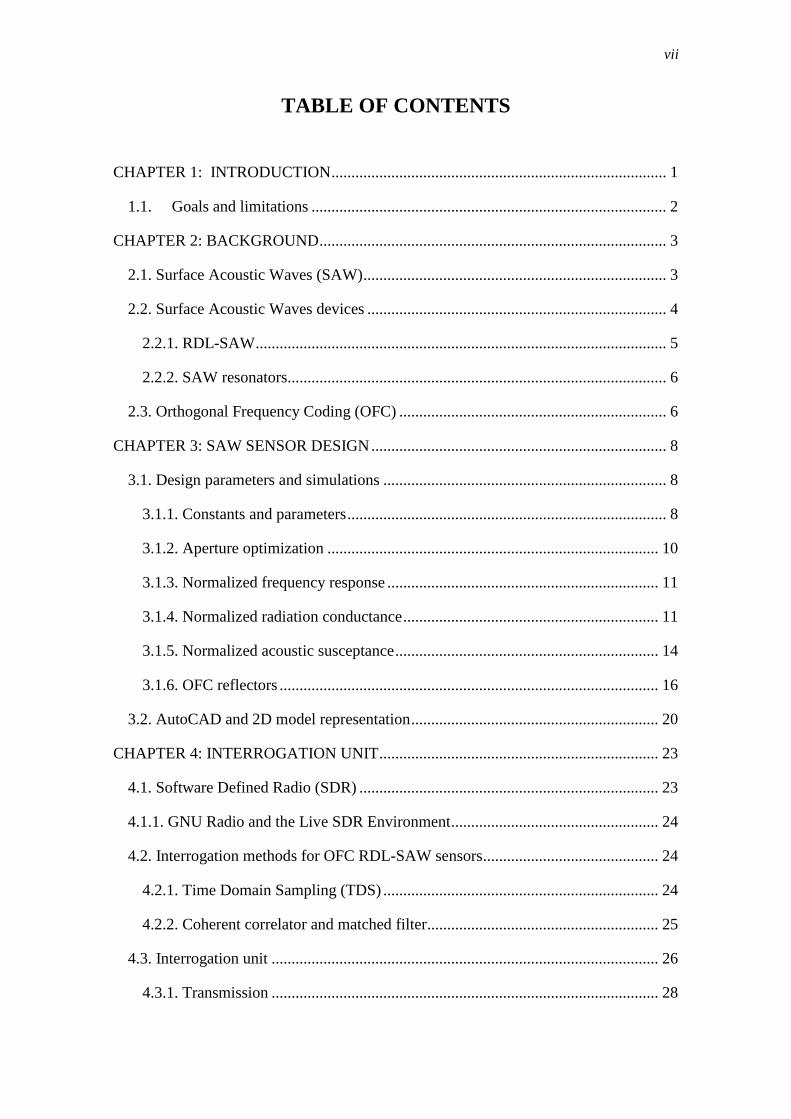
TABLE OF CONTENTS
CHAPTER 1: INTRODUCTION .................................................................................... 1
1.1. Goals and limitations ......................................................................................... 2
CHAPTER 2: BACKGROUND ....................................................................................... 3
2.1. Surface Acoustic Waves (SAW) ............................................................................ 3
2.2. Surface Acoustic Waves devices ........................................................................... 4
2.2.1. RDL-SAW ....................................................................................................... 5
2.2.2. SAW resonators............................................................................................... 6
2.3. Orthogonal Frequency Coding (OFC) ................................................................... 6
CHAPTER 3: SAW SENSOR DESIGN .......................................................................... 8
3.1. Design parameters and simulations ....................................................................... 8
3.1.1. Constants and parameters ................................................................................ 8
3.1.2. Aperture optimization ................................................................................... 10
3.1.3. Normalized frequency response .................................................................... 11
3.1.4. Normalized radiation conductance ................................................................ 11
3.1.5. Normalized acoustic susceptance .................................................................. 14
3.1.6. OFC reflectors ............................................................................................... 16
3.2. AutoCAD and 2D model representation .............................................................. 20
CHAPTER 4: INTERROGATION UNIT ...................................................................... 23
4.1. Software Defined Radio (SDR) ........................................................................... 23
4.1.1. GNU Radio and the Live SDR Environment .................................................... 24
4.2. Interrogation methods for OFC RDL-SAW sensors ............................................ 24
4.2.1. Time Domain Sampling (TDS) ..................................................................... 24
4.2.2. Coherent correlator and matched filter.......................................................... 25
4.3. Interrogation unit ................................................................................................. 26
4.3.1. Transmission ................................................................................................. 28
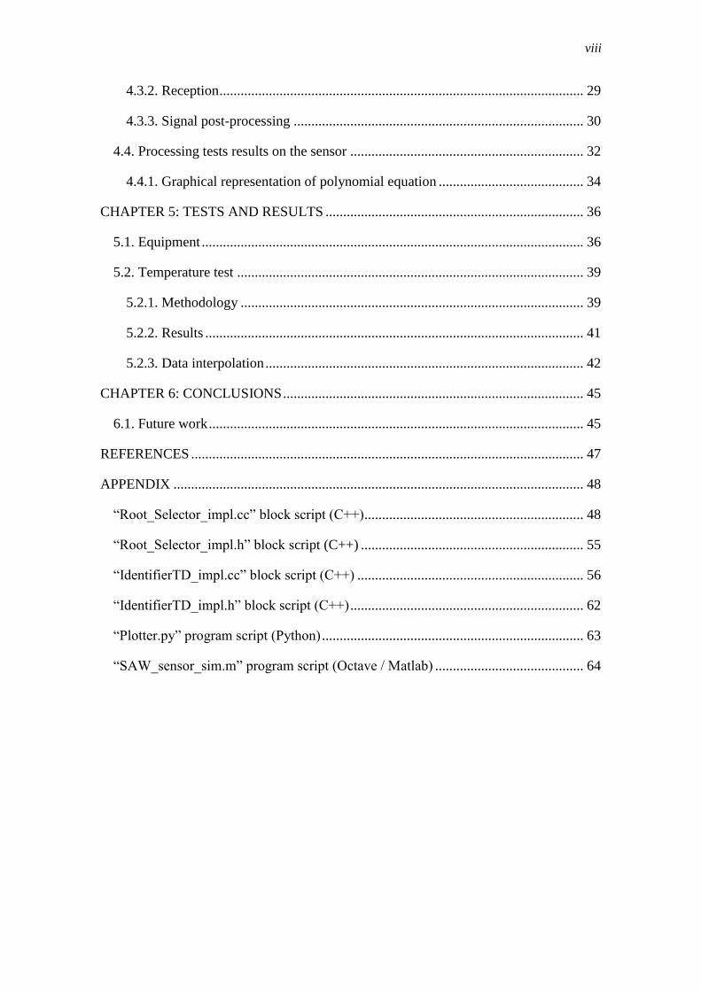
viii
4.3.2. Reception ....................................................................................................... 29
4.3.3. Signal post-processing .................................................................................. 30
4.4. Processing tests results on the sensor .................................................................. 32
4.4.1. Graphical representation of polynomial equation ......................................... 34
CHAPTER 5: TESTS AND RESULTS ......................................................................... 36
5.1. Equipment ............................................................................................................ 36
5.2. Temperature test .................................................................................................. 39
5.2.1. Methodology ................................................................................................. 39
5.2.2. Results ........................................................................................................... 41
5.2.3. Data interpolation .......................................................................................... 42
CHAPTER 6: CONCLUSIONS ..................................................................................... 45
6.1. Future work .......................................................................................................... 45
REFERENCES ............................................................................................................... 47
APPENDIX .................................................................................................................... 48
“Root_Selector_impl.cc” block script (C++) .............................................................. 48
“Root_Selector_impl.h” block script (C++) ............................................................... 55
“IdentifierTD_impl.cc” block script (C++) ................................................................ 56
“IdentifierTD_impl.h” block script (C++) .................................................................. 62
“Plotter.py” program script (Python) .......................................................................... 63
“SAW_sensor_sim.m” program script (Octave / Matlab) .......................................... 64
ix
LIST OF IMAGES
Figure 2.1. Schematic of the system developed [1]. ........................................................ 3
Figure 2.2. Rayleigh waves propagation and individual motion of molecules of the
substrate [2] ...................................................................................................................... 3
Figure 2.3. Schematic representation of an IDT and its principle of operation [2]. ........ 4
Figure 2.4. Schematic representation of a Bragg reflector and its principle of operation
[2]. .................................................................................................................................... 4
Figure 2.5. (a) Reflection of the wave generated by the IDT (b) Ideal readings of the
echoed wave from the interrogation unit point of view [4]. ............................................. 5
Figure 2.6. Left figure: SAW resonator schematic representation. Right figure: example
of SAW resonator response [3]. ....................................................................................... 6
Figure 2.7. Example of the spectrum of a SAW device with 4 OFC gratings. Note how
at the peak frequency of each grating the response of the rest tends to a minimum [5]. . 7
Figure 3.1. Graphical representation of the IDT wavelength. Source: ResearchGate. .... 9
Figure 3.2. Graphical representation of the IDT wavelength (p) and aperture (A).
Source: ResearchGate. .................................................................................................... 10
Figure 3.3. Graphical representation of normalized radiation conductance; f0 = 435
MHz, BW = 10 MHz (models 435T1 and 435T2). .................................... 12
Figure 3.4. Graphical representation of normalized radiation conductance; f0 = 435
MHz, BW = 8 MHz (models 435T3 and 435T4). .......................................................... 12
Figure 3.5. Graphical representation of normalized radiation conductance; f0 = 910
MHz, BW = 10 MHz (models 910T1 and 910T2). ...................................... 13
Figure 3.6. Graphical representation of normalized radiation conductance; f0 = 910
MHz, BW = 8 MHz (models 910T3 and 910T4). .......................................................... 13
Figure 3.7. Graphical representation of normalized acoustic susceptance; f0 = 435
MHz, BW = 10 MHz (models 435T1 and 435T2). ........................................................ 14
Figure 3.8. Graphical representation of normalized acoustic susceptance; f0 = 435
MHz, BW = 8 MHz (models 435T3 and 435T4). .......................................................... 15
Figure 3.9. Graphical representation of normalized acoustic susceptance; f0 = 910
MHz, BW = 10 MHz (models 910T1 and 910T2). ........................................................ 15
Figure 3.10. Graphical representation of normalized acoustic susceptance; f0 = 910
MHz, BW = 8 MHz (models 910T3 and 910T4). .......................................................... 16
x
Figure 3.11. Graphical representation of normalized frequency response of the IDT and
the OFC gratings; f0 = 435 MHz, BW = 10 MHz (models 435T1 and 435T2). ............ 17
Figure 3.12. Graphical representation of normalized frequency response of the IDT and
the OFC gratings; f0 = 435 MHz, BW = 8 MHz (models 435T3 and 435T4). .............. 17
Figure 3.13. Graphical representation of normalized frequency response of the IDT and
the OFC gratings; f0 = 910 MHz, BW = 10 MHz (models 910T1 and 910T2). ............ 18
Figure 3.14. Graphical representation of normalized frequency response of the IDT and
the OFC gratings; f0 = 910 MHz, BW = 8 MHz (models 910T3 and 910T4). .............. 18
Figure 3.15. AutoCAD representation of model 435T4, marking IDT pads, the sensing
width and the separation between reflectors. Source: own AutoCAD Drawing. ........... 19
Figure 3.16. AutoCAD drawing of model 435T1.......................................................... 20
Figure 3.17. AutoCAD drawing of model 435T2.......................................................... 20
Figure 3.18. AutoCAD drawing of model 435T3.......................................................... 20
Figure 3.19. AutoCAD drawing of model 435T4.......................................................... 20
Figure 3.20. AutoCAD drawing of model 910T1.......................................................... 20
Figure 3.21. AutoCAD drawing of model 910T2.......................................................... 21
Figure 3.22. AutoCAD drawing of model 910T3.......................................................... 21
Figure 3.23. AutoCAD drawing of model 910T4.......................................................... 21
Figure 3.24. Zoomed out AutoCAD drawing of the whole wafer. ................................ 22
Figure 3.25. Zoomed in image of the central part of the wafer. Note how the number of
the device has been added to its model name. ................................................................ 22
Figure 4.1. Ettus B200 board available at UCCS laboratory. Source: own camera. ..... 23
Figure 4.2. Image of a Vert 400 antenna [8].................................................................. 24
Figure 4.3. Block diagram of a TDS transmitter / receiver [9]...................................... 25
Figure 4.4. Graphical representation of the convolution between the matched filter and
the signal from the sensor, sweeping the scaling factor to obtain the maximum
correlation peak. ............................................................................................................. 26
Figure 4.5. Flowgraph of the complete interrogation unit, “Interrogation_unit”. Source:
GNU Radio. .................................................................................................................... 27
Figure 4.6. GUI of the “Interrogation_Unit” program. Source: GNU Radio. ............... 28
Figure 4.7. Transmission module. Source: GNU Radio. ............................................... 29
Figure 4.8. Reception module. Source: GNU Radio. .................................................... 29
Figure 4.9. Post-processing module. Source: GNU Radio. ........................................... 31
Figure 4.10. GUI of the “Proc_tests” program. Source: GNU Radio............................ 32
xi
Figure 4.11. Flowgraph of the “Proc_tests” program. Source: GNU Radio. ................ 33
Figure 4.12. Polyfit function syntax. Source: GNU Radio. ........................................... 33
Figure 4.13. Polyder function syntax. Source: GNU Radio. ......................................... 33
Figure 4.14. Polyval function syntax. Source: GNU Radio. ......................................... 33
Figure 4.15. Elimination of complex critical points. Source: GNU Radio.................... 34
Figure 4.16. Polynomial coefficients label, example: a2 (second degree coefficient).
Source: GNU Radio ........................................................................................................ 34
Figure 4.17. Ubuntu terminal during “Plotter.py” execution. ....................................... 34
Figure 4.18. Graphical representation of the test data and the interpolation equation. . 35
Figure 5.1. S11 of SAW device tested. Source: Agilent E8364A spectrum analyzer.
Source: Excel .................................................................................................................. 36
Figure 5.2. Wafer containing SAW devices, including the one used in the tests [4]. ... 37
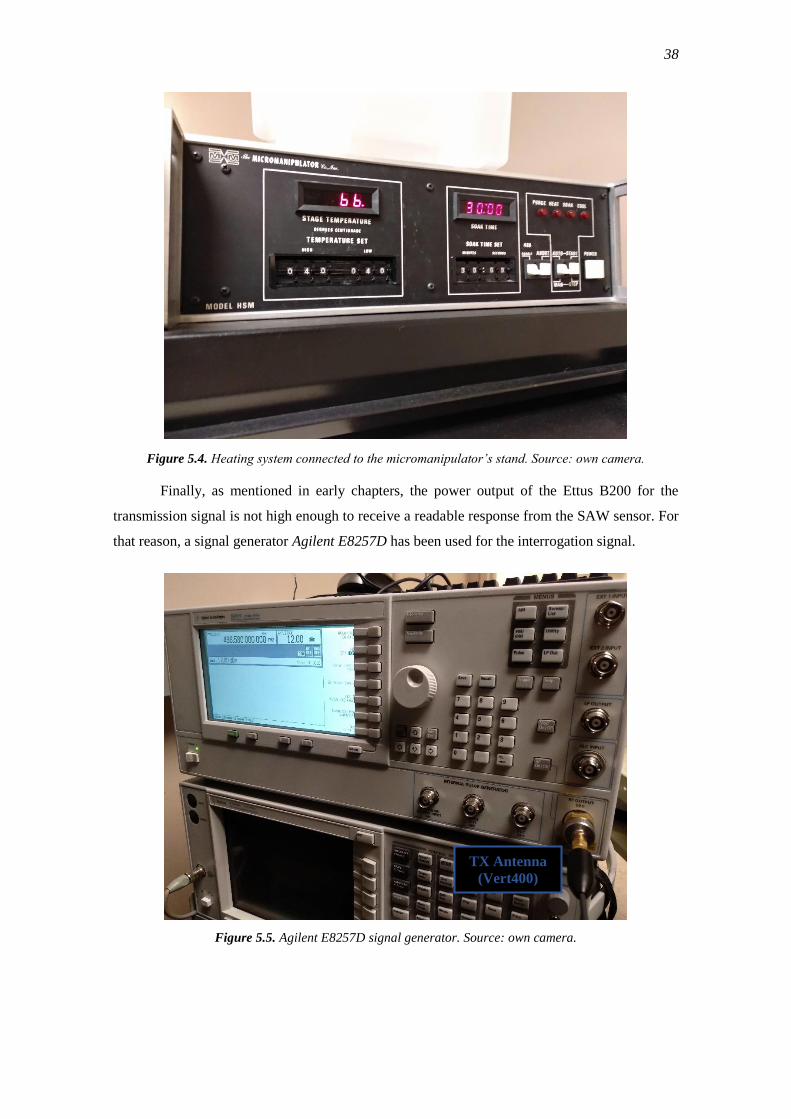
Figure 5.3. Micromanipulator, available at UCCS lab. Source: own camera. .............. 37
Figure 5.4. Heating system connected to the micromanipulator’s stand. Source: own
camera. ............................................................................................................................ 38
Figure 5.5. Agilent E8257D signal generator. Source: own camera. ............................ 38
Figure 5.6. Arrangement of the equipment used for the tests. Source: own camera. .... 39
Figure 5.7. Ettus B200 with a Vert400 antenna for reception. Source: own camera. ... 40
Figure 5.8. SAW wafer placed on heating stand, with single pole antenna connected to
micrometric probe. Source: own camera ........................................................................ 40
Figure 5.9. Probe placement on SAW metallic fingers. Source: own camera, through
microscope lens. ............................................................................................................. 41
Figure 5.11. Example of the data gathered, zoomed in to see peaks (reflectors
response). Temperature = 33 ºC. Source: GNU Radio. .................................................. 42
Figure 5.12. Graphical representation of data gathered. X Axis: Temperature (ºC). Y
Axis: Time (µs). Source: GNU Radio. ........................................................................... 43
Figure 5.13. Graphical representation of data gathered, discarding outside values.
X Axis: Temperature (ºC). Y Axis: Time (µs). Source: GNU Radio. ............................ 43
Figure 5.14. Coefficients for the 4th degree interpolating equation calculated by the
“Proc_tests” program. Source: GNU Radio. .................................................................. 44

xii
LIST OF TABLES
Table 3.1. Summary of the SAW devices designed and its most important parameters. 8
Table 3.2. Optimum aperture value calculated. ............................................................. 11
Table 3.3. Summary of the parameters defined in section 3.1.6. for each SAW model
designed. ......................................................................................................................... 19
Table 4.1. Specs of the host laptop. ............................................................................... 24
Table 5.1. Time delay measured at different wafer temperatures.................................. 42
1
CHAPTER 1: INTRODUCTION
Surface acoustic wave sensors are small, passive, cheap and wireless; all these qualities
make SAW technology very attractive for Internet of Things (IoT) applications, which is an
extended concept in today’s day and age regarding the data exchange between physical devices
embedded with electronics, specially sensors. The scope of this project is to develop an automatic,
real-time interrogation unit that can communicate with RDL-SAW sensors and extract the value
of the variable of study, using a software-defined radio and signal post-processing in the GNU
Radio environment. The design process of RDL-SAW devices incorporating OFC techniques will
also be covered.
In chapter 2, the basics of the foundation of the SAW technology will be explained: the
relationship between piezoelectricity and Rayleigh waves, how can that be used to measure
physical variables like temperature or stress, and the embodiment of such devices. Identification
methods of such devices will also be detailed, focusing on orthogonal frequency coding (OFC),
especially interesting for its reduced power loss and multiple interrogation methods available.
Chapter 3 will cover the design process of various models of OFC RDL-SAW devices,
detailing the equations used to obtain their most important parameters. Simulations will be
conducted using GNU Octave, a free numerical computation programming language included in
the “Live SDR Environment”, in order to make sure that the sensors work as intended. Lastly, the
layout of the devices will be drawn in AutoCAD, following the results of the design process.
Chapter 4 focuses on the interrogation unit and the software-defined radio (SDR),
developed in the software toolkit GNU Radio, available in the “Live SDR Environment” bootable
Ubuntu drive image. Interrogation techniques will be explained, and the interrogation unit
flowgraph will be detailed block by block, including custom ones. Complementary programs
developed to aid with the signal post-processing will also be described.
In chapter 5 tests results are presented, as well as the process of data fitting so that the
interrogation unit can extract values of the variable being studied using the test data as a base.
Temperature and stress tests will be conducted and detailed.
Finally, chapter 6 will include the conclusions of this project and how can it be improved,
the future work that can be done using it as a reference. The code for all original GNU Radio
blocks and Python / Octave programs will be available in the appendix.
2
1.1. Goals and limitations
The main goal of this project is to achieve a multi-functional interrogation unit that can
be tuned to any frequency and extract information from any RDL-SAW sensor using time domain
processing techniques. It should also accomplish this task in real-time, as an improvement of
previous work conducted at the University of Colorado at Colorado Springs.
The equipment for the SDR available at the UCCS lab used in this project is an Ettus
B200, described in Chapter 4. Its limited transmission gain caused that, even though it is
completely operational, an external signal generator has been needed to supply enough power to
be able to read the SAW sensor response.
The fact that the GNU Radio environment has been booted from an external hard drive
has limited the amount of processing power of the host PC, causing GNU Radio to freeze with
demanding sample rate values. This means that higher processing speed, and so better
performance of the radio unit, can be achieved using a different configuration.
Even though stress tests were supposed to be conducted for the SAW sensors designed,
they ended up not being viable due to difficulties to extract devices from a wafer and accurately
placing them in a way that known stress could be applied to them. The way that the interrogation
unit would extract stress values, however, is the same as temperature, so the data interpolation
process and information extraction is common to both variables.
3
CHAPTER 2: BACKGROUND
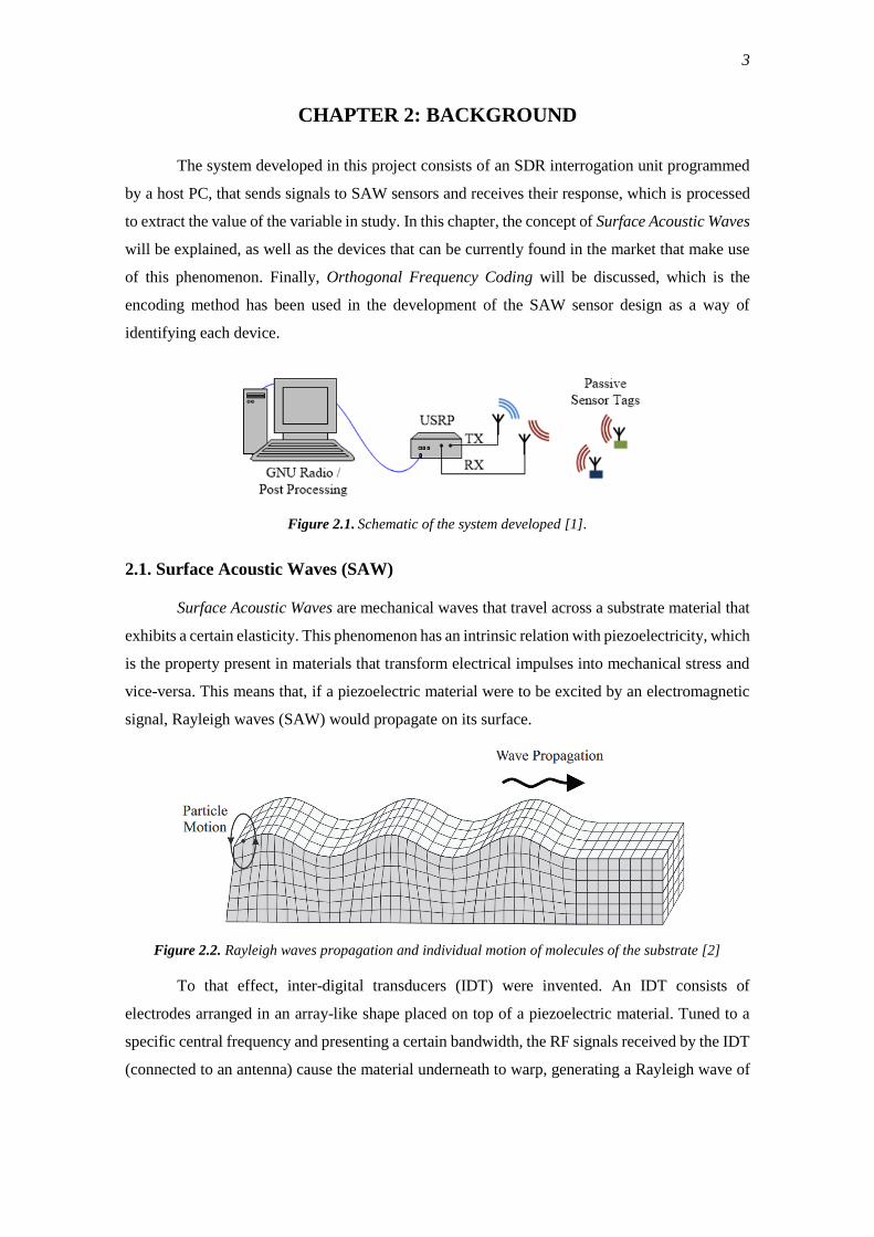
The system developed in this project consists of an SDR interrogation unit programmed
by a host PC, that sends signals to SAW sensors and receives their response, which is processed
to extract the value of the variable in study. In this chapter, the concept of Surface Acoustic Waves
will be explained, as well as the devices that can be currently found in the market that make use
of this phenomenon. Finally, Orthogonal Frequency Coding will be discussed, which is the
encoding method has been used in the development of the SAW sensor design as a way of
identifying each device.
Figure 2.1. Schematic of the system developed [1].
2.1. Surface Acoustic Waves (SAW)
Surface Acoustic Waves are mechanical waves that travel across a substrate material that
exhibits a certain elasticity. This phenomenon has an intrinsic relation with piezoelectricity, which
is the property present in materials that transform electrical impulses into mechanical stress and
vice-versa. This means that, if a piezoelectric material were to be excited by an electromagnetic
signal, Rayleigh waves (SAW) would propagate on its surface.
Figure 2.2. Rayleigh waves propagation and individual motion of molecules of the substrate [2]
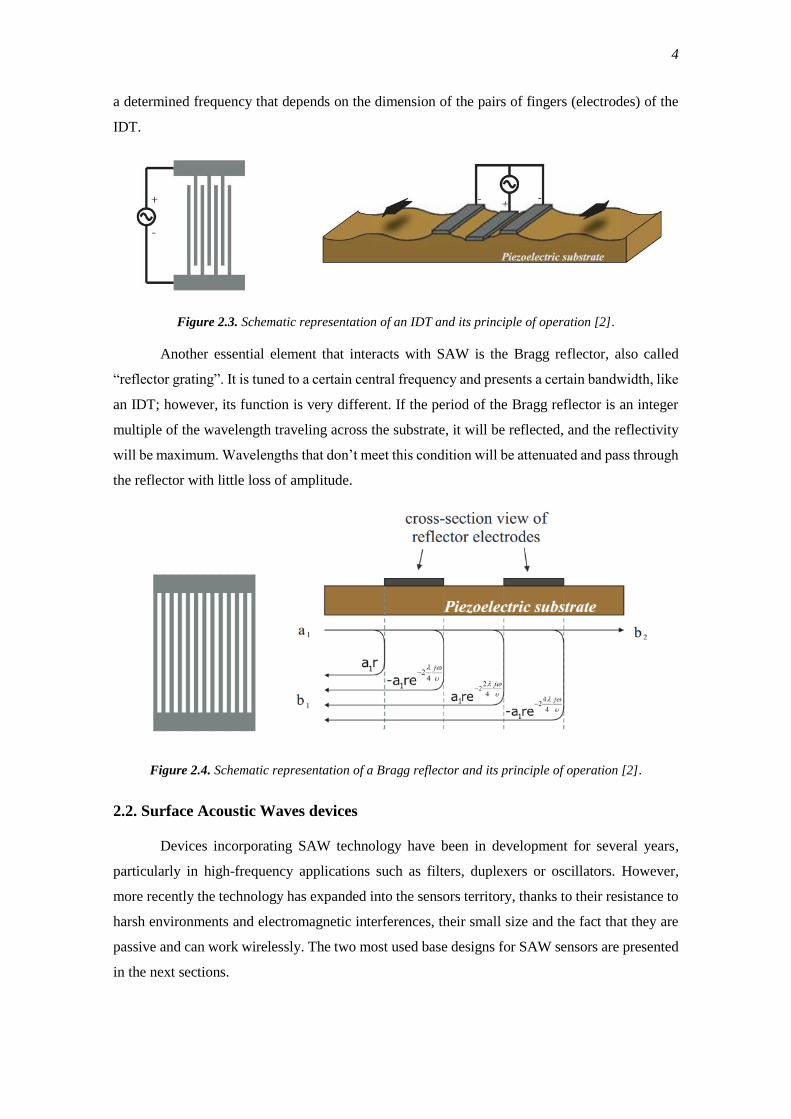
To that effect, inter-digital transducers (IDT) were invented. An IDT consists of
electrodes arranged in an array-like shape placed on top of a piezoelectric material. Tuned to a
specific central frequency and presenting a certain bandwidth, the RF signals received by the IDT
(connected to an antenna) cause the material underneath to warp, generating a Rayleigh wave of
4
a determined frequency that depends on the dimension of the pairs of fingers (electrodes) of the
IDT.
Figure 2.3. Schematic representation of an IDT and its principle of operation [2].
Another essential element that interacts with SAW is the Bragg reflector, also called
“reflector grating”. It is tuned to a certain central frequency and presents a certain bandwidth, like
an IDT; however, its function is very different. If the period of the Bragg reflector is an integer
multiple of the wavelength traveling across the substrate, it will be reflected, and the reflectivity
will be maximum. Wavelengths that don’t meet this condition will be attenuated and pass through
the reflector with little loss of amplitude.
Figure 2.4. Schematic representation of a Bragg reflector and its principle of operation [2].
2.2. Surface Acoustic Waves devices
Devices incorporating SAW technology have been in development for several years,
particularly in high-frequency applications such as filters, duplexers or oscillators. However,
more recently the technology has expanded into the sensors territory, thanks to their resistance to
harsh environments and electromagnetic interferences, their small size and the fact that they are
passive and can work wirelessly. The two most used base designs for SAW sensors are presented
in the next sections.
5
2.2.1. RDL-SAW
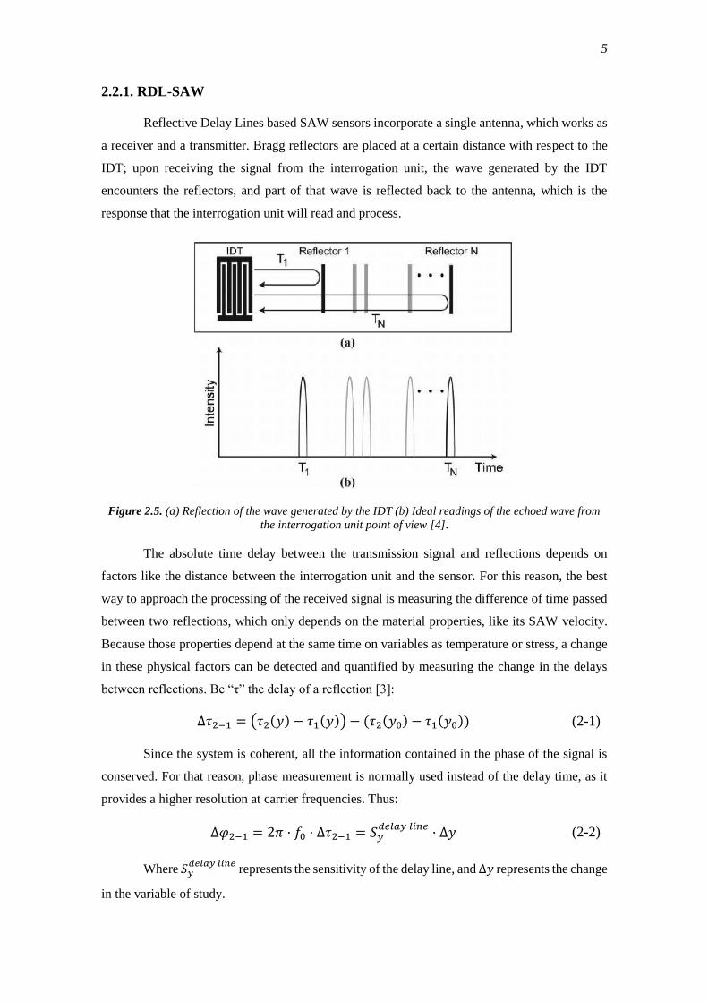
Reflective Delay Lines based SAW sensors incorporate a single antenna, which works as
a receiver and a transmitter. Bragg reflectors are placed at a certain distance with respect to the
IDT; upon receiving the signal from the interrogation unit, the wave generated by the IDT
encounters the reflectors, and part of that wave is reflected back to the antenna, which is the
response that the interrogation unit will read and process.
Figure 2.5. (a) Reflection of the wave generated by the IDT (b) Ideal readings of the echoed wave from
the interrogation unit point of view [4].
The absolute time delay between the transmission signal and reflections depends on
factors like the distance between the interrogation unit and the sensor. For this reason, the best
way to approach the processing of the received signal is measuring the difference of time passed
between two reflections, which only depends on the material properties, like its SAW velocity.
Because those properties depend at the same time on variables as temperature or stress, a change
in these physical factors can be detected and quantified by measuring the change in the delays
between reflections. Be “τ” the delay of a reflection [3]:
∆𝜏2−1 = (𝜏2(𝑦) − 𝜏1(𝑦)) − (𝜏2(𝑦0) − 𝜏1(𝑦0)) (2-1)
Since the system is coherent, all the information contained in the phase of the signal is
conserved. For that reason, phase measurement is normally used instead of the delay time, as it
provides a higher resolution at carrier frequencies. Thus:
∆𝜑2−1 = 2𝜋 · 𝑓0 · ∆𝜏2−1 = 𝑆𝑦𝑑𝑒𝑙𝑎𝑦 𝑙𝑖𝑛𝑒
· ∆𝑦 (2-2)
Where 𝑆𝑦𝑑𝑒𝑙𝑎𝑦 𝑙𝑖𝑛𝑒
represents the sensitivity of the delay line, and ∆𝑦 represents the change
in the variable of study.
6
The sensor designed in this project corresponds to this type of SAW device, and so time
domain post-processing techniques will be used in order to extract the values of the physical
parameters of interest.
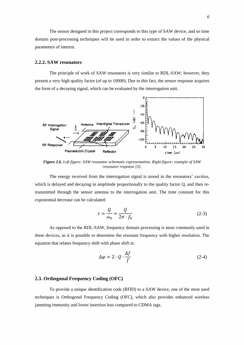
2.2.2. SAW resonators
The principle of work of SAW resonators is very similar to RDL-SAW; however, they
present a very high quality factor (of up to 10000). Due to this fact, the sensor response acquires
the form of a decaying signal, which can be evaluated by the interrogation unit.
Figure 2.6. Left figure: SAW resonator schematic representation. Right figure: example of SAW
resonator response [3].
The energy received from the interrogation signal is stored in the resonators’ cavities,
which is delayed and decaying in amplitude proportionally to the quality factor Q, and then re-
transmitted through the sensor antenna to the interrogation unit. The time constant for this
exponential decrease can be calculated:
𝜏 =𝑄
𝜔0=
𝑄
2𝜋 · 𝑓0 (2-3)
As opposed to the RDL-SAW, frequency domain processing is most commonly used in
these devices, as it is possible to determine the resonant frequency with higher resolution. The
equation that relates frequency shift with phase shift is:
∆𝜑 = 2 · 𝑄 ·∆𝑓
𝑓 (2-4)
2.3. Orthogonal Frequency Coding (OFC)
To provide a unique identification code (RFID) to a SAW device, one of the most used
techniques is Orthogonal Frequency Coding (OFC), which also provides enhanced wireless
jamming immunity and lower insertion loss compared to CDMA tags.
7
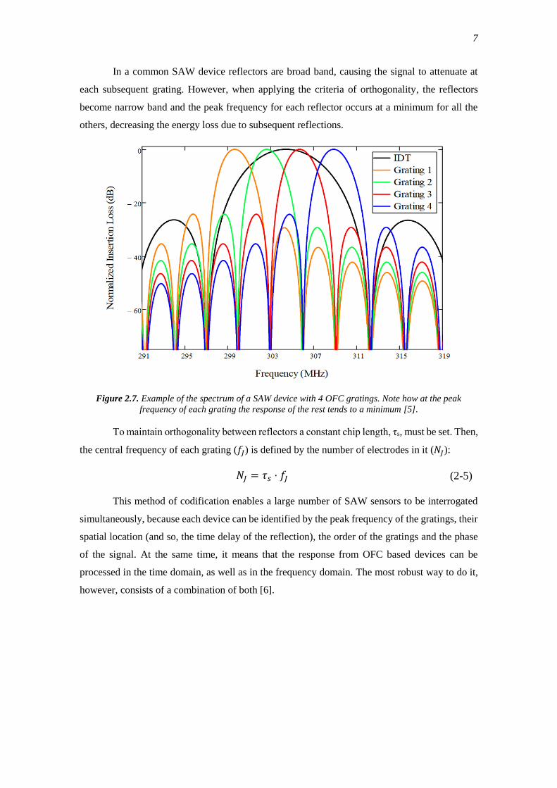
In a common SAW device reflectors are broad band, causing the signal to attenuate at
each subsequent grating. However, when applying the criteria of orthogonality, the reflectors
become narrow band and the peak frequency for each reflector occurs at a minimum for all the
others, decreasing the energy loss due to subsequent reflections.
Figure 2.7. Example of the spectrum of a SAW device with 4 OFC gratings. Note how at the peak
frequency of each grating the response of the rest tends to a minimum [5].
To maintain orthogonality between reflectors a constant chip length, τs, must be set. Then,
the central frequency of each grating (𝑓𝐽) is defined by the number of electrodes in it (𝑁𝐽):
𝑁𝐽 = 𝜏𝑠 · 𝑓𝐽 (2-5)
This method of codification enables a large number of SAW sensors to be interrogated
simultaneously, because each device can be identified by the peak frequency of the gratings, their
spatial location (and so, the time delay of the reflection), the order of the gratings and the phase
of the signal. At the same time, it means that the response from OFC based devices can be
processed in the time domain, as well as in the frequency domain. The most robust way to do it,
however, consists of a combination of both [6].
8
CHAPTER 3: SAW SENSOR DESIGN
In this chapter the design process of the SAW sensor will be explained, detailing the
parameters desired for the device and its most important characteristics, as well as the results of
the simulations conducted in Octave. AutoCAD has been used for the 2D representation of the
device layout.
3.1. Design parameters and simulations
A wafer containing multiple SAW sensors will be fabricated for the purpose of this
project. The parameters desired are the following:
− Central frequency: 435 MHz / 910 MHz
− Substrate material: ST-Quartz
− OFC reflectors implementation
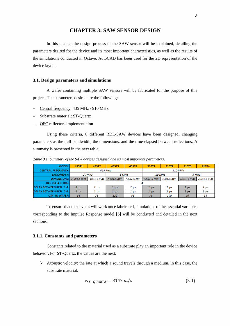
Using these criteria, 8 different RDL-SAW devices have been designed, changing
parameters as the null bandwidth, the dimensions, and the time elapsed between reflections. A
summary is presented in the next table:
Table 3.1. Summary of the SAW devices designed and its most important parameters.
To ensure that the devices will work once fabricated, simulations of the essential variables
corresponding to the Impulse Response model [6] will be conducted and detailed in the next
sections.
3.1.1. Constants and parameters
Constants related to the material used as a substrate play an important role in the device
behavior. For ST-Quartz, the values are the next:
➢ Acoustic velocity: the rate at which a sound travels through a medium, in this case, the
substrate material.
𝑣𝑆𝑇−𝑄𝑈𝐴𝑅𝑇𝑍 = 3147 𝑚/𝑠 (3-1)
9
➢ Piezoelectric coupling coefficient: it defines the ratio of mechanical energy accumulated
in response to an electrical input or vice-versa in a piezoelectric material.
𝑘𝑆𝑇−𝑄𝑈𝐴𝑅𝑇𝑍 = √0.0016 = 0.04 (3-2)
➢ Capacitance per finger pair per unit length: measurement of the capacity present between
two electrodes of the IDT.
𝐶𝑆, 𝑆𝑇−𝑄𝑈𝐴𝑅𝑇𝑍 = 0.503385 · 10−12𝐹
𝑐𝑚 (3-3)
The next parameters listed are related to the design and necessary to be set in order to
simulate the SAW behavior:
➢ Central frequency: frequency at which the IDT / reflectors will be tuned. According to
design parameters:
𝑓0 = 435 𝑀𝐻𝑧 | 910 𝑀𝐻𝑧 (3-4)
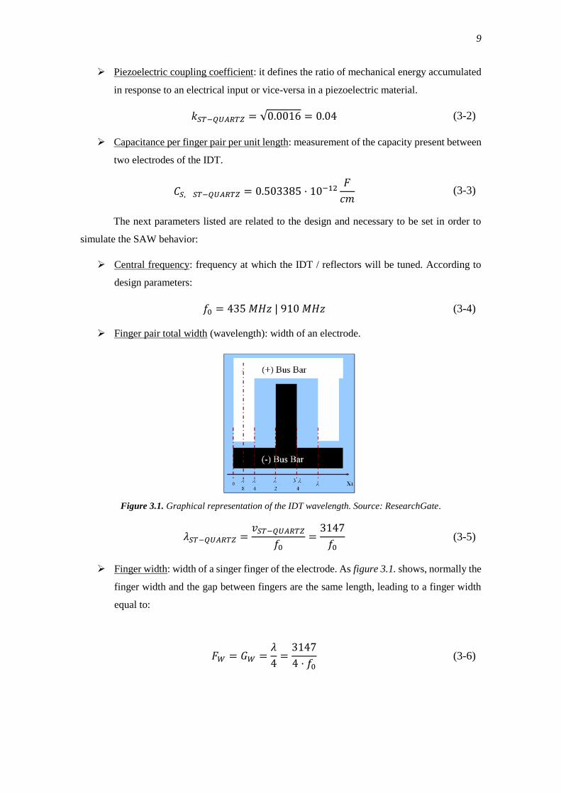
➢ Finger pair total width (wavelength): width of an electrode.
Figure 3.1. Graphical representation of the IDT wavelength. Source: ResearchGate.
𝜆𝑆𝑇−𝑄𝑈𝐴𝑅𝑇𝑍 =𝑣𝑆𝑇−𝑄𝑈𝐴𝑅𝑇𝑍
𝑓0=3147
𝑓0 (3-5)
➢ Finger width: width of a singer finger of the electrode. As figure 3.1. shows, normally the
finger width and the gap between fingers are the same length, leading to a finger width
equal to:
𝐹𝑊 = 𝐺𝑊 =𝜆
4=3147
4 · 𝑓0 (3-6)
10
➢ Null bandwidth: frequency where the first null of the spectral density occurs. It also
represents the width of the main lobe where most of the power of the signal resides. It
has been set by design to:
𝑁𝐵𝑊 = 10 𝑀𝐻𝑧 | 8 𝑀𝐻𝑧 (3-6)
A lower value of null bandwidth has been chosen for making model variations in the
event that the sample rate of the interrogation unit couldn’t perform well under such
bandwidth requirements.
The number of electrodes is also defined by the null bandwidth, like so (note that the
value resulting must be an integer):
𝑁𝑃 = 𝑟𝑜𝑢𝑛𝑑 (2 · 𝑓0𝑁𝐵𝑊
) (3-7)
➢ Signal source impedance: equivalent impedance of the source of the interrogation signal
as seen by the SAW device. The value chosen is the default output impedance for most
electronic equipment:
𝑅𝑖𝑛 = 50 Ω (3-8)
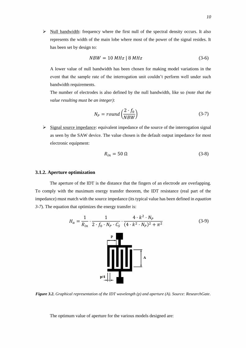
3.1.2. Aperture optimization
The aperture of the IDT is the distance that the fingers of an electrode are overlapping.
To comply with the maximum energy transfer theorem, the IDT resistance (real part of the
impedance) must match with the source impedance (its typical value has been defined in equation
3-7). The equation that optimizes the energy transfer is:
𝐻𝑎 =1
𝑅𝑖𝑛·
1
2 · 𝑓0 · 𝑁𝑃 · 𝐶𝑆·
4 · 𝑘2 · 𝑁𝑃(4 · 𝑘2 · 𝑁𝑃)2 + 𝜋2
(3-9)
Figure 3.2. Graphical representation of the IDT wavelength (p) and aperture (A). Source: ResearchGate.
The optimum value of aperture for the various models designed are:
11
Table 3.2. Optimum aperture value calculated.
3.1.3. Normalized frequency response
The frequency response of a SAW device is its transfer function, which is the ratio of the
output signal over the input, and it is shaped by the sinc function. To simplify the equation, an
auxiliary variable is defined:
𝑋 = 𝑁𝑃 · 𝜋 · (𝑓 − 𝑓0𝑓0
) (3-10)
𝐻(𝑓) = |4 · 𝑘2 · 𝐶𝑆 · 𝑁𝑃2 · (
sin(𝑋)
𝑋)
2
· 𝑒−𝑗·𝑁𝑃𝑓0 | (3-11)
To normalize it:
𝐻𝑛(𝑓) = 20 · log (𝐻(𝑓)) (3-12)
The normalized frequency response is a function of the central frequency at which the
IDT / reflector is tuned and of its bandwidth. The graphical representation of this parameter will
be presented in section 3.1.6., along with the frequency response of the OFC reflectors designed.
3.1.4. Normalized radiation conductance
The radiation conductance is the real part of the admittance. It presents a maximum at the
synchronous frequency f0, and it is normalized by dividing it by its value at its synchronous
frequency:
𝐺𝑎(𝑓) = 8 · 𝑘2 · 𝐶𝑆 · 𝐻𝑎 · 𝑁𝑃
2 · |𝑠𝑖𝑛𝑐(𝑋)|2 (3-13)
𝐺𝑛(𝑓) =𝐺𝑎(𝑓)
𝐺𝑎(𝑓0)
(3-14)
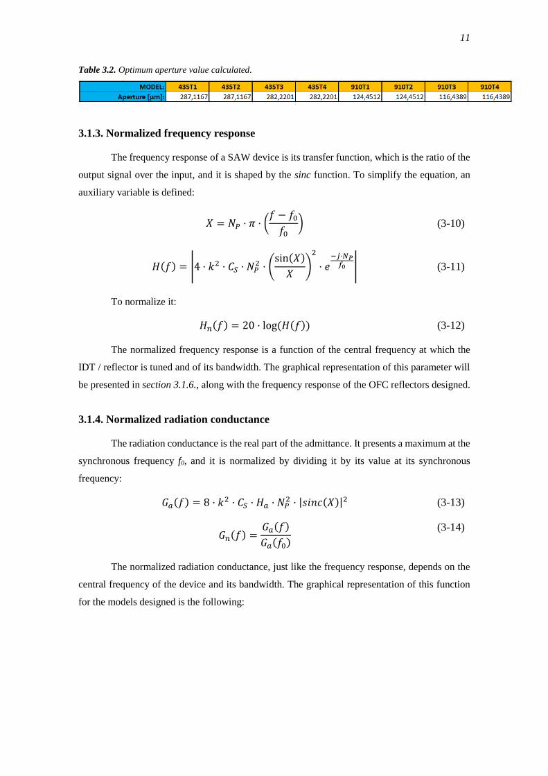
The normalized radiation conductance, just like the frequency response, depends on the
central frequency of the device and its bandwidth. The graphical representation of this function
for the models designed is the following:
12
Figure 3.3. Graphical representation of normalized radiation conductance; f0 = 435 MHz,
BW = 10 MHz (models 435T1 and 435T2).
Figure 3.4. Graphical representation of normalized radiation conductance; f0 = 435 MHz, BW = 8 MHz
(models 435T3 and 435T4).
13
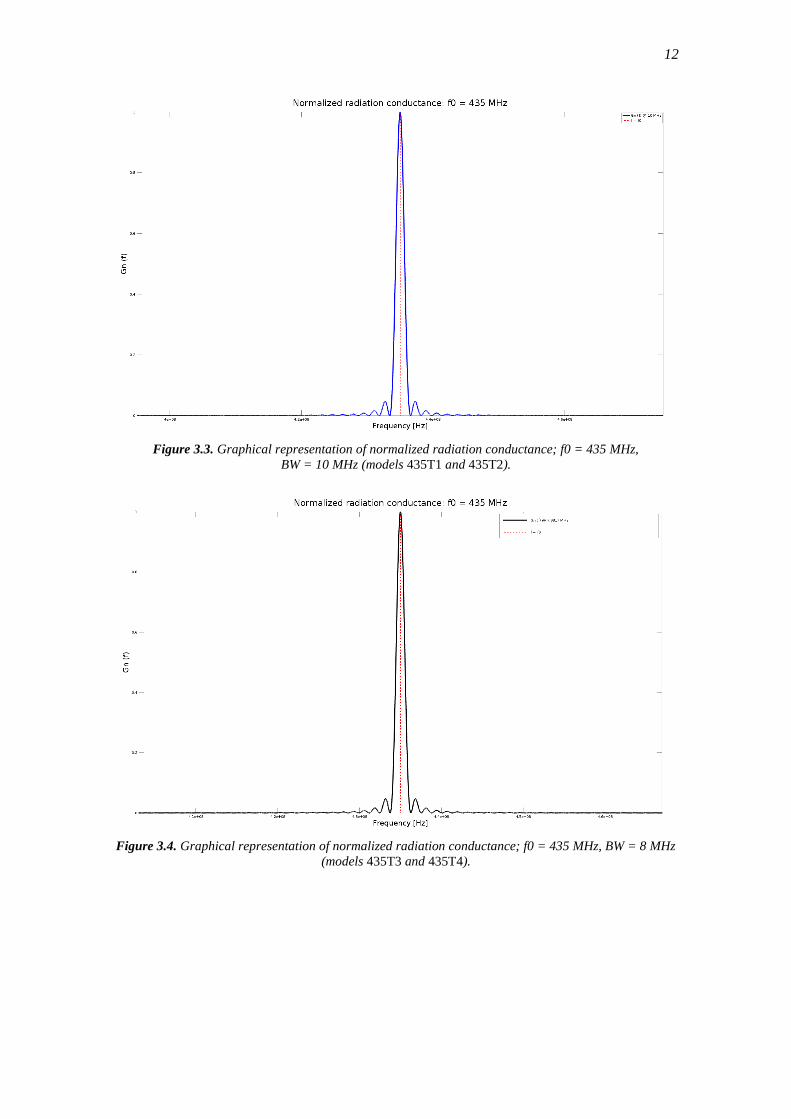
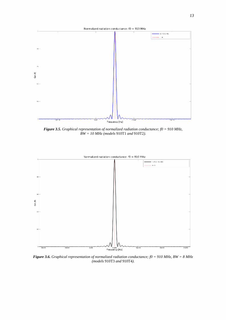
Figure 3.5. Graphical representation of normalized radiation conductance; f0 = 910 MHz,
BW = 10 MHz (models 910T1 and 910T2).
Figure 3.6. Graphical representation of normalized radiation conductance; f0 = 910 MHz, BW = 8 MHz
(models 910T3 and 910T4).
14
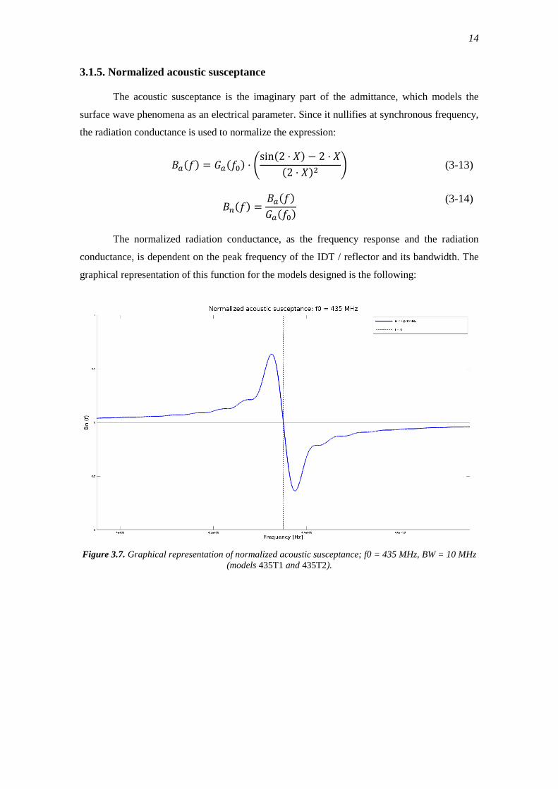
3.1.5. Normalized acoustic susceptance
The acoustic susceptance is the imaginary part of the admittance, which models the
surface wave phenomena as an electrical parameter. Since it nullifies at synchronous frequency,
the radiation conductance is used to normalize the expression:
𝐵𝑎(𝑓) = 𝐺𝑎(𝑓0) · (sin(2 · 𝑋) − 2 · 𝑋
(2 · 𝑋)2) (3-13)
𝐵𝑛(𝑓) =𝐵𝑎(𝑓)
𝐺𝑎(𝑓0)
(3-14)
The normalized radiation conductance, as the frequency response and the radiation
conductance, is dependent on the peak frequency of the IDT / reflector and its bandwidth. The
graphical representation of this function for the models designed is the following:
Figure 3.7. Graphical representation of normalized acoustic susceptance; f0 = 435 MHz, BW = 10 MHz
(models 435T1 and 435T2).
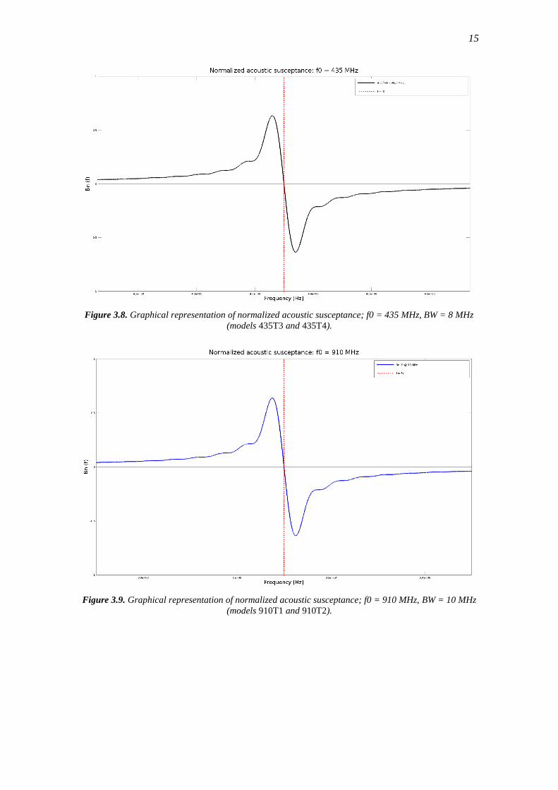
15
Figure 3.8. Graphical representation of normalized acoustic susceptance; f0 = 435 MHz, BW = 8 MHz
(models 435T3 and 435T4).
Figure 3.9. Graphical representation of normalized acoustic susceptance; f0 = 910 MHz, BW = 10 MHz
(models 910T1 and 910T2).
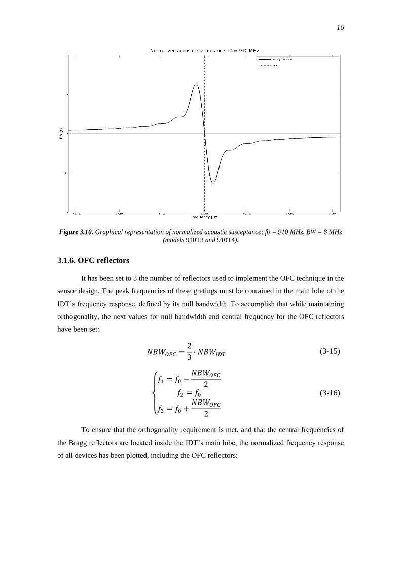
16
Figure 3.10. Graphical representation of normalized acoustic susceptance; f0 = 910 MHz, BW = 8 MHz
(models 910T3 and 910T4).
3.1.6. OFC reflectors
It has been set to 3 the number of reflectors used to implement the OFC technique in the
sensor design. The peak frequencies of these gratings must be contained in the main lobe of the
IDT’s frequency response, defined by its null bandwidth. To accomplish that while maintaining
orthogonality, the next values for null bandwidth and central frequency for the OFC reflectors
have been set:
𝑁𝐵𝑊𝑂𝐹𝐶 =2
3· 𝑁𝐵𝑊𝐼𝐷𝑇 (3-15)
{
𝑓1 = 𝑓0 −
𝑁𝐵𝑊𝑂𝐹𝐶
2𝑓2 = 𝑓0
𝑓3 = 𝑓0 +𝑁𝐵𝑊𝑂𝐹𝐶
2
(3-16)
To ensure that the orthogonality requirement is met, and that the central frequencies of
the Bragg reflectors are located inside the IDT’s main lobe, the normalized frequency response
of all devices has been plotted, including the OFC reflectors:
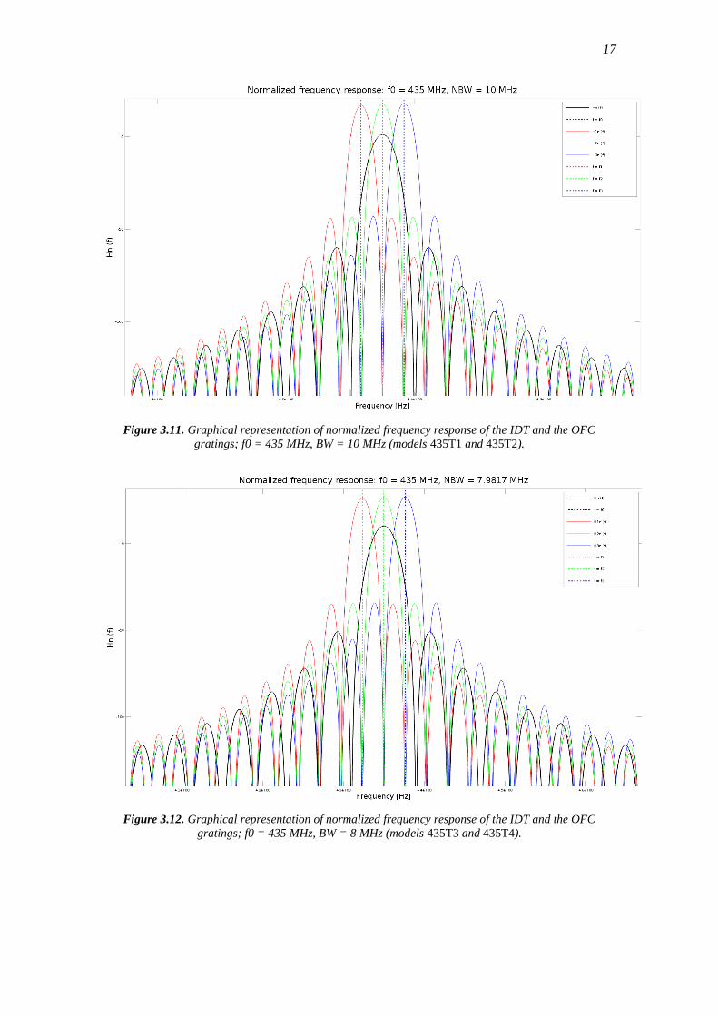
17
Figure 3.11. Graphical representation of normalized frequency response of the IDT and the OFC
gratings; f0 = 435 MHz, BW = 10 MHz (models 435T1 and 435T2).
Figure 3.12. Graphical representation of normalized frequency response of the IDT and the OFC
gratings; f0 = 435 MHz, BW = 8 MHz (models 435T3 and 435T4).
18
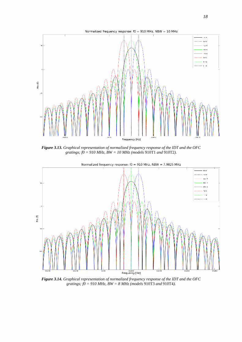
Figure 3.13. Graphical representation of normalized frequency response of the IDT and the OFC
gratings; f0 = 910 MHz, BW = 10 MHz (models 910T1 and 910T2).
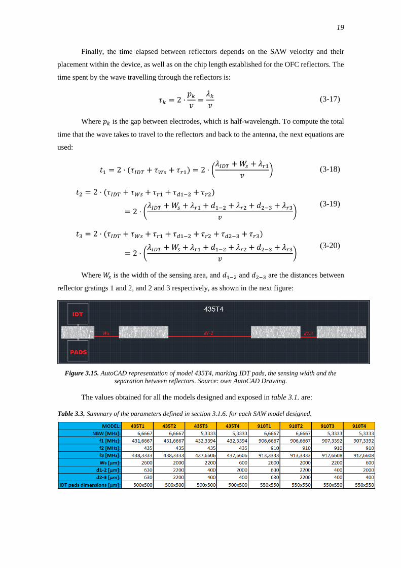
Figure 3.14. Graphical representation of normalized frequency response of the IDT and the OFC
gratings; f0 = 910 MHz, BW = 8 MHz (models 910T3 and 910T4).
19
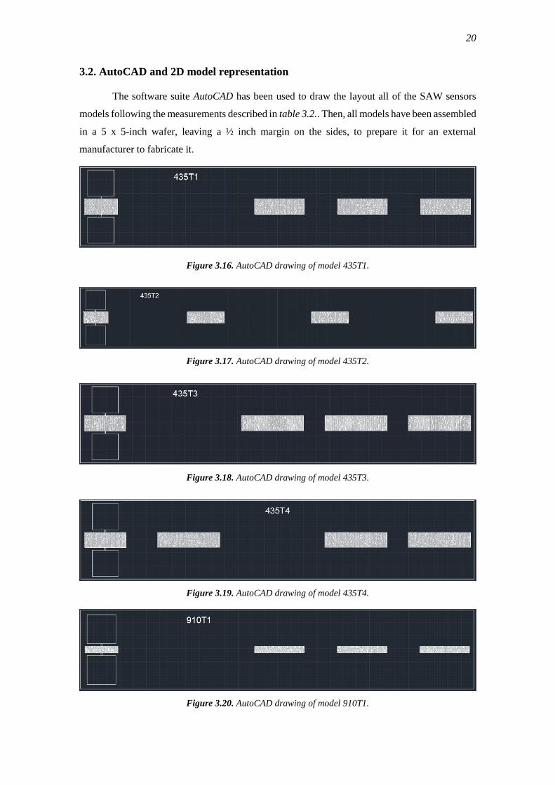
Finally, the time elapsed between reflectors depends on the SAW velocity and their
placement within the device, as well as on the chip length established for the OFC reflectors. The
time spent by the wave travelling through the reflectors is:
𝜏𝑘 = 2 ·𝑝𝑘𝑣=𝜆𝑘𝑣
(3-17)
Where 𝑝𝑘 is the gap between electrodes, which is half-wavelength. To compute the total
time that the wave takes to travel to the reflectors and back to the antenna, the next equations are
used:
𝑡1 = 2 · (𝜏𝐼𝐷𝑇 + 𝜏𝑊𝑠 + 𝜏𝑟1) = 2 · (𝜆𝐼𝐷𝑇 +𝑊𝑠 + 𝜆𝑟1
𝑣) (3-18)
𝑡2 = 2 · (𝜏𝐼𝐷𝑇 + 𝜏𝑊𝑠 + 𝜏𝑟1 + 𝜏𝑑1−2 + 𝜏𝑟2)
= 2 · (𝜆𝐼𝐷𝑇 +𝑊𝑠 + 𝜆𝑟1 + 𝑑1−2 + 𝜆𝑟2 + 𝑑2−3 + 𝜆𝑟3
𝑣)
(3-19)
𝑡3 = 2 · (𝜏𝐼𝐷𝑇 + 𝜏𝑊𝑠 + 𝜏𝑟1 + 𝜏𝑑1−2 + 𝜏𝑟2 + 𝜏𝑑2−3 + 𝜏𝑟3)
= 2 · (𝜆𝐼𝐷𝑇 +𝑊𝑠 + 𝜆𝑟1 + 𝑑1−2 + 𝜆𝑟2 + 𝑑2−3 + 𝜆𝑟3
𝑣)
(3-20)
Where 𝑊𝑠 is the width of the sensing area, and 𝑑1−2 and 𝑑2−3 are the distances between
reflector gratings 1 and 2, and 2 and 3 respectively, as shown in the next figure:
Figure 3.15. AutoCAD representation of model 435T4, marking IDT pads, the sensing width and the
separation between reflectors. Source: own AutoCAD Drawing.
The values obtained for all the models designed and exposed in table 3.1. are:
Table 3.3. Summary of the parameters defined in section 3.1.6. for each SAW model designed.
20
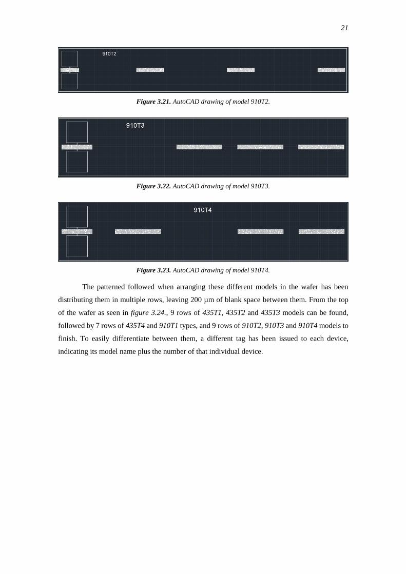
3.2. AutoCAD and 2D model representation
The software suite AutoCAD has been used to draw the layout all of the SAW sensors
models following the measurements described in table 3.2.. Then, all models have been assembled
in a 5 x 5-inch wafer, leaving a ½ inch margin on the sides, to prepare it for an external
manufacturer to fabricate it.
Figure 3.16. AutoCAD drawing of model 435T1.
Figure 3.17. AutoCAD drawing of model 435T2.
Figure 3.18. AutoCAD drawing of model 435T3.
Figure 3.19. AutoCAD drawing of model 435T4.
Figure 3.20. AutoCAD drawing of model 910T1.
21
Figure 3.21. AutoCAD drawing of model 910T2.
Figure 3.22. AutoCAD drawing of model 910T3.
Figure 3.23. AutoCAD drawing of model 910T4.
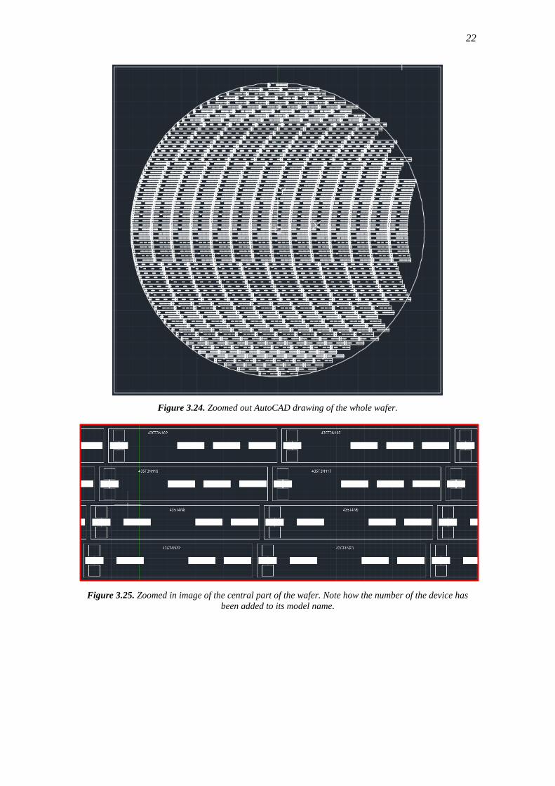
The patterned followed when arranging these different models in the wafer has been
distributing them in multiple rows, leaving 200 µm of blank space between them. From the top
of the wafer as seen in figure 3.24., 9 rows of 435T1, 435T2 and 435T3 models can be found,
followed by 7 rows of 435T4 and 910T1 types, and 9 rows of 910T2, 910T3 and 910T4 models to
finish. To easily differentiate between them, a different tag has been issued to each device,
indicating its model name plus the number of that individual device.
22
Figure 3.24. Zoomed out AutoCAD drawing of the whole wafer.
Figure 3.25. Zoomed in image of the central part of the wafer. Note how the number of the device has
been added to its model name.
23
CHAPTER 4: INTERROGATION UNIT
In this chapter the concept of Software Defined Radio (SDR) is presented, as well as the
software toolkit GNU Radio and its use in programming SDR and signal processing. Then, the
design of the interrogation unit developed for this project will be detailed, including the
transmission and reception modules, the signal post-processing and the novel custom blocks
created to accomplish this task.
4.1. Software Defined Radio (SDR)
A software-defined radio (SDR) is a communication system implemented using software
on a PC or an embedded system, such as an FPGA. Thanks to the evolution in digital electronics,
components that had traditionally been implemented in hardware can now be implemented by
means of software, achieving higher versatility and enabling adaptative techniques that reduce
the interferences to other systems.
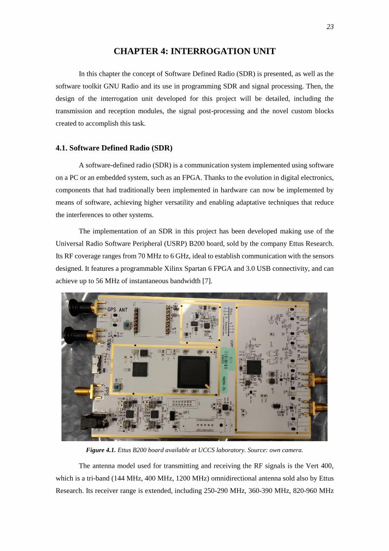
The implementation of an SDR in this project has been developed making use of the
Universal Radio Software Peripheral (USRP) B200 board, sold by the company Ettus Research.
Its RF coverage ranges from 70 MHz to 6 GHz, ideal to establish communication with the sensors
designed. It features a programmable Xilinx Spartan 6 FPGA and 3.0 USB connectivity, and can
achieve up to 56 MHz of instantaneous bandwidth [7].
Figure 4.1. Ettus B200 board available at UCCS laboratory. Source: own camera.
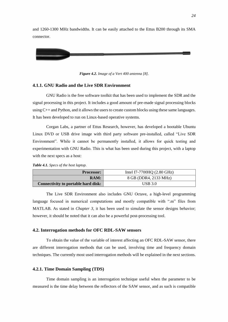
The antenna model used for transmitting and receiving the RF signals is the Vert 400,
which is a tri-band (144 MHz, 400 MHz, 1200 MHz) omnidirectional antenna sold also by Ettus
Research. Its receiver range is extended, including 250-290 MHz, 360-390 MHz, 820-960 MHz
24
and 1260-1300 MHz bandwidths. It can be easily attached to the Ettus B200 through its SMA
connector.
Figure 4.2. Image of a Vert 400 antenna [8].
4.1.1. GNU Radio and the Live SDR Environment
GNU Radio is the free software toolkit that has been used to implement the SDR and the
signal processing in this project. It includes a good amount of pre-made signal processing blocks
using C++ and Python, and it allows the users to create custom blocks using these same languages.
It has been developed to run on Linux-based operative systems.
Corgan Labs, a partner of Ettus Research, however, has developed a bootable Ubuntu
Linux DVD or USB drive image with third party software pre-installed, called “Live SDR
Environment”. While it cannot be permanently installed, it allows for quick testing and
experimentation with GNU Radio. This is what has been used during this project, with a laptop
with the next specs as a host:
Table 4.1. Specs of the host laptop.
Processor: Intel I7-7700HQ (2.80 GHz)
RAM: 8 GB (DDR4, 2133 MHz)
Connectivity to portable hard disk: USB 3.0
The Live SDR Environment also includes GNU Octave, a high-level programming
language focused in numerical computations and mostly compatible with “.m” files from
MATLAB. As stated in Chapter 3, it has been used to simulate the sensor designs behavior;
however, it should be noted that it can also be a powerful post-processing tool.
4.2. Interrogation methods for OFC RDL-SAW sensors
To obtain the value of the variable of interest affecting an OFC RDL-SAW sensor, there
are different interrogation methods that can be used, involving time and frequency domain
techniques. The currently most used interrogation methods will be explained in the next sections.
4.2.1. Time Domain Sampling (TDS)
Time domain sampling is an interrogation technique useful when the parameter to be
measured is the time delay between the reflectors of the SAW sensor, and as such is compatible
25
with RDL-SAW devices. The interrogation signal must cover the whole bandwidth of the sensor
at once, but it decreases with the pulse duration. The next condition must then be met [9]:
𝑡𝑝𝑢𝑙𝑠𝑒 ≤1
2 · 𝐵𝑊𝑠𝑒𝑛𝑠𝑜𝑟 (4-1)
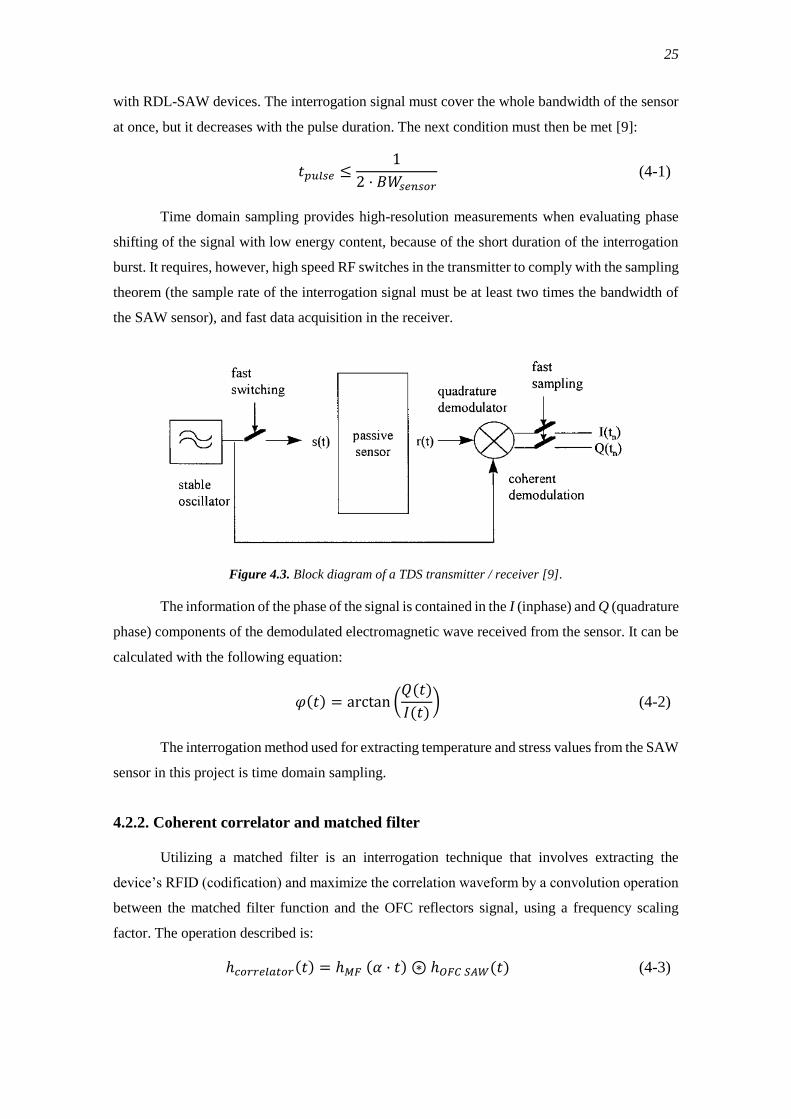
Time domain sampling provides high-resolution measurements when evaluating phase
shifting of the signal with low energy content, because of the short duration of the interrogation
burst. It requires, however, high speed RF switches in the transmitter to comply with the sampling
theorem (the sample rate of the interrogation signal must be at least two times the bandwidth of
the SAW sensor), and fast data acquisition in the receiver.
Figure 4.3. Block diagram of a TDS transmitter / receiver [9].
The information of the phase of the signal is contained in the I (inphase) and Q (quadrature
phase) components of the demodulated electromagnetic wave received from the sensor. It can be
calculated with the following equation:
𝜑(𝑡) = arctan (𝑄(𝑡)
𝐼(𝑡)) (4-2)
The interrogation method used for extracting temperature and stress values from the SAW
sensor in this project is time domain sampling.
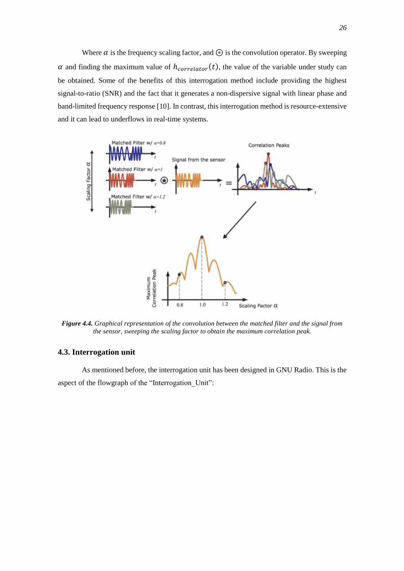
4.2.2. Coherent correlator and matched filter
Utilizing a matched filter is an interrogation technique that involves extracting the
device’s RFID (codification) and maximize the correlation waveform by a convolution operation
between the matched filter function and the OFC reflectors signal, using a frequency scaling
factor. The operation described is:
ℎ𝑐𝑜𝑟𝑟𝑒𝑙𝑎𝑡𝑜𝑟(𝑡) = ℎ𝑀𝐹 (𝛼 · 𝑡) ⊛ ℎ𝑂𝐹𝐶 𝑆𝐴𝑊(𝑡) (4-3)
26
Where 𝛼 is the frequency scaling factor, and ⊛ is the convolution operator. By sweeping
𝛼 and finding the maximum value of ℎ𝑐𝑜𝑟𝑟𝑒𝑙𝑎𝑡𝑜𝑟(𝑡), the value of the variable under study can
be obtained. Some of the benefits of this interrogation method include providing the highest
signal-to-ratio (SNR) and the fact that it generates a non-dispersive signal with linear phase and
band-limited frequency response [10]. In contrast, this interrogation method is resource-extensive
and it can lead to underflows in real-time systems.
Figure 4.4. Graphical representation of the convolution between the matched filter and the signal from
the sensor, sweeping the scaling factor to obtain the maximum correlation peak.
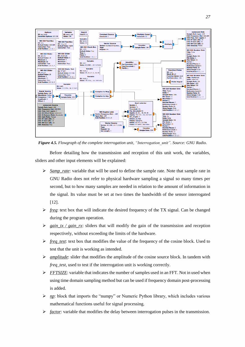
4.3. Interrogation unit
As mentioned before, the interrogation unit has been designed in GNU Radio. This is the
aspect of the flowgraph of the “Interrogation_Unit”:
27
Figure 4.5. Flowgraph of the complete interrogation unit, “Interrogation_unit”. Source: GNU Radio.
Before detailing how the transmission and reception of this unit work, the variables,
sliders and other input elements will be explained:
➢ Samp_rate: variable that will be used to define the sample rate. Note that sample rate in
GNU Radio does not refer to physical hardware sampling a signal so many times per
second, but to how many samples are needed in relation to the amount of information in
the signal. Its value must be set at two times the bandwidth of the sensor interrogated
[12].
➢ freq: text box that will indicate the desired frequency of the TX signal. Can be changed
during the program operation.
➢ gain_tx / gain_rx: sliders that will modify the gain of the transmission and reception
respectively, without exceeding the limits of the hardware.
➢ freq_test: text box that modifies the value of the frequency of the cosine block. Used to
test that the unit is working as intended.
➢ amplitude: slider that modifies the amplitude of the cosine source block. In tandem with
freq_test, used to test if the interrogation unit is working correctly.
➢ FFTSIZE: variable that indicates the number of samples used in an FFT. Not in used when
using time domain sampling method but can be used if frequency domain post-processing
is added.
➢ np: block that imports the “numpy” or Numeric Python library, which includes various
mathematical functions useful for signal processing.
➢ factor: variable that modifies the delay between interrogation pulses in the transmission.
28
➢ TxON: check box that enables or disables the transmission signal by modifying the
transmission gain.
➢ Input_x / Input_y: variables expected to be set by the user. They should correspond to the
results of the tests performed on the SAW sensor that will be interrogated. They are used
to obtain a polynomial equation that fits the sensor’s behavior and discriminate between
the roots of that equation to choose the coherent one.
➢ coefs: variable that contains the coefficients of the polynomial equation that fits the
variable of study evolution with the time delay measured. The value of this variable is
extracted through the “Proc_tests” program, which will be detailed in the sections to
come.
➢ roots: variable that contains the values of the roots of the coefs vector, which are sent to
the “Root_Selector” block through a vector source.
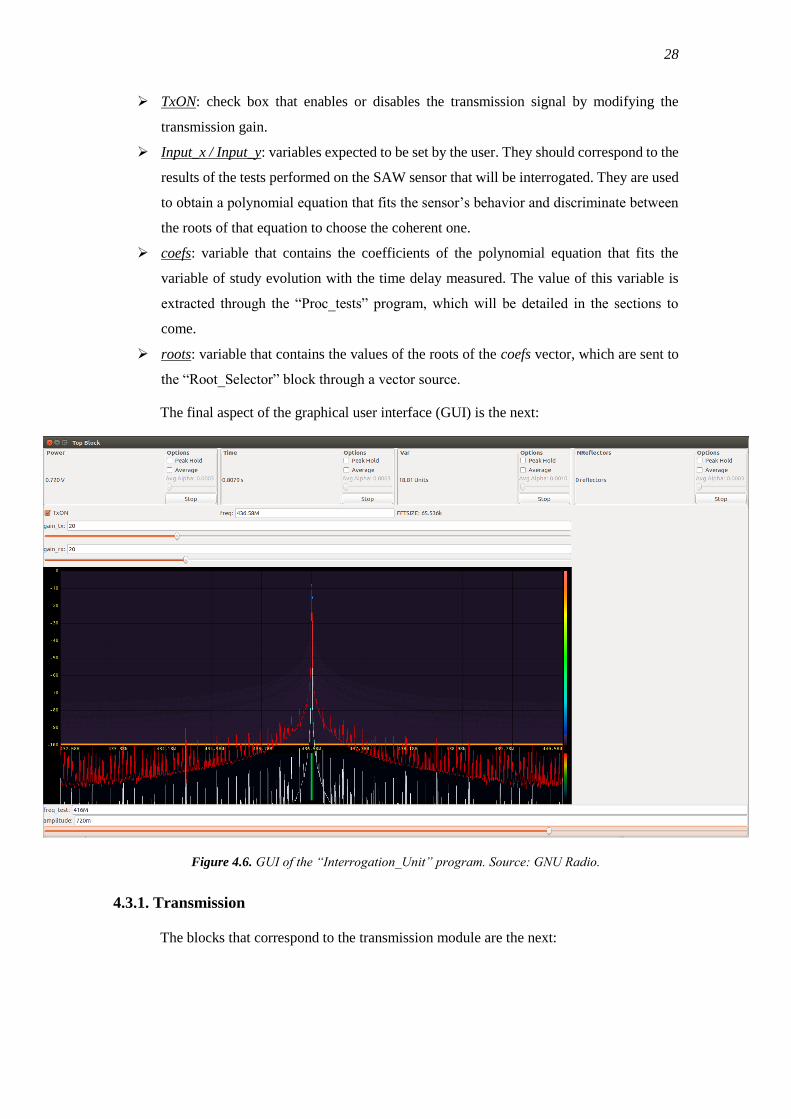
The final aspect of the graphical user interface (GUI) is the next:
Figure 4.6. GUI of the “Interrogation_Unit” program. Source: GNU Radio.
4.3.1. Transmission
The blocks that correspond to the transmission module are the next:
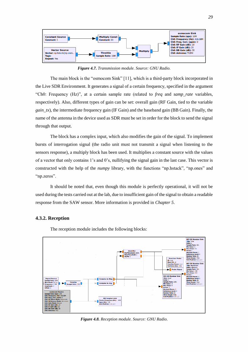
29
Figure 4.7. Transmission module. Source: GNU Radio.
The main block is the “osmocom Sink” [11], which is a third-party block incorporated in
the Live SDR Environment. It generates a signal of a certain frequency, specified in the argument
“Ch0: Frequency (Hz)”, at a certain sample rate (related to freq and samp_rate variables,
respectively). Also, different types of gain can be set: overall gain (RF Gain, tied to the variable
gain_tx), the intermediate frequency gain (IF Gain) and the baseband gain (BB Gain). Finally, the
name of the antenna in the device used as SDR must be set in order for the block to send the signal
through that output.
The block has a complex input, which also modifies the gain of the signal. To implement
bursts of interrogation signal (the radio unit must not transmit a signal when listening to the
sensors response), a multiply block has been used. It multiplies a constant source with the values
of a vector that only contains 1’s and 0’s, nullifying the signal gain in the last case. This vector is
constructed with the help of the numpy library, with the functions “np.hstack”, “np.ones” and
“np.zeros”.
It should be noted that, even though this module is perfectly operational, it will not be
used during the tests carried out at the lab, due to insufficient gain of the signal to obtain a readable
response from the SAW sensor. More information is provided in Chapter 5.
4.3.2. Reception
The reception module includes the following blocks:
Figure 4.8. Reception module. Source: GNU Radio.
30
The signal comes from two possible sources: a signal source block with a cosinus
function, used when testing the unit, or an “osmocom Source” block. Just like the sink block, this
third-party block enables the user to set a sample rate and a central frequency to the signal received
(it automatically applies a filter based on the values of these both variables, even though the
bandwidth of said filter can be set by the user), as well as the gain values for the reception. The
received signal is then plotted using the “WX fosfor sink” block, as shown in figure 4.6.
Then, the magnitude and phase of the samples are calculated by using the “Complex to
Mag” and “Complex to Arg” blocks respectively. The amplitude of the signal is shown in a
number sink, and sent to the “Identifier” block with the phase.
“Identifier” is a custom block that interprets the signal received from the sensor. When
its power goes over the “PwrThreshold” argument, the block understands that a transmission is
starting. As soon as the power decreases below that threshold, the time and phase are saved to
make future differential measurement. From that point onwards, when the reception signal
exceeds the threshold, the block will understand it as a reflection from the SAW sensor, increasing
the “nreflectors” count and calculating the time delay / phase shift since the last peak. The block
also measures the time passed since the last peak at the end of every cycle; when this value
exceeds the “TimeThreshold” arguments, the block will understand that the transmission has
finished, outputting the differential measurements and preparing for the next interrogation.
These measurements are then read by a “Probe signal”, which converts the stream into a
variable that can be accessed by other blocks. It will be sent to the coefs variable, so that the roots
of the polynomial equation can be calculated according to the time delay measured. It will also
be shown in a number sink, along with the number of reflectors counted by the block. Lastly, it is
also connected to the “Root_Selector” block, which is part of the post-processing module, covered
in the next section.
The “TD/FD” argument of the block sets the “Time Domain / Frequency Domain”
configuration with the values “1 / 0” respectively. In this project, it will be set to “Time Domain”;
however, it can be used in future work for frequency domain processing too.
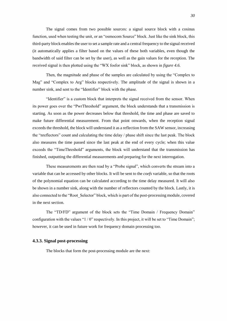
4.3.3. Signal post-processing
The blocks that form the post-processing module are the next:
31
Figure 4.9. Post-processing module. Source: GNU Radio.
The transformation of the time delay reading to the value of the variable of interest is
done through a polynomial equation, previously fitted to the data obtained in the tests conducted
on the sensor of interest. The type of equation to be solved is as follows:
𝑣𝑎𝑟 (𝑡) = 𝑐𝑜𝑒𝑓𝑠𝑛 · 𝑡𝑛 + 𝑐𝑜𝑒𝑓𝑠𝑛−1 · 𝑡
𝑛−1+ . . . + 𝑐𝑜𝑒𝑓𝑠1 · 𝑡 + 𝑐𝑜𝑒𝑓𝑠0 − 𝑟𝑒𝑎𝑑 (4-4)
Where coefsn are the values on the coefs vector and read is the output of the “Identifier”
block, read by the “Probe signal” block. The order of this polynomial is unknown, since the user
can choose it when using the “Proc_tests” program, and for this reason the roots of the equation
can be multiple.
The main block of this module is the “Root_Selector”, a custom block, and its function is
to choose most coherent root of the polynomial equation. It has two inputs: the first one is
connected to a vector source that feeds the block with the roots; the second one is connected to
the “Identifier” block, which sends the differential time measurements.
First of all, through the “Varmin” and “Varmax” arguments, the block eliminates the roots
that are out of the range of the physical variable of study, that is, smaller than “Varmin” or bigger
that “Varmax”. Then, making use of the “Input_x” and “Input_y” arguments, which contain the
data from the tests performed on the sensor, the code checks if the current reading is close to a
point from the test (subtracting its value to the input values and checking if it is under the
“Var_threshold” argument). If it is the case, and the change of the variable of study since the last
output doesn’t exceed a threshold (set as the 5% of its range, defined by “Varmin” and “Varmax”),
that root will be chosen as the correct one.
If no roots have met the previous conditions, the remaining ones are evaluated, and the
one that minimizes the difference to the last output is selected as the correct one. This criterion is
based in the fact that, in a real-time system, the evolution of the variable of study is expected not
to be chaotic.
32
It should be noted that the block must know the locations of the critical points of the
polynomial equation (“Xmaxs”, “Ymaxs”, “Xmins” and “Ymins” arguments) to distinguish in
which region of the equation the current reading is. The block supposes a slow-paced, one
direction evolution of the variable; this means that, even though the ‘y’ values at both sides of a
critical point are similar, the block should identify when the variable in study is increasing or
decreasing, in which direction it is evolving.
This is done by checking the proximity of the current reading to the critical points of the
equation using the “Var_threshold”. When the reading is approaching a maximum and the ‘y’
value, that was increasing, now starts decreasing, the block should identify that it has “crossed”
to the other side of the maximum. Similarly, when the reading is approaching a minimum and the
‘y’ value, that was decreasing, now starts increasing, the block should identify that it has
“crossed” to the other side of the minimum.
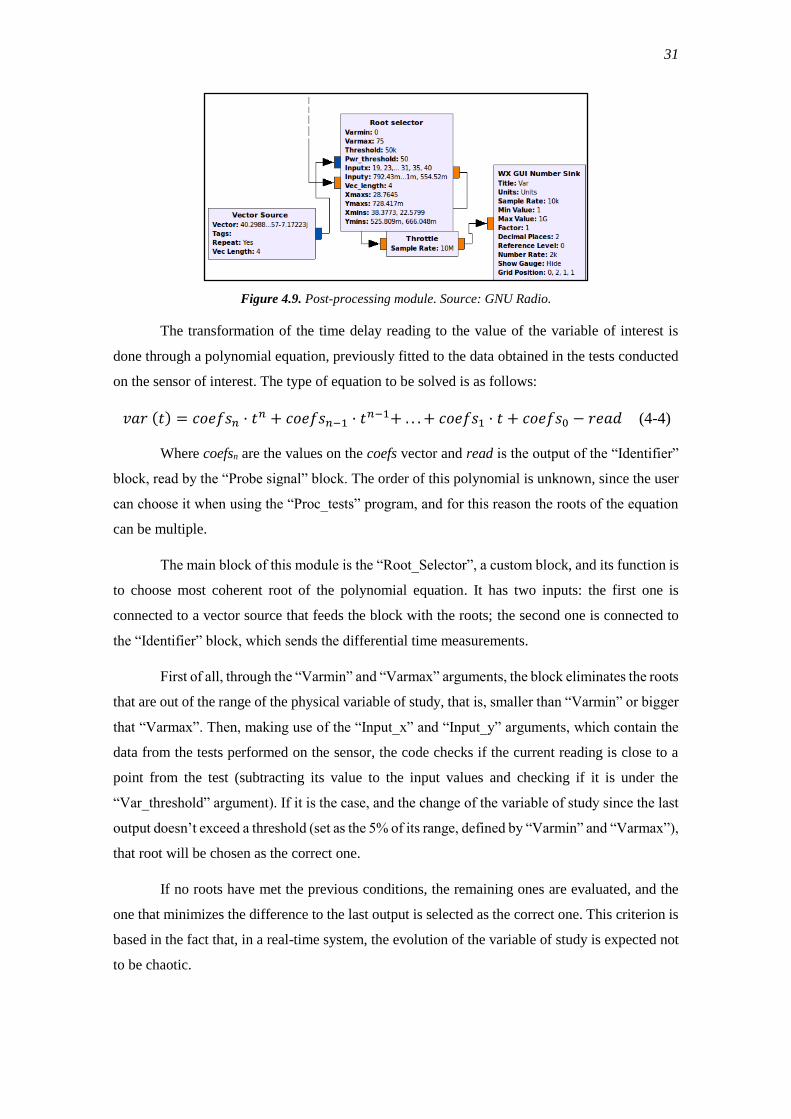
4.4. Processing tests results on the sensor
To make the interrogation unit be able to extract the value of the variable of interest, the
sensor must be characterized. Tests must be conducted to obtain the relation between the time
delay variation and the variable of study, in order to trace a fitting polynomial equation. An extra
program has been developed in GNU Radio to accomplish this task.
Figure 4.10. GUI of the “Proc_tests” program. Source: GNU Radio.
The “Proc_tests” program enables the user to calculate the coefficients of the polynomial
equation that will characterize the sensor’s behavior, choosing the desired order (between 1 and
33
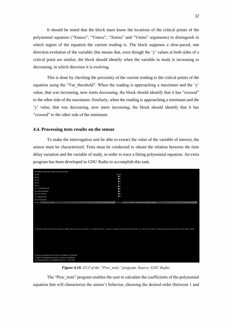
9). It will also point out its critical points, as well as their coordinates. For this task, the numpy
and Polynomial libraries are imported.
Figure 4.11. Flowgraph of the “Proc_tests” program. Source: GNU Radio.
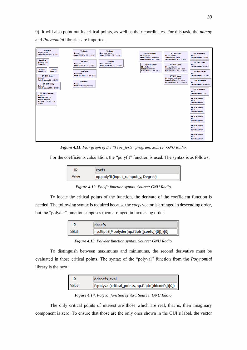
For the coefficients calculation, the “polyfit” function is used. The syntax is as follows:
Figure 4.12. Polyfit function syntax. Source: GNU Radio.
To locate the critical points of the function, the derivate of the coefficient function is
needed. The following syntax is required because the coefs vector is arranged in descending order,
but the “polyder” function supposes them arranged in increasing order.
Figure 4.13. Polyder function syntax. Source: GNU Radio.
To distinguish between maximums and minimums, the second derivative must be
evaluated in those critical points. The syntax of the “polyval” function from the Polynomial
library is the next:
Figure 4.14. Polyval function syntax. Source: GNU Radio.
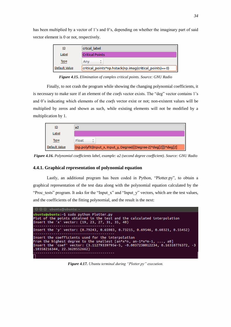
The only critical points of interest are those which are real, that is, their imaginary
component is zero. To ensure that those are the only ones shown in the GUI’s label, the vector
34
has been multiplied by a vector of 1’s and 0’s, depending on whether the imaginary part of said
vector element is 0 or not, respectively.
Figure 4.15. Elimination of complex critical points. Source: GNU Radio
Finally, to not crash the program while showing the changing polynomial coefficients, it
is necessary to make sure if an element of the coefs vector exists. The “deg” vector contains 1’s
and 0’s indicating which elements of the coefs vector exist or not; non-existent values will be
multiplied by zeros and shown as such, while existing elements will not be modified by a
multiplication by 1.
Figure 4.16. Polynomial coefficients label, example: a2 (second degree coefficient). Source: GNU Radio
4.4.1. Graphical representation of polynomial equation
Lastly, an additional program has been coded in Python, “Plotter.py”, to obtain a
graphical representation of the test data along with the polynomial equation calculated by the
“Proc_tests” program. It asks for the “Input_x” and “Input_y” vectors, which are the test values,
and the coefficients of the fitting polynomial, and the result is the next:
Figure 4.17. Ubuntu terminal during “Plotter.py” execution.
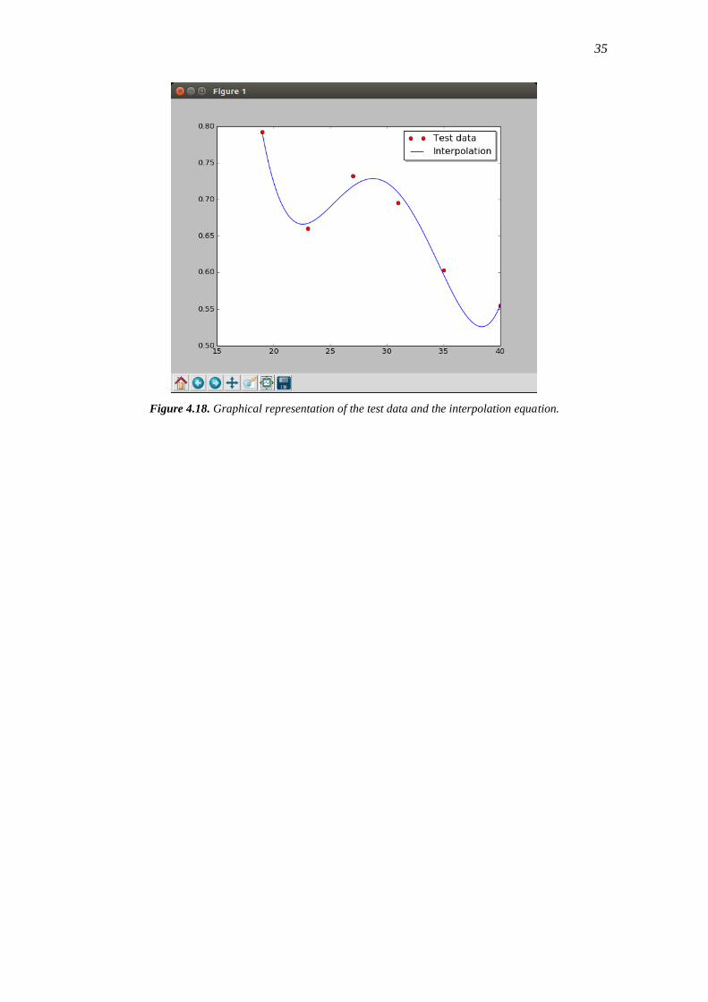
35
Figure 4.18. Graphical representation of the test data and the interpolation equation.
36
CHAPTER 5: TESTS AND RESULTS
In this chapter, the equipment used and the methodology followed in the SAW device and
interrogation unit testing will be described. The data extracted will be presented, as well as the
result of the polynomial interpolation fitting the device behavior.
5.1. Equipment
In order to get the interrogation unit running, the equipment used is the one that has been
presented in Chapter 4: an Ettus B200 board, with a Vert400 antenna attached to enable data
communication. The software-defined radio has been programmed with a host laptop running a
bootable image of Ubuntu, “Live SDR Environment”, using GNU Radio toolkit.
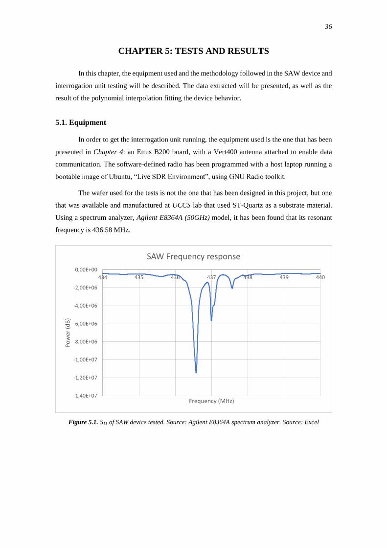
The wafer used for the tests is not the one that has been designed in this project, but one
that was available and manufactured at UCCS lab that used ST-Quartz as a substrate material.
Using a spectrum analyzer, Agilent E8364A (50GHz) model, it has been found that its resonant
frequency is 436.58 MHz.
Figure 5.1. S11 of SAW device tested. Source: Agilent E8364A spectrum analyzer. Source: Excel
-1,40E+07
-1,20E+07
-1,00E+07
-8,00E+06
-6,00E+06
-4,00E+06
-2,00E+06
0,00E+00
434 435 436 437 438 439 440
Po
wer
(d
B)
Frequency (MHz)
SAW Frequency response
37
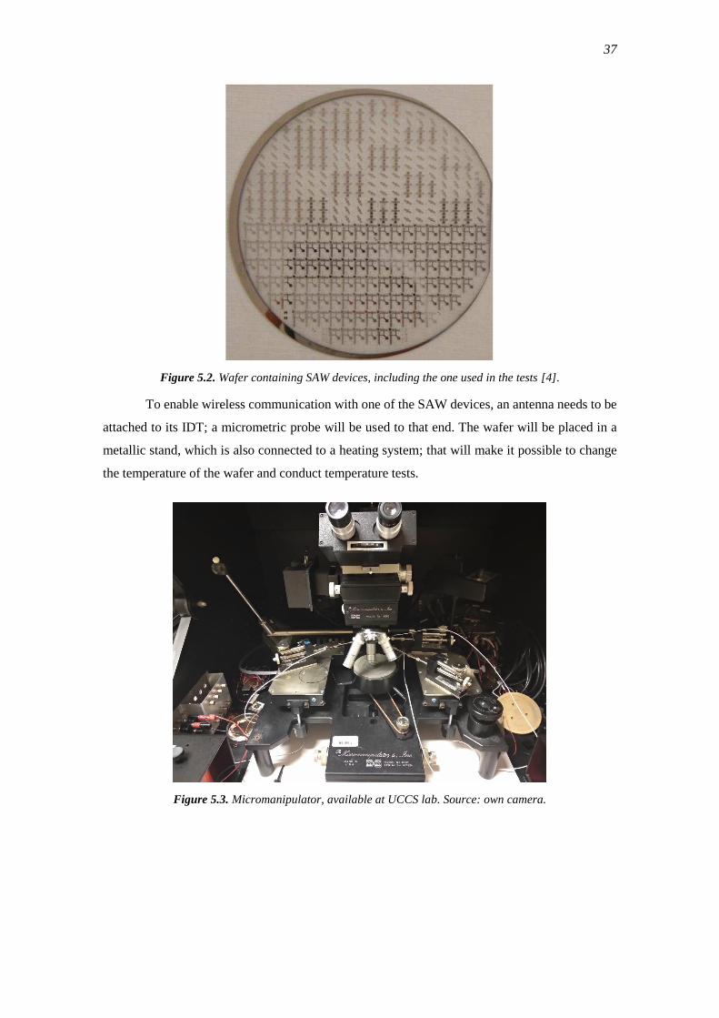
Figure 5.2. Wafer containing SAW devices, including the one used in the tests [4].
To enable wireless communication with one of the SAW devices, an antenna needs to be
attached to its IDT; a micrometric probe will be used to that end. The wafer will be placed in a
metallic stand, which is also connected to a heating system; that will make it possible to change
the temperature of the wafer and conduct temperature tests.
Figure 5.3. Micromanipulator, available at UCCS lab. Source: own camera.
38
Figure 5.4. Heating system connected to the micromanipulator’s stand. Source: own camera.
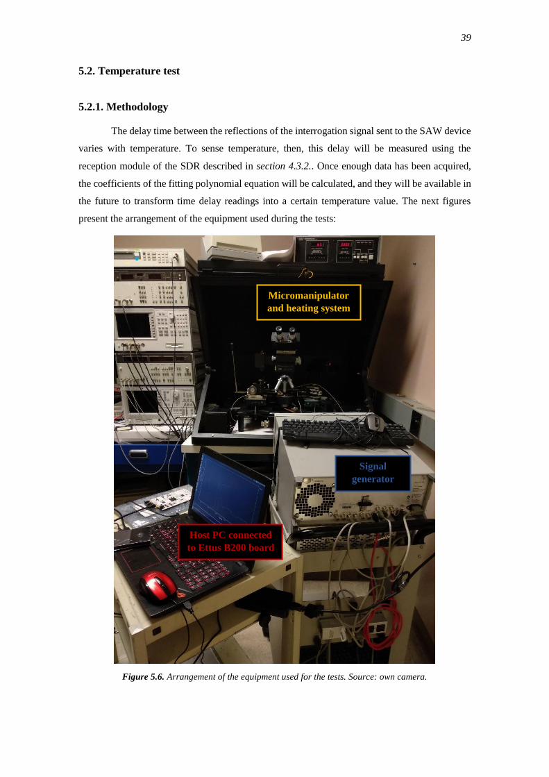
Finally, as mentioned in early chapters, the power output of the Ettus B200 for the
transmission signal is not high enough to receive a readable response from the SAW sensor. For
that reason, a signal generator Agilent E8257D has been used for the interrogation signal.
Figure 5.5. Agilent E8257D signal generator. Source: own camera.
TX Antenna
(Vert400)
39
5.2. Temperature test
5.2.1. Methodology
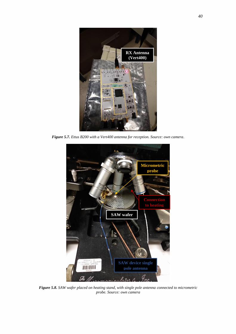
The delay time between the reflections of the interrogation signal sent to the SAW device
varies with temperature. To sense temperature, then, this delay will be measured using the
reception module of the SDR described in section 4.3.2.. Once enough data has been acquired,
the coefficients of the fitting polynomial equation will be calculated, and they will be available in
the future to transform time delay readings into a certain temperature value. The next figures
present the arrangement of the equipment used during the tests:
Figure 5.6. Arrangement of the equipment used for the tests. Source: own camera.
Host PC connected
to Ettus B200 board
Signal
generator
Micromanipulator
and heating system
40
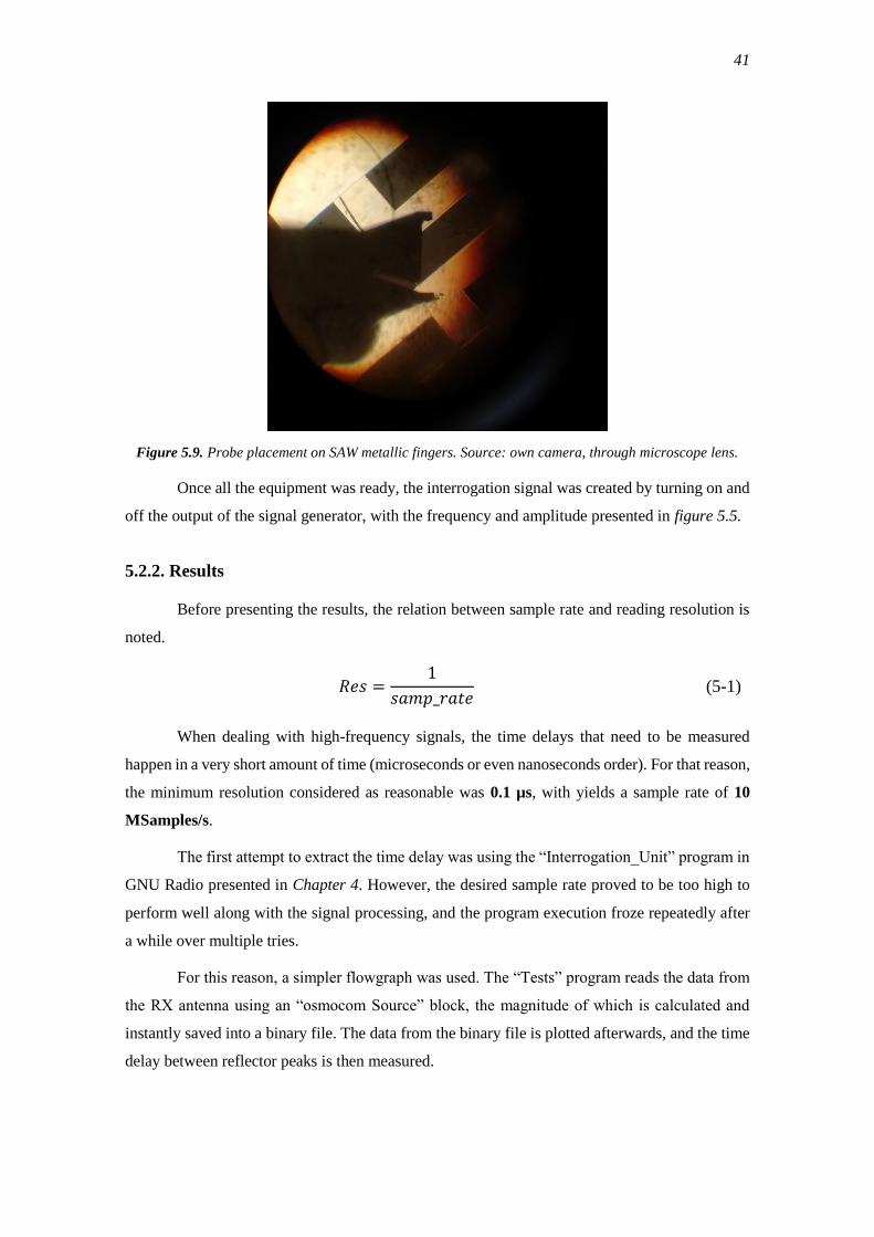
Figure 5.7. Ettus B200 with a Vert400 antenna for reception. Source: own camera.
Figure 5.8. SAW wafer placed on heating stand, with single pole antenna connected to micrometric
probe. Source: own camera
RX Antenna
(Vert400)
SAW device single
pole antenna
SAW wafer
Micrometric
probe
Connection
to heating
41
Figure 5.9. Probe placement on SAW metallic fingers. Source: own camera, through microscope lens.
Once all the equipment was ready, the interrogation signal was created by turning on and
off the output of the signal generator, with the frequency and amplitude presented in figure 5.5.
5.2.2. Results
Before presenting the results, the relation between sample rate and reading resolution is
noted.
𝑅𝑒𝑠 =1
𝑠𝑎𝑚𝑝_𝑟𝑎𝑡𝑒 (5-1)
When dealing with high-frequency signals, the time delays that need to be measured
happen in a very short amount of time (microseconds or even nanoseconds order). For that reason,
the minimum resolution considered as reasonable was 0.1 µs, with yields a sample rate of 10
MSamples/s.
The first attempt to extract the time delay was using the “Interrogation_Unit” program in
GNU Radio presented in Chapter 4. However, the desired sample rate proved to be too high to
perform well along with the signal processing, and the program execution froze repeatedly after
a while over multiple tries.
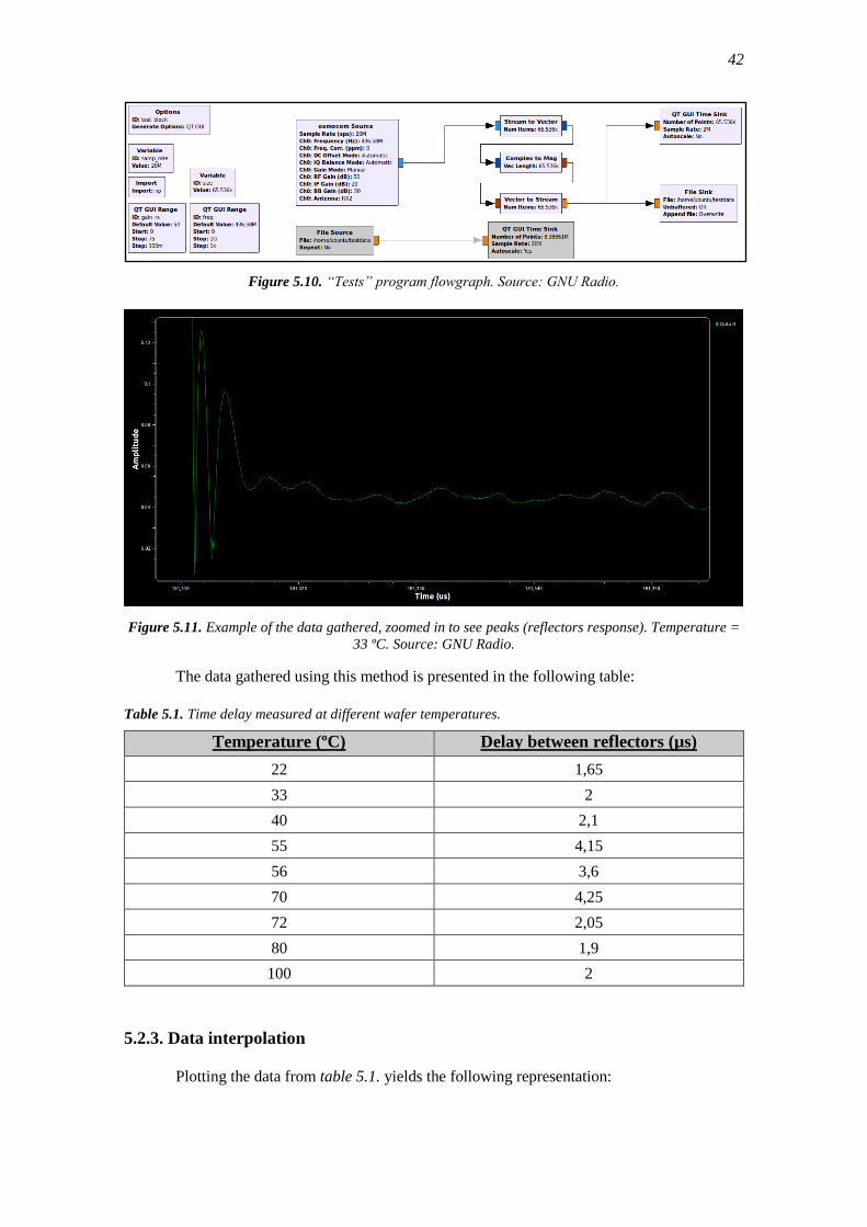
For this reason, a simpler flowgraph was used. The “Tests” program reads the data from
the RX antenna using an “osmocom Source” block, the magnitude of which is calculated and
instantly saved into a binary file. The data from the binary file is plotted afterwards, and the time
delay between reflector peaks is then measured.
42
Figure 5.10. “Tests” program flowgraph. Source: GNU Radio.
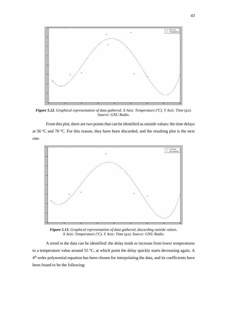
Figure 5.11. Example of the data gathered, zoomed in to see peaks (reflectors response). Temperature =
33 ºC. Source: GNU Radio.
The data gathered using this method is presented in the following table:
Table 5.1. Time delay measured at different wafer temperatures.
Temperature (ºC) Delay between reflectors (µs)
22 1,65
33 2
40 2,1
55 4,15
56 3,6
70 4,25
72 2,05
80 1,9
100 2
5.2.3. Data interpolation
Plotting the data from table 5.1. yields the following representation:
43
Figure 5.12. Graphical representation of data gathered. X Axis: Temperature (ºC). Y Axis: Time (µs).
Source: GNU Radio.
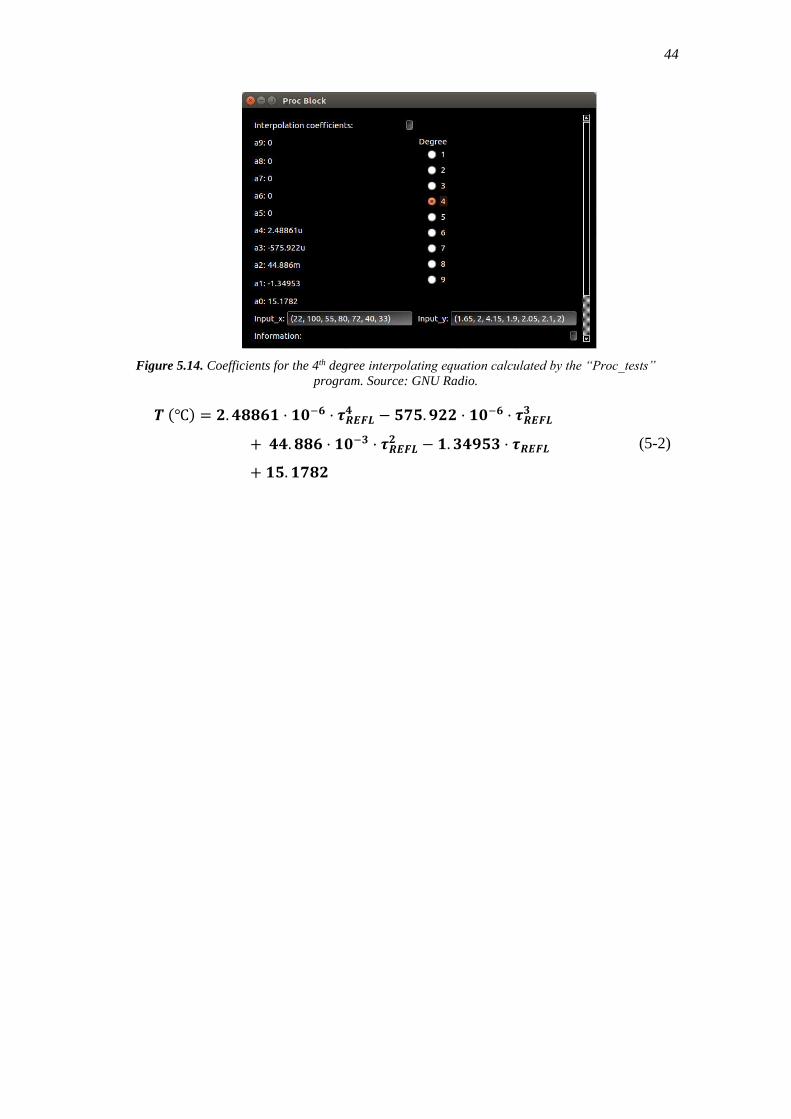
From this plot, there are two points that can be identified as outside values: the time delays
at 56 ºC and 70 ºC. For this reason, they have been discarded, and the resulting plot is the next
one:
Figure 5.13. Graphical representation of data gathered, discarding outside values.
X Axis: Temperature (ºC). Y Axis: Time (µs). Source: GNU Radio.
A trend in the data can be identified: the delay tends to increase from lower temperatures
to a temperature value around 55 ºC, at which point the delay quickly starts decreasing again. A
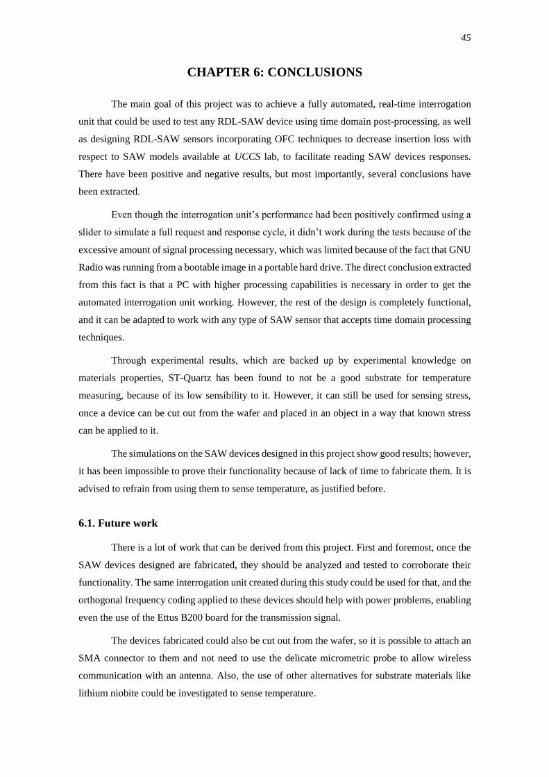
4th order polynomial equation has been chosen for interpolating the data, and its coefficients have
been found to be the following:
44
Figure 5.14. Coefficients for the 4th degree interpolating equation calculated by the “Proc_tests”
program. Source: GNU Radio.
𝑻 (℃) = 𝟐. 𝟒𝟖𝟖𝟔𝟏 · 𝟏𝟎−𝟔 · 𝝉𝑹𝑬𝑭𝑳𝟒 − 𝟓𝟕𝟓. 𝟗𝟐𝟐 · 𝟏𝟎−𝟔 · 𝝉𝑹𝑬𝑭𝑳
𝟑
+ 𝟒𝟒. 𝟖𝟖𝟔 · 𝟏𝟎−𝟑 · 𝝉𝑹𝑬𝑭𝑳𝟐 − 𝟏. 𝟑𝟒𝟗𝟓𝟑 · 𝝉𝑹𝑬𝑭𝑳
+ 𝟏𝟓. 𝟏𝟕𝟖𝟐
(5-2)
45
CHAPTER 6: CONCLUSIONS
The main goal of this project was to achieve a fully automated, real-time interrogation
unit that could be used to test any RDL-SAW device using time domain post-processing, as well
as designing RDL-SAW sensors incorporating OFC techniques to decrease insertion loss with
respect to SAW models available at UCCS lab, to facilitate reading SAW devices responses.
There have been positive and negative results, but most importantly, several conclusions have
been extracted.
Even though the interrogation unit’s performance had been positively confirmed using a
slider to simulate a full request and response cycle, it didn’t work during the tests because of the
excessive amount of signal processing necessary, which was limited because of the fact that GNU
Radio was running from a bootable image in a portable hard drive. The direct conclusion extracted
from this fact is that a PC with higher processing capabilities is necessary in order to get the
automated interrogation unit working. However, the rest of the design is completely functional,
and it can be adapted to work with any type of SAW sensor that accepts time domain processing
techniques.
Through experimental results, which are backed up by experimental knowledge on
materials properties, ST-Quartz has been found to not be a good substrate for temperature
measuring, because of its low sensibility to it. However, it can still be used for sensing stress,
once a device can be cut out from the wafer and placed in an object in a way that known stress
can be applied to it.
The simulations on the SAW devices designed in this project show good results; however,
it has been impossible to prove their functionality because of lack of time to fabricate them. It is
advised to refrain from using them to sense temperature, as justified before.
6.1. Future work
There is a lot of work that can be derived from this project. First and foremost, once the
SAW devices designed are fabricated, they should be analyzed and tested to corroborate their
functionality. The same interrogation unit created during this study could be used for that, and the
orthogonal frequency coding applied to these devices should help with power problems, enabling
even the use of the Ettus B200 board for the transmission signal.
The devices fabricated could also be cut out from the wafer, so it is possible to attach an
SMA connector to them and not need to use the delicate micrometric probe to allow wireless
communication with an antenna. Also, the use of other alternatives for substrate materials like
lithium niobite could be investigated to sense temperature.

46
Frequency domain processing techniques could be studied for the sensors incorporating
OFC reflectors, as they allow both time and frequency domain processing. Their combination is,
in fact, a very robust way to interrogate OFC-based SAW devices, as well as the matched filters
technique briefly described in this paper. A PC with higher processing capability should help with
this more exhaustive processing.
Last, but not least, it could be interesting to go to a lower layer in the interrogation unit
and directly program hardware, the Spartan 6 FPGA that the Ettus board features, so that
completely custom interrogation cycles could be accomplished, using listening windows and
buffers to send data to the PC after a certain number of samples. The measurements would not be
strictly real-time, but that could give the interrogation unit enough time to process the data, even
without a higher-end processor.
47
REFERENCES
[1] James H. “Passive, Wireless SAW OFC Strain Sensor and Software Defined Radio
Interrogator”. University of Central Florida. Summer term, 2016.
[2] Nikolai Y. Kozlovski. “Passive Wireless SAW sensors with new and novel reflector
structures: design and application”. University of Central Florida. Summer term, 2011.
[3] L. Reindl, G. Scholl, T. Ostertag, C.C.W. Ruppel, W. E. Bulst, F. Seifert. “SAW Devices as
Wireless Passive Sensors”. IEEE Electronic Symposium – 363. 1996.
[4] Fran S. Gonzalez. “Software-based interrogation unit and signal post-processing for SAW
temperature sensors for IoT applications”. University of Colorado at Colorado Springs. 2016.
[5] W. C. Wilson, M. D. Rogge, B. Fisher, M. J. Roller, D. M. Malocha, G. M. Atkinson. “SAW
sensor for Fastener Failure Detection”. NASA.
[6] William W. “Multifunctional Orthogonally-Frequency-Coded SAW Strain Sensor”. Virginia
Commonwealth University. 2013.
[7] Ettus Research. “USRP B200 / B210 Bus Series”. Ettus Webpage.
[8] Ettus Research. “Vert 400 Antenna”. Ettus Webpage.
[9] Alfred P. “A Review of Wireless SAW Sensors”. IEEE. March 2000.
[10] Donald C. Malocha, Mark G., Brian F., James H. Daniel G., Nikolai K.. “A Passive
Wireless Multi-Sensor SAW Technology Device and System Perspectives”. Sensors. May
2013.
[11] Osmocom Project. “osmocom GNU Radio Blocks”. Osmocom Webpage.
[12] GNU Radio “FAQ”. GNU Radio Wiki Webpage.
48
APPENDIX
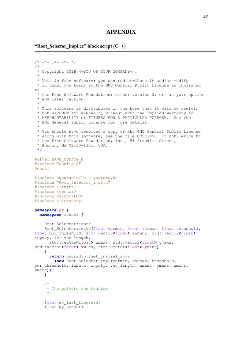
“Root_Selector_impl.cc” block script (C++)
/* -*- c++ -*- */
/*
* Copyright 2018 <+YOU OR YOUR COMPANY+>.
*
* This is free software; you can redistribute it and/or modify
* it under the terms of the GNU General Public License as published
by
* the Free Software Foundation; either version 3, or (at your option)
* any later version.
*
* This software is distributed in the hope that it will be useful,
* but WITHOUT ANY WARRANTY; without even the implied warranty of
* MERCHANTABILITY or FITNESS FOR A PARTICULAR PURPOSE. See the
* GNU General Public License for more details.
*
* You should have received a copy of the GNU General Public License
* along with this software; see the file COPYING. If not, write to
* the Free Software Foundation, Inc., 51 Franklin Street,
* Boston, MA 02110-1301, USA.
*/
#ifdef HAVE_CONFIG_H
#include "config.h"
#endif
#include <gnuradio/io_signature.h>
#include "Root_Selector_impl.h"
#include <limits>
#include <vector>
#include <algorithm>
#include <iterator>
namespace gr {
namespace rtssel {
Root_Selector::sptr
Root_Selector::make(float varmin, float varmax, float threshold,
float pwr_threshold, std::vector<float> inputx, std::vector<float>
inputy, int vec_length,
std::vector<float> xmaxs, std::vector<float> ymaxs,
std::vector<float> xmins, std::vector<float> ymins)
{
return gnuradio::get_initial_sptr
(new Root_Selector_impl(varmin, varmax, threshold,
pwr_threshold, inputx, inputy, vec_length, xmaxs, ymaxs, xmins,
ymins));
}
/*
* The private constructor
*/
float my_last_freqread;
float my_output;
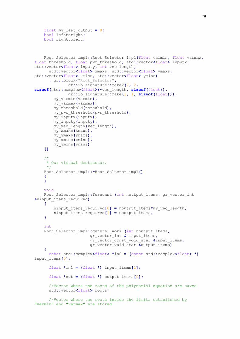
49
float my_last_output = 0;
bool lefttoright;
bool righttoleft;
Root_Selector_impl::Root_Selector_impl(float varmin, float varmax,
float threshold, float pwr_threshold, std::vector<float> inputx,
std::vector<float> inputy, int vec_length,
std::vector<float> xmaxs, std::vector<float> ymaxs,
std::vector<float> xmins, std::vector<float> ymins)
: gr::block("Root_Selector",
gr::io_signature::make2(2, 2,
sizeof(std::complex<float>)*vec_length, sizeof(float)),
gr::io_signature::make(1, 1, sizeof(float))),
my_varmin(varmin),
my_varmax(varmax),
my_threshold(threshold),
my_pwr_threshold(pwr_threshold),
my_inputx(inputx),
my_inputy(inputy),
my_vec_length(vec_length),
my_xmaxs(xmaxs),
my_ymaxs(ymaxs),
my_xmins(xmins),
my_ymins(ymins)
{}
/*
* Our virtual destructor.
*/
Root_Selector_impl::~Root_Selector_impl()
{
}
void
Root_Selector_impl::forecast (int noutput_items, gr_vector_int
&ninput_items_required)
{
ninput_items_required[0] = noutput_items*my_vec_length;
ninput_items_required[1] = noutput_items;
}
int
Root_Selector_impl::general_work (int noutput_items,
gr_vector_int &ninput_items,
gr_vector_const_void_star &input_items,
gr_vector_void_star &output_items)
{
const std::complex<float> *in0 = (const std::complex<float> *)
input_items[0];
float *in1 = (float *) input_items[1];
float *out = (float *) output_items[0];
//Vector where the roots of the polynomial equation are saved
std::vector<float> roots;
//Vector where the roots inside the limits established by
"varmin" and "varmax" are stored
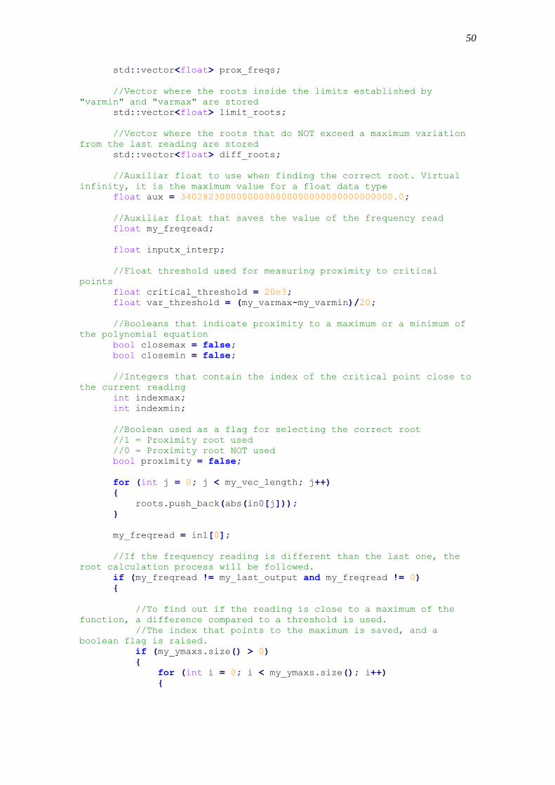
50
std::vector<float> prox_freqs;
//Vector where the roots inside the limits established by
"varmin" and "varmax" are stored
std::vector<float> limit_roots;
//Vector where the roots that do NOT exceed a maximum variation
from the last reading are stored
std::vector<float> diff_roots;
//Auxiliar float to use when finding the correct root. Virtual
infinity, it is the maximum value for a float data type
float aux = 34028230000000000000000000000000000000.0;
//Auxiliar float that saves the value of the frequency read
float my_freqread;
float inputx_interp;
//Float threshold used for measuring proximity to critical
points
float critical_threshold = 20e3;
float var_threshold = (my_varmax-my_varmin)/20;
//Booleans that indicate proximity to a maximum or a minimum of
the polynomial equation
bool closemax = false;
bool closemin = false;
//Integers that contain the index of the critical point close to
the current reading
int indexmax;
int indexmin;
//Boolean used as a flag for selecting the correct root
//1 = Proximity root used
//0 = Proximity root NOT used
bool proximity = false;
for (int j = 0; j < my_vec_length; j++)
{
roots.push_back(abs(in0[j]));
}
my_freqread = in1[0];
//If the frequency reading is different than the last one, the
root calculation process will be followed.
if (my_freqread != my_last_output and my_freqread != 0)
{
//To find out if the reading is close to a maximum of the
function, a difference compared to a threshold is used.
//The index that points to the maximum is saved, and a
boolean flag is raised.
if (my_ymaxs.size() > 0)
{
for (int i = 0; i < my_ymaxs.size(); i++)
{
51
if ((abs(my_freqread - my_ymaxs[i]) <
critical_threshold) and (abs(my_xmaxs[i] - my_last_output) <
var_threshold))
{
closemax = true;
indexmax = i;
}
}
}
//To find out if the reading is close to a minimum of the
function, a difference compared to a threshold is used.
//The index that points to the minimum is saved, and a
boolean flag is raised.
if (my_ymins.size() > 0)
{
for (int i = 0; i < my_ymins.size(); i++)
{
if ((abs(my_freqread - my_ymins[i]) <
critical_threshold) and (abs(my_xmins[i] - my_last_output) <
var_threshold))
{
closemin = true;
indexmin = i;
}
}
}
//If there had been a change of side in a critical point
("righttoleft", "lefttoright"),
//but the present reading is outside the threshold of
proximity with respect to that critical point ("closemax" or
"closemin" are "false"),
//the boolean flags "righttoleft" and "lefttoright" are
brought down.
if (((righttoleft == true) or (lefttoright == true)) and
((closemax == false) and (closemin == false)))
{
righttoleft = false;
lefttoright = false;
}
for (int i = 0; i < my_inputy.size(); i++)
{
if (abs(my_freqread - my_inputy[i]) < my_threshold)
{
prox_freqs.push_back(i);
}
}
if (prox_freqs.size() != 0)
{
if (my_last_output == 0)
{
int mindist;
for (int j = 0; j < prox_freqs.size(); j++)
{
if (abs(my_freqread - my_inputy[prox_freqs[j]])
< aux)
{
52
aux = abs(my_freqread -
my_inputy[prox_freqs[j]]);
mindist = prox_freqs[j];
}
}
my_output = my_inputx[mindist];
proximity = true;
}
else
{
for (int k = 0; k < roots.size(); k++)
{
if(abs(roots[k]-my_last_output) < var_threshold)
{
if(abs(roots[k]-my_last_output) < aux)
{
aux = abs(roots[k] - my_last_output);
my_output = roots[k];
//Root found by proximity
proximity = true;
}
}
}
}
}
//If the frequency read isn't close to any data from the
tests, another method for finding the correct root is used.
//First, roots inside the limits established (below "varmax"
and over "varmin") are counted.
//If there is just one, that is the correct one and it is
set as the output.
//Else, a maximum variation of the read variable between
consecutive readings is assumed.
//Roots that don't exceed that difference are stored; if
it is just one, that is the correct one and it is set as the output.
//If there are still multiple possible roots, the approach
followed is to find where the frequency read is located
//relative to the frequency data from the tests.
//Once the sweep has been completed, the root selected
as the correct one is the one closest to the data from the test.
//As there is no data from the test between points, the
value is calculated with a simple interpolation.
if (proximity != true)
{
for (int n = 0; n < roots.size(); n++)
{
if ((roots[n] > my_varmin) and (roots[n] <
my_varmax))
{
//The indexes of the roots that meet the
condition are saved
limit_roots.push_back(n);
}
}
if (limit_roots.size() == 1)
{
53
//If only one root met the condition, the output is
the root pointed by the vector
my_output = roots[limit_roots[0]];
}
else
{
for (int m = 0; m < limit_roots.size(); m++)
{
//The maximum variation between consecutives
readings is assumed as the 5% of the measurement range
if (abs(roots[limit_roots[m]] - my_last_output)
< var_threshold)
{
//The indexes of the roots that meet the
condition are saved
diff_roots.push_back(m);
}
}
if (diff_roots.size() == 1)
{
//If only one root met the condition, the output
is the root pointed by the vector
my_output = roots[diff_roots[0]];
}
else
{
//The root that will be considered is the
closest one to the last output
for (int n = 0; n < diff_roots.size(); n++)
{
if (abs(my_last_output-roots[diff_roots[n]])
< aux)
{
aux = abs(my_last_output-
roots[diff_roots[n]]);
my_output = roots[diff_roots[n]];
}
}
}
}
}
aux = 34028230000000000000000000000000000000.0;
//If the variable approaches a local maximum in the
polynomial function, a new criteria is used.
//When close to a maximum, if the frequency read is lower
than the previous one, it means that the
//'x' value (the variable value) is expected to be on the
other side of the critical point.
//Which is to say, if the last output (root) was bigger than
the maximum point, the next output will smaller;
54
//and if the last output was smaller than the maximum point,
the next output will be bigger.
if (closemax == true)
{
if ((my_freqread - my_last_freqread) < 0)
{
for (int n = 0; n < roots.size(); n++)
{
if ((my_last_output > my_xmaxs[indexmax]) and
(roots[n] < my_xmaxs[indexmax]) and (abs(my_last_output-roots[n]) <
aux) and (lefttoright == false))
{
aux = abs(my_last_output-roots[n]);
my_output = roots[n];
righttoleft = true;
}
else if ((my_last_output < my_xmaxs[indexmax])
and (roots[n] > my_xmaxs[indexmax]) and (abs(my_last_output-roots[n])
< aux) and (righttoleft == false))
{
aux = abs(my_last_output-roots[n]);
my_output = roots[n];
lefttoright = true;
}
}
}
}
//If the variable approaches a local minimum in the
polynomial function, a new criteria is used.
//When close to a minimum, if the frequency read is higher
than the previous one, it means that the
//'x' value (the variable value) is expected to be on the
other side of the critical point.
//Which is to say, if the last output (root) was bigger than
the minimum point, the next output will smaller;
//and if the last output was smaller than the maximum point,
the next output will be bigger.
if (closemin == true)
{
if ((my_freqread - my_last_freqread) > 0)
{
for (int n = 0; n < roots.size(); n++)
{
if ((my_last_output > my_xmins[indexmin]) and
(roots[n] < my_xmins[indexmin]) and (abs(my_last_output-roots[n]) <
aux) and (lefttoright == false))
{
aux = abs(my_last_output-roots[n]);
my_output = roots[n];
righttoleft = true;
}
else if ((my_last_output < my_xmins[indexmin])
and (roots[n] > my_xmins[indexmin]) and (abs(my_last_output-roots[n])
< aux) and (righttoleft == false))
{
aux = abs(my_last_output-roots[n]);
my_output = roots[n];
55
lefttoright = true;
}
}
}
}
}
my_last_output = my_output;
my_last_freqread = my_freqread;
*out = my_output;
// Tell runtime system how many input items we consumed on
// each input stream.
consume (0, ninput_items[0]);
consume (1, ninput_items[1]);
// Tell runtime system how many output items we produced.
return (noutput_items);
}
} /* namespace rtssel */
} /* namespace gr */
“Root_Selector_impl.h” block script (C++)
/* -*- c++ -*- */
/*
* Copyright 2018 <+YOU OR YOUR COMPANY+>.
*
* This is free software; you can redistribute it and/or modify
* it under the terms of the GNU General Public License as published
by
* the Free Software Foundation; either version 3, or (at your option)
* any later version.
*
* This software is distributed in the hope that it will be useful,
* but WITHOUT ANY WARRANTY; without even the implied warranty of
* MERCHANTABILITY or FITNESS FOR A PARTICULAR PURPOSE. See the
* GNU General Public License for more details.
*
* You should have received a copy of the GNU General Public License
* along with this software; see the file COPYING. If not, write to
* the Free Software Foundation, Inc., 51 Franklin Street,
* Boston, MA 02110-1301, USA.
*/
#ifndef INCLUDED_RTSSEL_ROOT_SELECTOR_IMPL_H
#define INCLUDED_RTSSEL_ROOT_SELECTOR_IMPL_H
#include <rtssel/Root_Selector.h>
namespace gr {
namespace rtssel {
class Root_Selector_impl : public Root_Selector
56
{
private:
// Nothing to declare in this block.
float my_varmin;
float my_varmax;
float my_threshold;
float my_pwr_threshold;
std::vector<float> my_inputx;
std::vector<float> my_inputy;
int my_vec_length;
std::vector<float> my_xmaxs;
std::vector<float> my_ymaxs;
std::vector<float> my_xmins;
std::vector<float> my_ymins;
public:
Root_Selector_impl(float varmin, float varmax, float threshold,
float pwr_threshold, std::vector<float> inputx, std::vector<float>
inputy, int vec_length,
std::vector<float> xmaxs, std::vector<float> ymaxs,
std::vector<float> xmins, std::vector<float> ymins);
~Root_Selector_impl();
// Where all the action really happens
void forecast (int noutput_items, gr_vector_int
&ninput_items_required);
int general_work(int noutput_items,
gr_vector_int &ninput_items,
gr_vector_const_void_star &input_items,
gr_vector_void_star &output_items);
};
} // namespace rtssel
} // namespace gr
#endif /* INCLUDED_RTSSEL_ROOT_SELECTOR_IMPL_H */
“IdentifierTD_impl.cc” block script (C++)
/* -*- c++ -*- */
/*
* Copyright 2018 <+YOU OR YOUR COMPANY+>.
*
* This is free software; you can redistribute it and/or modify
* it under the terms of the GNU General Public License as published
by
* the Free Software Foundation; either version 3, or (at your option)
* any later version.
*
* This software is distributed in the hope that it will be useful,
* but WITHOUT ANY WARRANTY; without even the implied warranty of
* MERCHANTABILITY or FITNESS FOR A PARTICULAR PURPOSE. See the
* GNU General Public License for more details.
*
* You should have received a copy of the GNU General Public License
* along with this software; see the file COPYING. If not, write to
* the Free Software Foundation, Inc., 51 Franklin Street,
* Boston, MA 02110-1301, USA.
57
*/
#ifdef HAVE_CONFIG_H
#include "config.h"
#endif
#include <gnuradio/io_signature.h>
#include "IdentifierTD_impl.h"
#include <boost/math/constants/constants.hpp>
namespace gr {
namespace IDTD {
IdentifierTD::sptr
IdentifierTD::make(float PwrThreshold, float TimeThreshold, float
FreqTX)
{
return gnuradio::get_initial_sptr
(new IdentifierTD_impl(PwrThreshold, TimeThreshold, FreqTX));
}
/*
* The private constructor
*/
const double pi = boost::math::constants::pi<double>();
std::vector<float> phases(1000);
std::vector<float> phasespans(1000);
std::vector<float> phasetotimespans(1000);
std::vector<float> freqs(1000);
std::vector<float> timespans;
float my_timespans_output;
std::vector<timespec> absolutetimes (1000);
//std::vector< std::vector<float> > my_vspansrefl(2,
std::vector<float>(100));
float my_output = 0;
float my_last_output;
float my_power;
float my_phase;
float my_last_phase;
float nperiods;
float my_freq;
timespec time1;
timespec time2;
timespec time3;
bool pulsedetect = false;
bool peakdetect = false;
int nreflectors = 0;
double result_d = 0;
bool buffout = false;
int outcount = 0;
IdentifierTD_impl::IdentifierTD_impl(float PwrThreshold, float
TimeThreshold, float FreqTX)
: gr::block("IdentifierTD",
gr::io_signature::make2(2, 2, sizeof(float),
sizeof(float)),
gr::io_signature::make2(2, 2, sizeof(float),
sizeof(float))),
58
my_pwr_threshold(PwrThreshold),
my_time_threshold(TimeThreshold),
my_TDFD(FreqTX)
{}
/*
* Our virtual destructor.
*/
IdentifierTD_impl::~IdentifierTD_impl()
{
}
void
IdentifierTD_impl::forecast (int noutput_items, gr_vector_int
&ninput_items_required)
{
ninput_items_required[0] = noutput_items;
ninput_items_required[1] = noutput_items;
}
int
IdentifierTD_impl::general_work (int noutput_items,
gr_vector_int &ninput_items,
gr_vector_const_void_star &input_items,
gr_vector_void_star &output_items)
{
//Magnitude readings
float *in0 = (float *) input_items[0];
//Phase readings
float *in1 = (float *) input_items[1];
//Timespans output, to be processed
float *out = (float *) output_items[0];
//Number of reflectors detected
float *out1 = (float *) output_items[1];
my_power = in0[0];
//my_TDFD == 1 --> Time Domain processing; my_TDFD == 0 -->
Frequency Domain Processing
if (my_TDFD == 1)
{
my_phase = in1[0];
}
else
{
my_freq = in1[0];
}
// Do <+signal processing+>
//As phase is a periodic function ranging between [-pi, pi],
//when the current reading presents a lower phase than the last
reading,
//it is necessary to increase the current value by 2*pi,
//because it means that the phase has rolled over to the next
interval.
if ((my_last_phase - 2*pi*nperiods) > my_phase)
{
nperiods++;
my_phase = my_phase + 2*pi*nperiods;
59
}
//If a pulse hasn't been detected yet, or the previous reading
has already finished,
//all input items are inspected to find out if the new pulse has
been sent.
//If it has, "pulsedetect" and "peakdetect" become "true".
if (my_power > my_pwr_threshold and pulsedetect == false)
{
pulsedetect = true;
peakdetect = true;
nreflectors = 0;
}
//If the pulse has been sent, the power of the signal exceeds a
certain threshold, and a peak hasn't been detected recently,
//the reading will be counted as a peak. To evade counting
multiple peaks, "peakdetect" will become "true"
//and will be used as a condition. Every peak translates to a
reflector in the SAW sensor.
//The power threshold will be relaxed compared to the sending
signal threshold, accounting for power losses in the process.
//if (ninput_items[1] != 0 and ninput_items[2] != 0)
if (my_power > my_pwr_threshold and (peakdetect == false) and
(pulsedetect == true))
{
peakdetect = true;
clock_gettime(CLOCK_MONOTONIC, &time2);
//Auxiliar timespec variable
struct timespec result ;
if ((time2.tv_sec < absolutetimes.at(nreflectors).tv_sec) ||
((time2.tv_sec == absolutetimes.at(nreflectors).tv_sec)
&&
(time2.tv_nsec <=
absolutetimes.at(nreflectors).tv_nsec))) { /* TIME1 <= TIME2? */
result.tv_sec = result.tv_nsec = 0 ;
} else { /* TIME1 > TIME2 */
result.tv_sec = time2.tv_sec -
absolutetimes.at(nreflectors).tv_sec ;
if (time2.tv_nsec <
absolutetimes.at(nreflectors).tv_nsec) {
result.tv_nsec = time2.tv_nsec + 1000000000L -
absolutetimes.at(nreflectors).tv_nsec ;
result.tv_sec-- ; /* Borrow a second. */
} else {
result.tv_nsec = time2.tv_nsec -
absolutetimes.at(nreflectors).tv_nsec ;
}
}
timespans.push_back( (float) result.tv_sec + (result.tv_nsec
/ 1000000000.0));
nreflectors++;
absolutetimes.at(nreflectors) = time2;
60
//Depending on the type of processing, the input expected to
the block is the phase / frequency of the peak
if (my_TDFD == 1)
{
phases.at(nreflectors) = my_phase;
phasespans.at(nreflectors-1) = phases.at(nreflectors) -
phases.at(nreflectors-1);
}
else
{
freqs.at(nreflectors) = my_freq;
}
}
//If the pulse has been sent, a peak has been detected recently,
and the power of the signal goes below a certain threshold,
//the boolean variable that indicates a peak had been detected
("peakdetect") will become "false" again, so that the next peak can be
detected.
//The threshold will be lower that the used for the peak
detection, in order to evade noise that could fake multiple peaks.
if (my_power < 0.9*my_pwr_threshold and (peakdetect == true) and
(pulsedetect == true))
{
peakdetect = false;
if (nreflectors == 0)
{
clock_gettime(CLOCK_MONOTONIC, &time1);
absolutetimes.at(0) = time1;
//Depending on the type of processing, the input
expected to the block is the phase / frequency of the peak
if (my_TDFD == 1)
{
phases.at(0) = my_phase;
}
else
{
freqs.at(0) = my_freq;
}
}
}
//Because the number of reflectors that the interrogated sensor
has is unknown at first,
//the reading will be considered done when a certain amount of
time has already passed.
//To measure that, at the end of every cycle the difference
between the last peak and the current time
//is measured; if it exceeds a certain threshold, the reading
will be completed.
if (pulsedetect == true and peakdetect == false)
{
clock_gettime(CLOCK_MONOTONIC, &time3);
//Auxiliar timespec variable
struct timespec result ;
61
if ((time3.tv_sec < absolutetimes.at(nreflectors).tv_sec) ||
((time3.tv_sec == absolutetimes.at(nreflectors).tv_sec)
&&
(time3.tv_nsec <=
absolutetimes.at(nreflectors).tv_nsec))) { /* TIME1 <= TIME2? */
result.tv_sec = result.tv_nsec = 0 ;
} else { /* TIME1 > TIME2 */
result.tv_sec = time3.tv_sec -
absolutetimes.at(nreflectors).tv_sec ;
if (time3.tv_nsec <
absolutetimes.at(nreflectors).tv_nsec) {
result.tv_nsec = time3.tv_nsec + 1000000000L -
absolutetimes.at(nreflectors).tv_nsec ;
result.tv_sec-- ; /* Borrow a second. */
} else {
result.tv_nsec = time3.tv_nsec -
absolutetimes.at(nreflectors).tv_nsec ;
}
}
result_d = (double) result.tv_sec + (result.tv_nsec /
1000000000.0);
if (abs(result_d) > my_time_threshold)
{
result_d = 0;
peakdetect = false;
pulsedetect = false;
buffout = true;
outcount = 0;
}
}
//If there is a new value to be sent, "buffout" will be "true".
if (buffout == true)
{
//If using time processing, outputs are timespans between
reflectors peaks
if (my_TDFD == 1)
{
if (outcount != timespans.size())
{
my_output = timespans.at(outcount);
*out = my_output;
outcount++;
}
else
{
buffout = false;
timespans.resize(0);
}
}
//If using frequency processing, outputs are peak
frequencies read from reflectors
else
{
if (freqs.at(outcount) != 0)
{
my_output = freqs.at(outcount);
*out = my_output;
outcount++;
62
}
else
{
buffout = false;
std::fill(freqs.begin(), freqs.end(), 0);
}
}
//If there is not a new value, the output will be kept as the
last output from the previous cycle.
}
else
{
*out = my_last_output;
}
my_last_phase = my_phase;
my_last_output = my_output;
*out1 = nreflectors;
// Tell runtime system how many input items we consumed on
// each input stream.
consume (0, noutput_items);
consume (1, noutput_items);
// Tell runtime system how many output items we produced.
return noutput_items;
}
} /* namespace IDTD */
} /* namespace gr */
“IdentifierTD_impl.h” block script (C++)
/* -*- c++ -*- */
/*
* Copyright 2018 <+YOU OR YOUR COMPANY+>.
*
* This is free software; you can redistribute it and/or modify
* it under the terms of the GNU General Public License as published
by
* the Free Software Foundation; either version 3, or (at your option)
* any later version.
*
* This software is distributed in the hope that it will be useful,
* but WITHOUT ANY WARRANTY; without even the implied warranty of
* MERCHANTABILITY or FITNESS FOR A PARTICULAR PURPOSE. See the
* GNU General Public License for more details.
*
* You should have received a copy of the GNU General Public License
* along with this software; see the file COPYING. If not, write to
* the Free Software Foundation, Inc., 51 Franklin Street,
* Boston, MA 02110-1301, USA.
*/
#ifndef INCLUDED_IDTD_IDENTIFIERTD_IMPL_H
#define INCLUDED_IDTD_IDENTIFIERTD_IMPL_H
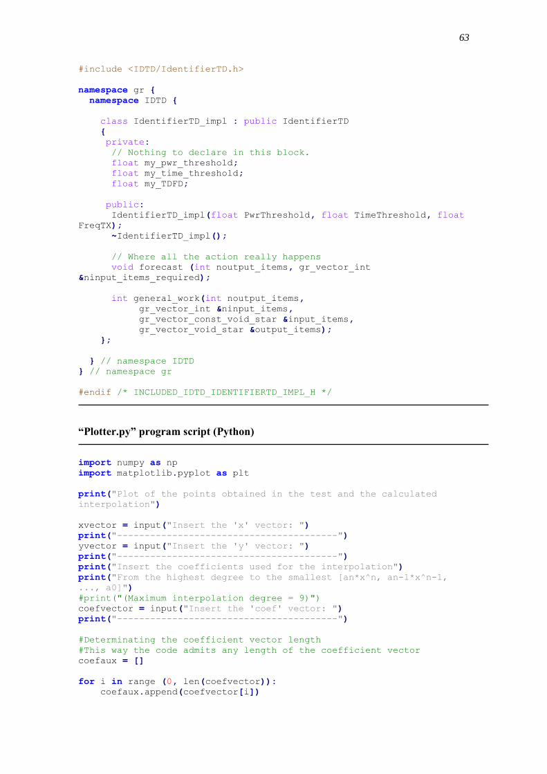
63
#include <IDTD/IdentifierTD.h>
namespace gr {
namespace IDTD {
class IdentifierTD_impl : public IdentifierTD
{
private:
// Nothing to declare in this block.
float my_pwr_threshold;
float my_time_threshold;
float my_TDFD;
public:
IdentifierTD_impl(float PwrThreshold, float TimeThreshold, float
FreqTX);
~IdentifierTD_impl();
// Where all the action really happens
void forecast (int noutput_items, gr_vector_int
&ninput_items_required);
int general_work(int noutput_items,
gr_vector_int &ninput_items,
gr_vector_const_void_star &input_items,
gr_vector_void_star &output_items);
};
} // namespace IDTD
} // namespace gr
#endif /* INCLUDED_IDTD_IDENTIFIERTD_IMPL_H */
“Plotter.py” program script (Python)
import numpy as np
import matplotlib.pyplot as plt
print("Plot of the points obtained in the test and the calculated
interpolation")
xvector = input("Insert the 'x' vector: ")
print("----------------------------------------")
yvector = input("Insert the 'y' vector: ")
print("----------------------------------------")
print("Insert the coefficients used for the interpolation")
print("From the highest degree to the smallest [an*x^n, an-1*x^n-1,
..., a0]")
#print("(Maximum interpolation degree = 9)")
coefvector = input("Insert the 'coef' vector: ")
print("----------------------------------------")
#Determinating the coefficient vector length
#This way the code admits any length of the coefficient vector
coefaux = []
for i in range (0, len(coefvector)):
coefaux.append(coefvector[i])
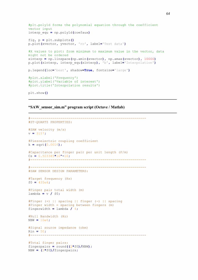
64
#plt.poly1d forms the polynomial equation through the coefficient
vector input
interp_equ = np.poly1d(coefaux)
fig, p = plt.subplots()
p.plot(xvector, yvector, 'ro', label='Test data')
#X values to plot: from minimum to maximum value in the vector, data
might not be ordered
xinterp = np.linspace(np.amin(xvector), np.amax(xvector), 10000)
p.plot(xinterp, interp_equ(xinterp), 'b', label='Interpolation')
p.legend(loc='best', shadow=True, fontsize='large')
#plot.xlabel('Frequency')
#plot.ylabel('Variable of interest')
#plot.title('Interpolation results')
plt.show()
“SAW_sensor_sim.m” program script (Octave / Matlab)
#----------------------------------------------------------
#ST-QUARTZ PROPERTIES:
#SAW velocity (m/s)
v = 3157;
#Piezoelectric coupling coefficient
k = sqrt(0.0016);
#Capacitance per finger pair per unit length (F/m)
Cs = 0.503385*10^-10;
#----------------------------------------------------------
#----------------------------------------------------------
#SAW SENSOR DESIGN PARAMETERS:
#Target frequency (Hz)
f0 = 435e6;
#Finger pair total width (m)
lambda = v / f0;
#Finger (+) || spacing || finger (-) || spacing
#Finger width = spacing between fingers (m)
fingerwidth = lambda / 4;
#Null Bandwidth (Hz)
NBW = 10e6;
#Signal source impedance (ohm)
Rin = 50;
#----------------------------------------------------------
#Total finger pairs:
fingerpairs = round((2*f0)/NBW);
NBW = (2*f0)/fingerpairs;
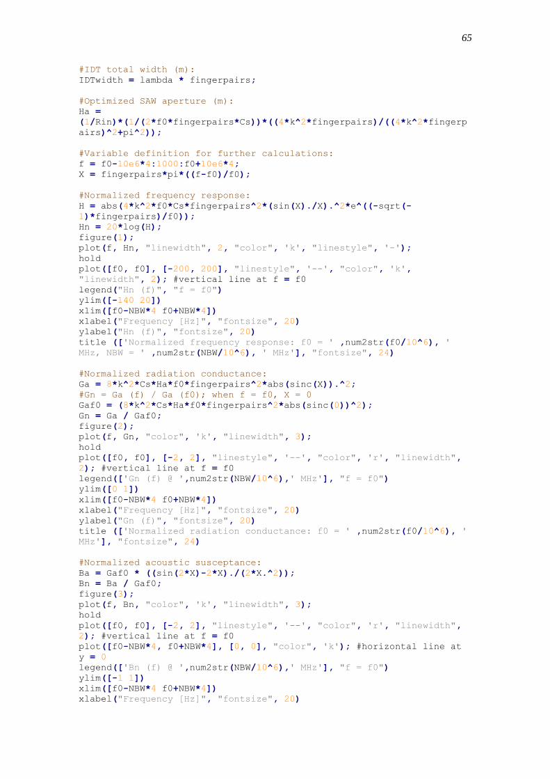
65
#IDT total width (m):
IDTwidth = lambda * fingerpairs;
#Optimized SAW aperture (m):
Ha =
(1/Rin)*(1/(2*f0*fingerpairs*Cs))*((4*k^2*fingerpairs)/((4*k^2*fingerp
airs)^2+pi^2));
#Variable definition for further calculations:
f = f0-10e6*4:1000:f0+10e6*4;
X = fingerpairs*pi*((f-f0)/f0);
#Normalized frequency response:
H = abs(4*k^2*f0*Cs*fingerpairs^2*(sin(X)./X).^2*e^((-sqrt(-
1)*fingerpairs)/f0));
Hn = 20*log(H);
figure(1);
plot(f, Hn, "linewidth", 2, "color", 'k', "linestyle", '-');
hold
plot([f0, f0], [-200, 200], "linestyle", '--', "color", 'k',
"linewidth", 2); #vertical line at f = f0
legend("Hn (f)", "f = f0")
ylim([-140 20])
xlim([f0-NBW*4 f0+NBW*4])
xlabel("Frequency [Hz]", "fontsize", 20)
ylabel("Hn (f)", "fontsize", 20)
title (['Normalized frequency response: f0 = ' ,num2str(f0/10^6), '
MHz, NBW = ' ,num2str(NBW/10^6), ' MHz'], "fontsize", 24)
#Normalized radiation conductance:
Ga = 8*k^2*Cs*Ha*f0*fingerpairs^2*abs(sinc(X)).^2;
#Gn = Ga (f) / Ga (f0); when f = f0, X = 0
Gaf0 = (8*k^2*Cs*Ha*f0*fingerpairs^2*abs(sinc(0))^2);
Gn = Ga / Gaf0;
figure(2);
plot(f, Gn, "color", 'k', "linewidth", 3);
hold
plot([f0, f0], [-2, 2], "linestyle", '--', "color", 'r', "linewidth",
2); #vertical line at f = f0
legend(['Gn (f) @ ',num2str(NBW/10^6),' MHz'], "f = f0")
ylim([0 1])
xlim([f0-NBW*4 f0+NBW*4])
xlabel("Frequency [Hz]", "fontsize", 20)
ylabel("Gn (f)", "fontsize", 20)
title (['Normalized radiation conductance: f0 = ' ,num2str(f0/10^6), '
MHz'], "fontsize", 24)
#Normalized acoustic susceptance:
Ba = Gaf0 * ((sin(2*X)-2*X)./(2*X.^2));
Bn = Ba / Gaf0;
figure(3);
plot(f, Bn, "color", 'k', "linewidth", 3);
hold
plot([f0, f0], [-2, 2], "linestyle", '--', "color", 'r', "linewidth",
2); #vertical line at f = f0
plot([f0-NBW*4, f0+NBW*4], [0, 0], "color", 'k'); #horizontal line at
y = 0
legend(['Bn (f) @ ',num2str(NBW/10^6),' MHz'], "f = f0")
ylim([-1 1])
xlim([f0-NBW*4 f0+NBW*4])
xlabel("Frequency [Hz]", "fontsize", 20)
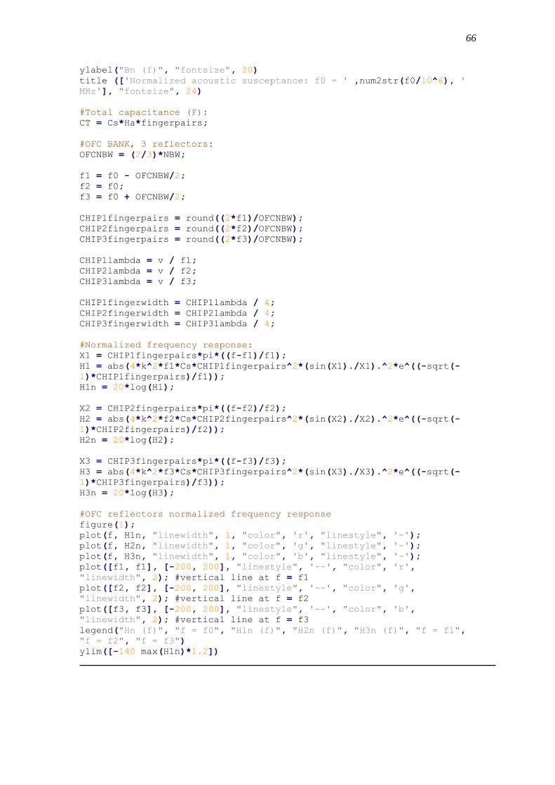
66
ylabel("Bn (f)", "fontsize", 20)
title (['Normalized acoustic susceptance: f0 = ' ,num2str(f0/10^6), '
MHz'], "fontsize", 24)
#Total capacitance (F):
CT = Cs*Ha*fingerpairs;
#OFC BANK, 3 reflectors:
OFCNBW = (2/3)*NBW;
f1 = f0 - OFCNBW/2;
f2 = f0;
f3 = f0 + OFCNBW/2;
CHIP1fingerpairs = round((2*f1)/OFCNBW);
CHIP2fingerpairs = round((2*f2)/OFCNBW);
CHIP3fingerpairs = round((2*f3)/OFCNBW);
CHIP1lambda = v / f1;
CHIP2lambda = v / f2;
CHIP3lambda = v / f3;
CHIP1fingerwidth = CHIP1lambda / 4;
CHIP2fingerwidth = CHIP2lambda / 4;
CHIP3fingerwidth = CHIP3lambda / 4;
#Normalized frequency response:
X1 = CHIP1fingerpairs*pi*((f-f1)/f1);
H1 = abs(4*k^2*f1*Cs*CHIP1fingerpairs^2*(sin(X1)./X1).^2*e^((-sqrt(-
1)*CHIP1fingerpairs)/f1));
H1n = 20*log(H1);
X2 = CHIP2fingerpairs*pi*((f-f2)/f2);
H2 = abs(4*k^2*f2*Cs*CHIP2fingerpairs^2*(sin(X2)./X2).^2*e^((-sqrt(-
1)*CHIP2fingerpairs)/f2));
H2n = 20*log(H2);
X3 = CHIP3fingerpairs*pi*((f-f3)/f3);
H3 = abs(4*k^2*f3*Cs*CHIP3fingerpairs^2*(sin(X3)./X3).^2*e^((-sqrt(-
1)*CHIP3fingerpairs)/f3));
H3n = 20*log(H3);
#OFC reflectors normalized frequency response
figure(1);
plot(f, H1n, "linewidth", 1, "color", 'r', "linestyle", '-');
plot(f, H2n, "linewidth", 1, "color", 'g', "linestyle", '-');
plot(f, H3n, "linewidth", 1, "color", 'b', "linestyle", '-');
plot([f1, f1], [-200, 200], "linestyle", '--', "color", 'r',
"linewidth", 2); #vertical line at f = f1
plot([f2, f2], [-200, 200], "linestyle", '--', "color", 'g',
"linewidth", 2); #vertical line at f = f2
plot([f3, f3], [-200, 200], "linestyle", '--', "color", 'b',
"linewidth", 2); #vertical line at f = f3
legend("Hn (f)", "f = f0", "H1n (f)", "H2n (f)", "H3n (f)", "f = f1",
"f = f2", "f = f3")
ylim([-140 max(H1n)*1.2])