interpretação, inversão 3d de dados magnéticos e
150
UNIVERSIDADE DE BRASÍLIA INSTITUTO DE GEOCIÊNCIAS INTERPRETAÇÃO, INVERSÃO 3D DE DADOS MAGNÉTICOS E MODELAGEM 3D DA SUSCEPTIBILIDADE MAGNÉTICA MEDIDA, APLICADAS À PROSPECÇÃO GEOFÍSICA DE DEPÓSITOS DE ÓXIDOS DE FERRO - COBRE - OURO (IOCG IRON OXIDE-COPPER-GOLD) – PROVÍNCIA MINERAL DE CARAJÁS, BRASIL MARCELO HENRIQUE LEÃO SANTOS Tese de Doutorado N° 117 Brasília - DF 2014
-
Upload
khangminh22 -
Category
Documents
-
view
1 -
download
0
Transcript of interpretação, inversão 3d de dados magnéticos e
UNIVERSIDADE DE BRASÍLIA INSTITUTO DE GEOCIÊNCIAS
INTERPRETAÇÃO, INVERSÃO 3D DE DADOS MAGNÉTICOS E
MODELAGEM 3D DA SUSCEPTIBILIDADE MAGNÉTICA
MEDIDA, APLICADAS À PROSPECÇÃO GEOFÍSICA DE
DEPÓSITOS DE ÓXIDOS DE FERRO - COBRE - OURO
(IOCG IRON OXIDE-COPPER-GOLD) –
PROVÍNCIA MINERAL DE CARAJÁS, BRASIL
MARCELO HENRIQUE LEÃO SANTOS
Tese de Doutorado N° 117
Brasília - DF
2014

ii
UNIVERSIDADE DE BRASÍLIA INSTITUTO DE GEOCIÊNCIAS
Área de Concentração:
Geologia Econômica e Prospecção
INTERPRETAÇÃO, INVERSÃO 3D DE DADOS MAGNÉTICOS E
MODELAGEM 3D DA SUSCEPTIBILIDADE MAGNÉTICA
MEDIDA, APLICADAS À PROSPECÇÃO GEOFÍSICA DE
DEPÓSITOS DE ÓXIDOS DE FERRO - COBRE - OURO
(IOCG IRON OXIDE-COPPER-GOLD) –
PROVÍNCIA MINERAL DE CARAJÁS, BRASIL
MARCELO HENRIQUE LEÃO SANTOS
Tese de Doutorado N° 117
Orientador: Dr. Roberto Alexandre Vitória de Moraes – Universidade de Brasília
Co-orientadores: Dr. Yaoguo Li – Colorado School of Mines
Dr. Misac Nabighian – Colorado School of Mines
Banca Examinadora: Dr. Augusto César Bittencourt Pires – Universidade de Brasília
Dra. Mônica Giannoccaro Von Huelsen – Universidade de Brasília
Dr. Francisco José Fonseca Ferreira – Universidade Federal do Paraná
Dr. Marcelo de Lawrence Bassay Blum – Polícia Federal
Brasília - DF
2014

iii
À Flávia,
Felipe, Mateus
e aos meus pais
Moisés e Telma

iv

Universidade de Brasília – Instituto de Geociências – Tese de Doutorado – Marcelo Henrique Leão Santos
v UnB
AGRADECIMENTOS
Agradeço a todas as pessoas, instituições e empresas que contribuíram para o
desenvolvimento deste projeto de pesquisa. Caso ocorra algum esquecimento nos nomes citados
perdoem o autor, pois não foi proposital.
- Primeiramente a Deus;
- A minha esposa Flávia e aos meus filhos Felipe e Mateus, pelo eterno amor, parceiros de vida e
neste trabalho com a “corrida ao velho oeste” dos Estados Unidos em Golden Colorado;
- Aos meus pais Moisés e Telma, alicerce da minha vida. Aos meus irmãos Andréa e Maurício pela
eterna irmandade. E a todos meus familiares;
- Ao Laboratório de Geofísica Aplicada (LGA), ao Instituto de Geociências (IG), a Universidade de
Brasília (UnB), a todos os professores e funcionários do IG, as secretárias da pós Alice e Stela;
- Ao meu orientador Roberto Moraes, e aos professores Augusto Pires e Adalene Moreira, pelos
ensinamentos, amizade e anos de convívio acadêmico;
- Aos membros da banca examinadora pela contribuição ao trabalho desenvolvido: Professores Dr.
Augusto César Bittencourt Pires (UnB), Dra. Mônica Giannoccaro Von Huelsen (UnB), Dr.
Francisco José Fonseca Ferreira (UFPR) e Dr. Marcelo de Lawrence Bassay Blum (Polícia
Federal). Aos membros da banca examinadora da qualificação do doutorado.
- A todos os meus amigos da graduação e da pós-graduação. A toda comunidade geológica e
geofísica. Aos amigos André Spigolon, Bruno Velasco, Edson Toledo, Fabio Mendonça, Fausto
Lazarin, Helio Azevedo, Leandro Duarte, Léo Melo, Luciano Cunha, Luciano Teixeira e Lorna
Crawford;
- A Colorado School of Mines (CSM), Center for Gravity, Electrical & Magnetic Studies (CGEM) e
Gravity and Magnetics Research Consortium (GMRC). Aos co-orientadores Dr. Yaoguo Li e Dr.
Misac Nabighian pelo aprendizado, amizade e oportunidade de viver uma experiência internacional.
Aos amigos da CSM: Dr. Richard Krahenbuhl, Cericia Martinez, Leon Foks, Jiajia Sun, Dr. Andy
Kaas, Camriel Coleman, Mohamed Abdulla, Brent Putman, Jeff Shoffner, Trevor Irons, Anya
Reitz, Dr. Magnus Skold, Dr. Marios Karaoulis, Luís Martins, Yaser Kattoum, Conrad Newton,
Julio Frigério, Esteban Pantin, Carla Carvajal e Miguel Nassif. Gostaria de fazer um agradecimento
especial ao amigo Dr. Dionisio Uendro da Vale S.A. e a amiga professora da China University of
Geosciences Dra. Shuling Li, parceiros de sala e muitas alegrias durante a temporada na CSM;
- A Professora Dra. Maria Irene Bartolomeu Raposo da Universidade da São Paulo (USP), Instituto
de Geociências (IGc), Laboratório de Anisotropias Magnéticas e Magnetismo de Rocha, pelos
ensinamentos, por orientar nas medidas e pelo uso do laboratório;
Universidade de Brasília – Instituto de Geociências – Tese de Doutorado – Marcelo Henrique Leão Santos
vi UnB
- A VALE S.A. – Diretoria de Exploração e Projetos Minerais e Gerência de Exploração Brasil –
pela permissão em publicar este trabalho, suporte financeiro para o projeto no Brasil e no exterior, e
pela cessão e permissão do uso dos dados geofísicos e geológicos neste projeto de pesquisa. Os
agradecimentos são em nome dos funcionários e ex-funcionários da época do início do trabalho há
cinco anos: Diretores Márcio Godoy, Fábio Masotti, Eduardo Ledsham e Tracey Keer; Gerentes
Fernando Greco, Fernando Matos, Filipe Porto e Noevaldo Teixeira; e amigos Wolney Rosa,
Rodrigo Mabub, Denisson Oliveira, Samuel Nunes, Gustavo Queiroz, Rigon, Carlos Medeiros
Cacá, Joaquim Nascimento, Messias, Rafael Bueno, Gabriel Araújo, Juliana Araújo, Fernando
Paula, Carlos Isaías Kaica, Sérgio Huhn, Edmundo Khoury, Fábio Cuoco, Douglas Zardo, Rogério
Caron, Takato, Valdocir, Mariana Oliveira, Alan Freitas, Flávio Freitas, Francisco, Zenha, Saney,
Rúbia, Brasileiro, Henrique, Joaniceli, Arlênia, Luiz Neto, Torquato, Robert, Cantão, Michel e
Jorge. Aos geólogos Gabriel Paulo e Sálvio Ribeiro pela ajuda nos modelos de minério e gráficos.
A equipe dos Recursos Humanos da empresa pelo apoio no período no exterior;
- A equipe Geofísica da VALE S.A. e todos que trabalhei junto por todo o apoio, suporte e divertido
convívio. Cantidiano Freitas, Florivaldo Sena, Kiyoshi Kadekaru, Célio Barreira, Alan King, João
Paulo, Daniel Brake, Rob Eso, Diogo Carvalho, Aline Silva, Chris Moura, Edvaldo Gomes, Kleiber
Ferreira e Leandro Santos. Ao técnico e amigo Joaquim Feijó pelo empenho e critério nas
amostragens e medidas petrofísicas, e pela sabedoria em levar a vida. Aos amigos Daniel Brake
pelas revisões no inglês e Alan King pelo apoio no início do projeto de pesquisa. E especialmente
ao amigo Cantidiano Freitas pelo acompanhamento e participação de toda a Tese;
- Ao Projeto Furnas da VALE S.A. pelos dados e muitas discussões geológicas usadas no estudo,
Aos amigos da equipe do projeto: Otávio Rosendo, Arthur Cardoso, Rafael Bueno, Gabriel Paulo,
Vicente Pinheiro, Antônio Benvindo, Cris Fianco, Junny Kyley, Maira Santos, Marco Figueiredo,
Marcelo Schwarz e Silvio Lopes;
- Ao Departamento de Planejamento e Desenvolvimento de Ferrosos da VALE S.A. – pelo uso de
dados magnéticos e pela oportunidade do trabalho de pesquisa no consórcio Gravity and Magnetics
Research Consortium (GMRC), da Colorado School of Mines. As atuais empresas patrocinadoras
são: Anadarko, Bell Geospace, BG Group, BGP, BP, ConocoPhillips, Fugro, Gedex, Lockheed
Martin, Marathon Oil, Shell, Petrobras e Vale. Aos Gerentes Henry Galbiatti e Dr. Marco Antonio
Braga, e ao Geofísico Dr. Dionísio Uendro;
- A Fundação CAPES, Coordenação de Aperfeiçoamento de Pessoal de Nível Superior, Ministério
da Educação do Brasil, pela concessão da bolsa sanduíche de um ano nos Estados Unidos;
- Ao revisor da Geophysics Peter Lelièvre e aos revisores anônimos da Geophysics e Economic
Geology pelos comentários que ajudaram a melhorar os artigos submetidos.
Universidade de Brasília – Instituto de Geociências – Tese de Doutorado – Marcelo Henrique Leão Santos
vii UnB
ABSTRACT
Leão-Santos, M.H., 2014, Interpretation, magnetic data 3D inversion and measured magnetic
susceptibility 3D modeling, applied to exploration geophysics of iron oxide - copper - gold (IOCG)
deposits – Carajás Mineral Province, Brazil: Doctorate thesis, Universidade de Brasília.
This thesis comprises the use of airborne magnetic data and magnetic susceptibility
measurements to aid mineral prospecting of iron oxide-copper-gold (IOCG) mineralization within
Furnas Southeast deposit, Carajás Mineral Province, Brazil. The susceptibility study allowed the
characterization of the calcic-sodic-potassic-magnetite hydrothermal alteration magnetic signatures
(biotite-garnet-grunerite-magnetite paragenesis).
The qualitative, semi-quantitative and quantitative interpretations of airborne magnetic data
were used in this work aiming to obtain the best possible three-dimensional model (from 3D
modeling / inversion) of the magnetic sources, responsible for the measured magnetic signature. A
3D spatial distribution model of the magnetic susceptibility measured on drill cores was also
obtained. The aim of the thesis was to define a geophysical-geological prospective model of the iron
oxide-copper-gold (IOCG) mineralization. Two ways were used on this purpose: by using 3D
modeling / inversion of the measured local magnetic field (indirect method) and by 3D
susceptibility measurements modeling (direct method). The results of the two approaches were
presented and discussed throughout the thesis.
In strong magnetization environments, it is sometimes difficult to accurately interpret its
sources due to the complex role played by induced field, remanent magnetizations and the
demagnetization effects. Moreover, in low magnetic latitudes the remanence effect is even more
pronounced and the inducing magnetic field is weaker. Carajás region IOCG type deposits are such
a case.
The results of the research are described in the thesis body with an introduction of priory
geological information and three papers dealing with: the magnetic interpretation (Paper 1) to
achieve a 3D inverse model (Paper 2) and a 3D forward model (Paper 3). The purpose is to focus on
the main prospecting stages, since the beginning of a greenfield exploration to brownfield and
advanced exploration projects using magnetic data.
With respect to the prospecting stages, the approach of the first paper would be that of
interpreting magnetic data in greenfield exploration. Following, the second paper describes an
approach to reliably recover the distribution of effective magnetic susceptibility using inversion of
magnetic data. It can be applied in either greenfield and brownfield exploration. The third paper
presents an approach to model the magnetic mineralized zone based on geologic data available from

Universidade de Brasília – Instituto de Geociências – Tese de Doutorado – Marcelo Henrique Leão Santos
viii UnB
drill hole cores and on petrophysical measurements taken on core samples. This is the kind of
knowledge normally available on advanced exploration project phases.
The results show that the 3D modeling of measured susceptibility data seems to gives a
better magnetic source definition and delineation. However, this can only be achieved through
systematic, expensive and time consuming measurements and geological interpretation. This
approach deals with a huge amount of petrophysical and geological data. On the other hand, the
inverse magnetic modeling can be a less time consuming tool with the use of equivalent source and
amplitude inversion techniques to reach a good tracking of the magnetic sources.
The proposal of this research was to deal with different approaches on the use of high-
density magnetic survey and magnetic physical property measurements on deep drill holes to
achieve a better understanding of the Furnas Southeast deposit and identify massive magnetite from
hydrothermal alterations associated with the high-grade ore.
Key words: iron oxide - copper - gold (IOCG) deposits, mineral exploration, magnetic
susceptibility, 3D magnetic amplitude inversion, 3D geophysical-geological modeling, Carajás
Mineral Province - Brazil.

Universidade de Brasília – Instituto de Geociências – Tese de Doutorado – Marcelo Henrique Leão Santos
ix UnB
RESUMO
Leão-Santos, M.H., 2014, Interpretação, inversão 3D de dados magnéticos e modelagem 3D da
susceptibilidade magnética medida, aplicadas à prospecção geofísica de depósitos de óxidos de
ferro - cobre - ouro (IOCG iron oxide-copper-gold) – Província Mineral de Carajás, Brasil: Tese de
Doutorado, Universidade de Brasília.
Esta Tese compreende o uso de dados magnéticos aéreos e medidas de susceptibilidade
magnética para auxiliar na prospecção de mineralizações de óxidos de ferro-cobre-ouro (iron oxide-
copper-gold IOCG) no depósito Furnas Sudeste, Província Mineral de Carajás, Brasil. O estudo da
susceptibilidade permitiu a caracterização das assinaturas magnéticas da alteração hidrotermal
calco-sódico-potássica-magnetítica (paragênese biotita-granada-grunerita-magnetita).
As interpretações qualitativa, semi-quantitativa e quantitativa de dados magnéticos foram
utilizadas neste trabalho para a obtenção do melhor modelo tridimensional (por modelagem /
inversão 3D) das fontes magnéticas responsáveis pela assinatura medida. Também foi obtido o
modelo 3D referente à distribuição espacial das susceptibilidades magnéticas medidas em amostras
dos testemunhos de furos de sonda. O objetivo da Tese foi definir um modelo geofísico-geológico
prospectivo da mineralização de óxidos de ferro-cobre-ouro. Para isso, foram usados dois caminhos:
um com a modelagem / inversão 3D dos dados magnéticos medidos no local (método indireto) e
outro pela modelagem espacial das susceptibilidades magnéticas medidas (método direto). Os
resultados das duas aproximações estão apresentados e encontram-se largamente discutidos.
Em ambientes com forte magnetização, às vezes é difícil interpretar com precisão suas
fontes devido ao complexo papel desempenhado pelo campo induzido, magnetização remanescente
e os efeitos de desmagnetização. Além disso, em baixas latitudes magnéticas o efeito de remanência
é ainda mais pronunciado e o campo magnético induzido é mais fraco. Este é o caso dos depósitos
tipo IOCG da região de Carajás.
Os resultados da pesquisa estão descritos no corpo da Tese com a introdução da informação
geológica e em três artigos que tratam da: interpretação magnética (Artigo 1) para se alcançar um
modelo inverso 3D (Artigo 2) e um modelo direto 3D (Artigo 3). O escopo é focar nos principais
estágios da prospecção com o uso de dados magnéticos, desde o início da exploração greenfield até
a exploração brownfield e projetos de avaliação de depósitos.
No que diz respeito às etapas de prospecção, a abordagem do primeiro artigo seria a
interpretação de dados magnéticos em exploração greenfield. Na sequência, o segundo artigo
descreve uma abordagem para se recuperar de forma confiável a efetiva distribuição de
susceptibilidade com o uso de dados magnéticos. Este enfoque pode ser aplicado tanto na

Universidade de Brasília – Instituto de Geociências – Tese de Doutorado – Marcelo Henrique Leão Santos
x UnB
exploração greenfield quanto na brownfield. O terceiro artigo lida com uma abordagem para
modelar a zona mineralizada magnética com base em dados geológicos de testemunhos de furos de
sonda disponíveis e em medidas petrofísicas realizadas em amostras de testemunhos. Este é o tipo
de conhecimento normalmente disponível em fases avançadas de projetos de exploração.
Os resultados mostram que a modelagem 3D dos dados de susceptibilidade medidos permite
uma melhor definição e delimitação da fonte magnética. Entretanto, isso só pode ser alcançado por
meio de descrições geológicas detalhadas e medidas de susceptibilidade sistemáticas, com um
grande custo e consumo de tempo. Este enfoque lida com uma grande quantidade de dados
petrofísicos e geológicos. Por outro lado, a modelagem de dados magnéticos por inversão pode ser
uma ferramenta que consome menos tempo, com o uso das técnicas da camada equivalente e da
inversão da amplitude para atingir um bom rastreamento das fontes magnéticas.
A proposta desta pesquisa foi tratar com diferentes abordagens o uso de levantamentos
magnéticos de alta densidade de dados e medidas de propriedades físicas magnéticas ao longo de
testemunhos de sondagem, para conseguir um melhor entendimento do depósito Furnas Sudeste e
identificar magnetita maciça de alterações hidrotermais associadas com minério de alto teor.
Palavras chave: depósitos de óxidos de ferro - cobre - ouro (IOCG), exploração mineral,
susceptibilidade magnética, inversão 3D dados de amplitude magnética, modelagem geofísico-
geológica 3D, Província Mineral de Carajás - Brasil.

Universidade de Brasília – Instituto de Geociências – Tese de Doutorado – Marcelo Henrique Leão Santos
xi UnB
SUMÁRIO
AGRADECIMENTOS...............................................................................................................
ABSTRACT.................................................................................................................................
RESUMO....................................................................................................................................
SIGLAS E ABREVIAÇÕES.....................................................................................................
LISTA DE FIGURAS................................................................................................................
LISTA DE TABELAS...............................................................................................................
CAPÍTULO 1 - INTRODUÇÃO..............................................................................................
1.1 CARACTERIZAÇÃO DOS PROBLEMAS.............................................................
1.2 ESTADO DA ARTE..................................................................................................
1.3 FOCO DOS RESULTADOS.....................................................................................
1.4 METODOLOGIA......................................................................................................
1.5 RESULTADOS ATINGIDOS...................................................................................
1.6 ESTRUTURA DA TESE...........................................................................................
1.7 FLUXOGRAMA DOS TRABALHOS DESENVOLVIDOS NA TESE..................
1.8 REFERÊNCIA...........................................................................................................
CAPÍTULO 2 - GEOLOGIA REGIONAL.............................................................................
2.1 ESTRATIGRAFIA....................................................................................................
2.2 UNIDADES LITOLÓGICAS....................................................................................
2.2.1 - Embasamento – Complexos Xingu e Pium……………………………..
2.2.2 - Granitos neoarqueanos - Suíte Plaquê…………………………………..
2.2.3 - Sequências vulcânicas e sedimentares - Supergrupo Itacaiúnas……….
2.2.4 - Formação Águas Claras…………………………………………………
2.2.5 - Diques e Sills máficos…………………………………………………...
2.2.6 - Granitos anorogênicos………………………………………………….
2.2.7 - Coberturas fanerozoicas………………………………………………...
2.3 MODELO TECTONOESTRATIGRÁFICO.............................................................
2.4 REFERÊNCIAS.........................................................................................................
CAPÍTULO 3 - MAGNETIC INTERPRETATION AND 2D MODELING AT AN IRON
OXIDE–COPPER–GOLD DEPOSIT, CARAJÁS MINERAL PROVINCE,
BRAZIL.......................................................................................................................................
3.1 ABSTRACT................................................................................................................
v
vii
ix
xiv
xvi
xxii
01
01
03
03
04
06
07
08
08
09
12
13
13
14
15
18
18
19
19
19
21
26
27

Universidade de Brasília – Instituto de Geociências – Tese de Doutorado – Marcelo Henrique Leão Santos
xii UnB
3.2 INTRODUCTION......................................................................................................
Location of the study area....................................................................................
Iron oxide-copper-gold (IOCG) deposits.............................................................
3.3 GEOLOGICAL SETTING.........................................................................................
3.4 MAGNETIC DATA…………………………................................................................
3.5 METHODS………………...........................................................................................
3.6 QUALITATIVE INTERPRETATION.........................................................................
Reduction to the Pole (RTP)……………...............................................................
Terracing..............................................................................................................
Magnetic Amplitude Anomaly…...........................................................................
Upward continuation............................................................................................
Derivative based filters….....................................................................................
Total Gradient (Analytic Signal)…......................................................................
Tilt Derivative or Analytic Signal Vector Inclination….......................................
Qualitative Interpretation....................................................................................
3.7 SEMI-QUANTITATIVE INTERPRETATION...........................................................
Power Spectrum……………..................................................................................
Euler Deconvolution............................................................................................
3.8 QUANTITATIVE INTERPRETATION
TWO-DIMENSIONAL PARAMETRIC MODELING................................................
3,9 RESULTS..................................................................................................................
3.10 CONCLUSIONS......................................................................................................
3.11 ACKNOWLEDGMENTS.........................................................................................
3.12 REFERENCES........................................................................................................
CAPÍTULO 4 - APPLICATION OF 3D MAGNETIC AMPLITUDE INVERSION TO
IRON OXIDE–COPPER–GOLD DEPOSITS AT LOW MAGNETIC LATITUDES: A
CASE STUDY FROM CARAJÁS MINERAL PROVINCE,
BRAZIL.......................................................................................................................................
4.1 ABSTRACT................................................................................................................
4.2 INTRODUCTION......................................................................................................
4.3 GEOLOGICAL SETTING AND GEOPHYSICAL DATA..........................................
Geology and Petrophysics....................................................................................
Magnetic data.......................................................................................................
27
29
30
32
35
36
38
38
39
40
42
43
44
45
46
47
47
48
49
52
57
57
58
61
62
62
65
65
70

Universidade de Brasília – Instituto de Geociências – Tese de Doutorado – Marcelo Henrique Leão Santos
xiii UnB
4.4 AMPLITUDE INVERSION…....................................................................................
Calculation of Amplitude Data............................................................................
3D Amplitude Inversion…....................................................................................
4.5 CORRELATION OF INVERSION RESULT WITH GEOLOGY...............................
4.6 CONCLUSIONS........................................................................................................
4.7 ACKNOWLEDGMENTS...........................................................................................
4.8 REFERENCES..........................................................................................................
CAPÍTULO 5 - MAGNETIC SUSCEPTIBILITY 3D MODEL AND SIGNATURES OF
IRON OXIDE-COPPER-GOLD (IOCG) MINERALIZATION: A CASE STUDY FROM
CARAJÁS MINERAL PROVINCE, BRAZIL...........................................................................
5.1 ABSTRACT................................................................................................................
5.2 INTRODUCTION......................................................................................................
5.3 DEPOSIT GEOLOGICAL SETTINGS......................................................................
5.4 HYDROTHERMAL ALTERATION AND MINERALIZATION….............................
5.5 METHODS................................................................................................................
Rock Magnetism…………………………………………………………………………
Magnetic susceptibility measurements.................................................................
Sampling methods of the magnetic susceptibility measurements.........................
5.6 COMPARISON BETWEEN DIFFERENT
SUSCEPTIBILITY METERS AND SAMPLING METHODS....................................
5.7 LABORATORY MEASUREMENTS..........................................................................
5.8 MAGNETIC SUSCEPTIBILITY SIGNATURES OF THE
IRON OXIDE-COPPER-GOLD (IOCG) MINERALIZATION……………………….
Lithotypes......................................................... ...................................................
Hydrothermal alteration zones.............................................................................
Magnetite, garnet-grunerite-magnetite and amphibole-magnetite
hydrothermal alteration zones.............................................................................
5.9 MAGNETIC SUSCEPTIBILITY 3D MODELING….............................................
5.10 CONCLUSIONS......................................................................................................
5.11 ACKNOWLEDGMENTS.........................................................................................
5.12 REFERENCES........................................................................................................
CAPÍTULO 6 - CONCLUSÕES DA TESE.............................................................................
71
71
75
79
82
82
83
85
86
87
88
93
96
96
97
98
101
102
105
111
114
116
119
121
122
123
125

Universidade de Brasília – Instituto de Geociências – Tese de Doutorado – Marcelo Henrique Leão Santos
xiv UnB
SIGLAS E ABREVIAÇÕES
2D Duas dimensões / Two-dimensions
3D Três dimensões / Three-dimensions
AMP Amplitude magnética / Magnetic amplitude
Au Ouro / Gold
BD Bacajá Domain
BIF Formação ferrífera bandada / Banded Iron Formation
°C Graus Centígrados / Degrees Celsius
CAPES Coordenação de Aperfeiçoamento de Pessoal de Nível Superior, Ministério da Educação do
Brasil
CD Carajás Domain
CGEM Center for Gravity, Electrical, & Magnetic Studies – Colorado School of Mines
Cm Centímetro / Centimeter
CMT Campo Magnético Total
CPRM Serviço Geológico do Brasil / Brazilian Geological Service
CSM Colorado School of Mines
Cu Cobre / Copper
CVRD Companhia Vale do Rio Doce
DB Domínio Bacajá
DC Domínio Carajás
Demag Desmagnetização / Demagnetization
DNPM Departamento Nacional de Produção Mineral / Brazilian Department of Mineral Production
DOCEGEO Rio Doce Geologia e Mineração S.A.
DRM Domínio Rio Maria
DZ Derivada Vertical / Vertical Derivative
E Leste / East
EFC Estrada de Ferro Carajás / Carajás Railroad
EGP Elementos do Grupo da Platina
Fe Ferro / Iron
FFT Transformada Rápida de Fourier / Fast Fourier Transform
G Gramas / Grams
Ga Bilhões de anos / Giga years
GMRC Gravity and Magnetics Research Consortium – Colorado School of Mines
Gr. Greenwich
HQ Diâmetro da broca do furo de sonda com 96,4 mm / Diameter drill bits with 96.4 mm
IAG Instituto de Astronomia, Geofísica e Ciências Atmosféricas da Universidade de São Paulo
IAS Inclinação do Sinal Analítico / Tilt Derivative or Inclination of Analytic Signal
ICP-MS Espectrometria de massa com plasma indutivamente acoplado / Inductively coupled plasma
mass spectrometry
IG Instituto de Geociências da Universidade de Brasília
IGc Instituto de Geociências da Universidade de São Paulo
IGRF Campo Geomagnético Internacional de Referência / International Geomagnetic Reference
Field
IOCG Óxidos de ferro – Cobre – Ouro / Iron oxide – Copper – Gold
kHz kiloHertz
KLY-4S Susceptibilímetro de Laboratório Kappabridge / Laboratory Susceptibility meter
Kappabridge
Km Quilômetro / Kilometer
KT-9 Susceptibilímetro modelo KT-9 / Susceptibility meter KT-9 model
KT-10 Susceptibilímetro modelo KT-10 / Susceptibility meter KT-10 model
LGA Laboratório de Geofísica Aplicada da Universidade de Brasília

Universidade de Brasília – Instituto de Geociências – Tese de Doutorado – Marcelo Henrique Leão Santos
xv UnB
LiDAR Tecnologia de sensoriamento remoto / Remote sensing technology (Light Detection And
Ranging)
M Metro/ Meters
Ma Milhões de anos / Million years
Mag Magnetometria / Magnetometry
Mm Milímetros / Milimeters
MMA Magnetic Magnitude Anomaly
Mn Manganês / Manganese
MPP-EM2S Susceptibilímetro modelo MPP-EM2S / Susceptibility meter MPP-EM2S model
MS Magnetic susceptibility
N Norte / North
Nd Neodímio / Neodymium
NE Nordeste / Northeast
Ni Níquel / Nickel
NQ Diâmetro da broca do furo de sonda com 76,2 mm / Diameter drill bits with 76.2 mm
nT NanoTesla
nT/m NanoTesla por metro / NanoTesla per meter
NW Noroeste / Northwest
O Oxigênio / Oxygen
P Grau de Anisotropia / Anisotropy Degree
PA Estado do Pará / Pará State
Pb Chumbo / Lead
PGE Platinoid Group Elements
PGRV Pseudo-gravimetria / Pseudo-gravity
Rad Radiano / Radian
Rb Rubídio / Rubidium
Rem Remanência / Remanence
RMD Rio Maria Domain
RTP Redução ao Pólo / Reducing to the Pole
S Segundos / Seconds
S Sul / South
SE Sudoeste / Southeast
SI Sistema Internacional de Unidades / International System of Units
SIG Sistema de Informações Geográficas / Geographic Information System
Sm Samário / Samarium
SM Susceptibilidade magnética
Sr Estrôncio / Strontium
SW Sudoeste / Southwest
T Tonelada / Tons
TER Terraceamento / Terracing
TG Gradiente Total ou Sinal Analítico / Total Gradient or Analytic Signal
TG3D Gradiente Total em 3D / Total Gradient in 3D
THG Gradiente Horizontal Total / Total Horizontal Gradient
TMI Total Magnetic Intensity
TTG Tonalito-Trondhjemito-Granodiorito / Tonalite-Trondhjemite-Granodiorite
U Urânio / Uranium
UFPR Universidade Federal do Paraná
UnB Universidade de Brasília
USP Universidade de São Paulo
W Oeste / West
% Porcentagem / Percentage
Β Parâmetro de regularização / Regularization Parameter

Universidade de Brasília – Instituto de Geociências – Tese de Doutorado – Marcelo Henrique Leão Santos
xvi UnB
LISTA DE FIGURAS
Figura 1.1. Desafios geológicos, geofísicos e prospectivos encontrados no projeto de pesquisa.......... 1
Figura 2.1. Compartimentação tectônica do Cráton Amazônico (Modificado de Santos et al., 2000).. 9
Figura 2.2. (a) Mapa geológico da Província Mineral de Carajás com a localização do depósito
Furnas Cu-Au e os principais depósitos de Fe, Mn, Ni e elementos do grupo da Pt (EGP). (b)
Mapa da Província Carajás com o Domínio Carajás (DC) e o Domínio Rio Maria (DRM). O
Domínio Bacajá (DB) está localizado a norte do Domínio Carajás. (c) Mapa do Brasil com a
localização da Província Carajás (em preto) e o Craton Amazônico (em cinza) (Modificado de
DOCEGEO, 1988; Araújo e Maia, 1991; Barros e Barbey, 1998; Vasquez et al., 2008; e
Xavier et. al., 2012)........................................................................................................................
11
Figure 3.1. Flowchart of qualitative, semi-quantitative and quantitative methods used in
interpreting magnetic data.............................................................................................................
28
Figure 3.2. Location of Carajás Mineral Province and the infrastructure of the north-northeast
region of Brazil: cities, main roads, hydrography, Carajás railroad and Tucuruí power plant…
30
Figure 3.3. Geological section of Furnas Southeast deposit (Modified from Vale, 2012)……………... 33
Figure 3.4. Drill hole 125 log with the iron oxide-copper-gold IOCG mineralization signatures:
hydrothermal alterations, magnetic susceptibility in SI x 10-3
, iron grade geochemical assays
in percentage, copper grade in percentage, gold in grams per ton and density in grams per
cubic centimeter……………………………………………………………………………………..……...
34
Figure 3.5. The observed total-field magnetic data of the Furnas Southeast deposit. (a) Flight lines
are shown in black traces and selected profiles for interpretation are shown in gray. (b) The
raw total-field magnetic data of the Furnas Southeast deposit. Units in nT. ................................
35
Figure 3.6. The observed total-field magnetic data of the Furnas Southeast deposit. (a) The total-
field magnetic anomaly of the Furnas deposit after all corrections. (b) Total magnetic intensity
profiles are shown over each flight line. Units in nT.....................................................................
36
Figure 3.7. The magnetic total-field data over the two profiles shown in Figure 3.6a. Units in nT….. 36
Figure 3.8. Image and profiles of reduction to the pole. Units in nT. ................................................... 38
Figure 3.9. Image and profiles of terracing. Units in nT....................................................................... 39
Figure 3.10. Images and profiles of magnetic amplitude calculation. Units in nT................................ 41
Figure 3.11. Images and profiles of Upward Continuation. (a) 100 m, (b) 250 m, (c) 500 m, (d) 750
m, (e) 1000 m and (f) 1500 m.........................................................................................................
42
Figure 3.12. (a) Total horizontal gradient of the anomalous magnetic field; (b) vertical derivative.
Units in nT/m..................................................................................................................................
43
Figure 3.13. Image and profile of Total Gradient (Analytic Signal). Units in nT/m.............................. 44
Figure 3.14. Image and profile of total gradient in 3D. Units in nT/m.................................................. 44

Universidade de Brasília – Instituto de Geociências – Tese de Doutorado – Marcelo Henrique Leão Santos
xvii UnB
Figure 3.15. Image and profile of tilt derivative or inclination of analytic signal, (a) gray color
distribution, (b) pseudocolour distribution. Units in radian..........................................................
45
Figure 3.16. (a) Magnetic domains outline over the total gradient in 3D image. (b) Qualitative
interpretation with magnetic domains and structures. Units in nT.……………..…………………..
46
Figure 3.17. Radially averaged power spectrum with depth estimates of shallow, intermediate and
deep sources…………………………………………………………………………………………………
47
Figure 3.18. Euler deconvolution solutions of structural index value 1 to dyke geometry, with total
magnetic field image background…………….................................................................................
48
Figure 3.19. Parametric modeling of magnetic profile without remanence and demagnetization……. 50
Figure 3.20. Parametric modeling of magnetic profile without remanence and with demagnetization
included………………………………………………………………………………………………………
50
Figure 3.21. Parametric modeling of magnetic profile with steep dip and remanence included, and
without demagnetization…………………………………………………………………………………..
51
Figure 3.22. Parametric modeling of magnetic profile with steep dip, remanence and
demagnetization included………………………………………………………………………………….
51
Figure 3.23. Correlation of magnetic profiles with orebody projection at surface of flight line A –
A’. TMI = total magnetic intensity field, RTP = reducing to the pole, PGRV = pseudo-gravity,
AMP = magnetic amplitude, TER = terracing, THG = total horizontal gradient, DZ = vertical
derivative, TG = total gradient or analytic signal, TG3D = total gradient in 3D and IAS = tilt
derivative or inclination of analytic signal……………………………………………………………...
53
Figure 3.24. Correlation of magnetic profiles with orebody projection at surface of flight line B –
B’. TMI = total magnetic intensity field, RTP = reducing to the pole, PGRV = pseudo-gravity,
AMP = magnetic amplitude, TER = terracing, THG = total horizontal gradient, DZ = vertical
derivative, TG = total gradient or analytic signal, TG3D = total gradient in 3D and IAS = tilt
derivative or inclination of analytic signal……………………………………………………………...
54
Figure 3.25. Correlation of high and low grade orebodies with images and profiles of: (a) total
magnetic intensity, (b) reduction to the pole, (c) magnetic amplitude, (d) terracing, (e) total
horizontal gradient (f) vertical derivative, (g) total gradient or amplitude of analytic signal in
2D, (h) total gradient in 3D, and (i) tilt derivative or inclination of analytic signal………………
55
Figure 3.26. Euler deconvolution correlation with high grade orebody and dip direction of NW
orebody. Structural index value 1 to dyke geometry.……………………………..……………………
56
Figure 4.1. Location of the study area and the distribution of main granites. The study area is in the
northeastern Carajás. Furnas Cu-Au deposit occurs along the Cinzento Lineament with a
strike in NWW direction, which is visible in the total horizontal gradient map of magnetic data.
66
Universidade de Brasília – Instituto de Geociências – Tese de Doutorado – Marcelo Henrique Leão Santos
xviii UnB
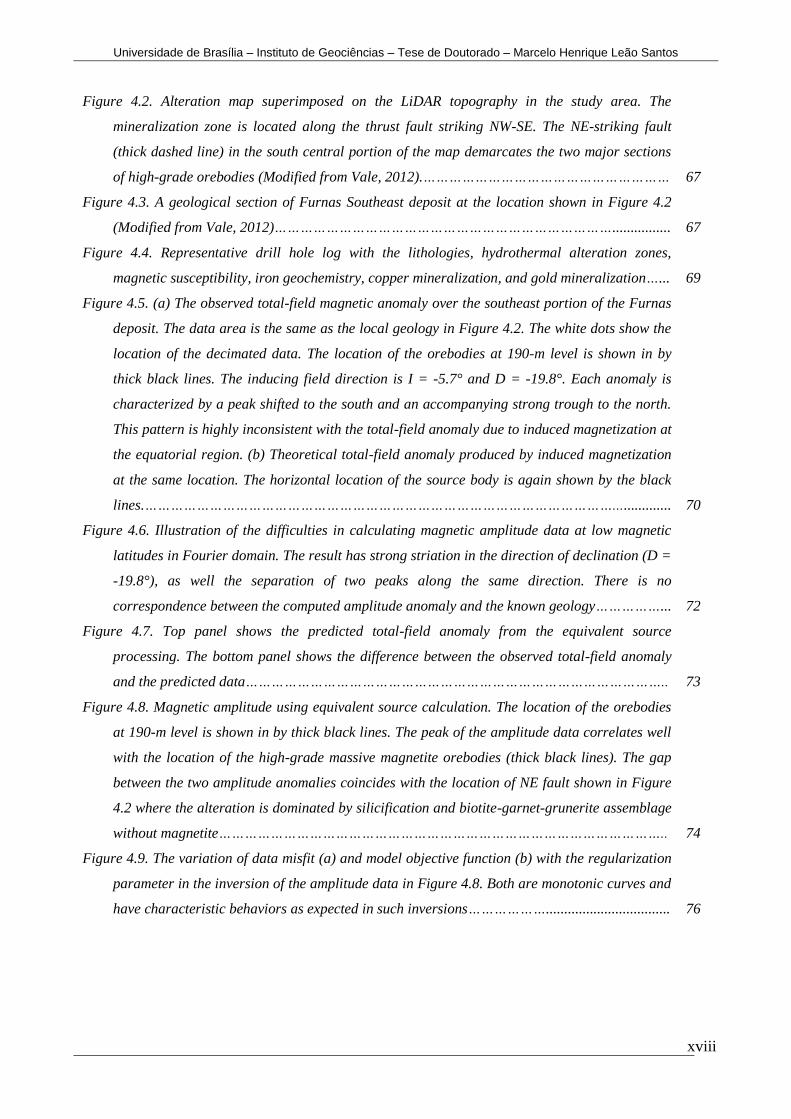
Figure 4.2. Alteration map superimposed on the LiDAR topography in the study area. The
mineralization zone is located along the thrust fault striking NW-SE. The NE-striking fault
(thick dashed line) in the south central portion of the map demarcates the two major sections
of high-grade orebodies (Modified from Vale, 2012).…………………………………………………
67
Figure 4.3. A geological section of Furnas Southeast deposit at the location shown in Figure 4.2
(Modified from Vale, 2012)……………………………………………………………………................
67
Figure 4.4. Representative drill hole log with the lithologies, hydrothermal alteration zones,
magnetic susceptibility, iron geochemistry, copper mineralization, and gold mineralization…...
69
Figure 4.5. (a) The observed total-field magnetic anomaly over the southeast portion of the Furnas
deposit. The data area is the same as the local geology in Figure 4.2. The white dots show the
location of the decimated data. The location of the orebodies at 190-m level is shown in by
thick black lines. The inducing field direction is I = -5.7° and D = -19.8°. Each anomaly is
characterized by a peak shifted to the south and an accompanying strong trough to the north.
This pattern is highly inconsistent with the total-field anomaly due to induced magnetization at
the equatorial region. (b) Theoretical total-field anomaly produced by induced magnetization
at the same location. The horizontal location of the source body is again shown by the black
lines.………………………………………………………………………………………………................
70
Figure 4.6. Illustration of the difficulties in calculating magnetic amplitude data at low magnetic
latitudes in Fourier domain. The result has strong striation in the direction of declination (D =
-19.8°), as well the separation of two peaks along the same direction. There is no
correspondence between the computed amplitude anomaly and the known geology……………...
72
Figure 4.7. Top panel shows the predicted total-field anomaly from the equivalent source
processing. The bottom panel shows the difference between the observed total-field anomaly
and the predicted data……………………………………………………………………………………..
73
Figure 4.8. Magnetic amplitude using equivalent source calculation. The location of the orebodies
at 190-m level is shown in by thick black lines. The peak of the amplitude data correlates well
with the location of the high-grade massive magnetite orebodies (thick black lines). The gap
between the two amplitude anomalies coincides with the location of NE fault shown in Figure
4.2 where the alteration is dominated by silicification and biotite-garnet-grunerite assemblage
without magnetite…………………………………………………………………………………………..
74
Figure 4.9. The variation of data misfit (a) and model objective function (b) with the regularization
parameter in the inversion of the amplitude data in Figure 4.8. Both are monotonic curves and
have characteristic behaviors as expected in such inversions………………..................................
76

Universidade de Brasília – Instituto de Geociências – Tese de Doutorado – Marcelo Henrique Leão Santos
xix UnB
Figure 4.10. L-curve estimation of optimal regularization parameter. (a) is the Tikhonov curve,
which has a well-defined corner at β = 10. (b) shows the variation of the complexity of
recovered 3D effective susceptibility models with the regularization parameter. All models are
displayed as volume-rendered images with a cutoff value of 0.15 SI………………………………..
77
Figure 4.11. Convergence curves for the final inversion of the amplitude data using the selected
optimal regularization parameter of 10…………………………………………………………………
78
Figure 4.12. Recovered 3D model of the magnetic susceptibility. The two 3D objects are the volume
rendered effective susceptibility from the amplitude inversion shown with a cutoff value of 0.15
SI, viewed from southeast. Superimposed are two cross-sections with color contours of the
effective susceptibility. The section located towards the NW of the image coincides with the
geological section in Figure 4.3………………………………………………………………………….
78
Figure 4.13. 3D correlation of the recovered susceptibility model (purple) with the known orebodies
(green) in the 3D geological model of the high-grade mineralization zones constructed from
extensive drilling in the Vale-Furnas Project…………………………………………………………..
80
Figure 4.14. Summary of the geologic interpretation of the amplitude inversion result in the cross-
section coinciding with that in Figure 4.3. The top panel shows the comparison between the
total-field anomaly and calculated amplitude data. The middle panel shows the calculated
amplitude data in a narrow strip surrounding the section. The bottom panel shows the
comparison between the inversion result and the geology. The recovered effective
susceptibility model (color contour) has characterized the massive magnetite (outlined in light
blue), and the known mineralized zone in dark blue. Measured magnetic susceptibilities are
also shown along several drill holes. The east most drill hole in this cross-section is the same
as that shown in Figure 4.4……………………………………………………………………………….
81
Figure 5.1. (a) Geological map of the Carajás Mineral Province with the location of the Furnas
deposit and the main Cu, Au, Fe, Mn, Ni and Pt group element (PGE) deposits. (b) Carajás
Province map with the Carajás domain (CD) and Rio Maria domain (RMD). The Bacajá
domain (BD) is located north of the Carajás domain. (c) Map of Brazil with the location of
Carajás Province (in black) and the Amazon Craton (in gray) (modified from DOCEGEO,
1988; Araújo and Maia, 1991; Barros and Barbey, 1998; Vasquez et al., 2008; and Xavier et.
al., 2012)……………………………………………………………………………………………………..
89
Figure 5.2. Magnetic total horizontal gradient with the location of the Furnas deposit along the
Cinzento lineament…………………………………………………………………………………………
90
Figure 5.3. Geological and hydrothermal alteration zone map of the Furnas Southeast deposit over
laser-LiDAR topography; the geological section location of Figure 5.4 is included (Modified
from Vale S.A., 2012)………………………………………………………………………………………
91

Universidade de Brasília – Instituto de Geociências – Tese de Doutorado – Marcelo Henrique Leão Santos
xx UnB
Figure 5.4. Geological section with the host rocks, hydrothermal alteration zones and mineralized
zones (Modified from Vale S.A., 2012)…………………………………………………………………..
91
Figure 5.5. Photographs of ore samples. (a) Chalcopyrite. (b) Bornite……………………………...….. 92
Figure 5.6. (a) Susceptibility meter KT-10. (b) Susceptibility/conductivity meter MPP - EM2S. (c)
Sketch of the sample - sensor contact surface. (d) Measurement procedure with the
susceptibility meter KT-10. (e) Measurement procedure with susceptibility meter/conductivity
meter MPP - EM2S……………………………………………………..………………………………….
98
Figure 5.7. Drill hole location map. Measurement schematics: lower sensitivity magnetic
susceptibility (MS) measurements (KT-9) in green; higher sensitivity MS measurements (KT-
10) in yellow; drill holes without MS measurements in white; and low grade orebody
projections at an elevation of 190 m in red. The geological section location (see Figure 5.4) is
indicated in the map, and the numbers of the drill holes used in this work are highlighted……...
99
Figure 5.8. Equipment used for laboratory determinations, Kappabridge model KLY-4S
(Laboratório de Anisotropias Magnéticas e de Magnetismo de Rocha - Instituto de
Geociências - Universidade de São Paulo)....................................................................................
100
Figure 5.9. Magnetic susceptibility measurements of the drill cores and geochemical sample
aliquots. Measurements with KT-9 and 0.5 m spacing (black profile), KT-10 and 0.5 m spacing
(blue profile), KT-10 and 0.2 m spacing (green profile), MPP and 0.2 m spacing (red profile),
and KT-10 in geochemical sample aliquots (magenta profile). Values in SI x 10-3……………….
101
Figure 5.10. Magnetic susceptibility measurements with laboratory (LAB SM), KT-10 meter and
MPP meter compared along the relative depths of drill holes 111, 112, 114 and 118……………
103
Figure 5.11. Correlation of the lithologies and hydrothermal alteration zones with the laboratory
magnetic susceptibility (graphs to the left) and anisotropy degree measurements (graphs to the
right). Drill holes 88, 111, 114 and 118.........................................................................................
104
Figure 5.12. Box plot log of magnetic susceptibility versus lithotypes with values from the higher
sensitivity susceptibility meter (KT-10). The predominance of ferrimagnetic, paramagnetic and
diamagnetic minerals is represented in red, green and blue rectangles respectively. HAZ =
hydrothermal alteration zone, Bt = biotite, Al = aluminous, Am = amphibolitic, Silicif =
silicification, Chlorit = chloritization, Mt = magnetite, Gru = grunerite, Grt = garnet, Amp =
amphibole, Gra = granite, BIF = banded iron formation………………………………………….…
105
Figure 5.13. Drill hole 88 log with strong iron oxide-copper-gold IOCG mineralization between
275 m and 350 m depths. Chloritization can be observed at the top and potassification and
silicification at the log base. The drill hole location can be found in Figure 5.7………………….
107

Universidade de Brasília – Instituto de Geociências – Tese de Doutorado – Marcelo Henrique Leão Santos
xxi UnB
Figure 5.14. Drill hole 48 log with the amphibolitic schist on top and aluminous schist on the base
hosting the mineralized zone. From depths of 169 to 211 m, the low magnetic susceptibility
and high iron grade signatures of the banded iron formation are shown. From depths of 230 to
400 m, the mineralized zone is dominated by silicification. The drill hole location can be found
in Figure 5.7. No positive gold assay values were obtained below the legend……………………..
108
Figure 5.15. Drill hole 34 log with the banded iron formation, magnetite and silica bands well
defined in the magnetic susceptibility, iron grade and density properties (212 to 260 m depths).
From depths of 145 to 192 m, the strong iron oxide-copper-gold IOCG mineralization can be
observed. The drill hole location can be found in Figure 5.7………………………………………...
109
Figure 5.16. Drill hole 31 log with the quartzite low susceptibility, low iron grade and low density
signature (65 to 122 m depths). From depths of 152 to 171 m, the strong iron oxide-copper-
gold IOCG mineralization can be observed. The drill hole location can be found in Figure 5.7.
109
Figure 5.17. Drill hole 125 log with the iron oxide-copper-gold IOCG mineralization signatures:
hydrothermal alterations, magnetic susceptibility in SI x 10-3
, iron grade geochemical assays
in percentage, copper grade in percentage, gold in grams per ton and density in grams per
cubic centimeter. The drill hole location can be found in Figure 5.7….……................................
110
Figure 5.18. Statistics and histograms of the magnetic susceptibility measurements. (a) Aluminous
schist. (b) Amphibolitic schist.........................................................................................................
111
Figure 5.19. Statistics and histogram of the banded iron formation magnetic susceptibility
measurements……………………………………………………………………………………...............
112
Figure 5.20. Statistics and histograms of magnetic susceptibility measurements. (a) Granite. (b)
Quartzite……………………………………………………………………………………………………..
113
Figure 5.21. Statistics and histograms of the magnetic susceptibility measurements. (a) Potassic
hydrothermal alteration zone. (b) Garnet-grunerite hydrothermal alteration zone……………….
114
Figure 5.22. Statistics and histograms of the magnetic susceptibility measurements. (a) Amphibole
hydrothermal alteration zone. (b) Chloritization………………………………………………………
115
Figure 5.23. Statistics and histogram of the silicification zone magnetic susceptibility measurements 115
Figure 5.24. Statistics and histograms of magnetic susceptibility measurements for magnetite-rich
alteration types. (a) Massive magnetite hydrothermal alteration zone. (b) Garnet-grunerite-
magnetite hydrothermal alteration zone.(c) Amphibole-magnetite hydrothermal alteration zone
117
Figure 5.25. (a) Three dimensional magnetic susceptibility model correlation with the copper low
grade orebodies projection at level 190 m. (b) Three dimensional magnetic susceptibility
model correlation with the copper high grade orebodies……………………………………………..
120
Figure 5.26. Detail of the magnetic susceptibility 3D model with isosurface of values higher than
500 x 10-3 SI (in red), and correlation with the copper high-grade orebodies (in blue, green
and yellow). Drill holes in black traces.……………………………..………………………………….
121

Universidade de Brasília – Instituto de Geociências – Tese de Doutorado – Marcelo Henrique Leão Santos
xxii UnB
LISTA DE TABELAS
Tabela 2.1. Coluna estratigráfica da Província de Carajás (Modificada de DOCEGEO, 1988; Villas
e Santos, 2001)...................................................................................................................
12
Table 3.1. Evidence of IOCG deposits and geophysical methods applied to mineral exploration……. 32
Table 4.1. The hydrothermal magnetite alteration zones susceptibilities………………………………… 68
Table 5.1. Lithotypes, hydrothermal alteration zones and mineralogy…………………………………… 94
Table 5.2. Main specifications of susceptibility meters KT-9 and KT-10 and susceptibility
meter/conductivity meter MPP-EM2S……………………………………………….………...
98

Universidade de Brasília – Instituto de Geociências – Tese de Doutorado – Marcelo Henrique Leão Santos
1 Capítulo 1 – Introdução
CAPÍTULO 1
INTRODUÇÃO
1.1 - CARACTERIZAÇÃO DOS PROBLEMAS
A interpretação de dados geofísicos e geológicos para a geração de alvos em ambientes
computacionais tem superado muito a capacidade do cérebro humano para analisar
quantitativamente grande volume de dados referenciados espacialmente. Entretanto, o cérebro
humano ainda é superior para computar, com seu grande número de unidades de cálculo (neurônios)
e interconexões (sinapses), que levam a um melhor desempenho do que computadores
convencionais (Zaknich, 2003).
Os principais desafios encontrados neste projeto de pesquisa foram divididos em geológicos,
geofísicos e prospectivos (Figura 1.1). Sistemas de forte alteração hidrotermal modificam as
propriedades físicas das rochas em depósitos IOCG. A espessa zona de intemperismo encontrada na
região amazônica dificulta o mapeamento geológico e a localização de ocorrências minerais. Além
do intemperismo o terreno acidentado também deve ser levado em consideração na inversão e
modelagem de dados geofísicos.
Figura 1.1. Desafios geológicos, geofísicos e prospectivos encontrados no projeto de pesquisa.

Universidade de Brasília – Instituto de Geociências – Tese de Doutorado – Marcelo Henrique Leão Santos
2 Capítulo 1 – Introdução
Existem diversas técnicas matemáticas e estatísticas disponíveis para processamento,
inversão e modelagem de dados geofísicos magnéticos. Entretanto, fazer o uso efetivo destas
técnicas é um desafio. A correta aplicação das técnicas disponíveis está correlacionada a
informações apriorísticas, essencial para o sucesso em termos de objetivos exploracionistas.
A interpretação em mapas, seções e perfis utiliza diversas técnicas e produtos transformados
que ajudam na localização e na estimativa das profundidades das fontes causadores das assinaturas
magnéticas observáveis. Modelagens em duas dimensões ajudam a dar forma a estas fontes
magnéticas. Para solucionar estes problemas, foram utilizados dados de levantamentos magnéticos
aerotransportados de alta resolução para cálculo dos produtos com algoritmos especializados.
Em ambientes de campos magnéticos anômalos fortes, localizados em baixas latitudes, às
vezes fica difícil fazer uma interpretação quantitativa precisa e geologicamente válida,
especialmente com modelos tridimensionais em termos das assinaturas magnéticas mapeadas,
devido ao complexo papel desempenhado pelo campo magnético resultante. O estudo das
magnetizações atual (induzida) e pretérita (remanescente) e dos efeitos da desmagnetização ajuda a
entender as mudanças na direção de magnetização do corpo e das diferentes assinaturas que
aparecem relacionadas a um mesmo conjunto de fontes que formam um corpo mineralizado. Estas
dificuldades estão bem retratadas em ambientes como o constituído pela mineralização em óxidos
de ferro e sulfetos de cobre tipo IOCG como o encontrado no depósito Furnas.
Para solucionar este problema, foram utilizados processos de otimização, de camada
equivalente e algoritmos de inversão 3D da amplitude da anomalia magnética de dados aéreos de
alta resolução.
As medidas de susceptibilidade magnética, realizadas em testemunhos de furos de sonda
podem ser utilizadas como informação a priori para diferenciar os litotipos e as zonas de alteração
hidrotermal em mineralizações IOCG. O volume de dados adquiridos nesta aproximação torna esta
uma atividade complexa, que se não for complementada por um entendimento das limitações dos
equipamentos, dos corretos controles de qualidade, de análises estatísticas, não permite que se
chegue a uma interpretação e modelagem confiável. No caso em foco os dados utilizados para
contornar estes problemas foram: medidas de susceptibilidade magnética tomadas com critério e
sob estrito controle de qualidade; descrição geológica e das alterações hidrotermais; medidas
complementares de densidade; e resultados de análises geoquímicas para ferro, cobre e ouro nos
testemunhos dos furos de sonda.

Universidade de Brasília – Instituto de Geociências – Tese de Doutorado – Marcelo Henrique Leão Santos
3 Capítulo 1 – Introdução
1.2 - ESTADO DA ARTE
A prospecção mineral envolve a aplicação de uma variedade de técnicas geocientíficas para
a descoberta de um depósito. A integração dos resultados de métodos e técnicas da geofísica com a
geologia é uma ferramenta poderosa para o sucesso de seus usos na exploração mineral. Neste
trabalho, dados sobre o comportamento da intensidade do campo magnético total (CMT ou TMI)
foram empregados desde a geração de temas transformados (filtragens no domínio de Fourier), até a
modelagem e inversão dos dados aéreos em 2D e 3D. Além disso, foi realizada a análise de medidas
de susceptibilidade e da geologia dos litotipos que formam tanto a mineralização na zona de
alteração hidrotermal como em suas encaixantes. Todos estes métodos e técnicas aplicados mostram
o estado da arte do conhecimento nestas áreas aqui desenvolvidas com foco na pesquisa mineral.
Tudo foi apoiado em hardware (equipamentos de informática, equipamentos geofísicos –
susceptibilímetros manuais e de laboratório); em softwares (algoritmos); e em dados magnéticos
(levantamentos geofísicos); que são o que existe de mais moderno na tecnologia disponível no
mercado atual.
1.3 - FOCO DOS RESULTADOS
O conhecimento de como as propriedades físicas e de magnetismo de rocha variavam, e de
assinaturas específicas ligadas à mineralização e suas encaixantes tiveram papel fundamental para
se entender o comportamento da magnetização do corpo. Os estudos feitos ajudaram inclusive na
definição de modelos prospectivos para o corpo de minério no depósito Furnas Sudeste, na
Província Mineral de Carajás, Pará, Brasil.
Ultimamente, o uso da modelagem de dados geofísicos assistida por técnicas de
minimização controlada de erros (inversão) em duas e três dimensões constitui instrumento
eficiente para ajudar o geocientista em aumentar a chance de fazer uma melhor interpretação e
identificar zonas mineralizadas. O uso destas técnicas, correlacionadas com a geologia, geoquímica,
geologia estrutural e outras informações geocientíficas, ampliam o êxito na pesquisa por minério.
Todas estas aproximações foram usadas na tentativa de produzir modelos bi e
tridimensionais do corpo de minério. Conseguiu-se assim, obtê-lo via a interpretação e inversão dos
dados magnéticos de alta resolução disponíveis, e via a modelagem espacial dos resultados das
medidas de susceptibilidade magnética feitas em testemunhos de sondagens disponíveis.
Todo o conjunto de informações geológicas obtidos nos estudos de campo e das amostras de
testemunhos de sondagens foi utilizado como suporte às aproximações geofísicas usadas –
modelagem de dados magnéticos e modelagem de dados espacialmente distribuídos das

Universidade de Brasília – Instituto de Geociências – Tese de Doutorado – Marcelo Henrique Leão Santos
4 Capítulo 1 – Introdução
susceptibilidades magnéticas. Isto foi possível pela excelente cobertura de dados geocientíficos
geradas sobre o lineamento Cinzento na região de Carajás em suas diversas fases de estudo.
Este trabalho enfoca justamente modos de se chegar a este modelo pelos dois caminhos
mencionados, de forma a simplificar e acrescentar muito mais informações sobre o modelo gerado.
Pode servir de guia em estudos sobre alvos semelhantes não só no Brasil mais em outros lugares do
mundo em ambientes metalogenéticos similares.
O escopo da tese foi o de explorar as potencialidades advindas das medições da intensidade
do campo magnético terrestre, com a aplicação do método com foco na prospecção da
mineralização de óxidos de ferro-cobre-ouro IOCG. Os três artigos preparados e que constituem o
corpo da tese em questão (submetidos para publicação) têm objetivos específicos, que se
complementam para atingir o escopo descrito acima, como resultado final.
1.4 - METODOLOGIA
Foram utilizados diversos métodos e técnicas durante as várias fases do projeto de pesquisa.
Estas fases podem ser divididas em quatro etapas que se complementam com o objetivo de definir
uma metodologia final de pesquisa. Todas as etapas tiveram o acompanhamento e orientação do
Professor Roberto Alexandre Vitória de Moraes da Universidade de Brasília. Uma grande parte da
base de dados foi cedida pela Vale S.A., a outra parte dos dados foi coletada e analisada pelo
trabalho de pesquisa nos testemunhos em campo e no laboratório da Universidade de São Paulo.
Na primeira etapa foi realizada a compilação bibliográfica; a caracterização e a
sistematização da base de dados geofísico-geológica; e o estudo da geologia regional, da geologia
do depósito e da mineralização IOCG. A base bibliográfica foi obtida na internet, de resumos
expandidos de congressos, publicações em revistas, trabalhos acadêmicos, e relatórios internos do
Projeto Furnas da Vale S.A..
Na segunda etapa foram utilizados diversos algoritmos computacionais com técnicas e
métodos de processamento de dados magnetométricos aéreos, como o controle de qualidade dos
dados; interpolações para a geração de malhas regulares; testes de eficácia deste processo;
homogeneização da representação espacial destes dados com técnicas de decorrugação, de modo a
conseguir a melhor imagem do campo magnético local para o depósito em estudo.
Posteriormente, foram geradas as transformações lineares com temas para ajudar na
interpretação qualitativa da imagem do campo magnético obtido. Finalmente, foram realizadas
interpretações semiquantitativas e quantitativas em duas dimensões para definir o melhor ajuste
entre o dado e o corpo resultante com o uso de informações empíricas a priori. Diversos programas
de Sistemas de Informações Geográficas, processamento, estimativa de profundidade e modelagem

Universidade de Brasília – Instituto de Geociências – Tese de Doutorado – Marcelo Henrique Leão Santos
5 Capítulo 1 – Introdução
2D de dados foi utilizada. Este trabalho contou com a orientação dos Professores Dr. Roberto
Alexandre Vitória de Moraes da Universidade de Brasília e Dr. Misac Nabighian da Colorado
School of Mines.
Na terceira etapa, foram utilizados algoritmos computacionais com capacidade de inversão
do campo magnético para estruturas tridimensionais complexas do depósito Furnas Sudeste, com a
seleção dos parâmetros de otimização e delimitação da profundidade de suas fontes geradoras.
Como resultado, foi recuperado de forma eficaz o modelo tridimensional do corpo magnético. A
interpretação do modelo magnético final foi correlacionada com os dados geológicos e estruturais
em Sistemas de Informações Geográficas 2D e 3D. Os algoritmos utilizados foram desenvolvidos
pelo Center for Gravity, Electrical & Magnetic Studies, Colorado School of Mines. Esta pesquisa
foi realizada na Colorado School of Mines, localizada em Golden, Colorado, Estados Unidos, como
doutorado sanduíche com período de um ano, suporte do Gravity and Magnetics Research
Consortium (GMRC) e orientação do Professor Dr. Yaoguo Li. Esta etapa teve apoio financeiro da
Vale S.A. e concessão de bolsa sanduíche da Fundação CAPES, Coordenação de Aperfeiçoamento
de Pessoal de Nível Superior, Ministério da Educação do Brasil.
Na quarta etapa foi utilizada a propriedade da susceptibilidade magnética para realizar
medidas sistemáticas e contínuas ao longo da maioria dos testemunhos de sondagens existentes na
área. Posteriormente foi realizada a análise estatística dos dados para caracterizar a assinatura
magnética dos litotipos e das alterações hidrotermais e a associação da mineralização com a
magnetita. Finalmente, os dados foram integrados em um programa para a geração de logs dos furos
de sonda, para a modelagem do corpo com alta susceptibilidade em três dimensões, e para estudar o
comportamento magnético do corpo.
Os dados de susceptibilidade magnética, geologia e análises geoquímicas de ferro, cobre e
ouro, foram levantados pelo Projeto Furnas da Vale S.A.. Os testes de medidas com métodos e
susceptibilímetros diferentes foram realizados pela equipe deste projeto de pesquisa. Também
foram realizadas análises de susceptibilidade e do grau de anisotropia no Laboratório de
Anisotropias Magnéticas e de Magnetismo de Rocha, do Instituto de Geociências, da Universidade
de São Paulo. As amostras e espécimes foram coletados e analisados pela equipe do projeto de
pesquisa. Esta pesquisa contou com a orientação do Professor Dr. Roberto Alexandre Vitória de
Moraes da Universidade de Brasília e da Professora Dra. Maria Irene Bartolomeu Raposo da
Universidade de São Paulo. Este trabalho também teve a participação dos geólogos Otávio Rosendo
e Arthur Cardoso na descrição e revisão do texto da geologia; e do técnico Joaquim Feijó na
amostragem e análises petrofísicas, todos da empresa Vale S.A..

Universidade de Brasília – Instituto de Geociências – Tese de Doutorado – Marcelo Henrique Leão Santos
6 Capítulo 1 – Introdução
O uso das diversas metodologias tanto de forma isolada como complementares constituem
ferramentas que podem ser utilizadas diretamente nas diferentes fases da pesquisa mineral de
depósitos associados a minerais ferromagnéticos. Essas metodologias são úteis tanto para resolver
questões relacionadas a depósitos de minerais magnéticos, como também outros tipos de depósitos
com a mineralização de interesse associada a minerais magnéticos.
1.5 - RESULTADOS ATINGIDOS
Consolidação do banco de dados geológico e geofísico;
Geologia regional e do depósito;
Geração dos Sistemas de Informações Geográficas (SIG) 2D/3D;
Especificações, controle de qualidade, processamento e geração de imagens transformadas
dos dados de levantamentos geofísicos de magnetometria aérea de alta resolução;
Interpretação qualitativa, semiquantitativa e quantitativa do campo magnético para definir a
fonte magnética, e obter o melhor ajuste entre o sinal obtido e a forma do corpo;
Seleção dos parâmetros de otimização para a inversão dos dados;
Inversão da amplitude magnética com o uso de camada equivalente para a geração do
modelo 3D do depósito Furnas Sudeste;
Método para levantamentos de medidas de susceptibilidade magnética;
Seleção, descrição e preparação de amostras para análises petrofísicas;
Medidas de susceptibilidade magnética sistemáticas nos testemunhos de furos de sonda e em
laboratório, para a geração de um modelo 3D de susceptibilidade;
Caracterização das assinaturas de susceptibilidade magnética dos litotipos e das zonas de
alteração hidrotermal;
Interpretação do modelo magnético e integração com os dados geológicos e estruturais, para
definir as assinaturas prospectivas para depósitos do tipo IOCG.

Universidade de Brasília – Instituto de Geociências – Tese de Doutorado – Marcelo Henrique Leão Santos
7 Capítulo 1 – Introdução
1.6 - ESTRUTURA DA TESE
CAPÍTULOS
1. INTRODUÇÃO DA TESE
2. GEOLOGIA REGIONAL
3. MAGNETIC INTERPRETATION AND 2D MODELING AT AN IRON OXIDE–
COPPER–GOLD DEPOSIT, CARAJÁS MINERAL PROVINCE, BRAZIL
Marcelo Leão-Santos1,2,4
*, and Roberto Moraes1
4. APPLICATION OF 3D MAGNETIC AMPLITUDE INVERSION TO IRON OXIDE–
COPPER–GOLD DEPOSITS AT LOW MAGNETIC LATITUDES: A CASE STUDY
FROM CARAJÁS MINERAL PROVINCE, BRAZIL
Marcelo Leão-Santos1,2,4*
, Yaoguo Li2, and Roberto Moraes
1
5. MAGNETIC SUSCEPTIBILITY 3D MODEL AND SIGNATURES OF IRON OXIDE-
COPPER-GOLD (IOCG) MINERALIZATION: A CASE STUDY FROM CARAJÁS
MINERAL PROVINCE, BRAZIL
Marcelo Leão-Santos1,2,4*
, Roberto Moraes1, Maria Irene Raposo
3, Otávio Rosendo
4,
Arthur Cardoso4, and Joaquim Feijó
4
6. CONCLUSÕES DA TESE
1 Universidade de Brasília, Instituto de Geociências, Campus Universitário Darcy Ribeiro ICC, Ala
Central, Brasília, DF, 70910-900, [email protected], [email protected]
2 Colorado School of Mines, Center for Gravity, Electrical & Magnetic Studies, 1500 Illinois St.,
Golden, CO, 80401, [email protected] , [email protected]
3 Universidade de São Paulo, Instituto de Geociências, Rua do Lago, 562, Cidade Universitária,
São Paulo, SP, 05508-080, [email protected]
4 VALE S.A., Av. Getúlio Vargas, 671, 13º andar, Funcionários, Belo Horizonte, MG, 30112-020,

Universidade de Brasília – Instituto de Geociências – Tese de Doutorado – Marcelo Henrique Leão Santos
8 Capítulo 1 – Introdução
1.7 - DIAGRAMA DOS TRABALHOS DESENVOLVIDOS NA TESE
1.8 - REFERÊNCIA
A. Zaknich, 2003, Neural Networks for Intelligent Signal Processing: World Scientific, Singapore,
484.

Universidade de Brasília – Instituto de Geociências – Tese de Doutorado – Marcelo Henrique Leão Santos
9 Capítulo 2 – Geologia Regional
CAPÍTULO 2
GEOLOGIA REGIONAL
Neste capítulo é abordado o arcabouço conceitual geológico referente à Província Mineral
de Carajás com destaque para o Supergrupo Itacaiúnas, no qual o depósito Furnas está inserido.
Com base no contexto geotectônico, a Província de Carajás está localizada no Escudo do
Brasil Central e inserida na porção sudeste da Província Amazonas Central, limitada pela Província
Transamazônica (Maroni-Itacaiúnas), a norte, e pela Faixa Araguaia, a leste, conforme mostra a
Figura 2.1 (Santos et al., 2000).
Figura 2.1. Compartimentação tectônica do Cráton Amazônico (Modificado de Santos et al., 2000).
Província Mineral
de Carajás
Limite do bloco

Universidade de Brasília – Instituto de Geociências – Tese de Doutorado – Marcelo Henrique Leão Santos
10 Capítulo 2 – Geologia Regional
A litoestratigrafia proposta para a Província Mineral de Carajás (Figura 2.2) é definida por
diversas unidades pré-cambrianas e agrupadas por suas características em: embasamento cristalino
mesoarqueano, denominados Complexos Xingu (granitóides de associação TTG - tonalito-
trondhjemito-granodiorito) e Pium (rochas granulíticas); e sequências metavulcanossedimentares do
tipo greenstone belt. Além dessas, foram distinguidos os granitos neoarqueanos denominados Suíte
Plaquê (rochas graníticas); e as sequências metassedimentares e metavulcanossedimentares
neoarqueanas, as quais constituem o Supergrupo Itacaiúnas. Outra unidade definida foram os
granitóides anorogênicos, representados por plútons graníticos com idades relacionadas ao
proterozoico inferior/médio. Estas intrusões cortam todas as unidades do Supergrupo Itacaiúnas,
bem como as rochas da Formação Águas Claras. Finalmente, foram definidas as unidades das
coberturas fanerozoicas, correlacionáveis ao Grupo Serra Grande (DOCEGEO, 1988; Araújo e
Maia, 1991; Barros e Barbey, 1998; Vasquez et al., 2008).
O depósito Furnas Sudeste está inserido no contexto de rochas metavulcanossedimentares do
Supergrupo Itacaiúnas (2.76 Ga; Wirth et al., 1986), rochas sedimentares da Formação Águas
Claras, granito anorogênico Cigano (1,8 Ga) e coberturas fanerozoicas (Figura 2.2). Na porção
noroeste do depósito Furnas, fora da área de estudo, ocorrem rochas granitóides do embasamento
que foram informalmente denominadas de Granito Furnas. Este granito possui características
petrológicas similares aos granitóides do fácies hornblenda-biotita monzogranito do Stock Granítico
Geladinho, com idade de 2.688 ± 11 Ma (Pb-Pb por evaporação de zircão; Barbosa et al., 2001).
Do ponto de vista metalogenético, essa província mineral constitui uma das mais bem
estudadas regiões do Cráton Amazônico que engloba importantes depósitos de Fe, Cu, Au, Ni, Mn e
elementos do grupo da platina (EGP).

Universidade de Brasília – Instituto de Geociências – Tese de Doutorado – Marcelo Henrique Leão Santos
11 Capítulo 2 – Geologia Regional
Figura 2.2. (a) Mapa geológico da Província Mineral de Carajás com a localização do depósito Furnas e dos principais
depósitos de Fe, Cu-Au, Mn, Ni e elementos do grupo da Pt (EGP). (b) Mapa da Província Carajás com o Domínio
Carajás (DC) e o Domínio Rio Maria (DRM). O Domínio Bacajá (DB) está localizado a norte do Domínio Carajás. (c)
Mapa do Brasil com a localização da Província Carajás (em preto) e o Craton Amazônico (em cinza) (Modificado de
DOCEGEO, 1988; Araújo e Maia, 1991; Barros e Barbey, 1998; Vasquez et al., 2008; e Xavier et. al., 2012).

Universidade de Brasília – Instituto de Geociências – Tese de Doutorado – Marcelo Henrique Leão Santos
12 Capítulo 2 – Geologia Regional
2.1 - ESTRATIGRAFIA
A Província Mineral de Carajás é alvo de intenso debate que se reflete nas inúmeras colunas
estratigráficas que foram e são propostas, à medida que novos dados são obtidos. A síntese do
conhecimento regional acumulado nas décadas de 60 e 70 levou Hirata et al. (1982) a proporem
uma coluna estratigráfica informal para a região.
De modo a facilitar o entendimento da evolução geológica da região e uniformizar a
nomenclatura para as unidades definidas, foi proposta uma coluna litoestratigráfica pela equipe do
Distrito Amazônia da DOCEGEO, elaborada a partir dos dados acumulados pela empresa desde
1974, somados aos resultados de trabalhos desenvolvidos por outras empresas e instituições de
pesquisas (DOCEGEO, 1988), conforme Tabela 2.1.
Tabela 2.1. Coluna estratigráfica da Província de Carajás (Modificada de DOCEGEO, 1988; Villas e Santos, 2001).
ÉON Idade
(Ga)
Cinturão de Cisalhamento Itacaiúnas
Complexos, Supergrupos
ou Unidades
Grupos (Gr) ou
Formações (Fm) Rochas Intrusivas
PROTEROZOICO 1,8 Granitos tipo-A Granitos anorogênicos (Central Carajás,
Cigano, Pojuca, Breves, Young Salobo, etc)
ARQUEANO
2,6 Fm. Aguas Claras/
Gr Rio Fresco
2,7 Sills e diques básicos, metagabros
2,5 - 2,7 Granitos neoarqueanos Suíte Plaquê, Old Salobo, Itacaiúnas, Estrela,
Planalto, Pedra Branca, Igarapé Gelado, etc
2,76 Supergrupo
Itacaiúnas
Gr Buritirama
Gr Igarapé Bahia
Gr Grão Pará
Gr Ig, Pojuca
Gr Ig. Salobo
2,76 Complexo Luanga Intrusão acamadada máfica-ultramáfica
2,8 – 3,0 Complexo Xingu Granitóides mesoarqueanos
3,0 Complexo Pium (Granulitos)
Trabalhos como os de Lindenmayer (1990), Araújo e Maia (1991), Costa et al. (1993),
Barros (1997), Barros et al. (1995), e Pinheiro e Holdsworth (1995), deram atenção ao
entendimento do quadro geológico regional da Serra dos Carajás.
Na década passada e trabalhos mais recentes têm dado ênfase à evolução
tectonoestratigráfica, petrogênese, metalogênese e, principalmente, a geocronologia das rochas da
Província Mineral de Carajás (p.e. Pinheiro e Holdsworth, 2000; Althoff et al., 2000; Pidgeon et al.
2000; Leite, 2001; Barros et al., 2001; Macambira et al., 2001; Barbosa et al., 2001; Villas e Santos,
2001; Tallarico et al., 2005; Monteiro et al., 2008; Feio, 2011; Moreto et al., 2012; Xavier et al.
2012; entre outros).

Universidade de Brasília – Instituto de Geociências – Tese de Doutorado – Marcelo Henrique Leão Santos
13 Capítulo 2 – Geologia Regional
2.2 - UNIDADES LITOLÓGICAS
As principais unidades litoestratigráficas que ocorrem na região da área em estudo e
arredores estão sintetizadas adiante e podem ser observadas no mapa geológico regional
apresentado na Figura 2.2.
2.2.1 - Embasamento – Complexos Xingu e Pium
O termo Complexo Xingu foi sugerido originalmente por Silva et al. (1974), com referência
às rochas infracrustais encontradas em praticamente todo o Cráton Amazônico. O Complexo Xingu
é formado principalmente por gnaisses bandados/foliados de composição tonalítica à granodiorítica,
além de anfibolitos e migmatitos. Essas rochas foram datadas em 2.856 ± 2 Ma por Machado et al.
(1991), através do método U-Pb, em zircões provenientes de gnaisses. Outras datações também
realizadas por Machado et al. (1991), tem idade 2.519 ± 5 Ma em anfibolito (U-Pb em titanitas),
2.859 ± 2 Ma e 2.860 ± 2 Ma em leucosomas graníticos (U-Pb em zircões) e 2.851 ± 2 Ma em
gnaisses félsicos (U-Pb em zircões). Avelar et al. (1999) dataram ortognaisses granodioríticos em
2.974 ± 15 Ma (Pb-Pb em zircões). A derivação dessas rochas tem sido atribuída em parte ao
retrabalho de granitóides dos terrenos granito - greenstone (vide abaixo), particularmente às rochas
anfibolíticas e migmatíticas (Araújo et al., 1988; Costa et al., 1995).
Trabalhos mais recentes têm individualizado os granitóides mesoarqueanos. O granitóide
Rio Verde teve sua primeira datação realizada por Sardinha et al. (2004) em leucomonzogranitos
com 2.928 ± 1 Ma (Pb-Pb em zircões), posteriormente Feio (2011) datou throndjemito em 2.923 ±
15 Ma (Pb-Pb em zircões). O granito Serra Dourada foi datado por Moreto et al. (2011a) em 2.860
± 22 Ma (U-Pb em zircões) e por Feio (2011) em 2.831 ± 6 Ma (U-Pb em zircões). O granito Canaã
dos Carajás foi datado por Feio (2011) em 2.959 ± 6 Ma (U-Pb em zircões). O tonalito Bacaba foi
datado por Moreto et al. (2011a) em 3.001 ± 3,6 Ma e 3.004 ± 9 Ma (U-Pb em zircões). O granito
Sequeirinho foi datado por Moreto et al. (2011a) em 3.010 ± 21 Ma (U-Pb em zircões).
O Complexo Pium compreende rochas granulíticas de composições variadas: ortoderivadas,
tipo charnockitos/enderbitos; e paraderivadas, tais como gnaisses kinzigíticos (Costa e Hasuí,
1996). Araújo e Maia (1991) admitem que, em geral, as rochas deste complexo estão em contato
concordante com os gnaisses do Complexo Xingu, e são marcados por importantes zonas de
cisalhamento dúcteis. Rodrigues et al. (1992), com base no método Pb-Pb em rocha total, obtiveram
idades para essa unidade de 3.050 ± 114 Ma. Pidgeon et al. (2000) obtiveram duas idades pelo
método U-Pb (SHRIMP), uma de 3.002 ± 14 Ma (cristalização do protólito ígneo do granulito),
valores estes quase correspondentes àquela obtida por Rodrigues et al. (1992), e uma outra mais
nova, de 2.859 ± 9 Ma, que deve corresponder ao metamorfismo de fácies granulito. Localmente,
Universidade de Brasília – Instituto de Geociências – Tese de Doutorado – Marcelo Henrique Leão Santos
14 Capítulo 2 – Geologia Regional
ocorrem rochas básicas e ultrabásicas estratificadas (Hirata et al., 1982), expostas em lentes
orientadas na direção E-W, principalmente na borda Sul do Sistema Transcorrente Carajás.
2.2.2 - Granitos neoarqueanos - Suíte Plaquê
A Suíte Plaquê, definida por Araújo et al. (1988), corresponde ao grupo de granitóides
aflorantes em lentes com direção geral E-W, concordantes com as rochas do Complexo Xingu
(Araújo et al., 1991). Esta unidade tem idade com base no método Pb-Pb em torno de 2.727 ± 29
Ma (Avelar, 1996) e 2.736 ± 24 Ma (Avelar et al., 1999). Um exemplo desse tipo de granito é o
Granito Planalto (2.747 ± 2 Ma, Pb-Pb em zircão; Huhn et al., 1999) que aflora nas adjacências da
Serra do Rabo. Este granito também foi datado por Feio (2011) com idade 2.733 ± 2 Ma, Pb-Pb em
zircão.
Diversos trabalhos têm individualizado os granitos neooarqueanos. O granito Old Salobo,
localizado nas adjacências da área do Igarapé Salobo (Lindnmayer e Fyfe, 1991; Lindenmayer et
al., 1994) tem idade em torno de 2.573 ± 3 Ma (U-Pb em zircão; Machado et al., 1991). O granito
Itacaiúnas com rochas dacíticas a riolíticas foi datado em 2.525 Ma ± 38 (Pb-Pb em zircão; Souza et
al., 1996), 2.645 Ma ± 9 e 2.654 Ma ± 9 (SHRIMP U-Pb em zircão; Tallarico, 2003). O granito
Rancho Alegre (Pinheiro, 1997) foi datado em 2.743 Ma (U-Pb zircão; Sardinha et al., 2001). O
stock granítico Geladinho foi datado em 2.688 ± 11 Ma (Pb-Pb por evaporação de zircão; Barbosa
et al., 2001), este granito também denominado Igarapé Gelado foi datado por Barbosa (2004) em
2.731 Ma ± 26 (Pb-Pb em zircão). O Complexo granítico Estrela (Barros, 1997) que aflora na
porção leste da região de Carajás, foi datado por Rb-Sr em 2.527 ± 34 Ma (Barros et al, 1992),
posteriormente foi datado em 2.763 ± 7 Ma, por Pb-Pb em zircão (Barros et al, 2004), 2.734 ± 4 Ma
por Pb-Pb em zircão de biotita-hornblenda granito e 2.765 ± 39 Ma, por U-Pb em zircão de
throndjemito (Sardinha et al, 2004). O diorito Cristalino foi datado por Huhn et al. (1999) em 2.738
± 6 Ma por Pb-Pb em zircão. A Suite Pedra Branca foi datada em 2.750 ± 5 Ma por U-Pb em zircão
(Feio, 2011). O granito granofírico do Sossego foi datado por Moreto et al. (2011b) em 2.740 ± 26
Ma por U-Pb em zircão.
Anteriormente, muitos desses granitos e granitóides meso a neoarqueanos estavam
indiferenciados no Complexo Xingu, a partir de estudos detalhados de suas relações de contato e de
suas idades, passaram a ser individualizados e ganharam nomes e posições estratigráficas próprias.
Os stocks graníticos do Geladinho subdividem-se em dez fácies petrográficas: hornblenda
tonalitos, biotita-hornblenda granodioritos, hornblenda-biotita granodioritos, biotita granodioritos,
hornblenda monzogranitos, biotita-hornblenda monzogranitos, hornblenda-biotita monzogranitos,
biotita monzogranitos, leuco monzogranitos, leuco sienogranitos e veios pegmatóides (Barbosa,

Universidade de Brasília – Instituto de Geociências – Tese de Doutorado – Marcelo Henrique Leão Santos
15 Capítulo 2 – Geologia Regional
2004). O granitóide de fácies hornblenda-biotita monzogranito se assemelha com as rochas
graníticas do depósito Furnas, que foi denominado informalmente como Granito Furnas. O Granito
Furnas aflora nas adjacências do depósito, compreendem rochas de composição monzogranítica,
coloração cinza, granulação fina a média, constituída por quartzo, plagioclásio, microclina e
biotita/clorita. Localmente, ocorrem variações para fácies pegmatóides quartzo-feldspáticas e de
texturas granofíricas.
2.2.3 - Sequências vulcânicas e sedimentares - Supergrupo Itacaiúnas
O Supergrupo Itacaiúnas está em contato discordante com os gnaisses do Complexo Xingu.
Este supergrupo engloba todas as sequências de rochas supracrustais da Província Mineral de
Carajás, que diferem em grau metamórfico e composição das sequências de Greenstone-Belts do
Supergrupo Andorinhas. Desse modo, foram agrupados, da base para o topo, os Grupos Igarapé
Salobo, Igarapé Pojuca, Grão-Pará, Igarapé Bahia e Buritirama.
Grupo Igarapé Salobo
É considerado como basal por conter as rochas de mais alto grau metamórfico. Compreende
uma faixa deformada, de direção WNW, composto por anfibolitos datados em 2.555 ± 3 Ma (U-Pb
em zircões), anfibolitos foliados datados em 2.761 ± 3 Ma e 2.497 ± 5 Ma (U-Pb em titanitas),
formações ferríferas datadas em 2.551 ± 2 Ma (U-Pb em monazitas), metagrauvacas, xistos e
quartzitos (Machado et al., 1991). Veios graníticos também foram datados por Machado et al.
(1991) em 2.732 Ma (Pb-Pb em zircões) e 2.581 ± 5 Ma e 2.584 ± 5 Ma (U-Pb em titanitas).
Estas rochas foram descritas inicialmente como metamórficas no depósito de Cu-Au do
Salobo (Lindenmayer, 1990), posteriormente foram reinterpretadas como provenientes de processos
de alteração hidrotermal em rochas supracrustais do Supergrupo Itacaiúnas que acompanharam a
deposição dos sulfetos de cobre (Lindenmayer e Teixeira, 1999).
Grupo Igarapé Pojuca
O Grupo Igarapé Pojuca tem ampla distribuição nas bordas do "Sinclinório Carajás",
abrange sequências de rochas metavulcanossedimentares, de fácies xisto-verde a anfibolito,
orientadas segundo direção geral WNW-ESE com mergulhos que variam entre 50° NE a 60° SW. A
seção tipo foi definida na área que abriga os depósitos de Cu-Zn e Cu-Au-Mo e descrita por
DOCEGEO (1988) como rochas metavulcânicas básicas a intermediárias (muitas vezes com
alteração hidrotermal para cordierita-antofilita, anfibólios, sílica, biotita), anfibolitos, gnaisses,
cherts, formações ferríferas bandadas e xistos de composições diversas. Foi caracterizada a

Universidade de Brasília – Instituto de Geociências – Tese de Doutorado – Marcelo Henrique Leão Santos
16 Capítulo 2 – Geologia Regional
Formação Corpo Quatro, que abriga depósito homônimo e caracteriza-se por dois grupamentos
litológicos principais: rochas bandadas e rochas com fragmentos. As rochas bandadas correspondem
a sedimentos químicos com sulfetos (pirrotita, calcopirita, esfalerita), níveis descontínuos de chert
e/ou formação ferrífera bandada fácies óxido, bem como vários níveis de sulfeto maciço. As rochas
com fragmentos apresentam disseminações de pirrotita, calcopirita e, eventualmente, esfalerita.
Anfibolitos do Grupo Igarapé Pojuca foram datados por Machado et al. (1991) em torno de
2.732 ± 2 Ma pelo método U-Pb em zircões. Pimentel et al (2003) dataram metaandesitos em 2.719
± 80 Ma (Sm-Nd em rocha total).
As mineralizações de Cu-Zn são consideradas singenéticas e relacionadas à fácies sulfeto
das formações ferríferas bandadas, enquanto que a mineralização de Cu-Au-Mo está provavelmente
relacionada a sistemas pórfiros (Biagini, 1990).
Grupo Grão-Pará
O Grupo Grão Pará (Beisiegel et al., 1973) é profundamente importante no contexto da
Província Mineral de Carajás, por incluir as jazidas de ferro de alto teor. É formado por três
unidades da base para o topo: Formação Parauapebas (DOCEGEO, 1988), Formação Carajás
(Beisiegel et al., 1973) e a Sequência Paleovulcânica Superior (Beisiegel et al., 1973; DOCEGEO,
1988 ou Upper Metasedimentary Sequence, Gibbs et al., 1986).
A Formação Parauapebas é constituída por basaltos e basaltos andesíticos datados em 2.687
± 54 Ma (Rb-Sr em rocha total; Gibbs et al., 1986), riolitos e shoshonitos, cortados por corpos
quartzo-dioríticos (Gibbs et al., 1986; Teixeira e Eggler, 1994), metamorfisados na fácies xisto-
verde e pouco deformados. No topo da Formação Parauapebas dominam rochas vulcânicas félsicas
datadas em 2.758 ± 39 Ma (U-Pb em zircões; Wirth et al., 1986), riolitos datados em 2.759 ± 2 Ma
(U-Pb em zircões, Machado et al. 1991), metariolitos porfiríticos datados em 2.760 ± 11 Ma
(SHRIMP U-Pb em zircão; Trendall et al. 1998) e traquiandesitos. Estes dados indicam sincronismo
entre a Formação Parauapebas e a deposição dos Grupos Salobo e Pojuca.
A Formação Carajás abriga as formações ferríferas bandadas fácies óxido e carbonato, que
representam o protominério dos depósitos de ferro supergênicos. Teixeira e Eggler (1994)
observaram que existem dolomitos na base da formação em contato gradacional com as formações
ferríferas. Sua idade mínima é determinada por um sill máfico datado de 2.740 ± 8 Ma. (U-Pb,
zircão, Trendall et al., 1998).
A Formação Paleovulcânica Superior compreende rochas vulcânicas, metagrauvacas, siltitos
tufáceos, filitos, arenitos, com derrames basálticos, tufos e arenitos tufáceos (Gibbs et al., 1986).

Universidade de Brasília – Instituto de Geociências – Tese de Doutorado – Marcelo Henrique Leão Santos
17 Capítulo 2 – Geologia Regional
Grupo Igarapé Bahia
O Grupo Igarapé Bahia, de ocorrência restrita à área da mina inativa de ouro do mesmo
nome, é considerado por DOCEGEO (1988), como sobreposto às rochas do Grupo Grão Pará.
Compreende uma sequência de rochas metavulcanossedimentares de baixo grau metamórfico, que
contém mineralização primária de Cu, associado a Au, Mo e Ag, e mineralização secundária de Au
em gossans. Tem direção aproximada NNW, mergulham cerca de 70° ENE no Corpo
Acampamento Sul, que afloram em uma janela estrutural. Este grupo é dominado por rochas
metassedimentares (pelitos e ritmitos) e metavulcanoclásticas (félsicas a máficas), que se intercalam
com metavulcânicas e intrusivas máficas (DOCEGEO, 1988). Brechas hidrotermais são bem
caracterizadas nas zonas de minério, que são preferencialmente hospedadas na interface de rochas
vulcânicas com rochas piroclásticas/ritmitos do pacote.
Datações geocronológicas feitas por Ferreira Filho (1985) indicam idades de 2.577 ± 72 Ma
(Rb-Sr) em granófiros básicos e 2.270 ± 50 Ma (Rb-Sr) em rochas piroclásticas silicosas, admitidas
como idade mínima para a sequência metavulcanossedimentar. Mougeot et al. (1996), utilizaram os
métodos Rb-Sr, Sm-Nd, U-Pb e Pb-Pb para realizar análises em sulfetos (calcopirita, pirita, galena e
molibdenita) em diversas zonas mineralizadas da Região de Carajás e estabeleceram para a
mineralização de Cu e Au do Igarapé Bahia a idade mínima de 2.850 ± 65 Ma, o que caracteriza
uma mineralização primária arqueana. Idades isotópicas (Galarza, 2002; Galarza e Macambira,
2002a) obtidas em rochas metavulcânicas máficas (2.745 ± 1 Ma, Pb-Pb em zircão) e em rochas
metapiroclásticas (2.747 ± 1 Ma, Pb-Pb em zircão) mostraram definitivamente o sincronismo com
as rochas do Supergrupo Itacaiúnas. Tallarico et al. (2005) também dataram rochas metavulcânicas
máficas que confirmaram idades similares de 2.748 ± 34 Ma (SHRIMP U-Pb em zircão).
A intrusão máfica-ultramáfica acamadada do Luanga (2.763 ± 6 Ma., Machado et al., 1991)
e o sill de gabro do depósito de Cu-Au Gameleira (2.757 ± 81 Ma., Pimentel et al., 2003) atestam
também a ocorrência de magmatismo basáltico naquela época.
Grupo Buritirama
É representado por um pacote de metassedimentos clásticos e químicos de direção N55°W,
que aflora na serra homônima na porção norte da Província Mineral de Carajás. Este grupo é
composto, da base para o topo, por quartzitos bandados, quartzitos micáceos e xistos variados; e
contém importantes reservas de manganês.

Universidade de Brasília – Instituto de Geociências – Tese de Doutorado – Marcelo Henrique Leão Santos
18 Capítulo 2 – Geologia Regional
2.2.4 - Formação Águas Claras
Essa formação foi sugerida por Araújo et al., (1988) e descrita por Nogueira (1995),
anteriormente correlacionada por DOCEGEO (1988) ao Grupo Rio Fresco. Compreende rochas
sedimentares marinhas a fluviais cortadas por sills e diques de rochas máficas (Soares et al., 1994).
Encontra-se de forma discordante sobre as rochas do Supergrupo Itacaiúnas.
Na base, é constituída, predominantemente, por siltitos e argilitos laminados de cor cinza a
avermelhado. Nas faixas onde ocorre maior deformação, as rochas são transformadas em
metassiltitos, metapelitos e quartzo-mica-xistos. As estruturas primárias mais comuns preservadas
são laminações plano-paralelas, estratificação cruzada de baixo ângulo tipo hummocky e estruturas
de fluidização e carga.
Para o topo, ocorrem metarenitos e metarcóseos de coloração branca, granulação média à
grossa, com grãos sub-angulosos mal selecionados e apresentam, localmente, hematita, clorita e
sericita na matriz. Intercalam-se nestes arenitos, lentes de microconglomerados. As camadas têm
formato lenticularizado. Neste pacote predominam estruturas do tipo de acamamento gradacional,
estratificações cruzadas tabular e acanalada de pequeno porte e marcas de ondas ligeiramente
assimétricas. As rochas metassedimentares estão dispostas segundo direção NW-SE com mergulhos
suaves, com média de 20o para NE, as quais, nas proximidades de falhas, podem chegar a
mergulhos de médio a alto ângulo.
A deformação das rochas da Formação Águas Claras possui caráter rúptil e está limitada às
zonas de falhas direcionais, como a Falha Carajás. É marcante o arranjo tectônico da formação
segundo horsts e grabens. O depósito de Au-Cu de Águas Claras encontra-se relacionado a esse
comportamento rúptil nos arenitos do Membro Superior (Soares et al., 1994).
Trendall et al. (1998) dataram arenitos com zircão proveniente de rochas vulcânicas
sindeposicionais em 2.681 ± 5 Ma (SHRIMP U-Pb em zircões); e Dias et al. (1996) dataram diques
de gabro que cortam o pacote sedimentar em 2.645 ± 12 Ma (U-Pb em zircões).
2.2.5 - Diques e Sills máficos
São metagabros, metadioritos e metadiabásios abundantes na região. Sabe-se que existem
várias fases de magmatismo máfico, mas a sua divisão é muito difusa. Têm idades desde arqueanas
(gabros de 2,7 Ga no depósito de Águas Claras), passam a proterozoicas (dioritos do Igarapé Aquiri,
com cerca 1,9 Ga, Hirata et al. 1982) a até brasilianas (diques encontrados na área do Salobo,
Lindenmayer, 1990). Variam também na sua forma, desde corpos tabulares expressivos, como o
gabro Santa Inês, até pequenos diques (DOCEGEO, 1988).

Universidade de Brasília – Instituto de Geociências – Tese de Doutorado – Marcelo Henrique Leão Santos
19 Capítulo 2 – Geologia Regional
Mougeot et al. (1996) dataram metagabros em 2.708 ± 37 Ma (U-Pb em zircões); Galarza e
Macambira (2002b) dataram rochas intrusivas máficas em 2.705 ± 2 Ma (Pb-Pb em zircões); e
Pimentel et al. (2003) dataram metagabros e rochas metavulcânicas cogenéticas em 2.757 ± 81 Ma
(Sm-Nd em rocha total).
2.2.6 - Granitos anorogênicos
Diversos plútons de granitos anorogênicos ocorrem na região, com idades relacionadas ao
proterozoico inferior/médio. Essas intrusões cortam todas as unidades do Supergrupo Itacaiúnas,
bem como as rochas da Formação Águas Claras. Datações geocronológicas, realizadas em zircões
pelo método (U-Pb), estabeleceram idades em torno de 1.880 Ma. (Gibbs et al., 1986; Machado et
al., 1991 e Macambira e Lafon, 1995). Possivelmente, essas intrusões estão associadas ao evento
plutônico-vulcânico Uatumã, que recobre extensas porções do Cráton Amazônico com rochas
extrusivas félsicas. Destacam-se, pelas proximidades geográficas com a área estudada, o Granito
Central Carajás com idade de 1.820 ± 49 Ma obtida pelo método U-Pb em zircão (Wirth et al.
1986), e 1.880 ± 2 Ma obtida pelo método U-Pb em zircão; Granito Cigano com idade 1.883 ± 2 Ma
em zircão U-Pb; Granito Pojuca com idade 1.874 ± 2 Ma em zircão U-Pb (Machado et al. 1988;
Machado et al. 1991); Granito Breves com idade com idade 1.879 ± 6 Ma em zircão U-Pb SHRIMP
(Tallarico et al. 2004) e Granito Young Salobo com idade com idade 1.880 ± 80 Ma (Rb-Sr em
rocha total; Cordani, 1981); além de outros menores ainda pouco conhecidos.
2.2.7 - Coberturas fanerozoicas
Coberturas fanerozoicas são registradas como as unidades mais jovens que afloram na
porção norte da região de Carajás e constituem sequências sedimentares correlacionáveis ao Grupo
Serra Grande (Caputo e Lima, 1984).
2.3 - MODELO TECTONOESTRATIGRÁFICO
A região da Serra dos Carajás, inicialmente, foi compreendida como uma bacia que
comportava um pacote de rochas vulcanossedimentares sob a forma de um grande sinclinório ou
sinclinal (Beisiegel et al., 1973; Hirata et al., 1982; DOCEGEO 1988).
A bacia tem forma sigmoidal alongada segundo a direção geral da foliação ESE, que denota
um comportamento dominantemente transcorrente-sinistral. Deslocamentos de até 30 km são
registrados ao longo da Falha Carajás, que corta toda a bacia e são indicativos das falhas
transcorrentes WNW-ESE. As falhas de direção NE-SW, como a falha McCandless, representam
outra importante direção de estruturas, no âmbito da Província Mineral de Carajás.

Universidade de Brasília – Instituto de Geociências – Tese de Doutorado – Marcelo Henrique Leão Santos
20 Capítulo 2 – Geologia Regional
O modelo proposto por Pinheiro (1997), e Holdsworth e Pinheiro (2000), sugere que a
evolução tectônica de Carajás foi iniciada com o estabelecimento de uma zona de cisalhamento
dúctil arqueana, de direção E-W (Zona de Cisalhamento Itacaiúnas), responsável pelo
aparecimento, nas rochas do embasamento (Complexos Pium e Xingu), de uma fábrica milonítica
de alta temperatura (fácies anfibolito médio a alto), gerada por transpressão sinistral.
Posteriormente, se instalou sobre o embasamento as rochas do Grupo Igarapé Pojuca, que
foram deformadas por transpressão e, sobre estas, os litotipos do Grupo Grão Pará (2,7 Ga).
Discordantes sobre essas rochas, foram depositados os sedimentos da Formação Águas Claras.
Seguiu-se, um evento transtensional dextral, responsável pela subsidência dessas rochas no
interior da Bacia de Carajás, a Sul, e ao longo do Sistema Transcorrente Cinzento, a Norte, que
gerou uma geometria sigmoidal alongada com tendência E-W, fortemente controlada pela
geometria das zonas de cisalhamento pretéritas. A Falha Carajás marca o limite de subsidência e
deslocamento dextral transtensivo da Estrutura de Carajás, a qual foi invadida por um enxame de
diques e sills máficos por volta de 2,6 Ga. Um episódio de transpressão sinistral entre 2,6 Ga e 2,0
Ga, reativou a Falha Carajás, o que provocou a deformação das rochas situadas no interior da
Estrutura Carajás e, no contexto do Sistema Transcorrente Cinzento, deu origem às estruturas
sidewall ripout do Salobo e duplex do Cururu.
Um último episódio deformacional, controlado por uma extensão E-W a NE-SW, ocorrida
durante o Proterozoico Inferior e o início do Mesoproterozoico, no Cráton Amazônico, deu origem
a fraturas e falhas regionais de direção N-S e permitiu a intrusão de plútons graníticos (Granitos
Carajás, Cigano, etc) e, possivelmente, novos diques máficos. Localmente, em virtude da reativação
de falhas maiores pretéritas, ocorreu a formação de pequenas bacias, onde foram depositados os
sedimentos da Formação Gorotire.
O modelo descrito acima que destaca um evento transtensional dextral relacionado ao
Sistema de Cisalhamento Cinzento, representa a principal feição identificada no contexto do alvo
Furnas, sobre a qual estão condicionadas as rochas do depósito.

Universidade de Brasília – Instituto de Geociências – Tese de Doutorado – Marcelo Henrique Leão Santos
21 Capítulo 2 – Geologia Regional
2.4 - REFERÊNCIAS
Althoff, F.J., P. Barbey, A.M. Boullier, 2000, 2.8-3.0 Ga plutonism and deformation in the SE
Amazonian craton: the Archean granitoids of Marajoara (Carajás Mineral province, Brazil):
Precambrian Research, 104, 187–206.
Araújo, O.J.B., R.G.N. Maia, X.S. Jorge João, J.B.S. Costa, 1988, A megaestruturação arqueana da
Folha Serra dos Carajás: 1º Congresso Latino Americano de Geologia, Anais, 324–338.
Araújo, O.J.B., R.G.N. Maia, 1991, Projeto especial mapas de recursos minerais, de solos e de
vegetação para a área do Programa Grande Carajás; Subprojeto Recursos Minerais; Folha
SB.22-Z-A Serra dos Carajás - Estado do Pará: DNPM/CPRM.
Avelar, V.G., J.M. Lafon, F.C. Correia JR., E.M.B. Macambira, 1999, O magmatismo arqueano da
região de Tucumã – Província Mineral de Carajás: Novos dados geocronológicos: Revista
Brasileira de Geociências, 29, no. 4, 453–460.
Avelar, V.G., 1996, Geocronologia Pb-Pb por evaporação em monocristal de zircão do
magmatismo da região de Tucumã, SE do Estado do Pará, Amazônia oriental: Dissertação de
Mestrado, Universidade Federal do Pará.
Barbosa, J.P.O., 2004, Geologia Estrutural, Geoquímica, Petrografia e Geocronologia de granitoides
da região de Igarapé Gelado, norte da Província Mineral de Carajás: Dissertação de Mestrado,
Universidade Federal do Pará.
Barbosa, J.P.O, C.E.M. Barros, M.B. Macambira, A.G. Vale, 2001, Geologia e Geocronologia do
Stock Granítico Geladinho, região de Parauapebas, Província Mineral de Carajás: 7º Simpósio
de Geologia da Amazônia, SBG, Resumos Expandidos.
Barros, C. E. M., 1997, Pétrologie et struture du Complexe Granitique Estrela (2.5 Ga) et de son
encaissant métavolcano-sédimentaire (Province Métallifère de Carajás, Brésil): Tese de
Doutorado, Université Henri Poincaré - Nancy.
Barros, C.E.M., Dall’Agnol, R., Lafon, J.M., Teixeira, N.P., Ribeiro, J.W., 1992, Geologia e
geocronologia Rb-Sr do Gnaisse Estrela, Curionópolis, PA: Boletim do Museu Paraense
Emilio Goeldi, Ciências da Terra, 4, 83–102.
Barros, C.E.M., Dall’Agnol, R., Vieira, E.A.P., Magalhães, M.S., 1995. Granito Central da Serra
dos Carajás: avaliação do potencial metalogenético para estanho com base em estudos da borda
oeste do corpo. Boletim do Museu Paraense Emílio Goeldi. Série Ciências da Terra 7, 93–123.
Barros, C.E.M., Barbey, P., 1998. A importância da granitogênese tardi-arqueana (2,5 Ga.) na
evolução tectono-metamórfica da província mineral de Carajás – O Complexo Granítico
Estrela e sua auréola de contato: Revista Brasileira de Geociências. 28, no. 4, 513–522.
Barros, C.E.M., M.J.B. Macambira, P. Barbey, 2001, Idade de zircão do Complexo Granítico
Estrela: relações entre magmatismo, deformação e metamorfismo na Província Mineral de
Carajás: 7º Simpósio de Geologia da Amazônia, SBG, Resumos Expandidos.
Barros, C.E.M., Macambira, M.J.B., Barbey, P., Scheller, T., 2004, Dados isotópicos Pb-Pb em
zircão (evaporação) e Sm-Nd do Complexo Granítico Estrela, Província Mineral de Carajás,
Brasil: implicações petrológicas e tectônicas: Revista Brasileira de Geociências, 34, 531−538.
Beisegel, V.R., A.L. Bernardelli, N.F. Drummond, A.W. Ruff, J.W. Tremaine, 1973, Geologia e
recursos minerais da Serra dos Carajás: Revista Brasileira de Geociências, 3, 215–242.
Biagini, D.O., 1990, Considerações sobre algumas feições metalogenéticas de Carajás: DOCEGEO,
Relatório Interno.

Universidade de Brasília – Instituto de Geociências – Tese de Doutorado – Marcelo Henrique Leão Santos
22 Capítulo 2 – Geologia Regional
Caputo, M.V., E.C. Lima, 1984, Estratigrafia, idade e correlação do Grupo Serra Grande - Bacia do
Parnaíba: 33º Congresso Brasileiro de Geologia, SBG, Resumos Expandidos, 8, 740–753.
Cordani, U., 1981, Comentários sobre as determinações geocronológicas da região da Serra dos
Carajás: Universidade de São Paulo - Docegeo, Relatório.
Costa, J.B.S., Y. Hasuí, 1996, Evolução geológica da Amazônia, in M. L. Costa, R.S. Angélica,
1997, Contribuições à geologia da Amazônia, 15–90.
Costa J.B.S., O.J.B. Araújo, A. Santos, X.S. Jorge João, M.J.B. Macambira, J.M. Lafon, 1995, A
Província Mineral de Carajás: aspectos tectono estruturais, estratigráficos e geocronológicos:
Boletim do Museu Paraense Emílio Goeldi, Série Ciências da Terra 7, 199–235.
Costa, J.B.S., Y. Hasuí, R.L. Bemerguy, M.S. Borges, A.R. Costa, W. Travassos, J.A. Mioto,
H.L.S. Igreja, 1993, Aspectos fundamentais da neotectônica na Amazônia Brasileira: Simpósio
Internacional do Quaternário da Amazônia, Resumos e Contribuições Científicas, 103–106.
Dias, G.S., Macambira, M.B., Dall’Agnol, R., Soares, A.D.V., Barros, C.E.M., 1996, Datações de
zircões de sill de metagabro: comprovação de idade arqueana da Formação Águas Claras,
Carajás, Pará: 5th Simpósio de Geologia da Amazônia, SBG, Resumos Expandidos, 376−378.
DOCEGEO (Rio Doce Geologia e Mineração S.A), 1988, Revisão litoestratigráfica da Província
Mineral de Carajás: Congresso Brasileiro de Geologia, SBG, Resumos expandidos, 35, 10–54.
Feio, G.R.L., 2011, Magmatismo granitóide arqueano da área de Canaã dos Carajás: implicações
para a evolução crustal da Província Carajás: Tese de Doutorado, Universidade Federal do
Pará.
Ferreira Filho, C.F., 1985, Geologia e mineralizações sulfetadas do Prospecto Bahia, Província
Mineral de Carajás: Dissertação de Mestrado, Universidade de Brasília.
Galarza, T.M.A., 2002, Geocronologia e geoquímica isotópica dos depósitos de Cu-Au Igarapé
Bahia e Gameleira, Província Mineral de Carajás (PA), Brasil: Tese de Doutorado,
Universidade Federal do Pará.
Galarza, M.A., M.J.B. Macambira, 2002a, Petrologia e geocronologia das rochas encaixantes do
depósito de Cu-Au Igarapé Bahia, Província Mineral de Carajás, Pará, Brasil, in E.L. Kein,
M.L. Vasquez, L.T. Rosa-Costa: Contribuições à Geologia da Amazônia, SBG/NN 3, 153–168.
Galarza, M.A., M.J.B. Macambira, 2002b, Geocronologia e Evolução Crustal da Área do Depósito
de Cu- Au Gameleira, Província Mineral de Carajás (Pará), Brasil: Geologia USP Série
Científica 2, 143–159.
Gibbs, A.K., K.R. Wirth, W.K. Hirata, W.J. Olszewski Jr., 1986, Age and composition of the Grão
Pará Group volcanics, Serra dos Carajás: Revista Brasileira de Geociências, 16, no. 2,
201−211.
Hirata, W.K., J.C. Rigon, A.A.C. Cordeiro, E.M. Meireles, 1982, Geologia regional da Província
Mineral de Carajás: 1º Simpósio de Geologia da Amazônia, SBG, Resumos Expandidos, 100–
108.
Holdsworth, R., R. Pinheiro, 2000, The anatomy of shallow-crustal transpressional structures:
Insights from the Archean Carajás fault zone, Amazon, Brazil: Journal of Structural Geology,
22, 1105−1123.
Huhn S.R.B., M.J.B. Macambira, R. Dall'Agnol, 1999, Geologia e geocronologia Pb/Pb do granito
alcalino Arqueano Planalto, Região da Serra do Rabo, Carajás – PA: 6º Simpósio de Geologia
da Amazônia, SBG, Resumos Expandidos, 463–466.

Universidade de Brasília – Instituto de Geociências – Tese de Doutorado – Marcelo Henrique Leão Santos
23 Capítulo 2 – Geologia Regional
Leite, A.A.S., 2001, Geoquímica, petrogênese e evolução estrutural dos granitóides arqueanos da
região de Xinguara, SE do Cráton Amazônico: Tese de Doutorado, Universidade Federal do
Pará.
Lindenmayer, Z.G., 1990, Salobo Sequence, Carajás, Brazil: geology, geochemistry and
metamorphism: Ph.D. thesis, University of Western Ontario.
Lindenmayer, Z.G., W.S. Fyfe, 1991, Metamorfismo de alta temperatura e baixa pressão no
depósito de cobre do Salobo: evidência do rift continental arqueano no Cráton Amazônico: 3º
Simpósio de Geologia da Amazônia, SBG, Resumos Expandidos, 36–48.
Lindenmayer, Z.G., W.S. Fyfe, V.L.S. Bocalon, 1994, Nota preliminar sobre as intrusões
granitóides do depósito de cobre do Salobo, Carajás: Acta Geológica Leopoldensia, 17, no. 40,
153–184.
Lindenmayer, Z.G., J.B.G. Teixeira, 1999, Ore Genesis at the Salobo Copper Deposit, Serra dos
Carajás, in M.G. Silva, A. Misi, eds., Base Metal Deposits of Brazil: MME/CPRM/DNPM,
33–43.
Macambira, M.J.B., J.M. Lafon, 1995, Geocronologia da Província Mineral de Carajás; Síntese dos
dados e novos desafios: Boletim do Museu Paraense Emílio Goeldi, Série Ciências da Terra 7,
263–288.
Macambira, M.J.B., L.M. Lima, R.V.L. Pinheiro, Lima, F.D., 2001, Idades de Cristais Detríticos de
Zircão da Serra dos Carajás, Pará; Evidências sobre a Formação da Crosta: 7º Simpósio de
Geologia da Amazônia, SBG, Resumos Expandidos, 72–75.
Machado, N., D. Lindenmayer, Z. Lindenmayer, 1988, Geocronologia U-Pb da Província
Metalogenética de Carajás, Pará: resultados preliminares: 7º Congresso Latinoamericano de
Geologia, SBG/DNPM, Resumos Expandidos, 339–347.
Machado, W., Z.G. Lindenmayer, T.E. Krogh, D. Lindenmayer, 1991, U-Pb geochronology of
Archean magmatism and basement reactivation in the Carajás área, Amazon shield, Brazil:
Precambrian Research, 49, 329–354.
Monteiro, L.V.S., R.P. Xavier, E.R. Carvalho, M.W. Hitzman, C.A. Johnson, C.R.S. Filho, I.
Torresi, 2008, Spatial and temporal zoning of hydrothermal alteration and mineralization in the
Sossego iron oxide–copper–gold deposit, Carajás Mineral Province, Brazil: paragenesis and
stable isotope constraints: Mineralium Deposita, 43, 129–159.
Moreto, C.P.N., L.V.S. Monteiro, R.P. Xavier, W.S. Amaral, T.J.S. Santos, C. Juliani, C.R. Souza
Filho, 2011a, Mesoarchean (3.0 and 2.86 Ga) host rocks of the iron oxide-Cu-Au Bacaba
deposit, Carajás mineral province: U-Pb geochronology and metallogenetic implications:
Mineralium Deposita, 46, 789−811.
Moreto, C.P.N., L.V.S. Monteiro, R.P. Xavier, T.I.S. Kemp, C.R. Souza Filho, 2011b, In situ LA-
ICPMS U-Pb zircon dating of the host rocks of the Sossego and Bacaba iron oxide-copper-gold
deposits, Carajás mineral province, Brazil: 11th Biennial SGA Meeting.
Moreto, C.P.N., L.V.S. Monteiro, R.P. Xavier, T.I.S. Kemp, K. Sato, W.S. Amaral, 2012, SHRIMP
and LA-ICPMS U-Pb zircon geochronology of the host rocks of the Sossego, Bacaba and
Castanha IOCG deposits, Carajás mineral province, Brazil: 34th
International Geology
Congress.
Mougeot, R., J.P. Respaut, L. Brique, P. Lédru, J.P. Milesi, C. Lerouge, E. Maroux, S.B. Huhn,
M.J.M. Macambira, 1996, Isotope geochemistry constrains for Cu, Au mineralizations and
evolution of the Carajás Province (Pará, Brazil): 39th
Congresso Brasileiro de Geologia, SBG,
Resumos Expandidos, 7, 321–324.

Universidade de Brasília – Instituto de Geociências – Tese de Doutorado – Marcelo Henrique Leão Santos
24 Capítulo 2 – Geologia Regional
Nogueira, A.C.R., 1995, Análise faciológica e aspectos estruturais da Formação Águas Claras,
Região Central da Serra dos Carajás – Pará: Dissertação de Mestrado, Universidade Federal do
Pará.
Pidgeon, R.T., M.J.B. Macambira, J.M. Lafon, 2000, Th-U-Pb isotopic systems and internal
structures of complex zircons from an enderbite from the Pium Complex, Carajás Province,
Brazil: evidence for the ages of granulite facies metamorphism and the protolith of the
enderbite: Chemical Geology, 166, 159–171.
Pinheiro, R.V.L., 1997, Reactivation history of the Carajás and Cinzento Strike-Slip System,
Amazon, Brazil: Ph.D. thesis, University of Durham.
Pinheiro, R.V.L., R.E. Holdsworth, 1995, Significado tectônico da clivagem transversa (transecting
cleavage) em dobras na Mina de Serra Pelada, Pará: Boletim do Museu Paraense Emílio
Goeldi, Série Ciências da Terra 7, 259–278.
Pinheiro, R.V.L., R.E. Holdsworth, 2000, Evolução Tectonoestratigráfica dos Sistemas
Transcorrentes Carajás e Cinzento, Cinturão Itacaiúnas, na borda leste do Cráton Amazônico,
Pará: Revista Brasileira de Geociências, 30, no. 4, 597–606.
Pimentel, M.M., Z.G., Lindenmayer, Laux, J.H., Armstrong, R., Araújo, J.C., 2003, Geochronology
and Nd geochemistry of the Gameleira Cu-Au deposit, Serra dos Carajás, Brazil: 1.8−1.7 Ga
hydrothermal alteration and mineralization: Journal of South American Earth Sciences, 15,
803−813.
Rodrigues, E.S., J.M. Lafon, T. Scheller, 1992, Geocronologia Pb-Pb da Província Mineral de
Carajás: primeiros resultados: 37º Congresso Brasileiro de Geologia, SBG, Resumos
Expandidos, 2, 183–184.
Santos, J.O.S, L.A. Hartmann, H.E. Gaudette, D.I. Groves, N.J. McNaughton, I.R. Fletcher, 2000,
A new understanding of the provinces of the Amazon Craton based on integration of field
mapping and U-Pb and Sm-Nd geochronology: Gondwana Research, 3, no. 4, 453–488.
Sardinha, A.S., C.E.M. Barros, R. Krymski, M.J.B. Macambira, 2001, Petrografia e Geocronologia
U-Pb em zircão do Granito Serra do Rabo, Província Mineral de Carajás, Pará: 7º Simpósio de
Geologia da Amazônia, SBG, Resumos Expandidos.
Sardinha, A.S., R. Dall’Agnol, A.C.B. Gomes, M.J.B. Macambira, M.A. Galarza, 2004,
Geocronologia Pb-Pb e U-Pb em zircões de granitóides arqueanos da região de Canaã dos
Carajás, Província Mineral de Carajás: 42nd
Congresso Brasileiro de Geologia, Resumos
Expandidos.
Silva, G.G., M.J.C. Lima, A.R.F. Andrade, R.S. Issler, G. Guimarães, 1974, Geologia das folhas
SB-22 Araguaia e parte SC-22 Tocantins: Projeto RADAMBRASIL, geologia, geomorfologia,
solos e uso potencial da terra, Levantamento de Recursos Naturais, 4.
Soares, A.V., A.B. Santos, E.A. Vieira, V.M. Bella, L.P.B. Martins, 1994, Área Águas Claras
contexto geológico e mineralizações: 4º Simpósio de Geologia da Amazônia, SBG, Resumos
Expandidos, 379–382.
Souza, S.R.B., M.J.B. Macambira, T. Sheller, 1996, Novos dados geocronológicos para os granitos
deformados do Rio Itacaiúnas (Serra dos Carajás, PA); implicações estratigráficas: 5º Simpósio
de Geologia da Amazônia, SBG, Resumos Expandidos, 380–383.
Tallarico, F.H.B., 2003, O cinturão cupro-aurífero de Carajás, Brasil: Tese de Doutorado,
Universidade Estadual de Campinas.

Universidade de Brasília – Instituto de Geociências – Tese de Doutorado – Marcelo Henrique Leão Santos
25 Capítulo 2 – Geologia Regional
Tallarico, F.H.B., N.J. McNaughton, D.I. Groves, I.R. Fletcher, B.R. Figueiredo, B.J. Carvalho, L.J.
Rego, A.R. Nunes, 2004, Geological and SHRIMP II U-Pb constraints on the age and origin of
the Breves Cu-Au- (W-Bi-Sn) deposit, Carajás, Brazil: Mineralium Deposita, 39, 68−86.
Tallarico, F.H.B., B.R. Figueiredo, D.I. Groves, N. Kositcin, N.J. McNaughton, I.R. Fletcher, J.L.
Rego, 2005, Geology and SHRIMP U-Pb geochronology of the Igarapé Bahia deposit, Carajás
copper-gold belt, Brazil: An Archean (2.57 Ga) example of iron-oxide Cu-Au-(U-REE)
mineralization: Economic Geology, 100, 7−28.
Teixeira, J.B.G., D.H. Eggler, 1994, Petrology, Geochemistry, and Tectonic Setting of Archaean
Basaltic and Dioritic Rocks from the N4 Iron Deposit, Serra dos Carajás, Pará, Brazil: Acta
Geologica Leopoldensia, 17, no. 40, 71–114.
Trendall, A.F., M.A.S. Basei, J.R. Laeter, D.R. Nelson, 1998, SHRIMP zircon U-Pb constraints on
the age of the Carajás formation, Grão Pará Group, Amazon Craton: Journal of South
American Earth Sciences, 11, no. 3, 265–277.
Vasquez, M.L., C.S. Sousa, J.M.A Carvalho, 2008, Mapa Geológico e de Recursos Minerais do
Estado do Pará, escala 1:1.000.000: Programa Geologia do Brasil (PGB), Companhia de
Pesquisa de Recursos Minerais - Serviço Geológico do Brasil.
Villas R.N., M.D. Santos, 2001, Gold deposits of the Carajás Mineral Province: deposit types and
metallogenesis: Mineralium Deposita, 36, 300–331.
Wirth, K.R., A.K. Gibbs, W.J. Olszewski, 1986, U-Pb ages of zircons from the Grão-Pará group
and Serra dos Carajás Granite, Pará, Brazil: Revista Brasileira de Geociências, 16, no. 2, 195–
200.
Xavier, R.P., L.V.S. Monteiro, C.P.N. Moreto, A.L.S. Pestilho, G.H.C. Melo, M.A.D. Silva, B.
Aires, C. Ribeiro, and F.H.F. Silva, 2012, The iron oxide copper-gold systems of the Carajás
Mineral Province, Brazil, in Geology and Genesis of Major Copper Deposits and Districts of
the World: A Tribute to Richard Sillitoe, Special Publication, Society of Economic Geologists.

Universidade de Brasília – Instituto de Geociências – Tese de Doutorado – Marcelo Henrique Leão Santos
26 Capítulo 3 – Magnetic interpretation and 2D modeling at IOCG deposits
CAPÍTULO 3
MAGNETIC INTERPRETATION AND 2D MODELING AT AN IRON OXIDE–COPPER–
GOLD DEPOSIT, CARAJÁS MINERAL PROVINCE, BRAZIL
Manuscript submitted to the Journal Geophysics in August 12th
of 2014.
Thank you for submitting your manuscript, GEO-2014-0380, to GEOPHYSICS
[email protected] <[email protected]> Tue, Aug 12, 2014 at 4:37 PM To: [email protected], [email protected] Cc: [email protected], [email protected], [email protected], [email protected] 12-Aug-2014 Re: GEO-2014-0380, "MAGNETIC INTERPRETATION AND 2D MODELING AT IRON OXIDE–COPPER–GOLD DEPOSITS, CARAJÁS MINERAL PROVINCE, BRAZIL", Leão-Santos, Marcelo; Moraes, Roberto Dear Mr. Marcelo Leão-Santos: Thank you for submitting your manuscript listed above to GEOPHYSICS. Please refer to the manuscript number in all correspondence. Your paper is undergoing review.

Universidade de Brasília – Instituto de Geociências – Tese de Doutorado – Marcelo Henrique Leão Santos
27 Capítulo 3 – Magnetic interpretation and 2D modeling at IOCG deposits
MAGNETIC INTERPRETATION AND 2D MODELING AT AN IRON OXIDE–COPPER–
GOLD DEPOSIT, CARAJÁS MINERAL PROVINCE, BRAZIL
Marcelo Leão-Santos1,2,3
, and Roberto Moraes1
1 Universidade de Brasília, Instituto de Geociências, Brasília, Brazil.
E-mail: [email protected], [email protected].
2 Colorado School of Mines, Center for Gravity, Electrical & Magnetic Studies, Golden, Colorado.
3 VALE S.A., Department of Exploration and Mineral Projects, Belo Horizonte, Brazil.
E-mail: [email protected].
3.1 - ABSTRACT
Magnetic signatures are often used to interpret physical properties of massive magnetite
from strong hydrothermal alteration in iron oxide–copper–gold deposits (IOCG). In areas with
strong magnetization, the presence of remanence and self-demagnetization can yield a total
magnetization orientation which differs significantly from the direction of the inducing field and
which can easily lead to an erroneous interpretation. Qualitative, semi-quantitative and quantitative
analysis can help to understand the behavior of the magnetic anomaly, give support to accomplish a
best approach to interpretation, in obtaining a good correlation with geological data and assisting
future three-dimensional (3D) modeling. Several linear transformations can be useful to a
successful interpretation of the magnetic data. This can be enhanced by correct magnetic profiles
interpretations to allow a better understanding of body geometry. Depth estimations provided by
this approach are a powerful tool to define the body position in subsurface. Finally, the estimation
of magnetic properties as priori information to two-dimensional (2D) parametric modeling can
achieve good results. We demonstrate that the application of all these tools in the Furnas Southeast
Fe oxide–Cu–Au deposit located at low magnetic latitude in Carajás Mineral Province, Brazil, can
reliably define the structures of magnetite hydrothermal alterations associated with the high and low
grade ores.
3.2 - INTRODUCTION
Airborne magnetic surveys are frequently used in the exploration for copper sulfides and
gold ores in IOCG deposits because of their association with magnetite, thus providing a cost-
effective systematic structural mapping and interpretation for these magnetic sources.
Magnetic data interpretation can be done both qualitatively and quantitatively using some of
the techniques shown in Figure 3.1.

Universidade de Brasília – Instituto de Geociências – Tese de Doutorado – Marcelo Henrique Leão Santos
28 Capítulo 3 – Magnetic interpretation and 2D modeling at IOCG deposits
Figure 3.1. Flowchart of qualitative, semi-quantitative and quantitative methods used in interpreting magnetic data.
The qualitative interpretation can be done by visual inspection of the images and profiles in
maps and cross-sections, in some of the many linear transformations available. This allows for the
definition of domains and lineaments related to the local magnetic field configuration. In the present
study, we focused on using the measured TMI (Total Magnetic Field Intensity) data to understand
the spatial distribution of the magnetic sources and how can they be grouped spatially (magnetic
fabric) which then points to the different regions where the magnetic material is distributed. Further

Universidade de Brasília – Instituto de Geociências – Tese de Doutorado – Marcelo Henrique Leão Santos
29 Capítulo 3 – Magnetic interpretation and 2D modeling at IOCG deposits
information can be obtained on the underlain rock volumes themselves, on the brittle, and on ductile
structures imposed on them.
Several methods and techniques were used to aid the qualitative interpretation of magnetic
data. One group of methods uses direct (TMI) or residual magnetic field (RMI) data to perform
various filtering operations in frequency domain (e.g. reduction to the pole, pseudo-gravity, upward
continuation and vertical derivatives). Another group of methods use spatial derivatives of various
orders depending on the high spatial noise frequency present in the magnetic data (e.g. analytic
signal, analytic signal vector inclination (tilt derivative), total and horizontal field gradients,
magnetic amplitude, terracing).
These were followed by semi-quantitative methods, starting first with a technique to
determine the depth to the top of magnetic sources by studying the amplitude versus wave number
relation from 2D radially averaged power spectrum analysis. These results can then be
complimented by using depth estimates using Euler deconvolution techniques. These methods can
be applied either to the whole survey area or to selected areas with individual magnetic signatures.
The presence of remanent magnetization and self-demagnetization effects certainly pose
many problems thus complicating the interpretation of magnetic sources. In addition, the fact that
the inducing field intensity is much smaller at low magnetic latitudes than at higher magnetic
latitudes further exacerbates the problem.
The final step attempts, using all previously gained information, is a quantitative
interpretation by using two-dimensional (2D) parametric or structural modeling which can be
extended to a 3D physical model representation (intrinsic magnetic susceptibility modeling).
The main objective of this paper is to apply the above mentioned magnetic data analysis
procedures to study an iron oxide–copper–gold mineralization (IOCG) using a set of high-resolution
airborne magnetic data at the Furnas copper-gold deposit.
Location of the study area
The Carajás Mineral Province is located in the state of Pará in northern Brazil approximately
1,100 km from Brasilia (Figure 3.2). The province is located at low latitude with magnetic
inclination -7.3°. The Carajás Mineral Province is bounded to the west by the Xingu River and to
the east by the Araguaia-Tocantins River. The Gradaús and Bacajá Mountain Ranges by the
province to the south and north, respectively (Hirata et al., 1982).

Universidade de Brasília – Instituto de Geociências – Tese de Doutorado – Marcelo Henrique Leão Santos
30 Capítulo 3 – Magnetic interpretation and 2D modeling at IOCG deposits
Figure 3.2. Location of Carajás Mineral Province and the infrastructure of the region: cities, main roads, hydrography,
Carajás railroad and Tucuruí power plant.
The infrastructure of the region is privileged because of the easy electricity supply from the
Tucuruí Hydroelectric Power Plant, which is 275 km to the north. The Carajás Railroad (Estrada de
Ferro Carajás – EFC) with approximately 892 km in extension can be used to transportation and
provides access to the Port of Madeira in São Luís – Maranhão. The study area can be accessed
from the state capital, Belém, through the state highways PA-475 and PA-150 to Marabá and then
through highway PA-150 to the city of Eldorado dos Carajás and PA-275 to the cities of
Parauapebas and Carajás (Figure 3.2).
The Carajás Mineral Province has adequate infrastructure in place to support mineral
extraction. The Furnas deposit is located approximately 35 km from the Parauapebas city, 45 km
from the Carajás Airport, 60 km from the Carajás city and 10 km north of the Carajás Railroad.
Iron oxide-copper-gold (IOCG) deposits
Carajás is known as an economically important metallogenic province where numerous
types of mineral deposits are found. In addition to the IOCG mineralization, there are deposits types
of banded iron formations, lateritic gold, lateritic manganese, mafic-ultramafic layered intrusions
hosting platinum group elements, nickel laterite and nickel sulfide deposits. In terms of
geotectonics, the Carajás Province is located in the Central Brazilian Shield within the southeastern

Universidade de Brasília – Instituto de Geociências – Tese de Doutorado – Marcelo Henrique Leão Santos
31 Capítulo 3 – Magnetic interpretation and 2D modeling at IOCG deposits
portion of the Central Amazonian Province, which is bordered by the Transamazonian Province
(Maroni-Itacaiúnas) to the north and Araguaia Belt to the east (Santos et al., 2000).
Hitzman et al. (1992) originally defined IOCG deposits as a unique type after the discovery
and study of the Olympic Dam in the Gawler Craton in southern Australia (Oreskes and Einaudi
1990, 1992). IOCG deposits may contain only copper or gold, and others may be rich in iron oxides
with phosphorus as an accessory (e.g., Kiruna) or with rare earth elements (e.g., Bayan Obo;
Nykänen, 2008). The IOCG deposits can also be divided in three main types: magnetite group (e.g.
Salobo, Sossego, Candelaria), hematite group (e.g. Olympic Dam, Prominent Hill, Manto Verde)
and magnetite + hematite group (e.g. Sue Dianne, North Portia, Rakkurijärvi).
Williams et al. (2005) addresses a broad discussion on IOCG geology, space-time
distribution, and possible modes of origin. From an economic perspective, the most significant
IOCG deposits are those in Chile and Peru in the coastal batholithic belt (Jurassic-Cretaceous
extended continental margin arc); in Australia within the Gawler craton and Cloncurry districts (late
Paleoproterozoic to Mesoproterozoic debated intracratonic or distal subduction-related settings);
and in Brazil in the Carajás province (Archean, Amazon craton). Williams et al. (2005), do not
classify the Kiruna-type iron oxide-apatite ores and iron skarns as IOCG deposits even though they
share some features with IOCG deposits. Monteiro et al. (2008) described the spatial and temporal
zoning of hydrothermal alteration and mineralization in the Sossego IOCG deposit. Xavier et al.
2012 summarize the Iron Oxide Copper-Gold Systems of the Carajás Mineral Province. Groves et
al. (2010) described IOCG deposits through Earth history, the implications for origin and
lithospheric setting, and distinction from other epigenetic iron oxide deposits.
Although definitions vary somewhat, in this study, IOCG is used as a term to describe
deposits with hydrothermal alteration and mineralization that have significant amounts of
magnetite, copper and gold. The main features can be summarized as follows (Nykänen et al.,
2008):
(i) proximity to cratonic areas;
(ii) controlled by structures, faults and lineament intersections;
(iii) presence of granitic intrusions, particularly those that may be enriched in either
compatible and incompatible elements;
(iv) occurrence of anomalous magnetic signatures related to the concentration of magnetite
in the deposit;
(v) occurrence of radiometric signatures with high values in the uranium channel;
(vi) anomalous presence of copper, gold and iron; and
(vii) association of incompatible elements with the mineralization.

Universidade de Brasília – Instituto de Geociências – Tese de Doutorado – Marcelo Henrique Leão Santos
32 Capítulo 3 – Magnetic interpretation and 2D modeling at IOCG deposits
Table 3.1 summarizes the predictive variables and respective geophysical methods that are
used in prospecting for IOCG deposits.
Table 3.1. Evidence of IOCG deposits and geophysical methods applied to mineral exploration.
Evidence Geophysical Method
Sequences rich in iron oxides Magnetic
Main and secondary structures in large deep crustal faults Magnetic
Lineament density and zones of structural opening Magnetic
Strong hydrothermal alteration with magnetite Magnetic
Presence of uranium Gamma spectrometry
Potassic alteration areas Gamma spectrometry
High density because of the presence of sulfides and magnetite Gravimetry
High chargeability and low resistivity – disseminated ore Induced polarization (IP)
Electromagnetic conductors – massive ore or interconnected sulfides and magnetite Electromagnetic (EM)
3.3 - GEOLOGICAL SETTING
The Furnas Copper Deposit is located in the Carajás Mineral Province, along the regional
Cinzento transcurrent shear zone striking WNW-ESE. Metavolcano-sedimentary rocks correlated to
the Grão Pará Group, of the 2.76 Ga Itacaiúnas Supergroup (Wirth et al., 1986), and sedimentary
rocks correlated to the Águas Claras Formation host the deposit. The shear zone defines a contact
between amphibole schist to the north (hanging wall) and aluminous schist to the south (footwall)
of the Itacaiúnas Supergroup (Figure 3.3), interrupted by the intrusion of the 1.8 Ga Cigano Granite
to the east. The region is metamorphosed from greenschist to amphibolite facies (CVRD, 2006).
The deposit is poorly exposed with a wide laterite cover (thickness of about 60 m). The
copper-gold mineralization is hosted in biotite-garnet-grunerite-magnetite hydrothermal alteration
assemblages, with moderate to strong foliation. The mineralization itself is contained in massive
magnetite, silicification, sodic-calcic, and potassic alteration as can be easily seen on the geological
cross section through the high and low-grade orebodies (Figure 3.3). The alteration zone is
associated with a late-stage chalcopyrite and bornite veinlets and breccias.
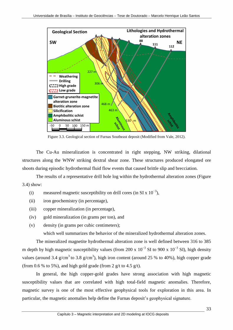
Universidade de Brasília – Instituto de Geociências – Tese de Doutorado – Marcelo Henrique Leão Santos
33 Capítulo 3 – Magnetic interpretation and 2D modeling at IOCG deposits
Figure 3.3. Geological section of Furnas Southeast deposit (Modified from Vale, 2012).
The Cu-Au mineralization is concentrated in right stepping, NW striking, dilational
structures along the WNW striking dextral shear zone. These structures produced elongated ore
shoots during episodic hydrothermal fluid flow events that caused brittle slip and brecciation.
The results of a representative drill hole log within the hydrothermal alteration zones (Figure
3.4) show:
(i) measured magnetic susceptibility on drill cores (in SI x 10−3
),
(ii) iron geochemistry (in percentage),
(iii) copper mineralization (in percentage),
(iv) gold mineralization (in grams per ton), and
(v) density (in grams per cubic centimeters);
which well summarizes the behavior of the mineralized hydrothermal alteration zones.
The mineralized magnetite hydrothermal alteration zone is well defined between 316 to 385
m depth by high magnetic susceptibility values (from 200 x 10−3
SI to 900 x 10−3
SI), high density
values (around 3.4 g/cm3
to 3.8 g/cm3), high iron content (around 25 % to 40%), high copper grade
(from 0.6 % to 5%), and high gold grade (from 2 g/t to 4.5 g/t).
In general, the high copper-gold grades have strong association with high magnetic
susceptibility values that are correlated with high total-field magnetic anomalies. Therefore,
magnetic survey is one of the most effective geophysical tools for exploration in this area. In
particular, the magnetic anomalies help define the Furnas deposit’s geophysical signature.
SW NE
Lithologies and Hydrothermal alteration zones
Garnet-grunerite-magnetite alteration zoneBiotitic alteration zoneSilicificationAmphibolitic schistAluminous schist
227 m
306 m
468 m
-50 0 50 100 150 m
WeatheringDrillingHigh gradeLow grade
112111
88
463 m
530 m
Geological Section

Universidade de Brasília – Instituto de Geociências – Tese de Doutorado – Marcelo Henrique Leão Santos
34 Capítulo 3 – Magnetic interpretation and 2D modeling at IOCG deposits
Figure 3.4. Representative drill hole 125 log with the iron oxide-copper-gold IOCG mineralization signatures:
hydrothermal alterations, magnetic susceptibility in SI x 10-3
, iron grade geochemical assays in percentage, copper
grade in percentage, gold in grams per ton and density in grams per cubic centimeter.

Universidade de Brasília – Instituto de Geociências – Tese de Doutorado – Marcelo Henrique Leão Santos
35 Capítulo 3 – Magnetic interpretation and 2D modeling at IOCG deposits
3.4 - MAGNETIC DATA
The magnetic data was acquired using a sensor mounted on a helicopter, and in a draped
survey with a nominal terrain clearance of 80 m above ground. The survey was carried out in 2012.
Survey line spacing was 200 m and the line direction was held at N30°E (Figure 3.5a). Tie line
spacing was 5,000 m and the direction was N60°W. The sample rating was 0.1 s and the average
sample spacing was 3 m. The ambient field has an inclination of -7.3º, a declination of -20.1º, and a
field strength of 25,300 nT.
A subset of the TMI data over the southeast portion of the deposit is shown in Figure 3.5.
The corrugation effect seen in raw data (Figure 3.5b) required a great amount of compensation,
correction and decorrugation to obtain the final corrected total magnetic field data (Figure 3.6a).
(a) (b)
Figure 3.5. The observed total-field magnetic data of the Furnas Southeast deposit. (a) Flight lines are shown in black
traces and selected profiles for interpretation are shown in gray. (b) The raw total-field magnetic data of the Furnas
Southeast deposit. Units in nT.
The observed profiles over each flight line are shown in Figure 3.6b. As can be seen, the
TMI data shows an anomalous target in the NW-SE direction. This anomaly exhibits an interesting
feature: it changes its behavior along its length. At its NW end it resembles a typical middle
northern magnetic latitude anomaly: big positive values at its southern portion and big negative
values at its northern portion. In contrast, its SE end resembles the magnetic signature typical for
magnetic equatorial regions, marked by negative values at its central portion and with positive
FLIGHT LINES MAPSelected Profiles
0 500 1000
(meters)
24705 2572124856 25008 25159 25311 25462
TOTAL MAGNETIC INTENSITY TMI (nT)
01000
2000
3000
01000
2000
3000
0 1000 2000
0 1000 2000
A
B
A'
B'
RAW DATA0 500 1000
(meters)
24620 2578324794 24967 25140 25313 25486
TOTAL MAGNETIC INTENSITY TMI (nT)
0100
0200
03000
0100
0200
03000
0 1000 2000
0 1000 2000

Universidade de Brasília – Instituto de Geociências – Tese de Doutorado – Marcelo Henrique Leão Santos
36 Capítulo 3 – Magnetic interpretation and 2D modeling at IOCG deposits
values at both the southern and northern portions (Figure 3.6b). In order to compare the different
qualitative interpretation techniques two profiles were selected perpendicular over each zone
(Figure 3.5a) and the two obtained profiles are shown in Figure 3.7. The profile (A – A´)
corresponds to the geological section of Figure 3.3.
(a) (b)
Figure 3.6. The observed total-field magnetic data of the Furnas Southeast deposit. (a) The total-field magnetic anomaly
of the Furnas Southeast deposit after all corrections. (b) Total magnetic intensity profiles are shown over each flight
line. Units in nT.
Figure 3.7. The magnetic total-field data over the two profiles shown in Figure 3.5a. Units in nT.
3.5 - METHODS
Before attempting to interpret magnetic field data, one must be aware of the main physical
property, its interactions past and present with the Earth geomagnetic field and the physics behind
this processes. The main magnetic property, the magnetization is a vectorial quantity related to the
main inducing magnetic field as:
m
(1),
CONTOUR MAP0 500 1000
(meters)
24705 2572124856 25008 25159 25311 25462
TOTAL MAGNETIC INTENSITY TMI (nT)
0100
0200
03000
0100
0200
03000
0 1000 2000
0 1000 2000
2 4 9 00
1
0
2 5 2 0 0
0 0 2 5 2
00252
2 5 3 0 0
2 5 4 0 0
00
05
2
25
0
TMI PROFILES MAP0 500 1000
(meters)
24705 2572124856 25008 25159 25311 25462
TOTAL MAGNETIC INTENSITY TMI (nT)
0100
0200
03000
0100
0200
03000
0 1000 2000
0 1000 2000
FLIGHT LINES MAPSelected Profiles
NE (A')(A) SW
(B) SW NE (B')
0 500 1000
(meters)
24705 2572124856 25008 25159 25311 25462
TOTAL MAGNETIC INTENSITY TMI (nT)
24900
25200
25500
nT
2150 m
25100
25200
25300
1800 m

Universidade de Brasília – Instituto de Geociências – Tese de Doutorado – Marcelo Henrique Leão Santos
37 Capítulo 3 – Magnetic interpretation and 2D modeling at IOCG deposits
where:
is the induced magnetization (A/m); is the inducing magnetic field (A/m); and m is
the magnetic susceptibility, a tensorial quantity but normally expressed by a single constant (non-
dimensional). The susceptibility is the relevant physical property and is responsible for magnetic
induced field anomalies in the material near the Earth surface. More important, in the case of
geologic material it is usually related closely to the most common Earth magnetic rock-forming
mineral, the magnetite. As such, magnetization is not an intrinsic rock physical property, but it is
produced by magnetite concentrations that can either be dispersed in a rock volume or located in
specific rock structure, such as the brittle ones (faults).
With these considerations in mind, it becomes more comfortable and reliable to extract the
best possible information out of the magnetic field data (after it is properly reduced to represent the
portion of the magnetic field to be analyzed).
To achieve the desired goal, which was to delineate spatially the target ore, a series of linear
transformations on TMI data in the Fourier domain were performed. Following the procedure
scheduled earlier for this purpose, the qualitative interpretation started with a brief analysis of the
TMI data.
The observed gradient pointed out is the magnetite rich orebody, the target of this research.
Since the studied area is located at low magnetic latitude the correct expected magnetic signature is
the one seen on the southern portion of the area (see Figure 3.6b). The changing signature behavior
on the northern part is probably a clear example of remanence.
With that, the remanent magnetization becomes more relevant in characterizing the magnetic
signatures in the deposit. The resultant (induced plus remanent) magnetic anomaly resembles those
that could be found on similar geological environment at middle latitudes in the northern
hemisphere. This behavior was well shown on the petrophysical measurements carried out as part of
these studies. It indicated that the magnetization direction may be changing within the orebody with
high anisotropy.
Finally, with all information gained from the analysis, we carried out qualitative
interpretation and quantitative interpretation using two-dimensional (2D) parametric and structural
modeling, supposing a dipping dike-like body. It confirmed the presence of remanent magnetization
and demagnetization effects observable on studying the magnetic field signatures of the TMI
images.

Universidade de Brasília – Instituto de Geociências – Tese de Doutorado – Marcelo Henrique Leão Santos
38 Capítulo 3 – Magnetic interpretation and 2D modeling at IOCG deposits
3.6 - QUALITATIVE INTERPRETATION
The following linear and nonlinear transformations were used to qualitatively interpret the
TMI data.
Reduction to the Pole (RTP)
A magnetic anomaly depends on the inclination and declination of the body’s magnetization,
the inclination and declination of the local earth’s magnetic field, and the orientation of the body
with respect to magnetic north. To simplify anomaly shape, Baranov (1957) and Baranov and
Naudy (1964) proposed a mathematical approach known as reduction to the pole. This method
transforms the observed magnetic anomaly into the anomaly that would have been measured if the
magnetization and ambient field were both vertical — as if the measurements were made at the
magnetic pole. The RTP operator however becomes unstable at lower magnetic latitudes because of
a singularity that appears when the azimuth of the body and the magnetic inclination both approach
zero. If not properly accounted for the obtained RTP data shows a strong striation in the direction of
magnetic declination. To calculate RTP at low latitudes we used an in-house code based on
modified series expansion of the RTP operator which tries to stabilize using an upward/downward
continuation process (Figure 3.8). A slightly different version of this approach was developed by
Mendonça and Silva, 1993.
Figure 3.8. Image and profiles of reduction to the pole. Units in nT.
NE (A')(A) SW
(B) SW NE (B')
2150 m
1800 m
0 500 1000
(meters)
-2439 1588-574 -484 -389 -288 -182 -39 94 249
Reduction to the pole (nT)
01000
2000
3000
01000
2000
3000
0 1000 2000
0 1000 2000
A
B
A'
B'
-700-600-500-400
-800
-400
0
nT

Universidade de Brasília – Instituto de Geociências – Tese de Doutorado – Marcelo Henrique Leão Santos
39 Capítulo 3 – Magnetic interpretation and 2D modeling at IOCG deposits
Terracing
Terracing operates iteratively on magnetic data to generate areas of constant field amplitude
that are divided by sharp frontiers (Figure 3.9). Terracing is computed by moving a window over
the data and calculating the curvature at the center of the window (Cordell and MacCafferty, 1989;
Philips, 1992). The inflection points of the curvature are located approximately over the edges of
the targets. The technique iteratively increases the slopes of the first horizontal derivatives around
the inflection point until they become vertical. The resulting map is similar to a terraced landscape,
hence the name applied to this technique. Magnetic data is generally converted to pseudo-gravity
before using terracing (Baranov, 1957). We applied this transformation with an in-house code, to
Furnas Southeast deposit reduction to the pole (RTP) data (Figure 3.9).
Figure 3.9. Image and profiles of terracing. Units in nT.
(A) SW 2150 m
1800 m
0 500 1000
(meters)
NE (A')
(B) SW NE (B')
-1171 355-846 -728 -586 -483 -390 -313 -255
Terracing (nT)
010
00
20
00
3000
010
00
20
00
3000
0 1000 2000
0 1000 2000
A
B
A'
B'
-800-400
0
nT
-600
-450

Universidade de Brasília – Instituto de Geociências – Tese de Doutorado – Marcelo Henrique Leão Santos
40 Capítulo 3 – Magnetic interpretation and 2D modeling at IOCG deposits
Magnetic Amplitude Anomaly
The best approach in processing the data was provided by the calculation of the amplitude of
the anomalous magnetic field as a direct indicator of target orebody and mineralized zones. Given
the influence on the magnetic data by remanent magnetization and self-demagnetization, we chose
to use the magnetic amplitude calculation, which is minimally dependent on the magnetization
direction (Shearer 2005; Li et al. 2010; CGEM, 2012; Leão-Santos et al, 2014). This can be
considered the anomalous magnetic field intensity, also denoted Magnetic Magnitude Anomaly
(MMA).
As Nabighian (1972) has shown, the amplitude of the analytic signal in 2D, which is the
total gradient, is independent on the magnetization direction. This property also holds true for the
amplitude of the anomalous magnetic vector in 2D. In 3D, this invariant property does not strictly
hold true, but both quantities are only weakly dependent on the magnetization direction (e.g.,
Stavrev and Gerovska, 2000; Haney et al., 2003).
The amplitude data is defined as
√
(2),
where Bax, Bay, and Baz are the three components of the anomalous magnetic vector in the x-, y-, and
z-directions, respectively. The amplitude data conserve the low-wavenumber content and thus retain
the signal due to deep magnetic bodies.
The challenge is the need to calculate the three anomalous magnetic components. In our
current study, this operation is difficult to undertake because of the low survey magnetic latitude.
The commonly used wavenumber-domain approach encounters the similar low-latitude instability
problems as in the reduction to the pole (RTP) calculation, albeit to a lesser degree.
To overcome the difficulty of low-latitude instability, we chose to use the equivalent source
technique (Dampney, 1969). Also, to accommodate the rugged observation surface, we used a 3D
equivalent layer consisting of susceptibility values that can be either negative or positive. We
constructed an equivalent source from the total-field anomaly (Figure 3.5b) using an algorithm
similar to that in Li and Oldenburg (1996) but without any bound constraints on the susceptibility.
The equivalent source layer is located immediately below the lowest topographic point and consists
of cubes of 50 m size.
Once the equivalent source is obtained, we used it to calculate the three orthogonal
components of the magnetic anomaly and obtain the magnetic amplitude data by equation 2 with a
code developed by Shearer (2005; Figure 3.10).

Universidade de Brasília – Instituto de Geociências – Tese de Doutorado – Marcelo Henrique Leão Santos
41 Capítulo 3 – Magnetic interpretation and 2D modeling at IOCG deposits
The main purpose was to reduce the asymmetry in total-field magnetic anomaly due to the
oblique directions of magnetization and background field, so that the magnetic anomaly is centered
over the source bodies. However, RTP operation suffers from two major challenges, namely, the
unknown magnetization direction and the instability at low magnetic latitudes. The amplitude data,
on the other hand, achieve the same objective approximately but do not rely on the magnetization
direction and suffers much less from the low latitude instability (Figure 3.10).
Figure 3.10. Images and profiles of magnetic amplitude calculation. Units in nT.
(A) SW 2150 m
1800 m
0 500 1000
(meters)
NE (A')
(B) SW NE (B')nT
51 110998 121 148 179 211 241 288 349 442 534
Magnetic Amplitude (nT)
01000
2000
3000
01000
2000
3000
0 1000 2000
0 1000 2000
A
B
A'
B'
300400500600700
200
300

Universidade de Brasília – Instituto de Geociências – Tese de Doutorado – Marcelo Henrique Leão Santos
42 Capítulo 3 – Magnetic interpretation and 2D modeling at IOCG deposits
Upward continuation
Magnetic data measured on a given plane can be transformed to data measured at a higher or
lower elevation, thus either attenuating or emphasizing shorter wavelength anomalies (Kellogg,
1953). Thus the upward continuation operator behaves as a low-pass filter as shown on the upward
continuation data of 100 m, 250 m, 500 m, 750 m, 1000 m and 1500 m (Figures 3.11a to 3.11f,
respectively). These results show the attenuation of high spatial frequency on the TMI data which
helps the understanding of the regional magnetic background.
(a) (b) (c)
(d) (e) (f)
Figure 3.11. Images and profiles of Upward Continuation. (a) 100 m, (b) 250 m, (c) 500 m, (d) 750 m, (e) 1000 m and
(f) 1500 m.
(A) SW 2150 m
1800 m
0 500 1000
(meters)
NE (A')
(B) SW NE (B')
24852 2553525041 25159 25200 25231 25278
Upward Continuation 100 m (nT)
0100
0200
03000
0100
0200
03000
0 1000 2000
0 1000 2000
A
B
A'
B'
25200
25240
25280
25000
2520025400
nT
(A) SW 2150 m
1800 m
0 500 1000
(meters)
NE (A')
(B) SW NE (B')
24956 2541225070 25159 25210 25237 25270
Upward Continuation 250 m (nT)
01000
2000
3000
01000
2000
3000
0 1000 2000
0 1000 2000
A
B
A'
B'
25050
25200
25350
nT
252202524025260
(A) SW 2150 m
1800 m
0 500 1000
(meters)
NE (A')
(B) SW NE (B')
25008 2531825097 25157 25213 25243 25266
Upward Continuation 500 m (nT)
01000
2000
3000
01000
2000
3000
0 1000 2000
0 1000 2000
A
B
A'
B'
25100
25200
nT
25240
25260
(A) SW 2150 m
1800 mnT
0 500 1000
(meters)
NE (A')
(B) SW NE (B')
25035 2528125111 25157 25205 25240 25258
Upward Continuation 750 m (nT)
01000
2000
3000
01000
2000
3000
0 1000 2000
0 1000 2000
A
B
A'
B'
25100
25200
25220
25240
25260
(A) SW 2150 m
1800 mnT
0 500 1000
(meters)
NE (A')
(B) SW NE (B')
25054 2528625116 25156 25198 25231 25250
Upward Continuation 1000 m (nT)
0100
0200
03000
0100
0200
03000
0 1000 2000
0 1000 2000
A
B
A'
B'
2508025140
25200
2522025240
25260
25280
(A) SW 2150 m
1800 mnT
0 500 1000
(meters)
NE (A')
(B) SW NE (B')
25072 2529125123 25156 25189 25218 25241
Upward Continuation 1500 m (nT)
01000
2000
3000
01000
2000
3000
0 1000 2000
0 1000 2000
A
B
A'
B'
251202516025200
25220252402526025280

Universidade de Brasília – Instituto de Geociências – Tese de Doutorado – Marcelo Henrique Leão Santos
43 Capítulo 3 – Magnetic interpretation and 2D modeling at IOCG deposits
Derivative based filters
The first and second order partial derivatives of TMI data in X, Y and Z directions can be
combined in various ways for further analysis of magnetic data. Many modern methods for edge
detection and depth to source estimation rely on horizontal and vertical derivatives. Cordell and
Grauch (1982, 1985) used crests of the magnitude of the horizontal gradient of the pseudo-gravity
field (the total horizontal gradient) as an approximate tool for locating the edges of magnetic bodies.
In practice, this approach can also be applied to the reduced-to-the-pole magnetic field (Figure
3.12a).
Similarly, vertical derivatives help to enhance the location and edges of the magnetic body
in the area of the highest magnetic gradient on the NW part and low magnetic areas in the SE
(Figure 3.12b).
(a) (b)
Figure 3.12. (a) Total horizontal gradient of the anomalous magnetic field; (b) vertical derivative. Units in nT/m.
(A) SW 2150 m
1800 m
0 500 1000
(meters)
NE (A')
(B) SW NE (B')
0.002 3.3800.196 0.260 0.320 0.445 0.664 1.004
Total Horizontal Gradient (nT/m)
0100
0200
03000
0100
0200
03000
0 1000 2000
0 1000 2000
A
B
A'
B'
1.00
2.00
nT/m
0.001.002.003.00
NE (A')(A) SW
(B) SW NE (B')
0 500 1000
(meters)
0.0001 0.23180.0383 0.0765 0.1146 0.1528 0.1910
dz Vertical Derivative (nT/m)
01000
2000
3000
01000
2000
3000
0 1000 2000
0 1000 2000
A
B
A'
B'
-1.50
0.00
nT/m
2150 m
-1.00
0.00
1.001800 m

Universidade de Brasília – Instituto de Geociências – Tese de Doutorado – Marcelo Henrique Leão Santos
44 Capítulo 3 – Magnetic interpretation and 2D modeling at IOCG deposits
Total Gradient (Analytic Signal)
The total gradient (analytic signal) is another popular method for locating the edges of
magnetic bodies. For magnetic profile data, the horizontal and vertical derivatives fit naturally into
the real and imaginary parts of a complex analytic signal (Nabighian, 1972, 1974, 1984; Craig,
1996). In 2D (Nabighian, 1972), the amplitude of the analytic signal is the same as the total gradient
and is independent of the direction of magnetization. In 3D, Roest et al. (1992) introduced the total
gradient of magnetic data as an extension to the 2D case. Unlike the 2D case, the total gradient in
3D is weakly dependent on the direction of magnetization (Haney et al., 2003). It is worth noting
that what is now commonly called analytic signal should correctly be called the total gradient. The
calculated amplitude of analytic signal in 2D or the total gradient (Figure 3.13) and the total
gradient in 3D (also called amplitude of analytic signal in 3D; Figure 3.14) show clearly the
location of magnetic sources.
Figure 3.13. Image and profile of Total Gradient
(Analytic Signal). Units in nT/m.
Figure 3.14. Image and profile of total gradient in 3D.
Units in nT/m.
(A) SW 2150 m
1800 m
0 500 1000
(meters)
NE (A')
(B) SW NE (B')
0.02 4.700.18 0.24 0.28 0.34 0.44 0.61 0.83 1.47
Total Gradient or Analytic Signal (nT/m)
0100
0200
03000
01000
200
03000
0 1000 2000
0 1000 2000
A
B
A'
B'
1.00
2.00
nT/m
0.400.801.20
(A) SW 2150 m
1800 m
0 500 1000
(meters)
NE (A')
(B) SW NE (B')
0.0001 0.23180.0383 0.0765 0.1146 0.1528 0.1910
Total Gradient in 3D (nT/m)
0100
0200
03000
0100
0200
03000
0 1000 2000
0 1000 2000
A
B
A'
B'
0.00
0.60
1.20
1.00
2.00
3.00
nT/m

Universidade de Brasília – Instituto de Geociências – Tese de Doutorado – Marcelo Henrique Leão Santos
45 Capítulo 3 – Magnetic interpretation and 2D modeling at IOCG deposits
Tilt Derivative or Analytic Signal Vector Inclination
The tilt derivative, also called inclination of analytic signal, is helpful for delineating
shallow and deep sources of various structures and lineaments (Figure 3.15). The tilt angle is
determined by the ratio of the first vertical derivative of the potential field to the total horizontal
gradient of the field (Miller and Singh, 1994).
The expected anomaly of inclination of analytic signal over a vertical dyke at equatorial
magnetic latitudes is a high-low-high response whereas the shape of the anomaly at Furnas
Southeast deposit resembles those at intermediate latitude (Verduzco et al., 2004).
The main purpose of this transformation is that it expresses the amplitude of the TMI
vertical spatial derivative, weighted by the amplitude of the horizontal gradient (positive part) in a
bandwidth of –π/2 to +π/2 thus providing an excellent tool for the magnetic fabric relief studies
(magnetic structures).
(a) (b)
Figure 3.15. Image and profile of tilt derivative or inclination of analytic signal, (a) gray color distribution, (b)
pseudocolour distribution. Units in radian.
(A) SW 2150 m
1800 m
0 500 1000
(meters)
NE (A')
(B) SW NE (B')
-1.570 1.435-1.194 -0.818 -0.443 -0.067 0.308 0.684 1.060
Tilt Derivative or Inclination of AS (rad)
0100
0200
03000
01000
200
03000
0 1000 2000
A
B
A'
B'
-1.00
0.00
1.00
rad
-1.00
0.00
1.00
(A) SW 2150 m
1800 m
0 500 1000
(meters)
NE (A')
(B) SW NE (B')
-1.558 -1.181 -0.804 -0.427 -0.050 0.328 0.657 0.987 1.317
Tilt Derivative or Inclination of AS (rad)
01000
2000
3000
01000
2000
3000
0 1000 2000
A
B
A'
B'
-1.00
0.00
1.00
-1.00
0.001.00
rad

Universidade de Brasília – Instituto de Geociências – Tese de Doutorado – Marcelo Henrique Leão Santos
46 Capítulo 3 – Magnetic interpretation and 2D modeling at IOCG deposits
Qualitative Interpretation
Using the data provided above the qualitative interpretation was performed by visual
inspection of the images and profiles in maps and cross-sections, based on the many
transformations available. The magnetic domains and lineaments related to the local magnetic field
configuration were delineated by eye and by hand (Figures 3.16a and 3.16b). The magnetic relief is
dominated by a high amplitude anomaly outlined by a red polygon with its axis indicated with a
dashed black thick line. The main magnetic structures of the area have a NW-SE direction (Figure
3.16b).
(a) (b)
Figure 3.16. (a) Magnetic domains outline over the total gradient in 3D image. (b) Qualitative interpretation with
magnetic domains and structures. Units in nT.
Magnetic Domains0 500 1000
(meters)
0.046 0.173 0.290 0.457 1.115
TG 3DnT/m
01000
2000
3000
01000
2000
3000
0 1000 2000
0 1000 2000
Magnetic Interpretation Magnetic amplitudeHighMediumLowVery Low
MagneticStructures
0 500 1000
(meters)
NE (A')
0100
0200
03000
0100
0200
03000
0 1000 2000
0 1000 2000

Universidade de Brasília – Instituto de Geociências – Tese de Doutorado – Marcelo Henrique Leão Santos
47 Capítulo 3 – Magnetic interpretation and 2D modeling at IOCG deposits
3.7 - SEMI-QUANTITATIVE INTERPRETATION
Power Spectrum
The radially averaged power spectrum is the average of all possible directional power
spectra for a given radius. It can be summarized as the direction-autonomous average spectrum. The
radially averaged power spectrum supplies an appropriate means to visualize and confront
information contained in 2-D spectra in 1-D. The radially averaged power spectrum is calculated
using the Fast Fourier Transform (FFT) of an input matrix and it does not account for corner values
outside averaging radius (Matlab, 2014). The power spectrum was performed over the area of the
maps to estimate the depth of the magnetic sources. The power spectrum of Furnas deposit shows
the shallow sources from 0 m to 200 m, the intermediate sources from 200 m to 500 m, and the deep
sources up to 800 m (Figure 3.17).
Figure 3.17. Radially averaged power spectrum with depth estimates of shallow, intermediate and deep sources.
Km

Universidade de Brasília – Instituto de Geociências – Tese de Doutorado – Marcelo Henrique Leão Santos
48 Capítulo 3 – Magnetic interpretation and 2D modeling at IOCG deposits
Euler Deconvolution
The source depth can be estimated at the edge location using advanced depth determination
techniques that use both the vertical and horizontal derivatives. Examples of techniques that
estimate the source depths are Euler deconvolution (Thomson, 1982; Reid et al., 1990;
Mushayandebvu et al., 1999; Nabighian and Hansen, 2001) and Werner deconvolution (Hartman et
al, 1971; Hansen and Simmonds, 1993). For Euler deconvolution, the structural index is an
exponential factor corresponding to the rate at which the field falls off with distance, for a source of
a given geometry. A structural index value of 1 is appropriate for dyke geometry that is the
configuration of the deposit (Figure 3.18). The complex hydrothermal alteration of Furnas deposit
limits the use of the Euler deconvolution because it is based on a homogenous function and needs
homogeneous targets.
Figure 3.18. Euler deconvolution solutions of structural index value 1 to dyke geometry, with total magnetic field image
background.
Euler Deconvolution Index 1
0 500 1000
(meters)
20
40
60
80
100
110
120
130
140150160170
190210230
270300350410470590740
mDepth
24800 25100 25400 25700
TMI Image (nT)
01000
2000
3000
01000
2000
3000
0 1000 2000
0 1000 2000

Universidade de Brasília – Instituto de Geociências – Tese de Doutorado – Marcelo Henrique Leão Santos
49 Capítulo 3 – Magnetic interpretation and 2D modeling at IOCG deposits
3.8 - QUANTITATIVE INTERPRETATION
TWO-DIMENSIONAL PARAMETRIC MODELING
Finally, with all acquired knowledge, a quantitative interpretation using two-dimensional
modeling (controlled error minimization algorithm – inversion) was performed. This helped to
estimate some of the magnetic feature distribution, such as apparent magnetic susceptibility and the
geometry of causative bodies by using isolated elongated (2D) anomalies to understand more fully
the structurally controlled hydrothermal alteration in iron oxide–copper–gold deposits (IOCG) in
this region.
The 2D parametric modeling was applied to magnetic data with the empirical use of
geometry, magnetic susceptibility, remanence and demagnetization to evaluate the behavior of the
anomaly. Also it was used to define the presence of remanence on the total magnetization and the
influence of demagnetization effects.
This problem was treated as parametric, because there are fewer parameters to describe the
model than there are measurements. This is an "over-determined" problem and it`s interpretation is
non unique.
First, we selected a representative section of the total magnetic field airborne dataset. The
anomaly has a dipolar profile with high values on the south and low values in the north (Figure
3.19), different from the expected typical equatorial anomaly with a symmetric high-low-high
structure. This shape of the anomaly could imply strong remanence and/or demagnetization. The
anomaly is primarily caused by the top of the body.
Then we used a selected profile to compare with the modeled response of a dipping dike-like
body with and without remanence and demagnetization. The main parameters selected were:
distance around 1500 m, strike -70°, length 1000 m and density 2.67 g/cm3. Units are assigned a
relatively high susceptibility, around 2 SI, in order to fit the large measured anomalies in the
magnetic data.
In the first attempt, the modeling was performed without remanence and demagnetization.
The modelled response exhibits a moderate fit to anomaly shape but the dips are too shallow
(Figure 3.19).

Universidade de Brasília – Instituto de Geociências – Tese de Doutorado – Marcelo Henrique Leão Santos
50 Capítulo 3 – Magnetic interpretation and 2D modeling at IOCG deposits
Figure 3.19. Parametric modeling of magnetic profile without remanence and demagnetization.
In the second attempt, the modeling was performed without remanence and with
demagnetization included. The modelled response exhibits a moderate fit to anomaly shape and the
dips are still too shallow (Figure 3.20).
Figure 3.20. Parametric modeling of magnetic profile without remanence and with demagnetization included.
In the third attempt, the modeling was performed with a steep dip constraint, remanence
included but without demagnetization. The remanence (Kn=1.5) is assigned roughly along the dip
direction (Inclination = -65° and Declination = 0°). The modelled response exhibits a poor fit to
anomaly shape but the anomaly has a symmetric equatorial style (Figure 3.21).
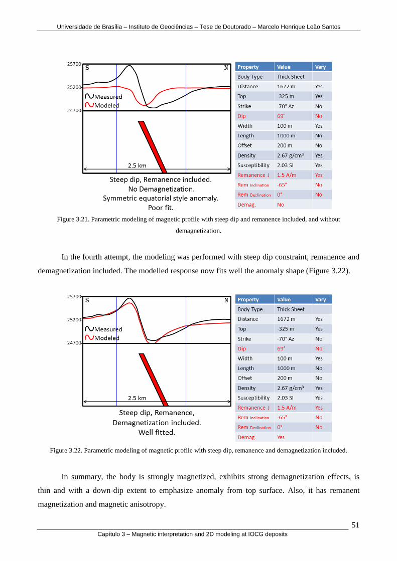
Universidade de Brasília – Instituto de Geociências – Tese de Doutorado – Marcelo Henrique Leão Santos
51 Capítulo 3 – Magnetic interpretation and 2D modeling at IOCG deposits
Figure 3.21. Parametric modeling of magnetic profile with steep dip and remanence included, and without
demagnetization.
In the fourth attempt, the modeling was performed with steep dip constraint, remanence and
demagnetization included. The modelled response now fits well the anomaly shape (Figure 3.22).
Figure 3.22. Parametric modeling of magnetic profile with steep dip, remanence and demagnetization included.
In summary, the body is strongly magnetized, exhibits strong demagnetization effects, is
thin and with a down-dip extent to emphasize anomaly from top surface. Also, it has remanent
magnetization and magnetic anisotropy.

Universidade de Brasília – Instituto de Geociências – Tese de Doutorado – Marcelo Henrique Leão Santos
52 Capítulo 3 – Magnetic interpretation and 2D modeling at IOCG deposits
3.9 - RESULTS
The success of the quantitative and qualitative interpretation is evaluated not only by the
level of correlation with the orebody, but more importantly, by the correspondence between the
estimated magnetic properties of 2D model structure and the known source, which is the massive
magnetite orebody in this case.
The flight lines A – A’ and B – B’, highlighted in the maps, were selected to evaluate and
compare the shape of the signals. The profile (A – A´) corresponds to the geological section of
Figure 3.3. The results show the good correlation of the projection of the orebody at surface, and the
transformations profiles: total magnetic intensity field (TMI), reduction to the pole (RTP), pseudo-
gravity (PGRV), magnetic amplitude (AMP), terracing (TER), total horizontal gradient (THG),
vertical derivative (DZ), total gradient or analytic signal (TG), total gradient in 3D (TG3D) and tilt
derivative or inclination of analytic signal (IAS), from top to base (Figures 3.23 and 3.24).
Total magnetic intensity correlated with the high and low grade ore shows that the northern
body has an anomaly that resembles those at middle latitude probably due to remanence. Part of the
southern anomaly pattern is consistent with the anomalies at low magnetic latitude (Figure 3.25a).
Reduction to the pole transformed the observed magnetic anomaly into the anomaly as if the
measurements were made at the magnetic pole. The results peaks have a good correlation with the
orebody and have positive values indicating dip to NE (Figure 3.25b).
The magnetic amplitude was one of the main interpretation tools. This set of computed
amplitude data is much simpler in pattern and its peak coincides with the location of the orebody.
The excellent correspondence with known geology indicate that the equivalent source technique has
worked well (Figure 3.25c).
Terracing applied to the Furnas’ Southeast deposit TMI data delineated the low grade SW
limit along the deposit. It also created a sharp step that defined a terrace over the orebody that
continues to NE indicating the dip direction (Figure 3.25d).
Horizontal derivatives enhanced the horizontal gradient and consequently helped to find the
lateral limits of the anomaly sources (Figure 3.25e). Vertical derivative enhanced the location of the
magnetic source in the highest magnetic gradient on the NW ore body and within low magnetic
value at SE ore body (Figure 3.25f).
The interpretation of the calculated amplitude of analytic signal in 2D or total gradient of
Furnas Southeast deposit show a good correlation between the low and high grade orebodies due to
the strong association of copper sulfides and magnetite (Figure 3.25g). The total gradient in 3D and
the orebodies also showed a good correlation (Figure 3.25h). Comparing the two transformations it
can be seen that the 3D total gradient (Figure 3.25h) gives a smoother and cleaner response

Universidade de Brasília – Instituto de Geociências – Tese de Doutorado – Marcelo Henrique Leão Santos
53 Capítulo 3 – Magnetic interpretation and 2D modeling at IOCG deposits
compared to the total gradient (analytic signal) that gives effective boundary delineation (Figure
3.25g).
The inclination of analytic signal delineates the orebody between the low in the north and
the high in the south. The main magnetic lineaments indicate the predominant NW-SE structures
directions (Figure 3.25i).
Figure 3.23. Correlation of magnetic profiles with orebody projection at surface of flight line A – A’. TMI = total
magnetic intensity field, RTP = reduction to the pole, PGRV = pseudo-gravity, AMP = magnetic amplitude, TER =
terracing, THG = total horizontal gradient, DZ = vertical derivative, TG = total gradient or analytic signal, TG3D = total
gradient in 3D and IAS = tilt derivative or inclination of analytic signal.
NESW Orebody projection at surface
Fiducial
2150 m
24900
25200
25500
T M
I (
nT
)
-800
-400
0
RT
P (
nT
)
-0.01
0.00
0.01
PG
RA
V(P
mG
al)
300
400
500
600
700
A M
P (
nT
)
1600 1800 2000 2200 24001490 2572
-800
-400
0
TE
R (
nT
)
NESW Orebody projection at surface
Fiducial
2150 m
1600 1800 2000 2200 24001490 2572
-1
0
1
IAS
(ra
d)
1
2
3
TG
3D
(n
T/m
)
1
2
TG
(n
T/m
)
-1.5
0.0
DZ
(n
T/m
)
1
2
TH
G (
nT
/m)
(A) (A’)
(A) (A’)

Universidade de Brasília – Instituto de Geociências – Tese de Doutorado – Marcelo Henrique Leão Santos
54 Capítulo 3 – Magnetic interpretation and 2D modeling at IOCG deposits
Figure 3.24. Correlation of magnetic profiles with orebody projection at surface of flight line B – B’. TMI = total
magnetic intensity field, RTP = reduction to the pole, PGRV = pseudo-gravity, AMP = magnetic amplitude, TER =
terracing, THG = total horizontal gradient, DZ = vertical derivative, TG = total gradient or analytic signal, TG3D = total
gradient in 3D and IAS = tilt derivative or inclination of analytic signal.
NESW Orebody projection at surface
Fiducial
1800 m
-700
-600
-500
-400
RT
P (
nT
)
0.002
0.004
0.006
PG
RA
V
(Pm
Gal)
200
300
AM
P (
nT
)
-600
-450
TE
R (
nT
)
3700 3800 3900 4000 4100 4200 4300 44003596 4508
25100
25200
25300
TM
I (n
T)
NESW Orebody projection at surface
Fiducial
1800 m
0.4
0.8
1.2
TH
G (
nT
/m)
-1
0
1
DZ
(n
T/m
)
0.4
0.8
1.2
TG
(n
T/m
)
0.0
0.6
1.2
TG
3D
(n
T/m
)
-1
0
1
ISA
(ra
d)
3700 3800 3900 4000 4100 4200 4300 44003596 4508
(B) (B’)
(B) (B’)

Universidade de Brasília – Instituto de Geociências – Tese de Doutorado – Marcelo Henrique Leão Santos
55 Capítulo 3 – Magnetic interpretation and 2D modeling at IOCG deposits
(a) (b) (c)
(d) (e) (f)
(g) (h) (i)
Figure 3.25. Correlation of high and low grade orebodies with images and profiles of: (a) total magnetic intensity, (b)
reduction to the pole, (c) magnetic amplitude, (d) terracing, (e) total horizontal gradient (f) vertical derivative, (g) total
gradient or amplitude of analytic signal in 2D, (h) total gradient in 3D, and (i) tilt derivative or inclination of analytic signal.
NE (A')(A) SW
(B) SW NE (B')
0 500 1000
(meters)Low gradeHigh grade
Orebodies at level 190 m
24705 2572124856 25008 25159 25311 25462
TOTAL MAGNETIC INTENSITY TMI (nT)
0100
0200
03000
0100
0200
03000
0 1000 2000
0 1000 2000
A
B
A'
B'
24900
25200
25500
TM
I (n
T)
25100
25200
25300
TM
I (n
T)
NE (A')(A) SW
(B) SW NE (B')
2150 m
1800 m
0 500 1000
(meters)
-2439 1588-574 -484 -389 -288 -182 -39 94 249
Reduction to the pole (nT)
Low gradeHigh grade
Orebodies at level 190 m
01000
2000
3000
01000
2000
3000
0 1000 2000
0 1000 2000
A
B
A'
B'
-700-600-500-400
-800
-400
0
(A) SW 2150 m
1800 m
0 500 1000
(meters)
NE (A')
(B) SW NE (B')nT
51 110998 121 148 179 211 241 288 349 442 534
Magnetic Amplitude (nT)
Low gradeHigh grade
Orebodies at level 190 m
01000
2000
3000
01000
2000
3000
0 1000 2000
0 1000 2000
A
B
A'
B'
300400500600700
200
300
(A) SW 2150 m
1800 m
0 500 1000
(meters)Low gradeHigh grade
Orebodies at level 190 m
NE (A')
(B) SW NE (B')
-1171 355-846 -728 -586 -483 -390 -313 -255
Terracing (nT)
01000
2000
3000
01000
2000
3000
0 1000 2000
0 1000 2000
A
B
A'
B'
-800-400
0
nT
-600
-450
(A) SW 2150 m
1800 m
0 500 1000
(meters)
NE (A')
(B) SW NE (B')
0.002 3.3800.196 0.260 0.320 0.445 0.664 1.004
Total Horizontal Gradient (nT/m)
Low gradeHigh grade
Orebodies at level 190 m
0100
0200
03000
01000
200
03000
0 1000 2000
0 1000 2000
A
B
A'
B'
1.00
2.00
nT/m
0.001.002.003.00
NE (A')(A) SW
(B) SW NE (B')
0 500 1000
(meters)
0.0001 0.23180.0383 0.0765 0.1146 0.1528 0.1910
dz Vertical Derivative (nT/m)
Low gradeHigh grade
Orebodies at level 190 m
01000
2000
3000
01000
2000
3000
0 1000 2000
0 1000 2000
A
B
A'
B'
-1.50
0.00
nT/m
2150 m
-1.00
0.00
1.001800 m
(A) SW 2150 m
1800 m
0 500 1000
(meters)Low gradeHigh grade
Orebodies at level 190 m
NE (A')
(B) SW NE (B')
0.02 4.700.18 0.24 0.28 0.34 0.44 0.61 0.83 1.47
Total Gradient or Analytic Signal (nT/m)
0100
0200
03000
01000
200
03000
0 1000 2000
0 1000 2000
A
B
A'
B'
1.00
2.00
nT/m
0.400.801.20
(A) SW 2150 m
1800 m
0 500 1000
(meters)
NE (A')
(B) SW NE (B')
0.0001 0.23180.0383 0.0765 0.1146 0.1528 0.1910
Total Gradient in 3D (nT/m)
Low gradeHigh grade
Orebodies at level 190 m
0100
0200
03000
0100
0200
03000
0 1000 2000
0 1000 2000
A
B
A'
B'
0.00
0.60
1.20
1.00
2.00
3.00(A) SW 2150 m
1800 m
0 500 1000
(meters)
NE (A')
(B) SW NE (B')
Low gradeHigh grade
Orebodies at level 190 m
-1.558 -1.181 -0.804 -0.427 -0.050 0.328 0.657 0.987 1.317
Tilt Derivative or Inclination of AS (rad)
01000
2000
3000
01000
2000
3000
0 1000 2000
A
B
A'
B'
-1.00
0.00
1.00
-1.00
0.001.00
rad

Universidade de Brasília – Instituto de Geociências – Tese de Doutorado – Marcelo Henrique Leão Santos
56 Capítulo 3 – Magnetic interpretation and 2D modeling at IOCG deposits
The Euler solutions delineated the main structures and lineaments in the area. The Euler
deconvolution results, with structural index 1 representing dyke geometry, indicated the main NW-
SE direction of the orebodies (Figure 3.26). Also, the depth estimations show the dip direction of
the NW magnetic body from cold colors, indicating shallow estimations, to hot colors, indicating
deep estimations. The depth estimations to the SE magnetic body indicated shallow responses.
Figure 3.26. Euler deconvolution correlation with high grade orebody and dip direction of NW orebody. Structural
index value 1 to dyke geometry.
The joint qualitative interpretation of those several linear transformations delineated the
location of the orebody. The images and profiles of terracing indicated that the orebody direction
dips to northeast. The analytic signal or total horizontal gradient determined the peak anomaly
above the causative magnetic body. The power spectrum semi-quantitative analysis, estimated
shallow, intermediate and deep sources associated with the dipping-dike orebody, from 0 m to 800
m depth. The semi-quantitative Euler deconvolution estimated the source depth from 0 m to 700 m.
The use of parametric 2D modeling quantitative analysis indicated the presence of remanence, self-
demagnetization and recovered the geometry of the orebody. The deeper extension of the 2D
parametric modeling indicates that the actual orebody might extend much deeper than that
intersected by the existing drill holes.
Euler Deconvolution Index 1
0 500 1000
(meters)
20
40
60
80
100
110
120
130
140150160170
190210230
270300350410470590740
mDepth
24800 25100 25400 25700
TMI Image (nT)
High gradeOrebodies at level 190 m
01000
2000
3000
01000
2000
3000
0 1000 2000
0 1000 2000
Dip
direc
tion

Universidade de Brasília – Instituto de Geociências – Tese de Doutorado – Marcelo Henrique Leão Santos
57 Capítulo 3 – Magnetic interpretation and 2D modeling at IOCG deposits
3.10 - CONCLUSIONS
The qualitative and quantitative magnetic interpretation techniques in the presence of strong
remanent magnetization, self-demagnetization and at equatorial latitudes is applied to a dataset
acquired at Furnas Southeast deposit as a case study in the exploration for iron oxide-copper-gold
deposits (IOCG) in Carajás Mineral Province, Brazil.
In this work, we have first calculated several magnetic transformations for qualitative
interpretation. Then we carried out some depth estimations to semi-quantitative interpretation.
Finally, we performed two-dimensional parametric modeling for quantitative interpretation. The
results successfully delineated the massive magnetite associated with the high-grade copper-gold
ore. The good correspondence between the transformations, the depth estimations and the 2D
modeling results using a priori information constraints, with the known geology and the orebody
demonstrate the value of this approach.
The qualitative and quantitative analysis performed allow us to conclude that to obtain a
dipolar anomaly for steeply dipping east-west magnetic dike like bodies at equatorial latitudes we
must follow the above procedures. The body must be strongly magnetized. The body must be
affected by demagnetization, i.e. thin with a considerable down dip extent to emphasize anomaly
from top surface. And the body must have remanent magnetization or a magnetic anisotropy that
creates additional magnetization down dip.
This case study shows that this approach is effective in this complex scenario to aid
interpretation and recover the geometry of the orebody. The methodology has good potential in the
exploration for IOCG-type deposits and magnetite related deposits.
3.11 - ACKNOWLEDGMENTS
The authors would like to thank Vale – Department of Exploration and Mineral Projects –
for supporting and permission to publish this work and for providing magnetic data. Vale – Furnas
Project for providing the geological data used in this study and for many discussions. We also
would like to thank Dr. Misac Nabighian who advised us in some aspects of data processing. We
also thank CAPES–Capes Foundation, Ministry of Education of Brazil for the scholarship. This
work was supported in part by the Gravity and Magnetics Research Consortium (GMRC) and we
express our appreciation to Dr. Yaoguo Li for his help. The current sponsoring companies are
Anadarko, Bell Geospace, BG Group, BGP, BP, CGG, ConocoPhillips, ExxonMobil, Gedex,
Lockheed Martin, Marathon Oil, Micro-g LaCoste, Shell, Petra Energia, Petrobras, Tullow Oil and
Vale.

Universidade de Brasília – Instituto de Geociências – Tese de Doutorado – Marcelo Henrique Leão Santos
58 Capítulo 3 – Magnetic interpretation and 2D modeling at IOCG deposits
3.12 - REFERENCES
Baranov, V., 1957, A new method for the interpretation of aeromagnetic maps: pseudogravimetric
anomalies: Geophysics, 22, 359–383.
Baranov, V., and Naudy, H., 1964, Numerical calculation of the formula of reduction to the
magnetic pole: Geophysics, 29, 67–79.
Blakely, R.J., 1996, Potential Theory in Gravity & Magnetic Applications: Cambridge University
Press.
CGEM Software, 2012, AMP3D Software package for magnetic amplitude inversion: Colorado
School of Mines, http://geophysics.mines.edu/cgem/software.html, accessed 21 October 2013.
Cordell, L., and V.J.S. Grauch, 1982, Mapping basement magnetization zones from aeromagnetic
data in the San Juan Basin, New Mexico: 52nd Annual International Meeting, SEG, Expanded
Abstracts, 246–247.
Cordell, L., and V.J.S. Grauch, 1985, Mapping basement magnetization zones from aeromagnetic
data in the San Juan Basin, New Mexico, in W. J. Hinze, eds., The utility of regional gravity
and magnetic anomalies maps: SEG, 181–197.
Cordell, L., and A.E. McCafferty, 1989, A terracing operator for physical property mapping with
potential field data: Geophysics, 54, 621–634.
Craig, M., 1996, Analytic Signals for Multivariate Data: Mathematical Geology, 28, 315.
CVRD (Companhia Vale do Rio Doce), 2006, Relatório de etapa, Alvo Furnas, Volume 1: Internal
report: Technical report.
Dampney, C. N. G., 1969, The equivalent source technique: Geophysics, 34, 39–53.
Gerkens, J.C.d’A., 1989, Foundation of Exploration Geophysics: Methods in Geochemistry and
Geophysics: Elsevier.
Groves, D.I., F.P. Bierlein, L.D. Meinert, and M.W. Hitzman, 2010, Iron oxide copper-gold (IOCG)
deposits through Earth history: Implications for origin, lithospheric setting, and distinction
from other epigenetic iron oxide deposits: Economic Geology, 105, no. 3, 641–654.
Haney, M., C. Johnston, Y. Li, and M. Nabighian, 2003, Envelopes of 2d and 3d magnetic data and
their relationship to the analytic signal: Preliminary results: 73rd Annual International Meeting,
SEG, Expanded Abstracts, 596–599.
Hansen, R.O., and M. Simmonds, 1993, Multiple source Werner deconvolution: Geophysics, 58,
no. 12, 1792–1800.
Hartman, R.R., Teskey, D.J., and Friedberg, J.L., 1971, A system for rapid digital aeromagnetic
interpretation: Geophysics, 36, no.5, 891–918.
Hirata, W.K., J.C. Rigon, A.A.C. Cordeiro, and E. M. Meireles, 1982, Geologia Regional da
Província Mineral de Carajás: 1o Simpósio de Geologia da Amazônia, SBG, 100–108.
Hitzman, M.W., N. Oreskes, and M.T. Einaudi, 1992, Geological characteristics and tectonic setting
of Proterozoic iron oxide (Cu–U–Au–REE) deposits: Precambrian Research, 58, 241–287.
Kellogg, O. D., 1953, Foundations of potential theory: Dover publications Inc.
Leão-Santos, M.H., Y. Li, and R.A.V. Moraes, 2014, Application of 3D magnetic amplitude
inversion to Fe oxide–Cu–Au deposits at low magnetic latitudes: A case study from Carajás
Mineral Province, Brazil: Geophysics, In Press.

Universidade de Brasília – Instituto de Geociências – Tese de Doutorado – Marcelo Henrique Leão Santos
59 Capítulo 3 – Magnetic interpretation and 2D modeling at IOCG deposits
Li, Y., and D. W. Oldenburg, 1996, 3-D inversion of magnetic data: Geophysics, 61, 394–408.
Li, Y., S. E. Shearer, M. M. Haney, and N. Dannemiller, 2010, Comprehensive approaches to 3d
inversion of magnetic data affected by remanent magnetization: Geophysics, 75, L1–L11.
Matlab, 2014, Matlab webpage, Mathworks, http://www.mathworks.com/matlabcentral, accessed
31 March 2014.
Mendonça, C.A., and J.B.C. Silva, 1993, A stable truncated series approximation of the reduction-
to-the-pole operator: Geophysics, 58, no. 8, 1084–1090.
Miller, H.G., and V.J. Singh, 1994, Potential Field tilt - A new concept for location of potential
field sources: Applied Geophysics, 32, 213–217.
Monteiro, L.V.S., R.P. Xavier, E.R. Carvalho, M.W. Hitzman, C.A. Johnson, C.R.S. Filho and I.
Torresi, 2008, Spatial and temporal zoning of hydrothermal alteration and mineralization in the
Sossego iron oxide–copper–gold deposit, Carajás Mineral Province, Brazil: paragenesis and
stable isotope constraints: Mineralium Deposita, 43, 129–159.
Mushayandebvu, M.F., P. Van Driel, A.B. Reid, and J.D. Fairhead, 1999, Magnetic source
parameters of two dimensional structures using extended Euler deconvolution: Geophysics, 66,
814–823.
Nabighian, M., 1972, The analytic signal of two-dimensional magnetic bodies with polygonal cross-
section: its properties and use for automated anomaly interpretation: Geophysics, 37, 507–517.
Nabighian, M., 1974, Additional comments on the analytic signal of two-dimensional magnetic
bodies with polygonal cross-section: Geophysics, 39, 507–517.
Nabighian, M., 1984, Toward a three-dimensional automatic interpretation of potential field data
via generalized Hilbert transforms – Fundamental relations: Geophysics, 49, 780–786.
Nabighian, M., and R.O. Hansen, 2001, Unification of Euler and Werner deconvolution in three
dimensions via the generalized Hilbert transform: Geophysics, 66, no. 6, 1805–1810.
Nykänen, V.M., 2008, Spatial data analysis as a tool for mineral prospectivity mapping: Academic
dissertation, University of Oulu.
Nykänen, V., D.I. Groves, V.J. Ojala, P. Eilu, and S.J. Gardoll, 2008, Reconnaissance-scale
conceptual fuzzy-logic prospectivity modeling for iron oxide copper – gold deposits in the
northern Fennoscandian Shield, Finland: Australian Journal of Earth Sciences, 55, no. 1, 25–
38.
Oreskes, N., and M.T. Einaudi, 1990, Origin of rare earth element enriched hematite breccias at the
Olympic Dam Cu-U-Au-Ag deposit, Roxby Downs, South Australia: Economic Geology, 85,
no. 1, 1–28.
Oreskes, N., and M.T. Einaudi, 1992, Origin of hydrothermal fluids at Olympic Dam: preliminary
results from fluid inclusion and stable isotopes: Economic Geology, 87, no. 1, 64–90.
Philips J.D., 1992, TERRACE: A terracing procedure for gridded data, with Fortran programs, and
VAX Command Procedure, Unix C-Shell, and DOS batch file implementations: Department of
the interior, US geological survey open file report, 5–92.
Reid, A.B., J.M. Allsop, H. Granser, A.J. Millett, and I.W. Somerton, 1990, Magnetic interpretation
in the three dimension using Euler deconvolution: Geophysics, 55, 80–91.
Roest, W.R., J. Verhoef, and M. Pilkington, 1992, Magnetic interpretation using the 3-D analytic
signal: Geophysics, 57, 116–125.
Universidade de Brasília – Instituto de Geociências – Tese de Doutorado – Marcelo Henrique Leão Santos
60 Capítulo 3 – Magnetic interpretation and 2D modeling at IOCG deposits
Santos, J.O.S, L.A. Hartmann, H.E. Gaudette, D.I. Groves, N.J. McNaughton, I.R. Fletcher, 2000,
A new understanding of the provinces of the Amazon Craton based on integration of field
mapping and U-Pb and Sm-Nd geochronology: Gondwana Research, 3, no. 4, 453–488.
Shearer, S., 2005, Three-dimensional inversion of magnetic data in the presence of remanent
magnetization: M.S. thesis, Colorado School of Mines.
Stavrev, P., and D. Gerovska, 2000, Magnetic field transforms with low sensitivity to the direction
of source magnetization and high centricity: Geophysical Prospecting, 48, 317–340.
Thomson, D.T., 1982, EULDEPH: a new technique for making computer-assisted depth estimates
from magnetic data: Geophysics, 47, 31–37.
Vale S.A., 2012, Projeto Furnas, Relatório Final de Geologia: Internal report: Technical report.
Verduzco, B., J.D. Fairhead, C.M. Green, and C. Mackenzie, 2004, New insights into magnetic
derivatives for structural mapping: The Leading Edge, 23, 116–119.
Williams, P.J., M.D. Barton, D.A. Johnson, L. Fontboté, A. Haller, G. Mark, N.H.S. Oliver, R.
Marschik, 2005, Iron Oxide Copper-Gold Deposits: Geology, Space-Time Distribution, and
Possible Modes of Origin: Economic Geology, 100th Anniversary Volume, 371–405.
Wirth, K.R., A.K. Gibbs, and W.J. Olszewski, 1986, U-Pb ages of zircons from the Grão-Pará
group and Serra dos Carajás Granite, Pará, Brazil: Revista Brasileira de Geociências, 16, no. 2,
195–200.
Xavier, R.P., L.V.S. Monteiro, C.P.N. Moreto, A.L.S. Pestilho, G.H.C. Melo, M.A.D. Silva, B.
Aires, C. Ribeiro, and F.H.F. Silva, 2012, The iron oxide copper-gold systems of the Carajás
Mineral Province, Brazil, in Geology and Genesis of Major Copper Deposits and Districts of
the World: A Tribute to Richard Sillitoe, Special Publication, Society of Economic Geologists.

Universidade de Brasília – Instituto de Geociências – Tese de Doutorado – Marcelo Henrique Leão Santos
61 Capítulo 4 – Magnetic amplitude inversion at IOCG deposit
CAPÍTULO 4
APPLICATION OF 3D MAGNETIC AMPLITUDE INVERSION TO IRON OXIDE-
COPPER-GOLD DEPOSITS AT LOW MAGNETIC LATITUDES: A CASE STUDY FROM
CARAJÁS MINERAL PROVINCE, BRAZIL
Manuscript submitted to the Journal Geophysics in February 18th
of 2014, currently the minor
revision needed requested by the reviewers was performed and submitted in August 6th
of 2014.
GEO-2014-0082 - Minor revision needed [email protected] <[email protected]> Wed, Jul 9, 2014 at 12:15 AM To: [email protected] Cc: [email protected], [email protected], [email protected], [email protected], [email protected], [email protected] 08-Jul-2014 Re: GEO-2014-0082, Application of 3D magnetic amplitude inversion to iron oxide-copper-gold deposits at low magnetic latitudes: A case study from Caraj\'{a}s Mineral Province, Brazil Reviewer 1: Open comments to editors and authors: This manuscript deals with the issues of inverting magnetic data that contains the response of bodies that exhibit remanent magnetization and self-demagnetization. Further issues related to low magnetic latitude are also considered. The authors invert a challenging set of magnetic data for an interesting geological scenario and achieve impressive results. They perform some interesting and intelligent analyses. The manuscript is well written with very helpful illustrations. This is excellent work. I think more can be done to improve the paper (see comments) but this manuscript is certainly good enough to be published as-is. Thank you for submitting your manuscript, GEO-2014-0082.R1 , to GEOPHYSICS [email protected] <[email protected]> Wed, Aug 6, 2014 at 12:43 AM To: [email protected] Cc: [email protected], [email protected], [email protected], [email protected] 05-Aug-2014 Re: GEO-2014-0082.R1, "Application of 3D magnetic amplitude inversion to iron oxide-copper-gold deposits at low magnetic latitudes: A case study from Caraj\'{a}s Mineral Province, Brazil" Thank you for submitting your revised manuscript listed above to GEOPHYSICS. Please refer to the manuscript number in all correspondence. Your paper is being processed.
Universidade de Brasília – Instituto de Geociências – Tese de Doutorado – Marcelo Henrique Leão Santos
62 Capítulo 4 – Magnetic amplitude inversion at IOCG deposit
APPLICATION OF 3D MAGNETIC AMPLITUDE INVERSION TO IRON OXIDE-
COPPER-GOLD DEPOSITS AT LOW MAGNETIC LATITUDES: A CASE STUDY FROM
CARAJÁS MINERAL PROVINCE, BRAZIL
Marcelo Leão-Santos1,2,3
, Yaoguo Li2, and Roberto Moraes
1
1 Universidade de Brasília, Instituto de Geociências, Brasília, Brazil.
E-mail: [email protected], [email protected].
2 Colorado School of Mines, Center for Gravity, Electrical & Magnetic Studies, Golden, Colorado.
E-mail: [email protected].
3 VALE S.A., Department of Exploration and Mineral Projects, Belo Horizonte, Brazil.
E-mail: [email protected].
4.1 - ABSTRACT
Strong hydrothermal alteration modifies rock physical properties in iron oxide-copper-gold
deposits (IOCG) and may result in characteristic signatures detectable in geophysical surveys.
Magnetic data are commonly used in characterizing orebodies and 3D inversions are often
employed to assist in interpretations. In areas with strong remanence and self-demagnetization, the
total magnetization can have directions different from the inducing field direction. This deviation
precludes the use of traditional inversion methods. Magnetic amplitude inversion offers one
solution to this challenge since the amplitude data are weakly dependent on the magnetization
direction. In addition, low magnetic latitude also imposes difficulty to amplitude data calculation
due to the instability in the component conversion in the wavenumber domain. To formulate a
practical approach, we present a case study on applying the magnetic amplitude inversion to the
Furnas Southeast iron oxide-copper-gold deposit at low magnetic latitude in Carajás Mineral
Province, Brazil, and demonstrate that the approach can reliably recover an interpretable
distribution of effective magnetic susceptibility and identify massive magnetite from hydrothermal
alterations associated with the high-grade ore.
4.2 - INTRODUCTION
The exploration for copper sulfides and gold ore in iron oxide-copper-gold deposits (IOCG)
frequently uses the magnetic method because of the strong association between mineralization and
high magnetic susceptibility due to the presence of abundant magnetite. However, in strongly
magnetic geological environments, it is sometimes difficult to reliably interpret for magnetic

Universidade de Brasília – Instituto de Geociências – Tese de Doutorado – Marcelo Henrique Leão Santos
63 Capítulo 4 – Magnetic amplitude inversion at IOCG deposit
sources due to the complex role played by remanent magnetization and the self-demagnetization
effect.
In low magnetic latitude and equatorial regions, the effect of remanent magnetization is even
more pronounced. Near the equatorial region such as in Brazil, the inducing magnetic field is
approximately three times weaker compared with that in regions of high magnetic latitudes, and so
is the corresponding induced magnetization given the same magnetic susceptibility. Consequently,
the effect of remanent magnetization is more important in these regions.
The Furnas deposit is such a case in point. It is located in the magnetic equatorial zone, but
has a total-field magnetic anomaly resembling those at middle latitudes in the northern hemisphere.
It is clear that the magnetization at Furnas deposit is significantly different from the current
inducing field direction at this site.
The Furnas copper-gold disseminated mineralization was produced by biotite-garnet-
grunerite-magnetite hydrothermal alteration with the chalcopyrite and bornite high-grade ores
associated with the presence of magnetite. The drill core sample measurements indicate that the
average and median susceptibility of the massive magnetite hydrothermal zone is 2.7 and 0.989 SI,
respectively. The laboratory measurements have shown strong anisotropy in magnetic
susceptibility, with a ratio of major over minor axis of the anisotropy ellipsoid (anisotropy degree)
of 1.5 in the host rocks. The anisotropy degree can be as high as 2.5 to 3 in the magnetic
hydrothermal alteration zones. The major axis of the anisotropy ellipsoid is aligned with the dip of
the orebodies. Thus, it is certain that both self-demagnetization effect and the susceptibility
anisotropy contribute to deviating magnetization direction. Laboratory work also indicates that the
Curie temperature in the orebody is higher than in the host rocks and the pure magnetite. Therefore,
a stronger remanent magnetization is expected in the orebodies.
Laboratory measurements of oriented samples have also shown strong remanent
magnetization. Furthermore, petrophysical measurements show that the remanent magnetization
direction not only deviates significantly from the current inducing field direction but is also
changing within the orebody. The hydrothermal alteration emplacing the orebodies is structurally
controlled and resulting deposit consists of a number of bodies of sigmoidal shape. The injection of
magnetite pulses from hydrothermal fluids form multiple magnetic source bodies that acquired
remanent magnetization at different times and have different magnetization directions.
The significant remanence and self-demagnetization present in the Furnas deposit and the
resultant deviating magnetization direction severely limit the use of magnetic inversion methods
that recover the susceptibility distribution by assuming a magnetization in the same direction as the
current inducing field. Alternative approaches are required. Paine et al. (2001) transformed the

Universidade de Brasília – Instituto de Geociências – Tese de Doutorado – Marcelo Henrique Leão Santos
64 Capítulo 4 – Magnetic amplitude inversion at IOCG deposit
total-field anomaly into quantities that are weakly dependent on the magnetization direction by
vertically integrating the total gradient of total-field anomaly or by calculating the total gradient of
the vertical integration of the magnetic anomaly. They then treated these quantities as if they were
RTP data and applied the magnetic susceptibility inversion by Li and Oldenburg (1996). Despite the
severe inconsistency between these quantities and the algorithm used to invert them, the approach
produced interpretable results and became an inspiration for other development. Li et al. (2010)
presented a two-pronged approach to tackling the problem of remanent magnetization. For simple
isolated anomalies, one can estimate the magnetization direction by using methods such as Helbig's
moment method (Lourenco and Morrison, 1973; Phillips, 2005) or the cross-correlation methods
(Dannemiller and Li, 2006; Gerovska et al., 2009), and then supply the direction to invert for the
magnitude of the magnetization. An alternative method is to invert the amplitude of anomalous
magnetic vector for the magnitude of the total magnetization. This method is more effective when
the magnetization direction is variable (Shearer, 2005). Lelièvre and Oldenburg (2009) formulated a
direct approach by inverting for the 3D distribution of magnetization vectors. Later on, Ellis et al.
(2012) also presented this method, and Liu et al. (2013) applied it to multi-component borehole
data. This approach is generally applicable, but requires site-specific constraints to be effective
(Lelièvre and Oldenburg, 2009). A similar approach based on parametric inversion is to invert for
the magnetization vectors within causative bodies together with their geometric shapes. Mueller et
al. (1997) used this approach to interpret borehole magnetic data in the presence of strong remanent
magnetization. Foss and McKenzie (2011) apply this approach to multiple sources in order to model
complex anomalies.
In this paper, we focus on the application of 3D magnetic amplitude inversion to a set of
high-resolution aeromagnetic data at Furnas Southeast deposit to recover the distribution of the
magnitude of the total magnetization. The reasons are twofold. First, the total magnetization
direction is variable and a single estimated direction is not expected to perform well. Secondly, it is
desirable to develop a strategy in this exploration region to invert magnetic data without detailed
constraints so that it can have the maximum applicability. We also use this data set as a case study
to examine the required processing steps that ensure the general applicability and success of the
magnetic amplitude inversion technique in exploration problems at low-latitude and equatorial
regions.
In the following, we first describe the site geology, mineral deposit model, and the magnetic
properties of different geological units. We then examine the total-field anomaly data and the use of
the equivalent source technique to stably calculate the magnetic amplitude data for use in the
subsequent inversion. We next carry out the amplitude inversion and investigate the use of the L-

Universidade de Brasília – Instituto de Geociências – Tese de Doutorado – Marcelo Henrique Leão Santos
65 Capítulo 4 – Magnetic amplitude inversion at IOCG deposit
curve criterions to select the optimal regularization parameter in such inversions. We conclude the
study by carrying out the geological interpretation of the 3D inversion, and demonstrate the strong
correlation between amplitude inversion results with the known geology and mineralized zones
from drilling.
4.3 - GEOLOGICAL SETTING AND GEOPHYSICAL DATA
Geology and Petrophysics
The Furnas deposit is located in the Carajás Mineral Province, in the Northern region of
Brazil. The deposit is situated along the regional Cinzento transcurrent shear zone striking WNW-
ESE. The Cinzento lineament can be observed in the total horizontal gradient in Figure 4.1.
Metavolcano-sedimentary rocks correlated to the Grão Pará Group, of the 2.76 Ga Itacaiúnas
Supergroup (Wirth et al., 1986), and sedimentary rocks correlated to the Águas Claras Formation
host this portion of the deposit. The shear zone defines a contact between amphibole schist to the
north (hanging wall) and aluminous schist to the south (footwall) of the Itacaiúnas Supergroup,
interrupted by the intrusion of the 1.8 Ga Cigano Granite to the east (Wirth et al., 1986; Figure 4.2).
Regionally, the Itacaiúnas Supergroup is surrounded by tonalitic to trondhjemitic gneisses of the
Xingu Complex (2.8 Ga U-Pb in zircon; Machado et al. 1991). The region is metamorphosed to
greenschist to amphibolite facies (CVRD, 2006).

Universidade de Brasília – Instituto de Geociências – Tese de Doutorado – Marcelo Henrique Leão Santos
66 Capítulo 4 – Magnetic amplitude inversion at IOCG deposit
Figure 4.1. Location of the study area and the distribution of main granites. The study area is in the
northeastern Carajás. Furnas Cu-Au deposit occurs along the Cinzento lineament with a strike in NWW direction,
which is visible in the total horizontal gradient map of magnetic data.
The southeast segment of the Furnas copper-gold disseminated mineralization has a biotite-
garnet-grunerite-magnetite hydrothermal alteration assemblage. The mineralization is hosted by
massive magnetite, silicification, sodic-calcic, and potassic alteration. Figure 4.2 shows the detailed
local geology in the selected study area of 3 km by 3 km. Figure 4.3 displays the geology in a cross
section through the high-grade orebody. The location of the section is indicated in Figure 4.2. The
alteration zone is associated with a late-stage chalcopyrite and bornite veinlets and breccia. The
deposit is poorly exposed with a wide laterite profile of about 60 m.

Universidade de Brasília – Instituto de Geociências – Tese de Doutorado – Marcelo Henrique Leão Santos
67 Capítulo 4 – Magnetic amplitude inversion at IOCG deposit
Figure 4.2. Alteration map superimposed on the LiDAR topography in the study area. The mineralization zone is
located along the thrust fault striking NW-SE. The NE-striking fault (thick dashed line) in the south central portion of
the map demarcates the two major sections of high-grade orebodies (Modified from Vale, 2012).
Figure 4.3. A geological section of Furnas Southeast deposit at the location shown in Figure 4.2 (Modified from Vale,
2012).
122SW NE
Lithologies and Hydrothermal alteration zones
Garnet-grunerite-magnetite alteration zoneBiotitic alteration zoneSilicificationAmphibolitic schistAluminous schist
WeatheringDrillingHigh gradeLow grade
-50 0 50 100 150 m
250 m
296 m
258 m
361 m
454 m
491 m
Geological Section

Universidade de Brasília – Instituto de Geociências – Tese de Doutorado – Marcelo Henrique Leão Santos
68 Capítulo 4 – Magnetic amplitude inversion at IOCG deposit
The alteration zone is associated with moderate to strong foliation. The Cu-Au
mineralization is concentrated in right stepping, NW striking, dilational structures along the WNW-
striking dextral shear zone. These structures produced elongated ore shoots during episodic
hydrothermal fluid flow events that caused brittle slip and brecciation.
The Furnas project carried out 17,789 measurements of magnetic susceptibility continuously
along 17,739 m of drill core from 69 drill holes (Vale, 2012). The hydrothermal magnetite alteration
is divided in three zones with strong magnetic susceptibility signatures (Table 4.1).
Table 4.1. The hydrothermal magnetite alteration zones susceptibilities.
Hydrothermal alteration zone Mean (SI x 10-3
) Median (SI x 10-3
)
Massive magnetite 2,777 989
Amphibole and magnetite 1,550 308
Garnet, grunerite and magnetite 1,383 409
Figure 4.4 shows a representative drill hole log with the lithologies, hydrothermal alteration
zones, magnetic susceptibility measured on drill cores (in SI x 10-3
), iron geochemistry (in
percentage), copper mineralization (in percentage) and gold mineralization (in grams per ton). This
figure summarizes the magnetic susceptibility behavior of the mineralized hydrothermal alteration
zones. We can observe that the mineralized magnetite hydrothermal alteration zone is well defined
between 275 to 350 m depth by high magnetic susceptibility values. Inside this interval we can
observe, around 310 and 340 m depth, two narrow mineralized silicification zones without
magnetite and consequently without magnetic susceptibility response. The same response can be
observed from 225 to 275 m depth on a mineralized silicification and chloritization zone. Around
180 and 215 m, we can see peaks of high magnetic susceptibility values associated with two narrow
magnetic hydrothermal alteration pulses. In general, the high copper-gold grades have strong
association with high magnetic susceptibility values that are correlated with high total-field
magnetic anomalies. Therefore, magnetic survey is one of the most effective geophysical tools for
exploration in this area. In particular, the magnetic anomalies help define the Furnas Southeast
deposit's geophysical signature.

Universidade de Brasília – Instituto de Geociências – Tese de Doutorado – Marcelo Henrique Leão Santos
69 Capítulo 4 – Magnetic amplitude inversion at IOCG deposit
Figure 4.4. Representative drill hole 88 log with the lithologies, hydrothermal alteration zones, magnetic susceptibility,
iron geochemistry, copper mineralization, and gold mineralization.

Universidade de Brasília – Instituto de Geociências – Tese de Doutorado – Marcelo Henrique Leão Santos
70 Capítulo 4 – Magnetic amplitude inversion at IOCG deposit
Magnetic data
The magnetic data were acquired in 2010 in a draped survey using a fixed wing aircraft and
a nominal terrain clearance of 100 m. The line direction was held at 78° NW and the line spacing
was 100 m. We use a subset of the data in the southeast portion of the deposit in this study in Figure
4.5a. The ambient field has an inclination of -5.7°, a declination of -19.8°, and a field strength of
25,400 nT. The corresponding local geology in the same area is shown in Figure 4.2.
(a) (b)
Figure 4.5. (a) The observed total-field magnetic anomaly over the southeast portion of the Furnas deposit. The data
area is the same as the local geology in Figure 4.2. The white dots show the location of the decimated data. The location
of the high-grade orebodies at 190-m level is shown in by thick black lines. The inducing field direction is I = -5.7° and
D = -19.8°. Each anomaly is characterized by a peak shifted to the south and an accompanying strong trough to the
north. This pattern is highly inconsistent with the total-field anomaly due to induced magnetization at the equatorial
region. (b) Theoretical total-field anomaly produced by induced magnetization at the same location. The horizontal
location of the source body is again shown by the black lines.
We decimated the total-field data from approximately 0.6 m sample spacing of the original
dataset to approximately 50-m spacing along the flight lines. We removed the IGRF field (25,400
nT) and performed no additional regional-residual separation. There are two main anomalies in
Figure 4.5a. A weak one is located in the southeast part of the area and a stronger anomaly in the
central-northwest part of the data area. The two anomalies are separated by a northeast-southwest
fault that has been previously mapped (Figure 4.2). The topography data were acquired in 2010
with a LiDAR system. We incorporate the elevation data fully in the processing and inversion, but
choose not to reproduce them here for brevity.
Superimposed on the total-field magnetic anomaly is also high-grade orebody at the
elevation of 190-m, which has a strike direction of NWW and dips to NE (see Figure 4.3). The two

Universidade de Brasília – Instituto de Geociências – Tese de Doutorado – Marcelo Henrique Leão Santos
71 Capítulo 4 – Magnetic amplitude inversion at IOCG deposit
anomalies follow the direction of the orebody, but the peak of the anomalies are shifted to the
southwest, and there is a pronounced negative peak towards the north accompanying each anomaly.
It is clear that these anomalies are not of the pattern that would be produced by induced
magnetization at this low magnetic latitude. For comparison, Figure 4.5b shows the total-field
anomaly produced by two source bodies with induced magnetization only. Instead, the anomalies
appear more similar to anomalies at middle latitudes in north hemisphere. Given this observation
and the petrophysical information discussed in the preceding section, it is clear that remanent
magnetization and self-demagnetization are playing an important role here.
4.4 - AMPLITUDE INVERSION
Calculation of Amplitude Data
The main objective of this study is to recover a three-dimensional representation of the
magnitude of the total magnetization as a direct indicator of target orebody and mineralized zones.
Given the influence on the magnetic data by remanent magnetization and self-demagnetization, we
choose to use the magnetic amplitude inversion (e.g., Shearer, 2005; Li et al., 2010), which does not
rely critically on the knowledge of the magnetization direction.
As Nabighian (1972) has shown, the amplitude of the analytic signal in 2D, which is the
total gradient, is independent on the magnetization direction. This property also holds true for the
amplitude of the anomalous magnetic vector in 2D. In 3D, this invariant property does not strictly
hold true, but both quantities are only weakly dependent on the magnetization direction (e.g.,
Stavrev and Gerovska, 2000; Haney et al., 2003).
In particular, the amplitude data is defined as
√ (1),
where Bax, Bay, and Baz are the three components of the anomalous magnetic vector in the x-,
y-, and z-directions, respectively. Given the weak dependence of Ba on the magnetization direction,
we can treat this quantity as our data and invert directly for the magnitude of magnetization vector
with an assumed magnetization direction. The amplitude data conserve the low-wavenumber
content and retain the signal due to deep magnetic bodies. The benefit of the amplitude inversion is
that we can invert multiple anomalies with different magnetization directions in complicated areas.
Although there is a small number of systems that can acquire three-component magnetic
data (e.g., Dransfield et al., 2003) and the data can be used directly in amplitude data calculation,
the majority of current surveys measure total-field and the majority of existing data from on-going

Universidade de Brasília – Instituto de Geociências – Tese de Doutorado – Marcelo Henrique Leão Santos
72 Capítulo 4 – Magnetic amplitude inversion at IOCG deposit
exploration projects world wide are total-field data. The challenge, therefore, is the need to
calculate the three components from total-field magnetic data. In our current study, this operation is
difficult because of the low magnetic latitude (-5.7°). The commonly used wavenumber-domain
approach encounters the similar low-latitude instability as in the reduction-to-the-pole (RTP)
calculation, albeit to a lesser degree.
To illustrate the low-latitude instability, we calculate the three orthogonal components of the
magnetic anomaly in the Fourier domain, and then obtain the magnetic amplitude data using
equation 1. The result is displayed in Figure 4.6. The result has strong striation in the direction of
declination, as well the separation of two peaks along the same direction. There is little
correspondence between the computed amplitude anomaly and the known geology. The amplitude
inversion using this set of computed amplitude data is nonsensical and uninterpretable. For brevity,
we have not reproduced it. Thus, the Fourier domain conversion has failed as expected at this low
magnetic latitude.
Figure 4.6. Illustration of the difficulties in calculating magnetic amplitude data at low magnetic latitudes in Fourier
domain. The result has strong striation in the direction of declination (D = -19.8°), as well the separation of two peaks
along the same direction. There is no correspondence between the computed amplitude anomaly and the known
geology.
To overcome the difficulty of low-latitude instability, we choose to use the equivalent source
technique Dampney (1969). Many authors have used equivalent source technique in magnetic data
processing (e.g., Hansen and Miyazaki, 1984; Blakely, 1996; Silva, 1986; Li and Oldenburg, 2010).
More recently, Li and Li (2014) used this technique to calculate amplitude data in order to
accommodate an rugged observation surface. We use the similar approach here to deal with low

Universidade de Brasília – Instituto de Geociências – Tese de Doutorado – Marcelo Henrique Leão Santos
73 Capítulo 4 – Magnetic amplitude inversion at IOCG deposit
magnetic latitude and an uneven surface at the same time. We use a 3D equivalent source consisting
of susceptibility values that can be either negative or positive. We construct an equivalent source
consisting of 50-m cubic cells from the total-field anomaly data shown in Figure 4.5a by placing it
immediately below the lowest topographic point. The optimal misfit level to the observed total-field
anomaly is determined by using the L-curve criterion during.
To verify the validity of the equivalent source calculation, we display the predicted total-
field magnetic anomaly and the difference map in Figure 4.7. We note that the predicted data
reproduces the observed total-field anomaly in Figure 4.5a well. The difference is small and
distributed symmetrically about zero. There is no long-wavelength residual either.
Figure 4.7. Top panel shows the predicted total-field anomaly from the equivalent source processing. The bottom panel
shows the difference between the observed total-field anomaly and the predicted data.
Once the equivalent source is obtained, we use it to calculate the three orthogonal
components of the magnetic anomaly and obtain the magnetic amplitude data by equation 1. The
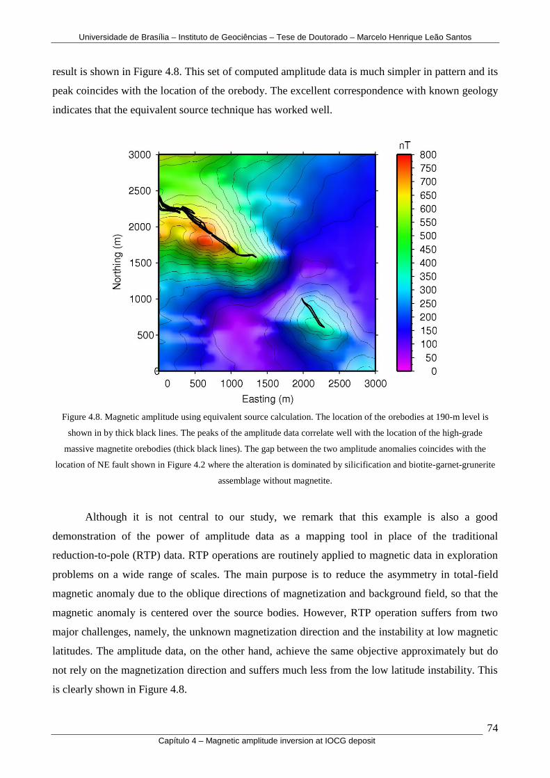
Universidade de Brasília – Instituto de Geociências – Tese de Doutorado – Marcelo Henrique Leão Santos
74 Capítulo 4 – Magnetic amplitude inversion at IOCG deposit
result is shown in Figure 4.8. This set of computed amplitude data is much simpler in pattern and its
peak coincides with the location of the orebody. The excellent correspondence with known geology
indicates that the equivalent source technique has worked well.
Figure 4.8. Magnetic amplitude using equivalent source calculation. The location of the orebodies at 190-m level is
shown in by thick black lines. The peaks of the amplitude data correlate well with the location of the high-grade
massive magnetite orebodies (thick black lines). The gap between the two amplitude anomalies coincides with the
location of NE fault shown in Figure 4.2 where the alteration is dominated by silicification and biotite-garnet-grunerite
assemblage without magnetite.
Although it is not central to our study, we remark that this example is also a good
demonstration of the power of amplitude data as a mapping tool in place of the traditional
reduction-to-pole (RTP) data. RTP operations are routinely applied to magnetic data in exploration
problems on a wide range of scales. The main purpose is to reduce the asymmetry in total-field
magnetic anomaly due to the oblique directions of magnetization and background field, so that the
magnetic anomaly is centered over the source bodies. However, RTP operation suffers from two
major challenges, namely, the unknown magnetization direction and the instability at low magnetic
latitudes. The amplitude data, on the other hand, achieve the same objective approximately but do
not rely on the magnetization direction and suffers much less from the low latitude instability. This
is clearly shown in Figure 4.8.

Universidade de Brasília – Instituto de Geociências – Tese de Doutorado – Marcelo Henrique Leão Santos
75 Capítulo 4 – Magnetic amplitude inversion at IOCG deposit
3D Amplitude Inversion
We now proceed to the inversion of the amplitude data in Figure 4.8. We use the algorithm
presented by Shearer (2005) and Li et al. (2010). The method recovers a 3D distribution of the
magnitude of magnetization. For convenience, we normalized the magnetization by the inducing
field strength to define an effective susceptibility. The algorithm uses a Tikhonov regularization
formalism and relies on the nonlinear relationship between the amplitude data and the 3D effective
susceptibility model. Similar to 3D inversion of total-field anomaly, a depth weighting function is
applied and bound constraints are imposed to ensure the effective susceptibility is positive. The
inverse solution is obtained by solving the following constrained minimization problem,
minimize
subject to (2),
where is the data misfit function, the model objective function, the regularization
parameter, and an upper bound on the effective susceptibility .
To perform the inversion, we first used a coarse mesh whose cells have width of 50 m in x-,
and y-directions and thickness ranging from 25 m near the surface to 50 m in the vertical direction
down to a depth of 1.2 km. Padding cells were added to extend the mesh beyond the data area in all
directions to account for any regional component that may be in the data. Once we determine the
optimal parameters using this coarse mesh, we complete the final inversion with a finer mesh whose
cell width is 12.5 m in the core. We have used a depth weighting function consistent with the
inverse distance-cubed decay of magnetic kernel function, a model objective function consisting a
smallest term and flatness terms in all three-directions, and zero reference model. The zero
reference model is chosen to test the performance of the amplitude inversion in the absence of site
specific geological constraints so as to understand its utility in greenfield explorations.
The primary concern is the regularization parameter. Figure 4.9 display the change of data
misfit and model objective function with the regularization parameter. Both are well-behaved
monotonic functions. Since we do not have a prior estimation of the error standard deviation, we
rely on the L-curve criterion (Hansen, 1992) to determine the optimal level of regularization. This is
illustrated in Figure 4.10a, by using the similar graphical representation as in Krahenbuhl and Li
(2011). The Tikhonov curve (plot of model objective function versus the data misfit on a log-log
scale) has a well defined corner near the regularization parameter value of 10. We also visually
inspect the recovered models with all regularization parameters using similar cutoff values (Figure
4.10b) to see the effect of data misfit level on the recovered model. It is clear that the models are
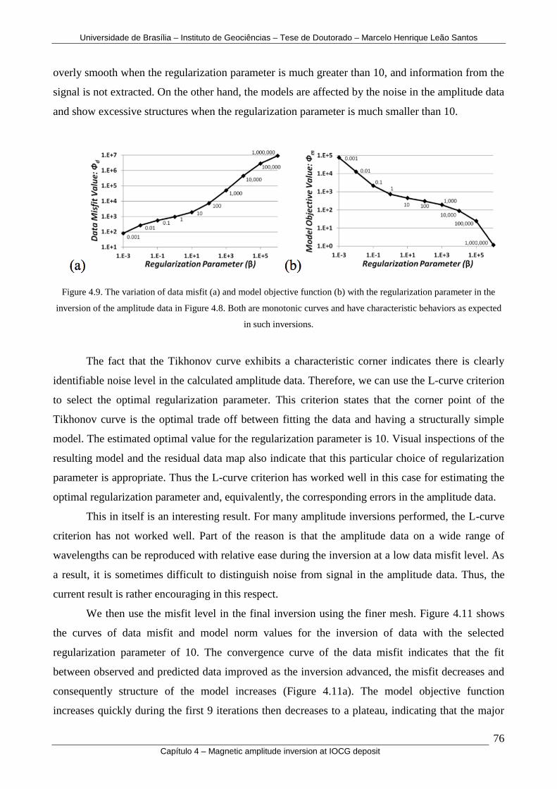
Universidade de Brasília – Instituto de Geociências – Tese de Doutorado – Marcelo Henrique Leão Santos
76 Capítulo 4 – Magnetic amplitude inversion at IOCG deposit
overly smooth when the regularization parameter is much greater than 10, and information from the
signal is not extracted. On the other hand, the models are affected by the noise in the amplitude data
and show excessive structures when the regularization parameter is much smaller than 10.
Figure 4.9. The variation of data misfit (a) and model objective function (b) with the regularization parameter in the
inversion of the amplitude data in Figure 4.8. Both are monotonic curves and have characteristic behaviors as expected
in such inversions.
The fact that the Tikhonov curve exhibits a characteristic corner indicates there is clearly
identifiable noise level in the calculated amplitude data. Therefore, we can use the L-curve criterion
to select the optimal regularization parameter. This criterion states that the corner point of the
Tikhonov curve is the optimal trade off between fitting the data and having a structurally simple
model. The estimated optimal value for the regularization parameter is 10. Visual inspections of the
resulting model and the residual data map also indicate that this particular choice of regularization
parameter is appropriate. Thus the L-curve criterion has worked well in this case for estimating the
optimal regularization parameter and, equivalently, the corresponding errors in the amplitude data.
This in itself is an interesting result. For many amplitude inversions performed, the L-curve
criterion has not worked well. Part of the reason is that the amplitude data on a wide range of
wavelengths can be reproduced with relative ease during the inversion at a low data misfit level. As
a result, it is sometimes difficult to distinguish noise from signal in the amplitude data. Thus, the
current result is rather encouraging in this respect.
We then use the misfit level in the final inversion using the finer mesh. Figure 4.11 shows
the curves of data misfit and model norm values for the inversion of data with the selected
regularization parameter of 10. The convergence curve of the data misfit indicates that the fit
between observed and predicted data improved as the inversion advanced, the misfit decreases and
consequently structure of the model increases (Figure 4.11a). The model objective function
increases quickly during the first 9 iterations then decreases to a plateau, indicating that the major

Universidade de Brasília – Instituto de Geociências – Tese de Doutorado – Marcelo Henrique Leão Santos
77 Capítulo 4 – Magnetic amplitude inversion at IOCG deposit
structures were constructed during the first iterations (Figure 4.11b). The solution converges in 28
iterations when the intended misfit is achieved and there is no more large reduction in the model
objective function.
(a)
(b)
Figure 4.10. L-curve estimation of optimal regularization parameter. (a) is the Tikhonov curve, which has a well-
defined corner at β = 10. (b) shows the variation of the complexity of recovered 3D effective susceptibility models with
the regularization parameter. All models are displayed as volume-rendered images with a cutoff value of 0.15 SI.

Universidade de Brasília – Instituto de Geociências – Tese de Doutorado – Marcelo Henrique Leão Santos
78 Capítulo 4 – Magnetic amplitude inversion at IOCG deposit
Figure 4.11. Convergence curves for the final inversion of the amplitude data using the selected optimal regularization
parameter of 10.
The final inverted effective susceptibility model is shown in Figure 4.12 without padding
cells. Two strongly magnetic units are present as shown by the volume rendered image with a cutoff
value of 0.15 SI. The variation of the recovered effective susceptibility is also shown as color
contours in two cross-sections that intersect the two inverted magnetic bodies. Superimposed in the
image is also the position of the low-grade orebodies at level 190 m altitude and the drill hole
traces. We observe that the recovered magnetic bodies are aligned in the NW direction and dip to
the NE. To the first order, the amplitude inversion has produced a model that is consistent with the
general geology at the deposit.
Figure 4.12. Recovered 3D model of the magnetic susceptibility. The two 3D objects are the volume rendered effective
susceptibility from the amplitude inversion shown with a cutoff value of 0.15 SI, viewed from southeast. Superimposed
are two cross-sections with color contours of the effective susceptibility. The section located towards the NW of the
image coincides with the geological section in Figure 4.3.

Universidade de Brasília – Instituto de Geociências – Tese de Doutorado – Marcelo Henrique Leão Santos
79 Capítulo 4 – Magnetic amplitude inversion at IOCG deposit
4.5 - CORRELATION OF INVERSION RESULT WITH KNOWN GEOLOGY
The success of the amplitude inversion is evaluated not only by the level of data misfit and
the structural simplicity of the recovered model, but more importantly, by the correspondence
between the recovered 3D model of the effective susceptibility and the known source, which is the
massive magnetite orebody in this case. We now proceed to the detailed interpretation by
correlating with the specifics of the orebodies.
The structurally controlled hydrothermal alteration has large variations along the strike. The
deposit exhibits dilational structures, brecciations, and it consists of a number of bodies of
sigmoidal shape. These separate bodies open and close the ore shoots. The injection of magnetite
pulses from hydrothermal fluids form multiple magnetic source bodies that acquired remanent
magnetization at different times and have different magnetization directions. Despite the complexity
of the hydrothermal alteration system, the magnetic amplitude calculation and the inversion result
have a good correlation with the strike and the dip of the orebodies. In the following, we examine
the inversion result in plan- and cross-sections, and in 3D representations.
First, we note again that the magnetic amplitude calculated using equivalent source
technique is highly consistent with the horizontal location of the orebody as shown in Figure 4.8.
Also this image shows the gap between the two anomalies, which is consistent with a mapped fault
and the mineralization associated to silicification zone without the presence of magnetite. This
correlation has also translated to the inversion result as shown in Figure 4.12.
As shown in Figure 4.4, there is a strong association of copper-gold grades with magnetic
susceptibility. Thus, it follows that any subsurface region with high recovered effective
susceptibility can be interpreted as the high-grade orebodies.
The amplitude inversion has recovered two distinct magnetic bodies. The 3D correlation
between their strike direction and dip with the strike and dip of the known orebodies is excellent
(Figure 4.12).
Vale's Furnas Project has delineated the 3D deposit model of the high-grade copper
orebodies that represents the mineralized magnetite hydrothermal alteration zones using 69 drill
holes and has accurate information about their 3D configurations. Thus, we can compare the
interpreted orebodies from the amplitude inversion with the true orebodies. This is shown in 3D
volume rendered images viewed end-on (Figure 4.13a) and top-down (Figure 4.13b) from the
southeast. We observed that the elongated broad source (purple color) towards the NW resembles
the main massive magnetite body with high-grade ores (green). The smaller source resembles the
injection of mineralized magnetite pulses from hydrothermal fluid. There is an excellent spatial
correlation between the orebodies imaged by the amplitude inversion and orebodies delineated from

Universidade de Brasília – Instituto de Geociências – Tese de Doutorado – Marcelo Henrique Leão Santos
80 Capítulo 4 – Magnetic amplitude inversion at IOCG deposit
drill holes. The region between the two orebodies has mineralization from hydrothermal alteration,
but it is dominated by silicification and biotite-garnet-grunerite assemblage without magnetite. The
amplitude inversion therefore did not recover significant magnetic source and, as expected, could
not image the presence of mineralization there. Thus, the strong correlation both with magnetic
orebodies and non-magnetic mineralized zone demonstrates that the amplitude inversion has
performed well in this case. We further remark that this inversion has produced a good result
without using specific geological constraints. This is particularly important in greenfield mineral
exploration. Therefore, the methodology used in this test case is transferrable to other areas in this
region.
(a)
(b)
Figure 4.13. 3D correlation of the recovered susceptibility model (purple) with the known orebodies (green) in the 3D
geological model of the high-grade mineralization zones constructed from extensive drilling in the Vale-Furnas Project.

Universidade de Brasília – Instituto de Geociências – Tese de Doutorado – Marcelo Henrique Leão Santos
81 Capítulo 4 – Magnetic amplitude inversion at IOCG deposit
As a summary comparison, Figure 4.14 shows the geologic interpretation of the amplitude
inversion result in the representative section of the deposit displayed in Figure 4.3. There is a good
correlation between the recovered magnetic zone and the massive magnetite, the measured
susceptibility from drill cores, and the copper-gold mineralization zone. Over all, the recovered
susceptibility model has characterized the massive magnetite (outlined in light blue), and the known
mineralized zone (dark blue). The deeper extension of the recovered susceptibility indicates that the
actual orebody might extend much deeper than that intersected by the existing drill holes.
Figure 4.14. Summary of the geologic interpretation of the amplitude inversion result in the cross-section coinciding
with that in Figure 4.3. The top panel shows the comparison between the total-field anomaly and calculated amplitude
data. The middle panel shows the calculated amplitude data in a narrow strip surrounding the section. The bottom panel
shows the comparison between the inversion result and the geology. The recovered effective susceptibility model (color
contour) has characterized the massive magnetite (outlined in light blue), and the known mineralized zone in dark blue.
Measured magnetic susceptibilities are also shown along several drill holes. The east most drill hole in this cross-
section is the same as that shown in Figure 4.4.

Universidade de Brasília – Instituto de Geociências – Tese de Doutorado – Marcelo Henrique Leão Santos
82 Capítulo 4 – Magnetic amplitude inversion at IOCG deposit
4.6 - CONCLUSIONS
The magnetic amplitude inversion in the presence of strong remanent magnetization is
applied to a dataset acquired at Furnas Southeast deposit as a case study in the exploration for iron
oxide-copper-gold deposits (IOCG) in Carajás Mineral Province, Brazil. The Furnas deposit is
magnetically anisotropic, remanently magnetized, and has self-demagnetization effect. Further
compounding the difficulty is the location at an extremely low magnetic latitude, which poses
challenges in data processing.
In this work, we have first calculated the magnetic amplitude data using the equivalent
source technique. Then we carry out the amplitude inversion using an optimal regularization
parameter obtained using the L-curve criterion. The inverted effective susceptibility successfully
delineates the massive magnetite associated with the high-grade copper-gold ore. The strong
correspondence between the amplitude inversion without using structural or drill hole constraints
and the known geology and deposit model demonstrate the value of this approach.
This study also highlights the utility of amplitude data as a means for qualitative
interpretation and mapping tool in place of the traditional reduction-to-pole (RTP) data. Similar to
RTP data, amplitude data also reduce the asymmetry in total-field magnetic anomaly with respect to
the horizontal locations of source bodies. Amplitude may be more advantageous since their
calculation do not require the knowledge of magnetization direction. However, they are not entirely
independent of the magnetization direction, and it is important to be aware of this limitation in
interpretation based on such data directly or via inversions. Detailed numerical studies may be
required to further understand this aspect.
Overall, the case study shows that the approach of amplitude inversion is effective in this
complex scenario with multiple factors such as remanent magnetization and self-demagnetization
that affect the total magnetization direction, as well as the complications due to the extremely low
magnetic latitude. The methodology has high potential in the exploration for IOCG-type deposits in
the Carajás Mineral Province and other similar areas.
4.7 - ACKNOWLEDGMENTS
The authors would like to thank Vale – Department of Exploration and Mineral Projects –
for permission to publish this work, Vale – Department of Planning and Development of Ferrous –
for providing the magnetic data, and Vale – Furnas Project – for providing the geophysical and
geological data used in this study and for many discussions. The first author wishes to thank
CAPES-Capes Foundation, Ministry of Education of Brazil for the scholarship. We thank Maria
Irene Raposo for advice on the laboratory petrophysical measurements and Misac Nabighian for

Universidade de Brasília – Instituto de Geociências – Tese de Doutorado – Marcelo Henrique Leão Santos
83 Capítulo 4 – Magnetic amplitude inversion at IOCG deposit
helpful discussions. The comments by Reviewer Peter Lelièvre and an anonymous Reviewer have
helped improve the manuscript. This work is supported in part by the Gravity and Magnetics
Research Consortium (GMRC) and Vale. The current sponsoring companies are Anadarko, Bell
Geospace, BG Group, BGP, BP, CGG, ConocoPhillips, ExxonMobil, Gedex, Lockheed Martin,
Marathon Oil, Micro-g LaCoste, Shell, Petra Energia, Petrobras, Tullow Oil and Vale.
4.8 - REFERENCES
Blakely, R., 1996, Potential theory in gravity and magnetic applications: Cambridge University
Press.
CVRD (Companhia Vale do Rio Doce), 2006, Relatório de etapa, Alvo Furnas, Volume 1: Internal
report: Technical report.
Dampney, C.N.G., 1969, The equivalent source technique: Geophysics, 34, 39–53.
Dannemiller, N., and Y. Li, 2006, A new method for estimation of magnetization direction:
Geophysics, 71, L69–L73.
Dransfield, M., A. Christensen, and G. Liu, 2003, Airborne vector magnetic mapping of remanently
magnetized banded iron formations at Rocklea, Western Australia: Exploration Geophysics,
34, 93–96.
Ellis, R., B. de Wet, and I.M. Macleod, 2012, Inversion of magnetic data from remanent and
induced sources: Presented at the 22nd ASEG International Geophysical Conference.
Foss, C., and B. McKenzie, 2011, Inversion of anomalies due to remanent magnetisation: an
example from the Black Hill Norite of South Australia: Australian Journal of Earth Sciences,
58, 391–405.
Gerovska, D., M.J. Aráuzo-Bravo, and P. Stavrev, 2009, Estimating the magnetization direction of
sources from southeast Bulgaria through correlation between reduced-to-the-pole and total
magnitude anomalies: Geophysical Prospecting, 57, 491–505.
Haney, M., C. Johnston, Y. Li, and M. Nabighian, 2003, Envelopes of 2d and 3d magnetic data and
their relationship to the analytic signal: Preliminary results: 73rd Annual International Meeting,
SEG, Expanded Abstract, 596–599.
Hansen, P.C., 1992, Analysis of discrete ill-posed problems by means of the L-curve: SIAM
Review, 34, 561–580.
Hansen, R.O., and Y. Miyazaki, 1984, Continuation of potential fields between arbitrary surfaces:
Geophysics, 49, 787–795.
Krahenbuhl, R., and Y. Li, 2011, Regularization, model weighting and solution appraisal in binary
inversion for time-lapse gravity monitoring: Presented at the GEM Beijing 2011: International
Workshop on Gravity, Electrical and Magnetic Methods and their Applications, SEG.

Universidade de Brasília – Instituto de Geociências – Tese de Doutorado – Marcelo Henrique Leão Santos
84 Capítulo 4 – Magnetic amplitude inversion at IOCG deposit
Lelièvre, P.G., and D.W. Oldenburg, 2009, A 3d total magnetization inversion applicable when
significant, complicated remanence is present: Geophysics, 74, L21–L30.
Li, S., and Y. Li, 2014, Inversion of magnetic anomaly on rugged observation surface in the
presence of strong remanent magnetization: Geophysics, 79, J11–J19.
Li, Y., and D.W. Oldenburg, 1996, 3-D inversion of magnetic data: Geophysics, 61, 394–408.
Li, Y., and D.W. Oldenburg, 2010, Rapid construction of equivalent sources using wavelets:
Geophysics, 75, L51–L59.
Li, Y., S.E. Shearer, M.M. Haney, and N. Dannemiller, 2010, Comprehensive approaches to 3d
inversion of magnetic data affected by remanent magnetization: Geophysics, 75, L1–L11.
Liu, S., X. Hu, T. Liu, J. Feng, W. Gao, and L. Qiu, 2013, Magnetization vector imaging for
borehole magnetic data based on magnitude magnetic anomaly: Geophysics, 78, D429–D444.
Lourenco, J. S., and H.F. Morrison, 1973, Vector magnetic anomalies derived from measurements
of a single component of the field: Geophysics, 38, 359–368.
Machado, W., Z. Lindenmayer, T.E. Krogh and D. Lindenmayer, 1991, U-Pb geochronology of
Archean magmatism and basement reactivation in the Carajás area, Amazon shield, Brazil:
Precambrian Research, 49, 29–354.
Mueller, E.L., W.A. Morris, P.G. Killeen, and S. Balch, 1997, Combined 3-d interpretation of
airborne, surface, and borehole vector magnetics at the McConnell nickel deposit: Presented at
the 67th Annual International Meeting, SEG.
Nabighian, M., 1972, The analytic signal of two-dimensional magnetic bodies with polygonal cross-
section: Geophysics, 37, 507–517.
Paine, J., M. Haederle, and M. Flis, 2001, Using transformed TMI data to invert for remanently
magnetised bodies: Exploration Geophysics, 32, 238–242.
Phillips, J. D., 2005, Can we estimate total magnetization directions from aeromagnetic data using
Helbig’s formulas: Earth, Planets, and Space, 57, 681–689.
Shearer, S., 2005, Three-dimensional inversion of magnetic data in the presence of remanent
magnetization: M.S. thesis, Colorado School of Mines.
Silva, J.B.C., 1986, Reduction-to-the-pole as an inverse problem and its application to low-latitude
anomalies: Geophysics, 51, 369–382.
Stavrev, P., and D. Gerovska, 2000, Magnetic field transforms with low sensitivity to the direction
of source magnetization and high centricity: Geophysical Prospecting, 48, 317–340.
Vale S.A., 2012, Projeto Furnas, Relatório Final de Geologia: Internal report: Technical report.
Wirth, K.R., A.K. Gibbs, and W.J. Olszewski, 1986, U-Pb ages of zircons from the Grão-Pará
Group and Serra dos Carajás Granite, Pará, Brazil: Revista Brasileira de Geociências, 16, no. 2,
195–200.

Universidade de Brasília – Instituto de Geociências – Tese de Doutorado – Marcelo Henrique Leão Santos
85 Capítulo 5 – Magnetic susceptibility 3D model at IOCG deposits
CAPÍTULO 5
MAGNETIC SUSCEPTIBILITY 3D MODEL AND SIGNATURES OF IRON OXIDE-
COPPER-GOLD (IOCG) MINERALIZATION: A CASE STUDY FROM CARAJÁS
MINERAL PROVINCE, BRAZIL
Manuscript submitted to the Journal Economic Geology in August 13th
of 2014.
Submission Confirmation for MAGNETIC SUSCEPTIBILITY 3D MODEL AND SIGNATURES OF IRON OXIDE - COPPER - GOLD (IOCG) MINERALIZATION: A CASE STUDY FROM CARAJÁS MINERAL PROVINCE, BRAZIL Economic Geology <[email protected]> Wed, Aug 13, 2014 at 10:27 AM A manuscript number has been assigned to MAGNETIC SUSCEPTIBILITY 3D MODEL AND SIGNATURES OF IRON OXIDE-COPPER-GOLD (IOCG) MINERALIZATION: A CASE STUDY FROM CARAJÁS MINERAL PROVINCE, BRAZIL Economic Geology <[email protected]> Wed, Aug 13, 2014 at 11:18 AM Reply-To: Economic Geology <[email protected]> To: Marcelo Henrique Leão-Santos <[email protected]> Dear Dr. Leão-Santos, Your submission entitled "MAGNETIC SUSCEPTIBILITY 3D MODEL AND SIGNATURES OF IRON OXIDE-COPPER-GOLD (IOCG) MINERALIZATION: A CASE STUDY FROM CARAJÁS MINERAL PROVINCE, BRAZIL" has been been assigned the following manuscript number: SEG-D-14-00111. You will be able to check on the progress of your paper by logging on to Editorial Manager as an author. The URL is http://seg.edmgr.com/. Thank you for submitting your work to Economic Geology. Kind regards, Larry Meinert Editor Economic Geology

Universidade de Brasília – Instituto de Geociências – Tese de Doutorado – Marcelo Henrique Leão Santos
86 Capítulo 5 – Magnetic susceptibility 3D model at IOCG deposits
MAGNETIC SUSCEPTIBILITY 3D MODEL AND SIGNATURES OF IRON OXIDE-
COPPER-GOLD (IOCG) MINERALIZATION: A CASE STUDY FROM CARAJÁS
MINERAL PROVINCE, BRAZIL
Marcelo Leão-Santos1,2
, Roberto Moraes1, Maria Irene Raposo
3, Otávio Rosendo
2,
Arthur Cardoso2, and Joaquim Feijó
2
1 Universidade de Brasília, Instituto de Geociências, Brasília, Brazil.
E-mail: [email protected], [email protected].
2 VALE S.A., Department of Exploration and Mineral Projects, Belo Horizonte, Brazil.
E-mail: [email protected], [email protected], [email protected],
3 Universidade de São Paulo, Instituto de Geociências, São Paulo, Brazil.
E-mail: [email protected].
5.1 - ABSTRACT
Petrophysical measurements were performed along drill cores from the Furnas Southeast
deposit, which is located in the Carajás Mineral Province, Brazil. Magnetic susceptibilities were
incorporated into a three dimensional (3D) model and used to define the magnetic signatures of the
various hydrothermal alteration types associated with the iron oxide-copper-gold (IOCG)
mineralization. The disseminated copper and gold mineralization is associated with a calcic-sodic-
potassic hydrothermal alteration (dominated by biotite-garnet-amphibole-magnetite alteration
minerals) and followed by intense iron metasomatism with massive magnetite. The copper
(chalcopyrite and bornite) and gold mineralization are usually associated with magnetite. Magnetic
characterization related to the different hydrothermal alteration types and their host rocks show an
association of high-grade mineralization with magnetite.
High measured magnetic susceptibility values (mean = 2,277 x 10-3
SI and median = 989 x
10-3
SI) on hydrothermally altered rocks that contain massive magnetite indicate an abundance of
ferromagnetic minerals.
Measurements made using different equipment and measurement protocols were assessed to
determine the appropriate methodology needed to efficiently, and effectively, characterize the
magnetic signature of the host rocks and ore deposit.
The hydrothermal alteration is controlled by breccias, dilational structures, and several
bodies with sigmoidal shape that open and close the ore zones. The alteration types have large
variations along the deposit.

Universidade de Brasília – Instituto de Geociências – Tese de Doutorado – Marcelo Henrique Leão Santos
87 Capítulo 5 – Magnetic susceptibility 3D model at IOCG deposits
The geological knowledge included here followed qualitative criteria that can be subjective
in the definition of lithotypes because of the great complexity in hydrothermal alteration types. This
study shows how the detailed characterization of physical properties in the IOCG system and three-
dimensional modeling can be used to define magnetic susceptibility signatures and describe
hydrothermal alteration zones with quantitative criteria to improve mineral exploration and the
evaluation of deposits.
Keywords: magnetic susceptibility, magnetite hydrothermal alterations, magnetic susceptibility
signatures, iron oxide-copper-gold (IOCG) deposit, Carajás Mineral Province.
5.2 - INTRODUCTION
In recent decades, geophysical surveys have been used for prospecting iron oxide-copper-
gold (IOCG) deposits. Although the main characteristics of this type of mineralization are known, a
more detailed characterization is still required of how their physical properties define and
characterize their geophysical signatures, especially their magnetic signature.
The importance of iron oxide-copper-gold (IOCG) deposits has increased as one of the most
important classes of mineral deposits because of a number of major discoveries, such as the
Olympic Dam, Salobo, Prominent Hill, etc. The complexity and variability of this type of deposit
do not permit the definition of a single geological exploration model. Thus, detailed physical
property measurements on drill cores of the host rocks and hydrothermal alteration zones can help
characterize these deposits and assist with defining an exploration model.
The geological and magnetic characteristics of IOCG deposits have been discussed in the
literature. Worldwide, IOCG deposits were defined by Hitzman et al. (1992) and further described
by Porter (2000). In Brazil, Hitzman et al. (1992) include the Sossego and Salobo deposits from the
Carajás Mineral Province within the IOCG type. Some work applied magnetic petrophysics and
magnetic petrology to geological interpretation of magnetic surveys (Clark et al., 1992; Clark, 1997,
1999). Smith (2002) provided a generic description of the geophysical features of an IOCG deposit.
Afterwards, Sandrin and Elming (2007), and Sandrin et al. (2009) offered a more detailed
description of the physical properties, petrology and geophysics of this type of deposit. Recently,
numerous petrophysical studies have been conducted to solve the various problems and difficulties
encountered in the modeling of magnetic data, such as remanence, demagnetization and low
latitudes. Studies such as the one by Austin et al. (2013) used constrained modeling of petrophysical
data for IOCG deposits in Australia. The magnetic effects of hydrothermal alteration in porphyry
copper and iron-oxide copper–gold systems were reviewed by Clark (2014).

Universidade de Brasília – Instituto de Geociências – Tese de Doutorado – Marcelo Henrique Leão Santos
88 Capítulo 5 – Magnetic susceptibility 3D model at IOCG deposits
In magnetite-rich hydrothermal environments, it is sometimes difficult to interpret physical
property measurements because of the strong magnetization and the variation of magnetic
properties as a result of different types of hydrothermal alteration events. The deposit has
undergone multiple alteration events that have imparted variations in the magnetic properties of the
rocks within and surrounding the deposit. Such an environment is represented by the IOCG type
mineralization found in the Furnas Southeast deposit. The mineralization consists of copper sulfides
(chalcopyrite and bornite) and gold ore that are spatially and genetically associated with iron oxide.
There are no previous studies that use petrophysical measurements to develop a magnetic
susceptibility model of an IOCG deposit in the Carajás region. This study presents physical
property measurements that were made on drill cores from the Furnas Southeast deposit. Particular
attention was given to a section of the deposit with high grade mineralization associated with the
presence of massive magnetite. In this section, multiple methods were used to measure the magnetic
susceptibility. The results are compared and an efficient methodology is established.
The purpose of this study was threefold: 1) to investigate the relationship between the high
grade mineralization and magnetite, 2) to distinguish the different magnetic susceptibility signatures
of the hydrothermal alteration zones, and 3) to conduct a 3D modeling based on appropriate
magnetic susceptibility measurements. The measurements were made on drill core samples from the
deposit using handheld magnetic susceptibility meters and laboratory techniques.
The final goal of this study was to characterize the magnetic susceptibility signature of the
copper-gold prospect, define a susceptibility model for the IOCG mineralization and hydrothermal
alterations of the same type. The results can be used when generating an IOCG exploration model.
5.3 - DEPOSIT GEOLOGICAL SETTINGS
The lithostratigraphy in the Carajás Mineral Province is complex and mostly consists of
Precambrian rocks that are overlain by younger sediments (Figure 5.1; Hirata et al., 1982;
DOCEGEO, 1988). The lithostratigraphy consists of several Precambrian units (Xingu, Pium and
Luanga Complexes; Plaquê and Cateté Suites), Neoarchean metasedimentary and
metavolcanosedimentary sequences (Itacaiúnas Supergroup), Proterozoic anorogenic granitoids
(granitic plutons with Lower/Middle Proterozoic ages) and Phanerozoic cover units (Hirata et al.,
1982; DOCEGEO, 1988).
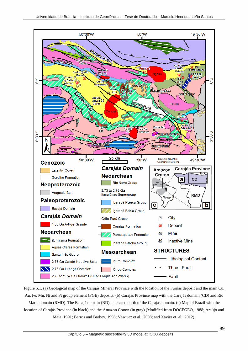
Universidade de Brasília – Instituto de Geociências – Tese de Doutorado – Marcelo Henrique Leão Santos
89 Capítulo 5 – Magnetic susceptibility 3D model at IOCG deposits
Figure 5.1. (a) Geological map of the Carajás Mineral Province with the location of the Furnas deposit and the main Cu,
Au, Fe, Mn, Ni and Pt group element (PGE) deposits. (b) Carajás Province map with the Carajás domain (CD) and Rio
Maria domain (RMD). The Bacajá domain (BD) is located north of the Carajás domain. (c) Map of Brazil with the
location of Carajás Province (in black) and the Amazon Craton (in gray) (Modified from DOCEGEO, 1988; Araújo and
Maia, 1991; Barros and Barbey, 1998; Vasquez et al., 2008; and Xavier et. al., 2012).

Universidade de Brasília – Instituto de Geociências – Tese de Doutorado – Marcelo Henrique Leão Santos
90 Capítulo 5 – Magnetic susceptibility 3D model at IOCG deposits
The Furnas Southeast deposit is located along the WNW-trending Cinzento Transcurrent
System that is approximately 200 km long (Figure 5.2). The deposit is hosted in rocks correlated
with the metamorphosed volcano-sedimentary rocks of the Grão Pará Group, which belongs to the
Itacaiúnas Supergroup (2.76 Ga) and Águas Claras Formation (Wirth et al., 1986; Figure 5.2). In the
Furnas Southeast deposit, a shear zone defines a contact between an amphibole schist on the north
(hanging wall) and aluminous schist on the south (footwall; Figures 5.3 and 5.4). These host rocks
were also, altered by hydrothermal processes. The Cinzento shear zone was intruded by the
anorogenic Cigano Granite (1.8 Ga) to the east and continues northwestward towards the Salobo
deposit (Wirth et al., 1986; Figure 5.2). The region is metamorphosed in the greenschist to
amphibolite facies and is covered by a thick lateritic cover.
Figure 5.2. Magnetic total horizontal gradient with the location of the Furnas deposit along the Cinzento lineament.

Universidade de Brasília – Instituto de Geociências – Tese de Doutorado – Marcelo Henrique Leão Santos
91 Capítulo 5 – Magnetic susceptibility 3D model at IOCG deposits
Figure 5.3. Geological and hydrothermal alteration zone map of the Furnas Southeast deposit over laser-LiDAR
topography; the geological section location of Figure 5.4 is included (Modified from Vale S.A., 2012).
Figure 5.4. Geological section with the host rocks, hydrothermal alteration zones and mineralized zones
(Modified from Vale S.A., 2012).
122SW NE
Lithologies and Hydrothermal alteration zones
Garnet-grunerite-magnetite alteration zoneBiotitic alteration zoneSilicificationAmphibolitic schistAluminous schist
WeatheringDrillingHigh gradeLow grade
-50 0 50 100 150 m
250 m
296 m
258 m
361 m
454 m
491 m
Geological Section

Universidade de Brasília – Instituto de Geociências – Tese de Doutorado – Marcelo Henrique Leão Santos
92 Capítulo 5 – Magnetic susceptibility 3D model at IOCG deposits
The rocks of the Furnas Southeast deposit can be correlated with supracrustal rocks of the
Igarape Salobo Group observed at the nearby Salobo Cu-Au deposit (Lindenmayer, 1990;
Lindenmayer and Teixeira, 1999). The rocks are difficult to interpret because of the intense
alteration. In general, an alteration that progresses from high- to low-temperatures is observed. The
high-temperature alteration is characterized by a biotite-garnet-amphibole-magnetite hydrothermal
assemblage, whereas the subsequent low-temperature alteration shows a biotite-chlorite-tourmaline-
carbonate-quartz-epidote-albite-hematite-magnetite assemblage. The mineralization itself is
associated with chalcopyrite- and bornite-rich late stage veins and breccias (Figure 5.5). The
hydrothermal alteration zones have a lenticular shape and thicknesses of 20 to 600 m, and extending
approximately 9 kilometers along the entire deposit. The study area of this paper is located at two
kilometers in the extreme southeast of the deposit being dominated by high-temperature alterations
(biotite-garnet-amphibole-magnetite hydrothermal assemblage).
(a)
(b)
Figure 5.5. Photographs of ore samples. (a) Chalcopyrite. (b) Bornite.
In the Furnas Northwest deposit, which is outside of the study area, a basement
monzogranitic rock with local pegmatites and granophyres is found. This unit is informally referred
to as Furnas granitoid and has penetrative foliation from heterogeneous ductile deformation events.
They are similar to the hornblende-biotite monzogranite facies from the Geladinho Granite Stock,
aged 2.688 ± 11 Ma (Pb-Pb by zircon evaporation; Barbosa et al., 2001).
Quartzites and schists occur to the north and south of the deposit, respectively (Figure 5.3).
The quartzites may be correlated with the Águas Claras Formation. The schists contain andalusite-
kyanite-sillimanite-staurolite and have been described as resulting from the deformation and
metamorphism of aluminous pelitic sediments that are most likely correlated with the Águas Claras
Formation. In the northern portion, schists contain amphiboles (Figure 5.3). They are interpreted to

Universidade de Brasília – Instituto de Geociências – Tese de Doutorado – Marcelo Henrique Leão Santos
93 Capítulo 5 – Magnetic susceptibility 3D model at IOCG deposits
result from deformation and metamorphism of volcanic rocks with the mostly likely protoliths
being the Grão-Pará Group. The presence of both, the aluminous and the amphibole alteration could
be considered pre-mineralization distal halos. There are banded iron formations in the Grão-Pará
Group.
In the eastern portion, the anorogenic Cigano Granite, aged 1.8 Ga (Wirth et al., 1986), is
described as an isotropic monzogranitic rock with portions of moderate primary foliation (Figure
5.3). Cigano Granite rocks are leucocratic with gray-pinkish colour, coarse to medium grained,
monzogranitic composition, with amphibole and biotite. Those rocks have a discordant contact with
the quartzites correlated with Águas Claras Formation.
The observed tectonic features of Furnas Southeast deposit are related to heterogeneous
deformation of different grades. In general, the deposit rocks have mylonitic fabrics (transposition
foliation) with a brittle-ductile behavior at spaced zones. They present at least two brittle to brittle-
ductile overlapping fabrics (concordant or not). The brittle to brittle-ductile fabrics are characterized
by bands of cataclastic flows. They also bear regions of hydraulic fracturing marked by a
predominance of breccias (cataclastic, hydraulic, hydrothermal), faults and veins/veinlets consisting
of quartz + albite + hematite + specularite + chlorite + amphibole biotite epidote tourmaline
carbonate, and with sulfides overlapping these fabrics. The directions range from WNW-ESE to
NNW-SSE (plunging from 30° NE to 88° NE). These are the most common and important fabrics
in the tectonic-hydrothermal context of the area and they conditioned the mineralizing input of the
deposit. The fabrics are related to the mechanism of shear deformation under high amounts of
hydrothermal fluids. Furthermore, the fabrics are typical for hydrothermal conduits controlled by
cataclastic flow with fragmentation of crystals and grains, and dragging along the conduits.
5.4 - HYDROTHERMAL ALTERATION AND MINERALIZATION
The Furnas Southeast deposit copper-gold disseminated mineralization has a biotite-garnet-
amphibole-magnetite hydrothermal alteration assemblage. Although the hydrothermal alteration and
mineralization type and intensity vary throughout the orebodies, a consistent alteration and
mineralization paragenetic sequence could be distinguished (Table 5.1). The hydrothermal
alteration characterizations were based on the macroscopic observations supported by petrographic
studies.

Universidade de Brasília – Instituto de Geociências – Tese de Doutorado – Marcelo Henrique Leão Santos
94 Capítulo 5 – Magnetic susceptibility 3D model at IOCG deposits
Table 5.1. Lithotypes, hydrothermal alteration zones and mineralogy.
DESCRIPTION
ALTERATION
TYPE
MINERALOGY
Hy
dro
ther
ma
l a
lter
ati
on
zon
es
Chlorite alteration Chloritization Chlorite
Amphibole-Magnetite
hydrothermal alteration
Calcic-Sodic-
Magnetite
Amphibole (Actinolite), Magnetite ± Garnet ± Quartz ±
Biotite ± Chlorite
Amphibole
hydrothermal alteration Calcic-Sodic Amphibole (Actinolite) ± Quartz ± Biotite ± Chlorite
Massive Magnetite
hydrothermal alteration Magnetite
Magnetite ± Amphibole (Grunerite, Actinolite,
Hornblende = Hastingsite) ± Quartz
Garnet-Grunerite-Magnetite
hydrothermal alteration Calcic-Magnetite
Garnet (Almandine), Amphibole (Grunerite), Magnetite ±
Biotite ± Chlorite
Garnet-Grunerite
hydrothermal alteration Calcic
Garnet (Almandine), Amphibole (Grunerite) ± Quartz ±
Chlorite ± Biotite
Biotite
hydrothermal alteration Potassic Biotite, Quartz, Plagioclase, Phengite ± Garnet
Silicification Silicic Silica, Sericite
Albitization Sodic Albite
Ho
st r
ock
s
Monzogranite
Quartz, Plagioclase, Microcline, Biotite, Chlorite
(±pegmatites, granophyres)
Quartzite Quartz ± Sericite
Amphibolitic schist
Amphibole (Grunerite), Quartz ± Hornblende =
Hastingsite
Banded iron formation Magnetite, Silica
Aluminous schist Quartz, Biotite, Sericite, Andalusite, Staurolite, Silimanite
± Garnet ± Chlorite
The presence of magnetite was first tested using a handheld magnet. Magnetic susceptibility
measurements were subsequently used to show magnetic properties of the various lithologies and
alteration zones.
Sodic alteration is the earliest alteration type observed. The sodic alteration is mainly
associated with albite veins in the Furnas Southeast deposit. However, the alteration is best
observed in the Furnas Northwest deposit, outside the study area, where host rocks consist of the
Furnas Granite.
A silicic alteration type is widely distributed over the deposit that can completely transform
the host rock. The silica-rich alteration forms zones that are lenticular. Narrow bands of sericite and
quartz characterize the silicic alteration type. The silicic alteration may also contain chalcopyrite
and rarely bornite. Importantly, magnetite is absent.
Potassic alteration type is common near the brittle-ductile to brittle deformed rocks.
Mineralized bodies are commonly associated with potassic zones that are essentially composed of
biotite with a schistose texture and locally within tectonic-hydrothermal breccias cemented with
Universidade de Brasília – Instituto de Geociências – Tese de Doutorado – Marcelo Henrique Leão Santos
95 Capítulo 5 – Magnetic susceptibility 3D model at IOCG deposits
biotite. In addition, the potassic zone has a significant association with garnet, magnetite and silica
alteration minerals.
The calcic alteration type is concurrent with or subsequent to potassic alteration. Calcic
alteration exhibits coarse-grained garnet proximal to mineralized zones with fine-grained garnets
found more distal. This alteration is associated with aluminous schists and biotite, grunerite and
magnetite alteration minerals.
The calcic alteration type typically overprints potassic alteration. The mineral assemblage
includes garnet-grunerite. The alteration occurs in association with bands of silicic alteration. The
garnet-grunerite calcic alteration has variations from isotropic to anisotropic textures, and from
ductile to brittle-ductile deformations. This alteration also occurs in association with a garnet-
grunerite-magnetite mineral assemblage.
Magnetite is directly associated with high-grade copper and gold mineralization. This stage
of high iron metasomatism forms massive magnetite. The magnetite-bearing fluid flow was
structurally controlled. The magnetite alteration type overprints the calcic-sodic alteration type and
forms bands with the garnet-grunerite-magnetite assemblage. There is also a strong association with
the brecciated silicification.
The calcic-sodic atleration type is dominated by amphiboles (predominance of actinolite)
and has variable amounts of quartz, tourmaline and plagioclase. Chalcopyrite and bornite are locally
found. This alteration type often occurs after the magnetite, potassic and silicic alteration types.
However, magnetite infiltrations also appear in the calcic-sodic alteration that is dominated by the
amphiboles. In general, sulfidation occurs in association with these amphibole-magnetite
assemblages.
Subsequently, some final weak alteration types occur and were not included in Table 2. The
first is a new potassic alteration process with biotitization that occurs followed by a strong chloritic
process, which partially or completely alters the rocks of the area, with local areas of hydrothermal
breccias with mineralized chlorite-hematite-magnetite. The other late alterations are related to
carbonation and silicification. Calcite occurs in association with quartz-hematite-magnetite-pyrite-
chalcopyrite-epidote-albite-biotite-tourmaline veinlets.

Universidade de Brasília – Instituto de Geociências – Tese de Doutorado – Marcelo Henrique Leão Santos
96 Capítulo 5 – Magnetic susceptibility 3D model at IOCG deposits
5.5 - METHODS
Rock magnetism
Magnetic susceptibility ( m ) measures the magnetization capacity of a material when
subjected to a magnetic field. The proportionality coefficient ( m ) defines the magnetic
susceptibility of the environment or material considered.
m
, (1),
where
is the induced magnetization in ampere per meter (A/m); is the inducing magnetic
field in ampere per meter (A/m); and m is the magnetic susceptibility of the material (non-
dimensional).
The magnetic behavior of a rock under the action of a magnetic field depends on its
mineralogical composition. All the diamagnetic, paramagnetic and ferromagnetic minerals present
in a rock contribute to its magnetic susceptibility. Most existing minerals have low susceptibility,
and a small portion of the magnetic minerals that compose the rocks is usually responsible for the
higher susceptibility values.
In diamagnetic minerals, susceptibility is weak, negative and reversible; the mineral is
magnetized in the direction opposite to the applied magnetic field, and the magnetization drops to
zero when the magnetic field is removed. Diamagnetic minerals have susceptibility values of
approximately -10-6
SI, with quartz and calcite as examples.
In paramagnetic minerals, susceptibility is small, positive, reversible and varies inversely
with temperature; the mineral is magnetized in the same direction as the applied magnetic field, and
the magnetization drops to zero when the magnetic field is removed. In paramagnetic minerals, the
susceptibility values vary between 10-5
and 10-4
SI, and examples of minerals with this property are
amphibole, biotite, feldspar and plagioclase.
Ferromagnetic minerals exhibit strong spontaneous magnetization and high magnetic
susceptibility values. Ferromagnetic is a general term that encompasses both ferrimagnetic
minerals, such as magnetite, and antiferromagnetic minerals, such as hematite1. The iron-titanium-
oxygen series has a solid solution of magnetic minerals that ranges from magnetite (Fe2O4) to
ulvospinel (Fe2TiO4). The most abundant ferromagnetic mineral is magnetite, whose Curie
temperature is 580° C. The magnetic characteristic of the rock is affected by the fabric, distribution,
1 Hematite (Fe2O3) is a commom iron oxide classified as an antiferromagnetic material. The occurrence of a parasite
antiferromagnetism can generate magnetic anomalies in hematites. In the iron-sulfur series, pyrrhotite can be either ferromagnetic or
antiferromagnetic depending on its composition with iron-poor end-members being ferromagnetic and iron-rich end-members being
antiferromagnetic.

Universidade de Brasília – Instituto de Geociências – Tese de Doutorado – Marcelo Henrique Leão Santos
97 Capítulo 5 – Magnetic susceptibility 3D model at IOCG deposits
shape and size of the magnetic grains. A common method of classifying the magnetic character of
the rock is to evaluate the amount of magnetite (Kearey et al. 2002).
Magnetic anomalies can be associated with the alteration of magnetic minerals in rocks that
host mineral deposits related to hydrothermal systems (Hanna, 1969; Criss and Champion, 1984;
Clark, 2014) and delineate “fossil” hydrothermal activity zones. Porphyry systems commonly
make/destroy magnetite in host rocks (Hoschke, 2008). However, direct detection of ore body is
limited to iron resources that occur in magnetite-rich banded iron formations. The magnetic method
is a key tool for inferring the subsurface structures and for mapping anomalous concentrations of
magnetite, which is the main magnetic material in the crust. It can similarly be used on magnetite
concentration mapping occurring on many economic mineral deposits where this mineral is
associated (Hoover et al. 1992; Clark, 2014).
Magnetic susceptibility measurements
The susceptibility meters KT-9 and KT-10 (Figure 5.6a) and the susceptibility (and
conductivity) meter MPP – EM2S (Figure 5.6b) were used. Their manufacturers and basic technical
specifications are listed below (Table 5.2).
It was seen that the magnetic susceptibility value:
(i) increases with the amount of magnetite in the sample (expected),
(ii) decreases as the distance between the sensor and the sample increases,
(iii) depends on the shape of the sample and
(iv) tends to increase with an increase of the contact surface for an equivalent content
magnetic ore (Figure 5.6c).
All the measurements were conducted on split drill cores that were at least 40-mm-thick to
ensure a good contact area with the sensor (Figures 5.6d and 5.6e). Measured conductivity values
were recorded and positive results were not obtained, which are possibly related to the disseminated
character of the mineralization (not massive).

Universidade de Brasília – Instituto de Geociências – Tese de Doutorado – Marcelo Henrique Leão Santos
98 Capítulo 5 – Magnetic susceptibility 3D model at IOCG deposits
(a) (b) (c)
(d) (e)
Figure 5.6. (a) Susceptibility meter KT-10. (b) Susceptibility/conductivity meter MPP - EM2S. (c) Sketch of the sample
- sensor contact surface. (d) Measurement procedure with the susceptibility meter KT-10. (e) Measurement procedure
with susceptibility meter/conductivity meter MPP - EM2S.
Table 5.2. Main specifications of susceptibility meters KT-9 and KT-10 and susceptibility meter/conductivity meter
MPP-EM2S.
Susceptibility meter KT-9 KT-10 – Plus MPP – EM2S
Manufacturer Georadis Instrumentation GDD
Susceptibility sensitivity 1 x 10⁻⁵
SI 1 x 10⁻⁶
SI 1 x 10⁻³
SI
Susceptibility range 9.9 x 10⁻³
SI to
999.9 x 10⁻³
SI
-0.999 x 10⁻³
to
9,999 x 10-3
SI
10-3
to 9,000 x 10-3
SI
Operating frequency 10 kHz 10 kHz 10 kHz
Operating temperature -10 to 55°C -20 to 60°C 0 to 50°C
Dimensions 18.7 x 6.5 cm 20 x 5.7 x 3 cm 31 x 25 x 18 cm
Coil diameter 6.5 cm 6.5 cm 2.54 cm
Sampling methods of the magnetic susceptibility measurements
Magnetic susceptibility measurements were made on drill cores from the Furnas Southeast
deposit. These measurements were used to characterize the magnetic signature of the lithotypes and
hydrothermal alteration zones associated with the deposit. A total of 17,789 measurements were
made along 17,739 meters of drill cores from 69 drill holes. The drill cores were HQ diameter
(96.40 mm) through the weathered material and NQ diameter (76.20 mm) in fresh rock. The
systematic magnetic susceptibility measurements along the deposit were taken with two different
sensitivities described below (Figure 5.7).

Universidade de Brasília – Instituto de Geociências – Tese de Doutorado – Marcelo Henrique Leão Santos
99 Capítulo 5 – Magnetic susceptibility 3D model at IOCG deposits
Figure 5.7. Drill hole location map. Measurement schematics: lower sensitivity magnetic susceptibility (MS)
measurements (KT-9) in green; higher sensitivity MS measurements (KT-10) in yellow; drill holes without MS
measurements in white; and low grade orebody projections at an elevation of 190-m in red. The geological section
location (see Figure 5.4) is indicated in the map, and the numbers of the drill holes used in this work are highlighted.
Four rounds of magnetic susceptibility measurements were made:
1 - The first round of data collection used the KT-9 susceptibility meter (having lower
sensitivity of 1 x 10⁻⁵
SI units), with 8,514 measurements acquired along 6,862.35 m of 30 drill
holes. Measurements were taken every 1 m (CVRD, 2006).
2 - The second round used the KT-10 meter (with a sensitivity of 1 x 10⁻⁶
SI units). A total
of 9,275 measurements were acquired along 10,877.13 m of 39 drill holes. Measurements were
taken every 1 m (Vale S.A., 2012).
3 - In the third round, different equipment and measuring configurations were conducted on
the drill hole number 88. The purpose was to establish an optimal sampling and measurement
procedure. Sample intervals of 0.2 m and 0.5 m along the drill cores were tested. Also,
measurements were made on sample aliquots collected every meter along the drill core that were
analyzed for chemistry. These aliquots were prepared by homogenizing the drill cores along each
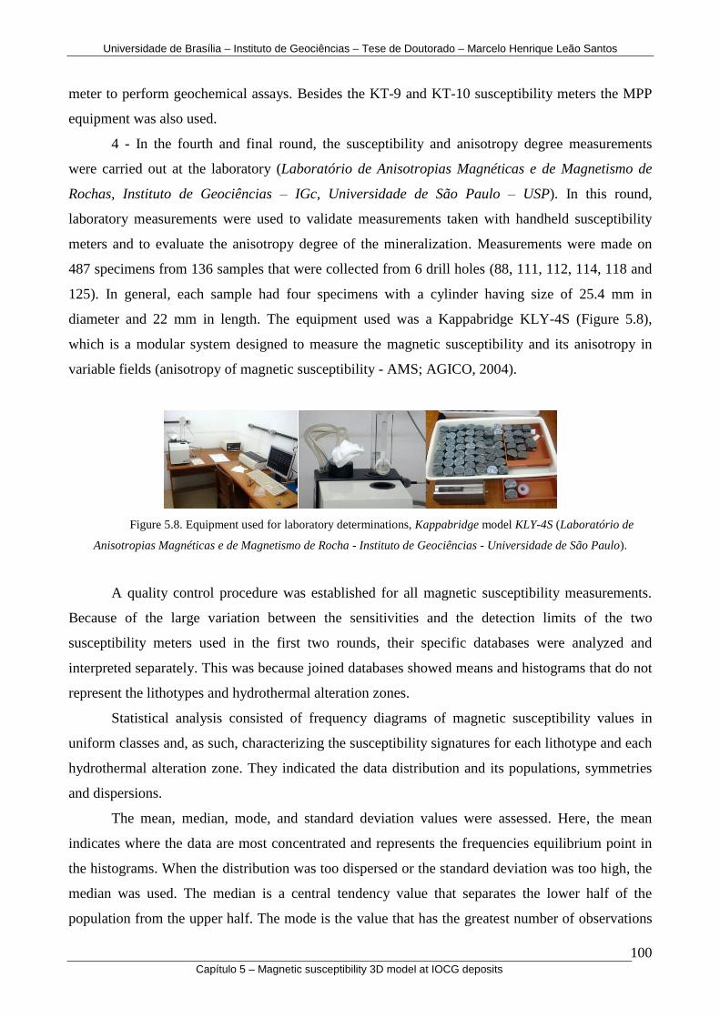
Universidade de Brasília – Instituto de Geociências – Tese de Doutorado – Marcelo Henrique Leão Santos
100 Capítulo 5 – Magnetic susceptibility 3D model at IOCG deposits
meter to perform geochemical assays. Besides the KT-9 and KT-10 susceptibility meters the MPP
equipment was also used.
4 - In the fourth and final round, the susceptibility and anisotropy degree measurements
were carried out at the laboratory (Laboratório de Anisotropias Magnéticas e de Magnetismo de
Rochas, Instituto de Geociências – IGc, Universidade de São Paulo – USP). In this round,
laboratory measurements were used to validate measurements taken with handheld susceptibility
meters and to evaluate the anisotropy degree of the mineralization. Measurements were made on
487 specimens from 136 samples that were collected from 6 drill holes (88, 111, 112, 114, 118 and
125). In general, each sample had four specimens with a cylinder having size of 25.4 mm in
diameter and 22 mm in length. The equipment used was a Kappabridge KLY-4S (Figure 5.8),
which is a modular system designed to measure the magnetic susceptibility and its anisotropy in
variable fields (anisotropy of magnetic susceptibility - AMS; AGICO, 2004).
Figure 5.8. Equipment used for laboratory determinations, Kappabridge model KLY-4S (Laboratório de
Anisotropias Magnéticas e de Magnetismo de Rocha - Instituto de Geociências - Universidade de São Paulo).
A quality control procedure was established for all magnetic susceptibility measurements.
Because of the large variation between the sensitivities and the detection limits of the two
susceptibility meters used in the first two rounds, their specific databases were analyzed and
interpreted separately. This was because joined databases showed means and histograms that do not
represent the lithotypes and hydrothermal alteration zones.
Statistical analysis consisted of frequency diagrams of magnetic susceptibility values in
uniform classes and, as such, characterizing the susceptibility signatures for each lithotype and each
hydrothermal alteration zone. They indicated the data distribution and its populations, symmetries
and dispersions.
The mean, median, mode, and standard deviation values were assessed. Here, the mean
indicates where the data are most concentrated and represents the frequencies equilibrium point in
the histograms. When the distribution was too dispersed or the standard deviation was too high, the
median was used. The median is a central tendency value that separates the lower half of the
population from the upper half. The mode is the value that has the greatest number of observations

Universidade de Brasília – Instituto de Geociências – Tese de Doutorado – Marcelo Henrique Leão Santos
101 Capítulo 5 – Magnetic susceptibility 3D model at IOCG deposits
and occurs most frequently in the data set. Thus, in situations where the mean and the median were
not well defined, the mode was used. The standard deviation is the common measure of statistical
dispersion showing the variation around the mean.
The geochemical assays of iron, copper and gold from the drill cores were performed in the
samples collected along every 1 meter. The analytical methods included Fire Assay for gold (in g/t)
and multi-acid/ICP-MS for iron and copper (in percentage) (CVRD, 2006; Vale S.A., 2012).
5.6 - COMPARISON BETWEEN DIFFERENT
SUSCEPTIBILITY METERS AND SAMPLING METHODS
Profiles sampled with different intervals and equipment in the third round of measurements
from drill hole 88 were plotted for comparison. As expected, the readings with a spacing of 0.5 m
from KT-9 meter (black profile) have much lower resolution compared to that from KT-10 meter
(blue profile; Figure 5.9). Differences in sensitivity and detection limits of the equipment are the
reasons of this contrast (Table 3). These results indicate that the KT-10 meter may provide more
reliable measurements.
Figure 5.9. Magnetic susceptibility measurements of the drill cores and geochemical sample aliquots. Measurements
with KT-9 and 0.5 m spacing (black profile), KT-10 and 0.5 m spacing (blue profile), KT-10 and 0.2 m spacing (green
profile), MPP and 0.2 m spacing (red profile), and KT-10 in geochemical sample aliquots (magenta profile).
m
50
100
150
200
250
300
350
400
450
0 100
200
300
400
500
600
700
800
900
0100
200
300
400
500
600
700
800
900
0100
200
300
400
500
600
700
800
900
0
500
1000
1500
2000
0 100
200
300
400
500
600
700
800
KT10 - ALÍQUOTAMPP - 20 cmKT10 - 20 cmKT10 - 50cmKT9 - 50 cm
No
measurements
No
measurements
SI x 10-3 SI x 10-3 SI x 10-3 SI x 10-3 SI x 10-3
ALIQUOT

Universidade de Brasília – Instituto de Geociências – Tese de Doutorado – Marcelo Henrique Leão Santos
102 Capítulo 5 – Magnetic susceptibility 3D model at IOCG deposits
The KT-10 meter data, with an increase in sampling density readings at 0.2 m intervals
(green profile), provided a better definition for the magnetic levels when compared to the 0.5 m
spaced data (blue profile; Figure 5.9). Another interesting observation is that the KT-10 meter data
(green profile) proved more effective in delineating lower susceptibility values than the MPP (red
profile; for example depth interval 0-150 m in Figure 5.9). This may be due to its lower detection
limit compared to the MPP meter (Table 3).
For measurements taken at depths interval from 150 to 400 m on the samples prepared for
the geochemical assays (magenta profile), the results showed better stability when compared to the
measurements on the drill cores. Also, the aliquot measurements are, in general, lower than the
measurements made on the drill core (Figure 5.9). Possibly, this is because of the greater
homogenization of the contents of these samples in the representation of the same intervals.
5.7 - LABORATORY MEASUREMENTS
The high sensitivity magnetic susceptibility laboratory measurements performed in the
fourth round with the Kappabridge (KLY-4S) meter were used to check and to validate the
handheld acquired data. Comparison of measurements from the different meters shows that there is
agreement between data from KT-10, MPP, and KLY-4S (Figure 5.10). Thus there is high
confidence in the KT-10 measurements made on drill cores.
Magnetic susceptibility measurements have been plotted along with corresponding alteration
types (Figure 5.11). The magnetic susceptibility measurements depict three main signatures
(Figures 5.11a, 5.11c, 5.11e and 5.11g):
(i) intermediate values (averaging 1 x 10⁻³
SI) correlated with the aluminous schists host
rocks and hydrothermal alteration zones without magnetite (garnet-grunerite and
amphibole hydrothermal alteration zones),
(ii) low values (less than 0.5 x 10⁻³
SI) occur in the silicic zone, and
(iii) (very) high values (over 100 x 10-3
SI to >9999 x 10-3
SI) in the hydrothermal
alteration zones that contains magnetite (massive magnetite, garnet-grunerite-
magnetite and amphibole-magnetite hydrothermal alteration zones).
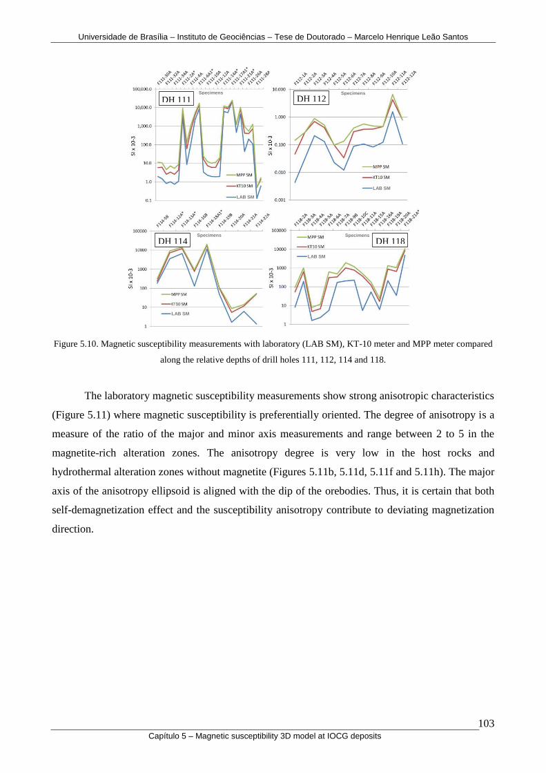
Universidade de Brasília – Instituto de Geociências – Tese de Doutorado – Marcelo Henrique Leão Santos
103 Capítulo 5 – Magnetic susceptibility 3D model at IOCG deposits
Figure 5.10. Magnetic susceptibility measurements with laboratory (LAB SM), KT-10 meter and MPP meter compared
along the relative depths of drill holes 111, 112, 114 and 118.
The laboratory magnetic susceptibility measurements show strong anisotropic characteristics
(Figure 5.11) where magnetic susceptibility is preferentially oriented. The degree of anisotropy is a
measure of the ratio of the major and minor axis measurements and range between 2 to 5 in the
magnetite-rich alteration zones. The anisotropy degree is very low in the host rocks and
hydrothermal alteration zones without magnetite (Figures 5.11b, 5.11d, 5.11f and 5.11h). The major
axis of the anisotropy ellipsoid is aligned with the dip of the orebodies. Thus, it is certain that both
self-demagnetization effect and the susceptibility anisotropy contribute to deviating magnetization
direction.
LAB SM
LAB SM
LAB SM
LAB SM
Specimens Specimens
Specimens Specimens
DH 111 DH 112
DH 114 DH 118
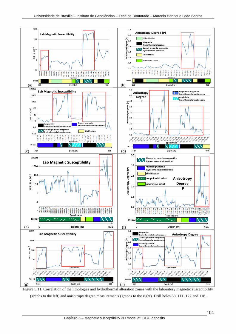
Universidade de Brasília – Instituto de Geociências – Tese de Doutorado – Marcelo Henrique Leão Santos
104 Capítulo 5 – Magnetic susceptibility 3D model at IOCG deposits
(a) (b)
(c) (d)
(e) (f)
(g) (h) Figure 5.11. Correlation of the lithologies and hydrothermal alteration zones with the laboratory magnetic susceptibility
(graphs to the left) and anisotropy degree measurements (graphs to the right). Drill holes 88, 111, 122 and 118.

Universidade de Brasília – Instituto de Geociências – Tese de Doutorado – Marcelo Henrique Leão Santos
105 Capítulo 5 – Magnetic susceptibility 3D model at IOCG deposits
5.8 - MAGNETIC SUSCEPTIBILITY SIGNATURES OF THE
IRON OXIDE-COPPER-GOLD (IOCG) MINERALIZATION
Magnetic susceptibility measurements are used to characterize the magnetic signature of the
Furnas Southeast IOCG deposit. Statistical analyses on measured data are related to drill core
observations. A synthesis shows the magnetic susceptibility behavior of the various rocks and
alteration types (Figure 5.12).
Figure 5.12. Box plot log of magnetic susceptibility versus lithotypes with values from the higher sensitivity
susceptibility meter (KT-10). The predominance of ferrimagnetic, paramagnetic and diamagnetic minerals is
represented in red, green and blue rectangles respectively. HAZ = hydrothermal alteration zone, Bt = biotite, Al =
aluminous, Am = amphibolitic, Silicif = silicification, Chlorit = chloritization, Mt = magnetite, Gru = grunerite, Grt =
garnet, Amp = amphibole, Gra = granite, BIF = banded iron formation.

Universidade de Brasília – Instituto de Geociências – Tese de Doutorado – Marcelo Henrique Leão Santos
106 Capítulo 5 – Magnetic susceptibility 3D model at IOCG deposits
High median values were tied to lithotypes bearing ferromagnetic minerals: magnetite, in
this case. The highest values are associated with massive magnetite in the hydrothermal alteration
zone. Additional high values are observed in the garnet-grunerite-magnetite and amphibole-
magnetite altered rocks, as well as unaltered rocks in the banded iron formations. The intermediate
median values are representative of the biotite, garnet-grunerite, amphibole and chlorite
hydrothermal alteration zones, which is likely due to the presence of more paramagnetic minerals,
opposed to ferromagnetic magnetite. In addition, the amphibolitic and aluminous schist lithotypes
also have intermediate values. The lowest median values are correlated with granite and quartzite
lithotypes, as well as the silicic alteration type. This is interpreted to be due to an abundance of
paramagnetic and diamagnetic minerals.
Five drill holes, numbers 88, 48, 34, 31 and 125, were selected to show characteristic
magnetic susceptibility signatures because they best represent the lithotypes and the mineralization.
Their individual core logs (Figures 5.13 to 5.17) were used to describe the lithotypes and
hydrothermal alteration zones synthetized above (Figure 5.12).
Drill hole 88 shows strong correlation between lithotypes, alteration, and magnetic susceptibility
(Figure 5.13). A magnetic zone with high grade mineralization is well defined between 275 m and
350 m depths by their high magnetic susceptibility values. Inside this magnetite zone, there are two
narrow zones with no response at 310 m and 340 m depths, which correspond to silicic altered rocks
with higher Cu and Au grades. The same response can be observed in the depth range of 257 to 275
m, in another mineralized silicification zone. Two narrow zones with high grade mineralization are
located in secondary faults at depths of 180 m and 215 m. These zones have high magnetic
susceptibility values that are related to magnetite-rich hydrothermal alteration (Figure 5.13). Similar
behavior can also be found on data for drill holes 48 (Figure 5.14), 34 (Figure 5.15), 31 (Figure
5.16) and 125 (Figure 5.17).

Universidade de Brasília – Instituto de Geociências – Tese de Doutorado – Marcelo Henrique Leão Santos
107 Capítulo 5 – Magnetic susceptibility 3D model at IOCG deposits
Figure 5.13. Drill hole 88 log with strong iron oxide-copper-gold IOCG mineralization between 275 m and 350 m
depths. Chloritization can be observed at the top and potassification and silicification at the log base. The drill hole
location can be found in Figure 5.7.

Universidade de Brasília – Instituto de Geociências – Tese de Doutorado – Marcelo Henrique Leão Santos
108 Capítulo 5 – Magnetic susceptibility 3D model at IOCG deposits
Figure 5.14. Drill hole 48 log with the amphibolitic schist on top and aluminous schist on the base hosting the
mineralized zone. From depths of 169 to 211 m, the low magnetic susceptibility and high iron grade signatures of the
banded iron formation are shown. From depths of 230 to 400 m, the mineralized zone is dominated by silicification.
The drill hole location can be found in Figure 5.7. No positive gold assay values were obtained below the legend.

Universidade de Brasília – Instituto de Geociências – Tese de Doutorado – Marcelo Henrique Leão Santos
109 Capítulo 5 – Magnetic susceptibility 3D model at IOCG deposits
Figure 5.15. Drill hole 34 log with the banded iron formation, magnetite and silica bands well defined in the magnetic
susceptibility, iron grade and density properties (212 to 260 m depths). From depths of 145 to 192 m, the strong iron
oxide-copper-gold IOCG mineralization can be observed. The drill hole location can be found in Figure 5.7.
Figure 5.16. Drill hole 31 log with the quartzite low susceptibility, low iron grade and low density signature (65 to 122
m depths). From depths of 152 to 171 m, the strong iron oxide-copper-gold IOCG mineralization can be observed. The
drill hole location can be found in Figure 5.7.

Universidade de Brasília – Instituto de Geociências – Tese de Doutorado – Marcelo Henrique Leão Santos
110 Capítulo 5 – Magnetic susceptibility 3D model at IOCG deposits
Figure 5.17. Drill hole 125 log with the iron oxide-copper-gold IOCG mineralization signatures: hydrothermal
alterations, magnetic susceptibility in SI x 10-3
, iron grade geochemical assays in percentage, copper grade in
percentage, gold in grams per ton and density in grams per cubic centimeter. The drill hole location can be found in
Figure 5.7.

Universidade de Brasília – Instituto de Geociências – Tese de Doutorado – Marcelo Henrique Leão Santos
111 Capítulo 5 – Magnetic susceptibility 3D model at IOCG deposits
Lithotypes
The magnetic responses of the lithotypes are characterized using measurements taken with
the higher sensitivity equipment (KT-10). The exception was on the banded iron formations that
were analyzed with both the higher sensitivity data (KT-10) to evaluate the absolute values and the
lower sensitivity equipment (KT-9) to generate the histogram because of the larger number of
samples measured.
The schist host rocks have susceptibilities grouped in histograms that show normal
distribution (Figures 5.18a and 5.18b). Typical magnetic susceptibility values for schists are around
1.5 x 10⁻³
SI (Telford et al., 1990) which agrees well with the observed median and mean values,
1.8 and 2.44 x 10⁻³
SI respectively, for the aluminous schists. The amphibolitic schist has higher
susceptibility values. It has a median value of 8 x 10⁻³
SI, a mean value of 36 x 10-3
SI and mode of
4 x 10⁻³
SI. The large number of samples for these rocks (3,119) reflects the large extension drilled
to intercept the mineralized area, especially in the amphibolitic schist, which is the upper host rock
(2,085 samples).
Drill hole 48 shows the amphibolitic schist at the top and aluminous schist at the base
hosting the mineralized zone. At depths of 49 m and 511 m, the input of non-mineralized
hydrothermal alteration fluids is observed along with amphibole and garnet-grunerite (Figure 5.14).
(a)
(b)
Figure 5.18. Statistics and histograms of the magnetic susceptibility measurements. (a) Aluminous schist.
(b) Amphibolitic schist.
# Samples:Minimum:Maximum:Average:
Median:Mode:Stan.Deviat:
# S
am
ple
s:
SI x 10-3
MagneticSusceptibility
SI x 10 -3
0.01 160
0
60
120
10%
30%
50%
70%
90% 1034 -0.0035
155.18 2.44
1.80 0.32 5.33
1.8
1 10Aluminous
Schist
# Samples:Minimum:Maximum:Average:
Median:Mode:Stan.Deviat:
# S
am
ple
s:
SI x 10-3
MagneticSusceptibility
SI x 10 -3
0.1 4500
0
70
140
10%
30%
50%
70%
90% 2085 0.27
4026.04 36.38
8.84 4.22
147.3
7.2
1 10 100Amphibolitic
Schist
5 cm
Staurolite Andalusite
Amphibole Quartz
5 cm

Universidade de Brasília – Instituto de Geociências – Tese de Doutorado – Marcelo Henrique Leão Santos
112 Capítulo 5 – Magnetic susceptibility 3D model at IOCG deposits
The banded iron formations occur mainly on the southeast portion of the studied area.
Statistical analysis of the magnetic susceptibility measurements using the higher sensitivity data
(KT-10) for these rocks show that they have median value of 182 x 10-3
SI, a mean value of 1,758 x
10-3
SI and the maximum value of 8,665 x 10-3
SI. The lower sensitivity equipment (KT-9) was
used to generate the histogram because of the larger number of samples measured (Figure 5.19).
The histogram shows bimodal distribution with high values reflecting the ferrimagnetic behavior of
the bands with magnetite, which peak at 104.8 x 10⁻³
SI, whereas the lower values reflects the
diamagnetic behavior of the silica bands, which peak at 0.72 x 10⁻³
SI (Figure 5.19).
In drill hole 48, the banded iron formation signature can be observed between depths of 169
and 211 m (in gray); there is an absence of magnetic susceptibility response because of the presence
of hematite in this interval, which was observed in the iron geochemistry. The susceptibility
response associated with the punctual presence of magnetite can be observed at the beginning of
this interval (Figure 5.14).
For drill hole 34, a similarity of magnetic susceptibility signatures, iron grade and density is
found between depths of 212 and 260 m for the magnetite and silica bands in the iron formations.
No copper and gold mineralization is present on the banded iron formations (Figure 5.15).
Figure 5.19. Statistics and histogram of the banded iron formation magnetic susceptibility measurements.
The monzogranite rocks have been affected by albite hydrothermal alteration. These
rocks have low magnetic susceptibility values which likely reflect the predominance of
paramagnetic minerals in the rock, such as feldspar, plagioclase and biotite, and diamagnetic
minerals, such as quartz. The median value is 0.8 x 10⁻³
SI, the mode is 0.2 x 10⁻³
SI and the mean
is 3.5 x 10⁻³
SI, (Figure 5.20a). The low number of samples (61) is a result of the low occurrence of
these rocks in the Furnas Southeast deposit.
# S
am
ple
s:
SI x 10-3
# Samples:Minimum:Maximum:Average:
Median:Mode:Stan.Deviat:
MagneticSusceptibility
SI x 10 -3
0.01 800
0
8
16
10%
30%
50%
70%
90% 188 0.03
779.00 72.02
25.70 0.32
104
0.72 104.8
1 10 100Banded iron
formation
Magnetite
5 cm
Silica
Silica Magnetite
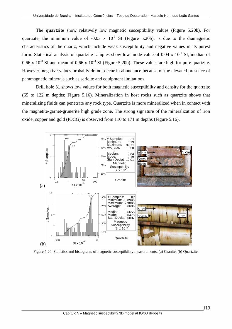
Universidade de Brasília – Instituto de Geociências – Tese de Doutorado – Marcelo Henrique Leão Santos
113 Capítulo 5 – Magnetic susceptibility 3D model at IOCG deposits
The quartzite show relatively low magnetic susceptibility values (Figure 5.20b). For
quartzite, the minimum value of -0.03 x 10⁻³
SI (Figure 5.20b), is due to the diamagnetic
characteristics of the quartz, which include weak susceptibility and negative values in its purest
form. Statistical analysis of quartzite samples show low mode value of 0.04 x 10⁻³
SI, median of
0.66 x 10⁻³
SI and mean of 0.66 x 10⁻³
SI (Figure 5.20b). These values are high for pure quartzite.
However, negative values probably do not occur in abundance because of the elevated presence of
paramagnetic minerals such as sericite and equipment limitations.
Drill hole 31 shows low values for both magnetic susceptibility and density for the quartzite
(65 to 122 m depths; Figure 5.16). Mineralization in host rocks such as quartzite shows that
mineralizing fluids can penetrate any rock type. Quartzite is more mineralized when in contact with
the magnetite-garnet-grunerite high grade zone. The strong signature of the mineralization of iron
oxide, copper and gold (IOCG) is observed from 110 to 171 m depths (Figure 5.16).
(a)
(b)
Figure 5.20. Statistics and histograms of magnetic susceptibility measurements. (a) Granite. (b) Quartzite.
# Samples:Minimum:Maximum:Average:
Median:Mode:Stan.Deviat:
# S
am
ple
s:
SI x 10-3
MagneticSusceptibility
SI x 10 -3
0.1 100
0
4
8
10%
30%
50%
70%
90% 61 0.19 99.71 3.50
0.83 0.19
12.91
1.2
0.5
1 10 Granite
# Samples:Minimum:Maximum:Average:
Median:Mode:Stan.Deviat:
# S
am
ple
s:
SI x 10-3
MagneticSusceptibility
SI x 10 -3
0.01 3
0
5
10
10%
30%
50%
70%
90% 87 -0.0390 2.9895 0.6686
0.6655 0.0475 0.6007
1.2
1 Quartzite
5 cm
5 cm
Albite
Biotite
Quartz
Silica
Sericite

Universidade de Brasília – Instituto de Geociências – Tese de Doutorado – Marcelo Henrique Leão Santos
114 Capítulo 5 – Magnetic susceptibility 3D model at IOCG deposits
Hydrothermal alteration zones
Within the hydrothermal alteration zones, a trend of higher susceptibility values compared to
the host rocks can be observed, especially in the potassic zone and garnet-grunerite zone. In these
zones, the maximum values reach 5,113 x 10-3
SI and 3,717 x 10-3
SI, respectively, and likely
reflects magnetite precipitated during the hydrothermal event (Figures 5.21a and 5.21b). The only
exception is the silicic alteration.
(a)
(b)
Figure 5.21. Statistics and histograms of the magnetic susceptibility measurements. (a) Potassic hydrothermal alteration
zone. (b) Garnet-grunerite hydrothermal alteration zone.
Amphibole, garnet, biotite, and chlorite are the main silicate alteration phases. These
minerals have paramagnetic behavior because of the presence of Fe2+
, Fe3+
or Mn3+
. However, some
silicates can appear ferromagnetic because of impurities such as magnetite. In complex
hydrothermal environments the impurities becomes common. These minerals start to show
remanence and exhibit hysteresis. In general, the predominance of paramagnetic minerals such as
biotite (Figure 5.21a), garnet-amphibole (Figure 5.21b), amphibole (Figure 5.22a) and chlorite
(Figure 5.22b) in the hydrothermal alteration zones keeps the median susceptibility values between
4 x 10⁻³
SI and 7 x 10⁻³
SI, the mean between 23 x 10-3
SI and 77 x 10-3
SI and modes between 0.4 x
10-3
SI and 4 x 10⁻³
SI.
# Samples:Minimum:Maximum:Average:
Median:Mode:Stan.Deviat:
# S
am
ple
s:
SI x 10-3
MagneticSusceptibility
SI x 10 -3
0.1 6000
0
70
140
10%
30%
50%
70%
90% 1416 0.12
5113.26 33.57
4.99 0.45
190.4
6.5
1 10 100 1000
Biotitehydrothermal
alteration zone
# Samples:Minimum:Maximum:Average:
Median:Mode:Stan.Deviat:
# S
am
ple
s:
SI x 10-3
MagneticSusceptibility
SI x 10 -3
0.1 4000
0
22.5
45
10%
30%
50%
70%
90% 509 0.38
3717.81 77.12
7.07 2.08
315.8
3
16
1 10 100 1000
GarnetGrunerite
hydrothermalalteration zone
5 cm
Biotite Quartz
5 cm
Garnet Grunerite

Universidade de Brasília – Instituto de Geociências – Tese de Doutorado – Marcelo Henrique Leão Santos
115 Capítulo 5 – Magnetic susceptibility 3D model at IOCG deposits
(a)
(b)
Figure 5.22. Statistics and histograms of the magnetic susceptibility measurements. (a) Amphibole hydrothermal
alteration zone. (b) Chloritization.
The only exception is the silicification alteration zone. Since quartz is diamagnetic it’s
expected negative values, as observed, has a minimum of -0.04 x 10⁻³
SI. The histogram for the
silicic alteration type shows a typical normal distribution with a median value of 0.6 x 10⁻³
SI, a
mean value of 2.51 x 10⁻³
SI and a maximum value of 357 x 10-3
SI (Figure 5.23). The presence of
paramagnetic minerals and instrumental limitations to measure negative values justify the low
positive susceptibility values. In almost all the drill cores, an abundance of silicification is closely
related to the low grade mineralization (Figures 5.14, 5.16 and 5.17). However, in many places, it
can also be associated with high grade mineralization (such as in Figure 5.13 at a 310 m depth and
in Figure 5.14 near the contact zone at 241 m depth).
Figure 5.23. Statistics and histogram of the silicification zone magnetic susceptibility measurements.
# Samples:Minimum:Maximum:Average:
Median:Mode:Stan.Deviat:
# S
am
ple
s:
SI x 10-3
MagneticSusceptibility
SI x 10 -3
0.1 1800
0
40
80
10%
30%
50%
70%
90% 342 0.51
1618.83 23.69
4.64 2.08
122.2
5
1 10 100
Amphibole hydrothermal
alteration zone
# Samples:Minimum:Maximum:Average:
Median:Mode:Stan.Deviat:
# S
am
ple
s:
SI x 10-3
MagneticSusceptibility
SI x 10 -3
0.1 1600
0
17.5
35
10%
30%
50%
70%
90% 298 0.61
1488.98 49.74
5.23 4.81
170.8
4.8
1 10 100 Chloritization
# Samples:Minimum:Maximum:Average:
Median:Mode:Stan.Deviat:
# S
am
ple
s:
SI x 10-3
MagneticSusceptibility
SI x 10 -3
0.01 400
0
125
250
10%
30%
50%
70%
90% 2260 -0.0440
357.01 2.5100
0.6035 0.2195 15.28
0.56
1 10 Silicification
ORE 1.4 % Cu
5 cm
Grunerite Chalcopyrite
5 cm
Chlorite
ORE 4.2 % Cu & 0.77 g/t Au 5 cm
Silica Chalcopyrite

Universidade de Brasília – Instituto de Geociências – Tese de Doutorado – Marcelo Henrique Leão Santos
116 Capítulo 5 – Magnetic susceptibility 3D model at IOCG deposits
The potassic alteration type fingerprint is the biotite hydrothermal alteration zone that
may or may not be associated with mineralization. Biotite can be both paramagnetic and
ferromagnetic. In addition, magnetite commonly precipitates between the biotite sheets planar
voids, as well as in fractures associated with this type of alteration. Together, these phenomena
likely account for the higher observed susceptibilities within the potassic altered rocks (Figure
5.21a).
In drill hole 88 between the depths of 380 and 438 m, alternating zones of biotite
hydrothermal alteration and silicic alteration with low copper grade are observed. The signatures are
well defined by the contrast in iron geochemical signatures and density (Figure 5.13). For drill hole
31, the biotite hydrothermal alteration zone is interspersed with the magnetite hydrothermal
alteration zones and with silicification, and they are all mineralized (137 to 236 m depths; Figure
5.16).
The garnet-grunerite and amphibole hydrothermal alteration zones have a close
relationship with the low to medium grade mineralized zones. As can be seen in drill hole 125,
between the depths of 83 and 115 m, the magnetic signature of the garnet-grunerite hydrothermal
alteration zone shows low susceptibility values (Figure 5.17).
Along drill hole 34, between the depths of 127 and 140 m, the amphibole hydrothermal
alteration zone has a low copper-gold grade and a low density relative to the magnetite
hydrothermal alteration zone. At the top of this interval, the contact between the amphibole and
garnet-grunerite hydrothermal alteration zones have values that reach 50 x 10-3
SI because of the
infill of magnetite (Figure 5.15).
Drill hole 88 also shows at the top a strong chlorite hydrothermal alteration zone that may
or may not be associated with mineralization (Figure 5.13). This process has low susceptibility
values with a median of 5 x 10⁻³
SI (Figure 5.22b). The variation from low and intermediate values
is interpreted to be the result of magnetite precipitation along fractures or between sheets of biotite.
The hydrothermal process of chloritization is strong. It alters partially or completely the rocks of the
area.
Magnetite, garnet-grunerite-magnetite and amphibole-magnetite hydrothermal alteration
zones
Magnetite is the most abundant ferromagnetic mineral in the hydrothermal alteration and, as
said, is responsible for the high susceptibility values. The median magnetic susceptibility values
decrease from the massive magnetite alteration zone with 989 x 10-3
SI (Figure 5.24a) to the
garnet-grunerite-magnetite alteration zone with 409 x 10-3
SI (Figure 5.24b) and amphibole-

Universidade de Brasília – Instituto de Geociências – Tese de Doutorado – Marcelo Henrique Leão Santos
117 Capítulo 5 – Magnetic susceptibility 3D model at IOCG deposits
magnetite alteration zone with 308 x 10-3
SI (Figure 5.24c). Among the magnetite-rich alteration
zones, the mean susceptibility values are 2,777 x 10-3
for the massive magnetite zone (Figure
5.24a), 1,550 x 10-3
for the amphibole-magnetite zone (Figure 5.24c), and 1,383 x 10-3
for the
garnet-grunerite-magnetite zone (Figure 5.24b). Both the median and mean are consistent with what
is observed in the drill core samples, which shows that the magnetite hydrothermal alteration zone
has higher magnetite content than the garnet-grunerite-magnetite and amphibole-magnetite zones
(Figures 5.16 and 5.17).
(a)
(b)
(c)
Figure 5.24. Statistics and histograms of magnetic susceptibility measurements for magnetite rich-alteration types. (a)
Massive magnetite hydrothermal alteration zone. (b) Garnet-grunerite-magnetite hydrothermal alteration zone.
(c) Amphibole-magnetite hydrothermal alteration zone.
# Samples:Minimum:Maximum:Average:
Median:Mode:Stan.Deviat:
# S
am
ple
s:
SI x 10-3
MagneticSusceptibility
SI x 10 -3
0.1 12000
0
8
16
10%
30%
50%
70%
90% 138 0.71
9999.99 2777.23
989.739999.99
3310
915
1 10 100 1000
Magnetitehydrothermal
alteration zone
# Samples:Minimum:Maximum:Average:
Median:Mode:Stan.Deviat:
# S
am
ple
s:
SI x 10-3
MagneticSusceptibility
SI x 10 -3
0.1 12000
0
30
60
10%
30%
50%
70%
90% 932 0.32
9999.99 1383.48
409.239999.99
2143
Garnet-GruneriteMagnetite
hydrothermalalteration zone
454
1 10 100 1000
# Samples:Minimum:Maximum:Average:
Median:Mode:Stan.Deviat:
# S
am
ple
s:
SI x 10-3
MagneticSusceptibility
SI x 10 -3
0.1 12000
0
4
8
10%
30%
50%
70%
90% 82 0.92
9999.99 1550.78
308.68 0.92
2277
1 10 100 1000
AmphiboleMagnetite
hydrothermalalteration zone
ORE 0.74 % Cu & 0.33 g/t Au
ORE 5.4 % Cu & 0.86 g/t
Au
ORE 0.8 Cu % & 0.5 g/t Au
5 cm
5 cm
5 cm
Chalcopyrite
Chalcopyrite Amphibole Massive Magnetite
Garnet Magnetite Grunerite
Magnetite Amphibole
Massive Magnetite
Magnetite Garnet
Grunerite

Universidade de Brasília – Instituto de Geociências – Tese de Doutorado – Marcelo Henrique Leão Santos
118 Capítulo 5 – Magnetic susceptibility 3D model at IOCG deposits
In the magnetite alteration zone, there is a susceptibility population centered at high values
around 915 x 10-3
SI, which is near the median of 989 x 10-3
SI and represents the presence of
massive magnetite (Figure 5.24a).
In the garnet-grunerite-magnetite alteration zone the distribution becomes more complex.
It shows two populations of high susceptibility values. The highest valued population is centered
near 454 x 10-3
SI and represents massive magnetite. The other population has values lower than 10
x 10-3
SI. This population has a significant concentration of paramagnetic minerals such as grunerite
and garnet (Figure 5.24b).
A third population observed in the amphibole-magnetite alteration zone, indicates that the
values in histogram are much widely distributed, which is most likely a result of the greater
presence of amphiboles (Figure 5.24c).
This variation from high to intermediate to low values is observed in the drill cores, wherein
the garnet-grunerite and amphibole alteration zones are constantly altered by the input of magnetite,
which produces a great fluctuation in the susceptibility measurements (Figures 5.13, 5,15, 5.16 and
5.17).
The garnet-grunerite-magnetite alteration occurs in greater abundance relative to the
amphibole-magnetite alteration zone (Figure 5.17). In addition, the garnet-grunerite-magnetite
alteration has higher correlation with the massive magnetite zone. This observation is corroborated
by analyzing the mode, which is >9,999 x 10-3
SI and 0.92 x 10⁻³
SI in the garnet-grunerite-
magnetite and amphibole-magnetite alteration zones, respectively (Figures 5.24b and 5.24c).
When magnetite and silicic banding is present, descriptively differentiating the banded iron
formation from the magnetite hydrothermal alteration zone becomes more difficult. However, when
comparing the susceptibility values, this difference is easily noticeable. Between the depths of 145
m and 192 m in drill hole 34, the magnetite hydrothermal alteration zone is marked by a high
increase on the values of magnetic susceptibility, iron, copper, gold and density, when compared to
the banded iron formation between the depths of 212 and 260 m (Figure 5.15). The banded iron
formations are not mineralized, and normally show low values for susceptibility, iron content and
density, when compared to the magnetite hydrothermal alteration zone. This difference can be
observed when looking at the median values, which is 182 x 10-3
SI for the banded iron formation
(Figure 5.19) and 989 x 10-3
SI for the magnetite hydrothermal alteration zone (Figure 5.24a). The
median value of the banded iron formation is low, even when compared to the medians of the
garnet-grunerite-magnetite (400 x 10-3
SI; Figure 5.24b) and amphibole-magnetite (300 x 10-3
SI;
Figure 5.24c) hydrothermal alteration zones.

Universidade de Brasília – Instituto de Geociências – Tese de Doutorado – Marcelo Henrique Leão Santos
119 Capítulo 5 – Magnetic susceptibility 3D model at IOCG deposits
5.9 - MAGNETIC SUSCEPTIBILITY 3D MODELING
A 3D magnetic susceptibility model was derived from the measurements made on drill core.
The measurements were geolocated in 3D space and contoured using a 3D kriging algorithm
(Geosoft, 2014). Drill hole spacing was approximately 100 m with down hole measurements every
1 m, with the resultant susceptibility model having 5 m cubic cells. The weight of the direction with
a 300° azimuth was used to improve the effect of sampling in this direction, which is the deposit
strike direction with less sampling relative to perpendicular direction of greatest sampling.
The physical models show data with values greater than 500 x 10-3
SI for the measurements
made with the high sensitivity equipment (KT-10) and values greater than 60 x 10-3
SI for those
made with the low sensitivity equipment (KT-9). These values were selected based on the statistical
analyses of the susceptibility data, as previously analyzed. The two envelope surfaces results of the
susceptibilities higher than the threshold values in both cases, complement each other because of
the different distributions of the drill holes used in the measurements (see Figure 5.7). It is
important to emphasize that the susceptibility model reflects only the northwestern portion of the
study area, which is where the studied drill holes are located (Figure 5.7).
The 3D magnetic susceptibility model shows similarities to ore-grade models. Comparison
of the obtained susceptibility model (Figure 5.25a) with the copper high grade ore model from 69
drill holes (Figure 5.25b; Vale S.A., 2012), shows excellent correlation.

Universidade de Brasília – Instituto de Geociências – Tese de Doutorado – Marcelo Henrique Leão Santos
120 Capítulo 5 – Magnetic susceptibility 3D model at IOCG deposits
(a)
(b) Figure 5.25. (a) Three dimensional magnetic susceptibility model correlation with the copper low grade orebodies
projection at level 190 m. (b) Three dimensional magnetic susceptibility model correlation with the copper high grade
orebodies.
This susceptibility model versus ore concentration when seen in detail, shows the direct
correlation between the magnetite hydrothermal alteration zones, represented by high magnetic
susceptibility values (envelope of the values greater than 500 x 10-3
SI), and high grade orebodies
with values higher than 0.6 % copper (Figure 5.26).

Universidade de Brasília – Instituto de Geociências – Tese de Doutorado – Marcelo Henrique Leão Santos
121 Capítulo 5 – Magnetic susceptibility 3D model at IOCG deposits
Figure 5.26. Detail of the magnetic susceptibility 3D model with isosurface of values higher than 500 x 10-3
SI (in red),
and correlation with the copper high-grade orebodies (in blue, green and yellow). Drill holes in black traces.
5.10 - CONCLUSIONS
Magnetic susceptibility measurements on drill core were used to define a physical property
model that can help target exploration for IOCG deposits. The results showed strong correlation
between magnetite-rich, hydrothermally altered rocks and iron, copper, and gold enrichment
The values obtained in the magnetic susceptibility measurements also enabled the
interpolation of a 3D model with their distribution, which traces fairly well the known boundaries of
the studied mineralization.
Magnetic susceptibility measurements were carried out using different instrumentation and
related drill core logs that described lithology and alteration types. In all cases, increased magnetite
content seemed to correlate with alteration types.
The magnetic susceptibility measurements carried out on the geochemical samples showed
an excellent correlation with those performed on the drill cores, and they also represent a better
approximation of the mineralization model because of the sample material homogenization. This
methodology could easily be implemented rather than measuring along drill core samples and
provides a high return on investment as the equipment and time needed for measurements is
minimal.
It is interesting to note that an efficient quality control of measured data discussed herein is
crucial for the correct analysis of measured magnetic susceptibilities and interpolation of a reliable
3D model.
The methods and geological-geophysical interpretations presented in this study can be useful
for:
Universidade de Brasília – Instituto de Geociências – Tese de Doutorado – Marcelo Henrique Leão Santos
122 Capítulo 5 – Magnetic susceptibility 3D model at IOCG deposits
(i) characterizing ore zones and hydrothermal alteration zones;
(ii) assisting in the correlation and geological interpretation of mineralized lithotypes;
(iii) supporting sections interpretation for the generation of geological and ore models;
(iv) improving and validating the use of magnetic surveys as well as mineral prospecting
techniques and geophysical equipment; and
(v) providing an excellent support for using magnetic data for constrained inversion.
In the case here presented, in general, the hydrothermal alteration zones with magnetite are
proximal to the mineralized zone. Outward from the magnetite-rich zones are silicic, garnet-
grunerite, amphibole, potassic and chloritic type alteration zones. Geological macroscopic
observations supported by petrographic studies, and the knowledge of magnetic susceptibility
signatures were used to establish the paragenetic sequence of the deposit. The use of physical
properties to define the magnetic behavior in a quantitative manner showed the importance of the
approach exercised for a better characterization of the magnetic susceptibility signatures. This
helped to improve the paragenetic sequence in the studied area.
The correlation between the increase in magnetic susceptibility values and mineralization is
shown by iron, copper and gold high grades. The direct relationship between high densities and
mineralized hydrothermal alteration bodies is also evident because of the presence of dense
minerals (magnetite and sulfides).
It is known that in the studied deposit, the magnetite, garnet-grunerite-magnetite and
amphibole-magnetite hydrothermal alteration zones are the most important zones because of their
direct relationship with chalcopyrite and bornite sulfides. The best susceptibility signatures were
outlined for these magnetite-rich zones, and the 3D interpolation showed an excellent correlation
between the generated susceptibility model and the orebody that was modeled based on the drill
holes. Thus, it is believed that the approach described herein can be of great value in a mineral
program.
5.11 - ACKNOWLEDGMENTS
The authors would like to thank Vale S.A. – Department of Mineral Exploration and
Projects – for the financial support, permission to publish this study, and permission to use the
geophysical and geological data in this research project. We also would like to thank the Vale S.A.
Geophysical Team for all their support, the Vale S.A. Furnas Project for the data and numerous
geological arguments used in this study, and geologists Gabriel Paulo and Sálvio Ribeiro for their
assistance with the ore models and graphs. We express our appreciation to Dr. Misac Nabighian and
geophysicist Daniel Brake for their help in English review.

Universidade de Brasília – Instituto de Geociências – Tese de Doutorado – Marcelo Henrique Leão Santos
123 Capítulo 5 – Magnetic susceptibility 3D model at IOCG deposits
5.12 - REFERENCES
AGICO Advanced Geoscience Instruments Co., 2004, KLY- 4 / KLY- 4S / CS- 3 / CS- L User’s
Guide, Modular system for measuring magnetic susceptibility, anisotropy of magnetic
susceptibility, and temperature variation of magnetic susceptibility, Version 1.2,
http://www.agico.com/, accessed 15 October 2004.
Araújo, O.J.B., and R.G.N. Maia, 1991, Projeto especial mapas de recursos minerais, de solos e de
vegetação para a área do Programa Grande Carajás; Subprojeto Recursos Minerais; Folha
SB.22-Z-A Serra dos Carajás - Estado do Pará: DNPM/CPRM, Brasília.
Austin, J.R., P.W. Schmidt, and C.A. Foss, 2013, Magnetic modeling of iron oxide copper-gold
mineralization constrained by 3D multiscale integration of petrophysical and geochemical data:
Cloncurry District, Australia: Interpretation, 1, no.1, T63–T84.
Barbosa, J.P.O, C.E.M. Barros, M.B. Macambira, and A.G. Vale, 2001, Geologia e Geocronologia
do Stock Granítico Geladinho, região de Parauapebas, Província Mineral de Carajás: 7th
Simpósio de Geologia da Amazônia, SBG, Expanded Abstract.
Barros, C.E.M., and P. Barbey, 1998, A importância da granitogênese tardi-arqueana (2.5 Ga.) na
evolução tectono-metamórfica da província mineral de Carajás – O Complexo Granítico
Estrela e sua auréola de contato: Revista Brasileira de Geociências, 28, no. 4, 513–522.
Clark, D.A., 1997, Magnetic petrophysics and magnetic petrology: aids to geological interpretation
of magnetic surveys: Journal of Australian Geology and Geophysics, 17, 83–103.
Clark, D.A., 1999, Magnetic petrology of igneous intrusions: implications for exploration and
magnetic interpretation: Exploration Geophysics, 30, 5–26.
Clark, D.A., 2014, Magnetic effects of hydrothermal alteration in porphyry copper and iron-oxide
copper–gold systems: A review: Tectonophysics, 624, 46–65.
Clark, D.A., D.H. French, M.A. Lackie, and P.W. Schmidt, 1992, Magnetic petrology: Application
of integrated rock magnetic and petrological techniques to geological interpretation of
magnetic surveys: Exploration Geophysics, 23, 65–68.
Criss, R.E., and D.E. Champion, 1984, Magnetic properties of granitic rocks from the southern half
of the Idaho Batholith - influences of hydrothermal alteration and implications for
aeromagnetic interpretation: Journal of Geophysical Research, 89, no. B8, 7061–7076.
CVRD (Companhia Vale do Rio Doce), 2006, Relatório de etapa, Alvo Furnas, Volume 1: Internal
report: Technical report.
DOCEGEO (Rio Doce Geologia e Mineração S.A), 1988, Revisão Litoestratigráfica da Província
Mineral de Carajás: 35th Congresso Brasileiro de Geologia, SBG, Expanded Abstract, 11-56.
Geosoft Inc., 2014, Target Software, 3D Kriging GX, http://www.geosoft.com, accessed 15 April
2014.
Hanna, W.F., 1969, Negative aeromagnetic anomalies over mineralized areas of the Boulder
batholith, Montana: U.S. Geological Survey Professional Paper, 650, D, 159–167.
Hirata, W.K., J.C. Rigon, A.A.C. Cordeiro, and E.M. Meireles, 1982, Geologia Regional da
Província Mineral de Carajás: 1o Simpósio de Geologia da Amazônia, SBG, 100–108.
Hitzman, M.W., N. Oreskes, and M.T. Einaudi, 1992, Geological characteristics and tectonic setting
of Proterozoic iron oxide (Cu–U–Au–REE) deposits: Precambrian Research, 58, 241–287.
Universidade de Brasília – Instituto de Geociências – Tese de Doutorado – Marcelo Henrique Leão Santos
124 Capítulo 5 – Magnetic susceptibility 3D model at IOCG deposits
Hoover, D.B., W.D. Heran, P.L. Hill, 1992, The Geophysical Expression of Selected Mineral
Deposit Models: Editors, USGS Open File Report, 92–557.
Hoschke, T., 2008, Geophysical signatures of copper-gold porphyry and epithermal gold deposits:
Arizona Geological Society Digest, 22, 85–100.
Kearey, P., M. Brooks, and I. Hill, 2002, An introduction to geophysical exploration: Blackwell
Science.
Lindenmayer, Z.G., 1990, Salobo Sequence, Carajás, Brazil: geology, geochemistry and
metamorphism: Ph.D. thesis, University of Western Ontario.
Lindenmayer, Z.G., and J.B.G. Teixeira, 1999, Ore Genesis at the Salobo Copper Deposit, Serra dos
Carajás, in M.G. Silva, and A. Misi, eds., Base Metal Deposits of Brazil: MME/CPRM/DNPM,
33–43.
Porter, T.M., 2000, Hydrothermal Iron Oxide–Copper–Gold and Related Deposits: A Global
Perspective: Eds., PGC Publishing.
Sandrin, A, and S. Elming, 2007, Physical properties of rocks from borehole TJ71305 and
geophysical outline of the Tjårrojåkka Cu-prospect, northern Sweden: Ore Geology Reviews,
30, 56–73.
Sandrin, A, Å. Edfelt, T.E. Waight, R. Berggren, and S. Elming, 2009, Physical properties and
petrologic description of rock samples from an IOCG mineralized area in the northern
Fennoscandian Shield, Sweden: Journal of Geochemical Exploration, 103, 80–96.
Smith, R.J., 2002, Geophysics of iron oxide-copper-gold deposits, in T.M. Porter, ed.,
Hydrothermal Iron Oxide–Copper–Gold and Related Deposits: A Global Perspective vol. 2:
PGC Publishing, 357–367.
Telford, W.M., L.P. Geldart, and R.E. Sheriff, 1990, Applied geophysics 2 ed.: Cambridge
University Press.
Vale S.A., 2012, Projeto Furnas, Relatório Final de Geologia: Internal report: Technical report.
Vasquez, M.L., C.S. Sousa, and J.M.A Carvalho, 2008, Mapa Geológico e de Recursos Minerais do
Estado do Pará, escala 1:1.000.000: Programa Geologia do Brasil (PGB), Companhia de
Pesquisa de Recursos Minerais - Serviço Geológico do Brasil.
Wirth, K.R., A.K. Gibbs, and W.J. Olszewski, 1986, U-Pb ages of zircons from the Grão-Pará
group and Serra dos Carajás Granite, Pará, Brazil: Revista Brasileira de Geociências, 16, no. 2,
195–200.
Xavier, R.P., L.V.S. Monteiro, C.P.N. Moreto, A.L.S. Pestilho, G.H.C. Melo, M.A.D. Silva, B.
Aires, C. Ribeiro, and F.H.F. Silva, 2012, The iron oxide copper-gold systems of the Carajás
Mineral Province, Brazil, in Geology and Genesis of Major Copper Deposits and Districts of
the World: A Tribute to Richard Sillitoe, Special Publication, Society of Economic Geologists.

Universidade de Brasília – Instituto de Geociências – Tese de Doutorado – Marcelo Henrique Leão Santos
125 Capítulo 6 – Conclusões da Tese
CAPÍTULO 6
CONCLUSÕES DA TESE
Neste projeto de pesquisa foram realizadas determinações das propriedades físicas, assim
como uma ampla interpretação, com o uso de diversas técnicas e métodos magnéticos
correlacionados ao contexto geológico, que teve como resultado um modelo prospectivo da
mineralização de óxidos de ferro-cobre-ouro (IOCG). Isto foi possível devido à mineralização
disseminada de calcopirita ± bornita estar relacionada à alteração hidrotermal cálcio-sódico-
potássica (bornita-granada-anfibólio-magnetita) com os altos teores de cobre-ouro associados à
presença de magnetita.
O trabalho foi implementado em três artigos que se complementam para atingir as várias
etapas da exploração mineral. O primeiro artigo teve como resultado as interpretações qualitativas e
semi-quantitativas de dados de magnetometria, que mapearam a configuração estrutural do
depósito. Este artigo também teve como resultado uma interpretação quantitativa com a modelagem
paramétrica 2D que forneceu uma primeira visão em profundidade da geometria do corpo e o
entendimento de fatores complicadores como a presença de remanência e desmagnetização.
O segundo artigo, também com base apenas nos dados magnéticos da área, focou nas
transformações destes dados com o uso do princípio da camada equivalente para a obtenção do que
seria a intensidade do campo magnético anômalo (MMA, Magnetic Magnitude Anomaly), seguida
da modelagem (inversão) 3D para estruturas complexas, assistida por técnicas de otimização, numa
recuperação mais eficaz e detalhada da distribuição da susceptibilidade magnética intrínseca. O
principal desafio encontrado para se atingir resultados positivos foi a presença de remanência
agravado pelo fato do depósito estar situado numa região de baixas latitudes magnéticas que podem
resultar em direções da magnetização total bem diferentes daquela induzida.
O terceiro artigo teve como base o conjunto de dados geológicos e das susceptibilidades
magnéticas medidas em testemunhos de furos de sonda. O trabalho desenvolvido possibilitou a
caracterização das assinaturas de susceptibilidade para os diversos litotipos encaixantes e para as
zonas de alterações hidrotermais. Mais do que isso, possibilitou-se obter o modelo 3D referente à
distribuição espacial das susceptibilidades magnéticas medidas.
Com isso, os principais resultados obtidos com este trabalho foi a definição de dois modelos
para a mineralização no local estudado: (i) o geofísico, conseguido pela modelagem / inversão 3D
dos dados magnéticos (método indireto) e (ii) o geológico obtido pela modelagem espacial das
susceptibilidades magnéticas medidas (método direto).

Universidade de Brasília – Instituto de Geociências – Tese de Doutorado – Marcelo Henrique Leão Santos
126 Capítulo 6 – Conclusões da Tese
Para uma validação dos resultados, estes modelos foram comparados entre si e com as
informações provenientes da extensiva campanha de sondagem exploratória realizada. As
conclusões mostram que a modelagem 3D dos dados de susceptibilidade medidos permite uma
melhor definição e delimitação da fonte magnética. Entretanto, o trabalho mostrou que isso só pode
ser alcançado por meio de medidas sistemáticas bastante trabalhosas e de uma interpretação
complexa e exaustiva, com um grande custo e consumo de tempo. Este enfoque lida com uma
grande quantidade de dados petrofísicos (susceptibilidade magnéticas medidas) e geológicos
(estudos pormenorizados dos testemunhos de sondagens). Por outro lado, a modelagem de dados
magnéticos por inversão de sua transformação em amplitude da anomalia magnética (através da
camada equivalente), consome menos tempo, e fornece, mesmo assim, uma excelente aproximação
ao mapeamento espacial das fontes magnéticas complexas.
Ambas as aproximações delimitaram a zona de magnetita maciça associada aos altos teores
de minério. As metodologias abordadas neste estudo tem alto potencial para as diversas etapas de
exploração (greenfield, brownfield e avaliação de recursos) de depósitos tipo IOCG e para depósitos
associados à magnetita.
Magnetic interpretation and 2D modeling at
iron oxide-copper-gold deposits, Carajás Mineral Province
Este trabalho aborda os diversos passos seguidos na interpretação dos dados magnéticos
disponibilizados para o estudo. Descreve os resultados das diversas transformações lineares usadas
para alicerçar a interpretação qualitativa com a caracterização em mapa das diversas fontes que
compõem o relevo magnético local. Sua evolução, possibilitou estimar as profundidades destas
fontes numa interpretação semi-quantitativa. Finalmente, este conjunto de informações serviu de
base a uma modelagem paramétrica 2D para a interpretação quantitativa. A boa correspondência
entre os resultados da modelagem 2D, e a geologia conhecida a o corpo de minério demonstram o
sucesso desta abordagem.
Este trabalho mostrou caminhos para que se possa lidar com um corpo magnético complexo
que constitui o ambiente da mineralização, como é o caso da remanência acentuada que varia ao
longo do mesmo. O ensaio com a modelagem 2D possibilitou a verificação de que o corpo é
fortemente magnético, que se tem que lidar com o fenômeno da desmagnetização, e de uma
magnetização remanente associada a uma anisotropia magnética.
Este estudo de caso mostra que esta seria uma abordagem eficaz em cenários com esta
complexidade, permitindo-se ter uma ideia da geometria do corpo de minério.

Universidade de Brasília – Instituto de Geociências – Tese de Doutorado – Marcelo Henrique Leão Santos
127 Capítulo 6 – Conclusões da Tese
Application of 3D magnetic amplitude inversion to iron oxide-copper-gold deposits at low
magnetic latitudes: a case study from Carajás Mineral Province
Este trabalho sequencia o anterior e inicia-se pelo cálculo da amplitude da anomalia
magnética com o uso do conceito de camada equivalente para lidar com o terreno acidentado da
área. Sobre esta transformação, e com informações do primeiro ensaio interpretativo, foi realizada a
modelagem assistida por técnicas de minimização de erros (inversão) com o uso do parâmetro
ótimo de regularização obtido com o critério da curva L. A susceptibilidade invertida recuperada
delineou com sucesso a magnetita maciça associada ao minério de cobre e ouro de alto teor. Este
processo de inversão mostrou-se bastante robusto no sentido de prescindir aprioristicamente, do
controle estrutural, da geologia e do modelo de minério de dados dos testemunhos de furos de sonda
do depósito, usados depois para comprovar o êxito desta abordagem.
Este estudo também reforça a utilidade da transformação empregada da amplitude da
anomalia magnética, também como substituta da tradicional redução ao polo (RTP). Similarmente à
RTP, dados de amplitude também representam uma versão corrigida dos efeitos de fase do sinal
magnético e reduzem a polarização magnética para inclinações diferentes de 90º. A amplitude da
anomalia magnética pode ser mais vantajosa do que a RTP devido não ser necessário o
conhecimento da direção da magnetização para seu cálculo.
Este estudo de caso mostra que a inversão da amplitude é eficiente neste complexo ambiente
com múltiplos fatores como magnetização remanente e desmagnetização que afetam a direção da
magnetização total. Assim como as complicações devidas a localização em latitudes magnéticas
extremamente baixas.
Magnetic susceptibility 3D model and signatures of iron oxide-copper-gold (IOCG)
mineralization: A case study from Carajás Mineral Province, Brazil
As assinaturas da susceptibilidade magnética medidas em testemunhos de furos de sonda se
provaram um método eficiente para caracterizar as zonas onde houve o enriquecimento em ferro,
cobre e ouro. Além disso, o comportamento magnético dos minerais permitiram a descrição das
assinaturas magnéticas associadas com os litotipos e zonas de alteração hidrotermal. Os valores
obtidos nas medidas de susceptibilidade também permitiram uma interpolação 3D que possibilitou
verificar sua distribuição espacial. Este resultado delimitou muito bem a mineralização conhecida.
Medidas de susceptibilidade realizadas igualmente, mas agora com o uso de amostras que
representam alíquotas empregadas nas dosagens geoquímicas, mostraram excelente correlação

Universidade de Brasília – Instituto de Geociências – Tese de Doutorado – Marcelo Henrique Leão Santos
128 Capítulo 6 – Conclusões da Tese
àquelas realizadas em testemunhos de furos de sondas mecânicas. Elas representaram uma melhor
aproximação ao modelo de mineralização devido à homogeneização realizada no material
previamente preparado para dosagens geoquímicas.
Os resultados obtidos ao longo dos testemunhos com susceptibilímetros portáteis foram
aferidos por medidas laboratoriais. Em ambos os casos, mostraram a presença de valores elevados
para a susceptibilidade magnética, e para os resultados em laboratório um alto grau de anisotropia.
No caso aqui estudado, de forma geral, as zonas de alteração hidrotermal com magnetita são
proximais a zona mineralizada, seguidas da silicificação, zona de granada-grunerita, zona de
anfibólio, potassificação e cloritização. O conhecimento geológico e o comportamento magnético
qualitativo foram utilizados para estabelecer a sequência paragenética do depósito.
O uso da susceptibilidade para definir o comportamento magnético de uma forma
quantitativa mostrou a importância desta abordagem para a caracterização das assinaturas
magnéticas. Isto pode ajudar a melhorar a sequência paragenética de uma área estudada.
Aqui é conhecido que as zonas de alteração hidrotermal a magnetita, granada-grunerita-
magnetita e anfibólio-magnetita são as zonas mais importantes por causa de sua relação direta com
os sulfetos de calcopirita e bornita. As melhores assinaturas de susceptibilidade foram delineadas
para estas zonas ricas em magnetita.
Por fim, a interpolação volumétrica destas medidas projetadas ao longo de seus respectivos
segmentos nos furos de sondas mostrou uma excelente correlação entre o modelo de
susceptibilidade 3D assim gerado com o modelo conseguido com as interpretações e modelagens
magnéticas conduzidas e destas com os dados dos testemunhos usados.