Recent Changes in Soil Total Phosphorus in the Everglades: Water Conservation Area 3
Upload
khangminh22Category
view
4download
0
ISSN 2095-6339
CN 10-1107/P
Available online at www.sciencedirect.com
INTERNATIONAL SOIL AND WATER CONSERVATION RESEARCH (ISWCR)
Volume 8, No. 2, June 2020
CONTENTS
International Soil and Water C
onservation Research (ISW
CR
) Vol. 8 (2020) 103 – 212
82
Volume 8, No. 2, June 2020
N.S.B. Nasir Ahmad , F.B. Mustafa , S.Y. Muhammad Yusoff , G. Didams A systematic review of soil erosion control practices on the agricultural land in Asia . . . . . . . 103
X. Shi , F. Zhang , L. Wang , M.D. Jagirani , C. Zeng , X. Xiao , G. Wang Experimental study on the effects of multiple factors on spring meltwater erosion on an alpine meadow slope . . . . . . . . . . . . . . . . . . . . . . . . . . . . . . . . . . . . . . . . . . . . . . . . . . . . . . . . . . . . . 116
K.d.S. Falc ã o , E. Panachuki , F.d.N. Monteiro , R. da Silva Menezes , D.B.B. Rodrigues , J.S. Sone , P.T.S. Oliveira
Surface runoff and soil erosion in a natural regeneration area of the Brazilian Cerrado . . . . . 124
Y. Deng , X. Duan , S. Ding , C. Cai Effect of joint structure and slope direction on the development of collapsing gully in tuffaceous sandstone area in South China . . . . . . . . . . . . . . . . . . . . . . . . . . . . . . . . . . . . . . . . . . . . . . . . 131
F. Choukri , D. Raclot , M. Naimi , M. Chikhaoui , J.P. Nunes , F. Huard , C. H é rivaux , M. Sabir , Y. P é pin
Distinct and combined impacts of climate and land use scenarios on water availability and sediment loads for a water supply reservoir in northern Morocco . . . . . . . . . . . . . . . . . . . . . . 141
H. Burezq Combating wind erosion through soil stabilization under simulated wind f ow condition – Case of Kuwait . . . . . . . . . . . . . . . . . . . . . . . . . . . . . . . . . . . . . . . . . . . . . . . . . . . . . . . . . . . . . . . . . 154
B. Mondal , N. Loganandhan , S.L. Patil , A. Raizada , S. Kumar , G.L. Bagdi Institutional performance and participatory paradigms: Comparing two groups of watersheds in semi-arid region of India . . . . . . . . . . . . . . . . . . . . . . . . . . . . . . . . . . . . . . . . . . . . . . . . . . . 164
H. Liu , G. H ö rmann , B. Qi , Q. Yue Using high-resolution aerial images to study gully development at the regional scale in southern China . . . . . . . . . . . . . . . . . . . . . . . . . . . . . . . . . . . . . . . . . . . . . . . . . . . . . . . . . . . . 173
A.C. Sokolowski , B. Prack McCormick , J. De Grazia , J.E. Wolski , H.A. Rodr í guez , E.P. Rodr í guez-Frers , M.C. Gagey , S.P. Debelis , I.R. Paladino , M.B. Barrios
Tillage and no-tillage effects on physical and chemical properties of an Argiaquoll soil under long-term crop rotation in Buenos Aires, Argentina . . . . . . . . . . . . . . . . . . . . . . . . . . . . . . . . . 185
A. Lazaar , A.M. Mouazen , K. EL Hammouti , M. Fullen , B. Pradhan , M.S. Memon , K. Andich , A. Monir
The application of proximal visible and near-infrared spectroscopy to estimate soil organic matter on the Triffa Plain of Morocco . . . . . . . . . . . . . . . . . . . . . . . . . . . . . . . . . . . . . . . . . . . . 195
J.M. Gonzalez , L.R. Murphy , C.J. Penn , V.M. Boddu , L.L. Sanders Atrazine removal from water by activated charcoal cloths . . . . . . . . . . . . . . . . . . . . . . . . . . . . 205
ISWCR_v8_i2_COVER.indd 1ISWCR_v8_i2_COVER.indd 1 03-06-2020 14:05:1503-06-2020 14:05:15

The International Research and Training Center on Erosion and Sedimentation (IRTCES) was jointly set up by the Government of China and UNESCO. It aims at the promotion of international exchange of knowledge and cooperation in the studies of erosion and sedimentation.
China Water & Power Press (CWPP) is affi liated to the Ministry of Water Resources of China, which takes leadership of science and technology publishing in China.
China Institute of Water Resources and Hydropower Research is the largest and most comprehensive research institute in the fi eld of water resources and hydropower in China.
The International Soil and Water Conservation Research (ISWCR) is the offi cial journal of World Association of Soil and Water Conservation (WASWAC), which is a non-governmental, non-profi t organization. The mission of WASWAC is to promote the wise use of management practices, to improve and safeguard the quality of land and water resources. The Journal is co-owned by the International Research and Training Center on Erosion and Sedimentation, China Water & Power Press, and China Institute of Water Resources and Hydropower Research.
20 Chegongzhuang West Road IRTCES Building 401-514 Beijing 100048, China +86 10 68766413 [email protected] www.irtces.org
Building D, No. 1, South Yuyuantan Road,Beijing 100038, China +86 10 68545912 [email protected] http://www.waterpub.com.cn
A-1 Fuxing Road,Beijing100038, China+86 10 68781650 [email protected] http://www.iwhr.com
Publishing services provided by Elsevier B.V. on behalf of KeAi
ISWCR_v8_i2_COVER.indd 2ISWCR_v8_i2_COVER.indd 2 03-06-2020 14:04:5603-06-2020 14:04:56
Editorial Board
Editor-In-ChiefNearing, Mark USDA-ARS Southwest Watershed Research Center, [email protected], TingwuChina Agricultural University, [email protected]
Editor in Chief for EnglishLaf en, John Iowa State University, USAlaf [email protected]
International Soil and Water Conservation Research (ISWCR)
AdvisorBlum, Winfried University of Natural Resources and Life Sciences, Austria Critchley, WilliamCIS-Centre for International Cooperation, NetherlandsDumanski, JulianWorld Bank; Gov’t of Canada, CanadaEl-Swaify, Samir University of Hawai‘I, USALal, Rattan Ohio State University, USA
Li, RuiInstitute of Soil and Water Conservation,Chinese Academy of Sciences, ChinaLiu, GuobinInstitute of Soil and Water Conservation,Chinese Academy of Sciences, ChinaShao, MinganInstitute of Geographic Science and Natural Resources Research, Chinese Academy of Sciences (CAS), ChinaShen, Guofang Beijing Forestry University, China
Sombatpanit, Samran Department of Land Development Bangkhen, ThailandSun, Honglie Institute of Geographic Science and Natural Resources Research, Chinese Academy of Sciences, ChinaTang, Keli Institute of Soil and Water Conservation, Chinese Academy of Sciences, China
Editorial CommitteeLiu, Ning Kuang, Shangfu Ying, Youfeng Wang, YujieNing, Duihu Li, Zhongfeng Liu, Guangquan
Associate Editors
Al-Hamdan, OsamaTexas A&M University, Kingsville, USABaffaut, ClaireUSDA-ARS Columbia, MO, USABorrelli, PasqualeUniversity of Basel, SwitzerlandBruggeman, AdrianaEnergy, Environment and Water Research Center of the Cyprus Institute, CyprusChen, HongsongInstitute of Subtropical Agriculture, Chinese Academy of Sciences, China Dazzi, Carmelo University of Palermo, ItalyFang, HongweiTsinghua Univeristy, ChinaFullen, Mike University of Wolverhampton, UKGolabi, Mohammad University of Guam, USAGolosov, Valentin Kazan Federal University, RussiaGomez, Jose AlfonsoInstitute for Sustainable Agriculture, CSIC, Cordob, Spain
Gomez Macpherson, Helena Institute for Sustainable Agriculture (IAS-CSIC), SpainGuzmán, GemaUniversidad of Cordoba, SpainHuang, Chi-hua USDA-ARS National Soil Erosion Research Laboratory, USAKrecek, Josef Czech Technical University, CZ Licciardello, FelicianaUniversity of Catania, ItalyLorite Torres, IgnacioCentro Alameda del Obispo, IFAPA, Junta de Andalucía, SpainMerten, Gustavo University of Minnesota Duluth, USANapier, Ted Ohio State University, USANouwakpo, SayjroUSDA -ARS Northwest Irrigation and Soils Research Laboratory, USANunes, JoãoUniveristy of Lisbon, Portugal
Obando-Moncayo, FrancoGeographic Institute Agustin Codazzi, Soil Survey Department, ColombiaOliveira, Paulo Tarso S.Federal University of Mato Grosso do Sul, BrazilOsorio, JavierTexas A&M University, USAPla Sentís, IldefonsoUniversitat de Lleida, SpainPolyakov, ViktorUSDA-ARS Southwest Watershed Research Center, USAReichert, Jose MiguelFederal University of Santa Maria, Brazil Sadeghi, Seyed HamidrezaTarbiat Modares University, IranSun, Weiling Peking University, ChinaWagner, Larry USDA-ARS, Rangeland Resources & Systems Research Unit, USAWalling, Des E. University of Exeter, UK
Wei, HaiyanSouthwest Watershed Research, USDA-ARS, USA Williams, JasonSouthwest Watershed Research, USDA-ARS, USAYin, ShuiqingBeijing Normal University, China Yu, Xinxiao Beijing Forestry University, China Zhang, GuanghuiBeijing Normal University, China Zhang, QingwenCAAS Institute of Agro-Environment and Sustainable Development, China Zhang, YongguangInternational Institute for Earth System Science, Nanjing University, ChinaZheng, Fenli Institute of Soil and Water Conservation, Chinese Academy of Sciences, ChinaZlatic, MoidragUniversity of Belgrade, Serbia
Editorial Board MembersBehera, Umakant, India Bhan, Suraj, IndiaCai, Qiangguo, ChinaChen, Su-Chin, China (Taiwan)Chen, Yongqin David, China (Hong Kong)Cui, Peng, ChinaDazzi, Carmelo, ItalyDelgado, Jorge A., USADu, Pengfei, ChinaDuan, Xingwu, ChinaHe, Binghui, ChinaHorn, Rainer, GermanyKapur, Selim, TurkeyKukal, Surinder Singh, IndiaKunta, Karika, ThailandLi, Yingkui, USA
Li, Zhanbin, ChinaLiang, Yin, ChinaLiu, Baoyuan, ChinaLiu, Benli, ChinaLiu, Xiaoying, ChinaLo, Kwong Fai Andrew, China (Taiwan)Mahoney, William B., USAMiao, Chiyuan, ChinaMotavalli, Peter, USAMrabet, Rachid, FranceMu, Xingmin, ChinaNi, Jinren, ChinaOliveira, Joanito, BrazilOuyang, Wei, China Owino, James, KenyaPaz-Alberto, Annie Melinda, Philippines
Peiretti, Roberto, ArgentinaReinert, Dalvan, BrazilRitsema, Coen, NetherlandsShahid, Shabbir, UAEShi, Xuezheng, ChinaShi, Zhihua, ChinaSukvibool, Chinapat, ThailandTahir Anwar, Muhammad, PakistanTorri, Dino, ItalyWang, Bin, ChinaWang, Tao, ChinaWu, Gaolin, ChinaYao, Wenyi, ChinaYu, Yang, ChinaZhang, Fan, ChinaZhang, Kebin, China
Managing EditorsChyu, Paige International Research and Training Center on Erosion and Sedimentation, China [email protected]
Zhang, Tan China Water and Power Press, [email protected]

Volume 8, Number 2, June 2020
International Soil and Water Conservation Research (ISWCR)
International Research and Training Center on Erosion and Sedimentation and China Water and Power Press

AIMS AND SCOPEThe International Soil and Water Conservation Research (ISWCR), the offi cial journal of World Association of Soil and Water Conservation (WASWAC) www.waswac.org, is a multidisciplinary journal of soil and water conservation research, practice, policy, and perspectives. It aims to disseminate new knowledge and promote the practice of soil and water conservation. The scope of International Soil and Water Conservation Research includes research, strategies, and technologies for prediction, prevention, and protection of soil and water resources. It deals with identif cation, characterization, and modeling; dynamic monitoring and evaluation; assessment and management of conservation practice and creation and implementation of quality standards.
Examples of appropriate topical areas include (but are not limited to):∑ Soil erosion and its control∑ Watershed management ∑ Water resources assessment and management∑ Nonpoint-source pollution∑ Conservation models, tools, and technologies∑ Conservation agricultural∑ Soil health resources, indicators, assessment, and management∑ Land degradation∑ Sedimentation ∑ Sustainable development ∑ Literature review on topics related soil and water conservation research
© 2020 International Research and Training Center on Erosion and Sedimentation and China Water and Power Press. Production and hosting by Elsevier B.V.Peer review under responsibility of IRTCES and CWPP.
NoticeNo responsibility is assumed by the International Soil and Water Conservation Research (ISWCR) nor Elsevier for any injury and/or damage to persons, property as a matter of product liability, negligence, or otherwise, or from any use or operation of any methods, products, instructions, or ideas contained in the material herein.Although all advertising material is expected to conform to ethical standards, inclusion in this publication does not constitute a guarantee or endorsement of the quality or value of such product or of the claims made of it by its manufacturer.
Full text available on ScienceDirect

INTERNATIONAL SOIL AND WATER CONSERVATION RESEARCH (ISWCR)
Volume 8, No. 2, June 2020
CONTENTS
N.S.B. Nasir Ahmad , F.B. Mustafa , S.Y. Muhammad Yusoff , G. Didams A systematic review of soil erosion control practices on the agricultural land in Asia . . . . . . . . . . . . . . . 103
X. Shi , F. Zhang , L. Wang , M.D. Jagirani , C. Zeng , X. Xiao , G. Wang Experimental study on the effects of multiple factors on spring meltwater erosion on an alpine meadow slope . . . . . . . . . . . . . . . . . . . . . . . . . . . . . . . . . . . . . . . . . . . . . . . . . . . . . . . . . . . . . . . . . . . . . . . . . . . . 116
K.d.S. Falc ã o , E. Panachuki , F.d.N. Monteiro , R. da Silva Menezes , D.B.B. Rodrigues , J.S. Sone , P.T.S. Oliveira
Surface runoff and soil erosion in a natural regeneration area of the Brazilian Cerrado . . . . . . . . . . . . . 124
Y. Deng , X. Duan , S. Ding , C. Cai Effect of joint structure and slope direction on the development of collapsing gully in tuffaceous sandstone area in South China . . . . . . . . . . . . . . . . . . . . . . . . . . . . . . . . . . . . . . . . . . . . . . . . . . . . . . . . 131
F. Choukri , D. Raclot , M. Naimi , M. Chikhaoui , J.P. Nunes , F. Huard , C. H é rivaux , M. Sabir , Y. P é pin Distinct and combined impacts of climate and land use scenarios on water availability and sediment loads for a water supply reservoir in northern Morocco. . . . . . . . . . . . . . . . . . . . . . . . . . . . . . . . . . . . . . 141
H. Burezq Combating wind erosion through soil stabilization under simulated wind f ow condition – Case of Kuwait . . . . . . . . . . . . . . . . . . . . . . . . . . . . . . . . . . . . . . . . . . . . . . . . . . . . . . . . . . . . . . . . . . . . . . . . . . . 154
B. Mondal , N. Loganandhan , S.L. Patil , A. Raizada , S. Kumar , G.L. Bagdi Institutional performance and participatory paradigms: Comparing two groups of watersheds in semi-arid region of India . . . . . . . . . . . . . . . . . . . . . . . . . . . . . . . . . . . . . . . . . . . . . . . . . . . . . . . . . . . . . . . . . . 164
H. Liu , G. H ö rmann , B. Qi , Q. Yue Using high-resolution aerial images to study gully development at the regional scale in southern China . . . . . . . . . . . . . . . . . . . . . . . . . . . . . . . . . . . . . . . . . . . . . . . . . . . . . . . . . . . . . . . . . . . . . . . . . . . . 173
A.C. Sokolowski , B. Prack McCormick , J. De Grazia , J.E. Wolski , H.A. Rodr í guez , E.P. Rodr í guez-Frers , M.C. Gagey , S.P. Debelis , I.R. Paladino , M.B. Barrios
Tillage and no-tillage effects on physical and chemical properties of an Argiaquoll soil under long-term crop rotation in Buenos Aires, Argentina . . . . . . . . . . . . . . . . . . . . . . . . . . . . . . . . . . . . . . . . . . . . . . . . . 185
A. Lazaar , A.M. Mouazen , K. EL Hammouti , M. Fullen , B. Pradhan , M.S. Memon , K. Andich , A. Monir The application of proximal visible and near-infrared spectroscopy to estimate soil organic matter on the Triffa Plain of Morocco . . . . . . . . . . . . . . . . . . . . . . . . . . . . . . . . . . . . . . . . . . . . . . . . . . . . . . . . . . . . 195
J.M. Gonzalez , L.R. Murphy , C.J. Penn , V.M. Boddu , L.L. Sanders Atrazine removal from water by activated charcoal cloths . . . . . . . . . . . . . . . . . . . . . . . . . . . . . . . . . . . . 205

Review Paper
A systematic review of soil erosion control practices on theagricultural land in Asia
Nur Syabeera Begum Nasir Ahmad*, Firuza Begham Mustafa,Safiah @ Yusmah Muhammad Yusoff, Gideon DidamsDepartment of Geography, Faculty of Arts and Social Sciences, University of Malaya, Kuala Lumpur, Malaysia
a r t i c l e i n f o
Article history:Received 30 September 2019Received in revised form25 March 2020Accepted 1 April 2020Available online 8 April 2020
Keywords:Systematic literature reviewSoil erosionControl practicesAgricultural landAsia
a b s t r a c t
Soil is the basis of production in agriculture activities. The combination of intensive farming activities,improper farming practices, rainfall regimes, and topography conditions that taken place in agriculturalland lead to the soil erosion problem. Soil erosion is the major constraint to agriculture that affects theyield production and degraded environmental sustainability. Furthermore, soil erosion that occurs in theagricultural area has jeopardized the sustainability of agriculture activities. Asia is one of the majoragricultural producers in the world. It is essential to know how to mitigate soil erosion in Asian agri-cultural land. This systematic review aims to analyze the existing literature on research that has beendone on control practices that had been taken in Asia agricultural land towards soil erosion. This article isguided by the PRISMA Statement (Preferred Reporting Items for Systematic reviews and Meta-Analysis)review method. The authors systematically reviewed the literature to study the control practices thatbeen taken and tested to control soil erosion on the agricultural land in Asia. Accordingly, this systematicreview identified 39 related studies about the topic based on the Web of Science and Scopus databases.This article divided the control practices into three main themes, which are agronomic practices, agro-stological practices, and mechanical practices. The three main themes then produced a total of 11 sub-themes. Further specific and sustained research is needed to tackle this severe environmental problemthrough a better method, such as this systematic review method. The systematic review helps farmersand policymakers to implement the most practical approach to control and reduce soil erosion.© 2020 International Research and Training Center on Erosion and Sedimentation and China Water andPower Press. Production and Hosting by Elsevier B.V. This is an open access article under the CC BY-NC-
ND license (http://creativecommons.org/licenses/by-nc-nd/4.0/).
Contents
1. Introduction . . . . . . . . . . . . . . . . . . . . . . . . . . . . . . . . . . . . . . . . . . . . . . . . . . . . . . . . . . . . . . . . . . . . . . . . . . . . . . . . . . . . . . . . . . . . . . . . . . . . . . . . . . . . . . . . . . . . . . 1042. Methodology . . . . . . . . . . . . . . . . . . . . . . . . . . . . . . . . . . . . . . . . . . . . . . . . . . . . . . . . . . . . . . . . . . . . . . . . . . . . . . . . . . . . . . . . . . . . . . . . . . . . . . . . . . . . . . . . . . . . . 105
2.1. PRISMA . . . . . . . . . . . . . . . . . . . . . . . . . . . . . . . . . . . . . . . . . . . . . . . . . . . . . . . . . . . . . . . . . . . . . . . . . . . . . . . . . . . . . . . . . . . . . . . . . . . . . . . . . . . . . . . . . . . . 1052.2. Information sources and search . . . . . . . . . . . . . . . . . . . . . . . . . . . . . . . . . . . . . . . . . . . . . . . . . . . . . . . . . . . . . . . . . . . . . . . . . . . . . . . . . . . . . . . . . . . . . . . 1052.3. Eligibility and exclusion criteria . . . . . . . . . . . . . . . . . . . . . . . . . . . . . . . . . . . . . . . . . . . . . . . . . . . . . . . . . . . . . . . . . . . . . . . . . . . . . . . . . . . . . . . . . . . . . . . 1052.4. Systematic searching strategy . . . . . . . . . . . . . . . . . . . . . . . . . . . . . . . . . . . . . . . . . . . . . . . . . . . . . . . . . . . . . . . . . . . . . . . . . . . . . . . . . . . . . . . . . . . . . . . . . 105
3. Result . . . . . . . . . . . . . . . . . . . . . . . . . . . . . . . . . . . . . . . . . . . . . . . . . . . . . . . . . . . . . . . . . . . . . . . . . . . . . . . . . . . . . . . . . . . . . . . . . . . . . . . . . . . . . . . . . . . . . . . . . . . . 1063.1. Tillage operation . . . . . . . . . . . . . . . . . . . . . . . . . . . . . . . . . . . . . . . . . . . . . . . . . . . . . . . . . . . . . . . . . . . . . . . . . . . . . . . . . . . . . . . . . . . . . . . . . . . . . . . . . . . . 1083.2. Intercropping . . . . . . . . . . . . . . . . . . . . . . . . . . . . . . . . . . . . . . . . . . . . . . . . . . . . . . . . . . . . . . . . . . . . . . . . . . . . . . . . . . . . . . . . . . . . . . . . . . . . . . . . . . . . . . . 1083.3. Cover crop . . . . . . . . . . . . . . . . . . . . . . . . . . . . . . . . . . . . . . . . . . . . . . . . . . . . . . . . . . . . . . . . . . . . . . . . . . . . . . . . . . . . . . . . . . . . . . . . . . . . . . . . . . . . . . . . . . 1083.4. Mulching . . . . . . . . . . . . . . . . . . . . . . . . . . . . . . . . . . . . . . . . . . . . . . . . . . . . . . . . . . . . . . . . . . . . . . . . . . . . . . . . . . . . . . . . . . . . . . . . . . . . . . . . . . . . . . . . . . 1093.5. Organic matter . . . . . . . . . . . . . . . . . . . . . . . . . . . . . . . . . . . . . . . . . . . . . . . . . . . . . . . . . . . . . . . . . . . . . . . . . . . . . . . . . . . . . . . . . . . . . . . . . . . . . . . . . . . . . . 1093.6. Cultivation of grass . . . . . . . . . . . . . . . . . . . . . . . . . . . . . . . . . . . . . . . . . . . . . . . . . . . . . . . . . . . . . . . . . . . . . . . . . . . . . . . . . . . . . . . . . . . . . . . . . . . . . . . . . . 1103.7. Mechanical method . . . . . . . . . . . . . . . . . . . . . . . . . . . . . . . . . . . . . . . . . . . . . . . . . . . . . . . . . . . . . . . . . . . . . . . . . . . . . . . . . . . . . . . . . . . . . . . . . . . . . . . . . . 110
* Corresponding author.E-mail address: [email protected] (N.S.B. Nasir Ahmad).
Contents lists available at ScienceDirect
International Soil and Water Conservation Research
journal homepage: www.elsevier .com/locate/ iswcr
https://doi.org/10.1016/j.iswcr.2020.04.0012095-6339/© 2020 International Research and Training Center on Erosion and Sedimentation and China Water and Power Press. Production and Hosting by Elsevier B.V. Thisis an open access article under the CC BY-NC-ND license (http://creativecommons.org/licenses/by-nc-nd/4.0/).
International Soil and Water Conservation Research 8 (2020) 103e115
4. Discussion . . . . . . . . . . . . . . . . . . . . . . . . . . . . . . . . . . . . . . . . . . . . . . . . . . . . . . . . . . . . . . . . . . . . . . . . . . . . . . . . . . . . . . . . . . . . . . . . . . . . . . . . . . . . . . . . . . . . . . . . . 1115. Future direction and conclusion . . . . . . . . . . . . . . . . . . . . . . . . . . . . . . . . . . . . . . . . . . . . . . . . . . . . . . . . . . . . . . . . . . . . . . . . . . . . . . . . . . . . . . . . . . . . . . . . . . . . . 113
References . . . . . . . . . . . . . . . . . . . . . . . . . . . . . . . . . . . . . . . . . . . . . . . . . . . . . . . . . . . . . . . . . . . . . . . . . . . . . . . . . . . . . . . . . . . . . . . . . . . . . . . . . . . . . . . . . . . . . . . . 113
1. Introduction
Land is very precious and plays an essential role in every livingthing in this world. The Sustainable Development Goals (SDGs) (17goals) is one of the ways proposed by the United Nations in 2015 toachieve a better and more sustainable future for all. An increase inpressure on land is highly likely to happen to achieve the SDGs thatrelated to food, health, water, and climate (Keesstra et al., 2018).The current demographic trends and projected growth in the globalpopulation (to exceed nine billion by 2050) are estimated to resultin a 60% increase in demand for food, feed, and fiber (Food andAgriculture Organization of the United Nations, 2015). In order tofulfill the desire to have a sustainable generation in term of nopoverty, zero hunger, good health and wellbeing, land need to beexplored to satisfy all these needs through agriculture and devel-opment. By exploring the land has created land degradationproblems. Therefore, there is an urgent need to stop land degra-dation and establish frameworks for sustainable land systems(Food and Agriculture Organization of the United Nations, 2015).SDG 15.3 is specifically focused on land degradation neutrality. Soilis an important part of the land, and land degradation means willbe affecting the soil systems that link to other systems such as thewater system. Thus, to comply with the related SDGs, soil act as acritical element and need special attention. Soil science is one of theland-related disciplines and has an essential linked with severalSDGs (Keesstra et al., 2016). One of the land degradation issuesrelated to the soil that has attract different stakeholder attention issoil erosion.
Soil erosion is a global problem and rise as one of the majorissues in many countries. Soil erosion generally means thedestruction of soil by the action of natural phenomena (e.g., water,wind, and snow) and human-made factors (e.g., intensive andextensive agriculture) operating in conjunction (Zachar, 1982).According to Holy (1980), erosion can be classified as a natural or anaccelerated process, depending on its intensity. In the first category,soil erosion occurs under normal conditions that take place formillion years and is the means for the formation of new soils. Whileaccelerated soil erosion is a result of human activities mostlythrough deforestation, overgrazing, and non-suitable farmingpractices where soil loss is much more than its formation. Soilerosion has negative impacts on agricultural production, quality ofsource water, and ecosystem health in terms of aquatic and landenvironment (Fayas, Abeysingha, Nirmanee, Samaratunga, &Mallawatantri, 2019). Few factors lead to soil erosion, which aresoil erodibility, climate erosivity, terrain, and ground cover.
Soil is the basis of production in agriculture. Soil erosion thatoccurs in the agricultural area has jeopardized the sustainability ofagriculture activities. Accelerated soil erosion has unfavorableenvironmental and economic impacts (Lal, 1998). Productivity ef-fects of soil erosion are likely occurred both on-site and off-site. Theon-site and off-site productivity loss due to soil erosion is attributedto three interacting effects, which are a reduction in soil quality,long-term productivity effects, short-term productivity effects (Lal,2001). In the agricultural land, the detachment and segregation ofparticles from the soil mass happen when rain splashes hit the soilsurface that already loose because of the improper agriculturepractices such as intensive tillage. The soil particles could be
thrown through the air over distances of several centimeters whenthe raindrops strike the soil surface (Morgan, 2005) and continuousexposure to heavy rainfall considerably weakens the soil. Manyexperimental studies have been conducted that show the influenceof cropping on erosion rates (Nearing, Xie, Liu, & Ye, 2017). One ofthe effects of soil erosion is the denudation of topsoil and reductionof soil fertility which makes the land involves unfavorable foragriculture and will impact the production of yield in agriculturalland. Apart from that, the fine materials of the eroded sediment,which will ultimately reach surface-water bodies will also createproblems such as high sedimentation that then lead to flooding. Ifpesticides or fertilizers are contained in the eroded material,degradation of downstream water quality or ingestion of thesecontaminants by aquatic organisms is also likely to occur.
Asia produces 90% of the world’s total supply of rice and pro-duces a variety of subtropical and tropical fruit, primarily for localconsumption (Narasimhan et al., 2019). Other than that, Asia alsonoted for several plantations of important cash crops such as tea,palm oil, coconut, sugarcane, and rubber. Unfortunately, despitegenerating good income for Asia, agriculture activities bring anegative impact on the environment, which is soil erosion. Asiaprobably has suffered more from soil erosion than any othercontinent. The total area that affected by soil erosion in Asia is 663Mha (Lal, 2001), and this is considered higher compared to othercontinents. Borrelli et al. (2017), listed several soil erosion hot-spotsthat the erosion rates are higher than 20 Mg ha�1 yr�1. The largestandmost intensively eroded regions are predicted in few countries,and Asian countries are included. The Asian countries are China(0.47 million km2; 6.3% of the country), India (0.20 million km2;7.5% of the country) and Indonesia (0.076 million km2; 5% of thecountry). Soil erosion has been a major environmental issue inChina (Guo, Hao, & Liu, 2015). According to them, the regionaldifferences in the soil loss rate in China were mainly observed onfallow land and farmland, however almost no differences wereobserved on forest, shrub, and grasslands. In the northwest andsouthwest China, the soil loss rates of farmland with conventionaltillage were much higher than in most other countries (Guo et al.,2015). In India, the land degradation caused by erosion happenedbecause of inappropriate agricultural practices and has a direct andadverse effect on the food and livelihood security of farmers(Bhattacharyya et al., 2016). According to Sumiahadi and Acar(2019), agricultural land is a major area with the highest soilerosion rate in Indonesia, and it is because of inappropriate agri-cultural practices such as agriculture activities on very steep slopes(more than 15%) and cultivation in a sloping area without anyprotective measures.
In an attempt to manage soil erosion off-site and on-site effectson the agricultural area in Asia, researchers have come out withproper control practices and strategies to reduce the amount of soilerosion. Controlling soil erosion is a matter of encouraging inno-vative approaches in land management techniques and methods.Lots of research had been done on control practices of soil erosionin terms of management every year in Asia. Studies mostly focus onthe effect of different management practices, such as tillage oper-ation (L. Wang et al., 2019), mulching (Pan et al., 2018), cover crop(Dai, Liu, Wang, Li, & Zhou, 2018), and intercropping (Sharma et al.,2017) on runoff generation and erosion process. Not only in Asia but
N.S.B. Nasir Ahmad et al. / International Soil and Water Conservation Research 8 (2020) 103e115104
studies on control practices also very encouraging in other parts ofthe world. Those studies also apply various kinds of practices, suchas using straw mulch (Keesstra et al., 2019) and using catch crop(Cerd�a, Rodrigo-Comino, Gim�enez-Morera, & Keesstra, 2018). Re-searchers in the related field has always come out with studies onhow to deal with soil erosion problems and turned out with manyfindings that are sometimes conflicting. These happen may due tostudy differences, flaws, or chance (sampling variation). Therefore,it is not clear about the real situation, or the most reliable resultsshould be used and practiced. Thus, a systematic review is neededto identify research that been done.
A systematic review is a review of clearly formulated questionthat uses systematic and explicit methods to identify, select, andcritically appraise relevant research, and to collect and analyze datafrom the studies that included in the review. Statistical methodsmay ormay not be used to analyze and summarize the results of theincluded studies (Higgins et al., 2011). To construct a relevant sys-tematic review, this article was guided by the main researchquestion - what are the soil erosion control practices that beentested the suitability of the practices in Asia agricultural land. Theobjectives of this article are to identifies and characterizes the soilerosion control practices research in the Asian agricultural areas.This article also aims to see how far the existing research has beenconducted to control soil erosion and themost widely usedmethodfor controlling soil erosion. This article primarily focuses on thepractices to control soil erosion in the agricultural area that isaffected by topography, rainfall, and intensive agriculture activities.This study will only review soil erosion control practices on fieldlevel practice that will cover 11 subthemes as listed in the result.
2. Methodology
The method used to retrieve articles related to control soilerosion practices in Asia agricultural land was discussed in thissection. A method called PRISMA was used to do this systematicliterature review that includes resources, eligibility and exclusioncriteria, the systematic review process, and data abstraction andanalysis.
2.1. PRISMA
Preferred Reporting Items Systematic reviews and Meta-Analyses (PRISMA) guided this review article. Authors can ensurethe transparent and complete reporting of systematic reviews andmeta-analyses by using the PRISMA Statement (Liberati et al.,2009). PRISMA is actually developed for health and medicalrelated review. But recently, PRISMA is often utilized within theenvironmental management field (Shaffril, Krauss, & Samsuddin,2018). This is because, according to Sierra-Correa and Kintz(2015), PRISMA offers a few valuable advantages towards the sys-tematic review process. The advantages are (i) a clear researchquestions that permits systematic review will be defined; (ii) theexplicitly will identifies inclusion and exclusion criteria; and (iii) itaims to assess huge amount of relevant and available scientificliterature as possible in defined time. Thus, those advantages makethis method is suitable to be used in other fields, not only field that
related to health and medical.
2.2. Information sources and search
The primary sources of information were the electronic journaldatabases Web of Science (WoS) and Scopus. WoS is a databaseestablished by Clarivate Analytics that covers about 256 disciplinessuch as science, social science, arts, and humanities from >33,000journals. The temporal coverage of the database is from 1900 untilthe present. While Scopus is a database that provides by Elsevierthat covers that cover 27 major disciplines with þ300 minor dis-ciplines such as health sciences, physical sciences, social sciences,and life sciences. Both databases have an Advanced Search tool thatallows a rigorous search to find the related result. Boolean opera-tors “AND” and “OR”were used to combine the strategic terms thathad been decided earlier. The strategic terms came from thekeyword and synonym of the concept and topic of the research. Thestudies retrieved after the search are imported into Endnote X9 ©2018 Clarivate software package for the detection and removal ofduplicates. Although studies in soil erosion control practices are notlimited to only these two electronic journal databases, but theyhost top peer-reviewed journals with high impacts factors in thefield of soil erosion.
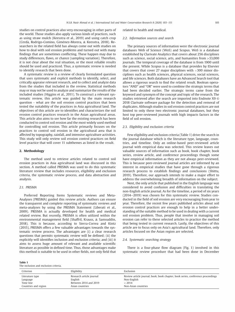
2.3. Eligibility and exclusion criteria
Few eligibility and exclusion criteria (Table 1) drive the search inthe journal database which is the literature type, language, coun-tries, and timeline. Only an online-based peer-reviewed articlejournal with empirical data was selected. This review leaves outvaluable sources of information such as book, book chapter, bookseries, review article, and conference proceedings though somehave empirical information as they are not always peer-reviewed.This is because peer-reviewed journal articles are informed by aninterest in empirical studies that have gone through a rigorousresearch process to establish findings and conclusions (Shittu,2019). Therefore, our approach intends to make a major effort toaddress the overwhelming breadth of information on the subject.
Next, the only article that published in the English language wasconsidered to avoid confusion and difficulties in translating thenon-English article journal. As for the timeline, a period of six years(2014e2019) was chosen for this systematic review. Studies con-ducted in the field of soil erosion are very encouraging from year toyear. Therefore, the recent few years published articles about soilerosion control practices are enough to help in a better under-standing of the suitable method to be used in dealing with a currentsoil erosion problem. Thus, people that involve in managing soilerosion can refer to these selected articles to practice the methodthat being tested in current research. Lastly, the objectives of thisarticle are to focus only on Asia’s agricultural land. Therefore, onlyarticles focused on the Asian region are selected.
2.4. Systematic searching strategy
There is a four-phase flow diagram (Fig. 1) involved in thissystematic review procedure that had been done in December
Table 1The inclusion and exclusion criteria.
Criterion Eligibility Exclusion
Literature type Research article journal Review article journal, book, book chapter, book series, conference proceedingsLanguage English Non-EnglishTime line Between 2014 and 2019 < 2014Countries and region Asian countries Non-Asian countries
N.S.B. Nasir Ahmad et al. / International Soil and Water Conservation Research 8 (2020) 103e115 105
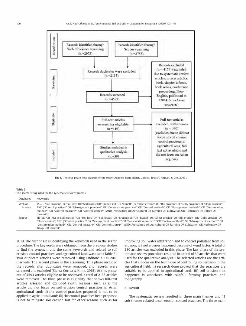
2019. The first phase is identifying the keywords used in the searchprocedure. The keywords were obtained from the previous studiesto find the synonym and the same keywords and related to soilerosion, control practices, and agricultural land was used (Table 2).Two duplicate articles were removed using Endnote X9 © 2018Clarivate. The second phase is the screening. This phase includedthe records after duplicates were removed, and records werescreened and excluded (Sierra-Correa & Kintz, 2015). At this phase,out of 4593 articles eligible to be reviewed, a total of 2135 articleswere removed. The third phase is eligibility that shows full-textarticles assessed and excluded (with reasons) such as i) thearticle did not focus on soil erosion control practices in Asianagricultural land; ii) the control practices proposed is not to beapplied in agricultural land; iii) the control practices been proposedis not to mitigate soil erosion but for other reasons such as for
improving soil water infiltration and to control pollutant from soilerosion; iv) soil erosion happened because of wind factor. A total of380 articles was excluded in this phase. The last phase of the sys-tematic review procedure resulted in a total of 39 articles that wereused for the qualitative analysis. The selected articles are the arti-cles that i) focus on the technique of controlling soil erosion in theagricultural field; ii) research done proved that the practices aresuitable to be applied in agricultural land; iii) soil erosion thathappened is associated with rainfall, farming practices, andtopography.
3. Result
The systematic review resulted in three main themes and 11sub-themes related to soil erosion control practices. The three main
Fig. 1. The four-phase flow diagram of the study (Adapted from Moher, Liberati, Tetzlaff, Altman, & Grp, 2009).
Table 2The search string used for the systematic review process.
Databases Keywords
Web ofScience
TS¼ ((“Soil erosion” OR “Soil loss” OR “Soil losses” OR “Eroded soil” OR “Runoff” OR “Sheet erosion” OR “Rill erosion” OR “Gully erosion” OR “Slope erosion”)AND (“Control practice*" OR “Management practice*" OR “Conservation practice*" OR “Control method*" OR “Management method*" OR “Conservationmethod*" OR “Control measure*" OR “Control strateg*") AND (Agriculture OR Agricultural OR Farming OR Cultivation OR Husbandry OR Tillage ORHarvest*))
Scopus TITTLE-ABS-KEY ((“Soil erosion” OR “Soil loss” OR “Soil losses” OR “Eroded soil” OR “Runoff” OR “Sheet erosion” OR “Rill erosion” OR “Gully erosion” OR“Slope erosion”) AND (“Control practice*" OR “Management practice*" OR “Conservation practice*" OR “Control method*" OR “Management method*" OR“Conservation method*" OR “Control measure*" OR “Control strateg*") AND (Agriculture OR Agricultural OR Farming OR Cultivation OR Husbandry ORTillage OR Harvest*))
N.S.B. Nasir Ahmad et al. / International Soil and Water Conservation Research 8 (2020) 103e115106
themes are agronomics practices, agrostological practices, andmechanical practices. Agronomics and agrostological practices areboth considered as a biological method. The 11 sub-themes are
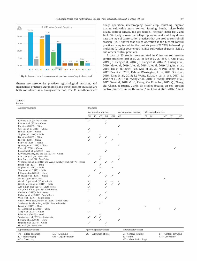
tillage operation, intercropping, cover crop, mulching, organicmatter, cultivation grass, contour farming, bunds, micro basintillage, contour terrace, and geo-textile. The result (Refer Fig. 2 andTable 3) clearly shown that tillage operation and mulching domi-nate the type of conservation practices that are used to control soilerosion. Fig. 2 shows that tillage operation is the highest controlpractices being tested for the past six years (22.73%), followed bymulching (21.21%), cover crop (18.18%), cultivation of grass (15.15%),and others control practices.
A total of 23 studies concentrated in China on soil erosioncontrol practices (Dai et al., 2018; Fan et al., 2015; S. F.; Guo et al.,2019; J.; Huang et al., 2016; J.; Huang et al., 2014; Z.; Huang et al.,2019; Mo et al., 2019; Li et al., 2018; Li et al., 2019; Lingling et al.,2014; Liu et al., 2014; Pan, Gao, et al., 2017; Pan, Song, et al.,2017; Pan et al., 2018; Rahma, Warrington, & Lei, 2019; Sui et al.,2016; Tang et al., 2015; L.; Wang, Dalabay, Lu, & Wu, 2017; L.;Wang et al., 2019; Q.; Wang et al., 2018; Y.; Wang, Dalabay, et al.,2017; Xu et al., 2018; G. H.; Zhang, Xie, Pi, & Zuo, 2015; Q.; Zhang,Liu, Cheng, & Huang, 2016), six studies focused on soil erosioncontrol practices in South Korea (Ahn, Choi, & Kim, 2016; Ahn &
Fig. 2. Research on soil erosion control practices in Asia’s agricultural land.
Table 3Results.
Authors/countries Practices
Agronomics practices Agrostological practices Mechanical practices
TO IC CC ML OM CG CF BU MT CT GT
L. Wang et al. (2019) e China ✓ ✓
Rahma et al. (2019) e China ✓
Mo et al. (2019) e China ✓
S. F. Guo et al. (2019) e China ✓
Li et al. (2019) e China ✓
Singh et al. (2019) e India ✓ ✓ ✓
Dai et al. (2018) e China ✓ ✓ ✓
Li et al. (2018) e China ✓ ✓
Pan et al. (2018) e China ✓
Q. Wang et al. (2018) e China ✓
Xu et al. (2018) e China ✓
Rasoulzadeh et al. (2018) e Iran ✓
L. Wang, Dalabay, Lu, and Wu (2017) e China ✓
Pan, Gao, et al. (2017) e China ✓ ✓
Pan, Song, et al. (2017) e China ✓ ✓
Y. Wang, Cao, et al. (2017) and Wang, Dalabay, et al. (2017) e China ✓ ✓ ✓
Lenka et al. (2017) e India ✓
Singh et al. (2017) e India ✓ ✓
Sharma et al. (2017) e India ✓
J. Huang et al. (2016) e China ✓ ✓
Q. Zhang et al. (2016) e China ✓ ✓ ✓
Sui et al. (2016) e China ✓
Ghosh, Dogra, et al. (2016) e India ✓ ✓ ✓ ✓
Ghosh, Meena, et al. (2016) e India ✓ ✓ ✓ ✓
Ahn & Kim et al. (2016) - South Korea ✓ ✓
Ahn, Choi, & Kim. (2016) - South Korea ✓
Choi et al. (2016)- South Korea ✓
Maharjan et al. (2016) - South Korea ✓
Won et al. (2016) e South Korea ✓
Choi Y., Won, Shin, Park et al. (2016) - South Korea ✓
Satriawan, Fuady, & Mayani (2017) e Indonesia ✓
Fan et al. (2015) e China ✓
G. H. Zhang et al. (2015) e China ✓ ✓ ✓
Tang et al. (2015) e China ✓
Eshel et al. (2015) e Israel ✓
Satriawan et al. (2015) e Indonesia ✓ ✓ ✓
J. Huang et al. (2014) e China ✓ ✓
Lingling et al. (2014) e China ✓ ✓
Liu et al. (2014) e China ✓
Agronomics practices Agrostological practices Mechanical practices
TO ¼ Tillage operationIC ¼ IntercroppingCC ¼ Cover crop
ML ¼ MulchingOM ¼ Organic matter
CG ¼ Cultivation of grass CF¼ Contour farmingBU ¼ BundMT ¼ Micro basin tillage
CT ¼ Contour terracingGT ¼ Geo-textile
N.S.B. Nasir Ahmad et al. / International Soil and Water Conservation Research 8 (2020) 103e115 107
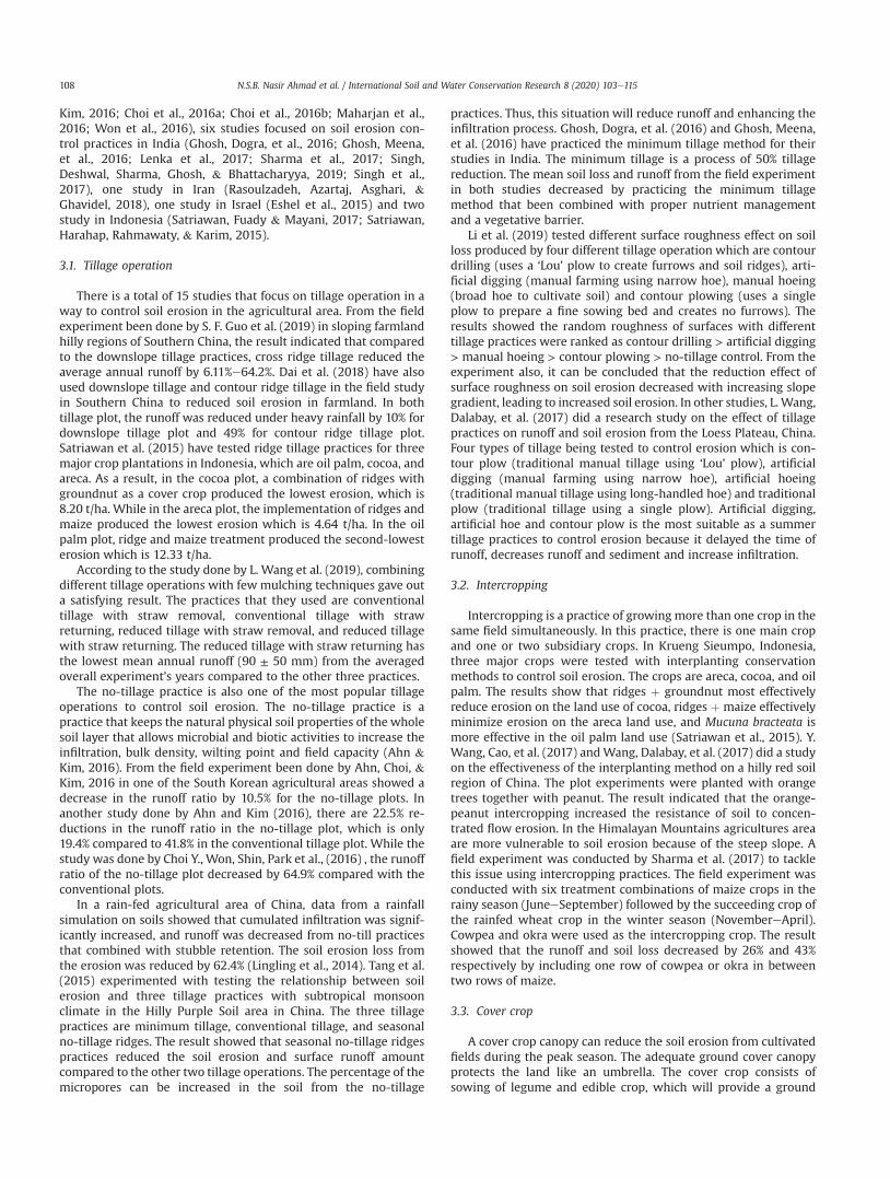
Kim, 2016; Choi et al., 2016a; Choi et al., 2016b; Maharjan et al.,2016; Won et al., 2016), six studies focused on soil erosion con-trol practices in India (Ghosh, Dogra, et al., 2016; Ghosh, Meena,et al., 2016; Lenka et al., 2017; Sharma et al., 2017; Singh,Deshwal, Sharma, Ghosh, & Bhattacharyya, 2019; Singh et al.,2017), one study in Iran (Rasoulzadeh, Azartaj, Asghari, &Ghavidel, 2018), one study in Israel (Eshel et al., 2015) and twostudy in Indonesia (Satriawan, Fuady & Mayani, 2017; Satriawan,Harahap, Rahmawaty, & Karim, 2015).
3.1. Tillage operation
There is a total of 15 studies that focus on tillage operation in away to control soil erosion in the agricultural area. From the fieldexperiment been done by S. F. Guo et al. (2019) in sloping farmlandhilly regions of Southern China, the result indicated that comparedto the downslope tillage practices, cross ridge tillage reduced theaverage annual runoff by 6.11%e64.2%. Dai et al. (2018) have alsoused downslope tillage and contour ridge tillage in the field studyin Southern China to reduced soil erosion in farmland. In bothtillage plot, the runoff was reduced under heavy rainfall by 10% fordownslope tillage plot and 49% for contour ridge tillage plot.Satriawan et al. (2015) have tested ridge tillage practices for threemajor crop plantations in Indonesia, which are oil palm, cocoa, andareca. As a result, in the cocoa plot, a combination of ridges withgroundnut as a cover crop produced the lowest erosion, which is8.20 t/ha. While in the areca plot, the implementation of ridges andmaize produced the lowest erosion which is 4.64 t/ha. In the oilpalm plot, ridge and maize treatment produced the second-lowesterosion which is 12.33 t/ha.
According to the study done by L. Wang et al. (2019), combiningdifferent tillage operations with few mulching techniques gave outa satisfying result. The practices that they used are conventionaltillage with straw removal, conventional tillage with strawreturning, reduced tillage with straw removal, and reduced tillagewith straw returning. The reduced tillage with straw returning hasthe lowest mean annual runoff (90 ± 50 mm) from the averagedoverall experiment’s years compared to the other three practices.
The no-tillage practice is also one of the most popular tillageoperations to control soil erosion. The no-tillage practice is apractice that keeps the natural physical soil properties of the wholesoil layer that allows microbial and biotic activities to increase theinfiltration, bulk density, wilting point and field capacity (Ahn &Kim, 2016). From the field experiment been done by Ahn, Choi, &Kim, 2016 in one of the South Korean agricultural areas showed adecrease in the runoff ratio by 10.5% for the no-tillage plots. Inanother study done by Ahn and Kim (2016), there are 22.5% re-ductions in the runoff ratio in the no-tillage plot, which is only19.4% compared to 41.8% in the conventional tillage plot. While thestudy was done by Choi Y., Won, Shin, Park et al., (2016) , the runoffratio of the no-tillage plot decreased by 64.9% compared with theconventional plots.
In a rain-fed agricultural area of China, data from a rainfallsimulation on soils showed that cumulated infiltration was signif-icantly increased, and runoff was decreased from no-till practicesthat combined with stubble retention. The soil erosion loss fromthe erosion was reduced by 62.4% (Lingling et al., 2014). Tang et al.(2015) experimented with testing the relationship between soilerosion and three tillage practices with subtropical monsoonclimate in the Hilly Purple Soil area in China. The three tillagepractices are minimum tillage, conventional tillage, and seasonalno-tillage ridges. The result showed that seasonal no-tillage ridgespractices reduced the soil erosion and surface runoff amountcompared to the other two tillage operations. The percentage of themicropores can be increased in the soil from the no-tillage
practices. Thus, this situation will reduce runoff and enhancing theinfiltration process. Ghosh, Dogra, et al. (2016) and Ghosh, Meena,et al. (2016) have practiced the minimum tillage method for theirstudies in India. The minimum tillage is a process of 50% tillagereduction. The mean soil loss and runoff from the field experimentin both studies decreased by practicing the minimum tillagemethod that been combined with proper nutrient managementand a vegetative barrier.
Li et al. (2019) tested different surface roughness effect on soilloss produced by four different tillage operation which are contourdrilling (uses a ‘Lou’ plow to create furrows and soil ridges), arti-ficial digging (manual farming using narrow hoe), manual hoeing(broad hoe to cultivate soil) and contour plowing (uses a singleplow to prepare a fine sowing bed and creates no furrows). Theresults showed the random roughness of surfaces with differenttillage practices were ranked as contour drilling > artificial digging> manual hoeing > contour plowing > no-tillage control. From theexperiment also, it can be concluded that the reduction effect ofsurface roughness on soil erosion decreased with increasing slopegradient, leading to increased soil erosion. In other studies, L. Wang,Dalabay, et al. (2017) did a research study on the effect of tillagepractices on runoff and soil erosion from the Loess Plateau, China.Four types of tillage being tested to control erosion which is con-tour plow (traditional manual tillage using ‘Lou’ plow), artificialdigging (manual farming using narrow hoe), artificial hoeing(traditional manual tillage using long-handled hoe) and traditionalplow (traditional tillage using a single plow). Artificial digging,artificial hoe and contour plow is the most suitable as a summertillage practices to control erosion because it delayed the time ofrunoff, decreases runoff and sediment and increase infiltration.
3.2. Intercropping
Intercropping is a practice of growing more than one crop in thesame field simultaneously. In this practice, there is one main cropand one or two subsidiary crops. In Krueng Sieumpo, Indonesia,three major crops were tested with interplanting conservationmethods to control soil erosion. The crops are areca, cocoa, and oilpalm. The results show that ridges þ groundnut most effectivelyreduce erosion on the land use of cocoa, ridges þ maize effectivelyminimize erosion on the areca land use, and Mucuna bracteata ismore effective in the oil palm land use (Satriawan et al., 2015). Y.Wang, Cao, et al. (2017) andWang, Dalabay, et al. (2017) did a studyon the effectiveness of the interplanting method on a hilly red soilregion of China. The plot experiments were planted with orangetrees together with peanut. The result indicated that the orange-peanut intercropping increased the resistance of soil to concen-trated flow erosion. In the Himalayan Mountains agricultures areaare more vulnerable to soil erosion because of the steep slope. Afield experiment was conducted by Sharma et al. (2017) to tacklethis issue using intercropping practices. The field experiment wasconducted with six treatment combinations of maize crops in therainy season (JuneeSeptember) followed by the succeeding crop ofthe rainfed wheat crop in the winter season (NovembereApril).Cowpea and okra were used as the intercropping crop. The resultshowed that the runoff and soil loss decreased by 26% and 43%respectively by including one row of cowpea or okra in betweentwo rows of maize.
3.3. Cover crop
A cover crop canopy can reduce the soil erosion from cultivatedfields during the peak season. The adequate ground cover canopyprotects the land like an umbrella. The cover crop consists ofsowing of legume and edible crop, which will provide a ground
N.S.B. Nasir Ahmad et al. / International Soil and Water Conservation Research 8 (2020) 103e115108
cover that can reduce raindrop impact, reduces water velocities,decreases runoff, and increases water infiltration in the soil.Therefore, cover crops are one of the ways to reduce soil erosion.Dai et al. (2018) used daylily as a groundcover that being planted intwo hedgerows on a downslope tillage treatment plot. As a result,the runoff depth was reduced by 37%.
Besides daylily, white clover also acts as an excellent groundcover. Pan, Gao, et al. (2017) usedwhite clover vegetation filter strip(VFS) in an experimental plot to see the ability of the VFS togetherwith the white clover as an agricultural best management practice.The experiment showed that a white clover vegetation filter striphas a good soil infiltration capability and excellent runoff trappingcapacity. White clover has also been used as a cover crop in Pan,Gao, et al. (2017) and Pan, Song, et al. (2017) study at ChineseLoess Plateau jujube orchard. The result showed that white clover isa good ground cover. The white clover treatment has the lowestrunoff coefficient compared to the other treatment being tested inthe study. Other than that, in the simulation study done by J. Huanget al. (2016) in sloping ground jujube orchards, white clover hasalso been used as a cover crop. The ground cover percentage underwhite clover cover was the largest in all growth periods caused thatthe annual mean time to a runoff under white clover cover was thelargest and significantly larger than under other treatments (J.Huang et al., 2016). In the study done by J. Huang et al. (2014) forpear-jujube orchards, white clover cover has increased the infil-tration of water amount and soil moisture. From these two studies(J. Huang et al., 2014; J. Huang et al., 2016) shows a good signbecause as the time to runoff is high and the infiltration of wateramount increased, the chances of soil erosion to occur will be lower.
In Haean catchment South Korea, sediment from the agricul-tural area been transported to the water bodies because of soilerosion. Maharjan et al. (2016) used winter cover crops togetherwith split fertilization practices in their study as a control practiceto reduce the amount of sediment yield from four major drylandscrops (cabbage, potato, radish, and soybean). The cultivation ofcover crops showed significant reductions of sediment yieldcompared to conventional practice. Eshel et al. (2015), used adifferent type of cover crops to see the impact of each cover crop inpotato cultivation in Israel regarding the effects of the cover cropstowards soil erosion, runoff and weed suppression. Five treatmentsplot were built consists of oats, triticale, oats with purple vetch,clover, and rapeseed as a cover crop in potato agricultural site. Theoverall result shows that under the cover crops treatments, soilerosion, and runoff reduced by 95% and more than 60%, respec-tively. Among the five cover crops, oats are the most efficient covercrop. In Indonesia, Satriawan et al. (2017) usedMucuna bracteata asa cover crop. The result showed the combination treatment ofupland rice planted sequentially with soybean þ strip Mucunabracteata as a cover crop in oil palm crops (age 7e25 months, at15e25% slopes) efficiently reducing the rate of runoff and preventsoil erosion from happening. There are also few other cover cropsbeen used as soil erosion control practices in past studies such asbirdsfoot trefoil and crown vetch.
3.4. Mulching
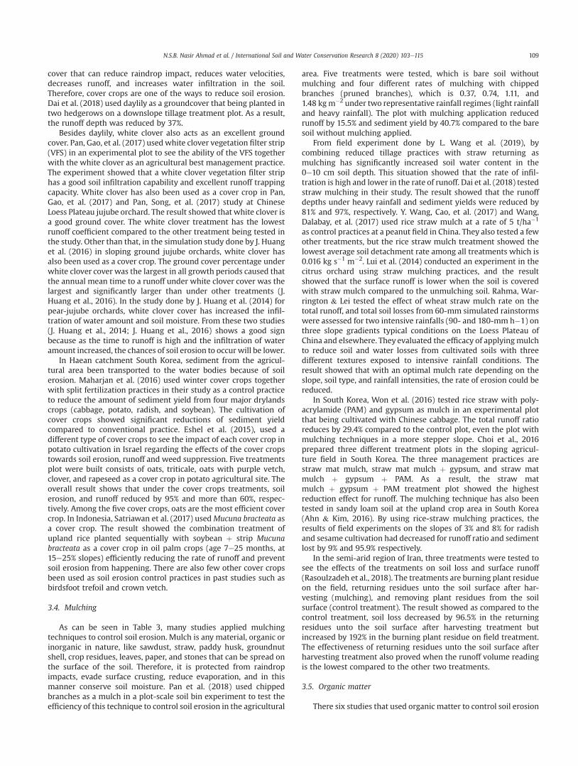
As can be seen in Table 3, many studies applied mulchingtechniques to control soil erosion. Mulch is any material, organic orinorganic in nature, like sawdust, straw, paddy husk, groundnutshell, crop residues, leaves, paper, and stones that can be spread onthe surface of the soil. Therefore, it is protected from raindropimpacts, evade surface crusting, reduce evaporation, and in thismanner conserve soil moisture. Pan et al. (2018) used chippedbranches as a mulch in a plot-scale soil bin experiment to test theefficiency of this technique to control soil erosion in the agricultural
area. Five treatments were tested, which is bare soil withoutmulching and four different rates of mulching with chippedbranches (pruned branches), which is 0.37, 0.74, 1.11, and1.48 kgm�2 under two representative rainfall regimes (light rainfalland heavy rainfall). The plot with mulching application reducedrunoff by 15.5% and sediment yield by 40.7% compared to the baresoil without mulching applied.
From field experiment done by L. Wang et al. (2019), bycombining reduced tillage practices with straw returning asmulching has significantly increased soil water content in the0e10 cm soil depth. This situation showed that the rate of infil-tration is high and lower in the rate of runoff. Dai et al. (2018) testedstraw mulching in their study. The result showed that the runoffdepths under heavy rainfall and sediment yields were reduced by81% and 97%, respectively. Y. Wang, Cao, et al. (2017) and Wang,Dalabay, et al. (2017) used rice straw mulch at a rate of 5 t/ha�1
as control practices at a peanut field in China. They also tested a fewother treatments, but the rice straw mulch treatment showed thelowest average soil detachment rate among all treatments which is0.016 kg s�1 m�2. Lui et al. (2014) conducted an experiment in thecitrus orchard using straw mulching practices, and the resultshowed that the surface runoff is lower when the soil is coveredwith straw mulch compared to the unmulching soil. Rahma, War-rington & Lei tested the effect of wheat straw mulch rate on thetotal runoff, and total soil losses from 60-mm simulated rainstormswere assessed for two intensive rainfalls (90- and 180-mm h�1) onthree slope gradients typical conditions on the Loess Plateau ofChina and elsewhere. They evaluated the efficacy of applyingmulchto reduce soil and water losses from cultivated soils with threedifferent textures exposed to intensive rainfall conditions. Theresult showed that with an optimal mulch rate depending on theslope, soil type, and rainfall intensities, the rate of erosion could bereduced.
In South Korea, Won et al. (2016) tested rice straw with poly-acrylamide (PAM) and gypsum as mulch in an experimental plotthat being cultivated with Chinese cabbage. The total runoff ratioreduces by 29.4% compared to the control plot, even the plot withmulching techniques in a more stepper slope. Choi et al., 2016prepared three different treatment plots in the sloping agricul-ture field in South Korea. The three management practices arestraw mat mulch, straw mat mulch þ gypsum, and straw matmulch þ gypsum þ PAM. As a result, the straw matmulch þ gypsum þ PAM treatment plot showed the highestreduction effect for runoff. The mulching technique has also beentested in sandy loam soil at the upland crop area in South Korea(Ahn & Kim, 2016). By using rice-straw mulching practices, theresults of field experiments on the slopes of 3% and 8% for radishand sesame cultivation had decreased for runoff ratio and sedimentlost by 9% and 95.9% respectively.
In the semi-arid region of Iran, three treatments were tested tosee the effects of the treatments on soil loss and surface runoff(Rasoulzadeh et al., 2018). The treatments are burning plant residueon the field, returning residues unto the soil surface after har-vesting (mulching), and removing plant residues from the soilsurface (control treatment). The result showed as compared to thecontrol treatment, soil loss decreased by 96.5% in the returningresidues unto the soil surface after harvesting treatment butincreased by 192% in the burning plant residue on field treatment.The effectiveness of returning residues unto the soil surface afterharvesting treatment also proved when the runoff volume readingis the lowest compared to the other two treatments.
3.5. Organic matter
There six studies that used organic matter to control soil erosion
N.S.B. Nasir Ahmad et al. / International Soil and Water Conservation Research 8 (2020) 103e115 109
rate. Organic matter can be derived from the manure application ororganic fertilizer. Manure decomposition has high organic mattercontent because of the manure decomposition. Y. Wang, Cao, et al.(2017) and Wang, Dalabay, et al. (2017) used organic manure fer-tilizer, which is fresh pig manure in research to reduces the soilerosion rates in the Red Soil Region of China. As a result, thetreatment plot with the manure application has a low detachmentrate, and this is because of the high organic matter content thatmakes it more resistant to detachment in the soil. Manuring canenhance soil aggregation that will improve soil structure. There-fore, this will reduce soil erosion rates. The combination use oforganic matter with other soil erosion control practices can reducesoil loss in regions with intense agricultural activity (Q. Zhang et al.,2016). Li et al. (2018) suggested from their research that manureapplication in combination with seasonal fallow reduces soilerosion.
In the research done by Q. Zhang et al. (2016), the application oforganic matter was used together with contour tillage, and strawmulching practices to control soil erosion. The runoff depthreduced by 19% and 50% in two treatment plots (contourtillage þ organic matter and contour tillage þ organicmatter þ straw mulching). The soil erodibility values under thetwo-treatment plot also decrease respectively by 14% and 30%.Ghosh, Dogra, et al. (2016) used farmyard manure and poultrymanure in a few treatment plots for maize and wheat crops thatcombinewith other control practices to increase the organic matterin the soil. The reduction of runoff and soil through bio-resources(farmyard manure and poultry manure) from this study is ex-pected as carbon input from organic matters helps in the formationof more water stable macro-aggregates. Singh et al. (2017), testeddifferent organic matter effect towards soil conservation of maize-wheat rotation agriculture field in north-western Indian Himalayasfor seven years. Seven experiment plots were set up which arecontrol (0), 100% NPK through inorganic fertilizers (100-0), 100% Nthrough farmyard manure (FYM) (0e100), substitution of 50% Nthrough four different organic manures viz., FYM (50 þ 50 FYM),vermicompost (50 þ 50 VC), poultry manure (50 þ 50 PM) and in-situ green manuring (50 þ 50 GM) of sunnhemp (Crotalaria junceaL.). The result showed the least runoff and soil loss values wereobserved with 50 þ 50 (GM) in all the years.
3.6. Cultivation of grass
Cultivation of grass is one of the agrostological methods thatsuitable to apply in eroded agricultural land. Few types of grass andnon-edible plant been used to control soil erosion in agriculturalland. Ten studies use the agrostological method as a method tocontrol soil erosion. Q. Wang et al. (2018), tested the effect of twotypes of grass hedges (Melilotus hedges; Pennisetum hedges) onrunoff loss under different rain intensities and slope gradient on amaize field. Both of the grass hedges decreased surface runoff by27%e72%. According to Q. Wang et al. (2018), the Pennisetum grassshowed better efficacy compared to Melilotus grass, especiallyunder high rain intensity. G. H. Zhang et al. (2015) used Bahia grassthat planted in two ways as a soil erosion control practice. The firstway is the citrus trees and Bahia grass was planted on the rain-fedterrace bed. The grass was planted on the bunds. Secondly is thehorizontal terrace of orchards with Bahia grass planted on the riser(10%e50% vegetation cover). The result showed that the Bahia grassplanted on the riser and bunds is a useful method for soil erosionconservation on sloping red soil land in China.
Four studies use cocksfoot grass as vegetative cover in China tocontrol soil erosion (Pan, Gao, et al., 2017; J.; Huang et al., 2016; J.;Huang et al., 2014; Pan, Song, et al., 2017). All four studies use thevegetative filter strip method to plant the cocksfoot. From the four
studies, Huang et al. (2016) and Huang et al. (2014) concluded thatcocksfoot seemed to best the best vegetative ground cover forrainfed sloping jujube orchards and in pear-jujube orchards on dryslopes respectively. Mo et al. (2019) used Bermuda grass to reducethe amount of runoff in sloping citrus land, Southern China. Theycarried out four runoff plot experiment: (i) no vegetation, bare land(BL); (ii) conventional treatment, citrus without grass cover (CK);(iii) citrus with strip planting of Bermuda grass (SP); (iv) citrus withfull cover of Bermuda grass (FC). Results showed that the annualrunoff volumes were significantly (P < 0.05) reduced using SP(27.2 mm) and FC (33.0 mm) compared with CK (311.4 mm) and BL(456.7 mm) treatments (Mo et al., 2019).
In India, two studies used Palmarosa grass and Panicum grass asa vegetation strip in terms of controlling soil erosion. In bothstudies (Ghosh, Dogra, et al., 2016 & Ghosh, Meena, et al., 2016),cultivation of Palmorasa as vegetative barriers along with organicamendments, weed mulch application and minimum tillage iseffective in decreasing runoff and soil erosion. Results also show animprovement in soil quality and an increase in soil systemproductivity.
3.7. Mechanical method
From the systematic review procedure, there are only a fewstudies that adapted themechanical method as away to control soilerosion. The first mechanical method is terracing contour. Terracingis a process of dividing the long slope into more short slopes.Therefore, there will change in the landform and reduces the slopegradient. As a result, the amount of soil erosion and the runoffamount and rate will be reduced. Xu et al. (2018) studied the effectof terracing on runoff and erosion in the Three Gorges area, China.Four experimental plots were set up consists of terraced orchard(3�), terraced cropland (3�), unterraced orchard (25�), and unter-raced cropland (25�). The results show the average runoff coeffi-cient of the terraced plot (orchard and cropland) was decreasing by47.2% compared with the unterraced plot, and the average erosionrate of the terraced plot was reduced by 83.9% compared to theunterraced plots. Narrow terraces are also one of the terracingmethods being implemented to control soil erosion in agriculturalland.
In the Black Soil Region of Northeast China, a plot experimentwas conducted to assess the effect of micro basin tillage as a me-chanical method to control soil erosion in agricultural land (Suiet al., 2016). Results indicate that by using micro basin tillage,runoff and sediment rate reduced by 63% and 96%, respectively. G.H. Zhang et al. (2015) applied a level terrace on an experimental sitetogether with bunds build on the outer edge of the terrace. Anothertreatment plot consisted of horizontal terraces of an orchard with aBahia grass planted on the riser. The result indicated that surfacerunoff and soil erosion the two experimental plots were less thanthe control plot (bare land).
In India, Singh et al. (2019) used agro-geo-textiles in slopingcroplands of the Indian Himalayan region as a soil conservationpractice. Seven treatments have been tested during two years ofexperiment. Field experiments were conducted on zero tilledmaize, minimum tilled garden pea and wheat crops planted inrainy, autumn, and winter seasons. Different vegetative filters andagro-geo-textile were used in the treatment. Cowpea cover cropand grass weed acted as a vegetative filter between the maize row.While maize straw, Arundo donax (giant cane), and coir as geo-textile between the maize row. The result showed that conserva-tion tillage together with Arundo donax geotextile reduced runoffby 24% and soil loss by 8.22 t ha�1 compared to only conservationtillage practice.
Contour farming or also called contour cultivation, is also one of
N.S.B. Nasir Ahmad et al. / International Soil and Water Conservation Research 8 (2020) 103e115110
the conservation ways of agriculture. Farmers will plant the cropsacross a slope by following its elevation contour lines. Soil erosionrate will be reduced by practicing contour farming in agriculturalland because the arrangement of plants will break up the flow ofwater and increase the rate of infiltration. Fan et al. (2015) testedcontour hedgerows farming to control soil erosion on sloping landin the Three Gorges Reservoir Region, China. They built fewexperimental plots of rowsmulberry on a contour hedgerowwith amustard-corn rotation and one control plot (nomulberry hedgerowwith mustard-corn rotation). The result shows that by plantingmulberry in a contour hedgerow, the amount of runoff and soilerosion significantly reduces compared to the control plot, whichadapts a conventional practice (no hedgerows).
4. Discussion
This study has attempted to systematically analyze the existingliterature on control practices of soil erosion in Asia agriculturalland. Heavy perception, intensive farming, and topography have ledto soil erosion that needed to be controlled. A rigorous reviewsourced from the Web of Science and Scopus has resulted in 39articles related to research on soil erosion control practices in Asiaagricultural land. Three themes and 11 sub-themes emerged withinthe scope of this review. This review shows that the research oncontrol practices that been adapted in Asia between the year 2014until 2019 are more focused on the biological method rather thanthe mechanical method. The biological method consists of agro-nomics practices and agrostological practices. Tillage operation andmulching are themost control practices been used and suggested inthe year 2014 until 2019 to control soil erosion in Asia agriculturalland. Asian region itself consists of a variation of climates such astropical, subtropical climate, Mediterranean, and temperateclimate. Thus, this discussion will be divided according to thecountry in the result focusing on climate regimes.
China is one of the biggest countries in the world. Some parts ofChina fall under tropical, sub-tropical, and temperate climate.Therefore, the control practices being applied in China to controlsoil erosion are varied. According to the systematic review that hasbeen done, most research in China about soil erosion controlpractices in agricultural land is located in the wet sub-tropical area.In the wet sub-tropical area, many control practices have beenapplied because of the seasonal variation. Some places will beplanted with different crops in winter and summer. Tillage opera-tion is the most favorable techniques to be tested to control soilerosion in agricultural land. In China, modern research on conser-vation tillage, such as no-tillage started to get attention as aneffective way for reducing soil erosion, and this explains the bignumber of articles from China in the past six years. The conserva-tion tillage (no-tillage) has lots of benefits that gain acceptance inmany parts of the world in terms of enhancing global sustainableagriculture (Kassam et al., 2012). The conservation tillage systemshave many favorable effects on soil structure and have been re-ported in different soil types and climates (Oyedele, Schjonning,Sibbesen, & Debosz, 1999).
However, for no-tillage practices, the adaptability of the pro-cedures may be different from one place to another based on theclimate and other ecosystem conditions (Golabi, El-Swaify, & Iye-kar, 2014). According to them, the no-tillage method is moremanagement intensive and its success or failure depends onknowledge associated with the soil and other ecosystems condi-tions where no-tillage is practiced. Furthermore, it is being re-ported that the weather conditions in the growing season are vitalin the success of no-tillage practices system (Wang, Cai, Hoogmoed,Oenema, & Perdok, 2006). From the report of Food and AgricultureOrganization (2012), climate adaption benefits of no-tillage can be
significant. According to the report, wheat grown under no-tillagepractices was more resilient, leading to yield increases overconventionally cultivated crops in the drought and high tempera-ture in one of the Asian countries. Kargas, Kerkides, andPoulovassilis (2012) stated from their observation that an untilledplot retains more water than tilled plots. There are more stableaggregates in the upper surface of soils been associated with no-tillsoils than tilled soils and this resulted in high total porosity in no-tillage plot (Busari, Kukal, Kaur, Bhatt, & Dulazi, 2015). Thereforeno-tillage is recommended for a high temperature area. From thesystematic review, by practicing no-tillage and minimum tillagepractices, proven that these practices can reduce soil erosion, im-proves soil structure, increases soil water infiltration, and conservessoil moisture. Other than that, ridge tillage practices also are sug-gested to be used to control soil erosion in China.
From all of the control practices being listed in Table 3 that beingtested in China, mulching is also one of the popular methods. Thereare two types of basic mulch which are organic and inorganicmulch from the studies that been reviewed. Farmers need toconsider which one is better to apply depends on the land use typeand climate in Asia. Using an organic mulch will give more benefitsto the plants because through time, organic mulches will slowlydecompose and release nutrients into the soil and will improve thestructure. Other than that, the organic mulch will keep the soilcooler and retain soil moisture levels, and this is suitable for a dryperiod in Asia. As in China, most of the wet sub-tropical areas willreceive rainfall between April to September. Therefore, with thehelp of organic mulch to retain soil moisture levels in soil, this willhelp in the period of the low rainfall season. Organic mulch thatoften used in China is straw mulch.
Cover crop and cultivation of grass also play an important role inmitigating soil erosion in China. Cover crops and cultivation of grasshave been used for a long time as one of the ways to control soilerosion. A very dense layer of the cover crop will reduce the speedof rainfall when it hits the ground and causing the soil not to splash.A cover crop will allow the soil to absorb water more efficientlybecause of the improvement in the water holding capacity andinfiltration (Taguas et al., 2010) due to the abundant root networksof cover crops that keep soil firmly in place. Furthermore, groundcover such as legume, will not only reduce soil erosion throughinfiltration, reducing surface runoff, it also will increase thenutrient in the soil which is necessary for crop production sincelegumes are high in nitrogen. The cover crop and cultivation ofgrass usually being planted in a row or vegetative filter strip. It willbe located between the main crop. In a heavier rainfall event, theplant covers significantly promoted infiltration compared withclear cultivation treatments (Pan, Song, et al., 2017). Therefore, thissituation is really needed when the agricultural area in China sub-tropical area having a rainfall season.
However, some disadvantages using this method to reduce soilerosion such as the plant cover crop species may compete with themajor crop planted for soil water and lead to declines in the yield ofthe major crops such as fruit plant (Pan, Song et al., 2017).Furthermore, the costs to implement cover crop as a conservationmeasure includes increased direct costs, potentially reduced in-come if cover crops interferewith other attractive crops, productionexpenses, difficulties in predicting nitrogen mineralization, andslow soil warming (Snapp et al., 2005). Additionally, a ground covereither cover crop or cultivation of grass will increase the cost for thecommercial farmers. The ground cover must be planted at a time,therefore there will be an additional cost for planting the groundcover and then tiling it back under which means the farmers needto pay an extra cost for the labor and machinery. According toSwanson, Schnitkey, Coppess, and Armstrong (2018), at the farmlevel, establishing a cover crop will increases cost. From their
N.S.B. Nasir Ahmad et al. / International Soil and Water Conservation Research 8 (2020) 103e115 111

research on an average Central Illinois farm, a cereal rye cover cropincreases non-land costs by 5% from $563 to $591 per acre and therye or vetch blend pushes non-land costs up to $621 whichapproximately above the baseline. From the analysis, cost increasesbecause of the expenses of cover crop seed and the cost to drill it(Swanson et al., 2018).
Analysis from the systematic reviews shows less number ofresearch on mechanical methods to control soil erosion in Asiaagricultural land. The main control practices used under the me-chanical method in China’s agricultural land are terracing andcontour farming. The basic function of terracing is the interceptionof water, which either absorbed or conducted slowly from theagricultural field, depending on the particular requirements of thelocality (Nichols & Chambers, 1938). Xu et al. (2018) stated thatclimate change had only little influence on runoff and erosion in theterraced system. They also suggested that terracing will be moresuitable to be applied in citrus orchard compared to cropland.Micro basin tillage also one of the treatments under a mechanicalmethod that is suitable to be applied in China. It is a conservationpractice that requires building individual earth blocks along thefurrow (Sui et al., 2016). If this practice is being applied with anoptimal block interval, it can be a useful practice not just to controlsoil erosion but also to control water loss and agricultural diffusepollution (Sui et al., 2016).
South Korea is also one of the countries that are effectively doingresearch on soil erosion control practices. Most of the researchabout controlling soil erosion in South Korea focusing more onagronomic practices. South Korea has a sub-tropical and temperateclimate. Therefore, soil erosion control practices must be suitableand able to perform well to mitigate soil erosion in their agricul-tural land. In South Korea, most farmers follow the traditionaltillage practices for almost all crops they planted (Choi Y., Won,Shin, Park, et al., 2016). As years passing by, more research showedthat conservation tillage could yield as much as conventional tillageand protecting the environment at the same time reducing soilerosion. From the systematic review, most research in South Koreaabout conservation tillage is about no-tillage practices. Accordingto Choi, Choi, Lim, and Shin (2005), no-tillage method can be asuitable alternative to reduce soil erosion from the steep uplands inKorea if the crops cultivated are corn, soybean, wheat, and barley.However, in the high mountain alpine fields, the major crops arepotato, radish, carrot Chinese cabbage and few other vegetables,moreover, those crop cultures need conventional tillage (Choi et al.,2005). Therefore, researchers and farmers need to consider othercontrol practices and mulching is one of their options.
From the systematic review, rice straw mulch has always beenthe most frequently mulch used to protect the soil surface frombeing eroded. Rice straw mulch is an organic mulch and give lots ofbenefits to the soil. However, farmers need to consider that theymay need to replenish the organic mulch frequently than theinorganic mulch because it will decompose. If farmers use theinorganic mulch such as plastic film and stone, it doesn’t breakdown, and farmers can save time and money because inorganicmulch does not require regular replacement. From all the articlesthat used mulching as one of the techniques to control soil erosion,the rate of infiltration is increasing. There are studies shown thatthe infiltration rate has a positive relationship with the applicationrate of the mulch. The soil surface is protected from the rain im-pacts by the application of the mulch. This helps to retain the soil inthe same place. There are also studies suggested to use mulchtogether with soil amendments in South Korea such as PAM andgypsum to help mulching to be more effective. PAM and gypsumwill increase soil cohesion, reducing soil detachment and transport(Won et al., 2016). Thus, by combining themulching techniquewithsoil amendments, soil erosion rates can be reducedmore efficiently.
Although there is no recent research done about using the me-chanical method in South Korea agricultural land to control soilerosion, but this method already been practiced in South Koreaupland. Choi et al. (2005) suggested using a mechanical methodsuch as terrace, sediment basin and trap, drainage ditch andchannel, and grade stabilization structure on steep sloped upland inSouth Korea.
India is one of the countries facing a soil erosion problem in theiragricultural land. India climate is ranging by most of the area istropical, and some part is a sub-tropical and temperate climate. Likein every other country, tillage operation is the most considerablepractice used to control soil erosion in India. Recent studies in Indiaabout tillage method are suggesting to use minimum tillage prac-tices (Ghosh, Dogra, et al., 2016; Ghosh, Meena, et al., 2016). Min-imum tillage is a 50% tillage activity reduction. They suggestedcombining minimum tillage with other control practices such asweed mulching, grass vegetative barrier, and the application oforganic matter to see the effectiveness of the practices in sub-temperate agricultural land. Studies show the implementation ofthe minimum tillage together with the addition of organic matterhas enhanced soil aggregation process and water stable aggregatesand decreased long term soil erosion on a gentle slope in the IndianHimalayas (Ghosh, Dogra, et al., 2016).
Li et al. (2018) refers to the ideas of Gholami, Sadeghi, andHomaee (2016) and Lalande, Gagnon, Simard, and Cote (2000)that organic matter such as manure application will enhanceenzyme activities and microbial biomass reduces splash erosionand delays runoff and sediment concentration time. Farmyardmanure is one of the organic matters that farmers used in India.Organic matter is an essential component of the soil that keeps thesoil particles clumped together, and thereby this will create resis-tance against soil erosion. The presence of organic matter is a mustfor microorganisms to flourish in the soil. Microorganisms secretesome slimy substance which helps in binding together of soil par-ticles. The more frequent farmers added the organic matter to thesoil, a structural unit called aggregates would form from the syn-thesis of complex organic compounds that bind the soil particles.Rainfall will percolate and infiltrate better downward through thesoil because these aggregates help in maintaining the open, loose,and granular condition. Therefore, this situation reduces surfacerunoff and at the same time the amount of soil erosion will bedecreasing.
In the sub-tropical area of India, maize and wheat are importantcrops in their agricultural land. Planting a cover crop or as in-situgreen manuring such as sunnhemp between maize or wheatbrings lots of benefits. Sunnhemp can be grown as dual purpose,firstly as a green manure as well as fiber crop because after har-vesting of fiber crop, the top portion (30 cm from the top) can beincorporated into the soil (Sarkar & Ghoroi, 2007) which substan-tially increase the yield of the major crop. By combining sunnhempwith inorganic fertilizers will lead to more conservation of naturalresources, particularly soil of maize-wheat system in a longerperiod of years (Singh et al., 2017). Cover cropmanagement practicealso suitable in sloping agricultural land of north-eastern India.Under the cover management treatment with selective andcontrolled weed retention has resulted in lower soil loss. Accordingto Lenka et al. (2017), using selective weed retention as covermanagement practices has brought to a cost-effective managementstrategy for conserving soil, water and plants nutrients on slopinglands of areas under shifting cultivation in the north-eastern regionof India. They also suggested that this practice is suitable to beadopted by farmers who are experiencing similar soil erosionproblems in the hilly area of tropical and sub-tropical areas becauseof the simple and low-cost technology.
Agro-geo-textiles cover is also one of the suitable control
N.S.B. Nasir Ahmad et al. / International Soil and Water Conservation Research 8 (2020) 103e115112
practices in India especially in the sub-tropical area. These practicesnot just effective in controlling soil erosion but also help in terms ofeconomy. With proper management, mineral fertilizer applicationscan be decreased because of less runoff and soil loss (Singh et al.,2019). Not just that, by applying agro-geo-textiles treatment, itwill be resulted in cost-effective in the long-term situation. Cost fora synthetic geotextile is very high compared to agro-geo-textilessuch as maize straw and Arundo donax where can be found easilyand abundantly available.
Indonesia is one of the biggest agricultural producers in theworld and it falls under the tropical climate. There are varieties ofcrop in tropical areas such as oil palm and cocoa. For tropical area,cover crop plays an important role in order to minimize soilerosion. A cover crop that is planted in the intercropping systemhaslots of benefits towards the cropland. Satriawan et al. (2015) sug-gested that intercropping combined with ridges tillage is effectiveto reduce erosion and runoff at cocoa and areca land use. This isbecause ridges tillage will modify the soil surface to become morerugged and will collect more water to be stored in the soil(Satriawan et al., 2015) instead of becoming a runoff flow. Thetropical area will receive rainfall throughout the year. Therefore, itis really suitable to use cover crops in Indonesian agricultural landbecause the cover crop will reduce the runoff rates from the rainerosivity through the interception process.
Oil palm is one of the very important crops in Indonesia andcontributes lots to the Indonesian economy. Therefore, it is vital toknow the control practices that need to be applied in the oil palmagricultural land. Usually in Indonesia, oil palm being planted onslope areas. The age of oil palm and land slope combined with soilconservation measures had a significant effect on soil erosion(Satriawan et al., 2017). The use ofMucuna bracteata as a cover cropreally helps to reduce soil erosion in oil palm agricultural land. Thedense root ofMucuna bracteatawill bind the soil particles and givesmore stabilization to the slope.
The climate in Iran is influenced by Iran’s location, the climate isarid sub-tropical and wet sub-tropical. In semi-arid regions, soilerosion is one of the most important problems (Rasoulzadeh et al.,2018). According to Marques, Bienes, Jim�enez, and P�erez-Rodríguez(2007), there is a clear relationship between soil erosion andrainfall in semi-arid regions which will lead to soil degradation.From the systematic review, a past study suggested to use amulching technique which is returning plant residue to soil de-creases soil erosion and soil loss by increasing soil organic mattercontent and decreasing surface runoff (Rasoulzadeh et al., 2018).The researchers stated that removing plant residue and burning itare the most common practices in the region and by burning themhas negative impacts on soil physical properties and generate moresoil erosion event. Therefore, they suggested returning the plantresidue to soil because it has lots of benefits. According to Eshel andEgozi (2013), the soil loss rates under conventional agriculture inthe Mediterranean climate is about 4e7 mm year�1. In the centralIsrael Mediterranean coastal plain, the most common crop is po-tato, watermelon, carrot, sweet potato and cereals. The cover crophas been suggested to be used to mitigate soil erosion in the potatofield (Eshel et al., 2015). According to Eshel et al. (2015), oat as acover crop in potato field supplies efficient cover for the soil surfacebefore the rainy season and allowing penetration into the soil,therefore indirectly lowering the quantities of surface water runoffand peak flow that will decrease soil erosion rate.
From Table 3, clearly shown that a smaller number of researchesbeen done about mechanical method on soil erosion control prac-tices in Asia agricultural land. There are more mechanical methodscan be applied in the agricultural area to control soil erosion such asbasin leaching, contour trenching, sub-soiling and ridging. Me-chanical methods are designed to control soil erosion and runoff in
agricultural land where biological control practices alone areinsufficient to reduce soil erosion to permissible levels (Blanco &Lal, 2010). The construction of the mechanical method willchange the agricultural landscape features and involves soildisturbance, while the biological method will not change thelandscape and disturb the soil. Biological methods that consist ofagronomics and agrostological practices are also less expensivethan mechanical structures method. This might the reason forexplaining the choices of the biological method compared to themechanical method in Asia agricultural land. However, it is sug-gested to combine both biological and mechanical methods in theagriculture area to effectively reduce soil erosion rates.
In terms of economy, choosing the right control practices isreally important. This is because, by choosing the right controlpractices with proper management can give a positive impact interms of the economy.
5. Future direction and conclusion
This systematic review focusing on the last six years and theresult shows that research on control practices to control soilerosion in Asia agricultural land focusing more on the biologicalmethod instead of the mechanical method. Therefore, it is sug-gested that the review efforts in the future will consist of a fewpoints. Firstly, researchers can do a review of research related tomechanical methods to control soil erosion in Asia agricultural landwith a longer time review period. Mechanical approaches such asterracing, micro basin tillage and fish-scale pits that used to miti-gate soil erosion are proven effectively reducing the soil loss rate.50 years of the review period will give a good picture and newinsight into related stakeholders on how the mechanical methodcan help to control soil erosion. Next, researchers can also reviewthe efforts and support from local government regarding financialmanagement, training, and policies to control soil erosion.
This systematic review has highlighted the method and prac-tices to control soil erosion in Asia agricultural land. Soil erosion isone of the main soil degradation phenomena that will threaten theenvironment sustainability and soil productivity, thus affectingfood security. The interaction between rainfall regime, soil prop-erties, vegetation covers, slope characteristics, and land use man-agement will result in soil erosion. Soil erosion in the agriculturalarea is a severe problem that needs to be tackled from the root.Understanding soil erosion in the agricultural field is an essentialstep toward developing effective soil conservation strategies. Fromthis review, it is clearly shown that tillage operation and mulchingare the most preferable and proposed methods to be practiced inthe agricultural area. Human being has an enormous duty to ensurefood security for the present and future generations. Furthermore,they also have a great responsibility to reverse the soil degradationtrends. In order to protect, maintain and improve the soil’s pro-ductivity and environment, there is a need for high-level commit-ment in all sectors of society. By substantially decreasing soil loss,conservation practices will conserve the soil’s fertility and allow theland to sustain higher crop yields that will have a positive impact onAsia’s economy.
References
Ahn, S. R., Choi, J. D., & Kim, S. J. (2016). Hydrologic evaluation of river basin scaletillage effects on non-point source loads from upland crop areas. Irrigation andDrainage, 65, 200e208. https://doi.org/10.1002/ird.2025.
Ahn, S. R., & Kim, S. J. (2016). The effect of rice straw mulching and No-tillagepractice in upland crop areas on nonpoint-source pollution loads based onHSPF. Water, 8(3). https://doi.org/10.3390/w8030106.
Bhattacharyya, R., Ghosh, B. N., Dogra, P., Mishra, P. K., Santra, P., Kumar, S., et al.(2016). Soil conservation issues in India. Sustainability, 8(6), 565.
Blanco, H., & Lal, R. (2010). Soil and water conservation. In Principles of soil
N.S.B. Nasir Ahmad et al. / International Soil and Water Conservation Research 8 (2020) 103e115 113
conservation and management (p. 2). Springer.Borrelli, P., Robinson, D. A., Fleischer, L. R., Lugato, E., Ballabio, C., Alewell, C., et al.
(2017). An assessment of the global impact of 21st century land use change onsoil erosion. Nature Communications, 8(1), 1e13.
Busari, M. A., Kukal, S. S., Kaur, A., Bhatt, R., & Dulazi, A. A. (2015). Conservationtillage impacts on soil, crop and the environment. International Soil and WaterConservation Research, 3(2), 119e129.
Cerd�a, A., Rodrigo-Comino, J., Gim�enez-Morera, A., & Keesstra, S. D. (2018). Hy-drological and erosional impact and farmer’s perception on catch crops andweeds in citrus organic farming in Canyoles river watershed, Eastern Spain.Agriculture, Ecosystems & Environment, 258, 49e58.
Choi, J., Choi, Y. H., Lim, K. J., & Shin, Y. C. (2005). Soil erosion measurement andcontrol techniques. Food and Fertilizer Technology Center.
Choi, J., Won, C., Shin, M., Choi, Y., Park, W., Lee, S., et al. (2016a). Effect of surfacecover on NPS pollution from sloping fields under intensive farming in Korea.Irrigation and Drainage, 65, 150e158. https://doi.org/10.1002/ird.2046.
Choi, Y., Won, C., Shin, M., Park, W., Lee, S., Shin, Y., et al. (2016b). Effect of No-tillpractice on runoff and nonpoint source pollution from an intensively farmedfield in Korea. Irrigation and Drainage, 65, 175e181. https://doi.org/10.1002/ird.2072.
Dai, C., Liu, Y., Wang, T., Li, Z., & Zhou, Y. (2018). Exploring optimal measures toreduce soil erosion and nutrient losses in southern China. Agricultural WaterManagement, 210, 41e48. https://doi.org/10.1016/j.agwat.2018.07.032.
Eshel, G., & Egozi, R. (2013). The soil in cultivated fields is slipping from underfoot.Ecology and Environment, 4, 134e136 (In Hebrew).
Eshel, G., Egozi, R., Goldwasser, Y., Kashti, Y., Fine, P., Hayut, E., et al. (2015). Benefitsof growing potatoes under cover crops in a Mediterranean climate. Agriculture,Ecosystems & Environment, 211, 1e9. https://doi.org/10.1016/j.agee.2015.05.002.
Fan, F., Xie, D., Wei, C., Ni, J., Yang, J., Tang, Z., et al. (2015). Reducing soil erosion andnutrient loss on sloping land under crop-mulberry management system. Envi-ronmental Science and Pollution Research, 22(18), 14067e14077. https://doi.org/10.1007/s11356-015-4608-2.
Fayas, C. M., Abeysingha, N. S., Nirmanee, K. G. S., Samaratunga, D., &Mallawatantri, A. (2019). Soil loss estimation using rusle model to prioritizeerosion control in KELANI river basin in Sri Lanka. International Soil and WaterConservation Research, 7(2), 130e137.
Food and Agriculture Organization. (2012). Advancement and impact of conserva-tion agriculture/no till technology adoption in Kazakhstan. Retrieved fromhttp://www.fao.org/tempref/AG/agp/ca/CA_CoP_March13/FAO_Info_note_on_CA_in_Kazakhstan.pdf.
Food and Agriculture Organization of the United Nations. (2015). Sustainabledevelopment goals e land and soils. Retrieved from http://www.fao.org/sustainable-development-goals/overview/fao-and-the-post-2015-development-agenda/land-and-soils/en/.
Gholami, L., Sadeghi, S. H. R., & Homaee, M. (2016). Different effects of sheepmanure conditioner on runoff and soil loss components in eroded soil. Catena,139, 99e104.
Ghosh, B. N., Dogra, P., Sharma, N. K., Alam, N. M., Singh, R. J., & Mishra, P. K. (2016a).Effects of resource conservation practices on productivity, profitability andenergy budgeting in maizeewheat cropping system of Indian sub-himalayas.Proceedings of the National Academy of Sciences, India - Section B: BiologicalSciences, 86(3), 595e605. https://doi.org/10.1007/s40011-015-0492-2.
Ghosh, B. N., Meena, V. S., Alam, N. M., Dogra, P., Bhattacharyya, R., Sharma, N. K.,et al. (2016b). Impact of conservation practices on soil aggregation and thecarbon management index after seven years of maize-wheat cropping systemin the Indian Himalayas. Agriculture, Ecosystems & Environment, 216, 247e257.https://doi.org/10.1016/j.agee.2015.09.038.
Golabi, M. H., El-Swaify, S. A., & Iyekar, C. (2014). Experiment of" No-tillage" farmingsystem on the volcanic soils of tropical Islands of Micronesia. International Soiland Water Conservation Research, 2(2), 30e38.
Guo, Q., Hao, Y., & Liu, B. (2015). Rates of soil erosion in China: A study based onrunoff plot data. Catena, 124, 68e76.
Guo, S. F., Zhai, L. M., Liu, J., Liu, H. B., Chen, A. Q., Wang, H. Y., et al. (2019). Cross-ridge tillage decreases nitrogen and phosphorus losses from sloping farmlandsin southern hilly regions of China. Soil and Tillage Research, 191, 48e56. https://doi.org/10.1016/j.still.2019.03.015.
Higgins, J. P. T., Altman, D. G., Gotzsche, P. C., Juni, P., Moher, D., Oxman, A. D., …Cochrane Stat Methods, G. (2011). The Cochrane Collaboration’s tool forassessing risk of bias in randomised trials. BMJ British Medical Journal, 343, 9.
Holy, M. (1980). Erosion and environment- (Environmental sciences and aplication(Vol. 9). Oxford: Pergamon Press Ltd.
Huang, Z., Sun, L., Liu, Y., Liu, Y. F., L�opez-Vicente, M., Wei, X. H., et al. (2019). Alfalfaplanting significantly improved alpine soil water infiltrability in the Qinghai-Tibetan Plateau. Agriculture, Ecosystems & Environment, 285. https://doi.org/10.1016/j.agee.2019.106606.
Huang, J., Wang, J., Zhao, X. N., Li, H. B., Jing, Z. L., Gao, X. D., et al. (2016). Simulationstudy of the impact of permanent groundcover on soil and water changes injujube orchards on sloping ground. Land Degradation & Development, 27(4),946e954. https://doi.org/10.1002/ldr.2281.
Huang, J., Wang, J., Zhao, X. N., Wu, P. T., Qi, Z. M., & Li, H. B. (2014). Effects ofpermanent ground cover on soil moisture in jujube orchards under slopingground: A simulation study. Agricultural Water Management, 138, 68e77.https://doi.org/10.1016/j.agwat.2014.03.002.
Kargas, G., Kerkides, P., & Poulovassilis, A. (2012). Infiltration of rain water in semi-arid areas under three land surface treatments. Soil and Tillage Research, 120,
15e24.Kassam, A., Friedrich, T., Derpsch, R., Lahmar, R., Mrabet, R., Basch, G., et al. (2012).
Conservation agriculture in the dry Mediterranean climate. Field Crops Research,132, 7e17.
Keesstra, S. D., Bouma, J., Wallinga, J., Tittonell, P., Smith, P., & Bardgett, R. D. (2016).The significance of soils and soil science towards realization of the UnitedNations Sustainable Development Goals. Soils, 2, 111e128.
Keesstra, S., Mol, G., De Leeuw, J., Okx, J., De Cleen, M., & Visser, S. (2018). Soil-related sustainable development goals: Four concepts to make land degrada-tion neutrality and restoration work. Land, 7(4), 133.
Keesstra, S. D., Rodrigo-Comino, J., Novara, A., Gim�enez-Morera, A., Pulido, M., DiPrima, S., et al. (2019). Straw mulch as a sustainable solution to decrease runoffand erosion in glyphosate-treated clementine plantations in Eastern Spain. Anassessment using rainfall simulation experiments. Catena, 174, 95e103.
Lal, R. (1998). Soil erosion impact on agronomic productivity and environmentquality. Critical Reviews in Plant Sciences, 17(4), 319-464.
Lal, R. (2001). Soil degradation by erosion. Land Degradation & Development, 12(6),519e539.
Lalande, R., Gagnon, B., Simard, R. R., & Cote, D. (2000). Soil microbial biomass andenzyme activity following liquid hog manure application in a long-term fieldtrial. Canadian Journal of Soil Science, 80(2), 263e269.
Lenka, N. K., Satapathy, K. K., Lal, R., Singh, R. K., Singh, N. A. K., Agrawal, P. K., et al.(2017). Weed strip management for minimizing soil erosion and enhancingproductivity in the sloping lands of north-eastern India. Soil and TillageResearch, 170, 104e113. https://doi.org/10.1016/j.still.2017.03.012.
Li, T. T., Zhao, L. S., Duan, H. T., Yang, Y. F., Wang, Y., & Wu, F. Q. (2019). Exploring theinteraction of surface roughness and slope gradient in controlling rates of soilloss from sloping farmland on the Loess Plateau of China. Hydrological Processes.https://doi.org/10.1002/hyp.13588.
Liberati, A., Altman, D. G., Tetzlaff, J., Mulrow, C., Gotzsche, P. C., Ioannidis, J. P. A.,et al. (2009). The PRISMA statement for reporting systematic reviews and meta-analyses of studies that evaluate health care interventions: Explanation andelaboration. PLoS Medicine, 6(7), 28.
Lingling, L., Renzhi, Z., Zhuzhu, L., Weili, L., Junhong, X., & Liqun, C. (2014). Evolutionof soil and water conservation in rain-fed areas of China. International Soil andWater Conservation Research, 2(1), 78e90. https://doi.org/10.1016/S2095-6339(15)30015-0.
Liu, Y., Wang, J., Liu, D. B., Li, Z. G., Zhang, G. S., Tao, Y., et al. (2014). Straw mulchingreduces the harmful effects of extreme hydrological and temperature condi-tions in citrus orchards. PloS One, 9(1). https://doi.org/10.1371/journal.pone.0087094.
Li, M., Wang, Y. K., Xu, P., Fu, B., Tian, C. S., & Wang, S. (2018). Cropland physicaldisturbance intensity: Plot-scale measurement and its application for soilerosion reduction in mountainous areas. Journal of Mountain Science, 15(1),198e210. https://doi.org/10.1007/s11629-017-4574-x.
Maharjan, G. R., Ruidisch, M., Shope, C. L., Choi, K., Huwe, B., Kim, S. J., et al. (2016).Assessing the effectiveness of split fertilization and cover crop cultivation inorder to conserve soil and water resources and improve crop productivity.Agricultural Water Management, 163, 305e318. https://doi.org/10.1016/j.agwat.2015.10.005.
Marques, M. J., Bienes, R., Jim�enez, L., & P�erez-Rodríguez, R. (2007). Effect of vegetalcover on runoff and soil erosion under light intensity events. Rainfall simulationover USLE plots. The Science of the Total Environment, 378(1e2), 161e165.
Moher, D., Liberati, A., Tetzlaff, J., Altman, D. G., & Grp, P. (2009). Preferred reportingItems for systematic reviews and meta-analyses: The PRISMA statement. Jour-nal of Clinical Epidemiology, 62(10), 1006e1012.
Mo, M. H., Liu, Z., Yang, J., Song, Y. J., Tu, A. G., Liao, K. T., et al. (2019). Water andsediment runoff and soil moisture response to grass cover in sloping citrus land,Southern China. Soil and Water Research, 14(1), 10e21. https://doi.org/10.17221/147/2017-swr.
Morgan, R. P. C. (2005). Soil erosion and conservation (3rd ed.). Oxford, UnitedKingdom: Blackwell Publishing Ltd.
Narasimhan, C. V., Owen, L., Leinbach, T. R., Alexeeva, N. N., Celal Seng€or, A. M.,Yefremov, Y. K., et al. (2019). Asia. Retrieved from https://www.britannica.com/place/Asia/Agriculture.
Nearing, M. A., Xie, Y., Liu, B., & Ye, Y. (2017). Natural and anthropogenic rates of soilerosion. International Soil and Water Conservation Research, 5(2), 77e84.
Nichols, M. L., & Chambers, T. B. (1938). Mechanical measures of erosion control. USDepartment of agriculture.
Oyedele, D. J., Schjonning, P., Sibbesen, E., & Debosz, K. (1999). Aggregation andorganic matter fractions of three Nigerian soils as affected by soil disturbanceand incorporation of plant material. Soil and Tillage Research, 50(2), 105e114.
Pan, D. L., Gao, X. D., Dyck, M., Song, Y. Q., Wu, P., & Zhao, X. I. (2017a). Dynamics ofrunoff and sediment trapping performance of vegetative filter strips: Run-onexperiments and modeling. The Science of the Total Environment, 593, 54e64.https://doi.org/10.1016/j.scitotenv.2017.03.158.
Pan, D. L., Song, Y. Q., Dyck, M., Gao, X. D., Wu, P. T., & Zhao, X. N. (2017b). Effect ofplant cover type on soil water budget and tree photosynthesis in jujube or-chards. Agricultural Water Management, 184, 135e144. https://doi.org/10.1016/j.agwat.2017.01.009.
Pan, D. L., Zhao, X. N., Gao, X. D., Song, Y. Q., Dyck, M., Wu, P. T., et al. (2018).Application rate influences the soil and water conservation effectiveness ofmulching with chipped branches. Soil Science Society of America Journal, 82(2),447e454. https://doi.org/10.2136/sssaj2017.10.0371.
Rahma, A. E., Warrington, D. N., & Lei, T. W. (2019). Efficiency of wheat straw
N.S.B. Nasir Ahmad et al. / International Soil and Water Conservation Research 8 (2020) 103e115114
mulching in reducing soil and water losses from three typical soils of the LoessPlateau, China. International Soil and Water Conservation Research, 7(4),335e345. https://doi.org/10.1016/j.iswcr.2019.08.003.
Rasoulzadeh, A., Azartaj, E., Asghari, A., & Ghavidel, A. (2018). Effects of plant res-idue management on soil properties, surface runoff, and soil loss under rainfallsimulation in a semi-arid region in Iran. Arid Land Research and Management.https://doi.org/10.1080/15324982.2018.1537320.
Sarkar, S. K., & Ghoroi, A. K. (2007). Sunnhemp as a green manure. InternationalJournal of Agricultural Sciences, 3(1), 244e248.
Satriawan, H., Fuady, Z., & Mayani, N. (2017). Soil conservation by vegetative sys-tems in oil palm cultivation. Polish Journal of Soil Science, 49(2), 223.
Satriawan, H., Harahap, E. M., Rahmawaty, & Karim, A. (2015). Effectiveness of soilconservation to erosion control on several land use types. Agriculture, 61(2),61e68. https://doi.org/10.1515/agri-2015-0011.
Shaffril, H. A. M., Krauss, S. E., & Samsuddin, S. F. (2018). A systematic review onAsian’s farmers’ adaptation practices towards climate change. Science of theTotal Environment, 644, 683e695.
Sharma, N. K., Singh, R. J., Mandal, D., Kumar, A., Alam, N. M., & Keesstra, S. (2017).Increasing farmer’s income and reducing soil erosion using intercropping inrainfed maize-wheat rotation of Himalaya, India. Agriculture, Ecosystems &Environment, 247, 43e53. https://doi.org/10.1016/j.agee.2017.06.026.
Shittu, O. (2019). Emerging sustainability concerns and policy implications of urbanhousehold consumption: A systematic literature review. Journal of CleanerProduction, 119034.
Sierra-Correa, P. C., & Kintz, J. R. C. (2015). Ecosystem-based adaptation forimproving coastal planning for sea-level rise: A systematic review for mangrovecoasts. Marine Policy, 51, 385e393.
Singh, R. J., Deshwal, J. S., Sharma, N. K., Ghosh, B. N., & Bhattacharyya, R. (2019).Effects of conservation tillage based agro-geo-textiles on resource conservationin sloping croplands of Indian Himalayan Region. Soil and Tillage Research, 191,37e47. https://doi.org/10.1016/j.still.2019.03.012.
Singh, R. J., Ghosh, B. N., Sharma, N. K., Patra, S., Dadhwal, K. S., Meena, V. S., et al.(2017). Effect of seven years of nutrient supplementation through organic andinorganic sources on productivity, soil and water conservation, and soil fertilitychanges of maize-wheat rotation in north-western Indian Himalayas. Agricul-ture, Ecosystems & Environment, 249, 177e186. https://doi.org/10.1016/j.agee.2017.08.024.
Snapp, S. S., Swinton, S. M., Labarta, R., Mutch, D., Black, J. R., Leep, R., et al. (2005).Evaluating cover crops for benefits, costs and performance within croppingsystem niches. Agronomy Journal, 97(1), 322e332.
Sui, Y., Ou, Y., Yan, B., Xu, X., Rousseau, A. N., & Zhang, Y. (2016). Assessment ofmicro-basin tillage as a soil and water conservation practice in the black soilregion of Northeast China. PloS One, 11(3). https://doi.org/10.1371/journal.pone.0152313.
Sumiahadi, A., & Acar, R. (2019). Soil erosion in Indonesia and its control. InS. Dursun, Z. C. Ayturan, & F. Kunt (Eds.), International symposium for
environmental science and engineering research (pp. 545e554). Konya: SagePublication.
Swanson, K., Schnitkey, G., Coppess, J., & Armstrong, S. (2018). Understandingbudget implications of cover crops. Farmdoc daily, 8(119).
Taguas, E. V., Pe~na, A., Ayuso, J. L., P�erez, R., Yuan, Y., & Gir�aldez, J. V. (2010). Rainfallvariability and hydrological and erosive response of an olive tree microcatch-ment under no-tillage with a spontaneous grass cover in Spain. Earth SurfaceProcesses and Landforms: The Journal of the British Geomorphological ResearchGroup, 35(7), 750e760.
Tang, J. L., Cheng, X. Q., Zhu, B., Gao, M. R., Wang, T., Zhang, X. F., et al. (2015).Rainfall and tillage impacts on soil erosion of sloping cropland with subtropicalmonsoon climate - a case study in hilly purple soil area, China. Journal ofMountain Science, 12(1), 134e144. https://doi.org/10.1007/s11629-014-3241-8.
Wang, X.-B., Cai, D.-X., Hoogmoed, W. B., Oenema, O., & Perdok, U. D. (2006). Po-tential effect of conservation tillage on sustainable land use: a review of globallong-term studies. Pedosphere, 16(5), 587e595.
Wang, Y., Cao, L., Fan, J., Lu, H., Zhu, Y., Gu, Y., et al. (2017). Modelling soil detach-ment of different management practices in the red soil region of China. LandDegradation & Development, 28(5), 1496e1505. https://doi.org/10.1002/ldr.2658.
Wang, L., Dalabay, N., Lu, P., & Wu, F. (2017). Effects of tillage practices and slope onrunoff and erosion of soil from the Loess Plateau, China, subjected to simulatedrainfall. Soil and Tillage Research, 166, 147e156. https://doi.org/10.1016/j.still.2016.09.007.
Wang, Q., Li, C., Pang, Z., Wen, H., Zheng, R., Chen, J., et al. (2018). Effect of grasshedges on runoff loss of soil surface-applied herbicide under simulated rainfallin Northern China. Agriculture, Ecosystems & Environment, 253, 1e10. https://doi.org/10.1016/j.agee.2017.10.024.
Wang, L., Yuan, X., Liu, C., Li, Z., Chen, F., Li, S., et al. (2019). Soil C and N dynamicsand hydrological processes in a maize-wheat rotation field subjected todifferent tillage and straw management practices. Agriculture, Ecosystems &Environment, 285. https://doi.org/10.1016/j.agee.2019.106616.
Won, C., Shin, M., Lee, S., Park, Y., Lee, Y., Shin, Y., et al. (2016). NPS pollutionreduction from alpine fields using surface cover material and soil amendments.Irrigation and Drainage, 65, 193e199. https://doi.org/10.1002/ird.2068.
Xu, Q. X., Wu, P., Dai, J. F., Wang, T. W., Li, Z. X., Cai, C. F., et al. (2018). The effects ofrainfall regimes and terracing on runoff and erosion in the Three Gorges area,China. Environmental Science and Pollution Research, 25(10), 9474e9484. https://doi.org/10.1007/s11356-018-1198-9.
Zachar, D. (1982). Soil erosion. New York: Elsevier Scientific Publishing Company.Zhang, Q., Liu, D., Cheng, S., & Huang, X. (2016). Combined effects of runoff and soil
erodibility on available nitrogen losses from sloping farmland affected byagricultural practices. Agricultural Water Management, 176, 1e8. https://doi.org/10.1016/j.agwat.2016.05.018.
Zhang, G. H., Xie, C. B., Pi, X. Y., & Zuo, C. Q. (2015). Effectiveness of soil conservationmethods in preventing red soil erosion in Southern China. Journal of MountainScience, 12(5), 1281e1291. https://doi.org/10.1007/s11629-014-3152-8.
N.S.B. Nasir Ahmad et al. / International Soil and Water Conservation Research 8 (2020) 103e115 115
Original Research Article
Experimental study on the effects of multiple factors on springmeltwater erosion on an alpine meadow slope
Xiaonan Shi a, b, *, Fan Zhang a, b, c, Li Wang a, Muhammad Dodo Jagirani a, Chen Zeng a, c,Xiong Xiao a, c, Guanxing Wang a
a Key Laboratory of Tibetan Environment Changes and Land Surface Processes, Institute of Tibetan Plateau Research, Chinese Academy of Sciences (CAS),Beijing, 100101, Chinab CAS Center for Excellence in Tibetan Plateau Earth Sciences, Beijing, 100101, Chinac University of Chinese Academy of Sciences, Beijing, 100049, China
a r t i c l e i n f o
Article history:Received 18 December 2019Received in revised form14 February 2020Accepted 18 February 2020Available online 22 February 2020
Keywords:Meltwater erosionAlpine meadowSlope erosionImpact factors
a b s t r a c t
Meadow degradation provides a major indication of increased soil erosion in alpine regions. Serious soilerosion is observed during the spring in particular because soil thawing coincides with the period ofsnowmelt and the meadow coverage is very low at this time. Studies relating to soil erosion caused byspring meltwater are, however, limited and controversial. Therefore, a field experimental study wasconducted in a typical meadow in the Binggou watershed on the northern edge of the Tibetan Plateau toassess the impact of multiple factors on spring meltwater erosion on an alpine meadow slope. Themultiple factors included three flow rates (1, 2, and 3 L/min), four slope gradients (10�, 15�, 20�, and 25�),and three underlying surface conditions (meadow, disturbed meadow, and alluvial soil). An equal volumeof concentrated meltwater flow was used in all experiments. The results showed that rapid melting at ahigh flow rate could accelerate soil erosion; as the flow rate increased from 1 to 3 L/min, the total surfacerunoff increased by a factor of 0.7 and the total sediment yield increased by more than 6-fold. The in-fluence of the slope gradient on the amount of runoff was positively linear and the influence wasrelatively low; when the slope increased from 10� to 25�, the total runoff only increased by 16%. However,the slope gradient had a strong impact on soil erosion. The total sediment yield doubled when the slopeincreased from 10� to 20� and then slightly decreased at 25�. The meadow could effectively reduce soilerosion, although when the meadow was disturbed, the total runoff increased by 60% and the sedimentyield by a factor of 1.5. The total runoff from the alluvial soil doubled in comparison to the meadow, whilethe sediment yield increased nearly 7-fold. The findings of this study could be helpful to understand thecharacteristics and impact of multiple controlling factors of spring meltwater erosion. It also aims toprovide a scientific basis for an improved management of alpine meadows as well as water and soilconservation activities in high-altitude cold regions.© 2020 International Research and Training Center on Erosion and Sedimentation and China Water andPower Press. Production and Hosting by Elsevier B.V. This is an open access article under the CC BY-NC-
ND license (http://creativecommons.org/licenses/by-nc-nd/4.0/).
1. Introduction
Alpine meadows are located above the forest line and below thealpine ice and snow belts, and are mainly distributed in sub-cold,sub-humid, and cold temperate alpine areas in the NorthernHemisphere. On the Tibetan Plateau, alpine meadows are an
important land-use type, which provide a natural pasture for localresidents who rely on animal husbandry for their livelihood. Thesurface layer of an alpine meadow is generally affected by freezingand thawing of soil, while the bottom layer is generally permafrostor seasonally frozen soil (Wang et al., 2017). Due to the thin soillayer and poor stability, the alpine meadow is known as a fragilelandscape, which is very prone to erosion, and once this occurs, theresult is an irreversible loss. Recently, the degradation of meadowshas been considered to be one of the main forms of soil and waterloss in alpine regions. Therefore, soil erosion in such regions shouldbe given more attention.
* Corresponding author. Key Laboratory of Tibetan Environment Changes andLand Surface Processes, Institute of Tibetan Plateau Research, Chinese Academy ofSciences (CAS), Beijing, 100101, China.
E-mail address: [email protected] (X. Shi).
Contents lists available at ScienceDirect
International Soil and Water Conservation Research
journal homepage: www.elsevier .com/locate/ iswcr
https://doi.org/10.1016/j.iswcr.2020.02.0012095-6339/© 2020 International Research and Training Center on Erosion and Sedimentation and China Water and Power Press. Production and Hosting by Elsevier B.V. Thisis an open access article under the CC BY-NC-ND license (http://creativecommons.org/licenses/by-nc-nd/4.0/).
International Soil and Water Conservation Research 8 (2020) 116e123
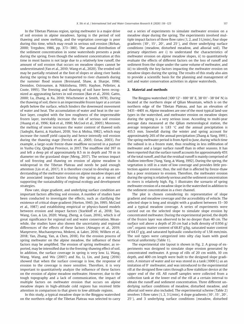
In the Tibetan Plateau region, spring meltwater is a major driveof soil erosion in alpine meadows. Spring is the period of soilthawing and snow melting, and the vegetation coverage is poorduring this time, which may result in serious soil erosion (Birhan,2000; Tregubov, 1986, pp. 373e380). The annual distribution ofthe sediment concentration in some watersheds presents a peakduring the spring. Even though the sediment concentration at thistime in most basins is not large due to a relatively low runoff, theamount of soil erosion that occurs on meadow slopes cannot beunderestimated (Fan et al., 2010;Wang et al., 2020). The eroded soilmay be partially retained at the foot of slopes or along river banksduring the spring to then be transported to river channels duringthe summer flood season (Brennand, Shaw, & Sharpe, 1996;Demidov, Ostroumov, & Nikitishena, 1995; Hayhoe, Pelletier, &Coote, 1995). The freezing and thawing of soil have been recog-nized as aggravating factors in soil erosion (Ban et al., 2016; Gatto,2000; Lu, Zhang, & Xu, 2010; Wischmeier & Smith, 1978). Duringthe thawing of soil, there is an impermeable frozen layer at a certaindepth below the surface, which hinders the downward movementof water and heat. The accumulation of water and heat in the sur-face layer, coupled with the low roughness of the impermeablefrozen layer, inevitably increase the risk of serious soil erosion(Huang et al., 1996; Kok et al., 1990; McCool et al., 2005). Moreover,the melting of snow increases the water content of thawed soils(Sadeghi, Raeisi, & Hazbavi, 2018; Yoo & Molna, 1982), which mayincrease the runoff yield capacity and hence intensify soil erosionduring the thawing stage (Ferrick et al., 2005; Oztas, 2003). Forexample, a large-scale freeze-thaw mudflow occurred in a pasturein Yushu City, Qinghai Province, in 2017. The mudflow slid 397 mand left a deep pit of approximately 8.5 m in depth and 70 m indiameter on the grassland slope (Meng, 2017). The serious impactof soil freezing and thawing on erosion of alpine meadow iswidespread in the Tibetan Plateau and needs be paid enoughattention (Lin et al., 2017). It is therefore crucial to develop an un-derstanding of themeltwater erosion on alpine meadow slopes andthe associated impact factors during the spring as a means ofsupporting the sustainability of regional ecology and developmentstrategies.
Flow rate, slope gradient, and underlying surface condition areimportant factors affecting soil erosion. A number of studies havebeen conducted to investigate the effects, such as clarifying theexistence of critical slope gradient (Horton, 1945; Jin, 1995; McCoolet al., 1987) and establishing empirical or physics-based modelsbetween erosion and impact factors (Starkloff et al., 2018; Tao,Wang, Guo, & Lin, 2020; Wang, Zheng, & Guan, 2016), which is ofgreat significance for regional soil and water conservation. Mean-while, the studies have also shown the uncertainty and regionaldifferences of the effects of these factors (Almagro et al., 2019;Manyevere, Muchaonyerwa, Mnkeni, & Laker, 2016; Wilken et al.,2018; Yan, Zhang, Yan, & Chen, 2018). For the erosion process ofspring meltwater on the alpine meadow, the influence of thesefactors may be amplified. The erosion of spring meltwater, as re-ported,may be intensified due to the freezing-thawing effect of soil.In addition, the surface coverage in spring is very low. Li, Wang,Wang, Wang, and Wu (2007) and Xu, Li, Lin, and Jiang (2016)showed that when the surface coverage is low, the response oferosion to the coverage is more sensitive. Therefore, it is veryimportant to quantitatively analyze the influence of these factorson the erosion of alpine meadow meltwater. However, due to thetough topography and a lack of communication, the impact ofmultiple factors on meltwater erosion that occurs on alpinemeadow slopes in high-altitude cold regions has received littleattention in comparison to that given to low-altitude regions.
In this study, a typical meadow slope in the Binggou watershedon the northern edge of the Tibetan Plateau was selected to carry
out a series of experiments to simulate meltwater erosion on ameadow slope during the spring. The experiments involved mul-tiple impact factors of three flow rates (1, 2, and 3 L/min), four slopegradients (10�, 15�, 20�, and 25�), and three underlying surfaceconditions (meadow, disturbed meadow, and alluvial soil). Theprimary objectives are i) to understand the characteristics ofmeltwater erosion on alpine meadow slopes, ii) to quantitativelyevaluate the effects of different factors on the loss of runoff andsediment from the slope under the same volume of meltwater, andiii) to identify the key factors impacting the meltwater erosion onmeadow slopes during the spring. The results of this study also aimto provide a scientific basis for the planning and management ofsoil and water conservation activities in alpine watersheds.
2. Material and methods
The Binggou watershed (100�120e100�180 E, 38�010e38�040 N) islocated at the northern slope of Qilian Mountain, which is on thenorthern edge of the Tibetan Plateau, and has an elevation of3431e4401m. Alpinemeadows are one of the most typical land-usetypes in the watershed, and meltwater erosion on meadow slopesduring the spring is a very serious issue. According to multi-yearaverage data measured at the Qilian meteorological station, theaverage temperature is 1.83 �C and the annual precipitation is415.5 mm. Snowfall during the winter and spring account forapproximately 26% of the annual precipitation (Zhang& Yang,1991).The springmeltwater period is from April to June, duringwhich timethe subsoil is in a frozen state, thus resulting in less infiltration ofmeltwater and a larger surface runoff than in other seasons. It hasbeen reported that the surface runoff accounts for approximately 45%of the total runoff, and that the residual runoff ismainly comprised ofshallow interflow (Yang, Yang,&Wang,1992). During the spring, thevegetation is still in a state of low coverage and provides little pro-tection against erosion; thus, the soil that is affected by freeze-thawhas a poor resistance to erosion. Therefore, the meltwater erosionduring the spring is relatively serious and the sediment concentrationin rivers is relatively high. Fig. 1 illustrates the scenario of springmeltwater erosion of ameadow slope in thewatershed in addition tothe sediment concentration in a river channel.
The plot is chosen considering its representative of slopegradient and meadow coverage and the accessibility of vehicle. Theselected slope is long and straight with a gradient between 15e30and a typical meadow coverage. A series of experiments werecarried out on the selected slope to simulate slope erosion byconcentratedmeltwater. During the experimental period, the depthof the frozen layer was observed to be no deeper than 40 cm. Thesurface soil above a depth of 20 cm had a bulk density of 0.956 g/cm3, organic matter content of 68.87 g/kg, saturated water contentof 64.17 g/g, and saturated hydraulic conductivity of 1.58 mm/min.The soil types were categorized into silty clay loam with goodvertical uniformity (Table 1).
The experimental site layout is shown in Fig. 2. A group of ex-periments was designed to simulate slope erosion generated byconcentrated meltwater. A group of rills of 20 cm width, 10 cmdepth, and 400 cm length were built to the designed slope gradi-ents. A mixture of water and ice was stored in a tank (1000 L) as animitation of 0� meltwater, and was introduced to the experimentalrill at the designed flow rates through a flow stabilizer device at theupper end of the rill. All runoff samples were collected from acollection tank at the lower end of the rill at a certain interval toobtain the runoff and sediment concentration. Three different un-derlying surface conditions of meadow, disturbed meadow, andalluvial soil were also included. The experimental scheme (Table 2)involves 3 flow rates (1, 2, 3 L/min), 4 slope gradients (10�, 15�, 20�,25�), and 3 underlying surface conditions (meadow, disturbed
X. Shi et al. / International Soil and Water Conservation Research 8 (2020) 116e123 117
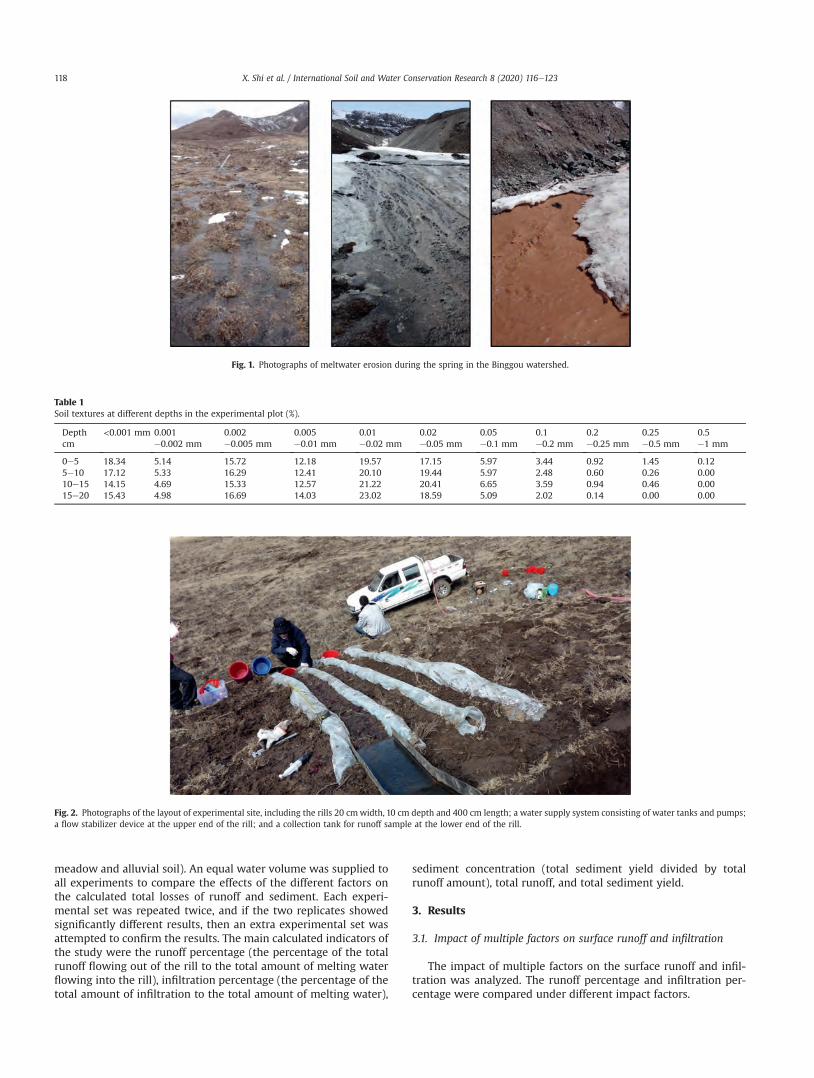
meadow and alluvial soil). An equal water volume was supplied toall experiments to compare the effects of the different factors onthe calculated total losses of runoff and sediment. Each experi-mental set was repeated twice, and if the two replicates showedsignificantly different results, then an extra experimental set wasattempted to confirm the results. The main calculated indicators ofthe study were the runoff percentage (the percentage of the totalrunoff flowing out of the rill to the total amount of melting waterflowing into the rill), infiltration percentage (the percentage of thetotal amount of infiltration to the total amount of melting water),
sediment concentration (total sediment yield divided by totalrunoff amount), total runoff, and total sediment yield.
3. Results
3.1. Impact of multiple factors on surface runoff and infiltration
The impact of multiple factors on the surface runoff and infil-tration was analyzed. The runoff percentage and infiltration per-centage were compared under different impact factors.
Fig. 1. Photographs of meltwater erosion during the spring in the Binggou watershed.
Table 1Soil textures at different depths in the experimental plot (%).
Depthcm
<0.001 mm 0.001e0.002 mm
0.002e0.005 mm
0.005e0.01 mm
0.01e0.02 mm
0.02e0.05 mm
0.05e0.1 mm
0.1e0.2 mm
0.2e0.25 mm
0.25e0.5 mm
0.5e1 mm
0e5 18.34 5.14 15.72 12.18 19.57 17.15 5.97 3.44 0.92 1.45 0.125e10 17.12 5.33 16.29 12.41 20.10 19.44 5.97 2.48 0.60 0.26 0.0010e15 14.15 4.69 15.33 12.57 21.22 20.41 6.65 3.59 0.94 0.46 0.0015e20 15.43 4.98 16.69 14.03 23.02 18.59 5.09 2.02 0.14 0.00 0.00
Fig. 2. Photographs of the layout of experimental site, including the rills 20 cmwidth, 10 cm depth and 400 cm length; a water supply system consisting of water tanks and pumps;a flow stabilizer device at the upper end of the rill; and a collection tank for runoff sample at the lower end of the rill.
X. Shi et al. / International Soil and Water Conservation Research 8 (2020) 116e123118
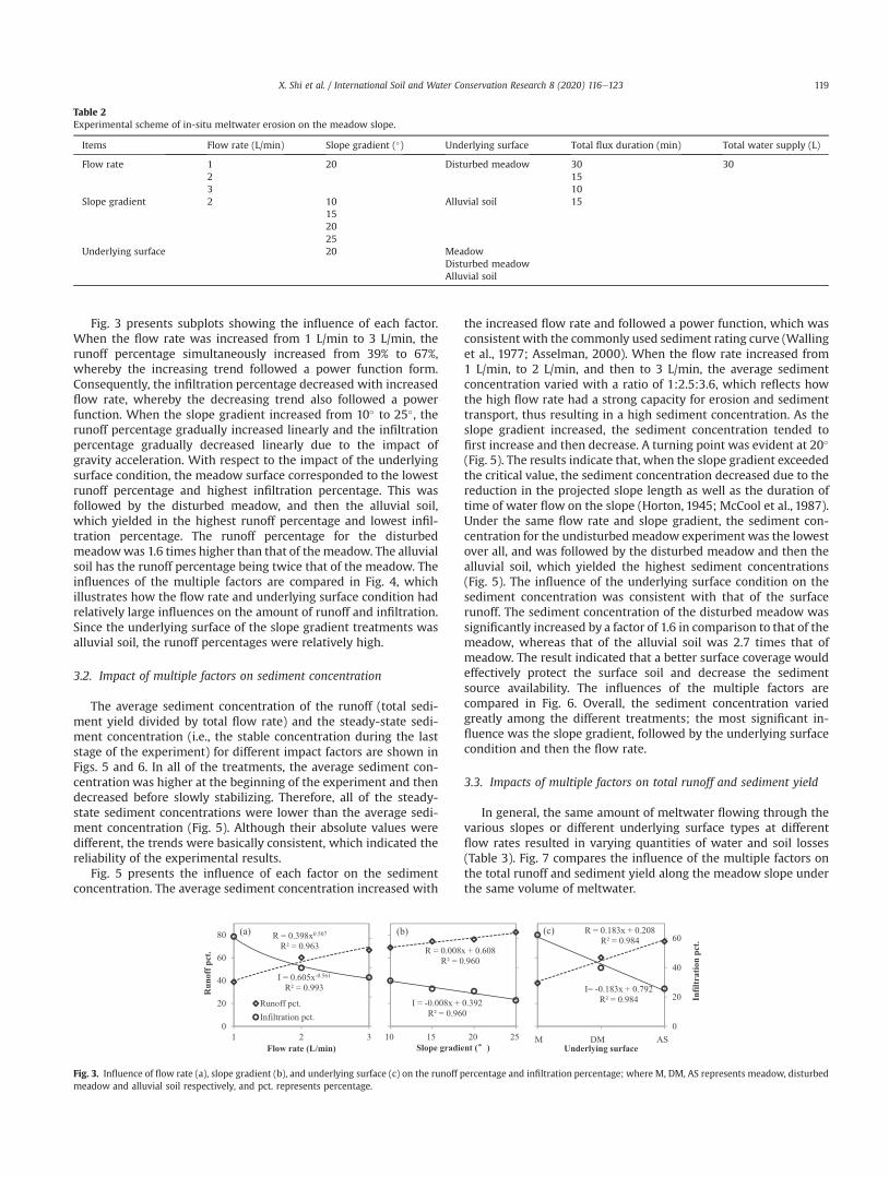
Fig. 3 presents subplots showing the influence of each factor.When the flow rate was increased from 1 L/min to 3 L/min, therunoff percentage simultaneously increased from 39% to 67%,whereby the increasing trend followed a power function form.Consequently, the infiltration percentage decreased with increasedflow rate, whereby the decreasing trend also followed a powerfunction. When the slope gradient increased from 10� to 25�, therunoff percentage gradually increased linearly and the infiltrationpercentage gradually decreased linearly due to the impact ofgravity acceleration. With respect to the impact of the underlyingsurface condition, the meadow surface corresponded to the lowestrunoff percentage and highest infiltration percentage. This wasfollowed by the disturbed meadow, and then the alluvial soil,which yielded in the highest runoff percentage and lowest infil-tration percentage. The runoff percentage for the disturbedmeadowwas 1.6 times higher than that of the meadow. The alluvialsoil has the runoff percentage being twice that of the meadow. Theinfluences of the multiple factors are compared in Fig. 4, whichillustrates how the flow rate and underlying surface condition hadrelatively large influences on the amount of runoff and infiltration.Since the underlying surface of the slope gradient treatments wasalluvial soil, the runoff percentages were relatively high.
3.2. Impact of multiple factors on sediment concentration
The average sediment concentration of the runoff (total sedi-ment yield divided by total flow rate) and the steady-state sedi-ment concentration (i.e., the stable concentration during the laststage of the experiment) for different impact factors are shown inFigs. 5 and 6. In all of the treatments, the average sediment con-centration was higher at the beginning of the experiment and thendecreased before slowly stabilizing. Therefore, all of the steady-state sediment concentrations were lower than the average sedi-ment concentration (Fig. 5). Although their absolute values weredifferent, the trends were basically consistent, which indicated thereliability of the experimental results.
Fig. 5 presents the influence of each factor on the sedimentconcentration. The average sediment concentration increased with
the increased flow rate and followed a power function, which wasconsistent with the commonly used sediment rating curve (Wallinget al., 1977; Asselman, 2000). When the flow rate increased from1 L/min, to 2 L/min, and then to 3 L/min, the average sedimentconcentration varied with a ratio of 1:2.5:3.6, which reflects howthe high flow rate had a strong capacity for erosion and sedimenttransport, thus resulting in a high sediment concentration. As theslope gradient increased, the sediment concentration tended tofirst increase and then decrease. A turning point was evident at 20�
(Fig. 5). The results indicate that, when the slope gradient exceededthe critical value, the sediment concentration decreased due to thereduction in the projected slope length as well as the duration oftime of water flow on the slope (Horton, 1945; McCool et al., 1987).Under the same flow rate and slope gradient, the sediment con-centration for the undisturbedmeadow experiment was the lowestover all, and was followed by the disturbed meadow and then thealluvial soil, which yielded the highest sediment concentrations(Fig. 5). The influence of the underlying surface condition on thesediment concentration was consistent with that of the surfacerunoff. The sediment concentration of the disturbed meadow wassignificantly increased by a factor of 1.6 in comparison to that of themeadow, whereas that of the alluvial soil was 2.7 times that ofmeadow. The result indicated that a better surface coverage wouldeffectively protect the surface soil and decrease the sedimentsource availability. The influences of the multiple factors arecompared in Fig. 6. Overall, the sediment concentration variedgreatly among the different treatments; the most significant in-fluence was the slope gradient, followed by the underlying surfacecondition and then the flow rate.
3.3. Impacts of multiple factors on total runoff and sediment yield
In general, the same amount of meltwater flowing through thevarious slopes or different underlying surface types at differentflow rates resulted in varying quantities of water and soil losses(Table 3). Fig. 7 compares the influence of the multiple factors onthe total runoff and sediment yield along the meadow slope underthe same volume of meltwater.
Table 2Experimental scheme of in-situ meltwater erosion on the meadow slope.
Items Flow rate (L/min) Slope gradient (�) Underlying surface Total flux duration (min) Total water supply (L)
Flow rate 1 20 Disturbed meadow 30 302 153 10
Slope gradient 2 10 Alluvial soil 15152025
Underlying surface 20 MeadowDisturbed meadowAlluvial soil
Fig. 3. Influence of flow rate (a), slope gradient (b), and underlying surface (c) on the runoff percentage and infiltration percentage; where M, DM, AS represents meadow, disturbedmeadow and alluvial soil respectively, and pct. represents percentage.
X. Shi et al. / International Soil and Water Conservation Research 8 (2020) 116e123 119
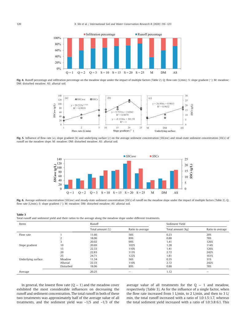
In general, the lowest flow rate (Q ¼ 1) and the meadow coverexhibited the most considerable influences on decreasing therunoff and sediment concentration. The total runoff in both of thesetwo treatments was approximately half of the average value of alltreatments, and the sediment yield was ~1/5 and ~1/3 of the
average value of all treatments for the Q ¼ 1 and meadow,respectively (Table 3). As for the influence of a single factor, whenthe flow rate increased from 1 L/min, to 2 L/min, and then to 3 L/min, the total runoff increased with a ratio of 1.0:1.5:1.7, whereasthe total sediment yield increased with a ratio of 1.0:3.8:6.1. This
Fig. 4. Runoff percentage and infiltration percentage on the meadow slope under the impact of multiple factors (Table 2). Q: flow rate (L/min); S: slope gradient (�); M: meadow;DM: disturbed meadow; AS: alluvial soil.
Fig. 5. Influence of flow rate (a), slope gradient (b) and underlying surface (c) on the average sediment concentration (SSCave) and stead-state sediment concentration (SSCs) ofrunoff on the meadow slope. M: meadow; DM: disturbed meadow; AS: alluvial soil.
Fig. 6. Average sediment concentration (SSCave) and steady-state sediment concentration (SSCs) of runoff on the meadow slope under the impact of multiple factors (Table 2). Q:flow rate (L/min); S: slope gradient (�); M: meadow; DM: disturbed meadow; AS: alluvial soil.
Table 3Total runoff and sediment yield and their ratios to the average along the meadow slope under different treatments.
Items Runoff Sediment Yield
Total amount (L) Ratio to average Total amount (kg) Ratio to average
Flow rate 1 11.66 58% 0.23 20%2 18.06 89% 0.88 78%3 20.02 99% 1.41 126%
Slope gradient 10 20.69 102% 1.28 114%15 22.33 110% 1.41 126%20 22.83 113% 2.72 242%25 24.71 122% 1.81 161%
Underlying surface Meadow 11.34 56% 0.35 31%Alluvial 22.33 110% 2.72 242%Disturbed 18.06 89% 0.88 78%
Average 20.25 e 1.12 e
X. Shi et al. / International Soil and Water Conservation Research 8 (2020) 116e123120
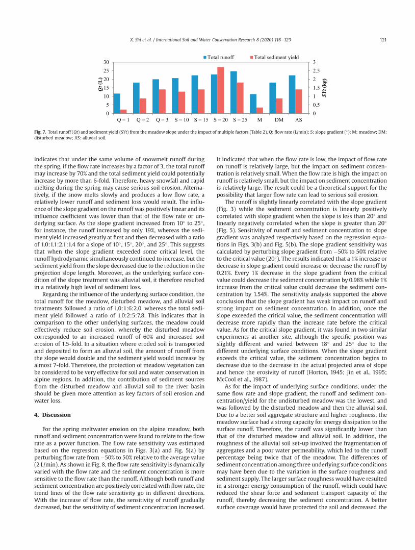
indicates that under the same volume of snowmelt runoff duringthe spring, if the flow rate increases by a factor of 3, the total runoffmay increase by 70% and the total sediment yield could potentiallyincrease by more than 6-fold. Therefore, heavy snowfall and rapidmelting during the spring may cause serious soil erosion. Alterna-tively, if the snow melts slowly and produces a low flow rate, arelatively lower runoff and sediment loss would result. The influ-ence of the slope gradient on the runoff was positively linear and itsinfluence coefficient was lower than that of the flow rate or un-derlying surface. As the slope gradient increased from 10� to 25�,for instance, the runoff increased by only 19%, whereas the sedi-ment yield increased greatly at first and then decreased with a ratioof 1.0:1.1:2.1:1.4 for a slope of 10�, 15�, 20�, and 25�. This suggeststhat when the slope gradient exceeded some critical level, therunoff hydrodynamic simultaneously continued to increase, but thesediment yield from the slope decreased due to the reduction in theprojection slope length. Moreover, as the underlying surface con-dition of the slope treatment was alluvial soil, it therefore resultedin a relatively high level of sediment loss.
Regarding the influence of the underlying surface condition, thetotal runoff for the meadow, disturbed meadow, and alluvial soiltreatments followed a ratio of 1.0:1:6:2.0, whereas the total sedi-ment yield followed a ratio of 1.0:2:5:7.8. This indicates that incomparison to the other underlying surfaces, the meadow couldeffectively reduce soil erosion, whereby the disturbed meadowcorresponded to an increased runoff of 60% and increased soilerosion of 1.5-fold. In a situation where eroded soil is transportedand deposited to form an alluvial soil, the amount of runoff fromthe slope would double and the sediment yield would increase byalmost 7-fold. Therefore, the protection of meadow vegetation canbe considered to be very effective for soil and water conservation inalpine regions. In addition, the contribution of sediment sourcesfrom the disturbed meadow and alluvial soil to the river basinshould be given more attention as key factors of soil erosion andwater loss.
4. Discussion
For the spring meltwater erosion on the alpine meadow, bothrunoff and sediment concentrationwere found to relate to the flowrate as a power function. The flow rate sensitivity was estimatedbased on the regression equations in Figs. 3(a) and Fig. 5(a) byperturbing flow rate from�50% to 50% relative to the average value(2 L/min). As shown in Fig. 8, the flow rate sensitivity is dynamicallyvaried with the flow rate and the sediment concentration is moresensitive to the flow rate than the runoff. Although both runoff andsediment concentration are positively correlatedwith flow rate, thetrend lines of the flow rate sensitivity go in different directions.With the increase of flow rate, the sensitivity of runoff graduallydecreased, but the sensitivity of sediment concentration increased.
It indicated that when the flow rate is low, the impact of flow rateon runoff is relatively large, but the impact on sediment concen-tration is relatively small. When the flow rate is high, the impact onrunoff is relatively small, but the impact on sediment concentrationis relatively large. The result could be a theoretical support for thepossibility that larger flow rate can lead to serious soil erosion.
The runoff is slightly linearly correlated with the slope gradient(Fig. 3) while the sediment concentration is linearly positivelycorrelated with slope gradient when the slope is less than 20� andlinearly negatively correlated when the slope is greater than 20�
(Fig. 5). Sensitivity of runoff and sediment concentration to slopegradient was analyzed respectively based on the regression equa-tions in Figs. 3(b) and Fig. 5(b). The slope gradient sensitivity wascalculated by perturbing slope gradient from �50% to 50% relativeto the critical value (20�). The results indicated that a 1% increase ordecrease in slope gradient could increase or decrease the runoff by0.21%. Every 1% decrease in the slope gradient from the criticalvalue could decrease the sediment concentration by 0.98%while 1%increase from the critical value could decrease the sediment con-centration by 1.54%. The sensitivity analysis supported the aboveconclusion that the slope gradient has weak impact on runoff andstrong impact on sediment concentration. In addition, once theslope exceeded the critical value, the sediment concentration willdecrease more rapidly than the increase rate before the criticalvalue. As for the critical slope gradient, it was found in two similarexperiments at another site, although the specific position wasslightly different and varied between 18� and 25� due to thedifferent underlying surface conditions. When the slope gradientexceeds the critical value, the sediment concentration begins todecrease due to the decrease in the actual projected area of slopeand hence the erosivity of runoff (Horton, 1945; Jin et al., 1995;McCool et al., 1987).
As for the impact of underlying surface conditions, under thesame flow rate and slope gradient, the runoff and sediment con-centration/yield for the undisturbed meadow was the lowest, andwas followed by the disturbed meadow and then the alluvial soil.Due to a better soil aggregate structure and higher roughness, themeadow surface had a strong capacity for energy dissipation to thesurface runoff. Therefore, the runoff was significantly lower thanthat of the disturbed meadow and alluvial soil. In addition, theroughness of the alluvial soil set-up involved the fragmentation ofaggregates and a poor water permeability, which led to the runoffpercentage being twice that of the meadow. The differences ofsediment concentration among three underlying surface conditionsmay have been due to the variation in the surface roughness andsediment supply. The larger surface roughness would have resultedin a stronger energy consumption of the runoff, which could havereduced the shear force and sediment transport capacity of therunoff, thereby decreasing the sediment concentration. A bettersurface coverage would have protected the soil and decreased the
Fig. 7. Total runoff (Qt) and sediment yield (SYt) from the meadow slope under the impact of multiple factors (Table 2). Q: flow rate (L/min); S: slope gradient (�); M: meadow; DM:disturbed meadow; AS: alluvial soil.
X. Shi et al. / International Soil and Water Conservation Research 8 (2020) 116e123 121
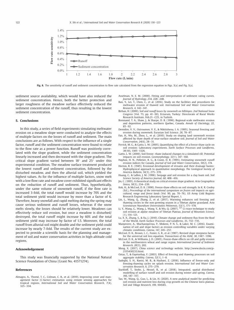
sediment source availability, which would have also reduced thesediment concentration. Hence, both the better protection andlarger roughness of the meadow surface effectively reduced thesediment concentration of the runoff, thus resulting in the lowestsediment concentration.
5. Conclusions
In this study, a series of field experiments simulating meltwatererosion on a meadow slope were conducted to analyze the effectsof multiple factors on the losses of runoff and sediment. The mainconclusions are as follows. With respect to the influence of a singlefactor, runoff and the sediment concentration were found to relateto the flow rate as a power function. Runoff was positively corre-lated with the slope gradient, while the sediment concentrationlinearly increased and then decreased with the slope gradient. Thecritical slope gradient varied between 18� and 25� under thisexperimental condition. The meadow surface treatment producedthe lowest runoff and sediment concentration, followed by thedisturbed meadow, and then the alluvial soil, which yielded thehighest values. As for the influence of multiple factors, snow meltwith a low flow rate andmeadow cover exhibited significant effectson the reduction of runoff and sediment. Thus, hypothetically,under the same volume of snowmelt runoff, if the flow rate isincreased 3-fold, the total runoff would increase by 70% and thetotal sediment yield would increase by more than a factor of 6.Therefore, heavy snowfall and rapid melting during the spring maycause serious sediment and runoff losses, whereas if the snowmelts slowly, the losses should be relatively lower. Meadows caneffectively reduce soil erosion, but once a meadow is disturbed/destroyed, the total runoff might increase by 60% and the totalsediment yield may increase by factor of 1.5. Moreover, the totalrunoff from alluvial soil might double and the sediment yield couldincrease by nearly 7-fold. The results of the current study are ex-pected to provide a scientific basis for the planning and manage-ment of soil and water conservation activities in high-altitude coldregions.
Acknowledgement
This study was financially supported by the National NaturalScience Foundation of China (Grant No. 41571274).
References
Almagro, A., Thom�e, T. C., Colman, C. B., et al. (2019). Improving cover and man-agement factor (C-factor) estimation using remote sensing approaches fortropical regions. International Soil and Water Conservation Research, 7(4),325e334.
Asselman, N. E. M. (2000). Fitting and interpretation of sediment rating curves.Journal of Hydrology, 234, 228e248.
Ban, Y., Lei, T., Chen, C., et al. (2016). Study on the facilities and procedures formeltwater erosion of thawed soil. International Soil and Water ConservationResearch, 4, 142e147.
Birhan, H. (2000). Soil and runoff losses by snowmelt on hillslopes. 2nd National SnowCongress (Vol. 73, pp. 41e50). Erzurum, Turkey: Directorate of Rural WorksResearch Institute. Feb.21eC25, in Turkish.
Brennand, T. A., Shaw, J., & Sharpe, D. R. (1996). Regional-scale meltwater erosionand deposition patterns, northern Quebec, Canada. Annals of Glaciology, 22,85e92.
Demidov, V. V., Ostroumov, V. E., & Nikitishena, I. A. (1995). Seasonal freezing anderosion during snowmelt. Eurasian Soil Science. 28, 78e87.
Fan, H., Wu, M., Zhou, L., et al. (2010). Study on sloping land snowmelt erosionaffected by thaw depth of near-surface meadow soil. Journal of Soil and WaterConservation, 24(6), 28e31.
Ferrick, M. G., & Gatto, L. W. (2005). Quantifying the effect of a freeze-thaw cycle onsoil erosion: Laboratory experiments. Earth Surface Processes and Landforms,30(10), 1305e1326.
Gatto, L. W. (2000). Soil freezeethaw-induced changes to a simulated rill: Potentialimpacts on soil erosion. Geomorphology, 32(1), 147e160.
Hayhoe, H. N., Pelletier, R. G., & Coote, D. R. (1995). Estimating snowmelt runofferosion indices for Canada. Journal of Soil and Water Conservation, 50(2), 174.
Horton, R. E. (1945). Erosional development of streams and their drainage basins:Hydrophysical approach to quantitative morphology. The Geological Society ofAmerica Bulletin, 56(3), 275e370.
Huang, C., & Laflen, J. M. (1996). Seepage and soil erosion for a clay loam soil. SoilScience Society of America Journal, 60, 408e416.
Jin, C. (1995). A theoretical study on critical erosion slope gradient. Acta GeographicaSinica, 50(3), 234e239.
Kok, H., & McCool, D. K. (1990). Freeze-thaw effects on soil strength. In K. R. Cooley(Ed.), Proceedings of the international symposium on frozen soil impacts on agri-cultural, range and forest lands (Vol. 90, pp. 70e76). US Army Cold RegionsResearch Engineering Laboratory Special Report, 1.
Lin, L., Wang, Q., Zhang, Z., et al. (2017). Warming enhances soil freezing andthawing circles in the non-growing season in a Tibetan alpine grassland. ActaScientiarum Nauralium Universitaties Pekinensis, 53(1), 171e178.
Li, Y., Wang, G., Wang, J., Wang, Y., & Wu, Q. (2007). 137 Cs trace technique to studysoil erosion at alpine meadow of Tibetan Plateau. Journal of Mountain Science,(1), 114e121.
Lu, X. X., Zhang, S., & Xu, J. (2010). Climate change and sediment flux from the Roofof the World. Earth Surface Processes and Landforms, 35, 732e735.
Manyevere, A., Muchaonyerwa, P., Mnkeni, P. N. S., & Laker, M. C. (2016). Exami-nation of soil and slope factors as erosion controlling variables under varyingclimatic conditions. Catena, 147, 245e257.
McCool, D. K., Brown, L. C., Foster, G. R., et al. (1987). Revised slope steepness factorfor the universal soil loss equation. Transactions of the ASAE, 30, 1387e1396.
McCool, D. K., & Williams, J. D. (2005). Freeze-thaw effects on rill and gully erosionin the northwestern wheat and range region. International Journal of SedimentResearch, 20(3), 202.
Meng, X. (2017). China science and technology website. http://www.docin.com/p-2155430233.html.
Oztas, T., & Fayetorbay, F. (2003). Effect of freezing and thawing processes on soilaggregate stability. Catena, 52(1), 1e8.
Sadeghi, S. H., Raeisi, M. B., & Hazbavi, Z. (2018). Influence of freeze-only andfreezing-thawing cycles on splash erosion. International Soil and Water Con-servation Research, 6, 275e279.
Starkloff, T., Stolte, J., Hessel, R., et al. (2018). Integrated, spatial distributedmodelling of surface runoff and soil erosion during winter and spring. Catena,166, 147e157.
Tao, W., Wang, Q., Guo, L., & Lin, H. (2020). A new analytical model for predictingsoil erosion and nutrient loss during crop growth on the Chinese loess plateau.Soil and Tillage Research, 199, 104585.
Fig. 8. The sensitivity of runoff and sediment concentration to flow rate calculated from the regression equation in Figs. 3(a) and Fig. 5(a).
X. Shi et al. / International Soil and Water Conservation Research 8 (2020) 116e123122

Tregubov, P. S. (1986). Mechanisms and spatial variability of erosion caused bymeltwater in the USSR. Modelling Snowmelt-Induced Processes (Vol. 155). IAHSPubl.
Walling, D. E. (1977). Assessing the accuracy of suspended sediment rating curvesfor a small basin. Water Resources Research, 13(3), 531e538.
Wang, T., Li, P., Liu, Y., et al. (2020). Experimental investigation of freeze-thawmeltwater compound erosion and runoff energy consumption on loessalslopes. Catena, 185, 104310.
Wang, Q., Zhang, T., Jin, H., et al. (2017). Observational study on the active layerfreeze-thaw cycle in the upper reaches of the Heihe River of the north-easternQinghai-Tibet Plateau. Quaternary International, 440, 13e22.
Wang, B., Zheng, F., & Guan, Y. (2016). Improved USLE-K factor prediction: A casestudy on water erosion areas in China. International Soil and Water ConservationResearch, 4(3), 168e176.
Wilken, F., Baur, M., Sommer, M., et al. (2018). Uncertainties in rainfall kineticenergy-intensity relations for soil erosion modelling. Catena, 171, 234e244.
Wischmeier, W. H., & Smith, D. D. (1978). Predicting rainfall erosion losses: A guide toconservation planning. Agriculture handbook (USA): United States Dept ofAgriculture.
Xu, H., Li, Z., Lin, J., & Jiang, A. (2016). Influences of rainfall and underlying surfaceconditions on soil erosion and sediment yield in Yanshan rock mountain area.Mountain Research, 34(1), 46e53.
Yang, Z., Yang, Z., & Wang, Q. (1992). Run of analysis and estimation of the Binggoubasin in the qilian mountain. Journal of Glaciology and Geocryology, 14(3),251e257.
Yan, R., Zhang, X., Yan, S., & Chen, H. (2018). Estimating soil erosion response to landuse/cover change in a catchment of the Loess Plateau, China. International Soiland Water Conservation Research, 6(1), 13e22.
Yoo, K. H., & Molna, U. M. (1982). Simulation of soil erosion from winter runoff inthe Palouse Prairie. Transactions of the ASAE, 25(6), 1628e1636.
Zhang, X., & Yang, Z. (1991). The primary analysis of water-balance in Binggou basinof qilian mountains. Journal of Glaciology and Geocryology, 13(1), 35e42.
X. Shi et al. / International Soil and Water Conservation Research 8 (2020) 116e123 123
Original Research Article
Surface runoff and soil erosion in a natural regeneration area of theBrazilian Cerrado
Karina dos Santos Falc~ao a, El�oi Panachuki a, Felipe das Neves Monteiro a,Roniedison da Silva Menezes a, Dulce B.B. Rodrigues b, Jullian Souza Sone c, *,Paulo Tarso S. Oliveira b
a Department of Agronomy, State University of Mato Grosso do Sul, Agronomy Department, Aquidauana, MS, 79200-000, Brazilb Federal University of Mato Grosso do Sul, CxP 549, Campo Grande, MS, 79070-900, Brazilc Department of Hydraulics and Sanitation, S~ao Carlos School of Engineering, University of S~ao Paulo, CxP. 359, S~ao Carlos, SP, 13566-590, Brazil
a r t i c l e i n f o
Article history:Received 22 December 2019Received in revised form31 March 2020Accepted 7 April 2020Available online 13 April 2020
Keywords:Cerrado deforestationForest regenerationSoil erosion
a b s t r a c t
The Brazilian Cerrado has been converted to farmland, and there is little evidence that this expansion willdecrease, mainly because agriculture is the country’s main economic sector. However, the impacts ofintense modification of land use and land cover on surface runoff and soil erosion are still poorly un-derstood in this region. Here, we assessed surface runoff and soil loss in a woodland Cerrado area under aformer pasture area, which was abandoned and has undergone a natural regeneration process for 7 years(RC). Its results were compared with that found in an undisturbed area of woodland Cerrado (CE), 40-month-old eucalyptus (3.0 � 1.8 m) (EU), and pasture under rotational grazing (PA). The study wasconducted on Red Acrisol located in the Brazilian Cerrado. We performed rainfall simulations on a plot of0.7 m2 and using three constant rainfall intensities of 60, 90, and 120 mm h�1 for 1 h. For each rainfallintensity, we carried out four repetitions using different plots in each treatment, i.e. 12 plots per treat-ment studied and 48 plots in total. We noted that the soil physical properties were improved in RC and,consequently, water infiltration and soil erosion control; RC presented surface runoff and soil lossdifferent from EU and PA (a ¼ 0.05). The macroporosity and soil bulk density affected surface runoff in RCand PA because the RC was used as pasture and is currently regenerating back to the cerrado vegetation.As the rainfall intensity increased, EU became more similar to PA, which showed the highest surfacerunoff and soil loss. Our findings indicate that natural regeneration processes (pasture to the cerradovegetation) tend to improve the soil ecosystem services, improving infiltration and reducing surfacerunoff and soil erosion.© 2020 International Research and Training Center on Erosion and Sedimentation and China Water andPower Press. Production and Hosting by Elsevier B.V. This is an open access article under the CC BY-NC-
ND license (http://creativecommons.org/licenses/by-nc-nd/4.0/).
1. Introduction
The Cerrado is the second largest biome in South America,occupying approximately 20% of Brazil’s land area. Most of theCerrado is located in Brazil’s central highlands and is home to themost important water sources in the country (Oliveira et al., 2014).It is one of the richest savannas in the world (Klink & Machado,
2005), and it is considered a hotspot for world biodiversity con-servation due to the high concentration of endemic species and thehigh loss of natural habitats (Myers, Mittermeier, Mittermeier, daFonseca, & Kent, 2000). Furthermore, approximately 55% of itsoriginal cover has already been deforested (Sano, Rosa, Brito, &Ferreira, 2010). The deforestation rate in the Cerrado is largerthan in the Amazon and threatens the sustainability of theecosystem. These changes have converted the natural landscapeinto an area of food and energy production (Foley, 2005).
The biome is the last agricultural frontier in the world (Borlaug,2002), and it is estimated to account for 55% of the country’s beefproduction including 53 million hectares of cultivated pastures(Dias-Filho, 2011). However, 60% of pasture areas in the cerrado
* Corresponding author.E-mail addresses: [email protected] (K.S. Falc~ao), [email protected]
(E. Panachuki), [email protected] (F.N. Monteiro), [email protected](R. da Silva Menezes), [email protected] (D.B.B. Rodrigues), [email protected](J.S. Sone), [email protected] (P.T.S. Oliveira).
Contents lists available at ScienceDirect
International Soil and Water Conservation Research
journal homepage: www.elsevier .com/locate/ iswcr
https://doi.org/10.1016/j.iswcr.2020.04.0042095-6339/© 2020 International Research and Training Center on Erosion and Sedimentation and China Water and Power Press. Production and Hosting by Elsevier B.V. Thisis an open access article under the CC BY-NC-ND license (http://creativecommons.org/licenses/by-nc-nd/4.0/).
International Soil and Water Conservation Research 8 (2020) 124e130
present some form of degradation (Embrapa, 2014). Degraded soilscause crop yield decrease due to the removal of the richest layer oforganic matter and clay, as well as contamination of water bodies(Cardoso, Silva, DeCarvalho, De Freitas, & Avanzi, 2012; Ribeiro,Ribeiro, Mincato, Curi, & Kawakubo, 2016). Minimizing degrada-tion and improving productivity requires studies on best soil andagricultural management practices. Soil loss due to water erosionthreatens the environment and generally exceeds soil formationtime.
Associated with the agricultural expansion in Brazil, which hasbrought several economic benefits, is an environmental cost thatmay cause negative long-term impacts on society and economicgrowth. Furthermore, environment, economy and society areinterrelated, so that expanding agricultural frontiers withoutconsidering environmental aspects such as hydrological regimeand loss of biodiversity will trigger water-food-energy nexusinsecurity (Oliveira et al., 2019). The intensified use of arable landshas compacted and deteriorated soil physical properties (Hamza &Anderson, 2005). Moreover, Latin America and the Caribbean willhave up to 780 million ha of agricultural land degraded due tounsustainable use (Premanandh, 2011). In Brazil, annual absoluteland productivity has already decreased by about 6.9% by 2011 dueto severe soil erosion (Sartori et al., 2019).
Forests are more efficient in protecting the soil from erosionprocesses caused by water erosion due to litter and vegetationcanopy interception (Oliveira, Nearing, & Wendland, 2015). How-ever, there are few experimental studies evaluating the influence offorest vegetation under regeneration on hydrological and soilerosion processes (Anache, Wendland, Rosalem, Youlton, &Oliveira, 2019; Oliveira et al., 2015). Thus, this study aimed toexperimentally quantify soil erosion and surface runoff in aregenerating area of woodland Cerrado (sensu stricto), comparingwith two agricultural land uses, using a portable rainfall simulator.
2. Material and methods
2.1. Study area
This study was conducted at the Experimental Farm of the StateUniversity of Mato Grosso do Sul, located in the city of Aquidauana,Mato Grosso do Sul (Fig. 1). According to the K€oppen classification,the climate is rainy tropical with dry winter (Aw). It has a rainyseason during the summer, from November to April, and a clear dryseason during the winter, fromMay to October. The average annualtemperature is 23.3 �C, with an average rainfall of 1,400 mm. Theregion’s topography varies from flat to slightly undulating, and thesoil is characterized as dystrophic Red Acrisol with a sandy loamtexture (Table 1).
2.2. Experimental design and treatments
We assessed surface runoff and soil loss in a regenerating area ofcerrado, a native cerrado vegetation, and two agricultural land uses,which consist of (i) eucalyptus plantation in triple-row treearrangement at 3.0 m� 1.8 m x 9.0 m spacing (1,111 trees ha�1) and(ii) pasture under rotational grazing for beef cattle production (fordetailed description see Table 1). We performed rainfall simula-tions using three constant rainfall intensities of 60, 90, and120 mm h�1 during 1 h, which represents a return period in theregion of 8, 99, and 590 years, respectively (Santos, Figueiredo,Oliveira, & Griebeler, 2009). For each rainfall intensity, we carriedout four repetitions using different plots in each treatment, sum-ming to 12 plots per treatment. A total of 48 plots of 0.7 m2 wereplaced on the land uses hillslopes with a mean slope steepness of5%.
2.3. Soil physical properties
Soil samples were collected in the experimental units to eval-uate soil bulk density (BD), macroporosity (Ma), microporosity (Mi)and total pore volume (TPV). Theywere determined by undisturbedsoil samples from the 0e0.1, 0.1e0.2, and 0.2e0.4 m soil depths.Four intact soil cores (100 cm3) were obtained in each soil depth.After we saturated the soil cores for 24 h, we drained the water byapplying a tension of 6 kPa, so that we obtained the microporosity.Macroporosity was computed by the difference between Mi andTPV.
For the aggregate analysis, the geometric mean diameter (GMD)and themeanweighted diameter (MWD) indices were evaluated byusing the wet sieving method (Teixeira, Donagemma, Fontana,Teixeira, & Martins, 2017). Regarding the GMD and MWD,disturbed soil samples were collected from the 0e0.1, 0.1e0.2 and0.2e0.4 m soil layer. Samples of 50 g were transferred into the stackof sieves arranged in opening sizes of sieves 0.105 to 2.00 mm andsubjected to vertical shaking in the Yoder apparatus for 15 min(Yoder, 1936). Afterwards, the remaining material in each sieve wasoven-dried at 105 �C until constant mass.
To evaluate the organic matter contents (OM), the samples weretaken in the same depth ranges and performed by the potassiumdichromate volumetric method (Walkley Black method), asdescribed by Teixeira et al. (2017). All the vegetal mass found on thesurface of the plots was collected and oven-dried to determine thedry biomass (DBM). We also measured the initial gravimetric soilwater content at 0e0.1 m soil depth prior to each rainfall simula-tion by using sample rings of 100 cm3 with four repetitions perrainfall simulation (Table 2).
2.4. Surface runoff and soil loss data
We used a rainfall simulator with 0.7-m2 runoff plots, whichare bordered by 2-mm thick galvanized iron sheets (AlvesSobrinho, G�omez-Macpherson, & G�omez, 2008). The plots havea downward-slope side with a triangular form that directs thesurface runoff to the collecting point. Two parallel Veejet 80.150flat spray nozzles that provide 2-mm raindrops when placed at aheight of 2.3 m and a working pressure of 35.6 kPa compose thesimulator. We calibrated the simulator to provide three differentrainfall intensities of 60, 90 and 120 mm h�1 for 60 min aftersurface runoff onset (Panachuki, Bertol, Alves Sobrinho, TarsoSanches de Oliveira, & Buchala Bicca Rodrigues, 2011). Addition-ally, the plots were pre-wet 24 h before every simulation foruniform humidity conditions in all treatments (Cogo,Moldenhauer, & Foster, 1984).
We recorded the runoff start-time in all rainfall simulations. Forsurface runoff, we collected and measured the surface runoff vol-ume each minute using a graduated cylinder. For soil loss, surfacerunoff samples were also sampled using a 1-L bottle during 1min ata time interval of 6 min between each measurement. At the labo-ratory, we added hydrochloric acid (HCl) to the samples to floccu-late the suspended solid material. After 24 h, the samples wereplaced in an oven at 80 �C for enough time to ensure total waterevaporation. Thus, soil loss in each treatment was calculated as thetotal sediment load divided by the plot area.
2.5. Statistical analyses
We performed the Dunn’s tests after we verified any statisticaldifferences among the treatments by using Kruskal-Wallis(a ¼ 0.05), so that surface runoff and soil loss were divided intogroups with similar results. Moreover, hierarchical cluster analysis(HCA) was performed using the Euclidean distance (Nearest
K.S. Falc~ao et al. / International Soil and Water Conservation Research 8 (2020) 124e130 125
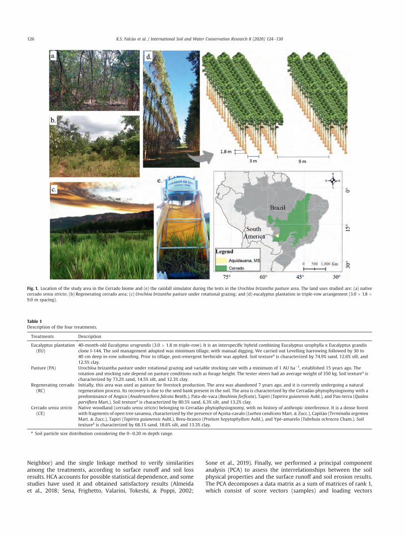
Neighbor) and the single linkage method to verify similaritiesamong the treatments, according to surface runoff and soil lossresults. HCA accounts for possible statistical dependence, and somestudies have used it and obtained satisfactory results (Almeidaet al., 2018; Sena, Frighetto, Valarini, Tokeshi, & Poppi, 2002;
Sone et al., 2019). Finally, we performed a principal componentanalysis (PCA) to assess the interrelationships between the soilphysical properties and the surface runoff and soil erosion results.The PCA decomposes a data matrix as a sum of matrices of rank 1,which consist of score vectors (samples) and loading vectors
Fig. 1. Location of the study area in the Cerrado biome and (e) the rainfall simulator during the tests in the Urochloa brizantha pasture area. The land uses studied are: (a) nativecerrado sensu stricto; (b) Regenerating cerrado area; (c) Urochloa brizantha pasture under rotational grazing; and (d) eucalyptus plantation in triple-row arrangement (3.0 � 1.8 �9.0 m spacing).
Table 1Description of the four treatments.
Treatments Description
Eucalyptus plantation(EU)
40-month-old Eucalyptus urograndis (3.0 � 1.8 m triple-row). It is an interspecific hybrid combining Eucalyptus urophylla x Eucalyptus grandisclone I-144. The soil management adopted was minimum tillage, with manual digging. We carried out Levelling harrowing followed by 30 to40 cm deep in-row subsoiling. Prior to tillage, post-emergent herbicide was applied. Soil texturea is characterized by 74.9% sand, 12.6% silt, and12.5% clay.
Pasture (PA) Urochloa brizantha pasture under rotational grazing and variable stocking rate with a minimum of 1 AU ha�1, established 15 years ago. Therotation and stocking rate depend on pasture conditions such as forage height. The tester steers had an average weight of 350 kg. Soil texturea ischaracterized by 73.2% sand, 14.5% silt, and 12.3% clay.
Regenerating cerrado(RC)
Initially, this area was used as pasture for livestock production. The area was abandoned 7 years ago, and it is currently undergoing a naturalregeneration process. Its recovery is due to the seed bank present in the soil. The area is characterized by the Cerrad~ao phytophysiognomy with apredominance of Angico (Anadenanthera falcata Benth.), Pata-de-vaca (Bauhinia forficata), Tapiri (Tapirira guianensis Aubl.), and Pau-terra (Qualeaparviflora Mart.). Soil texturea is characterized by 80.5% sand, 6.3% silt, and 13.2% clay.
Cerrado sensu stricto(CE)
Native woodland (cerrado sensu stricto) belonging to Cerrad~ao phytophysiognomy, with no history of anthropic interference. It is a dense forestwith fragments of open tree savanna, characterized by the presence of Açoita-cavalo (Luehea candicansMart.& Zucc.), Capit~ao (Terminalia argenteaMart. & Zucc.), Tapiri (Tapirira guianensis Aubl.), Breu-branco (Protium hepytaphyllum Aubl.), and Ype-amarelo (Tabebuia ochracea Cham.). Soiltexturea is characterized by 68.1% sand, 18.6% silt, and 13.3% clay.
a Soil particle size distribution considering the 0e0.20 m depth range.
K.S. Falc~ao et al. / International Soil and Water Conservation Research 8 (2020) 124e130126
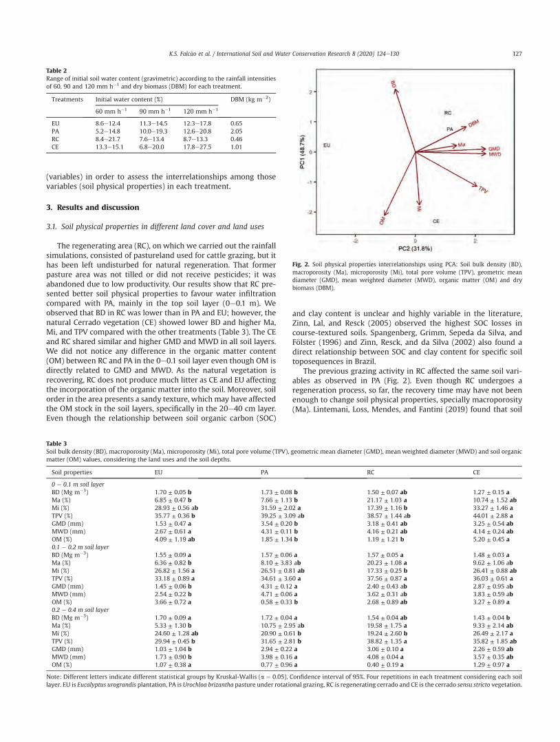
(variables) in order to assess the interrelationships among thosevariables (soil physical properties) in each treatment.
3. Results and discussion
3.1. Soil physical properties in different land cover and land uses
The regenerating area (RC), on which we carried out the rainfallsimulations, consisted of pastureland used for cattle grazing, but ithas been left undisturbed for natural regeneration. That formerpasture area was not tilled or did not receive pesticides; it wasabandoned due to low productivity. Our results show that RC pre-sented better soil physical properties to favour water infiltrationcompared with PA, mainly in the top soil layer (0e0.1 m). Weobserved that BD in RC was lower than in PA and EU; however, thenatural Cerrado vegetation (CE) showed lower BD and higher Ma,Mi, and TPV compared with the other treatments (Table 3). The CEand RC shared similar and higher GMD and MWD in all soil layers.We did not notice any difference in the organic matter content(OM) between RC and PA in the 0e0.1 soil layer even though OM isdirectly related to GMD and MWD. As the natural vegetation isrecovering, RC does not produce much litter as CE and EU affectingthe incorporation of the organic matter into the soil. Moreover, soilorder in the area presents a sandy texture, whichmay have affectedthe OM stock in the soil layers, specifically in the 20e40 cm layer.Even though the relationship between soil organic carbon (SOC)
and clay content is unclear and highly variable in the literature,Zinn, Lal, and Resck (2005) observed the highest SOC losses incourse-textured soils. Spangenberg, Grimm, Sepeda da Silva, andF€olster (1996) and Zinn, Resck, and da Silva (2002) also found adirect relationship between SOC and clay content for specific soiltoposequences in Brazil.
The previous grazing activity in RC affected the same soil vari-ables as observed in PA (Fig. 2). Even though RC undergoes aregeneration process, so far, the recovery time may have not beenenough to change soil physical properties, specially macroporosity(Ma). Lintemani, Loss, Mendes, and Fantini (2019) found that soil
Table 2Range of initial soil water content (gravimetric) according to the rainfall intensitiesof 60, 90 and 120 mm h�1 and dry biomass (DBM) for each treatment.
Treatments Initial water content (%) DBM (kg m�2)
60 mm h�1 90 mm h�1 120 mm h�1
EU 8.6e12.4 11.3e14.5 12.3e17.8 0.65PA 5.2e14.8 10.0e19.3 12.6e20.8 2.05RC 8.4e21.7 7.6e13.4 8.7e13.3 0.46CE 13.3e15.1 6.8e20.0 17.8e27.5 1.01
Table 3Soil bulk density (BD), macroporosity (Ma), microporosity (Mi), total pore volume (TPV), geometric mean diameter (GMD), mean weighted diameter (MWD) and soil organicmatter (OM) values, considering the land uses and the soil depths.
Soil properties EU PA RC CE
0 e 0.1 m soil layerBD (Mg m�3) 1.70 ± 0.05 b 1.73 ± 0.08 b 1.50 ± 0.07 ab 1.27 ± 0.15 aMa (%) 6.85 ± 0.47 b 7.66 ± 1.13 b 21.17 ± 1.03 a 10.74 ± 1.52 abMi (%) 28.93 ± 0.56 ab 31.59 ± 2.02 a 17.39 ± 1.16 b 33.27 ± 1.46 aTPV (%) 35.77 ± 0.36 b 39.25 ± 3.09 ab 38.57 ± 1.44 ab 44.01 ± 2.88 aGMD (mm) 1.53 ± 0.47 a 3.54 ± 0.20 b 3.18 ± 0.41 ab 3.25 ± 0.54 abMWD (mm) 2.67 ± 0.61 a 4.31 ± 0.11 b 4.16 ± 0.21 ab 4.14 ± 0.24 abOM (%) 4.09 ± 1.19 ab 1.85 ± 1.34 b 1.19 ± 1.21 b 5.20 ± 0.45 a0.1 e 0.2 m soil layerBD (Mg m�3) 1.55 ± 0.09 a 1.57 ± 0.06 a 1.57 ± 0.05 a 1.48 ± 0.03 aMa (%) 6.36 ± 0.82 b 8.10 ± 3.83 ab 20.23 ± 1.08 a 9.62 ± 1.06 abMi (%) 26.82 ± 1.56 a 26.51 ± 0.81 ab 17.33 ± 0.25 b 26.41 ± 0.88 abTPV (%) 33.18 ± 0.89 a 34.61 ± 3.60 a 37.56 ± 0.87 a 36.03 ± 0.61 aGMD (mm) 1.45 ± 0.06 b 4.31 ± 0.12 a 2.40 ± 0.43 ab 2.87 ± 0.95 abMWD (mm) 2.54 ± 0.22 b 4.71 ± 0.06 a 3.62 ± 0.31 ab 3.83 ± 0.59 abOM (%) 3.66 ± 0.72 a 0.58 ± 0.33 b 2.68 ± 0.89 ab 3.27 ± 0.89 a0.2 e 0.4 m soil layerBD (Mg m�3) 1.70 ± 0.09 a 1.72 ± 0.04 a 1.54 ± 0.04 ab 1.43 ± 0.04 bMa (%) 5.33 ± 1.30 b 10.75 ± 2.95 ab 19.58 ± 1.75 a 9.33 ± 2.14 abMi (%) 24.60 ± 1.28 ab 20.90 ± 0.61 b 19.24 ± 2.60 b 26.49 ± 2.17 aTPV (%) 29.94 ± 0.45 b 31.65 ± 2.81 b 38.82 ± 1.35 a 35.82 ± 1.85 abGMD (mm) 1.03 ± 1.04 b 2.94 ± 0.22 a 3.06 ± 0.10 a 2.26 ± 0.59 abMWD (mm) 1.73 ± 0.90 b 3.98 ± 0.16 a 4.08 ± 0.04 a 3.57 ± 0.35 abOM (%) 1.07 ± 0.38 a 0.77 ± 0.96 a 0.40 ± 0.19 a 1.29 ± 0.97 a
Note: Different letters indicate different statistical groups by Kruskal-Wallis (a ¼ 0.05). Confidence interval of 95%. Four repetitions in each treatment considering each soillayer. EU is Eucalyptus urograndis plantation, PA is Urochloa brizantha pasture under rotational grazing, RC is regenerating cerrado and CE is the cerrado sensu stricto vegetation.
Fig. 2. Soil physical properties interrelationships using PCA: Soil bulk density (BD),macroporosity (Ma), microporosity (Mi), total pore volume (TPV), geometric meandiameter (GMD), mean weighted diameter (MWD), organic matter (OM) and drybiomass (DBM).
K.S. Falc~ao et al. / International Soil and Water Conservation Research 8 (2020) 124e130 127
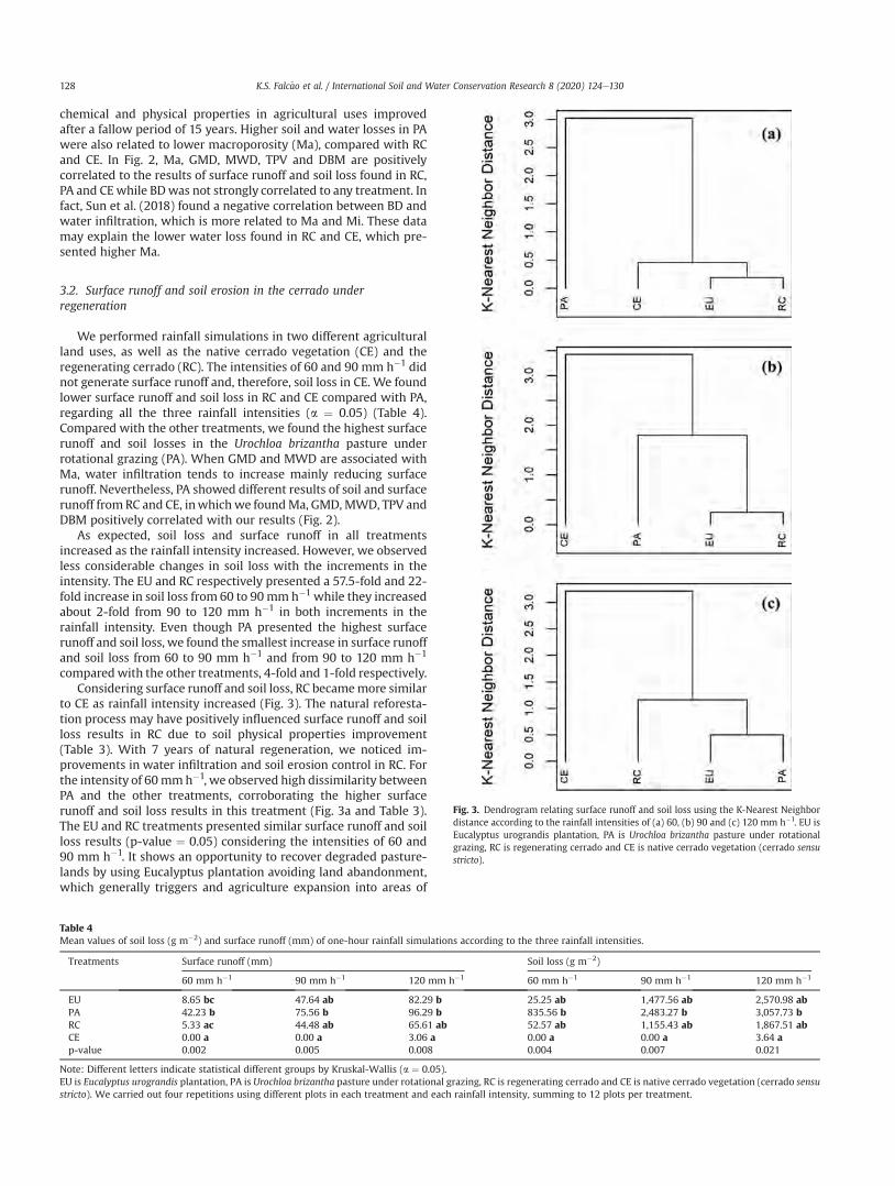
chemical and physical properties in agricultural uses improvedafter a fallow period of 15 years. Higher soil and water losses in PAwere also related to lower macroporosity (Ma), compared with RCand CE. In Fig. 2, Ma, GMD, MWD, TPV and DBM are positivelycorrelated to the results of surface runoff and soil loss found in RC,PA and CEwhile BDwas not strongly correlated to any treatment. Infact, Sun et al. (2018) found a negative correlation between BD andwater infiltration, which is more related to Ma and Mi. These datamay explain the lower water loss found in RC and CE, which pre-sented higher Ma.
3.2. Surface runoff and soil erosion in the cerrado underregeneration
We performed rainfall simulations in two different agriculturalland uses, as well as the native cerrado vegetation (CE) and theregenerating cerrado (RC). The intensities of 60 and 90 mm h�1 didnot generate surface runoff and, therefore, soil loss in CE. We foundlower surface runoff and soil loss in RC and CE compared with PA,regarding all the three rainfall intensities (a ¼ 0.05) (Table 4).Compared with the other treatments, we found the highest surfacerunoff and soil losses in the Urochloa brizantha pasture underrotational grazing (PA). When GMD and MWD are associated withMa, water infiltration tends to increase mainly reducing surfacerunoff. Nevertheless, PA showed different results of soil and surfacerunoff fromRC and CE, inwhich we foundMa, GMD,MWD, TPV andDBM positively correlated with our results (Fig. 2).
As expected, soil loss and surface runoff in all treatmentsincreased as the rainfall intensity increased. However, we observedless considerable changes in soil loss with the increments in theintensity. The EU and RC respectively presented a 57.5-fold and 22-fold increase in soil loss from 60 to 90mmh�1 while they increasedabout 2-fold from 90 to 120 mm h�1 in both increments in therainfall intensity. Even though PA presented the highest surfacerunoff and soil loss, we found the smallest increase in surface runoffand soil loss from 60 to 90 mm h�1 and from 90 to 120 mm h�1
comparedwith the other treatments, 4-fold and 1-fold respectively.Considering surface runoff and soil loss, RC becamemore similar
to CE as rainfall intensity increased (Fig. 3). The natural reforesta-tion process may have positively influenced surface runoff and soilloss results in RC due to soil physical properties improvement(Table 3). With 7 years of natural regeneration, we noticed im-provements in water infiltration and soil erosion control in RC. Forthe intensity of 60mmh�1, we observed high dissimilarity betweenPA and the other treatments, corroborating the higher surfacerunoff and soil loss results in this treatment (Fig. 3a and Table 3).The EU and RC treatments presented similar surface runoff and soilloss results (p-value ¼ 0.05) considering the intensities of 60 and90 mm h�1. It shows an opportunity to recover degraded pasture-lands by using Eucalyptus plantation avoiding land abandonment,which generally triggers and agriculture expansion into areas of
Table 4Mean values of soil loss (g m�2) and surface runoff (mm) of one-hour rainfall simulations according to the three rainfall intensities.
Treatments Surface runoff (mm) Soil loss (g m�2)
60 mm h�1 90 mm h�1 120 mm h�1 60 mm h�1 90 mm h�1 120 mm h�1
EU 8.65 bc 47.64 ab 82.29 b 25.25 ab 1,477.56 ab 2,570.98 abPA 42.23 b 75.56 b 96.29 b 835.56 b 2,483.27 b 3,057.73 bRC 5.33 ac 44.48 ab 65.61 ab 52.57 ab 1,155.43 ab 1,867.51 abCE 0.00 a 0.00 a 3.06 a 0.00 a 0.00 a 3.64 ap-value 0.002 0.005 0.008 0.004 0.007 0.021
Note: Different letters indicate statistical different groups by Kruskal-Wallis (a ¼ 0.05).EU is Eucalyptus urograndis plantation, PA is Urochloa brizantha pasture under rotational grazing, RC is regenerating cerrado and CE is native cerrado vegetation (cerrado sensustricto). We carried out four repetitions using different plots in each treatment and each rainfall intensity, summing to 12 plots per treatment.
Fig. 3. Dendrogram relating surface runoff and soil loss using the K-Nearest Neighbordistance according to the rainfall intensities of (a) 60, (b) 90 and (c) 120 mm h�1. EU isEucalyptus urograndis plantation, PA is Urochloa brizantha pasture under rotationalgrazing, RC is regenerating cerrado and CE is native cerrado vegetation (cerrado sensustricto).
K.S. Falc~ao et al. / International Soil and Water Conservation Research 8 (2020) 124e130128

natural vegetation. For both intensities of 90 and 120 mm h�1, wefound high dissimilarity between CE and the other agricultural landuses, including the RC (Fig. 3b and c).
With the increase in the rainfall intensity, RC became moresusceptible to the erosive power of rain. Since vegetation is notcompletely restored, fallow areas undergoing a regeneration pro-cess is less resilient to endure extreme events. Protective measureshave to be taken in order to protect those areas. The transitionperiod of reforestation is critical for water erosion. Every land use isprone to soil erosion independently of the land use/cover so thatadopting soil and water conservation practices is paramount,mainly in agricultural land uses recently converted from naturalvegetation. Agricultural land uses with adequate management maypresent soil erosion and infiltration rates similar to or less thanthose found in natural vegetation (Labri�ere, Locatelli, Laumonier,Freycon, & Bernoux, 2015; Sone et al., 2019). Especially in humidtropics such as in Brazil, soil erosion is rarely explained by human-managed or natural vegetation (Labri�ere et al., 2015). However, landmanagement plays a key role in the erosion process.
Conservation and preservation of regenerating and remnantareas are crucial for halting the increasing soil erosion rates in theCerrado, regarding its current deforestation scenario. Agriculturalland uses with poor management strategies deplete soil resourcesreducing soil security through a drastic reduction of the soilecosystem services. For instance, intrinsic to soil erosion anddegradation is the decrease in agricultural productivity, which, inturn, affects the water-food-energy security globally as Brazil playsan important role in the world’s food production. Other studieshave found different agricultural management strategies in order toincrease production while promoting the conservation of soil andwater resources.
4. Conclusions
We investigated soil erosion and surface runoff at a plot scale ina regenerating area of woodland Cerrado, comparing our observa-tion with natural and undisturbed Cerrado vegetation and twoagricultural land uses. We carried out 48 rainfall simulations withthree different rainfall intensities. We noted that the woodlandCerrado area under natural regeneration (RC) presented similar soilphysical properties and soil loss and surface runoff to the undis-turbed Cerrado (CE). The pasture area under rotational grazingpresented the highest soil loss and surface runoff, showing theimportance of having adequate agricultural management withadaptive stocking rates. In the long term, it avoids productivitydecrease and future land abandonment. In addition, eucalyptuscultivation seems to be an alternative for the recovery of degradedareas, but soil conservation practices should be adopted to increasesoil resilience during the highest rainfall intensity events.
We conclude that natural regeneration processes (degradedpasture to the cerrado vegetation) tend to increase infiltration anddecrease surface runoff and soil erosion. Therefore, it is importantto recover degraded areas before increasing the deforestation inundisturbed cerrado areas. Further studies comprising the hydro-logical responses in areas under regeneration with other Cerradophytophysiognomies and environmental characteristics areneeded. They will foster new knowledge and support for policy-makers to decide on subidies regarding a more efficient landcover and land use in this region.
Funding
This study was supported by the Ministry of Science, Technol-ogy, Innovation and Communication eMCTIC; National Council forScientific Technological Development e CNPq [grant numbers
441289/2017-7 and 306830/2017-5]; and the Coordination for theImprovement of Higher Education Personnel - Brasil (CAPES) -Finance Code 001 and CAPES PrInt.
Declaration of competing interest
None.
References
Almeida, W. S., Panachuki, E., Oliveira, P. T. S., Silva Menezes, R., Sobrinho, T. A., &Carvalho, D. F. (2018). Effect of soil tillage and vegetal cover on soil waterinfiltration. Soil and Tillage Research, 175, 130e138. https://doi.org/10.1016/j.still.2017.07.009.
Alves Sobrinho, T., G�omez-Macpherson, H., & G�omez, J. A. (2008). A portable inte-grated rainfall and overland flow simulator. Soil Use & Management, 24(2),163e170. https://doi.org/10.1111/j.1475-2743.2008.00150.x.
Anache, J. A. A., Wendland, E., Rosalem, L. M. P., Youlton, C., & Oliveira, P. T. S. (2019).Hydrological trade-offs due to different land covers and land uses in the Bra-zilian Cerrado. Hydrology and Earth System Sciences, 23(3), 1263e1279. https://doi.org/10.5194/hess-23-1263-2019.
Borlaug, N. E. (2002). Feeding a world of 10 billion people: The miracle ahead.In Vitro Cellular and Developmental Biology - Plant, 38(2), 221e228. https://doi.org/10.1079/IVP2001279.
Cardoso, D. P., Silva, M. L. N., De Carvalho, G. J., De Freitas, D. A. F., & Avanzi, J. C.(2012). Plantas de no controle das perdas de solo, �agua e nutrientes por eros~aohídrica. Revista Brasileira de Engenharia Agrícola e Ambiental, 16(6), 632e638.Retrieved from http://www.agriambi.com.br.
Cogo, N. P., Moldenhauer, W. C., & Foster, G. R. (1984). Soil loss reductions fromconservation tillage practices. Soil Science Society of America Journal, 48(2),368e373.
Dias-Filho, M. B. (2011). Degradaç~ao de pastagens: Processos, causas e estrat�egias derecuperaç~ao (4th ed.) Bel�em: Ediç~ao do Autor.
Embrapa. (2014). Sistema de observaç~ao e monitoramento da agricultura no Brasil:SOMA Brasil. Retrieved October 22, 2019, from https://mapas.cnpm.embrapa.br/somabrasil/webgis.html.
Foley, J. A. (2005). Global consequences of land use. Science, 309(5734), 570e574.https://doi.org/10.1126/science.1111772.
Hamza, M. A., & Anderson, W. K. (2005). Soil compaction in cropping systems. Soiland Tillage Research, 82(2), 121e145. https://doi.org/10.1016/j.still.2004.08.009.
Klink, C. A., & Machado, R. B. (2005). Conservation of the Brazilian cerrado. Con-servation Biology, 19(3), 707e713. https://doi.org/10.1111/j.1523-1739.2005.00702.x.
Labri�ere, N., Locatelli, B., Laumonier, Y., Freycon, V., & Bernoux, M. (2015). Soilerosion in the humid tropics: A systematic quantitative review. Agriculture,Ecosystems & Environment, 203, 127e139. https://doi.org/10.1016/j.agee.2015.01.027.
Lintemani, M. G., Loss, A., Mendes, C. S., & Fantini, A. C. (2019). Long fallows allowsoil regeneration in slash-and-burn agriculture. Journal of the Science of Foodand Agriculture, jsfa, 10123. https://doi.org/10.1002/jsfa.10123.
Myers, N., Mittermeier, R. A., Mittermeier, C. G., da Fonseca, G. A. B., & Kent, J.(2000). Biodiversity hotspots for conservation priorities. Nature, 403(6772),853e858. https://doi.org/10.1038/35002501.
Oliveira, P. T. S., Almagro, A., Colman, C. B., Kobayashi, A. N. A., Rodrigues, D. B. B.,Meira Neto, A. A., et al. (2019). Nexus of water-food-energy-ecosystem servicesin the Brazilian Cerrado. In R. C. Vieira da Silva, C. E. M. Tucci, & C. A. Scott (Eds.),Water and climate - modeling in large basins (5th ed., pp. 7e30). Porto Alegre:ABRHidro.
Oliveira, P. T. S., Nearing, M. A., Moran, M. S., Goodrich, D. C., Wendland, E., &Gupta, H. V. (2014). Trends in water balance components across the BrazilianCerrado. Water Resources Research, 50(9), 7100e7114. https://doi.org/10.1002/2013WR015202.
Oliveira, P. T. S., Nearing, M. A., & Wendland, E. (2015). Orders of magnitude increasein soil erosion associated with land use change from native to cultivatedvegetation in a Brazilian savannah environment. Earth Surface Processes andLandforms, 40(11), 1524e1532. https://doi.org/10.1002/esp.3738.
Oliveira, P. T. S., Wendland, E., Nearing, M. A., Scott, R. L., Rosolem, R., & daRocha, H. R. (2015). The water balance components of undisturbed tropicalwoodlands in the Brazilian cerrado. Hydrology and Earth System Sciences, 19(6),2899e2910. https://doi.org/10.5194/hess-19-2899-2015.
Panachuki, E., Bertol, I., Alves Sobrinho, T., Tarso Sanches de Oliveira, P., & BuchalaBicca Rodrigues, D. (2011). Perdas de solo e de �agua e infiltraç~ao de �agua emLatossolo vermelho sob sistemas de manejo. Revista Brasileira de Ciencia do Solo,35, 1777e1785.
Premanandh, J. (2011). Factors affecting food security and contribution of moderntechnologies in food sustainability. Journal of the Science of Food and Agriculture,91(15), 2707e2714. https://doi.org/10.1002/jsfa.4666.
Ribeiro, A., Ribeiro, A. dos S., Mincato, R. L., Curi, N., & Kawakubo, F. S. (2016).Environmental vulnerability to water erosion in a hydrographic sub-basin byanalytic hierarchy process. Revista Brasileira de Geografia Física, 9(1). https://doi.org/10.26848/rbgf.v9.1.p016-031, 016e031.
Sano, E. E., Rosa, R., Brito, J. L. S., & Ferreira, L. G. (2010). Land cover mapping of the
K.S. Falc~ao et al. / International Soil and Water Conservation Research 8 (2020) 124e130 129

tropical savanna region in Brazil. Environmental Monitoring and Assessment,166(1e4), 113e124. https://doi.org/10.1007/s10661-009-0988-4.
Santos, G. G., Figueiredo, C. C., Oliveira, L. F. C., & Griebeler, N. P. (2009). Intensidade-duraç~ao-frequencia de chuvas para o Estado de Mato Grosso do Sul. RevistaBrasileira de Engenharia Agrícola e Ambiental, 13, 899e905.
Sartori, M., Philippidis, G., Ferrari, E., Borrelli, P., Lugato, E., Montanarella, L., et al.(2019). A linkage between the biophysical and the economic: Assessing theglobal market impacts of soil erosion. Land Use Policy, 86, 299e312. https://doi.org/10.1016/j.landusepol.2019.05.014.
Sena, M., Frighetto, R. T., Valarini, P., Tokeshi, H., & Poppi, R. (2002). Discriminationof management effects on soil parameters by using principal componentanalysis: A multivariate analysis case study. Soil and Tillage Research, 67(2),171e181. https://doi.org/10.1016/S0167-1987(02)00063-6.
Sone, J. S., Oliveira, P. T. S., Zamboni, P. A. P., Vieira, N. O. M., Carvalho, G. A.,Macedo, M. C. M., et al. (2019). Effects of long-term crop-livestock-forestrysystems on soil erosion and water infiltration in a Brazilian cerrado site. Sus-tainability, 11(19), 5339. https://doi.org/10.3390/su11195339.
Spangenberg, A., Grimm, U., Sepeda da Silva, J. R., & F€olster, H. (1996). Nutrient storeand export rates of Eucalyptus urograndis plantations in eastern Amazonia
(Jari). Forest Ecology and Management, 80(1e3), 225e234. https://doi.org/10.1016/0378-1127(95)03615-6.
Sun, D., Yang, H., Guan, D., Yang, M., Wu, J., Yuan, F., et al. (2018). The effects of landuse change on soil infiltration capacity in China: A meta-analysis. The Science ofthe Total Environment, 626, 1394e1401. https://doi.org/10.1016/j.scitotenv.2018.01.104.
Teixeira, P. C., Donagemma, G. K., Fontana, A., Teixeira, W. G., & Martins, E. de S.(2017). Manual de m�etodos de an�alise de solo. Embrapa (3rd ed.). Brasilia:Embrapa.
Yoder, R. E. (1936). A direct method of aggregate analysis of soils and a study of thephysical nature of erosion Losses1. Agronomy Journal, 28(5), 337. https://doi.org/10.2134/agronj1936.00021962002800050001x.
Zinn, Y. L., Lal, R., & Resck, D. V. S. (2005). Changes in soil organic carbon stocksunder agriculture in Brazil. Soil and Tillage Research, 84(1), 28e40. https://doi.org/10.1016/j.still.2004.08.007.
Zinn, Y., Resck, D. V. S., & da Silva, J. E. (2002). Soil organic carbon as affected byafforestation with Eucalyptus and Pinus in the Cerrado region of Brazil. ForestEcology and Management, 166(1e3), 285e294. https://doi.org/10.1016/S0378-1127(01)00682-X.
K.S. Falc~ao et al. / International Soil and Water Conservation Research 8 (2020) 124e130130
Original Research Article
Effect of joint structure and slope direction on the development ofcollapsing gully in tuffaceous sandstone area in South China
Yusong Deng a, *, Xiaoqian Duan b, Shuwen Ding b, Chongfa Cai b, **
a Forestry College of Guangxi University, Nanning, Guangxi, 530004, Chinab College of Resources and Environment of Huazhong Agricultural University, Wuhan, Hubei, 430070, China
a r t i c l e i n f o
Article history:Received 19 December 2019Received in revised form31 March 2020Accepted 2 April 2020Available online 17 April 2020
Keywords:Soil erosionJointSlope directionMain gullyBranch gully
a b s t r a c t
This study focuses on the collapsing gullies in tuffaceous sandstone area and investigates the slope di-rection and morphological characteristics of the main and branch gullies. Furthermore, we assess thestructural characteristics of the rock joints within this area, including their strike, dip direction and dipangle. The results show that there are 405 collapsing gullies in the study area. The slope directionsassociated with collapsing gullies and the directions of the main gullies largely fall within the ranges ofNE20�-NE90�, SE90�-SE160�, SW240�-SW270�, and NW270�-NW290�. The collapsing gullies include1103 branch gullies in total, most of which have directions that fall within the ranges of NE20�-NE40�,NE50�-NE70�, NW280�-NW300�, and NW330�-NW350�. The joints in the bedrock are directional andregional, and they can be divided into two main groups. The number of southward dip directions isgreater than the number of northward dip directions, and most of the measured dip angles are greaterthan 60�. The mean dip angle is greatest for joints with measured strike values of NW280�-NW290�, witha value of 85.2�. The development of collapse gullies is affected by both the slope direction and joints. Theslope direction determines the direction of the main gullies, with a correlation coefficient of 0.809(P<0.01). The branch gullies are mainly affected by joints, with a correlation coefficient of 0.876 (P<0.01).The joint structure also influences the degree of development of the collapsing gullies, and the averagedepth of the gullies that parallel the dominant joint orientation is significantly larger than that of gullieswith other directions. Moreover, the average depth of the gullies associated with the dip angle of 85.2�
measured relative to the joint strike is 6.89 m, which is significantly greater than that associated withlower dip angles. The dip angles of joints have an important effect on the infiltration of water, and highdip angles accelerate the erosion associated with collapsing gullies.© 2020 International Research and Training Center on Erosion and Sedimentation and China Water andPower Press. Production and Hosting by Elsevier B.V. This is an open access article under the CC BY-NC-
ND license (http://creativecommons.org/licenses/by-nc-nd/4.0/).
1. Introduction
Gully erosion is a form of surface runoff that washes away theparent material and cuts into the surface, which is one of the maintypes of soil erosion in gully regions (Wells et al., 2013; Yan et al.,2015). Collapse gully is a special gully erosion phenomenon in thetropical and subtropical hilly areas of China in which the slope soilis disturbed, washed away and collapses downslope under the joint
action of hydraulic processes and gravity. This process is catego-rized as a mixed soil erosion process, which is referred to asBenggang by locals (Deng et al., 2017; Jiang et al., 2014; Xia, Deng,Wang, Ding, & Cai, 2015; Xu, 1996). These features have becomethe most serious form of soil erosion in South China and causedconsiderable harm to the regional ecological environment, so as tohave a significant impact on the sustainable economic and socialdevelopment (Feng, Liao, Li, & Lu, 2009; Zhong, Peng, Zhang, Ma, &Gao, 2013). In recent years, it has become the focus of research andattracted the attention of many scholars. Previous studies mainlyfocused on the hazards of collapsing gully, including regional dis-tribution, formation process and soil stability (Deng et al., 2017;Liao et al., 2019; Lin et al., 2015; Luk et al., 1997; Shi, 1984; Xu &Zeng, 1992). However, according to the statistics on collapsinggullies reported by the Chinese Ministry of Water Resources in
* Corresponding author.** Corresponding author. Forestry College of Guangxi University, Nanning 530004,China.
E-mail addresses: [email protected] (Y. Deng), [email protected] (X. Duan), [email protected] (S. Ding), [email protected](C. Cai).
Contents lists available at ScienceDirect
International Soil and Water Conservation Research
journal homepage: www.elsevier .com/locate/ iswcr
https://doi.org/10.1016/j.iswcr.2020.04.0032095-6339/© 2020 International Research and Training Center on Erosion and Sedimentation and China Water and Power Press. Production and Hosting by Elsevier B.V. Thisis an open access article under the CC BY-NC-ND license (http://creativecommons.org/licenses/by-nc-nd/4.0/).
International Soil and Water Conservation Research 8 (2020) 131e140
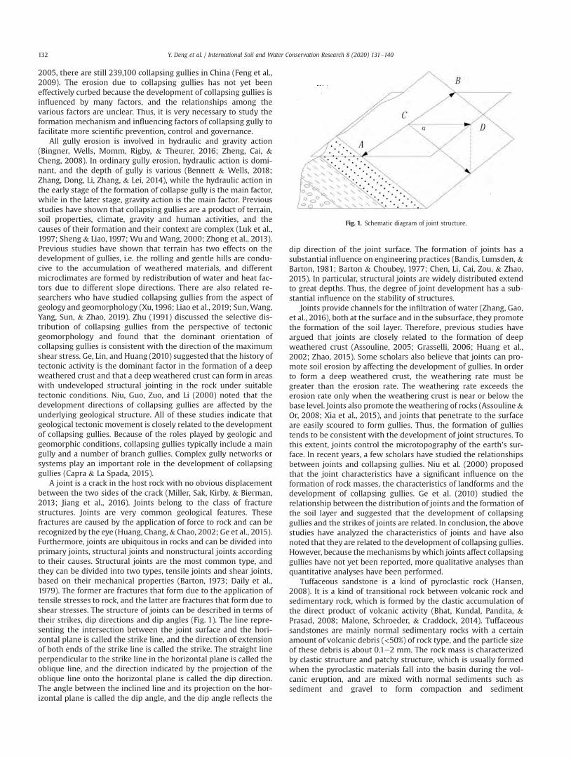
2005, there are still 239,100 collapsing gullies in China (Feng et al.,2009). The erosion due to collapsing gullies has not yet beeneffectively curbed because the development of collapsing gullies isinfluenced by many factors, and the relationships among thevarious factors are unclear. Thus, it is very necessary to study theformation mechanism and influencing factors of collapsing gully tofacilitate more scientific prevention, control and governance.
All gully erosion is involved in hydraulic and gravity action(Bingner, Wells, Momm, Rigby, & Theurer, 2016; Zheng, Cai, &Cheng, 2008). In ordinary gully erosion, hydraulic action is domi-nant, and the depth of gully is various (Bennett & Wells, 2018;Zhang, Dong, Li, Zhang, & Lei, 2014), while the hydraulic action inthe early stage of the formation of collapse gully is the main factor,while in the later stage, gravity action is the main factor. Previousstudies have shown that collapsing gullies are a product of terrain,soil properties, climate, gravity and human activities, and thecauses of their formation and their context are complex (Luk et al.,1997; Sheng & Liao, 1997; Wu and Wang, 2000; Zhong et al., 2013).Previous studies have shown that terrain has two effects on thedevelopment of gullies, i.e. the rolling and gentle hills are condu-cive to the accumulation of weathered materials, and differentmicroclimates are formed by redistribution of water and heat fac-tors due to different slope directions. There are also related re-searchers who have studied collapsing gullies from the aspect ofgeology and geomorphology (Xu,1996; Liao et al., 2019; Sun,Wang,Yang, Sun, & Zhao, 2019). Zhu (1991) discussed the selective dis-tribution of collapsing gullies from the perspective of tectonicgeomorphology and found that the dominant orientation ofcollapsing gullies is consistent with the direction of the maximumshear stress. Ge, Lin, and Huang (2010) suggested that the history oftectonic activity is the dominant factor in the formation of a deepweathered crust and that a deep weathered crust can form in areaswith undeveloped structural jointing in the rock under suitabletectonic conditions. Niu, Guo, Zuo, and Li (2000) noted that thedevelopment directions of collapsing gullies are affected by theunderlying geological structure. All of these studies indicate thatgeological tectonic movement is closely related to the developmentof collapsing gullies. Because of the roles played by geologic andgeomorphic conditions, collapsing gullies typically include a maingully and a number of branch gullies. Complex gully networks orsystems play an important role in the development of collapsinggullies (Capra & La Spada, 2015).
A joint is a crack in the host rock with no obvious displacementbetween the two sides of the crack (Miller, Sak, Kirby, & Bierman,2013; Jiang et al., 2016). Joints belong to the class of fracturestructures. Joints are very common geological features. Thesefractures are caused by the application of force to rock and can berecognized by the eye (Huang, Chang,& Chao, 2002; Ge et al., 2015).Furthermore, joints are ubiquitous in rocks and can be divided intoprimary joints, structural joints and nonstructural joints accordingto their causes. Structural joints are the most common type, andthey can be divided into two types, tensile joints and shear joints,based on their mechanical properties (Barton, 1973; Daily et al.,1979). The former are fractures that form due to the application oftensile stresses to rock, and the latter are fractures that form due toshear stresses. The structure of joints can be described in terms oftheir strikes, dip directions and dip angles (Fig. 1). The line repre-senting the intersection between the joint surface and the hori-zontal plane is called the strike line, and the direction of extensionof both ends of the strike line is called the strike. The straight lineperpendicular to the strike line in the horizontal plane is called theoblique line, and the direction indicated by the projection of theoblique line onto the horizontal plane is called the dip direction.The angle between the inclined line and its projection on the hor-izontal plane is called the dip angle, and the dip angle reflects the
dip direction of the joint surface. The formation of joints has asubstantial influence on engineering practices (Bandis, Lumsden, &Barton, 1981; Barton & Choubey, 1977; Chen, Li, Cai, Zou, & Zhao,2015). In particular, structural joints are widely distributed extendto great depths. Thus, the degree of joint development has a sub-stantial influence on the stability of structures.
Joints provide channels for the infiltration of water (Zhang, Gao,et al., 2016), both at the surface and in the subsurface, they promotethe formation of the soil layer. Therefore, previous studies haveargued that joints are closely related to the formation of deepweathered crust (Assouline, 2005; Grasselli, 2006; Huang et al.,2002; Zhao, 2015). Some scholars also believe that joints can pro-mote soil erosion by affecting the development of gullies. In orderto form a deep weathered crust, the weathering rate must begreater than the erosion rate. The weathering rate exceeds theerosion rate only when the weathering crust is near or below thebase level. Joints also promote theweathering of rocks (Assouline&Or, 2008; Xia et al., 2015), and joints that penetrate to the surfaceare easily scoured to form gullies. Thus, the formation of gulliestends to be consistent with the development of joint structures. Tothis extent, joints control the microtopography of the earth’s sur-face. In recent years, a few scholars have studied the relationshipsbetween joints and collapsing gullies. Niu et al. (2000) proposedthat the joint characteristics have a significant influence on theformation of rock masses, the characteristics of landforms and thedevelopment of collapsing gullies. Ge et al. (2010) studied therelationship between the distribution of joints and the formation ofthe soil layer and suggested that the development of collapsinggullies and the strikes of joints are related. In conclusion, the abovestudies have analyzed the characteristics of joints and have alsonoted that they are related to the development of collapsing gullies.However, because themechanisms bywhich joints affect collapsinggullies have not yet been reported, more qualitative analyses thanquantitative analyses have been performed.
Tuffaceous sandstone is a kind of pyroclastic rock (Hansen,2008). It is a kind of transitional rock between volcanic rock andsedimentary rock, which is formed by the clastic accumulation ofthe direct product of volcanic activity (Bhat, Kundal, Pandita, &Prasad, 2008; Malone, Schroeder, & Craddock, 2014). Tuffaceoussandstones are mainly normal sedimentary rocks with a certainamount of volcanic debris (<50%) of rock type, and the particle sizeof these debris is about 0.1e2 mm. The rock mass is characterizedby clastic structure and patchy structure, which is usually formedwhen the pyroclastic materials fall into the basin during the vol-canic eruption, and are mixed with normal sediments such assediment and gravel to form compaction and sediment
Fig. 1. Schematic diagram of joint structure.
Y. Deng et al. / International Soil and Water Conservation Research 8 (2020) 131e140132
cementation. The composition of tuffaceous sandstone includesclastic and interstitial materials, and the clastic materials aremainly quartz, feldspar, mica, etc. the interstitial materials are alsodivided into hetero base and cement, and the high hetero basecomponents are kaolin, hydromica, etc. (Zhen, Wang, Chen, Yan, &Tao, 2010). The joints of tuffaceous sandstone are highly developed,and the rock blocks are easy to be broken, which are mainlydistributed on the surface of side slope. The developed soil is easyto disintegrate or even muddy under the action of rainfall or drywet cycle (Critelli, Marsaglia, & Busby, 2002). However, there arefew researches on the phenomenon and mechanism of soil erosionin tuffaceous sandstone area.
In this study, we focus on the effect of joint structure and slopeaspect on the development of collapsing gully. According to theclimate and geographical conditions, collapsing gullies wereselected in tuffaceous sandstone area in Yudu County of SouthChina. The objectives of this study are: (i) to investigate the dis-tribution characteristics of collapsing gullies and the direction anddevelopment degree of main and branch gullies; (ii) to study thecharacteristics of strikes, dip directions and dip angles of joints oftuffaceous sandstone in collapsing gully area; (iii) to explore theinfluence of joint structure and slope direction on the developmentdirection and degree of collapsing gully. Our results can provide thebasis for the development mechanism and control measures ofcollapsing gully, and also provide the theory for the influence ofjoints on gully erosion.
2. Materials and methods
2.1. Study area
The study area is located in south-central Jiangxi Province(115�110-115�490 E, 25�350-26�210 N) in southeastern China. YuduCounty experiences a typical subtropical humid monsoon climatewith an annual average temperature of 19.7 �C, and the extremetemperature is 39.9 h and �8 n. The frost-free period is up to 305days, and the annual precipitation is 1507 mm, the rainfall fromApril to May accounts for about 47% of the whole year, and theannual sunshine hours are 1621.9 h. The dominant soil types foundin the county are acidic red soils (Ultisols). Yudu County is locatedin the north end of the third-order structural unit of the Caledonianfold system in South China. The landform in the territory is com-plex. The terrain in the south, East and north directions is relativelyhigh, and gradually inclines to the central and western regions,which forms a closed low mountain and hilly terrain mainlycomposed of hills, low mountains and basins and converged bylarge and small rivers. The parent material of the study area istypical tuffaceous sandstone. The land use pattern is the mixture ofsparse secondary grass and shrub. The main vegetation typesinclude Pinus massoniana, Dicranopteris linearis, Lespedeza bicolor,etc. The special topography and the characteristics of tuffaceoussandstone create conditions for soil erosion. Yudu county is one ofthe counties with the most serious soil erosion in Jiangxi Province.The area of soil erosion in the whole county is 843.82 km2, ac-counting for 29.17% of the total area of land, and the moderateerosion above 64.01% of the total area of soil erosion. There areabout 4062 collapsing gullies in the county, with an area of1738.4 hm2, accounting for 8.41% of the total area of collapsinggullies in Jiangxi Province. Active collapsing gullies account for98.74% of the total number of collapsing gullies and 98.82% of thetotal erosion area, while relatively stable collapsing gullies onlyaccount for 1.26% of the total number and 1.18% of the total erosionarea, which reflects that most of the collapsing gullies in Yudu aremainly active, indicating that most of them are in the stage ofvigorous development (Zhao, Tang, & Niu, 2014).
2.2. Investigation method
We selected a typical area containing collapsing gullies in Jin-qiao village in Yudu County, and a total of 405 collapsing gullieswere investigated and analyzed (Fig. 2). Each collapsing gully has itsown main ditch, a total of 405 main gullies are counted, and eachcollapsing gully has several branch gullies, and our research has atotal of 1103 branch gullies. The field investigation included mea-surements of the slope direction associated with the collapsinggullies, the directions of the main gullies and the branch gullies andthe depths of the gullies. The slopes and the directions of the maingullies and branch gullies were measured using a geological com-pass (DQY-1). Before measuring the target orientation, it is neces-sary to calibrate the geological compass. Then stand on the top ofthe main and branch gullies, hold the instrument tightly and stickto the body to reduce shaking, and measure the direction of thegullies. Finally, the compass is adjusted to the center of the bubble,and the magnetic needle indicates the direction in which the targetis located. The same operation is applied to the direction of thehillside. The depths of the gullies were measured using a Laserrangefinder (SWe600S). Considering that some gullies are toowide, we use laser rangefinder to measure the distance from bothsides to the deepest part of the gullies. The depth of gullies iscalculated from the angle, which can be determined by multiplyingthe measured distance by the sine value of the angle. In addition,we selected typical areas to measure the structure of the joints.
In order to ensure the representativeness of rock joint mea-surement, we randomly selected the surroundings of 6 collapsinggullies to investigate the joints of tuffaceous sandstone. In eacharea, a sample of 1 m � 1 m is selected to measure the basic situ-ation of the joint, including the strikes, dip directions, and dipangles. A total of 525 joints are counted. The density of the 6selected joint investigation sample areas is highly dense. Somesample areas have the joint density of more than 100 pieces/m2,and some are less than 30 pieces/m2, most of the rock mass is cut tobe highly broken. The strike of the joint is very complex, there areobviously conjugate joints, the average joint fissure degree is about0.05 m, the maximum is more than 0.30 m, the minimum is only0.002 m. The joints in the rock mass are very obvious. The fillingmaterial in the fissures developed from joints is quartz. After therock developed into soil, it can be seen that the quartz vein can cutthe complete soil into very broken pieces, and finally cut intoseveral small soil blocks. In the structure measurement of tuffa-ceous sandstone, the long side of the geological compass shall beclose to the rock stratum, and then the compass shall be rotated tocenter the blister of the chassis level. The scale indicated by thereading pointer is the strike of the joint. The dip directions mea-surement operation is to press the compass against the rock surfaceand rotate it to center the blister of the chassis level, and read thescale indicated by the compass. The dip angle measurement is toensure that the compass is upright, and move the compass alongthe rock surfacewith a long side against the inclined line of the rocklayer, and adjust the movable button at the bottom of the compassto center the bubble and read out the maximum value.
The soil erosion in the study area is very serious, most of thesoils in the A layers are eroded, and the soils in the B layers areexposed. The gully heads mainly include three soil configurations:A-B-C, BeC and C. The A-B-C configuration is the least of the threesoil configurations, followed by the BeC configuration, and themost of the C configuration. As a result, there is little original redsoil on the surface of the gully area, and almost all of the gullies aregray white soil in the early stage of tuffaceous sandstone devel-opment. The soils of A and B layers are relatively viscous and havelow erodibility, while the soils of C layers have loose texture, weakcementation and strong erodibility. We randomly selected several
Y. Deng et al. / International Soil and Water Conservation Research 8 (2020) 131e140 133
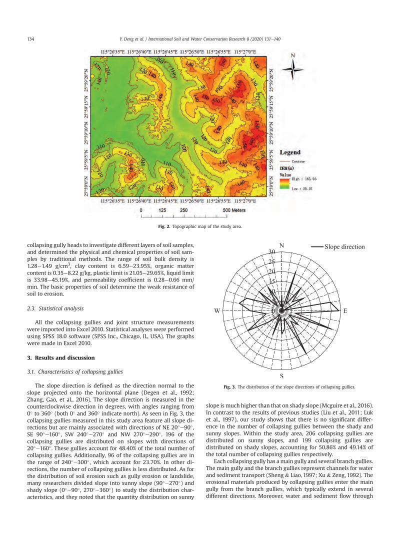
collapsing gully heads to investigate different layers of soil samples,and determined the physical and chemical properties of soil sam-ples by traditional methods. The range of soil bulk density is1.28e1.49 g/cm3, clay content is 6.59e23.95%, organic mattercontent is 0.35e8.22 g/kg, plastic limit is 21.05e29.65%, liquid limitis 33.98e45.19%, and permeability coefficient is 0.28e0.66 mm/min. The basic properties of soil determine the weak resistance ofsoil to erosion.
2.3. Statistical analysis
All the collapsing gullies and joint structure measurementswere imported into Excel 2010. Statistical analyses were performedusing SPSS 18.0 software (SPSS Inc., Chicago, IL, USA). The graphswere made in Excel 2010.
3. Results and discussion
3.1. Characteristics of collapsing gullies
The slope direction is defined as the direction normal to theslope projected onto the horizontal plane (Degen et al., 1992;Zhang, Gao, et al., 2016). The slope direction is measured in thecounterclockwise direction in degrees, with angles ranging from0� to 360� (both 0� and 360� indicate north). As seen in Fig. 3, thecollapsing gullies measured in this study area feature all slope di-rections but are mainly associated with directions of NE 20�e90�,SE 90�e160�, SW 240�e270� and NW 270�e290�. 196 of thecollapsing gullies are distributed on slopes with directions of20�e160�. These gullies account for 48.40% of the total number ofcollapsing gullies. Additionally, 96 of the collapsing gullies are inthe range of 240�e300�, which account for 23.70%. In other di-rections, the number of collapsing gullies is less distributed. As forthe distribution of soil erosion such as gully erosion or landslide,many researchers divided slope into sunny slope (90�e270�) andshady slope (0�e90�, 270�e360�) to study the distribution char-acteristics, and they noted that the quantity distribution on sunny
slope is much higher than that on shady slope (Mcguire et al., 2016).In contrast to the results of previous studies (Liu et al., 2011; Luket al., 1997), our study shows that there is no significant differ-ence in the number of collapsing gullies between the shady andsunny slopes. Within the study area, 206 collapsing gullies aredistributed on sunny slopes, and 199 collapsing gullies aredistributed on shady slopes, accounting for 50.86% and 49.14% ofthe total number of collapsing gullies respectively.
Each collapsing gully has amain gully and several branch gullies.The main gully and the branch gullies represent channels for waterand sediment transport (Sheng & Liao, 1997; Xu & Zeng, 1992). Theerosional materials produced by collapsing gullies enter the maingully from the branch gullies, which typically extend in severaldifferent directions. Moreover, water and sediment flow through
Fig. 2. Topographic map of the study area.
Fig. 3. The distribution of the slope directions of collapsing gullies.
Y. Deng et al. / International Soil and Water Conservation Research 8 (2020) 131e140134
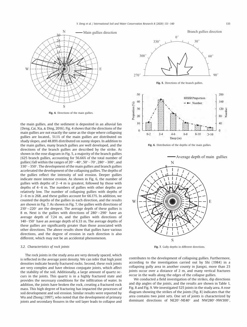
the main gullies, and the sediment is deposited in an alluvial fan(Deng, Cai, Xia,& Ding, 2016). Fig. 4 shows that the directions of themain gullies are not exactly the same as the slope where collapsinggullies are located., 51.1% of the main gullies are distributed onshady slopes, and 48.89% distributed on sunny slopes. In addition tothe main gullies, many branch gullies are well developed, and thedirections of the branch gullies are described by the strike. Asshown in the rose diagram in Fig. 5, a majority of the branch gullies(625 branch gullies, accounting for 56.66% of the total number ofgullies) fall within the ranges of 20�e40�, 50�e70�, 280�e300�, and330�e350�. The development of themain gullies and branch gulliesaccelerated the development of the collapsing gullies. The depths ofthe gullies reflect the intensity of soil erosion. Deeper gulliesindicate more intense erosion. As shown in Fig. 6, the number ofgullies with depths of 2e4 m is greatest, followed by those withdepths of 4e6 m. The numbers of gullies with other depths arerelatively low. The number of collapsing gullies with depths of2e6 m is 268, and these gullies account for 66.17%. In addition, wecounted the depths of the gullies in each direction, and the resultsare shown in Fig. 7. As shown in Fig. 7, the gullies with directions of210�e220� are the deepest. The average depth of these gullies is8 m. Next is the gullies with directions of 280�e290� have anaverage depth of 7.24 m, and the gullies with directions of140e150� have an average depth of 6.33 m. The average depths ofthese gullies are significantly greater than those associated withother directions. The above results show that gullies have variousdirections, and the degree of erosion in each direction is alsodifferent, which may not be an accidental phenomenon.
3.2. Characteristics of rock joints
The rock joints in the study area are very densely spaced, whichis reflected in the average joint density. We can infer that high jointdensities indicate heavily fractured rocks. Second, these rock jointsare very complex and have obvious conjugate joints, which affectthe stability of the soil. Additionally, a large amount of quartz oc-curs in the joints. This quartz is in a highly fractured state andprovides the necessary conditions for the infiltration of water. Inaddition, the joints have broken the rock, creating a fractured rockmass. This high degree of fracturing has impacted the processes ofsoil development and soil erosion. Similar results were reported byWu and Zhong (1997), who noted that the development of primaryjoints and secondary fissures in the soil layer leads to collapse and
contributes to the development of collapsing gullies. Furthermore,according to the investigation carried out by Shi (1984) in acollapsing gully area in another county in Jiangxi, more than 23joints occur over a distance of 2 m, and many vertical fracturesoccur in the walls along the edges of the collapse gullies.
We conducted a field investigation of the strikes, dip directionsand dip angles of the joints, and the results are shown in Table 1,Fig. 8 and Fig. 9. We investigated 525 joints in the study area. A rosediagram showing the strikes of the joints (Fig. 8) indicates that thearea contains two joint sets. One set of joints is characterized bydominant directions of NE20�-NE40� and NW280�-NW300�,
Fig. 4. Directions of the main gullies.
Fig. 5. Directions of the branch gullies.
Fig. 6. Distribution of the depths of the main gullies.
Fig. 7. Gully depths in different directions.
Y. Deng et al. / International Soil and Water Conservation Research 8 (2020) 131e140 135
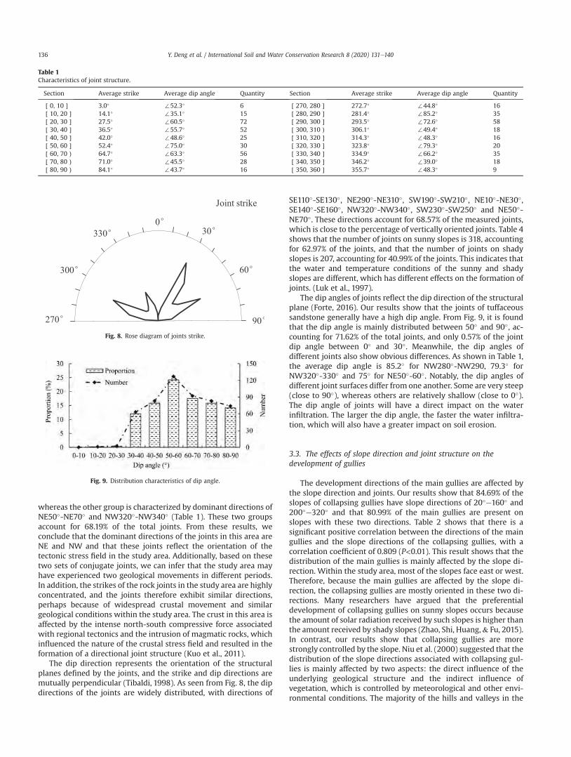
whereas the other group is characterized by dominant directions ofNE50�-NE70� and NW320�-NW340� (Table 1). These two groupsaccount for 68.19% of the total joints. From these results, weconclude that the dominant directions of the joints in this area areNE and NW and that these joints reflect the orientation of thetectonic stress field in the study area. Additionally, based on thesetwo sets of conjugate joints, we can infer that the study area mayhave experienced two geological movements in different periods.In addition, the strikes of the rock joints in the study area are highlyconcentrated, and the joints therefore exhibit similar directions,perhaps because of widespread crustal movement and similargeological conditions within the study area. The crust in this area isaffected by the intense north-south compressive force associatedwith regional tectonics and the intrusion of magmatic rocks, whichinfluenced the nature of the crustal stress field and resulted in theformation of a directional joint structure (Kuo et al., 2011).
The dip direction represents the orientation of the structuralplanes defined by the joints, and the strike and dip directions aremutually perpendicular (Tibaldi, 1998). As seen from Fig. 8, the dipdirections of the joints are widely distributed, with directions of
SE110�-SE130�, NE290�-NE310�, SW190�-SW210�, NE10�-NE30�,SE140�-SE160�, NW320�-NW340�, SW230�-SW250� and NE50�-NE70�. These directions account for 68.57% of the measured joints,which is close to the percentage of vertically oriented joints. Table 4shows that the number of joints on sunny slopes is 318, accountingfor 62.97% of the joints, and that the number of joints on shadyslopes is 207, accounting for 40.99% of the joints. This indicates thatthe water and temperature conditions of the sunny and shadyslopes are different, which has different effects on the formation ofjoints. (Luk et al., 1997).
The dip angles of joints reflect the dip direction of the structuralplane (Forte, 2016). Our results show that the joints of tuffaceoussandstone generally have a high dip angle. From Fig. 9, it is foundthat the dip angle is mainly distributed between 50� and 90�, ac-counting for 71.62% of the total joints, and only 0.57% of the jointdip angle between 0� and 30�. Meanwhile, the dip angles ofdifferent joints also show obvious differences. As shown in Table 1,the average dip angle is 85.2� for NW280�-NW290, 79.3� forNW320�-330� and 75� for NE50�-60�. Notably, the dip angles ofdifferent joint surfaces differ from one another. Some are very steep(close to 90�), whereas others are relatively shallow (close to 0�).The dip angle of joints will have a direct impact on the waterinfiltration. The larger the dip angle, the faster the water infiltra-tion, which will also have a greater impact on soil erosion.
3.3. The effects of slope direction and joint structure on thedevelopment of gullies
The development directions of the main gullies are affected bythe slope direction and joints. Our results show that 84.69% of theslopes of collapsing gullies have slope directions of 20�e160� and200�e320� and that 80.99% of the main gullies are present onslopes with these two directions. Table 2 shows that there is asignificant positive correlation between the directions of the maingullies and the slope directions of the collapsing gullies, with acorrelation coefficient of 0.809 (P<0.01). This result shows that thedistribution of the main gullies is mainly affected by the slope di-rection. Within the study area, most of the slopes face east or west.Therefore, because the main gullies are affected by the slope di-rection, the collapsing gullies are mostly oriented in these two di-rections. Many researchers have argued that the preferentialdevelopment of collapsing gullies on sunny slopes occurs becausethe amount of solar radiation received by such slopes is higher thanthe amount received by shady slopes (Zhao, Shi, Huang,& Fu, 2015).In contrast, our results show that collapsing gullies are morestrongly controlled by the slope. Niu et al. (2000) suggested that thedistribution of the slope directions associated with collapsing gul-lies is mainly affected by two aspects: the direct influence of theunderlying geological structure and the indirect influence ofvegetation, which is controlled by meteorological and other envi-ronmental conditions. The majority of the hills and valleys in the
Table 1Characteristics of joint structure.
Section Average strike Average dip angle Quantity Section Average strike Average dip angle Quantity
[0, 10] 3.0� :52.3� 6 [270, 280] 272.7� :44.8� 16[10, 20] 14.1� :35.1� 15 [280, 290] 281.4� :85.2� 35[20, 30] 27.5� :60.5� 72 [290, 300] 293.5� :72.6� 58[30, 40] 36.5� :55.7� 52 [300, 310) 306.1� :49.4� 18[40, 50] 42.0� :48.6� 25 [310, 320] 314.3� :48.3� 16[50, 60] 52.4� :75.0� 30 [320, 330] 323.8� :79.3� 20[60, 70) 64.7� :63.3� 56 [330, 340] 334.9� :66.2� 35[70, 80) 71.0� :45.5� 28 [340, 350] 346.2� :39.0� 18[80, 90) 84.1� :43.7� 16 [350, 360] 355.7� :48.3� 9
Fig. 8. Rose diagram of joints strike.
Fig. 9. Distribution characteristics of dip angle.
Y. Deng et al. / International Soil and Water Conservation Research 8 (2020) 131e140136
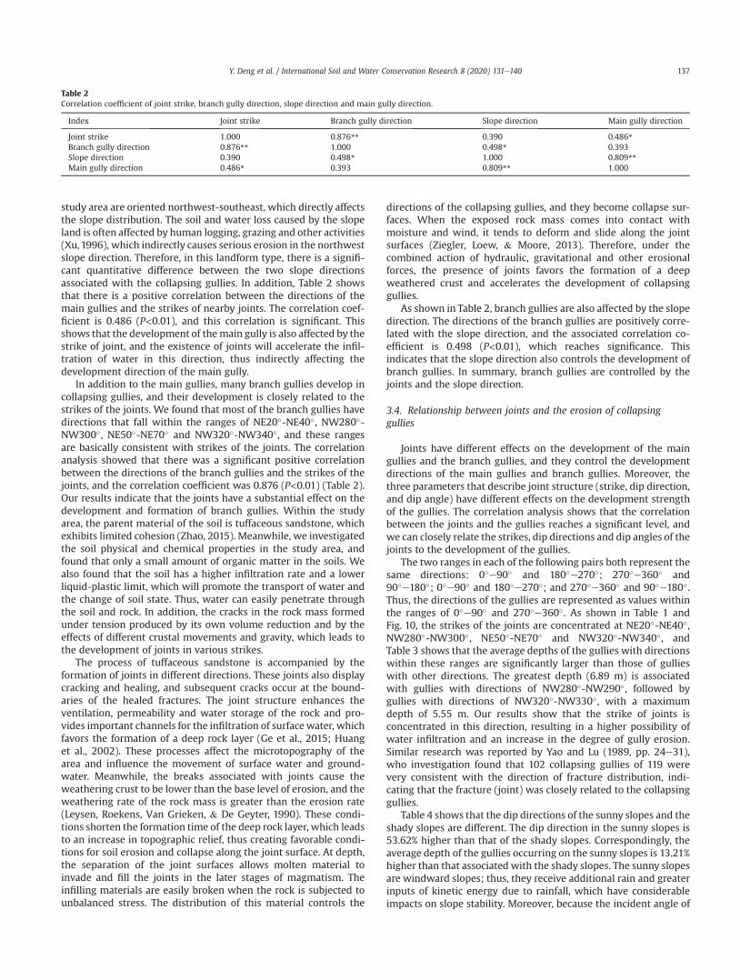
study area are oriented northwest-southeast, which directly affectsthe slope distribution. The soil and water loss caused by the slopeland is often affected by human logging, grazing and other activities(Xu,1996), which indirectly causes serious erosion in the northwestslope direction. Therefore, in this landform type, there is a signifi-cant quantitative difference between the two slope directionsassociated with the collapsing gullies. In addition, Table 2 showsthat there is a positive correlation between the directions of themain gullies and the strikes of nearby joints. The correlation coef-ficient is 0.486 (P<0.01), and this correlation is significant. Thisshows that the development of themain gully is also affected by thestrike of joint, and the existence of joints will accelerate the infil-tration of water in this direction, thus indirectly affecting thedevelopment direction of the main gully.
In addition to the main gullies, many branch gullies develop incollapsing gullies, and their development is closely related to thestrikes of the joints. We found that most of the branch gullies havedirections that fall within the ranges of NE20�-NE40�, NW280�-NW300�, NE50�-NE70� and NW320�-NW340�, and these rangesare basically consistent with strikes of the joints. The correlationanalysis showed that there was a significant positive correlationbetween the directions of the branch gullies and the strikes of thejoints, and the correlation coefficient was 0.876 (P<0.01) (Table 2).Our results indicate that the joints have a substantial effect on thedevelopment and formation of branch gullies. Within the studyarea, the parent material of the soil is tuffaceous sandstone, whichexhibits limited cohesion (Zhao, 2015). Meanwhile, we investigatedthe soil physical and chemical properties in the study area, andfound that only a small amount of organic matter in the soils. Wealso found that the soil has a higher infiltration rate and a lowerliquid-plastic limit, which will promote the transport of water andthe change of soil state. Thus, water can easily penetrate throughthe soil and rock. In addition, the cracks in the rock mass formedunder tension produced by its own volume reduction and by theeffects of different crustal movements and gravity, which leads tothe development of joints in various strikes.
The process of tuffaceous sandstone is accompanied by theformation of joints in different directions. These joints also displaycracking and healing, and subsequent cracks occur at the bound-aries of the healed fractures. The joint structure enhances theventilation, permeability and water storage of the rock and pro-vides important channels for the infiltration of surfacewater, whichfavors the formation of a deep rock layer (Ge et al., 2015; Huanget al., 2002). These processes affect the microtopography of thearea and influence the movement of surface water and ground-water. Meanwhile, the breaks associated with joints cause theweathering crust to be lower than the base level of erosion, and theweathering rate of the rock mass is greater than the erosion rate(Leysen, Roekens, Van Grieken, & De Geyter, 1990). These condi-tions shorten the formation time of the deep rock layer, which leadsto an increase in topographic relief, thus creating favorable condi-tions for soil erosion and collapse along the joint surface. At depth,the separation of the joint surfaces allows molten material toinvade and fill the joints in the later stages of magmatism. Theinfilling materials are easily broken when the rock is subjected tounbalanced stress. The distribution of this material controls the
directions of the collapsing gullies, and they become collapse sur-faces. When the exposed rock mass comes into contact withmoisture and wind, it tends to deform and slide along the jointsurfaces (Ziegler, Loew, & Moore, 2013). Therefore, under thecombined action of hydraulic, gravitational and other erosionalforces, the presence of joints favors the formation of a deepweathered crust and accelerates the development of collapsinggullies.
As shown in Table 2, branch gullies are also affected by the slopedirection. The directions of the branch gullies are positively corre-lated with the slope direction, and the associated correlation co-efficient is 0.498 (P<0.01), which reaches significance. Thisindicates that the slope direction also controls the development ofbranch gullies. In summary, branch gullies are controlled by thejoints and the slope direction.
3.4. Relationship between joints and the erosion of collapsinggullies
Joints have different effects on the development of the maingullies and the branch gullies, and they control the developmentdirections of the main gullies and branch gullies. Moreover, thethree parameters that describe joint structure (strike, dip direction,and dip angle) have different effects on the development strengthof the gullies. The correlation analysis shows that the correlationbetween the joints and the gullies reaches a significant level, andwe can closely relate the strikes, dip directions and dip angles of thejoints to the development of the gullies.
The two ranges in each of the following pairs both represent thesame directions: 0�e90� and 180�e270�; 270�e360� and90�e180�; 0�e90� and 180�e270�; and 270�e360� and 90�e180�.Thus, the directions of the gullies are represented as values withinthe ranges of 0�e90� and 270�e360�. As shown in Table 1 andFig. 10, the strikes of the joints are concentrated at NE20�-NE40�,NW280�-NW300�, NE50�-NE70� and NW320�-NW340�, andTable 3 shows that the average depths of the gullies with directionswithin these ranges are significantly larger than those of gullieswith other directions. The greatest depth (6.89 m) is associatedwith gullies with directions of NW280�-NW290�, followed bygullies with directions of NW320�-NW330�, with a maximumdepth of 5.55 m. Our results show that the strike of joints isconcentrated in this direction, resulting in a higher possibility ofwater infiltration and an increase in the degree of gully erosion.Similar research was reported by Yao and Lu (1989, pp. 24e31),who investigation found that 102 collapsing gullies of 119 werevery consistent with the direction of fracture distribution, indi-cating that the fracture (joint) was closely related to the collapsinggullies.
Table 4 shows that the dip directions of the sunny slopes and theshady slopes are different. The dip direction in the sunny slopes is53.62% higher than that of the shady slopes. Correspondingly, theaverage depth of the gullies occurring on the sunny slopes is 13.21%higher than that associatedwith the shady slopes. The sunny slopesare windward slopes; thus, they receive additional rain and greaterinputs of kinetic energy due to rainfall, which have considerableimpacts on slope stability. Moreover, because the incident angle of
Table 2Correlation coefficient of joint strike, branch gully direction, slope direction and main gully direction.
Index Joint strike Branch gully direction Slope direction Main gully direction
Joint strike 1.000 0.876** 0.390 0.486*Branch gully direction 0.876** 1.000 0.498* 0.393Slope direction 0.390 0.498* 1.000 0.809**Main gully direction 0.486* 0.393 0.809** 1.000
Y. Deng et al. / International Soil and Water Conservation Research 8 (2020) 131e140 137
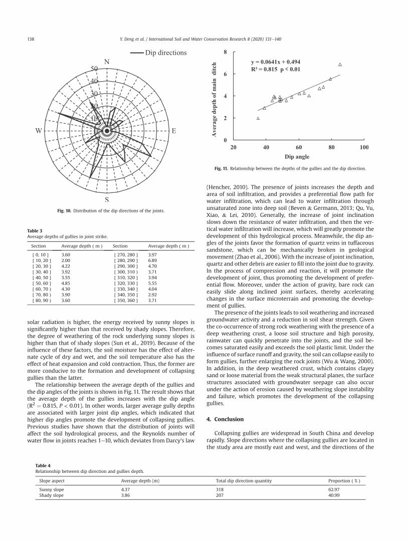
solar radiation is higher, the energy received by sunny slopes issignificantly higher than that received by shady slopes. Therefore,the degree of weathering of the rock underlying sunny slopes ishigher than that of shady slopes (Sun et al., 2019). Because of theinfluence of these factors, the soil moisture has the effect of alter-nate cycle of dry and wet, and the soil temperature also has theeffect of heat expansion and cold contraction. Thus, the former aremore conducive to the formation and development of collapsinggullies than the latter.
The relationship between the average depth of the gullies andthe dip angles of the joints is shown in Fig. 11. The result shows thatthe average depth of the gullies increases with the dip angle(R2 ¼ 0.815, P < 0.01). In other words, larger average gully depthsare associated with larger joint dip angles, which indicated thathigher dip angles promote the development of collapsing gullies.Previous studies have shown that the distribution of joints willaffect the soil hydrological process, and the Reynolds number ofwater flow in joints reaches 1e10, which deviates from Darcy’s law
(Hencher, 2010). The presence of joints increases the depth andarea of soil infiltration, and provides a preferential flow path forwater infiltration, which can lead to water infiltration throughunsaturated zone into deep soil (Beven & Germann, 2013; Qu, Yu,Xiao, & Lei, 2010). Generally, the increase of joint inclinationslows down the resistance of water infiltration, and then the ver-tical water infiltrationwill increase, which will greatly promote thedevelopment of this hydrological process. Meanwhile, the dip an-gles of the joints favor the formation of quartz veins in tuffaceoussandstone, which can be mechanically broken in geologicalmovement (Zhao et al., 2006).With the increase of joint inclination,quartz and other debris are easier to fill into the joint due to gravity.In the process of compression and reaction, it will promote thedevelopment of joint, thus promoting the development of prefer-ential flow. Moreover, under the action of gravity, bare rock caneasily slide along inclined joint surfaces, thereby acceleratingchanges in the surface microterrain and promoting the develop-ment of gullies.
The presence of the joints leads to soil weathering and increasedgroundwater activity and a reduction in soil shear strength. Giventhe co-occurrence of strong rock weathering with the presence of adeep weathering crust, a loose soil structure and high porosity,rainwater can quickly penetrate into the joints, and the soil be-comes saturated easily and exceeds the soil plastic limit. Under theinfluence of surface runoff and gravity, the soil can collapse easily toform gullies, further enlarging the rock joints (Wu & Wang, 2000).In addition, in the deep weathered crust, which contains clayeysand or loose material from the weak structural planes, the surfacestructures associated with groundwater seepage can also occurunder the action of erosion caused by weathering slope instabilityand failure, which promotes the development of the collapsinggullies.
4. Conclusion
Collapsing gullies are widespread in South China and developrapidly. Slope directions where the collapsing gullies are located inthe study area are mostly east and west, and the directions of the
Fig. 10. Distribution of the dip directions of the joints.
Table 3Average depths of gullies in joint strike.
Section Average depth(m) Section Average depth(m)
[0, 10] 3.60 [270, 280] 3.97[10, 20] 2.00 [280, 290] 6.89[20, 30] 4.22 [290, 300] 4.70[30, 40] 3.92 [300, 310) 3.71[40, 50] 3.55 [310, 320] 3.94[50, 60] 4.85 [320, 330] 5.55[60, 70) 4.30 [330, 340] 4.04[70, 80) 3.90 [340, 350] 2.92[80, 90) 3.60 [350, 360] 3.71
Table 4Relationship between dip direction and gullies depth.
Slope aspect Average depth (m) Total dip direction quantity Proportion(%)
Sunny slope 4.37 318 62.97Shady slope 3.86 207 40.99
Fig. 11. Relationship between the depths of the gullies and the dip direction.
Y. Deng et al. / International Soil and Water Conservation Research 8 (2020) 131e140138
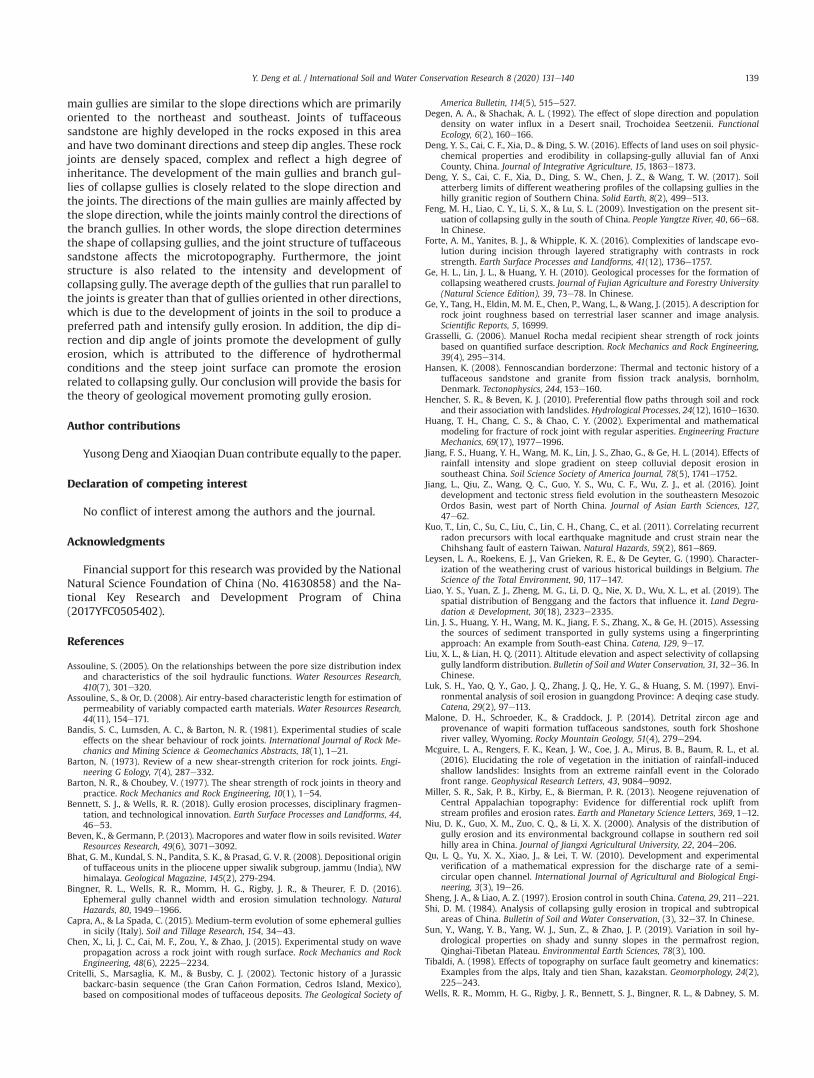
main gullies are similar to the slope directions which are primarilyoriented to the northeast and southeast. Joints of tuffaceoussandstone are highly developed in the rocks exposed in this areaand have two dominant directions and steep dip angles. These rockjoints are densely spaced, complex and reflect a high degree ofinheritance. The development of the main gullies and branch gul-lies of collapse gullies is closely related to the slope direction andthe joints. The directions of the main gullies are mainly affected bythe slope direction, while the joints mainly control the directions ofthe branch gullies. In other words, the slope direction determinesthe shape of collapsing gullies, and the joint structure of tuffaceoussandstone affects the microtopography. Furthermore, the jointstructure is also related to the intensity and development ofcollapsing gully. The average depth of the gullies that run parallel tothe joints is greater than that of gullies oriented in other directions,which is due to the development of joints in the soil to produce apreferred path and intensify gully erosion. In addition, the dip di-rection and dip angle of joints promote the development of gullyerosion, which is attributed to the difference of hydrothermalconditions and the steep joint surface can promote the erosionrelated to collapsing gully. Our conclusion will provide the basis forthe theory of geological movement promoting gully erosion.
Author contributions
Yusong Deng and Xiaoqian Duan contribute equally to the paper.
Declaration of competing interest
No conflict of interest among the authors and the journal.
Acknowledgments
Financial support for this research was provided by the NationalNatural Science Foundation of China (No. 41630858) and the Na-tional Key Research and Development Program of China(2017YFC0505402).
References
Assouline, S. (2005). On the relationships between the pore size distribution indexand characteristics of the soil hydraulic functions. Water Resources Research,410(7), 301e320.
Assouline, S., & Or, D. (2008). Air entry-based characteristic length for estimation ofpermeability of variably compacted earth materials. Water Resources Research,44(11), 154e171.
Bandis, S. C., Lumsden, A. C., & Barton, N. R. (1981). Experimental studies of scaleeffects on the shear behaviour of rock joints. International Journal of Rock Me-chanics and Mining Science & Geomechanics Abstracts, 18(1), 1e21.
Barton, N. (1973). Review of a new shear-strength criterion for rock joints. Engi-neering G Eology, 7(4), 287e332.
Barton, N. R., & Choubey, V. (1977). The shear strength of rock joints in theory andpractice. Rock Mechanics and Rock Engineering, 10(1), 1e54.
Bennett, S. J., & Wells, R. R. (2018). Gully erosion processes, disciplinary fragmen-tation, and technological innovation. Earth Surface Processes and Landforms, 44,46e53.
Beven, K., & Germann, P. (2013). Macropores and water flow in soils revisited.WaterResources Research, 49(6), 3071e3092.
Bhat, G. M., Kundal, S. N., Pandita, S. K., & Prasad, G. V. R. (2008). Depositional originof tuffaceous units in the pliocene upper siwalik subgroup, jammu (India), NWhimalaya. Geological Magazine, 145(2), 279-294.
Bingner, R. L., Wells, R. R., Momm, H. G., Rigby, J. R., & Theurer, F. D. (2016).Ephemeral gully channel width and erosion simulation technology. NaturalHazards, 80, 1949e1966.
Capra, A., & La Spada, C. (2015). Medium-term evolution of some ephemeral gulliesin sicily (Italy). Soil and Tillage Research, 154, 34e43.
Chen, X., Li, J. C., Cai, M. F., Zou, Y., & Zhao, J. (2015). Experimental study on wavepropagation across a rock joint with rough surface. Rock Mechanics and RockEngineering, 48(6), 2225e2234.
Critelli, S., Marsaglia, K. M., & Busby, C. J. (2002). Tectonic history of a Jurassicbackarc-basin sequence (the Gran Ca~non Formation, Cedros Island, Mexico),based on compositional modes of tuffaceous deposits. The Geological Society of
America Bulletin, 114(5), 515e527.Degen, A. A., & Shachak, A. L. (1992). The effect of slope direction and population
density on water influx in a Desert snail, Trochoidea Seetzenii. FunctionalEcology, 6(2), 160e166.
Deng, Y. S., Cai, C. F., Xia, D., & Ding, S. W. (2016). Effects of land uses on soil physic-chemical properties and erodibility in collapsing-gully alluvial fan of AnxiCounty, China. Journal of Integrative Agriculture, 15, 1863e1873.
Deng, Y. S., Cai, C. F., Xia, D., Ding, S. W., Chen, J. Z., & Wang, T. W. (2017). Soilatterberg limits of different weathering profiles of the collapsing gullies in thehilly granitic region of Southern China. Solid Earth, 8(2), 499e513.
Feng, M. H., Liao, C. Y., Li, S. X., & Lu, S. L. (2009). Investigation on the present sit-uation of collapsing gully in the south of China. People Yangtze River, 40, 66e68.In Chinese.
Forte, A. M., Yanites, B. J., & Whipple, K. X. (2016). Complexities of landscape evo-lution during incision through layered stratigraphy with contrasts in rockstrength. Earth Surface Processes and Landforms, 41(12), 1736e1757.
Ge, H. L., Lin, J. L., & Huang, Y. H. (2010). Geological processes for the formation ofcollapsing weathered crusts. Journal of Fujian Agriculture and Forestry University(Natural Science Edition), 39, 73e78. In Chinese.
Ge, Y., Tang, H., Eldin, M. M. E., Chen, P., Wang, L., & Wang, J. (2015). A description forrock joint roughness based on terrestrial laser scanner and image analysis.Scientific Reports, 5, 16999.
Grasselli, G. (2006). Manuel Rocha medal recipient shear strength of rock jointsbased on quantified surface description. Rock Mechanics and Rock Engineering,39(4), 295e314.
Hansen, K. (2008). Fennoscandian borderzone: Thermal and tectonic history of atuffaceous sandstone and granite from fission track analysis, bornholm,Denmark. Tectonophysics, 244, 153e160.
Hencher, S. R., & Beven, K. J. (2010). Preferential flow paths through soil and rockand their association with landslides. Hydrological Processes, 24(12), 1610e1630.
Huang, T. H., Chang, C. S., & Chao, C. Y. (2002). Experimental and mathematicalmodeling for fracture of rock joint with regular asperities. Engineering FractureMechanics, 69(17), 1977e1996.
Jiang, F. S., Huang, Y. H., Wang, M. K., Lin, J. S., Zhao, G., & Ge, H. L. (2014). Effects ofrainfall intensity and slope gradient on steep colluvial deposit erosion insoutheast China. Soil Science Society of America Journal, 78(5), 1741e1752.
Jiang, L., Qiu, Z., Wang, Q. C., Guo, Y. S., Wu, C. F., Wu, Z. J., et al. (2016). Jointdevelopment and tectonic stress field evolution in the southeastern MesozoicOrdos Basin, west part of North China. Journal of Asian Earth Sciences, 127,47e62.
Kuo, T., Lin, C., Su, C., Liu, C., Lin, C. H., Chang, C., et al. (2011). Correlating recurrentradon precursors with local earthquake magnitude and crust strain near theChihshang fault of eastern Taiwan. Natural Hazards, 59(2), 861e869.
Leysen, L. A., Roekens, E. J., Van Grieken, R. E., & De Geyter, G. (1990). Character-ization of the weathering crust of various historical buildings in Belgium. TheScience of the Total Environment, 90, 117e147.
Liao, Y. S., Yuan, Z. J., Zheng, M. G., Li, D. Q., Nie, X. D., Wu, X. L., et al. (2019). Thespatial distribution of Benggang and the factors that influence it. Land Degra-dation & Development, 30(18), 2323e2335.
Lin, J. S., Huang, Y. H., Wang, M. K., Jiang, F. S., Zhang, X., & Ge, H. (2015). Assessingthe sources of sediment transported in gully systems using a fingerprintingapproach: An example from South-east China. Catena, 129, 9e17.
Liu, X. L., & Lian, H. Q. (2011). Altitude elevation and aspect selectivity of collapsinggully landform distribution. Bulletin of Soil and Water Conservation, 31, 32e36. InChinese.
Luk, S. H., Yao, Q. Y., Gao, J. Q., Zhang, J. Q., He, Y. G., & Huang, S. M. (1997). Envi-ronmental analysis of soil erosion in guangdong Province: A deqing case study.Catena, 29(2), 97e113.
Malone, D. H., Schroeder, K., & Craddock, J. P. (2014). Detrital zircon age andprovenance of wapiti formation tuffaceous sandstones, south fork Shoshoneriver valley, Wyoming. Rocky Mountain Geology, 51(4), 279e294.
Mcguire, L. A., Rengers, F. K., Kean, J. W., Coe, J. A., Mirus, B. B., Baum, R. L., et al.(2016). Elucidating the role of vegetation in the initiation of rainfall-inducedshallow landslides: Insights from an extreme rainfall event in the Coloradofront range. Geophysical Research Letters, 43, 9084e9092.
Miller, S. R., Sak, P. B., Kirby, E., & Bierman, P. R. (2013). Neogene rejuvenation ofCentral Appalachian topography: Evidence for differential rock uplift fromstream profiles and erosion rates. Earth and Planetary Science Letters, 369, 1e12.
Niu, D. K., Guo, X. M., Zuo, C. Q., & Li, X. X. (2000). Analysis of the distribution ofgully erosion and its environmental background collapse in southern red soilhilly area in China. Journal of Jiangxi Agricultural University, 22, 204e206.
Qu, L. Q., Yu, X. X., Xiao, J., & Lei, T. W. (2010). Development and experimentalverification of a mathematical expression for the discharge rate of a semi-circular open channel. International Journal of Agricultural and Biological Engi-neering, 3(3), 19e26.
Sheng, J. A., & Liao, A. Z. (1997). Erosion control in south China. Catena, 29, 211e221.Shi, D. M. (1984). Analysis of collapsing gully erosion in tropical and subtropical
areas of China. Bulletin of Soil and Water Conservation, (3), 32e37. In Chinese.Sun, Y., Wang, Y. B., Yang, W. J., Sun, Z., & Zhao, J. P. (2019). Variation in soil hy-
drological properties on shady and sunny slopes in the permafrost region,Qinghai-Tibetan Plateau. Environmental Earth Sciences, 78(3), 100.
Tibaldi, A. (1998). Effects of topography on surface fault geometry and kinematics:Examples from the alps, Italy and tien Shan, kazakstan. Geomorphology, 24(2),225e243.
Wells, R. R., Momm, H. G., Rigby, J. R., Bennett, S. J., Bingner, R. L., & Dabney, S. M.
Y. Deng et al. / International Soil and Water Conservation Research 8 (2020) 131e140 139
(2013). An empirical investigation of gully widening rates in upland concen-trated flows. Catena, 101, 114e121.
Wu, ZF, & Wang, JZ (2000). elationship Between Slope Disintegration and Rock-soilCharacteristics of Granite Weathering Mantle in South China. Journal of Soil andWater Conservation, 14(2), 31e35.
Wu, Z. F., & Zhong, W. Q. (1997). Gravity gully erosion and it’s influence. EcologicScience, 16, 91e96. In Chinese.
Xia, D., Deng, Y. S., Wang, S. L., Ding, S. W., & Cai, C. F. (2015). Fractal features of soilparticle-size distribution of different weathering profiles of the collapsinggullies in the hilly granitic region, south China. Natural Hazards, 79, 455e478.
Xu, J. X. (1996). Benggang erosion: The influencing factors. Catena, 27, 249e263.Xu, J. X., & Zeng, G. H. (1992). Benggang erosion in sub-tropical granite weathering
crust geo- ecosystems: An example from guangdong Province. In D. E. Walling,et al. (Eds.), Erosion, debris flows and environment in mountain regions (pp.455e463). IAHS Publication No. 209.
Yan, Q. H., Lei, T. W., Yuan, C. P., Lei, Q. X., Yang, X. S., Zhang, M. L., et al. (2015).Effects of watershed management practices on the relationships among rainfall,runoff, and sediment delivery in the hilly-gully region of the Loess Plateau inChina. Geomorphology, 228, 735e745.
Yao, Q. Y., & Lu, Z. X. (1989). Granite fracture structure and its influence on weatheringand rock mass destruction. Study on Soil and water conservation in GuangdongProvince. Beijing: Science Press.
Zhang, L. T., Gao, Z. L., Li, Z. B., & Tian, H. W. (2016). Downslope runoff and erosionresponse of typical engineered landform to variable inflow rate patterns fromupslope. Natural Hazards, 80(2), 775e796.
Zhang, Q. W., Dong, Y. Q., Li, F., Zhang, A. P., & Lei, T. W. (2014). Quantifyingdetachment rate of eroding rill or ephemeral gully for WEPP with flume
experiments. Journal of Hydrology, 519, 2012e2019.Zhao, J. (2006). Erosion and formation conditions of collapsing gully in Jiangxi.
Applied Technology of Soil and Water Conservation, 5, 16e17. In Chinese.Zhao, J. (2015). Study on the distribution characteristics and erosion mechanism of
Collapsing gully in Yudu County. Jiangxi Agricultural University.Zhao, J., Shi, Y. F., Huang, Y. S., & Fu, J. W. (2015). Uncertainties of snow cover
extraction caused by the nature of topography and underlying surface. Journalof Arid Land, 7, 1e11.
Zhao, J., Tang, J. B., & Niu, D. K. (2014). Study on spatial distribution of collapsinggully erosion in Jiangxi, Yudu based on GIS. Journal of Yangtze River ScientificInstitute, 31, 18e21.
Zhen, Y., Wang, Z. Q., Chen, J. L., Yan, Q. R., & Tao, W. (2010). Detrital record ofneoproterozoic arc-magmatism along the NW margin of the yangtze block,China: U-Pb geochronology and petrography of sandstones. Journal of Asianearth ences, 37(4), 322e334.
Zheng, M. G., Cai, Q. G., & Cheng, Q. J. (2008). Modelling the runoff-sediment yieldrelationship using a proportional function in hilly areas of the loess plateau,north China. Geomorphology, 93(3e4), 288e301.
Zhong, B. L., Peng, S. Y., Zhang, Q., Ma, H., & Gao, S. X. (2013). Using an ecologicaleconomics approach to support the restoration of collapsing gullies in southernChina. Land Use Policy, 32, 119e124.
Zhu, G. W. (1991). The selective development of collapsing gully and its prevention -a case study of Wuhua County. Tropical geology, 11, 152e156. In Chinese.
Ziegler, M., Loew, S., & Moore, J. R. (2013). Distribution and inferred age of exfoli-ation joints in the Aar granite of the central Swiss Alps and relationship toquaternary landscape evolution. Geomorphology, 201, 344e362.
Y. Deng et al. / International Soil and Water Conservation Research 8 (2020) 131e140140
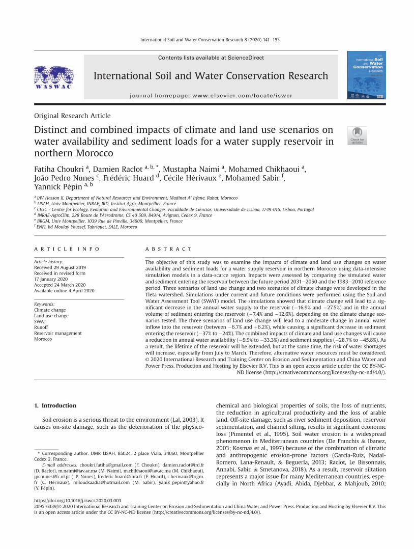
Original Research Article
Distinct and combined impacts of climate and land use scenarios onwater availability and sediment loads for a water supply reservoir innorthern Morocco
Fatiha Choukri a, Damien Raclot a, b, *, Mustapha Naimi a, Mohamed Chikhaoui a,Jo~ao Pedro Nunes c, Fr�ed�eric Huard d, C�ecile H�erivaux e, Mohamed Sabir f,Yannick P�epin a, b
a IAV Hassan II, Department of Natural Resources and Environment, Madinat Al Irfane, Rabat, Moroccob LISAH, Univ Montpellier, INRAE, IRD, Institut Agro, Montpellier, Francec CE3C - Centre for Ecology, Evolution and Environmental Changes, Faculdade de Ciencias, Universidade de Lisboa, 1749-016, Lisboa, Portugald INRAE-AgroClim, 228 Route de l’A�erodrome, CS 40 509, 84914, Avignon, Cedex 9, Francee BRGM, Univ Montpellier, 1039 Rue de Pinville, 34000, Montpellier, Francef ENFI, bd Moulay Youssef, Tabriquet, SALE, Morocco
a r t i c l e i n f o
Article history:Received 29 August 2019Received in revised form17 January 2020Accepted 24 March 2020Available online 4 April 2020
Keywords:Climate changeLand use changeSWATRunoffReservoir managementMorocco
a b s t r a c t
The objective of this study was to examine the impacts of climate and land use changes on wateravailability and sediment loads for a water supply reservoir in northern Morocco using data-intensivesimulation models in a data-scarce region. Impacts were assessed by comparing the simulated waterand sediment entering the reservoir between the future period 2031e2050 and the 1983e2010 referenceperiod. Three scenarios of land use change and two scenarios of climate change were developed in theTleta watershed. Simulations under current and future conditions were performed using the Soil andWater Assessment Tool (SWAT) model. The simulations showed that climate change will lead to a sig-nificant decrease in the annual water supply to the reservoir (�16.9% and �27.5%) and in the annualvolume of sediment entering the reservoir (�7.4% and �12.6%), depending on the climate change sce-narios tested. The three scenarios of land use change will lead to a moderate change in annual waterinflow into the reservoir (between �6.7% and þ6.2%), while causing a significant decrease in sedimententering the reservoir (�37% to �24%). The combined impacts of climate and land use changes will causea reduction in annual water availability (�9.9% to �33.3%) and sediment supplies (�28.7% to �45.8%). Asa result, the lifetime of the reservoir will be extended, but at the same time, the risk of water shortageswill increase, especially from July to March. Therefore, alternative water resources must be considered.© 2020 International Research and Training Center on Erosion and Sedimentation and China Water andPower Press. Production and Hosting by Elsevier B.V. This is an open access article under the CC BY-NC-
ND license (http://creativecommons.org/licenses/by-nc-nd/4.0/).
1. Introduction
Soil erosion is a serious threat to the environment (Lal, 2003). Itcauses on-site damage, such as the deterioration of the physico-
chemical and biological properties of soils, the loss of nutrients,the reduction in agricultural productivity and the loss of arableland. Off-site damage, such as river sediment deposition, reservoirsedimentation, and channel silting, results in significant economicloss (Pimentel et al., 1995). Soil water erosion is a widespreadphenomenon in Mediterranean countries (De Franchis & Ibanez,2003; Kosmas et al., 1997) because of the combination of climaticand anthropogenic erosion-prone factors (García-Ruiz, Nadal-Romero, Lana-Renault, & Beguería, 2013; Raclot, Le Bissonnais,Annabi, Sabir, & Smetanova, 2018). As a result, reservoir siltationrepresents a major issue for many Mediterranean countries, espe-cially in North Africa (Ayadi, Abida, Djebbar, & Mahjoub, 2010;
* Corresponding author. UMR LISAH, Bat.24, 2 place Viala, 34060, MontpellierCedex 2, France.
E-mail addresses: [email protected] (F. Choukri), [email protected](D. Raclot), [email protected] (M. Naimi), [email protected] (M. Chikhaoui),[email protected] (J.P. Nunes), [email protected] (F. Huard), [email protected] (C. H�erivaux), [email protected] (M. Sabir), [email protected](Y. P�epin).
Contents lists available at ScienceDirect
International Soil and Water Conservation Research
journal homepage: www.elsevier .com/locate/ iswcr
https://doi.org/10.1016/j.iswcr.2020.03.0032095-6339/© 2020 International Research and Training Center on Erosion and Sedimentation and China Water and Power Press. Production and Hosting by Elsevier B.V. Thisis an open access article under the CC BY-NC-ND license (http://creativecommons.org/licenses/by-nc-nd/4.0/).
International Soil and Water Conservation Research 8 (2020) 141e153
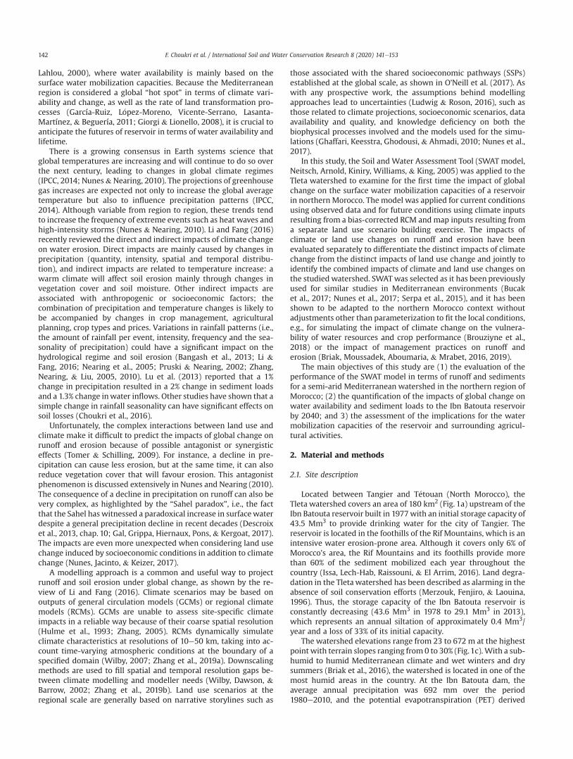
Lahlou, 2000), where water availability is mainly based on thesurface water mobilization capacities. Because the Mediterraneanregion is considered a global “hot spot” in terms of climate vari-ability and change, as well as the rate of land transformation pro-cesses (García-Ruiz, L�opez-Moreno, Vicente-Serrano, Lasanta-Martínez, & Beguería, 2011; Giorgi & Lionello, 2008), it is crucial toanticipate the futures of reservoir in terms of water availability andlifetime.
There is a growing consensus in Earth systems science thatglobal temperatures are increasing and will continue to do so overthe next century, leading to changes in global climate regimes(IPCC, 2014; Nunes&Nearing, 2010). The projections of greenhousegas increases are expected not only to increase the global averagetemperature but also to influence precipitation patterns (IPCC,2014). Although variable from region to region, these trends tendto increase the frequency of extreme events such as heat waves andhigh-intensity storms (Nunes & Nearing, 2010). Li and Fang (2016)recently reviewed the direct and indirect impacts of climate changeon water erosion. Direct impacts are mainly caused by changes inprecipitation (quantity, intensity, spatial and temporal distribu-tion), and indirect impacts are related to temperature increase: awarm climate will affect soil erosion mainly through changes invegetation cover and soil moisture. Other indirect impacts areassociated with anthropogenic or socioeconomic factors; thecombination of precipitation and temperature changes is likely tobe accompanied by changes in crop management, agriculturalplanning, crop types and prices. Variations in rainfall patterns (i.e.,the amount of rainfall per event, intensity, frequency and the sea-sonality of precipitation) could have a significant impact on thehydrological regime and soil erosion (Bangash et al., 2013; Li &Fang, 2016; Nearing et al., 2005; Pruski & Nearing, 2002; Zhang,Nearing, & Liu, 2005, 2010). Lu et al. (2013) reported that a 1%change in precipitation resulted in a 2% change in sediment loadsand a 1.3% change inwater inflows. Other studies have shown that asimple change in rainfall seasonality can have significant effects onsoil losses (Choukri et al., 2016).
Unfortunately, the complex interactions between land use andclimate make it difficult to predict the impacts of global change onrunoff and erosion because of possible antagonist or synergisticeffects (Tomer & Schilling, 2009). For instance, a decline in pre-cipitation can cause less erosion, but at the same time, it can alsoreduce vegetation cover that will favour erosion. This antagonistphenomenon is discussed extensively in Nunes and Nearing (2010).The consequence of a decline in precipitation on runoff can also bevery complex, as highlighted by the “Sahel paradox”, i.e., the factthat the Sahel has witnessed a paradoxical increase in surfacewaterdespite a general precipitation decline in recent decades (Descroixet al., 2013, chap. 10; Gal, Grippa, Hiernaux, Pons, & Kergoat, 2017).The impacts are even more unexpected when considering land usechange induced by socioeconomic conditions in addition to climatechange (Nunes, Jacinto, & Keizer, 2017).
A modelling approach is a common and useful way to projectrunoff and soil erosion under global change, as shown by the re-view of Li and Fang (2016). Climate scenarios may be based onoutputs of general circulation models (GCMs) or regional climatemodels (RCMs). GCMs are unable to assess site-specific climateimpacts in a reliable way because of their coarse spatial resolution(Hulme et al., 1993; Zhang, 2005). RCMs dynamically simulateclimate characteristics at resolutions of 10e50 km, taking into ac-count time-varying atmospheric conditions at the boundary of aspecified domain (Wilby, 2007; Zhang et al., 2019a). Downscalingmethods are used to fill spatial and temporal resolution gaps be-tween climate modelling and modeller needs (Wilby, Dawson, &Barrow, 2002; Zhang et al., 2019b). Land use scenarios at theregional scale are generally based on narrative storylines such as
those associated with the shared socioeconomic pathways (SSPs)established at the global scale, as shown in O’Neill et al. (2017). Aswith any prospective work, the assumptions behind modellingapproaches lead to uncertainties (Ludwig & Roson, 2016), such asthose related to climate projections, socioeconomic scenarios, dataavailability and quality, and knowledge deficiency on both thebiophysical processes involved and the models used for the simu-lations (Ghaffari, Keesstra, Ghodousi, & Ahmadi, 2010; Nunes et al.,2017).
In this study, the Soil and Water Assessment Tool (SWAT model,Neitsch, Arnold, Kiniry, Williams, & King, 2005) was applied to theTleta watershed to examine for the first time the impact of globalchange on the surface water mobilization capacities of a reservoirin northern Morocco. The model was applied for current conditionsusing observed data and for future conditions using climate inputsresulting from a bias-corrected RCM and map inputs resulting froma separate land use scenario building exercise. The impacts ofclimate or land use changes on runoff and erosion have beenevaluated separately to differentiate the distinct impacts of climatechange from the distinct impacts of land use change and jointly toidentify the combined impacts of climate and land use changes onthe studied watershed. SWATwas selected as it has been previouslyused for similar studies in Mediterranean environments (Bucaket al., 2017; Nunes et al., 2017; Serpa et al., 2015), and it has beenshown to be adapted to the northern Morocco context withoutadjustments other than parameterization to fit the local conditions,e.g., for simulating the impact of climate change on the vulnera-bility of water resources and crop performance (Brouziyne et al.,2018) or the impact of management practices on runoff anderosion (Briak, Moussadek, Aboumaria, & Mrabet, 2016, 2019).
The main objectives of this study are (1) the evaluation of theperformance of the SWAT model in terms of runoff and sedimentsfor a semi-arid Mediterranean watershed in the northern region ofMorocco; (2) the quantification of the impacts of global change onwater availability and sediment loads to the Ibn Batouta reservoirby 2040; and 3) the assessment of the implications for the watermobilization capacities of the reservoir and surrounding agricul-tural activities.
2. Material and methods
2.1. Site description
Located between Tangier and T�etouan (North Morocco), theTleta watershed covers an area of 180 km2 (Fig. 1a) upstream of theIbn Batouta reservoir built in 1977with an initial storage capacity of43.5 Mm3 to provide drinking water for the city of Tangier. Thereservoir is located in the foothills of the Rif Mountains, which is anintensive water erosion-prone area. Although it covers only 6% ofMorocco’s area, the Rif Mountains and its foothills provide morethan 60% of the sediment mobilized each year throughout thecountry (Issa, Lech-Hab, Raissouni, & El Arrim, 2016). Land degra-dation in the Tleta watershed has been described as alarming in theabsence of soil conservation efforts (Merzouk, Fenjiro, & Laouina,1996). Thus, the storage capacity of the Ibn Batouta reservoir isconstantly decreasing (43.6 Mm3 in 1978 to 29.1 Mm3 in 2013),which represents an annual siltation of approximately 0.4 Mm3/year and a loss of 33% of its initial capacity.
The watershed elevations range from 23 to 672 m at the highestpoint with terrain slopes ranging from 0 to 30% (Fig.1c). With a sub-humid to humid Mediterranean climate and wet winters and drysummers (Briak et al., 2016), the watershed is located in one of themost humid areas in the country. At the Ibn Batouta dam, theaverage annual precipitation was 692 mm over the period1980e2010, and the potential evapotranspiration (PET) derived
F. Choukri et al. / International Soil and Water Conservation Research 8 (2020) 141e153142
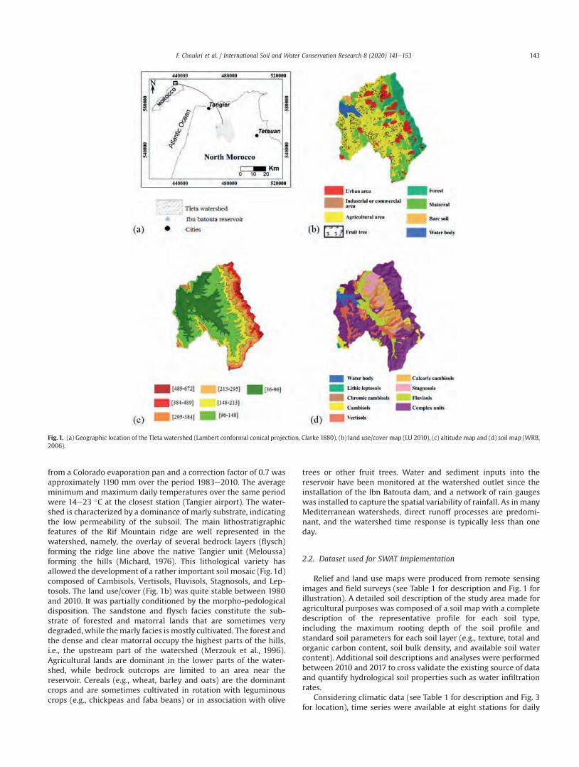
from a Colorado evaporation pan and a correction factor of 0.7 wasapproximately 1190 mm over the period 1983e2010. The averageminimum and maximum daily temperatures over the same periodwere 14e23 �C at the closest station (Tangier airport). The water-shed is characterized by a dominance of marly substrate, indicatingthe low permeability of the subsoil. The main lithostratigraphicfeatures of the Rif Mountain ridge are well represented in thewatershed, namely, the overlay of several bedrock layers (flysch)forming the ridge line above the native Tangier unit (Meloussa)forming the hills (Michard, 1976). This lithological variety hasallowed the development of a rather important soil mosaic (Fig. 1d)composed of Cambisols, Vertisols, Fluvisols, Stagnosols, and Lep-tosols. The land use/cover (Fig. 1b) was quite stable between 1980and 2010. It was partially conditioned by the morpho-pedologicaldisposition. The sandstone and flysch facies constitute the sub-strate of forested and matorral lands that are sometimes verydegraded, while themarly facies is mostly cultivated. The forest andthe dense and clear matorral occupy the highest parts of the hills,i.e., the upstream part of the watershed (Merzouk et al., 1996).Agricultural lands are dominant in the lower parts of the water-shed, while bedrock outcrops are limited to an area near thereservoir. Cereals (e.g., wheat, barley and oats) are the dominantcrops and are sometimes cultivated in rotation with leguminouscrops (e.g., chickpeas and faba beans) or in association with olive
trees or other fruit trees. Water and sediment inputs into thereservoir have been monitored at the watershed outlet since theinstallation of the Ibn Batouta dam, and a network of rain gaugeswas installed to capture the spatial variability of rainfall. As in manyMediterranean watersheds, direct runoff processes are predomi-nant, and the watershed time response is typically less than oneday.
2.2. Dataset used for SWAT implementation
Relief and land use maps were produced from remote sensingimages and field surveys (see Table 1 for description and Fig. 1 forillustration). A detailed soil description of the study area made foragricultural purposes was composed of a soil map with a completedescription of the representative profile for each soil type,including the maximum rooting depth of the soil profile andstandard soil parameters for each soil layer (e.g., texture, total andorganic carbon content, soil bulk density, and available soil watercontent). Additional soil descriptions and analyses were performedbetween 2010 and 2017 to cross validate the existing source of dataand quantify hydrological soil properties such as water infiltrationrates.
Considering climatic data (see Table 1 for description and Fig. 3for location), time series were available at eight stations for daily
Fig. 1. (a) Geographic location of the Tleta watershed (Lambert conformal conical projection, Clarke 1880), (b) land use/cover map (LU 2010), (c) altitude map and (d) soil map (WRB,2006).
F. Choukri et al. / International Soil and Water Conservation Research 8 (2020) 141e153 143
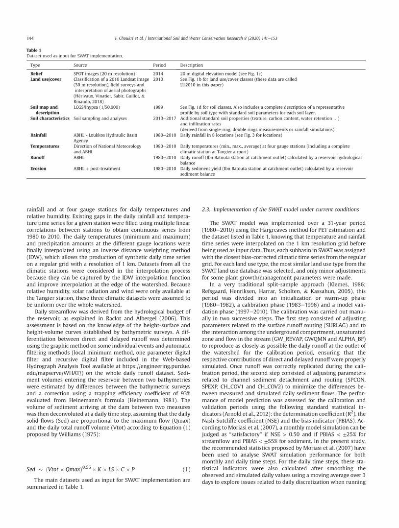
rainfall and at four gauge stations for daily temperatures andrelative humidity. Existing gaps in the daily rainfall and tempera-ture time series for a given station were filled using multiple linearcorrelations between stations to obtain continuous series from1980 to 2010. The daily temperatures (minimum and maximum)and precipitation amounts at the different gauge locations werefinally interpolated using an inverse distance weighting method(IDW), which allows the production of synthetic daily time serieson a regular grid with a resolution of 1 km. Datasets from all theclimatic stations were considered in the interpolation processbecause they can be captured by the IDW interpolation functionand improve interpolation at the edge of the watershed. Becauserelative humidity, solar radiation and wind were only available atthe Tangier station, these three climatic datasets were assumed tobe uniform over the whole watershed.
Daily streamflow was derived from the hydrological budget ofthe reservoir, as explained in Raclot and Albergel (2006). Thisassessment is based on the knowledge of the height-surface andheight-volume curves established by bathymetric surveys. A dif-ferentiation between direct and delayed runoff was determinedusing the graphic method on some individual events and automaticfiltering methods (local minimum method, one parameter digitalfilter and recursive digital filter included in the Web-basedHydrograph Analysis Tool available at https://engineering.purdue.edu/mapserve/WHAT/) on the whole daily runoff dataset. Sedi-ment volumes entering the reservoir between two bathymetrieswere estimated by differences between the bathymetric surveysand a correction using a trapping efficiency coefficient of 93%evaluated from Heinemann’s formula (Heinemann, 1981). Thevolume of sediment arriving at the dam between two measureswas then deconvoluted at a daily time step, assuming that the dailysolid flows (Sed) are proportional to the maximum flow (Qmax)and the daily total runoff volume (Vtot) according to Equation (1)proposed by Williams (1975):
Sed � ðVtot � QmaxÞ0:56 �K � LS� C � P (1)
The main datasets used as input for SWAT implementation aresummarized in Table 1.
2.3. Implementation of the SWAT model under current conditions
The SWAT model was implemented over a 31-year period(1980e2010) using the Hargreaves method for PET estimation andthe dataset listed in Table 1, knowing that temperature and rainfalltime series were interpolated on the 1 km resolution grid beforebeing used as input data. Thus, each subbasin in SWATwas assignedwith the closest bias-corrected climatic time series from the regulargrid. For each land use type, themost similar land use type from theSWAT land use database was selected, and only minor adjustmentsfor some plant growth/management parameters were made.
In a very traditional split-sample approach (Kleme�s, 1986;Refsgaard, Henriksen, Harrar, Scholten, & Kassahun, 2005), thisperiod was divided into an initialization or warm-up phase(1980e1982), a calibration phase (1983e1996) and a model vali-dation phase (1997e2010). The calibration was carried out manu-ally in two successive steps. The first step consisted of adjustingparameters related to the surface runoff routing (SURLAG) and tothe interaction among the underground compartment, unsaturatedzone and flow in the stream (GW_REVAP, GWQMN and ALPHA_BF)to reproduce as closely as possible the daily runoff at the outlet ofthe watershed for the calibration period, ensuring that therespective contributions of direct and delayed runoff were properlysimulated. Once runoff was correctly replicated during the cali-bration period, the second step consisted of adjusting parametersrelated to channel sediment detachment and routing (SPCON,SPEXP, CH_COV1 and CH_COV2) to minimize the differences be-tween measured and simulated daily sediment flows. The perfor-mance of model prediction was assessed for the calibration andvalidation periods using the following standard statistical in-dicators (Arnold et al., 2012): the determination coefficient (R2), theNash-Sutcliffe coefficient (NSE) and the bias indicator (PBIAS). Ac-cording to Moriasi et al. (2007), a monthly model simulation can bejudged as “satisfactory” if NSE > 0.50 and if PBIAS < ±25% forstreamflow and PBIAS < ±55% for sediment. In the present study,the recommended statistics proposed by Moriasi et al. (2007) havebeen used to analyse SWAT simulation performance for bothmonthly and daily time steps. For the daily time steps, these sta-tistical indicators were also calculated after smoothing theobserved and simulated daily values using a moving average over 3days to explore issues related to daily discretization when running
Table 1Dataset used as input for SWAT implementation.
Type Source Period Description
Relief SPOT images (20 m resolution) 2014 20 m digital elevation model (see Fig. 1c)Land use/cover Classification of a 2010 Landsat image
(30 m resolution), field surveys andinterpretation of aerial photographs(H�erivaux, Vinatier, Sabir, Guillot, &Rinaudo, 2018)
2010 See Fig. 1b for land use/cover classes (these data are calledLU2010 in this paper)
Soil map anddescription
LCGS/Inypsa (1/50,000) 1989 See Fig. 1d for soil classes. Also includes a complete description of a representativeprofile by soil type with standard soil parameters for each soil layer.
Soil characteristics Soil sampling and analyses 2010e2017 Additional standard soil properties (texture, carbon content, water retention …)and infiltration rates(derived from single-ring, double rings measurements or rainfall simulations)
Rainfall ABHL - Loukkos Hydraulic BasinAgency
1980e2010 Daily rainfall in 8 locations (see Fig. 3 for locations)
Temperatures Direction of National Meteorologyand ABHL
1980e2010 Daily temperatures (min., max., average) at four gauge stations (including a completeclimatic station at Tangier airport)
Runoff ABHL 1980e2010 Daily runoff (Ibn Batouta station at catchment outlet) calculated by a reservoir hydrologicalbalance
Erosion ABHL þ post-treatment 1980e2010 Daily sediment yield (Ibn Batouta station at catchment outlet) calculated by a reservoirsediment balance
F. Choukri et al. / International Soil and Water Conservation Research 8 (2020) 141e153144
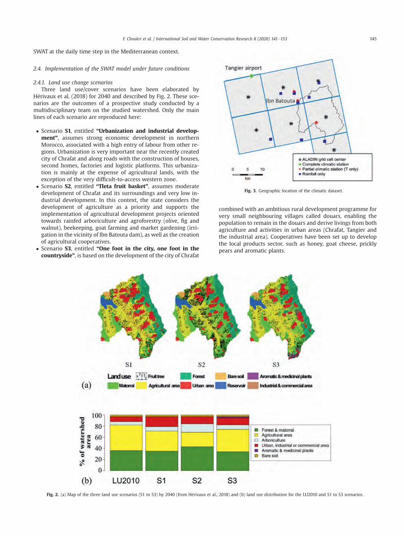
SWAT at the daily time step in the Mediterranean context.
2.4. Implementation of the SWAT model under future conditions
2.4.1. Land use change scenariosThree land use/cover scenarios have been elaborated by
H�erivaux et al. (2018) for 2040 and described by Fig. 2. These sce-narios are the outcomes of a prospective study conducted by amultidisciplinary team on the studied watershed. Only the mainlines of each scenario are reproduced here:
� Scenario S1, entitled “Urbanization and industrial develop-ment”, assumes strong economic development in northernMorocco, associated with a high entry of labour from other re-gions. Urbanization is very important near the recently createdcity of Chrafat and along roads with the construction of houses,second homes, factories and logistic platforms. This urbaniza-tion is mainly at the expense of agricultural lands, with theexception of the very difficult-to-access western zone.
� Scenario S2, entitled “Tleta fruit basket”, assumes moderatedevelopment of Chrafat and its surroundings and very low in-dustrial development. In this context, the state considers thedevelopment of agriculture as a priority and supports theimplementation of agricultural development projects orientedtowards rainfed arboriculture and agroforestry (olive, fig andwalnut), beekeeping, goat farming and market gardening (irri-gation in the vicinity of Ibn Batouta dam), as well as the creationof agricultural cooperatives.
� Scenario S3, entitled “One foot in the city, one foot in thecountryside”, is based on the development of the city of Chrafat
combined with an ambitious rural development programme forvery small neighbouring villages called douars, enabling thepopulation to remain in the douars and derive livings from bothagriculture and activities in urban areas (Chrafat, Tangier andthe industrial area). Cooperatives have been set up to developthe local products sector, such as honey, goat cheese, pricklypears and aromatic plants.
Fig. 2. (a) Map of the three land use scenarios (S1 to S3) by 2040 (from H�erivaux et al., 2018) and (b) land use distribution for the LU2010 and S1 to S3 scenarios.
Fig. 3. Geographic location of the climatic dataset.
F. Choukri et al. / International Soil and Water Conservation Research 8 (2020) 141e153 145
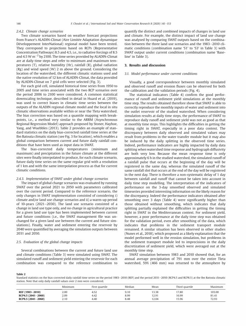
2.4.2. Climate change scenariosTwo climate scenarios based on weather forecast projections
from France’s ALADIN-Climat (Aire Limit�ee Adaptation dynamiqueD�eveloppement InterNational) regional model have been tested.They correspond to projections based on RCPs (RepresentativeConcentration Pathways) 8.5 and 4.5, i.e., to radiative forcings of 8.5and 4.5Wm�2 by 2100. The time series provided by ALADIN-Climatare at daily time steps and refer to minimum and maximum tem-peratures (T), relative humidity (Hr), rainfall (R), global radiation(Rg) and wind speed (W) 2 m above the ground. Considering thelocation of the watershed, the different climatic stations used andthe native resolution of 12 km of ALADIN-Climat, the data providedby ALADIN-Climat on 7 grid cells were selected (Fig. 3).
For each grid cell, simulated historical time series from 1950 to2005 and time series associated with the two RCP scenarios overthe period 2006 to 2100 were considered. A common statisticaldownscaling technique, described in detail in Huard et al. (2019),was used to correct biases in climatic time series between theoutputs of the ALADIN regional climate model and the local in situclimatic observations available within or near the Tleta watershed.The bias correction was based on a quantile mapping with break-points, i.e., a method very similar to the ARRM (AsynchronousRegional Regression Model) approach proposed by Stoner, Hayhoe,Yang, and Wuebbles (2013). Table 2 provides an example of stan-dard statistics on the daily bias-corrected rainfall time series at theIbn Batouta climatic station (see Fig. 3 for location), which enables aglobal comparison between current and future daily rainfall con-ditions that have been used as input data in SWAT.
The bias-corrected daily temperatures (minimum andmaximum) and precipitation in the future climate at the differentsites were finally interpolated to produce, for each climate scenario,future daily time series on the same regular grid with a resolutionof 1 km and with the same interpolation process as that for currentclimatic conditions.
2.4.3. Implementation of SWAT under global change scenariosThe impact of global change scenarios was evaluated by running
SWAT over the period 2021 to 2050 with parameters calibratedover the current period. Compared to the reference scenario, theonly changes in SWAT implementation consisted of considering i)climate and/or land use change scenarios and ii) a warm-up periodof 10-years (2021e2030). The land use scenario consisted of achange in land use type only, and no change in agricultural practicefor a given land use type has been implemented between currentand future conditions (i.e., the SWAT management file was un-changed for a given land use between the current and future sim-ulations). Finally, water and sediment entering the reservoir by2040 were quantified by averaging the simulation outputs between2031 and 2050.
2.5. Evaluation of the global change impacts
Several combinations between the current and future land useand climate conditions (Table 3) were simulated using SWAT. Thesimulated runoff and sediment yield entering the reservoir for eachcombination was compared to the reference combination to
quantify the distinct and combined impacts of changes in land useand climate. For example, the distinct impact of land use changewas analysed by comparing SWAT outputs based on the combina-tion between the three land use scenarios and the 1983e2010 cli-matic conditions (combination name ‘S1’ to ‘S3’ in Table 3) withSWAT output under current conditions (combination name ‘Base-line’ in Table 3).
3. Results and discussion
3.1. Model performance under current conditions
Visually, a good correspondence between monthly simulatedand observed runoff and erosion fluxes can be observed for boththe calibration and the validation periods (Fig. 4).
The statistical indicators (Table 4) confirm the good perfor-mance of runoff and sediment yield simulations at the monthlytime step. The results obtained therefore show that SWAT is able tocorrectly reproduce the monthly inputs of water and sediment intothe outlet reservoir of the studied watershed. When consideringsimulation results at daily time steps, the performance of SWAT toreproduce daily runoff and sediment yield was not as good as thatat monthly time steps. This highlights the difficulties in getting thetiming right in SWAT, especially in a poor data context. Thediscrepancy between daily observed and simulated values mayresult from problems in the water transfer module but it may alsobe induced by the daily splitting in the observed time series.Indeed, performance indicators are highly impacted by daily datasplitting whenwatershed time response and hydrograph diffusivityare both very low. Because the mean response time is onlyapproximately 6 h in the studiedwatershed, the simulated runoff ofa rainfall pulse that occurs at the beginning of the day will beregistered in the same day, whereas the simulated runoff of thesame rainfall slot that occurs at the end of the day will be registeredin the next day. There is therefore a non-systematic delay of 1 daybetween rainfall and runoff that cannot be taken into account indaily time step modelling. The interpretation of the indicators ofperformance on the 3-day smoothed observed and simulatedtimeseries provided interesting information on the likely reason forthe discrepancy. Indeed the performance indicators obtained aftersmoothing over 3 days (Table 4) were significantly higher thanthose obtained without smoothing, which indicates that dailysplitting partially explained the difficulties in getting the timingright in SWAT in the Mediterranean context. For sediment yield,however, a poor performance at the daily time step was obtainedfor the validation period, even after smoothing of the data, whichindicates that problems in the sediment transport moduleremained. A similar situation has been observed in other studies(Nunes et al., 2018), which proposed as a likely explanation that themodel performed well in the erosion simulation, but problems inthe sediment transport module led to imprecisions in the dailydiscretization of sediment yield, which were averaged out at themonthly time step.
SWAT simulation between 1983 and 2010 showed that, for anannual average precipitation of 791 mm over the entire Tletawatershed, 59% (466 mm) was returned to the atmosphere by
Table 2Standard statistics on the bias-corrected daily rainfall time series on the period 1983e2010 (REF) and the period 2031e2050 (RCP4.5 and RCP8.5) at the Ibn Batouta climaticstation. Note that only daily rainfall values over 2 mm were considered.
Minimum First quartile Median Mean Third quartile Maximum
REF (1983e2010) 2.00 4.52 9.10 13.38 17.80 103.00RCP4.5 (2041e2060) 2.09 4.42 8.99 12.91 16.99 81.41RCP8.5 (2041e2060) 2.10 4.40 8.48 12.04 15.96 72.93
F. Choukri et al. / International Soil and Water Conservation Research 8 (2020) 141e153146
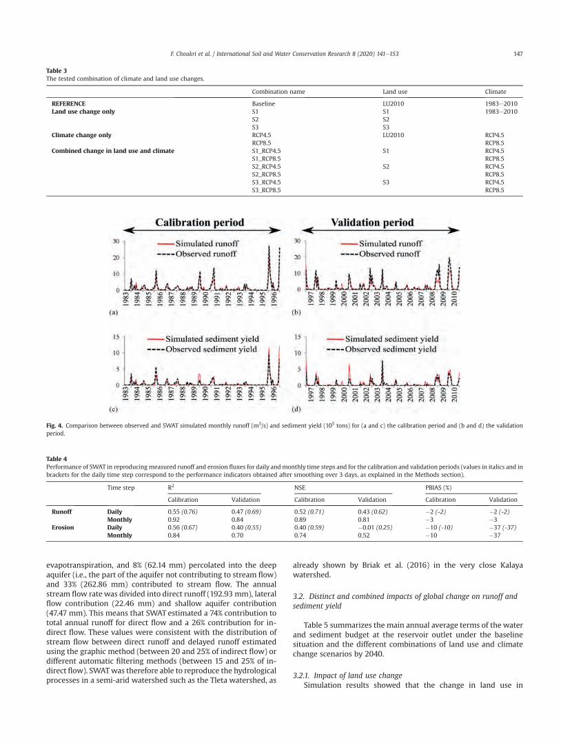
evapotranspiration, and 8% (62.14 mm) percolated into the deepaquifer (i.e., the part of the aquifer not contributing to stream flow)and 33% (262.86 mm) contributed to stream flow. The annualstream flow rate was divided into direct runoff (192.93 mm), lateralflow contribution (22.46 mm) and shallow aquifer contribution(47.47 mm). This means that SWAT estimated a 74% contribution tototal annual runoff for direct flow and a 26% contribution for in-direct flow. These values were consistent with the distribution ofstream flow between direct runoff and delayed runoff estimatedusing the graphic method (between 20 and 25% of indirect flow) ordifferent automatic filtering methods (between 15 and 25% of in-direct flow). SWATwas therefore able to reproduce the hydrologicalprocesses in a semi-arid watershed such as the Tleta watershed, as
already shown by Briak et al. (2016) in the very close Kalayawatershed.
3.2. Distinct and combined impacts of global change on runoff andsediment yield
Table 5 summarizes the main annual average terms of the waterand sediment budget at the reservoir outlet under the baselinesituation and the different combinations of land use and climatechange scenarios by 2040.
3.2.1. Impact of land use changeSimulation results showed that the change in land use in
Table 3The tested combination of climate and land use changes.
Combination name Land use Climate
REFERENCE Baseline LU2010 1983e2010Land use change only S1 S1 1983e2010
S2 S2S3 S3
Climate change only RCP4.5 LU2010 RCP4.5RCP8.5 RCP8.5
Combined change in land use and climate S1_RCP4.5 S1 RCP4.5S1_RCP8.5 RCP8.5S2_RCP4.5 S2 RCP4.5S2_RCP8.5 RCP8.5S3_RCP4.5 S3 RCP4.5S3_RCP8.5 RCP8.5
Fig. 4. Comparison between observed and SWAT simulated monthly runoff (m3/s) and sediment yield (105 tons) for (a and c) the calibration period and (b and d) the validationperiod.
Table 4Performance of SWAT in reproducingmeasured runoff and erosion fluxes for daily andmonthly time steps and for the calibration and validation periods (values in italics and inbrackets for the daily time step correspond to the performance indicators obtained after smoothing over 3 days, as explained in the Methods section).
Time step R2 NSE PBIAS (%)
Calibration Validation Calibration Validation Calibration Validation
Runoff Daily 0.55 (0.76) 0.47 (0.69) 0.52 (0.71) 0.43 (0.62) �2 (-2) �2 (-2)Monthly 0.92 0.84 0.89 0.81 �3 �3
Erosion Daily 0.56 (0.67) 0.40 (0.55) 0.40 (0.59) �0.01 (0.25) �10 (-10) �37 (-37)Monthly 0.84 0.70 0.74 0.52 �10 �37
F. Choukri et al. / International Soil and Water Conservation Research 8 (2020) 141e153 147
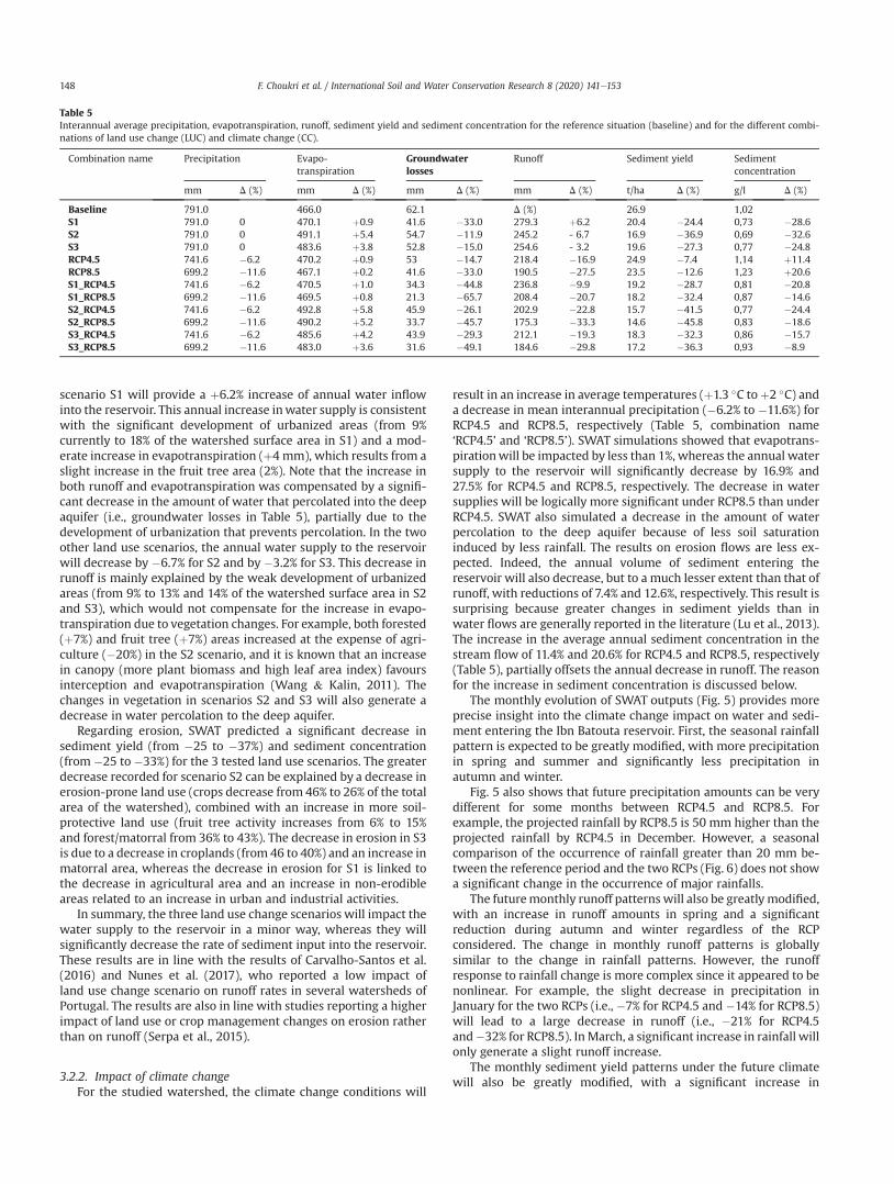
scenario S1 will provide a þ6.2% increase of annual water inflowinto the reservoir. This annual increase inwater supply is consistentwith the significant development of urbanized areas (from 9%currently to 18% of the watershed surface area in S1) and a mod-erate increase in evapotranspiration (þ4 mm), which results from aslight increase in the fruit tree area (2%). Note that the increase inboth runoff and evapotranspiration was compensated by a signifi-cant decrease in the amount of water that percolated into the deepaquifer (i.e., groundwater losses in Table 5), partially due to thedevelopment of urbanization that prevents percolation. In the twoother land use scenarios, the annual water supply to the reservoirwill decrease by �6.7% for S2 and by �3.2% for S3. This decrease inrunoff is mainly explained by the weak development of urbanizedareas (from 9% to 13% and 14% of the watershed surface area in S2and S3), which would not compensate for the increase in evapo-transpiration due to vegetation changes. For example, both forested(þ7%) and fruit tree (þ7%) areas increased at the expense of agri-culture (�20%) in the S2 scenario, and it is known that an increasein canopy (more plant biomass and high leaf area index) favoursinterception and evapotranspiration (Wang & Kalin, 2011). Thechanges in vegetation in scenarios S2 and S3 will also generate adecrease in water percolation to the deep aquifer.
Regarding erosion, SWAT predicted a significant decrease insediment yield (from �25 to �37%) and sediment concentration(from �25 to �33%) for the 3 tested land use scenarios. The greaterdecrease recorded for scenario S2 can be explained by a decrease inerosion-prone land use (crops decrease from 46% to 26% of the totalarea of the watershed), combined with an increase in more soil-protective land use (fruit tree activity increases from 6% to 15%and forest/matorral from 36% to 43%). The decrease in erosion in S3is due to a decrease in croplands (from 46 to 40%) and an increase inmatorral area, whereas the decrease in erosion for S1 is linked tothe decrease in agricultural area and an increase in non-erodibleareas related to an increase in urban and industrial activities.
In summary, the three land use change scenarios will impact thewater supply to the reservoir in a minor way, whereas they willsignificantly decrease the rate of sediment input into the reservoir.These results are in line with the results of Carvalho-Santos et al.(2016) and Nunes et al. (2017), who reported a low impact ofland use change scenario on runoff rates in several watersheds ofPortugal. The results are also in line with studies reporting a higherimpact of land use or crop management changes on erosion ratherthan on runoff (Serpa et al., 2015).
3.2.2. Impact of climate changeFor the studied watershed, the climate change conditions will
result in an increase in average temperatures (þ1.3 �C toþ2 �C) anda decrease in mean interannual precipitation (�6.2% to �11.6%) forRCP4.5 and RCP8.5, respectively (Table 5, combination name‘RCP4.5’ and ‘RCP8.5’). SWAT simulations showed that evapotrans-pirationwill be impacted by less than 1%, whereas the annual watersupply to the reservoir will significantly decrease by 16.9% and27.5% for RCP4.5 and RCP8.5, respectively. The decrease in watersupplies will be logically more significant under RCP8.5 than underRCP4.5. SWAT also simulated a decrease in the amount of waterpercolation to the deep aquifer because of less soil saturationinduced by less rainfall. The results on erosion flows are less ex-pected. Indeed, the annual volume of sediment entering thereservoir will also decrease, but to a much lesser extent than that ofrunoff, with reductions of 7.4% and 12.6%, respectively. This result issurprising because greater changes in sediment yields than inwater flows are generally reported in the literature (Lu et al., 2013).The increase in the average annual sediment concentration in thestream flow of 11.4% and 20.6% for RCP4.5 and RCP8.5, respectively(Table 5), partially offsets the annual decrease in runoff. The reasonfor the increase in sediment concentration is discussed below.
The monthly evolution of SWAT outputs (Fig. 5) provides moreprecise insight into the climate change impact on water and sedi-ment entering the Ibn Batouta reservoir. First, the seasonal rainfallpattern is expected to be greatly modified, with more precipitationin spring and summer and significantly less precipitation inautumn and winter.
Fig. 5 also shows that future precipitation amounts can be verydifferent for some months between RCP4.5 and RCP8.5. Forexample, the projected rainfall by RCP8.5 is 50 mm higher than theprojected rainfall by RCP4.5 in December. However, a seasonalcomparison of the occurrence of rainfall greater than 20 mm be-tween the reference period and the two RCPs (Fig. 6) does not showa significant change in the occurrence of major rainfalls.
The futuremonthly runoff patterns will also be greatlymodified,with an increase in runoff amounts in spring and a significantreduction during autumn and winter regardless of the RCPconsidered. The change in monthly runoff patterns is globallysimilar to the change in rainfall patterns. However, the runoffresponse to rainfall change is more complex since it appeared to benonlinear. For example, the slight decrease in precipitation inJanuary for the two RCPs (i.e., �7% for RCP4.5 and �14% for RCP8.5)will lead to a large decrease in runoff (i.e., �21% for RCP4.5and�32% for RCP8.5). InMarch, a significant increase in rainfall willonly generate a slight runoff increase.
The monthly sediment yield patterns under the future climatewill also be greatly modified, with a significant increase in
Table 5Interannual average precipitation, evapotranspiration, runoff, sediment yield and sediment concentration for the reference situation (baseline) and for the different combi-nations of land use change (LUC) and climate change (CC).
Combination name Precipitation Evapo-transpiration
Groundwaterlosses
Runoff Sediment yield Sedimentconcentration
mm D (%) mm D (%) mm D (%) mm D (%) t/ha D (%) g/l D (%)
Baseline 791.0 466.0 62.1 D (%) 26.9 1,02S1 791.0 0 470.1 þ0.9 41.6 �33.0 279.3 þ6.2 20.4 �24.4 0,73 �28.6S2 791.0 0 491.1 þ5.4 54.7 �11.9 245.2 - 6.7 16.9 �36.9 0,69 �32.6S3 791.0 0 483.6 þ3.8 52.8 �15.0 254.6 - 3.2 19.6 �27.3 0,77 �24.8RCP4.5 741.6 �6.2 470.2 þ0.9 53 �14.7 218.4 �16.9 24.9 �7.4 1,14 þ11.4RCP8.5 699.2 �11.6 467.1 þ0.2 41.6 �33.0 190.5 �27.5 23.5 �12.6 1,23 þ20.6S1_RCP4.5 741.6 �6.2 470.5 þ1.0 34.3 �44.8 236.8 �9.9 19.2 �28.7 0,81 �20.8S1_RCP8.5 699.2 �11.6 469.5 þ0.8 21.3 �65.7 208.4 �20.7 18.2 �32.4 0,87 �14.6S2_RCP4.5 741.6 �6.2 492.8 þ5.8 45.9 �26.1 202.9 �22.8 15.7 �41.5 0,77 �24.4S2_RCP8.5 699.2 �11.6 490.2 þ5.2 33.7 �45.7 175.3 �33.3 14.6 �45.8 0,83 �18.6S3_RCP4.5 741.6 �6.2 485.6 þ4.2 43.9 �29.3 212.1 �19.3 18.3 �32.3 0,86 �15.7S3_RCP8.5 699.2 �11.6 483.0 þ3.6 31.6 �49.1 184.6 �29.8 17.2 �36.3 0,93 �8.9
F. Choukri et al. / International Soil and Water Conservation Research 8 (2020) 141e153148

sediment yield amounts in March for both RCPs and a significantreduction during autumn, while a reduction in sediment yield willbe observed from May to December. During January and February,sediment yield will increase for RCP8.5 and decrease for RCP4.5.The increase in sediment yield for RCP8.5 in January combined witha decrease in rainfall highlights the complex and nonlinearresponse of sediment yield to rainfall change. This result is in linewith previous studies that have already shown that erosion in theMediterranean context was highly nonlinear (Gonz�alez-Hidalgo,Pẽna-Monn�e, & de Luis, 2007).
Analysing the monthly average sediment concentration undercurrent and future climates (Fig. 5) highlights a significant increasein sediment concentration in the streamflow, especially fromJanuary to March. Since no significant change in the seasonal
occurrence of major events has been detected, it is more likely thatthe large increase in sediment concentration from January toMarchis the result of a reduction in soil protection by vegetation. Indeed,the sharp drop in rainfall fromOctober to January will result in botha decrease and delay in vegetation development, which will favoursoil detachment by rainfall during the same months and thefollowing months (February and March). The decrease in vegeta-tion development is confirmed by the decrease in biomass simu-lated by SWAT, especially for croplands, orchards, forests andmatorrals.
Most existing studies that have analysed the impact of climatechange on runoff and erosion are generally based on the 2000Special Report on Emission Scenarios (SRES) named by family (A1,A2, B1 and B2). To relate the results of these existing studies tothose of our studies based on the RCPs defined in 2010, we canconsider that A2 is quite similar to RCP8.5, B1 is quite similar toRCP4.5, and A1B and B2 are intermediate scenarios between RCP4.5and RCP8.5. More details on the comparison between SRES and RCPcan be found at https://www.globalchange.gov/browse/multimedia/emissions-concentrations-and-temperature-projections. Most of these studies have indicated that slight varia-tions in the amount of precipitation can have significant effects onannual average runoff and that climate change is therefore a mainfactor determining total runoff in a watershed (Yang, 2013). Forexample, Bussi, Franc�es, Horel, L�opez-Taraz�on, and Batalla (2014)assessed the impact of climate change on the hydrological andsedimentological cycles of the �Esera River catchment (Spain) underA2 and B2 scenarios (2070e2100). They found that the total wateryield is expected to decrease by 40 and 35% under the A2 and B2scenarios, respectively, while the total precipitation is expected todecrease by only 13 and 12%. Nunes et al. (2017) simulated adecrease in runoff of approximately 25% in a Mediterraneanwatershed of Vale do Gaio, south of Portugal, under the two climatescenarios A1B and B1 over the period 2071e2100, while theamount of precipitation decreased by only 9%. The impact ofclimate change on sediment yield described in other Mediterra-nean studies often showed an increase in erosion rates in responseto a decrease in rainfall. For example, Paroissien et al. (2015)
Fig. 5. Monthly SWAT simulated values of rainfall, runoff, sediment yield and sediment concentration at the Tleta watershed outlet during the period 1983e2010 (REF) and theperiod 2031e2050 (RCP4.5 and RCP8.5).
Fig. 6. Seasonal occurrence of major rainfall events using boxplots based on rainfallevents greater than 20 mm during the period 1983e2010 (REF) and the period2031e2050 (RCP4.5 and RCP8.5).
F. Choukri et al. / International Soil and Water Conservation Research 8 (2020) 141e153 149
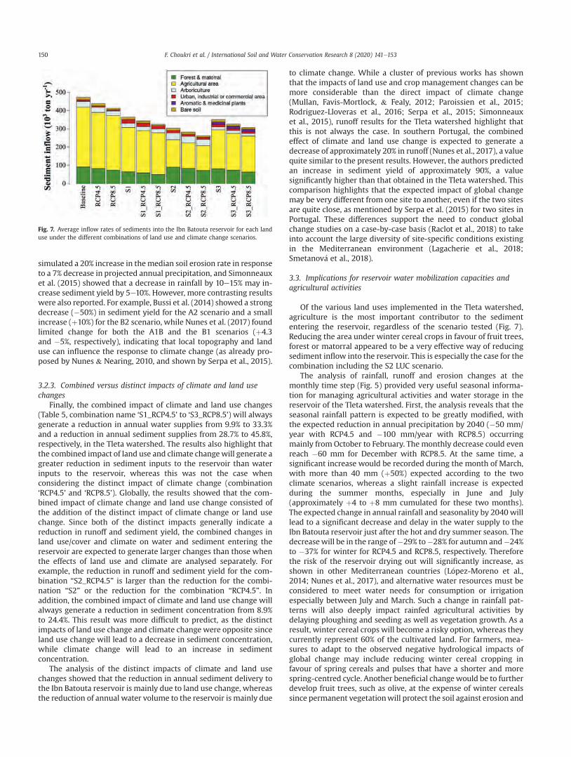
simulated a 20% increase in themedian soil erosion rate in responseto a 7% decrease in projected annual precipitation, and Simonneauxet al. (2015) showed that a decrease in rainfall by 10e15% may in-crease sediment yield by 5e10%. However, more contrasting resultswere also reported. For example, Bussi et al. (2014) showed a strongdecrease (�50%) in sediment yield for the A2 scenario and a smallincrease (þ10%) for the B2 scenario, while Nunes et al. (2017) foundlimited change for both the A1B and the B1 scenarios (þ4.3and �5%, respectively), indicating that local topography and landuse can influence the response to climate change (as already pro-posed by Nunes & Nearing, 2010, and shown by Serpa et al., 2015).
3.2.3. Combined versus distinct impacts of climate and land usechanges
Finally, the combined impact of climate and land use changes(Table 5, combination name ‘S1_RCP4.5’ to ‘S3_RCP8.5’) will alwaysgenerate a reduction in annual water supplies from 9.9% to 33.3%and a reduction in annual sediment supplies from 28.7% to 45.8%,respectively, in the Tleta watershed. The results also highlight thatthe combined impact of land use and climate changewill generate agreater reduction in sediment inputs to the reservoir than waterinputs to the reservoir, whereas this was not the case whenconsidering the distinct impact of climate change (combination‘RCP4.5’ and ‘RCP8.5’). Globally, the results showed that the com-bined impact of climate change and land use change consisted ofthe addition of the distinct impact of climate change or land usechange. Since both of the distinct impacts generally indicate areduction in runoff and sediment yield, the combined changes inland use/cover and climate on water and sediment entering thereservoir are expected to generate larger changes than those whenthe effects of land use and climate are analysed separately. Forexample, the reduction in runoff and sediment yield for the com-bination “S2_RCP4.5” is larger than the reduction for the combi-nation “S2” or the reduction for the combination “RCP4.5”. Inaddition, the combined impact of climate and land use change willalways generate a reduction in sediment concentration from 8.9%to 24.4%. This result was more difficult to predict, as the distinctimpacts of land use change and climate change were opposite sinceland use change will lead to a decrease in sediment concentration,while climate change will lead to an increase in sedimentconcentration.
The analysis of the distinct impacts of climate and land usechanges showed that the reduction in annual sediment delivery tothe Ibn Batouta reservoir is mainly due to land use change, whereasthe reduction of annual water volume to the reservoir is mainly due
to climate change. While a cluster of previous works has shownthat the impacts of land use and crop management changes can bemore considerable than the direct impact of climate change(Mullan, Favis-Mortlock, & Fealy, 2012; Paroissien et al., 2015;Rodriguez-Lloveras et al., 2016; Serpa et al., 2015; Simonneauxet al., 2015), runoff results for the Tleta watershed highlight thatthis is not always the case. In southern Portugal, the combinedeffect of climate and land use change is expected to generate adecrease of approximately 20% in runoff (Nunes et al., 2017), a valuequite similar to the present results. However, the authors predictedan increase in sediment yield of approximately 90%, a valuesignificantly higher than that obtained in the Tleta watershed. Thiscomparison highlights that the expected impact of global changemay be very different from one site to another, even if the two sitesare quite close, as mentioned by Serpa et al. (2015) for two sites inPortugal. These differences support the need to conduct globalchange studies on a case-by-case basis (Raclot et al., 2018) to takeinto account the large diversity of site-specific conditions existingin the Mediterranean environment (Lagacherie et al., 2018;Smetanov�a et al., 2018).
3.3. Implications for reservoir water mobilization capacities andagricultural activities
Of the various land uses implemented in the Tleta watershed,agriculture is the most important contributor to the sedimententering the reservoir, regardless of the scenario tested (Fig. 7).Reducing the area under winter cereal crops in favour of fruit trees,forest or matorral appeared to be a very effective way of reducingsediment inflow into the reservoir. This is especially the case for thecombination including the S2 LUC scenario.
The analysis of rainfall, runoff and erosion changes at themonthly time step (Fig. 5) provided very useful seasonal informa-tion for managing agricultural activities and water storage in thereservoir of the Tleta watershed. First, the analysis reveals that theseasonal rainfall pattern is expected to be greatly modified, withthe expected reduction in annual precipitation by 2040 (�50 mm/year with RCP4.5 and �100 mm/year with RCP8.5) occurringmainly from October to February. The monthly decrease could evenreach �60 mm for December with RCP8.5. At the same time, asignificant increase would be recorded during the month of March,with more than 40 mm (þ50%) expected according to the twoclimate scenarios, whereas a slight rainfall increase is expectedduring the summer months, especially in June and July(approximately þ4 to þ8 mm cumulated for these two months).The expected change in annual rainfall and seasonality by 2040 willlead to a significant decrease and delay in the water supply to theIbn Batouta reservoir just after the hot and dry summer season. Thedecreasewill be in the range of�29% to�28% for autumn and�24%to �37% for winter for RCP4.5 and RCP8.5, respectively. Thereforethe risk of the reservoir drying out will significantly increase, asshown in other Mediterranean countries (L�opez-Moreno et al.,2014; Nunes et al., 2017), and alternative water resources must beconsidered to meet water needs for consumption or irrigationespecially between July and March. Such a change in rainfall pat-terns will also deeply impact rainfed agricultural activities bydelaying ploughing and seeding as well as vegetation growth. As aresult, winter cereal crops will become a risky option, whereas theycurrently represent 60% of the cultivated land. For farmers, mea-sures to adapt to the observed negative hydrological impacts ofglobal change may include reducing winter cereal cropping infavour of spring cereals and pulses that have a shorter and morespring-centred cycle. Another beneficial changewould be to furtherdevelop fruit trees, such as olive, at the expense of winter cerealssince permanent vegetationwill protect the soil against erosion and
Fig. 7. Average inflow rates of sediments into the Ibn Batouta reservoir for each landuse under the different combinations of land use and climate change scenarios.
F. Choukri et al. / International Soil and Water Conservation Research 8 (2020) 141e153150
therefore participate in the expansion of the reservoir lifetime.An overall decrease in sediment input to the reservoir is ex-
pected to be distributed almost year-round (Fig. 5), except duringsome months at the beginning of the year depending on the RCPconsidered. Higher precipitation and runoff amounts can explainthe sediment yield increase in March, but only a change in vege-tation development could explain the increase for the othermonths. The benefit on erosion rates of a clear decrease in rainfallduring the fall season when cereal cropped lands are bare istherefore very significant. By reducing the siltation rate of thereservoir, global change is likely to expand the lifetime of thereservoir. Table 6 shows the remaining water volume capacity ofthe reservoir in 2040. It also provides the year when the waterstorage capacity of the reservoir will fall below 1 Mm3, assuming aconstant annual erosion rate beyond 2040 and a trapping efficiencyupdated each year using Heinemann’s formula.
An increase in internal deposition in the watershed, particularlyin the stream, can also be expected due to higher concentrations ofsediment in the stream flow associated with a decrease in streamfrequency and flow that will result in a decrease in hydro-sedimentological connectivity.
4. Conclusions
The Soil and Water Assessment Tool was applied to the Tletawatershed to determine for the first time the distinct and combinedimpacts of global change (climate and land use changes) on therunoff and erosion responses in northern Morocco. All combina-tions of three climate and four land use scenarios (one being thereference conditions) were simulated by the SWAT model over theperiod 2031e2050 with calibrated parameters over the referenceperiod 1983e2010. The SWATmodel successfully reproducedwaterand sediment entering the reservoir located downstream of thestudied watershed over the reference period 1983e2010. Climatechange resulted in an increase in average temperatures (þ1.3 �Cto þ2 �C) and a decrease in mean interannual precipitation (�6.2%to �11.6%) for RCP4.5 and RCP8.5, respectively, with the highestreduction in the fall and winter seasons. The combined impact ofclimate and land use changes is expected to generate a reduction inwater availability for consumption and irrigation (9.9%e33.3%) anda large reduction in annual sediment entering the downstreamreservoir of the Tleta watershed (28.7%e45.8%). The combinedchanges in land use/cover and climate on water balance and sedi-ment outputs will generate larger changes compared to those of theeffects of land use/cover change alone. The analysis of the distinctimpacts of climate and land use changes suggests that the reduc-tion in annual sediment delivery to the reservoir is mainly due toland use change, whereas the reduction in annual water volume tothe reservoir is chiefly due to climate change. A seasonal analysis of
the change highlights the need for the adaptation of agriculturalactivities and of water supply from the reservoir because of thehigher risk of reservoir depletion between July and March. Finally,consideration should be given to the use of alternative water re-sources to meet the region’s water needs. Comparison with theresults obtained for other Mediterranean regions shows that theexpected impact of global change can be very different from onesite to another, even if the two sites are very close to each other.This supports the need to conduct global change studies on a case-by-case basis to be able to take into account site-specific conditions.Future developments will require testing awider range of scenariosand quantifying uncertainties associated with the results providedon the expected changes.
Declaration of competing interest
I declare no conflict of interest.
Acknowledgements
This work benefits from the financial support of JEAI “Vecteurs”funded by IRD institution, ALMIRA (ANR-12-TMED-0003 funded byANR) and MASCC (through ARIMNET2, an ERA-NET funded by theEuropean Union’s Seventh Framework Program for research, tech-nological development and demonstration under grant agreementno. 618127) projects. J.P. Nunes was further supported by a researchgrant from the Fundaç~ao para a Ciencia e a Tecnologia (IF/00586/2015).
References
Arnold, J., Moriasi, D., Gassman, P., Abbaspour, K., White, M., Srinivasan, R., et al.(2012). Swat: Model use, calibration, and validation. Transactions of the ASABE,55(4), 1491e1508.
Ayadi, I., Abida, H., Djebbar, Y., & Mahjoub, R. (2010). Sediment yield variability incentral Tunisia: A quantitative analysis of its controlling factors. HydrologicalSciences Journal, 55, 446e458. https://doi.org/10.1080/02626661003741526.
Bangash, R. F., Passuello, A., Sanchez-Canales, M., Terrado, M., L�opez, A., JavierElorza, F., et al. (2013). Ecosystem services in Mediterranean river basin: Climatechange impact on water provisioning and erosion control. The Science of theTotal Environment, 458e460, 246e255. https://doi.org/10.1016/j.scitotenv.2013.04.025.
Briak, H., Moussadek, R., Aboumaria, K., & Mrabet, R. (2016). Assessing sedimentyield in Kalaya gauged watershed (Northern Morocco) using GIS and SWATmodel. International Soil and Water Conservation Research, 4(3), 177e185.
Briak, H., Mrabet, R., Moussadek, R., & Aboumaria, K. (2019). Use of a calibratedSWAT model to evaluate the effects of agricultural BMPs on sediments of theKalaya river basin (North of Morocco). International Soil and Water ConservationResearch, 7, 176e183.
Brouziyne, Y., Abouabdillah, A., Hirich, A., Bouabid, R., Zaaboul, R., & Benaabidate, L.(2018). Modeling sustainable adaptation strategies toward a climate-smartagriculture in a Mediterranean watershed under projected climate changescenarios. Agricultural Systems, 162, 154e163. https://doi.org/10.1016/j.agsy.2018.01.024.
Bucak, T., Trolle, D., Andersen, H. E., Thodsen, H., Erdogan, S., Levi, E. E., et al. (2017).
Table 6Impact of the different scenarios on reservoir volume capacity by 2040 and the year the storage capacity of the reservoir would fall below 1 Mm3.
Combination name Remaining reservoir volume in 2040 (106 m3) Year when reservoir storage capacity would fall below 1.10⁶ m3
Baseline 19.01 2093S1 20.19 2114S2 20.80 2131S3 20.32 2117RCP4.5 19.35 2097RCP8.5 19.59 2100S1_RCP4.5 20.38 2118S1_RCP8.5 20.55 2122S2_RCP4.5 21.00 2137S2_RCP8.5 21.19 2144S3_RCP4.5 20.54 2122S3_RCP8.5 20.72 2127
F. Choukri et al. / International Soil and Water Conservation Research 8 (2020) 141e153 151
Future water availability in the largest freshwater Mediterranean lake is at greatrisk as evidenced from simulations with the SWAT model. The Science of theTotal Environment, 581e582, 413e425. https://doi.org/10.1016/j.scitotenv.2016.12.149.
Bussi, G., Franc�es, F., Horel, E., L�opez-Taraz�on, J. A., & Batalla, R. J. (2014). Modellingthe impact of climate change on sediment yield in a highly erodible Mediter-ranean catchment. Journal of Soils and Sediments, 14(12), 1921e1937.
Carvalho-Santos, C., Nun�es, J. P., Monteiro, A. T., Hein, L., & Honrado, J. P. (2016).Assessing the effects of land cover and future climate conditions on the pro-vision of hydrological services in a medium-sized watershed of Portugal. Hy-drological Processes, 30(5), 720e738.
Choukri, F., Chikhaoui, M., Naimi, M., Raclot, D., Pepin, Y., & Lafia, K. (2016). Impactdu changement climatique sur L’�evolution de L’�erosivit�e des pluies dans le RifOccidental (nord du maroc). European Scientific Journal, ESJ, 12(32).
De Franchis, L., Bleu, P., & Ibanez, F. (2003). Threats to soils in mediterranean coun-tries: Document review.
Descroix, L., Moussa, I. B., Genthon, P., Sighomnou, D., Mah�e, G., Mamadou, I., et al.(2013). Impact of drought and landeuse changes on surfaceewater quality andquantity: The ‘sahelian’ paradox. In P. M. Bradley (Ed.), Current perspectives incontaminant hydrology and water resources sustainability (pp. 243e271). https://doi.org/10.5772/54536 2013.
Gal, L., Grippa, M., Hiernaux, P., Pons, L., & Kergoat, L. (2017). The paradoxicalevolution of runoff in the pastoral Sahel: Analysis of the hydrological changesover the agoufou watershed (Mali) using the KINEROS-2 model. Hydrology andEarth System Sciences, 21, 4591e4613. https://doi.org/10.5194/hess-21-4591-2017.
García-Ruiz, J. M., L�opez-Moreno, J. I., Vicente-Serrano, S., Lasanta-Martínez, T., &Beguería, S. (2011). Mediterranean water resources in a global change scenario.Earth-Science Reviews, 105, 121e139.
García-Ruiz, J. M., Nadal-Romero, E., Lana-Renault, N., & Beguería, S. (2013). Erosionin mediterranean landscapes: Changes and future challenges. Geomorphology,198, 20e36.
Ghaffari, G., Keesstra, S., Ghodousi, J., & Ahmadi, H. (2010). SWAT-simulated hy-drological impact of land-use change in the Zanjanrood basin, Northwest Iran.Hydrological Processes: International Journal, 24(7), 892e903.
Giorgi, F., & Lionello, P. (2008). Climate change projections for the Mediterraneanregion. Global and Planetary Change, 63(2e3), 90e104.
Gonz�alez-Hidalgo, J. C., Pẽna-Monn�e, J. L., & de Luis, M. (2007). A review of daily soilerosion in Western Mediterranean areas. Catena, 71, 193e199.
Heinemann, H. G. (1981). A new sediment trap efficiency curve for small reservoirs.Water Resources Bulletin, 17, 825e830.
H�erivaux, C., Vinatier, F., Sabir, M., Guillot, F., & Rinaudo, J. D. (2018). Combiningscenario workshops, quantitative approaches and land use change modeling todesign plausible future land use scenarios in the Tleta catchment (Morocco). InInternational Conference “Vulnerability of the Mediterranean soils to watererosion: State of knowledge and adaptation strategies in the face of global change”(pp. 20e21). novembre 2018, Rabat, Morocco.
Huard, F., Choukri, F., Raclot, D., P�epin, Y., Chikhaoui, M., Naimi, M., et al. (2019).Spatialisation fine des projections climatiques dans le bassin versant du Tleta(Nord Maroc). Revue Marocaine des Sciences Agronomiques et V�et�erinaires, 7(2).Available at: https://www.agrimaroc.org/index.php/Actes_IAVH2/article/view/694.
Hulme, M., & Kelly, M. (1993). Exploring the links between desertification andclimate change. Environment: Science and Policy for Sustainable Development,35(6), 4e45.
IPCC. (2014). Climate change 2014: Synthesis report. In R. K. Pachauri, & L. A. Meyer(Eds.), Contribution of working groups I, II and III to the fifth assessment report ofthe intergovernmental panel on climate change, Core Writing Team (p. 151).Geneva, Switzerland: IPCC. Available at: https://www.ipcc.ch/report/ar5/syr/.
Issa, L. K., Lech-Hab, K. B. H., Raissouni, A., & El Arrim, A. (2016). Cartographiequantitative du risque d’erosion des sols par approche SIG/USLE au niveau dubassin versant Kalaya (Maroc Nord Occidental). Journal of Materials and Envi-ronmental Science, 7(8), 2778e2795.
Kleme�s, V. (1986). Operational testing of hydrological simulation models. Hydro-logical Sciences Journal, 31, 13e24. https://doi.org/10.1080/02626668609491024.
Kosmas, C., Danalatos, N., Cammeraat, L. H., Chabart, M., Diamantopoulos, J.,Farand, R., et al. (1997). The effect of land use on runoff and soil erosion ratesunder Mediterranean conditions. Catena, 29(1), 45e59.
Lagacherie, P., �Alvaro-Fuentes, J., Annabi, M., Bernoux, M., Bouarfa, S., Douaoui, A.,et al. (2018). Managing Mediterranean Soil resources under global changes.Regional Environmental Change, 18(3), 663e675.
Lahlou, A. (2000). Quelques aspects environnementaux dans les pays du Maghreb.Rabat, Maroc: ISESCO.
Lal, R. (2003). Soil erosion and the global carbon budget. Environment International,29(4), 437e450.
Li, Z., & Fang, H. (2016). Impacts of climate change on water erosion: A review.Earth-Science Reviews, 163, 94e117.
L�opez-Moreno, J. I., Zabalza, J., Vicente-Serrano, S. M., Revuelto, J., Gilaberte, M.,Azorin-Molina, C., et al. (2014). Impact of climate and land use change on wateravailability and reservoir management: Scenarios in the upper arag�on river,Spanish pyrenees. The Science of the Total Environment, 493, 1222e1231. https://doi.org/10.1016/j.scitotenv.2013.09.031.
Ludwig, R., & Roson, R. (2016). Climate change, water and security in theMedi-terranean: Introduction to the special issue. The Science of the Total Environment,543, 847e850. https://doi.org/10.1016/j.scitotenv.2015.10.142.
Lu, X., Ran, L., Liu, S., Jiang, T., Zhang, S., & Wang, J. (2013). Sediment loads responseto climate change: A preliminary study of eight large Chinese rivers. Interna-tional Journal of Sediment Research, 28(1), 1e14.
Merzouk, A., Fenjiro, I., & Laouina, A. (1996). Cartographie de l’�evolution des formesd’�erosion dans le Rif Occidental (maroc): �Etude multidate utilisant un SIGbassin versant. Bulletin-R�eseau Erosion, 16, 444e456.
Michard, A. (1976). El�ements de g�eologie marocaine. �Editions du Service g�eologiquedu Maroc.
Moriasi, D., Arnold, J., Van Liew, M., Bingner, R., Harmel, R., & Veith, T. (2007). Modelevaluation guidelines for systematic quantification of accuracy in watershedsimulations. Transactions of the American Society of Agricultural and BiologicalEngineers, 50(3), 885e900.
Mullan, D., Favis-Mortlock, D., & Fealy, R. (2012). Addressing key limitations asso-ciated with modelling soil erosion under the impacts of future climate change.Agricultural and Forest Meteorology, 156, 18e30.
Nearing, M. A., Jetten, V., Baffaut, C., Cerdan, O., Couturier, A., Hernandez, M., et al.(2005). Modeling response of soil erosion and runoff to changes in precipitationand cover. Catena, 61(2e3), 131e154.
Neitsch, S., Arnold, J., Kiniry, J., Williams, J., & King, K. (2005). Soil and waterassessment tool: Theoretical documentation. Texas, USA: version 2005.
Nunes, J. P., Jacinto, R., & Keizer, J. J. (2017). Combined impacts of climate and socio-economic scenarios on irrigation water availability for a dry Mediterraneanreservoir. The Science of the Total Environment, 584, 219e233.
Nunes, J. P., Naranjo Quintanilla, P., Santos, J. M., Serpa, D., Carvalho-Santos, C.,Rocha, J., et al. (2018). Afforestation, subsequent forest fires and provision ofhydrological services: A model-based analysis for a mediterranean moun-tainous catchment. Land Degradation & Development, 29(3), 776e788.
Nunes, J. P., & Nearing, M. (2010). Modelling impacts of climatic change: Casestudies using the new generation of erosion models. Handbook of ErosionModelling, 289e312.
O’Neill, B. C., Kriegler, E., Ebi, K. L., Kemp-Benedict, E., Riahi, K., Rothman, D. S., et al.(2017). The roads ahead: Narratives for shared socioeconomic pathwaysdescribing world futures in the 21st century. Global Environmental Change, 42,169e180.
Paroissien, J.-B., Darboux, F., Couturier, A., Devillers, B., Mouillot, F., Raclot, D., et al.(2015). A method for modeling the effects of climate and land use changes onerosion and sustainability of soil in a Mediterranean watershed (Languedoc,France). Journal of Environmental Management, 150, 57e68.
Pimentel, D., Harvey, C., Resosudarmo, P., Sinclair, K., Kurz, D., McNair, M., et al.(1995). Environmental and economic costs of soil erosion and conservationbenefits. Science, 267(5201), 1117e1123.
Pruski, F., & Nearing, M. (2002). Climate-induced changes in erosion during the 21stcentury for eight US locations. Water Resources Research, 38(12), 34-31-34-11.
Raclot, D., & Albergel, J. (2006). Runoff and water erosion modelling using WEPP ona Mediterranean cultivated catchment. Physics and Chemistry of the Earth,31(17), 1038e1047.
Raclot, D., Le Bissonnais, Y., Annabi, M., Sabir, M., & Smetanova, A. (2018). Mainissues for preserving Mediterranean soil resources from water erosion underglobal change. Land Degradation & Development, 29(3), 789e799.
Refsgaard, J. C., Henriksen, H. J., Harrar, W. G., Scholten, H., & Kassahun, A. (2005).Quality assurance in model based water management e review of existingpractice and outline of new approaches. Environmental Modelling & Software,20, 1201e1215. https://doi.org/10.1016/j.envsoft.2004.07.006.
Rodriguez-Lloveras, X., Buytaert, W., & Benito, G. (2016). Land use can offset climatechange induced increases in erosion in Mediterranean watersheds. Catena, 143,244e255. https://doi.org/10.1016/j.catena.2016.04.012.
Serpa, D., Nunes, J. P., Santos, J., Sampaio, E., Jacinto, R., Veiga, S., et al. (2015). Im-pacts of climate and land use changes on the hydrological and erosion processesof two contrasting Mediterranean catchments. The Science of the Total Envi-ronment, 538, 64e77.
Simonneaux, V., Cheggour, A., Deschamps, C., Mouillot, F., Cerdan, O., & LeBissonnais, Y. (2015). Land use and climate change effects on soil erosion in asemi-aridmountainous watershed (High Atlas, Morocco). Journal of Arid Envi-ronments, 122, 64e75.
Smetanov�a, A., Le Bissonnais, Y., Raclot, D., Nunes, J. P., Licciardello, F., LeBouteiller, C., et al. (2018). Temporal variability and time compression of sedi-ment yield in small mediterranean catchments: Impacts for land and watermanagement. Soil Use & Management, 34(3), 388e403. https://doi.org/10.1111/sum.12437.
Stoner, A. M., Hayhoe, K., Yang, X., & Wuebbles, D. J. (2013). An asynchronousregional regression model for statistical downscaling of daily climate variables.International Journal of Climatology, 33(11), 2473e2494.
Tomer, M. D., & Schilling, K. E. (2009). A simple approach to distinguish land-useand climate-change effects on watershed hydrology. Journal of hydrology,376(1), 24e33.
Wang, R., & Kalin, L. (2011). Modelling effects of land use/cover changes underlimited data. Ecohydrology, 4(2), 265e276.
Wilby, R. (2007). Decadal climate forecasting techniques for adaptation and devel-opment planning: A briefing document on available methods, constraints, risks andopportunities. UK: Department for International Development.
Wilby, R. L., Dawson, C. W., & Barrow, E. M. (2002). SDSMda decision support toolfor the assessment of regional climate change impacts. Environmental Modelling& Software, 17(2), 145e157.
Williams, J. R. (1975). Sediment-yield prediction with universal equation usingrunoff energy factor. In Present and prospective technology for predicting
F. Choukri et al. / International Soil and Water Conservation Research 8 (2020) 141e153152

sediment yield and sources (pp. 244e252). Washington DC: US Department ofAgriculture, Agriculture Research Service.
WRB. (2006).World reference base for soil resources. IUSS Working Group. Rome: FAO.World Soil Resources Reports No. 103 http://www.fao.org/3/a-a0510e.pdf.
Yang, H. (2013). The hydrologic effects of climate change and urbanization in the LasVegas Wash Watershed, Nevada. University of Cincinnati.
Zhang, R., Corte-Real, J., Moreira, M., Kilsby, C., Birkinshaw, S., Burton, A., et al.(2019b). Downscaling climate change on water availability, sediment yield andextreme events: Application to a Mediterranean basin. International Journal ofClimatology. https://doi.org/10.1002/joc.5994.
Zhang, R., Corte-Real, J., Moreira, M., Kilsby, C., Burton, A., Fowler, H. J., et al. (2019a).Downscaling climate change of mean climatology and extremes of precipitationand temperature: Application to a Mediterranean climate basin. InternationalJournal of Climatology. https://doi.org/10.1002/joc.6122.
Zhang, G. H., Nearing, M., & Liu, B. (2005). Potential effects of climate change onrainfall erosivity in the Yellow River basin of China. Transactions of the ASAE,48(2), 511e517.
Zhang, Y.-G., Nearing, M., Zhang, X.-C., Xie, Y., & Wei, H. (2010). Projected rainfallerosivity changes under climate change from multimodel and multiscenarioprojections in Northeast China. Journal of hydrology, 384(1), 97e106.
F. Choukri et al. / International Soil and Water Conservation Research 8 (2020) 141e153 153
Original Research Article
Combating wind erosion through soil stabilization under simulatedwind flow condition e Case of Kuwait
Hana’a BurezqDesert Agriculture and Ecosystems Program (DAEP), Environment and Life Sciences Research Center (ELSRC), Kuwait Institute for Scientific Research (KISR),P.O. Box 24885 Safat, 13109, Kuwait
a r t i c l e i n f o
Article history:Received 15 August 2019Received in revised form4 March 2020Accepted 6 March 2020Available online 10 March 2020
Keywords:Biodegradable-productBiocharSoil-stabilityWind-erosionWind-tunnelSaltation
a b s t r a c t
The soil survey of Kuwait has revealed the landscapes dominated by loose sandy material, that arevulnerable to wind erosion. Globally three modes of soil particle movement (creep, saltation & sus-pension) by wind have been recognized. To evaluate these modes in the deserts of Kuwait, sixty surfacesoil samples were collected and analyzed for particle sizes to quantify relative occurrence of modes ofparticle movement in the deserts of Kuwait. This analysis revealed distribution of particles in the sizeranges, as follows: saltation (70%) > Creep (20%) > Suspension (10%) confirming saltation is the mainmode of soil movement. This has provided basic information to set up a pilot scale experiment to reducethe wind erosion rate through sand stabilization using various sand binding products in three treat-ments; T1 (native sandy soil); T2 (sand mixed with biochar and animal manure); T3 (sand mixed withbiochar, animal manure, Urea Formaldehyde (UF), Sulfonated Naphthalene Formaldehyde (SNF), and PolyVinyl Alcohol (PVA). The results showed that the erosion rate of native sandy soil (T1) has increased from3.33, 4.77 to 7.35 g/(m2. min) when wind speed was increased from 5, 10 to 15 m/s, respectively. At thesame wind speeds, the measured erosion loss was 1.99, 3.07, 5.32 g/(m2. min) in T2 and 1.17, 2.6, 4.24 g/(m2. min) in T3. From these results, it can be concluded that there is a possibility to reduce wind erosionin the deserts of Kuwait through sand stabilization and save the deserts from further degradation.© 2020 International Research and Training Center on Erosion and Sedimentation and China Water andPower Press. Production and Hosting by Elsevier B.V. This is an open access article under the CC BY-NC-
ND license (http://creativecommons.org/licenses/by-nc-nd/4.0/).
1. Introduction
Soil erosion refers to the loss of soil by water and wind. It isaccelerated when native landscapes, such as deserts, are over-grazed by uncontrolled animals. The top soil is exposed and is oftenblown away bywind, including nutrients and organic matter losses.Land degradation by water and wind erosion is a serious problemworldwide. According to the European Commission’s World Atlasof Desertification, more than 75 percent of Earth’s land area isalready degraded, and more than 90 percent could becomedegraded by 2050. Each year, an estimated 24 billion tons of fertilesoil are lost due to erosion. That’s 3.4 tones lost every year for everyperson on the planet. A new study estimates global annual cost of 8billion US dollars to global GDP (Sartori et al., 2019) due to erosion.Among various land degradation processes, soil erosion is recog-nized as a major environmental problem causing a loss of top soil
and nutrients, reduced soil fertility (Zhao, Mu, Wen, Wang, & Gao,2013), and as a consequence, reduced crop yields (Telles,Guimaraes, & Dechen, 2011). Furthermore, soil erosion may in-crease the losses of CO2, exacerbating the climate change (Lugatoet al., 2018). According to soil quotes released by Global Soil Part-nership at the 2019 World Soil Day Event, i) soil erosion is thenumber 1 threat to our planet’s soils, ii) soil erosion can lead up to50% losses in crop yield (Global Soil Partnership). The author, beingthe national focal point at Global Soil Partnership, has initiated aprogram to reduce soil degradation in Kuwait to conserve ecosys-tems for better services and for agriculture production to supportnational food security.
It is common sense that the desert like conditions (infertilelandscape without vegetation) are considered as the endpoint ofland degradation process. The particles lifted by the wind cause acascading effect, and when they fall and strike the soil surface; theykick more particles into the air in a chain reaction. Three distin-guished modes of soil particles movement (creep, saltation andsuspension) are recognized (Bagnold, 1973). The particles(>500 mm) start moving due to the impact of saltating particles
E-mail address: [email protected]: http://www.kisr.edu.kw
Contents lists available at ScienceDirect
International Soil and Water Conservation Research
journal homepage: www.elsevier .com/locate/ iswcr
https://doi.org/10.1016/j.iswcr.2020.03.0012095-6339/© 2020 International Research and Training Center on Erosion and Sedimentation and China Water and Power Press. Production and Hosting by Elsevier B.V. Thisis an open access article under the CC BY-NC-ND license (http://creativecommons.org/licenses/by-nc-nd/4.0/).
International Soil and Water Conservation Research 8 (2020) 154e163
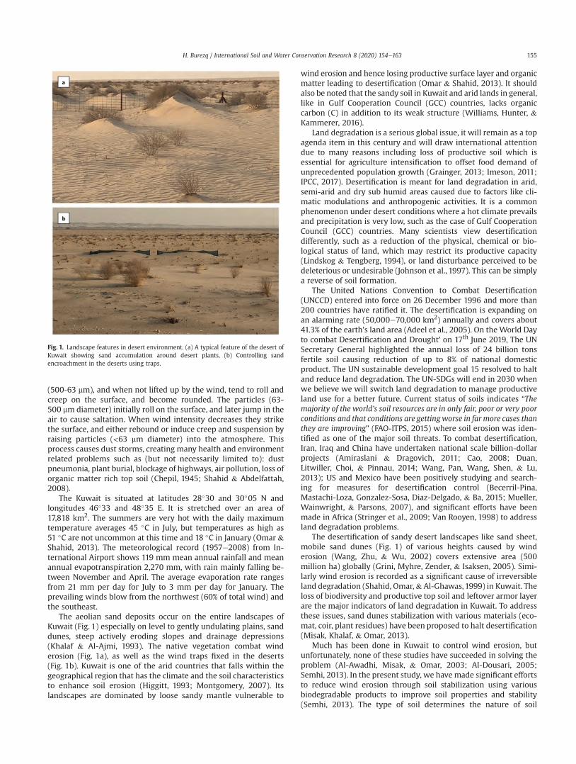
(500-63 mm), and when not lifted up by the wind, tend to roll andcreep on the surface, and become rounded. The particles (63-500 mm diameter) initially roll on the surface, and later jump in theair to cause saltation. When wind intensity decreases they strikethe surface, and either rebound or induce creep and suspension byraising particles (<63 mm diameter) into the atmosphere. Thisprocess causes dust storms, creating many health and environmentrelated problems such as (but not necessarily limited to): dustpneumonia, plant burial, blockage of highways, air pollution, loss oforganic matter rich top soil (Chepil, 1945; Shahid & Abdelfattah,2008).
The Kuwait is situated at latitudes 28�30 and 30�05 N andlongitudes 46�33 and 48�35 E. It is stretched over an area of17,818 km2. The summers are very hot with the daily maximumtemperature averages 45 �C in July, but temperatures as high as51 �C are not uncommon at this time and 18 �C in January (Omar &Shahid, 2013). The meteorological record (1957e2008) from In-ternational Airport shows 119 mm mean annual rainfall and meanannual evapotranspiration 2,270 mm, with rain mainly falling be-tween November and April. The average evaporation rate rangesfrom 21 mm per day for July to 3 mm per day for January. Theprevailing winds blow from the northwest (60% of total wind) andthe southeast.
The aeolian sand deposits occur on the entire landscapes ofKuwait (Fig. 1) especially on level to gently undulating plains, sanddunes, steep actively eroding slopes and drainage depressions(Khalaf & Al-Ajmi, 1993). The native vegetation combat winderosion (Fig. 1a), as well as the wind traps fixed in the deserts(Fig. 1b). Kuwait is one of the arid countries that falls within thegeographical region that has the climate and the soil characteristicsto enhance soil erosion (Higgitt, 1993; Montgomery, 2007). Itslandscapes are dominated by loose sandy mantle vulnerable to
wind erosion and hence losing productive surface layer and organicmatter leading to desertification (Omar & Shahid, 2013). It shouldalso be noted that the sandy soil in Kuwait and arid lands in general,like in Gulf Cooperation Council (GCC) countries, lacks organiccarbon (C) in addition to its weak structure (Williams, Hunter, &Kammerer, 2016).
Land degradation is a serious global issue, it will remain as a topagenda item in this century and will draw international attentiondue to many reasons including loss of productive soil which isessential for agriculture intensification to offset food demand ofunprecedented population growth (Grainger, 2013; Imeson, 2011;IPCC, 2017). Desertification is meant for land degradation in arid,semi-arid and dry sub humid areas caused due to factors like cli-matic modulations and anthropogenic activities. It is a commonphenomenon under desert conditions where a hot climate prevailsand precipitation is very low, such as the case of Gulf CooperationCouncil (GCC) countries. Many scientists view desertificationdifferently, such as a reduction of the physical, chemical or bio-logical status of land, which may restrict its productive capacity(Lindskog & Tengberg, 1994), or land disturbance perceived to bedeleterious or undesirable (Johnson et al., 1997). This can be simplya reverse of soil formation.
The United Nations Convention to Combat Desertification(UNCCD) entered into force on 26 December 1996 and more than200 countries have ratified it. The desertification is expanding onan alarming rate (50,000e70,000 km2) annually and covers about41.3% of the earth’s land area (Adeel et al., 2005). On the World Dayto combat Desertification and Drought’ on 17th June 2019, The UNSecretary General highlighted the annual loss of 24 billion tonsfertile soil causing reduction of up to 8% of national domesticproduct. The UN sustainable development goal 15 resolved to haltand reduce land degradation. The UN-SDGs will end in 2030 whenwe believe we will switch land degradation to manage productiveland use for a better future. Current status of soils indicates “Themajority of the world’s soil resources are in only fair, poor or very poorconditions and that conditions are getting worse in far more cases thanthey are improving” (FAO-ITPS, 2015) where soil erosion was iden-tified as one of the major soil threats. To combat desertification,Iran, Iraq and China have undertaken national scale billion-dollarprojects (Amiraslani & Dragovich, 2011; Cao, 2008; Duan,Litwiller, Choi, & Pinnau, 2014; Wang, Pan, Wang, Shen, & Lu,2013); US and Mexico have been positively studying and search-ing for measures for desertification control (Becerril-Pina,Mastachi-Loza, Gonzalez-Sosa, Diaz-Delgado, & Ba, 2015; Mueller,Wainwright, & Parsons, 2007), and significant efforts have beenmade in Africa (Stringer et al., 2009; Van Rooyen, 1998) to addressland degradation problems.
The desertification of sandy desert landscapes like sand sheet,mobile sand dunes (Fig. 1) of various heights caused by winderosion (Wang, Zhu, & Wu, 2002) covers extensive area (500million ha) globally (Grini, Myhre, Zender, & Isaksen, 2005). Simi-larly wind erosion is recorded as a significant cause of irreversibleland degradation (Shahid, Omar,& Al-Ghawas,1999) in Kuwait. Theloss of biodiversity and productive top soil and leftover armor layerare the major indicators of land degradation in Kuwait. To addressthese issues, sand dunes stabilization with various materials (eco-mat, coir, plant residues) have been proposed to halt desertification(Misak, Khalaf, & Omar, 2013).
Much has been done in Kuwait to control wind erosion, butunfortunately, none of these studies have succeeded in solving theproblem (Al-Awadhi, Misak, & Omar, 2003; Al-Dousari, 2005;Semhi, 2013). In the present study, we havemade significant effortsto reduce wind erosion through soil stabilization using variousbiodegradable products to improve soil properties and stability(Semhi, 2013). The type of soil determines the nature of soil
Fig. 1. Landscape features in desert environment. (a) A typical feature of the desert ofKuwait showing sand accumulation around desert plants, (b) Controlling sandencroachment in the deserts using traps.
H. Burezq / International Soil and Water Conservation Research 8 (2020) 154e163 155
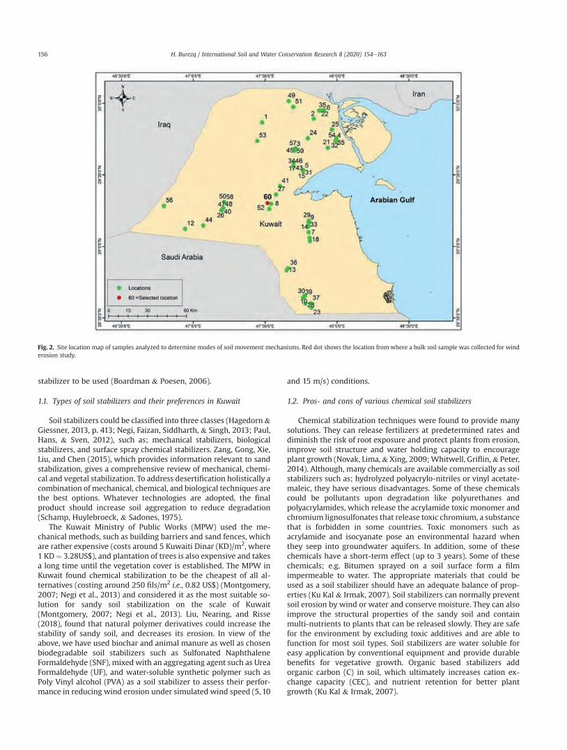
stabilizer to be used (Boardman & Poesen, 2006).
1.1. Types of soil stabilizers and their preferences in Kuwait
Soil stabilizers could be classified into three classes (Hagedorn&Giessner, 2013, p. 413; Negi, Faizan, Siddharth, & Singh, 2013; Paul,Hans, & Sven, 2012), such as; mechanical stabilizers, biologicalstabilizers, and surface spray chemical stabilizers. Zang, Gong, Xie,Liu, and Chen (2015), which provides information relevant to sandstabilization, gives a comprehensive review of mechanical, chemi-cal and vegetal stabilization. To address desertification holistically acombination of mechanical, chemical, and biological techniques arethe best options. Whatever technologies are adopted, the finalproduct should increase soil aggregation to reduce degradation(Schamp, Huylebroeck, & Sadones, 1975).
The Kuwait Ministry of Public Works (MPW) used the me-chanical methods, such as building barriers and sand fences, whichare rather expensive (costs around 5 Kuwaiti Dinar (KD)/m2, where1 KD¼ 3.28US$), and plantation of trees is also expensive and takesa long time until the vegetation cover is established. The MPW inKuwait found chemical stabilization to be the cheapest of all al-ternatives (costing around 250 fils/m2 i.e., 0.82 US$) (Montgomery,2007; Negi et al., 2013) and considered it as the most suitable so-lution for sandy soil stabilization on the scale of Kuwait(Montgomery, 2007; Negi et al., 2013). Liu, Nearing, and Risse(2018), found that natural polymer derivatives could increase thestability of sandy soil, and decreases its erosion. In view of theabove, we have used biochar and animal manure as well as chosenbiodegradable soil stabilizers such as Sulfonated NaphthaleneFormaldehyde (SNF), mixed with an aggregating agent such as UreaFormaldehyde (UF), and water-soluble synthetic polymer such asPoly Vinyl alcohol (PVA) as a soil stabilizer to assess their perfor-mance in reducing wind erosion under simulated wind speed (5, 10
and 15 m/s) conditions.
1.2. Pros- and cons of various chemical soil stabilizers
Chemical stabilization techniques were found to provide manysolutions. They can release fertilizers at predetermined rates anddiminish the risk of root exposure and protect plants from erosion,improve soil structure and water holding capacity to encourageplant growth (Novak, Lima,& Xing, 2009;Whitwell, Griflin,& Peter,2014). Although, many chemicals are available commercially as soilstabilizers such as; hydrolyzed polyacrylo-nitriles or vinyl acetate-maleic, they have serious disadvantages. Some of these chemicalscould be pollutants upon degradation like polyurethanes andpolyacrylamides, which release the acrylamide toxic monomer andchromium lignosulfonates that release toxic chromium, a substancethat is forbidden in some countries. Toxic monomers such asacrylamide and isocyanate pose an environmental hazard whenthey seep into groundwater aquifers. In addition, some of thesechemicals have a short-term effect (up to 3 years). Some of thesechemicals; e.g. Bitumen sprayed on a soil surface form a filmimpermeable to water. The appropriate materials that could beused as a soil stabilizer should have an adequate balance of prop-erties (Ku Kal & Irmak, 2007). Soil stabilizers can normally preventsoil erosion by wind or water and conserve moisture. They can alsoimprove the structural properties of the sandy soil and containmulti-nutrients to plants that can be released slowly. They are safefor the environment by excluding toxic additives and are able tofunction for most soil types. Soil stabilizers are water soluble foreasy application by conventional equipment and provide durablebenefits for vegetative growth. Organic based stabilizers addorganic carbon (C) in soil, which ultimately increases cation ex-change capacity (CEC), and nutrient retention for better plantgrowth (Ku Kal & Irmak, 2007).
Fig. 2. Site location map of samples analyzed to determine modes of soil movement mechanisms. Red dot shows the location fromwhere a bulk soil sample was collected for winderosion study.
H. Burezq / International Soil and Water Conservation Research 8 (2020) 154e163156

1.3. Soils of Kuwait
Of the 12 soil orders distributed worldwide (Soil Survey Staff,2014), only two, that is, Aridisols and Entisols were mapped inKuwait (KISR, 1999; Omar & Shahid, 2013). Aridisols occupy 65.47%and Entisols 27.89% of the surveyed area whereas 6.64% was the
miscellaneous area. Seven major (Torripsamments 27.7%; Hap-localcids 7.72%; Aquisalids 7.08%; Calcigypsids 6.18%; Petrocalcids11.05%; Petrogypsids 33.39%; and Torriorthents 0.62%) and a minor(Haplogypsids 0.05%) soil great groups are mapped. The torrip-samments are true sandy soils where there is no accumulation ofcalcium carbonates, gypsum and hardpanwithin the upper 100 cm.
Table 1Percent sizes in different movement modes in the deserts of Kuwait.
S.No Latitude Longitude Creep >500 mm (%) Saltation 500-63 mm (% Suspension <63 mm (%)
1 29� 86’ 58. 5446 47� 47’ 86. 7236 19.0 57.6 23.22 29� 89’ 21. 3501 47� 83’ 77. 2189 39.4 53.4 7.23 29� 67’ 70. 9605 47� 70’ 55. 1245 12.0 82.1 6.94 29� 73’ 60.1286 47� 98’ 87.6061 12.0 72.6 15.45 29� 52’ 63. 0864 47� 76’ 38.1278 32.3 49.7 18.06 29� 95’ 31. 8210 47� 91’ 01.8233 22.8 57.2 20.07 29� 06’ 04. 1963 47� 80’ 82.4613 18.3 72.0 9.78 29� 26’ 26. 9806 47� 52’ 94.6304 14.9 81.0 4.19 29� 16’ 46. 4588 47� 80’ 22. 5235 18.5 76.6 4.510 28� 65’ 55. 9151 47� 77’ 61.1 908 19.4 74.9 5.711 29� 17’ 42. 1001 47� 80’ 34. 0650 29.0 65.9 5.112 28� 63’ 48. 3969 42� 17’ 48. 2843 7.1 84.9 8.013 28� 83’ 30. 7378 47� 64’ 95. 7916 34.8 58.4 6.814 29� 09’ 94. 6042 47� 80’ 21. 2700 33.14 57.8 8.815 29� 53’ 20. 9673 47� 76’ 39. 3932 15.1 70.2 14.716 29� 25’ 37. 9213 47� 19’ 59. 0562 17.3 58.7 12.517 29� 58’ 53. 8969 47� 69’ 89. 0221 15.3 79.0 5.718 29� 03’ 79. 3161 47� 81’ 17. 3202 21.4 70.8 7.819 29� 26’ 86. 7311 47� 20’ 88. 2858 14.2 76.4 9.220 29� 94’ 91. 6822 47� 89’ 38. 3698 5.1 91.2 3.721 29� 68’ 92. 1099 47� 93’ 53. 2473 16.8 64.7 18.522 29� 94’ 88. 1308 47� 87’ 58. 7911 6.3 74.3 19.423 28� 57’ 16. 2047 47� 82’ 23. 0457 13.9 72.7 13.424 29� 75’ 50. 0524 47� 79’ 67. 3913 22.4 59.3 18.325 29� 81’ 55. 1810 47� 96’ 41. 0063 11.5 77.1 11.426 29� 25’ 82. 5532 47� 20’ 15. 5688 20.1 73.9 6.027 29� 36’ 16. 4410 47� 57’ 54. 0321 18.4 74.4 7.228 28� 60’ 01. 9480 47� 78’ 05. 4822 25.7 62.1 12.229 29� 18’ 00. 9904 47� 80’ 43. 1702 13.7 81.1 5.230 28� 64’ 84. 9760 47� 77’ 05. 7368 30.2 64.4 5.431 29� 52’ 97. 3209 47� 76’ 40. 0905 16.5 68.0 15.532 29� 75’ 58. 5029 47� 99’ 48. 9993 13.3 66.4 20.333 29� 13’ 82. 6219 47� 79’ 92. 3440 16.1 75.2 8.734 29� 55’ 83. 1487 47� 69’ 69. 6436 33.9 65.2 10.935 29� 94’ 85. 9065 47� 89’ 18. 0077 12.5 78.4 9.136 28� 84’ 75. 8938 47� 66’ 00. 7026 19.2 73.5 7.337 28� 60’ 12. 2117 47� 81’ 64. 6219 20.5 71.5 8.038 29� 66’ 78. 5493 47� 70’ 48. 6211 18.8 71.2 10.039 28� 64’ 16. 4087 47� 76’ 40. 0251 19.6 71.6 8.840 29� 25’ 82. 5532 47� 20’ 15. 5688 20.1 73.9 6.041 29� 41’ 91. 8045 47� 60’ 35. 7041 24.1 64.1 11.942 29� 66’ 78. 5493 47� 70’ 48. 6211 18.8 71.2 10.043 29� 58’ 53. 8969 47� 69’ 89. 0221 15.3 79.0 5.744 28� 65’ 86. 9538 42� 30’ 15. 2552 41.6 54.6 3.845 29� 68’ 48. 9776 47� 71’ 12. 6867 22.5 68.7 8.846 29� 55’ 83. 1487 47� 69’ 69. 6436 23.9 65.2 10.947 29� 25’ 37. 9213 47� 19’ 59. 0562 17.3 70.2 12.548 29� 26’ 86. 7311 47� 20’ 88. 2858 14.2 76.4 9.449 30� 01’ 53. 9108 47� 66’ 43. 3621 27.7 61.8 12.650 29� 30’ 94. 7223 47� 21’ 58. 2143 20.0 74.3 5.851 29� 97’ 44. 8053 47� 69’ 56. 4896 12.7 65.4 21.952 29� 29’ 63. 1537 47� 54’ 20. 1325 25.9 66.2 7.953 29� 73’ 68. 5369 47� 44’ 50. 9331 20.6 59.4 20.054 29� 73’ 60. 1286 47� 98’ 87. 6061 8.1 81.5 10.455 29� 73’ 60. 1286 47� 98’ 87. 6061 12.0 72.6 15.456 28� 79’ 49. 9999 42� 02’ 72. 0267 22.2 72.8 5.157 29� 68’ 14. 9301 47� 71’ 14. 7679 17.4 77.6 5.058 29� 30’ 58. 8956 47� 21’ 58. 7783 22.4 73.0 4.659 29� 67’ 72. 6734 47� 70’ 55. 1704 12.0 82.1 6.960 29� 30’ 17. 1240 47� 51’ 61. 7070 25.7 68.0 6.3Grand total 1174.94 4139.1 613.5Average 19.58 68.98 10.23Relative distribution on whole soil basis (%) 20.0 70.0 10.0Grand total
H. Burezq / International Soil and Water Conservation Research 8 (2020) 154e163 157
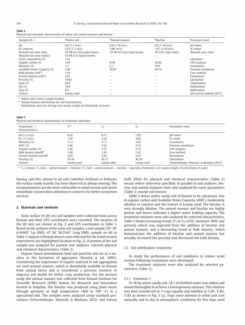
Having said this, almost in all soils (whether Aridisols or Entisols)the surface sandymantle, has been observed as always moving. Thetorripsamments are the most vulnerable to wind erosion and needsimmediate conservation attention to conserve for better ecosystemservices.
2. Materials and methods
Sixty surface (0-20 cm) soil samples were collected from acrossKuwait and their GPS coordinates were recorded. The location ofthe 60 sites are shown in Fig. 2 and GPS coordinates in Table 1.Based on the analysis of the sixty soil samples, a soil sample (29� 180
6.16465" Lat DMS; 47 300 58.2145" Long DMS, sample no 60 inTable 1) typical of Kuwait deserts was collected for thewind erosionexperiment (see highlighted location in Fig. 2). A portion of the soilsample was analyzed for particle size analyses, selected physicaland chemical characteristics (Table 2).
Organic based amendments bind soil particles and act as a nu-cleus in the formation of aggregates (Bronick & Lal, 2005).Considering the importance of organic material in soil aggregationwe used animal manure, which is abundantly available in Kuwaitfrom animal farms and is considered a precious resource toimprove soil health for better crop production. For the presentstudy the animal manure was collected from Kuwait Institute forScientific Research (KISR) Station for Research and Innovationlocated in Sulaybia. The biochar was produced using plant wastethrough pyrolysis at high temperature (400 to 700 �C) in aspecialized kiln. The samples were analyzed using standard pro-cedures (Schoeneberger, Wysocki, & Benham, 2012; Soil Survey
Staff, 2014) for physical and chemical characteristics (Table 2)except where otherwise specified. In parallel to soil analyses, bio-char and animal manures were also analyzed for same parameters(Table 2) except soil texture.
Table 2 shows native sandy soil of Kuwait to be calcareous, lowin organic carbon and Available Water Capacity (AWC), moderatelyalkaline in reaction and the texture is Loamy sand. The biochar isvery strongly alkaline. The animal manure and biochar are highlyporous and hence indicates a higher water holding capacity. Thetreatment mixtures were also analyzed for selected characteristics,Table 3 shows increasing trends (T1 to T3) of EC, moisture, AWC andporosity which was expected from the addition of biochar andanimal manure, and a decreasing trend in bulk density; whichdemonstrates the addition of biochar and animal manure hasactually increased the porosity and decreased the bulk density.
2.1. Soil stabilization treatments
To study the performance of soil stabilizers to reduce winderosion following treatments were developed.
The treatment mixtures were also analyzed for selected pa-rameters (Table 3).
2.1.1. Treatment 1To 18 kg native sandy soil, 1.8 L of distilled water was added and
mixed thoroughly to achieve a homogeneous mixture. This mixturewas then transferred to 3 trays equally and labelled as T1R1, T1R2,T1R3 as shown in Fig. 3 (a). Trays were allowed to settle and curenaturally and to dry at atmospheric conditions for five days until
Table 2Physical and chemical characteristics of native soil, animal manure and biochar.
Samples ID/ aNative soil bAnimal manure bBiochar Procedure used
pH 8.0 (1:1 w/v) 8.0 (1:10 w/v) 9.9 (1:10 w/v) pH meterEC (mS/cm) 3.32 (1:1 w/v) 3.88 (w/v) 1.67 (1:10 w/v) EC meterMunsell soil color (dry) 10 YR 6/3 (dry) pale brown 10 YR 3/3 (dry) dark brown 5Y 2.5/1 (dry) black Munsell color chartMunsell soil color (moist) 10 YR 5/3 (moist) brown e e
CaCO3 equivalents (%) 11.6 CalcimeterOrganic carbon (%) 1.05 9.36 52.09 CNS analyzerMoisture (%) 1.7 2.7 10.9 GravimetricAvailable Water Capacity (%) 3.46 50.07 44.74 Pressure membraneBulk density (t/M3) 1.59 e e Core methodParticle density (t/M3) 2.65 e e PycnometerPorosity (%) 39.83 e e CalculationSand (%) 82.0 e e cHydrometerSilt (%) 10.0 e e HydrometerClay (%) 8.0 e e HydrometerTexture Loamy sand e e Soil survey manual (2017)
a Native soil is from a single location.b Animal manure and biochar are soil amendments.c Hydrometer and wet sieving; w/v means weight of soil/volume of water.
Table 3Physical and chemical characteristics of treatment substrates.
Treatments /CharacteristicsY
T1a T2 T3 Procedures used
pH (1:2 w/v) 8.25 8.17 7.93 pH meterEC (1:2 w/v) 1.36 3.18 3.06 EC meterMoisture (%) 11.5 11.7 14.0 GravimetricAWC (%) 3.46 5.32 6.13 Pressure membraneOrganic carbon (%) 1.62 1.97 2.14 CNS analyzerBulk density tons/M3 1.60 1.42 1.42 Core methodParticle density tons/M3 2.63 2.59 2.59 PycnometerPorosity (%) 39.16 45.17 45.29 CalculaltionTexture Loamy sand Loamy sand Loamy sand Schoeneberger, Wysocki, & Benham (2012)
a T1 (control); T2 (soil þ animal manure þ biochar); T3 (soil þ animal manure þ biochar þ specialty chemicals); w/v means weight of soil/volume of water.
H. Burezq / International Soil and Water Conservation Research 8 (2020) 154e163158
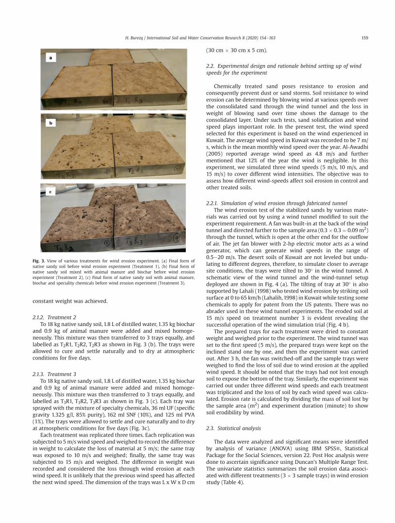
constant weight was achieved.
2.1.2. Treatment 2To 18 kg native sandy soil, 1.8 L of distilled water, 1.35 kg biochar
and 0.9 kg of animal manure were added and mixed homoge-neously. This mixture was then transferred to 3 trays equally, andlabelled as T2R1, T2R2, T2R3 as shown in Fig. 3 (b). The trays wereallowed to cure and settle naturally and to dry at atmosphericconditions for five days.
2.1.3. Treatment 3To 18 kg native sandy soil, 1.8 L of distilled water, 1.35 kg biochar
and 0.9 kg of animal manure were added and mixed homoge-neously. This mixture was then transferred to 3 trays equally, andlabelled as T3R1, T3R2, T3R3 as shown in Fig. 3 (c). Each tray wassprayed with the mixture of specialty chemicals, 36 ml UF (specificgravity 1.325 g/l, 85% purity), 162 ml SNF (10%), and 125 ml PVA(1%). The trays were allowed to settle and cure naturally and to dryat atmospheric conditions for five days (Fig. 3c).
Each treatment was replicated three times. Each replicationwassubjected to 5m/swind speed andweighed to record the differencein weight to calculate the loss of material at 5 m/s; the same traywas exposed to 10 m/s and weighed; finally, the same tray wassubjected to 15 m/s and weighed. The difference in weight wasrecorded and considered the loss through wind erosion at eachwind speed. It is unlikely that the previous wind speed has affectedthe next wind speed. The dimension of the trays was L x W x D cm
(30 cm � 30 cm x 5 cm).
2.2. Experimental design and rationale behind setting up of windspeeds for the experiment
Chemically treated sand poses resistance to erosion andconsequently prevent dust or sand storms. Soil resistance to winderosion can be determined by blowing wind at various speeds overthe consolidated sand through the wind tunnel and the loss inweight of blowing sand over time shows the damage to theconsolidated layer. Under such tests, sand solidification and windspeed plays important role. In the present test, the wind speedselected for this experiment is based on the wind experienced inKuwait. The average wind speed in Kuwait was recorded to be 7 m/s, which is the mean monthly wind speed over the year. Al-Awadhi(2005) reported average wind speed as 4.8 m/s and furthermentioned that 12% of the year the wind is negligible. In thisexperiment, we simulated three wind speeds (5 m/s, 10 m/s, and15 m/s) to cover different wind intensities. The objective was toassess how different wind-speeds affect soil erosion in control andother treated soils.
2.2.1. Simulation of wind erosion through fabricated tunnelThe wind erosion test of the stabilized sands by various mate-
rials was carried out by using a wind tunnel modified to suit theexperiment requirement. A fan was built-in at the back of the windtunnel and directed further to the sample area (0.3� 0.3¼ 0.09m2)through the tunnel, which is open at the other end for the outflowof air. The jet fan blower with 2-hp electric motor acts as a windgenerator, which can generate wind speeds in the range of0.5e20 m/s. The desert soils of Kuwait are not leveled but undu-lating to different degrees, therefore, to simulate closer to averagesite conditions, the trays were tilted to 30� in the wind tunnel. Aschematic view of the wind tunnel and the wind-tunnel setupdeployed are shown in Fig. 4 (a). The tilting of tray at 30� is alsosupported by Lahali (1998) who tested wind erosion by striking soilsurface at 0 to 65 km/h (Lahalih,1998) in Kuwait while testing somechemicals to apply for patent from the US patents. There was noabrader used in these wind tunnel experiments. The eroded soil at15 m/s speed on treatment number 3 is evident revealing thesuccessful operation of the wind simulation trial (Fig. 4 b).
The prepared trays for each treatment were dried to constantweight and weighed prior to the experiment. The wind tunnel wasset to the first speed (5 m/s), the prepared trays were kept on theinclined stand one by one, and then the experiment was carriedout. After 3 h, the fan was switched-off and the sample trays wereweighed to find the loss of soil due to wind erosion at the appliedwind speed. It should be noted that the trays had not lost enoughsoil to expose the bottom of the tray. Similarly, the experiment wascarried out under three different wind speeds and each treatmentwas triplicated and the loss of soil by each wind speed was calcu-lated. Erosion rate is calculated by dividing the mass of soil lost bythe sample area (m2) and experiment duration (minute) to showsoil erodibility by wind.
2.3. Statistical analysis
The data were analyzed and significant means were identifiedby analysis of variance (ANOVA) using IBM SPSS®, StatisticalPackage for the Social Sciences, version 22. Post Hoc analysis weredone to ascertain significance using Duncan’s Multiple Range Test.The univariate statistics summarizes the soil erosion data associ-ated with different treatments (3 � 3 sample trays) inwind erosionstudy (Table 4).
Fig. 3. View of various treatments for wind erosion experiment. (a) Final form ofnative sandy soil before wind erosion experiment (Treatment 1), (b) Final form ofnative sandy soil mixed with animal manure and biochar before wind erosionexperiment (Treatment 2), (c) Final form of native sandy soil with animal manure,biochar and speciality chemicals before wind erosion experiment (Treatment 3).
H. Burezq / International Soil and Water Conservation Research 8 (2020) 154e163 159
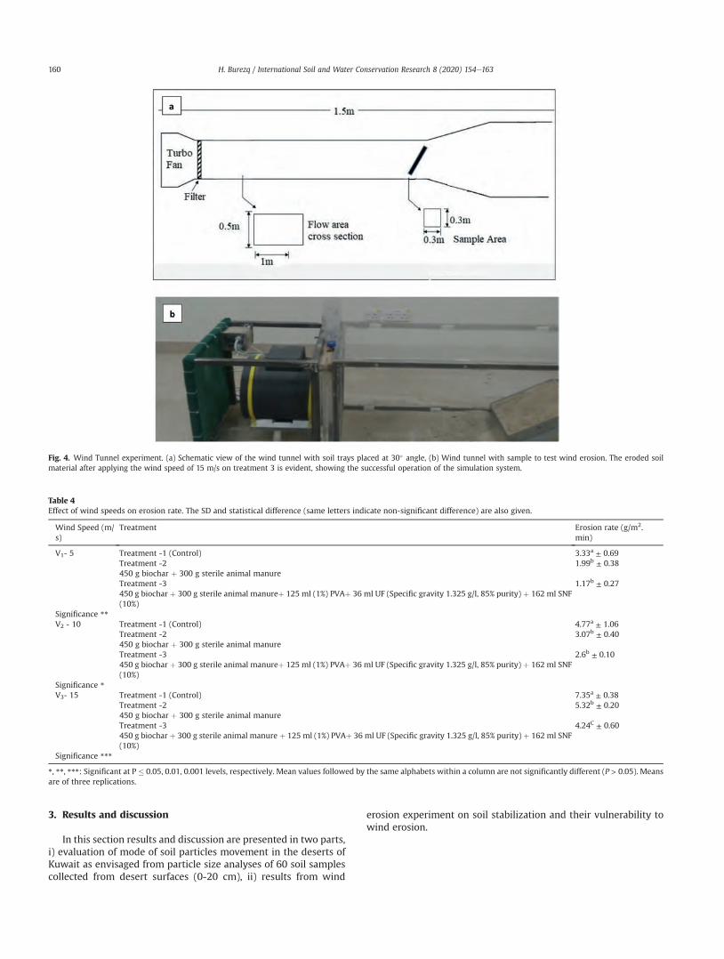
3. Results and discussion
In this section results and discussion are presented in two parts,i) evaluation of mode of soil particles movement in the deserts ofKuwait as envisaged from particle size analyses of 60 soil samplescollected from desert surfaces (0-20 cm), ii) results from wind
erosion experiment on soil stabilization and their vulnerability towind erosion.
Fig. 4. Wind Tunnel experiment. (a) Schematic view of the wind tunnel with soil trays placed at 30� angle, (b) Wind tunnel with sample to test wind erosion. The eroded soilmaterial after applying the wind speed of 15 m/s on treatment 3 is evident, showing the successful operation of the simulation system.
Table 4Effect of wind speeds on erosion rate. The SD and statistical difference (same letters indicate non-significant difference) are also given.
Wind Speed (m/s)
Treatment Erosion rate (g/m2.min)
V1- 5 Treatment -1 (Control) 3.33a ± 0.69Treatment -2450 g biochar þ 300 g sterile animal manure
1.99b ± 0.38
Treatment -3450 g biochar þ 300 g sterile animal manureþ 125 ml (1%) PVAþ 36 ml UF (Specific gravity 1.325 g/l, 85% purity) þ 162 ml SNF(10%)
1.17b ± 0.27
Significance **V2 - 10 Treatment -1 (Control) 4.77a ± 1.06
Treatment -2450 g biochar þ 300 g sterile animal manure
3.07b ± 0.40
Treatment -3450 g biochar þ 300 g sterile animal manureþ 125 ml (1%) PVAþ 36 ml UF (Specific gravity 1.325 g/l, 85% purity) þ 162 ml SNF(10%)
2.6b ± 0.10
Significance *V3- 15 Treatment -1 (Control) 7.35a ± 0.38
Treatment -2450 g biochar þ 300 g sterile animal manure
5.32b ± 0.20
Treatment -3450 g biochar þ 300 g sterile animal manure þ 125 ml (1%) PVAþ 36 ml UF (Specific gravity 1.325 g/l, 85% purity) þ 162 ml SNF(10%)
4.24C ± 0.60
Significance ***
*, **, ***: Significant at P � 0.05, 0.01, 0.001 levels, respectively. Mean values followed by the same alphabets within a column are not significantly different (P > 0.05). Meansare of three replications.
H. Burezq / International Soil and Water Conservation Research 8 (2020) 154e163160
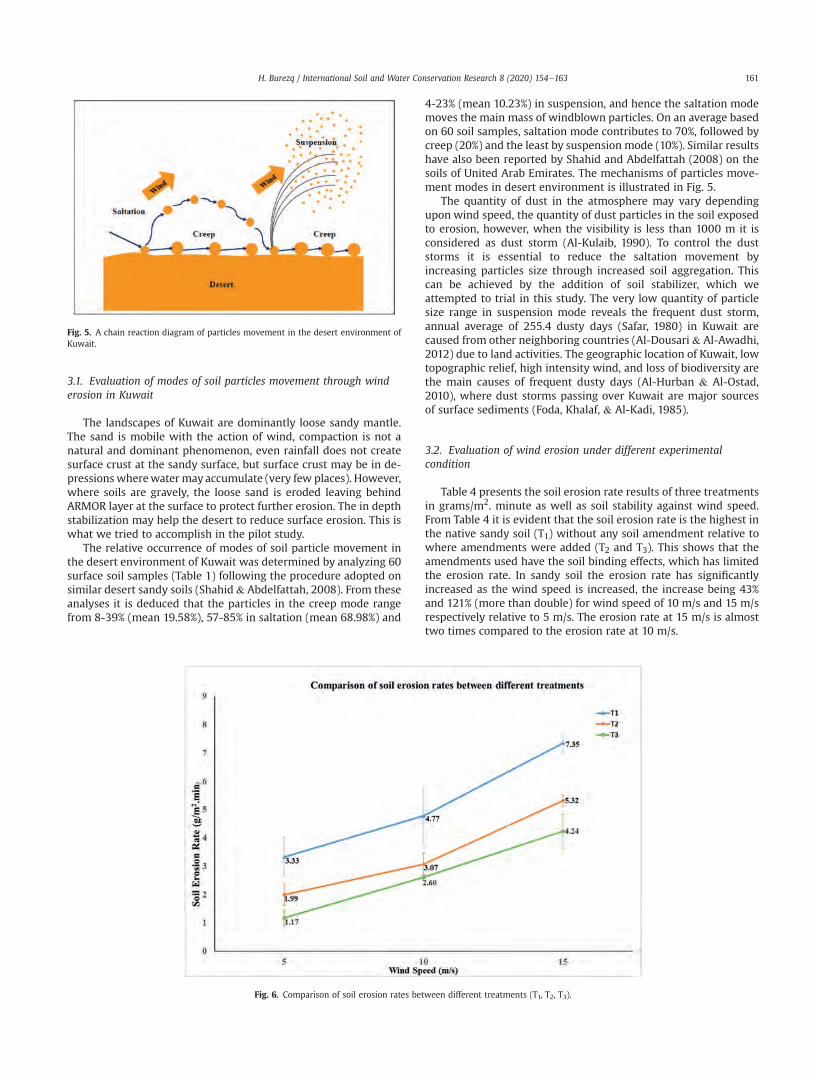
3.1. Evaluation of modes of soil particles movement through winderosion in Kuwait
The landscapes of Kuwait are dominantly loose sandy mantle.The sand is mobile with the action of wind, compaction is not anatural and dominant phenomenon, even rainfall does not createsurface crust at the sandy surface, but surface crust may be in de-pressionswherewatermay accumulate (very few places). However,where soils are gravely, the loose sand is eroded leaving behindARMOR layer at the surface to protect further erosion. The in depthstabilization may help the desert to reduce surface erosion. This iswhat we tried to accomplish in the pilot study.
The relative occurrence of modes of soil particle movement inthe desert environment of Kuwait was determined by analyzing 60surface soil samples (Table 1) following the procedure adopted onsimilar desert sandy soils (Shahid & Abdelfattah, 2008). From theseanalyses it is deduced that the particles in the creep mode rangefrom 8-39% (mean 19.58%), 57-85% in saltation (mean 68.98%) and
4-23% (mean 10.23%) in suspension, and hence the saltation modemoves the main mass of windblown particles. On an average basedon 60 soil samples, saltation mode contributes to 70%, followed bycreep (20%) and the least by suspension mode (10%). Similar resultshave also been reported by Shahid and Abdelfattah (2008) on thesoils of United Arab Emirates. The mechanisms of particles move-ment modes in desert environment is illustrated in Fig. 5.
The quantity of dust in the atmosphere may vary dependingupon wind speed, the quantity of dust particles in the soil exposedto erosion, however, when the visibility is less than 1000 m it isconsidered as dust storm (Al-Kulaib, 1990). To control the duststorms it is essential to reduce the saltation movement byincreasing particles size through increased soil aggregation. Thiscan be achieved by the addition of soil stabilizer, which weattempted to trial in this study. The very low quantity of particlesize range in suspension mode reveals the frequent dust storm,annual average of 255.4 dusty days (Safar, 1980) in Kuwait arecaused from other neighboring countries (Al-Dousari & Al-Awadhi,2012) due to land activities. The geographic location of Kuwait, lowtopographic relief, high intensity wind, and loss of biodiversity arethe main causes of frequent dusty days (Al-Hurban & Al-Ostad,2010), where dust storms passing over Kuwait are major sourcesof surface sediments (Foda, Khalaf, & Al-Kadi, 1985).
3.2. Evaluation of wind erosion under different experimentalcondition
Table 4 presents the soil erosion rate results of three treatmentsin grams/m2. minute as well as soil stability against wind speed.From Table 4 it is evident that the soil erosion rate is the highest inthe native sandy soil (T1) without any soil amendment relative towhere amendments were added (T2 and T3). This shows that theamendments used have the soil binding effects, which has limitedthe erosion rate. In sandy soil the erosion rate has significantlyincreased as the wind speed is increased, the increase being 43%and 121% (more than double) for wind speed of 10 m/s and 15 m/srespectively relative to 5 m/s. The erosion rate at 15 m/s is almosttwo times compared to the erosion rate at 10 m/s.
Fig. 5. A chain reaction diagram of particles movement in the desert environment ofKuwait.
Fig. 6. Comparison of soil erosion rates between different treatments (T1, T2, T3).
H. Burezq / International Soil and Water Conservation Research 8 (2020) 154e163 161
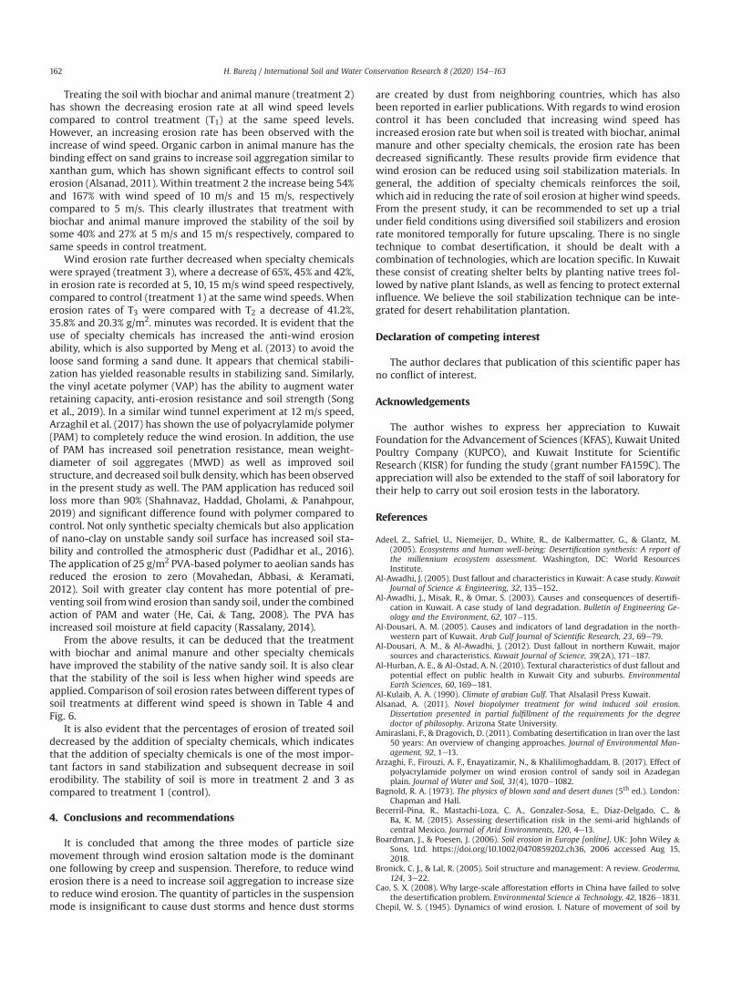
Treating the soil with biochar and animal manure (treatment 2)has shown the decreasing erosion rate at all wind speed levelscompared to control treatment (T1) at the same speed levels.However, an increasing erosion rate has been observed with theincrease of wind speed. Organic carbon in animal manure has thebinding effect on sand grains to increase soil aggregation similar toxanthan gum, which has shown significant effects to control soilerosion (Alsanad, 2011). Within treatment 2 the increase being 54%and 167% with wind speed of 10 m/s and 15 m/s, respectivelycompared to 5 m/s. This clearly illustrates that treatment withbiochar and animal manure improved the stability of the soil bysome 40% and 27% at 5 m/s and 15 m/s respectively, compared tosame speeds in control treatment.
Wind erosion rate further decreased when specialty chemicalswere sprayed (treatment 3), where a decrease of 65%, 45% and 42%,in erosion rate is recorded at 5, 10, 15 m/s wind speed respectively,compared to control (treatment 1) at the same wind speeds. Whenerosion rates of T3 were compared with T2 a decrease of 41.2%,35.8% and 20.3% g/m2. minutes was recorded. It is evident that theuse of specialty chemicals has increased the anti-wind erosionability, which is also supported by Meng et al. (2013) to avoid theloose sand forming a sand dune. It appears that chemical stabili-zation has yielded reasonable results in stabilizing sand. Similarly,the vinyl acetate polymer (VAP) has the ability to augment waterretaining capacity, anti-erosion resistance and soil strength (Songet al., 2019). In a similar wind tunnel experiment at 12 m/s speed,Arzaghil et al. (2017) has shown the use of polyacrylamide polymer(PAM) to completely reduce the wind erosion. In addition, the useof PAM has increased soil penetration resistance, mean weight-diameter of soil aggregates (MWD) as well as improved soilstructure, and decreased soil bulk density, which has been observedin the present study as well. The PAM application has reduced soilloss more than 90% (Shahnavaz, Haddad, Gholami, & Panahpour,2019) and significant difference found with polymer compared tocontrol. Not only synthetic specialty chemicals but also applicationof nano-clay on unstable sandy soil surface has increased soil sta-bility and controlled the atmospheric dust (Padidhar et al., 2016).The application of 25 g/m2 PVA-based polymer to aeolian sands hasreduced the erosion to zero (Movahedan, Abbasi, & Keramati,2012). Soil with greater clay content has more potential of pre-venting soil fromwind erosion than sandy soil, under the combinedaction of PAM and water (He, Cai, & Tang, 2008). The PVA hasincreased soil moisture at field capacity (Rassalany, 2014).
From the above results, it can be deduced that the treatmentwith biochar and animal manure and other specialty chemicalshave improved the stability of the native sandy soil. It is also clearthat the stability of the soil is less when higher wind speeds areapplied. Comparison of soil erosion rates between different types ofsoil treatments at different wind speed is shown in Table 4 andFig. 6.
It is also evident that the percentages of erosion of treated soildecreased by the addition of specialty chemicals, which indicatesthat the addition of specialty chemicals is one of the most impor-tant factors in sand stabilization and subsequent decrease in soilerodibility. The stability of soil is more in treatment 2 and 3 ascompared to treatment 1 (control).
4. Conclusions and recommendations
It is concluded that among the three modes of particle sizemovement through wind erosion saltation mode is the dominantone following by creep and suspension. Therefore, to reduce winderosion there is a need to increase soil aggregation to increase sizeto reduce wind erosion. The quantity of particles in the suspensionmode is insignificant to cause dust storms and hence dust storms
are created by dust from neighboring countries, which has alsobeen reported in earlier publications. With regards to wind erosioncontrol it has been concluded that increasing wind speed hasincreased erosion rate but when soil is treated with biochar, animalmanure and other specialty chemicals, the erosion rate has beendecreased significantly. These results provide firm evidence thatwind erosion can be reduced using soil stabilization materials. Ingeneral, the addition of specialty chemicals reinforces the soil,which aid in reducing the rate of soil erosion at higher wind speeds.From the present study, it can be recommended to set up a trialunder field conditions using diversified soil stabilizers and erosionrate monitored temporally for future upscaling. There is no singletechnique to combat desertification, it should be dealt with acombination of technologies, which are location specific. In Kuwaitthese consist of creating shelter belts by planting native trees fol-lowed by native plant Islands, as well as fencing to protect externalinfluence. We believe the soil stabilization technique can be inte-grated for desert rehabilitation plantation.
Declaration of competing interest
The author declares that publication of this scientific paper hasno conflict of interest.
Acknowledgements
The author wishes to express her appreciation to KuwaitFoundation for the Advancement of Sciences (KFAS), Kuwait UnitedPoultry Company (KUPCO), and Kuwait Institute for ScientificResearch (KISR) for funding the study (grant number FA159C). Theappreciation will also be extended to the staff of soil laboratory fortheir help to carry out soil erosion tests in the laboratory.
References
Adeel, Z., Safriel, U., Niemeijer, D., White, R., de Kalbermatter, G., & Glantz, M.(2005). Ecosystems and human well-being: Desertification synthesis: A report ofthe millennium ecosystem assessment. Washington, DC: World ResourcesInstitute.
Al-Awadhi, J. (2005). Dust fallout and characteristics in Kuwait: A case study. KuwaitJournal of Science & Engineering, 32, 135e152.
Al-Awadhi, J., Misak, R., & Omar, S. (2003). Causes and consequences of desertifi-cation in Kuwait. A case study of land degradation. Bulletin of Engineering Ge-ology and the Environment, 62, 107e115.
Al-Dousari, A. M. (2005). Causes and indicators of land degradation in the north-western part of Kuwait. Arab Gulf Journal of Scientific Research, 23, 69e79.
Al-Dousari, A. M., & Al-Awadhi, J. (2012). Dust fallout in northern Kuwait, majorsources and characteristics. Kuwait Journal of Science, 39(2A), 171e187.
Al-Hurban, A. E., & Al-Ostad, A. N. (2010). Textural characteristics of dust fallout andpotential effect on public health in Kuwait City and suburbs. EnvironmentalEarth Sciences, 60, 169e181.
Al-Kulaib, A. A. (1990). Climate of arabian Gulf. That Alsalasil Press Kuwait.Alsanad, A. (2011). Novel biopolymer treatment for wind induced soil erosion.
Dissertation presented in partial fulfillment of the requirements for the degreedoctor of philosophy. Arizona State University.
Amiraslani, F., & Dragovich, D. (2011). Combating desertification in Iran over the last50 years: An overview of changing approaches. Journal of Environmental Man-agement, 92, 1e13.
Arzaghi, F., Firouzi, A. F., Enayatizamir, N., & Khalilimoghaddam, B. (2017). Effect ofpolyacrylamide polymer on wind erosion control of sandy soil in Azadeganplain. Journal of Water and Soil, 31(4), 1070e1082.
Bagnold, R. A. (1973). The physics of blown sand and desert dunes (5th ed.). London:Chapman and Hall.
Becerril-Pina, R., Mastachi-Loza, C. A., Gonzalez-Sosa, E., Diaz-Delgado, C., &Ba, K. M. (2015). Assessing desertification risk in the semi-arid highlands ofcentral Mexico. Journal of Arid Environments, 120, 4e13.
Boardman, J., & Poesen, J. (2006). Soil erosion in Europe [online]. UK: John Wiley &Sons, Ltd. https://doi.org/10.1002/0470859202.ch36, 2006 accessed Aug 15,2018.
Bronick, C. J., & Lal, R. (2005). Soil structure and management: A review. Geoderma,124, 3e22.
Cao, S. X. (2008). Why large-scale afforestation efforts in China have failed to solvethe desertification problem. Environmental Science & Technology, 42, 1826e1831.
Chepil, W. S. (1945). Dynamics of wind erosion. I. Nature of movement of soil by
H. Burezq / International Soil and Water Conservation Research 8 (2020) 154e163162
wind. Soil Science, 60, 305e320.Duan, J. T., Litwiller, E., Choi, S. H., & Pinnau, I. (2014). Evaluation of sodium lignin
sulfonate as draw solute in forward osmosis for desert restoration. Journal ofMembrane Science, 453, 463e470.
FAO-ITPS. (2015). Status of the world’s soil resources (SWSR) etechnical summary.Rome, Italy: Food and Agriculture Organization of the United Nations andIntergovernmental Panel on Soils.
Foda, M., Khalaf, F., & Al-Kadi, A. (1985). Estimation of dust fallout rates in thenorthern Arabian Gulf. Sedimentology, 32, 595e603.
Grainger, A. (2013). The threatening desert. In Controlling Desertification. London:Earthscan Publications Ltd.
Grini, A., Myhre, G., Zender, C. S., & Isaksen, I. S. A. (2005). Model simulations of dustsource and transport in the global troposphere: Effects of soil erodibility andwind speed variability. Journal of Geophysical Research, 110, D02205. https://doi.org/10.1029/2004JD005037.
Hagedorn, H., & Giessner, K. (2013). Dune stabilization; A survey of literature on duneformation and dune stabilization. West Germany: German Agency for TechnicalCooperation, 1977.
He, J. J., Cai, Q. J., & Tang, Z. Q. (2008). Wind tunnel experimental study on the effectof PAM on soil wind erosion control. Environmental Monitoring and Assessment,145(1e3), 185e193.
Higgitt, D. (1993). Soil erosion and soil problems. Progress in Physical Geography:Earth and Environment, 17, 461e472.
Imeson, A. (2011). Desertification, its causes and why it matters. In Desertification,land degradation and Sustainability (pp. 5e41), ISBN 978-0-470-71449-2.
Intergovernmental Panel on Climate Change (IPCC). (2017). IPCC special report onglobal warming of 1.5�C expert review of the first order draft and start of the thirdlead author meeting.
Johnson, D. L., Ambrose, S. H., Bassett, T. J., Bowmen, M. L., Isaacson, J. S.,Crummey, D. E., et al. (1997). Meanings of environmental terms. Journal ofEnvironmental Quality, 26, 81e589.
Khalaf, F. I., & Al-Ajmi, D. (1993). Aeolian process and sand encroachment problemsin Kuwait. Geomorphology, 6, 111e134.
Shahnavaz, M., Haddad, M. N., Gholami, A., & Panahpour, E. (2019). Investigating theefficiency of soil stabilizers against soil loss and their effects on chemicalproperties of soil. Arid Land Research and Management, 33(2), 119e135. https://doi.org/10.1080/15324982.2018.1531324.
KISR. (1999). Soil survey for the state of Kuwait e Vol II. Reconnaissance survey.Adelaide: AACM International.
Ku Kal, M. S., & Irmak, S. (2007). Climate-driven crop yield and yield variability andclimate change impacts on the U.S. Great plains agricultural production. Sci-entific Reports, 8, 3450.
Lahalih, S. M. (1998). Method and composition for stabilizing soil and process formaking the same. Patent number 5,824,727 (Oct. 20, 1998). The United StatesPatent.
Lindskog, A., & Tengberg, A. (1994). Drylands, sustainable use of rangelands into thetwenty-first century. Rome: International Fund for Agricultural Development(IFAD). Technical report.
Liu, B. Y., Nearing, M. A., & Risse, L. M. (2018). Slope gradient effects on soil loss forsteep slopes. Transactions of the ASAE, 37(6), 1835e1840.
Lugato, E., Smith, P., Borrelli, P., Panagos, P., Ballabio, C., Orgiazzi, A., et al. (2018). Soilerosion is unlikely to drive a future carbon sink in Europe. Science Advances,4(11). art. no. eaau3523.
Meng, X., Peng, G., Liu, B., Wang, B., Chen, H., Rong, L., et al. (2013). Synthesis andsand-fixing property of cationic poly (vinyl acetate-butyl acrylate-DMC)copolymer emulsions. Polymer - Plastics Technology and Engineering, 52,931e939.
Misak, R. F., Khalaf, F. I., & Omar, S. A. S. (2013). Managing the hazards of droughtand shifting sands in dry lands: The case study of Kuwait. Chapter 41. InS. A. Shahid, F. K. Taha, & M. A. Abdelfattah (Eds.), Developments in soil classi-fication, land use planning and policy implications: Innovative thinking of soilinventory for land use planning and management of land resources (pp. 703e729).
Montgomery, D. R. (2007). Soil erosion and agricultural sustainability. In Proceedingof the National Academy of Sciences of the United State of America (pp.13268e13272), 104(33).
Movahedan, M., Abbasi, N., & Keramati, M. (2012). Wind erosion control of soilsusing polymeric materials. Eurasian Journal of Soil Science, 2, 81e86.
Mueller, E. N., Wainwright, J., & Parsons, A. J. (2007). The stability of vegetationboundaries and the propagation of desertification in the American southwest: Amodelling approach. Ecological Modelling, 208, 91e101.
Negi, A. S., Faizan, M., Siddharth, D. P., & Singh, R. (2013). Soil stabilization usinglime. International Journal of Innovative Research in Science, Engineering andTechnology, 2(2), 448e453.
Novak, M., Lima, I., & Xing, B. (2009). Characterization of designer biochar producedat different temperatures and their effects on a loamy sand. Annals of Envi-ronmental Science, 3, 195e206.
Omar, S. A. S., & Shahid, S. A. (2013). Reconnaissance soil survey for the state ofKuwait. In S. A. Shahid, et al. (Eds.), Developments in soil classification, land useplanning and policy implications: Innovative thinking of soil inventory for land useplanning and management of land resources (pp. 85e107). https://doi.org/10.1007/978-94-007-5332-7_3.
Padidhar, M., Jalalian, A., Asgari, K., Abdouss, M., Najafi, P., Honarjoo, N., et al. (2016).The impacts of nanoclay on sandy soil stability and atmospheric dust control.Agriculturae Conspectus Scientificus, 81(4), 193e196.
Paul, M. G., Hans, M., & Sven, K. (2012). Verification of field settlement of in-situstabilized dredged sediments using cone penetration test data. EJGE, 17,3665e3680.
Rasslany, I. (2014). Effects of poly vinyl alcohol/starch as Soil Conditioners on thephysical properties of loamy sand and loam soils following different wettingand drying cycles. Journal of Natural Sciences Research, 4(24), 36e42.
Safar, M. I. (1980). Frequency of dust in day-time summer in Kuwait. Kuwait: Direc-torate General of Civil Aviation.
Sartori, M., Philippidis, G., Ferrari, E., Borrelli, P., Lugato, E., Montanarella, et al.(2019). A linkage between the biophysical and the economic: Assessing theglobal market impacts of soil erosion. Land Use Policy, 86, 299e312.
Schamp, N., Huylebroeck, J., & Sadones, M. (1975). Soil cond. Soil Science Society ofAmerica.
Schoeneberger, P. J., Wysocki, D. A., Benham, E. C., & Soil Survey Staff. (2012). Fieldbook for describing and sampling soils, version 3.0. Natural Resources ConservationService. Lincoln, NW: National Soil Survey Center.
Semhi, K. (2013). Research on soil erosion. International Journal of EnvironmentalStudies, 70(1), 160e161.
Shahid, S. A., & Abdelfattah, M. A. (2008). Soils of Abu Dhabi Emirate. In Terrestrialenvironment of abu Dhabi Emirate (pp. 71e91). Richards Perry.
Shahid, S. A., Omar, S. A. S., & Al-Ghawas, S. (1999). Indicators of desertification inKuwait and their possible management. Desertification control bulletin, 34,61e66.
Soil Survey Staff. (2014). In Kellogg soil survey laboratory methods manual. Soil surveyinvestigations report No. 42, version 5.0. R. Burt and soil survey staff. U.S.Department of Agriculture, Natural Resources Conservation Service.
Soil Science Division Staff. (2017). Soil survey manual. United States Department ofAgriculture. Agriculture Handbook No. 18.
Song, Z., Liu, J., Bai, Y., Wei, J., Li, D., Wang, Q., et al. (2019). Laboratory and fieldexperiments on the effect of vinyl acetate polymer-reinforced soil. Applied Sci-ences, 9, 208. https://doi.org/10.3390/app9010208.
Stringer, L. C., Dyer, J. C., Reed, M. S., Dougill, A. J., Twyman, C., & Mkwambisi, D.(2009). Adaptations to climate change, drought and desertification: Local in-sights to enhance policy in southern Africa. Environmental Science & Policy, 12,748e765.
Telles, T. S., Guimaraes, M. D. F., & Dechen, S. D. F. (2011). The cost of soil erosion.Revista Brasileira de Ciencia do Solo, 35(2), 287e298.
Van Rooyen, A. F. (1998). Combating desertification in the southern Kalahari:Connecting science with community action in South Africa. Journal of Arid En-vironments, 39, 285e297.
Wang, F., Pan, X., Wang, D., Shen, C., & Lu, Q. (2013). Combating desertification inChina: Past, present and future. Land Use Policy, 31, 311e313.
Wang, T., Zhu, Z. D., & Wu, W. (2002). Sandy desertification in the north of China.Science in China, Series A, 45, 23e34.
Whitwell, P., Griflin, W., & Peter, N. (2014). Process for soil conditioning by aerialapplication of water soluble of swellable polymers. U.S. Patent No.20160120130A1.
Williams, A., Hunter, M. C., & Kammerer, M. (2016). Soil water holding capacitymitigates downside risk and volatility in US rain-fed maize. Time to invest insoil organic matter? PLOS, 11(8), 1e11.
Zang, Y. X., Gong, W., Xie, H., Liu, B. L., & Chen, H. L. (2015). Chemical sand stabi-lization: A review of material, mechanism, and problems. Environmental Tech-nology Reviews, 4(1), 119e132. https://doi.org/10.1080/21622515.2015.1105307.
Zhao, G., Mu, X., Wen, Z., Wang, F., & Gao, P. (2013). Soil erosion, conservation, andeco-environment changes in the Loess Plateau of China. Land Degradation &Development, 24, 499e510.
H. Burezq / International Soil and Water Conservation Research 8 (2020) 154e163 163
Original Research Article
Institutional performance and participatory paradigms: Comparingtwo groups of watersheds in semi-arid region of India
Biswajit Mondal a, *, Nagarajan Loganandhan b, Sekhargowda L. Patil c, Anurag Raizada d,Suresh Kumar c, Gopal L. Bagdi e
a ICAR-National Rice Research Institute (NRRI), Cuttack, Indiab Krishi Vigyan Kendra, Hirehalli, ICAR-Indian Institute of Horticultural Research, Bangalore, Indiac ICAR-Indian Institute of Soil & Water Conservation, Bellary, Indiad National Research Centre on Integrated Farming, Pipra Kothi, East Champaran, Indiae ICAR-Central Sheep and Wool Research Institute, Avikanagar, India
a r t i c l e i n f o
Article history:Received 27 August 2019Received in revised form25 March 2020Accepted 1 April 2020Available online 8 April 2020
Keywords:Participation paradigm indexParticipatory watershed development indexRationality analysisSemi-arid regionStakeholder analysisWatershed development programme
a b s t r a c t
Watershed development programmes carried out in different agroclimatic conditions in India resulted inbeneficial impact in terms of productivity enhancement and natural resources conservation, but lessattention paid to institutional and participatory aspects. This paper explored the performance of variousinstitutions regarding execution of watershed development programmes in semi-arid region of India.Recorded observations from documents maintained at watershed level and information collectedthrough primary survey as well as focus group discussion with different types of stakeholders were usedfor analysis. The results indicated lacunae in participatory aspects during programme implementationprocess like monitoring activities, management of common property resources and equity. Gap inlinkages and differential level of performance of various watershed level functionaries indicates thenecessity for corrections in the structures and linkages pattern for sustainability of the infrastructure andinstitutions. The study also showed unequal priorities by the implementing agencies towards in-stitutions, land and water resources development, production enhancement activities and fodder re-sources development as well as rationalities of technical, economic, financial, political and social aspectsamong the watersheds.© 2020 International Research and Training Center on Erosion and Sedimentation and China Water andPower Press. Production and Hosting by Elsevier B.V. This is an open access article under the CC BY-NC-
ND license (http://creativecommons.org/licenses/by-nc-nd/4.0/).
1. Introduction
Since 1990s, watershed development (WSD) programmesstands as one of the massive and effective rural development ini-tiatives in India with substantial budget outlay. Major investmentshave been made from public sources through government organi-zations (Gray& Srinidhi, 2013), though voluntary organizations andnon-governmental organizations (NGOs) are also implementingwatershed development programmes in various parts of India.During 1990’s and 2000’s, Indian Rupees (INR) 77 billion (1.04billion US$) were spent on WSD programmes. Due to evolvingimportance, the World Bank has also sanctioned US$ 1.73 billionduring 1990e2004 (Darghouth, Ward, Gambarelli, Styger, & Roux,
2008), and Government of India has spent more than US$ 6billion during the period 1996e2004 (World Resources Institute,2005). During recent years, the Mahatma Gandhi National RuralEmployment Guarantee Act (MGNREGA), with an annual budget ofINR 400 billion (5.41 billion US$), is being mingled with the WSDprogrammes in various states to synergize and augment theirimpact to development, and it has immensely increased the sig-nificance and backing of WSD programmes in India (Jain & Gandhi,2016). Such huge investment made during last few decadescertainly calls for assessment of the impact and other necessaryparadigms.
Currently, watershed development projects are implementedthrough diverse group of institutions, which include the
* Corresponding author.E-mail address: [email protected] (B. Mondal).
Contents lists available at ScienceDirect
International Soil and Water Conservation Research
journal homepage: www.elsevier .com/locate/ iswcr
https://doi.org/10.1016/j.iswcr.2020.04.0022095-6339/© 2020 International Research and Training Center on Erosion and Sedimentation and China Water and Power Press. Production and Hosting by Elsevier B.V. Thisis an open access article under the CC BY-NC-ND license (http://creativecommons.org/licenses/by-nc-nd/4.0/).
International Soil and Water Conservation Research 8 (2020) 164e172
government organizations (GOs) like state government de-partments and panchayat raj institutions (PRIs) and non-governmental organizations (NGOs). The NGOs were found toenjoy greater freedom in choosing their area of work (Farrington,Turton, & James, 1999; Fernandez, 1994; Kerr, 2002). Thoughseveral NGOs are working in diverse agroclimatic zones of thecountry, rarely does one NGO take up watershed projects in totallydifferent agroclimatic situations at the same time. Furthermore,they choose watersheds, where there are greater scope of land aswell as non-land based activities. For example, Mysore Resettle-ment and Development Agency (MYRADA), an NGO that has hadextensive experience in land and water development programmesin southern India prefers villages with less landless people(Fernandez, 1994). Farrington et al. (1999) indicated that usuallyNGOs and donor agencies look for watersheds where there is less ofsocial stratification and administrative boundaries of the villagescoincide with thewatershed boundaries. Hence, it is said that NGOsare ‘choosy’ in their selection of watersheds (Reddy, 1998). Thewatershed projects implemented by the government agenciesinvariably have to tackle a large agroclimatic landscape with variedspread and features, partly by following the guidelines and some-times due to compelling socio-political pressure. Hence, evaluationof differential impact has to see from the inherent structures/characteristics of the organizational set up for the purpose.
Evaluation studies carried out for past as well as new generationwatersheds located in different agroclimatic situations and it wasindicated mostly positive externalities through productivityenhancement besides conservation of natural resources (Joshi, Jha,Wani, Joshi, & Shiyani, 2005; Kerr, Pangare, & Pangare, 2002;Mondal et al., 2017; Pal et al., 2017; Palanisami & Kumar, 2009;Reena, Siwach, & Singh, 2019; Samra & Sharma, 2009). Adoption ofsoil andwater conservation approaches arrests surface run-off water,which become prime source during dry spells in rainfed semi-aridregions (Wani et al., 2008). Pathak, Chourasia, Wani, and Sudi(2013) reported several benefits from the watershed developmentprogram in terms of availability of water, reduction of soil loss,enhanced agricultural productivity, income and environmental/ecological status as well as socioeconomic well-being of the house-holds. There are also quite a few studies, which underlined theadvantage of participatory watershed development programmesand identified the factors which are responsible for sustainablewatershed development through people’s participation (Bagdi &Kurothe, 2014; Mondal, Singh, & Sekar, 2013; Sharma & Sisodia,2008). There is no difference of opinion about the beneficialimpact of watershed projects, but the varied nature of interventionsand its implementation procedures under different programmes/schemes like Drought Prone Areas Programme (DPAP), NationalWatershed Development Project for Rainfed Areas (NWDPRA) andIntegrated Wasteland Development Programme (IWDP), certainlyhad differential impact of the project. Most of the earlier watershedprojects laid more stress on the nature of works being carried outrather than on the extent and efficiency of resource enhancementthat the particular work is supposed to bring about (Vaidyanathan,2001). Even though few workers have attempted earlier to under-stand the institutional arrangements (Kurian, 2004; Mondal et al.,2015; Saravanan, 2002; Tanguilig & Tanguilig, 2009), interactionand linkages among various stakeholder groups in the watersheddevelopment programmes were not addressed adequately. There-fore, it was imperative to study the role performance of differentinstitutions in the process of watershed development programmes.This paper evaluated the watershed development programmes thathad been implemented under different institutional structures andagencies (government department vs. NGOs) under semi-arid situ-ations and the programmes were assessed in terms of participatoryand institutional dimensions.
2. Methodology
2.1. Study area and sample
Geographically, about 17% and 36% of total land area of thecountry comes under arid and semi-arid regions, respectively(Government of India, 2004; Sathyakumar and Sivakumar, 2007),which is characterized by low and inconsistent rainfall, recurrentdroughts and different types of vegetation and soils. Amongstdifferent rainfed areas, semi-arid regions are most vulnerable(Kumar, Raizada, Biswas, Srinivas, & Mondal, 2016) and the stateswhich are accommodating in semi-arid region include Andhra Pra-desh and Karnataka and parts of Gujarat, Madhya Pradesh, Chhat-tisgarh, Maharashtra, Rajasthan and Tamil Nadu. The proportion ofrainfed agriculture is about 73% in above-mentioned states, of whichthe two states (Karnataka and Andhra Pradesh) contribute around40% (Bhatia, 2005). The crops grown mainly in this region includecoarse cereals like jowar, bajra and ragi; pulses like bengalgram andhorsegram and oilseed crops like groundnut and sunflower. Perhectare yield are low in rainfed areas of semi-arid regions and theinstability in both area and yield for most of the crops in these statesis much higher than the all-India average. Further, the semi-aridareas have been subject to degradation of natural resources atdifferent scales caused by the soil erosion, depletion of forests anddeclining common pool resources (Kumar et al., 2016; Mondal,Loganandhan, & Raizada, 2014; Raizada et al., 2018).
Most of the parts of Andhra Pradesh and Karnataka falls undersemi-arid tracts, hence, these two states were selected and onedistrict each, viz. Bellary (Karnataka) and Anantapur (Andhra Pra-desh) were chosen purposively because of typical representation ofsemi-arid region like low soil depth, high run-off/soil loss and lowaverage rainfall (Mondal et al., 2014). In a district, one watershedeach implemented under government organization (Lottinekereand Mangampally watershed) and NGO (Kalvi and Mallapuramwatershed) were selected for detailed investigation. A brief outlineof the characteristics of selected watersheds is presented in Table 1.The area of selected watersheds ranged between 500 and 864 ha.Average rainfall varied between as low as 350 mm to maximum of587 mm and rainfed area varied between 75 and 96% of the arablearea. Sorghum, bajra, sunflower, groundnut, cotton and sesamumare major crops grown in the area with lower yields that rangesfrom 0.8 t ha�1 in case of cereals, 0.6 to 0.8 t ha�1 in sunflower and0.5 t ha�1 in groundnut.
Stakeholders are the actors or groups who affect and/or areaffected by the policies, decisions and actions of the any develop-mental programme (Nuga, Akinbola, & Nuga, 2009). There existstwo groups of stakeholders in this study, the first group includesmembers of project implementing agency (PIA), watershed devel-opment team (WDT) and, representatives of various community-based organizations like watershed committee (WC), self-helpgroups (SHGs) and user groups (UGs) as well as various linedepartment officials associated with the watershed programme(Table 1). Another group of stakeholders are the beneficiaryhouseholds, who directly could be affected by the externalities,either positively or negatively. Two representatives from each ofthe stakeholder institutions under first group and fifteen benefi-ciary households with representation of various land-holding sizeclasses under second group from each micro-watershed villagewere chosen as respondents for the study.
2.2. Data and analysis
2.2.1. Participatory paradigmsDocumented observations (from records maintained at water-
shed office) as well as information on various participatory
B. Mondal et al. / International Soil and Water Conservation Research 8 (2020) 164e172 165
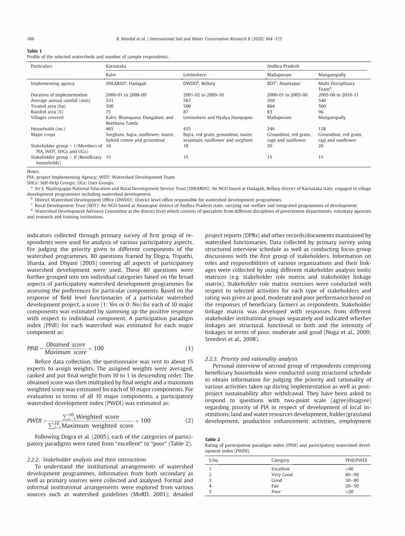
indicators collected through primary survey of first group of re-spondents were used for analysis of various participatory aspects.For judging the priority given to different components of thewatershed programmes, 80 questions framed by Dogra, Tripathi,Sharda, and Dhyani (2005) covering all aspects of participatorywatershed development were used. These 80 questions werefurther grouped into ten individual categories based on the broadaspects of participatory watershed development programmes forassessing the preferences for particular components. Based on theresponse of field level functionaries of a particular watersheddevelopment project, a score (1: Yes or 0: No) for each of 10 majorcomponents was estimated by summing up the positive responsewith respect to individual component. A participation paradigmindex (PPdI) for each watershed was estimated for each majorcomponent as:
PPdI¼ Obtained scoreMaximum score
� 100 (1)
Before data collection, the questionnaire was sent to about 15experts to assign weights. The assigned weights were averaged,ranked and put final weight from 10 to 1 in descending order. Theobtained scorewas thenmultiplied by final weight and amaximumweighted scorewas estimated for each of 10major components. Forevaluation in terms of all 10 major components, a participatorywatershed development index (PWDI) was estimated as:
PWDI¼P10
i¼1Weighted scoreP10
i¼1Maximum weighted score� 100 (2)
Following Dogra et al. (2005), each of the categories of partici-patory paradigms were rated from “excellent” to “poor” (Table 2).
2.2.2. Stakeholder analysis and their interactionsTo understand the institutional arrangements of watershed
development programmes, information from both secondary aswell as primary sources were collected and analysed. Formal andinformal institutional arrangements were explored from varioussources such as watershed guidelines (MoRD, 2001); detailed
project reports (DPRs) and other records/documents maintained bywatershed functionaries. Data collected by primary survey usingstructured interview schedule as well as conducting focus-groupdiscussions with the first group of stakeholders. Information onroles and responsibilities of various organizations and their link-ages were collected by using different stakeholder analysis tools/matrices (e.g. stakeholder role matrix and stakeholder linkagematrix). Stakeholder role matrix exercises were conducted withrespect to selected activities for each type of stakeholders andrating was given as good, moderate and poor performance based onthe responses of beneficiary farmers as respondents. Stakeholderlinkage matrix was developed with responses from differentstakeholder institutional groups separately and indicated whetherlinkages are structural, functional or both and the intensity oflinkages in terms of poor, moderate and good (Nuga et al., 2009;Sreedevi et al., 2008).
2.2.3. Priority and rationality analysisPersonal interview of second group of respondents comprising
beneficiary households were conducted using structured scheduleto obtain information for judging the priority and rationality ofvarious activities taken up during implementation as well as post-project sustainability after withdrawal. They have been asked torespond to questions with two-point scale (agree/disagree)regarding priority of PIA in respect of development of local in-stitutions, land andwater resources development, fodder/grasslanddevelopment, production enhancement activities, employment
Table 1Profile of the selected watersheds and number of sample respondents.
Particulars Karnataka Andhra Pradesh
Kalvi Lottinekere Mallapuram Mangampally
Implementing agency SNEARDSa, Hadagali DWDOb, Bellary RDTc, Anantapur Multi-DisciplinaryTeamd
Duration of implementation 2000-01 to 2008-09 2001-02 to 2009-10 2000-01 to 2005-06 2005-06 to 2010-11Average annual rainfall (mm) 531 587 350 540Treated area (ha) 500 500 864 500Rainfed area (%) 75 87 83 96Villages covered Kalvi; Bhanayana, Dungabati, and
Beethana TandaLottinekere and Hyalya Hampapur Mallapuram Mangampally
Households (no.) 465 435 246 128Major crops Sorghum, bajra, sunflower, maize,
hybrid cotton and groundnutBajra, red gram, groundnut, maizesesamum, sunflower and sorghum
Groundnut, red gram,rage and sunflower
Groundnut, red gram,ragi and sunflower
Stakeholder group e I (Members ofPIA, WDT, SHGs and UGs)
16 18 20 20
Stakeholder group e II (Beneficiaryhouseholds)
15 15 15 15
Notes.PIA: project Implementing Agency; WDT: Watershed Development Team.SHGs: Self-Help Groups; UGs: User Groups.
a Sri S. Nijalingappa National Education and Rural Development Service Trust (SNEARDS): An NGO based at Hadagali, Bellary district of Karnataka state, engaged in villagedevelopment programmes including watershed development.
b District Watershed Development Office (DWDO): District level office responsible for watershed development programmes.c Rural Development Trust (RDT): An NGO based at Anantapur district of Andhra Pradesh state, carrying out welfare and integrated programmes of development.d Watershed Development Advisory Committee at the district level which consists of specialists from different disciplines of government departments, voluntary agencies
and research and training institutions.
Table 2Rating of participation paradigm index (PPdI) and participatory watershed devel-opment index (PWDI).
S.No. Category PPdI/PWDI
1 Excellent >902 Very Good 80e903 Good 50e804 Fair 20e505 Poor <20
B. Mondal et al. / International Soil and Water Conservation Research 8 (2020) 164e172166
generation activities or equity aspects during implementation ofthe programme and categorized as high, medium and low. Further,for judging the importance given to organizational, social, tech-nical, economic, financial and political issues addressed duringimplementation of each of the watershed programmes. The secondgroup of respondents were asked to response the questions with afive-point scale regarding various rationality issues during theimplementation of the watershed development programmes. Thefollowing rationality indicators (Gandhi, 2010) were used.
� Organizational rationality, which deals with the organizationaland coordination issues.
� Social rationality, which deals with the social or people settingthat include caste groups, farmers with different landholdingsizes, people with various professions, women and poor people.
� Technical rationality, which deals with the conversion of inputsinto outputs efficiently. Good institutions are equipped withbest/appropriate technology and operational procedures thatlead to high productive efficiency.
� Economic rationality, which deals with the consideration ofcosts, benefits and returns and involves the economically effi-cient use of scarce resources.
� Financial rationality, which deals with the discipline and carethat required for proper handling of financial resources as strongprocedures and accounting systems need to exist for effectiveuse of resources for the intended purposes and not misused orlost.
� Political rationality, deals with the involvement and participa-tion of various leaders and power/interest groups in theformulation of rules and plans, and the settlement of differ-ences/disputes that may arise during the course of watersheddevelopment programmes.
3. Results and discussion
3.1. Institutional arrangements and fund flow mechanism inwatershed development programme
In Karnataka, since 2001 a separate Watershed DevelopmentDepartment exist, which is headed by a Commissioner and assistedby Director of Watershed and Joint Director of different other de-partments. At the district level, District Watershed DevelopmentOfficers are the authority to implement the programmes, who areassisted by a multi-disciplinary team under the overall control/supervision of District Rural Development Agency (DRDA) (Fig. 1).In Andhra Pradesh state, the Watershed Project Implementationand Review Committee is the apex body which is headed by theChief Secretary and supported by Additional Chief Secretary, Agri-cultural Production Commissioner and Development Commis-sioner of the state and Department of Rural Development is thenodal agency. District Water Management Agency (DWMA) whichis headed by a Project Director is apex body at District level and zillapanchayat is the nodal agency. Administration and implementationof watershed development projects lies with the zilla panchayat,who receive funds from Government of India and hold the ultimatepower of administrative and financial control over PIAs and man-aging the accounts. A Multi-Disciplinary Team (MDT) or WatershedDevelopment Advisory Committee at the district level also exists,which consists of specialists from different disciplines of the Gov-ernment in DRDA, voluntary agencies and research and traininginstitutions at the district level.
At the watershed level, group of members from the villagecommunity, who indirectly or directly use watershed resources tomeet their livelihood needs from farming or other activities, isformed and registered as Watershed Association (WA). The WA,
nominate one President and other office bearers during a generalbody meeting with the representation of SHGs, UGs, women andscheduled caste (SC)/scheduled tribe (ST) and gram panchayat (GP)members and form a Watershed Committee (WC) for coordinationand execution of different activities. WC received the fund directlyfrom Government of India through DRDA and theWC andWA usedto make responsible for managing these funds. TheWC allocate thefunds to SHGs as revolving fund, to user groups for developingnatural resource linked asset base, and so on. The capacity buildingof watershed level institutions used to be done by the watersheddevelopment team (WDT). The voluntary contributions, made bythe UGs are to be accumulated to form a watershed developmentfund, meant for maintenance and management of natural resourcebase/assets of the village.
3.2. Complementarity and convergence of institutions andprogrammes
The new generation of watersheds sanctioned since 2008-09 isimplemented under a single programme namely IntegratedWatershed Management Programme (IWMP) following ‘CommonGuidelines (2008)’ (Government of India, 2011). A state level nodalagency (SLNA) constituted of representatives from Rural Develop-ment Department, National Rainfed Area Authority (NRAA),NABARD and Department of Agriculture, Animal Husbandry,Ground Water Board, NGOs and professional experts from researchinstitutions for managing and coordinating the different activitiesand fund-flow for watershed programmes in the state.
Government of India intended to develop a new project modelin order to congregate the IWMP with the ongoing MahatmaGandhi National Rural Employment Guarantee Act (MNREGA), asmore than 50% of MNREGA works relate to land based activities,more specifically, soil and water conservation works. As such thefunds available under watershed development project are insuffi-cient to treat a watershed fully, hence the convergence with otherdevelopment programmes helps not only to supplement resourcesfor holistic treatment but will also complement other developmentprogrammes. Under MNREGA, most of the watershed-based in-terventions are permitted; however, there is neither any specificcost norms for per unit area as in watershed development project,nor unit cost of work or activity. Therefore, the unit cost for works/activity in the watershed project area funded by MNREGA used tobe as per IWMP norms. Where convergence between MNREGA anda watershed programme funded by department of land resources(DoLR) is envisaged, the activities to be undertaken by MNREGA tobe identified by the Programme Implementing Agency (PIA) pre-paring the detailed project report for the watershed programme.
3.3. Participation paradigms
Participation paradigm index (PPdI) for the major componentsof watershed development programmes and an overall participa-tory watershed development index (PWDI) for all the selectedwatersheds were estimated. The results indicated that the partici-pation rate was higher in NGO implemented watersheds whichmight be due to better relation of NGO people with watershedcommunity and groups which are existing prior to implementation(Table 3). In all the selected watersheds, high priority was given forwatershed plan preparation though most of them were not tech-nically sound with subject matter specialists; however, they had abetter previous experience in watershed plan preparation andexecution with better social mobilization capability. In GOsimplemented watersheds (Lottinekere and Mangampally), the PIAcomprised of members from various government departments andwas technically sound and capable of good plan preparation for
B. Mondal et al. / International Soil and Water Conservation Research 8 (2020) 164e172 167

solving problems prevailed in the area through watershed-basedinterventions. The Mallapuram watershed executed by a reputedNGO (Rural Development Trust, Anantapur) and was capable ofmobilizing people and integrated them into various activities ofwatershed development programmes. The number of variousstakeholders’ institutions was higher that yielded higher partici-pation index for NGO implemented programmes compared to GOsimplemented programmes.
The transparency in implementing different activities by bothNGO and GOs were found to be satisfactory as indicated by higherindex, which in fact, is necessary for crafting sustainable in-stitutions (Blair, 1996). In Kalvi and Mallapuram watersheds,
number of meetings conducted with beneficiaries includingmaintenance of records and accounts was higher than their coun-terparts at Lottinekere and Mangampalli watershed. All the activ-ities of watershed programme were carried out with confidence ofstakeholders and also the accounts/records were maintained well.In Lottinekere watershed, few meetings were conducted andalmost all the watershed activities were implemented as per thenorms with less discussion among the watershed committeemembers. However, accounts were maintained correctly. All theselected watershed projects-initiated activities with standard ac-tion plan by adhering to the stipulated norms for different in-terventions, however, failed to include mid-term corrections in the
Fig. 1. Institutional structure of watershed management programmes in Karnataka and Andhra Pradesh state.
Table 3Participation paradigm indices (PPdIs) and Participatory Watershed Development Index (PWDI) of selected watersheds in Karnataka and Andhra Pradesh (in %) as rated byrespondents from community-based organizations.
Major Components Kalvi (PIA: NGO) Lottinikere (PIA: GO) Mallapuram (PIA: NGO) Mangampalli (PIA: GO)
Participation (15) 86.7 46.7 73.3 58.3Transparency (15) 66.7 66.7 71.7 65.0Watershed Plan Preparation (7) 85.7 85.7 75.4 60.7Watershed Stakeholders Institutions (9) 77.8 55.6 61.1 30.6Watershed Meetings & Accounts Records (10) 70.0 40.0 67.5 56.3Monitoring (6) 16.7 33.3 50.0 50.0Common Property Resource Management (9) 22.2 33.3 44.4 38.9Project Implementing Agency (2) 50.0 50.0 50.0 70.0Watershed Development Team (3) 100.0 100.0 58.3 58.3Equity (4) 50.0 25.0 50.0 54.2PWDI 70.1 54.8 67.3 55.2
Notes.� Components of participatory indicators arranged in descending order of final weights from 10 to 1.� Figures in parenthesis indicates number of questions as well as maximum score under each component.
B. Mondal et al. / International Soil and Water Conservation Research 8 (2020) 164e172168

action plan. The farmer’s contribution collected was not utilized forwatershed maintenance which was indicated through poor indexfor them.
In semi-arid watersheds, sustainability of the programmecrucially depends on the maintenance of common property re-sources and when the institutions adapt to the resource manage-ment problems better, it ensures higher participation ofstakeholders across groups for a sustainable institutional set-up(Dovers & Dore, 1999; IDS Workshop, 1998). However, it wasindicated that permanent water harvesting structures were con-structed and non-arable/community lands treated without anyclear-cut guidelines regarding distribution of benefits and/ormaintenance of vegetation and common facilities. These resulted in‘poor’ to ‘fair’ index for the programmes. Equity is one of the majorpolicy issues, with past watershed programmes often failed totarget the poor beneficiaries and disproportionately benefiting thebetter-off sections of the community. The value of index related toequity was 50% for Kalvi watershed and it was only 25% for Lotti-nekere watershed. The lower values were attributed to non-allocation of usufruct rights to poor/women for development ofcommon land and no leasing out of surplus land by rich farmers topoor/landless. Though equal wage opportunity for women/different sections of society prevails, no proper guidelines wereobserved to uphold livelihoods of the poor people.
The value of the PWDI, which considers the values of all PPdIs,ranged between 56% and 70% for the selected watersheds. Theseindicate that implementing agencies were able to fulfil around56%e70% of the possible components of participatory watersheddevelopment programmes with the rating of “good”, which placedexactly in the middle of 5-point scale.
3.4. Household and gender equity
Equity is about assuring livelihoods for the poor familiesthrough deriving maximum benefits out of watershed develop-ment programmes. There are several ways of interpreting, facili-tating and measuring equity in the perspective of watersheddevelopment. Economic, social and gender equity by harmonizingactivities for men and women, different land holding classes,landless people and members from different communities werefound to be effective to augment the impact of watershed pro-grammes (Sreedevi, Wani, & Pathak, 2007; Sreedevi &Wani, 2007;Wani, Anantha, & Sreedevi, 2014). However, this study wasparticularly looked upon the institutional space of equity and ob-servations related to the sharing of watershed benefits, and thefollowing observations have been made based on focus group dis-cussion with various stakeholder groups:
� The PIAs in all the watersheds created some space in differentinstitutions for marginalized people; most of the beneficiariesbelonging to one or other groups likeWC, SHGs and UGs. Whichis of immense importance from the equity point of view. How-ever, due to inherent bias of watershed development pro-grammes towards the landed families, more benefits wouldaccrue to them as indicated by the small and marginal farmers.
� Guidelines of watershed programmes stated employment gen-eration as one of the prime objectives, hence, preferences weregiven to landless and marginal farmers for every land-basedactivity. During discussion with the farmer, it was perceivedthat though employment potential increased in agriculturalactivities, migration rate did not halt due to continuous droughtsituation in the area. Hence, there was no significant increase inagricultural labour incomes for landless people also.
� Though representation of women in programme activities is animportant aspect, gender equity is generally less understood
aspects in the context of watershed development programmes.In fact, women have been benefited because the family landshave been treated and the gains so obtained flow into thehousehold incomes. The enhanced income does lead toimproved standards of living, better food, shelter and clothing.Another key gain for women had been the parity in wagesreceived. Further, through women thrift groups, they receivedinstitutional space in terms of maintenance of some of thecommunity assets and even ensure increased control overhousehold resources as well as decision-making.
� The value of index related to equity was ranged between 25%and 54% for the selected watersheds. The lower values wereattributed to non-allocation of usufruct rights to poor/womenfor development of common land and no leasing out of surplusland by rich farmers to poor/landless. Though equal wage op-portunity for women/different sections of society prevails, noproper guidelines were observed or livelihood opportunitiescreated for the poor people.
3.5. Performances and linkages among stakeholders
For understanding how different institutional structures haveperformed in each of the programme activities, a matrix was pre-pared and it was observed that WC is the prime institutionalstructure which is mainly responsible for implementation andmanagement of the programme at the watershed level (Table 4).The PIA was involved fully in many aspects of the programme ac-tivities. The role of UGs and SHGs were limited to few activitiesonly. Line departments were also involved insufficiently and role ofgram panchayat found to be inadequate in different aspects of theprogrammes.
In order to assess the linkages between different stakeholdergroups, two criteria were used: (i) type of linkage i.e. structural/functional; and (ii) intensity of the linkage in terms of good/mod-erate/poor. It is evident from the study that there were deficienciesamong the stakeholder groups both in terms of type and intensityof linkages. Linkages between PIA/WC and other organizations,which provide technical support and knowledge, were recorded asdeficient in all the watershed programmes studied (Table 5).
3.6. Priority and rationality by institutions
Watershed management towards sustainability can be realisedif there is assimilation between natural, institutional, technologicaland financial resources (Sriyana, De Gijt, Parahyangsari, &Niyomukiza, 2020). Though there was a clear-cut distinction interms of participatory aspects, the different categories of projectscan only be compared using qualitative ordinal scale in relation tothe priority given to various components (Joshi et al., 2005) and theresults indicated a mixed trend, when judged by the beneficiaryhouseholds with regard to emphasis on different components ofwatershed development programmes (Table 6). In fact, biomassdevelopment and production enhancement activities were lessemphasized in all the watershed programmes. Even though, theimpact in terms of various bio-physical and socio-economic in-dicators can be measured, the degree of impact in terms of creatingeconomic opportunities are not strictly comparable due to variationin physiographic and demographic characteristics of the water-sheds located across the states. Hence, the selected watershedswere compared in terms of number of issues addressed andmeasured by rationality analysis and it was observed that NGOimplemented projects addressed organizational, financial andsocio-political aspects better, whereas, GO implemented pro-grammes addressed technical aspects strongly (Table 7). In an
B. Mondal et al. / International Soil and Water Conservation Research 8 (2020) 164e172 169
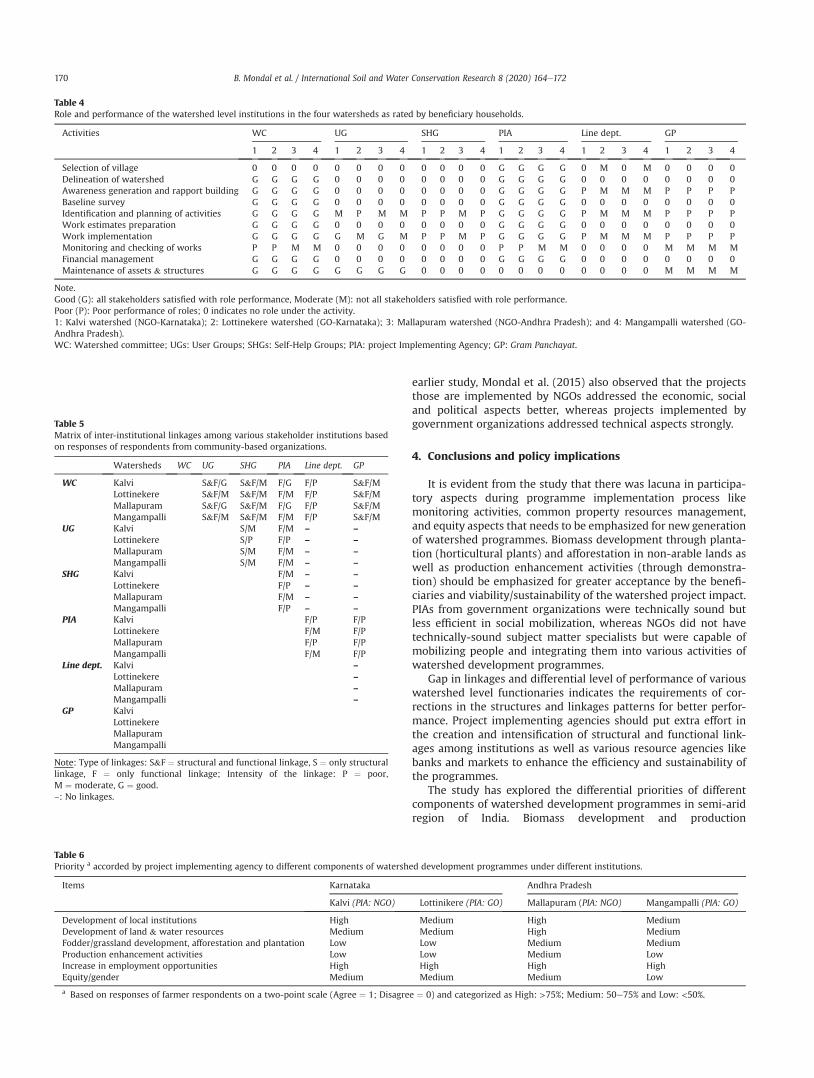
earlier study, Mondal et al. (2015) also observed that the projectsthose are implemented by NGOs addressed the economic, socialand political aspects better, whereas projects implemented bygovernment organizations addressed technical aspects strongly.
4. Conclusions and policy implications
It is evident from the study that there was lacuna in participa-tory aspects during programme implementation process likemonitoring activities, common property resources management,and equity aspects that needs to be emphasized for new generationof watershed programmes. Biomass development through planta-tion (horticultural plants) and afforestation in non-arable lands aswell as production enhancement activities (through demonstra-tion) should be emphasized for greater acceptance by the benefi-ciaries and viability/sustainability of the watershed project impact.PIAs from government organizations were technically sound butless efficient in social mobilization, whereas NGOs did not havetechnically-sound subject matter specialists but were capable ofmobilizing people and integrating them into various activities ofwatershed development programmes.
Gap in linkages and differential level of performance of variouswatershed level functionaries indicates the requirements of cor-rections in the structures and linkages patterns for better perfor-mance. Project implementing agencies should put extra effort inthe creation and intensification of structural and functional link-ages among institutions as well as various resource agencies likebanks and markets to enhance the efficiency and sustainability ofthe programmes.
The study has explored the differential priorities of differentcomponents of watershed development programmes in semi-aridregion of India. Biomass development and production
Table 4Role and performance of the watershed level institutions in the four watersheds as rated by beneficiary households.
Activities WC UG SHG PIA Line dept. GP
1 2 3 4 1 2 3 4 1 2 3 4 1 2 3 4 1 2 3 4 1 2 3 4
Selection of village 0 0 0 0 0 0 0 0 0 0 0 0 G G G G 0 M 0 M 0 0 0 0Delineation of watershed G G G G 0 0 0 0 0 0 0 0 G G G G 0 0 0 0 0 0 0 0Awareness generation and rapport building G G G G 0 0 0 0 0 0 0 0 G G G G P M M M P P P PBaseline survey G G G G 0 0 0 0 0 0 0 0 G G G G 0 0 0 0 0 0 0 0Identification and planning of activities G G G G M P M M P P M P G G G G P M M M P P P PWork estimates preparation G G G G 0 0 0 0 0 0 0 0 G G G G 0 0 0 0 0 0 0 0Work implementation G G G G G M G M P P M P G G G G P M M M P P P PMonitoring and checking of works P P M M 0 0 0 0 0 0 0 0 P P M M 0 0 0 0 M M M MFinancial management G G G G 0 0 0 0 0 0 0 0 G G G G 0 0 0 0 0 0 0 0Maintenance of assets & structures G G G G G G G G 0 0 0 0 0 0 0 0 0 0 0 0 M M M M
Note.Good (G): all stakeholders satisfied with role performance, Moderate (M): not all stakeholders satisfied with role performance.Poor (P): Poor performance of roles; 0 indicates no role under the activity.1: Kalvi watershed (NGO-Karnataka); 2: Lottinekere watershed (GO-Karnataka); 3: Mallapuram watershed (NGO-Andhra Pradesh); and 4: Mangampalli watershed (GO-Andhra Pradesh).WC: Watershed committee; UGs: User Groups; SHGs: Self-Help Groups; PIA: project Implementing Agency; GP: Gram Panchayat.
Table 5Matrix of inter-institutional linkages among various stakeholder institutions basedon responses of respondents from community-based organizations.
Watersheds WC UG SHG PIA Line dept. GP
WC Kalvi S&F/G S&F/M F/G F/P S&F/MLottinekere S&F/M S&F/M F/M F/P S&F/MMallapuram S&F/G S&F/M F/G F/P S&F/MMangampalli S&F/M S&F/M F/M F/P S&F/M
UG Kalvi S/M F/M – –
Lottinekere S/P F/P – –
Mallapuram S/M F/M – –
Mangampalli S/M F/M – –
SHG Kalvi F/M – –
Lottinekere F/P – –
Mallapuram F/M – –
Mangampalli F/P – –
PIA Kalvi F/P F/PLottinekere F/M F/PMallapuram F/P F/PMangampalli F/M F/P
Line dept. Kalvi –
Lottinekere –
Mallapuram –
Mangampalli –
GP KalviLottinekereMallapuramMangampalli
Note: Type of linkages: S&F ¼ structural and functional linkage, S ¼ only structurallinkage, F ¼ only functional linkage; Intensity of the linkage: P ¼ poor,M ¼ moderate, G ¼ good.–: No linkages.
Table 6Priority a accorded by project implementing agency to different components of watershed development programmes under different institutions.
Items Karnataka Andhra Pradesh
Kalvi (PIA: NGO) Lottinikere (PIA: GO) Mallapuram (PIA: NGO) Mangampalli (PIA: GO)
Development of local institutions High Medium High MediumDevelopment of land & water resources Medium Medium High MediumFodder/grassland development, afforestation and plantation Low Low Medium MediumProduction enhancement activities Low Low Medium LowIncrease in employment opportunities High High High HighEquity/gender Medium Medium Medium Low
a Based on responses of farmer respondents on a two-point scale (Agree ¼ 1; Disagree ¼ 0) and categorized as High: >75%; Medium: 50e75% and Low: <50%.
B. Mondal et al. / International Soil and Water Conservation Research 8 (2020) 164e172170
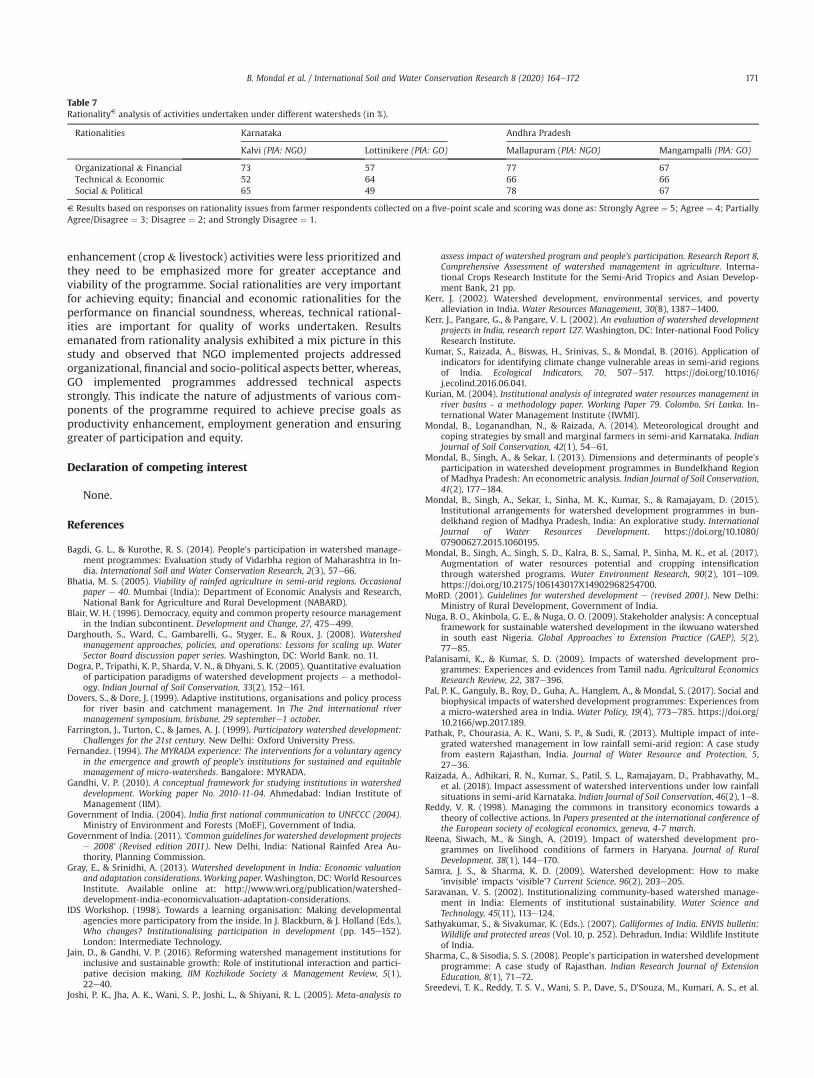
enhancement (crop & livestock) activities were less prioritized andthey need to be emphasized more for greater acceptance andviability of the programme. Social rationalities are very importantfor achieving equity; financial and economic rationalities for theperformance on financial soundness, whereas, technical rational-ities are important for quality of works undertaken. Resultsemanated from rationality analysis exhibited a mix picture in thisstudy and observed that NGO implemented projects addressedorganizational, financial and socio-political aspects better, whereas,GO implemented programmes addressed technical aspectsstrongly. This indicate the nature of adjustments of various com-ponents of the programme required to achieve precise goals asproductivity enhancement, employment generation and ensuringgreater of participation and equity.
Declaration of competing interest
None.
References
Bagdi, G. L., & Kurothe, R. S. (2014). People’s participation in watershed manage-ment programmes: Evaluation study of Vidarbha region of Maharashtra in In-dia. International Soil and Water Conservation Research, 2(3), 57e66.
Bhatia, M. S. (2005). Viability of rainfed agriculture in semi-arid regions. Occasionalpaper e 40. Mumbai (India): Department of Economic Analysis and Research,National Bank for Agriculture and Rural Development (NABARD).
Blair, W. H. (1996). Democracy, equity and common property resource managementin the Indian subcontinent. Development and Change, 27, 475e499.
Darghouth, S., Ward, C., Gambarelli, G., Styger, E., & Roux, J. (2008). Watershedmanagement approaches, policies, and operations: Lessons for scaling up. WaterSector Board discussion paper series. Washington, DC: World Bank. no. 11.
Dogra, P., Tripathi, K. P., Sharda, V. N., & Dhyani, S. K. (2005). Quantitative evaluationof participation paradigms of watershed development projects e a methodol-ogy. Indian Journal of Soil Conservation, 33(2), 152e161.
Dovers, S., & Dore, J. (1999). Adaptive institutions, organisations and policy processfor river basin and catchment management. In The 2nd international rivermanagement symposium, brisbane, 29 septembere1 october.
Farrington, J., Turton, C., & James, A. J. (1999). Participatory watershed development:Challenges for the 21st century. New Delhi: Oxford University Press.
Fernandez. (1994). The MYRADA experience: The interventions for a voluntary agencyin the emergence and growth of people’s institutions for sustained and equitablemanagement of micro-watersheds. Bangalore: MYRADA.
Gandhi, V. P. (2010). A conceptual framework for studying institutions in watersheddevelopment. Working paper No. 2010-11-04. Ahmedabad: Indian Institute ofManagement (IIM).
Government of India. (2004). India first national communication to UNFCCC (2004).Ministry of Environment and Forests (MoEF), Government of India.
Government of India. (2011). ‘Common guidelines for watershed development projectse 2008’ (Revised edition 2011). New Delhi, India: National Rainfed Area Au-thority, Planning Commission.
Gray, E., & Srinidhi, A. (2013). Watershed development in India: Economic valuationand adaptation considerations. Working paper. Washington, DC: World ResourcesInstitute. Available online at: http://www.wri.org/publication/watershed-development-india-economicvaluation-adaptation-considerations.
IDS Workshop. (1998). Towards a learning organisation: Making developmentalagencies more participatory from the inside. In J. Blackburn, & J. Holland (Eds.),Who changes? Institutionalising participation in development (pp. 145e152).London: Intermediate Technology.
Jain, D., & Gandhi, V. P. (2016). Reforming watershed management institutions forinclusive and sustainable growth: Role of institutional interaction and partici-pative decision making. IIM Kozhikode Society & Management Review, 5(1),22e40.
Joshi, P. K., Jha, A. K., Wani, S. P., Joshi, L., & Shiyani, R. L. (2005). Meta-analysis to
assess impact of watershed program and people’s participation. Research Report 8,Comprehensive Assessment of watershed management in agriculture. Interna-tional Crops Research Institute for the Semi-Arid Tropics and Asian Develop-ment Bank, 21 pp.
Kerr, J. (2002). Watershed development, environmental services, and povertyalleviation in India. Water Resources Management, 30(8), 1387e1400.
Kerr, J., Pangare, G., & Pangare, V. L. (2002). An evaluation of watershed developmentprojects in India, research report 127. Washington, DC: Inter-national Food PolicyResearch Institute.
Kumar, S., Raizada, A., Biswas, H., Srinivas, S., & Mondal, B. (2016). Application ofindicators for identifying climate change vulnerable areas in semi-arid regionsof India. Ecological Indicators, 70, 507e517. https://doi.org/10.1016/j.ecolind.2016.06.041.
Kurian, M. (2004). Institutional analysis of integrated water resources management inriver basins - a methodology paper. Working Paper 79. Colombo, Sri Lanka. In-ternational Water Management Institute (IWMI).
Mondal, B., Loganandhan, N., & Raizada, A. (2014). Meteorological drought andcoping strategies by small and marginal farmers in semi-arid Karnataka. IndianJournal of Soil Conservation, 42(1), 54e61.
Mondal, B., Singh, A., & Sekar, I. (2013). Dimensions and determinants of people’sparticipation in watershed development programmes in Bundelkhand Regionof Madhya Pradesh: An econometric analysis. Indian Journal of Soil Conservation,41(2), 177e184.
Mondal, B., Singh, A., Sekar, I., Sinha, M. K., Kumar, S., & Ramajayam, D. (2015).Institutional arrangements for watershed development programmes in bun-delkhand region of Madhya Pradesh, India: An explorative study. InternationalJournal of Water Resources Development. https://doi.org/10.1080/07900627.2015.1060195.
Mondal, B., Singh, A., Singh, S. D., Kalra, B. S., Samal, P., Sinha, M. K., et al. (2017).Augmentation of water resources potential and cropping intensificationthrough watershed programs. Water Environment Research, 90(2), 101e109.https://doi.org/10.2175/106143017X14902968254700.
MoRD. (2001). Guidelines for watershed development e (revised 2001). New Delhi:Ministry of Rural Development, Government of India.
Nuga, B. O., Akinbola, G. E., & Nuga, O. O. (2009). Stakeholder analysis: A conceptualframework for sustainable watershed development in the ikwuano watershedin south east Nigeria. Global Approaches to Extension Practice (GAEP), 5(2),77e85.
Palanisami, K., & Kumar, S. D. (2009). Impacts of watershed development pro-grammes: Experiences and evidences from Tamil nadu. Agricultural EconomicsResearch Review, 22, 387e396.
Pal, P. K., Ganguly, B., Roy, D., Guha, A., Hanglem, A., & Mondal, S. (2017). Social andbiophysical impacts of watershed development programmes: Experiences froma micro-watershed area in India. Water Policy, 19(4), 773e785. https://doi.org/10.2166/wp.2017.189.
Pathak, P., Chourasia, A. K., Wani, S. P., & Sudi, R. (2013). Multiple impact of inte-grated watershed management in low rainfall semi-arid region: A case studyfrom eastern Rajasthan, India. Journal of Water Resource and Protection, 5,27e36.
Raizada, A., Adhikari, R. N., Kumar, S., Patil, S. L., Ramajayam, D., Prabhavathy, M.,et al. (2018). Impact assessment of watershed interventions under low rainfallsituations in semi-arid Karnataka. Indian Journal of Soil Conservation, 46(2), 1e8.
Reddy, V. R. (1998). Managing the commons in transitory economics towards atheory of collective actions. In Papers presented at the international conference ofthe European society of ecological economics, geneva, 4-7 march.
Reena, Siwach, M., & Singh, A. (2019). Impact of watershed development pro-grammes on livelihood conditions of farmers in Haryana. Journal of RuralDevelopment, 38(1), 144e170.
Samra, J. S., & Sharma, K. D. (2009). Watershed development: How to make‘invisible’ impacts ‘visible’? Current Science, 96(2), 203e205.
Saravanan, V. S. (2002). Institutionalizing community-based watershed manage-ment in India: Elements of institutional sustainability. Water Science andTechnology, 45(11), 113e124.
Sathyakumar, S., & Sivakumar, K. (Eds.). (2007). Galliformes of India. ENVIS bulletin:Wildlife and protected areas (Vol. 10, p. 252). Dehradun, India: Wildlife Instituteof India.
Sharma, C., & Sisodia, S. S. (2008). People’s participation in watershed developmentprogramme: A case study of Rajasthan. Indian Research Journal of ExtensionEducation, 8(1), 71e72.
Sreedevi, T. K., Reddy, T. S. V., Wani, S. P., Dave, S., D’Souza, M., Kumari, A. S., et al.
Table 7RationalityV analysis of activities undertaken under different watersheds (in %).
Rationalities Karnataka Andhra Pradesh
Kalvi (PIA: NGO) Lottinikere (PIA: GO) Mallapuram (PIA: NGO) Mangampalli (PIA: GO)
Organizational & Financial 73 57 77 67Technical & Economic 52 64 66 66Social & Political 65 49 78 67
V Results based on responses on rationality issues from farmer respondents collected on a five-point scale and scoring was done as: Strongly Agree ¼ 5; Agree ¼ 4; PartiallyAgree/Disagree ¼ 3; Disagree ¼ 2; and Strongly Disagree ¼ 1.
B. Mondal et al. / International Soil and Water Conservation Research 8 (2020) 164e172 171

(2008). A comparative analysis of institutional arrangements in watersheddevelopment projects in India. Global Theme on Agro-ecosystems Report No. 50.Hyderabad, India: International Crops Research Institute for the Semi-AridTropics (ICRISAT).
Sreedevi, T. K., & Wani, S. P. (2007). Leveraging institutions for enhanced collectiveaction in community watersheds through harnessing gender power for sus-tainable development. In S. Mudrakartha (Ed.), Empowering the poor in the era ofknowledge economy (pp. 27e39). Gujarat, India: VIKSAT, Ahmedabad.
Sreedevi, T. K., Wani, S. P., & Pathak, P. (2007). Harnessing gender power and col-lective action through integrated watershed management for minimizing landdegradation and sustainable Development. Journal of Financing Agriculture, 36,23e32.
Sriyana, I., De Gijt, J. G., Parahyangsari, S. K., & Niyomukiza, J. B. (2020). Watershedmanagement index based on the village watershed model (VWM) approachtowards sustainability. International Soil and Water Conservation Research.https://doi.org/10.1016/j.iswcr.2020.01.003.
Tanguilig, H. C., & Tanguilig, V. C. (2009). Institutional aspects of local participatorystrategies in natural resource management. Field Actions Science Report.Retrieved from www.factsreports.org.
Vaidyanathan, A. (2001). Watershed development: Reflections on recent de-velopments. In K. N. Nair, & Chattopadhyay & Srikumar (Eds.), ‘Watershedmanagement for sustainable development field experiences and issues’, Keralaresearch programme on local level development, Trivandrum.
Wani, S. P., Anantha, K. H., & Sreedevi, T. K. (2014). Gender issues in watershedmanagement. In A. A. Cronin, P. K. Mehta, & A. Prakash (Eds.), Gender issues inwater and sanitation programmes: Lessons from India (pp. 99e119). India: Sage.
Wani, S. P., Joshi, P. K., Raju, K. V., Sreedevi, T. K., Wilson, J. M., Shah, A., et al. (2008).Community watershed as a growth engine for development of dryland areas. Acomprehensive assessment of watershed programs in India. Global theme onagroecosystems, ICRISAT, patancheru, Andhra Pradesh (p. 145). Report No. 47.
World Resources Institute. (2005). World resources report 2005. Washington, DC:World Resources Institute.
B. Mondal et al. / International Soil and Water Conservation Research 8 (2020) 164e172172
Original Research Article
Using high-resolution aerial images to study gully development at theregional scale in southern China
Honghu Liu a, b, *, Georg H€ormann c, Bingyu Qi a, Qiuxing Yue a
a State Key Lab Soil Erosion and Dryland Farming on the Loess Plateau, Institute of Soil and Water Conservation, Chinese Academy of Sciences and Ministryof Water Resources, Xinong Rd 26, 712100, Yangling, Shaanxi Province, PR Chinab Changjiang River Scientific Research Institute, Changjiang Water Resource Commission, No 23 Huangpuda Street, 430010, Wuhan, Hubei province, PRChinac Department of Hydrology and Water Resources Management, Institute of Natural Resource Conservation, Kiel University, Olshausenstr. 75, D-24098 Kiel,Germany
a r t i c l e i n f o
Article history:Received 15 August 2019Received in revised form6 March 2020Accepted 30 March 2020Available online 16 April 2020
Keywords:Digital elevation modelSlope gradientExposed landsUpstream contributing area
a b s t r a c t
There are 239,100 gullies in southern China, which cause the degradation of ecological system. However,studies on gully development at the regional scale is relatively lack. The purpose of this study is toanalyze the regional gully dynamics and explore how land use and topographic factors affect gullydevelopment. Input data consists of land use maps derived from high-resolution images from 2004 to2014, and topography maps from a digital elevation model with a pixel size of 8 m � 8 m in two 25-km2
study sites of Anxi (AX) and Xingning county (XN). The following results were obtained: (1) AX gulliesdecreased from 2006 to 2014 while XN first increased from 2004 to 2009, and then decreased from 2009to 2014. Both AX and XN gully area in percentage of the total area ranged from 1% to 3%, which washigher than the average 0.25% of the whole southern China by the artificial survey in 2005. (2) Most of AXand XN gullies occurred along the ridgeline and had the close relationships with the upstreamcontributing area and slope gradient. (3) New gullies developed on the exposed land and forestland. Thelost gullies were converted into forestland and grassland. In fact, most of these gullies were only coveredby vegetation, not real disappearance. These results proved that gully decreased, but construction ofroads and buildings intensified gully development. Consequently, these findings reveal that vegetationprotection and ecological restoration should be adopted in southern China.© 2020 International Research and Training Center on Erosion and Sedimentation and China Water andPower Press. Production and Hosting by Elsevier B.V. This is an open access article under the CC BY-NC-
ND license (http://creativecommons.org/licenses/by-nc-nd/4.0/).
1. Introduction
Gully formation depends on rainfall, surface runoff, topog-raphy, and land use (Valentin, Poesen, & Li, 2005). Gulliesoccurred in farmlands can cause the hyperconcentrated flow (Xu,1992), degradation of ecological system (Poesen, Nachtergaele,Verstraeten, & Valentin, 2003), downstream aggregation(Poesen et al., 2003), and sediment deposition (Lin, Huang, Wang,Zhang, & Ge, 2015). Gully development often occurs in combina-tion with heavy rain, in which huge amounts of sediment are putinto motion that can lead to the destruction of property and loss of
life (Shi, 1984). To prevent gullies from occurring, it is necessary tounderstand how they develop.
Gullies occur everywhere in the world and have already beenthe subject of many studies. The five most important methods todescribe the morphology of gullies are manual methods, GPS, 3Dscanner, aerial images, and 3D photo-reconstruction. Manualmethods include the rule and tape as well as the micro-topographic profile meter. A cross-section of the gully is dividedinto a sequence of simple geometric shapes such as rectangles andtriangles, which are added together to obtain the area and volumeof the gully (Casalí, Loizu, Campo, & �Alvarez-Mozos, 2006; Xie,Wei, & Zhang, 2012; Ren, Ding, Wu, & Li, 2015). GPS is used toobtain the coordinates of the gully such as the gully head and theedges (Zabihi et al., 2018). Based on these values, GIS software isused to create a digital elevation model (DEM) of the gully (Huet al., 2007; Lin et al., 2012). A 3D scanner can be used to
* Corresponding author. Changjiang River Scientific Research Institute, Chang-jiang Water Resource Commission, No 23 Huangpuda street, 430010, Wuhan, Hubeiprovince, PR China.
E-mail address: [email protected] (H. Liu).
Contents lists available at ScienceDirect
International Soil and Water Conservation Research
journal homepage: www.elsevier .com/locate/ iswcr
https://doi.org/10.1016/j.iswcr.2020.03.0042095-6339/© 2020 International Research and Training Center on Erosion and Sedimentation and China Water and Power Press. Production and Hosting by Elsevier B.V. Thisis an open access article under the CC BY-NC-ND license (http://creativecommons.org/licenses/by-nc-nd/4.0/).
International Soil and Water Conservation Research 8 (2020) 173e184
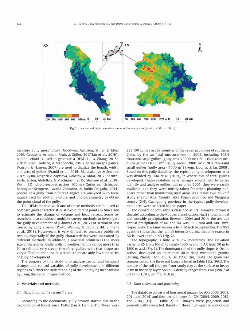
measure gully morphology (Goodwin, Armston, Stiller, & Muir,2016, Goodwin, Armston, Muir, & Stiller, 2017(Liu et al., 2019)).A point cloud is used to generate a DEM (Liu & Zhang, 2015a,2015b; Vinci, Todisco, & Mannocchi, 2016). Aerial images (James,Watson, & Hansen, 2007) are used to digitize the length, width,and area of gullies (Frankl et al., 2015; Mararakanye & Sumner,2017; Rysin, Grigoriev, Zaytseva, Golosov, & Aidar, 2017; Shruthi,Kerle, Jetten, Abdellah, & Machmach, 2015; Slimane et al., 2018).With 3D photo-reconstruction (G�omez-Guti�errez, Schnabel,Berenguer-Sempere, Lavado-Contador, & Rubio-Delgado, 2014),photos of a gully from different angles are analyzed with tech-niques used for motion capture and photogrammetry to obtainthe point cloud of the gully.
The DEMs created with one of these methods can be used tocompare gully characteristics at two different points in times andto estimate the change of volume and head retreat. Some re-searchers also combined multiple survey methods to investigatethe gully development of (C�anovas et al., 2017) or sediment losscaused by gully erosion (Porto, Walling, & Capra, 2014; Slimaneet al., 2018). However, it is very difficult to compare publishedresults, especially if the gully characteristics were measured bydifferent methods. In addition, a practical problem is the sheersize of the gullies. Gully walls in southern China can be more than10 m tall and very steep; therefore, gullies with that shape arevery difficult to monitor. As a result, there are only few time seriesof gully development.
The purpose of this study is to analyze spatial and temporalchanges and control variables of gully development in differentregions to further the understanding of the underlyingmechanismsby using the aerial images method.
2. Materials and methods
2.1. Description of the research areas
According to the documents, gully erosion started due to theexploitation of forest since 1940s (Liu & Lian, 2011). There were
239,100 gullies in 362 counties of the seven provinces of southernChina by the artificial measurement in 2005, including 108.4thousand large gullies (gully area >3000 m2), 60.1 thousand me-dium gullies (1000 m2 <gully area� 3000 m2), 70.6 thousandsmall gullies (gully area �1000 m2) (Feng, Liao, Li, & Lu, 2009).Based on this gully database, the typical gully development areawas divided by Liao et al. (2019), in where 75% of total gulliesdeveloped. High-resolution aerial images would help to betteridentify and analyze gullies, but prior to 2005, they were rarelyavailable, and they were mostly taken for urban planning pur-poses rather than monitoring rural areas. As a result, two 25-km2
study sites of Anxi County (AX), Fujian province and Xingningcounty (XN), Guangdong province in the typical gully develop-ment area were selected in this paper.
The climate of both sites is classified as Cfa (humid subtropicalclimate) according to the K€oppen classification. Fig. 2 shows annualand monthly precipitation. Between 2004 and 2014, the averageannual precipitation of XN and AX was 1505 mm and 1481 mm,respectively. The rainy season is fromMarch to September. The 95%quantile shows that the rainfall intensity during the rainy season inAX is lower than in XN (Fig. 2).
The topography is hilly with low mountains. The elevationvaries in XN from 100 m to nearly 1000 m and in AX from 50 m to1500 m a.s.l. (Fig. 1). The dominant soil of the gully slopes is Orthicacrisol, developed on more than 40-m-deep weathered granite(Huang, Zhang, Chen, Liu, & He, 1996; Qiu, 1994). The grain sizecomposition of the three soil layers is listed in Table 1 (Li, 1992). Thetexture of the soil changes from sandy clay at the surface to heavyloam in the deep layer. Soil bulk density ranges from 1.44 g cm�3 at0.3 m to 1.79 g cm�3 at 16.0 m.
2.2. Data collection and processing
The database consists of four aerial images for AX (2006, 2008,2011, and 2014) and four aerial images for XN (2004, 2009, 2012,and 2014) (Fig. 3, Table 2). All images were projected andgeometrically corrected. Based on these high-quality and cloud-
Fig. 1. Location and digital elevation model of the study sites (pixel size 30 m � 30 m).
H. Liu et al. / International Soil and Water Conservation Research 8 (2020) 173e184174
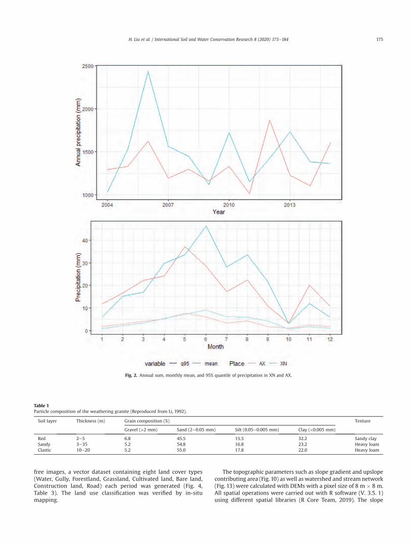
free images, a vector dataset containing eight land cover types(Water, Gully, Forestland, Grassland, Cultivated land, Bare land,Construction land, Road) each period was generated (Fig. 4,Table 3). The land use classification was verified by in-situmapping.
The topographic parameters such as slope gradient and upslopecontributing area (Fig. 10) as well as watershed and stream network(Fig. 13) were calculated with DEMs with a pixel size of 8 m � 8 m.All spatial operations were carried out with R software (V. 3.5. 1)using different spatial libraries (R Core Team, 2019). The slope
Table 1Particle composition of the weathering granite (Reproduced from Li, 1992).
Soil layer Thickness (m) Grain composition (%) Texture
Gravel (>2 mm) Sand (2e0.05 mm) Silt (0.05e0.005 mm) Clay (<0.005 mm)
Red 2e5 6.8 45.5 15.5 32.2 Sandy claySandy 3e35 5.2 54.8 16.8 23.2 Heavy loamClastic 10e20 5.2 55.0 17.8 22.0 Heavy loam
Fig. 2. Annual sum, monthly mean, and 95% quantile of precipitation in XN and AX.
H. Liu et al. / International Soil and Water Conservation Research 8 (2020) 173e184 175
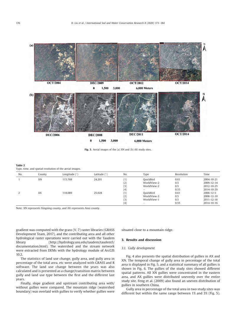
gradient was computed with the grass (V. 7) raster libraries (GRASSDevelopment Team, 2017), and the contributing area and all otherhydrological raster operations were carried out with the Taudemlibrary (http://hydrology.usu.edu/taudem/taudem5/documentation.html). The watershed and the stream networkwere extracted from DEMs with the hydrology module of ArcGIS10.2.
The statistics of land use change, gully area, and gully area inpercentage of the total area, etc were analyzed with GRASS and Rsoftware. The land use change between the years was alsocalculated and is presented as a change/transition matrix betweengully and land use type between the first and the different lastyears.
Finally, slope gradient and upstream contributing area with/without gullies were compared. The mountain ridge (watershedboundary) was overlaid with gullies to verify whether gullies were
situated close to a mountain ridge.
3. Results and discussion
3.1. Gully development
Fig. 4 also presents the spatial distribution of gullies in AX andXN. The temporal change of gully area in percentage of the totalarea is displayed in Fig. 5, and a statistical summary of all gullies isshown in Fig. 6. The gullies of the study sites showed differentspatial patterns. All XN gullies were concentrated in the easternarea, and AX gullies were distributed unevenly over the entirestudy site. Feng et al. (2009) also found an uneven distribution ofgullies in southern China.
Gully area in percentage of the total area in two study sites wasdifferent but within the same range between 1% and 3% (Fig. 5).
Fig. 3. Aerial images of the (a) XN and (b) AX study sites.
Table 2Type, time, and spatial resolution of the aerial images.
No. County Longitude (�) Latitude (�) No. Type Resolution Time
1 XN 115.768 24.201 (1) QuickBird 0.61 2004-10-21(2) WorldView-2 0.5 2009-12-14(3) WorldView-2 0.5 2012-10-25(4) e 0.55 2014-10-29
2 AX 118.089 25.028 (1) QuickBird 0.61 2006-12-5(2) WorldView-2 0.5 2008-12-10(3) WorldView-1 0.5 2011-12-18(4) e 0.55 2014-10-16
Note: XN represents Xingning county, and AX represents Anxi county.
H. Liu et al. / International Soil and Water Conservation Research 8 (2020) 173e184176
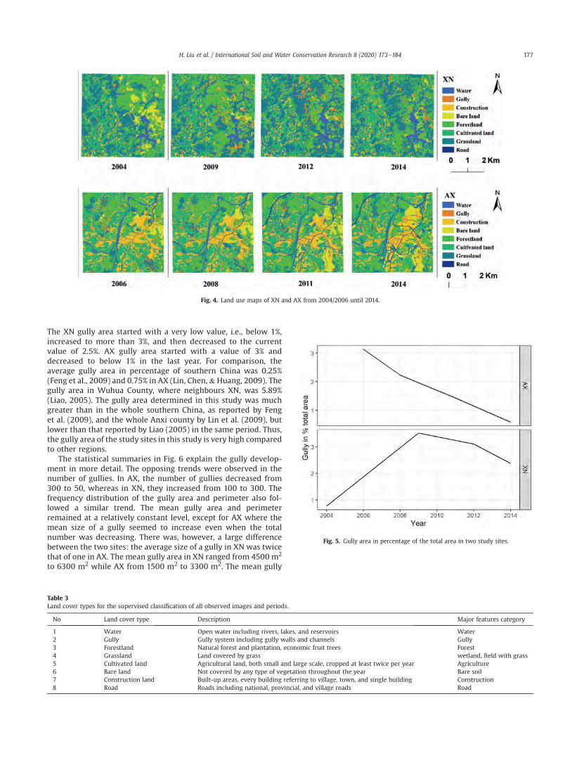
The XN gully area started with a very low value, i.e., below 1%,increased to more than 3%, and then decreased to the currentvalue of 2.5%. AX gully area started with a value of 3% anddecreased to below 1% in the last year. For comparison, theaverage gully area in percentage of southern China was 0.25%(Feng et al., 2009) and 0.75% in AX (Lin, Chen, &Huang, 2009). Thegully area in Wuhua County, where neighbours XN, was 5.89%(Liao, 2005). The gully area determined in this study was muchgreater than in the whole southern China, as reported by Fenget al. (2009), and the whole Anxi county by Lin et al. (2009), butlower than that reported by Liao (2005) in the same period. Thus,the gully area of the study sites in this study is very high comparedto other regions.
The statistical summaries in Fig. 6 explain the gully develop-ment in more detail. The opposing trends were observed in thenumber of gullies. In AX, the number of gullies decreased from300 to 50, whereas in XN, they increased from 100 to 300. Thefrequency distribution of the gully area and perimeter also fol-lowed a similar trend. The mean gully area and perimeterremained at a relatively constant level, except for AX where themean size of a gully seemed to increase even when the totalnumber was decreasing. There was, however, a large differencebetween the two sites: the average size of a gully in XN was twicethat of one in AX. The mean gully area in XN ranged from 4500 m2
to 6300 m2 while AX from 1500 m2 to 3300 m2. The mean gully
Fig. 4. Land use maps of XN and AX from 2004/2006 until 2014.
Table 3Land cover types for the supervised classification of all observed images and periods.
No Land cover type Description Major features category
1 Water Open water including rivers, lakes, and reservoirs Water2 Gully Gully system including gully walls and channels Gully3 Forestland Natural forest and plantation, economic fruit trees Forest4 Grassland Land covered by grass wetland, field with grass5 Cultivated land Agricultural land, both small and large scale, cropped at least twice per year Agriculture6 Bare land Not covered by any type of vegetation throughout the year Bare soil7 Construction land Built-up areas, every building referring to village, town, and single building Construction8 Road Roads including national, provincial, and village roads Road
Fig. 5. Gully area in percentage of the total area in two study sites.
H. Liu et al. / International Soil and Water Conservation Research 8 (2020) 173e184 177
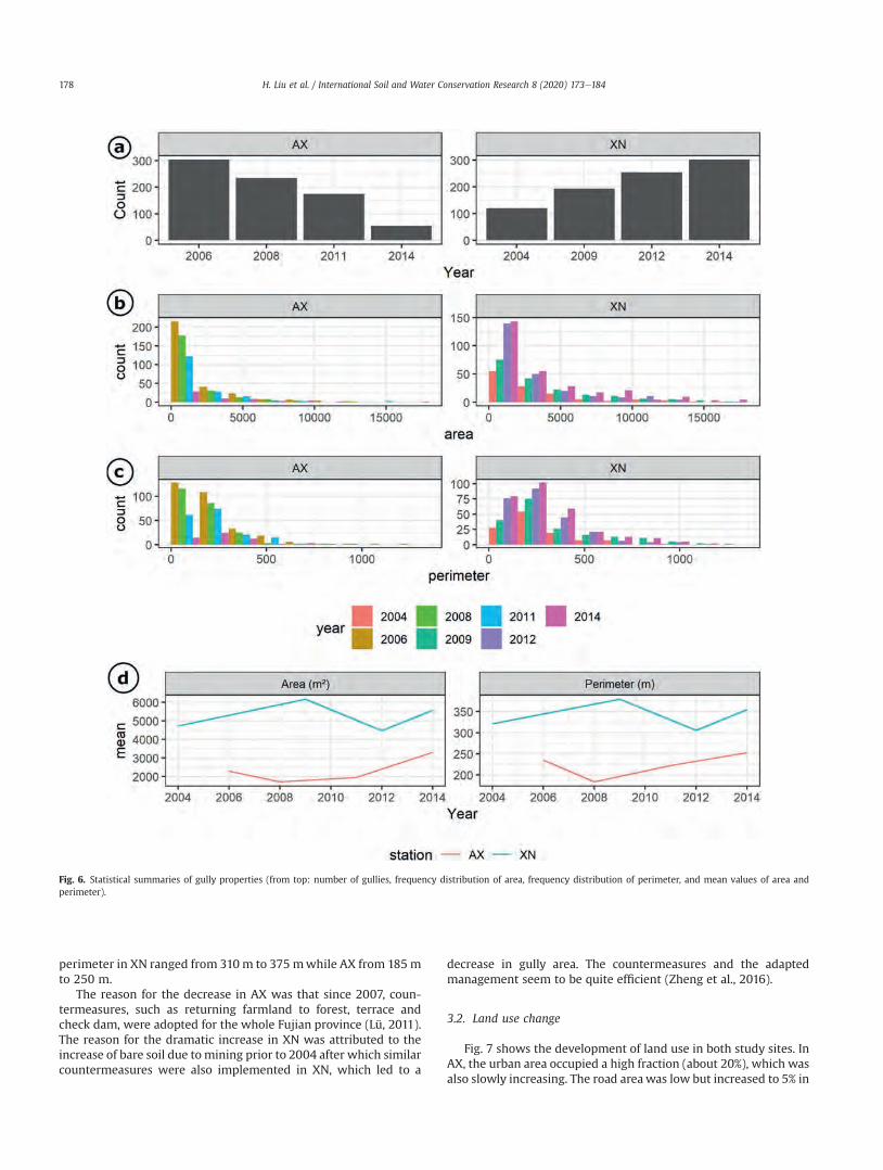
perimeter in XN ranged from 310m to 375 mwhile AX from 185mto 250 m.
The reason for the decrease in AX was that since 2007, coun-termeasures, such as returning farmland to forest, terrace andcheck dam, were adopted for the whole Fujian province (Lü, 2011).The reason for the dramatic increase in XN was attributed to theincrease of bare soil due tomining prior to 2004 after which similarcountermeasures were also implemented in XN, which led to a
decrease in gully area. The countermeasures and the adaptedmanagement seem to be quite efficient (Zheng et al., 2016).
3.2. Land use change
Fig. 7 shows the development of land use in both study sites. InAX, the urban area occupied a high fraction (about 20%), which wasalso slowly increasing. The road areawas low but increased to 5% in
Fig. 6. Statistical summaries of gully properties (from top: number of gullies, frequency distribution of area, frequency distribution of perimeter, and mean values of area andperimeter).
H. Liu et al. / International Soil and Water Conservation Research 8 (2020) 173e184178
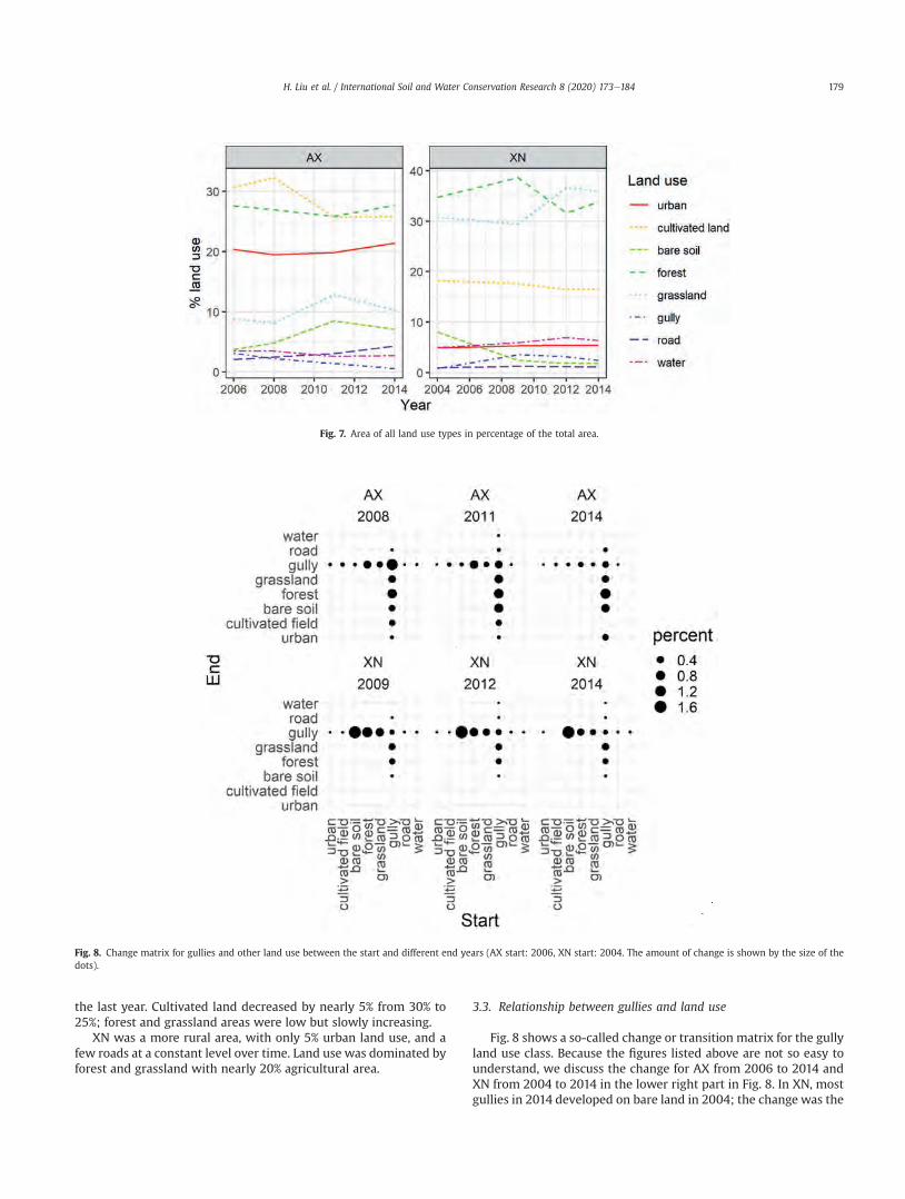
the last year. Cultivated land decreased by nearly 5% from 30% to25%; forest and grassland areas were low but slowly increasing.
XN was a more rural area, with only 5% urban land use, and afew roads at a constant level over time. Land use was dominated byforest and grassland with nearly 20% agricultural area.
3.3. Relationship between gullies and land use
Fig. 8 shows a so-called change or transition matrix for the gullyland use class. Because the figures listed above are not so easy tounderstand, we discuss the change for AX from 2006 to 2014 andXN from 2004 to 2014 in the lower right part in Fig. 8. In XN, mostgullies in 2014 developed on bare land in 2004; the change was the
Fig. 7. Area of all land use types in percentage of the total area.
Fig. 8. Change matrix for gullies and other land use between the start and different end years (AX start: 2006, XN start: 2004. The amount of change is shown by the size of thedots).
H. Liu et al. / International Soil and Water Conservation Research 8 (2020) 173e184 179
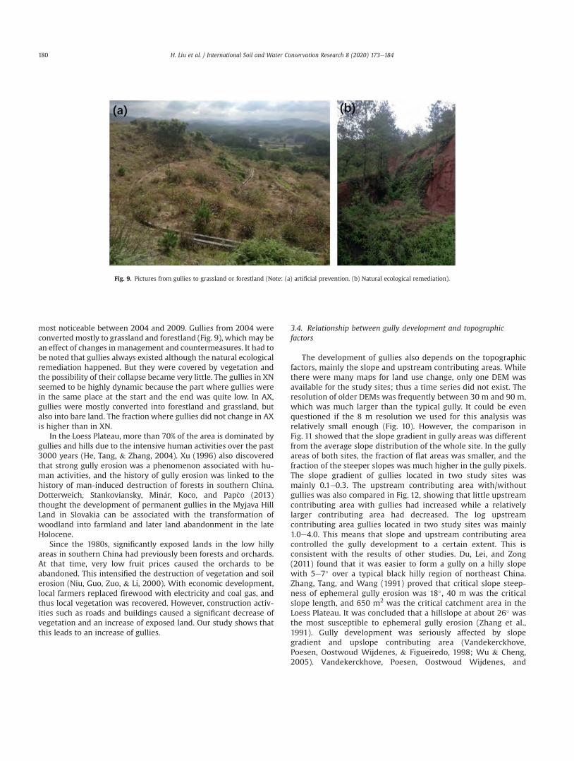
most noticeable between 2004 and 2009. Gullies from 2004 wereconvertedmostly to grassland and forestland (Fig. 9), whichmay bean effect of changes in management and countermeasures. It had tobe noted that gullies always existed although the natural ecologicalremediation happened. But they were covered by vegetation andthe possibility of their collapse became very little. The gullies in XNseemed to be highly dynamic because the part where gullies werein the same place at the start and the end was quite low. In AX,gullies were mostly converted into forestland and grassland, butalso into bare land. The fraction where gullies did not change in AXis higher than in XN.
In the Loess Plateau, more than 70% of the area is dominated bygullies and hills due to the intensive human activities over the past3000 years (He, Tang, & Zhang, 2004). Xu (1996) also discoveredthat strong gully erosion was a phenomenon associated with hu-man activities, and the history of gully erosion was linked to thehistory of man-induced destruction of forests in southern China.Dotterweich, Stankoviansky, Min�ar, Koco, and Pap�co (2013)thought the development of permanent gullies in the Myjava HillLand in Slovakia can be associated with the transformation ofwoodland into farmland and later land abandonment in the lateHolocene.
Since the 1980s, significantly exposed lands in the low hillyareas in southern China had previously been forests and orchards.At that time, very low fruit prices caused the orchards to beabandoned. This intensified the destruction of vegetation and soilerosion (Niu, Guo, Zuo, & Li, 2000). With economic development,local farmers replaced firewood with electricity and coal gas, andthus local vegetation was recovered. However, construction activ-ities such as roads and buildings caused a significant decrease ofvegetation and an increase of exposed land. Our study shows thatthis leads to an increase of gullies.
3.4. Relationship between gully development and topographicfactors
The development of gullies also depends on the topographicfactors, mainly the slope and upstream contributing areas. Whilethere were many maps for land use change, only one DEM wasavailable for the study sites; thus a time series did not exist. Theresolution of older DEMs was frequently between 30 m and 90 m,which was much larger than the typical gully. It could be evenquestioned if the 8 m resolution we used for this analysis wasrelatively small enough (Fig. 10). However, the comparison inFig. 11 showed that the slope gradient in gully areas was differentfrom the average slope distribution of the whole site. In the gullyareas of both sites, the fraction of flat areas was smaller, and thefraction of the steeper slopes was much higher in the gully pixels.The slope gradient of gullies located in two study sites wasmainly 0.1e0.3. The upstream contributing area with/withoutgullies was also compared in Fig. 12, showing that little upstreamcontributing area with gullies had increased while a relativelylarger contributing area had decreased. The log upstreamcontributing area gullies located in two study sites was mainly1.0e4.0. This means that slope and upstream contributing areacontrolled the gully development to a certain extent. This isconsistent with the results of other studies. Du, Lei, and Zong(2011) found that it was easier to form a gully on a hilly slopewith 5e7� over a typical black hilly region of northeast China.Zhang, Tang, and Wang (1991) proved that critical slope steep-ness of ephemeral gully erosion was 18�, 40 m was the criticalslope length, and 650 m2 was the critical catchment area in theLoess Plateau. It was concluded that a hillslope at about 26� wasthe most susceptible to ephemeral gully erosion (Zhang et al.,1991). Gully development was seriously affected by slopegradient and upslope contributing area (Vandekerckhove,Poesen, Oostwoud Wijdenes, & Figueiredo, 1998; Wu & Cheng,2005). Vandekerckhove, Poesen, Oostwoud Wijdenes, and
Fig. 9. Pictures from gullies to grassland or forestland (Note: (a) artificial prevention. (b) Natural ecological remediation).
H. Liu et al. / International Soil and Water Conservation Research 8 (2020) 173e184180
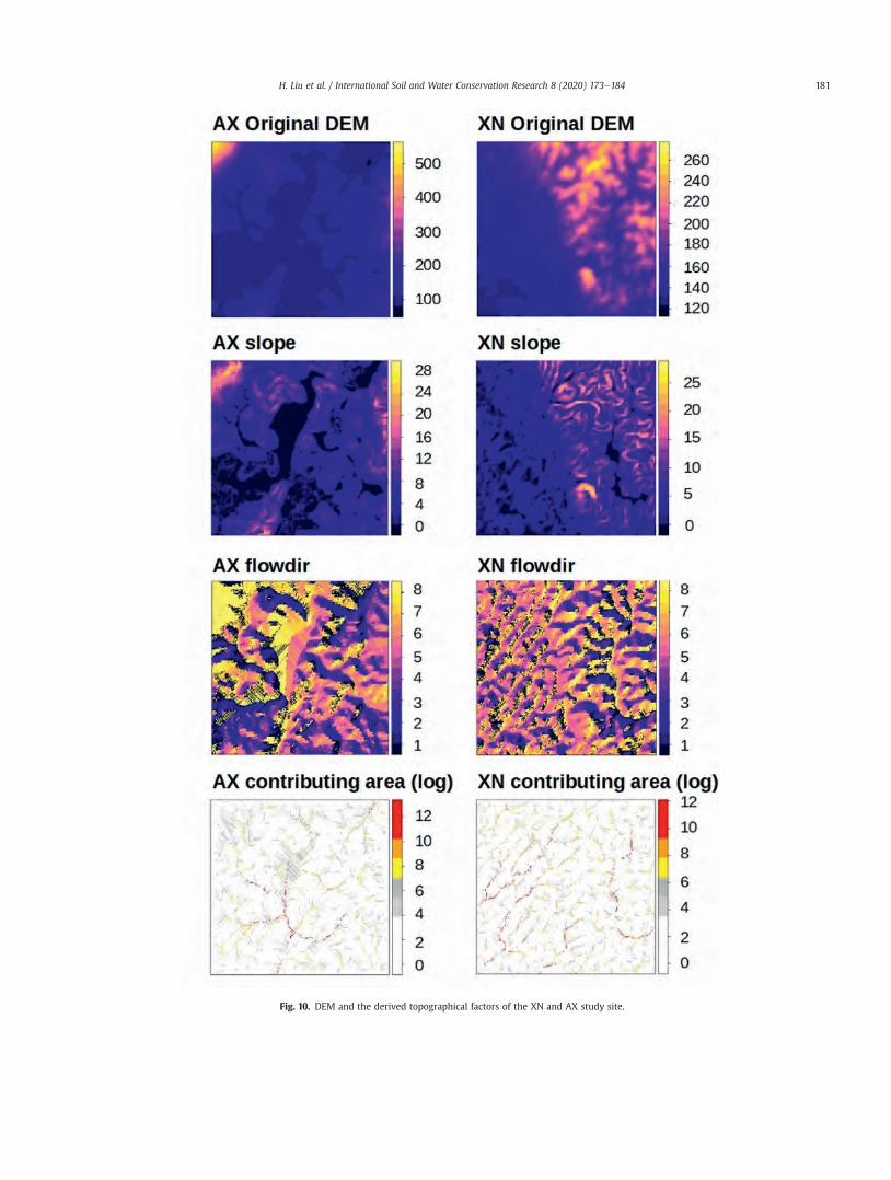
Fig. 10. DEM and the derived topographical factors of the XN and AX study site.
H. Liu et al. / International Soil and Water Conservation Research 8 (2020) 173e184 181
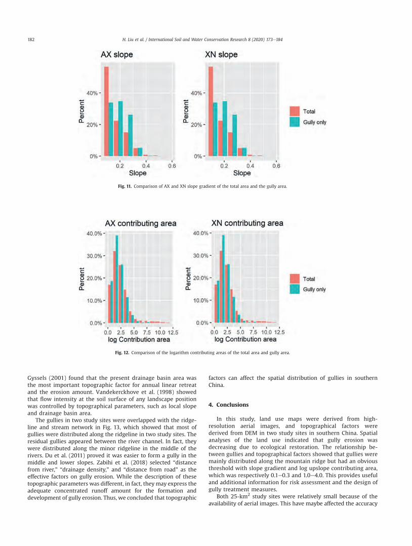
Gyssels (2001) found that the present drainage basin area wasthe most important topographic factor for annual linear retreatand the erosion amount. Vandekerckhove et al. (1998) showedthat flow intensity at the soil surface of any landscape positionwas controlled by topographical parameters, such as local slopeand drainage basin area.
The gullies in two study sites were overlapped with the ridge-line and stream network in Fig. 13, which showed that most ofgullies were distributed along the ridgeline in two study sites. Theresidual gullies appeared between the river channel. In fact, theywere distributed along the minor ridgeline in the middle of therivers. Du et al. (2011) proved it was easier to form a gully in themiddle and lower slopes. Zabihi et al. (2018) selected “distancefrom river,” “drainage density,” and “distance from road” as theeffective factors on gully erosion. While the description of thesetopographic parameters was different, in fact, theymay express theadequate concentrated runoff amount for the formation anddevelopment of gully erosion. Thus, we concluded that topographic
factors can affect the spatial distribution of gullies in southernChina.
4. Conclusions
In this study, land use maps were derived from high-resolution aerial images, and topographical factors werederived from DEM in two study sites in southern China. Spatialanalyses of the land use indicated that gully erosion wasdecreasing due to ecological restoration. The relationship be-tween gullies and topographical factors showed that gullies weremainly distributed along the mountain ridge but had an obviousthreshold with slope gradient and log upslope contributing area,which was respectively 0.1e0.3 and 1.0e4.0. This provides usefuland additional information for risk assessment and the design ofgully treatment measures.
Both 25-km2 study sites were relatively small because of theavailability of aerial images. This have maybe affected the accuracy
Fig. 11. Comparison of AX and XN slope gradient of the total area and the gully area.
Fig. 12. Comparison of the logarithm contributing areas of the total area and gully area.
H. Liu et al. / International Soil and Water Conservation Research 8 (2020) 173e184182
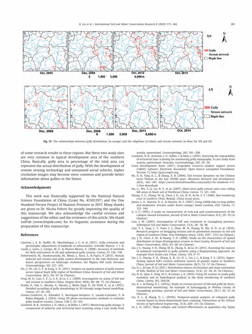
of some research results in these regions. But these two study sitesare very common in typical development area of the southernChina. Basically, gully area in percentage of the total area canrepresent the actual distribution of gully. With the development ofremote sensing technology and unmanned aerial vehicles, higherresolution images may become more common and provide betterinformation about gullies in the future.
Acknowledgments
This work was financially supported by the National NaturalScience Foundation of China (Grant No. 41301297) and the OneHundred Person Project of Shannxi Province in 2017. Many thanksare given to Dr. Nicola Fohrer for greatly improving the quality ofthis manuscript. We also acknowledge the careful revision andsuggestions of the editor and the reviewers of this article. We thankLetPub (www.letpub.com) for its linguistic assistance during thepreparation of this manuscript.
References
C�anovas, J. A. B., Stoffel, M., Martínduque, J. F., et al. (2017). Gully evolution andgeomorphic adjustments of badlands to reforestation. Scientific Reports, 7, 1e8.
Casalí, J., Loizu, J., Campo, M. A., & �Alvarez-Mozos, A. (2006). Accuracy of methodsfor field assessment of rill and ephemeral gully erosion. Catena, 67, 128e138.
Dotterweich, M., Stankoviansky, M., Min�ar, J., Koco, �S., & Pap�co, P. (2013). Humaninduced soil erosion and gully system development in the Late Holocene andfuture perspectives on landscape evolution, the Myjava Hill Land, Slovakia.Geomorphology, 201, 227e245.
Du, G. M., Lei, G. P., & Zong, X. D. (2011). Analysis on spatial pattern of gully erosionacross typical black hilly region of Northeast China. Research of Soil and WaterConservation, 18(2), 94e97 (In Chinese).
Feng, M. H., Liao, C. Y., Li, S. X., & Lu, S. L. (2009). Investigation on status of hill andsoil erosion in southern China. Yangtze River, 40(8), 66e68, 75. (In Chinese).
Frankl, A., Stal, C., Abraha, A., Nyssen, J., Rieke-Zapp, D., De Wulf, A., et al. (2015).Detailed recording of gully morphology in 3D through image-based modelling.Catena, 127, 92e101.
G�omez-Guti�errez, �A., Schnabel, S., Berenguer-Sempere, F., Lavado-Contador, F., &Rubio-Delgado, J. (2014). Using 3D photo-reconstruction methods to estimategully headcut erosion. Catena, 120(1), 91e101.
Goodwin, N. R., Armston, J. D., Muir, J., & Stiller, I. (2017). Monitoring gully change: Acomparison of airborne and terrestrial laser scanning using a case study from
aratula, queensland. Geomorphology, 282, 195e208.Goodwin, N. R., Armston, J. D., Stiller, I., & Muir, J. (2016). Assessing the repeatability
of terrestrial laser scanning for monitoring gully topography: A case study fromaratula, queensland, Australia. Geomorphology, 262, 24e36.
Grass Development Team. (2017). Geographic resources analysis support system(GRASS) software. Electronic document: Open Source Geospatial Foundation.Version 7.2 http://grass.osgeo.org.
He, X. B., Tang, K. L., & Zhang, X. B. (2004). Soil erosion dynamics on the ChineseLoess Plateau in the last 10,000 years. Mountain Research and Development,24(4), 342e347. https://www.freesoftwarefiles.com/math/r-for-windows-3-5-1-free-download.
Hu, G., Wu, Y. Q., Liu, B. Y., et al. (2007). Short-term gully retreat rates over rollinghill areas in black soil of Northeast China. Catena, 71, 321e329.
Huang, Z. G., Zhang, W. Q., Chen, J. H., Liu, R. H., & He, Z. Y. (1996). Red weatheringcrust in southern China. Beijing: China ocean press.
James, L. A., Watson, D. G., & Hansen, W. F. (2007). Using LiDAR data to map gulliesand headwater streams under forest canopy: South Carolina, USA. Catena, 71,132e144.
Li, S. P. (1992). A study on characteristic of rock-soil and countermeasures of thecollapse mound formation. Journal of Soil & Water Conservation, 6(3), 29e35 (inChinese).
Liao, J. W. (2005). Investigation of hill and treatment in Guangdong province.Subtropical Soil and Water Conservation, 17(4), 28e30, 48.
Liao, Y. S., Tang, C. Y., Yuan, Z. J., Zhuo, M. N., Huang, B., Nie, X. D., et al. (2019).Research progress on benggang erosion and its prevention measure in red soilregion of southern China. Acta Pedologica Sinica, 55(6), 1297e1312 (in Chinese).
Lin, J. H., Chen, Z. M., & Huang, Y. H. (2009). Study on the charactistics of spatialdistribution of slope disintegration erosion in Anxi County. Research of Soil andWater Conservation, 16(6), 63e68 (In Chinese).
Lin, J. S., Huang, Y. H., Wang, M. K., Zhang, X., & Ge, H. (2015). Assessing the sourcesof sediment transported in gully systems using a fingerprinting approach: Anexample from South-east China. Catena, 129, 9e17.
Lin, J. S., Huang, Y. H., Zhang, X. B., Ge, H. L., Lin, J. L., & Jiang, F. S. (2012). Appor-tioning typical hill’s erosion sediment sources of granite region in SouthernChina. Journal of Soil and Water Conservation, 26(3), 53e57 (In Chinese).
Liu, X. L., & Lian, H. Q. (2011). Distribution choices of elevation and slope orientationof hills. Bulletin of Soil and Water Conservation, 31(4), 32e36, 41. (In Chinese).
Liu, H. H., Qian, F., Ding, W. F., & G�omez, J. A. (2019). Using 3D scanner to study gullyevolution and its hydrological analysis in the deep weathering of southernChina. Catena, 183, 104218.
Liu, X. L., & Zhang, D. L. (2015a). Study on erosion process of hill and gully by three-dimensional monitoring: An example of liantanggang in Wuhua county ofGuangdong province. Journal of Soil and Water Conservation, 29(1), 26e31 (InChinese).
Liu, X. L., & Zhang, D. L. (2015b). Temporal-spatial analyses of collapsed gullyerosion based on three-dimensional laser scanning. Transactions of the ChineseSociety of Agricultural Engineering, 31(4), 204e211 (In Chinese).
Lü, L. H. (2011). Slope collapse and control effectiveness in quanzhou city, fujian
Fig. 13. The relationships between gully distribution (in orange) and the ridgelines (in black) and stream network (in blue) for XN and AX.
H. Liu et al. / International Soil and Water Conservation Research 8 (2020) 173e184 183
province. Subtropical Soil and Water Conservation, 23(4), 47e49 (in Chinese).Mararakanye, N., & Sumner, P. S. (2017). Gully erosion-a comparison of contributing
factors in two catchments in South Africa. Geomorphology, 288, 99e110.Niu, D. K., Guo, X. M., Zuo, C. Q., & Li, X. X. (2000). Analysis of the distribution and
environmental surroundings of collapsed hills land of red soil in south of China.Acta Agriculturae Universitatis Jiangxiensis, 22(2), 204e208.
Poesen, J., Nachtergaele, J., Verstraeten, G., & Valentin, C. (2003). Gully erosion andenvironmental change: Importance and research needs. Catena, 50, 91e133.
Porto, P., Walling, D. E., & Capra, A. (2014). Using 137Cs and 210Pbex measurementsand conventional surveys to investigate the relative contributions of interrill/rilland gully erosion to soil loss from a small cultivated catchment in Sicily. Soil andTillage Research, 135, 18e27.
Qiu, S. J. (1994). The process and mechanism of red earth slope disintegrationerosion. Bulletin of Soil and Water Conservation, 14(6), 31e40.
R Core Team. (2019). R: A language and environment for statistical computing. Vienna,Austria: R Foundation for Statistical Computing. https://www.R-project.org.
Ren, B. F., Ding, S. W., Wu, D. G., & Li, S. X. (2015). Study of headward erosioncharacteristics of collapsed downland in granite region in southeast Hubeiprovince. Yangtze River, 46(7), 76e79 (In Chinese).
Rysin, I., Grigoriev, I., Zaytseva, M., Golosov, V. N., & Aidar, S. (2017). Long-termmonitoring of gully erosion in Udmurt Republic, Russia. Proc. IAHS, 375, 1e4.
Shi, D. M. (1984). Analysis of gully erosion in the tropical and subtropical regions ofChina. Bulletin of Soil and Water Conservation, 3, 32e37 (In Chinese).
Shruthi, R. B. V., Kerle, N., Jetten, V., Abdellah, L., & Machmach, I. (2015). Quantifyingtemporal changes in gully erosion areas with object-oriented analysis. Catena,128, 262e277.
Slimane, A. B., Raclot, D., Rebai, H., Le Bissonnais, Y., Planchon, O., & Bouksila, F.(2018). Combining field monitoring and aerial imagery to evaluate the role ofgully erosion in a Mediterranean catchment (Tunisia). Catena, 170, 73e83.
Valentin, C., Poesen, J., & Li, Y. (2005). Gully erosion: Impacts, factors and control.Catena, 63, 132e153.
Vandekerckhove, L., Poesen, J., Oostwoud Wijdenes, D., & Figueiredo, T. D. (1998).Topographical thresholds for ephemeral gully initiation in intensively cultivatedareas of the Mediterranean. Catena, 33, 271e292.
Vandekerckhove, L., Poesen, J., Oostwoud Wijdenes, D., & Gyssels, G. (2001). Short-term bank gully retreat rates in Mediterranean environments. Catena, 44,133e161.
Vinci, A., Todisco, F., & Mannocchi, F. (2016). Calibration of manual measurements ofrills using Terrestrial Laser Scanning. Catena, 140, 164e168.
Wu, Y., & Cheng, H. (2005). Monitoring of gully erosion on the Loess Plateau ofChina using a global positioning system. Catena, 63(2e3), 154e166.
Xie, J. B., Wei, B. C., & Zhang, H. S. (2012). The gully erosion rate in the red soil regionof Guangdong province. Guangdong Water Resources and Hydropower, A01,13e15 (In Chinese).
Xu, J. X. (1992). Hyperconcentrated flow in the Southern China granite region andthe implications in geomorphology. Journal of Sedimentary Research, 2, 12e19(In Chinese).
Xu, J. X. (1996). Benggang erosion: The influencing factors. Catena, 27, 249e263.Zabihi, M., Mirchooli, F., Motevalli, A., Khaledi Darvishan, A., Pourghasemi, H. R.,
Zakeri, M. A., et al. (2018). Spatial modelling of gully erosion in MazandaranProvince, northern Iran. Catena, 161, 1e13.
Zhang, K. L., Tang, K. L., & Wang, B. K. (1991). A study on characteristic value ofshallow gully erosion genesis on slope farmland in the Loess Plateau. Journal ofSoil & Water Conservation, 5(2), 8e13 (In Chinese).
Zheng, G. Q., Yang, X. J., Wen, M. L., Gong, Q. H., Yang, L., & Tian, T. (2016). Quan-titative evaluation of benefits from comprehensive watershed harness -A casestudy of Yao’an small watershed of qingyuan city in Guangdong province.Bulletin of Soil and Water Conservation, 36(4), 237e243 (in Chinese).
H. Liu et al. / International Soil and Water Conservation Research 8 (2020) 173e184184
Original Research Article
Tillage and no-tillage effects on physical and chemical properties of anArgiaquoll soil under long-term crop rotation in Buenos Aires,Argentina
Ana Clara Sokolowski, Barbara Prack McCormick*, Javier De Grazia, Jos�e E. Wolski,Hern�an A. Rodríguez, Eric P. Rodríguez-Frers, María C. Gagey, Silvina P. Debelis,Ileana R. Paladino, M�onica B. BarriosUniversidad Nacional de Lomas de Zamora, Facultad de Ciencias Agrarias, RP N�4 Km 2, Llavallol, CP 1836, Buenos Aires, Argentina
a r t i c l e i n f o
Article history:Received 1 September 2019Received in revised form17 February 2020Accepted 18 February 2020Available online 22 February 2020
Keywords:TillageDirect seedingSoil qualitySoil propertiesLong-term field experiment
a b s t r a c t
No-tillage systems are able to reduce the negative effects of agricultural intensification on soil properties.However, knowledge of long-term impacts of no-tillage systems on soil properties is insufficient. It isessential to know which soil quality indicators are the most sensitive to management practices in eachparticular environment. Therefore, the objective of this work is to determine which soil quality prop-erties are more sensitive to the impact of two tillage systems in a vertic Argiaquoll soil from Buenos Aires,Argentina. This work started in 2006 and included crop rotation and tillage systems, including bothtillage and no-tillage. Physical and chemical properties were measured in three consecutive years (2013e2015) at two depths (0e10 cm and 10e20 cm). The tillage system modified soil physical and chemicalproperties, mainly in the surface layer. No-tillage showed significantly higher bulk density (2013e2015p < 0.05), gravimetric moisture (2013; 2014 p < 0.05), organic carbon (2013e2015 p < 0.05), and ag-gregates stability in the face of a heavy rain (2013; 2015 p < 0.05), than soil under tillage. Soil saturation(or total porosity) was significantly greater under tillage. The tillage system did not affect hydraulicconductivity, total nitrogen and extractable phosphorus from the surface, nor physical and chemicalproperties from the second depth. No-tillage alleviates, but is not enough to mitigate, the loss of soilorganic carbon and aggregate stability caused by continuous cropping in this vertic Argiaquall. Bulkdensity, organic carbon, aggregates stability and saturation are indicators for future studies performed inenvironments with similar soil and climate conditions.© 2020 International Research and Training Center on Erosion and Sedimentation and China Water andPower Press. Production and Hosting by Elsevier B.V. This is an open access article under the CC BY-NC-
ND license (http://creativecommons.org/licenses/by-nc-nd/4.0/).
1. Introduction
Between 1950 and 2019, the world’s population grew between1% and 2% each year, with the number of people rising from 2.5billion to more than 7.7 billion (United Nations Department ofEconomic and Social Affairs, 2019). As a consequence, there hasbeen an increase in food production through agricultural
intensification and land use change. On the one hand, agricultureintensification has contributed to increase food production andimprove economic profitability. However, continuous cropping,soybean monoculture and conventional crop management prac-tices have deteriorated soil quality and water conservation, as wellas increased the demand for inputs, the area affected by erosion anddegradation processes and the emission of greenhouse gases(Kirschenmann, 2010; Micucci & Taboada, 2006). On the otherhand, the conversion of natural ecosystems into agricultural landhas affected biodiversity and water, carbon and nutrients cycles.Finally, these local changes have regional and global consequences(Austin, Pi~neiro, & Gonz�alez-Polo, 2006).
Agricultural management practices, such as crop rotations,tillage and fertilization, modify soil physical-, chemical- and
* Corresponding author.E-mail addresses: [email protected] (A.C. Sokolowski), b.mcprack@gmail.
com (B. Prack McCormick), [email protected] (J. De Grazia), [email protected] (J.E. Wolski), [email protected] (H.A. Rodríguez),[email protected] (E.P. Rodríguez-Frers), [email protected](M.C. Gagey), [email protected] (S.P. Debelis), [email protected] (I.R. Paladino), [email protected] (M.B. Barrios).
Contents lists available at ScienceDirect
International Soil and Water Conservation Research
journal homepage: www.elsevier .com/locate/ iswcr
https://doi.org/10.1016/j.iswcr.2020.02.0022095-6339/© 2020 International Research and Training Center on Erosion and Sedimentation and China Water and Power Press. Production and Hosting by Elsevier B.V. Thisis an open access article under the CC BY-NC-ND license (http://creativecommons.org/licenses/by-nc-nd/4.0/).
International Soil and Water Conservation Research 8 (2020) 185e194
biological properties in both, the short term and the long term.Therefore they have a direct impact on crops development andproductivity, as well as agriculture sustainability (Zubeldia,Agostini, Domínguez, Studdert, & Tourn, 2018, pp. 684e689).
Conservation and no-tillage practices have been incorporated asstrategies to improve agricultural soils conservation (Fabrizzi,2005). No-tillage systems, particularly direct seeding, were intro-duced in the 1990s and adopted at an exponential rate (Duval,Galantini, Iglesias, & Krüger, 2013). Argentina has applied no-tillage on a large scale (Soracco, Lozano, Sarli, Gelati, & Filgueira,2010) reaching to, approximately, 90% of total cropping land(NocelliPac, 2017). No-tillage systems made it possible to performagriculture in less productive areas (Derpsch, Friedrich, Kassam, &Li, 2010). These systems have economical- and environmental-advantages when compared with conventional systems; i.e. lowerproduction costs and reduced operational time while reducing soilerosion and improving, soil aggregates stability, water conservationand carbon sequestration (Viglizzo & Jabbagy, 2010). However, no-tillage practices can negatively impact some soil physical proper-ties, due to surface compaction, e.g. reduction of macropores(Strudley, Green, & Ascoug, 2008). The former impact is morefrequent when heavy machinery is used, especially on wet soils(Botta, Tolon-Becerra, Lastra-Bravo, & Tourn, 2010). Finally, authorshave reported stratification of some physical- and chemical pro-prieties, such as organic matter or phosphorus content, in soilsunder no-tillage practices (Powlson et al., 2014; Julca-Otiniano,Meneses-Florian, Blas-Sevillano, & Bello-Amez, 2006).
No-tillage is suggested to mitigate the adverse effects ofcontinuous cropping. However, its impact on soil properties is notwidely studied in the long term (Golik, 2009, p. 162). Given thatagronomic productivity and sustainability are the result of theinteraction between soil quality, environmental factors and man-agement, it is of great importance to study this interaction locally inthe long term.
Soil proprieties sensitive to management practices, could beused as indicators and contribute to the diagnosis of a particularproduction system. Therefore, they could support further decisionmaking regarding which techniques should be implemented todevelop a productive system based on a sustainable, resourceconservative, energy-efficient and socially viable agriculture (Duvalet al., 2013). A minimum number of soil properties should beselected and quantified to assess soil quality (Govaerts, Sayre, &Deckers, 2006). Among the variety of proprieties proposed themost studied ones are: (1) physical properties such as, infiltrationcapacity, soil aggregates stability, porosity, pH, bulk density, me-chanical resistance to penetration, water storage capacity, and (2)chemical properties such as, organic matter, total nitrogen andavailable phosphorus content (Aparicio & Costa, 2007).
Soil quality indicators should be selected according to theirsensitivity to the management practices and the environment un-der study. When studying the effect of tillage systems on soilquality, many soil properties interact and are affected, with highvariability (Jaramillo-Jaramillo, Gonz�alez-S�anchez, & �Alvarez-Mejía, 2008; Souza, Marques-Júnior, Pereira, & S�anchez-S�aenz,2009). Therefore, assessing them simultaneously and globally isessential to understand which are the most sensitive and which isthe effect of the different tillage systems on soil quality in thatparticular environment (Camacho-Tamayo, Luengas,& Leiva, 2010).Finally, monitoring changes in soil quality indicators associatedwith a particular environment could determine if a tillage system isin a situation of stability, improvement or degradation (Shukla, Lal,& Ebinger, 2006).
Therefore, the objective of this study was to identify the soilquality properties more sensitive to the impact of two differenttillage systems in a Vertic Argiaquoll soil from Buenos Aires,
Argentina, under crop rotation.
2. Materials and methods
The experiment is located in Ezeiza Atomic Center 34� 490 0000
Latitude South, 58� 340 1700 Longitude West, Buenos Aires,Argentina.
The area is under a humid temperate climate, with an averageannual temperature of 16.7 �C. The rainfall regime is isohygro; theaverage annual rainfall is 1019.8 mm. Lower monthly rainfall isrecorded between June and September while the highest betweenOctober and March (Fig. 1). Winds have a southwest-northeastdirection with an average speed of 12.3 km h�1 (‘ServicioMeteorol�ogico Nacional’).
The soil under-study was classified as a Vertic Argiaquoll (SoilSurvey Staff, 2010). Texture ranges from clay-loam to clay, withhigh clay content (Table 1). Moreover, it has signs of hydro-morphism (mottling) from the BA horizon; it is moderately well-drained, with an average slope of 1%. The reaction throughout thesoil profile is neutral to slightly acidic, the total organic mattercontent is 4.12% from 0 to 20 on the surface horizon and it hasmoderate N content.
This study was carried out in a tillage system- and crop rotationfield experiment started in 2006. The previous crop sequence was:soybean (2005/06), wheat/soybean (2006/07), corn (2007/08),soybean (2008/09), wheat (2009), corn (2010/11), soybean (2011/12), soybean (2012/13), corn (2013/14) and wheat (2014). For thisstudy, soil samples were collected within the crop rotation soybean(Glycine max) - corn (Zea mays) - wheat (Triticum aestivum). In thetime between crops, the soil was left to rest (fallow). The time offallow depended on the crops’ cycles, e.g. it lasted four monthsbetween soybean and corn (2013) and five months between cornand wheat (2013). During this time the soil remained covered bycrop residues and spontaneous vegetationwith no animals grazing.Fig. 2 gives details about sowing and harvest dates, fallowing time,soil sampling dates and accumulated rainfall during fallow,throughout the crop cycle and the two months before sampling.
In this study two treatments were assessed, tillage and no-tillage. In ‘no-tillage’, no tillage work was performed. At the endof the fallow and prior to sowing, these plots were treated withglyphosate (3 L ha�1) applied manually. In “tillage”, the plots wereachieved by one moldboard plough (2 m) pass followed by threedisc plough (2.5 m) passes, performed at the end of every fallow.The plowing depth did not surpass the initial 15 cm, only affectingthe A horizon. Sowing and tillage were performed with a mediumsize John Deere tractor (model 5603, 4500 kg, 75 Hp). The experi-mental design was a randomized complete block design with twotreatments and four repetitions. Each experimental unit (plot) hadan area of 250 m2.
Soil physical and chemical properties were analyzed in threemoments: (1) before corn sowing, (2) before wheat sowing and (3)after wheat harvest. Both, physical and chemical, determinationswere made at two depths, 0e10 cm and 10e20 cm.
The following soil physical properties were determined: BulkDensity (BD), Gravimetric Moisture (GM), Saturation (Sat) or totalporosity, Hydraulic Conductivity (KH) and Aggregates Stability(AgrStab). Bulk density was determined by the cylinder method,using cylinders with a volume of 250 cm3 (Blake & Hartge, 1986).Gravimetric moisture was determined by weight difference(Gardner, 1986). Saturation was calculated using the regressionequation developed by Saxton and Rawls (1986) based on soiltexture, bulk density and organic matter content. Hydraulic con-ductivity was determined with an infiltrometer or disk per-memeter. The infiltrometers were located by removing thesuperficial plant material without removing the soil and using sand
A.C. Sokolowski et al. / International Soil and Water Conservation Research 8 (2020) 185e194186

to level the surface. Partial measurements of infiltrationwere madefor 60 min at a constant speed, and the result was expressed in cmhs�1. Being the soil a Vertic Argiaquall it is possible to find cracks onthe surface when there is lack of moisture. Therefore, bulk densityand infiltration were measured a few days after a rainfall.
Aggregate Stability was determined in plots under tillage, no-tillage and the adjacent natural environment (native pasture withCeltis tala trees) by Le Bissonnais (1996). This method consists insubmitting soil aggregates of between 3e5-mm to three pre-treatments to calculate the Mean Weight Diameter (MWD) of sta-ble aggregates. The pre-treatments were: fast wetting (immersionof aggregates in water to study the dry soil behaviour in the face ofheavy rain like storms in summer); slow wetting (corresponds to afield condition of wetting under gentle rain like dry soil behaviourin the face of mild rain) and stirring after pre-wetting (immersion
of aggregates in ethanol to test the wet mechanical cohesion ofaggregates independently of slaking to study wet soil behaviour inthe face of heavy rain). The pre-treatment that generated MWDresults showing higher differences between tillage systems wasselected for the multivariate and the correlation analyses.
The following soil chemical properties were determined: TotalOrganic Carbon content (TOC), Total Nitrogen content (TN) andExtractable Phosphorus content (ExtP). We worked with a soilsample composed by 10 subsamples for each plot. Once collected,the samples were air-dried and passed through a 2000 mm sieve. Alldeterminations were made by triplicate. Total organic carbon wasdetermined according to the procedure proposed by Walkley &Black (Jackson, 1976). Total nitrogen was determined by the Semi-Micro Kjeldahl Method according to SAMLA (2004). Total organiccarbon and total nitrogen results were expressed in Mg ha�1,
Fig. 1. Climate records during cropping. Rainfall in mm (bar) and T: average temperature in �C (line) during the development of each crop. Sampling points are indicated with spots.
Table 1Initial characterization of the soil under study.
Horizon Sequence Deep (cm) Clay (%) Silk (%) Sand (%) Soil texture BD g/cm3 SAT (%) pH TOC (%)
A1 0e10 39.1 39.1 21.7 Clay loam 1.24 53.30 6.84 2.96A2 10e20 39.9 39.9 20.3 Clay loam to silty clay 1.30 50.80 6.75 1.82BA 20e30 51.7 27.2 21.1 Clayey 1.30 50.80 6.07 1.31Bt1 30e50 68.1 23.2 8.7 Clayey 1.25 52.90 5.86 0.92Bt2 50e75 67.6 17.9 14.5 Clayey 1.30 50.90 5.91 0.42BC 75e90 55.0 26.0 19.1 Clayey 1.29 51.30 6.65 0.16C 90-þ 31.1 38.3 30.6 Clay loam 1.53 42.40 8.15 0.17
Soil texture: clay, sand and silt percentage (USDA triangle); BD: Bulk density by cylinder method (Blake & Hartge, 1986); Sat: saturation or total porosity (Saxton and Rawls,1986); pH in water by potenciometry (SAMLA, 2004) and TOC: Total Organic Carbon by Walkley and Black (Jackson, 1976).
Fig. 2. Details about crop rotation during this study. Sampling points are indicated with arrows. S: sowing, H: harvest. Elaborated with climatic data from the National Meteo-rological Service- Agro meteorological station from Ezeiza, series: 1959e2009.
A.C. Sokolowski et al. / International Soil and Water Conservation Research 8 (2020) 185e194 187
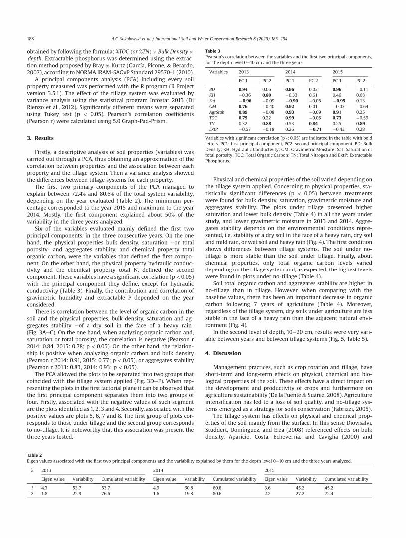
obtained by following the formula: %TOC ðor %TNÞ� Bulk Density�depth. Extractable phosphorus was determined using the extrac-tion method proposed by Bray & Kurtz (García, Picone, & Berardo,2007), according to NORMA IRAM-SAGyP Standard 29570-1 (2010).
A principal components analysis (PCA) including every soilproperty measured was performed with the R program (R Projectversion 3.5.1). The effect of the tillage system was evaluated byvariance analysis using the statistical program Infostat 2013 (DiRienzo et al., 2012). Significantly different means were separatedusing Tukey test (p < 0.05). Pearson’s correlation coefficients(Pearson r) were calculated using 5.0 Graph-Pad-Prism.
3. Results
Firstly, a descriptive analysis of soil properties (variables) wascarried out through a PCA, thus obtaining an approximation of thecorrelation between properties and the association between eachproperty and the tillage system. Then a variance analysis showedthe differences between tillage systems for each property.
The first two primary components of the PCA managed toexplain between 72.4% and 80.6% of the total system variability,depending on the year evaluated (Table 2). The minimum per-centage corresponded to the year 2015 and maximum to the year2014. Mostly, the first component explained about 50% of thevariability in the three years analyzed.
Six of the variables evaluated mainly defined the first twoprincipal components, in the three consecutive years. On the onehand, the physical properties bulk density, saturation eor totalporosity- and aggregates stability, and chemical property totalorganic carbon, were the variables that defined the first compo-nent. On the other hand, the physical property hydraulic conduc-tivity and the chemical property total N, defined the secondcomponent. These variables have a significant correlation (p < 0.05)with the principal component they define, except for hydraulicconductivity (Table 3). Finally, the contribution and correlation ofgravimetric humidity and extractable P depended on the yearconsidered.
There is correlation between the level of organic carbon in thesoil and the physical properties, bulk density, saturation and ag-gregates stability eof a dry soil in the face of a heavy rain-(Fig. 3AeC). On the one hand, when analyzing organic carbon and,saturation or total porosity, the correlation is negative (Pearson r2014: 0.84, 2015: 0.78; p < 0.05). On the other hand, the relation-ship is positive when analyzing organic carbon and bulk density(Pearson r 2014: 0.91, 2015: 0.77; p < 0.05), or aggregates stability(Pearson r 2013: 0.83, 2014: 0.93; p < 0.05).
The PCA allowed the plots to be separated into two groups thatcoincided with the tillage system applied (Fig. 3DeF). When rep-resenting the plots in the first factorial plane it can be observed thatthe first principal component separates them into two groups offour. Firstly, associated with the negative values of such segmentare the plots identified as 1, 2, 3 and 4. Secondly, associatedwith thepositive values are plots 5, 6, 7 and 8. The first group of plots cor-responds to those under tillage and the second group correspondsto no-tillage. It is noteworthy that this association was present thethree years tested.
Physical and chemical properties of the soil varied depending onthe tillage system applied. Concerning to physical properties, sta-tistically significant differences (p < 0.05) between treatmentswere found for bulk density, saturation, gravimetric moisture andaggregates stability. The plots under tillage presented highersaturation and lower bulk density (Table 4) in all the years understudy, and lower gravimetric moisture in 2013 and 2014. Aggre-gates stability depends on the environmental conditions repre-sented, i.e. stability of a dry soil in the face of a heavy rain, dry soiland mild rain, or wet soil and heavy rain (Fig. 4). The first conditionshows differences between tillage systems. The soil under no-tillage is more stable than the soil under tillage. Finally, aboutchemical properties, only total organic carbon levels varieddepending on the tillage system and, as expected, the highest levelswere found in plots under no-tillage (Table 4).
Soil total organic carbon and aggregates stability are higher inno-tillage than in tillage. However, when comparing with thebaseline values, there has been an important decrease in organiccarbon following 7 years of agriculture (Table 4). Moreover,regardless of the tillage system, dry soils under agriculture are lessstable in the face of a heavy rain than the adjacent natural envi-ronment (Fig. 4).
In the second level of depth, 10e20 cm, results were very vari-able between years and between tillage systems (Fig. 5, Table 5).
4. Discussion
Management practices, such as crop rotation and tillage, haveshort-term and long-term effects on physical, chemical and bio-logical properties of the soil. These effects have a direct impact onthe development and productivity of crops and furthermore onagriculture sustainability (De la Fuente& Su�arez, 2008). Agricultureintensification has led to a loss of soil quality, and no-tillage sys-tems emerged as a strategy for soils conservation (Fabrizzi, 2005).
The tillage system has effects on physical and chemical prop-erties of the soil mainly from the surface. In this sense Diovisalvi,Studdert, Domínguez, and Eiza (2008) referenced effects on bulkdensity, Aparicio, Costa, Echeverría, and Caviglia (2000) and
Table 2Eigen values associated with the first two principal components and the variability explained by them for the depth level 0e10 cm and the three years analyzed.
l 2013 2014 2015
Eigen value Variability Cumulated variability Eigen value Variability Cumulated variability Eigen value Variability Cumulated variability
1 4.3 53.7 53.7 4.9 60.8 60.8 3.6 45.2 45.22 1.8 22.9 76.6 1.6 19.8 80.6 2.2 27.2 72.4
Table 3Pearson’s correlation between the variables and the first two principal components,for the depth level 0e10 cm and the three years.
Variables 2013 2014 2015
PC 1 PC 2 PC 1 PC 2 PC 1 PC 2
BD 0.94 0.06 0.96 0.03 0.96 �0.11KH �0.36 0.89 �0.33 0.61 0.46 0.68Sat ¡0.96 �0.09 ¡0.90 �0.05 ¡0.95 0.13GM 0.76 �0.40 0.92 0.01 �0.03 �0.64AgrStab 0.89 �0.08 0.93 �0.09 0.91 0.25TOC 0.75 0.22 0.99 �0.05 0.73 �0.59TN 0.32 0.88 0.53 0.84 0.25 0.89ExtP �0.57 �0.18 0.26 ¡0.71 �0.43 0.28
Variables with significant correlation (p < 0.05) are indicated in the table with boldletters. PC1: first principal component, PC2; second principal component. BD: BulkDensity; KH: Hydraulic Conductivity; GM: Gravimetric Moisture; Sat: Saturation ortotal porosity; TOC: Total Organic Carbon; TN: Total Nitrogen and ExtP: ExtractablePhosphorus.
A.C. Sokolowski et al. / International Soil and Water Conservation Research 8 (2020) 185e194188
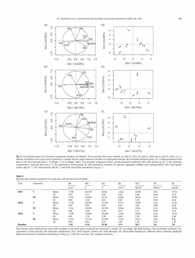
Fig. 3. First factorial plane of a Principal Components Analysis, for depth 0e10 cm and the three years studied. (a) and (d): 2013, (b) and (e): 2014 and (c) and (f): 2015. (a)e(c)Unitary correlation circle; each vector represents a variable and the angles between variables or components indicate the correlation between them. (d)e(f) Representation of theplots in the first factorial plane, 1e4 ‘tillage’, 5e8 ‘no-tillage’. Dim1: first principal component, Dim2: second principal component, BD: bulk density (g cm�3); Kh: hydraulicconductivity at saturated flow (cm h�1); Sat: saturation or total porosity (%); GM: gravimetric moisture (%); AgrStab: aggregates stability (Fast wetting, MWD); TOC: total organiccarbon (Mg ha�1); TN: total nitrogen (Mg ha�1) and ExtP: extractable phosphorus (mg kg�1).
Table 4Physical and chemical properties for each year and the first level of depth.
Year Treatment BD MG Sat Kh TOC TN EP
g cm�3 % % cm h�1 Mg ha�1 Mg ha�1 mg kg�1
2013 T Mean 1.19b 24.27b 54.9a 1.22a 22.8b 2.6a 14.7aSD 0.01 0.71 0.65 0.54 2.90 0.44 2.10
NT Mean 1.25a 26.98a 52.7b 0.88a 26.0a 2.7a 10.8aSD 0,02 1,40 0,51 0,47 3,14 0,18 3,64
2014 T Mean 1.11b 29.33b 57.25a 0.71a 18.8b 2.2a 11.0aSD 0.03 0.45 0.62 0.37 1.02 0.06 2.58
NT Mean 1.21a 32.47a 54.13b 0.50a 23.5a 2.7a 12.0aSD 0.06 1.26 2.19 0.37 1.31 0.59 3.74
2015 T Mean 1.20b 16.68a 54.68a 3.34a 20.4b 2.6a 10.3aSD 0.01 1.18 0.30 0.94 1.56 0.49 1.46
NT Mean 1.25a 16.74a 53.03b 3.37a 24.1a 2.6a 8.9aSD 0.02 0.83 0.71 1.07 1.19 0.27 1.78
Baseline 1.24 31.6 53.30 3.11 36.7 3.0 7.8
The average values obtained for each of the variables in the three years evaluated are indicated. T: tillage; NT: no-tillage; BD: Bulk Density; GM: gravimetric moisture; Sat:saturation or total porosity; Kh: hydraulic conductivity, TOC: Total Organic Carbon; TN: Total Nitrogen; EP: Extractable Phosphorus. Different letters indicate significantdifferences between treatments according to Tukey (p < 0.05) for each year. SD: standard deviation.
A.C. Sokolowski et al. / International Soil and Water Conservation Research 8 (2020) 185e194 189
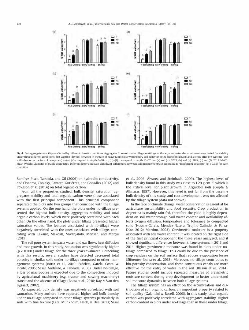
Ramírez-Pisco, Taboada, and Gil (2006) on hydraulic conductivity,and Cisneros, Cholaky, Cantero-Guti�errez, and Gonz�alez (2012) andPowlson et al. (2014) on total organic carbon.
From all the properties studied, bulk density, saturation, ag-gregates stability and total organic carbon were those associatedwith the first principal component. This principal componentseparated the plots into two groups that coincided with the tillagesystems applied. On the one hand, the plots under no-tillage pre-sented the highest bulk density, aggregates stability and totalorganic carbon levels, which were positively correlated with eachother. On the other hand, the plots under tillage presented highersaturation values. The features associated with no-tillage werenegatively correlated with the ones associated with tillage, coin-ciding with Kakaire, Makokh, Mwanjalolo, Mensah, and Menya(2015).
The soil pore system impacts water and gas flows, heat diffusionand root growth. In this study, saturation was significantly higher(p < 0.001) under tillage, for the three years evaluated. Coincidingwith this results, several studies have detected decreased totalporosity in similar soils under no-tillage compared to other man-agement systems (Botta et al., 2010; Fabrizzi, García, Costa, &Picote, 2005; Sasal, Andriulo, & Taboada, 2006). Under no-tillage,a loss of macropores is expected due to the compaction inducedby agricultural machinery (e.g. tractor and sowing machinery)transit and the absence of tillage (Botta et al., 2010; Kay & Van denBygaart, 2002).
As expected, bulk density was negatively correlated with soilsaturation. Many authors have reported higher soil bulk densityunder no-tillage compared to other tillage systems particularly insoils with fine texture (Lars, Munkholm, Heck, & Dee, 2013; Sasal
et al., 2006; �Alvarez and Steinbach, 2009). The highest level ofbulk density found in this study was close to 1.29 g cm�3, which isthe critical level for plant growth in Argiudoll soils (Gupta &Allmaras, 1987). However, this level is not far from the baselinebulk density of this study, and root development was not affectedby the tillage system (data not shown).
In the face of climate change, water conservation is essential foragriculture sustainability and food security. Crop production inArgentina is mainly rain-fed, therefore the yield is highly depen-dent on soil water storage. Soil water content and availability af-fects oxygen diffusion, temperature and tolerance to compactedsoils (Hossne-García, M�endez-Natera, Trujillo-Galindo, & Parra-Díaz, 2012; Martino, 2003). Gravimetric moisture is a propertyassociated with soil water content. It was located on the right sideof the first principal component the three years analyzed, and itshowed significant differences between tillage systems in 2013 and2014. Higher gravimetric moisture was found in plots under no-tillage compared to tillage. This could be due to the presence ofcrop residues on the soil surface that reduces evaporation losses(Sifuentes-Ibarra et al., 2018). Moreover, no-tillage contributes tobio-porosity conservation, and these continuous canals are moreeffective for the entry of water in the soil (Blas�on et al., 2014).Future studies could include repeated measures of gravimetricmoisture content during crop development to better understandsoil moisture dynamics between both tillage systems.
The tillage system has an effect on the accumulation and dis-tribution of soil organic carbon, an important property related tosoil quality (Galantini & Rosell, 2006). In this study, total organiccarbon was positively correlated with aggregates stability. Highercarbon content in plots under no-tillage than in those under tillage,
Fig. 4. Soil aggregates stability as affected by different climatic conditions. Aggregates from soil under tillage, no-tillage or the adjacent natural environment were tested for stabilityunder three different conditions: fast wetting (dry soil behavior in the face of heavy rain); slow wetting (dry soil behavior in the face of mild rain) and stirring after pre-wetting (wetsoil behavior in the face of heavy rain). (a)e(c) Correspond to depth 0e10 cm; (d)e(f) correspond to depth 10e20 cm. (a) and (d): 2013; (b) and (e): 2014; (c) and (f): 2015. MWD:Mean Weight Diameter of stable aggregates. Different letters indicate significant differences between soil management/use according to “Bonferroni posttests” (p < 0.05) for eachcondition.
A.C. Sokolowski et al. / International Soil and Water Conservation Research 8 (2020) 185e194190
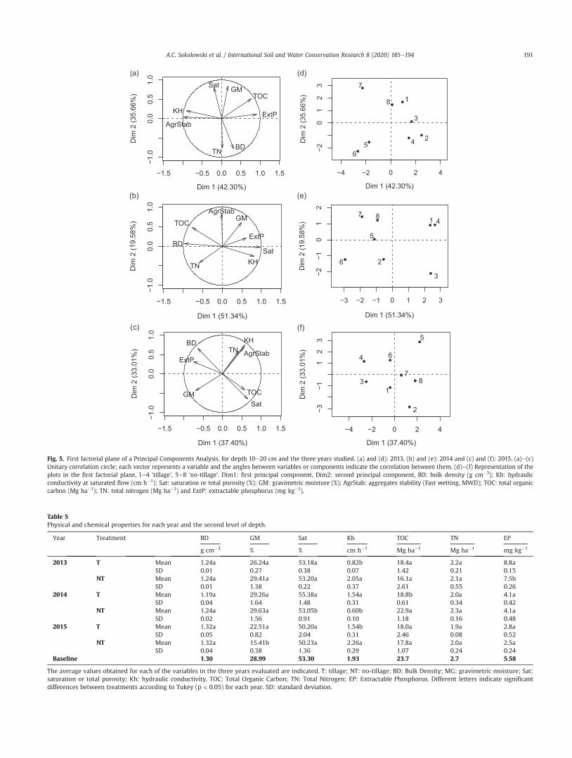
Fig. 5. First factorial plane of a Principal Components Analysis, for depth 10e20 cm and the three years studied. (a) and (d): 2013, (b) and (e): 2014 and (c) and (f): 2015. (a)e(c)Unitary correlation circle; each vector represents a variable and the angles between variables or components indicate the correlation between them. (d)e(f) Representation of theplots in the first factorial plane, 1e4 ‘tillage’, 5e8 ‘no-tillage’. Dim1: first principal component, Dim2: second principal component, BD: bulk density (g cm�3); Kh: hydraulicconductivity at saturated flow (cm h�1); Sat: saturation or total porosity (%); GM: gravimetric moisture (%); AgrStab: aggregates stability (Fast wetting, MWD); TOC: total organiccarbon (Mg ha�1); TN: total nitrogen (Mg ha�1) and ExtP: extractable phosphorus (mg kg�1).
Table 5Physical and chemical properties for each year and the second level of depth.
Year Treatment BD GM Sat Kh TOC TN EP
g cm�3 % % cm h�1 Mg ha�1 Mg ha�1 mg kg�1
2013 T Mean 1.24a 26.24a 53.18a 0.82b 18.4a 2.2a 8.8aSD 0.01 0.27 0.38 0.07 1.42 0.21 0.15
NT Mean 1.24a 29.41a 53.20a 2.05a 16.1a 2.1a 7.5bSD 0.01 1.38 0.22 0.37 2.61 0.55 0.26
2014 T Mean 1.19a 29.26a 55.38a 1.54a 18.8b 2.0a 4.1aSD 0.04 1.64 1.48 0.31 0.61 0.34 0.42
NT Mean 1.24a 29.63a 53.05b 0.60b 22.9a 2.3a 4.1aSD 0.02 1.56 0.91 0.10 1.18 0.16 0.48
2015 T Mean 1.32a 22.51a 50.20a 1.54b 18.0a 1.9a 2.8aSD 0.05 0.82 2.04 0.31 2.46 0.08 0.52
NT Mean 1.32a 15.41b 50.23a 2.26a 17.8a 2.0a 2.5aSD 0.04 0.38 1.36 0.29 1.07 0.24 0.24
Baseline 1.30 28.99 53.30 1.93 23.7 2.7 5.58
The average values obtained for each of the variables in the three years evaluated are indicated. T: tillage; NT: no-tillage; BD: Bulk Density; MG: gravimetric moisture; Sat:saturation or total porosity; Kh: hydraulic conductivity, TOC: Total Organic Carbon; TN: Total Nitrogen; EP: Extractable Phosphorus. Different letters indicate significantdifferences between treatments according to Tukey (p < 0.05) for each year. SD: standard deviation.
A.C. Sokolowski et al. / International Soil and Water Conservation Research 8 (2020) 185e194 191

as found in this study, were also reported by many authors (B�aez &Aguirre-Medina, 2011; Espinoza, 2010). On the one hand, undertillage, crop residues are incorporated into the soil, making themavailable to organisms, reducing soil coverage and favoring tem-perature increase (Triplett & Dick, 2008). Moreover, soil aggregatesdisruption caused by tillage exposes soil organic carbon, favoringits loss by mineralization (Espinoza, 2010). All this organic carbonlost from the soil becomes in turn part of the greenhouse gases(Reicosky, 2003). On the other hand, the presence of soil coveragein soils under no-tillage reduces carbon losses due to soil erosion(Castilla, 2013; Martens, 2000).
Powlson et al. (2014) argued that no-tillage is beneficial for soilquality and adaptation of agriculture to climate change, but its rolein mitigation is widely overstated. In this study, regardless of thetillage system, soil organic carbon and aggregates stability arenegatively affected by 7 years of agriculture. Therefore, these re-sults suggest that no-tillage alleviates, but is not enough to miti-gate, the loss of soil organic carbon and aggregates stability causedby continuous cropping, in this Vertic Argiaquall. In future studies itwould be of great importance to analyze soil biodiversity and bio-logical activity to better understand soil dynamics and designmanagement practices for soil carbon sequestration and foodsecurity.
The response of extractable P to the tillage system was veryvariable over the years. This nutrient is highly dependent on soilmanagement conditions (Acevedo, �Alvarez-S�anchez, Hern�andez-Acosta, & Maldonado-Torres, 2008; Ruffo, Bollero, Hoeft, &Bullock, 2005). There are studies reporting higher P availability insoils under: (1) no-tillage, due to crop residues deposition on thesurface (Ramírez-Barrientos, Figueroa-Sandoval, Ordaz-Chaparro,& Volke-Haller, 2006), and (2) tillage, due to occluded P minerali-zation (Galantini, Su~ner, & Iglesias, 2007). However, coincidingwith this study, available P was not affected by the tillage system insoils from ‘Pampa Ondulada’ Argentina with low available P(<20 mg kg�1) (Guti�errez-Boem et al., 2008). In our geographicarea, available Pwas lower than the critical level for corn andwheat(Díaz-Zorita, Grove, Murdock, Herbeck, & Perfect, 2004). Cropresidues could have low P content and this could be preventingdifferential P accumulation between tillage systems.
The hydraulic conductivity seems not to be associated with thetillage systems studied. Infiltration rate and hydraulic conductivityare soil properties directly related to its structural stability, to bulkdensity and to the diameter, continuity and connectivity of soilpores (Tisdall & Adem, 1986). In this study, hydraulic conductivitycorrelated with aggregates stability only the last year analyzed(Pearson r 0.64; p < 0.04). However, while aggregates stability wassignificantly different depending on the tillage system, the hy-draulic conductivity was not, possibly due to its high variability. Inline with these results, Roll�an and Bachmeier (2015) concluded thatthe configuration of soil pores and their hydraulic properties do notstabilize even after a long period under no-tillage.
Total N was located every year on the right side of the firstprincipal component, where no-tillage plots were located. How-ever, the variance analysis showed no significant differences be-tween the tillage systems. Many studies conclude that soil Ncontent is affected by tillage (e.g. Diovisalvi et al., 2008). However,the magnitude of the effect depends on soil texture, climate, tillageaggressiveness and crop rotations (Chagas, Marelli, &Santanatoglia, 1994). Some authors reported increased N contentin soil surface horizon, due to the accumulation of plant residues(Abril, Salas, Lovera, Kopp, & Casado-Murillo, 2005; Bowman &Halvorson, 1998; Heenan, Chan, & Knight, 2004). Under no-tillage, as organic matter decomposition is slower, N mineraliza-tion rate decreases (Echeverría & Sainz-Rozas, 2001). Locally,�Alvarez and Steinbach (2009) added that when soil N content is
low, there are no differences between tillage systems. However,according to V�azquez and Terminiello (2008), the soil of this studyis a well-equipped soil (TN between 0.2 and 0.3%).
In the second depth level (10e20 cm), no significant differenceswere found in soil properties in response to the tillage system,possibly due to the high variability of the results. For bulk density,the absence of effect of the tillage system at this depth was alsoreported for a long-term trial with agricultural rotations performedat the Barrow Integrated Agricultural Experiment Station,Argentina (Manso, Studdert, Forj�an, & San Martino, 2012). How-ever, in this study, bulk density increased with depth in both tillagesystems. This effect could be attributed to the presence of cropresidues in the surface which benefits organic matter formationmainly in the surface (Pisco et al., 2006).
There are different results reported regarding the effect of thetillage system on organic carbon in depth. On the one hand, someauthors have reported a superficial increase without differences indepth (Cisneros et al., 2012; Diovisalvi et al., 2008; Domínguez,Diovisalvi, Studdert, & Monterubbianesi, 2009; García, Studdert,Domingo, & Domínguez, 2016; Guti�errez-Boem et al., 2008),similar towhat was observed in this study. On the other hand, otherauthors affirmed that in no-tillage the most significant changesoccur in deeper layers (Varvel & Wilhem, 2011).
Regardless of the tillage system, extractable P and total Ndecreased with soil depth. This effect was previously reported inno-tillage by different authors (e.g. Su~ner, Galantini, Varela, &Rosell, 2007). Crops absorb available nutrients from deeper layersof the soil. Under no-tillage, crop residues remain in soil surface.Therefore, a stratification of nutrients, organic matter andmicrobialactivity occurs (Crist�obal-Acevedo, �Alvarez-S�anchez, Hern�andez-Acosta, & Am�endola-Massiotti, 2011; Powlson et al., 2014).
Finally, the sequence of crop rotation in long-term experimenthas to be taken into account, because it modifies the quantity,timing and quality of the materials that enter the soil (Lorenz & Lal,2005). In this sense, organic matter mineralization depends on thequantity and type of residues both in their physical form (size,density and diameter) and in their chemical composition (C/N ratio,lignin content, etc.) and the climatic conditions of the area of study(Valenzuela & Visconti, 2018).
5. Conclusion
Tillage systems such as tillage or no-tillage differentially affectthe physical and chemical properties of a Vertic Argiaquoll soillocated in Ezeiza, Buenos Aires, Argentina. The changes occurmainly in the first centimeters of the soil (0e10 cm), because atgreater depth (10e20 cm) the variability between the years ishigher.
There are soil quality properties that explain better than othersthe impact produced by the tillage system. Bulk density, saturation,aggregates stability and total organic carbon content are theproperties that could be taken into account to explain the vari-ability in soil quality due to the tillage system. It would not beconvenient to take into account hydraulic conductivity as it is notalways associated with the same treatment given its variabilitybetween years and crops.
In the soil surface, no-tillage has higher bulk density, gravi-metric moisture content and aggregates stability, but reducedsaturation (or total porosity), compared with tillage. Also, bulkdensity regardless of the tillage system increases with depth.
The chemical parameter most affected by the tillage system istotal organic carbon content, which is higher under no-tillagemainly in the first level of depth. However, there has been animportant decrease in organic carbon following 7 years of agri-culture. Therefore, these results suggest that no-tillage is not
A.C. Sokolowski et al. / International Soil and Water Conservation Research 8 (2020) 185e194192
enough to mitigate the loss of soil organic carbon caused bycontinuous cropping.
Depending on, climatic and edaphic conditions, and the previ-ous crop at the time of sampling, total nitrogen and extractablephosphorus change. Therefore, their responses are very variablebetween years and depths. The levels of extractable phosphorus,regardless of the tillage system and the year, were always higher atthe first depth compared to the second one.
The edaphic properties more sensitive to changes in soil func-tions could be used as quality indicators, and could be used todetermine the state of degradation or conversion of a soil under aspecific management practice. Finally, future studies on the exis-tence of correlations between the soil properties studied and cropyield and quality could determine the agronomic importance ofeach of them in the area under study.
Funding sources
This work was supported by the Cooperation INTA-AUDEAS-CONADEV [CIAC: 940110] and LomasCyT [Res. Nº 043/2013]. Thefunding sources had no involvement in the collection, analysis orinterpretation of data; in the writing of the report; nor in the de-cision to submit the article for publication.
Declaration of competing interest
None.
Acknowledgements
We are grateful to the “Comisi�on Nacional de Energía At�omica,Gobierno de Argentina” for providing the field for this study andhelping with field work.
References
Abril, A., Salas, P., Lovera, E., Kopp, S., & Casado-Murillo, N. (2005). Efecto acumu-lativo de la siembra directa sobre algunas características del suelo en la regi�onsemi�arida central de Argentina. Ciencia del Suelo, 23(2), 179e188.
Acevedo, D. C., �Alvarez-S�anchez, M. E., Hern�andez-Acosta, E., & Maldonado-Torres, R. (2008). Variabilidad espacial de propiedades químicas del suelo y suuso en el dise~no de experimentos. Terra Latinoamericana, 26(4), 324.
�Alvarez, R., & Steinbach, H. S. (2009). A review of the effects of tillage systems onsome soil physical properties, water content, nitrate availability and crops yieldin the Argentine Pampas. Soil Research, 104, 1e15.
Aparicio, V., & Costa, J. L. (2007). Soil quality indicators under continuous croppingsystems in the Argentinean Pampas. Soil Research, 96, 155e165.
Aparicio, V., Costa, J. L., Echeverría, H., & Caviglia, O. (2000). Evaluaci�on de pro-piedades ed�aficas y crecimiento del maíz bajo diferentes sistemas de labranzaen cuatro sitios del sudoeste bonaerense. RIA, 31(3), 55e71. ISSN 0325-8718.
Austin, A., Pi~neiro, G., & Gonz�alez-Polo, M. (2006). More is less: Agricultural impactson the N cycle in Argentina. Biogeochemistry, 79, 45e60.
B�aez, M. A., & Aguirre-Medina, J. F. (2011). Efecto de la labranza de conservaci�onsobre las propiedades del suelo. Sociedad Mexicana de la Ciencia del Suelo, A.C.Chapingo, M�exico. Terra Latinoamericana, 29(2), 113e121.
Blake, G. R., & Hartge, K. H. (1986). Bulk density in: Klute: Methods of soil analysis (2�
ed., Vol. 9, pp. 363e375). Madison: American Society of Agronomy (ASA).Blas�on, A. D., Fern�andez, N. R., Barrios, M. B., Makar, D., Molla-Kralj, A., &
Rodríguez, R. O. (2014). Gradientes t�ermicos del suelo superficial cultivado conmaíz en labranza convencional y en siembra directa. Revista de la Facultad deAgronomía y Ciencias Agroalimentarias, 9y10, 29e46.
Botta, G. F., Tolon-Becerra, A., Lastra-Bravo, X., & Tourn, M. (2010). Tillage and trafficeffects (planters and tractors) on soil compaction and soybean (Glycine max L.)yields in Argentinean pampas. Soil and Tillage Research, 110, 167e174.
Bowman, R. A., & Halvorson, A. D. (1998). Soil chemical changes after nine years ofdifferential N fertilization in a no-till dryland wheat-corn-fallow rotation. SoilScience, 163, 241e247.
Camacho-Tamayo, J. H., Luengas, C. A., & Leiva, F. R. (2010). Evaluaci�on de propie-dades físicas de dosoxisoles en la altillanura colombiana mediantean�alisis multi-variado Suelos Ecuatoriales, 40(2), 170e175.
Castilla, F. (2013). Siembra directa. La elegida para conservar el suelo. RIA, 39(2),118e123.
Chagas, C. I., Marelli, H. J., & Santanatoglia, O. J. (1994). Propiedades físicas y con-tenido hídrico de un Argiudol típico bajo tres sistemas de labranza. Ciencia del
Suelo, 12(1), 11e16.Cisneros, J. M., Cholaky, C. G., Cantero-Guti�errez, A., & Gonz�alez, J. (2012). Erosi�on
hídrica UniRio editora. C�ordoba, Argentina: Universidad Nacional de Río Cuarto.Crist�obal-Acevedo, D., �Alvarez-S�anchez, M. E., Hern�andez-Acosta, E., & Am�endola-
Massiotti, R. (2011). Concentraci�on de nitr�ogeno en suelo por efecto de manejoorg�anico y convencional. Terra. Latinoamericana, 29(3), 325e332.
De la Fuente, E., & Su�arez, S. (2008). Problemas ambientales asociados a la actividadhumana: La agricultura. Ecología Austral, 18(3), 239e252. ISSN 1667-782X.
Derpsch, R., Friedrich, T., Kassam, A., & Li, H. W. (2010). Current status of adoption ofno-till farming in the world and some of it main benefits. International Journalof Agricultural and Biological Engineering, 3(1).
Di Rienzo, J. A., Casanoves, F., Balzarini, M. G., Gonz�alez, L., Tablada, M., &Robledo, C. W. (2012). InfoStat. Grupo InfoStat. Argentina: FCA, UniversidadNacional de C�ordoba. http://www.infostat.com.ar.
Díaz-Zorita, M., Grove, J. H., Murdock, L., Herbeck, J., & Perfect, E. (2004). Soilstructural disturbance effects on crop yields and soil properties in a no-tillproduction system. Agronomy Journal, 96, 1651e1659.
Diovisalvi, N. V., Studdert, G. A., Domínguez, G. F., & Eiza, M. E. (2008). Fracciones decarbono y nitr�ogeno org�anicos y nitr�ogeno anaer�obico bajo agricultura continuacon dos sistemas de labranza. Ciencia del Suelo, 26(1), 1-1.
Domínguez, G. F., Diovisalvi, N. V., Studdert, G. A., & Monterubbianesi, M. G. (2009).Soil organic C and N fractions under continuous cropping with contrastingtillage systems on mollisols of the southeastern pampas. Soil and TillageResearch, 102, 93e100.
Duval, M., Galantini, J., Iglesias, J., & Krüger, H. (2013). El cultivo de trigo en la regi�onsemi�arida bonaerense: Impacto sobre algunas propiedades químicas del suelo.RIA, 39(2), 178e184.
Echeverría, H. E., & Sainz-Rozas, H. R. (2001). Eficiencia de recuperaci�on delnitr�ogeno aplicado al estadio de seis hojas del maíz bajo riego en siembradirecta y labranza convencional. Ciencia del Suelo, 19, 57e66.
Espinoza, Y. (2010). Efecto de la labranza sobre la materia org�anica y tama~no deagregados en un suelo cultivado con maíz en condiciones tropicales. Bioagro,22(3), 177e184.
Fabrizzi, K. P., García, F. O., Costa, J. L., & Picote, L. I. (2005). Soil water dynamics,physical properties and corn and wheat responses to minimum and no-tillagesystems in the southern Pampas of Argentina. Soil Research, 81, 57e69.
Galantini, J., & Rosell, R. (2006). Long-term fertilization effects on soil organicmatter quality and dynamics under different production systems in semiaridPampean soils. Soil Research, 87, 72e79.
Galantini, J. A., Su~ner, L., & Iglesias, J. O. (2007). Sistemas de labranza en el sudoestebonaerense: Efectos de largo plazo sobre las formas de f�osforo en el suelo.Revista Investigaciones Agropecuarias (RIA e INTA), 36(1), 63e81.
García, F. O., Picone, L. I., & Berardo, A. (2007). F�osforo. In H. E. En Echeverría, &F. O. García (Eds.), Fertilidad de Suelos y fertilizaci�on de Cultivos (pp. 99e121).Ediciones INTA, Bs As.
García, G. V., Studdert, G. A., Domingo, M. N., & Domínguez, G. F. (2016). Nitr�ogenomineralizado en anaerobiosis: Relaci�on con sistemas de cultivos de agriculturacontinua. Cs Suelo, 34, 127e138.
Gardner, W. H. (1986). Water content: Methods of soil analysis. American Society ofAgronomy Madison.
Golik, S. I. (2009). Efecto de los sistemas de labranza, fertilizaci�on nitrogenada ygenotipo sobre el sistema radical en etapas avanzadas del cultivo de trigo y suincidencia en el rendimiento, calidad y sanidad. UNLP-FCAyF tesis doctoral. http://sedici.unlp.edu.ar/bitstream/handle/10915/1821/Documento_completo.pdf?sequence¼1&isAllowed¼y_Last_view_el_29/12/18.
Govaerts, B., Sayre, K. D., & Deckers, J. (2006). A minimum data set for soil qualityassessment of wheat and maize cropping in the highlands of Mexico. Soil andTillage Research, 87, 163e174.
Gupta, S. C., & Allmaras, R. R. (1987). Models to assess the susceptibility of soils toexcessive compaction. Advances in Soil Sciences, 6, 65e100.
Guti�errez-Boem, F. H., �Alvarez, C. R., Cabello, M. J., Fern�andez, P. L., Bono, A.,Prystupa, P., et al. (2008). Phosphorus retention on soil surface of tilled and no-tilled soils. Soil Science Society of America Journal, 72, 1158e1162.
Heenan, D. P., Chan, K. Y., & Knight, P. G. (2004). Long-term impact of rotation,tillage and stubble management on the loss of soil organic carbon and nitrogenfrom a Chromic Luvisol. Soil Research, 76, 59e68.
Hossne-García, A. J., M�endez-Natera, J. R., Trujillo-Galindo, M. E.del V., & Parra-Díaz, F. J. (2012). Interacci�on de la frecuencia de riego, relaci�on de solidez ytensi�on cortante en la profundidad de enraizamiento de la soya (Glycinemax (L.)Merril.). Revista Científica UDO Agrícola, 12(1), 97e105.
Jackson, M. L. (1976). An�alisis químicos de suelo. Ediciones OMEGA, S.A. Casanova220 Barcelona Tercera Edici�on.
Jaramillo-Jaramillo, D. F., Gonz�alez-S�anchez, H., & �Alvarez-Mejía, F. (2008). Varia-bilidad espacial de algunas propiedades físico - mec�anicas de suelos de texturapesada. CES Medicina Veterinaria y Zootecnia, 3, 10e19.
Julca-Otiniano, A., Meneses-Florian, L., Blas-Sevillano, R., & Bello-Amez, S. (2006). Lamateria org�anica, importancia y experiencia de su uso en la agricultura. Idesia,24(1), 49e61. https://doi.org/10.4067/S0718-34292006000100009.
Kakaire, J., Makokh, G. L., Mwanjalolo, M., Mensah, A. K., & Menya, E. (2015). Effectsof mulching on soil hydro-physical properties in kibaale sub-catchment, SouthCentral Uganda. Applied Ecology and Environmental Sciences, 3(5), 127e135.
Kay, B. D., & Van den Bygaart, A. J. (2002). Conservation tillage and depth stratifi-cation of porosity and soil organic matter. Soil and Tillage Research, 66, 107e118.
Kirschenmann, F. (2010). Alternative agriculture in an energy- and resourcedepleting future. Renewable Agriculture and Food Systems, 25, 85e89.
A.C. Sokolowski et al. / International Soil and Water Conservation Research 8 (2020) 185e194 193
Lars, J., Munkholm, R., Heck, J., & Dee, B. (2013). Long-term rotation and tillageef fects on soil structure and crop yield. Soil and Tillage Research, 127, 85e91.
Le Bissonnais, Y. (1996). Aggregate stability and assessment of soil crustability anderodability. I. Theory and metodology. European Journal of Soil Science, 47,425e437.
Lorenz, K., & Lal, R. (2005). The depth distribution of soil organic carbon in relationto land use and management and the potential of carbon sequestration insubsoil horizons. Advances in Agronomy, 88, 35e66.
Manso, M. L., Studdert, G. A., Forj�an, H. J., & San Martino, S. (2012). Efecto de sis-temas de labranza contrastantes sobre algunas propiedades de un molisol deTres Arroyos bajo distintos usos previos. Revista. FCA UNCUYO, 44, 85e99.Mendoza.
Martens, D. A. (2000). Nitrogen cycling under different soil management systems.Advances in Agronomy, 70, 143e191.
Martino, D. L. (2003). Manejo de restricciones físicas del suelo en sistemas de siembradirecta, Grupo de Riego, Agroclima. Montevideo: Ambiente y Agricultura Satelital(GRAS) del Instituto Nacional de Investigaci�on Agropecuaria de Uruguay.
Micucci, F., & Taboada, M. A. (2006). Soil physical properties and soybean (Glycinemax Merrill) root abundance in conventionally and zero-tilled soils in the hu-mid Pampas of Argentina. Soil and Tillage Research, 86, 152e162.
NocelliPac, S. (2017). Evoluci�on de Siembra Directa en Argentina Campa~na 2016-2017.Asociaci�on Argentina de Productores en Siembra Directa (Aapresid). Last viewhttps://www.aapresid.org.ar/wp-content/uploads/2018/03/Estimacio%CC%81n-de-superficien-en-SD.pdf. (Accessed 22 March 2019).
NORMA IRAM-SAGyP 29570-1. (2010). Norma Argentina. Calidad ambiental y calidadde suelo. Determinaciones de f�osforo extraíble de los suelos. 1� edici�on, 20 pp.
Pisco, R. R., Taboada, M. A., & Gil, R. (2006). Efectos a largo plazo de la labranzaconvencional y la siembra directa sobre las propiedades físicas de un argiudoltípico de la Pampa Ondulada Argentina. Revista FacNalAgr Medellín, 59(1),3237e3256.
Powlson, D. S., Stirling, C. M., Jat, M. L., Gerard, B. G., Palm, C. A., S�anchez, P. A., et al.(2014). Limited potential of no-till agriculture for climate change mitigation.NatureClimate Ch, 4, 678e683.
Ramírez-Barrientos, C., Figueroa-Sandoval, B., Ordaz-Chaparro, V. M., & Volke-Haller, V. H. (2006). Efecto del sistema de labranza cero en un vertisol. Terra-latinoamerica, 24(1), 108e118.
Ramírez-Pisco, R., Taboada, M. A., & Gil, R. (2006). Efectos a largo plazo de la lab-ranza convencional y la siembra directa sobre las propiedades físicas de unargiudol típico de la pampa ondulada Argentina. Revista Facultad Nacional deAgronomía Medellín, 59(1), 3237e3256.
Reicosky, D. C. (2003). Tillage-induced soil properties and chamber mixing effectson gas exchange. In Proceedings of international soil tillage research organiza-tions. Brisbane, Australia, 17 pp.
Roll�an, A. A., & Bachmeier, O. A. (2015). Efecto de la siembra directa continua sobreel comportamiento físico-funcional de los suelos franco limosos de la regi�onsemi�arida central de la provincia de C�ordoba (Argentina). Terra Latinoam, 33(4),275e284.
Ruffo, M. L., Bollero, G. A., Hoeft, R. G., & Bullock, D. G. (2005). Spatial variability ofthe Illinois soil nitrogen test: Implications for soil sampling. Agronomy Journal,97, 1485e1492.
SAMLA. (2004). Secretaría de Agricultura, ganadería, pesca y alimentaci�on de laNaci�on Argentina. Buenos Aires, Argentina: Direcci�on de Producci�on Agrícola.Sistema de Apoyo Metodol�ogico a los Laboratorios de An�alisis de Suelos Agua,Vegetales y Enmiendas Org�anicas, 120 pp.
Sasal, M. C., Andriulo, A. E., & Taboada, M. A. (2006). Soil porosity characteristics andwater movement under zero tillage in silty soils in Argentinian Pampas. Soil
Research, 87, 9e18.Saxton, K. E., Rawls, W. J., Romberger, J. S., & Papendick, R. I. (1986). Estimating
generalized soil water characteristics from texture. Transactions of the AmericanSociety of Agricultural Engineers, 50, 1031e1035.
Servicio Meteorol�ogico Nacional, s.f.. Estadísticas climatol�ogicas normales - from1981 to 2010 Ezeiza station. Last view https://www.smn.gob.ar/descarga-de-datos. (Accessed 25 January 2019).
Shukla, M. K., Lal, R., & Ebinger, M. (2006). Determining soil quality indicators byfactor analisis. Soil and Tillage Research, 87, 194e204.
Sifuentes-Ibarra, E., Macías-Cervantes, J., Mendoza-P�erez, C., V�asquez-Díaz, D. A.,Salinas-Verduzco, D. A., & Inzunza-Ibarra, M. A. (2018). Efecto de la siembradirecta en las propiedades del suelo y aprovechamiento de riego en maíz enSinaloa, M�exico. Revista Mexicana de Ciencias Agrícolas. Volumen especial, 20,4235e4243.
Soil Survey Staff. (2010). Claves para la taxonomía de suelos (11th ed.). Washington,DC, USA: USDA-Natural Resources Conservation Service, 374 pp.
Soracco, C. G., Lozano, L. A., Sarli, G. O., Gelati, P. R., & Filgueira, R. (2010). Anisotropyof Saturated Hydraulic Conductivity in a soil under conservation and no-tilltreatments. Soil and Tillage Research, 109, 18e22.
Souza, Z. M., Marques-Júnior, J., Pereira, G. T., & S�anchez-S�aenz, C. M. (2009). Spatialvariability of aggregate stability in Latosols under sugarcane. Revista Brasileirade Ciencia do Solo, 33, 245e253.
Strudley, M. W., Green, T. R., & Ascoug, J. C. (2008). Tillage effect on soil hydraulicproperties in space and time: State of the science. Soil Research, 99, 4e48.
Su~ner, L., Galantini, J., Varela, P., & Rosell, R. (2007). Estratificaci�on de las formas def�osforo en siembra directa y su relaci�on con la disponibilidad para los cultivos.Revista T�ecnica Especial en Siembra Directa AAPRESID, CIC, CERZOS y UNS, 28e31.
Tisdall, J. M., & Adem, H. H. (1986). Effect of water content of soil at tillage on size-distribution of aggregates and infiltration. Australian Journal of ExperimentalAgriculture, 26, 193e195.
Triplett, G. B., & Dick, W. A. (2008). No- tillage crop production: A revolution inagriculture. Agronomy Journal, 100(supplements). S- 153-S-165.
United Nations Department of Economic and Social Affairs, population Division.(2019). Word population prospects 2019. https://www.pewresearch.org/fact-tank/2019/06/17/worlds-population-is-projected-to-nearly-stop-growing-by-the-end-of-the-century/ft_19-06-17_worldpopulation_world-population-growth-projected-flatten/.
Valenzuela, I. G., & Visconti, E. F. (2018). Influencia del clima, uso del suelo y pro-fundidad sobre el contenido de carbono org�anico en dos pisos altitudinalesandinos del departamento Norte de Santander, Colombia. Revista Colombiana deCiencias Hortícolas, 12(1), 233e243.
Varvel, G. E., & Wilhem, W. W. (2011). No-tillage increases soil profile carbon andnitrogen Ander long-term rainfed cropping system. Soil and Tillage Research,114, 28e36.
V�azquez, M., & Terminiello, A. (2008). Recuperaci�on de suelos degradados depeque~nos productores del cintur�on hortícola del Gran La Plata. Valoraci�on delproblema y estrategias correctivas. FCAyF, UNLP. Last view https://www.agro.unlp.edu.ar/sites/default/files/paginas/2008._manual_cinturon_horticola_la_plata_directora_mabel_vazquez.pdf. (Accessed 22 January 2019).
Viglizzo, E. F., & Jobaggy, E. (Eds.). (2010). Expansi�on de la frontera agropecuariaArgentina y su impacto ecol�ogico-ambiemtal (p. 102). INTA. Last view https://www.agro.unlp.edu.ar/sites/default/files/paginas/2008._manual_cinturon_horticola_la_plata_directora_mabel_vazquez.pdf. (Accessed 22 January 2019).
Zubeldia, T., Agostini, M. A., Domínguez, G. F., Studdert, G. A., & Tourn, S. N. (2018).Evaluaci�on de algunas propiedades físicas de un suelo del sudeste bonaerense bajodistintos sistemas de cultivo. XXVI Congreso Argentino de la Ciencia del Suelo.
A.C. Sokolowski et al. / International Soil and Water Conservation Research 8 (2020) 185e194194
Original Research Article
The application of proximal visible and near-infrared spectroscopy toestimate soil organic matter on the Triffa Plain of Morocco
Ayoub Lazaar a, *, Abdul Mounem Mouazen b, Kamal EL Hammouti a, Michael Fullen c,Biswajeet Pradhan d, Muhammad Sohail Memon e, Karim Andich f, Abdelilah Monir g
a Laboratory of Applied Geosciences, Department of Geology, Faculty of Science, Mohammed First University, Oujda, Moroccob Division of Mechatronics, Biostatistics and Sensors (MeBioS), Faculty of Bioscience Engineering, Kasteelpark Arenberg 30, B-3001 Heverlee, Belgiumc Faculty of Science and Engineering, University of Wolverhampton, Wolverhampton, WV1 1LY, United Kingdomd Center for Advanced Modelling and Geospatial Information Systems (CAMGIS), Faculty of Engineering and Information Technology, University ofTechnology Sydney, Sydney, 2007, NSW, Australiae Faculty of Agricultural Engineering, Sindh Agriculture University, Tandojam, 70060, Pakistanf Laboratory of Applied Geomatics and Soil Science, National Institute of Agronomic Research (INRA), Oujda, Moroccog Department of Mathematics, EDP and Scientific Computing Team, Moulay Ismail University, M�eknes, Morocco
a r t i c l e i n f o
Article history:Received 14 October 2019Received in revised form13 April 2020Accepted 15 April 2020Available online 21 April 2020
Keywords:Soil organic matterVIS-NIR spectroscopyReflectance spectraSOM estimationSOM analysis
a b s t r a c t
Soil organic matter (SOM) is a fundamental soil constituent. The estimation of this parameter in thelaboratory using the classical method is complex time-consuming and requires the use of chemical re-agents. The objectives of this study were to assess the accuracy of two laboratory measurement setups ofthe VIS-NIR spectroscopy in estimating SOM content and determine the important spectral bands in theSOM estimation model. A total of 115 soil samples were collected from the non-root zone (0e20 cm) ofsoil in the study area of the Triffa Plain and then analysed for SOM in the laboratory by the WalkleyeBlack method. The reflectance spectra of soil samples were measured by two protocols, ContactProbe (CP) and Pistol Grip (PG)) of the ASD spectroradiometer (350e2500 nm) in the laboratory. Partialleast squares regression (PLSR) was used to develop the prediction models. The results of coefficient ofdetermination (R2) and the root mean square error (RMSE) showed that the pistol grip offers reasonableaccuracy with an R2 ¼ 0.93 and RMSE ¼ 0.13 compared to the contact probe protocol with an R2 ¼ 0.85and RMSE ¼ 0.19. The near-Infrared range were more accurate than those in the visible range for pre-dicting SOM using the both setups (CP and PG). The significant wavelengths contributing to the pre-diction of SOM for (PG) setup were at: 424, 597, 1432, 1484, 1830,1920, 2200, 2357 and 2430 nm, whilewere at 433, 587, 1380, 1431, 1929, 2200 and 2345 nm for (CP) setup.© 2020 International Research and Training Center on Erosion and Sedimentation and China Water andPower Press. Production and Hosting by Elsevier B.V. This is an open access article under the CC BY-NC-
ND license (http://creativecommons.org/licenses/by-nc-nd/4.0/).
1. Introduction
The soil is a vital and non-renewable natural resource withpotentially rapid degradation rates and extremely slow formationand regeneration processes. It is a complex, heterogeneous andself-organized system, extremely variable in chemical and physicalcomposition (Lavelle et al., 2007) both spatially and temporarily.The physicochemical properties of soils determine their potentialand limitations for agricultural use (Leone et al., 2012; Tümsavas,
Tekin, Ulusoy, & Mouazen, 2018), but these vary inter- and intra-fields. Whatever the scale is, it is essential to predict and mapvariability accurately in order to manage farm input resources.
Soil organic matter (SOM) is an important parameter for soilfunctions and is an indicator of soil fertility. It takes a major role informing and stabilizing soil aggregates for the long term sustain-ability (Memon et al., 2018; Six, Conant, Paul, & Paustian, 2002).Powlson, Brookes, Whitmore, Goulding, and Hopkins (2011) andHong et al. (2018) mentioned that SOM is the decisive factor of soilfertility, and its content is directly related to the soil fertilityproperties, such as nutrient holding capacity, soil microbial quan-tity and activity, soil water-holding capacity, nutrient use efficiencyand crop yield. St Luce et al. (2014) indicated that assessment and
* Corresponding author. Department of Geology, Mohammed First University,Oujda, Morocco.
E-mail address: [email protected] (A. Lazaar).
Contents lists available at ScienceDirect
International Soil and Water Conservation Research
journal homepage: www.elsevier .com/locate/ iswcr
https://doi.org/10.1016/j.iswcr.2020.04.0052095-6339/© 2020 International Research and Training Center on Erosion and Sedimentation and China Water and Power Press. Production and Hosting by Elsevier B.V. Thisis an open access article under the CC BY-NC-ND license (http://creativecommons.org/licenses/by-nc-nd/4.0/).
International Soil and Water Conservation Research 8 (2020) 195e204
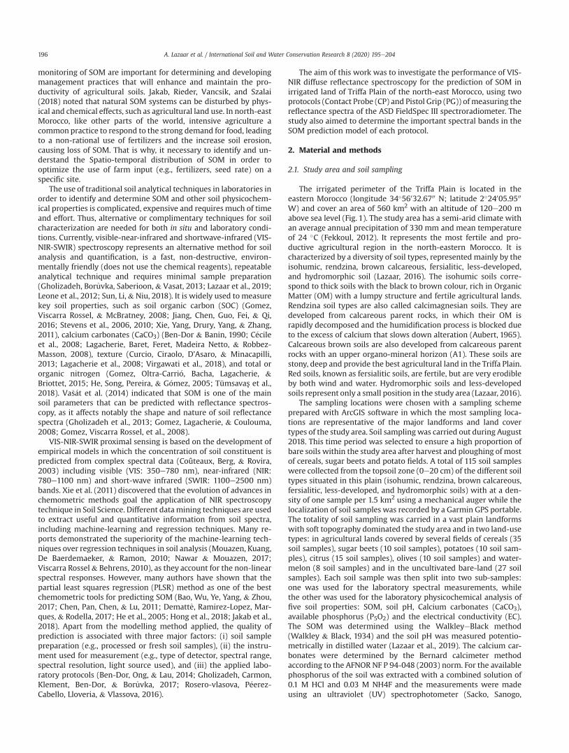
monitoring of SOM are important for determining and developingmanagement practices that will enhance and maintain the pro-ductivity of agricultural soils. Jakab, Rieder, Vancsik, and Szalai(2018) noted that natural SOM systems can be disturbed by phys-ical and chemical effects, such as agricultural land use. In north-eastMorocco, like other parts of the world, intensive agriculture acommonpractice to respond to the strong demand for food, leadingto a non-rational use of fertilizers and the increase soil erosion,causing loss of SOM. That is why, it necessary to identify and un-derstand the Spatio-temporal distribution of SOM in order tooptimize the use of farm input (e.g., fertilizers, seed rate) on aspecific site.
The use of traditional soil analytical techniques in laboratories inorder to identify and determine SOM and other soil physicochem-ical properties is complicated, expensive and requires much of timeand effort. Thus, alternative or complimentary techniques for soilcharacterization are needed for both in situ and laboratory condi-tions. Currently, visible-near-infrared and shortwave-infrared (VIS-NIR-SWIR) spectroscopy represents an alternative method for soilanalysis and quantification, is a fast, non-destructive, environ-mentally friendly (does not use the chemical reagents), repeatableanalytical technique and requires minimal sample preparation(Gholizadeh, Bor�uvka, Saberioon, & Vasat, 2013; Lazaar et al., 2019;Leone et al., 2012; Sun, Li,& Niu, 2018). It is widely used to measurekey soil properties, such as soil organic carbon (SOC) (Gomez,Viscarra Rossel, & McBratney, 2008; Jiang, Chen, Guo, Fei, & Qi,2016; Stevens et al., 2006, 2010; Xie, Yang, Drury, Yang, & Zhang,2011), calcium carbonates (CaCO3) (Ben-Dor & Banin, 1990; C�ecileet al., 2008; Lagacherie, Baret, Feret, Madeira Netto, & Robbez-Masson, 2008), texture (Curcio, Ciraolo, D’Asaro, & Minacapilli,2013; Lagacherie et al., 2008; Virgawati et al., 2018), and total ororganic nitrogen (Gomez, Oltra-Carri�o, Bacha, Lagacherie, &Briottet, 2015; He, Song, Pereira, & G�omez, 2005; Tümsavas et al.,2018). Va�s�at et al. (2014) indicated that SOM is one of the mainsoil parameters that can be predicted with reflectance spectros-copy, as it affects notably the shape and nature of soil reflectancespectra (Gholizadeh et al., 2013; Gomez, Lagacherie, & Coulouma,2008; Gomez, Viscarra Rossel, et al., 2008).
VIS-NIR-SWIR proximal sensing is based on the development ofempirical models in which the concentration of soil constituent ispredicted from complex spectral data (Coûteaux, Berg, & Rovira,2003) including visible (VIS: 350e780 nm), near-infrared (NIR:780e1100 nm) and short-wave infrared (SWIR: 1100e2500 nm)bands. Xie et al. (2011) discovered that the evolution of advances inchemometric methods goal the application of NIR spectroscopytechnique in Soil Science. Different datamining techniques are usedto extract useful and quantitative information from soil spectra,including machine-learning and regression techniques. Many re-ports demonstrated the superiority of the machine-learning tech-niques over regression techniques in soil analysis (Mouazen, Kuang,De Baerdemaeker, & Ramon, 2010; Nawar & Mouazen, 2017;Viscarra Rossel& Behrens, 2010), as they account for the non-linearspectral responses. However, many authors have shown that thepartial least squares regression (PLSR) method as one of the bestchemometric tools for predicting SOM (Bao, Wu, Ye, Yang, & Zhou,2017; Chen, Pan, Chen, & Lu, 2011; Dematte, Ramirez-Lopez, Mar-ques, & Rodella, 2017; He et al., 2005; Hong et al., 2018; Jakab et al.,2018). Apart from the modelling method applied, the quality ofprediction is associated with three major factors: (i) soil samplepreparation (e.g., processed or fresh soil samples), (ii) the instru-ment used for measurement (e.g., type of detector, spectral range,spectral resolution, light source used), and (iii) the applied labo-ratory protocols (Ben-Dor, Ong, & Lau, 2014; Gholizadeh, Carmon,Klement, Ben-Dor, & Bor�uvka, 2017; Rosero-vlasova, P�eerez-Cabello, Lloveria, & Vlassova, 2016).
The aim of this work was to investigate the performance of VIS-NIR diffuse reflectance spectroscopy for the prediction of SOM inirrigated land of Triffa Plain of the north-east Morocco, using twoprotocols (Contact Probe (CP) and Pistol Grip (PG)) of measuring thereflectance spectra of the ASD FieldSpec III spectroradiometer. Thestudy also aimed to determine the important spectral bands in theSOM prediction model of each protocol.
2. Material and methods
2.1. Study area and soil sampling
The irrigated perimeter of the Triffa Plain is located in theeastern Morocco (longitude 34�56032.6700 N; latitude 2�24005.9500
W) and cover an area of 560 km2 with an altitude of 120e200 mabove sea level (Fig. 1). The study area has a semi-arid climate withan average annual precipitation of 330 mm and mean temperatureof 24 �C (Fekkoul, 2012). It represents the most fertile and pro-ductive agricultural region in the north-eastern Morocco. It ischaracterized by a diversity of soil types, represented mainly by theisohumic, rendzina, brown calcareous, fersialitic, less-developed,and hydromorphic soil (Lazaar, 2016). The isohumic soils corre-spond to thick soils with the black to brown colour, rich in OrganicMatter (OM) with a lumpy structure and fertile agricultural lands.Rendzina soil types are also called calcimagnesian soils. They aredeveloped from calcareous parent rocks, in which their OM israpidly decomposed and the humidification process is blocked dueto the excess of calcium that slows down alteration (Aubert, 1965).Calcareous brown soils are also developed from calcareous parentrocks with an upper organo-mineral horizon (A1). These soils arestony, deep and provide the best agricultural land in the Triffa Plain.Red soils, known as fersialitic soils, are fertile, but are very erodibleby both wind and water. Hydromorphic soils and less-developedsoils represent only a small position in the study area (Lazaar, 2016).
The sampling locations were chosen with a sampling schemeprepared with ArcGIS software in which the most sampling loca-tions are representative of the major landforms and land covertypes of the study area. Soil samplingwas carried out during August2018. This time period was selected to ensure a high proportion ofbare soils within the study area after harvest and ploughing of mostof cereals, sugar beets and potato fields. A total of 115 soil sampleswere collected from the topsoil zone (0e20 cm) of the different soiltypes situated in this plain (isohumic, rendzina, brown calcareous,fersialitic, less-developed, and hydromorphic soils) with at a den-sity of one sample per 1.5 km2 using a mechanical auger while thelocalization of soil samples was recorded by a Garmin GPS portable.The totality of soil sampling was carried in a vast plain landformswith soft topography dominated the study area and in two land-usetypes: in agricultural lands covered by several fields of cereals (35soil samples), sugar beets (10 soil samples), potatoes (10 soil sam-ples), citrus (15 soil samples), olives (10 soil samples) and water-melon (8 soil samples) and in the uncultivated bare-land (27 soilsamples). Each soil sample was then split into two sub-samples:one was used for the laboratory spectral measurements, whilethe other was used for the laboratory physicochemical analysis offive soil properties: SOM, soil pH, Calcium carbonates (CaCO3),available phosphorus (P5O2) and the electrical conductivity (EC).The SOM was determined using the WalkleyeBlack method(Walkley & Black, 1934) and the soil pH was measured potentio-metrically in distilled water (Lazaar et al., 2019). The calcium car-bonates were determined by the Bernard calcimeter methodaccording to the AFNOR NF P 94-048 (2003) norm. For the availablephosphorus of the soil was extracted with a combined solution of0.1 M HCl and 0.03 M NH4F and the measurements were madeusing an ultraviolet (UV) spectrophotometer (Sacko, Sanogo,
A. Lazaar et al. / International Soil and Water Conservation Research 8 (2020) 195e204196
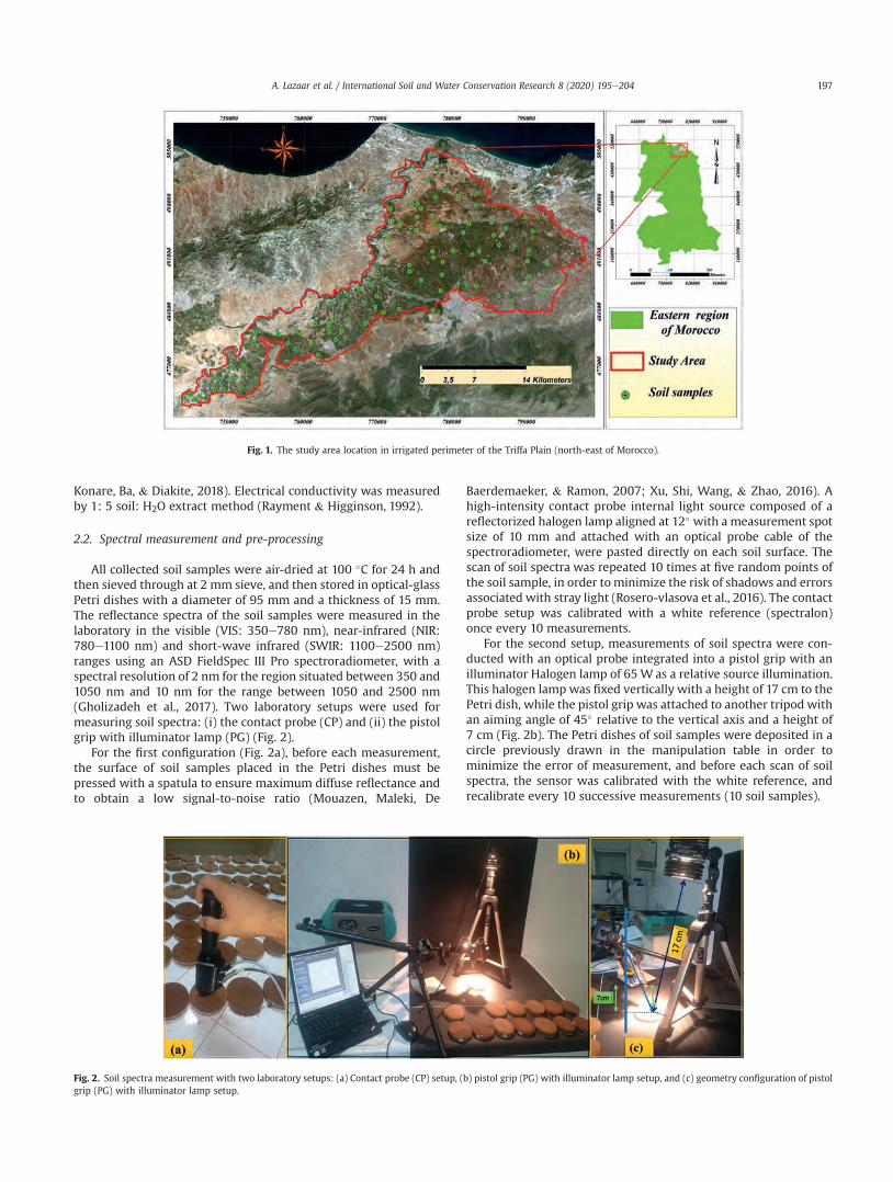
Konare, Ba, & Diakite, 2018). Electrical conductivity was measuredby 1: 5 soil: H2O extract method (Rayment & Higginson, 1992).
2.2. Spectral measurement and pre-processing
All collected soil samples were air-dried at 100 �C for 24 h andthen sieved through at 2 mm sieve, and then stored in optical-glassPetri dishes with a diameter of 95 mm and a thickness of 15 mm.The reflectance spectra of the soil samples were measured in thelaboratory in the visible (VIS: 350e780 nm), near-infrared (NIR:780e1100 nm) and short-wave infrared (SWIR: 1100e2500 nm)ranges using an ASD FieldSpec III Pro spectroradiometer, with aspectral resolution of 2 nm for the region situated between 350 and1050 nm and 10 nm for the range between 1050 and 2500 nm(Gholizadeh et al., 2017). Two laboratory setups were used formeasuring soil spectra: (i) the contact probe (CP) and (ii) the pistolgrip with illuminator lamp (PG) (Fig. 2).
For the first configuration (Fig. 2a), before each measurement,the surface of soil samples placed in the Petri dishes must bepressed with a spatula to ensure maximum diffuse reflectance andto obtain a low signal-to-noise ratio (Mouazen, Maleki, De
Baerdemaeker, & Ramon, 2007; Xu, Shi, Wang, & Zhao, 2016). Ahigh-intensity contact probe internal light source composed of areflectorized halogen lamp aligned at 12� with a measurement spotsize of 10 mm and attached with an optical probe cable of thespectroradiometer, were pasted directly on each soil surface. Thescan of soil spectra was repeated 10 times at five random points ofthe soil sample, in order tominimize the risk of shadows and errorsassociated with stray light (Rosero-vlasova et al., 2016). The contactprobe setup was calibrated with a white reference (spectralon)once every 10 measurements.
For the second setup, measurements of soil spectra were con-ducted with an optical probe integrated into a pistol grip with anilluminator Halogen lamp of 65 W as a relative source illumination.This halogen lamp was fixed vertically with a height of 17 cm to thePetri dish, while the pistol grip was attached to another tripod withan aiming angle of 45� relative to the vertical axis and a height of7 cm (Fig. 2b). The Petri dishes of soil samples were deposited in acircle previously drawn in the manipulation table in order tominimize the error of measurement, and before each scan of soilspectra, the sensor was calibrated with the white reference, andrecalibrate every 10 successive measurements (10 soil samples).
Fig. 1. The study area location in irrigated perimeter of the Triffa Plain (north-east of Morocco).
Fig. 2. Soil spectra measurement with two laboratory setups: (a) Contact probe (CP) setup, (b) pistol grip (PG) with illuminator lamp setup, and (c) geometry configuration of pistolgrip (PG) with illuminator lamp setup.
A. Lazaar et al. / International Soil and Water Conservation Research 8 (2020) 195e204 197

In order to enhance the SOM model prediction, the spectro-scopic data acquired in the two-setups of laboratory measurementneeded several pre-treatments. The aim of this pre-processing wasto remove the undesired variation in the data (Leone et al., 2012).Spectral regions 350e399 nm and 2451e2500 nm were removedbecause they are affected by the noise. The measured reflectancespectra (400e2450 nm) of soil samples were transformed intoabsorbance (log 1/R) to improve correlation to sample concentra-tion (Bellon-Maurel, Fernandez-Ahumada, Palagos, Roger, &McBratney, 2010; Ji et al., 2016). Several pre-treatments wereconsidered such as the standard normal variate and detrending forreducing scatter and particles size effects and to remove the linearor curvilinear of the spectrum (Barnes, Dhanoa, & Lister, 1989), themean and maximum normalization, the multiplicative scatter, andthe first and second derivate (Fystro, 2002; Mouazen, Saeys, Xing,De Baerdemaeker, & Ramon, 2005; Van Waes, Mestdagh, Lootens,& Carlier, 2005). Moreover, in order to create a robust model pre-diction of SOM, many pre-treatment methods were tested, such asthe standard normal variate (SNV), detrend, a combination of SNVand detrend, multiplicative scatter and maximum normalization.Finally, the transformation of reflectance into absorbance (log1/R)and the applied of first derivative transformationwith the Savitsky-Golay smoothing algorithms (Savitzky & Golay, 1964) with a win-dow size of 10 and polynomial of order 2 was chosen as the opti-mum data pre-treatment method. All pre-treatments andprocedures were conducted using Unscrambler 10.4 software.
2.3. Partial least squares regression (PLSR) analysis and IDW GIS-Kriging
2.3.1. Partial least squares regression methodPLSR is the widely most used method for spectral calibration
and prediction (Ji et al., 2016) because it gives more strongercorrelated results compared to the different multivariate methods(Bogrekci & Lee, 2004; Chang, Laird, Mausbach, & Hurburgh, 2001;Tümsavas et al., 2018). In this study, the PLSR technique coupledwith cross-validation was used to create and establish a modelprediction between the soil spectra of soil samples and the refer-ence value of SOM. Twomodel calibrations were developed, one forthe contact probe configuration and the second for the pistol gripconfiguration. The selection criteria for evaluating the performanceof model prediction is based on coefficient of determination (R2)value, and the rootmeans square error of prediction (RMSEP) (Aïchiet al., 2009; Mouazen et al., 2007; Viscarra Rossel, Walvoort,McBratney, Janik, & Skjemstad, 2006).
Before running the analysis of SOM prediction using the PLSRmethod for the two measurement protocols, the data set wasdivided into a calibration set (75 % or 85 soil samples) will allow usto create the model and a validation set (25% or 30 soil samples)which measures the error of the final model on data it has neverseen before. For this validation set cannot be considered to becompletely independent from the calibration set due to the spatialautocorrelation in spectral data or SOM content arising betweensamples situated in close proximity or belonging to the same field.
2.3.2. Spatial variability mapping of SOM with IDW interpolationmethod
IDW is one of the most applied and deterministic interpolationtechniques used in soil science for mapping the spatial variability ofsoil proprieties (Xu, Li, Li, Lu, & Wang, 2013). The mapping of SOMvariability in the study area was created using ArcGIS software,using the inverse distance weighting (IDW) interpolation method,in order to evaluate the influence of the laboratory procedures onthe statistical model predicted for the (CP) and (PG) setups.
2.4. Statistical analysis
The data of soil chemical analysis were identified by severalstatistical parameters such as mean, maximum, minimum, stan-dard deviation, variance, median range, skewness and kurtosis.Mean, maximum, minimum and median were used to describe thecentral tendency and distribution of soil parameter values. Thestandard deviation, range and variance were used to measure thedispersion between the soil parameters. The skewness and kurtosiswere used to measure the asymmetry of the soil parameters anddescribes the extent of the degree of flatness. The descriptive sta-tistics were conducted using Unscrambler 10.4 software.
3. Results and discussion
3.1. Soil properties
Summary statistics for the soil samples of Triffa plain, includingminimum, maximum, mean, Standard Deviation (SD), variance,median, range, skewness and kurtosis are shown below (Table 1).The SOM content of the reference dataset is ranged from 1.12% to3.30% with a mean of 2.27% and an SD of 0.5. The skewness of 0.90and a kurtosis of 0.56 indicate that the SOM content of dataset has anormal distribution. According to the SOM results of samples, thesoils of Triffa plain are characterized by low to medium SOM con-tents (Carr, 2018; Lazaar et al., 2019). The spatial variability of SOMcontent is probably due to the nature of topsoils (isohumic,rendzina, brown calcareous, fersialitic, less-developed, and hydro-morphic soils), soil textures, soil degradation and the percentage ofCaCO3 content. Concerning the CaCO3 content, the samples rep-resented a wide range of CaCO3 ranged from 0 to 38.69% with amean value of 8.72 %. According to the AFNOR NF P 94-048 (2003)norm, the soils in the study area are generally characterized byslightly to moderately calcareous soil classes. Our results confirmthose obtained by Lazaar et al. (2019) and Ruellan (1971). Theassessment of soil salinity is based on electrical conductivity (EC)data and their spatial distribution. The EC value of soil samples isvaried between 0.11 and 0.9 ms/cm, according to Horneck, Sullivan,Owen, and Hart (2011), the soils of Triffa plain are characterized bylow salinity. Soil pH ranged from 6.94 to 7.84 with a mean value of7.39. Following the soil pH range edited by Horneck et al. (2011), thesoils in the study area are considered moderately alkaline (95% soilsamples) and others are neutral (5% soil samples). The results of ourwork confirmed those obtained by Bendra et al. (2012) and Lazaaret al. (2019). The available phosphorus of soil samples varied from0.45 to 357.68 ppm with a mean of 74.73 ppm. According toHorneck et al. (2011), the Triffa plain is characterized by soils with awide range of available phosphorus content varied between low(3%), medium (10%), high (80) and excessive.
Also statistics for the SOM content in all soil samples used in thecalibration and validation models of the two measurement setupsis varied between 1.12 and 3.30% for the calibration samples and 1.5to 3.27 for the validation samples (Table 1).
3.2. Comparison between soil spectra and data pre-treatment
The results of the two measurement setups (CP) and (PG) of soilspectra showed that all soil samples have similar reflectancespectra in the range between 400 and 2450 nm, where the reflec-tance was generally lower in the VIS range (400e780 nm) andhigher in the NIR range (781e2450 nm). These spectra present twosmall absorption peaks appear at 430 nm and 530 nm in the visiblerange, due to the presence of iron oxides and blue colour absorptionbands (Sherman & Waite, 1985; Tekin, Tumsavas, & Mouazen,2012). In the NIR range, three distinct absorption peaks are
A. Lazaar et al. / International Soil and Water Conservation Research 8 (2020) 195e204198
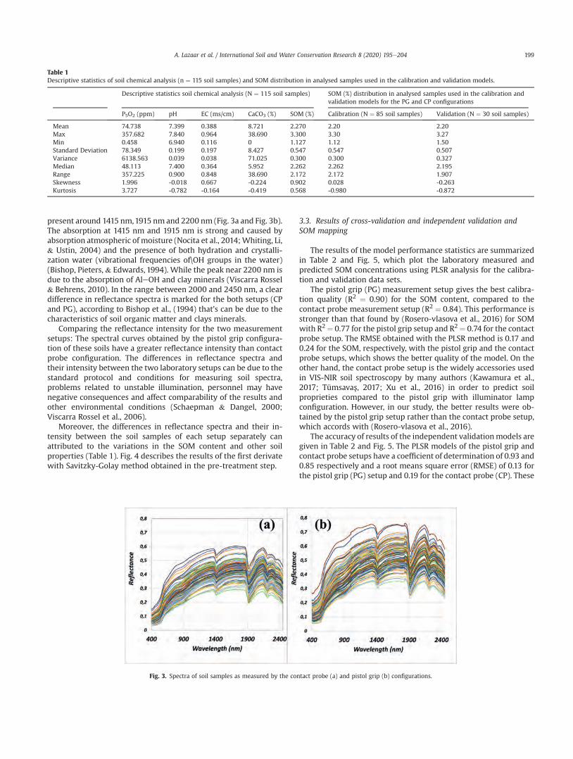
present around 1415 nm,1915 nm and 2200 nm (Fig. 3a and Fig. 3b).The absorption at 1415 nm and 1915 nm is strong and caused byabsorption atmospheric of moisture (Nocita et al., 2014;Whiting, Li,& Ustin, 2004) and the presence of both hydration and crystalli-zation water (vibrational frequencies of\OH groups in the water)(Bishop, Pieters, & Edwards, 1994). While the peak near 2200 nm isdue to the absorption of AleOH and clay minerals (Viscarra Rossel& Behrens, 2010). In the range between 2000 and 2450 nm, a cleardifference in reflectance spectra is marked for the both setups (CPand PG), according to Bishop et al., (1994) that’s can be due to thecharacteristics of soil organic matter and clays minerals.
Comparing the reflectance intensity for the two measurementsetups: The spectral curves obtained by the pistol grip configura-tion of these soils have a greater reflectance intensity than contactprobe configuration. The differences in reflectance spectra andtheir intensity between the two laboratory setups can be due to thestandard protocol and conditions for measuring soil spectra,problems related to unstable illumination, personnel may havenegative consequences and affect comparability of the results andother environmental conditions (Schaepman & Dangel, 2000;Viscarra Rossel et al., 2006).
Moreover, the differences in reflectance spectra and their in-tensity between the soil samples of each setup separately canattributed to the variations in the SOM content and other soilproperties (Table 1). Fig. 4 describes the results of the first derivatewith Savitzky-Golay method obtained in the pre-treatment step.
3.3. Results of cross-validation and independent validation andSOM mapping
The results of the model performance statistics are summarizedin Table 2 and Fig. 5, which plot the laboratory measured andpredicted SOM concentrations using PLSR analysis for the calibra-tion and validation data sets.
The pistol grip (PG) measurement setup gives the best calibra-tion quality (R2 ¼ 0.90) for the SOM content, compared to thecontact probe measurement setup (R2 ¼ 0.84). This performance isstronger than that found by (Rosero-vlasova et al., 2016) for SOMwith R2 ¼ 0.77 for the pistol grip setup and R2 ¼ 0.74 for the contactprobe setup. The RMSE obtained with the PLSR method is 0.17 and0.24 for the SOM, respectively, with the pistol grip and the contactprobe setups, which shows the better quality of the model. On theother hand, the contact probe setup is the widely accessories usedin VIS-NIR soil spectroscopy by many authors (Kawamura et al.,2017; Tümsavas, 2017; Xu et al., 2016) in order to predict soilproprieties compared to the pistol grip with illuminator lampconfiguration. However, in our study, the better results were ob-tained by the pistol grip setup rather than the contact probe setup,which accords with (Rosero-vlasova et al., 2016).
The accuracy of results of the independent validationmodels aregiven in Table 2 and Fig. 5. The PLSR models of the pistol grip andcontact probe setups have a coefficient of determination of 0.93 and0.85 respectively and a root means square error (RMSE) of 0.13 forthe pistol grip (PG) setup and 0.19 for the contact probe (CP). These
Table 1Descriptive statistics of soil chemical analysis (n ¼ 115 soil samples) and SOM distribution in analysed samples used in the calibration and validation models.
Descriptive statistics soil chemical analysis (N ¼ 115 soil samples) SOM (%) distribution in analysed samples used in the calibration andvalidation models for the PG and CP configurations
P5O2 (ppm) pH EC (ms/cm) CaCO3 (%) SOM (%) Calibration (N ¼ 85 soil samples) Validation (N ¼ 30 soil samples)
Mean 74.738 7.399 0.388 8.721 2.270 2.20 2.20Max 357.682 7.840 0.964 38.690 3.300 3.30 3.27Min 0.458 6.940 0.116 0 1.127 1.12 1.50Standard Deviation 78.349 0.199 0.197 8.427 0.547 0.547 0.507Variance 6138.563 0.039 0.038 71.025 0.300 0.300 0.327Median 48.113 7.400 0.364 5.952 2.262 2.262 2.195Range 357.225 0.900 0.848 38.690 2.172 2.172 1.907Skewness 1.996 -0.018 0.667 -0.224 0.902 0.028 -0.263Kurtosis 3.727 -0.782 -0.164 -0.419 0.568 -0.980 -0.872
Fig. 3. Spectra of soil samples as measured by the contact probe (a) and pistol grip (b) configurations.
A. Lazaar et al. / International Soil and Water Conservation Research 8 (2020) 195e204 199
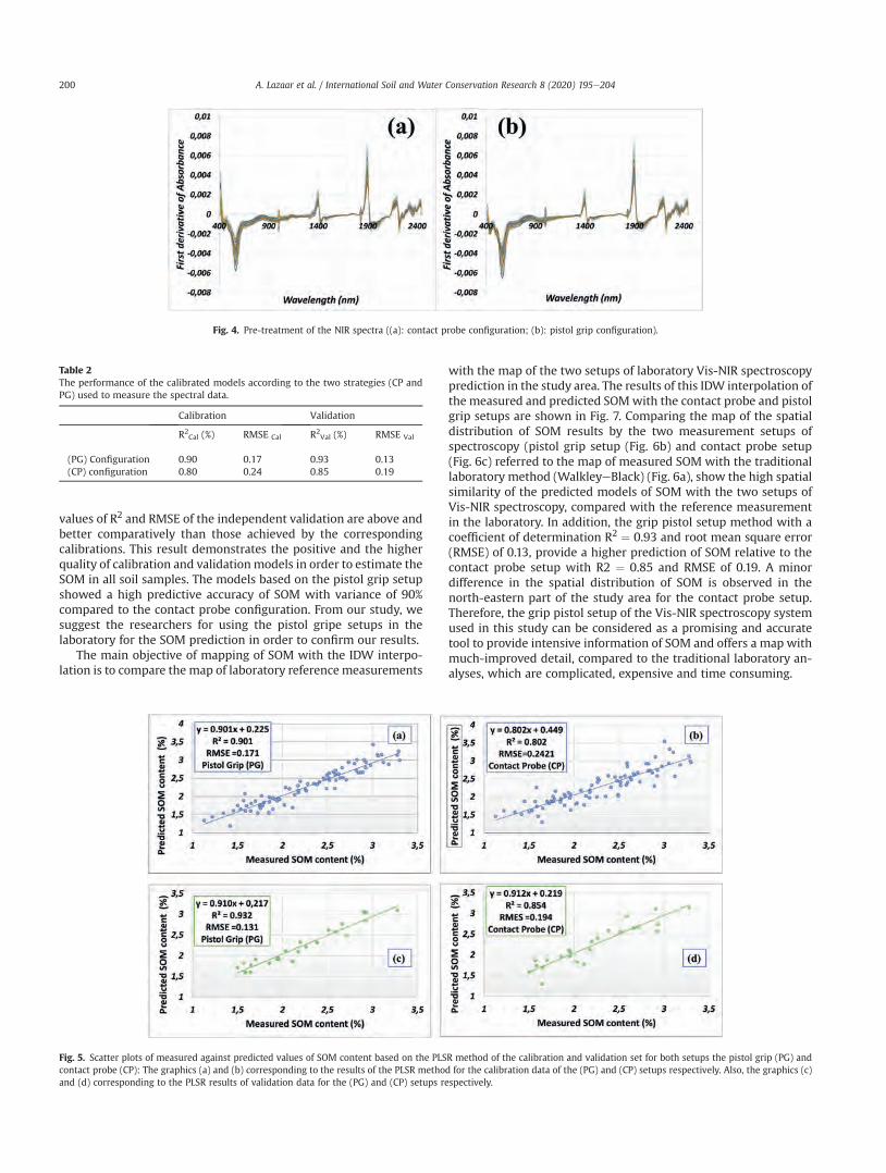
values of R2 and RMSE of the independent validation are above andbetter comparatively than those achieved by the correspondingcalibrations. This result demonstrates the positive and the higherquality of calibration and validationmodels in order to estimate theSOM in all soil samples. The models based on the pistol grip setupshowed a high predictive accuracy of SOM with variance of 90%compared to the contact probe configuration. From our study, wesuggest the researchers for using the pistol gripe setups in thelaboratory for the SOM prediction in order to confirm our results.
The main objective of mapping of SOM with the IDW interpo-lation is to compare the map of laboratory referencemeasurements
with the map of the two setups of laboratory Vis-NIR spectroscopyprediction in the study area. The results of this IDW interpolation ofthe measured and predicted SOMwith the contact probe and pistolgrip setups are shown in Fig. 7. Comparing the map of the spatialdistribution of SOM results by the two measurement setups ofspectroscopy (pistol grip setup (Fig. 6b) and contact probe setup(Fig. 6c) referred to the map of measured SOM with the traditionallaboratory method (WalkleyeBlack) (Fig. 6a), show the high spatialsimilarity of the predicted models of SOM with the two setups ofVis-NIR spectroscopy, compared with the reference measurementin the laboratory. In addition, the grip pistol setup method with acoefficient of determination R2 ¼ 0.93 and root mean square error(RMSE) of 0.13, provide a higher prediction of SOM relative to thecontact probe setup with R2 ¼ 0.85 and RMSE of 0.19. A minordifference in the spatial distribution of SOM is observed in thenorth-eastern part of the study area for the contact probe setup.Therefore, the grip pistol setup of the Vis-NIR spectroscopy systemused in this study can be considered as a promising and accuratetool to provide intensive information of SOM and offers a map withmuch-improved detail, compared to the traditional laboratory an-alyses, which are complicated, expensive and time consuming.
Fig. 4. Pre-treatment of the NIR spectra ((a): contact probe configuration; (b): pistol grip configuration).
Table 2The performance of the calibrated models according to the two strategies (CP andPG) used to measure the spectral data.
Calibration Validation
R2Cal (%) RMSE Cal R2
Val (%) RMSE Val
(PG) Configuration 0.90 0.17 0.93 0.13(CP) configuration 0.80 0.24 0.85 0.19
Fig. 5. Scatter plots of measured against predicted values of SOM content based on the PLSR method of the calibration and validation set for both setups the pistol grip (PG) andcontact probe (CP): The graphics (a) and (b) corresponding to the results of the PLSR method for the calibration data of the (PG) and (CP) setups respectively. Also, the graphics (c)and (d) corresponding to the PLSR results of validation data for the (PG) and (CP) setups respectively.
A. Lazaar et al. / International Soil and Water Conservation Research 8 (2020) 195e204200
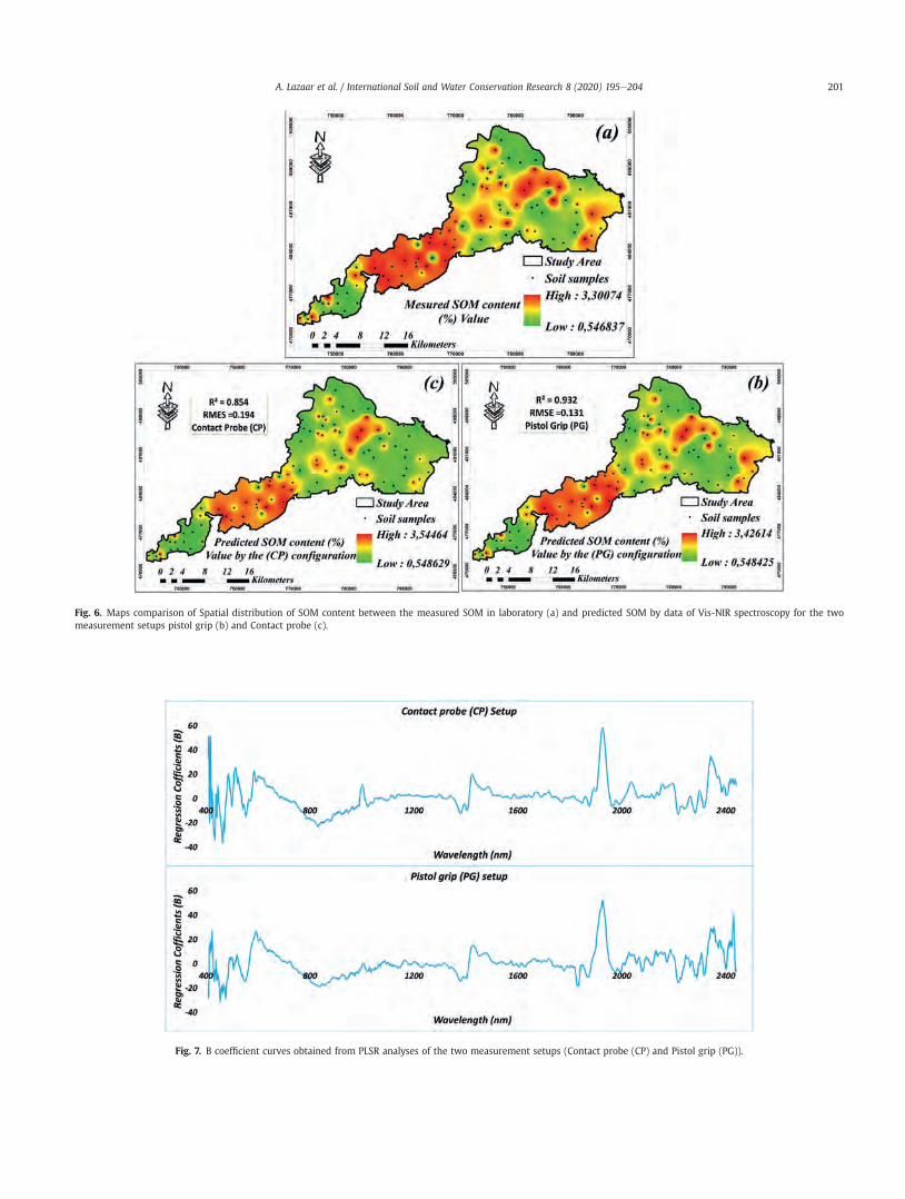
Fig. 6. Maps comparison of Spatial distribution of SOM content between the measured SOM in laboratory (a) and predicted SOM by data of Vis-NIR spectroscopy for the twomeasurement setups pistol grip (b) and Contact probe (c).
Fig. 7. B coefficient curves obtained from PLSR analyses of the two measurement setups (Contact probe (CP) and Pistol grip (PG)).
A. Lazaar et al. / International Soil and Water Conservation Research 8 (2020) 195e204 201

3.4. Correlation coefficients of wavelengths
The contribution of each band of the VIS-NIR spectral range ofthe SOM content predictionmodels is distinct from the b coefficientof PLSR. The regression coefficients (or b coefficient) summarizesthe association between all predictors and a given response andprovide information about the importance of the X-variables. Tekinet al., 2012 indicated that the plot of coefficient regression illus-trates the importance of wavelengths associated with properties, inthis case of our study SOM content. Fig. 7 shows the regressioncoefficient of the two laboratory setups CP and PG from the cross-validation PLSR analysis for SOM.
Comparing the regression coefficient curves of the contactprobe configuration with the pistol grip configuration in the rangebetween 400 and 2450 nm reveals substantial similarities, partic-ularly for significant absorption wavelengths 1430, 1929 and2220 nm. The wavelengths appear at 1430 nm and 1920 nm wererelated towater absorption (Hong et al., 2018;Mouazen et al., 2007;Nocita et al., 2014; Viscarra; Viscarra Rossel & Behrens, 2010), andthe wavelength appears at 2200 nm due to the lattice OH in clayminerals (Nocita et al., 2014; Viscarra; Viscarra Rossel & Behrens,2010).
For the pistol grip (PG) setup, the most important peaks used topredict SOM are situated in the visible range for the wavelengths424, 500, 521 and 597 nm and in the NIR range for the wavelength840, 1379, 1432, 1484, 1830, 1920, 2200, 2357 and 2430 nm. Con-cerning the contact probe (CP) setup the important peaks appear inthe visible range for the wavelengths 433, 470, 483, 517, 553, 587and 615 nm, and in the NIR range for 830, 1004, 1380, 1431,1929,2041, 2200 and 2345 nm.
In the visible range, the significant wavelengths at 424 nm for(PG) and 433, 470 and 483 nm for (CP) setups can be attributed toblue colour absorption (Tekin et al., 2012). The absorbance peaknear 500 nm, 521 and 597 nm for the (PG) and near 517, 553 and587 nm for the (CP) setups be could due to the chromophore FeOOHfound in goethite, free iron oxides and small amounts of hematite(Fe2O3) (Ben-Dor et al., 2008; Viscarra; Mortimore, Marshall,Almond, Hollins, & Matthews, 2004; Viscarra Rossel & Behrens,2010). In the NIR region, the band found at 840 nm and 830 nmfor (PG) and (CP) setups respectively can be associated to thechromophorous constituents iron oxides mainly hematite andgoethite (Sherman & Waite, 1985) and to the SOM content (Ben-Dor, Irons, & Epema, 1999). The highest correlation b coefficientswere observed in the range between 1000 and 2450 nm for bothsetups (CP and PG). The featured absorption bands around 1379,1432, 1484, 1830 and 1920 nm for the (PG) and 1380, 1431, 1830,2041 and 2200 nm for the (CP) setups were considered in detail fortheir relationships with clay, soil water content, and SOM content(Hong et al., 2018; Mouazen et al., 2007; Nocita et al., 2014; ViscarraRossel & Behrens, 2010; Thomasson, Sui, Cox, & AleRajehy, 2001).The wavelengths appear at 2357 nm and 2430 nm for the (PG) and2345 nm for the (CP) configurations can be attributed to AleOHbend plus OeH stretch combinations, that are diagnostic absorp-tion features in clay mineral identification (Clark, King, Klejwa,Swayze, & Vergo, 1990). From the discussion above it can beconcluded that the near infrared (NIR) spectrum were more accu-rate than those in the visible (VIS) spectral range for predictingSOM using both setups (contact probe(CP) and grip pistol (PG)),which confirms the results obtained byMilo�s and Bensa (2017). Thesignificant wavelengths contributing to the prediction of SOM forthe pistolet grip (PG) setup were at 424, 597,1432,1484, 1830,1920,2200, 2357 and 2430 nm, while were at 433, 587, 1380, 1431, 1929,2200 and 2345 nm for the contact probe setup (CP).
4. Conclusions
The present study demonstrated the ability of the combinedapplication of soil Vis-NIR spectroscopy and the PLSR method toanalyse and predict the SOM of the soils of the Triffa Plain of north-east Morocco using two laboratory setups, the contact probe (CP)and pistol grip (PG) and the IDW interpolation method for map-ping. The mains conclusions are:
1) Vis-NIR spectroscopy is a useful tool for predicting the SOM inthe irrigated perimeter of Triffa Plain.
2) The pistol grip setup gives the highest calibration quality forSOM content compared to the contact probe measurementsetup.
3) The PLSR is widely and most used method for spectral calibra-tion and prediction, because it gives more stronger correlatedresults of SOM with the laboratory Vis-NIR spectroscopymeasurements.
4) The pistol grip setup measurement of the Vis-NIR spectroscopysystem used in this study can be considered as a promising andaccurate tool to provide intensive information on SOM. Is offersa map with much-improved detail, compared to the contactprobe setup and to the traditional laboratory analyses which arecomplicated, expensive and time consuming.
Declaration of competing interest
The authors declare that they have no known competingfinancial interests or personal relationships that could haveappeared to influence the work reported in this paper.
Acknowledgments
The authors acknowledge the facilities and financial supportsprovided by the Mohammed First University and the NationalInstitute of Agronomic Research (INRA) of Oujda. I want to thank allresearchers of the Applied Geosciences Laboratory and all re-searchers of INRA for his help in collecting the soil samples andtheir analysis in the laboratory.
References
AFNOR NF P 94-048. (2003). Sols : Recognition and testing - determination of car-bonate content - calcimeter method.
Aïchi, H., Fouad, Y., Walter, C., Viscarra Rossel, R. A., Lili Chabaane, Z., & Sanaa, M.(2009). Regional predictions of soil organic carbon content from spectralreflectance measurements. Biosystems Engineering, 104(3), 442e446. https://doi.org/10.1016/j.biosystemseng.2009.08.002.
Aubert, G. (1965). Soil classification: Tables of classes, subclasses, groups and sub-groups of soils used by the ORSTOM pedology section. ORSTOM notebook:Pedology Series, III, 269e288.
Bao, N., Wu, L., Ye, B., Yang, K., & Zhou, W. (2017). Assessing soil organic matter ofreclaimed soil from a large surface coal mine using a field spectroradiometer inlaboratory. Geoderma, 288, 47e55. https://doi.org/10.1016/j.geoderma.2016.10.033.
Barnes, R. J., Dhanoa, M. S., & Lister, S. J. (1989). Standard normal variate trans-formation and de-trending of near-infrared diffuse reflectance spectra. AppliedSpectroscopy, 43(5), 772e777. https://doi.org/10.1366/0003702894202201.
Bellon-Maurel, V., Fernandez-Ahumada, E., Palagos, B., Roger, J. M., & McBratney, A.(2010). Critical review of chemometric indicators commonly used for assessingthe quality of the prediction of soil attributes by NIR spectroscopy. Trends inAnalytical Chemistry, 29(9), 1073e1081. https://doi.org/10.1016/j.trac.2010.05.006.
Ben-Dor, E., & Banin, A. (1990). Near-infrared reflectance analysis of carbonateconcentration in soils. Applied Spectroscopy, 44(6), 1064e1069. https://doi.org/10.1366/0003702904086821.
Ben-Dor, E., Irons, J., & Epema, G. (1999). Soil reflectance. In A. N. Rencz (Ed.), Remotesensing for the earth sciences: Manual of remote sensing (pp. 111e188). New York:USA.
A. Lazaar et al. / International Soil and Water Conservation Research 8 (2020) 195e204202
Ben-Dor, E., Ong, C., & Lau, I. C. (2014). Reflectance measurement of soils in thelaboratory : Standards and protocols. Geoderma, 245e246, 112e124. https://doi.org/10.1016/j.geoderma.2015.01.002.
Ben-Dor, E., Taylor, R. G., Hill, J., Dematte, J. A. M., Whiting, M. L., Chabrillat, S., et al.(2008). Imaging spectrometry for soil applica tions. Advances in Agronomy, 97,321e392. https://doi.org/10.1016/S0065-2113(07)00008-9, 07.
Bendra, B., Fetouani, S., Laffray, X., Vanclooster, M., Sbaa, M., & Aleya, L. (2012).Effects of irrigation on soil physico-chemistry : A case study of the Triffa plain (Morocco ). Irrigation and drainage. https://doi.org/10.1002/ird.688.
Bishop, J. L., Pieters, C. M., & Edwards, J. O. (1994). Infrared spectroscopic analyseson the nature of water in montmorillonite. Clays and Clay Minerals, 42,702e716.
Bogrekci, I., & Lee, W. S. (2004). Spectral signatures of common phosphates in soilsand their effect on absorbance spectra of soil samples with different phos-phorus concentrations. Annual International Meeting, 1e12. https://doi.org/10.13031/2013.16739.
Carr, M. (2018). Hidden hunger and intelligent guesswork. In Advances in teaagronomy (pp. 253e276). https://doi.org/10.1017/9781316155714.014.
Chang, C. W., Laird, D. A., Mausbach, M. J., & Hurburgh, C. R. (2001). Near-Infraredreflectance spectroscopyeprincipal components regression analyses of soilproperties. Soil Science Society of America Journal, 65(2), 480. https://doi.org/10.2136/sssaj2001.652480x.
Chen, H., Pan, T., Chen, J., & Lu, Q. (2011). Waveband selection for NIR spectroscopyanalysis of soil organic matter based on SG smoothing and MWPLS methods.Chemometrics and Intelligent Laboratory Systems, 107(8), 139e146. https://doi.org/10.1016/j.chemolab.2011.02.008.
Clark, R. N., King, T. V. V., Klejwa, M., Swayze, G., & Vergo, N. (1990). High spectralresolution reflectance spectroscopy of minerals. Journal of Geophysical Research,95(B8), 12653e12680. https://doi.org/10.1029/JB095iB08p12653.
Coûteaux, M. M., Berg, B., & Rovira, P. (2003). Near infrared reflectance spectroscopyfor determination of organic matter fractions including microbial biomass inconiferous forest soils. Soil Biology and Biochemistry, 35(12), 1587e1600. https://doi.org/10.1016/j.soilbio.2003.08.003.
Curcio, D., Ciraolo, G., D’Asaro, F., & Minacapilli, M. (2013). Prediction of soil texturedistributions using VNIR-SWIR reflectance spectroscopy. Procedia Environ-mental Sciences, 19, 494e503. https://doi.org/10.1016/j.proenv.2013.06.056.
Dematte, J. A. M., Ramirez-Lopez, L., Marques, K. P. P., & Rodella, A. A. (2017).Chemometric soil analysis on the determination of specific bands for thedetection of magnesium and potassium by spectroscopy. Geoderma,288(February), 8e22. https://doi.org/10.1016/j.geoderma.2016.11.013.
Fekkoul, A. (2012). Groundwater contamination by nitrates, salinity and pesticides:Case of the unconfined aquifer of Triffa plain (eastern Morocco). Revue Mar-ocaine Des Sciences Agronomiques et V�et�erinaires, 2, 12e36. https://doi.org/10.4409/Am-034-11-0034.
Fystro, G. (2002). The prediction of C and N content and their potential minerali-sation in heterogeneous soil samples using ViseNIR spectroscopy andcomparative methods. Plant and Soil, 246(2), 139e149. https://doi.org/10.1023/A.
Gholizadeh, A., Bor�uvka, L., Saberioon, M., & Vasat, R. (2013). Mid-Infrared spec-troscopy applications for soil assessment with emphasis on soil organic mattercontent and quality. Applied Spectroscopy OA, 67(12), 1349e1362. https://doi.org/10.1366/13-07288.
Gholizadeh, A., Carmon, N., Klement, A., Ben-Dor, E., & Bor�uvka, L. (2017). Agri-cultural soil spectral response and properties assessment: Effects of measure-ment protocol and data mining technique. Remote Sensing, 9(10), 1e14. https://doi.org/10.3390/rs9101078.
Gomez, C., Lagacherie, P., & Coulouma, G. (2008a). Continuum removal versus PLSRmethod for clay and calcium carbonate content estimation from laboratory andairborne hyperspectral measurements. Geoderma, 148(2), 141e148. https://doi.org/10.1016/j.geoderma.2008.09.016.
Gomez, C., Oltra-Carri�o, R., Bacha, S., Lagacherie, P., & Briottet, X. (2015). Evaluatingthe sensitivity of clay content prediction to atmospheric effects and degradationof image spatial resolution using Hyperspectral VNIR/SWIR imagery. RemoteSensing of Environment, 164, 1e15. https://doi.org/10.1016/j.rse.2015.02.019.
Gomez, C., Viscarra Rossel, R. A., & McBratney, A. B. (2008b). Soil organic carbonprediction by hyperspectral remote sensing and field vis-NIR spectroscopy: AnAustralian case study. Geoderma, 146(3e4), 403e411. https://doi.org/10.1016/j.geoderma.2008.06.011.
He, Y., Song, H., Pereira, A. G., & G�omez, A. H. (2005). Measurement and analysis ofsoil nitrogen and organic matter content using near-infrared spectroscopytechniques. Journal of Zhejiang University - Science, 6B(11), 1081e1086. https://doi.org/10.1631/jzus.2005.B1081.
Hong, Y., Chen, S., Zhang, Y., Chen, Y., Yu, L., Liu, Yanfang, et al. (2018). Rapididentification of soil organic matter level via visible and near-infrared spec-troscopy: Effects of two-dimensional correlation coefficient and extremelearning machine. The Science of the Total Environment, 644, 1232e1243. https://doi.org/10.1016/j.scitotenv.2018.06.319.
Horneck, D. a, Sullivan, D. M., Owen, J. S., & Hart, J. M. (2011). Soil test interpretationguide. Oregon State University, Extension Service. https://doi.org/10.1017/CBO9781107415324.004. July.
Jakab, G., Rieder, �A., Vancsik, A. V., & Szalai, Z. (2018). Soil organic matter charac-terisation by photometric indices or photon correlation spectroscopy: Are theycomparable? Hungarian Geographical Bulletin, 67(2). https://doi.org/10.15201/hungeobull.67.2.1.
Ji, W., Adamchuk, V. I., Biswas, A., Dhawale, N. M., Sudarsan, B., Zhang, Y., et al.
(2016). Assessment of soil properties in situ using a prototype portable MIRspectrometer in two agricultural fields. Biosystems Engineering, 152, 14e27.https://doi.org/10.1016/j.biosystemseng.2016.06.005. December 2017.
Jiang, Q., Chen, Y., Guo, L., Fei, T., & Qi, K. (2016). Estimating soil organic carbon ofcropland soil at different levels of soil moisture using VIS-NIR spectroscopy.Remote Sensing, 8(9). https://doi.org/10.3390/rs8090755.
Kawamura, K., Tsujimoto, Y., Rabenarivo, M., Asai, H., Andriamananjara, A., &Rakotoson, T. (2017). Vis-NIR spectroscopy and PLS regression with wavebandselection for estimating the total C and N of paddy soils in Madagascar. RemoteSensing, 9(10). https://doi.org/10.3390/rs9101081.
Lagacherie, P., Baret, F., Feret, J. B., Madeira Netto, J., & Robbez-Masson, J. M. (2008).Estimation of soil clay and calcium carbonate using laboratory, field andairborne hyperspectral measurements. Remote Sensing of Environment, 112(3),825e835. https://doi.org/10.1016/j.rse.2007.06.014.
Lavelle, P., Barot, S., Blouin, M., Deca€ens, T., Jimenez, J. J., & Jouquet, P. (2007).Earthworms as key actors in self-organized soil systems. Theoretical EcologySeries, 4(C). https://doi.org/10.1016/S1875-306X(07)80007-4.
Lazaar, A. (2016). The contribution of hyperspectral remote sensing in the soil char-acterization of the Triffa Plain (Eastern Morocco) (Master’s thesis). Oujda,Morocco: Mohammed First University.
Lazaar, A., Mahyou, H., Gholizadeh, A., Elhammouti, K., Bilal, M., Andich, K., et al.(2019). Potential of VIS-NIR spectroscopy to characterize and discriminatetopsoils of different soil types in the Triffa plain (Morocco). Soil Science Annual,70(1). https://doi.org/10.2478/ssa-2019-0007.
Leone, A., Viscarra-Rossel, R. A., Amenta, P., & Buondonno, A. (2012). Prediction ofsoil properties with PLSR and vis-NIR spectroscopy: Application to Mediterra-nean soils from southern Italy. Current Analytical Chemistry, 8, 283e299. https://doi.org/10.2174/157341112800392571.
Memon, M. S., Guo, J., Tagar, A. A., Perveen, N., Ji, C., Memon, S. A., et al. (2018). Theeffects of tillage and straw incorporation on soil organic carbon status, rice cropproductivity, and sustainability in the rice-wheat cropping system of easternChina. Sustainability, 10(March), 1e14. https://doi.org/10.3390/su10040961.
Milo�s, B., & Bensa, A. (2017). Prediction of soil organic carbon using VIS-NIR spec-troscopy : Application to Red Mediterranean soils from Croatia. Eurasian Journalof Soil Science, 6(4), 365e373. https://doi.org/10.18393/ejss.319208.
Mortimore, J. L., Marshall, L. J. R., Almond, M. J., Hollins, P., & Matthews, W. (2004).Analysis of red and yellow ochre samples from Clearwell Caves and Catalhoyukby vibrational spectroscopy and other techniques. Spectrochimica Acta Part A:Molecular and Biomolecular Spectroscopy, 60(5), 1179e1188. https://doi.org/10.1016/j.saa.2003.08.002.
Mouazen, A. M., Kuang, B., De Baerdemaeker, J., & Ramon, H. (2010). Comparisonamong principal component, partial least squares and back propagation neuralnetwork analyses for accuracy of measurement of selected soil properties withvisible and near infrared spectroscopy. Geoderma, 158(1e2), 23e31. https://doi.org/10.1016/j.geoderma.2010.03.001.
Mouazen, A. M., Maleki, M. R., De Baerdemaeker, J., & Ramon, H. (2007). On-linemeasurement of some selected soil properties using a VIS-NIR sensor. Soil andTillage Research, 93(1), 13e27. https://doi.org/10.1016/j.still.2006.03.009.
Mouazen, A. M., Saeys, W., Xing, J., De Baerdemaeker, J., & Ramon, H. (2005). Nearinfrared spectroscopy for agricultural materials: An instrument comparison.Journal of Near Infrared Spectroscopy, 13(2), 87e97. https://doi.org/10.1255/jnirs.461.
Nawar, S., & Mouazen, A. M. (2017). Predictive performance of mobile vis-nearinfrared spectroscopy for key soil properties at different geographical scalesby using spiking and data mining techniques. Catena, 151(December), 118e129.https://doi.org/10.1016/j.catena.2016.12.014.
Nocita, M., Stevens, A., Toth, G., Panagos, P., van Wesemael, B., & Montanarella, L.(2014). Prediction of soil organic carbon content by diffuse reflectance spec-troscopy using a local partial least square regression approach. Soil Biology andBiochemistry, 68, 337e347. https://doi.org/10.1016/j.soilbio.2013.10.022.
Powlson, D. S., Brookes, P. C., Whitmore, A. P., Goulding, K. W. T., & Hopkins, D. W.(2011). Soil organic matters. European Journal of Soil Science, 62(1), 1e4. https://doi.org/10.1111/j.1365-2389.2010.01338.x.
Rayment, G. E., & Higginson, F. R. (1992). Australian laboratory handbook of soil andwater chemical methods. Australia: Inkata Press.
Rosero-vlasova, O. A., P�eerez-Cabello, F., Lloveria, R. M., & Vlassova, L. (2016).Assessment of laboratory VIS-NIR-SWIR setups with different spectroscopyaccessories for characterisation of soils from wildfire burns. Biosystems Engi-neering, 1e17. https://doi.org/10.1016/j.biosystemseng.2016.06.011.
Ruellan, A. (1971). Soils with a differentiated calcareous profile of the plains of lowerMoulouya (Eastern Morocco). Paris: FR: OROSTOM.
Sacko, B. D., Sanogo, S., Konare, H., Ba, A., & Diakite, T. (2018). Capability of visible-near infrared spectroscopy in estimating soils carbon, potassium and phos-phorus. Optics and Photonics Journal, 123e134. https://doi.org/10.4236/opj.2018.85012, 08(05).
Savitzky, A., & Golay, M. J. E. (1964). Smoothing and differentiation of data bysimplified least squares procedures. Analytical Chemistry, 36(8), 1627e1639.https://doi.org/10.1021/ac60214a047.
Schaepman, M. E., & Dangel, S. (2000). Solid laboratory calibration of a nonimagingspectroradiometer. Applied Optics, 39(21), 3754e3764. https://doi.org/10.1364/AO.39.003754.
Sherman, D. M., & Waite, T. D. (1985). Electronic spectra of Fe3 þ oxides and oxidehydroxides in the near IR to near UV. American Mineralogist, 70, 1262e1269.
Six, J., Conant, R. T., Paul, E. A., & Paustian, K. (2002). Stabilization mechanisms ofsoil organic matter: Implications for C- saturation of soils. Plant and Soil, 241,
A. Lazaar et al. / International Soil and Water Conservation Research 8 (2020) 195e204 203
155e176. https://doi.org/10.1023/A.St Luce, M., Ziadi, N., Zebarth, B. J., Grant, C. A., Tremblay, G. F., & Gregorich, E. G.
(2014). Rapid determination of soil organic matter quality indicators usingvisible near infrared reflectance spectroscopy. Geoderma, 232e234, 449e458.https://doi.org/10.1016/j.geoderma.2014.05.023.
Stevens, A., Udelhoven, T., Denis, A., Tychon, B., Lioy, R., Hoffmann, L., et al. (2010).Measuring soil organic carbon in croplands at regional scale using airborneimaging spectroscopy. Geoderma, 158(1e2), 32e45. https://doi.org/10.1016/j.geoderma.2009.11.032.
Stevens, A., Van Wesemael, B., Vandenschrick, G., Tour�e, S., & Tychon, B. (2006).Detection of carbon stock change in agricultural soils using spectroscopictechniques. Soil Science Society of America Journal, 70, 844e850. https://doi.org/10.2136/sssaj2005.0025.
Sun, W., Li, X., & Niu, B. (2018). Prediction of soil organic carbon in a coal miningarea by Vis-NIR spectroscopy. PLoS One, 13(4), 1e10. https://doi.org/10.1371/journal.pone.0196198.
Tekin, Y., Tumsavas, Z., & Mouazen, A. M. (2012). Effect of moisture content onprediction of organic carbon and pH using visible and near-infrared spectros-copy. Soil Science Society of America Journal, 76(1), 188. https://doi.org/10.2136/sssaj2011.0021.
Thomasson, J. A., Sui, R., Cox, M. S., & AleRajehy, A. (2001). Soil reflectance sensingfor determining soil properties in precision agriculture. Transactions of the ASAE,44(6), 1445e1453. https://doi.org/10.13031/2013.7002.
Tümsavas, Z. (2017). Application of visible and near infrared reflectance spectros-copy to predict total nitrogen in soil. Journal of Environmental Biology, 38,1101e1106. https://doi.org/10.22438/jeb/38/5(SI)/GM-29, 5(SI).
Tümsavas, Z., Tekin, Y., Ulusoy, Y., & Mouazen, A. M. (2018). Prediction and mappingof soil clay and sand contents using visible and near-infrared spectroscopy.Biosystems Engineering, 1e12. https://doi.org/10.1016/j.biosystemseng.2018.06.008.
Van Waes, C., Mestdagh, I., Lootens, P., & Carlier, L. (2005). Possibilities of nearinfrared reflectance spectroscopy for the prediction of organic carbon concen-trations in grassland soils. Journal of Agricultural Science, 143(6), 487e492.https://doi.org/10.1017/S0021859605005630.
Va�s�at, R., Kode�sov�a, R., Bor�uvka, L., Klement, A., Jak�sík, O., & Gholizadeh, A. (2014).Consideration of peak parameters derived from continuum-removed spectra topredict extractable nutrients in soils with visible and near-infrared diffusereflectance spectroscopy (VNIR-DRS). Geoderma, 232e234, 208e218. https://doi.org/10.1016/j.geoderma.2014.05.012.
Virgawati, S., Mawardi, M., Sutiarso, L., Shibusawa, S., Segah, H., & Kodaira, M.(2018). Mapping the variability of soil texture based on VIS-NIR proximalsensing. Journal of Applied Geospatial Information, 2(1), 108e116. https://doi.org/10.30871/jagi.v2i1.798.
Viscarra Rossel, R. A., & Behrens, T. (2010). Using data mining to model and interpretsoil diffuse reflectance spectra. Geoderma, 158(1e2), 46e54. https://doi.org/10.1016/j.geoderma.2009.12.025.
Viscarra Rossel, R. A., Walvoort, D. J. J., McBratney, A. B., Janik, L. J., & Skjemstad, J. O.(2006). Visible, near infrared, mid infrared or combined diffuse reflectancespectroscopy for simultaneous assessment of various soil properties. Geoderma,131(1e2), 59e75. https://doi.org/10.1016/j.geoderma.2005.03.007.
Walkley, A., & Black, I. A. (1934). An examination of the degtjareff method fordetermining soil organic matter, and a proposed modification of the chromicacid titration method. Soil Science, 37(1), 29e38. https://doi.org/10.1097/00010694-193401000-00003.
Whiting, M. L., Li, L., & Ustin, S. L. (2004). Predicting water content using Gaussianmodel on soil spectra. Remote Sensing of Environment, 89(4), 535e552. https://doi.org/10.1016/j.rse.2003.11.009.
Xie, H. T., Yang, X. M., Drury, C. F., Yang, J. Y., & Zhang, X. D. (2011). Predicting soilorganic carbon and total nitrogen using mid- and near-infrared spectra forBrookston clay loam soil in Southwestern Ontario, Canada. Canadian Journal ofSoil Science, 91(1), 53e63. https://doi.org/10.4141/cjss10029.
Xu, G. C., Li, Z. B., Li, P., Lu, K. X., & Wang, Y. (2013). Spatial variability of soil organiccarbon in a typical watershed in the source area of the middle Dan River, China.Soil Reasearch, 51(1), 41e49. https://doi.org/10.1071/SR12327.
Xu, S., Shi, X., Wang, M., & Zhao, Y. (2016). Effects of subsetting by parent materialson prediction of soil organic matter content in a hilly area using vis-NIRspectroscopy. PLoS One, 11(3), 1e17. https://doi.org/10.1371/journal.pone.0151536.
A. Lazaar et al. / International Soil and Water Conservation Research 8 (2020) 195e204204
Original Research Article
Atrazine removal from water by activated charcoal cloths
Javier M. Gonzalez a, *, Lynnette R. Murphy b, c, Chad J. Penn a, Veera M. Boddu d,Laura L. Sanders b
a National Soil Erosion Research Laboratory, USDA-ARS, West Lafayette, IN, 47907, USAb Earth Science Department, Northeastern Illinois University, Chicago, IL, 60625, USAc O’Neill School of Public and Environmental Affairs, University of Indiana, Bloomington, IN, 47405, USAd Plant Polymer Research Unit, National Center for Agriculture Utilization Research, USDA-ARS, Peoria, IL, 61604, USA
a r t i c l e i n f o
Article history:Received 10 February 2020Received in revised form19 March 2020Accepted 23 March 2020Available online 3 April 2020
Keywords:AtrazineActivated charcoalWater qualityPesticideCloth
a b s t r a c t
Pollution control structures may be adapted to enhance the removal of nutrients and pesticides fromwater. Charcoal-like material is known to sorb organic compounds in solution, including atrazine, aherbicide used to control broadleaf weeds, which persists in soils and can migrate from soils to waterbodies, ultimately affecting water quality. The primary goal of this study was to investigate if activatedcharcoal cloths (single-weave, SW; double-weave, DW; and knitted, KT) are more efficient to removeatrazine from aqueous solutions than a cloth without activated charcoal (control) currently used inpollution control structures. The approach consisted of sorption kinetics, flow-through, and desorption/degradation experiments using 50 and 1000 mg L-1 atrazine solutions. Results showed that within 30 minof contact time, the control sorbed from 22.6 to 36.1% of atrazine in solution; whereas the activatedcharcoal cloths sorbed from 76 to 99% of atrazine in solution (SW > KT > DW). The flow-through ex-periments showed that the SW sorbed 88.2, 76.1, and 52.2% of atrazine at the contact time of 0.75, 5, and10 min, respectively. After 28 days of incubation, previously sorbed atrazine on the SW cloth did notdegrade and <2.0% was desorbed. The results showed that activated charcoal cloths are a practicalalternative for improving atrazine removal in water in pollution control structures.© 2020 International Research and Training Center on Erosion and Sedimentation and China Water andPower Press. Production and Hosting by Elsevier B.V. This is an open access article under the CC BY-NC-
ND license (http://creativecommons.org/licenses/by-nc-nd/4.0/).
1. Introduction
Farmed closed depressions are common fertile landforms in theUS Midwest which are often drained with tile risers that route flowto the nearby waterways (Smith & Livingston, 2013). However, oneproblem with the tile risers is that the drained water may containpollutants (e.g. nutrients and pesticides) and sediments. An alter-native to the tile risers are the blind inlets, which are pollutioncontrol structures and intended to allow drainage of closed de-pressions while removing sediment and some pollutants(Feyereisen et al., 2015; Gonzalez, Smith, Livingston,Warnemuende-Pappas, & Zwonitzer, 2016; Smith & Livingston,2013). The blind inlet is constructed using geotextile cloth, gravel,and coarse sand (Fig. 1) (Gonzalez et al., 2016; Smith & Livingston,2013). These pollution control structures can potentially beimproved by incorporating media that sorb target compounds of
interest, e.g., herbicides. Atrazine is a widely used pre- and post-emergent herbicide to control broadleaf weeds in corn (Zea mays)(NASS, 2016); however, this herbicide persists in soil and is a water-soluble compound (Lewis, Tzilivakis, Warner, & Green, 2016),allowing it to be transported to surface and groundwater. The U.S.Environmental Protection Agency (USEPA) established a thresholdconcentration of 3 mg L-1 as the maximum contaminant level (MCL)for atrazine in drinking water supplies (USEPA, 2009). The atrazineMCL is often observed in agricultural waterways in the U.S. Mid-west, mainly during the time of atrazine application (Shipitalo &Owens, 2003). High atrazine concentrations are observed inrunoff waters; e.g., under natural rainfall in the day of atrazineapplication in small watersheds (0.45e0.79 has), atrazine concen-trations reached up to 3452 mg L-1 (Shipitalo & Owens, 2003).Conversely, 1e2 days after the application of atrazine under rainfallsimulations in agricultural fields, high atrazine concentrationsreached 300e500 mg L-1 (Gonzalez, 2018; Warnemuende,Patterson, Smith, & Huang, 2007). Atrazine is often found along-side its primary metabolites, desethylatrazine (DEA) and* Corresponding author.
E-mail address: [email protected] (J.M. Gonzalez).
Contents lists available at ScienceDirect
International Soil and Water Conservation Research
journal homepage: www.elsevier .com/locate/ iswcr
https://doi.org/10.1016/j.iswcr.2020.03.0022095-6339/© 2020 International Research and Training Center on Erosion and Sedimentation and China Water and Power Press. Production and Hosting by Elsevier B.V. Thisis an open access article under the CC BY-NC-ND license (http://creativecommons.org/licenses/by-nc-nd/4.0/).
International Soil and Water Conservation Research 8 (2020) 205e212

desisopropylatrazine (DIA). These compounds do not have estab-lished MCLs; however, they have been found to exceed the MCL foratrazine as late as 100 days after application (Shipitalo & Owens,2003). Pollution control structures aimed at reducing losses ofatrazine and its metabolites can help to improve water quality.
One potential material that can be placed into pollution controlstructures to filter atrazine is pyrogenic carbon (PC). This carbonmaterial has high surface area, aromatic nature, microporous size,and potential to attain various polar functional groups (Kloss et al.,2012; Krull, Baldock, Skjemstad, & Smernik, 2009). Under labora-tory conditions, oak (Quercus spp.)-derived biochar sorbed >99% of1000 mg L-1 atrazine in solution, while shredded tires, limestone,and steel slag sorbed 42%, <7%, and <1%, respectively (Gonzalez,Shipitalo, Smith, Warnemuende-Pappas, & Livingston, 2016a).Furthermore, fast sorption kinetics of atrazine onto biochar wasreported with >99% of atrazine in solution removed in less than anhour (Gonzalez et al., 2016a; Penn, Gonzalez,& Chagas, 2018). Thus,biochar-related material in pollution control structures mayimprove the removal of atrazine from solution. Landscape cloth isused to control weeds and retain soil moisture (Derr & Appleton,1989), and to reduce soil erosion (Frobel, Werner, & Wewerka,1987). The cloth used in the blind inlet separates and secures ma-terials to prevent the gravel layer frommixing with the coarse sandwhile retaining surface runoff sediments (Smith & Livingston,2013). Because of their design and chemical composition, clothsmay sorb contaminants. For example, cloth fibers (jute, hemp, andpolyamide) sorbed more diuron, isoproturon, and azoxystrobinthan did sediments (Boutron et al., 2009). The inclusion of activatedcarbon in cloths has broadened the practical applications of thesematerials to remove organic pollutants from aqueous solutions(Boutron et al., 2009; Mohammad & Ahmed, 2017). An activatedcarbon cloth was used to remove two triazine compounds (atrazine
and ametryn), up to “10-fold decreased” of the initial concentration(Ayranci & Hoda, 2004, 2005). Thus, it is reasonable to hypothesizethat these activated charcoal cloths may sorb atrazine.
The primary goal of this study was to investigate if activatedcharcoal cloths are more efficient at removing atrazine fromaqueous solutions than a standard landscape cloth without acti-vated charcoal (control). This study had three specific objectives:(1) to investigate the sorption kinetics of atrazine by three types ofactivated charcoal cloths (single-weave, SW; double-weave, DW;and knitted, KT) and a control; (2) to quantify the sorption capacityof the SW and control under flow-through conditions utilizingcontact times of 10, 5, and 0.75 min, which are common forpollution control structures; and (3) to characterize the desorptionand degradation of the previously sorbed atrazine under staticconditions.
2. Materials and methods
2.1. Materials
Three different activated charcoal cloths (single-weave, SW;double-weave, DW; and knitted, KT) (Charcoal House, LLC, Craw-ford, NE, USA) and a control cloth (“Duraweb Geotextile”, modelnumber 23045, Consolidated Foam, Buffalo Grove, IL, USA) boughtit in a local home improvement store) were used as sorption mediafor atrazine. The cloths were used as received and were not pre-treated before testing. Some properties of these cloths are pre-sented in Table 1. Nitrile gloveswere usedwhen handling the clothsto minimize contamination. Target stock solutions of 50 and1000 mg L-1 atrazine, prepared in 0.01 M CaCl2 as backgroundelectrolyte, were used to target concentrations observed fromrunoff under natural and simulated rainfall (Gonzalez, 2018;Shipitalo & Owens, 2003; Warnemuende et al., 2007).
2.2. Sorption kinetics
For the sorption kinetic studies, a 1-cm x 1-cm cloth piece and20 mL of either 50 or 1000 mg L-1 atrazine solution were placed in a50-mL Teflon tube and shaken on a reciprocating shaker (100 os-cillations/min) at several time intervals (0, 0.0125, 0.083, 0.167,0.25, 0.50,1, 3, 6,18, and 24 h). After each time interval, an aliquot ofthe supernatant was filtered through a 0.45 mm PTFE filter andplaced into 2-mL glass vials for analysis. Three replicates were usedper treatment (4 types of cloth x 2 atrazine concentrations x 11sampling times). Checks for this experiment included 0, 50, and1000 mg L-1 atrazine solution without the cloth.
The kinetic sorption parameters were calculated according toGonzalez et al. (2016a) and Tseng, Wu, Wu, & Juang (2014). Briefly,pseudo-first- and second-order reaction models were used to fitthe kinetic sorption data to calculate the pseudo-first-order, k1 (h-1)and the pseudo-second-order rate constants, k2 (mg∙kg�1 h�1).These values were used to calculate the time required for atrazineto reach equilibrium with the cloth (Gonzalez et al., 2016a).
2.3. Flow-through sorption
The flow-through studies (Penn et al., 2018) were designed tosimulate atrazine loading and hydraulic contact time in pollutioncontrol structures. Experiments on single-weave cloth were con-ducted using 1000 mg L-1 atrazine in 0.01 M CaCl2 and retentiontimes of 10, 5, and 0.75 min Each flow-through cell (47 mm indiameter) consisted of (from bottom to top) a 0.45 mm filter, a 47-mm diameter single-weave cloth, and 12.4 g silica sand to ach-ieve a 40% porosity. Also, to achieve the desired contact times, theatrazine solutionwas pumped through the flow-through cell with a
Fig. 1. Blind inlet installation (a) and after 10 years installed in a soybean field(b).
J.M. Gonzalez et al. / International Soil and Water Conservation Research 8 (2020) 205e212206
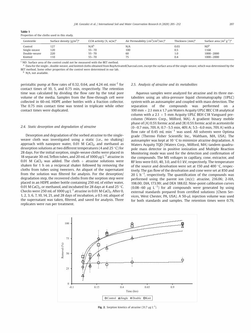
peristaltic pump at flow rates of 0.32, 0.64, and 4.24 mL min-1 forcontact times of 10, 5, and 0.75 min, respectively. The retentiontime was calculated by dividing the flow rate by the total porevolume of the media. Samples from the flow-through cell werecollected in 60-mL HDPE amber bottles with a fraction collector.The 0.75 min contact time was tested in triplicate while othercontact times were duplicated.
2.4. Static desorption and degradation of atrazine
Desorption and degradation of the sorbed atrazine to the single-weave cloth was investigated using a static (i.e., no shaking)approach with nanopore water, 0.01 M CaCl2, and methanol asdesorption solutions at two different temperatures (4 and 25 �C) for28 days. For the initial sorption, single-weave cloths were placed in18 separate 30-mLTeflon tubes, and 20mL of 1000 mg L-1 atrazine in0.01 M CaCl2 was added. The cloth þ atrazine solutions wereshaken for 1 h on a reciprocal shaker followed by removing thecloths from tubes using tweezers. An aliquot of the supernatantfrom the solution was filtered for analysis. For the desorption/degradation step, the recovered cloths from the sorption step wereplaced in an HDPE amber bottle containing 250 mL of either water,0.01M CaCl2, or methanol, and incubated for 28 days at 4 and 25 �C.Checks were 250 mL of 1000 mg L-1 atrazine in 0.01 M CaCl2. After 0,1, 2, 3, 6, 7, 10, 14, 21, and 28 days of incubation, a 0.5 mL aliquot ofthe supernatant was taken, filtered, and saved for analysis. Threereplicates were run per treatment.
2.5. Analysis of atrazine and its metabolites
Aqueous samples were analyzed for atrazine and its three me-tabolites using an ultra-pressure liquid chromatography (UPLC)systemwith an autosampler and coupled with mass detection. Theseparation of the compounds was performed on a100mm� 2.1mm x 1.7 mmWaters Acquity UPLC BEC C18 analyticalcolumn with a 2.1 � 5 mm Acquity UPLC BEH C18 Vanguard pre-column (Waters Corp., Milford, MA). A gradient binary mobilephase of (A) 0.5% formic acid and (B) 0.5% formic acid in acetonitrile(0e0.7 min, 70% A; 0.7e5.5 min, 40% A; 5.5e6.0 min, 70% A) with aflow rate of 0.45 mL min�1 was used. All solvents were Optimagrade (Thermo Fisher Scientific Inc., Waltham, MA, USA). Theautosampler was kept at 10 �C to minimize atrazine degradation. AWaters Acquity TQD (Waters Corp., Milford, MA) tandem quadru-pole mass detector in positive ionization and Multiple ReactionMonitoring mode was used for the detection and confirmation ofthe compounds. The MS voltages in capillary, cone, extractor, andRF lens were 0.61, 40, 3.0, and 0.1 kV, respectively. The temperatureof the source and desolvation were set at 150 and 400 �C, respec-tively. The gas flow of the desolvation and cone were set at 850 and20 L h�1, respectively. The quantification of the compounds wasperformed using the parent ion (m/z): atrazine, 216.06; 2-HA,198.00; DIA, 173.99; and DEA 188.02. Nine-point calibration curves(0.08e60 mg L�1) for all compounds were generated by usingexternal standards prepared from certified solutions (Chem Ser-vices, West Chester, PA, USA). A 50-mL injection volume was usedfor both standards and samples. The retention times were 0.79,
Table 1Properties of the cloths used in this study.
Geotextile Surface density (g/m2)a CCl4 activity (%, w/w)a Air Permeability (cm3/cm2/sec)a Thickness (mm)a Surface area (m2 g-1)a
Control 127 N/Ab N/A 0.03 NDb
Single-weave 120 55e70 100 0.5 1168Double-weave 220 55e70 60 1.0 1000e2000Knitted 110 55e70 75 0.4 1000e2000
c ND: Surface area of the control could not be measured with the BET method.a Data for the single-, double-weave, and knitted cloths obtained from BuyActivatedCharcoal.com, except the surface area of the single-weave, whichwas determined by the
BET method. Some other properties of the control were determined in our lab.b N/A, not available.
Fig. 2. Sorption kinetics of atrazine (31.7 mg L-1).
J.M. Gonzalez et al. / International Soil and Water Conservation Research 8 (2020) 205e212 207
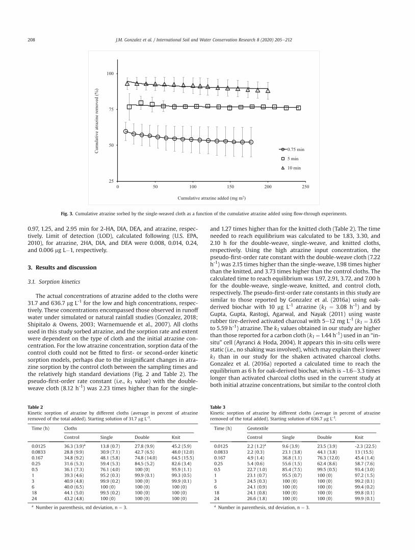
0.97, 1.25, and 2.95 min for 2-HA, DIA, DEA, and atrazine, respec-tively. Limit of detection (LOD), calculated following (U.S. EPA,2010), for atrazine, 2HA, DIA, and DEA were 0.008, 0.014, 0.24,and 0.006 mg L�1, respectively.
3. Results and discussion
3.1. Sorption kinetics
The actual concentrations of atrazine added to the cloths were31.7 and 636.7 mg L-1 for the low and high concentrations, respec-tively. These concentrations encompassed those observed in runoffwater under simulated or natural rainfall studies (Gonzalez, 2018;Shipitalo & Owens, 2003; Warnemuende et al., 2007). All clothsused in this study sorbed atrazine, and the sorption rate and extentwere dependent on the type of cloth and the initial atrazine con-centration. For the low atrazine concentration, sorption data of thecontrol cloth could not be fitted to first- or second-order kineticsorption models, perhaps due to the insignificant changes in atra-zine sorption by the control cloth between the sampling times andthe relatively high standard deviations (Fig. 2 and Table 2). Thepseudo-first-order rate constant (i.e., k1 value) with the double-weave cloth (8.12 h-1) was 2.23 times higher than for the single-
and 1.27 times higher than for the knitted cloth (Table 2). The timeneeded to reach equilibrium was calculated to be 1.83, 3.30, and2.10 h for the double-weave, single-weave, and knitted cloths,respectively. Using the high atrazine input concentration, thepseudo-first-order rate constant with the double-weave cloth (7.22h-1) was 2.15 times higher than the single-weave, 1.98 times higherthan the knitted, and 3.73 times higher than the control cloths. Thecalculated time to reach equilibriumwas 1.97, 2.91, 3.72, and 7.00 hfor the double-weave, single-weave, knitted, and control cloth,respectively. The pseudo-first-order rate constants in this study aresimilar to those reported by Gonzalez et al. (2016a) using oak-derived biochar with 10 mg L-1 atrazine (k1 ¼ 3.08 h-1) and byGupta, Gupta, Rastogi, Agarwal, and Nayak (2011) using wasterubber tire-derived activated charcoal with 5e12 mg L-1 (k1 ¼ 3.65to 5.59 h-1) atrazine. The k1 values obtained in our study are higherthan those reported for a carbon cloth (k1 ¼1.44 h-1) used in an “in-situ” cell (Ayranci & Hoda, 2004). It appears this in-situ cells werestatic (i.e., no shaking was involved), whichmay explain their lowerk1 than in our study for the shaken activated charcoal cloths.Gonzalez et al. (2016a) reported a calculated time to reach theequilibrium as 6 h for oak-derived biochar, which is ~1.6e3.3 timeslonger than activated charcoal cloths used in the current study atboth initial atrazine concentrations, but similar to the control cloth
Table 2Kinetic sorption of atrazine by different cloths (average in percent of atrazineremoved of the total added). Starting solution of 31.7 mg L-1.
Time (h) Cloths
Control Single Double Knit
0.0125 36.3 (3.9)a 13.8 (0.7) 27.8 (9.9) 45.2 (5.9)0.0833 28.8 (9.9) 30.9 (7.1) 42.7 (6.5) 48.0 (12.0)0.167 34.8 (9.2) 48.1 (5.8) 74.8 (14.0) 64.5 (15.5)0.25 31.6 (5.3) 59.4 (5.3) 84.5 (5.2) 82.6 (3.4)0.5 36.1 (7.3) 76.1 (4.0) 100 (0) 95.9 (1.1)1 39.3 (4.6) 95.2 (0.3) 99.9 (0.1) 99.3 (0.5)3 40.9 (4.8) 99.9 (0.2) 100 (0) 99.9 (0.1)6 40.0 (6.5) 100 (0) 100 (0) 100 (0)18 44.1 (5.0) 99.5 (0.2) 100 (0) 100 (0)24 43.2 (4.8) 100 (0) 100 (0) 100 (0)
a Number in parenthesis, std deviation, n ¼ 3.
Table 3Kinetic sorption of atrazine by different cloths (average in percent of atrazineremoved of the total added). Starting solution of 636.7 mg L-1.
Time (h) Geotextile
Control Single Double Knit
0.0125 2.2 (1.2)a 9.6 (3.9) 23.5 (3.9) -2.3 (22.5)0.0833 2.2 (0.3) 23.1 (3.8) 44.1 (3.8) 13 (15.5)0.167 4.9 (1.4) 36.8 (1.1) 76.3 (12.0) 45.4 (1.4)0.25 5.4 (0.6) 55.6 (1.5) 62.4 (8.6) 58.7 (7.6)0.5 22.7 (1.0) 85.4 (7.5) 99.5 (0.5) 93.4 (3.0)1 23.1 (0.7) 95.5 (0.7) 100 (0) 97.2 (1.5)3 24.5 (0.3) 100 (0) 100 (0) 99.2 (0.1)6 24.1 (0.9) 100 (0) 100 (0) 99.4 (0.2)18 24.1 (0.8) 100 (0) 100 (0) 99.8 (0.1)24 26.6 (1.8) 100 (0) 100 (0) 99.9 (0.1)
a Number in parenthesis, std deviation, n ¼ 3.
Fig. 3. Cumulative atrazine sorbed by the single-weaved cloth as a function of the cumulative atrazine added using flow-through experiments.
J.M. Gonzalez et al. / International Soil and Water Conservation Research 8 (2020) 205e212208
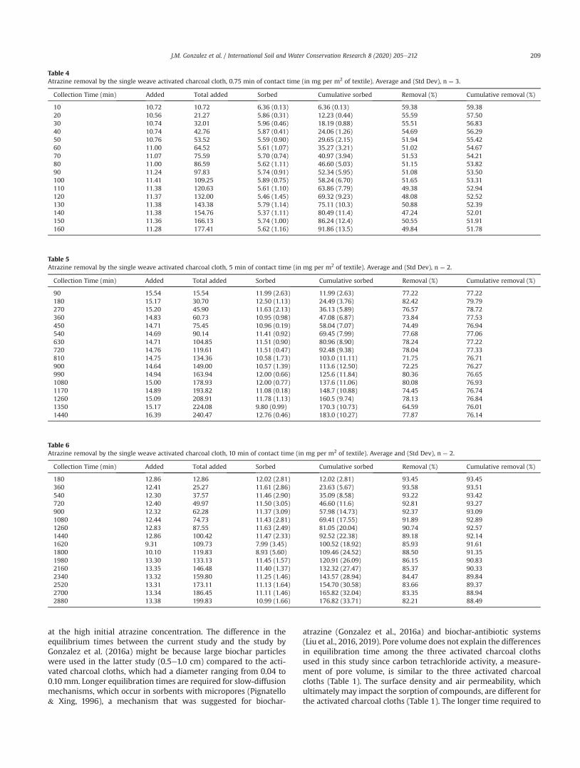
at the high initial atrazine concentration. The difference in theequilibrium times between the current study and the study byGonzalez et al. (2016a) might be because large biochar particleswere used in the latter study (0.5e1.0 cm) compared to the acti-vated charcoal cloths, which had a diameter ranging from 0.04 to0.10 mm. Longer equilibration times are required for slow-diffusionmechanisms, which occur in sorbents with micropores (Pignatello& Xing, 1996), a mechanism that was suggested for biochar-
atrazine (Gonzalez et al., 2016a) and biochar-antibiotic systems(Liu et al., 2016, 2019). Pore volume does not explain the differencesin equilibration time among the three activated charcoal clothsused in this study since carbon tetrachloride activity, a measure-ment of pore volume, is similar to the three activated charcoalcloths (Table 1). The surface density and air permeability, whichultimately may impact the sorption of compounds, are different forthe activated charcoal cloths (Table 1). The longer time required to
Table 4Atrazine removal by the single weave activated charcoal cloth, 0.75 min of contact time (in mg per m2 of textile). Average and (Std Dev), n ¼ 3.
Collection Time (min) Added Total added Sorbed Cumulative sorbed Removal (%) Cumulative removal (%)
10 10.72 10.72 6.36 (0.13) 6.36 (0.13) 59.38 59.3820 10.56 21.27 5.86 (0.31) 12.23 (0.44) 55.59 57.5030 10.74 32.01 5.96 (0.46) 18.19 (0.88) 55.51 56.8340 10.74 42.76 5.87 (0.41) 24.06 (1.26) 54.69 56.2950 10.76 53.52 5.59 (0.90) 29.65 (2.15) 51.94 55.4260 11.00 64.52 5.61 (1.07) 35.27 (3.21) 51.02 54.6770 11.07 75.59 5.70 (0.74) 40.97 (3.94) 51.53 54.2180 11.00 86.59 5.62 (1.11) 46.60 (5.03) 51.15 53.8290 11.24 97.83 5.74 (0.91) 52.34 (5.95) 51.08 53.50100 11.41 109.25 5.89 (0.75) 58.24 (6.70) 51.65 53.31110 11.38 120.63 5.61 (1.10) 63.86 (7.79) 49.38 52.94120 11.37 132.00 5.46 (1.45) 69.32 (9.23) 48.08 52.52130 11.38 143.38 5.79 (1.14) 75.11 (10.3) 50.88 52.39140 11.38 154.76 5.37 (1.11) 80.49 (11.4) 47.24 52.01150 11.36 166.13 5.74 (1.00) 86.24 (12.4) 50.55 51.91160 11.28 177.41 5.62 (1.16) 91.86 (13.5) 49.84 51.78
Table 5Atrazine removal by the single weave activated charcoal cloth, 5 min of contact time (in mg per m2 of textile). Average and (Std Dev), n ¼ 2.
Collection Time (min) Added Total added Sorbed Cumulative sorbed Removal (%) Cumulative removal (%)
90 15.54 15.54 11.99 (2.63) 11.99 (2.63) 77.22 77.22180 15.17 30.70 12.50 (1.13) 24.49 (3.76) 82.42 79.79270 15.20 45.90 11.63 (2.13) 36.13 (5.89) 76.57 78.72360 14.83 60.73 10.95 (0.98) 47.08 (6.87) 73.84 77.53450 14.71 75.45 10.96 (0.19) 58.04 (7.07) 74.49 76.94540 14.69 90.14 11.41 (0.92) 69.45 (7.99) 77.68 77.06630 14.71 104.85 11.51 (0.90) 80.96 (8.90) 78.24 77.22720 14.76 119.61 11.51 (0.47) 92.48 (9.38) 78.04 77.33810 14.75 134.36 10.58 (1.73) 103.0 (11.11) 71.75 76.71900 14.64 149.00 10.57 (1.39) 113.6 (12.50) 72.25 76.27990 14.94 163.94 12.00 (0.66) 125.6 (11.84) 80.36 76.651080 15.00 178.93 12.00 (0.77) 137.6 (11.06) 80.08 76.931170 14.89 193.82 11.08 (0.18) 148.7 (10.88) 74.45 76.741260 15.09 208.91 11.78 (1.13) 160.5 (9.74) 78.13 76.841350 15.17 224.08 9.80 (0.99) 170.3 (10.73) 64.59 76.011440 16.39 240.47 12.76 (0.46) 183.0 (10.27) 77.87 76.14
Table 6Atrazine removal by the single weave activated charcoal cloth, 10 min of contact time (in mg per m2 of textile). Average and (Std Dev), n ¼ 2.
Collection Time (min) Added Total added Sorbed Cumulative sorbed Removal (%) Cumulative removal (%)
180 12.86 12.86 12.02 (2.81) 12.02 (2.81) 93.45 93.45360 12.41 25.27 11.61 (2.86) 23.63 (5.67) 93.58 93.51540 12.30 37.57 11.46 (2.90) 35.09 (8.58) 93.22 93.42720 12.40 49.97 11.50 (3.05) 46.60 (11.6) 92.81 93.27900 12.32 62.28 11.37 (3.09) 57.98 (14.73) 92.37 93.091080 12.44 74.73 11.43 (2.81) 69.41 (17.55) 91.89 92.891260 12.83 87.55 11.63 (2.49) 81.05 (20.04) 90.74 92.571440 12.86 100.42 11.47 (2.33) 92.52 (22.38) 89.18 92.141620 9.31 109.73 7.99 (3.45) 100.52 (18.92) 85.93 91.611800 10.10 119.83 8.93 (5.60) 109.46 (24.52) 88.50 91.351980 13.30 133.13 11.45 (1.57) 120.91 (26.09) 86.15 90.832160 13.35 146.48 11.40 (1.37) 132.32 (27.47) 85.37 90.332340 13.32 159.80 11.25 (1.46) 143.57 (28.94) 84.47 89.842520 13.31 173.11 11.13 (1.64) 154.70 (30.58) 83.66 89.372700 13.34 186.45 11.11 (1.46) 165.82 (32.04) 83.35 88.942880 13.38 199.83 10.99 (1.66) 176.82 (33.71) 82.21 88.49
J.M. Gonzalez et al. / International Soil and Water Conservation Research 8 (2020) 205e212 209
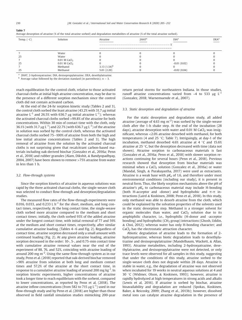
reach equilibration for the control cloth, relative to those activatedcharcoal cloths at initial high atrazine concentration, may be due tothe presence of a different sorption mechanism since the controlcloth did not contain activated carbon.
At the end of the 24-hr sorption kinetic study (Tables 2 and 3),the control cloth sorbed the least atrazine (43.2%with 31.7 mg initialatrazine L-1 and 26.5% with 636.7 mg initial atrazine L-1); whereasthe activated charcoal cloths sorbed >99.8% of the atrazine for bothconcentrations. Within 30 min of contact time with the cloth, only36.1% (with 31.7 mg L-1) and 22.7% (with 636.7 mg L-1) of the atrazinein solution was sorbed by the control cloth, whereas the activatedcharcoal cloths sorbed 75e100% of atrazine from both the high andlow initial atrazine concentrations (Tables 2 and 3). The highremoval of atrazine from the solution by the activated charcoalcloths is not surprising given that recalcitrant carbon-based ma-terials including oak-derived biochar (Gonzalez et al., 2016a; Pennet al., 2018) and rubber granules (Alam, Dikshit, & Bandyopadhyay,2004, 2007) have been shown to remove >75% atrazine fromwaterin less than 1 h.
3.2. Flow-through systems
Since the sorption kinetics of atrazine in aqueous solutions wasrapid by the three activated charcoal cloths, the single-weave clothwas selected to conduct flow-through and desorption/degradationstudies.
The measured flow rates of the flow-through experiments were0.016, 0.033, and 0.233 L h-1 for the short, medium, and long con-tact times, respectively. At the long contact time, the single-weavecloth sorbed more atrazine compared to the medium and shortcontact times; initially, the cloth sorbed 93% of the added atrazineunder the longest contact time, with initial removal of 77 and 59%at the medium and short contact times, respectively, after similarcumulative atrazine loading. (Tables 4e6 and Fig. 2). Regardless ofcontact time, atrazine sorption decreased only a small amount withcontinued loading (Fig. 2). At any given atrazine loading, atrazinesorption decreased in the order: 10-, 5-, and 0.75-min contact timewith cumulative atrazine removal values near the end of theexperiment of 88, 76, and 52%, coinciding with atrazine loading ofaround 200 mg m-2. Using the same flow-through system as in ourstudy, Penn et al. (2018) reported that oak-derived biochar removed>90% atrazine from solution at both long and medium contacttimes and 57.2% of the atrazine at the short contact time, inresponse to a cumulative atrazine loading of around 200 mg kg-1. Insorption kinetic experiments, higher concentrations of atrazinetook a longer time to reach equilibriumwith the sorbent, comparedto lower concentrations, as reported by Penn et al. (2018). Theatrazine inflow concentrations (from 582 to 715 mg L-1) used in ourflow-through study and by Penn et al. (2018) are higher than thoseobserved in field rainfall simulation studies mimicking 200-year
return period storms for northeastern Indiana. In those studies,runoff atrazine concentrations varied from ~4 to 533 mg L-1
(Gonzalez, 2018; Warnemuende et al., 2007).
3.3. Static desorption and degradation of atrazine
For the static desorption and degradation study, all addedatrazine (average of 4.63 mg m-2) was sorbed by the single-weavecloth after the 1-h shake step. At the end of the incubation (28days), atrazine desorption with water and 0.01 M CaCl2 was insig-nificant, whereas <2.0% atrazine desorbed with methanol, for bothtemperatures (4 and 25 �C; Table 7). Intriguingly, at day-1 of theincubation, methanol desorbed 4.6% atrazine at 4 �C and 15.6%atrazine at 25 �C, but the desorption decreased with time (data notshown). Atrazine sorption to carbonaceous materials is fast(Gonzalez et al., 2016a; Penn et al., 2018) with slower sorption re-actions continuing for several hours (Penn et al., 2018). Previousresearch showed that desorption from biochar materials wasminimal when a CaCl2 solution (Gonzalez et al., 2016a) or water(Mandal, Singh, & Purakayastha, 2017) were used as extractants.Atrazine is a weak base with pKa of 1.6, and therefore under mostenvironmental conditions (including our study), it is present inneutral form. Thus, the likely sorption mechanisms above the pH ofatrazine’s pKa to carbonaceous material may include H-bonding(both H-acceptor and -donor) and hydrophobic and p-p in-teractions (Laird & Koskinen, 2008; Penn et al., 2018). In this study,only methanol was able to desorb atrazine from the cloth, whichcould be explained by the solvation properties of the solvents usedin the static desorption step. Methanol is a stronger solvent fororganic molecules than water, and CaCl2 solution due to itsamphiphilic character, i.e., hydrophilic (H-donor and -acceptorbonding) and hydrophobic (CH3 group) interactions (Ghosh, Uddin,& Choi, 2012); whereas water has only H-bonding character; andCaCl2 has the electrostatic attraction character.
Abiotic degradation of atrazine leads to the formation of 2-hydroxyatrazine, whereas biotic degradation leads to desethyla-trazine and desisopropylatrazine (Mandelbaum, Wackett, & Allan,1993). Atrazine metabolites, including 2-hydroxyatrazine, dese-thylatrazine, and desisopropylatrazine were not detected, or onlytrace levels were observed for all samples in this study, suggestingthat under the conditions of this study, atrazine sorbed to thesingle-weave cloth does not degrade within 28 days. Atrazine isstable in water, e.g., the degradation of atrazine was not observedwhen incubated for 19 weeks in neutral aqueous solutions at 4 and30 �C (Widmer, Olson, & Koskinen, 1993); however, atrazine israpidly hydrolyzed at high temperatures in strong acids and alkalis(Lewis et al, 2016). If atrazine is sorbed by biochar, atrazinebioavailability and degradation are reduced (Spokas, Koskinen,Baker, & Reicosky, 2009; Zhang et al., 2013b); however, dissolvedmetal ions can catalyze atrazine degradation in the presence of
Table 7Average desorption of atrazine (% of the total atrazine sorbed) and degradation metabolites of atrazine (% of the total atrazine sorbed).
Temp. (◦C) Solution Atrazine 2HATa DIAa DEAa
————————————————————————————————— %——————————————————————————————————
7 Water 0 0 0 025 Water 0 0 0 07 0.01 M CaCl2 0 0 0 025 0.01 M CaCl2 0 0 -0.01 (0.02) 07 Methanol 3.13 (1.54)b 0 0 025 Methanol 5.01 (2.20) 0 -0.02 (0.04) 0
a 2HAT, 2-hydroxyatrazine; DIA, desisopropylatrazine; DEA, desethylatrazine.b Average value followed by the deviation standard (in parenthesis); n ¼ 3.
J.M. Gonzalez et al. / International Soil and Water Conservation Research 8 (2020) 205e212210

manure-derived biochar for 12 h (Zhang, Sun, Yu, & Sun, 2013a). Inour study, Al, Fe, Cu, and Mnwere detected in the cloths used (datanot shown); these metals were reported in solution by Zhang et al.(2013a). The results from the static desorption/degradation studysuggest that the atrazine sorbed by the cloths is strongly sorb andminimal atrazine may desorb and transport to waterways.
The kinetic sorption, static desorption/degradation, and flow-through results from this study suggest that activated charcoalcloths are effective materials to remove atrazine from aqueoussolutions. The fast removal of atrazine by the activated charcoal andthe insignificant desorption/degradation by water and CaCl2 solu-tion makes these materials suitable for atrazine removal from wa-ter. If these cloths are used in combinationwith biochar in pollutioncontrol structures, then the ability to remove atrazine from waterincreases significantly. However, there are several unknowns forthese cloths, including (1) their durability and (2) their maximumsorption capacity for atrazine. In this study, up to 200 mg of atra-zine was sorbed per sq meter of cloth using the flow-through(Table 5), but the material clearly possessed the ability to sorbhigher amounts of atrazine as cumulative sorption curves revealedthat they were still steadily removing atrazine at the end of theexperiment (i.e., little to no decrease in percent cumulativeremoval; Fig. 3). Using the flow-through equations developed byPenn and Bowen (2017), the maximum atrazine loading at a 10 mincontact time until becoming non-effective is 5.7 g m-2, corre-sponding to cumulative removal of 20.8%, or 1.18 g m-2 over thatcumulative loading. If the single-weave cloth is used in a blind inletstructure (4.25 m � 4.25 m) at a 10 min contact time, 21.3 g ofatrazine could be removed. Shipitalo and Owens (2003) reportedthat under no-till systems, from 0.38 to 6.50 g atrazine ha-1 werelost per growing season via surface runoff when atrazine wasapplied at 2.24 kg ha-1 to corn. Gonzalez (2018) reported atrazinelosses of 11 g ha-1 under no-till systems using rainfall simulations torepresent a stormwith a 200-year return period. Thus, a blind inletconstructed to treat runoff from 1 ha, using the activated charcoalcloth would last for nearly 16 years before becoming non-effective.For an initial cloth with no previous atrazine sorption, a blind inletwould remove 76% of the atrazine delivered in a 200-yr storm.Regardless of the cloth type to be used in blind inlets, furtherstudies are needed to determine the long-term fate of atrazinesorbed to the cloth.
4. Conclusions
In this study, the removal of atrazine in solution (31.7 and636.7 mg atrazine L-1) by activated charcoal cloths (single-weave,SW; double-weave, DW; and knitted, KT) was faster and higherthan the control cloth. Within 30 min and relative to the control,the removal of atrazine with the activated charcoal cloths increasedby 111e177% and by 277e340% (SW < KT <DW) at the low and highatrazine concentrations, respectively. Within 3 h, the activatedcharcoal cloths removed more than 99% of the atrazine in solution;whereas, the control cloth removed from 24 to 41% of the atrazinein solution. Under flow-through conditions, the longer the contacttime, the higher of atrazine removal by the cloth; the SW clothremoved 52.2, 76.1, and 88.2% at contact times of 0.75, 5, and10 min, respectively. Furthermore, the sorbed atrazine by the SWcloth did not degrade, and low amounts (<2% of the atrazine sor-bed) were desorbed with methanol in a 28-day incubation study.The results of this study indicate that activated charcoal cloths areeffective media for the removal of atrazine from aqueous solutions,and an alternative that may be used effectively in pollution controlstructures.
Disclaimer
USDA is an equal opportunity provider and employer. Mentionof trade names or commercial products in this publication is solelyfor the purpose of providing specific information and does notimply recommendation or endorsement by the US Department ofAgriculture.
This research did not receive any specific grant from fundingagencies in the public, commercial, or not-for-profit sectors.
Acknowledgments
The authors would like to thank the staff and students at theUSDA- ARS-NSERL and USDA-ARS-NCAUR.
References
Alam, J. B., Dikshit, A. K., & Bandyopadhyay, M. (2004). Sorption and desorption of2,4-D and atrazine from water environment by waste tyre rubber granules andits management. Global Nest Journal, 6, 105e115.
Alam, J. B., Dikshit, A. K., & Bandyopadhyay, M. (2007). Kinetic study of sorption of2,4-D and atrazine on rubber granules. Journal of Dispersion Science and Tech-nology, 28, 511e517.
Ayranci, E., & Hoda, N. (2004). Studies on removal of metribuzin, bromacil, 2,4-d and atrazine from water by adsorption on high area carbon cloth. Journal ofHazardous Materials, 112, 163e168.
Ayranci, E., & Hoda, N. (2005). Adsorption kinetics and isotherms of pesticides ontoactivated carbon-cloth. Chemosphere, 60, 1600e1607.
Boutron, O., Gouy, V., Touze-Foltz, N., Benoit, P., Chovelon, J. M., & Margoum, C.(2009). Geotextile fibres retention properties to prevent surface water nonpointcontamination by pesticides in agricultural areas. Geotextiles and Geo-membranes, 27, 254e261.
Derr, J. F., & Appleton, B. L. (1989). Weed control with landscape fabrics. Journal ofEnvironmental Horticulture, 7, 129e133.
Feyereisen, G. W., Francesconi, W., Smith, D. R., Papiernik, S. K., Krueger, E. S., &Wente, C. D. (2015). Effect of replacing surface inlets with blind or gravel inletson sediment and phosphorus subsurface drainage losses. Journal of Environ-mental Quality, 44, 594e604.
Frobel, R. K., Werner, G., & Wewerka, M. (1987). Geotextiles as filters in erosioncontrol, geotextile testing and the design engineer. ASTM International.
Ghosh, M. K., Uddin, N., & Choi, C. H. (2012). Hydrophobic and hydrophilic associ-ations of a methanol pair in aqueous solution. Journal of Physical Chemistry B,116, 14254e14260.
Gonzalez, J. M. (2018). Runoff and losses of nutrients and herbicides under long-termconservation practices (no-till and crop rotation) in the U.S. Midwest: A variableintensity simulated rainfall approach (Vol. 6, pp. 265e274).
Gonzalez, J. M., Shipitalo, M. J., Smith, D. R., Warnemuende-Pappas, E., &Livingston, S. J. (2016a). Atrazine sorption by biochar, tire chips, and steel slag asmedia for blind inlets: A kinetic and isotherm sorption approach (Vol. 8, p. 1266).
Gonzalez, J. M., Smith, D. R., Livingston, S., Warnemuende-Pappas, E., &Zwonitzer, M. (2016b). Blind inlets: Conservation practices to reduce herbicidelosses from closed depressional areas. Journal of Soils and Sediments, 16,1921e1932.
Gupta, V. K., Gupta, B., Rastogi, A., Agarwal, S., & Nayak, A. (2011). Pesticides removalfrom waste water by activated carbon prepared from waste rubber tire. WaterResearch, 45, 4047e4055.
Kloss, S., Zehetner, F., Dellantonio, A., Hamid, R., Ottner, F., Liedtke, V., et al. (2012).Characterization of slow pyrolysis biochars: Effects of feedstocks and pyrolysistemperature on biochar properties. Journal of Environmental Quality, 41,990e1000.
Krull, E. S., Baldock, J. A., Skjemstad, J. O., & Smernik, R. J. (2009). Characteristics ofbiochar: Organo-chemical properties. In J. Lehmann, & S. Joseph (Eds.), Biocharfor environmental management: Science and technology.
Laird, D. A., & Koskinen, W. C. (2008). Chapter 21 - triazine soil interactions. InM. L. Homer, E. M. Janis, & O. C. Burnside (Eds.), The triazine herbicides (pp.275e299). San Diego: Elsevier.
Lewis, K. A., Tzilivakis, J., Warner, D., & Green, A. (2016). An international databasefor pesticide risk assessments and management. Human and Ecological RiskAssessment: An International Journal, 22, 1050e1064.
Liu, C.-H., Chuang, Y.-H., Li, H., Boyd, S. A., Teppen, B. J., Gonzalez, J. M., et al. (2019).Long-term sorption of lincomycin to biochars: The intertwined roles of porediffusion and dissolved organic carbon. Water Research, 161, 108e118.
Liu, C.-H., Chuang, Y.-H., Liu, H., Teppen, B., Boyd, S., Gonzalez, J., et al. (2016).Sorption of lincomycin by manure-derived biochars from water. Journal ofEnvironmental Quality, 45, 519e527.
Mandal, A., Singh, N., & Purakayastha, T. J. (2017). Characterization of pesticidesorption behaviour of slow pyrolysis biochars as low cost adsorbent for atrazineand imidacloprid removal. The Science of the Total Environment, 577, 376e385.
Mandelbaum, R. T., Wackett, L. P., & Allan, D. L. (1993). Rapid hydrolysis of atrazineto hydroxyatrazine by soil bacteria. Environmental Science & Technology, 27,
J.M. Gonzalez et al. / International Soil and Water Conservation Research 8 (2020) 205e212 211

1943e1946.Mohammad, S. G., & Ahmed, S. M. (2017). Preparation of environmentally friendly
activated carbon for removal of pesticide from aqueous media. InternationalJournal of Industrial Chemistry, 8, 121e132.
NASS. (2016). In N. A. S. Service (Ed.), Agricultural chemical usage. Field crop sum-mary. Washington, DC: USDA- National Agricultural Statistics Service. Online.
Penn, Chad, J, & Bowen, J. M. (2017). Design and construction of phosphorus removalstructures for improving water quality. Cham, Switzerland: Springer Interna-tional Publishing AG.
Penn, C. J., Gonzalez, J. M., & Chagas, I. (2018). Investigation of atrazine sorption tobiochar with titration calorimetry and flow-through analysis: Implications fordesign of pollution-control structures (Vol. 6).
Pignatello, J. J., & Xing, B. (1996). Mechanisms of slow sorption of organic chemicalsto natural particles. Environmental Science & Technology, 30, 1e11.
Shipitalo, M. J., & Owens, L. B. (2003). Atrazine, deethylatrazine, and deisopropy-latrazine in surface runoff from conservation tilled watersheds. EnvironmentalScience & Technology, 37, 944e950.
Smith, D. R., & Livingston, S. J. (2013). Managing farmed closed depressional areasusing blind inlets to minimize phosphorus and nitrogen losses. Soil Use &Management, 29, 94e102.
Spokas, K. A., Koskinen, W. C., Baker, J. M., & Reicosky, D. C. (2009). Impacts ofwoodchip biochar additions on greenhouse gas production and sorption/degradation of two herbicides in a Minnesota soil. Chemosphere, 77, 574e581.
Tseng, R.-L., Wu, P.-H., Wu, F.-C., & Juang, R.-S. (2014). A convenient method todetermine kinetic parameters of adsorption processes by nonlinear regressionof pseudo-nth-order equation. Chemical Engineering Journal, 237, 153e161.
USEPA. (2009). National primary drinking water regulations. USEPA.U.S. EPA. (2010). Lowest concentration minimum reporting level (LCMRL) calculator.
U.S. EPA.Warnemuende, E. A., Patterson, J. P., Smith, D. R., & Huang, C.-h. (2007). Effects of
tilling no-till soil on losses of atrazine and glyphosate to runoff water undervariable intensity simulated rainfall. Soil and Tillage Research, 95, 19e26.
Widmer, S. K., Olson, J. M., & Koskinen, W. C. (1993). Kinetics of atrazine hydrolysisin water. Journal of Environmental Science & Health Part B, 28, 19e28.
Zhang, P., Sun, H., Yu, L., & Sun, T. (2013a). Adsorption and catalytic hydrolysis ofcarbaryl and atrazine on pig manure-derived biochars: Impact of structuralproperties of biochars. Journal of Hazardous Materials, 244e245, 217e224.
Zhang, X., Wang, H., He, L., Lu, K., Sarmah, A., Li, J., et al. (2013b). Using biochar forremediation of soils contaminated with heavy metals and organic pollutants.Environmental Science & Pollution Research, 20, 8472e8483.
J.M. Gonzalez et al. / International Soil and Water Conservation Research 8 (2020) 205e212212
INTRODUCTION
Types of paper Contributions falling into the following categories will be considered for publication: Original research papers, reviews, letters to the editor.
Please ensure that you select the appropriate article type from the list of options when making your submission. Authors contributing to special issues should ensure that they select the special issue article type from this list.
BEFORE YOU BEGIN
Ethics in Publishing For information on Ethics in Publishing and Ethical guidelines for journal publication see http://www.elsevier.com/publishingethics and http://www.elsevier.com/ethicalguidelines.
Confl ict of interest All authors are requested to disclose any actual or potential conf ict of interest including any f nancial, personal or other relationships with other people or organizations within three years of beginning the submitted work that could inappropriately inf uence, or be perceived to inf uence, their work. See also http://www.elsevier.com/conf ictsof nterest.
Submission declaration Submission of an article implies that the work described has not been published previously (except in the form of an abstract or as part of a published lecture or academic thesis), that it is not under consideration for publication elsewhere, that its publication is approved by all authors and tacitly or explicitly by the responsible authorities where the work was carried out, and that, if accepted, it will not be published elsewhere including electronically in the same form, in English or in any other language, without the written consent of the copyright-holder.
Changes to authorship This policy concerns the addition, deletion, or rearrangement of author names in the authorship of accepted manuscripts:
Before the accepted manuscript is published in an online issue: Requests to add or remove an author, or to rearrange the author names, must be sent to the Journal Manager from the corresponding author of the accepted manuscript and must include: (a) the reason the name should be added or removed, or the author names rearranged and (b) written conf rmation (e-mail, fax, letter) from all authors that they agree with the addition, removal or rearrangement. In the case of addition or removal of authors, this includes conf rmation from the author being added or removed. Requests that are not sent by the corresponding author will be forwarded by the Journal Manager to the corresponding author, who must follow the procedure as described above. Note that: (1) Journal Managers will inform the Journal Editors of any such requests and (2) publication of the accepted manuscript in an online issue is suspended until authorship has been agreed.
After the accepted manuscript is published in an online issue: Any requests to add, delete, or rearrange author names in an article published in an online issue will follow the same policies as noted above and result in a corrigendum.
Copyright [example: Upon acceptance of an article, authors will be asked to complete a ‘Journal Publishing Agreement’. Acceptance of the agreement will ensure the widest possible dissemination of information. An e-mail will be sent to the corresponding author conf rming receipt of the manuscript together with a ‘Journal Publishing Agreement’ form or a link to the online version of this agreement.
Permission of the International Research and Training Center on Erosion and Sedimentation or the China Water and Power Press is required for resale or distribution outside the institution and for all other derivative works, including compilations and translations (please consult [email protected] or [email protected]). If excerpts from other copyrighted works are included, the author(s) must obtain written permission from the copyright owners and credit the source(s) in the article.]
Role of the funding source You are requested to identify who provided f nancial support for the conduct of the research and/or preparation of the article and to brief y describe the role of the sponsor(s), if any, in study design; in the collection, analysis and interpretation of data; in the writing of the report; and in the decision to submit the paper for publication. If the funding source(s) had no such involvement then this should be stated. Please see http://www.elsevier.com/funding.
Language and language services Please write your text in good English (American or British usage is accepted, but not a mixture of these). Authors who require information about language editing and copyediting services pre- and post-submission please visit http://webshop.elsevier.com/languageediting or our customer support site at http://support.elsevier.com for more information.
Submission Submission to this journal proceeds totally online. Use the following guidelines to prepare your article. Via the homepage of this journal (http://www.evise.com/evise/faces/pages/navigation/NavController.jspx?JRNL_ACR=ISWCR) you will be guided stepwise through the creation and uploading of the various f les. The system automatically converts source f les to a single Adobe Acrobat PDF version of the article, which is used in the peer-review process. Please note that even though manuscript source f les are converted to PDF at submission for the review process, these source f les are needed for further processing after acceptance. All correspondence, including notif cation of the Editor’s decision and requests for revision, takes place by e-mail and via the author’s homepage, removing the need for a hard-copy paper trail. If you are unable to provide an electronic version, please contact the editorial off ce prior to submission [example: e-mail: [email protected] or [email protected]; telephone: +86 10 68786416; or fax: 86 10 68411174].
Additional Information Tables and f gures may be presented with captions within the main body of the manuscript; if so, f gures should additionally be uploaded as high resolution f les.
PREPARATION
Use of wordprocessing software It is important that the f le be saved in the native format of the wordprocessor used. The text should be in single-column format. Keep the layout of the text as simple as possible. Most formatting codes will be removed and replaced on processing the article. In particular, do not use the wordprocessor’s options to justify text or to hyphenate words. However, do use bold face, italics, subscripts, superscripts etc. When preparing tables, if you are using a table grid, use only one grid for each individual table and not a grid for each row. If no grid is used, use tabs, not spaces, to align columns. The electronic text should be prepared in a way very similar to that of conventional manuscripts (see also the Guide to Publishing with Elsevier: http://www.elsevier.com/guidepublication). Note that source f les of f gures, tables and text graphics will be required whether or not you embed your f gures in the text. See also the section on Electronic illustrations.
GUIDE FOR AUTHORS
To avoid unnecessary errors you are strongly advised to use the “spell-check” and “grammar-check” functions of your wordprocessor.
LaTeX If the LaTeX f le is suitable, proofs will be produced without rekeying the text. The article should preferably be written using Elsevier’s document class “elsarticle”, or alternatively any of the other recognized classes and formats supported in Elsevier’s electronic submissions system, for further information see http://www.elsevier.com/wps/f nd/authorsview.authors/latex-ees-supported.
The Elsevier “elsarticle” LaTeX style f le package (including detailed instructions for LaTeX preparation) can be obtained from the Quickguide: http://www.elsevier.com/latex. It consists of the f le: elsarticle.cls, complete user documentation for the class f le, bibliographic style f les in various styles, and template f les for a quick start.
Article structure Subdivision - numbered sections Divide your article into clearly def ned and numbered sections. Subsections should be numbered 1.1 (then 1.1.1, 1.1.2, ...), 1.2, etc. (the abstract is not included in section numbering). Use this numbering also for internal cross-referencing: do not just refer to “the text”. Any subsection may be given a brief heading. Each heading should appear on its own separate line.
Introduction State the objectives of the work and provide an adequate background, avoiding a detailed literature survey or a summary of the results.
Material and methods Provide suff cient detail to allow the work to be reproduced. Methods already published should be indicated by a reference: only relevant modif cations should be described.
Theory/calculation A Theory section should extend, not repeat, the background to the article already dealt with in the Introduction and lay the foundation for further work. In contrast, a Calculation section represents a practical development from a theoretical basis.
Results Results should be clear and concise.
Discussion This should explore the signif cance of the results of the work, not repeat them. A combined Results and Discussion section is often appropriate. Avoid extensive citations and discussion of published literature.
Conclusions The main conclusions of the study may be presented in a short Conclusions section, which may stand alone or form a subsection of a Discussion or Results and Discussion section.
Appendices If there is more than one appendix, they should be identif ed as A, B, etc. Formulae and equations in appendices should be given separate numbering: Eq. (A.1), Eq. (A.2), etc.; in a subsequent appendix, Eq. (B.1) and so on. Similarly for tables and f gures: Table A.1; Fig. A.1, etc.
Essential title page information • Title. Concise and informative. Titles are often used in information-
retrieval systems. Avoid abbreviations and formulae where possible.• Author names and affi liations. Where the family name may
be ambiguous (e.g., a double name), please indicate this clearly. Present the authors’ aff liation addresses (where the actual work was done) below the names. Indicate all aff liations with a lower-case superscript letter immediately after the author’s name
and in front of the appropriate address. Provide the full postal address of each aff liation, including the country name, and, if available, the e-mail address of each author.
• Corresponding author. Clearly indicate who will handle correspondence at all stages of refereeing and publication, also post-publication. Ensure that telephone and fax numbers (with country and area code) are provided in addition to the e-mail address and the complete postal address. Contact details must be kept up to date by the corresponding author.
• Present/permanent address. If an author has moved since the work described in the article was done, or was visiting at the time, a “Present address” (or “Permanent address”) may be indicated as a footnote to that author’s name. The address at which the author actually did the work must be retained as the main, aff liation address. Superscript Arabic numerals are used for such footnotes.
Abstract A concise and factual abstract is required. The abstract should state brief y the purpose of the research, the principal results and major conclusions. An abstract is often presented separately from the article, so it must be able to stand alone. For this reason, References should be avoided, but if essential, then cite the author(s) and year(s). Also, non-standard or uncommon abbreviations should be avoided, but if essential they must be def ned at their f rst mention in the abstract itself.
Keywords Authors are invited to submit keywords associated with their paper.
Abbreviations Def ne abbreviations that are not standard in this f eld in a footnote to be placed on the f rst page of the article. Such abbreviations that are unavoidable in the abstract must be def ned at their f rst mention there, as well as in the footnote. Ensure consistency of abbreviations throughout the article.
Acknowledgements Collate acknowledgements in a separate section at the end of the article before the references and do not, therefore, include them on the title page, as a footnote to the title or otherwise. List here those individuals who provided help during the research (e.g., providing language help, writing assistance or proof reading the article, etc.).
Nomenclature and units Follow internationally accepted rules and conventions: use the international system of units (SI). If other quantities are mentioned, give their equivalent in SI. Authors wishing to present a table of nomenclature should do so on the second page of their manuscript.
Math formulae Present simple formulae in the line of normal text where possible and use the solidus (/) instead of a horizontal line for small fractional terms, e.g., X/Y. In principle, variables are to be presented in italics. Powers of e are often more conveniently denoted by exp. Number consecutively any equations that have to be displayed separately from the text (if referred to explicitly in the text).
Footnotes Footnotes should be used sparingly. Number them consecutively throughout the article, using superscript Arabic numbers. Many wordprocessors build footnotes into the text, and this feature may be used. Should this not be the case, indicate the position of footnotes in the text and present the footnotes themselves separately at the end of the article. Do not include footnotes in the Reference list.
Table footnotes Indicate each footnote in a table with a superscript lowercase letter.
Artwork Electronic artwork General points • Make sure you use uniform lettering and sizing of your original
artwork. • Save text in illustrations as “graphics” or enclose the font. • Only use the following fonts in your illustrations: Arial, Courier,
Times, Symbol. • Number the illustrations according to their sequence in the text. • Use a logical naming convention for your artwork f les. • Provide captions to illustrations separately. • Produce images near to the desired size of the printed version. • Submit each f gure as a separate f le.
A detailed guide on electronic artwork is available on our website: http://www.elsevier.com/artworkinstructions
You are urged to visit this site; some excerpts from the detailed information are given here.
Formats Regardless of the application used, when your electronic artwork is f nalised, please “save as” or convert the images to one of the following formats (note the resolution requirements for line drawings, halftones, and line/halftone combinations given below):
EPS: Vector drawings. Embed the font or save the text as “graphics”. TIFF: color or grayscale photographs (halftones): always use a minimum of 300 dpi. TIFF: Bitmapped line drawings: use a minimum of 1000 dpi. TIFF: Combinations bitmapped line/half-tone (color or grayscale): a minimum of 500 dpi is required.
If your electronic artwork is created in a Microsoft Off ce application (Word, PowerPoint, Excel) then please supply “as is”.
Please do not: • Supply f les that are optimised for screen use (like GIF, BMP, PICT,
WPG); the resolution is too low; • Supply f les that are too low in resolution; • Submit graphics that are disproportionately large for the content.
Color artwork Please make sure that artwork f les are in an acceptable format (TIFF, EPS or MS Off ce f les) and with the correct resolution. If, together with your accepted article, you submit usable color f gures then Elsevier will ensure, at no additional charge, that these f gures will appear in color on the Web (e.g., ScienceDirect and other sites) regardless of whether or not these illustrations are reproduced in color in the printed version.
Figure captions Ensure that each illustration has a caption. Supply captions separately, not attached to the f gure. A caption should comprise a brief title (not on the f gure itself) and a description of the illustration. Keep text in the illustrations themselves to a minimum but explain all symbols and abbreviations used.
Tables Number tables consecutively in accordance with their appearance in the text. Place footnotes to tables below the table body and indicate them with superscript lowercase letters. Avoid vertical rules. Be sparing in the use of tables and ensure that the data presented in tables do not duplicate results described elsewhere in the article.
References Citation in text Please ensure that every reference cited in the text is also present in the reference list (and vice versa). Any references cited in the abstract must be given in full. Unpublished results and personal
communications are not recommended in the reference list, but may be mentioned in the text. If these references are included in the reference list they should follow the standard reference style of the journal and should include a substitution of the publication date with either “Unpublished results” or “Personal communication” Citation of a reference as “in press” implies that the item has been accepted for publication.
Web references As a minimum, the full URL should be given and the date when the reference was last accessed. Any further information, if known (DOI, author names, dates, reference to a source publication, etc.), should also be given. Web references can be listed separately (e.g., after the reference list) under a different heading if desired, or can be included in the reference list.
References in a special issue Please ensure that the words ‘this issue’ are added to any references in the list (and any citations in the text) to other articles in the same Special Issue.
Reference management software This journal has standard templates available in key reference management packages EndNote (http://www.endnote.com/support/enstyles.asp) and Reference Manager (http://refman.com/support/rmstyles.asp). Using plug-ins to wordprocessing packages, authors only need to select the appropriate journal template when preparing their article and the list of references and citations to these will be formatted according to the journal style which is described below.
Reference style The International Soil and Water Conservation Research (ISWCR) follows the Publication Manual of the American Psychological Association (APA) 6th for reference lists and text citation. The author are referred to the Publication Manual of the American Psychological Association, Fifth Edition, ISBN 1-55798-790-4, copies of which may be ordered from http://www.apa.org/books/4200061.html or APA Order Dept., P.O.B. 2710, Hyattsville, MD 20784, USA. or APA, 3 Henrietta Street, London, WC3E 8LU, UK. Details concerning this referencing style can also be found at http://humanities.byu.edu/linguistics/Henrichsen/APA/APA01.html.
Examples: Text: All citations in the text should refer to:
One author –Smith (2002) found…–(Smith, 2002).
Two Authors:–Smith and Jones (2003) found…–(Smith & Jones, 2003).
Three or More Authors–Smith et al. (2001) found…- (Phelps et al., 2004)–Smith et al. (2002) found…
Groups as Authors:–1st Citation: (American Psychological Association [APA], 2000).–Subsequent Citations:(APA, 2000).
Anonymous or No Author–Use fi rst few words of reference list entry (usually title):(—Study Finds, 1995)(TEA, 2007)
Authors with Same Surname–Include initials: S. T. Smith (2000) and J. D. Smith (1999)
Two of more works within the same parentheses–In order alphabetically, as they would appear in references, separated by semi-colons (Jones, 2003; Thomas, 2010)–If by same author, then by date(Jones, 2003, 2007)
References should be arranged f rst alphabetically and then further sorted chronologically if necessary. More than one reference from the same author(s) in the same year must be identif ed by the letters “a”, “b”, “c”, etc., placed after the year of publication
Reference to a journal publication Carlson, L. A. (2003). Existential theory: Helping school counselors attend to youth at risk for violence. Professional School Counseling, 6(5), 10-15.
Sagarin, B. J., & Lawler-Sagarin, K. A. (2005). Critically evaluating competing theories: An exercise based on the Kitty Genovese murder. Teaching of Psychology, 32(3), 167–169.
Hughes, J. C., Brestan, E. V., & Valle, L. A. (2004). Problem-solving interactions between mothers and children. Child and Family Behavior Therapy, 26(1), 1-16.
Journal with more than seven authorsGilbert, D. G., McCleron, J. F., Rabinovich, N. E., Sugai, C., Plath, L. C., Asgaard, G., Botros, N. (2004). Effects of quitting smoking on EEG activation and attendtionlast for more than 31 days and are more severe with stress. Nicotine and Tobacco Research, 6, 249-267.
Herbst-Damm, K.L., & Kulik, J.A. (2005). Volunteer support, marital status, and the survival times of terminally ill patients. Health Psychology, 24, 225-229. doi: 10.1037/0278-6133.24.2.225
Silick, T.J., & Schutte, N.S. (2006). Emotional intelligence and self-esteem mediate between perceived early parental love and adult happiness. E-Journal of Applied Psychology, 2(2), 38-48. Retrieved from http://ojs.lib.swin.edu.au/index.php/ejap.
Reference to a bookBeck, C. A. J., & Sales, B. D. (2001). Family mediation: Facts, myths, and future prospects. Washington, DC: American Psychological Association.
Johnson, R. A. (1989). Retrieval inhibition as an adaptive mechanism in human memory. In H. L. RoedigerIII & F. I. M. Craik(Eds.), Varieties of memory & consciousness (pp. 309-330). Hillsdale, NJ: Erlbaum.
English translation of a book:Lang, P. S. (1951). A philosophical essay on probabilities (F. W. Truscott & F. L. Emory, Trans.). New York, NY: Dover. (Original work published 1814)
*In text, cite original date and translation date: (Lang, 1814/1951).
Dissertations and ThesesCaprette, C. L. (2005). Conquering the cold shudder: The origin and evolution of snake eyes (Doctoral dissertation). Ohio State University, Columbus, OH.
Pecore, J. T. (2004). Sounding the spirit of Cambodia: The living tradition of Khmer music and dance-drama in a Washington, DC community (Doctoral dissertation). Retrieved from Dissertations and Theses database. (UMI No. 3114720)
Caprette, C. L. (2005). Conquering the cold shudder: The origin and evolution of snake eyes (Doctoral dissertation). Retrieved from http://www.ohiolink.edu/etd/send-pdf.cgi?acc_num=osu1111184984
Online resource from group/governmentU.S. Department of Health and Human Services. (2003). Managing asthma: A guide for schools. Retrieved from http://www.nhibi.nih.gov/health/prof/lung/asthma/asth_sch.pdf
Reference in other Language Hughes, J. C., Brestan, E. V., & Valle, L. A. (2004). Problem-solving interactions between mothers and children. Child and Family Behavior Therapy, 26(1), 1-16. (In Chinese)
Journal abbreviations source Journal names should be abbreviated according to Index Medicus journal abbreviations: http://www.nlm.nih.gov/tsd/serials/lji.html; List of title word abbreviations: http://www.issn.org/2-22661-LTWA-online.php; CAS (Chemical Abstracts Service): http://www.cas.org/sent.html.
Submission checklist The following list will be useful during the f nal checking of an article prior to sending it to the journal for review. Please consult this Guide for Authors for further details of any item.
Ensure that the following items are present: One Author designated as corresponding Author: • E-mail address • Full postal address • Telephone and fax numbers
All necessary f les have been uploaded • Keywords • All f gure captions • All tables (including title, description, footnotes)
Further considerations • Manuscript has been “spellchecked” and “grammar-checked” • References are in the correct format for this journal • All references mentioned in the Reference list are cited in the text,
and vice versa • Permission has been obtained for use of copyrighted material from
other sources (including the Web) • Color f gures are clearly marked as being intended for color
reproduction on the Web (free of charge) and in print or to be reproduced in color on the Web (free of charge) and in black-and-white in print
• If only color on the Web is required, black and white versions of the f gures are also supplied for printing purposes
For any further information please visit our customer support site at http://support.elsevier.com.
AFTER ACCEPTANCE
Use of the Digital Object Identifi er The Digital Object Identif er (DOI) may be used to cite and link to electronic documents. The DOI consists of a unique alpha-numeric character string which is assigned to a document by the publisher upon the initial electronic publication. The assigned DOI never changes. Therefore, it is an ideal medium for citing a document, particularly ‘Articles in press’ because they have not yet received their full bibliographic information. The correct format for citing a DOI is shown as follows (example taken from a document in the journal Physics Letters B): doi:10.1016/j.physletb.2010.09.059 When you use the DOI to create URL hyperlinks to documents on the web, they are guaranteed never to change.
Proofs One set of page proofs (as PDF f les) will be sent by e-mail to the corresponding author (if we do not have an e-mail address then paper
proofs will be sent by post) or, a link will be provided in the e-mail so that authors can download the f les themselves. Elsevier now provides authors with PDF proofs which can be annotated; for this you will need to download Adobe Reader version 7 (or higher) available free from http://get.adobe.com/reader. Instructions on how to annotate PDF f les will accompany the proofs (also given online). The exact system requirements are given at the Adobe site: http://www.adobe.com/products/reader/systemreqs.
If you do not wish to use the PDF annotations function, you may list the corrections (including replies to the Query Form) and return them to Elsevier in an e-mail. Please list your corrections quoting line number. If, for any reason, this is not possible, then mark the corrections and any other comments (including replies to the Query Form) on a printout of your proof and return by fax, or scan the pages and e-mail, or by post. Please use this proof only for checking the typesetting, editing, completeness and correctness of the text, tables and f gures. Signif cant changes to the article as accepted for publication will only be considered at this stage with permission from the Editor. We will do everything possible to get your article published quickly and accurately – please let us have all your corrections within 72 hours. It is important to ensure that all corrections are sent back to us in one communication: please check carefully before replying, as inclusion of any subsequent corrections cannot be guaranteed. Proofreading is solely your responsibility. Note that Elsevier may proceed with the publication of your article if no response is received.
Offprints The corresponding author, at no cost, will be provided with a PDF f le of the article via e-mail. For an extra charge, paper offprints can be ordered via the offprint order form which is sent once the article is accepted for publication. The PDF f le is a watermarked version of the published article and includes a cover sheet with the journal cover image and a disclaimer outlining the terms and conditions of use.
More information about article offprint is available here: http://webshop.elsevier.com/
AUTHOR INQUIRIES
For inquiries relating to the submission of articles (including electronic submission) please visit this journal’s homepage. Contact details for questions arising after acceptance of an article, especially those relating to proofs, will be provided by the publisher. You can track accepted articles at http://www.elsevier.com/trackarticle. You can also check our Author FAQs (http://www.elsevier.com/authorFAQ) and/or contact Customer Support via http://support.elsevier.com.

Copyright © 2022 FDOKUMEN