
International Journal of computational Engineering Research ...
203
International Journal of computational Engineering Research (IJCER) ISSN: 2250-3005 VOLUME 2 July-August 2012 ISSUE 4 Email: [email protected] Url : www.ijceronline.com International Journal of computational Engineering Research (IJCER)
-
Upload
khangminh22 -
Category
Documents
-
view
0 -
download
0
Transcript of International Journal of computational Engineering Research ...

International Journal of computational Engineering
Research (IJCER) ISSN: 2250-3005
VOLUME 2 July-August 2012 ISSUE 4
Email: [email protected] Url : www.ijceronline.com
International Journal of computational Engineering
Research (IJCER)

Editorial Board
Editor-In-Chief
Prof. Chetan Sharma Specialization: Electronics Engineering, India
Qualification: Ph.d, Nanotechnology, IIT Delhi, India
Editorial Committees
DR.Qais Faryadi
Qualification: PhD Computer Science
Affiliation: USIM(Islamic Science University of Malaysia)
Dr. Lingyan Cao
Qualification: Ph.D. Applied Mathematics in Finance
Affiliation: University of Maryland College Park,MD, US
Dr. A.V.L.N.S.H. HARIHARAN
Qualification: Phd Chemistry
Affiliation: GITAM UNIVERSITY, VISAKHAPATNAM, India
DR. MD. MUSTAFIZUR RAHMAN
Qualification: Phd Mechanical and Materials Engineering
Affiliation: University Kebangsaan Malaysia (UKM)
Dr. S. Morteza Bayareh
Qualificatio: Phd Mechanical Engineering, IUT
Affiliation: Islamic Azad University, Lamerd Branch
Daneshjoo Square, Lamerd, Fars, Iran
Dr. Zahéra Mekkioui
Qualification: Phd Electronics
Affiliation: University of Tlemcen, Algeria
Dr. Yilun Shang
Qualification: Postdoctoral Fellow Computer Science
Affiliation: University of Texas at San Antonio, TX 78249
Lugen M.Zake Sheet
Qualification: Phd, Department of Mathematics
Affiliation: University of Mosul, Iraq
Mohamed Abdellatif
Qualification: PhD Intelligence Technology

Affiliation: Graduate School of Natural Science and Technology
Meisam Mahdavi
Qualification: Phd Electrical and Computer Engineering
Affiliation: University of Tehran, North Kargar st. (across the ninth lane), Tehran, Iran
Dr. Ahmed Nabih Zaki Rashed
Qualification: Ph. D Electronic Engineering
Affiliation: Menoufia University, Egypt
Dr. José M. Merigó Lindahl
Qualification: Phd Business Administration
Affiliation: Department of Business Administration, University of Barcelona, Spain
Dr. Mohamed Shokry Nayle
Qualification: Phd, Engineering
Affiliation: faculty of engineering Tanta University Egypt
Contents : S.No. Title Name Page No.
1 Performance Evaluation and Model Using DSDV and DSR routing in
Ad-hoc network
Chetan adhikary, Dr. HB Bhuvaneswari, Prof K. Jayaraman
977-980
2 Determine the Fatigue behavior of engine damper caps screw bolt
R. K. Misra 981-990
3 Removal of Impulse Noise Using Eodt with Pipelined ADC
Prof.Manju Devi, Prof.Muralidhara, Prasanna R Hegde 991-996
4 Analysis of Handover in Wimax for Ubiquitous connectivity
Pooja bhat, Bijender mehandia 997-1000
5 Dampening Flow Induced Vibration Due To Branching Of Duct at
Elbow
M.Periasamy, D.B.Sivakumar, Dr. T. Senthil Kumar
1001-1004
6 Location Aware Routing in Intermittently Connected MANETs
Sadhana V, Ishthaq Ahmed K 1005-1011
7 Three Bad Assumptions: Why Technologies for Social Impact Fail
S. Revi Sterling John K. Bennett 1012-1015
8 Solution of Fuzzy Games with Interval Data Using Approximate Method
Dr.C.Loganathan & M.S.Annie Christi 1016-1019
9 Low Power Glitch Free Modeling in Vlsi Circuitry Using Feedback
Resistive Path Logic
Dr M.ASHARANI N.CHANDRASEKHAR, R.SRINIVASA RAO
1020-1025
10
To Find Strong Dominating Set and Split Strong Dominating Set of an
Interval Graph Using an Algorithm
Dr. A. Sudhakaraiah, V. Rama Latha, E. Gnana Deepika,
T.Venkateswarulu
1026-1034
11 A Compact Printed Antenna For Wimax, Wlan & C Band Applications
Barun Mazumdar 1035-1037
12 Declined Tank Irrigated Area Due ToInactive Water User’s Association
B.Anuradha, V.Mohan, S.Madura, T.Ranjitha4 and C.Babila
Agansiya
1038-1041
13 Performance of Steel Fiber Reinforced Self Compacting Concrete
Dr. Mrs. S.A. Bhalchandra, Pawase Amit Bajirao 1042-1046
14 Study of Color Visual Cryptography
Asmita Kapsepatil, Apeksha Chavan 1047-1048
15
Laplace Substitution Method for Solving Partial Differential Equations
Involving Mixed Partial Derivatives
Sujit Handibag, B. D. Karande
1049-1052
16 ARkanoid: Development of 3D Game and Handheld Augmented Reality
Markus Santoso, Lee Byung Gook 1053-1059
17 A Selective Survey and direction on the software of Reliability Models
Vipin Kumar 1060-1064

18 An Application of Linguistic Variables in Assignment Problem with
Fuzzy Costs K.Ruth Isabels, Dr.G.Uthra
1065-1069
19 Characterization of Paired Domination Number of a Graph
G. Mahadevan, A. Nagarajan A. Rajeswari 1070-1075
20
The Role of Decision Tree Technique for Automating Intrusion
Detection System
Neha Jain, Shikha Sharma
1076-1078
21
Echo Cancellation by Adaptive Combination of Nsafs daptedbystocastic
Gradient Method
Rekha Saroha, Sonia Malik, Rohit Anand
1079-1083
22
An Improved Self Cancellation Scheme to Reduce Non-Linearity in
OFDM Spectrum
Kunal mann, Rakesh kumar, Poonam
1084-1086
23 A Survey on Models and Test strategies for Event-Driven Software
Mr.J.Praveen Kumar, Manas Kumar Yogi 1087-1091
24
Comparison of Power Consumption and Strict Avalanche Criteria at
Encryption/Decryption Side of Different AES Standards
Navraj Khatri, Rajeev Dhanda, Jagtar Singh
1092-1096
25
A Simple Algorithm For Reduction Of Blocking Artifacts Using Saws
Technique Based On Fuzzy Logic
Sonia Malik, Rekha Saroha], Rohit Anand
1097-1101
26
A Study on Strength Characteristics of Flyash, Lime and Sodium Silicate
Mixtures at Their Free Pouring Conditions
P.V.V.Satayanarayana, Ganapati Naidu. P, S .Adiseshu,
P.Padmanabha Reddy
1102-1108
27
Performance Analysis of Epileptic Seizure Detection Using DWT & ICA
with Neural Network
M. Stella Mercy
1109-1113
28 Self-Timed SAPTL using the Bundled Data Protocol
K.V.V.Satyanarayana, T.Govinda Rao, J.Sathish Kumar
1114-1121
29
A survey on retrieving Contextual User Profiles from Search Engine
Repository
G.Ravi, JELLA SANTHOSH
1122-1125
30 Optimized solutions for mobile Cloud Computing
Mr.J.Praveen Kumar, Rajesh Badam 1126-1129
31
Effect of dyke structure on ground water in between Sangamner and
Sinnar area: A Case study of Bhokani Dyke.
P. D. Sabale, S. A. Meshram
1130-1136
32 Algorithm for Merging Search Interfaces over Hidden Web
Harish Saini, Kirti Nagpal 1137-1144
33 Performance Evaluation in Wireless Network
Harish Saini, Renu Ghanghs
1145-1152

34 A survey on anonymous ip address blocking
Prof. P.Pradeepkumar, .Amer Ahmed khan, .B. Kiran Kumar 1153-1159
35
A Technique for Importing Shapefile to Mobile Device in a Distributed
System Environment
Manish Srivastava, Atul Verma, Kanika Gupta
1160-1164
36
Experimental Evaluation of Mechanical Properties of 3d Carbon
Fiber/Sic Composites Prepared By LSI
Dr. S. Khadar Vali, Dr. P. Ravinder Reddy, Dr. P. Ram Reddy
1165-1172

Chetan adhikary, Dr. HB Bhuvaneswari, Prof K. Jayaraman /International Journal Of Computational
Engineering Research / ISSN: 2250–3005
IJCER | July-August 2012 | Vol. 2 | Issue No.4 |977-980 Page 977
Performance Evaluation and Model Using DSDV and DSR routing in
Ad-hoc network
Chetan adhikary1, Dr. HB Bhuvaneswari
2, Prof K. Jayaraman
3
1 M.Tech Scholar, Department of Electronics and Communications Engineering, AMC Engineering College, Bangalore-
560010 2 Professor, Department of Electronics and Communications Engineering, AMC Engineering College, Bangalore-560010
3 Research Scholar, Mentor & Competancy Developer
Abstract: A mobile ad hoc network (MANET) is a collection of wireless mobile nodes communicating with each other using multi-
hop wireless links without any existing network infrastructure or centralized administration. Previously, a variety of routing
protocols targeting specifically at this environment was developed and some performance simulations were made.
However, the related works took the simulation model with a constant network size. On the contrary, this paper considers
the problem from a different perspective, using the simulation model with dynamic network size. Furthermore, based on
Quality Of Service QoS (delay, jitter) and routing load, this paper systematically discusses the performance evaluation and
comparison of two typical routing protocols of ad hoc networks with different simulation model and metrics.
Keywords: Ad hoc networks, Performance evaluation, QoS, Routing protocols, Network simulation.
1. Introduction In an Ad hoc network, mobile nodes communicate with each other using multi-hop wireless links. Such networks find
applicability in disaster management environment, crowd control, military applications and conferences. Each of these
applications has specific QoS to be met. There is no stationary infrastructure such as base stations in ad hoc networks. Each
node in the network is also acts a router, forwarding data packets for other nodes. Moreover bandwidth, energy and
physical security are limited. These constraints in combination with network topology make routing protocols in ad hoc
networks challenging.
In this paper a systematic performance study of two routing protocols of ad hoc networks, which is distance vector
routing protocol DSDV [2] and Dynamic Source Routing DSR [3] is done. Destination Sequenced Distance-Vector
(DSDV) routing protocol is one of the first protocols proposed for ad hoc wireless network. It is an enhanced version of the
distributed Bellman-Ford algorithm. DSDV is a table driven protocol. Every mobile node in the network maintains a
routing table in which all of the possible destinations within the network and the number of hops to each destination are
recorded. DSR has an on-demand behavior, in which they initiate routing activity only in the presence of date packet in
need of a route.
This paper discusses the performance evaluation of DSDV and DSR routing protocol which takes the QoS (delay,
jitter) and routing load as evaluation metrics.
2. Simulation Model and Evaluation Metrics The simulator for evaluating routing protocol is implemented with the Network Simulator version 2 (ns2) [4].
Simulation model varies the network size from 10 to 50 nodes placed within 1000m×1000m area. The mobile nodes are
stationary. Time required for each simulation 50s.
A. Channel and radio model
Generally there are three propagation models in ns2, the free space model, two-ray ground reflection model and
the shadowing model. The free space propagation model assumes the ideal propagation condition where there is only one
clear line-of-sight path between the transmitter and receiver. H.T Friss[5] presents the following equation to calculate the
received signal power in free space at distance d from the transmitter.
(1)
where Pt is the transmitted signal power, and are the antenna gains of the transmitter and receiver respectively,
L(L>=1) is the system loss and 𝞴 is the wavelength. Generally, Gt = Gr= 1 and L=1 in ns2 simulations. The free space
model basically represents the communication range as a circle around the transmitter. If the receiver is within the circle, it
receives all the packets. A single line-of-sight path between two mobile nodes is seldom the only means of propagation.

Chetan adhikary, Dr. HB Bhuvaneswari, Prof K. Jayaraman /International Journal Of Computational
Engineering Research / ISSN: 2250–3005
IJCER | July-August 2012 | Vol. 2 | Issue No.4 |977-980 Page 978
The two-ray ground reflection model considers both the direct path and a ground reflection path. S. Corson and J. Macker
[6] showed that this model gives more accurate prediction at long distance than the free space model. The received power at
distance d is predicted by
(2)
where ht and hr are the heights of the transmitting and receiving antennas respectively.
The above equation shows a faster power loss than Eq.(1) when the distance increases. However, the two-ray
model does not give a good result for a short distance due to oscillation caused by the constructive and destructive
combination of the two rays. Instead, the free space model is still used when d is small. Therefore, a cross-over distance dc
is calculated in this model. When d<dc Eq. (1) is used. When d>dc , Eq.(2) is used . At cross-over distance, Eqs.(1) and (2)
give the same result. So dc can be calculated as
(3)
The free space model and the two-ray model predict the received power as a deterministic function of distance.
They both represent the communication range as an ideal circle. In reality, the received power at certain distance is a
random variable due to multipath propagation effects, which is also known as fading effects. In fact, the above two models
predicts the mean received power at distance d.
B. MAC protocol and traffic pattern
The IEEE 802.11 MAC protocol with Distributed Coordination Function (DCF) [7] is used as the MAC layer in
our scenarios. DCF is the basic access method used by the mobile nodes to share the wireless channel under independent ad
hoc configuration. It uses a RTS/CTS/DATA/ACK pattern for all unicast packets and simply sends out DATA for all
broadcast packets. The access scheme is Carrier Sense Multiple Access/collision avoidance (CSMA/CA) with
acknowledgements.
A traffic generator named cbrgen was developed to simulate constant bit rate sources in ns2. We use it to generate
6 pair/12 pair/24 pair/30 pair/60 pair of udp stream stochastically. Each CBR package size is 512 bytes and one package is
transmitted in 1second.
C. Performance metrics
The following metrics are applied for comparing the protocol performance. Some of these metrics are suggested by
the MANET working group for routing protocol evaluation [6].
Average end-to-end data delay: This includes all possible delays caused by buffering during routing discovery
latency, queuing at the interface queue and retransmission delays at the MAC, propagation and transfer times.
Jitter: the delay variation between each received data packets
Normalized routing load: the sum of the routing control messages such as HELLO,RREQ etc., counted by k bit/s.
3. Simulation Results and Performance Analysis A. End to End delay analysis
DSDV protocol exhibits a shorter delay because it is a kind of table-driven routing protocol, each node maintains a
routing table in which all the possible destination are recorded, only packets belonging to valid routes at the ending instant
get through. A lot of packets are lost until new (valid) route table entries have been propagated through the network by the
route update messages in DSDV.
Fig 1. End to end delay versus number of nodes.

Chetan adhikary, Dr. HB Bhuvaneswari, Prof K. Jayaraman /International Journal Of Computational
Engineering Research / ISSN: 2250–3005
IJCER | July-August 2012 | Vol. 2 | Issue No.4 |977-980 Page 979
When requesting a new route, DSR first searches the route cache storing routes information it has learned over the past
routing discovery stage and has not used the timer threshold to restrict the stale information which may lead to a routing
failure. Moreover DSR needs to put the routes information not only in the route reply message but also in the data packets
which relatively makes the data packets longer than before. Both of the two mechanism make DSR to have a long delay
than DSDV.
B. Jitter Analysis
DSDV is continuous to present the trend of ascending with the size larger than 20. This is depicted in Fig 2.
Fig 2. Average jitter versus no of nodes
C. Routing Load Analysis
The routing load of a protocol has influenced node efficiency of battery energy and decided its scalability
especially under an environment of narrower bandwidth and easier congestion.
For DSDV the routing load naturally increases at a faster rate along with the number of nodes increasing as shown
in Fig.3.
Fig 3. Routing Load versus no of nodes.
Nearly an order of magnitude separates DSR, which has the heavier overhead with the number of nodes smaller than 50.
D. Performance summary
When DSDV must maintain the entire situation information, when topology changes frequently and network size
increases, the increment of routing load is very quick, and it is not fit for large scale and high speed moving wireless
environment.
DSR routing load is moderate and a long delay which is suitable to a medium scale network environment without
higher delay demand.
4. Conclusion DSDV can be employed in scenario wherein the network topology is known and not dynamically changing. An
existing wired network protocol can be applied to ad hoc wireless network with many fewer modifications.
This paper discusses the simulation model for variable network size. This paper contributes in area of impact of
different simulation model on routing protocol.

Chetan adhikary, Dr. HB Bhuvaneswari, Prof K. Jayaraman /International Journal Of Computational
Engineering Research / ISSN: 2250–3005
IJCER | July-August 2012 | Vol. 2 | Issue No.4 |977-980 Page 980
References [1] Li Layuan, Li Chunlin and Yaun Peiyan, “Performance evaluation and simulations of routing protocols in Adhoc
network”, Computer communication 30 (2007) 1890-1898.
[2] Charles E. Perkins and Pravin Bhagwat “Highly dynamic Destination Sequenced Distance Vector routing (DSDV)
for mobile computers”, in: Proceedings of SIFCOMM’ 94 Conference on Communication Architectures, Protocols
and Applications, August1994, pp.234-244.
[3] David B. Johnson, David A. Maltz and Yih-Chun Hu, “The Dynamic Source Routing Protocol for Mobile Ad Hoc
Networks”, draft-ietf-manet-dsr-10.txt, July 2004.
[4] The Network Simulator –ns2. Available from http://www.isi.edu/nsnam/ns/index.html/
[5] H.T Friss, “A note on a simple transmission formula”, in: Proc: IRE, 34, 1946.
[6] S. Corson and J. Macker, “Mobile Ad hoc Networking (MANET) Routing Protocol Performance Issues and
Evaluation[S]”, RFC2501, 1999.
[7] T.S Rappaport, Wireless Communication: Principles and Practice, Oct, Prentice Hall, Upper Saddle River, NJ, 1995.
[8] IEEE Computer Society LAN MAN Standards Committee,”Wireless LAN Medium Access Protocol (MAC) and
Physical Layer (PHY) Specification”, IEEE Std 802.11-1997, The Institute of Electrical and Electronics Engineers,
New York, 1997.

R. K. Misra /International Journal Of Computational Engineering Research / ISSN: 2250–3005
IJCER | July-August 2012 | Vol. 2 | Issue No.4 |981-990 Page 981
Determine the Fatigue behavior of engine damper caps screw bolt
R. K. Misra School of Mechanical Engineering, Gautam Buddha University,
Greater Noida, Uttar Pradesh-201308
Abstract In this paper, fatigue strength of the engine damper cap screw bolt is determined. Engine damper cap screw is critical
fastener. Critical fastener is a term used to describe a cap screw that, upon failure, causes immediate engine shutdown or
possible harm to person. So, determination of fatigue strength is important. S-N method is used for cap screw fatigue
strength determination by testing number of samples at different alternating load keeping mean load constant. Alternating
load is increased until cap screws begin to fail. But for measurement of axial load in fasteners, ultrasonic bolt gauging
method is used. It has been observed that fatigue failure takes place on the thread of cap screw bolt due to high stress
concentration on the thread.
Keywords: Caps screw bolt, Fatigue strength, Ultrasonic elongation, Preload.
1. Introduction Generally pure static loading is rarely observed in engineering components or structures. The majority of structures are
subjected to fluctuating or cyclic loads. There is difficulty to detect fatigue failure of bolts in complex system until a
catastrophic fracture occurs, without warning [1]. In complex structure, it is difficult to determine the response analytically.
Therefore, experimental, numerical or a combination of both methods are used for fatigue life evaluations. Nut and bolts are
very important elements in automobiles and aerospace industries. They are used in large scale in modern car and aircraft and
potential source of fatigue crack initiation. There are various parameters which are responsible for failure of bolts are thread
root radius, low tightening force, material [2-6]. Bolts and nut are usually manufactured in either coarse or fine threads.
Various researchers have studied experimentally the effect of thread pitch on fatigue life of bolts [7].
An ultrasonic method is used to measure tensile stress in high tension bolts after developing longitudinal and shear wave
velocities. But main problem is the precision, how much tightening force is required in bolts. Insufficient or excessive
tightening force is also the cause of bolted joint failure. There are various procedures to measure the bolt tension. The
ultrasonic method is considered as a best method to measure elongation of bolts based on time of flight because it is easy to
measure bolt tension with accuracy. However, before fastening ultrasonic method requires original length of the bolts and
material constants such as young’s modulus to determine the actual tensile load from ultrasonic elongation of the bolts [8].
However, it is difficult to determine the fatigue behavior of a nut-loaded bolt due to complexity of the stress distribution.
This complexity is present in the system. There are three causes for this: distribution of non-uniform load between the teeth
of bolt and nut [9, 10], teeth generates the stress concentration [11] and due to presence of residual stresses (manufacturing
process), stress field distorted [12, 13].
The effects of internal stresses were studied experimentally and numerically. Experimental evaluation is complex therefore
scientist did more theoretical work [14, 15]. Experimental data are very limited [16]. But James–Anderson approach is very
popular. It is used mostly [17, 18].
Earlier study was limited to stress analysis of the thread connectors [19-21].Later on using the finite element analysis; stress
analysis of the thread root was studied. It gave the distribution laws of the stress concentration factors. The photo elastic
stress-frozen technique was applied to determine the stress distributions both at the thread roots and on the screw flanks [22-
23].Distribution of non-uniform load direct influence stress analysis of the connectors, especially in higher stress zone. Zhao
[24] studied the behaviour of load distribution in a bolt-nut connector using the Virtual Contact Loading (VCL) method.
Results obtained from VLC method was near to analytical and numerical solutions [25-26]. This method is based on mixed
finite element and stress influence function methods. It has higher computational accuracy and efficiency [27]. In this paper
fatigue strength of the cap screw bolt using S-N curve and failure location of bolt under fatigue testing has been studied.
2. Experimental Studies
Damper
A damper is designed to reduce torsional vibrations by converting vibration energy into heat. For engine generally two types
of engine damper is used. These are following
Tuned, rubber (or elastomer) dampers
Viscous fluid dampers

R. K. Misra /International Journal Of Computational Engineering Research / ISSN: 2250–3005
IJCER | July-August 2012 | Vol. 2 | Issue No.4 |981-990 Page 982
Engine dampers are normally effective at natural frequency of crank vibration and do not affect attached system vibrations.
Sometimes damper are installed in other parts of driveline to add inertia and de-tune components.
Critical fastener
Critical fastener is a term used to describe a cap screw that, upon failure, causes immediate engine shut down, mission
disabling malfunction, or possible harm to person such as operators or bystanders. The critical fasteners are defined as
cylinder head, main bearing cap, connecting rod, vibration damper and flywheel cap screws.
Damper cap screws
The purpose of bolt is to clamp two or more parts together. The clamping load stretches or elongates the bolt, the load is
obtained by twisting the nut until the bolt has elongated to the elastic limit. If the bolt does not loosen, this bolt tension
remains as the preload or clamping force. This clamping force is called the pre-tension or bolt preload. It exists in the
connection after the nut has been properly tightened no matter whether the external load P is exerted or not. When
tightening, the mechanic should hold the bolt head stationary and twist the nut in this way the bolt shank should not bear the
thread friction torque. During clamping, the clamping force which produces tension in the bolt induces compression in the
members [28]. Damper cap screws are used to secure a vibration damper to crankshaft. Cap screws are subjected to
vibration, fatigue and corrosive environment. Damper cap screw bolts mounting on engine has been shown in Figure 1.
Design of cap screw is an iterative process. The designer must balance preload requirement with acceptable alternating loads
by adjusting grade selection and thread diameter. All cap screws must verify the preload, fatigue strength, torque
requirement behavior and other attributes.
Technical specifications of the Damper cap screw bolt
Damper cap screws are used to secure a damper to the crankshaft. Details of the cap screw are given below [29]:
Type : 12 point cap screw bolt
No. of cap screw : 06 Nos.
Assembly torque : 410 lb-ft
Nut factor : 0.16 to 0.2
Mean dia : 0.71
Length : 4”
Grade : 8
Thread : ¾- 16 fine thread series UNF
Stress Area : 0.373 inch2
Thread per inch : 16
Pitch : 1/16 = 0.0625 inch
Proof Load : 44800 lb
Tensile Strength (Min) : 5600 lb
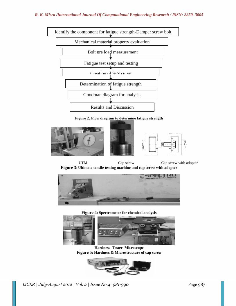
3. Evaluation of Mechanical Properties Figure 2 shows the approach to determine the fatigue strength of cap screw bolt.
Material property evaluation requirements
a. Surface hardness, Ultimate tensile strength was obtained prior to the fatigue test. Cap screws which were used in
the evaluation. Those cap screws were not used as a fatigue test specimens.
b. Hardness of the shank is obtained through hardness tester.
c. Cap screws were tested to failure in tension, using the grip length or gage length and thread engagement of the
intended fastener application.
d. Chemical analysis results obtained at the center of head after clean- up the surface
UTS (Ultimate tensile strength)
Tension tests provide information on the strength and ductility of materials under uniaxial tensile stresses. To perform
tensile test, SAE [29, 30] and ASTM [31] procedure has been adopted. Figure 3 shows the ultimate tensile machine (UTM)
and cap screw with adopter. Details of the test procedure have been given below:
The cap screw was inserted in the UTS machine with the test washer placed under the cap screw head.
The test nut was assembled onto the cap screw by turning the cap screw head until the cap screw is seated against
the hardened washer.
Precaution was taken that a minimum of two threads protrude through the nut. Wedge grips were used for holding
the specimen.

R. K. Misra /International Journal Of Computational Engineering Research / ISSN: 2250–3005
IJCER | July-August 2012 | Vol. 2 | Issue No.4 |981-990 Page 983
Then the cap screw were continuously and uniformly tightened at a speed not to exceed 30 rpm with a torque-
measuring device or equivalent means, until either the torque or the tension value, as required, was developed and both
torque and tension readings were recorded.
Axial loading was applied until failure.
It was ensured that the cap screw shall not fracture before having withstood the minimum tensile load specified for
the applicable size, thread series, grade and the failure location.
Table 1 shows the ultimate test results. Stress area, mean tensile strength and mean tensile stress is 0.373 inch2, 71361
pound and 191315 pound/inch2 respectively.
Chemical Analysis Chemical analysis was performed using spectrometer [32] and spectrometer has been shown in figure 4. Procedure for
chemical analysis has been given below:
Specimen was prepared for chemical analysis at the center of cap screw head by cleaning upper surface.
A capacitor discharge was produced between the flat, ground surface of the disk specimen and a conically shaped
electrode by spectrometer. The discharge was terminated at a predetermined intensity time integral of a selected iron line, or
at a predetermined time, and the relative radiant energies of the analytical lines were recorded. The most sensitive lines of
arsenic, boron, carbon, nitrogen, phosphorus, sulfur, and tin lie in the vacuum ultraviolet region. The absorption of the
radiation by air in this region was overcome by evacuating the spectrometer and flushing the spark chamber with argon.
Chemical composition for each element (C, Si, Mn, P, S, Cr, Mo, Ni) in percentage was noted. Chemical
analysis results have been shown in table 2.
Hardness and Microstructure
The Rockwell hardness test is an empirical indentation hardness test that can provide useful information about metallic
materials. This information may correlate to tensile strength, wear resistance, ductility and other physical characteristics of
metallic materials, and may be useful in quality control and selection of materials. Figure 5 shows the hardness tester and
microscope for analysis of hardness and microstructure of cap screw respectively.
Test procedure has been described below:
Placed the cap screw on hardness tester as per attached figure.
Moved the indenter into contact with the test surface in a direction perpendicular to the surface.
Measured the hardness of cap screw.
Observed the microstructure of specimen at microscope.
Table 3 shows the hardness & microstructure test results of the cap screw.
Coating
Cap screw bolts were coated with the zinc phosphate and oil coatings to provide a corrosion protection and a low &
consistent friction coefficient. The most consistent preload is achieved with an as-received zinc phosphate and oil coating.
Minimum grade requirement
Critical cap screws were used for dampers shall be grade 8 or above [29] for inch products or property class 10.9 or above
[33] for metric products. Property class 12.9 fasteners are susceptible to stress corrosion cracking and are not recommended.
4. Determination of bolt pre-load The purpose of the bolt was to clamp two or more parts together. The clamping load stretches or elongates the bolts; the
load was obtained by twisting the nut until the bolt elongated to the elastic limit. When the bolt did not loosen, this bolt
tension remains as the preload or clamping force. This clamping force is called the pre-tension or bolt preload. It exists in
the connection after the nut has been properly tightened no matter whether the external load P is exerted or not. The preload
is the force required to hold the joint together correctly. The preload cannot be calculated directly, but it can be estimated
using available empirical data and then confirmed by measurements for the particular cap screw and joint.
Theoretical calculation of preload The relationship between the torque applied to a fastener and tension created from the resulting bolt elongation has been
described below
T= F. K.D
Where T, K, D & F are torque, friction factor, bolt diameter and preload respectively. The K value can be thought of as
summarization of anything and everything that affect the relationship between torque and preload. Table 4 gives brief list of

R. K. Misra /International Journal Of Computational Engineering Research / ISSN: 2250–3005
IJCER | July-August 2012 | Vol. 2 | Issue No.4 |981-990 Page 984
some estimated K factors [34]. A K factor for zinc phosphate coated cap screws was assumed between 0.16 and 0.20 for
approximate calculations of preload. Preload value of the damper cap screw has been shown in table 5.
Experimental measurement of preload
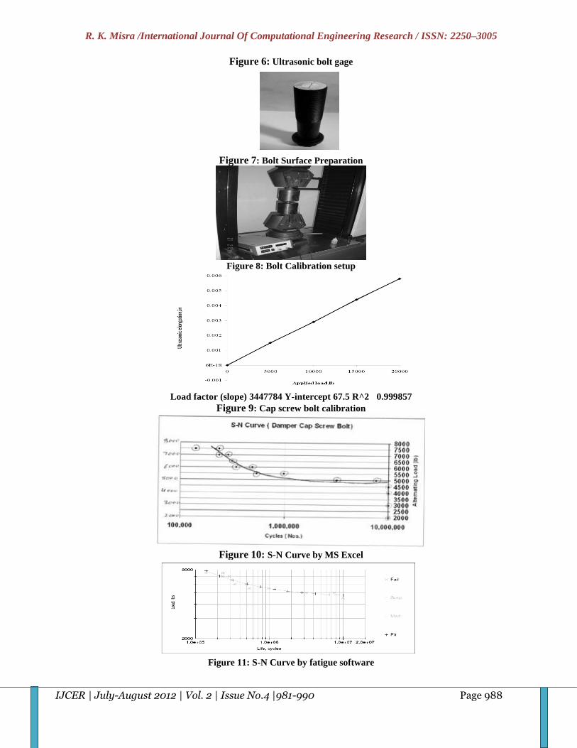
In this work, axial load is measured by ultrasonic method using ultrasonic bolt gauge. Figure 6 shows the ultrasonic bolt
gauge. The purpose of ultrasonic bolt gauging is to estimation of axial load in fasteners. The ultrasonic method of measuring
the elongation of bolts based on time of flight to measure bolt tension with better accuracy. However, the ultrasonic method
requires the original length of bolts and Young’s modulus before fastening to determine the actual tensile load from
ultrasonic elongation of the bolts [8].
The purpose of using ultrasonic bolt gage is to use ultrasonically measured elongation to determine cap screw preload. The
cap screws are calibrated in a load frame to relate cap screw stretch (the ultrasonic elongation) to applied load. The cap
screw stretches as torque is applied to joint. Using the ultrasonic length measurement, the stretch is related to preload
through the cap screw calibration.
Before calibration, bolt gage were ground on top and bottom. Grinding improves connection between ultrasonic transducer
to bolt. Preparation of the bolt surface has been shown in figure 7. After preparation of the cap screw bolt surface, cap screw
bolt gage has been calibrated. Figure 8 shows the calibration set up. Length of the calibration bar is measured in this
process. It is very necessary to makes sure that the bolt system is working properly. Initially ultrasonic length is measured
before loading the bolt. Later on load is applied on bolt to measure ultrasonic elongation. Load and elongation were used to
determine a calibration curve and load factor. Calibration of the damper capscrew bolt has been shown in Table 6 and
Figure 9. After that, cap screw was installed on engine to mount damper with crankshaft. The cap screws were tightened in
sequence. Torque all cap screw as per specification. Load (tension) was calculated for all stretch by multiplying the load
factor, determined through calibration curve. Table 7 shows the value of preload using ultrasonic bolt gauge. 40651 lbf,
average pre-load on cap screw bolts has been determined. Therefore 40,000 lbf, mean load has considered for fatigue test.
5. Fatigue testing
The purpose of the fatigue test is to make sure that a cap screw has adequate fatigue strength to survive in an engine
environment under engine loading. Engine conditions are measured and duplicated in a tension-tension axial fatigue test.
Fatigue test procedure
i.Mounted the screw bolt test fixture on closed loop servo hydraulic fatigue test system.
ii.Set gage length 64 mm.
iii.Set the load on the servo hydraulic fatigue test system.
iv.Cycle of the machine was set at approximately 15 Hz.
v.Maintained mean load 40000 lbs during testing & alternating load varying from 2000 lbs to 7500 lbs (Fatigue testing of
samples should be at 2 to 4 times engine alternating load).
vi.Recorded the load and cycles to failure.
vii.Repeated above steps for all samples.
Fatigue test cycle
In the conventional fatigue design, the fatigue limit was obtained at 107 number of stress cycle to determine the allowable
stress level for design against high cycle fatigue.
Post test processing of the raw test data was used to obtain the estimate of the cap screw’s mean fatigue strength, standard
deviation, coefficient of variation of strength. These post test results can be used for comparison with a minimum fatigue
test requirement .Table 8 shows the fatigue test results. Raw data can be effectively presented in an S-N plot and Goodman
plot.
S-N Curve
S-N curve for cap screw was determined using the alternating load. The load was increased until cap screw begin to fail.16
sample were tested to determine the shape of fatigue curve. The Data from this sample were analyzed using software and
M.S. Excel. After drawn S-N curve, Endurance limit was determined. Figure 10 and 11 shows the S-N curve made using
M.S. Excel and fatigue software respectively.
Goodman diagram Goodman diagram is a tool for estimating infinite fatigue life of a component undergoing mean and alternating load.

R. K. Misra /International Journal Of Computational Engineering Research / ISSN: 2250–3005
IJCER | July-August 2012 | Vol. 2 | Issue No.4 |981-990 Page 985
6. Results and discussion Following observation is observed after analyzing the table 1, 2 & 3:
Damper cap screw bolt can bear maximum tensile stress 191315 pound square inch before failure.
It contains maximum amount of manganese. After that, chromium, nickel and carbon come in the row. Due to
presence of high manganese hardenability, machinability and strength improves.
Chromium and nickel improves toughness. Therefore bolt bears maximum distortion energy before fracture.
The role of carbon is also very significant. Carbon increases the damping property. When fatigue load is applied,
bolt dissipates more amount of energy to atmosphere. So life of the bolt increases.
Bolt is very hard. Its hardness varies between 39-42 HRC.
Tempered martensite structure is observed after seeing the bolt from microscope and thread rolling is done after
heat treatment. Laps/cracks are absent at root or flanks of the threads.
Table 5 shows the pre-load calculations theoretically of the damper cap screw bolt. Preload is applied to hold the joint
together correctly. The preload cannot be calculated directly, but it can be estimated using available empirical data and then
confirmed by measurements for the particular cap screw and joint. Theoretical average value of the preload is 38737.8
pound. To measure the value of preload experimentally, ultrasonic method is used. Table 7 shows the value of preload using
ultrasonic bolt gauge. 40651 pound average pre-load has been determined from ultrasonic bolt gauge. After calculating
preload from both procedures, fatigue experiment has been performed. At the time of performing fatigue test, maximum and
minimum load were changing but mean load was fixed. That was 40,000 pound. It was very near to average preload. Fatigue
test results have been shown in table 8. When minimum and maximum load was 35,500 pound and 44,500 pound
respectively, bolt was safe after passing 10000000 cycles. As soon as the value of maximum load reaches up to 45,000. Bolt
fails at 7608380 cycles. Number of cycles decreases drastically after addition of 500 pound load in maximum load. S-N
curve has been drawn using table 8 data in MS Excel sheet. Figure 10 shows the S-N curve. To validate table 8 data and S-N
curve, fatigue software was used. Figure 11 shows the S-N curve by fatigue software. It is observed that bolt is safe, when
alternating load is below 5000 pound.
Goodman line has been shown in figure 12.The Goodman line is used as criteria of failure when the component is subjected
to mean stress as well as stress amplitude.
Conclusion
The fatigue strength of damper cap screw bolt is determined by S-N curve method. Data for S-N curve was generated on
servo hydraulic fatigue test system by axial force controlled method. Fatigue strength of cap screw bolt is 4582 pound at
mean load of 40000 pound.
The purpose of fatigue test is to make sure that a cap screw has adequate fatigue strength to survive in an engine
environment under engine loading. Engine conditions are measured and duplicated in a tension-tension axial fatigue test.
Alternating load due to engine operation for particular damper cap screw bolt should be less than 4582 pound. For better
design the alternating load should be half of fatigue strength. Goodman diagram plotted based on fatigue strength, mean
load and ultimate tensile strength to find the Goodman diagram can be used for finding the design margin at different mean
load & alternating load.
References:
1. Nishida, S, Failure analysis in engineering applications. Great Britain: Butterworth-Heinemann; 1992.
2. Milan MT, Spinelli D, Bose Filho WW, Montezuma MFV, Tita V. Failure analysis of a SAE 4340 steel locking bolt. Eng
Fail Anal 2004; 11:915–24.
3. Baggerly RG. Hydrogen-assisted stress cracking of high-strength wheel bolts. Eng Fail Anal 1996; 3(4):231–40.
4. Yu Z, Xu X. Failure analysis of connecting bolts and location pins assembled on the plate of main-shaft used in a
locomotive turbocharger. Eng Fail Anal 2008; 15: 471–9.
5. Chen Hsing-Sung, Tseng Pi-Tang, Hwang Shun-Fa. Failure analysis of bolts on an end flange of a steam pipe. Eng Fail
Anal 2006; 13:656–68.
6. Rabb R. Fatigue failure of a connecting rod. Eng Fail Anal 1996; 3(1):13–28.
7. Majzoobi, G.H., Farrahi, G.H, Habibi, N. Experimental evaluation of the effect of thread pitch on fatigue life of bolts.
International Journal of fatigue 2005; 27:189-196.
8. Nohyu, Kim and Minsung, Hong. Measurement of axial stress using mode-converted ultrasound. NDT&E International
2009; 42:164-169.
9. Goodier J. The distribution of load in threads of screws. J Appl Mech Trans ASME 62; 1940, p. A10–A16.
10. D’Eramo M, Cappa P. An experimental validation of load distribution in screw threads. Exp Mech 1991; 31:70–5.
11. Pilkey W. Peterson’s stress concentration factors. 2nd Ed. New York: Wiley; 1997. [ISBN: 978-0-471-53849-3].
12. Fetullazade E et al. Effects of the machining conditions on the strain hardening and the residual stresses at the roots of screw
threads. Mater Des 2009; 31(4):2025–31.

R. K. Misra /International Journal Of Computational Engineering Research / ISSN: 2250–3005
IJCER | July-August 2012 | Vol. 2 | Issue No.4 |981-990 Page 986
13. Bradley N. Influence of cold rolling threads before or after heat treatment on the fatigue resistance of high strength fine
thread bolts for multiple preload conditions. In: Toor P, editor. ASTM STP 1487 structural integrity of fastener. West
Conshohocken, PA: ASTM International; 2007, p. 98–112.
14. Olsen K. Fatigue crack growth analyses of aerospace threaded fasteners – Part I: State-of-practice bolt crack growth
analyses method. In: Toor P, editor. ASTM STP 1487 structural integrity of fastener. West Conshohocken, PA: ASTM
International; 2007, p. 125–40.
15. Toribio J et al. Stress intensity factor solutions for a cracked bolt under tension, bending and residual stress loading. Eng
Fract Mech 1991; 39(2):359–71.
16. Mettu S, et al. Stress intensity factor solutions for fasteners in NASGRO 3.0. In: Toor P, editor. ASTM STP 1391 structural
integrity of fasteners, vol. 2. West Conshohocken, PA: ASTM International; 2000, p. 133–9.
17. James L, Anderson W. A simple procedure for stress intensity calibration. Eng Fract Mech 1969; 1:565–8.
18. Shen H, Guo W. Modified James–Anderson method for stress intensity factors of three-dimensional cracked bodies. Int J
Fatigue 2005; 27:624–8.
19. Fukuoka, T., Yamasaki, N., Kitagawa, H. and Hamada, M., Stress in bolt and nut. Bull. JSME, 1986, 29, 3275–3279.
20. Tanaka, M., Miyazawa, H., Asaba, E. and Hongo, K., Application of the finite element method to bolt-nut joints. Bull.
JSME, 1981, 24, 1064–1071.
21. Tafreshi, A. and Dover, W. D., Stress analysis of drillstring threaded connections using the finite element method. Int. J.
Fatigue, 1993, 15, 429–438.
22. Kenny, B. and Patterson, E. A., Load and stress distribution in screw threads. Exp. Mech, 1985, 25, 208–213.
23. Fessler, H. and Jobson, P. K., Stress in a bottoming stud assembly with chamfers at the ends of the threads. J. Strain Anal,
1983, 18, 15–22.
24. Zhao, H., Analysis of the load distribution in a bolt-nut connector. Comput. Struct, 1994, 53, 1465–1472.
25. Sopwith, D. G., The distribution of load in screw threads. Proc. Inst. Mech. Engrs, 1948, 159, 319–398.
26. Bretl, J. L. and Cook, R. D., Modeling the load transfer in threaded connections by the finite element method. Int. J. Numer.
Meth. Engng, 1979, 14, 1359–1377.
27. Zhao, H., The virtual contact loading method for contact problems considering material and geometric nonlinearities.
Comput. Struct, 1996, 58, 621–632.
28. Shigley, J.E and Mischake, C.R., Mechanical engineering design. McGraw Hill Publications, 1989.
29. SAE J429, Mechanical and material requirements for externally threaded fasteners, 1999.
30. SAE J174, Torque-Tension test procedure for steel threaded fasteners – inches & metric series, 1998.
31. ASTM standard E8/E8M, Standard test methods for tension testing of metallic materials, 2008.
32. ASTM standards E415, “Standard test method for atomic emission vacuum spectrometric analysis of carbon and low-alloy
steel”, 2008.
33. ASTM standard F568M, “Standard specification for carbon and alloy steel externally threaded metric fasteners”, 2007.
34. FS7028, “Fastenal Technical reference guide”, 2005.
Figure
Crank Shaft Vibration Damper Cap screw Bolt
Figure 1: Cap Screw Bolt Mounting on Engine
R. K. Misra /International Journal Of Computational Engineering Research / ISSN: 2250–3005
IJCER | July-August 2012 | Vol. 2 | Issue No.4 |981-990 Page 987
Figure 2: Flow diagram to determine fatigue strength
UTM Cap screw Cap screw with adopter
Figure 3: Ultimate tensile testing machine and cap screw with adopter
Figure 4: Spectrometer for chemical analysis
Hardness Tester Microscope
Figure 5: Hardness & Microstructure of cap screw
Identify the component for fatigue strength-Damper screw bolt
Mechanical material property evaluation
Bolt pre load measurement
Fatigue test setup and testing
Creation of S-N curve
Determination of fatigue strength
Goodman diagram for analysis
Results and Discussion
R. K. Misra /International Journal Of Computational Engineering Research / ISSN: 2250–3005
IJCER | July-August 2012 | Vol. 2 | Issue No.4 |981-990 Page 988
Figure 6: Ultrasonic bolt gage
Figure 7: Bolt Surface Preparation
Figure 8: Bolt Calibration setup
Load factor (slope) 3447784 Y-intercept 67.5 R^2 0.999857
Figure 9: Cap screw bolt calibration
Figure 10: S-N Curve by MS Excel
Figure 11: S-N Curve by fatigue software

R. K. Misra /International Journal Of Computational Engineering Research / ISSN: 2250–3005
IJCER | July-August 2012 | Vol. 2 | Issue No.4 |981-990 Page 989
Table
Table 1: Ultimate tensile test results
Sr. No. Sample Failure Load (KN) Failure Load (lb) Failure Stress (Psi)
1 1 320 71939 192865
2 2 324 72838 195276
3 3 330 74187 198892
4 4 322 72388 194069
5 5 314 70590 189249
6 6 310 69691 186839
7 7 302 67892 182016
Average(UTS) 318 71361 191315
Table 2: Chemical Analysis results
Sr. No. Element
%
C Si Mn P S Cr Mo Ni
1 Lot1 0.41 0.25 0.88 0.014 0.006 0.51 0.15 0.51
2 Lot1 0.4 0.26 0.85 0.02 ----- 0.54 0.16 0.5
3 Lot1 0.38 0.15 0.73 0.017 0.01 0.58 0.19 -------
Standard ASTM
E415
0.37/
0.44
0.15/
0.35
0.70/
1.05
0.035
max
0.04
max
0.35/
0.65
0.15/
0.25
0.35/
0.75
Standard SAE 8640 0.38/
0.43
0.15/
0.35
0.75/
1.00
0.035
max
0.04
max
0.40/
0.60
0.15/
0.25
0.40/
0.60
Table 3: Hardness & Microstructure test results
Sr.
No.
Sample Hardness Microstructure
1 1 39-42 HRC Fine tempered martensite. Cracks/laps are not observed at root/flanks of
the threads. Decarburization
2 2 38-39 HRC Tempered martensite. Thread rolling is done after heat treatment.
Laps/cracks are absent at root or flanks of the threads.
3 3 38-40 HRC Tempered martensite. Thread rolling is done after heat treatment.
Laps/cracks are absent at root or flanks of the threads.
Table 4: K factors
Bolt Condition K
Non-plated, black finish 0.20 ------ 0.30
Zinc-plated 0.17 ------ 0.22
Lubricated 0.12 ------ 0.16
Cadmium-plated 0.11 ------ 0.15
Table 5: Preload calculation –Damper cap screw
Assembly torque (T) lb.ft 410 410 410 410 410
Capscrew diameter (Din) inch 0.71 0.71 0.71 0.71 0.71
Capscrew diameter (D),ft = Din/12 0.0592 0.0592 0.0592 0.0592 0.0592
Nut factor (K), assume 0.16 0.17 0.18 0.19 0.20
Preload (P), lb = T/(D*K) 43309.9 40762.2 38497.7 36471.5 34647.9
Average Torque (lb.ft) 38737.8
Table 6: Damper Capscrew bolt calibration

R. K. Misra /International Journal Of Computational Engineering Research / ISSN: 2250–3005
IJCER | July-August 2012 | Vol. 2 | Issue No.4 |981-990 Page 990
Sr. No. Applied load, lb Measured ultrasonic elongation, in
1 0 0.0000
2 5000 0.0015
3 10000 0.0029
4 15000 0.0044
5 20000 0.0058
Table 7: Torque tension test results
Torque = 400 lb.ft & Load factor = 3447784
Cap Screw No. Stretch Load
1 0.0110 37960
2 0.0117 40339
3 0.0129 44476
4 0.0121 41718
5 0.0131 45166
6 0.0112 38615
7 0.0118 40684
8 0.0127 43787
9 0.0114 39305
10 0.0116 39994
11 0.0120 41373
12 0.0101 34823
13 0.0120 41373
14 0.0111 38270
15 0.0116 39994
16 0.0126 43442
17 0.0114 39305
18 0.0119 41029
19 0.0112 38615
20 0.0124 42753
Sample size Average stretch Average load
20 0.0118 40651
Std Dev = 2504, Min load = 34823 &Max load = 45166
Table 8: Fatigue test results
Sample
No.
Mean load,
(lbs)
Alternating load,
(lbs)
Min load,
(lbs)
Max load,
(lbs)
Cycles to
failure
status
1 40000 2000 38000 42000 10000000 Pass
2 40000 3000 37000 43000 10000000 Pass
3 40000 4000 36000 44000 10000000 Pass
4 40000 4500 35500 44500 10000000 Pass
5 40000 5000 35000 45000 7608380 Fail
6 40000 5000 35000 45000 3190347 Fail
7 40000 5500 34500 45500 539646 Fail
8 40000 5500 34500 45500 982412 Fail
9 40000 6000 34000 46000 342895 Fail
10 40000 6000 34000 46000 490985 Fail
11 40000 6500 33500 46500 314736 Fail
12 40000 6500 33500 46500 314780 Fail
13 40000 7000 33000 47000 235024 Fail
14 40000 7000 33000 47000 286642 Fail
15 40000 7500 32500 47500 236327 Fail
16 40000 7500 32500 47500 140086 Fail

Prof.Manju Devi, Prof.Muralidhara, Prasanna R Hegde /International Journal Of Computational
Engineering Research / Issn: 2250–3005
IJCER | July-August 2012 | Vol. 2 | Issue No.4 |991-996 Page 991
Removal of Impulse Noise Using Eodt with Pipelined ADC
1Prof.Manju Devi,
2 Prof.Muralidhara,
3Prasanna R Hegde
1 Associate Prof, ECE, BTLIT Research scholar,2 HOD, Dept. Of ECE, PES MANDYA.
3 VIII- SEM ECE, BTLIT,
Abstract Corrupted Image and video signals due to impulse noise during the process of signal acquisition and transmission can be
corrected. In this paper the effective removal of impulse noise using EODT with pipelined architecture and its VLSI
implementation is presented. Proposed technique uses the denoising techniques such as Edge oriented Denoising technique
(EODT) which uses 7 stage pipelined ADC for scheduling. This design requires only low computational complexity and
two line memory buffers. It’s hardware cost is quite low. Compared with previous VLSI implementations, our design
achieves better image quality with less hardware cost. The Verilog code is successfully implemented by using FPGA
Spatron-3 family.
Index Terms—Image denoising, impulse noise, pipeline architecture, VLSI.
1. Introduction Most of the video and image signals are affected by noise. Noise can be random or white noise with no coherence, or
coherent noise introduced by the capturing device's mechanism or processing algorithms. The major type of noise by which
most of the signals are corrupted is salt and pepper noise. You might have observed the dark white and black spots in old
photos, these kind of noise presented in images are nothing but the pepper and salt noise. Pepper and salt noise together
considered as Impulse noise.
Fig1. Example of pepper and salt noise
The above pictures give us the insight of impulse noise. Number of dots in the pictures will bring down the clarity and
quality of the image. In other applications such as printing skills, scanning, medical imaging and face recognition images
are often corrupted by noise in the process of signal acquisition and transmission. It’s more sophisticated in medical
imaging when the edges of the object in image are affected by noise, which may lead to the misdetection of the problem.
So efficient denoising technique is important in the field of image processing. many image denoising methods have[1]-[8]
been proposed to carry out the impulse noise suppression some of them employ the standard median filter or its
modifications to implement denoising process. However, these approaches might blur the image since both noisy and
noise-free pixels are modified. The switching median filter consists of two steps:
1) Impulse Detection and
2) Noise filtering.
New Impulse Detector (NID) for switching median filter. NID used the minimum absolute Value of four convolutions
which are obtained by using 1-D Laplacian operators to detect noisy pixels. A method named as differential rank impulse
detector (DRID) is presented in. The impulse detector of DRID is based on a comparison of signal samples within a narrow
rank window by both rank and absolute value. Another technique named efficient removal of impulse noise (ERIN)[8]
based on simple fuzzy impulse detection technique.
2. Proposed Technique All previous techniques involve high computational complexity and require large memory which affects the cost and
performance of the system. So less memory consumption and reduced computational complexity are become main design
aspects. To achieve these requirements Edge Oriented Denoising Technique (EODT) is presented. This requires only two
line memory buffers and simple arithmetic operations like addition, subtraction.

Prof.Manju Devi, Prof.Muralidhara, Prasanna R Hegde /International Journal Of Computational
Engineering Research / Issn: 2250–3005
IJCER | July-August 2012 | Vol. 2 | Issue No.4 |991-996 Page 992
EODT is composed of three components: extreme data detector, edge-oriented noise filter and impulse arbiter. The extreme
data detector detects the minimum and maximum luminance values in W, and determines whether the luminance values of
P(i,j) and its five neighboring pixels are equal to the extreme data. By observing the spatial correlation, the edge-oriented
noise filter pinpoints a directional edge and uses it to generate the estimated value of current pixel. Finally, the impulse
arbiter brings out the Result.
3. Vlsi Implementation Of Eodt EODT has low computational complexity and requires only two line buffers, so its cost of VLSI implementation is low.
For better timing performance, we adopt the pipelined architecture which can produce an output at every clock cycle. In
our implementation, the SRAM used to store the image luminance values is generated with the 0.18µm TSMC/Artisan
memory compiler. According to the simulation, we found that the access time for SRAM is about 6 ns. Since the operation
of SRAM access belongs to the first pipeline stage of our design, we divide the remaining denoising steps into 6 pipeline
stages evenly to keep the propagation delay of each pipeline stage around 6 ns. The pseudo code and the RTL schematic
(Fig2) we obtained is given below
Pseudo code
for(i=0; i<row; i=i+1) /* input image size: row(height) × col(width) */
{
for(j=0; j<col; j=j+1)
{
/ * Extreme Data Detector * /
Get W, the 3×3 mask centered on (i, j);
Find MINinW and MAXinW in W;
/ * the minimum and maximum values from the first W to current W * /
φ=0; / * initial values * /
if ((fi,j = MINinW) or (fi,j = MAXinW))
φ=1; / * Pi.j is suspected to be a noisy pixel * /
if(φ=0)
{
i,j = fi,j;
break; / * P i,j is a noise-free pixel * /
}
B = b1b2b3b4b5 = “00000”; / * initial values * /
if ((fi,j-1 = MINinW) or (fi,j-1 = MAXinW))
b1=1; / * Pi,j-1 is suspected to be a noisy pixel * /
if ((fi,j+1 = MINinW) or (fi,j+1 = MAXinW))
b2=1; / * P i,j+1 is suspected to be a noisy pixel * /
if ((fi+1,j-1 = MINinW) or (fi+1,j-1 = MAXinW))
b3=1; / * P i+1,j-1 is suspected to be a noisy pixel * /
if ((fi+1,j = MINinW) or (fi+1,j = MAXinW))
b4=1; / * Pi+1,j is suspected to be a noisy pixel * /
if ((fi+1,j+1 = MINinW) or (fi+1,j+1 = MAXinW))
b5=1; / * P i+1,j+1 is suspected to be a noisy pixel * /
/ * Edge-Oriented Noise Filter * /
Use B to determine the chosen directions across Pi,j according to figure 4.;
if(B=”11111”)
i.j = ( i-1,j-1 + 2 × i-1,j + i-1,j+1)/4; / * no edge is considered * /
else
{
Find Dmin (the smallest directional difference among the chosen directions);
i.j = the mean of luminance values of the two pixels which own Dmin

Prof.Manju Devi, Prof.Muralidhara, Prasanna R Hegde /International Journal Of Computational
Engineering Research / Issn: 2250–3005
IJCER | July-August 2012 | Vol. 2 | Issue No.4 |991-996 Page 993
}
/ * Impulse Arbiter * /
if(|fi,j - i.j| > Ts)
i,j = i.j ; / * Pi,j is judged as a noisy pixel * /
else
i,j = fi,j ; / * Pi,j is judged as a noise-free pixel *
}
}
Fig2. RTL Schematic of EODT
3.1 Extreme data Detector The extreme data detector detects the minimum and maximum luminance values (MIN in W and MAX in W) in those
processed masks from the first one to the current one in the image. If a pixel is corrupted by the fixed value impulse noise,
its luminance value will jump to be the minimum or maximum value in gray scale. If (f i,j) is not equal to (MIN in W and
MAX in W) , we conclude that (P i,j)is a noise-free pixel and the following steps for de-noising (P i,j) are skipped.
If fi,j is equal to MINinW or MAXinW, we set φ=1, check whether its five neighboring pixels are equal to the extreme data
and store the binary compared results into B.
3.2 Edge-oriented noise filter To locate the edge existed in the current W, a simple edge catching technique which can be realized easily with VLSI
circuit is adopted. To decide the edge, we consider 12 directional differences, from D1toD2, as shown in fig 3. Only those
composed of noise free pixels are taken into account to avoid possible misdetection. If a bit in B is equal to 1, it means that
the pixel related to the binary flag is suspected to be a noisy pixel. Directions passing through the suspected pixels are
discarded to reduce misdetection. In each condition, at most four directions are chosen for low-cost hardware
implementation. If there appear over four directions, only four of them are chose according to the variation in angle.
Fig3. 12 Directional difference of EODT

Prof.Manju Devi, Prof.Muralidhara, Prasanna R Hegde /International Journal Of Computational
Engineering Research / Issn: 2250–3005
IJCER | July-August 2012 | Vol. 2 | Issue No.4 |991-996 Page 994
Table1. Thirty two possible values of B and their corressponding directions.
Table 1 shows the mapping table between and the chosen directions adopted in the design. If P i,j-1 , Pi,j+1 , Pi+1,j-1 , Pi+1,j and
Pi+1,j+1 are all suspected to be noisy pixels (B = “11111”) , no edge can be processed, so i.j (the estimated value of Pi,j) is
equal to the weighted average of luminance values of three previously denoised pixels and calculated as i.j = ( i-1,j-1 + 2 ×
i-1,j + i-1,j+1)/4.
The smallest directional difference implies that it has the strongest spatial relation with, and probably there exists an edge
in its direction. Hence, the mean of luminance values of the two pixels which possess the smallest directional difference is
treated as i.j.
3.3 Impulse arbiter Since the value of a pixel corrupted by the fixed-value impulse noise will jump to be the minimum/maximum value in gray
scale, we can conclude that if Pi,j is corrupted, fi,j is equal MINinW or MAXinW. However, the conversion is not true. If fi,j
is equal to MINinW or MAXinW, Pi,j may be corrupted or just in the region with the highest or lowest luminance.
In other words, a pixel whose value is MINinW or MAXinW might be identified as noisy pixel even if it is not corrupted.
To overcome this drawback, we add another condition to reduce the possibility of misdetection. If P i,j is a noise free pixel
and the current mask has high spatial correlation, fi,j should be close to i.j and |fi,j - i.j| is small. That is to say, Pi,j might
be a noise-free pixel value is MINinW or MAXinW if |fi,j - i.j| is small.
We measure |fi,j - i.j| and compare it with a threshold to determine whether Pi,j is corrupted or not. The threshold, denoted
as Ts, is a predefined value. Obviously, the threshold affects the performance of proposed method.
A more appropriate threshold can achieve a better detection result. However, it is not easy to derive an optimal threshold
through analttic formulation. According to our experimental result, we set the threshold Ts as 20. If Pi,j is judged as a
corrupted pixel, the reconstructed luminance value fi,j = i.j . The part of the scheduling of EODT is shown in Table 2.
Table 2: Part of the scheduling of EODT
From Table 2 it is clear that one clock cycle is required to fetch the pixel from register bank, and three clock cycles are
required for extreme data detector and 2 clock cycles needed for edge oriented noise filter and finally impulse arbiter needs
one clock cycle to provide the result.
4. Simulation Results:

Prof.Manju Devi, Prof.Muralidhara, Prasanna R Hegde /International Journal Of Computational
Engineering Research / Issn: 2250–3005
IJCER | July-August 2012 | Vol. 2 | Issue No.4 |991-996 Page 995
Fig4: simulation results
If the current part of the image is corrupted by fixed value of impulse noise then the value will jump either to the minimum
or to the maximum in gray scale. So in our approach we are considering the minimum value pixel is a noisy pixel. For
example if the values of nine pixels of corrupted part of the image are 11_22_33_44_00_66_AA_88_77 then we assume 5th
pixel is noisy as shown in Fig 4. So now we will take the average values of its neighboring pixels. Here neighboring pixels
are having the values 44 and 66 (in hexadecimal) first these two pixels are added and then divided by 2. That is
66+44=AA, when AA divided by 2 will get 55. This new value will be restored in the place of corrupted pixel.
5. FUTURE WORK
In EODT we are using 12 directional differences and it’s quite difficult to understand and more time consuming. This
problem can be solved out by introducing new technology called Reduced EODT. This technique uses only 3 directional
differences and only 5 clock cycles are needed to complete the process. But due to only three directional differences the
image quality may not be as good as EODT
6. CONCLUSION In this paper, an efficient removal of impulse noise using pipelined ADC is presented. The extensive experimental results
demonstrate that our design achieves excellent performance in terms of quantitative evaluation and visual quality, even the
noise ratio is as high as 90%. For real-time applications, a7-stage pipeline architecture for EODT is developed and
implemented. As the outcome demonstrated, EODT outperforms other chips with the lowest hardware cost. The
architectures work with monochromatic images, but they can be extended for working with RGB colour images and
videos.
REFERENCES [1] W. K. Pratt, Digital Image Processing. New York: Wiley-Interscience,1991.
[2] T. Nodes and N. Gallagher, “Median filters: Some modifications and their properties,” IEEE Trans. Acoust., Speech, Signal
Process., vol. ASSP-30, no. 5, pp. 739–746, Oct. 1982.
[3] S.-J. Ko and Y.-H. Lee, “Center weighted median filters and their applications to image enhancement,” IEEE Trans. Circuits
Syst., vol. 38,no. 9, pp. 984–993, Sep. 1991.
[4] H. Hwang and R. Haddad, “Adaptive median filters: New algorithms and results,” IEEE Trans. Image Process., vol. 4, no. 4,
pp. 499–502, Apr. 1995.
[5] T. Sun and Y. Neuvo, “Detail-preserving median based filters in image processing,” Pattern Recog. Lett., vol. 15, no. 4, pp.
341–347, April 1994.
[6] S. Zhang and M. A. Karim, “A new impulse detector for switching median filter,” IEEE Signal Process. Lett., vol. 9, no. 11,
pp. 360–363, Nov. 2002.
[7] I. Aizenberg and C. Butakoff, “Effective impulse detector based on rank-order criteria,” IEEE Signal Process. Lett., vol. 11,
no. 3, pp.363–366, Mar. 2004.

Prof.Manju Devi, Prof.Muralidhara, Prasanna R Hegde /International Journal Of Computational
Engineering Research / Issn: 2250–3005
IJCER | July-August 2012 | Vol. 2 | Issue No.4 |991-996 Page 996
[8] W. Luo, “Efficient removal of impulse noise from digital images,”IEEE Trans. Consum. Electron., vol. 52, no. 2, pp. 523–527,
May 2006.
[9] W. Luo, “An efficient detail-preserving approach for removing impulse noise in images,” IEEE Signal Process. Lett., vol. 13,
no. 7, pp. 413–416, Jul. 2006.
[10] K. S. Srinivasan and D. Ebenezer, “A new fast and efficient decisionbased algorithm for removal of high-density impulse
noises,” IEEE Signal Process. Lett., vol. 14, no. 3, pp. 189–192, Mar. 2007.
[11] C.-T. Chen, L.-G. Chen, and J.-H. Hsiao, “VLSI implementation of a selective median filter,” IEEE Trans. Consum. Electron.,
vol. 42, no. 1, pp. 33–42, Feb. 1996.
[12] Pei-Yin Chen, Chih-Yuan Lien, and Hsu-Ming Chuang, “A Low-Cost VLSI Implementation for Efficient Removal of Impulse
Noise” IEEE 2009.
Prof. Manju Devi
Working as an Associate Professor in the department of ECE at BTLIT,B’lore. Almost sixteen years of
teaching experience in engineering colleges. Completed B.E in Electronics and Communication Engg. ,M.Tech in Applied
Electronics and pursuing Ph.D from VTU in the field of analog and mixed mode VLSI.
Dr K.N.Muralidhara:
Obtained his B.E. In E&C engg from PES college of Engg , Mandya during 1981, ME during 1987from and
Ph.D during 2002 from University of Roorkee. His field of interest is on semiconductor devices and presently working as
professor and Head at the Dept. He is guiding 5 candidates for Ph.D programme and actively participated in all the
developmental activities of the college. He has about 25 publications to his credit.
Prasanna R Hegde
Obtained B.E in Electronics and Communication Engineering from BTLIT in 2012. His field of interest is on
Digital electronics and VLSI. Actively participated in National and International level conferences. Student member of
IETE.
Pooja bhat, Bijender mehandia /International Journal Of Computational Engineering Research
/ ISSN: 2250–3005
IJCER | July-August 2012 | Vol. 2 | Issue No.4 |997-1000 Page 997
Analysis of Handover in Wimax for Ubiquitous connectivity
Pooja bhat1, Bijender mehandia
2
1,2Gurgaon Institute of Technology and Management, Bilaspur, Gurgaon
Abstract
WIMAX is Wireless Interoperability for Microwave
Access. It is a telecommunication technology that provides
wireless data over long distances in several ways, from
point-to-point links to full mobile cellular type access. The
main consideration of Mobile Wimax is to achieve
seamless handover such that there is no loss of data. In
Wimax both mobile station (MS) and base station (BS)
scans the neighbouring base stations for selecting the best
base station for a potential handover. Two types of
handovers in wimax are: Hard handover (break before
make) and Soft handover (make before break). To avoid
data loss during handover we have considered soft
handovers this research topic. We have proposed a
technique to select a base station for potential soft
handover in wimax. We have developed a base station
selection procedure that will optimize the soft handover
such that there is no data loss; handover decision is taken
quickly and thus improving overall handover performance.
We will compare the quality of service with hard handover
and soft handover. We have analysed the proposed
technique with an existing scheme for soft handover in
wimax with simulation results.
Keywords: Wimax, Topology, handover, QOS,
ubiquitous connectivity.
I. Introduction IEEE 802.16 standard defines the air interface for fixed
Broadband Wireless Access (BWA) systems to be used in
WMANs (Wireless Metropolitan Area Networks),
commonly referred to as Wimax
(Worldwide Interoperability for Microwave Access). The
original standard IEEE 802.16 does not support mobility
and for this purpose IEEE 802.16e-2005 was introduced. It
is also known as Mobile Wimax .It is the new mobile
version of the older Wimax specification known as IEEE
802.16e-2004 which is wireless but fixed, it lacks the
ability for user to move during data transmission. The main
purpose of Wimax is to provide users in rural areas with
high speed communications as an alternative to expensive
wired connections (e.g. cable or DSL). That is Wimax is
capable to provide high speed internet to last mile
connections. But this is not the only purpose of Wimax
systems. Mobile Wimax allows the user to move freely
during data transmission. The main consideration of
mobile Wimax is that there should be no data loss when
the moving user switches from one base station to another
i.e. during handover. Handover is procedure when a mobile
station changes the serving base station. The reason for
handover could be relatively low signal strength or work
load of base station.
Wimax is a state-of-the-art wireless technology
which utilizes adaptive modulation and coding, supports
single carrier (SC) and orthogonal frequency division
multiplexing techniques (OFDM) and several frequency
bands for different operation environments.
II. Materials and methods
1.1 Handovers in Wimax
A special requirement of a mobile device is the ability to
change its serving base station if there exists another base
station with better signal strength in the reach of mobile
station (MS). Handover is a procedure that provides
continuous connection when a MS migrates from the air-
interface of one BS to another air-interface provided by
another BS without disturbing the existing connections.
Handovers are needed to support mobility.
For a handover to occur, one needs to have at least two
base stations : serving base station(SBS) and target base
station(TBS). The handover is generally considered as
change in serving base station but it does not necessarily
mean that the base station must be changed. In some cases
there may be different reasons why a handover might be
conducted:
When the MS is moving away from the area covered
by one cell and enters the area covered by another cell
the connection is transferred to the second cell in order
to avoid data loss when the MS gets outside the range
of the first cell;
When the capacity for connections of a given cell is
used up, the new connection which is located in an
area overlapped by another cell, is transferred to that
cell in order to free-up some capacity in the first cell
for other users, who can only be connected to that cell;
When the channel used by the MS becomes interfered
with by another MS using the same channel in a
different cell, the call is transferred to a different
channel in the same cell or to a different channel in
another cell in order to avoid the interference;
Signal strength is not enough for maintaining proper
connection.

Pooja bhat, Bijender mehandia /International Journal Of Computational Engineering Research
/ ISSN: 2250–3005
IJCER | July-August 2012 | Vol. 2 | Issue No.4 |997-1000 Page 998
Behaviour of MS changes, for example in case of fast
moving MS suddenly stopping; the large cell size can be
adjusted by a small size cell with better capacity.
In CDMA networks a soft handover may be induced in
order to reduce the interference to a smaller neighbouring
cell due to the "near-far" effect even when the phone still
has an excellent connection to its current cell;
1.1.1 Stages of Handover procedure:
Call restriction
Handover decision/initiation
Synchronization
Termination of service
Types of handovers
There are two types of handovers used in cellular network
systems: hard handover and soft handover
Hard handover
The hard handover is used when the communication
channel is released first and the new channel is acquired
later from the neighbouring cell. For real-time users it
means a short disconnection of communication. Thus,
there is a service interruption when the handover occurs
reducing the quality of service.
1.2.1 Methods of Soft Handovers in Wimax
I. Macro Diversity Handover (MDHO)
The MDHO supported by MS and by BS, the “Diversity
Set” is maintained by MS and BS. The Diversity Set is a
list of the BSs, which are involved in the handover
procedure. The Diversity Set is maintained by the MS and
BS and it is updated via MAC (Medium Access Control)
management messages. A sending of these messages is
usually based on the long-term CINR (Carrier to Noise
plus Interface Ratio) of BSs and depends on two
thresholds: Add Threshold and Delete Threshold.
Threshold values are broadcasted in the DCD (Downlink
Channel Descriptor) message. The Diversity Set is defined
for each MS in the network. The MS continuously
monitors the BSs in the Diversity Set and defines an
“Anchor BS”. The Anchor BS is one of the BSs from
Diversity Set in MDHO. The MS is synchronized and
registered to the Anchor BS, further performs ranging and
monitors the downlink channel for control information.
The MS communicates (including user traffic) with
Anchor BS and Active BSs in the Diversity Set[1]
II. Fast Base Station Switching (FBSS)
We are considering fast base station switching technique.
In this method a diversity set is maintained for each mobile
station. The serving base station and mobile station
monitors the neighbouring base stations that can be added
in diversity set. Diversity set is maintained by both mobile
station and serving base station. Diversity set is collection
of base stations that can chosen as target base station for a
handover. Handover decision can be taken by mobile
station, base station or base station controller depending
upon the implementation.
Modification in Efficient FBSS technique
In the proposed technique, we are trying to modify the
FBSS procedure to optimize target base station selection
for soft handovers in wimax. We have introduced monitor
base station which is selected from diversity set of mobile
station. The function of monitor base station (MBS) is to
communicate with mobile station and maintain the
database of potential target base stations for a handover for
mobile station. Another advantage of MBS is that
whenever ABS fails, mobile station can start data
communication with MBS without any loss of data by
sending register message.
The mobile station sends its current location to MBS and
according to history of mobile station movement and its
current location, MBS sorts the TBS’s having maximum
div parameter.
Div= s/w- d
S= received signal strength
w= work load
d= distance between mobile station and base station
d=√ (xs – xi)2 + (ys-yi)
2
where (xs , ys) are coordinates of mobile station and (xi , yi
) are coordinates of i’th base station where i=1,2,3…. N
N = total number of base station in diversity set
s= (k* st )/d
Where st= transmitted signal strength
k= other factors affecting signal (interference)
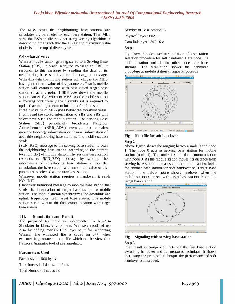
Pooja bhat, Bijender mehandia /International Journal Of Computational Engineering Research
/ ISSN: 2250–3005
IJCER | July-August 2012 | Vol. 2 | Issue No.4 |997-1000 Page 999
The MBS scans the neighbouring base stations and
calculates div parameter for each base station. Then MBS
sorts the BS’s in diversity set using sorting algorithm in
descending order such that the BS having maximum value
of div is on the top of diversity set.
Selection of MBS
When a mobile station gets registered to a Serving Base
Station (SBS), it sends scan_req message to SBS, it
responds to this message by sending the data of its
neighboring base stations through scan_rsp message.
With this data the mobile station will choose the MBS
having maximum value of div parameter. That is mobile
station will communicate with best suited target base
station so at any point if SBS goes down, the mobile
station can easily switch to MBS. As the mobile station
is moving continuously the diversity set is required to
updated according to current location of mobile station.
If the div value of MBS goes below the threshold value.
It will send the stored information to SBS and SBS will
select new MBS the mobile station. The Serving Base
Station (SBS) periodically broadcasts Neighbor
Advertisement (NBR_ADV) message that contains
network topology information or channel information of
available neighbouring base stations. The mobile station
sends
(SCN_REQ) message to the serving base station to scan
the neighbouring base station according to the current
location (div) of mobile station. The serving base station
responds to SCN_REQ message by sending the
information of neighboring base station as per the
calculation, the base station with maximum value of div
parameter is selected as monitor base station.
Whenever mobile station requires a handover, it sends
HO_INIT
(Handover Initiation) message to monitor base station that
sends the information of target base station to mobile
station. The mobile station synchronizes the downlink and
uplink frequencies with target base station. The mobile
station can now start the data communication with target
base station
III. Simulation and Result The proposed technique is implemented in NS-2.34
Simulator in Linux environment. We have modified ns-
2.34 by adding mac802.16-e layer to it for supporting
Wimax. The wimax.tcl file is coded on c++, when
executed it generates a .nam file which can be viewed in
Network Animator tool of ns2 simulator.
Parameters Used
Packet size : 1500 bytes
Time interval of data sent : 6 ms
Total Number of nodes : 3
Number of Base Station : 2
Physical layer : 802.11
Data link layer : 802.16-e
Step 1
Fig. shows 3 nodes used in simulation of base station
selection procedure for soft handover. Here node 1 is
mobile station and all the other nodes are base
stations. The simulation shows the handover
procedure as mobile station changes its position
Fig Nam file for soft handover
Step 2
Above figure shows the ranging between node 0 and node
1. The node 0 acts as serving base station for mobile
station (node 1). The node 1 starts data communication
with node 0. As the mobile station moves, its distance from
serving base station increases and the mobile station looks
for another base station for soft handover ie. Target Base
Station. The below figure shows handover when the
mobile station connects with target base station. Node 2 is
target base station.
Fig Signaling with serving base station
Step 3
First result is comparison between the fast base station
switching handover and our proposed technique. It shows
that using the proposed technique the performance of soft
handover is improved.

Pooja bhat, Bijender mehandia /International Journal Of Computational Engineering Research
/ ISSN: 2250–3005
IJCER | July-August 2012 | Vol. 2 | Issue No.4 |997-1000 Page 1000
Fig Graph of soft handover with modified
FBBS technique
Step 4
The x axis denotes the time and y-axis denotes the packet
received
Fig Graph for hard hand over
IV. Conclusion: We simulated the more realistic handover in the mobile
WiMAX using NS-2 with WiMAX and mobility modules.
The goal of this simulation is to find out the relationship
between the handover latency and the velocity of mobile
station. It can be seen that the current handover mechanics
used in the NS-2 module meets the requirement of
seamless handover in mobile WiMAX when the mobile
station travel at the speed of 20 m/s. Although, using link-
going down mechanism will dramatically reduce the
handover latency, it is still a challenge to achieve the full
mobility: up to 120 km/h, handover latency of less than 50
ms with an associated packet loss that is less than 1
percent.
V. Future scope: As extension to this research work, two topics for future
research investigations are suggested. Since there is a trade
off between handover threshold and margin, an adaptive
threshold window could be used to balance the load of base
station and the QoS of the mobile.Also, the current work is
restricted to hard handover only. Possibilities of extending
this work to macro diversity and fast base station switching
can be worthy of an investigation. Although these are soft
handover techniques and currently optional in the WiMAX
standard, the BS selection procedure based on location
predication algorithms and current load factors of the target
BSs give an alternative way of deciding the target BS.
Further, reducing the number of handovers is highly
desirable from a system perspective.
References:
[1] Andrews, J. G., A. Ghosh, Fundamentals of WiMAX
Understanding broadband wireless networking,
Prentice Hall ,et al. (2007).
[2] Zdenek Becvar, Jan Zelenka ,Handovers in the
Mobile WiMAX.
[3] N. P. Singh, Brahmjit Singh, Performance
Enhancement of Cellular Network Using Adaptive
Soft Handover Algorithm.
[4] Zdenek BECVAR, Pavel MACH, Robert BESTAK,
Initialization of Handover Procedure in WiMAX
Networks.
[5] Kumar Mrinal , Chetan Aneja, Vikram Gupta, Swati
Sharma , Mobility Improvement In IEEE 802.16.
[6] Rajat Prakash and Venugopal V. Veeravalli, Locally
Optimal Soft Handoff Algorithms.
[7] IEEE Std: “Soft Handover and Fast BS Switching
Procedure,” IEEE 802.16 Broadband Wireless
Access Working Group, June 2004.

M.Periasamy, D.B.Sivakumar, Dr. T. Senthil Kumar/International Journal Of Computational
Engineering Research / ISSN: 2250–3005
IJCER | July-August 2012 | Vol. 2 | Issue No.4 |1001-1004 Page 1001
Dampening Flow Induced Vibration Due To Branching Of Duct at
Elbow M.Periasamy
1, D.B.Sivakumar
2, Dr. T. Senthil Kumar
3
1, 2, 3, Post Graduate Student, Department of Mechanical Engineering, Anna University Of Technology, Trichy
Abstract Ducts are closed path used for conveying air, Flue gas, Material, ash and etc from one system to another, in the power
plant and in the industries. Ducts are routed to long distances, having abrupt change in direction and cross section which
requires proper design for preventing the energy losses. Elbows are used for changing the direction of flow to 900.Due
to this abrupt change, eddies, Recirculation zones are formed. These Eddies having energy gradients, which produces
thrust and in turn Vibration to the duct wall. Eddies Should be broken by stream lining the flow before taking any
branching from the main duct. But in some ducting system either in power plant or Industrial, due to constraints Elbow
duct itself is to be branched out. This paper presents dampening flow induced vibration, by analyzing the various
arrangements using computational Fluid dynamic software Gambit-Fluent.
Keywords- Flow Induced Vibration, Flow Recirculation, Eddy, Sharp Elbow Branching
1. Introduction
Elbow ducts are used pre dominantly in the ducting system for diverting the flow to 900. Guidelines is to be followed
for avoiding pressure drop, recirculation etc in the design of elbow. Three Dimensional Model of a typical ducting is
shown in Fig 1. This ducting having sharp elbow, but as per design guidelines, guide vanes are to be used to streamline
the flow at the elbow. Since branching is done at sharp elbow, Guide vanes could not be used. So the duct system
becomes sharp 900 Elbow with branching at the elbow itself. The flow inside this ducting system is quite complicated
and its difficult to predict the flow in this system by analytical methods. The flow pattern inside this arrangement can
be visualised by using computational fluid dynamic software Gambit- Fluent.
Grid is formed representing Flow field by using elements connected at the nodes using elements in the Gambit.
The grid is then exported to Fluent , where the Boundary condition is applied and Solved. The Fluent have inviscid,
Laminat, Spalart Almaras(1 equation), K-epsilon(2 equation), K omega( 2 Equation), Reynolds stress( 7
Equation),Detached Eddy simulation and Large eddy simulation for modeling the Viscous flow
The K-epsilon model is one of the most common turbulence models, although it just doesn't perform well in
cases of large adverse pressure gradients. It is a two equation model that means, it includes two extra transport
equations to represent the turbulent properties of the flow. This allows a two equation model to account for history
effects like convection and diffusion of turbulent energy. The first transported variable is turbulent kinetic energy, K.
The second transported variable in this case is the turbulent dissipation,€ . It is the variable that determines the scale of
the turbulence, whereas the first variable, K, determines the energy in the turbulence.
There are two major formulations of K-epsilon models that of Launder and Sharma is typically called the
"Standard” K-epsilon Model. The original impetus for the K-epsilon model was to improve the mixing-length model, as
well as to find an alternative to algebraically prescribing turbulent length scales in moderate to high complexity
flows.K-epsilon model has been shown to be useful for free-shear layer flows with relatively small pressure gradients.
Similarly, for wall-bounded and internal flows, the model gives good results only in cases where mean pressure
gradients are small; accuracy has been shown experimentally to be reduced for flows containing large adverse pressure
gradients. The equation for the K-epsilon model is in built in fluent software itself.
2. Modified System
Fig.1 Three Dimensional Model (Base Duct, With Vertical Divider, With Horizontal Divider, With Distributor)
Guide Vanes are used for streamlining the flow at sharp 900 elbows. Since there is a branch in elbow itself,
Guide vanes cannot be provided. Hence for streamlining the flow three options Vertical Divider, Horizontal Divider,
Distributor are considered.

M.Periasamy, D.B.Sivakumar, Dr. T. Senthil Kumar/International Journal Of Computational
Engineering Research / ISSN: 2250–3005
IJCER | July-August 2012 | Vol. 2 | Issue No.4 |1001-1004 Page 1002
Vertical divider is placed parallel to the vertical axis, spaced equally by dividing the flow volume by fourth.
Vertical divider is located 200 mm minimum away from the cavity. Horizontal divider is placed parallel to the
Horizontal axis, spaced equally by dividing the flow volume by fourth. Horizontal divider is located 200 mm minimum
away from the cavity. Both horizontal and vertical divider does not affect flow volume much since thickness face only
opposes the flow. Distributor is located and staggered to vertical axis as in Figure. Distributor obstructs flow volume
unlike in horizontal and vertical divider. Distributor also placed by maintaining 200 mm gap minimum from the cavity.
3. Results and Discussion
Fig.2
Base Model Static Pressure Fig.3 Horizontal Divider Static Pressure
Fig.4 Vertical Divider Static Pressure Fig.5 Distributor Static Pressure
Pressure gradients as in Fig.2 creates eddies. The energy in eddies creates vibration on the duct wall.
Horizontal Divider breaks the eddies to some extend as the velocity gradient decreases. Even Though vertical divider
breaks the eddies to 90 percent as in Fig 5, there exist some low pressure zone. But in Distributor model the pressure
distribution is uniform at the vibrating Zone as in Fig.5

M.Periasamy, D.B.Sivakumar, Dr. T. Senthil Kumar/International Journal Of Computational
Engineering Research / ISSN: 2250–3005
IJCER | July-August 2012 | Vol. 2 | Issue No.4 |1001-1004 Page 1003
.
Fig.6 Base Model Velocity Fig.7 Horizontal Divider Velocity
Fig.8 Vertical Model Velocity Fig.9 Distributor Velocity
The Velocity plot in the base model (Fig.6) illustrates recirculation zones (Velocity gradient at the section) in
the vibrating zone. Horizontal Divider avoids recirculation zones only at few locations. Even though vertical divider
avoids recirculation zones, Velocity becomes minimal at sharp corner. In Distributor plate velocity becomes maximum
at Distributor section, and stream lined in further zones.
4. Conclusion: Three Dimensional Computational Fluid Dynamic analysis of Base Ducting, Modified horizontal Divider with
base duct, Vertical divider with base duct, Distributor plate with Base duct was done using Gambit-Fluent for the
turbulent intensity level of five, Ten, Fifteen and Twenty percent . From the analysis it is seen that Distributor plate
breaks eddies and avoid recirculation zones. This pattern is repeated for all the turbulent intensity level of Five percent,
Ten percent, Fifteen percent and Twenty percent. Further Distributor plate requires minimum material, easy to attach to
the existing system. Hence Distributor plate model is selected.

M.Periasamy, D.B.Sivakumar, Dr. T. Senthil Kumar/International Journal Of Computational
Engineering Research / ISSN: 2250–3005
IJCER | July-August 2012 | Vol. 2 | Issue No.4 |1001-1004 Page 1004
References: [1] A. Leonard And A. Roshko , Aspects Of Flow-induced Vibration, Journal of Fluids and Structures (2001) 15,
415-425.
[2] Peter Vasilyev, Leonid Fromzel,Published, Analytical Study of Piping Flow-induced Vibration. Example of
Implementation, Transactions of the 17th International Conference on Structural Mechanics in
Reactor Technology (SMiRT 17) Prague, Czech Republic, August 17 –22, 2003
[3] Y.S.Choy, J.Huang, L.Huang,Y.Zhou, An Experimental Study of Flow Induced Vibration on a Tensioned
Membrane,Journal of Mechanical Science and Technology 21 (2007) 1359-1366.
[4] Benny KUAN, William YANG ,Chris SOLNORDAL, CFD Simulation And Experimental Validation of
dilute particulate turbulent flows in a 900
Duct Bend, Third International Conference on CFD in the Mineral
and Process Industries CSIRO, Meibourne, Australia.
[5] ArindamMandal, SomnathBhattecharjee, Rabin Debnath, Debasish Roy, SnehamoyMajumder, Experimental
Investigation of Turbulent Fluid Flow through a Rectangular Elbow ,International Journal of
Engineering Science and Technology Vol. 2(6), 2010, 1500-1506”
[6] Bing Yang, FupingGao, Yingxiang Wu, Experimental Study on Flow Induced Vibration of a Cylinder with
Two Degrees of Freedom Near a rigid Wall,Proceedings of the Eighteenth (2008) International Offshore
and Polar Engineering Conference Vancouver, BC, Canada, July 6-11, 2008 “
[7] Stappenbelt B, Flow-induced vibration mitigation using attached splitter-plates , “2009 Annual Bulletin of
the Australian Institute of High Energetic Materials v.l (20 I0) pp. 23-33
[8] S.Mittal, V.Kumar, Finite Element Study of Vortex-Induced Cross-Flow and in-Line Oscillations of Circular
cylinder at Low Reynolds Number , International Journal for Numerical methods in
Fluids,Int.J.Number.Meth.Fluids 31 : 1087-1120(1999)
[9] R. T. FAAL, D. DERAKHSHAN , Flow-Induced Vibration of Pipeline on Elastic Support, The Twelfth
East Asia-Pacific Conference on Structural Engineering and Construction , Procedia Engineering 14
(2011) 2986–2993” Available in Science Direct.
[10] Ruth MOSSAD, William YANG, M. Philip SCHWARZ, NUMERICAL PREDICTION OF AIR FLOW IN
A SHARP 90º ELBOW,Seventh International Conference on CFD in the Mineral and Process Industries
CSIRO, Meibourne, Australia 9-11 December 2009”.
[11] I.ChienLee,Kun Yu Chen, Jing Wang yu, Vibration reduction of the flue gas duct system on the site of
TAICHUNG NO. 9 Power Plant ,18th
Conference of the Electric Power supply Industry
[12] Cyril M.Harris,Allan G.Piersol,R.D.Blevins, Harris’ Shock and Vibration Handbook, Mcgraw Hill, pp
29.1-29.67

Sadhana V, Ishthaq Ahmed K /International Journal Of Computational Engineering Research
/ Issn: 2250–3005
IJCER | July-August 2012 | Vol. 2 | Issue No.4 |1005-1011 Page 1005
Location Aware Routing in Intermittently Connected MANETs
Sadhana V, Ishthaq Ahmed K CSE Department, JNTU University
Abstract Existing mobile ad hoc routing protocols like AODV, DSR and GPSR allow nodes to communicate with one another with
an assumption that there exists a connected path from source to destination. Due to limited transmission range, power
limitations, mobility of nodes, and the wide physical conditions over which ad hoc networks must be deployed; in some
scenarios it is likely that this assumption is invalid leading to intermittent connectivity and absence of end-to-end
connections. In this work, we propose a geographical routing algorithm called location-aware routing for delay-tolerant
networks (LAROD), enhanced with a location service, location dissemination service (LoDiS), which together are shown to
suit an intermittently connected MANET (IC-MANET). LAROD uses a beaconless strategy combined with a position-
based routing for forwarding the packets resulting in less overhead. LoDiS maintains a local database of node locations,
which is updated using broadcast gossip combined with routing overhearing.
Keywords— Delay-tolerant networks, location service, mobile ad hoc networks (MANETs), routing protocols,
intermittent connectivity.
I. INTRODUCTION Intermittently connected mobile ad hoc networks (IC-MANET) are wireless networks where the nodes do not form a
completely connected network. Instead, they will form connected partitions that changes their topology often. This kind of
intermittent connectivity may happen when the network is quite sparse, in which case it can be viewed as a set of
disconnected, time-varying clusters of nodes. Intermittently connected mobile ad hoc networks is a type of Delay Tolerant
Networks (DTN) [1], that is, networks were incurred delays can be very large and unpredictable. There are many real
networks that fall into this category. Examples include disaster scenarios and military operations, wildlife tracking and
habitat monitoring sensor networks (IPN) etc.
Since in the IC-MANET model there may not exist an end-to-end path between a source and a destination, existing ad-
hoc network routing protocols, such as GPSR, DSR, AODV etc., would fail. To overcome the disconnected nature of IC-
MANETs and to successfully route the packets under such conditions, a store-carry forward technique is used. Mobility can
be exploited when wireless nodes cannot forward the packet.
In this paper we present a geographical routing protocol called Location Aware Routing for Opportunistic Delay-
Tolerant networks (LAROD) which relies on position information of the nodes. LAROD is a beaconless protocol that
greedily forwards packets towards the destination. When greedy forwarding is not possible a packet is temporarily stored
by the current custodian until a suitable forwarding node comes up. Routing of packets toward the geographical location
has shown to work well in IC-MANETs.
Clearly, a geographical routing protocol needs to be supplemented by a location service [2] that can provide the current
physical location of the destination node for a packet. A location service can range from simple flooding-based services to
hierarchical services. There have been many suggestions on how a location service can be provided in MANETs, but there
have been no suggestions on how this service can be provided in an IC-MANET or DTN setting. The location
dissemination service (LoDiS) is the first location service for IC-MANETs which disseminates node locations in the
network using a Brownian gossip technique.
In the next section we go over some existing routing algorithms for IC-MANETs and location services. Section III
presents LAROD and LoDiS protocol. Section IV, presents our evaluation of LAROD with LoDiS and compare the results
with spray and wait. Finally in section V we end the paper with some conclusions and ideas on future work.
II. BACKGROUND AND RELATED WORK Proposals on how we can route packets in fully connected MANETs have been studied to a great extent. In the last
decade, this interest has broadened into networks with intermittent connectivity. In this section, we give an overview of IC-
MANET routing and location services.
A. Routing in IC-MANET
In a wireless mobile ad hoc network where an end-to-end path can never be assumed to exist between any two nodes,
mobility can be used to bridge the partitions. When there is no suitable forwarding node, a routing node can choose to

Sadhana V, Ishthaq Ahmed K /International Journal Of Computational Engineering Research
/ Issn: 2250–3005
IJCER | July-August 2012 | Vol. 2 | Issue No.4 |1005-1011 Page 1006
temporarily store a packet until node mobility presents a suitable forwarding node. This routing principle is called store–
carry–forward.
The design of an IC-MANET routing protocol depends on the amount of contact information available with the node.
The mobility of the nodes will constantly change the network topology and that nodes constantly come in contact with new
nodes and leave the communication range of others. Node contacts can be classified based on their predictability into
scheduled, predicted and opportunistic contacts. In scheduled contacts, the nodes know when they will be able to
communicate with a specific node. In predicted contacts, nodes can estimate likely meeting times or meeting frequencies
with specific nodes. If no such contact information is available with node then the contacts are opportunistic. LAROD
neither requires scheduled contacts nor predicted contacts and is thus well suited for networks with opportunistic contacts.
Routing in IC-MANETs with opportunistic contacts is challenging since contact information is not known in advance.
Three simple location unaware routing protocols for this environment are Randomized Routing, Epidemic Routing and
Spray and Wait. Randomized Routing [3] is a single copy routing scheme in which a packet randomly moves around the
network until it reaches the destination. Epidemic routing [6] extends the concept of flooding in IC-MANETs where every
node in the network receives a copy of the packet. Spray and Wait [5] routing protocol ―sprays‖ a limited number of copies
into the network, and then ―waits‖ until one of these nodes meets the destination.
If nodes are location-aware, then the relative position of the nodes can be used to make the forwarding decision. This is
a property used by LAROD. In addition to LAROD there are two other delay-tolerant geographical routing protocols
published. These protocols are motion vector (MoVe) and GeoDTN+Nav. Both these protocols are used in vehicular ad hoc
networks (VANETs) and assume the destination to be static.
Most of the proposed MANET routing protocols transfer packets between nodes in a unicast transfer mode and thus
does not exploit the broadcast nature of wireless transmissions. Opportunistic routing (OR) [8] fully embraces the broadcast
nature of wireless medium and thus an optimal route is constructed between the source and the destination by selecting the
―best‖ next forwarder. One way of selecting the best forwarder is by geographical selection that is the selection depends on
closeness to the destination. This approach is used in contention-based forwarding (CBF) [11] and beaconless routing
(BLR) [10]. LAROD is built on these principles and extends them to meet the requirements of an IC-MANET.
B. Location Services
A geographical routing protocol must be complemented by a location service that can provide position information for
all potential destinations. In this section, we will give an overview of the location services [2] used in MANETs and
discuss why most of them are not directly applicable to an IC-MANET.
Fig 1 shows taxonomy of the location services. At the top level, location services can be divided into flooding-based and
rendezvous-based or mapping-based approaches. A major difference between the flooding-based location services and the
mapping-based services lies with the number of nodes that act as location servers.
In the flooding-based services, all nodes in the network act
Fig. 1 Taxonomy of location services
as location servers. In the mapping-based services, only a subset of the nodes in the network act as location servers and the
location queries must be routed to one of these location servers.
In a mapping-based location service, the node that needs the location information of the destination node sends the
request to one of the node that act as location servers. In a delay-tolerant perspective, this case will significantly delay the
time until a message can be sent toward its destination due to the transport time for a location request and its response.
In the flooding-based services, the location information is located in the source node itself so there is no delay for
reaching the location service, but the time to acquire the location information differs between proactive and reactive
location services. A reactive location service tries to obtain the destination position information only when needed. If the
required information is not available in the local cache, then the location server broadcasts a location query over the

Sadhana V, Ishthaq Ahmed K /International Journal Of Computational Engineering Research
/ Issn: 2250–3005
IJCER | July-August 2012 | Vol. 2 | Issue No.4 |1005-1011 Page 1007
network. Due to the disconnected nature of the network, the reactive location services will result in delays as for the
mapping-based location services. To limit the cost of a location request the location service uses a Brownian gossip [13]
technique. In Brownian gossiping, nodes exchange information on previous encounters when two nodes meet. This
information can be used to guide a location request toward the destination node‘s position.
In the proactive location service, each node periodically distributes its location information to other nodes in the network,
which means that location information is immediately available when needed in the source node. Examples of proactive
location services are: 1) the DREAM location service (DLS) [9] and 2) the simple location service (SLS) [9]. In DLS, a
node broadcasts its location to nearby nodes at a given rate and to nodes far away at a lower rate. The rates depend on a
node‘s speed. In SLS, location data are only exchanged between neighbors. This exchanging of location tables between
neighbors keeps the communication local while permitting the location data to be distributed globally in the system. In both
DLS and SLS, if the required location data are not available in the source node, they inquire a node location by
broadcasting a request. As previously discussed, these systemwide broadcasts are problematic in an IC-MANET.
In order to minimize routing delays in an IC-MANET, all nodes must have a location service that has location data for all
other nodes in the network. Due to the disconnected nature of IC-MANETs, this information provided by the location
service might be old for some nodes. Even such inaccurate data can be used to route the packets successfully with a proper
design of the routing protocol. LoDiS is based on SLS and modify the concept as required to meet the demands of an IC-
MANET environment.
III. LOCATION AWARE ROUTING
This section describes the IC-MANET geographical routing protocol LAROD [4], followed by a description of the IC-
MANET location service LoDiS.
A. LAROD
LAROD is a geographical routing protocol for IC-MANETs that use greedy packet forwarding when possible. When
greedy forwarding is not possible, the node that currently holds the packet (the custodian) waits until node mobility makes
it possible to resume greedy forwarding. It is a beaconless protocol that combines geographical routing with the store–
carry–forward principle.
A custodian forwards a message toward the destination by simply broadcasting it. All nodes within a predefined
forwarding area are called tentative custodians and are eligible to forward the packet. All tentative custodians set a delay
timer td specific for each node, and the node whose delay timer expires first is selected as the new custodian. The new
custodian forwards the message in the same manner as the previous custodian. The old custodian that forwarded the
message and other tentative custodians will overhear this broadcast and conclude that a new node has taken over custody of
the packet. If the current custodian does not overhear any such broadcast within an interval of tr (rebroadcast time), it
repeats the broadcast of the message until a new custodian becomes available due to node mobility.
It is also possible that all nodes in the forwarding area may not overhear the transmission made by the new custodian,
thereby producing packet duplicates. This case will not only increase the load in the system but results in exploration of
multiple paths toward the destination. When the paths of two copies cross, only one copy will continue to be forwarded.
When the time to live tTTL for a packet, which is expressed as duration, expires, a packet is deleted by its custodian. This is
done to prevent a packet from indefinitely trying to find a path to its destination.
Fig 2 LAROD forwarding areas

Sadhana V, Ishthaq Ahmed K /International Journal Of Computational Engineering Research
/ Issn: 2250–3005
IJCER | July-August 2012 | Vol. 2 | Issue No.4 |1005-1011 Page 1008
Fig 3 LAROD pseudo code
The forwarding area can have many shapes as shown in fig 2. Examples of shapes include a 60◦ circle sector, a
Reuleaux, triangle, or a circle [Fig. 2(a)–(c)]. The longest distance between two points within these shapes must be the
assumed radio range. If we want to maximize the probability of determining a new custodian, then the forwarding area
should include all nodes that guarantee progress toward the destination [Fig. 2(d)]. In this paper, we have chosen progress
forwarding area.
Source node at data packet generation
Get location data for destination from location service
Broadcast data packet
Set up the timer for rebroadcast to tr
Destination node at data packet reception
If the packet is received for the first time
Deliver data packet to application
Broadcast ack packet
Else
Broadcast ack packet
All intermediate (non-destination) nodes at data packet
reception
Update location service with location information of the
data packet
//Packet has been received by the destination
If an ack has been received for the packet
Broadcast ack packet
//The node is a tentative custodian
If the node is the forwarding area
If the node has an active copy of the packet
Set up timer for rebroadcast to td
Else
Do nothing
Else
Remove active copy of the packet if it has one
At ack packet reception
Update location service with location information of the
ack packet
If the node has an active copy of the packet
Broadcast ack packet
Remove data packet
Else
Do nothing
When a data packet rebroadcasting timer expires
If the packet‘s TTL has expired
Remove packet
Else
Update data packet‘s location information with
location server data
Broadcast data packet
Set up the timer for rebroadcast to tr

Sadhana V, Ishthaq Ahmed K /International Journal Of Computational Engineering Research
/ Issn: 2250–3005
IJCER | July-August 2012 | Vol. 2 | Issue No.4 |1005-1011 Page 1009
When a packet has been received by the destination, it sends an acknowledgement packet (ack) to stop further
transmission of a packet by custodians and tentative custodians. All nodes that hear an acknowledgement will store the
acknowledgement information until the packet times out. If a node receives a packet for which it previously has received an
acknowledgement, then it broadcasts an acknowledgement packet to stop further transmission of the packet.
LAROD inquires the location service at each packet hop to overcome the inaccuracies of an IC-MANET location
service, and if more recent position data are available, then the routed packet is updated. In this way, the location data is
incrementally updated with accurate data as the packet approaches the destination. To still improve the quality of the
location data in the location service, LAROD routing protocol provides it with the location data available in received
packets. Fig. 3 shows the pseudocode for LAROD routing protocol.
B. LoDiS
Due to the network partitioning of an IC-MANET environment, the information exchanged between the nodes can be
delayed, which means that any time-dependent information that is received is more or less inaccurate. This indicates that
any location service in an IC-MANET will generally provide inaccurate location data. This may be due to the time taken
for a location update to reach the location server and/or the time taken for a location request to be answered by a location
service. To avoid such delays, in LoDiS, every node acts as a location server, and location updates are made by data
exchanges as nodes encounter each other. The reason for treating all nodes as location servers is to avoid delaying the
packet at the source node.
When the routing protocol requests a location from the location service, LoDiS, the location data provided by
LoDiS will be wrong due to the mobility of the nodes, but if the provided location points the data packet in the approximate
right direction, it should be possible to use it as an initial estimate. To limit the location error, the geographical routing
protocol should update the packet‘s location information for each node that the packet traverses. This is carried out by
inquiring the node‘s local location server whether it has more accurate location information for the destination. This is
based on the fact that nodes closer to the destination should have correct information on the destination‘s location. Thus the
accuracy of the destination location is incrementally increased.
LoDiS is built on the conceptual solution used by SLS. A LoDiS location server periodically broadcasts the
information it has in its location table. Any node receiving this broadcast compares the information with the one it has, and
the most recent information will be propagated when that node makes its LoDiS broadcast. In this way, the location
information is distributed throughout the network. In addition to this
Fig 4 LoDiS pseudocode
routing protocol. The geographical routing protocol provides the location service with location information present in the
packet that it routes, which helps to improve the data in the location service. The pseudocode for LoDiS is shown in Fig.4.
IV. EVALUATION In this section, the results from the evaluations of LAROD–LoDiS are shown. The routing protocols have been evaluated
in the network simulator ns-2. The LAROD–LoDiS scheme is compared with an efficient delay-tolerant routing algorithm
called spray and wait and is shown to have a competitive edge, both in terms of delivery ratio and overhead.
Delivery ratio and effort required for each generated data packet (overhead) are the two main evaluation metrics
used. The delivery ratio determines the quality of service as perceived by the user or application and it is the most
important evaluation criterion. The effort will be measured as the number of transmissions performed per generated data
packet.
Broadcast location data at a set interval
Select location data vector with elements(node, location,
timestamp)
Broadcast location data
When a LoDiS broadcast is received
If the received location data is more recent
Update the entry in the LoDiS server
When the location data is received from the routing protocol
If the data received is more recent
Update the entry in the LoDiS server

Sadhana V, Ishthaq Ahmed K /International Journal Of Computational Engineering Research
/ Issn: 2250–3005
IJCER | July-August 2012 | Vol. 2 | Issue No.4 |1005-1011 Page 1010
Comparing the delivery ratio and overhead of LAROD–LoDiS with spray and wait, a leading nongeographic delay
tolerant routing scheme, we see that the benefit of using geographical information and active forwarding is very high (see
Figs. 5–8). Fig. 5 shows the impact of the packet lifetime on the delivery ratio. As shown, both routing protocols benefit
from having more time to find a path from the source to the destination. The performance of LAROD is high compared to
spray and wait because spray and wait mainly uses node mobility to forward packets, whereas LAROD actively forwards
the packet through peers toward the destination. Due to frequent node encounters, the protocols that actively forward the
packets outperform protocols that rely on node mobility. As shown in fig. 6, the overhead for spray and wait is about
double that of LAROD–LoDiS. Overhead in spray and wait are due to the beacons and the query and response packets, i.e.,
packets not present in LAROD–LoDiS.
Comparing the two routing protocols with respect to varying node densities, we can make some interesting observations.
For both routing protocols, the delivery ratio improves with increased node density (see Fig. 7). Looking at
Fig 5 Delivery Ratio for different packet life times
Fig 6 Overhead for different packet lifetimes
Fig 7 Delivery ratio for different node densities
Fig 8 Overhead for different node densities

Sadhana V, Ishthaq Ahmed K /International Journal Of Computational Engineering Research
/ Issn: 2250–3005
IJCER | July-August 2012 | Vol. 2 | Issue No.4 |1005-1011 Page 1011
the overhead in Fig. 8, we observe that the overhead for LAROD-LoDiS is less compared to spray and wait.
V. CONCLUSION Geographical routing protocols works efficiently in MANETs and IC-MANETs due to the availability of node location
information. One major criterion for a geographical routing protocol is a well-performing location service. The location
service provides the location information of the destination to route a packet toward.
This paper has shown that, by continuous updation of packet‗s location information, geographical routing in IC-
MANETs is possible. The location service (LoDiS) has then been integrated with a routing protocol (LAROD) and
thoroughly studied in comparison with a high-performance baseline.
Further studies can be done on different location services for MANETs and IC-MANETs. Performance metrics
can be evaluated for LAROD-LoDiS based on the location service chosen.
LAROD-LoDiS routing algorithm handles intermittent connectivity but it is not suitable for systems with varying
density (sparse and dense areas). For sparse systems, distribution of location information takes much time. For very large
systems with thousands of nodes, the difficulty will be to distribute the location information to all the nodes in the system.
The transfer of location information in such dense systems consumes much bandwidth of the network. In such scenarios,
one can probably employ the density based techniques to overcome the density variation problem. The basic idea behind
this technique is to detect the density of the network and defining the broadcast rate based on density.
REFERENCES [1] F. Warthman, Delay-Tolerant Networks (DTNs): A Tutorial v1.1. Warthman Assoc., Mar. 2003. [Online]. Available:
http://www.dtnrg.
org/docs/tutorials/warthman-1.1.pdf
[2] S. M. Das, H. Pucha, and Y. C. Hu, ―Performance comparison of scalable location services for geographic ad hoc
routing,‖ in Proc. IEEE 24th
Annu. Joint Conf. IEEE Comput. Commun. Soc., 2005, pp. 1228–1239.
[3] T. Spyropoulos, K. Psounis, and C. S. Raghavendra, ―Efficient routing in intermittently connected mobile networks:
The single-copy case,‖ IEEE/ACM Trans. Netw., vol. 16, no. 1, pp. 63–76, Feb. 2008.
[4] E. Kuiper and S. Nadjm-Tehrani, ―Geographical routing in intermittently connected ad hoc networks,‖ in Proc. 1st
IEEE Int.Workshop Opportunistic Netw., 2008, pp. 1690–1695.
[5] T. Spyropoulos, K. Psounis, and C. S. Raghavendra, ―Spray and wait: An efficient routing scheme for intermittently
connected mobile networks,‖ in Proc. ACM SIGCOMM Workshop Delay-Tolerant Netw., 2005, pp. 252–259.
[6] A. Vahdat and D. Becker, ―Epidemic routing for partially connected ad hoc networks,‖ Duke Univ., Durham, NC,
Tech. Rep. CS-2000-06, 2000.
[7] V. Cerf, S. Burleigh, A. Hooke, L. Torgerson, R. Durst, K. Scott, K. Fall, and H.Weiss, Delay-tolerant networking
architecture. RFC 4838. [Online]. Available: ftp://ftp.rfc-editor.org/in-notes/rfc4838.txt
[8] R. Bruno and M. Nurchis, ―Survey on diversity-based routing in wireless mesh networks: Challenges and solutions,‖
Comput. Commun., vol. 33, no. 3, pp. 269–282, Feb. 2010.
[9] T. Camp, J. Boleng, and L. Wilcox, ―Location information services in mobile ad hoc networks,‖ in Proc. IEEE Int.
Conf. Commun., 2002, pp. 3318–3324.
[10] M. Heissenbüttel, T. Braun, T. Bernoulli, and M. Wälchi, ―BLR: Beaconless routing algorithm for mobile ad hoc
networks,‖ Comput. Commun., vol. 27, no. 11, pp. 1076–1086, Jul. 2004.
[11] H. Füler, J. Widmer, M. Käsemann, M. Mauve, and H. Hartenstein, ―Contention-based forwarding for mobile ad hoc
networks,‖ Ad Hoc Netw., vol. 1, no. 4, pp. 351–369, Nov. 2003.
[12] D. Johnson and D. Maltz, ―Dynamic source routing in ad hoc wireless networks,‖ in Mobile Computing. Norwell,
MA: Kluwer, 1996, pp. 153–181.
[13] R. R. Choudhury, ―Brownian gossip: Exploiting node mobility to diffuse information in ad hoc networks,‖ in Proc.
Int. Conf. Collaborative Comput.: Netw., Appl. Worksharing, 2005, pp. 1–5.

S. Revi Sterling John K. Bennett/International Journal Of Computational Engineering Research /
Issn: 2250–3005
IJCER | July-August 2012 | Vol. 2 | Issue No.4 |1012-1015 Page 1012
Three Bad Assumptions: Why Technologies for Social Impact Fail
1S. Revi Sterling
2John K. Bennett
1,2ATLAS Institute University of Colorado Boulder, USA
Abstract While an increasing number of technologists want to develop humanitarian technologists, most projects suffer from
mismatched expectations between the technologist and target community. There are methods to promote “correct”
community engagement, but the majority of humanitarian technologists do not have the time or resources to learn relevant
social science theory and practice. From practical experience and research, we suggest five strategies and corresponding
tactics to help address this problem.
Keywords-humanitarian technology, community development
I. INTRODUCTION: HOW THE CHASM IS CREATED
Although humanitarian technologies often support particular traditional development sectors such as agriculture or health,
the communities with whom we work do not self-arrange in this manner. People do not live in sectors. This simple
statement helps explain decades of development inefficiencies, competing efforts, and gaps in services and programs. With
the best of intentions, humanitarian technologists continue to perpetuate myopic development initiatives. Contradictions
underlie both engineering as a discipline and humanitarianism as a goal. The developing world is littered with the vestiges
of failed technology-for-development projects. Communities are increasingly skeptical of visitors who over-promise, under
deliver, and rarely return. People in the developing world are tired of being research subjects.
There is a growing awareness of the ubiquity of failure in humanitarian technology. FailFaires are becoming must-attend
events where we admonish ourselves for our short-sightedness, and praise ourselves for acknowledging suboptimal
outcomes [1]. Exposés on the downsides of the “Playpump” [2] and the hyperbole of Three Cups of Tea [3] are intended to
keep us honest as practitioners, as are EWB Canada’s excellent Failure Report [4]. Recent efforts have attempted to
develop a taxonomy of technology failure [5]. Three errant assumptions continue to lead many NGO and academic efforts
toward failures, and many developing communities to a rejection of technology as a viable development strategy.
Communities have gone so far as to tell their well-meaning humanitarian technology visitors to never return.
II. THE THREE BAD ASSUMPTIONS A. Because a community did not have a certain technology before, the community will certainly be better off now that the
project has been implemented.
The thinking (perhaps reasonable to us) is that “they had nothing of this sort, and now they at least have something that has
to be better than nothing.” Creating and deploying a novel technology may feel like it will inevitably move the
development needle – until we see that the project does not actually meet a real community need, is deemed useless or
cumbersome by community, or worse, exacerbates or introduces discord in the community.
B. The quality bar for humanitarian technologies is low.
While it is of course necessary to consider sustainability concerns such as local sources of materials and the capacity of the
community to maintain the technology, simple design does not mean poor design. Time is the enemy of quality of projects
for development projects. A student or team that only has Spring Break to visit a field site and install a working prototype
is likely to cut corners to meet a deadline. In mature markets, this is forgivable, even standard operating procedure – we
like to alpha- and beta-test new technologies; we understand that the software will have service packs and fixes after its
release. But prototypes and early adopters have no place in humanitarian technology. When it comes to field deployment,
testing should not happen in communities where livelihoods are at stake. It is usually wrong to offer a community a “proof
of concept” technology that we would not offer paying customers in the developed world.
C. Install and forget works in development.
Very few development efforts make a truly long-term commitment to the communities they seek to serve. We have yet to
visit a community anywhere in the developing world that does not have a story about an NGO or student group that
promised to come back and never did. We know the value of long-term relationships with communities, and no one wants
to tell community members that they will not likely return, We often justify not returning because we have left the
community with a technology – something they didn’t have before. After all, we have done the important part of the job,
which is the project itself. Perhaps we have even left some training and repair manuals and some spare parts. Anything
beyond that is simply relationship building and PR. There are two flaws with this thinking. First, is a community loses its

S. Revi Sterling John K. Bennett/International Journal Of Computational Engineering Research /
Issn: 2250–3005
IJCER | July-August 2012 | Vol. 2 | Issue No.4 |1012-1015 Page 1013
trust in our intentions; any future work is a non-started. Second, our primary goal is to actually improve the quality of
someone’s life. We should know if that goal is realized, and if not, we need to understand why not. Answering these
questions requires an actual sustained presence in the community.
III. TECHNOLOGY VS. SOCIAL SCIENCE Many organizations have created frameworks, checklists and top ten lists to ensure the soundness and credibility of their
development projects. We point our students to the growing “mea culpa” literature and step them through such resources as
BRIDGES.org’s “Real Access / Real Impact criteria” and “12 Habits of Highly Effective Development Initiatives” [6].
These resources are unequivocally useful for class discussions and have unquestionable value. They remind us of the UN
Millennium Development Goals themselves -- who could be against universal education and health [7]? Our students
emphatically nod: of course they will do their research on the area; of course they will conduct community assessments. Of
course they will be participatory, because we have said over and over again that community participation is the key to
project success. What we fail to teach them, however, is that these activities are hard, time-consuming, and often lead to
conflicting information.
It is unrealistic to expect to turn technologies and engineers into development experts and social scientists with a little in-
class instruction. It is similarly unrealistic to teach social scientists to be computer scientists and engineers in a semester.
Yet humanitarian technology initiatives require expertise – real expertise – in both fields.
We share an enthusiasm for the potential of technology to help address the complex challenges associated with
development. Too often, however, we lead with the technology, focusing on our understanding of the solutions before we
really understand the problem. Understanding a community’s needs (and its priorities) is essential, but such assessment
takes both time and expertise. We should expect to spend a lot of time listening to community members (especially
dissenting voices), and, where appropriate, we should seek out colleagues whose knowledge and experience compliments
our own.
With that focus in mind, we offer five principles that have helped us work successfully with communities. These
suggestions represent practical advice that, in our experience, has helped obtain community participation, and the
perception of projects as successful by both practitioners and community members.
IV. THE FIVE PRINCIPLES These five principles have guided our work for several years. They have contributed to productive and participatory
community engagement. These ideas are neither surprising nor unique, but they have helped the authors (a social scientist
and a computer scientist) communicate honestly with each other and with the communities with whom we have worked. We
believe the use of these principles lends to an engagement strategy that has a higher potential for success.
A. The community matters – your ideas don’t
We are in the field of humanitarian technology because we are moved to action against inequity. We develop our foci around
certain problem and community types – a region, a disease, a cause. Often, this agenda runs up against conflicting
community perceptions. A humanitarian team focused on malaria reduction is in for a surprise when the community does not
place malaria as its top priority. If the community identifies lack of education as its most pressing concern, this presents an
option to link malaria reduction with school absence, likely requiring a shift in project design. Trying to convince a
community that our priorities should be theirs is counterproductive at best.
There are many development anecdotes that describe the best of intentions gone wrong -- a community health post built
upon land that no one in the community will walk on because of its bloody history, the well that is build closer to town -- to
the dismay of women who now no longer get to enjoy their only time to chat with other women, the arsenic-free water pump
whose water tastes unpalatable to those who prefer the poisonous water. If a family dislikes the taste of bread made in a solar
oven, they are not going to use it just because we tell them it is better for the environment. Truly listening to community
members about their perceptions and priorities will necessarily require changes to the project design that we have spent
months or years developing. While that project may represent our “baby” (or our dissertation), we should not expect, and we
cannot require, the community to adopt our priorities.
B. Don’t use the community as a research subject
There is often discord when development practice and research abut in the field. Much has been written on the real goals of
humanitarian technology, and active debate persists among development practitioners and researchers over objectives.
Does “development” require an actual improvement in the quality of life of community members, or is it acceptable to
conduct research that may not impact community development in the foreseeable future, but which may have a long-term
potential for positive change? Our own thinking on this subject leans strongly toward development as positive impact. Pilot
projects are particularly problematic in this instance, and should not be undertaken unless the community specifically
understands that the pilot means short-term engagement and a low probability of immediate positive community impact.

S. Revi Sterling John K. Bennett/International Journal Of Computational Engineering Research /
Issn: 2250–3005
IJCER | July-August 2012 | Vol. 2 | Issue No.4 |1012-1015 Page 1014
Data collection and development are not the same. Using a community for project and usability data is only appropriate
when explicit consent can be negotiated [8]. Otherwise, the implied promise of engagement and change is broken, which
leaves a community without a usable technology and often with diminished trust of development initiatives in general. For
this reason, we advocate that students go through the Institutional Review Board (IRB) process at their institution – not
because it is a terribly useful tool in the field, but because the process of writing an IRB brings these questions and risks to
the forefront, and makes evident what needs to be negotiated at the community level [9]. Many humanitarian technology
projects eschew the IRB because they are not doing traditional research, but are project-based. The value of the IRB in
humanitarian technology is not about research, but about respect for other people.
C. Buy-in from one community “champion” is not enough
This recommendation contradicts conventional development wisdom. Project leaders are often instructed to find a
community champion to adopt and “sponsor” the technology being introduced. Usually, this is a mayor or equivalent – a
chief, a group of elders. This idea stems from the belief that communities follow the example set by the persons in charge,
especially in collective-oriented communities. While this may be true at least to some extent, it fails to recognize that those
in power often do not share power. Many humanitarian technology failures, even those developed by the most engaged
technology companies, stem from giving community leaders control of the technology. Follow-up visits to such
communities frequently demonstrate that the dominant family or group in the community is the primary beneficiary of the
initiative.
We have found our projects are much more sustainable and equitably used when we have transferred project or technology
management to those who are already on the margins of the community – women, the elderly – especially widows, and
those with disabilities. These groups of people understand the power relations in the community, and often appreciate the
opportunity to work outside the dominant paradigm. Due to the cachet of an NGO or university, those in charge rarely
challenge this unorthodox deployment; likewise, these unlikely champions enjoy a shift in status and recognition, which
serves as a form of development in itself. Widows, who are often the most ostracized members of a community, set a
powerful example. If they, as outcasts, can use and benefit from the technology, the perception is often that everyone can.
Women and those with disabilities are often the least mobile and least likely to leave a community, unlike those in more
powerful positions; thus, a project can enjoy consistency and a greater chance of sustainability.
D. Poor people are not monolithic
Because many humanitarian technologists do not have the luxury of getting to know the community well, they have a
difficult time recognizing the power differentials in a community based on class/caste, race, gender and religion. We tend
instead to lump “poor people” together as a self-organized unit with little internal differentiation. After all, they share many
characteristics that we aim to impact; they are all without the options and opportunities afforded to those in higher
socioeconomic strata. We have a tendency to also present “the poor” as a virtuous and grateful group that is happy we are
willing to help, and who will do the right thing with the technology presented to them. This is frequently a misperception.
Often, outsiders are viewed with suspicion, especially in communities with a colonial past, or those that have been
disappointed by previous encounters with development efforts. Gratitude is not a given – often, we are simply brining the
living standard of a community up to the most basic level. It is also presumptuous to assume that those in dire straits will
use new resources in the way that we think they should. Project members are often disappointed when people use the
donated laptop to read about movie stars rather than find employment or health information, or that a family will chose to
go to a Bollywood film rather than pay back a loan. The poor are like all of us in this regard; we sometimes chose to act on
taste and preference rather than logic. We should not be surprised when people do not drink the chlorine-treated water
because they prefer the taste of untreated water or that they sell donated mosquito nets for a profit, any more that we should
be surprised when our colleagues smoke, consume trans fatty acids, or collect debt on vanity items. We only have to look
at the emerging body of literature in behavioral economics in development to realize that we are not the arbiters of
judgment [10].
E. The customer is always right
It is condescending to view the beneficiaries of humanitarian technologies as anything other than customers. If our
technology is being used in unanticipated ways, or not at all, it is because we have failed to correctly address human needs
and wants with a technology. If we fail to serve our market, our project will become another failure. If we fail to
understand the market for our produce, or if the market is already flooded with a competing product, we are likely to fail. If
we fail to embrace existing standards, or if we develop a product of poor quality, we should not be surprised when our
customers look elsewhere. Instead of being a standards-free zone, humanitarian technology should be governed by the
same standards that we employ at home. The use of community devices, technologies and protocols is almost a more cost-
effective and more success-prone approach that developing a custom solution. Our efforts should attempt to amplify
existing community practices, rather than replace them.

S. Revi Sterling John K. Bennett/International Journal Of Computational Engineering Research /
Issn: 2250–3005
IJCER | July-August 2012 | Vol. 2 | Issue No.4 |1012-1015 Page 1015
V. CONCLUSION The history of humanitarian technology is replete with mismatched expectations between the practitioner and the
community intended to benefit from the provided technology. Recent work examining the failures that result from this
mismatch shows promise, but few actionable recommendations for closing the chasm between practitioner and community
have emerged. We have offered a few ideas that have worked for us. They are based upon several years of experience and
practice. We encourage our colleagues to test these ideas.
REFERENCES [1] Failfaire. (2011). [Online]. Available: http://failfaire.org.
[2] L. Freschi. (2011). Some NGOs CAN adjust to Failure: The PlayPumps Story [Online]. Available:
http://aidwatchers.com/2010/02/some-ngos-can-adjust-to-failure-the-playpumps-story/.
[3] N. Kristof. (2011). Three Cups of Tea, Spilled [Online]. Available:
http://www.nytimes.com/2011/04/21/opinion/21kristof.html.
[4] Engineers withouth Borders Canada. (2010). Failure Reports [Online]. Available:
http://www.ewb.ca/en/whoweare/accountable/failure.html.
[5] L. Dodson, unpublished work.
[6] Bridges.org. (2006). 12 Habits of Highly Effective ICT-Enabled Development Initiatives and Real Access / Real
Impact criteria [Online]. Available: http://www.bridges.org/12_habits
and http://www.bridges.org/Real_Access.
[7] Millenium Development Goals. (2005). [Online]. Available: http://www.un.org/millenniumgoals/.
[8] S.R. Sterling and N. Rangaswamy, “Constructing Informed Consent in ICT4D Research,” in Proceedings of the
4th
ACM/IEEE Conference on Information and Communication Technology. London, UK, 2010.
[9] Ibid.
[10] A. Banerjee and E. Duflo, Poor Economics: A Radical Rethinking of the Way to Fight Global Poverty, NewYork,
NY: PublicAffairs, 2011.

Dr.C.Loganathan & M.S.Annie Christi/International Journal Of Computational Engineering Research /
ISSN: 2250–3005
IJCER | July-August 2012 | Vol. 2 | Issue No.4 |1016-1019 Page 1016
Solution of Fuzzy Games with Interval Data Using Approximate Method
Dr.C.Loganathan Department of Mathematics
Maharaja Arts and Science College
Coimbatore – 641407, India
M.S.Annie Christi Department of mathematics
Providence College for Women,
Coonoor-643104, India
Abstract In this paper, we evaluate the value of the fuzzy game matrix with interval data using the approximate method. This
method gives an approximate solution for the value of the game and the true value can be determined to any degree of
accuracy. This method assumes that each player will play in such a manner so as to maximize the expected gain or to
minimize the expected loss.
Keywords: Approximate method, Interval data, matrix game, value of the game.
1. Introduction The solution methods of interval matrix games are studied by many authors. Most of the solution techniques are based on
linear programming methods for interval numbers. We present, in this paper an approximate method for solving 3x3 or
higher interval matrix games and illustrate this with a numerical example.The algebraic method is generally adopted to
solve the game for which the graphical method cannot be applied, but the games with large payoff matrices are extremely
tiresome to solve by algebraic method. For such large games the iterative method is very powerful to hand as well as
machine computations.
1.1 Interval Numbers:
An interval number is of the form a = [L (a), U (a)] = {xR: L (a) xU (a)}.
If L (a) = U (a) then a is a real number. Mid point of a m ( a ) and range of a r ( a ) is defined as
m ( a ) = 2
)()( aUaL and r ( a ) =
2
)()( aLaU respectively.
The basic operations are defined as follows:
Let a = [L (a), U (a)], b = [L (b), U (b)], be two intervals. Then,
(i) a + b = [L (a) +L (b), U (a) +U (b)],
(ii) a _ b = [L (a)-L (b), U (a)-U (b)],
(iii) a b =[ min{L(a).L(b), L(a).U(b), U(a).L(b), U(a).U(b), },
max{ L(a).L(b), L(a).U(b), U(a).L(b), U(a).U(b),}],
(iv) a = [ L(a), U(a)] if > 0.
= [ U (a), L (a)] if <0.
Similarly the other binary operations are defined.
1.2 Comparison Of Intervals: Comparison of intervals is very important problem in interval analysis. Comparison on interval numbers
is given by Nayak and Pal[8].
Disjoint Intervals:
Let a = [L (a), U (a)], b = [L (b), U (b)], be two intervals. Then a <b if
U (a) < L (b).

Dr.C.Loganathan & M.S.Annie Christi/International Journal Of Computational Engineering Research /
ISSN: 2250–3005
IJCER | July-August 2012 | Vol. 2 | Issue No.4 |1016-1019 Page 1017
Example: Let a = [2, 5] and b = [6, 8] then a <b .
Nested Sub-Intervals:
Let a = [L (a), U (a)], b = [L (b), U (b)], be two intervals. If L(a)≤L(b)≤U(b)≤U(a), then b is contained
in a ,which is the concept of inclusion. The extension of the set inclusion here only describes the condition that the interval
b is nested in a but it cannot order a and b in terms of its value.
2. Matrix Games:
Given a matrix game A= ( ija ), the element ija is called a saddle interval of A if
ija ≤ ila l=1, 2…n
ija ≥ kja k= 1, 2…m.
(i.e.) the element ija is simultaneously a minimum interval in its row and a maximum interval in its column.
When there is no saddle interval in a matrix game, an iterative method can be used to get an approximate solution
3. Procedure: STEP: 1
Let the player A arbitrarily selects a row which will be the superior one of his other strategies and places it under
the matrix.
STEP: 2
Player B examines this row and chooses a column corresponding to the smallest interval in the row and places to
the right of the matrix.
STEP: 3
Player A now examines this column and chooses a row corresponding to the largest interval in this column. This
row is added to the row last chosen and is placed under the previous row chosen.
STEP: 4
Player B then chooses the column corresponding to the smallest number in the new row and adds this column to the
column chosen. In case of a tie, the player will select that row or column which is different from his last choice.
STEP: 5
The procedure is repeated for a finite number of iterations.
STEP: 6
The smallest elements in each succeeding row with the largest elements in each succeeding column are encircled.
STEP: 7
The approximate strategies after a certain number of iterations are found by dividing the number of encircled
intervals in each row or column by total number of iterations.
STEP: 8
The upper bound for the value of the game can be determined by dividing the largest interval in the last column by
the total number of iterations. Likewise the lower bound can be determined by dividing the smallest element in the last row
by the total number of iterations. Thus the approximate value of game and the optimal strategies are evaluated.
4. Illustration:

Dr.C.Loganathan & M.S.Annie Christi/International Journal Of Computational Engineering Research /
ISSN: 2250–3005
IJCER | July-August 2012 | Vol. 2 | Issue No.4 |1016-1019 Page 1018
]2,1[]6,3[]1,0[
]2,1[]0,2[]6,5[
]4,3[]1,0[]1,4[
[0,1] [3,5] [6,9] [9,13] [5,12] [8,16] [4,15] [4,16] [4,17] [4,8] 1q =10
2
[-2,0] [-1,2] [0,4] [1,6] [6,12] [7,14] [12,20] [10,20] [8,20] [6,20] 2q =10
3
[3,6] [2,8] [1,10] [0,12] [0,13] [-1,15] [-1,16] [2,22] [5,28] [8,34]
3q =10
5
[5, 6] [-2, 0] [1, 2]
[5, 7] [1, 6] [0, 4]
[5, 8] [4, 12] [-1, 6]
[5, 9] [7, 18] [-2, 8]
[1, 8] [7, 19] [1, 12]
6, 14] [5, 19] [2, 14]
[2, 13] [5, 20] [5, 18]
[7, 19] [3, 20] [6, 20]
[12, 25] [1, 20] [7, 22]
[12, 26] [4, 26] [6, 24]
1p =10
2 2p =
10
43p =
10
4
The strategies are approximate values. Hence they were taken as fuzzy strategies so that we have the expected pay-offs as
1p [-4,-1]+ 2p [5, 6] + 3p [0, 1] = [10
12,10
22]

Dr.C.Loganathan & M.S.Annie Christi/International Journal Of Computational Engineering Research /
ISSN: 2250–3005
IJCER | July-August 2012 | Vol. 2 | Issue No.4 |1016-1019 Page 1019
1p [0, 1]+ 2p [-2, 0] + 3p [3, 4] = [10
4,10
18]
1p [3, 4]+ 2p [1, 2] + 3p [-1, 2] = [10
6,10
24]
1q [-4, -1] + 2q [0, 1] + 3q [3, 4] = [10
7,10
21]
1q [5, 6]+ 2q [-2, 0] + 3q [1, 2] = [10
9,10
22]
1q [0, 1]+ 2q [3, 6] + 3q [-1, 2] = [10
4,10
28]
These values lie around 4.5. Hence the value of the fuzzy game is approximately equal to v = [3, 6]. It lies between
[-4, -1] and [5, 6] with R( v ) = 4.5.
Conclusion: An approximate method is applied to find out the value of the game matrix with interval data.Defuzzification
is done to convert the fuzzy values to crisp values. These ideas can be applied to other fuzzy problems
References: [1] Bellman, R.E., Zadeh, L.A., (1970). Decision making in a fuzzy environment, management science, vol, 17, No.4,
B-141-B-164.
[2] Chen S.M., Hsiao. W.H. and Hong Y.J, knowledge based method for fuzzy quary processing for document
retrieval, Cybernetics and Systems, Vol.28, No. 1, pp.99-119, (1997).
[3] Dubois., and Prade, H., (1978). Operations on fuzzy numbers, int.J.Systems.Sci. Vol.9, 613-626.
[4] Dubois., and Prade, H., (1978). The mean value of a fuzzy number, Fuzzy sets and systems 24, 279-300.
[5] Martyin Shubik, (1957). The uses and Methods of Game Theory, New York, American Elsevier
[6] Paul R. Thie, (1988). An introduction to linear programming and game theory, John Wiley & Sons, New York..
[7] Porchelvi, T., Stephen Dinagar, D.,( 2010). An approximate Method for Solving Fuzzy Games, Advances in
Fuzzy Mathematics, Vol.5, No.4, pp.295-300.
[8] Nayak, P.K., Madhumangal Pal, (2007).Solution Rectangular Fuzzy Games, OPSEARCH, Vol.44, No.3.

Dr M.ASHARANI N.CHANDRASEKHAR, R.SRINIVASA RAO/International Journal Of Computational
Engineering Research / ISSN: 2250–3005
IJCER | July-August 2012 | Vol. 2 | Issue No.4 |1020-1025 Page 1020
Low Power Glitch Free Modeling in Vlsi Circuitry Using Feedback
Resistive Path Logic
Dr M.ASHARANI1, N.CHANDRASEKHAR
2, R.SRINIVASA RAO
3
1ECE Department, Professor, JNTU, Hyderabad
2,3ECE Department, Associate Professor, Khammam Institute of Technology and Sciences, Khammam
Abstract Low power has emerged as a principal theme in today‟s electronics industry. This work focus on the development of low
power VLSI design methodology on system level modeling and circuit level modeling for power optimization. This work
develops a power optimization approach in bus transitions using hamming coding scheme called „Unbounded Lagger
algorithm‟ for transition power reduction in VLSI design. The developed transition optimization approach further merged
with circuit level power optimization using Glitch minimization technique. A resistive feed back method is developed for
the elimination of glitches in the CMOS circuitry which result in power consumption and reducing performance of VLSI
design. The proposed system is developed on Active HDL for designing a Bus transition Optimization algorithm using
Unbounded Lagger algorithm, where an encoder and decoder units are designed for the minimization of transition for
parallel bus transition in data transfer.
Introduction In past, the major concerns of the VLSI designer were area, performance, cost and reliability; power consideration was
mostly of only secondary importance. With advanced Nickel-Metal-Hydride (secondary) battery technologies offering
around 65 watt W hours/kilograms, this terminal would require an unacceptable 6 kilograms of batteries for 10 hours of
operation between recharges. Even with new battery technologies such as rechargeable lithium ion or lithium polymer
cells, it is anticipated that the expected battery lifetime will increase to about 90-110 watt-hours/kilogram over the next 5
years which still leads to an unacceptable 3.6-4.4 kilograms of battery cells. In the future, it can be extrapolated that a large
microprocessor, clocked at 500 MHz (which is a not too aggressive estimate for the next decade) would consume about
300 W. Every 100C increase in operating temperature roughly doubles a component‟s failure rate.
Low-Power Vlsi Design Power dissipation in CMOS circuits is caused by three sources:
1) The leakage current which is primarily determined by the fabrication technology, consists of reverse bias current
in the parasitic diodes formed between source and drain.
2) The short-circuit (rush-through) current which is due to the DC path between the supply rails during output transitions
and
3) The charging and discharging of capacitive loads during logic changes.
4) The dynamic power dissipation and is given by:
Where C is the physical capacitance of the circuit, Vdd is the supply voltage, E(sw) referred as the switching activity is the
average number of transitions in the circuit per 1/fclk time, and fclk is the clock frequency.
Low power design space
Optimizing for power entails an attempt to reduce one or more of these factors.
Voltage
Because of these factors, designers are often willing to sacrifice increased The limit of how low the Vt can go is set by the
requirement to set adequate noise margins and control the increase in sub threshold leakage currents. The optimum Vt must
be determined based on the current drives at low supply voltage operation and control of the leakage currents. Since the
inverse threshold slope (S) of a MOSFET is invariant with scaling, for every 80-100 mV (based on the operating
temperature) reduction in Vt, the standby current will be increased by one order of magnitude. This tends to limit Vt to
about 0.3 V for room temperature operation of CMOS circuits. Basically, delay increases by 3x for a delta Vdd of
plus/minus 0.15 V at Vdd of 1 V.
Physical capacitance

Dr M.ASHARANI N.CHANDRASEKHAR, R.SRINIVASA RAO/International Journal Of Computational
Engineering Research / ISSN: 2250–3005
IJCER | July-August 2012 | Vol. 2 | Issue No.4 |1020-1025 Page 1021
Dynamic power consumption depends linearly on the physical capacitance being switched. Approximate estimates can be
obtained by using information derived from a companion placement solution or by using stochastic procedural interconnect
models. As with voltage, however, we are not free to optimize capacitance independently.
Switching Activity
There are two components to switching activity: fclk which determines the average periodicity of data arrivals and E(sw)
which determines how many transitions each arrival will generate. For circuits that do not experience glitching, E(sw) can
be interpreted as the probability that a power consuming transition will occur during a single data period. Even for these
circuits, calculation of E(sw) is difficult as it depends not only on the switching activities of the circuit inputs and the logic
function computed by the circuit, but also on the spatial and temporal correlations among the circuit inputs.
Calculation Of Switching Activity
Delay model
Based on the delay model used, the power estimation techniques could account for steady-state transitions (which consume
power, but are necessary to perform a computational task) and/or hazards and glitches (which dissipate power without
doing any useful computation). Sometimes, the first component of power consumption is referred as the functional activity
while the latter is referred as the spurious activity. It is shown that the mean value of the ratio of hazardous component to
the total power dissipation varies significantly with the considered circuits (from 9% to 38% in random logic circuits) and
that the spurious power dissipation cannot be neglected in CMOS circuits.
Power Estimation Techniques
In the following section, various techniques for power estimation at the circuit, logic and behavioral levels will be
reviewed. These techniques are divided into two general categories: simulation based and no simulation based.
Simulative Approaches
A. Brute force simulation
Power Mill is a transistor-level power simulator and analyzer which applies an event-driven timing simulation algorithm
(based on simplified table-driven device models, circuit partitioning and single-step nonlinear iteration) to increase the
speed by two to three orders of magnitude over SPICE. Switch-level simulation techniques are in general much faster than
circuit- level simulation techniques, but are not as accurate or versatile. Standard switch-level simulators (such as IRSIM)
can be easily modified to report the switched capacitance (and thus dynamic power dissipation) during a simulation run.
B. Hierarchical simulation
A simulation method based on a hierarchy of simulators are presented in past. The idea is to use a hierarchy of power
simulators (for example, at architectural, gate-level and circuit-level) to achieve a reasonable accuracy and efficiency
tradeoff. Another good example is Entice-Aspen. This power analysis system consists of two components: Aspen which
computes the circuit activity information and Entice which computes the power characterization data.
C. Monte Carlo simulation
A Monte Carlo simulation approach for power estimation which alleviates the input pattern dependence problem were also
suggested. This approach consists of applying randomly generated input patterns at the circuit inputs and monitoring the
power dissipation per time interval T using a simulator. Based on the assumption that the power consumed by the circuit
over any period T has a normal distribution, and for a desired percentage error in the power estimate and a given
confidence level, the number of required power samples is estimated.
Non-Simulative Approaches
A. Behavioral level
The power model for a functional unit may be parameterized in terms of its input bit width. For example, the power
dissipation of an adder (or a multiplier) is linearly (or quadratically) dependent on its input bit width.The library thus
contains interface descriptions of each module, description of its parameters, its area, delay and internal power dissipation
(assuming pseudo-random white noise data inputs).
B. Logic level
Estimation under a Zero Delay Model Most of the power in CMOS circuits is consumed during charging and discharging
of the load capacitance. Methods of estimating the activity factor E n (sw) at a circuit node n involve estimation of signal
probability prob(n), which is the probability that the signal value at the node is one. Under the assumption that the values
applied to each circuit input are temporally independent (that is, value of any input signal at time t is independent of its
value at time t-1), we can write:

Dr M.ASHARANI N.CHANDRASEKHAR, R.SRINIVASA RAO/International Journal Of Computational
Engineering Research / ISSN: 2250–3005
IJCER | July-August 2012 | Vol. 2 | Issue No.4 |1020-1025 Page 1022
(2)
Computing signal probabilities has attracted much attention. In the recent years, a computational procedure based on
Ordered Binary-Decision Diagrams (OBDDs) has become widespread. In this method, which is known as the OBDD-
based method, the signal probability at the output of a node is calculated by first building an OBDD corresponding to the
global function of the node and then performing a post order traversal of the OBDD using equation:
(3)
This leads to a very efficient computational procedure for signal probability estimation. The activity factor of line x can be
expressed in terms of these transition probabilities as follows:
(4)
The various transition probabilities can be computed exactly using the OBDD representation of the logic function of x in
terms of the circuit inputs. A mechanism for propagating the transition probabilities through the circuit which is more
efficient as there is no need to build the global function of each node in terms of the circuit inputs. This work has been
extended to handle highly correlated input streams using the notions of conditional independence and isotropy of signals. .
Given these waveforms, it is straight-forward to calculate the switching activity of x which includes the contribution of
hazards and glitches, that is:
(5)
Given such waveforms at the circuit inputs and with some convenient partitioning of the circuit, the authors examine every
sub-circuit and derive the corresponding waveforms at the internal circuit nodes.
Cmos Device And Voltage Scaling
In the future, the scaling of voltage levels will become a crucial issue. The main force behind this drive is the ability to
produce complex, high performance systems on a chip. Two CMOS device and voltage scaling scenarios are described,
one optimized for the highest speed and one trading off high performance for significantly lower power (the speed of the
low power case in one generation is about the same as the speed of the high-performance case of the previous generation,
with greatly reduce power consumption). It is shown that the low power scenario is very close to the constant electric-field
(ideal) scaling theory.
Cad Methodologies And Techniques
Behavioral synthesis
The behavioral synthesis process consists of three steps: allocation, assignment and scheduling. These steps determine how
many instances of each resource are needed, on what resource each operation is performed and when each operation is
executed. This approach requires various support circuitry including level-converters and DC/DC converters. Consider a
module M in an RTL circuit that performs two operations A and B. Hence, the power dissipation depends on the module
binding. Similarly, consider a register R that is shared between two data values X and Y. The switching activity of R
depends on the correlations between these two variables X and Y.
Logic synthesis
Logic synthesis fits between the register transfer level and the netlist of gate specification. It provides the automatic
synthesis of netlists minimizing some objective function subject to various constraints. Depending on the input
specification (combinational versus sequential, synchronous versus asynchronous), the target implementation (two-level
versus multi-level, unmapped versus mapped, ASICs versus FPGAs), the objective function (area, delay, power,
testability) and the delay models used (zero-delay, unit-delay, unit-fanout delay, or library delay models), different
techniques are applied to transform and optimize the original RTL description.
Physical design
Physical design fits between the netlist of gates specification and the geometric (mask) representation known as the layout.
It provides the automatic layout of circuits minimizing some objective function subject to given constraints. Depending on
the target design style (full-custom, standard-cell, gate arrays, FPGAs), the packaging technology (printed circuit boards,

Dr M.ASHARANI N.CHANDRASEKHAR, R.SRINIVASA RAO/International Journal Of Computational
Engineering Research / ISSN: 2250–3005
IJCER | July-August 2012 | Vol. 2 | Issue No.4 |1020-1025 Page 1023
multi-chip modules, wafer-scale integration) and the objective function (area, delay, power, reliability), various
optimization techniques are used to partition, place, resize and route gates.
Power Management Strategies
In many synchronous applications a lot of power is dissipated by the clock. The clock is the only signal that switches all
the time and it usually has to drive a very large clock tree. Moreover in many cases the switching of the clock causes a lot
of additional unnecessary gate activity. For that reason, circuits are being developed with controllable clocks.
TRANSITION POWER OPTIMIZATION USING LAGGER ALGORITHM
Bus transition logic
Activation of external buses consumes significant power as well, because many input–output (I/O) pins and large I/O
drivers are attached to the buses. Typically, 50% of the total power is consumed at the I/Os for well-designed low-power
chips by R.Wilson. Thus, reducing the power dissipated by buses becomes one of the most important concerns in low-
power VLSI design. The dynamic power dissipated in a bus is expressed as the following;
Where Cload is the total load capacitance attached to a bus line, VDD is the voltage swing at operation, and Ntrans is the
number of transitions per second. There are two approaches to reduce the dynamic power of buses. One is to save the
dynamic power per activation by reducing either Cload or VDD.
Sequence-switch coding
The I/O data are transferred consecutively at a relatively constant rate. This kind of transfer pattern gives us a new
opportunity to reduce the number of bus and I/O) transitions during data transmission. When a sequence of data moves
through a bus, its transmission sequence can be chosen to minimize the number of bus transitions. For example, the effect
of the sequence on the number of bus transitions is illustrated in Fig. 1. Let us assume that there are eight data to be sent
via a bus, and Fig. 3.1(a) is the waveform of the bus when these are transmitted without any modification.
Resistive Feedback Power Optimization
Logical modeling
The formulation might become non-linear, since changing the W/L ratio of a MOSFET changes the channel resistance as
well as the associated parasitic capacitances Thus, an n-diffusion capacitor and a resistor wire with a blocking mask is
developed. The blocking mask increases the resistivity of the polysilicon resistor. To simulate a realistic situation, each
delay element is driven by an inverter gate and is also loaded with an inverter. The circuit set up is shown in Figure1.The
inverter and the transmission gate cells are made of transistors with minimum sizes.
Figure 1. Circuit setup for resistive load placement
The delay/power (metric 1) and delay/area (metric 2) are used as the referencing values for power minimization. The delay
values used to calculate both metrics are given in column 2 of the table 1. The power consumption values used to calculate
metric 1 are expressed in µW. Since the delay elements are implemented as standard cells with fixed height, the area is
measured in terms of the number of grid units along the width. This delay element is called as resistive feedthrough logic.
The resistance of a rectangular slab of length L, width W and thickness t can be calculated in terms of a material specific
constant called resistivity ρ, as R=ρL/(Wt).
Glitch free physical design
The resistances found from the lookup table are automatically designed as standard cells. These feedthrough cells are
inserted into the original circuit by modifying a HDL netlist of the circuit. The place-and-route layout of the modified
netlist is then done using a commercial tool such as Tanner.
DESIGN IMPLEMENTATION

Dr M.ASHARANI N.CHANDRASEKHAR, R.SRINIVASA RAO/International Journal Of Computational
Engineering Research / ISSN: 2250–3005
IJCER | July-August 2012 | Vol. 2 | Issue No.4 |1020-1025 Page 1024
Figure 2. Implemented system diagram on Aldec‟s Block diagram
Result Analysis
For the evaluation of the suggested approach an simulation is carried out in Active HDL tool and then the units are
developed on tanner tool for the glitch minimization. The obtained simulation results are as shown below,
With stray capacitance:
Figure 3. Simulation observation with stray capacitance
After feed-back path offered:
Figure 4. Spice simulation showing the glitch minimization
DEVICE UTILIZATION SUMMARY
---------------------------
Selected Device: 2vpx70ff1704-7
Number of Slices : 11533 out of 33088 34%
Number of Slice Flip Flops : 571 out of 66176 0%
Number of 4 input LUTs : 20312 out of 66176 30%
Number of bonded IOBs : 326 out of 996 32%

Dr M.ASHARANI N.CHANDRASEKHAR, R.SRINIVASA RAO/International Journal Of Computational
Engineering Research / ISSN: 2250–3005
IJCER | July-August 2012 | Vol. 2 | Issue No.4 |1020-1025 Page 1025
Number of GCLKs : 1 out of 16 6%
CONCLUSION The Low power-designing objective is successfully developed based circuit level and behavioral level design flow. This
was done without re-design of the CMOS logic with resister feedback. The new design flow is effective in designing
minimum transient energy standard cell based digital CMOS circuits. The objective is achieved with CMOS level
developing on Tanner CAD tool and simulating it on Spice simulator. The power optimization is also achieved by using
Bus transition minimization where a Lagger algorithm is realized for the minimization of transitions to reduce power
consumption in Bus architecture.
References [1] M.Alidina, J. Monteiro, S. Devadas, A. Ghosh, and M. Papaefthymiou." Pre computation- based sequential
logic optimization for low power. “In Proceedings of the 1994 International Workshop on Low Power Design,
pages 57-62, April 1994.
[2] W.C.Athas, L. J. Svensson, J.G.Koller, N.Thartzanis and E. Chou. " Low-Power Digital Systems Based on
Adiabatic-Switching Principles. " IEEE Transactions on VLSI Systems, 2(4)398-407:, December 1994
[3] H. Bakoglu, Circuits, Interconnections, and Packaging for VLSI, Addison-Wesley, Menlo Park, CA, 1990.
[4] L . Benini, M. Favalli, and B. Ricco. “Analysis of hazard contribution to power dissipation in CMOS IC’s.” In
Proceedings of the 1994 International Workshop on Low Power Design, pages 27–32, April 1994.
[5] M. Berkelaar and J. Jess. “Gate sizing in MOS digital circuits with linear programming” In Proceedings of the
European Design Automation Conference, pages 217-221, 1990.
[6] R. Bryant. “Graph-based algorithms for Boolean function manipulation.” IEEE Transactions on Computers,
volume C-35, pages 677–691, August 1986.

Dr. A. Sudhakaraiah, V. Rama Latha, E. Gnana Deepika, T.Venkateswarulu/International Journal Of
Computational Engineering Research / ISSN: 2250–3005
IJCER | July-August 2012 | Vol. 2 | Issue No.4 |1026-1034 Page 1026
To Find Strong Dominating Set and Split Strong Dominating Set of an
Interval Graph Using an Algorithm
Dr. A. Sudhakaraiah*, V. Rama Latha
1, E. Gnana Deepika
2, T.Venkateswarulu
3
Department of Mathematics, S.V . University, Tirupati-517502, Andhra Pradesh, India.
Abstract: Strong and weak domination arise naturally in certain practical situations. For example, consider a network of roads
connecting a number of locations. In such a network, the degree of a vertex v is the number of roads meeting at v . Suppose
deg deg .u v Naturally, the traffic at u is heavier than that at v . If we consider the traffic between u and v , preference
should be given to the vehicles going from u to v . Thus, in some sense, u strongly dominates v and v weakly
dominates u . In this paper we present an algorithm to find a strong dominating set and split strong dominating set of an
interval graph which is connected.
Keywords: domination number, dominating set, Interval family, Interval graph, strong domination number , split
dominating set, spit strong dominating set, strong dominating set.
1. Introduction We have defined a graph as a set and a certain relation on that set. It is often convenient to draw a “picture” of the graph. This
may be done in many ways usually one draws an interval graph corresponding to I for each vertex and connects vertex
u and vertex v with a directed arrow whenever uv is an edge. If both uv and vu are edges then some times a single line
joints u and v without arrows.
Let 1 2{ , ,....., }nI I I I be the given interval family. Each interval i in I is represented by
[ , ]i ia b , for 1,2,.....,i n . Here ia is called the left endpoint and ib the right endpoint of the interval iI . Without loss of generality
we may assume that all end points of the intervals in I which are distinct between 1and 2n. The intervals are labelled in the
increasing order of their right endpoints. Two intervals i and j are said to intersect each other, if they have non-empty
intersection. Interval graphs play important role in numerous applications, many of which are scheduling problems. They are a
subset of perfect graphs [1]. A graph ( , )G V E is called an interval graph if there is a one-to-one correspondence between
V and I such that two vertices of G are joined by an edge in E if and only if their corresponding intervals in I intersect. That is,
if [ , ]i ii a b and [ , ]j jj a b , then i and j intersect means either j ia b or i ja b .
Let G be a graph, with vertex set V and edge set E . The open neighbourhood set of a vertex v V is
( ) { / }nbd v u V uv E
The closed neighbourhood set of a vertex v V is
[ ] ( ) { }nbd v nbd v v
A vertex in a graph G dominates itself and it‟s neighbours. A set D V is called dominating set if every vertex in
V D is adjacent to some vertex in D . The domination studied in [2-3]. The domination number of G is the
minimum cardinality of a dominating set. The domination number is well-studied parameter. We can see this from the
bibliography [4] on domination. In [5] , Sampathkumar and Pushpa Latha have introduced the concept of strong domination
in graphs. Strong domination has been studied [6-67]. Kulli.V.R. et all [8] introduced the concept of split and non-split
domination in graphs. A dominating set D is called split dominating set if the induced subgraph V D is disconnected.
The split domination number of s of G is the minimum cardinality of a split dominating set. Let ( , )G V E be a graph
and ,u v V . Then u strongly dominates v if
(i) uv E (ii) deg v deg u .
A set stD V is a strong dominating set of G if every vertex in stV D is strongly dominated by atleast one vertex in
stD . The strong domination number ( )st G of G is the minimum cardinality of a strong dominating set. Define

Dr. A. Sudhakaraiah, V. Rama Latha, E. Gnana Deepika, T.Venkateswarulu/International Journal Of
Computational Engineering Research / ISSN: 2250–3005
IJCER | July-August 2012 | Vol. 2 | Issue No.4 |1026-1034 Page 1027
( ) , if bi jNI i j a and there do not exist an interval k such that i k jb a a . If there is no such j , then define
( )NI i null . Nsd (i) is the set of all neighbours whose degree is greater than degree of i and also greater than i. If there is no
such neighbor then define ( ) .sdN i null M (S) is the largest highest degree vertex in the set S. nbd
+ (i) is the set of all
adjacent vertices which are greater than i. nbd- (i) is the set of all adjacent vertices which are less than i. d
+ (i) is the number
of adjacent vertices which are greater than i. d- (i) is the number of adjacent vertices which are less than i.
3. Algorithms 3.1. To find a Strong dominating set of an interval graph using an algorithm
Input: Interval family 1 2{ , ,....., }nI I I I .
Output: Strong dominating set of an interval graph of a given interval family.
1 1 : [1]Step S nbd .
2 :Step S = The set of vertices in 1S which are adjacent to all other vertices in 1S .
3 :Step stD = The largest highest degree interval in S .
4 :Step LI = The largest interval in stD .
5 :Step If ( )sdN LI exists
5.1 : a = M(N ( ))sdStep LI .
5.2 :Step b = The largest highest degree interval in nbd [a].
5.3 : D { }st stStep D b goto step 4.
end if
else
6 :Step Find ( )NI LI
6.1:Step If ( )NI LI null goto step 7.
2 6.2 : S [ ( )]Step nbd NI LI .
6.3 : Step 3S = The set of all neighbors of ( )NI LI which are greater than or equal
to ( )NI LI .
6.4 : Step 4S = The set of all vertices in 3S which are adjacent to all vertices in 3S .
6.5 : Step c = The largest highest degree interval in 4S .
6.6 : D { }st stStep D c goto step 4.
7 : EndStep
3.2. To find a split strong dominating set(sdst) of an interval graph using an algorithm.
Input : Interval family 1 2{ , ,....., }nI I I I .
Output : Split strong dominating set of an interval graph of an interval family I.
1 1 : S [1]Step nbd .
2 :Step 2S =The set of all vertices in 1S which are adjacent to all other vertices in 1S .
3 : SD { }stStep a , where „a‟ is the largest highest degree interval in 2S .
4 :Step Count = The number of pendent vertices or number of vertices with degree one in G.
5 :Step If Count > 0 then goto step 7
Else
6 :Step If there exists at least one edge ( , )u v such that ( ) & v nbd ( )u nbd a a
6.1 : Step Count = Count + 1.
6.2 : Step Take largest v .
6.3 : SD { } { , }st stStep SD v a v .
Endif
7 :Step LI = The largest interval in SDst .

Dr. A. Sudhakaraiah, V. Rama Latha, E. Gnana Deepika, T.Venkateswarulu/International Journal Of
Computational Engineering Research / ISSN: 2250–3005
IJCER | July-August 2012 | Vol. 2 | Issue No.4 |1026-1034 Page 1028
8 :Step If ( ) 1d LI then (If already checked this condition for the same vertex skip)
8.1 :Step Count = Count + 1.
9 :Step If 1Count then goto step 12
Else
10 :Step If there exists atleast one edge ( , )w x such that ( ) & x nbd ( )w nbd LI LI
10.1 : Step Count = Count + 1.
10.2 : Step Take largest x .
10.3 : SD { }st stStep SD x .
Endif
11 :Step If ( ) 1d x
10.1 : Step Count = Count + 1.
12 :Step If ( )sdN LI exists
12.1 : a = M(N ( ))sdStep LI .
12.2 : Step b = The largest highest degree interval in nbd [a].
12.3 : SD { }st stStep SD b goto step 7.
end if
else
13 :Step Find ( )NI LI
13.1:Step If ( )NI LI null goto step 14.
2 13.2 : S [ ( )]Step nbd NI LI .
13.3 :Step 3S = The set of all neighbors of ( )NI LI which are greater than or equal
to ( )NI LI .
13.4 :Step 4S = The set of all vertices in 3S which are adjacent to all vertices in 3S .
13.5 :Step c = The largest highest degree interval in 4S .
13.6 : D { }st stStep D c goto step 7.
14 : EndStep
4. Main Theorems.
Theorem 4.1 : Let G be an interval graph corresponding to an interval family 1 2{ , ,....., }nI I I I . If i and j are any two
intervals in I such that sti D , where stD is a minimum strong dominating set of the given interval graph G , 1j and j is
contained in i and if there is at least one interval to the left of j that intersects j and at least one interval k i to the right of j
that intersects j then ( ) ( ).st sstG G
Proof : Let G be an interval graph corresponding to an interval family 1 2{ , ,....., }nI I I I . Let i and j be any two intervals in
I such that sti D , where stD is a minimum strong dominating set of the given interval graph G , 1j and j is contained in
i and Suppose there is at least one interval to the left of j that intersects j and at least one interval k i to the right of j that
intersects j . Then it is obviously we know that j is adjacent to k in the induced sub graph stV D . Then there will be a
connection in stV D . Since there is at least one interval to the left of j that intersects j , there will be a connection in
stV D to it‟s left. In this connection we introduce another interval „h‟, which is to the right of j and i and also interest i
and j to stD for disconnection in the induced subgraph stV D . We also formulated Split strong dominating set as
follows
{ }st stSD D h { }st stSD D h .
Since stD , h are disjoint { }st stSD D h Or { } = st stD h SD .
( ) { } ( )st sstG h G .

Dr. A. Sudhakaraiah, V. Rama Latha, E. Gnana Deepika, T.Venkateswarulu/International Journal Of
Computational Engineering Research / ISSN: 2250–3005
IJCER | July-August 2012 | Vol. 2 | Issue No.4 |1026-1034 Page 1029
( ) ( )st sstG G .
ILLUSTRATION
As follows an algorithm with illustration for neighbours as given interval family I.
We construct an interval graph G from an interval family I={1, 2,……,10}as follows
nbd 1 1,2,3 , nbd 2 1,2,3,4 , nbd 3 1,2,3,4,6 , nbd 4 2,3,4,5,6 ,
nbd 5 4,5,6,7 , nbd 6 3,4,5,6,7,9 , nbd 7 5,6,7,8,9 , nbd 8 7,8,9,10 ,
nbd 9 6,7,8,9,10 , nbd 10 8,9,10 .
sd sd sd sd sd sd sdN 1 2,3 , N 2 3,4 , N 3 6 , N 4 6 , N 5 6 , N 6 null, N 7 null,
sd sd sdN 8 9 , N 9 null, N 10 null.
NI 1 4, NI 2 5, NI 3 5, NI 4 7, NI 5 8, NI 6 8, NI 7 10,
NI 8 null, NI 9 null, NI 10 null.
Procedure for finding a strong dominating set( Dst) of an interval graph using an algorithm.
Input : Interval family {1,2,......,10}I .
Step 1 : 1 {1,2,3}S .
Step 2 : {1,2,3}S .
Step 3 : {3}stD .
Step 4 : 3LI .
Step 5 : (3) {6}sdN .
Step 5.1 : ( (3)) ({6}) 6sda M N M .
Step 5.2 : 6b .
Step 5.3 : {3} {6} {3,6}stD .
Step 6 : 6LI .
Step 7 : (6) 8NI .
Step 7.1 : 2 [8] ={7,8,9,10}S nbd .
Step 7.2 : 3 {8,9,10}S .
Step 7.3 : 4 {8,9,10}S .
Step 7.4 : 9c .
Step 7.5 : {9} {3,6} {9} {3,6,9}st stD D .
Step 8 : 9LI .
Step 9 : Nsd(9) = null and NI (9) = null.
Step 10 : End.
Output : {3,6,9} is the strong dominating set of an interval graph of given interval family.
Procedure for finding a split strong dominating set(SDst) of an interval graph using an algorithm.
Input : Interval family {1,2,......,10}I .
Step 1 : 1 {1,2,3}S .
Step 2 : 2 {1,2,3}S .
Step 3 : {3}stSD .
Step 4 : Count = 0.
Step 5 : There exists (2,4) such that 2 (3) {1,2}nbd and 4 (3) {4,6}nbd .
12
3
4
5
67
8
9
10
Figure 1. Interval Family

Dr. A. Sudhakaraiah, V. Rama Latha, E. Gnana Deepika, T.Venkateswarulu/International Journal Of
Computational Engineering Research / ISSN: 2250–3005
IJCER | July-August 2012 | Vol. 2 | Issue No.4 |1026-1034 Page 1030
Step 5.1 : Count = Count +1 .
Step 5.2 : {3} {4} {3,4}stSD .
Step 6 : 4LI .
Step 7 : (4) {6}sdN .
Step 5.1 : ( (4)) ({6}) 6sda M N M .
Step 5.2 : 6b .
Step 5.3 : {3,4} {6} {3,4,6}stSD .
Step 8 : 6LI .
Step 9 : (6) 8NI .
Step 9.1 : 2 [8] ={7,8,9,10}S nbd .
Step 9.2 : 3 {8,9,10}S .
Step 9.3 : 4 {8,9,10}S .
Step 9.4 : 9c .
Step 9.5 : {9} {3,6} {9} {3,6,9}st stD D .
Step 10 : 9LI .
Step 11 : Nsd(9) = null and NI (9) = null.
Step 12 : End.
Output : {3,4,6,9} is the split strong dominating set of an interval graph of given interval family.
{3,6,9}stD .
{3,4,6,9}stSD .
st stD SD .
( ) ( )st sstG G .
Theorem 4.2 : Let stD be a strong dominating set of the given interval graph G corresponding to an interval family
1 2{ , ,....., }nI I I I . If i and j are any two intervals in I such that j is contained in i and if there is no other interval k i
that intersects j then the strong dominating set stD is also a split strong dominating set of an interval graph G.
Proof : Let 1 2{ , ,....., }nI I I I be an interval family and G is an interval graph corresponding to I . Let i and j be any two
intervals in I such that j is contained in i . If there is no interval k i that intersect j . Then clearly i lies in the strong
dominating set stD . Further in induced subgraph stV D the vertex j is not adjacent to any other vertex and then j
becomes as an solated vertex in induced sub graph stV D . There is a disconnection in stV D .Hence the strong
dominating set, which we considered is split strong dominating set.Hence we follows an algorithm to find strong dominating set
and split strong dominating set of an interval graph with an illustration.
ILLUSTTRATION
As follows an algorithm with illustration for neighbours as given interval family I.
We construct an interval graph G from an interval family I={1, 2,……,9}as follows
nbd 1 1,2 , nbd 2 1, 2, 3 , nbd 3 2,3,4,5 , nbd 4 3,4,5,6 , nbd 5 3,4,5,6 ,
nbd 6 4,5,6,7,8 ,nbd 7 6,7,8,9 , nbd 8 6,7,8,9 , nbd 9 7,8,9
sd sd sd sd sd sdN 1 2 , N 2 3 , N 3 null, N 4 6 , N 5 6 , N 6 null,
sd sd sdN 7 null, N 8 null, N 9 null.
NI 1 3, NI 2 4, NI 3 6, NI 4 7, NI 5 7, NI 6 9, NI 7 null,
1
2
3
4
5
6
7
8
9
Figure 2.Interval Family

Dr. A. Sudhakaraiah, V. Rama Latha, E. Gnana Deepika, T.Venkateswarulu/International Journal Of
Computational Engineering Research / ISSN: 2250–3005
IJCER | July-August 2012 | Vol. 2 | Issue No.4 |1026-1034 Page 1031
NI 8 null, NI 9 null.
Procedure for finding a strong dominating set( Dst) of an interval graph using an algorithm.
Input : Interval family {1,2,......,9}I .
Step 1 : 1 [1] {1,2}S nbd .
Step 2 : {1,2}S .
Step 3 : {2}stD .
Step 4 : 2LI .
Step 5 : (2) {3}sdN .
Step 5.1 : ( (2)) ({3}) 3sda M N M .
Step 5.2 : 5b .
Step 5.3 : {2} {5} {2,5}stD .
Step 6 : 5LI .
Step 7 : (5) {6}sdN .
Step 7.1 : ( (5)) ({6}) 6sda M N M .
Step 7.2 : 6b .
Step 7.3 : {2,5} {6} {2,5,6}stD .
Step 8 : 6LI .
Step 9 : (6) 9NI .
Step 9.1 : 2 [9] ={7,8,9}S nbd .
Step 9.2 : 3 {9}S .
Step 9.3 : 4 {9}S .
Step 9.4 : 9c .
Step 9.5 : {9} {2,5,6} {9} {2,5,6,9}st stD D .
Step 10 : 9LI .
Step 11: Nsd(9) = null and NI (9) = null.
Step 12 : End.
Output : {2,5,6,9} is the strong dominating set of an interval graph of given interval family.
Procedure for finding a split strong dominating set(SDst) of an interval graph using an algorithm.
Input : Interval family {1,2,......,9}I .
Step 1: 1 [1] {1,2}S nbd .
Step 2 : {1,2}S .
Step 3 : {2}stSD .
Step 4 : Count = 1.
Step 5 : 2LI .
Step 6 : (2) 1d .
Step 6.1 : Count = 1 + 1 = 2.
Step 7 : (2) {3}sdN .
Step 7.1 : ( (2)) ({3}) 3sda M N M .
Step 7.2 : 5b .
Step 7.3 : {2} {5} {2,5}stD .
Step 8 : 5LI .
Step 9 : (5) {6}sdN .
Step 9.1 : ( (4)) ({6}) 6sda M N M .
Step 9.2 : 6b .

Dr. A. Sudhakaraiah, V. Rama Latha, E. Gnana Deepika, T.Venkateswarulu/International Journal Of
Computational Engineering Research / ISSN: 2250–3005
IJCER | July-August 2012 | Vol. 2 | Issue No.4 |1026-1034 Page 1032
Step 9.3 : {2,5} {6} {2,5,6}stSD .
Step 10 : 6LI .
Step 11 : (6) 9NI .
Step 11.1 : 2 [9] ={7,8,9}S nbd .
Step 11.2 : 3 {9}S .
Step 11.3 : 4 {9}S .
Step 11.4 : 9c .
Step 11.5 : {9} {2,5,6} {9} {2,5,6,9}st stD D .
Step 12 : 9LI .
Step 13 : Nsd(9) = null and NI (9) = null.
Step 14 : End.
Output : {2,5,6,9} is the split strong dominating set of an interval graph of given interval family.
{2,5,6,9}stD , {2,5,6,9}stSD .
st stD SD .
Theorem 4.3 : Let 1 2{ , ,....., }nI I I I be an interval family and stD is a strong dominating set of the given interval graph G. If
i , j , k are any three consecutive intervals such that i j k and if stj D , and i intersects j , j intersect k and i does
not intersect k then st stD SD .
Proof : Suppose 1 2{ , ,....., }nI I I I be an interval family . If i , j , k be three consecutive intervals such that i j k and i
intersect j , j intersect k , but i does not intersect k . Suppose stj D , where stD is a strong dominating set. Then i and k
are not adjacent in the induced subgraph stV D . There exists a a disconnection between i and k . That is, there is no m I ,
m k such that m intersects k . If possible suppose that such an m exists, then since m k we must have
m i j k ( m k ). Now m intersects k implies i and j also intersect. Then there is a path between i and k and are
adjacent. This is a contradiction to hypothesis. So such a m does not exists. Hence we get disconnection. Hence stD is also a split
strong dominating set of the given interval graphG . As usual as follows an algorithm to find a strong dominating set and split
strong dominating set of an interval graph G .
ILLUSTRATION
We construct an interval graph from an interval family I={1,2,3,4,5,6,7,8,9} as follows.
nbd 1 1,2 , nbd 2 1,2,3,4 , nbd 3 2,3,4,5 , nbd 4 2,3,4,5 , nbd 5 3,4,5,6 ,
nbd 6 5,6,7,8 , nbd 7 6,7,8,9 , nbd 8 6,7,8,9 , nbd 9 7,8,9 .
sd sd sd sd sd sdN 1 2 , N 2 null, N 3 null, N 4 null, N 5 null, N 6 null,
sd sd sdN 7 null, N 8 null, N 9 null.
NI 1 3, NI 2 5, NI 3 6 , NI 4 6, NI 5 7, NI 6 9, NI 7 null,
NI 8 null, NI 9 null.
Procedure for finding a strong dominating set( Dst) of an interval graph using an algorithm.
Input : Interval family {1,2,......,9}I .
Step 1 : 1 [1] {1,2}S nbd .
Step 2 : {1,2}S .
Step 3 : {2}stD .
Step 4 : 2LI .
Step 5 : (2) 5NI .
1
23
4 6
7
8
95
Figure 3.Interval Family I.

Dr. A. Sudhakaraiah, V. Rama Latha, E. Gnana Deepika, T.Venkateswarulu/International Journal Of
Computational Engineering Research / ISSN: 2250–3005
IJCER | July-August 2012 | Vol. 2 | Issue No.4 |1026-1034 Page 1033
Step 5.1 : 2 [5] ={3,4,5,6}S nbd .
Step 5.2 : 3 {5,6}S .
Step 5.3 : 4 {5,6}S .
Step 5.4 : 6c .
Step 5.5 : {6} {2} {6} {2,6}st stD D .
Step 6 : 6LI .
Step 7 : (6) 9NI .
Step 7.1 : 2 [9] ={7,8,9}S nbd .
Step 7.2 : 3 {9}S .
Step 7.3 : 4 {9}S .
Step 7.4 : 9c .
Step 7.5 : {6} {2,6} {9} {2,6,9}st stD D .
Step 8 : 9LI .
Step 9: Nsd(9) = null and NI (9) = null.
Step 12 : End.
Output : {2,6,9} is the strong dominating set of an interval graph of given interval family.
Procedure for finding a split strong dominating set(SDst) of an interval graph using an algorithm.
Input : Interval family {1,2,......,9}I .
Step 1 : 1 [1] {1,2}S nbd .
Step 2 : {1,2}S .
Step 3 : {2}stSD .
Step 4 : Count = 1.
Step 5 : 2LI .
Step 6 : d+(2) = 1.
Step 6.1 : Count = 1 + 1 = 2.
Step 7 : (2) {3}sdN .
Step 7.1 : ( (2)) ({3}) 3sda M N M .
Step 7.2 : 5b .
Step 7.3 : {2} {5} {2,5}stD .
Step 8 : 5LI .
Step 9 : (5) {6}sdN .
Step 9.1 : ( (4)) ({6}) 6sda M N M .
Step 9.2 : 6b .
Step 9.3 : {2,5} {6} {2,5,6}stSD .
Step 10 : 6LI .
Step 11 : (6) 9NI .
Step 11.1 : 2 [9] ={7,8,9}S nbd .
Step 11.2 : 3 {9}S .
Step 11.3 : 4 {9}S .
Step 11.4 : 9c .
Step 11.5 : {9} {2,5,6} {9} {2,5,6,9}st stD D .
Step 12 : 9LI .
Step 13 : Nsd(9) = null and , NI (9) = null.
Step 14 : End.
Output : {2,5,6,9} is the split strong dominating set of an interval graph of given interval family.

Dr. A. Sudhakaraiah, V. Rama Latha, E. Gnana Deepika, T.Venkateswarulu/International Journal Of
Computational Engineering Research / ISSN: 2250–3005
IJCER | July-August 2012 | Vol. 2 | Issue No.4 |1026-1034 Page 1034
{2,5,6,9}stD
{2,5,6,9}stSD .
st stD SD .
5. Conclusions In this paper we introduced an algorithm for finding strong dominating set and split strong dominating set of an interval graph
which is connected.
6. Acknowledgements
The authors are very grateful to the referees for many valuable suggestions and corrections which have helped to significantly
improve the quality of the presentation of the paper.. This work was supported by S.V. University, Tirupati-517502, Andhra
Pradesh, India.
References [1] M.C. Golumbic, “Algorithmic graph theory and perfect graphs” ,Academic press ,1980.
[2] T. W. Haynes, S.T. Hedetniemi and P.J.Slater, Fundamentals of domination in graphs, Marcel Dekker, Inc., New
York (1998).
[3] T. W. Haynes, S.T. Hedetniemi and P.J.Slater, Domination in Graphs: advanced topics , , Marcel Dekker, Inc., New
York (1998).
[4] S.T. Hedetniemi and R.C. Laskar, 1990, 86, 257-277
[5] E. Sampathkumar, L.Pushpa Latha , 1996, 161, 235-242
[6] J.H. Hahingh, M.A.Henning, 1998, 26 ,73-92.
[7] D.Rautenbach, 2000, 215 , 201-212.
[8] Kulli.V. R. and Janakiram . B, 2000,Vol.19. No.2, pp. 145-156.

International Journal Of Computational Engineering Research (ijceronline.com) Vol. 2 Issue.4
Issn 2250-3005(online) August| 2012 Page 1035
A Compact Printed Antenna For Wimax, Wlan & C Band Applications
Barun Mazumdar Assistant Professor, ECE Department, AIEMD, West Bengal, India
Abstract: A single feed compact microstrip antenna is proposed in this paper. One L slit & one H slit are introduced on the right edge
of the patch to study the effect of the slit on radiation behaviour with respect to a conventional microstrip patch. An extensive
analysis of the return loss, radiation pattern and efficiency of the proposed antenna is shown in this paper. For the optimize
value of the slit parameters antenna resonant frequencies are obtained at 2.53, 4, 5.73 & 7.54 GHz with corresponding
bandwidth 12.48 MHz, 37.97 MHz, 80.68 MHz , 230.67 MHz and return loss of about -17.4, -32.5, -12.4 & -29.7 dB
respectively. The antenna size has been reduced by 75% when compared to a conventional microstrip patch. The
characteristics of the designed structure are investigated by using MoM based electromagnetic solver, IE3D. The simple
configuration and low profile nature of the proposed antenna leads to easy fabrication and make it suitable for the
applications in Wireless communication system. Mainly it is developed to operate in the WiMAX & WLAN application.
Keywords: Compact, patch antenna, Quad band, slit.
1. Introduction: Microstrip patch antennas [1] are popular in wireless communication, because they have some advantages due to their
conformal and simple planar structure. They allow all the advantages of printed-circuit technology. There are varieties of
patch structures available but the rectangular, circular and triangular shapes [2] are most frequently used. Design of WLAN
antennas also got popularity with the advancement of microstrip antennas. Wireless local area network (WLAN) requires
three bands of frequencies: 2.4GHz (2400-2484MHz), 5.2GHz (5150-5350MHz) and 5.8GHz (5725-5825MHz). WiMax [7]
(Worldwide Interoperability for Microwave access) has three allocated frequency bands. The low band (2.5-2.69 GHz), the
middle band (3.2-3.8 GHz) and the upper band (5.2-5.8 GHz).The size of the antenna are effectively reduced by cutting slot
in proper position on the microstrip patch. It has a gain of 4.60 dBi at 4 GHz, 4.35 dBi at 5.73GHz & 3.49 dBi at 7.54 GHz
presents a size reduction of about 75% when compared to a conventional microstrip patch. Due to the Small size, low cost
and low weight this antenna is a good candidate for the application of wireless communication systems [4-6], mobile phones
and laptops.
2. Antenna Design: The configuration of the proposed antenna is shown in the fig 1. The antenna is an 18mm x 14mm
rectangular patch. The dielectric material selected for this design is an FR4 epoxy with dielectric constant (εr) =4.4 and
substrate height (h) =1.6 mm.
Fig 1. Antenna 1 configuration. Fig 2. Antenna 2 configuration.
The optimal parameter values of the L slits & H slits are listed in Table:
Table:
3. Simulated Results & Discussion: Simulated (using IE3D [9]) results of return loss of the Conventional & proposed
antenna are shown in Figure 3 & 4. In Conventional antenna only one frequency is obtained below -10 dB which is 4.73 GHz
& return loss is found about -20.43 dB with 103.09 MHz bandwidth. For the proposed antenna resonant frequencies are 2.53
GHz, 4GHz, 5.73 GHz, 7.54 GHz and their corresponding return losses are -17.4 dB, -32.5 dB, -12.4 & -29.7 dB
respectively. Simulated 10 dB bandwidths are 12.48 MHz, 37.97 MHz 80.68 & 230.67 MHz respectively.

International Journal Of Computational Engineering Research (ijceronline.com) Vol. 2 Issue.4
Issn 2250-3005(online) August| 2012 Page 1036
4.0 4.5 5.0 5.5 6.0
-25
-20
-15
-10
-5
0
Return
loss in
dB
Frequency in GHz 2 3 4 5 6 7 8
-35
-30
-25
-20
-15
-10
-5
0
5
Return
loss in
dB
Frequency in GHz
Fig 3. Return loss of the Conventional antenna Fig 4. Return loss of the proposed antenna
Simulated radiation pattern
The simulated E –H plane radiation patterns for antenna 2 are shown in Figure 5-12.
Fig 5. E plane Radiation Pattern of Fig 6. H plane Radiation Pattern of
the antenna for 2.51 GHz the antenna for 2.51 GHz
Fig 7. E plane Radiation Pattern of Fig 8. H plane Radiation Pattern of
the antenna for 4 GHz the antenna for 4 GHz
Fig 9. E plane Radiation Pattern of Fig 10. H plane Radiation Pattern of
the antenna for 5.73 GHz the antenna for 5.73 GHz
Fig 11. E plane Radiation Pattern of Fig 12. H plane Radiation Pattern of
the antenna for 7.54 GHz the antenna for 7.54 GHz
Figure 13 shows the Gain versus frequency plot for the antenna 2.It is observed that gain is about 4.6 dBi for 4GHz, 4.35
dBi for 5.73 GHz & 3.49 dBi for 7.54 GHz.
Efficiency of the antenna 2 with the variation of frequency is shown in figure 14. It is found that antenna efficiency is about
67.52 % for 4 GHz, 61.94 % for 5.73 GHz & 46.06 % for 7.54 GHz

International Journal Of Computational Engineering Research (ijceronline.com) Vol. 2 Issue.4
Issn 2250-3005(online) August| 2012 Page 1037
2 3 4 5 6 7 8
-30
-25
-20
-15
-10
-5
0
5
Gain
in dB
i
Frequecy in GHz
2 3 4 5 6 7 8
-10
0
10
20
30
40
50
60
70
80
Effici
ency
in Pe
rcenta
ge
Frequency in Ghz
Antenna efficiency
Radiating efficiency
Fig 13. Gain versus frequency plot for the proposed antenna. Fig14. Antenna efficiency versus frequency plot for the proposed antenna.
4. Experimental results: Comparisons between the measured return losses with the simulated ones are shown in Fig. 15 &
Fig.16. All the measurements are carried out using Vector Network Analyzer (VNA) Agilent N5 230A.The agreement
between the simulated and measured data is reasonably good. The discrepancy between the measured and simulated results is
due to the effect of improper soldering of SMA connector or fabrication tolerance.
4.0 4.5 5.0 5.5 6.0
-25
-20
-15
-10
-5
0
Retur
n los
s in d
B
Frequency in GHz
simulated result
Measured result
2 3 4 5 6 7 8
-40
-35
-30
-25
-20
-15
-10
-5
0
5
Retu
rn lo
ss in
dB
Frequency in GHz
simulated result
Measured result
Fig 15. Comparison between measured and simulated Fig 16. Comparison between measured and return losses for
conventional antenna. simulated return losses for proposed antenna.
5. Conclusions: A single feed single layer microstrip antenna has been proposed in this paper. It is shown that the proposed
antenna can operate in four frequency bands. The slits reduced the size of the antenna by 75 % and increase the bandwidth up
to 230.67 MHz with a return loss of -29.7 dB, absolute gain about 3.49 dBi. Efficiency of antenna has been achieved 67.52
%. An optimization between size reduction and bandwidth enhancement is maintained in this work.
6. References: 1. R. L. Li, B. Pan, T. Wu, J. Laskar, and M. M.Tentzeris "A Triple-Band Low-Profile Planar Antenna for Wireless
Applications" December15, 2008, IEEE Xplore.R. K. Gupta "Printed TRI-BAND Monopole Antenna Structures For
Wireless Applications" Issue 2, Vol I, Apr 2010.
2. S. Bhunia, M.-K. Pain, S. Biswas, D. Sarkar, P. P. Sarkar, and B. Gupta, “Investigations on Microstrip Patch Antennas
with Different slots and Feeding Points” , Microwave and Optical Technology Letters, VOL 50, NO. 11, November
2008 pp 2754-2758.
3. F. Yang, X. -X. Zhang, X. Ye, and Y. Rahmat-Samii, “ Wide-Band Eshaped Patch Antennas for Wireless
Communications,” IEEE Trans. Antennas Propagat., vol. 49, no. 7, pp. 1094-1100, July. 2001.
4. D. N. Elsheakh, H. A. Elsadek, and E. A. Abdallah "Reconfigurable Single and MultiBand Inset Feed Microstrip Patch
Antenna For Wireless Communication Devices" Progress In Electromagnetics Research C, Vol. 12, 191{201, 2010}.
5. B.Mazumdar, U.Chakraborty, S. K. Chowdhury, and A. K. Bhattacharjee, “A Compact Microstrip patch Antenna for
Wireless Communication,” Global Journal Of Researches in Engineering (F) Volume XII Issue V Version I April,
2012.
6. B. Mazumdar, A.Kumar “A compact dual band printed antenna for WiMAX & HIPERLAN applications”, IJECCE
journal, Vol-3, Issue-3, June 2012.
7. C.A.Balanis, “Advanced Engineering Electromagnetics”, John Wiley & Sons., New York, 1989.
Zeland Software Inc. IE3D: MoM-Based EM Simulator.Web: http://www.zeland.com

International Journal Of Computational Engineering Research (ijceronline.com) Vol. 2 Issue.4
Issn 2250-3005(online) August| 2012 Page 1038
Declined Tank Irrigated Area Due ToInactive Water User’s Association
B.Anuradha1, V.Mohan
2, S.Madura
3, T.Ranjitha
4 and C.Babila Agansiya
5
1, 2, 3, 4,5Department of Civil Engineering, Madha Engineering College, Chennai-69, India
Abstract The rainfed tank sector has traditionally been an important mainstay of Tamilnadu rural economy. In the years following
independence, the performance of the sector declined for a number of economic and institutional reasons one among the
predominant is inactive Water user‟s Association (WUA) in villages. WUA is a group of water users, such as irrigation, who
pool their financial, technical, material and human resources for the operation and maintenance of a water system. Due to
absence of WUA agricultural productivity is drastically reduced in terms of decreased cropping season and change in
cropping pattern. Water scarcity from the sources (tank) due to irregular usage is the main reason for less crop production.
Hence two tanks namely, Kolathur and Vellarai of Kancheepuram district, Sriperambathur taluk in Tamilnadu were selected
for this study to probe the impact of inactive WUA on total land holding and cultivated land in command area by the
respondents. Primary data were collected through interview schedule and was analysed using Statistical Package for Social
Science. Expected result will give the regression equation for farm size, income and expenditure.
Keywords : Irrigation, tank, water user‟s association, agriculture, crop production, SPSS
Introduction There was a large variety of community managed irrigation system in ancient India. Tank irrigations one of the oldest
sources of irrigation and is particularly important in South India, where it accounts for about one-third of the rice irrigated
area. Now it is necessary to take up a programme of revising local water management groups and water rights, the law
should recognize those existing water user group as in effects having control and consider irrigation management as a socio-
technical system. (Murthy 1997). Tank systems, developed ingeniously and maintained over the centuries, have provided
insulation from recurring droughts, floods due to vagaries of the monsoon and offered the much-needed livelihood security
to the poor living in fragile semi-arid regions (Sakthivadivel and Gomathinayagam 2004b). Almost all monsoon countries in
the semi-arid tropics have small water bodies like tanks (Vaidyanathan 2001; Sengupta 1985). Problems involved in the
formation of WUA are lack of cooperation among the farmers, crop diversification in the field and identifying and promoting
leadership can prove to be a major crisis in the formation of WUA‟s. But if devoted leaders are identified properly with the
help of some socio-metric analysis, further work goes ahead smoothly. Reorientation training will be necessary for active
participation of WUA in water management. Improving the tank management will enhance tank supplies which in turn will
reduce the demand for more number of wells in the tank command area and hence efforts should be made to improve the
system efficiencies through tank modernisation strategies involving the water users organisations / associations (Palanisami
et al 2008). Multiple uses of tanks make village community including landless to become members of the water users group
(Sakthivadivel 2000). According to Makombe et al (2007) high, average and marginal productivities of land under irrigation
suggest that expanding irrigation development with WUA, as articulated by Government ambitious plans, may be a viable
development strategy.
Sakthivadivel (2005) studied the estimation of water and land productivities in tank commands and its temporal and spatial
values. His study has indicated that water productivity was low when tank water alone is used for irrigating crops in the
command area especially in the absence of WUA parcitipation. Sustainable institution for management of the tank and
ground water systems are the prerequisites to enhance tank water productivity. Palanisami and Flinn (1989) estimated the
direct and indirect impacts of varying irrigation water supplies on rice yields for a set of tank irrigation systems in south
India through a simultaneous equation model. The model captured the direct effect of varying water supplies on rice yield
through the influence of moisture stress on crop growth and indirect effects through its influence on farmer‟s use of
complementary input such as fertiliser and crop management.
Methodology From the fig 1 it is clear that two villages which do not possess Water user‟s Association were selected as study areas. They
are stratified in to three categories such as reach, source and size of land holding by the farmers. In case of reach, lands
located closer to the tank is considered as head reach and farther away is taken as tail reach and the remaining portion is
middle reach. Also famers using only well and only tank water for irrigating their fields are classified under source. With
respect to size of land holding, farmers owning land less than 1 ha are marginal farmers, from 1 to 2 ha are small farmers and

International Journal Of Computational Engineering Research (ijceronline.com) Vol. 2 Issue.4
Issn 2250-3005(online) August| 2012 Page 1039
above 2 ha are big farmers. With the matrix of above stratification, thirty respondents of each village were selected and
interview schedule was used to collect primary data.
Fig 1 Frame work for methodology adopted
The gathered information was coded, master tabulated and analysed using Statistical Package for Social Science. The results
are given in the form of regression equation interms of farm size, income and expenditure.
STUDY AREA
Kolathur village is located at latitude of 12o 9‟ N and at longitude of 79
o 9‟ E. The total village area is 422.66hectares and
consists of 451 households. The total irrigated land is 376.27hectares and rain fed land is 68.41hectares. The only source of
irrigation for this village is tank (Kolathur big tank). The irrigation schemes are not available in this village, i.e., no Water
users association (WUA) exists. There are four sluices present in the tank. Depth of water stored in the tank is about 3.55
meters.
Vellarai village
is located at latitude of 12o 9‟ N and at longitude of 80
o 0‟E with a total area of 191.16hectares. This village has only tank
irrigation system (Vellarai tank) and the length of the tank is 1760 meters. Water users association was formed earlier and
was not successfully functioned later due to various conflicts raised among the members. Total irrigated area is 94.42hectares
and rain fed land is 14.27hectares. The soil type found here is clay. There are only three sluices present in the village tank.
A total income and expenditure detail for one acre of paddy cultivation is clearly shown in Table1. From nursery to harvest,
crop grown period is 120 days. Different varieties of paddy cultivated in Tamilnadu are Ponni, Super ponni, ADT-43, ADT-
45, Bapatlal etc. In study villages, Ponni is cultivated widely. The final produce is 25 bags/acre at the cost of Rs.850/bag
(each bag weighs 75kg). Hence the total gross income from one acre of paddy cultivation is Rs.21,250. On the other hand the
expenses constitutes various activities like nursery, ploughing, sapling, fertilizer and pesticide application, weeding,
harvesting, transportation, marketing etc. Approximately 20 kg of seeds are required for one acre of paddy cultivation at the
cost of Rs.25/kg. Two persons are in need of nursery work at Rs 300/person.
For transplantation 10 labours are necessary at Rs 200/person as wage rate. DAP, urea, potash and gypsum are applied as
fertilizer and Prudon is sprayed three times as insecticide. Removal of weed needs 9 workers at Rs 100/person. Machine
harvest is carried out at the cost of Rs 1500/acre for 2.30 hours. While marketing, 25 bags of paddy will be transported from
field to market at the cost of Rs 300/acre. Mediator cost is approximately 2% of gross income. Hence the total expenditure is
Rs 13,440/-. Net profit is arrived by deducting total expenses from gross income.
Table 1 Total income and Expenditure details for one acre of paddy cultivation in study villages

International Journal Of Computational Engineering Research (ijceronline.com) Vol. 2 Issue.4
Issn 2250-3005(online) August| 2012 Page 1040
Analysis and Interpretation In statistics, regression analysis includes any techniques for modeling and analyzing several variables, when the focus is on
the relationship between a dependent variable and one or more independent variables. More specifically, regression analysis
helps to understand how the typical value of the dependent variable changes when any one of the independent variables is
varied, while the other independent variables are held fixed. In all cases, the estimation target is a function of the independent
variables called the regression function.
Regression Analysis for Total Land Holding by the Respondents
1. Dependent Variable : Farming Expenditure (Y)
2. Independent Variable : Income in Rs (X1) and Size of land in acres (X2)
3. Multiple R Value : 0.841
4. R Square Value : 0.707
5. Adjusted R Square Value : 0.695
6. F Value : 61.517
7. P Value : 0.000**
Note: ** refers it is more significant at 1 % level.
Here the dependent variable is farming expenditure and independent variables are income in rupees and size of land in acres.
Multiple R values show the correlation coefficient between actual value of Y and the predicted value of Y. Since R2=0.841
which is greater than 0.5, it is highly correlated. R2
value is the coefficient of determination. Here 70.7% information about
farming expenditure is extracted from income and size of land holding. Adjusted R2 value is 0.695 and R
2 value is 0.707,
which means sample number is higher than Y. Since P-value is less than 0.01, R2 is highly correlated at 1% level in case of
total land holding by the respondents.
Table 2 Regression Analysis for Total Land Holding by the Respondents
Regression Equation for Total Land Holding by the Respondents
Y = 2.971 + 0.400 X1 + 0.292 X2
It is proved from the Table 2, if income is increased by Rs.1000, then the expenditure is increased by Rs.318 and if 1 acre of
land is cultivated by the respondents, then expected increase in expenditure is Rs.552.
Regression Analysis for Total Cultivated Land by the Respondents:
1. Dependent Variable : Farming Expenditure (Y)
2. Independent Variable : Income (X1) in Rs and Size of Land in acres (X2)
3. Multiple R Value : 0.860
4. R Square Value : 0.739
5. Adjusted R Square Value : 0.729
6. F-Value : 72.350
7. P-Value : 0.000**
Note: ** refers it is more significant at 1 % level.
Here the dependent variable is farming expenditure and independent variables are income in rupees and size of land in acres.
Multiple R values shows the correlation coefficient between actual value of Y and the predicted value of Y. Since R2=0.860
which is greater than 0.5, it is highly correlated. R2
value is the coefficient of determination. Here 73.9% information about
farming expenditure is extracted from income and size of land holding. Adjusted R2 value is 0.729 and R
2 value is 0.739,
which means sample number is higher than Y. Since P-value is less than 0.01, R2 is highly correlated at 1% level in case of
total cultivated land by the respondents.

International Journal Of Computational Engineering Research (ijceronline.com) Vol. 2 Issue.4
Issn 2250-3005(online) August| 2012 Page 1041
Table 3 Regression Analysis for Total Cultivated Land by the Respondents
Regression Equation (For Total Cultivated Land):
Y = 3.354 + 0.011 X1 + 0.358 X2
It is proved from the Table 3, if income is increased by Rs.1000, then the expenditure is increased by Rs.900 and if 1 acre of
land is cultivated by the respondents, then expected increase in expenditure is Rs.851.
Discussion And Conclusion The functioning of Water User‟s Association is never an easy job since those are formed by the farmers and are expected to
run practically on their own contributions both in terms of finance and manpower. If it is not performing properly, the
available water in the storage structure will not be efficiently utilized by the farmers for irrigating their land. Unplanned
distribution of water leads to wastage of water and the end result will be the declining tank irrigated area. For example if the
farmer owns 5ha of land, he could not cultivate the whole area, rather he will cultivate only 2ha by leaving the remaining
land fallow. Most of the time he will go in for only one paddy cultivation season among three seasons. Expenditure interms
of agriculture labour, machine harvesting, fertilizer and pesticide cost, transportation of manure to the field and produce to
the market, mediator charge will be less when large area is cultivated by a single owner. Incase of agricultural labour, wage
rate is less for larger area compared to less cultivated area. Because if land extent is high, labours will adjust their job timing
and complete the work with nominal rate since they can get more number of days with a single owner. Otherwise their
demand will be high inorder to compensate the income until they get next opportunity. Carrying fertilizer to land, final
produce to market, collection of straw from field after harvest etc is done with the help of bullock cart or small truck. For
large area, transportation is easy which leads to nominal charge/acre. But for smaller area it is very difficult to reach the
field. Drivers are demanding huge amount from the land owners which will reduce their net income. Mediator for marketing
the produce is felt necessary by farmers for getting good rate/bag. Mediators charge is high incase of less produce. If they get
produce in mass, their work will become effortless to earn more money in a short period. Therefore it is very clear that
cultivating larger extent of land by farmers will reduce the expenditure and increase the net income. Efficient use of available
water in storage structure by Water User‟s Association helps farmers to plan for cultivating the entire area they possess. So it
is necessary to form a new WUA in the villages where it does‟nt exist so far. Also WUA should be revived in a place where
it is not functioning well.
Reference
1. Makombe G., Kelemework D. and Aredo D. (2007), „A comparative analysis of rainfed and irrigated agricultural
production in Ethiopia‟, Irrigation and Drainage System, Vol. 21, pp. 35-44.
2. Narasihma Murthy (1997), “Water User‟s Association – Formation and function”, National seminar on Farmers
participation in Tank Rehabilitation and Management, IMTI.
3. Palanisami K. and Flinn. J.C. (1989), „Impact of varying water supply on input use and yield of tank – Irrigated Rice‟,
Agricultural Water Management, Vol. 15, pp. 347-359.
4. Palanisami K., Gemma M. and Ranganathan C.R. (2008), „Stabilisation value around water in Tank Irrigation
systems‟, Indian Journal of Agricultural Economics, Vol. 63, No.1, Jan – March.
5. Sakthivadivel (2005), „Tank water productivity in Palar basin‟, Report of the Fourth IWMI Tata Annual Partner‟s
Meet, February.
6. Sakthivadivel R. (2000), „Two decades of tank rehabilitation in India: Investment, Institutional and policy issues
IWMI‟, Tata Water Policy Research Program, and Annual Partners Meet 2000.
7. Sakthivadivel R. and Gomathinayagam P. (2004a), „Institutional analysis of best performing locally managed tanks in
India‟, Third IWMI-Tata Annual Partners Meet, Anand, February 2004.
8. Sengupta N. (1985), „Irrigation: Traditional vs moderns‟, Economic and Political Weekly, Vol. 20, pp. 1919-1938.
9. Vaidyanathan A. (Ed.) (2001), „Tanks of South India‟, Center for Science and Environment, New Delhi.

International Journal Of Computational Engineering Research (ijceronline.com) Vol. 2 Issue. 4
Issn 2250-3005(online) August| 2012 Page 1042
Performance of Steel Fiber Reinforced Self Compacting Concrete
Dr. Mrs. S.A. Bhalchandra Associate Professor, Department of Applied Mechanics
Govt. College of Engineering, Aurangabad (M.S.) India
Pawase Amit Bajirao Post Graduate Student
Govt. College of Engineering, Aurangabad (M.S.) India
Abstract: Construction of durable concrete structures requires skilled labor for placing and compacting concrete. Self Compacting Concrete
achieves this by its unique fresh state properties. In the plastic state, it flows under its own weight and homogeneity while completely
filling any formwork and passing around congested reinforcement. In the hardened state, it equals or excels standard concrete with
respect to strength and durability.
This work is aimed to study the performance of steel fiber reinforced self compacting concrete as plain self compacting
concrete is studied in depth but the fiber reinforced self compacting concrete is not studied to that extent.
Key words: Self compacting concrete, fibers, compressive strength, flexure strength.
I Introduction Though concrete possess high compressive strength, stiffness, low thermal and electrical conductivity, low combustibility and toxicity
but two characteristics limited its use are, it is brittle and weak in tension. However the developments of Fiber Reinforced Composites
(FRC) have provided a technical basis for improving these deficiencies. Fibers are small pieces of reinforcing materials added to a
concrete mix which normally contains cement, water, fine and course aggregate.[1] Among the most common fibers used is steel,
glass, asbestos, polypropylene etc. When the loads imposed on the concrete approach that for failure, crack will propagate, sometimes
rapidly, fibers in concrete provides a means of arresting the crack growth. If the modulus of elasticity of fiber is high with respect to
the modulus of elasticity of concrete or mortar binder the fiber helps to carry the load, thereby increasing the tensile strength of the
material. Fibers increase the toughness, the flexural strength, and reduce the creep strain and shrinkage of concrete. [2] Several
European countries recognized the significance and potentials of SCC developed in Japan. During 1989, they founded European
federation of natural trade associations representing producers and applicators of specialist building products (EFNARC). The
utilization of SCC started growing rapidly. EFNARC, making use of board practical experiences of all members of European
federation with SCC, has drawn up specification and guide lines to provide a framework for design and use of high quality SCC,
during 2002[3].
Self Compacting Concrete has been desired as “The Most Revolutionary Development in Concrete Construction for
Several Decades”.
Ii Objective The objective of this study is to optimize the Steel Fiber Reinforced Self Compacting Concrete (SFRSCC) in the fresh and in hardened
state. But the literature indicates that some studies are available on plain SCC but sufficient literature is not available on SFRSCC with
different mineral admixtures. Hence an attempt is made in this work to study the mechanical properties of both plain SCC and
SFRSCC.
Iii Materials Used For the present study ordinary Portland cement of 53 Grade, Natural sand from river Godavari (Paithan) confirming IS 383-1970 along
with potable water and natural aggregates were used for preparation of concrete.
The super plasticizer used for the present study was supplied by the manufacturer Sika India Pvt. Ltd., Mumbai complies IS:
9103- 1999 (Amended 2003).
The viscosity modifying agent (VMA)was also supplied by the manufacturer Sika India Pvt. Ltd.
Dramix steel fibers conforming to ASTM A820 type-I are used for experimental work. Dramix RC - 80/60 - BN are high
tensile steel cold drawn wire with hooked ends, glued in bundles & specially engineered for use in concrete. Fibers are made available
from Shakti Commodities Pvt. Ltd., New Delhi.
Fly Ash (FLA) which is available in dry powder form and is procured from Dirk India Pvt. Ltd., Nashik. It is available in
30Kg bags, color of which is light gray under the product name "Pozzocrete 60" was used for the present study.
Iv Methodology
After performing all required tests on the ingredients of concrete such as cement, sand, coarse aggregates etc. mix design for SCC was
done.

International Journal Of Computational Engineering Research (ijceronline.com) Vol. 2 Issue. 4
Issn 2250-3005(online) August| 2012 Page 1043
Mix Design For Scc:- Rational method is used for mix design of M-30 grade of concrete. The optimum percentage of fly ash to give maximum compressive
strength was achieved by making trial mixes with fly ash at a constant interval of 3% by weight of cement. The trial mixes were made
for fly ash from 12% to 36%. The compressive strength went on increasing up to 33% at it decreased at 36%. The maximum
compressive strength was achieved at 33%. Hence, fly ash at 33% by weight of cement was added to concrete in this experiment. A
Flow-chart describing the procedure for design of SCC mix is
Figure 1: SCC Mix Design Procedure (EFNARC, 2005) [3].
shown in figure No.1
At the end after performing the entire test following mix proportion was used for the present study.
The quantity of ingredient materials and mix proportions as per EFNARC guide lines is shown in the Table No.1.
Table1 Quantity of Materials per Cubic Meter of Concrete
Material Proportion by
Weight
Weight in
Kg/m3
Cement 1 450.00
F.A. 2.18 983.63
Fly ash 0.33 148.50
C.A. (<12
mm) 1.78 803.00
W/C 0.40 180.00
After finalizing the proportion of ingredients following mix proportions with different designations according to Steel Fiber
content were used. The details are shown in Table No.2
Table No.2 Mix Designations Used
TEST SPECIMENS USED FOR THE STUDY:-
Sr.no. Mix
designation
FLA
(%)
Steel Fiber
content (%)
W/C
ratio
01. M0 33.0 0.0 0.40
02. M1 33.0 0.5 0.40
03. M2 33.0 1.0 0.40
04. M3 33.0 1.25 0.40
05. M4 33.0 1.5 0.40
06. M5 33.0 1.75 0.40
07. M6 33.0 2.0 0.40
08. M7 33.0 2.25 0.40
09. M8 33.0 2.5 0.40
10. M9 33.0 2.75 0.40
11. M10 33.0 3.0 0.40

International Journal Of Computational Engineering Research (ijceronline.com) Vol. 2 Issue. 4
Issn 2250-3005(online) August| 2012 Page 1044
The specimens used were cubes, beam specimens. Dimensions of each test specimen are as under:
Cube: 100 mm x 100 mm x 100 mm
Beam: 100 mm x 100 mm x 500 mm
Above specimens were used to determine the compressive strength test and flexural strength test respectively.
V Test Results and Discussion. Compressive Strength Test on Cube
A cube compression test was performed on standard cubes of plain and SFRSCC of size 100 x 100 x 100 mm after 7 days and
28 days of immersion in water for curing. Results are shown in Table No.3 and graphical presentation between compressive strength
and percentage fiber volume fraction is shown in graph No.1.(Appendix I)
Table N0.3 Compressive Strength of Normal SCC and SFRSCC, MPa
Flexural Strength Test on Beam: Flexural strength is obtained for various fiber volume fractions and results are presented in Table No. 4 and the variation of flexural
strength with respect to fiber volume fraction is shown in Graph
No.2 (Appendix I)
Table No.4 Variation of Flexural Strength Normal SCC and SFRSCC, MPa Sr.
No. % of
Steel
Fiber
Flexural
Strength in
N/mm2
% variation in
Flexural Strength
Over Control
Concrete
7 days 28 days 7 days 28 days
01 0 4.31 5.29 0.000 0.000
02 0.5 4.46 5.55 3.48 4.91
03 1.0 4.63 5.86 7.42 10.77
04 1.25 4.74 5.94 9.97 12.28
05 1.5 5.02 6.13 16.47 15.87
06 1.75 5.41 6.32 25.52 19.47
07 2.0 5.45 6.44 26.45 21.73
08 2.25 5.60 6.48 29.93 22.49
09 2.5 5.74 6.68 33.17 26.27
10 2.75 6.02 6.97 39.67 31.76
11 3.0 6.11 7.14 41.76 34.97
Sr.
No
.
Fiber
Conten
t (%)
Compressive
Strength (fcu)
MPa
% Variation in
Compressive
Strength Over
Control
Concrete
7
Days
28
Days
7
Days
28
Days
01. 0 35.55 45.63 00.00 00.00
02. 0.5 35.75 48.41 0.619 6.092
03. 1.0 36.92 50.33 3.854 10.256
04. 1.25 37.03 52.14 4.163 14.267
05. 1.5 37.85 54.95 6.469 20.425
06. 1.75 38.92 57.38 9.479 25.751
07. 2.0 39.49 61.75 11.083 35.328
08. 2.25 39.68 63.82 11.617 39.864
09. 2.5 40.84 65.89 14.880 44.401
10. 2.75 41.97 68.97 18.059 51.151
11. 3.0 43.14 70.04 21.350 53.496

International Journal Of Computational Engineering Research (ijceronline.com) Vol. 2 Issue. 4
Issn 2250-3005(online) August| 2012 Page 1045
Discussion on Test Results:
Results of compressive strength are shown in Table 3. It indicates the optimum volume fraction of fibers which gives maximum
strength at 28 days is 3.0%. The percentage increase in strength at this volume fraction of fibers over normal SCC at 7 and 28 days is
21.35% and 53.49% respectively. Cracks occur in microstructure of concrete and fibers reduce the crack formation and propagation.
Also fly ash improves the microstructure of concrete. Here, this might be the reason for the enhancement of compressive strength.
From above Table 4, it is observed that the flexural strength increases with increase in fiber content up to 3.0%. The
maximum values at 7 and 28 days are 6.11 and 7.14 respectively. Thus, there is enhancement in flexural strength of concrete from
3.48% to 41.76% at 7 days and from 4.91% to 34.97% at 28 days.
Vi Conculsions Following conclusion are drawn based on the result discussed above
1. In general, the significant improvement in various strengths is observed with the inclusion of Hooked end steel fibres in the plain
concrete. However, maximum gain in strength of concrete is found to depend upon the amount of fibre content. The optimum fibre
content to impart maximum gain in various strengths varies with type of the strengths.
2. In general the compressive strength and the flexural strength increase with increase in the percentage of fibre content.
3. In addition to the compressive strength and the flexural strength on the concrete split tension test was also performed on the
SFRSCC the results of which are not mentioned in the paper (because the scope is limited to compressive and flexural strength of
the SFRSCC) and it was found that the split tensile strength went on increasing with the addition of fibers. The optimum fiber
content for increase in split tensile strength is 1.75% and percentage increase is 24.49% of SFRSCC over normal SCC.
4. The increase in compressive strength is 25.75% and increase in flexural strength is 19.47% of SFRSCC over normal SCC for the
fibre content of 1.75%.
5. Satisfactory workability was maintained with increasing volume fraction of fibers by using super plasticizer.
6. With increasing fiber content, mode of failure was changed from brittle to ductile failure when subjected to compression and
bending.
References 1. Hajime Okamura and Masahiro Ouchi, “Self Compacting Concrete”, Journal of Advanced Concrete Technology Vol. 1, No. 1,
April 2003, pp. 5-15.
2. Khayat K. H., “Workability, Testing and Performance of Self Consolidating Concrete”, ACI Materials Journal, Vol. 96, No. 3,
May-June 1999, pp.346-354.
3. EFNARC, “The European Guidelines for Self Compacting Concrete Specification, Production and Use”, May 2005.
4. Jacek K.,“ Steel Fiber and Steel Fiber Reinforced Concrete in Civil Engineering”, The Pacific Journal of Science And
Technology, Vol. 7, No. 1, May2006, pp.53-58.
5. Chuan Mein Wong, “Use of Short Fibres in Structural Concrete to Enhance Mechanical Properties”, University of Southern
Queensland, November 2004.
6. Vítor M.C.F. Cunha, Joaquim A.O. Barros, José M. Sena-Cruz, “Pullout Behaviour of Hooked End Steel Fibres in Self
Compacting Concrete”, University of Minho, Portugal, April 2007.
7. Joaquim A.O.B., Lucio A.P., Varma R.K. and Delfina M.F., “Cost Competitive Steel Fiber Reinforced SCC for Structural
Applications”, The Indian Concrete Journal published by ACC limited, Vol.83, No.8, August 2009, pp.15-26.
8. Jain M.K., Govilkar S.D. and Bhandare U., “High-early Strength SCC for Flyover Project in Mumbai”, The Indian Concrete
Journal published by ACC limited, Vol.83, No.8, August 2009, pp.33-37.
9. Rame G. M., Narasimhan M.C., Karisddappa and Rajeeva S. V., “Study of the Properties of SCC with Quarry Dust”, The Indian
Concrete Journal published by ACC limited, Vol.83, No.8, August 2009, pp.54-60.
10. Lakshmipathy M., Satyanarayanan K.S., Jayasree G. and Mageshwaran V., “Reinforced Cement Concrete Pipes Made with SCC
Technology”, The Indian Concrete Journal, August 2009, pp.38-44.
11. Subramania B. V., Ramasamy J.V., Ragupathy R. and Seenivasan, “Workability and Strength Study of High Volume Fly Ash
Self Compacting Concrete” The Indian Concrete Journal published by ACC limited, March 2009, pp. 17-22.
12. Mattur C. Narasimhan, Gopinatha Nayak, Shridhar K.C., “Strength and Durability of High-Volume Fly-ash Self-compacting
Concrete”, ICI Journal, January-March 2009, pp. 7-16.
13. Liberato Ferrara, Yon-Dong Park, Surendra P. Shah, “A Method for Mix-Design of Fiber-Reinforced Self Compacting
Concrete”, Cement and Concrete Research, Vol. 37, March 2007, pp.957-971.
14. Pai B.V.B., “How Economic is Self-Compacting Concrete”, The Indian Concrete Journal published by ACC limited, June2004,
pp.58-59.
15. Buquan Miao, Jenn-Chuan Chern and Chen-An Yang “Influences of Fiber Content on Properties of Self-Compacting Steel Fiber
Reinforced Concrete”, Journal of the Chinese Institute of Engineers, Vol. 26, No. 4, 2003, pp. 523-530.
16. Eduardo N.B., Pereira, Joaquim A.O., Barros and Aires Cameos, “Steel Fibre Reinforced Self Compacting Concrete;
Experimental Research and Numerical Simulation, Journal of Structural Engineering”, ASCE, Auguest-2008, pp.1310-1315.
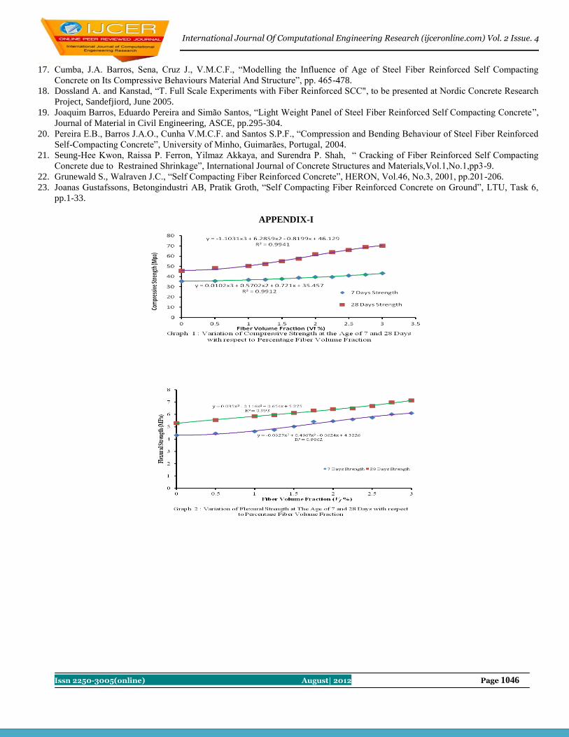
International Journal Of Computational Engineering Research (ijceronline.com) Vol. 2 Issue. 4
Issn 2250-3005(online) August| 2012 Page 1046
17. Cumba, J.A. Barros, Sena, Cruz J., V.M.C.F., “Modelling the Influence of Age of Steel Fiber Reinforced Self Compacting
Concrete on Its Compressive Behaviours Material And Structure”, pp. 465-478.
18. Dossland A. and Kanstad, “T. Full Scale Experiments with Fiber Reinforced SCC", to be presented at Nordic Concrete Research
Project, Sandefjiord, June 2005.
19. Joaquim Barros, Eduardo Pereira and Simão Santos, “Light Weight Panel of Steel Fiber Reinforced Self Compacting Concrete”,
Journal of Material in Civil Engineering, ASCE, pp.295-304.
20. Pereira E.B., Barros J.A.O., Cunha V.M.C.F. and Santos S.P.F., “Compression and Bending Behaviour of Steel Fiber Reinforced
Self-Compacting Concrete”, University of Minho, Guimarães, Portugal, 2004.
21. Seung-Hee Kwon, Raissa P. Ferron, Yilmaz Akkaya, and Surendra P. Shah, “ Cracking of Fiber Reinforced Self Compacting
Concrete due to Restrained Shrinkage”, International Journal of Concrete Structures and Materials,Vol.1,No.1,pp3-9.
22. Grunewald S., Walraven J.C., “Self Compacting Fiber Reinforced Concrete”, HERON, Vol.46, No.3, 2001, pp.201-206.
23. Joanas Gustafssons, Betongindustri AB, Pratik Groth, “Self Compacting Fiber Reinforced Concrete on Ground”, LTU, Task 6,
pp.1-33.
APPENDIX-I

International Journal Of Computational Engineering Research (ijceronline.com) Vol. 2 Issue. 4
Issn 2250-3005(online) August| 2012 Page 1047
STUDY OF COLOR VISUAL CRYPTOGRAPHY
ASMITA KAPSEPATIL, APEKSHA CHAVAN Pillai’s Institute of Information Technology, New Panvel, India 410206
Abstract: This paper shows the study on the concept of color visual cryptography. This paper includes study of color visual
cryptography which involves visual information pixel (VIP) synchronization and error diffusion technique applicable for
color visual cryptography. VIP carries visual information of original image and VIP synchronization helps to keep the same
position of pixels throughout the color channels. Error diffusion generates shares which are clear and visible to human eyes
and it improves the visibility of shares. With the help of these two concepts it results in visual quality improvement of
images. It also includes a brief description of color model used for the process color visual cryptography.
Keywords: error diffusion, visual cryptography, visual information pixel, visual information pixel synchronization
Introduction
Visual cryptography, is an emerging cryptography technology, uses the characteristics of human vision to decrypt encrypted
images. It needs neither cryptography knowledge nor complex computation. For security concerns, it also ensures that
hackers cannot perceive any clues about a secret image from individual cover images. There have been many published
studies of visual cryptography. Most of them, however, have concentrated on discussing black-and-white images, and just
few of them have proposed methods for processing gray-level and color images. Based on previous study in binary image and
grey level images this analyzed concept gives a better visual cryptography method for color images and it provides pleasant
feel of shares and high visual quality to human eye using Visual Information Pixel and Error Diffusion Technique.
Visual Cryptography for Color Images In visual cryptography the secret information that is an image is split into shares such that the decryption can be performed
by the human visual system by simply superimposing the shares. No computations are involved in the reconstruction of
images. This section provides an overview on a color visual cryptography which is simple and good. This method involves C,
M, Y subtractive color model in which the color is represented by applying the combinations of colored lights reflected from
the surface of an object because most of the objects do not radiate by them [1].
Fig 1. Subtractive color model [1]
This proposed method includes the concept of visual pixel information synchronization and error diffusion.
Error Diffusion: This is simple but efficient method for image halftone generation. The quantization error is filtered and fed
to future inputs. The error filter is designed in a way that the low frequency differences between the input and output images
are minimized and it produces pleasing halftone images to human vision.
VIP synchronization: Synchronization of the visual information pixel across the color channels improves visual contrast of
shares. In color VC schemes the colors of encrypted pixels and the contrast can be degraded due to random matrix
permutation. Random matrix permutations are key security features in VC schemes [3]. In gray scale VC schemes it does not
affect the visual schemes however in color schemes, independent execution of random matrix permutation for each color
channel can cause color distortion by placing VIPs at random positions in sub pixels which finally degrades the visual
quality. VIP synchronization prevents the color and contrast of original images from degradation even with matrix
permutations. In this concept it derives basis matrices from the given set of matrices which is used in standard VCS.

International Journal Of Computational Engineering Research (ijceronline.com) Vol. 2 Issue. 4
Issn 2250-3005(online) August| 2012 Page 1048
VIP pixels include the color information of original image which helps in making encrypted shares meaningful. In this
process a set of basis matrices Scc1,c2,,cn
(c,c1,c2,,,cn € {0,1}) is generated where c is a pixel bit of message and c1,,,,cn
indicates the corresponding pixel bits from the shares. In each row of Scc1, c2, cn
there are q number of VIPs which are denoted
as ci and the values are defined by halftone process. The actual bit values of ci are defined by referring the pixel values of
original shares which are not known at the matrix derivation stage and then errors are diffused away. In this analyzed method
each pixel carries visual information as well as message information [3], while other method used needs extra pixels in
addition to the pixel expansion to produce meaningful shares. Since each VIP is placed at the same position in sub pixels
across three color channels, VIP represents accurate colors of original image. In this method ω (Sc[i]) is a hamming weight of
‘OR’ -ed row vector up to i
th rows in Sc
c1, c2, cn. This row vector should not contain any ci as elements. Since the values of ci are
undefined, it can be represented as 0 or 1 in the halftone stage which ensures the placement of ci at the same position in each
row of Sc [3].
Thus each encrypted sub pixel has the same VIP positions across three channels which mean that these sub pixels carry
accurate visual information of the original image and this result in high visual quality in encrypted shares.
EXAMPLE FOR ANALYZED METHOD
Fig. 2 Secret Image [2]
Fig. 4 Shares of original image [2]
Fig. 5 Reconstruction of shares [2]
Conclusion Review of this proposed method provides a study on a better visual cryptography for color images and it provides pleasant
feel with high visual quality.
References 1. Young Chang Hou,2003,vol 36,pp 1619-1629
2. Duo Jin, Wei-Qi Yan, Mohan S. Kankanhalli ,”Progressive Color Visual Cryptography ” , JEI,2004
3. InKoo Kang, Gonzalo R Arce, Heung Kyu Lee, “Color Extended Visual Cryptography using Error Diffusion” ,
2009

International Journal Of Computational Engineering Research (ijceronline.com) Vol. 2 Issue. 4
Issn 2250-3005(online) August| 2012 Page 1049
Laplace Substitution Method for Solving Partial Differential Equations
Involving Mixed Partial Derivatives
Sujit Handibag1, B. D. Karande
2
1Department of Mathematics, Mahatma Basweshwar Mahavidyalaya, Latur-413 512, Maharashtra, India.
2Department of Mathematics, Maharashtra Udaygiri Mahavidyalaya, Udgir, India.
Abstract: In this paper we introduced a new method, named Laplace substitution method (LSM), which is based on Lapalce transform.
This new method with a convenient way to find exact solution with less computation as compared with Method of Separation
of Variables(MSV) and Variational iteration method (VIM). The proposed method solves linear partial differential equations
involving mixed partial derivatives.
Keywords: Approximate solution, Adomian decomposition method, Laplace decomposition method, Nonlinear
partial differential equations.
Introduction: Nonlinear ordinary or partial differential equations involving mixed partial derivatives arise in various fields of science,
physics and engineering. The wide applicability of these equations is the main reason why they have gained so much
attention from many mathe- maticians and scientists. Unfortunately they are sometimes very difficult to solve, either
Numerically or theoretically. There are many methods to obtain approximate solutions of these kinds of equations. Partial
differential equations (PDE) are differential equations that contain unknown multi variable functions and their partial
derivatives. PDEs are used to formulate problems involving functions of several variables, and are either solved by hand,
or used to create a relevant computer model. The Method of separation of variables [8] and Variational iteration method [2-4]
has been extensively worked out for many years by numerous authors. Starting from the pioneer ideas of the Inokuti -Se
kine- Mura method [5], JI-Huan He [4] developed the Variational iteration method (VIM) in 1999. The variational iteration
method , has been widely applied to solve nonlinear problems, more and more merits have been discovered and some
modifications are suggested to overcome the demerits arising in the solution procedure. For example, T.A.Abassy. et al [6,7]
also proposed further treatments of these modification results by using Pade approximants and the Laplace transform. The
Laplace transform is a widely used integral transform. The Laplace transform has the useful property that many relationships
and operations over the originals f(t) correspond to simpler relationships and operations over the images F(s). It is named for
Pierre-Simon Laplace (1749-1827) [1], who introduced the transform in his work on probability theory.
The main goal of this paper is to describe new method for solving linear partial
Differential equations involving mixed partial derivatives. This powerful method will be proposed in section 2; in section 3
we will apply it to some examples and in last section we give some conclusion.
2. Laplace Substitution Method: The aim of this section is to discuss the Laplace substitution method. We consider the general form of non homogeneous
partial differential equation with initial conditions is given below
u(x, 0) = f(x), uy(0, y) = g(y) (2.2)
is the remaining linear terms in which contains only first order
partial derivatives of u(x, y) with respect to either x or y and h(x, y) is the source term. We
can write equation (2.1) in the following form

International Journal Of Computational Engineering Research (ijceronline.com) Vol. 2 Issue. 4
Issn 2250-3005(online) August| 2012 Page 1050
Substituting in equation (2.3), we get
Taking Laplace transform of equation (2.4) with respect to x, we get
Taking inverse Laplace transform of equation (2.5) with respect to x, we get
Re-substitute the value of U(x, y) in equation (2.6), we get
This is the first order partial differential equation in the variables x and y. Taking the
Laplace transform of equation (2.7) with respect to y, we get
Taking the inverse Laplace transform of equation (2.8) with respect to y, we get
The last equation (2.9) gives the exact solution of initial value problem (1.1).
3. Applications: To illustrate this method for coupled partial differential equations we take three examples
in this section.
Example 1: Consider the partial differential equation
with initial conditions u(x, 0) = 0 , uy(0, y) = 0 (3.11)
In the above initial value problem Lu(x, y) = , and general linear term Ru(x,y) is zero.
Equation (3.10) we can write in the following form
(3.12)
Substituting in equation (3.12), we get

International Journal Of Computational Engineering Research (ijceronline.com) Vol. 2 Issue. 4
Issn 2250-3005(online) August| 2012 Page 1051
(3.13)
This is the non homogeneous partial differential equation of first order. Taking Laplace
transform on both sides of equation (3.13) with respect to x, we get
Taking inverse Laplace transform of equation (3.13) with respect to x, we get
(3.14)
This is the partial differential equation of first order in the variables x and y. Taking
Laplace transform of equation (3.14) with respect to y, we get
(3.15)
Taking inverse Laplace transform of equation (3.15) with respect to y, we get
(3.16)
This is the required exact solution of equation (3.10). Which can be verify through the
substitution. Which is same the solution obtained by (MSV) and (VIM).
Example 2: Consider the partial differential equation
(3.17)
u (x, 0)=1+ cosx , uy(0, y)= -2siny (3.18)
In the above example assume that ux(x, y) and uy(x, y) both are differentiable in the domain of definition of function u(x, y)
[Young's Theorem]. This implies that . Given initial conditions (3.18) force to write the equation (3.17) in
following form and use the substitution
(3.19)
(3.20)
Taking Laplace transform of equation (3.20) with respect to x, we get
(3.21)
Taking inverse Laplace transform of equation (3.21) with respect to x, we get
(3.22)
Taking Laplace transform of equation (3.22) with respect to y, we get
(3.23)
Taking inverse Laplace transform of equation (3.23) with respect to y, we get
u (x, y)=(1+cosx) cos y (2.24)
This is the required exact solution of equation (3.17). Which can be verify through the
substitution. Which is same the solution obtained by (MSV) and (VIM).
Example 3: Consider the following partial differential equation with
With initial conditions
u(x, 0)=1, u(0, y)=y , u y(0, y)=0 (3.26)

International Journal Of Computational Engineering Research (ijceronline.com) Vol. 2 Issue. 4
Issn 2250-3005(online) August| 2012 Page 1052
In the above example Ru(x, y) = Use the substitution in equation (3.25), we get
(3.27)
Taking Laplace transform of equation (3.27) with respect to x, we get
(3.28)
Taking inverse Laplace transform of equation (3.28) with respect to x, we get
(3. 29)
Taking Laplace transform of equation (3.29) with respect to y, we get
(3.30)
Taking inverse Laplace transform of equation (3.30) with respect to y, we get
(3.31)
We cannot solve the equation (3.31) because our goal u(x, y) is appeared in both sides of equation (3.31). Therefore the
equation (3.25) we cannot solve by using LSM because of .
3. Conclusion In this paper, we proposed Laplace Substitution Method (LSM) is applicable to solve
partial differential equations in which involves mixed partial derivatives and general linear
term Ru(x, y) is zero. The result of first two examples compared with (MSV) and (VIM), tell us that these methods can be
use alternatively for the solution of higher order initial value problem in which involves the mixed partial derivatives with
general linear term Ru(x, y) is zero. But the result of example number three tell us that (LSM) is not applicable for those
partial differential equations in which R u(x, y) 0.Consequently the (LSM) is promising and can be applied for other
equations that appearing in various scientific fields.
References [1] Joel L. Schiff, The Laplace Transform: Theory and Applications, Springer
[2] J. H. He, Approximate analytical solution for seepage ow with fractional derivatives in porous media, Comput.
Methods Appl. Mech. Engrg. 167(1998)57-68.
[3] J. H. He, Approximate solution of nonlinear differential equations with convolution product nonlinearities, Comput.
Methods Appl. Mech. Engrg. 167(1998)69-73.
[4] J.-H. He, Variational iteration method- a kind of non-linear analytical technique: some examples, Internat. J. Non-
Linear. Mech. 34 (1999) 699-708.
[5] M. Inokuti, H. Sekine, T. Mura, General use of the Lagrange multiplier in nonlinear mathematical physics,
Variational Methods in the Mechanics of Solids, Pergamon Press, New York, 1978, pp. 156162.
[6] T. A. Abassy , M.A.El-Tawil ,H.El-Zoheiry, Solving nonlinear partial differential equations using the modified
variational iteration Pade technique ,Journal of Computational and Applied Mathematics 207 (1)(2007)73-91.
[7] T. A. Abassy, M.A.El-Tawil ,H.El-Zoheiry, Exact solutions of some nonlinear partial diferential using the
variational iteration method linked with Laplace transforms and the Pade technique, Computers and Mathematics
with Applications,54 (7-8))(2007)940-954.
[8] Richard Jozsa, DAMTP Cambridge, PDEs on bounded domains: Separation of vari-ables, Part II, (2011).

International Journal Of Computational Engineering Research (ijceronline.com) Vol. 2 Issue. 4
Issn 2250-3005(online) August| 2012 Page 1053
ARkanoid: Development of 3D Game and Handheld Augmented Reality 1Markus Santoso,
2Lee Byung Gook
1Ph.D Candidate, Visual Content Department, Dongseo University, South Korea.
2Professor, Visual Content Department, Dongseo University, South Korea.
Abstract In this paper, researcher presents ARkanoid, a 3D Handheld Augmented Reality game. Through this project, researcher tried
to remake the old 2D game and brought it into something new. This time, researcher chooses an Arkanoid game which was
first introduced in 1986 and became very famous together with the raise of video game era on that moment. Not only makes it
in the 3D version, but also researcher combines it with an Augmented Reality (AR) technology. And finally, this AR project is
finalized through handheld devices so that it can be commercialized to the real world in the future. This paper discusses the
technical aspect of the game, the design and development process and the result of user study. The goal of this research is to
explore the affordances and constraints of handheld AR interfaces for 3D games. This project showed some promising results
of handheld AR application in game. User feels that the game presentation with 3D and AR technology is more interesting
than general 2D game, the immersion of virtual object in real world also brings unique game ambient and touch-screen
gameplay makes the player becomes more engaged to the game. Researcher hopes this research can be the milestone and will
inspire the further research of respected field. Researcher also hopes this Arkanoid AR game can educate the user of handheld
device who mostly grew up in previous era of Arkanoid game, that they can easily get familiar with AR technology
applications.
Keywords – Arkanoid game, 3D Game, Handheld AR
I. Introduction
These last decades, the 3D technology has been well developed and this knowledge has become more mature than
before. We can see that 3D technology has been used in several fields in our daily life. However, to reach the end user or
audience, this 3D technology needs to be displayed. In general, there are 4 types of 3D display, namely stereoscopic,
augmented and virtual reality, integral image and holographic display. Figure 1 will display a simple graph of 3D technology
display.
Figure 1. 3D Technology Display
Historically, 3D technology was developed based on 2D graphic. In the early of 90’s 2D graphic technology got its
popularity. Then, 3D technology became mature and started to be commercialized. Several fields had been reached by
previous 3D technology. 3D technology then derived again become 3D stereoscopic that been massively used these days.
After that, researchers tried to find another way to display 3D technology, and then augmented/virtual reality appeared.
Recently, an augmented and virtual reality has reached certain level to bring them from research lab into real world. The core
technology has been mature enough to be applied in several fields of human life, such as entertainment, education and others.
The integral image is starting to develop as well these days. It rose to overcome several disadvantages appeared from
3D stereoscopic technology, such as parallax problem. This technology is still in process to find their maturity in research lab.
And finally, the most ideal 3D technology display is holographic display. The previous 3D display however is still covered by
the screen. It is just the illusion of 3D display behind the screen. Holographic display will display the 3D object in the free-
space and can interact directly with the user. Figure 2 will display the 3D display technology transition.
Figure 2. Display Technology Transition

International Journal Of Computational Engineering Research (ijceronline.com) Vol. 2 Issue. 4
Issn 2250-3005(online) August| 2012 Page 1054
In this paper, researcher decided to develop a project related to handheld augmented reality. Some expertise believed
that an AR/VR is a proper bridge to reach an ideal 3D display, holographic. While the integral image is still in the research and
development phase, an AR/VR technology has reached their maturity. Reaching more than 10 years since its first official
conference, this research field has grown significantly. Based on this fact, lately several parties started to move this technology
to real world so it can give benefit a lot of people. Previously this technology had several barriers related with the
commercialization effort. But the invention of handheld devices happened recently and helped AR technology to reach end
user easier than before. Based on these facts, researcher chose an augmented reality that is finalized in handheld device to
display the 3D object in this game.
From this project, researcher would like to support the commercialization effort of AR technology. Several AR
projects have been developed before in the various fields and now researcher wanted to represent one of the famous games in
previous era, Arkanoid, and combined it with recent technology. This research is expected to be a proper milestone for further
research and development of AR technology in various fields. It is the right time for AR technology to show its contribution to
real human life.
II. Previous Work
The commercialization effort of AR technology has been appeared since several years ago. Various fields have been
reached by AR technology but in general there are six types of applications, namely personal information system, industrial
and military applications, medical applications, entertainment, office applications, education and training [1]. But, still it found
some difficulties to reach end user in real world. The invention of handheld device, such as smart phone and computer tablet,
which had been massively used by people recently really helped AR technology to reach real world application. It also had
domino effect to the number of research in handheld AR. Survey found that the published papers about handheld AR has
become more popular these days [2].
In education field, Markus et al had developed an AR edutainment content for Sungsan elementary school (SES) in
Busan - South Korea[9]. The project name is EDUtangram and it combined conventional Tangram edutainment tool with AR
technology. This project was also finalized using handheld devices, iPad2. An AR Tangram edutainment was then installed on
30 iPads belonged to SES and they used it regularly during their class session.
Figure 3. EDUtangram project.
In entertainment field, these days there are several great AR projects released. At least there are three big names in
entertainment industry exploring AR technology for their activity. Transformer creates an AR application for iPad device to
support their movie in the theater. This year Marvel Corp. also releases an AR application for one of their most famous hero
characters, Iron Man. And lastly, to support the commercial release of newest Spiderman movie in theater, they also create AR
application for handheld device. Together with conventional promotion media such as poster and website, this handheld AR
application become an integrated and creative marketing tools.
Figure 4. Transfomer Handheld AR Applications
Figure 5. Marvel Handheld AR Applications

International Journal Of Computational Engineering Research (ijceronline.com) Vol. 2 Issue. 4
Issn 2250-3005(online) August| 2012 Page 1055
Figure6. Spiderman 4 Handheld AR Applications.
Not only in entertainment field, increasing number of AR project also happened in game field. Several published
plug-in or software for AR purpose had contribute to blooming number of AR applications in this field both for PC- based,
handheld device-based and other possible device. One of the developers who develop 3D AR game for handheld device is
Fuzzy Logic. They developed an Augmentron for iPad2 device.
Figure7. Augmentron handheld AR applications
III. Game Description
ARkanoid was chosen as the main theme of this project. Arkanoid is an arcade game developed by Taito in 1986 and
it first released for Atari consol. This game is well-known on that moment so that it reproduced again for several game
consoles that released after Atari console era. In simple way, the player of Arkanoid will control the paddle and prevent a ball
falling down from playing field. When the ball hit the paddle, it will bounce against the brick that are provided in the field.
The objective is to finish all of the bricks, end the game and move to next stage. The objective is simple but the challenge is
not that easy. It makes the player become addicted to this game. In 1989, Arkanoid was reviewed by Patricia Hartley and Kirk
Lesser. In their “The Role of Computers” column, the reviewers gave this game 5 out of 5 stars.
Figure8. Arkanoid Game in Early Era.
Children who play an Arkanoid game in early released era had been grown up now, finished their higher education
and some of them already maybe working. The most important thing is they are the user of the handheld devices recently. By
combining the game that famous in their childhood era with AR technology, researcher tries to educate this generation to be
familiar with this recent technology. So that, they will be able to get used with further AR application easily.
IV. Augmented Reality Augmented reality topic was first introduced by Sutherland in 1960. Then it became an emerging research topic when
Milgram and Kishino published their paper and introduce about the concept of “Virtuality Continuum”[7]. In this concept,
they clarify the position of the augmented reality in the simple graph as seen in figure 9. This concept then became the
milestone of the Augmented Reality development until these days.
Figure9. Virtual Continuum Concept

International Journal Of Computational Engineering Research (ijceronline.com) Vol. 2 Issue. 4
Issn 2250-3005(online) August| 2012 Page 1056
Augmented reality is technology which allows computer generated virtual imagery to exactly overlay physical
objects in real time. AR allows user to interact with the virtual images using real objects in a seamless way [4]. Furthermore,
Azuma provide commonly accepted definition of AR as a technology which combines real and virtual imagery, interactive in
real time and registers the virtual imagery with the real world [8]. In order to provide an effective AR experience there are
number of factors that must be developed, namely graphics rendering hardware and software, tracking techniques, tracker
calibration and registration tools, display hardware, computer processing hardware and interaction techniques [2]. During the
evolution of AR, there are various research topics appeared and developed extensively.
In general, there are 2 groups of AR research topic [2]. First group contains the main research areas of Tracking
techniques, Interaction techniques, Calibration and Registration, AR Applications and Display techniques. This group
represents the core AR technology areas which are needed to deliver an AR application. Second group of topic reflects more
emerging research interest, including Evaluating/testing, Mobile/Handheld AR, AR Authoring, Visualization, Multimodal AR,
Rendering [2]. Since the invention of handheld devices in our daily life, the number of research in mobile AR has been raised
as well.
One of the main components for AR is display. There are three major types of AR displays, namely Head-Mounted
Display (HMD), Spatial Display and Handheld Display [3]. HMD is a display device worn on the head or as part of helmet
and that places both images of the real and virtual environment over the user’s view of the world. Spatial Display makes use of
video projector, optical elements, holograms, radio frequency tags and other tracking technologies to display graphical
information directly onto physical object without requiring the user to wear it or carry the display. Handheld display employs
small computing devices with a display that the user can hold in their hands. There are three distinct classes of commercially
available handheld display that are being used for AR system, namely Smart-phones, PDA and Tablet PC [3].
The presence of handheld devices in AR field is expected to contribute more in commercialization effort of AR
technology. The reason is because handheld AR is predicted to fulfill some requirements to be successful systems in the
market. Carmigniani and Furht stated there are three requirements for systems to reach its success in market. First is socially
acceptable, it means that is subtle, discrete and unobtrusive. Second is natural interaction which is needed to be able to interact
with the system in a natural way. And last factor is fashionably acceptable so that user does not need to look strange while
operating the system [3].
V. Design And Development Process ARkanoid is a project that combines conventional Arkanoid game with Augmented Reality technology and installed
on handheld device. The gameplay of Arkanoid itself will remain unchanged, still related to paddle, ball and brick. But this
time, researcher represented Arkanoid game in 3D version.
To build this game, researcher used Unity3D game engine. Unity3D game engine right now has been widely used by
game developer. There are tons of advantages offer by Unity3D, such as multi-platform device possibility (iOS, android,
Xbox, Nintendo wii, PC), graphical advantages, simple user interface and others. Unity3D is supported by 3 common
programming languages such as java, c# and boo. Unity3D also has a strong community to support each member in this area
and it becomes another advantage for the various skill range of user (www.unity3d.com).
To build the AR session, researcher used Vuforia. Vuforia is the AR extension created by Qualcomm and it perfectly
bundled with Unity3D software.Vuforia is a marker-based AR system and it enables vision detection and tracking
functionality into Unity3D IDE, it also allows developers to easily create AR application and games. A Vuforia based AR
application is composed of the following core components: camera, image converter, tracker, video background renderer,
application code and target resources. Figure 10 is the data flow diagram of Vuforia Ar extension (http://ar.qualcomm.at).
Figure10. Data Flow Diagram of the Vuforia AR Extension
Basically, Vuforia is Marker-based AR extension. Because of that, we need the marker so that the system can detect
it, track it and then visualize the 3D object above the marker. Unlike the previous AR tool, Vuforia allow us to create colorful
marker because they just extract the edge and contrast as a feature point. Figure 11 show the design of marker for ARkanoid
project.

International Journal Of Computational Engineering Research (ijceronline.com) Vol. 2 Issue. 4
Issn 2250-3005(online) August| 2012 Page 1057
Figure11. ARkanoid Marker Design.
To play ARkanoid AR game, user needs to prepare and put the marker in the horizontal position. After that, they need
to point device’s camera into the marker. When the camera already capture the marker, 3D object will automatically appeared
in the screen and audience can start to play the game. Figure 12 show the gameplay procedure of ARkanoid AR game.
Figure12. ARkanoid Gameplay Procedure
Previously, player needs to use joystick, keyboard or any other 3rd
parties to move the paddle. But, since this new
ARkanoid is built on the handheld devices that had no additional button, researcher added slide function to move the paddle.
Using this function, player can slide their finger on the device’s screen to move the paddle to the respected direction. Figure 13
show the slide function of ARkanoid 3D game.
Figure13. Slide Function of ARkanoid 3D Game
In conclusion, researcher try to bring the same gameplay experience from the conventional while in the same time
researcher should adjust some parts to fit the AR technology and handheld devices. The general gameplay is still remaining
the same, but the 2D graphic display was changed into 3D graphic display. This game also created on marker-based AR
technology. Finally, since it built on handheld devices, rather than using 3rd
parties to interact with 3D object, player can
directly touch and interact with the paddle on this game.
VI. User Study 4.1 Goals and Participant Recruitment
After complete ARkanoid game prototype, researcher conducted small user study with 10 participants. Specifically,
researcher hoped to explore their opinion about the comparison of 3D AR game with the conventional 2D game, the
augmented reality technology embedded with game and the gameplay of new Arkanoid. We were interested to find out their
interest about an AR game and their feedback about the gameplay itself would be valuable information for the further research
in AR game.
To recruit participants, we have several situations to be considered. First, the participant should have an experience
playing an early Arkanoid game, no matter what game console they used at that time. Since we want to compare between
conventional Arkanoid games with our new Arkanoid, so the previous experience of an early Arkanoid game should be
fulfilled by participant. Second, we try to find participant from various background of knowledge as long as they can satisfy
first requirement. They can be a student from various major, workers, housewife and other else. And last, we try to observe
multi-nation participant. Rather than focusing in one nation or races, we open this research for participant from various
nationalities.
Finally, we found 10 participants with the age range from late of 20’s to mid of 30’s. Since they spent their childhood
in 1980’s until early of 1990’s, all of them definitely had an experience playing early Arkanoid game. 2 of them are the
undergraduate students from non computer science major, 4 of them are graduate students from computer science major, 2 of
them are workers, and 2 of them are housewife. The participants were from 5 countries, namely Korea, China, Malaysia,
Indonesia and Russia. Except the graduate students, all of them do not have prior knowledge and experience in augmented
reality games before. For the research in Indonesia, researcher sent the application installer to the participant and the survey
was completed by skype chatting.

International Journal Of Computational Engineering Research (ijceronline.com) Vol. 2 Issue. 4
Issn 2250-3005(online) August| 2012 Page 1058
4.2 Procedure and Setting
The user study was divided into three parts. First, researcher gave a brief explanation about the gameplay procedure;
in this case researcher already prepared the marker and handheld device. After that, researcher let the participant played the
game directly and there was no game time limitation. Participant could decide by themselves when they wanted to stop
playing the game. Except for the participant in Indonesia, all the research was done in the research lab with one condition
should be considered, it should be indoor. Indoor place was chosen to prevent unexpected distraction to the tracking
robustness ability. And last, researcher interviewed the participant to gather needed information, data and opinion.
The user study also conducts individually. It means that it separately from one participant to each other. Since mostly
of user study were done by interviewing, it would be easier to explore their opinion when discussions were held individually.
By using individual interview, not only we can observe more about participant opinion but also it can keep privacy from each
recruited participant.
VII. Discussion Through the user study, participants gave us valuable feedback about ARkanoid AR game. We interviewed the
participants whether they like or dislike the new appearance of Arkanoid game. 8 of the participants were pros to the new
ARkanoid AR game. Most of them explained that the using of 3D graphic and AR technology bring this game to the next
level and it is more interesting than conventional 2D game. The rest participants choose to cons the new ARkanoid AR game
since they felt there is no significant difference to early Arkanoid game and there is no urgency to use 3D and AR technology
since they already like early Arkanoid format.
Next, we try to observe their opinion about the AR technology that embedded in this game. 6 of the participants said
that they are excited and interested about the AR technology. Rather than playing a fully virtual game, the immersion of
virtual object in the real world gave them a unique sensation during game session. The rest participants stand for cons position
since they felt that AR technology made the gameplay become more difficult because they needed to point the camera to the
marker during game session, the other else said that it was quite heavy to hold the device during game session.
Last, we observe their opinions about the gameplay of new ARkanoid game. 7 of the participants said that they like
the new way of the ARkanoid gameplay. Previously, they need to move the paddle using 3rd
parties’ device such as joystick,
keyboard and other else. But using handheld device and sliding function, participants could interact with the paddle directly
from the screen. It made them comfortable and more engaged with the game itself. 2 of the participants said that using
handheld device to play a game was fine and they give suggestion to put the virtual button in the screen to move the paddle
rather than using slide function. And 1 of the participant said that playing with the joystick was better especially in controlling
the paddle.
VIII. Conclusion In this paper, we conducted research about the potential of combination 3D game and handheld AR technology then
analyzed the user study from it. In contrast with the early design of Arkanoid game, researcher tried to represent it into 3D
platform game and furthermore combine it with an AR technology. And finally, the new ARkanoid game was finalized in the
recent handheld devices that already massively used these days.
Our research about the combination of 3D game and handheld AR technology found promising result and it can be
the basic of the further research to bring this technology from research lab to the real world. We can conclude that users feel
the game presentation with 3D graphic and AR technology is more interesting than general 2D game, the immersion of virtual
object in real world also brings unique game ambient and touch-screen gameplay makes the gap between player and the game
became closer and it makes them more engaged to the game.
As we move forward, researcher hope this research can be milestone and will inspire further research of respected
field. Researcher also hopes can educate the user of handheld device who mostly grew up in the previous era of Arkanoid
game, so that they can easily get familiar with AR technology applications. Since AR is pretty new technology in our daily
life, we need to educate the people as end user so that they can get used and familiar with this technology. In the long run, we
hope to explore an AR technology deeper and observe the application of AR technology in various fields, any other purposes
and brings more benefit to people in the real world.
Acknowledgement This research was supported by Basic Science Research Program through the National Research Foundation of Korea (NRF)
funded by the Ministry of Education, Science and Technology (2010-0009003).

International Journal Of Computational Engineering Research (ijceronline.com) Vol. 2 Issue. 4
Issn 2250-3005(online) August| 2012 Page 1059
References 1. D.W.F. Van Krevelen, R. Poelman. A Survey of Augmented Reality Technologies, Applications and Limitations. In The
International Journal of Virtual Reality, 2010, 9(2), pp1-20.
2. F. Zhou, H.B.L. Duh, M. Billinghurst. Trends in Augmented reality Tracking, Interaction and Display: A Review of Ten
Years of ISMAR. In International Symposium on Mixed and Augmented Reality (ISMAR’08).
3. J. Carmigniani, B. Furht. Augmented Reality: An Overview. In Handbook of Augmented Reality. ISBN: 978-1-4614-
0063-9. Springer Science, London.
4. M. Billinghurst. Augmented Reality in Education. New Horizons for Learning. Retrieved from:
http://www.it.civil.aau.dk/it/education /reports/ar_edu.pdf.2002.
5. M. Billinghurst, A. Henrysson. Research Direction in Handheld AR. In The International Journal of Virtual Reality,
2006, 5(2), pp51-58.
6. M. Haller, M. Billinghurst, B. Thomas. Augmented Reality: Interfaces and Design. ISBN: 1-59904-066-2. Idea Group
Publishing.
7. P. Milgram, F.Kishino. A Taxonomy of Mixed Reality Visual Displays. In IEICE Transactions on Information Systems,
VolE77D, No. 12, December 1994.
8. R.T. Azuma. A Survey of Augmented Reality. In Presence:Teleoperators and Virtual Environment, 6:4, 355-385, August
1997.
9. S. Markus, F.Y. Wang, B.G. Lee. Development of Edutainment Content for Elementary School Using Mobile
Augmented Reality. Proceeding of ICCRD’12 (Chengdu, China, May 5-6, 2012).

International Journal Of Computational Engineering Research (ijceronline.com) Vol. 2 Issue. 4
Issn 2250-3005(online) August| 2012 Page 1060
A Selective Survey and direction on the software of Reliability Models
Vipin Kumar Research Scholar, S.M. Degree College, Chandausi
Abstract: Software development, design and testing have become very intricate with the advent of modern highly distributed
systems, networks, middleware and interdependent application. The demand for complex software systems has increased
more rapidly than the ability to design, implement, test, and maintain them and the reliability of software systems has
become a major concern for our modern society. Software reliability modeling and measurements have drawn quite a bit
of attention recently in various industries due to concerns about the quality of software. In few years of 21st century, many
reported system outages or machine crashes were traced back to computer software failures.
In this paper, I have many challenges in getting wide spread use of software reliability models. I am focus
on software reliability models and measurements. A software reliability model specifies the general form of the
dependence of the failure process on the principal factors that affect it: fault introduction, fault removal and the
operational environment. During the test phase, the failure rate of a software system is generally decreasing due to
discovery and correction of software faults. With careful record-keeping procedures in place, it is possible to use
statistical methods to analyze the historical record. The purpose of these analyses is twofold:(1) to predict the additional
time needed to achieve a specified reliability objective; (2) to predict the expected reliability when testing is finished.
Key words: Dynamic model, Growth model, Reliability software, Static model, Telecommunication.
Introduction: In few year of century, many reported system outages or machine crashes were traced back to computer software failures.
Consequently, recent literature is replete with horror stories due to software problems. Software failure has impaired
several high visibility programs in space, telecommunications and defense and health industries. The Mars Climate
Orbiter crashed in 1999. The Mars Climate Orbiter Mission failure investigation Board [1] concluded that “The root cause
of the loss of the spacecraft was the failed translation of English unit into metric units in a segment of ground based,
navigation related mission software. Current versions of the Osprey aircraft, developed at a cost of billions of dollars, are
not deployed because of software induced field failure. In the health industry [2], the Yherac-25 radiation therapy
machine was hit by software errors in its sophisticated control systems and claimed several patients’ lives in 1985 &1986.
Even in the telecommunications industry, known for its five nines reliability, the nationwide long distance network of a
major carrier suffered an embarrassing network outage on January 1990, due to software problem. In 1991, a series of
local network outage occurred in a number of US cities due to software problems in central office switches [3].
Software reliability is defined as the probability of failure free software operations for a specified
period of time in a specified environment [4]. The software reliability field discusses ways of quantifying it and using it
for improvement and control of the software development process.. Software reliability is operationally measured by the
number of field failures, or failures seen in development, along with a variety of ancillary information. The ancillary
information includes the time at which the failure was found, in which part of the software it was found, the state of
software at that time, the nature of the failure. ISO9000-3 [5] is the weakest amongst the recognized standards, in that it
specifies measurement of field failures as the only required quality metric.
In this paper, I take a narrower view and just look at models that are used in software reliability-their
efficacy and adequacy without going into details of the interplay between testing and software reliability models.
Software reliability measurement includes two types of model: static and dynamic reliability estimation, used typically in
the earlier and later stages of development respectively. These will be discussed in the following two sections. One of the
main weaknesses of many of the models is that they do not take into account ancillary information, like churn in system
during testing. Such a model is described in Growth reliability. A key use of the reliability models is in the area of when
to stop testing. An economic formulation is discussed in next paragraph.
Static Models:
One purpose of reliability models is to perform reliability prediction in an early stage of software development. This
activity determines future software reliability based upon available software metrics and measures. Particularly when field
failure data are not available (e.g. software is in design or coding stage), the metrics obtained from the software
development process and the characteristics of the resulting product can be used to estimate the reliability of the software

International Journal Of Computational Engineering Research (ijceronline.com) Vol. 2 Issue. 4
Issn 2250-3005(online) August| 2012 Page 1061
upon testing or delivery. I am discussing two prediction models: the phase based model by Gaffney and Davis [10] and a
predictive development life cycle model from Telcordia Technologies by Dalal and Ho [11].
(a) Phase based Model: Gaffney and Davis [10] proposed the phase based model, which divides the software development cycle into different
phases (e.g. requirement review, design, implementation, unit test, software integration, system test, operation etc.)
and assumes that code size estimates are available during the early phases follow a Raleigh density function when
normalized by the lines of code. The idea is to divide the stage of development along a continuous time (i.e. t=0-
1means requirements analysis and so on) and overlay the Raleigh density function with a scale parameter, known as
fault discovery phase constant, is estimate by equating the area under the curve between earlier phases with observed
error rates normalized by the lines of code. This method gives an estimate of the fault density for any later phase. The
model also estimates the number of faults in a given phase by multiplying the fault density by the number of lines of
code.
This method is clearly motivated by the corresponding model used in hardware reliability and the
predictions are hardwired in the model based on one parameter. In spite of this criticism, this model is one of the first
to leverage information available in earlier development life cycle phases.
(b) Predictive Development Life Cycle Model:
In this model the development life cycle is divided into the same phases as in Phase based method. However, it does
not postulate a fixed relationship (i.e. Raleigh distribution) between the numbers of faults discovered during different
phases. Instead, it leverages past releases of similar products to determine the relationships. The relationships are not
postulated beforehand, but are determined from data using only a few releases per product. Similarity is measured by
using an empirical hierarchical bays framework. The number of releases used as data is kept minimal and, typically,
only the most recent one or two releases are used for prediction. The lack of data is made up for by using as many
products as possible that were being developed in a software organization at around the same time. In that sense it is
similar to meta analysis [12], where a lack of longitudinal data is overcome by using cross-sectional data.
22 products and their releases versus observed (+) and predicted Fault Density connected by dash lines. Solid
vertical lines are 90% predictive intervals for Faulty Density
Conceptually, the two basic assumptions behind this model are as follows that one is “defect rates from different products
in the same product life cycle phase are samples from a statistical universe of products coming from that development
organization” and the second is “different releases from a given product are samples from a statistical universe of
releases for that product”.
Dynamic Models: Reliability Growth Models Software reliability estimation determines the current software reliability by applying statistical inference techniques to
failure data obtained during system test or during system operation. Since reliability tends to improve over time during the
software testing and operation periods because of removal of faults, the models are also called reliability growth models.
They model the underlying failure process of the software, and use the observed failure history as a guideline, in order to
estimate the residual number of faults in the software and the test time required to detect them. This can be used to make

International Journal Of Computational Engineering Research (ijceronline.com) Vol. 2 Issue. 4
Issn 2250-3005(online) August| 2012 Page 1062
release and development decisions. Most current software reliability models fall into this category. Details of these
models can be found in Lyu [9], Musa et al. [8], Singpurwalla and Wilson [13], and Gokhale et al. [14].
Classes of Models:
I am describing a general class of models. In binominal models the total number of faults is some number N; the number
found by time t has a binominal distribution with mean ( )t NF t , where F (t) is the probability of a particular fault
being found by time t. Thus, the number of faults found in any interval of time (including the interval (t, ∞) is also
binominal. F (t) could be any arbitrary cumulative distribution function. Then, a general class of reliability models is
obtained by appropriate parameterization of µ (t) and N.
Letting N be Poisson (with some mean υ) gives the related Poisson model; now, the number of
faults found in any interval is Poisson, and for disjoint intervals these numbers are independent. Denoting the derivative of
F by F׳, rate at time t is ( )F t /[1-F(t)]. These models are Markovian but not strongly Markoviaan, except when F is
exponential; minor variations of this case were studied by Jelinski and Moranda [15], Shooman [16], Schneidewind [17],
Musa [18], Moranda [19], and Goel and okomoto [20]. Schick and Wolverton [21] and crow [22] made F a Weibull
distribution; Yamada et al. [23] made F a Gamma distribution; and Littlewood’s model [24] is equivalent to aassuming F
to be Pareto. Musa and Okumoto [25] assumed the hazard rate to be an inverse linear function of time; for this
“Logarithmic Poisson” model the total number of failures is infinite. The success of a model is often judged by how well
it fits an estimated reliability curve µ(t) to the observed “number of faults versus time” function.
Let us examine the real example plotted in above Figure from testing a large software system at a
telecommunications research company. The system had been developed over years, and new releases were created and
tested by the same development and testing groups respectively. In this figure, the elapsed testing time in staff day’s t is
plotted against the cumulative number of faults found for one of the releases. It is not clear whether there is some “total
number” of bugs to be found, or whether the number found will continue to increase indefinitely. However, from data
such as that in figure, an estimation of the tail of a distribution with a reasonable degree of precision is not possible. I also
fit a special case of the general reliability growth model described above corresponding to N being Poisson and F being
exponential.
Reliability Growth Modeling:
We have so far discussed a number of different kinds of reliability model of varying degrees of plausibility, including
phase-based models depending upon a Raleigh curve, growth models like the Goel-okumoto model, etc. The growth
models take us at input either failure time on failure count data, and fit a stochastic process model to reflect reliability
growth. The differences between the models lie principally in assumptions made on the underlying stochastic process
generating the data.
Most existing models assume that no explanatory variables are available. This assumption is assuredly simplistic, when
the models are used to model a testing process, for all but small systems involving short development and life cycles. For
large systems (e.g. greater than 100 KNCSL, i.e. thousands of non-commentary source lines) there are variables, other
than time, that are very relevant. For example, it is typically assumed that the number of faults (found and unfound) in a
system under test remains stable during testing. This implies that the code remains frozen during testing. However, this is
rarely the case for large systems, since aggressive delivery cycles force the final phases of development to overlap with
the initial stages of system test. Thus, the size of code and, consequently, the number of faults in a large system can vary
widely during testing. If these changes in code size are not considered as a covariate, one is , at best, likely to have an
increase in variability and a loss in predictive performance; at worst, a poor fitting model with unstable parameter
estimates is likely. I briefly describe a general approach proposed by Dalal and McIntosh [28] for incorporating covariates
along with a case study dealing with reliability modeling during product testing when code is changing.
3000
NCNCSL
0 200 400 600 800 1000 1200 1400
Staff days

International Journal Of Computational Engineering Research (ijceronline.com) Vol. 2 Issue. 4
Issn 2250-3005(online) August| 2012 Page 1063
800
Cumulative faults 400
0 800 1000 1500 2000
Staff days Model fit
As an example, consider a new release of a large telecommunications system with approximately 7 million NCSL and 300
KNCNCSL (i.e. thousands of lines off non-commentary new or changed source lines). For a faster delivery cycle, the
source code used for system test was updated every night throughout the test period. At the end of each of 198 calendar
days in the test cycle, the number of faults found, NCNCSL, and thee staff time spent on testing were collected. Above
figure portrays the growth of the system in terms of NCNCSL and of faults against staff time. The corresponding
numerical data are providing in Dalal and McIntosh [28].
Assume that the testing process is observed at time ti , i=0, 1,. . ., h, and at any given time the
amount of time it takes to find specific bug is exponential with rate m. At time ti, the total number of faults remaining in
the system is Poisson with mean li+1, and NCNCSL is increased by an amount Ci. This change adds a Poisson number of
faults with mean proportional to C, say qCi, These assumption lead to the mass blance equation, namely that the expected
number of faults in the system at ti (after possible modification) is the expected number of faults in the system at ti-1
adjusted by the expected number found in the interval (ti-1, ti) plus the faults introduced by the changes made at ti:
1
1i im t t
i i il l e qC
for i= 1, 2, 3….h. Note that q represent the number of new faults entering the system per additional NCNCSL, and l1
represent the number of faults in the code at the starts of system test. Both of these parameters make it possible to
differentiate between the new code added in the current release and the older code. For the example, the estimated
parameters are q=0.025, m=0.002, and l1=41. The fitted and the observed data are plotted against staff time in the given
above figure (bottom). The fit is evidently very good. Of course, assessing the model on independent or new data is
required for proper validation.
Now, I examine the efficacy of creating a statistical model. The estimate of q in the example is
highly significant, both statistically and practically, showing the need for incorporating changes in NCNCSL as a
covariate. Its numerical value implies that for every additional 10000 NCNCSL added to the system, 25 faults are being
added as well. For these data, the predicted number of faults at the end of the test period is Poisson distributed with mean
145. Dividing this quantity by the total NCNCSL, gives 4.2 per 10000 NCNCSL as an estimated field fault density. These
estimates of the incoming and outgoing quality are valuable in judging the efficacy of system testing and for deciding
where resources should be allocated to improve the quality. Here, for example, system testing was effective, in that it
removed 21 of every 25 faults. However, it raises another issue: 25 faults per 10000 NCNCSL entering system test may
be too high and a plan ought to be considered to improve the incoming quality.
None of the above conclusion could have been made without using a statistical model. These
conclusions are valuable for controlling and improving the process.
Conclusion: In this paper, I am described key software reliability models for early stages, as well as for the test and operational phases
and have given some examples of their uses. I have also proposed some new research directions useful to practitioners,
which will lead to wider use of software reliability models.
References: 1. Mars Climate Orbiter Mishap Investigation Board Phase I Report, 1999, NASA.
2. Lee L. The day the phones stopped: how people get hurt when computers go wrong. New York: Donald I. Fine, Inc.;
1992
3. Dalal SR, Horgan JR, Kettenring JR. Reliable software and communication: software quality, reliability, and safety.
IEEE J spec Areas Commun 1993; 12; 33-9.
4. Institute of Electrical and Electronics Engineers. ANSI/IEEE standard glossary of software engineering
terminology, IEEE Std. 729-1991.
5. ISO 9000-3. Quality management and quality assurance standard- part 3: guidelines for the application of ISO 9001
to the development, supply and maintenance of software. Switzerland: ISO; 1991.
6. Paulk M, Curtis W, Chrises M, Weber C., Capability maturity model for software, version 1.1, CMU/SEI-93-TR-
24.Carnegie Mellon University, Software engineering Institute, 1993.

International Journal Of Computational Engineering Research (ijceronline.com) Vol. 2 Issue. 4
Issn 2250-3005(online) August| 2012 Page 1064
7. Emam K, Jean Normand D, Melo W. Spice: the theory and practice of software process improvement and capability
determination. IEEE computer Society Press; 1997.
8. Musa JD, Iannio A, Okumoto K. Software reliability measurement, prediction, application. New York: Mc Grawth-
Hill; 1987.
9. Lyu MR, editor. Handbook of software reliability engineering. New York: MC Grawth- Hill; 1996.
10. Gaffney JD, Davis CF. An approach to estimating software errors and availability. SPC-TR-88-007, version
1.0,1988.
11. Dalal SR, and Ho YY. Predicting later phase faults knowing early stage data using hierarchical Bayes models.
Technical Report, Telcordia Technologies, 2000.
12. Thomas D, Cook T, Cooper H, Cordray D, Hartmann H, Hedges L, Light R, Louis T, Mosteller F. Meta analysis for
explanation: a casebook. New York: Russell Sage Fiundation; 1992.
13. Singpurwalla ND, Wilson SP. Software reliability modeling, Int Stat Rev 1994; 62 (3): 289-317.
14. Gokhale S, Marinos P, Trivedi K. Important milestones in software reliability modeling. In: Proceeding of software
Engineering and knowledge Engineering (SEKE 96), 1996.p. 345-52.
15. Jelinski Z, Moranda PB. Software reliability research. In: Statistical computer performance evaluation. New York:
Academic Press; 1972. P.465-84.
16. Shooman ML. Probabilistic models for software reliability prediction. In: Statistical computer performance
evaluation. New York: Academic Press; 1972. P.485-502.
17. Schneidewind NF. Analysis of error processes in computer software. Sigplan Note 1975; 10(6): 337-46.
18. Mussa JD, A theory of software reliability and its application. IEEE Trans software Eng 1975; SE-1(3): 312-27.
19. Moranda PB. Predictions of software reliability during debugging. In: Proceeding of the Annual Reliability and
Maintainability Symposium, Washington, DC, 1975.p 327-32.
20. Goal AL, Okumoto K. Time dependent error detection rate model for software and other performance measures.
IEEE Trans Reliab 1979; R-28 (3): 206-11.
21. Schick GJ, Wolverton RW. Assessment of software reliability. In: Proceeding, Operation Research. Wurzburg
Wien: Physica Verlag; 1973. P. 395-422.
22. Crow LH. Reliability analysis for complex repairable systems. In: Proschan F, Serfling RJ, editors. Reliability and
biometry. Philadelphia: SIAM; 1974.p. 379-410.
23. Yamada S, Obha M, Osaki S. S-shaped reliability growth modeling for software error detection. IEEE Tran Reliab
1983; R-32 (5):475-8.
24. Littlewood B. Stochastic reliability growth: a model for fault removal in computer programs and hardware designs.
IEEE Tran Reliab 1981; R-30 (4):313-20.
25. Musa JD, Okumoto K. A logarithmic Poisson executive time model for software reliability measurement. In:
Proceeding seventh International conference on Engineering, Orlando (FL), 1984. p.230-8.
26. Miller D. Exponential order statistic models of software reliability growth. IEEE Trans software Eng 1986; SE-
12(1):12-24.
27. Gokhale S, Lyu M, Trivedi K. Software reliability analysis incorporating debugging activities. In: Proceeding of
International Symposium on software Reliability Engineering (ISSRE 98), 1998.P.202-11.
28. Dalal SR, Mcintosh AM. When to stop testing for large software system with changing code. IEEE Trans software
Eng 1994; 20:318-23.

International Journal Of Computational Engineering Research (ijceronline.com) Vol. 2 Issue. 4
Issn 2250-3005(online) August| 2012 Page 1065
An Application of Linguistic Variables in Assignment Problem with
Fuzzy Costs
1K.Ruth Isabels, Dr.G.Uthra
2
Associate Professor
Department Of Mathematics
Saveetha Engineering College
Thandalam -602 105
Abstract This paper presents an assignment problem with fuzzy costs, where the objective is to minimize the cost. Here each fuzzy
cost is assumed as triangular or trapezoidal fuzzy number. Yager’s ranking method has been used for ranking the fuzzy
numbers. The fuzzy assignment problem has been transformed into a crisp one, using linguistic variables and solved by
Hungarian technique. The use of linguistic variables helps to convert qualitative data into quantitative data which will be
effective in dealing with fuzzy assignment problems of qualitative nature.
A numerical example is provided to demonstrate the proposed approach.
Key words: Fuzzy Assignment Problem, Fuzzy Numbers, Hungarian method, Ranking of Fuzzy numbers
Introduction Much information that we need to deal with day to day life is vague, ambiguous, incomplete, and imprecise. Crisp logic or
conventional logic theory is inadequate for dealing with such imprecision, uncertainty and complexity of the real world. It is
this realization that motivated the evolution of fuzzy logic and fuzzy theory.
The fundamental concept of fuzzy theory is that any field X and theory Y can be fuzzified by replacing the concept of a crisp
set in X and Y by that of a fuzzy set. Mathematically a fuzzy set [4] can be defined by assigning to each possible individual
in the universe of discourse, a value representing its grade of membership in the fuzzy set. The membership function denoted
by μ is defined from X to [0, 1].
An assignment problem (AP) is a particular type of transportation problem where n tasks (jobs) are to be assigned to an equal
number of n machines (workers) in one to one basis such that the assignment cost (or profit) is minimum (or maximum).
Hence, it can be considered as a balanced transportation problem in which all supplies and demands are equal, and the
number of rows and columns in the matrix are identical.
Sakthi et al [1] adopted Yager’s ranking method [2] to transform the fuzzy assignment problem to a crisp one so that the
conventional solution methods may be applied to solve the AP. In this paper we investigate an assignment problem with
fuzzy costs or times ijC
~represented by linguistic variables which are replaced by triangular or trapezoidal fuzzy numbers.
Definitions and Formulations
Triangular fuzzy number
A triangular fuzzy number ậ is defined by a triplet (a1, a2, a3). The membership function is defined as
μậ (x) = { (x - a1) / (a2 - a1) if a1 ≤ x ≤ a2
(a3 - x) / (a3 – a2) if a2 ≤ x ≤ a3
0 otherwise}
The triangular fuzzy number is based on three-value judgement: The minimum possible value a1, the most possible value a2
and the maximum possible value a3

International Journal Of Computational Engineering Research (ijceronline.com) Vol. 2 Issue. 4
Issn 2250-3005(online) August| 2012 Page 1066
Trapezoidal fuzzy number A trapezoidal fuzzy number ậ is a fuzzy number (a1, a2, a3, a4) and its membership function is defined as
μậ (x) = { (x - a1) / (a2 - a1) if a1 ≤ x ≤ a2
1 if a2 ≤ x ≤ a3
(x – a4) / (a3 – a4) if a3 ≤ x ≤ a4
0 otherwise}
Linguistic Variable
A linguistic variable [3] is a variable whose values are linguistic terms. The concept of linguistic variable is applied in
dealing with situations which are too complex or too ill-defined to be reasonably described in conventional quantitative
expressions.
For example, ‘height; is a linguistic variable, its values can be very high, high, medium, low, very low etc., These values can
also be represented by fuzzy numbers.
α-cut and strong α-cut Given a fuzzy set A defined on X and any number α [0,1], the α- cut αA, and the strong α-cut αA+, are the crisp sets
αA = {x/A(x) ≥ α}
αA+ = {x/A(x) > α}
The Proposed Method
The assignment problem can be stated in the form of n x n cost matrix [cij] of real numbers as given in the following table:
Jobs
Persons
1 2 3 ---j--- n
1 c11 c12 c13 --c1j-- c1n
2 c21 c22 c23 --c2j-- c2n
- - - - - -
- - - - - -
i ci1 ci2 ci3 --cij— cin
- - - - - -
n cn1 cn2 cn3 cnj cnn
Mathematically assignment problem can be stated as
Minimize Z=
n
i
n
j
ijij xc1 1
i=1,2,……n: j=1,2,…….n
Subject to
n
j
ijx1
1 , i=1,2,……n ….(1)
11
n
i
ijx , j=1,2,……n xij ,1,0

International Journal Of Computational Engineering Research (ijceronline.com) Vol. 2 Issue. 4
Issn 2250-3005(online) August| 2012 Page 1067
where xij = 1, if the ith
person is assigned the jth
job
0, otherwise
is the decision variable denoting the assignment of the person i to job j, Cij is the cost of assigning the jth
job to the ith
person.
The objective is to minimize the total cost of assigning all the jobs to the available persons. (One job to one person). When
the costs ijC~
are fuzzy numbers, then the fuzzy assignment problem becomes
ij
n
i
n
j
ij xcYzY )~()~(1 1
……(2)
subject to the same conditions (1).
We defuzzify the fuzzy cost coefficients into crisp ones by a fuzzy number ranking method. Yager’s Ranking index [2] is
defined by
Y( c~ ) = ),(5.01
0
UL cc where (cL
,cU
) is the - level cut of the fuzzy number c~ .
The Yager’s ranking index Y( c~ ) gives the representative value of the fuzzy number c~ . Since Y( ijC~
) are crisp values, this
problem is obviously the crisp assignment problem of the form (1) which can be solved by Hungarian Method.
The steps of the proposed method are
Step 1: Replace the cost matrix Cij with linguistic variables by triangular or trapezoidal fuzzy numbers.
Step 2: Find Yager’s Ranking index.
Step 3: Replace Triangular or Trapezoidal numbers by their respective ranking indices.
Step 4: Solve the resulting AP using Hungarian technique to find optimal assignment.
Numerical Example
Let us consider a Fuzzy Assignment Problem with rows representing four persons W, X, Y, Z and columns representing the
four jobs, Job1, Job2, Job3 and Job4 with assignment cost varying between 0$ to 50$. The cost matrix [ ijC~
] is given whose
elements are linguistic variables which are replaced by fuzzy numbers. The problem is then solved by Hungarian method to
find the optimal assignment.
Solution: The Linguistic variables showing the qualitative data is converted into quantitative data using the following table.
As the assignment cost varies between 0$ to 50$ the minimum possible value is taken as 0 and the maximum possible value
is taken as 50.
1 2 3 4
W
fairlylowfairlylowlowveryhigh
owextremelylverylowighextremelyhmedium
veryhighhighverylowlow
ighextremelyhfairlyhighlowowextremelyl
X
Y
Z
Extremely low (0,2,5)
Very low (1,2,4)
Low (4,8,12)
Fairly low (15,18,20)
Medium (23,25,27)
Fairly High (28,30,32)
High (33,36,38)
Very High (37,40,42)
Extremely High (44,48,50)

International Journal Of Computational Engineering Research (ijceronline.com) Vol. 2 Issue. 4
Issn 2250-3005(online) August| 2012 Page 1068
The linguistic variables are represented by triangular fuzzy numbers
Now
we calculate Y(0,2,5) by applying the Yager’s Ranking Method.
The membership function of the triangular fuzzy number (0,2,5) is
)(x
5252
5
20,02
0
xx
xx
The α − cut of the fuzzy number (0,2,5) is (cαL , cα
U ) = (2α ,5 −3α ) for which
Y( c~ 11 ) = Y(0,2,5) =
1
0
1
0
)352(5.0),(5.0 ddcc UL = 2.25
Proceeding similarly, the Yager’s indices for the costs c~ ij are calculated as:
Y( c~ 12) = 8, Y( c~ 13) = 31, Y( c~ 14) = 47.5, Y( c~ 21) = 8,Y( c~ 22) = 1.75, Y( c~ 23) = 81.5, Y( c~ 24) = 79.5, Y( c~ 31) =25,
Y( c~ 32) = 47.5, Y( c~ 33) =1.75, Y( c~ 34) = 2.25, Y( c~ 41) = 79.5, Y( c~ 42) = 8, Y( c~ 43) = 35.5, Y( c~ 44) = 35.5.
We replace these values for their corresponding c~ ij in (3) and solve the resulting assignment problem by using Hungarian
method.
75.1775.17875.39
25.275.15.4725
75.3975.3575.18
5.4731825.2
Performing row reductions
75.975.9075.31
5.0075.4525.23
3834025.6
25.4575.2875.50
Performing column reductions
25.975.9075.31
0075.4525.23
5.3734025.6
75.4475.2875.50
1 2 3 4
W
)20,18,15()20,18,15()12,8,4()42,40,37(
)5,2,0()4,2,1()50,48,44()27,25,23(
)42,40,37()38,36,33()4,2,1()12,8,4(
)50,48,44()32,30,28()12,8,4()5,2,0(
…(3)
X
Y
Z

International Journal Of Computational Engineering Research (ijceronline.com) Vol. 2 Issue. 4
Issn 2250-3005(online) August| 2012 Page 1069
The optimal assignment matrix is
05.0075.31
00555.32
25.2875.24025.6
75.445.1975.50
The optimal assignment schedule is 4,3,2,1 ZYXW .
Conclusions: In this paper, the assignment costs are considered as linguistic variables represented by fuzzy numbers. The fuzzy assignment
problem has been transformed into crisp assignment problem using Yager’s ranking indices. Hence we have shown that the
fuzzy assignment problems of qualitative nature can be solved in an effective way. This technique can also be tried in solving
other types of problems like Transportation problems, project scheduling problems, network flow problems etc.,
References
Journals [1] Sakthi Mukherjee and Kajla Basu, “Application of Fuzzy Ranking Method for solving Assignment Problems with
Fuzzy Costs”, International Journal of Computational and Applied Mathematics, ISSN 1819-4966 Volume 5 Number
3(2010). Pp.359-368.
[2] Yager.R.R., “A procedure for ordering fuzzy subsets of the unit interval,” Information Sciences, vol 24, pp. 143-161,
1981
[3] Zadeh, L. A., “The concept of a linguistic variable and its application to approximate reasoning”, Part 1, 2 and 3,
Information Sciences, Vol.8, pp.199- 249, 1975; Vol.9, pp.43-58, 1976.
[4] Zadeh L. A, Fuzzy sets, Information and Control 8 (1965) 338–353.
Book: [1] Klir G. J, Yuan B, Fuzzy Sets and Fuzzy Logic: Theory and Applications, Prentice-Hall, International Inc., 1995.
[2] S.Baskar,Operations Research for Technical and Managerial courses, Technical Publishers.
International Journal Of Computational Engineering Research (ijceronline.com) Vol. 2 Issue. 4
Issn 2250-3005(online) August| 2012 Page 1070
Characterization of Paired Domination Number of a Graph
G. Mahadevan1, A. Nagarajan
2 A. Rajeswari
3
1Department of Mathematics, Anna University of Technology, Tirunelveli -627 002
2Department of Mathematics, V.O.Chidambaram College, Tuticorin- 628 008
3Aarupadai Veedu Institute of Technology, Paiyanoor, Chennai -603 104
Abstract: Paired domination is a relatively interesting concept introduced by Teresa W. Haynes [9] recently with the following
application in mind. If we think of each vertex s ∈ S, as the location of a guard capable of protecting each vertex
dominated by S, then for a paired domination the guards location must be selected as adjacent pairs of vertices so that
each guard is assigned one other and they are designated as a backup for each other. A set S V is a paired dominating
set if S is a dominating set of G and the induced subgraph <S> has a perfect matching. The paired domination number
pr(G) is the minimum cardinality taken over all paired dominating sets in G. The minimum number of colours required
to colour all the vertices so that adjacent vertices do not receive the same colour and is denoted by . In [3],
Mahadevan G proved that pr + 2n 1, and characterized the corresponding extremal graphs of order up to 2n 5.
In this paper we characterize the classes of all graphs whose sum of paired domination number and chromatic number
equals to 2n 6, for any n ≥ 4.
Keywords: Paired domination number, Chromatic number AMS (2010) 05C69
1. Introduction
Throughout this paper, by a graph we mean a finite, simple, connected and undirected graph G(V, E). For notations and
terminology, we follow [11]. The number of vertices in G is denoted by n. Degree of a vertex v is denoted by deg(v). We
denote a cycle on n vertices by Cn, a path of n vertices by Pn, complete graph on n vertices by Kn. If S is a subset of V, then
<S> denotes the vertex induced subgraph of G induced by S. A subset S of V is called a dominating set of G if every
vertex in V-S is adjacent to at least one vertex in S. The domination number (G) of G is the minimum cardinality of all
such dominating sets in G. A dominating set S is called a total dominating set ,if the induced subgraph <S> has no
isolated vertices. The minimum cardinality taken over all total dominating sets in G is called the total domination number
and is denoted by t(G). One can get a comprehensive survey of results on various types of domination number of a graph
in [10]. The chromatic number χ(G) is defined as the minimum number of colors required to color all the vertices such
that adjacent vertices receive the same color.
Recently many authors have introduced different types of domination parameters by imposing conditions on the
dominating set and/or its complement. Teresa W. Haynes [9] introduced the concept of paired domination number of a
graph. If we think of each vertex s ∈ S, as the location of a guard capable of protecting each vertex dominated by S, then
for domination a guard protects itself, and for total domination each guard must be protected by another guard. For a
paired domination the guards location must be selected as adjacent pairs of vertices so that each guard is assigned one
other and they are designated as a backup for each other. Thus a paired dominating set S with matching M is a
dominating set S = { v1, v2, v3,…v2t-1, v2t } with independent edge set M = { e1, e2, e3, …. et } where each edge ei is
incident to two vertices of S, that is M is a perfect Matching in <S>. A set S V is a paired dominating set if S is a
dominating set of G and the induced subgraph <S> has a perfect matching. The paired domination number pr(G) is the
minimum cardinality taken over all paired dominating sets in G
Several authors have studied the problem of obtaining an upper bound for the sum of a domination parameter and
a graph theoretic parameter and characterized the corresponding extremal graphs. In [8], Paulraj Joseph J and Arumugam
S proved that γ + ≤ p, where denotes the vertex connectivity of the graph. In [7], Paulraj Joseph J and
Arumugam S proved that c + p + 1 and characterized the corresponding extremal graphs. They also proved similar
results for and t. In [6], Mahadevan G Selvam A, Iravithul Basira A characterized the extremal of graphs for which the
sum of the complementary connected domination number and chromatic number. In [3], Mahadevan G proved that pr +
2n 1, and characterized the corresponding extremal graphs of order up to 2n 5. Motivated by the above results, in
this paper we characterize all graphs for which pr(G) + (G) = 2n 6 for any n .
We use the following preliminary results and notations for our consequent characterization:

International Journal Of Computational Engineering Research (ijceronline.com) Vol. 2 Issue. 4
Issn 2250-3005(online) August| 2012 Page 1071
Theorem 1.1[9] For any connected graph G of order n pr(G) n 1 and equality holds if and only if G = C3, C5 or
subdivided star S*(K1,n)
Notation 1.2 C3(n1 , n2 , n3 ) is a graph obtained from C3 by attaching n1 times the pendent vertex of (Path
on m1 vertices) to a vertex ui of C3 and attaching n2 times the pendent vertex of (Path on m2 vertices) to a vertex uj for
i j of C3 and attaching n3 times the pendent vertex of (Path on m3 vertices) to a vertex uk for i j k of C3.
Notation 1.3 C3(u( , )) is a graph obtained from C3 by attaching the pendent vertex of (Path on m1 vertices) and
the pendent vertex of (Paths on m2 vertices) to any vertex u of C3.
Notation 1.4 K5(n1 , n2 , n3 , n4 , n5 ) is a graph obtained from K5 by attaching n1 times the pendent vertex
of (Paths on m1 vertices) to a vertex ui of K5 and attaching n2 times the pendent vertex of (Paths on m2 vertices) to
a vertex uj for i j of K5 and attaching n3 times the pendent vertex of (Paths on m3 vertices) to a vertex uk for i j
k of K5 and attaching n4 times the pendent vertex of (Paths on m4 vertices) to a vertex ul for i j k l of K5 and
attaching n5 times the pendent vertex of (Paths on m5 vertices) to a vertex um for i j k l m of K5.
Notation 1.5 C3(Pn) is the graph obtained from C3 by attaching the pendant edge of Pn to any one vertices of C3 and
Kn(Pm) is the graph obtained from Kn by attaching the pendant edge of Pm to any one vertices of Kn. For n ≤ p, Kp(n) is the
graph obtained from Kp by adding a new vertex and join it with n vertices of Kp.
2. Main Result Theorem 2.1 For any connected graph G of order n, n ≥ 3, γpr + χ = 2n - 6 if only if G K8, C6, P6, S*(K 1,3),
K1,4, K4(P4), K4(P3), K4(2P2), K4(P3, P2, 0, 0), K4(P2, P2, 0, 0), P5(0, P2, 0, 0, 0), C4(P3), C4(P2), C4(P2, P2, 0, 0), C4(P2, 0,
P2, 0), K4(, P2, P2, P2, 0), K6(1), K6(2), K6(3), K6(4), K6(5) or any one of the graphs shown in Figure 2.1.
Figure 2.1
Proof: If G is any one the graphs given in the Figure 2.1, then it can be verified that γpr(G) + χ(G) = 2n - 6.
Conversely, let γpr(G) + χ(G) = 2n - 6 .Then the various possible cases are (i) γpr(G) = n - 1 and χ(G) = n - 5 (ii) γpr(G) =
n - 2 and χ(G) = n - 4 (iii) γpr(G) = n - 3 and χ(G) = n - 3 (iv) γpr(G) = n - 4 and χ(G) = n - 2 (v) γpr(G) = n - 5 and χ(G) = n
- 1 (vi) γpr(G) = n - 6 and χ(G) = n.
V3
U2
3
V1 V2
U4 U3
U1
G1
V3 V2 V1
U2 U1 G2
V3
U2
3
V1 V2
U4 U3
U1
G3
V3
U2
3
V1 V2
U4 U3
U1
G4
V3
U2
3
V1 V2
U4 U3
U1
G5
U2
3
V1 V2
U4 U3
U1
G6
U2
3
V1 V2
U4 U3
U1
G7
U2
3
V1 V2
U4 U3
U1
G8
U2
3
V1 V2
U4 U3
U1
G9
U2
3
V1 V2
U4 U3
U1
G10
U2
3
V1 V2
U4 U3
U1
G11
U2
3
V1 V2
U4 U3
U1
G12
U2
3
V1 V2
U4 U3
U1
G13
U2
3
V1 V2
U4 U3
U1
G14
U2
3
V1 V2
U4 U3
U1
G15
U2
3
V1 V2
U4 U3
U1
G17
U2
3
V1 V2
U4 U3
U1
G16

International Journal Of Computational Engineering Research (ijceronline.com) Vol. 2 Issue. 4
Issn 2250-3005(online) August| 2012 Page 1072
Case i. γpr(G) = n - 1 and χ(G) = n – 5.
Since γpr(G) = n – 1, By theorem 1.1, G is isomorphic to C3, C5 or subdivided star S*(K1,n). Hence χ(G) = 2 or 3.
If χ(G) = 3 we have n = 8, which is a contradiction. If χ(G) = 2 we have n = 7. Hence G is isomorphic to S*(K 1,3).
Case ii. γpr(G) = n - 2 and χ(G) = n – 4.
Since χ(G) = n - 4, G contains a clique on n - 4 vertices or does not contain clique on n-4 vertices. Let G
contains a clique on n - 4 vertices. Let S = {v1, v2, v3, v4}. Then the induced subgraph <S> has the following possible
cases. <S> = K4, , P4, C4, K1,3, K2 K2, K3 K1, {K4 - e},) C3(1, 0, 0), P3 K1, K2 2.
Subcase i. Let <S> = K4.
Since G is connected, there exists a vertex ui of Kn-4 which is adjacent to any one of {v1, v2, v3, v4}. Let
ui be adjacent to v1 for some i in Kn-4. Then {v1, ui} is an γpr set of G, so that γpr = 2 and n = 4, which is a contradiction.
Hence no graph exists.
Subcase ii. Let <S> = .
Let {v1,v2,v3,v4} be the vertices of . Since G is connected, two vertices of the are adjacent to one vertex say
ui and the remaining two vertices of are adjacent to one vertex say uj for i ≠ j. In this case {ui ,uj} for i ≠ j is a γpr set
of G, so that γpr = 2 and n = 4, which is a contradiction. Hence no graph exists. Since G is connected, one vertex of is
adjacent to ui and the remaining three vertices of are adjacent to vertex say uj for i ≠ j . In this case {ui ,uj} for i ≠ j
forms a γpr set of G, so that γpr = 2 and n = 4 , which is a contradiction. Hence no graph exists. Since G is connected, all
the vertices of are adjacent to one vertex say ui in the vertices of Kn-4 . In this case {ui, uj} for i ≠ j is a γpr set of G, so
that γpr = 2 and n = 4, which is a contradiction. Hence no graph exists. Since G is connected, two vertices of is
adjacent to ui and one vertex is adjacent to uj for i ≠ j and the remaining one vertex is adjancent to a vertex say uk for i ≠ j
≠ k. In this case γpr set does not exist. If ui is adjacent to v1 and uj for i ≠ j is adjacent to v2 and uk for i ≠ j ≠ k is adjacent to
v3 and us for i ≠ j ≠ k ≠ s is adjacent to v4. In this case {ui, uj, ur, us} for i ≠ j ≠ k ≠ s is a γpr set of G, so that γpr = 4 and n
= 6, which is a contradiction.
Subcase iii. Let <S> = P4 = v1v2v3v4.
Since G is connected, there exists a vertex ui in Kn-4 which is adjacent to v1(or v4) or v2(or v3). If ui is adjacent to
v1, then {ui, v1, v2, v3} forms a γpr set of G, so that γpr = 4 and n = 6. Hence K = K2 = u1u2. If u1 is adjacent to v1. If deg(v1)
= 2 = deg(v2) = deg(v3), deg(v4) = 1, then G P6. Let u1 be adjacent to v1 and u2 be adjacent to v4. If deg(v1) = 2 =
deg(v2), deg(v3) = 2 = deg(v4), then G C6. Let u1 be adjacent to v1 and u2 be adjacent to v2. If deg(v1) = 2 =
deg(v3), deg(v2) = 3, deg(v4) = 1, then G C4(P3). If ui is adjacent to v2, then {uj, uk, v2, v3} forms a γpr set of G, so
that γpr = 4 and n = 6 and hence K = K2 = u1u2. Let u1 be adjacent to v2. If deg(v1) = 1, deg(v2) = deg(v3) = 2, deg(v4) = 1,
then G S*(K1,3). Let u1 be adjacent to v2 and u2 be adjacent to v3. If deg(v1) = 1, deg(v2) = deg(v3) = 3, deg(v4) = 1, then
G C4(P2, P2, 0, 0).
Subcase iv. Let <S> = K2 K2.
Let v1, v2 be the vertices of K2 and v3, v4 be the vertices of K2. Since G is connected, there exists a vertex ui in
Kn-4 which is adjacent to any one of {v1, v2} and any one of {v3, v4}. Let ui be adjacent to v1 and v3. In this case {ui, uj, v1,
v3} forms an γpr set of G so that γpr = 4 and n = 6 and hence K = K2 = u1u2. Let u1 be adjacent to v1 and u1 be adjacent to v3,
then G S*(K1,3). Let u1 be adjacent to v1 and v3 and u2 be adjacent to v4, then G C4(P3). Let u2 be adjacent
to v2 and u1 be adjacent to v1 and v3, then G S*(K1,3). Since G is connected, there exists a vertex ui in kn-4 which is
adjacent to v1 and uj for i ≠ j is adjacent to v3. In this case {ui, uj, v1, v3} forms an γpr set of G so that γpr = 4 and n = 6
and hence K = K2 = u1u2. Let u1 be adjacent to v3 and u2 be adjacent to v1, then G P6. Let u1 be adjacent to v3 and u2 be
adjacent to v1 and v4, then G C4(P3).
Subcase v. <S> = K2 2.
Let v1,v2 be the vertices of 2 and v3, v4 be the vertices of K2. Since G is connected, there exists a vertex ui in
Kn-4, which is adjacent to v1 and v2 and any one of {v3,v4}. Let ui be adjacent to v1, v2, v3. In this case {ui,v3} is a γpr set of
G so that γpr = 2 and n = 4, which is a contradiction . Hence no graph exists. Since G is connected, there exists a vertex ui

International Journal Of Computational Engineering Research (ijceronline.com) Vol. 2 Issue. 4
Issn 2250-3005(online) August| 2012 Page 1073
in Kn-4 which is adjacent to v1 and there exists a vertex uj for i ≠ j in Kn-4 is adjacent to v2 and v3. In this case {ui, uj, uk, v3}
forms an γpr set of G so that γpr = 4 and n = 6 and hence K = K2 = u1u2. Let u1 be adjacent to v1 and u2 be adjacent to v2 and
v3, then G S*(K1,3). Since G is connected, there exists a vertex ui in Kn-4 which is adjacent v1 and uj for i ≠ j is adjacent
to v2 and uk for i ≠ j ≠ k is adjacent to v3. In this case {ui, uj, uk, v4} forms a γpr set of G. So that γpr = 4 and hence K = K2,
which is a ontradiction. Hence no graph exists.
Subcase vi. <S> = P3 K1.
Let v1, v2, v3 be the vertices of P3 and v4 be the vertex of K1. Since G is connected, there exists a vertex ui in Kn-
4 which is adjacent to any one of {v1, v2, v3} and v4. In this case {ui, v1, v2, v4} is a γpr set of G so that γpr = 4 and n
= 6. Hence K = K2 = u1u2. Let u1 be adjacent to v1 and v4. If deg(v1) = 2 = deg(v2), deg(v4) = 1 = deg(v3) then G P5(0,
P2, 0, 0, 0). Let u1 be adjacent to v1 and v4 and u2 be adjacent to v2. If deg(v1) = 2, deg (v2) = 3, deg(v3) = 1 = deg(v4), then
G C4(P2, 0, P2, 0). Since G is connected, there exists a vertex ui in Kn-4 which is adjacent to v1 and uj for i ≠ j is
adjacent to v4. In this case {ui, uj, v1, v2} is a γpr set of G, so that γpr = 4 and n = 6 and hence K = K2 = u1u2. Let u1 be
adjacent to v1 and u2 be adjacent to v4, then G P6. Let u1 be adjacent to v1 and v3 and u2 be adjacent to v4, then G
C4(P3). Since G is connected, there exists a vertex ui in Kn-4, which is adjacent to v2 and v4. In this case {ui, v2}is a γpr
set of G, so that γpr = 2 and n = 4, which is a contradiction. Hence no graph exists. Since G is connected, there exists a
vertex ui in Kn-4 which is adjacent to v2 and uj for i ≠ j is adjacent to v4. In this case {ui, uj, uk, v2} is a γpr set of G, so that
γpr = 4 and n = 6 and hence K = K2 = u1u2. Let u1 be adjacent to v2 and u2 be adjacent to v4. If deg(v1) = 1 , deg(v2) = 3,
deg(v3) = deg(v4) = 1, then G P5(0, P2, 0, 0, 0).
Subcase vii . <S> = K3 K1.
Let v1, v2, v3 be the vertices of K3 and v4 be the vertices of K1. Since G is connected, there exists a vertex ui in
Kn-4 is adjacent to any one of {v1, v2, v3} and v4. In this case {ui, v2} is a γpr set of G, so that γpr = 2 and n = 4, which is a
contradiction. Hence no graph exists. Since G is connected, there exists a vertex ui in Kn-4 which is adjacent to v2 and uj
for i ≠ j is adjacent to v4. In this case {ui, uj, uk, v2} for i ≠ j ≠ k is a γpr set of G, so that γpr = 4 and n = 6 and hence
K = K2, which is a contradiction. Hence no graph exists.
Subcase viii. <S>=K4-{e}
Let v1, v2, v3, v4 be the vertices of K4. Let {e} be any one the edge inside the cycle C4. Since G is connected,
there exists a vertex ui in Kn-4 which is adjacent to v1. In this case {ui, v1} is a γpr set of G, so that γpr = 2 and n = 4, which
is a contradiction. Hence no graph exists.
Subcase ix. <S> = C3(1, 0, 0).
Let v1, v2, v3 be the vertices of C3 and let v4 be adjacent to v1. Since G is connected, there exists a vertex ui in Kn-4 which is
adjacent to v2. In this case {ui, uj, v1, v2} is a γpr set of G, so that γpr = 4 and n = 6, which is a contradiction. Hence no
graph exists.
Subcase x. <S> = K1,3.
Let v1 be the root vertex and v2, v3, v4 are adjacent to v1. Since G is connected, there exists a vertex ui in Kn-4
which is adjacent to v1. In this case {ui, v1} is a γpr set of G, so that γpr = 2 and n = 4, which is a contradiction. Hence
no graph exists. Since G is connected, there exists a vertex ui in Kn-4 which is adjacent to any one of {v2, v3, v4}. Let ui
be adjacent to v2. In this case {ui, uj, v2, v1}is a γpr set of G, so that γpr = 4 and n = 6, and hence K = K2 = u1u2. Let u1 be
adjacent to v2. If deg (v1) = 3, deg(v3) = deg(v4) = 1, deg(v2) = 2, then G P5(0, P2, 0, 0, 0). Let u1 be adjacent to v2 and
v3. If deg(v1) = 3, deg(v2) = 2 = deg(v3), deg(v4) = 1, then G C4(P2, 0, P2, 0). Let u1 be adjacent to v2 and
v4. If deg(v1) = 3, deg(v2) = 2 = deg(v4), deg(v3) = 1, then G C4(P2, 0, P2, 0).
Subcase xi. <S> = C4.
In this case it can be verified that no new graph exists.
If G does not contain clique on n-4 vertices, then it can be verified that no new graph exists.
Case iii. γpr = n - 3 and χ = n – 3.
Since χ = n - 3, G contains a clique K on n - 3 vertices or does not contain a clique K on n - 3 vertices. Let G
contains a clique K on n - 3 vertices. Let S = V(G) - V(K) = {v1, v2, v3}. Then the induced subgraph <S> has the
following possible cases. <S> = K3 , 3, P3, K2 K1.
Subcase i. <S> = K3.

International Journal Of Computational Engineering Research (ijceronline.com) Vol. 2 Issue. 4
Issn 2250-3005(online) August| 2012 Page 1074
Since G is connected, there exists a vertex ui in Kn-3 which is adjacent to any one of {v1, v2, v3}. Let ui be
adjacent to v1, then {ui, v1}is a γpr set of G, so that γpr = 2 and n = 5, which is a contradiction. Hence no graph exists.
Subcase ii. <S> = 3.
Since G is connected, one of the vertices of Kn-3 say ui is adjacent to all the vertices of S (or) ui be adjacent to
v1 ,v2 and uj be adjacent to v3 (i ≠ j) (or) ui be adjacent v1 and uj be adjacent to v2 and uk be adjacent to v3 (i ≠ j ≠ k). If ui
for some i is adjacent to all the vertices of S, then {ui, v} for some v in Kn-3 is a γpr set of G, so that γpr = 2 and n = 5 and
hence K = K2 = u1u2. If u1 is adjacent to v1, v2 and v3, then G K1,4. If ui is adjacent to v1 and uj for i ≠ j is adjacent to v2
and v3, then {ui,uj} is an γpr set of G, so that γpr = 2 and n = 5. Hence K = K2 = u1u2. If u1 is adjacent to v1 and v2 and u2 is
adjacent to v3, then G S*(K1,3). Since G is connected, there exists a vertex ui in Kn-3 which is adjacent to v1 and uj for i ≠
j in Kn-3 is adjacent to v2 and uk for i ≠ j ≠ k in Kn-3, which is adjacent to v3. In this case {ui, uj, uk, v} for some v in Kn-3 is
a γpr set of G, so that γpr = 4 and n = 7, and hence K = K4 = <u1, u2, u3, u4> . Let u1 be adjacent to v1 and u2 be adjacent to
v2 and u4 be adjacent to v3. If deg(v1) = deg(v2) = deg(v3) = 1, then G K4(, P2, P2, P2, 0). Let u1 be adjacent
to v1 and u2 be adjacent to v2 and u3 be adjacent to v1 and u4 be adjacent to v3. If deg(v1) = 2, deg(v2) = deg(v3) = 1, , then
G G1.
Subcase iii. <P3> = v1v2v3.
Since G is connected, there exists a vertex ui in Kn-3 which is adjacent to v1 (or equivalently v3) or v2. If ui is
adjacent to v2, then {ui, v2} is a γpr set of G, so that γip = 2 and n = 5. Hence K = K2 = u1u2. If u1 is adjacent to v2, then
G S*(K1,3). If u1 is adjacent to v2 and u2 is adjacent to v3, then G C4(P2). If u1 is adjacent to v2 and u2 is adjacent to
v1 and v3. If deg (v1) = 2, deg(v2) = 3, deg(v3) = 2, then G G2. Since G is connected, there exists a vertex ui in Kn-3
which is adjacent to v1, then {ui,uj,v1,v2} for some i ≠ j is a γpr set of G, so that γpr = 4 and n = 7 and hence K = K4 = < u1,
u2, u3, u4 >. Let u1 be adjacent to v1, then G K4(P4). Let u1 be adjacent to v1 and u3 be adjacent to v1. If deg(v1) = 3,
deg(v2) = 2, deg(v3) = 1, then G G3 . Let u1 be adjacent to v1 and u3 be adjacent to v1 and u2 be adjacent to v1. If deg(v1)
= 4, deg(v2) = 2, deg(v3) = 1, then G G4.
Subcase iv. <S> = K2 K1.
Let v1, v2 be the vertices of K2 and v3 be the isolated vertex. Since G is connected, there exists a vertex ui in
Kn-3 which is adjacent to any one of {v1, v2} and {v3} (or) ui is adjacent to any one of {v1, v2} and uj for i ≠ j is adjacent
to v3. In this case {v1, v2, v3, uj} is a γpr set of G, so that γpr = 4 and n = 7 and hence K = K4 = <u1,u2,u3,u4>. Let u1 be
adjacent to v1 and u2 be adjacent to v3. If deg(v1) = 2, deg(v2) = 1 = deg(v3), then G K4(P3, P3, 0, 0). Let u1 be adjacent
to v1 and u2 be adjacent to v3 and u3 be adjacent to v1 and u4 be adjacent to v1. If deg(v1) = 4, deg(v2) = 1 = deg(v3), then
G G5. If a vertex ui in Kn-3 is adjacent to v1&v3 then {ui,v1} is a γpr set of G, so that γpr=2 and n=5 and hence K = K2
= <u1, u2>. Let u1 be adjacent to v1 and v3. If deg(v1) = 2, deg(v2) = 1 = deg(v3) then G S*(K1,3).
If G does not contain a clique K on n - 3 vertices, then it can be verified that no new graph exists.
Case v. γpr = n - 4 and χ = n – 2.
Since χ = n - 2, G contains a clique K on n - 2 vertices or does not contain a clique K on n - 2 vertices. Let G
contains a clique K on n - 2 vertices. Let S = V(G) - V(K) = {V1, V2}. Then <S> = K2, 2.
Subcase i. <S> = K2.
Since G is connected, there exists a vertex ui in Kn-2 is adjacent to any one of {v1, v2} then {ui, v1} is a γpr set
of G, so that γpr = 2 and n = 6 and hence K = K4 = <u1, u2, u3, u4>. Let u1 be adjacent to v1. If deg(v1) = 2, deg(v2) = 1,
then G K4(P3). Let u1 be adjacent to v1 and u3 be adjacent to v1. If deg(v1) = 3, deg(v2) = 1, then G G6. Let u1 be
adjacent to v1 and u3 be adjacent to v1 and u4 be adjacent to v1. If deg(v1) = 4, deg(v2) = 1 then G G7. Let u1 be adjacent
to v1 and u2 be adjacent to v2. If deg(v1) = 2 = deg(v2), then G G8. Let u1 be adjacent to v1 and u2 be adjacent to v2 and
u3 be adjacent to v1. If deg(v1) = 3, deg(v2) = 2, then G G9. Let u1 be adjacent to v1 and u2 be adjacent to v2 and u3 be
adjacent to v2 and u4 be adjacent to v2. If deg(v1) = 2, deg(v2) = 4, then G G10. Let u1 be adjacent to v1 and u2 be
adjacent to v1 and v2. If deg(v1) = 3, deg(v2) = 2, G G11.
Subcase ii. Let <S> = 2.

International Journal Of Computational Engineering Research (ijceronline.com) Vol. 2 Issue. 4
Issn 2250-3005(online) August| 2012 Page 1075
Since G is connected, v1 and v2 are adjacent to a common vertex say ui of Kn-2 (or) v1 is adjacent to ui for some i
and v2 is adjacent to uj for some i ≠ j in Kn-2. In both cases {ui, uj} is a γpr set of G, so that γpr = 2 and n = 6 and hence K
= K4 = <u1, u2, u3, u4>. Let u1 be adjacent to v1 and u2 be adjacent to v2. If deg(v1) = 1 = deg(v2), then G K4(P2,P2,0,0).
Let u1 be adjacent to v1 and v2. If deg (v1) = 1 = deg(v2), then G K4(2P2). Let u1 be adjacent to v1 and v2 and u2 be
adjacent to v2. If deg(v2) = 2, then G G12. Let u1 be adjacent to v1 and v2 and u2 be adjacent to v1 and v2. If deg(v1) = 2 =
deg(v2), then G G13. Let u1 be adjacent to v1 and u2 be adjacent to v2 and u3 be adjacent to v1 and u4 be adjacent to v2. If
deg(v1) = 2 = deg(v2), then G G14. Let u1 be adjacent to v1 and v2 and u3 be adjacent to v1. If deg(v1) = 2, deg(v2) = 1,
then G G15. Let u1 be adjacent to v1 and v2 and u2 be adjacent to v2 and u4 be adjacent to v2. If deg(v1) = 1, deg(v2) = 3,
then G G16. Let u1 be adjacent to v1 and v2 and u2 be adjacent to v1 and v2 and u3 be adjacent to v1 and u4 be adjacent
to v2. If deg(v1) = deg(v2) = 3, then G G17.
If G does not contain a clique K on n - 2 vertices, then it can be verified that no new graph exits.
Case v. γpr = n - 5 and χ = n – 1.
Since χ = n - 1, G contains a clique K on n - 1 vertices. Let v1 be the vertex not on Kn-1. Since G is connected,
there exists a vertex v1 is adjacent to one vertex ui of Kn-1. In this case {ui,v1} is a γpr set of G, so that γpr = 2 and n = 7 and
hence K = K6 = <u1,u2,u3,u4,u5,u6>. Let u1 be adjacent to v1. If deg(v1) = 1, then G K6(1). Let u1 be adjacent to v1 and u2
be adjacent to v1. If deg(v1) = 2, then G K6(2). Let u1 be adjacent to v1 and u2 be adjacent to v1 and u3 be adjacent to v1.
If deg(v1) = 3, then G K6(3). Let u1 be adjacent to v1 and u2 be adjacent to v1 and u3 be adjacent to v1 and u4 be adjacent
to v1. If deg (v1) = 4, then G K6(4). Let u1 be adjacent to v1 and u2 be adjacent to v1 and u3 be adjacent to v1 and u4 be
adjacent to v1 and u5 be adjacent to v1. If deg(v1) = 5, then G K6(5).
Case vi. γpr = n - 6 and χ = n.
Since χ = n, G = Kn. But for Kn, γpr = 2, so that n = 8. Hence G K8.
References: [1] Berge C. (1962): Theory of graphs and its applications, Methuen London.
[2] Harary F. (1972) : Graph Theory, Addison Wesley Reading Mass.
[3] Mahadevan G. (2005): On domination theory and related concepts in graphs, Ph.D. thesis, Manonmaniam
Sundaranar University, Tirunelveli, India.
[4] Mahadevan G, Selvam Avadayappan and Amra Parveen M. (2008): Graphs whose sum of independent domination
number and chromatic number equals to 2n-6 for any n > 3, International Journal of Physical Sciences, (Ultra
Science), Vol. 20(3)M, 757-762.
[5] Mahadevan G, Selvam A. and Hajmeral (2008): On connected efficient domination number of a graph,
International Journal of Intelligent Information Processing, 2(2), July-December, pp.313-319.
[6] Mahadevan G, Selvam Avadayappan and Iravithual Basira A. (2008): Sum of complementary connected
domination number and chromatic number of a graph, International Journal of Computing and Mathematical
Applications, Vol. 2, No. 1-2, pp.159-169.
[7] Paulraj Joseph J. and Arumugam. S. (1995): Domination in graphs. International Journal of Management
Systems, 11: 177-182.
[8] Paulraj Joseph J. and Arumugam S. (1992): Domination and connectivity in graphs, International Journal of
Management and systems, 8 No.3: 233-236.
[9] Teresa W. Haynes (2001): Paired domination in graphs, Congr. Numer 150.
[10] Teresa W. Haynes, Stephen T. Hedetniemi and Peter J. Slater (1998): Domination in graphs, Advanced Topics,
Marcel Dekker, New York.
[11] Teresa W. Haynes, Stephen T. Hedetniemi and Peter J.Slater (1998): Fundamentals of domination in graphs,
Marcel Dekker, New York.

International Journal Of Computational Engineering Research (ijceronline.com) Vol. 2 Issue. 4
Issn 2250-3005(online) August| 2012 Page 1076
The Role of Decision Tree Technique for Automating Intrusion Detection
System
Neha Jain, Shikha Sharma Department of Software Engineering, Suresh Gyan Vihar University, Jaipur
Department of Computer Science & Information Technology, ECA, Ajmer
Abstract-Security of computers and the networks that
connect them is increasingly becoming of great significance.
Intrusion detection is a mechanism of providing security to
computer networks. Although there are some existing
mechanisms for Intrusion detection, there is need to improve
the performance. Data mining techniques, such as decision
tree analysis, offers a semi-automated approach to detect
threats. In this paper, decision tree technique is applied on a
small set of network data. Then build a decision tree model,
and incorporates the model’s logic into snort signatures or
firewall rules.
Keywords: Denial of Service, Data mining, IDS, Network
security, decision tree
I. INTRODUCTION One of the main challenges in the security management of
large-scale high-speed networks is the detection of
suspicious anomalies in network traffic patterns due to
Distributed Denial of Service (DDoS) attacks or worm
propagation [1][2] A secure network must provide the
following:
1. Data confidentiality: Data that are being transferred
through the network should be accessible only to those that
have been properly authorized.
2. Data integrity: Data should maintain their integrity from
the moment they are transmitted to the moment they are
actually received. No corruption or data loss is accepted
either from random events or malicious activity.
3. Data availability: The network should be resilient to
Denial of Service attacks.
An intrusion detection system (IDS) inspects all inbound
and outbound network activity and identifies suspicious
patterns that may indicate a network or system attack from
someone attempting to break into or compromise a system.
When a potential attack is detected the IDS logs the
information and sends an alert to the console. IDS try to find
data packets that contain any known intrusion-related
signatures or anomalies related to Internet protocols.
II IDS TAXONOMY The goal of IDS is to detect malicious traffic. In order to
accomplish this, the IDS monitor all incoming and outgoing
traffic. There are several approaches on the implementation
of IDS. Among those, two are the most popular [11]:
A. Anomaly detection: This technique is based on the
detection of traffic anomalies. The deviation of the
monitored traffic from the normal profile is measured.
Various different implementations of this technique have
been proposed, based on the metrics used for measuring
traffic profile deviation.
B. Misuse/Signature detection: This technique looks for
patterns and signatures of already known attacks in the
network traffic [12]. A constantly updated database is
usually used to store the signatures of known attacks. The
way this technique deals with intrusion detection resembles
the way that anti-virus software operates. [3][4][5][6][7].
III. DRAWBACKS OF IDS
Intrusion Detection Systems (IDS) have become a standard
component in security infrastructures as they allow network
administrators to detect policy violations.
Current IDS have a number of significant drawbacks:
1. Current IDS are usually tuned to detect known service
level network attacks. This leaves them vulnerable to
original and novel malicious attacks.
2. Data overload: Another aspect which does not relate
directly to misuse detection but is extremely important is
how much data an analyst can efficiently analyze. That
amount of data he needs to look at seems to be growing
rapidly. Depending on the intrusion detection tools
employed by a company and its size there is the possibility
for logs to reach millions of records per day.
3. False positives: A common complaint is the amount of
false positives a IDS will generate. A false positive occurs
when normal attack is mistakenly classified as malicious
and treated accordingly.
4. False negatives: This is the case where an IDS does not
generate an alert when an intrusion is actually taking place.
(Classification of malicious traffic as normal)
Data mining can help improve intrusion detection by
addressing each and every one of the above mentioned
problems.
IV. DATA MINING: DEFINITION Data mining is, at its core, pattern finding. Data miners are
experts at using specialized software to find regularities
(and irregularities) in large data sets. Here are a few specific
things that data mining might contribute to an intrusion
detection project:
Remove normal activity from alarm data to allow
analysts to focus on real attacks

International Journal Of Computational Engineering Research (ijceronline.com) Vol. 2 Issue. 4
Issn 2250-3005(online) August| 2012 Page 1077
Identify false alarm generators and “bad” sensor
signatures
Find anomalous activity that uncovers a real attack
Identify long, ongoing patterns (different IP address,
same activity)
To accomplish these tasks, data miners use one or more
of the following techniques [8][9][10]:
Data summarization with statistics, including finding
outliers
Visualization: presenting a graphical summary of the
data
Clustering of the data into natural categories
Association rule discovery: defining normal activity and
enabling the discovery of anomalies
Classification: predicting the category to which a
particular record belongs
V. DECISION TREE: A CLASSIFICATION
TECHNIQUE A decision tree is defined as “a predictive modeling
technique from the fields of machine learning and statistics
that builds a simple tree-like structure to model the
underlying pattern [of data]”.
Decision trees are one example of a classification algorithm.
Classification is a data mining technique that assigns objects
to one of several predefined categories. From an intrusion
detection perspective, classification algorithms can
characterize network data as malicious, benign, scanning, or
any other category of interest using information like
source/destination ports, IP addresses, and the number of
bytes sent during a connection.
VI. WHY USE DECISION TREE Decision trees is a viable tool in the intrusion detection
toolkit, the technique needs to satisfy a minimum set of
requirements. The technique needs to be beneficial to the
intrusion analysis mission and produce real results for an
organization.
In addition, decision trees must be unique among existing
tools. If other tools exist with the same functionality
provided by decision trees, then decision trees may be
redundant and unnecessary.
VII. USING DECISION TREE FOR INTRUSION
DETECTION Two prerequisites for the analysis are data collection (i.e.
identifying and collecting data of interest) and tool
acquisition and selection (i.e. identifying and deploying data
mining tools). The gathered data requires a pre-processing
phase to move it into the form necessary for decision tree
algorithms. After the data is processed, decision trees can be
trained using the processed data and tools. Running and
analyzing the result of this data is an important next step to
understand the resulting model and its rule sets. The final
step is using the results of the analysis to run the decision
rules in real-time.
Fig 1: Process to implement decision tree for Intrusion
Detection
VIII. IMPLEMENTATION 1. Implementing decision trees can require some network
data. Download the following files from
http://www.openpacket.org/
example.com-3.pcap
example.com-4.pcap
example.com-5.pcap
zeus-sample-3.pcap (botnet traffic)
2. Implementing decision trees can require various tools:
Feature extraction tools: used during the data pre-
processing phase. For this we use tcptrace tool to
perform feature extraction from pcap files.
Download and install tcptrace from
http://www.tcptrace.org/
Data mining analysis tool: Weka is used for this
purpose. Of all the open-source tools, Weka has been
described as “perhaps the best-known open-source
machine learning and data mining environment”
Download and install Weka from
http://www.cs.waikato.ac.nz/ml/weka/
3. Now the Feature Extraction tool is used to collect and
structure the features from a dataset in a format that can
be used for training the decision tree.
Steps:
i) For each pcap file, run the command:
tcptrace --csv -l filename1.pcap > filename1.csv
(where filename is the name of the pcap file)
ii) From each csv file, remove rows 1-8 (the row
before conn #)
iii) From each csv file, delete the following columns
EXCEPT
port_a
port_b
total_packets_a2b
total_packets_b2a
unique_bytes_sent_a2b
unique_bytes_sent_b2a

International Journal Of Computational Engineering Research (ijceronline.com) Vol. 2 Issue. 4
Issn 2250-3005(online) August| 2012 Page 1078
iv) Add new column called “class” to each spreadsheet.
Fill in each cell of the new column with either “normal”
or “malicious”.
v) Copy and paste all cells from the spreadsheets into a
single csv file called analysis_of_traffic.csv
4. Run Weka
i) From the Weka GUI Chooser, click on the Explorer
button
ii) From the Weka Explorer GUI, click on Open File.
iii) Using the explorer, open the traffic_analysis.csv file
iv) Click on the Classify tab at the top of the Weka
Explorer GUI
Click on the “choose” button to select a classifier
From the menu, expand the trees icon
Click on the J48 Tree classifier
v) On the Classify GUI, click on the Start button to start
the classifier
5. Weka Output
This decision tree in the output listed above states that
connections with port_a <= 1049 and port_b <= 445 are
malicious, otherwise the connection is normal.
For reference, tcptrace defines port_a as the port of the
machine initiating the connection and port_b as the port
of the machine receiving the connection.
Fig 2: Weka output
Fig 3: Tree view
IX. CONCLUSIONS
This paper has presented a decision tree technique that
categorize new piece of information into a number of
predefined categories. Decision tree uses a pre-classified
dataset to learn to categorize data based on existing trends
and patterns. After the tree is created, the logic from the
decision tree can be incorporated into number of intrusion
detection technologies including firewalls and IDS
signatures.
With the increasing incidents of cyber attacks, building an
effective intrusion detection models with good accuracy and
real-time performance are essential. Data mining is
relatively new approach for intrusion detection. More data
mining techniques should be investigated and their
efficiency should be evaluated as intrusion detection
models.
REFERENCES [1] Christos Douligeris, Aikaterini Mitrokotsa, ”DDoS
attacks and defense mechanisms: classification and
state-of-the-art” ,Computer Networks: The
International Journal of Computer and
Telecommunications Networking,Vol. 44, Issue 5 , pp:
643 - 666, 2004.
[2] Z. Chen, L. Gao, K. Kwiat, Modeling the spread of
active worms,Twenty- Second Annual Joint
Conference of the IEEE Computer and
Communications Societies (INFOCOM), Vol. 3, pp.
1890 1900, 2003.
[3] Mithcell Rowton, Introduction to Network
SecurityIntrusion Detection,December 2005.
[4] Biswanath Mukherjee, L.Todd Heberlein, Karl
N.Levitt, ”Network Intrusion Detection”,IEEE, June
1994.
[5] Presentation on Intrusion Detection Systems, Arian
Mavriqi.
[6] Intrusion Detection Methodologies Demystified,
Enterasys Networks TM.
[7] Protocol Analysis VS Pattern matching in Network
and Host IDS, 3rd
Generation Intrusion Detection
Technology from Network ICE
[8] Han, J. and Kamber, M. (2000). Data Mining:
Concepts and
Techniques, Morgan Kaufmann Publisher.
[9] Mannila, H., Smyth, P., and Hand, D. J. (2001).
Principles of Data Mining. MIT Press. Mannila, H.,
Toivonen, H., and Verkamo, A. I. (1997)
[10] Berry, M. J. A. and Lino_,G. (1997). Data Mining
Techniques. John Wiley and Sons, Inc
[11] Mithcell Rowton, Introduction to Network Security
Intrusion
Detection, December 2005.
[12] Mounji, A. (1997). Languages and Tools for Rule-
Based Distributed Intrusion Detection. PhD thesis,
Faculties Universitaires Notre-Dame dela Paix Namur
(Belgium).

International Journal Of Computational Engineering Research (ijceronline.com) Vol. 2 Issue. 4
Issn 2250-3005(online) August| 2012 Page 1079
Echo Cancellation by Adaptive Combination of Nsafs Adaptedbystocastic
Gradient Method
Rekha Saroha [1]
, Sonia Malik [2],
Rohit Anand [3]
[1] [2] Department of Electronics and Communication Engineering, NCCE, Panipat, INDIA
[3] Assistant Professor, Electronics and Communication Engineering, NCCE, Panipat, INDIA
Abstract In acoustic echo cancellation the highly correlated speech input signal and very large impulse response path of echo signal will
slow down the convergence rate of adaptive filters if fullband adaptive filter is used. To solve these problems subband adaptive
filters are used. Adaptive combination methods provide an interesting way to improve adaptive filter’s performance. A tradeoff
between fast convergence rate and small steady state mean square error (MSE) in adaptive combination is achieved by stochastic
gradient algorithm. The individual each filter is independently adapted by it’s own error signal while combination is adapted by
sum of squared subband errors as the cost function. Adaptive combination of normalized sub band adaptive filters is used. In our
proposed method, adaptive combination of sub band signals before going to the adaptive filters. Experimental results show that
the combination method can obtain both fast convergence rate and small steady state MSE by using less number of adaptive
filters.
General Terms: Acoustic Echo Cancellation, subband adaptive filters, echo return loss enhancement.
Keywords: Round Trip Delay (RTD), Acoustic Echo Cancellation (AEC), Normalized Least Mean Square Algorithm (NLMS),
Mean Square Error (MSE), Subband Adaptive Filters (SAF), Adaptive Combination Normalized Subband Adaptive Filters
(NSAF) ,signal to noise ratio (SNR).
1. Introduction
The history of echo cancellation begins on 10th July 1962.In telephones and teleconferencing; a reflection can occur where there
is an impedance mismatch. If the reflected signal reaches the far end subscriber with a RTD of a few milliseconds then it is
perceived as reverberator. If RTD exceeds a few tens of milliseconds the reflection is known as distinct echo [1].
Echo suppressor was used to remove echo which introduces a very large transmission loss in return path. A new technique that
did not interrupt the echo return path called echo cancellation. The AEC estimates the characteristics of the echo path and
generates a replica of the echo. The echo is then subtracted from the received signal. Adaptive filters are used as echo canceller.
The normalized least-mean-square (NLMS) algorithm is one of the most popular adaptive filters. Speech input signal of the
adaptive filter is highly correlated and the impulse response of the acoustic echo path is very long.These two characteristics will
slow down the convergence rate of the acoustic echo canceller. So sub band adaptive filtering is used to solve these problems. In
SAFs, each sub band uses an individual adaptive sub filters. Recently, an adaptive combination of fullband adaptive filters has
been proposed in [8], and its mean-square performance has been analyzed in [9]. More recently, a combination of SAFs for AEC
has been proposed [10], which is based on a conventional sub band structure. In this paper we propose a new scheme for adaptive
combination of subband adaptive filters deal with the tradeoff problem encountered in AEC which are implemented by NSAFs.
The NSAF can be viewed as a subband generalization of the NLMS based adaptive filter. In the proposed combination, mixing
parameter that controls the combination is adapted by means of a stochastic gradient algorithm which employs the sum of squared
subband errors as the cost function.
Section II represents the Simulink model for fullband adaptive filter acts as acoustic echo cancellation [2].Section III represents
sub band adaptive filter and adaptive combination of normalized sub band adaptive filters. Section IV improved adaptive
combination of normalized subband adaptive filters. Section v represents Experiment results.
Notation: Symbols in uppercase letters are used for matrices and in lower cases are used for vectors. Other notations are as
follows: (.) T represents transpose,E(.) is expectation, || ⋅|| represents the Euclidean vector, and diag(�) stands for a diagonal
matrix.
2. Simulink Model Of Fullband Adaptive Filter Acts As Acoustic Echo Cancellation A block diagram of AEC is shown in Fig.1 [2].

International Journal Of Computational Engineering Research (ijceronline.com) Vol. 2 Issue. 4
Issn 2250-3005(online) August| 2012 Page 1080
Fig. 1: Block diagram of fullband adaptive filter acts as AEC
Speech signal originating from loudspeaker is received by microphone passing through acoustic echo path. The acoustic echo is
removed by adaptive filters. The d (n) signal contains the speech signal and noise signal. The goal of the adaptive filter w (n) is to
produce a replica of the echo signal y (n). y(n) can be used to cancel the echo by subtracting it from the microphone signal d(n)
resulting in error free signal e(n)[3].Algorithm for AEC is as follows [2]:
Adjustable tap weights can be expressed as:
..(1)
Input signal can be expressed as
U (n) = …. (2)
The output signal y(n) of adaptive filter is the multiplication of w(n) and u(n).
Y (n) = = …. (3)
The error signals difference between the desired response d (n) and filter response y (n) is expressed as:
e (n)=d(n)- u(n)……..(4)
3. Simulink Model of Nsaf and Its Adaptive Combination 3.1 Simulink Model of NSAF
The block diagram of normalized subband adaptive filter is shown in fig. 2[5,6].
Fig. 2: Block diagram of NSAF

International Journal Of Computational Engineering Research (ijceronline.com) Vol. 2 Issue. 4
Issn 2250-3005(online) August| 2012 Page 1081
The input speech signal u (n) and desired output d(n) are decomposed into N spectral bands using analysis filters. Analysis
filtering is then performed in these sub-bands by a set of independent filters (h0 (n), h1 (n),…, hM-1(n))[2].The sub band signals
are further processed by individual adaptive sub filters Wi(z).Each sub band is computing error signal e(n). By updating the tap
weights, minimizes the sub band error signal. The full band error signal e(n) is finally obtained by interpolating and recombining
all the subband error signals using a synthesis filter bank. The updating equation of NSAFs is written as follows [3]:
+ …..(5)
Where i=1,2,…N-1. Where
,M is the length of the adaptive filter wˆ (k) ,μ is the step-size, and δ is the
regularization parameter[3].
3.2 Simulink Model of Adaptive Combination of NSAFs
The block diagram of adaptive combination of normalized subband adaptive filters is shown in fig.3[9].
Fig. 3: Adaptive combination of NSAFs
A large step size yields a fast convergence rate but also a large steady state MSE [7].To achieve fast convergence rate and small
steady state MSE, adaptive combination of subband adaptive filters is done .So that large step sizes adaptive filters give fast
convergence rate and small step sizes adaptive filters give small steady state MSE.So idea becomes to adapt different step sizes
filters independently and combination is carried out by using a mixing parameter lambda.
The input signal is U (n)= , weight vectors are .
So output becomes y(n)= . The update eq. of sub band adaptive filter is given in eq. 5.
+ Where
= d(n)- (n) and = d(n)- (n) and
, . Consider , then adaptive filter has faster convergence rate and large steady
state MSE whereas has slower faster convergence rate but small steady state MSE.So our purpose is to get large
convergence rate and small steady state MSE ,So combine both adaptive filters. The output of overall filter is:
Y(n)= (n)+[1- ] (n)……….(6) where is mixing parameter. The overall filter with tap weight factor of the form is:
w(n)= (n)+ [1- ] (n).For adaptation of mixing parameter ,use stocastic gradient method to minimize error of
overall filter .

International Journal Of Computational Engineering Research (ijceronline.com) Vol. 2 Issue. 4
Issn 2250-3005(online) August| 2012 Page 1082
However instead of directly adjusting (n), we will adapt a variable that defines (n) as a sigmoidal function. (n)=sgm
[α(n)]= …….(7)
The update eq. for α(n) is given as:
α(n+1)=α(n)+µ e(n) [ (n)- (n)] (n)[1- (n)]………..(8)
where µ is the step size for adapting α(n).since the mixing parameter is defined by the sigmoidal function[15],which insists the
mixing parameter to lie exactly inside the interval (0,1), this combination is convex combination.[14][3].
4. Improved Adaptive Combination Of Normalized Subband Adaptive Filters
In improved adaptive combination of normalized subband adaptive filters,we take the following assumption.
1) d(n) and u(n) are related by a linear regression model d(n)= (n)u(n)+
for some unknown weight vector of length M and where is an independent distributed noise.
2) The initial condition (0), (0) and a(0) are independent of u(n),d(n) or all n.
3)
A large convergence rate and small steady state MSE can be greatly achieved by using less amount of adaptive filters as
comparison to the previous adaptive combination method. This can be achieved by using the idea of adaptive combination of
speech input signal before going to the NSAF.
5. Experimental Results The full-band and sub-band systems, adaptive combination of subband adaptive filters and its improvement were modeled in
Matlab Simulink and many simulations for different inputs and number of sub-bands were performed. For the adaptive algorithm
several different algorithms can be used, but the most common one is the normalized least mean squares (NLMS). The order of
the NLMS filters was chosen from N=64 to N=2 . The designs were made in Matlab-Simulink environment and the simulations
were run for 5000 samples for Gaussian noise and sine wave input, respective 12*104 samples in the case of speech input. A
reverberating effect was added to the input by an artificial Schroeder I reverberator which contained four comb filters in parallel
and two all-passes filters series connected. The first estimation of a system capability is represented by the (output error-voice
input), but in order to measure its potential, Echo Return Loss Enhancement (ERLE) should be computed; it is defined as the ratio
of the power of the desired signal over the power of the residual signal. Comparison between full band, sub bands, adaptive
combination, and their improvement is done based on SNR and MSE and by using output error- voice input and ERLE.
6. Conclusion The NSAF is a good candidate for implementing acoustic echo cancellers because of its fast convergence rate. However, it
requires a tradeoff between fast convergence rate and small steady-state MSE. This paper presented an adaptive convex
combination of two NSAFs to solve this problem. In addition to the conventional coupling update method for component filters,
we also proposed a coupling update mechanism which requires less number of adaptive filters as than used in conventional
method. To verify the effectiveness of the proposed scheme, simulations using different input signals as well as system noises
with different SNRs were performed. The experimental results demonstrated that the proposed scheme can obtain improved
performance as compared to the conventional NSAF.
7. Acknowledgments With a deep sense of gratitude and heartiest honor, I would like to express my immense thanks to Mr. Rohit Anand, Assistant
Professor, N.C College of Engineering, Panipat for their valuable and sustained guidance, constant encouragement and careful
supervision during the entire course which made the project successful. I proudly acknowledge my sincere and heartfelt thanks to

International Journal Of Computational Engineering Research (ijceronline.com) Vol. 2 Issue. 4
Issn 2250-3005(online) August| 2012 Page 1083
Ms. Sonia Malik, Department of N.C College of Engineering, Panipat for their valuable help, constant encouragement and
careful supervision during the entire course which made the project successful.
References [1] M. M. Sondhi, “The history of echo cancellation,” IEEE Signal Process.Mag., vol. 23, no. 5, pp. 95–98, Sep. 2006.
[2] K. A. Lee, W. S. Gan, and S. M. Kuo, Subband Adaptive Filtering: Theory and Implementation. Hoboken, NJ: Wiley,
2009.
[3] Jingen Ni and Feng Li ,”adaptive combination of subband adaptive filters for acoustic echo cancellation.” IEEE
Transactions on Consumer Electronics, Vol. 56, No. 3, August 2010
[4] Irina Dornean, Marina Topa, Botond Sandor Kirei, Marius Neag, “Sub-band adaptive filtering for acoustic echo
cancellation.”2009.
[5] B. Farhang-Boroujeny, Adaptive Filters: Theory and Applications, New York: John Wiley & Sons, Inc., 1998.
[6] J. J. Shynk, ‘Frequency domain and multirate adaptive filtering filtering’, IEEE Signal Processing Mag., 9, January 1992,
14–37.
[7] N. J. Bershad, J. C. M. Bermudez and J.-Y. Tourneret, “An affine combination of two LMS adaptive filtersTransient
mean-square analysis,” IEEE Trans. Signal Process., vol. 56, no. 5, pp. 1853–1864, May 2008.
[8] J. Arenas-García, M. Martínez-Ramón, A. Navia-Vázquez, and A. R. Figueiras-Vidal, “Plant identification via adaptive
combination of transversal filters,” Signal Process., vol. 86, pp. 2430–2438, 2006.
[9] J. Arenas-Garcia, A. R. Figueiras-Vidal, and A. H. Sayed, “Mean-square performance of a convex combination of two
adaptive filters,” IEEE Trans. Signal Process., vol. 54, no. 3, pp. 1078–1090, Mar. 2006.
[10] L. A. Azpicueta-Ruiz, A. R. Figueiras-Vidal, and J. Arenas-García, “Acoustic echo cancellation in frequency domain
using combinations of filters,” in 19th Int. Congress on Acoustics (ICA), Madrid, Sep. 2007.
[11] J. Arenas-García, V. Gómez-Verdejo, M. Martínez-Ramón, and A. R. Figueiras-Vidal, “Separate-variable adaptive
combination of LMS adaptive filters for plant identification,” in Proc. 13th IEEE Int. Workshop Neural Networks Signal
Processing, Toulouse, France, 2003, pp. 239–248.
[12] J. Arenas-García, M. Martínez-Ramón, V. Gómez-Verdejo, and A. R. Figueiras-Vidal, “Multiple plant identifier via
adaptive LMS convex combination,” in Proc. IEEE Int. Symp. Intel. Signal Processing, Budapest, Hungary, 2003, pp.
137–142.
[13] A. H. Sayed, Fundamentals of Adaptive Filtering. New York: Wiley,2003.
[14] N. J. Bershad, J. C. M. Bermudez and J.-Y. Tourneret, “An affine combination of two LMS adaptive filters —Transient
mean-square analysis,” IEEE Trans. Signal Process., vol. 56, no. 5, pp. 1853–1864, May 2008.
[15] K. A. Lee and W. S. Gan, “Improving convergence of the NLMS algorithm using constrained subband updates,” IEEE
Signal Process. Lett., vol. 11, no. 9, pp. 736–739 , Sep. 2004.
[16] P. P. Vaidyanathan, Multirate Systems and Filter Banks. Englewood Cliffs, NJ: Prentice-Hall, 1993.
[17] S. Haykin, Adaptive Filter Theory. Upper Saddle River, NJ: Prentice- Hall, 2002.

International Journal Of Computational Engineering Research (ijceronline.com) Vol. 2 Issue. 4
Issn 2250-3005(online) August| 2012 Page 1084
An Improved Self Cancellation Scheme to Reduce Non-Linearity in OFDM
Spectrum
Kunal mann1, Rakesh kumar
2, Poonam
3
Abstract-- As the wireless communication system has
evolved tremendously, leading to the need for high
performance and much higher capacity for the multiuser
communication systems but within the constraints of limited
spectrum and limited bandwidth. The main function of
OFDM is to convert a frequency selective channel into a
collection of frequency- Flat sub channels with partially
overlapping spectra. The differentiating factor of this
scheme is the orthogonality provided to the subcarriers that
provided synchronisation and helps in avoiding ISI .An
OFDM signal consists of a number of closely spaced
modulated carriers.
I. Introduction Cognitive radio is:” A radio which is capable of sensing its
operational environment and can adjust its parameters
according to the environment dynamically and behave
accordingly.”The most significant objectives for which
cognitive radio networks were introduced are:
i. To utilise the spectrum efficiently.
ii. To make highly reliable communication networks
available wherever and whenever needed
As it is known that there is rapid deployment of wireless
devices, as a result the demand of wireless radio spectrum is
also increasing rapidly. But fixed spectrum assignment
policy is proving a bottleneck in efficient utilisation of
spectrum. Cognitive radio networks helps in eliminating
inefficient usage of limited spectrum by using various
dynamic spectrum access techniques, through which,
unlicensed users called Secondary users, are allowed to
temporarily use the unused portion of licensed spectrum.
The licensed users are called Primary users. In cognitive
radio networks, secondary users dynamically access the
spectrum in opportunistic fashion, without interfering with
the primary users.
Ii Literature Survey Technically, Cognitive Radio is a kind of two way radio that
can automatically change its transmission or reception
parameters in such a way that the entire wireless
communication network communicates efficiently, while
avoiding interference between licensed or unlicensed users.
The definition of Cognitive radio can be “a cognitive radio
is a software radio whose control processes leverage
situational knowledge and intelligent processing to work for
achieving the goals related to the needs of the user,
Application, and/or network”. The concept of Cognitive
emerges from Software defined Radios as Cognitive radio is
a “step ahead” of SDR technology. Cognitive radio can be
summarized through following definitions:
Definition 1: A radio or system that senses its operational
electromagnetic environment and can dynamically and
autonomously adjust its radio operating parameters to
modify system operation, such as maximize throughput,
mitigate interference, facilitate interoperability, access
secondary markets.
Definition 2: A cognitive radio is an adaptive, multi-
dimensionally aware, autonomous radio system that learns
from its experiences to reason, plan, and decide future
actions to meet user needs.
Depending upon the type of parameters taken into
consideration while transmission or reception, there can be
various types of cognitive radios:
Full Cognitive Radio: In this CR, each and every parameter
which is observable by a wireless network is taken into
account.
Spectrum Sensing Cognitive Radio: In this CR, only
Radio Frequency spectrum is taken into account.
Licensed Band Cognitive Radio: In this, along with
unlicensed bands, CR can use bands assigned to licensed
users.
Unlicensed Band Cognitive Radio: In this, CR can use
only unlicensed bands of radio frequency spectrum.
III Problem Defination The main aim of this paper is to optimize the Parallel
Cooperative sensing technique and to simulate efficient
results for better spectrum utilization .For this scheme a
spectrum would be generated to analyze the effect of
various parameters like noise, throughput etc on the overall
efficiency. A parallel scheme would be used for carrying out
the signal transmission.
Cognitive Radio System
Figure Cognitive Radio System

International Journal Of Computational Engineering Research (ijceronline.com) Vol. 2 Issue. 4
Issn 2250-3005(online) August| 2012 Page 1085
The RF architecture of a CR system consists of a “sensing
antenna” to continuously monitor the wireless channels and
to look for unused frequency bands (holes) and a
“reconfigurable transmit/receive antenna” to perform the
required communication within those unused frequency
channels. “Spectrum Sensing” and “Spectrum Decision”
modules are required to determine the unused frequency
bands and assign the appropriate frequency to the secondary
users. Based on the output of these modules the “Switch
Controller” will communicate with the switch activation
circuit in order to change the physical/electrical structure of
the reconfigurable antenna.
Analysis of Inter-Carrier Interference
The main disadvantage of OFDM, however, is its
susceptibility to small differences in frequency at the
transmitter and receiver, normally referred to as frequency
offset. This frequency offset can be caused by Doppler shift
due to relative motion between the transmitter and receiver,
or by differences between the frequencies of the local
oscillators at the transmitter and receiver. In this project, the
frequency offset is modeled as a multiplicative factor
introduced in the channel, as shown in Figure: shows.
Figure : Frequency Offset Model
The received signal is given by,
)()()(
2
nwenxny N
nj
Where ε is the normalized frequency offset, and is given by
∆fNTs. ∆f is the frequency difference between the
transmitted and received carrier frequencies and Ts
is the
sub-carrier symbol period. w(n) is the AWGN introduced in
the channel. The effect of this frequency offset on the
received symbol stream can be understood by considering
the received symbol Y(k) on the kth
sub-carrier.
1..........1,0
)()()0()()(1
,0
Nk
nklSlXSkXkY k
N
kll
Where N is the total number of sub-carriers, X(k) is the
transmitted symbol (M-ary phase-shift keying (M-PSK), for
example) for the kth
sub-carrier, is the FFT of w(n), and S(l-
k) are the complex coefficients for the ICI components in
the received signal. The ICI components are the interfering
signals transmitted on sub-carriers other than the kth
sub-
carrier. The complex coefficients are given by
To analyze the effect of ICI on the received signal, we
consider a system with N=16 carriers. The frequency offset
values used are 0.2 and 0.4, and l is taken as 0, that is, we
are analyzing the signal received at the sub-carrier with
index 0. The complex ICI coefficients S(l-k) are plotted for
all sub-carrier indices in figure.
0 5 10 150
0.1
0.2
0.3
0.4
0.5
0.6
0.7
0.8
0.9
1
Subcarrier Index k
|S(l-k
)|
= 0.2
= 0.4
Figure ICI Coefficients for N=16
Carriers
This figure shows that for a larger ε, the weight of the
desired signal component, S(0), decreases, while the weights
of the ICI components increases. The authors also notice
that the adjacent carrier has the maximum contribution to
the ICI. This fact is used in the ICI self-cancellation
technique described.
IV CONCLUSION In this project, the performance of OFDM systems in the
presence of frequency offset between the transmitter and the
receiver has been studied in terms of the Carrier-to-
Interference ratio (CIR) and the bit error rate (BER)
performance. Inter-carrier interference (ICI), which results
from the frequency offset, degrades the performance of the
OFDM system.
One method is explored in this project for mitigation of the
ICI i.e. ICI self-cancellation (SC). By using this method the
BER is improved in comparison to simple OFDM system.
.

International Journal Of Computational Engineering Research (ijceronline.com) Vol. 2 Issue. 4
Issn 2250-3005(online) August| 2012 Page 1086
References [1] www.mprg.org/people/gametheory/files/chapter%201.
pdf.
[2] Beibei Wang and K. J. Ray Liu , “Advances in
Cognitive Radio Networks: A Survey”, IEEE
JOURNAL OF SELECTED TOPICS IN SIGNAL
PROCESSING, VOL. 5, NO. 1, FEBRUARY 2011.
[3] http://en.wikipedia.org/wiki/Cognitive_radio.
[4] Federal Communications Commission, “Notice of
proposed rule making and order: Facilitating
opportunities for flexible, efficient, and reliable
spectrum use employing cognitive radio technologies,”
ET Docket No. 03-108, Feb. 2005.
[5] www.wirelessinnovation.org/assets/documents/tut-
cognitive_radio.pdf.
[6] Sugata Sanyal , Rohit Bhadauria and Chittabrata
Ghosh, “Secure Communication in Cognitive
RadioNetworks”, 2009 International Conference on
Computers and Devices for Communication.
[7] Luca Bixio, Marina Ottonello, Mirco Raffetto, Carlo
S. Regazzoni ,“ A comparison between stand-alone
and distributed architectures for spectrum hole
detection”,IEEE,2010.
[8] Q. Zhao and B. M. Sadler, “A survey of dynamic
spectrum access,”IEEE Sig. Proc. Mag., vol. 24, pp.
79–89, May 2007.
[9] S. Srinivasa and S. A. Jafar, “The throughput potential
of cognitive radio: a theoretical perspective,” IEEE
Comm. Mag., vol. 45, pp. 73–79, May 2007.
[10] Citeseerx.ist.psu.edu/viewdoc/download?doi=10.1.1.9
1.567.
[11] Rajni Dubey and Sanjeev Sharma ,“ Distributed
Shared Spectrum Techniques for Cognitive Wireless
Radio Networks”, 2010 International Conference on
Computational Intelligence and Communication
Networks.
[12] Ines AISSA, Mounir FRIKHA and Sami TABBANE
,“ Dynamic Spectrum Hole Management in Cognitive
Radio”,IEEE,2011.

International Journal Of Computational Engineering Research (ijceronline.com) Vol. 2 Issue. 4
Issn 2250-3005(online) August| 2012 Page 1087
A Survey on Models and Test strategies for Event-Driven Software
1Mr.J.Praveen Kumar
2Manas Kumar Yogi
Asst.Prof. CSE Dept.
Malla Reddy College of Engineering and Technology
Abstract A Graphical User Interface (GUI) testing tool is one to test
applications user
Interface and to detect the correctness of applications
functionality. Event-Driven Software (EDS) can change state
based on incoming events; common examples are GUI and
web applications.
These EDS pose a challenge to testing because there are a
large number of possible event sequences that users can invoke
through a user interface. While valuable contributions have
been made for testing these two subclasses of EDS, such
efforts have been disjoint. This work provides the first single
model that is generic enough to study GUI and web
applications together. This paper presentsdetail survey of the
existing GUI testing tools . This paperalso summarizes various
existing automated GUI testing approaches such as
PerformanceTesting and Analysis (PTA), Model Based
Testing (MBT), Combinatorial InteractionTesting (CIT),
(GUI)-based Applications (GAPs). The feasibility of using
java GUI captureand replay tools for GUI performance test
automation has been studied.
The severelimitations of GUI tools when used for recording
and replaying realistic session of the realworld Java
applications have been also addressed. Various GUI testing
tool are comparedin terms of performance.In this we use the
model to define generic prioritization criteria that are
applicable to both GUI and web applications. Our ultimate
goal is to evolve the model and use it to develop a unified
theory of how all EDS should be tested.
Keywords: Graphical User Interface, Performance Testing,
event driven software (EDS), t-way interaction coverage, test
suite prioritization, user-session testing, web-application
testing, GUI testing
1. Introduction The GUI testing is a process to test application's user interface
and to detect if application is
functionally correct. GUI testing involves carrying set of tasks
and comparing the result of same withthe expected output and
ability to repeat same set of tasks multiple times with different
data input and same level of accuracy. GUI Testing includes
how the application handles keyboard and mouse events, how
different GUI components like menubars, toolbars, dialogs,
buttons, edit fields, list controls,images etc. reacts to user input
and whether or not it performs in the desired manner.
ImplementingGUI testing for your application early in the
software development cycle speeds up developmentimproves
quality and reduces risks towards the end of the cycle. GUI
Testing can be performed bothmanually with a human tester or
could be performed automatically with use of a software
program.
Every software organization tests its software’s, still the end
product always have some issues
left. Testing team tries their best to find all the bugs before
release of the software but still there areissues left in the
product and they often re-appear as new modules are added to
the software. Even thebest of manual testing process struggle
to deliver an effective, efficient, accurate and increased
testcoverage.
Manual testing is often error prone and there are chances of
most of the test scenarios left out.
Automated GUI Testing is a software program which is used
to analyze whether the desktop
application is functionally correct. Automated GUI Testing
includes automating manual testing taskswhich are mostly
time consuming and error prone. Automated GUI Testing is a
more accurate,efficient, reliable and cost effective replacement
to manual testing. Automated GUI Testing involves carrying
set of tasks automatically and comparing the result of same
with the expected output andability to repeat same set of tasks
multiple times with different data input and same level of
accuracy.
Implementing GUI Testing for your application early in the
software development cycle speeds updevelopment improves
quality and reduces risks towards the end of the cycle .
Automated GUI Testing is a solution to all the issues raised
with Manual GUI Testing. An
Automated GUI Testing tool can playback all the recorded set
of tasks, compare the results of
execution with the expected behavior and report success or
failure to the test engineers. Once the GUItests are created they
can easily be repeated for multiple number of times with
different data sets andcan be extended to cover additional
features at a later time. Most of the software organizations
considerGUI Testing as critical to their functional testing
process and there are many things which should beconsidered
before selecting an Automated GUI Testing tool. A company
can make great strides usingfunctional test automation. The
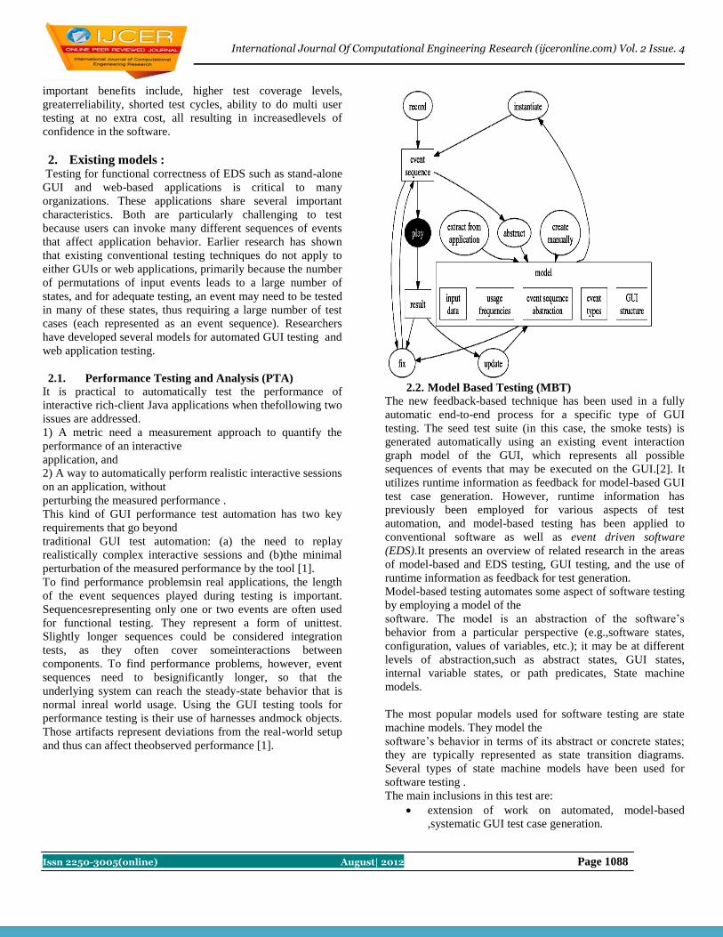
International Journal Of Computational Engineering Research (ijceronline.com) Vol. 2 Issue. 4
Issn 2250-3005(online) August| 2012 Page 1088
important benefits include, higher test coverage levels,
greaterreliability, shorted test cycles, ability to do multi user
testing at no extra cost, all resulting in increasedlevels of
confidence in the software.
2. Existing models : Testing for functional correctness of EDS such as stand-alone
GUI and web-based applications is critical to many
organizations. These applications share several important
characteristics. Both are particularly challenging to test
because users can invoke many different sequences of events
that affect application behavior. Earlier research has shown
that existing conventional testing techniques do not apply to
either GUIs or web applications, primarily because the number
of permutations of input events leads to a large number of
states, and for adequate testing, an event may need to be tested
in many of these states, thus requiring a large number of test
cases (each represented as an event sequence). Researchers
have developed several models for automated GUI testing and
web application testing.
2.1. Performance Testing and Analysis (PTA)
It is practical to automatically test the performance of
interactive rich-client Java applications when thefollowing two
issues are addressed.
1) A metric need a measurement approach to quantify the
performance of an interactive
application, and
2) A way to automatically perform realistic interactive sessions
on an application, without
perturbing the measured performance .
This kind of GUI performance test automation has two key
requirements that go beyond
traditional GUI test automation: (a) the need to replay
realistically complex interactive sessions and (b)the minimal
perturbation of the measured performance by the tool [1].
To find performance problemsin real applications, the length
of the event sequences played during testing is important.
Sequencesrepresenting only one or two events are often used
for functional testing. They represent a form of unittest.
Slightly longer sequences could be considered integration
tests, as they often cover someinteractions between
components. To find performance problems, however, event
sequences need to besignificantly longer, so that the
underlying system can reach the steady-state behavior that is
normal inreal world usage. Using the GUI testing tools for
performance testing is their use of harnesses andmock objects.
Those artifacts represent deviations from the real-world setup
and thus can affect theobserved performance [1].
2.2. Model Based Testing (MBT)
The new feedback-based technique has been used in a fully
automatic end-to-end process for a specific type of GUI
testing. The seed test suite (in this case, the smoke tests) is
generated automatically using an existing event interaction
graph model of the GUI, which represents all possible
sequences of events that may be executed on the GUI.[2]. It
utilizes runtime information as feedback for model-based GUI
test case generation. However, runtime information has
previously been employed for various aspects of test
automation, and model-based testing has been applied to
conventional software as well as event driven software
(EDS).It presents an overview of related research in the areas
of model-based and EDS testing, GUI testing, and the use of
runtime information as feedback for test generation.
Model-based testing automates some aspect of software testing
by employing a model of the
software. The model is an abstraction of the software’s
behavior from a particular perspective (e.g.,software states,
configuration, values of variables, etc.); it may be at different
levels of abstraction,such as abstract states, GUI states,
internal variable states, or path predicates, State machine
models.
The most popular models used for software testing are state
machine models. They model the
software’s behavior in terms of its abstract or concrete states;
they are typically represented as state transition diagrams.
Several types of state machine models have been used for
software testing .
The main inclusions in this test are:
extension of work on automated, model-based
,systematic GUI test case generation.

International Journal Of Computational Engineering Research (ijceronline.com) Vol. 2 Issue. 4
Issn 2250-3005(online) August| 2012 Page 1089
definition of new relationships among GUI events
based on their execution.
utilization of runtime state to explore a larger input
space and improve fault detection.
Immersion of the feedback-based technique into a
fully automatic end-to-end GUI
testing process and demonstration of its effectiveness
on fielded and fault-seeded
applications.
Empirical evidence tying fault characteristics to types
of test suites.
Demonstration that certain faults require well crafted
combinations of test cases and
oracles.
2.3. Combinatorial Interaction Testing (CIT)
Combinatorial Interaction Testing is a method which focuses
on test prioritization techniques for GUI. The specific
contributions of this work include: the first single model for
testing stand-alone GUI and Web-based applications, a shared
prioritization function based on the abstract model, and shared
prioritization criteria. We validate the usefulness of these
artifacts through an empirical study. The results show that GUI
and Web-based applications, when recast using the model,
showed similar behavior, reinforcing our belief that these
classes of applications should be modeled and studied
together. Other results show that GUI and Web applications
behave differently, which has created opportunities for
evolving the model and further experimentation.The generalize
the model by evaluating its applicability and usefulness for
other software testing activities, such as test generation.
It also makes contributions toward test prioritization research.
Many of our prioritization criteria
improve the rate of fault detection of the test cases over
random orderings of tests. We also develop hybrid
prioritization criteria that combine several criteria that work
well individually and evaluate whether the hybrid criteria
result in more effective test orders.
3. Proposed model: 3.1. Modeling Test Cases
A test case is modeled as a sequence of actions. For
eachaction, a user sets a value for one or more parameters.We
provide examples of test cases for both GUI and
webapplications next.

International Journal Of Computational Engineering Research (ijceronline.com) Vol. 2 Issue. 4
Issn 2250-3005(online) August| 2012 Page 1090
Previous work treats stand-alone GUI and web-based
applications as separate areas of research. However, these
types of applications have many similarities that allow us to
create a single model for testing such event driven systems.
This model may promote future research to more broadly
focus on stand-alone GUI and web-based applications instead
of addressing them as disjoint topics. Within the context of this
model, we develop and empirically evaluate several
prioritization criteria and apply them to four stand-alone GUI
and three web-based applications and their existing test suites.
Our empirical study evaluates the prioritization criteria. We
present our threats to validity in this section because several
opportunities for future research are created by the threats to
validity of the results of our empirical study. Threats to
construct validity are factors in the study
design that may cause us to inadequately measure concepts of
interest.
Test suit
3.2. Test suites
Models of the TerpOffice applications, called event-flow
graphs [1], were used to generate test cases. The test-case
generation algorithm has also been described earlier [1]; in
summary, the algorithm is based on graph traversal;
starting in one of the events in the application’s main
window,the event-flow graphs were traversed, outputting the
encountered event sequences as test cases. In all, 300 test cases
were generated for each application.
The suites for web applications are based on usage of the
application, also referred to as user-session-based testsuites.
A total of 125 test cases were collected for Book, by asking for
volunteer users by sending emails to local newsgroups and
posting advertisements in the University of Delaware’s
classifieds. For CPM, 890 test cases were collected from
instructors, teaching assistants, and students using CPM during
the 2004-05 and
2005-06 academic years at the University of Delaware. A total
of 169 test cases were collected when our third subject
application, Masplas, was deployed for the Mid-Atlantic
Symposium on Programming Languages .
Table shows the characteristics of the test casesused in our
study, such as the total number of testcases for each
application, and statistics on the lengths
of the test cases. We also report the total numberof unique
parameter-values and the percentage of 2-way parameter-value
interactions covered in the test suites. We compute the
percentage of 2-way parametervalueinteractions by counting
the number of uniqueparameter-values on each window that
can be selectedin combination with unique parameter-values
on otherwindows within the application.

International Journal Of Computational Engineering Research (ijceronline.com) Vol. 2 Issue. 4
Issn 2250-3005(online) August| 2012 Page 1091
4. Conclusion stand-alone GUI and web-based applications as separate areas
of research. However, these types of applications have many
similarities that allow us to create a single model for testing
such eventdriven systems. This model may promote future
research to more broadly focus on stand-alone GUI and
webbased applications instead of addressing them as disjoint
topics. Other researchers can use our common model to apply
testing techniques more broadly. their existing test suites. Our
empirical study evaluates the prioritization criteria. Our ability
to develop prioritization
criteria for two types of event-driven software indicates the
usefulness of our combined model for the
problem of test prioritization. Our results are promising as
many of the prioritization criteria that we use improve
the rate of fault detection over random ordering of test cases.
We learn that prioritization by 2-way and PV-LtoS
generally result in the best improvement for the rate of fault
detection in our GUI applications and one of our
web applications. However, for our web applications
,frequency-based techniques provide the best rate of fault
detection in 2 out of the 3 subjects. We attribute this to the
source of the test cases. The test suites for the
web applications come from real user-sessions, whereas the
GUI test cases were automatically generated without
influence from users.
REFERENCES [1] A. M. Memon and Q. Xie, “Studying the fault-detection
effectiveness of GUI test cases for rapidly evolving
software,” IEEE Trans. Softw. Eng., vol. 31, no. 10, pp.
884–896, Oct. 2005.
[2] A. Andrews, J. Offutt, and R. Alexander, “Testing web
applications by modeling with FSMs,” Software and
Systems Modeling, vol. 4, no. 3, pp. 326–345, Jul. 2005.
[3] G. D. Lucca, A. Fasolino, F. Faralli, and U. D. Carlini,
“Testing web applications,” in the IEEE Intl. Conf. on
Software Maintenance. Montreal, Canada: IEEE
Computer Society, Oct. 2002, pp. 310–319.
[4] F. Ricca and P. Tonella, “Analysis and testing of web
applications,” inthe Intl. Conf. on Software Engineering.
Toronto, Ontario, Canada: IEEE Computer Society,
May 2001, pp. 25–34.
[5] R. C. Bryce and A. M. Memon, “Test suite
prioritization by interactioncoverage,” in Proceedings of
The Workshop on Domain-Specific Approaches to
Software Test Automation (DoSTA 2007); co-located
with The 6th joint meeting of the European Software
Engineering Conference and the ACM SIGSOFT
Symposium on the Foundations of Software
Engineering. Dubrovnik, Croatia: ACM, Sep. 2007, pp.
1–7.
[6] S. Sampath, R. Bryce, G. Viswanath, V. Kandimalla, and
A. G. Koru, “Prioritizing user-session-based test cases
for web application testing,” in the International
Conference on Software Testing, Verification and
Validation. Lillehammer, Norway: IEEE Computer
Society, Apr. 2008, pp. 141–150. IEEE
TRANSACTIONS ON SOFTWARE ENGINEERING,
VOL. 37, NO. 1, JAN/FEB 2011 IEEE
TRANSACTIONS ON SOFTWARE ENGINEERING,
VOL. X, NO. X, JANUARY 2010 18
[7] P. Brooks, B. Robinson, and A. M. Memon, “An initial
characterization of industrial graphical user interface
systems,” in Proceedings of the International Conference
on Software Testing, Verification and Validation, 2009,
pp. 11–20.
[8] L. White, “Regression testing of GUI event interactions,”
in Proceedings of the International Conference on
Software Maintenance. IEEE Computer Society, Nov.
1996, pp. 350–358.
[9] “Web site test tools and site management tools,”
accessed on
<http://www.softwareqatest.com/qatweb1.html>,
accessed on Apr. 5, 2009.
[10] D. C. Kung, C.-H. Liu, and P. Hsia, “An object-oriented
web test model for testing web applications,” in The First
Asia-Pacific Conf. on Quality Software. Singapore: IEEE
Computer Society, Oct. 2000, pp. 111–120.
Authors Description
Manas Kumar Yogi Pursuing Mtech.(CSE Dept.)
Malla Reddy College of Engineering and
Technology, Hyderabad.
Mr.J.Praveen Kumar
Asst.Prof. CSE Dept.
Malla Reddy College of Engineering and
Technology, Hyderabad.

International Journal Of Computational Engineering Research (ijceronline.com) Vol. 2 Issue. 4
Issn 2250-3005(online) August| 2012 Page 1092
Comparison of Power Consumption and Strict Avalanche Criteria at
Encryption/Decryption Side of Different AES Standards
Navraj Khatri [1]
, Rajeev Dhanda [2],
Jagtar Singh [3]
[1] [2] Department of Electronics and Communication Engineering, NCCE, Israna, Panipat, INDIA
[3] Senior Lecturer, Electronics and Communication engineering, NCCE, Israna, Panipat, INDIA
Abstract: The selective application of technological and related procedural safeguards is an important responsibility of every
organization in providing adequate security to its electronic data systems. Now as the world is moving towards high speed
of communication (larger data rate),more secure and fast algorithms are required to keep the information secret. In the
present work, a new model is proposed and implemented, which is very similar to the conventional AES. The fundamental
difference in the AES and proposed model is in block size which has been increased from 128 bits in conventional AES to
200 bits in proposed algorithm[1-4].The proposed algorithm is giving very good randomness and hence enhances the
security in comparison to conventional AES. The performance is measured based upon Power Consumption at
Encryption/Decryption time, and Strict Avalanche Criteria of various AES Standards. In this paper, we showed the effect
in security increment through AES methodology.
Keywords: Plain text, cipher text, stream cipher, Symmetric Encryption, Computer Security.
1. Introduction: The introduction of wireless data communication at the beginning of 20
th century resulted in an increasing interest in
cryptography due to insecure nature of Wireless medium.In this paper,symmetric block cipher algorithm is proposed
likewise Advance Encryption Standard (AES).The proposed algorithm differs from AES as it has 200 bits block size and
key size both. Number of rounds is constant and equal to ten in this algorithm.The key expansion and substitution box
generation are done in the same way as in conventional AES block cipher.AES has 10 rounds for 128-bit keys,12 rounds
for 192-bit keys, and 14 rounds for 256-bit keys[5].Section 2 describes the Our Proposed Algorithm properly.Section 3
gives the Comparison of Power Consumption at Encryption and Decryption side and Strict Avalanche Criteria of different
AES Standards. Section 4 gives the Advantages and Disadvantages of AES.Section 5 and Section 6 gives us the
Conclusion and Acknowledgement..
2. Proposed Algorithm 2.1 General Definitions Block size and key size are the important parameters of any encryption algorithm because the level of security provided by
a cipher completely depends upon these two parameters.In our proposed encryption algorithm,we are using 200 bits block
and key size instead of 128 bit used in conventional Rijndael’salgorithm.[6-8].This increased block and key size will
improve the security level of the cipher with a negligible loss in efficiency.The original data which needs to be encrypted
will be termed as plaintext.Our encryption algorithm is a symmetric block cipher algorithm.This algorithm will operate on
fixed size blocks of plaintext to generate ciphertext.In the process of encryption, the first step is formation of data blocks
from the original plaintext.Our basic block length is 200 bits which can be shown by a 5 by 5 matrix of byte. The data
bytes are filled first in the column then in the rows.Once the data block is formed, different rounds take place to modify
data to the cipher text.
Figure 1. Making of data block from stream
2.2 The Round Transformation
There are ten rounds, and in each of the round there are series of transformations takes place except the final round.A
pseudo algorithm for each of the common round is given below and later the final round transformation algorithm is
given.The state is referred as the output of the previous transformation. Each function in the round is explained later.The
final round is equal to others when mix-column transformation is removed from general one.
Algorithm 1: (For Common Rounds)
Round(state, Round Key)

International Journal Of Computational Engineering Research (ijceronline.com) Vol. 2 Issue. 4
Issn 2250-3005(online) August| 2012 Page 1093
{
ByteSub(state);
ShiftRow(state);
MixColumn(state);
AddRoundKey(state, Round Key);
}
Algorithm 2: (For Final Round)
FinalRound(state, Round Key)
{
ByteSub(state);
ShiftRow(state);
AddRoundKey(state, Round Key);
}
2.3 The Byte Sub Transform The ByteSub transformation is a non linear byte substitution that acts on every byte of the state in isolation to produce a
new byte value using an S-box substitution table.In this transformation, each of the byte in the state matrix is replaced with
another byte as per the S-box (Substitution Box).The S-box is generated by calculating the respective reciprocal of that
byte in GF (28) and then affine transform is applied.Similarly,Inverse S-Matrix can be formed during the decryption of the
cipher text.For increasing the efficiency,we use Rijndael S-box.
Table 1. S-Box
2.4 The Shift Row Transform
For encryption, the 1st row remain unchanged, 2nd row is shifted 1 byte to the left, 3rd is 2 byte to the left, 4th is 3 byte to
the left and 5th row is shifted 4 byte to the left.For decryption the operation is similar to that for encryption but in reverse
direction.
2.5 The Mix Column Transform
(a) (b)
Figure 2. (a) Polynomial Matrix (b) Inverse Polynomial Matrix for Mix column transformation.
This is a complex procedure as it involves severely the byte multiplication under GF (28). The whole state is to be
multiplied with pre-defined matrix called polynomial matrix. It completely changes the scenario of the cipher even if the
all bytes look very similar. The Inverse Polynomial Matrix does exist in order to reverse the mix column transformation.
Each Column is replaced by the multiplicative value such as b(x)=c(x)*a(x), where, ‘*’ refers to multiplication under GF
(28).
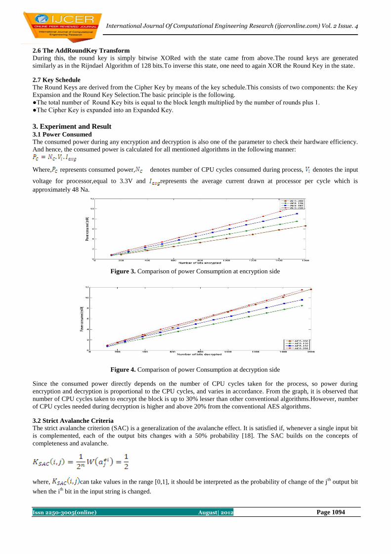
International Journal Of Computational Engineering Research (ijceronline.com) Vol. 2 Issue. 4
Issn 2250-3005(online) August| 2012 Page 1094
2.6 The AddRoundKey Transform
During this, the round key is simply bitwise XORed with the state came from above.The round keys are generated
similarly as in the Rijndael Algorithm of 128 bits.To inverse this state, one need to again XOR the Round Key in the state.
2.7 Key Schedule
The Round Keys are derived from the Cipher Key by means of the key schedule.This consists of two components: the Key
Expansion and the Round Key Selection.The basic principle is the following.
●The total number of Round Key bits is equal to the block length multiplied by the number of rounds plus 1.
●The Cipher Key is expanded into an Expanded Key.
3. Experiment and Result 3.1 Power Consumed
The consumed power during any encryption and decryption is also one of the parameter to check their hardware efficiency.
And hence, the consumed power is calculated for all mentioned algorithms in the following manner:
Where, represents consumed power, denotes number of CPU cycles consumed during process, denotes the input
voltage for processor,equal to 3.3V and represents the average current drawn at processor per cycle which is
approximately 48 Na.
Figure 3. Comparison of power Consumption at encryption side
Figure 4. Comparison of power Consumption at decryption side
Since the consumed power directly depends on the number of CPU cycles taken for the process, so power during
encryption and decryption is proportional to the CPU cycles, and varies in accordance. From the graph, it is observed that
number of CPU cycles taken to encrypt the block is up to 30% lesser than other conventional algorithms.However, number
of CPU cycles needed during decryption is higher and above 20% from the conventional AES algorithms.
3.2 Strict Avalanche Criteria The strict avalanche criterion (SAC) is a generalization of the avalanche effect. It is satisfied if, whenever a single input bit
is complemented, each of the output bits changes with a 50% probability [18]. The SAC builds on the concepts of
completeness and avalanche.
where, can take values in the range [0,1], it should be interpreted as the probability of change of the jth
output bit
when the ith
bit in the input string is changed.

International Journal Of Computational Engineering Research (ijceronline.com) Vol. 2 Issue. 4
Issn 2250-3005(online) August| 2012 Page 1095
is input word to the system and here less than 256 always.
The Security of the proposed model is examined by performing the test: Strict Avalanche Criterion and Bit Independence
Criterion. SAC tells about the probability of the bit change while the BIC states the correlation that output bit possess. Both
of the criteria are analyzed and the proposed algorithm falls within the desired level of security.
Fig Figure 5. Avalanche probability for various algorithms
From the plot, it can be seen that probability to get a bit changed for a highly correlated input, in proposed work, is very
similar to the conventional AES, which results this in a secure algorithm and validates it to be used in communication.
4. Advantages and Disadvantages
Advantages
Resistance against all known attacks.
Speed and code compactness on a wide range of platforms.
Design simplicity.
Our proposed algorithm can be implemented to run at speeds unusually fast for a block cipher on a Pentium
(Pro).There is a trade-off between table size / performance.
The round transformation is parallel by design, an important advantage in future processors and dedicated
hardware.
Limitations
The inverse cipher is less suited to be implemented on a smart card than the cipher itself: it takes more code and
cycles.
In software, the cipher and its inverse make use of different code and/or tables.
In hardware, the inverse cipher can only partially re-use the circuitry that implements the cipher.
5. Conclusion The announcement of AES attracted concentration of cryptanalysts to measure its level of security.As mentioned earlier,
there is always a trade-off between the security and performance of wireless network. AES provides a very high level of
security in an efficient way, but it also has some flaws in terms of security and the performance[11-14].The improvement
AES must possess similar level of security as in conventional AES.The proposed model has bigger block size which is 200
bits rather than conventional 128 bits. Also, the block is made by 5 rows and 5 columns unlike the AES’s 4 rows and 4
columns.As the size of the matrix has increased, all the transformations of the AES don’t need to change except the
mixcolumn transformation. During mixcolumn transformation, the diffusion takes place in form of matrix multiplication
under finite field. Having a bigger block, hence, requires a new matrix of size 5 X 5, to enable matrix multiplication.Here
number of CPU cycles taken to encrypt the block is up to 30% lesser than other conventional algorithms.However, number
of CPU cycles needed during decryption is higher and above 20% from the conventional AES algorithms.Hence, it can be
said that the proposed model is secure and can be considered for communication where high data rate is required[20-24].
6. Acknowledgement I proudly acknowledge my sincere and heartfelt thanks to Mr. Jagtar Singh, Senior Lecturer, N.C College of Engineering,
Panipat for their valuable and sustained guidance, constant encouragement and careful supervision during the entire course
which made the project successful.I would like to express my immense thanks to my friend Mr. Rajeev Dhanda,Associate
Professor,ECE Dept,RVIT,U.P for providing me all the help to pursue my dessirtation to its successful accomplishment.

International Journal Of Computational Engineering Research (ijceronline.com) Vol. 2 Issue. 4
Issn 2250-3005(online) August| 2012 Page 1096
Reference: [1] C.Shannon,Communication theory of secrecy systems,Bell Systems Technical Journal,vol.28,1949.
[2] Schneier B. and Whiting D.,Performance Comparison of AES Finalist,2000.
[3] ”National Policy on the Use of the AES to Protect National Security Systems and National Security
Information”,Lynn Hathnway(June 2003),Retrieved 2011-02-15.
[4] ”Performance Comparison of the AES submissions”,1999-02-01.Retrieved 2010-12-28.
[5] ”An Efficient Approach For Increasing Security to Symmetric Data Encryption”,International Journal of Computer
Science and Network Security,Vol.8 No.4,April,2008.
[6] J.Daemen and V.Raemen,The Design of Rijndael:AES-The Advanced Encryption Standards.Springer-Verlag,2002.
[7] J. Daemen, V. Rijmen, The block cipher Rijindael, Proceedings of the Third International Conference on smart
card Research and Applications, CARDIS’98, Lecture Notes in computer Science, vol.1820, Springer, Berlin, 2000,
pp.277_284.
[8] Federal Information Processing Standards Publications (FIPS 197), Advanced Encryption Standard (AES) ,26 Nov.
2001.
[9] Shivkumar S, Umamaheswari G., Performance Comparison of Advanced Encryption Standard(AES) and AES key
dependent S-box - Simulation using MATLAB, International Journal of Computer Theory , 2011.
[10] Fahmy A., Shaarawy M., El-Hadad K., Salama G. and Hassanain K., A Proposal For A Key-Dependent AES,
SETIT, Tunisia, 2005.
[11] Schneier B., Applied Cryptography: Protocols, Algorithms and Source Code in C. John Wiley and Sons, 1996.
[12] Stallings W., Cryptography and Network Security, Third Edition, Pearson Education, 2003.
[13] Anne Canteaut, Ongoing Research Areas in Symmetric Cryptography, 1999.
[14] Heys H. M., A Tutorial on Linear and Differential Cryptanalysis, St. John’s, NF, Canada, 2008.
[15] Chandrashekharan, J., et al. A chao Based Approach for Improving Non-linearity in the S-box Design of Symmetric
Key Cryptosystem, Advances in Networks and communication, First International Conference on Computer Science
and Information Technology (CSIT), Springer Bangalore, p. 516, ISBN- 978-3-642-17877-1, India, 2011.
[16] Nyberg K., Perfect Nonlinear S-boxes, Advances in Cryptography, Brioghtenpp 378-386, 1991.
[17] IBM Corporation MARS, A Candidate of AES cipher, http://www.research.ibm.com/security/mars.html, 1999.
[18] Burwick, C., Coppersmith, D., D.Avignon, E., Gennaro, R., Halevi, S., Jutla, C., Matyas,S., O.Connor, L.,
Peyravian, M., Safford, D., Zunic, N.: MARS- a candidate cipher for AES. Proceedings of the First AES Conference
(1999). Revised September 22, 1999.
[19] Parker G. M., Generalised S-Box Nonlinearity, SBoxLin.tex, 11.02.03, IST -1999-12324, 2003.
[20] Keliher, L., Substitution permutation network cryptosystem using S-boxes.
[21] Stoianov N., One Software Tool for Testing Square S-boxes, Technical University of Sofia (TUS), Bulgaria 2008.
[22] Ahmed N., Testing an S-Box for Cryptographic Use, International Journal of Computer and Electrical Engineering.
[23] Adams, C. M.: Designing S-Boxes For Ciphers Resistant To Differential Cryptanalysis (Extended Abstract), Feb
2010.
[24] M. Dawson, S. Tavares, An Expanded Set of S-box Design Criteria Based on Information Theory and its Relation to
Differential-like Attacks, Advances in Cryptology, Springer-Verlag, 1991.

International Journal Of Computational Engineering Research (ijceronline.com) Vol. 2 Issue. 4
Issn 2250-3005(online) August| 2012 Page 1097
A SIMPLE ALGORITHM FOR REDUCTION OF BLOCKING ARTIFACTS USING
SAWS TECHNIQUE BASED ON FUZZY LOGIC
Sonia Malik [1]
, Rekha Saroha [2],
Rohit Anand [3]
[1] [2]
Department of Electronics and Communication Engineering, NCCE, Panipat, INDIA
[3] Assistant Professor, Electronics and Communication Engineering, NCCE, Panipat, INDIA
ABSTRACT Reducing blocking artifacts encountered in highly compressed images is a very active research area in image processing. Coding
artifacts are very annoying in these highly compressed images. Most of the artifact reduction techniques blur the details of the
images while removing coding artifacts. In this paper , we propose a novel and explicit approach for reducing coding artifacts in
an image by using the combination of SAWS equation and Fuzzy Rules. We use FIDRM for the detection of noisy pixel and
NAFSM filter for correction. Experimental results demonstrate that the proposed approach achieves excellent visual quality and
PSNR as compared to a number of deblocking methods in the literature.
Keywords: Block Based Discrete Cosine Transform (BDCT), Deblocking Block (DB), Fuzzy Impulse Artifact Detection and
Reduction Method (FIDRM), Noise Adaptive Fuzzy Switching Median Filter (NAFSM), Signal Adaptive Weighted Sum
Technique (SAWS).
I. Introduction Image compression is a very important issue in both image and video coding applications. The main purpose of image
compression is to reduce storage and transmission costs while maintaining image quality.
It is known that blocking artifacts are introduced by coarse quantization of transform coefficients at low bit rates and independent
quantization of each block [2]. There are three types of blocking artifacts in BDCT coded images. One is staircase noise along the
image edges, another is grid noise in monotone area, and the other one is corner outliers in corner point of 8 x 8 DCT block.[1]
To remove blocking artifacts, many deblocking techniques have been proposed in last decade, but they often introduce excessive
blurring, ringing and in many cases they produce poor deblocking results at certain areas of image. So to reduce excessive
blurring and removing artifacts a algorithm is proposed for BDCT- coded images, based on Signal Adaptive Weighted Sum
Technique. In this method the center pixel is calculated as the weighted sum of the boundary pixels. Therefore SAWS technique
is applied to center pixel and boundary pixels. We adjust the weights according to directional correlation and block activities [3].
In this paper, we propose a blocking artifact removal algorithm for BDCT-coded images using SAWS technique based on
combination of FIDRM And NAFSM. FIDRM is a two step filter: the detection phase and the filtering phase. The detection phase
uses fuzzy rule to determine whether a pixel is corrupted or not. Then we try to indicate the values of detected pixels (k
{1,..., n} with 1≤ n< 255 ). After this detection fuzzy filtering focuses on only values [4]. The NAFSM filter uses a square
filtering window with odd dimensions which is used to satisfy the criterion of choosing only a noise free pixel as the median pixel
[5]. The rest of the paper is organised as follows. Section II introduces SAWS technique. Section III represents the proposed
method of reducing artifacts using SAWS technique along with NAFSM and FIDRM filters. Experimental results and Conclusion
are presented in Sections IV and V.
II. Saws Equation A Deblocking block and its subblocks are shown in the Fig. 1. A pixel in Deblocking Block (DB) is modified by using three
pixels at block boundaries, to remove block discontinuities in this SAWS technique. And these three pixels belongs to three
SubBlocks except for the SubBlock containing the to-be-modified pixel.
Let be the modified pixel of in the DB, and the weighted sum equation is given by
(1)
Where m is N/2 if I is less than N/2; otherwise, (N/2)-1, and n is N/2 if j is less than N/2 otherwise, (N/2)-1. In the above equation
and are the boundary pixels lying on the ’s row and column, respectively, and is a boundary pixel lying on
diagonal position.
The weights a, b and c are functions of distance between and its boundary pixel.

International Journal Of Computational Engineering Research (ijceronline.com) Vol. 2 Issue. 4
Issn 2250-3005(online) August| 2012 Page 1098
Fig. 1. A Deblocking Block (DB) and its SubBlocks.
III. PROPOSED METHOD In our proposed method instead of using only above saws equation we are using the combination of SAWS technique, fuzzy
gradient values as introduced with GOA filter [6],[7] and median filter[5].
3.1 Fuzzy Gradient Values
For each pixel (i,j) of the image, not a border pixel, we use a 3x3 neighborhood window as shown in Fig. 2
Fig. 2. Neighborhood of a central pixel.
Each neighbor with respect to (i,j) corresponds to one direction {NW= north west, N= north, NE= north east, W= west, E= east,
S= south, SE= south east, SW= south West}.
If A denotes input image then the gradient is defined as the difference
Del(k,l)A(i,j) = A(i+k, j+l) – A(i,j) with k,l € {-1,0,1} (2)
where the pair (k,l) corresponds to one of the eight directions and (i,j) is called center of gradient. The eight gradient values are
called the basic gradient values. One such gradient value can be used to determine if a central pixel is corrupted or not because if
gradient is large it indicates that some artifacts are present in the central pixel (i,j), but this conclusion is wrong in two cases.
1) If the central pixel is not noisy, but one of the neighbors is then this can also cause large gradient values.
2) An edge in an image causes some kind of natural large gradient values.
To solve first case, only only one gradient value is used, and to solve the second case one basic and two related gradient values
for each direction. The two related gradient values are determined by the centers making a right angle with the direction of the
basic gradient.

International Journal Of Computational Engineering Research (ijceronline.com) Vol. 2 Issue. 4
Issn 2250-3005(online) August| 2012 Page 1099
Fig. 3. Involved centers for the calculation of the related gradient values in the NW-direction.
Table1. Involved gradient values to calculate fuzzy gradient
Table 1 gives an overview of the involved gradient values. First column gives the direction corresponds to a position with respect
to central position. Column two gives basic gradient values and column three gives the two related gradients. Eight fuzzy gradient
values are defined for each of the eight directions. The fuzzy gradient value for direction R(R€ {NW, N, NE, E, SE, S, SW, W}),
is calculated by the fuzzy rule.
IF │delR A(i,j)│ is large AND │del’R A(i,j)│ is small
OR
│delR A(i,j)│ is large AND │del’’R A(i,j)│ is small
OR
delR A(i,j) is big positive AND del’R A(i,j) AND del’’R A(i,j) are big negative
OR
delR A(i,j) is big negative AND del’R A(i,j) AND del’’ A(i,j) are big positive
THEN fuzzy gradient value is large.
Where delR A(i,j) is basic gradient value and del’R A(i,j) and del’’R A(i,j) are two related gradient values for direction R. Large,
small, big positive and big negative are nondeterministic features, therefore these can be represented as fuzzy sets [8].
Fuzzy set can be represented by membership functions, as the membership function large represents fuzzy set large, small
represents fuzzy set small, big positive represents fuzzy set big positive and big negative represents fuzzy set big negative as
shown in fig.4.

International Journal Of Computational Engineering Research (ijceronline.com) Vol. 2 Issue. 4
Issn 2250-3005(online) August| 2012 Page 1100
(a)
(b)
Fig. 4 . Membership functions (a) SMALL, respectively, LARGE; (b) BIG NEGATIVE, respectively, BIG POSITIVE.
A. Detection stage
To decide whether the central pixel contains block discontinuity or not, we use the following fuzzy rule:
IF most of the eight gradient values are large THEN the central pixel A(i,j) is an block discontinuous pixel.
We translate this rule by: if for a certain central pixel (i,j) more than half of the fuzzy gradient values are part of the support of the
fuzzy set large[8], then we can conclude that pixel as a block discontinued pixel.
B. Filtering stage
The NAFSM filter uses a square filtering window W(i,j) with odd (2s+1) x (2s+1) dimensions. The noise free pixels are used for
selecting median pixel, given by
M(i,j) = median {X(i+m, j+n)} with N(i+m, j+n) = 1 (3)
After median pixel M(i,j) is found, the local information in a 3x3 window is extracted by first computing the absolute luminous
difference d(i,j) as given by
D(i+k, j+l) = │X(i+k, j+l) – X(i,j)│
with (i+k, j+l) ≠ (i,j) (4)
Then the local information is defined as the maximum absolute luminance difference in the 3x3 filtering window
D(i,j) = max{d(i+k, j+l)} (5)
Fig.5 Fuzzy set adopted by NAFSM filter
In NAFSM filter, fuzzy reasoning is applied to the extracted local information D(i,j). The fuzzy set adopted is shown in fig.5 and
defined by the fuzzy membership function F(i,j)

International Journal Of Computational Engineering Research (ijceronline.com) Vol. 2 Issue. 4
Issn 2250-3005(online) August| 2012 Page 1101
(6)
where the local information D(i,j) is used as fuzzy input variable and the two predefined thresholds T1 and T2 are set to 10 and
30, respectively, for optimal performance[9][10].
Finally, the correction term to restore a detected ‘noise pixel’ is a linear combination between the processing pixel X(i,j) and
median pixel M(i,j). the restoration term Y(i,j) is given as
Y(i,j) = [1- F(i,j)] . X(i,j) + F(i,j) . M(i,j) (7)
where the fuzzy membership value F(i,j) lends a weight on whether more of pixel X(i,j) or M(i,j) is to be used.
4. Experimental Results To demonstrate the performance of the proposed algorithm, we conduct comprehensive experiments with a number of 512x512
grayscale images, Lena, Peppers, and Goldhill. These images are compressed at various bit rates. Initially, we provide the
objective performance in PSNR by proposed algorithm, and compare them with some of the existing deblocking methods.
Experimental results shows that the proposed algorithm gives improved PSNR then the other debloking methods in the literature.
5. Conclusion In this paper a new approach for reducing artifact is presented which is based on two types of filter i.e FIDRM and NAFSM
filters. These filters are based on fuzzy rules. The main feature of FIDRM filter is that it leaves the noise free pixels unchanged.
Experimental results show the feasibility of the new algorithm. A numerical measure, such as PSNR, and visual quality show
convincing results for grayscale images . The proposed approach can be used in many mobile devices that have limted storage
and bandwidth and therefore suffer from blocking artifacts.
6. Acknowledgments With a deep sense of gratitude and heartiest honour, I would like to express my immense thanks to Dr. Vijay Nehra, Associate
Professor, ECE Dept, BPSMV Khanpur, Sonipat for providing me all the facilities to pursue my dessertation to its successful
accomplishment. I proudly acknowledge my sincere and heartfelt thanks to Mr. Rohit Anand, Assistant Professor, N.C College of
Engineering, Panipat for his valuable and sustained guidance, constant encouragement and careful supervision during the entire
course which made the project successful.
References [1] Y. Lee, H. Kim, and H. Park, “Blocking effect reduction of JPEG images by signal adaptive filtering,” IEEE Trans. Image
Process., vol. 7, no. 2, pp. 229-234, Feb. 1998.
[2] T. Chen, H. R. Wu, and B. Qiu, “Adaptive postfiltering of transform coefficients for the reduction of blocking artifacts,”
IEEE Trans. Circuits Syst. Video Technol., vol. 11, no. 5, pp. 594-602, May 2001.
[3] Jongho Kim and Chun Bo Sim, “Compression artifacts removal by signal adaptive weighted sum technique,” IEEE
Transactions on Consumer Electronics, Vol. 57, No. 4, November 2011.
[4] Stefan Schulte, Mike Nachtegael, Valérie De Witte, Dietrich Van der Weken, and Etienne E. Kerre, “A Fuzzy Impulse
Noise Detection and Reduction Method,” IEEE Transactions On Image Processing, Vol. 15, No. 5, May 2006.
[5] Kenny Kal Vin Toh, Student Member, IEEE, and Nor Ashidi Mat Isa, Member, IEEE, “Noise adaptive fuzzy switching
median filter for salt-and-pepper noise reduction” IEEE Signal Processing Letters, Vol. 17, No. 3, March 2010.
[6] D. Van De Ville, M. Nachtegael, D. Van derWeken, E. E. Kerre, and W. Philips, “Noise reduction by fuzzy image
filtering,” IEEE Trans. Fuzzy Syst., vol. 11, no. 4, pp. 429–436, Aug. 2001.
[7] M. Nachtegael, D. Van der Weken, and E. E. Kerre, “Fuzzy techniques in image processing: three case studies,” Int. J.
Comput. Anticipatory Syst., vol. 12, pp. 89–104, Aug. 2002.
[8] E. E. Kerre, Fuzzy Sets and Approximate Reasoning . Xian, China: Xian Jiaotong Univ. Press, 1998.
[9] K. K. V. Toh, H. Ibrahim, and M. N. Mahyuddin, “Salt-and-pepper noise detection and reduction using fuzzy switching
median filter,” IEEE Trans. Consumer Electron., vol. 54, no. 4, pp. 1956–1961, Nov. 2008.
[10] W. Luo, “Eficient removal of impulse noise from digital images,” IEEE Trans. Consumer Electron., vol. 52, no. 2, pp. 523–
527, May 2006.

International Journal Of Computational Engineering Research (ijceronline.com) Vol. 2 Issue. 4
Issn 2250-3005(online) August| 2012 Page 1102
A Study on Strength Characteristics of Flyash, Lime and Sodium
Silicate Mixtures at Their Free Pouring Conditions
1P.V.V.Satayanarayana
2Ganapati Naidu. P
3S .Adiseshu
4P.Padmanabha Reddy
1Professor
2, 4 M.E
3 Associate Professor
Department of Civil Engineering
Andhra University, Visakhapatnam
Abstract: For the utilization of flyash in improving the strength of problematic soils a detail experimental study on the behavior of
flyash stabilized with various percentages of lime and sodium silicate and the strength characteristics at their free pouring
(30%, 35% & 40% of water by weight of flyash)consistencies have been studied. Different percentages of lime and sodium
silicate (gel) were added to flyash and tested for UCS and split tensile strength for different curing periods like 3 days, 7
days and 28 days to obtain optimum dosage of lime and sodium silicate. From the test data it was found that 10 to 15 % of
lime and 3 to 5 % of sodium silicate have been identified as optimum dosages. These mixes can be used for bricks and
grouting techniques in civil engineering sector.
Keywords– flyash, sodium silicate (gel), unconfined compressive strength (UCS), split tensile strength.
Introduction: To meet the demands of industrialization and urbanization high volume of road a network is required. Performance of road
depends on the structural components such as subgrade, sub base, and base course etc. when roads are running on
problematic subgrade such as expansive, soft, collapsible sub grades. Partial or complete failure of pavements takes place;
repeated failures require lot of maintenance cost. This can be reduced by ground improvement techniques like full
replacement, partial by stabilized material and grouting etc can be used.
Lot of researches has been conducted on flyashes with admixtures, some of these are Yudbhir and Honjo (1991)
considered unconfined compressive strength of flyashes as a measure of self hardening property of flyashes. They explain
free lime content of flyash contributes to pronounced self hardening. Sherwood and Ryley (1966); and Raymond(1961)v
reported that the fraction of lime, present as free lime in the form of calcium hydroxide controls self hardening
characteristics of flyashes. Syngh (1996a) studied the unconfined compressive strength of flyashes as a function of free
lime present in them and found that flyashes having higher free lime content shows higher strength. In addition to these
flyash columns and flyash admixture columns can also be used. In this study NTPC fly ash is stabilized with lime and
sodium silicate and performed tests like Unconfined compressive strength, Split tensile strength to identify optimum
dosage of lime and sodium silicate for bulk utilization of fly ash.
2.0 Material used The materials used in this investigation are Flyash (NTPC), Lime and sodium silicate.
Flyash is collected from NTPC Paravada in Visakhapatnam and laboratory study was carried out for salient geotechnical
characteristics of such as grading, Atterberg limits, compaction and strength. The physical properties of flyash shown in
table 2 and chemical composition of flyash shown in table : 1.
Table: 1
Compound Formula Percentage (%)
Magnesium
oxide MgO 0.86
Aluminum
trioxide Al2O3 30.48
Silica dioxide SiO2 59.83
Calcium oxide CaO 1.74
Titanium
oxide TiO2 6.91
Zinc oxide ZnO 0.09

International Journal Of Computational Engineering Research (ijceronline.com) Vol. 2 Issue. 4
Issn 2250-3005(online) August| 2012 Page 1103
Table : 2
3.0 Experimental programme: In this study dry flyash has mixed with lime (5%, 10% and 15%) and Sodium silicate gel (1, 2, 3, 4 and 5%) by percentage
weight of dry flyash and added water of 30%, 35% and 40% by their weight and thoroughly mixed to get the required
consistency and poured these samples into given sizes(38mm X 76mm) of samplers and kept cured for 1 day , 3 days, 7
days and 28 days respectively by maintaining 100% humidity and without loss of moisture from the samples.
4.0 Results and Discussions: 4.1 Unconfined Compressive strength (kg/ cm
2):
The samples of sizes 38 mm diameter and height of 76 mm were prepared as said above by free pouring in the UCS
moulds. All the prepared samples were cured for 1 day, 3 days, 7 days and 28 days by maintaining 100% humidity.
Compressive strength test were conducted after completion of their curing period at a strain rate of 1.25 mm/min.
Unconfined Compressive strength of flyash with 5% lime and sodium silicate (free pouring consistency):
Table: 3
Property Values
Sand (%) 28
Fines (%) 72
a. Silt(%) 72
b. Clay(%) 0
Liquid Limit (%) 24
Plastic Limit (%) NP
Specific gravity 2.1
OMC (IS heavy Compaction)
Optimum moisture content (%) 21.0
Maximum dry density (g/cc) 1.28
California bearing ratio 3
Curing
period
Water
content
sodium silicate %
1 2 3 4 5 6
1
30 0.569 0.823 0.84 0.9 1.12
35 0.52 0.8 0.84 0.88 1 1.19
40 0.5 0.75 0.8 0.84 0.86 1.12
3
35 0.84 2.06 1.96 1.86 1.52
40 1.19 2.12 2.89 3.34 2.85 2.62
30 3.88 5.52 8.89 7.46 7.02 6.84
7
40 2.32 4.26 3.28 2.89 2.65
30 3.02 3.68 5.74 5.12 4.06
35 5.08 9.06 14.4 13.2 12.5 12
28
30 3.42 5.24 8.78 8.24 7.58
35 5.72 8.62 10.32 9.24 8.84 .
40 8.06 11.42 18.35 17.04 16.17

International Journal Of Computational Engineering Research (ijceronline.com) Vol. 2 Issue. 4
Issn 2250-3005(online) August| 2012 Page 1104
Fig: 1
For 5% lime, at different percentage of water content 3% sodium silicate gives good strength of flyash at all curing periods
and the maximum strength observed at 40% water content and 28 days curing period is 18.35kg/cm2.
Unconfined Compressive strength of flyash with 5% lime and sodium silicate (free pouring consistency):
Curing
period
Water
content
sodium silicate %
1 2 3 4 5 6
1
30 1.232 1.454 1.982 2.539 2.394 2.094
35 1.14 1.69 2.07 2.842 2.53 2.21
40 1.42 1.962 2.48 3.02 2.69 2.34
3
35 2.49 4.07 6.12 6.69 5.49 5.02
40 4.18 6.39 8.12 10.68 9.12 8.24
30 6.56 10.19 13.56 15.75 14.25 13.82
7
40 5.704 8.81 10.28 11.95 11.21 10.86
30 8.78 12.45 14.8 15.32 14.24 13.63
35 11.56 16.1 18.74 21.97 20.54 20.02
28
30 8.38 14.95 16.59 21.7 19.24 18.65
35 10.82 14.95 17.62 21.71 19.23 18.12
40 15.89 21.4 26.89 30.62 28.8 26.7
Table: 4
Fig: 2
For 10% lime, at different percentage of water content 4% sodium silicate gives good strength of flyash at all curing
periods and the maximum strength observed at 40% water content and 28 days curing period is 30.62kg/cm2.
Unconfined Compressive strength of flyash with 5% lime and sodium silicate (free pouring consistency):
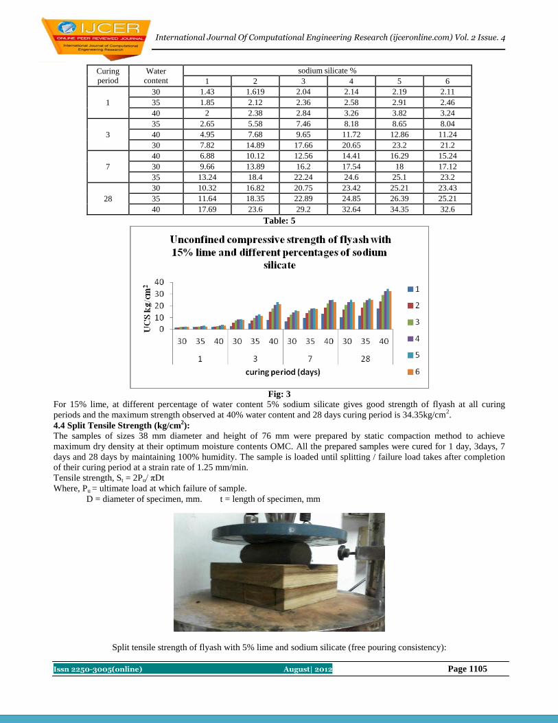
International Journal Of Computational Engineering Research (ijceronline.com) Vol. 2 Issue. 4
Issn 2250-3005(online) August| 2012 Page 1105
Curing
period
Water
content
sodium silicate %
1 2 3 4 5 6
1
30 1.43 1.619 2.04 2.14 2.19 2.11
35 1.85 2.12 2.36 2.58 2.91 2.46
40 2 2.38 2.84 3.26 3.82 3.24
3
35 2.65 5.58 7.46 8.18 8.65 8.04
40 4.95 7.68 9.65 11.72 12.86 11.24
30 7.82 14.89 17.66 20.65 23.2 21.2
7
40 6.88 10.12 12.56 14.41 16.29 15.24
30 9.66 13.89 16.2 17.54 18 17.12
35 13.24 18.4 22.24 24.6 25.1 23.2
28
30 10.32 16.82 20.75 23.42 25.21 23.43
35 11.64 18.35 22.89 24.85 26.39 25.21
40 17.69 23.6 29.2 32.64 34.35 32.6
Table: 5
Fig: 3
For 15% lime, at different percentage of water content 5% sodium silicate gives good strength of flyash at all curing
periods and the maximum strength observed at 40% water content and 28 days curing period is 34.35kg/cm2.
4.4 Split Tensile Strength (kg/cm2):
The samples of sizes 38 mm diameter and height of 76 mm were prepared by static compaction method to achieve
maximum dry density at their optimum moisture contents OMC. All the prepared samples were cured for 1 day, 3days, 7
days and 28 days by maintaining 100% humidity. The sample is loaded until splitting / failure load takes after completion
of their curing period at a strain rate of 1.25 mm/min.
Tensile strength, St = 2Pu/ πDt
Where, Pu = ultimate load at which failure of sample.
D = diameter of specimen, mm. t = length of specimen, mm
Split tensile strength of flyash with 5% lime and sodium silicate (free pouring consistency):
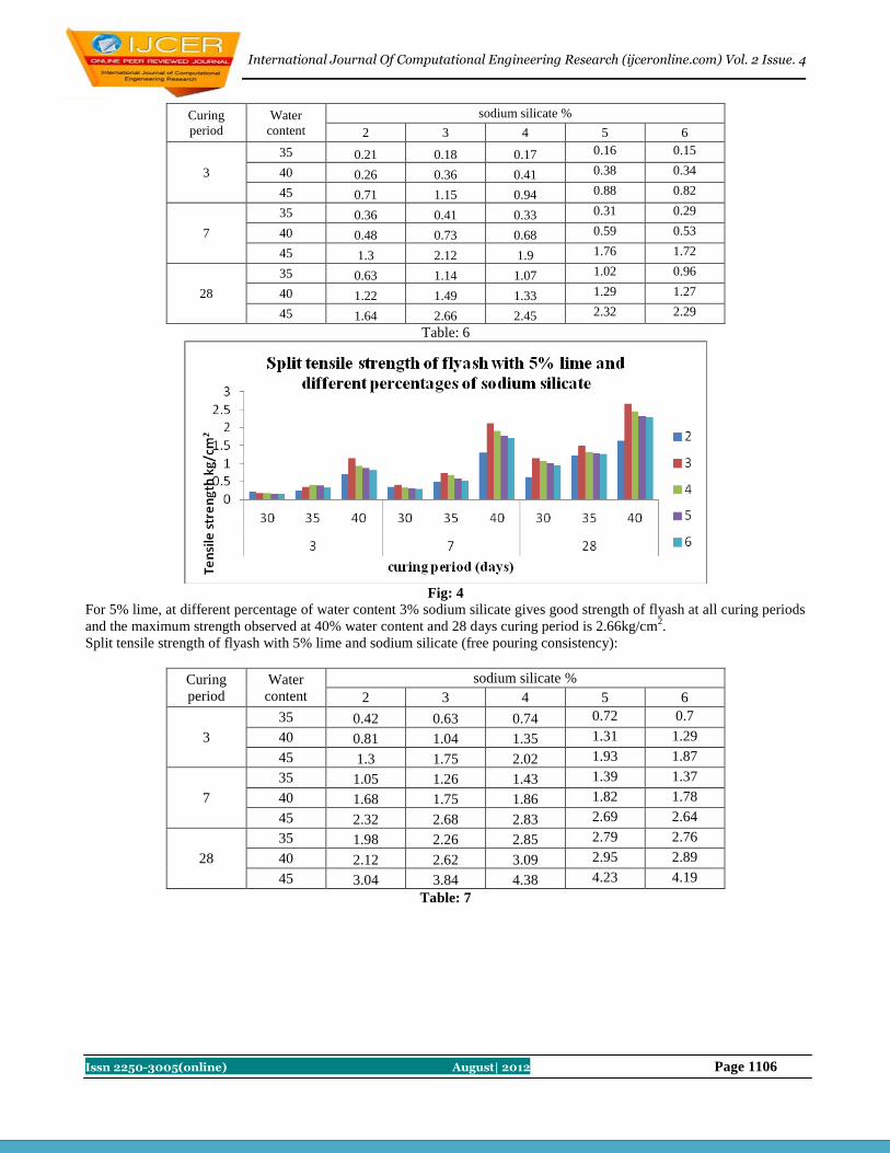
International Journal Of Computational Engineering Research (ijceronline.com) Vol. 2 Issue. 4
Issn 2250-3005(online) August| 2012 Page 1106
Curing
period
Water
content
sodium silicate %
2 3 4 5 6
3
35 0.21 0.18 0.17 0.16 0.15
40 0.26 0.36 0.41 0.38 0.34
45 0.71 1.15 0.94 0.88 0.82
7
35 0.36 0.41 0.33 0.31 0.29
40 0.48 0.73 0.68 0.59 0.53
45 1.3 2.12 1.9 1.76 1.72
28
35 0.63 1.14 1.07 1.02 0.96
40 1.22 1.49 1.33 1.29 1.27
45 1.64 2.66 2.45 2.32 2.29
Table: 6
Fig: 4
For 5% lime, at different percentage of water content 3% sodium silicate gives good strength of flyash at all curing periods
and the maximum strength observed at 40% water content and 28 days curing period is 2.66kg/cm2.
Split tensile strength of flyash with 5% lime and sodium silicate (free pouring consistency):
Curing
period
Water
content
sodium silicate %
2 3 4 5 6
3
35 0.42 0.63 0.74 0.72 0.7
40 0.81 1.04 1.35 1.31 1.29
45 1.3 1.75 2.02 1.93 1.87
7
35 1.05 1.26 1.43 1.39 1.37
40 1.68 1.75 1.86 1.82 1.78
45 2.32 2.68 2.83 2.69 2.64
28
35 1.98 2.26 2.85 2.79 2.76
40 2.12 2.62 3.09 2.95 2.89
45 3.04 3.84 4.38 4.23 4.19
Table: 7
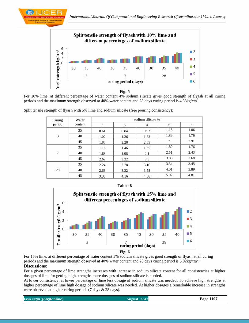
International Journal Of Computational Engineering Research (ijceronline.com) Vol. 2 Issue. 4
Issn 2250-3005(online) August| 2012 Page 1107
Fig: 5
For 10% lime, at different percentage of water content 4% sodium silicate gives good strength of flyash at all curing
periods and the maximum strength observed at 40% water content and 28 days curing period is 4.38kg/cm2.
Split tensile strength of flyash with 5% lime and sodium silicate (free pouring consistency):
Curing
period
Water
content
sodium silicate %
2 3 4 5 6
3
35 0.61 0.84 0.92 1.15 1.06
40 1.02 1.26 1.52 1.89 1.76
45 1.88 2.28 2.65 3 2.91
7
35 1.16 1.46 1.65 1.89 1.76
40 1.68 1.98 2.1 2.51 2.43
45 2.62 3.22 3.5 3.86 3.68
28
35 2.24 2.78 3.16 3.54 3.45
40 2.68 3.32 3.58 4.01 3.89
45 3.38 4.16 4.66 5.02 4.81
Table: 8
Fig: 6
For 15% lime, at different percentage of water content 5% sodium silicate gives good strength of flyash at all curing
periods and the maximum strength observed at 40% water content and 28 days curing period is 5.02kg/cm2.
Discussions: For a given percentage of lime strengths increases with increase in sodium silicate content for all consistencies at higher
dosages of lime for getting high strengths more dosages of sodium silicate is needed.
At lower consistency, at lower percentage of lime less dosage of sodium silicate was needed. To achieve high strengths at
higher percentage of lime high dosage of sodium silicate was needed. At higher dosages a remarkable increase in strengths
were observed at higher curing periods (7 days & 28 days).

International Journal Of Computational Engineering Research (ijceronline.com) Vol. 2 Issue. 4
Issn 2250-3005(online) August| 2012 Page 1108
The increases in strengths are due to interaction between lime and sodium silicate and flyash. This interaction leads to
formation of calcium silicate and aluminate hydrated gels for getting high strengths. This gel formation combines particles
together and make permanent because of the pozzolanic interaction between flyash, lime and silicate particles over a period
of time i.e., at higher curing periods (7 days & 28 days).
Conclusions: With increase in percentage of lime and sodium silicate the mix has shown higher values. This is due to pozzolanic
action between the particles of flyash and lime.
For higher percentage of lime more amount of sodium silicate is required.
As the percentage of lime increases the requirement of water is more for stabilization.
It is observed that at 28 days curing periods, the strength values are maximum at all percentages of mixes.
References: Bowders, J.J, Jr., Usmen, M.A. and Gidluy, J.S. (1987). Stabilized flyash for use as low permeability barriers,
proceedings of American society of civil engineers specialty conference.
Chu.T.Y, Davidson, D.T Goecker, W.L. Moh, Z.C. (1955), Soil stabilization with lime flyash mixes: preliminary
studies with silty and clayey soils, Highway research Bulletin, 102-112.
Das, S.C. and Pakrasha, S. (1990).Behaviour of lime stabilized Tit garh PFA through Laboratory tests, IE (1)
journal-CV,vol. 70, PP. 181-186.
Herrin, M. and Mitchell, H. (1961), Lime soil mixtures, highway research board Bulletin, 304, 99-138.
Mehra, S.R. and Chadda, L.R. (1955), Use of lime in Soil stabilization, Journal of Indian road congress, 19: 3,483.
Thompson, M.R. (1965), Split tensile strength of lime stabilized soils, Highway research record, 92, 69-82.
Ghosh RK, Pant, C.S. and Sharma RK. (1979), Stabilization of alluvial soil with lime and flyash. Journal of IRC,
New Delhi, vol.35-3, nov.1973.
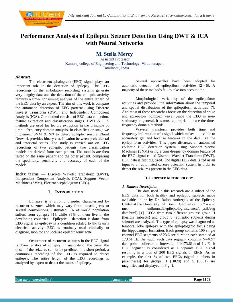
International Journal Of Computational Engineering Research (ijceronline.com) Vol. 2 Issue. 4
Issn 2250-3005(online) August| 2012 Page 1109
Performance Analysis of Epileptic Seizure Detection Using DWT & ICA
with Neural Networks
M. Stella Mercy Assistant Professor
Kamaraj college of Engineering and Technology, Virudhunager,
Tamilnadu, India.
Abstract The electroencephalogram (EEG) signal plays an
important role in the detection of epilepsy. The EEG
recordings of the ambulatory recording systems generate
very lengthy data and the detection of the epileptic activity
requires a time- consuming analysis of the entire length of
the EEG data by an expert. The aim of this work is compare
the automatic detection of EEG patterns using Discrete
wavelet Transform (DWT) and Independent Component
Analysis (ICA). Our method consists of EEG data collection,
feature extraction and classification stages. DWT & ICA
methods are used for feature extraction in the principle of
time – frequency domain analysis. In classification stage we
implement SVM & NN to detect epileptic seizure. Nural
Network provides binary classification between preictal/ictal
and interictal states. The study is carried out on EEG
recordings of two epileptic patients; two classification
models are derived from each patient. The models are then
tested on the same patient and the other patient, comparing
the specificity, sensitivity and accuracy of each of the
models.
Index terms — Discrete Wavelet Transform (DWT),
Independent Component Analysis (ICA), Support Vector
Machines (SVM), Electroencephalogram (EEG).
I. INTRODUCTION
Epilepsy is a chronic disorder characterized by
recurrent seizures which may vary from muscle jerks to
several convolutions. Estimated 1% of world population
suffers from epilepsy [1], while 85% of them live in the
developing countries. Epileptic detection is done from
EEG signal as epilepsy is a condition related to the brain’s
electrical activity. EEG is routinely used clinically to
diagnose, monitor and localize epileptogenic zone.
Occurrence of recurrent seizures in the EEG signal
is characteristics of epilepsy. In majority of the cases, the
onset of the seizures cannot be predicted in a short period, a
continuous recording of the EEG is required to detect
epilepsy. The entire length of the EEG recordings is
analyzed by expert to detect the traces of epilepsy.
Several approaches have been adopted for
automatic detection of epileptiform activities [2]-[6]. A
majority of these methods fail to take into account the
Morphological variability of the epileptiform
activities and provide little information about the temporal
and spatial distributions of the epileptiform activities [7].
And most of these researches focus on the detection of spike
and spike-slow complex wave. Since the EEG is non-
stationary in general, it is most appropriate to use the time-
frequency domain methods.
Wavelet transform provides both time and
frequency information of a signal which makes it possible to
accurately get and localize features in the data like the
epileptiform activities. This paper discusses an automated
epileptic EEG detection system using Support Vector
Machines (SNM) using a time-frequency domain feature of
the EEG signal called Discrete Wavelet Transform (DWT).
EEG data is first digitized. The digital EEG data is fed as an
input to an automated seizure detection system in order to
detect the seizures present in the EEG data.
II. PROPOSED METHODOLOGY
A. Dataset Description
The data used in this research are a subset of the
EEG data for both healthy and epileptic subjects made
available online by Dr. Ralph Andrzejak of the Epilepsy
Centre at the University of Bonn, Germany (http:// www.
meb. unibonn.de/epileptologie/science/physik/eeg
data.html) [1]. EEGs from two different groups: group H
(healthy subjects) and group S (epileptic subjects during
seizure) are analyzed. The type of epilepsy was diagnosed as
temporal lobe epilepsy with the epileptogenic focus being
the hippocampal formation. Each group contains 100 single
channel EEG segments of 23.6 sec duration each sampled at
173.61 Hz. As such, each data segment contains N=4097
data points collected at intervals of 1/173.61th of 1s. Each
EEG segment is considered as a separate EEG signal
resulting in a total of 200 EEG signals or EEGs. As an
example, the first 6s of two EEGs (signal numbers in
parentheses) for groups H (H029) and S (S001) are
magnified and displayed in Fig. 1.
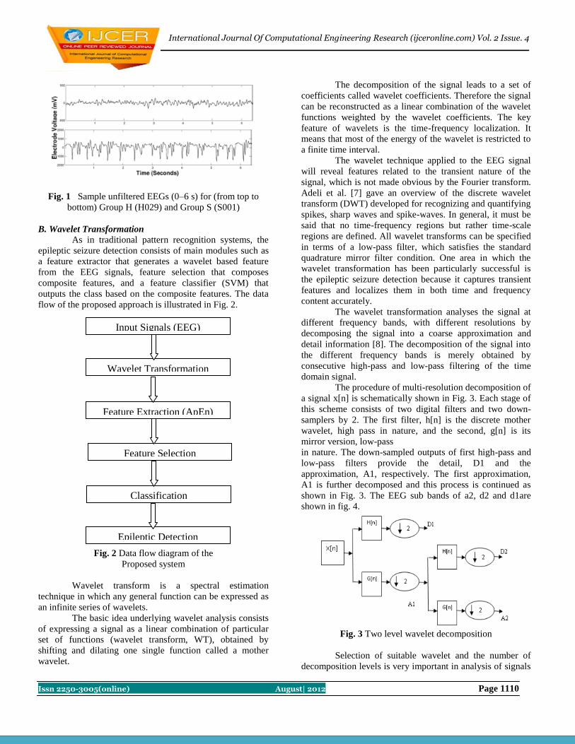
International Journal Of Computational Engineering Research (ijceronline.com) Vol. 2 Issue. 4
Issn 2250-3005(online) August| 2012 Page 1110
Feature Extraction (ApEn)
Input Signals (EEG)
Epileptic Detection
Classification
Feature Selection
Wavelet Transformation
Fig. 1 Sample unfiltered EEGs (0–6 s) for (from top to
bottom) Group H (H029) and Group S (S001)
B. Wavelet Transformation
As in traditional pattern recognition systems, the
epileptic seizure detection consists of main modules such as
a feature extractor that generates a wavelet based feature
from the EEG signals, feature selection that composes
composite features, and a feature classifier (SVM) that
outputs the class based on the composite features. The data
flow of the proposed approach is illustrated in Fig. 2.
Fig. 2 Data flow diagram of the
Proposed system
Wavelet transform is a spectral estimation
technique in which any general function can be expressed as
an infinite series of wavelets.
The basic idea underlying wavelet analysis consists
of expressing a signal as a linear combination of particular
set of functions (wavelet transform, WT), obtained by
shifting and dilating one single function called a mother
wavelet.
The decomposition of the signal leads to a set of
coefficients called wavelet coefficients. Therefore the signal
can be reconstructed as a linear combination of the wavelet
functions weighted by the wavelet coefficients. The key
feature of wavelets is the time-frequency localization. It
means that most of the energy of the wavelet is restricted to
a finite time interval.
The wavelet technique applied to the EEG signal
will reveal features related to the transient nature of the
signal, which is not made obvious by the Fourier transform.
Adeli et al. [7] gave an overview of the discrete wavelet
transform (DWT) developed for recognizing and quantifying
spikes, sharp waves and spike-waves. In general, it must be
said that no time-frequency regions but rather time-scale
regions are defined. All wavelet transforms can be specified
in terms of a low-pass filter, which satisfies the standard
quadrature mirror filter condition. One area in which the
wavelet transformation has been particularly successful is
the epileptic seizure detection because it captures transient
features and localizes them in both time and frequency
content accurately.
The wavelet transformation analyses the signal at
different frequency bands, with different resolutions by
decomposing the signal into a coarse approximation and
detail information [8]. The decomposition of the signal into
the different frequency bands is merely obtained by
consecutive high-pass and low-pass filtering of the time
domain signal.
The procedure of multi-resolution decomposition of
a signal x[n] is schematically shown in Fig. 3. Each stage of
this scheme consists of two digital filters and two down-
samplers by 2. The first filter, h[n] is the discrete mother
wavelet, high pass in nature, and the second, g[n] is its
mirror version, low-pass
in nature. The down-sampled outputs of first high-pass and
low-pass filters provide the detail, D1 and the
approximation, A1, respectively. The first approximation,
A1 is further decomposed and this process is continued as
shown in Fig. 3. The EEG sub bands of a2, d2 and d1are
shown in fig. 4.
Fig. 3 Two level wavelet decomposition
Selection of suitable wavelet and the number of
decomposition levels is very important in analysis of signals

International Journal Of Computational Engineering Research (ijceronline.com) Vol. 2 Issue. 4
Issn 2250-3005(online) August| 2012 Page 1111
using the wavelet transformation. The number of
decomposition levels is chosen based on the dominant
frequency components of the signal. In the present study,
since the EEG signals do not have any useful frequency
components above 30 Hz, the number of decomposition
levels was chosen to be 2. Thus, the EEG signals were
decomposed into details D1–D2 and one final
approximation, A2. Usually, tests are performed with
different types of wavelets and the one, which gives
maximum efficiency, is selected for the particular
application. The smoothing feature of the
Daubechies wavelet of order 4 (db4) made it more
appropriate to detect changes of EEG signals. Hence, the
wavelet coefficients were computed using the db4 in the
present study. The proposed method was applied on both
data set of EEG data (Sets H and S).
In the discrete wavelet analysis, a signal can be represented
by its approximations and details. The detail at level j is
defined as
…………… (1)
and the approximation at level J is defined as
………… (2)
It becomes obvious that
……...…... (3)
And,
.………… (4)
Wavelet has several advantages, which can
simultaneously possess compact support, orthogonality,
symmetry, and short support, and high order approximation.
We experimentally found that time-frequency domain
feature provides superior performance over time domain
feature in the detection of epileptic EEG signals.
Fig. 4 Level 2 decomposition of the band-limited EEG into
three EEG sub bands using fourth-order Daubechies wavelet
(s=a2+d2+d1)
C. Classification The idea of using a hyper plane to separate the feature
vectors into two groups works well when there are only two
target categories, but how does SVM handle the case where
the target variable has more than two categories? Several
approaches have been suggested, but two are the most
popular:
(1) “One against many” where each category is
split out and all of the other categories are merged.
(2) “One against one” where k(k-1)/2 models are
constructed where k is the number of categories.
The SVM classify function uses results from SVM
train to classify vectors x according to the following
equation:
………. (5)
Where si are the support vectors, αi are the weights,
b is the bias, and k is a kernel function. In the case of a linear
kernel, k is the dot product. If c ≥ 0, then x is classified as a
member of the first group, otherwise it is classified as a
member of the second group.
Where C is the capacity constant, w is the vector of
coefficients, b a constant and are parameters for handling
non separable data (inputs). The index i labels the N training
cases.
Note that is the class labels and xi is the
independent variables. The kernel is used to transform data
from the input (independent) to the feature space.
It should be noted that the larger the C, the more
the error is penalized. Thus, C should be chosen with care to
avoid over fitting.
For classification tasks, most likely use C-
classification with the RBF kernel(default), because of its
good general performance and the few number of
parameters (only two: C and γ). Libsvm suggest to try small
and large values for C— like 1to1000— first, then to decide
which are better for the data by cross validation, and finally
to try several γ's for the better C's.
Fig.5 The classification between normal and ictal stages
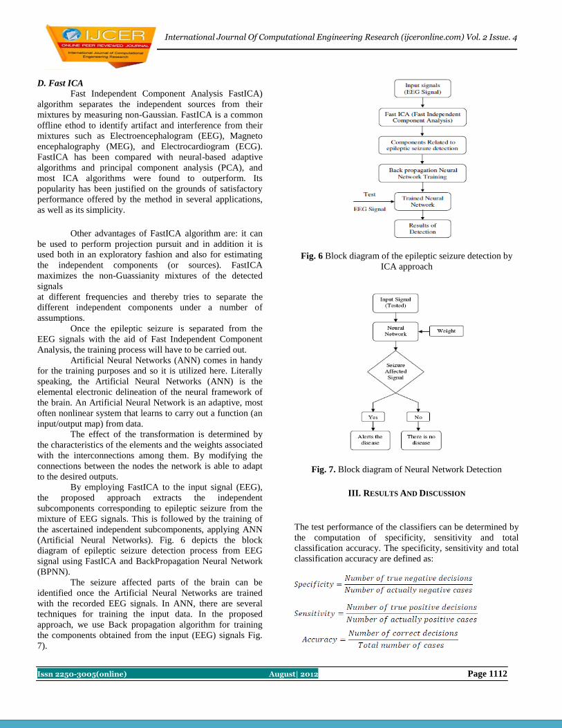
International Journal Of Computational Engineering Research (ijceronline.com) Vol. 2 Issue. 4
Issn 2250-3005(online) August| 2012 Page 1112
D. Fast ICA
Fast Independent Component Analysis FastICA)
algorithm separates the independent sources from their
mixtures by measuring non-Gaussian. FastICA is a common
offline ethod to identify artifact and interference from their
mixtures such as Electroencephalogram (EEG), Magneto
encephalography (MEG), and Electrocardiogram (ECG).
FastICA has been compared with neural-based adaptive
algorithms and principal component analysis (PCA), and
most ICA algorithms were found to outperform. Its
popularity has been justified on the grounds of satisfactory
performance offered by the method in several applications,
as well as its simplicity.
Other advantages of FastICA algorithm are: it can
be used to perform projection pursuit and in addition it is
used both in an exploratory fashion and also for estimating
the independent components (or sources). FastICA
maximizes the non-Guassianity mixtures of the detected
signals
at different frequencies and thereby tries to separate the
different independent components under a number of
assumptions.
Once the epileptic seizure is separated from the
EEG signals with the aid of Fast Independent Component
Analysis, the training process will have to be carried out.
Artificial Neural Networks (ANN) comes in handy
for the training purposes and so it is utilized here. Literally
speaking, the Artificial Neural Networks (ANN) is the
elemental electronic delineation of the neural framework of
the brain. An Artificial Neural Network is an adaptive, most
often nonlinear system that learns to carry out a function (an
input/output map) from data.
The effect of the transformation is determined by
the characteristics of the elements and the weights associated
with the interconnections among them. By modifying the
connections between the nodes the network is able to adapt
to the desired outputs.
By employing FastICA to the input signal (EEG),
the proposed approach extracts the independent
subcomponents corresponding to epileptic seizure from the
mixture of EEG signals. This is followed by the training of
the ascertained independent subcomponents, applying ANN
(Artificial Neural Networks). Fig. 6 depicts the block
diagram of epileptic seizure detection process from EEG
signal using FastICA and BackPropagation Neural Network
(BPNN).
The seizure affected parts of the brain can be
identified once the Artificial Neural Networks are trained
with the recorded EEG signals. In ANN, there are several
techniques for training the input data. In the proposed
approach, we use Back propagation algorithm for training
the components obtained from the input (EEG) signals Fig.
7).
Fig. 6 Block diagram of the epileptic seizure detection by
ICA approach
Fig. 7. Block diagram of Neural Network Detection
III. RESULTS AND DISCUSSION
The test performance of the classifiers can be determined by
the computation of specificity, sensitivity and total
classification accuracy. The specificity, sensitivity and total
classification accuracy are defined as:
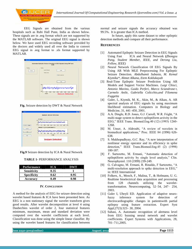
International Journal Of Computational Engineering Research (ijceronline.com) Vol. 2 Issue. 4
Issn 2250-3005(online) August| 2012 Page 1113
EEG Signals are obtained from the various
hospitals such as Rubi Hall Pune, India as shown below.
These signals are in .eeg format which are not supported by
the MATLAB software. The original EEG signal is shown
below. We have used EEG recording software provided by
the doctors and widely used all over the India to convert
EEG signal in .eeg format to .xls format supported by
MATLAB.
Fig. Seizure detection by DWT & Nural Network
Fig.9 Seizure detection by ICA & Nural Network
TABLE 1- PERFORMANCE ANALYSIS
Performance ICA DWT
Sensitivity 0.35 1
Specificity 0.62 0.95
Accuracy 0.49 0.98
IV. CONCLUSION
A method for the analysis of EEG for seizure detection using
wavelet based features & ICA have been presented here. As
EEG is a non stationary signal the wavelet transform gives
good results. After wavelet decomposition at level 4 using
Daubechies wavelet of order 2, four statistical features
minimum, maximum, mean and standard deviation were
computed over the wavelet coefficients at each level.
Classification was done using the simple linear classifier. By
using the wavelet based features for classification between
normal and seizure signals the accuracy obtained was
99.5%. It is greater than ICA method.
In future, apply this same dataset to other epileptic
detection methods and compare all their performance.
REFERENCES
[1] Automated Epileptic Seizure Detection in EEG Signals
Using Fast ICA and Neural Network (Zhongyu
Pang, Student Member, IEEE, and Derong Liu,
Fellow, IEEE)
[2] Neural Network Classification Of EEG Signals By
Using AR With MLE Preprocessing For Epileptic
Seizure Detection. Abdulhamit Subasia, M. Kemal
Kiymika*, Ahmet Alkana, Etem Koklukayab
[3] Real-Time Epileptic Seizure Prediction Using AR
Models and Support Vector Machines. Luigi Chisci,
Antonio Mavino, Guido Perferi, Marco Sciandrone∗,
Carmelo Anile, Gabriella Colicchio,and Filomena
Fuggetta
[4] Guler, I., Kiymik, M. K., Akin, M., & Alkan, A. AR
spectral analysis of EEG signals by using maximum
likelihood estimation. Computers in Biology and
Medicine, 31, 441–450, 2001.
[5] A.A. Dingle, R.D. Jones, G.J. Carroll, W.R. Fright, “A
multi-stage system to detect epileptiform activity in the
EEG,” IEEE Trans. Biomed.Eng.40 (12) (1993) 1260-
1268.
[6] M. Unser, A. Aldroubi, “A review of wavelets in
biomedical applications,” Proc. IEEE 84 (1996) 626-
638.
[7] S. Mukhopadhyay, G.C. Ray, “A new interpretation of
nonlinear energy operator and its efficiency in spike
detection,” IEEE Trans.Biomed.Eng.45 (2) (1998)
180-187.
[8] F. Sartoretto, M. Ermani, “Automatic detection of
epileptiform activity by single level analysis,” Clin.
Neurophysiol. 110 (1999) 239-249.
[9] G. Calvagno, M. Ermani, R. Rinaldo, F Sartoretto, “A
multi-resolution approach to spike detection in EEG,”
in: IEEE International
[10] Folkers, A., Mosch, F., Malina, T., & Hofmann, U. G.
Realtime bioelectrical data acquisition and processing
from 128 channels utilizing the wavelet-
transformation. Neurocomputing, 52–54, 247– 254,
2003.
[11] Guler I, Ubeyli ED. Application of adaptive neuro-
fuzzy inference system for detection of
electrocardiographic changes in patientswith partial
epilepsy using feature extraction. Expert Syst
Appl;27(3):323– 30, 2004.
[12] Subasi, A. Automatic recognition of alertness level
from EEG byusing neural network and wavelet
coefficients. Expert Systems with Applications, 28,
701–711,2005.

International Journal Of Computational Engineering Research (ijceronline.com) Vol. 2 Issue. 4
Issn 2250-3005(online) August| 2012 Page 1114
Self-Timed SAPTL using the Bundled Data Protocol
K.V.V.Satyanarayana1T.Govinda Rao
2J.Sathish Kumar
3
1Associate Professor
K.L. University 2, 3
Assistant Professor
Usha Rama college of Engg and technology
Abstract
This paper presents the design and implementation of a low-energy asynchronous logic topology using sense amplifier- based
pass transistor logic (SAPTL). The SAPTL structure can realize very low energy computation by using low-leakage pass
transistor networks at low supply voltages. The introduction of asynchronous operation in SAPTL further improves energy-
delay performance without a significant increase in hardware complexity. We show two different self-timed approaches: 1)
the bundled data and 2) the dual-rail handshaking protocol. The proposed self-timed SAPTL architectures provide robust and
efficient asynchronous computation using a glitch-free protocol to avoid possible dynamic timing hazards. Simulation and
measurement results show that the self-timed SAPTL with dual-rail protocol exhibits energy-delay characteristics better than
synchronous and bundled data self-timed approaches in 180-nm, 120-nm CMOS.
Keywords: pass transistor, self-timing, sense amplifier-based pass transistor logic (SAPTL)
I. Introduction A CMOS technology continues to scale, both supply Voltage and device threshold voltage must scale down Together to
achieve the required performance. Lowering the supply voltage effectively reduces dynamic energy consumption but is
accompanied by a dramatic increase in leakage energy due to the lower device threshold voltage needed to maintain
performance [1].As a result, for low-energy applications, the leakage energy that the system can tolerate ultimately limits the
minimum device threshold voltage. Speed, therefore, benefits little from technology scaling. The sense amplifier-based pass
transistor logic (SAPTL) [2] is a novel circuit topology that breaks this tradeoff in order to achieve very low energy without
sacrificing speed. The initial SAPTL circuits were designed to operate synchronously [2] but with the intent of being able to
Operate asynchronously with some minor modifications.
As the effects of process variations continue to increase dramatically with technology scaling, it is becoming harder to design
variation-tolerant timing schemes using the traditional synchronous methodologies. To meet a certain timing requirement, the
synchronous approach must use a very conservative “worst case” design that is slow enough for the needs of the statistically
slowest circuit elements and, thus, will fail to exercise the whole capacity of statistically faster parts of the circuit. The
asynchronous approach, on the other hand, can exploit local timing information to achieve “average-case” performance. An
asynchronous design can get the best performance out of all components independent of statistical variations in local speed
while guaranteeing correct circuit operation.
Asynchronous operation is also attractive to the low-power designer. The absence of a clock distribution network can
significantly reduce the power overhead needed to generate timing information. Furthermore, an idle asynchronous system
avoids consuming any active power. Despite the advantages of asynchronous operation, the circuit complexity and
performance overhead required to implement the needed handshaking protocol may not be trivial. The overhead cost might
offset all benefits and make the asynchronous approach impractical. The SAPTL, however, offers a relatively easy way to
realize asynchronous operation. Because of the differential signaling used, it is easy to determine when a logical operation
completes. Therefore, the self-timed SAPTL topology is a promising candidate for reducing power consumption and
improving speed in extremely low energy applications.
II. Saptl Architecture The basic architecture of the SAPTL circuit is shown in Fig. 1. It is composed of a pass transistor stack, a driver, and a sense
amplifier [2]. The SAPTL achieves low energy operation 1) by decoupling sub threshold leakage current from the stack
threshold voltage, allowing for increased performance without an increase in leakage energy, and 2) by confining sub
threshold leakage to well-defined and controllable paths found only in the drivers and sense amplifiers.
Note that the total energy consumed by the SAPTL is composed of the following: 1) the energy used by the driver to energize
the stack; 2) the energy used by the sense amplifier to resolve the correct logical levels and drive the inputs of the fan-out
stacks; and (3) the energy needed to generate the appropriate timing information, either globally, such as clock distribution
networks, or locally, as in handshaking circuits.
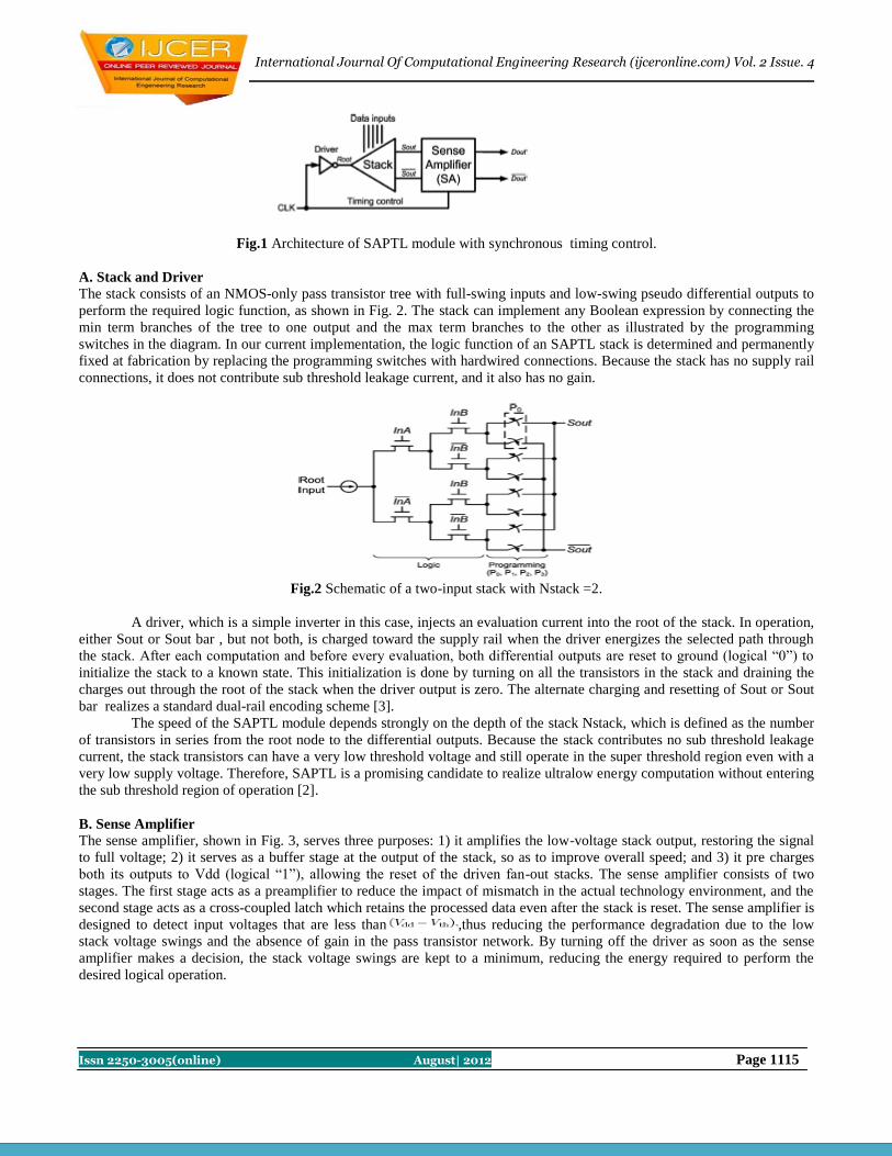
International Journal Of Computational Engineering Research (ijceronline.com) Vol. 2 Issue. 4
Issn 2250-3005(online) August| 2012 Page 1115
Fig.1 Architecture of SAPTL module with synchronous timing control.
A. Stack and Driver
The stack consists of an NMOS-only pass transistor tree with full-swing inputs and low-swing pseudo differential outputs to
perform the required logic function, as shown in Fig. 2. The stack can implement any Boolean expression by connecting the
min term branches of the tree to one output and the max term branches to the other as illustrated by the programming
switches in the diagram. In our current implementation, the logic function of an SAPTL stack is determined and permanently
fixed at fabrication by replacing the programming switches with hardwired connections. Because the stack has no supply rail
connections, it does not contribute sub threshold leakage current, and it also has no gain.
Fig.2 Schematic of a two-input stack with Nstack =2.
A driver, which is a simple inverter in this case, injects an evaluation current into the root of the stack. In operation,
either Sout or Sout bar , but not both, is charged toward the supply rail when the driver energizes the selected path through
the stack. After each computation and before every evaluation, both differential outputs are reset to ground (logical “0”) to
initialize the stack to a known state. This initialization is done by turning on all the transistors in the stack and draining the
charges out through the root of the stack when the driver output is zero. The alternate charging and resetting of Sout or Sout
bar realizes a standard dual-rail encoding scheme [3].
The speed of the SAPTL module depends strongly on the depth of the stack Nstack, which is defined as the number
of transistors in series from the root node to the differential outputs. Because the stack contributes no sub threshold leakage
current, the stack transistors can have a very low threshold voltage and still operate in the super threshold region even with a
very low supply voltage. Therefore, SAPTL is a promising candidate to realize ultralow energy computation without entering
the sub threshold region of operation [2].
B. Sense Amplifier
The sense amplifier, shown in Fig. 3, serves three purposes: 1) it amplifies the low-voltage stack output, restoring the signal
to full voltage; 2) it serves as a buffer stage at the output of the stack, so as to improve overall speed; and 3) it pre charges
both its outputs to Vdd (logical “1”), allowing the reset of the driven fan-out stacks. The sense amplifier consists of two
stages. The first stage acts as a preamplifier to reduce the impact of mismatch in the actual technology environment, and the
second stage acts as a cross-coupled latch which retains the processed data even after the stack is reset. The sense amplifier is
designed to detect input voltages that are less than ,thus reducing the performance degradation due to the low
stack voltage swings and the absence of gain in the pass transistor network. By turning off the driver as soon as the sense
amplifier makes a decision, the stack voltage swings are kept to a minimum, reducing the energy required to perform the
desired logical operation.

International Journal Of Computational Engineering Research (ijceronline.com) Vol. 2 Issue. 4
Issn 2250-3005(online) August| 2012 Page 1116
Fig.3 Sense amplifier circuit.
The leakage of the sense amplifier accounts for most of the leakage energy of the SAPTL module. It can be directly
traded off against the input sensitivity of the sense amplifier to size and threshold voltage mismatch as shown in Fig. 4. Using
a supply voltage of 300 mV and a minimum input voltage of 100 mV, 55% of the sense amplifier leakage is due to the four
output buffers (inverters). Thus, an increase in sense amplifier performance can be achieved 1) by reducing the minimum
input voltage or 2) by increasing the output drive of the sense amplifier, either of which would result in an increase in leakage
current.
III. Bundled Data Self-Timed Saptl Design The circuit implementation of the self-timed SAPTL module using the bundled data protocol [7] is shown in Fig. 4. The main
data path, composed of a driver and stack, evaluates data or resets after receiving the request signal Rqein and data input
signals Din and Din bar from the previous SAPTL stage. The control path, which consists of a delay line and a C-element,
produces the local clock signal Enable to trigger the sense amplifier.
Fig.4 Architecture of self-timed SAPTL module with bundled data protocol.
The delay line mimics the delay of the stack to generate the control signal Ready indicating that the stack has
finished an operation. The C-element then produces Enable by collecting Ready and the acknowledge signal Ackin from the
next SAPTL stage. In multiple fan-in and fan-out situations, additional C-element can be employed to reconverge multiple
request and acknowledge events from the different fan-in and fan-out stages. When triggered by Enable , the sense amplifier
latches the stack output data or resets depending on the logical state of Enable. The full-swing data output signals Dout and
Dout bar are made available at the outputs of the sense amplifier. The AND gate serves

International Journal Of Computational Engineering Research (ijceronline.com) Vol. 2 Issue. 4
Issn 2250-3005(online) August| 2012 Page 1117
Fig.5 Timing diagram of self-timed SAPTL.
As a completion detection circuit, generating the handshake signals Ackout and Requot that indicate the completion of the
current operation. We can summarize the relationship between the input and output signals of the th SAPTL stage as
IV. Dual-Railself-Timed Saptl Design In a self-timed SAPTL structure using the bundled data protocol, RTA2 is the most critical design constraint. In order to
guarantee correct operation under process, voltage, and temperature variations, the latency of the delay line can become very
large and can severely limit the overall performance. Because the SAPTL uses dual-rail coding to represent data, we can use
the output signals of the stack and, instead of from the delay line, to trigger the C-element. As a result, we can 1) eliminate
the delay line and 2) design the C-element to respond immediately after the stack finishes operation, without being limited by
RTA2.
Furthermore, we can combine the sense amplifier and C-element circuits into a composite block through
gate-level optimization, yielding a more energy-efficient architecture, as shown in Fig.7. The optimized architecture with
dual-rail protocol [7] eliminates the traditional
Fig.6 Architecture of glitch-free self-timed SAPTL module with dual-rail protocol.

International Journal Of Computational Engineering Research (ijceronline.com) Vol. 2 Issue. 4
Issn 2250-3005(online) August| 2012 Page 1118
Sense amplifier circuit and directly employs two C-element circuits as a complex gain stage at the outputs of the
stack. The overall conversion speed, however, may be slower than the design with a sense amplifier due to the absence of a
differential amplification and
Fig.7 Logic combination of two-input C element and sense amplifier circuits.
The loss the loss of a positive-feedback mechanism between the two data paths Fig.6 shows the implementation of a
glitch-free self-timed SAPTL architecture without the delay line.
Fig.7: Two-input C-element circuit with additional decision-making logic for glitch-free self-timed SAPTL.
The design and performance of the C-element circuits are particularly important in this architecture because the C-
element not only plays the role of the gain stage but also serves as the handshaking element. The self-timed SAPTL with
dual-rail protocol has latency and cycle time expressions similar to (4)–(8). Note that the speed enhancement discussed in
Section IV-C does not apply to the dual-rail design in Fig.6, because of the absence of the internal signal. However, the
single self-timed SAPTL stage is now elastic and able to achieve the best performance across process, voltage, and
temperature variations and different input characteristics. The self-timed SAPTL can thus exercise the full potential of
asynchronous computation without the limitations of the delay line. It is interesting tonote that the optimized self-timed
SAPTL architecture in Fig.6.
Has almost the same hardware complexity as the original synchronous SAPTL design in Fig. 1. This means that,
with almost “zero cost,” SAPTL is able to achieve both better performance and better robustness in the presence of variability
by operating asynchronously.
Fig.8 Test setup for energy and delay measurements.
The energy and delay of the various SAPTL5
Implementations were measured using N=8.

International Journal Of Computational Engineering Research (ijceronline.com) Vol. 2 Issue. 4
Issn 2250-3005(online) August| 2012 Page 1119
V. Performance Evaluation And Comparison We evaluated and compared the performance of the self-timed and synchronous SAPTL circuits using the Spectre circuit
simulator. We also performed Monte Carlo simulations to ensure the correct operation of the SAPTL circuits even with 6σ
process variations. In addition, we implemented the self-timed SAPTL circuits in a 120-nm CMOS test chip and compared
the actual measurement results to the simulated data. This section presents the energy-delay and leakage comparisons of
synchronous versus self-timed SAPTL. The simulations exclude the parasitic contributions from the interconnect wires and
the clock network. However, the effect of global parameters, such as clocks and long interconnect wires, should be done at
the system level, in the context of an actual application. Comparisons between the synchronous SAPTL and other logic styles
can be found in [2].
Fig .9.1 Simulation results
Fig .9.2 Layout design for Bundled –Data Self-Timed SAPTL
Fig .9.3 Layout design for Dual-rail-self timed SAPTL
Energy-Delay Characteristics
The pre-layout simulated energy and delay behavior of the synchronous SAPTL5 and both versions of the self-timed
SAPTL5 is shown in Fig.9.4.

International Journal Of Computational Engineering Research (ijceronline.com) Vol. 2 Issue. 4
Issn 2250-3005(online) August| 2012 Page 1120
Fig.9.4 Measured versus simulated energy-delay plots for The 120-nm CMOS Self-timed SAPTL5, as the supply
Voltage is varied from 300 mV to 1.2 V
Table .1 Comparisons of different Methodologies
V. Conclusion The asynchronous operation of the SAPTL provides robustness in the presence of variability as well as performance
advantages over synchronous operation. While the self-timed SAPTL using the bundled data protocol can potentially achieve
higher speed performance by overlapping the data evaluation and reset cycle, the self-timed design based on the dual-rail
protocol has less rigid relative timing constraints, which leads to better energy and speed performance in technologies with
increased process variations. The early reset operation ofself-timed SAPTL not only prevents dynamic timing hazards from
glitches but also improves both energy and speed performance. We evaluated and compared the performance of the self-
timed and synchronous SAPTL circuits using the Spectre circuit simulator. We also performed Monte Carlo simulations to
ensure the correct operation of the SAPTL circuits even with process variations. In addition, we implemented the self-timed
SAPTL circuits a 120-nm CMOS test chip and compared the actual measurement results is less than the simulated data.
And also 180-nm CMOS is less than the simulated data This section presents the energy-delay and leakage comparisons of
synchronous versus self-timed SAPTL. The simulations exclude the parasitic contributions from the interconnect wires and
the clock network. However, as pointed out earlier in Section II-D, the effect of global parameters, such as clocks and long
interconnect wires, should be done at the system level, in the context of an actual application. Comparisons between the
synchronous SAPTL and other logic styles can be found in [2].
REFERENCES
[1] T. Sakurai, “Perspectives on power-awar electronics,” in ISSCC Dig. Te ch. Papers, 2003, vol.1, pp. 26–29.
[2] L. Alarcón, T.-T. Liu, M. Pierson, and J. Rabaey, “Exploring very lowenergy logic: A case study,” J. Low Power Electron.,
vol. 3, no. 3, pp. 223–233, Dec. 2007.
[3] J. Sparsø and S. Furber, Principles of Asynchronous Circuit Design.Norwell, MA: Kluwer, 2001.
[4] J. Rabaey, A. Chandrakasan, and B. Nikolic, Digital Integrated Circuits:A Design Perspective, 2nd ed . Englewood Cliffs,
NJ: Prentice-Hall, 2003.
[5] H. Li, S. Bhunia, Y. Chen, K. Roy, and T. Vijaykumar, “DCG: deterministic clock-gating for low-power microprocessor
design,” IEEE Trans. Very Large Scale Integr. (VLSI) Syst., vol. 12, no. 3, pp. 245–254,Mar. 2004.
Technology Power
(180 nm
Technology)
Power
(120 nm
Technology)
synchronous 16.87µW 16.58µW
Bundled-data 16.35µW 15.64µW
Dual-rail 15.64µW 6.99µW

International Journal Of Computational Engineering Research (ijceronline.com) Vol. 2 Issue. 4
Issn 2250-3005(online) August| 2012 Page 1121
[6] N. Banerjee, K. Roy, H. Mahmoodi, and S. Bhunia, “Low power synthesis of dynamic logic circuits using fine-
grained clock gating,” in Proc. DATE, Mar.2006, vol. 1, pp. 1–6.
[7] T.-T. Liu, L. Alarcón, M. Pierson, and J. Rabaey, “Asynchronous computing in sense amplifier-based pass transistor
logic,” in Proc. 14th
IEEE Int. Symp. ASYNC, Apr. 2008, pp. 105–115.
[8] T. Williams, “Performance of iterative computation in self-timed rings,” J. VLSI Signal Process., vol. 7, no. 1/2,
pp. 17–31, Feb. 1994.
[9] K. Stevens, R. Ginosar, and S. Rotem, “Relative timing,” IEEE Trans. Very Large Scale Integr. (VLSI) Syst., vol.
11, no. 1, pp. 129–140, Feb. 2003.
[10] I. Sutherland, “Micropipelines,” Commun. ACM, vol. 32, no. 6, pp.720–738, Jun.1989.
[11] S. Narendra, “Scaling of stack effect and its application for leakage reduction,” in Proc. ISLPED, Aug. 2001, pp.
195–200.
[12] K. Yano, Y. Sasaki, K. Rikino, and K. Seki, Top- down pass-transistor logic design. IEEE Journal of Solid-State
Circuits 31, 792 (1996).
13] R. Shelar and S. Sapatnekar, BDD decomposition for delay oriented pass transistor logic synthesis. IEEE
Transactions on Very Large Scale Integration (VLSI) Systems 13, 957 (2005).
[14] P. Buch, A. Narayan, A. Newton, and A. Sangiovanni-Vincentelli, Logic synthesis for large pass transistor circuits.
IEEE/ACM International Conference on Computer-Aided Design, November (1997), pp. 663–670.
[15] W. C. Elmore, The transient analysis of damped linear networks with particular regard to wideband amplifiers. J.
Appl. Phys. 19, 55 (1948).
[16] V. Kheterpal, V. Rovner, T. Hersan, D. Motiani, Y. Takegawa, A. Strojwas, and L. Pileggi, Design methodology for
IC manufacturability based on regular logic-bricks. Proceedings of the 42nd
Design Automation Conference, June
(2005), pp. 353–358.
K. V. V. Satyanarayana received the M.Tech degree from Jawaharlal Nehru Technological University,
Kakinada in 2008 in Electronics and Communication engineering. He is an Associate Professor in the Department of
Electronics and Communication engineering, K.L.University,Vaddeswaram. His current research interests include the area of
Communications, video coding techniques, and Architectures design.
T. GOVINDA RAO received the M.Tech (VLSISD) degree from Jawaharlal Nehru Technological
University, Kakinada in 2011 in Electronics and Communication engineering. he is an Assistant Professor in the Department
of Electronics and Communication engineering, Usha Rama College Of Engineering and Technology, Vijayawada. His
current research interests include the areas of very large scale integration (VLSI) testing and fault-tolerant computing, video
coding techniques, and Architectures design.
J. SATHISH KUMAR received the M.Tech degree from Jawaharlal Nehru Technological University,
Hyderabad in 2011 in Electronics and Communication Engineering. He is an Assistant Professor in the Department of
Electronics and Communication Engineering, Usha Rama College of Engineering and Technology, Vijayawada. His current
research interests include the areas of very large scale integration (VLSI) testing and fault-tolerant computing, video coding
techniques and Architectures design.
International Journal Of Computational Engineering Research (ijceronline.com) Vol. 2 Issue. 4
Issn 2250-3005(online) August| 2012 Page 1122
A survey on retrieving Contextual User Profiles from Search Engine
Repository
1G.Ravi,
2JELLA SANTHOSH
1Asst.Prof. CSE Dept. 2 Mtech. (CSE Dept.)
Malla Reddy College of Engineering and Technology, Hyderabad.
Abstract Personalized search is an important research area that aims to resolve the ambiguity of query terms. Therefore a
Personalized Search engine return the most appropriate search results related to users interest. For example, a query
“apple” a farmer would be interested in the apple fruits plants, farm etc. a technician would be interested in apple OS, Mac,
Macintosh where as a gadget freak would be interested in latest apple products like ipad, iphone, iPod etc.
Here we focus on search engine personalization and develop several concept-based user profiling methods that are
based on both positive and negative preferences. We evaluate the proposed methods against our proposed personalized
query clustering method.
Experimental results show that profiles which capture and utilize both of the user’s positive and negative
preferences perform the best. An important result from the experiments is that profiles with negative preferences can
increase the separation between similar and dissimilar queries. The separation provides a clear threshold for an
agglomerative clustering algorithm to terminate and improve the overall quality of the resulting query clusters.
Keywords-Negative Preferences, Personalization, Positive Preferences, User Profiling.
1. Introduction A web search engine is designed to search for information on the World Wide Web and FTP servers. The search results are
generally presented in a list of results and are often called hits. The information may consist of web pages, images,
information and other types of files.A Query is the content the text that the user submits to the search engine. Most
commercial search engines return roughly the same results for the same query, regardless of the user’s real interest. Since
queries submitted to search engines tend to be short and ambiguous, they are not likely to be able to express the user’s
precise needs.
User profiling is a fundamental component of any personalization applications. Most existing user profiling
strategies are based on objects that users are interested in (i.e. positive preferences), but not the objects that users dislike
(i.e. negative preferences).Is personalisation for every organisation? Probably not. If your website does not have enough
content to personalise then there is little point in trying to fragment it into profiles or tracked experiences - but if your site
is large and you are struggling to ensure users get presented with appropriate content - then it would be one very powerful
way to improve the user experience. Recommended systems technologies have been introduced to help people deal with these vast amounts of
information, and they have been widely used in research as well as e-commerce applications, such as the ones used by
Amazon and Netflix. The most common formulation of the recommendation problem relies on the notion of ratings, i.e.,
recommender systems estimate ratings of items (or products) that are yet to be consumed by users, based on the ratings of
items already consumed. Recommender systems typically try to predict the ratings of unknown items for each user, often
using other users’ ratings, and recommend top N items with the highest predicted ratings. Accordingly, there have been
many studies on developing new algorithms that can improve the predictive accuracy of recommendations. However, the
quality of recommendations can be evaluated along a number of dimensions, and relying on the accuracy of
recommendations alone may not be enough to find the most relevant items for each user. In particular, the importance of
diverse recommendations has been previously emphasized in several studies. These studies argue that one of the goals of
recommender systems is to provide a user with highly idiosyncratic or personalized items, and more diverse
recommendations result in more opportunities for users to get recommended such items. With this motivation, some studies
proposed new recommendation methods that can increase the diversity of recommendation sets for a given individual user,
often measured by an average dissimilarity between all pairs of recommended items, while maintaining an acceptable level
of accuracy. These studies measure recommendation diversity from an individual user’s perspective (i.e., individual
diversity).

International Journal Of Computational Engineering Research (ijceronline.com) Vol. 2 Issue. 4
Issn 2250-3005(online) August| 2012 Page 1123
As a model for knowledge description and formalization, ontology’s are widely used to represent user profiles
in personalized web information gathering. However, user profiles, many models have utilized only knowledge from either
a global knowledge base or user local information.
By this survey we conclude that
Most of the present search engines are not personalized.
Users queries that is what the user is interested in searching are not anticipated correctly.
Users interested search results are not appropriately received.
Users previous search record is not maintained. Whatever interested or his clicked are done by the user are not
recorded.
Few personalized search engine exists, but ask user to fill a detailed form of his personal information based on
that information these search engines generate a near about personalized search results.
Most of the users refrain from providing their detailed information to unknown website.
2.Proposed System
User past search history is recorded.
User is given a login account.
User profile is created based on the previous searches done by the user.
User positive and negative preferences are calculated. Positive preferences are the concepts or the topics in which
a user is interested and negative preferences are the concepts in which the user is not interested at all.
A track is maintained on what user clicked.
Next time when a user login to his personalized search engine account he receives his most interested hits.
Next time when he fires the same previous query he gets the results with his interested concept appended to the
query.
To extract users’ positive preferences PClick algorithm is used and to extract users positives and negative
preferences PmJoachims_C algorithm is used.
Concept clustering is done using Personalized Agglomerative Clustering algorithm.
2. 1. CONSTRUCTING A USER PROFILE
Any personal documents such as browsing history and emails on a user’s computer could be the data source for user
profiles. This focus on frequent terms limits the dimensionality of the document set, which further provides a clear
description of users’ interest. This approach proposes to build a hierarchical user profile based on frequent terms. In the
hierarchy, general terms with higher frequency are placed at higher levels, and specific terms with lower frequency are
placed at lower levels.
2.2. PRIVACY VS SEARCH QUALITY
In this experiment, users are required to try different privacy thresholds to explore the relationship between privacy
preservation and search quality. For each query, all parameters are fixed. A group of search results is presented to show
how search quality is affected by the amount of private information that is exposed. These include general interest terms
like “research”, “search”, “sports” and websites frequently visited such as “Google” and “NYTimes”. Experiments showed
that these general terms are especially helpful in identifying ambiguous queries like “conference” and “IT news”. At the
opposite extreme, over 100 terms are exposed. Most of these terms indicate specific events that happened recently, such as
“websites that are occasionally visited (such as friends’ blogs) which are too detailed to help refine the search.

International Journal Of Computational Engineering Research (ijceronline.com) Vol. 2 Issue. 4
Issn 2250-3005(online) August| 2012 Page 1124
2.3. QUERY CLUSTERING
User’s queries can be classified into different query clusters. Concept-based user profiles are employed in the
clustering process to achieve personalization effect. The personalized clustering algorithm iteratively merges the most
similar pair of query nodes, and then, the most similar pair of concept nodes, and then, merge the most similar pair of query
nodes, and so on. Each individual query submitted by each user is treated as an individual node and each query with a user
identifier. 2.4. CLICK THROUGHS
when the user searches for the query “apple,” the concept space derived from our concept extraction method contains the
concepts “macintosh,” “iPod,” and “fruit.” If the user is indeed interested in “apple” as a fruit and clicks on pages
containing the concept “fruit,” the user profile represented as a weighted concept vector should record the user interest on
the concept “apple” and its neighborhood (i.e., concepts which having similar meaning as “fruit”),
while downgrading unrelated concepts such as“macintosh,” “ipod,” and their neighborhood. The click-based profile
PClick in which the user is interested in information about “macintosh.” Hence, the concept “macintosh” receives the
highest weight among all of the concepts extracted for the query “apple.” The weights of the concepts “mac os,”
“software,” “apple store,” “iPod,” “iPhone,” and “hardware” are increased based on method we used, because they are
related to the concept “macintosh.” The weights for concepts “fruit,” “apple farm,” “juice,” and “apple grower” remain
zero, showing that the user is not interested in information about “apple fruit.”
3.Conclusion An accurate user profile can greatly improve a search engine’s performance by identifying the information needs
for individual users. In this paper, we proposed and evaluated several user profiling strategies. The techniques
make use of click through data to extract from Web-snippets to build concept-based user profiles automatically. We
Applied preference mining rules to infer not only users’ positive preferences but also their negative preferences, and
Utilized both kinds of preferences in deriving users profiles.
The user profiling strategies were evaluated and compared with the personalized query clustering method that we
proposed previously. Our experimental results show that profiles capturing both of the user’s positive and negative
preferences perform the best among the user profiling strategies studied. Apart from improving the quality of the
resulting clusters, the negative preferences in the proposed user profiles also help to separate similar and dissimilar queries
into distant clusters, which helps to determine near optimal terminating points for our clustering algorithm. We plan to take
on the following two directions forfuture work. First, relationships between users can be mined from the concept-based
user profiles to perform collaborative filtering. This allows users with th same interests to share their profiles. Second, the
existing user profiles can be used to predict the intent of unseen queries,such that when a user submits a new query,
personalization can benefit the unseen query. Finally, the concept-based user profiles can be integrated into the ranking
algorithms of a search engine so that search results can be ranked according to individual users’ interests.

International Journal Of Computational Engineering Research (ijceronline.com) Vol. 2 Issue. 4
Issn 2250-3005(online) August| 2012 Page 1125
References [1] E. Agichtein, E. Brill, and S. Dumais, “Improving Web Search Ranking by Incorporating User Behavior
Information,” Proc. ACM SIGIR, 2006.
[2] E. Agichtein, E. Brill, S. Dumais, and R. Ragno, “Learning User Interaction Models for Predicting Web Search
Result Preferences,” Proc. ACM SIGIR, 2006.
[3] Appendix: 500 Test Queries, http://www.cse.ust.hk/~dlee/ tkde09/Appendix.pdf, 2009.
[4] R. Baeza-yates, C. Hurtado, and M. Mendoza, “Query Recommendation Using Query Logs in Search Engines,”
Proc. Int’l Workshop Current Trends in Database Technology, pp. 588-596, 2004.
[5] D. Beeferman and A. Berger, “Agglomerative Clustering of a Search Engine Query Log,” Proc. ACM SIGKDD,
2000.
[6] C. Burges, T. Shaked, E. Renshaw, A. Lazier, M. Deeds, N. Hamilton, and G. Hullender, “Learning to Rank Using
Gradient Descent,” Proc. Int’l Conf. Machine learning (ICML), 2005.
[7] K.W. Church, W. Gale, P. Hanks, and D. Hindle, “Using Statistics in Lexical Analysis,” Lexical Acquisition:
Exploiting On-Line Resources to Build a Lexicon, Lawrence Erlbaum, 1991.
[8] Z. Dou, R. Song, and J.-R. Wen, “A Largescale Evaluation and Analysis of Personalized Search Strategies,” Proc.
World Wide Web (WWW) Conf., 2007.
[9] S. Gauch, J. Chaffee, and A. Pretschner, “Ontology-Based Personalized Search and Browsing,” ACM Web
Intelligence and Agent System, vol. 1, nos. 3/4, pp. 219-234, 2003.
[10] T. Joachims, “Optimizing Search Engines Using Clickthrough Data,” Proc. ACM SIGKDD, 2002.
[11] K.W.-T. Leung, W. Ng, and D.L. Lee, “Personalized Concept- Based Clustering of Search Engine Queries,” IEEE
Trans. Knowledge and Data Eng., vol. 20, no. 11, pp. 1505-1518, Nov. 2008.
[12] B. Liu, W.S. Lee, P.S. Yu, and X. Li, “Partially Supervised Classification of Text Documents,” Proc. Int’l Conf.
Machine Learning (ICML), 2002.
Jella Santhosh
Pursuing Mtech. (CSE Dept.) Malla Reddy College of Engineering and Technology, Hyderabad.
Mr. G.Ravi Asst.Prof. CSE Dept. Malla Reddy College of Engineering and Technology, Hyderabad.

International Journal Of Computational Engineering Research (ijceronline.com) Vol. 2 Issue. 4
Issn 2250-3005(online) August| 2012 Page 1126
Optimized solutions for mobile Cloud Computing
1Mr.J.Praveen Kumar,
2 Rajesh Badam
1Asst.Prof.CSE Dept. 2Mtech.(CSE Dept.)
Malla Reddy College of Engineering and Technology
Abstract: As mobile device popularity grows, end-user
demands to run heavier applications are equally increasing.
Mobile cloud computing integrates the cloud computing
into the mobile environment and overcomes obstacles
related to the performance environment and security
discussed in mobile computing. This paper gives an idea of
MCC, which helps general readers have an overview of
the MCC including the architecture, applications and
solutions. The issues, existing solutions and approaches are
presented. In addition, the future research directions of
MCC are discussed
Keywords- Mobile cloud computing, offloading,
Mobile services.
Introduction Mobile devices are becoming an important part of human
life as the most effective and convenient communication
tools not bounded by time and place. The rapid progress of
mobile computing becomes a powerful trend in the
development of IT technology as well as commerce and
industry fields.
The mobile devices are facing many challenges in their
resources(e.g., battery life, storage, and bandwidth) and
communications (e.g., mobility and security) . The limited
resources significantly impede the improvement of service
qualities.
“Mobile Cloud Computing at its simplest, refers to an
infrastructure where both the data storage and the data
processing happen outside of the mobile device. Mobile
cloud applications move the computing power and data
storage away from mobile phones and into the cloud,
bringing applications and mobilecomputing to not just
smartphone users but a much broader range of mobile
subscribers”.
The term “mobile cloud computing” was introduced not
long after the concept of “cloud computing” launched in
mid-2007. It has been attracting the attentions of
entrepreneurs as a profitable business option that reduces
the development and running cost of mobile applications,
of mobile users as a new technology to achieve rich
experience of a variety of mobile services at low cost, and
of researchers as a promising solution for green IT . This
section provides an overview of MCC including definition,
architecture, and advantages of MCC.
MCC as a new paradigm for mobile applications whereby
the data processing and storage are moved from the mobile
device to powerful and centralized computing platforms
located in clouds. These centralized applications are then
accessed over the wireless connection based on a thin
native client or web browser on the mobile devices.
CC offers some advantages by allowing users to use
infrastructure, platforms and software .
Existing approaches/solutions:
Mobile phones preserve the advantages of weight,
size and device independence but will always impose
basic limits on processing power, storage capacity,
battery lifetime and display size.
Conventional desktop applications are redesigned to
operate on mobile hardware platforms, thereby often
losing functionality.
Demanding applications typically require specific
hardware resources that are not available on mobile
devices.
To get the display users connect over a wired local
area network to the central company server executing
typical office applications.
Proposed solutions for mobile challenges:
The principle of mobile cloud computing physically
separates the user interface from the application
logic.
Here, a Viewer component is executed on the mobile
device, which is operating as a remote display for the
applications running on distant servers in the cloud.
Remote display framework is composed of three
components: a server side component that intercepts
encodes and transmits the application graphics to the
client, a viewer component on the client and a remote
display protocol that transfers display updates and
user events between both endpoints.
In a mobile cloud computing environment, the
remote display protocol deliver complex multimedia
graphics over wireless links and render these graphics
on a resource constrained mobile device. Offloading
applications to the cloud is a straight forward way to
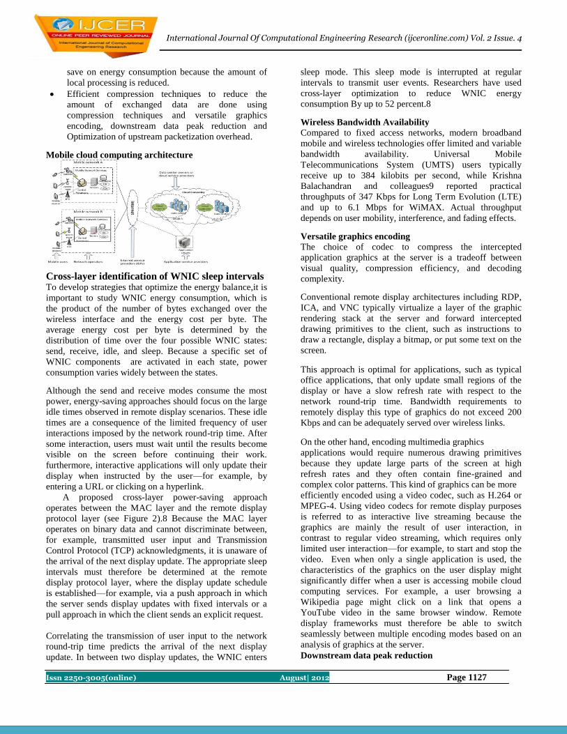
International Journal Of Computational Engineering Research (ijceronline.com) Vol. 2 Issue. 4
Issn 2250-3005(online) August| 2012 Page 1127
save on energy consumption because the amount of
local processing is reduced.
Efficient compression techniques to reduce the
amount of exchanged data are done using
compression techniques and versatile graphics
encoding, downstream data peak reduction and
Optimization of upstream packetization overhead.
Mobile cloud computing architecture
Cross-layer identification of WNIC sleep intervals To develop strategies that optimize the energy balance,it is
important to study WNIC energy consumption, which is
the product of the number of bytes exchanged over the
wireless interface and the energy cost per byte. The
average energy cost per byte is determined by the
distribution of time over the four possible WNIC states:
send, receive, idle, and sleep. Because a specific set of
WNIC components are activated in each state, power
consumption varies widely between the states.
Although the send and receive modes consume the most
power, energy-saving approaches should focus on the large
idle times observed in remote display scenarios. These idle
times are a consequence of the limited frequency of user
interactions imposed by the network round-trip time. After
some interaction, users must wait until the results become
visible on the screen before continuing their work.
furthermore, interactive applications will only update their
display when instructed by the user—for example, by
entering a URL or clicking on a hyperlink.
A proposed cross-layer power-saving approach
operates between the MAC layer and the remote display
protocol layer (see Figure 2).8 Because the MAC layer
operates on binary data and cannot discriminate between,
for example, transmitted user input and Transmission
Control Protocol (TCP) acknowledgments, it is unaware of
the arrival of the next display update. The appropriate sleep
intervals must therefore be determined at the remote
display protocol layer, where the display update schedule
is established—for example, via a push approach in which
the server sends display updates with fixed intervals or a
pull approach in which the client sends an explicit request.
Correlating the transmission of user input to the network
round-trip time predicts the arrival of the next display
update. In between two display updates, the WNIC enters
sleep mode. This sleep mode is interrupted at regular
intervals to transmit user events. Researchers have used
cross-layer optimization to reduce WNIC energy
consumption By up to 52 percent.8
Wireless Bandwidth Availability
Compared to fixed access networks, modern broadband
mobile and wireless technologies offer limited and variable
bandwidth availability. Universal Mobile
Telecommunications System (UMTS) users typically
receive up to 384 kilobits per second, while Krishna
Balachandran and colleagues9 reported practical
throughputs of 347 Kbps for Long Term Evolution (LTE)
and up to 6.1 Mbps for WiMAX. Actual throughput
depends on user mobility, interference, and fading effects.
Versatile graphics encoding
The choice of codec to compress the intercepted
application graphics at the server is a tradeoff between
visual quality, compression efficiency, and decoding
complexity.
Conventional remote display architectures including RDP,
ICA, and VNC typically virtualize a layer of the graphic
rendering stack at the server and forward intercepted
drawing primitives to the client, such as instructions to
draw a rectangle, display a bitmap, or put some text on the
screen.
This approach is optimal for applications, such as typical
office applications, that only update small regions of the
display or have a slow refresh rate with respect to the
network round-trip time. Bandwidth requirements to
remotely display this type of graphics do not exceed 200
Kbps and can be adequately served over wireless links.
On the other hand, encoding multimedia graphics
applications would require numerous drawing primitives
because they update large parts of the screen at high
refresh rates and they often contain fine-grained and
complex color patterns. This kind of graphics can be more
efficiently encoded using a video codec, such as H.264 or
MPEG-4. Using video codecs for remote display purposes
is referred to as interactive live streaming because the
graphics are mainly the result of user interaction, in
contrast to regular video streaming, which requires only
limited user interaction—for example, to start and stop the
video. Even when only a single application is used, the
characteristics of the graphics on the user display might
significantly differ when a user is accessing mobile cloud
computing services. For example, a user browsing a
Wikipedia page might click on a link that opens a
YouTube video in the same browser window. Remote
display frameworks must therefore be able to switch
seamlessly between multiple encoding modes based on an
analysis of graphics at the server.
Downstream data peak reduction

International Journal Of Computational Engineering Research (ijceronline.com) Vol. 2 Issue. 4
Issn 2250-3005(online) August| 2012 Page 1128
Interactive applications only update their display when
instructed by the user. These display updates usually
involve sending a large amount of data to the client in a
short interval, which requires an instantaneous bandwidth
much higher than the average bandwidth requirement.
Furthermore, this bursty traffic pattern is unfavorable in
wireless network environments, as it might induce
additional collisions on the wireless channel.
Optimization of upstream Packetization overhead
User events are the principal source of upstream remote
display traffic from client to server. Individually, each user
event embodies only a small amount of information: a key
or button ID, one bit to discriminate between the press and
release actions, and possibly the current pointer
coordinates. Nevertheless, user events induce important
upstream traffic because they are often generated shortly
after each other. Entering a single character results in two
user events to indicate the press and release actions,
whereas moving the mouse results in a sequence of pointer
position updates.
Usually, the system transmits user events as they occur to
minimize interaction latency. Because data packets sent
upstream often contain a single user event, headers added
at the TCP, IP, and wireless link layer cause large
Packetization overhead. Table 3 quantifies the
Packetization overhead of TCP/IP headers of three
commonly used remote display protocols—the VNC
Remote Framebuffer (RFB) Protocol, RDP, and ICA—
when sending a single keystroke to the server. Optional
headers and the wireless link layer header further increase
total overhead.
Interaction Latency While technological advances are likely to overcome
bandwidth limitations, interaction latency—the delay users
experience between generating some input and seeing the
result on their display—is an intrinsic challenge of mobile
cloud computing because the device must communicate
even the most trivial user operations to the server.
Solutions to mitigate interaction latency try to either reduce
the number of hops on the end-to-end path by moving the
application closer to the client or provide better
synchronization mechanisms between client and server
Computing display updates in advance
Given the current application state, the application server
can predict potential display updates and stream them in
advance to the client. Contrary to video streaming, in
which the frame order is known in advance, in mobile
cloud computing, the next display update depends on user
input. For example, when a user opens an application
menu, the server can precompute all dialog windows that
can be opened by selecting one of the menu items.
Image buffering for virtual environment streaming
Due to limitations in mobile bandwidth and mobile device
memory resources, in most cases, streaming all possible
next display updates in advance is unfeasible. Furthermore,
the gains of this precomputing technique are highly
dependent on prediction accuracy. A better
strategy might be to buffer some key display updates, for
which the server only needs to provide a differential
update.
Scene object caching
For more static applications, such as office applications,
the potential next updates can be more accurately predicted
as, for example, a menu layout will rarely change.
Consequently, the number of corrective server updates will
be more limited. A typical example would be the list of
recently opened files in a text editor’s File menu. Scene
description languages such as MPEG-4 BiFS are
particularly suited to support this client-side handling of
user input.13 The client not only receives graphic updates,
but also is informed about the structure of the displayed
scene and its composing objects, as well as how the user
can manipulate these objects.
By physically separating the user interface from the
application logic, mobile cloud computing allows access to
even the most demanding applications from intrinsically
resource-constrained mobile devices. Developers tailor
contemporary remote display optimization techniques to
mobile devices’ short battery lifetime, the varying and
limited bandwidth availability on wireless links, and
interaction latency. Although each of these solutions
adequately addresses specific mobile cloud computing
challenges, an overall approach is currently lacking.
Because of user mobility, the wide diversity of
applications, and the varying wireless channel status, the
mobile cloud computing context is highly dynamic. Future
research should therefore focus on the design of a
comprehensive framework that integrates the existing
solutions and activates the most appropriate one depending
on the current device, network, and cloud server status.
Conclusion Mobile cloud computing is one of mobile technology
trends in the future since it combines the advantages of
both mobile computing and cloud computing, thereby
providing optimal services for mobile users. This article
has provided an overview of mobile cloud computing in
which its definitions, architecture, and optimized solutions
have been presented. The applications supported by mobile
cloud computing including mobile commerce, mobile
learning, and mobile healthcare have been discussed which
clearly show the applicability of the mobile cloud
computing to a wide range of mobile services. Then, the
issues and related approaches for mobile cloud computing
have been discussed. Finally, the future research directions
have been outlined.
References

International Journal Of Computational Engineering Research (ijceronline.com) Vol. 2 Issue. 4
Issn 2250-3005(online) August| 2012 Page 1129
[1.] C. Albanesius, “Smartphone Shipments Surpass PC
Shipments for First Time. What’s Next?” PC
Magazine, 8 Feb. 2011; www.pcmag.com/article
2/0,2817,2379665,00.asp.
[2.] V.S. Pendyala and S.S.Y. Shim, “The Web as the
Ubiquitous Computer,” Computer, Sept. 2009, pp.
90-92.
[3.] F. Lamberti and A. Sanna, “A Streaming-Based
Solution for Remote Visualization of 3D Graphics
on Mobile Devices,” IEEE Trans. Visualization
and Computer Graphics, Mar./Apr. 2007, pp. 247-
260.
[4.] H. Kawashima et al., “Virtual PC-Type Thin Client
System,” NEC Technical J., Sept. 2007, pp. 42-47.
[5.] K. Pentikousis, “In Search of Energy-Efficient
Mobile Networking,” IEEE Comm. Magazine, Jan.
2010, pp. 95-103.
[6.] K. Kumar and Y.-H. Lu, “Cloud Computing for
Mobile Users: Can Offloading Computation Save
Energy?” Computer, Apr. 2010, pp. 51-56.
[7.] T. Kim et al., “An Energy-Aware Transmission
Mechanism for WiFi-Based Mobile Devices
Handling Upload TCP Traffic,” Int’l J. Comm.
Systems, May 2009, pp. 625-640.
[8.] P. Simoens et al., “Cross-Layer Optimization of
Radio Sleep Intervals to Increase Thin Client
Energy Efficiency,” IEEE Comm. Letters, Dec.
2010, pp. 1095-1097.
[9.] K. Balachandran et al., “Performance Assessment
of Next-Generation Wireless Mobile Systems,”
Bell Labs Technical J., Feb. 2009, pp. 35-58.
[10.] http://onlinelibrary.wiley.com/doi/10.1002/wcm.12
03/abstract,
[11.] I. Nave et al., “Games@Large Graphics Streaming
Architecture,” Proc. IEEE Int’l Symp. Consumer
Electronics (ICSE 08), IEEE Press, 2008, pp. 205-
208.
[12.] K.-J. Tan et al., “A Remote Thin Client System for
Real-Time Multimedia Streaming over VNC,”
Proc. IEEE Int’l Conf. Multimedia and Expo
(ICME 10), IEEE Press, 2010, pp. 992-997.
Author’s profile
Rajesh Badam: Pursuing Mtech. (CSE
Dept.) Malla Reddy College of
Engineering and Technology,
Hyderabad. Mr. J.Praveen Kumar
Asst.Prof. CSE Dept.
Malla Reddy College of Engineering and
Technology, Hyderabad.

International Journal Of Computational Engineering Research (ijceronline.com) Vol. 2 Issue. 4
Issn 2250-3005(online) August| 2012 Page 1130
Effect of dyke structure on ground water in between Sangamner and
Sinnar area: A Case study of Bhokani Dyke.
1. P. D. Sabale, 2 S. A. Meshram
1 Associate Professor, Deccan College (Deemed University), Pune.
2. Associate Professor in Geology, College Of Engg, Pune (COEP.)
Abstract In semi-arid regions, particularly in hard rock areas, shallow aquifers are a major source of potable groundwater. These
aquifers are indiscriminately exploited to meet the growing demand of water for domestic, irrigation as well as industrial uses.
Therefore, peoples in this area are continuously pumping ground water from the well and in most of the days they found
empty. Due to the over pumping through tube wells and dug wells, the ground water level is goes down below day to day.
Therefore, due to such situation, people move to search the water from one place to another. In this situation, presence of a
dyke is gives a new avenue to recharge the wells in the concern area.
Dykes in the Deccan Trap areas are to a great extent, known to control the movement of groundwater, and success or
otherwise of the well in the field area depends very much upon its location. The Bhokani dyke area has opened the door of
excellent irrigation. Those wells which are taken on dyke are giving good yield and therefore farmers are pumping water
continuously.
In short, in areas of harsh Ground water situation, presence of dyke is an good as avenue for the ground water in the said
region. This avenue acts as a source for the supply for irrigation and drinking water needs of the study area. Therefore this is
an important factor in deciding the socio-economical conditions of the farmers in this area. This paper deals with study of such
dyke which occurs near Sangamner area.
Introduction: Failure of open dug wells and tube wells in most of parts of the hard rock areas in Deccan Traps is a common phenomenon.
This problem usually arises, either because of the over exploitation / pumping of water from the existing wells or due to
missing of the exact water potential zones in this terrain. As on the hard rock region water mainly exists in fracture and joints,
locating such zones and predicting the flow processes is a difficult process.
Draught in the semiarid areas of hard rock is mainly due to low rate of precipitation and results into low irrigation in dry
regions. Therefore, in this region, there is a growing demand for ground water resource as the surface water resources are not
available adequately.
In semi-arid regions where groundwater occurs in shallow weathered zones, the rise in groundwater level is a direct
consequence of precipitation, particularly in the monsoon season, when the groundwater withdrawal is minimum (Mondal et
al., 2011).
India is seventeenth largest country in the world with diverse climate, topography, geology; soil types, land cover and land use
pattern (National Institute of Hydrology, Report, 1998-99). The water resources of India are enormous but they are unevenly
distributed in several terms. Seasonally, regionally, basin wise cultivator cross wise and crop wise.
In general, the ground water potential of hard rock’s is poor, though relatively high yields may be obtained from in restricted
locations under favorable circumstances of topography and rainfall. The size and the frequency of opening s in the fractured
rocks are normally restricted to shallow depth resulting in low void ratio and hydraulic conductivity.
Draught in the semiarid area of hard rock is due to low rainfall and low irrigation in dry regions. Therefore, during summer
groundwater from the basaltic aquifers is the prime source of water (Kale and Kulkarni, 1992).
Failure of tube well and open well in many parts of the hard rock regions are common phenomenon. This problem usually
arises, either because of the over abstraction in existing wells or due to the missing of the exact water potential zone. As on the
hard rock region water mainly exists in fracture and joints, locating such zones and predicting the flow processes are a difficult
process.

International Journal Of Computational Engineering Research (ijceronline.com) Vol. 2 Issue. 4
Issn 2250-3005(online) August| 2012 Page 1131
The geometry of the joint and fracture set is determined by the types of rock and the stress to which they have been subjected,
besides the effect of weathering and relief which makes the void space constituting the system progressively larger and
approaching the surface. The study area is also parts of hard rock terrain and the same situation is observed in this area. The
population in the rural area is mainly dependent on the ground water as a source of drinking and irrigation (Srikanth, 2009).
But, successful wells in study area are also become dry because of the over pumping practices.
In hard rock region, there is a growing demand for ground water resource as the surface water resources are not available
adequately (National Institute of Hydrology, Report, 1998-99).
Study Area:
Study area is southern boundaries of Sinnar and northern boundaries of Sangamner and is belongs to a severe part of draught
prone regions of Ahmednagar and Nasik district respectively of Maharashtra (Fig. 1). This area lies between latitude 19° 40’
04” N to 19°51’05’ and longitude 74° 04’11”E to 74°14’10”E on Survey of India (SOI) toposheet No. 47I/1 and 2. This
region is located 10 miles from east of Sinnar (Nasik) and 16 miles from Sangamner (Ahmednagar district).
Geomorphology of the area:
Geomorphologically the terrain shows plain to undulating topography. The highest elevation in this area is 2824 mts. at east of
Chas i.e. southern end while lowest elevation is 1836 mts. at north of Panchale i.e. northern boundary of study area.
The main drain in this area is Deo river, which is right side tributary of Godavari, confluences at Somathane village, NW of
Kopargaon. In this study area, the locations of the tributaries of Deo River are shows good network of drainage. Along the
channel of this river, the surface shows moderate to stiff slope.
Geology of the area:
The study area is a part of Deccan Volcanic Province (DVP). This region consists of alternate flows of compact and
amygdaloidal basalt. Compact basalt flows are thick, tabular and shows more lateral extent while amygdaloidal basalt flows
are thin, irregular and shows less extent than compact basalt flows.
Study area is a part of Deccan Volcanic Province (DVP) which generally shows (i) pipe amygdale flows shows irregular
vesicles, weak tabular, glassy and sub horizontal sheet joints at the bottom (ii) compact, absence of vesicles, joints and
fractures, and (iii) sub horizontal sheet joints with spheroidal amygdales (unfilled with vesicles) at the top (Kale and Kulkarni,
1992). The relative thickness in between these three layers is varying place to place.
These flows are characterized by variable thickness, irregularity, local dips, small extent , and lateral variation (Chaubey,
1973, Sukheswala and Polder Vaart, 1958; West, 1958, Gupte, 2007). In addition to the above predominant flows, at places
some pocket deposit or cluster of volcanic breccias observed which might be outpoured in the volcanic activity during post –
Deccan Trap period (Gupte et al., 1984).
Weathering and Erosion in Deccan Trap:
Due to the effect of physical weathering agents, rock found degraded condition and micro cracks are developed. Therefore,
due to such continuous disintegration on the exposure of the rock, resulting depth of weathering goes deep and deep.
Resulting, up to this weathered portion, surface water is penetrating down and ground water is formed. Here the trough
shaped upper portion of the dyke is filled and surrounded by thick or thin blanket of black cotton soil, followed by deeply
weathered, moderately weathered and finally fresh rock at the bottom. A typical stratigraphical section in study area is shown
in (Fig. 2). Amygdaloidal basalt gives better response than compact to such kind of activity (Sabale, 2005). And the study area
is more dominant region of Amygdaloidal basalt than compact.
Water bearing characters of Deccan Trap:
As stated above, in the Deccan Trap, water table conditions occurs under in weathered and jointed traps, and under confined
conditions in weathered and jointed traps, and under confined conditions in the zeolitic and vesicular traps. Wells in valleys
nearer to nallas and zeolotic traps yielded better than those located on elevated areas. The saturated fractures and joints found
in the relatively unweathered bed rock are capable of yielding a substantial quantity of water at greater depth. The fractures
and joints are mostly sheet type, sometimes are having good lateral extent and interconnected with each other. Therefore,
groundwater level in this zonesis not readily affected by seasonal changes.

International Journal Of Computational Engineering Research (ijceronline.com) Vol. 2 Issue. 4
Issn 2250-3005(online) August| 2012 Page 1132
In dry draught prone areas, in harsh situation, presence of dyke is get as a avenue for the ground water Supply for drinking
situation. This paper deals with study of such dyke which occur Deccan Volcanic Province (DVP) of draught prone region
near Sangamner – Shirdi area.
The groundwater possibilities in the three groups viz.1.Numerous dolerite dykes in Deccan Traps of Dhulia district (2) Areally
extensive trap flows resulting from slow and quiescent type of flood eruption occupying the gently undulating terrain, of
Sholapur and Osmanabad districts and (3) the traps characterised by intertrappean sediments, dolerite dykes and volcanic ash
beds, indicative of violent outbursts resulting in the Sahyadri geomorphologic unit of Kolaba, Thana and Bombay-Poona
regions, are to a great extent governed by the nature and constitution of the individual flows. This character is given by
Adyalkar and Mani(1971), based on their mode of emplacement, geomorphic setting and hydro geological of the Deccan
Traps of western Maharashtra.
Single Unit of Deccan Trap Groundwater Province into 3 Sub-Provinces, based on geomorphological, geological and
geohydrological setting in the region of western Maharashtra of the present investigation.
The dolerite dykes most of the time control the movement of groundwater, and success or otherwise of the well field area
depends very much upon its location with reference to adjacent dykes, found in the Dhulia district.Thick vesicular, extensive
traps with their gentle dips towards east have to be explored for possible artesian conditions in the down dip directions of the
trappean units to be tapped, in Sholapur district (GSDA & CGWB Report, 2007-08).
The Bhokani Dyke Areas:
Bhokani dyke is doleritic type, width ranging from 7 ft. to 16 ft and 28.50 kilometers in length. This dyke is having N07°E
strike and showing N-NE to S-SW trend. Dyke rock is black colored doleritic rock with well prismatic joints. The local
people used term ‘KAR’ in Marathi for dyke in this area. It is move through Dodi, Khambale, Bhokani, Tamaswadi, Dambra,
Chauri, Mendi villages etc. from S-SW to N-NE trend. At the beginning at S-SW portion, it is crossing Mhaladevi river and at
the N-NE side it confluence in the Godavari river.
As per as the dug well and tube wells are concern, the maximum number of wells are present on the dyke alignment. Most of
the wells (of about 95%) are yielding good amount of water. Therefore, the green zone is observe along the whole alignment
of dyke, while rest of the area is found dry and partly green (only rainy and autumn season) due to the less irrigation. Because
most of the wells in this area are dry of seasonal. Therefore, farmers are pumping day-night water from these wells with one or
at some places two pumps of 5 or 10 HP are set up on the well.
Well Inventory:
In India, ground water has been exploited substantially during the past few decaded for irrigation. Most of the ground water
utilization in India is from shallow depth aquifer zones at depth less than 100 m (Khepar and Chaturvedi, 1982, Rangnath,
1982). But the dykes which are constructed on dyke are yielding good amount of ground water. Therefore, to know the ground
water conditions of such wells, a detailed well inventory survey was carried out in central part of the study area i.e. especially
at Bhokani and Khambale area. In this survey well inventory work for 22 wells were carried out. To know the exact water
carrying capacity and ground water situation, for this study the wells are selected in middle reaches or central zone out of total
extension in this area of dyke.
During this survey well number, name of owner, whether it is lined or unlined (i.e. whether it is constructed or non-
constructed) is reported. If it is lined the type and nature of material, cement or mortar, with the help of dressed stone, which
are available in the surrounding area. In addition to this, the important ground water information such as depth of ground water
from ground level and pumping hours for respective well in summer etc. is given in the following table.
Trend Well
No.
Name of owner /
farmer
Constructed /
Non-
constructed
Well dimension
Width Depth
(ft.) (ft.)
Water level
From bottom
(ft.)
Width
of
dyke
(ft.)
S-SW 1. Kisan S. Sabale Masonry
constructed
17 47 4 14-16
2. Trimbak G. Sabale Masonry
constructed
16 45 6 17-19
3. Chandrakant Masonry 12 34 2 10-12

International Journal Of Computational Engineering Research (ijceronline.com) Vol. 2 Issue. 4
Issn 2250-3005(online) August| 2012 Page 1133
Domaji Ranshivre constructed
4. Chandrakant D.
Ranshivre
Masonry
constructed
12 46 4 8-10
5. Eknath Ranshivre Masonry
constructed
10 42 5 8-10
6. Dr. Ranshivre Masonry
constructed
10 40 5 6-8
7. Ranshivre Masonry
constructed
12 42 7-10
Centr
e
1. Mahadu Y. Sirsat Masonry
constructed
14 42 5 10-12
2. Chandrabhan S.
Shirole
Masonry
constructed
15 44 6 12-14
3. ChandrabhanP.
Walekar
Masonry
constructed
14 36 4 10-12
4. Chandrabhan P.
Walekar
Masonry
constructed
16 46 5 10-12
5. NamdeoMalhariWa
lekar
Masonry
constructed
11 34 2.5 8-10
6. Trimbak N. Shirole Masonry
constructed
18 47 4.5 10-12
7. Bibhishen N.
Walekar
Masonry
constructed
17 42 6 14-16
8. Rahadu A. Shirole Masonry
constructed
12 35 2 12-14
9. Navnath K. Shirole Masonry
constructed
16 44 4 10-12
10. Ramchandra
Shirole
Masonry
constructed
16 44 4.5 10-12
11. Ramchandra
Shirole
Masonry
constructed
17 45 3.5 11-12
12. Bhima K. Kale Masonry
constructed
17 46 5 15-16
13. Datta S. Kale unconstructed 14 37 2.5 10-12
14. Narayan B. Shirole Masonry
constructed
12 48 4 8-10
15. Bhaskar B. Shirole Masonry
constructed
14 44 5 7-8
16. Pandurang K.
Shirole
Masonry
constructed
12 36 4.5 8-10
Ground water condition in the well along the dyke:
As we know, dyke is having prismatic joints, which acts as an avenue for ground water flows, just like is leaky pipe. The water
carrying capacity of a dyke is depend upon a. nature of joints (whether it is tight or open) b. presence of type of joints c.
Dimension of the dyke. Slope of the area e. Water body in the path of the dyke. As describe above, the of Bhokani dyke is
from Northern region of Akola and south of Sinnar from Ahmednagar and Nasik district respectively. In this area, at the
beginning, the dyke is crossing a percolation tank. Therefore, this dyke is become recharge and it carries water from south to
north part.
Crop Yield / Production of crop in the study area:
During the well inventory survey, type of crops, their yield and production of crop in the zone of dyke and outside the dike
area for one acre area is collected from the local farmers. Then this crop wise production data is compared to each other in the
study area.

International Journal Of Computational Engineering Research (ijceronline.com) Vol. 2 Issue. 4
Issn 2250-3005(online) August| 2012 Page 1134
Season Sr. No. Name of the crop Production in the zone of
dyke area (Ton/acre).
Production outside of the dyke
area (Ton/acre).
Rainy 1 Legume / ground nut 20 16
2 onion 30 16
3 Bajar 25 17
4 Maize 20 10
Summer 1 Wheat 27 15
The table data reveals that, crop production (in ton/acre) in the zone of dyke area is roughly double than production outside of
the dyke area. This excess production in the zone of dyke area is only due to the good recharge of the well.
Improvement in the standard of living of peoples:
Ground water recharging conditions in the wells of the study areas farmers could able to good practice of irrigation. The
production of food in the zone is high as compare to the peripheral areas. Therefore, standards of living of the farmers are
increasing day to day in this area. In addition to this, very important change observed here is in the ‘Standard of living’ of the
people. The main reason for the up gradation of these peoples in this area because i. wells are constructed up to deeper level
and therefore they store large amount of water can store. ii. Water level in the wells which are located on dyke is rise due to
good recharge conditions due to the presence prismatic joints of dyke.iii. Due to the presence of dyke the wells in the villages
have enough of water. iv. Farmers have sufficient work on the farm and they are fully involved in taking more crops. v. The
fodder is enough available for their cattle. vi. Milk production has increased drastically. vii.Resulting, women do not have to
go to long distance for drinking water and viii. Due to good irrigation practices, milk production, and scheme for women
development the economical condition of the people is increased and standard of living has also increased.
Results and discussion:
According to Bondre et al. (2006), numerous large dimensional mafic dyke outcrops are generally shows NE-SW to E-W
trending in outcrop around Sangamner in the Western Deccan Volcanic Province. He also argued that, this area is a part of
broader region of postulated to be a shield like feature and major eruption centre. But as per as the Bhokani dyke is concern,
whether it is concern with the same dyke swarm, that has to check. Because, as per as the distribution of dykes identified and
given by Bondre et al. (2006), northern extension of his Fig. 2, is up to Dapur (North of Akole), while southern extension of
this dyke is up to Godavari river. These dykes are compositionally similar to the south western Deccan formations, although
most of them can be best related to either Poladpur formation or Khandala formation. While geochemical composition is not
necessarily correlated with location, in this area (Bondre, et al., 2006).
While much of the previous work pertains to lava flows, a few workers (e.g. Deshmukh and Sehgal, 1988, Bhattacharji et al.
1996; Mellusco et al.1999; Subbarao et al. 1999) have also studied the two principal dike swarm in this province, where the
dike occur with high frequency. The West Coast Dike Swarm (WCDS) trending N-S to NNW –SSE, consist of tholeitic and
alkaline compositions. The Narmada-Tapi Dike Swarm (NTDS) also contains tholeitic as well as alkaline dikes has
predominant ENE-WSW trend (Sheth, 1998; Molluso et al. 1999).
Beane et al. (1986) observed that their compositions are similar to those of the associated flows. Bhattacharji et al. (1996)
considered the random orientation to the result of stress regime dictated by large crustal magma chambers. Sheth (2000)
argued that true feeder dikes in central volcanoes usually have a radial arrangement, not random arrangement.
Conclusion: The dolerite dykes most of the time control the movement of groundwater, and success or otherwise of the well field area
depends very much upon its location with reference to adjacent dykes, found in the Dhulia district.
Bhokani dyke is doleritic type, with sufficient dimensions and extensions. Due to the presence of prismatic joints, those wells
which are found on the dyke and side of the dyke yielding good amount of ground water. Therefore, this dyke throughout his
length giving recharge to the connecting and adjacent wells along its N-NE to S-SW trend. Resulting, the farmers are able to
take more crops with good yield. Therefore, the green zone is observe along the whole alignment of dyke, while rest of the
area is found dry and partly green (only rainy and autumn season) due to the less irrigation. Good irrigation practices, milk
production, etc. activities are responsible for improvement of the economiccondition of people in this area. Many social
changes took place and especially the women’s groups became independent in decision making and their involvement has

International Journal Of Computational Engineering Research (ijceronline.com) Vol. 2 Issue. 4
Issn 2250-3005(online) August| 2012 Page 1135
increased in day to day activities. Due to education, the number of students has increased. Awareness tendency has been
generated in the minds of illiterate village people.
This results into the improvement of the economic condition of the peoples in this area.
References: [1.] Adyalkar, P. G. and Mani, V. S. (1971) Paleogeography, geomorphological setting and groundwater possibilities in the
Deccan Traps. Bulletin Volcanologique, 35 (3), pp.696-708.
[2.] Beane J E, Turner C A, Hooper P R, Subbarao K V and Walsh J N 1986 Stratigraphy, composition and form of the
Deccan basalts,Western Ghats, India; Bull. Volcanol. 48, pp.61-83
[3.] Bhattacharji S, Chatterjee N, Wampler J M and Gazi M 1994 Ma_c dikes in Deccan volcanics - indicator of India
intraplate rifting, crustal extension and Deccan flood basalt volcanism. In: Volcanism, ed. K V Subbarao Geol.Soc.
India, 253, pp.27.
[4.] Bondre, N. R., Hart, W. K., Sheth, H. C. (2006) Geology and geochemistry of the Sangamner mafic dike swarm,
western Deccan volcanic province, India: Implications for regional stratigraphy. J. Geol., v. 114, pp. 155-170.
[5.] Chaubey,V.D.(1973). Long Distance Correlation of Deccan Flow, Central India, Geological Society of America,
Bulletin 84, pp.2785-2790.
[6.] Khepar, S. D. and Chaturvedi, M. C. : 1982, ‘Optimum cropping and groundwater management’,
Water Resources Bulletin 18 (4), 655–660.
[7.] Deshmukh, S. S., Sehgal, M. N. (1988) Mafic dyke swarms in Deccan Volcanic Province of Madhya Pradesh and
Maharashtra. In: Subbarao, K. V. (Ed.), Deccan Flood Basalts. Geol. Soc. Ind. Mem., v. 10, pp. 323-340.
[8.] DYNAMIC GROUNDWATER RESOURCES OF MAHARASHTRA ABRIDGED REPORT (AS ON 2007-08)
.Prepared by -Groundwater Surveys and Development Agency, GoM & Central Ground Water Board, Central Region,
Nagpur, GoI.
[9.] Gupte, R.B. (2008). Indian Geology. A Text of Engineering Geology. Third Edition (Revised), Pune Vidyarthi Griha
Publication, Pune. pp.105-148.
[10.] Gupte, R.B., Kulkarni, S.R. and Marathe, S.S. (1984). Post –Deccan Trap Volcanic Activity in Western Maharashtra.
Indian Mineralogist. pp. 69-74.
[11.] Kale, V. S. and Kulkarni, H. (1992) IRS-1A and LANDSAT data in mapping Deccan Trap flows around Pune, India:
Implications in hydrogeological modeling. Archives Int. Soc. Photogramm. and Rem. Sensing, 29(B-7): 429-435.
[12.] Melluso, L., Sethna, S. F., Morra, V., Khateeb, A., Javeri, P. (1999) Petrology of the mafic dyke swarm of the Tapti
River in the Nandurbar area (Deccan Volcanic Province). In: Subbarao, K. V.
[13.] (Ed.), Deccan Volcanic Province. Geol. Soc. Ind. Mem., v. 43, pp. 735-755.
[14.] Mondal, Nepal C, Singh, Vijay P. and Somayaji Sankaran (2011). Demarcation of prospective groundwater recharge
zones in hard rock area from Southern India. Scientific Research and Essays Vol. 6(16), pp. 3539-3552.
[15.] National Institute of Hydrology, Report, (1998-99). Hydrological Problems of Hard Rock Region- State of Art
Report. National Institute of Hydrology. Roorki.
[16.] Peshwa A, V. and Kale, V. S. (1988). Role of remote sensing in the detection of potential sites for landslides /
rockfalls in the Deccan Trap lava terrain of western India. Environmental Geotechnics and Problematic Soils and
Rocks; Balkema, Rotterdam;, pp.367 - 374.
[17.] Sabale, P.D. (2005). “Watershed Development and Management in Siddheshwarwadi: A Review”. ICEM, Vol.5,
Editor-Anji Reddy, B.S.Publ., J.N.T.U., H’bad. Pp. 318-325.
[18.] Rangnath, 1982
[19.] Sheth, 1998. Geochemistry, petrogenesis,Stratigraphy and structure of Deccanflood basalts of the western Satpura-
Tapi region,india. Ph.D dissertation, Indian Institute of Technology, Bomboy.
[20.] Subbarao et al. 1999 Narmada dyke. In Subbarao, K.V., ed. Deccan Volcanic Province. Geol. Soc. India Mem. 43,
pp.891-902.
[21.] Srikanth, R. (2009). Challenges of sustainable water quality management in rural india Current Science, Vol.97, No.3,
pp.317-325.
[22.] Sukheswala R N and Poldervaart A 1958 Deccan basalts of the Bombay area, India: Bull. Geol. Soc. Am. 69, pp.1475-
1494.
[23.] West W D 1958 The petrography and petrogenesis of forty- eight flows of Deccan Traps penetrated by borings in
western India; Trans. Nat. Inst. Sci. India 4, pp.1-56.

International Journal Of Computational Engineering Research (ijceronline.com) Vol. 2 Issue. 4
Issn 2250-3005(online) August| 2012 Page 1136
International Journal Of Computational Engineering Research (ijceronline.com) Vol. 2 Issue. 4
Issn 2250-3005(online) August| 2012 Page 1137
Algorithm for Merging Search Interfaces over Hidden Web
Harish Saini1, Kirti Nagpal
2
1Assistant Professor N.C.College of Engineering Israna, Panipat 2Research Scholar, N.C.College of Engineering Israna, Panipat
Abstract: This is the world of information. The size of
world wide web [4,5] is growing at an exponential rate day
by day. The information on the web is accessed through
search engine. These search engines [8] uses web crawlers to
prepare the repository and update that index at an regular
interval. These web crawlers [3, 6] are the heart of search
engines. Web crawlers continuously keep on crawling the web
and find any new web pages that have been added to the web,
pages that have been removed from the web and reflect all
these changes in the repository of the search engine so that the
search engines produce the most up to date results.
Keywords: Hidden Web, Web Crawler, Ranking, Merging
I. INTRODUCTION This is the world of information. The size of world wide web
[4,5] is growing at an exponential rate day by day. The
information on the web is accessed through search engine.
These search engines [8] uses web crawlers to prepare the
repository and update that index at an regular interval. Web
crawlers continuously keep on crawling the web and find any
new web pages that have been added to the web, pages that
have been removed from the web and reflect all these changes
in the repository of the search engine so that the search
engines produce the most up to date results. There is some
data on the web that is hidden behind some query interfaces
and that data can’t be accessed by these search engines. These
kind of data is called hidden web [41] or deep web. These
days the contents on the hidden web are of higher interests to
the users because the contents of hidden web are of higher
quality and greater relevance. The contents on hidden web can
be accessed by filling some search forms which are also
called sometimes search interfaces. Search interfaces [37] are
the entry points to the hidden web and make it possible to
access the contents on the hidden web. These search
interfaces are simply like filling any forms like forms for
creating e-mail ids etc. Each search interface has number of
input controls like text boxes, selection lists, radio buttons etc..
To access hidden web one needs to fill these search interfaces
for which a crawler is required which finds for forms on the
web known as form crawler. There can be multiple search
interfaces for the same information domain on the web. In that
case all those search interfaces are required to be merged or
integrated so that crawler[3] finds all data relevant to the user
input despite of existence of multiple search interfaces for the
same domain. Hidden web crawler is the crawler which
continuously crawls hidden web so that it could be indexed by
search engines. The major functions which are to be
performed by hidden web crawler are getting form filled,
finding search query, submitting query and indexing the
results. The challenge of the hidden web crawlers are the huge
and dynamic nature of the hidden web. The merging[46] or
integration of search interfaces over hidden web is required to
response queries so that it answers queries at its best. For the
integration of search interfaces over hidden web two steps are
required
Finding semantic mapping over the different search
interfaces to be merged.
Merging search interfaces on the basis of semantic
mappings found earlier.
A Ranking the Web Pages by Search Engine
Search for anything using our favorite crawler-based search
engine will sort through the millions of pages it knows about
and present you with ones that match your topic. The matches
will even be ranked, so that the most relevant ones come first.
Of course, the search engines don't always get it right. So,
how do crawler-based search engines go about determining
relevancy, when confronted with hundreds of millions of web
pages to sort through? They follow a set of rules, known as an
algorithm. Exactly how a particular search engine's algorithm
works is a closely kept trade secret.
One of the main rules in a ranking algorithm involves the
location and frequency of keywords on a web page. Call it the
location/frequency method. Pages with the search terms
appearing in the HTML title tag are often assumed to be more
relevant than others to the topic. Search engines will also
check to see if the search keywords appear near the top of a
web page, such as in the headline or in the first few
paragraphs of text. They assume that any page relevant to the
topic will mention those words right from the beginning.
Frequency is the other major factor in how search engines
determine relevancy. A search engine will analyze how often
keywords appear in relation to other words in a web page.
Those with a higher frequency are often deemed more
relevant than other web pages.

International Journal Of Computational Engineering Research (ijceronline.com) Vol. 2 Issue. 4
Issn 2250-3005(online) August| 2012 Page 1138
B. Web Crawler
A crawler [14,20] is a program that are typically programmed
to visit sites that have been submitted by their owners as new
or updated. The contents of the Entire sites or specific pages
is selectively visited and indexed. The key reason of using
web crawlers is to visit web pages and add them to the
repository so that a database can be prepared which in turn
serves applications like search engines.
Crawlers use graph structure of the web to move from pages
to pages. The simplest architecture of web crawler is to start
from a seed web page and traverse all hyperlinks encountered
in this web pages then all encountered hyperlinks are added to
the queue which in turn are traversed. The process is repeated
until a sufficient number of pages are identified...
The main goal of the web crawler is to keep the coverage and
freshness of the search engine index as high as possible which
is not informed by user interaction. For this task the crawler
and other parts of the search engine have no communication
between them. Because web is a purely dynamic collection of
web pages there is a need for crawling cycles frequently to
refresh the web repository so that all new pages that have
been added to the web are included in the repository similarly
the web pages that have been removed from web are deleted
from web repository
C Hidden Web Crawler
Current day crawlers crawls only publicly indexable web
(PIW) i.e set of pages which are accessible by following
hyperlinks ignoring search pages and forms which require
authorization or prior registration. In reality they may ignore
huge amount of high quality data which is hidden behind
search forms. Pages in hidden web are dynamically generated
in response to the queries submitted via search forms.
Crawling the hidden web is highly challenging task because
of scale and the need for crawlers to handle search interfaces
designed primarily for human beings. The other challenges of
hidden web data are:
Ordinary web crawlers can’t be used for hidden web
The data in hidden web can be accessed only through
a search interface
Usually the underlying structure of the database is
unknown.
The size of hidden web is continuously increasing as more
and more organizations are putting their high quality data
online hidden behind search forms. Because there are no static
links to hidden web pages therefore search engines can’t
discover and index these web pages.
Because the only entry point to hidden web is search interface
the main challenge is how to generate meaningful queries to
issue to the site. Hidden web crawler is the one which
automatically crawls hidden web so that it can be indexed by
search engines. Hidden web crawler is able to allow an
average use to explore the amount of information, which is
mostly hidden behind search interfaces. The other motive for
hidden web crawler is to make hidden web pages searchable
at a central location so that the significant amount of time and
effort wasted in searching the hidden web can be reduced.
One more motive for hidden web crawlers is that due to heavy
reliance of web users on search engines for locating
information, search engine influence how the users perceive
the web..
There are two core challenges while implementing an
effective hidden web crawler
The crawler has to be able to understand and model a
query interface.
The crawler has to come up with meaningful queries
to issue to the query interface.
The first of the two challenges was addressed by a method for
learning search interfaces. For the latter challenge if the
search interface is able to list all possible values for a query
with help of some selection list or drop down list in that case
solution is straight forward. possible so all of the possible
queries can’t be exhaustively listed.
D Search Interfaces
While accessing hidden web [49] search query is submitted to
the search interface of the hidden web crawler. The selection
of web pages and the relevance of results produced from
hidden web is determined by the effectiveness of search
interfaces [42,43]. The different actions performed by search
interfaces are getting input from user, selection of query,
submitting query to the hidden web and merging of results
produced by hidden web crawlers.
The most important activity of search interface is selection of
query which may be implemented in variety of ways. One
method is random method in which random keywords are
selected from the English dictionary and are submitted to the
database. Random approach generates a reasonable number of
relevant pages. The other technique is using generic frequency.
In this method we find a document and obtain general
distribution frequency of each word in the document. Based
on this frequency distribution we find the most frequent
keyword, issue it to the hidden web database and retrieve the
result. The same process is repeated with the second most
frequent word and so on till the downloaded resources are
exhausted. After that it analyses the returned web pages that
whether they contain results or not. Another method is
adaptive in this method the documents returned from the
previous queries issued to the Hidden-Web database is
analysed and it is estimated which keyword is most likely to

International Journal Of Computational Engineering Research (ijceronline.com) Vol. 2 Issue. 4
Issn 2250-3005(online) August| 2012 Page 1139
return the most documents. Based on this analysis, the process
is repeated with the most promising queries.
E Problems in Integration of Hidden Web
Recently keen interest has been developed in the retrieval and
integration of hidden web with the intention of having high
quality data for the databases. As the size of information in
hidden web is growing, search forms or search interfaces are
needed to be located which serves as an entry point to hidden
web database. But there exists crawlers which focus search on
specific database domains and retrieve invariable diversified
set of forms like login form, quote request forms and
searchable forms from multiple domains. The process of
grouping these search interfaces or search forms over the
same database domain is called integration of search
interfaces.
These search form are input to algorithm which finds
correspondences among attributes of different forms. This
task is not so easy because of dynamic nature of the web the
new information is added to web and new information is
being modified or even removed. Therefore a scalable
solution suitable for large scale integration is required for the
purpose of large scale integration. In addition in a well
defined domain there may be variation in both structure and
vocabulary of search forms. So in order to obtain information
that covers the whole domain it is required to find
correspondences among attributes of forms and for that a
broad search is needed to be performed.
For this either full crawl is needed to be performed but this is
really inefficient approach as it can take weeks for the
exhaustive crawling process. Another alternative can be focus
crawling in which only pages relevant to a specific topic are
crawled. This has a better quality index as compared to
exhaustive crawling. In this case focused crawler that focus
solely on the contents of retrieved web pages may not be a
very good alternative also because forms are sparsely
distributed and thus the number of forms retrieved per total
number of pages retrieved may be very low. For tackling this
problem a focused crawler has been developed which used
reinforcement learning to build a focus crawler that is
effective for sparse concepts.
The kind of web crawler which crawl web pages
which contain search forms are called form crawlers. Since
form crawler find thousand of forms for the same domain.
Those different forms even for the same domain may be
different in the structure and vocabulary they use. For that
semantic mappings are required to be found among all
attributes of those forms and after finding semantic mappings
those are integrated so that queries involving that domain can
be answered suppressing the existence of multiple search
forms using different structures and vocabulary. There exist
multiple integration techniques which integrates these search
forms over the hidden web. Most of those are semiautomatic.
F. Need For Merging Search Interfaces
It seems that there will always be more then one search
interfaces even for the same domain. Therefore,
coordination(i.e. mapping, alignment, merging) of search
interfaces is a major challenge for bridging the gaps between
agents with different conceptualizations.
Two approaches are possible:
(1) merging the search interfaces to create a single coherent
search interface
(2) aligning the search interfaces by establishing links
between them and allowing them to reuse information from
one another.
Here we propose a new method for search interface merging.
Whenever multiple search forms are to be integrated the task
can be divided into two major steps
Finding semantic mapping among search forms or
interfaces
Merging search interfaces on the basis of mapping
The first step in merging [46] of search forms or interfaces
are finding semantic mapping and correspondences among
attributes of those forms so that on the basis of that mapping
search interfaces or forms could be merged. This semantic
mapping serves as the domain specific knowledge base for the
process of merging [47] of search interfaces. The proposed
algorithm is semi automatic. It finds similar terms from a
look-up table which stores all similar terms in the different
search interfaces to be merged along with the relationship
between those similar terms so that it may be decided which
term will be appearing in the merged search interface. The
algorithm makes use of search interfaces in form of a
taxonomy tree to cluster the concepts in the search interfaces
on the basis of level
II Merging of Search Interfaces More and more applications are in need to utilize multiple
heterogeneous search interfaces across various domains. To
facilitate such applications it is urgent to reuse and
interoperate heterogeneous search interfaces. Both merge and
integration produces a static search interface based on the
existing search interfaces. The resulting search interface is
relatively hard to evolve with the change of existing search
interfaces.

International Journal Of Computational Engineering Research (ijceronline.com) Vol. 2 Issue. 4
Issn 2250-3005(online) August| 2012 Page 1140
The search interface merge module takes source
search interfaces as input and a table that lists all similar terms
coming from different search interfaces along with the
relationship between those similar terms. The similar terms
can have relationship like meronym, hyper name and
synonym. The search interface merge process is divided into
several steps. Step 1. Find set of similar terms
Step 2. Children of similar terms are merged and point to the
same parent.
A Merging Observations and Results
Let us consider two source search interfaces and apply the
above stated algorithm to merge those search interfaces as a
case study. The source search interfaces under consideration
are given along with the domain specific knowledge base.
Table 1.1 Domain specific knowledge base
Concept Concept Relation
Optical_drive OpticalDisk Synonym
HardDrive HardDisk Synonym
DVD DVD-Rom Synonym
CDRW CD-RW Synonym
CDRom CD-ROM Synonym
Computer Personal Computer Synonym
The taxonomy trees of search interfaces A and B respectively are as following
Fig1.1TaxonomytreeforSearchInterfaceS1
The codes assigned to the terms in the source search interface
are as follows. Let us consider search interface a first and see
the codes assigned
Table 1.2 Codes of terms in search interface A
Term Code
Recurso A
CPU A01
Hard Disk A02
Personal computer A03
Memory A04
Architecture A05
Optical disk A06
Operating System A07
IBM A0101
Intel A0102
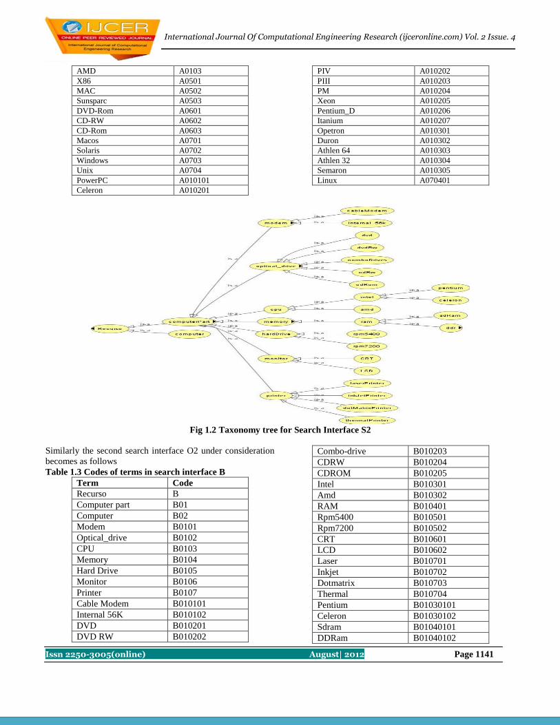
International Journal Of Computational Engineering Research (ijceronline.com) Vol. 2 Issue. 4
Issn 2250-3005(online) August| 2012 Page 1141
AMD A0103
X86 A0501
MAC A0502
Sunsparc A0503
DVD-Rom A0601
CD-RW A0602
CD-Rom A0603
Macos A0701
Solaris A0702
Windows A0703
Unix A0704
PowerPC A010101
Celeron A010201
PIV A010202
PIII A010203
PM A010204
Xeon A010205
Pentium_D A010206
Itanium A010207
Opetron A010301
Duron A010302
Athlen 64 A010303
Athlen 32 A010304
Semaron A010305
Linux A070401
Fig 1.2 Taxonomy tree for Search Interface S2
Similarly the second search interface O2 under consideration
becomes as follows
Table 1.3 Codes of terms in search interface B
Term Code
Recurso B
Computer part B01
Computer B02
Modem B0101
Optical_drive B0102
CPU B0103
Memory B0104
Hard Drive B0105
Monitor B0106
Printer B0107
Cable Modem B010101
Internal 56K B010102
DVD B010201
DVD RW B010202
Combo-drive B010203
CDRW B010204
CDROM B010205
Intel B010301
Amd B010302
RAM B010401
Rpm5400 B010501
Rpm7200 B010502
CRT B010601
LCD B010602
Laser B010701
Inkjet B010702
Dotmatrix B010703
Thermal B010704
Pentium B01030101
Celeron B01030102
Sdram B01040101
DDRam B01040102

International Journal Of Computational Engineering Research (ijceronline.com) Vol. 2 Issue. 4
Issn 2250-3005(online) August| 2012 Page 1142
Now depending upon the length of codes assigned to each
term search interface can be divided into clusters so that all
terms having codes of same length reside in the same cluster.
The methodology used for clustering has been defined earlier.
The clusters becomes as follows for each search interface.
The algorithm suggested above makes use of recursive calls
so that all children of the terms under consideration are also
checked for the similarity. We take example of term Intel in
search interface o1 and the same term Intel in search interface
O2. Then we try to combine the children of both terms. This
term has been selected for the purpose of clarity and
simplicity only so that it doesn’t become too complex.
Level 0 Level 1
Level 0 Level 1
Level 2
Level 3
Level 2 Level 3
Fig 1.3 Clusters for Search Interface S1
To see how the process of merging of search interfaces will
take place we consider example of term CPU which appears
in both search interfaces. The process of merging will be
followed as per the algorithm suggested above.First of all
both search interfaces O1 and O2 will be passed to function
Integrate. The two tables table 1 and table 2 are already
available with us as given above. While scanning through
these tables as given in the algorithm it will be detected that
cpu appearing in table 1 is same as cpu appearing in table 2
and whenever two same or similar terms are encountered the
codes of both terms are fetched. From tables the fetched codes
of both terms in different search interfaces are A01 and
B0103 in search interface 1 and 2 respectively. These two
codes A01 and B0103 will be passed to function merge.
Function merge will make two queues from these two codes
one for each code having all its descendants upto any level.
So that those queues can be passed to function combine and
queues can be merged. In function merge q1 and q2 will be
created having code A01 and B0103 in q1 and q2 respectively.
The color will be assigned to each term in the queue just to
check whether immediate children of the term have been
added to the queue or not. Initially term will be of white color
and the color will be changed to black when its children has
been added to the queue. The process will be repeated until all
terms in the queue are black which represents that children of
each term has been added to the queue.
Level 0
A01, A02,
A03, A04,
A05, A06,
A07
A
A0101,A0102
,A0103,A050
1,A0502,A05
03,A0601,A0
602,A0603,A
0701,A0702,
A0703,A0704
A010101,A0102
01,A010202,A0
10203,A010204,
A010205,A0102
06,A010207,A0
10301,A010302,
A010303,A0103
04,A010305,A0
70401
B B01
B02
B0101,B0102,
B0103,B0104,
B0105,B0106,
B0107
B010101,B0101
02,B010201,B0
10202,B010203,
B010204,B0102
05,B010301,B0
10302,B010404,
B010505,B0105
02,B010601,B0
10602,B010701,
B010702,B0107
03,B010704,
B01030101,B01030102
B01040101,B01040102
Level 4
Fig 1.4Clusters for Search Interface S2
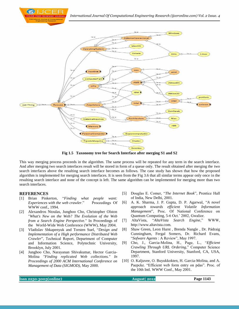
International Journal Of Computational Engineering Research (ijceronline.com) Vol. 2 Issue. 4
Issn 2250-3005(online) August| 2012 Page 1143
Fig 1.5 Taxonomy tree for Search Interface after merging S1 and S2
This way merging process proceeds in the algorithm. The same process will be repeated for any term in the search interface.
And after merging two search interfaces result will be stored in form of a queue only. The result obtained after merging the two
search interfaces above the resulting search interface becomes as follows. The case study has shown that how the proposed
algorithm is implemented for merging search interfaces. It is seen from the Fig 3.6 that all similar terms appear only once in the
resulting search interface and none of the concept is left. The same algorithm can be implemented for merging more than two
search interfaces.
REFERENCES [1] Brian Pinkerton, “Finding what people want:
Experiences with the web crawler.” Proceedings Of
WWW conf., 1994.
[2] Alexandros Ntoulas, Junghoo Cho, Christopher Olston
"What's New on the Web? The Evolution of the Web
from a Search Engine Perspective." In Proceedings of
the World-Wide Web Conference (WWW), May 2004.
[3] Vladislav Shkapenyuk and Torsten Suel, “Design and
Implementation of a High performance Distributed Web
Crawler”, Technical Report, Department of Computer
and Information Science, Polytechnic University,
Brooklyn, July 2001.
[4] Junghoo Cho, Narayanan Shivakumar, Hector Garcia-
Molina "Finding replicated Web collections." In
Proceedings of 2000 ACM International Conference on
Management of Data (SIGMOD), May 2000.
[5] Douglas E. Comer, “The Internet Book”, Prentice Hall
of India, New Delhi, 2001.
[6] A. K. Sharma, J. P. Gupta, D. P. Agarwal, “A novel
approach towards efficient Volatile Information
Management”, Proc. Of National Conference on
Quantum Computing, 5-6 Oct.’ 2002, Gwalior.
[7] AltaVista, “AltaVista Search Engine,” WWW,
http://www.altavista.com.
[8] Shaw Green, Leon Hurst , Brenda Nangle , Dr. Pádraig
Cunningham, Fergal Somers, Dr. Richard Evans,
“Sofware Agents : A Review”, May 1997.
[9] Cho, J., Garcia-Molina, H., Page, L., “Efficient
Crawling Through URL Ordering,” Computer Science
Department, Stanford University, Stanford, CA, USA,
1997.
[10] O. Kaljuvee, O. Buyukkokten, H. Garcia-Molina, and A.
Paepcke. “Efficient web form entry on pdas”. Proc. of
the 10th Intl. WWW Conf., May 2001.

International Journal Of Computational Engineering Research (ijceronline.com) Vol. 2 Issue. 4
Issn 2250-3005(online) August| 2012 Page 1144
[11] Ching-yao wang, ying-chieh lei, pei-chi chang and
shian- shyong tsen National chiao-tung university, “A
level wise clustering algorithm on structured
documents”
[12] Benjamin Chin Ming Fung, “Hierarchical document
clustering using frequent itemsets”
[13] Francis Crimmins, “Web Crawler Review”.
[14] A.K.Sharma, J.P.Gupta, D.P.Agarwal, “An Alternative
Scheme for Generating Fingerprints of Static
Documents”, accepted for publication in Journal of
CSI..
[15] Allan Heydon, Marc Najork, 1999,“ Mercator: “A
Scalable, Extensible Web Crawler”, Proceedings of the
Eighth International World Wide Web Conference,
219-229, Toronto, Canada, 1999.
[16] F.C. Cheong, “Internet Agents: Spiders, Wanderers,
Brokers and Bots ”, New Riders Publishing,
Indianapolis, Indiana, USA, 1996.
[17] Frank M. Shipman III, Haowei Hsieh, J. Michael
Moore, Anna Zacchi , ”Supporting Personal
Collections across Digital Libraries in Spatial
Hypertext”
[18] Stephen Davies, Serdar Badem, Michael D. Williams,
Roger King, “Google by Reformulation”: Modeling
Search as Successive Refinement
[19] Gautam Pant, Padmini Srinivasan1, and Filippo
Menczer, “Crawling the Web”
[20] Monica Peshave ,”How Search engines work and a
web crawler application”
[21] Ben Shneiderman ,” A Framework for Search
Interfaces”
[22] Danny C.C. POO Teck Kang TOH, “ Search Interface
for Z39.50 Compliant Online Catalogs Over The
Internet”
[23] David Hawking CSIRO ICT Centre, “Web Search
Engines: Part 1”
[24] M.D. Lee, G.M. Roberts, F. Sollich, and C.J. Woodru,
“Towards Intelligent Search Interfaces”
[25] Sriram Raghavan Hector Garcia-Molina, “Crawling the
Hidden Web”
[26] Jared Cope, “Automated Discovery of Search
Interfaces on the Web”
[27] IVataru Sunayama' Yukio Osan-a? and Iviasahiko
Yachida', “Search Interface for Query Restructuring
with Discovering User Interest”
[28] Stephen W. Liddle, Sai Ho Yau, and David W.
Embley, “On the automatic Extraction of Data from
the Hidden Web”
[29] Gualglei song, Yu Qian, Ying Liu and Kang Zhang,
“Oasis: a Mapping and Integrated framework for
Biomedical ontologies”
[30] Miyoung cho, Hanil Kim and Pankoo Kim, “ A new
method for ontology merging based on the concept
using wordnet”
[31] Pascal Hitzler, Markus Krotzsch, Marc Ehrig and York
Sure, “ What is ontology merging”
[32] Natalya Fridman Noy and Mark A. Musen, “PROMPT:
Algorithm and tool for automated ontology merging and
alignment”
[33] Dinesh Sharma, Komal Kumar Bhatia, A.K Sharma,
“Crawling the Hidden web resources”, NCIT-07 , Delhi
[34] Dinesh Sharma, “Crawling the hidden web resources
using agent” ETCC-07. NIT- Hamirpur
International Journal Of Computational Engineering Research (ijceronline.com) Vol. 2 Issue. 4
Issn 2250-3005(online) August| 2012 Page 1145
Performance Evaluation in Wireless Network
Harish Saini1, Renu Ghanghs
2
1Assistant Professor N.C.College of Engineering Israna, Panipat 2Research Scholar, N.C.College of Engineering Israna, Panipat
Abstract: An ad hoc network is a self –configuring network
of wireless links connecting mobile nodes. These nodes may be
routers and/or hosts. Each node or mobile device is equipped
with a transmitter and receiver. They are said to be purpose-
specific, autonomous and dynamic. Ad hoc networking is a
concept in computer communications, which means that users
wanting to communicate with each other from a temporary
network, without any form of central administration. Term ad
hoc means a network, which can take different forms in terms
of topologies and in term of devices used. Ad hoc devices can
be mobile, standalone or networked. A Mobile Ad hoc
Network (MANET) is an autonomous system of mobile hosts,
which are free to move around randomly and organize
themselves arbitrarily. MANET is viewed as suitable systems
which can support some specific applications as virtual
classrooms, military communications, emergency search and
rescue operations, data acquisition in hostile environments,
communications set up in exhibitions, conferences and
meetings, in battle field among soldiers to coordinate defense
or attack, at airport terminals for workers to share files etc. In
ad hoc networks nodes can change position quite frequently.
The nodes in an ad-hoc network can be laptops, PDA (Personal
Digital Assistant) or palm tops etc. These are often limited in
resources such as CPU capacity, storage capacity, battery
power, and bandwidth. Each node participating in the network
acts both as a router and as a host and must therefore be willing
to transfer packets to other nodes. For this purpose routing
protocol is needed and the new protocol should try to minimize
control traffic. An ad hoc network has certain characteristics,
which impose new demands on routing protocols. The most
important characteristic is dynamic topology, which is a
consequence of node mobility. It should be reactive i.e.
calculates routes only upon receiving a specific request.
I. INTRODUCTION Wireless and mobile environments bring different challenges to
users and service providers when compared to fixed, wired
networks. Physical constraints become much more important,
such as device weight, battery power, screen size, portability,
quality of radio transmission, error rates. Mobility brings
additional uncertainties, as well as opportunities to provide new
services and supplementary information to users in the
locations where they find themselves. If a user, application or
company wishes to make data portable, mobile and accessible
then wireless network is the answer. A wireless networking
system would rid of the downtime normally have in a wired
network due to cable problems. It will also save time and
money due to the fact that it would square the expenses of
installing a lot of cables. Wireless networking can prove to be
very useful in public places, libraries, guesthouses, and hotels
where one might find wireless access to Internet. In general,
most application software, operating systems and network
infrastructures are intended for more conventional
environments, and so the mobile wireless user has great
difficulty exploiting the computational infrastructure as fully as
he or she might. There is an emerging consensus among
researchers that a new architecture and dynamic infrastructure
is inappropriate way to address this problem.
As the Internet becomes ever more pervasive, and wireless
access to it becomes more common, there will be a growing
need for middleware that can mediate among several parties
involved. Infrastructure providers can provide location-based
information to the subscribers and service-providers; they can
also exploit aggregate and individual location information to
better manage their own communication infrastructure. Mobile
ISPs can provide value added services that enhance the user’s
awareness of services in the environment, and provide means
of interacting with those services. Users perceive a rich,
adaptive electronic infrastructure that presents the entire
Internet to them in a convenient, controllable, dynamic way.
A Objective
The objective of this M.Tech(IT) thesis is to differentiate
between various Ad hoc routing protocols by comparing all
protocols with the help of simulator. To compare some factors
like number of packets delivered, numbers of packets sent,
pause time, congestion, efficiency, total number of nodes in
network, number of connections between nodes, size of packets
etc.
B. Research Method Used
In this thesis empirical research method is followed to compare
the different Ad hoc routing algorithms. It is part of the
scientific method, but is often mistakenly assumed to be
synonymous with the experimental method. In this research the
following steps have been tried to follow. Though step order
may vary depending on the subject matter and researcher, the
following steps are usually part of most formal research, both
basic and applied:
Formation of the topic
Hypothesis
Conceptual definitions
Operational definitions
Gathering of data
Analysis of data
Test, revising of hypothesis
Conclusion
11. LITERATURE REVIEW

International Journal Of Computational Engineering Research (ijceronline.com) Vol. 2 Issue. 4
Issn 2250-3005(online) August| 2012 Page 1146
A. Mobile Ad-hoc Network (MANET)
An Ad hoc wireless network is a collection of two or more
devices equipped with wireless communications and
networking capability. Such devices can communicate with
another node that is immediately within their range or one that
is outside their radio range. For the latter scenario, an
intermediate node is used to rely or forward the packet from the
source to destination. An ad hoc wireless network is self-
organizing and adaptive. This means that a formed network can
be de formed on the fly without the need of system
administration. The term Ad hoc tends to imply “can take
different forms” and “can be mobile, stand alone, or
networked.” Ad hoc nodes or devices should be able to detect
the presence of other such devices and to perform the necessary
handshaking to allow the sharing of information and services.
B. Applications
A mobile Ad hoc network includes several advantages over
traditional wireless networks, including: ease of deployment,
speed of deployment, and decreased dependence on a fixed
infrastructure. MANET is attractive because it provides an
instant network formation without the presence of fixed base
stations and system administrations. MANET is being viewed
as suitable systems for some specific applications including:
Personal communications like cell phones, laptops.
Group communication such as communication set up in
exhibitions, conference, presentation, meeting, and
lectures.
Military, emergency, discovery and civil communication.
C. Characteristics of Manet
A MANET consists of mobile platforms (e.g. a router with
multiple hosts and wireless communication devices), herein
simply referred to as “nodes”, which are free to move about
arbitrarily. The nodes may be located in or on airplanes, ships,
trucks, cars, perhaps, even on people or very small devices, and
there may be multiple hosts per router. A MANET is an
autonomous system of mobile nodes. The system may operate
in isolation, or may have gateways to and interface with a fixed
network. In the latter operational mode, it is typically
envisioned to operate as a stub network connecting to a fixed
network. Stub networks carry traffic originating at and/or
destined for internal nodes, but do not permit exogenous traffic
to transit through the stub network.
MANET nodes are equipped with wireless transmitter and
receivers using antennas, which may be Omni directional
(broadcast), highly directional (point to point), possibly steer
able, or some combination thereof. At a given point in time,
depending on node position and their transmitter and receiver
coverage pattern, transmission power levels and co-channel
interfaces levels, a wireless connectivity in the form of random,
multi hop graph or ad-hoc network exists between the nodes.
This Ad hoc topology may changes with time as nodes move or
adjusts their transmission and reception parameters.
MANETs have several salient characteristics that have to be
taken into account when considering their design and
deployment.
1. Dynamic Topologies: Nodes are free to move arbitrarily:
thus, the network topology, which is typically multihop,
may change randomly and rapidly at unpredictable times,
and may consist of both bi-directional and unidirectional
links.
2. Bandwidth-constrained, variable capacity links: wireless
links will continue to face significantly lower capacity
than their hardwired counterparts. In addition, the realized
throughput of wireless communications, after accounting
for the effects of multiple access, fading, noise and
interference conditions, etc, is often much less than a
radio’s maximum transmission rate. As the mobile
network is often simply an extension of the fixed network
infrastructure, mobile ad-hoc users will demand similar
services. These demands will continue to increase
multimedia computing and collaborative network
applications rise.
3. Energy-constrained operation: some or all of the nodes in
a MANET may rely on batteries or other exhaustible
means for their energy. For these nodes, the most
important system design criteria for optimization may be
energy conservation.
4. Limited Physical Security: Mobile wireless networks are
generally more prone to physical security threats than are
fixed cable nets. The increased possibility of
eavesdropping, spoofing, and denial-of-service attacks
should be carefully considered. Existing link security
techniques are often applied within wireless network to
reduce security threats. As a benefit, the additional
robustness against the single points of failure of more
centralized approaches.
111. ROUTING APPROACHES A. Classification of routing protocols
Routing is the process of selecting paths in a network along
which to send network traffic. Routing is performed for many
kinds of networks, including the telephone network, electronic
data networks (such as the Internet), and transportation
(transport) networks. Different Routing approaches are as
following:
Proactive (Table Driven) Protocols
These protocols are based on distance vector/ link state
algorithms. These algorithms attempt to monitor the current
status of network topology by maintaining routing tables. The
information in tables may be updated periodically at regular
time intervals. Alternatively, the information in table may be
updated when an event occur independent of traffic demand.
An event may be a predefined distance traveled by a node, or a
predefined number of links formed or broken by the movement
of a node.
The advantage of such protocols is that route information for
each destination is available whenever required. On the other
hand these protocols waste network capacity to keep routing
information current, even though most of information becomes
stale even before it is used, due to node mobility. The
communication overhead involved in maintaining global
information about the networks is not acceptable for networks
whose bandwidth and battery power are severely limited. These
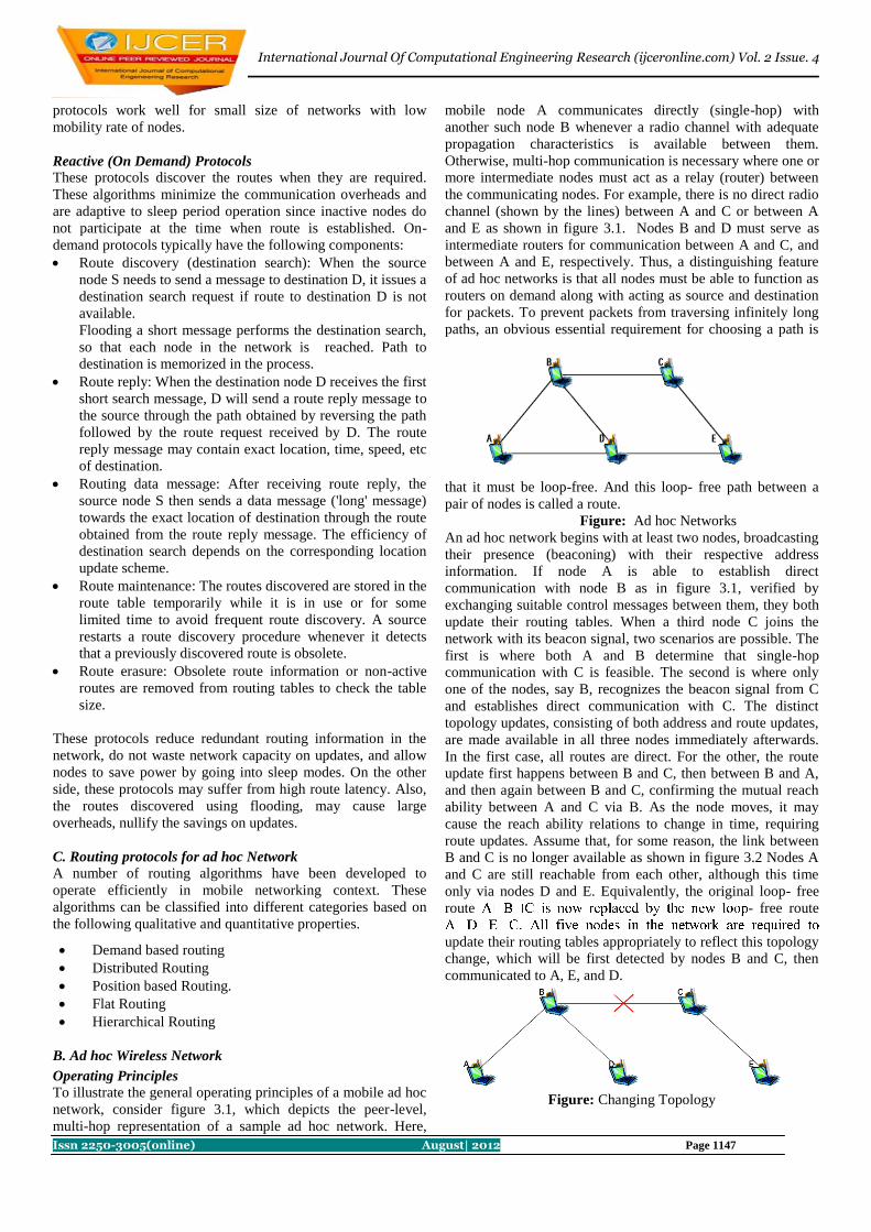
International Journal Of Computational Engineering Research (ijceronline.com) Vol. 2 Issue. 4
Issn 2250-3005(online) August| 2012 Page 1147
protocols work well for small size of networks with low
mobility rate of nodes.
Reactive (On Demand) Protocols
These protocols discover the routes when they are required.
These algorithms minimize the communication overheads and
are adaptive to sleep period operation since inactive nodes do
not participate at the time when route is established. On-
demand protocols typically have the following components:
Route discovery (destination search): When the source
node S needs to send a message to destination D, it issues a
destination search request if route to destination D is not
available.
Flooding a short message performs the destination search,
so that each node in the network is reached. Path to
destination is memorized in the process.
Route reply: When the destination node D receives the first
short search message, D will send a route reply message to
the source through the path obtained by reversing the path
followed by the route request received by D. The route
reply message may contain exact location, time, speed, etc
of destination.
Routing data message: After receiving route reply, the
source node S then sends a data message ('long' message)
towards the exact location of destination through the route
obtained from the route reply message. The efficiency of
destination search depends on the corresponding location
update scheme.
Route maintenance: The routes discovered are stored in the
route table temporarily while it is in use or for some
limited time to avoid frequent route discovery. A source
restarts a route discovery procedure whenever it detects
that a previously discovered route is obsolete.
Route erasure: Obsolete route information or non-active
routes are removed from routing tables to check the table
size.
These protocols reduce redundant routing information in the
network, do not waste network capacity on updates, and allow
nodes to save power by going into sleep modes. On the other
side, these protocols may suffer from high route latency. Also,
the routes discovered using flooding, may cause large
overheads, nullify the savings on updates.
C. Routing protocols for ad hoc Network
A number of routing algorithms have been developed to
operate efficiently in mobile networking context. These
algorithms can be classified into different categories based on
the following qualitative and quantitative properties.
Demand based routing
Distributed Routing
Position based Routing.
Flat Routing
Hierarchical Routing
B. Ad hoc Wireless Network
Operating Principles
To illustrate the general operating principles of a mobile ad hoc
network, consider figure 3.1, which depicts the peer-level,
multi-hop representation of a sample ad hoc network. Here,
mobile node A communicates directly (single-hop) with
another such node B whenever a radio channel with adequate
propagation characteristics is available between them.
Otherwise, multi-hop communication is necessary where one or
more intermediate nodes must act as a relay (router) between
the communicating nodes. For example, there is no direct radio
channel (shown by the lines) between A and C or between A
and E as shown in figure 3.1. Nodes B and D must serve as
intermediate routers for communication between A and C, and
between A and E, respectively. Thus, a distinguishing feature
of ad hoc networks is that all nodes must be able to function as
routers on demand along with acting as source and destination
for packets. To prevent packets from traversing infinitely long
paths, an obvious essential requirement for choosing a path is
that it must be loop-free. And this loop- free path between a
pair of nodes is called a route.
Figure: Ad hoc Networks
An ad hoc network begins with at least two nodes, broadcasting
their presence (beaconing) with their respective address
information. If node A is able to establish direct
communication with node B as in figure 3.1, verified by
exchanging suitable control messages between them, they both
update their routing tables. When a third node C joins the
network with its beacon signal, two scenarios are possible. The
first is where both A and B determine that single-hop
communication with C is feasible. The second is where only
one of the nodes, say B, recognizes the beacon signal from C
and establishes direct communication with C. The distinct
topology updates, consisting of both address and route updates,
are made available in all three nodes immediately afterwards.
In the first case, all routes are direct. For the other, the route
update first happens between B and C, then between B and A,
and then again between B and C, confirming the mutual reach
ability between A and C via B. As the node moves, it may
cause the reach ability relations to change in time, requiring
route updates. Assume that, for some reason, the link between
B and C is no longer available as shown in figure 3.2 Nodes A
and C are still reachable from each other, although this time
only via nodes D and E. Equivalently, the original loop- free
route - free route
update their routing tables appropriately to reflect this topology
change, which will be first detected by nodes B and C, then
communicated to A, E, and D.
Figure: Changing Topology

International Journal Of Computational Engineering Research (ijceronline.com) Vol. 2 Issue. 4
Issn 2250-3005(online) August| 2012 Page 1148
This reach ability relation among the nodes may also change
for various reasons. For example, a node may wander too far
out of range, its battery may be depleted, or it may just suffer
from software or hardware failure. As more nodes join the
network, or some of the existing nodes leave, the topology
updates become more numerous, complex, and usually, more
frequent, thus diminishing the network resources available for
exchanging user information (i.e., data). Finding a loop-free
path between a source-destination pair may therefore become
impossible if the changes in network topology occur too
frequently. Too frequently here means that there may not be
enough time to propagate to all the pertinent nodes the changes
arising from the last change in network topology. Thus the
ability to communicate degrades with increasing mobility and
as a result the knowledge of the network topology becomes
increasingly inconsistent. A network is combinatorial stable if,
and only if, the topology changes occur slowly enough to allow
successful propagation of all topology updates as necessary or
if the routing algorithm is efficient enough to propagate the
changes in the network before the next change occurs. Clearly,
combinatorial stability is determined not only by the
connectivity properties of the networks, but also by the
efficiency of the routing protocol in use and the instantaneous
computational capacity of the nodes, among others.
Combinatorial stability thus forms an essential consideration
for attaining efficient routing objectives in an ad hoc network.
1V. ROUTING PROTOCOLS A. Mobile Routing Protocols
The Mobile Routing Protocols can be of two types.
Table Driven Routing Protocols (Proactive Protocols)
On Demand Routing Protocols (Reactive Protocols)
B. Table Driven Routing Protocols in Ad hoc Networks
In table driven routing protocols, consistent and up-to-date
routing information to all nodes is maintained at each node.
Following are the mainly used Table Driven Routing Protocols
in ad hoc Networks: -
DBF
GSR
DSDV
WRP
STAR
On Demand Routing Protocols
In On-Demand routing protocols, the routes are
created as and when required. When a source wants to send to a
destination, it invokes the route discovery mechanisms to find
the path to the destination. Following are the mainly use On
Demand Routing Protocols:-
DDR
DSR
AODV
RDMAR
TORA
Bellman Ford Algorithm (DBF)
Shortest path routing algorithm based on distributed technique.
According to DBF, a routing node knows the length of the
shortest path from each neighbor to every network destination
and this information is used to compute the shortest path
successor in the path to each destination. It is table driven
protocol, supports a flat architecture. Performance of this
algorithm is as follows:
(a) Shortest path routing
(b) Simple in use
(c) Better computation efficiency due to distributed
characteristic.
(d) It is available for both wire line and wireless
networks.
Distance Sequenced Distance Vector Routing (DSDV)
Distance Sequenced Distance Vector (DSDV) routing protocol
is a variant of distance vector routing method by which mobile
nodes cooperate among themselves to form an ad hoc network.
DSDV is based on RIP (Routing Information Protocol), which
is used for Intra-Domain routing in Internet. DSDV requires
each node in the network to maintain complete list of distance
information to reach each node in the ad hoc network. In
DSDV, each node uses a Sequence Number, which is a counter
that can be incremented only by that node. Each node
increments the Sequence Number every time it sends an update
message and this Sequence Number uniquely identifies the
update messages sent from a particular node. Routing
information is propagated using broadcast or multicasting the
messages periodically or triggered upon a change in the
topology. DSDV uses only bi-directional links for routing as it
is based on Distance Vector Routing. So in DSDV, each node
does not insert information into its Routing table received from
other neighbors unless the node is sure that the other node can
listen to its advertisements.
Wireless Routing Protocol (WRP)
WRP is another protocol based on distributed Bellman-Ford
algorithm (DBF). It substantially reduces the number of cases
in which routing loops (count-to-infinity problem) can occur. It
utilizes information regarding the length and second to last hop
(predecessor) of the shortest path to each destination. Each
node maintains a distance table, a routing table, a link-cost
table and a message retransmission list. The distance table of a
node contains tuples <destination, next hop, distance,
predecessor (as reported by next hop)> for each destination and
each neighbor. The routing table of a node contains tuples
<destination, next hop, distance, predecessor, and marker> for
each known destination where marker specifies whether the
entry corresponds to a simple path, a loop or a destination that
has not been marked. The link-cost table contains the cost of
the link to each neighbor and the number of periodic update
periods elapsed since the node received any error-free message
from it. The message transmission list (MRL) contains
sequence number of update message, retransmission counter,
and acknowledgement required flag vector with one entry per
neighbor, and a list of updates sent in the update message. It
records which updates of an update message have to be
transmitted and which neighbors should be requested to
acknowledge such retransmission.
GLOBAL STATE ROUTING (GSR) PROTOCOL
This protocol is based on Link State routing, which has the
advantage of routing accuracy, and dissemination method used
in DBF, to avoid inefficient flooding in LS routing. Each node

International Journal Of Computational Engineering Research (ijceronline.com) Vol. 2 Issue. 4
Issn 2250-3005(online) August| 2012 Page 1149
maintains a neighbor list, a topology table, a next hop table and
a distance table. The neighbor list contains the list of nodes
adjacent to the node. The topology table contains the link state
information reported by a destination and a timestamp
indicating the time at which this is generated. The next hop
table and the distance table contain the next hop and the
distance of the shortest path for each destination respectively.
Initially, each node learns about its neighbors and the distance
of the link to it (generally hop count equals one) by examining
each packet in its inbound queue and broadcasts this
information to its neighbors. Upon receiving the link state
message from its neighbors, each node updates the link state
information corresponding to that neighbor in the topology
table to the most up to date information using timestamps.
Then, the node rebuilds the routing table based on newly
computed topology table and broadcasts it to its neighbors. The
routing table information is exchanged periodically with the
neighbors only.
Fisheye State Routing (FSR) Protocol
FSR protocol is an extension of GSR protocol. It attempts to
reduce the size of update messages in GSR without seriously
affecting the routing accuracy. The reduction in routing size is
obtained by using different exchange periods for different
entries in the routing table. Entries corresponding to nodes
within the smaller scope are propagated to the neighbors with
the highest frequency.
Temporally Ordered Routing Algorithm (TORA)
TORA is designed to work below Internet Protocol (IP). It does
not have properties of link state or distance-vector algorithms,
but link-reversal. The protocol is adaptive, and highly scalable.
It is designed to minimize reaction to topological changes.
TORA control messages are localized to a very small set of
nodes near the occurrence of a topological change. To achieve
this, nodes maintain routing information about adjacent nodes.
TORA quickly discovers multiple routes on demand. Route
does not have to be optimal, but it guarantees that all routes are
loop-free. TORA only does the routing job, and heavily
depends on Internet MANET Encapsulation Protocol (IMEP).
A good analogy would be water flowing down the hill through
pipes. Hilltop is the source, pipes are links, and pipe
connections are nodes. TORA assigns level numbers to each
node down the hill. When two intermediate nodes cannot
communicate, the last node raises its level higher than any of
its neighbors, so that water, which is data, flows back out of it.
Dynamic Source Routing (DSR)
Dynamic source routing is a Source routed On-Demand routing
protocol in ad hoc networks. It uses Source Routing, which is a
technique in which the sender of a packet determines the
complete sequence of nodes through which the node has travel.
The sender of the packet explicitly mentions the list of all
nodes in the packet’s header, identifying each forwarding ‘hop’
by the address of the next node to which to transmit the packet
on its way to destination host. In this protocol the nodes don’t
need to exchange the Routing table information periodically
and thus reduces the bandwidth overhead in the network. Each
Mobile node participating in the protocol maintains a ‘routing
cache’, which contains the list of routes that the node has learnt.
Whenever the node finds a new route it adds the new route in
its ‘routing cache’. Each mobile node also maintains a
sequence counter ‘request id’ to uniquely identify the requests
generated by a mobile host. The pair < source address, request
id > uniquely identifies any request in the ad hoc network. The
protocol does not need transmissions between hosts to work in
bi-direction. The main phases in the protocol are Route
Discovery process and Route Maintenance process.
Ad hoc On-Demand Distance Vector (AODV)
The ad hoc On Demand Distance Vector (AODV) routing
protocol is intended for use by the mobile nodes for routing
data in Ad Hoc networks. AODV is an extension of Distance
Sequenced Distance Vector (DSDV) routing protocol, a Table
Driven routing protocol for Ad hoc networks that is discussed
in the previous section. AODV is designed to improve upon the
performance characteristics of DSDV in the creation and
maintenance of routes.
Relative Distance Micro Discovery Ad hoc Routing Protocol
(RDMAR)
RDMAR is a loop free routing protocol for ad hoc mobile
networks. The protocol is highly adaptive, efficient and
scaleable and is well suited in large mobile networks. The
protocol is called Relative Distance Micro Discovery Ad hoc
Routing Protocol (RDMAR). It uses the mechanism for route
discovery, called Relative Distance Micro discovery (RDM).
The concept is that query flood can be localized by knowing
the relative distance between two terminals. RDMAR does not
use a route cache. Each node has a routing table that lists all
available destinations and number of hops to each. It is on
demand routing with hybrid architecture.
Summary of the Routing Protocols:
DSDV was the only proactive protocol discussed. AODV is
reactive, an on-demand version of DSDV. Authors of AODV,
who were also authors of DSDV added multicast capability to
AODV. Reactive approach of AODV is similar to DSR’s. They
both have a route discovery mode, which uses messaging to
find new routes. DSR uses source routing; the route is in each
packet. Thus, DSR learns more routes than AODV. DSR
supports unidirectional links due to its vast knowledge on the
topology. TORA runs on top of IMEP, and suffers for its
internal instability and IMEP’s too frequent HELLO messages
generating too much control overhead in the network. DSDV
and GSR are table-driven protocols that use destination
sequence numbers to keep routes loop-free and up-to-date.
HSR is a hierarchical routing protocol derived from FSR. FSR
reduces the size of tables to be exchanged by maintaining less
accurate information about nodes farther away. CGSR is a
cluster-based routing protocol where nodes are grouped into
clusters of transmission size ranges.
TABLE: Comparison of Major ad-hoc Routing Protocols
Protocol
Property
DSDV AODV DSR ZRP TORA
Loop free Yes Yes Yes Yes Yes
Multiple
routes
No No Yes No Yes
Distributed Yes Yes Yes Yes Yes
Reactive No Yes Yes Variable Yes
Unidirectional No No Yes No Yes
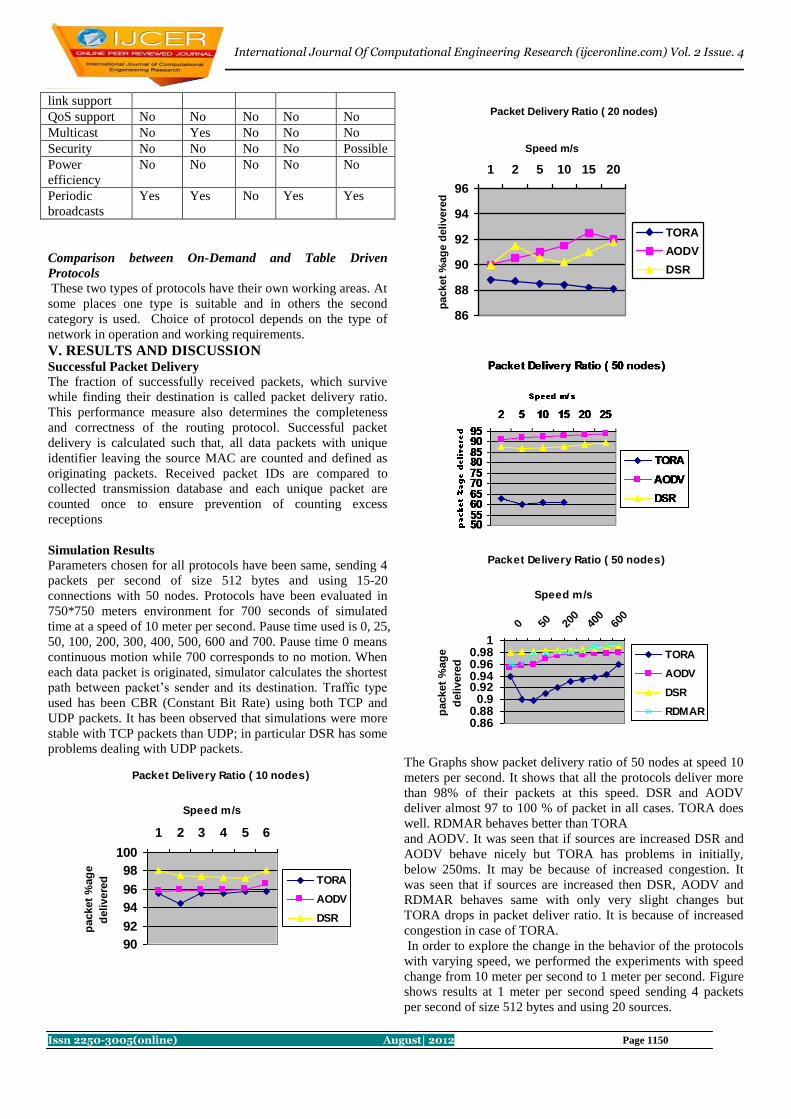
International Journal Of Computational Engineering Research (ijceronline.com) Vol. 2 Issue. 4
Issn 2250-3005(online) August| 2012 Page 1150
link support
QoS support No No No No No
Multicast No Yes No No No
Security No No No No Possible
Power
efficiency
No No No No No
Periodic
broadcasts
Yes Yes No Yes Yes
Comparison between On-Demand and Table Driven
Protocols
These two types of protocols have their own working areas. At
some places one type is suitable and in others the second
category is used. Choice of protocol depends on the type of
network in operation and working requirements.
V. RESULTS AND DISCUSSION Successful Packet Delivery
The fraction of successfully received packets, which survive
while finding their destination is called packet delivery ratio.
This performance measure also determines the completeness
and correctness of the routing protocol. Successful packet
delivery is calculated such that, all data packets with unique
identifier leaving the source MAC are counted and defined as
originating packets. Received packet IDs are compared to
collected transmission database and each unique packet are
counted once to ensure prevention of counting excess
receptions
Simulation Results
Parameters chosen for all protocols have been same, sending 4
packets per second of size 512 bytes and using 15-20
connections with 50 nodes. Protocols have been evaluated in
750*750 meters environment for 700 seconds of simulated
time at a speed of 10 meter per second. Pause time used is 0, 25,
50, 100, 200, 300, 400, 500, 600 and 700. Pause time 0 means
continuous motion while 700 corresponds to no motion. When
each data packet is originated, simulator calculates the shortest
path between packet’s sender and its destination. Traffic type
used has been CBR (Constant Bit Rate) using both TCP and
UDP packets. It has been observed that simulations were more
stable with TCP packets than UDP; in particular DSR has some
problems dealing with UDP packets.
Packet Delivery Ratio ( 10 nodes)
90
92
94
96
98
100
1 2 3 4 5 6
Speed m/s
packet
%ag
e
delivere
d TORA
AODV
DSR
Packet Delivery Ratio ( 20 nodes)
86
88
90
92
94
96
1 2 5 10 15 20
Speed m/s
pa
cket
%ag
e d
eli
vere
d
TORA
AODV
DSR
Packet Delivery Ratio ( 50 nodes)
0.860.88
0.90.920.940.960.98
1
0 50 200
400
600
Speed m/s
packet
%ag
e
delivere
d
TORA
AODV
DSR
RDMAR
The Graphs show packet delivery ratio of 50 nodes at speed 10
meters per second. It shows that all the protocols deliver more
than 98% of their packets at this speed. DSR and AODV
deliver almost 97 to 100 % of packet in all cases. TORA does
well. RDMAR behaves better than TORA
and AODV. It was seen that if sources are increased DSR and
AODV behave nicely but TORA has problems in initially,
below 250ms. It may be because of increased congestion. It
was seen that if sources are increased then DSR, AODV and
RDMAR behaves same with only very slight changes but
TORA drops in packet deliver ratio. It is because of increased
congestion in case of TORA.
In order to explore the change in the behavior of the protocols
with varying speed, we performed the experiments with speed
change from 10 meter per second to 1 meter per second. Figure
shows results at 1 meter per second speed sending 4 packets
per second of size 512 bytes and using 20 sources.

International Journal Of Computational Engineering Research (ijceronline.com) Vol. 2 Issue. 4
Issn 2250-3005(online) August| 2012 Page 1151
It was observed that with change in speed, all protocols deliver
above 98% of the packets with slight drops in case of TORA
and RDMAR DSR and AODV were excellent in performances
at all speeds. Overhead also have less effect for DSR and
AODV. DSR caching is effective at faster speeds, but works
much better at slower speeds also. Some simulation studies for
protocols have been done earlier also, although those
simulations used different parameters and sources with varying
results. No study involving RDMAR comparisons have been
published earlier. In this study, several existing routing
protocols for ad hoc wireless networks have been described.
Results based on the simulations have been analyzed and
presented with the advantages and disadvantages of each
protocol. It is not simple to determine which of the four
protocols under comparison is the best for Ad hoc network
environment. No Protocol is ideal for all scenarios. A good
criterion to choose a protocol might be the size and expected
traffic load in the target network. The simulations presented
here clearly show that there is a need for routing protocols
specifically tuned to the characteristics of ad-hoc networks.
Overall, the proactive protocols (AODV and DSR) behaved
similar in terms of delivery and throughput. On the basis of this
study both should be considered suitable for mobile ad-hoc
networks. However, a number of differences among the
protocols do exist. The source routes used by DSR give
increased byte over-head compared to AODV when routes
have many hops and packet rates are high. DSR is, on the other
hand, efficient in finding (learning) routes in terms of the
number of control packets used, and does not use periodic
control messages. Data packets in AODV carry the destination
address only. Therefore, the byte overhead for AODV is the
lowest of the examined protocols. The overhead is high in
terms of packets since AODV broadcasts periodic Hello
messages to its neighbors. DSR behaves better in this case.
Each of the routing protocol generated different amount of
overhead. DSR has the least overhead, TORA has maximum
overhead. DSR, TORA and AODV are all on demand protocols
and their overhead drops as mobility rate drops. It has been
found from Graph that
(a) DSR performance is very good at all mobility rates
and movement speeds with all the metrics of
comparison.
(b) TORA is the worst performer in all the experiments
the network was unable to handle all the routing
traffic and lots of packets were dropped.
(c) AODV has performed as well as DSR and
accomplishes its goal of eliminating source routing
overhead and
(d) RDMAR has performed well.
V1. CONCLUSION AND FUTURE STUDY The performance of the protocol has been evaluated with other
common ad-hoc network routing protocols like DSR, AODV
and TORA using a detailed packet level simulator NS. The
traffic schemes assigned are TCP and UDP. Simulations have
been carried out in an area as large as 1km x 1km with many
sources connected to each other. More sources lead to more
network load. Results have shown that quick management of
route maintenance is an important factor that affects all the
performance measures, especially the successful delivery rate
at high workloads and increased speed.
It is found that the AODV has highest packet delivery ratio for
all speeds and pause times. In other protocols, for very high-
speed networks, AODV performs much better in successful
packet delivery. The packet delivery rate of DSR, which is a
source routing protocol, is directly related to the generation of
control messages. Therefore it is related to the frequency of
data packet transmissions. At very high speeds DSR cache
transmission suffers and a loss in packet delivery occurs.
TORA has the lowest throughput and generates a large amount
of control messages to manage DAGs, and its control messages
encapsulated in IP are dropped because of collisions, which
lead to much more decrease in performance. AODV have used
much less control messages, limited to the hosts involved in
routing process, therefore they have the highest standard
division. This means that they distribute the load over the
network in least efficient way.
Results have been derived from a series of experiments
conducted on simulated network. The following observations
can be made:
Best packet delivery ratio: AODV is the best in terms of
packet transmission. More packets are transmitted than
any of the studied protocols. This is true even in case of
changing scenario and fast moving nodes. So it is able to
achieve one of the most important objectives of ad-hoc
networks as successful packet delivery.
Simple: AODV can easily be implemented and executed.
The simulation studies have been conducted on Pentium-
IV with standard configurations. Though it is best
performing under LINUX environment but can be easily
implemented on Windows platform also. Efficiency is
particularly important when the software implementing
the routing algorithm must run on a computer with
limited physical resources.
Route Repair: The route phase of the protocol is unique
as compared to other such protocols and outperform all in
its category. It describes the maintenance process, which
can be done as fast as possible. It describes the level of
self-organization in the network. The protocol uses local
route repair of routing process.
Future Work
Some of the objectives remained untouched due to the limited
time available. On the other hand, outcome of the current
research has exhibited the possibilities of further extensions.
List of the work that can be carried out in future as an
extension of current work is given below:
(a) There is limitation of Battery Life in an ad hoc
environment. Battery is most commonly used; none of the
protocols discussed the concept of Power as one of the
deciding factor in route selection
(b) The existing strategies use fixed scenarios for carrying
out simulations. It means before start of the simulation
process, position of the nodes is known and also total
sources used are fixed, but real life situations demand
random scenes and varying sources.
(c) If a link breaks in the route process due to any reason,
repair starts and it involves reconstruction of new path.

International Journal Of Computational Engineering Research (ijceronline.com) Vol. 2 Issue. 4
Issn 2250-3005(online) August| 2012 Page 1152
Reconstruction phase requires better approach in all
protocols for fast selection of new routes.
References 1. A. Kush, P. Gupta, R. Chauhan, C.J. Hwang and A.
Pandey(2004), “Power Aware Virtual Node Routing
Scheme In Mobile Ad hoc Networks”, Proceedings of
International Conference On Mobile Computing IASTED
2004, Banff , CANADA, pp 698-702, July 2004.
2. P. Bose, P. Morin , I. Stojmenovic and J. Urrutia(1999)
“Routing with Guaranteed Delivery in
Ad hoc Wireless Networks”, Proceedings of the 3rd
International Workshop on Discrete Algorithms and
Methods for Mobile Computing and Communications,
Seattle, WA USA, August 20, 1999 pp 47-53.
3. Ajay R. Mishra(2004) “Fundamentals of Cellular Network
Planning and Optimisation: 2G/2.5G/3G ... Evolution to
4G” John Wiley and Sons,pp 213-215, 2004.
4. A. TanenBaum, “Computer Networks”, Prentice Hall of
India, 2002.
5. C.K. Toh(2005), “Ad hoc mobile wireless Networks”,
Prentice Hall New Jersey, pp 121-128, 2005.
6. Y. Lin, I. Chlamtac(2005), “Wireless and Mobile
Architectures”, Wiley Computer Publications, USA, pp
171-177, 2005.
7. A. Nasipuri, R. Castaneda, and R. SamirDas(1999),
“Performance of Multi path Routing for On Demand
Protocols in Mobile Ad hoc Networks”, ACM/Baltzer
Journal of Mobile Networks( MONET) pp 377-381,1999.
8. National Science foundation, “Research Priorities in
Wireless and Mobile networking”, available at
www.cise.nsf.gov.
9. J.B. Evans, G.J. Minden, K.S. Shanmugan , G. Prescott ,
V.S. Frost , B. Ewy, R. Sanchez, C. Sparks, K.
Malinimohan, J. Roberts, R. Plumb and D. Petr(1999),
“The Rapidly Deployable Radio Network”, IEEE
Communications, Vol. 17, No. 4, pp. 689-702 , 1999.
10. Fasbender et al, “Any Network, Any Terminal, Anywhere”,
IEEE Personal communications, Volume 6(2), pp 22-30,
1999.
11. J. Schiller(2004), “Mobile Communication “, Addison
Wesley, PHI New Jersey USA, pp 412-414, 2004.
12. GSM (Global System for Mobile Communication) Data,
Intel Corporation Draft EN (04.60) V 6.0.0 available at
www.gsmdata.com, 1998.
13. F. Halsall(2003), “Data Communication, Computer
Networks and Open System”, Addison Wesley, Prentice
Hall New Jersey USA, pp 342-351, 2003.
14. TIA/EIA/IS-702-A.2, “TDMA Cellular Radio Mobile
Station Base Structure Compatibility”, 136 A, pp 283-
287,March 1999.
15. S. Keshov, “An Engineering Approach to Computer
Networks”, Addison Wesley, Prentice Hall New Jersey
USA, pp 189-198, 1997.
16. W.R. Young, “Advanced Mobile Phone Service (AMPS)”,
Bell systems technical journal, Volume 58, pp 234-
237,1979.
17. B. D. Johnson, A.M. Davis, "Dynamic Source Routing in
Ad hoc Networks", Mobile Computing (T. Imielinski and
H. Korth, Editions), Dordrecht, The Netherlands: Kluwer
Academic Publishers, Chap 5, pp. 152-81, February 1996.
18. N. Nikaein and B. Christina, “Dynamic Routing
Algorithm”, available at Institute Eurecom,
19. V.D. Park and M.S. Corson, "A Highly Adaptive
Distributed Routing Algorithm for Mobile Wireless
Networks", Proceedings of INFOCOM'97, pp 9-12, April
1997.
20. C. Parkins and M.R. Elizabeth(1999), “Ad hoc On Demand
Distance Vector Routing”, Proceedings of IEEE
WMCSA’99, New Orleans, LA, pp. 90-100, February
1999.
21. C.E. Perkins and P. Bhagwat, “Highly Dynamic
Destination-Sequenced Distance Vector Routing (DSDV)
for Mobile Computers”, ACM SIGCOMM’94 Computer
Communication Review, pp. 234–244, October 1994.
22. NS notes and documentation available at www.isi.edu/vint.
23. Lee, S.-J. and M. Gerla, “A Simulation Study of Table-
Driven and On-Demand Routing Protocols for Mobile Ad
hoc Networks”, IEEE Network, pp. 48-54, August 1999.
24. Z.J. Hass and M. R. Pearlman, "The Zone Routing
Protocol (ZRP) for Ad hoc Networks” lnternet Draft
available at draft-ietf-manet-zone-zrp.txt, 2000.
25. P. Merlin and A. Segall, “A Failsafe Distributed Routing
Protocol”, IEEE Communications, September 1979.
26. V. Garg and J. Wilkes, “Principals and Applications of
GSM”, Prentice Hall, New Jersey, pp 134-141,1999.
27. D.C. Cox, “Wireless Personal Communications”, IEEE
communications, pp 117-156, April 1995.
28. D. Bertsekas and R. Gallager, “Data Networks – 2nd
Edition”, Prentice Hall, New Jersy, ISBN 0-13-200916-1.
29. T. Wei, L. Chen and M. Gerla, "Global State Routing: A
New Routing Scheme for Ad-hoc Wireless Networks",
Proceedings of IEEE ICC' 98, pp 23-28, 1998.
30. MohammedTarique, Kemal E.Tepe “Minimum energy
hierarchical dynamic source routing for MANET” in
ScienceDirect pp 1125-1135, August 2009.
31. Michael Q. Rieck, Sukesh Pai, Subhankar Dhar Computer
Networks, Volume 47, Issue 6, Pages 785-799,22 April
2005.
32. Tom Goff, NaelAbu-Ghazaleh, Dhananjay Phatak,Ridvan
Kahvecioglu “Journal of Parallel and Distributed
Computing”, Volume 63, Issue 2, pp 12-14February 2003.

International Journal Of Computational Engineering Research (ijceronline.com) Vol.2 Issue.4
Issn 2250-3005(online) AUGUST| 2012 Page 1153
A survey on anonymous ip address blocking 1. Prof. P.Pradeepkumar
2.Amer Ahmed khan
3.B. Kiran Kumar
ABSTRACT These days, the Internet is full of suspicious actions and people. We always advise to not take a chance in protecting your IP
Address information online.
TheIP was being shown everywhere! To advertisersandother places ,even from SPAM who compromised usersidentity. No
more I said, and developed software that would hide ip address.we outline a security protocol that uses resource constrained
trusted hardware to facilitate anonymous IP-address blocking in anonym zing networks such as Tor.
Tor allows users to access Internet services privately by using a series of Tor routers to obfuscate the route from the client to
the server, thereby hiding the client’s IP address from the server. The success of Tor, however, has been limited because of
malicious users who misuse the network. administrators block all known exit nodes of anonymizing networks, denying
nonymous access to misbehaving and behaving users alike.
To address this problem, we present Nymble, a system in which servers can ―blacklist‖ misbehaving users, thereby blocking
users without compromising their anonymity. Our system is thus agnostic to different servers’ definitions of misbehavior
servers can blacklist users for whatever reason, and the privacy of blacklisted users is maintained.
The IP-address anonymity provided by Tor, however, makes it difficult for administrators to deny access to such
offenders .As a result, administrators resort to blocking all Tor exit nodes, effectively denying
anonymous access for all Tor’s users. Our solution makes use of trusted hardware and allows services like Tor to provide
anonymous blocking of IP addresses while requiring only a modest amount of storage at the trusted node.
Key terms: IP , pockets, NYMBLE,Anonymizing networks, privacy.
Introduction Anonymizing networks such as re-route a user’s traffic between several nodes in different domains. Since these nodes are
operated independently, users are able to trust the anonymizing network to provide anonymity. Real-world deployments of
anonymizing networks, however, have had limited success because of their misuse
Administrators of websites are unable to blacklist malicious users’ IP addresses because of their anonymity. Left with no
other choice, these administrators opt to blacklist the entire anonymizing network. This approach eliminates malicious
activity through such networks, but at the cost of the anonymity of honest users. In other words, a few ―bad apples‖ can spoil
the fun for everybody else using the anonymizing network. (In fact, this has happened repeatedly with To solve this problem,
we present a secure protocol based on trusted hardware that allows servers to block anonymous users without knowledge of
their actual IP addresses. Although this work applies to anonymizing networks in general, we consider Tor for purposes of
exhibition. Building and prototyping a system based on our proposed solution is ongoingwork. In this paper we present our
proposed solution and protocol.
Anonymizing networks such as Tor allow users to access Internet services privately by using a series of routers to hide the
client’s IP address from the server. The success of such networks, however, has been limited by users employing this
anonymity for abusive purposes such as defacing popular websites.
Website administrators routinely rely on IP-address blocking for disabling access to misbehaving users, but blocking IP
addresses is not practical if the abuser routes through an anonymizing network. As a result,
2 An Overview To Nymble We now present a high-level overview of the Nymblesystem, and defer the entire protocol description
and security analysis to subsequent sections.

International Journal Of Computational Engineering Research (ijceronline.com) Vol.2 Issue.4
Issn 2250-3005(online) AUGUST| 2012 Page 1154
To limit the number of identities a user can obtain (called the Sybil attack), the Nymble system binds nymbles to
resources that are sufficiently difficult to obtain in great numbers. For example, we have used IP addresses as
the resource in our implementation, but our scheme gener-
alizes to other resources such as email addresses, identity certificates, and trusted hardware. We address the
practical issues related with resource-based blocking in Section 8, and suggest other alternatives for resources.
Wedonotclaimto solvethe Sybi lattack.
Thisproblemisfacedbyanycredentialsystem],andwesuggestsomepromisingapproachesbasedonresource-based
blocking since we aim to create a real-world deployment.
2.2 The Pseudonym Manager
The user must first contact the Pseudonym Manager (PM) and demonstrate control over a resource;for ip-address
blocking the user must connect to the PM directly (i.e., not through a known anonymizing network), We
assume the PM has knowledge about Tor routers, for example, and can ensure that users are communicating with
it directly.6 Pseudonyms are deterministically chosen based on the controlled resource, ensuring that the same
pseudo-nym is always issued for the same resource.
Note that the user does not disclose what server he or she intends to connect to, and the PM’s duties are limited
to mapping IP addresses (or other resources) to pseudonyms. As we will explain, the user contacts the PM only
once per linkability
window (e.g., once a day).
2.3 The Nymble Manager
After obtaining a pseudonym from the PM, the user connects to the Nymble Manager (NM) through
the anonymizing network, and requests nymbles for access to a particular server (such as Wikipedia). A user’s
requests to the NM are therefore pseudonymous, and nymbles are generated using the user’s pseudonym
and the server’s identity. These nymbles are thus specific to a particular user-serverpair. Nevertheless, as
long as the PM and the NM do not collude, the Nymble system cannot identify which user is connecting to
what server; the NM knows only the pseudonym-server pair, and the PM knows only the user identity-
pseudonym pair.
To provide the requisite cryptographic protection and security properties, the NM encapsulates nymbles
within nymble tickets. Servers wrap seeds into linking tokens, and therefore, we will speak of linking tokens being
used to link future nymble tickets. The importance of these constructs will become apparent as we proceed.
Nymble tickets are bound to specific time periods, time is divided into linkability windows
of durationW, each of which is split into L time periods of
duration T (i.e., W ¼ L T ). We will refer to time periods
and linkability windows chronologically as t1; t2; . . . ; tL and w1;w2;..., respectively. While a user’s access within a
time period is tied to a single nymble ticket, the use of different
nymble tickets across time periods grants the user anonymity between time periods. Smaller time periods
provide users with higher rates of anonymous authentication, while longer time periods allow servers to rate-limit
the number
of misbehaviors from a particular user before he or she is blocked. For example, T could be set to five minutes,
and W to one day (and thus, L ¼ 288). The linkability window allows for dynamism since resources such as IP
addresses can get reassigned and it is undesirable to blacklist such resources indefinitely, and it ensures

International Journal Of Computational Engineering Research (ijceronline.com) Vol.2 Issue.4
Issn 2250-3005(online) AUGUST| 2012 Page 1155
forgiveness of misbehavior after a certain period of time. We assume all entities are time synchronized (for
example, with time.nist.gov via the Network Time Protocol (NTP)), and can thus calculate the current linkability
window and time period.Summary of Updates to the Nymble Protocol We highlight the changes to Nymble since
our onferencepaper [24]. Previously, we had proved only the privacy properties associated with nymbles as
part of a two-tiered hash chain. Here, we prove security at the protocol level. This process gave us insights into
possible (subtle) attacks against privacy, leading us to redesign our protocols and refine our definitions of
privacy. For example, users are now either legitimate or illegitimate, and are anonymous within these sets. This
redefinition affects how a user establishes a ―Nymble connection‖ , and now prevents the server from
distinguishing between users who have already connected in the same time period and those who are
blacklisted, resulting in larger anonymity sets.A thorough protocol redesign has also resulted in several
optimizations.
We have eliminated blacklist version numbers and users do not need to repeatedly obtain the current version
number from the NM. Instead servers obtain proofs of freshness every time period, and users directly verify the
freshness of blacklists upon download. Based on a hash chain approach, the NM issues lightweightdaisiestoservers
as proof of a blacklist’s freshness, thus making blacklist updates highly efficient. Also, instead of embedding
seeds, on which users must perform computation to verify their blacklist status, the NM now embeds a unique
identifier nymble , which the user can directly recognize. Finally, we have compacted several data structures,
especially the servers’ blacklists, which are downloaded by each user.
Our Nymble Construction System Setup
During setup, the NM and the PM interact as follows:
1. The NM executes NMInitStateðÞ (see Algorithm 10) and initializes its state nmState to the algorithm’s output.
2. The NM extracts macKeyNP from nmState and sends it to the PM over a type-Auth channel.
macKeyNP is a shared secret between the NM and the PM, so that the NM can verify the authenticity of
pseudonyms issued by the .
3. The PM generates nymKeyP by running Mac.Key-Gen() and initializes its state pmState to the pair
ðnymKeyP ; macKeyNP Þ.
4. The NM publishes verKeyN innmState in a way that the users in Nymble can obtain it and verify its
integrity at any time (e.g., during registration).
Server Registration To participate in the Nymble system, a server with identity sid initiates a type-Auth channel to the NM, and
registers with the NM according to the Server Registration protocol below. Each server may register at most
once in any linkability window.
User Registration
In this procedure, user Alice interacts with the PM in order to register herself to the NYMBLE system for linkability window
k. Alice obtains a pseudonym from the PM upon a successful termination of such an interaction. The communication channel
between them is confidential and PM-authenticated.
To register, Alice authenticates herself as a user with identity id to the PM by demonstrating her control over some
resource(s) as discussed, after which the PM computes pnymHkhkP (id, k) and macPNHMAChmkNP (pnym, k), and returns
hpnym, macPNi to Alice, who stores it privately.
Acquisition of Nymble Tickets In order for Alice to authenticate to any server Sj during any linkability window Wk, she
must present a nymble ticket to the server. The following describes how she can obtain a credential from the NM containing
such tickets. The communication channel is anonymous
(e.g., through Tor), confidential and NM-authenticated.
Alice sends her hpnym, macPNi to the NM, after which the NM:
1. asserts that macPN = HMAChmkNP (pnym, k),
2. computesnymbleTKT` NymbleTktGennmsk (pnym, j, k, `), for ` = 1 to L, and
3. returns cred as hseed, nymbleTKT1, nymbleTKT2, . . . , nymbleTKTLi, where seed =
HkhkN (pnym, j, k) is the seed used within NymbleTktGen.
Alice may acquire credentials for different servers and different linkability windows at
any time. She stores these credentials locally before she needs them.

International Journal Of Computational Engineering Research (ijceronline.com) Vol.2 Issue.4
Issn 2250-3005(online) AUGUST| 2012 Page 1156
Efficiency. This protocol has a timing complexity of O(L).6 All the computations are
quick symmetric operations—there are two cryptographic hashes, two HMACs and one
symmetric encryption per loop-iteration A credential is of size O(L).
Request for Services
At a high level, a user Alice presents to server Bob the nymble ticket for the current time
period. As nymble tickets are unlinkable until servers complain against them (and thereby
blacklisting the corresponding user or IP address), Alice must check whether she is on
Bob’s blacklist, and verify its integrity and freshness. If Alice decides to proceed, she
presents her nymble ticket to Bob, and Bob verifies that the nymble ticket is not on his
blacklist. Bob also retains the ticket in case he wants to later complain against the current
access. For example,Wikipedia might detect a fraudulent posting several hours after it has
been made. The nymble ticket associated with that request can be used to blacklist future
accesses by that user.
Ticket Examination 1. The user sets ticketDisclosed in usrEntries½sid inusrState to true. She then sends hticketi to the server,
where ticket is ticket½tnow
in cred in usrEntries½sid in usrState.Note that the user discloses ticket for time period tnow
after
verifying blist’s freshness for tnow
. This procedure avoids the situation in which the user verifies the current blacklist
just before a time period ends, and then presents a newer ticket for the next time period.
2. On receiving hticketi, the server reads the currenttime period and linkability window as tnow
andwnow
,returns false, the NM terminates with failure; it proceeds otherwise.
3.The NM runsNMCreateCredentialnmStateðpnym; sid; wnowÞ;which returns a credential. The NM sends cred to the user
and terminates with success.
4.The user, on receiving cred, creates usrEntry:¼ðsid; cred;falseÞ.
Nymble Connection establishment
To establish a connection to a server sid, the user initiates a type-Anon channel to the server, followed by the
Nymbleconnection establishment protocol described below.
5.5.1 Blacklist Validation
1. The server sends hblist; certi to the user, where blist
is its blacklist for the current time period and cert is the certificate on blist. (We will describe how the
server can update its blacklist soon.)
2. The user reads the current time period and linkability window as tnow
andwnow
andassumes these
values to be current for the rest of the protocol.
3. For freshness and integrity, the user checks if VerifyBLusrStatesid; tnow
; wnow; blist; cert ¼ true:If not, she
terminates the protocol with failure.
5.5.2 Privacy Check
Since multiple connection establishment attempts by a user
to the same server within the same time period can be
linkable, the user keeps track of whether she has alreadyrespectively. The server then checks that:ticket
isfresh,i.e.,ticket
2slistinserver’s state. ticket is valid, i.e., on input ðtnow
; wnow
; ticketÞ,ServerVerifyTicket returns true. Ticket is
not linked ServerLinkTicketsvrStateðticketÞ ¼ false:
If any of the checks above fails, the server sendshgoodbyei to the user and terminates with failure. Otherwise,
it adds ticket to slist in its state, sends hokayi to the user, and terminates with success.On receiving hokayi, the user
terminates with success.
Algorithm:.ServerLinkTicketInput: ticket 2 T
Persistent state: svrState 2 SS
Output: b 2 ftrue; falseg

International Journal Of Computational Engineering Research (ijceronline.com) Vol.2 Issue.4
Issn 2250-3005(online) AUGUST| 2012 Page 1157
1: Extract lnkng-tokens from svrState2: ð ;nymble; Þ :¼ ticket
3: for all i ¼ 1 to jlnkng-tokensj do
4: if ð ;nymbleÞ ¼ lnkng-tokens½i then
5: return true 6: return false
Conclusions We have proposed and built a comprehensive credential system called Nymble, which can be used to add a
layer of accountability to any publicly known anonymizing net-
work. Servers can blacklist misbehaving users while maintaining their privacy, and we show how these
proper-
ties can be attained in a way that is practical, efficient, and sensitive to the needs of both users and services.
We hope that our work will increase the mainstream acceptance of anonymizing networks such as Tor,
which has, thus far, been completely blocked by several services because of users who abuse their anonymity.
References 1. Giuseppe Ateniese, Jan Camenisch, Marc Joye, and Gene Tsudik. A practical and provably
secure coalition-resistant group signature scheme. In MihirBellare, editor, CRYPTO, volume
1880 of LNCS, pages 255–270.Springer, 2000.
2. MihirBellare, Daniele Micciancio, and BogdanWarinschi. Foundations of group signatures:
Formal definitions, simplified requirements, and a construction based on general assumptions.
In Eli Biham, editor, EUROCRYPT, volume 2656 of LNCS, pages 614–629. Springer, 2003.
3. MihirBellare, Haixia Shi, and Chong Zhang. Foundations of group signatures: The case of
dynamic groups. In Alfred Menezes, editor, CT-RSA, volume 3376 of LNCS, pages 136–153.
Springer, 2005.
4. Stefan Brands. Untraceable off-line cash in wallets with observers (extended abstract). In
Douglas R. Stinson, editor, CRYPTO, volume 773 of LNCS, pages 302–318. Springer, 1993.
5. Jan Camenisch, Susan Hohenberger, MarkulfKohlweiss, Anna Lysyanskaya, and Mira
Meyerovich. How to win the clonewars: efficient periodic n-times anonymous authentication. In
Ari Juels, Rebecca N. Wright, and Sabrina De Capitani di Vimercati, editors, ACM Conference
on Computer and Communications Security, pages 201–210. ACM, 2006.
6. Jan Camenisch, Susan Hohenberger, and Anna Lysyanskaya.Compact e-cash. In Ronald
Cramer, editor, EUROCRYPT, volume 3494 of LNCS, pages 302–321. Springer, 2005.
7. Jan Camenisch and Anna Lysyanskaya. An efficient system for non-transferable anonymous
credentials with optional anonymity revocation. In Birgit Pfitzmann, editor, EUROCRYPT, volume
2045 of LNCS, pages 93–118.Springer, 2001.
8. Jan Camenisch and Anna Lysyanskaya. Signature schemes and anonymous credentials from
bilinear maps. In Matthew K. Franklin, editor, CRYPTO, volume 3152 of LNCS, pages 56–72.
Springer, 2004.
9. David Chaum. Untraceable electronic mail, return addresses, and digital pseudonyms. Communications
of the ACM, 4(2), February 1981.
10. David Chaum. Blind signatures for untraceable payments. In CRYPTO, pages 199–203, 1982.
11. David Chaum. Showing credentials without identification transfeering signatures between
unconditionallyunlinkable pseudonyms. In Jennifer Seberry and Josef Pieprzyk, editors,
AUSCRYPT, volume 453 of LNCS, pages 246–264. Springer, 1990.

International Journal Of Computational Engineering Research (ijceronline.com) Vol.2 Issue.4
Issn 2250-3005(online) AUGUST| 2012 Page 1158
12. David Chaum and Eug`ene van Heyst. Group signatures. In EUROCRYPT, pages 257–265,
1991.
13. Lidong Chen. Access with pseudonyms. In Ed Dawson and Jovan Dj. Golic, editors, Cryptography:
Policy and Algorithms, volume 1029 of LNCS, pages 232–243.Springer, 1995
.
14. Ivan Damg°ard. Payment systems and credential mechanisms with provable security against
abuse by individuals. In ShafiGoldwasser, editor, CRYPTO, volume 403 of LNCS, pages 328–
335. Springer, 1988.
15. Roger Dingledine, Nick Mathewson, and Paul Syverson. Tor: The Second-Generation Onion
Router. In Usenix Security Symposium, pages 303–320, August 2004.
16. John R. Douceur. The sybil attack. In Peter Druschel, M. FransKaashoek, and Antony I. T.
Rowstron, editors, IPTPS, volume 2429 of LNCS, pages 251–260. Springer, 2002.
17
17. Jason E. Holt and Kent E. Seamons.Nym: Practical pseudonymity for anonymous networks.
Internet Security Research Lab Technical Report 2006-4, Brigham Young University, June 2006.
18. AggelosKiayias, YiannisTsiounis, and Moti Yung.Traceable signatures. In Christian Cachin
and Jan Camenisch, editors, EUROCRYPT, volume 3027 of LNCS, pages 571–589. Springer,
2004.
19. Anna Lysyanskaya, Ronald L. Rivest, AmitSahai, and Stefan Wolf. Pseudonym systems. In
Howard M. Heys and Carlisle M. Adams, editors, Selected Areas in Cryptography, volume 1758
of LNCS, pages 184–199. Springer, 1999
.
20. NIST. FIPS 186-2: Digital signature standard (dss). Technical report, National Institute of
Standards and Technology (NIST), 2000. http://csrc.nist.gov/publications/
fips/fips186-2/fips186-2-change1.pdf.
AUTHORS PROFILE
Prof Pradeep Kumar Puram
B.E M.Tech(Ph.D) having several
years of experience inAcademic & Industry.
Currently he is the Professor & Head of
Department Of Computer Science & Engineering At Vivekananda Institute of
Technology & Science, Karimnagar, he has guided many UG & PG students. His research areas of interest are Software
Engineering, Data mining &Data Warehousing, Information Security, Web
Technologies
2.
Amer Ahmed khan pursuing M.TechCS
fromVivekananda Institute of Technology &Science, Karimnagar,. His

International Journal Of Computational Engineering Research (ijceronline.com) Vol.2 Issue.4
Issn 2250-3005(online) AUGUST| 2012 Page 1159
Research areas include Programming
In JAVA,Security, Cryptography &
Web Technologies currently focusing on Information estimation on Wireless Networks.
3.
KiranKumar B
Assistant Professor,
Dept of CSE,
VITS Karimnagar.
He received M .Tech from JNTUH .
He has the sound knowledge in computer networks and assembly language programming ,expertised in C with real time
application development.

International Journal Of Computational Engineering Research (ijceronline.com) Vol. 2 Issue.4
Issn 2250-3005(online) August| 2012 Page 1160
A Technique for Importing Shapefile to Mobile Device in a Distributed
System Environment.
1Manish Srivastava
, 2Atul Verma
, 3Kanika Gupta
1Academy of Business Engineering and Sciences,Ghaziabad, 201001,India
2Indian Institute of Information Technology Allahabad, Devghat Jhalwa ,IIITA,Allahabad, 211012, India
3Academy of Business Engineering and Sciences,Ghaziabad,201001, India
AbstractMobile GIS emerged in the 1990s, with integration of GPS is one of the leading technique. It is a Location Based Services
which can be defined as any application that extends spatial information processing or GIS capabilities to end users (based on
their geographic location) (ESRI 2000 & 2001d). In other words it can be used to gather information from any place, and in no
time. It’s where wireless and GIS technologies meet on the Web and it is changing the way businesses and individuals
operate”(ESRI 2001a). The technology of mobile devices has been improving since 2000.The various improvements has
resulted in developing a high promising technology by taking into account issues like
Portability
• ‘Ruggedness’ and
• All-day battery life.
Presently we are designing a mobile application for importing shapefile to a mobile device which on other hand support
geospatial vector data format of geographic information systems software. It was firstly developed and regulated by ESRI A
"shapefile" commonly refers to a collection of files with ".shp", ".shx", ".dbf". To import a shapefile we need to use an open
source software known as geoserver which helps to fetch the desired vector image.
With the help of wireless technology like Bluetooth we can import shapefile to mobile even if the shapefile is located on
different system. This will help in fetching information associated within the shapefile ,thus helping to obtained important
information without considering its place of storage and location. In this work we have taken MNNIT Allahabad as area of
research.
Keywords: Shape file, geoserver, personnel digital assistant (pda) and wireless technology
Introduction Mobile GIS is the expansion of GIS technology from the office into the field. A mobile GIS enables field-based personnel to
capture, store, update, manipulate, analyze, and display geographic information. Mobile GIS integrates one or more of the
following technologies:
Mobile Devices,
Global Positioning Systems, and
Wireless Communications for Internet GIS access
GIS applications are software applications that process large amounts of geospatial data, involving heavy computations.
Traditionally, these applications have resided on high performance workstations and servers equipped with the necessary
resources: large amounts of primary and secondary memory, fast CPUs and graphics processors, and large screens for
displaying the data. The recent decade, however, has seen a move of GIS applications onto smaller platforms, including
mobile platforms such as personal digital assistants (PDAs). These platforms offer a number of attractive features, primary
among which are their extreme mobility: because of its small size, a PDA can be carried and used practically anywhere[1].

International Journal Of Computational Engineering Research (ijceronline.com) Vol. 2 Issue.4
Issn 2250-3005(online) August| 2012 Page 1161
Figure 1: Overall Architecture of Mobile GIS (Ali Monsourian et.al 2008)
M-GIS Components A Mobile Geographic Information System (M-GIS) project consists of several components which represent individual
technological fields conceptual to the architectural design of the project (Sarjakoski & Lehto 2003). Client components consist
of all the physical mobile devices that are compatible with the front-end requirements of an M-GIS application; in other
words, they are the mobile devices that the application can run on. The communication technologies and infrastructure
components ("middleware") allow for the transmission of requests and responses between the client and server components.
The server components are all the hardware and software involved in serving the client-side of the M-GIS project on the web
server and the map server.
Importing Shapefile in Mobile
Basic Aspect of Shapefile The ESRI Shape file or simply a shape file is a popular geospatial vector data format for geographic information systems
software. It is developed and regulated by ESRI as a (mostly) open specification for data interoperability among ESRI and
other software products. A "shape file" commonly refers to a collection of files with ".shp", ".shx", ".dbf"[2].
The Shape file Format ESRI (Environmental Systems Research Institute) is a leading developer of GIS software and the Shape file format used by
their products is one of the most popular mediums for storing vector map data. An ESRI shape file is actually composed of
three separate files: a main file with a .SHP extension, an index file with a .SHX extension, and a dBase file with a .DBF
extension that contains the associated attribute data. The three files must have the same base name and follow 8.3 naming
conventions as shown in the figure below
Figure 2: Component of Shape file.
The main file (with a .SHP extension) is the primary component and its structure begins with a fixed-length, 100-byte header
containing information about the total length of the file, the file version, and the type of shapes it contains. This file header is
then followed by a list of variable-length records, with each record defining the geometry for a single ESRI shape[3]. An ESRI
shape might be a polygon that represents the political boundary of a country, a polyline that represents the path of a city street,
or a point object that indicates the location of a city. The figure below illustrates the format of a .SHP file. It contain record
file, header file with a header name constituting 100 byte. The other supporting file which are required are to collect
information about File number, File version, File code, File length and Shape type. We use class ShapeFileHeader to read the
content of the shape file which usually contain the address of 100 byte header file.
Reading Database Attributes The dBase file associated with a shape file contains the attribute data and essentially represents a single database table. There
is a one-to-one correspondence between the rows in this table and the shape records in the .SHP file. A typical attribute field
that you may find in a dBase table is a field that identifies the name of the corresponding shape (such as a state or province
name).

International Journal Of Computational Engineering Research (ijceronline.com) Vol. 2 Issue.4
Issn 2250-3005(online) August| 2012 Page 1161
Figure 3: Mapping between shape file and data base file
Methodology
The methodology adopted for the present work has been shown with the help of a flow diagram in Figure.
Figure 4: Designing Mobile Web Services
Detailed Planning The methodology adopted for the thesis work is based on the following factors:
Availability of the maps of MNNIT Allahabad with respect to the different functionality to be analyzed for the
establishment of a mapping application.
Preparation of the mapping application for the purpose of designing the required functionality.
Preparing Shape file using ARC GIS. The different layer that are prepared using this software are
a. Road Layer,
b. Railway Layer, and
c. Mnnit Poly Layer.
Developing a Mobile Device Application and,
Deploying the overall application on the client side that is on Mobile.
The approach is defined by the above flowchart in section. This flowchart indicates the process of work been carried out. Basis
for the work comprises of the literature review which is done to develop a methodology. This literature review helps to find
out the objectives of the work and further far. The Web Feature Service defines interface for describing data manipulation
operations of geographic features. Data Manipulation operations include the ability to
Query feature based on spatial and non spatial constraints.
Create a new feature instance.
Delete a new feature instance.
Update a new feature instance.
A Web Map Service (WMS) is a standard protocol for serving georeferenced map images over the Internet that are generated
by a map server using data from a GIS database WMS specifies a number of different request types, two of which are required
by any WMS server:
After identifying the prime objectives the next was to carry out the detail analysis of the work to be carried out. The individual
parameters are identified.
Prepration Of Geo Spatial
Database The following aspect has been considered for the design of the Geospatial databases for the present work: Firstly, the map for
MNNIT campus is scanned. Then, this has been used as the base map and its coordinate system has been adopted for
integrating other maps with this map. The image to image registration has been carried out to geo reference institute map.
From this scanned map, digitization of the institute campus, hostels and staff colony were carried out.After the completion of
registration, the on screen digitization process was followed for creation of various thematic layers. This is an important part
of project as different layers can then be derived as per the requirement of the study. This will help in populating the database
of the project. The various layers prepared in the present work are:-
Institute Campus Block,
Staff Colony Block,
Hostel Block, and
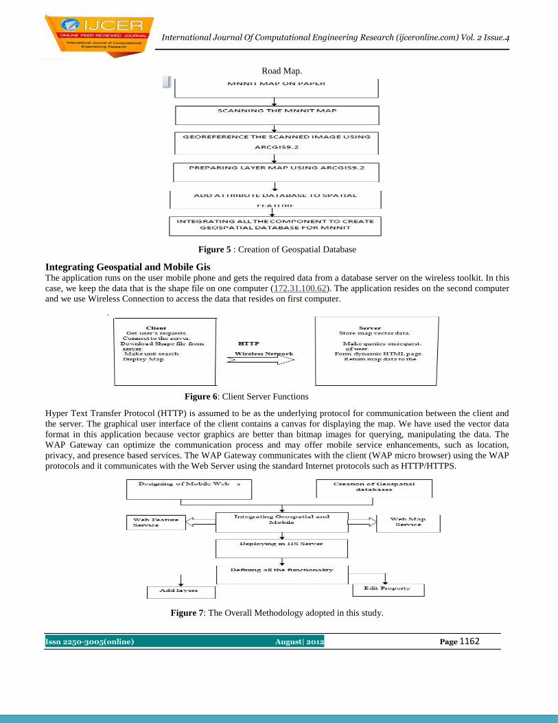
International Journal Of Computational Engineering Research (ijceronline.com) Vol. 2 Issue.4
Issn 2250-3005(online) August| 2012 Page 1162
Road Map.
Figure 5 : Creation of Geospatial Database
Integrating Geospatial and Mobile Gis
The application runs on the user mobile phone and gets the required data from a database server on the wireless toolkit. In this
case, we keep the data that is the shape file on one computer (172.31.100.62). The application resides on the second computer
and we use Wireless Connection to access the data that resides on first computer.
Figure 6: Client Server Functions
Hyper Text Transfer Protocol (HTTP) is assumed to be as the underlying protocol for communication between the client and
the server. The graphical user interface of the client contains a canvas for displaying the map. We have used the vector data
format in this application because vector graphics are better than bitmap images for querying, manipulating the data. The
WAP Gateway can optimize the communication process and may offer mobile service enhancements, such as location,
privacy, and presence based services. The WAP Gateway communicates with the client (WAP micro browser) using the WAP
protocols and it communicates with the Web Server using the standard Internet protocols such as HTTP/HTTPS.
Figure 7: The Overall Methodology adopted in this study.
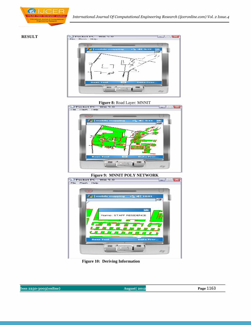
International Journal Of Computational Engineering Research (ijceronline.com) Vol. 2 Issue.4
Issn 2250-3005(online) August| 2012 Page 1163
RESULT
Figure 8: Road Layer: MNNIT
Figure 9: MNNIT POLY NETWORK
Figure 10: Deriving Information

International Journal Of Computational Engineering Research (ijceronline.com) Vol. 2 Issue.4
Issn 2250-3005(online) August| 2012 Page 1164
Conclusion Drawn Maps or Shape file have a definite role to play in a Mobile GIS environment. In their interactive and dynamic appearance they
will guide and assist the user in solving geospatial analysis problems. This can be proved with the help of this work that with
the increased availability of mobile devices, proper software and abundant data, maps can play these various roles anywhere
and at any time. It uses wireless network and communication network and communication protocol by getting the mapping
data from the server and displays shape file on the phone along with many functionality.
In traditional GIS, spatial object were primary focus while in Mobile GIS, the focus has been changed to a particular scene or
of a particular location
Future Recommendations The future recommendation for this work can be in implementing:
A dynamic Database Application for Mobile GIS.
It may take a long time to establish a connection between a client and the server on a wireless network. So, the latency
time should kept minimum.
References [1] Maruto Masserie Sardadi, "Quadtree Spatial Indexing Use to Make Faster Showing Geographical Map in Mobile
Geographical Information System Technology Using an Oracle 10g Application Server and Map Viewer
Applications,", IJCSNS International Journal of Computer Science and Network Security, 2008.
[2] E.Poorazizi, "Developing a Mobile GIS for Field Geospatial data Acquisition,". A.A.Alesheikh and S.Behzadi, Ed.
Asian Network for Scientific Information: Journal of Applied Sciences, 2008.
[3] E. Mensah, "Designing a Prototype Mobile GIS to Support Cadastral Data Collection in Ghana," 2007.
[4] A. Vckovski, “Interoperability and spacial information theory. Interoperating Geographic Information Systems."
1999.
[5] M. J. Kraak,"Current trends in visualization of geographic data with special reference to cartography. Invited paper:
In Proceedings of the XXIIth INCA Congress Indian National Cartographic Association:" Convergence of Imagery
Information and Maps, vol. 22, pp. 319-324, 2002.

International Journal Of Computational Engineering Research (ijceronline.com) Vol. 2 Issue. 4
Issn 2250-3005(online) August| 2012 Page 1165
Experimental Evaluation of Mechanical Properties of 3d Carbon
Fiber/Sic Composites Prepared By LSI
Dr. S. Khadar Vali1*
Dr. P. Ravinder Reddy2 Dr. P. Ram Reddy
3
1. Professor and Head, MED, M. J. College of Engineering and Technology, Banjara Hills, Hyderabad, India.
2. Professor and Head, MED, Chaitanya Bharati Institute of Technology, Hyderabad, India.
3. Former Registrar, JNTU Hyderabad, Presently Director, Malla Reddy Institute of Engg. & Technology, Hyderabad,
India
Abstract
The structural engineer needs to be familiar with the property of the composite material structures. The behavior of
ceramic composite material under impact load plays a pivotal role in designing such structures. An impact test is a test
for determining the energy absorbed in fracturing a test piece at high velocity. The impact resistance of a part is, in many
applications, a critical measure of service life. In the current work, an attempt is made to present the dynamic behavior of
the advanced ceramic composite material, i.e., 3 Dimensional Carbon-Silicon Carbide (3D C-SiC) under the impact,
tensile and flexure loads and the mechanical properties, viz., Impact Strength, Tensile Strength and Flexural Strength are
determined. 3D C-SiC composite specimens with a fiber volume fraction of 40% are prepared by Liquid Silicon
Infiltration (LSI) process to conduct the required experiments for evaluating the mechanical properties. The experimental
results of impact, tensile, flexure and shear strengths recorded during the tests are 26.82 kJ/m2, 70.2 MPa, 230.3 MPa and
30.5 MPa respectively.
Keywords: Carbon Silicon Carbide (C-SiC), Impact strength, Liquid Silicon Infiltration (LSI)
1. Introduction The minimum knowledge required about a material to characterize fracture properties comes from a force-time (or force-
displacement) diagram. When performing a test with an instrumented falling weight, it is possible to record the force
acting on the specimen throughout the impact. Silicon carbide matrix based composites exhibit promising mechanical
properties at high temperatures and offer very good oxidation and thermal shock resistance. They are finding increasing
applications in aerospace, defense and industries. Carbon fiber-reinforced SiC matrix composites are preferred to C-C
composites for oxidizing and highly erosive environment. C-SiC composites are used up to 15000 C for long durations
and up to 20000C for short durations. The mechanical properties of the fiber-reinforced composites can be tailored by
adjusting fiber volume fraction and fiber orientation to meet the needs of the application. C-SiC composites retain
mechanical strength up to 17000C. There are several methods to fabricate C-SiC composites, such as chemical vapor
infiltration (CVI), slurry infiltration combined with hot pressing, polymer-infiltration-pyrolysis (PIP), etc. Among these
methods, Liquid Silicon Infiltration (LSI) process offers many potential advantages such as single step process, low
processing temperature, and near-net-shape processing. Continuous fiber reinforced ceramic matrix composites (CFCCs)
are very interesting structural materials because of their higher performance and higher fracture toughness. For this
reason, CFCCs are considered as the most potential to be used in advanced aero engines. Among the CFCCs, carbon
fiber reinforced silicon carbide matrix composites (C-SiC) are most promising and have been receiving considerable
interest. Many investigations have been conducted on two dimensional woven C-SiC composite materials. Recently,
attention has been focused on three dimensional woven or braided ceramic matrix composite materials in order to meet
mechanical property requirements along the thickness of the composites.
2. The LSI Process The LSI (Liquid Silicon Infiltration) process consists of 3 stages. Beginning with a carbon fiber reinforced ceramic
(CFRC) made of a coal tar pitch with high carbon content, a green-body preform is manufactured. This preform is then
pyrolised under inert atmosphere at temperatures greater than 9000C, converting the CFRC into a higher porous carbon-
carbon (C-C) composite. In a final step, the porous material is infiltrated with liquid silicon under vacuum to
manufacture the final C-SiC ceramic. The quality of the C-SiC materials is influenced by each individual processing
stage.
3. Experimental Investigations 3D stitched preform is the simplest case of the 3D composites development; several layers of 8 H satin carbon fabric
layers are stitched together with 6000 Carbon fibers to impart third direction reinforcement (Fig.1). The fiber volume
fraction is worked out, taking into consideration the infiltration abilities of molten silicon vis-à-vis the thermo
mechanical properties.

International Journal Of Computational Engineering Research (ijceronline.com) Vol. 2 Issue. 4
Issn 2250-3005(online) August| 2012 Page 1166
Fig. 1 The fixture of carbon fiber perform
4. Specimen Preparation And Test Methods The instrument used to perform impact test is quite similar to drop weight machines. It is usually equipped with a
piezoelectric or strain gauge load cell. The standard specimens are prepared with composition shown in Table 1.
Table 1 Composition of Carbon Silicon Carbide (C-SiC)
After preparing the C-SiC
specimens as per the required composition, they are cut into required sizes according to ASTM D256 standards (Fig. 2).
The Izod impact tests are conducted using Fractovis drop weight instrumented impact tester acquired with a DAS 8000
WIN data acquisition system as shown in Fig. 3.
Fig. 2 Izod Test specimen geometry according to ASTM D 256 standards
(a) (b)
Fig. 3 Two Views of the Fractovis Instrumented Impact Tester
5.1 Measurement of Mechanical Properties- Impact Test
Mechanical properties of the C-SiC composite materials are characterized under impact loading to get the reliable design
properties at room temperature. Instrumented impact tests on notched Izod samples are conducted as per ASTM D 256
standards to determine the energy absorbing capability and dynamic fracture behavior of the composite materials. The
sample sizes are 10.16 x 12.7 x 32.5 mm and the impact velocity of 3 m/s is chosen. The dynamic fracture toughness
(k) is calculated using equation:
k = W / bh
where W is the absorbing energy of materials during impact processing, b and h are thickness and width of
specimen respectively.
S. No. Constituents Percentage (%
Vol.)
1. Carbon (Fibre) 40%
2 SiC 45%
3 Si 10%
4 C 5%
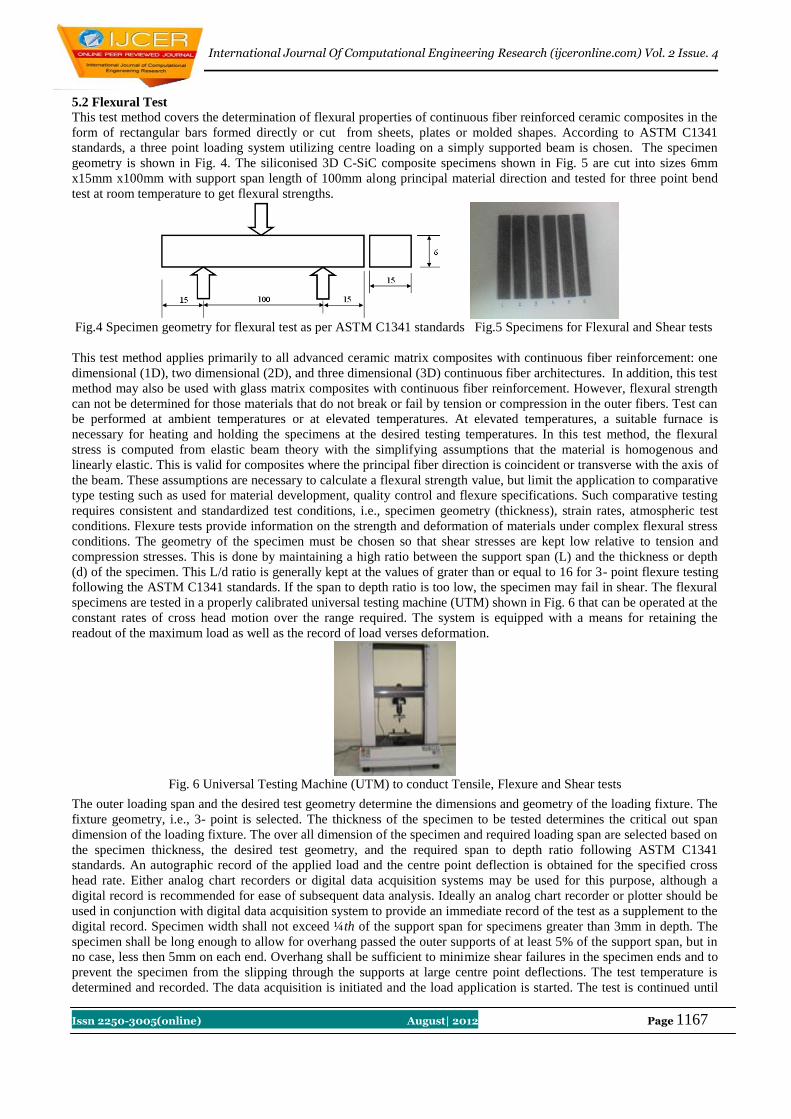
International Journal Of Computational Engineering Research (ijceronline.com) Vol. 2 Issue. 4
Issn 2250-3005(online) August| 2012 Page 1167
5.2 Flexural Test
This test method covers the determination of flexural properties of continuous fiber reinforced ceramic composites in the
form of rectangular bars formed directly or cut from sheets, plates or molded shapes. According to ASTM C1341
standards, a three point loading system utilizing centre loading on a simply supported beam is chosen. The specimen
geometry is shown in Fig. 4. The siliconised 3D C-SiC composite specimens shown in Fig. 5 are cut into sizes 6mm
x15mm x100mm with support span length of 100mm along principal material direction and tested for three point bend
test at room temperature to get flexural strengths.
Fig.4 Specimen geometry for flexural test as per ASTM C1341 standards Fig.5 Specimens for Flexural and Shear tests
This test method applies primarily to all advanced ceramic matrix composites with continuous fiber reinforcement: one
dimensional (1D), two dimensional (2D), and three dimensional (3D) continuous fiber architectures. In addition, this test
method may also be used with glass matrix composites with continuous fiber reinforcement. However, flexural strength
can not be determined for those materials that do not break or fail by tension or compression in the outer fibers. Test can
be performed at ambient temperatures or at elevated temperatures. At elevated temperatures, a suitable furnace is
necessary for heating and holding the specimens at the desired testing temperatures. In this test method, the flexural
stress is computed from elastic beam theory with the simplifying assumptions that the material is homogenous and
linearly elastic. This is valid for composites where the principal fiber direction is coincident or transverse with the axis of
the beam. These assumptions are necessary to calculate a flexural strength value, but limit the application to comparative
type testing such as used for material development, quality control and flexure specifications. Such comparative testing
requires consistent and standardized test conditions, i.e., specimen geometry (thickness), strain rates, atmospheric test
conditions. Flexure tests provide information on the strength and deformation of materials under complex flexural stress
conditions. The geometry of the specimen must be chosen so that shear stresses are kept low relative to tension and
compression stresses. This is done by maintaining a high ratio between the support span (L) and the thickness or depth
(d) of the specimen. This L/d ratio is generally kept at the values of grater than or equal to 16 for 3- point flexure testing
following the ASTM C1341 standards. If the span to depth ratio is too low, the specimen may fail in shear. The flexural
specimens are tested in a properly calibrated universal testing machine (UTM) shown in Fig. 6 that can be operated at the
constant rates of cross head motion over the range required. The system is equipped with a means for retaining the
readout of the maximum load as well as the record of load verses deformation.
Fig. 6 Universal Testing Machine (UTM) to conduct Tensile, Flexure and Shear tests
The outer loading span and the desired test geometry determine the dimensions and geometry of the loading fixture. The
fixture geometry, i.e., 3- point is selected. The thickness of the specimen to be tested determines the critical out span
dimension of the loading fixture. The over all dimension of the specimen and required loading span are selected based on
the specimen thickness, the desired test geometry, and the required span to depth ratio following ASTM C1341
standards. An autographic record of the applied load and the centre point deflection is obtained for the specified cross
head rate. Either analog chart recorders or digital data acquisition systems may be used for this purpose, although a
digital record is recommended for ease of subsequent data analysis. Ideally an analog chart recorder or plotter should be
used in conjunction with digital data acquisition system to provide an immediate record of the test as a supplement to the
digital record. Specimen width shall not exceed ¼th of the support span for specimens greater than 3mm in depth. The
specimen shall be long enough to allow for overhang passed the outer supports of at least 5% of the support span, but in
no case, less then 5mm on each end. Overhang shall be sufficient to minimize shear failures in the specimen ends and to
prevent the specimen from the slipping through the supports at large centre point deflections. The test temperature is
determined and recorded. The data acquisition is initiated and the load application is started. The test is continued until

International Journal Of Computational Engineering Research (ijceronline.com) Vol. 2 Issue. 4
Issn 2250-3005(online) August| 2012 Page 1168
the specimen breaks into two pieces. The maximum load is recorded. After completing the test, the action of the test
machine and the data acquisition system is disabled. In addition to the location, carefully the mode of the fracture
initiation and crack extension is noted. Fracture may initiate on the tensile (lower) face, on the compression (upper) face
of the bar or by shear failure. The bar may fail by a sequential combination of modes. The tensile fracture crack may
extend towards the neutral axis directly or may be deflected along low strength planes such as inter laminar regions.
Flexural Stress (σ):
When tested in flexure, a simple beam experiences maximum tensile stresses in the outer fibers and maximum
compressive stresses in the inner fibers. The location of the maximum stress along the length of the beam is at the centre
point for 3- point testing. Equation for calculating the flexural stress for the 3-point test is give as: Flexure Stress, σ =
3PL/2bd2
Where, P = Load at given point in the test (N)
L = Support span (mm)
b = Specimen width (mm)
d = Specimen depth or thickness (mm)
Flexural Strength (σ f):
The flexural strength is equal to the maximum stress in the outer fibers at the point of maximum load. It is calculated
using the equation:
Flexural Strength, σ f = 3PUL/ 2bd2
Where, PU = Maximum load in flexural test (N)
L = Support span (mm)
b = Specimen width (mm)
d = Specimen depth or thickness (mm)
5. 3 SHEAR TEST Shear strength of 3D C-SiC composites is measured by conducting a three point bend test in the same UTM. The shear
strength is calculated by the following equation.
= 3P/4bh
Where P is the fracture load (N), b and h are width and thickness of the specimen respectively.
5. 4 TENSILE TEST
The test specimens cut into sizes 3mm x 6mm x 100mm length according to ASTM C 1275 standards (Fig. 7) are shown
in Fig. 8. They are fixed in the universal testing machine (UTM) to conduct tensile test by choosing the tensile fixture
and properly adjusting the movable jaw so as to keep the gauge length of 25mm. The tensile load (P) is gradually applied
along principal material direction. When the applied load reaches ultimate value, the specimen breaks catastrophically
and the load falls to zero.
Fig. 7 Tensile test specimen geometry as per ASTM C1275 standards Fig.8 Tensile test specimens
The equation for calculating longitudinal strength in tension is expressed as:
σt = PU/A
where PU = Ultimate load (kN)
A = Area of cross-section perpendicular to the direction of applied load
6. Results And Discussions A typical Force-deformation curve recorded in the impact test is shown in Fig. 9. The test data for 7 sample specimens
out of total 31 specimens tested is also shown in Table 2. First of all, when the striker touches the specimen the impact
point is immediately accelerated from zero velocity to the initial velocity of the striker. This instantaneous acceleration,
for the Newton’s second law, causes a first peak of force named inertial peak (because of the inertial nature of this
phenomenon). After this, strong oscillation force increases linearly. At low displacements, in fact any material can be
considered elastic so that force is proportional to displacement (and therefore to time, if impact energy is high). When
the specimen is affected by a great deflection, however, plastic deformation occurs: the load deformation curve deviates
from linearity showing the characteristic yield region. Since the materiel chosen for test is C-SiC which is very hard and
brittle, there is no noticeable yield region. When the material approaches its maximum deflection, fracture occurs and the
measured force falls to zero. From the load displacement curve the evaluation is made on fracture toughness, i.e., the
energy absorbed by the specimen during the fracture. The absorbed energy is a measure of material strength and the

International Journal Of Computational Engineering Research (ijceronline.com) Vol. 2 Issue. 4
Issn 2250-3005(online) August| 2012 Page 1169
ductility can be graphically represented as the area beneath the load-displacement curve. Further the impact strength is
obtained by calculating the energy absorbed during fracture per unit cross sectional area of the specimen. The
experimental values of fracture toughness and impact strength obtained during impact testing of the specimens with
corresponding measured fiber volume fractions is given in Table 3. Fig. 10 and Fig. 11 clearly indicate the increase in
fracture toughness and impact strength with the increase of fiber volume fraction in 3D C-SiC specimens. In the
specimens tested, a considerable fiber pullout is observed (Fig. 12) indicating the increase of fracture toughness. It is
obvious that 3D C-SiC composite materials exhibit an excellent impact damage tolerance because of Z-direction fibers.
The measured properties of 3D C – SiC composites are compared with the properties of 2D C-SiC (available from
literature) fabricated by different routes as shown in Table 4. The experimental results of impact strength of various
specimens with 40 % fiber volume fraction are shown in Table 5. The flexural strengths calculated and maximum load
recorded in the test for various specimens having fiber volume fractions 40 % is given in the Table 6. The broken
specimen after conducting flexural test (Fig.13) shows lot of fibers being pulled out. This may be the reason for increase
in flexural strength. The tensile strengths calculated for the ultimate loads recorded in the test for various specimens
having fiber volume fraction of 40 % is shown in Table 7. Fig.14 shows the broken specimen after conducting tensile
test. More or less a brittle failure can be observed from this figure which may be attributed to the fact of less tensile
strength. The load deflection curves obtained in 3- point bend test for the specimens is shown in Fig.15. The load
deformation curves obtained in the tensile test for the specimens are shown in Fig.16.The experimental results of shear
strength is shown in Table 8.
0
0.5
1
1.5
2
2.5
3
3.5
4
0 10 20 30 40 50
Fiber Volume Fraction (% V)
Fra
ctu
re T
oughness (J)
Fig. 9 Force-Deformation curves obtained in impact test up to failure Fig.10 Fracture Toughness Vs Fiber
VolumeFraction
0
5
10
15
20
25
30
0 10 20 30 40 50
Fiber Volume Fraction (% V)
Impa
ct S
tren
gth
(kJ/
m2)
Fig. 11 Variation of Impact strength with fiber volume fraction Fig.12 Fiber pull out in impact test
Fig. 13 Broken specimens in Flexural Test Fig. 14 Broken specimen in Tensile Test
0
100
200
300
400
500
600
700
800
900
0 1 2 3
Deflection, mm
Load
, N
Specimen 1
0
100
200
300
400
500
600
700
800
900
0 1 2 3
Deflection, mm
Load
, N
Specimen 2
0
100
200
300
400
500
600
700
800
900
0 1 2 3
Deflection, mm
Load
, N
Specimen 3
0
100
200
300
400
500
600
700
800
900
0 1 2 3
Deflection, mm
Load
, N
Specimen 4
0
100
200
300
400
500
600
700
800
900
0 1 2 3
Deflection, mm
Load
, N
Specimen 5
Fig.15 Load-Deflection curves of specimens obtained in Flexural Test

International Journal Of Computational Engineering Research (ijceronline.com) Vol. 2 Issue. 4
Issn 2250-3005(online) August| 2012 Page 1170
0
0.2
0.4
0.6
0.8
1
1.2
1.4
0 0.1 0.2 0.3
Deformation, mm
Load
, kN
Specimen 1
0
0.2
0.4
0.6
0.8
1
1.2
1.4
1.6
0 0.05 0.1 0.15 0.2 0.25
Deformation, mm
Load
, kN
Specimen 2
0
0.2
0.4
0.6
0.8
1
1.2
1.4
1.6
0 0.1 0.2 0.3
Deformation, mm
Load
, kN
Specimen 3
0
0.2
0.4
0.6
0.8
1
1.2
1.4
1.6
1.8
0 0.1 0.2 0.3
Deformation, mm
Load
, kN
Specimen 4
0
0.2
0.4
0.6
0.8
1
1.2
1.4
1.6
1.8
0 0.1 0.2 0.3
Deformation, mm
Load
, kN
Specimen 5
Fig. 16 Load-Deformation curves of specimens obtained in Tensile Test
Table 2 Impact Test Data of 3D C – SiC specimens
Table 3 Variation of Fracture Toughness and Impact Strength with Fiber Volume Fraction of 3D C-SiC specimens
Table 4 Comparison of mechanical properties of 2D C–SiC composites (from literature) with experimental results of 3D
C-SiC specimens
Properties Literature Values Experimental results of present work
Unit 2D C – SiC (LSI) 3D C – SiC (LSI)
Fiber Volume Vol. % 40 –42 40
Density g/cc 2.4 2.2 – 2.4
Flexural Strength MPa 180 – 200 210 – 230
Tensile Strength MPa 80 – 90 70 – 90
Young’s Modulus GPa 25 – 30 32 – 35

International Journal Of Computational Engineering Research (ijceronline.com) Vol. 2 Issue. 4
Issn 2250-3005(online) August| 2012 Page 1171
Strain to failure % 0.25 – 0.35 0.20 – 0.28
Impact strength kJ / m2
20 – 21 26 – 27
Table 5 Experimental results of impact strength of specimens with 40 % Fiber Volume Fraction
Specimen No. Fracture
toughness (J)
Impact strength (kJ/m2)
From Experiment
1 3.39 26.27
2 3.40 26.35
3 3.42 26.50
4 3.46 26.82
5 3.48 26.98
Table 6 Experimental results of flexural strengths of 3D C-SiC specimens
Specimen No.
Max. load (PU) recorded
during flexural test (N)
Flexural strength, f (MPa)
From Experiment
1 757 210.2
2 780 216.6
3 789 219.2
4 805 223.6
5 829 230.3
Table 7 Experimental results of tensile strengths of 3D C-SiC specimens
Specimen No.
Max. load (PU) during
tensile test (kN)
Tensile strength, t (MPa)
From Experiment
1 1.264 70.2
2 1.346 74.8
3 1.437 79.8
4 1.525 84.7
5 1.619 89.9
Table 8 Experimental results of Shear Strengths of 3D C-SiC specimens
Specimen No. Fracture load (P) in shear test (kN) Shear strength, (MPa)
1 3.38 28.16
2 3.64 30.33
3 3.55 29.58
4 3.66 30.50
5 3.52 29.33
The stress transfer capability of the interface between the fiber and matrix governs the mechanical properties of
fiber reinforced composite materials. The interfacial compatibility is related to the interfacial shear stress, which
characterizes the combination of stress necessary to de-bond the interface and the frictional forces developed at the
interface. The 3D carbon preform is infiltrated by liquid silicon and the density obtained is 2.2–2.4 g cm-3
. The non-
linear failure behavior is observed in the present composite material and it could also be observed that the failure of three
dimensional C-SiC composite material occurred in a controlled manner. The average result of flexural strength is
observed to be 220 MPa. The variation of failure behavior of composites is caused by alteration of the interfacial
bonding between fiber and matrix. The tensile stress within the interfacial phase along the fiber radial direction is
generated after the composite material is cooled down from the infiltration temperature to room temperature. It is easy
for the carbon fiber to debond and be pulled out from the silicon carbide matrix. Above infiltration temperatures, the
stresses at the interface become compressive which may lead to strong bond in between the constituents of the
composite. Moreover, tensile stresses are developed in carbon fiber. Hence, the fiber is broken in the matrix. With the
result, the composite material showed catastrophic fracture behavior as it is difficult to pull out the fiber from the matrix.
Further the composite materials exhibited a non-linear fracture behavior at 16000C, because of creep in silicon carbide
matrix. It is understood that the micro cracks contribute to the non-linear fracture mode of the composites by deflecting
the crack growth. The interfacial bond in between the constituents of the composites depends on the properties of

International Journal Of Computational Engineering Research (ijceronline.com) Vol. 2 Issue. 4
Issn 2250-3005(online) August| 2012 Page 1172
interfacial phase and temperatures. The average value of shear strength obtained (Table 8) is 30 MPa. In the composites
studied, no layer de-bonding is noticed. The average flexural strength obtained is observed to be 220 MPa. It gives an
average work of fracture 26.58 kJ/m2 for the 3D C-SiC specimens with 40% fiber volume fraction. It is observed that this
value is four times that of two dimensional laminated ceramic materials. Also it is higher than that of laminated SiC
composite (4.625 kJ/m2) and much larger than monolithic ceramic material (Silicon Nitride, 80 J/m
2).
7. Conclusions In the present work 3D C–SiC composites are prepared by LSI process using stitched preforms. The process for the
fabrication of specimens is established with coal tar pitch impregnation into 3D carbon fiber preforms. The important
conclusions drawn from the present work are:
1. The SEM micrographs reveal the uniformity of siliconisation and relatively less amount of un reacted silicon and
carbon in the final composites.
2. It is also observed that the concentration of silicon in the composites is more at grain boundaries and at fiber
bundles. This is because of slow diffusion of silicon into C-SiC in grains and relatively low availability of carbon
in the fiber bundles compared to matrix bulk.
3. The mechanical properties of 3D C–SiC composites are determined experimentally. When fiber volume fraction is
increased, fracture toughness and impact strength are increased correspondingly, which is proved by the
experimental results obtained by conducting impact test as shown in Table 3.
4. The impact curve gives a lot of information about material properties. It also gives the information about the kind
of fracture (brittle or nearly ductile) which is depicted graphically. The instrumented impact provides a better
characterization of the material.
5. The experimental value of impact strength obtained for the sample Specimen No.4 with 40 % fiber volume fraction
is 26.82 kJ/m2 .
6. The maximum flexural strength obtained for the sample Specimen No.5 by conducting flexural test is 230.3 MPa.
7. The maximum shear stress from the experiment is observed to be 30.5 MPa.
8. The tensile strength obtained for the sample Specimen No.1 from the experiment is observed to be 70.2 MPa.
References [1] R. Naslain, Ceramic Matrix Composites, Chapman & Hall, London, 1992, 199-243.
[2] T.M. Besmann, B.W. Sheldon, R.A. Lowden, Vapor-Phase Fabrication and Properties of Continuous-Filament
Ceramic Composites, Science, 253, 1991, 1104-1109.
[3] T. Ishikawa, S. Kajii, K. Matsanaga, T. Hogani, Y. Kohtoku, T. Nagasawa, A Tough, Thermally Conductive
Silicon Carbide Composite with High Strength up to 1600°C in Air, Science, 282,1998, 1295–1297.
[4] K.M. Prewo, Fiber-Reinforced Ceramics: New Opportunities for Composite Materials, American Ceramic
Society Bulletin, 68, 1989, 395-400.
[5] M. Wang, C. Laird, Damage and fracture of a crosswoven C/SiC composite subject to compression loading,
Journal of Material Science, 31, 1996, 2065-2069.
[6] J.J. Brenann, Interfacial studies of chemical-vapor-infiltrated ceramic matrix composites, Material Science &
Engineering A, 126, 1990, 203-223
[7] D. Singh, J.P. Singh, M.J. Wheeler, Mechanical Behavior of SiC(f)/SiC Composites and Correlation to in situ
Fiber Strength at Room and Elevated Temperatures, Journal of the American Ceramic Society, 79, 1996, 591-
596.
[8] S. Prouhet, G. Camus, C. Labrugee, A. Guette, Mechanical Characterization of Si–C(O) Fiber/SiC (CVI) Matrix
Composites witrTa BN–Interphase, Journal of the American Ceramic Society, 77, 1994, 649-656.
[9] F.K KO, Preform Fibre Architecture for Ceramic-Matrix Composites, American Ceramic Society Bulletin,
68, 1989, 401-414.
[10] P. Pluvinage, A.P. Majidi, T.W. Chou, Damage characterization of two-dimensional woven and three-
dimensional braided SiC-SiC composites, Journal of Material Science, 31, 1996, 232–241.
[11] Y.D. Xu, L.T. Zhang, Three-Dimensional Carbon/Silicon Carbide Composites Prepared by Chemical Vapour
Infiltration, Journal of the American Ceramic Society, 80, 1997, 1897-1900.
[12] Y.D. Xu, L.T. Zhang, L.F. Cheng, D.T. Yan, Microstructure and mechanical properties of three-dimensional
carbon/silicon carbide composites fabricated by chemical vapor infiltration, Carbon, 36, 1998, 1051-1056.
[13] Yongdong Xu, Laifei Cheng, Litong Zhang, Hongfeng Yin, Xiaowei Yin, Mechanical Properties of 3D fiber
reinforced C/SiC composites, Material science & Engineering A, 300, 2001, 196-202.
[14] Per F. Perterson, Charles W. Forsberg, Paul S. Pickard, Advanced CSiC composites for high-
temperature nuclear heat transport with helium, molten salt, and sulfur-iodine thermo mechanical hydrogen
process fluids, Second Information Exchange meeting on Nuclear production of Hydrogen, Argonne National
Laboratory, Illinois, USA, 2-3 October, 2003.