1

Interaction between Underground Employment and Unions in selected Italian industries

Bruno Chiarini and Elisabetta Marzano♦ (University of Naples, Parthenope)

JEL: E26, J51, C32. Keywords: Underground employment; Net wages; Trade Unions; VECM.

Abstract

In this paper we investigated empirically the nature of the relation between underground employment and unions in Italy, focusing on certain productive sectors. The motivation for this analysis is the hypothesis of the existence of two different opposite channels through which unions affect underground employment: a macro-effect, generating shadow activities via higher wages and market rigidities; a micro-effect, entailing a negative impact of trade union power on underground employment. We consider two different measures of the bargaining power of trade unions, i.e. wages and net density. Econometric analysis of Italian data yields three main results. First, mechanisms of interaction between underground employment and unions change profoundly according to the nature of the industry. Second, the two indexes of the trade unions’ bargaining power play a different role vis-à-vis the extent of underground employment. Third, there is a counter-intuitive interaction between wage and underground employment, which may be explained in an insider-outsider framework.

VERY PRELIMINARY DRAFT DO NOT QUOTE

♦ Address correspondence to: Elisabetta Marzano, Dipartimento di Studi Economici, Università "Parthenope", Via Medina, 40, 80133 Napoli, Italy, elisabetta.marzano@uniparthenope.it.

2

1. Introduction In the literature on economics and industrial relations the determinants of unionism and its effects on labour market behaviour have been extensively examined. However, the effect of labour unions on the “hidden economy” is rarely investigated.1 This is surprising since most European countries, where over three-quarters of the workforce have wages that are covered by collective or sector bargaining, show a sizeable underground economy (for a survey on the size on the hidden economy around the world see Schneider and Enste, 2002). The existence of substantial hidden production greatly affects the labour market (institutions and behaviour), as amply shown elsewhere. 2 There are at least three main reasons for expecting unions to be involved with the hidden sector. First, in a unionized labour market, wages lie above the competitive solution and firms adjust upward according to their demand schedules, hiring fewer and more able workers. However, these circumstances may lead firms and “outsiders” to by-pass higher labour costs and rigidity by operating in the underground economy. Second, union power is also reflected in increased worker dignity and legal protection against a number of harassment practices and excessive worker exploitation, whereas avoiding social contributions, health insurance and other extensive labour benefits are the primary “rewards” of underground production. Third, underground workers tend to reduce union membership, and, hence, union power. Ex ante, it may be difficult to envisage the net effect. In all likelihood, it is related to, amongst others, the productive sectors, technology, taxation system and evasion possibilities, union power and the industrial relations system. In this paper we use a dataset from the Italian economy, a country with both a considerable size of underground economy and strong labour unions, to provide evidence for how this relationship works in selected industries. First of all, we investigate the structural characteristics and dynamics throughout the business cycle of the main attributes of the labour market in the presence of underground employment. Sectoral features and cyclical analysis allow us to gain new information on union power and hidden sector relationships. Our analysis is accomplished using cointegrating bivariate models, to investigate, for the period 1980-2004, long-run and short-run interactions between some proxies of union power and the irregularity ratio (underground to total workers). Econometric investigation with Italian data yielded three main results. First, interaction mechanisms between underground employment and unions are greatly affected by sectoral peculiarities. Second, the two indexes of trade union bargaining power play a different role vis-à-vis the size of underground employment. Third, there is a counter-intuitive interaction between wage and underground employment which can be explained within an insider-outsider framework.

1 ILO (1999) surveys the experience of trade unions in the informal sector in nine countries (Ghana, Kenya; India and the Philippines; Bulgaria, Hungary and Italy; Colombia and El Salvador). The nine national studies represent testimonies that trade unions can contribute to the improvement of working conditions for the informal sector’s workers. However, in this paper we don’t deal with informal economy, but only with underground economy’s employment (OECD, 2002). 2 See, among others, Loayza, 1996; Boeri and Garibaldi, 2002; Fugazza and Jacques, 2003; Marzano, 2004; Busato et al. 2005a; Kolm and Larsen, 2006.

3

The paper is organized as follows. The next section shows magnitudes and features of underground employment and trade union density in Italy, whereas Section 3 gives some insights into major issues affecting the relationship between trade unions and underground employment. Section 4 describes the main characteristics of the examined productive sectors. Section 5 provides some evidence based on econometric analysis for Italy and Section 6 concludes the article. 2. Trade unions and underground employment: the evidence in Italy Underground employment is a widespread phenomenon in Italy, and has attracted a great deal of attention from policy-makers as well as researchers.3 The National Institute of Statistics (ISTAT) provides a time series estimate of underground employment covering the period 1980-2004 for the country as a whole, providing data detailed for the main productive sectors. The ISTAT method of estimating the size of the underground employment (labour input method) is well described in OECD (2002). This procedure is based on a comparison between the labour input estimates based on data from households and enterprises: it is expected that the former give more complete coverage of labour input to GDP than do the enterprise survey data. As the household survey data are expressed in terms of employment and/or hours worked, whereas data from enterprises are usually expressed in terms of jobs, they must be converted to the same standard units of labour input. In fact, ISTAT estimates are expressed as fulltime equivalent employment. The magnitude of underground employment, common in the various productive sectors over the period 1980-2004, is described in Figure 1, from which it is clear that differences are remarkable. Figure 1: underground employment ratio (underground to total workers, %) by economic sector

-

10,0

20,0

30,0

40,0

1980

1982

1984

1986

1988

1990

1992

1994

1996

1998

2000

2002

2004

total economyagricultureindustryservices

Source: ISTAT The largest size of the irregularity ratio (underground to total employees) is recorded in agriculture, amounting to around 30% over the whole period considered. By contrast, industry

3 See, among others, Busetta and Giovannini (1998); Camera dei Deputati (1998); Bovi (1999); Bianco (2002); Zizza (2002); Dell’Anno (2003); Lucifora (2003); Chiarini and Marzano (2004); Marigliani, Pisani (2006).

4

always displays a lower than 10% value for the underground employment ratio, and quite a stable pattern. Conversely, in services we observe a notably upward trend; with the share of underground employment rising from 9.8% in 1980 to a peak of 20.2 % at the end of the millennium. The graphs in Figure 1 also emphasize the reduction in the underground employment share in recent years (2002-04), mainly due to a sharp reduction among irregular foreigners workers, resulting from the amnesty given in 2002 (law no. 189). As to the trade unions’ presence in Italy during recent decades, their evolution has been quite similar to that recorded in other European countries. From 1968 to 1980 Italy experienced a considerable increase in unionization. Subsequently, union membership in industry, agriculture and public services, sectors in which unions were traditionally strongest, was reduced. The rise of employment in market services where unions had greater organizational problems, and changes in the system of industrial relations in a context of high tension between the three union confederations, have generated a downward trend in active union membership; Figure 3 shows this pattern for the two main confederations CGIL and CISL. Figure 2: net membership in the two leading confederations

0

1000000

2000000

3000000

4000000

1985

1987

1989

1991

1993

1995

1997

1999

2001

2003

CISL

CGIL

Source: Feltrin (2005) These trends have been observed and studied since the 1980s (see amongst others Santi 1988; and more recently Visser, 1991; CESOS 1995; Chiarini 1999; Feltrin 2005). The latest available data confirm that more than half of total members are now pensioners. In the next section we will give some possible explanations for the relationship between trade unions and underground employment. 3. Trade unions and underground employment: possible interactions The role of unions in the dynamics of the underground labour market has two main determinants:

1. the bargaining power of trade unions; 2. the arguments of the utility function of trade unions.

5

The first issue relates to the institutional features of the labour market and, in particular, to the degree of coverage.4 The presence of unions reduces labour market flexibility and raises wages and therefore should make firms and “outsiders” prone to use the hidden labour market, especially when the coverage is high. In Italy the nature of collective bargaining and the almost general level of the associated coverage generate a sort of closed shop for the regular labour market (actually workers do not join the unions but undergo their sector/national contracts and hence reinforce their power), whereas the underground sector of the market is completely competitive. Therefore, union wage claims, under circumstances which “legitimate” firms’ tax evasion (for instance, a low probability of being detected and fined, and an inappropriate surcharge penalty), may well induce firms to escape the institutional constraints of the regular market by hiring irregular workers. As to the utility function of the trade union (second issue), the simplest traditional interpretation of the unions’ objective function assumes that they are only concerned with the welfare of their members (rent seeking).5 However, unions’ social concerns should increase their vigilance on recruitment rules since irregular workers very often experience worse job conditions than regular workers.6 In addition, consistent with dynamic union models (Kidd and Oswald, 1987; Charini and Marchetti, 2000), unions clearly have a specific interest in opposing underground labour. All of these motivations imply that the stronger the union is, the more difficult it is to employ underground workers.7 The two issues described imply an opposite expected sign of the relationship between the union’s power to underground employment: a positive one, referred to as wage/macro effect, in the first case; a negative relation, referred to as opposition/micro effect, is expected to arise as a consequence of the second issue. These effects are not so straightforward to investigate due to the composition of the underground labour input. To simplify, we may assume two different types of underground employment: irregularly paid overtime hours, more suitable for skilled workers; and underground positions (unskilled workers).8 Distinguishing these types of irregular employment has important consequences for assessing the interaction with trade unions. In particular, the opposition/micro effect mainly relates to the underground positions (unskilled

4 In Italy there are no official statistics on collective bargaining coverage. However Lawrence and Ishikawa (2005) estimated that in 2000 84% of total employment was covered by collective agreements. 5 For a survey on the economics of trade unions see Booth, 1995. 6 A different situation occurs when workers divide their working time between regular and underground employment, in other words, when they are moonlighters. See Cowell, 1990, for some definitions of firms which operate in the informal sector; Busato and Chiarini, 2004 and Busato et al., 2005b, provide an application of the moonlighter firm in a general equilibrium framework. 7 Unions are a natural barrier to the exploitation of informal work in each single firm; nonetheless, they can adopt a “macro” strategy against the underground economy. Recent evidence is given in Italy by the so-called contratti di riallineamento, a sort of local bargaining between unions and firms specifically addressed to induce the latter to act above ground. To this end, a fiscal amnesty is proposed so that they declare their informal workers. See also the strategy of the main Italian union, CGIL, “Against the shadow economy” recently announced on the Web. It aims to help workers involved in the shadow economy as well as elaborate policy proposals. 8 We are aware that this is a very simplified framework, since also skilled workers, in some areas of Italy with very high unemployment rates, may well be involved in underground positions. In addition, many of the recent contract types, very widespread among young and highly educated workers, such as CO.CO.Pro, are often a screen to conceal subordinate employment relationships.

6

workers), mostly involved in poor working conditions compared to workers doing irregular overtime hours. Moreover, membership dynamics is not necessarily affected by irregular paid overtime hours, since the employees involved are already regular workers, possibly also members of trade unions. As emerges from Table 1, the picture is much more complex: on the basis of the results of inspections conducted by the Institute for Private Sector Social Welfare (INPS), we note that the inspectors found that on average 0.22% of underground workers benefit from wage supplementation (CIG); 9.8% are illegal immigrants and about 75% are simply shadow workers. Finally, about 13% of irregular workers have a regular contract but experience some kind of irregular arrangement, such as irregularly paid overtime. Table 1: Types of irregular workers, 2001 (based on INPS investigation)

CIG Insurance

Sickness Insurance

Unempl. Insurance

Second job

Minors Immigr. Students Retired Others Irregular contracts

0.22 0.05 0.9 0.18 0.22 9.8 0.23 0.67 74.78 12.94

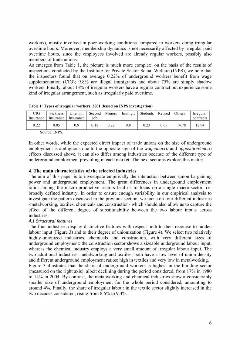
Source: INPS. In other words, while the expected direct impact of trade unions on the size of underground employment is ambiguous due to the opposite sign of the wage/macro and opposition/micro effects discussed above, it can also differ among industries because of the different type of underground employment prevailing in each market. The next sections explore this matter. 4. The main characteristics of the selected industries The aim of this paper is to investigate empirically the interaction between union bargaining power and underground employment. The great differences in underground employment ratios among the macro-productive sectors lead us to focus on a single macro-sector, i.e. broadly defined industry. In order to ensure enough variability in our empirical analysis to investigate the pattern discussed in the previous section, we focus on four different industries -metalworking, textiles, chemicals and construction- which should also allow us to capture the effect of the different degree of substitutability between the two labour inputs across industries. 4.1 Structural features The four industries display distinctive features with respect both to their recourse to hidden labour input (Figure 3) and to their degree of unionization (Figure 4). We select two relatively highly-unionized industries, chemicals and construction, with very different sizes of underground employment: the construction sector shows a sizeable underground labour input, whereas the chemical industry employs a very small amount of irregular labour input. The two additional industries, metalworking and textiles, both have a low level of union density and different underground employment ratios: high in textiles and very low in metalworking. Figure 3 illustrates that the share of underground workers is highest in the building sector (measured on the right axis), albeit declining during the period considered, from 17% in 1980 to 14% in 2004. By contrast, the metalworking and chemical industries show a considerably smaller size of underground employment for the whole period considered, amounting to around 4%. Finally, the share of irregular labour in the textile sector slightly increased in the two decades considered, rising from 8.6% to 9.4%.

7

Figure 3: underground employment ratios (underground workers as a % of total workers), selected economic sectors

right axis

0

4

8

12

1980

1981

1982

1983

1984

1985

1986

1987

1988

1989

1990

1991

1992

1993

1994

1995

1996

1997

1998

1999

2000

2001

2002

2003

2004

0

5

10

15

20

textiles metalworking chemicals construction

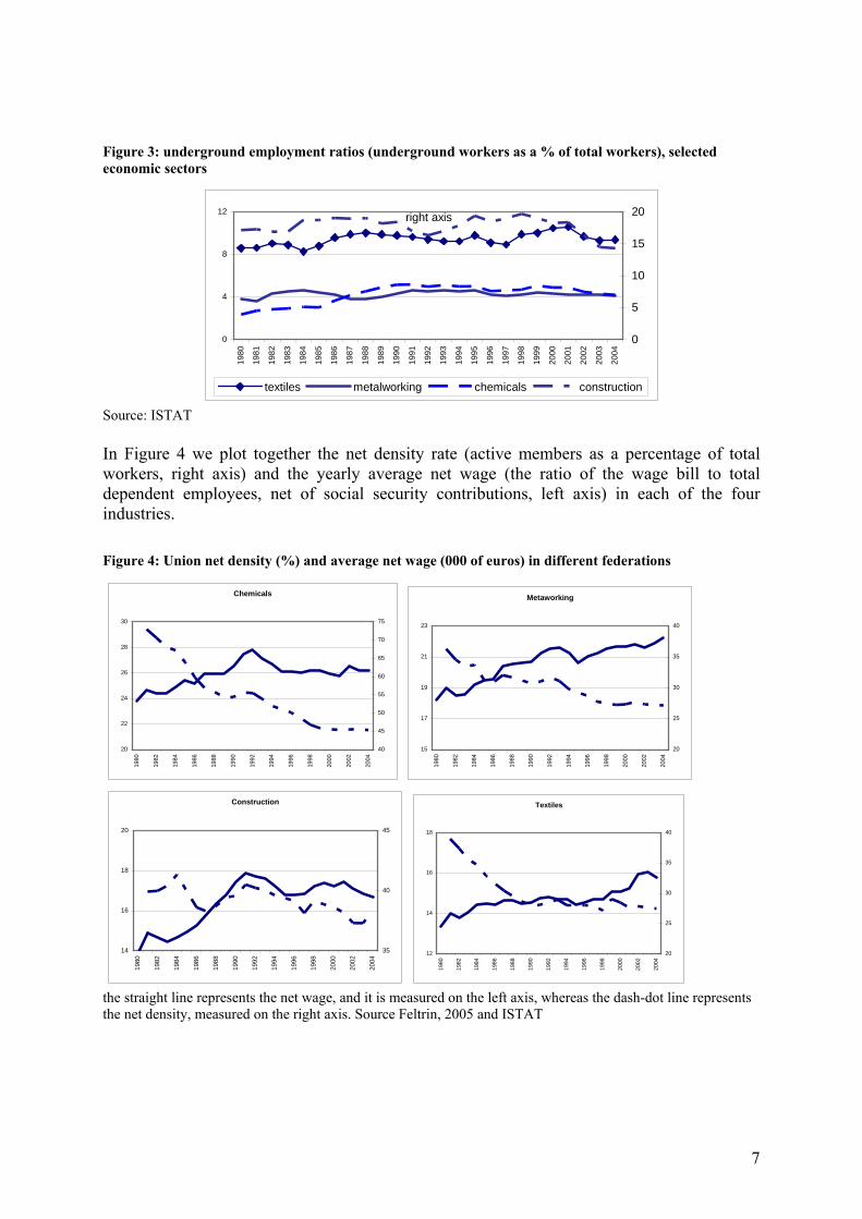
Source: ISTAT In Figure 4 we plot together the net density rate (active members as a percentage of total workers, right axis) and the yearly average net wage (the ratio of the wage bill to total dependent employees, net of social security contributions, left axis) in each of the four industries. Figure 4: Union net density (%) and average net wage (000 of euros) in different federations

Chemicals

20

22

24

26

28

30

1980

1982

1984

1986

1988

1990

1992

1994

1996

1998

2000

2002

2004

40

45

50

55

60

65

70

75

Metaworking

15

17

19

21

23

1980

1982

1984

1986

1988

1990

1992

1994

1996

1998

2000

2002

2004

20

25

30

35

40

Construction

14

16

18

20

1980

1982

1984

1986

1988

1990

1992

1994

1996

1998

2000

2002

2004

35

40

45

Textiles

12

14

16

18

1980

1982

1984

1986

1988

1990

1992

1994

1996

1998

2000

2002

2004

20

25

30

35

40

the straight line represents the net wage, and it is measured on the left axis, whereas the dash-dot line represents the net density, measured on the right axis. Source Feltrin, 2005 and ISTAT

8

The first point to note is the divergent path displayed by these two variables in all the industries concerned, with the single exception of construction, where a similar, and declining, pattern is recorded both for the net wage and the net density starting from the late 1980s. In the remaining industries, a declining trend in trade union membership is jointly observed with an upward pattern for the net wage. As discussed previously (see also Chiarini, 1999), in the same period there was a considerable increase in retired and public sector components of trade union membership, contributing to a rise in trade union bargaining power. Figure 4 also shows that union net density varies considerably among the four productive sectors. The chemical industry exhibits the largest membership rate, despite declining in the examined period. The second largest membership is found in the construction industry, while metalworking and textiles show the lowest density rate. The selection of the sectors is also motivated by the major differences concerning the production structure and wage structure. In Table 1, we report some characteristics of the four industries, which allow us to distinguish two different groups. The first, comprising the construction and textile industries, has a smaller size in terms of dependent employees, a lower share of overtime hours, and lower wage and profit indicators. We can refer to the first group as the small-sized industry, and thus the second would be the large-sized industry. Moreover, in both sectors of the small-sized industry, the relative share of underground employment is quite high, though in terms of union density the two industries are less homogeneous. Table 1: main characteristics of the selected industries, Italy

Industry characteristics Reference

year Chemical Metalworking Construction Textile % of firms without employees 2004 25-49 32-53 40-58 40.0 Average no. of employees 2004 12-46 8-39 3-9 8 Overtime per worker (per year) 2000 65-93 67-95 51.0 64.0 Overtime per worker(% of total) 2000 3.3-4.7 3.3-4.9 2.6 3.3 Total Unit Labour cost (000) 2000 36-44 28-34 27.0 23.0 Diff. between wage Max and Min (%) 2000 85-104 50-74 54 46 ROE 2001-2003 2.2-12.4 2.5-28.5 3.5-6.9 1.3-6.9 ROI 2001-2003 6.2-12.8 5.7-9.9 6.2-9.8 5.6-6.2 Union density rate 2000 47.9 28.5 47.3 31.8 Underground employment ratio 2000 0.7-8.5 2.8-7.5 9.1-21.3 8.8-10.9

Source: ISTAT; Confindustria Lastly, Table 1 shows that in large-sized industries the amount of overtime per worker is higher with respect to small-sized ones. The high recourse to overtime in some industries is a signal that labour turnover costs, principally training costs, are particularly high. Intuition suggests that it is also more difficult to substitute insider/regular workers with outsider/underground ones. This points to a different use of the two margins of underground labour input, irregular overtime and underground positions, commented on in Section 3. In particular, we expect greater use of the intensive irregular margin (irregular overtime), rather than the extensive one (underground positions) in large-sized industries. 4.2 Business cycle features In this section we investigate business cycle stylized facts related to the use of underground labour input, in order to gain additional knowledge about differences in its exploitation in the

9

industries in question. Several differences emerge among the industries, both in terms of volatility and pro-cyclicality (i.e. contemporary correlation), as also stressed by the statistics reported in Tables 2 and 3, which will be commented upon briefly. 9 4.2.1 The co-movement of underground employment with output With regard to the co-movement of underground employment with the business cycle, Table 2 displays, for the irregularity ratio, the size of the contemporary and maximum correlations. In all the industries, with the exception of the chemical industry, there is a clearly counter-cyclical dynamic of the irregularity ratio, tending to lag the cycle. Table 2: cyclical statistics for underground employment ratio (underground to total full time equivalent subordinate workers), HP filtered

chemical metalworking construction textile Contemporary corr with VA 0.33 -0.49 -0.60 0.25 Maximum correlation with VA 0.33 -0.49 -0.84 -0.51 Leading (+) /lagging (-) the cycle 0 0 -1 -2 Contemporary corr. between regular and underground employment

0.80 0.17 -0.64 0.64

If we look at the correlation between regular and underground employment, we find that in two industries (textiles and chemicals) the two labour inputs move together over the business cycle; moreover, in the statistical appendix (section A2) we also show that they are both pro-cyclical. As to the remaining industries, a positive but no significant correlation is found in the metalworking industry whereas a negative correlation emerges in the construction sector. In the latter industry regular employment is pro-cyclical (0.77) whereas underground employment is counter-cyclical (-0.31). These differences are striking, since they suggest that an opposite mechanism of substitutability between the two labour inputs is at work during the business cycle in the industries considered:

1. substitution effect: it operates in the construction industry where, during a recession (expansion), firms substitute regular (underground) with underground (regular) employees, and the irregularity ratio rises (falls).

2. complementary effect: it operates in the textile and chemical industries where, during a recession (expansion), firms reduce (increase) both regular and underground employment. However, this seems to have no significant impact on the irregularity ratio over the cycle.

3. neutrality effect: it operates in the metalworking industry, where no significant correlation is found between the short-term component of the two labour inputs. However, the irregularity ratio is counter-cyclical.

These remarks confirm that the nature of underground employment may differ in the various industries, providing a channel through which to smooth (or boost) both production and labour input over the business cycle. 4.2.2 The volatility of underground employment For each industry, Table 3 reports standard deviations of irregular ratio and regular and irregular worker fluctuations both as a percentage and compared to VA standard deviations. 9 Business cycle properties are based upon ISTAT annual time-series data for the period 1980-2004. Observed time-series were de-trended using the Hodrick-Prescott (H-P) filter.

10

On inspecting the volatility of underground employment over the business cycle, we note that in all the investigated industries the fluctuations of underground employment, both in terms of ratio and in absolute values, are always greater than the cyclical fluctuations of the value added (last column). As the irregular ratios indicate, all the industries record intensive short-run fluctuations ranging from 4 to 6%, as shown by the second column of Table 3, where for each industry the standard deviation of the short-term (H-P filtered) component of underground employment is listed. Table 3: business cycle volatility

σi σi / σVA Chemicals: underground employment ratio ( nirr/ntot) 0.058 2.15 Chemicals: underground employment (nirr) 0.078 2.87 Chemicals: regular employment (nreg) 0.023 0.86 Metalworking: underground employment ratio ( nirr/ntot) 0.06 1.57 Metalworking: underground employment (nirr) 0.062 1.62 Metalworking: regular employment (nreg) 0.025 0.64 Construction: underground employment ratio ( nirr/ntot) 0.055 1.68 Construction: underground employment (nirr) 0.036 1.08 Construction: regular employment (nreg) 0.038 1.17 Textiles: underground employment ratio ( nirr/ntot) 0.044 1.37 Textiles: underground employment (nirr) 0.06 1.87 Textiles: regular employment (nreg) 0.023 0.70 Moreover, the units of underground workers ( )ni irσ are much more volatile than the regular employment component ( )ni rσ . The single exception occurs in the construction sector, where irregular workers are almost as volatile as regular workers; in addition, it is the industry with the largest absolute standard deviation in regular employment (3.8% compared to 2.3% in the other three industries). The evidence presented so far shows that the sectors in question have quite different structural and cyclical characteristics, which may be due to their own sectoral determinants as well as their different union influence. This suggests a complex relationship with union power, although some regularities can be stressed. For instance, the lower volatility of regular than irregular employment confirms the role of labour market institutions, among which trade unions certainly play a major role. 5. Econometric estimates Our econometric analysis is designed to answer the two questions we posed in the Introduction: whether there is a relationship between underground economy and union power and, if so, whether this effect is homogeneous across industries. We focus on the four different industrial sectors described above (textiles, metalworking, chemicals and construction), using annual data covering the period 1981-2004.

11

An important caveat is that the dataset does not allow us to specify a structural model, but we can, at best, set up bi-variate statistical models. This means that we are not estimating labour demand or supply for regular or irregular labour input. Quite simply, our analysis is an initial empirical step to draw some aggregate stylized facts from the Data Generating Process. In order to investigate trade union “pushfulness”, the literature has used several proxy variables, such as the density/membership ratio and the hours lost in union strikes and labour conflict. None of them, of course, are completely convincing; moreover, depending upon the degree of coverage, trade union influence has an immediate effect on the bargained wage. To this end, we intend to use two different kinds of proxies of union influence:

1. average wages, as a ratio of the wage bill to the total dependent employees (regular plus irregular) in each industry, net of social security contributions. The latter are not included for two reasons: first, because unions are interested in wage claims, net of the tax burden; second, because national accounts data (ISTAT) include irregular workers in estimating the wage bill but not in estimating social security contributions;

2. net density, which is simply calculated as a ratio between active membership (as declared by trade unions, collected in Feltrin, 2005) and total dependent employees (regular plus irregular) in each industry (ISTAT).

These two proxies, as already highlighted in Figure 4, display quite a different pattern in the considered time span, suggesting underlying determinants that may be used to explain the relationship with the underground labour market. Given this evidence, we estimate, for all four productive sectors, two different sets of bi-variate Vector Autoregressive models (VAR) with, respectively, the following endogenous variables:

1. the ratio of underground to total subordinate employment and net density 2. the ratio of underground to total subordinate employment and the net wage per

worker. For each bivariate VAR model we test for the existence of a cointegration relation, relying on the cointegration tests (Johansen). The statistical appendix (section A3) reports tests and technical results for each estimated model. Once the existence of a long-run relationship is ascertained, we proceed to model a VECM (vectorial error correction model) and examine the shape of the impulse responses. 5.1 Statistical characteristics Before analysing the relationship between irregular workers and the two proxies of union power, we show the results of stationary tests on the variables involved. It is essential to identify the non-stationary nature of our series and avoid problems of spurious regressions.

Table 4 ADF tests. H0 unit root. Constant and trend in level, constant in first difference

Net density Underg. Empl. ratio Net wage Level First

Difference Level First

Difference Level First

Difference Chemicals -2.675 -3.28* -1.302 -3.961** -2.191 -3.719** Metalworking -2.472 -4.201*** -3.317 -3.120** -2.826 -3.753** Construction -2.982 -3.945*** -1.66 -3.829*** -2.161 -1.824 Textiles -2.450 -3.744** -2.940 -4.198*** -2.262 -4.026*** ***; **, *: the null can be rejected at, respectively, 1, 5 and 10% level. For the chemical industry the test considers a quadratic trend

12

The calculated t-statistics are greater than the critical values when considering the first differences of the variables. Hence we reject the null H0 (variables have a unit root) at conventional test sizes for the differenced variables. However, the net wage in the construction sector deserves more attention. Although the ADF test does not confirm that the series is I(1), additional tests, i.e. KPSS and Phillips-Perron, both suggest that the first difference is stationary (the p-values are, respectively, 0.45 and 0.006). 5.2 Underground employment and net density model The first model, estimated for each industry, involves the irregularity ratio and the net density. Our estimation procedure is the following: after setting the appropriate lag-length of the VAR model, we determine whether the system is conditioned on some dummy variable for controlling structural breaks. Then we test for the existence of a cointegration (stationary) relationship, and finally for weak exogeneity. The procedure is carried out separately for the four industries, and in Table 5 we report the estimated long-run relationship between the variables involved, and the adjustment coefficients to the long-run equilibrium, respectively the β parameters in the cointegration relation and the loading factors α. The coefficient of the first variable, the underground employment ratio, in the cointegration relation is normalized to one. Therefore, in all the specifications, the cointegration relation reads as follows (all the variables, except the time trends, are in log): (1) Underground employment ratio = Constant + β1 (Net density) + β2 (Trend) 5.2.1 The long-run equilibrium and the adjustment coefficients Table 5 shows that the long-run elasticities between the underground employment ratio and net density are negative in all the industries except for metalworking, though the intensity varies substantially across industries. The model shows a long-run underground ratio-net density elasticity of about 3 for the construction sector, but the estimated stationary relation also implies that an increase in underground ratio reduces, in the long run, the net density by almost 0.34%.10 By contrast, the result shows an underground ratio which is much less sensitive to changes in union power in the textile sector (with a long-run elasticity of 0.68), which, however, implies a strong long-run effect of the net density to underground ratio (the elasticity is about 1.5). For the chemical industry we are unable to find a cointegrating vector, and hence the estimated elasticities are not reliable. The α terms of the dynamic part of the model measure the speed of adjustment of the underground employment and the net density towards the equilibrium once a shock occurs. Table 5: cointegration parameters (β) and loading factors (α). Underground ratio-union density model

Chemicals Metalworking Construction Textiles Constant 31.76 (7.3) -7.8 (2.8) 13.8 (1.75) 4.52 (0.54) Net density -7.1 (1.67) 2.6 (0.8) -2.95 (0.47) -0.68 (0.16) Trend -0.14 (0.04) 0.028 (0.009) -0.0033 (0.0016) - Loading factors

10 The long-run relation (1) is normalized with respect to the underground ratio. If the relationship is stationary, we can equally normalize with respect to net density obtaining as elasticity the value )/1( 1β .

13

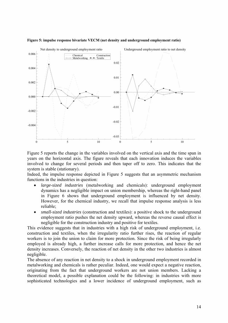
Chemicals Metalworking Construction Textiles α1 (Undergr. Ratio) -0.17 (0.04) -0.38 (0.12) -0.47 (0.2) -0.80 (0.18) α2 (Net density) -0.023 (0.017) 0.15 (0.08) -0.26 (0.057) 0 (p-value 0.55) Standard errors are given in parenthesis; when restrictions are imposed, the p-value is shown. We cannot reject the hypothesis that the net density, in the textile industry, is weakly exogenous with respect to the long-run parameters and the restriction ( 02 =α ) is binding under the assumption that there is one cointegrating relation. This means that in this industry, the speed at which net density adjusts to the disequilibrium is zero.11 A further important feature that deserves mention concerns the size of the adjustment. In the VECM, the lower limit on the adjustment coefficients of -1 implies that there is no distinction between the short run and the long run. Moving on to our estimates, for the underground ratio the coefficient 1α indicates that 17% of the disequilibrium is removed in a year in the chemical industry. This size rises to 38% in metalworking and to 40% in construction, reaching 80% in the textile industry. The speed of the adjustment of net density is much slower: only 2.3% of the disequilibrium is now removed after a year and in the construction sector the yearly adjustment achieves its maximum value of 26%. Estimates of the underground ratio’s loading factor highlight how the industry attempts to reallocate labour inputs (regular and irregular) whenever a shock impinges on the sector, changing the equilibrium relationship. This reallocation mechanism, as expected, is stronger in textiles and construction and weaker in the chemical sector. By contrast, the net density is not sensitive or cannot be used to restore equilibrium in any sector except for construction. Of course it is easier to adjust the size and “quality” of a firm’s labour force than to influence union membership, as also confirmed by the high volatility of the underground employment ratio commented upon in Section 4.2. 5.2.2 Impulse response analysis The decomposition of long-run equilibrium coefficients, error correction coefficients and short-run dynamic is important to help us understand the characteristics of the relations. However, the analysis requires that long-run equilibrium, short-term dynamics and intertemporal adjustment processes generated by equilibrium errors are simultaneously taken into account. Indeed, Lutkepohl (1991; 1994) shows that it is problematic to interpret the coefficients of cointegrating relations as long-run elasticities since such an interpretation ignores the dynamic of the system. Impulse-response analysis, relying upon the full system, may provide a more reliable conclusion. To this end we perform impulse response analysis, allowing a standard deviation innovation to hit each variable for each industry.12 The results stress that all the industries considered, with the single exception of textiles, display a negative reaction of the underground employment ratio to a positive shock in the net density. This evidence suggests that unions counteract underground employment through active membership. The size of the reaction and persistence of the shock differ greatly among industries, as the right-hand panel in Figure 5 amply shows.

11 The definition of weak exogeneity is due to Engle, Hendry and Richard (1983). 12 When the variables have different scales it is common to use, as innovation, one standard deviation rather than unit shocks.

14

Figure 5: impulse response bivariate VECM (net density and underground employment ratio)

0 5 10

-0.004

-0.002

0.000

0.002

0.004

0.006Net density to underground employment ratio

Chemical Metalworking

Construction Textile

0 5 10

-0.03

-0.02

-0.01

0.00

0.01

0.02

Underground employment ratio to net density

Figure 5 reports the change in the variables involved on the vertical axis and the time span in years on the horizontal axis. The figure reveals that each innovation induces the variables involved to change for several periods and then taper off to zero. This indicates that the system is stable (stationary). Indeed, the impulse response depicted in Figure 5 suggests that an asymmetric mechanism functions in the industries in question:

• large-sized industries (metalworking and chemicals): underground employment dynamics has a negligible impact on union membership, whereas the right-hand panel in Figure 6 shows that underground employment is influenced by net density. However, for the chemical industry, we recall that impulse response analysis is less reliable;

• small-sized industries (construction and textiles): a positive shock to the underground employment ratio pushes the net density upward, whereas the reverse causal effect is negligible for the construction industry and positive for textiles.

This evidence suggests that in industries with a high risk of underground employment, i.e. construction and textiles, when the irregularity ratio further rises, the reaction of regular workers is to join the union to claim for more protection. Since the risk of being irregularly employed is already high, a further increase calls for more protection, and hence the net density increases. Conversely, the reaction of net density in the other two industries is almost negligible. The absence of any reaction in net density to a shock in underground employment recorded in metalworking and chemicals is rather peculiar. Indeed, one would expect a negative reaction, originating from the fact that underground workers are not union members. Lacking a theoretical model, a possible explanation could be the following: in industries with more sophisticated technologies and a lower incidence of underground employment, such as

15

chemicals and metalworking, the irregular labour practice should be mainly related to the intensive margin, i.e. regularly employed workers (skilled workers, see also Section 3). These workers, possibly by joining a trades union, are willing to experience some kind of irregular arrangement with their employer in order to gain some extra hours of work free of tax. In this case, a rise in the irregularity ratio is more likely to have a negligible impact on net density. 5.3 Underground employment and net wage model In a second set of estimates we investigate interaction between underground employment ratio and net wage, calculated as the average workers’ remuneration, net of the social security component. The long-run estimated coefficients, which characterize the stationary relationship between the variables, are displayed in Table 6. Table 6: cointegration parameters (β) and loading factors (α). Underground ratio-wage model

Chemicals Metalworking Construction Textiles Constant 19.2 (3.52) 3.08 (0.80) 3.79 (0.72) -1.36 (1.78) Net wage 6.35 (1.08) -0.52 (0.26) -0.35 (0.27) 1.34 (0.66) Trend 0 (Pi-value 0.44) - 0.006 (0.003) - α1 -0.19 (0.13) 0 (Pi-value 0.74) -0.57 (0.18) -0.93 (0.41) α2 0.08 (0.03) -0.24 (0.06) 0.14 (0.09) 0.22 (0.12) Standard errors are given in parenthesis; when restrictions are imposed, the p-value is shown. 5.3.1 Long-run elasticities and error correction coefficients The long-run elasticities shown in Table 6 do not confirm the equilibrium featured in the previous underground ratio-union density model. This casts some doubt on the equivalence of the proxies selected for union power. In all likelihood, they are reflecting different aspects of union influence, and along with the structural features of the industries, these proxies reveal different channels available to unions to impinge on the labour input. Now, with the exception of construction, the equilibrium relationship reports a different sign. Increases in union wage claims entail a long-run increase in the underground ratio in the chemical and textile sectors, whereas in construction and metalworking the long-run wage effect is reversed. Finally, it should be noted that, unlike the previous model, in the chemical industry we find a reliable cointegrating relation between the endogenous variables. With regard to the adjustment coefficients, the table shows that in the metalworking industry the underground employment ratio is weakly exogenous and, according to the evidence displayed in table, we can draw the following insights about the speed of the short-run responses to disequilibrium: with the exception of metalworking industry, the adjustment to disequilibrium is faster for the irregular workers rather than wages. In textile sector, the change in irregular workers account for a 63% adjustment in period t to the disequilibrium in period t-1, whereas the net wage adjustment coefficient is rather slow. In a year only the 16% of the disequilibrium has been removed via wages. 5.3.2 Impulse response analysis The estimated impulse responses are shown in Figure 6. As in Figure 5, we report one standard deviation innovation to each variable for each sector, while responses are traced by changes in the relative variables. The first point to stress is that the industries display quite a similar pattern, except for construction, which acts in the completely opposite way.

16

Figure 6: impulse response bivariate VECM (net wage and underground employment ratio)

0 5 10

0.004

0.003

0.002

0.001

0.000

0.001

0.002

0.003

0.004

0.005Wage to underground employment ratio

Chemical Metalworking

Construction Textile

0 5 10-0.0075

-0.0050

-0.0025

0.0000

0.0025

0.0050

0.0075

0.0100

0.0125

Underground employment ratio to wage

The result seems to indicate that in all the industries except construction, the so-called wage/macro effect does occur. Indeed, the chemical, metalworking and textile industries react with a rise in the underground employment ratio after a rise in net wage paid in the regular sector. Moreover, this reaction appears to be powerful and immediate in the metalworking industry, but less remarkable, and also lagged in the other two industries. A wage rise provides a drop in the underground employment ratio only in construction. This may indicate that in this sector recourse to underground employment is not linked to the high cost of regular employment, but to more general, structural advantages.13 The construction industry also stands out when considering the effect of an exogenous shock in the underground employment ratio on the net wage (left-hand panel of Figure 6). The innovation immediately pushes wages up in large-sized industries and, after a short lag, in textiles, whereas a wage drop is observed in the construction sector. A wage drop should be the expected outcome when the relative size of underground employment rises, for it is tantamount to a weaker demand for regular workers. The results found for textiles, metalworking and chemicals evokes a worrying scenario, namely the vicious circle of irregular labour input and wages: as long as wages rise, underground employment does too; yet an increase in underground employment also generates an upward jump in net wages. 6. Concluding remarks In this paper we investigated the nature of the relation between underground employment and unions. The starting hypothesis is the existence of two different and opposite channels through which unions affect underground employment: the wage/macro effect, that would generate a rise in underground employment; and the opposition/micro effect, that would generate a drop in underground labour input. 13 As is well known, what affects the demand for labour is also the size of so-called adjustment costs.

17

Econometric investigation, substantially based on statistical models, yielded three main results. First, the nature of the relationship between underground employment and unions’ strength is not definite. The so called macro-effect (the presence of unions generates shadow activities via higher wages and market rigidities) occurs when considering time series data for underground employment and net wages for Italian industry in the broad sense. This effect does not operate when considering a different measure of union influence, i.e. active membership. Indeed, in this case, data show that unions are effective in countering underground practices in all industries but textiles, through their active involvement in the regular market, i.e. through net density. Second, the relationship between union-wages and underground labour input is strongly affected by sectoral peculiarities. The most important features that may explain the different interaction observed in the industries concern cyclical behaviour, recourse to overtime, the different degree of substitutability of the two labour inputs (skilled and unskilled and/or intensive extensive margin), sectoral size and technology. Finally, a shock in underground employment raises wages in all industries, with the exception of construction. This counter-intuitive effect can be traced back to the insider-outsider framework of the labour market (for a recent survey see Lindbeck and Snower, 2002), where labour turnover costs explain the market power of insiders/regular workers. When these costs are particularly high, insiders can demand higher wages, even when outsider size rises. Conversely, when turnover and training costs are low, the two labour inputs are easily substitutable, due to the very simple content of the work activity; in this situation (for instance the construction sector) the pressure of a rising size of outsiders is a threat to insider/regular workers, which impacts upon the wage size. In terms of future research, these results call for the setting up of a model structure which can provide theoretical predictions consistent with observations and empirical analyses.

18

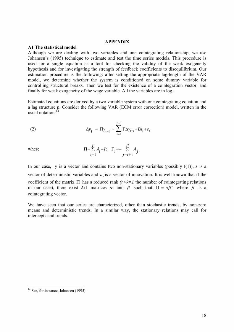
APPENDIX A1 The statistical model Although we are dealing with two variables and one cointegrating relationship, we use Johansen’s (1995) technique to estimate and test the time series models. This procedure is used for a single equation as a tool for checking the validity of the weak exogeneity hypothesis and for investigating the strength of feedback coefficients to disequilibrium. Our estimation procedure is the following: after setting the appropriate lag-length of the VAR model, we determine whether the system is conditioned on some dummy variable for controlling structural breaks. Then we test for the existence of a cointegration vector, and finally for weak exogeneity of the wage variable. All the variables are in log. Estimated equations are derived by a two variable system with one cointegrating equation and a lag structure p. Consider the following VAR (ECM error correction) model, written in the usual notation:14

(2) 1

11

p

t i t tti

y y y Bzt ε−

−−=

Δ = Π + ΓΔ + +∑

where ;1 1

p pA I Ai i j

i j iΠ= − Γ =−∑ ∑

= = +

In our case, y is a vector and contains two non-stationary variables (possibly I(1)), z is a

vector of deterministic variables and tε is a vector of innovation. It is well known that if the coefficient of the matrix Π has a reduced rank (r<k=1 the number of cointegrating relations in our case), there exist 2x1 matrices α and β such that 'αβΠ = where β is a cointegrating vector. We have seen that our series are characterized, other than stochastic trends, by non-zero means and deterministic trends. In a similar way, the stationary relations may call for intercepts and trends.

14 See, for instance, Johansen (1995).

19

A2 THE DATASET CODE VARIABLE (all variable are in log) SOURCE LnetDensity Net density (active membership/total regular

workers) Author elaboration upon Istat (2005) and Feltrin (2005).

LNetWage Wages Net of social security contributions (thousands of euros per unit of workers)

Istat

LURatio Ratio underground to total full time equivalent subordinate workers (%)

Istat

Matrix of correlations, filtered (HP de-trended) series (0.3961 is the threshold for a two tales test).

Table A2.1

TEXTILES VA Wage Regular workers

Underground Workers

Net Density

VA -0.39 0.61 0.43 -0.13 Wage -0.33 -0.29 0.004 Regular workers 0.64 -0.45 Underground Workers 0.48 Net Density

Table A2.2

CHEMICALS VA Wage Regular

workers Underground Workers

Net Density

VA -0.05 0.57 0.43 -0.34

Wage 0.01 0.18

Regular workers 0.80 -0.67

Underground Workers -0.49

Net Density

Table A2.3

COSTRUCTION VA Wage Regular

workers Underground Workers

Net Density

VA 0.68 0.77 -0.31 0.22 Wage 0.49 -0.08 0.18 Regular workers -0.64 0.17 Underground Workers -0.31 Net Density

Table A2.4

METALWORKING VA Wage Regular

workers Underground Workers

Net Density

VA -0.15 0.66 -0.23 -0.31 Wage -0.01 -0.39 0.55 Regular workers 0.17 -0.04 Underground Workers -0.05 Net Density

20

VECM: Endogenous variables

1980 1985 1990 1995 2000 2005

1.00

1.25

1.50

1.75 Endogenous Variables Chemical industry: level and first differencesLUratio

1980 1985 1990 1995 2000 2005

0.0

0.1

0.2DLUratio

1980 1985 1990 1995 2000 2005

4.0

4.2Lnetdensity1

1980 1985 1990 1995 2000 2005

-0.050

-0.025

0.000

0.025DLnetdensity1

1980 1985 1990 1995 2000 2005

3.20

3.25

3.30

3.35LNetWage

1980 1985 1990 1995 2000 2005-0.025

0.000

0.025DLNetWage

1980 1985 1990 1995 2000 2005

2.7

2.8

2.9

3.0 Endogenous Variables Construction industry: level and first differencesLUratio

1980 1985 1990 1995 2000 2005

-0.1

0.0

0.1 DLUratio

1980 1985 1990 1995 2000 2005

3.65

3.70Lnetdensity1

1980 1985 1990 1995 2000 2005

-0.025

0.000

0.025 DLnetdensity1

1980 1985 1990 1995 2000 2005

2.7

2.8

2.9LNetWage

1980 1985 1990 1995 2000 2005

0.00

0.05

DLNetWage

1980 1985 1990 1995 2000 2005

1.3

1.4

1.5

Endogenous Variables Metalworking industry: level and first differencesLUratio

1980 1985 1990 1995 2000 2005

-0.1

0.0

0.1

0.2DLUratio

1980 1985 1990 1995 2000 2005

3.4

3.5

3.6Lnetdensity1

1980 1985 1990 1995 2000 2005

-0.05

0.00

DLnetdensity1

1980 1985 1990 1995 2000 2005

3.0

3.1 LNetWage

1980 1985 1990 1995 2000 2005

-0.025

0.000

0.025

0.050DLNetWage

1980 1985 1990 1995 2000 2005

2.2

2.3

Endogenous Variables Textile industry: level and first differencesLUratio

1980 1985 1990 1995 2000 2005

0.0

0.1 DLUratio

1980 1985 1990 1995 2000 2005

3.4

3.5

3.6

3.7Lnetdensity1

1980 1985 1990 1995 2000 2005-0.05

0.00

0.05DLnetdensity1

1980 1985 1990 1995 2000 2005

2.60

2.65

2.70

2.75 LNetWage

1980 1985 1990 1995 2000 2005

0.000

0.025

DLNetWage

21

A3 VECM ESTIMATION OUTPUT Underground employment and net density model

CHEMICAL INDUSTRY Unrestricted variables: DUMMY 85-92; Restricted variables: Constant; Trend. Number of lags used in the analysis: 2 I(1) cointegration analysis, 1983 to 2004 H0:rank<= Trace test [ Prob] 0 29.831 [0.013] * 1 8.6702 [0.207] Estimated cointegrating relation

1985 1990 1995 2000 2005

-0.3

-0.2

-0.1

0.0

0.1

0.2

0.3

0.4 vector1

correlation of structural residuals (standard deviations on diagonal) DLUratio DLnetdensity DLUratio 0.035976 -0.25720 DLnetdensity -0.25720 0.015084 TEST SUMMARY DLUratio : Portmanteau( 3): 3.59333 DLnetdensity: Portmanteau( 3): 5.22077 DLUratio : AR 1-2 test: F(2,15) = 0.59413 [0.5645] DLnetdensity: AR 1-2 test: F(2,15) = 2.9880 [0.0809] DLUratio : Normality test: Chi^2(2) = 1.5875 [0.4522] DLnetdensity: Normality test: Chi^2(2) = 0.24010 [0.8869] DLUratio : ARCH 1-1 test: F(1,16) = 0.50703 [0.4867] DLnetdensity: ARCH 1-1 test: F(1,16) =0.00022806 [0.9881] DLUratio : hetero test: F(6,11) = 0.45609 [0.8266] DLnetdensity: hetero test: F(6,11) = 0.76266 [0.6139] DLUratio : Not enough observations for hetero-X test DLnetdensity: Not enough observations for hetero-X test Vector Portmanteau( 3): 12.3244 Vector EGE-AR 1-2 test: F(8,26) = 0.84068 [0.5761] Vector Normality test: Chi^2(4) = 1.9544 [0.7442] Vector hetero test: F(18,25) = 0.47206 [0.9476] Not enough observations for hetero-X test METALWORKING INDUSTRY Restricted variables: Constant, Trend. Number of lags used in the analysis: 2 I(1) cointegration analysis, 1983 to 2004 H0:rank<= Trace test [ Prob] 0 25.963 [0.047] * 1 11.807 [0.065]

22

Estimated cointegrating relation

1985 1990 1995 2000 2005

-0.05

0.00

0.05

0.10

0.15

vector1

correlation of structural residuals (standard deviations on diagonal) DLUratio DLnetdensity DLUratio 0.035630 0.18712 DLnetdensity 0.18712 0.022968 TEST SUMMARY DLUratio : Portmanteau( 3): 3.36656 DLnetdensity: Portmanteau( 3): 0.955819 DLUratio : AR 1-2 test: F(2,16) = 0.37261 [0.6948] DLnetdensity: AR 1-2 test: F(2,16) = 0.29704 [0.7470] DLUratio : Normality test: Chi^2(2) = 0.12386 [0.9400] DLnetdensity: Normality test: Chi^2(2) = 8.9162 [0.0116]* DLUratio : ARCH 1-1 test: F(1,17) = 0.22736 [0.6396] DLnetdensity: ARCH 1-1 test: F(1,17) = 0.15493 [0.6988] DLUratio : hetero test: F(6,12) = 0.69998 [0.6554] DLnetdensity: hetero test: F(6,12) = 0.34966 [0.8968] DLUratio : Not enough observations for hetero-X test DLnetdensity: Not enough observations for hetero-X test Vector Portmanteau( 3): 6.98648 Vector EGE-AR 1-2 test: F(8,28) = 0.57745 [0.7875] Vector Normality test: Chi^2(4) = 9.2442 [0.0553] Vector hetero test: F(18,28) = 0.46875 [0.9514] Not enough observations for hetero-X test CONSTRUCTION INDUSTRY Unrestricted variables: DUMMY 2002-04; Restricted variables: Constant, Trend. Number of lags used in the analysis: 2 I(1) cointegration analysis, 1983 to 2004 H0:rank<= Trace test [ Prob] 0 38.412 [0.001] ** 1 9.4490 [0.158] Estimated cointegrating relation

23

1985 1990 1995 2000 2005

-0.3

-0.2

-0.1

0.0

0.1

vector1

correlation of structural residuals (standard deviations on diagonal) DLUratio DLnetdensity DLUratio 0.042459 -0.45210 DLnetdensity -0.45210 0.012441 TEXTILE INDUSTRY Unrestricted variables: DUMMY 1980-90. Restricted variables: Constant. Number of lags used in the analysis: 2 I(1) cointegration analysis, 1983 to 2004 H0:rank<= Trace test [ Prob] 0 19.297 [0.066] 1 2.6353 Estimated cointegrating relation

1985 1990 1995 2000 20050.075

0.050

0.025

0.000

0.025

0.050

0.075

vector1

correlation of structural residuals (standard deviations on diagonal) DLUratio DLnetdensity DLUratio 0.039062 -0.52621 DLnetdensity -0.52621 0.020068 TEST SUMMARY DLUratio : Portmanteau( 3): 3.6964 DLnetdensity: Portmanteau( 3): 2.79471 DLUratio : AR 1-2 test: F(2,16) = 1.3044 [0.2987] DLnetdensity: AR 1-2 test: F(2,16) = 1.4313 [0.2680] DLUratio : Normality test: Chi^2(2) = 2.6241 [0.2693] DLnetdensity: Normality test: Chi^2(2) = 4.7764 [0.0918] DLUratio : ARCH 1-1 test: F(1,17) = 0.11469 [0.7390]

24

DLnetdensity: ARCH 1-1 test: F(1,17) = 0.031858 [0.8604] DLUratio : hetero test: F(6,12) = 0.47405 [0.8151] DLnetdensity: hetero test: F(6,12) = 1.3918 [0.2941] DLUratio : hetero-X test: F(9,9) = 0.84836 [0.5948] DLnetdensity: hetero-X test: F(9,9) = 1.1682 [0.4103] Vector Portmanteau( 3): 13.0016 Vector EGE-AR 1-2 test: F(8,28) = 0.48802 [0.8543] Vector Normality test: Chi^2(4) = 11.111 [0.0253]* Vector hetero test: F(18,28) = 0.93327 [0.5510] Vector hetero-X test: F(27,21) = 1.2717 [0.2887] [0.656]

25

Underground employment and net wage model CHEMICAL INDUSTRY Restricted variables: Constant; Trend. Number of lags used in the analysis: 2 I(1) cointegration analysis, 1982 to 2004 H0:rank<= Trace test [ Prob] 0 14.599 [0.614] 1 4.6935 [0.646] Estimated cointegrating relation

1985 1990 1995 2000 2005

-0.25

-0.20

-0.15

-0.10

-0.05

0.00

0.05

0.10

0.15 vector1

correlation of structural residuals (standard deviations on diagonal) DLUratio DLNetWage DLUratio 0.058056 -0.0078467 DLNetWage -0.0078467 0.013547 TEST SUMMARY DLUratio : Portmanteau( 3): 3.21196 DLNetWage : Portmanteau( 3): 2.98398 DLUratio : AR 1-2 test: F(2,18) = 2.1187 [0.1492] DLNetWage : AR 1-2 test: F(2,18) = 2.1870 [0.1412] DLUratio : Normality test: Chi^2(2) = 1.5722 [0.4556] DLNetWage : Normality test: Chi^2(2) = 0.58570 [0.7461] DLUratio : ARCH 1-1 test: F(1,19) = 0.065951 [0.8001] DLNetWage : ARCH 1-1 test: F(1,19) = 0.53563 [0.4732] DLUratio : hetero test: F(6,14) = 0.42391 [0.8510] DLNetWage : hetero test: F(6,14) = 1.5411 [0.2360] DLUratio : hetero-X test: F(9,11) = 0.51304 [0.8371] DLNetWage : hetero-X test: F(9,11) = 0.81671 [0.6133] Vector Portmanteau( 3): 12.4217 Vector EGE-AR 1-2 test: F(8,32) = 1.5214 [0.1889] Vector Normality test: Chi^2(4) = 2.1426 [0.7095] Vector hetero test: F(18,34) = 0.92920 [0.5530] Vector hetero-X test: F(27,26) = 0.58616 [0.9129] _____________________________________________________________________________________- METALWORKING INDUSTRY Restricted variables: Constant. Number of lags used in the analysis: 4 I(1) cointegration analysis, 1984 to 2004 H0:rank<= Trace test [ Prob] 0 19.846 [0.056] 1 5.2905 [0.262] Estimated cointegrating relation

26

1985 1990 1995 2000 2005

0.100

0.075

0.050

0.025

0.000

0.025

0.050

0.075vector1

correlation of structural residuals (standard deviations on diagonal) DLUratio DLNetWage DLUratio 0.038922 -0.59065 DLNetWage -0.59065 0.014149 CONSTRUCTION INDUSTRY Unrestricted variables: DUMMY 2002-2004; Restricted variables: Constant; Trend. Number of lags used in the analysis: 2 I(1) cointegration analysis, 1982 to 2004 H0:rank<= Trace test [ Prob] 0 23.708 [0.090] 1 7.5506 [0.299] Estimated cointegrating relation

1985 1990 1995 2000 2005-0.30

-0.25

-0.20

-0.15

-0.10

-0.05

0.00

0.05vector1

correlation of structural residuals (standard deviations on diagonal) DLUratio DLNetWage DLUratio 0.035613 0.32719 DLNetWage 0.32719 0.017214 TEST SUMMARY DLUratio : Portmanteau( 3): 1.80036 DLNetWage : Portmanteau( 3): 3.1307 DLUratio : AR 1-2 test: F(2,16) = 1.2140 [0.3230] DLNetWage : AR 1-2 test: F(2,16) = 1.2988 [0.3001] DLUratio : Normality test: Chi^2(2) = 0.64986 [0.7226] DLNetWage : Normality test: Chi^2(2) = 3.6630 [0.1602] DLUratio : ARCH 1-1 test: F(1,17) = 0.047027 [0.8309] DLNetWage : ARCH 1-1 test: F(1,17) = 8.8796 [0.0084]** DLUratio : hetero test: F(7,11) = 0.71330 [0.6635]

27

DLNetWage : hetero test: F(7,11) = 0.28026 [0.9488] DLUratio : Not enough observations for hetero-X test DLNetWage : Not enough observations for hetero-X test Vector Portmanteau( 3): 12.6177 Vector EGE-AR 1-2 test: F(8,28) = 1.4568 [0.2175] Vector Normality test: Chi^2(4) = 3.4412 [0.4869] Vector hetero test: F(21,26) = 0.41450 [0.9785] Not enough observations for hetero-X test TEXTILE INDUSTRY Unrestricted variables: DUMMY 1980-90; Restricted variables: Constant. Number of lags used in the analysis: 4 I(1) cointegration analysis, 1984 to 2004 H0:rank<= Trace test [ Prob] 0 11.729 [0.482] 1 2.6161 [0.659] Estimated cointegrating relation

1985 1990 1995 2000 2005

-0.20

-0.15

-0.10

-0.05

0.00

0.05

vector1

correlation of structural residuals (standard deviations on diagonal) DLUratio DLNetWage DLUratio 0.040042 -0.35127 DLNetWage -0.35127 0.011762 TEST SUMMARY DLUratio : Portmanteau( 3): 1.34073 DLNetWage : Portmanteau( 3): 0.833235 DLUratio : AR 1-2 test: F(2,11) = 2.2958 [0.1468] DLNetWage : AR 1-2 test: F(2,11) = 1.3556 [0.2977] DLUratio : Normality test: Chi^2(2) = 1.4570 [0.4826] DLNetWage : Normality test: Chi^2(2) = 0.53003 [0.7672] DLUratio : ARCH 1-1 test: F(1,16) = 0.19899 [0.6615] DLNetWage : ARCH 1-1 test: F(1,16) = 0.48008 [0.4983] DLUratio : Not enough observations for hetero test DLNetWage : Not enough observations for hetero test DLUratio : Not enough observations for hetero-X test DLNetWage : Not enough observations for hetero-X test Vector Portmanteau( 3): 7.7107 Vector EGE-AR 1-2 test: F(8,26) = 0.47355 [0.8635] Vector Normality test: Chi^2(4) = 1.6449 [0.8007] Not enough observations for hetero test Not enough observations for hetero-X test

28

References Bianco, G. (2002) Il Lavoro e le Imprese in Nero. Carocci, Roma. Boeri, T. and P. Garibaldi (2002), Shadow Activity and Unemployment in a Depressed Labor Market, CEPR Discussion papers n.3433 Booth, A.L. (1995), The Economics of the Trade Union, Cambridge University Press, Cambridge. Bovi, M. (1999), Un miglioramento del metodo di Tanzi per la stima dell’economia sommersa in Italia, ISTAT, Quaderni di Ricerca 2, 5-51. Busato, F. and B. Chiarini (2004), Market and underground activities in a two sector dynamic equilibrium model, Economic Theory, 23, pp. 831-861. Busato F., B. Chiarini, P. De Angelis and E. Marzano (2005a), Capital Subsidies and Underground Economy, University of Aarhus, Department of Economics, Working Paper No. 2005-10. Busato F., B. Chiarini, G.M. Rey, (2005b), Equilibrium Implications of Fiscal Policy with Tax Evasion, University of Aarhus, Department of Economics, Working Paper No. 2005-4. Busetta, P. and E. Giovannini (a cura di), (1998), Capire il Sommerso, Liguori Editore, Napoli. Camera dei Deputati (1998), Lavoro nero e minorile. Atti Parlamentari XIII Legislatura, Commissione XI (lavoro pubblico e privato). Cesos (1995), Le Relazioni Sindacali in Italia: Rapporto 1993/94, Roma: Edizioni Lavoro. Chiarini, B. (1999), The role of pensioners in Italian unions, British Journal of Industrial relations, 37, pp.577-600. Chiarini, B. and E. Marchetti (2000), Modelli dinamici del sindacato: estensioni e critiche, Economia Politica, 1, pp.113-148. Chiarini, B. and E. Marzano (2004), Dimensione e dinamica dell’economia sommersa: un approfondimento del Currency Demand Approach. Politica Economica 3, 303-334. Cowell, F.A. (1990), Cheating the Government, The MIT Press, Cambridge, Massachusetts. Dell’Anno, R. (2003), Estimating the shadow economy in Italy: a structural equation approach, University of Aarhus, Department of Economics, Working Paper No. 2003-7. Engle R.F., Hendry D.F. and J.F. Richard (1983), Exogeneity, Econometrica, 51, 277-304. Feltrin, P. (2005), La Sindacalizzazione in Italia (1986-2004), Edizioni Lavoro, Roma. Fugazza M. and J.F. Jacques (2003) Labor market institutions, taxation and the underground economy. Journal of Public Economics 88, 395-418. Hodrick R. and Prescott E. C. (1997), Postwar U.S. business cycles: An empirical investigation, Journal of Money, Credit and Banking, 29, 1-16. ILO (1999), Trade Unions in the Informal Sector: Finding their Bearings, Labour Education 199/3, N0. 116. Istat (2005), La misura dell’economia sommersa secondo le statistiche ufficiali, Statistiche in Breve, 22 settembre 2005, Roma. Johansen, S. (1988), Statistical analysis of cointegration vector, Journal of Economic Dynamics and Control, 12, 231-54. Johansen, S. (1995), Likelihood-based Inference in Cointegrated Vector Autoregressive Models, Oxford, Oxford University Press. Kidd, D.P. and A.J. Oswald (1987), A dynamic model of trade union behaviour, Economica, 54, pp. 355-365.

29

Kolm, A. and B. Larsen (2006), Wages, Unemployment and the Underground Economy, in Agell, J. and P.B. Sorensen (edited by) Tax Policy and Labor Market Performance, MIT press. Lawrence, S. and J. Ishikawa (2005), Social Dialogue Indicators, Trade union membership and collective bargaining coverage: Statistical concepts, methods and findings, Geneva, International Labour Office, INTEGRATION Paper No. 59. Lindbeck, A. and D. Snower (2002), The Insider-Outsider Theory: A Survey, IZA Discussion Paper No. 534. Loayza, N.V. (1996), “The economics of the informal sector: a simple model and some empirical evidence from Latin America”, Carnegie-Rochester Conference Series on Public Policy, 45: pp.129-162 Lucifora, C. (2003) Economia Sommersa e Lavoro Nero. Il Mulino, Bologna. Lutkephol, H. (1991) Introduction to Multiple Time Series Analysis, Springer-Verlag: Berlin. Lutkepohl, H. (1994) Interpretation of cointegration relations, Econometric Reviews, 13, 391- 394. Marigliani, M. and S. Pisani (2006), Le basi imponibili IVA. Aspetti generali e principali risultati per il periodo 1982-2002, Ministero dell’Economia e delle Finanze, Documenti di Lavoro dell’Ufficio Studi, 2006/1. Marzano, E. (2004) Dual labour market theories and irregular jobs: is there a dualism even in the irregular sector?, Università degli Studi di Salerno, Discussion Papers Celpe, n.81. OECD (2002), Measuring the non Observed Economy. A Handbook, www.oecd.org. Santi, E. (1988), Ten years of unionization in Italy (1977-1986), Labour, 2: 153-82. Schneider, F. and D.H. Enste (2002) The Shadow Economy. An International Survey. Cambridge University Press, Cambridge. Visser, J. (1991), Trends in trade union membership, OECD Employment Outlook, 1991, Paris, pp. 97-134. Zizza, R. (2002) Metodologie di stima dell’economia sommersa: un’applicazione al caso italiano. Banca d’Italia, Temi di Discussione, 4.