Intellectual capital: from intangible assets to fitness landscapes

Intellectual capital: from intangible assets to ®tness landscapes

B. Kittsa,*, L. Edvinssonb, T. Bedingc

aVignette Corporation, 19 Newcrossing Road, Reading, MA 01867, USAbSkandia Corporation, Villa Askudden, P.O. Box 153, S-185 22 Vaxholm, Sweden

cHagatornet AB, Haga Nygata 28, S-411 22 Gothenburg, Sweden

Abstract

Intellectual Capital (IC) has been proposed by Edvinsson and Malone (Intellectual capital, Harper, 1997) as a technique for quantifying a

company's intangible assets. A careful analysis can result in hundreds of variables, and extracting knowledge from these measurements can

be dif®cult. We introduce a knowledge management technique called IC mapping that attempts to synthesize this data into a ®tness

landscape. Using the map, managers can query the surrounding landscape, view the company's trajectory across the landscape, and calculate

what parameters need to be changed to reach new locations. IC mapping provides a novel knowledge management tool for understanding,

managing, and representing a company's intangible knowledge assets. q 2001 Elsevier Science Ltd. All rights reserved.

Keywords: Intellectual capital; Intargible assets; Fitness landscapes

1. Introduction

Managing corporations is a dif®cult and risky business.

Doing it well requires the ability to understand factors

including market, customers, employees, technology,

culture, history, and opportunities. Management is made

all the more dif®cult because variables interact. For

instance, increasing expenditure on information technology

may decrease next year's pro®tability, but increase the

number of projects completed on-time. Such variable inter-

actions may be separated in time, non-causal, non-linear,

and involve multiple variables.

This is where a knowledge management tool and can help.

This paper introduces a knowledge management technique

we call ªIC mappingº. IC mapping extracts knowledge

from historical company data and converts them into an inter-

active three-dimensional landscape. Using this map,

managers can interactively query the landscape, perform

what-if analysis, identify problems in their business, and

understand their company's performance in relation to others.

2. Multivariate measures of company performance

With the growth of the services sector in major

industrialized countries (USBLS, 1999), many authors

have suggested that non-traditional or ªintangibleº assets

of business operations Ð such as customer relationships,

and skills of employees may be increasingly important,

and worthy of reporting on pro®t±loss sheets in their

own right. In effect, a wider measurement net needs to

be cast in order to capture the ®tness of a company

(Edvinsson & Malone, 1997; Karlgaard, 1993; Kaplan

& Norton, 1996).

Leif Edvinsson pioneered the development of diversi®ed

measures of company performance from 1990±1997

(Edvinsson & Malone, 1997). The system he devised,

ªIntellectual Capitalº (IC), measures performance in ®ve

major areas: Financial, what appears on ordinary balance

sheets; Human, the skills and experience of the employees;

Customer, goodwill, relationships, and brandname; Process,

which measures how ef®cient internal functions are; and

Renewal, which measures growth and long-term research

and development.

By using variables from diverse areas, Edvinsson hoped

to probe for problems that would remain hidden in ordinary

pro®t and loss balance sheets. This information could then

be used to inform strategic decisions as to expenditure in

different organizational areas, new investments, and busi-

ness reorganization.

Our own detailed analysis of Skandia companies has

con®rmed the importance of diverse company measurements.

We acquired data from Skandia over the period 1991 to 1997

and ran a correlation between variables and future earnings.

Expert Systems with Applications 20 (2001) 35±50PERGAMON

Expert Systemswith Applications

0957-4174/01/$ - see front matter q 2001 Elsevier Science Ltd. All rights reserved.

PII: S0957-4174(00)00047-6

www.elsevier.com/locate/eswa

* Corresponding author. Tel.: 11-781-487-2478, ext. 136; fax: 11-781-

487-2800.

E-mail addresses: [email protected] (B. Kitts), ledvinsson@skan-

dia.com (L. Edvinsson), [email protected] (T. Beding).

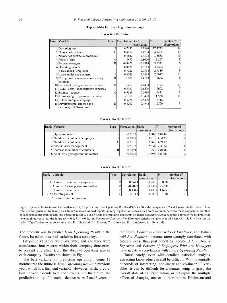
The problem was to predict Total Operating Result in the

future, based on observed variables for a company.

Fifty-nine variables were available, and variables were

transformed into zscores within their company timeseries,

to prevent any effect from the absolute operating size of

each company. Results are shown in Fig. 1.

The best variable for predicting operating income 12

months into the future is Total Operating Result in previous

year, which is a ®nancial variable. However, as the predic-

tion horizon extends to 2 and 3 years into the future, the

predictive utility of ®nancials decreases. At 2 and 3 years in

the future, Contracts Processed Per Employee, and Value-

Add Per Employee become more strongly correlated with

future success than past operating income. Administrative

Expenses and Percent of Employees Who are Managers

have negative correlations with future Operating Result.

Unfortunately, even with detailed statistical analysis,

extracting knowledge can still be dif®cult. With potentially

hundreds of interacting, non-linear and co-linear IC vari-

ables, it can be dif®cult for a human being to grasp the

overall state of an organization, or anticipate the multiple

effects of changing one or more variables. Edvinsson and

B. Kitts et al. / Expert Systems with Applications 20 (2001) 35±5036

Fig. 1. Top variables (in terms of strength of effect) for predicting Total Operating Result (MSEK) at Skandia companies 1, 2 and 3 years into the future. These

results were generated by taking data from Skandia's Annual reports, joining together variables which were common between these companies, and then

collecting together training data and operating result 1, 2 and 3 years after training data sample is taken. Operating Result becomes unpredictive for predicting

revenue three years into the future �F � 0:1; R � 20:1�; but Number of Contracts Per Employee remains reliable over all years �F . 3; R . 0:4�: (in the

tables ªTypeº refers to the focus area with F� Financial, P� Process, C� Customer, E� Employee, R� Renewal).

Malone recognized this problem, and wrote of the need for a

way to collect these variables together into a form which

could be easily comprehended by a human being:

Somehow, then, all of these regions must be

pulled together into an overall format ¼. what

is needed in Intellectual Capital is a map that

captures all of the value of an enterprise, color-

coded so that one can quickly ascertain the quality

of the topology Ð where there are swamps and

lush forests, mountains and deserts. (Edvinsson &

Malone, 1997, pp. 67)

The ideal method of presentation should make it possible

to see such interactions, and allow human beings to quickly

comprehend what was happening within the company. This

article describes a new method that we believe ful®lls these

requirements. The technique extracts knowledge from

historical IC measurements, and represents them using a

knowledge map. The map shows the ®tness of a company

for different combinations of parameters, and supports inter-

active what-if analysis.

3. The promise of mapping

IC Mapping is designed to provide a visual tool that

uni®es the operating state of the company, and is easy to

use. The method is based on a body of well-known statis-

tical methods including multi-dimensional scaling, which

was pioneered by Kruskal (1978), Shepard (1974), Torger-

son (1958), Young (1987, 1998), and others; and non-para-

metric estimation investigated by Girosi, Jones and Poggio

(1993) among others.

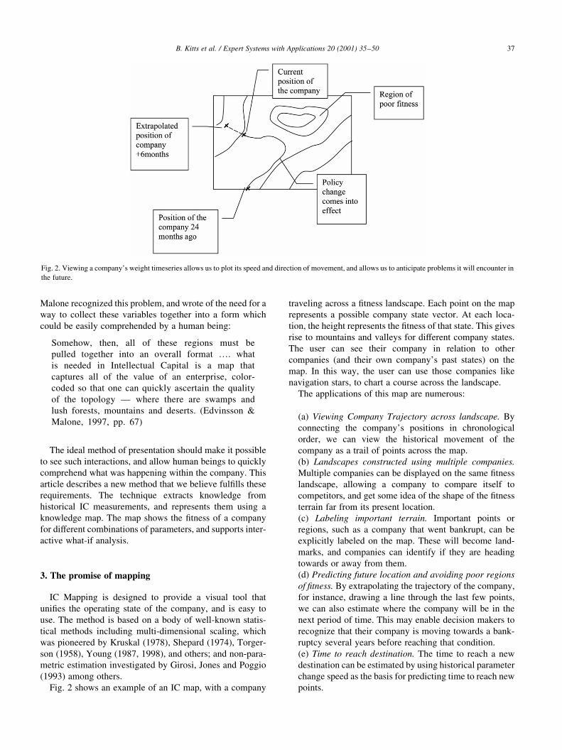
Fig. 2 shows an example of an IC map, with a company

traveling across a ®tness landscape. Each point on the map

represents a possible company state vector. At each loca-

tion, the height represents the ®tness of that state. This gives

rise to mountains and valleys for different company states.

The user can see their company in relation to other

companies (and their own company's past states) on the

map. In this way, the user can use those companies like

navigation stars, to chart a course across the landscape.

The applications of this map are numerous:

(a) Viewing Company Trajectory across landscape. By

connecting the company's positions in chronological

order, we can view the historical movement of the

company as a trail of points across the map.

(b) Landscapes constructed using multiple companies.

Multiple companies can be displayed on the same ®tness

landscape, allowing a company to compare itself to

competitors, and get some idea of the shape of the ®tness

terrain far from its present location.

(c) Labeling important terrain. Important points or

regions, such as a company that went bankrupt, can be

explicitly labeled on the map. These will become land-

marks, and companies can identify if they are heading

towards or away from them.

(d) Predicting future location and avoiding poor regions

of ®tness. By extrapolating the trajectory of the company,

for instance, drawing a line through the last few points,

we can also estimate where the company will be in the

next period of time. This may enable decision makers to

recognize that their company is moving towards a bank-

ruptcy several years before reaching that condition.

(e) Time to reach destination. The time to reach a new

destination can be estimated by using historical parameter

change speed as the basis for predicting time to reach new

points.

B. Kitts et al. / Expert Systems with Applications 20 (2001) 35±50 37

Fig. 2. Viewing a company's weight timeseries allows us to plot its speed and direction of movement, and allows us to anticipate problems it will encounter in

the future.

(f) What-if analysis. We can interactively test the

outcome of making changes to one or more variables,

for instance, doubling the administration budget. After a

change is made, the updated position of the company can

be displayed on the landscape.

(g) Means±ends analysis. We can look for desirable

regions, and ®nd out the variable settings that underlie

that point, and are required to reach that location. Means±

ends analysis involves building an inverse model

mapping 2D surface position back to high-dimensional

IC vector.

(h) Path planning. Optimal trajectories can be calculated

by ®nding a path that maximizes ®tness between source

and destination, constrained by time allowed to reach

destination; in other words, maximizing the path integral,

bounded by a particular time allowed. The path planning

model can be made more elaborate by estimating

ªcurrentsº or natural interactions between variables

which will tend to move parameters in particular direc-

tions. Exploitation of drift currents might enable positions

to be reached faster at lower cost.

4. Building a map

The mapping process consists of two stages. The ®rst task

is to project the high dimensional company data into two

dimensions. The second is to add a ®tness variable as a third

dimension, and then interpolate between those points to

predict the shape of the ®tness surface connecting these

regions.

4.1. Step 1: multidimensional scaling

The objective of MDS is to represent high dimensional

data in 1±3 dimensions so that a human being can visually

understand the data. Because its not possible to directly

visualize more than three spatial dimensions, the method

focuses instead on preserving the inter-point distances of

the high-dimensional data. MDS therefore ®nds a set of

points in two dimensions which have distances as close as

possible to the inter-point distances in the high dimensional

space. If the method succeeds, then a human looking at the

points will be able to correctly judge that their present posi-

tion is ªvery different fromº some other point on the map,

and that judgement will also hold in the difference between

the two high-dimensional vectors (Norusis, 1997; Young &

Hamer, 1987; Young, 1998)

The axes of the new, low-dimensional space are not intui-

tively interpretable since each is constructed out of conve-

nience to retain the distance relationships. The only features

that make sense in the new landscape are the concepts of

ªmore similar to-ª or ªmore different from-ª x, where x is a

known case. Thus, this is somewhat analogous to a paper

topographic map, where landmarks are shown (the other

data points), and the user can see how distant these land-

marks are to his or her position.

To generate the new coordinates one has to minimize the

error between the distance between points in the orignal data

dij, and in the 2D representation 2ij. This ªerrorº is known as

stress, and was introduced by Kruskal and Shepard (Krus-

kal, 1978; Shepard, 1974):

Stress�d; 2� �Xn

i

Xn

j

�dij 2 2ij�222

ij

�1�

Many different algorithms can be used to minimize stress

(Kohonen, 1996; Young, 1987). In our own work we have

found that the Torgerson Projection (Torgerson, 1958)

followed by several iterations of a Nelder±Mead simplex

optimization (Betteridge, Wade & Howard, 1985; Nelder &

Mead, 1965) can generate very good results. Other empirical

comparisons of MDS algorithms can be found in Li (1993),

Li, de Vel & Coomans (1995) and Duch and Naud (1998).

4.1.1. Torgerson's classic metric MDS algorithm

Torgerson showed in the 1950s that if a distance matrix

was double centered such that, given a raw distance matrix

B, the double-centered matrix D is de®ned as

dij � 20:5�b2ij 2 b2

i´ 2 b2´j 1 b2

´´� �2�then the following relationship held:

D � XXT �3�This meant that any distance matrix could be changed

into a coordinate matrix by taking a matrix square root of

D. To derive a set of coordinates with less than the original

number of dimensions, singular value decomposition could

be used to identify the two largest eigenvalues, and then

reconstruct coordinates with only the two largest eigenva-

lues. This will result in coordinates which capture as much

of the variance as possible in the selection of coordinates.

USU T � D �4�

X � US 1=2 �5�

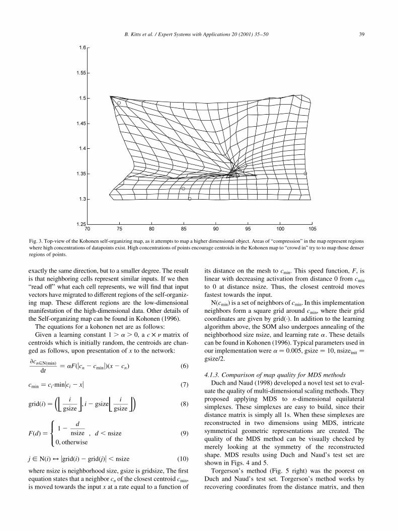
4.1.2. Self-organizing map

Self-organizing maps are a new technique originally formu-

lated as a model of human visual cortex (von der Malsburg,

1973). The self-organizing map consists of an array of neurons

which each store a prototype of the input they most prefer

(their tuning curve). As input comes in, the cell with the proto-

type vector most similar to the input ªwinsº, and adjusts its

prototype to be more similar to the input. Each cell also has a

ªneighborhoodº of other cells. This can be seen in the ®gures

below (Figs. 3 and 8) and as a mesh connecting the cells. When

all the cells start off, they are in a perfect grid. Over time this

grid will deform to ªmapº the input.

Whenever one neuron adjusts its vector, the other cells in

the neighborhood also have their prototypes adjusted in


exactly the same direction, but to a smaller degree. The result

is that neighboring cells represent similar inputs. If we then

ªread offº what each cell represents, we will ®nd that input

vectors have migrated to different regions of the self-organiz-

ing map. These different regions are the low-dimensional

manifestation of the high-dimensional data. Other details of

the Self-organizing map can be found in Kohonen (1996).

The equations for a kohonen net are as follows:

Given a learning constant 1 . a . 0; a c £ n matrix of

centroids which is initially random, the centroids are chan-

ged as follows, upon presentation of x to the network:

2cn[N�min�dt

� aF�ucn 2 cminu��x 2 cn� �6�

cmin � ci´minuci 2 xu �7�

grid�i� � i

gsize

� �; i 2 gsize

i

gsize

� �� 8�

F�d� � 1 2d

nsize

0; otherwise

8><>: ; d , nsize �9�

j [ N�i� $ ugrid�i�2 grid�j�u , nsize �10�where nsize is neighborhood size, gsize is gridsize, The ®rst

equation states that a neighbor cn of the closest centroid cmin,

is moved towards the input x at a rate equal to a function of

its distance on the mesh to cmin. This speed function, F, is

linear with decreasing activation from distance 0 from cmin

to 0 at distance nsize. Thus, the closest centroid moves

fastest towards the input.

N(cmin) is a set of neighbors of cmin. In this implementation

neighbors form a square grid around cmin, where their grid

coordinates are given by grid(´). In addition to the learning

algorithm above, the SOM also undergoes annealing of the

neighborhood size nsize, and learning rate a . These details

can be found in Kohonen (1996). Typical parameters used in

our implementation were a � 0:005; gsize � 10; nsizeinit �gsize=2:

4.1.3. Comparison of map quality for MDS methods

Duch and Naud (1998) developed a novel test set to eval-

uate the quality of multi-dimensional scaling methods. They

proposed applying MDS to n-dimensional equilateral

simplexes. These simplexes are easy to build, since their

distance matrix is simply all 1s. When these simplexes are

reconstructed in two dimensions using MDS, intricate

symmetrical geometric representations are created. The

quality of the MDS method can be visually checked by

merely looking at the symmetry of the reconstructed

shape. MDS results using Duch and Naud's test set are

shown in Figs. 4 and 5.

Torgerson's method (Fig. 5 right) was the poorest on

Duch and Naud's test set. Torgerson's method works by

recovering coordinates from the distance matrix, and then


Fig. 3. Top-view of the Kohonen self-organizing map, as it attempts to map a higher dimensional object. Areas of ªcompressionº in the map represent regions

where high concentrations of datapoints exist. High concentrations of points encourage centroids in the Kohonen map to ªcrowd inº try to to map those denser

regions of points.

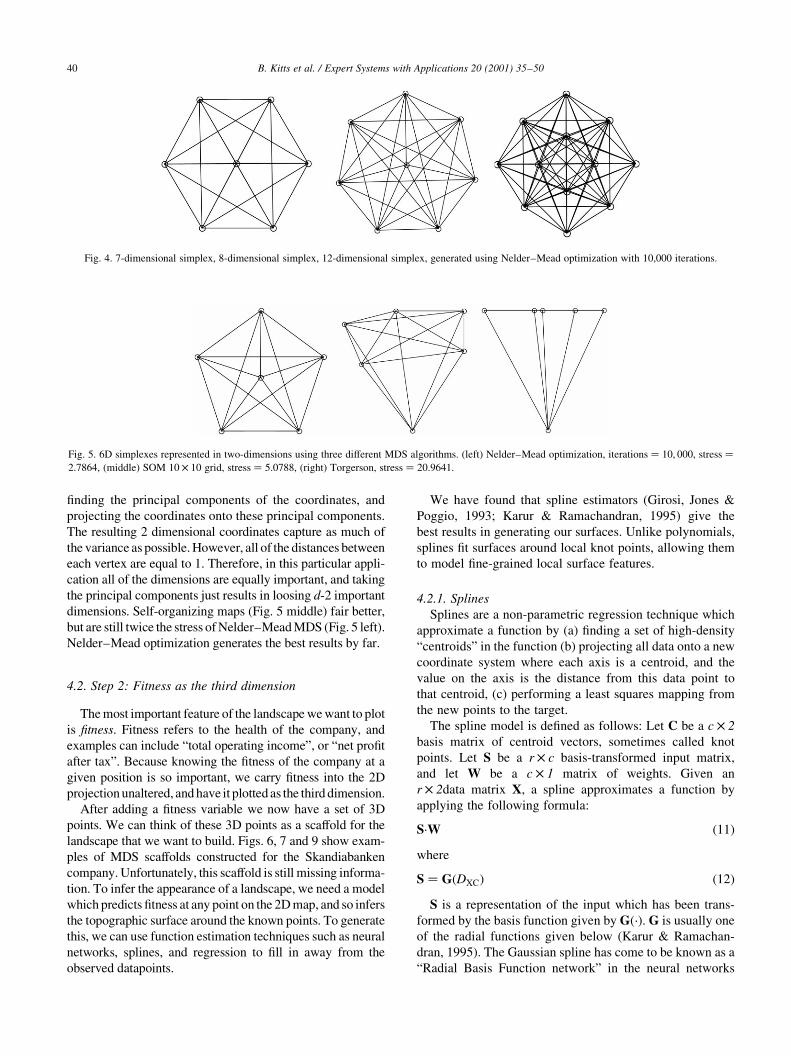
®nding the principal components of the coordinates, and

projecting the coordinates onto these principal components.

The resulting 2 dimensional coordinates capture as much of

the variance as possible. However, all of the distances between

each vertex are equal to 1. Therefore, in this particular appli-

cation all of the dimensions are equally important, and taking

the principal components just results in loosing d-2 important

dimensions. Self-organizing maps (Fig. 5 middle) fair better,

but are still twice the stress of Nelder±Mead MDS (Fig. 5 left).

Nelder±Mead optimization generates the best results by far.

4.2. Step 2: Fitness as the third dimension

The most important feature of the landscape we want to plot

is ®tness. Fitness refers to the health of the company, and

examples can include ªtotal operating incomeº, or ªnet pro®t

after taxº. Because knowing the ®tness of the company at a

given position is so important, we carry ®tness into the 2D

projection unaltered, and have it plotted as the third dimension.

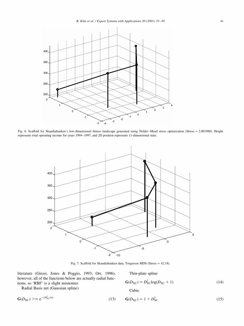
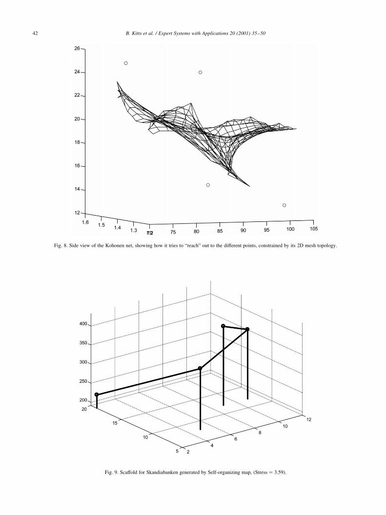
After adding a ®tness variable we now have a set of 3D

points. We can think of these 3D points as a scaffold for the

landscape that we want to build. Figs. 6, 7 and 9 show exam-

ples of MDS scaffolds constructed for the Skandiabanken

company. Unfortunately, this scaffold is still missing informa-

tion. To infer the appearance of a landscape, we need a model

which predicts ®tness at any point on the 2D map, and so infers

the topographic surface around the known points. To generate

this, we can use function estimation techniques such as neural

networks, splines, and regression to ®ll in away from the

observed datapoints.

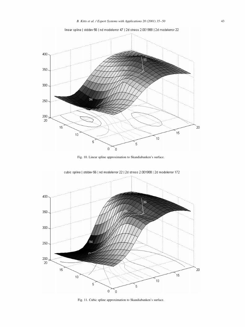
We have found that spline estimators (Girosi, Jones &

Poggio, 1993; Karur & Ramachandran, 1995) give the

best results in generating our surfaces. Unlike polynomials,

splines ®t surfaces around local knot points, allowing them

to model ®ne-grained local surface features.

4.2.1. Splines

Splines are a non-parametric regression technique which

approximate a function by (a) ®nding a set of high-density

ªcentroidsº in the function (b) projecting all data onto a new

coordinate system where each axis is a centroid, and the

value on the axis is the distance from this data point to

that centroid, (c) performing a least squares mapping from

the new points to the target.

The spline model is de®ned as follows: Let C be a c £ 2

basis matrix of centroid vectors, sometimes called knot

points. Let S be a r £ c basis-transformed input matrix,

and let W be a c £ 1 matrix of weights. Given an

r £ 2data matrix X, a spline approximates a function by

applying the following formula:

S´W �11�where

S � G�DXC� �12�S is a representation of the input which has been trans-

formed by the basis function given by G(´). G is usually one

of the radial functions given below (Karur & Ramachan-

dran, 1995). The Gaussian spline has come to be known as a

ªRadial Basis Function networkº in the neural networks


Fig. 4. 7-dimensional simplex, 8-dimensional simplex, 12-dimensional simplex, generated using Nelder±Mead optimization with 10,000 iterations.

Fig. 5. 6D simplexes represented in two-dimensions using three different MDS algorithms. (left) Nelder±Mead optimization, iterations � 10; 000; stress �2:7864; (middle) SOM 10 £ 10 grid, stress � 5:0788; (right) Torgerson, stress � 20:9641:

literature (Girosi, Jones & Poggio, 1993; Orr, 1996),

however, all of the functions below are actually radial func-

tions, so `RBF' is a slight misnomer.

Radial Basis net (Gaussian spline)

G�DXC� .� e2�D2XC=s� �13�

Thin-plate spline

G�DXC� � D2XClog�DXC 1 1� �14�

Cubic

G�DXC� � 1 1 D3XC �15�


Fig. 6. Scaffold for Skandiabanken's low-dimensional ®tness landscape generated using Nelder±Mead stress optimization �Stress � 2:001988�: Height

represents total operating income for years 1994±1997, and 2D position represents 11-dimensional state.

Fig. 7. Scaffold for Skandiabanken data, Torgerson MDS �Stress � 42:18�:


Fig. 9. Scaffold for Skandiabanken generated by Self-organizing map, �Stress � 3:59�:

Fig. 8. Side view of the Kohonen net, showing how it tries to ªreachº out to the different points, constrained by its 2D mesh topology.


Fig. 11. Cubic spline approximation to Skandiabanken's surface.

Fig. 10. Linear spline approximation to Skandiabanken's surface.

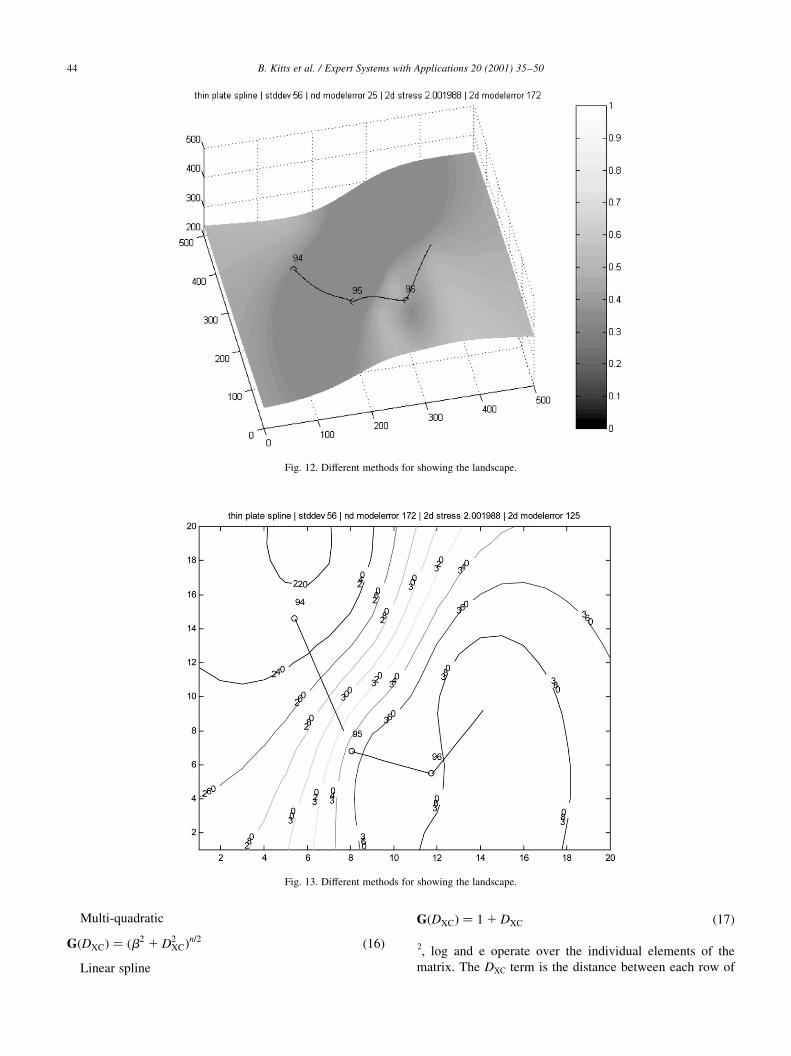
Multi-quadratic

G�DXC� � �b2 1 D2XC�n=2 �16�

Linear spline

G�DXC� � 1 1 DXC �17�2, log and e operate over the individual elements of the

matrix. The DXC term is the distance between each row of


Fig. 13. Different methods for showing the landscape.

Fig. 12. Different methods for showing the landscape.


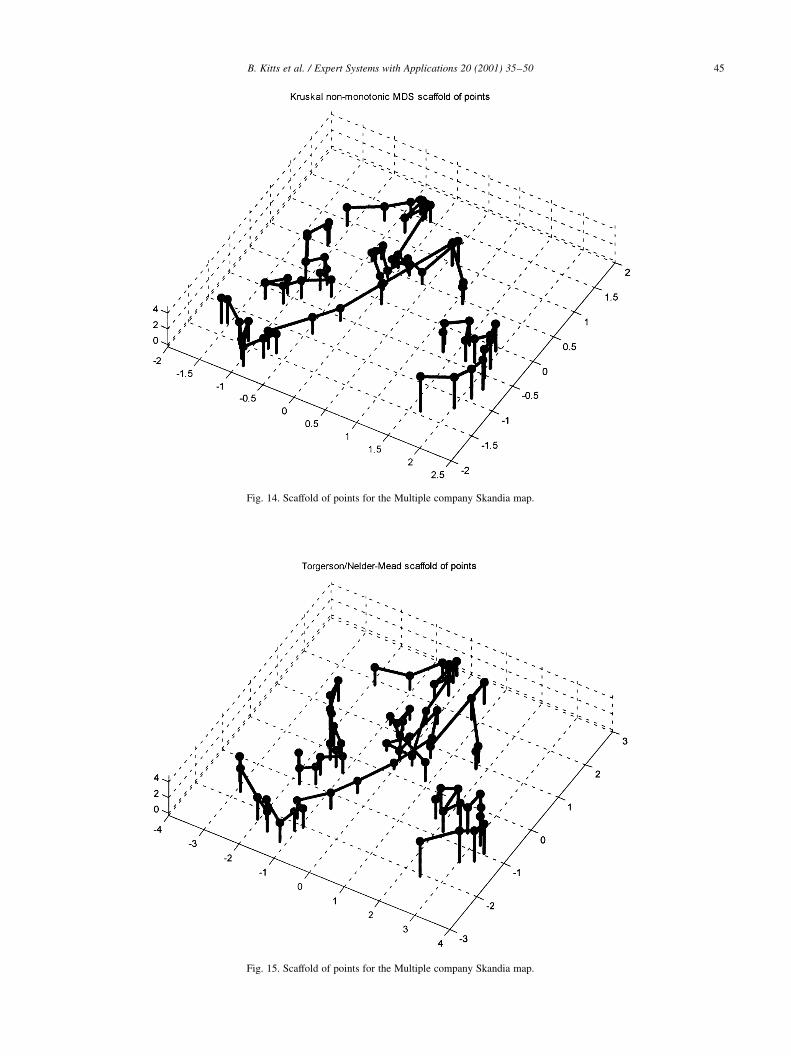
Fig. 14. Scaffold of points for the Multiple company Skandia map.

Fig. 15. Scaffold of points for the Multiple company Skandia map.

X and the centroid points, C. Therefore, S can be thought of

as a dot product between the input and the bases, normalized

by the size of both X and C, and then put through a non-

linear transform.

DXC � 22C´XT 1 CTC 1 XTX �18�

We also ensured that all activations were normalized such

that

;rXv

v�1

Srv � 1 �19�

where v is the number of centroids. Normalization meant

that extrapolation outside the range of datapoints did not

result in overly large or small values. Instead, the surface

far from the points converges to the average of the datapoint

values. Given the small number of datapoints, we also set

the rows of C to be equal to the existing datapoints, so each

centroid was a datapoint.

Examples of linear, cubic, and thin-plate spline surface

approximation for Skandiabanken's ®tness landscape are

shown in Figs. 10±13.

5. Adding details to the map

Once the ®nal landscape is built, a variety of details

can be added to the basic map. Some observations

may coincide with an important event, for instance

ªcompetitor came onto the marketº, ªcompany went

publicº, and so on. We can carry these labels from

our high dimensional data into our 2D map, and

display them on the map. This can help the user navi-

gate the map.

Finally if the trajectory across the landscape is itself

observed once every 12 months, the points in-between

are not known. Since linearly connecting these points

would be assuming a linear interpolation, we have

connected points using smoothing splines to convey

less certainty as to the nature of the points in-between

the observations.

6. Time to reach destination

In the early days of navigation, ship captains used

calipers to measure the distance between locations on


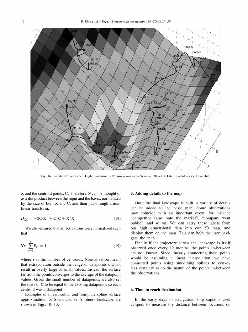
Fig. 16. Skandia IC landscape. Height dimension is IC. Am�American Skandia, UK�UK Life, In� Intercaser, Di� Dial.

their map. They would measure speed by dropping buoys and

using a stopwatch to calculate speed across water, a process

known as ªheaving the logº (Bowditch, 1826). Using these

tools, ships could estimate the time to reach their destination.

On IC Maps the same calculation can be performed. A

simple method is to compare the parameter difference

needed to reach the new location, with the company's

historical parameter change speed per year:

DT�C; a; b� � Absolute parameter change

Average parameter change per year

DT�C; a; b� �

Xi

uai 2 biu

1

T 2 1

XT 2 1

t�1

Xi

uxCt11; i 2 xCt; iu

where a and b are the points we want to travel between, C

the company which will be traveling, xti a historical

company value for variable i at time t, and T the total

number of historical observations.

This assumes that a company is able to change each of its

parameters equally well, and is limited by an inherent

magnitude of change per year. Other methods for estimating

time can also be used; for instance it is also possible to take

into account historical interactions between the IC variables

to estimate ªcurrentsº that might increase or decrease time

to reach destination.

7. Experiment 1: Skandia ®tness landscape

In order to test whether IC Mapping could be used for real

companies, we selected four companies from the large

multinational Skandia investment group to be projected

together onto a ®tness map. The companies were Intercaser,

Dial, American, and UK Life. Intercaser, American, and UK

Life are the Spanish, American, and UK branches of Skan-

dia Investment ®rm. Dial is a telemarketing insurance

company which operates throughout Nordic countries.


Fig. 17. Top±down view of Skandia IC map.

Fig. 18. Distances on the Skandia IC Map versus the high-dimensional

points. Distances on the IC map are very close to their high-dimensional

counterparts, with a correlation of 0.91. Thus map positions a good repre-

sentation of company differences.

The state of each company was ®xed with a vector of ®ve

variables Ð one from each IC focus area. The ®ve variables

used were total operating result, number of customers,

number of employees, contracts processed per employee,

and % new contracts. Missing values were estimated

using stepwise timeseries imputation. The variables were

transformed into Z-scores. Ideally the ®tness metric for

the companies should be predictive of future earnings poten-

tial, and we could have developed a regression equation for

this purpose. However, for the purposes of the test, we

decided to let ®tness be a linear standardized sum of the

IC focus areas.

The multi-dimensional scaling was performed using a

Torgerson projection and ®ne-tuned via Nelder±Mead

minimization. Optimizations took a couple of hours on

a 200 MHz Pentium computer, and resulted in a stress

of approximately 17.32 with correlation between original

and projected distances equal to 0.91 (Figs. 18 and 19).

Tests using other methods achieved similar stresses and

2D point positions, lending con®dence to the landscape

produced (Figs. 14 and 15 shows scaffolds generated

using different methods).

The ®nal Skandia map is shown in Figs. 16 and 17. The

map shows American Skandia rapidly zigzagging across the

landscape, and increasing its Intellectual Capital. Intercaser

is also doing well, and is headed out of the map area, while

Link is maintaining steady ®tness. UK Life, however, is

losing Intellectual Capital and slipping down the slope.

7.1. Application

American Skandia has experienced sharp growth in the

1990s, rising from a small company of 94 employees, to a

successful investment company employing over 599. The

older UK Life, has experienced slower growth during the

1990s. Should UK Life adopt operating practices more like

those of American Skandia?

The main difference between UK Life in 97 and 93 are

drops in Customer and Renewal capital (Fig. 20). UK Life

would need to increase its number of customers and rate of

new contracts in order to get back to the position it occupied

in 1993.

American Skandia 1997 meanwhile, has a lower level of

overall ®tness, and reaching Am97 would take 2.8 years,

whilst UK93 is 2.2 years away. As a result, management

should conclude that it is better for UK Life to return to oper-

ating practices similar to 1993 by increasing expenditure on


Fig. 19. Prediction accuracy of the Skandia ®tness surface calculated using hold-out validation. The accuracy of using a 5-dimensional vector to predict ®tness

was also tested, to gauge the degradation in accuracy due to the low-dimensional map. The test revealed that accuracy did degrade, although the map

predictions of ®tness were still strongly correlated to actual values.

Fig. 20. Difference between UK97 and UK93.

customer satisfaction and running programs to acquire new

customers (Fig. 21).

8. Experiment 2: UN Map

Each year the World Bank Organization publishes a

document titled The World Development Indicators Report,

1998, in which statistics for 140 countries over 35 years are

listed. From the electronic version of this report, we

obtained 64 variables with low percentages of missing

values, and chose 44 countries for analysis. For purposes

of the experiment, we have chosen to use an extremely

simple indicator of the well-being, the ªlife expectancyº

for citizens in these countries.

The resulting landscape is shown in Fig. 22. The map is


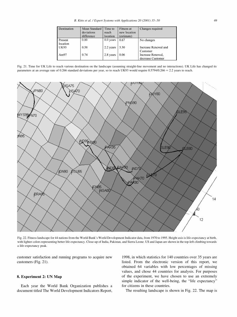
Fig. 21. Time for UK Life to reach various destination on the landscape (assuming straight-line movement and no interactions). UK Life has changed its

parameters at an average rate of 0.266 standard deviations per year, so to reach UK93 would require 0:5794=0:266 � 2:2 years to reach.

Fig. 22. Fitness landscape for 44 nations from the World Bank's World Development Indicator data, from 1970 to 1995. Height axis is life-expectancy at birth,

with lighter colors representing better life expectancy. Close-up of India, Pakistan, and Sierra Leone. US and Japan are shown in the top-left climbing towards

a life-expectancy peak.

stretched along one dimension, with developing countries at

one end, and developed countries at the other. This stretch-

ing could be caused because many of the variables are co-

linear, and correlated with the same underlying cause, such

as gross domestic product.

One of the nice surprises about this landscape, is that many

developing countries have progressed up the landscape in the

35-year measurement period. Papua New Guinea has moved

from a life expectancy of 46±58. India and Pakistan have also

both improved their life expectancies from 49 to 63 and 49 to

64, respectively. India and Pakistan have similar positions on

the map (Fig. 22). Most of these countries, including the

United States and Japan, are traveling ªupº the landscape in

a direction of greater life expectancy.

The country with poorest life expectancy on earth in 1998

was Sierra Leone. Sierra Leone brie¯y appears to be getting

better from 1980±1990, however, by 1995, the direction of

movement is at tangent to other countries who are marching up

the life-expectancy landscape, and into territory no other

nation has traversed. This is probably a bad sign!

9. Conclusion

We have developed a method for organizing company

knowledge into a highly interpretable form; a 3D map.

The map metaphor seamlessly conveys acquired knowledge

such as predictions of company ®tness at untested para-

meters (shown on the map as the landscape around known

points); forecasted position in the next six months; effect of

changing variables; and time and cost required to reach new

states such as higher ®tness regions.

The work presented here is merely a beginning for the

development of this method. For example, error estimates

have not been displayed on the map. Error arises from the

MDS procedure, surface interpolation, and the rate of defor-

mation of the landscape itself (so that more distant areas are

likely to change before the company reaches them). Error

estimates could be added to the landscape as a transparent

mist that covers the landscape above and below, with a

thicker mist indicating higher uncertainty.

References

Betteridge, D., Wade, A., & Howard, A. (1985). Re¯ections on the modi-

®ed simplex II. Talanta, 32 (8B), 723±734.

Bowditch, N., (1826). The new American practical navigator (6th ed.),

Edmund L. Blunt, New York. http://www.iws.net/wier/logline.html.

Comparative Civilian Labor Force Statistics, Ten Countries, 1959±1999.

US Department of Labor, Bureau of Labor Statistics, Of®ce of Produc-

tivity and Technology, 27 May 1999. http://stats.bls.gov/¯sdata.htm.

Duch, W., & Naud, A. (1998). Simplexes, multi-dimensional scaling and

self-organized mapping, Technical Report, Department of Computer

Methods, Nicholas Copernicus University, Poland. http://www.phys.u-

ni.torun.pl/kmk.

Edvinsson, L., & Malone, M. (1997). Intellectual capital, Harper.

Girosi, F., Jones, M., & Poggio, T. (1993). Priors, stabilizers and basis

functions: from regularization to radial, tensor and additive splines. AI

Memo 1430, CBCL Paper 75, http://www.ai.mit.edu/people/girosi/

home-page/memos.html.

Kaplan, R., & Norton, D. (1996). The balanced scorecard: translating

strategy into action, Harvard, MA: Harvard Business School Press.

Karlgaard, R. (1993). Rest in Peace, Book Value, Forbes ASAP, 25 Octo-

ber, p. 9.

Karur, S., & Ramachandran, P. (1995). Augmented thin plate spline

approximation in DRM. Boundary Elements Communications, 6, 55±

58 (http://wuche.wustl.edu/~karur/papers.html).

Kohonen, T. (1996). Self-organizing maps, Springer Series in Information

Sciences, vol. 30. Berlin: Springer.

Kruskal, J. (1978). Multidimensional scaling, Sage University Series.

Beverly Hills, CA: Sage University Press.

Li, S. (1993). Dimensionality reduction using the self-organizing map,

Honours Thesis, James Cook University, North Queensland. http://

www.cs.jcu.edu.au/ftp/pub/.

Li, S., de Vel, O., & Coomans, D. (1995). Comparative performance analy-

sis of non-linear dimensionality reduction methods. Proceedings of the

Fifth International Workshop on Arti®cial Intelligence and Statistics,

Fort Lauderdale, FL. http://www.cs.jcu.edu.au/ftp/pub/techreports/94-

8.ps.gz.

von der Malsburg (1973). Self-organization of orientation sensitive cells in

striate cortex. Kybernetik, 14, 85±100.

Nelder, J., & Mead, R. (1965). A simplex method for function minimiza-

tion. Computer Journal, 7, 308±313.

Norusis, M. (1997). Multidimensional scaling examples, SPSS Professional

Statistics 7.5 User Manual.

Orr, M. (1996). Introduction to radial basis function networks, Centre for

Cognitive Science, University of Edinburgh, 2 Buccleuch Place, Edin-

burgh EH8 9LW, Scotland, http://www.cns.ed.ac.uk/people/mark/intro/

intro.html.

Shepard, R. (1974). Representation of structure in similarity data. Psycho-

metrika, 39, 373±421.

Torgerson, W. (1958). Multidimensional scaling. In P. Colgan, Quantita-

tive ethology (pp. 175±217). New York: Wiley.

World Development Indicators 1998 CD-ROM, The World Bank, ISBN: 0-

8213-4375-0, http://www.worldbank.org/html/extpb/wdi99.htm.

Young, F., & Hamer, R. (1987). Multidimensional scaling: history, theory

and applications, Hillsdale, NJ: Lawrence Erlbaum.

Young, F. (1998). Multidimensional scaling, Lecture notes, Univer-

sity of North Carolina, http://forrest.psych.unc.edu/teaching/p230/

p230.html.


Intellectual capital: from intangible assets to fitness landscapes

Documents

Transcript of Intellectual capital: from intangible assets to fitness landscapes