Integrating short turning and deadheading in the optimization ...
16
Integrating short turning and deadheading in the optimization of transit services Cristián E. Cortés a,⇑ , Sergio Jara-Díaz a , Alejandro Tirachini b a Civil Engineering Department, Universidad de Chile, Blanco Encalada 2002, Santiago, Chile b Institute of Transport and Logistics Studies (ITLS), The University of Sydney Business School, The University of Sydney, NSW 2006, Australia article info Article history: Received 2 July 2009 Received in revised form 11 January 2011 Accepted 2 February 2011 Keywords: Deadheading Short turning Public transport Users cost Operator cost abstract Urban transit demand exhibits peaks in time and space, which can be efficiently served by means of different fleets, increasing frequencies in those groups of stops with larger pas- senger inflow. In this paper we develop a model that combines short turning and dead- heading in an integrated strategy for a single transit line, where the optimization variables are both of a continuous and discrete nature: frequencies within and outside the high demand zone, vehicle capacities, and those stations where the strategy begins and ends. We show that closed solutions can be obtained for frequencies in some cases, which resembles the classical ‘‘square root rule’’. Unlike the existing literature that com- pares different strategies with a given normal operation (no strategy – single frequency), we use an optimized base case, in order to assess the potential benefits of the integrated strategy on a fair basis. We found that the integrated strategy can be justified in many cases with mixed load patterns, where unbalances within and between directions are observed. In general, the short turning strategy may yield large benefits in terms of total cost reduc- tions, while low benefits are associated with deadheading, due to the extra cost of running empty vehicles in some sections. Ó 2011 Elsevier Ltd. All rights reserved. 1. Introduction In urban systems, the demand for public transport generally presents different shapes in space and time. This poses dif- ferent design problems in order to provide a reasonable level of service to users. A major difficulty is how to deal with both spatial and temporal peak periods of demand in their daily operation, which results in inefficient schemes when the unbal- ances are improperly treated by offering the same bus supply along the entire route and during a long period. If we focus the analysis on the spatial dimension, the specialized literature shows several strategies to better assign the available fleet by increasing the frequency on the most demanded route segments in order to adjust the demand to the effective capacity of buses. Among the spatial-type of fleet assignment strategies, the most relevant operational schemes proposed in recent years are short turning (Furth, 1987; Delle Site and Filippi, 1998; Ceder, 1989, 2003b), deadheading (Furth, 1985; Eberlein et al., 1998, 1999; Fu et al., 2003) and expressing (Jordan and Turnquist, 1979; Furth, 1986; Eberlein et al., 1999). Short turning consists in selecting a portion of the fleet to serve short cycles on those route sections exhibiting high demand; deadheading consists in increasing the frequency in the most demanded direction by allowing some of the buses to skip the stops in the low de- mand direction; and express services operate just stopping at a subset of the normal service stops. Studies and applications of such strategies suggest that the concentration of demand on one direction would motivate the use of deadheading, while 0965-8564/$ - see front matter Ó 2011 Elsevier Ltd. All rights reserved. doi:10.1016/j.tra.2011.02.002 ⇑ Corresponding author. Tel.: +56 2 9784380; fax: +56 2 6894206. E-mail addresses: [email protected] (C.E. Cortés), [email protected] (S. Jara-Díaz), [email protected] (A. Tirachini). Transportation Research Part A 45 (2011) 419–434 Contents lists available at ScienceDirect Transportation Research Part A journal homepage: www.elsevier.com/locate/tra
-
Upload
khangminh22 -
Category
Documents
-
view
2 -
download
0
Transcript of Integrating short turning and deadheading in the optimization ...
Transportation Research Part A 45 (2011) 419–434
Contents lists available at ScienceDirect
Transportation Research Part A
journal homepage: www.elsevier .com/locate / t ra
Integrating short turning and deadheading in the optimization oftransit services
Cristián E. Cortés a,⇑, Sergio Jara-Díaz a, Alejandro Tirachini b
a Civil Engineering Department, Universidad de Chile, Blanco Encalada 2002, Santiago, Chileb Institute of Transport and Logistics Studies (ITLS), The University of Sydney Business School, The University of Sydney, NSW 2006, Australia
a r t i c l e i n f o
Article history:Received 2 July 2009Received in revised form 11 January 2011Accepted 2 February 2011
Keywords:DeadheadingShort turningPublic transportUsers costOperator cost
0965-8564/$ - see front matter � 2011 Elsevier Ltddoi:10.1016/j.tra.2011.02.002
⇑ Corresponding author. Tel.: +56 2 9784380; faxE-mail addresses: [email protected] (C.E. Cort
a b s t r a c t
Urban transit demand exhibits peaks in time and space, which can be efficiently served bymeans of different fleets, increasing frequencies in those groups of stops with larger pas-senger inflow. In this paper we develop a model that combines short turning and dead-heading in an integrated strategy for a single transit line, where the optimizationvariables are both of a continuous and discrete nature: frequencies within and outsidethe high demand zone, vehicle capacities, and those stations where the strategy beginsand ends. We show that closed solutions can be obtained for frequencies in some cases,which resembles the classical ‘‘square root rule’’. Unlike the existing literature that com-pares different strategies with a given normal operation (no strategy – single frequency),we use an optimized base case, in order to assess the potential benefits of the integratedstrategy on a fair basis. We found that the integrated strategy can be justified in many caseswith mixed load patterns, where unbalances within and between directions are observed.In general, the short turning strategy may yield large benefits in terms of total cost reduc-tions, while low benefits are associated with deadheading, due to the extra cost of runningempty vehicles in some sections.
� 2011 Elsevier Ltd. All rights reserved.
1. Introduction
In urban systems, the demand for public transport generally presents different shapes in space and time. This poses dif-ferent design problems in order to provide a reasonable level of service to users. A major difficulty is how to deal with bothspatial and temporal peak periods of demand in their daily operation, which results in inefficient schemes when the unbal-ances are improperly treated by offering the same bus supply along the entire route and during a long period. If we focus theanalysis on the spatial dimension, the specialized literature shows several strategies to better assign the available fleet byincreasing the frequency on the most demanded route segments in order to adjust the demand to the effective capacityof buses.
Among the spatial-type of fleet assignment strategies, the most relevant operational schemes proposed in recent years areshort turning (Furth, 1987; Delle Site and Filippi, 1998; Ceder, 1989, 2003b), deadheading (Furth, 1985; Eberlein et al., 1998,1999; Fu et al., 2003) and expressing (Jordan and Turnquist, 1979; Furth, 1986; Eberlein et al., 1999). Short turning consistsin selecting a portion of the fleet to serve short cycles on those route sections exhibiting high demand; deadheading consistsin increasing the frequency in the most demanded direction by allowing some of the buses to skip the stops in the low de-mand direction; and express services operate just stopping at a subset of the normal service stops. Studies and applicationsof such strategies suggest that the concentration of demand on one direction would motivate the use of deadheading, while
. All rights reserved.
: +56 2 6894206.és), [email protected] (S. Jara-Díaz), [email protected] (A. Tirachini).
420 C.E. Cortés et al. / Transportation Research Part A 45 (2011) 419–434
the concentration of journeys over a specific sector of the route probably would require the implementation of a short turn.There are cases, however, in which the demand configuration indeed presents unbalances but does not suggest a priori thetype of strategy to follow in order to optimize the use of the fleet. In some portions of the route a short turning strategy couldbe useful, while in the next segment either expressing or deadheading might be better. In these cases a mixed or integratedstrategy is worth exploring.
Let us consider a linear bus corridor. Particularly interesting are those cases where in one direction the demand is largerthan in the other and, besides, local demand concentrations in different sectors of the route are observed. Therefore, if thesemixed patterns appeared it would not be clear which strategy is better in order to efficiently distribute the bus supply alongthe entire corridor. Our research group has analyzed both strategies individually, namely short turning and deadheading,based on a microeconomic approach to model public transport systems, accounting for all costs involved, users’ and oper-ators’, and considering station-to-station demand information (Tirachini and Cortés, 2006; Tirachini et al., 2011). Under thesame microeconomic principles, in this paper we develop a new model that integrates short turning and deadheading for alinear bus line and a single period of operation, where the variables to be optimized are the frequencies within and outsidethe high demand zone and vehicle sizes (continuous variables), and the stations where the strategy begins and ends (discretevariables). In the proposed model, we clearly identify all components of both users and operators costs – whose sum is min-imized – to investigate how the integrated strategy affects both parties.
Unlike the existing literature that compares different strategies with a given normal operation or base case (no strategy isapplied, resulting in a single frequency along the entire route), in our model the normal operation scheme and the integratedstrategy are both optimized, i.e. aimed at minimizing total costs, to perform the comparison on a fair basis. The new model –which is formulated using spatially disaggregated demand information – allows us to better characterize the effects of theintegrated strategy on the different agents of the system (users differentiated by origin–destination and operators). This per-mits the identification at a tactical level of those demand patterns that are good candidates for the combined strategy. Undersome assumptions, optimal frequencies in cases with and without the strategy are analytically obtained, which permits thestudy of the influence of the parameters involved in the final solution. In other cases, results are obtained numerically.
The remainder of this section contains a brief review of the literature regarding the most interesting formulations andstudies related to deadheading, expressing and short turning, within an operation planning context. The integrated strategyis formally defined in Section 2, together with the analytical formulation of the problem, highlighting the conditions underwhich the hybrid scheme recovers the basic strategies, namely deadheading and short turning. In Section 3 some numericalexamples are shown and Section 4 concludes.
Deadheading as a pre-planned strategy has been studied by a limited number of authors. Furth (1985) proposes to applythis concept to corridors with unbalanced demand between directions (in which deadheaded buses skip the entire low de-mand direction). According to his findings, the strategy reduces both the operator cost – by means of savings in fleet size –and the user cost – by reducing the waiting time of passengers. Three objective functions are explored: the minimization ofthe fleet size by imposing a maximum headway condition into the formulation; the minimization of waiting times for a fixedfleet size; and the sum of operator and users costs. Ceder and Stern (1981) and Ceder (2003a, 2004) consider the insertion ofan empty trip between two terminals (deadheading trip) in order to reduce the fleet size subject to satisfying a given scheduleof bus departures from the terminals. Eberlein et al. (1998, 1999) and Fu et al. (2003) consider a different problem: dead-headed vehicles start their trip empty until a station to be determined and, from that stop, these buses start their normalservice until the end of their route. Under this scheme, vehicles save time and reduce the headway with respect to thebus ahead. Both works formulate mixed integer non-linear problems, quadratic in the continuous variables (headway be-tween vehicles). Eberlein et al. (1998) only accounts for the waiting time in the objective function, obtaining a very complexformulation. They then resolve a simplified version of their original problem. On the other hand, Fu et al. (2003) assume thatif a vehicle is going to skip stations, necessarily the next bus has to serve the entire route, which simplifies the problem andprovides a minimum level of service for passengers waiting at skipped stations. The authors minimize the costs associatedwith both waiting an in-vehicle travel time. We also find interesting studies of expressing (Jordan and Turnquist, 1979;Furth, 1986; Leiva et al., 2010), in which a public transport corridor is divided into sectors, where some vehicles serve se-lected segments or bus stops while others serve the entire corridor.
Short turning has been studied by many authors using different assumptions and solution methodologies. Furth (1987)focuses on the efficient use of short turning, constraining the frequency of vehicles performing the short turn (hereafter, fleetB) to be a multiple n of the frequency of those vehicles serving the entire route (hereafter, fleet A), which is equivalent toassume a scheduled operation scheme; the parameter n is known as the ‘‘scheduling mode’’. The author formulates threeoptimization problems, pursuing the minimization of the fleet size (through the maximization of vehicle headway), the min-imization of passenger waiting times for a fixed fleet size, and a combination of both. The optimization considers as exog-enous the number of short turns, the limit stations for the short turn and the bus capacities. By using an aggregated demandmodel, Ceder (1989, 2003b) proposes a two-stage optimization approach. In a first stage, the fleet size is minimized for agiven demand level while in a second stage, the number of trips using the short turn is minimized to reduce the effect ofthe strategy on passenger times. Vijayaraghavan and Anantharmaiah (1995) propose the insertion of express services as wellas short turns for the service of some trips pursuing the reduction of fleet size. The authors report benefits when applyingtheir approach in terms of fleet and crew utilization and users’ performance in terms of passenger travel times. Delle Site andFilippi (1998) develop a multi-period short turning using both elastic and inelastic demand and extending the work by Furth(1987) to the case of Poisson bus arrivals. They formulate a maximization of social benefits (elastic demand case), and a
C.E. Cortés et al. / Transportation Research Part A 45 (2011) 419–434 421
minimization of user plus operator costs (inelastic demand case). The decision variables are frequency, fare and limit stationsof the short turn (start and end) plus the capacity of vehicles (both treated parametrically). They show with an example thatthe strategy turns out to be beneficial only if demand patterns exhibit pronounced peaks.
We can finally mention some efforts to formulate problems combining several strategies, like the works by Eberlein(1995) and Eberlein et al. (1999), who formulate a real-time control model encompassing holding, deadheading and express-ing, aimed at solving problems such as bunching or service disruptions, i.e. as a tool to make real-time operational decisionsaccording to the conditions of the system. Bus holding seems to be the best strategy. With a similar real-time purpose, Fuet al. (2003) also find through simulation that the applications of a combined version of holding and deadheading turnsout to be more effective than the application of each strategy separately, in terms of reduction of waiting and in-vehicletimes. Note that this research is not aimed at an ex-ante design of the system, which is the objective of ours.
2. Characterization, modeling and optimization of the integrated strategy
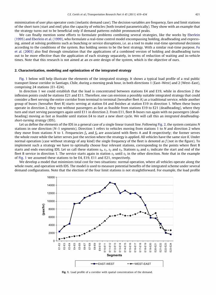
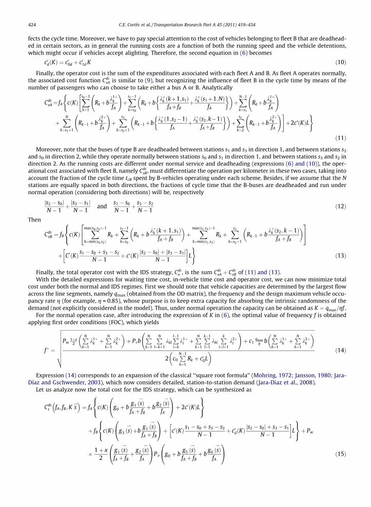
Fig. 1 below will help illustrate the elements of the integrated strategy. It shows a typical load profile of a real publictransport linear corridor in Santiago, Chile, during a morning peak hour, in both directions 1 (East–West) and 2 (West–East),comprising 24 stations (E1–E24).
In direction 1 we could establish that the load is concentrated between stations E4 and E19, while in direction 2 theinflexion points could be stations E21 and E11. Therefore, one can envision a possibly suitable integrated strategy that couldconsider a fleet serving the entire corridor from terminal to terminal (hereafter fleet A) as a traditional service, while anothergroup of buses (hereafter fleet B) starts serving at station E4 and finishes at station E19 in direction 1. When these busesoperate in direction 2, they run without passengers as fast as feasible from stations E19 to E21 (deadheading), where theyturn and start serving passengers again until E11 in direction 2. From E11, fleet B-buses run again with no passengers (dead-heading) moving as fast as feasible until station E4 to start a new short cycle. We will call this an integrated deadheading-short-turning strategy (IDS).
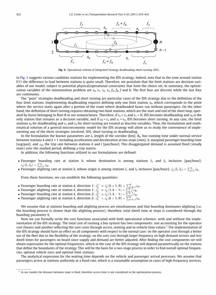
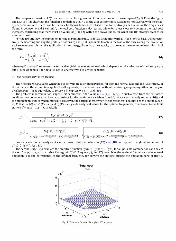
Let us define the elements of the IDS in a general case of a single linear transit line. Following Fig. 2, the system contains Nstations in one direction (N–1 segments). Direction 1 refers to vehicles moving from stations 1 to N and direction 2 whenthey move from stations N to 1. Frequencies fA and fB are associated with fleets A and B respectively; the former servesthe whole route while the latter serves just the section where the strategy is applied. All vehicles have the same size K. Undernormal operation (case without strategy of any kind) the single frequency of the fleet is denoted as f (not in the figure). Toimplement such a strategy we have to optimally choose four relevant stations, corresponding to the points where fleet Bstarts and ends executing IDS. Let us call these stations s0, s1, s2 and s3. Stations s0 and s1 indicate the start and end of thefleet B service in direction 1. The service starts again in station s3 until s2 in the other direction. Note that in the exampleof Fig. 1 we assumed these stations to be E4, E19, E11 and E21, respectively.
We develop a model that minimizes total cost for two situations: normal operation, where all vehicles operate along thewhole route, and operation with IDS. The model is used to measure potential benefits of the integrated scheme under severaldemand configurations. Note that the election of the four limit stations is not straightforward. For example, the load profile
0
2000
4000
6000
8000
10000
12000
14000
16000
E1-E
2
E2-E
3
E3-E
4
E4-E
5
E5-E
6
E6-E
7
E7-E
8
E8-E
9
E9-E
10
E10-
E11
E11-
E12
E12-
E13
E13-
E14
E14-
E15
E15-
E16
E16-
E17
E17-
E18
E18-
E19
E19-
E20
E20-
E21
E21-
E22
E22-
E23
E23-
E24
(pax
/hr)
Segments
EAST-WEST WEST-EAST
Fig. 1. Load profile of a corridor with spatial concentration of the demand.
N
1N −
1
2
0s
Bf
1sA Bf f+Af
Af
AfAf
Af
3s2sA Bf f+
N
1N −
1
2
0s
Bf
1sA Bf f+Af
Af
AfAf
Af
3s2sA Bf f+
Fig. 2. Operational scheme of Integrated Strategy deadheading-short-turning (IDS).
422 C.E. Cortés et al. / Transportation Research Part A 45 (2011) 419–434
in Fig. 1 suggests various candidate stations for implementing the IDS strategy. Indeed, note that in the zone around stationE11 the difference in load between stations is quite small. Therefore, we postulate that the limit stations are decision vari-ables of our model, subject to potential physical/operational constraints that limit the choice set. In summary, the optimi-zation variables of the minimization problem are s0, s1, s2, s3, fA, fB, f and K. The first four are discrete while the last fourare continuous.
The ‘‘pure’’ strategies deadheading and short turning are particular cases of the IDS strategy due to the definition of thefour limit stations. Implementing deadheading requires defining only one limit station, s0, which corresponds to the pointwhere the service starts again after a portion of the route where deadheaded buses run without passengers. On the otherhand, the definition of short turning requires obtaining two limit stations, which are the start and end of the short loop, oper-ated by buses belonging to fleet B in our nomenclature. Therefore, if s2 = s3 and s1 = N, IDS becomes deadheading and s0 is theonly station that remains as a decision variable, and if s0 = s2 and s1 = s3, IDS becomes short turning. In any case, the limitstations s0 for deadheading and s1 and s2 for short turning are treated as discrete variables. Then, the formulation and math-ematical solution of a general microeconomic model for the IDS strategy will allow us to study the convenience of imple-menting any of the three strategies involved: IDS, short turning or deadheading.
In the formulation the known parameters are L, length of the corridor [km]; Rk, bus running time under normal servicebetween stations k and k + 1 including acceleration and deceleration at bus stops [min]; b, marginal passenger boarding time[seg/pax]; and kkl, the trip rate between stations k and l [pax/hour]. This disaggregated demand is assumed fixed (steadystate) over the studied period, defining a trip matrix.
In addition, the following functions utilized in our formulations are defined:
� Passenger boarding rate at station k, whose destination is among stations l1 and l2 inclusive [pax/hour]:kþk ðl1; l2Þ ¼
Pl2l¼l1
kkl.� Passenger alighting rate at station k, whose origin is among stations l1 and l2 inclusive [pax/hour]: k�k ðl1; l2Þ ¼
Pl2l¼l1
klk.
From these functions, we can establish the following quantities:
� Passenger boarding rate at station k, direction 1: k1þk � kþk ðkþ 1;NÞ ¼
PNl¼kþ1kkl.
� Passenger alighting rate at station k, direction 1: k1�k � k�k ð1; k� 1Þ ¼
Pk�1l¼1 klk.
� Passenger boarding rate at station k, direction 2: k2þk � kþk ð1; k� 1Þ ¼
Pk�1l¼1 kkl.
� Passenger alighting rate at station k, direction 2: k2�k ¼ k�k ðkþ 1;NÞ ¼
PNl¼kþ1klk.
We assume that at stations boarding and alighting process are simultaneous and that boarding dominates alighting (i.e.the boarding process is slower than the alighting process); therefore, total dwell time at stops is considered through theboarding parameter b.
Now we can formally write the cost functions associated with both operational schemes: with and without the imple-mentation of the IDS strategy. The total cost of running a bus system has two components: one accounting for the operatorcost (buses) and another reflecting the user costs through access, waiting and in-vehicle time values.1 The implementation ofthe IDS strategy should have an effect on all components with respect to the normal case: on the operator cost through a betteruse of the fleet due to the flexibility of the strategy; on the user cost through larger frequency on high demand sectors and lessdwell times for passengers on board since supply and demand are better adjusted. After finding the cost components we willobtain expressions for the optimal frequencies, which in the case of the IDS strategy will depend parametrically on the stationsthat define the boundaries of the strategy. This will be the basis for a two-stage process in order to find overall optimal frequen-cies, optimal vehicle sizes and optimal limit stations.
The analytical expression for the waiting time depends on the vehicle and passenger arrival processes. We assume thatpassengers arrive at stations uniformly at a fixed rate, which is a reasonable assumption in cases of high frequency services.
1 In our models the distance between stops is fixed, therefore access time is not considered in the optimization process.
C.E. Cortés et al. / Transportation Research Part A 45 (2011) 419–434 423
Buses are assumed to arrive either Poisson or regularly spaced; the average waiting time at each station is equal to the entireheadway in the former case and to half of the headway in the second. This can be handled generally using an auxiliary binaryvariable x that is equal to 1 in the Poisson case and 0 in the regularly spaced case. The waiting time cost (Cw) is the totalwaiting time multiplied by the waiting time value (Pw). Recalling that the headway is the inverse of frequency and that totalridership is the sum of the demand in all stations, Cw for the normal operation is:
Cw ¼ Pw1þ x
2
XN
k¼1
k1þk
fþXN
k¼1
k2þk
f
( )ð1Þ
When the IDS strategy is applied, users observe different frequencies depending on their position along the route. Passen-gers traveling between stations s0 and s1 in direction 1, or between s2 and s3 in direction 2 observe a frequency fA + fB,whereas the other passengers only board vehicles that belong to fleet A (i.e., we assume that users do not transfer betweenvehicles A and B). Then, the waiting time cost after applying the IDS strategy, namely Cds
w , can be calculated as
Cdsw ¼ Pw
1þ x2
Xs0�1
k¼1
k1þk
fAþXs1�1
k¼s0
kþk ðkþ 1; s1ÞfA þ fB
þ kþk ðs1 þ 1;NÞfA
� �þXN
k¼s1
k1þk
fAþXN
k¼s3þ1
k2þk
fA
(
þXs3
k¼s2þ1
kþk ð1; s2 � 1ÞfA
þ kþk ðs2; k� 1ÞfA þ fB
� �þXs2
k¼1
k2þk
fA
)ð2Þ
Regarding the in-vehicle time cost (Cv) for the normal operation, the travel time tkl between stations k and l (not neces-sarily consecutive) is calculated as
Pl�1
i¼kRi þ b
k1þif
� �if k < l
Pki¼lþ1
Ri�1 þ bk2þ
if
� �if l < k
8>>><>>>:
ð3Þ
Multiplying expression (3) by the demand rate between k and l, kkl, and adding over all OD pairs, the total in-vehicle timecost Cv can be obtained as follows:
Cv ¼ PvXN
k¼1
XN
l¼kþ1
Xl�1
i¼k
Ri þ bk1þ
i
f
!" #kkl þ
XN
k¼1
Xk�1
l¼1
Xk
i¼lþ1
Ri�1 þ bk2þ
i
f
!" #kkl
( )ð4Þ
where Pv represents the in-vehicle time value. The analytical formulation for Cv when the IDS strategy is applied turns outvery complicated, since a trip may encompass sections where users board vehicles at rates kþi =fA or kþi =ðfA þ fBÞ, depending onthe case. Synthetically, the in-vehicle time cost for the case with strategy Cds
v can be expressed as:
Cdsm ¼ Pm 2
XN�1
k¼1
Rk þ bg5ð~sÞ
fA þ fBþ b
g6ð~sÞfA
( )ð5Þ
The set of functions gið~sÞ are defined and explained in Appendix A. They are second order expressions of the trip rates kkl
specified in terms of the limit stations~s ¼ ðs0; s1; s2; s3Þ.Regarding the operator cost Co, we consider two components (temporal and spatial). The former includes items such as
personnel costs (crew), while the latter comprises running costs, such as fuel consumption, lubricants, tires, and mainte-nance. Following Jansson (1980) and Oldfield and Bly (1988), the unit operator costs are expressed as a linear function ofthe vehicle capacity K, where c (K) is the vehicle–hour cost (expressed in $/vh) and c0 (K) corresponds to the vehicle–kilome-ter cost (expressed in $/vkm). Analytically
cðKÞ ¼ c0 þ c1K c0ðKÞ ¼ c00 þ c01K ð6Þ
Co ¼ cðKÞF þ c0ðKÞvF ð7Þ
where v is the bus system commercial speed (including dwell times) and F represents the fleet size. F is computed as theproduct of the frequency and the cycle time tc (considering not only the running time but also the time spent in transferringpassengers at stations), that is F = ftc. Thus, (7) can be rewritten as a function of tc, f and L (length of the corridor) as shown in(8) and (9) for the case of normal operationCo ¼ cðKÞftc þ 2c0ðKÞfL ð8Þ
Co ¼ f cðKÞXN�1
k¼1
Rk þ bk1þ
k
f
!þXN
k¼2
Rk�1 þ bk2þ
k
f
!" #þ 2c0ðKÞL
( )ð9Þ
The operator cost after applying the IDS strategy is analyzed separately for fleets A and B. In the case of fleet A, we have toconsider two groups of passengers, boarding the buses at rates either kþi =fA or kþi =ðfA þ fBÞ depending on the case, which af-
424 C.E. Cortés et al. / Transportation Research Part A 45 (2011) 419–434
fects the cycle time. Moreover, we have to pay special attention to the cost of vehicles belonging to fleet B that are deadhead-ed in certain sectors, as in general the running costs are a function of both the running speed and the vehicle detentions,which might occur if vehicles accept alighting. Therefore, the second equation in (6) becomes
c0dðKÞ ¼ c00d þ c01d K ð10Þ
Finally, the operator cost is the sum of the expenditures associated with each fleet A and B. As fleet A operates normally,the associated cost function Cds
oA is similar to (9), but recognizing the influence of fleet B in the cycle time by means of thenumber of passengers who can choose to take either a bus A or B. Analytically
CdsoA¼ fA cðKÞ
Xs0�1
k¼1
Rkþbk1þ
k
fA
!þXs1�1
k¼s0
Rkþbkþk ðkþ1;s1Þ
fAþ fBþkþk ðs1þ1;NÞ
fA
� �� �þXN�1
k¼s1
Rkþbk1þ
k
fA
!"(
þXN
k¼s3þ1
Rk�1þbk2þ
k
fA
!þXs3
k¼s2þ1
Rk�1þbkþk ð1;s2�1Þ
fAþkþk ðs2;k�1Þ
fAþ fB
� �� �þXs2
k¼2
Rk�1þbk2þ
k
fA
!#þ2c’ðKÞL
)
ð11Þ
Moreover, note that the buses of type B are deadheaded between stations s1 and s3 in direction 1, and between stations s2
and s0 in direction 2, while they operate normally between stations s0 and s1 in direction 1, and between stations s3 and s2 indirection 2. As the running costs are different under normal service and deadheading (expressions (6) and (10)), the oper-ational cost associated with fleet B, namely Cds
oB, must differentiate the operation per kilometer in these two cases, taking intoaccount the fraction of the cycle time tcB spent by B-vehicles operating under each scheme. Besides, if we assume that the Nstations are equally spaced in both directions, the fractions of cycle time that the B-buses are deadheaded and run undernormal operation (considering both directions) will be, respectively
js2 � s0jN � 1
þ js3 � s1jN � 1
ands1 � s0
N � 1þ s3 � s2
N � 1ð12Þ
Then 2 38
CdsoB ¼ fB cðKÞXmaxðs0 ;s2Þ�1
k¼minðs0 ;s2ÞRk þ
Xs1�1
k¼s0
Rk þ bkþk ðkþ 1; s1Þ
fA þ fB
� �þ
Xmaxðs1 ;s3Þ�1
k¼minðs1 ;s3ÞRk þ
Xs3
k¼s2þ1
Rk�1 þ bkþk ðs2; k� 1Þ
fA þ fB
� �4 5<:
þ C0ðKÞ s1 � s0 þ s3 � s2
N � 1þ c0ðKÞ js2 � s0j þ js3 � s1j
N � 1
� L
)ð13Þ
Finally, the total operator cost with the IDS strategy, Cdso , is the sum Cds
oA þ CdsoB of (11) and (13).
With the detailed expressions for waiting time cost, in-vehicle time cost and operator cost, we can now minimize totalcost under both the normal and IDS regimes. First we should note that vehicle capacities are determined by the largest flowacross the line segments, namely qmax (obtained from the OD matrix), the frequency and the design maximum vehicle occu-pancy rate g (for example, g = 0.85), whose purpose is to keep extra capacity for absorbing the intrinsic randomness of thedemand (not explicitly considered in the model). Thus, under normal operation the capacity can be obtained as K ¼ qmax=gf .
For the normal operation case, after introducing the expression of K in (6), the optimal value of frequency f is obtainedapplying first order conditions (FOC), which yields
f � ¼
ffiffiffiffiffiffiffiffiffiffiffiffiffiffiffiffiffiffiffiffiffiffiffiffiffiffiffiffiffiffiffiffiffiffiffiffiffiffiffiffiffiffiffiffiffiffiffiffiffiffiffiffiffiffiffiffiffiffiffiffiffiffiffiffiffiffiffiffiffiffiffiffiffiffiffiffiffiffiffiffiffiffiffiffiffiffiffiffiffiffiffiffiffiffiffiffiffiffiffiffiffiffiffiffiffiffiffiffiffiffiffiffiffiffiffiffiffiffiffiffiffiffiffiffiffiffiffiffiffiffiffiffiffiffiffiffiffiffiffiffiffiffiffiffiffiffiffiffiffiffiffiffiffiffiffiffiffiffiffiffiffiffiffiffiffiffiffiffiffiffiffiffiffiffiffiffiffiffiffiffiffiffiffiffiffiffiffiffiffiffiffiffiffiffiffiffiffiffiffiffiffiffiffiffiffiffiffiffiffiffiffiffiffiPw
1þx2
PNk¼1
k1þk þ
PNk¼1
k2þk
� �þ Pmb
PNk¼1
PNl¼kþ1
kklPl�1
i¼kk1þ
i þPNk¼1
Pk�1
l¼1kkl
Pki¼lþ1
k2þi
!þ c1
qmaxg b
PNk¼1
k1þk þ
PNk¼1
k2þk
� �
2 c0PN�1
k¼1Rk þ c00L
� �
vuuuuuuut ð14Þ
Expression (14) corresponds to an expansion of the classical ‘‘square root formula’’ (Mohring, 1972; Jansson, 1980; Jara-Díaz and Gschwender, 2003), which now considers detailed, station-to-station demand (Jara-Diaz et al., 2008).
Let us analyze now the total cost for the IDS strategy, which can be synthesized as
Cdst fA; fB;K s
!� �¼ fA cðKÞ g0 þ b
g1 ðsÞ!
fA þ fBþ b
g2 ðsÞ!
fA
0@
1Aþ 2c0ðKÞL
8<:
9=;
þ fB cðKÞ g3 ðsÞ!þb
g1 ðsÞ!
fA þ fB
0@
1Aþ c0ðKÞ s1 � s0 þ s3 � s2
N � 1þ c0dðKÞ
js2 � s0j þ s3 � s1
N � 1
� L
8<:
9=;þ Pw
� 1þ x2
g1 ðsÞ!
fA þ fBþ g2 ðsÞ
!
fA
0@
1APv g0 þ b
g5 ðsÞ!
fA þ fBþ b
g6 ðsÞ!
fA
0@
1A ð15Þ
C.E. Cortés et al. / Transportation Research Part A 45 (2011) 419–434 425
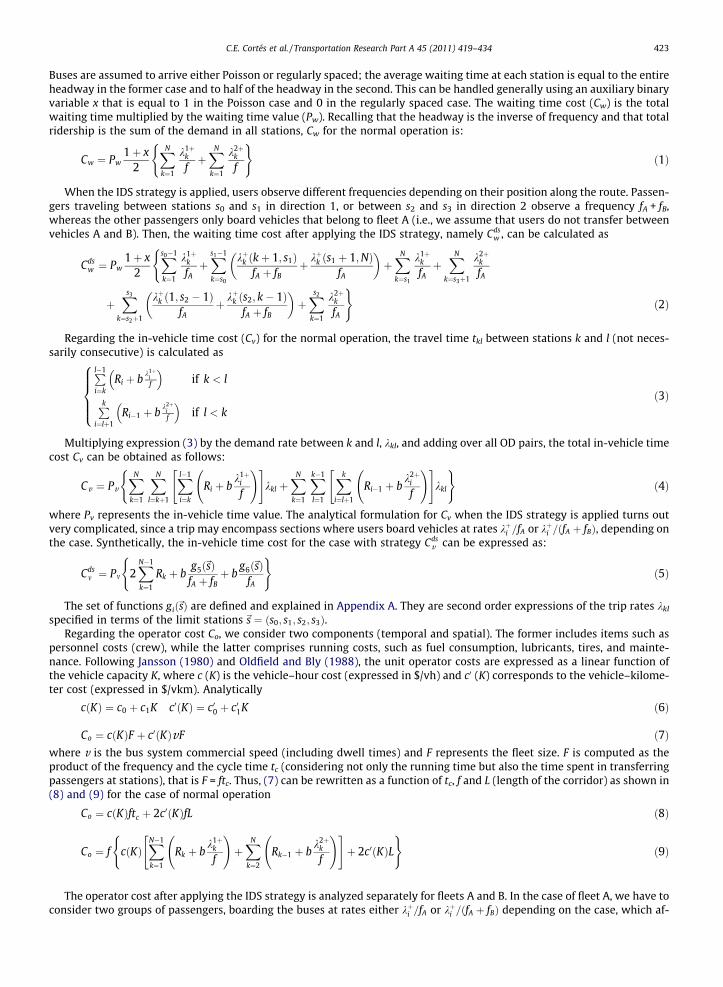
The complex expression of Cdst can be visualized for a given set of limit stations as in the example of Fig. 3. From the figure
and Eq. (15), it is clear that the function is undefined at fA = 0 as the user cost for those passengers not favored with the strat-egy becomes infinite (there is no bus service for them). Besides, we observe that for relatively small values of the frequencies(fA and fB between 0 and 1 veh/min), the total cost function is decreasing, while for values close to 3 veh/min the total costincreases, concluding that there must be values of f �A and f �B within the drawn range, for which the IDS strategy reaches itsminimum cost.
For the IDS strategy the expression for the maximum load K is not as straightforward as in the normal case. Using recur-sively the boarding and alighting rates at stations kþk and k�k , it is possible to obtain the load of the buses along their route foreach segment considering the application of the strategy. From that, the capacity can be set as the maximum load, which is ofthe form
K ¼ 1g
r0 ðsÞ!
fAþ r1 ðsÞ
!
fA þ fB
0@
1A ð16Þ
where r0ð~sÞ and r1ð~sÞ represent the terms that yield the maximum load, which depends on the selection of stations s0, s1, s2
and s3 (see Appendix B for details). Let us analyze two bus arrival schemes.
2.1. Bus arrivals distributed Poisson
The first case we analyze is when the bus arrivals are distributed Poisson, for both the normal case and the IDS strategy. Inthe latter case, the assumption applies for all segments, i.e. those with and without the strategy (operating either normally ordeadheading). This is equivalent to set x = 1 in expressions (14) and (15).
The problem is solved in two-stages. First parametric in the value of~s ¼ ðs0; s1; s2; s3Þ. In such a case, from the first orderconditions we do not obtain closed expressions for the continuous variables f �A and f �B (since K was already set as in (16)) andthe problem must be solved numerically. However, the particular case when the operator cost does not depend on the capac-ity K, that is c (K) = c, c0 ðKÞ ¼ c00 and c0d ðKÞ ¼ c0d, yields analytical values for the optimal frequencies, conditional to the limitstations~s ¼ ðs0; s1; s2; s3Þ. Analytically
f �A ðsÞ!¼
ffiffiffiffiffiffiffiffiffiffiffiffiffiffiffiffiffiffiffiffiffiffiffiffiffiffiffiffiffiffiffiffiffiffiffiffiffiffiffiffiffiffiffiffiffiffiffiffiffiffiffiffiffiffiffiffiffiffiffiffiffiffiffiffiffiffiffiffiffiffiffiffiffiffiffiffiffiffiffiffiffiffiffiffiffiffiffiffiffiffiffiffiffiffiffiffiffiffiffiffiffiffiffiffiffiffiffiffiPwg2 ðsÞ
!þPvbg6 ðsÞ
!
cðg0 � g3 ðsÞ!Þ þ c0 2� s1�s0þs3�s2
N�1
� �L� c0d
js2�s0 jþjs3�s1 jN�1 L
vuuut ð17Þ
f �B ðsÞ!¼
ffiffiffiffiffiffiffiffiffiffiffiffiffiffiffiffiffiffiffiffiffiffiffiffiffiffiffiffiffiffiffiffiffiffiffiffiffiffiffiffiffiffiffiffiffiffiffiffiffiffiffiffiffiffiffiffiffiffiffiffiffiffiffiffiffiffiffiffiffiffiffiffiffiffiffiffiffiffiffiffiffiffiffiPwg1 ðsÞ
!þPvbg5 ðsÞ
!
cðg3 ðsÞ!þc0 s1�s0þs3�s2
N�1 Lþ c0djs2�s0 jþjs3�s1 j
N�1 L
vuuut �
ffiffiffiffiffiffiffiffiffiffiffiffiffiffiffiffiffiffiffiffiffiffiffiffiffiffiffiffiffiffiffiffiffiffiffiffiffiffiffiffiffiffiffiffiffiffiffiffiffiffiffiffiffiffiffiffiffiffiffiffiffiffiffiffiffiffiffiffiffiffiffiffiffiffiffiffiffiffiffiffiffiffiffiffiffiffiffiffiffiffiffiffiffiffiffiffiffiffiffiffiffiffiffiffiffiffiffiffiPwg2 ðsÞ
!þPvbg6 ðsÞ
!
cðg0 � g3 ðsÞ!Þ þ c0 2� s1�s0þs3�s2
N�1
� �L� c0d
js2�s0 jþjs3�s1 jN�1 L
vuuut ð18Þ
From a second order analysis, it can be proven that the values in (17) and (18) correspond to a global minimum ofCds
t ðfA; fB;~s), 8ðfA; fBÞ 2 R2þ.
The second stage is to evaluate the objective function Cdst ðf �A ð~sÞ; f �B ð~sÞ;~sÞ � �Cds
t ð~sÞ for all possible combinations and selectthe set ~s� ¼ ðs�0; s�1; s�2; s�3Þ such that ~s ¼ arg min
~sCds
t ð~sÞ Frequency f �A in (17) resembles the optimal frequency under normaloperation (14) and corresponds to the optimal frequency for serving the stations outside the operation zone of fleet B,
Total cost
fB fA
Fig. 3. Total cost function for a given IDS strategy.
426 C.E. Cortés et al. / Transportation Research Part A 45 (2011) 419–434
i.e., as if the segment between min{s0, s2} and max{s1, s3} did not exist for the calculation of the operator cost. On the contrary,the optimal frequency of the fleet B, which serves only the high demand area (between s0 and s1 in direction 1, between s2
and s3 in direction 2), is computed as the difference between the optimal frequency to serve the high demand area only (firstterm of 18) and the frequency already provided by the entire route services, f �A (second term of 18).
By observing the expression for f �B ð~sÞ, we note that if the demand favored by the strategy were small with respect to therest of the trips, that is those trips with origin and destination between s0 and s1 in direction 1, and between s2 and s3 indirection 2, it is unlikely that the strategy would be applicable, as the value of f �B ð~sÞ is reduced, even to the point of becomingnegative, in cases where the limit stations s0, s1, s2 and s3 are not properly chosen.
If the second stage (election of limit stations s�) is solved by explicit enumeration of feasible solutions, the number of op-tions to be evaluated would be N2 (N � 1)2/4, since the number of discrete variables are 4. As an example, recalling the con-ceptual (but real) example of Fig. 1, the line comprises 24 stations, which represents 76,176 possible combinations of s0, s1, s2
and s3. Nevertheless, a proper processing of the load profiles permits to considerably bind the feasible solution space. Thus,for example, observing Fig. 1, we can predict that s0 will be between E4 and E6 (three stations), s1 between E17 and E19(three stations), s2 between E11 and E7 (five stations), and s3 will be E21 as that station represents a big jump in the loadprofile. With these considerations, the number of options reduces to 45, saving computation time due to the informationprovided by the shape of the curves. Note that the particular cases of short turning or deadheading only are much easierto deal with, as they have just two and one limit stations to search for, respectively, and explicit enumeration becomes avery effective method, even for the analysis of long bus corridors (for the short turning case, see Tirachini et al., 2011).
2.2. Scheduled bus arrivals
For the case of a scheduled service, we consider x = 0 and fB = nfA, where n is the ‘‘scheduling mode’’ introduced by Furth(1987) as explained in Section 1. In this case, the vehicle capacity can be expressed as:
K ¼ 1g
r0 ðsÞ!
fAþ r1 ðsÞ
!
ðnþ 1ÞfA
24
35 ¼ 1
gfAr0 ðsÞ
!þ r1 ðsÞ
!
ðnþ 1Þ
24
35 � rmaxðn; ðsÞ
!Þ
gfAð19Þ
This expression is introduced into the total cost, leaving the cost expression as a function of n, the stations s0, s1, s2 and s3, andthe only continuous variable fA, whose optimal condition is
@Cdst
@fA¼ c0 g0 ðsÞ
!þng3 ðsÞ
!� þ 2c00Lþ nL c00
s1 � s0 þ s3 � s2
N � 1þ c00d
js2 � s0j þ js3 � s1jN � 1
�
� 1f 2A
Pwg1 ðsÞ
!
2ðnþ 1Þ þg2 ðsÞ
!
2
24
35þ Pvb
g5 ðsÞ!
nþ 1þ g6 ðsÞ
!24
35þ c1b
rmaxðn; s!Þ
g½g1 ðsÞ
!þg2 ðsÞ
!�
8<:
9=; ¼ 0 ð20Þ
Then, the optimal frequency is expressed as (21)
f �A ðn;~sÞ ¼
ffiffiffiffiffiffiffiffiffiffiffiffiffiffiffiffiffiffiffiffiffiffiffiffiffiffiffiffiffiffiffiffiffiffiffiffiffiffiffiffiffiffiffiffiffiffiffiffiffiffiffiffiffiffiffiffiffiffiffiffiffiffiffiffiffiffiffiffiffiffiffiffiffiffiffiffiffiffiffiffiffiffiffiffiffiffiffiffiffiffiffiffiffiffiffiffiffiffiffiffiffiffiffiffiffiffiffiffiffiffiffiffiffiffiffiffiffiffiffiffiffiffiffiffiffiffiffiffiffiffiffiffiffiPw
g1ð~sÞ2ðnþ1Þ þ
g2ð~sÞ2
h iþ Pvb g5ð~sÞ
ðnþ1Þ þ g6ð~sÞh i
þ c1b rmaxðn;~sÞg g1ð~sÞ þ g2ð~sÞ½ �
C0 g0ð~sÞ þ ng3ð~sÞ½ � þ 2c00; Lþ nL c00;s1�s0þs3�s2
N�1 þ js2�s0 jþjs3�s1 jN�1
h ivuuut ð21Þ
The term (21) can be evaluated in the objective function, Cdst ðf �A ðn;~sÞ;n;~sÞ � �Cds
t ðn;~sÞ. Thus, the global optimum ðn�;~s�Þ isthe one that minimizes Cds
t ðn;~sÞ, ðn�;~s�Þ ¼ arg minn;~s
Cdst ðn;~sÞ. Finally, with all these elements we can compute the capacity of
the vehicles as
K� ¼ rmaxðn�;~s�Þgf �A ðn�;~s�Þ
ð22Þ
3. Numerical applications
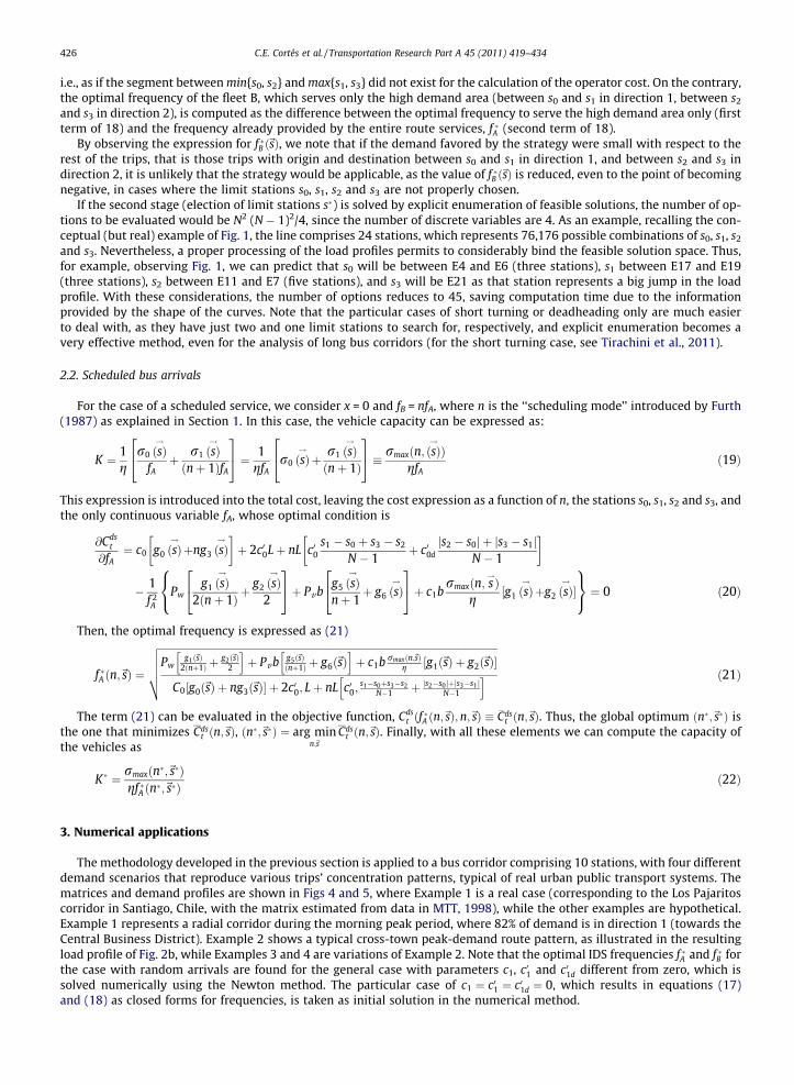
The methodology developed in the previous section is applied to a bus corridor comprising 10 stations, with four differentdemand scenarios that reproduce various trips’ concentration patterns, typical of real urban public transport systems. Thematrices and demand profiles are shown in Figs 4 and 5, where Example 1 is a real case (corresponding to the Los Pajaritoscorridor in Santiago, Chile, with the matrix estimated from data in MTT, 1998), while the other examples are hypothetical.Example 1 represents a radial corridor during the morning peak period, where 82% of demand is in direction 1 (towards theCentral Business District). Example 2 shows a typical cross-town peak-demand route pattern, as illustrated in the resultingload profile of Fig. 2b, while Examples 3 and 4 are variations of Example 2. Note that the optimal IDS frequencies f �A and f �B forthe case with random arrivals are found for the general case with parameters c1, c01 and c01d different from zero, which issolved numerically using the Newton method. The particular case of c1 ¼ c01 ¼ c01d ¼ 0, which results in equations (17)and (18) as closed forms for frequencies, is taken as initial solution in the numerical method.
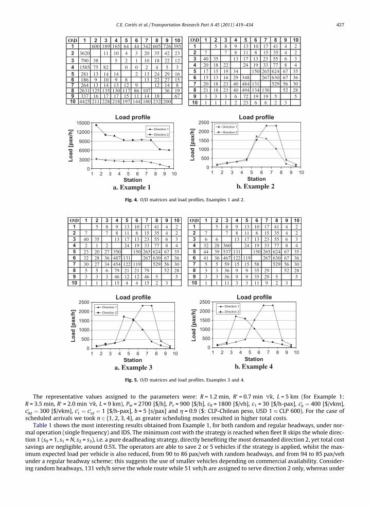
O\D 1 2 3 4 5 6 7 8 9 101 600 189 165 64 44 342 605 726 3952 3620 11 10 4 3 20 35 42 23
3 790 38 5 2 1 10 18 22 124 1585 75 82 0 0 2 4 5 35 281 13 14 14 2 13 24 29 166 186 9 10 9 8 13 22 27 157 264 13 14 13 12 9 12 14 88 2631 125 135 130 117 86 107 36 199 337 16 17 17 15 11 14 18 6710 4425 211 228 218 197 144 180 232 200
O\D 1 2 3 4 5 6 7 8 9 101 5 8 9 13 10 17 41 4 22 7 7 8 11 8 15 35 4 23 40 35 13 17 13 23 55 6 34 20 18 22 24 19 33 77 8 45 17 15 19 34 150 265 624 67 356 15 13 16 29 348 267 630 67 367 20 18 23 40 484 131 529 56 308 21 18 23 40 494 134 130 52 289 3 3 3 6 72 19 19 5 510 1 1 1 2 23 6 6 2 3
Load profile
0
500
1000
1500
2000
2500
Station
Load
[pax
/h] Direction 1
Direction 2
a. Example 1 b. Example 2
Load profile
0
3000
6000
9000
12000
15000
1 2 3 4 5 6 7 8 9 101 2 3 4 5 6 7 8 9 10Station
Load
[pax
/h] Direction 1
Direction 2
Fig. 4. O/D matrices and load profiles, Examples 1 and 2.
O\D 1 2 3 4 5 6 7 8 9 101 5 8 9 13 10 17 41 4 22 7 7 8 11 8 15 35 4 23 40 35 13 17 13 23 55 6 34 2 1 2 24 19 33 77 8 45 23 20 27 350 150 265 624 67 356 32 28 36 487 131 267 630 67 367 30 27 34 454 122 119 529 56 308 5 5 6 79 21 21 79 52 289 3 3 3 46 12 12 46 5 510 1 1 1 15 4 4 15 2 3
O\D 1 2 3 4 5 6 7 8 9 101 5 8 9 13 10 17 41 4 22 7 7 8 11 8 15 35 4 23 6 6 13 17 13 23 55 6 34 32 28 360 24 19 33 77 8 45 44 39 537 131 150 265 624 67 356 41 36 467 122 119 267 630 67 367 5 5 59 15 15 58 529 56 308 3 3 36 9 9 35 29 52 289 3 3 36 9 9 35 29 5 510 1 1 11 3 3 11 9 2 3
Load profile
0
500
1000
1500
2000
2500
1 2 3 4 5 6 7 8 9 10Station
Load
[pax
/h] Direction 1
Direction 2
Load profile
0
500
1000
1500
2000
2500
1 2 3 4 5 6 7 8 9 10Station
Load
[pax
/h] Direction 1
Direction 2
a. Example 3 b. Example 4
Fig. 5. O/D matrices and load profiles, Examples 3 and 4.
C.E. Cortés et al. / Transportation Research Part A 45 (2011) 419–434 427
The representative values assigned to the parameters were: R = 1.2 min, R0 = 0.7 min "k, L = 5 km (for Example 1:R = 3.5 min, R0 = 2.0 min "k, L = 9 km), Pw = 2700 [$/h], Pv = 900 [$/h], c0 = 1800 [$/vh], c1 = 30 [$/h-pax], c00 ¼ 400 [$/vkm],c00d ¼ 300 [$/vkm], c01 ¼ c01d ¼ 1 [$/h-pax], b = 5 [s/pax] and g = 0.9 ($: CLP-Chilean peso, USD 1 � CLP 600). For the case ofscheduled arrivals we took n 2 {1, 2, 3, 4}, as greater scheduling modes resulted in higher total costs.
Table 1 shows the most interesting results obtained from Example 1, for both random and regular headways, under nor-mal operation (single frequency) and IDS. The minimum cost with the strategy is reached when fleet B skips the whole direc-tion 1 (s0 = 1, s1 = N, s2 = s3), i.e. a pure deadheading strategy, directly benefiting the most demanded direction 2, yet total costsavings are negligible, around 0.5%. The operators are able to save 2 or 5 vehicles if the strategy is applied, whilst the max-imum expected load per vehicle is also reduced, from 90 to 86 pax/veh with random headways, and from 94 to 85 pax/vehunder a regular headway scheme; this suggests the use of smaller vehicles depending on commercial availability. Consider-ing random headways, 131 veh/h serve the whole route while 51 veh/h are assigned to serve direction 2 only, whereas under
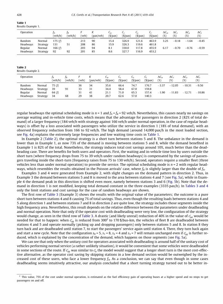
Table 1Results Example 1.
Operation fA
(veh/h)fB
(veh/h)F(veh)
K(pax/veh)
Cw
($/pax)Cv
($/pax)Co
($/pax)Ct
($/pax)DCw
(%)DCv
(%)DCo
(%)DCt
(%)
Random Normal 175 (f) 213 90 15.4 326.9 121.6 463.9 3.25 �0.18 �1.64 �0.45Headways Strategy 131 51 208 86 15.9 326.3 119.6 461.8Regular Normal 166 (f) 203 94 8.1 330.0 117.8 455.9 6.17 �0.70 �0.76 �0.59Headways Strategy 92 92 201 85 8.6 327.7 116.9 453.2
Table 2Results Example 2.
Operation fA
(veh/h)fB
(veh/h)F(veh)
K(pax/veh)
Cw
($/pax)Cv
($/pax)Co
($/pax)Ct
($/pax)DCw
(%)DCv
(%)DCo
(%)DCt
(%)
Random Normal 75 (f) 36 34 35.6 66.4 74.7 176.7 �3.37 �12.05 �10.31 �9.56Headways Strategy 39 91 33 31 34.4 58.4 67.0 159.8Regular Normal 64 (f) 31 41 21.1 71.0 65.3 157.4 �1.90 �11.83 �12.71 �10.86Headways Strategy 34 68 29 38 20.7 62.6 57.0 140.3
428 C.E. Cortés et al. / Transportation Research Part A 45 (2011) 419–434
regular headways the optimal scheduling mode is n = 1 and fA = fB = 92 veh/h. Nevertheless, this causes nearly no savings onaverage waiting and in-vehicle time costs, which means that the advantage for passengers in direction 2 (82% of total de-mand) of a larger frequency (184 veh/h with strategy against 166 veh/h under normal operation, in the case of regular head-ways) is offset by a loss associated with passengers who utilize the service in direction 1 (18% of total demand), with anobserved frequency reduction from 166 to 92 veh/h. The high demand (around 14,000 pax/h in the most loaded section,see Fig. 4a) explains the extremely large frequencies and low waiting time costs in Table 1.
In Example 2 (Table 2), the optimal strategy is a short turn between stations 5 and 8. The unbalance in the demand islower than in Example 1, as now 73% of the demand is moving between stations 5 and 8, while the demand benefited inExample 1 is 82% of the total. Nonetheless, the strategy induces total cost savings around 10%, much better than the dead-heading case. There are benefits for both users and operators. First, the waiting and in-vehicle time loss by users outside theshort turn (where frequency drops from 75 to 39 veh/h under random headways) is compensated by the savings of passen-gers traveling inside the short-turn (frequency raises from 75 to 130 veh/h). Second, operators require a smaller fleet (threevehicles less than under normal operation) to provide the service. The optimal scheduling mode is n = 2 with regular head-ways, which resembles the results obtained in the Poisson arrivals’ case, where fB is slightly larger than the double of fA.
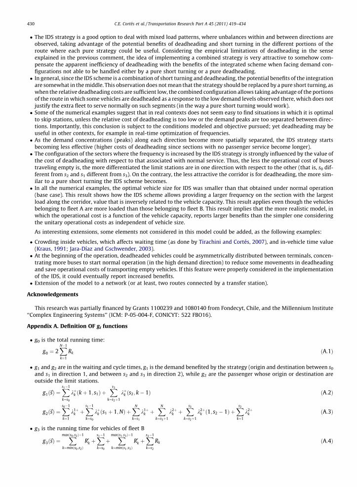
Examples 3 and 4 were generated from Example 2, with slight changes on the demand pattern in direction 2. Thus, inExample 3 the demand between stations 5 and 8 is moved to the area between stations 4 and 7 (see Fig. 5a), while in Exam-ple 4 the demand peak in this direction is shifted even more, namely between stations 3 and 6 (Fig. 5b). Note that the de-mand in direction 1 is not modified, keeping total demand constant in the three examples (3335 pax/h). In Tables 3 and 4only the limit stations and cost savings for the case of random headways are shown.
The first row of Table 3 (Example 3) shows the results with the original value of the parameters; the outcome is a pureshort turn between stations 4 and 8 causing 7% of total savings. Thus, even though the resulting loads between stations 4 and5 along direction 1 and between stations 7 and 8 in direction 2 are quite low, the strategy includes those segments inside thehigh frequency area. Nevertheless, this result depends on the relative difference between the parameters under deadheadingand normal operation. Note that only if the operator cost with deadheading were very low, the configuration of the strategywould change, as seen in the third row of Table 3. A drastic (and likely unreal) reduction of 40% in the value of c00d would beneeded for that to happen: when c00d is reduced from 3002 to 170 $/bus-km, the vehicles of fleet B are deadheaded betweenstations 4 and 5 and operate normally (picking up and dropping passengers) only between stations 5 and 8. In station 8 theyturn back and are deadheaded until station 7, to start the passengers’ service again until station 4. There, they turn back againand start a new cycle. Note that the configuration s0 = 5, s1 = 8, s2 = 4 and s3 = 7 will remain unchanged even if c00d is further re-duced, which is explained by the concentration of the demand, which happens on those segments (see Fig. 5a).
We can see that only when the unitary cost for operators associated with deadheading is around half of the unitary cost ofvehicles performing normal service (a rather unlikely situation), it would be convenient that some vehicles were deadheadedin some sections of the route. If c00d was similar to c00 the model would suggest that a longer short turn is the most cost-effec-tive alternative, as the operator cost saving by skipping stations in a low demand section would be outweighed by the in-creased cost of these users, who face a lower frequency fA. As a conclusion, we can say that even though in some casesdeadheading seems intuitively attractive, our analysis concluded that a short turning strategy turned out to be better in-
2 This value, 75% of the cost under normal operation, is estimated as the fuel efficiency gain of operating buses at a higher speed and no stops to getpassengers on and off.
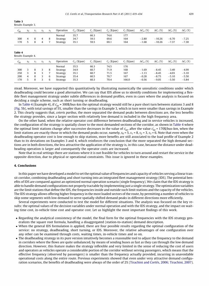
Table 3Results Example 3.
c00d s0 s1 s2 s3 Operation Cw ($/pax) Cv ($/pax) Co ($/pax) Ct ($/pax) DCw (%) DCv (%) DCo (%) DCt (%)
Normal 35.7 66.3 74.6 177300 4 8 4 8 Strategy 34.7 59.5 69.6 164 �2.80 �10.26 �6.70 �7.25170 5 8 4 7 Strategy 35.1 59.5 69.1 164 �1.68 �10.26 �7.37 �7.30
Table 4Results Example 4.
c00d s0 s1 s2 s3 Operation Cw ($/pax) Cv ($/pax) Co ($/pax) Ct ($/pax) DCw (%) DCv (%) DCo (%) DCt (%)
Normal 35.5 66.3 74.5 176300 3 8 3 8 Strategy 34.9 60.7 71.9 168 �1.69 �8.45 �3.49 �4.99250 3 8 3 7 Strategy 35.1 60.7 71.5 167 �1.13 �8.45 �4.03 �5.10200 4 8 3 6 Strategy 35.4 60.5 70.7 167 �0.28 �8.75 �5.10 �5.50170 5 8 3 6 Strategy 35.3 60.3 70.4 166.0 �0.56 �9.05 �5.50 �5.84
C.E. Cortés et al. / Transportation Research Part A 45 (2011) 419–434 429
stead. Moreover, we have supported this quantitatively by illustrating numerically the unrealistic conditions under whichdeadheading could become a good alternative. We can say that IDS allow us to identify conditions for implementing a flex-ible fleet management strategy under subtle differences in demand profiles, even in cases where the analysis is focused ondeciding a single scheme, such as short turning or deadheading.
In Table 4 (Example 4), if c00d = 300$/bus-km the optimal strategy would still be a pure short turn between stations 3 and 8(Fig. 5b), with total savings of 5%, smaller than the savings in Example 3, which in turn were smaller than savings in Example2. This clearly suggests that, ceteris paribus, the more separated the demand peaks between directions are, the less benefitsthe strategy provides, since a larger section with relatively low demand is included in the high frequency area.
On the other hand, when the relative operator cost difference between deadheading and in service vehicles is increased,the configuration of the strategy is spatially closer to the most demanded sections of the corridor, as shown in Table 4 wherethe optimal limit stations change after successive decreases in the value of c00d, after the value c00d = 170$/bus-km, when thelimit stations are exactly those in which the demand peaks occur, namely, s0 = 5, s1 = 8, s2 = 3, s3 = 6. Note that even when thedeadheading operator cost is low enough to skip stations, more benefits are still associated to the load profile of Example 2than to its deviations on Examples 3 and 4, which reinforces the conclusion that the more separated the high demand sec-tions are in both directions, the less attractive the application of the strategy is, in this case, because the distance under dead-heading operation is larger and consequently the operator costs are increased.
Note that in real settings there are stations where it is not feasible for vehicles to turn around and restart the service in theopposite direction, due to physical or operational constraints. This issue is ignored in these examples.
4. Conclusions
In this paper we have developed a model to set the optimal value of frequencies and capacity of vehicles serving a linear tran-sit corridor, combining deadheading and short turning into an integrated fleet management strategy (IDS). The potential ben-efits of IDS are compared against an optimized normal operation scenario (single frequency). We claim that the IDS strategy isable to handle demand configurations not properly tractable by implementing just a single strategy. The optimization variablesare the limit stations that define the IDS, the frequencies inside and outside such limit stations and the capacity of the vehicles.The IDS strategy allows offering higher frequency in the most loaded sectors of the route, by permitting a number of vehicles toskip some segments with low demand to serve spatially shifted demand peaks in different directions more efficiently.
Several experiments were conducted to test the model for different situations. The analysis was focused on the key re-sults: the optimal values of the decision variables under normal operation and with the IDS strategy, and the impact on wait-ing time cost, in-vehicle time cost and operator cost. Let us highlight the most important findings of this work.
� Regarding the analytical consistency of the model, the final form for the optimal frequencies with the IDS strategy gen-eralizes the square root formula, handling a disaggregated (station-to-station) demand description.� When the general IDS formulation is applied, there are four possible results regarding the optimal configuration of the
service: no strategy, deadheading, short turning, or IDS. Moreover, the relative advantages of one configuration overany other can be examined through costs, waiting times, in-vehicle times and so on.� The deadheading strategy in its pure version intuitively becomes a reasonable tool to adjust the frequency to the demand
in corridors where the flows are quite unbalanced, by means of sending buses as fast as they can through the low demanddirection. However, this feature makes the strategy inflexible and very limited in the sense of reducing the cost of usersand operators as vehicles operate a considerable portion of the corridor without serving passengers, which means that theeffective frequency (observed by passengers) is smaller than the frequency actually provided, incurring in unavoidableoperational costs along the entire route. Previous experiments showed that even under very attractive demand configu-ration scenarios, the benefits of deadheading were always of the order of 2% (Tirachini and Cortés, 2006; Tirachini, 2007).
430 C.E. Cortés et al. / Transportation Research Part A 45 (2011) 419–434
� The IDS strategy is a good option to deal with mixed load patterns, where unbalances within and between directions areobserved, taking advantage of the potential benefits of deadheading and short turning in the different portions of theroute where each pure strategy could be useful. Considering the empirical limitations of deadheading in the senseexplained in the previous comment, the idea of implementing a combined strategy is very attractive to somehow com-pensate the apparent inefficiency of deadheading with the benefits of the integrated scheme when facing demand con-figurations not able to be handled either by a pure short turning or a pure deadheading.� In general, since the IDS scheme is a combination of short turning and deadheading, the potential benefits of the integration
are somewhat in the middle. This observation does not mean that the strategy should be replaced by a pure short turning, aswhen the relative deadheading costs are sufficient low, the combined configuration allows taking advantage of the portionsof the route in which some vehicles are deadheaded as a response to the low demand levels observed there, which does notjustify the extra fleet to serve normally on such segments (in the way a pure short turning would work).� Some of the numerical examples suggest that in real contexts does not seem easy to find situations in which it is optimal
to skip stations, unless the relative cost of deadheading is too low or the demand peaks are too separated between direc-tions. Importantly, this conclusion is subject to the conditions modeled and objective pursued; yet deadheading may beuseful in other contexts, for example in real-time optimization of frequencies.� As the demand concentrations (peaks) along each direction become more spatially separated, the IDS strategy starts
becoming less effective (higher costs of deadheading since sections with no passenger service become longer).� The configuration of the sectors where the frequency is increased by the IDS strategy is strongly influenced by the value of
the cost of deadheading with respect to that associated with normal service. Thus, the less the operational cost of busestraveling empty is, the more differentiated the limit stations are in one direction with respect to the other (that is, s0 dif-ferent from s2 and s1 different from s3). On the contrary, the less attractive the corridor is for deadheading, the more sim-ilar to a pure short turning the IDS scheme becomes.� In all the numerical examples, the optimal vehicle size for IDS was smaller than that obtained under normal operation
(base case). This result shows how the IDS scheme allows providing a larger frequency on the section with the largestload along the corridor, value that is inversely related to the vehicle capacity. This result applies even though the vehiclesbelonging to fleet A are more loaded than those belonging to fleet B. This result implies that the more realistic model, inwhich the operational cost is a function of the vehicle capacity, reports larger benefits than the simpler one consideringthe unitary operational costs as independent of vehicle size.
As interesting extensions, some elements not considered in this model could be added, as the following examples:
� Crowding inside vehicles, which affects waiting time (as done by Tirachini and Cortés, 2007), and in-vehicle time value(Kraus, 1991; Jara-Díaz and Gschwender, 2003).� At the beginning of the operation, deadheaded vehicles could be asymmetrically distributed between terminals, concen-
trating more buses to start normal operation (in the high demand direction) to reduce some movements in deadheadingand save operational costs of transporting empty vehicles. If this feature were properly considered in the implementationof the IDS, it could eventually report increased benefits.� Extension of the model to a network (or at least, two routes connected by a transfer station).
Acknowledgements
This research was partially financed by Grants 1100239 and 1080140 from Fondecyt, Chile, and the Millennium Institute‘‘Complex Engineering Systems’’ (ICM: P-05-004-F, CONICYT: 522 FBO16).
Appendix A. Definition OF gi functions
� g0 is the total running time:
g0 ¼ 2XN�1
k¼1
Rk ðA:1Þ
� g1 and g2 are in the waiting and cycle times, g1 is the demand benefited by the strategy (origin and destination between s0
and s1 in direction 1, and between s2 and s3 in direction 2), while g2 are the passenger whose origin or destination areoutside the limit stations.
g1ð~sÞ ¼Xs1�1
k¼s0
kþk ðkþ 1; s1Þ þXs3
k¼s2þ1
kþk ðs2; k� 1Þ ðA:2Þ
g2ð~sÞ ¼Xs0�1
k¼1
k1þk þ
Xs1�1
k¼s0
kþk ðs1 þ 1;NÞ þXN
k¼s1
k1þk þ
XN
k¼s3þ1
k2þk þ
Xs3
k¼s2þ1
k2þk ð1; s2 � 1Þ þ
Xs2
k¼1
k2þk ðA:3Þ
� g3 is the running time for vehicles of fleet B
g3ð~sÞ ¼Xmaxðs0 ;s2Þ�1
k¼minðs0 ;s2ÞR0k þ
Xs1�1
k¼s0
þXmaxðs1 ;s3Þ�1
k¼minðs1 ;s3ÞR0k þ
Xs3�1
k¼s2
Rk ðA:4Þ
C.E. Cortés et al. / Transportation Research Part A 45 (2011) 419–434 431
� g4 is the in-vehicle time experienced by passengers
N N l�1
Table AIn-veh
Loca
k
k
k
g4 ¼Xk¼1
Xl¼1
kkl
Xi¼k
Ri ðA:5Þ
g5 and g6 are the factors to calculate the total dwell time; g5 refers to the passengers that are better off (frequency fA + fB) afterthe frequency is applied, and g6 is for those users that are worse off (frequency fA). They accommodate quadratic terms ondemand that arise as all travelers that board buses impose a time cost on all passengers already on board. To understand howg5 and g6 are obtained, it is necessary to look at the shape of the in-vehicle time cost function. For any origin destination pair(k, l), in-vehicle time of demand kkl includes the running time between stops
Pl�1i¼kRi (included in factor g4) and the time spent
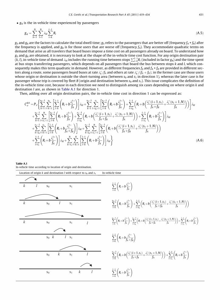
at bus stops transferring passengers, which depends on all passengers that board the bus between stops k and l, which con-sequently makes this term quadratic in demand. However, as different frequencies fA and fA + fB are provided in different sec-tors along a route, some passengers board buses at rate kþk =fA and others at rate kþk =ðfA þ fBÞ; in the former case are those userswhose origin or destination is outside the short-turning area (between s0 and s1 in direction 1), whereas the later case is forpassenger whose trip is covered by fleet B (origin and destination between s0 and s1). This issue complicates the definition ofthe in-vehicle time cost, because in each direction we need to distinguish among six cases depending on where origin k anddestination l are, as shown in Table A.1 for direction 1.
Then, adding over all origin destination pairs, the in-vehicle time cost in direction 1 can be expressed as:
Cds1v ¼Pv
Xs0�1
k¼1
Xs0
l¼kþ1
Xl�1
i¼k
Riþbk1þ
i
fA
!" #kklþ
Xs0�1
k¼1
Xs1
l¼s0þ1
Xs0�1
i¼k
Riþbk1þ
i
fA
!þXl�1
i¼s0
Riþbkþi ðiþ1;s1Þ
fAþ fBþkþi ðs1þ1;NÞ
fA
� �� �" #kkl
(
þXs0�1
k¼1
XN
l¼s1þ1
Xs0�1
i¼k
Riþbk1þ
i
fA
!þXs1�1
i¼s0
Riþbkþi ðiþ1;s1Þ
fAþ fBþkþi ðs1þ1;NÞ
fA
� �� �þXl�1
i¼s1
Riþbk1þ
i
fA
!" #kkl
þXs1�1
k¼s0
Xs1
l¼kþ1
Xl�1
i¼k
Riþbk1þ
i
fAþ fB
!" #kklþ
Xs1�1
k¼s0
XN
l¼s1þ1
Xs1�1
i¼k
Riþbkþi ðiþ1;s1Þ
fAþ fBþkþi ðs1þ1;NÞ
fA
� �� �"
þXl�1
i¼s1
Riþbk1þ
i
fA
!#kklþ
XN
k¼s1
XN
l¼kþ1
Xl�1
i¼k
Riþbk1þ
i
fA
!" #kkl
)ðA:6Þ
.1icle time according to location of origin and destination.
tion of origin k and destination l with respect to s0 and s1 In-vehicle time
s0 s1 l Xl�1
i¼k
Riþbk1þ
i
fA
!
s0 s1 l Xs0�1
i¼k
Riþbk1þ
i
fA
!þXl�1
i¼s0
Riþbkþi ðiþ1;s1Þ
fAþ fBþkþi ðs1þ1;NÞ
fA
� �� �
s0 s1 lXs0�1
i¼k
Riþbk1þ
i
fA
!þXs1�1
i¼s0
Riþbkþi ðiþ1;s1Þ
fAþ fBþkþi ðs1þ1;NÞ
fA
� �� �þXl�1
i¼s1
Riþbk1þ
i
fA
!
s0 s1k l Xl�1
i¼k
Riþbk1þ
i
fAþ fB
!
s0 s1k lXs1�1
i¼k
Riþbkþi ðiþ1;s1Þ
fAþ fBþkþi ðs1þ1;NÞ
fA
� �� �þXl�1
i¼s1
Riþbk1þ
i
fA
!
s0 s1 k lXl�1
i¼k
Riþbk1þ
i
fA
!
432 C.E. Cortés et al. / Transportation Research Part A 45 (2011) 419–434
The quadratic terms on demand that appear in (A.6) reflect that all passengers that get on buses between stations k and lincrease the boarding time of all passengers that travel between those stops, kkl. Expression (A.6) is formulated in syntheticform as
Cds1v ¼ Pv
XN�1
k¼1
Rk þ bg1
5ðs0; s1ÞfA þ fB
þ bg1
6ðs0; s1ÞfA
( )ðA:7Þ
where g15 and g1
6 encompass all the quadratic terms in demand observed in (A.6):
g15ðs1;s2Þ¼
Xs0�1
k¼1
Xs1
l¼s0þ1
kkl
Xl�1
i¼s0
kþi ðiþ1;s1ÞþXs0�1
k¼1
XN
l¼s1þ1
kkl
Xs1�1
i¼s0
kþi ðiþ1;s1ÞþXs1�1
k¼s0
Xs1
l¼kþ1
kkl
Xl�1
i¼k
k1þi þ
Xs1�1
k¼s0
XN
l¼s1þ1
kkl
Xs1�1
i¼k
kþi ðiþ1;s1Þ ðA:8Þ
g16ðs1; s2Þ ¼
Xs0�1
k¼1
Xs0
l¼kþ1
kkl
Xl�1
i¼k
k1þi þ
Xs0�1
k¼1
Xs1
l¼s0þ1
kkl
Xs0�1
i¼k
k1þi þ
Xl�1
i¼s0
kþi ðs1 þ 1;NÞ" #
þXs0�1
k¼1
XN
l¼s1þ1
kkl
Xs0�1
i¼k
k1þi þ
Xs1�1
i¼s0
kþi ðs1 þ 1;NÞ þXl�1
i¼s1
k1þi
" #þ m
s1�1
k¼s0
XN
l¼s1þ1
kkl
Xs1�1
i¼k
kþi ðs1 þ 1;NÞ þXl�1
i¼s1
k1þi
" #
þXN
k¼s1
XN
l¼kþ1
kkl
Xl�1
i¼k
k1þi ðA:9Þ
Analogously, for direction 2 we obtain:
Cds2v ¼ Pv
XN�1
k¼1
Rk þ bg2
5ðs2; s3ÞfA þ fB
þ bg2
6ðs2; s3ÞfA
( )ðA:10Þ
where
g25ðs2; s3Þ ¼
XN
k¼s3þ1
Xs3�1
l¼s2
kkl
Xs3
i¼lþ1
kþi ðs2; i� 1Þ þXN
k¼s3þ1
Xs2�1
l¼1
kkl
Xs3
i¼s2þ1
kþi ðs2; i� 1Þ þXs1
k¼s2þ1
Xk�1
l¼s2
kkl
Xk
i¼lþ1
k2þi
þXs3
k¼s2þ1
Xs2�1
l¼1
kkl
Xk
i¼s2þ1
kþi ðs2; i� 1Þ ðA:11Þ
g26ðs2; s3Þ ¼
XN
k¼s3þ1
Xk�1
l¼s3
kkl
Xk
i¼lþ1
k2þi þ
XN
k¼s3þ1
Xs3�1
l¼s2
kkl
Xk
i¼s3þ1
k2þi þ
Xs3
i¼lþ1
kþi ð1; s2 � 1Þ" #
þXN
k¼s3þ1
Xs2�1
l¼1
kkl
Xk
i¼s3þ1
k2þi þ
Xs3
i¼s2þ1
kþi ð1; s2 � 1Þ þXs2
i¼lþ1
k2þi
" #þXs3
k¼s2þ1
Xs2�1
l¼1
kkl
Xk
i¼s2þ1
kþi ð1; s2 � 1Þ þXs2
i¼lþ1
k1þi
" #
þXs2
k¼1
Xk�1
l¼1
kkl
Xk
i¼lþ1
k2þi ðA:12Þ
Finally, the total in-vehicle time cost (5) is
Cdsm ¼ Cds1
m þ Cds2m ¼ Pm 2
XN�1
k¼1
Rk þ bg5ð~sÞ
fA þ fBþ b
g6ð~sÞfA
( )ðA:13Þ
with g5 ð~sÞ ¼ g15ðs1; s2Þ þ g2
5ðs2; s3Þ and g6 ð~sÞ ¼ g16ðs1; s2Þ þ g2
6ðs2; s3Þ given by expressions (A.8), (A.9), (A.11), and (A.12).
Appendix B. Load of vehicles between stations
B.1. Load of vehicles serving the entire corridor (fleet A)
Direction 1
p1k ¼
p1k�1 þ
k1þkfA� k1�
kfA
if 1 6 k 6 s0 � 1
p1k�1 þ
kþkðkþ1;s1ÞfAþfB
þ kþkðs1þ1;NÞ
fA� k�k ð1;s0�1Þ
fA� k�k ðs0 ;k�1Þ
fAþfBif s0 6 k 6 s1
p1k�1 þ
k1þkfA� k1�
kfA
ifs1 þ 1 6 k 6 N
8>>>><>>>>:
C.E. Cortés et al. / Transportation Research Part A 45 (2011) 419–434 433
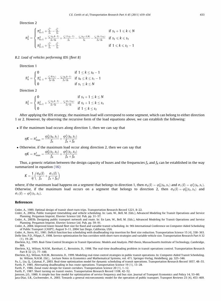
Direction 2
p2k ¼
p2kþ1 þ
k2þkfA� k2�
kfA
if s3 þ 1 6 k 6 N
p2kþ1 þ
kþkðs2 ;k�1ÞfAþfB
þ kþkð1;s2�1Þ
fA� k�k ðs3þ1;NÞ
fA� k�k ðkþ1;s3Þ
fAþfBif s2 6 k 6 s3
p2kþ1 þ
k2þkfA� k2�
kfA
if 1 6 k 6 s2 � 1
8>>>><>>>>:
B.2. Load of vehicles performing IDS (fleet B)
Direction 1
~p1k ¼
0 if 1 k s0 � 1
~p1k�1 þ
kþkðk;s1Þ
fAþfB� k�k ðs0 ;k�1Þ
fAþfBif s0 k s1 � 1
0 if s1 k N
8><>:
Direction 2
~p2k ¼
0 if s3 þ 1 k N
~p2kþ1 þ
kþkðs2 ;k�1ÞfAþfB
� k�k ðkþ1;s3ÞfAþfB
if s2 þ 1 k s3
0 if 1 k s2
8><>:
After applying the IDS strategy, the maximum load will correspond to some segment, which can belong to either direction1 or 2. However, by observing the recursive form of the load equations above, we can establish the following:
� If the maximum load occurs along direction 1, then we can say that
gK ¼ p1max ¼
u10ðs0; s1Þ
fAþu1
1ðs0; s1ÞfA þ fB
� Otherwise, if the maximum load occur along direction 2, then we can say that
gK ¼ p1max ¼
u20ðs2; s3Þ
fAþu2
1ðs2; s3ÞfA þ fB
Thus, a generic relation between the design capacity of buses and the frequencies fA and fB can be established in the waysummarized in equation (16):
K ¼ 1g
r0ð~sÞfAþ r1ð~sÞ
fA þ fB
� �
where, if the maximum load happens on a segment that belongs to direction 1, then r0ð~sÞ ¼ u10ðs0; s1Þ and r1ð~sÞ ¼ u1
1ðs0; s1Þ.Otherwise, if the maximum load occurs on a segment that belongs to direction 2, then r0ð~sÞ ¼ u2
0ðs2; s3Þ andr1ð~sÞ ¼ u2
1ðs2; s3Þ.
References
Ceder, A., 1989. Optimal design of transit short-turn trips. Transportation Research Record 1221, 8–22.Ceder, A., 2003a. Public transport timetabling and vehicle scheduling. In: Lam, W., Bell, M. (Eds.), Advanced Modeling for Transit Operations and Service
Planning. Pergamon Imprint, Elsevier Science Ltd. Pub, pp. 31–57.Ceder, A., 2003b. Designing public transport network and route. In: En Lam, W., Bell, M. (Eds.), Advanced Modeling for Transit Operations and Service
Planning. Pergamon Imprint, Elsevier Science Ltd. Pub, pp. 59–91.Ceder, A., 2004. Improved lower-bound fleet size for fixed and variable transit scheduling. In: 9th International Conference on Computer-Aided Scheduling
of Public Transport (CASPT), August 9–11, 2004 San Diego, California, USA.Ceder, A., Stern, H.I., 1981. Deficit function bus scheduling with deadheading trip insertion for fleet size reduction. Transportation Science 15 (4), 338–363.Delle Site, P.D., Filippi, F., 1998. Service optimization for bus corridors with short-turn strategies and variable vehicle size. Transportation Research Part A 32
(1), 19–28.Eberlein, X.J., 1995. Real-Time Control Strategies in Transit Operations: Models and Analysis. PhD thesis, Massachusetts Institute of Technology, Cambridge,
MA.Eberlein, X.J., Wilson, N.H.M., Barnhart, C., Bernstein, D., 1998. The real-time deadheading problem in transit operations control. Transportation Research
Part B 32 (2), 77–100.Eberlein, X.J., Wilson, N.H.M., Bernstein, D., 1999. Modeling real-time control strategies in public transit operations. In: Computer-Aided Transit Scheduling.
In: Wilson, N.H.M. (Ed.), . Lecture Notes in Economics and Mathematical Systems, vol. 471. Springer-Verlag, Heidelberg, pp. 325–346.Fu, L., Liu, Q., Calamai, P., 2003. Real-time optimization model for dynamic scheduling of transit operations. Transportation Research Record 1857, 48–55.Furth, P., 1985. Alternating deadheading in bus route operations. Transportation Science 19 (1), 13–28.Furth, P., 1986. Zonal route design for transit corridors. Transportation Science 20 (1), 1–12.Furth, P., 1987. Short turning on transit routes. Transportation Research Record 1108, 42–52.Jansson, J.O., 1980. A simple bus line model for optimization of service frequency and bus size. Journal of Transport Economics and Policy 14, 53–80.Jara-Díaz, S.R., Gschwender, A., 2003. Towards a general microeconomic model for the operation of public transport. Transport Reviews 23 (4), 453–469.
434 C.E. Cortés et al. / Transportation Research Part A 45 (2011) 419–434
Jara-Diaz, S.R., Tirachini, A., Cortés, C.E., 2008. Modeling public transport corridors with aggregate and disaggregate demand. Journal of Transport Geography16, 430–435.
Jordan, W.C., Turnquist, M.A., 1979. Zone scheduling of bus routes to improve service reliability. Transportation Science 13 (3), 242–268.Kraus, M., 1991. Discomfort externalities and marginal cost transit fares. Journal of Urban Economics 29, 249–259.Leiva, C., Muñoz, J.C., Giesen, R., Larrain, H., 2010. Design of limited-stop services for an urban bus corridor with capacity constraints. Transportation
Research Part B 44 (10), 1186–1201.Mohring, H., 1972. Optimization and scale economies in urban bus transportation. American Economic Review 62, 591–604.MTT – Ministerio de Transportes y Telecomunicaciones, Chile, 1998. Estudio de Demanda del Sistema de Transporte Público de Superficie de Santiago 1997.Oldfield, R.H., Bly, P.H., 1988. An analytic investigation of optimal bus size. Transportation Research 22B, 319–337.Tirachini, A., 2007. Estrategias de asignación de flota en un corredor de transporte público. MSc Thesis, Universidad de Chile. Available from: <http://
www.cybertesis.cl/tesis/uchile/2007/tirachini_ah/html/index-frames.html, accessed January 2011>.Tirachini, A., Cortés, C.E., 2006. La estrategia deadheading en corredores de transporte público (Deadheading strategy in public transport corridors, in
Spanish). In: Proceedings of the XIV Panamerican Congress on Transport and Traffic Engineering. Las Palmas de Gran Canaria, Spain, 20–23 September2006.
Tirachini, A., Cortés, C.E., 2007. Disaggregated modeling of pre-planned short-turning strategies in transit corridors. In: CD Proceedings, TransportationResearch Board (TRB) 86th Annual Meeting, Washington, DC, USA.
Tirachini, A., Cortés, C.E., Jara-Diaz, S.R., 2011. Optimal design and benefits of a short turning strategy for a bus corridor. Transportation 38 (1), 169–189.Vijayaraghavan, T.A., Anantharmaiah, K.M., 1995. Fleet assignment strategies in urban transportation using express and partial services. Transportation
Research Part A 29 (2), 157–171.