Integrating Emotional Processes into Decision Making Models

Emotions and Decisions 1

Integrating Emotional Processes into Decision Making Models

Jerome R. Busemeyer, Eric Dimperio, & Ryan K. Jessup

Indiana University

May 19, 2006

Chapter to appear in

Gray, W. (Ed.) Integrated models of cognitive systems. Oxford University Press.

Send Correspondence to: Jerome R. Busemeyer 1101 E. 10th St. Bloomington, Indiana, 47405 812 -855 - 4882 [email protected]

This research was funded by 21st Century Research and Technology Fund grant # 1110030618 National Science Foundation award # ACI-0325846

mailto:[email protected]


During the heyday of neo-behaviorism, motivational processes held sway over

general system theories of behavior (Hull, 1943; Spence; 1956; Skinner, 1953). Basic

drives and learned incentive motives were postulated to guide behavior. Theorizing about

unobservable mental processes was shunned (Tolman, 1958, was an exception). Such a

stilted understanding of mental processing eventually led to the downfall of these grand

and systematic theories.

The rise of the computer-information-processing metaphor in the 1950’s paved

the way for a Cognitive Revolution. Cognitive scientists re-aligned their attention on

mental processing mechanisms. Short and long term memory storage and retrieval were

postulated and serial or parallel processes controlled flow of information. A second major

attempt to construct general system theories of behavior was initiated (Newell, 1990;

Anderson et al., 1998; Meyer and Kieras, 1997). However, motivation and emotion was

foreign to computer systems, and it was eschewed by information processing theorists.

The ‘goals’ of a production rule system had to be hard-wired directly by human hand.

The Cognitive Revolution removed the heart from its systems, leaving an artificial

intelligence unable to understand the value of its goals. This restricted view of motivation

and emotions may eventually lead to the breakdown of the Cognitive Revolution.

This chapter presents a formal model for integrating emotion and cognition within

the decision process that is used to select goals. Emotion enters this decision process by

affecting the weights and values that form the basis of decisions. We begin by reviewing

some basic facts and concepts from research on emotion. Then we review recent

experimental research that examines the influence of emotion and motivation on


decisions. Finally, we present a formal model called decision field theory (Busemeyer,

Townsend, & Stout, 2002) where motives and emotions dynamically guide the decision

process for selecting goals.

I. What are we trying to integrate?

Let us begin by defining some basic concepts and summarizing some of their

characteristics. Plans are action-event sequences designed to achieve specific goals, and

problem solving is a process used to generate potential plans. Decision making processes

are used to select one of the plans generated by problem solving for execution. Decisions

are based on judgments, which evaluate consequences and estimate likelihoods of events.

Evaluations of consequences are based on the satisfaction or dissatisfaction of motives.

Motives are persistent biological and cultural needs. These consist of basic drives

such hunger, thirst, pain, and sex; but secondary needs are built from these primary needs

such as safety and affection; and eventually higher order needs emerge, such as curiosity

and freedom (cf. Maslow, 1962). Emotions are temporary states reflecting changes in

motivational levels. For example joy may be temporarily experienced by a sudden gain of

power and wealth; anger may be experienced by a sudden loss of power and wealth; fear

may be experienced by threatened loss of power and wealth. Affect is an evaluation of an

emotional state according to a positive (approach) or negative (avoidance) feeling

(movement tendency). For example, joy produces positive affect and anger produces

negative affect. Emotions have a dynamic time course, and moods reflect lingering affect

that can moderate later cognitive processing. For example, joy can produce a lingering

positive mood, which can make a person feel optimistic about subsequent events; anger

can produce a lingering negative mood, which can make a person feel pessimistic about


subsequent events (Lewis & Haviland-Jones, 2000). The dynamic nature of motives and

emotions present a challenge to traditional static theories of decision making, and

decision field theory attempts to formally address these dynamic characteristics.

II. What are the bases for emotions?

Emotional experiences have broad influences across the neural, physiological, and

behavioral systems. Emotional experiences produce changes in neural brain activation,

increasing activation in some cases (such as fear), and decreasing activation in other

cases (such as sadness). Neural transmitters are released, such as GABA inhibitors, or

dopamine reward signals. Emotions produce hormonal responses – either adrenaline

(epinephrine), causing anxiety and preparation for fleeing; or nor-adrenaline (nor-

epinephrine), activating aggression and preparation for a fight. Physiological reactions of

the autonomic nervous system consist of changes in pupil size, heart rate, respiratory rate,

skin temperature, and skin conductance (from perspiration). The behavioral reactions

include changes in facial expression, and body posture, as well as programmed reactions

and coping responses (fight or flight).

The cognitive system has a crucial function in interpreting, appraising, and

facilitating these neural, physiological, and behavioral reactions (Schachter & Singer,

1962; Lazarus, 1991; Weiner, 1986). For example, if someone else caused an event to

happen, and the person had substantial control over the event, and the event generated a

negative effect, then your cognitive system would categorize this emotional experience as

anger toward the person who caused this negative result. However, if you personally

caused an event to happen, and you had control over the event, and the event generated a

negative effect, then your cognitive system would categorize this emotional experience as


guilt for your role in causing this negative result (see Roseman, Antonius, & Jose, 1996).

Thus the cognitive system categorizes the emotional experience on the basis of the affect

and contextual information about the event.

III. Single versus dual system views of emotion

Neuro-physiological research on emotions indicates that two neural pathways

underlay emotional experiences (Buck, 1984; Gray, 1994; LeDoux, 1996; Levenson,

1994; Scherer, 1994; Panksepp, 1994; Zajonc, 1980). First there is a sub-cortical direct

route, which is fast, spontaneous, unconscious, physiological, and involuntary reaction.

This is mediated through a direct (thalamus amygdala motor cortex) limbic circuit.

Second, there is an indirect neocortical route, which has a slower coping response based

on a conscious appraisal of the situation. This is mediated through an indirect (thalamus

sensory cortex prefrontal cortex amygdala motor cortex) neocortical circuit.

Recently, however, Damasio (1994) has argued for an integration of two systems taking

place in the orbital (ventral medial) prefrontal cortex.

This neurophysiological evidence gives rise to opposing views about how

emotions and cognitions interact to influence decision making. Some argue strongly that

there are two separate and independent systems for making decisions; while others argue

that these two sources are integrated into a single emotional – cognitive decision making

process.

A two system point of view has been promoted by many theorists (Epstein, 1994;

Kahneman & Frederick, 2002; Loewenstein & O’Donoghue, 2005; Metcalfe & Mischel,

1999; Peters & Slovic, 2000; Sloman, 1996; Stanovich & West, 2000; Hammond, 2000).

According to this view, the first system is an emotional, intuitive, affective based system


for making decisions. It processes in parallel, is fast, implicit, unconscious, automatic,

associative, non-compensatory, highly contextual and based on experience. This system

places little demand on working memory. The second system is a rational, analytic,

reasoning based system for making decisions. It is slow, serial, explicit, conscious,

controlled, compensatory, comprehensive, and based on abstractions. This system places

large demands on working memory. The systems operate independently, and only

interact by having the second system correct the errors of the first, if needed, and if there

is sufficient time and working memory available.

A single integrated system approach has been advocated by a smaller number of

theorists (e.g., Damasio, 1994; Gray, 2004; Mellers, Schwarz, Ho, & Ritov, 1997).

According to this view, emotions provide dynamic signals that feed into and help guide

the cognitive system over time for making decisions. A major challenge for this

viewpoint is to describe exactly how this temporal integration and interaction occurs.

Decision field theory, described below, provides dynamic mechanisms for integrating fast

emotionals signals with slower cognition information to guide decisions.

IV. Review of Research on Emotions and Decisions

This brief review is organized around a series of questions concerning the

relevance of emotions for decision theory. For a more thorough review see Loewenstien

and Lerner (2003).

1. Do we need to change decision theory for emotional consequences?

Early evidence pointing towards a need to include emotion came from studies

examining the effects of anticipated regret (Zeelenberg, Beattie, van der Plight, & de

Vries, 1996; see also Mellers, Schwartz, Ho, & Ritov, 1997, for related research). In


these experiments, participants were given a series of choices between safe versus risky

gambles. On some trials, they were informed that they would receive outcome feedback

immediately after the choice, while on other trials they were informed that feedback

would not be provided. Standard utility theories predict that the opportunity for outcome

feedback should not have any effect on preference; however, the expectation was that

regret would be anticipated for not choosing risky options when feedback was presented.

In agreement with the latter prediction, preferences tended to reverse and switch toward

the riskier gamble when immediate feedback was anticipated.

Another line of evidence petitioning for change came from research on the effects

of emotional outcomes on decision weights (Rottenstreich & Hsee. 2001). According to

weighted utility theories, the utility of a simple gamble of the form ‘win x with

probability p, otherwise nothing’ is determined by the product of the utility of the

outcome, x, multiplied by the decision weight associated with the probability, p. Both the

utility and the decision weight are subjective and depend on an individual’s personal

beliefs and values. However, a critical assumption is that these two factors are separable,

and in particular, the decision weight is a function of p alone and not a function of x. This

decision weight function has typically been estimated using monetary gambles, and it is

usually found to be an inverse S shaped function of p (Kahneman & Tversky, 1979).

However, Rottenstreich & Hsee (2001) found that the shape of the decision weight

function changed depending on whether the x was a purely monetary outcome versus an

outcome with greater affective impact (e.g., avoidance of an electric shock). The decision

weight function was estimated to be flatter in the middle of the probability scale when

emotional outcomes were used as compared to monetary outcomes.


Emotions also change the rate of temporal discounting in choices between long

term large rewards over short term smaller rewards. Gray (1999) found that participants

who were shown aversive images (producing a feeling of being threatened) had higher

discount rates. Stress focused individuals’ attention on immediate returns making them

appear more impulsive.

Finally, a third line of evidence comes from research examining the type of

decision strategy used to make choices (Luce, Bettman, Payne, 1997). Compensatory

strategies, such as those enlisting a weighted sum of utilities, require making difficult

trade-offs and integrating information across all the attributes. Non-compensatory

strategies, such as a lexico-graphic rule, only require rank ordering alternatives on a

single attribute and thus avoid difficult tradeoffs. Luce et al. (1997) found that when

faced with emotionally difficult decisions, individuals tend to switch from a

compensatory to non-compensatory strategies to avoid making difficult negative

emotional tradeoffs.

2. Can emotions distort or disturb our reasoning processes?

One line of evidence supporting this idea comes from research on emotional

carry-over effects (Goldberg, Lerner, & Tetlock, 1999; Lerner, Small & Loewenstein,

2004). For example, in the study by Goldberg et al., participants watched a movie about

a disturbing murder. The murderer was brought to trial, and in one condition, the

murderer was acquitted on a technicality but in another condition the murderer was found

guilty. After watching the film, the participants were asked to make penalty judgments

for a series of unrelated misdemeanors. Goldberg et al. found that when the murderer

was freed on a technicality, anger aroused by watching the murder movie spilled over to


produce higher punishments for unrelated crimes, as compared to the condition in which

the murderer was convicted.

Shiv and Fedorikhin (1999) examined conflicts between motivation and

cognition. Participants were given a choice between a healthy and unhealthy snack under

either a high stimulating condition (real cakes or fruit snacks visibly present) or a low

stimulating condition (symbolic information about cakes and fruits). Also in one

condition they made this decision under a high memory load (they were asked to rehearse

items for a later recall test) or under no memory load. Considering the reasons for the

choice, participants generally favored the healthy snack. However, under when hunger

was stimulated under the vivid condition, and the healthy thoughts were suppressed (by

the working memory task), then preferences reversed and the unhealthy snack was

chosen most frequently.

A similar line of research was conducted by Markman and Brendl (2000).

Habitual smokers were offered the opportunity to purchase raffle tickets for one of two

lotteries--one with a cash prize and one with a cigarette prize, to be awarded after a

couple of weeks delay. Half of the smokers were approached before smoking a post-class

cigarette (and hence they had a strong need to smoke a cigarette). The other half were

approached just after smoking their post-class cigarette (and hence the strength of the

need to smoke a cigarette was diminished). Those who had not yet smoked purchased

more raffle tickets to win cigarettes than did those who had already smoked. In contrast,

they purchased fewer raffle tickets for the cash prize than did those who already smoked.

Thus the need to smoke exaggerated the value of the cigarette lottery relative to the

monetary lottery even though the latter could be used to purchase cigarettes.


3. Does reasoning always improve decision making?

Apparently this is not the case. Wilson et al. (1993) asked participants to provide

their preference for either posters picturing animals in playful poses or posters of abstract,

impressionist paintings. One group of participants was forced to provide reasons for their

preference whereas the other group was not. Those who were forced to provide reasons

for their preference were more likely to prefer the posters of the cute animals whereas

those who were not compelled to provide reasons preferred the impressionist posters.

Participants were given the poster of their choice and a few weeks later were asked how

satisfied they were with their selection. Those who were forced to provide reasons for

their preference were significantly less satisfied with their selection than those who were

not. These results suggest that thinking about reasons led to a focus on information about

the domain that was not important to people in the long run.

4. Can we predict the effect of emotions on our decisions?

Research indicates we are not very good at this. Loewenstein & Lerner (2003)

review a number of experiments illustrating what they call Hot-Cold Empathy Gaps.

When in a cold state, (not hungry), people under-predict how they will feel in a hot state

(hungry) (see Read & van Leeuwen, 1998). When in a hot state (sexually aroused),

people cannot accurately predict how they will later feel when in a cold state (morning

after effect) and vice versa. This concludes our brief review illustrating some interesting

interactions between motives, emotions, and decision making.

V. Decision Field Theory

Now we summarize a dynamic theory that describes how to incorporate

motivational processes into decision making. First, we introduce a dynamic model of


decision making called decision field theory (DFT). This theory has been previously used

to explain choices between uncertain actions (Busemeyer & Townsend, 1993), multi-

attribute choices (Diederich, 1997), multi-alternative choices (Roe, Busemeyer, &

Townsend, 2001), and the relations between choices and prices (Johnson & Busemeyer,

in press). In this chapter, we build on our previous efforts to extend decision field theory

to account for the effects of motivation and emotion on decision making (Busemeyer et

al., 2002). DFT advances older static models by providing a dynamic account of the

decision process over time. This is important for explaining interactions between

emotional and cognitive processes as the product of one integrated system rather than as a

two system approach.

1. Decision Process.

It will be helpful to have a concrete decision in mind when presenting the theory.

The following example was chosen to highlight the application of the theory to

navigational decisions under emergency or crisis conditions producing high time pressure

and high emotional stress. A man was on a mission that required riding cross country on

his motorcycle. He was cruising around 50 mph down a two lane state highway when he

came up behind a truck full of old car tires. The highway was not in good shape, with

many pot holes left by snow plows from the previous winter. The truck bumped into of

one of these pits, causing a tire to somersault out of the truck and land flat on the road,

directly in the motorcyclist’s path. Although this example concerns navigating a

motorcycle, it contains aspects that are shared in other navigational decisions, such as

emergencies that occur during a plane flight.


The motorcyclist assessed the situation and noted that there was no shoulder on

the road to serve as an escape route, and that there was a line of cars following closely

behind him. Thus the man was faced with a difficult problem solving task, upon which he

very quickly generated three potential plans of action: (A) drive straight over the tire, (B)

swerve to the side, or (C) slam on the breaks. Each action involved planning a complex

sequence of perceptual-motor movements. For example, driving straight across the tire

required accelerating a little to push across the tire, hitting the tire dead center with

sufficient speed to overcome it, a strong grip on the handle bars, and careful balancing of

the bike. 1

Each course of action could result (for simplicity) in one of four possible

consequences: (c1) a safe maneuver without damage or injury; (c2) laying the motorcycle

down and damaging the motorcycle, but escaping with minor cuts and bruises; (c3)

crashing into another vehicle, damaging the motorcycle and suffering serious injury, (c4)

flipping the motorcycle over and getting killed.

<Insert Table 1 about here>

An abstract representation for this decision problem is shown in Table 1, where

the rows represent actions, columns represent consequences, and the cells represent the

likelihoods that an action produces a consequence. The affective evaluations of the

consequences are represented by the values mj shown in the columns of the table, and the

beliefs are represented by decision weights, wij, shown in the cells of the table. In the

motorcyclist’s opinion, option A was very risky, with high possibilities for the extreme

1 This example is based on a personal experience of the first author, who decided to go straight across the tire, and managed to survive to tell this story.


consequences, c1 and c4. Action B was more likely to produce consequence c2, and

action C was more likely to produce consequence c3.

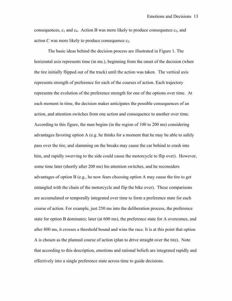
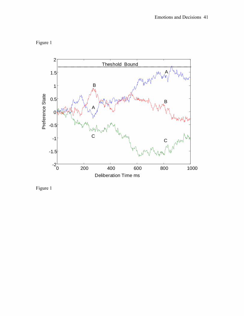
The basic ideas behind the decision process are illustrated in Figure 1. The

horizontal axis represents time (in ms.), beginning from the onset of the decision (when

the tire initially flipped out of the truck) until the action was taken. The vertical axis

represents strength of preference for each of the courses of action. Each trajectory

represents the evolution of the preference strength for one of the options over time. At

each moment in time, the decision maker anticipates the possible consequences of an

action, and attention switches from one action and consequence to another over time.

According to this figure, the man begins (in the region of 100 to 200 ms) considering

advantages favoring option A (e.g. he thinks for a moment that he may be able to safely

pass over the tire, and slamming on the breaks may cause the car behind to crash into

him, and rapidly swerving to the side could cause the motorcycle to flip over). However,

some time later (shortly after 200 ms) his attention switches, and he reconsiders

advantages of option B (e.g., he now fears choosing option A may cause the tire to get

entangled with the chain of the motorcycle and flip the bike over). These comparisons

are accumulated or temporally integrated over time to form a preference state for each

course of action. For example, just 250 ms into the deliberation process, the preference

state for option B dominates; later (at 600 ms), the preference state for A overcomes, and

after 800 ms, it crosses a threshold bound and wins the race. It is at this point that option

A is chosen as the planned course of action (plan to drive straight over the tire). Note

that according to this description, emotions and rational beliefs are integrated rapidly and

effectively into a single preference state across time to guide decisions.


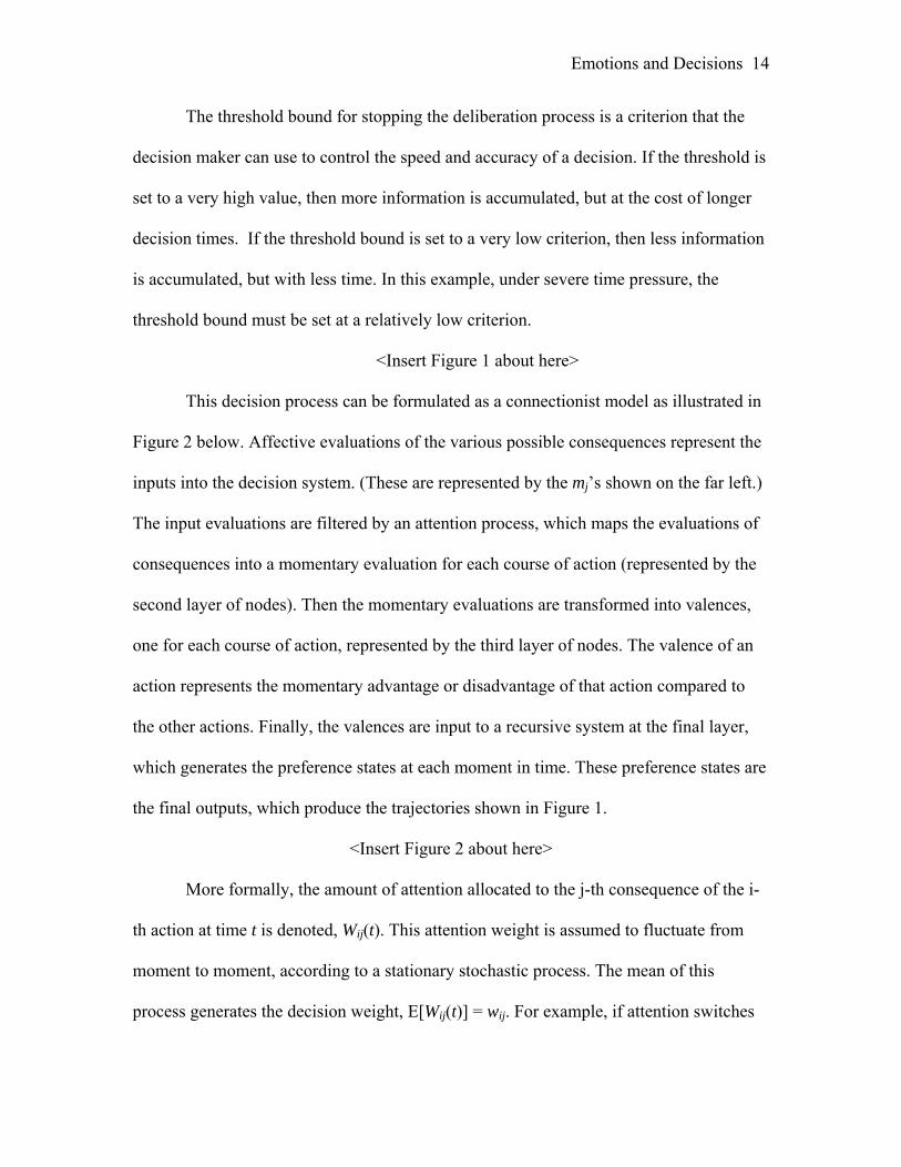
The threshold bound for stopping the deliberation process is a criterion that the

decision maker can use to control the speed and accuracy of a decision. If the threshold is

set to a very high value, then more information is accumulated, but at the cost of longer

decision times. If the threshold bound is set to a very low criterion, then less information

is accumulated, but with less time. In this example, under severe time pressure, the

threshold bound must be set at a relatively low criterion.

<Insert Figure 1 about here>

This decision process can be formulated as a connectionist model as illustrated in

Figure 2 below. Affective evaluations of the various possible consequences represent the

inputs into the decision system. (These are represented by the mj’s shown on the far left.)

The input evaluations are filtered by an attention process, which maps the evaluations of

consequences into a momentary evaluation for each course of action (represented by the

second layer of nodes). Then the momentary evaluations are transformed into valences,

one for each course of action, represented by the third layer of nodes. The valence of an

action represents the momentary advantage or disadvantage of that action compared to

the other actions. Finally, the valences are input to a recursive system at the final layer,

which generates the preference states at each moment in time. These preference states are

the final outputs, which produce the trajectories shown in Figure 1.


More formally, the amount of attention allocated to the j-th consequence of the i-

th action at time t is denoted, Wij(t). This attention weight is assumed to fluctuate from

moment to moment, according to a stationary stochastic process. The mean of this

process generates the decision weight, E[Wij(t)] = wij. For example, if attention switches


in an all – or – none manner, then Wij(t) = 1 or 0, and wij = E[Wij(t)] is the probability that

attention will be focused on a consequence of an action at any moment. Thus the decision

weight is the average amount of time spent thinking about a consequence. It is assumed

to be affected by the likelihood of the consequence, but according to this interpretation,

other factors that attract attention may also affect these decision weights.

The momentary evaluation of the i-th action is an attention weighted average:

Ui(t) = ∑ Wij(t)⋅mj, where j is an index associated with one of the possible consequences

of an action, Wij(t) represents the amount of attention allocated to a particular

consequence at any moment, and mj is the affective evaluation of a consequence. Note

that Ui(t) is a random variable (because Wij(t) is a random variable), but its mean is a

weighted average E[Ui(t) ] = ∑ wij⋅mj = ui, which corresponds to a weighted utility

commonly used by decision theorists (cf. Luce, 2000).

The valence of an action is defined as the difference vi(t) = Ui(t) – U.(t), where

U.(t) is the average evaluation over all actions.2 The valence represents the momentary

advantage/disadvantage for option i at time t compared to the average of all actions at

that moment. The sum across valences always equals zero.

The valences for an action are integrated over time to form a preference state for

each action, denoted Pi for option i. This preference state can range from positive

(approach) to zero (neutral) to negative (avoidance). Each preference state starts with an

initial value, Pi(0), which may be biased by past experience (in Figure 1, they start out

2 In the past, we defined U. as the average of all options other than option i. Here we define it as the average of all options. However, the definition used here produces a valence that is proportional to the previous version: the previously defined valence equals [N/(N-1)] times the currently defined valence, where N is the number of options in the choice set.


unbiased). The preference state evolves during the deliberation according to the following

linear dynamic stochastic difference equation (where h is a small time step):

Pi(t+h) = ∑ sij ⋅ Pj(t) + vi(t+h) (1)

The coefficients sij allow feedback from previous preference states to influence the new

state. The self feedback coefficient, sii for i = j,, controls the memory for past valences.

The lateral inhibitory links, sij = sji for i ≠ j, produce a competitive system in which strong

preferences grow and weak preferences are suppressed. Lateral inhibition is commonly

used in artificial neural networks and connectionist models of decision making to form a

competitive system in which one option gradually emerges as a winner dominating over

the other options (cf. Grossberg, 1988; Rumelhart & McClelland, 1986). The lateral

inhibitory coefficients are important for explaining context effects on choice (see Roe et

al., 2001).

In summary, a decision is reached by the following deliberation process: as

attention switches across consequences over time, different affective values are

probabilistically considered, and these values are compared across actions to produce

valences, and finally these valences are integrated into preference states for each action.

This process continues until the preference for one action exceeds a threshold criterion, at

which point in time the winner is chosen. Note that a single system is postulated to

temporally integrate rational beliefs about potential consequences with affective reactions

to these consequences over time.3

3 Formally, this is a Markov process, and matrix formulas have been mathematically derived for computing the choice

probabilities and distribution of choice response times (See Busemeyer & Townsend, 1992; Busemeyer & Diederich, 2002; Diederich & Busemeyer, 2003). Alternatively, computer simulation can be used to generate predictions from the model. Normally we use the matrix computations because they are more precise and faster, but to show how easy it is to simulate this model, we used the simulation program shown in the Appendix for the analyses presented next.


To illustrate the dynamic behavior of the model, consider a decision whether or

not to take a gamble. Suppose action A has an equal chance of winning $250 or losing

$100, and action B is just status quo (not gambling, not winning or lose anything). In this

simple case, we set the evaluations to the following values: (m1 = 250/250 = 1, m2 = 0,

m3= −100/250 = -.4). For Action A, we assume a .50 probability of attending to m1 and

.50 probability of attending to m3, i.e., wA1 = E[WA1(t)] = .50 and wA3 = E[WA3(t)] = .50.

For action B, only one outcome is possible, zero, so that wB2 = E[WB2(t)] = 1. The time

step was set to h = .01, self feedback was set to sii = 1 – (.07)⋅h, the lateral inhibition was

set to sAB = sBA = 0, and the initial state was set to PA(t) = -1 (initially biased in favor of

not playing).

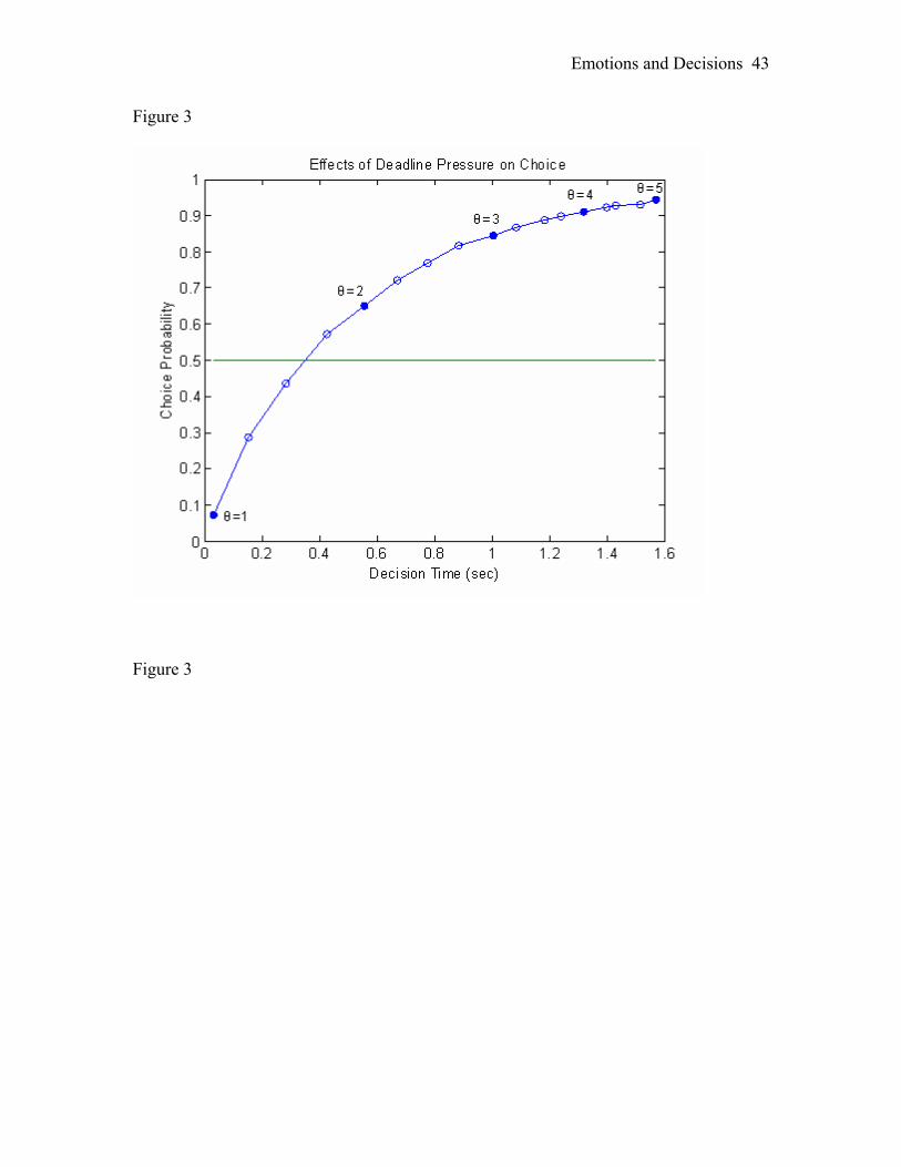
Under these assumptions, we ran a simulation 5,000 times (see Appendix) to

generate the choice probabilities and the mean deliberation times, for a wide range of

threshold parameters (θ ranged from 1 to 5 in steps of .25).4 Figure 3 plots the relation

between choice probability and mean decision time for option A, the gamble, as a

function of the threshold parameter. Both decision time and choice probability increase

monotonically with the threshold magnitude, starting below 50% choice of the gamble

(because of the initial bias) and gradually rising above 50% choice for the gamble

(because it has a positive expected value). Busemeyer (1985), Diederich (2003), and

Diederich & Busemeyer (in press) presents empirical evidence supporting these types of

dynamic predictions for choices between gambles.


4 These closely matched the calculations from the Markov chain equations; however the latter are more accurate and didn’t produce the little dip that appears at the end of Figure 3. The Markov chain method was also a couple of orders of magnitude faster to compute.


2. Affective Evaluation of Consequences.

Now we turn to a more detailed analysis of the evaluations, mj, and how they are

affected by emotions. In general, consequences are described and evaluated according to

various objectives or attributes that a person is trying to maximize (or as in this case,

minimize). In the motorcycle example, the evaluation of consequences depends on

minimizing two attributes: personal injury and motorcycle damage. Note that the

motorcyclist may be willing to sacrifice some personal injury to avoid motorcycle

damage. The success of the mission (the cross country trip) depends on an operational

motorcycle, and a few cuts and bruises will heal and can be tolerated.

The effect of an attribute on an evaluation of a consequence depends on two

factors: 1) the quality or amount of satisfaction that a consequence can deliver with

respect to an attribute, and 2) the importance or need for the attribute. For example,

suppose a consequence scores high with respect to minimizing personal injury but low

with regard to minimizing motorcycle damage. The final evaluation depends on the

importance of the motorcycle relative to personal injury. If the mission is very important,

and the motorcycle is crucial for completing the mission, then this is evaluated as an

unattractive consequence; however, if the mission and the motorcycle are not considered

very important, then this is an attractive consequence. Thus attribute importance

moderates the effect of attribute quality.

More formally, decision theorists (cf. Keeney & Raiffa, 1976) generally postulate

that each consequence can be characterized by a number of attributes, and each attribute

has an importance weight, here denoted nk for the k-th attribute. Additionally, each

consequence has a quality (amount of satisfaction) that can be gained on an attribute, here


denoted as qjk for the value of the j-th consequence with respect to the k-th attribute.

These two factors are combined according to a multiplicative rule, nk⋅ qjk to produce the

net effect of an attribute on the evaluation of a consequence. Furthermore, if the attributes

are independent, then the effects of each attribute add to form a weighted value of a

consequence: mj = ∑ nk⋅ qjk .

So far, this is simply a static representation of an evaluation, which is commonly

used by decision theorists. Decision field theory (Busemeyer et al., 2002) departs from

this static representation by postulating that importance weights depend on personal

needs, which are assumed to vary dynamically across time: nk(t). DFT also diverges by

considering the quality a consequence has on an attribute as the degree of satisfaction a

consequence is expected to provide with respect to the attribute: qjk. Consequently, we

assume that evaluations are changing across time according to mj(t) = ∑ nk(t)⋅ qjk , and

momentary evaluations now involve stochastic attention weights as well as dynamic

evaluations: Ui(t) = ∑ Wij(t)⋅mj(t). The rest of decision field theory (e.g., Equation 1)

accommodates this new dynamical feature in a natural way, as it continues to operate in

the same manner as previously described for making decisions. This is one of the

advantages of using a dynamic model for decision making.

Personal needs, nk(t), are postulated to change across time. A control feedback

loop forms the basis for adjusting these needs over time (Busemeyer et al., 2002; see also

Carver and Sheier, 1990 and Toates, 1980). We assume that an individual has an ideal

point on each attribute, denoted as gk (for goal state) as well as a current level of

achievement or status quo for an attribute, denoted ak(t). The discrepancy between these

two values, [gk – ak(t)], provides a feedback signal for adjusting the need for that


attribute, nk(t). For example, if gk is the ideal level of hunger, and ak(t) is the current level

of hunger (operationalized as hours without food), then the difference between these two

determines the adjustment for the need to eat. Positive discrepancies produce an increase

in need, and negative discrepancies produce are decrease in need. Accordingly, the need

for an attribute varies across time according to the following difference equation

nk(t+h) = Lk⋅nk(t) + [gk – ak(t+h)], (2)

where Lk is a constant that determines the rate of feedback control of needs over time,

which may depend on the type of attribute. For example, the consumatory effect of eating

when hungry may be slower than the consumatory effect of drinking when thirsty. These

differential feedback rates provide a formal means to account for the fast direct versus

slow indirect neural pathways for emotion in the brain.

Figure 4 provides a depiction of the integrated cognitive-motivational network,

illustrating how cognitions and emotions interact over time. Returning to the

motorcyclist’s decision, we can trace the decision process along the network. We assume

that there is an ideal goal state for maintaining the operation of the motorcycle (and

completing the mission) gm as well as a goal for personal safety gp. Let us focus on

changes in the needs for personal safety np(t) during the deliberation process. The sudden

appearance of the tire in the middle of the road produces an abrupt drop in the current

level of personal safety, that is a drop in the variable ap(t) (emotionally felt as fear). This

generates a gap or an error signal, [gp – ap(t)], which causes a rapid growth in the need

for personal safety, np(t). The quality (amount of satisfaction) that a consequence

produces for personal safety, qjp, will then be combined with the need for personal safety,

np(t), to generate a dynamic value mj(t) of each consequence. These dynamic values are


combined with the shifting attention weights, Wij(t), to form momentary evaluations,

Ui(t). The momentary evaluation of an action is compared with other actions to produce a

valence for each action, vi(t). Finally, the valences feed into the preference states Pi(t) to

determine the selected course of action.

VI. Computation Example Applied to Emergency Decisions

To illustrate an important dynamic property generated by Equation 2, let us return

to the motorcyclist’s dilemma. Tables 2 and 3 show the decision weights and the quality

values used in this example. According to Table 2, action A (driving straight across the

tire) is risky – it is likely to produce either of the two extreme consequences, a c1 (safe

maneuver) or c4 (getting killed); action B (swerving) is likely to produce an intermediate

but safer consequence c2 (laying down the motorcycle); and action C (slamming the

brakes) is likely to produce consequence c3.(hitting a vehicle). The qualities, qik

(achievement scores), on the personal safety and motorcycle maintenance attributes, are

shown in Table 3 (higher scores are more desirable). According to Table 3, c1 scores best

on both attributes, c2 score well on the first attribute but very poorly on the second, c3

score moderately bad on both, and c4 scores the worst on both. Additionally, the

predictions for the mean preferences were computed from Equations 1 and 2 using the

following dynamic parameters: we set the gaps equal to [gp–ap(t)], = .80 and [gm–am(t)],

= .40 indicating a larger gap for personal safety; LP = .90 and LM = .70 indicating a

larger feedback control parameter for the personal safety attribute; and finally we set sii =

.9 (self feedback for i = j) and sij = -.05 (lateral inhibition for i ≠ j) in Equation 1 to

control the dynamics of the preference states. (The time step was set to h =1 for

simplicity).


<Insert Tables 2 and 3 about here>

The predictions are shown in Figure 5. As can be seen in the top panel of this

figure, the need for personal safety grows more slowly and to a much higher asymptote as

compared to the need for motorcycle maintenance. This shift in needs produces a reversal

in preference over time between actions A and B. As can be seen in the bottom panel, the

risky action, A, initially is preferred, but later the safer action B dominates. In other

words, as deliberation progresses, the person’s preference switches from the risky to the

safer action. This shows how the model can explain what is called the chickening out

effect (Van Boven, Loewenstein, & Dunning, 2005). In conclusion, DFT allows for

preference reversals over time, which cannot occur with a static utility theory.5


VII. Applications to Previous Research

Let us briefly outline a DFT account of some of the past findings reviewed earlier.

Consider first the emotional carry-over effect reported by Goldberg et al. (1999). In this

case, anger aroused in the first part of an experiment carried over to affect punishment

decisions in second phase. According to DFT, the anger aroused in the first stage decays

exponentially over time as described by Equation 2. This persistence of anger would

enhance the need and thus the importance for the retribution attribute of later punishment

decisions. The earlier studies did not examine how this effect changes over time, but one

testable prediction from the present theory is that the effect should decay exponentially as

a function of the time interval between the initial arousal of anger and the subsequent test

on irrelevant penalty judgments.

5 Appendix II provides a more formal derivation of this property of the theory.


Next consider the experiment by Shiv and Fedorikhim (1999) who examined

conflicts between reasons and emotions. According to DFT, hunger stimulation produces

an increase in the need to satisfy hunger, increasing the importance of the food taste

attribute, and consequently increasing the preference for the unhealthy snack; at the same

time, the memory load would decrease the attention weight to the attributes related to

heath maintenance. A test of this theory could be performed by factorially manipulating

the taste quality of the unhealthy snack and the degree of hunger. We predict that these

two factors should interact according to a multiplicative rule.

In the study by Markman and Brendl (2000), unsatiated smokers were more

interested in winning cigarettes than those whose had just finished smoking. In the

framework of DFT, smoking decreases the need for future smoking and decreases the

importance of obtaining more cigarettes. The motivation for winning cigarettes over

money is lowered. Just as above, we predict that the size of the cigarette prize will

interact according to a multiplicative rule with the time since smoking a cigarette.

As a final example, consider the study by Rottenstreich & Hsee (2001) who found

that emotions cause changes in the probability weighting function. This finding cannot

be readily explained in terms of the effects of emotions on needs for attributes. In this

case, we may be required to formulate a new mechanism that allows emotions to

moderate the amount of attention various consequences receive (i.e, a model for changing

the decision weights, wij, depending on the quality of the emotion produced by an

outcome). This has yet to be done within the DFT framework.


Concluding Comments

Emotions and motives are dynamic reactions to environmental challenges. A

threat, for example, rapidly generates a fear reaction, promoting actions to seek safety to

quell the rising fear. Consequently, dynamic models are required to track their effects on

decisions over time. Decision field theory differs prominently from other standard

decision theories by providing a dynamic description of decision processes, This

characteristic of the theory provides a natural way to incorporate the dynamic effects of

emotions and motivations. The goal of this chapter was to present a formal model for

integrating cognition and emotion into a single decision process.

At the beginning of this chapter we presented two opposing views about the way

emotions could influence decision making. According to a two system view, there is a

type 1 (emotion based system) and a type 2 (reason based system), and the type 1 system

is corrected by the type 2 system. Alternatively, according to a single system view,

motives and emotions control cognition by adjusting the importance weights on the basis

of needs, which vary dynamically over time. This integrated view of emotion and

cognition was actually proposed long ago by one of the founders of the Cognitive

Revolution, Herb Simon (1967). Decision field theory provides a formal mechanism for

implementing the single system view.

It is worthwhile to step back and try to assess the advantages and disadvantages of

each approach. One of the important reasons for advocating a two system approach is the

fact there are at least two separate neural pathways for emotions, the direct versus the

indirect path. However, the two system approach has not been clearly articulated as a

detailed neural model and so this remains a fairly rough correspondence at best.


Furthermore, it not difficult to incorporate fast and slower emotional signals into a

dynamic integrated model of cognition, and so this is not strictly speaking evidence for a

two systems approach. In particular, the dynamic model for need (represented by

Equation 2) provides differential feedback rates to accommodate fast direct versus slow

indirect neural pathways for emotion.

One of the main advantages of the integrated approach presented here is that we

have a formal or computational model that is able to derive precise predictions for

cognitive and emotional interactions. The separate systems approach fails on this

criterion. Although the system 2 part of the theory is precisely worked out (this is just the

standard utility theory), there is a lack of formal modeling for the type 1 (the emotional)

component of this approach. Thus one cannot predict a priori whether a decision will be

based on the type 1 versus the type 2 system, nor is it clear what decision the type 1

system will make.

Finally, we have tried to emphasize two important points in this chapter: (a)

inclusion of motivation and emotional processes are critical and are necessary for the

development of a complete computational model of cognition; and (b) it is feasible to

formulate computational models that integrate emotion and cognition by having what are

commonly thought of as two processes combined in the decision making process.

Decision field theory provides one example of how this can be accomplished.


References

Anderson, J. R., Lebiere, C., Lovett, M. C. & Reder, L. M. (1998). ACT-R: A higher-

level account of processing capacity. Behavioral & Brain Sciences, 21, 831-32.

Buck, R. (1984). The communication of emotion.New York: Guilford Press.

Carver, C. S., & Scheier, M. F. (1990). Origins and functions of positive and negative

affect: A control-process view. Psychological Review, 97(1), 19-35.

Busemeyer, J. R. (1985). Decision making under uncertainty: A comparison of simple

scalability, fixed sample, and sequential sampling models. Journal of

Experimental Psychology, 11, 538-564.

Busemeyer, J. R., & Diederich, A. (2002). Survey of decision field theory. Mathematical

Social Sciences, 43, 345-370.

Busemeyer, J. R., & Townsend, J. T. (1992). Fundamental derivations for decision field

theory. Mathematical Social Sciences, 23, 255-282.

Busemeyer, J. R., & Townsend, J. T. (1993). Decision field theory: A dynamic-cognitive

approach to decision making in an uncertain environment. Psychological Review,

100, 432-459.

Busemeyer, J. R., Townsend, J. T., & Stout, J. C. (2002). Motivational underpinnings of

utility in decision making: Decision Field Theory analysis of deprivation and

satiation. In S. Moore (Ed.), Emotional Cognition.Amsterdam: John Benjamins.

Damasio, A. R. (1994). Descartes' error: emotion, reason, and the human brain.New

York: Putnam.

Diederich, A. (1997). Dynamic stochastic models for decision making under time

constraints. Journal of Mathematical Psychology, 41, 260-274.


Diederich, A. (2003). MDFT account of decision making under time pressure.

Psychonomic Bulletin and Review, 10(1), 157-166.

Diederich, A., & Busemeyer, J. R. (2003). Simple matrix methods for analyzing diffusion

models of choice probability, choice response time, and simple response time.

Journal of Mathematical Psychology, 47(3), 304-322.

Diederich, A. & Busemeyer, J. R. (in press). Modeling the effects of payoffs on response

bias in a perceptual discrimination task: Threshold bound, drift rate change, or

two stage processing hypothesis. Perception and Psychophysics.

Epstein, S. (1994). Integration of the cognitive and the psychodynamic unconscious.

American Psychologist, 49(8), 709-724.

Goldberg, J. H., Lerner, J. S., & Tetlock, P. E. (1999). Rage and reason: The psychology

of the intuitive prosecutor. European Journal of Social Psychology, 29(5-6), 781-

795.

Gray, J. A. (1994). Three fundamental emotion systems. In P. Ekman & R. J. Davidson

(Eds.), The nature of emotion: Fundamental questions (pp. 243-247). New York:

Oxford University Press.

Gray, J. R. (1999). A bias toward short-term thinking in threat-related negative emotional

states. Personality & Social Psychology Bulletin, 25(1), 65-75.

Gray, J. R. (2004). Integration of emotion and cognitive control. Current Directions in

Psychological Science, 13(2), 46-48.

Grossberg, S. (1988). Neural networks and natural intelligence.Cambridge, MA: MIT

Press.

Hammond, K. R. (2000). Coherence and correspondence theories in judgment and


decision making. In T. Connolly & H. R. Arkes (Eds.), Judgment and decision

making: An interdisciplinary reader. (2nd ed., pp. 53-65). New York: Cambridge

University Press.

Hull, C. L. (1943). Principles of behavior, an introduction to behavior theory.New York:

D. Appleton-Century Co.

Johnson, J. G., & Busemeyer, J. R. (in press). A dynamic, computational model of

preference reversal phenomena. Psychological Review.

Kahneman, D., & Frederick, S. (2002). Representativeness revisited: Attribute

substitution in intuitive judgment. In T. Gilovich & D. Griffin (Eds.), Heuristics

and biases: The psychology of intuitive judgment (pp. 49-81). New York:

Cambridge University Press.

Kahneman, D., & Tversky, A. (1979). Prospect theory: An analysis of decision under

risk. Econometrica, 47, 263-291.

Keeney, R. L., & Raiffa, H. (1976). Decisions with multiple objectives: preferences and

value tradeoffs.New York: Wiley.

Lazarus, R. S. (1991). Emotion and adaptation.London: Oxford University Press.

LeDoux, J. E. (1996). The emotional brain: The mysterious underpinnings of emotional

life.New York: Simon & Schuster.

Lerner, J. S., Small, D. A., & Loewenstein, G. (2004). Heart Strings and Purse Strings:

Carryover effects of emotions on economic decisions. Psychological Science,

15(5), 337-341.

Levenson, R. W. (1994). Human emotion: A functional view. In P. Ekman & R. J.

Davidson (Eds.), The nature of emotion: Fundamental questions (pp. 123-126).


New York: Oxford University Press.

Lewis, M., & Haviland-Jones, J. M. (2000). Handbook of emotions (2nd ed.). New York:

Guilford Press.

Loewenstein, G. (1996). Out of control: Visceral influences on behavior. Organizational

Behavior & Human Decision Processes, 65(3), 272-292.

Loewenstein, G., & Lerner, J. S. (2003). The role of affect in decision making. In R. J.

Davidson, K. R. Scherer & H. H. Goldsmith (Eds.), Handbook of affective

sciences (pp. 619-642). Oxford: New York.

Loewenstein, G., & O'Donoghue, T. (2005). Animal spirits: Affective and deliberative

processes in economic behavior.Manuscript in preparation.

Luce, M. F., Bettman, J. R., & Payne, J. W. (1997). Choice processing in emotionally

difficult decisions. Journal of Experimental Psychology: Learning, Memory, &

Cognition, 23(2), 384-405.

Luce, R. D. (2000). Utility of gains and losses: Measurement-theoretical and

experimental approaches.Mahwah, NJ: Lawrence Erlbaum Associates.

Markman, A. B., & Brendl, C. M. (2000). The influence of goals on value and choice. In

D. L. Medin (Ed.), The psychology of learning and motivation: Advances in

research and theory (Vol. 39, pp. 97-128). San Diego, CA: Academic Press.

Maslow, A. H. (1962). Toward a psychology of being.Oxford, England: Van Nostrand.

Mellers, B. A., Schwartz, A., Ho, K., & Ritov, I. (1997). Decision affect theory:

Emotional reactions to the outcomes of risky options. Psychological Science,

8(6), 423-429.

Metcalfe, J., & Mischel, W. (1999). A hot/cool-system analysis of delay of gratification:


Dynamics of willpower. Psychological Review, 106(1), 3-19.

Meyer, D. E., & Kieras, D. E. (1997). A computational theory of executive cognitive

processes in multiple-task performance: Part I. Basic mechanisms. Psychological

Review, 104, 3-65.

Newell, A. (1990). Unified Theories of Cognition. Cambridge, MA: Harvard University

Press.

Panksepp, J. (1994). The basics of basic emotions. In P. Ekman & R. J. Davidson (Eds.),

The nature of emotion: Fundamental questions (pp. 20-24). New York: Oxford

University Press.

Peters, E., & Slovic, P. (2000). The springs of action: Affective and analytical

information processing in choice. Personality & Social Psychology Bulletin,

26(12), 1465-1475.

Read, D., & van Leeuwen, B. (1998). Predicting hunger: The effects of appetite and delay

on choice. Organizational Behavior & Human Decision Processes, 76(2), 189-

205.

Roe, R. M., Busemeyer, J. R., & Townsend, J. T. (2001). Multi-alternative decision field

theory: A dynamic connectionist model of decision-making. Psychological

Review, 108, 370-392.

Roseman, I. J., Antoniou, A. A., & Jose, P. E. (1996). Appraisal determinants of

emotions: Constructing a more accurate and comprehensive theory. Cognition &

Emotion, 10(3), 241-277.

Rottenstreich, Y., & Hsee, C. K. (2001). Money, kisses, and electric shocks: On the

affective psychology of risk. Psychological Science, 12(3), 185-190.


Rumelhart, D., & McClelland, J. L. (1986). Parallel Distributed Processing: Explorations

in the Microstructure of Cognition. (Vol. 1). Cambridge, MA: MIT Press.

Schachter, S., & Singer, J. (1962). Cognitive, social, and physiological determinants of

emotional state. Psychological Review, 69, 379-399.

Scherer, K. R. (1994). Toward a concept of modal emotions. In P. Ekman & R. J.

Davidson (Eds.), The nature of emotion: Fundamental questions (pp. 25-31). New

York: Oxford University Press.

Shiv, B. & Fedorikhin, A. (1999) Heart and mind in conflict: The interplay of affect and

cognition in consumer decision making. Journal of Consumer Research, 26,

278-292.

Simon, H. A. (1967). Motivational and emotional controls of cognition. Psychological

Review, 74(1), 29-39.

Skinner, B. F. (1953). Science and human behavior.New York: Macmillan.

Sloman, S. A. (1996). The empirical case for two systems of reasoning. Psychological

Bulletin, 119(1), 3-22.

Spence, K. W. (1956). Behavior theory and conditioning.New Haven: Yale University

Press.

Stanovich, K. E., & West, R. F. (2000). Individual differences in reasoning: Implications

for the rationality debate? Behavioral & Brain Sciences, 23(5), 645-726.

Toates, F. M. (1980). Animal behaviour: A systems approach.Chichester, England: New

York.

Tolman, E. C. b. (1958). Behavior and psychological man; essays in motivation and

learning.Berkeley: University of California Press.


Van Boven, L., & Loewenstein, G. (2003). Social Projection of Transient Drive States.

Personality & Social Psychology Bulletin, 29(9), 1159-1168.

Van Boven, L., Loewenstein, G., & Dunning, D. (2005) The illustion of courage in social

predictions: Underestimating the impact of fear of embarrassment on other

people. Organizational Behavior and Human Decision Processes, 96 (2) 130-141.

Weiner, B. (1986). Attribution, emotion, and action. In R. M. Sorrentino & E. T. Higgins

(Eds.), Handbook of motivation and cognition: foundations of social behavior

(pp. 281-312). New York: Guilford Press.

Wilson, T. D., Lisle, D. J., Schooler, J. W., Hodges, S. D., & et al. (1993). Introspecting

about reasons can reduce post-choice satisfaction. Personality & Social

Psychology Bulletin, 19(3), 331-339.

Zajonc, R. B. (1980). Feeling and thinking: Preferences need no inferences. American

Psychologist, 35(2), 151-175.

Zeelenberg, M., Beattie, J., van der Pligt, J., & de Vries, N.K. (1996). Consequences of

regret aversion: Effects of Expected Feedback on Risky Decision Making.

Organizational Behavior & Human Decision Processes, 65(2), 148-158.


Appendix

% Simulate DFT predictions for two alternative choice % Simulation Parameters

N= 1000; % no of reps % model parameters h = .01; hh=sqrt(h); % time step theta = 5; % threshold bound W = [.5 ; .5]; % Attention weights for two outcome gamble b = .07; c = 0; % Feedback matrix S2 = [b c ; c b]; C2 = [1 -1; -1 1]; % Contrast matrix M2 = [250 -100; 0 0]/250; % Value Matrix P0 = [-1; 1]; % initial preference state % Model P2 = []; T2 =[]; U2=M2*W; V2=U2-mean(U2); for n = 1:N % Replication loop B = 0; t=0; P = P0; while (B < theta) % Choice Trial w = W(1) > rand; w = [w ; (1-w)]; U2=M2*W; E2 = U2*(w-W) ; P = P + (S2*h)*P + V2*h + hh*E2; [B,Ind] = max(P); t = t+h; end P2 = [P2 ; Ind]; T2 = [T2; t]; end P2 = [sum(P2 == 1) ; sum(P2==2)]/N; % Choice Probability T2 = mean(T2); % Mean Choice Time


Appendix II

This appendix presents a detailed derivation from the equations presented earlier.

To simplify the analysis, we will examine a special case in which the time step is set to h

=1 (this only fixes the time unit and does not change the qualitative conclusions).

Furthermore, we commonly assume that the self feedback coefficients are all equal (sii =

s). Usually we assume that the lateral inhibition coefficient connecting a pair of actions

depends on the similarity between the two actions. However, if all the actions are equally

dissimilar, which we will assume in this case, then all of the lateral inhibitory coefficients

are equal (sij = -c for i ≠ j). Finally, we commonly assume the initial preference states

sum to zero, ∑ j Pi(0) = 0, from which it follows that ∑ j Pi(t) = 0 for every t. Under these

assumptions, Equation 1 reduces to

Pi(t+1) = s⋅Pi(t) – c⋅ ∑ i≠j Pj(t) + vi(t+1)

= s⋅Pi(t) – c⋅[– Pi(t)] + vi(t+1)

= (s + c)⋅Pi(t) + vi(t+1) = α ⋅Pi(t) + vi(t+1) , (3)

where α = (s + c). The expected value of Equation 3 is equal to

E[Pi(t+1)] = E[α⋅Pi(t) + vi(t+1) ]

= α ⋅ E[Pi(t)] + E[vi(t+1)]. (4)

Assuming that 0 < α < 1 then the solution to Equation 4 is

E[Pi(t+1)] = α t+1 ⋅ Pi(0) + ∑ τ = 0,t α τ ⋅ E[vi(t −τ+1)]. (5)

Next consider the expectation of the valence, which is given by

E[vi(t)] = E[Ui(t) – U.(t)] = E[Ui(t)] – E[U.(t)] = ui(t) – u.(t),

where ui(t) = E[Ui(t)] and u.(t) = ∑ uj(t)/N for N alternatives. Substituting this into the

solution Equation 5 yields


E[Pi(t+1)] = α t+1 ⋅ Pi(0) + ∑ τ = 0,t α τ ⋅[ui(t−τ+1) – u.(t−τ+1)]

= α t+1 ⋅ Pi(0) + ∑ τ = 0,t α τ ⋅ui(t−τ+1) – ∑ τ = 0,t α τ ⋅u.(t−τ+1). (6)

Choice probabilities are determined by the mean difference between any two

preference states. Consider the difference between two actions, i versus i*. The second

sum in Equation 6 cancels out when we compute differences:

E[Pi(t+1)] − E[Pi*(t+1)] = α t+1 ⋅ [Pi(0) – Pi*(0)]

+ ∑ τ = 0,t α τ ⋅[ui(t−τ+1) – ui*(t−τ+1)]. (7)

Recall that ui(t) = E[Ui(t)] = E[∑ Wij(t)⋅mj(t)] = ∑ wij⋅mj(t) , so that

ui(t) – ui*(t) = ∑ wij⋅mj(t) − ∑ wi*j⋅mj(t) = ∑ (wij − wi*j )⋅mj(t),

and inserting this into Equation 7 produces

E[Pi(t+1)] − E[Pi*(t+1)] = α t+1 ⋅ [Pi(0) – Pi*(0)]

+ ∑ τ = 0,t α τ ⋅ [ ∑ j (wij − wi*j )⋅mj(t-τ+1) ]. (8)

At this point, note that if mj(t) was fixed across time at mj = ∑ nk⋅ qjk (i.e., a static

weighted value), then Equation 8 reduces to

E[Pi(t+1)] − E[Pi*(t+1)] = α t+1 ⋅ [Pi(0) – Pi*(0)] + (∑ τ = 0,t α τ ) ⋅ ( ∑ j (wij − wi*j )⋅mj)

= α t+1 ⋅ [Pi(0) – Pi*(0)] + ⎟⎟⎠

⎞⎜⎜⎝

⎛−− +

αα

11 1t

⋅( ∑ j (wij − wi*j )⋅mj)

= α t+1 ⋅ [Pi(0) – Pi*(0)] + ⎟⎟⎠

⎞⎜⎜⎝

⎛−− +

αα

11 1t

⋅(ui – ui*), (9)

It is informative to compare Equation 9 with a static weighted utility model, where the

latter assumes that the preference between actions i and i* is determined solely by the

static difference in weighted utilities (ui – ui*) = ∑ j(wij −wi*j)⋅mj. Both theories share a

common set of parameters: the decision weights wij and the values mj; but DFT adds two


new parameters, the initial state Pi(0) and growth-decay rate α. If the initial preference

state is zero (neutral), then the first term in Equation 9 drops out, and the mean difference

in preference states for DFT is always consistent with the mean difference in weighted

utilities. However, if the initial preferences are ordered opposite of the weighted utilities,

then preferences will reverse over time (as illustrated in Figure 3). To simplify the

remaining analyses, we will assume that the initial preference state is zero.

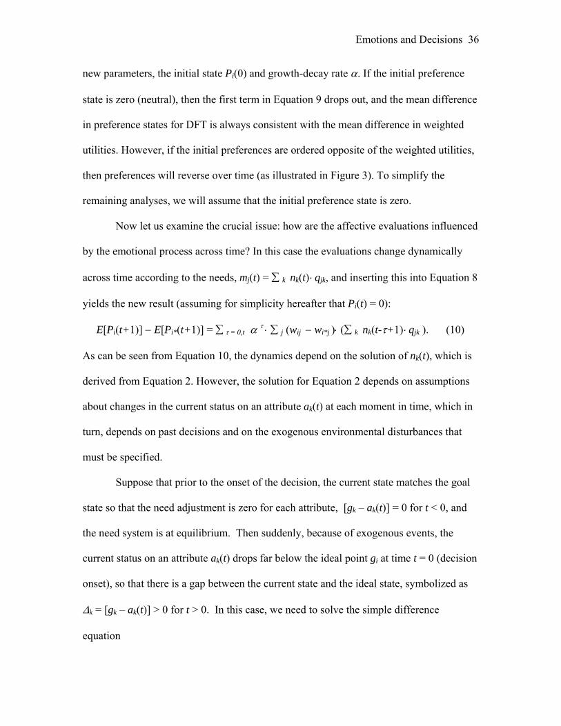
Now let us examine the crucial issue: how are the affective evaluations influenced

by the emotional process across time? In this case the evaluations change dynamically

across time according to the needs, mj(t) = ∑ k nk(t)⋅ qjk, and inserting this into Equation 8

yields the new result (assuming for simplicity hereafter that Pi(t) = 0):

E[Pi(t+1)] − E[Pi*(t+1)] = ∑ τ = 0,t α τ ⋅ ∑ j (wij − wi*j )⋅ (∑ k nk(t-τ+1)⋅ qjk ). (10)

As can be seen from Equation 10, the dynamics depend on the solution of nk(t), which is

derived from Equation 2. However, the solution for Equation 2 depends on assumptions

about changes in the current status on an attribute ak(t) at each moment in time, which in

turn, depends on past decisions and on the exogenous environmental disturbances that

must be specified.

Suppose that prior to the onset of the decision, the current state matches the goal

state so that the need adjustment is zero for each attribute, [gk – ak(t)] = 0 for t < 0, and

the need system is at equilibrium. Then suddenly, because of exogenous events, the

current status on an attribute ak(t) drops far below the ideal point gi at time t = 0 (decision

onset), so that there is a gap between the current state and the ideal state, symbolized as

∆k = [gk – ak(t)] > 0 for t > 0. In this case, we need to solve the simple difference

equation


nk(t+1) = Lk⋅ nk(t) + ∆k

and assuming 0 < Lk < 1, then the solution is given by

nk(t) = ∑ τ = 0,t-1 Lkτ ⋅ ∆k = ∆k ⋅ (∑ τ = 0,t-1 Lk

τ ) = kk

tk

LL

∆⋅⎟⎟⎠

⎞⎜⎜⎝

⎛

−−

11 . (11)

Substituting this solution into the expression for ui(t) yields

ui(t) = ∑ j wij ⋅ mj(t) = ∑ j wij ⋅ (∑ k nk(t)⋅ qjk ) = ∑ j wij ⋅ (∑ k kk

tk

LL

∆⋅⎟⎟⎠

⎞⎜⎜⎝

⎛

−−

11

⋅ qjk) .

Finally, inserting the solution given by Equation 11 into Equation 10 produces the final

solution:

E[Pi(t+1)] − E[Pi*(t+1)] = ∑ τ = 0,t α τ ⋅∑ j (wij – wi*j ) ⋅ (∑ k kk

tk

LL

∆⋅⎟⎟⎠

⎞⎜⎜⎝

⎛

−− +−

11 1τ

⋅ qjk) (12)

It is instructive to compare Equation 12 with the static weighted utility theory,

according to which (ui – ui*) = ∑ j (wij – wi*j ) ⋅ (∑ k nk⋅ qjk) completely determines

preference. Both theories share a common set of parameters: nk, qjk, wij, but DFT adds

the following two additional parameters, α and Lk. The critical qualitative property that

distinguishes DFT from the static utility model is that DFT allows preferences to reverse

across deliberation time, which is impossible with the static theory.


Tables

Table 1: Abstract Payoff Matrix for Motorcycle Decision

Possible Consequences

Actions m1 m2 m3 m4

Act A wA1 wA2 wA3 wA4

Act B wB1 wB2 wB3 wB4

Act C wC1 wC2 wC3 wC4


Table 2: Decision Weights for Motorcycle Example

Consequence

Action

c1

no damage; no

injury

c2

damage motorcycle;

minimal injury

c3

damage motorcycle;

serious injury

c4

get killed

Action A (Drive straight)

.55 0 0 .45

Action B (Swerve)

0 .90 .10 0

Action C (Slam brakes)

0 .10 .90 0

Table 3: Quality Values for Motorcycle Example NOTE: In DFT quality is the degree of satisfaction a consequence is expected to provide with respect to the attribute

Attribute

Consequence

Personal Safety Motorcycle Maintenance

c1

(safe maneuver)

1 1

c2

(lay down motorcycle)

.70 0

c3

(crash into vehicle)

.20 .40

c4

(flip motorcycle)

0 0


Figures

Figure 1. A simulation of the decision process. Horizontal axis is time, vertical axis is

preference strength, and each trajectory represents one course of action. The top bar is the

threshold bound. The first option to hit the bound wins the race and is chosen.

Figure 2. Diagram illustrating the connectionist interpretation of the decision process.

The inputs are the evaluations of consequences, the first layer represents weighted

evaluations, the second layer represent valences for each option, the third layer represents

the preference state for each option.

Figure 3. Multiple simulations demonstrate that the choice probability and the average

decision time increase monotonically as the threshold θ is increased.

Figure 4. Cognitive-Motivational Network. The highlighted regions indicate the parts of

the decision process related to emotions. The difference between the Goal State and the

actual Attribute Achievement is used to update the Need for a given attribute. This need

is in turn combined with expected satisfaction (Quality) to provide a motivational value

for all considered consequences.

Figure 5. Results of simulations run under conditions λP = .80 and λM = .40; indicating a

larger gap for personal safety; LP = .90 and LM = .70 indicating a larger feedback

control parameter for the personal safety attribute; and sii = .90 and sij = -.05 for i ≠ j. The

need for Personal safety gradually grows toward an asymptote. This change in need

directly causes an increase in preference for the less risky action B.


Figure 1

0 200 400 600 800 1000-2

-1.5

-1

-0.5

0

0.5

1

1.5

2

Deliberation Time ms

Pref

eren

ce S

tate

Theshold Bound

C

A

B

C

A

B

Figure 1


Figure 2

Figure 2

B

A

B

C

A

C C

B

A

m1

m2

m3

Weights Contrasts Valences Preferences

m4


Figure 3

Figure 3


Figure 4

Figure 4

Momentary Evaluations

Quality Motivational values

Valences qjk vi(t)

⋅mj(t)

Current Attribute Needs

nk(t) Goal State Preferences Attention

Weights gk Pi(t) Achievement Wij ak(t)

Ui(t)


Figure 5

0 20 40 60 80 1000

2

4

6

8N

eeds

0 20 40 60 80 1000

10

20

30

Time

Pre

fere

nce

personalmotorcycle

BA

Figure 5

Integrating Emotional Processes into Decision Making Models

Documents

Transcript of Integrating Emotional Processes into Decision Making Models