Integrating contextual and commonsense information for ...
197
HAL Id: tel-03523670 https://tel.archives-ouvertes.fr/tel-03523670 Submitted on 12 Jan 2022 HAL is a multi-disciplinary open access archive for the deposit and dissemination of sci- entific research documents, whether they are pub- lished or not. The documents may come from teaching and research institutions in France or abroad, or from public or private research centers. L’archive ouverte pluridisciplinaire HAL, est destinée au dépôt et à la diffusion de documents scientifiques de niveau recherche, publiés ou non, émanant des établissements d’enseignement et de recherche français ou étrangers, des laboratoires publics ou privés. Integrating contextual and commonsense information for automatic discourse understanding : contributions to temporal relation classification and bridging anaphora resolution Onkar Pandit To cite this version: Onkar Pandit. Integrating contextual and commonsense information for automatic discourse under- standing : contributions to temporal relation classification and bridging anaphora resolution. Artificial Intelligence [cs.AI]. Université de Lille, 2021. English. NNT : 2021LILUB004. tel-03523670
-
Upload
khangminh22 -
Category
Documents
-
view
1 -
download
0
Transcript of Integrating contextual and commonsense information for ...

HAL Id: tel-03523670https://tel.archives-ouvertes.fr/tel-03523670
Submitted on 12 Jan 2022
HAL is a multi-disciplinary open accessarchive for the deposit and dissemination of sci-entific research documents, whether they are pub-lished or not. The documents may come fromteaching and research institutions in France orabroad, or from public or private research centers.
L’archive ouverte pluridisciplinaire HAL, estdestinée au dépôt et à la diffusion de documentsscientifiques de niveau recherche, publiés ou non,émanant des établissements d’enseignement et derecherche français ou étrangers, des laboratoirespublics ou privés.
Integrating contextual and commonsense information forautomatic discourse understanding : contributions to
temporal relation classification and bridging anaphoraresolutionOnkar Pandit
To cite this version:Onkar Pandit. Integrating contextual and commonsense information for automatic discourse under-standing : contributions to temporal relation classification and bridging anaphora resolution. ArtificialIntelligence [cs.AI]. Université de Lille, 2021. English. �NNT : 2021LILUB004�. �tel-03523670�

École Doctorale Sciences Pour l’Ingénieur
Thèse de DoctoratSpécialité : Informatique et Applications
préparée au sein de l’équipe Magnet, du laboratoire Cristalet du centre de recherche Inria Lille - Nord Europe
Onkar Pandit
Integrating Contextual and Commonsense Informationfor Automatic Discourse Understanding
Contributions to Temporal Relation Classification and Bridging Anaphora Resolution
Intégration d’informations contextuelles et de sens commun pour lacompréhension automatique du discours
Contributions à la classification des relations temporelles et à la résolution des anaphoresassociatives
sous la direction de Prof. Marc Tommasiet l’encadrement des Dr. Pascal Denis et Prof. Liva Ralaivola
Soutenue publiquement à Villeneuve d’Ascq, le 23 Septembre 2021devant le jury composé de:
Mme Ivana Kruijff-Korbayova Saarland University, Germany RapporteureM. Vincent Ng University of Texas, Dallas RapporteurM. Sylvain Salvati Université de Lille Président du juryM. Philippe Muller Université Paul Sabatier ExaminateurMme Natalia Grabar Université de Lille ExaminatriceM. Pascal Denis INRIA Lille EncadrantM. Liva Ralaivola Criteo AI Labs EncadrantM. Marc Tommasi Université de Lille Directeur


To my parents


Acknowledgements
I am fortunate to have two excellent advisors, Pascal Denis, and Liva Ralaivola. They
shaped a researcher in me by asking intriguing questions and providing valuable sugges-
tions in our weekly interactions. It would have been impossible to produce this thesis
without their guidance.
I also take this opportunity to thank Utpal Garain of Indian Statistical Institute, Kolkata,
with whom I worked prior to joining my Ph.D. He has been a kind and encouraging person
who has trusted me and given me the opportunity to work at his NLP lab. The learnings at
his lab have been a major contribution to getting the current Ph.D. position.
Though due to the COVID19 pandemic it was difficult to interact with fellow re-
searchers, I was fortunate to meet Yufang Hou at the online ACL conference. Further
interactions with her have been fruitful and informative. I extend my gratitude to her for
these interesting discussions and for sharing her knowledge.
I express my gratitude to all the teachers from Annasaheb Patil Prashala, Solpaur,
Siddheshwar Prashala, Solpaur, Sangmeshwar College, Solpaur, Shri Gurugobind Singhji
Institute of Engineering and Technology, Nanded, IIT Kanpur, Kanpur, Indian Statistical
Institute, Kolkata, and Université de Lille, Lille. Their teachings have directly or indirectly
have lead to this dissertation.
I am grateful to all the people of MAGNET, especially to Arijus Pleska, Nathalie Vauquier,
Carlos Zubiaga, William de Vazelhes, Mathieu Dehouck, Mariana Vargas Vieyra, Cesar
Sabater, Brij Mohan Lal, Remi Gilleron, and Marc Tommasi. They made my stay in Lille
really fun and enjoyable. I extend my sincere gratitude to Mathieu, Nathalie, and Remi for
helping me in maintaining a roof over my head!
I thank all my friends back in India, especially, N. Prakash Rao, Shivraj Patil, Sanket
Deshmukh, Mahesh Bagewadi, Swapnil Pede, Omkar Gune, Vinay Narayane, Ravikant
Patil, Abhishek Chakrabarty, Akshay Chaturvedi, Nishigandha Patil, Sanket Kalamkar,
Shraddha Pandey, Vivek G, A Krishna Phaneendra, Raghvendra K, Sachin Kadam, Mathew
Manuel, Pranam K, Abhijit Bahirat, Gunjan Deotale and all my beloved friends from IIT
Kanpur. Though they have not directly contributed to the thesis, having them in life has
been a great pleasure.

iv
I am grateful to my family for their constant love and support. Pranali, my wife, has
been incredible especially at the challenging times of the pandemic. She has encouraged
and supported me at every step of research in the last two years. I am also grateful to
my ever-loving grandparents, talking to them has always filled me with enthusiasm and
positivity. I thank my sister, Aparna, for being such a loving sibling.
I reserve my special gratitude for my parents. I am eternally grateful to them for toiling
their whole life for our better future. Your love and trust in me have propelled me to come
so far. Though these two lines are not enough either to mention your sacrifices or my
feelings of gratitude. I will just say, love you and thank you, Aai-Baba!
I believe that outcome of any work also depends on the factors which are not under
the control of the doer. There can be many factors which were not in my control but they
some way positively affected the final success of the dissertation. I acknowledge such
time-bound or timeless entities, intentional or unintentional events that have directly or
indirectly lead to this dissertation. I thank them all!

Résumé
Etablir l’ordre temporel entre les événements et résoudre les anaphores associatives sont
cruciaux pour la compréhension automatique du discours. La résolution de ces tâches
nécessite en premier lieu une représentation efficace des événements et de mentions
d’entités. Cette thèse s’attaque directement à cette problématique, à savoir la conception
de nouvelles approches pour obtenir des représentations d’événements et de mentions
plus expressives.
Des informations contextuelles et de sens commun sont nécessaires pour obtenir de
telles représentations. Cependant, leur acquisition et leur injection dans les modèles
d’apprentissage est une tâche difficile car, d’une part, il est compliqué de distinguer le
contexte utile à l’intérieur de paragraphes ou de documents plus volumineux, et il est
tout aussi difficile au niveau computationnel de traiter de plus grands contextes. D’autre
part, acquérir des informations de sens commun à la manière des humains reste une
question de recherche ouverte. Les tentatives antérieures reposant sur un codage manuel
des représentations d’événements et de mentions ne sont pas suffisantes pour acquérir
des informations contextuelles. De plus, la plupart des approches sont inadéquates
pour capturer des informations de sens commun, car elles ont à nouveau recours à
des approches manuelles pour acquérir ces informations à partir de sources telles que
des dictionnaires, le Web ou des graphes de connaissances. Dans notre travail, nous
abandonnons ces approches inefficaces d’obtention de représentations d’événements et
de mentions.
Premièrement, nous obtenons des informations contextuelles pour améliorer les
représentations des événements en fournissant des n-grams de mots voisins de l’événement.
Nous utilisons également une représentation des événements basée sur les caractères
pour capturer des informations supplémentaires sur le temps et l’aspect de la structure
interne des têtes lexicales des événements. Nous allons aussi plus loin en apprenant
les interactions sur ces représentations d’événements pour obtenir des représentations
riches de paires d’événements. Nous constatons que nos représentations d’événements
améliorées démontrent des gains substantiels par rapport à une approche qui ne re-
pose que sur les plongements de la tête lexical de l’événement. De plus, notre étude

vi
d’ablation prouve l’efficacité de l’apprentissage d’interactions complexes ainsi que le rôle
des représentations basées sur les caractères.
Ensuite, nous sondons les modèles de langage de type transformer (par exemple BERT)
qui se sont révélés meilleurs pour capturer le contexte. Nous étudions spécifiquement les
anaphores associatives pour comprendre la capacité de ces modèles à capturer ce type de
relation inférentielle. Le but de cette étude est d’utiliser ces connaissances pour prendre
des décisions éclairées lors de la conception de meilleurs modèles de transformer afin
d’améliorer encore les représentations des mentions. Pour cela, nous examinons individu-
ellement la structure interne du modèle puis l’ensemble du modèle. L’examen montre
que les modèles pré-entraînés sont étonnamment bons pour capturer des informations
associatives et que ces capacités dépendent fortement du contexte, car elles fonctionnent
mal avec des contextes déformés. De plus, notre analyse qualitative montre que BERT
est capable de capturer des informations de base de sens commun mais ne parvient pas
à capturer des informations sophistiquées, qui sont nécessaires pour la résolution des
anaphores associatives.
Enfin, nous combinons à la fois des informations contextuelles et de sens commun
pour améliorer encore les représentations des événements et des mentions. Nous injec-
tons des informations de sens commun à l’aide de graphes de connaissances pour les
tâches de classification des relations temporelles et de résolution d’anaphores associatives.
Notre approche pour acquérir de telles connaissances se fonde sur des plongements de
nœuds de graphe appris sur des graphes de connaissances pour capturer la topologie glob-
ale du graphe, obtenant ainsi des informations externes plus globales. Plus précisément,
nous combinons des représentations basées sur des graphes de connaissances et des
représentations contextuelles apprises avec des plongements uniquement textuels pour
produire des représentations plus riches en connaissances. Nous évaluons notre approche
sur des jeux de données standard comme ISNotes, BASHI et ARRAU pour la résolution
des anaphores associatives et MATRES pour la classification des relations temporelles.
Nous observons des gains substantiels de performance par rapport aux représentations
uniquement textuelles sur les deux tâches démontrant l’efficacité de notre approche.

Abstract
Establishing temporal order between events and resolving bridging references are
crucial for automatic discourse understanding. For that, effective event and mention rep-
resentations are essential to accurately solve temporal relation classification and bridging
resolution. This thesis addresses exactly that and designs novel approaches to obtain
more expressive event and mention representations.
Contextual and commonsense information is needed for obtaining such effective
representations. However, acquiring and injecting it is a challenging task because, on
the one hand, it is hard to distinguish useful context itself from bigger paragraphs or
documents and also equally difficult to process bigger contexts computationally. On the
other hand, obtaining commonsense information like humans acquire, is still an open
research question. The earlier attempts of hand engineered event and mention repre-
sentations are not sufficient for acquiring contextual information. Moreover, most of the
approaches are inadequate at capturing commonsense information as they again resorted
to hand-picky approaches of acquiring such information from sources like dictionaries,
web, or knowledge graphs. In our work, we get rid of these inefficacious approaches of
getting event and mention representations.
First, we obtain contextual information to improve event representations by provid-
ing neighboring n-words of the event. We also use character-based representation of
events to capture additional tense, and aspect information from the internal structure
of event headwords. We also go a step further and learn interactions over these event
representations to get rich event-pair representations. We find that our improved event
representations demonstrate substantial gains over an approach which relied only on
the event head embeddings. Also, our ablation study proves the effectiveness of complex
interaction learning as well as the role of character-based representations.
Next, we probe transformer language models (e.g. BERT) that are proved to be better
at capturing context. We investigate specifically for bridging inference to understand the
capacity of these models at capturing it. The purpose of this investigation is to use these
understandings for making informed decisions at designing better transformer models
to further improve mention representations. For that, we examine the model’s internal
structure individually and then the whole model. The investigation shows that pre-trained
models are surprisingly good at capturing bridging information and these capabilities
are highly context dependent, as they perform poorly with distorted contexts. Further,
our qualitative analysis shows that BERT is capable of capturing basic commonsense

viii
information but fails to capture sophisticated information which is required for bridging
resolution.
Finally, we combine both contextual and commonsense information for further improv-
ing event and mention representations. We inject commonsense information with the
use of knowledge graphs for both temporal relation classification and bridging anaphora
resolution tasks. We take a principled approach at acquiring such knowledge where we
employ graph node embeddings learned over knowledge graphs to capture the overall
topology of the graph as a result gaining holistic external information. Specifically, we
combine knowledge graph based representations and contextual representations learned
with text-only embeddings to produce knowledge-aware representations. We evaluate our
approach over standard datasets like ISNotes, BASHI, and ARRAU for bridging anaphora
resolution and MATRES for temporal relation classification. We observe substantial gains
in performances over text-only representations on both tasks proving the effectiveness of
our approach.

Table of contents
List of figures xiii
List of tables xv
1 Introduction 1
1.1 Automatic discourse understanding . . . . . . . . . . . . . . . . . . . . . . . . 1
1.2 Temporal processing and bridging resolution . . . . . . . . . . . . . . . . . . 3
1.3 Event and mention representations . . . . . . . . . . . . . . . . . . . . . . . . 5
1.4 Research questions and contributions . . . . . . . . . . . . . . . . . . . . . . . 7
1.5 Organization of the dissertation . . . . . . . . . . . . . . . . . . . . . . . . . . 10
2 Background 11
2.1 Tasks . . . . . . . . . . . . . . . . . . . . . . . . . . . . . . . . . . . . . . . . . . 12
2.1.1 Temporal relation classification . . . . . . . . . . . . . . . . . . . . . . 12
2.1.1.1 Definition . . . . . . . . . . . . . . . . . . . . . . . . . . . . . . 12
2.1.1.2 Supervised learning approach . . . . . . . . . . . . . . . . . . 16
2.1.1.3 Corpora . . . . . . . . . . . . . . . . . . . . . . . . . . . . . . . 17
2.1.1.4 Evaluation . . . . . . . . . . . . . . . . . . . . . . . . . . . . . . 21
2.1.2 Bridging anaphora resolution . . . . . . . . . . . . . . . . . . . . . . . . 24
2.1.2.1 Definition . . . . . . . . . . . . . . . . . . . . . . . . . . . . . . 24
2.1.2.2 Supervised learning approach . . . . . . . . . . . . . . . . . . 26
2.1.2.3 Corpora . . . . . . . . . . . . . . . . . . . . . . . . . . . . . . . 27
2.1.2.4 Evaluation . . . . . . . . . . . . . . . . . . . . . . . . . . . . . . 28
2.2 Artificial neural networks . . . . . . . . . . . . . . . . . . . . . . . . . . . . . . 28
2.3 Representation learning . . . . . . . . . . . . . . . . . . . . . . . . . . . . . . . 32
2.4 Word representations . . . . . . . . . . . . . . . . . . . . . . . . . . . . . . . . . 35
2.4.1 Distributed representations . . . . . . . . . . . . . . . . . . . . . . . . . 36
2.4.1.1 Word2vec . . . . . . . . . . . . . . . . . . . . . . . . . . . . . . 37
2.4.1.2 Global vector (Glove) . . . . . . . . . . . . . . . . . . . . . . . 40

x Table of contents
2.4.1.3 FastText . . . . . . . . . . . . . . . . . . . . . . . . . . . . . . . 41
2.4.2 Contextual word representations . . . . . . . . . . . . . . . . . . . . . . 42
2.4.2.1 ELMo . . . . . . . . . . . . . . . . . . . . . . . . . . . . . . . . . 42
2.4.2.2 BERT . . . . . . . . . . . . . . . . . . . . . . . . . . . . . . . . . 43
2.5 Composing word representations . . . . . . . . . . . . . . . . . . . . . . . . . 48
2.5.1 Fixed composition functions . . . . . . . . . . . . . . . . . . . . . . . . 49
2.5.2 Learned composition functions . . . . . . . . . . . . . . . . . . . . . . 50
2.6 Knowledge graphs and representations . . . . . . . . . . . . . . . . . . . . . . 51
2.6.1 Knowledge graphs . . . . . . . . . . . . . . . . . . . . . . . . . . . . . . 51
2.6.1.1 WordNet . . . . . . . . . . . . . . . . . . . . . . . . . . . . . . . 53
2.6.1.2 TEMPROB . . . . . . . . . . . . . . . . . . . . . . . . . . . . . . 53
2.6.2 Graph node embeddings . . . . . . . . . . . . . . . . . . . . . . . . . . 56
2.6.2.1 Unified framework . . . . . . . . . . . . . . . . . . . . . . . . . 57
2.6.2.2 Matrix factorization based approaches . . . . . . . . . . . . . 58
2.6.2.3 Random walk based approaches . . . . . . . . . . . . . . . . . 59
2.7 Summary . . . . . . . . . . . . . . . . . . . . . . . . . . . . . . . . . . . . . . . . 60
3 Related Work 61
3.1 Temporal relation classification . . . . . . . . . . . . . . . . . . . . . . . . . . 61
3.1.1 Work on event representations . . . . . . . . . . . . . . . . . . . . . . . 62
3.1.1.1 Manually designed representations . . . . . . . . . . . . . . . 62
3.1.1.2 Automatic representation learning . . . . . . . . . . . . . . . 63
3.1.2 Work on models and inference . . . . . . . . . . . . . . . . . . . . . . . 66
3.1.3 Summary . . . . . . . . . . . . . . . . . . . . . . . . . . . . . . . . . . . . 68
3.2 Bridging anaphora resolution . . . . . . . . . . . . . . . . . . . . . . . . . . . . 69
3.2.1 Work on mention representation . . . . . . . . . . . . . . . . . . . . . . 70
3.2.1.1 Manually designed representation . . . . . . . . . . . . . . . 70
3.2.1.2 Automatic representation learning . . . . . . . . . . . . . . . 73
3.2.2 Work on models and inference . . . . . . . . . . . . . . . . . . . . . . . 74
3.2.3 Summary . . . . . . . . . . . . . . . . . . . . . . . . . . . . . . . . . . . . 75
4 Learning Rich Event Representations and Interactions 77
4.1 Introduction . . . . . . . . . . . . . . . . . . . . . . . . . . . . . . . . . . . . . . 77
4.2 Effective event-pair representations . . . . . . . . . . . . . . . . . . . . . . . . 78
4.3 Method . . . . . . . . . . . . . . . . . . . . . . . . . . . . . . . . . . . . . . . . . 81
4.3.1 Representation Learning . . . . . . . . . . . . . . . . . . . . . . . . . . 81
4.3.2 Interaction Learning . . . . . . . . . . . . . . . . . . . . . . . . . . . . . 82

Table of contents xi
4.4 Experiments . . . . . . . . . . . . . . . . . . . . . . . . . . . . . . . . . . . . . . 83
4.4.1 Datasets and Evaluation . . . . . . . . . . . . . . . . . . . . . . . . . . . 83
4.4.2 Training details . . . . . . . . . . . . . . . . . . . . . . . . . . . . . . . . 83
4.4.3 Baseline systems . . . . . . . . . . . . . . . . . . . . . . . . . . . . . . . 84
4.4.4 Ablation setup . . . . . . . . . . . . . . . . . . . . . . . . . . . . . . . . . 85
4.5 Results . . . . . . . . . . . . . . . . . . . . . . . . . . . . . . . . . . . . . . . . . 85
4.5.1 Comparison to baseline Systems . . . . . . . . . . . . . . . . . . . . . . 85
4.5.2 Comparison with state-of-the-art . . . . . . . . . . . . . . . . . . . . . 86
4.6 Ablation study . . . . . . . . . . . . . . . . . . . . . . . . . . . . . . . . . . . . . 87
4.7 Conclusions . . . . . . . . . . . . . . . . . . . . . . . . . . . . . . . . . . . . . . 88
5 Probing for Bridging Inference in Transformer Language Models 91
5.1 Introduction . . . . . . . . . . . . . . . . . . . . . . . . . . . . . . . . . . . . . . 92
5.2 Probing transformer models . . . . . . . . . . . . . . . . . . . . . . . . . . . . 94
5.2.1 Probing for relevant information . . . . . . . . . . . . . . . . . . . . . . 95
5.2.2 Probing approaches . . . . . . . . . . . . . . . . . . . . . . . . . . . . . 95
5.3 Methodology . . . . . . . . . . . . . . . . . . . . . . . . . . . . . . . . . . . . . . 96
5.4 Probing individual attention heads . . . . . . . . . . . . . . . . . . . . . . . . 97
5.4.1 Bridging signal . . . . . . . . . . . . . . . . . . . . . . . . . . . . . . . . 97
5.4.2 Experimental setup . . . . . . . . . . . . . . . . . . . . . . . . . . . . . . 98
5.4.3 Results with only Ana-Ante sentences . . . . . . . . . . . . . . . . . . . 98
5.4.4 Results with all sentences . . . . . . . . . . . . . . . . . . . . . . . . . . 100
5.4.5 Discussion . . . . . . . . . . . . . . . . . . . . . . . . . . . . . . . . . . . 100
5.5 Fill-in-the-gap probing: LMs as Bridging anaphora resolvers . . . . . . . . . 102
5.5.1 Of-Cloze test . . . . . . . . . . . . . . . . . . . . . . . . . . . . . . . . . . 102
5.5.2 Experimental setup . . . . . . . . . . . . . . . . . . . . . . . . . . . . . . 103
5.5.3 Results and Discussion . . . . . . . . . . . . . . . . . . . . . . . . . . . . 103
5.5.3.1 Results on candidates scope . . . . . . . . . . . . . . . . . . . 103
5.5.3.2 Results on Ana-Ante distance . . . . . . . . . . . . . . . . . . 104
5.6 Importance of context: Of-Cloze test . . . . . . . . . . . . . . . . . . . . . . . . 105
5.6.1 Experimental setup . . . . . . . . . . . . . . . . . . . . . . . . . . . . . . 105
5.6.2 Results on different contexts . . . . . . . . . . . . . . . . . . . . . . . . 106
5.7 Error analysis: Of-Cloze test . . . . . . . . . . . . . . . . . . . . . . . . . . . . . 107
5.8 Conclusions . . . . . . . . . . . . . . . . . . . . . . . . . . . . . . . . . . . . . . 108

xii Table of contents
6 Integrating knowledge graph embeddings to improve representation 109
6.1 Introduction . . . . . . . . . . . . . . . . . . . . . . . . . . . . . . . . . . . . . . 110
6.2 Commonsense knowledge . . . . . . . . . . . . . . . . . . . . . . . . . . . . . . 111
6.2.1 Significance for effective representation . . . . . . . . . . . . . . . . . 114
6.2.2 Challenges in integration . . . . . . . . . . . . . . . . . . . . . . . . . . 116
6.3 Our approach . . . . . . . . . . . . . . . . . . . . . . . . . . . . . . . . . . . . . 118
6.3.1 Knowledge graphs: WordNet and TEMPROB . . . . . . . . . . . . . . . 118
6.3.1.1 WordNet . . . . . . . . . . . . . . . . . . . . . . . . . . . . . . . 119
6.3.1.2 TEMPROB . . . . . . . . . . . . . . . . . . . . . . . . . . . . . . 121
6.3.2 Normalization: Simple rules and lemma . . . . . . . . . . . . . . . . . 122
6.3.3 Sense disambiguation: Lesk and averaging . . . . . . . . . . . . . . . . 123
6.3.4 Absence of knowledge: Zero vector . . . . . . . . . . . . . . . . . . . . 124
6.4 Improved mention representation for bridging resolution . . . . . . . . . . . 124
6.4.1 Knowledge-aware mention representation . . . . . . . . . . . . . . . . 124
6.4.2 Ranking model . . . . . . . . . . . . . . . . . . . . . . . . . . . . . . . . 125
6.4.3 Experimental setup . . . . . . . . . . . . . . . . . . . . . . . . . . . . . . 126
6.4.4 Results . . . . . . . . . . . . . . . . . . . . . . . . . . . . . . . . . . . . . 128
6.4.5 Error analysis . . . . . . . . . . . . . . . . . . . . . . . . . . . . . . . . . 132
6.4.5.1 Mention normalization and sense disambiguation . . . . . . 132
6.4.5.2 Anaphor-antecedent predictions . . . . . . . . . . . . . . . . 132
6.5 Improved event representation for temporal relation classification . . . . . . 134
6.5.1 Knowledge-aware event representations . . . . . . . . . . . . . . . . . 135
6.5.2 Neural model . . . . . . . . . . . . . . . . . . . . . . . . . . . . . . . . . 136
6.5.2.1 Constrained learning . . . . . . . . . . . . . . . . . . . . . . . 136
6.5.2.2 ILP Inference . . . . . . . . . . . . . . . . . . . . . . . . . . . . 138
6.5.3 Experimental setup . . . . . . . . . . . . . . . . . . . . . . . . . . . . . . 139
6.5.4 Results . . . . . . . . . . . . . . . . . . . . . . . . . . . . . . . . . . . . . 141
6.5.5 Discussion . . . . . . . . . . . . . . . . . . . . . . . . . . . . . . . . . . . 144
6.6 Conclusion . . . . . . . . . . . . . . . . . . . . . . . . . . . . . . . . . . . . . . . 145
7 Conclusions 147
References 151
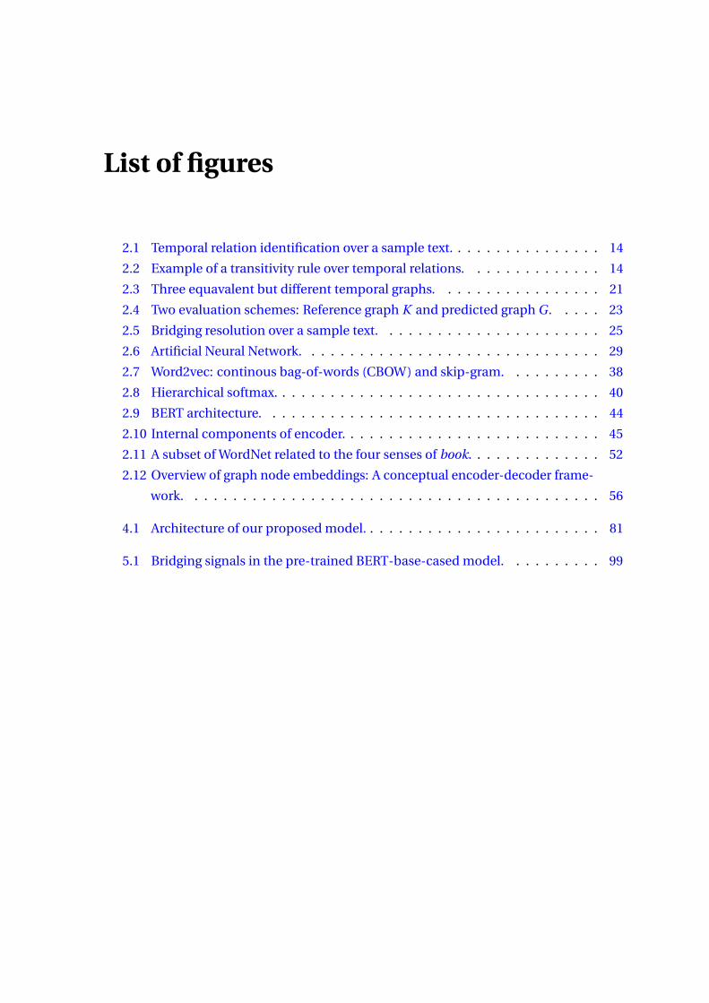
List of figures
2.1 Temporal relation identification over a sample text. . . . . . . . . . . . . . . . 14
2.2 Example of a transitivity rule over temporal relations. . . . . . . . . . . . . . 14
2.3 Three equavalent but different temporal graphs. . . . . . . . . . . . . . . . . 21
2.4 Two evaluation schemes: Reference graph K and predicted graph G . . . . . 23
2.5 Bridging resolution over a sample text. . . . . . . . . . . . . . . . . . . . . . . 25
2.6 Artificial Neural Network. . . . . . . . . . . . . . . . . . . . . . . . . . . . . . . 29
2.7 Word2vec: continous bag-of-words (CBOW) and skip-gram. . . . . . . . . . 38
2.8 Hierarchical softmax. . . . . . . . . . . . . . . . . . . . . . . . . . . . . . . . . . 40
2.9 BERT architecture. . . . . . . . . . . . . . . . . . . . . . . . . . . . . . . . . . . 44
2.10 Internal components of encoder. . . . . . . . . . . . . . . . . . . . . . . . . . . 45
2.11 A subset of WordNet related to the four senses of book. . . . . . . . . . . . . . 52
2.12 Overview of graph node embeddings: A conceptual encoder-decoder frame-
work. . . . . . . . . . . . . . . . . . . . . . . . . . . . . . . . . . . . . . . . . . . 56
4.1 Architecture of our proposed model. . . . . . . . . . . . . . . . . . . . . . . . . 81
5.1 Bridging signals in the pre-trained BERT-base-cased model. . . . . . . . . . 99


List of tables
2.1 Allen’s interval temporal relations. . . . . . . . . . . . . . . . . . . . . . . . . . 13
2.2 TimeML temporal relations and corresponding Allen’s interval relations. . . 18
2.3 Temporal relation classification: Corpora details. . . . . . . . . . . . . . . . . 19
2.4 Ambiguous as well as rare relations mapped to coarse-grained relations. . . 20
2.5 Temporal relation classification: Evaluation results with two different schemes. 23
2.6 Briading anaphora resolution: Corpora details . . . . . . . . . . . . . . . . . . 27
2.7 A portion of TEMPROB. . . . . . . . . . . . . . . . . . . . . . . . . . . . . . . . 54
4.1 Results of baseline and state-of-the-art systems . . . . . . . . . . . . . . . . . 86
4.2 Ablation study. . . . . . . . . . . . . . . . . . . . . . . . . . . . . . . . . . . . . . 88
5.1 Examples of easy and difficult bridging relations for the prominent heads. . 101
5.2 Result of selecting antecedents for anaphors. . . . . . . . . . . . . . . . . . . 104
5.3 Anaphor-antecedent distance-wise accuracy. . . . . . . . . . . . . . . . . . . 105
5.4 Accuracy of selecting antecedents with different types of context. . . . . . . 106
6.1 Results of our experiments and state-of-the-art models. . . . . . . . . . . . . 129
6.2 Number of mentions from the datasets and proportion of them absent in
WordNet. . . . . . . . . . . . . . . . . . . . . . . . . . . . . . . . . . . . . . . . . 132
6.3 Few examples of mention mapping and mention sense selection. . . . . . . 133
6.4 Composition rules on end-point relations present in MATRES dataset. . . . 138
6.5 Results of the experiments over MATRES. . . . . . . . . . . . . . . . . . . . . . 142


Chapter 1
Introduction
1.1 Automatic discourse understanding
Discourse is a bigger chunk of language than a sentence such as paragraph, document,
etc., which often comprises multiple sentences. The sentences can be uttered by a single
person or multiple people with the constraint that discourse as a unit produces coherent
communication (Hobbs, 1979; Scha et al., 1986). A coherent communication conveys a sin-
gle core subject with multiple discourse elements producing continuous sense by relating
to previously mentioned elements. On the contrary, a random sequence of sentences that
does not possess such continuity of senses can not be a discourse (De Beaugrande and
Dressler, 1986; Mann and Thompson, 1986). A discourse can be between writer–reader
(text) or speaker–listener (dialogue). In this work, we concentrate on the written text so
that discourses are monologues that communicate with the reader.
In discourse, linguistic units are connected by different relations to maintain coherence
and deciphering these relations is a part of discourse understanding (Stede, 2011; Webber,
2019). The linguistic units such as sentences, clauses, or events (smaller linguistic units
that indicate situations within clauses) can be temporally related to each other (Bramsen
et al., 2006). Temporal relations between them denote the chronological order in which
they occur (e.g. precedence, succession, concurrence, etc.). In addition to temporal
relations, a relation on a semantic or pragmatic level can link clauses, sentences, or larger
portions of discourse to each other. These relations are known as discourse relations (also
called as coherence or rhetorical relations). The exact number of discourse relations
varies depending on the postulated granularity but generally they indicate consequence,
explanation, elaboration, or contrast between discourse units (Carlson et al., 2001; Prasad
et al., 2008; Stede, 2011). Apart from these relations, there can be expressions in different
sentences which link to previously mentioned expressions either directly or indirectly.

2 Introduction
We are talking specifically about mentions that refer to real or abstract entities. Mentions
are either named (e.g. Barack Obama), nominal (e.g. the chairman, a car, the driver) or
pronominal (e.g. he, she) expressions. They exhibit certain relations with each other.
Mentions can hold either bridging relation where mentions refer to different entities
but are associated with each other (e.g. the driver-a car) or coreference relation where
mentions refer to the same entity (e.g. He-Barack Obama).
Let us explain this further with a following simple discourse (modified from Hobbs
(1979)):
This discourse tells a reader that Paul traveled in the first-class compartment of the
train from Paris to Istanbul and he enjoyed the ride. After that Paul traveled in a boat to
reach Cyprus. This understanding is possible because a human reader unravels various
relations from the discourse:
• “the first-class compartment” indicates the first-class of the train in which Paul
traveled. (bridging relation between “a train” and“the first-class compartment”)
• Both instances of the pronouns, “He”, “He” refer to “Paul”. (Coreference relation)
• Paul’s journey was pleasant “because” the seats were comfortable. (causal Discourse
relation )
• Paul traveled to Cyprus “after” the train journey from Paris to Istanbul. (Temporal
relation)
Uncovering these relations is essential for automatic discourse understanding. Out
of these relations, temporal and bridging relations are relatively less studied in NLP
than discourse relations (Braud and Denis, 2015; Dai and Huang, 2018; Ji and Eisenstein,
2015; Lin et al., 2009; Liu et al., 2020; Liu and Li, 2016; Marcu and Echihabi, 2002; Pitler
et al., 2008; Saito et al., 2006; Shi and Demberg, 2019; Varia et al., 2019; Wang and Lan,
2015; Wellner et al., 2006) and coreference relations (Clark and Manning, 2015, 2016a,b;
Daumé III and Marcu, 2005; Denis and Baldridge, 2008; Durrett and Klein, 2013; Finkel

1.2 Temporal processing and bridging resolution 3
and Manning, 2008; Joshi et al., 2020; Lee et al., 2017; Luo et al., 2004; Soon et al., 2001;
Wiseman et al., 2015, 2016; Zhang et al., 2019a). Consequently, we specifically concentrate
on temporal relation classification and bridging resolution tasks, which automatically
detect the temporal and bridging relations from text. The following sections discuss in
detail about them.
1.2 Temporal processing and bridging resolution
Temporal processing Automatic temporal analysis is critical to perform automatic pro-
cessing and understanding of discourse. Detecting temporal relations between events
accurately unravels the intended meaning conveyed by the writer. For instance, consider
two events from a discourse: people were furious and police used water canons. Assigning
two different temporal relations to them affects the meaning of the discourse: police
used water canons before people were furious means people became furious because of
police’s action, whereas police used water canons after people were furious conveys police
used water canons to placate angry people. Additionally, the temporal relations help to
establish discourse relations between clauses (Wang et al., 2010), which can be seen from
the previous example, where police used water canons causes people were furious given
that it happens before, whereas after temporal relation reverses causality. This shows a
clear need to establish accurate temporal relations to extract the overall intended meaning
out of discourse.
Besides its significance in discourse understanding, temporal analysis has important
practical implications. In document summarization, knowledge about the temporal order
of events can enhance both the content selection and the summary generation processes
(Barzilay et al., 2002; Ng et al., 2014). In question answering (QA), temporal analysis is
needed to determine “when” or “how long” a particular event occurs and temporal order
between them (Meng et al., 2017; Prager et al., 2000). The temporal modeling can also
help machine translation systems (Horie et al., 2012). In addition, temporal information
is highly beneficial in the clinical domain for applications such as patient’s timeline
visualization, early diagnosis of disease, or patients selection for clinical trials (Augusto,
2005; Choi et al., 2016; Jung et al., 2011; Raghavan et al., 2014).
For a given discourse, the temporal processing task can be divided into two main
parts: 1. Detecting temporal entities such as events and time expressions (TimEx)1, and
2. Establishing temporal ordering between these temporal entities. The latter task is
1Time expressions are phrases that indicate moment, intervals or other time regions. The phrases suchas 15 Aug. 1947, two weeks or today fall into this category. We detail this in the next chapter.

4 Introduction
called temporal relation classification which particularly determines temporal relations
between event-event, event-TimEx and TimEx-TimEx pairs. In this work, we are focusing
on the temporal relation classification for event-event pairs because it is challenging
in comparison to other pairs. But, the proposed methods can be easily extended for
determining relations between the other two pairs as well.
Bridging resolution Mentions also possess certain relations between each other like
temporal relations between sentences, clauses, or events. Specifically, an anaphor is a spe-
cial mention that depends on previously appeared mention(s), referred to as antecedent(s),
for its complete interpretation. As stated previously, anaphor-antecedent can be related
to each other either by a bridging or coreference relation. Bridging relation indicates an
association between anaphor and antecedent but non-identical relation (e.g. the first-class
compartment–a train) whereas coreference denotes identical relation (e.g. He–Paul). Au-
tomatically identifying bridging relations is more challenging than coreference resolution
as bridging encodes various abstract relations between mentions as opposed to identical
relations in coreference. These context-dependent abstract relations also require world
knowledge to make a connection between them. Additionally, the annotated corpora
for bridging are smaller in comparison increasing the difficulty level further. Bridging
relations are the second topic of focus in this work, as even though difficult, realizing
bridging relations is crucial for discourse comprehension.
Identifying bridging relations is also beneficial for various tasks such as textual en-
tailment, QA, summarization, and sentiment analysis. Textual entailment establishes
whether a hypothesis can be inferred from a particular text, and bridging can be used in
determining this inference (Mirkin et al., 2010). For QA system, (Harabagiu et al., 2001)
resolved a subset of bridging relations (meronymic) in the context for better accurately
identifying answers. Resolving bridging relations is important for summarization, as differ-
ent sentences can be combined based on it (Fang and Teufel, 2014). Bridging resolution is
also of help in aspect-based sentiment analysis (Kobayashi et al., 2007), where the aspects
of an object, for example, the zoom of a camera, are often bridging anaphors.
Computational task for identifying bridging relations is called bridging resolution.
That can be further broken into two main tasks: bridging anaphora identification which
identifies bridging anaphors from documents, and bridging anaphora resolution which
links them to appropriate antecedents. This work focuses on the second task of anaphora
resolution.

1.3 Event and mention representations 5
1.3 Event and mention representations
Importance of context and commonsense information Automatic processing of tem-
poral and bridging relations is difficult which can be seen from the low state-of-the-art
results. However, humans perform these tasks very easily. We hypothesize that the reasons
might be that human readers can access contextual information from the given discourse
itself as well as use their prior experience in the form of commonsense knowledge to figure
out these relations.
A context2 is important for establishing temporal ordering between linguistic units
and making bridging associations. In fact, it is crucial for overall discourse understanding,
for instance, in the previous example, we can not understand “from where he went to
Cyprus?” if the last sentence “He went by boat from there to Cyprus” is read without the
earlier sentences. To specifically see the importance of context for temporal relations, let
us look at the following examples that are adapted from Lascarides and Asher (1993):
(1) Max switchede1 on the light. The room was pitch darke2 .
(2) Max switchede1 off the light. The room was pitch darke2 .
From the discourse in example 1, a human reader can understand that the room was
dark before Max switched on the light. But, in example 2, the room was dark after Max
switched off the light. The chronology of events switching and room becoming dark is
changed depending on the context in which they are used.
Similarly, context is significant for establishing bridging relations, which can be under-
stood from the following examples:
(3) A car is more fuel efficient than a rocket as the engine requires less fuel.
(4) A car is more fuel efficient than a rocket as the engine requires more fuel.
In example 3, the engine refers to the car engine as it requires less fuel and we said that
cars are more fuel efficient that rockets. But, because of change in the context, when we
say the engine requires more fuel in 4, here, the engine refers to the rocket engine and not
the car engine.
2Throughout this thesis, context refers to linguistic context. Context can be derived from different sourcessuch as physical context depends on the place of discourse deliverance, participants in communicationhaving similar background knowledge share epistemic context, or social context is derived from same socialconducts of participants. But, here we are referring to linguistic context where communication is built onthe previous text and a meaning is derived from them.
6 Introduction
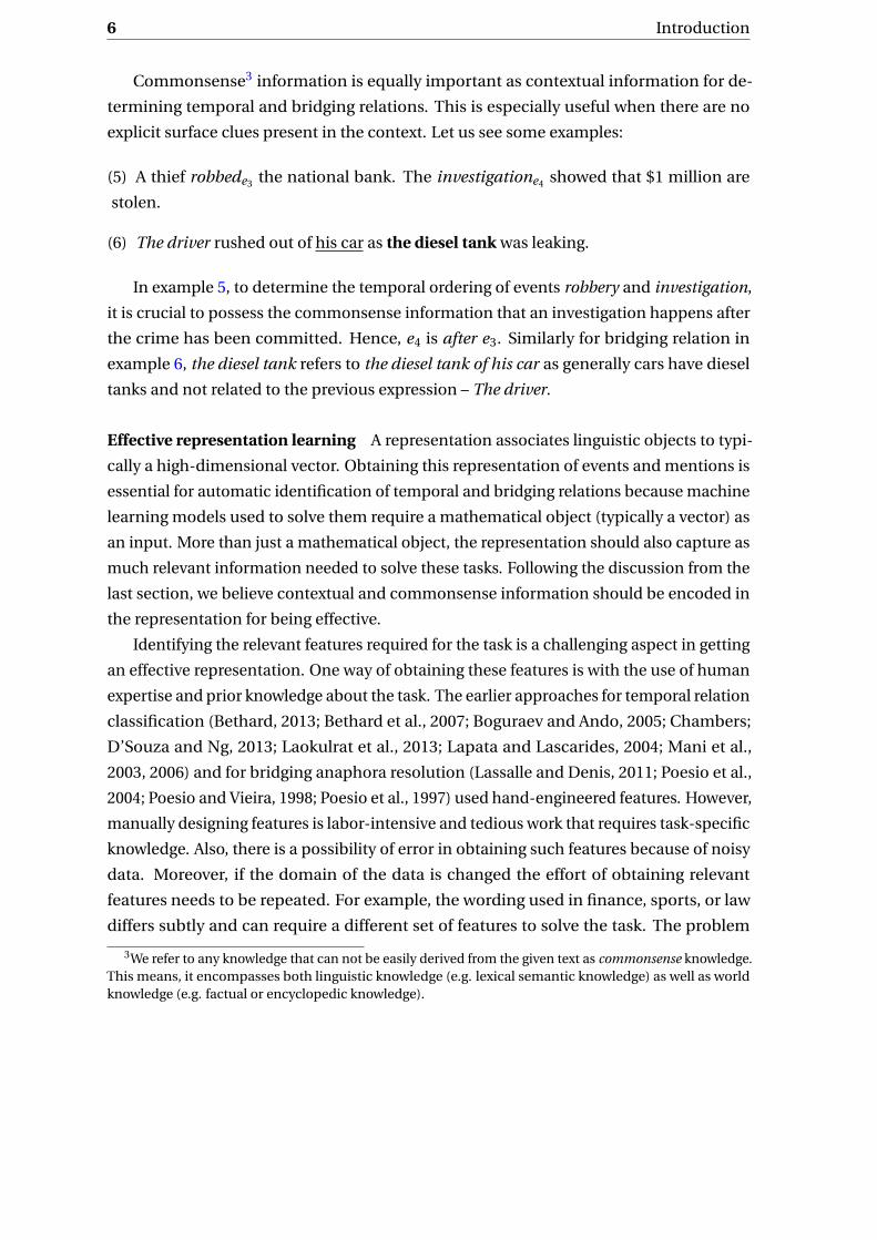
Commonsense3 information is equally important as contextual information for de-
termining temporal and bridging relations. This is especially useful when there are no
explicit surface clues present in the context. Let us see some examples:
(5) A thief robbede3 the national bank. The investigatione4 showed that $1 million are
stolen.
(6) The driver rushed out of his car as the diesel tank was leaking.
In example 5, to determine the temporal ordering of events robbery and investigation,
it is crucial to possess the commonsense information that an investigation happens after
the crime has been committed. Hence, e4 is after e3. Similarly for bridging relation in
example 6, the diesel tank refers to the diesel tank of his car as generally cars have diesel
tanks and not related to the previous expression – The driver.
Effective representation learning A representation associates linguistic objects to typi-
cally a high-dimensional vector. Obtaining this representation of events and mentions is
essential for automatic identification of temporal and bridging relations because machine
learning models used to solve them require a mathematical object (typically a vector) as
an input. More than just a mathematical object, the representation should also capture as
much relevant information needed to solve these tasks. Following the discussion from the
last section, we believe contextual and commonsense information should be encoded in
the representation for being effective.
Identifying the relevant features required for the task is a challenging aspect in getting
an effective representation. One way of obtaining these features is with the use of human
expertise and prior knowledge about the task. The earlier approaches for temporal relation
classification (Bethard, 2013; Bethard et al., 2007; Boguraev and Ando, 2005; Chambers;
D’Souza and Ng, 2013; Laokulrat et al., 2013; Lapata and Lascarides, 2004; Mani et al.,
2003, 2006) and for bridging anaphora resolution (Lassalle and Denis, 2011; Poesio et al.,
2004; Poesio and Vieira, 1998; Poesio et al., 1997) used hand-engineered features. However,
manually designing features is labor-intensive and tedious work that requires task-specific
knowledge. Also, there is a possibility of error in obtaining such features because of noisy
data. Moreover, if the domain of the data is changed the effort of obtaining relevant
features needs to be repeated. For example, the wording used in finance, sports, or law
differs subtly and can require a different set of features to solve the task. The problem
3We refer to any knowledge that can not be easily derived from the given text as commonsense knowledge.This means, it encompasses both linguistic knowledge (e.g. lexical semantic knowledge) as well as worldknowledge (e.g. factual or encyclopedic knowledge).

1.4 Research questions and contributions 7
of designing features becomes more difficult if the language of the text is changed. As a
result, it is critical to learn these relevant features rather than relying on manually designed
representation.
The recent approaches based on neural networks attempt to remedy issues of manually
designed features by automatically learning these representations but these approaches
are few. In the case of temporal relation classification, either approaches ignored context
completely (Mirza and Tonelli, 2016) or added syntactic tree preprocessing burden to
encode contextual information (Cheng and Miyao, 2017; Choubey and Huang, 2017; Meng
et al., 2017) 4. Also, the approaches proposed to encode commonsense information relied
on certain hand-designed features (Ning et al., 2018a) or used a portion of knowledge
source (Ning et al., 2019). Similarly, for bridging anaphora resolution recently proposed
bridging-specific embeddings (Hou, 2018a,b) ignored context whereas BERT based ap-
proaches (Hou, 2020a; Yu and Poesio, 2020) neglected commonsense information.
As stated earlier, an effective representation learning should capture contextual and
commonsense information as they are important for both tasks, but incorporating these
two types of information poses various challenges. The major problem in injecting con-
textual knowledge is to understand what kind of context to provide and how much. It
is possible, that humans derive context from previous sentences, paragraphs, or even
documents. But including this context in the learning models is difficult because of the
limited processing abilities of the models as well as the overall capacity to decipher the
useful context. On the other hand, commonsense information inclusion poses other type
of problems. Since humans acquire commonsense knowledge from various sources, in
general from their world experiences, it is not easy to replicate them in computational
approaches. In recent years, studies based on both contextual and commonsense knowl-
edge are gaining traction, as approaches using various sources of external knowledge like
knowledge graphs (Faruqui et al., 2015; Mihaylov and Frank, 2018; Shangwen Lv and Hu,
2020), images (Cui et al., 2020; Li et al., 2019; Rahman et al., 2020), videos (Huang et al.,
2018; Palaskar et al., 2019), or crowdsourced resources (Krishna et al., 2016) have been
proposed.
1.4 Research questions and contributions
From this discussion, we see that the previously proposed approaches fail to simultane-
ously capture both contextual information and commonsense information effectively.
4We are talking about the period before the proposal of our system (Pandit et al., 2019), significantimprovements have been made since then.
8 Introduction
We intend to fill this gap. Our aim in this thesis is to design efficient approaches for
learning effective event representations for temporal relation classification and mention
representations for bridging anaphora resolution. We include both contextual as well as
commonsense knowledge because of their importance in these representations. We argue
that the amount of commonsense information that can be learned from only text-based
approaches is limited. Hence, there is a need to complement text-based information with
commonsense information learned from external knowledge sources. This understanding
leads to different objectives and contributions:
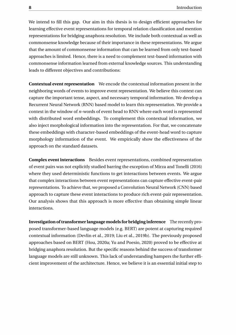
Contextual event representation We encode the contextual information present in the
neighboring words of events to improve event representation. We believe this context can
capture the important tense, aspect, and necessary temporal information. We develop a
Recurrent Neural Network (RNN) based model to learn this representation. We provide a
context in the window of n-words of event head to RNN where each word is represented
with distributed word embeddings. To complement this contextual information, we
also inject morphological information into the representation. For that, we concatenate
these embeddings with character-based embeddings of the event-head word to capture
morphology information of the event. We empirically show the effectiveness of the
approach on the standard datasets.
Complex event interactions Besides event representations, combined representation
of event pairs was not explicitly studied barring the exception of Mirza and Tonelli (2016)
where they used deterministic functions to get interactions between events. We argue
that complex interactions between event representations can capture effective event-pair
representations. To achieve that, we proposed a Convolution Neural Network (CNN) based
approach to capture these event interactions to produce rich event-pair representation.
Our analysis shows that this approach is more effective than obtaining simple linear
interactions.
Investigation of transformer language models for bridging inference The recently pro-
posed transformer-based language models (e.g. BERT) are potent at capturing required
contextual information (Devlin et al., 2019; Liu et al., 2019b). The previously proposed
approaches based on BERT (Hou, 2020a; Yu and Poesio, 2020) proved to be effective at
bridging anaphora resolution. But the specific reasons behind the success of transformer
language models are still unknown. This lack of understanding hampers the further effi-
cient improvement of the architecture. Hence, we believe it is an essential initial step to

1.4 Research questions and contributions 9
investigate these transformer models for bridging information because with that under-
standing mention representations can be further improved. Specifically, we want to probe
how capable are these transformer models at capturing bridging inference and which
layers of these big models are focusing on bridging. Importantly, we also check what kind
of context is required for these models to produce decent results. We design our probing
methods keeping these objectives in mind.
We employ two approaches for this investigation. First, we probe individual attention
heads of the transformer models for bridging inference. Our investigation shows that the
higher layers better capture bridging information than the middle and lower layers. Sec-
ond, we go a step further to investigate whole transformer model so as to understand how
effectively they perform cumulatively. We design a novel Of-Cloze test, a fill-in-the-blank
test that scores candidate antecedents for each anaphor and selects the highest scoring
mention as predicted antecedent. This Of-Cloze formulation produces competitive results
for bridging anaphora resolution indicating transformer models’ ability at capturing bridg-
ing information. Finally, we investigate the importance of context by providing a different
set of contexts to Of-Cloze test. We also, qualitatively investigate BERT to assess its ability
at capturing commonsense information required for bridging, which shows insufficiency
of BERT at them.
Knowledge-aware mention and event representation Our investigation of transformer
language models suggests that they are good at capturing contextual information but
inadequate at capturing commonsense information which is in line with the previous
studies (Da and Kasai, 2019; Park et al., 2020). So, we design approaches to inject such
knowledge for mention and event representations, and propose to use knowledge graph
node embeddings for this purpose. We claim that this way of injecting knowledge is more
effective than designing features based on external knowledge. However, this approach
poses a few challenges: First, mapping mentions or events to graph nodes is a non-trivial
task as they are inherently different objects (nodes can be abstract concepts whereas
mentions are linguistic units containing tokens). Second, the mapping can lead to multiple
nodes (due to the several meanings of the word) or no node at all (due to the absence of
knowledge from the graph). We propose simple approaches to address these questions
that can be applied over for any knowledge graph. Specifically, we use two knowledge
graphs separately, WordNet (Fellbaum, 1998), and TEMPROB (Ning et al., 2018a), and
empirically show the effectiveness of these proposed methods for both tasks, followed by
analysis for a better understanding.

10 Introduction
1.5 Organization of the dissertation
The remainder of the document is mainly divided into three parts. First, we introduce the
background information and prior work. The next three chapters detail our contributions
and finally, we conclude by noting down our findings and future directions.
Chapter 2 describes necessary task definitions, the corpora used in the experiments,
and evaluation strategies. Further, we briefly introduce artificial neural networks that
are used extensively in the thesis as a base model. Next, the chapter details the different
word representation approaches that are central to our work. Finally, we describe different
knowledge graphs, and graph node embeddings framework.
Chapter 3 explores related work for both temporal relation classification and bridging
resolution. For both tasks, we focus on the previous event and mention representation
approaches while briefly discussing model and inference related work.
Chapter 4 details our rich event representation and complex interaction learning
approach used for temporal relation classification. We understand from previous studies
that less attention is given to capture context for event representations. To remedy that,
we propose RNN based model to get event representation and CNN to capture complex
interactions. We detail our proposed neural model in this chapter, and we present results
from experiments to prove the efficacy of our approach. We also provide ablation studies
to understand the importance of different components in our system.
Chapter 5 focuses on the probing of transformer models for bridging inference. This
chapter talks about three important things: first, the ability of individual attention heads
at capturing bridging signal, second, our novel Of-Cloze test that checks the potency of the
whole transformer model, and third, the effect of context on their ability of understanding
bridging. The detailed error analysis is also done to understand the shortcomings of
transformer models as well as of our formulation.
Chapter 6 proposes an approach for obtaining knowledge-aware mention and event
representations. We first describe the challenges posed by the process of injecting com-
monsense information with the use of knowledge graphs. Then we propose a unifying
strategy to inject such knowledge for bridging anaphora resolution and temporal relation
classification. We provide empirical evidence of the effectiveness of our approach and a
detail analysis of our results.
Finally, Chapter 7 provides a formal conclusion of the thesis and a discussion of
promising future directions.

Chapter 2
Background
This chapter serves as a background for the rest of the thesis. It describes three important
items: (i) task definitions of both temporal relation classification and bridging anaphora
resolution, components of supervised approaches used to solve them including essential
factors: event, and mention representation, corpora used in the work, and evaluation
strategies, (ii) artificial neural networks which are popularly used for representation
learning and modeling, and (iii) representation learning and related fields, previously
proposed approaches to learn word representations, several composition functions over
them to obtain representations of word sequences (phrases, sentences, or paragraphs),
and knowledge graphs and graph node representations.
Section 2.1 details two central tasks of the thesis: temporal relation classification and
bridging anaphora resolution. For both tasks, we first provide formal definitions, then
specify three main components of supervised learning approaches used to solve them:
event and mention representations, models, and inference strategies. Further, we detail
corpora used for training and evaluating proposed approaches, and evaluation schemes.
In recent years, Artificial neural networks have been used ubiquitously for represen-
tation learning as well as modeling. Due to their potency, we also used them to improve
representations and for modeling. Therefore, we provide brief introduction of them in
Section 2.2. We explain the fundamental element of these models (neuron), activation
functions, hyperparameters, and optimization strategies. Further, we describe some of the
regularly used neural network architectures such as Feed-forward neural networks (FFNN),
Recurrent neural networks (RNN), and Convolutional neural networks (CNN).
The remaining chapter focuses on representation learning and various popularly
employed approaches to learning representations of words, word sequences, and graph
nodes. Section 2.3 discusses representation learning and related fields like metric learning,
and dimensionality reduction. Next, in section 2.4 we look at different distributional

12 Background
and contextual approaches of obtaining word representations. We first describe popular
distributional embeddings such as Word2vec (Mikolov et al., 2013a), Glove (Pennington
et al., 2014), and FastText (Bojanowski et al., 2017) which are used in the thesis, followed by
recently proposed contextual embeddings like ELMo (Peters et al., 2018), and BERT (Devlin
et al., 2019). Further, in section 2.5 we look at different ways of combining these word
embeddings to obtain representations of word sequences i.e. bigger chunks of language
than words like phrases, sentences, paragraphs, or documents. At last, we brief about
knowledge graphs and describe WordNet (Fellbaum, 1998) and TEMPROB (Ning et al.,
2018a), followed by details of conceptual framework and two broad families of node
embeddings approaches in Section 2.6.
2.1 Tasks
In this thesis, we focus on two discourse tasks: temporal relation classification and bridg-
ing anaphora resolution. We detail about them in this section.
2.1.1 Temporal relation classification
Time is a critical part of a language that is grasped from either explicitly or implicitly
present temporal information in the text, and automatically extracting such temporal
information is necessary for discourse understanding. In a discourse, various types of
linguistic units can be related temporally to each other such as sentences, clauses, or
smaller linguistic units like events, and expressions (TimEx) (Bramsen et al., 2006). Events
and TimEx, the granular units compared to sentences and clauses, are fundamental
for temporal information in language (Moens and Steedman, 1988). Hence, all recent
approaches consider these temporal entities, events and TimEx, as the ordering units for
establishing temporal relations (Bethard, 2013; Bethard et al., 2007; Chambers; D’Souza
and Ng, 2013; Laokulrat et al., 2013). We also follow a similar definition in our work.
In the following sections, we formally define temporal relation classification task (Sec-
tion 2.1.1.1), describe main components of common supervised learning approaches used
to solve them (Section 2.1.1.2), detail on corpora used in the experiments (Section 2.1.1.3),
and specify evaluations schemes (Section 2.1.1.4).
2.1.1.1 Definition
Temporal relation classification establishes temporal relations between temporal entities
such as events, and time expressions (TimEx) present in the given document. Events

2.1 Tasks 13
Relation Symbol Symbol forinverse
Pictorialview
X before Y b a XXX YYY
X meets Y m mi XXXYYY
X overlaps Y o oi XXXYYY
X during Y d di XXXYYYYYY
X starts Y s si XXXYYYYY
X finishes Y f fi XXXYYYYY
X equal Y = = XXXYYY
Table 2.1 Allen’s interval temporal relations (Allen, 1983).
denote actions, occurrences, or reporting and can last for longer period of time or com-
plete in a moment (Pustejovsky et al., 2003b). Events are often expressed with verbs (e.g.
raced, declared), and sometimes with noun phrases (e.g. deadly explosion), statives (e.g.
he is an idiot), adjectives (e.g. the artist is active), predicatives (e.g. Biden is the presi-
dent), or prepositional phrases (e.g. soldiers will be present in uniform) may also indicate
events (Steedman, 1982). The second temporal entity, TimEx denotes exact or relative
pointer of time (e.g. now, last week, 26 Jan. 1950). It can be a moment, or an interval that
can state unambiguous time like 26 Jan. 1950 or a reference from the utterance such as
last week, now.
In this thesis, we consider temporal entities (events and TimEx) as intervals of time
that have start-point and end-point where start-point occurs before end-point (Hobbs
and Pan, 2004). This interval perspective holds true even in the case of a moment because
it still has start-point and end-point, albeit, not far from each other. Based on this interval
notion of temporal entities, Allen (1983) defined 13 possible temporal relations that can
be assigned between pair of temporal entities as shown in Table 2.1.
For the given document, temporal relations between temporal entities can be pre-
sented with the use of a graph where nodes are temporal entities and edges denote
temporal relations between them. This graph formed over temporal entities with temporal
relations between them is called temporal graph. Figure 2.1 shows the temporal graph
generated over a sample text. The figure also illustrates the complete process of temporal

14 Background
Fig. 2.1 Temporal relation identification over a sample text. From the given text (a), eventsand TimEx are extracted (b), bold-faced words denote events and underlined wordsare TimEx and then, temporal relations are assigned between events/TimEx to create atemporal graph (c) with nodes as event or TimEx and edge denoting temporal relation.Temporal graph shows edges as John studied (e1) before joined (e3), interned (e2) during in2010 (t1) where both these happened during studied (e1).
relation extraction, first from the given raw text events and are extracted and then, a
temporal graph is formed over them.
Over these temporal relations, logical rules like symmetry and transitivity can be
applied as they possess algebraic properties (Allen, 1983). Suppose A, B and C are some
arbitrary events, then the rule of symmetry over temporal relations states that if A is before
B then B must be after A, because before and after are inverse temporal relations. This
symmetric rule can be generalized to other relations and their inverse relations mentioned
in Table 2.1. Formally, a symmetry rule Si , j between a r, r inverse relation pair can be
given as:
Si , j : ri , j → r j ,i (2.1)
where i , j denote any temporal interval and ri , j , r j ,i denote respectively temporal relations
r , r between i , j and j , i .
In addition to rules of symmetry, several transitivity rules can be applied over temporal
relations, for instance, if A meets B and B overlaps C, then A must be before C as illustrated
in Fig. 2.2. Here, we mentioned single transitivity rule over a specific pair of temporal
Fig. 2.2 (A m B)∧ (B o C ) → (A b C ).
relations: meets, and overlaps, but similar transitivity rules can be applied over all possible

2.1 Tasks 15
pairs of relations which is detailed in (Allen, 1983). Formally, a generic transitivity rule
Ti , j ,k can be given as:
Ti , j ,k : ri , j ∧ r j ,k → r ′i ,k (2.2)
where i , j ,k are any temporal intervals and ri , j , r j ,k ,r ′i ,k respectively denote temporal
relations r, r ,r ′ between i − j , j −k, and i −k, and r ′ is the relation obtained by composing
r and r .
Unknown temporal relations can be inferred from other known relations with the
application of these logical rules. Consider the above example, if the temporal relation
between A and C was unknown, then the transitivity rule over known relations between
A-B and B-C could easily tell us that A occurs before C. The process of applying these
transitivity rules to infer all the possible temporal relations from a temporal graph is known
as temporal graph saturation or temporal closure. As a consequence, temporal relations
between certain pair dictate relations between all other pairs because of propagation of
constraints (Allen, 1983). Therefore, it is mandatory for a pair present in the temporal
graph to obey the constraints put by other pairs. The temporal graph which follows all the
constraints is called consistent temporal graph. Conversely, if some of the constraints can
not be enforced in the temporal graph then such a graph is called inconsistent temporal
graph. The inconsistent temporal graph is practically useless for any downstream task
as it can not convey any useful information. Also, given an inconsistent temporal graph,
it is impossible to point out the wrong temporal relation that introduced inconsistency.
To illustrate that, let us again consider the previous example, suppose now a temporal
graph shows A meets B and B overlaps C but A is after C, then all the temporal orderings
are useless as it is impossible to find out the wrong relation from them.
Formally, suppose a given document D contains set of events, E = {e1,e2, · · · ,ene },
TimEx, T = {t1, t2, · · · ,ent }, and R = {r1,r2, · · · ,rnr } be the set of possible temporal rela-
tions. Then the temporal relation classification generates a consistent temporal graph
G = (V ,E) where V ,E are nodes and edges such that V = E ∪T and E = {(i , j ,ri j )|i , j ∈V ,ri j ∈R} with the condition that all the temporal constraints C are obeyed in G , where
C = {Si , j ,Ti , j ,k |∀i , j ,k ∈ V }, Si , j denote symmetry constraints as shown in Eq. 2.1, and
Ti , j ,k denote set of transitivity constraints similar to Eq. 2.2.
Even though the complete definition of temporal relation classification involves find-
ing relations between event-event, TimEx-TimEx, and event-TimEx pairs, previously
proposed approaches frequently concentrated only on event-event pair relation assign-
ments, as it is the most challenging task among them. Besides the solution proposed for
it can be easily extended to other temporal entity pairs (Ning et al., 2017). Thus, going

16 Background
forward we only target event pairs with the assumption that the solution proposed for
them can be extended to TimEx-event as well as TimEx-TimEx pairs.
2.1.1.2 Supervised learning approach
In our proposed approach, we cast temporal relation classification as a supervised learning
problem. It consists of three main components: event and event-pair representations,
models, and inference. We discuss them in the following paragraphs.
Event and event-pair representation The essential part of supervised learning approaches
for temporal relation classification is a representation of events. Event representations as-
sociate a set of events present in a document to a real-valued vector, which acts as an input
for the models. A generic function ZE is designed to map an events to a de -dimensional
vector:
ZE : E →Rde (2.3)
ei 7→ZE (ei )
where ei ∈ E .
Next, it is equally important to combine the event representations to get event-pair
representations, as temporal relation is a binary relation (between pair of events). Suppose
for ei ,e j ∈ E representations obtained with ZE are ei := ZE (ei ),ej := ZE (e j ), then an
effective event-pair representations is modeled as:
ZP : Rde ×Rde →Rd ′e (2.4)
(ei,ej) 7→ZP (ei,ej)
In this thesis, we learn these functions (ZE ,ZP ) to obtain better event and event-pair
representations to solve the task more accurately. In the next chapter (Section 3.1.1), first
we detail about the previously proposed approaches to obtain these functions and then in
Chapters 4 and 6 we present our approach.
Models To solve temporal relation classification task, commonly two types of models are
used: local models and global models. The local models learn model parameters without
considering temporal relation between other pairs (Chambers et al., 2007; Mani et al.,
2006). This makes the task a pairwise classification problem where a confidence score
corresponding to each temporal relation is predicted for a given pair of events. Generally a
2.1 Tasks 17
local model learns a function of the form: PL,θ : Rd ′e →R|R| where d ′
e -dimensional vector
representation obtained from ZP , and R is a set of possible temporal relations. On the
contrary, global models learn parameters globally while considering temporal relations
between other pairs, thus, the learning function takes all event-pair representations and
outputs confidence scores corresponding to each pair, modeled as: PG ,φ : Rn×d ′e →Rn×|R|
where n is number of event pairs.
Inference Both these models produce a confidence score corresponding to each tem-
poral relation for all the event pairs. Therefore, a strategy must be designed to get the
temporal graph from these scores. The most straightforward strategy is to choose the
temporal relation for a pair that has the highest confidence score. But, this strategy may
lead to inconsistent temporal graph prediction. Therefore, a more global strategy needs to
be designed. Initially, greedy approaches (Mani et al.; Verhagen and Pustejovsky, 2008)
were used. These strategies start with the empty temporal graph, then either add a node
or an edge while maintaining the temporal consistency of the graph. Though they pro-
duce temporally consistent graphs, they fail to produce optimal solutions. For this, the
constraints were converted into Integer Linear Programming (ILP) problem and an op-
timization objective is solved to produce the graph (Denis and Muller, 2011; Mani et al.,
2006; Ning et al., 2017).
In our work, we used a local model with a simple inference strategy to obtain rich
event-pair representations in Chapter 4, and a global model with ILP based inference
approach in Chapter 6 where commonsense knowledge is integrated with contextual
information. We also briefly discuss several previously proposed approaches for modeling
and inference in the next chapter in Section 3.1.2.
2.1.1.3 Corpora
The corpora for temporal relation classification is annotated with events, time expressions
(TimEx), and temporal relations between them. TimeML (Pustejovsky et al., 2003b) is the
most widely used annotation scheme for denoting this temporal information in docu-
ments. Popular corpora that are used in the thesis such as TimeBank (Pustejovsky et al.,
2003a), AQUAINT (Graff, 2002), TimeBank-Dense (Cassidy et al., 2014), TE-Platinum (Uz-
Zaman et al., 2013), and MATRES (Ning et al., 2018b) are all based on TimeML annotation
scheme that contains three core data elements EVENT, TIMEX, and TLINK1. Event tokens
present in the document are denoted by EVENT whereas time expressions are denoted
1There are other elements defined by TimeML such as SIGNAL, SLINK,etc. which are not widely used forthe task.

18 Background
TimeML Relations Allen’s Interval Relations
BEFORE beforeAFTER afterINCLUDES containsIS_INCLUDED duringIBEFORE meetsIAFTER met byBEGINS startsBEGUN_BY started byENDS endsENDED_BY ended byDURING during | equalsDURING_INV contains | equalsSIMULTANEOUS equalsIDENTITY equals
Table 2.2 TimeML temporal relations and corresponding Allen’s interval relations. Notethat there is no equivalent of Allen’s overlaps and overlapped by relations in TimeML.
by TIMEX, and temporal relations between them are denoted by TLINK. In the scheme,
events and TimEx are represented as time intervals, so temporal relations can have thir-
teen possible types that almost resemble Allen’s interval relations, Table 2.2 shows the
correspondence between them. Now, with this brief understanding of TimeML annotation
scheme, let us look at several corpora that are used in the thesis.
TimeBank TimeBank (Pustejovsky et al., 2003a) is the largest dataset available for tempo-
ral relation classification containing 183 news documents (the New York Times, Wall Street
Journal, Associated Press). It is a human annotated dataset based on TimeML annotation
scheme with 7935 EVENTs, and 6418 TLINKs, Table 2.3 shows further distribution over each
temporal relation.
AQUAINT AQUAINT (Graff, 2002) contains 73 documents and have similar temporal rela-
tions annotated as TimeBank. It contains 4431 EVENTs and 5977 TLINKs. The distribution
of TLINKs with different temporal relations can be seen in column 3 of Table 2.3.
TE-Platinum TempEval-3 (UzZaman et al., 2013) provided TE-Platinum dataset contain-
ing twenty documents for evaluating the systems. This is also a human annotated corpus
based on TimeML, similar to previous two datasets (Table 2.3 Column 4).

2.1 Tasks 19
TimeBank AQUAINT TE-PT TimeBank-Dense MATRES
Documents 183 73 20 36 276Events 7935 4431 748 1729 12366TLINK s 6418 5977 889 12715 13558
– BEFORE 1408 2507 330 2590 6874– AFTER 897 682 200 2104 4570– INCLUDES 582 1051 89 836 –– IS_INCLUDED 1357 1172 177 1060 –– SIMULTANEOUS 671 63 93 215 470*– VAGUE 0 0 0 5910 1644– IDENTITY 743 283 15 – –– DURING 302 37 2 – –– ENDED_BY 177 22 2 – –– ENDS 76 17 3 – –– BEGUN_BY 70 22 3 – –– BEGINS 61 65 2 – –– IAFTER 39 17 10 – –– IBEFORE 34 39 8 – –– DURING_INV 1 0 1 – –
Table 2.3 Corpora statistics. *MATRES contains EQUAL temporal relation and not SIMUL-TANEOUS but both are treated as equivalent.
These three datasets are annotated with the same fourteen temporal relations (Ta-
ble 2.3). However, recently proposed systems have classified temporal relations over a
truncated set of relations instead of all the annotated relations (Chambers et al., 2014;
Mirza and Tonelli, 2016; Ning et al., 2017). They obtained this truncated list of possible
temporal relations by mapping a few relations to their corresponding approximate rela-
tions. Temporal relations mentioned after the dashed line in Table 2.3 are mapped to the
temporal relations from the set of relations above the dashed line as shown in Table 2.4.
The main reason for these mappings is the rarity of annotations of such relations which
leads to class-imbalance making the classification difficult. For instance, distinguishing
between relations like BEFORE and IBEFORE (immediately before), AFTER and IAFTER
(immediately after) can complicate an already difficult task. In these cases, IBEFORE ,
IAFTER can be respectively considered as special cases of BEFORE and AFTER . Simi-
larly, relations such as ENDS and BEGINS are special cases of IS_INCLUDED whereas
ENDED_BY and BEGUN_BY are mapped to INCLUDES . Besides, added benefits of using
these fine-grained temporal relations are not clear (Chambers et al., 2014). Next, TimeML
IDENTITY relation indicates event coreference which means the two events are mentions
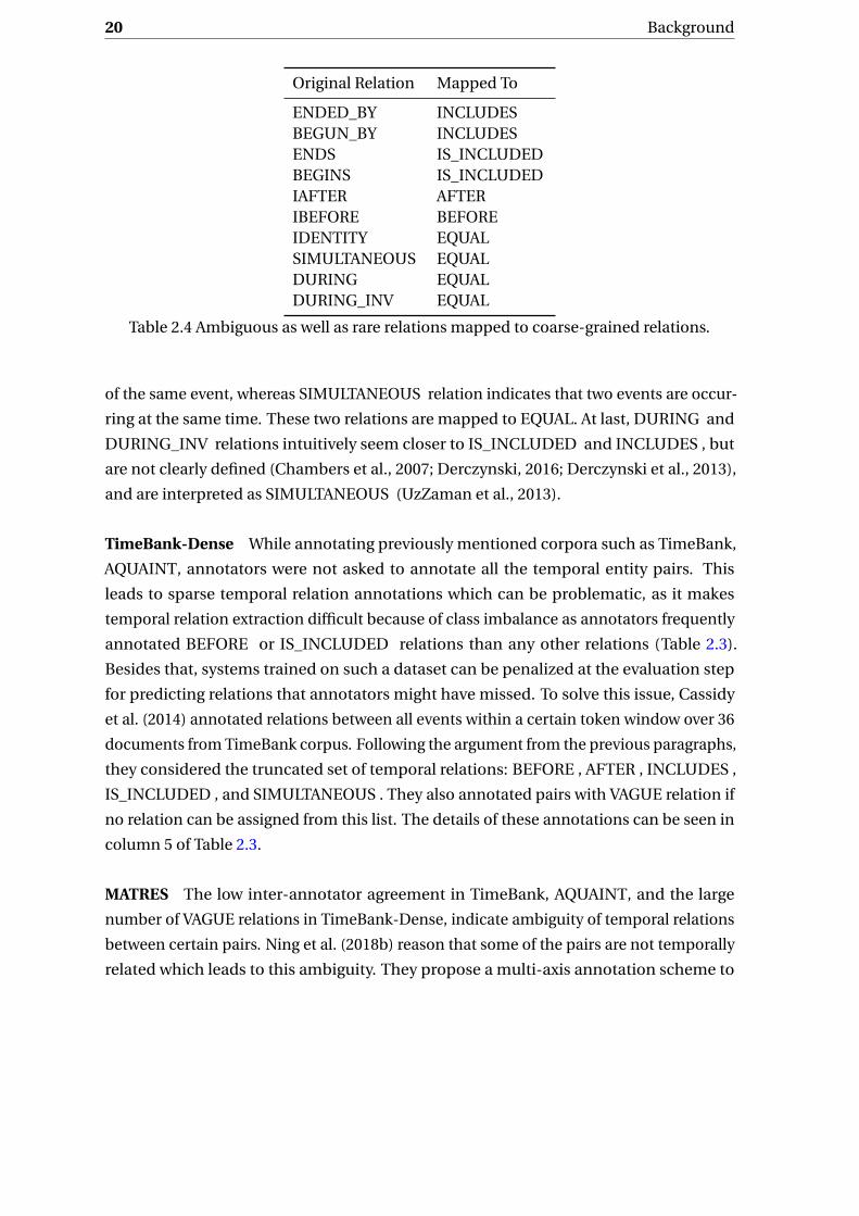
20 Background
Original Relation Mapped To
ENDED_BY INCLUDESBEGUN_BY INCLUDESENDS IS_INCLUDEDBEGINS IS_INCLUDEDIAFTER AFTERIBEFORE BEFOREIDENTITY EQUALSIMULTANEOUS EQUALDURING EQUALDURING_INV EQUAL
Table 2.4 Ambiguous as well as rare relations mapped to coarse-grained relations.
of the same event, whereas SIMULTANEOUS relation indicates that two events are occur-
ring at the same time. These two relations are mapped to EQUAL. At last, DURING and
DURING_INV relations intuitively seem closer to IS_INCLUDED and INCLUDES , but
are not clearly defined (Chambers et al., 2007; Derczynski, 2016; Derczynski et al., 2013),
and are interpreted as SIMULTANEOUS (UzZaman et al., 2013).
TimeBank-Dense While annotating previously mentioned corpora such as TimeBank,
AQUAINT, annotators were not asked to annotate all the temporal entity pairs. This
leads to sparse temporal relation annotations which can be problematic, as it makes
temporal relation extraction difficult because of class imbalance as annotators frequently
annotated BEFORE or IS_INCLUDED relations than any other relations (Table 2.3).
Besides that, systems trained on such a dataset can be penalized at the evaluation step
for predicting relations that annotators might have missed. To solve this issue, Cassidy
et al. (2014) annotated relations between all events within a certain token window over 36
documents from TimeBank corpus. Following the argument from the previous paragraphs,
they considered the truncated set of temporal relations: BEFORE , AFTER , INCLUDES ,
IS_INCLUDED , and SIMULTANEOUS . They also annotated pairs with VAGUE relation if
no relation can be assigned from this list. The details of these annotations can be seen in
column 5 of Table 2.3.
MATRES The low inter-annotator agreement in TimeBank, AQUAINT, and the large
number of VAGUE relations in TimeBank-Dense, indicate ambiguity of temporal relations
between certain pairs. Ning et al. (2018b) reason that some of the pairs are not temporally
related which leads to this ambiguity. They propose a multi-axis annotation scheme to

2.1 Tasks 21
solve these problems. The first step of their annotation scheme involves anchoring events
depending on their types to a specific axis such as main axis, intention axis, opinion axis,
etc. Next, only events that are on the same axis and in the window of two sentences are
eligible for assigning temporal relations. Also, their annotations differ from the previous
datasets, as they assign temporal relation between start-points of the events instead
of the whole time intervals of events. As a result, possible temporal relations in the
dataset are BEFORE , AFTER , EQUAL or VAGUE, because only these relations can be
assigned between two points. Additionally, instead of relying on expert annotators, they
crowdsourced the annotation effort. They initially annotated only 36 documents from
TimeBank-Dense dataset but recently extended annotations over all the documents from
TimeBank, AQUAINT, and TE-Platinum. As a result, MATRES contains 276 documents
and cumulative EVENTs as shown in Table 2.3.
2.1.1.4 Evaluation
The obvious way of evaluating temporal relation classification systems is a direct compari-
son of system predicted relations with reference relations i.e. for a given pair of events
from the gold annotations, predicted relation of the same event pair is compared. But,
evaluating a temporal classification system based on this simple assessment is not suffi-
cient as the same temporal information can be presented in different ways. This makes
the evaluation of temporal systems non-trivial.
A B
C
A B
C
A B
C
=
<
=
<
=
<<
Referencegraph
System predictedgraph
Temporal closureon graph
Fig. 2.3 Three equavalent but different representations (Setzer et al., 2002).
Consider the case presented in Fig 2.3 where the human annotated reference graph
contains temporal relations which says events A−B are occurring simultaneously and B
occurs before C and certain system asserted that A−B are are occurring simultaneously but
A is before C . Here, if we measure the system’s performance only by the direct comparison
of the graphs, the system will get a non-perfect evaluation score despite predicting all
relations correctly. Because, from the annotated relations B occurs before C can be easily

22 Background
inferred with transitivity. This demonstrates that evaluation schemes must do more than
just a pairwise comparison to assess a system.
Due to which several evaluation schemes have been proposed. Earliest work (Setzer
et al., 2002) proposed a graph based evaluation for limited number of relations such
as before, simultaneous and includes. They performed graph closure over both system
predicted graph and reference graph to calculate recall and precision. This method was
generalized over all temporal relations in (Muller and Tannier, 2004) due to which system
with all Allen’s relations can be evaluated with this measure. In SemEval’07 campaign (Ver-
hagen et al., 2007) proposed another temporal evaluation metric which was very specific
to the dataset used in the shared tasks. After that, Tannier and Muller (2011) proposed a
promising evaluation scheme that compares transitively reduced temporal graphs over
the end-points of events. Further, temporal awareness evaluation metric is proposed by
UzZaman et al. (2013) which is widely used for evaluating temporal relation classification
systems.
In our work, for direct comparison of our systems with previous approaches, we
evaluated our systems with the same two evaluation schemes that they used (Mirza and
Tonelli, 2016; Ning et al., 2017): direct evaluation and temporal awareness. We discuss them
in the following paragraphs. While explaining these evaluation schemes, we use common
notations where for a given document, we denote the true reference (gold-annotated)
temporal graph as K and system predicted temporal graph as G . The total number of
edges of the graph x are denoted as |x| and |x ∩ y | denote the number of common edges
in the two graphs x, y .
Direct Evaluation This is the most straightforward evaluation metric that measures the
precision of a system as a ratio of the number of pairs with correct temporal relation
predictions to the number of all the pairs for which temporal relation is predicted. Next,
it calculates the recall as a ratio of the number of pairs with correct temporal relations
predictions to the number of pairs with true reference relations. Finally, F1-score is
calculated by considering the harmonic mean of precision and recall as:
P = |G ∩K ||G| R = |G ∩K |
|K | F1 = 2PR
P +R(2.5)
Temporal Awareness Similar to the previously proposed approaches (Setzer et al., 2002;
Tannier and Muller, 2008), temporal awareness evaluation (UzZaman et al., 2013) also per-
forms temporal closure over reference and system predicted graphs but do not compare
these graphs directly. Instead, it compares the accuracy of core relations, relations which

2.1 Tasks 23
K A B C D E< < < <
<<
< < <
G A B C D E< <
<<
Fig. 2.4 Reference graph K and predictedgraphs G . In the graphs thick connectededges show actual annotation, whereas dot-ted lines denote inferred relations, and thesymbol < indicates before relation.
Evaluation scheme P R F1
Direct Evaluation 75.0 60.0 66.67Temporal Awareness 100.0 50.0 66.67
Table 2.5 Evaluation results of G with re-spect to K with two different schemes.
can not be derived from other relations. It performs graph closure over system produced
graph G and reference graph K to get G+, K +, respectively. Conversely, the redundant
relations are removed from the original graphs G and K to construct reduced graphs as
G−, K −, respectively, that contain only core relations.
Then, precision calculates the percentage of core relations identified accurately, and
recall checks the percentage of actual core relations identified by the system. Finally,
compact temporal awareness score is calculated as F1-score:
P = |G−∩K +||G−| R = |G+∩K −|
|K −| F1 = 2PR
P +R(2.6)
Difference of evaluation schemes The difference between these two evaluation schemes
can be illustrated with a simple example shown in Fig. 2.4. Suppose, we are given anno-
tated document D containing five temporal entities: A,B ,C ,D, and E , and true temporal
relations between them. Let the graph K shown in Fig. 2.4 be the reference graph obtained
from D, and G be the predicted temporal graph from some arbitrary system. In the graphs,
actual annotations are shown with thick edges, whereas inferred relations are denoted
with dotted lines. The evaluation of graph G with the two evaluation schemes, Direct Eval-
uation (DE) and Temporal Awareness (TA) is shown in Table 2.5. We see, precision drops
with DE even though all the predictions are accurate, because without temporal closure of
graph K , the relation between A−E can not be determined. Next, recall scores are also
different as DE considers all five annotated relations (thick lines in K ) equally important
and calculates recall 60% as only 3 out of 5 relations are predicted accurately. On the other
hand, TA calculates recall as 50% as it assigns no score for predicting temporal relations
between A−D , A−E as they can be inferred from other temporal relations.

24 Background
2.1.2 Bridging anaphora resolution
Bridging is an essential part of discourse understanding (Clark, 1975). The reader may
have to bridge the currently encountered expression to a previously known information
either from the text or from her memory. In his pioneering work, Clark (1975) considered
this broad phenomenon as bridging, which connects any expressions that can not be
understood without the context to previously appearing phrases. The expression which
can not be interpreted without the context is called as anaphor, and the phrase on which
it depends for meaning is referred to as antecedent. The earlier definition of bridging
included an identical relation between anaphor and antecedent, which is commonly
known as coreference. But, over the period, the scope of bridging has changed, so now
bridging refers to any association between anaphor and antecedent except coreference.
Also, another difference is that, in bridging defined by Clark (1975), an antecedent can be
a sentence or a clause that can be useful for interpretation of an anaphor. But, in this work,
we are considering only those anaphor-antecedent pairs which are noun phrases (NP) (as
practiced by recent researchers). Apart from Clark, Hawkins (1978); Prince (1981, 1992)
also studied bridging but referred to this phenomenon differently. Hawkins (1978) termed
it as associative anaphora and only considered definite NPs as anaphors, whereas Prince
(1981) referred to anaphors which can be inferred from previously mentioned expressions
as inferrables.
With this understanding of bridging, we describe the computational task which identi-
fies it automatically: bridging anaphora resolution, in the coming sections. Section 2.1.2.1
formally defines the task, Section 2.1.2.2 discusses main components of supervised learn-
ing approaches of solving it, next Section 2.1.2.3 details corpora used in this work, and
finally, Section 2.1.2.4 presents an evaluation metric.
2.1.2.1 Definition
Bridging resolution is the computational task corresponding to the bridging phenomenon.
It consists of two tasks, bridging anaphora recognition which identifies all the bridging
anaphors from a given document, and bridging anaphora resolution which connects these
bridging anaphors to their antecedents. We are solving the latter task.
Mention is a term used to denote named entities, and NPs, or pronominals that refer to
entities. For instance, entity such as Barack Obama, and NP references like the president,
the senator, or pronominal reference like he, him, are mentions. We are considering
only those anaphors and antecedents that can be NPs in our work, so can be considered
as sub-type of mentions. Consequently, bridging resolution task can be visualized as

2.1 Tasks 25
Fig. 2.5 Bridging resolution over a sample text. From the given text (a), all the mentionsare detected (b), bold-faced words denote mentions, in next step bridging anaphors arefound out (c), the underlined words are bridging anaphors and finally, bridging anaphoraresolution is executed to link these anaphors to antecedents (d). In the generated graph(d) thick line denotes bridging relation. The size, the living room and the garden are allspecifically related to a new house. So, bridging anaphors b1,b2,b3 are linked to the sameantecedent m2. Then another bridging anaphor his children are related to the personwho bought the house, He, thus, showing bridging relation between b4 and m1. Note thatthere is no bridging relation between antecedents m1 - m2 as well as between bridginganaphors - b1,b2,b3,b4.
pipeline where first mentions are detected, from this set of mentions bridging anaphors
are identified in bridging anaphora recognition, and finally bridging anaphora resolution
connects these anaphors to corresponding antecedents. This is depicted with a sample
text in Fig. 2.5.
Formally, let D be a given document containing set of mentions: M = {m1,m2, · · · ,mnm },
and bridging anaphors :A = {a1, a2, · · · , ana }. Then the bridging anaphora resolution gen-
erates a set of anaphor and predicted antecedent pairs as: {(ai , yi )|∀ai ∈A , yi ∈M }.

26 Background
2.1.2.2 Supervised learning approach
Similar to temporal relation classification, in this task as well we are taking supervised
learning approach to solve bridging anaphora resolution. This involves three important
components: mention representations, models and inference. We detail them here.
Mention representations As both anaphors and antecedents are assumed to be a subset
of mentions, obtaining mention representations becomes essential. For that, a generic
function ZM is found out as follows:
ZM : M →Rdm (2.7)
mi 7→ZM (mi )
where mi ∈ M . We develop an approach to learn this function where contextual and
commonsense information is acquired (Chapter 6). Before that, in the next chapter, we
detail previously proposed approaches to get this function in Section 3.2.1.
Models Similar to temporal relation classification, local models and global models are
used for bridging anaphora resolution as well. In the local models for bridging anaphora
resolution, a confidence score for bridging anaphor and a previously occurring mention is
predicted (Markert et al., 2003; Poesio et al., 2004). Formally, these models learn a function
of the form: BL,θ : Rdm ×Rdm → R. On the contrary, global models find corresponding
antecedents for anaphors simultaneously (Hou et al., 2013b). This work with global
modeling approach did not explicitly find the mention representations but employed
Markov Logic Networks (MLN) (Domingos and Lowd, 2009) for global inference.
Inference In bridging anaphora resolution, infererence is not as complicated as in tem-
poral relation classification, as it does not follow any complex symmetry or transitivity
constraint. The inference step in local models is similar to the best-first clustering. Initially,
antecedent candidates are arranged depending on the confidence scores predicted from
the model, then the highest scoring candidate antecedent is selected as the predicted
antecedent for the bridging anaphor. In case of a global model, Hou et al. (2013b) put
some linguistic constraints such as anaphor have less probability of being antecedent,
or antecedents have higher probability for being antecedent for other anaphors, in her
inference strategy and obtained global inference with MLN. We provide more details about
it in the next chapter.

2.1 Tasks 27
ISNotes BASHIARRAU
RST TRAINS PEAR GNOME
Documents 50 50 413 114 20 5
Domain news news news dialogues spokennarratives
medical
Bridginganaphors
663 459 3777 710 333 692
Mentions 11272 18561 72013 16999 4008 6562
Table 2.6 Bridging corpora used in the thesis.
We used local model to solve bridging anaphora resolution but applied different
strategy while learning, instead of casting it as classification problem we employed ranking
strategy. Next, we used simple inference strategy where top ranking candidate antecedent
is selected from the list of candidates for the anaphor. We detail about this in Section 6.4.2.
2.1.2.3 Corpora
ISNotes Markert et al. (2012) annotates 50 documents from the Wall Street Journal (WSJ)
portion of OntoNotes corpus (Weischedel et al., 2013) with bridging information which
contains 663 bridging anaphors (Table 2.6). These are all referential bridging anaphors
which means they strictly require the context for interpretation (Kobayashi and Ng, 2021;
Roesiger et al., 2018). All the anaphors are NPs, whereas antecedents are either enti-
ties or events (verb phrases (VPs) or clauses). Out of all 663 anaphors, 622 anaphors
have NPs as antecedents and the remaining are events. ISNotes also categorizes these
anaphor-antecedent pairs based on the relations they possess: set/membership (45),
part-of/attribute-of (92), action (16), though most of the relations are unspecified and
marked as Other (530) relation.
BASHI Roesiger (2018a) annotated 50 documents (different set of documents than IS-
Notes) from OntoNotes with bridging information (Table 2.6). The corpus contains 459
bridging anaphors where they categorize them as: definite (275), indefinite (114), and
comparative (70). Out of these 70 comparative anaphors, 12 have more than one link
to antecedents. Also, similar to ISNotes all the anaphors are referential type and NPs,
whereas antecedents can be entity or event.

28 Background
ARRAU The first version of ARRAU was created by Poesio and Artstein (2008), recently
Uryupina et al. (2019) proposed the latest version. The corpus contains documents from
four different domains: news (RST), spoken narratives (PEAR), dialogues (TRAINS), and
medical (GNOME). In total it consists of 5512 bridging pairs, Table 2.6 shows division
of these pairs. The type of bridging is different than ISNotes and BASHI as most of the
anaphors are lexical bridging (e.g. Europe-Spain) that do not strictly depend on the context
for interpretation whereas some are of referential (Kobayashi and Ng, 2021; Roesiger et al.,
2018). Also, antecedents are only entities and anaphors are NPs. Bridging pairs from RST
portion of the corpus are annotated with relations such as subset, comparative, possessive,
element, and inverse of these relations. The pairs which can not be categorized into
these relations are marked as underspecified. Addition to bridging, ARRAU consists of
annotations for coreference as well as discourse deixies.
2.1.2.4 Evaluation
The quality of prediction is assessed with accuracy measure, the ratio of correctly linked
anaphors with their respective antecedents to the total number of anaphors. We consider
an anaphor linking correct if it is linked to any mention of the true antecedent entity. If
there are na number of anaphors and out of those, for nca number of anaphors antecedents
were correctly found then the accuracy is calculated as:
A = nca
na(2.8)
2.2 Artificial neural networks
So far, we detailed the tasks that are tackled in this thesis. Now, we briefly introduce
artificial neural networks which are powerful at learning representations as well as potent
at modeling many tasks.
Artificial neural networks are computational systems inspired from the biological
neural networks, and neurons are the fundamental computation unit in them. A neuron
processes inputs by applying pre-designed function (generally, non-linear function known
as activation functions) to produce output. Further, a number of neurons are aggregated
into a layer where the first layer of the network always receives input and the final layer
produces output, and there can be any number of layers in between which are called
hidden layers. The neurons, in turn, layers, are interconnected to produce a network or
graph, where neurons are nodes and edges denote a connection between them, hence
the name neural network. The connections are directed labeled edges that indicate the

2.2 Artificial neural networks 29
Fig. 2.6 Simple neural network. Fig.(a) shows a simple neural network with three layers -input layer, hidden layer, and output layer where information flows from input layer tohidden layer and finally to output layer. The nodes denote neurons, and edges show aweighted connection between them. A single neuron is detailed in Fig. (b). It takes inputfrom the previous layer and calculates weighted sum which is passed through activationfunction a to produce output.
direction and weight of the signal. These weights control the connection and are adjusted
at the training step of the network.
A simple neural network is shown in Fig. 2.6, which contains three layers − input, hid-
den, and output layer, respectively having four, two, and one neurons. A neuron produces
output based on the inputs, the associated weights, biases and the activation function (Fig.
2.6 (b)), where weights and biases are called parameters of the network and are learned at
the training step. A neural network can have any number of layers, any number of neurons
in them, and different kinds of connections between them. These are hyperparameters2
which depend on the type of problem the neural network solves. In any neural network,
the produced output depends on the input and the various transformations applied to
it at each layer. Hence, the output y obtained from a neural network as a (non-linear)
transformation on input x, controlled by parameters θ is given as:
y = fθ(x) (2.9)
2Learning rate, learning algorithm, epoch (number of iteration of training), activation function, dropoutare some other hyperparameters.

30 Background
where fθ is composition of different (non-linear) transformations at various layers: fθ =f1 ◦ f2 ◦ · · · ◦ fl .
Training of neural network determines the values of parameters. At the beginning of
this step, all the parameters, i.e. weights and biases, are randomly initialized. Then the
training adjusts these parameters values so as to produce the desired output. The differ-
ence between the desired and actual output is measured with a loss function. Suppose,
D = {(xi , yi )ni=1} is training data where xi denote input features and yi shows associated
label. The cumulative loss is given as:
L (θ) = ∑(xi ,yi )∈D
l (yi , yi ) (2.10)
where l is a error function which gives difference between true output yi and predicted
output yi := fθ(xi ). Then, following optimization objective is solved to get appropriate
parameters:
minθ
L (θ) (2.11)
The objective function L (θ) is non-convex function because of non-linear activation
functions and obtaining analytical solution is difficult.
Gradient descent algorithms are commonly used for minimizing this objective. The
algorithm updates parameters of the network iteratively and the parameter values are
reduced by the value proportional to the gradient of the loss function with respect to the
parameter. The update rule at (t +1)th iteration is given as:
θt+1 ← θt −γ ∂L (θ)
∂θ(2.12)
where θt denotes the parameters of the neural network at iteration t in gradient descent,
and learning rate.
However, obtaining a gradient with respect to each parameter in the network is a
computationally expensive operation. Backpropagation (backward propagation of errors)
algorithm (Goodfellow et al., 2016; Kelley, 1960; Rumelhart et al., 1986b) is used to calculate
the gradient of the error function with respect to the neural network’s weights. The
gradient calculation proceeds in the backward direction, i.e. first the gradient of the error
is calculated with the final layer, then, these values are propagated with the chain rule
to obtain gradients with parameters from the previous layers. This produces efficient

2.2 Artificial neural networks 31
computation of the gradient at each layer versus the naive approach of calculating the
gradient of each layer separately.
Additionally, to speed up the learning process different variants of gradient descent
algorithms such as batch, mini-batch, and stochastic gradient descent are used. Recently,
various improvements have also been proposed for the gradient descent algorithms:
Adagrad (Duchi et al., 2011), Adadelta (Zeiler, 2012), RMSProp (Tieleman and Hinton,
2012), Adam (Kingma and Ba, 2017), etc.
Different types of neural networks produce different transformations of the input data.
We describe few popular neural networks that are used in this work as well.
• Feedforward networks: In these networks, the information flows from the input neu-
rons to hidden neurons to output neurons (example Fig. 2.6). Formally, the output of
i th layer having ni neurons, hi ∈Rni is given as:
hi =ψi (W Ti hi−1 +bi ) (2.13)
where hi−1 ∈Rni−1 is output from (i −1)th-layer, Wi ∈Rni−1×ni ,bi ∈Rni are weights and
biases, and ψi is activation function for i th-layer. Here, i ∈ {1,2, · · · , l } for l-layered
feed-forward network and h0 denotes input to the network.
• Convolutional neural network (CNN): CNN (Lecun et al., 1998) is a special type of
feed-forward network which commonly consists of convolution layer, application of
non-linear activation function, and followed by pooling-layer. The input is convolved
with weight matrices that are learned, called filters or kernels. Intuitively, in convolution
operation, the filter slides over the input, obtains element-wise products, and sums
them. Formally, for a given input3 X ∈Rdh×dw and filter F ∈Rd f ×d f , result is given as:
Rm,n =∑i
∑j
X(m−i ),(n− j )Fi , j (2.14)
where R ∈Rdch×dcw , dch = dh − f +1, dcw = dw − f +1. Next, non-linear projection with
activation is given as:
R ′ =ψ(R) (2.15)
3CNNs are used often over images that are stored with two or more dimensional data. Hence, we areconsidering 2-dimensional input, but convolutions over 1-dimensional input can be obtained in the similarway with filter sliding over only one dimension.

32 Background
Finally, it is passed through pooling-layer ϕ to get the final output as:
Y =ϕ(R ′) (2.16)
commonly, ϕ is max-pooling layer or average-pooling layer.
• Recurrent neural network (RNN): Unlike feed-forward networks, RNNs (Rumelhart
et al., 1986a) have loops. Because of this feedback mechanism, the output depends
on the current as well as the previous input which also leads to a sequential behavior
where different states produce different outputs. There are many variants of RNNs: Long
Short-term Memory (LSTM) (Hochreiter and Schmidhuber, 1997), Gated Recurrent Unit
(GRU) (Cho et al., 2014), etc. We present a simple RNN (Elman, 1990; Jordan, 1997)
which is extended to produce these more advanced variants.
ht =ψh(W Th xt +U T
h ht−1 +bh) (2.17)
yt =ψy (W Ty ht +by ) (2.18)
where ht ,ht−1 ∈Rnh are hidden states at t , t −1, respectively, xt ∈Rnx and yt ∈Rny are
input and output at time t , Wh ∈Rnx×nh ,Wy ∈Rny×nh ,Uh ∈Rnh×nh are weight matrices,
bh ∈Rnh ,by ∈Rny are biases, and ψh ,ψy are activation functions.
2.3 Representation learning
In Section 2.1, we detailed task definitions of two tasks that are addressed in this thesis.
Then in the previous section, we introduced artificial neural networks which are used
widely to solve many tasks especially for learning effective representations. In this section,
we discuss representation learning and related fields. This discussion sets a base for the
various representation learning approaches described in the next section.
Most NLP models require real valued vectors (or tensors in general) as an input. These
numeric representations of linguistic objects are either designed or automatically learned
for the purpose of inputting to machine learning models. Converting any type of data into
vectors, i.e. obtaining representation, is an important part of the whole process of applying
a machine learning algorithm. Not only that, it is crucial to obtain a good representation
so that the task of the machine learning algorithm in the pipeline becomes easier. A good
representation should capture as many relevant features present in the original data that
are required for solving the underlying NLP task.

2.3 Representation learning 33
Feature engineering is one way of obtaining such relevant features which are designed
by experts of the field. But, feature engineering is an arduous job which requires task-
specific knowledge and immense human effort. Besides, the noisy data can induce errors
in obtaining such features. Moreover, changes in the domain of underlying data can
lead to a repetition of efforts on the new data. This is especially severe for NLP tasks
where domain changes are quite frequent. For instance, wordings used in a political
discourse are different from a corporate discourse which is again different from a medical
discourse, as a result, the solutions designed for one domain may not be effective for other
domains. The problem aggravates in the case of language change which may require
different experts of the language to design new features. To address these drawbacks of
feature engineering, it is necessary to automatically discover features. Representation
learning or feature learning does exactly that and retrieves relevant features from the data
automatically without the need of any human expert.
Representation learning approaches for text can be divided into two categories: 1.
Supervised representation learning, and 2. Unsupervised representation learning. Su-
pervised representation learning approaches are generally applied to get the task-specific
representations of the linguistic units. These approaches assume that text data containing
labels are available for training. Let us suppose n-data samples, D = {(xi , yi )}ni=1 are given,
where xi is the linguistic object and yi the corresponding label. Let X be the generic set of
these linguistic objects such that xi ∈X as well as Y be the set of possible labels, yi ∈Y .
Then the supervised task-specific representation learning algorithm learns a parameterized
function which maps each linguistic object to corresponding vector representation while
encoding the label-related information as:
fY ,θ : X →Rd (2.19)
where θ are parameters to be learned. Most of the neural network based approaches used
to solve a specific task fall into this category such as the recently proposed approach for
temporal relation classification (Han et al., 2019a,b) or bridging resolution (Hou, 2020a;
Yu and Poesio, 2020).
On the other hand, unsupervised representation learning approaches obtain generic
representations with unlabeled texts. These representations are not task-specific so can
be used as a base representations for other tasks. The commonly used word embeddings
such as Word2vec (Mikolov et al., 2013a), Glove (Pennington et al., 2014) can be considered
as unsupervised representation approaches. Formally, these approaches learn parameters

34 Background
θ only from an unlabeled data D = {(xi )}ni=1 as:
fθ : X →Rd (2.20)
Representation learning shares resemblance with metric learning (Bellet et al., 2013)
in the sense that metric learning projects similar data samples on similar vectors 4. This
is governed by learning distance metric between two data samples, d :Rd ×Rd →R. The
whole idea in the metric learning algorithms is to learn appropriate distance measure d
so that it correctly produces small distances between similar objects and bigger distances
for dissimilar objects. One of the examples of this distance measure is Mahalanobis
distance (Mahalanobis, 1936), which calculates the distance between two objects x, x ′ as:
dM (x, x ′) =√
(x −x ′)T M(x −x ′) (2.21)
Following this, various methods (Bellet et al., 2013) are proposed that learn matrix M to
get the distance between data-points based on above-mentioned similarity constraint (i.e.
similar object pairs should have smaller distance and dissimilar pairs bigger distance).
After learning this distance metric, it is applied to the unseen data to accurately predict the
output. In other words, metric learning can be seen as weakly supervised representation
learning with the additional condition of learning metric which measures the distance be-
tween data points. Consequently, metric learning can be used to improve the performance
of classification (Meyer et al., 2018; Weinberger and Saul, 2009) for ranking in information
retrieval (Cakir et al., 2019; McFee and Lanckriet, 2010), for recommending relevant items
to users (Hsieh et al., 2017), etc.
Dimensionality reduction (Xie et al., 2018) is another sub-field that shares similarity
with representation learning. But, the fundamental goal in the two tasks is different where
on one hand representation learning approaches concentrate on finding the meaningful
representations, on the other hand, dimensionality reduction approaches compress the
representation while preserving as much original information as possible. The necessity
of reducing the dimensions of the representation rises due to the high-dimensional input
representations. Because having a higher number of features to represent the data can be
detrimental to the generalization of machine learning models. Additionally, dimensional-
ity reduction provides numerous advantages such as a reduction in the computational
cost (both in space and time) of the algorithms used over the data, or the removal of
the possible noise introduced when picking up the data. Due to these benefits, usually,
it is a good idea to reduce the feature space (dimensions of the input representation)
4It generally holds true, but more specifically depends on properties of matrix M (Eq. 2.21).

2.4 Word representations 35
while preserving the relevant information. Dimensionality reduction approaches obtain
functions that project higher dimension data into lower dimensional space fd :Rk →Rd
where k ≫ d . Broadly there are two approaches to achieve this: feature selection (Chan-
drashekar and Sahin, 2014) where certain important features are selected from the original
set of features that are useful for the further task and other is feature extraction (Dara and
Tumma, 2018; Khalid et al., 2014) which combines given features into smaller features.
Many methods have been proposed to reduce dimension with feature extraction, such as
matrix factorization approaches: Principle Component Analysis (PCA) (Jolliffe, 2011), Sin-
gular Value Decomposition (Golub and Reinsch, 2007), recently proposed deep learning
methods: autoencoders (Baldi, 2011), etc.
2.4 Word representations
In any text, words are considered as core constituents and treated as the lowest meaningful
units of a language5. It is also assumed that meanings of the bigger units of language
such as phrases, sentences, or documents can be derived from the constituent words.
Besides, often some form of text (i.e. a sequence of words) is an input for several NLP
tasks. Therefore, it is essential to obtain a meaningful representations of words to solve
NLP tasks.
The ideal word representation algorithm should map all the words in a language to
its vector representation. However, obtaining all the words in the language is difficult as
language is evolving and new words are added constantly. This is addressed by creating a
huge vocabulary containing millions or billions of words and getting a vector representa-
tion for each word in the vocabulary. A word representation learning algorithm finds a
map from each word in vocabulary to their corresponding d-dimensional vector. Let us
assume that the vocabulary of words be V , then the algorithm finds following map f :
f : V →Rd (2.22)
One of the simplest ways of word representations is one-hot vector representation
which is quite intuitive. The algorithm assigns one-hot vector to each word from the
vocabulary V which contains 1 only at the position of the word otherwise 0. Formally, for
a word w which occurs at l th position in V , the corresponding one-hot vector w is given
as w = {0,1}|V |, and vector element wl = 1.
5It is not true in the stricter sense as words can be further broken into morphemes, but for the scope ofthis discussion, we consider words as the lowest units.

36 Background
Though it is a simple approach to obtain word representation, it has multiple disad-
vantages. The main drawback of this method is the failure at encoding any semantic or
syntactic information of the word. For example, in this way of representation, “dog” and
“cat” are equally unrelated as “dog” and “machine”. This is evident from the dot product of
vectors corresponding to these words, as for all the pairs of different words the similarity
will be 0. This method also suffers from producing high-dimensional sparse vectors,
because each vector will be of the size of the vocabulary. This sparse representation is not
so useful for the downstream tasks.
2.4.1 Distributed representations
The drawbacks of one-hot vector representations are solved with the distributed represen-
tations of words. On the contrary to high-dimensional one-hot vector representations,
distributed representations use continuous low-dimensional vectors as word representa-
tions and encode semantic information related to the word in the corresponding vector.
These approaches produce a dense representation which means multiple dimensions may
capture one concept and each dimension in the vector may capture multiple concepts.
These dense distributed representations of words are commonly derived from the
words’ context and are based on the distributional hypothesis of linguistic objects (Firth,
1957; Harris, 1954): Linguistic units possessing similar text distribution have similar
meanings. It implies, the more similar two linguistic objects are the more distributionally
similar they will be. In turn suggesting that semantically similar linguistic objects occur
in similar linguistic contexts. By applying this hypothesis specifically to words, it can be
stated that words that occur in a similar context tend to possess a similar meaning.
Though the words distributed (representations) and distributional (hypothesis) sound
similar, they are not strictly related. The only relation they possess is that generally the
distributional hypothesis is used to obtain a distributed representation. The embed-
dings which are obtained with the use of distributional hypothesis are a specific type of
distributed embeddings which are also called distributional embeddings (Ferrone and
Zanzotto, 2020). However, it is possible to obtain distributed representations without
the use of distributional hypothesis. For instance, obtaining word representations based
on the semantic networks is distributed but not distributional (Baroni and Lenci, 2010).
Semantic network contains concepts as nodes, and edges as semantic relations between
them, for instance, WordNet (Fellbaum, 1998) is a specific example of semantic network 6.
Thus, the word representations obtained only with the use of WordNet are called dis-
6We will use embeddings learned over WordNet as well in this work which will be introduced later.

2.4 Word representations 37
tributed but not distributional. In this section, we focus on the distributed embeddings
which are obtained based on the distributional hypothesis as those are widely used for
word representations.
Several models have been proposed based on this hypothesis to produce continuous
valued vectors (Elman, 1990; Hinton et al., 1986; Rumelhart et al., 1986a). Before the
popularity of the neural models to obtain word representations, dimensionality reduction
techniques such as PCA, SVD are used over the co-occurrence matrix to get the low
dimensional vector representations (Dhillon et al., 2015; Lebret and Collobert, 2014). A
promising approach based on neural network (Bengio et al., 2003) learned language model
and continuous vector representation words simultaneously.
Most of these word representation algorithms make use of language modeling objec-
tive to produce the embeddings. Let us brief about language modeling task before diving
into these embedding algorithms. Language modeling (LM) finds probability distribution
over a sequence of words. It gives a likelihood of a sequence of words appearing in a
language. Formally, for a sequence of words w1, w2, · · · , wN , LM produces joint probability
by considering the tokens that appeared before the current token as:
p(w1, w2, · · · , wN ) =ΠNi=1p(wi |w1, w2, · · · , wi−1) (2.23)
Calculating exact joint probability for all the sequences is computationally infeasible, so
Markov assumption is applied. The assumption simplifies the calculation as it curtails the
dependence of the current word to only n prior words. The approximate joint probability
is given as:
p(w1, w2, · · · , wN ) ≈ΠNi=1p(wi |wi−n , wi−n+1, · · · , wi−1) (2.24)
Word embedding algorithms learn parameterized joint probabilities while learning the
word representations to optimize the LM objective. With this brief understanding of LM,
we discuss different popular word embeddings algorithms in the coming sections.
2.4.1.1 Word2vec
The basic idea in Word2vec (Mikolov et al., 2013a,b,c) is to produce vectors depending on
the context of words (distributional hypothesis). Their approach uses simple feed-forward
neural networks with a single hidden layer to reconstruct either a word from the given
context (Continuous bag-of-words (CBOW)), or the context from a given word (skip-gram)
and the output from the hidden layer is considered as a Word2vec representation for
words.

38 Background
Fig. 2.7 Two neural models - (a) continous bag-of-words (CBOW) which takes input as acontext of words and predicts the word, on othe hand (b) skip-gram predicts context ofwords from the given of word.
Continuous Bag-of-Words (CBOW) based neural model predicts a word from its con-
text. The architecture is shown in Fig. 2.7(a). The input to the model is all the words in the
window of some randomly chosen number. In the figure, a window of 2 is used, therefore,
two words prior to the word and two words after the word are given as an input to the
feed-forward model. Then each word is projected onto the same space with the use of
a single layer perceptron and then all these vectors are added. This sum of vectors is
multiplied with weight matrix and then passed through a softmax to get the probability
score.
Let w j−l , w j−l+1, · · · , w j , · · · , w j+l−1, w j+l be the context of word w j in the window of
l -words. CBOW model produces conditional probability of w j given the context as:
P (w j |wt (|t− j |≤l ,t = j );Θ) = es j∑|V |j ′=1 es j ′
(2.25)
where s j is a j th element of vector s ∈R|V | which denotes confidence score for word w j
being the context of wt (|t− j |≤l ,t = j ). The confidence score s for each word in vocabulary is
calculated as:
s = M T∑
|t− j |≤l ,t = jH T wt (2.26)

2.4 Word representations 39
where M ∈Rm×|V | and H ∈R|V |×m are hidden layer projection matrices learned by neural
network, and wt ∈R|V | be the V -dimensional one-hot vector of word wt (where V is the
vocabulary of words).
The parametersΘ are learned to minimize negative log probabilities :
L (Θ) =−∑j
P (w j |wt (|t− j |≤l ,t = j );Θ) (2.27)
Skip-gram is opposite in the functionality to CBOW. It produces probability for context
words given a target word. It is depicted in the section (b) of Fig. 2.7. Consider the same
context as mentioned in CBOW, w j−l , w j−l+1, · · · , w j , · · · , w j+l−1, w j+l , for which the skip-
gram model produces probabilities for all the words wt where |t − j | ≤ l , t = j in the
context of a given word w j as:
P (wt |w j ;Θ) = est∑|V |t ′=1 est ′
(2.28)
Here, st denotes confidence score of context word wt given the target word w j which
subtly differs from CBOW. The score s ∈ R|V | for each word in vocabulary denoting the
compatibility with word w j is given as:
s = M T H T wj (2.29)
where similar to CBOW, M ∈Rm×|V | and H ∈R|V |×m are hidden layer projection matrices,
and wj ∈R|V | be the V -dimensional one-hot vector of word w j .
Similar to CBOW, the parametersΘ are learned by reducing sum of negative log proba-
bilities:
L (Θ) =−∑j
∑|t− j |≤l ,t = j
P (wt |w j ;Θ) (2.30)
Negative sampling and Hierarchical softmax The above approach of finding probabili-
ties suffers from huge time complexity because of softmax calculation (Eq. 2.25 and 2.28),
because for probability calculation of a single word, all the words have to be considered.
Word2vec proposed two approaches to solve them, Negative sampling and Hierarchical
softmax.
In negative sampling, instead of considering all the words to calculate the softmax
probability only a few words (n) are considered as negative samples. These are selected
based on the word co-occurrence frequency, with which top-n words having the smallest

40 Background
Fig. 2.8 Hierarchical softmax.
frequency are chosen. This simple approximation reduces the calculation from |V | words
to only n +1 words.
Hierarchical softmax approximation approach is inspired from the binary trees pro-
posed by Morin and Bengio (2005). The actual softmax calculation can be considered as
a tree of depth 1 where all the words are leaves in this tree. Then probability estimation
requires |V | calculations because it has to go over all the nodes. But, in hierarchical soft-
max the balanced binary tree is created which has log2(|V |) depth. Consider the example
in Fig. 2.8, the softmax calculation is similar to the one-depth tree shown in (a) part of
the figure, and the hierarchical softmax approximation (b) shows words arranged in the
balanced tree. This formulation enables the decomposition of probability calculation
of one word to a sequence of probability calculation of words in the path of the word.
Specifically, the probability for each word is calculated by multiplying all probabilities on
the path from root to the word, so for instance, the probability for word w3 is given as
p0 ×p01 ×p010. So the overall, calculation reduces from |V | to log2(|V |).
Once the models are trained with these approximations, the embeddings for a given
word are obtained from the hidden layer of the network. Precisely, the weight matrix H of
the hidden layer produces m-dimensional Word2vec vector representation as: H T wj.
2.4.1.2 Global vector (Glove)
Word2vec embeddings are capable of capturing the semantics of words but they only
use local context to learn these embeddings. Because CBOW predicts a word given its
context, whereas the skip-gram objective predicts a word’s context given the word itself.
As a result, global statistical information is ignored which can be crucial for deriving word
representations. Global Vectors (Glove)(Pennington et al., 2014) solve this problem by

2.4 Word representations 41
obtaining global co-occurrence matrix X where each Xi j indicates the frequency of word
wi co-occurring with w j .
They optimize following loss function which reduces the difference between actual
and predicted co-occurrence frequency as:
J (θ) =V∑
i , j=1f (Xi j )(wT
i +w′j +bk +b′
j − log (Xi j ))2 (2.31)
where wi ∈Rd is a d-dimensional word vector for wi , w′j ∈Rd is a d-dimensional context
word embeddings of w j , bk and b′j are bias terms, and f (x) is weighting function. The
weighting function f (x) in the paper is defined as:
f (x) ={
( xβ )α if x <β
1 otherwise
where α,β are pre-defined scalars which are set to α= 1 and β= 100.
2.4.1.3 FastText
Word representation algorithms like Word2vec and Glove capture the general semantics
of words using their co-occurrence context. However, these methods neglect the internal
structure of the word. Hence, they lack in finding representations for words which occur
rarely but are morphologically similar (those words which possess a similar sequence of
characters) because there is no parameter sharing between words which have overlapping
character patterns. For example, vectors for words “eat” and “eaten” are distinct even
though they have overlapping internal structures. These problems are especially severe
for morphologically rich languages. Moreover, these methods fail at producing vectors for
out-of-vocabulary (OOV) words.
FastText (Bojanowski et al., 2017) remedies both these issues as it generates embed-
dings for character n-grams instead of directly producing the word representation. The
word representation is obtained by summing all the vector representations of character
n-grams present in the word. Thus, retaining morphological information in the represen-
tation as well as solving the OOV problem.
They achieve this by extending the continuous skip-gram (Mikolov et al., 2013b)
method with subword information (Section 2.4.1.1), where each word is considered as a
bag of character n-grams. Before creating these character n-grams for a word, markers “<”
and “>” are added as prefix and suffix, respectively. Plus, in addition to all the character
n-grams, embeddings for actual word is also added to the list of these n-grams. Let us see

42 Background
this with an example, for word learn with n=3, all character n-grams are:
< le, lea, ear, ar n, ar n, r n >, < l ear n >
Suppose, for a word w , Mw is the corresponding set of character n-grams, then in this
model, a scoring function s(w,c) measures the confidence of word c being in the context
of w as:
s(w,c) = ∑m∈Mw
umT vc (2.32)
where um is vector representation of characters m and vc is vector representation of word
c. Based on this confidence score, the objective function is optimized which is similar to
skip-gram negative sampling objective mentioned in Eq.2.30.
2.4.2 Contextual word representations
A word can have multiple meanings, polysemy. Therefore, there should be different repre-
sentations of the same word depending on the meaning in which it is present. However,
the previous distributed representations produce one vector per word irrespective of
the meaning. For instance, in these algorithms, a word “Bank” will have a single vector
independent of its meaning: financial institute or river-side. The contextual word repre-
sentation methods remedy this as they learn context-dependent representations where
they produce distinct word representations.
In the recent years, ELMo and BERT have been two popular approaches which produce
contextual embeddings, let us look at them here.
2.4.2.1 ELMo
Embeddings from Language Models (ELMo) (Peters et al., 2018) produces representa-
tions with the use of forward and backward language model: bidirectional Language
Model (biLM). The forward language model (FLM) is similar to the language model men-
tioned in Eq.2.23 where for sequence of words w1, w2, · · · , wN produces joint probability
by considering the tokens appeared before the current token as:
p(w1, w2, · · · , wN ) =ΠNi=1p(wi |w1, w2, · · · , wi−1) (2.33)

2.4 Word representations 43
Conversely, the backward language model (BLM) gives joint probability by considering
the tokens appearing after the current token, which is given as:
p(w1, w2, · · · , wN ) =ΠNi=1p(wi |wi+1, wi+2, · · · , wN ) (2.34)
ELMo combines these probabilities to jointly maximize the log-likelihood of the forward
and backward language models as:
L (Θ) =N∑
i=1log p(wi |w1, w2, · · · , wi−1;Θc ,Θ f )+ log p(wi |wi+1, wi+2, · · · , wN ;Θc ,Θb)
(2.35)
whereΘc are common parameters between forward and backward LMs whereasΘ f are
specific to FLM, andΘb correspond to BLM.
Separate LSTMs are trained for FLM and BLM. Typically, learning L-layers of LSTMs
produces L+1 representations for each word wk as :
Hk = {hk, j | j = 0,1, · · · ,L}
where hk, j at j = 0 is token input representation and otherwise concatenation of vectors
from the two LSTMs at j th layer, can be given as:
hk, j ={
hk,0 if j = 0
h fk, j ⊕hb
k, j otherwise
where h fk, j , hb
k, j are j th-layer output from forward and backward LSTM, respectively
and ⊕ denotes concatenation. Finally, to get the representation of the word wk all the
representations from the set Hk are weighted as :
wt askk = γt ask
L∑j=0
a j hk, j (2.36)
where a j are softmax normalized weights for layer j which are learned depending on the
task and γt ask is task-dependent scaling factor.
2.4.2.2 BERT
Bidirectional Encoder Representations from Transformer (BERT) (Devlin et al., 2019)
learns parameters jointly conditioned on the bidirectional language model (biLM) ob-
jective. The subtle difference between ELMo and BERT is that ELMo learns separate

44 Background
Fig. 2.9 BERT architecture (Devlin et al., 2019).
parameters for forward and backward language models as separate LSTMs are learned, on
the other hand, BERT learns only a single set of parameters for biLM.
BERT achieves this with masked language modeling (MLM) objective. The task is simi-
lar to Cloze task (Taylor, 1953) i.e. fill-in-the-blanks formulation where the model predicts
masked word appropriately depending on its context. For this, the model randomly masks
some tokens from the given sequence of words and attempts to predict them accurately.
Further, the authors think that the MLM does not capture relevant sentence level relations
which are useful for NLP tasks such as Question Answering, Natural Language Inference
(NLI), etc. For that, they use next sentence prediction (NSP) objective where for given two
sentences the model predicts whether the second sentence can truly be the next sentence
after the first one.
The input to BERT can be either single sentence or pair of sentences. The input
sentence is tokenized with WordPiece tokenizer (Wu et al., 2016) and input tokens can
only be from pre-defined dictionary of 30,000 tokens. Further, input to BERT always
starts with special token “[CLS]” and in case of two sentences, the sentence boundary is
indicated by token “[SEP]”. “[SEP]” token can also be used to indicate the end of input.
This is depicted in Fig. 2.9 with an example of pair of input sentences. Two sentences, “my
cat is cute” and actual next sentences “she likes playing”, are tokenized and tokens are
provided as an input with special tokens “[CLS],[SEP]”. Note from the figure that all the
words except “playing” of the given sentences are present in the dictionary because of
which they are not further tokenized but “playing” is divided into two tokens, “play” and
“ing”.

2.4 Word representations 45
Fig. 2.10 Internal components of encoder (Vaswani et al., 2017).
Once the tokenization is done, the m-dimensional vector representation for each
input token is obtained by summing their token embeddings, sentence embeddings, and
positional embeddings (as shown in Fig. 2.9). The token embeddings are randomly ini-
tialized for each token in the dictionary whereas sentence embeddings for each token
are determined based whether the token belongs to first or second sentence (denoted
as A and B in the figure). In addition to that, BERT considers the position of the to-
ken in the sentence by learning positional embeddings. All these embeddings are of
m-dimension so that they can be summed to produce vector xi ∈ Rm for i th token. Let
the m-dimensional vector representation of n tokens be arranged as row of the matrix
X ∈ Rn×m as X = [x1,x2, · · · ,xn−1,xn]T . This matrix X is passed through l-layers of en-
coders to obtain the final representation. BERT is trained with two different values of l :
BERT-base with l = 12 encoder layers and bigger BERT-large model with l = 24 encoders.
An encoder layer contains multiple attention heads as well as feed forward network as
shown in Fig. 2.10. Let us look at these parts one by one.
• Multi Head Attention: An encoder consists of multiple attention heads, i.e., number
of separate single attention heads. An attention head captures different interaction
between all the tokens. Here, the number of attention heads is pre-decided, let that
number be denoted as h. Let us look at the mathematical operations happening in a

46 Background
single attention head to understand it better. Initially, the input matrix representation
X ∈ Rn×m is projected with three different matrices: W K ∈ Rm×dk ,W V ∈ Rm×dv ,W Q ∈Rm×dk to get key, value, and query. The dimensions are set to dk = dv = m/h where m
is input dimension. At each layer, each attention head in multi-head attention, learns
different set of matrices, in turn yielding different key, query, and value. For instance,
for i th attention head, key, query, and value matrices are obtained as:
Ki = X W Ki (2.37)
Qi = X W Qi (2.38)
Vi = X W Vi (2.39)
where Ki ∈Rn×dk ,Vi ∈Rn×dv ,Qi ∈Rn×dk .
With the use of key and query matrices, n ×n attention weight matrix between every
token is calculated as:
Ai =σ(Qi K T
i√dk
) (2.40)
where row-wise softmax function σ normalizes scores. This is the crucial part of the
encoder architecture where different attention heads capture various interaction be-
tween input tokens. This attention matrix Ai ∈Rn×n is used to weight the embeddings
captured by the value matrix as:
Hi = Ai Vi (2.41)
Then these weighted embeddings output of each attention head is concatenated to
produce the H as:
H = [H1, H2, · · · , Hh] ∈Rn×(h.dv ) (2.42)
Finally, projection matrix Wo ∈R(h.dv )×m is learned to get the output M ∈Rn×m dimen-
sion from multi-head attention same as input dimension with the following operation:
M = HWo (2.43)
• Feed-forward network: This matrix M is passed through two layers as:
F = max(0, MW1 +b1)W2 +b2 (2.44)
where W1 ∈ Rm×d f ,W2 ∈ Rd f ×m are weights, b1 ∈ Rn×d f ,b2 ∈ Rn×m are biases, and F ∈Rn×m .

2.4 Word representations 47
• Add & norm: The output from the multi-head attention or the feed-forward network is
passed through this layer (green rectangle in Fig. 2.10). The relation between input I
and output O obtained from this layer is given as:
O =ψ(I +ϕ(I )) (2.45)
where ψ is layer normalization function, and ϕ is either feed-forward or multi-head
attention output.
As shown in Fig. 2.9, these multiple encoders are stacked upon each other and the output
of the underneath layer is passed to the above encoder. Finally, the output of the l th layer
encoder is used for predicting the masked tokens as well as next sentence. The output
corresponding to the index of the masked token is used to predict the token whereas the
output of “[CLS]” token is used to predict if B is the next sentence of A. The whole BERT
model is trained by minimizing the sum of loss on MLM and NSP tasks.
L =LMLM +LN SP (2.46)
Loss for masked language modeling, LMLM , is calculated by considering the probabil-
ities over the masked token prediction. Let us assume that the i th position in the sentence
is masked and wi be the m-dimensional vector representation obtained from the last layer.
Then the predicted probability over all the tokens in the dictionary is given as:
q =σ(WMLM wi ) (2.47)
where WMLM ∈ R|V |×m is a learned projection matrix and σ denotes softmax function.
Then the loss is calculated as
LMLM =−|V |∑j=1
p j log q j (2.48)
Next sentence prediction loss, LN SP , is calculated as a cross entropy between pre-
dicted, y and true label y ∈ 0,1 where 1 denotes next sentence and 0 otherwise.
LN SP = y log (p(y |x;Θ))+ (1− y) log (1−p(y |x;Θ)) (2.49)
where predicted probability is calculated as p(y |x;Θ) = σ(hnsp .w[C LS]), hnsp ∈ Rm is
learned weight vector, w[C LS] is the vector representation corresponding to [CLS] token,
and σ is sigmoid function.

48 Background
The word representation is obtained after pre-training BERT model on large unlabeled
text. Sentences containing words for which we want representations are given as an
input to BERT and then the output from the last layer of encoders is considered as a
vector representation for each word. In some of the cases, the last l-layers output is also
combined either by summing or concatenating to get the representation for each word.
2.5 Composing word representations
In most of the NLP tasks, we are interested in obtaining representations of word sequences,
in other words, for bigger linguistic units such as phrases, sentences, paragraphs, or
documents rather than words. In these cases word representations are of little use directly,
for example, consider the task of sentence classification where we want to assign a certain
class to a sentence then it is beneficial to get the sentence representation, or consider the
task of assigning topics such as Sports, Finance, Medicine, etc. to documents which will
also require document representations.
It is usually assumed that linguistic structures are compositional i.e. simpler elements
are combined to form more complex ones. For example, morphemes are combined into
words, words into phrases, phrases into sentences, and so on. Therefore, it is reasonable
to assume that the meanings of bigger linguistic chunks such as phrases, sentences,
paragraphs, and documents are composed of the meaning of constituent words (Frege’s
principle). This compositional principle is used to obtain the representation of these
bigger chunks by composing the representations of constituent words7.
Suppose u is any bigger linguistic unit (phrase, sentence or document) containing se-
quence of words as w1, w2, · · · , wl and w1,w2, · · · ,wl is their corresponding representation.
Then representation u for linguistic unit u is obtained as :
u = f (w1,w2, · · · ,wl ) (2.50)
One of the important things while acquiring function f is that the syntax of the unit
u should be considered. Because the meaning of word sequence is derived not only
from the meaning of its constituent words but also from the syntax in which they are
combined (Partee, 1995). For example, if the syntax of the sentence is not considered
then the meaningful sentence “I ate pizza” will get a similar representation as “ate I pizza”.
7The representations of bigger linguistic units can be obtained without explicitly composing representa-tions of constituent units, we omitted that, as it is not relevant to the present discussion.
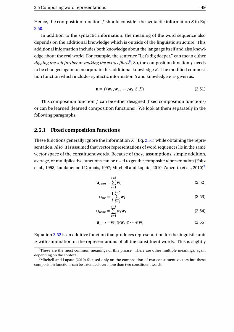
2.5 Composing word representations 49
Hence, the composition function f should consider the syntactic information S in Eq.
2.50.
In addition to the syntactic information, the meaning of the word sequence also
depends on the additional knowledge which is outside of the linguistic structure. This
additional information includes both knowledge about the language itself and also knowl-
edge about the real world. For example, the sentence “Let’s dig deeper.” can mean either
digging the soil further or making the extra efforts8. So, the composition function f needs
to be changed again to incorporate this additional knowledge K . The modified composi-
tion function which includes syntactic information S and knowledge K is given as:
u = f (w1,w2, · · · ,wl ,S,K ) (2.51)
This composition function f can be either designed (fixed composition functions)
or can be learned (learned composition functions). We look at them separately in the
following paragraphs.
2.5.1 Fixed composition functions
These functions generally ignore the information K ( Eq. 2.51) while obtaining the repre-
sentation. Also, it is assumed that vector representations of word sequences lie in the same
vector space of the constituent words. Because of these assumptions, simple addition,
average, or multiplicative functions can be used to get the composite representation (Foltz
et al., 1998; Landauer and Dumais, 1997; Mitchell and Lapata, 2010; Zanzotto et al., 2010)9.
usum =i=l∑i=1
wi (2.52)
uav = 1
l
i=l∑i=1
wi (2.53)
uw av =i=l∑i=1
αi wi (2.54)
umul = w1 ⊙w2 ⊙·· ·⊙wl (2.55)
Equation 2.52 is an additive function that produces representation for the linguistic unit
u with summation of the representations of all the constituent words. This is slightly
8These are the most common meanings of this phrase. There are other multiple meanings, againdepending on the context.
9Mitchell and Lapata (2010) focused only on the composition of two constituent vectors but thesecomposition functions can be extended over more than two constituent words.

50 Background
changed in equations 2.53 and 2.54 where unweighted and weighted averages are taken to
get the final representation. Hadamard product of the constituent words is taken in Eq.
2.55 to produce the composite representation.
2.5.2 Learned composition functions
The previous approach of combining the constituent word representations puts a lot of
constraints while designing the function, for instance these approaches assume that a
vector of word sequences also lies in the same space as word vectors, which may not hold
in reality. Also, often the functions designed are not effective because of their simplistic
way of combination. Because of this, instead of manually designing these functions,
functions are parameterized and the parameters governing the function are learned. The
general definition of these functions is slightly different from Eq. 2.51 which is given as:
u = f (w1,w2, · · · ,wl ;Θ) (2.56)
Here, parametersΘ are learned with machine learning models. It is important to learnΘ in
such a way that they can capture the syntactic information present in the unit u. Generally,
these parameters also capture a small amount of additional knowledge because of the
context but these methods also largely ignore the external knowledge while acquiring
the composite representation. Commonly, the parameters Θ are learned either in the
task-agnostic or task-specific fashion.
In the task-agnostic methods, the parameters are usually trained by unsupervised
or semi-supervised learning and can be served as features for many other NLP tasks
such as text classification and semantic textual similarity. This includes recursive auto-
encoders (Socher et al., 2011), ParagraphVector (Le and Mikolov, 2014), SkipThought
vectors (Kiros et al., 2015), FastSent (Hill et al., 2016), Sent2Vec (Pagliardini et al., 2018),
GRAN (Wieting and Gimpel, 2017), transformer based models like BERT (Devlin et al.,
2019).
On the other hand, in task-specific approach, the representation learning is combined
with downstream applications and trained by supervised learning. Different deep learning
models are trained to solve certain NLP tasks, FFNNs (Huang et al., 2013), (Chung et al.,
2014; Hochreiter and Schmidhuber, 1997), CNNs (Kalchbrenner et al., 2014; Kim, 2014;
Shen et al., 2014), and recursive neural networks (Socher et al., 2013).
Overall, the approaches based on the deep learning techniques have shown promising
performance for learning these parameters. Socher et al. (2012) show the efficiency of
deep learning approaches by comparing them with the simple average of word vectors,
2.6 Knowledge graphs and representations 51
elementwise multiplication, and concatenation. Further, similar results were observed
in (Socher et al., 2013).
2.6 Knowledge graphs and representations
In previous sections, we looked at various approaches of obtaining word embeddings
and several composition methods to get word sequences representations from them.
However, these word embedding algorithms use only text data to learn representations, as
a result, they fail to adequately acquire commonsense knowledge like semantic and world
knowledge. To address that limitation, various methods have been proposed to enrich
word embeddings with commonsense knowledge (Faruqui et al., 2015; Osborne et al.,
2016; Peters et al., 2019; Sun et al., 2020; Yu and Dredze, 2014).
As we also make use of such external knowledge in our work, in this section, we
describe one of the popular sources of commonsense knowledge: Knowledge Graph,
and approaches of representing knowledge held by them. Specifically, in Section 2.6.1,
we describe knowledge graph and look at the popular lexical knowledge source: Word-
Net (Fellbaum, 1998), which is used in this work. We also describe another knowledge
source, TEMPROB (Ning et al., 2018a), which is specifically constructed to store proba-
bilistic temporal relations information, and used for temporal relation classification in
this work. Next, in Section 2.6.2, we explain the problem of graph representations which is
a challenging task, as the information present in the whole topology of the graph should
be captured in the representation. Node embeddings learned over graphs proved to be
effective at capturing such knowledge (Hamilton et al., 2017) so we describe their general
framework and two prominent families of approaches in the subsequent subsections.
This background of node embeddings framework will be beneficial for understanding
specific node embedding algorithms used over WordNet and TEMPROB in Chapter 6.
2.6.1 Knowledge graphs
Commonsense knowledge is generally stored in a graph-structure format, commonly
called as Knowledge Graphs. In knowledge graphs, nodes denote real-world entities or
abstract concepts, and edges show relations between them. Because of this broad def-
inition, knowledge graphs can be found with a variety of data. Broadly speaking, they
can be categorized as open-domain or domain-specific knowledge graphs. For example,
popular knowledge graphs such as YAGO (Hoffart et al., 2011), DBpedia (Lehmann et al.,
2015) contain open-domain information as the nodes can be people, organizations, or

52 Background
places, and multiple relations between them are denoted with edges. On the other hand,
some knowledge graphs are designed for specific domains: language, specifically lexical
resources, WordNet (Fellbaum, 1998), FrameNet (Ruppenhofer et al., 2006), Concept-
Net (Speer et al., 2018), geography (Stadler et al., 2012), media (Raimond et al., 2014), and
many more.
Formally, let G = (V ,E ,R) be any knowledge graph where V , E denote nodes and edges
of the graph and R is a set of possible relations between nodes. Then, graphs can possess
different information depending on the types of edges. An unlabeled knowledge graph
contains edges that only have tuples of nodes: E = {(u, v) : u, v ∈V }. Next, the edges of a
knowledge graph with labels are set of triples: E = {(u,r, v) : u, v ∈V ,r ∈ R}. On the other
hand, for a probabilistic graph, in addition to relations there is a scalar value denoting
strength of the edge: E = {(u,r, v, s) : u, v ∈V ,r ∈ R, s ∈R}.
In this work, we used two knowledge graphs: WordNet (Fellbaum, 1998) and TEM-
PROB (Ning et al., 2018a). Let us look at them in the following sections.
Fig. 2.11 A subset of WordNet related to the four senses of book. Figures (1) book.n.01and (2) book.n.02 show two noun senses of book and their hyperonyms and hyponyms.Similarly, figures (3) book.v.01 (4) reserve.v.04 show two verb senses and their relatedsynsets.

2.6 Knowledge graphs and representations 53
2.6.1.1 WordNet
WordNet (Fellbaum, 1998) is a large lexical database that stores possible senses of words
and semantic relations between them 10. The senses of words that have similar meanings
are grouped and referred to as synset (synonym set). Each synset stores a simple definition
explaining the meaning of the synset as well as examples depicting the use of the word in
sentences. Further, each sense of the word is assigned its POS tag and a unique number to
differentiate between multiple senses of the same word. For instance, Fig. 2.11 depicts
multiple senses of word book: book.n(oun).01, book.v(erb).01, etc. Formally, WordNet
graph GW = (VW ,EW ,RW ) contains nodes, VW , which are synsets, RW , the set of semantic
relations, and EW , the set of edges consisting of triples having two synsets and semantic
relation between them: EW = {(u,r, v) : u, v ∈VW ,r ∈ RW }.
The set RW contains lexical semantic relations such as synonymy, antonymy, hyper-
onymy, hyponymy, meronymy, holonymy, etc. Where synonymy, antonymy indicates
similarity or dissimilarity between senses. Hyperonymy and hyponymy indicate “ISA”
relation between synsets. If X is a generic term for Y, then X is a hyperonym of Y. At the
same time, Y is a hyponym of X, as Y is a specific type of X. For example, animal is hyper-
onym of dog and dog is hyponym of animal. Whereas, meronymy and holonymy indicate
part-whole relation. If X is a part of Y, then X is a meronym of Y, conversely, Y is a holonym
of X. For instance, wheel is a meronym of car and car is a holonym of wheel.
In total, WordNet (English) contains 117,000 synsets where a synset can have POS tag
as noun, verb, adjective or adverb. However, the major portion of synsets is either nouns
or verbs. We show a small subset of WordNet concerning the word book in Fig. 2.11. For
the word book, WordNet contains 11 different senses, out of which 7 are nouns and 4 are
verbs (only two of each are shown in the figure). A book (noun) can mean a written or
published work: book.n.01, a physical object consisting of a number of pages: book.n.02, a
written version of play: script.n.01, a commercial record: ledger.n.01, or seven other senses
such as Bible, Quoran, etc. Also, book as verb has multiple meanings, engage someone
(artist) for performance: book.v.01, reserve a seat or ticket: reserve.v.04, etc. We show a
subset of these senses as well as their semantic relations (hyperonymy or hyponymy) with
other synsets in Fig. 2.11.
2.6.1.2 TEMPROB
Temporal relation probabilistic knowledge base (TEMPROB) (Ning et al., 2018a) is specially
constructed to hold prior temporal relation probabilities (frequencies) between semantic
10In the stricter sense, WordNet is not a graph but many graphs are constructed over it for the use.

54 Background
Verb1 Verb2 Temporal Relation Frequency
chop.01 taste.01 after 9chop.01 taste.01 before 285chop.01 taste.01 undef 44conspire.01 kill.01 after 6conspire.01 kill.01 before 117conspire.01 kill.01 equal 3conspire.01 kill.01 included 3conspire.01 kill.01 undef 30dedicate.01 promote.02 after 6dedicate.01 promote.02 before 71dedicate.01 promote.02 equal 1dedicate.01 promote.02 included 3dedicate.01 promote.02 undef 9
Table 2.7 A portion of TEMPROB where each row is a quadraple in the graph. Frequencyindicates likelihood of temporal relation, in case of chop and taste high frequency is forbefore relation, indicating chopping of food comes before taste. Similarly, in most of thecases conspire occurs before killing, and dedicated efforts are before promotion.
verb frames. Suppose GT = (VT ,ET ,RT ) denotes TEMPROB, then VT are the set of semantic
verb frames, RT is the set of temporal relations, and the edges store quadruples: ET ={(u, v,r, fu,v,r ) : u, v ∈VT ,r ∈ RT , fu,v,r ∈R}.
Now, let us look at different parts of graph GT to understand TEMPROB. Nodes VT , are
a set of semantic verb frames where each verb frame denotes the meaning of the verb in a
specific environment (frame). This notion is based on frame semantics (Fillmore, 1976)
that derives lexical meaning from prototypical situations captured by frames. For instance,
verb sew means stitching clothes in the frame corresponding to textile, cotton, fabrics,
whereas it also can mean stitching wounds in the medical frame containing doctors,
nurses, syringe, etc. Next, RT is a set of temporal relations which consists of after, before,
includes, included, or undef (vague). At last, the frequency fu,v,r denotes the number of
times relation r existed between semantic verb frames (u, v). Specifically, the frequency
measures the number of predictions of certain relations only over the pairs that appeared
in the corpus (1 million NYT times articles) considered while constructing TEMPROB. The
assumption is that these statistics can be generalized over other datasets, as a result, in
general, a higher frequency of certain temporal relation for the pair can be considered as
a higher likelihood of that relation. Overall, TEMPROB contains such 51 thousand nodes,
80 million temporal relations between them, and corresponding frequencies. The small
portion of TEMPROB is shown in Fig. 2.7.

2.6 Knowledge graphs and representations 55
Now, we detail the procedure of TEMPROB construction which can be beneficial for
gaining further insights. To construct TEMPROB, first, temporal relation classification
system is trained which is used over NYT articles to predict temporal relations between
detected event pairs. The aggregated frequency of the prediction of temporal relations for
each event-pair over all the documents is stored to form the knowledge base. Let us look
at these steps of the construction of TEMPROB separately:
1. Temporal relation classification system: Pairwise classification models to predict
temporal relations are trained. Specifically, two averaged perceptrons (Freund and
Schapire, 1998) each for event-pairs occurring in the same sentence, and adjacent
sentences are trained (rest of the event-pairs are not considered). TBDense (Cassidy
et al., 2014) dataset containing 36 documents is used in the experiment with Train
(22 docs), Dev (5 docs), and Test (9 docs) split. Further, simple hand-crafted features
such as POS tags of verbs and three surrounding words, number of tokens between
verbs, presence of modal verbs (e.g. would, might, may) and temporal indicators
(e.g. before, since), etc. are used in the model.
2. Event detection: After training the temporal relation classification system, the next
step is to apply it over the NYT articles. But, these documents do not contain
annotations for events. For this reason, they used an off-the-shelf Semantic Role
Labeling (SRL) system to detect events. Then, events that are nominals are deleted
from the list and only verbs (semantic verb frames) are kept.
3. Inference: Next, each article is considered separately where event pairs appearing in
the same sentences, and adjacent sentences are separated. First temporal relations
for verb pairs appearing in the same sentences are predicted and then verb pairs
from the adjacent sentences. Greedy strategy is used for inference where after the
addition of new temporal relation temporal graph closure is performed over the
document. The preference is given to the relation obtained from the graph closure
over the prediction such that relation is not at all predicted if it is already deduced.
4. Graph construction: Temporal graphs over each article are obtained, and the fre-
quencies for the verb pairs are aggregated to form the final knowledge base.
Out of these two knowledge graphs, we used WordNet for bridging anaphora resolution,
since it contains semantic relations which are beneficial for bridging inference such as
meronymy relations are especially useful (Hou, 2018b; Hou et al., 2013b). Next, we also
used it in temporal relation classification because semantic relations like hyperonymy

56 Background
Fig. 2.12 Overview of graph node embeddings: A conceptual encoder-decoder frame-work (Hamilton et al., 2017). Given the graph, encoder encodes the node a to low-dimensional vector va . Encoder takes into consideration node’s structure in the graphwhile projecting it into vector space. Then the decoder retrieves the original graph struc-ture of the node given its vector representation. The node embeddings are learned in thisencoder-decoder framework where they are optimized simultaneously.
can indicate event-subevent relations which can be beneficial for the task. In addition to
WordNet, for temporal relation classification, we separately used TEMPROB to exploit the
prior knowledge about events. We further detail about this in Section 6.2.
2.6.2 Graph node embeddings
Until now, we discussed knowledge graphs which are a special type of graphs that contain
useful commonsense information. But, in this section, we are going to consider generic
graph as a point of discussion (without narrowing down to only knowledge graph). The
reason being, the complexity because of graph-structure is prevalent in all graphs and not
specific to only knowledge graphs. Similarly, the proposed approaches are more general
and can be applied to any graph.
Incorporating knowledge possessed by graphs into machine learning models is a
challenging task, due to the difficulty of encoding high-dimensional non-Euclidean infor-
mation of the graph-structure. Because of this complexity, earlier approaches of feature
designing or use of summary statistics of graphs (e.g degree or clustering coefficients)
are rendered inefficient. Moreover, these approaches become computationally expensive
because of huge sizes of the graphs. Therefore, it is beneficial to learn low-dimensional
representations over graphs instead of relying on hand-crafted heuristics to utilize the
information held by graphs.
Graph embeddings achieve exactly that where they may encode the whole graph, sub-
graphs, or nodes into low-dimensional vector spaces. Fundamentally, graph embeddings
must preserve the structural information of the graph, i.e. in the case of graph node

2.6 Knowledge graphs and representations 57
embeddings, nodes which are in a neighborhood in the actual graph should have closer
representations in the latent space. This is the main constraint while designing the em-
beddings algorithm. In our work as well we resorted to graph node embeddings learned
over knowledge graphs for enriching event and mention representations. Because low-
dimensional node embeddings can encode node-specific information as well as global
structure which is advantageous for the downstream tasks.
Now, we provide an overview of graph node embedding algorithms. First, we describe
a unifying conceptual framework where the process of obtaining graph node embeddings
can be viewed as training of encoder-decoder pair (Hamilton et al., 2017). Further, we
discuss two broad categories of node embeddings approaches: 1. Matrix factorization
based approaches, and 2. Random walk based approaches. This background is useful
to understand the graph node embeddings algorithms presented in Section 6.3.1 over
WordNet and TEMPROB.
2.6.2.1 Unified framework
As stated earlier, node embeddings capture the global position of the node in the topology
as well as local neighborhood information. Let us suppose G = (V ,E) be the graph where
V and E respectively denote vertices, and edges of the graph. Here, we do not make any
assumptions about the type of graph G where it can be directional, unidirectional, labeled,
etc. Then, node embedding encodes structural information by transforming node into
d-dimensional vector space Rd where d ≪|V |.The node embeddings learning can be thought as a pair of encoder-decoder func-
tions (Hamilton et al., 2017). Let FE ,θ be the encoder function which converts graph
nodes to vectors:
FE ,Θ : V →Rd (2.57)
where Θ denote set of parameters to be learned associated with encoder. Then the
decoder function reconstructs graph properties from the encoded vectors. The embedding
algorithm decides which graph properties to reconstruct and designs a specific decoder
function. Suppose a decoder function FD,Ψ measures pairwise similarity between the
nodes in the actual graph through their embeddings as:
FD,Ψ :Rd ×Rd →R (2.58)
whereΨ are decoder specific set of parameters.
Next, the parametersΘ,Ψ are learned to minimize the reconstruction loss. Suppose
a,b ∈ G and va := FE ,Θ(a), vb := FE ,Θ(b) be their node embeddings. Let s(a,b) be a

58 Background
similarity score between nodes a,b obtained from the graph G with user-defined measure.
Then embeddings learning procedure minimizes the following reconstruction loss:
L (Θ,Ψ) = ∑(a,b)∈V
ℓ(FD,Ψ(va ,vb), s(a,b)) (2.59)
where ℓ : R×R → R is a loss function. The learning algorithms are usually agnostic
about the downstream tasks, as they depend solely on the design of the loss function ℓ
and similarity measure s. Once the parameters Θ,Ψ are learned, the encoder output is
considered as node embeddings of the provided graph node.
Following the discussion from the work (Hamilton et al., 2017), we note that most of
the node embedding algorithms differ in the way the encoder function, decoder function,
pairwise similarity function, or loss functions are designed. Broadly, two kinds of general
settings are prominently used to obtain node embeddings, we look at them separately in
the following sections.
2.6.2.2 Matrix factorization based approaches
These approaches learn node embeddings such that inner product of vector representa-
tions of nodes is closer to the deterministic similarity measure defined by the algorithm.
Hence, roughly they reduce the loss of the following form:
L = ||VT V−S||2 (2.60)
where V is the matrix of node embeddings and S is a pairwise node similarity matrix.
Concretely, the popular embedding algorithms based on this approach, Graph Factor-
ization (Ahmed et al., 2013), GraRep (Cao et al., 2015), and HOPE (Ou et al., 2016) design
their decoder function and loss function as follows:
FD (va ,vb) = vTa vb (2.61)
L (Θ) = ∑(a,b)∈V
||FD (va ,vb)− s(a,b)||2 (2.62)
where va ,vb are the learned vector representations for nodes a,b and s(a,b) is the graph
similarity between them. However, these three algorithms differ in the way similarity
between nodes is measured. The Graph Factorization uses adjacency matrix as to get the
similarity − s(a,b) = Aa,b , whereas GraRep uses higher power of adjacency matrix so as
to obtain more general similarity − s(a,b) = A2a,b , and HOPE measures general similarity
with Jaccard neighborhood overlap. The matrix factorization based approach (Saedi et al.,

2.6 Knowledge graphs and representations 59
2018), and Path2vec (Kutuzov et al., 2019) used for obtaining WordNet embeddings in
Section 6.3.1 can be considered to be matrix factorization approaches.
2.6.2.3 Random walk based approaches
In comparison to matrix factorization approaches, random walk based approaches differ
in the way the similarity between nodes is measured. The factorization based approaches
produce deterministic similarity scores between nodes, for instance with the use of the
adjacency matrix. On the contrary, the random walk based approaches use a stochastic
approach to obtain the pairwise similarity between nodes. More precisely, the similarity
between two nodes, a,b, is the probability of encountering node b if the random walk
started from node a.
Deepwalk (Perozzi et al., 2014) and Node2vec (Grover and Leskovec, 2016) are the two
popular algorithms based on random walk. In addition to them, a random walk based
graph node embeddings (Goikoetxea et al., 2015) algorithms used over WordNet employ
the similar strategy which is detailed in Section 6.3.1. In these approaches the decoder
function gives the approximate probability of the nodes being in the neighborhood. Hence,
the decoder function in these methods is given as:
FD (va ,vb) = evTa vb∑
c∈V evTa vc
(2.63)
The decoder score is approximately equals to the probability of nodes being in the neigh-
borhood i.e. FD (va ,vb) ≈ p(b|a) where p(b|a) is the probability of encountering b if
random walk started from a.
These approaches generate a sequence of nodes by sampling the random walks from
each node. This generated sequence is used as the training data for learning the em-
beddings. The core of these algorithms is Word2vec (Mikolov et al., 2013b) as once the
sequence of nodes is obtained with repeated random walks they can be treated as cor-
pus and then the algorithm is trained. Similar to the Word2vec objective, the following
negative log of probability loss is optimized:
L (Θ) =− ∑(a,b)∈D
log (FD (va ,vb)) (2.64)
where D is the data generated with random walks and Θ be the learning parameters to
be optimized. Notice that, Eq. 2.63 is similar to the probability calculation equations for
Word2vec (Section 2.4.1.1, Eq. 2.25 and 2.28). Therefore, similar to Word2vec, directly
optimizing Eq. 2.64 is computationally expensive because of the denominator term in

60 Background
Eq. 2.63. To solve this problem, deepwalk uses hierarchical softmax approach whereas
node2vec uses negative sampling approach, both of these approaches were introduced in
Section 2.4.1.1.
2.7 Summary
This chapter presented background information needed to understand the rest of the
thesis. First, we described task definitions and three main components of supervised
learning approaches: event and mention representations, local or global models, and
inference. We also described corpora used in the work and evaluation schemes for both
temporal relation classification and bridging anaphora resolution. Next, we briefly in-
troduced artificial neural networks and few popular types which are used in this work.
Further, we discussed representation learning and related fields. Then, we summarized
different distributional and contextual approaches of obtaining word representations.
The word embeddings algorithms such as Word2vec, and FastText are used in Chapters 4
for event representations whereas Chapter 5 probes BERT model. Many distributional
embeddings and BERT embeddings are again used for representations in Chapter 6. After-
ward, we briefly discussed different composition approaches of obtaining word sequences
representations from words which is similar to what we are doing but in task-specific
learning setting. Finally, we explained knowledge graphs and graph node embeddings. We
first discussed different types of knowledge graphs and detailed WordNet and TEMPROB
which are used in the work. Then we described a unified framework view and two families
of graph node embedding approaches. This context will be beneficial at understanding
graph node embeddings used in this work which are presented in Section 6.3.1.
In the next chapter, we detail the previously proposed approaches for event and men-
tion representations, and point out their drawbacks which is beneficial to gain perspective
about our proposed approaches. We also briefly describe some of the prominent models
and inference strategies in the same chapter.
Chapter 3
Related Work
In the previous chapter, we discussed different methods to obtain word representations,
followed by composition methods to obtain word sequences representations. These repre-
sentations learned in a task-agnostic way are insufficient to solve specific tasks. Contrarily,
a task-specific representation can associate with a desired output of the task, as a result pro-
ducing more accurate solutions. In this chapter, we review different approaches designed
to obtain event representations for temporal relation classification and mention repre-
sentations for bridging anaphora resolution. In addition, for both tasks, we also briefly
discuss other systems that did not specifically concentrate on improving representations
but focused more on modeling and inference.
3.1 Temporal relation classification
Earlier research in computational linguistics extensively studied temporal ordering be-
tween discourse units (Lascarides and Asher, 1993; Lascarides and Oberlander, 1993;
Passonneau, 1988; Webber, 1988). These works explored various temporal order defining
linguistic structures and features such as tense, aspect, temporal adverbials, rhetorical
relations, and pragmatic constraints. Then, the construction of annotated corpora, such as
TimeBank (Pustejovsky et al., 2003a) sparked the use of machine learning approaches for
temporal analysis (Boguraev and Ando, 2005; Bramsen et al., 2006; Lapata and Lascarides,
2004; Mani et al., 2003, 2006) and has further accelerated (Bethard, 2013; Bethard et al.,
2007; Chambers; Chambers et al., 2007; Laokulrat et al., 2013; Verhagen and Pustejovsky,
2008) by multiple TempEval campaigns (UzZaman et al., 2013; Verhagen et al., 2007, 2010).
The majority of these approaches employed supervised learning models, barring few
exceptions such as (Mirroshandel and Ghassem-Sani, 2014) which explored unsupervised

62 Related Work
learning methods. In our work too, we focus on supervised machine learning approaches
employed to solve temporal relation classification.
Recall from the previous chapter that supervised learning based temporal relation
classification systems have three main components: representation of events, model,
and inference. Most of the proposed systems generally differ in the way of obtaining
representation, in modeling (local, global models), or inference (e.g. greedy or ILP). In
the following sections, first, we present details about the methods that focus on event
representations, later we briefly discuss the approaches that concentrate on modeling
and inference.
3.1.1 Work on event representations
As a general trend in NLP, initial approaches obtained event representations by manually
designing features and later features were learned automatically with extensive neural
network use. We follow the same chronological order, first summarize manually hand-
engineered works followed by automatic representation learning approaches.
3.1.1.1 Manually designed representations
The initial studies on temporal ordering explored various ordering units: a clause, a
sentence, or an event (Boguraev and Ando, 2005; Lapata and Lascarides, 2004; Mani et al.,
2003). Despite these different discourse units, they resorted to similar lexical, grammatical,
and semantic features to obtain representations. Mani et al. (2003) found reference time
of the clause, and then established temporal order between them. They called reference
time of the clause as Temporal Value (tval) which can be an explicit time such as year 2001
or some implicit time inferred from the text, and it is obtained by employing different
rules, for instance, a number of temporal expressions present in the clause. This tval is
used as one of the features for establishing temporal order between events in addition to
temporal adverbials, sentence number, paragraph number, aspect, and tense. Further,
Lapata and Lascarides (2004) designed features to capture verb tense and aspect as well
as temporal indicators surrounding the verbs. Similar to these approaches, Boguraev and
Ando (2005) also used lexical features such as tokens, capitalization of tokens, headwords,
grammatical features such as POS of the tokens as well as of the words chunk, etc. to
obtain the event representation.
Later on, the prominent approaches (Bethard et al., 2007; D’Souza and Ng, 2013) used
TimeBank (Pustejovsky et al., 2003a) corpus for the analysis, hence, consistently used
event as one of the ordering units and improved the representation by proposing an

3.1 Temporal relation classification 63
additional set of features. Bethard et al. (2007) concentrated only on the event-pairs which
are present in the verb-clause syntax. They considered the verb from the clause as the first
event and then the head of the clause as another event. Features were designed based on
the words which connect the event words as these connecting words like because, since, as,
while indicate temporal relations, specifically, because, since indicate after relation and as,
while indicate overlap relation. In addition to that, syntactic features were also extracted
such as dependency paths between events to include in their feature-set. Further, they
used all the words in-between events and derived features from them and empirically
showed that among these different features, the syntactic features have helped the most.
Next, D’Souza and Ng (2013) proposed rich linguistic features to further improve
the representation. Their main contribution is the proposal of various pairwise relations
between events. So for instance, to establish temporal relations between two events e1 and
e2, the baseline features mostly concentrate on features related to either e1 or e2 but not
both. They filled this gap by extracting various relations like dependency, lexical, semantic,
and discourse relations between both events to improve pairwise representations. For the
events that are present in the same sentence, they argue dependency relation between
events implies simultaneous, before or after temporal relations. In addition to that, they
claim lexical relations such as antonymy, hyponymy, etc., are useful in capturing temporal
relations. To extract these lexical relations they used Webster dictionary and WordNet
graph. Further, they used semantic relations, particularly predicate-argument relations
such as cause as well as discourse relations: causation, elaboration and enablement. All
these features were evaluated empirically to show that the event-pair relations are crucial
for temporal relation classification.
3.1.1.2 Automatic representation learning
In the previous section, we have discussed the approaches that employed hand-crafted
features to represent events and event-pairs for temporal relation classification. The
process of acquiring representations by manually designing features is laborious and
requires expertise in the task. To mitigate these issues, automatically learned dense vectors
are used to represent events. Then interaction between these vectors is obtained to get
the event-pair representations. The assumption here is that the learned representation
adequately captures relevant features for temporal relation classification.
One of the first works (Mirza and Tonelli, 2016), assessed the effectiveness of the
use of word vectors for event representations that are learned over huge unannotated
texts. Also, they experimented on multiple simple ways of combining them to get the
event-pair representations. In their approach, events were represented with a pre-trained

64 Related Work
Word2vec (Mikolov et al., 2013b) vector of events’ headwords. Suppose ei and e j are the
two events having headwords wi and w j , respectively and wi,wj are the d-dimensional
Word2vec representations corresponding to them, and ei ,e j is the representation of
events. Then, event representations of each event is nothing but its headword embeddings:
ei := wi and e j := wj. This was much more efficient than designing multiple features to
represent an event. Because obtaining Word2vec vectors corresponding to events is fairly
simple as most of the events are either verbs or nouns.
Next, they conducted experiments over different approaches of combining these
event representations. In those experiments, they applied multiple simple ways to obtain
interaction between event-pairs such as concatenation, addition, or subtraction over
event representations. Let fe :Rd ×Rd →Rd ′be the function which models interactions
between event-pairs. They used different function forms to capture this interaction:
f ae (ei ,e j ) = ei +e j (3.1)
f se (ei ,e j ) = ei −e j (3.2)
f ce (ei ,e j ) = ei ⊕e j (3.3)
where ⊕ indicates concatenation of vectors, and observed that concatenation (Eq. 3.3) is
more effective in most of the cases.
The event representations obtained by considering the headword of the event was
efficient but still failed at capturing the context of events. The context of the event can
easily indicate the tense and aspect of the event as well as it can also show the presence
of any temporal markers such as before, after etc. As we have seen in the manually de-
signed features, this information is crucial for temporal relation classification. This issue
is partially handled by (Cheng and Miyao, 2017; Choubey and Huang, 2017; Meng et al.,
2017) who use dependency paths between events to obtain event-pair representations. In
these approaches, first dependency parsed trees are generated with the use of previously
proposed methods (e.g. Stanford Parser), and then these parsed trees of the sentences
containing both events are considered to get the context. For that, the common ancestor
between events is found and all the words from both the events up to this common an-
cestor are considered as a context. Next, all these words are represented with Word2vec
vectors and provided to an LSTM (Hochreiter and Schmidhuber, 1997). Finally, the output
of the LSTM is considered as event-pair representations. They observe that event-pair rep-
resentations with such approach is more beneficial than single headword representation
approach of Mirza and Tonelli (2016).

3.1 Temporal relation classification 65
One of the disadvantages of using dependency trees is that it can not be directly used
for events that are present in different sentences. To circumvent the issue, for both the
events dependency paths from them to roots of the respective sentences in which they are
present is considered and context is derived from these paths. This approach is exclusively
taken for those events which are present in different sentences, in addition to the previous
common ancestor approach for events in the same sentence. This leads to the overhead
of training another LSTM separately for event-pairs that are in the different sentences.
Also, in this approach, instead of all the words in the context, only those words which are
on the dependency tree path are considered. We solve this issue by considering all the
words in the context-window and use RNN to get the representation (Pandit et al., 2019)
which is detailed in the coming chapter.
The work of Han et al. (2019a,b) further improved the representation by including the
whole sentence as the context of the event. It inputs the whole sentence to a BiLSTM (for-
ward and backward LSTMs) where each word is represented by concatenating the word
vectors obtained with BERT (Devlin et al., 2019) model as well as POS vectors of each
word. Let ei be any event present in a sentence containing n words. Here, each k th word
is represented by vector
wk = bk ⊕pk (3.4)
where bk is BERT based representation, pk is POS embeddings of k th word, and ⊕ indi-
cates concatenation of vectors. Then all the words’ representations: w1, · · · ,wk , · · · ,wn are
passed through BiLSTM. The output from the forward LSTM and backward LSTM corre-
sponding to event word is concatenated to get the contextualized event representation.
So, the vector representation corresponding to event ei is obtained as, ei = fi ⊕bi where
fi ,bi are hidden vectors from forward and backward LSTMs corresponding to event ei .
Similarly, for event e j vector representation e j can be obtained. Finally, to get the event
pair representation both these embeddings are concatenated:
ei j = ei ⊕e j (3.5)
Also, these systems learned representations in a global fashion. As we will mention in
the models and inference section, these systems are trained with a deep structured learning
approach where Structured SVM (SSVM) is used to model the global loss. This leads to
more effective representation learning as underline neural networks capture the relations
between other event-pairs as well while training.
Using a different approach, Ning et al. (2018a) developed TEMPROB knowledge re-
source to improve event representations. As discussed in Section 2.6.1.2, TEMPROB

66 Related Work
contains prior probabilities for relations between different verbs, for instance, marry –
divorce have higher probability score for before relation than any other temporal rela-
tion. These prior probability scores between the event-pairs for each temporal relation
are used as one of the features to represent event-pairs. Their approach is conceptually
similar to ours where we also inject commonsense information in addition to text-based
embeddings, but they relied only on the specific prior information, even in that they
just used pairwise probability scores as a feature instead of getting overall information
from the general structure of TEMPROB. This naive method of injecting commonsense
knowledge is further improved in Ning et al. (2019) where they trained auxiliary Siamese
network (Bromley et al., 1993) over TEMPROB and a portion of ConceptNet (Speer et al.,
2018) and included features from this network into their main system.
Further, Wang et al. (2020) combined the previously mentioned BiLSTM based ap-
proach (Han et al., 2019a) and trained a MLP auxiliary network as proposed by Ning et al.
(2019) to include TEMPROB and ConceptNet information to improve the representations.
They used RoBERTa (Liu et al., 2019b) embeddings and external features obtained from
the trained auxiliary network to get event-pair representations. Their approach can also
be described with Eq. 3.4 with the only difference is that instead of bk BERT-based repre-
sentations, rk RoBERTa-based embeddings are used. Also, the pairwise representation
obtained in Eq. 3.5 is further concatenated by the knowledge graph based information,
elementwise multiplication, and subtraction of outputs of BiLSTMs. With this event-pair
representations they solved the broader event-event relation problem instead of just fo-
cusing on temporal relations by addressing event coreference as well as event parent-child
relation in their approach. This joint formulation seems to improve the performance
further.
In addition, some recent works (Han et al., 2020; Lin et al., 2020) have used similar tech-
niques to get the event-pair representations, where they extended these representations
to the biomedical domain temporal relation extraction.
3.1.2 Work on models and inference
So far, we discussed approaches that differed in the way of obtaining event representa-
tions. Now, we review the approaches that focus on the model or inference, the other
component of the supervised temporal relation classification systems. Local temporal
classification models learn temporal relations between temporal entities (event–event,
event–TimEx, TimEx–TimEx) independent of temporal relations between other pairs. The
general framework in these models is to obtain representations of event-pairs, then em-
ploy the machine learning classification models, such as SVM, CRF, or neural networks, to

3.1 Temporal relation classification 67
assign probability scores for each possible temporal relation. Followed by local inference
strategy to select the highest scoring relation as the predicted temporal relation for that
pair. It is crucial to note that the relations are inferred without considering predictions
between other pairs. The approaches (Bethard, 2013; Bethard et al., 2007; Chambers;
Chambers et al., 2007; Laokulrat et al., 2013; Mani et al., 2006; Verhagen and Pustejovsky,
2008) fall into this category. Despite the simplicity and wide use of these approaches, they
suffer from two major drawbacks. First, the temporal relations between pairs are learned
independent of each other, thus missing out on the available global information. Second,
due to local inference strategies, systems can produce inconsistent temporal relations
between event-pairs. For instance, these systems can predict A before B , B before C , and
A after C , which violates temporal constraints.
To solve the problem of inconsistent temporal relation predictions caused by local
inference, different strategies to impose global constraints were designed. Initially, the
approaches (Mani et al.; Verhagen and Pustejovsky, 2008) proposed greedy inference
strategies to solve the global inference problem. Further improvements in inference are
achieved by formulating inference as integer linear programming (ILP)(Bramsen et al.,
2006; Chambers and Jurafsky, 2008; Denis and Muller, 2011; Do et al., 2012). On similar
lines but a slightly different approach is developed by (Chambers et al., 2014; McDowell
et al., 2017): They employ many hand-crafted rules and machine learned classifiers called
sieves, to form a stack, and predicted temporal relations are passed from one sieve to
another where the consistency is enforced by inferring all possible relations before passing
by using greedy inference strategy similar to (Mani et al.; Verhagen and Pustejovsky, 2008).
Though these approaches solve the problem of inconsistent predictions, they still
learn parameters locally i.e. independent of temporal relations between other pairs.
This issue of local parameter learning is addressed by the global models which apply
structured learning approach to learn temporal relations globally and employ global
inference strategies (Han et al., 2019a,b; Ning et al., 2017; Yoshikawa et al., 2009). Ning
et al. (2017) applied semi-supervised constraint driven learning (Chang et al., 2012) to
learn consistent temporal relations, as they leveraged unlabeled data in their approach
to improve the performance of the system. The approaches (Han et al., 2019a,b) further
improved the performance with the application of deep structured learning. Both works
use the same neural model which consists of a BiLSTM network to learn scoring functions
for pairwise relations, and a SSVM to predict temporal relations that comply with global
constraints. The only difference is that the latter approach (Han et al., 2019b) predicts
events and temporal relations jointly, instead of taking a common approach of relying on
the gold event annotations.

68 Related Work
3.1.3 Summary
We observed that the earlier approaches predominantly employed hand-engineered fea-
tures for event representations. The hand-engineered approaches concentrated on tense,
aspect, modality, and certain grammatical features of the event. These approaches relied
mostly on event specific information, barring works such as (D’Souza and Ng, 2013),
which focused on the broader context to capture semantic and discourse relations be-
tween events. The earlier approaches also attempted to exploit contextual information by
looking for temporal clues like temporal markers such as an explicit mention of year, day,
etc. as well as clause connectors such as because, as, etc. Though these manually designed
representations attempt to leverage contextual information, they still remain inefficient
because of the inherent hand-picky approach taken, because the methods capture only
those features that experts deem important while neglecting broader contextual infor-
mation. This trend has changed with automatic representation learning due to neural
networks. The earliest work (Mirza and Tonelli, 2016) based on automatically learned
word vectors just used headword vectors by ignoring crucial contextual information. The
more recent approaches tried to solve the contextual information problem by using de-
pendency parse based context (Cheng and Miyao, 2017; Choubey and Huang, 2017; Meng
et al., 2017) as well as with window based context (Dligach et al., 2017). We argue that the
former study is difficult to be applied effectively if the events are not present in the same
sentence and latter study is not done on the standard dataset used for temporal relation
classification.
The pairwise representations of events is another necessary part of these approaches
because we are trying to capture the temporal relation between pair of events and not
the events separately. This is a less investigated area in the literature as most of the
works simply concatenated event representations of both events to get the pairwise
representations barring (D’Souza and Ng, 2013; Mirza and Tonelli, 2016). D’Souza and Ng
(2013) designed pairwise features such as pairwise grammatical features, features based
on the different lexical, semantic, and discourse relations, whereas (Mirza and Tonelli,
2016) resorted to linear operations such as summation, multiplication, etc. over event
representations to get the interaction between events.
Further, use of the external knowledge resources for capturing lexical relations is ex-
plored in (D’Souza and Ng, 2013) and in (Ning et al., 2018a) developed external knowledge
source with TEMPROB to capture prior temporal information of the events. However,
both these approaches resorted to hand-picked features for the event representations,
(D’Souza and Ng, 2013) used specific lexical relations where as (Ning et al., 2018a) used
prior temporal relation probability as a feature. The approaches (Ning et al., 2019; Wang

3.2 Bridging anaphora resolution 69
et al., 2020) attempted to remedy this by training auxilary network instead of relying
on hand-picked features, but it still captured only shallow features. As a result, these
approaches fail to acquire broader commonsense information available in the knowledge
sources encoded by the topology of the graph.
All in all, the representation learning approaches produced superior results in com-
parison to the feature engineering based approaches and seem to be a promising way of
obtaining representations. This was first shown by Mirza and Tonelli (2016) when they
experimented with Word2vec representations and observed absolute performance gain
of around 2 points in F1 score against strong sieve-based CAEVO (Chambers et al., 2014)
on TimeBank-Dense dataset. Further recent approaches (Han et al., 2019a,b; Ning et al.,
2019; Wang et al., 2020) also benefited from the improved representations and shown
gains in performances, albeit the systems were evaluated on different dataset (MATRES)
so direct comparison between earlier hand-crafted feature based approaches and these
approaches is difficult. Though there are improvements in event representations, they
still lack at acquiring some crucial information as discussed above.
In our work, we try to remedy all these shortcomings. We capture the contextual
information for the event representation with the window of n-words context to RNN
and then capture non-linear interaction with CNN between these representations to get
event-pair representation which is detailed in the next chapter (Chapter 4). Next, in the
final chapter (Chapter 6), we explain the work where we combine embeddings learned
over knowledge graphs such as TEMPROB, WordNet with text-based representations to
acquire both contextual and commonsense information.
3.2 Bridging anaphora resolution
Bridging anaphora resolution is a subtask of bridging resolution. Recall from the previous
chapter that bridging resolution involves identifying bridging anaphors which is referred
to as bridging anaphora recognition and linking these bridging anaphors to appropriate
antecedents is called bridging anaphora resolution. We are focusing on the latter task.
In the literature, Cahill and Riester (2012); Hou (2016, 2019); Hou et al. (2013a); Markert
et al. (2012); Rahman and Ng (2012) focused on bridging anaphora recognition, on the
other hand, Hou (2018a,b); Hou et al. (2013b); Lassalle and Denis (2011); Poesio et al.
(2004); Poesio and Vieira (1998); Poesio et al. (1997) studied bridging anaphora resolution,
whereas, Hou et al. (2014, 2018); Roesiger et al. (2018); Yu and Poesio (2020) solved both
problems. We focus on the work which solves the bridging anaphora resolution as that is
the main point of investigation in our study.

70 Related Work
All these works employed a supervised learning approach to solve bridging anaphora
resolution, then similar to temporal relation classification, we can divide them as well
into two broad categories: bridging anaphor and antecedent representations based work,
and task modeling and inference based work. First, we detail the approaches that focused
on the representations, later, we briefly note approaches that focused on models and
inference.
3.2.1 Work on mention representation
In all the models, we have to obtain representations for bridging anaphors, antecedents as
well as antecedent candidates. Recall from the previous chapter that all of these linguistic
objects are a subtype of mentions. Therefore, almost similar features are used to represent
them. In the earlier approaches, similar to all NLP tasks including temporal relation
classification, hand-engineered features were designed to get representations whereas
the latest work has exploited neural networks to learn them. So, first, we summarize the
mention representations obtained with hand-engineered features and then examine the
latest automatic representation learning approaches.
3.2.1.1 Manually designed representation
Most of the earlier approaches (Lassalle and Denis, 2011; Poesio et al., 2004; Poesio and
Vieira, 1998; Poesio et al., 1997) made a strong assumptions on bridging relations either by
considering only definite Noun Phrases (NPs) as bridging anaphors or limiting types of
relations can be held between bridging anaphor and antecedent (e.g. mostly considering
meronymic relations). But recent approaches have got rid of these restrictions and tackled
unrestricted bridging anaphora resolution (Hou, 2018a,b; Hou et al., 2013b).
Poesio et al. (2004) applied a pairwise model combining lexical semantic features
as well as salience features to perform mereological bridging resolution in the GNOME
corpus. They addressed only mereological bridging relations which is one type of bridging
reference. Lexical distance is used as one feature in their approach and WordNet is used
to acquire that distance, but sometimes relation between particular pair is not found
in WordNet, therefore, as an alternative, Google API is used to get the distance between
anaphor-antecedent. Given noun head ha of anaphor a and hm of potential antecedent
m, the query of the form “the ha of the hm” is provided to API to get the number of hits
and from that lexical distance is calculated. After obtaining these features, a multi-layer
perceptron is used for the classification. Their training dataset is constructed by keeping
a window size of 5, i.e., all the NPs occurring before an anaphor in the window of 5

3.2 Bridging anaphora resolution 71
sentences are considered as negative samples except antecedent. They also apply a data
undersampling strategy for data balancing.
Based on this method of Poesio et al. (2004), Lassalle and Denis (2011) developed
a system that resolved mereological bridging anaphors in French. They argued that
the linguistic resources are scarcer in languages other than English, thus the use of re-
sources like WordNet was difficult in other languages (e.g. French). To mitigate these
challenges, raw texts were used, specifically, the system was enriched with meronymic
information extracted from raw texts where they iteratively collected meronymic pairs and
the corresponding syntactic patterns in a bootstrapping fashion. Finally, they evaluated
their system on mereological bridging anaphors annotated in the DEDE (Gardent and
Manuélian, 2005) corpus.
Deviating from all the previous studies, Hou et al. (2013b) proposed the first work on
unrestricted bridging anaphora resolution. Also, they take a global approach to resolve
bridging anaphora. For that, they designed various new global and local features to get
mention representations. We detail their approach in Section 3.2.2, but for now, note
down the prominent features used by them for the mention representations.
We compile some of the generally used features for mention representations from the
previously proposed approaches (Hou et al., 2013b; Lassalle and Denis, 2011; Poesio et al.,
2004) as follows:
Semantic features
• Semantic class: Mentions are assigned one of the semantic classes (Markert et al.,
2012) e.g. location, organization, GPE (Geo-political Entity), product, language,
and so on, because certain semantic class pairs indicate bridging relation between
the mentions. For instance, suppose a semantic class of anaphor is a professional
role and that of candidate antecedent is organization. Then, they may exhibit
employee-employer relation, indicating bridging.
• Meronym relation: It captures part-of relation between mention pairs. Two ap-
proaches are broadly used to get this information. First, use of external resources like
WordNet which holds information about meronymy relation between nodes (Poesio
et al., 2004). This is done by measuring the shortest path length between an anaphor
and an antecedent candidate among all synset combinations. The inverse value of
this distance produces confidence about the relation between anaphor and can-
didate antecedent. On the other hand, the second approach exploits preposition
patterns like X of Y or possessive structure Y’s X (Hou et al., 2013b). The query
like "anaphor preposition antecedent" which is a generalization of "anaphor of an-

72 Related Work
tecedent" is created and passed to Google API to get the number of hits. This gives
probability of part-of relation between anaphor and candidate antecedent.
• Verb pattern: The compatibility of the anaphor and candidate antecedent is cap-
tured with the verb on which anaphor depends (Hou et al., 2013b). Suppose anaphor
depends on verb v then queries with all candidate antecedents of the subject-verb
and verb-object are searched over a corpus. The hits are transferred into the normal-
ized scores for each anaphor-candidate antecedent pair which indicates likeliness
of them being bridging pair.
Syntactic and lexical features
• Same head: Head of the anaphor and antecedent are rarely same, so it is good to
exclude those pairs (Hou et al., 2013b).
• Word overlap: Check if the anaphor is pronominally modified by the head of can-
didate antecedent (Hou et al., 2013b). For example the mine - mine security, the
headword mine modifies security in anaphor.
• Co-argument: The subject can not be the antecedent of the object anaphor in the
same clause (Hou et al., 2013b). This feature checks if it is the case.
Salience feature
Salient entities are preferred as antecedents. These features are captured by considering
the position of the antecedent candidate in the document.
• Global first mention: It is assumed that global salient entities are presented at the
beginning of the document (Poesio et al., 2004), based on that a binary feature is
designed to indicate if the mention is the first mention in the whole document.
• Local first mention: Binary feature denoting if the mention is the first in the last five
sentences is used (Poesio et al., 2004).
• Utterance distance: It calculates the number of sentences between anaphor and
candidate antecedent (Poesio et al., 2004).
• Document span: This captures the local context of the candidate antecedent, i.e.,
the sentences which contain antecedent (Hou et al., 2013b).

3.2 Bridging anaphora resolution 73
3.2.1.2 Automatic representation learning
Until now, we discussed hand-crafted features and approaches that proposed them. We
now move to approaches that automatically learn mention representations. There has
been little work (Hou, 2018a,b, 2020a; Yu and Poesio, 2020) on this front because of the
inherent difficulty of the task and more importantly small size of the annotated corpora.
Hou (2018b) learned embeddings_PP, a customized embeddings specifically for bridg-
ing resolution and extended them in (Hou, 2018a). In the first approach, she argues
distributional word embeddings learned in a task-agnostic way (e.g. Word2vec, Glove)
capture both genuine similarity and relatedness between words which is not quite suitable
for resolving bridging relation, as it requires more knowledge of lexical association. There-
fore, she resorts to the prepositional structure of NP, X of Y and possessive pattern Y’X (as
mentioned previously in 3.2.1.1) to acquire non-identical associative relation between
two nouns. On these noun-pairs having part-of relations, she learned embeddings_PP
while completely avoiding the hand-crafted ways of obtaining features. She empirically
showed that embeddings_PP significantly improved the accuracy of bridging resolution in
comparison to the task-agnostic word embeddings (Glove). In the following work (Hou,
2018a), she extended this approach and designed embeddings_bridging that combines
embeddings_PP and Glove (Pennington et al., 2014) embeddings, as embeddings_PP con-
tained representations only for nouns. This enhanced representation further improved
the accuracy of bridging anaphora resolution.
In the latest approaches (Hou, 2020a; Yu and Poesio, 2020), BERT embeddings are used
to get the contextualized representation of bridging anaphor and antecedent candidates.
However, both approaches differ in the way BERT is used. In the former approach, BERT
is fine-tuned for bridging whereas the latter approach uses pre-trained BERT embeddings
in their neural learning model.
BARQA system proposed by Hou (2020a) differs from commonly proposed approaches
in two ways: First, instead of relying on already extracted gold mentions to form the set
of antecedent candidates for bridging anaphors, the system extracts these candidates
itself, followed by selecting the appropriate antecedent from the set. Second, bridging
anaphora resolution is formulated as a question-answering problem where every anaphor
is rephrased as a question, and the answer generated by the system is considered as a
predicted antecedent. Specifically, for a bridging anaphor a, a question of the form “a
of what” is generated and context ca is provided to BERT. The context ca contains the
first sentence of the document, the previous two sentences from anaphor a and the
sentence containing a. Then the system predicts an answer for the question from the
context ca which is treated as predicted antecedent for a. This formulation produced

74 Related Work
effective representations as BARQA system achieved state-of-the-art performance over
ISNotes (Markert et al., 2012) as well as BASHI (Roesiger, 2018a) datasets.
The system proposed by Yu and Poesio (2020) also differs in the way the problem is
formulated. This system solved the more general and harder full bridging resolution task
where both bridging anaphor as well as antecedent candidates are detected and resolved.
Also, they formulated the task differently where they learn bridging and coreference res-
olution in multi-task fashion as both are similar tasks (reference resolution tasks). The
primary reason behind such a formulation is the lack of training data for bridging reso-
lution. Specifically, their system extends state-of-the-art coreference resolution system
(Kantor and Globerson, 2019; Lee et al., 2018) with the addition of a feedforward network
at the end and two different classifiers each for bridging and coreference resolution. They
mainly used part of ARRAU dataset (Uryupina et al., 2019) for training as it contains both
bridging as well as coreference annotations. Further, they evaluated their system on
ARRAU, ISNotes (Markert et al., 2012), BASHI (Roesiger, 2018a), and SciCorp (Roesiger,
2016). Their system achieved substantial improvements over previous best results for full
bridging resolution for all corpora.
3.2.2 Work on models and inference
Supervised learning approaches for the task have considered bridging anaphora resolution
as a classification problem and have commonly used two types of models: local and
global. Similar to the models for temporal relation classification, local models predict the
antecedent for anaphor, independent of other anaphor linkings. In a nutshell, the local
models construct a set of antecedent candidates for the anaphor, then formulate anaphor
linking as a classification problem and assign a compatibility score for each antecedent
candidate of the anaphor. At inference, the highest scoring candidate antecedent is
predicted as an antecedent for the anaphor. On the contrary, the learning in the global
models consider other bridging anaphor-antecedent pairs as well, though the dependency
on the other anaphor links is not so complex as temporal relations. The main constraints
in the bridging anaphor resolution are the low probability of bridging anaphor being the
antecedent for another anaphor, high probability of the entity being the antecedent for
another anaphor once it is an antecedent, and certain anaphor being more likely to share
the same antecedents. Because of these simple linguistic constraints to be enforced for
the bridging anaphora resolution, most of the works resorted to local models and simple
greedy inference strategy. Majority of the works (Hou, 2018a,b; Lassalle and Denis, 2011;
Poesio et al., 2004; Poesio and Vieira, 1998; Poesio et al., 1997) employed local models,
whereas (Hou et al., 2013b) used global model to resolve bridging anaphors.
3.2 Bridging anaphora resolution 75
The model (Hou et al., 2013b) integrates global as well as local features in the Markov
Logic Networks (MLN) (Domingos and Lowd, 2009), thus, differs from previous ap-
proaches where only local features were used to infer antecedent for an anaphor. They
argued that if antecedent candidates for linking anaphors are selected from a particular
window of sentences, it can result in either too many wrong candidates in case of bigger
window size or lose out correct antecedent in case of smaller window size. They solved
this by taking a global approach where candidate antecedents are not restricted to any
window size but all the NPs are considered as candidates. Specifically, in a local approach,
for anaphor a antecedents are selected from set Ea of NPs but in this approach the an-
tecedent is selected at discourse level from E =∪a∈A Ea where A denotes set of anaphors
in the document. Next, in their MLN system, three types of formulas were defined: hard
constraints, discourse level formulas, and local formulas. The hard constraints specified
rules like an anaphor can have only one antecedent, the antecedent of an anaphor should
occur before it, and some other rules. In discourse level formulas, they preferred globally
salient antecedents based on the assumption that similar or related anaphors in one doc-
ument are likely to have the same antecedent. The local formulas are based on previously
proposed local features (Poesio et al., 2004) and few new features proposed by them as
noted in the previous sections.
3.2.3 Summary
Similar to temporal relation classification approaches, the earlier mention representa-
tion approaches for the bridging anaphora resolution paid less attention to context. The
feature-engineered approaches mainly concentrated on semantic, lexical, syntactical,
and salient features, ignoring much of the contextual information. The learning based
approach Hou (2018a,b) that designed custom-tailored embeddings, emb_pp for bridg-
ing anaphors also neglected the broader context of the anaphors. This is changing in
recent approaches based on transformer language models as they leveraged the inherent
context capturing capabilities of these models. These approaches (Hou, 2020a; Yu and
Poesio, 2020) built on the bridging related information captured by pre-trained models.
They trained their models with different objectives, Hou (2020a) formulated bridging
as a question-answering task, on the other hand, Yu and Poesio (2020) jointly resolved
bridging and coreference tasks. However, there is no study done to assess the capability of
pre-trained transformer models at capturing bridging information, which could help at
designing better models for bridging. We think that this kind of study is necessary to get an
effective fine-tuning objective and in turn for an effective proposal of bridging resolution
systems based on transformer models.

76 Related Work
Though these models excelled at capturing contextual information, less attention has
been paid to capture commonsense information. The initial approaches based on manu-
ally designed features have tried to extract some information from WordNet, raw texts or
web(Hou et al., 2013b; Lassalle and Denis, 2011; Poesio et al., 2004). Specifically, they de-
signed features to capture certain semantic relations such as meronymy, hypernymy, etc.
Also, emb_pp (Hou, 2018a,b) leveraged the part-of relation by training these embeddings
over large unannotated corpora. However, these approaches still fail to capture broader
commonsense information encoded in the knowledge graphs which can be beneficial for
bridging anaphora resolution.
Overall, we observe that automatic mention representations produce better results
than manually designed approaches. On ISNotes dataset, the manually designed repre-
sentations with MLN (Hou et al., 2013b) produce accuracy of 41.3%, whereas mention
representation with emb_pp (Hou, 2018a) improves this performance and achieves an
accuracy of 46.5%. The gain is further enhanced by BARQA (Hou, 2020a) system which
achieves 50.7% accuracy on ISNotes. Unfortunately for recently proposed datasets: BASHI
and ARRAU, results with feature engineered approaches are not readily available for bridg-
ing anaphora resolution, so it is not straightforward to do a similar comparison for them.
However, results of full bridging resolution obtained over these datasets by Roesiger et al.
(2018) and performance gain achieved by Yu and Poesio (2020) over their system indicate
the similar trend observed in the case of ISNotes. Yet all these approaches fall short in
some aspects as pointed in the preceding paragraphs.
We fill these gaps in our work. In chapter 5, we investigate the pre-trained transformer
language models for bridging information. We carry out two complementary approaches
where we first probe internal parts of the transformer model individually and in the second
approach, we take a more general view by looking at the model as a whole. In chapter 6,
we present a detailed study on the inclusion of external knowledge for improved bridging
representation. We note challenges in adding such information, followed by proposed
solutions and empirical results.

Chapter 4
Learning Rich Event Representations
and Interactions
In the last chapter, we detailed the shortcomings of previously proposed approaches. We
observed that most existing systems for identifying temporal relations between events
heavily rely on hand-crafted features derived from the event words and explicit temporal
markers. On the other hand, the word embeddings based approach (Mirza and Tonelli,
2016) failed at capturing contextual information. Besides, less attention has been given to
automatically learning contextualized event representations or to finding complex inter-
actions between events. The work presented in this chapter fills this gap in showing that a
combination of rich event representations and interaction learning is essential to more
accurate temporal relation classification1. Specifically, we propose a neural architecture,
in which i) a Recurrent Neural Network (RNN) is used to extract contextual information for
pairs of events, ii) character embeddings capture morpho-semantic features (e.g. tense,
aspect), and iii) a deep Convolutional Neural Network (CNN) architecture is used to find
out intricate interactions between events. We show that the proposed approach outper-
forms most existing systems on commonly used datasets while replacing gold features of
TimeBank with fully automatic feature extraction and simple local inference.
4.1 Introduction
Recall from our task description from Section 2.1.1 that temporal relation extraction is
divided into two main tasks, i) the identification of events and time expressions (TimEx’s),
and ii) the classification of temporal relations (or TLINKs) among and across events and
1This work is an extension of our work (Pandit et al., 2019).

78 Learning Rich Event Representations and Interactions
time expressions. Possible temporal relations for this latter task include temporal prece-
dence (i.e., before or after), inclusion (i.e., includes or is_included), and others inspired
from Allen’s algebra (Allen, 1983). Here, we concentrate on temporal relation classification,
specifically event-event relations, the most frequent type of TLINKs and arguably the most
challenging task.
Previously we have seen that tense, aspect, temporal connectives such as before, during,
and temporal markers such as today, last day are crucial for determining temporal ordering
between events. We hypothesize that the context and morphology of the event capture
this useful temporal information. Consequently, it is important to encode the contextual
and morphological information into the event representations. Next, temporal relations
are determined between pairs of events (binary relations), thus, it is necessary to acquire
pairwise features that can capture the interaction between them. Section 4.2 talks in
more detail about the significance of context, morphology and interaction for effective
event-pair representations.
Based on the hypothesis, in section 4.3 we propose an approach that learns task-
specific event representations from event’s context and morphology. These representa-
tions include information both from the event words and its surrounding context, thus
giving access to the events’ arguments and modifiers. Furthermore, the character-based
model adds another type of information captured by morphology such as tense and aspect
of the event. Plus, we also attempt to learn the potentially rich interactions between events.
Concretely, our learning framework is based on a neural network architecture, wherein: i)
Recurrent Neural Network (RNN) is used to learn contextualized event representations,
ii) character embeddings is used to capture morphological information, hence encod-
ing tense, mood and aspect information, and iii) a deep Convolutional Neural Network
(CNN) architecture is then used to acquire complex, non-linear interactions between
these representations (Fig. 4.1).
Next, we empirically show the potency of our system. We first detail the experimental
setup in section 4.4 and present results in section 4.5. We also perform ablation studies to
see the effectiveness of each component of the system in section 4.6. Finally our findings
and observations are summarized in section 4.7.
4.2 Effective event-pair representations
Importance of context and morphology The fundamental requirement for event repre-
sentations in temporal relation classification is the presence of the event related temporal
information in the representations so that the further algorithms can use that information

4.2 Effective event-pair representations 79
to establish temporal relations accurately. The following are a few prominent factors that
are crucial for temporal analysis of events:
• Tense: The tense of the event provides the most useful temporal signal. It indicates if
the event has occurred in the past, present, or will occur in the future with reference to
the time of writing the text.
• Grammatical aspect2 The grammatical aspect adds granular details to the information
provided by the tense. It tells if the event is still going on (progressive), finished (perfect)
or event is started in the past but has a varying end (perfect progressive) in the given
tense. The presence of auxiliary verbs like will, was, is, etc. provides this information.
• Temporal indicators: The words like before, after which are used to connect different
clauses are also instant give-aways of the temporal relations. Similarly, connecting
words such as because, since, as, while indicate temporal relations − because, since
indicate after relation and as, while indicate overlap relation.
• Temporal markers: The temporal markers like “February”, “Thursday” are definite
indicators of exact time and are crucial for the analysis. In addition to that, the presence
of the words like “yesterday”, “today” as well as the markers like “last”, “next”, “since”
also offer certain reference time.
The earlier approaches (Bethard et al., 2007; Boguraev and Ando, 2005; Lapata and Las-
carides, 2004; Mani et al., 2003, 2006) acquired these features from TimeBank annotations.
In general, they detected the presence of certain words such as auxiliary verbs (e.g. is, was,
will, etc.), temporal markers (dates, days, etc.), temporal indicators (e.g. before, after,etc.)
from the context to acquire these features. Similarly, the event representation learning
approach should also capture these features from the context. However, recently proposed
event representation learning approaches either completely ignored them (Mirza and
Tonelli, 2016) or added extra pre-processing steps in the form of syntactic parsing (Cheng
and Miyao, 2017; Meng et al., 2017).
2Grammatical aspect (Comrie, 1976) is different from lexical aspect (Vendler, 1957). The lexical aspectdivides verbs into four categories: states, processes, accomplishment, and achievements. These distinctionsare mainly based on the temporal properties such as whether the event is ongoing or ended, whetherit occurs at a specified time or over a period. For instance, “running”, “writing” are processes whereas“knowing” is a state. Generally, these distinctions are independent of the tense in which verbs are used asthey depend on the verb’s inherent meaning. Though, lexical aspect is a fantastic temporal indicator (Costaand Branco, 2012) it is not readily marked in the corpora. On the other hand, TimeML (Pustejovsky et al.,2003b) is annotated with different grammatical aspects as progressive, perfect, perfect progressive, none.Hence, the latter being popularly used as a feature for temporal analysis.

80 Learning Rich Event Representations and Interactions
We argue that in addition to the context, the inflectional suffixes of event headword
can indicate the tense of the event. For instance, tense information can be captured from
context with auxiliary verbs (will, is), and in the absence of these words or in combination
with them, tense and aspect information of the event is expressed with inflectional suffixes
such as -ed, -ing, -en which respectively indicate paste tense, progressive, and paste
participle.
Importance of interaction learning The final goal of the temporal relation classifica-
tion task is to determine the temporal ordering between event-pairs, which makes their
representation indispensable. The first important step in that is to get the effective event
representations which we obtain with the contextual and morphological information.
Then the next equally important step is to acquire meaningful interactions between these
representations, which has been a less studied area in the literature. Mirza and Tonelli
(2016) experimented with simple operations like summation, multiplication, subtraction,
etc. over event representations to get the interactions, but these functions are inadequate
as they are inflexible at dynamically weighting the event representations.
Overall, we argue that though contextual, morphological information, and complex in-
teraction learning are essential for temporal relation classification, less attention has been
paid to acquiring them3. Recently proposed LSTM-based neural network architectures
(Cheng and Miyao, 2017; Dligach et al., 2017; Meng et al., 2017) learn event representa-
tions with the use of the event headwords as well as context. Also, the newly proposed
method (Meng and Rumshisky, 2018) has shown the efficacy of context with the use of
a gated RNN-attention based neural architecture. However, by using only word embed-
dings they fail to capture inflectional morphology of event headword, which includes
crucial linguistic information such as tense, aspect, and mood. Also, they lacked in finding
complicated interaction between events and relied only on the concatenation of event
features. Moreover, they (Cheng and Miyao, 2017; Meng et al., 2017) used syntactically
parsed trees as inputs to the LSTM which adds the burden of pre-processing. We remedy
that by proposing the neural model as described in the following sections.

4.3 Method 81
RNN
RNN
Concate
Concate
Conv.+
ReLu
Pooling
Conv.+
ReLu
Pooling
Conv.+
ReLu
Pooling
Dense
Layer
soft
max
ci
cj
ei
ej
li
lj
Wi
W j
pr
Interaction LearningRelation
ClassificationRepresentation
Learning
Fig. 4.1 Architecture of our proposed model.
4.3 Method
Our proposed neural architecture (Fig. 4.1), consists of two main components: Repre-
sentation Learning and Interaction Learning. In the Representation Learning part, a
bag-of-words based on a fixed size window centered on each event word is fetched and
fed into a RNN to get a more expressive and compact representation of events, as RNNs
have proven to be better at modeling sequential data. Output of the RNN is concate-
nated with the character embedding of the event headword to get the final vector for
each event. This vector representation is then used at the Interaction Learning stage: the
vector representation of each event is fed to a convolution layer and the final pooling
layer outputs an interaction vector between the events. A dense layer is used to combine
the interaction vector before obtaining a probability score for each temporal relation. All
these components are learned end-to-end with respect to the output of the model i.e.
based on the prediction of temporal relation.
4.3.1 Representation Learning
Context-aware Representation Each word is encoded in the event headword window
with word embeddings, as a result, each word is assigned a fixed d-dimensional vector rep-
3We are referring to systems which were proposed before this work, there has been significant improve-ment at capturing contextual information since then.

82 Learning Rich Event Representations and Interactions
resentation. Suppose wi is the event headword for an event ei , n is the window size such
that n surrounding words from the left and right of wi are considered, then the input given
to RNN is: Wi = [wi−n · · ·wi · · ·wi+n] ∈ R(2n+1)×d , where wk is word embeddings of word
wk (illustrated as Wi and W j for events ei , e j in Fig. 4.1). Also, note that while considering
event contexts we stop at sentence boundaries, and pad special symbols if the context is
less than n words. Further, recall from Section 2.2 that RNN is sequential in nature and
produces outputs corresponding to each input word (Eq. 2.18). We consider the output
vector of the last word of the event context (i+n) as the context-aware representation of
the event, as it captures the complete information about the whole sequence. Then for
events ei ,e j , we denote respective context-aware representations as ci,cj.
Morphological Representation Semantics and arguments of events are captured with
context-aware representations but they do not capture morphological information. The
event headword’s internal construction contains this information, and to acquire this
information we employed a character-based representations of event headwords, which
is obtained with FastText (Bojanowski et al., 2017) embeddings. As discussed in Sec-
tion 2.4.1.3, FastText obtains representations of character n-grams contained by each
word and sums those representations to get the final word representations. Let li and lj be
the morphological representations obtained with this approach corresponding to events
ei , e j , respectively.
Next, the context-aware representation ci and the morphological representation li
are concatenated to obtain the final event representation ei for event ei as: ei = ci ⊕ li.
Similarly, event representation ej = cj ⊕ lj is also obtained for event e j .
4.3.2 Interaction Learning
Next, a Deep Convolution Neural Network (DCNN) is employed to learn nonlinear in-
teractions over event representations ei and ej. Our DCNN contains three CNN layers
stacked on each other where a CNN layer consists of several filters, non-linear projection
layer and max-pooling layer (recall the discussion about CNN from Section 2.2). To get
the interaction between events, we concatenate vectors of event representations to get
xij: xij = ei ⊕ej. This vector representation xij is given to the first layer of DCNN and the
output from the last layer of the DCNN is considered as the interaction between event
representations, given as:
eij = DC N N (xij,θ) (4.1)
where θ are DCNN parameters.

4.4 Experiments 83
The output eij captures the interaction between event-pairs and is further fed to a
fully connected dense layer, followed by a softmax function to get a probability score for
each temporal relation class. Next, we use simple local inference strategy and select most
probable temporal relation for any given event-pair.
4.4 Experiments
4.4.1 Datasets and Evaluation
Temporal Relations Following recent work (Ning et al., 2017), a reduced set of tempo-
ral relations: AFTER , BEFORE , INCLUDES , IS_INCLUDED , EQUAL, and VAGUE are
considered for classification.
Evaluation Complying with common practice, a system’s performance is measured over
gold event pairs (pairs for which relation is known). Our main evaluation measure is the
Temporal Awareness metric (UzZaman and Allen, 2011), adopted in recent TempEval cam-
paigns. We also used standard precision, recall, and F1-score to allow direct comparison
with (Mirza and Tonelli, 2016). Further details on the exact calculations of the scores with
these evaluation schemes were presented in Section 2.1.1.4.
Datasets Following the data splits from previous work (Ning et al., 2017) for the direct
comparison of results, we used TimeBank (Pustejovsky et al., 2003a) and AQUAINT (Graff,
2002) datasets for training, TimeBank-Dense (Cassidy et al., 2014) for development and
TE-Platinum (UzZaman et al., 2013) datasets for test. We provided more details about
these datasets in Section 2.1.1.3.
4.4.2 Training details
We used pre-trained Word2vec vectors from Google4, and represented each word in the
context winow with this 300-dimensional vectors. Next, hyperparameters were tuned on
the development set using a simple grid search, where we considered different set of values
for each hyperparameter: window size (n): 3,4,5, number of neurons at RNN (#RNN):
64,128,256,512, number of filters for CNN (#filters): 32,64,128,256, and dropout rates:
0.1,0.2,0.3,0.4. We also explored several optimization algorithms such as AdaDelta (Zeiler,
2012), Adam (Kingma and Ba, 2017), RMSProp (Tieleman and Hinton, 2012) and Stochastic
4https://code.google.com/archive/p/word2vec/

84 Learning Rich Event Representations and Interactions
Gradient Descent (SGD). From our experiments on the validation datasets, we found out
the optimal hyperparameter values: n = 4,#RNN =256, #filters = 64, dropout = 0.4 and
Adam optimizer.5 Then we re-trained multiple models with 50 random seed values on the
combined training and development data and reported the averaged test performances.
4.4.3 Baseline systems
In addition to our main system we implemented a number of baselines for comparison.
Different representations In these baseline systems, we varied the approaches of getting
representations of events as follows:
• (i) Only headwords: First, we re-implemented the system of Mirza and Tonelli (2016).
Recall from the previous sections that event representations in their model is obtained
by considering word embeddings of event headwords. Specifically, word embeddings
wi and wj for events ei and e j are obtained with Word2vec of corresponding headwords.
These embeddings were simply concatenated (wi ⊕wj) as this combination produced
the best results in their experiments. Finally, we used scikit-learn logistic regression
module, using l2 regularization for learning.
• (ii) Addition of context: This is the variation of our system where we consider event
headwords as well as the n-word context to obtain event representations. To achieve
that, from our proposed system, we use only RNN model while removing character em-
beddings and DCNN used for interaction learning. For instance, for events ei and e j , the
event-pair representation in this baseline is obtained as: ci ⊕cj, only by concatenating
the context-aware representations ci,cj.
• (iii) Addition of morphology: We add morphological information in the previous setup
while still removing the interaction learning part obtained with DCNN. So, in this setup
also we use simple concatenation but this time over rich representations that combine
context-aware and morphological representations, to produce even-pair representa-
tions ei ⊕ej for events ei and e j .
Different interactions In this set of baseline systems, we keep the event representations
obtained with RNN and character representations of events in place and just vary the
interaction learning part of the system.
5We tried different unidirectional and bidirectional variations of RNN: LSTM, and GRU, but RNN gavethe best development results.

4.5 Results 85
• (iv) mlp: First, we used simple multi-layer perceptron (MLP) over rich event representa-
tions, ei,ej, and noted as mlp.
• (iv) cnn: Then, we went a step further to understand the gains produced by cnn over
mlp. Here, we employed simple CNN, noted as cnn.
4.4.4 Ablation setup
In addition to these baseline implementations, we systematically removed some compo-
nents of our system to assess the contributions made by individual components.
• Without morphological information: We remove the morphological information from
the system. To achieve that, we build our system without the character embeddings (Fast-
Text) but keep other components like contextual and interaction learning in place.
• Without rich representation: This system is implemented without contextual as well
as morphological information. Here, we remove the major part of the system, we get rid
of RNNs and character embeddings and only use event headwords to represent events.
The rest of the interaction learning is used to produce event-pair representations only
with headword information.
4.5 Results
4.5.1 Comparison to baseline Systems
We first compare our RNN-Deep CNN approach to various baseline systems to assess
the effectiveness of the learned event representations. Sections (a) and (b) of Table 4.1
summarize the performance of these different systems in terms of pairwise classification
accuracy and temporal awareness scores.
Section (a) of the table presents results with different representation learning strategies.
The first row notes the result obtained with Mirza and Tonelli (2016) system which uses
only event headword for representations (Baseline (i)). Next baseline is a variation of
our system where contextual information is added on top of the event headwords (Base-
line (ii)) and results are presented in the second row (noted as +Context). We further add
morphological information on top of the contextual information in this baseline (Base-
line (iii)), results are shown in the third row of Table 4.1 (noted as +Morphology). Looking
at the first two rows of the table, we see that, as hypothesized, contextually rich features
outperform pre-trained event headword embeddings even when combined with simple

86 Learning Rich Event Representations and Interactions
SystemsPair Classification Temporal Awareness
P R F1 P R F1(a) Different representations
Event head 39.3 34.2 35.5 27.1 45.8 34.1+ Context 35.7 38.9 37.2 36.5 35.9 36.2+ Morphology 37.6 44.5 40.8 41.2 45.9 43.4
(b) Different interactionsmlp 40.2 46.3 43.0 51.8 42.5 46.7cnn 38.2 53.7 44.6 41.7 60.1 49.2dcnn 39.4 58.9 47.2 43.2 70.1 53.4
(c) Comparison with state-of-the-artClearTK (Bethard, 2013) - - - 33.1 35.0 34.1LSTM (Meng et al., 2017) 38.7 43.1 40.5 34.6 51.7 41.4SP (Ning et al., 2017) - - - 69.1 65.5 67.2Our model 39.4 58.9 47.2 43.2 70.1 53.4
Table 4.1 Results of baseline and state-of-the-art systems
concatenation. We see improvement from 35.5 points to 37.2 in pairwise classification
evaluation and 34.1 to 36.2 in temporal awareness. A further gain in the performance is
seen with the addition of morphological information. Results from this section establish
the effectiveness of our rich representation learning.
Next, section (b) of the table compares different interaction learning strategies. Firstly,
we observe that the system with mlp (Baseline (iv)) interaction learning outperforms
simple concatenation (noted in the final row of section (a)). There is an improvement from
40.8 to 43.0 in the pairwise classification evaluation and 43.4 to 46.7 in the case of temporal
awareness. This itself establishes the importance of interaction learning over simple
concatenation. Further improvement in the results with the use of cnn (Baseline (v))
and dcnn strengthens our claims. There, the Deep CNN outperforms the single-layer
CNN, with F1 scores of 53.4 and 49.2, respectively in temporal awareness evaluation,
showing similar gains with pairwise classification evaluations. This further confirms the
importance of non-linear interaction learning in the task.
4.5.2 Comparison with state-of-the-art
Finally, we compare the performance of our best system with recently proposed systems
in section (c) of Table 4.1. We compare with two local models, ClearTK (Bethard, 2013),
and LSTM based system (Meng et al., 2017), and a global model based on structured

4.6 Ablation study 87
prediction (SP) approach (Ning et al., 2017). The local model ClearTK used gold features
to obtain the representation and was the winner of the TempEval 2013 campaign. For
fair comparison, we also compare with a representation learning system which employs
LSTM and syntactic parsed trees to get the context. Additionally, we compared with
SP system as it is the best system to date6. We observe, our system (Table 4.1) delivers
substantial improvements over ClearTK, proving effectiveness of our approach over hand-
crafted approach. In comparison with the LSTM-based system, we also see gains in
performance. However, our system lags in comparison with SP. The reason might be the
difference between learning and inference strategies. SP takes a global learning approach
which learns model parameters while considering relations between all the event-pairs
simultaneously. Further, they also used unlabeled data in their semi-supervised learning
setup.
4.6 Ablation study
Now, we assess the contributions of different components of our system.
Rich event representation: To assess the importance of rich event representations, we
remove both contextual (RNN) and morphological information (character embeddings)
from our system and rely only on the interaction learning part obtained with DCNN. We
compare result of this system (Table 4.2: row 2), with our system (Table 4.2: row 1). We
observe a significant drop in the results compared to our system with the reduction of 9.1
F1 points in the pairwise score and 14.9 points in the temporal awareness score. This drop
indicates the importance of our rich event representations which includes contextual as
well as morphological information.
Interaction learning: Next, we determine the role of interaction learning obtained with
the use of DCNN. For that, we simply concatenate the rich representation of events and
observe the results. The results in the third row of Table 4.2 show the drop of 6.4 F1 points
in pairwise evaluation whereas 10 points drop in temporal awareness. This is a slightly
lesser reduction in the results in comparison to the drop produced because of absence
of rich event representations (the second row of the table). This suggests, even though
the interaction learning is important, it adds less value in-comparison to the rich event
representations.
6This was true at the time we conducted experiments.

88 Learning Rich Event Representations and Interactions
SystemsPair Classification Temporal Awareness
P R F1 ∆F1 P R F1 ∆F1Our model 39.4 58.9 47.2 - 43.2 70.1 53.4 -
– Rich representation 39.3 36.8 38.1 -9.1 42.6 35.2 38.5 -14.9– Interaction learning 37.6 44.5 40.8 -6.4 41.2 45.9 43.4 -10.0– Morphology 42.4 41.3 41.8 -5.4 46.9 41.5 44.1 -9.3
Table 4.2 Ablation study.
Morphology: Finally, we remove morphology information obtained with character em-
beddings. The final row in Table 4.2 shows the result. The pairwise evaluation F1 score
drops by 5.4 points and temporal awareness score drops by 9.3 points. This is the least
of the reductions in the results in comparison to the previous two ablations. This shows
that character representations play a relatively small role at producing effective repre-
sentations. This again highlights the importance of the other two components of the
representations: contextual information and complex interaction learning.
4.7 Conclusions
We proposed a system to learn rich event representations and complex interactions be-
tween them to produce effective event-pair representations. To achieve that, we used RNN
to capture event-related contextual information from the window of n-words around the
event as well as added morphological information with character-based embeddings. We
used DCNN to further obtain the complex interaction between the rich representations.
Our experimental results prove that the system successfully captures the beneficial
features required to predict temporal relations more accurately. The system outperforms
previously proposed local models either based on hand-crafted representations or auto-
matically learned features, confirming its efficacy. Further, our analysis shows that the
rich event representation plays the biggest role in the system’s success in comparison to
the other components of the system: morphological information with character repre-
sentations and interaction learning. This solidifies our claim that context is required for
obtaining effective event representations. We also found that complex interaction learning
obtained with DCNN always outperformed simple interactions acquired with concate-
nation, MLP, or CNN. This signifies the role of complex interaction learning required to
accurately determine the temporal ordering between events.

4.7 Conclusions 89
Although the proposed system produces improvement over other local models, it
still misses at including other useful information such as semantic relations between
events, or world knowledge about event pairs. We think, in addition to the event-related
information captured with context and morphology, this information is also crucial for
the task. Also, here, we used a simple inference strategy to obtain final temporal relations
between events, and as pointed in Chapter 2 this may lead to inconsistent temporal graphs.
We work on both these limitations in the work detailed in Chapter 6.

Chapter 5
Probing for Bridging Inference in
Transformer Language Models
In the previous chapter, we developed an effective approach for capturing contextual
information to improve event representation for temporal relation classification. We
intend to design a similar approach to acquire contextual information for bridging res-
olution as well. The recently proposed transformer language models have shown to be
effective at capturing contextual information (Devlin et al., 2019; Liu et al., 2019b). Also,
these transformer language models have been successfully applied for various NLP tasks
(Joshi et al., 2020; Lee et al., 2020; Song et al., 2019; Sun et al., 2019) including bridging
resolution (Hou, 2020a; Yu and Poesio, 2020). In the future, it will be natural to employ
these models to further improve mention representations for bridging resolution. The first
step in this direction is to understand the overall capability of these pre-trained models
at capturing bridging information to design effective architecture and develop better
fine-tuning strategies. Next, if these models are potent at bridging inference then, it will
be interesting to understand what kind of input is required to get these results. We answer
these questions in this chapter 1. We probe pre-trained transformer language models for
bridging inference. We first investigate individual attention heads in BERT and observe
that attention heads at higher layers prominently focus on bridging relations compared
to the lower and middle layers. More importantly, we consider language models as a
whole in our second approach where bridging anaphora resolution is formulated as a
masked token prediction task (Of-Cloze test). Our formulation produces optimistic results
without any fine-tuning, which indicates that pre-trained language models substantially
capture bridging inference. Next, we experiment with different context constructions
to understand the role of context. Our investigation shows that the context provided to
1This chapter is based on our work (Pandit and Hou, 2021).

92 Probing for Bridging Inference in Transformer Language Models
language models and the distance between anaphor-antecedent play an important role in
the inference.
5.1 Introduction
Recall from section 2.1.2 that bridging inference involves connecting conceptually related
discourse entities: anaphors and antecedents (Clark, 1975). A bridging anaphor shares
non-identical relation with its antecedent and depends on it for complete interpretation.
Consider the following example:
“In Poland’s rapid shift from socialism to an undefined alternative, environmental
issues have become a cutting edge of broader movements to restructure the economy, cut
cumbersome bureaucracies, and democratize local politics.”
Bridging inference connects the anaphor “the economy” and its antecedent “Poland”
and deduces that “the economy” specifically refers to “the economy of Poland”.
We want to investigate if the pre-trained transformer language models that are known
to be proficient at acquiring contextual information capture any bridging inference in-
formation. We chose transformer models for the investigation, as they are superior to
RNNs (Lakew et al., 2018) that were used to capture the context in the previous chapter.
Because transformers are better at handling long distance dependencies of the given
sequence and can be easily parallelized to take full advantage of modern fast computing
devices such as TPUs and GPUs, as they avoid recursions. Due to these advantages of
transformers over RNNs, we also intend to use them to capture contextual information.
Though transformer based models are better, they are quite complex because of multiple
attention heads and several layers of encoders, resulting in unclarity of exact reasons
behind their success and little understanding of the information held by them. For that
reason, recently there has been an increasing interest in analyzing pre-trained transformer
based language models’ ability at capturing syntactic information (Clark et al., 2019),
semantic information (Kovaleva et al., 2019), as well as commonsense knowledge (Talmor
et al., 2020). There are also a few studies focusing on probing coreference information in
pre-tained language models (Clark et al., 2019; Sorodoc et al., 2020). So far, there has been
no work on analyzing bridging, which is conceptually similar to coreference. We try to fill
this gap in our work. Section 5.2 details previously proposed probing approaches for this
relevant linguistic information as well as few employed probing methods.
Next, section 5.3 clearly states the research questions we are addressing in this chapter.
The section also briefs the dataset used for the investigation as well as specifies the
transformer models used for the experiments.

5.1 Introduction 93
We employ two different but complementary approaches for the investigation of
pre-trained transformer language models for bridging inference. Section 5.4 details the
first approach where we investigate the core internal part of transformer models, self-
attention heads, in vanilla BERT (Devlin et al., 2019). We believe understanding which
attention head or group of attention heads at particular layer capture bridging information
will be beneficial for designing better representation learning strategies. We look at the
attention heads of each layer separately and measure the proportion of attention paid
from anaphor to antecedent and vice versa. This captures the magnitude of bridging
signal corresponding to each attention head. We observed that attention heads of higher
layers are more active at attending to bridging relations as well as some of the individual
attention heads prominently look at the bridging inference information.
In the second approach (Section 5.5), we treat pre-trained transformer language mod-
els as a black box and form bridging inference as a masked token prediction task. This
formulation takes into consideration the whole architecture and weights of the model
rather than concentrating on individual layers or attention heads, thus complementing
our first approach where we looked at the individual parts of the transformer model. For
each bridging anaphor, we provide input as “context anaphor of [MASK]” to language
models and get the scores of different antecedent candidates for mask token. We then
select the highest scoring candidate as the predicted antecedent. Surprisingly, the best
variation of this approach produces a high accuracy score of 28.05% for bridging anaphora
resolution on ISNotes (Markert et al., 2012) data without any task-specific fine-tuning of
the model. On the same corpus, the current state-of-the-art bridging anaphora resolution
model BARQA (Hou, 2020a) achieves an accuracy of 50.08%, while a solid mention-entity
pairwise model with carefully crafted semantic features (Hou et al., 2013b) produces an
accuracy score of 36.35%. This shows that substantial bridging information is captured in
the pre-trained transformer language models.
Thus far, our experiments show the decent capability of the transformer models at
acquiring bridging information but could not identify the exact role of the context in
achieving that. The fill-in-the-gap formulation for the antecedent selection task is flexible
enough to easily explore the role of context in their bridging inference ability. We provide
differently constructed contexts to the transformer language models to measure the
impact of the context on the accuracy of Of-Cloze test in section 5.6. Our analysis shows
that, although pre-trained language models capture bridging inference substantially, the
overall performance depends on the context provided to the model.
In the next section, Section 5.7, we analyze the errors incurred by the Of-Cloze test.
The error analysis shows the limitation of the transformer models as well as the inherent

94 Probing for Bridging Inference in Transformer Language Models
shortcomings of the Of-Cloze test. The analysis unearths interesting findings about the ca-
pability of transformer models, especially BERT, at acquiring commonsense information.
It reveals that BERT can capture basic commonsense information but fails at capturing
sophisticated commonsense information. With these findings, finally, we conclude in
Section 5.8.
5.2 Probing transformer models
The development of language models based on Transformers (Vaswani et al., 2017) has
been a significant breakthrough for the research in NLP. Specifically, BERT (Devlin et al.,
2019) pushed the state of the art for many NLP tasks (Hou, 2020a; Joshi et al., 2020; Lee
et al., 2020; Song et al., 2019; Sun et al., 2019). Evidently, these models are remarkably
good at capturing long-range dependencies from the given context. As a consequence,
the contextual embeddings produced by these models seem to be more effective than
the static embeddings (e.g. Word2vec, Glove) that fail to accommodate context-specific
information. Besides these prima facie arguments, the specific reasons behind their
success are still unknown. This lack of understanding hampers the further efficient
improvement of the architecture. The huge number of parameters trained in these models
makes this investigation further challenging as it restricts the ability to experiment with
pre-trained models and perform ablation studies. Because of the non-interpretability
of these models, a lot of work has been done to probe these models. These probing
approaches differ in their objectives. Some approaches probe the capability of transformer
models at capturing certain information such as syntactic (Htut et al., 2019; Jawahar
et al., 2019; Lin et al., 2019; Liu et al., 2019a), semantic (Broscheit, 2019; Ettinger, 2020;
Tenney et al., 2019) or world knowledge (Da and Kasai, 2019; Ettinger, 2020; Talmor
et al., 2020). Another set of approaches researched different training objectives and
architectures (Joshi et al., 2020; K et al., 2020; Liu et al., 2019a,b) whereas few others have
focused on overparameterization issue, and approaches to compression (Gordon et al.,
2020; Michel et al., 2019; Voita et al., 2019).
Out of all these approaches, we discuss a few that are relevant to our study. First, we
look at the approaches that investigate different entity reference information, as bridging
resolution also falls into this category. Next, we look for similar studies done on the ability
of BERT at capturing commonsense information as it is crucial for bridging inference.
Afterward, we briefly discuss different probing approaches used for the investigation.
Attention head analysis is the most commonly used approach because attention heads are

5.2 Probing transformer models 95
the core elements of the transformer models. Further, because of the masked modeling
objective used to train these models, fill-in-the-gap probing also has been used extensively.
5.2.1 Probing for relevant information
Entity Referential Probing Previous studies on entity referential probing mainly focus
on coreference. Clark et al. (2019) showed that certain attention heads in pre-trained
BERT correspond well to the linguistic knowledge of coreference. Particularly, the authors
found that one of BERT ’s attention heads achieves reasonable coreference resolution
performance compared to a string-matching baseline and performs close to a simple
rule-based system. Sorodoc et al. (2020) investigated the factors affecting pronoun resolu-
tion in transformer architectures. They found that transformer-based language models
capture both grammatical properties and semantico-referential information for pronoun
resolution. Recently, Hou (2020b) analyzed the attention patterns of a fine-tuned BERT
model for information status (IS) classification and found that the model pays more atten-
tion to signals that correspond well to the linguistic features of each IS class. For instance,
the model learns to focus on a few premodifiers (e.g., “more”, “other”, and “higher”) that
indicate the comparison between two entities.
Commonsense Knowledge Probing. A lot of work has been carried out to analyze vari-
ous types of commonsense knowledge encoded in transformer language models. Talmor
et al. (2020) constructed a set of probing datasets and test whether specific reasoning
skills are captured by pre-trained language models, such as age comparison and antonym
negation. Da and Kasai (2019) found that pre-trained BERT failed to encode some ab-
stract attributes of objects, as well as visual and perceptual properties that are likely to be
assumed rather than mentioned.
5.2.2 Probing approaches
Attention Analysis. Recently there has been an increasing interest in analyzing attention
heads in transformer language models. Although some researchers argue that attention
does not explain model predictions (Jain and Wallace, 2019), analyzing attention weights
still can help us to understand information learned by the models (Clark et al., 2019).
Researchers have found that some BERT heads specialize in certain types of syntactic
relations (Htut et al., 2019). Kovaleva et al. (2019) reported that pre-trained BERT ’s heads
encode information correlated to FrameNet’s relations between frame-evoking lexical
units (predicates, such as “address”) and core frame elements (such as “issues”). In our

96 Probing for Bridging Inference in Transformer Language Models
work, we try to analyze whether certain attention heads in a pre-trained BERT model
capture bridging relations between entities in an input text.
Fill-in-the-gap Probing. One of the popular approaches to probe pre-trained language
models is fill-in-the-gap probing, in which the researchers have constructed various
probing datasets to test a model’s ability on different aspects. Goldberg (2019) found
that BERT considers subject-verb agreement when performing the cloze task. Petroni
et al. (2019) reported that factual knowledge can be recovered from pre-trained language
models. For instance, “JDK is developed by [Oracle]”. Similarly, we apply fill-in-the-gap to
probe bridging by formulating bridging anaphora resolution as a Of-Cloze test.
5.3 Methodology
We mainly investigate the following research questions:
• How important are the self-attention patterns of different heads for bridging anaphora
resolution?
• Do pre-trained transformer language models capture information beneficial for
resolving bridging anaphora in English?
• How do the context and the distance between anaphor-antecedent influence pre-
trained language models for bridging inference?
We designed a series of experiments to answer these questions which will be detailed in
the coming sections. In these experiments, we used the PyTorch (Wolf et al., 2020) im-
plementation of BERT-base-cased, BERT-large-cased, RoBERTa-base and RoBERTa-large
pre-trained transformer language models with the standard number of layers, attention
heads, and parameters. In the attention head-based experiments, we have limited our
investigation only to the BERT-base-cased model as it is relatively smaller compared to
other models and findings of this model can be generalized to other models as well.
Probing Dataset We used ISNotes (Markert et al., 2012) dataset for all experiments. We
choose this corpus because it contains “unrestricted anaphoric referential bridging” anno-
tations among all available English bridging corpora (Roesiger et al., 2018) which covers a
wide range of different relations. Recall from Section 2.1.2 that ISNotes contains 663 bridg-
ing anaphors but only 622 anaphors have noun phrase antecedents, as a small number of
bridging antecedents in ISNotes are represented by verbs or clauses. In our experiments,

5.4 Probing individual attention heads 97
we only consider these 622 anaphors for investigation. For any anaphor, the predicted
antecedent is selected from the set of antecedent candidates. This set is formed by con-
sidering all the mentions which occur before the anaphor. We obtained the candidate
set for each anaphor by considering “gold mentions” annotated in ISNotes. Further, we
observed that only 531 anaphors have antecedents in either previous 2 sentences from
the anaphor or the first sentence of the document. Therefore, in the experiments when
antecedent candidates are considered from the window of previous two sentences plus
the document’s first sentence, only 531 anaphors are considered. In all the experiments,
accuracy is measured as the ratio between correctly linked anaphors to the total anaphors
used in that particular experiment (not total 663 anaphors).
5.4 Probing individual attention heads
Attention heads are an important part of transformer based language models. Each layer
consists of a certain number of attention heads depending on the model design and each
attention head assigns different attention weight from every token of the input sentence
to all the tokens. In our approach, we measure the attention flow between anaphors
and antecedents for each attention head separately. In this experiment we investigate all
the attention heads of every layer one-by-one. Specifically, the BERT-base-cased model
used for probing contains 12 layers and 12 attention heads at each layer. Therefore, we
investigate 144 attention heads for their ability to capture bridging signals.
5.4.1 Bridging signal
We look for two distinct bridging signals − one from anaphor to antecedent and other from
antecedent to anaphor. The bridging signal from anaphor to antecedent is calculated as
the ratio of the attention weight assigned to antecedent and the total cumulative attention
paid to all the words in the input. Similarly, the bridging signal from antecedent to anaphor
is found in a reverse way.
There are two difficulties while getting the attention weights corresponding to anaphor
or antecedent. First, the anaphor or antecedent can be a phrase with multiple words. So,
we need to decide how to aggregate words’ weights. For this, we decide to consider the
semantic heads of both anaphor and antecedent, and get the attention weight between
them. For instance, the semantic head for “the political value of imposing sanction against
South Africa” is “value”. Most of the time, a semantic head of an NP is its syntactic head
word as in the above example. However, for coordinated NPs such as “the courts and

98 Probing for Bridging Inference in Transformer Language Models
the justice department”, the syntactic head will be “and” which does not reflect this NP’s
semantic meaning. In such cases, we use the head word of the first element as its semantic
head (i.e., courts).
Secondly, transformer language models use the wordpiece tokenizer to break words
further. This produces multiple tokens from a single word if this word is absent from the
language model’s dictionary. Here, for a bridging anaphor a and its head word ah , we
first calculate the average weight of all word piece tokens of the head word ah to other
words. From these weights, we consider the weight from the anaphor a to its antecedent
(w1). Subsequently, we add weights from ah to all other tokens present in the sentence
and normalize the weight using sentence length (w2). Note that we neglected weights
assigned to special tokens (i.e. [CLS], [SEP], [PAD], etc.,) while calculating both weights as
previous work suggest that these special tokens are heavily attended in deep heads and
might be used as a no-op for attention heads (Clark et al., 2019). Finally, bridging signal is
measured as the ratio between w1 and w2 as mentioned earlier.
5.4.2 Experimental setup
We provide sentences containing a bridging anaphor (Ana) and its antecedent (Ante) to
the pre-trained BERT model as a single sentence without the “[SEP]” token in-between.
However, an anaphor and its antecedent do not always lie in the same or adjacent sen-
tence(s). Therefore, we design two different experiments. In the first setup, we provide
the model with only those sentences which contain Ana and Ante while ignoring all the
other sentences in-between. This setting is a bit unnatural as we are not following the
original discourse narration. In the second setup, we provide the model with sentences
which contain Ana and Ante as well as all the other sentences between Ana and Ante.
Note that in both experiments we add markers to denote the anaphor and its antecedent
in order to get exact corresponding attention weights.
5.4.3 Results with only Ana-Ante sentences
For the input of only sentences containing anaphors and antecedents, we plot the bridging
signals corresponding to each attention head separately (see the heatmaps in Fig. 5.1a).
The left heatmap shows the signals from anaphors to antecedents and the right one shows
the signals from antecedents to anaphors. Both heatmaps are based on the pre-trained
BERT-base-cased model. The x-axis represents the number of attention heads from 1-12
and the y-axis represents the number of layers from 1-12. The darker shade of the color
indicates stronger bridging signals and brighter color indicates a weak signal.

5.4 Probing individual attention heads 99
(a) Without any in-between sentences. (b) Anaphor-antecedent sent. distance 0
(c) Anaphor-antecedent sent. distance 1 (d) Anaphor-antecedent sent. distance 2
(e) Anaphor-antecedent sent. distance be-tween 3 and 5
(f) Anaphor-antecedent sent. distance be-tween 6 and 10
Fig. 5.1 Bridging signals in the pre-trained BERT-base-cased model with the input including ananaphor and its antecedent while providing different sets of context. Different heatmaps are showndepending on the number of sentences between sentences containing anaphor and antecedent.Heatmaps in (a) denote bridging signal with only anaphor and antecedent sentences provided asinput. Rest of the heatmaps show signals with the input including all the sentences between ananaphor and its antecedent. In all the figures, the first heatmap in each row shows the signal fromanaphor to antecedent and the second one from antecedent to anaphor. All the heatmaps presentthe attention heads on the x-axis and the layer numbers on the y-axis.
The plot shows that the lower layers capture stronger bridging signal in comparison
with the middle layers with an exception at the first attention head in the fifth layer. Also,
the higher layers pay most attention to bridging relations in comparison to the middle
and lower layers. The observation is consistent in both directions − from anaphors to
antecedents and from antecedents to anaphors.

100 Probing for Bridging Inference in Transformer Language Models
5.4.4 Results with all sentences
As stated earlier, for an anaphor, the antecedent can lie in the same sentence or any
previous sentence. This demands a separate investigation of bridging signals depending
on the distance (measured in terms of sentences) between anaphors and antecedents.
Therefore, we plot bridging signals captured by all attention heads depending on the
distance between anaphors and antecedents in Fig. 5.1b-5.1f.
The second plot in the first row (Fig. 5.1b) shows the signals between anaphors and
antecedents where the distance between them is 0 (i.e., they occur in the same sentence).
The plots in row 2 (Fig. 5.1c and Fig. 5.1d) show the bridging signals between anaphors and
antecedents in which the anaphor-antecedent sentence distance is 1 and 2, respectively.
In ISNotes, 77% of anaphors have antecedents occurring in the same or up to two
sentences prior to the anaphor. The remaining anaphors have distant antecedents and
each distance group only contains a small number of anaphor-antecedent pairs. Therefore,
we divide the remaining anaphors into two coarse groups. The plots in Fig. 5.1e and
Fig. 5.1f are plotted by combining anaphor-antecedent pairs which are apart by 3 to 5
sentences and 6 to 10 sentences, respectively. Note that we could not plot attention
signals for bridging pairs with sentence distance longer than 10 sentences because of the
limitation of the input size in BERT.
We observe that the patterns which are visible with only anaphor-antecedent sentences
as the input (Section 5.4.3) are consistent even with considering all the sentences between
anaphors and antecedents. It is clear that higher layers attend more to bridging relations
in comparison with lower and middle layers. Also, the lower layers fail to capture bridging
signal as the distance between anaphors and antecedents increases. Attention weights
assigned by certain attention heads (5:1, 9:12, 11:3 and 12:2-4) are fairly consistent. One
more important thing to observe is that as the distance between anaphors and antecedents
increases the overall bridging signal decreases. This can be observed by looking at all the
heatmaps in Fig. 5.1 as the heatmaps with lower distances are on the darker side.
5.4.5 Discussion
Based on the results from the previous two experiments, we observed that in the pre-
trained BERT model, the higher layers pay more attention to bridging relations in compar-
ison with the middle and the lower layers. This observation is in-line with other studies in
which the authors found that simple surface features were captured in the lower layers
and complex phenomenons like coreference were captured in the higher layers (Jawahar

5.4 Probing individual attention heads 101
Easy Bridging Relations
The move will make the drug available free of charge for a time to children withthe disease and symptoms of advanced infection.
Last year, when the rising Orange River threatened to swamp the course, the sameengineers rushed to build a wall to hold back the flood.
At age eight, Josephine Baker was sent by her mother to a white woman’s house to dochores in exchange for meals and a place to sleep – a place in the basement with thecoal.
Difficult Bridging Relations
In addition, Delmed, which makes and sells a dialysis solution used in treatingkidney diseases, said negotiations about pricing had collapsed between it and amajor distributor, National Medical Care Inc. Delmed said Robert S. Ehrlich resignedas chairman, president and chief executive. Mr. Ehrlich will continue as a directorand a consultant.
The night the Germans occupied all of France, Baker performed in Casablanca. TheFree French wore black arm bands, and when she sang “J’ai deux amours” they wept.Ms.Rose is best on the early years and World War II.
In Geneva, however, they supported Iran’s proposal because it would have left theSaudi percentage of the OPEC total intact, and increased actual Saudi volume tonearly 5.3M barrels daily from 5M. Some of the proposed modifications since,however, call on Saudi Arabia to “give back” to the production-sharing pool a token23,000 barrels.
Table 5.1 Examples of easy and difficult bridging relations for the prominent heads torecognize. Bridging anaphors are typed in boldface, antecedents in underscore.
et al., 2019). Also, the overall attention decreases with the increase in the distance between
anaphors and antecedents.
We also observed that there are some prominent attention heads which consistently
capture bridging relations (5:1, 9:12, 11:3 and 12:2-4). In order to check which bridging
relations are easier or harder for these prominent attention heads to capture, we further
investigated qualitatively to identify bridging pairs that get higher or lower attentions in
these attention heads. Specifically, we consider pairs which have the bridging signal ratio
(defined in Section 5.4.1) more than 70% as easier bridging relations for BERT heads to
recognize. If the bridging signal ratio is less than 10%, then the corresponding bridging
relation is considered as difficult for BERT heads to identify. We list a few easy and difficult
examples in Table 5.1. In general, we observe that semantically closer pairs are easy for
prominent heads to identify (e.g., house-basement, disease-infection). On the other hand,

102 Probing for Bridging Inference in Transformer Language Models
pairs that are distant and require more context-dependent as well as common-sense
knowledge inference are difficult for the prominent heads to recognize.
5.5 Fill-in-the-gap probing: LMs as Bridging anaphora re-
solvers
The transformer-based language models are trained with an objective to predict the
masked tokens given the surrounding context. Thus, they can also produce a score for
a word which can be placed at the masked token in a given sentence. We make use of
this property of the language models and propose a novel formulation to understand the
bridging anaphora resolution capacity of the pre-trained language models.
5.5.1 Of-Cloze test
The syntactic prepositional structure (X of Y, such as “the door of house” or “the chairman
of company”) encodes a variety of bridging relations. Previous work has used this property
to design features and develop embedding resources for bridging (Hou, 2018a,b; Hou
et al., 2013b).
Inspired by this observation, we formulate bridging anaphora resolution as a cloze
task. Specifically, given a bridging anaphor and its context, we insert “of [MASK]” after
the head word of the anaphor (see Example 7). We then calculate the probability of each
candidate to be filled as the mask token. The highest scoring candidate is selected as the
predicted antecedent for the anaphor. One of the advantages of our formulation is that
we can easily control the scope of the context for each bridging anaphor (e.g., no-context,
local context or global context). This allows us to test the effect of different types of context
for bridging inference.
(7) Original context: The survey found that over a three-year period 22% of the firms said
employees or owners had been robbed on their way to or from work or while on the job.
Seventeen percent reported their customers being robbed.
Cloze test context: The survey found that over a three-year period 22% of the firms said
employees or owners had been robbed on their way to or from work or while on the job.
Seventeen percent of [MASK] reported their customers being robbed.

5.5 Fill-in-the-gap probing: LMs as Bridging anaphora resolvers 103
5.5.2 Experimental setup
Recall that in our Of-Cloze test, antecedent candidates are provided and the highest
scoring candidate is selected as the predicted antecedent. These candidates are formed by
considering mentions which are occuring prior to the anaphor. We design two different
experiment sets based on the scope of antecedent candidates.
Candidates Scope We consider two different sets of antecedent candidates for an anaphor
a. The first set contains salient and nearby mentions as antecedent candidates. Here,
mentions only from the first sentence of the document, previous two sentences preceding
a and the sentence containing a are considered as candidates. This setup follows previ-
ous work on selecting antecedent candidates (Hou, 2020a). The second set contains all
mentions occurring before the anaphor a from the whole document. The second setup of
forming antecedent candidates is more challenging than the first one because the number
of candidates increases which makes selecting the correct antecedent difficult.
Next, we provide the same context for anaphors in both of the experiments described
above. We construct the context c for the bridging anaphor a. Precisely, c contains the
first sentence of the document, the previous two sentences occurring before a, as well as
the sentence containing a. We replace the head of a as “a of [MASK]”.
We also compare this fill-in-the-gap probing approach with the attention heads-based
approach for resolving bridging anaphors. Specifically, we use the prominent heads in
BERT for identifying bridging relations from Section 5.4. Here, we obtained attention
weights from an anaphor head to all antecedent candidate heads by adding attentions
from prominent heads 5:1, 9:12, 11:3, and 12:2-4. Then the highest scoring candidate is
predicted as the antecedent for the anaphor.
5.5.3 Results and Discussion
5.5.3.1 Results on candidates scope
Table 5.2 shows the accuracy of using only the prominent heads and our Of-Cloze test
approach for bridging anaphora resolution. All experiments are based on the same context
(i.e., the sentence containing an anaphor, the previous two sentences preceding the
anaphor as well as the first sentence from the document).
We find that the Of-Cloze probing approach achieves higher result in comparison to
the prominent attention head approach (31.64% vs. 20.15%) under the same conditions.
One reason might be that although other attention heads do not significantly attend to
bridging relations but cumulatively they are effective.

104 Probing for Bridging Inference in Transformer Language Models
AntecedentCandidate Scope
No.Anaphors
BERT-Base
BERT-Large
RoBERTa-Base
RoBERTa-Large
Prominent attention heads(1) Salient/nearby mentions 531 20.15 - - -
Of-Cloze test(2) Salient/nearby mentions 531 31.64 33.71 34.08 34.65(3) All previous mentions 622 26.36 28.78 27.49 29.90
Of-Cloze Test: Anaphors with antecedents in the provided contexts(4) All previous mentions 531 29.00 30.88 30.32 32.39
Of-Cloze Test: Anaphors with antecedents outside of the provided contexts(5) All previous mentions 91 10.98 16.48 10.98 15.38
Table 5.2 Result of selecting antecedents for anaphors with two different probing ap-proaches (Prominent attention heads and Of-Cloze test) based on the same context. Accu-racy is calculated over a different number of anaphors.
We also observe that in the Of-Cloze test, the results of using salient/nearby mentions
as antecedent candidates are better than choosing antecedents from all previous mentions
(Row (2) vs. Row (3), and Row (2) vs. Row (4)). This is because the model has to choose
from a smaller number of candidates in the first case as the average number of antecedent
candidates are only 22 per anaphor as opposed to 148 in the later case.
We further divide 622 anaphors in Row (3) into two groups (Row (4) and Row (5) in
Table 5.2) depending on whether the corresponding antecedents occur in the provided
contexts. It can be seen that the performance is significantly better when antecedents
occur in the contexts.
Finally, when comparing the results of each language model in each row separately,
it seems that the bigger models are always better at capturing bridging information.
In general, the RoBERTa-large model performs better than other models except when
antecedents do not occur in the provided contexts (Row (5)).
Note that the results in Table 5.2 are not calculated over all 663 anaphors in ISNotes.
Therefore, if the results are normalized over all anaphors then we get the best result with
the RoBERTa-large model (28.05%), which is reasonably fine in comparison with the state-
of-the-art result of 50.08% (Hou, 2020a) given that the model is not fine-tuned for the
bridging task.
5.5.3.2 Results on Ana-Ante distance
We further analyze the results of choosing antecedents obtained using the BERT-base-
cased model with all previous mentions as the antecedent candidate scope in our Of-Cloze
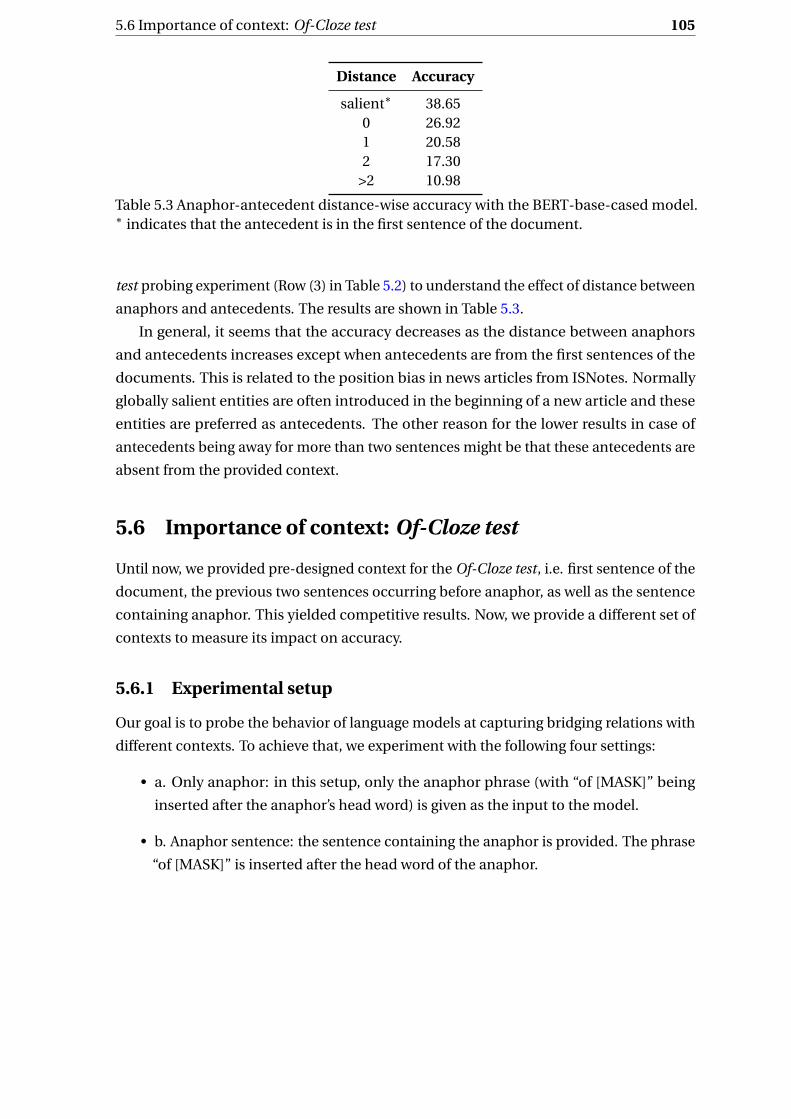
5.6 Importance of context: Of-Cloze test 105
Distance Accuracy
salient∗ 38.650 26.921 20.582 17.30
>2 10.98
Table 5.3 Anaphor-antecedent distance-wise accuracy with the BERT-base-cased model.∗ indicates that the antecedent is in the first sentence of the document.
test probing experiment (Row (3) in Table 5.2) to understand the effect of distance between
anaphors and antecedents. The results are shown in Table 5.3.
In general, it seems that the accuracy decreases as the distance between anaphors
and antecedents increases except when antecedents are from the first sentences of the
documents. This is related to the position bias in news articles from ISNotes. Normally
globally salient entities are often introduced in the beginning of a new article and these
entities are preferred as antecedents. The other reason for the lower results in case of
antecedents being away for more than two sentences might be that these antecedents are
absent from the provided context.
5.6 Importance of context: Of-Cloze test
Until now, we provided pre-designed context for the Of-Cloze test, i.e. first sentence of the
document, the previous two sentences occurring before anaphor, as well as the sentence
containing anaphor. This yielded competitive results. Now, we provide a different set of
contexts to measure its impact on accuracy.
5.6.1 Experimental setup
Our goal is to probe the behavior of language models at capturing bridging relations with
different contexts. To achieve that, we experiment with the following four settings:
• a. Only anaphor: in this setup, only the anaphor phrase (with “of [MASK]” being
inserted after the anaphor’s head word) is given as the input to the model.
• b. Anaphor sentence: the sentence containing the anaphor is provided. The phrase
“of [MASK]” is inserted after the head word of the anaphor.

106 Probing for Bridging Inference in Transformer Language Models
Context Scopewith“of”
without“of”
perturb
only anaphor 17.20 5.62 -ana sent. 22.82 7.71 10.28ana+ante sent. 27.81 9.61 10.93more context 26.36 12.21 11.41
Table 5.4 Accuracy of selecting antecedents with different types of context using BERT-of-Cloze Test.
• c. Ante+Ana sentence: on top of b, the sentence containing the antecedent is also
included in the context.
• d. More context: on top of b, the first sentence from the document as well as the
previous two sentences preceding the anaphor are included.
Without “of” Context To test the effect of the strong bridging indicating signal “of ”, we
further execute another set of experiments. Specifically, We remove “of” from “anaphorhead
of [MASK]” and instead, provide “anaphorhead [MASK]” for each type of the context de-
scribed above.
Perturbed Context In this setting, we perturb the context by randomly shuffling the
words in the context except for the anaphor and antecedent phrases for each type of the
context mentioned above. Note that we still have the “of ” indicator in this setup.
5.6.2 Results on different contexts
The results of experiments with different types of contexts are shown in Table 5.4. All
experiments are based on the BERT-base-cased model with all previous mentions as the
antecedent candidate scope. We refer to this model as BERT-Of-Cloze in the following
discussion.
In the first column of the table, BERT-Of-Cloze achieves an accuracy score of 17.20%
with only the anaphor information plus “of [mask]”. We can see that the results improve
incrementally with the addition of context. More specifically, the accuracy score improves
from 17.20% to 22.82% by adding sentences containing anaphors. Adding sentences which
contain antecedents (ana + ante sent.) further improves the accuracy score to 27.81%.
Finally, adding more local context and the first sentence leads to an accuracy score of
26.36%. Note that compared to “ana + ante sent.”, “more context” represents a more
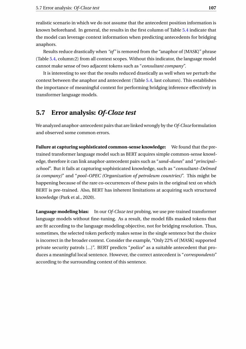
5.7 Error analysis: Of-Cloze test 107
realistic scenario in which we do not assume that the antecedent position information is
known beforehand. In general, the results in the first column of Table 5.4 indicate that
the model can leverage context information when predicting antecedents for bridging
anaphors.
Results reduce drastically when “of” is removed from the “anaphor of [MASK]” phrase
(Table 5.4, column:2) from all context scopes. Without this indicator, the language model
cannot make sense of two adjacent tokens such as “consultant company”.
It is interesting to see that the results reduced drastically as well when we perturb the
context between the anaphor and antecedent (Table 5.4, last column). This establishes
the importance of meaningful context for performing bridging inference effectively in
transformer language models.
5.7 Error analysis: Of-Cloze test
We analyzed anaphor-antecedent pairs that are linked wrongly by the Of-Cloze formulation
and observed some common errors.
Failure at capturing sophisticated common-sense knowledge: We found that the pre-
trained transformer language model such as BERT acquires simple common-sense knowl-
edge, therefore it can link anaphor-antecedent pairs such as “sand–dunes” and “principal–
school”. But it fails at capturing sophisticated knowledge, such as “consultant–Delmed
(a company)” and “pool–OPEC (Organization of petroleum countries)”. This might be
happening because of the rare co-occurrences of these pairs in the original text on which
BERT is pre-trained. Also, BERT has inherent limitations at acquiring such structured
knowledge (Park et al., 2020).
Language modeling bias: In our Of-Cloze test probing, we use pre-trained transformer
language models without fine-tuning. As a result, the model fills masked tokens that
are fit according to the language modeling objective, not for bridging resolution. Thus,
sometimes, the selected token perfectly makes sense in the single sentence but the choice
is incorrect in the broader context. Consider the example, “Only 22% of [MASK] supported
private security patrols [...]”. BERT predicts “police” as a suitable antecedent that pro-
duces a meaningful local sentence. However, the correct antecedent is “correspondents”
according to the surrounding context of this sentence.

108 Probing for Bridging Inference in Transformer Language Models
Unsuitable formulation for set-relations: Our Of-Cloze formulation produces awk-
ward phrases for some bridging pairs that possess set-relations. Considering a bridging
pair − “One man - employees”, in this case the model should assign high score for the
phrase − “One man of employees”. But, as this phrase is quite clumsy, BERT naturally
being a language model assigns low scores for these pairs.
5.8 Conclusions
We investigated the effectiveness of pre-trained transformer language models in capturing
bridging relation inference by employing two distinct but complementary approaches.
In the first approach, we probed individual attention heads in BERT and observed
that attention heads from higher layers prominently captured bridging compared to
the middle and lower layers and some specific attention heads consistently looked for
bridging relation. In our second approach, we considered using language models for
bridging anaphora resolution by formulating the task as a Of-Cloze test. We carefully
designed experiments to test the influence of different types of context for language
models to resolve bridging anaphors. Our results indicate that pre-trained transformer
language models encode substantial information about bridging.
We go one step further to analyze the role of context in achieving this bridging in-
formation. We separately provided a different set of contexts such as no context other
than anaphor phrase, removing “Of” from our fill-in-the-blank formulation, and shuffled
words context. We saw a substantial drop in the accuracy in comparison to the case where
provided context was appropriate. This shows BERT’s capability of bridging inference
depends on the input context, the more the appropriate context better the result.
Finally, our error analysis highlighted the crucial limitation of BERT at capturing
commonsense information which is required in bridging inference. We observed BERT
fails to accurately select antecedents for anaphors that required sophisticated common-
sense knowledge. It could easily resolve easy pairs such as “sand–dunes” and “principal–
school” but failed at “consultant–Delmed (a company)” and “pool–OPEC (Organization
of petroleum countries)”. For this reason, we need to design approaches that can fill this
missing commonsense information from BERT. We will look at that in the next chapter.

Chapter 6
Integrating knowledge graph
embeddings to improve representation
Until now we have explored the use of contextual information for both temporal relation
classification and bridging anaphora resolution. We developed an effective neural net-
work based approach for temporal relation classification in Chapter 4, followed by the
investigation of transformer language models for bridging inference in Chapter 5. Now,
we explore the use of commonsense information for both tasks and extend our work (Pan-
dit et al., 2020). To the best of our knowledge, this is the first work where a principled
approach is taken to represent knowledge graphs for bridging and temporal relation
identification. We discuss the significance of world knowledge for these tasks as well as
challenges in extracting them from knowledge graphs and injecting them into bridging
resolution and temporal relation classification systems. To address these challenges, we
design a generic approach that can be applied to both tasks. As a knowledge source, we
explore the use of WordNet (Fellbaum, 1998) for both the tasks and the specially designed
TEMPROB (Ning et al., 2018a) for temporal relation classification. More specifically, we
employ low-dimensional graph node embeddings learned on these knowledge graphs
to capture crucial features of the graph topology and rich commonsense information.
Thereafter, we propose simple methods to map mentions and events to knowledge graph
nodes and disambiguate senses to obtain embeddings corresponding to them. We also
tackle the case of the absence of knowledge from the graph. Once properly identified
from the mention and event text spans, these low dimensional graph node embeddings
are combined with contextual representations to provide enhanced mention and event
representations. We illustrate the effectiveness of our approach by evaluating it on com-
monly used datasets for both tasks where significant accuracy improvements are achieved
compared to standalone text-based representations

110 Integrating knowledge graph embeddings to improve representation
6.1 Introduction
Recall from the task definitions given in Section 2.1 that bridging anaphora resolution
links bridging anaphors to corresponding antecedents and temporal relation classification
determines temporal ordering between event pairs. To successfully solve these tasks,
effective mention and event representation is essential, and commonsense information is
critical to obtain such an effective representation.
Section 6.2 demonstrates the significance of commonsense information for effective
representation and discusses challenges in integrating such knowledge in the bridging
resolution and temporal relation classification systems. We first describe the importance
of this information and motivate it by providing examples. We also review previously
proposed approaches to acquire that information for both tasks. Next, we discuss chal-
lenges of incorporating such knowledge in the systems. The knowledge graphs used as
an external knowledge source contain information over abstract concepts and entities,
whereas mentions and events are linguistic units. This fundamental difference leads to
challenges such as mapping mentions and events to graph nodes, disambiguating distinct
senses due to mapping to multiple nodes, and tackling the instances of non-availability of
knowledge.
Consequently, we propose solutions to these challenges in Section 6.3. We propose
simple heuristics to map mentions and events to the graph nodes. Specifically, we remove
modifiers or use the semantic head of the mention, and lemmatize events to normalize
them. If this normalized form maps to multiple nodes in the graph then we use Lesk (Lesk,
1986) sense disambiguation algorithm or simple average over them, whereas in the case
of mapping to no nodes i.e. absence of knowledge, we use the zero vector. This proposed
approach is generic and can be applied to any knowledge graph. In this work, we specif-
ically evaluate our approach over two knowledge graphs: WordNet and TEMPROB. We
use WordNet to get lexical semantics such as hypernymy, hyponymy, meronymy, etc.,
and general relatedness between nodes, and TEMPROB to capture prior probabilities of
temporal relations between verbs, specifically for temporal relation classification. We use
various previously proposed graph node embedding algorithms to encode them such as
random walk based embeddings (Goikoetxea et al., 2015), Path2vec (Kutuzov et al., 2019),
matrix factorization based (Saedi et al., 2018) for WordNet and Uncertain Knowledge
Graph Embeddings (UKGE) (Chen et al., 2019) for TEMPROB.
Next, we applied these approaches to obtain knowledge-aware mention represen-
tation for bridging anaphora resolution in Section 6.4. We combine knowledge graph
embeddings with distributional text-based embeddings to produce improved mention
representation. As pointed in Section 3.2.2, bridging anaphora resolution is commonly

6.2 Commonsense knowledge 111
considered as a classification problem. In this work, we take a different approach where
we formulate bridging anaphora resolution as a ranking problem instead of classifica-
tion perspective, for it to be less sensitive to class-imbalance, and making it focused on
learning relative scores. Specifically, we train a ranking SVM model to predict scores for
anaphor-candidate antecedent pairs, an approach that has been successfully applied
to the related task of coreference resolution (Rahman and Ng, 2009). We observe that
integrating node embeddings with text-based embeddings produces increased accuracy,
substantiating the ability of graph node embeddings in capturing semantic information.
Afterwards, similar to knowledge-aware mention representation, we combine text-
based representations and knowledge graph embeddings to produce knowledge-aware
event representations for temporal relation classification in Section 6.5. We use current
state-of-the-art (Wang et al., 2020) system based on RoBERTa (Liu et al., 2019b) embed-
dings and LSTMs (Hochreiter and Schmidhuber, 1997) to obtain text-based embeddings
as well as for scoring temporal relations. We combine these text-based embeddings with
graph node embeddings to improve event representation. Next, to train the neural model,
a constrained learning objective that considers the accuracy of temporal relation predic-
tions, as well as global temporal symmetry and transitivity constraint, is optimized. These
constraints are applicable over temporal graph because of temporal algebra as described
in Section 2.1.1.1. Further, we used Integer Linear Programming (ILP) inference to get
globally coherent temporal relation predictions. Improvement in results over the use of
only text-based embeddings also over a system with hand-engineered commonsense
features, establishes the potency of our approach.
6.2 Commonsense knowledge
We refer commonsense as a broad knowledge that can not be easily acquired with only the
given linguistic context. Thus, our definition of commonsense knowledge encompasses
both linguistic and world knowledge. Linguistic knowledge can be any knowledge that
is associated only with the linguistic units of the language. Semantic knowledge can be
called a specific type of linguistic knowledge which involves semantic relations between
words, phrases, or sentences meanings. For example, lexical relations such as synonymy,
antonymy, hypernymy, etc. fall into this type of knowledge. On the other hand, world
knowledge is broader information which is not specific to any language but shared by
people. Factual or encyclopedic knowledge is a part of this kind of knowledge. For exam-
ple, Barack Obama was a president is a world knowledge, independent of any language.
Though making a clear distinction between linguistic knowledge and world knowledge is

112 Integrating knowledge graph embeddings to improve representation
difficult as different researchers define different boundaries to demarcate them (Ovchin-
nikova, 2012). In fact, commonsense knowledge is also a fuzzy term which can mean only
world knowledge but in our work it refers to both linguistic and world knowledge.
Word embeddings like Word2vec (Mikolov et al., 2013a), Glove (Pennington et al.,
2014), BERT (Devlin et al., 2019), etc. are considered to be capturing commonsense
knowledge but only up to some extent (Chen et al., 2013; Da and Kasai, 2019; Ettinger,
2020; Talmor et al., 2020). Hence, various approaches have been proposed to enrich these
unsupervised embeddings with commonsense knowledge contained by knowledge graphs.
The proposed approaches can be broadly divided into two categories: 1. Joint learning of
word embeddings with semantic constraints, and 2. Post-processing (retro-fitting) over
unsupervised word embeddings.
Joint learning models put semantic lexicons as additional constraints while learning
word embeddings. Many approaches fuse Word2vec with synonymy relations that reduce
the distance between similar words (Liu et al., 2015; Yu and Dredze, 2014) whereas few
approaches (Liu et al., 2018) also put constraints based on other lexical relations such
as hypernymy-hyponymy relations from WordNet. Similar ideas have been applied over
Glove by Bollegala et al. (2016), and Osborne et al. (2016). On the other hand, other models
utilize similar words alternatively in the same context and learn models over the original
and added context (Kiela et al., 2015; Niu et al., 2017). Recently, similar enhancements are
also applied over BERT embeddings (Hao et al., 2020; Peters et al., 2019; Sun et al., 2020;
Zhang et al., 2019b)
On the contrary to joint learning models, post-processing approaches take pre-trained
word embeddings and retro-fit them with additional information. Faruqui et al. (2015)
retrofit embeddings with information from WordNet with the addition of synonymy
information, approaches like (Glavaš and Vulic, 2018; Mrkšic et al., 2016) go a step further
and add antonymy information as well to increase the distance between dissimilar words.
In addition to these relations, Vulic et al. (2017) leverage morphological information where
they pull inflectional forms of the same word closer and push derivational antonyms
farther.
So far, we mentioned approaches which produced generic word embeddings without
focusing on solving any particular task. Now, we note a few approaches that learn repre-
sentations with the addition of external knowledge to solve specific tasks. For instance,
machine reading (Yang and Mitchell, 2017), Question Answering (QA) (Bauer et al., 2018;
Sun et al., 2018), natural language inference (Chen et al., 2018), reading comprehension
(Mihaylov and Frank, 2018; Wang and Jiang, 2019), and coreference resolution (Zhang
et al., 2019a). In addition to these approaches, earlier approaches designed hand-crafted

6.2 Commonsense knowledge 113
features to inject commonsense knowledge into systems such as (Emami et al., 2018;
Ovchinnikova, 2012; Rahman and Ng, 2011). Our approach too falls into this line of
research where we inject commonsense knowledge to solve specific tasks.
The linguistic knowledge can be obtained from different sources. For lexical-semantic
knowledge, WordNet (Fellbaum, 1998) is used extensively in NLP. In addition to WordNet,
FrameNet (Ruppenhofer et al., 2006) and ConceptNet (Speer et al., 2018) are other popular
semantic networks. FrameNet is based on frame semantics which briefly states that the
meaning of the words can be understood from knowledge about the other related concepts.
For example, meaning of the word cook is understood from cooking frame which contains
other related concepts such as food, bake, boil, apply heat. FrameNet contains such
1200 frames containing more than 13000 words with different part-of-speech tags. In
addition to that, it also contains semantic relations over frames. Other semantic network,
ConceptNet consists of basic facts and understanding possessed by people. It contains
more than 300,000 nodes and 1.6 million edges between them labeled by one of the 19
binary relations. ConceptNet is constructed by crowdsourced effort instead of manually
creating it as opposed to WordNet and FrameNet.
In addition to these knowledge sources which contain semantic knowledge, knowledge
graphs such DBPedia (Lehmann et al., 2015), YAGO (Hoffart et al., 2011) which are popular
among many others contain generic world knowledge. DBPedia is an automatically
created knowledge source by extracting factual information from Wikipedia pages and
stored in a structured format. It contains all the information related to the entity present
in Wikipedia pages, for instance, date of birth, place, occupation as well as a link to the
Wikipedia page. YAGO is an another such knowledge base which possesses a collection of
commonly known facts and information. It is also an automatically created knowledge
base that uses a lot of other sources to build their knowledge such as Wikipedia, WordNet,
Geonames, the Universal WordNet, and WordNet Domains. It contains knowledge of more
than 17 million entities (like persons, organizations, cities, etc.) and more than 150 million
facts about these entities.
Further, researchers have explored different sources other than knowledge graphs
to acquire such commonsense knowledge like images (Cui et al., 2020; Li et al., 2019;
Rahman et al., 2020), videos (Huang et al., 2018; Palaskar et al., 2019), or crowdsourced
resources (Krishna et al., 2016). We use knowledge graphs among these sources, as they
are specifically developed to hold world knowledge and are highly accurate in-comparison
to other sources.
We discussed so far what we mean by commonsense knowledge, why it is needed for
unsupervised word embeddings as well as for task-specific representation, and finally

114 Integrating knowledge graph embeddings to improve representation
we looked at different sources of linguistic and world knowledge. Now, we discuss why
commonsense knowledge is important for event and mention representations.
6.2.1 Significance for effective representation
In Chapter 3 while discussing previously proposed work, we briefly talked about the
significance of commonsense knowledge for temporal relation classification and bridging
anaphora resolution. We further detail that here.
Temporal relation classification We have seen that temporal relation classification sys-
tems use tense, aspects or temporal markers to accurately predict temporal ordering
between events. Sometimes, this information is not sufficient to make accurate predic-
tions. More than these contextual clues, the system should be able to access the world
knowledge which humans possess while reading the text. This is illustrated in the following
examples:
(8) He graduatede1 with a computer science degree. He joinede2 a reputed software
development firm.
(9) The government confirmed that 10 people diede3 . The explosione4 also damaged
nearby homes.
In example 8, to establish temporal order between events e1 and e2, it is crucial to have
commonsense information that people generally join a firm after they graduate. Similarly,
in example 9, knowing that people can die because of explosion is useful in establishing
precedence temporal relation between e4-e3.
Different approaches have been proposed to acquire such commonsense information
for temporal relation classification systems. For better event-pair representations, D’Souza
and Ng (2013) designed features based on WordNet and Webster dictionary. Specifically,
they used four types of WordNet relations, namely hypernymy, hyponymy, troponymy,
and synonymy to create eight binary features. A more advanced approach is taken by Ning
et al. (2018a) by proposing TEMPROB knowledge source containing event verbs and prior
probabilities of temporal relations between them. Ning et al. (2019, 2018a); Wang et al.
(2020) used this knowledge source in their approaches. Ning et al. (2018a) used prior prob-
abilities that are present in TEMPROB directly as one of the features in their system. Going
away from this naive approach of injecting commonsense knowledge, Ning et al. (2019)
trained Siamese network (Bromley et al., 1993) on the event pairs present in TEMPROB
and their prior probabilities to produce embeddings for each verb in the graph. Next,

6.2 Commonsense knowledge 115
Wang et al. (2020) used a similar principle to acquire commonsense knowledge. They used
partial relations from ConceptNet (Speer et al., 2018) in addition to TEMPROB knowledge.
They selected few pairs from ConceptNet that possess “HasSubevent”, “HasFirstSubevent”,
and “HasLastSubevent” relations as these relations encode temporal information. Then
they trained two separate feed-forward networks, one over TEMPROB and the other over
ConceptNet pairs, with contrastive loss to estimate the relations between these pairs.
Once the models are trained verb embeddings are obtained from them and injected into
their systems.
Bridging anaphora resolution Similar to temporal relation classification, common-
sense information is crucial for bridging resolution. Standard text-based features either
hand-crafted or automatically extracted from word embeddings (Mikolov et al., 2013a;
Pennington et al., 2014), are not sufficient for bridging resolution (Hou, 2018b). The diffi-
culty arises because, bridging indicates various relations between anaphor-antecedent
pair for instance part-of relation, set relation, or many abstract relations. Consider the
following examples:
(10) A car had an accident. The driver is safe, highway police reported.
(11) Starbucks has a new take on the unicorn frappuccino. One employee accidentally
leaked a picture of the secret new drink.
In example 10, to establish bridging link between anaphor “The driver” and antecedent
“a car”, it is crucial to know that generally a driver drives a vehicle so “the driver” refers
to “the driver of a car that had an accident” and not any other driver. On the same
lines, in example 11, if the resolution system knows that Starbucks is a company and
companies have employees, then it is easy to establish the link between “Starbucks” and
“One employee”.
Consequently, both rule-based, as well as machine learning-based systems for bridg-
ing resolution, have used external knowledge sources to get commonsense information.
The rule based systems (Hou et al., 2014; Roesiger, 2018b) designed various rules by consid-
ering building parts to get part-of relation, job based rules to capture employee-employer
relation, and meronymic relations from WordNet. The learning-based approaches (Hou
et al., 2013a,b) also designed features with WordNet and Google queries (Poesio et al.,
2004) to capture semantic relations. Recently, bridging-specific embeddings emb_pp
(Hou, 2018b) were proposed by exploiting the preposition pattern (X prep Y ) and posses-
sive pattern (X’s Y ) of NPs. Her approach is better at capturing fine-grained semantics than
vanilla word embeddings such as Word2vec (Mikolov et al., 2013a), Glove (Pennington

116 Integrating knowledge graph embeddings to improve representation
et al., 2014), etc. however, it still depends on the presence of the required noun-pairs in
the corpus. The use of knowledge graphs, either manually or automatically constructed,
can alleviate this problem as they contain general semantic and world knowledge.
All of these approaches, both for temporal relation classification as well as bridging
resolution, extract only shallow features, capturing relations between pairs of nodes
instead of taking advantage of broader information that is present in knowledge graphs.
Moreover, attempting to extend these strategies to take into account a larger amount
of information may translate into learning problems where the input space is of high
dimension. It might be a hurdle especially in the case of bridging resolution due to
moderate size datasets, for instance, ISNotes (Markert et al., 2012) and ARRAU (Uryupina
et al., 2019) respectively contain 663 training pairs and 5512 training pairs. The only
exceptions are approaches (Ning et al., 2019; Wang et al., 2020) proposed for temporal
relation classification. They stand out among all previous approaches as they acknowledge
the drawbacks of hand-designing features, therefore train models to get verb embeddings.
But, their approach also captures shallow features as it only encodes pairwise relations so
missing out on the information encoded by the whole graph topology.
6.2.2 Challenges in integration
We discussed in previous paragraphs that due to the limited capabilities of unsupervised
word embeddings algorithms at acquiring commonsense knowledge various approaches
have been proposed, some of the approaches were task-agnostic like (Faruqui et al., 2015;
Peters et al., 2019; Sun et al., 2020), and some solved specific tasks (Bauer et al., 2018;
Mihaylov and Frank, 2018; Sun et al., 2018; Wang et al., 2019). Our approach falls into the
latter category where we use knowledge graphs specifically to solve the tasks. There lie
some challenges in incorporating such knowledge from knowledge graphs. Though these
challenges are generic and can be faced by any NLP system trying to inject knowledge
from graphs, we focus our discussion on the challenges with respect to the tasks at hand:
bridging anaphora resolution and temporal relation classification.
Integration with linguistic information Integrating knowledge held by knowledge graphs
into NLP systems is not straightforward (recall the discussion in Section 2.6.2). Because the
information in the knowledge graph is stored in a structured way whereas text is relatively
unstructured 1. Generally, knowledge graphs encode information in the form of triplets:
1 We call text unstructured data only in the sense that it’s not stored in pre-defined format, models, orschema, nor it is easy to process or analyze.

6.2 Commonsense knowledge 117
(h,r, t) where the head(h) and tail(t) are nodes and r denotes relation between them2.
In addition to this, the topology encodes crucial information because of the connection
between different nodes either directly or through other nodes. This whole information
should be captured effectively and injected into the machine learning systems.
Event/Mention normalization The knowledge graph contains information about cer-
tain entities, for example, WordNet is a lexical knowledge graph containing different senses
of words. This means we first have to normalize event or mention to a corresponding
entity so that information about it might be present in the knowledge graph. Then the
entity is used to acquire corresponding knowledge from the graph. However, it is tricky
to get an entity from a given mention as a mention may contain words like quantifiers,
prepositions, or modifiers in addition to the entity. Consider mentions like the wall, one
employee, beautiful lady or the famous scientist Einstein which can not be matched with
the entity in the graph. These should be normalized to wall, employee, lady and Einstein,
respectively. Similarly, this issue exists in the case of events as well. Albeit, it is less severe,
as they are are mostly verb phrases and contain only verbs with inflections (e.g. said,
calling, reported). Though there are some cases of events being noun phrases, for instance
holy war, deadly explosion which should be respectively mapped to war, explosion, they
are relatively fewer.
Word sense disambiguation Once the event or mention is normalized, this normalized
token can map to multiple entries in the knowledge graph, as the same word can possess
different meanings, senses, or refer to multiple real world entities. This issue is pervasive
over all the knowledge graphs, hence needs to be addressed irrespective of which graph
is used. For example, in the case of mentions, bank can refer to an institution related
to finance or the land alongside river, Michael Jordan can refer to the scientist or the
basketball player. On the other hand, event verbs such as book can refer to reserving tickets
or recording a charge in police register, fall can mean descend or precipitate. The different
senses possess different knowledge, in other words different local structures in the graph.
Thus, recognizing the correct sense is crucial to get the accurate information.
Absence of knowledge The opposite situation of the previous case is an absence of any
node corresponding to the normalized event or mention. This can happen due to the
inherent limitation of the knowledge graph or normalization error. It is crucial to handle
these situations gracefully.
2There can be additional information as in TEMPROB where for an edge its strength is also added.

118 Integrating knowledge graph embeddings to improve representation
Choice of knowledge graph One of the least challenging but important aspect is a choice
of the knowledge graph. As mentioned in earlier paragraphs, different knowledge graphs
contain different information. So in a way, it becomes crucial to choose a knowledge graph
that contains relevant information. One simple criterion for knowledge graph selection is
to assess how many events or mentions can be mapped to the graph nodes. Then to select
a knowledge graph which contains a higher percentage of event or mention mappings.
Another aspect of this discussion is the use of multiple knowledge graphs to acquire
commonsense information. Because required commonsense knowledge can be present
in different knowledge graphs, it is prudent to use them all. In this case, the burden of
selecting relevant knowledge falls onto the learning system instead of the designer of the
system.
6.3 Our approach
We detail our approach for solving these challenges in the coming sections. First, we
specify our approach of representing knowledge and specific knowledge graphs used in
our work (Section 6.3.1). Then we describe simple rules used to normalize events and
mentions to map to graph nodes (Section 6.3.2). Next, we proposed simple heuristics
for the case of presence of multiple nodes (Section 6.3.3) or the absence of any node
(Section 6.3.4) in the knowledge graph corresponding to these normalized tokens.
6.3.1 Knowledge graphs: WordNet and TEMPROB
To obtain external knowledge, we used WordNet (Fellbaum, 1998) for both tasks and TEM-
PROB (Ning et al., 2018a) specifically for temporal relation classification. As mentioned
earlier, integrating the knowledge encoded by these graphs into machine learning systems
is not easy. One of the naive ways of capturing information present in knowledge graphs is
to design features or by executing queries over them. But these are inefficient approaches
and do not capture the holistic information present in the graph. To remedy that, graph
node embeddings were proposed to acquire the local and global structure of the graph
effectively, as discussed in Section 2.6.2. Similarly, graph node embeddings learned over
knowledge graphs can capture the encoded knowledge effectively. Therefore, here we
learn graph node embeddings over WordNet and TEMPROB and use them in our systems.
In the following paragraphs, first, we briefly review WordNet, and then summarize
different graph node embedding algorithms used over it, followed by a similar discussion
on TEMPROB.

6.3 Our approach 119
6.3.1.1 WordNet
As previously described in Section 2.6.1.1, WordNet (Fellbaum, 1998) primarily consists
of synsets, i.e., a set of synonyms of words. The synsets which refer to the same concept
are grouped together giving it a thesaurus-like structure. Each synset consists of its
definition and small example showing its use in a sentence. The synsets are connected
with different relations such as synonymy, antonymy, hypernymy, hyponymy, meronymy,
etc. In addition, it also includes relations between real world entities like cities, countries,
and famous people. This semantic information is already shown to be effective for bridging
and temporal relations, which makes WordNet obvious choice for the tasks. Subsequently,
the node embeddings learned on this graph automatically capture the commonsense
information associated with the senses.
Now, we discuss different node embedding algorithms that are used to encode Word-
Net in our study. These algorithms are not specially designed for WordNet but have been
proven to be effective at producing representations over it. We use random walk and neu-
ral language model based embeddings (RW) (Goikoetxea et al., 2015), matrix factorization
based embeddings (WNV) (Saedi et al., 2018), and graph-similarity based Path2vec (Kutu-
zov et al., 2019) embeddings. These embeddings differ in learning strategies and more
importantly the way different graphs are constructed over WordNet by varying types of
either nodes or edges. For instance, different graphs can be constructed by considering
actual synsets as nodes or corresponding words as nodes, similarly, in the case of edges,
either by considering semantic relations between nodes or ignoring these relation labels.
Because of these differences in graph constructions, the first two algorithms, RW and
WNV, produce word embeddings whereas Path2vec produces embeddings corresponding
to each synset present in WordNet. Because, RW and WNV conflate all the senses where
they first map them to words, and then learn embeddings over words, thus lose finer
semantic information in the process. But on the upside, they relieve the burden of sense
disambiguation because now the mapping from events or mentions is to words and not to
individual senses.
RW The approach proposed by Goikoetxea et al. (2015) is based on the well-known
neural language model CBOW and Skip-gram (Mikolov et al., 2013c) which we described
in Section 2.4.1.1. The main idea is to produce artificial sentences from WordNet and
to apply the language models on these sentences to produce word embeddings. For
this, they perform random walk starting at any arbitrary vertex in WordNet, then map
each WordNet sense to the corresponding word to produce an artificial sentence. Each
random walk produces a sentence, repeating this process several times gives a collection

120 Integrating knowledge graph embeddings to improve representation
of sentences. Finally, this collection of sentences is considered as the corpus for learning
word embeddings by applying the same objective function as in Mikolov et al. (2013c).
WNV A different approach based on matrix factorization is taken by (Saedi et al., 2018) to
produce these embeddings. The procedure starts by creating the adjacency matrix M from
WordNet graph. The element Mi j in the matrix M is set to 1 if there exists any relation
between words wi and w j . 3 Furthermore, words which are not connected directly but
via other nodes should also have an entry in the matrix, albeit with lower weights than
1. Accordingly, a matrix MG is constructed to get the overall affinity strength between
words. In the analytical formulation, MG can be constructed from the adjacency matrix
M as MG = (I −αM)−1 where I is the identity matrix and 0 <α< 1 decay factor to control
the effect of longer paths over shorter ones. Following that, matrix MG is normalized to
reduce the bias towards words that have more number of senses and finally a Principal
Component Analysis is applied to get vectors.
Path2vec Path2vec (Kutuzov et al., 2019) learns embeddings based on a pairwise similar-
ity between nodes. The fundamental concept is that pairwise similarity between nodes of
the graph should remain the same after their projection in the vector space. The model
is flexible enough to consider any user-defined similarity measure while encoding. The
objective function is designed to produce such embeddings for nodes which reduce the
difference between actual graph-based pairwise similarity and vector similarity. It also
preserves the similarity between adjacent nodes. Formally, for the graph G = (V ,E ) where
V ,E denote a set of vertices and edges, respectively, the objective is:
∑(a,b)∈V
minva ,vb
((vT
a vb − s(a,b))2 −α(vTa vn +vT
b vm))
where n,m are adjacent nodes of nodes a,b respectively, s(a,b) is the user-defined simi-
larity measure between a,b and va ,vb ,vn ,vm denote the embeddings of a,b,n,m, respec-
tively. In their experiments, to show the ability of their model in adapting to different
pairwise similarity measures, similarity function s(a,b) is obtained with four distinct simi-
larity measures: Leacock-Chodorow (Leacock and Chodorow, 1998); Jiang-Conrath (Jiang
and Conrath, 1997); Wu-Palmer (Wu and Palmer, 1994); and Shortest path (Lebichot et al.,
2018).
3They also experimented by weighting relations differently (e.g. 1 for hypernymy, hyponymy, antonymyand synonymy, 0.8 for meronymy and holonymy and 0.5 for others) but obtained the best results withoutweighting.

6.3 Our approach 121
6.3.1.2 TEMPROB
In addition to WordNet, specifically for temporal relation classification, we explored the
use of temporal information specific knowledge source: TEMPROB (Temporal relation
probabilistic knowledge base) (Ning et al., 2018a). Though a detailed description of
TEMPROB is given in Section 2.6.1.2, we quickly review it here. TEMPROB contains
specific prior temporal knowledge. The knowledge is stored in the form of quadruples:
(u, v,r, fu,v,r ) where u, v are semantic verb frame pairs, r is any temporal relation from
set R containing temporal relations after, before, includes, included, and undef (vague),
and fu,v,r is the frequency of temporal relation r appearing between u, v . This frequency
is measured as the number of times the classifier trained while constructing TEMPROB
has predicted relation r for pair u, v on the corpus (1 million NYT articles). Also, recall
that u, v are not verbs but semantic verb frames and there can be multiple semantic verb
frames corresponding to a verb depending on its meaning, for instance, verb sew has
multiple frames such as sew.01, sew.02, and more, depending on whether it is used for
stitching clothes,wounds, or in another sense.
We observed that while constructing TEMPROB, verb pairs are selected as they ap-
peared in the documents, so there are different valued edges between u, v and v,u. We
aggregated them for inverse temporal relation pairs, after–before, includes–included, equal–
equal, and undef–undef. We kept only one pair u, v and calculated frequency for relation
r by adding the frequency of r as well as r ′ (inverse relation) as fu,v,r ← fu,v,r + fv,u,r ′ .
After that we converted these frequencies for each relation into probability with a softmax
function:
pu,v,r = e− fu,v,r∑r∈R e− fu,v,r
(6.1)
Then, TEMPROB graph is modified to store quadruples containing these probabilities
in-place of frequencies as (u, v,r, pu,v,r ). This modified graph is further used for obtaining
node embeddings.
Uncertain Knowledge Graph Embeddings (UKGE) We used the UKGE (Chen et al.,
2019) embedding algorithm to obtain TEMPROB node embeddings. The primary reason is
that UKGE learns embeddings over a graph containing probabilistic (weighted) relations
between nodes, while the previously proposed algorithms can only learn over determinis-
tic edges. The graph considered in this algorithm is of the form G = (V ,E ,R) containing set
of vertices V , edges E , and relations R where E = {(l , sl )|l = (h,r, t ),h, t ∈V ,r ∈ R, 0 ≤ sl ≤ 1}.
It is the same as modified TEMPROB graph. The algorithm learns low-dimensional em-
beddings for h, t and r similar to translational models TransE (Bordes et al., 2013) such

122 Integrating knowledge graph embeddings to improve representation
that the predicted score between triplet (h,r, t ) will be closer to the true score sl . This is
the core working of UKGE algorithm. Besides, in addition to the given links, UKGE also
deduces new links with soft logic from the given (seen) links. Subsequently using them to
train the model by calculating the training loss on both seen and deduced links. But while
applying UKGE on TEMPROB, we did not deduce any new links and relied only on the seen
links. Because TEMPROB contains edges which are obtained from the temporal relation
classifier which is inherently error-prone, and by inferring new edges from these links
can lead to further propagation of errors. Finally, the modified loss which is optimized to
produce TEMPROB node embeddings is given as:
L (θ) = ∑(l ,sl )∈E
| fc (l ;θ)− sl |2 (6.2)
where fc (l ;θ) is the θ-parameterized confidence score based on the learned vector
representations h,t,r ∈Rd as fc (l ;θ) =ψ(g (r · (h⊙ t))) such that · denotes inner product,
⊙ denotes element-wise multiplication, and ψ : R→ [0,1]. The vectors h,t are encoded
with same function of the form fn : V →Rd to produce representations corresponding to
nodes of the graph. Consequently, once the model is trained, function fn is applied over
nodes to get corresponding graph node embeddings.
6.3.2 Normalization: Simple rules and lemma
Mention normalization. A mention can be a phrase containing multiple words, and
from these words we have to obtain an entity that can be mapped to the node in the graph
or a key of the dictionary that contains knowledge graph embeddings. We propose to
normalize them into a single word with the use of simple rules. For this, as a first step,
we remove articles and commonly used quantifiers like the, a, an, one, all etc. from the
mention. If we find an entry in the knowledge graph with this modified word then we
get the corresponding embeddings, otherwise, we go a step further and extract the head
of the mention and try to obtain embeddings for it. Specifically, we use the parsed tree
of the mention, and Collins’ head finder algorithm (Collins, 2003) to get the syntactic
head. Recall the discussion from Section 5.4 where we discussed that the syntactic head
approach fails for coordinated NPs (NPs containing coordinating conjunctions like and),
therefore we used the semantic head in these cases which are obtained with Stanford
CoreNLP toolkit (Manning et al., 2014).
Event normalization Though events could be phrases (verbs or nominals), the dataset
is already annotated with headword of events. For instance, “the deadly explosion” phrase

6.3 Our approach 123
is marked with headword “explosion”, “holy war” as “war”. As a result, the process of
normalizing events is much simpler than mention normalization. We use this headword
of event to map to the node in graph. For that, we obtain a lemma of the headword while
considering its part-of-speech tag. This is especially useful in the case of verbs as they are
inflected with suffixes such as -ing, -ed.
6.3.3 Sense disambiguation: Lesk and averaging
Once events and mentions are normalized to a single token4, the string matching is done
to map to graph nodes. This can yield multiple nodes for a single normalized token or no
node at all. The case of multiple nodes arises due to multiple senses of the word. Now, we
describe the solution for the case of multiple nodes and in the next section for the absence
of any node. We devise different strategies depending on the kind of graph embeddings
used.
Lesk We use Lesk algorithm (Lesk, 1986) to select an appropriate sense for a word de-
pending on its context. A simplified variation of Lesk applied specifically to disambiguate
senses present in WordNet relies on the corresponding definitions of senses contained in
WordNet. It calculates the overlap between the context of the word and the definition of
the sense by simply measuring the number of common words, and chooses a sense which
has the highest number of matching words from the senses.
Averaging of all senses A simple heuristic to obtain all possible senses corresponding to
a token and instead of narrowing down the sense of the word is to take an average over
the embeddings of all these senses. We use this as an alternative to the above strategy.
Token matching If the embeddings are generated for the words instead of actual nodes
(senses in case of WordNet) graph then there is no question of sense disambiguation.
This is true in two of the graph node embeddings algorithm we used: RW and WNV.
These embeddings internally map synsets to the words, creating a graph over words from
WordNet and produce embeddings over these words itself. As a consequence, in these
cases, the need for sense disambiguation disappears and with simple string matching,
knowledge graph embeddings can be obtained.
4This is even true for the cases where, ideally we should get multiple tokens. For example, in the cases ofnamed entities having multiple tokens like Hong Kong, Los Angeles are still mapped to a single token. Wediscuss these cases in the error analysis (Section 6.4.5.1).

124 Integrating knowledge graph embeddings to improve representation
6.3.4 Absence of knowledge: Zero vector
The opposite situation of mapping to multiple senses is mapping to no node at all. This
might happen because of the inherent limitation of the knowledge graph or some nor-
malization error. Consequently, it leads to the unavailability of the corresponding node
embeddings. To tackle this, we use the zero vector of the same dimensions.
6.4 Improved mention representation for bridging resolu-
tion
So far, we have discussed the challenges of injecting commonsense knowledge and de-
scribed our proposed approaches to solve them. Now, we apply these methods for improv-
ing mention representation by integrating commonsense knowledge. In Section 6.4.1, we
detail our approach to obtain knowledge-aware mention representation which combines
both text and commonsense information. Next, we describe our ranking model based on
SVM and inference strategy in Section 6.4.2. Further, Section 6.4.3 describes our experi-
mental setup and Section 6.4.4 presents results over various datasets. Lastly, error analysis
is presented in Section 6.4.5.
6.4.1 Knowledge-aware mention representation
We propose a new, knowledge-aware mention representations for bridging resolution.
These representations combine two components: (i) distributional embeddings learned
from raw text data, and (ii) graph node embeddings learned from relational data obtained
from a knowledge graph. Specifically, the final representation mi for a mention mi is
obtained by concatenating the text-based contextual embeddings gi and the knowledge
graph node embeddings hi: mi = gi ⊕hi.
For the distributional embeddings gi, we use off-the-shelf word embeddings such as
Word2vec (Mikolov et al., 2013a), Glove (Pennington et al., 2014), BERT (Devlin et al., 2019),
or embeddings_pp (Hou, 2018b). Except for BERT, we average over embeddings of the
mention’s head word and common nouns appearing in the mention before the head, as
mentioned in Hou (2018a). With BERT, mention embeddings are obtained by averaging
over embeddings of all the words of the mention.
Whereas, for knowledge graph node embeddings hi we use strategies described in the
previous section. Briefly, we first normalize mentions, then map them to nodes in the

6.4 Improved mention representation for bridging resolution 125
knowledge graph, use sense disambiguation strategies in the case of multiple mappings,
and use the zero vector for no mapping.
6.4.2 Ranking model
Let D be the given document containing set of mentions, M = {m1,m2, · · · ,mnm }, and
A = {a1, a2, · · · , ana } be the set of all anaphors such that A ⊂M . Let a be any anaphor in
the set A and j be its position in the set M , then Ea be the set of antecedent candidates
for a which is defined as Ea = {mi : mi ∈ M , i < j }. Let Ta and Fa be the set of true
antecedents and false antecedent candidates of a such that Ta ∪Fa = Ea ,Ta ∩Fa =;. Let
a be the knowledge-aware represention of a, and e be the representation of e ∈ Ea . Then
the goal is to predict a score s(a,e) between anaphor a and antecedent candidate e such
that this score for true antecedent is higher than the wrong one. The score denotes the
possibility of anaphor a having bridging relation with the antecedent candidate e, so a
higher score denotes a higher chance of e being true antecedent.
The model is trained to reduce the ranking loss calculated based on the scores obtained
between anaphor-antecedent candidates. The ranking strategy is fairly obvious: for an
anaphor a high scoring antecedent candidate from Ea is ranked higher than the low
scoring one. Let this prediction ranking strategy be r ′ and true ranking is given by r ∗. For
an antecedent candidate, if the predicted rank is not same as the true rank then it is called
discordant candidate, otherwise concordant. The difference between true and predicted
ranking strategy can be measured with Kendall’s rank correlation coefficient: τ. Formally,
concordant C , discordant D candidates and τ are defined as:
C = ∑(t , f )∈(Ta×Fa )
Is(a,t)>s(a,f) , D = |Ta ×Fa |−C and τ(r ∗,r ′) = C −D
C +D
where I is an indicator function which takes value 1 if s(a,t) > s(a, f) else 0, t, f are
knowledge-aware mention representations of t , f , respectively, and | · | denotes cardi-
nality of the set. The empirical ranking loss (Joachims, 2002) captures the number of
wrongly predicted ranks which is given as:
L = 1
na
na∑i=1
−τ(r ∗i ,r ′
i )
Inference We consider all the anaphors in the test document separately. For each
anaphor, we consider all previously occurring mentions as antecedent candidates and
find out the compatibility score for each anaphor-antecedent candidate pair with the

126 Integrating knowledge graph embeddings to improve representation
above ranking model. We choose highest scoring antecedent candidate as the predicted
antecedent. Formally, let a be any anaphor and Ea denote a set of antecedent candidates
for a. Let s(a,e) be the score between a and e where e ∈ Ea . Let ea be the predicted
antecedent of a which is given as: ea = ar g maxe∈Ea s(a,e)
6.4.3 Experimental setup
Data We used ISNotes (Markert et al., 2012), BASHI (Roesiger, 2018a) and ARRAU (Uryupina
et al., 2019) datasets for experiments. ISNotes and BASHI consist of 50 different OntoNotes
documents, containing 663 and 459 anaphors, respectively. The BASHI dataset annotates
comparative anaphors as bridging anaphors which are 115 in numbers, remaining are ref-
erential anaphors. Following the setup from Hou (2020a), we only consider 344 referential
bridging anaphors in this work as well from the BASHI dataset.
In the experiments over ISNotes and BASHI datasets, we implemented nested cross-
validation to select the best hyperparameter combination. The setup is: first we make
10 sets of train and test documents containing 45 and 5 documents respectively with
10-fold division. Then at each fold, 45 training documents are further divided into 5 sets
of 36-9 actual training and development documents. Each hyperparameter combination
is trained on these 5-sets and evaluated. The highest averaged accuracy over the 5-sets
of development documents gives the best hyperparameter combination. Once the best
hyperparameter setting is obtained the SVM model is re-trained over 45 documents (36+9).
For each fold number of accurately linked anaphors is calculated. The accurately predicted
number of anaphors over each fold is added to get the total number of accurately linked
anaphors from the complete dataset. Thus, the system is evaluated by the accuracy of
predicted pairs (Hou, 2020a).
For ARRAU dataset, the results are separately reported over different genres present:
RST (news articles), PEAR (stories) and TRAINS (dialogues). We followed the similar
setup on these datasets as previous studies (Roesiger, 2018b; Yu and Poesio, 2020). In
that, different experimental setup is used for each genre: RST dataset is relatively big
and there is train, dev, and test partition of dataset so model is trained on train while
hyperparameters are tuned with respect to dev and finally evaluated on test. The samples
for PEAR and TRAINS are small so for training 10-cross validation is done on train/dev set
and final result is reported on test set.
For the training data, we have positive samples where we know true anaphor-antecedent
pairs but no negative samples. We generate these pairs by considering all the noun phrases
(NPs) which occur before the anaphor in the window of some fixed number of sentences.
All the mention pairs which do not hold bridging relations are considered as negative

6.4 Improved mention representation for bridging resolution 127
samples for training. Similarly, at the test time, for an anaphor, all the previous mentions
in the window size are considered as antecedent candidates. Only the limited number of
antecedent candidates are used instead of all, because in ISNotes 77% of anaphors have
antecedent either in the previous two sentences or the first sentence of the document. So,
considering all the previous mentions (without the restriction of window size) could result
in way more false antecedent candidates and could lead to performance degradation.
Though we use window size to restrict antecedent candidates, the window size is treated
as a hyperparameter and the best value is chosen depending on the validation accuracy.
The list of values are mentioned in the following section.
Implementation We obtained pre-trained 300-dimensional Word2vec (Mikolov et al.,
2013a), 300-dimensional Glove (Pennington et al., 2014), 768-dimensional BERT (Devlin
et al., 2019) and 100-dimensional embeddings_pp (Hou, 2018b) embeddings. For BERT,
we specifically used spanBERT (Joshi et al., 2020) variation to get embeddings in our
experiments as it gave better results for Hou (2020a). Also, we used pre-trained Word-
Net embeddings provided by respective authors of RW (Goikoetxea et al., 2015), WNV
(Saedi et al., 2018), and Path2vec (Kutuzov et al., 2019). In the case of Path2vec (Kutuzov
et al., 2019), 300-dimensional embeddings learned with different similarity measures
such as: Leacock-Chodorow similarities (Leacock and Chodorow, 1998); Jiang-Conrath
similarities (Jiang and Conrath, 1997); Wu-Palmer similarities (Wu and Palmer, 1994); and
Shortest path similarities (Lebichot et al., 2018), are provided. We experimented with all
the four similarity measures and found out that the shortest path based similarity measure
produced better results most of the time, so used those embeddings in the experiments.
We used the Python implementation of Lesk from nltk5 library to select the best sense from
multiple senses of the mention. Two sentences previous to mention, two sentences after
the mention, and the sentence in which the mention occurs are given to this algorithm as
a context for a mention.
Both anaphor and antecedent candidate’s embeddings are obtained as mentioned
above, afterwards, element-wise product of these vectors is provided to the ranking SVM.
We also did preliminary experiments with the concatenation of the vectors but element-
wise product gave better results. We used SVMr ank (Joachims, 2006) implementation for
our experiments. In the experiments with SVM, we did grid search over C = 0.001,0.01,0.1,1,
10,100 with the use of the linear kernel. We also use the random fourier features (rff) trick
proposed by Rahimi and Recht (2008) to approximate non-linear kernels. We found that
the use of non-linear kernels slightly improved results in comparison to linear kernels so
5https://www.nltk.org/_modules/nltk/wsd.html

128 Integrating knowledge graph embeddings to improve representation
we reported only those results. We also varied different widow sizes of sentences: 2,3,4
and all previous sentences, in addition to NPs from the first sentence (salience), to get
antecedent candidates for an anaphor. Out of these settings, the window size of 2 and
salience have yielded the best results which are reported here.
6.4.4 Results
Comparison between distributional and graph embeddings is shown in Table 6.1 of
our experiments section. Each section summarizes the results over datasets used in the
experiment: ISNotes (Markert et al., 2012), BASHI (Roesiger, 2018a), ARRAU: RST, PEARS,
and TRAINS (Uryupina et al., 2019). The first row corresponding to each dataset section
shows the results with only text-based embeddings. We observe that on ISNotes, BASHI,
and RST datasets the best performance is obtained with the use of BERT embeddings
showing the efficacy of these embeddings when only one type of text-based embeddings
is used (underlined values in these sections). It shows that the context of the mention
plays an important role in resolving bridging anaphora, corroborating our observation
from Chapter 5. In the case of ISNotes and BASHI, the second best scores with only
text-based embeddings are obtained with embeddings_pp which are specially designed
embeddings for the task. But this is not true for RST, the reason might be the difference
of bridging types. Because embeddings_pp was designed for ISNotes which contains
different annotations than RST. We also observe further improvement in the results when
two best performing text-based embeddings: BERT and embeddings_pp are combined
(noted as BEP 6 in the Table).
However, these observations do not hold in the case of PEAR and TRAINS datasets
as the performance with BERT degrades drastically in comparison to distributional em-
beddings such as Word2vec or Glove. The best score with only text-based embeddings is
obtained with Word2vec for both the datasets. The primary reason is probably the small
size of these datasets in comparison to RST. TRAINS contains 98 documents whereas PEAR
contains 20 relatively small compared to 413 documents in RST. This might be leading to
the over-fitting of the learning model because of bigger BERT feature dimensions. This rea-
soning conflicts with the work (Yu and Poesio, 2020) where they used BERT successfully in
their experiment over PEAR and TRAINS dataset. But the difference between their system
and ours is of fine-tuning. We relied on the pre-trained BERT because of small training
dataset whereas they fine-tuned BERT specifically for bridging resolution by leveraging
the extra training data from coreference resolution with multi-task setup in their system.
6We combine BERT and embeddings_pp embeddings by concatenating both the vectors

6.4 Improved mention representation for bridging resolution 129
Data Our Experiments SOTA
WV GV BE EP BEP − SYS ACC
ISNotes
− 25.94 27.60 32.87 31.08 37.10 - PMIII 36.35+ PL 26.40 28.61 34.39 31.81 43.87∗ 20.06 MMII 41.32+ PA 24.74 30.92 33.18 33.24 39.82∗ 19.53 EB 39.52+ RW 27.75 27.6 34.12 33.24 46.30∗ 22.06 MMEB 46.46+ WNV 21.71 25.13 31.69 26.80 33.28 17.64 BARQA 50.08
BASHI
− 22.92 17.48 31.23 28.51 33.52 - PMIII -+ PL 30.95 21.49 35.53 29.26 36.68∗ 16.44 MMII -+ PA 24.07 19.2 35.24 29.48 38.94∗ 17.62 EB 29.94+ RW 26.64 18.91 34.38 28.91 38.83∗ 15.75 MMEB -+ WNV 20.92 18.05 26.36 21.20 27.80 12.97 BARQA 38.66
RST
− 34.62 34.74 35.68 30.75 44.8 - PMIII -+ PL 38.36 33.84 41.11 37.83 48.06∗ 30.42 MMII -+ PA 40.62 38.42 42.44 37.01 48.81∗ 31.7 EB -+ RW 39.6 34.95 36.87 33.72 49.28∗ 29.54 RULE 39.8+ WNV 34.59 33.35 36.17 28.83 41.54 22.98 MULTI 49.3
PEAR
− 42.09 40.6 21.95 20.9 21.95 - PMIII -+ PL 44.9 41.35 26.03 24.63 22.69 34.01 MMII -+ PA 49.56 48.23 26.87 27.62 24.93∗ 34.57 EB -+ RW 54.53∗ 51.24 12.69 26.95 24.18∗ 38.13 RULE 48.9+ WNV 36.87 32.09 24.03 30.06 22.45 16.39 MULTI 50.9
TRAINS
− 37.92 34.26 15.68 29.86 16.42 - PMIII -+ PL 43.29 34.33 21.65 37.32 22.39 28.79 MMII -+ PA 41.05 42.54 18.66 39.56 22.39 28.52 EB -+ RW 39.56 44.78∗ 26.87 36.72 19.81 25.94 RULE 28.2+ WNV 34.33 37.32 15.68 28.36 21.79 20.78 MULTI 61.2
Table 6.1 Results of our experiments and state-of-the-art models over popular bridgingdatasets: ISNotes, BASHI, ARRAU: RST, PEAR, TRAINS. In Our Experiments section, wepresent results for different text-based embeddings: Word2vec (WV), Glove (GV), BERT(BE), embeddings_pp (EP), BERT + embeddings_pp (BEP) and the last column − shows theabsence of text-based embeddings. Also, in each row except the first row, WordNet nodeembeddings based on different algorithms, are added: Path2vec with Lesk (PL), Path2vecwith averaged senses (PA), random walk based (RW) and WordNet embeddings (WNV).The bold-faced figures denote highest score over respective dataset and underlined figuresindicate best scores only with the use of single text-based embeddings. SOTA sectionof the table shows results with previously proposed systems: Pairwise Model III (PMIII),MLN model II (MMII) (Hou et al., 2013b), embeddings_bridging (EB) (Hou, 2018a), thecombination of embeddings_bridging and MLN model (MMEB) and the latest system,BARQA (Hou, 2020a). These previously proposed approaches do not have results overARRAU, so compared with rule based (RULE) (Roesiger, 2018b) and multitask (MULTI)learning approach (Yu and Poesio, 2020). The results with ∗ are statistically signficantin comparison to the results based only on text embeddings with p-value < 10−4 withMcNemar’s test and Wilcoxon signed-rank test.

130 Integrating knowledge graph embeddings to improve representation
The following rows (2-4) of Table 6.1 show the results obtained with the addition
of WordNet information with different embeddings algorithms: Path2vec (PL and PA),
random walk based embeddings (RW) and matrix factorization based embeddings (WNV).
The results from these rows in comparison with the result from the first row prove the
effectiveness of the external information and substantiates our claims. 7 Interestingly,
it also shows that BERT though trained on a huge unlabeled corpus is not inherently
efficient at capturing commonsense knowledge required for bridging anaphora resolution.
Consequently, validating our claims done with qualitative analysis from the previous
chapter. Moreover, external information seems to be complementing embeddings_pp
embeddings which are custom tailored for bridging tasks, further consolidating our claims.
Further, in each row of the second last column of the table, results obtained by combining
external information with BERT embeddings and embeddings_pp show that even the best
performing text-based embeddings can still benefit from the external information. We see
a similar trend over other datasets as well when we compare results from first row of each
dataset section with the rows 2-4.
Comparison between different WordNet embeddings We first examine the effective-
ness of external knowledge without any text-based embeddings. These scores are noted in
the last column of our experiments section against each WordNet graph node embeddings.
The overall lower scores in this column in comparison with text-based embeddings reveal
that the features learned with WordNet embeddings are not solely sufficient and should
be complemented with the contextual features. Next, we compare results from Path2vec
Lesk (PL) with Path2vec average (PA) to see which strategy of disambiguation is effective.
But the observations are not conclusive, as in some cases the performance with the use
of averaging strategy is better than choosing the best sense with Lesk. The reason is that
Lesk is a naive algorithm which considers overlapping words in the context to get the
best sense. Further, we consider results from averaged embedding over senses (PA) for
comparing Path2vec with the other two embeddings as it is the closest analogous setting to
correlate. This comparison shows that there is no best algorithm amongst these WordNet
embeddings as sometimes we get better results with Path2vec and sometimes with RW
embeddings. This result is surprising as even after losing some semantic information, RW
7But with the exception with the addition of WNV. Because, results with WNV are mostly inferior incomparison with only text-based embeddings. Lower coverage for WNV, around 65% as opposed to 90% forthe other two embeddings as only 60,000 words were present in pre-trained WNV embeddings, might be thepossible reason. Also, the vector dimension is significantly higher: 850 in comparison to 300 for the othertwo.

6.4 Improved mention representation for bridging resolution 131
produces competent results compared to Path2vec. This might be happening because of
errors in sense disambiguation with Path2vec (detailed explanation in Section 6.4.5.1).
Comparison with previous studies The results of different state-of-the-art systems on
all the datasets are presented in SOTA section of Table 6.1. We compare our results over
ISNotes and BASHI dataset with results obtained with Pairwise Model III (PMIII) and MLN
model II (MLNII) that are proposed by Hou et al. (2013b), embeddings_bridging (EB) and
EB with MLN model (MMEB) by Hou (2018a), and latest system BARQA (Hou, 2020a).
Results from these systems are not available over RST, PEAR, and TRAINS datasets so
we considered rule based system proposed by Roesiger (2018b) and multi-task learning
system of Yu and Poesio (2020).
We observe that on ISNotes dataset, our model’s performance is better than rule-
based approaches from Pairwise Model III and MLN model II (Hou et al., 2013b), em-
beddings_bridging based deterministic approach from Hou (2018a) and competitive in
comparison with the combination of MLN model and embeddings_bridging but lags to
BARQA model. The reason might be that MLN model combines hand-crafted rules in
addition to carefully crafted embeddings. On the other hand, BARQA system is trained on
additional data obtained by forming quasi-bridging pairs. However, with BASHI dataset
we observe the best results, as the model achieves significant gains in comparison with
embeddings_bridging and moderate gains against BARQA.
Our proposed approach performs substantially better than rule-based (RULE) ap-
proach of Roesiger (2018b) over all the genres of ARRAU dataset. On the other hand, the
results are mixed in comparison to multitask learning approach (MULTI) (Yu and Poesio,
2020). Over PEAR dataset our approach outperforms and yields competitive results over
RST, but lags in TRAINS dataset. We think the noisy text in TRAINS dataset is the reason
behind this gap. TRAINS contains dialogues, as a result, a lot of non-vocabulary words
like “um”, “uhhh” etc. are present in the text. Also few words are repeated as speakers can
sometimes repeat themselves. This lead to noisy context which is completely different
from the grammatically correct text data on which the word embeddings were trained.
This difficulty does not appear in MULTI system because the embeddings are fine-tuned
over this noisy data.

132 Integrating knowledge graph embeddings to improve representation
Dataset Mention Absent fromWordNet (%)
ISNotes 9574 977 (10.20%)BASHI 5933 482 (8.21%)ARRAU 52206 3843 (7.39%)
Table 6.2 Number of mentions from the datasets and proportion of them absent in Word-Net.
6.4.5 Error analysis
6.4.5.1 Mention normalization and sense disambiguation
We analyze the cases where normalized mention has failed to map to any sense in Word-
Net. We noted those numbers for each dataset in Table 6.2. We see that around 7 to 10
percentage of mentions were non-mappable to any WordNet node. There are broadly
two reasons for this: 1. Normalization error, and 2. Inherent limitations of WordNet. We
illustrate some of the examples from each category in Table 6.3. The first three mentions
are wrongly normalized (Los Angeles to Angeles and Hong Kong to Kong) while both
cities are present in WordNet. The cases like U.S.S.R shows a limitation of our simple
normalization approach, the normalization should map U.S.S.R to Soviet Russia which is
present in WordNet. The other three examples show the inherent limitations of WordNet
as those entities are absent from WordNet.
WordNet contains multiple senses for a given word because of which we get on an av-
erage 7 senses for the given mention. We used a simple Lesk algorithm for disambiguation
which takes into account the context of the normalized mention to determine the correct
sense. We present some examples of disambiguation with Lesk in Table 6.3. It correctly
disambiguates in the first three examples but fails for the following three. This is because
of the count of overlapping words between sense’s context and definition in WordNet. For
example, the last example contains words like blood, breeder in the context because of
which it selects sense as a group of organisms and not an organization.
6.4.5.2 Anaphor-antecedent predictions
We analyze a few anaphor-antecedent pairs which were identified incorrectly with BERT-
based mention representations but with the addition of WordNet information, we were
able to correct it. The underlined and bold lettered phrases denote antecedent and
anaphor, respectively.
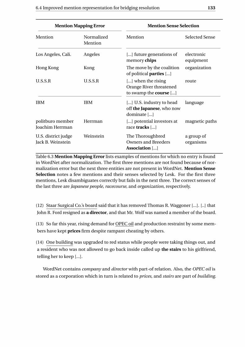
6.4 Improved mention representation for bridging resolution 133
Mention Mapping Error Mention Sense Selection
Mention NormalizedMention
Mention Selected Sense
Los Angeles, Cali. Angeles [...] future generations ofmemory chips
electronicequipment
Hong Kong Kong The move by the coalitionof political parties [...]
organization
U.S.S.R U.S.S.R [...] when the risingOrange River threatenedto swamp the course [...]
route
IBM IBM [...] U.S. industry to headoff the Japanese, who nowdominate [...]
language
politburo memberJoachim Herrman
Herrman [...] potential investors atrace tracks [...]
magnetic paths
U.S. district judgeJack B. Weinstein
Weinstein The ThoroughbredOwners and BreedersAssociation [...]
a group oforganisms
Table 6.3 Mention Mapping Error lists examples of mentions for which no entry is foundin WordNet after normalization. The first three mentions are not found because of nor-malization error but the next three entities are not present in WordNet. Mention SenseSelection notes a few mentions and their senses selected by Lesk. For the first threementions, Lesk disambiguates correctly but fails in the next three. The correct senses ofthe last three are Japanese people, racecourse, and organization, respectively.
(12) Staar Surgical Co.’s board said that it has removed Thomas R. Waggoner [...]. [..] that
John R. Ford resigned as a director, and that Mr. Wolf was named a member of the board.
(13) So far this year, rising demand for OPEC oil and production restraint by some mem-
bers have kept prices firm despite rampant cheating by others.
(14) One building was upgraded to red status while people were taking things out, and
a resident who was not allowed to go back inside called up the stairs to his girlfriend,
telling her to keep [...].
WordNet contains company and director with part-of relation. Also, the OPEC oil is
stored as a corporation which in turn is related to prices, and stairs are part of building.

134 Integrating knowledge graph embeddings to improve representation
This information from WordNet has been used for resolving these pairs as opposed to
relying only on the textual information in case of mention representation only with BERT.
Conversely, we also observed a few pairs where the addition of extra information has
been detrimental. The italic faced phrase is the selected antecedent with WordNet based
system but without WordNet correct antecedent (shown with underline) was selected for
boldfaced anaphor.
(15) Within the same nine months, News Corp. [...]. Meanwhile, American Health Partners,
publisher of American Health magazine is deep in debt, and Owen Lipstein, founder[...].
(16) [...] the magnificent dunes where the Namib Desert meets the Atlantic Ocean [...]Since
this treasure chest [...] up a diamond from the sand.
(17) The space shuttle Atlantis landed [...] that dispatched the Jupiter - bound Galileo
space probe. The five astronauts returned [...].
In example 15, News Corporation is closer to founder than Partners as head word is
Partners for the long phrase. Thus, the system assigns higher scores to wrong antecedent
candidate. Similarly, in example 16, the dunes are closer to sand than treasure chest.
In the example 17, WordNet contains Atalantis as legendary island and not as a space
shuttle thus astronauts is closer to space probe than island, thus receiving a higher
score than the correct antecedent. These mistakes can be attributed to the process of
normalizing mentions as well as limitations of WordNet. Interestingly, these examples
show the inadequacy of BERT in capturing the partOf relation but efficacy of capturing
some form of relatedness of the terms.
6.5 Improved event representation for temporal relation
classification
In the previous section we described our approach to obtain knowledge-aware mention
representation for bridging anaphora resolution. Now we apply conceptually similar ap-
proach to improve event representation for temporal relation classification. We combine
text-based and knowledge graph based event representations to obtain knowledge-aware
event representations in Section 6.5.1. We detail our neural model that is based on the
latest work (Wang et al., 2020), learning objective and inference strategy in Section 6.5.2,
our experimental setup in Section 6.5.3, and results in Section 6.5.4.

6.5 Improved event representation for temporal relation classification 135
6.5.1 Knowledge-aware event representations
Our knowledge-aware event representation consists of two parts similar to the mention
representation: 1. Text-based event representation, and 2. Knowledge-graph based
representation. Let us look at them in the following paragraphs.
Text-based event representation We use state-of-the-art (Wang et al., 2020) BiLSTM
based approach to get text-based embeddings. Let us suppose w1, w2, · · · , wi , · · · , wn
denote the sentence containing n-words. Let ei be the event present in the sentence
and wi be its corresponding event word. This sequence of words is inputed to RoBERTa-
base (Liu et al., 2019b) model to obtain pre-trained embeddings for each word. Let wi be
the RoBERTa embeddings for wi . Additionally, with the use of part-of-speech (POS) tag of
the word wi , one-hot encoded pi is also obtained. These embeddings are concatenated
vi = wi ⊕pi and used as an input to the forward and backward LSTMs. Let fi ,bi be the
output corresponding to i th word from the forward and backward LSTMs, respectively.
Then the text-based event representation gi is obtained by concatenating them: gi = fi ⊕bi .
Knowledge-graph based representation We obtain knowledge graph based representa-
tion for each event as detailed in Section 6.3. Briefly, we normalize event by using lemma
of the event word and then map this normalized token to the graph node. Then corre-
sponding sense embeddings are obtained. In case of multiple senses we averaged over all
possible senses 8. On the other hand, in case of non-availability of the node we used the
zero vector of the same size. Let the knowledge graph-based embedding obtained by this
procedure for an event ei be given as hi .
Event-pair representation For getting event-pair representation, we obtain knowledge-
aware event representation by concatenating the text-based representation and knowl-
edge graph-based representation. For ei it is given as ei = gi ⊕hi . Similarly, we obtain
knowledge-aware event representation for an event e j which is given as e j . Next, to obtain
event-pair representation from these knowledge-aware representations, we follow similar
approach used by Wang et al. (2020). They first concatenated event representations, then
resulting vectors from subtraction and multiplication of event representations also con-
catenated to get the event-pair representation. Suppose, ei ,e j are two events and ei ,e j be
8We have not used Lesk for disambiguation, as we observed in experiments for bridging anaphoraresolution, there was no added advantage of using Lesk over averaged senses. Besides, it can not be directlyapplied over semantic verb frames of TEMPROB.

136 Integrating knowledge graph embeddings to improve representation
their knowledge-aware representation. Then the event-pair representation ei j is obtained
as:
emi j = ei ⊗e j (6.3)
esi j = ei −e j (6.4)
eci j = ei ⊕e j (6.5)
ei j = emi j ⊕es
i j ⊕eci j (6.6)
6.5.2 Neural model
We extended the neural constrained learning model proposed by Wang et al. (2020) with
the addition of knowledge graph-based embeddings. As mentioned earlier, the model is
based on BiLSTM neural network which takes concatenated RoBERTa and POS tags em-
beddings as an input. We inject the commonsense knowledge with the knowledge graph
based embeddings corresponding to each event at the output obtained from BiLSTM.
Finally, this event-pair representation is fed to the scoring function which produces scores
for each temporal relation showing confidence over each relation. This score is used by
the model to optimize the aggregated loss from: pairwise classification loss, symmetry
constraint loss, and transitivity constraint loss. At the inference stage, ILP problem is
solved to produce globally coherent predictions.
Following the same notations from Section 2.1.1.1, we formally define the model as
follows. Let D be the document containing events E = {e1,e2, · · · ,ene } and true temporal
relations between events H = {(ei ,e j ,ri j )|ei ,e j ∈ E ,ri j ∈ R} where R is possible set of
temporal relations, so tuple (ei ,e j ,ri j ) denotes true temporal relation ri j between ei ,e j .
Let the event-pair representation obtained with our approach (Eq. 6.6) be ei j ∈Rd , and
z : Rd → R be the scoring function. Then, the pairwise confidence score parameterized
over θ is given as sr,i , j = z(ei j ;θ)∀r ∈ R . Based on this confidence score the pairwise
classification loss, symmetry constraint loss, transitivity constraint loss, and cumulative
loss is calculated as follows.
6.5.2.1 Constrained learning
Recall from Section 2.1.2.1 that temporal relations possess algebriac property, hence,
symmetry and transitivity rules can be applied over them. The neural model takes into
consideration these temporal constraints while learning model parameters. For that, a
constrained learning approach is taken where in addition to pairwise classification loss,

6.5 Improved event representation for temporal relation classification 137
losses incurred due to constraint violations are also considered while learning. We look at
those losses one by one.
Pairwise classification loss This is a local loss that calculates the difference between
actual temporal relation between event-pair and predicted temporal relation. The cross
entropy is used to calculate it. The confidence score produced by a scoring function is
used to get the loss. Suppose, (ei ,e j ,ri j ) ∈H and the score produced by neural model for
event-pair ei ,e j is sr,i , j∀r ∈R, the pairwise classification loss is calculated as:
Lp (θ) =− ∑(ei ,e j ,ri j )∈H
∑r∈R
yr,i , j log (sr,i , j ) (6.7)
where yr,i , j = 1 if (ei ,e j ,r ) ∈H else 0.
Symmetry constraint loss Temporal relations follow symmetry, therefore, if ei is before
e j , it means that e j is after ei . This is because after and before are inverse to each other,
whereas, equal and vague are inverse to themselves9. Let us suppose Rs = {(r, r )|r, r ∈R and r, r be symmetric relations}. Based on the symmetry constraint over all the event
pairs, a logical rule with a conjunction (∧
) of statements is given as:
∧ei ,e j∈E ,(r,r )∈Rs
ri j → ri j (6.8)
Then the symmetry constrained loss is obtained as:
Ls(θ) =∑ei ,e j∈E ,(r,r )∈Rs
| log (sr,i , j )− log (sr , j ,i )| (6.9)
Transitivity constraint loss Temporal relation also exhibit transitivity property, due to
that temporal relations between event-pairs can be obtained by composing temporal
relations (denoted as ◦) of other pairs. For instance, suppose ei is before e j and e j is before
ek , that implies, ei is before ek , ∀ei ,e j ,ek ∈ E . These transitivity rules are summarized in
Table 6.4.
Based on these composition rules, logical conjunction rule can be formed as:
∧ei ,e j ,ek∈E ,
ri k=ri j ◦r j k ,∀ri j ,r j k ,ri k∈R
ri j ∧ r j k → ri k (6.10)
9These are the only possible temporal relations between starting points of events.

138 Integrating knowledge graph embeddings to improve representation
◦ a b e va a - a -b - b b -e a b e -v - - - -
Table 6.4 Composition rules on end-point relations present in MATRES dataset: (a)fter,(b)efore, (e)qual, and (v)ague. The temporal relations in the first row are composed withrelations from first column to produce temporal relations at each row.
Opposite logical conjunction can be formulated which indicates non-possibility of
composition: ∧ei ,e j ,ek∈E ,
r ′i k =ri j ◦r j k ,
∀ri j ,r j k ,r ′i k∈R
ri j ∧ r j k →¬r ′i k (6.11)
Both of these rules are considered while calculating transitivity loss:
Lt (θ) =∑ei ,e j ,ek∈E ,
ri k=ri j ◦r j k ,∀ri j ,r j k ,ri k∈R
| log (sri j ,i , j )+ log (sr j k , j ,k )− log (sri k ,i ,k )|+
∑ei ,e j ,ek∈E ,
r ′i k =ri j ◦r j k ,
∀ri j ,r j k ,r ′i k∈R
| log (sri j ,i , j )+ log (sr j k , j ,k )− log (1− sr ′i k ,i ,k )| (6.12)
Constrained Learning Objective All three losses: pairwise loss (Eq. 6.7), symmetry con-
strain loss (Eq. 6.9), and transitivity constrain loss (Eq. 6.12) are weighted to get constrained
learning objective:
L (θ) =Lp (θ)+αLs(θ)+βLt (θ). (6.13)
where coefficients α,β≥ 0.
6.5.2.2 ILP Inference
To enforce the global consistency over predicted temporal relations, the inference problem
is formulated as an Integer Linear Programming (ILP) objective. The ILP constraints are
again based on the composition rules mentioned in Table 6.4. The formulation is given as:

6.5 Improved event representation for temporal relation classification 139
maximizeIr,i , j
∑ei ,e j∈E ,
r∈R
sr,i , j Ir,i , j (6.14a)
subject to Ir,i , j − I r , j ,i = 0, ∀ei ,e j ∈ E , (r, r ) ∈Rs , (6.14b)
Ir,i , j + Ir ′, j ,k − I r ,i ,k ≤ 1 ∀ei ,e j ,ek ∈ E , r = r ◦ r ′, (6.14c)
Ir,i , j∈ {0,1} ∀ei ,e j ∈ E ,∀r ∈R (6.14d)
6.5.3 Experimental setup
Dataset Following recent work (Han et al., 2019a,b; Wang et al., 2020), we used MATRES
(Ning et al., 2018b) dataset in our experiments, details of which are mentioned in Sec-
tion 2.1.1.3, here we briefly restate them. This dataset is based on previously proposed
TimeBank (Pustejovsky et al., 2003a), and AQUAINT (Graff, 2002) datasets. It annotates
275 documents with temporal relations between starting points of events as BEFORE,
AFTER, EQUAL, or VAGUE. Instead of annotating any event-pair, their annotation process
first divides events between four axes: main, intention, opinion, and hypothetical. And
temporal relations are annotated only between event pairs that lie on the same axes and
appear in the window of two adjacent sentences. These annotated documents are split
into 183, 72, and 20 documents for train, development, and test, respectively. We followed
the same setting for direct comparison with previous results.
Baseline Systems We implemented three baseline systems: 1. Without commonsense
knowledge, 2. Commonsense knowledge injected with simple features, and 3. Common-
sense knowledge learned from both ConceptNet and TEMPROB. All three systems are
variations of our proposed model. The first system does not contain the knowledge graph
embeddings part and relies solely on the context based embeddings learned from RoBERTa
and POS embeddings with BiLSTM. The second system adds simple commonsense fea-
tures such as prior probabilities for the event-pair obtained from TEMPROB on top of the
text-based representation similar to the previous approach (Ning et al., 2018a). The third
system is a much stronger baseline where commonsense knowledge is added from both
ConceptNet (Speer et al., 2018) and TEMPROB graphs. To get the knowledge from both
these knowledge graphs, we used an approach proposed by Wang et al. (2020). In that,
only small portion of ConceptNet is used where only those nodes that are connected with
specific relations such as “HasSubevent”, “HasFirstSubevent”, and “HasLastSubevent” are
selected. These are considered as “positive” training examples, then the equal number

140 Integrating knowledge graph embeddings to improve representation
of node pairs possessing other than these relations are randomly selected and used as
“negative” training samples. Then, auxiliary neural network (specifically, MLP) is trained
to estimate the likelihood of temporal relations between these pairs. Similarly, another
MLP is trained over TEMPROB as well. Once both MLPs are trained, their weights are not
updated while learning the main system and are used only to get the knowledge graph
features.
System with simple concatenation We experiment with another implementation of our
proposed system where instead of obtaining a complex interaction with multiplication,
and subtraction of knowledge graph embeddings, we simply concatenate them. This is
done to understand the effect of complex interaction of knowledge graph embeddings.
Implementation We obtained officially released pre-trained RoBERTa embeddings (Liu
et al., 2019b) and concatenated them with 18-dimensional one-hot encoded POS tag
embeddings. These embeddings are given to two LSTMs, each having 1024 neurons. The
output from LSTMs is concatenated with the knowledge graph-based embeddings to ob-
tain event-pair representation. As mentioned in Section 6.5.2, we relied on WordNet and
TEMPROB separately to capture such information. In the case of WordNet, we used the
same embedding algorithms that were employed in the experiments for bridging anaphora
resolution in the last section. Specifically, we used 300 dimensional vectors for random
walk based (RW) (Goikoetxea et al., 2015), matrix factorization based (WNV) (Saedi et al.,
2018), and Path2vec (PV) (Kutuzov et al., 2019) embeddings. In the case of Path2vec,
embeddings learned with shortest path similarities (Lebichot et al., 2018) are used as
those have produced better results in their paper as well as in our experiments on bridg-
ing resolution. We used officially released RW and WNV embeddings, but in the case of
Path2vec, the officially released embeddings are not trained with verb information so we
retrained the whole WordNet to get embeddings for all nodes. In the case of TEMPROB,
we trained UKGE embeddings with the procedure mentioned by the authors that pro-
duced 300-dimensional vectors corresponding to each semantic verb frame of the graph.
Finally, two fully connected layers with 1024 and 4 neurons are used over the event-pair
representations. The output of the final layer is considered as a score for four temporal
relations.
For training the model, the AMSGrad (Reddi et al., 2018) optimization algorithm is
used with 0.0001 learning rate. We kept the values of α,β (loss coefficients) to 0.2, same as
(Wang et al., 2020). The epoch value is kept at 50 which is sufficient for model convergence.
At the end of each epoch, the model is evaluated against the validation set and parameters
6.5 Improved event representation for temporal relation classification 141
of the epoch which produce the best validation score are stored. The best performing
model is evaluated against the test set and those results are reported.
Evaluation We report the micro-average of precision, recall, and F1 scores on test set
similar to previous studies (Han et al., 2019a,b; Wang et al., 2020). In addition to that, we
calculate temporal awareness (UzZaman and Allen, 2011) based precision, recall, and F1
score.
6.5.4 Results
Comparison with baseline systems As noted in the previous section, we implemented
three baseline systems: first, without any commonsense information but keeping the same
neural model, in the second system we added commonsense information but only prior
probabilities between event-pairs, whereas in the third system we added commonsense
information by employing a sophisticated approach. The results of the experiments are
shown in the initial three rows of Table 6.5.
Now, we compare results obtained with only text-based embeddings i.e. without addi-
tion of any commonsense information (Table 6.5: row 1) with commonsense knowledge
added with our approach (Table 6.5: section c). We see an increase in pairwise F1 scores
from 70.62 to 72.12, 71.36, 73.39, and 73.67, respectively with RW, PV, WNV, and UKGE
embeddings. This shows that the addition of commonsense information with knowl-
edge graph embeddings is effective over the system with only text-based embeddings,
proving the efficacy of our approach and substantiating our claims for temporal relation
classification task as well.
Second, we compare results obtained with addition of commonsense information
(Table 6.5: row 2 and 3) with the results from our model (Table 6.5: section c). When we
compare results of baseline (Table 6.5: row 2) that adds simple commonsense features
with results from our system (Table 6.5: section c), we see significant improvements. This
further confirms our claims that knowledge graph embeddings encode better information
than simple hand-crafted commonsense features. However, in comparison to the next
baseline (Table 6.5: row 3) where we added sophisticated commonsense features from
two knowledge graphs, we see slight or no improvement in the results. The highest score
obtained with TEMPROB (UKGE) (Table 6.5: section c) is only better by 0.72 F1 points
whereas WNV embeddings over WordNet produce just 0.44 F1 points gain. Further, the
other two embeddings: RW and PV produce lower results than the baseline. We present
reasons of this lower performance in the discussion section 6.5.5.
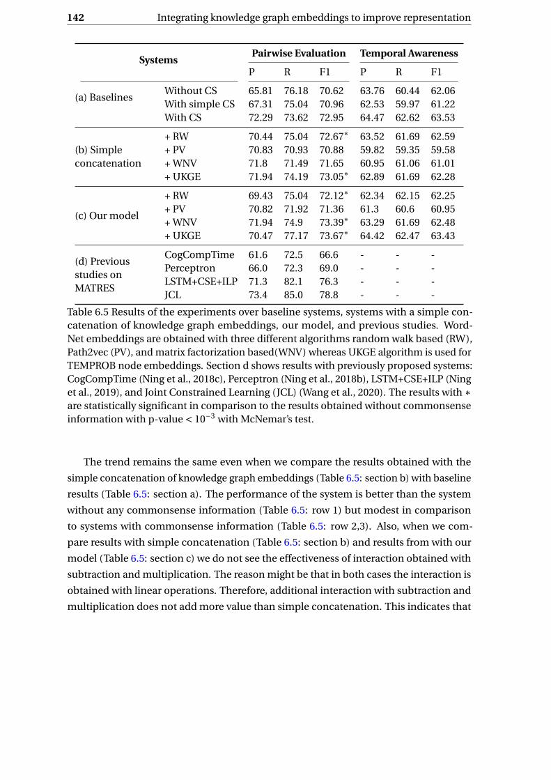
142 Integrating knowledge graph embeddings to improve representation
SystemsPairwise Evaluation Temporal Awareness
P R F1 P R F1
(a) BaselinesWithout CS 65.81 76.18 70.62 63.76 60.44 62.06With simple CS 67.31 75.04 70.96 62.53 59.97 61.22With CS 72.29 73.62 72.95 64.47 62.62 63.53
(b) Simpleconcatenation
+ RW 70.44 75.04 72.67∗ 63.52 61.69 62.59+ PV 70.83 70.93 70.88 59.82 59.35 59.58+ WNV 71.8 71.49 71.65 60.95 61.06 61.01+ UKGE 71.94 74.19 73.05∗ 62.89 61.69 62.28
(c) Our model
+ RW 69.43 75.04 72.12∗ 62.34 62.15 62.25+ PV 70.82 71.92 71.36 61.3 60.6 60.95+ WNV 71.94 74.9 73.39∗ 63.29 61.69 62.48+ UKGE 70.47 77.17 73.67∗ 64.42 62.47 63.43
(d) Previousstudies onMATRES
CogCompTime 61.6 72.5 66.6 - - -Perceptron 66.0 72.3 69.0 - - -LSTM+CSE+ILP 71.3 82.1 76.3 - - -JCL 73.4 85.0 78.8 - - -
Table 6.5 Results of the experiments over baseline systems, systems with a simple con-catenation of knowledge graph embeddings, our model, and previous studies. Word-Net embeddings are obtained with three different algorithms random walk based (RW),Path2vec (PV), and matrix factorization based(WNV) whereas UKGE algorithm is used forTEMPROB node embeddings. Section d shows results with previously proposed systems:CogCompTime (Ning et al., 2018c), Perceptron (Ning et al., 2018b), LSTM+CSE+ILP (Ninget al., 2019), and Joint Constrained Learning (JCL) (Wang et al., 2020). The results with ∗are statistically significant in comparison to the results obtained without commonsenseinformation with p-value < 10−3 with McNemar’s test.
The trend remains the same even when we compare the results obtained with the
simple concatenation of knowledge graph embeddings (Table 6.5: section b) with baseline
results (Table 6.5: section a). The performance of the system is better than the system
without any commonsense information (Table 6.5: row 1) but modest in comparison
to systems with commonsense information (Table 6.5: row 2,3). Also, when we com-
pare results with simple concatenation (Table 6.5: section b) and results from with our
model (Table 6.5: section c) we do not see the effectiveness of interaction obtained with
subtraction and multiplication. The reason might be that in both cases the interaction is
obtained with linear operations. Therefore, additional interaction with subtraction and
multiplication does not add more value than simple concatenation. This indicates that

6.5 Improved event representation for temporal relation classification 143
the complex non-linear interaction learning approach that we developed in Chapter 4 can
be further useful.
Next, we compare two baseline systems with each other (Table 6.5: row 1 and 2), to
check the effect of commonsense in these systems. Recall that the second baseline system
is similar to the first one, the only difference is the addition of commonsense knowledge.
We see a small difference in their performances. The reason might be that only prior
probability information from TEMPROB is added naively. But this improvement is lower
in comparison to the improvement of 5.9 F1 points with pairwise evaluation and 7.1 points
with temporal awareness shown in the original paper (Ning et al., 2018a). The reason
behind these lower gains might be the difference of evaluating datasets, as they evaluated
over TBDense dataset, whereas we evaluated over TE-Platinum. Above all, their text-based
event representation was not as sophisticated as used here, and the learning model was
also weaker, which might be the reason behind their comparatively large gains.
Comparison between different graph node embeddings Now, we compare results ob-
tained with different graph node embeddings with each other to understand which em-
bedding strategy or which knowledge graph is better suitable for temporal relation classifi-
cation. From the results of Section c of Table 6.5, we see TEMPROB and WordNet are both
comparable in the way they capture commonsense information for temporal relation
classification. This also shows that semantic relations such as meronymy, hypernymy,
synonymy, etc. are equally useful for classification as prior probability information en-
coded in TEMPROB. Within WordNet embeddings, WNV and RW approaches produce
slightly better results in comparison to Path2vec. The reason might be that with the use
of Path2vec, there is an explicit need of doing sense disambiguation but as the other two
embeddings produce word embeddings rather than sense embeddings the extra step of
sense disambiguation is not required.
Comparison with previous studies In Table 6.5: section d, we present results of previous
studies done over MATRES: CogCompTime (Ning et al., 2018c), Perceptron (Ning et al.,
2018b), LSTM+CSE+ILP (Ning et al., 2019), and Joint Constrained Learning (JCL) (Wang
et al., 2020). Though our proposed approach performs better than CogCompTime and
Perceptron approach, it lags by more than 2 F1 points in comparison with LSTM+CSE+ILP
and more than 5 points with JCL. One of the reasons might be that both approaches
added sophisticated commonsense knowledge by learning embeddings over TEMPROB
(similar to our baseline 3). In the case of JCL, the original model is jointly trained with
general event relation (e.g. Parent-child, coreference, etc.) classification task. This joint

144 Integrating knowledge graph embeddings to improve representation
training and cross task constraints have been shown to be beneficial in their ablation
studies. In our experiments, we omitted this part of joint learning, as our primary goal was
to assess the effectiveness of commonsense information injected with knowledge graph
embeddings and not to achieve state-of-the-art result.
6.5.5 Discussion
We observe from the results that our approach of injecting commonsense information
with knowledge graph embeddings produces better results in comparison to the system
without any external knowledge as well as with the addition of simple commonsense
features, however, our approach is ineffective in comparison to the carefully learned
commonsense knowledge. To understand the reasons behind this ineffectiveness, we first
checked how many events were mapped to WordNet and TEMPROB nodes. We observed
that out of a total 1019010 events, 195 were missed with WordNet whereas with TEMPROB
only 37 events were missed. This shows high coverage for events in both knowledge
graphs which clears the doubt that the absence of knowledge is not the reason behind the
ineffectiveness. Further, we believe the following factors might have contributed to the
moderate performance gains in comparison with the commonsense injection approach
of Wang et al. (2020).
Firstly, the commonsense knowledge extracted by (Wang et al., 2020) contains knowl-
edge from ConceptNet (Speer et al., 2018) which we have not explored in our experiments.
It might be possible that the event information encoded in ConceptNet is more beneficial
for temporal relation classification than the external knowledge encoded in WordNet or
TEMPROB. In addition to that, they encoded knowledge from multiple sources, i.e. they
used both ConceptNet as well as TEMPROB to get commonsense information. This might
have benefited them as well.
Further, we think the simple heuristics used to circumvent the need for sense disam-
biguation might be another reason. We simply averaged embeddings over all the senses
of the word to get Path2vec WordNet embeddings, similarly in the case of TEMPROB
embeddings. We think learning an appropriate sense of word instead of relying on the
simple heuristics can improve the system performance further.
Lastly, the graph node embeddings that are used in our system are learned in a task-
agnostic way. This means they are not specifically designed to capture information for
temporal relation classification. These embeddings may capture irrelevant information
10Though we have total 12366 events in MATRES, all of them are not unique verbs also not all the eventpairs are annotated with temporal relations. This is the reason behind a small number of events in compari-son to all events.

6.6 Conclusion 145
that might not be useful for the task. We think instead of relying on pre-trained static
graph node embeddings, learning them jointly with text-based embeddings in the process
of learning model parameters can be useful for the system.
All in all, we think that the use of other knowledge graphs such as ConceptNet which
encodes event specific information, or Verbocean (Chklovski and Pantel, 2004) which
possess temporal relation between verbs can be beneficial. The other promising way can
be to use multiple knowledge sources instead of relying on a single source of information.
Further, disambiguating senses while training the model for classification can also produce
better results. Lastly, we think the joint learning of knowledge graph embeddings rather
than using pre-trained embeddings can be beneficial.
6.6 Conclusion
We added commonsense knowledge into bridging resolution and temporal relation classi-
fication systems. For acquiring such knowledge, instead of relying on hand-engineered
features or partially selected pairs from knowledge graphs like previous approaches we
used graph node embeddings. We proposed a simple approach for mapping events and
mentions to the nodes of knowledge graphs to obtain corresponding graph node em-
beddings. Specifically, we used WordNet for both tasks, and TEMPROB, particularly for
temporal relation classification.
We observed significant gains in the results with the addition of knowledge graph em-
beddings in the system compared with only text-based representations for both bridging
anaphora resolution and temporal relation classification when evaluated on standard
datasets. This shows that both contextual and commonsense information are needed for
these tasks, establishing our central claim. Secondly, the results prove that word embed-
dings learned with only text data are inadequate at capturing commonsense information,
hence, must be complemented with commonsense information explicitly. This also cor-
roborates our observations from the last chapter. Further, our gains with knowledge graph
embeddings also show that node embeddings learned over knowledge graphs are an
effective way of encoding knowledge graphs in comparison to hand-crafted approach.
Apart from this, we observed similar gains with the use of WordNet and TEMPROB for
temporal relation classification, showing semantic relations such as meronymy, hyper-
nymy, synonymy, etc. encoded by WordNet are equally useful for classification as specific
temporal information present in prior probabilities between events.
Though the systems performed well, there are a number of ways to improve them
further. First, the sophisticated approach for mention and event normalization and

146 Integrating knowledge graph embeddings to improve representation
sense disambiguation instead of heuristics can be beneficial. Next, the use of multiple
knowledge resources instead of depending on a single source of knowledge can be useful
for the system’s performance. Further, we think learning knowledge graph embeddings
and text-based embeddings jointly can be valuable.

Chapter 7
Conclusions
Identifying temporal relations between events and establishing bridging links between
mentions is crucial for automatic discourse understanding. For that purpose, obtaining
effective events and mentions representations is necessary for NLP models employed to
determine these relations. We argued that contextual information and commonsense
information is crucial for such effective representations. The previously proposed compu-
tational approaches to determine these relations were inadequate at capturing both this
information simultaneously. This thesis solved that problem by developing efficient ways
to incorporate contextual and commonsense information to improve event and mention
representations.
We developed a neural network based approach for learning rich event representations
and interactions (Chapter 4). We used the context of the event in the window of n-words
and represented each word as pre-trained word embedding. Then provided this as an
input to RNN to produce context rich event representations. Further, we added morpho-
logical information by concatenating character embeddings of the event headword. At
last, we employed deep CNN to obtain rich interactions between the event representa-
tions. The empirical results proved the efficacy of this approach, as we obtained better
results than local models that relied on only event headword representations or simple
interactions. More importantly, the results demonstrated that contextual information is
needed to accurately predict temporal relations between events. Additionally, the study
showed that interaction learning over event representations is also important for the task.
Next, we investigated pre-trained transformer language models (e.g. BERT, RoBERTa)
for bridging resolution as an alternative way of capturing contextual information (Chap-
ter 5). We developed two complementary approaches to achieve that. First, we investi-
gated each attention head of transformer models individually to assess the amount of
bridging signal captured by them. Then, we developed Of-Cloze test to understand the

148 Conclusions
efficacy of the whole model. We found that pre-trained BERT models are significantly
capable of capturing bridging inference though it depends on the provided context. Also,
our qualitative analysis showed that BERT is inadequate at capturing commonsense
knowledge.
Finally, we combined both contextual and commonsense information for better
event and mention representations (Chapter 6). We acquired commonsense information
with knowledge graph embeddings learned over WordNet (Fellbaum, 1998) and TEM-
PROB (Ning et al., 2018a). We used simple methods to get knowledge based representa-
tions for events and mentions based on the node embeddings. Then these representations
are combined with contextual representations to get knowledge-aware event and men-
tion representations. We evaluated our proposed approach over standard datasets for
both bridging anaphora resolution and temporal relation classification. We observed
substantial improvements with the addition of commonsense information in the results
in comparison to only text-based representations for both tasks. These results show that
graph node embeddings learned over knowledge graphs are capable of encoding the
commonsense knowledge required for these tasks. The gains over text-only embeddings
by the addition of knowledge graph embeddings also substantiate the findings from the
investigation of pre-trained transformer models that transformer models lack at capturing
commonsense information. Above all, the results validate our claim that both contextual
and commonsense information is required to effectively represent events and mentions,
which is consequently necessary for accurately solving temporal relation classification
and bridging anaphora resolution.
We can see a few immediate ways of extending our work. From the findings of the
investigation of pre-trained transformer models, we can build a better system for bridging
anaphora resolution. We observed that the last layers and a few individual attention heads
target bridging information, so making specific use of these elements for bridging instead
of whole BERT can be an interesting exploration. Next, we can dynamically learn the
linking of mentions and events to knowledge graph nodes while addressing the issue of
sense disambiguation as well. This procedure can reduce the effects of normalization
and disambiguation errors which we identified in our analysis. Further, we believe that
graph node embeddings learned in task-agnostic way can project nodes that are less
probable to possess bridging relation into nearby space (e.g. cat-dog) because of their
proximity in the actual graph. A similar problem may occur for temporal relations as
well where the generic node embeddings algorithm may encode some noisy information.
Therefore, learning graph embeddings specifically for these tasks can be beneficial for
getting relevant knowledge.

149
More generally, we can extend the findings from this thesis for the other two tasks
of discourse understanding: discourse relation classification and coreference resolution.
These tasks being highly related to the tasks we solved, the insights gained from the thesis
can be useful. In fact, there have been attempts of making use of other relations while
proposing systems for particular relations (D’Souza and Ng, 2013; Ng et al., 2013; Yu and
Poesio, 2020), so it can also be interesting to go a step further to learn all of them jointly
with shared context and commonsense knowledge to exploit learnings from one another.
Apart from that, in our work, we focused on including commonsense knowledge but
have not worked on the reasoning capabilities of the systems. We think in addition to
commonsense knowledge, reasoning over it can lead to further accurate solutions.


References
Ahmed Amr, Shervashidze Nino, Narayanamurthy Shravan, Josifovski Vanja, and SmolaAlexander J. 2013. Distributed large-scale natural graph factorization. In Proceedingsof the 22nd International Conference on World Wide Web, WWW ’13, page 37–48, NewYork, NY, USA. Association for Computing Machinery.
Allen James F. 1983. Maintaining knowledge about temporal intervals. Commun. ACM,26(11):832–843.
Augusto Juan Carlos. 2005. Temporal reasoning for decision support in medicine. ArtificialIntelligence in Medicine, 33(1):1–24.
Baldi Pierre. 2011. Autoencoders, unsupervised learning and deep architectures. InProceedings of the 2011 International Conference on Unsupervised and Transfer LearningWorkshop - Volume 27, UTLW’11, page 37–50. JMLR.org.
Baroni Marco and Lenci Alessandro. 2010. Distributional memory: A general frameworkfor corpus-based semantics. Computational Linguistics, 36(4):673–721.
Barzilay Regina, Elhadad Noemie, and McKeown Kathleen R. 2002. Inferring strategies forsentence ordering in multidocument news summarization. J. Artif. Int. Res., 17(1):35–55.
Bauer Lisa, Wang Yicheng, and Bansal Mohit. 2018. Commonsense for generative multi-hop question answering tasks. In Proceedings of the 2018 Conference on EmpiricalMethods in Natural Language Processing, pages 4220–4230, Brussels, Belgium. Associa-tion for Computational Linguistics.
Bellet Aurélien, Habrard Amaury, and Sebban Marc. 2013. A survey on metric learning forfeature vectors and structured data. CoRR, abs/1306.6709.
Bengio Yoshua, Ducharme Réjean, Vincent Pascal, and Janvin Christian. 2003. A neuralprobabilistic language model. J. Mach. Learn. Res., 3(null):1137–1155.
Bethard Steven. 2013. ClearTK-TimeML: A minimalist approach to tempeval 2013. InSecond Joint Conference on Lexical and Computational Semantics (*SEM), Volume 2:Proceedings of the Seventh International Workshop on Semantic Evaluation (SemEval2013), pages 10–14, Atlanta, Georgia, USA. Association for Computational Linguistics.Winner of the shared task.
Bethard Steven, Martin James H., and Klingenstein Sara. 2007. Timelines from text:Identification of syntactic temporal relations. In International Conference on SemanticComputing (ICSC 2007), pages 11–18.
152 References
Boguraev Branimir and Ando Rie Kubota. 2005. Timeml-compliant text analysis for tem-poral reasoning. In Proceedings of the 19th International Joint Conference on ArtificialIntelligence, IJCAI’05, page 997–1003, San Francisco, CA, USA. Morgan Kaufmann Pub-lishers Inc.
Bojanowski Piotr, Grave Edouard, Joulin Armand, and Mikolov Tomas. 2017. Enrichingword vectors with subword information. Transactions of the Association for Computa-tional Linguistics, 5:135–146.
Bollegala Danushka, Mohammed Alsuhaibani, Maehara Takanori, and KawarabayashiKen-ichi. 2016. Joint word representation learning using a corpus and a semantic lexicon.In Proceedings of the Thirtieth AAAI Conference on Artificial Intelligence, AAAI’16, page2690–2696. AAAI Press.
Bordes Antoine, Usunier Nicolas, Garcia-Duran Alberto, Weston Jason, and YakhnenkoOksana. 2013. Translating embeddings for modeling multi-relational data. In Advancesin Neural Information Processing Systems, volume 26. Curran Associates, Inc.
Bramsen Philip, Deshpande Pawan, Lee Yoong Keok, and Barzilay Regina. 2006. Inducingtemporal graphs. In Proceedings of the 2006 Conference on Empirical Methods in NaturalLanguage Processing, EMNLP ’06, pages 189–198, Stroudsburg, PA, USA. Association forComputational Linguistics.
Braud Chloé and Denis Pascal. 2015. Comparing word representations for implicit dis-course relation classification. In Empirical Methods in Natural Language Processing(EMNLP 2015).
Bromley Jane, Guyon Isabelle, LeCun Yann, Säckinger Eduard, and Shah Roopak. 1993.Signature verification using a" siamese" time delay neural network. Advances in neuralinformation processing systems, 6:737–744.
Broscheit Samuel. 2019. Investigating entity knowledge in BERT with simple neuralend-to-end entity linking. In Proceedings of the 23rd Conference on ComputationalNatural Language Learning (CoNLL), pages 677–685, Hong Kong, China. Association forComputational Linguistics.
Cahill Aoife and Riester Arndt. 2012. Automatically acquiring fine-grained informationstatus distinctions in German. In Proceedings of the 13th Annual Meeting of the SpecialInterest Group on Discourse and Dialogue, pages 232–236, Seoul, South Korea. Associa-tion for Computational Linguistics.
Cakir Fatih, He Kun, Xia Xide, Kulis Brian, and Sclaroff Stan. 2019. Deep metric learning torank. In 2019 IEEE/CVF Conference on Computer Vision and Pattern Recognition (CVPR),pages 1861–1870.
Cao Shaosheng, Lu Wei, and Xu Qiongkai. 2015. Grarep: Learning graph representationswith global structural information. In Proceedings of the 24th ACM International onConference on Information and Knowledge Management, CIKM ’15, page 891–900, NewYork, NY, USA. Association for Computing Machinery.
References 153
Carlson Lynn, Marcu Daniel, and Okurovsky Mary Ellen. 2001. Building a discourse-taggedcorpus in the framework of Rhetorical Structure Theory. In Proceedings of the SecondSIGdial Workshop on Discourse and Dialogue.
Cassidy Taylor, McDowell Bill, Chambers Nathanael, and Bethard Steven. 2014. An anno-tation framework for dense event ordering. In Proceedings of the 52nd Annual Meetingof the Association for computational Linguistics, ACL 2014, June 22-27, 2014, Baltimore,MD, USA, Volume 2: Short Papers, pages 501–506.
Chambers Nathanael. Navytime: Event and time ordering from raw text.
Chambers Nathanael, Cassidy Taylor, McDowell Bill, and Bethard Steven. 2014. Denseevent ordering with a multi-pass architecture. Transactions of the Association for Com-putational Linguistics, 2:273–284.
Chambers Nathanael and Jurafsky Daniel. 2008. Jointly combining implicit constraintsimproves temporal ordering. In Proceedings of the 2008 Conference on Empirical Meth-ods in Natural Language Processing, pages 698–706. Association for ComputationalLinguistics.
Chambers Nathanael, Wang Shan, and Jurafsky Dan. 2007. Classifying temporal relationsbetween events. In Proceedings of the 45th Annual Meeting of the ACL on InteractivePoster and Demonstration Sessions, ACL ’07, pages 173–176, Stroudsburg, PA, USA.Association for Computational Linguistics.
Chandrashekar Girish and Sahin Ferat. 2014. A survey on feature selection methods.Computers & Electrical Engineering, 40(1):16–28.
Chang Ming-Wei, Ratinov Lev, and Roth Dan. 2012. Structured learning with constrainedconditional models. Mach. Learn., 88(3):399–431.
Chen Qian, Zhu Xiaodan, Ling Zhen-Hua, Inkpen Diana, and Wei Si. 2018. Neural natu-ral language inference models enhanced with external knowledge. In Proceedings ofthe 56th Annual Meeting of the Association for Computational Linguistics (Volume 1:Long Papers), pages 2406–2417, Melbourne, Australia. Association for ComputationalLinguistics.
Chen Xuelu, Chen Muhao, Shi Weijia, Sun Yizhou, and Zaniolo Carlo. 2019. Embedding un-certain knowledge graphs. Proceedings of the AAAI Conference on Artificial Intelligence,33(01):3363–3370.
Chen Yanqing, Perozzi Bryan, Al-Rfou Rami, and Skiena Steven. 2013. The expressivepower of word embeddings.
Cheng Fei and Miyao Yusuke. 2017. Classifying temporal relations by bidirectional lstmover dependency paths. In Proceedings of the 55th Annual Meeting of the Associationfor Computational Linguistics (Volume 2: Short Papers), pages 1–6. Association forComputational Linguistics.

154 References
Chklovski Timothy and Pantel Patrick. 2004. VerbOcean: Mining the web for fine-grainedsemantic verb relations. In Proceedings of the 2004 Conference on Empirical Meth-ods in Natural Language Processing, pages 33–40, Barcelona, Spain. Association forComputational Linguistics.
Cho Kyunghyun, van Merrienboer Bart, Gülçehre Çaglar, Bougares Fethi, Schwenk Holger,and Bengio Yoshua. 2014. Learning phrase representations using RNN encoder-decoderfor statistical machine translation. CoRR, abs/1406.1078.
Choi Edward, Schuetz Andy, Stewart Walter F, and Sun Jimeng. 2016. Using recurrentneural network models for early detection of heart failure onset. Journal of the AmericanMedical Informatics Association, 24(2):361–370.
Choubey Prafulla Kumar and Huang Ruihong. 2017. A sequential model for classifyingtemporal relations between intra-sentence events. In Proceedings of the 2017 Conferenceon Empirical Methods in Natural Language Processing, pages 1796–1802, Copenhagen,Denmark. Association for Computational Linguistics.
Chung Junyoung, Gülçehre Çaglar, Cho KyungHyun, and Bengio Yoshua. 2014. Em-pirical evaluation of gated recurrent neural networks on sequence modeling. CoRR,abs/1412.3555.
Clark Herbert H. 1975. Bridging. In Proceedings of the Conference on Theoretical Issues inNatural Language Processing, Cambridge, Mass., June 1975, pages 169–174.
Clark Kevin, Khandelwal Urvashi, Levy Omer, and Manning Christopher D. 2019. Whatdoes BERT look at? an analysis of BERT’s attention. In Proceedings of the 2019 ACLWorkshop BlackboxNLP: Analyzing and Interpreting Neural Networks for NLP, pages276–286, Florence, Italy. Association for Computational Linguistics.
Clark Kevin and Manning Christopher D. 2015. Entity-centric coreference resolution withmodel stacking. In Proceedings of the 53rd Annual Meeting of the Association for Com-putational Linguistics and the 7th International Joint Conference on Natural LanguageProcessing (Volume 1: Long Papers), pages 1405–1415, Beijing, China. Association forComputational Linguistics.
Clark Kevin and Manning Christopher D. 2016a. Deep reinforcement learning for mention-ranking coreference models. CoRR, abs/1609.08667.
Clark Kevin and Manning Christopher D. 2016b. Improving coreference resolution bylearning entity-level distributed representations. In Proceedings of the 54th AnnualMeeting of the Association for Computational Linguistics (Volume 1: Long Papers), pages643–653. Association for Computational Linguistics.
Collins Michael. 2003. Head-driven statistical models for natural language parsing. Com-putational Linguistics, 29(4):589–637.
Comrie Bernard. 1976. Aspect: An introduction to the study of verbal aspect and relatedproblems, volume 2. Cambridge university press.
References 155
Costa Francisco and Branco António. 2012. Aspectual type and temporal relation classifi-cation. In Proceedings of the 13th Conference of the European Chapter of the Associationfor Computational Linguistics, pages 266–275, Avignon, France. Association for Compu-tational Linguistics.
Cui Wanqing, Lan Yanyan, Pang Liang, Guo Jiafeng, and Cheng Xueqi. 2020. Beyondlanguage: Learning commonsense from images for reasoning. In Findings of the Associ-ation for Computational Linguistics: EMNLP 2020, pages 4379–4389, Online. Associationfor Computational Linguistics.
Da Jeff and Kasai Jungo. 2019. Cracking the contextual commonsense code: Understandingcommonsense reasoning aptitude of deep contextual representations. In Proceedingsof the First Workshop on Commonsense Inference in Natural Language Processing, pages1–12, Hong Kong, China. Association for Computational Linguistics.
Dai Zeyu and Huang Ruihong. 2018. Improving implicit discourse relation classificationby modeling inter-dependencies of discourse units in a paragraph. In Proceedings of the2018 Conference of the North American Chapter of the Association for ComputationalLinguistics: Human Language Technologies, Volume 1 (Long Papers), pages 141–151,New Orleans, Louisiana. Association for Computational Linguistics.
Dara Suresh and Tumma Priyanka. 2018. Feature extraction by using deep learning: Asurvey. In 2018 Second International Conference on Electronics, Communication andAerospace Technology (ICECA), pages 1795–1801. IEEE.
Daumé III Hal and Marcu Daniel. 2005. A large-scale exploration of effective globalfeatures for a joint entity detection and tracking model. In Proceedings of HumanLanguage Technology Conference and Conference on Empirical Methods in NaturalLanguage Processing, pages 97–104, Vancouver, British Columbia, Canada. Associationfor Computational Linguistics.
De Beaugrande Robert and Dressler Wolfgang U. 1986. Introduction to text linguistics.Longman linguistics library. Longman.
Denis Pascal and Baldridge Jason. 2008. Specialized models and ranking for coreferenceresolution. In Proceedings of the 2008 Conference on Empirical Methods in NaturalLanguage Processing, pages 660–669, Honolulu, Hawaii. Association for ComputationalLinguistics.
Denis Pascal and Muller Philippe. 2011. Predicting globally-coherent temporal structuresfrom texts via endpoint inference and graph decomposition. In IJCAI 2011, Proceedingsof the 22nd International Joint Conference on Artificial Intelligence, Barcelona, Catalonia,Spain, July 16-22, 2011, pages 1788–1793.
Derczynski Leon. 2016. Representation and learning of temporal relations. In Proceedingsof COLING 2016, the 26th International Conference on Computational Linguistics: Tech-nical Papers, pages 1937–1948, Osaka, Japan. The COLING 2016 Organizing Committee.
Derczynski Leon, Llorens Hector, and UzZaman Naushad. 2013. Timeml-strict: clarifyingtemporal annotation.

156 References
Devlin Jacob, Chang Ming-Wei, Lee Kenton, and Toutanova Kristina. 2019. BERT: Pre-training of deep bidirectional transformers for language understanding. In Proceedingsof the 2019 Conference of the North American Chapter of the Association for Computa-tional Linguistics: Human Language Technologies, Volume 1 (Long and Short Papers),pages 4171–4186, Minneapolis, Minnesota. Association for Computational Linguistics.
Dhillon Paramveer S., Foster Dean P., and Ungar Lyle H. 2015. Eigenwords: Spectral wordembeddings. Journal of Machine Learning Research, 16(95):3035–3078.
Dligach Dmitriy, Miller Timothy, Lin Chen, Bethard Steven, and Savova Guergana. 2017.Neural temporal relation extraction. In Proceedings of the 15th Conference of the Euro-pean Chapter of the Association for Computational Linguistics: Volume 2, Short Papers,pages 746–751, Valencia, Spain. Association for Computational Linguistics.
Do Quang Xuan, Lu Wei, and Roth Dan. 2012. Joint inference for event timeline con-struction. In Proceedings of the 2012 Joint Conference on Empirical Methods in NaturalLanguage Processing and Computational Natural Language Learning, pages 677–687.Association for Computational Linguistics.
Domingos Pedro and Lowd Daniel. 2009. Markov Logic: An Interface Layer for ArtificialIntelligence.
D’Souza Jennifer and Ng Vincent. 2013. Classifying temporal relations with rich linguisticknowledge. In Proceedings of the 2013 Conference of the North American Chapter ofthe Association for Computational Linguistics: Human Language Technologies, pages918–927, Atlanta, Georgia. Association for Computational Linguistics.
Duchi John, Hazan Elad, and Singer Yoram. 2011. Adaptive subgradient methods foronline learning and stochastic optimization. Journal of Machine Learning Research,12(61):2121–2159.
Durrett Greg and Klein Dan. 2013. Easy victories and uphill battles in coreference resolu-tion. In Proceedings of the 2013 Conference on Empirical Methods in Natural LanguageProcessing, pages 1971–1982, Seattle, Washington, USA. Association for ComputationalLinguistics.
Elman Jeffrey L. 1990. Finding structure in time. Cognitive science, 14(2):179–211.
Emami Ali, Trichelair P., Trischler Adam, Suleman Kaheer, Schulz Hannes, and Cheung J.C. K. 2018. The hard-core coreference corpus: Removing gender and number cues fordifficult pronominal anaphora resolution. ArXiv, abs/1811.01747.
Ettinger Allyson. 2020. What BERT is not: Lessons from a new suite of psycholinguisticdiagnostics for language models. Transactions of the Association for ComputationalLinguistics, 8:34–48.
Fang Yimai and Teufel Simone. 2014. A summariser based on human memory limitationsand lexical competition. In Proceedings of the 14th Conference of the European Chapterof the Association for Computational Linguistics, pages 732–741, Gothenburg, Sweden.Association for Computational Linguistics.

References 157
Faruqui Manaal, Dodge Jesse, Jauhar Sujay Kumar, Dyer Chris, Hovy Eduard, and SmithNoah A. 2015. Retrofitting word vectors to semantic lexicons. In Proceedings of the 2015Conference of the North American Chapter of the Association for Computational Linguis-tics: Human Language Technologies, pages 1606–1615, Denver, Colorado. Associationfor Computational Linguistics.
Fellbaum Christiane. 1998. WordNet: An Electronic Lexical Database. Bradford Books.
Ferrone Lorenzo and Zanzotto Fabio Massimo. 2020. Symbolic, distributed, and distri-butional representations for natural language processing in the era of deep learning: Asurvey. Frontiers in Robotics and AI, 6:153.
Fillmore Charles J. 1976. Frame semantics and the nature of language*. Annals of the NewYork Academy of Sciences, 280(1):20–32.
Finkel Jenny Rose and Manning Christopher D. 2008. Enforcing transitivity in coreferenceresolution. In Proceedings of the 46th Annual Meeting of the Association for Computa-tional Linguistics on Human Language Technologies: Short Papers, HLT-Short ’08, pages45–48, Stroudsburg, PA, USA. Association for Computational Linguistics.
Firth J. R. 1957. A synopsis of linguistic theory 1930-55. 1952-59:1–32.
Foltz Peter W, Kintsch Walter, and Landauer Thomas K. 1998. The measurement of textualcoherence with latent semantic analysis. Discourse processes, 25(2-3):285–307.
Freund Yoav and Schapire Robert E. 1998. Large margin classification using the perceptronalgorithm. In Proceedings of the Eleventh Annual Conference on Computational Learn-ing Theory, COLT’ 98, page 209–217, New York, NY, USA. Association for ComputingMachinery.
Gardent Claire and Manuélian H. 2005. Création d’un corpus annoté pour le traitementdes descriptions définies.
Glavaš Goran and Vulic Ivan. 2018. Explicit retrofitting of distributional word vectors.In Proceedings of the 56th Annual Meeting of the Association for Computational Lin-guistics (Volume 1: Long Papers), pages 34–45, Melbourne, Australia. Association forComputational Linguistics.
Goikoetxea Josu, Soroa Aitor, and Agirre Eneko. 2015. Random walks and neural networklanguage models on knowledge bases. In Proceedings of the 2015 Conference of theNorth American Chapter of the Association for Computational Linguistics: Human Lan-guage Technologies, pages 1434–1439, Denver, Colorado. Association for ComputationalLinguistics.
Goldberg Yoav. 2019. Assessing BERT’s syntactic abilities. ArXiv, abs/1901.05287.
Golub G. and Reinsch C. 2007. Singular value decomposition and least squares solutions.Numerische Mathematik, 14:403–420.
Goodfellow Ian, Bengio Yoshua, and Courville Aaron. 2016. Deep Learning. MIT Press.http://www.deeplearningbook.org.

158 References
Gordon Mitchell, Duh Kevin, and Andrews Nicholas. 2020. Compressing BERT: Studyingthe effects of weight pruning on transfer learning. In Proceedings of the 5th Workshop onRepresentation Learning for NLP, pages 143–155, Online. Association for ComputationalLinguistics.
Graff David. 2002. The aquaint corpus of english news text.
Grover Aditya and Leskovec Jure. 2016. Node2vec: Scalable feature learning for networks.In Proceedings of the 22nd ACM SIGKDD International Conference on Knowledge Dis-covery and Data Mining, KDD ’16, page 855–864, New York, NY, USA. Association forComputing Machinery.
Hamilton William L., Ying Rex, and Leskovec Jure. 2017. Representation learning ongraphs: Methods and applications. Cite arxiv:1709.05584Comment: Published in theIEEE Data Engineering Bulletin, September 2017; version with minor corrections.
Han Rujun, Hsu I-Hung, Yang Mu, Galstyan Aram, Weischedel Ralph, and Peng Nanyun.2019a. Deep structured neural network for event temporal relation extraction. In Pro-ceedings of the 23rd Conference on Computational Natural Language Learning (CoNLL),pages 666–106, Hong Kong, China. Association for Computational Linguistics.
Han Rujun, Ning Qiang, and Peng Nanyun. 2019b. Joint event and temporal relationextraction with shared representations and structured prediction. In Proceedings ofthe 2019 Conference on Empirical Methods in Natural Language Processing and the 9thInternational Joint Conference on Natural Language Processing (EMNLP-IJCNLP), pages434–444, Hong Kong, China. Association for Computational Linguistics.
Han Rujun, Zhou Yichao, and Peng Nanyun. 2020. Domain knowledge empowered struc-tured neural net for end-to-end event temporal relation extraction.
Hao Boran, Zhu Henghui, and Paschalidis Ioannis. 2020. Enhancing clinical BERT em-bedding using a biomedical knowledge base. In Proceedings of the 28th InternationalConference on Computational Linguistics, pages 657–661, Barcelona, Spain (Online).International Committee on Computational Linguistics.
Harabagiu Sanda, answering Server Question, Harabagiu A, Moldovan Dan, Pasca Marius,Surdeanu Mihai, Mihalcea Rada, Lacatusu Finley, Girju Roxana, Rus Vasile, Lctuu Fin-ley, Morarescu Paul, and Bunescu Razvan. 2001. Answering complex list and contextquestions with lccs question-answering server.
Harris Zellig. 1954. Distributional structure. Word, 10(2-3):146–162.
Hawkins John A. 1978. Definiteness and indefiniteness: a study in reference and grammat-icality prediction. Atlantic Highlands, N.J.: Humanities Press.
Hill Felix, Cho Kyunghyun, and Korhonen Anna. 2016. Learning distributed represen-tations of sentences from unlabelled data. In Proceedings of the 2016 Conference ofthe North American Chapter of the Association for Computational Linguistics: HumanLanguage Technologies, pages 1367–1377, San Diego, California. Association for Compu-tational Linguistics.
References 159
Hinton G. E., McClelland J. L., and Rumelhart D. E. 1986. Distributed Representations,page 77–109. MIT Press, Cambridge, MA, USA.
Hobbs Jerry R. 1979. Coherence and coreference. Cognitive science, 3(1):67–90.
Hobbs Jerry R. and Pan Feng. 2004. An ontology of time for the semantic web. ACMTransactions on Asian Language Information Processing, 3(1):66–85.
Hochreiter Sepp and Schmidhuber Jürgen. 1997. Long short-term memory. 9:1735–80.
Hoffart Johannes, Suchanek Fabian M., Berberich Klaus, Lewis-Kelham Edwin, de MeloGerard, and Weikum Gerhard. 2011. Yago2: Exploring and querying world knowledgein time, space, context, and many languages. In Proceedings of the 20th InternationalConference Companion on World Wide Web, WWW ’11, page 229–232, New York, NY,USA. Association for Computing Machinery.
Horie André, Tanaka-Ishii Kumiko, and Ishizuka Mitsuru. 2012. Verb temporality analysisusing Reichenbach’s tense system. In Proceedings of COLING 2012: Posters, pages471–482, Mumbai, India. The COLING 2012 Organizing Committee.
Hou Yufang. 2016. Incremental fine-grained information status classification usingattention-based LSTMs. In Proceedings of COLING 2016, the 26th International Confer-ence on Computational Linguistics: Technical Papers, pages 1880–1890, Osaka, Japan.The COLING 2016 Organizing Committee.
Hou Yufang. 2018a. A deterministic algorithm for bridging anaphora resolution. In Pro-ceedings of the 2018 Conference on Empirical Methods in Natural Language Processing,pages 1938–1948, Brussels, Belgium. Association for Computational Linguistics.
Hou Yufang. 2018b. Enhanced word representations for bridging anaphora resolution. InProceedings of the 2018 Conference of the North American Chapter of the Association forComputational Linguistics: Human Language Technologies, Volume 2 (Short Papers),pages 1–7, New Orleans, Louisiana. Association for Computational Linguistics.
Hou Yufang. 2019. Fine-grained information status classification using discourse context-aware self-attention.
Hou Yufang. 2020a. Bridging anaphora resolution as question answering. In Proceedingsof the 58th Annual Meeting of the Association for Computational Linguistics, pages1428–1438, Online. Association for Computational Linguistics.
Hou Yufang. 2020b. Fine-grained information status classification using discourse context-aware BERT. In Proceedings of the 28th International Conference on ComputationalLinguistics, Barcelona, Spain. Association for Computational Linguistics.
Hou Yufang, Markert Katja, and Strube Michael. 2013a. Cascading collective classificationfor bridging anaphora recognition using a rich linguistic feature set. In Proceedingsof the 2013 Conference on Empirical Methods in Natural Language Processing, pages814–820, Seattle, Washington, USA. Association for Computational Linguistics.

160 References
Hou Yufang, Markert Katja, and Strube Michael. 2013b. Global inference for bridginganaphora resolution. In Proceedings of the 2013 Conference of the North American Chap-ter of the Association for Computational Linguistics: Human Language Technologies,pages 907–917, Atlanta, Georgia. Association for Computational Linguistics.
Hou Yufang, Markert Katja, and Strube Michael. 2014. A rule-based system for unrestrictedbridging resolution: Recognizing bridging anaphora and finding links to antecedents. InProceedings of the 2014 Conference on Empirical Methods in Natural Language Process-ing (EMNLP), pages 2082–2093, Doha, Qatar. Association for Computational Linguistics.
Hou Yufang, Markert Katja, and Strube Michael. 2018. Unrestricted bridging resolution.Computational Linguistics, 44(2):237–284.
Hsieh Cheng-Kang, Yang Longqi, Cui Yin, Lin Tsung-Yi, Belongie Serge, and Estrin Deb-orah. 2017. Collaborative metric learning. In Proceedings of the 26th InternationalConference on World Wide Web, WWW ’17, page 193–201, Republic and Canton ofGeneva, CHE. International World Wide Web Conferences Steering Committee.
Htut Phu Mon, Phang Jason, Bordia Shikha, and Bowman Samuel R. 2019. Do attentionheads in bert track syntactic dependencies? ArXiv, abs/1911.12246.
Huang De-An, Buch Shyamal, Dery Lucio, Garg Animesh, Fei-Fei Li, and Niebles Juan Car-los. 2018. Finding “it”: Weakly-supervised, reference-aware visual grounding in in-structional videos. In IEEE Conference on Computer Vision and Pattern Recognition(CVPR).
Huang Po-Sen, He Xiaodong, Gao Jianfeng, Deng Li, Acero Alex, and Heck Larry. 2013.Learning deep structured semantic models for web search using clickthrough data. InProceedings of the 22nd ACM International Conference on Information amp; KnowledgeManagement, CIKM ’13, page 2333–2338, New York, NY, USA. Association for ComputingMachinery.
Jain Sarthak and Wallace Byron C. 2019. Attention is not Explanation. In Proceedings of the2019 Conference of the North American Chapter of the Association for ComputationalLinguistics: Human Language Technologies, Volume 1 (Long and Short Papers), pages3543–3556, Minneapolis, Minnesota. Association for Computational Linguistics.
Jawahar Ganesh, Sagot Benoît, and Seddah Djamé. 2019. What does BERT learn aboutthe structure of language? In Proceedings of the 57th Annual Meeting of the Associa-tion for Computational Linguistics, pages 3651–3657, Florence, Italy. Association forComputational Linguistics.
Ji Yangfeng and Eisenstein Jacob. 2015. One vector is not enough: Entity-augmenteddistributed semantics for discourse relations. Transactions of the Association for Com-putational Linguistics, 3:329–344.
Jiang Jay J. and Conrath David W. 1997. Semantic similarity based on corpus statistics andlexical taxonomy. In Proceedings of the 10th Research on Computational Linguistics In-ternational Conference, pages 19–33, Taipei, Taiwan. The Association for ComputationalLinguistics and Chinese Language Processing (ACLCLP).

References 161
Joachims Thorsten. 2002. Optimizing search engines using clickthrough data. In Proceed-ings of the Eighth ACM SIGKDD International Conference on Knowledge Discovery andData Mining, KDD ’02, page 133–142, New York, NY, USA. Association for ComputingMachinery.
Joachims Thorsten. 2006. Training linear svms in linear time. In Proceedings of the 12thACM SIGKDD International Conference on Knowledge Discovery and Data Mining, KDD’06, page 217–226, New York, NY, USA. Association for Computing Machinery.
Jolliffe Ian. 2011. Principal Component Analysis, pages 1094–1096. Springer Berlin Heidel-berg, Berlin, Heidelberg.
Jordan Michael I. 1997. Chapter 25 - serial order: A parallel distributed processing ap-proach. In John W. Donahoe and Vivian Packard Dorsel, editors, Neural-Network Modelsof Cognition, volume 121 of Advances in Psychology, pages 471–495. North-Holland.
Joshi Mandar, Chen Danqi, Liu Yinhan, Weld Daniel S., Zettlemoyer Luke, and LevyOmer. 2020. Spanbert: Improving pre-training by representing and predicting spans.Transactions of the Association for Computational Linguistics, 8:64–77.
Jung Hyuckchul, Allen James, Blaylock Nate, de Beaumont William, Galescu Lucian, andSwift Mary. 2011. Building timelines from narrative clinical records: Initial results based-on deep natural language understanding. In Proceedings of BioNLP 2011 Workshop,pages 146–154, Portland, Oregon, USA. Association for Computational Linguistics.
K Karthikeyan, Wang Zihan, Mayhew Stephen, and Roth Dan. 2020. Cross-lingual abilityof multilingual bert: An empirical study.
Kalchbrenner Nal, Grefenstette Edward, and Blunsom Phil. 2014. A convolutional neuralnetwork for modelling sentences. In Proceedings of the 52nd Annual Meeting of theAssociation for Computational Linguistics (Volume 1: Long Papers), pages 655–665,Baltimore, Maryland. Association for Computational Linguistics.
Kantor Ben and Globerson Amir. 2019. Coreference resolution with entity equalization. InProceedings of the 57th Annual Meeting of the Association for Computational Linguistics,pages 673–677, Florence, Italy. Association for Computational Linguistics.
Kelley Henry J. 1960. Gradient theory of optimal flight paths. Ars Journal, 30(10):947–954.
Khalid Samina, Khalil Tehmina, and Nasreen Shamila. 2014. A survey of feature selectionand feature extraction techniques in machine learning. In 2014 science and informationconference, pages 372–378. IEEE.
Kiela Douwe, Hill Felix, and Clark Stephen. 2015. Specializing word embeddings forsimilarity or relatedness. In Proceedings of the 2015 Conference on Empirical Methodsin Natural Language Processing, pages 2044–2048, Lisbon, Portugal. Association forComputational Linguistics.
Kim Yoon. 2014. Convolutional neural networks for sentence classification. In Proceedingsof the 2014 Conference on Empirical Methods in Natural Language Processing (EMNLP),pages 1746–1751, Doha, Qatar. Association for Computational Linguistics.

162 References
Kingma Diederik P. and Ba Jimmy. 2017. Adam: A method for stochastic optimization.
Kiros Ryan, Zhu Yukun, Salakhutdinov Russ R, Zemel Richard, Urtasun Raquel, TorralbaAntonio, and Fidler Sanja. 2015. Skip-thought vectors. In Advances in Neural Informa-tion Processing Systems, volume 28. Curran Associates, Inc.
Kobayashi Hideo and Ng Vincent. 2021. Bridging resolution: Making sense of the stateof the art. In Proceedings of the 2021 Conference of the North American Chapter ofthe Association for Computational Linguistics: Human Language Technologies, pages1652–1659, Online. Association for Computational Linguistics.
Kobayashi Nozomi, Inui Kentaro, and Matsumoto Yuji. 2007. Extracting aspect-evaluationand aspect-of relations in opinion mining. In Proceedings of the 2007 Joint Conferenceon Empirical Methods in Natural Language Processing and Computational Natural Lan-guage Learning (EMNLP-CoNLL), pages 1065–1074, Prague, Czech Republic. Associationfor Computational Linguistics.
Kovaleva Olga, Romanov Alexey, Rogers Anna, and Rumshisky Anna. 2019. Revealing thedark secrets of BERT. In Proceedings of the 2019 Conference on Empirical Methods inNatural Language Processing and the 9th International Joint Conference on Natural Lan-guage Processing (EMNLP-IJCNLP), pages 4365–4374, Hong Kong, China. Associationfor Computational Linguistics.
Krishna Ranjay, Zhu Yuke, Groth Oliver, Johnson Justin, Hata Kenji, Kravitz Joshua, ChenStephanie, Kalantidis Yannis, Li Li-Jia, Shamma David A., Bernstein Michael S., and LiFei-Fei. 2016. Visual genome: Connecting language and vision using crowdsourceddense image annotations.
Kutuzov Andrey, Dorgham Mohammad, Oliynyk Oleksiy, Biemann Chris, and PanchenkoAlexander. 2019. Learning graph embeddings from WordNet-based similarity measures.In Proceedings of the Eighth Joint Conference on Lexical and Computational Semantics(*SEM 2019), pages 125–135, Minneapolis, Minnesota. Association for ComputationalLinguistics.
Lakew Surafel Melaku, Cettolo Mauro, and Federico Marcello. 2018. A comparison oftransformer and recurrent neural networks on multilingual neural machine translation.In Proceedings of the 27th International Conference on Computational Linguistics, pages641–652, Santa Fe, New Mexico, USA. Association for Computational Linguistics.
Landauer T. and Dumais S. 1997. A solution to plato’s problem: The latent semantic analy-sis theory of acquisition, induction, and representation of knowledge. PsychologicalReview, 104:211–240.
Laokulrat Natsuda, Miwa Makoto, Tsuruoka Yoshimasa, and Chikayama Takashi.2013. Uttime: Temporal relation classification using deep syntactic features. InSemEval@NAACL-HLT, pages 88–92. The Association for Computer Linguistics.
Lapata Mirella and Lascarides Alex. 2004. Inferring sentence-internal temporal relations.In Proceedings of the Human Language Technology Conference of the North AmericanChapter of the Association for Computational Linguistics: HLT-NAACL 2004, pages153–160, Boston, Massachusetts, USA. Association for Computational Linguistics.

References 163
Lascarides Alex and Asher Nicholas. 1993. Temporal interpretation, discourse relationsand commonsense entailment. Linguistics and Philosophy, 16(5):437–493.
Lascarides Alex and Oberlander Jon. 1993. Temporal connectives in a discourse con-text. In Sixth Conference of the European Chapter of the Association for ComputationalLinguistics, Utrecht, The Netherlands. Association for Computational Linguistics.
Lassalle Emmanuel and Denis Pascal. 2011. Leveraging different meronym discoverymethods for bridging resolution in french. In Anaphora Processing and Applications- 8th Discourse Anaphora and Anaphor Resolution Colloquium, DAARC 2011, Faro,Portugal, October 6-7, 2011. Revised Selected Papers, volume 7099 of Lecture Notes inComputer Science, pages 35–46. Springer.
Le Quoc V. and Mikolov Tomás. 2014. Distributed representations of sentences anddocuments. CoRR, abs/1405.4053.
Leacock Claudia and Chodorow Martin. 1998. Combining Local Context and WordNetSimilarity for Word Sense Identification, volume 49, pages 265–.
Lebichot Bertrand, Guex Guillaume, Kivimäki Ilkka, and Saerens Marco. 2018. Aconstrained randomized shortest-paths framework for optimal exploration. CoRR,abs/1807.04551.
Lebret Rémi and Collobert Ronan. 2014. Word embeddings through hellinger PCA. In Pro-ceedings of the 14th Conference of the European Chapter of the Association for Computa-tional Linguistics, pages 482–490, Gothenburg, Sweden. Association for ComputationalLinguistics.
Lecun Y., Bottou L., Bengio Y., and Haffner P. 1998. Gradient-based learning applied todocument recognition. Proceedings of the IEEE, 86(11):2278–2324.
Lee Jinhyuk, Yoon Wonjin, Kim Sungdong, Kim Donghyeon, Kim Sunkyu, So Chan Ho, andKang Jaewoo. 2020. Biobert: a pre-trained biomedical language representation modelfor biomedical text mining. Bioinformatics, 36(4):1234–1240.
Lee Kenton, He Luheng, Lewis Mike, and Zettlemoyer Luke. 2017. End-to-end neuralcoreference resolution. In Proceedings of the 2017 Conference on Empirical Methods inNatural Language Processing, pages 188–197, Copenhagen, Denmark. Association forComputational Linguistics.
Lee Kenton, He Luheng, and Zettlemoyer Luke. 2018. Higher-order coreference resolu-tion with coarse-to-fine inference. In Proceedings of the 2018 Conference of the NorthAmerican Chapter of the Association for Computational Linguistics: Human LanguageTechnologies, Volume 2 (Short Papers), pages 687–692, New Orleans, Louisiana. Associa-tion for Computational Linguistics.
Lehmann Jens, Isele Robert, Jakob Max, Jentzsch Anja, Kontokostas Dimitris, MendesPablo N., Hellmann Sebastian, Morsey Mohamed, van Kleef Patrick, Auer Sören, andBizer Christian. 2015. DBpedia - a large-scale, multilingual knowledge base extractedfrom wikipedia. Semantic Web Journal, 6(2):167–195.

164 References
Lesk Michael. 1986. Automatic sense disambiguation using machine readable dictionaries:How to tell a pine cone from an ice cream cone. In Proceedings of the 5th AnnualInternational Conference on Systems Documentation, SIGDOC ’86, page 24–26, NewYork, NY, USA. Association for Computing Machinery.
Li Liunian Harold, Yatskar Mark, Yin Da, Hsieh Cho-Jui, and Chang Kai-Wei. 2019. Visual-bert: A simple and performant baseline for vision and language.
Lin Chen, Miller Timothy, Dligach Dmitriy, Sadeque Farig, Bethard Steven, and SavovaGuergana. 2020. A BERT-based one-pass multi-task model for clinical temporal relationextraction. In Proceedings of the 19th SIGBioMed Workshop on Biomedical LanguageProcessing, pages 70–75, Online. Association for Computational Linguistics.
Lin Yongjie, Tan Yi Chern, and Frank Robert. 2019. Open sesame: Getting inside BERT’slinguistic knowledge. In Proceedings of the 2019 ACL Workshop BlackboxNLP: Analyzingand Interpreting Neural Networks for NLP, pages 241–253, Florence, Italy. Associationfor Computational Linguistics.
Lin Ziheng, Kan Min-Yen, and Ng Hwee Tou. 2009. Recognizing implicit discourse relationsin the Penn Discourse Treebank. In Proceedings of the 2009 Conference on EmpiricalMethods in Natural Language Processing, pages 343–351, Singapore. Association forComputational Linguistics.
Liu Nelson F., Gardner Matt, Belinkov Yonatan, Peters Matthew E., and Smith Noah A.2019a. Linguistic knowledge and transferability of contextual representations. InProceedings of the 2019 Conference of the North American Chapter of the Association forComputational Linguistics: Human Language Technologies, Volume 1 (Long and ShortPapers), pages 1073–1094, Minneapolis, Minnesota. Association for ComputationalLinguistics.
Liu Qian, Huang Heyan, Zhang Guangquan, Gao Yang, Xuan Junyu, and Lu Jie. 2018.Semantic structure-based word embedding by incorporating concept convergence andword divergence. Proceedings of the AAAI Conference on Artificial Intelligence, 32(1).
Liu Quan, Jiang Hui, Wei Si, Ling Zhen-Hua, and Hu Yu. 2015. Learning semantic wordembeddings based on ordinal knowledge constraints. In Proceedings of the 53rd AnnualMeeting of the Association for Computational Linguistics and the 7th International JointConference on Natural Language Processing (Volume 1: Long Papers), pages 1501–1511,Beijing, China. Association for Computational Linguistics.
Liu Xin, Ou Jiefu, Song Yangqiu, and Jiang Xin. 2020. On the importance of word andsentence representation learning in implicit discourse relation classification.
Liu Yang and Li Sujian. 2016. Recognizing implicit discourse relations via repeated reading:Neural networks with multi-level attention. In Proceedings of the 2016 Conference onEmpirical Methods in Natural Language Processing, pages 1224–1233, Austin, Texas.Association for Computational Linguistics.
Liu Yinhan, Ott Myle, Goyal Naman, Du Jingfei, Joshi Mandar, Chen Danqi, Levy Omer,Lewis Mike, Zettlemoyer Luke, and Stoyanov Veselin. 2019b. Roberta: A robustly opti-mized BERT pretraining approach. CoRR, abs/1907.11692.

References 165
Luo Xiaoqiang, Ittycheriah Abe, Jing Hongyan, Kambhatla Nanda, and Roukos Salim.2004. A mention-synchronous coreference resolution algorithm based on the bell tree.In Proceedings of the 42nd Meeting of the Association for Computational Linguistics(ACL’04), Main Volume, pages 135–142, Barcelona, Spain.
Mahalanobis Prasanta Chandra. 1936. On the generalized distance in statistics. Proceed-ings of the National Institute of Sciences (Calcutta), 2:49–55.
Mani Inderjeet, Schiffman Barry, and Zhang Jianping. 2003. Inferring temporal orderingof events in news. In Companion Volume of the Proceedings of HLT-NAACL 2003 - ShortPapers, pages 55–57.
Mani Inderjeet, Verhagen Marc, Wellner Ben, Lee Chong Min, and Pustejovsky James. 2006.Machine learning of temporal relations. In Proceedings of the 21st International Confer-ence on Computational Linguistics and the 44th Annual Meeting of the Association forComputational Linguistics, ACL-44, pages 753–760, Stroudsburg, PA, USA. Associationfor Computational Linguistics.
Mani Inderjeet, Wellner Ben, Verhagen Marc, and Pustejovsky James. Three approaches tolearning tlinks in timeml.
Mann William C. and Thompson Sandra A. 1986. Relational propositions in discourse.Discourse Processes, 9(1):57–90.
Manning Christopher, Surdeanu Mihai, Bauer John, Finkel Jenny, Bethard Steven, andMcClosky David. 2014. The Stanford CoreNLP natural language processing toolkit. InProceedings of 52nd Annual Meeting of the Association for Computational Linguistics:System Demonstrations, pages 55–60, Baltimore, Maryland. Association for Computa-tional Linguistics.
Marcu Daniel and Echihabi Abdessamad. 2002. An unsupervised approach to recognizingdiscourse relations. In Proceedings of the 40th Annual Meeting of the Association forComputational Linguistics, pages 368–375, Philadelphia, Pennsylvania, USA. Associa-tion for Computational Linguistics.
Markert Katja, Hou Yufang, and Strube Michael. 2012. Collective classification for fine-grained information status. In Proceedings of the 50th Annual Meeting of the Associationfor Computational Linguistics (Volume 1: Long Papers), pages 795–804, Jeju Island,Korea. Association for Computational Linguistics.
Markert Katja, Nissim Malvina, and Modjeska Natalia. 2003. Using the web for nominalanaphora resolution. In Proceedings of the 2003 EACL Workshop on The ComputationalTreatment of Anaphora.
McDowell Bill, Chambers Nathanael, Ororbia II Alexander, and Reitter David. 2017. Eventordering with a generalized model for sieve prediction ranking. In Proceedings ofthe Eighth International Joint Conference on Natural Language Processing (Volume 1:Long Papers), pages 843–853, Taipei, Taiwan. Asian Federation of Natural LanguageProcessing.

166 References
McFee Brian and Lanckriet Gert. 2010. Metric learning to rank. In Proceedings of the 27thInternational Conference on International Conference on Machine Learning, ICML’10,page 775–782, Madison, WI, USA. Omnipress.
Meng Yuanliang and Rumshisky Anna. 2018. Context-aware neural model for temporalinformation extraction. In Proceedings of the 56th Annual Meeting of the Associationfor Computational Linguistics (Volume 1: Long Papers), pages 527–536. Association forComputational Linguistics.
Meng Yuanliang, Rumshisky Anna, and Romanov Alexey. 2017. Temporal informationextraction for question answering using syntactic dependencies in an LSTM-basedarchitecture. In Proceedings of the 2017 Conference on Empirical Methods in NaturalLanguage Processing, pages 887–896, Copenhagen, Denmark. Association for Computa-tional Linguistics.
Meyer Benjamin J., Harwood Ben, and Drummond Tom. 2018. Deep metric learningand image classification with nearest neighbour gaussian kernels. In 2018 25th IEEEInternational Conference on Image Processing (ICIP), pages 151–155.
Michel Paul, Levy Omer, and Neubig Graham. 2019. Are sixteen heads really betterthan one? In Advances in Neural Information Processing Systems, volume 32. CurranAssociates, Inc.
Mihaylov Todor and Frank Anette. 2018. Knowledgeable reader: Enhancing cloze-stylereading comprehension with external commonsense knowledge. In Proceedings ofthe 56th Annual Meeting of the Association for Computational Linguistics (Volume 1:Long Papers), pages 821–832, Melbourne, Australia. Association for ComputationalLinguistics.
Mikolov Tomás, Chen Kai, Corrado Greg, and Dean Jeffrey. 2013a. Efficient estimationof word representations in vector space. In 1st International Conference on LearningRepresentations, ICLR 2013, Scottsdale, Arizona, USA, May 2-4, 2013, Workshop TrackProceedings.
Mikolov Tomas, Sutskever Ilya, Chen Kai, Corrado Greg S, and Dean Jeff. 2013b. Distributedrepresentations of words and phrases and their compositionality. In C. J. C. Burges,L. Bottou, M. Welling, Z. Ghahramani, and K. Q. Weinberger, editors, Advances in NeuralInformation Processing Systems 26, pages 3111–3119. Curran Associates, Inc.
Mikolov Tomas, Yih Wen-tau, and Zweig Geoffrey. 2013c. Linguistic regularities in contin-uous space word representations. In Proceedings of the 2013 Conference of the NorthAmerican Chapter of the Association for Computational Linguistics: Human LanguageTechnologies, pages 746–751, Atlanta, Georgia. Association for Computational Linguis-tics.
Mirkin Shachar, Dagan Ido, and Padó Sebastian. 2010. Assessing the role of discoursereferences in entailment inference. In Proceedings of the 48th Annual Meeting of theAssociation for Computational Linguistics, pages 1209–1219, Uppsala, Sweden. Associa-tion for Computational Linguistics.

References 167
Mirroshandel Seyed Abolghasem and Ghassem-Sani Gholamreza. 2014. Towards unsuper-vised learning of temporal relations between events. CoRR, abs/1401.6427.
Mirza Paramita and Tonelli Sara. 2016. On the contribution of word embeddings totemporal relation classification. In Proceedings of COLING 2016, the 26th InternationalConference on Computational Linguistics: Technical Papers, pages 2818–2828. TheCOLING 2016 Organizing Committee.
Mitchell Jeff and Lapata Mirella. 2010. Composition in distributional models of semantics.Cognitive science, 34(8):1388–1429.
Moens Marc and Steedman Mark. 1988. Temporal ontology and temporal reference.Computational Linguistics, 14(2):15–28.
Morin F. and Bengio Yoshua. 2005. Hierarchical probabilistic neural network languagemodel. In AISTATS.
Mrkšic Nikola, Ó Séaghdha Diarmuid, Thomson Blaise, Gašic Milica, Rojas-BarahonaLina M., Su Pei-Hao, Vandyke David, Wen Tsung-Hsien, and Young Steve. 2016. Counter-fitting word vectors to linguistic constraints. In Proceedings of the 2016 Conferenceof the North American Chapter of the Association for Computational Linguistics: Hu-man Language Technologies, pages 142–148, San Diego, California. Association forComputational Linguistics.
Muller Philippe and Tannier Xavier. 2004. Annotating and measuring temporal relations intexts. In Proceedings of the 20th International Conference on Computational Linguistics,COLING ’04, Stroudsburg, PA, USA. Association for Computational Linguistics.
Ng Jun-Ping, Chen Yan, Kan Min-Yen, and Li Zhoujun. 2014. Exploiting timelines toenhance multi-document summarization. In Proceedings of the 52nd Annual Meeting ofthe Association for Computational Linguistics (Volume 1: Long Papers), pages 923–933,Baltimore, Maryland. Association for Computational Linguistics.
Ng Jun-Ping, Kan Min-Yen, Lin Ziheng, Feng Wei, Chen Bin, Su Jian, and Tan Chew-Lim.2013. Exploiting discourse analysis for article-wide temporal classification. In Proceed-ings of the 2013 Conference on Empirical Methods in Natural Language Processing, pages12–23, Seattle, Washington, USA. Association for Computational Linguistics.
Ning Qiang, Feng Zhili, and Roth Dan. 2017. A structured learning approach to temporal re-lation extraction. In Proceedings of the 2017 Conference on Empirical Methods in NaturalLanguage Processing, pages 1027–1037. Association for Computational Linguistics.
Ning Qiang, Subramanian Sanjay, and Roth Dan. 2019. An improved neural baselinefor temporal relation extraction. In Proceedings of the 2019 Conference on EmpiricalMethods in Natural Language Processing and the 9th International Joint Conference onNatural Language Processing (EMNLP-IJCNLP), pages 6203–6209, Hong Kong, China.Association for Computational Linguistics.
Ning Qiang, Wu Hao, Peng Haoruo, and Roth Dan. 2018a. Improving temporal relationextraction with a globally acquired statistical resource. In Proceedings of the 2018 Con-ference of the North American Chapter of the Association for Computational Linguistics:

168 References
Human Language Technologies, Volume 1 (Long Papers), pages 841–851, New Orleans,Louisiana. Association for Computational Linguistics.
Ning Qiang, Wu Hao, and Roth Dan. 2018b. A multi-axis annotation scheme for eventtemporal relations. In Proceedings of the 56th Annual Meeting of the Association forComputational Linguistics (Volume 1: Long Papers), pages 1318–1328, Melbourne,Australia. Association for Computational Linguistics.
Ning Qiang, Zhou Ben, Feng Zhili, Peng Haoruo, and Roth Dan. 2018c. CogCompTime: Atool for understanding time in natural language. In Proceedings of the 2018 Conferenceon Empirical Methods in Natural Language Processing: System Demonstrations, pages72–77, Brussels, Belgium. Association for Computational Linguistics.
Niu Yilin, Xie Ruobing, Liu Zhiyuan, and Sun Maosong. 2017. Improved word repre-sentation learning with sememes. In Proceedings of the 55th Annual Meeting of theAssociation for Computational Linguistics (Volume 1: Long Papers), pages 2049–2058,Vancouver, Canada. Association for Computational Linguistics.
Osborne Dominique, Narayan Shashi, and Cohen Shay B. 2016. Encoding prior knowl-edge with eigenword embeddings. Transactions of the Association for ComputationalLinguistics, 4:417–430.
Ou Mingdong, Cui Peng, Pei Jian, Zhang Ziwei, and Zhu Wenwu. 2016. Asymmetrictransitivity preserving graph embedding. In Proceedings of the 22nd ACM SIGKDDInternational Conference on Knowledge Discovery and Data Mining, KDD ’16, page1105–1114, New York, NY, USA. Association for Computing Machinery.
Ovchinnikova Ekaterina. 2012. Integration of world knowledge for natural languageunderstanding. In Atlantis Thinking Machines.
Pagliardini Matteo, Gupta Prakhar, and Jaggi Martin. 2018. Unsupervised learning ofsentence embeddings using compositional n-gram features. In Proceedings of the2018 Conference of the North American Chapter of the Association for ComputationalLinguistics: Human Language Technologies, Volume 1 (Long Papers), pages 528–540,New Orleans, Louisiana. Association for Computational Linguistics.
Palaskar Shruti, Libovický Jindrich, Gella Spandana, and Metze Florian. 2019. Multimodalabstractive summarization for how2 videos. In Proceedings of the 57th Annual Meet-ing of the Association for Computational Linguistics, pages 6587–6596, Florence, Italy.Association for Computational Linguistics.
Pandit Onkar, Denis Pascal, and Ralaivola Liva. 2019. Learning Rich Event Representationsand Interactions for Temporal Relation Classification. In ESANN 2019 - 27th EuropeanSymposium on Artificial Neural Networks, Computational Intelligence and MachineLearning, Bruges, Belgium.
Pandit Onkar, Denis Pascal, and Ralaivola Liva. 2020. Integrating knowledge graph em-beddings to improve mention representation for bridging anaphora resolution. InProceedings of the Third Workshop on Computational Models of Reference, Anaphoraand Coreference, pages 55–67, Barcelona, Spain (online). Association for ComputationalLinguistics.

References 169
Pandit Onkar and Hou Yufang. 2021. Probing for bridging inference in transformer lan-guage models. In Proceedings of the 2021 Conference of the North American Chapter ofthe Association for Computational Linguistics: Human Language Technologies, pages4153–4163, Online. Association for Computational Linguistics.
Park Sunghyun, Son Junsung, Hwang Seung-won, and Park KyungLang. 2020. Bert is notall you need for commonsense inference. In ICASSP 2020 - 2020 IEEE InternationalConference on Acoustics, Speech and Signal Processing (ICASSP), pages 8204–8208.
Partee Barbara. 1995. Lexical semantics and compositionality. An invitation to cognitivescience: Language, 1:311–360.
Passonneau Rebecca J. 1988. A computational model of the semantics of tense and aspect.Comput. Linguist., 14(2):44–60.
Pennington Jeffrey, Socher Richard, and Manning Christopher. 2014. Glove: Global vectorsfor word representation. In Proceedings of the 2014 Conference on Empirical Methods inNatural Language Processing (EMNLP), pages 1532–1543, Doha, Qatar. Association forComputational Linguistics.
Perozzi Bryan, Al-Rfou Rami, and Skiena Steven. 2014. Deepwalk: Online learning of socialrepresentations. In Proceedings of the 20th ACM SIGKDD International Conference onKnowledge Discovery and Data Mining, KDD ’14, page 701–710, New York, NY, USA.Association for Computing Machinery.
Peters Matthew E., Neumann Mark, Iyyer Mohit, Gardner Matt, Clark Christopher, LeeKenton, and Zettlemoyer Luke. 2018. Deep contextualized word representations. InProc. of NAACL.
Peters Matthew E., Neumann Mark, Logan Robert, Schwartz Roy, Joshi Vidur, Singh Sameer,and Smith Noah A. 2019. Knowledge enhanced contextual word representations. In Pro-ceedings of the 2019 Conference on Empirical Methods in Natural Language Processingand the 9th International Joint Conference on Natural Language Processing (EMNLP-IJCNLP), pages 43–54, Hong Kong, China. Association for Computational Linguistics.
Petroni Fabio, Rocktäschel Tim, Riedel Sebastian, Lewis Patrick, Bakhtin Anton, Wu Yuxi-ang, and Miller Alexander. 2019. Language models as knowledge bases? In Proceedingsof the 2019 Conference on Empirical Methods in Natural Language Processing and the9th International Joint Conference on Natural Language Processing (EMNLP-IJCNLP),pages 2463–2473, Hong Kong, China. Association for Computational Linguistics.
Pitler Emily, Raghupathy Mridhula, Mehta Hena, Nenkova Ani, Lee Alan, and Joshi Aravind.2008. Easily identifiable discourse relations. In Coling 2008: Companion volume: Posters,pages 87–90, Manchester, UK. Coling 2008 Organizing Committee.
Poesio Massimo and Artstein Ron. 2008. Anaphoric annotation in the ARRAU corpus. InProceedings of the Sixth International Conference on Language Resources and Evaluation(LREC’08), Marrakech, Morocco. European Language Resources Association (ELRA).
Poesio Massimo, Mehta Rahul, Maroudas Axel, and Hitzeman Janet. 2004. Learning toresolve bridging references. In Proceedings of the 42nd Annual Meeting of the Associationfor Computational Linguistics (ACL-04), pages 143–150, Barcelona, Spain.

170 References
Poesio Massimo and Vieira Renata. 1998. A corpus-based investigation of definite descrip-tion use. Computational Linguistics, 24(2):183–216.
Poesio Massimo, Vieira Renata, and Teufel Simone. 1997. Resolving bridging references inunrestricted text. In Operational Factors in Practical, Robust Anaphora Resolution forUnrestricted Texts.
Prager John, Brown Eric, Coden Anni, and Radev Dragomir. 2000. Question-answeringby predictive annotation. In Proceedings of the 23rd Annual International ACM SIGIRConference on Research and Development in Information Retrieval, SIGIR ’00, page184–191, New York, NY, USA. Association for Computing Machinery.
Prasad Rashmi, Dinesh Nikhil, Lee Alan, Miltsakaki Eleni, Robaldo Livio, Joshi Aravind K,and Webber Bonnie L. 2008. The penn discourse treebank 2.0. In LREC. Citeseer.
Prince E. 1981. Toward a taxonomy of given-new information.
Prince E. 1992. The zpg letter: Subjects, definiteness, and information-status.
Pustejovsky J., Hanks P., Sauri R., See A., Gaizauskas R., Setzer A., Radev D., Sundheim B.,Day D., Ferro L., and Lazo M. 2003a. The TIMEBANK corpus. In Proceedings of CorpusLinguistics 2003, pages 647–656, Lancaster.
Pustejovsky James, Castaño José, Ingria Robert, Saurí Roser, Gaizauskas Rob, Setzer Andrea,Katz Graham, and Radev Dragomir. 2003b. Timeml: Robust specification of event andtemporal expressions in text. pages 28–34.
Raghavan Preethi, Chen James L., Fosler-Lussier E., and Lai A. 2014. How essential areunstructured clinical narratives and information fusion to clinical trial recruitment?AMIA Summits on Translational Science Proceedings, 2014:218 – 223.
Rahimi Ali and Recht Benjamin. 2008. Random features for large-scale kernel machines. InJ. C. Platt, D. Koller, Y. Singer, and S. T. Roweis, editors, Advances in Neural InformationProcessing Systems 20, pages 1177–1184. Curran Associates, Inc.
Rahman Altaf and Ng Vincent. 2009. Supervised models for coreference resolution. In Pro-ceedings of the 2009 Conference on Empirical Methods in Natural Language Processing,pages 968–977, Singapore. Association for Computational Linguistics.
Rahman Altaf and Ng Vincent. 2011. Coreference resolution with world knowledge. InProceedings of the 49th Annual Meeting of the Association for Computational Linguistics:Human Language Technologies, pages 814–824, Portland, Oregon, USA. Association forComputational Linguistics.
Rahman Altaf and Ng Vincent. 2012. Learning the fine-grained information status ofdiscourse entities. In Proceedings of the 13th Conference of the European Chapter of theAssociation for Computational Linguistics, pages 798–807, Avignon, France. Associationfor Computational Linguistics.
Rahman Wasifur, Hasan Md. Kamrul, Lee Sangwu, Zadeh Amir, Mao Chengfeng, MorencyLouis-Philippe, and Hoque Ehsan. 2020. Integrating multimodal information in largepretrained transformers.

References 171
Raimond Yves, Ferne Tristan, Smethurst Michael, and Adams Gareth. 2014. The bbcworld service archive prototype. Journal of Web Semantics, 27-28:2–9. Semantic WebChallenge 2013.
Reddi Sashank, Kale Satyen, and Kumar Sanjiv. 2018. On the convergence of adam andbeyond. In International Conference on Learning Representations.
Roesiger Ina. 2016. SciCorp: A corpus of English scientific articles annotated for informa-tion status analysis. In Proceedings of the Tenth International Conference on LanguageResources and Evaluation (LREC’16), pages 1743–1749, Portorož, Slovenia. EuropeanLanguage Resources Association (ELRA).
Roesiger Ina. 2018a. BASHI: A corpus of wall street journal articles annotated with bridginglinks. In Proceedings of the Eleventh International Conference on Language Resources andEvaluation (LREC 2018), Miyazaki, Japan. European Language Resources Association(ELRA).
Roesiger Ina. 2018b. Rule- and learning-based methods for bridging resolution in theARRAU corpus. In Proceedings of the First Workshop on Computational Models ofReference, Anaphora and Coreference, pages 23–33, New Orleans, Louisiana. Associationfor Computational Linguistics.
Roesiger Ina, Riester Arndt, and Kuhn Jonas. 2018. Bridging resolution: Task definition,corpus resources and rule-based experiments. In Proceedings of the 27th InternationalConference on Computational Linguistics, pages 3516–3528, Santa Fe, New Mexico, USA.Association for Computational Linguistics.
Rumelhart D., Hinton Geoffrey E., and Williams R. J. 1986a. Learning representations byback-propagating errors. Nature, 323:533–536.
Rumelhart David E., McClelland James L., and PDP Research Group CORPORATE, editors.1986b. Parallel Distributed Processing: Explorations in the Microstructure of Cognition,Vol. 2: Psychological and Biological Models. MIT Press, Cambridge, MA, USA.
Ruppenhofer Josef, Ellsworth Michael, Schwarzer-Petruck Myriam, Johnson Christopher R,and Scheffczyk Jan. 2006. Framenet ii: Extended theory and practice.
Saedi Chakaveh, Branco António, António Rodrigues João, and Silva João. 2018. WordNetembeddings. In Proceedings of The Third Workshop on Representation Learning for NLP,pages 122–131, Melbourne, Australia. Association for Computational Linguistics.
Saito Manami, Yamamoto Kazuhide, and Sekine Satoshi. 2006. Using phrasal patternsto identify discourse relations. In Proceedings of the Human Language TechnologyConference of the NAACL, Companion Volume: Short Papers, pages 133–136, New YorkCity, USA. Association for Computational Linguistics.
Scha Remko JH, Bruce Bertram C, and Polanyi Livia. 1986. Discourse understanding.Center for the Study of Reading Technical Report; no. 391.
Setzer Andrea, Gaizauskas Robert J., and Hepple Mark. 2002. Using semantic inference fortemporal annotation comparison. In Proceedings of the Fourth International Workshopon Inference in Computational Semantics, ICOS-4.
172 References
Shangwen Lv Jingjing Xu Duyu Tang Nan Duan Ming Gong Linjun Shou Daxin Jiang Gui-hong Cao, Daya Guo and Hu Songlin. 2020. Graph-based reasoning over heterogeneousexternal knowledge for commonsense question answering. In The Thirty-Fourth AAAIConference on Artificial Intelligence, AAAI 2020, New York, USA, pages 8449–8456. AAAIPress.
Shen Yelong, He Xiaodong, Gao Jianfeng, Deng Li, and Mesnil Grégoire. 2014. A latentsemantic model with convolutional-pooling structure for information retrieval. InProceedings of the 23rd ACM International Conference on Conference on Informationand Knowledge Management, CIKM ’14, page 101–110, New York, NY, USA. Associationfor Computing Machinery.
Shi Wei and Demberg Vera. 2019. Next sentence prediction helps implicit discourserelation classification within and across domains. In Proceedings of the 2019 Conferenceon Empirical Methods in Natural Language Processing and the 9th International JointConference on Natural Language Processing (EMNLP-IJCNLP), pages 5790–5796, HongKong, China. Association for Computational Linguistics.
Socher Richard, Huang Eric H., Pennington Jeffrey, Ng Andrew Y., and Manning Christo-pher D. 2011. Dynamic pooling and unfolding recursive autoencoders for paraphrasedetection. In Proceedings of the 24th International Conference on Neural InformationProcessing Systems, NIPS’11, page 801–809, Red Hook, NY, USA. Curran Associates Inc.
Socher Richard, Huval Brody, Manning Christopher D., and Ng Andrew Y. 2012. Semanticcompositionality through recursive matrix-vector spaces. In Proceedings of the 2012Joint Conference on Empirical Methods in Natural Language Processing and Computa-tional Natural Language Learning, pages 1201–1211, Jeju Island, Korea. Association forComputational Linguistics.
Socher Richard, Perelygin Alex, Wu Jean, Chuang Jason, Manning Christopher D., NgAndrew, and Potts Christopher. 2013. Recursive deep models for semantic composi-tionality over a sentiment treebank. In Proceedings of the 2013 Conference on EmpiricalMethods in Natural Language Processing, pages 1631–1642, Seattle, Washington, USA.Association for Computational Linguistics.
Song Kaitao, Tan Xu, Qin Tao, Lu Jianfeng, and Liu Tie-Yan. 2019. Mass: Masked sequenceto sequence pre-training for language generation.
Soon Wee Meng, Ng Hwee Tou, and Lim Daniel Chung Yong. 2001. A machine learn-ing approach to coreference resolution of noun phrases. Computational Linguistics,27(4):521–544.
Sorodoc Ionut-Teodor, Gulordava Kristina, and Boleda Gemma. 2020. Probing for refer-ential information in language models. In Proceedings of the 58th Annual Meeting ofthe Association for Computational Linguistics, pages 4177–4189, Online. Association forComputational Linguistics.
Speer Robyn, Chin Joshua, and Havasi Catherine. 2018. Conceptnet 5.5: An open multilin-gual graph of general knowledge.

References 173
Stadler Claus, Lehmann Jens, Höffner Konrad, and Auer Sören. 2012. Linkedgeodata: Acore for a web of spatial open data. Semant. Web, 3(4):333–354.
Stede Manfred. 2011. Discourse processing. Synthesis Lectures on Human LanguageTechnologies, 4(3):1–165.
Steedman Mark J. 1982. Reference to past time, pages 125–157.
Sun Chi, Huang Luyao, and Qiu Xipeng. 2019. Utilizing bert for aspect-based sentimentanalysis via constructing auxiliary sentence. arXiv preprint arXiv:1903.09588.
Sun Haitian, Dhingra Bhuwan, Zaheer Manzil, Mazaitis Kathryn, Salakhutdinov Ruslan,and Cohen William. 2018. Open domain question answering using early fusion ofknowledge bases and text. In Proceedings of the 2018 Conference on Empirical Methodsin Natural Language Processing, pages 4231–4242, Brussels, Belgium. Association forComputational Linguistics.
Sun Tianxiang, Shao Yunfan, Qiu Xipeng, Guo Qipeng, Hu Yaru, Huang Xuanjing, andZhang Zheng. 2020. CoLAKE: Contextualized language and knowledge embedding. InProceedings of the 28th International Conference on Computational Linguistics, pages3660–3670, Barcelona, Spain (Online). International Committee on ComputationalLinguistics.
Talmor Alon, Elazar Yanai, Goldberg Yoav, and Berant Jonathan. 2020. oLMpics – on whatlanguage model pre-training captures. Transactions of the Association for Computa-tional Linguistics, 8.
Tannier Xavier and Muller Philippe. 2008. Evaluation Metrics for Automatic TemporalAnnotation of Texts. In Language Resources and Evaluation Conference (LREC), Mar-rakech, 28/05/2008-30/05/2008, page (on line), http://www.elra.info. European LanguageResources Association (ELRA).
Tannier Xavier and Muller Philippe. 2011. Evaluating Temporal Graphs Built from Textsvia Transitive Reduction. Journal of Artificial Intelligence Research, 40:375–413.
Taylor Wilson L. 1953. “cloze procedure”: A new tool for measuring readability. Journalismquarterly, 30(4):415–433.
Tenney Ian, Xia Patrick, Chen Berlin, Wang Alex, Poliak Adam, McCoy R Thomas, KimNajoung, Van Durme Benjamin, Bowman Samuel R., Das Dipanjan, and Pavlick Ellie.2019. What do you learn from context? Probing for sentence structure in contextualizedword representations. arXiv e-prints, page arXiv:1905.06316.
Tieleman T. and Hinton G. 2012. Lecture 6.5—RmsProp: Divide the gradient by a runningaverage of its recent magnitude. COURSERA: Neural Networks for Machine Learning.
Uryupina Olga, Artstein Ron, Bristot Antonella, Cavicchio Federica, Delogu Francesca,Rodriguez Kepa J., and Poesio Massimo. 2019. Annotating a broad range of anaphoricphenomena, in a variety of genres: The arrau corpus. Natural Language Engineering,pages 1–34.

174 References
UzZaman Naushad and Allen James F. 2011. Temporal evaluation. In Proceedings of the49th Annual Meeting of the Association for Computational Linguistics: Human LanguageTechnologies: Short Papers - Volume 2, HLT ’11, pages 351–356, Stroudsburg, PA, USA.Association for Computational Linguistics.
UzZaman Naushad, Llorens Hector, Derczynski Leon, Allen James, Verhagen Marc, andPustejovsky James. 2013. Semeval-2013 task 1: Tempeval-3: Evaluating time expressions,events, and temporal relations. In Second Joint Conference on Lexical and Computa-tional Semantics (*SEM), Volume 2: Proceedings of the Seventh International Workshopon Semantic Evaluation (SemEval 2013), pages 1–9. Association for ComputationalLinguistics.
Varia Siddharth, Hidey Christopher, and Chakrabarty Tuhin. 2019. Discourse relationprediction: Revisiting word pairs with convolutional networks. In Proceedings of the20th Annual SIGdial Meeting on Discourse and Dialogue, pages 442–452, Stockholm,Sweden. Association for Computational Linguistics.
Vaswani Ashish, Shazeer Noam, Parmar Niki, Uszkoreit Jakob, Jones Llion, Gomez Aidan N,Kaiser Ł ukasz, and Polosukhin Illia. 2017. Attention is all you need. In Advances inNeural Information Processing Systems, volume 30. Curran Associates, Inc.
Vendler Zeno. 1957. Verbs and times. The Philosophical Review, 66(2):143–160.
Verhagen Marc, Gaizauskas Robert, Schilder Frank, Hepple Mark, Katz Graham, and Puste-jovsky James. 2007. Semeval-2007 task 15: Tempeval temporal relation identification.In Proceedings of the 4th International Workshop on Semantic Evaluations, SemEval ’07,pages 75–80, Stroudsburg, PA, USA. Association for Computational Linguistics.
Verhagen Marc and Pustejovsky James. 2008. Temporal processing with the tarsqi toolkit.In 22Nd International Conference on on Computational Linguistics: Demonstration Pa-pers, COLING ’08, pages 189–192, Stroudsburg, PA, USA. Association for ComputationalLinguistics.
Verhagen Marc, Saurí Roser, Caselli Tommaso, and Pustejovsky James. 2010. SemEval-2010task 13: TempEval-2. In Proceedings of the 5th International Workshop on SemanticEvaluation, pages 57–62, Uppsala, Sweden. Association for Computational Linguistics.
Voita Elena, Talbot David, Moiseev Fedor, Sennrich Rico, and Titov Ivan. 2019. Analyz-ing multi-head self-attention: Specialized heads do the heavy lifting, the rest can bepruned. In Proceedings of the 57th Annual Meeting of the Association for ComputationalLinguistics, pages 5797–5808, Florence, Italy. Association for Computational Linguistics.
Vulic Ivan, Mrkšic Nikola, Reichart Roi, Ó Séaghdha Diarmuid, Young Steve, and KorhonenAnna. 2017. Morph-fitting: Fine-tuning word vector spaces with simple language-specific rules. In Proceedings of the 55th Annual Meeting of the Association for Computa-tional Linguistics (Volume 1: Long Papers), pages 56–68, Vancouver, Canada. Associationfor Computational Linguistics.
Wang Chao and Jiang Hui. 2019. Explicit utilization of general knowledge in machinereading comprehension. In Proceedings of the 57th Annual Meeting of the Associa-tion for Computational Linguistics, pages 2263–2272, Florence, Italy. Association forComputational Linguistics.
References 175
Wang Haoyu, Chen Muhao, Zhang Hongming, and Roth Dan. 2020. Joint constrainedlearning for event-event relation extraction.
Wang Jianxiang and Lan Man. 2015. A refined end-to-end discourse parser. In Proceedingsof the Nineteenth Conference on Computational Natural Language Learning - SharedTask, pages 17–24, Beijing, China. Association for Computational Linguistics.
Wang WenTing, Su Jian, and Tan Chew Lim. 2010. Kernel based discourse relation recogni-tion with temporal ordering information. In Proceedings of the 48th Annual Meetingof the Association for Computational Linguistics, pages 710–719, Uppsala, Sweden.Association for Computational Linguistics.
Wang Xiaoyan, Kapanipathi Pavan, Musa Ryan, Yu Mo, Talamadupula Kartik, AbdelazizIbrahim, Chang Maria, Fokoue Achille, Makni Bassem, Mattei Nicholas, and WitbrockMichael. 2019. Improving natural language inference using external knowledge in thescience questions domain. Proceedings of the AAAI Conference on Artificial Intelligence,33(01):7208–7215.
Webber Bonnie. 2019. Discourse processing for text analysis: Recent successes, currentchallenges. In BIRNDL@ SIGIR, pages 8–14.
Webber Bonnie Lynn. 1988. Tense as discourse anaphor. Computational Linguistics,14(2):61–73.
Weinberger Kilian Q. and Saul Lawrence K. 2009. Distance metric learning for large marginnearest neighbor classification. J. Mach. Learn. Res., 10:207–244.
Weischedel Ralph, Palmer Martha, Marcus Mitchell, Hovy Eduard, Pradhan Sameer,Ramshaw Lance, Xue Nianwen, Taylor Ann, Kaufman Jeff, Franchini Michelle, et al.2013. Ontonotes release 5.0 ldc2013t19. Linguistic Data Consortium, Philadelphia, PA,23.
Wellner Ben, Pustejovsky James, Havasi Catherine, Rumshisky Anna, and Saurí Roser. 2006.Classification of discourse coherence relations: An exploratory study using multipleknowledge sources. In Proceedings of the 7th SIGdial Workshop on Discourse andDialogue, pages 117–125, Sydney, Australia. Association for Computational Linguistics.
Wieting John and Gimpel Kevin. 2017. Revisiting recurrent networks for paraphrasticsentence embeddings. In Proceedings of the 55th Annual Meeting of the Associationfor Computational Linguistics (Volume 1: Long Papers), pages 2078–2088, Vancouver,Canada. Association for Computational Linguistics.
Wiseman Sam, Rush Alexander M., Shieber Stuart, and Weston Jason. 2015. Learninganaphoricity and antecedent ranking features for coreference resolution. In Proceedingsof the 53rd Annual Meeting of the Association for Computational Linguistics and the 7thInternational Joint Conference on Natural Language Processing (Volume 1: Long Papers),pages 1416–1426, Beijing, China. Association for Computational Linguistics.
Wiseman Sam, Rush Alexander M., and Shieber Stuart M. 2016. Learning global featuresfor coreference resolution. CoRR, abs/1604.03035.

176 References
Wolf Thomas, Debut Lysandre, Sanh Victor, Chaumond Julien, Delangue Clement, MoiAnthony, Cistac Pierric, Rault Tim, Louf Rémi, Funtowicz Morgan, Davison Joe, ShleiferSam, von Platen Patrick, Ma Clara, Jernite Yacine, Plu Julien, Xu Canwen, Scao Teven Le,Gugger Sylvain, Drame Mariama, Lhoest Quentin, and Rush Alexander M. 2020. Trans-formers: State-of-the-art natural language processing. In Proceedings of the 2020 Con-ference on Empirical Methods in Natural Language Processing: System Demonstrations,pages 38–45, Online. Association for Computational Linguistics.
Wu Yonghui, Schuster Mike, Chen Zhifeng, Le Quoc V., Norouzi Mohammad, MachereyWolfgang, Krikun Maxim, Cao Yuan, Gao Qin, Macherey Klaus, Klingner Jeff, ShahApurva, Johnson Melvin, Liu Xiaobing, Łukasz Kaiser, Gouws Stephan, Kato Yoshikiyo,Kudo Taku, Kazawa Hideto, Stevens Keith, Kurian George, Patil Nishant, Wang Wei,Young Cliff, Smith Jason, Riesa Jason, Rudnick Alex, Vinyals Oriol, Corrado Greg, HughesMacduff, and Dean Jeffrey. 2016. Google’s neural machine translation system: Bridgingthe gap between human and machine translation.
Wu Zhibiao and Palmer Martha. 1994. Verbs semantics and lexical selection. In Proceedingsof the 32nd Annual Meeting on Association for Computational Linguistics, ACL ’94, page133–138, USA. Association for Computational Linguistics.
Xie Haozhe, Li Jie, and Xue Hanqing. 2018. A survey of dimensionality reduction tech-niques based on random projection.
Yang Bishan and Mitchell Tom. 2017. Leveraging knowledge bases in LSTMs for improvingmachine reading. In Proceedings of the 55th Annual Meeting of the Association for Com-putational Linguistics (Volume 1: Long Papers), pages 1436–1446, Vancouver, Canada.Association for Computational Linguistics.
Yoshikawa Katsumasa, Riedel Sebastian, Asahara Masayuki, and Matsumoto Yuji. 2009.Jointly identifying temporal relations with Markov Logic. In Proceedings of the JointConference of the 47th Annual Meeting of the ACL and the 4th International Joint Confer-ence on Natural Language Processing of the AFNLP, pages 405–413, Suntec, Singapore.Association for Computational Linguistics.
Yu Juntao and Poesio Massimo. 2020. Multitask learning-based neural bridging referenceresolution. In Proceedings of the 28th International Conference on ComputationalLinguistics, pages 3534–3546, Barcelona, Spain (Online). International Committee onComputational Linguistics.
Yu Mo and Dredze Mark. 2014. Improving lexical embeddings with semantic knowledge.In Proceedings of the 52nd Annual Meeting of the Association for Computational Lin-guistics (Volume 2: Short Papers), pages 545–550, Baltimore, Maryland. Association forComputational Linguistics.
Zanzotto Fabio Massimo, Korkontzelos Ioannis, Fallucchi Francesca, and ManandharSuresh. 2010. Estimating linear models for compositional distributional semantics. InProceedings of the 23rd International Conference on Computational Linguistics (Coling2010), pages 1263–1271, Beijing, China. Coling 2010 Organizing Committee.
Zeiler Matthew D. 2012. Adadelta: An adaptive learning rate method.

References 177
Zhang Hongming, Song Yan, and Song Yangqiu. 2019a. Incorporating context and externalknowledge for pronoun coreference resolution. In Proceedings of the 2019 Conference ofthe North American Chapter of the Association for Computational Linguistics: HumanLanguage Technologies, Volume 1 (Long and Short Papers), pages 872–881, Minneapolis,Minnesota. Association for Computational Linguistics.
Zhang Zhengyan, Han Xu, Liu Zhiyuan, Jiang Xin, Sun Maosong, and Liu Qun. 2019b.ERNIE: Enhanced language representation with informative entities. In Proceedingsof the 57th Annual Meeting of the Association for Computational Linguistics, pages1441–1451, Florence, Italy. Association for Computational Linguistics.