Integrated water and economic modelling of the impacts of water market instruments on the South African economy

Jan H. van Heerdena , James Blignauta and Mark Horridgeb, 1,

aDepartment of Economics, University of Pretoria, Pretoria, South Africa

bCentre of Policy Studies, Monash University, Melbourne, Australia

Abstract

A static computable general equilibrium model of South Africa is adapted to compare new taxes on water demand by two industries, namely forestry, and irrigated field crops. Comparisons are made with respect to both the short and the long run, in terms of three target variables, namely (i) the environment; (ii) the economy; and (iii) equity. Since the taxes on the two industries do not raise the same amount of revenue, the target variables are calculated per unit of real government revenue raised by the new taxes (also referred to as the marginal excess burdens of the taxes). The model results are robust for moderate values of the water elasticity of demand in the two industries, in both the long and the short run. The tax on irrigated field crops performs better in terms of all three the target variables in the short run. In the long run the tax on irrigated filed crops is better in terms of water saving, but reduces real GDP and the consumption by poor households.

Keywords: Computable general equilibrium modelling; Water markets; Water tax; Market-based instruments; Social Accounting Matrix

1. Introduction

Water is a critical issue for developing countries where shortages of water, food, and energy are closely linked with poverty and other social disorders ([Ashton and Haasbroek, 2002] and [Falkenmark, 1994]). Water, as natural capital, is increasingly becoming the limiting factor to development (Aronson et al., 2006) as Scholes (2001) states:

The availability of water of acceptable quality is predicted to be the single greatest and most urgent development constraint facing South Africa. Virtually all the surface waters are already committed for use, and water is imported from neighbouring countries. Groundwater resources are quite limited; maintaining their quality and using them sustainably is a key issue.

Corresponding author. Tel.: +27 12 420 3451; fax: +27 12 362 5207. 1 Tel.: +61 3 9905 2464; fax: +61 3 9905 2426

In the past, rising water demand was addressed through supply-side mechanisms (Smakhtin et al., 2001), but this is becoming less viable due to resource constraints and the increasing marginal costs of engineering solutions. Alternative management options, such as demand-side management, have to be considered (Ashton and Seetal, 2002).

The South African Government, according to the National Water Act (DWAF, 1998), is the trustee and custodian of all water resources in the country. They have the responsibility, among others, to conduct water resource management, enact water pricing strategies, protect resources, and implement water augmentation schemes. To enable the government to fulfil its task the Act states (inter alia) that the Minister…may establish a pricing strategy for charges for any water use…(clause 56). This policy development is in line with international trends to allow for payments for ecosystem goods and services ([Pagiola et al., 2002] and [Landell-Mills and Porras, 2002]).

This paper describes how we linked information about water supply and use with a computable general equilibrium (CGE) model. We focus specifically on South Africa, and adjust an existing CGE model in two ways: (i) we add non-potable water use by each industry to the model database, and (ii) we add variables and equations to the existing model equations to link total demand for untreated water to water prices. We then run a number of policy simulations with the model and report the results.

The paper is organized as follows. After providing background about water demand and supply in South Africa, the paper describes the model and the data used in the model; first, the basic CGE model, and then the water extension to the model. Thereafter the outcome of the policy scenario model runs is discussed. The paper finishes with conclusions, policy recommendations, and future research options.

2. Background

2.1. Water in South Africa

The most comprehensive and detailed water balance, which coincides with the sectoral classification of the latest (1998) Social Accounting Matrix (SAM) of South Africa, is that of the CSIR (2001). Statistics South Africa released official water accounts later, but even those are based on this CSIR dataset. The CSIR's water accounts for 1991–1999 enabled the construction of a water pathway, shown in Table 1 below, and this data was also used by this study.

Only 8.3 per cent of South Africa's rainfall (precipitation, row b in Table 1) reaches the dam outlets and rivers controlled by water authorities (total surface water inflow, row i in Table 1). Since South Africa is an arid and hot country, most of the precipitation is lost through evapotranspiration and deep seepage (row c in Table 1). Many farms use ground (artesian or bore) water, but while measuring water use is relatively easy, the monitoring thereof is bad and the quality of the data weak (row f of Table 1). The single largest user (27 per cent) of surface water is the instream flow requirement (27 per cent) (row j), or ecological reserve, which is a statutory requirement by law, intended to maintain riparian ecosystem health.

With regard to economic use, irrigation agriculture is by far the largest user of water, namely 59 per cent of the total (row l, 1998/99). Most of this water is also subject to evapotranspiration and deep seepage, which implies that the return flow is very limited. Households are responsible for 10.2 per cent and bulk users 5.8 per cent of the total consumptive use of water. To accommodate the diverse

and multi-sectoral use of water as a resource, South Africa has a complex water tariff structure (see DWAF (Department of Water Affairs and Forestry), 2004, [Grosskopf, 2004] and [King, 2002]). But this varying structure does allow the government to charge different raw water charges to different water users. This enables us to tax the different water users differently as well. The policy environment has become more conducive to levying additional charges for resource use, since the National Treasury (2006) published a report canvassing the introduction of environmental taxes through a process of environmental fiscal reform.

Our reported model simulations focus on irrigated field crops and forestry only since it is in these water intensive sectors that a relatively small change in policy and tariff is expected to have a impact on water use in these sectors than in any other.

Why the focus on forestry? South Africa's natural forests fill only 0.3 per cent of its land area and do not provide enough wood for economic demand. As a result, plantations of exotic tree species have been established over the last century to provide for domestic timber, fibre, and pulp needs. South Africa now has around 1.5 per cent of its land area under these established timber plantations, making the country self-sufficient in forestry products (Thompson, 1999). Pine sawlogs are the main long rotation product, followed by mainly eucalypts for pulp or wattle for bark, poles, and timber (DBSA, 2000). Conversion of native vegetation to commercial timber plantations leads to a reduction in streamflow (water yield) from the mountain catchments areas. For example, the runoff from a pine forest is about half that from the same area of native scrubland. The water use is roughly proportional to the rate of biomass production, so the faster-growing foreign trees drink more. The competition for water between forestry and other (downstream) water users continues to be a source of conflict and contention. Hence forest expansion has been regulated since 1972, first by the Forest Act, and now as a streamflow reduction (SFR) activity by the National Water Act of 1998. Although the forests are rain-fed, not irrigated, they subtract from water supply and are to be taxed accordingly.

Likewise, why the focus on irrigation agriculture? While 13% of South Africa's land can be used for crop production, only 22% of this is high-potential arable land. The most important limiting factor is water availability. Rainfall is distributed unevenly across the country, with most inland areas prone to drought. More than 50% of South Africa's water is used for irrigation agriculture, with about 1.3 million hectares under irrigation2.

2 http://0-www.southafrica.info.innopac.up.ac.za:80/doing_business/economy/key_sectors/agricultural-sector.htm.

While water is a scarce commodity, it is forestry and irrigation agriculture that can do most to reduce the demand for water. We therefore concentrate in the rest of the paper on our model and consider different scenarios pertaining to an increase in the raw water tariff of water, focussing on the distributional and potential economic and environmental impacts thereof.

2.2. Literature

Water, and especially water trade, is a subject widely researched ([Berrittella et al., 2007], [Letsoalo et al., 2007], [Brouwer et al., 2005], [Roe et al., 2005], [Rehdanz et al., 2005], [Diao and Roe, 2003], [Cai et al., 2003] and [Rosegrant et al., 2000]). For example, Berrittella et al. (2007) focus on international trade and virtual water and the role water markets can play. They state Because of the current distortions of agricultural markets, water supply constraints could improve allocative efficiency; this welfare gain may more than offset the welfare losses due to the resource constraint. Roe et al. (2005) consider both macro and micro considerations within the framework of a CGE model within one country to test the effect of the policy (macro) linkages down to the water users and the effect of changes in behaviour (micro) on policy. In this study it is found that the sequence of policy introductions matters, in other words when which policies are introduce have different affects. Diao and Roe (2003), using a CGE model, illustrate that broader trade reform could offer a unique opportunity also for water policy reform and to remove some of the imbedded inefficiencies in a water pricing system. This is the case since trade reform has the plausible implication that farmers can earn more for their produce, hence increasing the affordability of a water price increase to remove any possible difference between the price paid for water and the marginal revenue of the water. Cai et al. (2003) model the link between sustainable irrigation agriculture and the environmental impacts of over extracting water and seek an equitable option for investment in improved and efficient irrigation infrastructure to minimise the damage of irrigation on the environment. Lastly, Rosegrant et al. (2000) model an increasing competition among water users for resource allocation within a river basin seeking the best economic resource allocation strategy.

From the above, clearly, water modelling attracts a wide range of issues. Here, in this paper and in Letsoalo et al. (2007), we are not necessarily concerned with water allocation per se, but with modelling the effect of a water tax on i) two of the largest single water consuming sectors, ii) seek ways how to and analyse the effect of returning the tax return to the economy and iii) analyse the impact of such a tax and handback scheme based on environmental, economic and equity considerations.

This is quite unique as will be elaborated upon in Section 3.2 below. This paper is, however, significantly different from Letsoalo et al. (2007) in the following three respects: (i) it allows for improvement in capital when a water tax is levied, while Letsoalo et al. (2007) only allows for the traditional Leontief type production

function; (ii) it has a very critical discussion of the values of the elasticities of demand for water in the applicable industries, while Letsoalo et al. (2007) merely adopted elasticities found in the South African literature; and (iii) this paper adds a sensitivity analysis with different possible values of the said elasticities.

The model used in this paper will be discussed in the next section.

3. Integrated model description

This section describes the standard parts of our CGE model; the extensions added to the model for water simulation purposes are described in the next section.

3.1. The CGE model

The model used here is called UPGEM, the University of Pretoria CGE Model of South Africa. It is similar to the ORANI-G model of the Australian economy, which is fully presented and explained by Horridge (2002). The model consists of thousands of equations that could not be repeated here3. We present a diagrammatic overview of the structure of the model in Fig. 1.

The model has a theoretical structure that is typical of most static CGE models, and consists of equations describing producers' demands for produced inputs and primary factors; producers' supplies of commodities; demands for inputs for capital formation; household demands; export demands; government demands; the relationship of basic values to production costs and to purchasers' prices; market-clearing conditions for commodities and primary factors; and numerous other macro-economic variables and price indices.

3.1.1. The model equations

Conventional neoclassical assumptions drive all private agents' behaviour in the model. Producers minimise cost while consumers maximise utility, resulting in the corresponding demand and supply equations of the model. The agents are assumed to be price takers, with producers operating in competitive markets, which prevent the earning of pure profits. In general, the static model with its overall Leontief production structure allows for limited substitution on the production side, and more substitution possibilities in consumption. It has constant elasticity of substitution (CES) sub-structures for (i) the choice between labour, capital and land, (ii) the choice between the different labour types in the model, and (iii) the choice between imported and domestic inputs into the

3 The reader may visit www.monash.edu.au/policy/oranig.htm for a summary of all the country models that have been built in the ORANI-G style, and may download a Word document with a description of the model. UPGEM was developed in the ORANI-G style.

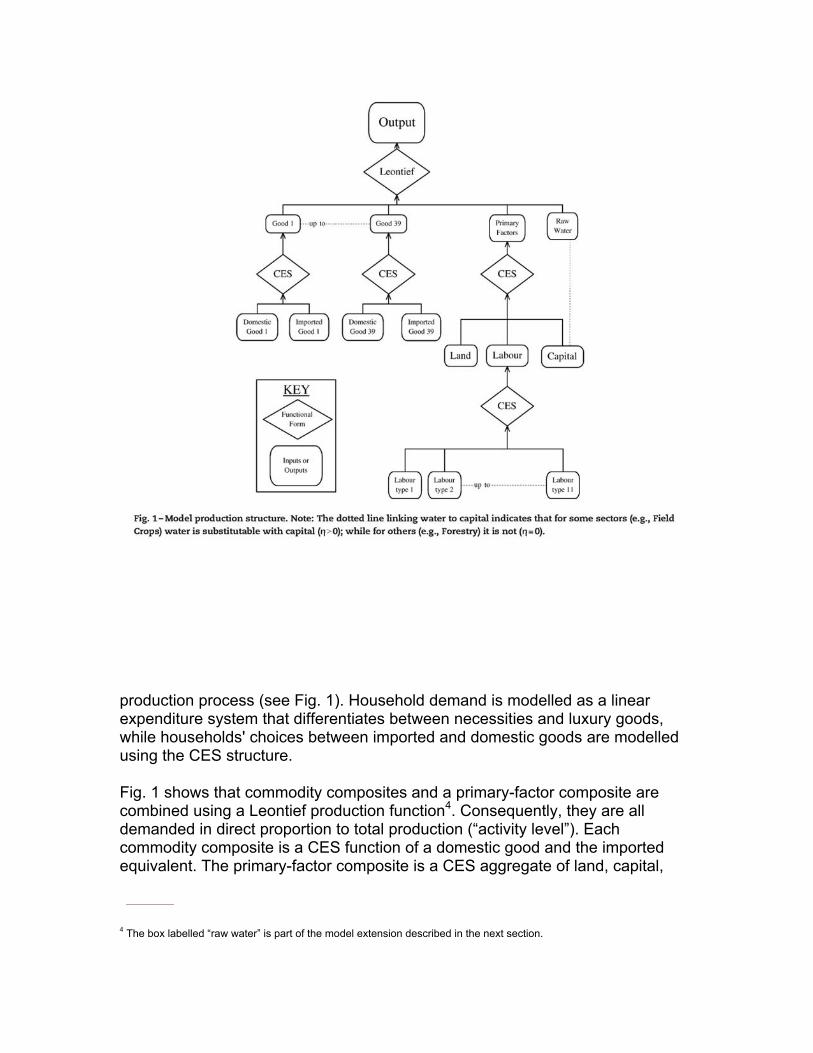
production process (see Fig. 1). Household demand is modelled as a linear expenditure system that differentiates between necessities and luxury goods, while households' choices between imported and domestic goods are modelled using the CES structure.

Fig. 1 shows that commodity composites and a primary-factor composite are combined using a Leontief production function4. Consequently, they are all demanded in direct proportion to total production (“activity level”). Each commodity composite is a CES function of a domestic good and the imported equivalent. The primary-factor composite is a CES aggregate of land, capital,

4 The box labelled “raw water” is part of the model extension described in the next section.

and composite labour. Composite labour is a CES aggregate of occupational labour types. Although all industries share this common production structure, input proportions and behavioural parameters may vary between industries (Horridge, 2002). The elasticities used for the CES functions in the model are summarised in Table 2.

3.1.2. Percent change production equations

At the heart of a CGE model are equations describing industry input demands and output prices. Although details vary, most CGE models assume a “nested” arrangement of CES sub-production functions like that of Fig. 1. Abstracting from details, the production function for one sector may be represented as:

Z=F(X1,X2,X3,…) where Z is output and X1, X2, X3, … are various inputs with prices P1, P2, P3, …. Usually the production function F has the property that if all inputs are doubled, output also doubles. It is assumed that the producer chooses input proportions to minimize the cost of producing given output Z; calculus leads to input demand functions of the form:

Xi=Z G(P1,P2,P3,…) where the G function is invariant to a doubling of all prices. The output price, P, is given by:

P Z=P1X1+P2X2+P3X3…

We could use the demand functions to replace the X terms above, so getting:

P=H(P1,P2,P3…)

Again the H function is homogeneous; if all input prices double, so will output prices. Note that the output price can be expressed as a function of input prices only: this is related to two other important properties that apply near the cost-minimizing choice:

• small changes in input proportions do not affect unit production cost; and

• we can replace a dollars-worth of input i with a dollars-worth of input k, without affecting output.

We use the second property in our water extension, to judge how much of other inputs might be needed to maintain crop output while using less water.

In GEMPACK the input demand equations are represented in percent change5 form as:

xi=z+C1p1+C2p2+C3p3+…

Here, the lower case letters represent small percentage deviations from an initial equilibrium; the C coefficients are called elasticities; they are regarded as locally constant, but in fact are functions of the Xi, and Pi. Such elasticities Cj show the percent change in demand for good i caused by a one percent rise in price of input j, holding output constant. In fact, the equations of the UPGEM model are formulated in terms of small changes. While computationally tractable, the linear equation system is only a local approximation to the non-linear model specification. However, the effects of larger changes can be accurately computed by stepwise integration techniques—in practice this means that the linear equation system is perturbed by a sequence of tiny shocks, all the while updating coefficients like the Cj above.

3.1.3. Incorporating raw water into a CGE system

Could we incorporate raw water demand into the above framework merely by distinguishing water as another input? We can anticipate difficulties, since, unlike the inputs assumed above, raw water is not usually a market good paid for by the gallon, and water users often cannot choose how much water is used. On the contrary, the normal situation is that agricultural water is free (ignoring fixed charges), while the weather and perhaps water authorities limit the amount used. Economic data (prices and quantities) are scarce, and our cost-minimizing assumptions are less useful than usual. We return to this problem below.

3.1.4. Long and short run

UPGEM is a comparative-static model: it does not explicitly track variables through time. Nevertheless, we report below both long run and short run results. The distinction between the two lies in the closure, i.e., in which variables are held constant. We think of the “short run” as about 2 years. For example, for

5 The small changes may be percent, proportional or d(log); the algebra is similar or identical.

short run simulations we hold the capital stock in each industry fixed (while industry rates of return vary): we think that 2 years is not long enough for investment decisions to translate into re-allocation of capital between industries. In contrast, for the long run simulations, we hold rates of return fixed while industry capital stocks vary.

A similar distinction is applied to the labour market. The model differentiates between 11 different labour groups that are classified as either skilled or unskilled. In South Africa there is a shortage of skilled labour and large unemployment of unskilled labour. Trade unions are strong, so wage flexibility is limited. So, for the short run, the supply of unskilled labour is assumed to be perfectly elastic at fixed post-tax real wages (i.e. nominal post-tax wages deflated by the economy-wide CPI). Our long run assumption is that unskilled employment is fixed (or, at least, unaffected by changes in water pricing). Skilled employment is assumed fixed in both short and long run.

How long is the short run? Cooper et al. (1985) approached the question by running parallel simulations using a comparative-static CGE model and an econometrically-based time-series macro model. They asked: which timescale in the macro model gives closest results to the short run results from the CGE model? 2 years seemed a reasonable estimate.

With reference to other macro-economic variables:

• aggregate investment is fixed in the short run, and follows capital stocks in the long run;

• government consumption is fixed in the short run, and follows household consumption in the long run;

• inventories are fixed in the short run, and follow industry output in the long run;

• aggregate household consumption follows wage income in the short run; in the long run it adjusts (with government consumption) to accommodate a fixed (Balance of trade/GDP) ratio;

• the share in aggregate consumption of each household and ethnic group follows their share in post-tax wage income;

• land use in each sector is fixed;

• exporters face a constant elasticity of world demand; and

• imports grow according to local demand and domestic/foreign price relativities.

With fixed government demands, and endogenous tax revenues, an increase in water charges moves the budget towards surplus. We have not modelled an explicit “handback” of water tax revenue. This affects results, and is further discussed below.

3.1.5. The flows database

A standard CGE database consists mainly of a table of flows, showing the expenditures by each industry and final demander on a range of commodities and on primary resources such as capital, labour, and land.

Most of the data for the UPGEM CGE model is drawn from the official 1998 SAM of South Africa, published by Statistics South Africa (SSA, 2001). The SAM divides households into 12 income times 4 ethnic groups, and distinguishes 27 economic sectors. We further disaggregate the energy and water intensive sectors to arrive at a total of 39 sectors6. The official SAM has only one sector for agriculture, but this sector was split into seven sub-sectors in order to be able to determine exactly which water policies would render the best results. The seven sub-sectors of agriculture are: irrigated and dry field crops, irrigated and dry horticultural crops, livestock, forestry, and other agriculture. The weights used for the splits are based on the input–output table of Conningarth (2002). The official SAM includes a water sector, mainly reflecting the cost of municipal water supply. Economic rents associated with water rights—the right to abstract raw water—are not separately distinguished.

3.2. Water extension to CGE model

A small number of changes were made to the existing CGE model, to capture the following effects:

(i) Water demands grow with the output of water users.

(ii) Water tax revenue is proportional to the tax rate and to water use.

(iii) Industries pass on water costs to consumers, so a tax on irrigation water increases the price of crops.

These first three mechanisms could easily be captured by an input–output model, or could be calculated in Excel using results from the standard CGE model. The remaining mechanisms are more sophisticated:

6 Six additional agricultural and six additional energy related sectors were added for two different studies, one on water taxes and one on energy taxes—see also Van Heerden et al. (2006).

(iv) A rise in the price of crops reduces crop demand and hence crop output and irrigation. This mechanism is part of the existing CGE model. It provides a way for a tax on crop irrigation to reduce water use, even if water/output ratios do not change.

(v) If water prices rise, farmers may find ways to reduce water intensity (the water/output ratio). This is another way that a tax may reduce water use.

(vi) A farmer who uses less water may suffer an output loss, or be forced to increase other inputs.

Mechanisms (v), and particularly (vi), are novel in terms of current (2006) water-related CGE modelling. We present the new and modified equations in small change form.

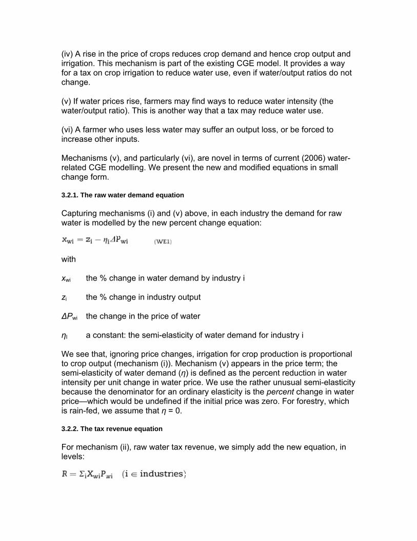
3.2.1. The raw water demand equation

Capturing mechanisms (i) and (v) above, in each industry the demand for raw water is modelled by the new percent change equation:

with xwi the % change in water demand by industry i

zi the % change in industry output

ΔPwi the change in the price of water

ηI a constant: the semi-elasticity of water demand for industry i

We see that, ignoring price changes, irrigation for crop production is proportional to crop output (mechanism (i)). Mechanism (v) appears in the price term; the semi-elasticity of water demand (η) is defined as the percent reduction in water intensity per unit change in water price. We use the rather unusual semi-elasticity because the denominator for an ordinary elasticity is the percent change in water price—which would be undefined if the initial price was zero. For forestry, which is rain-fed, we assume that η = 0.

3.2.2. The tax revenue equation

For mechanism (ii), raw water tax revenue, we simply add the new equation, in levels:

with R total revenue

Pwi the tax on water use by industry i

Xwi water used by industry i

In small change form (noting that ΔX = Xx/100):

3.2.3. The output price equation

We noted above that in a standard CGE model the output price for each industry is determined by levels equations like:

P Z=P1X1+P2X2+P3X3…

Where X1, X2, X3, … are the inputs for some industry. We merely add an additional term to the RHS, representing the cost of the water tax:

P Z=P1X1+P2X2+P3X3…+PwiXw

This implements mechanism (iii), which passes on water costs to crop users.

3.2.4. Increased use of other inputs

So far we have allowed for water tax to be a cost to farmers, who may respond by reducing water/output ratios. The questions arise, does water saving reduce farm yields, or (equivalently) must other inputs be increased to maintain farm output? In other words, do we need mechanism (vi)?

Some CGE modellers have answered “no” to these questions, being content to merely implement mechanisms similar to (i) to (v), as alluded to in Rehdanz et al. (2005). They seem to suggest that a cut in water use is a pure gain to the farmer, since water charges are avoided. Perhaps they feel that water is often so cheap that farmers waste it; and that this waste could be eliminated with little or no cost. This view might be resented by farmers, is inconsistent with the theory of cost minimization, and becomes less plausible as water prices are raised; Berrittella et al. (2007), however, corrected this in a later version of their model. Here we assume that to maintain output, lost water must be replaced by other inputs, in particular capital. Our thought is that better irrigation equipment may squeeze more benefit from remaining water. The higher are water prices, the more economic it would be to invest in such equipment.

Following the form noted above, our model's capital demand equation for one industry has the percent change form:

k=z+C1p1+C2p2+C3p3+…

We add to the RHS an additional substitution term, ε—the per cent increase in capital demand due to the change in water price7. To derive this additional term, we draw on the principle explained previously, that for a cost minimizer, substitution is costless at the margin. That is, the saving in water tax from using less water is just balanced by the cost of using more capital. Using the equations above we can see that the water cost saving is:

−PwXwxw/100=PwXwηΔPw/100.

This will equal the cost of extra capital, given by PkXkε/100 so PkXk=PwXwηΔPw

So our capital demand equation is augmented by the additional RHS price term, ε8:

Note that this additional input need, will indeed be negligible while the water charge Pw is tiny; it becomes more important as the water price rises. The substitution between capital and water is indicated by a dotted line in Fig. 1.

3.2.5. Additional data required

To implement our water modifications, we added 3 vectors to this conventional flows database. In principle, for each industry these showed:

• the quantity of “taxable water” used. This roughly corresponds to raw water abstracted from rivers, but also includes rain falling on tree plantations.

• a semi-elasticity showing how water intensity (water per output) might change in response to a change in volumetric water charges. For this paper we need a value only for Irrigated Field Crops (IFC)—we assume Forests cannot adjust their rainfall.

7 Our modification to the capital demand equations affects only those industries for which the water price changes and for which η is non-zero. So it applies here to Field Crops but not to Forestry. 8 The additional term ε does not enter into the labour-capital-land nest depicted in Fig. 2. The implication is that capital used for pipes and pump competes with the use of capital for other purposes.

• expenditure on volumetric raw water charges. We assumed these to be initially zero (i.e., existing charges are mainly fixed).

Column 2 of Table 3 shows quantities of water used. It is closely related to Table 1—they are based on the same data. Column 1 indicates three main types of sector. Those marked A are agricultural—large users of water who pay little in the form of volumetric charges. Those marked B are bulk users of non-potable water. We have distributed the raw water used by the (municipal) water industry among remaining industrial and household users of treated water. For forestry we have incorporated an estimate of the streamflow loss caused by thirsty foreign trees (as compared to native scrub). The final rows of Table 3 enable reconciliation with the last column of Table 1.

Column 3 of Table 3 shows a range of elasticity estimates from various sources. As discussed earlier, we would like to interpret these as the proportional change in water use per proportional change in the marginal cost of water. If, as we claim, charges paid by agricultural uses are mainly fixed (i.e., an extra cubic meter costs nothing), it is difficult to see how the agricultural estimates could have been derived. To interpret the elasticity for IFC (the only elasticity needed for this paper) we imagined that it assumed that the existing fixed levies paid by IFC (averaging 5 cents/m3) were in fact volumetric charges. In that case, an additional volumetric charge of 10 cents/m3 implies a 200% price increase. The implied semi-elasticity is 5009.

4. Model simulation results

We use the integrated model to simulate and compare two policy scenarios,

namely (i) a 10 cents/m3 streamflow reduction charge on the Forestry Industry,

and (ii) a 10 cents/m3 tax on untreated water used by the IFC industry. Water

authorities are considering both scenarios. More specifically, we compare the two

instruments in the short and long run, and compare their respective impacts on

(a) water saving, (b) economic growth, and (c) consumption of the poor in

9 To assess the plausibility of this number, note (in the results below) that substitution causes the 10 cents water charge to reduce water intensity in IFC by 30%, and increases production costs by 25%. Indeed our elasticity estimate is speculative, but it is based on an extensive literature search, and the sources are listed below Table 3. There are three main reasons for this:(a) Agricultural water use is often un-priced and crudely measured. There is not much to observe.(b) Suppose we did estimate an elasticity in a region or sector where water prices could be observed. It is difficult to apply this elasticity to another region or sector where initially water prices are zero. Our semi-elasticity approach tackles this problem. A similar approach is the so-called production elasticity: the proportional change in water use per [proportional change in total production cost attributable to new water charges]. Our semi-elasticity implies a production elasticity of – 1.2.(c) Elasticities are essentially point estimates of the curvature of a production function isoquant. Economists like to assume they are fixed within a relevant range. However, the situation where water is free is an extreme case, perhaps unrepresentative of behaviour when water is priced.

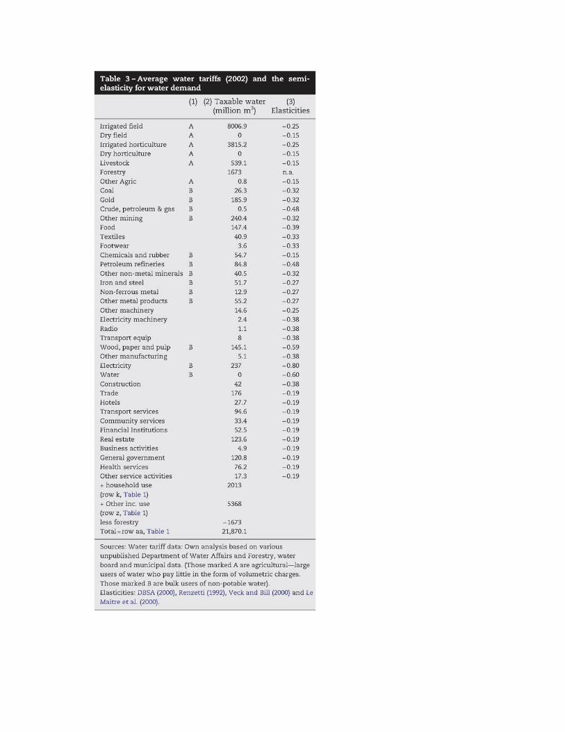
Table 3-Average water tarirrs (2002) and the semi­elasticity for water demand

(1) (2) Taxable water (3)(million m 3) Elasticities

Irrigated field A 8006.9 -0.25

Dry field A 0 -0.15Irrigated horticulture A 3815.2 -0.25Dry horticulture A 0 -0.15

Livestock A 539.1 -0.15Forestry 1673 n.a.Other Agric A 08 -0.15Co~ 8 26.3 -0.32

Gold 8 185.9 -0.32

Crude. petroleum & gas 8 05 -0.48Other mining 8 240.4 -0.32l'ood 147.4 -0.39

Textiles <0.9 -0.33Footwear 36 -0.33Chemicals and rubber 8 54] -0.15Petroleum refineries 8 ".8 -0.48Other non-metal miner;lis 8 <0.5 -0.32Iron and steel 8 51.7 -0.27Non-ferrous metal 8 12.9 -0.27Other metal products 8 55.2 -0.27

Other machinery 14.6 -0.25l:lectricity machinery- " -0.38Radio " -0.38Transpon equip 8 -0.38

Wood, paper and pulp 8 145.1 -0.59Other manufacturing 5' -0.38l:lectricity 8 '" -0.80Water 8 0 -0.60

Construction " -0.38

Trod. ,>6 -0.19Hotels 27.7 -0.19Transpon services 9<.6 -0.19

Community services 33.4 -0.19Financial Institutions 52.5 -0.19

Real estate 123.6 -0.19Business activities '.9 -0.19

General govemment 120.8 -0.19

Health services 76.2 -0.19Other service activities 17.3 -0.19... household use 2013(row k, Table 1)... Other inc. use 5368(row z, Table 1)less forestry- -1673Tot;li:row aa, Table 1 21,870.1

Sources: Water tariff data: Own analysis based on variousunpublished Department of Water Affairs and Forestry, waterboard and municipal data, (Those marked A are agricultural-largeusers of water who pay little in the form of volumetric charges.Those marked B are bulk users of non-potable water).I:lasticities: OSSA (2000), Renzetti (1992), Veck and Sill (2000) and LeMaitre et al. (2000).

South Africa. We are not only interested in decreasing water demand, but also seek a policy that slows economic growth as little as possible, and does not harm the poor. Full details of such a ‘triple dividend’ strategy and the measurement of triple dividend indicators are provided in Van Heerden et al. (2006). We first present the short run results, followed by the long run. Much uncertainty is attached to the semi-elasticity used in our water demand equation. Without a market in water, it is difficult to estimate such elasticities. Accordingly, we provide alternate simulations for IFC, in which the semi-elasticity is assumed to be zero. For Forestry, we always assume that the semi-elasticity is zero—since it is rain-fed, there is little scope to vary water use.

4.1. Short run simulation results

Changes in each target variable are expressed per change of government revenue, so that different policy scenarios could easily be compared to each other on the basis of equal extra tax revenues.

The marginal excess burden is defined as the decrease in real GDP divided by the increase in real government income10. We report on all three target

10 The marginal cost of public funds (MCPF) is equal to 1 + marginal excess burden (MEB).

variables, water demand, real GDP, and real consumption by the poor, in Table 4.

From the results in Table 4 we conclude that a 10 cents tax on water demanded by IFC leads to better results for all three the target variables than would the streamflow reduction charge on Forestry. The MEB's are smaller with IFC (row 17); the water saving per unit of government revenue larger (row 18); and the reduction in poor consumption per unit of government revenue also smaller (row 19). These are all desired results, namely, smaller negative effects of a new tax on real GDP, but a higher environmental dividend, and a smaller effect on real consumption of the poor.

In absolute terms it is not so obvious that the tax on IFC fares better with respect to all three the target variables. Both real GDP and poor consumption decrease more (rows 11 and 14 respectively), while only the total amount of water saved is higher (row 12). However, we should scale the target variables before comparing them. Row 16 shows that the two taxes, even though they are of the same order of magnitude, result in completely different amounts of government revenue raised. This is because the IFC industry uses much more water than Forestry. The same tax affects real GDP much more because the industry is so much larger. But if we compare the target variables per Rand revenue collected, the comparison is more accurate.

The marginal excess burdens are reported in row 17 of Table 4. The change in real GDP occurs in the numerator, so that a smaller number here is better. The tax on Forestry harms the economy by 21.3 cents real GDP per Rand collected, while the tax on IFC is less harmful, since for each Rand that the government collects, real GDP decreases by 14.9 cents. The reasons for the decrease in real GDP are that the new taxes (i) cause prices to rise, which causes the unskilled wage rates to rise, causing unskilled employment to fall—this is the main reason that GDP falls; (ii) raise production costs, which reduces export demands, and makes imports more attractive; (iii) raise tax revenue, which, if not handed back, reduces purchasing power and a contraction in total demand. (Van Heerden et al., 2006).

The MEB for the tax on IFC is lower than for Forestry in the short run, because the latter employs much more unskilled labour relative to other factors of production. Unskilled labour comprises 19.6 per cent of Forestry's input costs, but only 4.6 per cent of Irrigated Field Crops. Since unskilled labour is the only variable factor of production in the short run, the effect of the new tax on GDP, as measured by the MEB, is greater for Forestry.

The last row in Table 4 shows the percent change in real consumption by the poorest household group per unit of real government revenue. The result follows that of the marginal excess burdens in the short run: the tax on Forestry is again worse for the poorest group in that their consumption per unit of government

revenue collected decreases more than with a tax on IFC. The reason is that total consumption by the poorest household group also depends mostly on the total wage income of the unskilled, which shrinks proportionately more in Forestry.

4.2. Recycling the revenue

In the double dividend literature the revenue from a new tax would be recycled, perhaps by reducing other taxes. The environmental, economic and equity effects of the tax could then be compared to the respective effects of recycling the (same) revenue, to see whether net benefits would occur. That is why we calculate the different effects per unit of real government revenue.

To show this we included in Table 4 (Column 4) the effects of a decrease in indirect taxes paid by households that just offset the extra R441 m (row 16) of revenue from the IFC tax. The tax handback causes a GDP increase of R56.7 m (row 11), which does not offset the decrease in real GDP of R61.4 m from the IFC tax. Similarly, other target variables could be compared to find the net effects of combined tax and recycling schemes. However, it is not necessary to show the recycling effects to know which water tax would fare better when recycled.

4.3. Long run simulation results

Table 5 below reports results from the same shocks using a long run closure of the model. Short and long run closures make different factor supply assumptions: in the short run capital is fixed, while in the long run it adjusts to earn a set rate of return. Also, the trade balance is fixed in the long run. Changes in each target variable are still expressed per change of government revenue.

Capital movement is key to long run results since it is the variable factor of production. IFC is more capital intensive and shows a larger MEB. Table 5 shows that in the long run the SFR charge on Forestry betters the tax on IFC for two of the three target variables. The MEB's show that for each Rand collected from IFC, real GDP will decrease by almost R1, while the MEB for Forestry is only 31 cents (row 17). Also, consumption by the poor decreases more with IFC taxed than with Forestry (row 19). Water use is the only target variable where IFC gives better results for both short and long run; more water is saved in absolute or relative terms (per Rand raised) by taxing IFC than taxing Forestry (rows 12 and 18). As in the short run, this is because we assumed that IFC could reduce water intensity, while Forestry cannot (η = 0).

The last row in Table 5 shows the percent change in real consumption by the poorest household group per unit of real government revenue. Forestry has a

better result for the poor, because they employ less capital relative to IFC, and hence we find the opposite results from the short run.

4.4. Sensitivity analysis

To test the sensitivity of our results we ran all the IFC tax simulations using two different elasticities of IFC water demand, as reported in the first two columns of Table 4 and Table 5. The leftmost columns of the two Tables show the results for the tax on IFC if the elasticity of demand for water were 0.25, as suggested by the CSIR in Table 3. The middle column results show what would happen if the demand for water has an elasticity of zero. The elasticity assumed for Forestry is zero (see Column 3 of Table 4 and Table 5).

The IFC/Forestry rankings above for short and long run do not change if the IFC elasticity is zero. In the short run IFC fares better, whether the elasticity is 0 or 0.25 (or anything between). The long run orderings are also robust, namely that the MEB and equity targets are better for Forestry, while IFC would save more water—whether its elasticity is 0 or 0.25.

5. Conclusions

In this paper we presented a CGE model, which we extended by integrating physical water flows and tax functions into the model. Thus we can advise water policy makers on the use of market instruments to reduce water demand in two of the most water-intensive sectors. The CGE model was needed to assess the economy-wide impacts of a water demand reduction policy, using water charges. We further included excess burdens and equity considerations into the model.

We ran long run and short run simulations for two industries, Forestry and Irrigated Field Crops (IFC), and compared three target variables for each pair of simulations, namely (i) the decrease in total demand for water (environment), (ii) the decrease in real GDP (economy) and (iii) the decrease in real consumption by the poorest household group (equity). All the variables are divided through the change in real government revenue to find the target variables per Rand of net government revenue collected. Standardising the target variables like this allows us to compare different scenarios with each other.

Closure rules, as well as water demand elasticities, strongly influence model results. Yet one result is robust. A tax on IFC would always save more water per Rand collected than a tax on Forestry, whether we are interested in the short run or long run. Even with an elasticity of zero for both industries, a tax on IFC would save relatively more water.

The IFC water tax does less harm (than Forestry) to both GDP and poor consumption in the short run. These two target variables are driven by unskilled employment, and IFC employs proportionately much fewer unskilled workers than Forestry. In the long run the ranking for both effects is reversed—because IFC uses more capital, which is now the variable factor of production.

5.1. Policy recommendations

Water policy should not be short-term. Hence we should look at the long run simulations for policy guidance. However, their message is not clearcut.

If the water tax aims only to cut water use, then we should levy a tax on IFC, since that will save at least twice as much water in absolute terms, and save more water per Rand collected. However, wider economic and social criteria may be of concern. The IFC tax will harm the economy more, in terms of GDP per Rand collected, as well as the consumption levels of poor households.

5.2. Research agenda: improving detail in sectoral, temporal and spatial dimensions

This paper uses a CGE model of South Africa, based on the national SAM. We added water equations and water data vectors, to do the simulations. To a water

engineer, our treatment would seem over-simplified. A more realistic model would also offer more to the policy-maker. We could add detail by:

• incorporating more sectors. A finer breakdown of crop types, with different water needs, would be useful. With more crops, we would need to address the issue of crop switching.

• incorporating regional differences. Water scarcity, climate and crop types often vary a lot within a country. One difficulty is that the regions for which economic data are collected (e.g., provinces) may correspond poorly to river watersheds or climatic zones. Several studies provide a precedent: Chou et al. (2002) use a multi-regional CGE model to address water supply issues in Taiwan, where political regions luckily correspond (roughly) to river watersheds. Young et al. (2006) analyse region-specific water pricing strategies using the Australian TERM CGE model. It distinguishes 56 regions of Australia, which may be grouped to match river basins. Such models require regionalized water accounting data-like that described by (Brouwer et al., 2005).

• Water supply varies greatly during the year, and between years. During a monsoon, water may be so abundant that its scarcity value is zero—at other times water is precious. This presents difficult modelling (and data) challenges. Dams offer the chance to shift rainfall between seasons—introducing a time dimension. Annual rainfall variations (perhaps also alleviated by dams) point to the need for a stochastic approach. Temporal variation is closely linked to the sectoral and regional mentioned above: different crops require water in different seasons, and seasonal patterns will vary by region.

For South African CGE modelling of water use, we anticipate that progress will first be made by adding sectoral and regional detail. To build in a finer breakdown of crops, and regions approximating water basins would be both useful and achievable.

References

Aronson,J., Blignaut,)., Milton,]., Clewell, A., 2006. Natural capital: the limiting factor. Ecological Engineering 28,1-5.

Ashton, P.J., Haasbroek, B., 2002. Water demand management and social adaptive capacity: A South African case study. In: Turton, A.R., Henwood, R. (Eds.) Hydropolitics in the Developing World: A Southern African Perspective. African Water Issues Research Unit (AWIRU) and International Water Management Institute (IWMI), 24 pp.

Ashton, P.J., Seetal, A., 2002. Challenges of water resource management in Africa. African Renais-Science Conference, Durban, 12-15 March.

Berrittella, M., Hoekstra, A.Y., Rehdanz, K., Roson, R., Tol, R.S.J., 2007. The economic impact of restricted water supply: a computable general equilibrium analysis. Water Research 42,1799-1813.

Brouwer, R., Schenau, S., van der Veeren, R., 2005. Integrated river basin accounting and the European Water Framework Directive. Statistical Journal of the United Nations Economic

Commission for Europe 22 (2), 111-131. Cai, X., McKinney, D.C., Rosegrant, M.W., 2003. Sustainability analysis for irrigation water

management in the Aral Sea region. Agricultural Systems 76, 1043-1066. Chou, C, Hsu, S., Li, P., 2002. Impact on demand for water upon entering WTO—a Taiwanese

case study, paper presented at the 5th Annual Conference on Global Economic Analysis, Taipei, Taiwan.

Conningarth Consulting, 2002. Disaggregated Social Accounting Matrix for South Africa. Conningarth, Pretoria. Unpublished research report.

Cooper, R., McLaren, K., Powell, A., 1985. Macroeconomic closure in applied general equilibrium modelling: experience from ORANI and agenda for further research. In: Piggot, J., Whalley, J. (Eds.), New Developments in Applied General Equilibrium Analysis. Cambridge University Press.

CSIR, 2001. Water resource accounts for South Africa. Report to Statistics South Africa and The Department of Environment Affairs and Tourism. Report number ENV-P-C 2001-050.

DBSA, 2000. Environmental impacts of the forestry sector in South Africa with specific reference to water resources. CSIR Report: ENV-P-C 99016.

Diao, X., Roe, T., 2003. Can a water market avert the "double-whammy" of trade reform and lead to a "win-win" outcome? Journal of Environmental Management and Economics 45, 708-723.

DWAF (Department of Water Affairs and Forestry), 1998. National Water Act for South Africa. DWAF, Pretoria. DWAF (Department of Water Affairs and Forestry), 2004. National Water

Resource Strategy. September, Pretoria. Falkenmark, M., 1994. The dangerous spiral: near-future risks for water-related eco-conflicts.

Proceedings of the ICRC Symposium Water and War: Symposium on Water in Armed Conflicts, International Committee of the Red Cross, Montreux, Switzerland, 21-23 November. 16 pp.

Grosskopf, M., 2004. Towards internalising the cost of water pollution. In: Blignaut, J., De Wit, M. (Eds.), Sustainable options. UCT Press, Cape Town.

Horridge, M., 2002. ORANI-G: a generic single-country computable general equilibrium model. Edition prepared for the Practical GE Modelling Course, June 17-21, 2002.

King, N.A., 2002. Valuing a city's water: the case of Tshwane. Dissertation for masters degree, obtained from the University of Pretoria.

Landell-Mills, N., Porras, IT., 2002. Silver bullet or fools' gold? A global review of markets for forest environmental services and their impacts on the poor. London, Instruments for Sustainable Private Sector Forestry Series. International Institute for Environment and Development.

Le Maitre, D.C., Versveld, D.B., Chapman, R.A., 2000. The impact of invading alien plants on surface water resources in South Africa: a preliminary assessment. Water SA. 26 (3), 397-408.

Letsoalo, A., Blignaut, J., de Wet, T., de Wit, M., Hess, S., Tol, R.S.J., Van Heerden, J.H., 2007. Triple dividends of water consumption charges in South Africa. Water Resources Research. 43, W05412.

National Treasury, 2006. A Framework for Considering Market-based Instruments to Support Environmental Fiscal Reform in South Africa. National Treasury, Pretoria.

Pagiola, S., Bishop, J., Landell-Mills, N., 2002. Selling Forest Environmental Services. Earthscan.

Rehdanz, K., Berrittella, M., Roson, R., Tol, R.S.J., 2005. Water scarcity and world trade: a computable general Equilibrium approach, paper presented at the 8th Annual Conference on Global Economic Analysis, 2005 Liibeck, Germany.

Renzetti, S., 1992. Estimating the structure of industrial water demands: the case of Canadian manufacturing. Land Economics 68 (4).

Roe, T., Dinar, A., Tsur, Y., Diao, X., 2005. Feedback links between economy-wide and farm- level policies: with application to irrigation water management in Morocco. Journal of Policy Modeling 27, 905-928.

Rosegrant, M.W., Ringler, C, McKinney, D.C., Cai, X., Keller, A, Donoso, G, 2000. Integrated economic-hydrologic water modeling at the basin scale: the Maipo river basin. Agricultural Economics 24, 33-46.

Scholes, R., 2001. Global Terrestrial Observing System: Regional Implementation Plan for Southern Africa. GTOS-21.

Smakhtin, V., Ashton, P.J., Batchelor, A., Meyer, R., Maree, J.P., Murray, M., Barta, B., Bauer, N., Terblanche, D., Olivier, J., 2001. Unconventional water supply options in South Africa: possible solutions or intractable problems? Water International 26 (3), 314-334.

Statistics South Africa (SSA), 2001. Social Accounting Matrix for South Africa. Statistics South Africa, Pretoria.

Thompson, M.W., 1999. South African Land-cover Database project, Data Users Manual Final Report (Phases 1, 2 and 3). Unpublished CSIR Report ENV/P/C 98136. Pretoria.

Van Heerden, J.H., Gerlagh, R., Blignaut, J., Horridge, M., Hess, S., Mabugu, R., Mabugu, M., 2006. Searching for triple dividends in South Africa: fighting C02 pollution and poverty while promoting growth. Energy Journal 27 (2), 113-142.

Veck, G.A., Bill, M.R., 2000. Estimation of the residential price elasticity of demand for water by

means of a contingent valuation approach. Water Research Commission Report No: 790/1/00. .

Young, M., Proctor, W., Qureshi, E., Wittwer, G., 2006. Without water: the economics of supplying water to 5 million more Australians. Water for a Healthy Country Flagship report. CSIRO and Monash University. Melbourne, Victoria, Australia. 57 pp.