Integrated earth system dynamic modeling for life cycle impact assessment of ecosystem services
11
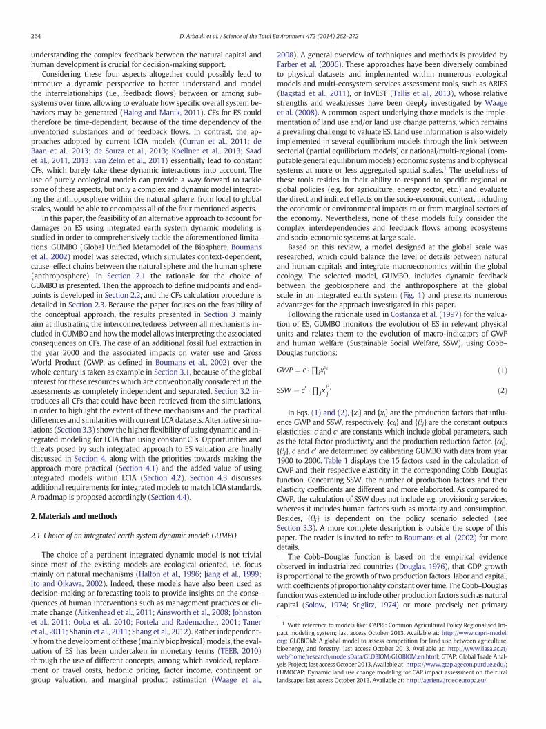
Integrated earth system dynamic modeling for life cycle impact assessment of ecosystem services Damien Arbault a,b,c,d , Mylène Rivière a,b,c,d , Benedetto Rugani a , Enrico Benetto a, ⁎, Ligia Tiruta-Barna b,c,d a Public Research Centre Henri Tudor/Resource Centre for Environmental Technologies, 6A avenue des Hauts-Fourneaux, L-4362 Esch-sur-Alzette, Luxembourg b Université de Toulouse, INSA, UPS, INP, LISBP, 135 Avenue de Rangueil, F-31077 Toulouse, France c INRA, UMR792, Laboratoire d'Ingénierie des Systèmes Biologiques et des Procédés, F-31400 Toulouse, France d CNRS, UMR5504, F-31400 Toulouse, France HIGHLIGHTS • Current LCIA models do not fully consider Ecosystem Services. • The use of integrated dynamic model- ing is investigated to overcome this limitation. • Preliminary results retrieved from the metamodel GUMBO are presented. • Outcomes and limitations are discussed and a roadmap is elaborated. GRAPHICAL ABSTRACT abstract article info Article history: Received 1 July 2013 Received in revised form 24 October 2013 Accepted 27 October 2013 Available online 28 November 2013 Keywords: Life Cycle Impact Assessment (LCIA) Life Cycle Assessment (LCA) Dynamic modeling Ecosystem Services (ES) Integrated modeling Global Unified Metamodel of the Biosphere (GUMBO) Despite the increasing awareness of our dependence on Ecosystem Services (ES), Life Cycle Impact Assessment (LCIA) does not explicitly and fully assess the damages caused by human activities on ES generation. Recent improvements in LCIA focus on specific cause–effect chains, mainly related to land use changes, leading to Characterization Factors (CFs) at the midpoint assessment level. However, despite the complexity and temporal dynamics of ES, current LCIA approaches consider the environmental mechanisms underneath ES to be indepen- dent from each other and devoid of dynamic character, leading to constant CFs whose representativeness is debatable. This paper takes a step forward and is aimed at demonstrating the feasibility of using an integrated earth system dynamic modeling perspective to retrieve time- and scenario-dependent CFs that consider the complex interlinkages between natural processes delivering ES. The GUMBO (Global Unified Metamodel of the Biosphere) model is used to quantify changes in ES production in physical terms – leading to midpoint CFs – and changes in human welfare indicators, which are considered here as endpoint CFs. The interpretation of the obtained results highlights the key methodological challenges to be solved to consider this approach as a robust alternative to the mainstream rationale currently adopted in LCIA. Further research should focus on increasing the granularity of environmental interventions in the modeling tools to match current standards in LCA and on adapting the conceptual approach to a spatially-explicit integrated model. © 2013 Elsevier B.V. All rights reserved. Science of the Total Environment 472 (2014) 262–272 ⁎ Corresponding author. Tel.: +352 425 991 6603; fax: +352 425 991 555. E-mail address: [email protected] (E. Benetto). 0048-9697/$ – see front matter © 2013 Elsevier B.V. All rights reserved. http://dx.doi.org/10.1016/j.scitotenv.2013.10.099 Contents lists available at ScienceDirect Science of the Total Environment journal homepage: www.elsevier.com/locate/scitotenv
Transcript of Integrated earth system dynamic modeling for life cycle impact assessment of ecosystem services
Science of the Total Environment 472 (2014) 262–272
Contents lists available at ScienceDirect
Science of the Total Environment
j ourna l homepage: www.e lsev ie r .com/ locate /sc i totenv
Integrated earth system dynamic modeling for life cycle impactassessment of ecosystem services
Damien Arbault a,b,c,d, Mylène Rivière a,b,c,d, Benedetto Rugani a, Enrico Benetto a,⁎, Ligia Tiruta-Barna b,c,d
a Public Research Centre Henri Tudor/Resource Centre for Environmental Technologies, 6A avenue des Hauts-Fourneaux, L-4362 Esch-sur-Alzette, Luxembourgb Université de Toulouse, INSA, UPS, INP, LISBP, 135 Avenue de Rangueil, F-31077 Toulouse, Francec INRA, UMR792, Laboratoire d'Ingénierie des Systèmes Biologiques et des Procédés, F-31400 Toulouse, Franced CNRS, UMR5504, F-31400 Toulouse, France
H I G H L I G H T S G R A P H I C A L A B S T R A C T
• Current LCIAmodels do not fully considerEcosystem Services.
• The use of integrated dynamic model-ing is investigated to overcome thislimitation.
• Preliminary results retrieved from themetamodel GUMBO are presented.
• Outcomes and limitations are discussedand a roadmap is elaborated.
⁎ Corresponding author. Tel.: +352 425 991 6603; fax:E-mail address: [email protected] (E. Benetto).
0048-9697/$ – see front matter © 2013 Elsevier B.V. All rihttp://dx.doi.org/10.1016/j.scitotenv.2013.10.099
a b s t r a c t
a r t i c l e i n f oArticle history:Received 1 July 2013Received in revised form 24 October 2013Accepted 27 October 2013Available online 28 November 2013
Keywords:Life Cycle Impact Assessment (LCIA)Life Cycle Assessment (LCA)Dynamic modelingEcosystem Services (ES)Integrated modelingGlobal Unified Metamodel of the Biosphere(GUMBO)
Despite the increasing awareness of our dependence on Ecosystem Services (ES), Life Cycle Impact Assessment(LCIA) does not explicitly and fully assess the damages caused by human activities on ES generation. Recentimprovements in LCIA focus on specific cause–effect chains, mainly related to land use changes, leading toCharacterization Factors (CFs) at the midpoint assessment level. However, despite the complexity and temporaldynamics of ES, current LCIA approaches consider the environmental mechanisms underneath ES to be indepen-dent from each other and devoid of dynamic character, leading to constant CFs whose representativeness isdebatable. This paper takes a step forward and is aimed at demonstrating the feasibility of using an integratedearth system dynamic modeling perspective to retrieve time- and scenario-dependent CFs that consider thecomplex interlinkages between natural processes delivering ES. The GUMBO (Global Unified Metamodel of theBiosphere) model is used to quantify changes in ES production in physical terms – leading to midpoint CFs –
and changes in human welfare indicators, which are considered here as endpoint CFs. The interpretation of theobtained results highlights the key methodological challenges to be solved to consider this approach as a robustalternative to the mainstream rationale currently adopted in LCIA. Further research should focus on increasingthe granularity of environmental interventions in the modeling tools to match current standards in LCA and onadapting the conceptual approach to a spatially-explicit integrated model.
© 2013 Elsevier B.V. All rights reserved.
+352 425 991 555.
ghts reserved.

263D. Arbault et al. / Science of the Total Environment 472 (2014) 262–272
1. Introduction and goals
Ecosystem Services (ES) result from ecosystem functions (Burkhardet al., 2012; de Groot et al., 2012; Costanza et al., 1997; Daily, 1997),which are ‘the capacity of natural processes and components to providegoods and services that satisfy human needs, directly or indirectly’ (deGroot et al., 2002). Over the last 15 years, scientific studies flourished inthe economic and biophysical valuation of ES (e.g. Gómez-Baggethunet al., 2010; TEEB, 2010). In particular, theMillennium Ecosystem Assess-ment (MEA) classified four categories of ES (MEA, 2005): provisioning,regulating, cultural and supporting services. The MEA has representedthe consensual umbrella for all the ES valuation approaches developed af-terwards. For example, The Economics of Ecosystems and Biodiversity(TEEB) approach, which is one of the most recommended frameworksto target ES and pursuing their benefits, especially at the country scale,incorporates many of the concepts, classification schemes and criteriadeveloped by MEA (TEEB, 2010). However, valuing the contribution ofES to human welfare demands robust methods to define and quantifyES (Crossman et al., 2013), especially if the accounting perspective aimsto address both economic, environmental and social (triple-bottom-line) aspects (Crossman et al., 2013; Cardinale et al., 2012; de Grootet al., 2010; Haines-Young et al., 2012; Maes et al., 2013).
Focusing on the environmental dimension, the growing interest forES valuation has permeated the larger environmental assessmentfield, and namely Life Cycle Assessment (LCA), which is awidely accept-ed methodology to evaluate the environmental impacts of a product orservice throughout its life cycle (ISO, 2006). Within LCA, the Life CycleImpact Assessment (LCIA) step translates the elementary flows (re-sources consumed and pollutants emitted) into environmental impacts,which are either problem-oriented (midpoint approach) or damage-oriented (endpoint approach) (European Commission, 2010a). To thisaim, so-called characterization factors (CFs) are developed using impactassessment models, reflecting the values associated with three mainAreas of Protection (AoP): Human Health (HH), Natural Resources(NR), and Natural Environment (NE). Whereas there is scientific con-sensus on the scope of HH, the evaluation of NR and NE remains debat-able, because of the intrinsic cross-linkages between the two areas (deBaan et al., 2013; European Commission, 2010b). The AoP of NR shouldcover the damage associated with the exploitation of natural resources,which can affect the delivering of ES. However, LCIA indicators (and re-lated CFs) have essentially been developed with regard to the useful-ness of natural resources for human purposes (see e.g. EuropeanCommission, 2010b, for a comprehensive list and analysis). Most ofthe indicators focus on the assessment of mineral and fossil resourcescarcity, by evaluating the future marginal cost of extraction/use ofthese resources. With regard to the AoP of NE, the aim is to quantifythe negative effects on the function and structure of natural ecosystemsas a consequence of the exposure to chemicals or other physical inter-ventions (European Commission, 2010b).
Recent researches have addressed the link among elementary flowsof Life Cycle Inventory (LCI) (mainly land occupation and land transfor-mation) and novel LCIA midpoint impact categories called ‘potentialdamage on Ecosystem Services’ (Koellner et al., 2013). Accordingly, spa-tially differentiated CFs were developed to assess potentials of e.g. bio-diversity damage (de Baan et al., 2013) climate regulation (Müller-Wenk and Brandão, 2010), biotic production (Brandão and Milà iCanals, 2013), erosion and freshwater regulation andwater purification(Saad et al., 2013), andwater supply from groundwater (van Zelm et al.,2011). The assessment of functional diversity within the different taxo-nomic groups of mammals, birds and plants was recently proposed as acomplement to the assessment of species richness (de Souza et al.,2013).While highlighting the lack of completeness of existing LCI data-bases, one of the main objectives reached is the definition, harmoniza-tion and ranking of a large set of land use and land use changeelementary flows created as a common inventory database for bothglobal and local (regionalized) assessments of ES, which can be directly
used in the LCIA practice. Other research streams have tried to integrateLCA with the emergy concept and method (Odum, 1996), providing anexplicit LCIA of ES that underlies a pure ecological orientation(Marvuglia et al., 2013; Rugani et al., 2013). However, this approach isnot fully operational yet because of some computational and systemboundary constraints associated with the combination of the twomethods, further hampered by a lack of consensus on emergy in theLCA community (Arbault et al., 2013; Raugei et al., in press).
The insufficient coverage of ES in the current LCIA practice (Zhanget al., 2010; Curran et al., 2011; de Baan et al., 2013) is hampering theconsistent application of LCA to a number of sectors which are very con-cerned by ES, e.g. agriculture. Despite the significant breakthrough ofthe recently developedmethods, four aspects were identified deservingfurther attention.
First, cause–effect chains originating from land occupation and trans-formation are modeled independently (Koellner et al., 2013), i.e. withoutconsidering the interconnections between the mechanisms of naturalprocesses. It is widely recognized that natural processes influence eachother in many complex and indirect ways and that indirect effects canbe delayed in time and widespread over the globe (Folke et al., 2011).This is therefore a significant simplification, as for instance an increasedterrestrial acidification is likely to alter the biological properties of soil,thus changing local biodiversity, which in turnmay change the sensitivityof ecosystems to toxic substances. CFs should thus not be constant, buttime dependent as a function of all emitted inventoried substances overtime.
Second, environmental mechanisms are investigated up to the mid-point level, whose impacts are expressed in physical units (Koellneret al., 2013). However, ES is a user-oriented concept, which has beendeveloped to assess the benefits that human societies yield from nature.Although the health of ecosystems can be measured in physical terms,benefits are commonly expressed in terms closer to human values,such as economic development or contribution to welfare (MEA,2005; de Groot et al., 2002; Costanza et al., 1997; TEEB, 2010). As aresult, the investigation should include also endpoint targets.
Third, the potential damages in LCIA are usually assessed by adoptinga marginal and short time perspective (Goedkoop et al., 2009). The focusis therefore on how the current state of ecosystems would be altered, inthe short term, by a perturbation, usually defined at local scale and in asimplistic manner, because of the granularity of LCI databases. An exam-ple could be the assessment of the effects of occupying a small piece ofland on the local species diversity during a short period. As a result, onlymarginal effects occurring right after the perturbation are included.Such an approachmisses the holistic perspective, inwhich environmentalmechanisms are influencing each other at various spatial scales and withboth short-term and long-term effects. A more comprehensive analysisshould therefore include, for instance, the effects on global climate changeto local water regulation and soil erosion during the next decades.
Fourth, nature and mankind interact in many complex ways.Human-driven systems use natural resources and generate waste andemissions that can affect the ecosystems. The production of ES occursat a limited pace. Over-exploitation of renewable resources may leadto a complete collapse of the local ecosystem. In turn, a degradation ofthe natural environment may challenge human welfare, so that inorder to sustain our living standards we may need to extract more re-newable resources, leading to even higher degradation of the environ-ment. Such vicious circle already occurred in the past (Diamond,2006) and still happens at present time (Steffen et al., 2007; Folke,2010). On the contrary, when the benefits of preserving this naturalcapital are evaluated against the long-term costs of destroying it, thetrend may change. While nowadays there is not enough empiricalevidence that comparing benefits of preserving natural capital (inmon-etary terms) against the long-term costs of destroying it (also in mone-tary terms) may necessarily lead to a virtuous circle, the precautionaryprinciple of preservation underlies the ES concept and the rationale be-hind their valuation in economic terms (TEEB, 2010). Therefore,
1 With reference to models like: CAPRI: Common Agricultural Policy Regionalised Im-pact modeling system; last access October 2013. Available at: http://www.capri-model.org; GLOBIOM: A global model to assess competition for land use between agriculture,bioenergy, and forestry; last access October 2013. Available at: http://www.iiasa.ac.at/web/home/research/modelsData/GLOBIOM/GLOBIOM.en.html; GTAP: Global Trade Anal-ysis Project; last accessOctober 2013. Available at: https://www.gtap.agecon.purdue.edu/;LUMOCAP: Dynamic land use change modeling for CAP impact assessment on the rurallandscape; last access October 2013. Available at: http://agrienv.jrc.ec.europa.eu/.
264 D. Arbault et al. / Science of the Total Environment 472 (2014) 262–272
understanding the complex feedback between the natural capital andhuman development is crucial for decision-making support.
Considering these four aspects altogether could possibly lead tointroduce a dynamic perspective to better understand and modelthe interrelationships (i.e., feedback flows) between or among sub-systems over time, allowing to evaluate how specific overall system be-haviors may be generated (Halog and Manik, 2011). CFs for ES couldtherefore be time-dependent, because of the time dependency of theinventoried substances and of feedback flows. In contrast, the ap-proaches adopted by current LCIA models (Curran et al., 2011; deBaan et al., 2013; de Souza et al., 2013; Koellner et al., 2013; Saadet al., 2011, 2013; van Zelm et al., 2011) essentially lead to constantCFs, which barely take these dynamic interactions into account. Theuse of purely ecological models can provide a way forward to tacklesome of these aspects, but only a complex and dynamic model integrat-ing the anthroposphere within the natural sphere, from local to globalscales, would be able to encompass all of the four mentioned aspects.
In this paper, the feasibility of an alternative approach to account fordamages on ES using integrated earth system dynamic modeling isstudied in order to comprehensively tackle the aforementioned limita-tions. GUMBO (Global Unified Metamodel of the Biosphere, Boumanset al., 2002) model was selected, which simulates context-dependent,cause–effect chains between the natural sphere and the human sphere(anthroposphere). In Section 2.1 the rationale for the choice ofGUMBO is presented. Then the approach to define midpoints and end-points is developed in Section 2.2, and the CFs calculation procedure isdetailed in Section 2.3. Because the paper focuses on the feasibility ofthe conceptual approach, the results presented in Section 3 mainlyaim at illustrating the interconnectedness between all mechanisms in-cluded in GUMBOand how themodel allows interpreting the associatedconsequences on CFs. The case of an additional fossil fuel extraction inthe year 2000 and the associated impacts on water use and GrossWorld Product (GWP, as defined in Boumans et al., 2002) over thewhole century is taken as example in Section 3.1, because of the globalinterest for these resources which are conventionally considered in theassessments as completely independent and separated. Section 3.2 in-troduces all CFs that could have been retrieved from the simulations,in order to highlight the extent of these mechanisms and the practicaldifferences and similarities with current LCA datasets. Alternative simu-lations (Section 3.3) show thehigher flexibility of using dynamic and in-tegrated modeling for LCIA than using constant CFs. Opportunities andthreats posed by such integrated approach to ES valuation are finallydiscussed in Section 4, along with the priorities towards making theapproach more practical (Section 4.1) and the added value of usingintegrated models within LCIA (Section 4.2). Section 4.3 discussesadditional requirements for integratedmodels tomatch LCIA standards.A roadmap is proposed accordingly (Section 4.4).
2. Materials and methods
2.1. Choice of an integrated earth system dynamic model: GUMBO
The choice of a pertinent integrated dynamic model is not trivialsince most of the existing models are ecological oriented, i.e. focusmainly on natural mechanisms (Halfon et al., 1996; Jiang et al., 1999;Ito and Oikawa, 2002). Indeed, these models have also been used asdecision-making or forecasting tools to provide insights on the conse-quences of human interventions such as management practices or cli-mate change (Aitkenhead et al., 2011; Ainsworth et al., 2008; Johnstonet al., 2011; Ooba et al., 2010; Portela and Rademacher, 2001; Taneret al., 2011; Shanin et al., 2011; Shang et al., 2012). Rather independent-ly from thedevelopment of these (mainly biophysical)models, the eval-uation of ES has been undertaken in monetary terms (TEEB, 2010)through the use of different concepts, among which avoided, replace-ment or travel costs, hedonic pricing, factor income, contingent orgroup valuation, and marginal product estimation (Waage et al.,
2008). A general overview of techniques and methods is provided byFarber et al. (2006). These approaches have been diversely combinedto physical datasets and implemented within numerous ecologicalmodels and multi-ecosystem services assessment tools, such as ARIES(Bagstad et al., 2011), or InVEST (Tallis et al., 2013), whose relativestrengths and weaknesses have been deeply investigated by Waageet al. (2008). A common aspect underlying those models is the imple-mentation of land use and/or land use change patterns, which remainsa prevailing challenge to valuate ES. Land use information is also widelyimplemented in several equilibrium models through the link betweensectorial (partial equilibriummodels) or national/multi-regional (com-putable general equilibriummodels) economic systems and biophysicalsystems at more or less aggregated spatial scales.1 The usefulness ofthese tools resides in their ability to respond to specific regional orglobal policies (e.g. for agriculture, energy sector, etc.) and evaluatethe direct and indirect effects on the socio-economic context, includingthe economic or environmental impacts to or from marginal sectors ofthe economy. Nevertheless, none of these models fully consider thecomplex interdependencies and feedback flows among ecosystemsand socio-economic systems at large scale.
Based on this review, a model designed at the global scale wasresearched, which could balance the level of details between naturaland human capitals and integrate macroeconomics within the globalecology. The selected model, GUMBO, includes dynamic feedbackbetween the geobiosphere and the anthroposphere at the globalscale in an integrated earth system (Fig. 1) and presents numerousadvantages for the approach investigated in this paper.
Following the rationale used in Costanza et al. (1997) for the valua-tion of ES, GUMBO monitors the evolution of ES in relevant physicalunits and relates them to the evolution of macro-indicators of GWPand human welfare (Sustainable Social Welfare, SSW), using Cobb–Douglas functions:
GWP ¼ c �∏ixaii ð1Þ
SSW ¼ c0 �∏ jxβ j
j ð2Þ
In Eqs. (1) and (2), {xi} and {xj} are the production factors that influ-ence GWP and SSW, respectively. {αi} and {βj} are the constant outputselasticities; c and c′ are constants which include global parameters, suchas the total factor productivity and the production reduction factor. {αi},{βj}, c and c′ are determined by calibrating GUMBO with data from year1900 to 2000. Table 1 displays the 15 factors used in the calculation ofGWP and their respective elasticity in the corresponding Cobb–Douglasfunction. Concerning SSW, the number of production factors and theirelasticity coefficients are different and more elaborated. As compared toGWP, the calculation of SSW does not include e.g. provisioning services,whereas it includes human factors such as mortality and consumption.Besides, {βj} is dependent on the policy scenario selected (seeSection 3.3). A more complete description is outside the scope of thispaper. The reader is invited to refer to Boumans et al. (2002) for moredetails.
The Cobb–Douglas function is based on the empirical evidenceobserved in industrialized countries (Douglas, 1976), that GDP growthis proportional to the growth of two production factors, labor and capital,with coefficients of proportionality constant over time. The Cobb–Douglasfunctionwas extended to include other production factors such as naturalcapital (Solow, 1974; Stiglitz, 1974) or more precisely net primary
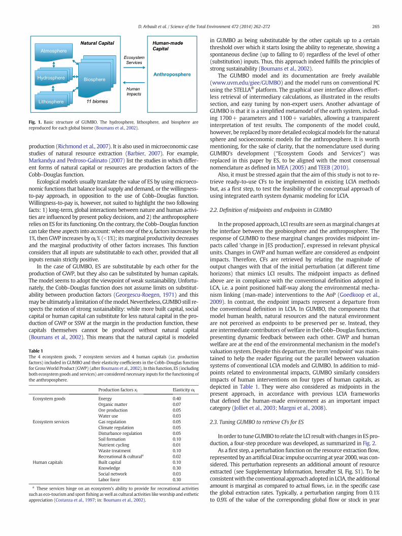
Fig. 1. Basic structure of GUMBO. The hydrosphere, lithosphere, and biosphere arereproduced for each global biome (Boumans et al., 2002).
265D. Arbault et al. / Science of the Total Environment 472 (2014) 262–272
production (Richmond et al., 2007). It is also used inmicroeconomic casestudies of natural resource extraction (Barbier, 2007). For example,Markandya and Pedroso-Galinato (2007) list the studies in which differ-ent forms of natural capital or resources are production factors of theCobb–Douglas function.
Ecological models usually translate the value of ES by using microeco-nomic functions that balance local supply and demand, or thewillingness-to-pay approach, in opposition to the use of Cobb–Douglas function.Willingness-to-pay is, however, not suited to highlight the two followingfacts: 1) long-term, global interactions between nature and human activi-ties are influenced by present policy decisions, and 2) the anthroposphererelies on ES for its functioning. On the contrary, the Cobb–Douglas functioncan take these aspects into account:when one of the xi factors increases by1%, then GWP increases by αi % (b1%); its marginal productivity decreasesand the marginal productivity of other factors increases. This functionconsiders that all inputs are substitutable to each other, provided that allinputs remain strictly positive.
In the case of GUMBO, ES are substitutable by each other for theproduction of GWP, but they also can be substituted by human capitals.Themodel seems to adopt the viewpoint of weak sustainability. Unfortu-nately, the Cobb–Douglas function does not assume limits on substitut-ability between production factors (Georgescu-Roegen, 1971) and thismaybeultimately a limitation of themodel. Nevertheless, GUMBOstill re-spects the notion of strong sustainability: while more built capital, socialcapital or human capital can substitute for less natural capital in the pro-duction of GWP or SSW at the margin in the production function, thesecapitals themselves cannot be produced without natural capital(Boumans et al., 2002). This means that the natural capital is modeled
Table 1The 4 ecosystem goods, 7 ecosystem services and 4 human capitals (i.e. productionfactors) included in GUMBO and their elasticity coefficients in the Cobb–Douglas functionfor GrossWorld Product (GWP) (after Boumans et al., 2002). In this function, ES (includingboth ecosystemgoods and services) are considered necessary inputs for the functioning ofthe anthroposphere.
Production factors xi Elasticity αi
Ecosystem goods Energy 0.40Organic matter 0.07Ore production 0.05Water use 0.03
Ecosystem services Gas regulation 0.05Climate regulation 0.05Disturbance regulation 0.05Soil formation 0.10Nutrient cycling 0.01Waste treatment 0.10Recreational & culturala 0.02
Human capitals Built capital 0.10Knowledge 0.30Social network 0.03Labor force 0.30
a These services hinge on an ecosystem's ability to provide for recreational activitiessuch as eco-tourism and sport fishing aswell as cultural activities likeworship and estheticappreciation (Costanza et al., 1997; in: Boumans et al., 2002).
in GUMBO as being substitutable by the other capitals up to a certainthreshold over which it starts losing the ability to regenerate, showing aspontaneous decline (up to falling to 0) regardless of the level of other(substitution) inputs. Thus, this approach indeed fulfills the principles ofstrong sustainability (Boumans et al., 2002).
The GUMBO model and its documentation are freely available(www.uvm.edu/giee/GUMBO) and the model runs on conventional PCusing the STELLA® platform. The graphical user interface allows effort-less retrieval of intermediary calculations, as illustrated in the resultssection, and easy tuning by non-expert users. Another advantage ofGUMBO is that it is a simplified metamodel of the earth system, includ-ing 1700+ parameters and 1100+ variables, allowing a transparentinterpretation of test results. The components of the model could,however, be replaced bymore detailed ecologicalmodels for the naturalsphere and socioeconomic models for the anthroposphere. It is worthmentioning, for the sake of clarity, that the nomenclature used duringGUMBO's development (“Ecosystem Goods and Services”) wasreplaced in this paper by ES, to be aligned with the most consensualnomenclature as defined in MEA (2005) and TEEB (2010).
Also, it must be stressed again that the aim of this study is not to re-trieve ready-to-use CFs to be implemented in existing LCIA methodsbut, as a first step, to test the feasibility of the conceptual approach ofusing integrated earth system dynamic modeling for LCIA.
2.2. Definition of midpoints and endpoints in GUMBO
In the proposed approach, LCI results are seen asmarginal changes atthe interface between the geobiosphere and the anthroposphere. Theresponse of GUMBO to these marginal changes provides midpoint im-pacts called ‘change in [ES production]’, expressed in relevant physicalunits. Changes in GWP and human welfare are considered as endpointimpacts. Therefore, CFs are retrieved by relating the magnitude ofoutput changes with that of the initial perturbation (at different timehorizons) that mimics LCI results. The midpoint impacts as definedabove are in compliance with the conventional definition adopted inLCA, i.e. a point positioned half-way along the environmental mecha-nism linking (man-made) interventions to the AoP (Goedkoop et al.,2009). In contrast, the endpoint impacts represent a departure fromthe conventional definition in LCIA. In GUMBO, the components thatmodel human health, natural resources and the natural environmentare not perceived as endpoints to be preserved per se. Instead, theyare intermediate contributors of welfare in the Cobb–Douglas functions,presenting dynamic feedback between each other. GWP and humanwelfare are at the end of the environmental mechanism in the model'svaluation system. Despite this departure, the term ‘endpoint’wasmain-tained to help the reader figuring out the parallel between valuationsystems of conventional LCIA models and GUMBO. In addition to mid-points related to environmental impacts, GUMBO similarly considersimpacts of human interventions on four types of human capitals, asdepicted in Table 1. They were also considered as midpoints in thepresent approach, in accordance with previous LCIA frameworksthat defined the human-made environment as an important impactcategory (Jolliet et al., 2003; Margni et al., 2008).
2.3. Tuning GUMBO to retrieve CFs for ES
In order to tuneGUMBO to relate the LCI resultwith changes in ESpro-duction, a four-step procedure was developed, as summarized in Fig. 2.
As a first step, a perturbation function on the resource extraction flow,representedby an artificial Dirac impulse occurring at year 2000,was con-sidered. This perturbation represents an additional amount of resourceextracted (see Supplementary Information, hereafter SI, Fig. S1). To beconsistentwith the conventional approach adopted in LCIA, the additionalamount is marginal as compared to actual flows, i.e. in the specific casethe global extraction rates. Typically, a perturbation ranging from 0.1%to 0.9% of the value of the corresponding global flow or stock in year
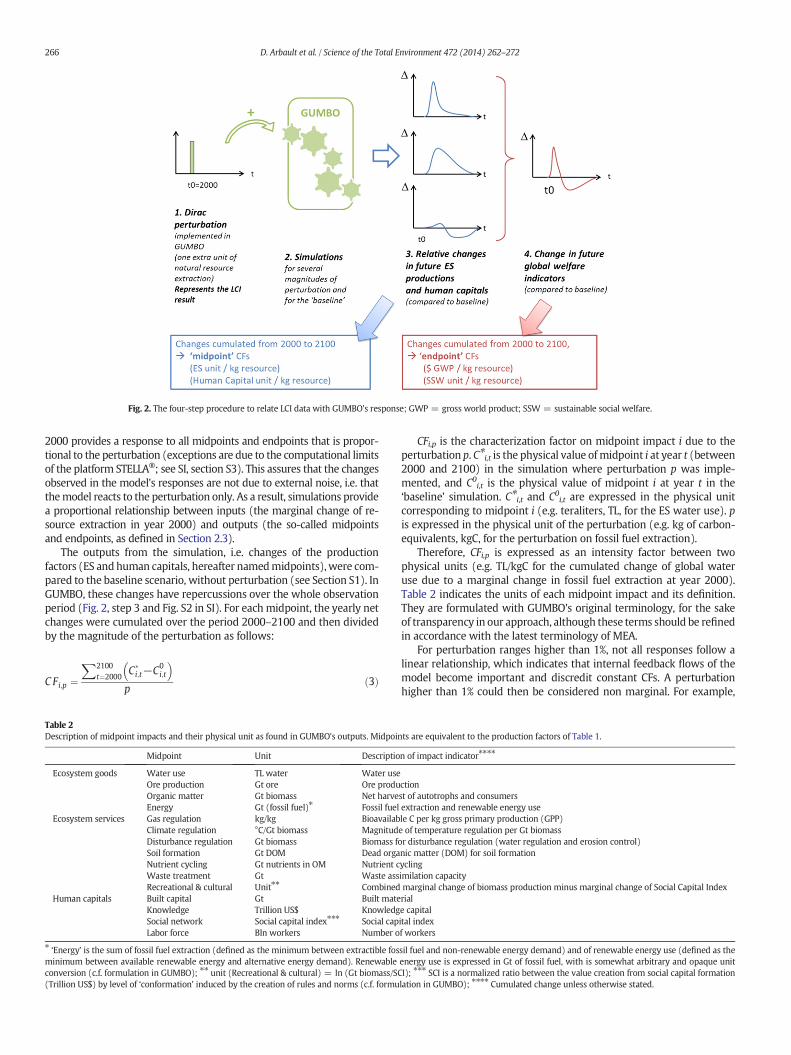
Fig. 2. The four-step procedure to relate LCI data with GUMBO's response; GWP = gross world product; SSW = sustainable social welfare.
266 D. Arbault et al. / Science of the Total Environment 472 (2014) 262–272
2000 provides a response to all midpoints and endpoints that is propor-tional to the perturbation (exceptions are due to the computational limitsof the platform STELLA®; see SI, section S3). This assures that the changesobserved in the model's responses are not due to external noise, i.e. thatthemodel reacts to the perturbation only. As a result, simulations providea proportional relationship between inputs (the marginal change of re-source extraction in year 2000) and outputs (the so-called midpointsand endpoints, as defined in Section 2.3).
The outputs from the simulation, i.e. changes of the productionfactors (ES andhuman capitals, hereafter namedmidpoints),were com-pared to the baseline scenario, without perturbation (see Section S1). InGUMBO, these changes have repercussions over the whole observationperiod (Fig. 2, step 3 and Fig. S2 in SI). For each midpoint, the yearly netchanges were cumulated over the period 2000–2100 and then dividedby the magnitude of the perturbation as follows:
CFi;p ¼X2100
t¼2000C�i;t−C0
i;t
� �
pð3Þ
Table 2Description of midpoint impacts and their physical unit as found in GUMBO's outputs. Midpoin
Midpoint Unit Descriptio
Ecosystem goods Water use TL water Water useOre production Gt ore Ore produOrganic matter Gt biomass Net harveEnergy Gt (fossil fuel)⁎ Fossil fuel
Ecosystem services Gas regulation kg/kg BioavailabClimate regulation °C/Gt biomass MagnitudDisturbance regulation Gt biomass Biomass foSoil formation Gt DOM Dead orgaNutrient cycling Gt nutrients in OM Nutrient cWaste treatment Gt Waste assRecreational & cultural Unit⁎⁎ Combined
Human capitals Built capital Gt Built mateKnowledge Trillion US$ KnowledgSocial network Social capital index⁎⁎⁎ Social capLabor force Bln workers Number o
⁎ ‘Energy’ is the sum of fossil fuel extraction (defined as the minimum between extractible fosminimum between available renewable energy and alternative energy demand). Renewableconversion (c.f. formulation in GUMBO); ⁎⁎ unit (Recreational & cultural) = ln (Gt biomass/SC(Trillion US$) by level of ‘conformation’ induced by the creation of rules and norms (c.f. formu
CFi,p is the characterization factor on midpoint impact i due to theperturbation p. C⁎i,t is the physical value ofmidpoint i at year t (between2000 and 2100) in the simulation where perturbation p was imple-mented, and C0i,t is the physical value of midpoint i at year t in the‘baseline’ simulation. C⁎i,t and C0i,t are expressed in the physical unitcorresponding to midpoint i (e.g. teraliters, TL, for the ES water use). pis expressed in the physical unit of the perturbation (e.g. kg of carbon-equivalents, kgC, for the perturbation on fossil fuel extraction).
Therefore, CFi,p is expressed as an intensity factor between twophysical units (e.g. TL/kgC for the cumulated change of global wateruse due to a marginal change in fossil fuel extraction at year 2000).Table 2 indicates the units of each midpoint impact and its definition.They are formulated with GUMBO's original terminology, for the sakeof transparency in our approach, although these terms should be refinedin accordance with the latest terminology of MEA.
For perturbation ranges higher than 1%, not all responses follow alinear relationship, which indicates that internal feedback flows of themodel become important and discredit constant CFs. A perturbationhigher than 1% could then be considered non marginal. For example,
ts are equivalent to the production factors of Table 1.
n of impact indicator⁎⁎⁎⁎
ctionst of autotrophs and consumersextraction and renewable energy usele C per kg gross primary production (GPP)e of temperature regulation per Gt biomassr disturbance regulation (water regulation and erosion control)nic matter (DOM) for soil formationyclingimilation capacitymarginal change of biomass production minus marginal change of Social Capital Indexriale capitalital indexf workers
sil fuel and non-renewable energy demand) and of renewable energy use (defined as theenergy use is expressed in Gt of fossil fuel, with is somewhat arbitrary and opaque unitI); ⁎⁎⁎ SCI is a normalized ratio between the value creation from social capital formationlation in GUMBO); ⁎⁎⁎⁎ Cumulated change unless otherwise stated.

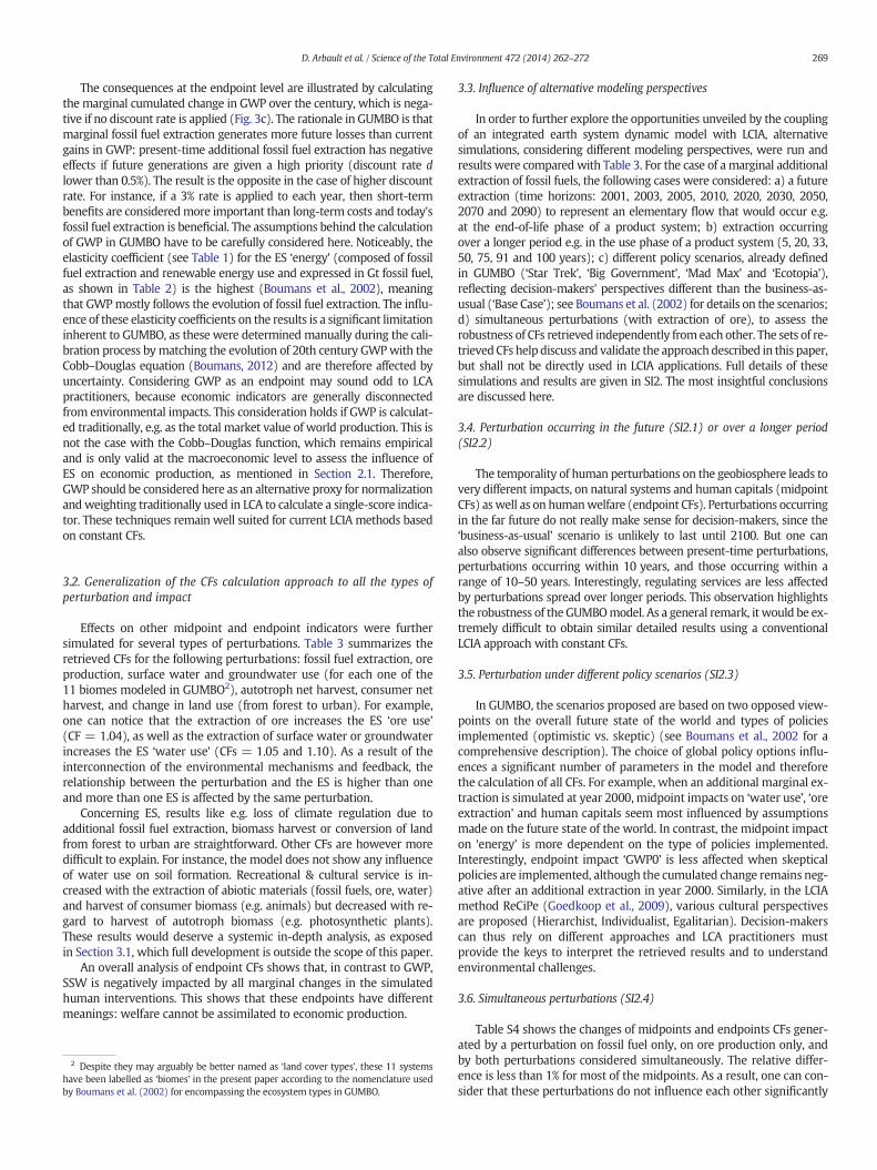
Fig. 3. a)Marginal changes ofwater use (TL/yr) over the21st century (compared towater usein the baseline scenario) induced by a marginal additional extraction of fossil fuel (FF) in yr2000; b) Linearity between marginal perturbation (in fossil fuel extraction, at yr 2000) andmarginal impacts (in water use, over the period 2000–2100), see Eq. (3); c) Endpoint CF‘GWP’ from fossil fuel use as a function of the discount rate (see Eqs. (4) and (5)).
267D. Arbault et al. / Science of the Total Environment 472 (2014) 262–272
fossil fuel extraction worldwide in year 2000 was 7.25 GtC and themarginal additional extraction ranged between 7.25 and 65.27 MtC:linearity was still respected at that range.
Endpoints CFs were computed following the same procedure,exception given for GWP in which annual change was weighted bya depreciation factor (Eqs. (4) and (5)), i.e. the Net Present Value(NPV) of a monetary unit of year t at present time (year 2000). NPVhas already been used in dynamic LCIA (Levasseur et al., 2010).
CFGWP;p;d ¼X2100
t¼2000C�GWP;t−C0
GWP;t
� �� NPVt;d
pð4Þ
with NPVt;d ¼ 11þ dð Þ t−2000ð Þ ð5Þ
The term d is the discount rate, which is constant over time: a highvalue of dmeans that short-term economic consequences are consideredmore important than long-term ones. Oppositely, if d is set to 0, economicconsequences for each year between 2000 and 2100 have equalimportance: in this case more emphasis is put on future generations.The value of d has therefore a critical influence on the endpointassessment. It reflects thepriorities set bydecisionmakers as beneficiariesof the LCIA. The endpoint CF related to the human welfare (SSW) wascomputed without discount rate, assuming that all human beings haveequal importance, regardless in which year they live.
3. Results
3.1. Example of midpoint and endpoint CFs calculation and interpretationfor a specific perturbation and impact
The case of an additional fossil fuel extraction in the year 2000 andthe associated impacts on water use and GWP over the whole centuryis taken as example. As shown in Fig. 3a, additional fossil fuel extractionin year 2000 results in additionalwater use the year after. Because of theindirect effects on other ES, water use is shown to drop dramaticallylater in the next century. The total cumulated change, expressed in TL(teraliters), is observed to be negative. The simulations show a linearrelationship between the magnitude of the input perturbation and thechanges in GUMBO's outputs (Fig. 3b). Therefore, a CF can be retrievedfor the midpoint impact, worth −0.07 L water per kg of fossil fuel. Inother terms, each additional kg of fossil fuel extracted in year 2000 isexpected to decrease the global, 21st-century water use by 0.07 L. It is,however, not straightforward to understand a priori whether this is abeneficial or detrimental consequence from a LCIA perspective, i.e. rela-tive to the AoP (Areas of Protection).Water use depends on both supply(freshwater made available by the natural system) and demand(human needs for freshwater). A reduction in water use could reflecta lower performance of ecosystems in delivering freshwater, but itcould also express a lower demand by human societies, due to e.g. amore efficient resource management or a reduction of global popula-tion. However, a deeper analysis of the data generated by GUMBOshowed that the simulated change in water demand (generated by anadditional marginal extraction of fossil fuel in year 2000) follows thesame pattern as the change in water use, while the change in availablewater for each biome follows completely different curves. This indicatesa demand-limited use, while the actual amount of available water hasmerely no influence on water use. In addition, in GUMBO, themodelingof water demand does not include an efficiency parameter: it is propor-tional to the sum of each capital's value (the four human capitalsdisplayed in Table 1 plus the natural capital, based on the value of allES) weighted by constant water need rates defined for each couplecapital-biome. Therefore, it can be concluded that in GUMBO the reduc-tion of ‘water use’ due to a marginal additional fossil fuel extraction inyear 2000 is directly related to the forecasted marginal regression of
economic activity during the mid-21st century (as compared to thebaseline scenario, where no additional fossil fuel extraction is simulat-ed). Such interpretation has a far larger scope than the one of the AoPof Natural Resource. It is thus important to consider GUMBO's responseas a whole, i.e. to track the modeled effects of the perturbation. Theholistic analysis of the model's results provides a more comprehensivepicture than a single CF andhighlights the importance of interconnectedmechanisms, dynamic feedback, and long-term effects, which arepresently not considered in LCIA methods.

Table 3Summary of characterization factors (CFs): impacts of perturbations on ES, human capitals, GWP and welfare.
OM: OrganicMatter; En: Energy; FF: Fossil Fuel; GR: Gas Regulation; CR: Climate Regulation; DR: Disturbance Regulation; SF: Soil Formation; NC: Nutrient Cycling;WT:Waste Treatment; RC: Recreation Cultural; BC: Built Capital; K: Knowledge; SN:Social Network; LF: Labor Force; GWP0: Gross World Product, 0% discount rate; GWP3: Gross World Product, 3% discount rate; SSW: Sustainable Social Welfare.
Units for each CF is the one displayed in Table 2, per unit of perturbation (shown in parenthesis in this table: Gt: Gigatons; TL: Teraliters; Mha: Million hectares).
F: Forest, G: Grassland, W: Wetland, L: Lake, U: Urban, O: Ocean, CO: Coastal Ocean, Cr: Cropland, D: Desert.
Perturbation (unit) Impact (unit)
Ecosystem goods Ecosystem services
Water (TL) Ore (Gt) OM (Gt) En(Gt F.F.) GR (kg/kg) CR (°C/Gt) DR (Gt) SF (Gt) NC (Gt) WT (Gt) RC (−)
FF extraction (Gt fossil fuel) −7.02 E-02 −1.66 E + 01 −1.66 E-02 5.66 E-03 2.07 E-01 −3.11 E-03 1.31 E-02 2.80 E-03 4.51 E-02 0 2.44 E-01Ore production (Gt Ore) 1.30 E-04 1.04 E + 00 1.20 E-04 8.17 E-06 −1.78 E-05 7.60 E-06 1.78 E-06 −9.83 E-07 4.52 E-05 0 1.29 E-04Surf. water: F,G,W,L,U (TL water) 1.05 E + 00 1.33 E + 01 −9.39 E-04 4.48 E-03 2.01 E-02 −6.60 E-04 6.75 E-04 0 2.63 E-03 0 1.45 E-02Surf. water: O, CO (TL water) 1.05 E + 00 1.33 E + 01 −3.08 E-03 6.00 E-03 1.96 E-02 −6.94 E-04 5.83 E-04 0 2.78 E-03 0 1.39 E-02Surf. water: Cr (TL water) 1.10 E + 00 1.40 E + 01 −1.12 E-03 4.93 E-03 2.11 E-02 −6.60 E-04 7.48 E-04 0 2.77 E-03 0 1.55 E-02Groundwater: D (TL water) 1.05 E + 00 1.33 E + 01 −8.86 E-04 4.53 E-03 2.00 E-02 −6.64 E-04 6.79 E-04 0 2.54 E-03 0 1.47 E-02Autotroph net harvest: Cr (Gt OM) −8.35 E-02 −1.49 E + 01 −4.98 E-01 5.91 E-02 1.56 E + 00 −4.37 E-02 −5.75 E-02 −9.94 E-03 −1.73 E-01 0 −3.30 E + 00Consumer net harvest (Gt OM) 1.64 E + 00 3.93 E + 02 5.43 E-01 1.06 E-01 −6.01 E-01 −1.00 E-02 −1.35 E-03 2.04 E-02 1.52 E-01 0 1.02 E + 00Land use change, from forest to urban (Mha) −3.88 E-04 −8.14 E-02 0 −7.71 E-05 1.19 E-04 −7.40 E-03 0 0 −8.77 E-05 0 −5.70 E-04
Perturbation (unit) Impact (unit)
Human capitals Endpoints
BC (Gt) K (trillion US$) SN (SCI) LF (Bln) GWP0 (trillion US$) GWP3 (trillion US$) SSW (−)
FF extraction (Gt fossil fuel) −3.13 E + 01 1.38 E + 01 −2.21 E-02 −1.68 E-02 −8.24 E + 00 1.77 E + 01 −1.41 E-02Ore production (Gt Ore) 9.30 E-02 2.33 E-02 4.41 E-05 −2.65 E-04 1.81 E-02 1.83 E-02 −6.99 E-04Surf water: F,G,W,L,U (TL water) 4.44 E + 01 1.06 E + 01 −4.84 E-04 −1.41 E-02 6.66 E + 00 6.53 E + 00 −3.04 E-03Surf water: O, CO (TL water) 4.44 E + 01 1.06 E + 01 −5.00 E-04 −1.47 E-02 6.66 E + 00 6.53 E + 00 −1.58 E-03Surf water: Cr (TL water) 4.65 E + 01 1.11 E + 01 −5.14 E-04 −1.46 E-02 6.99 E + 00 6.84 E + 00 −2.93 E-03Groundwater: D (TL water) 4.44 E + 01 1.06 E + 01 −5.32 E-04 −1.42 E-02 6.66 E + 00 6.53 E + 00 −3.09 E-03Autotroph net harvest: Cr (Gt OM) 3.10 E + 02 1.62 E + 02 −8.74 E-02 −4.13 E-01 −1.02 E + 01 1.14 E + 02 −7.08 E-02Consumer net harvest (Gt OM) 1.32 E + 03 2.98 E + 02 −2.57 E-01 8.86 E-01 1.97 E + 02 1.67 E + 02 −1.60 E-01Land use change, forest to urban (Mha) −2.48 E-01 −3.91 E-02 −5.89 E-05 5.74 E-05 −4.08 E-02 −1.47 E-02 −3.48 E-05
268D.A
rbaultetal./Scienceofthe
TotalEnvironment472
(2014)262
–272
269D. Arbault et al. / Science of the Total Environment 472 (2014) 262–272
The consequences at the endpoint level are illustrated by calculatingthe marginal cumulated change in GWP over the century, which is nega-tive if no discount rate is applied (Fig. 3c). The rationale in GUMBO is thatmarginal fossil fuel extraction generates more future losses than currentgains in GWP: present-time additional fossil fuel extraction has negativeeffects if future generations are given a high priority (discount rate dlower than 0.5%). The result is the opposite in the case of higher discountrate. For instance, if a 3% rate is applied to each year, then short-termbenefits are consideredmore important than long-term costs and today'sfossil fuel extraction is beneficial. The assumptions behind the calculationof GWP in GUMBO have to be carefully considered here. Noticeably, theelasticity coefficient (see Table 1) for the ES ‘energy’ (composed of fossilfuel extraction and renewable energy use and expressed in Gt fossil fuel,as shown in Table 2) is the highest (Boumans et al., 2002), meaningthat GWPmostly follows the evolution of fossil fuel extraction. The influ-ence of these elasticity coefficients on the results is a significant limitationinherent to GUMBO, as these were determined manually during the cali-bration process bymatching the evolution of 20th century GWPwith theCobb–Douglas equation (Boumans, 2012) and are therefore affected byuncertainty. Considering GWP as an endpoint may sound odd to LCApractitioners, because economic indicators are generally disconnectedfrom environmental impacts. This consideration holds if GWP is calculat-ed traditionally, e.g. as the total market value of world production. This isnot the case with the Cobb–Douglas function, which remains empiricaland is only valid at the macroeconomic level to assess the influence ofES on economic production, as mentioned in Section 2.1. Therefore,GWP should be considered here as an alternative proxy for normalizationandweighting traditionally used in LCA to calculate a single-score indica-tor. These techniques remain well suited for current LCIA methods basedon constant CFs.
3.2. Generalization of the CFs calculation approach to all the types ofperturbation and impact
Effects on other midpoint and endpoint indicators were furthersimulated for several types of perturbations. Table 3 summarizes theretrieved CFs for the following perturbations: fossil fuel extraction, oreproduction, surface water and groundwater use (for each one of the11 biomes modeled in GUMBO2), autotroph net harvest, consumer netharvest, and change in land use (from forest to urban). For example,one can notice that the extraction of ore increases the ES ‘ore use’(CF = 1.04), as well as the extraction of surface water or groundwaterincreases the ES ‘water use’ (CFs = 1.05 and 1.10). As a result of theinterconnection of the environmental mechanisms and feedback, therelationship between the perturbation and the ES is higher than oneand more than one ES is affected by the same perturbation.
Concerning ES, results like e.g. loss of climate regulation due toadditional fossil fuel extraction, biomass harvest or conversion of landfrom forest to urban are straightforward. Other CFs are however moredifficult to explain. For instance, the model does not show any influenceof water use on soil formation. Recreational & cultural service is in-creased with the extraction of abiotic materials (fossil fuels, ore, water)and harvest of consumer biomass (e.g. animals) but decreased with re-gard to harvest of autotroph biomass (e.g. photosynthetic plants).These results would deserve a systemic in-depth analysis, as exposedin Section 3.1, which full development is outside the scope of this paper.
An overall analysis of endpoint CFs shows that, in contrast to GWP,SSW is negatively impacted by all marginal changes in the simulatedhuman interventions. This shows that these endpoints have differentmeanings: welfare cannot be assimilated to economic production.
2 Despite they may arguably be better named as ‘land cover types’, these 11 systemshave been labelled as ‘biomes’ in the present paper according to the nomenclature usedby Boumans et al. (2002) for encompassing the ecosystem types in GUMBO.
3.3. Influence of alternative modeling perspectives
In order to further explore the opportunities unveiled by the couplingof an integrated earth system dynamic model with LCIA, alternativesimulations, considering different modeling perspectives, were run andresults were compared with Table 3. For the case of a marginal additionalextraction of fossil fuels, the following cases were considered: a) a futureextraction (time horizons: 2001, 2003, 2005, 2010, 2020, 2030, 2050,2070 and 2090) to represent an elementary flow that would occur e.g.at the end-of-life phase of a product system; b) extraction occurringover a longer period e.g. in the use phase of a product system (5, 20, 33,50, 75, 91 and 100 years); c) different policy scenarios, already definedin GUMBO (‘Star Trek’, ‘Big Government’, ‘Mad Max’ and ‘Ecotopia’),reflecting decision-makers' perspectives different than the business-as-usual (‘Base Case’); see Boumans et al. (2002) for details on the scenarios;d) simultaneous perturbations (with extraction of ore), to assess therobustness of CFs retrieved independently fromeach other. The sets of re-trievedCFs help discuss and validate the approachdescribed in this paper,but shall not be directly used in LCIA applications. Full details of thesesimulations and results are given in SI2. The most insightful conclusionsare discussed here.
3.4. Perturbation occurring in the future (SI2.1) or over a longer period(SI2.2)
The temporality of human perturbations on the geobiosphere leads tovery different impacts, on natural systems and human capitals (midpointCFs) aswell as on humanwelfare (endpoint CFs). Perturbations occurringin the far future do not really make sense for decision-makers, since the‘business-as-usual’ scenario is unlikely to last until 2100. But one canalso observe significant differences between present-time perturbations,perturbations occurring within 10 years, and those occurring within arange of 10–50 years. Interestingly, regulating services are less affectedby perturbations spread over longer periods. This observation highlightsthe robustness of the GUMBOmodel. As a general remark, it would be ex-tremely difficult to obtain similar detailed results using a conventionalLCIA approach with constant CFs.
3.5. Perturbation under different policy scenarios (SI2.3)
In GUMBO, the scenarios proposed are based on two opposed view-points on the overall future state of the world and types of policiesimplemented (optimistic vs. skeptic) (see Boumans et al., 2002 for acomprehensive description). The choice of global policy options influ-ences a significant number of parameters in the model and thereforethe calculation of all CFs. For example, when an additional marginal ex-traction is simulated at year 2000, midpoint impacts on ‘water use’, ‘oreextraction’ and human capitals seem most influenced by assumptionsmade on the future state of the world. In contrast, the midpoint impacton ‘energy’ is more dependent on the type of policies implemented.Interestingly, endpoint impact ‘GWP0’ is less affected when skepticalpolicies are implemented, although the cumulated change remains neg-ative after an additional extraction in year 2000. Similarly, in the LCIAmethod ReCiPe (Goedkoop et al., 2009), various cultural perspectivesare proposed (Hierarchist, Individualist, Egalitarian). Decision-makerscan thus rely on different approaches and LCA practitioners mustprovide the keys to interpret the retrieved results and to understandenvironmental challenges.
3.6. Simultaneous perturbations (SI2.4)
Table S4 shows the changes of midpoints and endpoints CFs gener-ated by a perturbation on fossil fuel only, on ore production only, andby both perturbations considered simultaneously. The relative differ-ence is less than 1% for most of the midpoints. As a result, one can con-sider that these perturbations do not influence each other significantly

270 D. Arbault et al. / Science of the Total Environment 472 (2014) 262–272
and hence the CFs can be used independently. The simulation shouldhowever be extended to the whole set of retrieved CFs throughout apairwise analysis for all of the perturbations displayed in Table 3 (seediscussion section).
4. Discussion
The results allowed validating the general conceptual approach ofusing integrated earth system dynamic modeling approach to retrievetime-dependent CFs accounting for the dynamic environmental mech-anisms and feedback flows underlying their calculation. However,limitations to this approach were also identified. Both advantages anddrawbacks are discussed in this section, alongwith a roadmap for futureresearch.
4.1. Need for harmonization between LCI datasets and integrated globalmodels
GUMBO considers only 4 resource categories:mineral ore, freshwater,organic matter and fossil fuel. Freshwater is split into surface water andgroundwater. Organic matter is divided in autotrophs and consumers.Only two land occupation types (urban and rural) are included. Thisresolution is much coarser than current LCI datasets. For example,ecoinvent 2.2 (Ecoinvent, 2010) has 7 elementary flows of biotic re-sources, 130mineral resources, 42 types of landoccupation (and80 trans-formation types), 5 airborne resources and 13 waterborne resources. TheLCIA method ReCiPe (Goedkoop et al., 2009) translates 55 mineralresources, 5 fossil fuel resources, 15 types of urban land occupation, 25types of agricultural/sylvicultural land occupation and 16 types of naturalland transformation (to/from artificial land) into endpoint impacts. Asshown in Table S5 with a tentative matching between the type andcategorization of flows found in LCI with those found in GUMBO, itseems unfeasible to reach such resolution in GUMBO without radicalchanges in the model that may jeopardize its stability.
Despite the intrinsic limitations in terms of ecosystem data resolution,process aggregation and certain basic calculation assumptions (e.g. theuse of the Cobb–Douglas function, as discussed in Section 2.1), GUMBOis able to take into account the inter-linkages among natural andhuman-driven systems, their feedback and the resulting connectionsamong multiple environmental mechanisms in a holistic way. Thesefeatures are poorly included in current LCIA models. For example, whilemodeling through land use does not take into account the major com-plexity of connections between natural processes, it implicitly includessome of this complexity e.g. through species-area curves, although in asimplistic manner (de Schryver et al., 2010; de Baan et al., 2013). Thisseems to be justified in LCIA by the criteria established in the ISO14044:2006, where impact categories, respective indicators and relatedCFs are proposed to avoid double counting. Therefore, this apparentdemand for simplification in LCIA may prevent from consideringthe complex role of ecosystems in the cause–effect chains of lifecycle models. The use of GUMBO and, in general, integrated ecologi-cal–socioeconomic modeling would overcome this limitation (seeSection 4.2).
4.2. Added value of formal use of integrated earth system dynamic modelswithin LCIA
Former attempts to integrate ES into LCIA delivered midpoint CFsexpressed in physical units, which are yet to be related to endpointimpacts. However, the complex interconnections between natural andhuman systems involve many (interrelated) indirect effects. Trying todecompose natural mechanisms into a set of independent cause–effectrelationships impacting the three conventional AoP (HH, NE, NR), aswell as the human-made environment (see Section 2.2) separately,seems a dead-end. For instance, a change in the natural environmentmay affect human health; deterioration of human health may increase
the need for resources; the generation of renewable resources is againdependent on a healthy natural environment. According to the overallrationale of GUMBO, the endpoints (GWP and SSW) are considered asthe ultimate indicators of global human development. The advantageof using the Cobb–Douglas function is that it enables relating theseindicators with important factors that are excluded in neo-classicaleconomics accounting, such as health factors for labor efficiency and,more important within the goal of this paper, ES. The simulation resultsshow that integrated earth system dynamic models like GUMBO canprovide a convenient platform to better internalize these externalitiesin the assessment. Another advantage of using indicators computed inan integrated model is to shrink the level of hidden subjectivity some-how existing in the calculation of endpoints in current LCIA methods.Instead of relying on an average weighing of three AoP considered asindependent from each other, decision-makers and practitioners couldmore easily be asked to select policy scenarios (see SI2.3) that corre-spond to their vision of the 21st century.
In order to compute a dataset of CFs for LCIA, it is necessary to in-vestigate the degree of mutual influence between perturbations and(midpoint and endpoint) impacts. In the specific case of GUMBO,perturbations on fossil fuel extraction and ore production have anegligible effect on each other. Such investigation shall be performedfor each couple of perturbations. If all perturbations that mimic LCIresults do not interfere with each other, the computed CFs could beconsidered as constants and thus be used directly for LCIA, indepen-dently from GUMBO. In contrast, if they are found to be influencingeach other, it is no more possible to retrieve constant CF. A possiblesolution would be to tune the model to automatically upload LCIresults and directly retrieve midpoint and endpoint impacts.Moreover, the information that could be retrieved from the modelwould be significantly richer than the one usually gathered fromconstant CFs. The model outputs may provide sound explanationson the evolution of variables and help identifying the main cause–effect chains, which constitute an added value for stakeholders anddecision markers.
4.3. Is further sophistication of integrated modeling necessary for LCIA?
Despite the distinction between rural and urban land occupationand the differentiation across ecosystem types (11 biomes) are thor-oughly implemented in GUMBO, the model is not designed to addresslocal or regional issues. For example, Table 3 shows that changes insurface water use are the same for several biomes (forest, grassland,wetlands, lake, urban). Such similarities are explained by the identicaltuning of each hydrologic parameter for these biomes, although differ-ent settings could be expected. Concerning groundwater use, GUMBOis tuned to give priority to the use of surface water. Therefore, all theCFs related to a change in groundwater use are null, except for thebiome ‘desert’, where surface water is not present.
Recent developments in LCIA clearly head towards spatially-explicitimpact assessment, based on geo-referenced datasets, in order to providefiner clues for decision-making (de Baan et al., 2013; IMPACT World+,2012; Koellner et al., 2013; Saad et al., 2011). There is therefore theneed to use more sophisticated ecological and economic sub-models,integrated in a meta-model following GUMBO's architecture. GUMBO'sdevelopers recently released MIMES (Boumans and Costanza, 2007),which is designed to embed also local assessment of ES within a globalsystem. MIMES can model multiregional systems, which are all inter-connected, and includes powerful GIS mapping tools for multi-scalecharacterization and dissemination purposes. Hence, MIMES appears asan interesting candidate to further explore the approach unveiled in thispaper following a spatially-explicit concern.
Numerous conceptual challenges and technical issues may arise,however, while designing a generic meta-model. First, the list of rele-vant ES is location-specific, aswell as their contribution to the economy.A generic model should take into account such specificities in nesting

271D. Arbault et al. / Science of the Total Environment 472 (2014) 262–272
local systems in the global one (Andrade et al., 2010). Second, their im-portance to the various economic sectors changes from place to place.The metamodel may take advantage of the mature structure of input–output tables for the design of a generic model, possibly extendedwith environmental intervention datasets (e.g. Lenzen et al., 2012;Tukker et al., 2013). Third, the Cobb–Douglas functions may no longerbe applicable in a multi-scale model and the welfare endpoints de-scribed here may thus need to be defined differently. The relationshipsbetween human capitals and economic sectors may also need furtherrefinements. Other issues not identified in this discussion are likely toarise, should such multi-scale model be developed.
4.4. Research roadmap
A preliminary roadmap for the development of such a meta-modelshall thus give priority to implementmulti-regional input–output tables(Lenzen et al., 2012) to first downscale the anthroposphere at nationalscale. A second step should be to develop the description of ES, whichis currently aggregated into four ecosystem goods and seven ecosystemservices in GUMBO. Local ES could be then modeled with GIS tools as inMIMES, and connected to the nation-wide economic model. This wouldlead to a multi-scale meta-model: global, national and local. Spatialinformation should be consistently harmonized or, at least, not havetoo high resolution, otherwise the link between local ES and nationalinput–output tables may become incongruous. Ultimately, dynamicmodels would potentially enhance the modeling of the human activityover a local territory, but the user of such model should be informedon its limited resolution. Undoubtedly such project would require alarge amount of data, heavy processes for quality-check, and multiplescientific skills to be coordinated.
5. Conclusions
Preliminary results from theGUMBOsimulations showed that it is fea-sible to retrieve CFs for ES and to connect midpoint changes to endpointsindicators such asGWPand SSW. TheCFs, however, cannot be yet straightcoupled to current LCIA methods because GUMBO does not match thegranularity of LCI datasets, and endpoints differ significantly from thecommon LCIA practice, nomenclature and definition of AoP. The rationalebehind the approach proposed here is however promising, as it showsthat integrated earth system dynamic modeling can potentially providemore detailed information on the interactions between human interven-tions (mostly resource extraction) and the natural and human capitalsthan plain datasets of constant CFs. It can take into account the potentialinteractions between human interventions, whereas it is not the casewith current CFs, and provide insights on the mechanisms that lead toshort-term, midpoint impacts, without disregarding the global, long-term picture. It can distinguish between human interventions occurringat present time, in the future, and over a long period and can be tunedup to estimate future world state conditions according to different policyscenarios, which is undoubtedly an interesting feature for decision-makers. The integrated coupling between the geobiosphere compart-ments and the anthroposphere enables linking cause–effect chains thatare currently artificially separated in LCIA models. It may also accountfor changes in human capitals, which are considered in LCA as an impor-tant AoP but not yet formally included in current models. Moreover, thehuman capital mid-point impact indicators considered in this study(Table 1) could be notably adapted for use in Social LCA, Life Cycle Costingor, more broadly, Life Cycle Sustainability Assessment (jointly withecosystem service indicators).
Despite these attractive potentialities, the integration with LCIA is farfrom being readily operational. A research roadmap has been envisagedaccordingly, including the use of more sophisticated and spatially explicitmodels such as MIMES.
Acknowledgment
This project was supported by the National Research Fund,Luxembourg (Ref 1063711) and the French National Research Fund(project EVALEAU ANR-08-ECOT-006-00 0894C0238).
Appendix A. Supplementary data
SI includes a detailed presentation of GUMBO, methodologicaldetails, as well as in-depth results and interpretation. Supplementarydata associated with this article can be found, in the online version, athttp://dx.doi.org/10.1016/j.scitotenv.2013.10.099.
References
Ainsworth CH, Varkey DA, Pitcher TJ. Ecosystem simulations supporting ecosystem-basedfisheries management in the Coral Triangle, Indonesia. Ecol Model 2008;214:361–74.
Aitkenhead MJ, Albanito F, Jones MB, Black HIJ. Development and testing of a process-basedmodel (MOSES) for simulating soil processes, functions and ecosystem services. EcolModel 2011;222:3795–810.
Andrade DC, Romeiro AR, Boumans R, Sobrinho RP, Tôsto SG. New methodologicalperspectives on the valuation of ecosystem services: toward a dynamic-integratedvaluation approach. International Society for Ecological Economics Conference:advancing sustainability in time of crisis. Germany: Oldenburg and Bremen; 2010.[22–25 August].
Arbault D, Rugani B, Marvuglia A, Tiruta-Barna L, Benetto E. Accounting for the energyvalue of life cycle inventory systems: insights from recent methodological advances.J. Environ. Account. Manage. 2013;1:103–17.
Bagstad KJ, Villa F, Johnson GW, Voigt B. ARIES — artificial intelligence for ecosystemservices: a guide to models and data, version 1.0. ARIES report series n.1; 2011.[Available at: http://www.ariesonline.org/docs/ARIESModelingGuide1.0.pdf].
Barbier EB. Valuing ecosystem services as productive inputs. Econ. Policy 2007;22:177–229.Boumans, R. Personal communication. 2012Boumans R, Costanza R. Themultiscale integrated Earth Systemsmodel (MIMES): the dy-
namics, modeling and valuation of ecosystem services. Issues in global water systemresearch—report on the joint TIAS-GWSP workshop held at the University ofMaryland University College, Adelphi, USA, 10 and 11 May 2007; 2007. p. 104–7.
Boumans R, Costanza R, Farley J, Wilson MA, Portela R, Rotmans J, et al. Modeling thedynamics of the integrated earth system and the value of global ecosystem servicesusing the GUMBO model. Ecol Econ 2002;41:529–60.
Brandão M, Milà i Canals L. Global characterisation factors to assess land use impacts onbiotic production. Int J Life Cycle Assess 2013;18:1243–52.
Burkhard B, Kroll F, Nedkov S, Müller F. Mapping ecosystem service supply, demand andbudgets. Ecol Indic 2012;21:17–29.
Cardinale BJ, Duffy JE, Gonzalez A, Hooper DU, Perrings C, Venail P, et al. Biodiversity lossand its impact on humanity. Nature 2012;486(7401):59–67.
Costanza R, d' Arge R, Groot R de, Farber S, Grasso M, Hannon B, et al. The value of theworld's ecosystem services and natural capital. Nature 1997;387:253–60.
Crossman ND, Burkhard B, Nedkov S, Willemen L, Petz K, Palomo I, et al. A blueprint formapping and modelling ecosystem services. Ecosyst. Serv. 2013;4:4–14.
Curran M, de Baan L, de Schryver AM, van Zelm R, Hellweg S, Koellner T, et al. Towardmeaningful end points of biodiversity in life cycle assessment. Environ Sci Technol2011;45:70–9.
Daily GC, editor. Nature's services: societal dependence on natural ecosystems. WashingtonDC: Island Press; 1997. p. 1–10.
de Baan L, Alkemade R, Koellner T. Land use impacts on biodiversity in LCA: a globalapproach. Int J Life Cycle Assess 2013;18:1216–30.
de Groot RS, Wilson MA, Boumans R. A typology for the classification, descriptionand valuation of ecosystem functions, goods and services. Ecol Econ 2002;41:393–408.
de Groot RS, Alkemade R, Braat L, Hein L, Willemen L. Challenges in integrating theconcept of ecosystem services and values in landscape planning, management anddecision making. Ecol Complex 2010;7(3):260–72.
de Groot RS, Brander L, van der Ploeg S, Costanza R, Bernard F, Braat L, et al. Globalestimates of the value of ecosystems and their services in monetary units. Ecosys.Serv. 2012;1:50–61.
de Schryver AM, Goedkoop MJ, Leuven RSEW, Huijbregts MAJ. Uncertainties in the appli-cation of the species area relationship for characterisation factors of land occupationin life cycle assessment. Int J Life Cycle Assess 2010;15(7):682–91.
de Souza DM, Flynn DFB, DeClerck F, Rosenbaum RK, Lisboa H de M, Koellner T. Landuse impacts on biodiversity in LCA: proposal of characterization factors based onfunctional diversity. Int J Life Cycle Assess 2013;18:1231–42.
Diamond JM. Collapse: how societies choose to fail or succeed. USA: Penguin Group;2006.
Douglas PH. The Cobb–Douglas production function once again: its history, its testing, andsome new empirical values. J Polit Econ 1976;84:903–15.
Ecoinvent. Ecoinvent database v2.2. Dübendorf Switzerland: Swiss Centre for Life-CycleInventories; 2010 [Available at: http://www.ecoinvent.org/database/].
European Commission. International Reference Life Cycle Data System (ILCD) handbook—general guide for life cycle assessment—detailed guidance. EUR 24708 ENEuropeanCommission, Joint Research Centre. Institute for Environment and Sustainability. 1sted. Luxemburg: Publications Office of the European Union; 2010a.

272 D. Arbault et al. / Science of the Total Environment 472 (2014) 262–272
European Commission. International Reference Life Cycle Data System (ILCD) handbook—framework and requirements for life cycle impact assessment models and indicators.EUR 24708 ENEuropean Commission, Joint Research Centre. Institute for Environmentand Sustainability. 1st ed. Luxemburg: PublicationsOffice of the EuropeanUnion; 2010b.
Farber S, Costanza R, Childers DL, Erickson J, Gross K, Grove M, et al. Linking ecology andeconomics for ecosystem management. Bioscience 2006;56(2):121–33.
Folke C. How resilient are ecosystems to global environmental change? Sustain Sci 2010;5:151–4.
Folke C, Jansson Å, Rockström J, Olsson P, Carpenter SR, Chapin FS, et al. Reconnecting tothe biosphere. Ambio 2011;40:719–38.
Georgescu-Roegen N. The entropy law and the economic process. Cambridge, MA:Harvard University Press; 1971.
Goedkoop M, Heijungs R, Huijbregts M, de Schryver A, Struijs J, van Zelm R. ReCiPe 2008 alife cycle impact assessment method which comprises harmonised category indicatorsat the midpoint and the endpoint level. VROM–Ruimte en Milieu, Ministerie vanVolkshuisvesting, Ruimtelijke Ordening en Milieubeheer; 2009. [www.lcia-recipe.net].
Gómez-Baggethun E, de Groot R, Lomas PL, Montes C. The history of ecosystem services ineconomic theory and practice: from early notions to markets and payment schemes.Ecol Econ 2010;69:1209–18.
Haines-Young R, Potschin M, Kienast F. Indicators of ecosystem service potential atEuropean scales: mappingmarginal changes and trade-offs. Ecol Indic 2012;21:39–53.
Halfon E, Schito N, Ulanowicz RE. Energy flow through the Lake Ontario food web:conceptual model and an attempt at mass balance. Ecol Model 1996;86:1–36.
Halog A, Manik Y. Advancing integrated systems modelling framework for life cyclesustainability assessment. Sustainability 2011;3:469–99.
IMPACT World+. Available at:http://www.impactworldplus.org/en/, 2012.ISO. 14044: environmental management—life cycle assessment—requirements and
guidelines. International Organization for Standardization; 2006.Ito A, Oikawa T. A simulation model of the carbon cycle in land ecosystems (Sim-CYCLE):
a description based on dry-matter production theory and plot-scale validation. EcolModel 2002;151:143–76.
Jiang H, Peng C, Apps MJ, Zhang Y, Woodard PM, Wang Z. Modelling the net primaryproductivity of temperate forest ecosystems in China with a GAP model. Ecol Model1999;122:225–38.
Johnston JM, McGarvey DJ, Barber MC, Laniak G, Babendreier J, Parmar R, et al. An inte-grated modeling framework for performing environmental assessments: applicationto ecosystem services in the Albemarle-Pamlico basins (NC and VA, USA). Ecol Model2011;222:2471–84.
Jolliet O, Brent A, GoedkoopM, Itsubo N, Mueller-Wenk R, Peña C, et al. Final report of theLCIA Definition study. Life Cycle Impact Assessment Programme of the Life CycleInitiative; 2003 [https://sph.umich.edu/riskcenter/jolliet/Jolliet%202003%20LCIA_defStudy.pdf].
Koellner T, de Baan L, Beck T, BrandãoM, Civit B, GoedkoopM, et al. Principles for life cycleinventories of land use on a global scale. Int J Life Cycle Assess 2013;18:1203–15.
Lenzen M, Kanemoto K, Moran D, Geschke A. Mapping the structure of the world econo-my. Environ Sci Technol 2012;46:8374–81.
Levasseur A, Lesage P, Margni M, Deschênes L, Samson R. Considering time in LCA: dy-namic LCA and its application to global warming impact assessments. Environ SciTechnol 2010;44:3169–74.
Maes J, Hauck J, Paracchini ML, Ratamäki O, Hutchins M, Termansen M, et al.Mainstreaming ecosystem services into EU policy. Curr Opin Environ Sustain 2013;5(1):128–34.
Margni M, Gloria T, Bare J, Seppälä J, Steen B, Struijs J, et al. Guidance on how to movefrom current practice to recommended practice in life cycle impact assessment.Paris: UNEP-SETAC Life Cycle Initiative; 2008 [Available at: http://acv.ibict.br/publicacoes/artigos-1/Guidance%20to%20LCA.pdf].
Markandya A, Pedroso-Galinato S. How substitutable is natural capital? Environ ResourEcon 2007;37:297–312.
Marvuglia A, Benetto E, Rios G, Rugani B. SCALE: software for calculating energy based onlife cycle inventories. Ecol Model 2013;248:80–91.
MEA. Millennium ecosystem assessment, ecosystems and human well-being: a frame-work for assessment. Washington DC: World Resources Institute; 2005.
Müller-Wenk R, BrandãoM. Climatic impact of land use in LCA—carbon transfers betweenvegetation/soil and air. Int J Life Cycle Assess 2010;15:172–82.
Odum HT. Environmental accounting, energy and decision making. NY: JohnWiley; 1996[370 pp.].
Ooba M, Wang Q, Murakami S, Kohata K. Biogeochemical model (BGC-ES) and itsbasin-level application for evaluating ecosystem services under forest managementpractices. Ecol Model 2010;221:1979–94.
Portela R, Rademacher I. A dynamic model of patterns of deforestation and their effect onthe ability of the Brazilian Amazonia to provide ecosystem services. Ecol Model2001;143:115–46.
Raugei M, Rugani B, Benetto E, IngwersenWW. Integrating energy into LCA: potential addedvalue and lingering obstacles. Ecol Model 2012. http://dx.doi.org/10.1016/j.ecolmodel.2012.11.025. [in press].
Richmond A, Kaufmann RK, Myneni RB. Valuing ecosystem services: a shadow price fornet primary production. Ecol Econ 2007;64:454–62.
Rugani B, Benetto E, Arbault D, Tiruta-Barna L. Energy-based midpoint valuation ofecosystem goods and services for life cycle impact assessment. Rev. Metall.-Paris2013;110:249–64.
Saad R, Margni M, Koellner T, Wittstock B, Deschênes L. Assessment of land use impactson soil ecological functions: development of spatially differentiated characterizationfactors within a Canadian context. Int J Life Cycle Assess 2011:1–14.
Saad R, Koellner T, Margni M. Land use impacts on freshwater regulation, erosion regula-tion, and water purification: a spatial approach for a global scale level. Int J Life CycleAssess 2013;18:1253–64.
Shang Z, He HS, Xi W, Shifley SR, Palik BJ. Integrating LANDIS model and a multi-criteriadecision-making approach to evaluate cumulative effects of forest management inthe Missouri Ozarks, USA. Ecol Model 2012;229:50–63.
Shanin VN, Komarov AS, Mikhailov AV, Bykhovets SS. Modelling carbon and nitrogendynamics in forest ecosystems of Central Russia under different climate changescenarios and forest management regimes. Ecol Model 2011;222:2262–75.
Solow RM. Intergenerational equity and exhaustible resources. Rev Econ Stud 1974;41:29–45.
SteffenW, Crutzen PJ, McNeill JR. The Anthropocene: are humans now overwhelming thegreat forces of nature. Ambio 2007;36:614–21.
Stiglitz J. Growth with exhaustible natural resources: efficient and optimal growth paths.Rev Econ Stud 1974;41:123–37.
Tallis HT, Ricketts T, Guerry AD, Wood SA, Sharp R, Nelson E, et al. InVEST 2.5.6 user'sguide. Stanford: The Natural Capital Project; 2013 [Available at: http://ncp-dev.stanford.edu/~dataportal/invest-releases/documentation/current_release/].
Taner MÜ, Carleton JN, Wellman M. Integrated model projections of climate changeimpacts on a North American lake. Ecol Model 2011;222:3380–93.
TEEB. The economics of ecosystems and biodiversity: ecological and economic foundations.In: Kumar Pushpam, editor. London and Washington: Earthscan; 2010.
Tukker A, de Koning A, Wood R, Hawkins T, Lutter S, Acosta J, et al. Exiopol—developmentand illustrative analyses of a detailed global Mr Ee Sut/Iot. ESRES, 25; 201350–70.
van Zelm R, Schipper AM, Rombouts M, Snepvangers J, Huijbregts MAJ. Implementinggroundwater extraction in life cycle impact assessment: characterization factorsbased on plant species richness for the Netherlands. Environ Sci Technol 2011;45:629–35.
Waage S, Stewart E, Armstrong K. Measuring corporate impact on ecosystems: a compre-hensive review of new tools. BSR, synthesis report; 2008. [Available at: http://www.bsr.org/reports/BSR_EMI_Tools_Application.pdf].
Zhang Y, Singh S, Bakshi BR. Accounting for ecosystem services in life cycle assessment,part I: a critical review. Environ Sci Technol 2010;44:2232–42.