electronics

Article

Integrated Chassis Control and Control Allocation for AllWheel Drive Electric Cars with Rear Wheel Steering

Pai-Chen Chien and Chih-Keng Chen *

�����������������

Citation: Chien, P.-C.; Chen, C.-K.

Integrated Chassis Control and

Control Allocation for All Wheel

Drive Electric Cars with Rear Wheel

Steering. Electronics 2021, 10, 2885.

https://doi.org/10.3390/

electronics10222885

Academic Editor: Carlos Andrés

García Vázquez

Received: 21 October 2021

Accepted: 20 November 2021

Published: 22 November 2021

Publisher’s Note: MDPI stays neutral

with regard to jurisdictional claims in

published maps and institutional affil-

iations.

Copyright: © 2021 by the authors.

Licensee MDPI, Basel, Switzerland.

This article is an open access article

distributed under the terms and

conditions of the Creative Commons

Attribution (CC BY) license (https://

creativecommons.org/licenses/by/

4.0/).

Department of Vehicle Engineering, National Taipei University of Technology, Taipei 10604, Taiwan;t108448013@ntut.org.tw* Correspondence: ckchen@ntut.edu.tw

Abstract: This study investigates a control strategy for torque vectoring (TV) and active rear wheelsteering (RWS) using feedforward and feedback control schemes for different circumstances. Acomprehensive vehicle and combined slip tire model are used to determine the secondary effect andto generate desired yaw acceleration and side slip angle rate. A model-based feedforward controlleris designed to improve handling but not to track an ideal response. A feedback controller based onclose loop observation is used to ensure its cornering stability. The fusion of two controllers is usedto stabilize a vehicle’s lateral motion. To increase lateral performance, an optimization-based controlallocation distributes the wheel torques according to the remaining tire force potential. The simulationresults show that a vehicle with the proposed controller exhibits more responsive lateral dynamicbehavior and greater maximum lateral acceleration. The cornering safety is also demonstrated usinga standard stability test. The driving performance and stability are improved simultaneously by theproposed control strategy and the optimal control allocation scheme.

Keywords: chassis control; torque vectoring; vehicle dynamics; secondary effect; rear wheel steering;control allocation

1. Introduction

Various chassis control systems have been studied and developed to increase drivingdynamics and safety. Growth in safety equipment and demand for space lead to an increasein modern vehicles’ weight. To improve performance and stability, many control systemshave been implemented. Yaw motion control for safety, such as an electronic stabilityprogram (ESP), is generally a standard equipment item. Advanced control systems, such astorque vectoring, rear wheel steering and active suspension become popular and commonbecause these types of control systems can improve driving performance for a vehicle.

Four-wheel steering (4WS) or active rear wheel steering (RWS) was introduced in the1980s on commercial vehicles. Nowadays, the technology is often used in high performanceor sports vehicles and is available as an optional extra on some passenger vehicles, suchas Porsche 911. The advantages of RWS are reducing the turning radius at low velocityand increasing the stability at high velocity by using the additional steering angle at therear axle.

All wheel drive (AWD) has been adopted for years to improve longitudinal accelera-tion performance [1], but it is also possible to control a vehicle’s yaw motion by distributingthe longitudinal tire forces on each wheel. During cornering, the tire lateral force ap-proaches its peak value, but it is still possible to produce longitudinal force. Direct yawmoment control (DYC) or torque vectoring (TV) systems control a vehicle’s motion byintentionally distributing the wheel driving or braking torques to increase the corneringperformance at the near-limit status [2]. In-wheel motor vehicles are used in sports or racecars to increase their efficiency and controllability. Each wheel produces either a drivingor a braking torque independently, without the physical limitations of the traditionalmechanical differential systems.

Electronics 2021, 10, 2885. https://doi.org/10.3390/electronics10222885 https://www.mdpi.com/journal/electronics

Electronics 2021, 10, 2885 2 of 19

Rear wheel steering and torque vectoring both produce a yaw moment around thevertical axis of the vehicle. Many control methods, such as sliding mode control (SMC) [3,4]and linear quadratic regulator (LQR), are investigated, but the approaches of differentresearches are diverse. Chen [5] used a combination of LQR, integral and feedforwardcontrol to eliminate the effect of steering input on side slip motion. Peters [6] used anopen-loop controller and a fine-tuned reference model to achieve precise and reproduciblebehavior under all circumstances, without the synthetic driving feeling from feedbackcontrollers. Since TV or DYC controllers are usually model based, and vehicles’ parametersand road conditions often change significantly, there are some approaches to increasing sys-tem robustness. Kissai [7] synthesized an H∞ controller to enhance the control robustnessagainst the uncertainties in vehicle parameters. Warth [8] designed a central feedforwardcontrol using an extended single-track model and the input-output linearization method,and made the reference generation adaptive by detecting the important parameters oftires. Hang [9] proposed a polytopic model to make the vehicle model adapt along withthe vehicle velocity and road friction coefficient, and developed a gain-scheduled robustcontroller to improve the vehicle’s stability in extreme conditions. Feedforward control iswidely used for chassis control systems and requires tuning that takes a long time. Theperformance might be degraded by model uncertainties; by contrast it has the advan-tage of being easily tunable and of reproducible behavior, which is important for humandrivers. Feedback control is more robust against model uncertainties; however, it relies onaccurate estimation.

For multi-input systems, the most popular issue is control allocation (CA). Thereare many approaches to implement the optimal distribution. Mokhiamar [3] proposedan optimum tire force distribution method to optimize the workload for each tire byusing equality constraints to eliminate variables, and ensuring the objective function isnot subjected to any constraints. Chen [5] used a weighted pseudo-inverse to approachthe desired longitudinal acceleration and desired yaw moment. Kissai [10] studied thedynamics of actuators and used model predictive control allocation (MPCA) to predictthe imminent saturation of actuators. Han [11] proposed “equal distribution” to minimizepower losses and increase energy efficiency. Xiao [12] used a weighted least squaresmethod to determine the optimal distribution to minimize control effort. There are manyapproaches to CA for over-actuated systems. Algebraic solvers require less computationaleffort; however, numerical methods are frequently used to deal with hard constraints suchas actuators’ limitations.

This study proposes a combined control method to allow sporty driving behavior innormal condition and guarantees safety in severe situations. Driving feeling is crucial forthe human driver. A reproducible linear dependency between the driver’s steering inputand the lateral acceleration output is preferred for sporty driving sensation. To achievethis driving behavior, a model-based feedforward controller with a reference generatoris proposed to improve lateral performance instead of tracking an ideal response. Thiskind of controller should take account of the secondary effect, which is proposed in [6], todescribe the interaction between longitudinal and lateral tie forces. The secondary effect ismore complex for independent all-wheel drive vehicles because front and rear axles canboth produce yaw torque. If a driver makes a mistake or road conditions deteriorate, thestability mode uses a feedback controller, intervenes in the vehicle’s motion to reduce itsinstability. The control allocation method maximizes the remaining friction potential in thetires and increases performance and safety.

This study is structured as follows. Section 2 presents the tire and vehicle model andthe coordinate system for this study. Section 3 details the method to calculate the secondaryeffect and shows how the secondary effect affects the vehicle’s motion. Section 4 presentsthe control and allocation algorithm in detail. Sections 4.2 and 4.3 detail the structuresof the feedforward and feedback controllers and Section 4.4 expresses the concept of thecontroller allocation method. Section 5 presents the test procedures and simulation results.Section 6 draws conclusions about the control system and details future opportunities.

Electronics 2021, 10, 2885 3 of 19

2. Modeling of Lateral Dynamics

This section presents a complex tire model, an advanced vehicle dynamics model withRWS and additional external yaw moment and a simplified single-track model. These arethe basics for the following design of controllers.

The proposed controller uses commands from the driver, an advanced vehicle modelwith individual wheel loads, and a semi-empirical tire model based on the methods ofPacejka [13] and Burhaumudin [14] to generate the reference responses.

2.1. Tire Model

For this study, the secondary effect, which is caused by the interaction betweenlongitudinal and lateral forces on the tire, is used for the feedforward controller. Basicmodels, such as linear tire models or the one used in [4], are not sufficient to presentthe combined slip characteristic. The semi-empirical Magic Formula considers all of therelevant factors for this study.

The following simulations use different vertical loads on the tires due to load transfer,the longitudinal slip and the side slip angle under combined slip situation. Other factors,such as temperature and pressure, are assumed to be constant. The equations for thelongitudinal and lateral force are:

Fx = GxDxcos{

Cx tan−1[

Bxκ − Ex

(Bx − tan−1(Bxκ)

)]}(1)

Fy = GyDycos{

Cy tan−1[

Byα − Ey

(By − tan−1(Byα

))]}+ Sy (2)

The parameters that are used in Equations (1) and (2) are defined in Table 1.

Table 1. Parameters for the magic formula.

Parameter Description

F Tire force at the center of contact patchG Weighting function for combined slipB Stiffness factorC Shape factorD Peak factorE Curvature factorκ Longitudinal slip ratioα Lateral slip angleSy Vertical shift of lateral force

Parameters B, C, D, E are a function of vertical load Fz, G is a function of longitudinalor lateral slip and Sy is related to the wheel camber angle, ply-steer or conicity. This isassumed to be zero for this study. These calculations result in the following equations:

Fx = fx(α, κ, Fz) (3)

Fy = fy(α, κ, Fz) (4)

The method to fit the tire model from experimental data is based on the CarSim tiretester procedure and a genetic algorithm. Using velocity, vertical load, and the road surface,the longitudinal slip ratio at different side slip angles and vertical loads are used to findthe unknown parameters for longitudinal behavior.

The blue lines in Figure 1a,b are the experimental data and the red lines represent theGA fitting results. The combined slip characteristic is used for this study, which is essentialfor the subsequent research, as shown in Figure 1c,d.

Electronics 2021, 10, 2885 4 of 19

Electronics 2021, 10, x FOR PEER REVIEW 4 of 19

The blue lines in Figure 1a,b are the experimental data and the red lines represent the GA fitting results. The combined slip characteristic is used for this study, which is essen-tial for the subsequent research, as shown in Figure 1c,d.

(a) Longitudinal Force 𝐹 (b) Lateral Force 𝐹

(c) Combined Slip 𝐹 (𝐹 = 3800 N) (d) Combined Slip 𝐹 (𝐹 = 3800 N)

Figure 1. Pacejka tire model. (a) Fitting results, longitudinal force; (b) Fitting results, longitudinal force; and (c,d) Com-bined slip characteristic under 3800 N vertical load.

The transient behavior of a tire is described using the linear first-order lag element (PT -element) method [8]. The time constant is converted using the vehicle’s velocity and the relaxation length as: 𝑇 𝐹 + 𝐹 = 𝐹 , 𝑇 𝑢 = 𝐿 (5)

where 𝐿 is the relaxation length, as specified in the CarSim tire model, 𝑇 is the time constant and 𝐹 is the steady state tire force. The defined relaxation length is 1/3 of the distance that the tire must roll before tire force is 95% of the steady-state value. Modeling the transient tire behavior allows the reference generator in the follow-up controller to account for additional dynamic effects on the driving behavior.

2.2. Vehicle Dynamics Model The vehicle model for this study is defined in ISO coordinates. A definition of vehicle

coordinates is shown in Figure 2. In the following equations, subscripts 𝑓𝑙, 𝑓𝑟, 𝑟𝑙, 𝑟𝑟 rep-resent the four different wheels of the vehicle.

Figure 1. Pacejka tire model. (a) Fitting results, longitudinal force; (b) Fitting results, longitudinal force; and (c,d) Combinedslip characteristic under 3800 N vertical load.

The transient behavior of a tire is described using the linear first-order lag element(PT1-element) method [8]. The time constant is converted using the vehicle’s velocity andthe relaxation length as:

Ty.F + F = F0, Tyu = Ly (5)

where Ly is the relaxation length, as specified in the CarSim tire model, Ty is the timeconstant and F0 is the steady state tire force. The defined relaxation length is 1/3 of thedistance that the tire must roll before tire force is 95% of the steady-state value. Modelingthe transient tire behavior allows the reference generator in the follow-up controller toaccount for additional dynamic effects on the driving behavior.

2.2. Vehicle Dynamics Model

The vehicle model for this study is defined in ISO coordinates. A definition of vehiclecoordinates is shown in Figure 2. In the following equations, subscripts f l, f r, rl, rrrepresent the four different wheels of the vehicle.

Electronics 2021, 10, 2885 5 of 19Electronics 2021, 10, x FOR PEER REVIEW 5 of 19

Figure 2. Coordinates of the vehicle dynamics model.

In this study, the feedforward controller uses four in-wheel motor torque vectoring and active rear wheel steering. The secondary effect is calculated using the combined slip characteristic for each wheel, so the model must allow the calculation of each tire force. An advanced four-wheel vehicle model that includes body lateral and yaw motion is used for this study. A simple load transfer equation is used to calculate each wheel load, which is necessary to produce the longitudinal and lateral tire forces. The equations of motions for the vehicle model are: 𝑟𝐼 = 𝐹 𝑎 − 𝐹 𝑏 + ∆𝑀 (6)

𝛽 = ∑ 𝐹𝑚𝑢 − 𝑟 (7)

where 𝑟 is body yaw rate, 𝛽 is body side slip angle, 𝑢 is longitudinal velocity, 𝑣 is lat-eral velocity, 𝐼 is yaw inertia of the vehicle, 𝐹 and 𝐹 are the summed lateral forces at the front and rear axles, 𝑎 and 𝑏 are, respectively, the distances between the front and rear axles to the center of gravity. ∆𝑀 is the yaw torque produced by torque vectoring, and is expressed as: ∆𝑀 = 𝑡2 𝐹 , − 𝐹 , + 𝑡2 𝐹 , − 𝐹 , (8)

where 𝑡 and 𝑡 are the track width at the front and rear axles. The calculation of wheel loads requires measured longitudinal and lateral accelera-

tion. The equations for load transfer are: 𝐹 , = 𝐹 , , − 𝑚𝐴 ℎ2𝐿 − 𝑘 ,𝑘 , 𝑚𝐴 ℎ𝑡 (9)

𝐹 , = 𝐹 , , − 𝑚𝐴 ℎ2𝐿 + 𝑘 ,𝑘 , 𝑚𝐴 ℎ𝑡 (10)

𝐹 , = 𝐹 , , + 𝑚𝐴 ℎ2𝐿 − 𝑘 ,𝑘 , 𝑚𝐴 ℎ𝑡 (11)

𝐹 , = 𝐹 , , + 𝑚𝐴 ℎ2𝐿 + 𝑘 ,𝑘 , 𝑚𝐴 ℎ𝑡 (12)

Figure 2. Coordinates of the vehicle dynamics model.

In this study, the feedforward controller uses four in-wheel motor torque vectoringand active rear wheel steering. The secondary effect is calculated using the combined slipcharacteristic for each wheel, so the model must allow the calculation of each tire force. Anadvanced four-wheel vehicle model that includes body lateral and yaw motion is used forthis study. A simple load transfer equation is used to calculate each wheel load, which isnecessary to produce the longitudinal and lateral tire forces. The equations of motions forthe vehicle model are:

.rIz = Fy f a − Fyrb + ∆MTV

z (6)

.β =

∑ Fy

mu− r (7)

where r is body yaw rate, β is body side slip angle, u is longitudinal velocity, v is lateralvelocity, Iz is yaw inertia of the vehicle, Fy f and Fyr are the summed lateral forces at thefront and rear axles, a and b are, respectively, the distances between the front and rear axlesto the center of gravity. ∆MTV

Z is the yaw torque produced by torque vectoring, and isexpressed as:

∆MTVz =

tF2

(Fx, f r − Fx, f l

)+

tR2(Fx,rr − Fx,rl) (8)

where tF and tR are the track width at the front and rear axles.The calculation of wheel loads requires measured longitudinal and lateral acceleration.

The equations for load transfer are:

Fz, f l = Fz,stat, f l −mAxh

2L−

kroll, f

kroll,tot

mAyhtF

(9)

Fz, f r = Fz,stat, f r −mAxh

2L+

kroll, f

kroll,tot

mAyhtF

(10)

Fz,rl = Fz,stat,rl +mAxh

2L−

kroll,r

kroll,tot

mAyhtR

(11)

Fz,rr = Fz,stat,rr +mAxh

2L+

kroll,r

kroll,tot

mAyhtR

(12)

Electronics 2021, 10, 2885 6 of 19

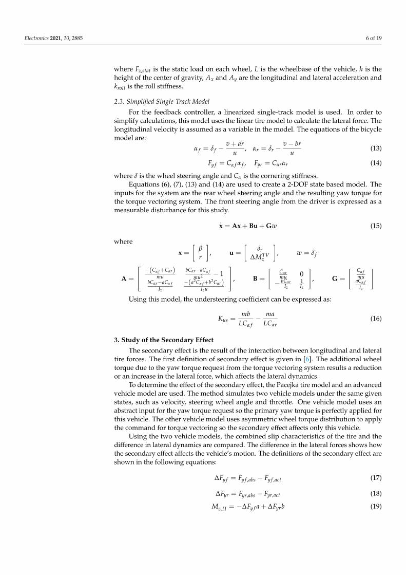
where Fz,stat is the static load on each wheel, L is the wheelbase of the vehicle, h is theheight of the center of gravity, Ax and Ay are the longitudinal and lateral acceleration andkroll is the roll stiffness.

2.3. Simplified Single-Track Model

For the feedback controller, a linearized single-track model is used. In order tosimplify calculations, this model uses the linear tire model to calculate the lateral force. Thelongitudinal velocity is assumed as a variable in the model. The equations of the bicyclemodel are:

α f = δ f −v + ar

u, αr = δr −

v − bru

(13)

Fy f = Cα f α f , Fyr = Cαrαr (14)

where δ is the wheel steering angle and Cα is the cornering stiffness.Equations (6), (7), (13) and (14) are used to create a 2-DOF state based model. The

inputs for the system are the rear wheel steering angle and the resulting yaw torque forthe torque vectoring system. The front steering angle from the driver is expressed as ameasurable disturbance for this study.

.x = Ax + Bu + Gw (15)

where

x =

[βr

], u =

[δr

∆MTVz

], w = δ f

A =

−(Cα f +Cαr)mu

bCαr−aCα fmu2 − 1

bCαr−aCα fIz

−(a2Cα f +b2Cαr)Izu

, B =

[Cαrmu 0

− bCαrIz

1Iz

], G =

[ Cα fmu

aCα fIz

]

Using this model, the understeering coefficient can be expressed as:

Kus =mb

LCα f− ma

LCαr(16)

3. Study of the Secondary Effect

The secondary effect is the result of the interaction between longitudinal and lateraltire forces. The first definition of secondary effect is given in [6]. The additional wheeltorque due to the yaw torque request from the torque vectoring system results a reductionor an increase in the lateral force, which affects the lateral dynamics.

To determine the effect of the secondary effect, the Pacejka tire model and an advancedvehicle model are used. The method simulates two vehicle models under the same givenstates, such as velocity, steering wheel angle and throttle. One vehicle model uses anabstract input for the yaw torque request so the primary yaw torque is perfectly applied forthis vehicle. The other vehicle model uses asymmetric wheel torque distribution to applythe command for torque vectoring so the secondary effect affects only this vehicle.

Using the two vehicle models, the combined slip characteristics of the tire and thedifference in lateral dynamics are compared. The difference in the lateral forces shows howthe secondary effect affects the vehicle’s motion. The definitions of the secondary effect areshown in the following equations:

∆Fy f = Fy f ,abs − Fy f ,act (17)

∆Fyr = Fyr,abs − Fyr,act (18)

Mz,I I = −∆Fy f a + ∆Fyrb (19)

Electronics 2021, 10, 2885 7 of 19

The subscript abs represents the model that uses an abstract input yaw torque, sub-script act represents the model that uses true actuators to produce the yaw torque and Mz,I Iis the secondary yaw torque due to the difference in the lateral forces for the two vehicles.

This study uses an electrical vehicle with independent all-wheel drive so the yawtorque command is applied on the vehicle through the front and rear axles. The controlallocation strategy and analysis of the secondary effect is more complex.

Changes in the lateral forces during a left turn are shown in Figure 3. Each circlerepresents a change in the lateral forces at the front and rear axles due to different yawtorque requests and torque distributions. Both the front and rear axles can produce a yawtorque. If using only one axle to produce yaw torque request, the stress of the tires ofthe axle might be increased significantly. This causes a radical change in lateral forcesand side slip. In a certain situation, such as certain velocity, lateral acceleration, and yawtorque request, there will exist a best torque distribution that minimizes the changes in thelateral forces.

Electronics 2021, 10, x FOR PEER REVIEW 7 of 19

𝑀 , = −∆𝐹 𝑎 + ∆𝐹 𝑏 (19)

The subscript 𝑎𝑏𝑠 represents the model that uses an abstract input yaw torque, sub-script 𝑎𝑐𝑡 represents the model that uses true actuators to produce the yaw torque and 𝑀 , is the secondary yaw torque due to the difference in the lateral forces for the two vehicles.

This study uses an electrical vehicle with independent all-wheel drive so the yaw torque command is applied on the vehicle through the front and rear axles. The control allocation strategy and analysis of the secondary effect is more complex.

Changes in the lateral forces during a left turn are shown in Figure 3. Each circle represents a change in the lateral forces at the front and rear axles due to different yaw torque requests and torque distributions. Both the front and rear axles can produce a yaw torque. If using only one axle to produce yaw torque request, the stress of the tires of the axle might be increased significantly. This causes a radical change in lateral forces and side slip. In a certain situation, such as certain velocity, lateral acceleration, and yaw torque request, there will exist a best torque distribution that minimizes the changes in the lateral forces.

Figure 3. Changes in the lateral force for different yaw torque requests and distributions.

Figures 4 and 5 show the step responses of yaw rate and the corresponding side slip angle during a left turn at 80 km/h for the same primary yaw torque request. Each dashed-line represents the different longitudinal distribution between the front and rear axles. Due to the different distribution of wheel torques, the deviations between vehicle models with the abstract inputs and with true-actuator inputs are different for the same primary yaw torque request. This shows the influence of the secondary effect. For high lateral ac-celeration, the secondary effect becomes more significant and can cause a spin if the lateral force at the rear axle is saturated.

Figure 3. Changes in the lateral force for different yaw torque requests and distributions.

Figures 4 and 5 show the step responses of yaw rate and the corresponding sideslip angle during a left turn at 80 km/h for the same primary yaw torque request. Eachdashed-line represents the different longitudinal distribution between the front and rearaxles. Due to the different distribution of wheel torques, the deviations between vehiclemodels with the abstract inputs and with true-actuator inputs are different for the sameprimary yaw torque request. This shows the influence of the secondary effect. For highlateral acceleration, the secondary effect becomes more significant and can cause a spin ifthe lateral force at the rear axle is saturated.

Electronics 2021, 10, 2885 8 of 19Electronics 2021, 10, x FOR PEER REVIEW 8 of 19

(a) (b)

Figure 4. Secondary effects for different distributions for a left turn at 80 km/h and 30 deg steering wheel input. (a) Yaw rate responses; (b) Side slip angle responses.

(a) (b)

Figure 5. Secondary effects for different distributions for a left turn at 80 km/h and 60 deg steering wheel input. (a) Yaw rate responses; (b) Side slip angle responses.

These results show that the secondary effect, which is a result of the interaction be-tween longitudinal and lateral tire forces, varies significantly with the primary yaw torque requests and the torque distributions. This effect should not be neglected for feedforward control because it can cause an unexpected extra slip that leads to loss of control during fierce driving. On the other hand, proper distribution of torque requests can minimize the stresses of the tires and keep the side slip response precise.

4. Controller Design Figure 6 shows the block diagram of the overall system. The strategy uses handling

mode to increase lateral performance and stability mode to stabilize the vehicle’s motion when losing control. The handling mode uses a feedforward controller that provides sporty and reproducible driving behavior and prevents a synthetic driving sensation, which is unacceptable for sports car drivers [6]. The stability mode uses a feedback con-troller to stabilize the vehicle’s motion when the vehicle loses control, which might be caused by a driver’s mistake. To make a smooth intervention of the stability mode, the stability criterion adjusts the weighting between two controllers according to the esti-mated understeering coefficient, then transits to stability mode when the vehicle experi-ences an undesired oversteer or understeer situation. The allocation scheme distributes

Figure 4. Secondary effects for different distributions for a left turn at 80 km/h and 30 deg steering wheel input. (a) Yawrate responses; (b) Side slip angle responses.

Electronics 2021, 10, x FOR PEER REVIEW 8 of 19

(a) (b)

Figure 4. Secondary effects for different distributions for a left turn at 80 km/h and 30 deg steering wheel input. (a) Yaw rate responses; (b) Side slip angle responses.

(a) (b)

Figure 5. Secondary effects for different distributions for a left turn at 80 km/h and 60 deg steering wheel input. (a) Yaw rate responses; (b) Side slip angle responses.

These results show that the secondary effect, which is a result of the interaction be-tween longitudinal and lateral tire forces, varies significantly with the primary yaw torque requests and the torque distributions. This effect should not be neglected for feedforward control because it can cause an unexpected extra slip that leads to loss of control during fierce driving. On the other hand, proper distribution of torque requests can minimize the stresses of the tires and keep the side slip response precise.

4. Controller Design Figure 6 shows the block diagram of the overall system. The strategy uses handling

mode to increase lateral performance and stability mode to stabilize the vehicle’s motion when losing control. The handling mode uses a feedforward controller that provides sporty and reproducible driving behavior and prevents a synthetic driving sensation, which is unacceptable for sports car drivers [6]. The stability mode uses a feedback con-troller to stabilize the vehicle’s motion when the vehicle loses control, which might be caused by a driver’s mistake. To make a smooth intervention of the stability mode, the stability criterion adjusts the weighting between two controllers according to the esti-mated understeering coefficient, then transits to stability mode when the vehicle experi-ences an undesired oversteer or understeer situation. The allocation scheme distributes

Figure 5. Secondary effects for different distributions for a left turn at 80 km/h and 60 deg steering wheel input. (a) Yawrate responses; (b) Side slip angle responses.

These results show that the secondary effect, which is a result of the interactionbetween longitudinal and lateral tire forces, varies significantly with the primary yawtorque requests and the torque distributions. This effect should not be neglected forfeedforward control because it can cause an unexpected extra slip that leads to loss ofcontrol during fierce driving. On the other hand, proper distribution of torque requests canminimize the stresses of the tires and keep the side slip response precise.

4. Controller Design

Figure 6 shows the block diagram of the overall system. The strategy uses handlingmode to increase lateral performance and stability mode to stabilize the vehicle’s motionwhen losing control. The handling mode uses a feedforward controller that provides sportyand reproducible driving behavior and prevents a synthetic driving sensation, which isunacceptable for sports car drivers [6]. The stability mode uses a feedback controller tostabilize the vehicle’s motion when the vehicle loses control, which might be caused by adriver’s mistake. To make a smooth intervention of the stability mode, the stability criterionadjusts the weighting between two controllers according to the estimated understeeringcoefficient, then transits to stability mode when the vehicle experiences an undesiredoversteer or understeer situation. The allocation scheme distributes the motor’s torque toeach wheel. This is an optimization problem to prevent the saturation of tire forces.

Electronics 2021, 10, 2885 9 of 19

Electronics 2021, 10, x FOR PEER REVIEW 9 of 19

the motor’s torque to each wheel. This is an optimization problem to prevent the satura-tion of tire forces.

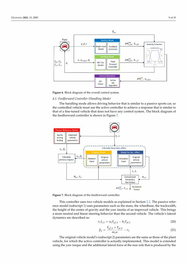
Figure 6. Block diagram of the overall control system.

4.1. Feedforward Controller (Handling mode) The handling mode allows driving behavior that is similar to a passive sports car, so

the controlled vehicle must use the active controller to achieve a response that is similar to that of a fine-tuned vehicle that does not have any control system. The block diagram of the feedforward controller is shown in Figure 7.

Figure 7. Block diagram of the feedforward controller.

This controller uses two vehicle models as explained in Section 2.2. The passive ref-erence model (subscript 1) uses parameters such as the mass, the wheelbase, the track-width, the height of the center of gravity and the yaw inertia of an improved vehicle. This brings a more neutral and linear steering behavior than the second vehicle. The vehicle’s lateral dynamics are described as: 𝑟 𝐼 , = 𝑎 𝐹 , − 𝑏 𝐹 , (20)

Figure 6. Block diagram of the overall control system.

4.1. Feedforward Controller (Handling Mode)

The handling mode allows driving behavior that is similar to a passive sports car, sothe controlled vehicle must use the active controller to achieve a response that is similar tothat of a fine-tuned vehicle that does not have any control system. The block diagram ofthe feedforward controller is shown in Figure 7.

Electronics 2021, 10, x FOR PEER REVIEW 9 of 19

the motor’s torque to each wheel. This is an optimization problem to prevent the satura-tion of tire forces.

Figure 6. Block diagram of the overall control system.

4.1. Feedforward Controller (Handling mode) The handling mode allows driving behavior that is similar to a passive sports car, so

the controlled vehicle must use the active controller to achieve a response that is similar to that of a fine-tuned vehicle that does not have any control system. The block diagram of the feedforward controller is shown in Figure 7.

Figure 7. Block diagram of the feedforward controller.

This controller uses two vehicle models as explained in Section 2.2. The passive ref-erence model (subscript 1) uses parameters such as the mass, the wheelbase, the track-width, the height of the center of gravity and the yaw inertia of an improved vehicle. This brings a more neutral and linear steering behavior than the second vehicle. The vehicle’s lateral dynamics are described as: 𝑟 𝐼 , = 𝑎 𝐹 , − 𝑏 𝐹 , (20)

Figure 7. Block diagram of the feedforward controller.

This controller uses two vehicle models as explained in Section 2.2. The passive refer-ence model (subscript 1) uses parameters such as the mass, the wheelbase, the trackwidth,the height of the center of gravity and the yaw inertia of an improved vehicle. This bringsa more neutral and linear steering behavior than the second vehicle. The vehicle’s lateraldynamics are described as:

.r1 Iz,1 = a1Fy f ,1 − b1Fyr,1 (20)

.β1 =

Fy f ,1 + Fyr,1

m1u− r1 (21)

The original vehicle model’s (subscript 2) parameters are the same as those of the plantvehicle, for which the active controller is actually implemented. This model is extendedusing the yaw torque and the additional lateral force at the rear axle that is produced by the

Electronics 2021, 10, 2885 10 of 19

torque vectoring and the rear wheel steering system. The lateral dynamics are describedusing the following equations. The responses are neither measured nor estimated valuesso this method is similar to a state-of-the-art look-up table.

.r2 Iz,2 = a2Fy f ,2 − b2

(Fyr,2 + ∆FRWS

yr, f f

)+ ∆MTV

z, f f (22)

.β2 =

Fy f ,2 + Fyr,2 + ∆FRWSyr, f f

m2u− r2 (23)

The objective is to achieve driving behavior that is comparable to the improved model.In an ideal scenario, this demand is expressed as:

.r1 =

.r2,

.β1 =

.β2 (24)

Using these equations, the required additional lateral force at the rear axle and theyaw torque request for torque vectoring are solved. The secondary effect is calculated usingthe method in Section 3, followed by compensation for the primary yaw torque request.The control commands are expressed as:

∆FRWSyr, f f =

[(−u(r1 − r2)m2 − Fy f ,2

)+

m2

m1

(Fy f ,1 + Fyr,1

)− Fyr,2

](25)

δr, f f = ∆FRWSyr, f f

∂αr,2

∂Fyr,2(26)

Mz,I =Iz,2

Iz,1

(a1Fy f ,1 − b1Fyr,1

)− a2Fy f ,2 + b2

(Fyr,2 + ∆Fy,RWS

)(27)

∆MTVz, f f = Mz,I − Mz,I I (28)

4.2. Feedback Controller (Stability Mode)

Unlike the feedforward controller, this controller does not consider driving feeling. Itconcentrates on stability. The block diagram of the feedback controller is shown in Figure 8.

Electronics 2021, 10, x FOR PEER REVIEW 10 of 19

𝛽 = 𝐹 , + 𝐹 ,𝑚 𝑢 − 𝑟 (21)

The original vehicle model’s (subscript 2) parameters are the same as those of the plant vehicle, for which the active controller is actually implemented. This model is ex-tended using the yaw torque and the additional lateral force at the rear axle that is pro-duced by the torque vectoring and the rear wheel steering system. The lateral dynamics are described using the following equations. The responses are neither measured nor es-timated values so this method is similar to a state-of-the-art look-up table. 𝑟 𝐼 , = 𝑎 𝐹 , − 𝑏 𝐹 , + ∆𝐹 , + ∆𝑀 , (22)

𝛽 = 𝐹 , + 𝐹 , + ∆𝐹 ,𝑚 𝑢 − 𝑟 (23)

The objective is to achieve driving behavior that is comparable to the improved model. In an ideal scenario, this demand is expressed as: 𝑟 = 𝑟 , 𝛽 = 𝛽 (24)

Using these equations, the required additional lateral force at the rear axle and the yaw torque request for torque vectoring are solved. The secondary effect is calculated us-ing the method in Section 3, followed by compensation for the primary yaw torque re-quest. The control commands are expressed as: ∆𝐹 , = −𝑢(𝑟 − 𝑟 )𝑚 − 𝐹 , + 𝑚𝑚 𝐹 , + 𝐹 , − 𝐹 , (25)

𝛿 , = ∆𝐹 , 𝜕𝛼 ,𝜕𝐹 , (26)

𝑀 , = 𝐼 ,𝐼 , 𝑎 𝐹 , − 𝑏 𝐹 , − 𝑎 𝐹 , + 𝑏 𝐹 , + ∆𝐹 , (27)

∆𝑀 , = 𝑀 , − 𝑀 , (28)

4.2. Feedback Controller (Stability Mode) Unlike the feedforward controller, this controller does not consider driving feeling.

It concentrates on stability. The block diagram of the feedback controller is shown in Fig-ure 8.

Figure 8. Block diagram of feedback controller.

For this study, a Linear Quadratic Regulator (LQR), which uses the single-track model in Section 2.3, is designed. The objective function of the controller is expressed as Equation (29). The designed reference value for yaw rate is expressed in (30) with a 10 ms time constant [7]. The reference value of the side slip angle in this scenario is zero.

Figure 8. Block diagram of feedback controller.

For this study, a Linear Quadratic Regulator (LQR), which uses the single-trackmodel in Section 2.3, is designed. The objective function of the controller is expressed asEquation (29). The designed reference value for yaw rate is expressed in (30) with a 10 mstime constant [7]. The reference value of the side slip angle in this scenario is zero.

J =12

∞∫0

[(x − xre f

)TQ(x − xref) + uT

f bRu f b

]dt (29)

rre f =u

L + Kus,desu2 δ f , βre f = 0 (30)

Electronics 2021, 10, 2885 11 of 19

where Q and R are the weighting matrices for the state deviations and the input effort.By solving the algebraic Riccati equation, the optimal control inputs minimizing the

objective function are provided as:

u f b =

[δr, f b

∆MTVz, f b

]= −K(x − xre f ) (31)

K = R−1BTP (32)

ATP + PA − PBR−1BTP + Q = 0 (33)

where K is the optimal state feedback gain and P is the symmetric matrix solved from thealgebraic Riccati equation.

4.3. Control Integration

The integration of the two controllers uses the current understeering coefficient, whichis calculated using Equation (16) with parameters estimated from a Kalman filter. Thethreshold is designed to maintain neutral steering behavior using the definition in [15], asexpressed in Equation (34). Note that the threshold is tunable, depending on the limits ofthe design or driver preference.

−Lu2 < K̂us <

2Lu2 (34)

In this region, the steering behavior is within an acceptable range so the vehicle’smotion is stable and responsive. In this scenario, the objective is to allow sporty drivingbehavior using the feedforward controller (handling mode). Outside this region, the vehiclemay be unstable or unresponsive. At this moment, the feedback controller (stability mode)intervenes to stabilize the vehicle’s motion.

The combination of feedforward and feedback controllers uses the estimation of theundersteering coefficient and this criterion to create an input vector that is merged usingthe inputs from two controllers. The weighting for the control inputs is defined in thefollowing equation and shown in Figure 9.

u = W f f ·u f f + W f b·u f b (35)

where

u f f =

[δr, f f

∆MTVz, f f

], W f b = 1 − W f f

Electronics 2021, 10, x FOR PEER REVIEW 12 of 19

Figure 9. Weighting between the feedforward and feedback controllers.

4.4. Control Allocation To properly distribute commands from the driver and the high-level controller, a

control allocation is designed as a low-level controller. The rear wheel steering system is straightforward because there is only one control input: The rear wheel steering angle (shown in Figure 6). The torque vectoring system is more complicated because of its multi-input nature. Hence, the allocation scheme in this study only contains the torque vectoring by the four wheel torques as inputs.

The objective of the optimization problem is to prevent the saturation of the tires. The method is to award a higher penalty to the wheel for which the potential of tire force is lower, usually with a lower vertical load or a higher slip. The friction value for the most stressed tire represents the current required tire-road friction value. The friction value is defined as: 𝜇 = 𝐹 + 𝐹𝐹 (36)

The optimization problem is solved by a QP-solver in Matlab/Simulink. The solver uses an Active Set Algorithm (ASA). This method is similar to the one in [7], but for this study the weighted objective function is designed to increase performance. The quadratic objective function of the optimization problem is: 𝑚𝑖𝑛 12 𝐮 𝐖𝐮 , 𝑠𝑢𝑏𝑗𝑒𝑐𝑡 𝑡𝑜 𝐁 𝐮 = 𝐯 ,−𝐮 𝐮 𝐮 (37)

where 𝐁 is the control effectiveness matrix that describes the relationship between the command vector 𝐯 and the input vector 𝐮 and 𝐮 is the maximum limit for the inputs. The conversion of required longitudinal tire force to wheel torque command is multiplied by the static wheel radius 𝑟 .

The parameters for the optimization problem are:

𝐮 = ⎣⎢⎢⎡𝑇𝑇𝑇𝑇 ⎦⎥⎥

⎤ , 𝐯 = 𝑎 ,∆𝑀 , 𝐁 = 1𝑟 ∙ 1𝑚 1𝑚 1𝑚 1𝑚− 𝑡2 𝑡2 − 𝑡2 𝑡2

𝜎 = 𝜅1 + 𝜅 , 𝜎 = tan 𝛼1 + 𝜅 , 𝜎 = 𝜎 + 𝜎

Figure 9. Weighting between the feedforward and feedback controllers.

Electronics 2021, 10, 2885 12 of 19

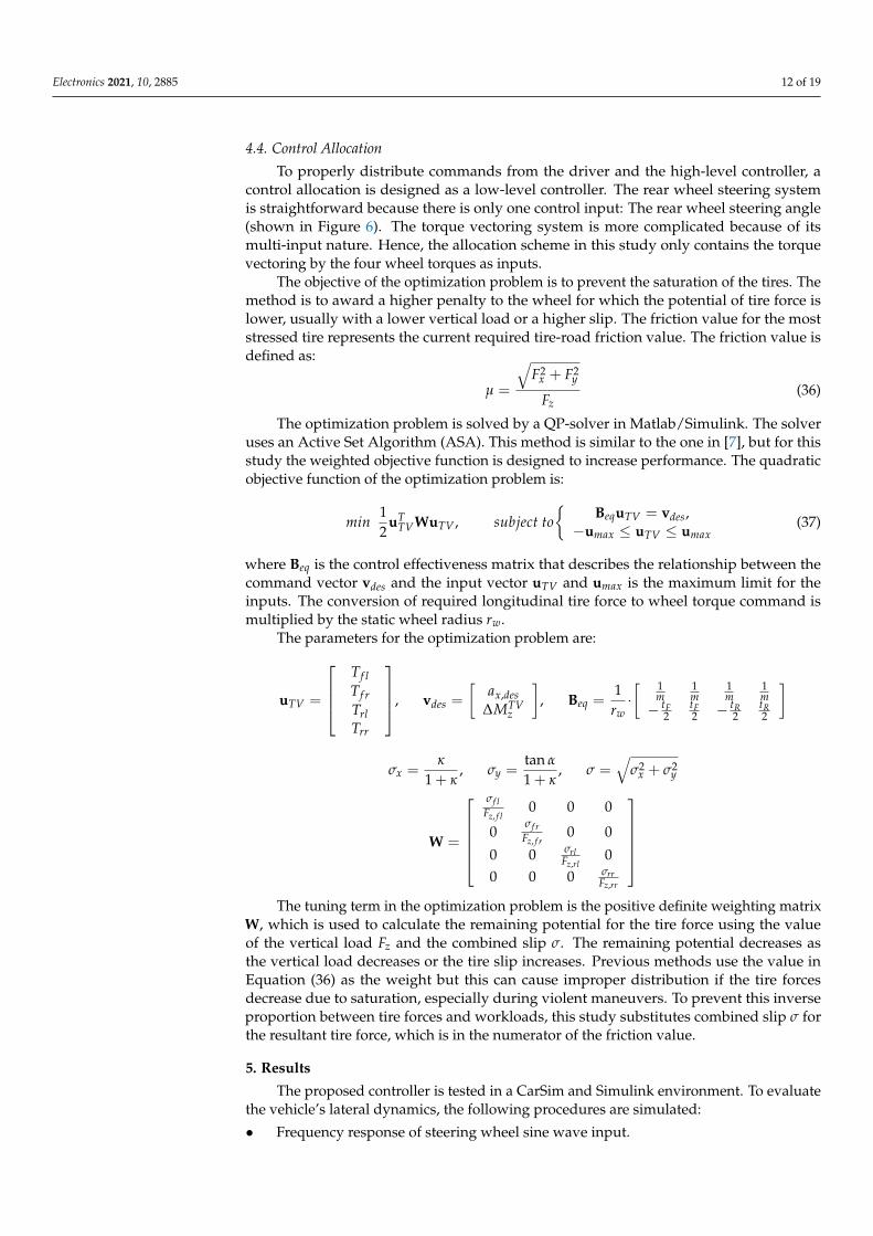
4.4. Control Allocation

To properly distribute commands from the driver and the high-level controller, acontrol allocation is designed as a low-level controller. The rear wheel steering systemis straightforward because there is only one control input: The rear wheel steering angle(shown in Figure 6). The torque vectoring system is more complicated because of itsmulti-input nature. Hence, the allocation scheme in this study only contains the torquevectoring by the four wheel torques as inputs.

The objective of the optimization problem is to prevent the saturation of the tires. Themethod is to award a higher penalty to the wheel for which the potential of tire force islower, usually with a lower vertical load or a higher slip. The friction value for the moststressed tire represents the current required tire-road friction value. The friction value isdefined as:

µ =

√F2

x + F2y

Fz(36)

The optimization problem is solved by a QP-solver in Matlab/Simulink. The solveruses an Active Set Algorithm (ASA). This method is similar to the one in [7], but for thisstudy the weighted objective function is designed to increase performance. The quadraticobjective function of the optimization problem is:

min12

uTTVWuTV , subject to

{BequTV = vdes,

−umax ≤ uTV ≤ umax(37)

where Beq is the control effectiveness matrix that describes the relationship between thecommand vector vdes and the input vector uTV and umax is the maximum limit for theinputs. The conversion of required longitudinal tire force to wheel torque command ismultiplied by the static wheel radius rw.

The parameters for the optimization problem are:

uTV =

Tf lTf rTrlTrr

, vdes =

[ax,des

∆MTVz

], Beq =

1rw

·[ 1

m1m

1m

1m

− tF2

tF2 − tR

2tR2

]

σx =κ

1 + κ, σy =

tan α

1 + κ, σ =

√σ2

x + σ2y

W =

σf l

Fz, f l0 0 0

0σf r

Fz, f r0 0

0 0 σrlFz,rl

00 0 0 σrr

Fz,rr

The tuning term in the optimization problem is the positive definite weighting matrix

W, which is used to calculate the remaining potential for the tire force using the valueof the vertical load Fz and the combined slip σ. The remaining potential decreases asthe vertical load decreases or the tire slip increases. Previous methods use the value inEquation (36) as the weight but this can cause improper distribution if the tire forcesdecrease due to saturation, especially during violent maneuvers. To prevent this inverseproportion between tire forces and workloads, this study substitutes combined slip σ forthe resultant tire force, which is in the numerator of the friction value.

5. Results

The proposed controller is tested in a CarSim and Simulink environment. To evaluatethe vehicle’s lateral dynamics, the following procedures are simulated:

• Frequency response of steering wheel sine wave input.

Electronics 2021, 10, 2885 13 of 19

• Slow ramp input of steering wheel at constant speed.• Sine with Dwell steering with a 5A amplitude.• Double lane change (DLC).

The first three procedures are open-loop tests. Maneuvering the same steering wheelinputs in both the passive and controlled vehicles. The DLC procedure uses the built-inpreview driver model with a 0.5 s preview time.

In this study, the steering wheel sine wave input, ramp input and DLC tests aredesigned to examine the improvement of handling performance. Thus, in these procedures,we do not apply extreme severe maneuvers to make the vehicle lose control. On thecontrary, the objective of the Sine with Dwell test is to examine the quality of stabilitymode. The maneuver in this test will be fierce to cause an unstable situation and activatestability mode.

The plant model used in this study is one of the B-class Hatchback vehicles in CarSim.The improved vehicle, which is used as the reference model, has a mass and yaw inertia of10% less to make the vehicle nimbler and more neutral. All procedures are tested on a flatroad for which the road coefficient is 0.85.

5.1. Frequency Responses

Figure 10 shows the frequency response plots for the yaw rate and side slip angle,from the steering wheel sine sweep maneuver. The amplitude of yaw rate increases andthe amplitude of side slip angle decreases from low to high frequency. The increase in thephase margin for yaw motion represents an improvement in the vehicle’s agility, whichis generally considered as a handling index by drivers. The bandwidths are increased forboth systems so the responsiveness and stability are increased.

Electronics 2021, 10, x FOR PEER REVIEW 14 of 19

(a) (b)

Figure 10. Frequency response in steering sine sweep test: (a) Yaw rate response; (b) Side slip angle response.

5.2. Slow Ramp Steer Response During the slow ramp steer procedure, the desired behavior is a linear and flat rela-

tionship between the lateral acceleration and the steering wheel input. For safety reasons, the side slip angle should decrease smoothly and not diverge at high lateral accelerations. Increasing the steering wheel angle when the lateral acceleration is saturated is an im-portant signal for the driver, which indicates that the vehicle is reaching its limit. In order to improve lateral performance, this must occur as late as possible.

Figure 11a shows the relationship between lateral acceleration and steering wheel input. The linear region for a controlled vehicle is extended to generate higher lateral ac-celerations and the maximum lateral acceleration is increased. This is beneficial for sports or race cars because a driver has a larger linear operating region and there is less risk of losing control.

Figure 11b shows the relationship between lateral acceleration and side slip angle. Both the passive and the controlled vehicle transit to understeer at the maximum lateral acceleration but the controlled vehicle exhibits a smaller side slip angle for the same lateral acceleration. This is the most significant effect of the rear wheel steering system, because it produces additional lateral force at an axle.

(a) 𝛿 vs. 𝐴 (b) 𝛽 vs. 𝐴

Figure 10. Frequency response in steering sine sweep test: (a) Yaw rate response; (b) Side slip angle response.

5.2. Slow Ramp Steer Response

During the slow ramp steer procedure, the desired behavior is a linear and flatrelationship between the lateral acceleration and the steering wheel input. For safetyreasons, the side slip angle should decrease smoothly and not diverge at high lateralaccelerations. Increasing the steering wheel angle when the lateral acceleration is saturatedis an important signal for the driver, which indicates that the vehicle is reaching its limit.In order to improve lateral performance, this must occur as late as possible.

Figure 11a shows the relationship between lateral acceleration and steering wheelinput. The linear region for a controlled vehicle is extended to generate higher lateralaccelerations and the maximum lateral acceleration is increased. This is beneficial for sports

Electronics 2021, 10, 2885 14 of 19

or race cars because a driver has a larger linear operating region and there is less risk oflosing control.

Electronics 2021, 10, x FOR PEER REVIEW 14 of 19

(a) (b)

Figure 10. Frequency response in steering sine sweep test: (a) Yaw rate response; (b) Side slip angle response.

5.2. Slow Ramp Steer Response During the slow ramp steer procedure, the desired behavior is a linear and flat rela-

tionship between the lateral acceleration and the steering wheel input. For safety reasons, the side slip angle should decrease smoothly and not diverge at high lateral accelerations. Increasing the steering wheel angle when the lateral acceleration is saturated is an im-portant signal for the driver, which indicates that the vehicle is reaching its limit. In order to improve lateral performance, this must occur as late as possible.

Figure 11a shows the relationship between lateral acceleration and steering wheel input. The linear region for a controlled vehicle is extended to generate higher lateral ac-celerations and the maximum lateral acceleration is increased. This is beneficial for sports or race cars because a driver has a larger linear operating region and there is less risk of losing control.

Figure 11b shows the relationship between lateral acceleration and side slip angle. Both the passive and the controlled vehicle transit to understeer at the maximum lateral acceleration but the controlled vehicle exhibits a smaller side slip angle for the same lateral acceleration. This is the most significant effect of the rear wheel steering system, because it produces additional lateral force at an axle.

(a) 𝛿 vs. 𝐴 (b) 𝛽 vs. 𝐴

Figure 11. Results in the steering ramp test: (a) Lateral acceleration vs. steering wheel angle input;(b) Lateral acceleration vs. side slip angle.

Figure 11b shows the relationship between lateral acceleration and side slip angle.Both the passive and the controlled vehicle transit to understeer at the maximum lateralacceleration but the controlled vehicle exhibits a smaller side slip angle for the same lateralacceleration. This is the most significant effect of the rear wheel steering system, because itproduces additional lateral force at an axle.

5.3. Sine with Dwell

Sine with Dwell is a standard stability test that was formulated by the NationalHighway Traffic Safety Administration (NHTSA) [16]. The first step of this test involvesmaneuvering with a slow steering ramp input until the vehicle’s lateral acceleration reaches0.3 g at 80 km/h. This defines the unit angle amplitude A of the steering wheel for thefollowing tests. For this study, the stability test tests a situation that the feedforwardcontroller (handling mode) cannot handle well due to violent maneuvering or modeluncertainties. The steering amplitude of 5 A is used for this test and the feedback controller(stability mode) must intervene to stabilize its motion. The open-loop steering command isshown in Figure 12.

Figure 13 shows the yaw rate and the side slip responses in the Sine with Dwell test.Due to the violent change in direction, the amplitude of yaw motion is increased. Thiseffect is known as a Scandinavian flick, and is usually used in rally races but is difficult tohandle for normal drivers. All vehicles become unstable after 2 s, but the passive vehicleloses control completely and the side slip angle becomes significant. The vehicle thatuses handling mode has a smaller side slip angle but does not return to the zero-dynamicquickly after the steering wheel angle returns to zero. Combined control with additionalstability mode maintains a lower side slip angle and returns to the zero-dynamic relativelyquickly. The feedback controller produces some oscillations in the yaw motion at about2 to 3 s, which produces a synthetic driving feeling. This is not beneficial to handlingimprovement scenarios.

Electronics 2021, 10, 2885 15 of 19

Electronics 2021, 10, x FOR PEER REVIEW 15 of 19

Figure 11. Results in the steering ramp test: (a) Lateral acceleration vs. steering wheel angle input; (b) Lateral acceleration vs. side slip angle.

5.3. Sine with Dwell Sine with Dwell is a standard stability test that was formulated by the National High-

way Traffic Safety Administration (NHTSA) [16]. The first step of this test involves ma-neuvering with a slow steering ramp input until the vehicle’s lateral acceleration reaches 0.3g at 80 km/h. This defines the unit angle amplitude A of the steering wheel for the following tests. For this study, the stability test tests a situation that the feedforward con-troller (handling mode) cannot handle well due to violent maneuvering or model uncer-tainties. The steering amplitude of 5A is used for this test and the feedback controller (sta-bility mode) must intervene to stabilize its motion. The open-loop steering command is shown in Figure 12.

Figure 12. Steering wheel input in the Sine with Dwell stability test.

Figure 13 shows the yaw rate and the side slip responses in the Sine with Dwell test. Due to the violent change in direction, the amplitude of yaw motion is increased. This effect is known as a Scandinavian flick, and is usually used in rally races but is difficult to handle for normal drivers. All vehicles become unstable after 2 s, but the passive vehicle loses control completely and the side slip angle becomes significant. The vehicle that uses handling mode has a smaller side slip angle but does not return to the zero-dynamic quickly after the steering wheel angle returns to zero. Combined control with additional stability mode maintains a lower side slip angle and returns to the zero-dynamic relatively quickly. The feedback controller produces some oscillations in the yaw motion at about 2 to 3 s, which produces a synthetic driving feeling. This is not beneficial to handling im-provement scenarios.

Figure 12. Steering wheel input in the Sine with Dwell stability test.

Electronics 2021, 10, x FOR PEER REVIEW 16 of 19

(a) (b)

Figure 13. Results in Sine with Dwell stability test: (a) Yaw rate responses; (b) Side slip angle responses.

5.4. Double Lane Change A double lane change (DLC) is a universally acknowledged handling test. For this

study, the standard test ISO 3888-1 is implemented using the built-in preview driver model with a 0.5 s preview time. The driver model in CarSim represents an average driver and generates a steering action for trajectory tracking. This procedure is known as a moose test or elk test because a quick change in direction tests the responsiveness, stability and oscillation of the lateral dynamics. The track layout and vehicle’s trajectory of ISO 3888-1 are shown in Figure 14. The longitudinal distance and the lateral offset of the centerline are fixed and the width of cones in each section is varied depending on the vehicle’s width. Although the trajectories of both vehicles are similar, the lateral dynamic responses are different. This demonstrates the benefits of the proposed controller.

The lateral distance error is not meaningful for the DLC test because drivers should plan the best route or racing line that allows the fastest passage in the real test. The lateral tracking error is affected by the driver model more than the chassis control system. There-fore, the DLC test should not be tested by virtual drivers only. A road test or driver in loop (DIL) environment is necessary to verify its performance.

Figure 13. Results in Sine with Dwell stability test: (a) Yaw rate responses; (b) Side slip angle responses.

5.4. Double Lane Change

A double lane change (DLC) is a universally acknowledged handling test. For thisstudy, the standard test ISO 3888-1 is implemented using the built-in preview driver modelwith a 0.5 s preview time. The driver model in CarSim represents an average driver andgenerates a steering action for trajectory tracking. This procedure is known as a moosetest or elk test because a quick change in direction tests the responsiveness, stability andoscillation of the lateral dynamics. The track layout and vehicle’s trajectory of ISO 3888-1are shown in Figure 14. The longitudinal distance and the lateral offset of the centerline arefixed and the width of cones in each section is varied depending on the vehicle’s width.Although the trajectories of both vehicles are similar, the lateral dynamic responses aredifferent. This demonstrates the benefits of the proposed controller.

Electronics 2021, 10, 2885 16 of 19

Electronics 2021, 10, x FOR PEER REVIEW 16 of 19

(a) (b)

Figure 13. Results in Sine with Dwell stability test: (a) Yaw rate responses; (b) Side slip angle responses.

5.4. Double Lane Change A double lane change (DLC) is a universally acknowledged handling test. For this

study, the standard test ISO 3888-1 is implemented using the built-in preview driver model with a 0.5 s preview time. The driver model in CarSim represents an average driver and generates a steering action for trajectory tracking. This procedure is known as a moose test or elk test because a quick change in direction tests the responsiveness, stability and oscillation of the lateral dynamics. The track layout and vehicle’s trajectory of ISO 3888-1 are shown in Figure 14. The longitudinal distance and the lateral offset of the centerline are fixed and the width of cones in each section is varied depending on the vehicle’s width. Although the trajectories of both vehicles are similar, the lateral dynamic responses are different. This demonstrates the benefits of the proposed controller.

The lateral distance error is not meaningful for the DLC test because drivers should plan the best route or racing line that allows the fastest passage in the real test. The lateral tracking error is affected by the driver model more than the chassis control system. There-fore, the DLC test should not be tested by virtual drivers only. A road test or driver in loop (DIL) environment is necessary to verify its performance.

Figure 14. Track layout and trajectories for ISO 3888-1.

The lateral distance error is not meaningful for the DLC test because drivers shouldplan the best route or racing line that allows the fastest passage in the real test. Thelateral tracking error is affected by the driver model more than the chassis control system.Therefore, the DLC test should not be tested by virtual drivers only. A road test or driverin loop (DIL) environment is necessary to verify its performance.

Figure 15 shows the yaw rate and the side slip responses for the DLC test. For thetarget path in Figure 14, the curvatures are the same for the first two and last two corners,but the yaw rate response for the passive vehicle is larger for corners 2 and 4 due to thelack of responsiveness. The controlled vehicle has a similar magnitude of response forevery corner and the side slip angle is decreased. Oscillations are also decreased when thecontrolled vehicle returns to a straight line after corners. It shows that the responsivenessand stability are improved simultaneously.

Electronics 2021, 10, x FOR PEER REVIEW 17 of 19

Figure 14. Track layout and trajectories for ISO 3888-1.

Figure 15 shows the yaw rate and the side slip responses for the DLC test. For the target path in Figure 14, the curvatures are the same for the first two and last two corners, but the yaw rate response for the passive vehicle is larger for corners 2 and 4 due to the lack of responsiveness. The controlled vehicle has a similar magnitude of response for every corner and the side slip angle is decreased. Oscillations are also decreased when the controlled vehicle returns to a straight line after corners. It shows that the responsiveness and stability are improved simultaneously.

(a) (b)

Figure 15. Results for ISO 3888-1 at 80 km/h: (a) Yaw rate response; (b) Side slip angle response.

Figure 16 shows the steering angles at the rear axle and the driver’s input. The pro-posed control system provides a sporty driving sensation and makes a driver pass the track with smoother steering wheel input.

(a) (b)

Figure 16. Steering angle for ISO 3888-1 at 80 km/h: (a) Rear wheel steering angle; (b) Steering wheel angle.

Figure 17 shows the tire workload for the passive and the controlled vehicle. The used friction value at the most stressed tire represents the current required tire-road fric-tion coefficient and must be as small as possible. The red horizontal lines show that the

Figure 15. Results for ISO 3888-1 at 80 km/h: (a) Yaw rate response; (b) Side slip angle response.

Figure 16 shows the steering angles at the rear axle and the driver’s input. Theproposed control system provides a sporty driving sensation and makes a driver pass thetrack with smoother steering wheel input.

Electronics 2021, 10, 2885 17 of 19

Electronics 2021, 10, x FOR PEER REVIEW 17 of 19

Figure 14. Track layout and trajectories for ISO 3888-1.

Figure 15 shows the yaw rate and the side slip responses for the DLC test. For the target path in Figure 14, the curvatures are the same for the first two and last two corners, but the yaw rate response for the passive vehicle is larger for corners 2 and 4 due to the lack of responsiveness. The controlled vehicle has a similar magnitude of response for every corner and the side slip angle is decreased. Oscillations are also decreased when the controlled vehicle returns to a straight line after corners. It shows that the responsiveness and stability are improved simultaneously.

(a) (b)

Figure 15. Results for ISO 3888-1 at 80 km/h: (a) Yaw rate response; (b) Side slip angle response.

Figure 16 shows the steering angles at the rear axle and the driver’s input. The pro-posed control system provides a sporty driving sensation and makes a driver pass the track with smoother steering wheel input.

(a) (b)

Figure 16. Steering angle for ISO 3888-1 at 80 km/h: (a) Rear wheel steering angle; (b) Steering wheel angle.

Figure 17 shows the tire workload for the passive and the controlled vehicle. The used friction value at the most stressed tire represents the current required tire-road fric-tion coefficient and must be as small as possible. The red horizontal lines show that the

Figure 16. Steering angle for ISO 3888-1 at 80 km/h: (a) Rear wheel steering angle; (b) Steering wheel angle.

Figure 17 shows the tire workload for the passive and the controlled vehicle. The usedfriction value at the most stressed tire represents the current required tire-road frictioncoefficient and must be as small as possible. The red horizontal lines show that thecontrolled vehicle has a significantly lower required friction value because the allocationmethod balances each tire’s workload and prevents early saturation for a single wheel.Retaining more capacity for tire force means that the vehicle produces greater accelerationand allows more aggressive driving, or maintains the same dynamics on a road with alower coefficient of friction, so the driving performance and safety are increased.

Electronics 2021, 10, x FOR PEER REVIEW 18 of 19

controlled vehicle has a significantly lower required friction value because the allocation method balances each tire’s workload and prevents early saturation for a single wheel. Retaining more capacity for tire force means that the vehicle produces greater acceleration and allows more aggressive driving, or maintains the same dynamics on a road with a lower coefficient of friction, so the driving performance and safety are increased.

(a) (b)

Figure 17. Tire workloads for ISO 3888-1 at 80 km/h: (a) Passive; (b) Handling mode.

6. Conclusions A combined controller for rear wheel steering and torque management is proposed.

The feedforward controller uses a complex combined slip tire model and an advanced vehicle model to analyze the secondary effect. It uses a passive improved vehicle model to generate the reference responses. This allows sporty and reproducible driving behavior. The method by which the reference is generated is similar to a state-of-the-art look-up table and involves changing the parameters for the reference model. This also produces a nature transient behavior compared to steady state reference generation. The feedforward controller does not achieve ideal and synthetic driving behavior, so the driving sensation is natural for sports car drivers. A road test driver study or a driver-in-loop (DIL) envi-ronment should be implemented for verification.

To address model uncertainties, the feedback controller ensures safety. It detects un-stable situations when there is risk of losing control. The stability criterion is a subject for future study because the strategy for stability control determines the balance between driving performance and safety.

Control allocation is complicated for an over-actuated system. The method for this study balances each tire’s workload and prevents saturation of the tires. The results show that the required tire-road friction is reduced by proper control allocation, so performance and stability are increased. The quality of the allocation is affected by the quality of the estimation and the actuator’s dynamics. These are the subjects for future study.

Author Contributions: Conceptualization, P.-CC. and C.-K.C.; methodology, P.-C.C.; formal anal-ysis, P.-C.C.; investigation, P.-C.C.; writing—original draft preparation, P.-C.C.; writing—review and editing, C.-K.C.; supervision, C.-K.C. All authors have read and agreed to the published version of the manuscript.

Funding: This work is supported by the Ministry of Science and Technology of Taiwan, ROC. Grant number MOST 104-2221-E-212-014-MY2.

Acknowledgments: The authors would like to thank Ping Huang for technical support.

Figure 17. Tire workloads for ISO 3888-1 at 80 km/h: (a) Passive; (b) Handling mode.

6. Conclusions

A combined controller for rear wheel steering and torque management is proposed.The feedforward controller uses a complex combined slip tire model and an advancedvehicle model to analyze the secondary effect. It uses a passive improved vehicle model togenerate the reference responses. This allows sporty and reproducible driving behavior.

Electronics 2021, 10, 2885 18 of 19

The method by which the reference is generated is similar to a state-of-the-art look-uptable and involves changing the parameters for the reference model. This also produces anature transient behavior compared to steady state reference generation. The feedforwardcontroller does not achieve ideal and synthetic driving behavior, so the driving sensation isnatural for sports car drivers. A road test driver study or a driver-in-loop (DIL) environmentshould be implemented for verification.

To address model uncertainties, the feedback controller ensures safety. It detectsunstable situations when there is risk of losing control. The stability criterion is a subjectfor future study because the strategy for stability control determines the balance betweendriving performance and safety.

Control allocation is complicated for an over-actuated system. The method for thisstudy balances each tire’s workload and prevents saturation of the tires. The results showthat the required tire-road friction is reduced by proper control allocation, so performanceand stability are increased. The quality of the allocation is affected by the quality of theestimation and the actuator’s dynamics. These are the subjects for future study.

Author Contributions: Conceptualization, P.-C.C. and C.-K.C.; methodology, P.-C.C.; formal analysis,P.-C.C.; investigation, P.-C.C.; writing—original draft preparation, P.-C.C.; writing—review andediting, C.-K.C.; supervision, C.-K.C. All authors have read and agreed to the published version ofthe manuscript.

Funding: This work is supported by the Ministry of Science and Technology of Taiwan, ROC. Grantnumber MOST 110-2221-E-027-093.

Acknowledgments: The authors would like to thank Ping Huang for technical support.

Conflicts of Interest: The authors declare no conflict of interest.

References1. Piyabongkarn, D.; Rajamani, R.; Lew, J.Y.; Yu, H. On the use of torque-biasing devices for vehicle stability control. In Proceedings

of the 2006 American Control Conference, Minneapolis, MN, USA, 14–16 June 2006.2. Shibahata, Y.; Shimada, K.; Tomari, T. Improvement of Vehicle Maneuverability by Direct Yaw Moment Control. Veh. Syst. Dyn.

1993, 22, 465–481. [CrossRef]3. Mokhiamar, O.; Abe, M. Simultaneous Optimal Distribution of Lateral and Longitudinal Tire Forces for the Model Following

Control. J. Dyn. Syst. Meas. Control. 2004, 126, 753–763. [CrossRef]4. Shen, H.; Tan, Y.-S. Vehicle handling and stability control by the cooperative control of 4WS and DYC. Mod. Phys. Lett. B 2017, 31,

1740090. [CrossRef]5. Chen, B.-C.; Kuo, C.-C. Electronic stability control for electric vehicle with four in-wheel motors. Int. J. Automot. Technol. 2014, 15,

573–580. [CrossRef]6. Peters, Y.; Stadelmayer, M. Control allocation for all wheel drive sports cars with rear wheel steering. Automot. Engine Technol.

2019, 4, 111–123. [CrossRef]7. Kissai, M.; Monsuez, B.; Mouton, X.; Tapus, A. Optimization-Based Control Allocation for Driving/Braking Torque Vectoring in a

Race Car. In Proceedings of the 2020 American Control Conference (ACC), Denvor, CO, USA, 1–3 July 2020.8. Warth, G.; Frey, M.; Gauterin, F. Design of a central feedforward control of torque vectoring and rear-wheel steering to beneficially

use tyre information. Veh. Syst. Dyn. 2019, 58, 1789–1822. [CrossRef]9. Hang, P.; Xia, X.; Chen, X. Handling Stability Advancement With 4WS and DYC Coordinated Control: A Gain-Scheduled Robust

Control Approach. IEEE Trans. Veh. Technol. 2021, 70, 3164–3174. [CrossRef]10. Kissai, M.; Monsuez, B.; Mouton, X.; Martinez, D.; Tapus, A. Model Predictive Control Allocation of Systems with Different

Dynamics. In Proceedings of the 2019 IEEE Intelligent Transportation Systems Conference (ITSC), Auckland, New Zealand, 27–30October 2019.

11. Han, Z.; Xu, N.; Chen, H.; Huang, Y.; Zhao, B. Energy-efficient control of electric vehicles based on linear quadratic regulator andphase plane analysis. Appl. Energy 2018, 213, 639–657. [CrossRef]

12. Xiao, F. Optimal torque distribution for four-wheel-motored electric vehicle stability enhancement. In Proceedings of the 2015IEEE International Transportation Electrification Conference (ITEC), Chennai, India, 27–29 August 2015.

13. Pacejka, H. Tire and Vehicle Dynamics; Elsevier: Amsterdam, The Netherlands, 2005.14. Burhaumudin, M.S.; Samin, P.M.; Jamaluddin, H.; Rahman, R.A.; Sulaiman, S. Modeling and validation of magic formula

tire model. In Proceedings of the International Conference on the Automotive Industry, Mechanical and Materials Science(ICAMME 2012), Penang, Malaysia, 19 May 2012.

Electronics 2021, 10, 2885 19 of 19

15. Huang, Y.; Chen, Y. Estimation and analysis of vehicle lateral stability region with both front and rear wheel steering. InProceedings of the Dynamic Systems and Control Conference, American Society of Mechanical Engineers, Tysons Corner,Virginia, 11–13 October 2017.

16. Proposed FMVSS No. 126 Electronic Stability Control Systems; Office of Regulatory Analysis and Evaluation, National Center forStatistics and Analysis: Washington, DC, USA, 2007.