INI'D RSPA HAl. i NHI O (NI iSI I()( NI.Al.1

1 '0 1 1 .1 lA NIS I'S I, AO AN I) bI P)

F by I emiaMefl)f

'1*moo

_______________ __'__ 7- ____

All 198

INDOOR SPATIAL MONITORING OF COMBUSTION GENERATED POLLUTANTS

(TSP, CO, AND BaP) BY INDIAN COOKSTOVES

by

Premlata Menon

Department of MeteorologyUniversity of Hawaii

Supported by ' /Resource Systems InstituteEast West Center, Honolulu

AND

Environmental Planning and Coordinating OrganizationDept. of Housing and Environment

Govt. of M.P., Bhopal, IndiaAcoession For--iIs GRA&IDTIC TABUnannounced .

July, 1988 _i!oatloml

Distributin/Availability Codes

Diet Special

ABSTRACr,,. ,

This dissertation focusses on indoor concentrations of

pollutants (TSP, CO and BaP) emitted by Indian cookstoves.

Experiments in a simulated village hut (SVH) determined size

distribution of particulates from burning of fuelwood and

cowdung, and investigated the effects of fuel, ventilation

condition and sampling location on TSP, CO and BaP

concentrations. 84 to 99 % of the total particulate mass in

wood and dung smoke had aerodynamic diameter less than

3.2 pm, which eliminated the need for particle size

discriminating sampling. These experiments finalised the field

sampling protocol.

The field survey included 291 households in three central

and two south Indian villages. The kitchens had either

thatched or tiled roofs with a variety of volumes and open

spaces on the walls. Fixed monitoring was done at roof, medium

and low levels close to stove or chula (cemented to floor) and

personal sampler on the cook monitored air in her breathing

zone.N TSP, CO and BaP were measured in 129 households in the

five villages. Pollutant levels varied with sampling site,

ventilation conditions and fuel quality. Mean TSP exposure to

cooks was 5 mg/m 3 , twenty times higher than the standard

specified by regulating agencies (U.S, WHO and India) for

ambient conditions. Mean CO exposure to cooks was 51 ppm,

three times higher than the corresponding standard. However,

i -

TSP and CO levels wer.e equal to OSHA standard. Mean BaP

exposures to cooks were 160 ng/m 3 , equal to ambient levels

found in cities in developed countries. While cook's mean

exposure to TSP and CO agrees with earlier studies, her

exposure to BaP is an order lower. The cook's exposure to TSP

and BaP was similar to lowest indoor fixed monitoring levels

but order of magnitude above outdoor concentrations. Next to

the chula TSP, CO and BaP levels increased with height. TSP,

CO and BaP levels in thatched huts were comparable to those

measured in SVH. Tiled hut roofs allowed smoke seepage

resulting in much lower concentrations than in thatched huts.

TSP (roof) and CO (cook) were significantly higher in winter

than during monsoon and, CO (cook) was higher in morning than

evening.

ii

TABLE OF CONTENTS

Pagre

ABSTRACT ............................................... i

LIST OF FIGURES ........................................... v

LIST OF TABLES .......................................... viii

LIST OF ABBREVIATIONS ..................................... xi

I. INTRODUCTION

1.1 Indoor air quality issue ....................... 1

1.2 Indoor air pollutants (Developing world) ..... 6

1.3 Research objectives ............................ 0

II. EXPOSURE TO COMBUSTION GENERATED POLLUTANTS-LITERATURE REVIEW

2.1 Background ...................................... 12

2.2 Traditional fuel use in India ................. 12

2.3 Justification for selecting TSP, CO, and BaPfor monitoring ................................. 17

2.4 Health effects of biomass generated smoke(TSP, CO, and BaP) ............................. 21

2.4.1 Total suspended particulates (TSP) ......... 26

2.4.2 Carbon Monoxide (CO) ......................... 31

2.4.3 Benzo(a)pyrene (BaP) ......................... 33

2.5 Review of studies related to indoormonitoring of combustion generatedpollutants emitted from cooking stoves usingtraditional fuels .............................. 41

iii

Paae

III. RESULTS AND DISCUSSION

3.1 Results of experiments performed inSimulated Village Hut .......................... 55

3.1.1 Size distribution of particulates .......... 56

3.1.2 Variation of particle size with burn time.. 62

3.1.3 Variation of TSP and CO concentration withburn time .................................... 66

3.1.4 Effect of fuel, ventilation and samplinglocation on TSP, CO and BaP concentrationand ratio of BaP to TSP ..................... 70

3.1.5 Summary and recommendations for fieldexperiments .................................. 85

3.2 Field experiments (India) ...................... 90

3.2.1 Socio-economic characteristics, fueluse and perception of problems relatedto smoke ..................................... 91

3.2.2 Cook's exposure to TSP, CO and BaP and theirspatial concentrations ..................... 109

3.2.3 Significant differences of cook's exposureto TSP and CO and levels of TSP at roof.... 135

3.2.4 Main effect and interactions of climate,ventilation conditions and samplinglocation on CO .............................. 143

3.2.5 Statistical model for estimating cook's

exposure to TSP .............................. 148

IV. SUMMARY AND RECOMMENDATIONS

4.1 Summary ........................................ 160

4.2 Recommendations for future studies ........... 165

ACKNOWLEDGEMENTS ................................... 166

REFERENCES .......................................... 168

iv

LIST OF FIGURES

FigureNumberPae

2.1 Form of the efficiency curve for particledeposition ..................................... 29

2.2 Respiratory deposition of particulatesaccording to size: .01-100 pm diameter ....... 30

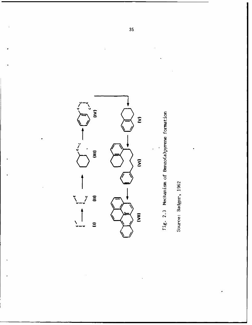
2.3 Mechanism of Benzo(a)pyrene formation ........ 35

3.1 Typical log probability plot of particleaerosol size for wood and dung smoke.(SVH, November, 1982) .......................... 59

3.2 Typical generalized histogram plot of aerosolparticle size for wood and dunQ smoke (SVH,November,1982) .................................. 61

3.3 Typical variation of particle size (arithmeticmean) with burn time for wood and dungsmoke ........................................... 63

3.4 Respirable fraction of combustion generatedparticulates sampled during typical cookingperiod in simulated village hut .............. 64

3.5 Typical TSP concentration (mg/m3 ) with burntime (min) for dung and wood smoke. Samplingprobe located at 1.6 m above floor and TSPsampled under limited ventilation condition(only door open) ................................ 67

3.6 Typical variation of CO concentration (ppm)in dung smoke with burn time (min) for a highand low level site. Sampling done under limitedventilation condition (only door open) using aGeneral Electric Co personal monitor ......... 69

3.7 Mean TSP concentration (mg/m3 ) measured at 11sites using a sequential sampler. Samplingdone for wood and dung smoke under limited(only door open) and better (door and windowopen) ventilation condition ................... 71

3.8a Variation of TSP concentration (mg/m3 ) forwood smoke with burn time (min) showing theeffect of ventilation. Sampling probelocated at 1.6 m above floor ................ 74

v

FigureNumber Page

3.8b Variation of TSP concentration (mg/m3) frwood smoke with burn time (min) showing theeffect of ventilation. Sampling probelocated at 1.6 m above floor ................ 75

3.9 Typical variation of CO concentration (ppm)in wood and dung smoke with burn time (min)for a high sampling site. Sampling doneunder limited ventilation condition (onlydoor open) using General Electric CO portablemonitor ......................................... 77

3.10 Effect of ventilation on reducing COconcentration (ppm) at high sampling site.General Electric portable sampler used tomonitor CO levels in wood smoke ............. 78

3.11 Sampling sites for measurement of TSPconcentration (mg/m3 ) in the rural kitchensusing personal samplers ....................... 88

3.12 Sampling sites for measurement of COconcentration (ppm) in the rural kitchensusing personal sampler ....................... 89

3.13 Designation of wall with respect to chula... 117

3.14 Indoor mean TSP concentration (mg/m3 )reported by several authors (comparablestudies). Area sampling means sampler fixedat some point, whereas, exposure meanssampler worn by cook .......................... 123

3.15 Indoor mean CO concentration (ppm) reportedby several authors (comparable studies) ..... 126

3.16 Indoor mean BaP concentration (ng/m3 )reported by several authors (comparablestudies) ....................................... 128

3.17 Photo illustrating the simulated village hut,a thatched roof hut and tiled roof hut ...... 142

vi

FigureNumber Pane

3.18 Proposed structural model showing direct andindirect relationships between meteorological,ventilation, fuel, stove and cook's exposureto TSP ......................................... 151

3.19 Model with path estimates ................... 159

4.1 Sketch of proposed rural kitchen with mud hoodand shorter wall adjacent to chula, door placedon the wall opposite to chula and a glass paneon the roof ..................................... 164

vii

LIST OF TABLES

TableNumber Page

1.1 Typical sources of air pollutants grouped byorigin ................................................ 4

1.2 Studies of indoor combustion generated pollutants

in developing countries .............................. 8

2.1 Patterns of energy use in rural India ............. 13

2.2 Source-wise energy consumption in rural householdsector ............................................... 14

2.3 Traditional rural fuel consumption (kg/yr/capita). 16

2.4 Comparison of air pollutant emissions from Energy-Equivalent Fuels (in kilograms) ..................... 18

2.5 Organic substances found in wood smoke emissions.. 19

2.6 Emission factors for cilia toxic and mucus coagul-ating agents observed in smoke and flue gas fromresidential wood combustion ......................... 19

2.7 Epidemiological studies on air pollution frombiomass combustion .................................. 22

2.8 Concentration of Toxic gases in smoke in houses inLagos, Nigeria ....................................... 42

2.9 Chemical analytical data: Situations analyzedduring cooking in huts .............................. 45

2.10 Average BaP concentration near breathing zones ofdomestic housewives using different local cookingfuels ............................................... 48

2.11 Summary of household data and measured concent-rations ............................................. 50

2.12 Levels of air pollutants observed and types offuels used at cooking places ....................... 52

Viii

TableNumber Page

3.1 Fuel, ventilation and burn parameter in SVHfor the Quart Crystal Mass Cascade ImpactorExperiments .......................................... 57

3.2 Average and range of TSP (mg/m3 ) and size (Am andGm) of combustion generated particulates fordifferent experimental setup during the QuartzCrystal Mass Cascade Impactor Experiments in thesimulated village hut ............................... 58

3.3 Average CO concentration (ppm) onitored at ninepoints in the simulated village hut for burnperiod lasting 15 minutes using fuel wood andcowdung .............................................. 68

3.4 Test of variance of CO by fuel type, ventilationcondition, sampling height and location in SVHusing split-plot analysis ........................... 79

3.5 Spatial indoor BaP concentrations (ng/m3) in theSVH by fuel type, ventilation condition, and sampleheight ............................................... 82

3.6 Integrated levels of TSP, CO and BaP during a typicalcooking period in SVH (November, 1982) ............ 83

3.7 Sumary statistics: Socio-Economic, fuel and smokeperception survey (7 pages) ......................... 95

3.8 Summary statistics: Field experiments in ruralkitchens of India (6 pages) ........................ 110

3.9 Mean TSP, CO and BaP concentrations in the fieldand in the simulated village hut .................. 121

3.10 Cook's exposure to BaP concentration in ruralkitchens of Nepal ................................. 130

3.11 Mean ratio of BaP to TSP (Qg/g) for Biomas smokereported by several author ....................... 131

ix

TableNumber Page

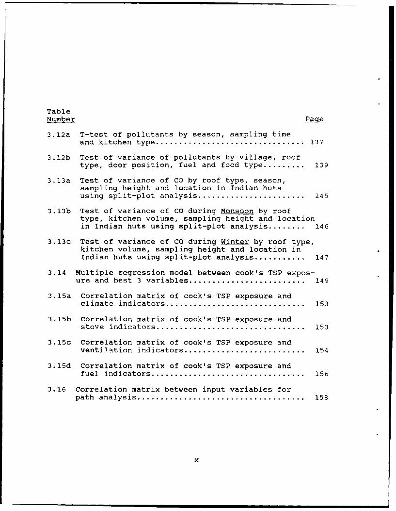
3.12a T-test of pollutants by season, sampling timeand kitchen type ................................. 137

3.12b Test of variance of pollutants by village, rooftype, door position, fuel and food type ......... 139

3.13a Test of variance of CO by roof type, season,sampling height and location in Indian hutsusing split-plot analysis ......................... 145

3.13b Test of variance of CO during Monsoon by rooftype, kitchen volume, sampling height and locationin Indian huts using split-plot analysis ........ 146

3.13c Test of variance of CO during Winter by roof type,kitchen volume, sampling height and location inIndian huts using split-plot analysis ........... 147

3.14 Multiple regression model between cook's TSP expos-ure and best 3 variables ........................... 149

3.15a Correlation matrix of cook's TSP exposure andclimate indicators ................................ 153

3.15b Correlation matrix of cook's TSP exposure andstove indicators .................................. 153

3.15c Correlation matrix of cook's TSP exposure andventilation indicators ............................ 154

3.15d Correlation matrix of cook's TSP exposure andfuel indicators ................................... 156

3.16 Correlation matrix between input variables forpath analysis ...................................... 158

x

List of Abbreviations

Am: Arithmetic Mean

ANOVA: Analysis of Variance

ARI: Acute Respiratory Infection

BaP: Benzo(a)pyrene

BHEL: Bharat Heavy Electricals Ltd. (India)

CIAE: Central Institute Of AgriculturalEngineering (Bhopal)

FP: Fine particulates

CO: Carbon Monoxide

GE: General Electric

Gm: Geometric Mean

GMDH: Group Method of Data Handling

HbCO: Carboxy Hemoglobin

Hi-Vol: High volume

HPLC: High Pressure Liquid Chromatography

MMD: Mass Median Diameter

NAS: National Science Academy (U.S.A)

OSHA: Occupation Safety and Health Adminstration

PAH: Poly Aromatic Hydrocarbon

POM: Polycyclic Organic Matter

QCMCI: Quartz Crystal Micro-balance Cascade Impactor

xi

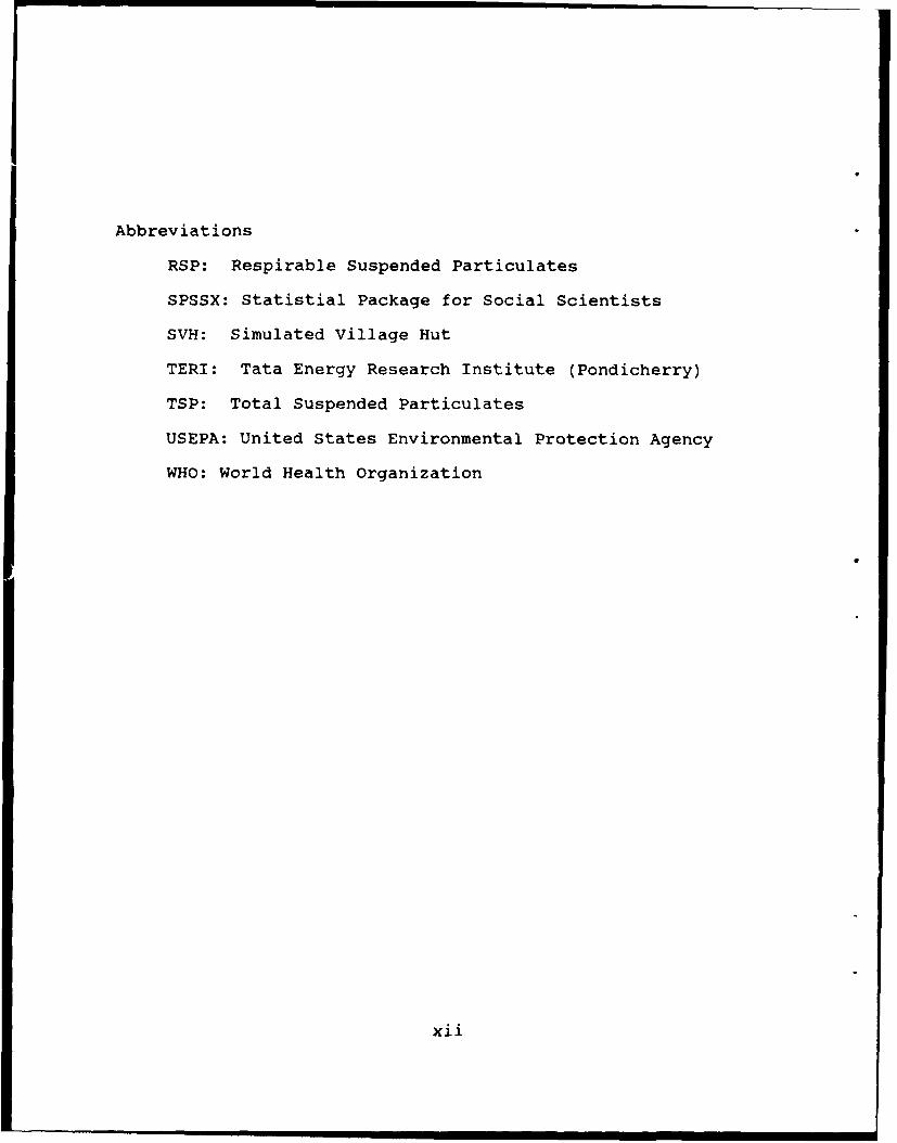
Abbreviations

RSP: Respirable Suspended Particulates

SPSSX: Statistial Package for Social Scientists

SVH: Simulated Village Hut

TERI: Tata Energy Research Institute (Pondicherry)

TSP: Total Suspended Particulates

USEPA: United States Environmental Protection Agency

WHO: World Health Organization

xii

1

I. INTRODUCTION

1.1 INDOOR AIR QUALITY ISSUE

Man may have first become aware of indoor air pollution

when he lit the first fires for cooking and space heating in

un-ventilated caves. With improvement of the design of

shelters, control of combustion products and substituting of

traditional fuels by electricity and gas, most of the indoor

combustion generated pollutants were minimized or vented

outside making indoors more comfortable and habitable.

However, it is disheartening that even today the indoor air

quality in kitchens of rural homes in the developing world,

where traditional fuels (wood, cowdung, crop residues etc.) are

the main sources of energy for cooking, is more or less like

the smoky conditions that must have occurred in unventilated

caves thousands of years earlier.

The first international conference on indoor climates

was organized in 1978, when it was recognized that indoor air

pollution levels had increased as a result of the use of new

less porous construction materials that entrapped indoor air

and reduced infiltration. The 1981 second international

symposium on Indoor Air Pollution, Health and Energy

Conservation (Moghissi, 1982) brought scientists together from

twelve developed countries to discuss public health concerns

focusing on formaldehyde, radon, biological aerosols, organic

vapors, combustion gases and soot. They emphasized that the

U.S. Clean Air Act of 1963 focussed attention only on cleaning

2

outdoor air and failed to address indoor air quality, inspite

the fact that people spent 80-90% of their time indoors, at

home, at work, or commuting. But it was also pointed out that

indoor air pollution is not only a problem for the developed

nations, is of great concern to third world, where cooking is

done indoors with traditional fuels on stoves that do not vent

outside.

The 1984 third international conference on Indoor Air

Quality and Climate produced five volumes titled INDOOR AIR

(Berglund, et al., 1984). Topics included recent advances in

the health sciences and building design, chemical analyses of

indoor air, sampling and analytical methods, indoor/outdoor

relationships of the pollutants, importance of personal

exposure, epidemiological studies of health disorders related

to housing, sick building syndrome,etc. Recently several

documents on INDOOR AIR QUALITY have been published. (WHO,

1979, 1982, 1983; Dudney & Walsh, 1981; Meyer & Hartley, 1982;

U.S. National Research Council, 1981; Proceedings of Second

International Symposium on Indoor Air Pollution, Health, and

Energy Conservation, 1982; Spengler and Colome, 1982, Yocom,

1982; Lebowitz, 1983; Spengler & Sexton, 1983; Kirsch, 1983;

Spengler & Soczek, 1984; Turiel, 1985; Meyer, 1983; Wadden and

Scheff, 1983). However, all above mentioned studies addressed

only the Indoor Air Quality and human exposures pertaining to

the developed countries.

3

Research on Indoor Air Quality started only during the

last few years, since previously air pollution was considered

to be an outdoor phenomenon and it was assumed that buildings

shelter their occupants from pollutants. Thus, air quality

legislation regulated only outdoor conditions, particularly as

caused by large-scale, highly visible sources, such as industry

and vehicle exhausts.

Recent studies (Binder, et al.,1976; Ferris, et al.,1979;

Dockery, et al.,1981; Sega, 1982; Tosteson, et al., 1932) have

shown that indoor air pollution levels can often be higher

than outdoors in the presence of indoor air pollutant sources.

Indoor air pollutants are released by various building

materials and consumer products, and combustion appliances.

People and pets normally emit C02 , moisture, odors, and

microbes. Tobacco smoking can be a significant source. The

soil under and around buildings emits radon gas. Table 1.1

lists the various sources of air pollution (both indoor and

outdoor) and some pollutants they emit. Studies by Binder, et

al., 1976, Sega, et al., 1982, Tosteson, et al. 1982, have

shown that indoor levels of pollutants may be significantly

higher than ambient levels measured at outdoor monitoring

stations. Spengler, and Soczek, 1984 found personal exposure

to indoor pollutants (carbon monoxide, (CO), Nitrogen dioxide

(NO2 ), formaldhyde, hydrocarbons, and suspended particulates)

4

Table 1.1 Typical Sources of Air Pollutants Grouped byOrigin

POLLUTANTS SOURCES

Group I. Sources predominantlyoutdoor:

Sulfur oxides (gases, Fuel combustion, smeltersparticles)

Ozone Photochemical reactions inthe atmosphere

Pollens Tree and other plants

Lead Automobiles, industrialemissions

Calcium, chlorine, silicon, Suspension of soils orcadmium industrial emissions

Organic substances Petrochemical solvents,natural sources, vaporizationof unburned fuels

Group II. Sources both indoor

and outdoor:

Nitric oxide, nitrogen dioxide Fuel-burning, tobacco smoke

Polycyclic hydrocarbons Fuel-burning, tobacco smoke

Carbon monoxide Fuel-burning, tobacco smoke

Carbon dioxide Metabolic activity,combustion

Suspended particulate matter Resuspension, condensation ofvapours, and combustionproducts

5

Table 1.1 (Continued) Typical Sources of Air PollutantsGrouped by Origin

POLLUTANTS SOURCES

Water vapour Biological activity,combustion, evaporation

Organic substances Volatilization, combustion,paint, metabolic action,pesticides, insecticides,fungicides

Spores Fungi, molds

Group III. Sources predominantlyindoor:

Radon Building materials (concrete,stone), water

Formaldehyde Particle board, insulation,furnishings, tobacco smoke

Asbestos, mineral, and Fire-retardant, accoustic,synthetic fibres thermal, or electrical

insulation

Organic substances Adhesives, cooking,cosmetics, solvents

Ammonia Metabolic activity, cleaningproducts

Mercury Fungicides in paints, spillsin dental-care facilities orlaboratories, thermometerbreakage

Aerosols Consumer products

Viable organisms Infections

Allergens House dust, animal dander

Source: WHO Publication No. 69, 1982.

6

better correlate to indoor source than to the levels measured

in the ambient air. They found personal monitoring equipments

to be useful in measuring pe-sonal exposures.

The removal rate of indoor pollutants depends mainly on the

air flow in and out of the building. As a result of the energy

crisis, efforts have been directed towards energy conservation.

One of the most cost-effective strategies for improving energy

efficiency of buildings is to reduce air flow rates. This is

usually brought about by building tighter homes and using

better insulating building materials. Unfortunately, in the

process the removal or transportation of the indoor generated

pollutants to the outside can be drastically slowed, resulting

in the trapping of indoor pollutants and a number of negative

impacts became apparent to the occupants.

1.2 INDOOR AIR POLLUTANTS IN THE DEVELOPING WORLD

High indoor air pollution also occur in the developing

world, but not because of the reasons cited above but because

of indoor combustion of traditional fuel in cookstoves without

flues. Recently Aggarwal, et al., 1982, and Smith, et al.,1983

found indoor air pollutant concentrations from biomass

combustion to be extremely high when compared to available

ambient air quality standards and benzo(a)pyrene levels

equivalent to the smoking of 20 packs of cigarettes a day.

Number of important agencies viz., 1) Committee on the

Epidemiology of Air Pollutants, National Research Council,

Washington, 1985, 2) World Health Organization, 1985 and 3)

7

India's Citizen's Report, 1985 have stressed the need for

further research in this area. Table (1.2) summarises studies

on indoor combustion generated pollutants in the developing

countries, details of which are given in Chapter Two.

There has been little research on characterization of the

emissions from biomass combustion in the developing world.

Almost all figures available on emissions are from wood burnt

in fireplaces in the U.S., Canada and Scandinivian countries.

Cooper, 1980 and Dasch, 1982 showed that CO, organic vapors and

particulate matter are generated during wood combustion.

Combustion of wood in stoves releases more TSP, polycyclic

organic matter(POM) and other hydrocarbons, and CO, per unit of

energy than combustion of oil and most coals Morris, 1982,

Cooper, 1980. Recent literature on woodsmoke have been

documented by Cooper, et al., 1982; De Angelis, et al., 1980;

Ayer, et al.,1981; APCA, 1982; Capellen, et al., 1982. These

experiments, conducted in developed countries, do not simulate

combustion conditions in most cooking stoves in the developing

world. Cooking in rural India, is generally performed indoors

using wood, cowdung, and crop residues in a stove (usually

called CHULA) consisting of just a horse-shoe shaped block of a

mixture of mud, cowdung, and straw. The chula top is designed

to fit the cooking pots in the house. The chula types range

from a simple three stone design to relatively complicated

stoves with a chimney, dampers and two or three pot holes.

8

Table 1.2 Studies of Indoor Combustion Generated Pollutants inDeveloping Countries

S.No Site/Country Pollutants Sampling ReferenceMonitored* Type**

1 Nigeria, Lagos CO, NO2 , SO2 , Grab Sample Sofoluwe,C6H6 1968

2 Western, TSP, HCHO, CO Simul. Cleary &Eastern, Pers. & Blackburn,Highlands, PNG Grab Sample 1968

3 Kenya TSP, BaP, Area Hoffman &BaA, Phenols, Wynder,CH3COOH 1972

4 Kenya --do-- --do-- Clifford,1972

5 Lufa, PNG TSP Area Anderson,1975

6 Gautemala CO Grab Sample Dary, etal., 1981

7 Kumjung, Nepal Pb, Cu, Al,Mg Simul. Davidson,Pers. et al.,

1981

8 Ahmedabad, TSP, BaP, Area Aggarwal,India NO2 , S02 1982

9 EWC, SVH, CO Simul. Dollar, etHawaii Pers. al., 1982

10 Gujarat, India TSP, BaP Exposure Smith, etal., 1983

11 Gujarat, India TSP, S02, NO2 Area Patel, etal., 1984

12 Calcutta, India TSP, SO2 , Area Dave, 1984NOx, BaP

9

Table 1.2 (Continued) Studies of Indoor Combustion GeneratedPollutants in Developing Countries

S.No. Site/Country Pollutants Sampling ReferenceMonitored Type

13 EWC, SVH, TSP, CO Simul. Smith etHawaii Pers. al., 1984

14 Nepal CO Simul. Joseph etPers. al., 1985

15 Several TSP, RSP, Simul. Davidson,villages, Nepal crustal Pers. et al.,

elements, 1986enrichedelements,SO4 , NO3 ,carbon(organic &elemental) &CO

16 Middle Hills, TSP, CO Simul. Reid, 1986Nepal Pers.

17 Xuan Wei, China TSP, BaP Area Mumford,(PAH) 1987

18 Bhopal & TSP, BaP, CO Simul. This studyPondicherry Pers. &villages, India Exposure

* Hypothetical levels of TSP concentrations (Indoor andOutdoors) in rural villages reported by Smith et al., 1981and Ramakrishna, 1982.** For TSP:

Area: Air drawn above 20 1pmSimul. Pers.: Air drawn at 1-4 lpm and device placed at

some siteExposure: Air drawn at 2-4 1pm and pump worn by the person

For CO:Grab sample: Air collected and analysedSimul. Pers.: Personal sampler placed at some siteExposure: Personal sampler placed at cooks breathing zone

10

1.3 REASEARCH OBJECTIVES:

The objectives of this study have been formulated through

a review of sampling methods and recent research discussed in

section 2.6. Research was divided into two phases:

1. Simulated village hut (SVH)

2. Rural Indian kitchens (Field)

In order to prepare for field experiments in India and

test instruments and gain experience, a number of experiments

were run in a simulated village hut at the East-West Center of

the University of Hawaii. Specifically, the objective was to

identify the major factors and minimize sources of variability

in ventilation, fuel and combustion chamber. The result of

this work was to develop a sampling protocol for utilizing in

field experiments in rural kitchens of central and southern

India. This sampling protocol is described in detail in Menon,

1988.

Research questions regarding pollutant concentration and

exposure, variability, and identification of factors

responsible for this variability addressed in this dissertation

are:

1. What is particulate size distribution of

smoke from traditional fuel?

2. How does TSP and CO concentration vary with

burn time?

11

3. What is the effect of fuel type,

ventilation condition, and sampling

location on TSP, CO, and BaP

concentrations?

4. What is the socio-economic conditions of

the villagers and their concern about fuel

and smoke?

5. What is the spatial concentration

distribution of TSP, CO and BaP in rural

Indian kitchens?

6. How are the stationary measurements of CO,

TSP and BaP related to personal exposure of

CO, TSP and BaP?

7. Do measured values of cook's exposure to

TSP and CO, and TSP concentration at roof

differ by season, village, ventilation

condition, fuel and combustion conditions?

8. What is the main and interaction effect of

season, ventilation condition and sampling

location on spatial concentrations of CO?

9. Can an empirical model be determined for

estimating cook's exposure to TSP as a

function of meteorological, ventilation,

fuel and stove parameters.

12

2. EXPOSURE TO COMBUSTION GENERATED POLLUTANTS -

LITERATURE REVIEW

2.1 BACKGROUND

One source of indoor air pollution in developing countries is

combustion of traditional fuels, which is the only way that

rural communities can meet their demands of fuel for cooking

and space heating. In order to understand the extent of

combustion-generated pollutant exposures to cooks and possible

health effects from using traditional fuels, we need first to

describe the pattern of traditional fuel usage.

2 2 TRADITIONAL FUEL USE IN INDIA

Hughart, 1979, points out that half of world's households

cook regularly with biomass fuel and the cooking task is

invariably performed by the women. Biomass fuels, which

include fuelwood, crop residues, and cowdung, are used in all

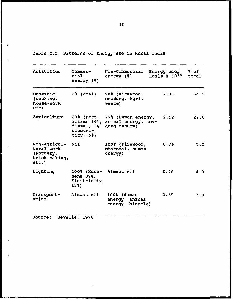
the rural areas of India for cooking and heating. Revelle

(1976) reported that cooking dominates the energy usage in the

rural sector (64%) followed by agricultural needs (22%),

village industries (7%), lighting (4%) and transportation (3%)

(Table 2.1). A source-wise energy consumption compiled (Table

2.2) for the rural household sector (Working Group on Energy

Po]icy, Planning Commission, Govt. of India, New Delhi, 1979)

lists firewood as the major source of fuel (68.5%) oil products

(16.9%), animal dung (8.3%), coal (2.3%), electricity (0.6%)

13

Table 2.1 Patterns of Energy use in Rural India

Activities Commer- Non-Commercial Energy used % ofcial energy (%) Kcals X 1014 totalenergy (%)

Domestic 2% (coal) 98% (Firewood, 7.31 64.0(cooking, cowdung, Agri.house-work waste)etc)

Agriculture 23% (Fert- 77% (Human energy, 2.52 22.0ilizer 14%, animal energy, cow-diesel, 3% dung manure)electri-city, 6%)

Non-Agricul- Nil 100% (Firewood, 0.76 7.0tural work charcoal, human(Pottery, energy)brick-making,etc.)

Lighting 100% (Kero- Almost nil 0.48 4.0sene 87%,Electricity13%)

Transport- Almost nil 100% (Human 0.35 3.0ation energy, animal

energy, bicycle)

Source: Revelle, 1976

14

Table 2.2 Source-wise Energy Consumption in Rural HouseholdSector

Energy Rural per Capita Energy Consumption% share of % share of source of supply of each formenergy forms Purchased Collected Home grown

Electricity 0.6 100.0 0.0 0.0Oil Products 16.9 100.0 0.0 0.0Coal Products 2.3 65.1 34.9 0.0Firewood 68.5 12.7 64.2 23.1Animal Dung 8.3 5.1 26.2 68.7Others 3.4 8.9 61.0 30.1

Share of comm- 20%ercial fuels

Share of non- 80%commercial fuels

Source: Report of Working Group on Energy Policy, PlanningCommission, Govt. of India, 1979

15

and others (3.4%). Wood and cowdung constitute the primary

domestic energy source for cooking (A.V.Desai, 1981). Table

2.3 gives rural per capita traditional fuel consumption

(kg/year) in the different geographical zones of India. Wood

and dung are the principal fuels for North-west, East & North

regions whereas wood is used all over the rural parts of India.

The use of dung varies from 4% in the South to 36% in the North

with wood making up the rest. Table 2.3 does not list crop

residues which may have been included under firewood. India

has a total forest area of about 75 million hectares or 23% of

the total area of the country. According to the Report of the

Fuelwood Study Committee 1982, the total requirement of

fuelwood is about 133 million ton per annum whereas the annual

availability is at only about 49 million ton. The acute

shortage of fuelwood in the rural areas is often referred to as

"poor man's energy crisis" and is of great concern to the

villagers. The shortage of fuelwood has resulted in increased

use of agriculture residues and animal dung which otherwise

would have been used to restore soil fertility and increase

food production.

16

Table 2.3 Traditional Rural Fuel Consumption (kg/yr/capita)

ZONE* FIREWOOD COWDUNG FIREWOOD COWDUNG(kg/year) (kg/year) (%) (%)

NORTH-WEST 349.16 157.11 69.0 31.0WEST 275.47 33.71 89.0 11.0SOUTH 281.37 10.71 96.0 4.0EAST 308.42 98.82 75.7 24.3NORTH 277.72 157.60 63.8 36.2

* The zones are defined as follows: NORTH-WEST: Punjab,Rajasthan, J&K, Delhi and Himachal Pradesh. WEST: Gujarat,Maharashtra & Karnataka, SOUTH: Kerala, Tamil-Nadu, Andhra-Pradesh. EAST: Orissa, Bihar, West Bengal, Assam, Manipur &Tripura. NORTH: Uttar Pradesh & Madhya Pradesh.

Source: Desai, 1981

17

2.3 JUSTIFICATION FOR SELECTING TSP, CO, AND BaP FOR

MONITORING .

The five combustion generated pollutants referred to as

Criteria Pollutants, for which ambient emission standards have

been set by different countries are :

Total Suspended Particulates (TSP)

Carbon Monoxide (CO)

Sulphur Oxides (SOx)

Nitrogen Oxides (NOx)

Hydrocarbons (HC)

Table 2.4 shows that for residential use of fuel wood,

emission of particulates, hydrocarbons, and carbon monoxides

are an order of magnitude higher than coal. The reason for

these high emission rates is incomplete combustion when burning

at one or two kg/hr. SO2 and NO2 emissions for wood are less

than for coal since sulfur is almost absent in wood and low

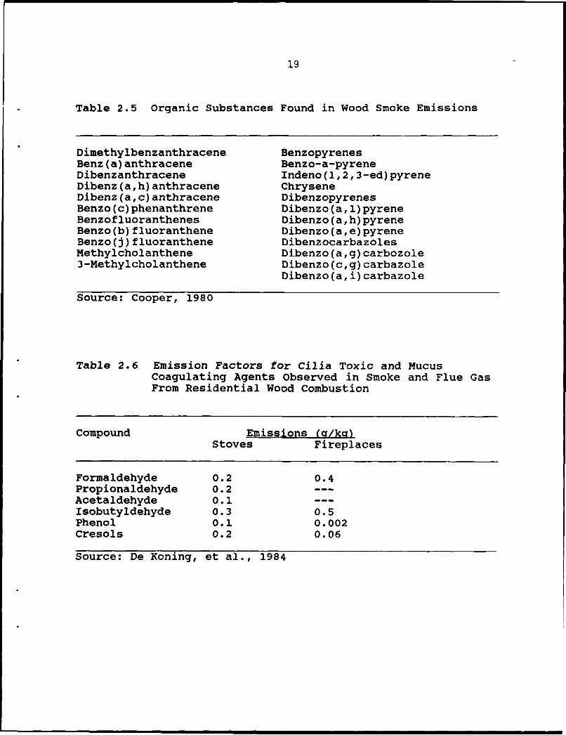
burn temperature releases negligible amounts of NO2. Cooper

(1980) identified several carcinogens, co-carcinogens and

several cilia toxic and mucus-coagulating substances in wood

smoke. DeKoning, et al., 1984 summarised Cooper's paper and

other sources, and listed a number of known and suspected

carcinogens (Table 2.5). He also listed emission factors for

cilia toxic and mucous coagulating agents observed in wood

smoke (Table 2.6).

18

Table 2.4 Comparison of Air Pollutant Emissions from Energy-Equivalent Fuels (in kilograms)

Fuel Fuel equi- Sus- Sul- Nit- Hydro- Carbonvalent to pended fur rogen carbon mon-one million parti- oxides oxides oxidemega-joules culatedelivered matter

INDUSTRIAL

Wood (70%) 80 metric tons 480 56 360 360 400

Coal (80%) 43 metric tons 2080 810 1180 6 45

Residualoil (80%) 33,000 litres 94 1310 240 4 20

Distillateoil (90%) 31,400 litres 8 1210 83 4 19

Naturalgas (90%) 28,200 m3 7 Neg. 99 2 8

RESIDENTIAL

Wood (40%) 144 metric tons 2170 86 110 1450 18790

Coal (50%) 69 metric tons 520 1200 270 430 2380

Distillateoil (85%) 32,900 litres 11 1170 71 4 20

Naturalgas (85%) 30,000 m3 7 Neg. 38 4 10

Source: De Koning, et al., 1985

19

Table 2.5 Organic Substances Found in Wood Smoke Emissions

Dimethylbenzanthracene BenzopyrenesBenz (a) anthracene Benzo-a-pyreneDibenzanthracene Indeno(l,2, 3-ed) pyreneDibenz (a,h) anthracene ChryseneDibenz (a,c) anthracene DibenzopyrenesBenzo(c)phenanthrene Dibenzo(a, l)pyreneBenz of luoranthenes Dibenzo (,h) pyreneBenzo(b) fluoranthene Dibenzo(a, e) pyreneBenzo(j) fluoranthene DibenzocarbazolesMethyicholanthene Dibenzoa, g) carbozole3-Methyicholanthene Dibenzo (c,g) carbazole

Dibenzo (a, i) carbazole

Source: Cooper, 1980

Table 2.6 Emission Factors for Cilia Toxic and MucusCoagulating Agents Observed in Smoke and Flue GasFrom Residential Wood Combustion

Compound Emissions (g/ki)Stoves Fireplaces

Formaldehyde 0.2 0.4Propionaldehyde 0.2--Acetaldehyde 0.1--Isobutyldehyde 0.3 0.5Phenol 0.1 0.002Cresols 0.2 0.06

Source: De Koning, et al., 1984

20

TSP, CO and BaP were selected for monitoring because:

1. CO and TSP are designated as "criteria

pollutants". BaP is well documented as a

suspected carcinogen belonging to the

family of polycyclic aromatic hydrocarbon

(PAH).

2. Emisssions of TSP, CO and HC for

residential fuelwood burning are

considerably higher than those for fossil

fuel (coal) burning.

3. Wood smoke literature in the developed countries has

documented the emissions of CO, TSP and BaP, in case

of wood heating stoves and fireplace emissions.

4. Availability of personal monitoring instruments for

TSP and CO (East West Center) and permission from the

Dept. of Agriculturp Piochemistry to carry out, BaP

analysis using HPLC (high performance liquid

chromatography), the latest technology for BaP

analysis.

5. Study by Aggarwal et al., 1382, and Smith

et al., 1983, reported, Indian cook's TSP

exposure from 4.3 to 58.6 mg/m 3 and BaP

from 833 to 25,000 ng/m 3 . These are very

high concentration when compared to WHO

recommended maximum 24-hour TSP levels of

0.2 mg/m 3 .

21

2.4 BIOMASS GENERATED SMOKE (TSP, CO, BaP) AND HEALTH

Indoor open biomass fires can result in substantial

quantities of pollutants due to incomplete combustion. Smith,

1987, has provided substantial evidence relating biomass smoke

with respiratory infection and lung diseases amongst rural

cooks. Table 2.7 summarizes epidemiological studies of

possible health risks from the exposure to biomass smoke.

Woolcock, 1967, attributed a prevalence of chronic bronchitis

and cor pulmonale among the highlanders in Papua New Guinea

(PNG). Sofoluwe, 1968 reported high levels of combustion

generated pollutants in Nigerian homes of nearly 100 infants

afflicted by bronchiolitis and bronchopneumonia. Hoffmann and

Wynder, 1972; correlated indoor wood smoke to carcinoma of

nasopharynx (NPC) among the highlanders of Kenya. Master, 1974

found a high prevalence of abnormal pulmonary signs in all age

groups, both sexes and non-smokers of PNG. He concluded "the

pathologic changes discovered suggest that air pollutants are

the most important factor in the development of lung disease in

New Guinea." However, Anderson, 1978, monitored respiratory

abnormalities of 112 Highland school (PNG) children but was not

able to find a significant correlation to woodsmoke exposures.

Pandey and Ghimire, 1975 after conducting clinical examination

of about 1800 heart patients in Nepal, reported high incidence

of cor pulmonale and pointed at cigarette smoking and exposure

to combustion related pollutants as important sources for this.

22

Table 2.7 (Page 1 of 3) Epidemiological Studies on AirPollution from Biomass Combustion

Pollutant Concentration Health Effects Author

TSP CO BaP Placemgm- 3 ppm ngm- 3

940 --- Lagos, Concentrations of CO, N02 (8.6 SofolNigeria ppm, ave. ) measured in the uwe,

homes of 98 infants with 1968bronchiolitis andbronchoneumonia. It wasestimated that the infantswere exposed to smoke fromwood-fueled stoves for anaverage of 3 h/d.

0.6- 21.3 --- Papua Wood smoke may be a factor in Wool-2.0 (ave) New causation and / or maintenance cock et5.0- 150.0 Guinea of non-tubercular lung al.,10.0 (peak) disease. Highlanders exposed 1967,

to high concentrations of 1970smoke and repeated chestinfections have high incidence Clearyof chronic respiratory symptom &and reduced ventilation Black-capacity. But Anderson, in a burn,comparative study of children 1968exposed to wood smoke andthose who were not, found no Ander-significant difference in son,symptoms. 1978

0.3- -.. 12- Kenya Positive association found Clif-7.8 291 between elevation and ford,

incidence of nasopharyngeal 1972cancer, and between elevationand amount of PAH inside Hof-homes. But relationship fmannbetween PAH and incidence of andcancer still not clear. Wynder,

1972

23

Table 2.7 (Continued, page 2 of 3) Epidemiological Studies onAir Pollution from Biomass Combustion

Pollutant Concentration Health Effects Author

TSP CO BaP Placemgm-3 ppm ngm-3

India Study of chronic cor pulmonale Pad-(heart disease secondary to mavatilung disease) in Delhi between and1958-1974. Conclusion: Among Arora,women the cause of the disease 1976was "damage to the lung fromexposure to smokey cookingfuels from girlhood onwards,followed by repeated chestinfections".

4.7- --- India Women cooking with traditional INIOH,11.5 fuels found to have a 1980

relatively high incidence ofcough, Dyspoenea, andrespiratory abnormalities.

Natal Study of acute lower Kos-S.Africa respiratory tract disease sove,

found 70% of infants with 1982wheezing, bronchitis, orpneumonia were exposed dailyto smoke from cooking and/orheating fires. Only 33% ofthe 18 infants with norespiratory problems had suchexposure. Conclusion: Woodsmoke is a potent risk factorin development of severe lowerrespiratory tract disease ininfants. Other factorsnormally thought to increaseinfant's risk such as socialclass, and sibling andparental symptoms may, infact, be expressions of thesame smoke-filled rooms.

24

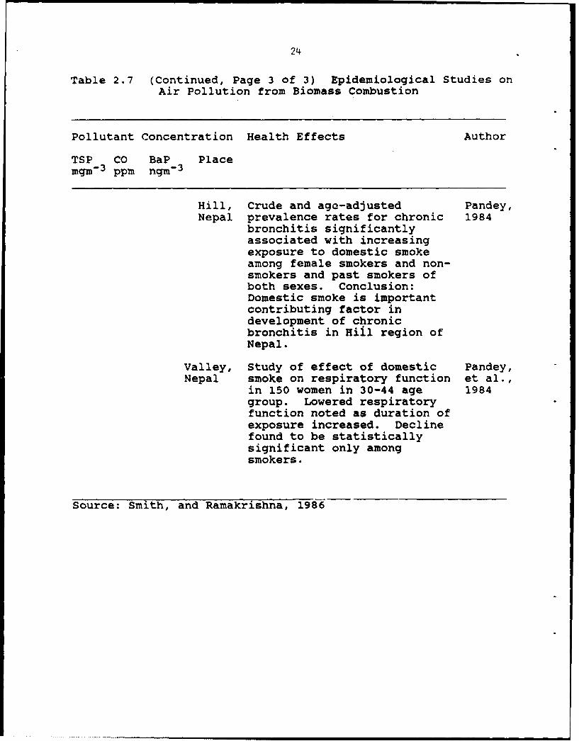
Table 2.7 (Continued, Page 3 of 3) Epidemiological Studies onAir Pollution from Biomass Combustion

Pollutant Concentration Health Effects Author

TSP CO BaP Placemgm 3 ppm ngm -3

Hill, Crude and age-adjusted Pandey,Nepal prevalence rates for chronic 1984

bronchitis significantlyassociated with increasingexposure to domestic smokeamong female smokers and non-smokers and past smokers ofboth sexes. Conclusion:Domestic smoke is importantcontributing factor indevelopment of chronicbronchitis in Hiil region ofNepal.

Valley, Study of effect of domestic Pandey,Nepal smoke on respiratory function et al.,

in 150 women in 30-44 age 1984group. Lowered respiratoryfunction noted as duration ofexposure increased. Declinefound to be statisticallysignificant only amongsmokers.

Source: Smith, and Ramakrishna, 1986

25

Padmavati and Arora, 1976, reported similar problems among

north Indian men and women patients based on a 15-year study.

They attributed this to combustion generated air pollution in

ill-ventilated kitchens. The 1980 annual report from the

National Institute of Occupational Health in India reported

high incidences of cough, cough with expectoration and dyspnoea

among Gujarati women using traditional biomass fuel as compared

to those using kerosene. Dary et al., 1981, found carboxy-

haemoglobin levels above 2% in Gautamalan women cooking with

biomass in poorly ventilated house. Kossove, 1982, attributed

the presence of severe lower respiratory tract disease (Acute

respiratory infection, ARI) in South African infants to

combustion generated pollutant exposure, as it is customary for

mothers to carry their infants while cooking with open fires.

Pandey, et al., 1983, reported high incidence of ARI and

suggested it to be an important cause of mortality and

morbidity among infants less than a year old. Recently,

Mumford et al., 1987, investigated the relationship between

domestic fuel and lung cancer in Xuan Wei county of China,

which has a high lung cancer mortality for non-smoking women.

They found a link to lung cancer and domestic "smoky coal"

burning but not to wood smoke or "smokeless coal".

26

2.4.1 TOTAL SUSPENDED PARTICULATES (TSP)

1. Mechanism

The mechanics, physics and chemistry of aerosols are

described by Friedlander, 1977; Hinds, 1982; Hidy, 1984; and

Spurny, 1986. Suspended particles in the atmosphere range in

size from molecular clusters with diameters on the order of

.001 um to dust particles of 100 pm or larger. This represents

a variation of 105 in size and 1015 in mass. Generally only

particles < 40 jam have sufficient atmospheric residence times

or mass concentrations to be important. Very small particles

grow rapidly by coagulation into the .1 to 1 jm range. TSP is

normally distributed bimodally in mass around a minimum

diameter of about 1 to 2 pm (Whitby, 1974). A nuclei mode may

appear when the size distribution is measured very near

combustion sources but is not normally evident elsewhere. The

accumulation mode is between 0.1 to 0.4 tm. The coarse mode is

5 and 20 pm. Stevens, et al., 1978, noted that each mode

consists of particulates from separate sources produced by

independent mechanisms and composed oZ different materials.

The accumulation mode consists of materials from combustion

processes either as primary emittants or secondary products of

gas to particle conversion (Dzubay and Stevens, 1975). The

coarse mode contains predominantly soil products such as silica

and calcium and reflects the local environment only. Smoke

particles, e.g., of soot, are often very small and nearly

27

spherical while dust particles are usually irregularly shaped,

and may also aggregate.

Incomplete combustion of traditional fuels results in a

mixture of particulates, gases, and vapors. Combustion

generated pollutants change concentration and particle size

distribution with volume and time and can go from solid to

liquid and vice versa. Aerosol coagulation, one of the most

important mechanisms modifying the size distribution, reduces

the number-concentration and increase the mean size of the

pa ticles.

2. Health effects

The three most important characteristics of the aerosols

affecting human health are particle size(size distribution),

particulate concentration, and chemical composition.

Undesirable health effects arise from deposition of aerosols in

respiratory tracts. Ambient air concentration limits of

particulates have been established such that lower levels

should not cause biological damage to people exposed to them

over a long period of time. OSHA (Occupation and Safety Health

Adminstration) has set standards and exposure limits for

different pollutants which the employers have to comply with.

The size of the particle is an important characteristic

for determining it's source, and potential toxic affect

(Whitby, et al., 1974). Characteristics of aerosols which

could adversely affect health of exposed populations have been

28

discussed in several documents. (Holland et al., 1979, Perera

& Ahmed, 3979, Hinds, 1982, Friedlander et al., 1977 and Hidy,

1984). knoledge of particulate size distribution is

valuable in &ssessing the impact on health, since deposition of

the particulates inside a human respiratory tract is largely

size deperdent. Fig.2.1 shows particle deposition in the lung

as a function of size for spherical particles of a given

density. For particles < 0.1 Fm, diffusion produces a

deposition rate inversely proportional to particle size,

whereas for particles > I um, gravitation produces a deposition

rate which increase with size. Between 0.1 um and 1 um,

deposition is at a minimum as these particles are too large to

diffuse rapidly and too small to deposit rapidly due to

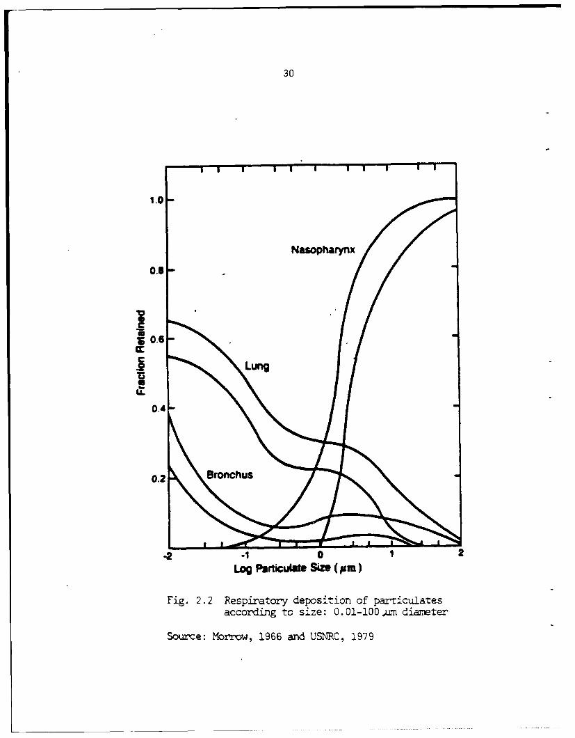
gravity. Fig 2.2 shows the deposition sites as a function of

particle size. For particle < 0.1 jm, deposition by diffusion

increases in the lower respiratory system. For particles > 1

pm, deposition increases in the upper respiratory system.

Respirable particulates (RSP) is defined as particulates of

size < 2.5 pm. This size is defined by the aerodynamic

diameter which is an important property characterizing

filtration, respiratory deposition etc. (Hinds, 1982). The

deposition sites of particulates in the human respiratory

system is closely related to particle size. The physics of

particle deposition in the respiratory tract is well developed

(Brain, 1979; Lippmann, 1980; Heyder, 1980; Raabe, 1982; and

Schreck, 1982). The Environmental Protection Agency, (EPA)

29

o1.0-

!U

I-D

U)0 .0

-

a 0.6 DIFFUSION

Z , SEDIMENTATIONo AND_0 0.4 IMPACTION

U- 0.2

0 o ,0.01 0.1 1.0 10

dp"m

Fig. 2.1 Form of the efficiency curve for particledeposition.

Source: Friedlander, 1977

30

I I I I I I I I I I

Nasopharynx

0.8-

0.6

.2 LungB

0.4-

0.2 Bronchus -

-2 0 2

og Particuate Size (0m)

Fig. 2.2 Respiratory deposition of particulatesaccording to size: 0.01-100.A.n diameter

Source: Morrow, 1966 and USNRC, 1979

31

recently recognized the importance of particle size and site of

deposition and converted the TSP standard to one based on

particle (PM1 0 ) less than 10 pm (U.S.Federal Register, 1984).

Cooper, 1980, Butcher and Sorenson, 1979, DeAngelis et. al.,

1980, found that the emitted particulates for fuelwood were

entirely in the respirable size range (<10 jm). By convention,

inhalable particulates, represent particulates sizes in the

range 2-3 pm or more recently as <1 pm. Butcher and

Ellenbecker, 1982 found 98.3% of the particulate emissions

inhalable. Dasch, 1982, reported that woodsmoke consisted of

spherical conglomeration, and ranging from 0.05 to 1 pm with a

mass median diameter of 0.17 pm. Saucy et al., 1983 and

Kamens, 1984, found woodsmoke particle size to be in the range

of 0.1 to 0.2 um, after aging in a teflon-walled chamber.

Carrcll, 1977 reported 90% of the smoke from burning rice straw

to be particulates with mass median size less than 2 pm.

Hovever, Mumford, et al, 1987, reported only 6% of wood

combustion-generated particles less than 1 um in diameter.

2.4.2 CARBON MONOXIDE (CO)

1. Mechanism

CO is a product of incomplete combustion with insufficient

air or with the ignition and flame zone maintained at too low

temperature by excess air. High moisture or organic-rich fuel

will yield an excess of volatiles and a vapor/air mixture which

will produce large emissions of CO, volatiles and particulates.

32

Poor physical arrangement of the fuels can also result in

increased CO generation.

2. Health effects

CO is a colorless, odorless gas having serious

debilitative health effects has been reviewed extensively by

Smith, (1987). Prolonged inhalation, at high concentrations

results in dizziness, physical weakness, headaches, and even

ultimately death. The immediate result of CO exposure is

lowering the blood's ability to transport oxygen to body

tissues. This is because, hemoglobin, a constituent of the

blood responsible for transporting oxygen, has an affinity for

CO more than 300 times greater than that for oxygen. A rough

guide of possible effects for exposures of less than a few

hours proposed by Henderson and Haggard, 1943 is:

Hours x ppm < 300 (no perceptible effect)

Hours x ppm = 300-600 (just perceptible effect)

Hours x ppm = 600-900 (headache and nausea)

Arnow, 1981, reported that exposing sensitive human

subjects (heart patients) to 50 ppm of CO for one hour raised

COHb levels from 1.09% to 2.02%, and exercise tolerance was

reduced. Stewart et al., 1970, reported no symptoms or changes

in objective physiological measures when humans were exposed to

levels below 100 ppm, mild sinus headaches after four hours of

exposure to 200 ppm, and mild frontal headaches with nausea

when exposed to 500 ppm for one hour. Goldsmith, 1970,

33

reported that exposure to CO levels above 500 ppm results in

observable physiological effects ranging from nausea, vertigo,

dyspnea, cerebral misfunction to cardiovascular abnormalities.

Three important reasons why CO is a pollutant of great

concern to women are (Dollar et al.,1982):

1. Women generally have less hemoglobin inreserve than men. One consequence of thisdifference is that women are more prone toanaemia than men. Another is that thenegative impacts of CO may occur at lowerdoses than would be the case for men.(Weintrob, 1967)

2. During pregnancy, there is an additionaldemand on women's hemoglobin, furtherlowering their reserves. (Weintrob, 1967)

3. There is evidence from animal studies andstudies of women who smoke that COexposures can affect the unborn child.Reduced body weight at birth, for example,has been associated with such exposures.(Penny et al., 1980; Williams et al.,1977)

2.4.3 BENZO(a)PYRENE (BaP)

1. Mechanism

Polyaromatic hydrocarbons are hydrocarbons consisting of

two or more benzene rings, usually referred to as Polycyclic

Organic Matter (POM), Polycyclic Aromatic Hydrocarbons (PAH),

or Polynuclear Aromatics (PNA). POM emission from natural

sources is negligible. Principal POM emission sources include

transportation, heat and power generation, burning of trash,

and industrial processes. The POM species found in the

atmosphere come invariably from combustion, mainly a by-product

34

of incomplete combustion. POM can be formed in the combustion

of fossil fuels or, more generally, compounds containing carbon

and hydrogen. Fig 2.3 illustrates the mechanism of POM

formation in the combustion processes (Badger, 1962) suggesting

that polynuclear hydrocarbons are formed via hydro-carbon free

radicals, which produced during pyrolysis, combine in a

pyro-synthesis to the thermodynamically favored PAH.

Consequently, higher yields of carcinogenic hydrocarbons and

volatile phenols are emitted by the combustion of materials

rich in aromatic hydrocarbons (Badger et al., 1958). Forest

fires and slash burning can be expected to produce POM, but,

there are no emission rates reported. Little is known about

the chemical nature of POM containing particulates, or how POM

is distributed with respect to size, or about their physical

and chemical characteristics of POM as it ages in the

atmosphere. The major portion of POM is presumed to be linked

to particulates, since POM has high melting and boiling points.

The very low vapor pressure of BaP (5.49 X 10 -9 torr at 250 C),

implys that little ambient BaP is present in the vapor phase.

Commins, 1962, and Thomas, 1968, reported the presence of BaP

in soot particles finding a constant amount of BaP per unit

weight of soot. Demaio, 1966, reported that more than 75% of

the weight of selected POM were associated with particulates

less than 2.5 um in radius. NAS, 1972, reported that POM was

highly reactive and degradable by photooxidation. The

half-life is less than a day for the BaP degradation on the

35

U4-U

/ \v

-4~

IC=)

w0

C=4

O

I' -- n

36

soot in the presence of sunlight (Thomas, 1968). In the

absence of solar radiation, the half-life increased to several

days (Falk et al., 1958). Katz, (1979) reported half-life of

BaP less than couple of hours. Very little is known about the

actual form of POM in the atmosphere.

Polycyclic organic matter in the atmosphere has been

identified with particulate matter, especially soot. It is

uncertain whether POM condenses out as discrete particles after

cooling or condenses on surfaces of existing particles after

formation during combustion (NAS, 1972).

BaP is used as an indicator of other POM because it is a

known carcinogen, it has been studied and it is widespread

(Santodonato, 1979, and Albert, 1978). Fossil fuel combustion

was considered to be a major source of POM in the U.S.

Hoffman, 1976, estimated the annual BaP emissions to be

900-1400 tons, mainly from coal-fired heat and power

generation, followed by refuse burning, forest fires and coke

production. USEPA (Super, 1985) now considers wood burning to

be chief cause of POM in U.S. Most researchers have used BaP

as an indicator of POM implying the presence of other

components of similar structure despite the lack of proof of a

relationship between benzopyrene and other compounds or the

carcinogenic significance of other POM molecules. NAS, 1972,

suggested BaP as an air pollution index, because it exists as

solid in air, and as it is usually adsorbed on particles it can

be filtered and collected. BaP concentrations in winter were

37

10-20 higher than summer at over 100 sampling sites in the

U.S. (Sawicki, 1960). Stocks et al., 1958 and 1961, attributed

PAH, benzo(a)pyrene, benzo(ghi)perylene, pyrene and

flouranthene in garages and offices to improperly vented

furnaces and incinerators, tobacco smoke, and leakage from the

outdoors. Tobacco smoking is an important source of POM

pollution e.g. Wynder et al 1968, showed in a room of size 40

m3, three smokers can produce BaP concentrations of 2 to 4

4ug/m3 of the air and Galuskinova, 1964, reported BaP

concentrations between 28 to 44 pg/m3 from cigarette smoke in

beer halls. Sawicki, 1960, 1962, 1965 reported in addition to

benzopyrene, several other types of POM in the ambient air,

viz., pyrene, anthanthrene, benz(a)anthracene,

benzofluoranthenes, dibenzanthracenes, fluoranthene, and alkyl

derivatives of these compounds. Hangebrauck, 1967, concluded

that of the four fuels coal, oil, gas and wood, coal burnt

inefficiently in hand fired furnaces produced most BaP

Studies of combustion of biomass material and characterization

of POM, are with the exception of cigarettes, few. Friedman,

1977, has found POM in smoke from leaf burning. Hall, 1980,

and Cooper, 1980, measured emissions of various POM in smoke

from wood burning. USDHEW, 1968, estimated an emission factor

of 50,000 pg of BaP per million Btu from wood burning. Dasch,

1982, reported that BaP was almost exclusively associated with

particulate emissions and not with gaseous emissions. Wolff et

al., 1981, reported that one-third of the organic fine

38

particulate matter in Denver aerosol could be attributed to

wood smoke emissions. Muhlbaier, 1981, reports BaP emission

factors of woodsmoke from fireplaces between 0.01 to 1.3 mg/kg

for burn rates between 3.2 to 4.8 kg/hr. Studies by Katz,

1963; Zdrojewoski et al., 1967; Hoffmann & Wynder, 1968, and

Cooke and Dennis, 1984, reported the majority of PAH in

polluted air as coming from incomplete combustion of organic

matter. There seems to be no published studies on PAH emission

factors from burning traditional fuels in open cookstoves.

2. Health effects

BaP has been found to be carcinogenic in animals and it is

suspected of being carcinogenic in man. Occupational exposures

to PAH are well documented and provide sufficient evidence that

lung cancer can be induced by inhalation. There are many

studies (Hammond, 1958 and 1966, and Kahn, 1966) attributing

human lung cancer to environmental factors, mainly cigarette

smoke, which is known to contain polycyclic hydrocarbons,

arsenic, nitrosamines, and polonium. Researchers indicate BaP,

one of the well known carcinogen as a potential candidate for

promoting lung cancer even though there are no studies linking

BaP in cigeratte smoke to lung diseases. Particulate POM can

be classified into two known animal carcinogens, PAH and their

neutral nitrogen analogues the aza-arenes (e.g., indoles and

carbazoles). Although POM represents only a very small

fraction of the total amount of particulate matter associated

39

with combustion, it is very important because of its potential

hazard to humans. The degree of the hazard may be assumed to

depend on the atmospheric particulate concentration. The first

cited occupational disease related to the burning of fossil

fuel occurred in 1775, when Percivall Pott, a doctor in London,

reported a prevalence of cancer of the scrotum in chimney

sweeps and attributed it to their constant exposure to soot.

In no instance has exposure to a specific PAH been proved to

cause tumor in man, though BaP has been demonstrated to be

carcinogenic in experimental animals (Epstein, 1966, and

Leiter, 1942). Falk et al., 1958, investigated "leaching" of

PAH in human tissues, and suggested a possible route of

degradation. Goldsmith, 1968, and Royal College of Physicians,

1970, demonstrated that BaP is irritating to the lungs of

experimental animals only at high dosages, while Ishikawa,

1969, showed that the severity of diseases like emphysema are

closely correlated with urban pollution levels but the role of

POM cannot be ascertained from his data. Falk, 1964, gives a

convincing discussion indicating BaP as a carcinogen for man

but NAS, 1972, suggested caution in accepting BaP as a major

carcinogen at the levels of atmospheric concentrations, based

upon findings by Freeman et al., 1971, who concluded BaP from

particulates collected in the ambient city air accounted for

less than 1% of carcinogenic activity of the air.

40

Moller, 1980 and Daisy, 1986, showed air particulate

extracts to exhibit mutagenic activity using the Salmonella

test. BaP's role as a mutagen suspected by Tomingas, 1977, and

Carnow, 1973 was disproved by Lofroth, 1978, Chrisp, 1978,

Jager, 1978 and Pitts, 1978 who showed nitroaromatic compounds

to be mutagenic. Ramdahl, 1982 demonstrated the presence of

nitrocompounds and oxygenated polycyclic compounds in emissions

from biomass combustion. Dasch 1982, Ramdahl et al., 1982, and

Alfheim, 1984, showed low direct-acting mutagenic activity of

the particulate extracts from wood smoke. Kamens et al., 1984

reported a substantial increase in direct mutagenic activity of

wood smoke when reacted with NO2 and 03 in the dark. He, 1985

reported that the PAH fraction of particulates accounted for

only a small fraction of the total mutagenic activity in both

the reacted and unreacted wood smoke. Above references focus

on the PAH in the particulate matter only. Recently

Kleindienst, 1986, demonstrated that both the gas and the

particulate phase components of wood combustion show little

direct-acting mutagenic activity, but when mixed with NOx,

their activity increased significantly.

41

2.5 REVIEW OF STUDIES RELATED TO INDOOR MONITORING OF

COMBUSTION GENERATED POLLUTANTS EMITTED FROM COOKING STOVES

USING TRADITIONAL FUELS.

The studies mentioned in Table 1.2 are reviewed to

familiarize the reader with reported methods, sampling

protocols, and specific indoor biomass combustion generated

pollutant levels, in the few of existing studies. They have

been classified as area or personal, depending on their

sampling protocol. Smith (1983), demonstrated the need for

personal monitoring when cook's exposure to combustion-

generated pollutants needs investigation. Some researchers

used Hi-Volume sampler to collect TSP samples, whereas, others

used personal samplers fixed at some site. None of the studies

reported simultaneous sampling for measurement of TSP, CO and

BaP. This study carried out area and personal monitoring for

TSP, CO and BaP.

Sofoluwe, 1968, investigated pollution from cooking fires

in the homes of 98 infants suffering from bronchiolitis and

bronchopneumonia in Lagos, Nigeria. CO levels (Table 2.8)

ranged from 100-3000 ppm, with average value of 940 ppm, NO2

from 0.5-50 ppm with average value of 8.6 ppm, SO2 from 5-100

ppm with average value of 37.8 ppm and Benzene (C6H6 )ranging

from 25-200 ppm with average value of 85.6 ppm. Maximum value

of CO appears questionable. Average duration of exposure of

42

Table 2.8 Concentration of Toxic Gases in Smoke in Houses inLagos, Nigeria

Gases Total No. Positive % Negative % Range of MeanTested Number Number Conc. Conc.

(ppm) (ppm)*

Carbon 46 46 100 1-- i00- 940.2monoxide 3000

Nitrogen 44 22 50 22 50.0 0.5- 8.6Dioxide 50

Sulfur 46 43 93.5 3 6.5 5-100 37.8Dioxide

Aromatic 46 33 71.7 13 28.3 25-200 85.6Hydrocar-bons(as benzene)

Source: Sofoluwe, 1968 * Zero values excluded incalculations of mean concentrations

43

the children to the smoke was estimated at 3.2 hrs per day

ranging from 1.3 to 9 hrs per day. Infants that were exposed

to smoke while carried by their mothers on the backs or laps

while cooking over open fuelwood fires. There was prevalence

of open shed community kitchen, where as many as 8 mothers

cooked simultaneously. 65 of the mothers used fuelwood, 39

kerosene, 7 coal, and 10 gas. The method and sampling protocol

were not reported explicitly except that samples were taken at

convenient times during cooking.

Cleary and Blackburn, 1968, reported high night time

values of smoke, formaldehyde and CO concentrations from open

wood fires used for indoor space heating at breathing height of

people sleeping inside thatched roof huts in Pompomere, in the

Eastern highlands of Papua New Guinea, 7,200 ft above sea level

and at Baiyer River, in the Western highlands between 4000 to

5,200 ft. above sea level. A high prevalence of chronic

non-tuberculous lung disease among the natives of the Eastern

highland was attributed to high indoor concentration of smoke

from open fires burning continuously during the night time.

The roofs of the huts in the Eastern highland were lower than

those of the Western highlanders. Another difference was that

Western highlanders slept on the floor, while Eastern

highlanders slept on bamboo shelves about one and half feet

above the ground level, resulting in a difference in

concentrations. TSP grab samples were collected three to five

times during the night. Six huts in the Western and 3 in the

44

Eastern highlands were monitored. Average concentrations at

Pompomere for TSP was 843 )ag/m 3 (Range 0-4.8 mg/m3 ), HCHO

1.23ppm (Range 0.3-3.8 ppm) and CO 30.5 ppm (Range 10-150 ppm).

At Baiyer river they were 359 ug/m3 (Range 0-1.25 mg/m3 ), 0.67

ppm(Range 0.1-1.9 ppm) and 11.3 ppm (0-60 ppm). A boundary

between a more dense upper smoke layer and a lower layer with

comparatively less smoke (3 to 4 ft. above ground level) was

noted. Smoke density was determined optically.

Higher levels of the pollutants in Pompomere were

attributed to

1. Lower roofs

2. Samples collected at higher level (18" above the

floor)

Hoffman and Wynder, 1972, and Clifford, 1972, measured

TSP, BaP, BaA phenols, and acetic acid in 8 Kenyan huts at

different altitudes, Table 2.9. The air volume sampled was

93,446 liters and 105,050 liters. The sampling

instrumentation, duration, flow rate, location of the sampling

port with respect to the source, or the method used for the

chemical analysis of PAH were not reported but they probably

monitored continuously for a few days at 10 to 20 liters per

minute, the usual rates for HI-Volume samplers. Huts of the

mountain tribes had smaller volume and wood fires burned more

continuously as compared to huts of coastal tribes. The

difference in hut size and fuel usage pattern was attributed to

an increased prevalence of nasopharynx cancer among the natives

45

Table 2.9 Chemical Analytical Data: Situations AnalyzedDuring Cooking in Huts

Geographic Ethnic Tribe & Sample TPM# TOM* BaP BaP/TSPLocation Group Hut No. Size@ mgm- 3 mgm- 3 ngm- 3 jUg/g

Mountain Bantu Nyeri 2 A 7.8 6.8 166 21

Mountain Bantu Nyeri 3 A 2.7 2.6 85 31

Coast Bantu Wadigo 1 A 1.5 0.8 24 16

Coast+ Bantu Wadigo 1 B 0.3 0.3 0 0

Mountain Nilo- Nandi 1 B 4.1 2.8 291 71Hamitic

Mountain Nilo- Nandi 2 B 5.6 3.9 140 25Hamitic

Central- Nilo- Samburu A 2.6 1.0 37 14Plateau Hamitic

@ Total Sample Size A=3,300 ft3 = 93.5 m3 , B=3,710 ft3 = 105 m3

# TPM = Total Particulate Matter Collected, *TOM = Totalorganicmatterextracted

+ Sample collected in the bedroom adjacent to kitchen

Source: Hoffmann and Wynder, 1972

46

in the mountains. TSP ranged from 1.5 to 7.8 mg/m3 , BaP from 0

to 291 ng/m 3 , BaA 16 to 515 ng/m 3, phenols 0.78 to 1.19 pg/m3

and acetic acid 5.05 to 8.82 ug/m 3 .

Anderson, 1978, used a portable air pump and filters, to

conduct indoor sampling in six Papua New Guinea houses with

volumes ranging from 40 to 80 m3 . TSP levels ranged from

0.8mg/rm3 to 11.2 mg/M 3 in early evening, when samples were

taken at sitting or squatting levels. Late evening samples in

sleeping area were mostly below 1mg/m 3 . Concentrations in the

sleeping area between 6.00pm and 4.00am ranged from 0.57 to

1.98 mg/m 3 .

Dary et al., 1981, studied ill-ventilated houses in two

Guatemalan communities at different altitudes. 200 randomly

selected houses were classified according to wall materials,

number and size of doors and windows, presence of chimney and

good or bad kitchen ventilation. In the lower altitude village,

71% of the houses had good ventilation, whereas in the higher

elevation only 30% had it. Gas chromatography was used to

analyze CO in the grab samples taken one meter from the fire

and at a height of 1 meter above the floor. The time of

sampling was not mentioned. Higher CO levels (30-50 ppm) were

found in poorly ventilated kitchens in both the villages.

Ventilation significantly reduced CO at the time of maximum

cooking. Blood samples for 208 women taken during the period

of maximum smokiness showed higher levels of HbCO for women

living in poorly ventilated houses in both the villages. Grut

47

et al., 1970, and Wright et al., 1975, mention several

countries that have set 32-40 ppm as the safe levels of

one-hour exposure to CO. Stewart, 1970 found HbCO levels above

two percent to be associated with an increased incidence of

cardiac disease. Dary suggests that HbCO levels between 1.5 to

2.5 percent which can, cause respiratory and eye diseases in

the children could be due to CO exposure for infants were

constantly carried on their mother's back.

Aggarwal et al., 1982, monitored TSP and BaP in 16 urban

kitchens in Ahmedabad,in Western India, where biomass is used

for cooking (Table 2.10). Mean TSP (mg/m3 ) exposure of the

cooks using wood was 7.2, cattle dung 16.0, cattle dung plus

wood 21.2, and coal 26.1 mg/m3 . Corresponding values for BaP

were 1300, 8200, 9300, and 4200 ng/m 3 . In addition to

concentration they reported, the ratio of BaP to TSP and

demonstrated it's usefulness in identifying the sources. The

mean BaP to TSP ratio for wood and dung smoke ranged from 200

to 600 )g/gm. TSP and BaP concentrations reported are possibly

the highest ever recorded in any part of the world. They used

a HI-Volume sampler 1.5 m above the floor for 15 minutes during

the morning and evening cooking period and the flow rate was

0.8 m3/min. It seems possible that the sampler flow induced

air currents dislodging soot deposited on the roof and

resuspended loosely packed fly-ash, dust and soot from the

walls and floor. The thermal draft carrying the soot and

fly-ash directly from the fire might also have been directed

48

Table 2.10 Average BaP Concentration Near Breathing Zones ofDomestic Housewives Using Different Local Cooking Fuels

Type of fuel No. of houses BaP TSP BaP/TSPsurveyed (ng/m3 ) (;ig/m 3 ) (Pg/gm)

Wood 5 1,270 7,203 188(963-1,683) (4,711-11,460) (147-219)

Cattle Dung 4 8,248 15,966 560(4,171-13,580) (9,590-20,036) (208-743)

Cattle dung + 7 9,317 21,165 534Wood (833-25,653) (9,968-58,577) (71-1,668)

Coal 3 4,207 26,147 273(488-10,820) (4,119-48,174) (224-321)

Source: Aggarwal et al., 1982

49

towards the sampler. Combustion conditions and emissions might

also have been affected by the forced sampler air flow. It

seems therefore questionable what they monitored should be

interpreted cook's personal exposure. Ventilation conditions

and building material of the kitchens were not mentioned nor

was a precision value for the BaP analysis.

In the simulated village hut on the East West Center

grounds, Dollar et al., 1982 measured CO using a sequential

sampler in line with an Ecolyzer model. They found increasing

levels of CO with heights, similar to Cleary and Blackburn

(1968).

Smith et al., 1983, monitored exposures of women cooks to

TSP and BaP in 36 households in four west Indian villages

during the morning and evening cooking periods. Personal

samplers were worn by the cooks during the complete cooking

duration, or to a maximum of 45 minutes. The samplers drew 1.7

to 3 liters of air per minute through a closed-face mode filter

cassette holding a pre-weighed 37mm glass fiber filter. The

filter cassette was hooked to the cook's collar and so drawing

the air in the breathing zone. BaP was determined using an

Aminco Bowman Spectrophoto-flourometer with an

excitation/emission wave length of 405 nm. A mean TSP

concentration of 7 mg/m 3 , a mean BaP concentration of 4000

ng/m3 were found and a mean BaP to TSP ratio of 900 pg/gm

(Table 2.11). Of the 36 houses sampled 13 were classified as

pucca (constructed of durable materials,such as brick and

50

Table 2.11 Summary of Household Data and MeasuredConcentrations

Mean Range Std. Number indev. sample

FamilySize

Kuccha 6.4 3-15 2.7 23Pucca 6.2 2-9 2.0 13

Income (rupees)Kuccha 4050 ($435) 600-15000 2940 23Pucca 10820 ($1160) 3000-21500 5600 13

Age(years)Of cook 33 13-57 10 36Began cooking 13 10-16 1.6 36CookingFuel use (kg)

Per day 6.5 2.5-11 1.9 36Per hour 1.9 0.5-4.3 0.8 65

Size of kitchen(m3 ) 42 8-100 19 36

Time (h)Cooking 2.8 1.5-5 0.9 36Other useof chula 1.7 0.5-3.5 0.8 36Indoor Conc.TSP (mgm-3) 6.9 1.1-56.6 7.5 65BaP (ngm- ) 3900 62-19284 3600 65BaP/TSP(Pgg-1 ) 860 10-8439 1200 65

Ambient Conc.Height ofmeasurement(m) 2.5 1.5-3.5 0.7 5Time of day 6.30 pm 5.50-7.00pm 5TSP (mgm-3) 1.5 0.5-2.5 0.8 5BaP (ngm-3 ) 230 107-410 110 5BaP/TSP (jagg-1 ) 190 70-560 170 5

Source: Smith, et al., 1983

51

cement) and 23 as kucha (constructed of thatch and mud)

houses. A cross-section of different house types were sampled

with various kitchen types and stove types. The socio-economic

conditions, family size, cook's age and number of years of

cooking, and amount of fuel used were noted as was the

ventilation and kitchen volumes. Annual doses of TSP and BaP

was estimated for a variety of exposure conditions and they

reported cooks receiving a larger dose of pollutants than the

residents of the dirtiest urban environments.

Dave, 1984, found S02 levels between 882 and 1390 ug/m3,

NOx from 43.8 to 47.4 ug/m3 , TSP from 78.5 to 157 .ig/m3 and BaP

from 14 to 23 ng/m 3 in Calcutta kitchens and huts where the

cooks used bituminous coal.

Patel et al., 1984, monitored S02, NO2 and TSP in 125

households in Gujarat, India using traditional and modern

fuels. Coal was included in the category of traditional fuels.

Besides air quality test, Pulmonary functional tests (PFT) of

housewives, 160 that cooked with traditional fuel and 89 that

used modern fuel, were carried out. Cooks using traditional

fuels were at greater risk to develop pulmonary disorders as

their PFT values were significantly lower. Excluding coal might

have changed this conclusion as it is well documented as a

dirty fuel. Table 2.12 shows that the highest level of SO2 in

the air occured for cooks using coal, with a mean of 1682 mg/m3

while fuelwood/cowdung and modern fuel users experienced

considerably lower values, 156-253 jug/m3. The highest levels

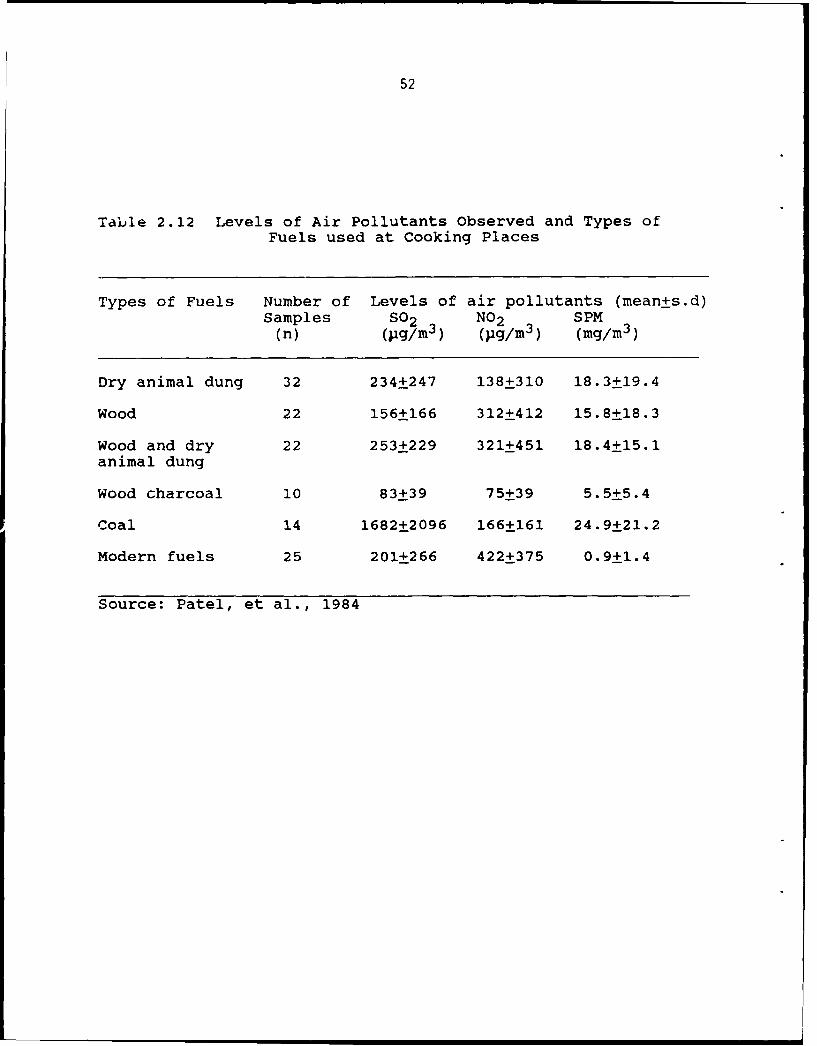
52

Table 2.12 Levels of Air Pollutants Observed and Types ofFuels used at Cooking Places

Types of Fuels Number of Levels of air pollutants (mean+s.d)Samples SO 2 NO 2 SPM(n) (pg/m3 ) (pg/m3 ) (mg/m 3 )

Dry animal dung 32 234+247 138+310 18.3+19.4

Wood 22 156+166 312+412 15.8+18.3

Wood and dry 22 253±229 321+451 18.4+15.1animal dung

Wood charcoal 10 83+39 75+39 5.5+5.4

Coal 14 1682+2096 166+161 24.9+21.2

Modern fuels 25 201+266 422+375 0.9+1.4

Source: Patel, et al., 1984

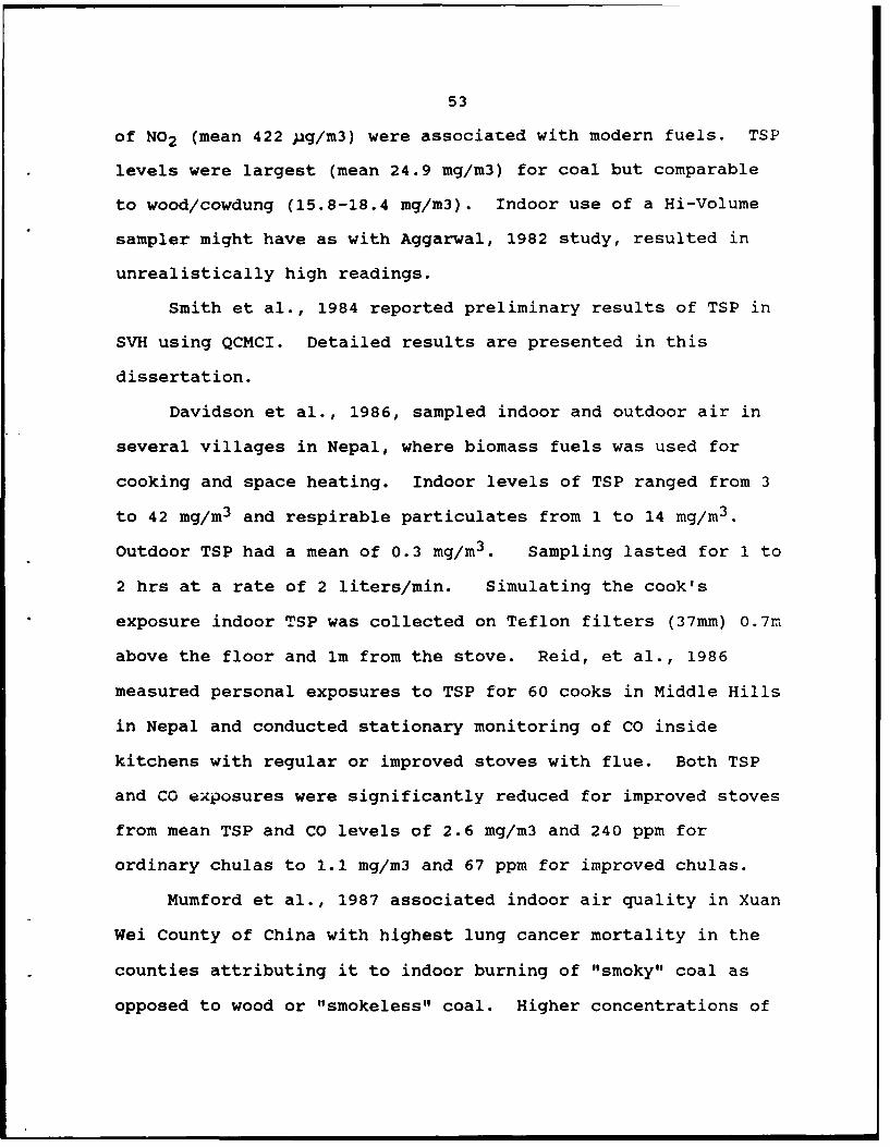
53

of NO2 (mean 422 pg/m3) were associated with modern fuels. TSP

levels were largest (mean 24.9 mg/m3) for coal but comparable

to wood/cowdung (15.8-18.4 mg/m3). Indoor use of a Hi-Volume

sampler might have as with Aggarwal, 1982 study, resulted in

unrealistically high readings.

Smith et al., 1984 reported preliminary results of TSP in

SVH using QCMCI. Detailed results are presented in this

dissertation.

Davidson et al., 1986, sampled indoor and outdoor air in

several villages in Nepal, where biomass fuels was used for

cooking and space heating. Indoor levels of TSP ranged from 3

to 42 mg/m3 and respirable particulates from 1 to 14 mg/m3 .

Outdoor TSP had a mean of 0.3 mg/m3 . Sampling lasted for 1 to

2 hrs at a rate of 2 liters/min. Simulating the cook's

exposure indoor TSP was collected on Teflon filters (37mm) 0.7m

above the floor and im from the stove. Reid, et al., 1986

measured personal exposures to TSP for 60 cooks in Middle Hills

in Nepal and conducted stationary monitoring of CO inside

kitchens with regular or improved stoves with flue. Both TSP

and CO exposures were significantly reduced for improved stoves

from mean TSP and CO levels of 2.6 mg/m3 and 240 ppm for

ordinary chulas to 1.1 mg/m3 and 67 ppm for improved chulas.

Mumford et al., 1987 associated indoor air quality in Xuan

Wei County of China with highest lung cancer mortality in the

counties attributing it to indoor burning of "smoky" coal as

opposed to wood or "smokeless" coal. Higher concentrations of

54

submicron particles containing mutagenic organics were found in

smoky coal emission than in that from wood or smokeless coal.

Hi-vol samplers with size selective inlet measured mean TSP

levels of 20 mg/m3 for households burning smoky coal/wood while

in smokeless coal households it was 2 mg/m3 . Organic

dissolved particulates were analyzed for PAH using GC/MS and

tests for assessing mutagenicity of organic extracts and

fractions were carried out.

55

III. RESULTS AND DISCUSSION

3.1 RESULTS OF THE EXPERIMENTS PERFORMED IN SVH

The results of experiments performed in SVH from fall 1982

to spring 1983 are discussed in the following paragraphs.

The objectives were:

1. Determine particle size distribution in wood and dung

smoke

2. Determine particle size variation with burn time

3. Determine variation of TSP and CO concentration with burn

time

4. Determine the effect of fuel type, ventilation

condition, and sampling location on TSP, CO, and BaP

concentrations

5. Summary of results and recommendations for field

experiments.

All material/method (listed below) used in SVH /

Ag.Biochemistry / Animal Sciences laboratory are discussed in

Appendix (A.1 to A.9), Menon (1988).

1. Fire lighting2. Filter weighing3. Filter cassette preparation4. Pump flowmeter calibration5. Fuel-supporting measurements (Ash, Moisture

and Calorific value)6. Amient measurement for TSP7. Particle-size of combustion generated particulates8. Spatial TSP and CO measurements in SVH9. Chemical analysis for BaP

56

3.1.1 PARTICLE SIZE DISTRIBUTION OF WOOD AND DUNG

SMOKE

Appendix A.7 (Menon,1988) presents method, data and

statistics for ten SVH experiments where smoke samples were

collected by a 10-size stage Quartz Crystal Mass Cascade

Impactor. The ten experiments were grouped into five

categories (Table 3.1) according to fuel type, ventilation

condition and sampling location.

Table 3.2 presents a summary of the data listing for each

category the range (in brackets) and average particle size (Am

& Gm) for TSP concentration.

Representative TSP concentrations are plotted in two ways

as functions of particle size:

1) Cumulative mass %) of TSP versus particle size on log

probability paper. Such plots are commonly used since if the

particulate concentration is log-normally distributed, as is

often found, the distribution will be straight line.

Representative data for beginning, middle and end of a burn for

wood and dung smoke is plotted in Fig 3.1. As can be seen

these data are poorly described by a straight line and thus not

log-normally distributed. This conclusion holds for all the

data in Appendix A.7 (Menon, 1988).

2) Mass ger impactor stage divided by the log of the size

interval of the stage (dM/dlogD) versus the log of the size

interval of the stage (dloqD). These plots, known as

generalised histograms, dM/d(log dp) plots or Lundgren plots,

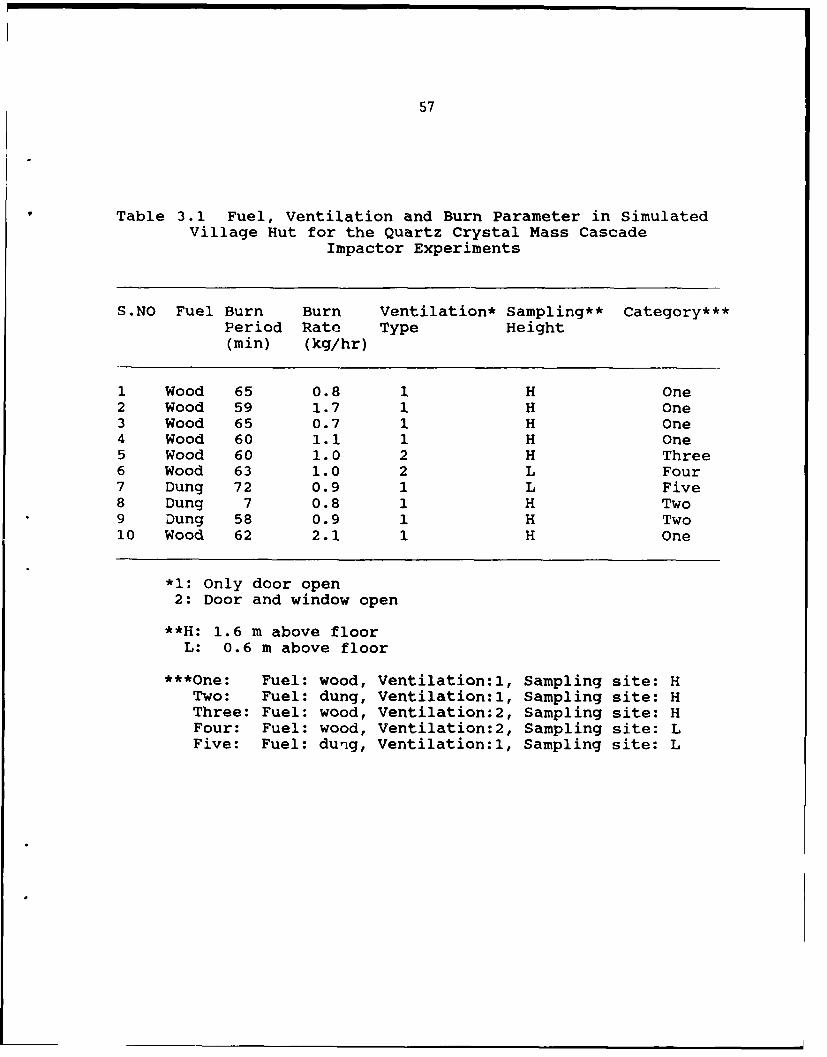
57

Table 3.1 Fuel, Ventilation and Burn Parameter in SimulatedVillage Hut for the Quartz Crystal Mass Cascade

Impactor Experiments

S.NO Fuel Burn Burn Ventilation* Sampling** Category***Period Rate Type Height(min) (kg/hr)

1 Wood 65 0.8 1 H One2 Wood 59 1.7 1 H One3 Wood 65 0.7 1 H One4 Wood 60 1.1 1 H One5 Wood 60 1.0 2 H Three6 Wood 63 1.0 2 L Four7 Dung 72 0.9 1 L Five8 Dung 7 0.8 1 H Two9 Dung 58 0.9 1 H Two10 Wood 62 2.1 1 H One

*1: Only door open2: Door and window open

**H: 1.6 m above floorL: 0.6 m above floor

***One: Fuel: wood, Ventilation:1, Sampling site: HTwo: Fuel: dung, Ventilation:l, Sampling site: HThree: Fuel: wood, Ventilation:2, Sampling site: HFour: Fuel: wood, Ventilation:2, Sampling site: LFive: Fuel: dung, Ventilation:l, Sampling site: L

58

Table 3.2

Average and Range@ of TSP (mg/m3 ) and Size (Am and Gm)* ofCombustion Generated Particulates for Different ExperimentalSetup During the Quartz Crystal Mass Cascade Impactor

Experiments in the Simulated Village Hut

Experi- Background TSP % Fine Am Gmmental** TSP Conc. Conc. TSP***

Category (mg/m3 ) (mg/m3 ) (pm) (pm)

I 0.07 3.28 91 0.93 0.18(.04-.12) (.2-10.5) (86-97) (.16-6.88) (.08-1.36)

II 0.14 17.7 93 0.88 0.20(.05-.24) (3.1-41.6) (89-97) (.23-3.72) (.11-.42)

III 0.10 2.5 99 0.60 0.16(0.4-4.3) (.14-1.20) (.09-.33)

IV 0.05 1.1 84 0.91 0.19(0.3-3.0) (.44-2.90) (.13-.31)

V 0.09 2.6 95 0.41 0.14(1.8-3.8) (.20-0.70) (.11-.20)

@ Range values in brackets* Am: Arithmetic mean & Gm: Geometric mean

**I: Fuelwood, only door open & sampler 1.6 m above floorII: Cowdung, only door open & sampler 1.6 m above floor

III:Fuelwood, door & window open, & sampler 1.6 m above floorIV:Fuelwood, door & window open, & sampler 0.6 m above floorV:Cowdung, only door open, & sampler 0.6 m above floor

***Percent of total mass in stages 5-10 ( < 3.2 pm in size)

59

99.99o BEGINNING* MIDDLE

99 VEND

"J 95S 90

so8wV60 oS

.. oun 40-z WOOD

z- 20

(f99.99 S V

CnUa,

S 9990 0 0

9- 0

800

60

40

20 DUNG

0.01 QI 1.0 10PARTICLE

AERODYNAMIC DIAMETER (..m)

Fig. 3. 1 Typical log probability pDo- ofparticle aerosol size for woodand dung smoke. (Sitirllated §v-llagehut, November, 1982)

Sampler: Quartz Crysta. Micro-balance Cascadelmpct or

60

have been used by several researchers viz., Miguel and

Friedlander, 1978, Van Vaeck, 1978, Raabe, 1982 and Knutson and

Lioy, 1983. Unlike statistical histograms, which have size

classes of equal width, the generalised histogram have size

classes which are not necessarily of equal width. The area,

and not height, of the histogram is proportional to the mass of

the TSP in the size range. Examples of such plots for dung and

wood smoke are given in Fig 3.2 which show that both wood and

dung smoke distributions are unimodal, have similar shapes and

peak in the same size range (0.1 to 0.2 ;m) despite almost

order of magnitude different in concentration. The average

geometric mean particulate size for all ten experiments was

0.17 um, for both wood and dung smoke (Table 3.1). This result

is similar to Dasch's (1982) of 0.17 pm MMD for wood smoke

sampled from fireplaces. Similar results have been reported by

Carroll, 1977, Butcher, 1982, and Saucy, 1983, who have

analyzed for wood/biomass smoke particle sizes.

Conclusions:

1. The cumulative mass of dung and wood smoke

are not log-normal distributed.

2. The average geometric mean for dung and

wood smoke particle size is 0.17 him.

61

5

4- WOOD

3

DUNG30

to -

0.01 0.1 1.0 10 100

PARTICLEAERODYNAMIC DIAMETER (jm) D-

Fig. 3.2 Typical generalized histogram plot of aerosolparticle size for wood and dung smke. (Simulatedvillage hut, NovemF 1982Y

Sampler: Quartz Crystal Micro-balance Cascade Impactor

62

3. Dung and wood smoke have unimodal size

distributions similar in shape and both

peak between 0.1 to 0.2 pm though total

mass is an order of magnitude larger for

dung smoke.

3.1.2 VARIATION OF PARTICLE SIZE WITH BURN TIME

Data from Appendix A.7 (Menon,1988) were plotted in two

ways to illustrate the variation of particle size with burn

time.

1. Mean size versus time. Fig 3.3 shows typical plots of

mean wood and dung smoke particle size versus burn time. The

variation in mean particle size is large ranging from 0.16 to

1.7 um for wood and from 0.23 to 3.72 pm for dung. The

fluctuations may be due to varying combustion intensity in the

uncontrolled open fires.

2. PercentaQe mass less than 3.2 nm versus time. Fig 3.4

shows typical plots of these wood and dung smoke percentage

(stages 5-10 of the QCMCI ) versus time during the burn.

Between 84 and 99 percent of the total particulate mass in wood

and dung smoke fell in this range . This limit, which

corresponds to particles of 2 g/cm3 with aerodynamic diameters

.05-3.2 pm (50% cutoffs), is roughly equivalent the upper limit

of "fine particulates", FP of 2.5 um. FP are of particular

concern because of the relatively high fraction that can

penetrate deep into the lung. Thus, it is not necessary to

63

I4-J

-0

00

N - 0

(W'TI)~~~~L 3L4JVG~IJVAO

z o.~v

614

)

/ )

0-

CDC zo0 00

00

ow

V 0 Cu

2 24

-0

o 0 0 0 0 0

(wr/Z'>) 01-9 S30ViS NISSVVY 1iviOl -AO %

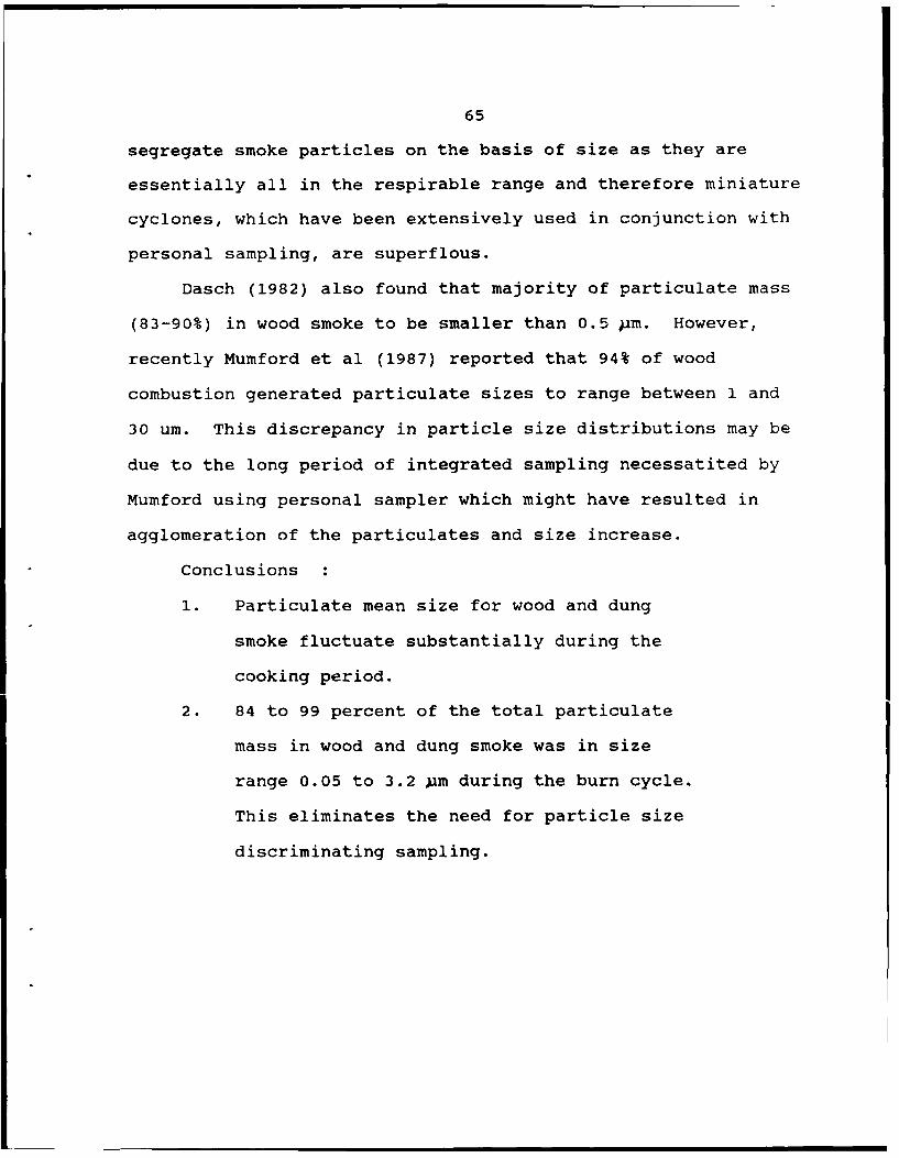
65

segregate smoke particles on the basis of size as they are

essentially all in the respirable range and therefore miniature

cyclones, which have been extensively used in conjunction with

personal sampling, are superflous.

Dasch (1982) also found that majority of particulate mass

(83-90%) in wood smoke to be smaller than 0.5 pm. However,

recently Mumford et al (1987) reported that 94% of wood

combustion generated particulate sizes to range between 1 and

30 um. This discrepancy in particle size distributions may be

due to the long period of integrated sampling necessatited by

Mumford using personal sampler which might have resulted in

agglomeration of the particulates and size increase.

Conclusions :

1. Particulate mean size for wood and dung

smoke fluctuate substantially during the

cooking period.

2. 84 to 99 percent of the total particulate

mass in wood and dung smoke was in size

range 0.05 to 3.2 jum during the burn cycle.

This eliminates the need for particle size

discriminating sampling.

66

3.1.3 VARIATION OF TSP AND CO CONCENTRATION WITHBURN TIME

Data from Appendix (Menon,1988) (for TSP and CO) were

analyzed to give mass variations as a function of time.

TSP versus burn time: Table 3.2 shows a large inter

experiment range of TSP concentrations for all experimental

setups. Fig 3.5 shows typical variations of TSP concentration

with time for wood and dung smoke. In this case TSP

concentration for dung smoke ranged between 3 to 42 mg/m3,

while that for wood smoke ranged between 0.3 to 3.4 mg/m3.

Though much smaller on an absolute scale, the wood smoke range

is about the same as that for dung smoke when normalized by the

mean concentration.

CO versus burn time: CO levels were read on a GE CO

personal monitor every six seconds after the fire was lit at

one of five low level and four high level sites. Sites 7 and 8

were too close to the fire to be monitored. A burn cycle

lasted 15 minutes. Table 3.3 presents the mean and range of Co

levels (1-min average) for fuel wood and cowdung smoke at the

sampling site used during each of the 22 experiments. Fig 3.6

shows a typical plot with a much larger absolute variation of

CO concentration (dung smoke) with burn time at a high level

site as compared to a low level site. When normalized by the

means the ranges are though about the same. This was found to

be true for all sites and for wood smoke as well. In almost

67

E Icr 40 '

EZo 30

DUNG

20zwZ 10

0WOOD\

a_

(-) .

I- 0 I0 20 30 40 50 60

TIME (minutes)

Fig. 3.5 Typical TSP concentration (mg/m 3) with burn time(min) for dung and wood smoke. Sam:. Lng probe*located at 1.6 m above floor and --S? sampled underlimited ventilation condition (on' door oen).(Simulated village hut, November, _952)

*Sampler: Quartz Crystal Micro-balance Cascade irpactor

68

Table 3.3

Average CO Concentration (ppm) Monitored at Nine Points in theSimulated Village Hut for Burn Period Lasting 15 Minutes Using

Fuel Wood and Cowdung

Site* FUELWOOD COWDUNG

VI V2 Vl V2MEAN RANGE MEAN RANGE MEAN RANGE MEAN RANGE

IL 21 5-46 .. . 16 3-25 ......3L 21 11-51 11 7-18 16 8-28 8 4-135L 23 11-52 --- 15 5-28 ... ...9L 20 13-45 --- 17 3-33 ... ...

IlL 12 3-25 --- 17 7-33 ......

2H 120 39-253 --- 113 30-190 ... ...4H 146 43-294 27 15-55 106 43-198 46 24-826H 136 42-265 121 44-157

10H 148 41-291 110 17-208

*Sampling grid: Fig. 3.7A L and H stand for low and high levelMVI *: Only door open, V2 **: door and window open

Sampler: General electric carbon monoxide detector(Model 15ECS3)

69

200

Z 150 O-0 0

0 0 00

0r 00

0

0 5

0

1 5 10 15

TIME (minutes)

Fig. 3.6 Typical variation of CO concentration (ppM) indung smmke with burn time (min) for a hig>; andflow level site*. Sampling done under liiiiedvetilation condition (only door open)

%Wigh site: 4SapiggiFg.37Low site: 3 apig~i i.37

Sampler: General Electric CO portable mionitor(Simulated village hut, Nov.-Dec., 1982)

70

all cases concentrations peak 7 to 10 mins after the fire was

lit. This probably coincides with the time of the mid burn

fuel feeding.

Conclusion

1. TSP and CO concentrations for both wood and

dung smoke vary considerably with time

during the burn. The range of fluctuation

is proportional to the wean value.

3.1.4 EFFECT OF FUEL, VENTILATION AND SAMPLING

LOCATION ON TSP, CO, BaP CONCENTRATION AND

RATIO OF BaP TO TSP

The following paragraphs discuss the results of

experiments conducted to investigate the effect of fuel,

ventilation and sampling location on

A. TSP concentration

B. CO concentration

C. BaP concentration

D. Ratio of BaP to TSP

A.TSP CONCENTRATIONS:

Appendix (Menon, 1988) presents method and lists data for

all 18 experiments conducted using a sequential sampler to

determine TSP levels at eleven indoor sites (Fig 3.7A). These

data are summarized in Fig 3.7B to 3.7E which show average TSP

concentration (mg/m3) for wood and dung smoke at the sites for

two ventilation conditions. Site 11 simulates a squatting

woman close to the chula.

71

ze 100i 271 ? Gcs )* t5346e OW5 m7IV.I I.

li :: ,. o

I !g, CJ II4ULA I £ I

(A) II) WOO0 ONLY DOOR OPEN (C) W0000 R ANqOWINDOW OPEN

4)3)5 B~m~ 2~3)5 14WOl4m2 3 &?1 mm")3*) +

/2-1310 310fll-

'94010 " 531I0604 U UM 34131 0

(D) DUNG ONLY DOR OPEN (E) D U4G CiXR ANDW9dOW OPEN

UO0 UNDIETECTA&E

Fig. 3.7 Mean TSP concentration (mg/m ) measured at11 sites using a sequential sampler. Samplingdone for wood and dung smoke under limited(only door open) and better (door and windowopen) ventilation condition.(Simulated village hut, Oct-Dec., 1982)

Note: Values in the bracket denote the number of timesthat site was sampled.

The vertical scale doubled for clarity

72

Effect of fuel type : With only door open woodsmoke (Fig 3.7B)

had TSP levels about half that for cowdung smoke (Fig 3.7DI at

most of the sites. This ratio is the same for door and window

open (Fig 3.7C-wood and Fig 3.7E-dung) as well. The highest

level monitored was 42.3 mg/m 3 at site 8, i.e directly above

the chula, with the dung burning and limited ventilation. As a

comparision the Hawaii Air Quality Standards limits the highest

24 hour mean TSP concentration to 0.15 mg/m3.

Fig 3.5 in which concentrations are plotted versus time

shows that higher smoke concentration prevailed for dung than

for wood throughout the burn cycle.

Effect of ventilation condition: With better ventilation i.e

door and window open (Fig 3.7C), all the sites except 7, 8 and

11 had undetectable particulate level for wood smoke, while

with only door open (Fig 3.7B) most sites had detectable

levels. The two sites above the chula had though higher

concentrations with better ventilation probably because the air

stream was created which moved the smoke past the point out

through the window before much dispersion could take place.

The concentration are reduced by roughly 50% for dung smoke as

well with improved ventilation. This shows the importance of

an open window above chula in reducing indoor smoke

concentrations. TSP levels were always below detection limit

at site 1, just opposite door at low level.

73

Fig 3.8a shows that TSP concentrations for wood smoke for

better ventilation condition (door and window open) remained

about half of that during limited ventilation condition

throughout the burn cycle.

Effect of sampling location: Mean TSP concentrations are higher

at higher levels than at lower levels. Concentration closer to

chula are higher than at sites away from the chula for limited

ventilation condition (Fig 3.7).

Fig 3.8b shows that TSP concentrations stay about twice as

high at high level than at low level for better ventilation

condition (door and window open) throughout the burn cycle.

Conclusions :

1. TSP concentrations range from below

detection limit (< 0.5 mg/m3) to 38.7 mg/m3

at the different indoor sites.

2. TSP concentration were higher at high level

sites than at low level sites.

3. The presence of an open window above chula

resulted in significant lower levels of TSP

at most of the sites.

4. TSP levels were about twice as high for

dung smoke than for wood smoke.

5. The effect of fuel type, ventilation

condition and sampling location did not

vary throughout the burn.

74

E 0I0 - ONLY DOOR OPEN--y°

o / ~0 _/

I 5-

/ DOOR AND

09 0 / I I I ,, I I0- 0 I0 20 30 40 50 60

TIME (minutes)

Fig. 3.8a Variation of 'TSP concentration (mg/mn3) for wood

smke with burn time (min) showing the effect ofventilation. Sampling probe* located at 1. 6 mabove floor.

*Sampler: Quartz Crystal Micro-balance Cascade Impactor(Siulated village hut, November, 1982)

Z

75

Eat 4-- 0 0

E 0HIGH- /z I-_ I \', I\'

2 Izz I01U 0 LOW

0_oC) 0- 0 10 20 30 40 50 60

TIME (minutes)

Fig..3.8b Variation of TSP concentration (mg/m3) forwood smoke with burn time (min) showing theeffect of sampling location.

Sampler: Quartz Crystal Micro-balance Cascade Impactor(Simulated village hut, November, 1982)

76

B. CO CONCENTRATIONS:

Appendix (Menon, 1988) gives CO data from GE monitor for

22 experiments which were analyzed to illustrate:

Effect of fuel type: Table 3.3 shows no marked difference

between wood and dung smoke for all sites. Fig 3.9 shows CO

concentration for wood and dung smoke similar through the burn

cycle.

Effect of ventilation condition: Table 3.3 shows CO levels are

about 2 to 4 times lower for better ventilation condition (door

and window open) than for limited ventilation condition (only

door open). The ratio is maintained throughout the burn cycle

(Fig 3.10).

Effect of sampling location: Table 3.3 shows CO levels in wood

and dung smoke about 100 ppm at high level sites and about 20

ppm at all low sites. The CO concentrations for the low level

sites do not vary substantially during the burn (Fig 3.6).

Further, CO data (Appendix A.8.4, Menon 1988) were

investigated using statistical technique (Split-plot Analysis)

to determine significant effect of fuel type, ventilation

condition, sampling location and their interactions. Table 3.4

summarizes and presents sum of squares, degrees of freedom,

mean squares, F ratios and probabilities associated with each F

ratio. We note that sampling height specified by the level

(high, medium or low) is significant at alpha=.0l.

77

300

E I \

z-I0o I

S200 -, P 20n," I 1 I, I L / b

UzUNz 0 /o

0 100.0 -01o -/

40 1 f1 5 10 15

TIME (minutes)Fig. 3.9 Typical variation of CO concentration (ppm)

in wood and dung smoke with burn time (min)for a-high sampling site:':. Sampling doneunder limited ventilation condition (onlydoor open)

*Site 4: Sampling grid Fig. 3.7a

*Site 4: Sampling grid Fig. 3.7a

Sampler: General Electric CO portable monitor(Simulated village hut, Nov.-Dec., 1982)

78

300 0E I\ '"ONLY DOOR OPEN

0.0

zo 200 P\ ,O-.OI-I/ \/

\0 Ncc /0z0

z' DOOR ANDI

000

00

TIME (minutes)

Fig. 3.10 Effect of ventilation on reducin.g COconcentration (ppm) at high samplingsite.* General Electric personal samplerused to monitor CO levels in wood smoke.

*Site 4: Sampling grid Fig. 3.7a

Sampler: General Electric portable monitor(Simulated village hut, Nov.-Dec., 1982)

79

Table 3.4

Test of Variance of CO by Fuel Type, VentilationCondition, Sampling Height and Location in Simulated

Village Hut

Whole Plot Analysis DF Mean Sq. F

Fuel Type 1 1016.11 0.04Ventilation 1 408452.16 16.80Level 2 1079902.23 44.30**

FLTYP X VENT 1 7181.27 0.3FLTYP X LEVEL 2 1892.65 0.1VENT X LEVEL 2 182814.94 7.5

Whole Plot Error

FLTYP X VENT X LEVEL 2 24369.8

Sub Plot Analysis

SITE 8 226.2 0.02SITE X FLTYP 8 661.7 0.53SITE X VENT 8 146.7 0.12SITE X LEVEL 16 792.7 0.64

SITE X FLTYP X VENT 8 566.4 0.46SITE X FLTYP X LEVEL 16 207.1 0.17SITE X VENT X LEVEL 16 282.4 0.23

SUB-PLOT ERROR 1528 1238.6

** Effect significant at .01 level

80

Conclusions:

1. CO concentrations for dung and wood smoke

ranged from 12 to 148 ppm with a mean of 18

ppm for low levels and 120 ppm for high

levels. No marked difference exists

between fuel type.

2. Better ventilation conditions reduced CO

levels about 2 to 4 times.

3. Mean CO concentrations for limited

ventilation condition are about 100 ppm at

high level sites and about 20 ppm at low

sites for both fuels. Effect of sampling

height is statistically significant at .01

level.

4. Effect of fuel, ventilation condition and

sampling location hold true throughout the

burn.

C. BaP CONCENTRATIONS:

TSP sampled filters used with personal samplers (Gilian

samplers) were chemically analyzed for BaP using HPLC.

Table 3.5 gives the average BaP concentrations for different

fuel, ventilation condition and sampling location. The result

were confirmed by a few TSP samples analyzed by HPLC at

Lawerence Berkley Laboratory (Table 3.6).

81

Effect of fuel type: No marked difference exists between fuel

type. In contrast, Aggarwal et al., 1982, found BaP

concentrations to be seven times higher for dung smoke.

Effect of ventilation condition: Roof BaP values are as high as

1800 ng/m3 for limited ventilation (only door open) for both

wood and dung smoke. These concentrations are almost twice of

those for better ventilation condition (door and window open).

Effect of sampling location: BaP concentration at roof level

are about six times higher than at low levels for both dung and

wood for limited ventilation but only about twice as high for

better ventilation condition. BaP concentrations at low levels

are comparable in all cases, ranging from 250 to 430 ng/m3,

whereas roof BaP were thousands of ng/m3.

D. RATIO OF BaP TO TSP:

Table 3.5 and 3.6 gives mean ratio of BaP to TSP for

different fuel, ventilation condition and sampling location.

Effect of fuel type: Ratio of BaP to TSP for wood smoke higher

(about twice) than that for dung smoke. This may be explained

due to presence of higher percentage of inorganics in dung. In

contrast, Aggarwal, (1982) reported higher (thrice) mean ratio

for dung smoke.

Effect of ventilation condition: No marked difference exists

between ventilation condition.

Effect of samplinQ location: Table 3.5 indicates no marked

difference between sampling location.

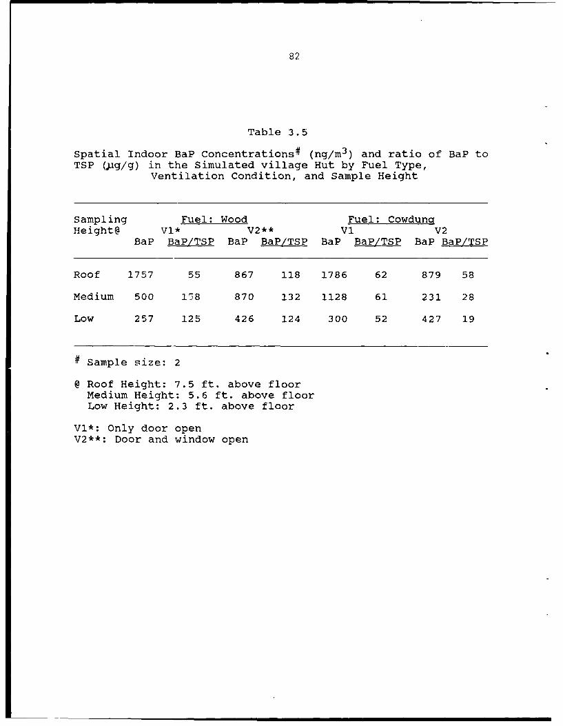
82

Table 3.5

Spatial Indoor BaP Concentrations# (ng/m3 ) and ratio of BaP toTSP (pg/g) in the Simulated village Hut by Fuel Type,

Ventilation Condition, and Sample Height

Sampling Fuel: Wood Fuel: CowdungHeight@ Vl* V2** Vl V2

BaP BaP/TSP BaP BaP/TSP BaP BaP/TSP BaP BaP/TSP

Roof 1757 55 867 118 1786 62 879 58

Medium 500 178 870 132 1128 61 231 28

Low 257 125 426 124 300 52 427 19

# Sample size: 2

@ Roof Height: 7.5 ft. above floorMedium Height: 5.6 ft. above floorLow Height: 2.3 ft. above floor

Vl*: Only door openV2**: Door and window open

83

Table 3.61

Integrated Levels of TSP, CO, BaP and Ratio of BaP to TSPDuring a Typical Cooking Period in Simulated Village

Hut.(November, 1982)

Experimental RSP@ Conc. CO Conc. BaP# Conc. BaP/RSPCategory* (mg/m3 ) (ppm) (ng/m3 ) (pg/g)

I 8.9 32 4884 549II 27.0 48 5066 223III 5.7 19 2170 381IV 4.2 11 323 77V 7.4 11 659 89

*I: Wood, only door open and sampling site 1.6m above floorII: Dung, only door open and sampling site 1.6m above floorIII: Wood, door & window open, sampling site 1.6m above floorIV: Wood, door & window open, sampling site 0.6m above floorV: Dung, only door open, sampling site 0.6m above floor

@ Particulates collected on teflon filter using cyclone fittedsampler (Prototype sampler-Lawrence Berkely Laboratory)

# BaP analysis done at Lawrence Berkley Laboratory using HighPerformance Liquid Chromatography

1 1 thank Mr. Mike Apte for operating the QCMCI andproviding us with RSP and BaP results analyzed at LawrenceBerkeley Lab.

84

Background levels of TSP. CO and BaP in SVH: Background levels

of TSP and BaP were measured on several occasions inside the

SVH, for about 24 hours with no fire using the Hi-volume

sampler. Appendix.A.6 presents method for using Hi-volume

sampler. TSP levels ranged from 43 to 215 jag/m 3 with mean

value of 94. Some of TSP background filters were analyzed for

BaP. Surprisingly BaP levels ranged between 65 to 150 ng/m 3,

with no fire, possibly a result of drawing settled soot from

walls / roof / floor, by the Hi-volume sampler. Background

levels of CO inside SVH were always less than 1 ppm.

Moisture, ash and calorfic value of fuel: Wood and cowdung

samples were analyzed for moisture and ash content for several

of the experiments. Appendix.A.5 (Menon,1988) presents method

used for determining moisture,ash and calorific value of fuel.

The moisture of fuelwood (leucaena) and cowdung ranged from 10

to 25% on dry wt. basis. The ash content for wood was

considerably lower than for cowdung, ranging between 1 to 6%

for wood and between 12 and 16% for cowdung. The mean calorific

value determined for leucaena wood was 4200 cal/gm (range 4000

to 4580 cal/gm) and for cowdung was 2800 cal/gm (range 2020 to

3500 cal/gm).

85

Conclusions:

1. BaP concentrations for wood and dung smoke

are about same but ratio of BaP to TSP

higher(twice) for wood smoke. This result

is contrary to Aggarwal, et al., (1982)

study.

2. Only roof BaP concentrations reduced as a result of

increasing ventilation.

3. Roof BaP concentrations were in the order

of thousand ng/m3 whereas at low levels

they were in hundreds.

4. BaP concentrations were well correlated to

TSP concentration.

3.1.5 SUMMARY AND RECOMMENDATIONS FOR FIELD

EXPERIMENTS

The main results of experiments in SVH are:

1. Particulate size, TSP and CO concentrations

for both wood and dung smoke vary

considerably during burn.

2. Particulate size for both wood and dung

smoke were in the respirable range( <3.2

'Um) .

3. TSP, CO and BaP concentrations depend

strongly on sampling location and

ventilation condition. TSP concentrations

for dung were substantially higher. TSP,

86

CO and BaP levels were greatly reduced with

window open and when the sampling location

was at low levels. Ratio of BaP to TSP

higher for wood smoke at all sampling

locations and both ventilation conditions.

4. TSP, and CO concentrations were extremely

high when compared to existing U.S Ambient

Air Quality Standards.

Partly as a result of the high levels of TSP, CO and BaP

obtained in SVH and research conducted by Agarwal (1982) Smith

et al (1983) it was deemed necessary to carry out field

experiments to see if the very hazardous respiratory

environment found in the SVH exists in rural Indian huts.

It was however not feasible to take QCMCI, sequential or

Hi-Vol sampler to the rural huts in India because continuous

supply of electricity is not available in rural huts, extremely

difficult to transport bulky equipments, and it was considered

important to monitor the exposure of cooks.

Five battery operated and light weight TSP (Gilian HFS

113) and one CO (Ecolyzer 210) samplers were procured. The

instruments were tested in the SVH in order to gain working

experience and develop a sampling protocol for rural kitchens

and to compare results with previously used samplers.

Eight experiments were therefore conducted collecting

simultaneous data for TSP and CO concentrations at different

locations and investigate effect of fuel type and ventilation.

87

Appendix.A.8.2 & A.8.4 (Menon,1988) lists the data obtained for

TSP and CO concentrations. The results obtained are similar to

results discussed in earlier section. Hence feasible sampling

design (using personal samplers) for monitoring TSP and CO

concentrations in rural huts was:

1. For TSP: Sampling cook's exposure along

with space at roof, medium and low levels

at a distance of about two feet from the

chula (Fig 3.11).

2. For CO: Sampling nine sites in front of

chula at three different levels along with

cook's exposure (Fig 3.12).

As the micro-meteorological variables such as indoor-

outdoor temperature, wind, relative humidity may interact with

fuel quality and combustion conditions it was decided to also

measure these during the tests in India. Several research

results exist relating fuel quality, burn rate and emission of

combustion generated pollutants. Exposure of cooks to indoor

pollutants should be highest during monsoon months, because of

poor fuel quality, ventilation conditions and unfavorable

meteorological conditions. While during the winter months

indoor pollutant levels should be lower because of better fuel

quality, ventilation conditions and general weather conditions.

Hence climatological conditions may significantly effect

pollutant levels.

88

qMEDIUM I

I fI ft.CHULA

Fig. 3. 11 Sampling sites for ieasurement of TSPconcentration (mg/rn in the rural kitchensusing personal samplers.

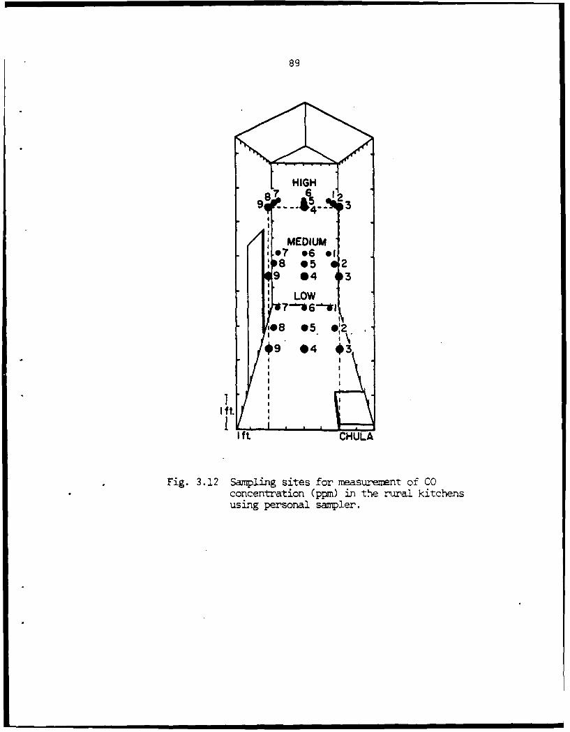
89

HIGH

7 3

MEDIUM7 6 108 05 29 @4 3

LOW

+9 04 43

I CHULA

Fig. 3.12 Sampling sites for measuryement of COconcentration (ppm) in the rural kitchensusing personal sampler.

90

The field sampling protocol was designed from finding of

the effect of fuel type, ventilation condition and sampling

location on pollutant concentration in SVH and consideration of

climatological conditions discussed in previous paragraph. To

evaluate statistically, it was necessary to carry out indoor

sampling in atleast 100 rural huts because of the large

variability in ventilation conditions, fuel quality, combustor

conditions and weather conditions.

3.2 FIELD EXPERIMENTS (INDIA)

The following paragraphs present the results of

experiments performed in Indian rural huts from July, 1983 to

February, 1984. The objectives were:

1. Determine socio-economic (housing)

conditions of the selected rural population

and their concern about fuel and smoke.

2. Determine cook's exposure to TSP, CO and

BaP and their concentrations at roof,

medium and low level within short distance

of chula.

91

3. Determine whether cook's exposure to TSP

and CO, and TSP concentration at roof were

significantly different for:

a. Villageb. Seasonc. Time of dayd. Kitchen typee. Roof typef. Door locationg. Fuel typeh. Food type

4. Determine the effect and interaction of

climate, ventilation and sampling location

on spatial concentrations of Co.

5. Model for estimating cook's exposure to TSP

as a function of meteorological,

ventilation, fuel and stove parameters.

3.2.1 SOCIO-ECONOMIC CHARACTERISTICS, FUEL USE

AND PERCEPTION OF PROBLEMS RELATED TO SMOKE

Field experiments were carried out in five villages of

India, two in the south and three in the central region. The

main criteria for the selection of villages were organizational

support, usage of wood and dung as principal cooking fuels,

distinct months of rainfall and winter conditions, no language

problem, and proximity to a city-- as the air sampling pumps

required daily electrical charging.

The three villages selected in central India were adopted

by Bharat Heavy Electricals Ltd. (author's parent organization)

and the Central Institute of Agricultural Engineering (CIAE)

92

under the India's late Prime-Minister Indira Gandhi's 20-point

program for rural development. The Tata Energy Research

Institute (TERI) had extension services connected with an

improved fuel-efficient stove program in the two villages in

south India. Organizational support facilitated

logistics/transportation and introduction to the village

population greatly helped in gaining the villager's trust and

cooperation.

Characteristics of villages selected in central India

The villages Padaria and Adampur, located in Madhya

Pradesh some 30 km west of Bhopal, were adopted by BHEL in an

effort to change the poverty and backwardness of the village.

Islamnagar, situated some 15 km north of Bhopal, was adopted by

the CIAE as part of their village extension program. About 100

families live in each of Adampur and Padaria while about 250

families live in Islamnagar. The main occupation in the

villages is agricultural-related. The monsoon dominates the

weather during late June to September while winter lasts from

November to February.

Most households have one single room with a verandah. The

stove is usually placed in a corner of the room and cementee to

the floor with mud. Some householders have a portable stove

and its position can change. The single room is used for:

dining and sleeping as well as entertaining guests. Most

93

households gather dead wood in the form of branches and twigs

from the nearby forests. Hardly anybody purchases fuel. The

villagers use a mixture of types of wood and it was very

difficult to identify particular speciesI . Fuelwood was often

used in conjunction with dung. Only for a few specific dish

was cooking done with dung alone. The chief food roti (bread

made from whole wheat) and dal (lentils), sometimes

supplemented by vegetables. Most households cook twice a day

(morning and evening). While cooking roti, the cook has to be

near the fire all the time, unlike rice when the cook only has

to attend the stove occasionally.

Characteristics of villages selected in south India

The Ariyur and Perambia villages, are located about 40 km

southwest Pondicherry in southeast India. The monsoon period

is October/November and the region does not experience a cold

winter. Most villagers in Perambia are landless agricultural

laborers living in thatched huts, whereas Ariyur has a strata

of economic conditions. Fuel is both bought and gathered.

Most southern cooks use logs of Casurina, and coconut husks and

fronds for fuel. Use of cowdung is minimal. Most stoves have

two ports. The main food is rice, dal and vegetables. Cooking

1 Appendix B.2 lists the local and scientific names fordifferent wood species. Mr.R. Singh's help in identifying thewood species and Dr.S.D.M Tiwari's (retired Principal ChiefConservator of forests, Govt.of Madhya Pradesh, India) help inproviding us with scientific names is greatly appreciated.

94

is usually done once a day, during the early afternoon or

evening, though sometimes it is done three times a day as

opposed to the central Indian villages where two meals are

prepared each day.

Appendix( B.1, Menon, 1988) presents the questionnaire,

(similar to that used in Smith, et al., 1983), used to collect

information from a large number of households in the villages

about their socio-economic conditions, physical characteristics

of their houses, kitchens and stoves, cooking patterns

perception of smoke and it's impact on health. The

questionnaire was invariably answered by the head of the family

- usually men -, only the section on smoke perception and

cooking practices was answered by one or more women. Appendix

(B.2, Menon,1988) presents graph of the results of the 67

questions. Table 3.7 summarizes the result. A total of 291

arbitrarily selected households were interviewed. The number

of households in the central Indian villages Adampur,

Islamnagar, and Padaria were 46, 73, 96 respectively, whereas

in the south Indian villages Ariyur and Perambia they were 38

each.

Five socio-economic variables were family size, smoking

habits, income, occupation of the head of the family, and house

ownership. Most households571%) had six or fewer members, 10%

had ten or more members, the largest one had 22. There were no

smokers in 45* of the households, one in 44% and more than two

in the remaining 11%. The smokers were all men who said they

95

Table 3.7 (Page 1 of 7) Summary Statistics: Socio-Economic,Fuel and Smoke Perception Survey

1. Village and Household Identification

V001 House Number 1 to 291

V002 Sampled Houses Adampur: 46by Village Islamnagar: 73

Padaria: 96Ariyur: 38Perambia: 38

2. Socio-Economic Characteristics

Mean Median std.dev. Max Min

V003 Family Size 7.0 6.0 3.1 22.0 1.0

V004 Smokers Number 1.0 1.0 0.9 8.0 0.0

V005 Income(Rs) 4898.0 3000.0 6249.0 50,000.0 0.0

V006 Occupation Farmer: 97Laborer: 82Stone cutter/Brick kilnWorker: 18

V007 House Ownership Owned: 279Rented: 11Other: 1

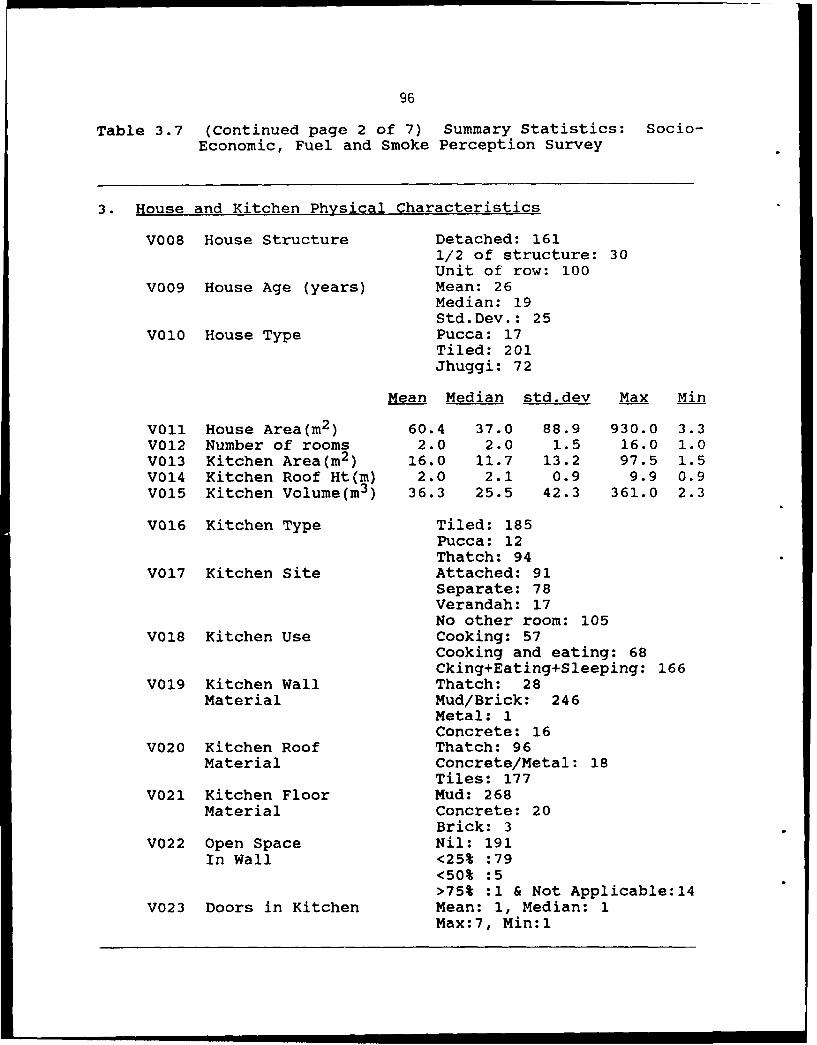
96

Table 3.7 (Continued page 2 of 7) Summary Statistics: Socio-Economic, Fuel and Smoke Perception Survey

3. House and Kitchen Physical Characteristics

V008 House Structure Detached: 1611/2 of structure: 30Unit of row: 100

V009 House Age (years) Mean: 26Median: 19Std.Dev.: 25

V010 House Type Pucca: 17Tiled: 201Jhuggi: 72

Mean Median std.dev Max Min

V011 House Area(m 2 ) 60.4 37.0 88.9 930.0 3.3V012 Number of rooms 2.0 2.0 1.5 16.0 1.0V013 Kitchen Area(m2 ) 16.0 11.7 13.2 97.5 1.5V014 Kitchen Roof Ht(m) 2.0 2.1 0.9 9.9 0.9V015 Kitchen Volume(m3 ) 36.3 25.5 42.3 361.0 2.3

V016 Kitchen Type Tiled: 185Pucca: 12Thatch: 94

V017 Kitchen Site Attached: 91Separate: 78Verandah: 17No other room: 105

V018 Kitchen Use Cooking: 57Cooking and eating: 68Cking+Eating+Sleeping: 166

V019 Kitchen Wall Thatch: 28Material Mud/Brick: 246

Metal: 1Concrete: 16

V020 Kitchen Roof Thatch: 96Material Concrete/Metal: 18

Tiles: 177V021 Kitchen Floor Mud: 268

Material Concrete: 20Brick: 3

V022 Open Space Nil: 191In Wall <25% :79

<50% :5>75% :1 & Not Applicable:14

V023 Doors in Kitchen Mean: 1, Median: 1Max:7, Min:l

97

Table 3.7 (Continued page 3 of 7) Summary Statistics: Socio-Economic, Fuel and Smoke Perception Survey

4. Stove and Cooking Characteristics

V024 Other Cooking Sites Yes: 104, NO: 187

V025 Other Cooking Sites- Open/Verandah: 74Specify Other room: 24

Same room: 5Not Applicable: 187

V026 Period for Cooking Summer: 49at Other Site Winter: 19

Monsoon: 3Guests/Celebration: 20Child birth: 5Not Applicable: 188All Season: 7

V027 Cooks for (number) Mean: 7, Median: 6std.dev: 3Max: 25, Min: 1

V028 Cooking Time Morning: 2Noon: 2Evening: 42Morn. & Noon: 1Morn. & Even: 198Noon & Even: 8Morn, Noon, Even: 38

V029 Guests per week Mean: 1, Median: 1Max: 9, Min: 0

V030 Food Type Rice & Curry: 68Roti & Curry: 95Rice & Roti: 128

V031 Number of Cooks Mean: 1, Median: 1Max: 4, Min: 1

V032 Cook's Age Mean & Median:30 std.dev:l1

V033 Years of Cooking Mean:19,Median:17 std.dev:ll

V034 Total Cooking Hours Mean:6,Median:3,std.dev:17Per Day Max:8, Min:3

98

Table 3.7 (Continued page 4 of 7) Summary Statistics: Socio-Economic, Fuel and Smoke Perception Survey

V035 Other People in Yes: 155, No: 135Kitchen whileCooking

V036 Present in Season Winter: 59,Mon, Win & Summer: 94Not Applicable: 136

V037 Cook Near Fire- Always: 132Duration Most of the Time: 24

Half of the Time: 78Less: 57

V038 Fire for other Zero hour: 108Purposes-Duration Half hour: 157

> One hour: 26

V054 Stove Type One mouth: 188Two mouth (attached): 29Two mouth (connected): 27Other: 47

V055 Stove Replacement Yearly: 117Once in Two Years: 18Birth of Child: 3Broken: 108Never: 45

V057 Ventilation Change Yes: 45In Monsoon No: 217

Don't Know: 29

V058 Ventilation Change Yes: 62In Winter No: 183

Don't know: 46

V059 Kerosene Lamp Yes: 232, NO: 59While Cooking

I I I | i

99

Table 3.7 (Continued page 5 of 7) Summary Statistics: Socio-Economic, Fuel and Smoke Perception Survey

5. Fuel Characteristics

V039 Fuel Type Wood: 46Dung: 4Wood & Dung: 209Wood & Crop Residue: 32

V040 Qty. of Fuel per Day Mean:14,Median:6,std.dev:25(kg) Max: 20, Min: 0.5

V041 Cost of Fuel per Mean:28,Median:3, std.dev:43Ten kg (Rs)

V042 Fuel Storage Kitchen roof: 49Separate Room: 31Verandah: 40Animal Shed/ out Shed: 29Open: 98None: 40

V043 Fuel Change in Last Yes: 21, No: 270Five Years

V044 Fuel Gathering- Mean:8, Median:4, std.dev:19Summer hours Max: 24, Min: 0

V045 Fuel Gathering- Mean:6, Median:0, std.dev:19Monsoon Hours Max:12, Min: 0

V046 Fuel Gathering- Mean:8,Median:4,std.dev:19Winter Hours Max: 15, Min: 0

V047 Fuel Gathered by Men: 137, Women: 19Children: 2Men & Women: 44Men, Women & Children: 14Women & Children: 4Not Applicable: 71

100

Table 3.7 (Continued page 6 of 7) Summary Statistics: Socio-Economic, Fuel and Smoke Perception Survey

V048 Ease in Collection Impossible: 57Difficult: 118Satisfactory: 7Easy: 64Not Applicable: 45

V049 Wood From Compound: 55Jungle: 169Buy from shop/others: 67

Mean Median std.dev Max. Min.

V050 Fuel Cost / Head 8.2 7.0 5.9 40.0 2.0

V051 Fuel Cost / Cycle 15.5 12.0 15.8 85.0 2.0

V052 Fuel Cost / Cart 69.0 57.0 65.0 600.0 4.0

V053 Type of Wood Used* Satkut: 176Beshram: 5Casurina: 18Portia: 3Mixture of CasurinaPortia and Sugar Cane: 24Don't Know: 30

* Appendix lists local and scientific names

101

Table 3.7 (Continued page 7 of 7) Summary Statistics: Socio-Economic, Fuel and Smoke Perception Survey

6. Villager's Perception About Fuel and Smoke

V064 Smoky Fuelood Gurgan: 69species Crop residue: 33

Other: 111Don't know: 41

V065 Less Smoky Species Sagun: 64Dry wood: 37Other: 85Don't know: 49

V066 Effort to get less Yes: 93, No: 156Smoky Fuel Yes but not available: 42

7. Cook's Attitude Towards Smoke

V060 Smoke Bother Yes: 243, No: 35Don't know: 13

V061 Smoke Dislike Very Much: 224Little: 44None: 23

V062 Perceived Health Yes: 166Problem No: 85

V063 Problem of Lungs: 59Eyes: 109Lungs and Eyes: 56Don't know & N.A: 67

V067 Desire to Get Rid Yes: 195Of Smoke No: 49

Don't Know: 47

V068 Desire Fuelwood Fuelwood Delivery: 291Delivery (at cost) Smokeless Chula: 0or Smokeless Chula(at no cost)

102

did not smoke in the kitchen. Most family heads were farmers

(33%) followed by agricultural laborers(28%), and 18% employees

of companies or the Government. There existed a wide range of

income among the sampled population. 2% of family had no

income at all and 2% had incomes of more than RS.24,000 p.a.

The mean annual income was Rs.4900, and the median Rs.3000. 96%

of the households owned their house.

Sixteen variables describe the house and the kitchen e.g.,

house structure and area, kitchen volume, location and sources

of ventilation. The houses were either detached(55%), part of

a row(34%) or half of a unit(ll%). The age of the houses,

ranged from 1 to 135 years with a mean age of 26 and a median

of 19. Twelve percent of the houses were built in the last 5

years and there appeared to be no differences between their

construction materials or structures and those of the older

houses. The floor area of the houses ranged from 3.3 to 930 m2

with a mean of 60 and median 37. The number of the rooms ranged

from 1 to 16 with a mean and median of 2. Most houses had

tiled roofs(69%) followed by roofs of thatch(25%) and the

remaining 6% of the houses were constructed of cement or

concrete. This is similar to census data 1971 of Madhya

Pradesh, which reported tiles, slate and shingle to be

predominant (70 to 80 %) of roof material of the rural houses.

36% of the houses had one room, one corner of which served as a

kitchen, 31%, had their kitchen attached to another room and

26%, had a separate room which was used solely for cooking

103

purposes and 6% did their cooking in one corner of the

verandah. A majority of the householders(57%) used the kitchen

area for cooking, eating, and sleeping, 20% used it for cooking

only and the remaining 23% used it for both cooking and eating.

Most kitchen walls were made of mud and brick(85%), 10% were of

thatch, and 5% of concrete. All houses had mud floors. Roof

material was an important variable for smoke seepage. In

thatched kitchens the researchers while questioning were forced

to sit on the floor because of intolerable levels of smoke.

Tiles on the roofs were laid on wooden rafters at a slight

angle, thereby leaving spaces for ventilation which prevented

the buildup of smoke indoors. A total of 177 houses, (61%),

had tiled kitchen roofs, and 96, (33%) had thatched roofs.

Kitchen areas ranged from 1.5 to 97.5 sq.m, with a mean of

15.5. Kitchen roof height was usually about 2 m with a maximum

of 9.1 and minimum of 0.9 m. Kitchen volume ranged from 2.3 to

360 m3 with a mean of 36 and median of 25. A majority of

kitchens (66%) had no opening in the walls, 27% had less than a

25% opening in the walls. Most kitchens(81%) had only one

door, 12% had 2 doors and the rest (7%) had 3 doors or more.

When asked if they changed the ventilation conditions (spacing

of tiles on roof) during monsoon or winter, most (63 to 75 %)

answered no. As the stove was usually in a dark place most of

the cooks(80%) use a small kerosene lamp near to the stove.

Twenty one stove and cooking variables provide information

about cooking sites, seasonal patterns of cooking periods,

104

cooking time and duration of nearness to the fire, food type,

cook's age and the number of years that she has performed the

chore, presence of other people in the kitchen etc. When

questioned if they sometimes cooked elsewhere, 36% answered

yes. 75% cooked outdoors or in the verandah much of the summer

and when relatives or friends visited. 68 percent of the cooks

performed their cooking chores during the morning and evening,

14% during the evening and the remaining 18% at other times.

Most cooks prepared meals for about 6 persons, but in some

households they cooked for as many as 25 persons. 84% percent

of the households had one or more guest per week. 64% percent

of the households had only one cook, 30% had 2 cooks, either

the wife or the daughters-in-law of the head of the family or

in some houses by a mother and her young daughters and the

remaining 6% had more than two cooks. The cook's age ranged

from 11 to 70 with both a mean and median of 30 years. The

number of years the cooks had been cooking with traditional

fuels ranged from 3 to 60 years with a mean of 19. 44 %

prepared both rice and roti, 33% only roti and dal, and the

rest rice and curry. Roti and dal is the predominant food in

central India whereas rice and curry is the staple food of the

south. Cooking of roti requires the cook to be close to the

fire throughout the cooking cycle whereas rice cooking requires

only occassional presence of the cook. Asked for the number of

hours of cooking per day, 3% had no idea and the rest mentioned

between 0.5 to 8 with a mean of 6 and median 2.5 hours. While

105

cooking most (70%) stayed close to the fire. When asked

whether other members of the family were present during

cooking, a little more than 50% answered yes. Sixty percent

said that other members were present where they cooked

throughout the year, whereas the rest specified that the others

were with them only during winter season, usually to warm

themselves in front of the cooking fires. When asked for how

long they used their fires for tasks other than cooking, about

37% answered never, 54%, for less than half an hour per day,

and the rest (9%) for more than 1 hour. 65% used a single port

stove, and the rest mostly in south, used a two port stove.

37% replaced the stoves only when broken, 28% did so annually

and the rest (35%) had never replaced a stove or had replaced

it once in two years. The cost of replacement of the stoves,

was estimated at Rs.l.

Fifteen fuel variables provide information about fuel type,

cost, storage, seasonal patterns of fuel gathering, by whom and

where the fuel was gathered, and level of difficulties

experienced in finding fuel. A great majority (93%) had always

used the same type of fuel and never changed to any other

energy source. 34% stored their fuel in the open, the others

stored it on the rafters below the kitchen roof, in a separate

room, verandah, or outside shed. 0.5 to 20 kg (median 6) of

fuel was used daily. 72% used both wood and cowdung in

combination, 16% used wood alone and the remaining 12% used

wood and crop residue. In the majority of the households(47%),

106

the fuelwood was procured only by male members, in 21% of the

households women members assisted in fuel gathering. During

summer as much as 24 hours per day was spent in procuring fuel

whereas during winter and monsoon periods 15 and 12 hours

respectively were used. During the monsoon 50% did not go for

fuel gathering at all relying on stored summer fuel. 41% had

great difficulty in getting the fuel, 20% thought fuel

gathering was relatively easy and the rest 20% found it to be

an almost impossible chore. 58% went to a nearby forest to

collect dead branches for firewood, 18% chopped trees on their

own land and the rest bought wood. 69% used whatever type of

fuel was gathered generally a mixture of seven different

species(satkut). 27% had no idea about the cost of fuelwood,

the rest estimated from 0 to Rs.2/kg. Fuel is usually sold by

headload, bicycle load or cart load. 60 to 70% had no

knowledge about the cost of fuel per head, cycle or cart.

Three variables pertaining to the villagers' knowledge about

smokiness as related to fuel type and their effort to procure

less smoky species of fuelwood. The cooks characterised a

number of fuelwood types as smoky, amongst which Gurgan was

most commonly mentioned in the north and crop residue in the

south. When asked if they knew less smoky fuel, 22% in central

region suggested Sagun while in the south many mentioned

Casurina. 54% did not try to get less smoky fuel, 32% did so

successfully, and the rest usually failed to get less smoky

fuel.

107

Five variables give information about the cook's

perception of the smoke, perceived health related problems and

desire to get rid of smoke. Most cooks(84%) said that smoke

bothered them very much. 57% indicated one related health

problem, mainly eye trouble, and 20% attributed both eye and

lung problems to smoke. 67% wanted to get rid of smoke but

when given a choice between a cost free smokeless chula and

fuelwood delivery at nominal cost, all opted for the latter,

suggesting fuel procurement as the priority need.

SUMMARY

1. Most of the rural population were farmers

and laborers and their income varied

considerably.

2. All kitchen had mud floors and most had

stone/brick with mud walls. Kitchens with

thatch roof had untolerable smoke levels

when compared to those with tiled roof.

Most kitchens had tiled roofs with a

variety of kitchen volume and open space on

the walls. Not a single kitchen had a

hood/chimney/open space above the chula.

Kitchen site was usually dark.

108

3. Cooking was mainly performed indoors on one

port stove. Cooks in central India spend

most of the cooking time close to the

stoves. Stoves, food type and cooking

pattern were similar within each geographic

region.

4. Most rural cooks in central India use mixed

species of fuelwood in conjunction with

cowdung and gathered fuelwood from

neighboring forest. They did not know cost

of fuelwood.

5. Villagers knew about less smoky fuel,

however most did not make an effort to

procure it.

6. Cooks were bothered by smoke and wanted to

get rid of smoke, however, fuel procurement

was their chief concern.

109

3.2.2 COOK'S EXPOSURE TO TSP, CO AND BaP AND

THEIR SPATIAL CONCENTRATIONS

Experiments were carried out during the monsoon and winter

months of 1983 to determine spatial distribution and the cook's

exposures to TSP, CO and BaP in the rural kitchens during

typical cooking period. The households selected met the

following criteria:

1. Cooking performed indoors(rooms with only a

door or rooms with a door and some openings

in the walls as well).

2. Cooking done on single u-shaped chula.

3. Fuel using wood and cowdung.

4. Willingness to take part in the study.

Appendix (Menon,1988) presents the field sampling

protocol and summary graphs for each of the variables measured

for the 129 households in the three central Indian villages and

two south Indian villages. The number of kitchens sampled in

the central Indian villages Adampur, Islamnagar, and Padaria

were 23, 42, 54 respectively whereas in the south Indian

villages Ariyur and Perambia were 4 and 6. Table 3.8

summarises meteorological (six variables), ventilation (nine

variables), fuel (thirteen variables), stove (four) and

pollutant (seventeen) characteristics.

110

Table 3.8 (Page 1 of 6) Summary Statistics: FieldExperiments in Rural Kitchens of India

1. Village and Household Identification

V001 House Number 1 to 129

V002 Village Adampur: 23Islamnagar: 42Padaria: 54Ariyur: 4Perambia: 6

V005 Region Central India: 119South India: 10

2. Meteorological Indicators

V006 Time of Day Morning: 60Evening: 69

V012 Climate Monsoon: 76

Winter: 53

Mean Median std.dev Max. Min.

V015 Indoor Temperature 27 29 5.7 39 14(deg. C)

V016 Outdoor Temperature 24 26 5.5 32 11(deg. C)

V017 Indoor rel. humidity 67 69 18.0 100 30

V018 Outdoor rel. humidity 78 84 19.4 100 10

111

Table 3.8 (Continued page 2 of 6) Summary Statistics: FieldExperiments in Rural Kitchens of India

3. Ventilation Indicators

V013 Kitchen Type Only Door: 91Door + open space: 38

V014 Roof Type Tiled: 100Pucca: 6Thatch: 23

Mean Median std. dev Max. Min.

V019 Volume I (m3 )* 27 23 18.1 98 4

V020 Volume II (m3)** 7 6 5.0 32 0

V021 Wall Height (m) 2 2 0.5 4 1

V022 Slant Height (m) 1 1 0.4 2 0

V023 Total Volume (m3 ) 35 29 22.0 116 6

V024 Area of Walls (m2 ) 30 27 13.2 72 8

V025 Wall Open Area (m2 ) 2 1 1.0 7 1

V026 Open Area Index 7 6 4.0 24 2

V027 Door w.r.t chula Back wall: 24Side wall: 31Front wall: 50Far side: 24

• Cubical volume within four walls•* Roof volume within slanted roofs

112

Table 3.8 (Continued page 3 of 6) Summary Statistics: FieldExperiments in Rural Kitchens of India

4. Fuel Indicators

V009 Fuel Type Wood: 36Cowdung: 1Wood + Cowdung: 90Wood + Crop Res.: 2

Mean Median std.dev Max. Min.

V028 Qty. of Wood (kg) 2 2 0.8 4 0

V029 Qty. of Cowdung (kg) 1 1 0.7 5 0

V030 Burn Time (hr) 1 1 0.3 2 0

V031 Burn Rate (kg/hr) 2 2 0.7 6 1

V032 Moisture wood (%) 13 12 4.2 35 7

V033 Moisture dung (%) 11 10 2.3 17 7

V034 Ash wood (%) 3 2 1.9 11 0.3

V035 Ash dung (%) 20 19 6.6 37 7

V036 Wood length (cm) 74 72 28.9 200 15

V037 Wood Thickness (cm) 5 4 2.5 13 1

V038 Diam. dung (cm) 24 24 4.5 33 12

V039 Thickness dung 3 3 1.3 8 1

5. Stove IndicatorsMean Median std.dev Max. Min.

V040 Stove volume(m3 ) 0.01 0.01 0.02 0.25 0.004

V041 Stove height (cm) 20 20 4.1 42 11

VOl0 Food cooked Rice: 12, Roti: 108Rice + Roti: 9

V011 Cooked for (number) Mean: 6, Median: 5, std.dev:2Max: 20, Min: 2

113

Table 3.8 (Continued page 4 of 6) Summary Statistics: FieldExperiments in Rural Kitchens of India

6. Pollutant Levels Measured

A. Total Suspended Particulates (TSP mg/m2 l

Location n Mean Median std.dev Max. Min.

V042 Roof 129 21 13 17.8 74 2

V043 Mediuma -do- 8 6 7.8 44 1

V044 Lowb -do- 4 3 3.4 21 1

V045 Cook -do- 5 4 2.6 13 1

* Outdoor 13 0.1 0.1 0.2 0.3 0.1

Ambient Air QualityStandardsff

WHO India U.S.A U.S.APublic Occupation

(Daily mean) (8 hr. mean) (Daily mean) (8 hr. mean)

0.1-0.15 0.20 0.25 5.00

a Site 5.6 ft above floor ( at 2 ft. from chula)b Site 2.3 ft above floor ( at 2 ft from chula)* During winter in central Indian villagesSource: Smith, 1987

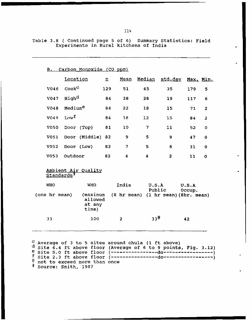
114

Table 3.8 ( Continued page 5 of 6) Summary Statistics: FieldExperiments in Rural kitchens of India

B. Carbon Monoxide (CO ppm)

Location n Mean Median std.dev Max. Min.

V046 Cookc 129 51 45 35 179 5

V047 Highd 84 28 28 19 117 6

V048 Mediume 84 22 18 15 71 2

V049 Low f 84 18 12 15 84 2

V050 Door (Top) 81 10 7 11 52 0

V051 Door (Middle) 82 9 5 9 47 0

V052 Door (Low) 82 7 5 6 31 0

V053 Outdoor 82 4 4 2 11 0

Ambient Air QualityStandards4

WHO WHO India U.S.A U.S.APublic Occup.

(one hr mean) (maximum (8 hr mean) (1 hr mean)(8hr. mean)allowedat anytime)

33 100 2 33@ 42

c Average of 3 to 5 sites around chula (1 ft above)d Site 6.4 ft above floor (Average of 6 to 9 points, Fig. 3.12)e Site 5.0 ft above floor (--------------- do -----------------)f Site 2.3 ft above floor (--------------- do ----------------- )@ not to exceed more than once# Source: Smith, 1987

115

Table 3.8 (Continued page 6 of 6) Summary Statistics: FieldExperiments in Rural Kitchens of India

C. Benzo(a)pyrene (BaP ng/mi,

Location n Mean Median std.dev Max. Min.

Roof 70 2053 699 2875 11,736 97

Medium 58 219 53 435 2,917 0

Cook 76 164 124 138 565 0

Outdoor 12* 4 3 5 7 3

D. Ratio of BaP to TSP (llct/Q)

Location n Mean std.dev Max. Min.

Roof 70 120 97 483 12

Medium 58 67 102 507 0

Cook 76 39 36 122 0

Outdoor 12 50 44 100 19

* During winter in central Indian villages

116

METEOROLOGICAL VARIABLES The six meteorological variables were

time of day, season, indoor temperature, outdoor temperature,

indoor relative humidity and outdoor relative humidity. 76

households were monitored during the monsoon and the remaining

53 during the winter season. The number of experiments

performed during the morning and evening were 60 and 69

respectively. The mean indoor temperature was 27 C and the

maximum 39 C whereas for outdoor the maximum recorded was 32 C.

The relative humidity was similar indoors and outdoors.

VENTILATION VARIABLES The nine kitchen ventilation variables

were kitchen type, roof type, volume, wall height, roof slant

height, wall area, open area in the walls and the position of

door with respect to chula. 70% had only door and the

remaining 30% had some form of opening in the walls. 92% of

the kitchen had tiled roofs, and the rest 8% had thatched

roofs. The kitchen volume was the sum of the cubical space

between the four walls and the triangular space beneath the

slanted roofs. The volume varied greatly ranging from 6 to 116

m3 with a mean and median of 35 and 29 respectively. A large

range of wall heights and total wall area were recorded, the

means were 2 m and 30 m2 respectively. The open area in the

walls, was defined as the ratio of the open wall area to the

total wall area ranged from 2 to 24 % with mean of 7. 40% had

door in the wall facing the chula (Fig.3.13), 24% had it in

side wall, and rest 36% had equally door on the back wall and

the far side wall.

117

00

U-I-

04J

44

I,1

Io 0

CYCW

_jH

3 9 r-4

118

FUEL VARIABLES The thirteen fuel variables were quantity of

wood and dung, total burn time sampled, fuel burn rate,

moisture of wood and dung, ash of wood and dung, wood length

and thickness, and dung length and thickness. 70% of cooks

used wood and dung together generally in a ratio of about 3 to

1, 28% used wood alone and the rest 3% used wood and crop

residue only. The fuel burn rate ranged between 1 to 6 kg per

hour with mean of 2. This large variation in burn rate may be

due to cook's differences in managing the fire burn. The

cook's age varied from 12 to 65 years. Burn rate for

experiments performed in SVH ranged between 1 to 3 kg per hour.

The average moisture content of both fuelwood and dung was

about 12%, whereas the mean ash content of the fuelwood (3%)

was considerably lower than that of dung (20%). Similar values

were obtained in SVH except for a larger ash content in dung

used in the rural kitchens which may be related to the fact

that village cows graze on meadows in rural India whereas

Hawaiian cows are fed in stalls.

STOVE VARIABLES The four stove variables were stove volume,

height, type of food cooked, and the number of people for whom

cooked. The stove size varied greatly ranging from .004 to .3

m3. 84% prepared roti, 9% rice and the rest 7% both. The food

was cooked for an average number of 6 members and in some

houses as much as 20 members.

119

POLLUTION VARIABLE-TSP Table 3.8 shows statistic for the

levels of TSP measured at cook's breathing site, at three

indoor sites (about 2 feet from chula) and outdoors1 . The

indoor sampling was performed for the whole period of cooking

or a maximum of two hours. Ambient standard level set by the

U.S, WHO and India for TSP is presented for reference.

The mean indoor TSP concentrations (mg/m3) at roof,

medium, low level and cook's breathing zone were 21, 8, 4 and

5. Ambient (outdoor)2 TSP levels with mean of 0.1 mg/m 3 is

comparable to values reported for rural Bombay (Rao, et al.,

1980) and rural Nepal (Davidson, 1986) but an order less than

reported by Smith et al., 1983. The least level of TSP sampled

indoors is an order higher than recommended by the ambient air

quality regulating agencies and equal to occupational standard

set by OSHA for nuisance dust (inert). Even though cooking can

be considered as occupation, using occupational standard (set

for young, healthy working group) does not seem appropriate in

this circumstances as cooking may be performed by very young

kll year olds), sick and very elderly women. The cook's

1 Sampling performed only during winter in the three

villages in central India using Hi-vol sampler borrowed fromNational Environmental Engineering Research Institute, Nagpur,India. Help rendered by Dr.A.L.Aggarwal and Dr.B.B.Sunderesanis greatly appreciated.

2 Sampling done during evening to early morning for two

consecutive days at 3-5 sites in the three villages (Padaria,Islamnagar and Adampur). Sampling during day time could not beperformed due to frequent power shortage.

120

exposure to TSP was similar to the indoor concentration at

lower level than levels measured outdoors. This finding is

similar to other indoor air pollution studies carried out in

the U.S and European countries for e.g., Binder, et al., 1976,

Sega, et al., 1982, Tosteson, et al., 1982, and Spengler &

Soczek, 1984, where they have reported that when the polluting

source is indoors, personal exposures are better correlated to

concentrations monitored indoors than outdoor level. The range

of values for indoor TSP was large with maximum of 74 mg/m3.

The average ratio of TSP concentrations at roof level to that

at low level and at the cook were both about 10, similar to SVH

results. These ratios for tiled kitchens varied from 1 to 50,

whereas, for thatched huts it ranged from 1 to 10. Thus the

smoke density in thatched huts was more uniform than in tiled

kitchens where air gaps between the slanted tiles allowed

bouyant smoke to escape preventing smoke build up in the

kitchen. Table 3.9 presents a comparisionl between TSP

concentrations in SVH and in field. With both door and window

open the SVH simulated the tiled roof huts rather well while

with only door open the SVH was closer to a thatched hut.

Fig 3.14 presents cook's exposure to TSP concentrations in

different rural ares of the developing world obtained by

several authors viz., Cleary and Blackburn, 1968, Hoffman and

Wynder, 1972, Anderson, 1975 Aggarwal, 1982, Smith, 1983,

1 Results comparing SVH to field data is not conclusive

due to small sample size of SVH experiments

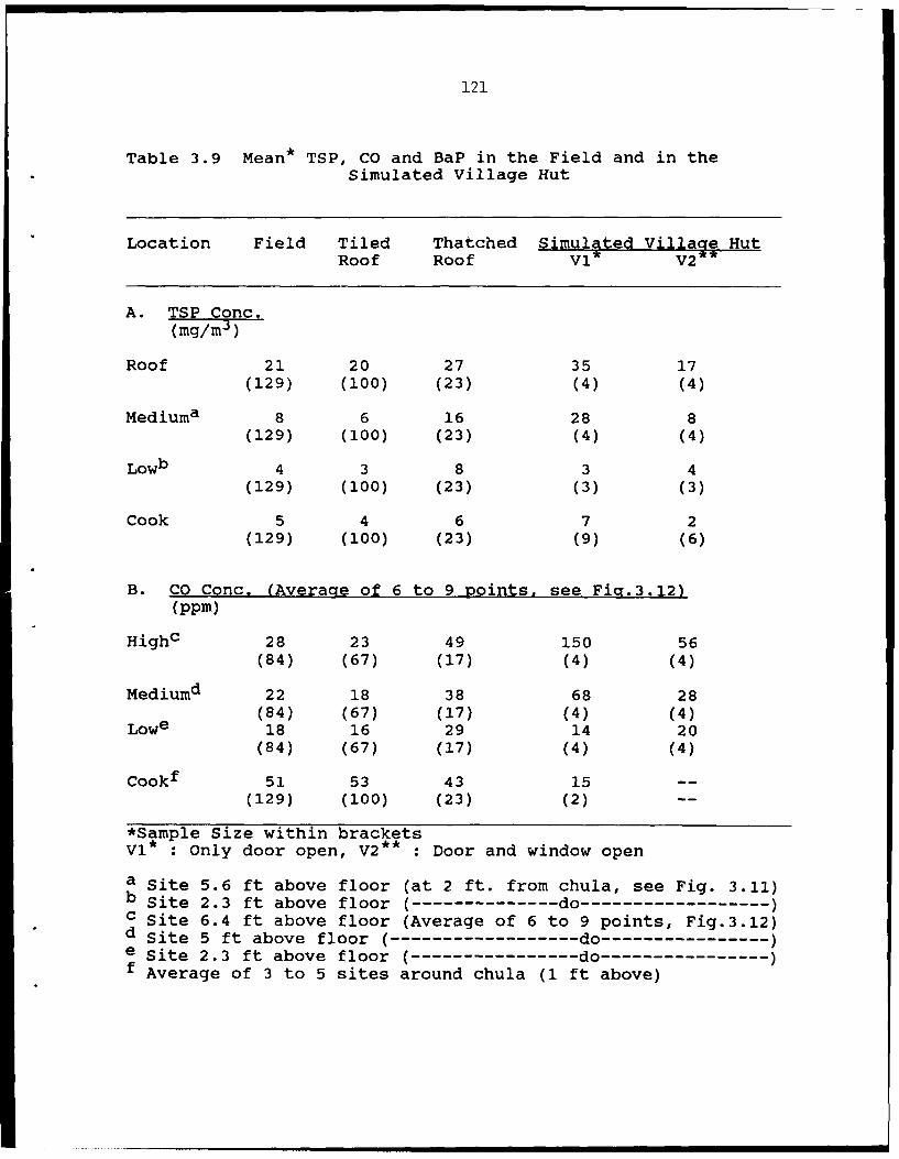
121

Table 3.9 Mean* TSP, CO and BaP in the Field and in theSimulated Village Hut

Location Field Tiled Thatched Simulated Village HutRoof Roof V* V2

A. TSP Conc.(mg/m 3)

Roof 21 20 27 35 17(129) (100) (23) (4) (4)

Mediuma 8 6 16 28 8(129) (100) (23) (4) (4)

Lowb 4 3 8 3 4(129) (100) (23) (3) (3)

Cook 5 4 6 7 2(129) (100) (23) (9) (6)

B. CO Conc. (Average of 6 to 9 points, see Fig.3.12)(ppm)

Highc 28 23 49 150 56(84) (67) (17) (4) (4)

Mediumd 22 18 38 68 28(84) (67) (17) (4) (4)

Lowe 18 16 29 14 20(84) (67) (17) (4) (4)

Cook f 51 53 43 15 --(129) (100) (23) (2) --

*Sample Size within brackets

VI * : Only door open, V2** : Door and window open

a Site 5.6 ft above floor (at 2 ft. from chula, see Fig. 3.11)b Site 2.3 ft above floor ( ------------- do ------------------ )c Site 6.4 ft above floor (Average of 6 to 9 points, Fig.3.12)d Site 5 ft above floor ( ---------------- do ----------------)e Site 2.3 ft above floor ( --------------- do ----------------)f Average of 3 to 5 sites around chula (1 ft above)

122

Table 3.9 (Continued) Mean* TSP, CO and BaP in the Field andin the Simulated Village Hut

Location Field Tiled Thatched Simulated Village HutRoof Roof VI V2

C. BaP Conc.(ng/m3 )

Roof 2053 .... 1172 873(70) (2) (2)

Medium 219 .... 814 551(58) (2) (2)

Cook 164 .... 279 427(76) (2) (2)

D. Ratio BaP to TSP(jUg/g)

Roof 120 .... 58 88(70) (2) (2)

Medium 67 .... 109 80(58) (2) (2)

Cook 39 .... 88 71(76) (2) (2)

*Sample Size within bracketsVI Only door open, V2 Door and window open

123

IL

cc -qw

z

x' C-L*

001

li(rw/fw NO0iIN: d d

124

Davidson, 1985, Reid, 1986 and Mumford, 1987. All these

studies, except for Smith, 1983 and Reid, 1986 reported levels

sampled at one stationary point in the kitchen and called this

the cook's exposure. This study, adopted Smith's 1983

methodology and sampled using personal samplers attached to the

cooks in addition to stationary sampling at three sites close

to chula. Fig 3.14 shows results to be comparable for studies

where personal sampler was used. The higher values reported by

Aggarwal and Mumford may be attributed to the use of Hi-volume

sampler. The high pump flow rate of which might have refloated

lightly deposited soot from walls/roof/floor and dust

particulates on mud floors. Further, Aggarwal's result could

have introduced error in using less sensitive analytical

balance (10-4 gm) as compared to ours (10-5 gm).

POLLUTION LEVEL- CO The mean indoor CO concentrations (ppm) at

high, medium, low level and cook's breathing zone were 28, 22,

18 and 51 whereas mean outdoor level was 4 (Table 3.8). The

cook's exposure was calculated as the average of CO levels

recorded at 5 points at one foot above the chula. The mean CO

at high , medium and low levels was calculated as the average

of CO levels recorded at several (6 to 9) sites. The levels of

CO monitored at the door at three different heights - high,

medium, and low level were 10, 9 and 7 respectively. Outdoor CO

concentrations ranged between 0 and 11 ppm with mean of 4.

Cook's exposure to CO was higher than at any of the stationary

sites. (CO was not measured at roof space, which would be

125

definitely higher). Table 3.8 shows increasing indoor CO

levels with height both at the door and close to the chula.

Table 3.9 shows similar result measured at SVH (High, medium

and low levels). CO levels measured for a simulated cook in

the SVH was considerably lower with mean of 15 ppm as compared

to cook's mean exposure of 51 ppm. This difference is because

in the field the CO was monitored around the stove and not

exactly at women's breathing zone. The well defined stratified

smoke is evident in the SVH and field CO data.

Fig 3.15 presents cook's exposure to CO concentrations as

measured by several authors: Sofoluwe, 1968, Cleary and

Blackburn, 1968, Dary et al., 1981, Davidson, 1986, Joseph,

1986, Reid, 1986. My results are comparable to Cleary and

Blackburn's, Dary's, and Davidson's. The high level sampled by

Reid may be due to the placement of sampler on shelf in the

wall back of chula where smoke dispersal might be minimum. The

exceptionally high levels monitored by Sofoluwe and Joseph may

be inaccurate because of low resolution in their methods.

Joseph used a monitor with a lowest measurable concentration of

100 ppm, whereas CO monitor used in this study could detect as

low as 1 ppm.

POLLUTION LEVELS-BaP The mean indoor BaP concentrations

(ng/m3) at roof, medium, and cook's breathing zone were 2053,

219, and 164 and outdoor level was 4 (Table 3.8). BaP analysis

was carried out on a limited number of and arbitrarily selected

filters. Table 3.8 shows large range of values for each of

126

-J

20

-4-j

2:

2.

~all221a)

(Ujdd N~lV8.L3:)NC) 0

127

indoor BaP levels. Table 3.9 shows that roof BaP levels were

similar for SVH and field but at the mid level BaP

concentrations were considerably smaller in field.

Fig 3.16 presents cook's exposure to BaP concentrations

measured by; Hoffmann & Wynder, 1972, Aggarwal, 1982, Smith,

1983, Mumford, 1987. All authors except Smith sampled at

stationary site and called it as cook's exposure. My results

for cook's exposure are comparable to Hoffmann and Wynder's.

The exceptionally high levels reported by Aggarwal and Mumford

may be questionable for reasons cited in earlier paragraph

relating to use of a Hi-volume sampler (page 124). The levels

of BaP found by Smith, et al., 1983 (mean 4000 ng/m3) seem

unrealistically high as compared to my mean results of 164.

Smith et al., reported levels >500 ng/m3 of BaP in 95% of the

sampled filter whereas in this study only 3% were above this

level. Smith et al., reported levels for the cook between 62

to 19,300 ng/m3 whereas my BaP results for the cook ranged

between 0 and 565. The highest level of BaP for roof was

11,800 which was closer to highest value reported by Smith et

al., for cook's exposure. This large difference1 in BaP result

between Smith et al., and my study was suggested to be due to

the storage period (6 to 12 months) of my TSP samples before

analysed. Hence ten filters exposed to smoke in the breathing

zones of cook's in rural kitchens of Nepal were analysed for

1 Literature (Rudling, et al., 1982)shows wide variationin PAH emission rates (fireplace) under slight changes incombustion conditions

128

0*

~iL

iileim .4

0 0 0 00 0 00 0 0wo v

(cw/bu) NOILVN.N30NOD dQS

129

BaP within three months of sampling for TSP. Table 3.10 shows

BaP concentrations obtained and the ratio of BaP to TSP. The

concentration ranged from 0 to 1056 ng/m3 with mean of 400

similar to my results. Ambient BaP levels with mean of 4 ng/m3

is comparable to values reported by Rao, 1980 for rural Bombay

site. However, it disagrees by almost two orders with the

ambient levels reported by Smith,83.

RATIO OF BAP TO TSP The indoor mean ratio of BaP to TSP for

roof, medium and cook is 120, 67 and 39 pg/g (Table 3.8). The

lower ratio for the cooks may indicate that the filters

collected ash/dust blown from the stove and mud floors.

Alternatively, the higher ratios for the roof might be due to

collection of refloated soot deposited on the roof. Table 3.9

does not show similar result for SVH data, which might be

expected as there were negligible soot deposits on the steel

roof.

Table 3.11 presents the ratio of BaP to TSP obtained by

several authors. We note the mean ratio obtained in this study

agrees with other studies (Hoffmann and Wynder, 1972, Dasch,

1982, and He, 1986) except that of Aggarwal, et al.,1982 and

Smith et al., 1983. The exceptionally high value obtained by

Smith, et al., 1983 is difficult to explain, especially

considering the identical sampling protocol (use of personal

samplers) and similar combustion conditions (mean burn rate of

2.0 kg/h).

130

Table 3.10 Cook's Exposure to BaP Concentration in RuralKitchens of Nepal*

Filter Code BaP Concentration Ratio BaP/TSP(ng/m3 ) (Pg/g)

H041 1056 i1

H042 0 0

H043 0 0

H044 760 83

HO64 622 160

HO65 187 160

HO66 553 62

HO67 233 27

HO68 373 36

H049# 3510 718

* Filter samples collected by Holly F.Reid.# HO49 was used as backup filter for several filters,

explaining for it's large difference in BaPconcentration

131

Table 3.11 Mean Ratio of BaP to TSP (pg/g) for Biomass SmokeReported by Several Authors

S.NO. n Mean Range Sampling Country Author(pg/g) (pg/g) Type

1 7 30 0-71 Area Kenya Hoffmann &

Wynder, 1972

2 9 52 3-141 Emission USA Dasch, 1982*

3 19 500 (71-1600) Area(Indoor)India Aggarwal-- 15 (11-19) Outdoor et al.,1982

4 65 800 (10-8000) Personal India Smith, et al.,5 190 (70-500) Outdoor 1983

5 9 71 (0-160) Personal Nepal Reid et al.,1986**

6 62 150 (----) Area China He, 198612 10 Outdoor

7 4 73 (55-118) Roof Area SVH This study

8 4 95 (28-158) Mid level SVH ---- do -----

9 4 80 (19-125) Low level SVH ---- do -----

10 6 384 (223-549) Mid level SVH@ ---- do -----

11 2 83 (77-89) Low level SVH@ ---- do -----

12 76 39 (0-122) Personal India ---- do -----

13 70 120 (12-483) Roof area ------- do---------

14 58 67 (0-507) Mid-level ------ do---------

15 12 50 (19-100) Outdoor do---------

* Fireplace emission** TSP Filter samples collected by Holly. F.Reid.

Filters analysed for BaP by author.@ Samples taken by Mr.Mike Apte during QCMCI

experiments (November, 1982) in simulated village hutand analysed for BaP at Lawrence Berkeley Laboratory.

132

Conclusions:

1. Ventilation condition varied greatly

between kitchens as indicated by an order

of magnitude difference in kitchen volume

and percentage of open area in the walls.

Wall heights differed by 3 m and roof slant

height by 2 m. Inspite of a very similar

fuel comparision, the burn rate of the fuel

used varied from 1 to 6 kg/hr. This may be

due to large variations in fuel quality as

moisture varied by a factor of 4 and ash

content by a factor of 8. Additionally

stove size varied by a factor of 30. The

cook's experience of maintaining the fire

varied considerably with the cook's ages

ranging from 8 to 65 years. Under these

different ventilation, fuel, stove

condition and cook's experience it is

reasonable to infer that indoor pollutant

levels varied greatly as a result of

complex interacting factors.

2. Mean TSP exposure to cooks was 5 mg/m3,

twenty times higher than standard specified

by regulating agencies (U.S, WHO, and

India) for ambient conditions. However, it

was equal to the 8-hour time weighted

133

average standard for occupational cndition

(OSHA standard for inert nuisance dust).

In thatched huts, 66% of the cook's were

exposed to TSP above the OSHA standard

while in tiled huts it was only 28%. The

percentage for twice OSHA standard were 16

and 4 for thatched and tiled roofs

respectively. Mean CO exposure to cooks

was 51 ppm, three times higher than

standard but equal to OSHA's 8-hour time

weighted average standard. In thatched

huts 25% of the cook's were exposed to CO

higher than OSHA standard while for tiled

huts it was 48% . Mean BaP exposures to

cooks were 160 ng/m3 equal to ambient

levels found in urban cities in developed

countries. No standard exists for BaP as

any amount ingested is harmful as it is

suspected to be a carcinogen. The mean

ratio of BaP to TSP for the cooks was 39

pg/g. The average cook's exposure to TSP

and CO agree with earlier studies in the

literature. The mean cook's exposure to

BaP is twenty times lower than that

reported by Aggarwal et al., (1982) and

Smith et al., (1983). Smith and Aggarwal

134

reported levels >500 ng/m3 of BaP in 95% of

the sampled filter, whereas in this study

only 3% were above this level. The higher

(20 times) value for the ratio of BaP to

TSP obtained by Smith et al., 1983 is

difficult to explain considering similar

sampling protocol and combustion

conditions.

3. TSP, CO and BaP levels are different at

different locations in the room with the

cook's exposure similar to low indoor

levels and an order of magnitude higher

than ambient(outdoor) concentrations.

Close to chula TSP, CO, BaP concentration

and ratio of BaP to TSP increased with

height. Mean TSP and BaP concentrations at

roof level were five and ten times higher

than those experienced by the cook's

whereas cook's exposure to CO was twice

than at standing height. In thatched huts,

TSP at standing height was almost all times

greater than cook's exposure while for

tiled huts it was so only in half the

cases. In case of thatched huts, 45% of CO

at standing height was greater than cook's

exposure while for tiled huts it was only

135

18%. These results indicate the uniform

stratification in thatched huts in

comparision to tiled huts and also indicate

existence of varying ventilation

conditions.

4. TSP, CO and BaP levels in thatched huts

were comparable to those measured by me in

SVH.

3.2.3 SIGNIFICANT DIFFERENCES OF COOK'S EXPOSURE

TO TSP AND CO AND LEVELS OF TSP AT ROOF

Analysis of variance (ANOVA) was one of the statistical

methods used to determine whether cook's exposure to TSP and

CO, and TSP concentration at roof were significantly different

for:

a. Villageb. Season*c. Time of day*d. Kitchen type*e. Roof typef. Door locationg. Fuel typeh. Food type

When only two groups are present, the ANOVA reduces to the

two-sample t-test and this method was used for variables having

two groups (indicated by asterisk) the ANOVA for the rest. The

t-Test procedure tests both the equality of means and variances

of the two groups. If the variances are significantly

different, the separate t-Test procedure is used to test

136

equality of means, otherwise the pooled t-Test procedure.

Table 3.12a shows t-Test result obtained for variables marked

in asterisk above.

The mean roof TSP levels was significantly (p <.01) lower

during monsoon (15 mg/m3) than during winter (30 mg/m3). This

seems reasonable, as during the winter season the chula was

usually used for space heating in early morning and late

evening. Thus smoke from space heating was sampled along with

smoke from cooking.

Mean CO exposure to the cook during monsoon (47 ppm) was

significantly (p <.05) lower than during the winter season (58

ppm). This can be explained by the fact that during the

monsoon, the cooks generally used dry wood stored and saved

during winter and summer months which burns more complete.

This is contrary to earlier stated (section 3.1.5, page 99)

hypothesis, that the poor fuel quality during monsoon months

would result in high exposures to cooks, during the monsoon

months.

Mean CO exposure of the cook was significantly (p <.01)

higher during the morning (60 ppm) than during the evening (44

ppm). This is probably a result of the chula being moist and

colder( chula not in use for about 12 hours) before the morning

fire is lit, whereas in the evening cooking period it's

opposite is true. Smith et al., (1983) and Reid et al., (1986)

reported higher evening concentrations of TSP and CO but

attributed these to local ground level atmospheric inversions.

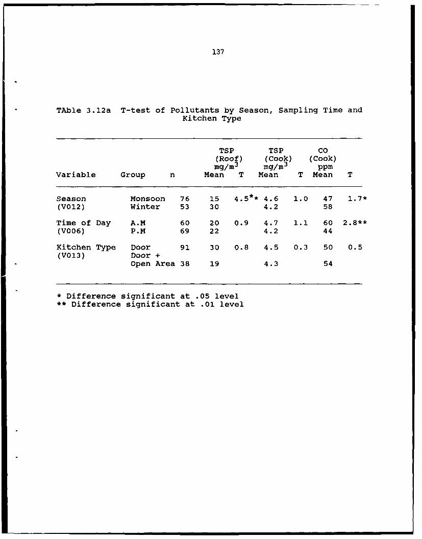
137

TAble 3.12a T-test of Pollutants by Season, Sampling Time andKitchen Type

TSP TSP CO(Roof) (Cook) (Cook)mg/m3 mg/m3 ppm

Variable Group n Mean T Mean T Mean T

Season Monsoon 76 15 4.5** 4.6 1.0 47 1.7*(V012) Winter 53 30 4.2 58

Time of Day A.M 60 20 0.9 4.7 1.1 60 2.8**(V006) P.M 69 22 4.2 44

Kitchen Type Door 91 30 0.8 4.5 0.3 50 0.5(V013) Door +

Open Area 38 19 4.3 54

* Difference significant at .05 level** Difference significant at .01 level

138

It seems more reasonable that the bouyancy of the smoke would

be a dominant factor in pollutant dispersion near the chula

during cooking periods rather than an outdoor inversion.

The ANOVA procedures enables one to carry out a posteriori

contrast, to determine the significantly different means. Two

of the many procedures is the SNK (Student-Newman-Keuls) and

Scheffe (Scheffe's test). The Table 3.12b summarizes the

results obtained for the remaining variables listed in previous

paragraph.

The significant difference ( p <.05) between the mean

level of CO that a cook is exposed to in the village Adampur

(36 ppm) and that at Islamnagar (65 ppm) is an effect of

experimental setup, since all the experiments in Islamnagar

were carried out in the morning period whereas all the

experiments in Adampur were carried out in the evening period

due to transportation constraint. As already found by the T-

test the CO exposure to the cooks were significantly higher in

the morning than in the evening.

Mean TSP (roof) concentrations were significantly (p <.05)

higher (22 mg/m3) when roti is cooked as opposed to when rice

is cooked (11 mg/m3). It is possible that the higher moisture

content during rice cooking might have led to greater

deposition of particulates on the walls.

The mean cook exposure to TSP was significantly (p < .01)

higher (6 mg/m3) in kitchens with thatched roofs when compared

to those in tiled roof (4 mg/m3). Intolerable smoke levels

139

Table 3.12b Test # of Variance of Pollutants by Village, RoofType, Door Position, Fuel and Food Type

TSP TSP CO(Roofj (Cookj (Cook)mg/m mg/m ppm

Variable Group n Mean Pair Mean Pair Mean PairSig. Sig. Sig.Diff. Diff. Diff.

Village l.Adampur 23 26 NONE 4 NONE 36 (1,2)*(V002) 2.Islamnagar 42 22 5 65

3.Padaria 54 20 5 494.Ariyur 4 13 3 615.Perambia 6 12 2 27

Roof Type Tiled(l) 100 20 NONE 4 (1,3)** 53 NONE(V014) P'cca(2) 6 17 4 37

Tllatch(3) 23 27 6 49

Door Back(l) 24 20 NONE 5 (3,4)* 45 NONEw.r.t Side(2) 31 23 5 41Chula Front(3) 50 21 4 55(V027) Far

Side (4) 24 19 6 63

One-way program in SPSSX (Statistical Package forSocial Scientists, Nie, 1980)

* Difference significant at .05 level** Difference significant at .01 level

140

Table 3.12b (Continued) Test# of Variance of Pollutants byVillage, Roof Type, Door Position, Fuel and Food Type

TSP TSP CO(Roofs (Cook (Cook)mg/m mg/m ppm

Variable Group n Mean Pair Mean Pair Mean PairSig. Sig. Sig.Diff. Diff. Diff.

Fuel Type Wood(l) 36 20 NONE 5 NONE 47 NONE(V009) Dung(2) 1 16 9 51

Wood andDung(3) 90 22 4 54CropResidue(4) 2 11 3 30

Food Type Rice(l) 12 11 (1,2)* 3 NONE 46 NONE(V010) Roti(2) 108 22 5 51

Rice andRoti (3) 9 23 5 65

• Difference significant at .05 level

141

inside thatched huts clearly demonstrated the need to include

roof type as one of the ventilation indicators. On entering a

thatched hut the researchers immediately got tears and squatted

on the floor to interview the cooks, whereas in tiled kitchens,

the air quality was tolerable and in some cases quite

comfortable while standing. The environment within SVH and

thatched hut were comparable. Fig 3.17 shows the different

roof types.

The cook's mean TSP exposure ( 4 mg/m3) was significantly (p

<.05) lower for the kitchens with the door in the front than

for those (6 mg/m3) with door on the far side (Fig 3.13).

Summary of significant differences in TSP (roof), cook's

exposure to TSP and CO:

1. CO higher for cooks in village Adampur than

cooks in Islamnagar, due to experimental

setup.

2. TSP (roof) and CO (cook) are higher in

winter than in monsoon.

3. CO (cook) higher in morning than evening.

4. No difference between kitchens with only

door and kitchens with door and open space.

5. TSP (cook) higher for kitchens with

thatched roofs than for tiled roofs.

6. TSP (cook) lower for kitchens with door in

front wall than kitchens with door in side

wall.

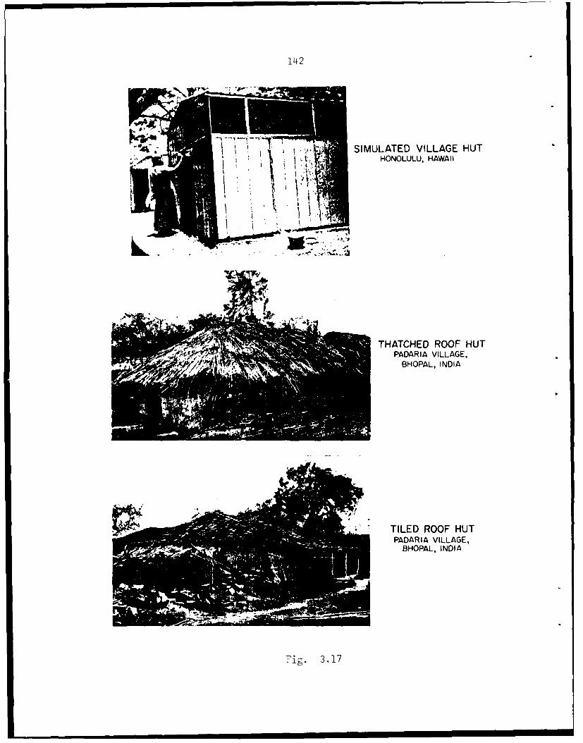
14~2

'4; SIMULATED VILLAGE HUTHONOLULU, HAWAII

lik

THATCHED ROOF HUTPADARIA VILLAGE,

BHOPAL, INDIA

* TILED ROOF HUTPADARIA VILLAGE,

BHOPAL, INDIA

Fig. 3.17

143

7. No difference between fuel type.

8. TSP (roof) higher for roti when compared to

rice.

3.2.4 MAIN EFFECT AND INTERACTIONS OF CLIMATE,

VENTILATION AND SAMPLING LOCATION ON CO

Indoor spatial CO data were obtained by repeatedly

measuring CO at 6 to 9 sites at three levels (high, medium and

low, Fig 3.12 ) in all the huts sampled in the 5 villages.

These data were used to statistically determine which of the

factors season, roof type, sampling site, sampling height, and

interaction amongst these, had significant effect on CO

concentration. The statistical procedure for this was the k-

way ANOVA. The reasons for selecting season, roof type,

sampling height and site as variables were:

1. The experiments were conducted in two

seasons, monsoon and winter. CO(cook) and

TSP(roof) were found to be significantly

higher during the later season.

2. Roof type was found to be an important

ventilation factor in determining pollutant

levels inside village huts.

3. Sampling height and site was found to

affect pollution concentration both in the

field and SVH experiments.

144

SPSSX ANOVA procedure was used to determine the effect and

interaction of climate, ventilation, sampling level and site.

Table 3.13a presents the result of this investigation. The

effects of roof type, sampling height, site and 2-way

interaction effect of level with roof type and site were found

to be significant. On finding the effect of season not

significant, kitchen volume was included as additional factor

of ventilation condition and the computation was performed this

time for monsoon and winter separately. As the volume of the

kitchens varied greatly, it was categorised into three classes:

1. Low volume (low-thru 22 m3)

2. Medium volume (22 thru 40 m3)

3. High volume (above 40 m3)

During both season (Table 3.13 b and c) the main effects

of roof type, sampling height level and site were found to be

significant. During the monsoon the 2-way interaction of roof

type with site had significant effect on CO, while during the

winter interaction with volume dominated.

Conclusion:

1. Roof type, sampling height and site

significantly affected CO concentrations.

2. During the monsoon 2-way interaction of

roof type with site had a significant

effect on CO, while during the winter

interaction with volume dominated.

145

Table 3.13a

Test of Variance of CO by Roof Type, Season, Sampling Heightand Location in Indian Huts Using Split-Plot Analysis

Whole Plot Analysis DF Mean Sq. F

Roof Type 1 106536.1 73.7**Season 1 854.8 0.6Level 2 77267.9 53.4**

Level X Roof Type 2 9293.1 6.4**Level X Season 2 2378.1 1.6Roof Type X Season 1 34.4 0.0

Whole Plot Error

RFTYP X SEAS X Level 2 1446.2

Sub-Plot Analysis

Site 8 67437.9 103.5*Site X RFTYP 8 1089.4 1.7*Site X Season 8 409.8 0.6Site X Level 16 1344.7 2.1*

Site X RFTYP X Season 8 608.9 0.9Site X RFTYP X Level 16 358.2 0.6Site X Season X Level 16 414.2 0.6

Sub-Plot Error 3076 651.4

* Significant at .05 level** Significant at .01 level

146

Table 3.13b

Test of Variance of CO During Monsoon by Roof Type, KitchenVolume, Sampling Height and Location in Indian Huts Using

Split-Plot Analysis

Whole Plot Analysis DF Mean Sq. F

Roof Type 1 52510.9 20.0*Volume 2 9276.3 3.5Level 2 62083.2 23.6**

Level X Roof Type 2 7674.6 2.9Level X Volume 4 669.6 0.3Volume X Roof Type 2 962.4 0.4

Whole Plot Error

RFTYP X VOL X Level 4 2626.4

Sub-Plot Analysis

Site 8 38727.9 61.2**Site X RFTYP 8 2001.1 3.2*Site X Volume 16 1030.9 1.6Site X Level 16 1281.9 2.0

Site X RFTYP X Volume 16 744.7 1.2Site X RFTYP X Level 16 366.1 0.6Site X Volume X Level 32 378.9 0.6

Sub-Plot Error 1769 632.4

* Significant at .05 level** Significant at .01 level

147

Table 3.13c

Test of Variance of CO During Winter by Roof Type, KitchenVolume, Sampling Height and Location in Indian Huts Using

Split-Plot Analysis

Whole Plot Analysis DF Mean Sq. F

Roof Type 1 39129.8 22.9**Volume 2 5921.6 3.5Level 2 19115.5 11.2*

Level X RFTYP 2 2886.6 1.7Level X Volume 4 161.2 0.1Volume X RFTYP 2 13833.1 8.1*

Whole Plot Error

RFTYP X VOL X Level 4 1701.4

Sub-Plot Analysis

Site 8 29550.6 46.8**Site X RFTYP 8 126.9 0.2Site X Vol 16 1065.9 1.7Site X Level 16 506.8 0.8

Site X RFTYP X VOL 16 938.4 1.5Site X RFTYP X Level 16 253.9 0.4Site X Vol X Level 32 241.7 0.4

Sub-Plot Error 1139 630.9

* Significant at .05 level** Significant at .01 level

148

3. For CO measured in SVH, we found only

sampling height had a significant effect

(Table 3.4 ). This may be due to

uniformity in fuel type and ventilation

conditions.

3.2.5 STATISTICAL MODEL FOR ESTIMATING COOK'S

EXPOSURE TO TSP

Three techniques were employed to develop a statistical

model for estimating cook's exposure to TSP in terms of

meteorological, ventilation, fuel and stove parameters:

A. Multiple linear regression

B. Path Analysis

C. Group Method of Data Handling (Ivakhnenko

polynomial) (GMDH)

A. A multiple linear regression model between cook's

exposure to TSP and several indicators of the independent

variables (meteorological, ventilation, fuel and stove)

variables was developed using step-wise regression procedure.

The best 3-variable model explained only 27% of the variance in

cook's exposure to TSP. The statistical relationship was in

terms of three variables (roof type, fuel type and volume of

the roof space) as listed in Table 3.14.

1149

Table 3.14 Multiple Regression* Model Between Cook's TSPExposure and Best 3 Variables

Maximum R-square Improvement for dependent variable (cook's

exposure to TSP)

R Square = 0.27 C(P) = -5.18

DF SUM OF SQUARES MEAN SQUARE F PROB>FREGRESSION 3 211.3 70.4 14.2 0.0001ERROR 115 572.4 4.9TOTAL 118 783.7

B VALUE STD ERROR TYPE II SS F PROB>FINTERCEPT -5.6FUEL TYPE 1.1 0.43 31.8 6.4 0.0129ROOF TYPE 1.0 0.18 .59.9 32.1 0.0001VOL.(ROOF AREA) 0.1 0.04 23.5 4.7 0.0319

THE ABOVE MODEL IS THE BEST 3 VARIABLE MODEL FOUND

* Using step-wise regression procedure, SAS

150

B. Path Analysis

A path model was hypothesized (Fig 3.18 ) showing the

direct and indirect relationships between meteorological,

ventilation, fuel, stove and cook's exposure to TSP. The

meteorological variable is employed as the source factor

affecting the ventilation, fuel quality, combustor conditions

and the pollutant concentration. Ventilation is shown

affecting fuel quality and combustor conditions. Fuel variable

is viewed as a function of the direct affect of both

meteorological and ventilation parameters. Finally the

pollutant concentration is viewed as a function of the direct

affects of fuel and stove and of the affects, both direct and

indirect of ventilation and meteorological factors.

LISREL (Joreskog and Sorbom, 1979) is one of the most

common method of path analysis known and is available at U.H.

Computing center. However, the use of LISREL in small sample

situations (< 1000) is not appropriate, therefore, the

procedure developed by Rao et al., (1980) at the Population

Genetics Laboratory of University of Hawaii was used to

evaluate the proposed model. The mathematical formulation and

it's salient features are discussed in Gunashekharan (1985).

The best indicators of meteorological, ventilation, stove

and fuel were obtained from the correlation matrix between

cook's exposure to TSP and the different indicators for each of

the independent parameters. Indoor relative humidity (In.R.H),

151

4-la--

a 0H

arz "0

wfr

W4--

152

roof type, fuel type and stove wall height were the best

indicators for meteorological, ventilation, stove and fuel

parameters respectively Fig 3.15 (a to d). The input for the

path analysis procedure is the correlation matrix (Table 3.16)

between these variables and cook's exposure to TSP. The result

of the path analysis is illustrated in Fig (3.19). The model

fits quite well (p =.60), but the linear association between

individual variables is weak. The only significant association

is between roof type and cook's exposure to TSP.

C. Group Method of Data Handling (Ivakhnenko polynomial)

Because of the weak linear relationship between the

meteorological, ventilation, fuel, and stove variables with

cook's TSP exposure, an interactive statistical approach for

identifying an optimally complex model, which may have greater

explanatory power (GMDH, Farlow, 1984) was employed. A complex

statistical model (Ivakhnenko polynomial) explaining 70% of the

variance in cook's TSP exposure was obtained in terms of the

variables roof type, position of door with respect to chula and

their interactions. The functional form was:

Cook's TSP exposure = 8.2 + 6.1(Roof type) - 9.2 (door w.r.t

chula) -1.0 (Roof type) 2 + 2.1 (door w.r.t

chula) 2-0.3 (Roof type X door w.r.t chula)

Conclusion:1. The relationships are not linear.2. GMDH method better than path analysis.

153

Table 3.15a Correlation Matrix of Cook's TSP Exposure andClimate Indicators

TIME SEASON INDOOR OUTDOOR INDOOR OUTDOOR COOK'S EXP

TEMP. TEMP. R.H. R.H. TSP

TIME 1.00 0.03 -0.23 -0.23 0.26 0.05 0.079

SEASON 1.00 0.81 0.79 0.62 0.45 0.145

INDOORTEMP. 1.00 0.94 0.37 0.36 0.141

OUTDOORTEMP. 1.00 0.40 0.35 0.152

INDOORR.H. 1.00 0.04 0.154

OUTDOORR.H. 1.00 0.072

COOK'S EXPTSP 1.00

Table 3.15b Correlation Matrix of Cook's TSP Exposure andStove Indicators

FOOD COOKED NUMBER STOVE STOVE COOK'S EXP

(PEOPLE) VOL. WALL HT. TSP

FOOD COOKED 1.00 -0.09 -0.04 -0.03 0.01

NUMBER(PEOPLE) 1.00 0.27 0.11 0.09

STOVEVOLUME 1.00 0.55 -0.03

STOVEWALL HT. 1.00 0.14

COOK'S EXPTSP 1.00

154

Table 3.15c Correlation Matrix of Cook's TSP Exposure andVentilation Indicators

KCHTYP RFTYP Cubical Roof Wall Slant Roof

Volume Volume Height Height

KCHTYP 1.00 0.11 -0.35 -0.13 -0.29 0.04

RFTYP 1.00 -0.11 0.01 -0.29 -0.01

CubicalVolume 1.00 0.68 0.44 -0.03

RoofVolume 1.00 0.19 0.48

WallHeight 1.00 0.18

Slant RoofHeight 1.00

Table 3.15c (Continued) Correlation Matrix of Cook's TSPExposure and Ventilation Indicators

Total Open Area Door w.r.t Cook'sKitchen Index Chula ExposureVolume TSP

KCHTYP -0.33 -0.41 -0.04 0.00

RFTYP -0.10 0.13 0.10 0.45

CubicalVolume 0.86 -0.12 0.14 0.06

RoofVolume 0.55 -0.14 0.03 0.16

WallHeight 0.41 0.20 0.17 -0.12

Slant RoofHeight -0.05 0.15 -0.01 0.05

155

Table 3.15c (Continued) Correlation Matrix of Cook's TSPExposure and Ventilation Indicators

Total Open Area Door w.r.t Cook'sKitchen Index Chula ExposureVolume TSP

TotalKitchenVolume 1.00 -0.18 0.04 0.01

Open AreaIndex 1.00 -0.17 -0.01

Door w.r.tChula 1.00 0.23

Cook's ExposureTSP 1.00

156

Table 3.15d Correlation Matrix of Cook's TSP Exposure and FuelIndicators

FLTYP Wood Dung Total Burn MoistureQty. Qty. Burn Rate Wood

Time

FLTYP 1.00 -0.04 -0.17 -0.09 -0.09 -0.03

Wood Qty. 1.00 -0.22 0.32 0.58 0.10

Dung Qty. 1.00 0.33 0.28 0.06

Total Burn Time 1.00 -0.19 0.08

Burn Rate 1.00 0.04

Moisture Wood 1.00

Table 3.15d (Continued) Correlation Matrix of Cook's TSPExposure and Fuel Indicators

IMoist Ash Ash Wood Wood Dung Dung Cook'sDung Wood Dung Length Thick Diam. Thick Expos.

TSP

FLTYP -0.44 -0.11 -0.39 -0.24 -0.09 -0.44 -0.42 0.19

Wood Qty. -0.28 0.16 -0.33 0.08 0'.18 -0.23 -0.17 0.00

Dung Qty. 0.54 0.05 0.45 0.01 0.11 0.48 0.36 -0.09

Total burnTime 0.14 0.05 0.04 0.22 0.03 0.15 0.18 -0.14

Burn Rate 0.02 0.15 0.02 -0.04 0.22 0.04 -0.05 0.02

MoistureWood 0.07 -0.07 -0.11 0.14 0.09 -0.07 -0.05 -0.06

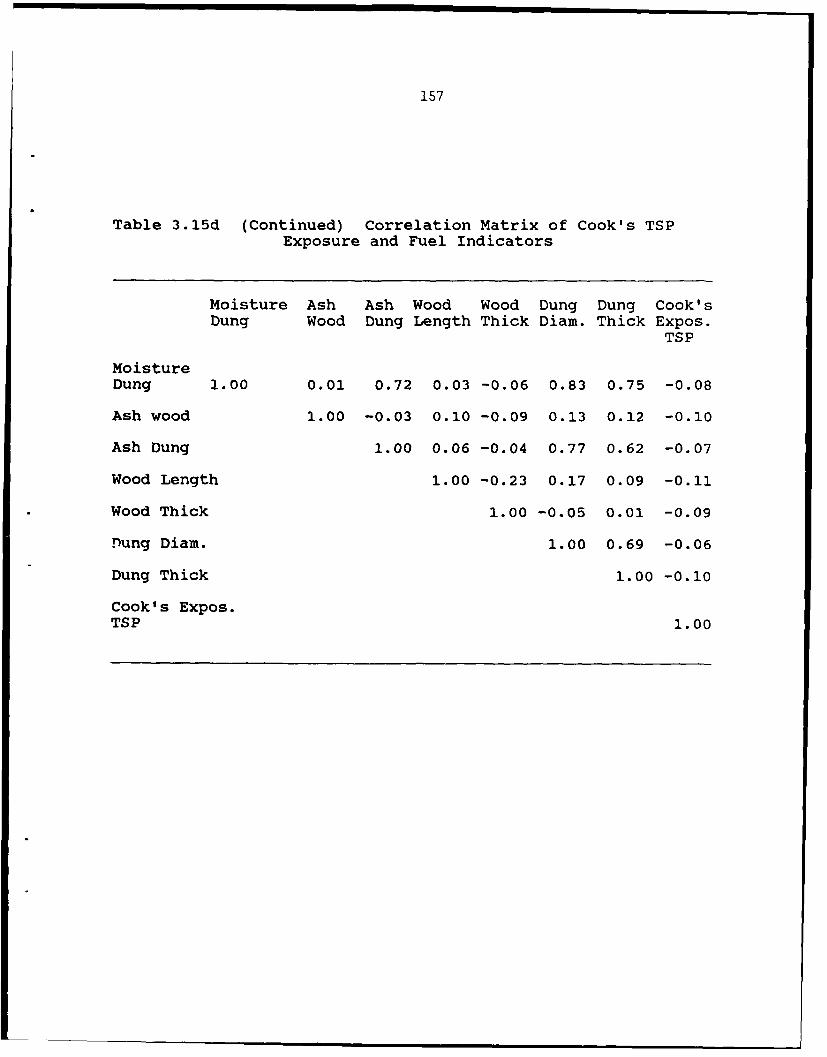
157

Table 3.15d (Continued) Correlation Matrix of Cook's TSPExposure and Fuel Indicators

Moisture Ash Ash Wood Wood Dung Dung Cook'sDung Wood Dung Length Thick Diam. Thick Expos.

TSP

Moisture

Dung 1.00 0.01 0.72 0.03 -0.06 0.83 0.75 -0.08

Ash wood 1.00 -0.03 0.10 -0.09 0.13 0.12 -0.10

Ash Dung 1.00 0.06 -0.04 0.77 0.62 -0.07

Wood Length 1.00 -0.23 0.17 0.09 -0.11

Wood Thick 1.00 -0.05 0.01 -0.09

Dung Diam. 1.00 0.69 -0.06

Dung Thick 1.00 -0.10

Cook's Expos.TSP 1.00

158

Table 3.16 Correlation Matrix Between Input Variables for PathAnalysis

INDOOR ROOF TYPE FUEL TYPE STOVE COOK'S EXPTEMP. WALL HT. TSP

INDOORTEMP. 1.00 0.07 0.00 0.02 0.15

ROOFTYPE 1.00 -0.00 0.09 0.45

FUELTYPE 1.00 0.03 0.19

STOVEWALL HT. 1.00 0.14

COOK'S EXPTSP 1.00

159

00-I-0

ux

0)a)

zI4.-

-Q

-4-

I*) A -

LLLL Q) a) Q)

CY)0

oa.~~~0 --- H r -4

Q) 4J-a) 0.

160

IV. SUMMARY AND RECOMMENDATIONS

4.1 SUMMARY

Indoor air pollution from burning biomass fuels for

cooking in the developing world has recently gained increased

attention though a few studies already in the 1960s and early

1970s reported high smoke levels inside rural huts. Recently

Smith et al., 1983 found rural Indian cooks's mean exposure to

BaP (benzo-a-pyrene, a known carcinogen) as high as

4,000 ng/m 3 , equivalent to smoking 20 packs of cigarettes per

day. Agencies such as the World Health Organisation, the

National Research Council in U.S.A., and the Centre for the

Environment in India have stressed the need for research in

this area.

This dissertation focusses on three indoor air

concentrations of combustion generated pollutants TSP, CO, and

BaP, emitted by Indian cookstoves. Initial experiments

conducted during Fall 1982 through Spring 1983 in a simulated

village hut (SVH) on the grounds of the East West Center and

the University of Hawaii, determined size distribution of

particulates emitted from burning of fuelwood leuceana and

cowdung, and investigated the effects of fuel, ventilation

condition and sampling location on TSP, CO and BaP

concentrations. 84 to 99% of the total particulate mass in

wood and dung smoke had aerodynamic diameter less than 3.2 um,

which eliminated the need for particle size discriminating

161

sampling. The geometric mean for dung and wood smoke particle

size was 0.17 um. TSP, CO and BaP levels were as high as 83

mg/m 3 , 294 ppm and 2000 ng/m 3 . Concentrations increased with

height. The presence of an open window above chula reduced the

concentrations significantly. TSP was about twice as high for

dung than for wood smoke. These experiments finalised the

field sampling protocol.

The field survey included 291 households in the three

central and two south Indian villages. Socio-economic, kitchen

ventilation conditions, fuel use and villagers' perception of

health problems related to smoke were surveyed. Most kitchens

(69%) had tiled roofs with a variety of volumes and open spaces

on the walls. Cooks used a mixture of several wood species and

dung and were all bothered by smoke, but stressed fuel

procurement as their chief concern. Fixed monitoring for TSP

was done at three different height (roof, medium and low) about

2 feet by side (where women squat) of the chula. A personal

sampler on the cook monitored air in her breathing zone. CO

was monitored consecutively at minimum of 6 and maximum of 9

sites ( at 2 ft ahead in front of chula) at three different

height (high, medium and low) in addition to cook's breathing

zone. 129 households in the five villages were sampled for TSP

and CO during the monsoon and winter months of 1983. About 300

arbitrarily selected filters were analyzed for BaP using HPLC.

Fuel samples were analysed for moisture, ash content and

calorific value.

162

Indoor pollutant levels varied considerably as a result of

differences in ventilation, fuel quality, and cook's

experience. Mean TSP exposure to cooks was 5 mg/m3 , twenty

times higher than the standard specified by regulating

agencies, e.g USEPA, WHO and Dept. of Environment, Govt. of

India for ambient conditions. Mean CO exposure to cooks was 51

ppm, three times higher than the corresponding standard.

However, TSP and CO levels are equal to OSHA (Occupational

Safety and Health Adminstration) standards. Mean BaP exposures

to cooks was 160 ng/m 3 , equal to ambient levels found in urban

cities in developed countries. While cook's mean exposure to

TSP and CO agrees with earlier studies, her exposure to BaP in

is an order of magnitude lower in this study. Pollution levels

varied considerably at different locations in the kitchens.

The cook's exposure was similar to lowest indoor levels but

order of magnitude above ambient (outdoor) concentrations.

Next to the stove or chula concentrations increased with

height. Concentrations in thatched huts were comparable to

those measured in SVH. Tiled hut roofs allowed smoke seepage

resulting in much lower concentrations than in thatched huts.

TSP (roof) and CO (cook) were significantly (alpha = .01)

higher in winter than during monsoon. CO (cook) was

significantly higher in morning than evening. Analysis of

variance (split-plot analysis) of the spatial CO data showed

significant effects of roof type, sampling level and sampling

location in addition to significant 2-way interaction effects

163

of roof type with volume and site. A linear model relating

cook's exposure to TSP and three independent variables (roof

type, fuel type, volume of roof space) explained only 25% of

the variance in cook's exposure to TSP, whereas a complex

statistical model (Ivakhnenko polynomial) in terms of roof type

and the position of door with respect to chula explained it's

70% of the variance. Path analysis was tried and found poor

linear relationship amongst the proposed parameters, though the

model fit was adequate.

The following steps may help in reducing the cook's

exposure to pollutants:

1. Cooks should be encouraged to cover their

face with their sari1 as preventive

measure.

2. Build short wall adjacent to chula and

place the door on the opposite wall

(Fig 4.1).

3. Build mud hoods at about two feet above the

chula enabling the smoke to be guided out

(Fig 4.1).

4. Glass pane (about 2 sq. ft) on the roof above

the chula (Fig 4.3.) will help lighting the dark

kitchens.

1 North Indian women do cover their face in front of elders(male In-laws)

16'4

GLAS

DOOR O3ft

CH L/,'

Fig4. Skthoprpsdrrlkthnwtmuhodadsotrwllajcn ocua

dorpaeIntewllopst ocua

anI lsspn n h of

165

5. Open area (about 2 sq.ft) on the higher level of the

walls adajacent to the chula.

6. Tiled roofs instead of thatched ones.

7. Use of dung as fuel should be discouraged.

4.2 RECOMMENDATIONS FOR FUTURE STUDIES

TSP exposures for the cook and at three heights near the

chula were measured during the cooking period. As the kitchens

had mud floors and the roofs above chula were covered by soot

and dust, the samples might have included resuspended soot and

dust along with smoke particulates from fires. Further studies

should incorporate background indoor sampling without fire

burning to determine the indoor air quality in rural huts to

allow a more precise determination of the contribution from

cooking.

TSP concentrations were obtained gravimetrically. Future

studies might determine dust and soot separately.

Part of the BaP analysis should have repeated Aggarwal's,

1982 and Smith's, 1983 method for a d; ect comparision.

Determining the precision of their method and the one used in

this study would make the comparision more meaningful. Filter

samples analysed for total POM might be better.

Ventilation from openings in the walls and roof was the

most effective factor, in reducing indoor smoke concentrations

both in SVH and in the field. A future study might concentrate

on different ways to increase ventilation.

166

ACKNOWLEDGEMENTS

My sincere thanks to Dr.C.S.Ramage and

Dr.T.A.Schroeder, Dept. of Meteorology, for helping me publish

this document which forms a part of my dissertation submitted

to the Univ.of Hawaii. Members of my dissertation committee

(Dr.A.P.Daniels, Dr.T.A.Schroeder, Dr.J.W.Hylin, Dr.R.I.McGee

and Dr.K.R.Smith) deserve particular mention for their

guidance, assistance,patience and encouragement.

In Hawaii, my particular thanks are due to Dr.A.M.Dollar,

Emeritus Prof., School of Public Health, Mr.Jim Morrow,

American Lung Assoc. of Hawaii, Mr.& Mrs. Yanagihara, Dept. of

Agric. Biochem., Dr. Rick.Vandebeldt and Dr.Brewbaker, College

of Tropical Agric. and Human Resources, Dr. Gunashekaran, Dept.

of Sociology, Ms. Ruth Nino Duponte, Dept. of Animal Science,

Mr.Mike Apte, Lawrence Berkeley Laboratory, Ms.THolly F.Reid,

Mrs. Mendl Djunaidy,Program officer, RSI and Dr. Fereidun

Fesharaki, Energy Program Leader,RSI, Mrs. Amanda Kautz,

Dr.M.Fernandez, Mrs. Padmini Gaunder and Ms.Soraya Abachi, East

West Center, and my husband, Unniettan, son, Krishnan, and all

family members in India for excellent moral support during the

last eight years.

In India, my acknowledgements are due to Mr.Arjun Singh,

Chief Minister of Madhya Pradesh, Mr.A.N.Verma, Secretary Dept.

of Housing and Environment, Mr.Avani Vaish, E.D, and

Dr.U.R.Singh, Environment Planning and Coordinating

Organization, Bhopal, Mr.S.P.Singh, Director Personnel,

167

B.H.E.L, New Delhi, Mr.B.R.Gulati, Mr.A.K.Verma, Dr.Shukla,

Mr.Kulshrestha and Mr.Mohan, B.H.E.L Bhopal, Dr.T.P.Ojha and

Dr.R.C.Maheswari, C.I.A.E, Bhopal, Dr.C.L. Gupta, Tata Energy

Research Institute, Pondicherry, Dr.B.B.Sunderesan and

Dr.A.L.Aggarwal, National Environmental Engineering Research

Institute, Nagpur and Mr.M.G.K.Menon (my father). The most

formidable task encountered during field research was the

procurement of Govt. of India's permission to import sampling

equipments and accessories which could not have been possible

without my father's help. Also, help rendered by Dr.Sharada

Nayak, Director, USEFI, is sincerely acknowledged. The

excellent cooperation from BHEL, EPCO, CIAE (Bhopal) and TERI

(Pondicherry) in providing logistics support is commendable.

My gratitude to all the village cooks who readily cooperated

without complaining our intrusion in their kitchen and made us

feel at home. Field researchers Mr.R.Singh, Mr.K.P.Singh,

Mrs.V.Vipit, and Ms.Kalpana Dave, EPCO, Bhopal; Mr.Bohra and

Mr.V.Pophli, CIAE, Bhopal; Ms.Lata, Ms.Usha Rao, Ms.Veena,

Ms.Mahalakshmi and Ms.Vijayalakshmi, TERI, Pondicherry,

provided help to carry out field experiments and obtain survey

data. Their dedication and patience is noteworthy. Help by

several other members at EPCO, BHEL, CIAE and TERI is duly

acknowledged. While this study would not have been possible

without help of all the people mentioned and unmentioned,

responsibility for the contents and any errors is entirely

mine.

168

REFERENCES

Aerosol Technology Committee., 1970: American and Industrial

Hygiene Association. Guide for respirable dust sampling.

Journal American Industrial Hygiene Association., 31:

133-137.

Aggarwal, A.L., Raiyani, C.V., Patel, P.D., Shah, P.G., and

Chatterjee S.K., 1982: Assessment of exposure to

benzo(a)pyrene in air for various population groups in

Ahmedabad. Atmospheric Environment., 16, 867-870.

Albert, R.E., 1978: Carcinogen Assessment Group's Final Report

on the Population Risk Due to Ambient Benzene Exposures,

U.S. Environmental Protection Agency, Washington, DC.

Alfheim, I., Ramdahl, T., 1984: Contribution of wood

combustion to Indoor air pollution as measured by

mutagenicity in Salmonella and Polycyclic Aromatic

Hydrocarbon Concentration. Environmental Mutagenesis., 6,

121- 130.

Anderson, H.R., 1975: Chronic lung disease and asthma in

highland Papua New Guinea. Melbourne University.,

Melbourne, Australia, M.D. Thesis pp 133-144.

, H.R., 1978: Respiratory abnormalities in Papua New

Guinea children: the effects of locality and domestic wood

smoke pollution. International Journal of Epidemiology.,

7: 63-72.

, H.R., 1979: Chronic lung disease in the Papua New

Guinea highlands. Thorax, 34: 647-653.

169

APHA., 1977: Methods of Air Sampling and Analysis. APHA

Intersociety Committee, American Public Health

Association, Washington, D.C.

Appel, B.R., Wall, S.M., Tokiwa, Y and M.Haik, 1980:

Simultaneous nitric acid, particulate nitrate and acidity

measurements in ambient air. Atmospheric Environment.,

14: 549-554.

Arnow, W.S., 1981: Aggravation of Angina Pectoris by two

percent Carboxyhemoglobin, American Heart Journal, 101:

154-157.

ASTM 1977: Standard test method for gross calorific value of

solid by isothermal-jacket bomb calorimeter. American

Society for Testing and Materials., D3286-77 pp 414-423.

Ayer, F.A., ed., 1981: Proceedings of Conference on Wood

Combustion Environmental Assessment, New Orleans, U.S.,

EPA 600 / a-81-029.

Badger, G.M., Buttery, R.G., et al., 1958: The formation of

aromatic hydrocarbons at high temperatures. Part I.

Introduction. Journal of Chemical Society., 2449- 2452.

, 1962: Mode of formation of carcinogens in human

environment. National Cancer Institute Monograph.,

9:1-16.

Berglund, B., Lindvall, T, & Sundell, J., eds., 1984: Indoor

Air. Five volumes. Proceedings of the 3rd International

Conference on Indoor Air Quality and Climate, Stockholm,

Swedish Council for Building Research.

170

Bialy, J., 1979: Firewood use in a Sri Lankan Village: A

Preliminary Survey. Edinburgh, Scotland: University of

Edinburgh, School of Engineering Science, Occasional

Papers on Approppriate Technology. 37pp.

Binder, R.E., Mitchell, C.A., et al., 1976: Importance of the

indoor environment in air pollution exposure. Archives of

Environmental Health., 31:277-279.

Brain, D.J., and P.A.Valberg, 1979: State of the art:

Deposition of aerosol in the respiratory tract. American

Review of Respiratory Diseases., 120, 1325.

Brewbaker, J.L and E.M. Hutton, 1979: Leucaena: Versatile

tropical tree legume. In G.A. Ritchie, ed. New

Agricultural Crops, Westview Press, Boulder, pp 207-259.

Buell, P., and J.E.Dunn, Jr., 1967a: Relative impact of

smoking and air pollution on lung cancer. Archives of

Environmental Health.,15: 291- 297.

, et al., 1967b: Cancer of the lung and Los Angeles-

type air pollution. Prospective study. Cancer., 20:

2139-2147.

Butcher, S., Rao, U., Smith, K.R., et al., 1984: Emission

factors and efficiences for small-scale open biomass

combustion: Toward standard measurement techniques.

Presented at the American Chemical Society Annual

Meetin ., Philadelphia.

171

, and Ellenbecker, M.J., 1982: Particulate

emission factors for small wood and coal stoves. Journal

of Air Pollution Control Association., 32(4): 380-384.

, and Sorenson, E.M., 1979: A study of wood stove

particulate emmissions. Journal of Air Pollution Control

Association, 29(7): 724-728.

, and Buckley, D.I., 1977: A preliminary study of

particulate emissions from small wood stoves. Journal of

Air Pollution Control Association., 27(4): 346- 348.

Cantuti, V., et al., 1965: Improved evaluation of polynuclear

hydrocarbons in atmosphere dust by gas chromatography.

Journal Chromatography., 17: 60-65.

Carnow, B.W., and Meier, P 1973: Air pollution and pulmonary

cancer. Archives of Environmental Health., 27: 207-218.

Carroll, J.J., Miller, G.E., and J.F.Thompson, 1977: The

dependence of open field burning emissions and plume

concentrations on meteorology, field conditions and

ignition ignition technique Atmospheric Environment., 11:

1037.

Carugno, N., and S.Rossi, 1967: Evaluation of polynuclear

hydrocarbons in cigarret smoke by glass capillary columns.

Journal of Gas Chro.aatography., 5; 103-106.

Chakraborty, B.B., and R.Long, 1967: Gas chromatographic

analysis of polycyclic aromatic hydrocarbons in soot

samples. Environmental Science and Technology., 1:

828-834.

172

Chandra, P.1964: Communication on some new ideas in a Madhya

Pradesh village. The Eastern Anthropologist., 17:

182-214.

Charlson, R.J., Ahlquist, N.C., Selvidge, H., and

MacCready,P.B., 1969: Monitoring of atmospheric aerosol

parameters with the integrating nephlometer. Journal of

Air Pollution Control Association., 19: 937-942.

Cleary, G.J., and Blackburn C.R.B., 1968: Air pollution in

native huts in the highlands of New Guinea. Archives of

Environmental Health., 17: 785-794.

Clifford, P., 1972: Carcinogens in the nose and throat:

nasopharyngeal carcinoma in Kenya. Proceedings of the

Royal Society of Medicine., 65: 682-686.

Commins, B.T., 1962: Interim report on the study of techniques

for determination of polycyclic aromatic hydrocarbons in

air. National Cancer Institute Monograph, 9: 225-233.

Cooke, M. & Dennis, A.J., eds., 1984: Polynuclear aromatic

hydrocarbons: formation, metabolism, and measurement.

Columbus, OH. Battele Press.

Cooper, J.A., 1980: Environmental impact of of residential

wood combustion emissions and its implications. Journal of

Air Pollution Control Association, 30(8): 855- 861.

Cooper, J.A., and Malek, D., 1982: Residential solid fuels:

Environmental impacts and solutions. Proceedings of a

Conference held in Portland, Oregon, June 1-4, 1981.

Beaverton, OR, Oregon Graduate Center, 1271pp.

173

Core, J.E., Cooper, J.A. and Neulicht, R.M., 1984: Current and

projected impacts of residential wood combustion on

Pacific Northwest air quality. Journal of Air Pollution

Control Association, 31: 138-143.

Daisey, J.M., Cheney, J.L., and Lioy, P.J., 1986: Profiles of

organic particulate emissions from air pollution sources:

Status and needs for receptor source apportionment

modeling. Journal of Air Pollution Control Association.

36(1), 17-33.

Dary, 0., Pineda, 0., and Belizan, J.M., 1981: Carbon monoxide

contamination in dwellings in poor rural areas of

Guatemala. Bulletin of Environmental Contamination and

Toxicologqy, 26: 24-30.

Dasch, J.M., 1981: Particulate and gaseous emissions from

residential fireplaces. GMR-3588 ENV#101, General Motors

Research Laboratories, Warren, Mich.

, 1982: Particulate and gaseous emissions from

wood- burning fireplaces. Environmental Science and

Technoloqy, 16:635-645.

Dave, J.M., 1984: Studies on emissions from coal burning

stoves (Sigris) as used in Eastern India. In Indoor Air,

Vol.4., Proceedings of the 3rd International Conference on

Indoor Air Quality & Climate' Stockholm: Swedish Council

for Building research. pp. 295-302.

174

Davidson, C., Grimm, T.C. and M.A. Nasta, 1982: Airborne lead

and other elements derived from local fires in the

Himalayas. Science, 214: 1344-1346.

Davidson, C.I., Lin, S.F., Osborn, J.F., et al., 1986: Indoor

and outdoor air pollution in the Himalayas. Environment

Science and Technoloqy., 561-567.

DeAngelis, D.G., Ruffin, D.S., and R.B.Reznick, 1980:

Preliminary characterization of Emissions from Wood-fired

Residential Combustion Equipment (Monsanto report).

Research Triangle Park, North Carolina: USEPA.

EPA-600/7-80-040.

DeKoning, H., Smith, K.R., and Last, J.M., 1984: Biomass fuel

combustion and health. EFP/84.64. Geneva: World Health

Organization.

DeKoning, H., Smith, K.R., and Last, J.M., 1985: Biomass fuel

combustion and health. Bulletin World Health

Organization, 63(1): 11-26.

De Lepeliere, G., K.K. Prasad, P. Verhaart and P. Visser,

1981: A woodstove Compendium. Eindhoven, Netherlands:

Eindhoven University of Technology. 379pp.

Delumyea, R.G., Chu, L.C., and Macias E.S., 1980:

Determination of elemental carbon component of soot in

ambient aerosol samples. Atmospheric Environment, 14,

647.

175

DeMaio, L., and Corn, M., 1966: Polynuclear aromatic

hydrocarbons associated with particulates in Pittsburgh

air. Journal of Air Pollution Control Association,

16:67-71.

DeMaio, L., and M. Corn, 1966: Gas chromatographic analysis of

polynuclear aromatic hydrocarbons with packed columns.

Application to air pollution studies. Analytical

Chemistry, 38: 131-133.

Desai, A.V., 1981: Inter fuel substitution in the Indian

economy, July, 1981. Energy in developing countries

series. Discussion paper D-73B. Resources for the

future. Washington, D.C.

Diamond, R.C., and Grimsrud, D.T., 1984: Manual on Indoor Air

Quality. Lawrence Berkely Lab. Electric Power Research

Institute, EM-3469. Project. 2034-3.

Dockery, D.W. & Spengler, J.D., 1981: Personal Exposures to

Respirable Particulates and Sulfates. Journal of Air

pollution Control Association, 31:153 - 159.

Dollar, A.M., Menon, P., & Smith, K.R., 1982: Women's Health

and Exposure to Air Pollution from Cooking Fuels. Paper

presented in the Conference on Women's Studies in

Different Cultural Contexts. University of Hawaii/ East

West Center Honolulu, Hawaii.

Dudney, C.S., & Walsh, P.J., 1981: Report of Ad Hoc Task Force

on Indoor Air Pollution, Oakridge National Laboratory,

ORNL/TM- 7679, 35pp.

176

Duncan, J.R., Morkin, K.M., and Schmierbach, M.P., 1980: Air

quality potential from residential wood-burning stoves.

Paper 80 - 7.2. 73rd Annual Meeting of the Air Pollution

Control Association, Montreal, June 22-27.

Dzubay, T.G. and R.K.Stevens, 1975: Ambient air analysis with

dichotomous sampler and X-ray Fluorescence spectrometer.

Environmental Science and Technology, 9, 663-668.

Elliot, L.P. and Rowe, D.R., 1975: Air quality during public

gatherings. Journal of Air Pollution Control Association,

25: 635-638.

Environmental Protection Agency, 1977: Air Ouality Criteria

for Lead, EPA, Washington, D.C. Publication

600/8-77-017, pp.7-2.

Epstein, S.S., et al., 1966: Carcinogenicity of organic

particulate pollutants in urban air after administration

of trace quantities to neonatal mice. Nature, 212:

1305-1307.

Falk, H.L., et al., 1956: Aromatic hydrocarbons. IV. Their

fate following emission into atmosphere and experimental

exposure to washed air and synthetic smog. Archives of

Industrial Health, 13: 13-17.

, et al., 1958: The disappearance of carcinogens

from soot in human lungs. Cancer, 11:482-489.

, et al., 1964: Polycyclic hydrocarbons as

carcinogens for man. Archives of Environmental Health, 8:

721-730.

177

Farlow, S.J., 1984: Self-Organizing methods in modeling. GMDH

tyve algorithms. Marcel Dekker, Inc., New York.

Ferris, B.G.Jr., Speizer, F.E., et al., 1979: Effects of

Sulfur Oxides and Respirable Particles on Human Health,

American Review of Respiratory Diseases, 120:767 - 779.

Foley, G. and P.Moss, 1983: Improved cooking stoves in

developing countries, Earthscan Energy Information

Programme, International Institute for Environment and

Development, London, Technical Report no. 2, 175pp.

Freeman, A.E., et al., 1971: Transformation of rat and hamster

embryo cells by extracts of city smog. Proceedings

National Academy of Science U.S.A, 68: 445-449.

Friedlander, K.S., 1977: Smoke, dust, and haze. New York: John

Wiley and Sons.

Galuskinova, V., 1964: 3,4-Benzpyrene determination in the

smoky atmosphere of social meeting rooms and restaurants.

A contribution to the problem of the noxiousness of

so-called passive smoking. Neoplasma, 11:465-468.

Goldsmith, J.R., 1970: Carbon monoxide research, recent aiid

remote. Archives of Environmental Health , 21: 118-120.

,_ 1968: Effects of air pollution on human health,

pp.547-615. In A.C. Stern, Ed. Air Pollution. Vol.l. Air

Pollution and its Effects (2nd edition) New York:

Academic Press Inc.

178

, Terraghi, J., and Hackney, J.D., 1963: Evaluation

of fluctuating Carbon Monoxide exposures. Journal

Archives of Environmental Health, 7, 647-663.

Govt. of India, 1979: Report of the Working Group on Energy

Policy, Planning Commission, New Delhi.

Govt. of India, 1982: Report of the Fuelwood Study Committee,

Planning Commission, New Delhi.

Grut et. al., 1970: Archives of Environmental Health, 21, 542.

Gunasekaran, S., 1985: Dynamic Analysis of Development and

Demographic change in the Districts of India, 1951-1971.

Ph.D dissertation, Department of Sociology, University of

Hawaii, Honolulu.

Gupta, C.L., and Rao, U.K., 1980: Domestic energy consumption

in India (Pondicherry Region). Energy, 5, 1213-1222.

Hall, R.E., and D.G.DeAngelis, 1980: EPA's research program for

controlling residential wood combustion emissions. Journal

of Air Pollution Control Association, 30: 862.

Hammond, E.C., 1966: Smoking in relation to the death rates of

one million men and women. National Cancer Institute

Monograph, 19: 127-204.

Hammond, E.C., and D.Horn, 1958: Smoking and death rates-

report on 44 months of follow-upof 187,783 men. Part I.

Total mortality. Part II. Death rates by cause. Jcurnal

of American Medical Association, 166: 1159-1172,

1294-1308.

179

Hangebrauck, R.P., D.J.von Lehmden, and J.E.Meeker., 1967:

Sources of Polynuclear Hydrocarbons in the Atmosphere.

Public Health Service Publication 999-AP-33. Cincinnati:

U.S.Dept. of Health, Education, and Welfare,48 pp.

Harker, A.P., A.Sandels and J.Burley, 1982: Calorific values

for wood and bark and a bibliography for fuelwood. Report

of the Tropical Products Institute, Oxford G162, iii.

Hatch, T.F., 1968: Significant dimensions of the dose-response

relationship. Archives of Environmental Health, 16:

571-578.

He, X., 1986: Lung Cancer and Indoor Air Pollution in China,

in Huang ed., Preventive Medicine in China: Cancer, Early

Diagnosis and Control, Univ. of Hong Kong, Hong Kong (in

Chinese)

Heimann, H., 1967: Status of air pollution and health

research. Archives of Environmental Health, 14, March,

488-503.

Henderson, Y. and W.W.Haggard, 1943: "Noxious gases", 2nd

Edition, Rheinhold, New York.

Heyder, J., Gebhart, J., and W.Stahlhoten,1980: In Generation

of Aerosols an Facilities for Exposure Experiments,

K.Willeke(ed), Ann Arbor Sci.Publ, p.65.

Hidy, G.M., 1984: Aerosols. New York, Academic press, 784pp.

Hinds, W.C., 1982: Aerosol technology: properties, behavior,

and measurement of airborne particles, New York, NY, John

Wiley and sons, 424 pp.

180

Hoffmann, D., E.L.Wynder, 1968: Chemical analysis and

carcinogenic bioassays of organic particulate. In Air

Pollution, 2nd edition, vol. II. Editor, A.C.Stern,

Academic Press, Inc., New York, pp. 187-247.

Hoffmann, D. and E.L.Wynder, 1972: Respiratory carcinogens:

their nature and precursors. In: International symposium

on identification and measurement of environmental

pollutants, June 1971, Ottawa, National Research Council

of Canada, pp. 9-16.

Hoffmann, D. and E.L.Wynder, 1976: Environmental respiratory

carcinogenesis. In Searle C.E., ed. Chemical Carcinogens,

American Chemical Society, Washington, D.C., ACS Monograph

No.17, pp.324-365.

Holland, W.W., Bennett, A.E., Cameron, I.R., et al., 1979:

Health effects of particulate pollution: reappraising the

evidence. American Journal of Epidemiology, 110: 527-659.

Hueper, W.C., 1961: Carcinogens in the human environment.

Archives of Pathology, 71: 237-267, 355-380.

Hughart, D., 1979: Prospects for Traditional and Non-

conventional Energy Sources in Developing Countries,

Washington, D.C., World Bank, Working Paper 346.

Indian National Institute of Occupational Health, (INIOH),

1980: Domestic source of air pollution and its effects on

high risk population groups in Ahmedabad. In: Annual

Report, National Institute of Occupational Health. Indian

Council for Medical Research, Ahmedabad, pp.18-22.

181

Ishikawa, S., et al., 1969: The "emphysema profile" in two

midwestern cities in North America. Archives of

Environmental Health, 18: 660-666.

India's Second Citizens' Report, 1985. The state of India's

environment 1984-85. Centre for Science and Environment,

New Delhi, India.

Jager, J., 1978: Detection and characterization of nitro

derivatives of some polycyclic aromatic hyrocarbons by

fluorescence quenching after thin-layer chromatography:

application to air pollution analysis. Journal of

Chromatography, 152: 575.

John, W. & G.Reischl, 1978: Measurements of the filtration

efficiences of selected filter types. Atmospheric

Environment, 12: 2015- 2019.

Johnson, R.L., Shah, J.J., Cary, R.A., and J.J. Huntzicker, in

press: In Proceedings of the American Society Symposium

on the Chemical Composition of Atmospheric Aerosols:

Source / Air Quality Relationships.

Joreskog, K.G., Sorbum, D., 1979: LISREL-IV. A general

computer program for estimating a linear structural

equation system involving multiple indicators of

unmeasured variables. National Educational Resources,

Chicago, U.S.A.

Kahn, H.A., 1966: The Dorn study of smoking and mortality

among U.S.Veterans: Report on eight and one-half years of

182

observation. National Cancer Institute Monograph,

19:1-125.

Kamens, R.M., Rives, G.D., Perry, J.M., et al., 1984:

Mutagenic changes in dilute smoke as it ages and reacts

with ozone and nitrogen dioxide: an outdoor chamber study.

Environmental Science and Technoloqy, 18: 523-530.

Kamens, R., Bell, D., et al., 1985: Mutagenic transformations

of dilute wood smoke systems in the presence of Ozone and

Nitrogen dioxide. Analysis of selected HPLC fr~vtions

from wood smoke particle extracts. Environmental Science

and Technology, 19, 63-69.

Katz, M., 1963: Air pollution in Canada-Current status report.

American Journal of Public Health, 53., 173-184.

Katz, M., et al., 1979: In Polvnuclear Aromatic Hydrocarbons,

P.W. Jones and P.Leber, Eds. Ann Arbor, MI: Ann Arbor

Science Publishers, Inc.

Kirsch, L.S.1983: Behind closed doors; the problem of indoor

pollutants. Part I. Environment 25: 17-20, 37-42.

Kleindienst, T.E., Shepson, P.B. et al., 1986: Wood smoke:

Measurement of the mutagenic activities of its Gas- and

particulate-phase Photo-oxidation Products. Environment

Science and TechnoloQy, 20, 493-501.

Knowland, William & Carol Ulinski, 1979: Traditional Fuels:

Present Data, Past Experience and Possible Strategies.

USAID, Washington, D.C. September, pp.88

183

Knutson, E.O and Lioy, P.J., 1983: Measurement and

presentation of aerosol size distributions. In Air

Sampling Instruments for evaluation of atmospheric

contaminants. 6th edition, edited by Paul J. Lioy.

American Conference of Governmental Industrial Hygienists

Cincinnati, Ohio.

Kodama, A.M., and Dollar, A.M., 1983: Indoor fires as a

possible cause of Cancers of the upper respiratory and

digestive systems in certain underdeveloped countries.

Journal of Environmental Health, 46(2), 88-90.

Kossove, D., 1982: Smoke-filled rooms and lower respiratory

disease in infants. South African Medical Journal, 61:

622-624.

Lebowitz, M.D., 1983: Health effects of indoor pollutants,

Annual Review of Public Health, 4: 203-221.

Ledford, C.J., et al., 1970: Separation of polynuclear

aromatic hydrocarbons in cigarette smoke using

high-resolution liquid chromatography. Tobacco Science,

14:158-160.

Leiter, J., and M.J.Shear., 1942: Production of tumors in mice

with tars from city air dusts. Journal of National Cancer

Institute, 3: 167-174.

184

Lioy, P.J., Lioy M.J.Y., 1983: Air Sampling Instruments for

evaluation of atmospheric contaminants. ACGIH.

Cincinnati, Ohio.

Lippmann, M., Yeates, D.B., and Albert, R.E., 1980: British

Journal of Industrial Medicine, 37, 577.

Liu, B.Y.H and Lee, K.W., 1976: Efficiency of membrane and

nucleopore filters for sub-micrometer aerosols.

Environmental Science and Technology, 10: 345-350.

Liu, B.Y.H., and Pui, D.Y.H., 1975: On the performance of the

electrical aerosol analyzer. Journal of Aerosol Scipnce,

6:249-264.

Loo, B.W., J.M. Jaklevic, F.Goulding, 1972: Dichotomous

Virtual Impactors for Large Scale Monitoring of Airborne

Particulate Matter, in Fine Particles, edited by

B.Y.H.Liu, Academic Press, New York, pp. 312-350.

Lowry, P.L., and Tillery, M.I. 1979: Filter weight stability

evaluation. Los Alamos Scientific Lab. report.

LA-8061-MS.

Lundgren, D.A., Carter, L.D., and Daley, P.S., 1976: Aerosol

mass measurement using piezoelectric crystal sensors. In

Fine Particles: Aerosol Generation. Measurement. Sampling

and Analysis. B.Y.H. Liu, Ed., Academic Press, New York.

Lynch, M. and Weiner, E., 1979: HPLC: High Performance Liquid

Chromatography. Environmental Science and Technology,

June Vol. 13., Number 6.

185

Manibog, F.R., 1984: Improved cooking stoves in developing

countries: problems and opportunities. Annual Review of

Energy, 9: 199-227.

Master, K.M., 1974: Air pollution in New Guinea: Cause of

chronic pulmonary disease among stone-age natives in the

Highlands. Journal of American Medical Association, 228:

1653-1655.

Menon, Premlata., 1988: Indoor spatial monitoring of

combustion generated pollutants (TSP, CO, and BaP) by

Indian cookstoves. Ph.D dissertation, Meteorology,

University of Hawaii, Honolulu, USA.

Meyer, B., 1983: Indoor Air Ouality, Reading, MA: Addison-

Wesley Publishing Company, Inc., 434pp.

Meyer, C.B., & Hartley, R., 1982: Inventory of current indoor

air auality-related research, Research Triangle Park, NC,

U.S. Environmental Protection Agency, EPA-600/57-81-119,

199pp.

Miguel, A.H and S.K. Friedlander, 1978: Distribution of

Benzo(a)pyrene and Coronene with respect to particle size

in Pasadena Aerosols in the submicron range. Atmospheric

Environment 12: 2407-2413.

Miller, S.S., 1978: Inhaled Particulates. Environmental

Science and Technology, 12, 1353-1355.

Moghissi, A.A., & B.D.Moghissi, 1982: INDOOR AIR POLLUTION.

Environment International, vol.8, nos 1-6.

186

Moller, M., and I. Alfheim, 1980: Mutagenicity and PAH -

Analysis of airborne particulate matter. Atmospheric

Environment, 14: 83.

Morris, G., 1982: Health effects of residential wood

combustion. The Implications of Environmental

Stochasticity. In Residential Solid Fuels, Environmental

Impacts and Solutions. Edited by J.A. Cooper and

D. Malek. Oregon Graduate Center, Beaverton, Oregon,

U.S.A.

Moschandreas, D.J., 1981: Exposure to pollutants and daily

time budgets of people. Bulletin New York Academy of

Medicine, 57: 845-859.

Muhlbaier, J.L., 1981: Particulate and gaseous emissions from

residential fireplaces. Warren, Michigan: General Motors

Research Laboratories, GMR-3588 #101, 23 pp.

Mumford, J.L., et al., 1987: Lung Cancer and Indoor Air

Pollution in Xuan Wei, China. Science, Vol.235, January

87, 217-220 pp.

Murphy, D.J., Buchan, R.M and D.G.Fox., 1984: Ambient total

suspended particulate matter and Benzo(a)pyrene

concentrations from residential wood combustion in a

mountain resort community. Journal American Industrial

HyQiene Association, 45(7): 431-435 (1984).

NAPCA, 1969: Air Quality Criteria for Particulate Matter,

National Air Pollution Control Adminstration Publication

No.AP- 49.

187

NAS, 1972: Biologic effects of Atmospheric Pollutants.

Particulate Polycyclic Organic Matter. NRC, Washington,

D.C.

NRC, 1985: Epidemiology and Air Pollution. NRC, Washington

D.C. 224 pp.

Nie, N.H., et al., 1980: Statistical Package for the Social

Sciences. McGraw-Hill Book Company, 675 pp.

NIOSH, 1973: The Industrial Environment. Its Evaluation and

Control. National Institute for Occupational Safety and

Health, U.S.Dept. of Health Education and Welfare-Public

Health Service, Cincinnatti.

NIOSH, 1977: Manual of Analytical Methods, vols I-III.

National Institute for Occupational Safety and Health,

Washington, D.C.

Ostle, B, 1969: Statistics in Research. Basic concepts and

Techniques for research workers. Second edition. The

Iowa State Univ. Press.

Pandey, M.R and Ghimire, M.,1975: Prevalence of various types

of h"cart diseaze in Kathrandii. Journal of the Nepal

Medical Association, 13: 37-46.

Padmavati, S. and S.Arora, 1976: Sex differences in chronic

cor pulmonale in Delhi. British Joiiurrn of "hest

Diseases, 70: 251-259.

Pandey, M.R., 1984: Domestic smoke pollution and chronic

bronchitis in a rural community of the Hill Region of

Nepal. Thorax, 39:337-339.

188

Pandey, M.R., Dhungel, S., Upadhyaya, K.D., Sayami, P., Regmi,

H.N., and R.P. Neupane, 1983: Acute respiratory infection

in infants and children in remote rural hill Jumla, Nepal.

Journal of the Institute of Medicine, 4:1-12.

Pandey, M.R., Regmi, H.N., Neupane, R.P., Gautam, A., and

D.Bhandari, 1984: Domestic smoke pollution and

respiratory function in rural Nepal. In Indoor Air.-

vol.4., Proceedings of the 3rd International Conference

on Indoor Air Quality and Climate, Stockholm, 1984.

Parr, 1968: Oxygen bomb calorimetry and combustion methods.

Manual No.130. Parr Instrument Company, Moline, Illinois,

56 pp.

Parikh, J.K., 1977: Environmental rroblems of India and their

Trends in Future, DST Report, Govt. of India, New Delhi.

Patel, T.S., Raiyani, C.V., et al., 1984: Indoor air pollution

problems: Traditional vs modern fuels. In Indoor Air,

vol. 4., Proceedings of the 3rd International Conference

on Indoor Air Quality & Climate, Stockholm: Swedish

Council for Building Research. pp 295-302

Penny, D.G., Baylerian, M.S. and Fanning, K.E., 1980:

Temporary and lasting cardiac effects of pre- and

postnatal exposure to carbon monoxide. Journal Toxicology

and applied pharmacology, 53: 271- 278.

Perera, F.P., and A.K.Ahmed, 1979: Respirable Particles:

Impact of airborne Fine Particulates on Health and the

189

nvironment. Cambridge, Massachusetts: Ballinger

Publishing Co. 181pp.

Pierson, W 7., and P.A.Rucsell, 1979: Aerosol carbon in the

Denver area in November 1973. Atmospheric Environment, 13,

1623.

Piomelli, S., Corash, L., Seaman, C., et al., 1980: Blood Lead

Concentrations in a Remote Himalayan Population. Science,

210, 1135.

Pitts, J.N., Belser, W.L., 1978: Atmospheric Reactions of

Polycyclic Aromatic Hydrocarbons: Facile Formation of

Mutagenic Nitro Deratives. Science, 202: 515.

Prakash, C.B., and F.E. Murray, 1972: Studies on air

emissions from the combustion of wood-waste. Combustion

Science and Technology, 6: 81-88.

Pybus, F.C., 1963: Cancer and atmospheric pollution.

Newcastle Medical Journal, 28: 31-66.

Raabe, O.G., 1982: In Mechanisms in Respiratory Toxicology, H.

Witschi and P.N.Nettesheim (eds.) CRS Press Inc., Boca

Raton, p.27.

Raabe, O.G., 1982: Application of statistics in the Analysis

of particle size Distributions. Presented in the First

annual meeting of the American Association of Aerosol

Research. Santa Monica, CA.

Ramakrishna, J., 1982: Traditional cooking fuel use and air

pollution in Uttar Pradesh, India. Masters Thesis, Dept.

of Geography, Univ. of Hawaii.

190

Ramdahl, T., Alfheim, I, et al., 1982: Chemical and Biological

Charaterization of Emissions from small resiential stoves

burning wood and charcoal. Chemosphere, 11, 601-611.

Ramdahl, T., and G.Becher, 1982: Characterization of

Polynuclear Aromatic Hyrocarbon derivatives in Emission

from wood and cereal straw combustion. Analytical Chimica

Acta, 1-1 144:83.

Rao, A.M., and K.G.Vohra, 1975: The Concentrations of

Benzo(a)pyrene in Bombay. Atmospheric Environment, Vol.9,

403-408.

Rao, A.M., et al., 1982: Measurements of Benzo(a)pyrene in the

city of Bombay for the Evaluation of Carcinogenic Risk.

The Science of the Total Environment, 22(1982), 105-113.

Rao, A.M., et al., 1983: Studies on oxidation of

Benzo(a)pyrene by sunlight and ozone. The Science of the

Total Environment, 27, 33-42.

Rao, D.C., Morton, N.E., and Yee, S., 1.980: WRIGHT- A computer

program for causal analysis of recursive systems with up

to three generations of causes. Technical report,

Population Genetics Laboratory, University of Hawaii,

Honolulu.

Reid, H.F., et al., 1986: Indoor smoke exposure from

Traditional and Improved cookstoves: Comparisons among

rural Nepali women. Mountain Research and Development, 6,

no.4, 293-304.

191

Repace, J.L., Ott, W.R., and L.A.Wallace, 1980: Total human

exposure to air pollution. Paper No.80-61-6, Presented at

the 73rd annual meeting of the Air Pollution Control

Association, June, 1980, Montreal, Canada.

Revelle, R., 1976: Energy use in rural India. Science,

192(4243), 969-975.

Royal College of Physicians, London, 1970: Committee on

Smoking and Atmospheric Pollution. Air Pollution and

Health. Summary and Report on Air Pollution and Its

Effect on Health, London: Pitman Medical and Scientific

Publishing Co., 1970.

Santodonato, J., et al., 1979: Health Assessment Document for

Polycyclic Organic Matter, U.S. Environmental Protection

Agency, Research Triangle Park, NC.

Saucy, D.A., Kamens, R.M., Linton, R.W., 1983: An aerosol

injection and outdoor chamber system for the study of

atmospheric gas-particle reactions. Atmospheric

Environment, 17: 2617-2624.

Sawicki, E., Elbert, W.C., et al., 1960: Benzo(a)pyrene

content of the air of American communities. Journal of

American Industrial Hygiene Association, 21:443-451.

Sawicki, E., Hauser, T.R., et al., 1962: Polynuclear aromatic

hydrocarbon composition of the atmosphere in some large

American cities. Journal of American Industrial Hygiene

Association, 23: 137-144.

192

Sawicki, E., 1964: The separation and analysis of polynuclear

aromatic hydrocarbons present in the human environment.

Chemical Analysis, 53: 24-26, 28-30, 56-62, 88-91.

Sawicki, E., McPherson, S.P., et al., 1965: Quantitative

composition of the urban atmosphere in terms of

polynuclear aza heterocyclic compounds and aliphatic and

polynuclear aromatic hydrocarbons. International Journal

of Air and Water Pollution, 9: 515-524.

Sawicki, E., 1967: Airborne carcinogens and allied compounds.

Archives of Environmental Health, 14: 46-53.

Scheff, P.A., and Wadden, R.A., 1979: Comparison of three

methods of particulate measurement in Chicago air.

Atmospheric Environment, 13: 639-643.

Schreck, R.M., 1982: Respiratory airway deposition of

aerosols, in Air Pollution-Physiological Effects;

Reasearch Topics in Physiology, J.J.McGruth and

C.D.Barnes(eds.), Academic Press.

Sega, K. and Fugas, M., 1982: Personal Exposure versus

Monitoring Station Data for Respirable Particles.

Environment International, 8:259-263.

Settle, D.M., and Patterson, C.C., 1980: Lead in Albacore:

Guide to Lead Pollution in Americans. Science, 207,

1167.

Searl, T.D., 1970: An analytical method for polynuclear

aromatic compounds in coke oven effluents by combined use

193

of gas chromatography and ultraviolet absorption

spectrometry. Analytical Chemistry, 42: 954-958.

Siddiqi, T.A., 1984: Environmental standards and national

energy policies. Ann. Rev. Energy 9, 81-104.

Siwatibau, S., 1981: Rural Energy in Fiji: A survey of

Domestic Rural Energy Use and Potential. International

Development Research Centre, Ottawa, IDRC-157e, 132pp.

Smith, K.R., Ramakrishna, J. and P.Menon, 1981: Air pollution

from the combustion of traditional fuels. East-West

Resource Systems Institute, Hon. HI. WP-81-5, 27 pp.

Smith, K.R., Aggarwal, A.L., and Dave, R.M., 1983: Air

pollution and rural biomass fuels in developing countries:

A pilot village study in India and implications for

research and policy. Atmospheric Environment, 17,

2343-2362.

Smith, K.R., Apte, M., Menon, P. and M.Shrestha, 1984: Carbon

monoxide and particulates from cooking stoves: results

from a simulated village kitchen. Presented at the Third

Annual Conference on Indoor Air Quality and Climate,

Stockholm.

Smith, K.R., and Ramakrishna, J. 1986: Biomass fuels and

health. ERG Monograph, # 98. International Development

Research Centre, Ottawa.

Smith, K.R., 1987: Biofuels, Air Pollution, and Health: A

Global review. Plenum press, New York, 452 pp.

194

Snedecor, G.W., and W.G.Cochran, 1967: Statistical Methods,

6th edition, Ames, Iowa State Univ. Press.

Sofoluwe, G.O., 1968: Smoke pollution in dwellings of infants

with bronchopneumonia. Archives of Environmental Health,

16:670- 672.

Spengler, J.D., and Colome, S.D., 1982: The in's and out's of

air pollution. Technology Review, Aug./Sept, 32-44pp.

Spengler, J.D. & Sexton, K, 1983: Indoor air pollution: a

public health perspective, Science, 221: 9-16.

Spengler, J.D. & Soczek, M.L., 1984. Evidence for improved

ambient air quality and the need for personal exposure

research. Environmental Science and Technology, 18(9):

268a-280a.

Spengler, J.D and Cohen, M.A., 1985: Emissions from Indoor

Combustion sources. In Indoor Air and Human Health,

edited by Gammage, R.B and S.V.Kaye, Lewis Publishers Inc.

Spurny, K.R., 1986: Physical and Chemical Characterization of

Individual Airborne Particles. Ellis Horwood Series in

Analytical Chemistry, Ellis Horwood Limited, England.

Stern, A.C., 1976: Air Pollution, volume III. Measuring,

Monitoring & Surveillance of Air Pollution. Academic

Press, New York.

Stevens, R.K., T.G. Dzubay, G.Russwurm, D.Richel, 1978:

Sampling and Analysis of Atmospheric Sulfates and Related

Species. Atmospheric Environment, 12, 55-68.

195

Stewart, R.D., Peterson, J.E., Barretta, E.D., Banchand, R.T.,

Hosko, M.J., and Herrman, A.A., 1970: Experimental human

exposure to carbon monoxide. Archives of Environmental

Health, 21: 154-164.

Stocks, P., et al., 1955: Lung cancer death rates among non-

smokers and pipe and cigarette smokers. An evaluation in

relation to air pollution by benzo(a)pyrene and other

substances. British Medical Journal, 2: 923-939.

Stocks, P., 1958: Air pollution and cancer mortality in

Liverpool Hospital region and North Wales. International

Journal of Air Pollution, 1, 1-13.

Stocks, P., 1960: On the relations between atmospheric

pollution in urban and rural localities and mortality from

cancer, bronchitis and pneumonia, with particular

reference to 3:4 benzo(a)pyrene, beryllium, molybdenum,

vanadium and arsenic. British Journal of Cancer,

14:397-418.

Stocks, P., Commins, B.T., and K.V.Aubrey, 1961: A study of

polycyclic hydrocarbons and trace elements in smoke in

Merseyside and other northern localities. International

Journal of Air and Water Pollution, 4:141-153.

Stocks, P., 1966: Recent epidemiological studies of lung

cancer mortality, cigarette smoking and air pollution,

with discussion of a new hypothesis of causation. British

Journal of Cancer, 20: 595-623.

196

Sub-Committee on Airborne Particles, 1979: Airborne Particles,

University Park Press, Baltimore, p.126.

Super, T.,1985: Old-time Heat Source Yields New Pollution.

EPA Journal. 11(3), 21-2.

Thomas, J.F., et al., 1968: Fate of airborne benzo(a)pyrene.

Environmental Science and Technology, 2:33-39, 1968.

Tomingas, R., et al., 1977: Direct Fluorometric analysis of

aromatic polycyclic hydrocarbons on thin layer

chromatograms. Science of the Total Environment, 7:261.

Turiel, I., 1985: Indoor air pollution. Stanford, CA: Stanford

University Press, 173pp.

Turner, W.A., Spengler, J.D., et al., 1979: Design and

performance of a reliable personal monitoring system for

respirable particles. Journal of Air Pollution Control

Association, 29: 747-749.

U.S.E.P.A, 1975: Scientific and Technical Assessment Report on

Particulate Polycyclic Organic Matter (PPOM),

U.S.Environmental Protection Agency, Washington, DC.

U.S. Federal Register, 1984: Proposed revisions to the

National Ambient Air Quality Standard for Particulate

Matter. FR vol.49, No.5, March, 20 pp. 10408-10462.

U.S. National Research Council, 1981: Indoor Pollutants.

Committee on Indoor Pollutants, Washington, D.C.: National

Academy Press, 537pp.

197

Van Vaeck, L & K. Van Canwenberghe, 1978: Cascade Impactor

measurements of the size distribution of the major classes

of organic pollutants in Atmospheric Particulate matter.

Atmospheric Environment, 12: 2229-2239.

Wadden, R.A., & Scheff, P.A., 1983: Indoor air pollution

characterization, prediction and control. Wiley,

Interscience, New York.

Waggoner, A.P. and Charlson, R.J., 1977: Aerosol

characteristics and visibility, U.S. Environmental

Protection Agency-PB-269-944.

Waggoner, A.P. and R.E.Weiss, 1980: Comparison of fine

particle mass concentrations and light scattering

extinction in ambient aerosol. Atmospheric Environment,

14, 623-626.

Whitby, K.T., R.J.Charlson, W.E.Wilson and R.K.Stevens, 1974:

The size of suspended particulate matter in the air.

Science, 183, 1098-1099.

Whitby, K.T., R.B.Husar, and B.Y.H.Liu, 1972: The aerosol size

distribution of Los Angeles smog. Journal of Colloid and

Interface Science, 39, 177-204.

Williams, L., Spence, M.A., and S.C.Tideman, 1977: Implication

of the observed effect of Air Pollution on Birth weight,

Journal Social Biology, 24, 1

Weintrob, M.M., 1967: Clinical Hematology, Lea & Febiger,

Philadelphia, sixth edition, 86.

198

Wolff, G.T., Countess, R.J., et al., 1981: Visibility-Reducing

species in the Denver "Brown Cloud"-II. Sources and

Temporal Patterns. Atmospheric Environment, 15, 2485-2502.

Woolcock, A.J. and C.R.B.Blackburn, 1967: Chronic lung disease

in the territory of Papua New Guinea--An epidemiological

study. Australian Annals of Medicine. 16: 11-19.

Woolcock, A.J., Blackburn, C.R.B., Freeman, M.H., Zylstra, W.

and H.R.Spring, 1970: Studies of chronic (nontuberculous)

lung disease in New Guinea populations. American Review

of Respiratory Diseases, 102: 575-590.

World Health Organization, 1979: Health aspects related to

indoor air aUality, Copenhagen: WHO, Euro Reports and

studies No.21, 32pp.

World Health Organisation, 1982: Estimating human exposure to

air pollutants, WHO, Geneva: EFP/82.31, 58pp.

World Health Organisation, 1983: Indoor air pollutants:

Exposure and health effects. EURO Reports and Studies,

78, Geneva.

World Health Organisation, 1986: Indoor Air Quality Research,

Euro Reports and Studies 103, World Health Organization,

Copenhagen.

Wright et al., 1975: Archives of Environmental Health, 30. 123

Wynder, E.L., and D.Hoffmann, 1968: Tobacco and tobacco smoke.

Studies in Experimental Carcinogenesis. New York,

Academic Press, 730 pp.

199Yocom, J.E., 1982: Indoor-outdoor air quality relationships: a

critical review. journal of Air Pollution and Control

Association, 32: 500-520.

Zdrojewosci, A.L., Dubris, G.E., et al., 1967: Column

chromatography and spectrosccopy in the analysis of

airborne polycyclic. Journal of Chromatog~raphy,. 28:

317-325.