Infrastructureless Spatial Storage Algorithms
42
Infrastructureless Spatial Storage Algorithms Jose Luis Fernandez-Marquez Artificial Intelligence Research Institute (IIIA), Spanish National Research Council (CSIC), Spain Giovanna Di Marzo Serugendo Birkbeck College, University of London, UK and Josep Lluis Arcos Artificial Intelligence Research Institute (IIIA), Spanish National Research Council (CSIC), Spain This paper defines and analyses a collection of algorithms for persistent storage of data at specific geographical zones exploiting the memory of mobile devices located in these areas. Contrarily to other approaches for data dissemination, our approach uses a viral programming model. Data performs an active role in the storage process. It acts as a virus or a mobile agent finding its own storage and relocating when necessary. We consider geographical areas of any shape and size. Simulation results show that our algorithms are scalable and converge quickly, even though none of them outperforms the others for all performance metrics considered. Categories and Subject Descriptors: C.2.4 [Distributed Systems]: ; C.2.3 [Microcomputers]: Portable devices; B.3.0 [Memory Structures]: General Terms: Algorithms, Performance Additional Key Words and Phrases: mobile code, spatial computing, data dissemination, wireless network 1. INTRODUCTION Amorphous Computing [Abelson et al. 2007] considers computational particles dispersed irregularly in an environment, communicating locally with each other. They form what is referred to as an amorphous computer. Particles are programmed identically but may store different values. Particles are all similar and generally stationary. Mobile particles considered so far are either swarms of robots or self-assembling robots. Primitives for programming amorphous computing take inspiration from self-organising natural systems and corresponding applications show a high level of robustness to particle errors. Spatial computing builds on the amorphous computing concept by considering physical geographical zones as computing elements while making abstraction of underlying com- putational devices (particles such as sensors, mobile phones, robots), e.g. geographical J. L. Fernandez-Marquez, IIIA-CSIC, Campus de la UAB, E-08193 Bellaterra, Catalonia (Spain), Spain Permission to make digital/hard copy of all or part of this material without fee for personal or classroom use provided that the copies are not made or distributed for profit or commercial advantage, the ACM copyright/server notice, the title of the publication, and its date appear, and notice is given that copying is by permission of the ACM, Inc. To copy otherwise, to republish, to post on servers, or to redistribute to lists requires prior specific permission and/or a fee. c 2010 ACM 1529-3785/2010/0700-0111 $5.00 Full version of Infrastructureless Spatial Storage Algorithms. ACM transactions on spatial computing. In press in 2011.
Transcript of Infrastructureless Spatial Storage Algorithms

Infrastructureless Spatial Storage Algorithms
Jose Luis Fernandez-MarquezArtificial Intelligence Research Institute (IIIA), Spanish National Research Council(CSIC), SpainGiovanna Di Marzo SerugendoBirkbeck College, University of London, UKandJosep Lluis ArcosArtificial Intelligence Research Institute (IIIA), Spanish National Research Council(CSIC), Spain
This paper defines and analyses a collection of algorithms for persistent storage of data at specificgeographical zones exploiting the memory of mobile devices located in these areas. Contrarily to
other approaches for data dissemination, our approach uses a viral programming model. Data
performs an active role in the storage process. It acts as a virus or a mobile agent finding its ownstorage and relocating when necessary. We consider geographical areas of any shape and size.
Simulation results show that our algorithms are scalable and converge quickly, even though none
of them outperforms the others for all performance metrics considered.
Categories and Subject Descriptors: C.2.4 [Distributed Systems]: ; C.2.3 [Microcomputers]: Portable devices;B.3.0 [Memory Structures]:
General Terms: Algorithms, Performance
Additional Key Words and Phrases: mobile code, spatial computing, data dissemination, wirelessnetwork
1. INTRODUCTION
Amorphous Computing [Abelson et al. 2007] considers computational particles dispersedirregularly in an environment, communicating locally with each other. They form whatis referred to as an amorphous computer. Particles are programmed identically but maystore different values. Particles are all similar and generally stationary. Mobile particlesconsidered so far are either swarms of robots or self-assembling robots. Primitives forprogramming amorphous computing take inspiration from self-organising natural systemsand corresponding applications show a high level of robustness to particle errors.
Spatial computing builds on the amorphous computing concept by considering physicalgeographical zones as computing elements while making abstraction of underlying com-putational devices (particles such as sensors, mobile phones, robots), e.g. geographical
J. L. Fernandez-Marquez, IIIA-CSIC, Campus de la UAB, E-08193 Bellaterra, Catalonia (Spain), SpainPermission to make digital/hard copy of all or part of this material without fee for personal or classroom useprovided that the copies are not made or distributed for profit or commercial advantage, the ACM copyright/servernotice, the title of the publication, and its date appear, and notice is given that copying is by permission of theACM, Inc. To copy otherwise, to republish, to post on servers, or to redistribute to lists requires prior specificpermission and/or a fee.c© 2010 ACM 1529-3785/2010/0700-0111 $5.00
Full version of Infrastructureless Spatial Storage Algorithms. ACM transactions on spatial computing. In press in 2011.

112 · Jose Luis Fernandez Marquez et al.
zones able to process tasks, collaborate with each other in order to produce some specificresult.
Our goal is to provide a spatial memory service for mobile users applications, whereboth stationary and mobile devices provide memory storage. A spatial memory is a set of(active) geographical zones (of any shape, possibly overlapping) each acting as a memorycell able to store any kind of information. This memory would constitute a base service forthe Spatial Computing paradigm. For instance, a Spatial Search and Rescue service couldcoordinate an emergency service to rescue survivors of a natural disaster by exploitingdata about survivors’ position and data about rescue team availability, both stored in sucha memory. Additionally, data can change while it is replicating (e.g. to create gradientfields) or different pieces of data can self-aggregate to create new data.
The challenge is to provide persistent storage (and retrieval) of information at specificlocations on top of a volatile (mobile and uncontrolled) storage media. By persistent wemean that the data must be stored and accessible at a fixed geographical area for the dura-tion required by the application (from a few minutes, to several hours to several days).
Our work so far concentrated on persistent storage algorithms using the concept of Hov-ering Information, thus providing a way of implementing the idea of Spatial Memory inan infrastructure-free and self-organising way. A piece of Hovering Information is a geo-localized information residing in a highly dynamic environment such as a mobile ad hocnetwork. This information is attached to a geographical area, called ”an anchor area”. Apiece of hovering information is responsible for keeping itself alive, available and acces-sible to other devices within its anchor area. Hovering information uses mechanisms suchas active hopping, replication and dissemination among mobile nodes to satisfy the aboverequirements. It does not rely on any central server. The appealing characteristics of thehovering information concept is the absence of a centralised entity and the active partic-ipation of the information in the storage and retrieval process. We are also working onretrieval algorithms and primitives for a complete spatial memory service, through bothsimulations and actual implementations using mobile phones. Well assessed results forretrieval are not yet available and are out of the scope of this paper.
Current proposals for location-based services consider data as a passive entity movedaround by the infrastructure intimately linked with the users (publishers or subscribers).Data is either stored on a fixed infrastructure and delivered to users when they reach acertain location [Eugster et al. 2005], or for infrastructureless scenarios, the publicationspace moves along with the publisher and a subscriber space must overlap the publisherspace to access the information [Eugster et al. 2009]. Other works for data disseminationover MANETs exploit mobile devices but do not address persistency of the informationor do so for specific scenarios only (e.g. intravehicular networks) [Leontiadis et al. 2009].Data itself is passive and not self-organising. Tasks of propagating or routing informationare left to the infrastructure (mobile or fixed nodes).
In our work, we consider data as an active self-organising entity acting as a mobileagent, which decides on its own where to go next and how to be stored. Data has a life ofits own; it is dissociated from the (human) users who produce and exploit it, and from themobile devices who act as storage media. In previous works, we defined the concept ofhovering information, provided persistent storage algorithms for circular areas and inves-tigated performances for single [Villalba Castro et al. 2008] and multiple (different) piecesof hovering information [Villalba Castro et al. 2009]. Our initial replication algorithmsFull version of Infrastructureless Spatial Storage Algorithms. ACM transactions on spatial computing. In press in 2011.
Infrastructureless Spatial Storage Algorithms · 113
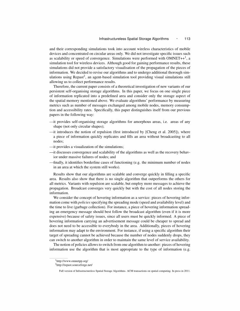
and their corresponding simulations took into account wireless characteristics of mobiledevices and concentrated on circular areas only. We did not investigate specific issues suchas scalability or speed of convergence. Simulations were performed with OMNET++1, asimulation tool for wireless devices. Although good for gaining performance results, thesesimulations did not provide a satisfactory visualisation of the propagation of the pieces ofinformation. We decided to revise our algorithms and to undergo additional thorough sim-ulations using Repast2, an agent-based simulation tool providing visual simulations stillallowing us to collect performance results.
Therefore, the current paper consists of a theoretical investigation of new variants of ourpersistent self-organising storage algorithms. In this paper, we focus on one single pieceof information replicated into a predefined area and consider only the storage aspect ofthe spatial memory mentioned above. We evaluate algorithms’ performance by measuringmetrics such as number of messages exchanged among mobile nodes, memory consump-tion and accessibility rates. Specifically, this paper distinguishes itself from our previouspapers in the following way:
—it provides self-organising storage algorithms for amorphous areas, i.e. areas of anyshape (not only circular shapes);
—it introduces the notion of repulsion (first introduced by [Cheng et al. 2005]), wherea piece of information quickly replicates and fills an area without broadcasting to allnodes;
—it provides a visualization of the simulations;—it discusses convergence and scalability of the algorithms as well as the recovery behav-
ior under massive failures of nodes; and—finally, it identifies borderline cases of functioning (e.g. the minimum number of nodes
in an area at which the system still works).
Results show that our algorithms are scalable and converge quickly in filling a specificarea. Results also show that there is no single algorithm that outperforms the others forall metrics. Variants with repulsion are scalable, but employ more messages to achieve thepropagation. Broadcast converges very quickly but with the cost of all nodes storing theinformation.
We consider the concept of hovering information as a service: pieces of hovering infor-mation come with policies specifying the spreading mode (speed and availability level) andthe time to live (garbage collection). For instance, a piece of hovering information spread-ing an emergency message should best follow the broadcast algorithm (even if it is moreexpensive) because of safety issues, since all users must be quickly informed. A piece ofhovering information carrying an advertisement message could be cheaper to spread anddoes not need to be accessible to everybody in the area. Additionally, pieces of hoveringinformation may adapt to the environment. For instance, if using a specific algorithm theirtarget of spreading cannot be achieved because the number of nodes suddenly drops, theycan switch to another algorithm in order to maintain the same level of service availability.
The notion of policies allows to switch from one algorithm to another: pieces of hoveringinformation use the algorithm that is most appropriate to the type of information (e.g.
1http://www.omnetpp.org/2http://repast.sourceforge.net/
Full version of Infrastructureless Spatial Storage Algorithms. ACM transactions on spatial computing. In press in 2011.

114 · Jose Luis Fernandez Marquez et al.
emergency information vs advertisement), to the propagation mode (faster vs slower) bychanging the repulsion rate, to accessibility rates threshold (100% of the users in the anchorarea must have access to the information vs it is acceptable if only 80% of the users haveaccess to the information).
The paper is organized as follows. Section 2 reports on related work. Section 3 presentsthe hovering information concepts and the storage areas considered. A series of storagealgorithms are discussed in Section 4. Simulations, measured performances, visualisationsand analysis of results are reported in Section 5.
2. RELATED WORK
Hovering information and spatial memory are related to different concepts such as memory,middleware, or dissemination of data. Below, we analyze previous work related to hoveringinformation.
2.1 Location-based publish/subscribe
Publish/subscribe approaches come into different flavours. Because the original pub-lish/subscribe systems were intended for stationary users through Internet access and didnot convey the notion of location [Eugster et al. 2003], it has been extended in differentmanners to accommodate mobility and location. Specifically,
—to accommodate user mobility and location, location-based publish/subscribe has beenproposed [Eugster et al. 2005]. Information is stored on a fixed infrastructure, and passedon to users when they reach a particular location and their subscription matches a par-ticular published topic;
—to alleviate the need for a fixed infrastructure, proposals exploiting mobile devices led toinfrastructureless publish/subscribe where the publication space moves along with thepublisher [Eugster et al. 2009]. Subscribers are notified when their space overlaps thepublication space of the publisher.
Hovering information and spatial memory complete this picture by providing a self-organizinginfrastructureless memory service for mobile users. Information is stored at some specificgeographic area without the need for a fixed infrastructure. It is available to users whenthey are in this area and is dissociated from its original publisher. Even though this paperfocuses on storage algorithms, we mention here a simple retrieval algorithm (also assumedin the simulations): every node for which there is another node in communication rangethat holds information de facto has access to the information and can retrieve the data (thereis no routing implied).
2.2 Dissemination Services
Alternative algorithms for spreading information include: opportunistic spatio-temporaldissemination services over MANETs [Leontiadis and Mascolo 2007b] focusing on cartraffic centred applications, epidemic models such as Epcast [Scellato et al. 2007], or Gos-sip models [Datta et al. 2004]. These works provide an interesting starting point for replica-tion algorithms, but do not offer a solution for ensuring the persistency of the information.
In the domain of location-driven routing over MANETs, we can mention works suchas GeoOpss [Leontiadis and Mascolo 2007a], search and query propagation over socialnetworks like PeopleNet [Motani et al. 2005] and collaborative services such as collab-orative backup of the MoSAIC project [Killijian et al. 2004; Courts et al. 2005]. TheFull version of Infrastructureless Spatial Storage Algorithms. ACM transactions on spatial computing. In press in 2011.

Infrastructureless Spatial Storage Algorithms · 115
work of [Leontiadis et al. 2009] provides persistent dissemination of data in intravehicularnetworks using data that ”sticks” to the locations where drivers should receive it.
Geocast [Maihfer 2004] consists in sending information to a group of nodes in a net-work within a geographical region. Geocast protocols exploit either a fixed or an ad hocinfrastructure and involve routing data from a sender (outside the geographical region) to agroup of nodes within the target geographical region. These protocols are concerned withthe delivery (routing or forwarding) of messages from a sending to a receiving region. Themain goal of hovering information or the Spatial Memory concept is to store data at somegeographical region and to make it available to all nodes in that region. There is no spe-cific routing, the data is produced from within the area where it is consumed. The nodescollaboratively serve as storage media.
All these approaches consider the data itself as a passive entity multicasted by mobiledevices. Self-organizing data, under the form of mobile agents as proposed in this paper,better supports Spatial Computing scenarios by adapting to local conditions (applying adhoc replication algorithms), or by modifying itself during the dissemination process.
2.3 Virtual Nodes
The virtual infrastructure project [Dolev et al. 2005; Dolev et al. 2004; Dolev et al. 2003;Dolev et al. 2005] aims to set up a set of virtual nodes having a well-known structureand trajectory over a mobile ad hoc network. Virtual nodes are equipped with a clockedautomaton machine, useful for implementing distributed algorithms such as leader election,routing, atomic memory, motion coordination, etc. This approach works on offering astructured abstraction layer of virtual nodes.
Within this project, the GeoQuorum approach [Dolev et al. 2003] proposes the imple-mentation of an atomic shared memory in ad hoc networks working in two parts. First,mobile hosts populate geographical regions, called focal points, that must not overlap.Within a focal point mobile hosts cooperate to implement the notion of abstract node. Fo-cal points represent virtual processes and each focal point is required to support a localbroadcast service providing reliable and totally ordered broadcast (all nodes receive thesame information and in the same order). Second, the notion of atomic shared memoryis then actually built on top of the (static) abstract nodes using a Geocast to communi-cate with the focal points nodes. The GeoQuorum algorithm ensures fault-tolerance andavailability of data by replicating memory data at a number of focal points.
Hovering information takes a different approach where each piece of hovering informa-tion is an autonomous entity responsible for its own survivability exploiting the dynamicsof underlying network to this aim. The Spatial Memory concept is very similar to theatomic shared memory (notion of virtual node and memory). The main difference is thatspatial memory is intended to be a best effort service (data may not be available and fault-tolerance is not specifically addressed), memory cells can overlap each other, data is active,and decides where to go next.
2.4 Persistent Node
The notion of PersistentNode from [Beal 2003] is inspired by the amorphous computingparadigm. An amorphous network is a set of uniformly randomly distributed particles overa 2D region. A PersistentNode is a key/value pair residing in a geographic region (a centralparticle and a circle of particles around that particle all holding the same key/value pair).The node (in fact the set of key/value pairs as a circle) may move towards another region
Full version of Infrastructureless Spatial Storage Algorithms. ACM transactions on spatial computing. In press in 2011.
116 · Jose Luis Fernandez Marquez et al.
of the 2D space (hop from particles to particles), especially when particles in the node aredamaged.
Like in the case of hovering information, data is the active entity and storage medium israther passive towards the data. A PersistentNode (i.e. a group of data inside some parti-cles) resides at some geographic locality and may move if necessary. However, the storagemedia, i.e. the particles, even though they can fail are not mobile, and all particles in thenode store the data. Hovering information considers mobile particles. At the moment, the“node” provided by hovering information is itself fixed and specified at some location. Ouralgorithms are such that data follows (is attracted by) the center of its storage area. In thecase where the storage area moves, the data just follows the center.
2.5 Middleware
The TOTA middleware (Tuples-On-The-Air) [Mamei and Zambonelli 2001; 2005] pro-poses an API to support the development of adaptive context-aware applications in perva-sive and mobile computing scenarios. The main component are tuples, which are prop-agated through the devices composing the system via the ad hoc network of the infras-tructure. TOTA follows a Linda-like approach to store and retrieve tuples through patternmatching. The tuples, defined by the user-application, are composed of three attributes:the content, the rules of propagation and the rules of maintenance. Spatial Memory couldbe implemented on top of TOTA by defining its own tuples and rules of propagation andmaintenance.
2.6 Data Clouds.
The Hovering Data Clouds (HDC) concept [Wegener et al. 2006; Fekete et al. 2006], whichis part of the AutoNomos project, is applied to the design of a distributed infrastructure-free car traffic congestion information system. Although HDCs are defined as informa-tion entities having properties similar to hovering information, the described algorithmsdo not consider them as an independent service but as part of the traffic congestion al-gorithms. The hovering information dissemination service is thought as a service inde-pendent from the applications using it. The Ad-Loc system [Corbet and Cutting 2006] isan infrastructure-free location-aware annotation system that shares similarities to hoveringinformation. However, Ad-Loc does not focus on: studying properties such as the criticalnumber of nodes or dealing with self-organizing algorithms allowing the information toadapt its behavior according to the network saturation.
2.7 Viral Programming
Paintable computing [Butera 2007] is a type of viral programming following the amor-phous computing concepts. A display is composed of numerous computing particles(fixed very small nodes) dispersed randomly on a “screen”. The programming model forpaintable computing is based on self-assembly of mobile code.
Pieces of hovering information are clearly mobile codes, self-replicating among mobilenodes. Paintable computing considers fixed particles, while in our case the particles aremobile. Pieces of hovering information are not self-assembling even though we have con-sidered the notion of swarms of pieces of hovering information: a piece too big to getstored into a single node breaks down into smaller pieces stored in different nodes; theylater self-assemble to produce the original data [Di Marzo Serugendo et al. 2007]
Smart messages [Borcea et al. 2004] are a type of mobile agents and provide an im-Full version of Infrastructureless Spatial Storage Algorithms. ACM transactions on spatial computing. In press in 2011.
Infrastructureless Spatial Storage Algorithms · 117
plementation for spatial programming with mobile computing devices. The idea of spatialmemory is very close to the notion of spatial programming: storing and retrieving informa-tion on top of an unreliable mobile storage media using spatial references. Smart messagesfollows a self-routing strategy to find their location.
Paradigms such as Amorphous Computing, Paintable Computing, and PersistentNodeshare similarities with our work: local-knowledge, self-organisation, autonomous behaviourof entities, biological inspiration, mobile code.
The novelty of the hovering information service (and later of the spatial memory) residesin the combination of the above described techniques, in particular the combination ofvirtual memory, persistent node (active and moving data) and viral programming (mobilecode).
3. HOVERING INFORMATION CONCEPT
3.1 Hovering Information
A piece of Hovering Information h is a geo-localized information attached to a geographi-cal area, called the anchor area. The main goal of h is to self-replicate among neighbouringmobile nodes in order to maintain itself in the specified anchor area and make itself acces-sible to mobile nodes in that area.
A piece of hovering information h is defined as a tuple:
h = (id,A,n,data, policies,size);
where id is the hovering information identifier, A is the anchor area (see below), n is themobile node where h is currently hosted, data is the actual data carried by h, policies arethe spreading policies of h, and size is its size.
In this paper, we do not investigate the active usage of policies for enhancing adaptation.The policy is the dissemination algorithm applied by the pieces when they spread in theirenvironment.
3.2 Circular Areas
Hovering information spread into indoor or outdoor spaces such as motorways, pedestrianroads, shopping center or leisure areas. The shape of the area can vary from a simple circlecentered on a focal point to more elaborate shapes of any type (regular, irregular, convexor not, etc.).
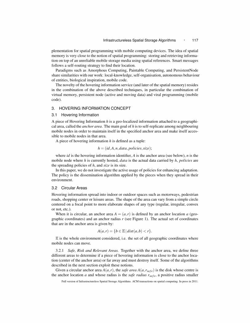
When it is circular, an anchor area A = (a,r) is defined by an anchor location a (geo-graphic coordinates) and an anchor radius r (see Figure 1). The actual set of coordinatesthat are in the anchor area is given by:
A(a,r) = {b ∈ E |dist(a,b) < r}.
E is the whole environment considered, i.e. the set of all geographic coordinates wheremobile nodes can move.
3.2.1 Safe, Risk and Relevant Areas. Together with the anchor area, we define threedifferent areas to determine if a piece of hovering information is close to the anchor loca-tion (center of the anchor area) or far away and must destroy itself. Some of the algorithmsdescribed in the next section exploit these notions.
Given a circular anchor area A(a,r), the safe area A(a,rsa f e) is the disk whose centre isthe anchor location a and whose radius is the safe radius rsa f e, a positive radius smaller
Full version of Infrastructureless Spatial Storage Algorithms. ACM transactions on spatial computing. In press in 2011.
118 · Jose Luis Fernandez Marquez et al.
Fig. 1. Circular Areas
than the anchor radius r, i.e. rsa f e < r and rsa f e ∈ R+:
A(a,rsa f e) = {b ∈ E |dist(a,b) < rsa f e}.
The risk area R(a,rsa f e,rrisk) is the ring given by;
R(a,rsa f e,rrisk) = A(a,rrisk)\A(a,rsa f e),
where rsa f e < r ≤ rrisk and rrisk,rsa f e ∈ R+.The relevant area is bigger than the risk area and serves to determine the scope of the
piece of information. If it is outside the relevant area, a piece of information h just destroysitself. The relevant area Rel(a,rrel) is the area given by:
Rel(a,rrel) = A(a,rrel),
where rrisk < rrel ∈ R+.Note that the difference between the relevant radius and the risk radius must be bigger
than the communication range of the nodes. This avoids replicating to nodes outside therelevant area and to be immediately destroyed.
The irrelevant area is the area outside the relevant area.
3.3 Amorphous Areas
Amorphous areas are anchor areas that do not have a regular shape like a circle or a square.Similarly to circular areas, the goal of a piece of hovering information is to spread itself inthe area in order to be accessible to nodes in that area.
Figure 2 represents an anchor area with 4 halls connected by 4 corridors. Nodes canmove freely in whatever direction (also outside the corridors), i.e. the hall and corridorsFull version of Infrastructureless Spatial Storage Algorithms. ACM transactions on spatial computing. In press in 2011.

Infrastructureless Spatial Storage Algorithms · 119
(a) Gradient (b) Binary
Fig. 2. Amorphous Areas
are not delimited by walls. The information must fill the anchor area, remain located insideit and must not spread outside. In particular, if a node is located in the center of Figure 2(thus not in a corridor), it may have access to a replica but should not store one.
This is a typical area for a shopping center and for a piece of information that must berelevant for people located in the corridors and meeting points, lifts or stairs (4 corners),but not when they are inside specific shops.
3.3.1 Binary Matrix and Gradient Matrix. Storage algorithms related to amorphousshapes do not use the notions of risk and safe area, they distinguish only between inside andoutside the anchor area. Therefore, pieces of hovering information are given the knowledgeof the area under the form of a matrix. We apply a grid on the area, the matrix contains thecoordinates of all the locations on the grid which are part of the area. This matrix is eithera binary matrix (Figure 2(b)): a series of points in a grid denoting whether or not a point isinside the area (matrix⊂ Ex{0,1}), or a gradient matrix (Figure 2(a)) where the points inthe matrix come with an integer value (matrix ⊂ E x N). Those closer to the inside of thearea have a higher value than those closer to the border.
The grid has the size of the space of the area we consider. For instance, let us considera museum area of 300m x 300m. The grid size is 300 x 300: one point in the grid refersto one meter in the real word. For the binary approach, the grid contains the informationbit 0 or 1. A piece of information, which wants to know if it is in the anchor area, checksits position and looks in the grid to know if its position is inside the area (1) or outside(0). For the gradient area, we use a grid too, but now the information in each point is abyte. The 0 value refers to the area outside the anchor area. The value increases when thereplica is inside the anchor area, 2553 being the inner part of the anchor area (darker shadeon the pictures). Thus, the center of the corridor has a value of 255 and also the center ofthe halls.
The actual set of coordinates that are in an amorphous area is given by:
A(matrix) = {b ∈ E | ((b,val) ∈ matrix ∧ val 6= 0)}.
As for circular areas, the irrelevant area is outside the matrix.We consider that the overhead for storing the matrix is neglictible compared to the actual
data (a few bits for each square meter).
3this could be less: 4, 8, 16, etc.)
Full version of Infrastructureless Spatial Storage Algorithms. ACM transactions on spatial computing. In press in 2011.

120 · Jose Luis Fernandez Marquez et al.
3.4 Assumptions
Pieces of hovering information have the following information (at any point in time t):
—Knowledge of the anchor area (either a pair A = (a,r), anchor location and radius; or abinary or gradient matrix);
—Position of the node it is currently in;—Position of neighbouring nodes and which of them has the information already.
We make the assumption that the information itself is more expensive to spread aroundthan getting information about position and data id stored by neighbouring nodes. Dueto the dynamic nature of the nodes, a hovering information service provides a best effortservice accommodating imprecise positions or unexpected movement of nodes.
4. ALGORITHMS
In this section we present the different replication algorithms that we compare in this paper.
4.1 Broadcast
At every simulation step (every second of simulation time) each piece of information ex-ecutes the Broadcast replication algorithm. In a real implementation, pieces of hoveringinformation would apply the algorithm at a regular interval (e.g. every second), but not ina synchronous way as it is for the simulations. For circular areas, replication is triggeredonly when the information is in the risk area (Algorithm 1). Despite the lack of activereplication within the safe area, the actual availability and further spreading of the replicasto all nodes in the anchor area occurs through the movement of the nodes.
For amorphous areas, replication is triggered when the information is inside the area(Algorithm 2).
Broadcast replicates to all nodes in communication range that do not hold a replica. Thiscan be viewed as a kind of multicast, we prefer to call it broadcast because the effect is toput a replica in each node.
Algorithm 1 Broadcast Replication Algorithm - Circular Areaspos← NodePosition()aPos← AnchorPosition()dist← Distance(pos,aPos)if (dist ≥ Rsa f e) and (dist ≤ Rrisk) then
Broadcast()
end
Algorithm 2 Broadcast Replication Algorithm - Amorphous Areaspos← NodePosition()if (IsInAnchorArea(pos)) then
Broadcast()
end
Full version of Infrastructureless Spatial Storage Algorithms. ACM transactions on spatial computing. In press in 2011.

Infrastructureless Spatial Storage Algorithms · 121
Broadcast spreads data in the neighborhood (to those nodes that are not yet storing theinformation). There is no selection of a subset of nodes based on their geographical posi-tion as in geocast.
4.2 Attractor Point
The Attractor Point algorithm avoids broadcasting to all neighbouring nodes. At eachsimulation step, a piece of information replicates only to the Kr nodes in communicationrange that are closer to the center of the anchor area (anchor location for circular areas, orhigher level of gradients for gradient matrix). Attractor Point does not apply with a binarymatrix. For circular areas, replication is triggered when the information is in the risk area(Algorithm 3), while for amorphous areas, it is triggered when the information is insidethe area (Algorithm 4).
Algorithm 3 Attractor Point Replication Algorithm - Circular Areaspos← NodePosition()aPos← AnchorPosition()dist← Distance(pos,aPos)neigbourNodes← NodeNeigbours()
if (dist ≥ Rsa f e) and (dist ≤ Rrisk) thenselectNodes← SelectKrClosest(neigbourNodes)Multicast(selectNodes)
end
Algorithm 4 Attractor Point Replication Algorithm - Amorphous Areaspos← NodePosition()neigbourNodes← NodeNeigbours()
if (IsInAnchorArea(pos)) thenselectNodes← SelectKrClosest(neigbourNodes)Multicast(selectNodes)
end
4.3 Cleaning
A piece of hovering information located in the irrelevant area removes itself and freesthe memory of the node in which it was stored. The cleaning algorithm ensures that thehovering information pieces stay in the anchor area and do not spread all over the envi-ronment. Additionally, we consider that at most one replica of the same piece of hoveringinformation is stored in a given a node at a certain point in time.
Full version of Infrastructureless Spatial Storage Algorithms. ACM transactions on spatial computing. In press in 2011.

122 · Jose Luis Fernandez Marquez et al.
4.4 Repulsion
The repulsion mechanism helps the system to spread the pieces of information over theanchor area maintaining good accessibility levels while keeping a minimum number ofreplicas (in order to use less memory). If two or more replicas are close to each other, oneof them will move away (remove itself from its current location and replicate further away).Additionally, repulsion enables to easily fill amorphous shapes: the information spreadsalong the shape until it fills it. The repulsion mechanism, inspired by the gas theory, hasbeen used in self-repairing formation for swarms of mobile agents [Cheng et al. 2005] andas an exploration mechanism in multi-swarm optimization algorithms [Fernandez-Marquezand Arcos 2009]. The main difference between our system and the self-repairing formationfor swarms of mobile agents is that pieces of hovering information do not have any controlover the movement of the mobile nodes.
Figure 3(a) shows how a replica creates a repulsion vector inversely proportional to thedistance between itself and neighbouring replicas, and how this replica subsequently movesto another node following the repulsion vector, as we see in Figure 3(b).
Fig. 3. Repulsion
Contrarily to the previously described Broadcast and Attractor Point, the replica, whichapplies the repulsion mechanism, removes itself from the current node.
Let h be a piece of information, r a replica of h, and n(r) the mobile node where r iscurrently located. Using the repulsion mechanism, the desired position for r at time t +1,~Pd(r)t+1, is calculated as follows:
~Pd(r)t+1 = ~P(r)t +~R(r)t , (1)
where ~P(r)t is the position of r at time t and ~R(r)t is the repulsion vector at time t.
~R(r)t = ∑i∈R(r,t)
~P(n(r))t −~P(n(i))t
dist(n(r),n(i))× (rcomm(n(r))−dist(n(r),n(i))) (2)
Full version of Infrastructureless Spatial Storage Algorithms. ACM transactions on spatial computing. In press in 2011.

Infrastructureless Spatial Storage Algorithms · 123
where:
—R(r, t) is the set of replicas of h in communication range of n(r) at time t;—dist(n(r),n(i)) is the Euclidean distance between the node n(r) and the node n(i);—~P(n( j))t is the position of node n( j) where the replica j is stored at time t;—× is the multiplier operator; and—rcomm is the communication range.
Once the desired position ~Pd(r)t+1 is known, the replica r must choose which node inits communication range is the closest to this desired position. If the closest node is itself,then repulsion is not applied. Otherwise r replicates to the new node and deletes itselffrom n(r). Basically, these equations produce a repulsion vector that moves the replica ofinformation to the less dense area inside its communication range.
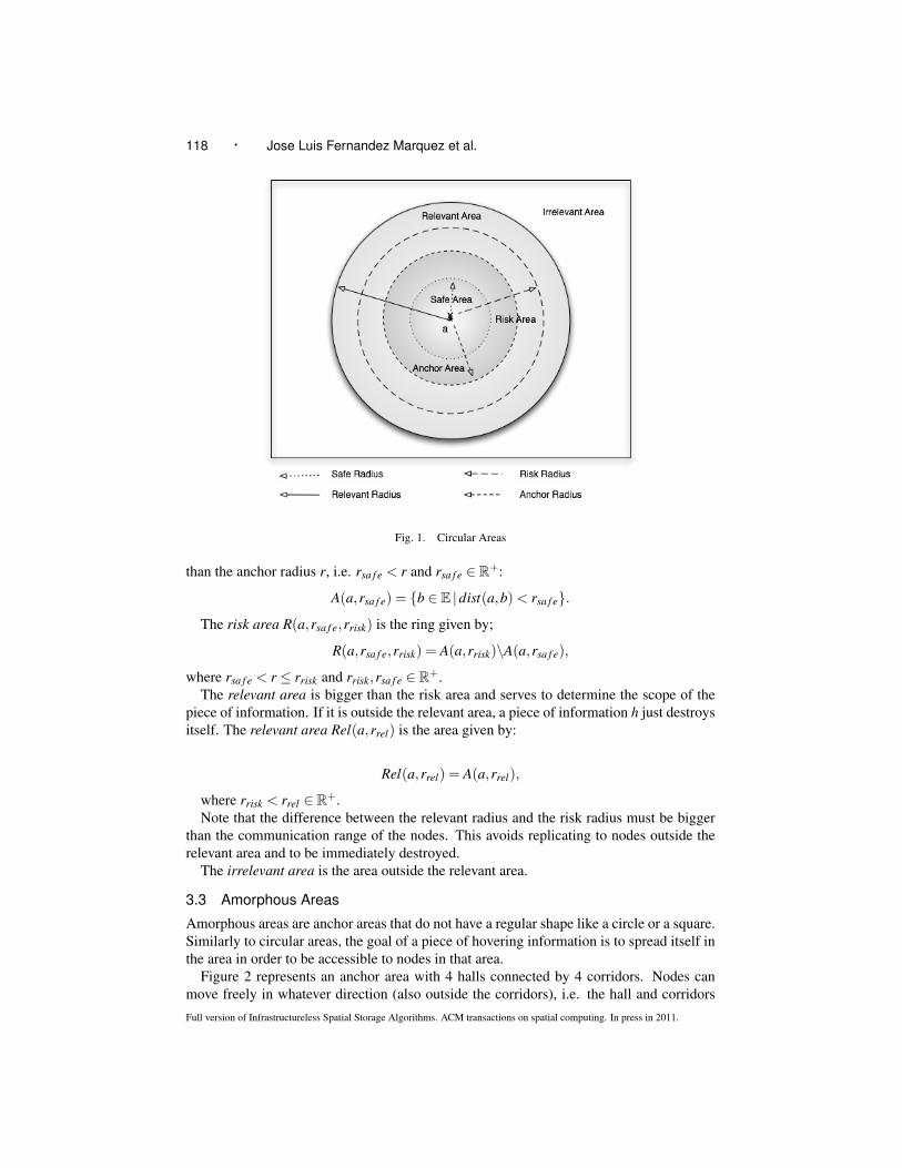
4.4.1 Broadcast with Repulsion. The Broadcast with Repulsion (see Algorithm 5) usesbroadcast as a replication algorithm and repulsion to spread away the replicas. A replicaapplies Broadcast with Repulsion independently of its location inside the anchor area (evenfor circular areas), provided it is inside the anchor area and there is no other replica incommunication range.
The main steps of the algorithm are shown in Figure 4. At the beginning, Step 1, the firstpiece of information is created and the anchor area is defined. This piece of informationexecutes the broadcast, since there is no other piece of information in its communicationrange. Step 2 shows how the nodes that are in communication range get a copy of thepiece of information. At Step 3, the pieces of information spread away due to the repulsionalgorithm. After the repulsion step, two of the three replicas have no other replica intheir communication range, then they execute the Broadcast algorithm and replicate toall the nodes in their communication range, Step 4. At Step 5 we see how the pieces ofinformation spread further due to the repulsion and finally fill the anchor area. Step 6shows how without getting stored in every node, the initial piece of information becomesavailable to all nodes in the anchor area (i.e. it ”fills” or ”covers” the whole anchor area).
Algorithm 5 Broadcast with Repulsion - Circular and Amorphous Areas (Binary)pos← NodePosition()neigbourNodes← NodeNeigbours()if (IsInAnchorArea(pos)) then
CalculateDesirePositionbyRepulsion() equations (1), (2)MoveToNodeClosestDesirePosition()if (¬ExistPieceOfInformation(neigbourNodes)) then
Broadcast()
endend
4.4.2 Attractor Point with Repulsion. The Attractor Point with Repulsion (see Algo-rithm 6) executes a multicast to the Kr nodes closer to the anchor location (circular areas)or to higher level of gradients (for gradient matrix). It applies independently of the locationinside the anchor area, as soon as there is no other piece of information in communicationrange.
Full version of Infrastructureless Spatial Storage Algorithms. ACM transactions on spatial computing. In press in 2011.
124 · Jose Luis Fernandez Marquez et al.
Step 1 Step 2 Step 3
Step 4 Step 5 Step 6
Fig. 4. Broadcast Repulsion Steps
Algorithm 6 Attractor Point with Repulsion - Circular and Amorphous Areas (Gradient)pos← NodePosition()neigbourNodes← NodeNeigbours()if (IsInAnchorArea(pos)) then
CalculateDesirePositionbyRepulsion() equations (1), (2)MoveToNodeClosestDesirePosition()if (¬ExistPieceOfInformation(neigbourNodes)) then
selectNodes← SelectKrClosest(neigbourNodes)Multicast(selectNodes)
endend
4.5 Metrics
We use the following notation: HoverIn f ot = (Nt ,Ht) is a Hovering Information Systemat time t. Nt is the set of nodes present in the system at time t. Ht is the set of pieces ofhovering information and any replica present in the system at time t. Since we consideronly one piece of information in this paper, Ht stands for h and all its replicas (sameidentity and data but stored at different nodes). Note that h itself is just a specific replica.We measure and compare the performances of each algorithms against the metrics below.
4.5.1 Survivability. A piece of hovering information is alive at some time t if there isat least one node hosting a replica r of this information.Full version of Infrastructureless Spatial Storage Algorithms. ACM transactions on spatial computing. In press in 2011.

Infrastructureless Spatial Storage Algorithms · 125
DEFINITION 1 SURVIVABILITY OF HOVERING INFORMATION h AT TIME t . The sur-vivability of h at time t is given by the boolean value:
sv(t) =
{1 if∃r ∈Ht ,n(r) ∈Nt
0 otherwise.
The survivability along a period of time is defined as the ratio between the amount oftime during which the hovering information has been alive and the overall duration of theobservation.
DEFINITION 2 RATE OF SURVIVABILITY OF HOVERING INFORMATION h AT TIME t .The survivability of h between time tc (creation time of h, always 0 in this paper) and timet is given by:
SV (t) =1
t− tc
t
∑τ=tc
sv(τ).
4.5.2 Accessibility. A piece of hovering information h is accessible by a node n atsome time t if the node is able to get this information, i.e. if it exists a node m being incommunication range of the interested node n and which contains a replica of h.
DEFINITION 3 ACCESSIBILITY OF HOVERING INFORMATION h FOR NODE n AT TIME t .Let n ∈Nt be a mobile node, the accessibility of h for n at time t is given by the booleanvalue:
ac(n, t) =
{1 if : ∃r ∈Ht ,n(r) : in AC(n)0 otherwise.
AC(n) is the area in communication range of node n.
DEFINITION 4 ACCESSIBILITY OF HOVERING INFORMATION h AT TIME t . The acces-sibility of h at time t is given by:
AC(t) =S(
⋃r∈Ht AC(n(r))∩A)
S(A)
where S(X) denotes the surface area of X, AC(n(r)) is the area of communication of thenode n storing replica r, and A is the anchor area.
4.5.3 Messages. A message is sent, each time a replica self-replicates to another node.
DEFINITION 5 NUMBER OF MESSAGES SENT AT TIME t . Let msg(n, t) be the numberof messages sent by node n between 0 and t, the number of messages sent at time t is givenby:
MSG(t) = ∑n∈Nt
msg(n, t)
4.5.4 Memory. The memory that the system uses at time t is the total number of repli-cas in the system at time t: |Ht |.
Full version of Infrastructureless Spatial Storage Algorithms. ACM transactions on spatial computing. In press in 2011.

126 · Jose Luis Fernandez Marquez et al.
Algorithms Circular Amorphous AmorphousAreas Gradient Binary
BB (risk area) X – –AP (risk area) X – –
BB (everywhere) – – XAP (everywhere) – X –BR (repulsion) X – X
APR (repulsion) X X –
Table I. Summary of Simulations
DEFINITION 6 RATE OF MEMORY USED AT TIME t . The Rate of Memory used at timet is:
MEM(t) =1
t− tc
t
∑τ=tc|Hτ |
For the simulations and the metrics above we used a synchronous model. In an actualimplementation, we would not measure those metrics on-the-fly. We would measure themetrics above by analysing mobile devices activity (e.g. how many times they received,replicated, discarded data) during a specific period of time.
5. SIMULATION RESULTS
We conducted diverse simulations involving the algorithms described above for both cir-cular and amorphous areas. We used the Recursive Porous Agent Simulation Toolkit(REPAST)4, a Java environment for agent simulations. In addition to performance mea-sures, it provides an event scheduler for simulating concurrency and a two-dimensionalagent environment that we use to visualise the nodes and the spreading of the pieces ofhovering information in the environment.
Table I summarises the different simulations we have performed. The first column refersto circular areas. Corresponding results are reported in Section 5.1. The second and thirdcolumns refer to amorphous areas described with a gradient and binary matrix respectively.Corresponding results are reported in Section 5.2.
For circular areas, both Broadcast and Attractor Point replicate only in the risk area.When used with the repulsion mechanism, replication is triggered independently of therisk area.
For amorphous areas, we dropped the notions of risk areas. Indeed, we noticed a con-tainment effect: replicas do not spread along the shape when the notion of risk area isextended to an amorphous area. Additionally, Broadcast with a gradient matrix behavesin the same way as Broadcast with a binary matrix (Broadcast applies as long as a pieceis inside the area, independently of the gradient). Attractor Point makes sense only for agradient matrix, since replicas are attracted to the center of the area (the highest values inthe matrix). We do not consider Attractor Point for a binary matrix.
4http://repast.sourceforge.net/
Full version of Infrastructureless Spatial Storage Algorithms. ACM transactions on spatial computing. In press in 2011.

Infrastructureless Spatial Storage Algorithms · 127
5.1 Circular Areas
We defined two scenarios: The indoor scenario where the communication range is 40 me-ters and the outdoor scenario where the communication range is 80 meters. The anchorarea is a circle located at the center of the environment (blackboard) and the mobility modelused for the nodes is Random Way Point. This mobility pattern in contrast to other patternslike Random Direction or Random Walk, creates the highest density of nodes at the centerof the environment. By locating the anchor area at the center a similar concentration ofnodes across our different experiments is ensured, i.e. we can infer meaningful conclu-sions. For each experiment, we executed 50 runs, each run spending 20000 simulationseconds. The results presented are the average over the 50 runs.
In this section we compare the Broadcast (BB) and Attractor Point (AP) algorithmsreplicating in the risk area versus the Broadcast with Repulsion (BR) and Attractor Pointwith Repulsion (APR) (first column of Table I).
Blackboard 600m x 400mMobility Model Random Way Point
Nodes speed 1m/s to 2m/sCommunication Range 40m or 80mReplication Time (TR) 1sCleaning Time (TC) 1s
Repulsion Time 10 sAnchor Radius (Ranchor) 100m
Safe Radius (rsa f e) 50mRisk Radius (rrisk) 100m
Relevant Radius (rrel) 140m or 180m
Table II. Circular Area - Scenario’s Settings
Table II summarizes the parameter settings of the Circular Area scenario.
5.1.1 Indoor Scenario. Although the WLAN 802.11 standard provides communica-tion ranges up to 70m for indoors and 250m for outdoors, most authors (e.g. [Roth 2003])consider that this is too high for realistic situations, and propose smaller values. In this pa-per, we decided to choose 40m for indoor and 80m for outdoor. The anchor area is a circlewith a 100m radius. The relevant radius is set accordingly to 140m (100m + 40m). Be-cause we want to avoid replicas that end up straight away into the irrelevant area, they arediscarded immediately. A relevant radius of 140m is enough to avoid this phenomenon. In-deed, replicas created from the risk area (100m radius) will always end up in nodes locatedin the relevant area (140m radius), since the communication range is 40m.
Figures 5 shows the survivability and accessibility rates of the four algorithms whenvarying the number of nodes. We observe how Broadcast and Attractor point present abetter survivability and accessibility, even for a small number of nodes, than the variantswith the repulsion mechanism. This is due to the fact that Broadcast and Attractor Pointuse a larger number of nodes to store the information. With more than 55 nodes the fouralgorithms present a survivability and accessibility of 1. This means that the informationis alive and accessible to all nodes during the whole simulation time and for all 50 runs.
Figure 6 presents the standard deviations (STD) found for survivability and accessibility.The standard deviation related to survivability increases between 20 and 40 nodes. This is
Full version of Infrastructureless Spatial Storage Algorithms. ACM transactions on spatial computing. In press in 2011.

128 · Jose Luis Fernandez Marquez et al.
(a) (b)
Fig. 5. Survivability and Accessibility - Circular Area - Indoor Scenario
(a) (b)
Fig. 6. Survivability and Accessibility STD- Circular Area - Indoor Scenario
due to the fact that the information disappears (it does not succeed in surviving) at somepoint during the simulation. When the number of nodes is enough to ensure survivability,the standard deviation falls to 0. The particular case of failure during the initialisation hasbeen investigated separately in Section 5.3.4. The standard deviation related to accessibil-ity (Figure 6(b)) is low. When the number of nodes increases, STD goes down, becausethe algorithm presents more stable results with a high number of nodes. However, a goodSTD is achieved even with a small number of nodes.
Figure 7(a) depicts the number of messages sent around given different number of nodes.As we can see, the main weakness of the variants with repulsion is the high number ofmessages sent among the nodes (e.g. 25% more than the variant without repulsion given80 nodes). This is a direct result of the repulsion mechanism: the replicas spread over theanchor area in the most uniform possible way, i.e. they need to move from one node toanother increases the number of messages. However, once the replicas are properly spreadover the anchor area, less nodes (and memory) are required to store the information and tokeep high accessibility rates.
Figure 7(b) shows the average number of nodes storing a replica during 20000 secondsof simulation. As expected, Broadcast and Attractor Point algorithms use more memorythan their variants with repulsion (43% and 30% more memory respectively in a 80 nodesscenario). Figure 8(a) shows the STD achieved in the Messages metric. The increase of theFull version of Infrastructureless Spatial Storage Algorithms. ACM transactions on spatial computing. In press in 2011.

Infrastructureless Spatial Storage Algorithms · 129
(a) (b)
Fig. 7. Messages and Memory - Circular Area - Indoor scenario
STD between 20 to 50 nodes is due to failures during the initialisation phase: the hoveringinformation dies before the end of the simulation and replication stops. Consequently, thetotal number of messages is lower for runs when the information dies before the end. Onthe contrary, the STD is close to 0 when the survivability is close to 1. For the same reason,in Figure 8(b), we observe a modest increase of the STD related to memory consumption.Thus, even when the hovering information dies before reaching the end of the simulation,the value is similar. All the algorithms present a low standard deviation.
(a) (b)
Fig. 8. Messages and Memory STD - Circular Area - Indoor scenario
5.1.2 Outdoor Scenario. In the outdoor scenario, nodes have a communication rangeof 80 meters. Similarly to the indoor scenario, the relevant radius is set to 180m.
The four algorithms present better survivability and accessibility rates than in the indoorscenarios, even with 40 nodes, as it is shown in Figure 9. Indeed, the longer communicationrange increases survivability, i.e. it decreases the probability that a piece of informationreplicates into the irrelevant area without having the possibility to replicate elsewhere be-fore. Analogously to the indoor scenario, the Broadcast and Attractor Point algorithmsachieve a better survivability rate even with a smaller number of nodes.
In Figure 10, we may observe that variants with repulsion increase the number of mes-sages with respect to Broadcast and Attractor Point (two times more), and decrease theaverage number of replicas in the system (two to three times less). It is worth noting the
Full version of Infrastructureless Spatial Storage Algorithms. ACM transactions on spatial computing. In press in 2011.

130 · Jose Luis Fernandez Marquez et al.
(a) (b)
Fig. 9. Survivability and Accessibility - Circular Area - Outdoor Scenario
(a) (b)
Fig. 10. Messages and Memory - Circular Area - Outdoor scenario
scalability results achieved by the Attractor Point with Repulsion: despite the increasingnumber of nodes present in the system, the number of nodes actually storing the informa-tion (memory usage) remains constant. Results for STD are similar to the indoor scenarioand we do not report them here.
5.1.3 Visualisation. Figure 26 shows snapshots of the simulations for the circular areadescribed above for each algorithm. Since the area is rather small, Broadcast and AttractorPoint store a replica in each node of the area, while the variants with repulsion do not floodthe whole area.
5.1.4 Conclusions. When the number of nodes in the system is small (less than 50 forindoor or 25 for outdoor scenarios), the probability that the information does not surviveduring the whole simulation is high. Broadcast and Attractor Point use a higher amountof replicas and thus present better survivability and accessibility rates. With larger numberof nodes (above 55 for indoor and 40 for outdoor scenarios), the variants with repulsionuse less memory, provide high survivability rates, but need more messages. Of four algo-rithms, the Attractor Point distinguishes itself: even though it uses more memory than thevariant with repulsion, it may be considered acceptable given the best results it providesfor scalability, low number of messages, survivability and accessibility rates. Regardingthe standard deviation, when the system has reached a critical mass of nodes to ensure thesurvivability of the information during the whole simulation, the STD tends to 0.Full version of Infrastructureless Spatial Storage Algorithms. ACM transactions on spatial computing. In press in 2011.

Infrastructureless Spatial Storage Algorithms · 131
5.2 Amorphous Areas
Amorphous areas are defined either with a gradient matrix or with a binary matrix. Inpreliminary simulations, we noticed that Broadcast and Attractor Point (as defined for thecircular shapes) couldn’t fill the amorphous areas when the notion of risk and relevant areaswere considered. Because there is no replication of the information inside the safe area,replicas have a tendency to remain concentrated at some point. Consequently, when usedfor amorphous shapes, replicas do not spread along the central axis of the shape.
Instead, we painted a gradient inside the area. The notion of gradient convenientlyreplaces the notion of risk area: the darker the color, the safer the location. The AttractorPoint algorithm replicates to those nodes that are closer to the safest area. The goal isthe same as for circular ares: ensure high accessibility levels with a minimum number ofmessages and a minimum number of nodes actually storing the information.
In this section we consider Broadcast with binary matrix and Attractor Point with gra-dient matrix and their corresponding variants with repulsion (second and third columns ofTable I).
Blackboard 1200m x 700mMobility Model Random Way Point
Nodes speed 1m/s to 2m/sCommunication Range 40m or 80mReplication Time (TR) 1s
Repulsion Time 10 sCleaning Time (TC) 1s
Table III. Amorphous Area - Scenario’s Settings
Table III summarizes the parameter settings for the Amorphous Areas scenarios. Foreach experiment, we executed 50 runs, each run spending 1000 simulation seconds. Theresults presented are the average over these 50 runs.
5.2.1 Indoor Scenario. In this scenario the communication range of the nodes is 40m.We also used the Random Way Point mobility model. The amorphous area considered isthe one shown in Figure 2 (4 corridors and 4 corners). Because this area is much larger thanthe circular area considered previously (1200mx700m), the minimum number of nodes isabove 200.
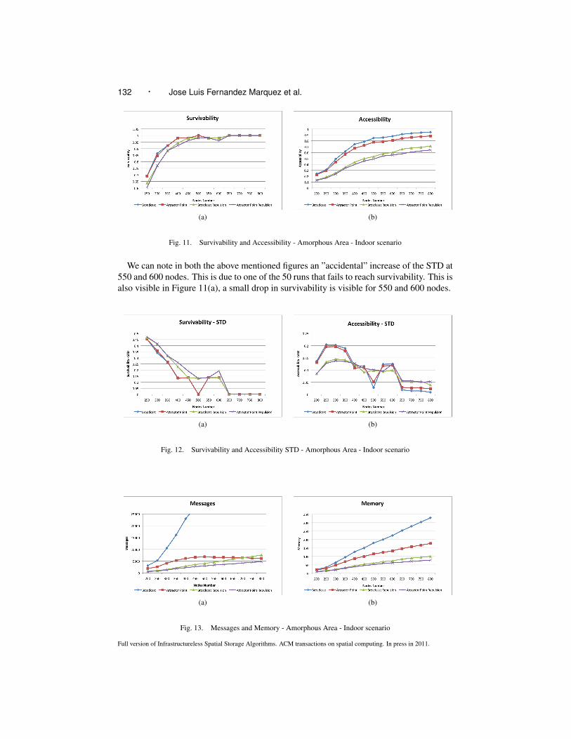
Figure 11 shows survivability and accessibility rates of the four algorithms consideredin this section. Again, Broadcast and Attractor Point outperform their respective variantswith repulsion since more nodes store the data.
Figure 12(a) shows the standard deviation (STD) related to survivability. We may ob-serve how STD is going down when the number of nodes increases. That is, the algorithmreduces the probability of failure when the number of nodes increase. When the number ofnodes is higher than 600, the STD tends to 0., i.e. at least 600 nodes are necessary to ensurethe survivability of the hovering information along the simulation. Figure 12(b) shows theSTD related to accessibility. The best STD is achieved when the number of nodes in thesystem is enough to ensure the survivability of the hovering information during the wholesimulation.
Full version of Infrastructureless Spatial Storage Algorithms. ACM transactions on spatial computing. In press in 2011.
132 · Jose Luis Fernandez Marquez et al.
(a) (b)
Fig. 11. Survivability and Accessibility - Amorphous Area - Indoor scenario
We can note in both the above mentioned figures an ”accidental” increase of the STD at550 and 600 nodes. This is due to one of the 50 runs that fails to reach survivability. This isalso visible in Figure 11(a), a small drop in survivability is visible for 550 and 600 nodes.
(a) (b)
Fig. 12. Survivability and Accessibility STD - Amorphous Area - Indoor scenario
(a) (b)
Fig. 13. Messages and Memory - Amorphous Area - Indoor scenario
Full version of Infrastructureless Spatial Storage Algorithms. ACM transactions on spatial computing. In press in 2011.

Infrastructureless Spatial Storage Algorithms · 133
Figure 13(a) shows that Broadcast employs much more messages and storage memorythan the other algorithms. It is clearly outperformed by the rest.
(a) (b)
Fig. 14. Messages and Memory STD - Amorphous Area - Indoor scenario
Figure 14(a) shows the STD of messages achieved by the different algorithms in theamorphous area. Except Broadcast that presents a high STD the rest of the algorithmspresent a STD lower than 10%. Figure 14(b) shows the STD related to memory. All thealgorithms reach a STD for memory lower than 8% when the system has enough numberof nodes to sustain the data. Here again, we observe that the same runs that affected theSTD in Figures 12(a) and (b) affect also Figures 14(a) and (b) for 550 and 600 nodes. Asit occurs in all the STD graphs presented in this work, a low number of nodes involves anunstable survivability, producing an increment in the STD.
Surprisingly, the Attractor Point with Repulsion outperforms its variant without repul-sion for both the number of messages and the memory storage. This result is due to thefact that the repulsion variant replicates only when there is no other replica in the commu-nication range.
5.2.2 Outdoor Scenario. This scenario uses the Random Way Point mobility modeland a communication range of 80 meters.
(a) (b)
Fig. 15. Survivability and Accessibility - Amorphous Area - Outdoor scenario
Full version of Infrastructureless Spatial Storage Algorithms. ACM transactions on spatial computing. In press in 2011.

134 · Jose Luis Fernandez Marquez et al.
Figure 15 shows survivability and accessibility rates for the outdoor scenario. Becauseof the increased communication range, both rates are better for all algorithms. Broadcastand Attractor Point still outperforming (even though slightly) the repulsion variants foraccessibility rates.
(a) (b)
Fig. 16. Messages and Memory - Amorphous Area - Outdoor scenario
As for the indoor scenario, Broadcast is clearly outperformed by the other three algo-rithms for both the number of messages sent around and the memory used. To facilitate theunderstanding, the messages for Broadcast are not included in Figure 16. Attractor Point(both variants) show similar levels of messages whereas the repulsion variant is using lessmemory.
5.2.3 Visualisations. In the Appendix, we provide some simulation images of the in-door scenario using the anchor area 2 for the Attractor Point with Repulsion (Figure 27)and the Broadcast algorithm (Figure 29). Moreover, we provide some simulation imagesfor these algorithms when the nodes fail in a sub-area (Figure 28) and (Figure 30). Theimages shows the faster refill after the failure.
We may see how the convergence speed vary for these algorithms. The Attractor Pointwith Repulsion takes more time to spread replicas over the whole area (280 seconds ofsimulation time), while Broadcast quickly fills the shape (at the 18th simulation secondalready). The difference in the number of nodes storing a replica (darker dots) is alsoclearly visible.
We experimented with massive failures of nodes (Steps 4 to 6). These will be explainedlater.
We experimented with different shapes, as for instance an amorphous area taking theshape of the number five (Figure 31). Information spreading for this area is given byFigure 33 and Figure 33.
5.2.4 Conclusions. For amorphous areas both indoor and outdoor, Attractor Point(both versions) are clearly the best options. Specifically, for higher availability rates (above95%) Attractor Point should be preferred whereas for acceptable lower availability rates(80%) and less memory storage, Attractor Point with Repulsion is the best option.Full version of Infrastructureless Spatial Storage Algorithms. ACM transactions on spatial computing. In press in 2011.

Infrastructureless Spatial Storage Algorithms · 135
5.3 Analysis of algorithms
This section investigates scalability issues, the impact of the repulsion rate on the results,cases where a newly created piece of information does not succeed to spread and diesalmost immediately, the minimum number of nodes below which the system cannot work,and a recovering scenario in case of massive failures of nodes.
5.3.1 Scalability. In this section we study the behaviour of the algorithms for verylarge numbers of nodes (up to 2000). This experiment involves the amorphous area ofFigure 2 and a communication range of 40m. We varied the number of nodes from 800to 2000. Just like for the other experiments, the Attractor Point and Attractor Point withRepulsion are using the gradient matrix (Figure 2(a)), while the Broadcast and Broadcastwith Repulsion are using the binary matrix (Figure 2(b)).
The four algorithms achieve very good accessibility rates due to the very large numbernodes involved, as shown in Figure 17(a). Broadcast and Attractor point present a betteraccessibility than the variants with repulsion, since they use also more memory, as shown inFigure 17(b). The main point is that the repulsion variants are scalable regarding memoryconsumption. The memory levels remain constant despite the higher number of nodes.
(a) (b)
Fig. 17. Accessibility and Memory - Scalability in Amorphous Areas - Indoor scenario
The main drawback of applying repulsion is the high number of messages sent aroundwhen compared to the variants without repulsion. Attractor Point (without repulsion) isscalable in terms of messages: the number of messages remains constant even though thenumber of nodes increases Figure 18(a). Broadcast (both variants) is not scalable at all interms of messages Figure 18(b).
To conclude, for amorphous areas and large number of nodes, Attractor Point scalesbetter in terms of messages than the Attractor Point with Repulsion, but employs morememory (up to four times more). The repulsion variant scales in terms of memory butuses far more messages. It is also worth noting that the Attractor Point doesn’t use anymechanism to spread the information over the area. The area gets filled as a result of themovements of nodes, they help the algorithm in spreading the information. The repulsionversion ensures that the information spreads over the area, even if the nodes are stationaryor less mobile. Broadcast (without repulsion) is not scalable and its variant with repulsionmust be preferred.
Full version of Infrastructureless Spatial Storage Algorithms. ACM transactions on spatial computing. In press in 2011.

136 · Jose Luis Fernandez Marquez et al.
(a) (b)
Fig. 18. Messages - Scalability in Amorphous Areas - Indoor scenario
Fig. 19. Accessibility - Varying the repulsion interval
5.3.2 Repulsion Interval. An important parameter of the repulsion mechanism is therepulsion interval, i.e. the time between two repulsion executions. When the repulsioninterval is shorter, the number of messages increases as does the accessibility rate. Whenthe repulsion interval is long, the number of messages decreases, but also the accessibilityrate.
In this experiment we computed the accessibility rate, the number of messages and thememory usage along 1000 simulation steps, over the average of 50 runs for Broadcast withRepulsion and Attractor Point with Repulsion. For this experiment we set the number ofnodes to 500 and the communication range to 40m. We consider the same amorphous areaas above.
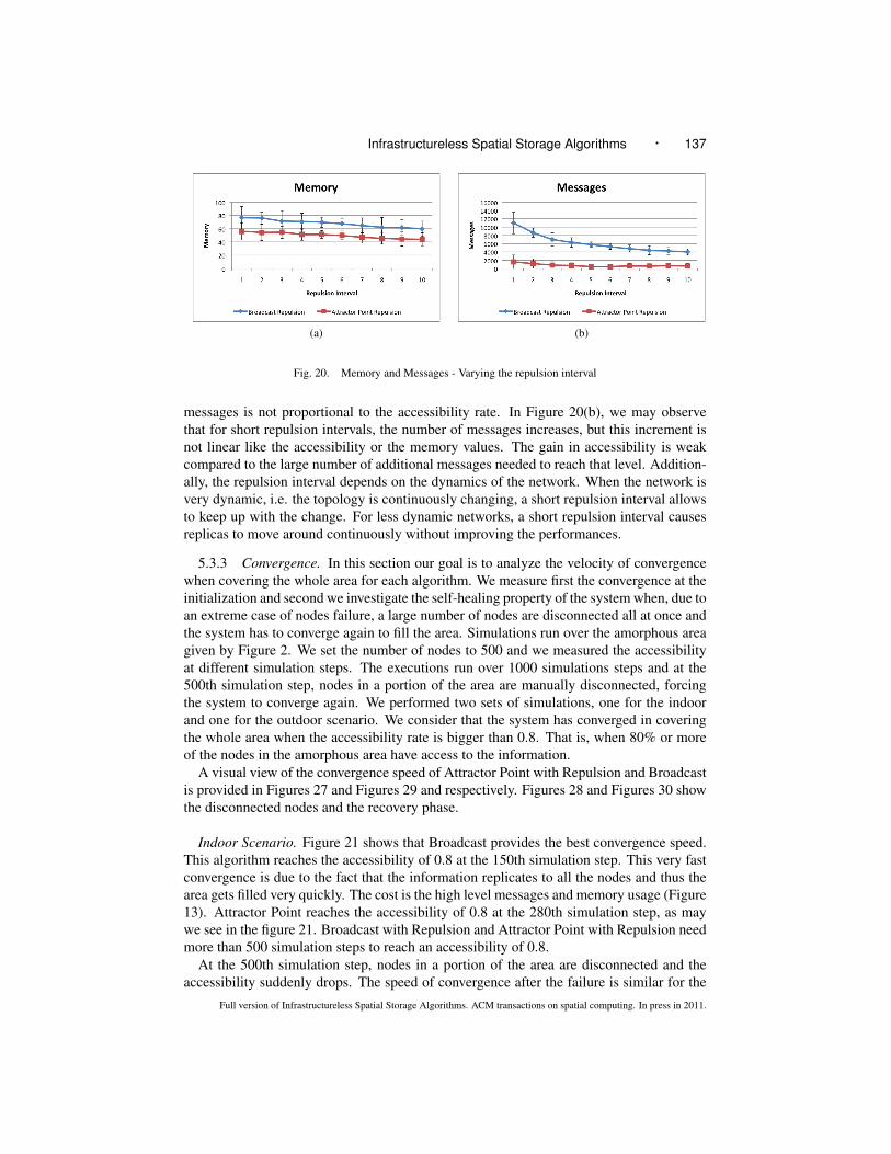
Figure 19 shows that accessibility rates are better with a shorter repulsion interval (every1s or 2s), since repulsion spreads faster the pieces of information over the area. It adaptsquickly to topology changes by moving around the replicas. When we increment the re-pulsion interval, repulsion applies less frequently (every 4s or less) and adapts less quicklyto topology changes, and accessibility rates decrease. For memory consumption, a shorterrepulsion interval causes more nodes to store replicas, while a longer repulsion interval de-creases the memory used. A shorter repulsion rate increases the number of time repulsionapplies, i.e improves the exploration of the space and is able to find better places where toreplicate increasing accessibility. The drawback is the higher memory consumptions, as itis shown in Figure 20.
The main issue with a shorter repulsion interval is that the increase in the number ofFull version of Infrastructureless Spatial Storage Algorithms. ACM transactions on spatial computing. In press in 2011.
Infrastructureless Spatial Storage Algorithms · 137
(a) (b)
Fig. 20. Memory and Messages - Varying the repulsion interval
messages is not proportional to the accessibility rate. In Figure 20(b), we may observethat for short repulsion intervals, the number of messages increases, but this increment isnot linear like the accessibility or the memory values. The gain in accessibility is weakcompared to the large number of additional messages needed to reach that level. Addition-ally, the repulsion interval depends on the dynamics of the network. When the network isvery dynamic, i.e. the topology is continuously changing, a short repulsion interval allowsto keep up with the change. For less dynamic networks, a short repulsion interval causesreplicas to move around continuously without improving the performances.
5.3.3 Convergence. In this section our goal is to analyze the velocity of convergencewhen covering the whole area for each algorithm. We measure first the convergence at theinitialization and second we investigate the self-healing property of the system when, due toan extreme case of nodes failure, a large number of nodes are disconnected all at once andthe system has to converge again to fill the area. Simulations run over the amorphous areagiven by Figure 2. We set the number of nodes to 500 and we measured the accessibilityat different simulation steps. The executions run over 1000 simulations steps and at the500th simulation step, nodes in a portion of the area are manually disconnected, forcingthe system to converge again. We performed two sets of simulations, one for the indoorand one for the outdoor scenario. We consider that the system has converged in coveringthe whole area when the accessibility rate is bigger than 0.8. That is, when 80% or moreof the nodes in the amorphous area have access to the information.
A visual view of the convergence speed of Attractor Point with Repulsion and Broadcastis provided in Figures 27 and Figures 29 and respectively. Figures 28 and Figures 30 showthe disconnected nodes and the recovery phase.
Indoor Scenario. Figure 21 shows that Broadcast provides the best convergence speed.This algorithm reaches the accessibility of 0.8 at the 150th simulation step. This very fastconvergence is due to the fact that the information replicates to all the nodes and thus thearea gets filled very quickly. The cost is the high level messages and memory usage (Figure13). Attractor Point reaches the accessibility of 0.8 at the 280th simulation step, as maywe see in the figure 21. Broadcast with Repulsion and Attractor Point with Repulsion needmore than 500 simulation steps to reach an accessibility of 0.8.
At the 500th simulation step, nodes in a portion of the area are disconnected and theaccessibility suddenly drops. The speed of convergence after the failure is similar for the
Full version of Infrastructureless Spatial Storage Algorithms. ACM transactions on spatial computing. In press in 2011.

138 · Jose Luis Fernandez Marquez et al.
Fig. 21. Accessibility - steps 0 to 1000 - Indoor Scenario
four algorithms. As we may see in Figure 22(b), the four algorithms follow the sameslope. This is due to the time that the MANET takes to fix the network after the failure, i.e.the time for the nodes to repopulate the area. Whatever the speed of convergence of thealgorithm, after a failure in the network, the speed of convergence is limited by the speedof the nodes in repopulating the area, i.e. the speed of convergence decreases due to thelack of nodes to fill the shape.
(a) Steps 0 - 250 (b) Steps 490 - 700
Fig. 22. Accessibility with zoom - Indoor Scenario
Outdoor Scenario. With a communication range of 80 meters, the convergence speedincreases. Figure 23(a) shows that the Broadcast algorithm reaches 80% of accessibilityat the 8th simulation step, Attractor Point at the 65th, Broadcast with Repulsion at the85th and Attractor Point with Repulsion at 150th. The more memory an algorithm con-sumes, the quicker it converges. When the failure occurs (Figure 24(b)) we see that theconvergence speed is similar (same slopes).
5.3.4 Faults - Initialization phase. One of the main problems we encountered was theinitialization of the information, i.e. the period of time between the creation of a piece ofinformation and the moment it covers the whole area. In many cases, due to a lack of nodesin the neighborhood or to random movements, the piece of information cannot replicateand dies before the anchor area is fully covered. We observed that once the initializationphase succeeds, i.e. once a large part of the anchor area is covered with replicas, thesystem gains in robustness. Indeed, the probability that all the replicas leave the anchorFull version of Infrastructureless Spatial Storage Algorithms. ACM transactions on spatial computing. In press in 2011.

Infrastructureless Spatial Storage Algorithms · 139
Fig. 23. Accessibility - steps 0 to 1000 - Outdoor Scenario
(a) Steps 0 - 250 (b) Steps 490 - 700
Fig. 24. Accessibility with zoom - Outdoor Scenario
area without replicating to neighboring nodes is lower than during the initialization process(when only one or a few replicas are available). During the initialization phase, the systemis very fragile and sensitive to random movements.
In this experiment we executed each algorithm 5000 times, each run spent 500 simu-lation seconds, i.e. enough time to ensure that the information has been initialized suc-cessfully. Over the 5000 runs we counted the number of times the information dies beforethe end of the run, corresponding to system failures. We studied the 4 algorithms abovefor circular areas: Broadcast (BB), Attractor Point (AP), Broadcast with Repulsion (BR),Attractor Point with Repulsion (APR). We reported the number of failures in each case inTables IV (indoor), V (outdoor) and Figures 25(a), 25(b) below.
The indoor case is clearly more sensitive to initial conditions than the outdoor case. Thisis due to the shorter communication range. The likelihood that random conditions preventa piece of information to replicate to neighboring nodes is higher in indoor scenarios. Out-door, the repulsion variants fail to initialize more frequently than their counterpart withoutrepulsion. Indoors, failures are comparable among the four algorithms. Finally, the morethe nodes in the environment, the less the risk of failure during the initialization phase.
We have seen that Broadcast and Attractor Point ensure a good survivability rate. Theyalso present a better convergence speed. The price is a higher level of memory storage.Broadcast with Repulsion and Attractor Point with Repulsion present a very low use ofmemory. For this reason, the best option is to use algorithms like Broadcast or Attrac-tor Point during the initialization of the system. Later, the information could switch to
Full version of Infrastructureless Spatial Storage Algorithms. ACM transactions on spatial computing. In press in 2011.

140 · Jose Luis Fernandez Marquez et al.
Nodes Number BB AP BR APR10 4573 4575 4484 448415 3674 3681 3521 352320 2575 2590 2444 244925 1624 1638 1578 158630 973 981 937 95135 688 701 636 64440 457 465 396 40445 289 293 293 29850 183 189 198 20255 136 141 154 15960 119 123 116 120
Table IV. Init Test in Indoor Scenario
Nodes Number BB AP BR APR10 1644 1675 2021 203215 496 551 928 94520 160 185 380 42825 64 75 203 24630 23 27 101 14335 10 14 66 8240 4 4 29 5145 1 2 30 5050 0 0 17 2455 0 0 8 2360 1 1 7 12
Table V. Init Test in Outdoor Scenario
(a) Steps 0 - 250 (b) Steps 490 - 700
Fig. 25. Faults - Initialization Phase
Broadcast with Repulsion or Attractor Point Repulsion in order to keep the use of memorylow.
5.3.5 Faults - Critical mass of nodes. We focus here on analyzing the minimum num-ber of nodes that the system needs in order to keep the information alive (survivable) duringthe whole simulation time. In this experiment we started with a large number of nodes, 80,in order to ensure the correct initialization of system (and to avoid the initialization failuresdiscussed above). At every 15000 simulation seconds, one node is removed at random. AsFull version of Infrastructureless Spatial Storage Algorithms. ACM transactions on spatial computing. In press in 2011.
Infrastructureless Spatial Storage Algorithms · 141
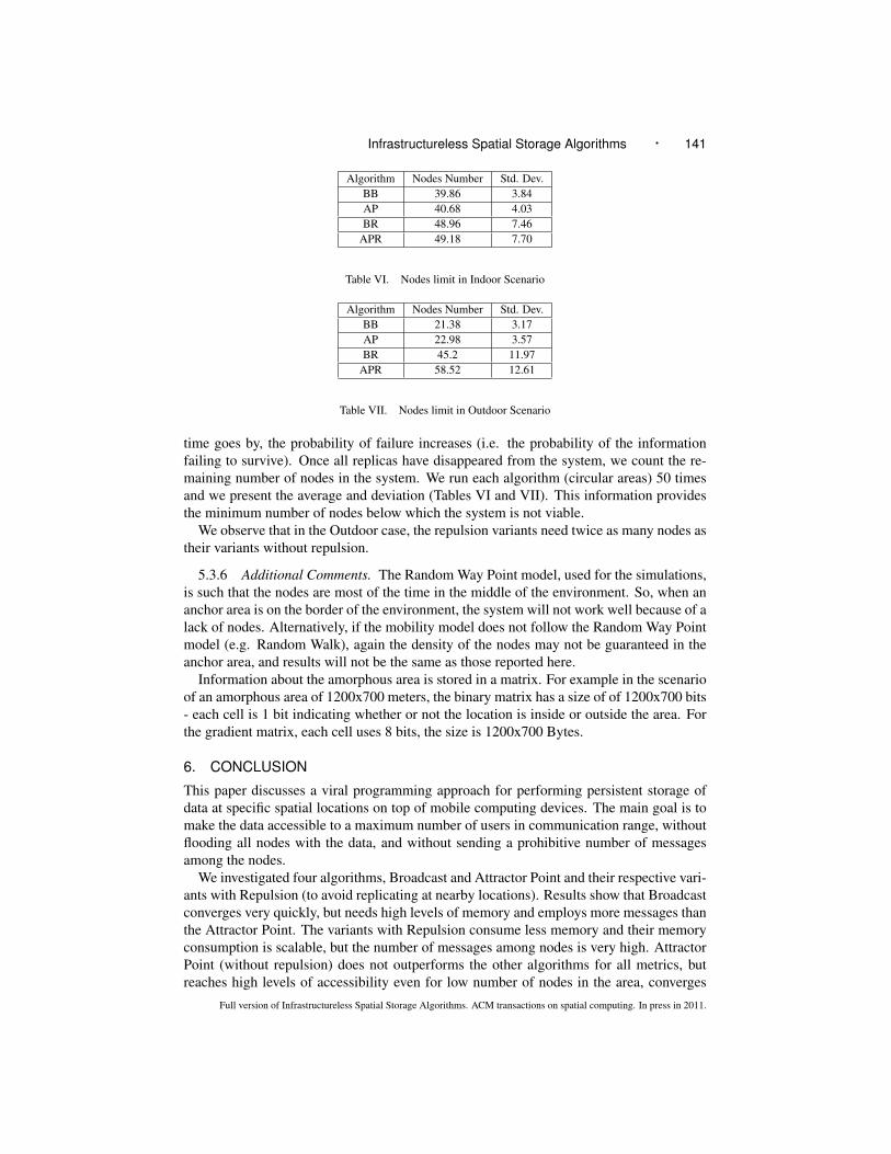
Algorithm Nodes Number Std. Dev.BB 39.86 3.84AP 40.68 4.03BR 48.96 7.46
APR 49.18 7.70
Table VI. Nodes limit in Indoor Scenario
Algorithm Nodes Number Std. Dev.BB 21.38 3.17AP 22.98 3.57BR 45.2 11.97
APR 58.52 12.61
Table VII. Nodes limit in Outdoor Scenario
time goes by, the probability of failure increases (i.e. the probability of the informationfailing to survive). Once all replicas have disappeared from the system, we count the re-maining number of nodes in the system. We run each algorithm (circular areas) 50 timesand we present the average and deviation (Tables VI and VII). This information providesthe minimum number of nodes below which the system is not viable.
We observe that in the Outdoor case, the repulsion variants need twice as many nodes astheir variants without repulsion.
5.3.6 Additional Comments. The Random Way Point model, used for the simulations,is such that the nodes are most of the time in the middle of the environment. So, when ananchor area is on the border of the environment, the system will not work well because of alack of nodes. Alternatively, if the mobility model does not follow the Random Way Pointmodel (e.g. Random Walk), again the density of the nodes may not be guaranteed in theanchor area, and results will not be the same as those reported here.
Information about the amorphous area is stored in a matrix. For example in the scenarioof an amorphous area of 1200x700 meters, the binary matrix has a size of of 1200x700 bits- each cell is 1 bit indicating whether or not the location is inside or outside the area. Forthe gradient matrix, each cell uses 8 bits, the size is 1200x700 Bytes.
6. CONCLUSION
This paper discusses a viral programming approach for performing persistent storage ofdata at specific spatial locations on top of mobile computing devices. The main goal is tomake the data accessible to a maximum number of users in communication range, withoutflooding all nodes with the data, and without sending a prohibitive number of messagesamong the nodes.
We investigated four algorithms, Broadcast and Attractor Point and their respective vari-ants with Repulsion (to avoid replicating at nearby locations). Results show that Broadcastconverges very quickly, but needs high levels of memory and employs more messages thanthe Attractor Point. The variants with Repulsion consume less memory and their memoryconsumption is scalable, but the number of messages among nodes is very high. AttractorPoint (without repulsion) does not outperforms the other algorithms for all metrics, butreaches high levels of accessibility even for low number of nodes in the area, converges
Full version of Infrastructureless Spatial Storage Algorithms. ACM transactions on spatial computing. In press in 2011.

142 · Jose Luis Fernandez Marquez et al.
rather quickly in covering the whole area, employs less messages and slightly more mem-ory than its variant with Repulsion.
Future works concentrate on developing a complete spatial memory concept includingboth storage and retrieval of data following a viral programming model. Actual implemen-tations of the storage algorithms on G1 phones are currently being performed.
Acknowledgments
This work was partially funded by projects EVE (TIN2009-14702-C02-01), IEA (TIN2006-15662-C02-01), and Agreement Technologies (CSD2007-0022), and by the Generalitat deCatalunya under the grant 2009-SGR-1434. The first author holds a FPI scholarship fromthe Spanish Government.
REFERENCES
ABELSON, H., BEAL, J., AND SUSSMAN, G. J. 2007. Amorphous computing. Tech. Rep. MIT-CSAIL-TR-2007-030, Computer Science and Artificial Intelligence Laboratory, MIT. June.
BEAL, J. 2003. Persistent nodes for reliable memory in geographically local networks. Tech. Rep. AI Memo2003-011, Artificial Intelligence Laboratory, MIT. April.
BORCEA, C., INTANAGONWIWAT, C., KANG, P., KREMER, U., AND IFTODE, L. 2004. Spatial programmingusing smart messages: Design and implementation. In Proceedings of ICDCS-2004.
BUTERA, W. 2007. Text display and graphics control on a paintable computer. In SASO ’07: Proceedings ofthe First International Conference on Self-Adaptive and Self-Organizing Systems. IEEE Computer Society,Washington, DC, USA, 45–54.
CHENG, J., CHENG, W., AND NAGPAL, R. 2005. Robust and self-repairing formation control for swarms ofmobile agents. In Proceedings of the Twentieth National Conference on Artificial Intelligence. AAAI Press,Menlo Park, California, 59–64.
CORBET, D. J. AND CUTTING, D. 2006. Ad loc: Location-based infrastructure-free annotation. In ICMU 2006.London, England.
COURTS, L., KILLIJIAN, M.-O., POWELL, D., AND ROY, M. 2005. Sauvegarde cooprative entre pairs pourdispositifs mobiles. In UbiMob ’05: Proceedings of the 2nd French-speaking conference on Mobility anduibquity computing. ACM Press, New York, NY, USA, 97–104.
DATTA, A., QUARTERONI, S., AND ABERER, K. 2004. Autonomous gossiping: A self-organizing epidemicalgorithm for selective information dissemination in mobile ad-hoc networks. In IC-SNW’04, InternationalConference on Semantics of a Networked World. LNCS. 126–143.
DI MARZO SERUGENDO, G., VILLALBA CASTRO, A., AND KONSTANTAS, D. 2007. Dependable requirementsfor hovering information. In Supplemental Volume - The 37th Annual IEEE/IFIP International Conference onDependable Systems and Networks (DSN’07). 36–39.
DOLEV, S., GILBERT, S., LAHIANI, L., LYNCH, N. A., AND NOLTE, T. 2005. Timed virtual stationary au-tomata for mobile networks. In OPODIS. 130–145.
DOLEV, S., GILBERT, S., LYNCH, N. A., SCHILLER, E., SHVARTSMAN, A. A., AND WELCH, J. L. 2004.Virtual mobile nodes for mobile ad hoc networks. In DISC.
DOLEV, S., GILBERT, S., LYNCH, N. A., SHVARTSMAN, A. A., AND WELCH, J. 2003. Geoquorums: Imple-menting atomic memory in mobile ad hoc networks. In DISC.
DOLEV, S., GILBERT, S., SCHILLER, E., SHVARTSMAN, A. A., AND WELCH, J. 2005. Autonomous virtualmobile nodes. In DIALM-POMC ’05: Proceedings of the 2005 joint workshop on Foundations of mobilecomputing. ACM Press, New York, NY, USA, 62–69.
EUGSTER, P., FELBER, P., GUERRAOUI, R., AND KERMARREC, A.-M. 2003. The many faces of pub-lish/subscribe. ACM Computing Surveys 35, 2, 114–131.
EUGSTER, P., GARBINATO, G., AND HOLZER, A. 2005. Location-based publish/subscribe. In Proc. of 4thSymp. on Network Computing and Applications.
EUGSTER, P., GARBINATO, G., HOLZER, A., AND LUO, J. 2009. Effective location-based publish/subscribein manets. In IEEE International Conference on Pervasive Computing and Communications (PerCom’09).
Full version of Infrastructureless Spatial Storage Algorithms. ACM transactions on spatial computing. In press in 2011.

Infrastructureless Spatial Storage Algorithms · 143
FEKETE, S. P., , SCHMIDT, C., WEGENER, A., AND FISCHER, S. 2006. Hovering data clouds for recognizingtraffic jams. In Proceedings 2nd International Symposium on Leveraging Applications of Formal Methods,Verification and Validation (IEEE-ISOLA). 213–218.
FERNANDEZ-MARQUEZ, J. L. AND ARCOS, J. L. 2009. Keeping diversity when exploring dynamic environ-ments. In Proceedings of the 24th Annual ACM Symposium on Applied Computing, D. Shin, Ed. 1192–1196.
KILLIJIAN, M.-O., POWELL, D., BANâTRE, M., COUDERC, P., AND ROUDIER, Y. 2004. Collaborativebackup for dependable mobile applications. In MPAC ’04: Proceedings of the 2nd workshop on Middlewarefor pervasive and ad-hoc computing. ACM Press, New York, NY, USA, 146–149.
LEONTIADIS, I., COSTA, P., AND MASCOLO, C. 2009. Persistent content-based information dissemination inhybrid vehicular networks. In IEEE International Conference on Pervasive Computing and Communications(PerCom’09).
LEONTIADIS, I. AND MASCOLO, C. 2007a. Geopps: Opportunistic geographical routing for vehicular networks.In Proceedings of the IEEE Workshop on Autonomic and Opportunistic Communications. (Colocated withWOWMOM07). IEEE Press, Helsinki, Finland.
LEONTIADIS, I. AND MASCOLO, C. 2007b. Opportunistic spatio-temporal dissemination system for vehicularnetworks. In MobiOpp ’07: Proceedings of the 1st international MobiSys workshop on Mobile opportunisticnetworking. ACM Press, New York, NY, USA, 39–46.
MAIHFER, C. 2004. A survey of geocast routing protocols. In IEEE Communications Surveys and Tutorials.Vol. 6. 32–42.
MAMEI, M. AND ZAMBONELLI, F. 2001. Programming pervasive and mobile computing applications: the totaapproach. ACM Transactions on Software Engineering and Methodology 2, 3 (09).
MAMEI, M. AND ZAMBONELLI, F. 2005. Programming stigmergic coordination with the tota middleware. InAAMAS ’05: Proceedings of the fourth international joint conference on Autonomous agents and multiagentsystems. ACM, New York, NY, USA, 415–422.
MOTANI, M., SRINIVASAN, V., AND NUGGEHALLI, P. S. 2005. Peoplenet: engineering a wireless virtual socialnetwork. In MobiCom ’05: Proceedings of the 11th annual international conference on Mobile computing andnetworking. ACM Press, New York, NY, USA, 243–257.
ROTH, J. 2003. The critical mass problem of mobile ad-hoc networks. In Proceedings of IADIS InternationalConference e-Society. IADIS Press, 243–250.
SCELLATO, S., MASCOLO, C., MUSOLESI, M., AND LATORA, V. 2007. Epcast: Controlled dissemination inhuman-based wireless networks by means of epidemic spreading models. CoRR abs/0711.2780.
VILLALBA CASTRO, A., DI MARZO SERUGENDO, G., AND KONSTANTAS, D. 2008. Hovering information- self-organising information that finds its own storage. In Proceedings of International IEEE Conference onSensor Networks, Ubiquitous and Trustworthy Computing (SUTC’08). 193–200.
VILLALBA CASTRO, A., DI MARZO SERUGENDO, G., AND KONSTANTAS, D. 2009. Hovering information- self-organising information that finds its own storage. In Autonomic Communications, M. K. S. P. W. Vasi-lakos, A.; Parashar, Ed. Springer-Verlag.
WEGENER, A., SCHILLER, E. M., HELLBRCK, H., FEKETE, S. P., AND FISCHER, S. 2006. Hovering dataclouds: A decentralized and self-organizing information system. In International Workshop on Self-OrganizingSystems. 243 – 247.
Full version of Infrastructureless Spatial Storage Algorithms. ACM transactions on spatial computing. In press in 2011.

Infrastructureless Spatial Storage Algorithms · App–1
THIS DOCUMENT IS THE ONLINE-ONLY APPENDIX TO:
Infrastructureless Spatial Storage AlgorithmsJose Luis Fernandez-MarquezArtificial Intelligence Research Institute (IIIA), Spanish National Research Council(CSIC), SpainGiovanna Di Marzo SerugendoBirkbeck College, University of London, UKandJosep Lluis ArcosArtificial Intelligence Research Institute (IIIA), Spanish National Research Council(CSIC), Spain
Full version of Infrastructureless Spatial Storage Algorithms. ACM transactions on spatial computing. In press in 2011., Vol. X, No. Y, 09 2010, Pages
111–0??.
Permission to make digital/hard copy of all or part of this material without fee for personal or classroom useprovided that the copies are not made or distributed for profit or commercial advantage, the ACM copyright/servernotice, the title of the publication, and its date appear, and notice is given that copying is by permission of theACM, Inc. To copy otherwise, to republish, to post on servers, or to redistribute to lists requires prior specificpermission and/or a fee.c© 2010 ACM 1529-3785/2010/0700-0111 $5.00
Full version of Infrastructureless Spatial Storage Algorithms. ACM transactions on spatial computing. In press in 2011.

App–2 · Jose Luis Fernandez Marquez et al.
Broadcast Attractor Point
Broadcast Repulsion Attractor Point Repulsion
Fig. 26. Broadcast, Attractor Point, Broadcast Repulsion and Attractor Point Repulsion
Full version of Infrastructureless Spatial Storage Algorithms. ACM transactions on spatial computing. In press in 2011.

Infrastructureless Spatial Storage Algorithms · App–3
Step 1 (1st simulation second)
Step 2 (122th simulation second)
Step 3 (280th simulation second)
Fig. 27. Attractor Point Repulsion - Convergence - Steps
Full version of Infrastructureless Spatial Storage Algorithms. ACM transactions on spatial computing. In press in 2011.
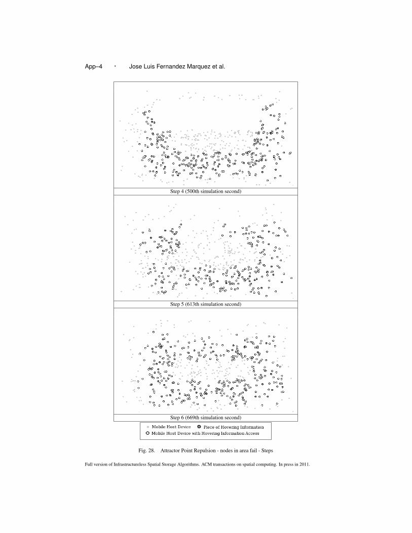
App–4 · Jose Luis Fernandez Marquez et al.
Step 4 (500th simulation second)
Step 5 (613th simulation second)
Step 6 (669th simulation second)
Fig. 28. Attractor Point Repulsion - nodes in area fail - Steps
Full version of Infrastructureless Spatial Storage Algorithms. ACM transactions on spatial computing. In press in 2011.

Infrastructureless Spatial Storage Algorithms · App–5
Step 1 (1th simulation second)
Step 2 (6th simulation second)
Step 3 (18th simulation second)
Fig. 29. Broadcast - convergence - Steps
Full version of Infrastructureless Spatial Storage Algorithms. ACM transactions on spatial computing. In press in 2011.

App–6 · Jose Luis Fernandez Marquez et al.
Step 4 (500th simulation second)
Step 5 (563th simulation second)
Step 6 (605th simulation second)
Fig. 30. Broadcast - Nodes in Area Fail - Steps
Full version of Infrastructureless Spatial Storage Algorithms. ACM transactions on spatial computing. In press in 2011.

Infrastructureless Spatial Storage Algorithms · App–7
Fig. 31. Amorphous Shape 5
Full version of Infrastructureless Spatial Storage Algorithms. ACM transactions on spatial computing. In press in 2011.

App–8 · Jose Luis Fernandez Marquez et al.
Step 1 (1th simulation second)
Step 2 (18th simulation second)
Step 3 (563th simulation second)
Fig. 32. Broadcast Simulation Steps in scenario ’5’
Full version of Infrastructureless Spatial Storage Algorithms. ACM transactions on spatial computing. In press in 2011.

Infrastructureless Spatial Storage Algorithms · App–9
Step 1 (1th simulation second)
Step 2 (50th simulation second)
Step 3 (589th simulation second)
Fig. 33. Broadcast Repulsion Simulation Steps in scenario ’5’
Full version of Infrastructureless Spatial Storage Algorithms. ACM transactions on spatial computing. In press in 2011.