INFRASTRUCTURE AND PRODUCTIVITY IN LATIN AMERICA: IS THERE A RELATIONSHIP IN THE LONG RUN?

CAIO CESAR MUSSOLINI VLADIMIR KUHL TELES

Fevereiro de 2010

TTeexxttooss ppaarraa DDiissccuussssããoo

246

TEXTO PARA DISCUSSÃO 246 • FEVEREIRO DE 2010 • 1

Os artigos dos Textos para Discussão da Escola de Economia de São Paulo da Fundação Getulio Vargas são de inteira responsabilidade dos autores e não refletem necessariamente a opinião da FGV-EESP. É permitida a reprodução total ou parcial dos artigos, desde que creditada a fonte.

Escola de Economia de São Paulo da Fundação Getulio Vargas FGV-EESP

www.fgvsp.br/economia

- 1 -

Infrastructure and productivity in Latin America: Is there a

relationship in the long run?

Vladimir Kühl Teles

Getulio Vargas Foundation

Sao Paulo School of Economics

Caio Mussolini

University of New South Wales

Australian School of Business

ABSTRACT

This article analyses the relationship between infrastructure and total factor productivity (TFP) in

the four major Latin American economies: Argentina, Brazil, Chile and Mexico. We hypothesise

that an increase in infrastructure has an indirect effect on long-term economic growth by raising

productivity. To assess this theory, we use the traditional Johansen methodology for testing the

cointegration between TFP and physical measures of infrastructure stock, such as energy, roads,

and telephones. We then apply the Lütkepohl, Saikkonen and Trenkler Test, which considers a

possible level shift in the series and has better small sample properties, to the same data set and

compare the two tests. The results do not support a robust long-term relationship between the

series; we do not find strong evidence that cuts in infrastructure investment in some Latin

American countries were the main reason for the fall in TFP during the 1970s and 1980s.

Keywords: Infrastructure, economic growth, total factor productivity, structural break

JEL Codes: O54, O23.

- 2 -

1. Introduction

Can investments in infrastructure explain the productivity slowdown in Latin America

during recent decades? Countries such as Argentina, Brazil, and Mexico have shown a

drastic reduction in their total factor productivity (TFP) together with a decrease in

infrastructure since the 1970s. The simultaneity of these two events suggests that

productivity slowdown might be related to the drop in investments in infrastructure. Such

a relationship is similar to the conclusion proposed by Aschauer (1989) in his seminal

article; Aschauer concluded that insufficient investments in infrastructure during the

1970s and 1980s were one of the main causes of productivity slowdown in the United

States. The fact that Chile, which did not decrease its investments in infrastructure, did

not present such a drop in productivity reinforces such reasoning.

As a result of the fiscal adjustments adopted during the 1980s and 1990s in

response to the Debt Crisis, most Latin American countries experienced a significant

reduction in public investment, especially in infrastructure. According to Servén (1997),

public investment (as a proportion of the GDP) dropped approximately 2.5 percentage

points during the 1980s in Latin American countries, whereas in East Asian countries

(which did not adopt fiscal adjustments), it increased by approximately 3.5 percentage

points. As a result, Latin America remained behind in terms of infrastructure expansion

and improvements compared to other developing countries.

Calderón, Easterly, and Servén (2003)1 showed that in Argentina, Brazil, and

Mexico, the reduction of public investments in infrastructure contributed to an increase in

the primary surplus of the GDP ratio (between the periods of 1980-84 and 1995-98) at

average rates of 54 percent, 174 percent, and 32 percent, respectively.2 Thus, in Brazil,

the decrease was larger than the adjustment itself, indicating that there were increases in

expenditures in other sectors of the government.

1 The authors calculate that in 1997, 232 phone lines per thousand workers (median) were installed in Latin

America, whereas in East Asia that figure was 500. As for electric energy, the total installed generating

capacity per worker in East Asian countries increased from 70% (1980) to 165% (1997) in relation to the

capacity of Latin American countries. The transportation sector also showed great discrepancies across

regions, and although Latin America and East Asia had the same amount of paved road mileage per worker,

both regions were still behind the developed countries, which had ten times more paved roads in 1997. 2 We recognise that the privatisation process has also contributed to the decrease in public investments.

- 3 -

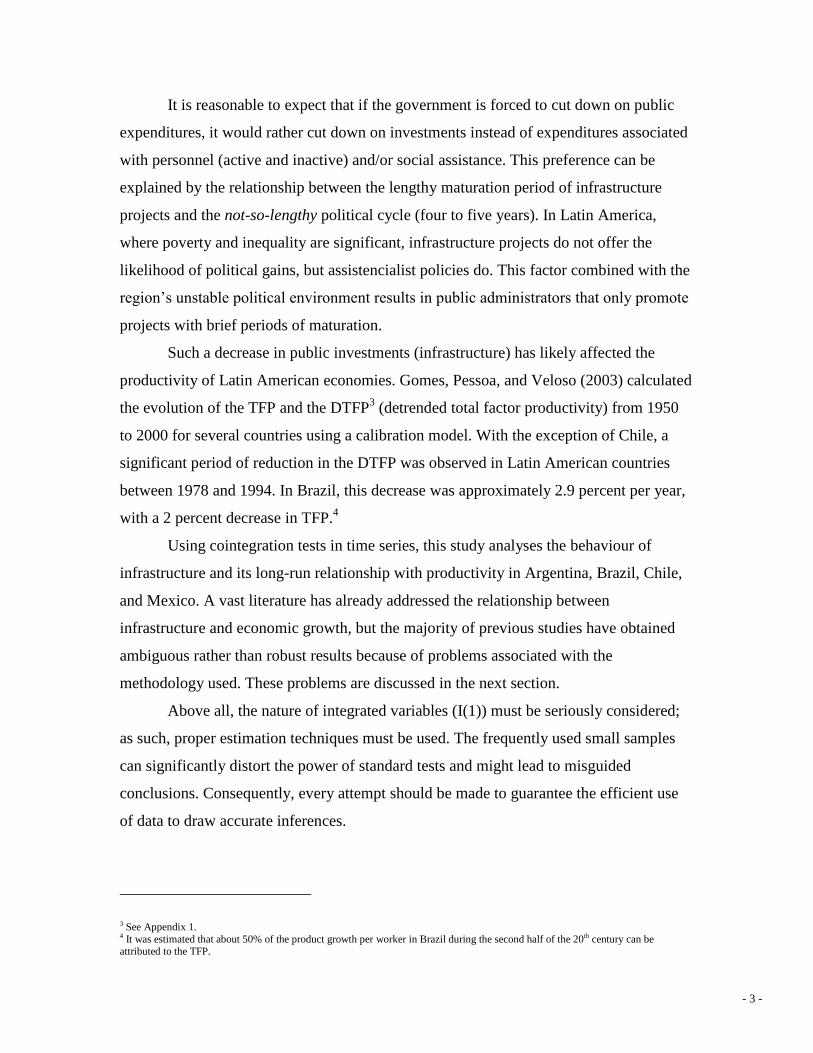
It is reasonable to expect that if the government is forced to cut down on public

expenditures, it would rather cut down on investments instead of expenditures associated

with personnel (active and inactive) and/or social assistance. This preference can be

explained by the relationship between the lengthy maturation period of infrastructure

projects and the not-so-lengthy political cycle (four to five years). In Latin America,

where poverty and inequality are significant, infrastructure projects do not offer the

likelihood of political gains, but assistencialist policies do. This factor combined with the

region’s unstable political environment results in public administrators that only promote

projects with brief periods of maturation.

Such a decrease in public investments (infrastructure) has likely affected the

productivity of Latin American economies. Gomes, Pessoa, and Veloso (2003) calculated

the evolution of the TFP and the DTFP3 (detrended total factor productivity) from 1950

to 2000 for several countries using a calibration model. With the exception of Chile, a

significant period of reduction in the DTFP was observed in Latin American countries

between 1978 and 1994. In Brazil, this decrease was approximately 2.9 percent per year,

with a 2 percent decrease in TFP.4

Using cointegration tests in time series, this study analyses the behaviour of

infrastructure and its long-run relationship with productivity in Argentina, Brazil, Chile,

and Mexico. A vast literature has already addressed the relationship between

infrastructure and economic growth, but the majority of previous studies have obtained

ambiguous rather than robust results because of problems associated with the

methodology used. These problems are discussed in the next section.

Above all, the nature of integrated variables (I(1)) must be seriously considered;

as such, proper estimation techniques must be used. The frequently used small samples

can significantly distort the power of standard tests and might lead to misguided

conclusions. Consequently, every attempt should be made to guarantee the efficient use

of data to draw accurate inferences.

3 See Appendix 1. 4 It was estimated that about 50% of the product growth per worker in Brazil during the second half of the 20th century can be attributed to the TFP.

- 4 -

In using time-series tests, we still face the possibility of structural breaks because

of a likely cointegrated relationship between productivity and infrastructure. Thus, it is

unclear what the estimated models represent. That is, do they represent a structural long-

run equilibrium or a spurious relationship? We believe that the present paper sheds some

light on this issue, which is of utmost importance. In summary, the main purpose of this

paper is threefold:

1. Because of heterogeneity problems, Durlauf (2001) questioned the validity of

previous studies that analyse growth. Within our analysis, we use time-series tests instead

of cross-sectional tests, eliminating potential heterogeneity associated with the data and

with the specificities of each country. Our goal is to offer new research based upon a

greater level of empirical rigor. We also analyse the importance of infrastructure within

the evolution of productivity for each specific case.

2. In addition to the Johansen (1988) test, we use a two-stage cointegration test

that increases the estimation’s efficiency in cases of small samples (like ours).

3. We take into account the fact that the relationship between economic activity

and infrastructure possibly involves structural breaks and can seriously affect the

properties of the test. Leybourne and Newbold (2003) found spurious cointegration

between two independently generated random walks. Using tests from Engle-Granger

(1987), Johansen (1988), and Banerjee et al. (1986) with the simulation of breaks in the

level as well as the slope of the series, Leybourne and Newbold showed that the tests’

inferences are vulnerable. To solve this problem, we use the Lutkepohl, Saikkonen, and

Trenkler (2004) test, which considers an unknown time level shift in the series.

In sum, the present paper addresses the empirical relationship between

infrastructure and economic growth for Argentina, Brazil, Chile and Mexico between

1950 and 2000. Section 2 presents a brief review of the related literature. Section 3

presents the databases used. Sections 4 and 5 describe the econometric techniques and

results. Section 6 concludes the paper.

- 5 -

2. Growth, Productivity, and Infrastructure

Four major issues documented in the literature are relevant to our analysis: the nature of

the relationship, the increments generated by investments, the increase in demand derived

from investment in infrastructure, and the simultaneity bias.

We mentioned that Aschauer (1989) initiated the empirical literature relating

infrastructure and economic growth (productivity). He estimated that the productivity

elasticity in relation to the public capital in the United States was 0.24 for the “core”

infrastructure (i.e., roads and highways, airports, gas and electrical and gas facilities,

mass transportation, sewers and water).

Despite the evidence presented, the methodology used has been called into

question. Based on the unit root Dickey-Fuller test, Tatom (1991) concluded that the

variables from the model developed by Aschauer are non-stationary5, and the first

difference estimation of the production function with public capital leads to an

insignificant coefficient. Therefore, the fact that product and public investment are non-

stationary variables might imply that the relationship obtained by the regressions, based

on data in time series, is spurious.

However, according to Munell (1992), first difference estimations minimise any

long-run relationship (the detection of which is exactly the goal of these models) and

generate implausible and non-significant coefficients for capital and labour. Munell also

noted that the best option would be to test whether variables show a tendency to move

together, i.e., whether they are cointegrated.

A review of the economic growth literature reveals that the perpetual inventory

method for the construction of series of capital is used most often in empirical models. In

addition to the well-known problems of this methodology, Pritchett (2000)6 raised

another important issue; he pointed out that the cost of investment is supposedly equal to

the increment it generates in capital stock. Such equality is expected to prevail in the

private sector, where agents (firms) are a priori considered efficient investors. However,

because of corruption and inefficient use of funds within the public sector, an additional

5 It is worth noting that Tatom’s sample is from 1950 to 1989, which differs slightly from the sample used by Aschauer (1989). The variable log(Y/K) is stationary around the trend whereas the other variables in the model show a stochastic trend. 6 Among the main issues, it is worth noting the following: 1) the value of the initial stock capital, which is often unknown, is

estimated; 2) the choice of the depreciation rate is usually constant along time; and 3) different price indexes are used to deinflate the series of investments. With regard to the last issue, an analysis of the Brazilian case is offered by Ellery Jr. et al. (2005).

- 6 -

dollar’s investment will not necessarily be converted to an additional dollar in capital

stock. Pritchett (2000) argued that this problem is quite persistent in developing

countries, where inefficiency is active in the public sector and the government is the main

investor. That is, the more inefficient the government is (or the larger the public

investment proportional to the total investment), the larger is this distortive effect in the

estimations.

In view of this constraint, Sanchez-Robles (1998) sought to relate physical capital

measures in infrastructure (as opposed to the stock built by the perpetual inventory

method) to the long-run growth rate. Given that these infrastructure measures are deeply

correlated (producing problems of multicollinearity), he constructed an aggregated

infrastructure index through principal component analysis. Based on a sample of 57 Latin

American countries and a sub-sample of 19 of these countries, the infrastructure index for

the period between 1970 and 1985 (derived from an OLS estimation) is significant and

positively correlated with the growth rate of the product per capita.

Another critique of the use of public capital relates to simultaneity bias. Such

investments are endogenous variables given that the increase in productivity (income)

can result in an increase in the demand for infrastructure services, which can lead to a

positive bias in the estimation of returns.

Additionally, several studies have seeksought to identify the relationship between

a specific infrastructure sector and economic growth, addressing solutions to the

simultaneity problem. Fernald (1999) analysed the highway sector and its impact on the

productivity of the US economy. He argued that the construction of highways has an

impact on the productivity of vehicle-intensive industries. That is, there is strong

evidence against the hypothesis of “reverse causation” between infrastructure and

productivity; if such were the case, industries would benefit from road building equally,

independent of the intensity of vehicle usage. Moreover, since productivity slowed down

after 1973 (when the highway network was practically finalised in the US), there is no

reason to believe that the direction of causation runs from TFP to infrastructure

investment. Like Aschauer (1989), he concluded that the US productivity slowdown was

greatly affected by the drop in infrastructure investment. To be precise, the decrease in

- 7 -

road building was responsible for 76 percent of the decrease in the TFP between 1973

and 1989.

Likewise, Röller and Waverman (2001) analysed the impact of the

telecommunications sector on the GDP in the long run while also addressing the problem

of simultaneity bias. The authors used a micro-model in addition to the production

function, which estimates equations of supply and demand for the telecommunication

stock for OCDE countries. They claimed that the size of the country is significant; that is,

there is an important scale effect. Moreover, the authors found that the effect of the

telecommunication stock7 on the product is non-linear, which suggests that the elasticity

is larger in countries where access to these services is universal (considering that each

household has 2.5 habitants on average). This result can be explained by this sector’s

network externalities; i.e., the more people there are who use it, the greater the value

attributed to it by users.

Finally, Calderón and Sérven (2003) estimated the elasticity of the product per

worker (for the period of 1960-1997) in relation to the telecommunication, energy, and

highway sectors for a panel of 101 countries. Based on the difference-GMM model, they

found elasticity between 15 and 17 percent for the three sectors. They also argued that

about a third of the increase in the output gap between the Latin American economies and

the East Asian Tigers8 in the 1980s and 1990s can be attributed to the reduction in the

formation of capital in the infrastructure.

In short, there is room in the literature for a deeper understanding of the

relationship between infrastructure and economic growth (productivity). Specifically,

there is great heterogeneity associated with this relationship among countries, as shown

by Esfahani and Ramírez (2003). Therefore, an estimation strategy specific to each

country is more suitable for the analysis in question. Moreover, there is little evidence to

support the idea that the relationship between infrastructure and productivity is stable in

the long run.9 We attempt to answer the following questions: Is there a long-run

7 The number of phone lines per capita is used as proxy for the telecommunication stock. When this value reaches a “critical mass” of

0.4 the returns are even larger. According to the authors, for a sample of countries outside the OCDE this value is in average 0.04 which suggests that one of the explanations of income divergence among countries could be the sector’s underdevelopment. 8 Hong Kong, Indonesia, Malaysia, Singapore, South Korea, Thailand, and Taiwan. 9 Ferreira and Malliagros (1998) offer evidences for the Brazilian case. However, these authors work with the total stock of infrastructure based on the perpetual inventory method.

- 8 -

relationship between infrastructure and productivity? Does this relationship exist in all

countries? Is this a stable relationship, or is it subject to structural breaks?

3. Database

The main source of data for the infrastructure stock was Canning’s (1998) annual

database of physical measures for a sample of 152 countries between 1950 and 1995. We

used Ferreira and Malliagros`(1998) values for Brazil given their compatibility with

Canning’s database. The series used in the current study are electric generating capacity

(million kilowatts), paved roads (kilometres) and telephones.10

The series for the 1990s were completed using the growth rate of the energy

production series from the World Development Indicators (WDI) and the growth rate in

the number of telephone main lines found by Canning (1998) for electric generating

capacity and telephones, respectively. We carried out a similar procedure for paved roads

using the actual growth rate of paved roads from the WDI. In cases of missing data

between years, linear interpolation was done. The economically active population (EAP)

we used is taken from the Penn World Table 6.1 and the TFP was found by Gomes,

Pessoa, and Veloso (2003).11

The TFP is calculated as a residue in a production function that has physical

(infrastructure and others) and human capital stocks as inputs. One might argue, though,

that the proper way to calculate the impact of infrastructure on productivity would be to

exclude the infrastructure capital from the production function when calculating the TFP.

This approach is not correct for the current study given that an important part of the

output explanation (per worker) would be disregarded as residue, and a positive

correlation between TFP and infrastructure would be created. Therefore, in trying to

detect a long-run relationship between infrastructure and TFP, we are actually trying to

identify the indirect effect of infrastructure on output per worker (via productivity), not

its direct effect, which is (hypothetically) equal to the capital’s share.

10 The telephone main lines are a better alternative; however, this series is smaller than telephones in general. 11 See Appendix 1.

- 9 -

4. Cointegration Tests

Because the variables used are I(1)12

, we can test the possibility of cointegration among

them while estimating their long-run relationship. We use the Johansen procedure to test

for cointegration among those variables.

In this section, the TFP elasticity, related to the physical measures of

infrastructure and normalised by the EAP/1000, is estimated for each of the countries in

the sample. The use of physical measures instead of the stock calculated through

perpetual inventory is more accurate in relation to the issues addressed by Pritchett

(2000). Because of the high correlation found between the series, one infrastructure

measurement is tested at a time, an approach that is commonly adopted in the literature.

4.1 Brazil

Figure 1 shows the evolution of TFP and infrastructure in Brazil between 1950

and 2000. Productivity reached its peak in the 1970s and drastically decreased until the

1990s, when it began to recover. With regard to paved roads, the growth tendency

changed over time and shows an apparent structural break in 1975.13

Most of the

investments in this sector were made before 1975, and the expansion rate of paved roads

was approximately 12.3 percent per year from the beginning of the series until 1974.

The electric energy generating capacity increased to approximately 800,000

kilowatts until 1980, when it stagnated. Araújo and Ferreira (2006) calculated that

between 1960 and 1980, the average annual growth of the total generating capacity was

10.3 percent, whereas that figure decreased to as low as 3.6 percent between 1981 and

2000. Lastly, the telecommunications sector shows a positive relationship in its trajectory

from the second half of the 1970s. Up until the 1970s, approximately 80 telephones per

thousand workers were installed; by 1995, this figures increased to 350. The privatisation

of the telecommunications sector started in 1996, and it is clear that it had a decisive role

in the universalisation of this service.

12 See Appendix 2. 13 Another break is evident in 1999, and both breaks appear to be related to data measurement problems. Araújo and Ferreira (2005) also mention this problem.

- 10 -

Figure 1: Brazil - TFP and Physical Measures of Infrastructure

70

80

90

100

110

120

130

140

50 55 60 65 70 75 80 85 90 95 00

PTF

0.0

0.2

0.4

0.6

0.8

1.0

1.2

50 55 60 65 70 75 80 85 90 95 00

ENE

0.0

0.4

0.8

1.2

1.6

2.0

2.4

2.8

3.2

50 55 60 65 70 75 80 85 90 95 00

ROD

0

100

200

300

400

500

600

700

800

50 55 60 65 70 75 80 85 90 95 00

TEL

Table 1 shows an estimation of the normalised cointegration vector14

and the

eigenvalue and trace statistics. All of the selection criteria15

point toward an estimation of

VAR with one lag in the models for roads and energy, which do not show a residual

autocorrelation. Productivity and electric energy cointegrate – a 1 percent increase in

generating capacity increases the TFP by 0.41 percent in the long run. The impact of

paved roads is smaller, with an elasticity of approximately 0.24. The variables cointegrate

through autovalue, not through trace. The installed phone variable does not show a long-

run relationship with the TFP. This series shows a sharp increase from 1974 onwards,

while productivity decreases dramatically during the same period (see Figure 1).

14 A negative β (cointegration coefficient) implies a positive relationship between variables in the long run. All variables are log

transformed. 15 Final Prediction Error (FPE), Akaike Information Criterion (AIC), Schwarz Information Criterion (SC) and Hannan-Quinn Information Criterion (HQ).

- 11 -

Table 1: Brazil – TFP Elasticity in Relation to Infrastructure

variable β intercept trend Ho trace eigenvalue sample lags

ene -0,413 -4,650 r = 0 38.717* 34.642* 50-00 1

[-5.464] [-63.32] r = 1 4,076 4,076

road -0,242 -4,952 0,015 r = 0 23,184 19.312** 50-00 1

[-3.513] [ 3.685] r = 1 3,872 3,872

tel r = 0 17,167 12,659 50-00 2

r = 1 4,508 4,508

**(*) Rejects Ho at 5%, t statistic in square brackets.

4.2. Argentina

The behaviour of Argentinean productivity is similar to that observed in Brazil.

However, the series presents more eminent cyclical components, which might indicate a

less stable level of activity. There was a drastic drop in TFP during the triennium of

1988/89/90 - a reflection of the severe recession combined with the hyperinflation faced

by the country during those years. The energy generating capacity grew steadily since

1950 and dropped only in the period subsequent to 1988. With the privatisation of this

sector in 1995, however, new investments started to come in. As a result, in 2000, the

generating capacity per thousand workers reached 1.63 million kilowatts. There are no

data for paved roads available from the 1950s, though we can note a significant increase

between the 1960s and 1980s, followed by a substantial drop in the 1990s. Private

concessionaires started to operate the majority of the roads in the country as a

consequence of the privatisation program implemented by the Menem government in

1990; however, no greenfield projects were implemented afterward. As in Brazil, the

number of installed phones showed a continuous increase that has accentuated in 1990

with the privatisation of the state-owned company ENTEL.16

16 After privatisation, ENTEL was further divided into four new companies: Telinter, Startel, Telecom S. A. and Telefônica de Argentina.

- 12 -

Figure 2: Argentina - TFP and Physical Measures of Infrastructure

70

80

90

100

110

120

130

50 55 60 65 70 75 80 85 90 95 00

PTF

0.2

0.4

0.6

0.8

1.0

1.2

1.4

1.6

1.8

50 55 60 65 70 75 80 85 90 95 00

ENE

1.5

2.0

2.5

3.0

3.5

4.0

4.5

5.0

5.5

50 55 60 65 70 75 80 85 90 95 00

ROD

100

200

300

400

500

600

700

800

50 55 60 65 70 75 80 85 90 95 00

TEL

The trace and eigenvalue statistics show that the variables “lene” and “lroad”

cointegrate with the TFP at a significance level of 1 percent. The productivity elasticity in

relation to energy is about 0.12, a low value compared to that of Brazil. A 10 percent

increase in the paved roads measure increased the TFP by approximately 4.2 percent in

the long run (in Brazil, the estimated impact is 2.4 percent). Although the Johansen test

indicates cointegration between installed phones and productivity, the respective

elasticity is not significant.

Table 2: Argentina – TFP Elasticity in Relation to Infrastructure

variable β intercept Trend Ho trace eigenvalue sample lags

ene -0,118 -4,477 r = 0 29.573* 24.762* 50-00 2

[-2.370] [-120.512] r = 1 4,810 4,810

road -0,427 -3,927 r = 0 34.100* 30.080* 61-99 1

[-3.591] [-23.302] r = 1 4,020 4,020

tel -0,115 -4,442 r = 0 28.209* 22.892* 50-00 1

[-0.670] [-4.703] r = 1 5,317 5,317

**(*) Rejects Ho at 5% (1%), t statistic in square brackets.

- 13 -

4.3. Mexico

The total factor productivity for Mexico can be divided into two very distinct

periods (see Figure 3). From 1950 to 1981, the TFP trended toward growth and remained

high throughout the entire period. From 1982 onward, productivity decreased drastically,

with a slight recovery in the second half of the 1990s. This drastic drop is the result of the

Mexican moratorium and the insolvency of many developing countries. On the other

hand, the energy generating capacity experienced growth throughout the entire period

with the exception of 1967, when it experienced a sudden drop, which might be due to

problems with the database.

Figure 3: Mexico - TFP and Infrastructure Physical Measures

90

100

110

120

130

140

150

50 55 60 65 70 75 80 85 90 95 00

PTF

0.0

0.4

0.8

1.2

1.6

2.0

50 55 60 65 70 75 80 85 90 95 00

ENE

1.6

2.0

2.4

2.8

3.2

3.6

50 55 60 65 70 75 80 85 90 95 00

ROD

0

100

200

300

400

500

600

700

50 55 60 65 70 75 80 85 90 95 00

TEL

The telecommunication series also rises over the entire period; in 1994, there

were 511 phones per thousand workers in Mexico. The privatisation of the sector took

place in 1990 with the sale of the state-owned TELMEX. The extension of the paved

roads network increased until 1976, when it reached 3.5 kilometres per thousand workers.

In the following decade, it stabilised at slightly below that figure, then increased slightly

in the 1990s.

- 14 -

Table 3 shows that the three measures of infrastructure cointegrate with TFP. A

VAR with two lags was estimated for electric energy (AIC and FPE), and the obtained

elasticity was 1.38; that is, an increase in this variable more than proportionally increased

productivity in the long run. A 10 percent increase in the extension of roads increased the

TFP in a model with four lags (AIC and FPE) by 8.8 percent. The estimated coefficient

for the number of phones is 0.53 with one lag (SC), but the residues present

autocorrelation in the first lag. There is no cointegration between the variables when a

model with two lags is estimated (indicated by the other criterias).

Table 3: Mexico – TFP Elasticity in Relation to Infrastructure

variable β intercept trend Ho trace eigenvalue sample lags

ene -1,386 -7,258 0,066 r = 0 29.270** 23.344** 50-00 2

[-6.380] [ 6.447] r = 1 5,926 5,926

road -0,878 -4,249 0,014 r = 0 30.392** 23.209** 50-99 4

[-11.36] [ 12.751] r = 1 7,183 7,183

tel -0,538 -3,104 0,039 r = 0 38.092* 28.096* 50-00 1

[-2.652] [ 2.958] r = 1 9,995 9,995

**(*) Rejects Ho at 5% (1%), t statistic in square brackets.

4.4. Chile

Chile is the only country that has not reversed its growth tendency of productivity.

Two drops in the TFP occurred, in 1975 and in the 1980s (probably as a consequence of

external shocks during those periods), followed by a quick recovery. Through the

alternative decomposition of growth, Gomes et al. (2003) calculated that, between 1950

and 2000, the TFP was responsible for 97 percent of the product growth per Chilean

worker.

Similar to the other countries in our analysis, the electric energy sector shows

considerable expansion throughout the period under study. Until the 1990s, the main

state-owned companies were privatised and divided into different companies. As opposed

to the Brazilian case, the entire Chilean energy supply is privately generated, which has

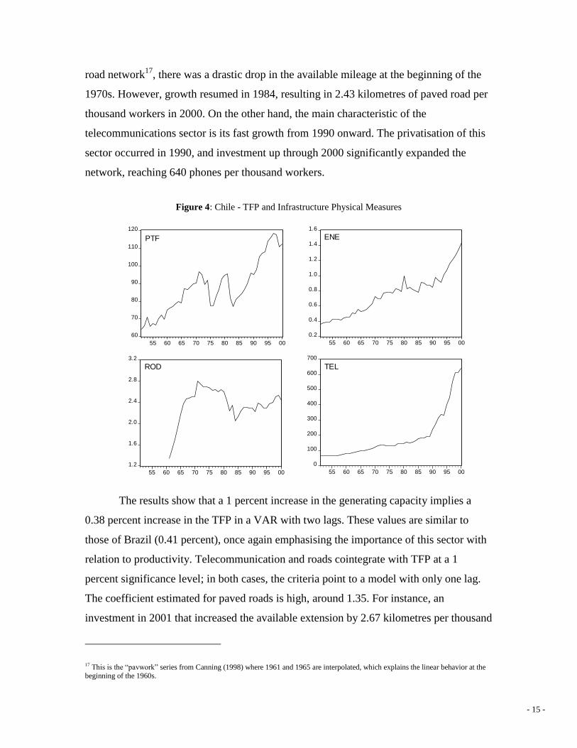
ensured massive investment in the sector. After an elevated period of growth in the paved

- 15 -

road network17

, there was a drastic drop in the available mileage at the beginning of the

1970s. However, growth resumed in 1984, resulting in 2.43 kilometres of paved road per

thousand workers in 2000. On the other hand, the main characteristic of the

telecommunications sector is its fast growth from 1990 onward. The privatisation of this

sector occurred in 1990, and investment up through 2000 significantly expanded the

network, reaching 640 phones per thousand workers.

Figure 4: Chile - TFP and Infrastructure Physical Measures

60

70

80

90

100

110

120

55 60 65 70 75 80 85 90 95 00

PTF

0.2

0.4

0.6

0.8

1.0

1.2

1.4

1.6

55 60 65 70 75 80 85 90 95 00

ENE

1.2

1.6

2.0

2.4

2.8

3.2

55 60 65 70 75 80 85 90 95 00

ROD

0

100

200

300

400

500

600

700

55 60 65 70 75 80 85 90 95 00

TEL

The results show that a 1 percent increase in the generating capacity implies a

0.38 percent increase in the TFP in a VAR with two lags. These values are similar to

those of Brazil (0.41 percent), once again emphasising the importance of this sector with

relation to productivity. Telecommunication and roads cointegrate with TFP at a 1

percent significance level; in both cases, the criteria point to a model with only one lag.

The coefficient estimated for paved roads is high, around 1.35. For instance, an

investment in 2001 that increased the available extension by 2.67 kilometres per thousand

17 This is the “pavwork” series from Canning (1998) where 1961 and 1965 are interpolated, which explains the linear behavior at the beginning of the 1960s.

- 16 -

workers would increase productivity up to 13.5 percent in the long run. The estimated

elasticity of installed phones is actually in opposition to the expected result, but it is not

statistically significant.

Table 4: Chile – TFP Elasticity in Relation to Infrastructure

variable β Intercept trend Ho trace eigenvalue sample lags

ene -0,385 -4,596 r = 0 15.473** 15.138** 51-00 2

[-7.373] r = 1 0,335 0,335

road -1,355 -2,906 -0,015 r = 0 34.641* 30.612* 61-00 1

[-5.480] [-4.653] r = 1 4,029 4,029

tel 0,040 -4,305 r = 0 44.762 36.441 51-00 1

[ 0.462] [-9.900] r = 1 8,321 8,321

**(*) Rejects Ho at 5% (1%), t statistic in square brackets.

5. Cointegration Tests with Structural Breaks

The result of a cointegration test can be modified if a change in the coefficient of

the deterministic components (intercept and trend) is taken into account. As mentioned in

the introduction, Leybourne and Newbold (2003) found spurious cointegration between

two independently generated random walks. Using tests from Engle-Granger (1987),

Johansen (1988), and Banerjee et al. (1986) while simulating breaks in the trend of the

series compromises the inferences of those tests. That is, the hypothesis of non-

cointegration among variables is rejected, implying a Type 1 Error.

In this section, the existence of cointegration among the aforementioned series is

tested, considering a possible structural break at the level of variables. To do so, we use

the cointegration test with endogenous break developed by Lütkepohl, Saikkonen and

Trenkler (2004) (summarised below).

5.1. The Lütkepohl, Saikkonen and Trenkler Test (LST)

Consider the vector ty (n x 1) determined by

tptpttt yAyAdty ...11110 (1)

where td is an intercept dummy, with 0td for t and 1td for t . The date of

the break is assumed unknown, as ][ T , and 10 , in which and

- 17 -

are real numbers arbitrarily next to zero and one respectively, and [.] indicates the

complete part of the argument. Equation (1) represents an unconstrained VAR of order p,

with jA representing a matrix n x n of coefficients and ),0.(..~ diit . The estimator of

is determined by

T

pt

tt

1

'ˆˆdetminarg~

in which tˆ are the residues of (1) estimated by OLS for a given p, chosen through any

selection criteria. The authors show that, in relation to some hypothesis, T/~ is a

consistent estimator of the sample fraction tˆ . Once the date of the break is estimated,

the test follows what Saikkonen and Lütkepohl (2000) have described. First, the series tx̂

is obtained and adjusted for deterministic terms based on

ˆ10ˆˆˆˆ

ttt dtyx

where the parameter vectors ,, 10 are estimated by a Feasible GLS.18

Next,

000 )(:)( rrkrH is tested against 001 )(:)( rrkrH in relation to the adjusted series in

a VECM. The test statistics are determined through the solution of a generalised

eigenvalue problem and given by the LR statistics

n

rj

jrLR1

0

0

)ˆ1log()(

of which the critical values can be found in Saikkonen and Lütkepohl (2000). A great

advantage of this procedure is that, under the null hypothesis, the asymptotic distribution

of the LR statistics is the same when the date of the break is known. Moreover, the

critical values do not depend on the date of the change in level. This does not hold true in

a similar test proposed by Johansen and Nielsen (1993), in which a new table has to be

obtained for every date of the break. Actually, as pointed out by Lütkephol et al. (2003),

in the case of such small samples, Saikkonen and Lütkepohl`s (2000) test is usually more

powerful and contains better properties than the test described by Johansen and Nielsen

(1993). The LST test presupposes the existence of a break in the data generator process;

18 It is worth noting that these parameters are not the same as (1); see the original article for a detailed analysis.

- 18 -

that is, it excludes the possibility of 0 or 1 . According to Perron (2006), however,

once the filter procedure of the series (Feasible GLS) is done, the asymptotic distribution

is not modified.

Table 5: Cointegration Tests with Structural Breaks

Brazil

β Ho LR 10% 5% 1% sample lags

ene -0.477 r = 0 10.14 13.78 15.83 19.85 50-00 2

r = 1 1.97 5.42 6.79 10.04

road -0.38 r = 0 9.38 13.78 15.83 19.85 50-00 2

r = 1 2.27 5.42 6.79 10.04

tel 1.26 r = 0 11.74 13.78 15.83 19.85 50-00 3

r = 1 3.56 5.42 6.79 10.04

Argentina

β Ho LR 10% 5% 1% sample lags

ene -1.102 r = 0 12.76 13.78 15.83 19.85 50-00 2

r = 1 4.65 5.42 6.79 10.04

road -0.011 r = 0 10.58 13.78 15.83 19.85 61-99 2

r = 1 4.35 5.42 6.79 10.04

tel -0.095 r = 0 15.61* 13.78 15.83 19.85 50-00 2

r = 1 4.98 5.42 6.79 10.04

Mexico

β Ho LR 10% 5% 1% sample lags

ene -1.482 r = 0 19.81** 13.78 15.83 19.85 50-00 2

r = 1 4.09 5.42 6.79 10.04

road -0.761 r = 0 14.56* 13.78 15.83 19.85 50-99 4

r = 1 6.26 5.42 6.79 10.04

tel -0.925 r = 0 10.79 13.78 15.83 19.85 50-00 2

r = 1 3.58 5.42 6.79 10.04

Chile

β Ho LR 10% 5% 1% sample lags

ene 1.275 r = 0 12.61 13.78 15.83 19.85 51-95 3

r = 1 4.30 5.42 6.79 10.04

road -3.22 r = 0 18.84** 13.78 15.83 19.85 61-00 2

r = 1 5.33 5.42 6.79 10.04

tel -0.148 r = 0 12.16 13.78 15.83 19.85 51-00 2

r = 1 4.34 5.42 6.79 10.04

(*),(**),(***) Rejects Ho at 10%, 5%, and 1%, respectively.

- 19 -

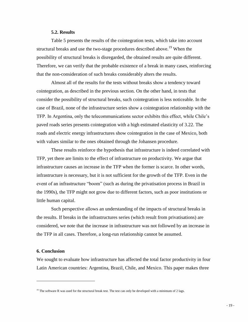
5.2. Results

Table 5 presents the results of the cointegration tests, which take into account

structural breaks and use the two-stage procedures described above.19

When the

possibility of structural breaks is disregarded, the obtained results are quite different.

Therefore, we can verify that the probable existence of a break in many cases, reinforcing

that the non-consideration of such breaks considerably alters the results.

Almost all of the results for the tests without breaks show a tendency toward

cointegration, as described in the previous section. On the other hand, in tests that

consider the possibility of structural breaks, such cointegration is less noticeable. In the

case of Brazil, none of the infrastructure series show a cointegration relationship with the

TFP. In Argentina, only the telecommunications sector exhibits this effect, while Chile’s

paved roads series presents cointegration with a high estimated elasticity of 3.22. The

roads and electric energy infrastructures show cointegration in the case of Mexico, both

with values similar to the ones obtained through the Johansen procedure.

These results reinforce the hypothesis that infrastructure is indeed correlated with

TFP, yet there are limits to the effect of infrastructure on productivity. We argue that

infrastructure causes an increase in the TFP when the former is scarce. In other words,

infrastructure is necessary, but it is not sufficient for the growth of the TFP. Even in the

event of an infrastructure “boom” (such as during the privatisation process in Brazil in

the 1990s), the TFP might not grow due to different factors, such as poor institutions or

little human capital.

Such perspective allows an understanding of the impacts of structural breaks in

the results. If breaks in the infrastructures series (which result from privatisations) are

considered, we note that the increase in infrastructure was not followed by an increase in

the TFP in all cases. Therefore, a long-run relationship cannot be assumed.

6. Conclusion

We sought to evaluate how infrastructure has affected the total factor productivity in four

Latin American countries: Argentina, Brazil, Chile, and Mexico. This paper makes three

19 The software R was used for the structural break test. The test can only be developed with a minimum of 2 lags.

- 20 -

additional contributions to the existing literature. First, the estimations used for the time

series avoid distortions related to the idiosyncrasies of each country. Second, the paper

analyses the relationship between TFP and the physical measures of infrastructure

through a cointegration analysis given the non-stationary nature of the series. Finally, the

two-stage test used here, which was developed by Lutkepohl, Saikkonen and Trenkler

(2004), takes into account structural breaks at levels in the cointegration relationship,

which empowers tests when analysing small samples.

The results from the traditional Johansen test show that there is a clear

cointegration relationship between infrastructure and productivity. However, when a two-

stage test with breaks was conducted, we obtained different results. In some cases, these

results go along with the results obtained with the first test, but in many cases they don`t.

Consequently, we can assume that the infrastructure stock is not sufficient to bring about

sustainable growth in the TFP.

We can assume, then, that although infrastructure is necessary for the growth of

the TFP, it is not enough, which implies an unstable long-run relationship. When other

factors (such as human capital and well-structured institutions) are deficient, the effects

of the increase in infrastructure might not imply an increase in the TFP. Consequently,

the indirect effect of infrastructure on output (via productivity) is not always verified,

although its direct effect (as an input) is of great importance.

- A -

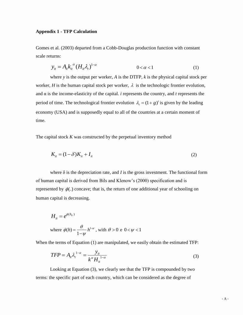
Appendix 1 - TFP Calculation

Gomes et al. (2003) departed from a Cobb-Douglas production function with constant

scale returns:

1)( titititit HkAy 10 (1)

where y is the output per worker, A is the DTFP, k is the physical capital stock per

worker, H is the human capital stock per worker, is the technologic frontier evolution,

and α is the income-elasticity of the capital. i represents the country, and t represents the

period of time. The technological frontier evolution t

t g)1( is given by the leading

economy (USA) and is supposedly equal to all of the countries at a certain moment of

time.

The capital stock K was constructed by the perpetual inventory method

ititit IKK )1( (2)

where δ is the depreciation rate, and I is the gross investment. The functional form

of human capital is derived from Bils and Klenow’s (2000) specification and is

represented by (.) concave; that is, the return of one additional year of schooling on

human capital is decreasing.

)( ith

it eH

where

1

1)( hh , with 0 e 10

When the terms of Equation (1) are manipulated, we easily obtain the estimated TFP:

1

1

it

ittit

Hk

yATFP (3)

Looking at Equation (3), we clearly see that the TFP is compounded by two

terms: the specific part of each country, which can be considered as the degree of

- B -

efficiency of their respective economy ( itA ), and the contribution of the frontier to the

product, considered as the technological progress (

1

it ).

The EAP, GDP and investment series were extracted from the PWT version 6.1,

whereas the education data came from Barro and Lee (2000). The values of the

parameters are: 4,0 ; 0153,0g ; 035,0 ; 32,0 ; 58,0 . The rate of

evolution of the frontier g was calculated based on the product growth per worker of the

USA between 1950 and 1972.20

They did not use the rate of the entire period (1959-

2000) because after the first Oil Shock, the growth of the TFP slowed down, as

mentioned previously. Finally, the TFP series was normalised by the US TFP from 1950.

For example, if the Brazilian TFP was 109 in 1970, this TFP was 9 percent larger than

that of the US TFP from 1950.

20 Gomes et al. (2003) have adjusted the exponential trend of this series corrected by the increase in EAP schooling.

- C -

Appendix 2 - Infrastructure Physical Measures Unit Root Tests21

Brazil Mexico

ADF p value ADF p value

tfp -2.0928 0.2484 tfp -1.95823 0.6093

dtfp -5.5117 0.0000 dtfp -5.28293 0.0001

ene -0.28388 0.989 ene -1.01394 0.7407

dene -3.93881 0.0002 dene -10.4866 0

road -0.27719 0.9893 road -2.58756 0.2875

droad -4.36552 0 droad -2.6309 0.0096

tel -2.14357 0.5086 tel -2.69311 0.2444

dtel -3.84084 0.0048 dtel -3.29621 0.0204

Argentina Chile

ADF p value ADF p value

tfp -2.0003 0.2858 tfp -2.31626 0.4175

dtfp -6.05547 0 dtfp -6.62989 0

ene -0.30767 0.9883 ene -1.77076 0.7033

dene -4.37868 0.001 dene -9.79693 0

road -0.18622 0.9911 road 0.935903 0.9039

droad -4.22789 0.01 droad -4.38511 0.0001

tel -0.39058 0.9853 tel -1.66384 0.7486

dtel -7.93842 0 dtel -4.75618 0.0003

21

d ( ) are first differenced series. All variables are log transformed.

- D -

References

Aschauer, D. 1989. “Is public expenditure productive?” Journal of Monetary

Economics 23: 177-200.

Araújo, C. H. and Ferreira, 2006. “ On the economic and fiscal effects of

infrastructure investment in Brazil.” Ensaios Econômicos EPGE/FGV:

http://epge.fgv.br/pt/ensaios-economicos.

Banerjee, A., Dolado, J. J., Hendry, D. F. and Smith, G. W. 1986. “Exploring

equilibrium relationships in econometrics through static models: Some Monte Carlo

evidence.” Oxford Bulletin of Economics and Statistics 48: 253–77.

Bils, M., and Klenow, P. J. 2000. “Does schooling cause growth?” American

Economic Review 90: 1160-1183.

Calderón, C., Easterly, W. and Servén, L. 2003. “Latin America’s infrastructure

in the era of macroeconomic crises.” In The limits of Stabilization: Infrastructure, Public

Deficits and growth in Latin America. Stanford University Press.

Calderón, C., Servén, L. 2003. “The output cost of Latin America’s infrastructure

gap.” In The limits of Stabilization: Infrastructure , Public Deficits and growth in Latin

America. Stanford University Press.

Canning, D. 1998. “A database of world stocks of infrastructure, 1950-1995.”

World Bank Economic Review 12: 529-547.

Durlauf, S. 2001. “Manifesto for a Growth Econometrics” Journal of

Econometrics, 100: 65-69.

Ellery Jr., R., Ferreira, P. C.; Gomes V. 2005. “Produtividade agregada brasileira

(1970-2000): declínio robusto e fraca recuperação.” Ensaios Econômicos EPGE/FGV:

http://epge.fgv.br/pt/ensaios-economicos.

Engle, R. F. and Granger, C. W.J. (1987). “Cointegration and Error Correction:

Representation, Estimation, and Testing”, Econometrica .55, 251-276.

Esfahani, H.S.; Ramírez M.T. 2003. Institutions, infrastructure, and economic

growth. Journal of Development Economics 70: 443–477.

Fernald, G. 1999. “ Roads to prosperity? Assessing the link between public

capital and productivity.” American Economic Review 89: 619-638.

Ferreira, P. C., and Malliagros, T. 1998. “Impactos produtivos da infra-estrutura

no Brasil- 1950/95.” Pesquisa e Planejamento Econômico 28, n.2: 315-338.

- E -

Gomes, V.; Pessôa S., Veloso, F. 2003 “Evolução da produtividade total dos

fatores na economia brasileira: uma análise comparativa.” Pesquisa e Planejamento

Econômico 33: 389-434.

Johansen, S. 1988. “Statistical Analysis of Cointegration Vectors”, Journal of

Economic Dynamics and Control 12: 231-254.

Johansen, S.1995. Likelihood-based inference in cointegrated vector

autoregressive models. Oxford University Press.

Johansen, S., Nielsen, B., 1993. “ Manual for the simulation program DisCo.”

Institute of Mathematical Statistics, University of Copenhagen:

http://math.ku.dk/~sjo/disco/disco.ps.

Leybourne, S. J., and Newbold, P. 2003.“Spurious rejections by cointegration

tests induced by structural breaks.” Applied Economics 35: 1117-1121.

Lütkephol, H., and Saikkonen, P. 1999. “Order selection in testing for the

cointegrating rank of a VAR process.” In Cointegration, Causality and Forecasting. A

Festschrift in Honour of Clive W. J. Granger. Oxford University Press.

Lütkephol, H., and Saikkonen, P. 2000. “Testing for the cointegration rank of a

VAR process with a time trend.” Journal of Econometric .95: 177-198.

Lütkephol, H., Saikkonen, P., and Trenkler, C. 2003. “Comparition of tests for

the cointegrating rank of a VAR process with structural shift.” Journal of Econometric.

113: 201-229.

Lütkephol, H., Saikkonen, P., and Trenkler, C. 2004. “Testing for the

cointegration rank of a VAR process with level shift at unknown time.” Econometrica

72: 647-662.

Munnel, A. 1992. “Infrastructure investment and economic growth.” Journal of

Economic Perspectives, 6: 189-198.

Perron, P. 2006 "Dealing with structural breaks." In Palgrave Handbook of

Econometrics, Vol. 1: Econometric Theory. Edited by K. Patterson and T.C. Mills.

Palgrave Macmillan: 278-352.

Pritchett, L. 2000. “The tyranny of concepts: CUDIE (cumulated, depreciated,

investment effort) is not capital.” Journal of Economic Growth 5: 361-384.

Röller, L., and Waverman L. 2001. “Telecommunications infrastructure and

economic development: a simultaneous approach.” American Economic Review 91: 909-

923.

- F -

Saikkonen P. e Lütkepohl, H. 2000. “Trend adjustment prior to testing for the

cointegrating rank of a vector autoregressive process.” Journal of Time Series Analysis

21: 435- 456.

Sanchez-Robles, B. 1998. “Infrastructure investment and growth: some empirical

evidence.” Contemporary Economic Policy 6: 98-108.

Servèn, L. 1997.“Uncertainty, instability, and irreversible investment.” World

Bank Policy Research Working Paper 1722. Washington D. C.: 1997

Tatom, J. 1991. “Public capital and private performance.” Review, Federal

Reserve Bank of St. Louis (1991): 3-15.