arX

iv:m

ath-

ph/0

3040

32v3

25

Sep

2003

Infinite Products of Large Random Matrices

and Matrix-valued Diffusion

Ewa Gudowska-Nowaka,b∗, Romuald A. Janikb†,Jerzy Jurkiewiczb‡and Maciej A. Nowaka,b§

a Gesellschaft fur Schwerionenforschung,

Planckstrasse 1,

D-64291 Darmstadt, Germanyb M. Smoluchowski Institute of Physics,

Jagellonian University,

Reymonta 4,

PL 30-059 Krakow, Poland

February 7, 2008

Abstract

We use an extension of the diagrammatic rules in random matrixtheory to evaluate spectral properties of finite and infinite productsof large complex matrices and large hermitian matrices. The infiniteproduct case allows us to define a natural matrix-valued multiplicativediffusion process. In both cases of hermitian and complex matrices,we observe the emergence of a ”topological phase transition”, when ahole develops in the eigenvalue spectrum, after some critical diffusiontime τcrit is reached. In the case of a particular product of two hermi-tian ensembles, we observe also an unusual localization-delocalizationphase transition in the spectrum of the considered ensemble. We verify

∗e-mail: gudowska@th.if.uj.edu.pl†e-mail: ufrjanik@if.uj.edu.pl‡e-mail: jurkiewicz@th.if.uj.edu.pl§e-mail: nowak@th.if.uj.edu.pl

1

the analytical formulas obtained in this work by numerical simulation.

PACS: 05.40.+j; 05.45+b; 05.70.Fh; 11.15.PgKeywords: Non-hermitian random matrix models, Diagrammatic ex-pansion, Products of random matrices.

2

Contents

1 Introduction 3

2 Hermitian Random Ensembles 7

3 Non-hermitian Random Ensembles 10

4 Product of Two Complex Matrices 15

5 Product of Arbitrary Number of Complex Matrices 19

6 Product of Two Hermitian Matrices 24

7 Products of Arbitrary Number of Hermitian Matrices 27

8 Numerical Tests 29

9 Stability and Lyapunov Exponents 33

10 Summary 35

1 Introduction

Applications of random matrix theory (RMT) in physics range from interpre-tation of complex spectra of energy levels in atomic and nuclear physics [1],studies of disordered systems [2, 3], chaotic behavior [4] to quantum grav-ity [5, 6, 7]. Use of progressively developed methods of RMT has also provedto be of particular interest in other sciences such as meteorology [8], imageprocessing [9], population ecology [10] or economy [11, 12].

In this work, we will be concerned with infinite products of random ma-trices (PRM) sampled from general Gaussian ensembles. Products of thattype appear in various branches of physics and interdisciplinary applications[13] where system dynamics is described in terms of evolution operators withrandom coefficients. Perhaps the best known examples are those relatedto thermal properties of disordered magnetic systems, in particular, to thelocalization of electronic wave functions in random potentials [14, 2]. Atten-tion has also been focused on applications of PRM to the analysis of chaoticdynamical systems [13, 15, 16, 17], where stability of trajectories and their

3

sensitive dependence on initial conditions are measured in terms of charac-teristic Lyapunov exponents. Moreover, there are several results exploringthe use of PRM formalism in applied physics and interdisciplinary research,ranging from the studies of stability of large eco- and social- systems [10],adaptive algorithms and the analysis of system performance under the in-fluence of external noises [18] to image compression [19] and communicationvia antenna arrays [20, 21]. However, despite the richness of the potentialapplications, the number of analytical results available in the PRM theory isstill rather limited.

In this paper we develop effective calculational techniques for studyingproducts of random matrices in the largeN limit, and use these tools to derivethe properties of the natural matrix valued generalization of the geometric(multiplicative) diffusion type process. The scalar versions of these processes,leading to log-normal distributions are ubiquitous in various fields [22] andwe expect the matrix valued generalizations to find numerous applications.

Let us briefly review the conventional (scalar) multiplicative (geometric)random walk in one dimension in the presence of some external drift force.The process belongs to the class of (Markovian) Ito diffusion processes, whosestochastic variable s undergoes an evolution

ds

s= µ(s, t)dt+ σ(s, t)dWt (1)

In the above stochastic differential equation (SDE), part of the evolution isdriven by a variable dWt that represents the Wiener process (integral of theGaussian white-noise), respecting

〈dWt〉 = 0⟨

dW 2t

⟩

= dt (2)

For simplicity we will limit ourselves to the constant drift µ and constantvariance σ. Finite time evolution of the system could be viewed as a stringof increments

s(T ) = limM→∞

(1 + µT

M+ σ

√

T

Mx1)(1 + µ

T

M+ σ

√

T

Mx2) . . .

. . . (1 + µT

M+ σ

√

T

MxM )

s(0) (3)

where M stands for the number of steps in the discretization of the timeinterval. After averaging s(T ) over the independent identical distributions

4

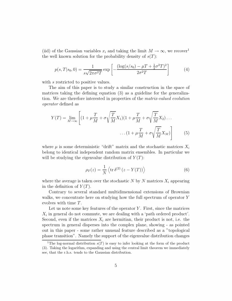
(iid) of the Gaussian variables xi and taking the limit M → ∞, we recover1

the well known solution for the probability density of s(T ):

p(s, T |s0, 0) =1

s√

2πσ2Texp

[

−(log(s/s0) − µT + 12σ2T )2

2σ2T

]

(4)

with s restricted to positive values.The aim of this paper is to study a similar construction in the space of

matrices taking the defining equation (3) as a guideline for the generaliza-tion. We are therefore interested in properties of the matrix-valued evolution

operator defined as

Y (T ) = limM→∞

(1 + µT

M+ σ

√

T

MX1)(1 + µ

T

M+ σ

√

T

MX2) . . .

. . . (1 + µT

M+ σ

√

T

MXM)

(5)

where µ is some deterministic “drift” matrix and the stochastic matrices Xi

belong to identical independent random matrix ensembles. In particular wewill be studying the eigenvalue distribution of Y (T ):

ρT (z) =1

N

⟨

tr δ(2) (z − Y (T ))⟩

(6)

where the average is taken over the stochastic N by N matrices Xi appearingin the definition of Y (T ).

Contrary to several standard multidimensional extensions of Brownianwalks, we concentrate here on studying how the full spectrum of operator Yevolves with time T .

Let us note some key features of the operator Y . First, since the matricesXi in general do not commute, we are dealing with a ‘path ordered product’.Second, even if the matrices Xi are hermitian, their product is not, i.e. thespectrum in general disperses into the complex plane, showing - as pointedout in this paper - some rather unusual feature described as a ”topologicalphase transition”. Namely the support of the eigenvalue distribution changes

1The log-normal distribution s(T ) is easy to infer looking at the form of the product(3). Taking the logarithm, expanding and using the central limit theorem we immediatelysee, that the r.h.s. tends to the Gaussian distribution.

5

from a simply-connected two-dimensional island to a two-dimensional islandwith a hole.

We note that the time evolution of some initial vector |0 > under Y formsa very general setup for several multivariate stochastic evolutions of the type

|τ〉 = Y (τ) |0〉 , (7)

Analytical results for such processes are however scarce. In a recent study,Jackson et al. [23] solved the matrix-valued evolution driven by Gaussiannoise of the type considered above in the case of 2 by 2 hermitian matrices.There are also some known results for the diffusion of the norm of vector |τ〉,since this problem can be linked to the Lyapunov exponents of the hermitianmatrix Y †Y . We briefly comment on this issue in section 9.

The main result of this work is the derivation of exact (finite M) andasymptotic (M → ∞) spectral formulas for the evolution operators Y , in thelimit where the dimension N of Y tends to infinity. For simplicity, we setto zero the deterministic entries µ – although one can easily include themusing our formalism. In this paper we also limit ourselves to ensembles of theGaussian type. Generalizations to non-Gaussian measures (involving finiteand infinite spectral supports) will be investigated elsewhere. We discusshere two cases depending on whether the Xi’s are (i) hermitian Gaussianmatrices (GUE) or (ii) complex (arbitrary) Gaussian matrices (GCE). Similarconstructions could be used for real and quaternionic matrices.

The main motivation for this work is to formulate a new and relativelysimple theoretical framework for studying spectra of the diffusive-like evo-lution operators with their further applications to various branches of thecomplex systems analysis in physics, mathematics and in interdisciplinaryscience.

In particular, the formalism outlined here could be used as a startingpoint for matrix versions of super- or sub-diffusions, generated by e.g. matrixLevy analogs of the stable power-tailed distributions. It will be used also forthe study of spectral statistics of infinite products of unitary operators (e.g.Polyakov lines) [24].

Most of the derivations presented in this paper will be based on diagram-matic methods. In order to make the paper self-contained, in the first twosections we briefly present the formalism, first for hermitian RMM (section 2)and then in section 3, we recall the extension of diagrammatic methods tothe non-hermitian case [27, 28], by using complex Gaussian non-hermitian

6

random matrix model as an example. In section 4 we move to the mainpart of our paper and introduce our method for the treatment of products ofrandom matrices by performing calculations for a product of two matrices.Then (section 5) we move toward the products of M complex matrices, andwe perform the limit M → ∞. We present the final formulas for the spectraldensity and the equations defining the boundary of the two-dimensional sup-port of the eigenvalues. In sections 6 and 7 we consider the case of hermitianmatrices which, surprisingly, is more difficult than the previous one. We an-alyze first (section 6) the product of two matrices. This is interesting on itsown, since it exhibits quite singular behavior – for evolution times smallerthan a certain critical value, the a priori complex eigenvalues are ”frozen”to the real axis. In section 7 we move toward the general case. For prod-ucts of matrices involving more than two hermitian matrices, the eigenvaluesalways form two-dimensional islands. We solve the spectral problem in thelarge M limit. In section 8 we show the numerical analysis, confirming ouranalytical predictions and the existence of “topological phase transitions”,corresponding to structural changes of the spectrum.

Finally, in section 9 we briefly discuss the problems of stability of suchproducts and the relation of our results to the standard Lyapunov exponents.Section 10 concludes the paper.

2 Hermitian Random Ensembles

A key problem in random matrix theories is to find the distribution of eigen-values λi, in the large N (size of the matrix H) limit, i.e

ρ(λ) =1

N

⟨

N∑

i=1

δ(λ− λi)

⟩

(8)

where the averaging 〈. . .〉 is done over the ensemble of N × N random her-mitian matrices generated with probability

P (H) ∝ e−NTrV (H). (9)

The eigenvalues of course lie on the real axis. By introducing the resolvent(Green’s function)

G(z) =1

N

⟨

Tr1

z −H

⟩

. (10)

7

with z = z1N and by using the standard relation

1

λ± iǫ= P.V.

1

λ∓ iπδ(λ) . (11)

the spectral function (8) can be derived from the discontinuities of the Green’sfunction (10)

1

2πilimǫ→0

(G(λ− iǫ) −G(λ+ iǫ)) =1

N〈Tr δ(λ−H)〉

=1

N

⟨

N∑

i=1

δ(λ− λi)

⟩

= ρ(λ) . (12)

There are several ways of calculating Green’s functions for HRMM [1, 7,3]. We will follow the diagrammatic approach introduced by [25]. A startingpoint of the approach is the expression allowing for the reconstruction of theGreen’s function from all the moments 〈TrHn〉,

G(z) =1

N

⟨

Tr1

z−H

⟩

=1

N

⟨

Tr[

1

z+

1

zH

1

z+

1

zH

1

zH

1

z+· · ·

]⟩

=1

N

∑

n

1

zn+1〈TrHn〉 (13)

The reason why the above procedure works correctly for hermitian matrixmodels is the fact that the Green’s function is guaranteed to be holomorphic

in the whole complex plane except at most on one or more 1-dimensional in-tervals. We will use the diagrammatic method to evaluate efficiently the sumof the moments on the right hand side. We will now restrict ourselves to thewell known case of a random hermitian ensemble with Gaussian distribution.

The first step is to introduce a generating function with a matrix-valuedsource J :

Z(J) =∫

dHe−N

2(TrH2)+TrH·J . (14)

where we integrate over all N2 elements of the matrix H . All the momentsfollow directly from Z(J) through the relation

〈TrHn〉 =1

Z(0)Tr

(

∂

∂J

)n

Z(J)∣

∣

∣

J=0(15)

8

1z �ba , b ac d hHabHcdi = 1N �cb�adFigure 1: Large N “Feynman” rules for “quark” and “gluon” propagators.= + + + + : : :Figure 2: Diagrammatic expansion of the Green’s function up to the O(H4)terms.

and are straightforward to calculate, since in the Gaussian case the partitionfunction (14) reads Z(J) = exp 1

2NTrJ2. Accordingly, the lowest nonzero

expectation value is

〈HabH

cd〉 =

∂2Z(J)

∂J ba∂Jdc

|J=0 =1

N

∂JcdZ(J)

∂J ba|J=0 =

1

Nδcbδ

ad . (16)

and the next non-vanishing expectation value reads

〈HabH

cdH

efH

gh〉 =

1

N2

(

δcbδadδgfδ

eh + δahδ

bgδcfδ

de + δafδ

beδchδdg

)

(17)

The key idea in the diagrammatic approach is to associate to the expressionsfor the moments, like the above, a graphical representation following from asimple set of rules. The power of the approach is that it enables to performa resummation of the whole power series (13) through the identification ofthe structure of the relevant graphs.

We depict the “Feynman” rules in Fig. 1, similar to the standard largeN diagrammatics for QCD [26]. The 1/z = 1/zδba in (13) is represented by ahorizontal straight line. The propagator (16) is depicted as a double line.

The diagrammatic expansion of the Green’s function is visualized inFig. 2, where one connects the vertices with the double line propagatorsin all possible ways. Each “propagator” brings a factor of 1/N , and eachloop a factor of δaa = N . From the three terms, corresponding to (17) con-tributing to 〈trH4〉 only the first two are presented in Fig. 2 (the third andthe fourth diagram). The diagram corresponding to the third term in (17)represents a non-planar contribution which is suppressed as 1/N2 and hence

9

� =Figure 3: Schwinger-Dyson equation for rainbow diagrams.

vanishes when N → ∞. In general, only planar graphs survive the large Nlimit.

The resummation of (13) is done by introducing the self-energy Σ com-prising the sum of all one-particle irreducible graphs (rainbow-like). Thenthe Green’s function reads

G(z) =1

z − Σ(z). (18)

In the large N limit the equation for the self energy Σ, follows fromresumming the rainbow-like diagrams of Fig. 2. The resulting equation(“Schwinger-Dyson” equation of Fig. 3) encodes pictorially the structure ofthese graphs and reads

Σ =1

NTrG1 =

N

NG = G. (19)

Equations (18) and (19) give immediately G(z−G) = 1 which can be solvedto yield

G∓(z) =1

2(z ∓

√z2 − 4) (20)

Only the G− is a normalizable solution, with the proper asymptotic behaviorG(z) → 1/z in the z → ∞ limit. From the discontinuity (cut), using (12),we recover Wigner’s semicircle [29] for the distribution of the eigenvalues forhermitian random matrices

ρ(λ) =1

2π

√4 − λ2. (21)

3 Non-hermitian Random Ensembles

The main difficulty in the treatment of non-hermitian random matrix modelsis the fact that now the eigenvalues accumulate in two-dimensional domains

10

in the complex plane and the Green’s function is no longer holomorphic.Therefore the power series expansion (13) no longer captures the full infor-mation about the Green’s function. In particular the eigenvalue distributionis related to the non-analytic (non-holomorphic behaviour of the Green’sfunction:

1

π∂zG(z) = ρ(z) . (22)

This phenomenon can be easily seen even in the the simplest non-hermitianensemble — the Ginibre-Girko one [30, 31], with non-hermitian matrices X,and measure

P (X) = e−NTrXX†

. (23)

It is easy to verify that all moments vanish 〈trXn〉 = 0, for n > 0 so theexpansion (13) gives the Green’s function to be G(z) = 1/z (diagrammati-cally this follows from the fact that the propagator < Xa

bXcd > vanishes and

hence the self-energy Σ = 0). The true answer is, however, different. Onlyfor |z| > 1 one has indeed G(z) = 1/z. For |z| < 1 the Green’s function isnonholomorphic and equals G(z) = z.

In spite of the above difficulties a diagrammatic approach can be usedfor recovering the full information including the eigenvalue density ρ(z). Thefirst step is to define a regularized Green’s function from which one can ex-tract ρ(z). This has been done by exploiting the analogy to two-dimensionalelectrostatics [4, 31, 32]. The resulting regularized Green’s function is how-ever difficult to calculate. The second step is to give an equivalent linearizedform which can form a basis for a diagrammatic calculation [27]. We willnow briefly review the above developments.

Let us define the “electrostatic potential”

F =1

NTr ln[(z −M)(z −M†) + ǫ2] . (24)

Then

limǫ→0

∂2F (z, z)

∂z∂z= lim

ǫ→0

1

N

⟨

Trǫ2

(|z−M|2 +ǫ2)2

⟩

=π

N

⟨

∑

i

δ(2)(z−λi)⟩

≡ πρ(x, y) (25)

11

represents Gauss law, where z = x + iy. The last equality follows from therepresentation of the complex Dirac delta

πδ(2)(z − λi) = limǫ→0

ǫ2

(ǫ2 + |z − λi|2)2(26)

In the spirit of the electrostatic analogy we can define the Green’s functionG(z, z), as an “electric field”

G ≡ ∂F

∂z=

1

Nlimǫ→0

⟨

Trz −X†

(z−X†)(z−X) +ǫ2)

⟩

. (27)

Then Gauss law reads

∂zG = πρ(x, y) (28)

in agreement with (22).As mentioned above, instead of working ab initio with the object (27),

and in view of applying diagrammatic methods it is much more convenientto proceed differently – as we will now discuss.

Following [27] we define the matrix-valued resolvent through

G =1

N

⟨

TrB2

(

z −X iǫiǫ z −X†

)−1⟩

=

=1

N

⟨

TrB2

(

A BC D

)⟩

≡(

G11 G11

G11 G11

)

(29)

with

A =z −X†

(z −X†)(z −X) + ǫ2

B =−iǫ

(z −X)(z−X†) + ǫ2

C =−iǫ

(z −X†)(z −X) + ǫ2

D =z −X

(z −X)(z−X†) + ǫ2(30)

and where we introduced the ‘block trace’ defined as

TrB2

(

A BC D

)

2N×2N

≡(

Tr A Tr BTr C Tr D

)

2×2

. (31)

12

Then, by definition, the upper-right component G11, is equal to the Green’sfunction (27).

The block approach has several advantages. First of all it is linear inthe random matrices X allowing for a simple diagrammatic calculationalprocedure. Let us define 2N by 2N matrices

Z =

(

z iǫ1iǫ1 z

)

, H =

(

X 00 X†

)

. (32)

Then the generalized Green’s function is given formally by the same definitionas the usual Green’s function G,

G =1

N

⟨

TrB21

Z −H

⟩

. (33)

What is more important, also in this case the Green’s function is completelydetermined by the knowledge of all matrix-valued moments

⟨

TrB2 Z−1HZ

−1H . . .Z−1⟩

. (34)

This last observation allows for a diagrammatic interpretation. The Feyn-man rules are analogous to the hermitian ones, only now one has to keeptrack of the block structure of the matrices, e.g. single straight lines willnow be associated with a matrix factor Z−1. We will now demonstrate theabove procedure by solving diagrammatically the complex Gaussian RandomMatrix Model.

Example: the Girko-Ginibre ensemble

The ensemble is defined by the measure

P (X) ∝ e−NTrXX†

. (35)

In this case the double line propagators are

〈XabX

cd〉 = 〈X†a

bX†c

d〉 = 0

〈XabX

†c

d〉 = 〈X†a

bXcd〉 =

1

Nδadδ

bc . (36)

As previously, we introduce the self-energy Σ, (but which is now matrix-valued), in terms of which we get a two by two matrix expression

G = (Z − Σ)−1. (37)

13

where the 2 by 2 matrix Z reads

Z =

(

z iǫiǫ z

)

(38)

The resummation of the rainbow diagrams for Σ is more subtle, but followseasily from the structure of the propagators (36). The analogue of (19) isnow:

Σ ≡(

Σ11 Σ11

Σ11 Σ11

)

=

(

0 G11

G11 0

)

. (39)

The two by two matrix equations (37-39) completely determine the prob-lem of finding the eigenvalue distribution for the Girko-Ginibre ensemble.Inserting (39) into (37) we get:

(

G11 G11

G11 G11

)

=1

|z|2 − G11G11

·(

z G11

G11 z

)

. (40)

Note that at this moment we can safely put to zero the regulators ǫ. Lookingat the off-diagonal equation

G11 =G11

|z|2 − G11G11

(41)

we see that there are two solutions: one with G11 = 0, and another withG11 6= 0. The first one leads to a holomorphic Green’s function, and astraightforward calculation gives

G(z) =1

z. (42)

The second one is nonholomorhic, imposing the condition

|z|2 − b2 = 1 (43)

where we denoted G11G11 ≡ b2, hence

G(z, z) = z (44)

which leads, via the Gauss law, to

ρ(x, y) =1

π

∂

∂zG(z, z) =

1

π. (45)

14

Both solutions match at the boundary b2 = 0 , which in this case reads zz = 1.In such a simple way we recovered the results of Ginibre and Girko for thecomplex non-hermitian ensemble. The eigenvalues are uniformly distributedon the unit disk |z|2 < 1.

This example illustrates more general properties of the matrix valued gen-eralized Green’s function. Each component of the matrix carries importantinformation about the stochastic properties of the system. There are alwaystwo solutions for G11, one holomorphic, another non-holomorphic. The sec-ond one leads, via Gauss law, to the eigenvalue distribution. The shape ofthe “coastline” bordering the “sea” of complex eigenvalues is determined bythe matching conditions for the two solutions, i.e. it is determined by im-posing on the non-holomorphic solution for b2 the equation b2 = 0. For otherimportant features of the explained above diagrammatic method and morecomplex examples see [27, 33].

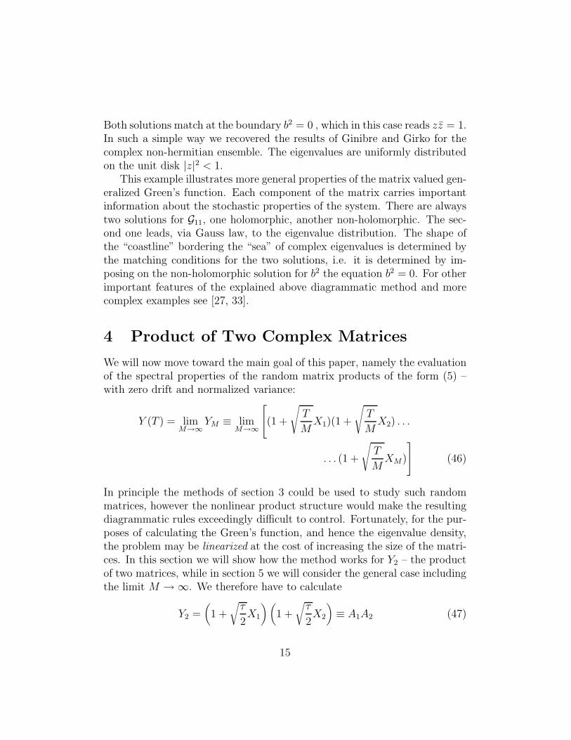
4 Product of Two Complex Matrices

We will now move toward the main goal of this paper, namely the evaluationof the spectral properties of the random matrix products of the form (5) –with zero drift and normalized variance:

Y (T ) = limM→∞

YM ≡ limM→∞

(1 +

√

T

MX1)(1 +

√

T

MX2) . . .

. . . (1 +

√

T

MXM)

(46)

In principle the methods of section 3 could be used to study such randommatrices, however the nonlinear product structure would make the resultingdiagrammatic rules exceedingly difficult to control. Fortunately, for the pur-poses of calculating the Green’s function, and hence the eigenvalue density,the problem may be linearized at the cost of increasing the size of the matri-ces. In this section we will show how the method works for Y2 – the productof two matrices, while in section 5 we will consider the general case includingthe limit M → ∞. We therefore have to calculate

Y2 =(

1 +

√

τ

2X1

)(

1 +

√

τ

2X2

)

≡ A1A2 (47)

15

where X1 and X2 belong to identical independent Gaussian Complex En-sembles (iiGCE=Girko-Ginibre). Since the matrices are non-hermitian wehave to use the formalism of section 3 with a conjugate ‘antiholomorphic’copy. ¿From now on in the rest of the paper we set the regulator ǫ to zero.In order to linearize the product structure we use a trick: we introduce afurther doubling, thus constructing an auxiliary 4N by 4N Green’s function

G(w) =

⟨

w 0 0 00 w 0 00 0 w 00 0 0 w

−

0 A1 0 0A2 0 0 0

0 0 0 A†2

0 0 A†1 0

−1

4N×4N

⟩

=

⟨

w −1 0 0−1 w 0 00 0 w −1

0 0 −1 w

−√

τ

2

0 X1 0 0X2 0 0 0

0 0 0 X†2

0 0 X†1 0

−1

4N×4N

⟩

≡⟨

[

W −√

τ/2X]−1

⟩

(48)

In the above we first separated the “deterministic” part from the “randomone” (second line) and in the last equality we introduced the notation similarto the hermitian and non-hermitian cases analyzed in the previous sections.

In analogy to (31), we define now a block-trace operation trB4, where wetrace each N by N block of the 4N by 4N matrix G(w) separately. In sucha way, we obtain a 4 by 4 auxiliary Green’s function

g(w) ≡

g11 g12 g11 g12

g21 g22 g21 g22

g11 g12 g11 g12

g21 g22 g21 g22

4×4

=1

Ntr B4G(w) (49)

The advantage of this function lies in the fact, that the eigenvalues of theproduct A1A2 coincide with the squares of the eigenvalues of the 2N × 2Nblock matrix

(

0 A1

A2 0

)

(50)

This is due to the off-diagonal structure of the sub-blocks in (50). For ageneral discussion for an arbitrary product see section 5.

16

As before we define a 4 by 4 matrix of self-energies Σij

g(w) = (W − Σ)−1 (51)

where W is the result of block-tracing ’bold’ W .Similarly as in the Girko-Ginibre case, we can now diagrammatically an-

alyze the content of the matrix Σ. We see that only the “double line” prop-agators

⟨

X1X†1

⟩

X1

and⟨

X2X†2

⟩

X2

are different from zero. Therefore from

all of the 16 elements of matrix Σ only four are nonzero. Moreover, due toidentical measures of X1 and X2 variables, we get

Σ11 = Σ22 = αg11 = αg22

Σ11 = Σ22 = αg11 = αg22 (52)

where the factor α = τ/2 comes from the propagator in the correspondingSchwinger-Dyson equation of the type discussed in the previous chapter.

Filling the matrix Σ with entries (52) we arrive at the 4 by 4 matrixequation for the elements of the Green’s function:

g11 g12 g11 g12

g21 g22 g21 g22

g11 g12 g11 g12

g21 g22 g21 g22

4×4

=

w −1 0 0−1 w 0 00 0 w −1

0 0 −1 w

−

−

0 0 αg11 00 0 0 αg11

αg11 0 0 00 αg11 0 0

−1

(53)

As in the Ginibre case, we solve it for g11 and g11. Then, using thesolution, we calculate g11. Coming back to original variables with w2 = z weset G(z, z) = g11(w). The eigenvalue distribution then follows from

ρ(x, y) =1

π

w

z∂zG(z, z) (54)

This is a consequence of the relation between the eigenvalues of the blockmatrix (50) and the eigenvalues of the product A1A2. A general derivationis outlined in the following section.

A little algebra (basically an inversion of the 4 by 4 matrix) shows, that, asbefore, we get two solutions for b2 = g11g11= g22g22: (i) the holomorphic one

17

-2 -1 1 2 3 4 5

-4

-2

2

4

Figure 4: Evolution of the contour of the non-holomorphic domain in theeigenvalue spectrum of the product of two Ginibre-Girko ensembles as afunction of evolution times τ = 0.1, 0.25, 0.5, 1, 1.5, 2, 3, 4, 5, 6, rising frominside to outside.

(corresponding to b2 = 0, i.e. all Σij equal to zero); (ii) the non-holomorphicone, given by the equation

τ

2

(

|w|2 − α2b2 + 1)

= (α2b2 − 1 + w2)(α2b2 − 1 + w2) − α2b2(w + w)2 (55)

The boundary of the eigenvalue support is given, as before, by the aboveequation with b2 set to 0. It is therefore a fourth order conchoid-like planarcurve, which in polar coordinates is given by

τ

2(1 + r) = r2 + 1 − 2r cosφ (56)

On Fig. 4 we show the shape of the nonholomorphic island for severalsample “evolution times” τ .

The Green’s function for the product follows from

g11(w) =w(w2 − 1) − α2b2w

det(57)

wheredet = (α2b2 − 1 + w2)(α2b2 − 1 + w2) − α2b2(w + w)2 (58)

18

5 Product of Arbitrary Number of Complex

Matrices

We consider now the product of an arbitrary number of matrices. To see thepattern, let us look briefly at the case of three matrices

Y3 =(

1 +

√

τ

3X1

)(

1 +

√

τ

3X2

)(

1 +

√

τ

3X3

)

≡ A1A2A3 (59)

where X1, X2, X2 again belong to the Girko-Ginibre ensemble.Our approach again follows from a very simple exact relation between the

eigenvalues of a product of N × N matrices A1A2A3 and the eigenvalues ofa block matrix

B3 =

0 A1 00 0 A2

A3 0 0

3N×3N

(60)

Indeed if {λi} are the eigenvalues of A1A2A3 then the eigenvalues of the block

matrix are {λ1/3i , λ

1/3i · e 2πi

3 , λ1/3i · e 4πi

3 }. This is an exact relation for any Nand follows from the relation between the resolvents (here the matrices Aiare of finite size and fixed i.e. no averaging)

GB3(w) =

1

3Ntr

1

w − B3GA1A2A3

(z) =1

Ntr

1

z − A1A2A3(61)

namelywGB3

(w) = zGA1A2A3(w3 ≡ z) (62)

This is due to the cyclic structure of the block matrix (60). Obviously, onlymultiplicities of the cubic powers of B3 contribute to the trace.

The relation between the eigenvalues now follows from the location of thefinite number of poles of both functions.

We can thus safely calculate the eigenvalue density for the block matrixB3 using the diagrammatic methods and then extract the density for theproduct through

ρA1A2...AM(z, z) =

1

π∂zGA1A2...AM

=1

M

ww

zzρBM

(w, w) (63)

where M = 3 and wM = z and ρBM(w, w) = 1

π∂wGB(w, w).

19

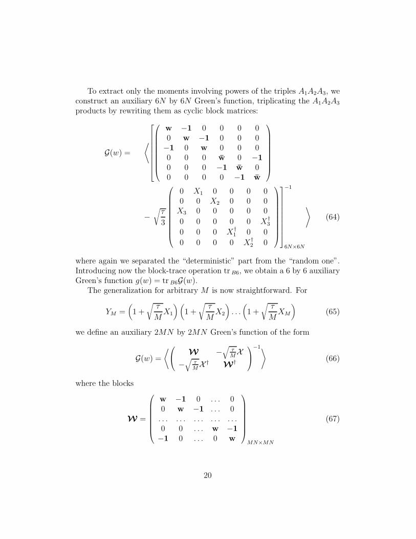
To extract only the moments involving powers of the triples A1A2A3, weconstruct an auxiliary 6N by 6N Green’s function, triplicating the A1A2A3

products by rewriting them as cyclic block matrices:

G(w) =

⟨

w −1 0 0 0 00 w −1 0 0 0−1 0 w 0 0 00 0 0 w 0 −1

0 0 0 −1 w 00 0 0 0 −1 w

−√

τ

3

0 X1 0 0 0 00 0 X2 0 0 0X3 0 0 0 0 0

0 0 0 0 0 X†3

0 0 0 X†1 0 0

0 0 0 0 X†2 0

−1

6N×6N

⟩

(64)

where again we separated the “deterministic” part from the “random one”.Introducing now the block-trace operation trB6, we obtain a 6 by 6 auxiliaryGreen’s function g(w) = tr B6G(w).

The generalization for arbitrary M is now straightforward. For

YM =(

1 +

√

τ

MX1

)(

1 +

√

τ

MX2

)

. . .(

1 +

√

τ

MXM

)

(65)

we define an auxiliary 2MN by 2MN Green’s function of the form

G(w) =

⟨

W −√

τMX

−√

τMX † W

†

−1⟩

(66)

where the blocks

W =

w −1 0 . . . 00 w −1 . . . 0. . . . . . . . . . . . . . .0 0 . . . w −1

−1 0 . . . 0 w

MN×MN

(67)

20

and

X =

0 X1 0 . . . 00 0 X2 . . . 0. . . . . . . . . . . . . . .0 0 . . . 0 XM−1

XM 0 . . . 0 0

MN×MN

(68)

are themselves NM by NM matrices, i.e. each of the listed elements in W

and in X is itself an N by N matrix, either diagonal, denoted by a boldsymbol, or a random entry Xi, otherwise an N by N block of zeroes.

We take now a block-trace operation tr BM , where we trace each N byN block of the 2MN by 2MN matrix G(w) separately. In such a way, weobtain an 2M by 2M auxiliary Green’s function

g(w) ≡

g11 . . . g1M g11 . . . g1M...

. . ....

.... . .

...gM1 . . . gMM gM 1 . . . gMM

g11 . . . g1M g11 . . . g1M...

. . ....

.... . .

...gM1 . . . gMM gM 1 . . . gMM

2M×2M

=1

NTrBMG(w) (69)

As before we define a 2M by 2M matrix of self-energies Σij

g(w) =

[(

W 00 W†

)

− Σ

]−1

(70)

where W is a result of block-tracing W. We can now diagrammaticallyanalyze the content of the matrix Σ. As previously, only “double line” prop-agators

⟨

XiX†i

⟩

Xi

for i = 1, . . . ,M are different from zero. Therefore from

all of the 4M2 elements of the matrix Σ only 2M are different from zero.Due to the symmetries we get

Σ11 = . . . = ΣMM = αg11 = αgMM ≡ αg

Σ11 = . . . = ΣMM = αg11 = αg1M ≡ αg (71)

where the factor α = τ/M comes from the propagator in the correspondingset of Schwinger-Dyson equations as in the previous chapter.

21

Inserting now the matrix Σ with entries (71) we arrive at a 2M by 2Mmatrix equation for the elements of the Green’s function. First, we solve itfor g and g. Second, using the solutions, we calculate g11. Third, using (63)we get an explicit equation for the spectral density

ρ(x, y) =1

π

1

M

ww

zz∂wg11(w, w) (72)

where z = x + iy. For arbitrary M , the algebra is rather involved. Luckily,both the block and the cyclic structure of the main entries W and Σ maketaking an inverse of the 2M by 2M matrix possible. The inverse of a cyclicmatrix is a cyclic matrix, and its explicit form can be obtained from thesolution of an associated recurrence relation, e.g. using the transfer matrixtechniques which we will now proceed to do.

At this moment, it is useful to introduce the notation

1 + |w|2 − α2b2 = 2|w| coshu

|w|/w = δ (73)

The inversion needed for the Green’s function reduces to finding explicitforms of the cyclic M by M matrices C, C defined as

C = [W ·W† − α2b21]−1 C = [W† · W − α2b21]−1 (74)

where b2 = gg. C is just the transpose, or equivalently, the complex conjugateof C. The elements c0, . . . cM−1 of the first row of the cyclic matrix C fulfillthe recurrence relation

(

ck+1

ck

)

=

(

2δ cosh u −δ2

1 0

)(

ckck−1

)

(75)

with the ‘boundary conditions’(

c1c0

)

=

(

2δ cosh u −δ2

1 0

)(

cMcM−1

)

− 1

w

(

10

)

(76)

The above recurrence can be easily solved using transfer matrix techniques,i.e. by diagonalizing the 2 by 2 transfer matrix in (75) and returning atthe end of the calculations to the original basis. An explicit solution for thecyclic string ck, for k = 0, 1, .., .M − 1 reads

ck =1

w(Λ+ − Λ−)

(

Λk+

ΛM+ − 1

− Λk−

ΛM− − 1

)

(77)

22

where Λ± = δe±u denote the eigenvalues of the transfer matrix.We may now express our key quantities for arbitrary M in terms of (77):

g11(w) = [W† · C]11 ≡ w · c0 − c∗M−1

g = αg[C]11 ≡ αg · c∗0g = αg[C]11 ≡ αg · c0 (78)

where ∗ denotes complex conjugation. As always in the case of the complexspectra, we have two solutions: trivial (holomorphic), corresponding to g =g = 0, and the nontrivial (non-holomorphic), corresponding to the case b2 ≡gg 6= 0.

Inserting the nonholomorphic solution into g11, redefining G(z, z) = g11(w)with wM = z, and using (63) yields the eigenvalue density for YM . Since∂wz = Mz/w, the result for the final spectral function can be further simpli-fied

ρ(x, y) =1

π

w

z∂zG(z, z) (79)

Explicit formulas for arbitrary M could be easily constructed e.g. byrunning any symbolic program using our solution. The shape of the bound-ary is given by the condition that the nonholomorphic solution meets theholomorphic one on the complex plane.

After solving the problem for arbitrary M , we can now address the orig-inal problem, i.e. the solution for a continuous product of matrices, corre-sponding to the limitM → ∞. This means, that we have to perform a carefullimiting procedure in the above formulas. Introducing U = Mu, expandingin M , and using the polar parametrization z = r exp iφ, we get the solution

G(z, z) =1

τlog r +

1

2− iU

τ

sin φ

sinhU(80)

where U =√

log2 r − τ 2b2 with b2 fulfilling the equation

cosφ = coshU − τ

2UsinhU (81)

The set of equations (80,81) completes the solution of the continuous productof large complex matrices with Gaussian disorder. We would like to note,

23

that due to the limiting procedure M → ∞ differentiation of the Green’sfunctions has to be done with care. Taking the large M limit of (79) yields

ρ(x, y) =1

π

1

z∂zG(z, z) (82)

As a cross-check of our calculations we verified that the spectral functionobtained in this way is real.

Substituting b2 = 0 in (81), we get the equation for the shape of the sup-port of the eigenvalues for arbitrary τ . Note that the shape of the boundarydepends on the variable log |z|, reflecting in the spectrum the multiplicative(geometric) feature of the stochastic process induced by the multiplicationof random matrices. Explicit solution for the boundary reads

τ

2

(

r2 − 1

ln r

)

= r2 + 1 − 2r cosφ (83)

It is rewarding to compare solution (83) to the solution of the conchoid-likeboundary in the case of two complex matrices (56). In the limit of infinitelymany products, the shape of the boundary acquires a new symmetry – (83) isinvariant under inversion operation r → 1/r. It is visible also from the gen-eral form (81), since the radial dependence for b2 = 0 is a function of | log r|only. This symmetry is responsible for the appearance of a structural changeof the spectrum – provided τ is sufficiently large, two boundaries, related byinversion in the radial variable, appear. We describe this structural change ofthe complex spectrum as a ”topological phase transition”. In Section 8, westudy numerically the spectral density predicted by our formulas, in partic-ular, the “diffusion” of the shape of the boundary caused by evolution withthe “time” parameter τ . We also confirm numerically the critical behaviorfor certain τcrit.

6 Product of Two Hermitian Matrices

In this section we will consider the spectral distribution of the product

Y2 =(

1 +

√

τ

2H1

)(

1 +

√

τ

2H2

)

(84)

where H1, H2 are not arbitrary complex matrices, but they are identical in-dependent hermitian Gaussian matrices (iiGUE). Contrary to naive expec-tations, the above problem is more subtle then the analogous problem of the

24

two complex Gaussian matrices. First, let us note, that the product of twohermitian matrices is not, in general, a hermitian matrix, so the spectrumof the strings of hermitian matrices develops complex eigenvalues.

Second, the case of only two hermitian matrices of the considered typeturns out to be in some sense singular – for certain values of the evolutionparameter τ , the a priori complex eigenvalues get localized on the real axis.This phenomenon reminds a bit the non-hermitian localization in the Hatano-Nelson model [38]. Third, the problem is algebraically more involved sincethere will be more nonzero propagators than in the complex case.

Since even a product of two hermitian matrices can develop a priori acomplex spectrum, we have to use the same type of auxiliary Green’s func-tion as in the complex Gaussian case. The construction parallels exactly thescheme for two complex matrices considered previously, with the matrices Xi

and X†i replaced both by Hi. The first new feature appears when we con-

struct the “Schwinger-Dyson” equations for the 4 by 4 self-energy matrix Σ.Since the matrices are hermitian (Hi = H†

i ), additional nonzero contractionsappear in the matrix Σ

Σ = α

0 g12 g11 0g21 0 0 g22

g11 0 0 g12

0 g22 g21 0

≡ α

0 h g 0h 0 0 g

g 0 0 h

0 g h 0

(85)

where again the factor α = τ/2 comes from the propagator, h and h arethe new entries and we have exploited the symmetries of the problem (e.g.g11 = g22 etc).

The solution of the 4 by 4 matrix equation for the 4 by 4 Green’s function

G(w) = (W − Σ)−1 (86)

is more involved, since we have to solve it not only for the “gaps” g and g butalso for additional gaps h and h. Only then we can calculate g11, to recoverthe wanted eigenvalue distribution in the same way as in the complex case(54).

Introducing d2 = (1 + αh)(1 + αh) and b2 = gg, we obtain two (modulotheir tilded partners) gap equations

g = −αg

det(α2b2 − |w|2 − d2)

h =1

det(α2b2(1 + αh) + (1 + αh)(w2 − (1 + αh)2) (87)

25

0.5 1 1.5 2

-1

-0.5

0.5

1

0.5 1 1.5 2 2.5

-1

-0.5

0.5

1

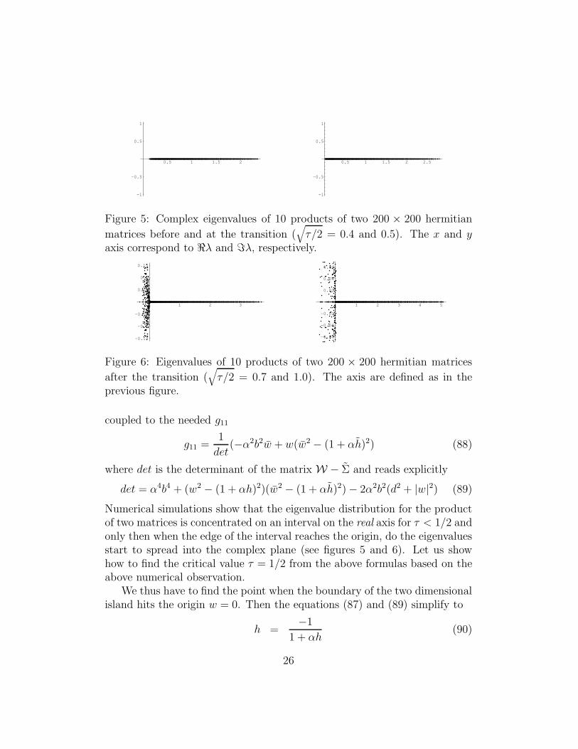
Figure 5: Complex eigenvalues of 10 products of two 200 × 200 hermitian

matrices before and at the transition (√

τ/2 = 0.4 and 0.5). The x and yaxis correspond to ℜλ and ℑλ, respectively.

1 2 3

-0.15

-0.1

-0.05

0.05

0.1

0.15

1 2 3 4 5

-0.06

-0.04

-0.02

0.02

0.04

0.06

Figure 6: Eigenvalues of 10 products of two 200 × 200 hermitian matrices

after the transition (√

τ/2 = 0.7 and 1.0). The axis are defined as in theprevious figure.

coupled to the needed g11

g11 =1

det(−α2b2w + w(w2 − (1 + αh)2) (88)

where det is the determinant of the matrix W − Σ and reads explicitly

det = α4b4 + (w2 − (1 + αh)2)(w2 − (1 + αh)2) − 2α2b2(d2 + |w|2) (89)

Numerical simulations show that the eigenvalue distribution for the productof two matrices is concentrated on an interval on the real axis for τ < 1/2 andonly then when the edge of the interval reaches the origin, do the eigenvaluesstart to spread into the complex plane (see figures 5 and 6). Let us showhow to find the critical value τ = 1/2 from the above formulas based on theabove numerical observation.

We thus have to find the point when the boundary of the two dimensionalisland hits the origin w = 0. Then the equations (87) and (89) simplify to

h =−1

1 + αh(90)

26

1 = αhh (91)

where we set b2 = gg = 0. Then it is easy to verify that this set of equationsis satisfied for α = 1/4 which is equivalent to τ = 1/2.

7 Products of Arbitrary Number of Hermi-

tian Matrices

Finally, we consider an arbitrary number of matrices belonging to iiGUE.

YM =(

1 +

√

τ

MH1

)(

1 +

√

τ

MH2

)

. . .(

1 +

√

τ

MHM

)

(92)

As before, the construction of the auxiliary Green’s function parallels thecomplex case, up to the point when we have to construct explicitly the ma-trix of self-energies Σ, corresponding to the set of 4M2 Schwinger-Dysonequations. Generalization of the results from the previous sections leads tothe explicit form of the auxiliary Green’s function. Introducing

G(w) =

(

W SS W†

)−1

(93)

with blocks

W =

w −1 − αh 0 . . . 00 w −1 − αh . . . 0. . . . . . . . . . . . . . .0 0 . . . w −1 − αh

−1 − αh 0 . . . 0 w

M×M

(94)

and

S = −α

g 0 0 . . . 00 g 0 . . . 0. . . . . . . . . . . . . . .0 0 . . . g 00 0 . . . 0 g

M×M

(95)

27

the consistent set of equations comes as

g11 = G1,1

h = G1,M

h = GM+1,M+2

g = G1,M+1

g = GM+1,1 (96)

i.e. requires an explicit inversion of the 2M by 2M matrix. The algebra ismore complicated since, like in the case of two hermitian matrices, we havenow two types of gap equations (for g and h and their tilded partners). Usingthe solutions, we calculate g11, then, we get an explicit equation for the spec-tral density (63). Finally, we perform the limiting procedure. Technically,one has to repeat the transfer matrix technique introduced in section 5 forthe complex case. The algebra is lengthy, but due to the cyclic nature ofthe blocks of matrix R the results form a rather surprisingly simple set ofequations. Returning to the original variable z = r exp(iφ) we get

G(z, z) =1

2τlog r +

3

4− iU

τsinψ/ sinhU (97)

and the gap equations read

h =1

2τlog r − 1

4− iU

τsinψ/ sinhU = G− 1 (98)

and

cosψ = coshU − τ

2UsinhU (99)

where ψ = φ + U sinψsinhU

and U =√

( log r2

+ τ/4)2 − τ 2gg. The above set ofequations completes the solution of the continuous product of matrices withGaussian hermitian disorder. Spectral density follows from (82). Note, thatthe dependence on log |z| reflects the multiplicative character of the Brown-ian motion. Again, the boundary has also an inversion-type symmetry, butnow it is of the form |z| → exp(−τ)/|z|. Due to the non-zero gap h, theboundary in the hermitian case is given by the pair of coupled transcenden-tal equations and can be presented numerically only. The appearance of the

28

aforementioned symmetry is responsible for the ”topological phase transi-tion” in the spectrum of the product of infinitely many matrices, similar tothe one observed for the product of infinitely many complex matrices.

In Section 8, we study numerically the spectral density predicted by ourformulas, in particular, the “diffusion” of the shape of the boundary causedby evolution with the “time” parameter τ . We confirm the appearance of a“phase transition” for certain τcrit in the hermitian case as well.

8 Numerical Tests

In this section we present the results of numerical simulations, confirm-ing our analytical predictions. We start from the complex case. Figure 7shows the evolution of the boundary for several sample evolution timesτ = 0.5, 1, 1.5, 2, 3, 4, 5, 6, 8, 12. To present the whole set of the boundarieson the same figure, each boundary is rescaled by a corresponding factorexp(−τ/2). We would like to note here that the effect of rescaling is equiv-alent to the non-rescaled process with drift µ = 1. One can see how theoriginal ellipse-like shape (innermost figure) evolves through a twisted-likeshape to the set of double-ring structures. The inner ring, always containingthe origin, is so small on the scale of the Fig. 7 that is not visible. At τ = 4,corresponding to the curve with an inner loop, we observe a topological phasetransition. The support of the spectrum is no longer simply connected, forτ ≥ 4 it is annulus-like, i.e. eigenvalues are expelled from the central region.For even larger times, the outside rim of the annulus approaches the circle,and the inner one shrinks to the point z = 0 in the τ = ∞ limit. Indeed forlarge τ the radius of the inner ring behaves like

r(τ) ∼ e−τ

2 (100)

The outer boundary then forms approximately a circle with the radius eτ/2.To visualize the repulsion of the eigenvalues from the region around z = 0 weperformed higher statistics simulations for τ = 4 and τ = 5, correspondingto Figs 9,10, respectively. Note that the eigenvalue distributions are quitehigh for small z and the size of the inner ring is indeed very small. Thereforeit is quite difficult to observe numerically the exact exclusion of eigenvaluesfrom the marked circle.

Figure 8 shows the comparison of numerically generated spectra versusthe analytical prediction of the shape of the support of eigenvalues of the

29

-1 -0.5 0.5 1 1.5

-1

-0.5

0.5

1

Figure 7: Evolution of the rescaled (see text) contour of non-holomorphic do-main in the eigenvalue spectrum of the Ginibre-Girko multiplicative diffusionas a function of several times τ .

”evolution operator”. Again, the same rescaling by exp(−τ/2) was applied.Figure 11 shows the evolution of the boundary for several sample evo-

lution times τ = 0.5, 1, 1.5, 2, 3, 4, 5, 6, 8, 12 in the case of GUE. Again, topresent the whole set of boundaries on the same figure, each boundary wasrescaled by a corresponding factor exp(−τ/2). One can observe how thealmost real (for small times τ) long-cigar shaped spectrum evolves into abroader shape, developing again singular behavior at τ = 4 at the leftmost-edge of the spectrum. Again, the spectrum develops a topological transition,although it is not as clearly visible in the figure as in the complex case. Thereason is that inversion symmetry has an additional exponential suppressionfactor, i.e. r → e−τ/r. For very large times, the outside rim of the spectrumapproaches the circle, and the inner one shrinks to a point in the τ → ∞limit.

As in the complex case, here we also show a sample simulation (Fig. 12)versus the analytical prediction for the shape of the island.

Finally in figures 5 and 6 above, we demonstrated the ”localization-delocalization” phase transition in the case of the product of two hermitianmatrix models of the considered type. Below τcrit, a priori complex spectracondense on the positive real axes. At τ = 1/2, the eigenvalues start todiffuse onto the x ≤ 0 half-plane. For very large times τ , eigenvalues startto appear on both sides of the x = 0 axis.

30

0.5 1.5 2 2.5 3

-1.5

-1

-0.5

0.5

1

1.5

Figure 8: Comparison of the analytical contour for the eigenvalue spectrumof Ginibre-Girko multiplicative diffusion at evolution time τ = 1., versus thenumerical simulation of the spectrum. The generated ensemble consisted of60 matrices, each for N = M = 100. Note that the vertical axis is located atx = 1 and not at x = 0. The origin lies outside the figure.

-0.4 -0.2 0.2 0.4

-1

-0.75

-0.5

-0.25

0.25

0.5

0.75

1

Figure 9: Comparison of the analytical contour for the eigenvalue spectrumof Ginibre-Girko multiplicative diffusion at evolution time τ = 4., versus thehigh-statistics numerical simulation of the spectrum.

31

-2 -1.5 -1 -0.5 0.5 1 1.5 2

-1

-0.75

-0.5

-0.25

0.25

0.5

0.75

1

Figure 10: Comparison of the analytical contour for the eigenvalue spectrumof Ginibre-Girko multiplicative diffusion at evolution time τ = 5, versus thenumerical simulation of the spectrum. The presence of few eigenvalues insidethe inner contour is caused by numerics, i.e. finite N and finite M effects.

-1 1 2 3

-1

-0.5

0.5

1

Figure 11: Evolution of the contour of non-holomorphic domain in the eigen-value spectrum of the GUE multiplicative diffusion as a function of evolutiontimes τ = 0.5, 1, 1.5, 2, 3, 4, 5, 6, 8, 12, from inside to outside, respectively.

32

1 2 3 4 5

-0.4

-0.2

0.2

0.4

Figure 12: Comparison of the analytical contour for the the eigenvalue spec-trum of GUE multiplicative diffusion at evolution time τ = 1., versus thenumerical simulation of the spectrum. The ensemble consists of 60 matrices,each obtained as a string of M = 100 of N by N matrices, where N = 100.

9 Stability and Lyapunov Exponents

In this section, we briefly discuss the relation between the spectrum of the“evolution operator” YM and Lyapunov spectra. In the studies of productsof random matrices one of the central issues is the use of limit theoremsthat would provide an information about the asymptotic limit of the ratesof growth and of the spectrum of the product for a sequence of matrices. Inparticular the limit

limM→∞

1

M〈ln |YM |〉 ≡ λ1 (101)

defines the maximum Lyapunov characteristic exponent. The existence ofthis limit is assured for an infinite product of matrices by the Furstenberg [13]theorem

YM =M∏

i=1

X(i) (102)

for independent random matrices X(i) characterized by the probability dis-tribution function dµ[X] = P[X]d[X]. It can be shown under very generalassumptions that λ1 is a non-random, self-averaging quantity, so that the

33

brackets 〈. . .〉 in the above expression can be dropped in almost any realiza-tion. The best known example is the use of λ1 in the description of the DCconductivity of a one dimensional disordered system coupled to two electronreservoirs. The conductivity κ of the system, given by the Landauer formulayields for large M

κ ≈ e−2λ1M (103)

where λ1 is the maximal Lyapunov exponent of the product YM . By the Bor-land conjecture, the inverse of λ1 gives the localization length measuring thedecay of an eigenvector of the system’s Hamiltonian over the chain composedof M units.

It turns out that the formalism of generalized Green functions (Section2 and 3) is particularly suitable for deriving an analytical formula [34, 35]for λ−1

1 for the one-dimensional disordered wires within the tight-bindingHamiltonian with a site diagonal disorder. Extensions to generalized Lya-punov exponents L(q) [13] related to the exponential growth rates of themoments of the matrix product

L(q) = limM→∞

1

Mln 〈|YM |q〉 (104)

have been also reported for systems described by Markovian evolutionaryoperators [36] used in the study of DC conductance statistics of the ran-dom dimer model introduced for explaining the exceptionally high electronictransport properties of some conjugated polymer chains.

The eigenvectors of the product Y †MYM form an orthonormal set of vectors

(Lyapunov basis) corresponding to characteristic Lyapunov exponents whoseexponentials, exp(λi) are eigenvalues of the matrix |Y †

MYM |1/2M in the limitof large M (Oseledec’s theorem).

The Lyapunov exponents are closely related to the linear stability analysisof the dynamic system x = F (x) for which small perturbations y around agiven solution x(t) evolve in time according to y(t2) = K(t2, t1)y(t1). Theyare defined as

λi = limt2→∞

1

t2 − t1log ||K(t2, t1)fi(t1)|| (105)

and for ergodic systems their spectrum describes global properties of thesystem’s attractor (does not depend on the initial point). In contrast to the

34

Lyapunov spectra, the Lyapunov basis for the ergodic sequence of matricesdescribes local properties of the PRM system.

Here we would like to underline, that Lyapunov exponents are in generaldifferent from the spectrum of eigenvalues obtained in this paper. Since thefirst Lyapunov exponent is defined as a property of the norm of the operatorY , it is related to the spectral properties of the Y †Y operator. This is whythe Lyapunov exponents are always real. The spectra studied in this papercorrespond to so-called stability exponents, which are directly related to theeigenvalues of the Y operator itself. As we have demonstrated above, theeigenvalues of YM are in general complex numbers and so are the stabilityexponents:

αi = limM→∞

1

M〈lnλi〉 (106)

Their real parts coincide with the Lyapunov exponents λi = Re(αi) only ifthe matrix YM can be written in a diagonal form.

The relation between the stability and Lyapunov exponents in a broadclass of dynamical systems has been investigated by Goldhirsch et al. [37].Motivated by mostly numerical results, the authors have conjectured thatLyapunov exponents equal stability ones for the ergodic dynamical systemswhose spectrum is non degenerate and the attractor is bounded. The geo-metrical argument behind that statement is that generically, stretching andshrinking of the relative separation of “trajectories”, starting at a given ini-tial point happen along fixed directions in the phase space. Taken fromthat perspective further elucidation would be required to clarify the relationbetween the Lyapunov stability and spectral properties of the generalizedstability matrix investigated in this work.

10 Summary

We have introduced a natural generalization of the concept of geometric ran-dom walk (‘geometric diffusion’) in the space of large, non-commuting matri-ces. In particular, we proposed a simple diagrammatic method, allowing tocalculate spectral properties of the resulting evolution operators as functionsof the ”evolution” time τ . The construction was explicitly presented in thecase of complex Gaussian ensembles and GUE ensembles.

Our method was based on an exact relation between the eigenvalues of aproduct matrix and the eigenvalues of a certain block matrix. The essential

35

simplification is the fact that the random matrices appear linearly in theblock matrix. Although we used the above identification only in the large Nlimit, it could a-priori be used to study the properties of the spectrum of theproduct matrix also in the microscopic limit, i.e. on the scale of eigenvaluespacing. But then different, non-diagrammatic, methods would have to beemployed.

Despite the simplicity of the random matrix models chosen as the build-ing blocks of the matrix-valued diffusion, the spectrum develops a surprisingfeature, namely a region without eigenvalues appears within the spectrum,thus changing its topological properties. We can thus describe this behavioras a topological phase transition. This points at the appearance of partic-ular repulsion mechanism for sufficiently large evolution times. Our resultswere based on the simulation based on Gaussian ensembles. We are how-ever tempted to conjecture, that unfolding the spectrum in the vicinity ofthe point where the topological change occurs may unravel a possible noveluniversal spectral behavior. We would like to mention, that the critical be-havior described here as a ”topological phase transition” appeared only inthe limit M → ∞, as a consequence of the inversion symmetry, acquired inthis limit, of the equation describing the boundary of the two-dimensionalsupport of eigenvalues. We would like to mention, that similar, qualitativeeffect of expulsion of complex eigenvalues from the certain region of com-plex plane was observed by Feinberg and Zee (first reference in [28]). Theyconsidered however, a single random complex ensemble with non-Gaussianmeasure and they imposed the rotational symmetry of the spectrum. Inour case, we considered the infinite product representing the Ginibre-Girko(therefore Gaussian) multiplicative diffusions, and we obtained the structuralchange of the spectrum for the general case, with non-trivial dependence onthe polar variables. It is an intriguing problem for further studies, to whatextent these results reflect the general ”single ring hypothesis”.

We pointed out, in agreement with [37], that stability exponents consid-ered in our paper carry much richer information about the properties of thesystem than the Lyapunov exponents.

As a by-product of our analysis, we found a previously unknown (as faras we know) critical behavior in the case of the particular product of twohermitian ensembles. The a-priori complex spectra of the product are nev-ertheless real for evolution times below a certain critical value τcrit, andmigrate into the complex plane only for τ > τcrit. A similar in spiritlocalization-delocalization phase transition was recently observed for a class

36

of non-hermitian Anderson Hamiltonians [38].One of the motivations for this work was to propose a general formalism,

which can provide a straightforward method of analyzing spectral propertiesof multivariate diffusion-like processes, with the idea that our method couldbe used in different branches of theoretical physics and interdisciplinary ap-plications. Some particular applications will be presented elsewhere. Finally,we would like to mention, that the presented formalism allows also to estab-lish a direct link to the diffusion processes based on Free Random Variablestechniques [39, 40, 41], in particular it can demonstrate the emergence of thecomplex Burgers equations governing the evolution of the spectral generatingfunctions [24].

Acknowledgments

This work was partially supported by the Polish State Committee for Scien-tific Research (KBN) grants 2P03B 09622 (2002-2004), 2P03B08225 (2003-2006) and the EU Center of Excellence in Information Society Technologies”COPIRA”. JJ and MAN would like to thank the Niels Bohr Institute,where a part of this work has been completed, for the hospitality. Their stayat NBI was supported by “MaPhySto”, the Center of Mathematical Physicsand Stochastics, financed by the National Danish Research Foundation.The authors would like to thank Angelo Vulpiani for interesting discussions.We are also very grateful to Roland Speicher and Piotr Sniady for commentsafter submitting this paper to math-ph and for valuable remarks in relationto Free Random Variable calculus.

References

[1] see e.g. M.L. Mehta, Random matrices (Academic Press, New York,1991); C.E. Porter, Statistical Theories of Spectra: Fluctuations (Aca-demic Press, New York, 1969).

[2] N. Dupuis and G. Montambaux, Phys. Rev. B 43 14390 (1991).

[3] T. Guhr, A. Mueller-Groeling and H.A. Weidenmueller, Phys. Rep. 299

(1998) 189 and references therein.

37

[4] F. Haake et al., Zeit. Phys. B88 (1992) 359;N. Lehmann, D. Saher, V.V. Sokolov and H.-J. Sommers, Nucl. Phys.

A582 (1995) 223.

[5] J. Ambjørn, J. Jurkiewicz and Yu.M. Makeenko, Phys. Lett. B251

(1990) 517.

[6] J. Ambjørn, L. Chekhov, C.F. Kristjansen and Yu. Makeenko, Nucl.Phys. B404 (1993) 127.

[7] see P. Di Francesco, P. Ginsparg and J. Zinn-Justin, Phys. Rept. 254

(1995) 1, and references therein.

[8] M.S. Santhanam and P.K. Patra, Phys. Rev. E. 64 016102 (2001).

[9] A.M. Sengupta and P.P. Mitra, Phys. Rev. E. 60 3389 (1999).

[10] H. Caswell, Matrix Population Models, Sinauer Ass. Inc, Sunderland,MA (2001).

[11] R. Mantegna and H. Stanley, An Introduction in Econophysics, Cam-bridge University Press, (2000).

[12] J.P. Bouchaud and M. Potters, Theory of Financial Risks, CambridgeUniversity Press, (2001).

[13] A. Crisanti, G. Paladin and A. Vulpiani, Products of Random Matrices

in Statistical Physics, Springer Verlag, Berlin, (1993).

[14] C.W.J. Beenakker, in: Transport Phenomena in Mesoscopic Systems,Springer Series in Solid State Sciences, Vol. 109, ed. by H. Fukuyamaand T. Ando, (Springer, Berlin 1992)

[15] X.R. Wang, J. Phys. A. 29 3053 (1996).

[16] F.K. Diakonos, D. Pingel and P. Schmelcher, Phys. Rev. E. 62 4413(2000).

[17] M.J. de Oliveira and A. Petri, Phys. Rev. E. 53 2960 (1996).

[18] D. Tse and O. Zeitouni, IEEE Trans. Inform. Theory 46 172 (2000).

38

[19] M.F. Barnsley, in The Science of Fractal Images, ed. by H.O. Peitgenand D. Saupe, Springer Verlag, Berlin (1988).

[20] I.E. Telatar, Eur. Trans. Telecommun. 10 585 (1999).

[21] R.R. Muller, IEEE Trans. Inform. Theory 48 2495 (2002).

[22] H.M. Taylor and S. Karlin, An introduction to stochastic modeling, Aca-demic Press, NY, (1998), 3rd edition.

[23] A.D. Jackson, B. Lautrup, P. Johansen and M. Nielsen, e-printphysics/0202037, Phys. Rev. E 66 (2002) 066124.

[24] in preparation

[25] E. Brezin and A. Zee, Phys. Rev. E49 (1994) 2588; E. Brezin and A.Zee, Nucl. Phys. B453 (1995) 531; E. Brezin, S. Hikami and A. Zee,Universal correlations for deterministic plus random Hamiltonians, e-print hep-th/9412230.

[26] G. ’t Hooft, Nucl. Phys. B75 (1974) 464.

[27] R.A. Janik, M.A. Nowak, G. Papp, J. Wambach and I. Zahed, Phys.

Rev. E55 (1997) 4100. R.A. Janik, M.A. Nowak, G. Papp and I. Zahed,Nucl. Phys. B501 (1997) 603. A different, but equivalent approach wasalso developed by [28].

[28] J. Feinberg and A. Zee, Nucl. Phys. B501 (1997) 643;J. Feinberg and A. Zee, Nucl. Phys. B504 (1997) 579;J.T. Chalker and Z. Jane Wang, Phys. Rev. Lett. 79 (1997) 1797;Y.V. Fyodorov and H.-J.Sommers, unpublished.

[29] E. Wigner, Can. Math. Congr. Proc. p.174 (University of Toronto Press)and other papers reprinted in C.E. Porter Statistical Theories of Spectra:

Fluctuations (Academic Press, New York, 1965);M.L. Mehta, Random Matrices (Academic Press, New York, 1991).

[30] J. Ginibre, J. Math. Phys. 6 (1965) 440.

[31] V.L. Girko, Spectral theory of random matrices (in Russian), Nauka,Moscow (1988) and references therein.

39

[32] Y.V. Fyodorov and H.-J.Sommers, J. Math. Phys. 38 (1997) 1918;Y.V. Fyodorov, B.A. Khoruzhenko and H.-J.Sommers, Phys. Lett. A226

(1997) 46;H.-J. Sommers, A. Crisanti, H. Sompolinsky and Y. Stein, Phys. Rev.

Lett. 60 (1988) 1895.

[33] R.A. Janik, W. Noerenberg, M.A. Nowak, G. Papp and I. Zahed, Phys.Rev. E60 (1999) 2699.

[34] E. Gudowska-Nowak, G. Papp and J. Brickmann, Chem Phys. 232 247(1998).

[35] E. Gudowska-Nowak, G. Papp and J. Brickmann, J. Phys. Chem. A 102

9554 (1998).

[36] M.J. de Oliveira and A. Petri, Phys. Rev. E. 53 2960 (1996).

[37] I. Goldhirsch, P.-L. Sulem and S.A. Orszag, Physica D 27 311 (1987).

[38] N. Hatano and D.R. Nelson, Phys. Rev. Lett. 77 (1996) 570.

[39] D. Voiculescu, Invent. Math. 104 (1991) 201; D.V. Voiculescu, K.J.Dykema and A. Nica, Free Random Variables, (Am. Math. Soc., Provi-dence, RI, 1992).

[40] R. Speicher, Math. Ann. 298 (1994) 611.

[41] Ph. Biane and R. Speicher, Ann. I. H. Poincare - PR 37, 5 (2001) 581.

40