Inequality and Partisanship: A Look at State Level Trends in Ticket Splitting
35
Inequality and Partisanship: A Look at State Level Trends in Ticket Splitting Matthew Sommerfeld George Mason University PUB 840 Professor Pfiffner Fall 2014
Transcript of Inequality and Partisanship: A Look at State Level Trends in Ticket Splitting

Inequality and Partisanship: A Look at State Level Trends in Ticket Splitting
Matthew Sommerfeld
George Mason University PUB 840 -‐ Professor Pfiffner
Fall 2014

2
Ticket Splitting and Partisanship
Much has been written, both in the popular media and in scholarship, about
the increasing partisanship and polarization among voters and politicians in
Washington.1 Indeed, a cursory examination of election data over the last 30 years
reveals trends that indicate voters are becoming less willing to vote for politicians
opposite to that of their individual partisan loyalties.2 As these partisan and
ideological loyalties become stronger with each passing election, the willingness of
voters to ‘split their ticket’ becomes less prevalent as well.3 The convergence of
elite-‐level polarization, mass level partisan sorting, and consequently the decline of
ticket splitting have led to various scholars to conclude that, short of substantial
process reforms, politics in Washington is destined to continue down its current
trend of gridlock, particularly in times of divided government.4
Since 1972 polarization and partisan sorting have both increased
substantially, and consequently ticket splitting has predictably decreased as well.
For instance, the number of House districts with opposite party candidates winning
elections has decreased from 44 in 1972 to just 6 in 2012. Likewise, in the Senate
the number of Senators representing a state in which their party’s presidential
1 Nolan McCarthy, Keith T. Poole, and Rosenthal, Polarized America: The Dance of Ideology and Unequal Riches, First MIT Press Paperback Ed. (Cambridge, MA:2006); Alan I. Abramowitz and Kyle L. Saunders, “Is Polarization a Myth?” The Journal of Politics. Vol. Vol. 70, No. 2, (2008), Pp. 542–555; Morris P. Fiorina and Samuel J. Abrams, “Political Polarization in the American Public,” Annual Review of Political Science, Vol. 11, (2008) pp. 563-‐568. 2 Gary C. Jacobson, “Partisan Polarization in American Politics: A Background Paper,” Presidential Studies Quarterly, Vol. 43. No. 4 (2013), pp. 688-‐708. 3 Ticket splitting refers to when an individual votes for different parties for different offices on the same ticket, i.e. if someone votes Democratic for Congress and Republican for President. 4 Sarah Binder, Stalemate: Causes and Consequences of Legislative Gridlock, Brookings Institution (Washington, DC:2003); Thomas E. Mann and Norman J. Orstein, It’s Even Worse than It Looks: How the American Constitutional System Collided with the New Politics of Extremism, Basic Books (New York:2012).

3
candidate lost in the most recent election has decreased from 59 to 21 during that
same time duration (Figure 1).5 As Republicans and Democrats in Congress have
become more ideologically homogenous in their respective caucuses, and
individuals in the electorate more ideologically consistent, the propensity among
voters to support candidates from different parties for different offices, broadly
speaking, has simultaneously decreased.
Data taken from Jacobson (2013), pp. 701
Although ticket splitting saw a short-‐lived spike in the late 1980s (largely
due to Reagan Democrats), the trend dropped off precipitously in the early 1990s,
just as the Southern Realignment crystallized under Gingrich’s tutelage.6 Many of
the explanations regarding polarization and partisan sorting can be applied to the
decline of ticket splitting – as voters become more ideologically consistent, and thus
5 Jacobson, “Partisan Polarization in American Politics: A Background Paper,” (2013), pp. 701 6 Sean M. Theriault and David W. Rohde, “The Gingrich Senators and Party Polarization in the U.S. Senate,” The Journal of Politics, Vol. 73, No. 4, (2011), Pp. 1011–1024.
0
10
20
30
40
50
60
70
1972 1976 1980 1984 1988 1992 1996 2000 2004 2008 2012
Figure 1: Split Ticket Voting in Districts and Senate Seats (1972-‐2012)
Senate
House

4
hold stronger partisan loyalty, then their willingness to support candidates of
opposite parties for different offices should decline as well.
However, despite these trends, some states continue to split their ticket with
a higher frequency than other states (see figure 2).7 Since the Senate went to a
popular vote (1912), tendency to ticket split at the state level ranges from about
53% (Montana) to 5.5 percent (Kansas). Most ticket splitting scholarship focuses on
micro-‐level characteristics of voters or particularistic factors of certain Senate and
House campaigns. However, few have examined statewide factors in order to
explain the variance of a state’s willingness to vote for different parties for President
and the Senate. This analysis attempts to fill this empirical shortcoming, specifically
emphasizing economic inequality as a key causal variable influencing why some
states split their tickets more frequently than others.
Data taken from Ostermeier (2011)
7 Eric Ostermeier, “Which States Have the Most Split-‐Ticket Voting in Presidential-‐U.S. Senate Election Cycles?” University of Minnesota Humphrey School of Public Policy, Oct. 5, 2011, URL: http://blog.lib.umn.edu/cspg/smartpolitics/2011/04/which_states_have_the_most_spl.php, accessed on: 11/02/14.
0
10
20
30
40
50
60
MT ND RI
OR
LA
MN
AR
DE
NH
PA
MA
MO GA
NV NJ
SD
WA
ME TN
AK
AL
NE
NY VA
CA
CO
FL
KY
HI IA
MD OH
AZ
MS
NM
SC
WV ID
OK
CT
MI
TX
VT
IL
WI
IN
NC
UT
WY KS
Figure 2: State % Split Ticket (1912-‐2010)

5
While some research does indeed examine inequality in relation to
polarization in Congress and micro-‐level partisan sorting, few have attempted to
empirically test the correlation between macro-‐level inequality and partisanship.8
The micro-‐level theoretical foundations in support of inequality as a contributing
factor to polarization and partisan sorting rests on the notion that as individuals
find themselves either on the lower or higher ends of the income ladder, they tend
to base their voting decisions more and more on economic policies, particularly
those on the wealthier end of the spectrum.9 One may thus hypothesize that similar
dynamics are at play at the macro level. As a geographical area becomes more
unequal economically, and the percentage of the populace that could be considered
‘middle-‐class’ declines, the levels of partisan attachment and polarization may
increase a long with it. Conversely, as inequality becomes more pronounced, the
electorate in that given area may cling to partisan and ideological attachments more
strongly. Thus, with this theoretical foundation in mind, a hypothesis is formulated
as follows: States with higher levels of inequality are less likely to split their ticket
(Senate and President) than states with lower levels of inequality. The subsequent
sections summarize the literature regarding polarization, partisan sorting, and
ticket splitting in more depth, specify the analytical framework employed to test the
hypothesis, and finally discuss the limitations and suggest strategies for future
research.
Polarization, Partisan Sorting, and Ticket Splitting
Polarized Congress – Empirical Evidence and Causes 8 McCarty, Poole, and Rosenthal, Polarized America (2006) 9 McCarty, Poole, and Rosenthal, Polarized America (2006), pp. 71-‐114

6
The most widely accepted measure of polarization at the Congressional level
comes from McCarty, Poole, and Rosenthal’s DW-‐NOMINATE (NOM) scoring system,
developed in the early 1980s. NOM analyzes every roll call vote in Congress and
identifies each Members’ ‘ideal point’, ranging from -‐1 (most liberal) to +1 (most
conservative).10 Common definitions of polarization in Congress take into account
the mean scores of Republicans and Democrats, while measuring the distance
between them. Based on this method, the 113th Congress was the most polarized
since the Civil War Era (Figure 3).
Figure 3: Party Polarization (1879-‐2012)
As the NOM scores were finished being tabulated for the 113th Congress,
there was literally zero overlap between the most liberal Republican and the most
Conservative Democrat for the first time in recent history.11 Likewise, the number of
moderates (measured as having a NOM score between -‐0.25 and +0.25) has
10 Keith Poole, Voteview, URL: www.voteview.com. Accessed on 11/10/14 11 Mann and Ornstein, It’s Even Worse Than It Looks (2012), p. 45

7
decreased from about 40% in 1980 (both the Senate and the House) to just six
percent of House Members and 13 percent of Senators in the 112th Congress.12
Theoretically, the two-‐party system employed by the United States should
induce candidates to appeal to the ‘median voter’ within their respective
constituencies, thus moderating the parties overall.13 However, as the foregoing
data indicate, lawmakers in Washington have been gravitating towards the extreme
ends of the ideological spectrum. Initial theories explaining this phenomenon
typically attribute the Southern Realignment as a primary causal factor that led to
the homogenization of the two parties. Prior to the 1960s, the ‘one party South’
unanimously supported Democratic candidates for both Presidential and
Congressional races, due largely to lingering resentment directed towards the party
of Lincoln.14 This tended to ‘moderate’ the Democratic Party because southerners,
despite voting Democratic, remained ideologically conservative. Thus, various
alliances would often develop between Republicans and Southern ‘Dixiecrats’ (the
Conservative Coalition), most notably while opposing various Civil Rights
proposals.15 Eventually, Republican candidates for president began to gain support
from Southern constituencies, beginning with the 1964 election between Lyndon
Johnson and Barry Goldwater (later Nixon would adopt what would be called the
‘Southern Strategy’, which was emulated by Reagan). Polsby attributes this
movement among southern conservatives to the invention and proliferation of air
12 Keith Poole, “An Update on Political Polarization through the 112th Congress”, URL: http://voteview.com/blog/?p=726, accessed on 11/10/14. 13 Anthony Downs, An Economic Theory of Democracy, Harper and Row, 1st Ed. (1957) 14 V.O. Key, Southern Politics in State and Nation. New York: A.A. Knopf (1949) 15 Nelson W. Polsby, How Congress Evolves: Social Bases of Institutional Change. Oxford University Press (New York: 2004)

8
conditioning, which facilitated the migration of northern conservatives to the
South.16 Others argue that President Johnson’s support of the Civil Rights Act was
the beginning of the end for Democrats in the South, as racial animosities finally
overcame ideological and partisan contradictions.17 These assertions are supported
by Sunquist’s observation that the undertaking of new issues, and thus the creation
of new cleavages, often leads to party realignments within the electorate.18
During that transitional period from about 1960-‐1994, polarization in
Congress remained relatively low as a result of conservative Dixiecrats in the South
that moderated the average NOM scores for the Democratic Party as a whole.
Meanwhile, northern Republicans, who have since largely disappeared since the
early 1990s as well, provided substantial ideological diversity within their own
party, thus decreasing the distance between parties. However, the Gingrich-‐led
‘Republican Revolution’ in 1994 shifted partisan loyalties in the South to
Republicans in Congressional races for the first time.19 The completion of the
realignment has resulted in the recent extinction of white Democratic Members of
Congress representing southern districts, further exacerbating polarization.20
Aside from the Southern Realignment, other institutional explanations have
been found to contribute to polarization in Congress as well. For instance, the
declining competition in Congressional races has been blamed on a combination of
16 Polsby, How Congress Evolves (2004), pp. 80-‐82 17 Richard H. Pildes, Why the Center Does Not Hold: The Causes of Hyperpolarized Democracy in America, 99 CALIF. L. REV. 273, 288 (2011). 18 James L. Sunquist, Dynamics of the Party System: Alignment and Realignment of Political Parties in the United States, The Brookings Institution, (Washington, D.C.:1983). 19 Mann and Ornstein, It’s Even Worse Than It Looks (2012), pp. 31-‐43. 20 Deirdre Walsh, “Last white Democrat from Deep South loses Congressional seat,” Nov. 5, 2014. URL: http://www.cnn.com/2014/11/05/politics/last-‐southern-‐white-‐democrat-‐in-‐congress/; accessed on 11/20/14.

9
gerrymandering and ‘partisan sorting’.21 Arguing for the latter, Bishop hypothesizes
that voters have been self-‐sorting into ideologically like-‐minded geographical areas,
which tends to result in single-‐party dominance in a higher proportion of districts
than was the case in the past. Silver’s analysis following the 2012 election supports
this claim, as the number of competitive seats (+/-‐ 5% of the national popular vote
margin) in Congressional elections has declined drastically since 1992.22 He finds
that out of the 103 districts (24%) that were deemed competitive in 1992, only 35
remain (8%). Moreover, Gerber and Morton claim that closed primaries induce
extremism by keeping moderate voters (who are less likely to register with one of
the two parties) out of the candidate selection process.23 However, this debate is far
from settled, as Hassel’s more recent analysis produced mixed results on the
‘primary effect’, largely due to the fact that turnout in primaries is often
inconsistent, regardless of whether it is open or closed.24 These analyses provide
empirical evidence for media narratives and other scholarly research that
emphasize the impact of the fear of being ‘primaried’ from a more ideologically pure
candidate from the left or from the right, respectively.25 This fear tends to
21 Bill Bishop. The Big Sort: Why the Clustering of Like-‐Minded America is Tearing Us Apart. Mariner Books (2009). 22 Nate Silver, “As Swing Districts Dwindle, Can a Divided House Stand?” The New York Times. 27 Dec. 2012. URL: http://fivethirtyeight.blogs.nytimes.com/2012/12/27/as-‐swing-‐districts-‐dwindle-‐can-‐a-‐divided-‐house-‐stand/ , accessed on: 11/20/14. 23 Elisabeth R. Gerber and Rebecca B. Morton, “Primary Election Systems and Representation,” Journal of Law, Economics, and Organization, Vol. 14 pp. 304-‐324. 24 Hans Hassel, “The Non-‐Existent Primary-‐Ideology Link, or Do Open Primaries Actually Limit Party Influence in Primary Elections? Presentation at the 2013 State Politics and Policy Conference, University of Iowa, Iowa City, Iowa.(2013) 25 Kathleen Bawn, Martin Cohen, David Karol, Seth Masket, Hans Noel, and John Zaller, “A Theory of Political Parties: Groups, Policy Demands and Nominations in American Politics, “ Perspectives in Politics, Vol. 10, (2012) pp 571-‐597.

10
incentivize lawmakers to cater to the more extreme members of their party, rather
than to the median voter in their district or state.
Partisan Sorting within the Electorate
The foregoing trends regarding the polarization of Congress and the decline
of competitive seats and states in presidential and Congressional elections had led
scholars to inquire as to whether the general electorate is becoming more extreme
in their views as well. This debate is largely unsettled, with disagreements centering
on measurement issues and conceptualization of what it means to be ‘polarized.’26
At the center of the dispute are Abramowitz and Fiorina, the former contending that
the electorate is in fact moving further apart, while the latter arguing that rather
than polarization, the phenomenon we are experiencing can be better characterized
as ‘partisan sorting’.27 Fiorina concedes that voters have become more ideologically
consistent and tend to identify more strongly with a party than they had in the past;
however, he claims that the extremity of their views is not necessarily more
pronounced than in past decades.28 Depending on the issue, Fiorina finds, the
electorate has either shifted to the right or left collectively, but not necessarily more
extreme on the ends, aside from a few issues. That being the case, there is no need to
sound the alarmist bells that the population at large is on the brink of tearing each
other apart over political differences.
26 Morris P. Fiorina, Samuel A. Abrams, Jeremy C. Pope, “Polarization in the American Public: Misconceptions and Misreadings,” The Journal of Politics, Vol. 70, No. 2, (2008), Pp. 556–560; Abramowitz and Saunders, “Is Polarization a Myth?” (2008). 27 Matthew Levendusky, The Partisan Sorty: How Liberals Became Democrats and Conservatives Became Republicans. University of Chicago Press (2009). 28 Levendusky, The Partisan Sort (2009)

11
Scholars do tend to agree that at the very least, a significant increase in
partisan sorting has been taking place in recent decades. A 2014 Pew Report
underscores these trends, finding that both Republicans and Democrats become
more ideologically consistent from 1994-‐2014, with perceptions of the ‘other party’
becoming more negative as well. 29 While it is unclear whether individuals in the
mass public hold stronger views on an issue-‐by-‐issue basis than they did in the past,
the evidence is clear that politics has become more tribal in recent decades.
Explanations regarding the causal mechanisms for partisan sorting vary as
well. For instance, Levendusky attributes partisan sorting to elite polarization, with
a causal process similar to that of Katz and Lazarsfeld’s influential two-‐step flow
model of media effects.30 He argues that polarized elites contribute to voters
becoming more loyal to their partisan identification (and more adversarial to the
opposite side) with the language they use and the bills proposed in Congress.
Levendusky’s causal process centers on two diverging routes that voters may take
to become more sorted: altering their ideology to conform to their partisanship, or
vice versa -‐ altering their partisanship to match their ideology. This elite-‐driven
explanation is supported by Abramowitz and Saunders’ argument, which posits
increases in education levels over the past 50 years has made individuals more
cognizant of their ideological and partisan leanings, and thus voters become more
consistent and polarized in the process (rather than changing their opinions on an
issue based on cognitive accessibility).
29 Pew Research Center, “Political Polarization in the American Public” (2014) 30 See Levendusky, p. 12-‐37 (2009); Elihu Katz and Paul Lazarsfeld Personal Influence: The Part Played by People in the Flow of Mass Communications. Transaction Publishers, 2nd (2005)

12
However, considerable scholarship identifies information sources as the
primary culprits contributing to partisan sorting and polarization. Prior’s emphasis
on the media environment serves as an especially compelling example.31 He argues
that when individuals only consumed network news because of a lack of
alternatives, their views were moderated by the more objective reporting
disseminated by these stations, a phenomenon often referred to as ‘by-‐product’
learning.32As cable news sources proliferated, only the genuinely interested (and
more inherently partisan) remained attuned to politics of the day, resulting in
increased demand for more partisan and extreme commentary in the media (those
who were not genuinely interested have opted for entertainment programming, an
option that was not available in the ‘pre-‐cable era’). While the polarizing effect on
the latent public may not be that pronounced, according to Prior, those who have
maintained interest in political news, despite other entertainment options, have
become more polarized over time. Contributing to the polarizing phenomenon, the
consumers of partisan political news are also more likely to participate in the
selection of candidates for office, leaving the disengaged ‘moderates’ to choose
between the two extremes. Prior’s findings lend support to Fiorina’s claims that,
while active partisans may have become more extreme in recent decades, a
substantial ‘moderate middle’ remains.
31 Markus Prior, Post-‐Broadcast Democracy: How Media Choice Increases Inequality in Political Involvement and Polarizes Elections. Cambridge University Press (2007). 32 Downs, An Economic Theory of Democracy (1957), p. 223

13
Ticket Splitting: Micro and Macro Explanations
Historically, ticket splitting has followed a similar path to that of polarization
and partisan sorting, albeit inversely. As polarization in Congress and partisan
sorting in the electorate have increased, ticket splitting has simultaneously
decreased as well. Focusing just on the Senate, one can see this inverse relationship
between the percentage of the electorate with ‘strong political attachments’ and the
number of Senators representing states that voted for the opposite party’s
candidate in the most recent presidential election (Figure 4).33
Data taken from Jacobson (2013)
Research regarding Senate voting behavior largely supports this trend,
finding ideology and partisanship as key factors influencing individuals’ candidate
preferences.34 Abramowitz, for instance, examines the political and demographic
characteristics of the state (partisanship, ideology, and population), characteristics
33 Jacobson, “Partisan Polarization in American Politics: A Background Paper” (2013) 34 Alan I. Abramowitz, “Explaining Senate Election Outcomes,” The American Political Science Review, Vol. 82, No. 2 (1988), pp. 385-‐403; (1988); Philip E. Converse, “The Concept of the ‘Normal Vote’”, in Elections and the Political Order, ed. Angus Campbell, Philip E. Converse, Warren E. Miller and Donald E. Stokes. New York: Wiley (1966); Steven J. Rosenstone, Forecasting Presidential Elections. Yale University Press, (New Have:1983).
0
10
20
30
40
50
60
70
1972 1976 1980 1984 1988 1992 1996 2000 2004 2008 2012
% Ticket Splitting/Strong Party
Attachment
Figure 4: Senate Ticket Splitting and Party Attachment (1972-‐2012)

14
of the candidates (voting record and congruence with ideology of electorate,
scandals, personal health, intra-‐party conflict, available funds, quality of challenger),
and national political conditions (party competence evaluations, midterm or
presidential year), finding that candidate characteristics had the strongest impact on
election outcomes.35 Jacobson, however, argues that campaign spending may
contribute to challengers overcoming incumbency advantages, but only at the
margins.36 Southwell examines the degree to which intra-‐party conflict potentially
damages incumbents in the form of a primary challenge.37 She finds that divisive
attacks during primaries can in fact leave partisans disappointed with their party’s
candidate during the general election, thus hurting their reelection chances. Finally,
Lewis-‐Beck and Rice find that presidential approval and the state of economy have a
positive effect on Senate candidates who share the same party label as the
president.38
In regards to the particular phenomenon of ticket splitting, Campell and
Sumners examine the ‘coattail effect’ in presidential and senate elections from 1972
to 1988. They find only a modest bump for Senate candidates of the same party as
the president, as partisanship and ideology are more predictive.39 Jacobson analyzes
candidate aptitude in order to explain why voters in the South continued to support
Democrats in House elections, despite consistently voting Republican in presidential
35 Abramowitz, “Explaining Senate Election Outcomes” (1988) 36 Gary Jacobson, “The Effects of Campaign Spending on Congressional Elections,” American Political Science Review, Vol. 72 (1978), pp. 769-‐783. 37 Priscilla Southwell, “The Politics of Disgruntlement: Nonvoting and Defection among Supporters of Nomination Losers, 1968-‐1984,” Political Behavior, Vol. 8 (1986) pp. 81-‐95. 38 Michael S. Lewis-‐Beck and Tom W. Rice, "Are Senate Election Outcomes Predictable?" PS: Political Science & Politics, Vol. 18.4 (1985) pp. 745-‐754. 39 James E. Campbell and Joe A. Sumners, “Presidential Coattails in Senate Elections,” The American Political Science Review, Vol. 84, No. 2 (1990), pp. 513-‐524.
15
races from 1946-‐1988.40 He claims that in addition to the Democrats fielding higher
quality candidates, voters actually preferred to have conservatives in charge of
national finances (the presidency), while simultaneously supporting Democratic
House candidates who continue to support spending programs locally. Alesina and
Rosenthal contribute to these findings, putting forward a ‘policy balancing’ model in
order to explain voter preference for divided government, and thus ticket splitting.41
They claim that many voters strategically split their ticket in order to achieve
moderate policies, which they perceive is the result of forcing the two parties to
compromise over major legislation.
Others have since tested and refuted the ‘candidate centered hypothesis’,
finding a strong correlation between the increase in party loyalty and a decrease in
ticket splitting over the years, the effect of which trumps any candidate-‐specific
qualities or economic conditions.42 In summary, the key micro-‐level characteristics
that predict ticket splitting tend to center on the strength of partisanship, ideology,
and candidate characteristics; while macro-‐level explanations emphasize national
economic conditions and presidential approval. However, the causal variable seems
to be influenced heavily on the time period in question. When ticket splitting was
common (from about 1950-‐1988), individual candidate qualities were more
predictive of electoral success; however, as we have entered an era in which ticket
40 Gary Jacobson, The Electoral Origin of Divided Government: Competition in U.S. House Elections, 1946-‐1988. Westview Press (1990). 41 Alberto Alesina and Howard Rosenthal, Partisan Politics, Divided Government, and the Economy, Cambridge University Press (1995). 42 Martin P. Wattenberg, The Rise of Candidate-‐Centerted Politics: Presidential Elections of the 1980s. Harvard University Press, (Cambridge, MA:1991); Elizabeth Gerber and Adam Many, “Incumbency-‐Led Ideological Balancing: A Hybrid Model of Split-‐Ticket Voting,” Presented at the annual meeting of Midwest Political Science Association, Chicago (1996).

16
splitting is less common, ideology and partisanship of the voters has become more
relevant.
Inequality and Ticket Splitting
Despite the plethora of scholarship on ticket splitting, partisanship, and
voting behavior, few have examined the effect that rising inequality may have on the
political divisiveness. As the gap between the ‘haves’ and the ‘have nots’ becomes
more pronounced, do individuals become more partisan as well? It stands to reason
that as individuals find themselves in economic hardship, their opinions become
more favorable to redistribution policies.43 Similarly, as one becomes more affluent,
he or she is likely to prefer policies that decrease the tax burden on those in the
wealthiest tax brackets.
As alluded to previously, McCarty, Poole, and Rosenthal do examine this
relationship, hypothesizing that ‘income inequality has important implications for
political conflict.44 They find that individuals are more likely to vote on economic
issues than they did in the past, a trend that can largely be explained by rising
inequality, which began to take off in the early 1980s.45 For instance, in 1956, a
respondent from the highest income quintile was only 25% more likely to identify
as a Republican than was a respondent from the lowest economic quintile. However,
in 1960, that number was only 13%, and throughout the 1990s, a respondent is
more than twice (100%) as likely to identify as a Republican if she is in the highest
quintile than if she is in the lowest. Although they employ these findings in order to
43 McCarty, Poole, and Rosenthall,, Polarized America (2006) p. 71-‐114 44 McCarty, Poole, and Rosenthal, Polarized America (2006) pp. 75. 45 McCarty, Poole, and Rosenthall,, Polarized America (2006) p. 71-‐114

17
explain Congressional polarization, similar theoretical logic may be attributed to
partisan strength at the state level.
Going back further in history, Ingraham plots the correlation between
inequality and polarization from 1917 to 2011.46 Years in which income inequality
has been the most pronounced (1927, 2007) have also been times of high political
polarization. He notes that the post-‐World War II era, in which both polarization
and inequality were low, relatively speaking, may actually have been an anomaly. He
then looks at individual voter preferences and the relationship with the proportion
of the income owned by the top 1% of the population. As Figure 5 illustrates,
Republicans have become much more partisan as wealthiest have accumulated a
higher percentage of the country’s total income (R2 = 0.56). Meanwhile, Democrats’
partisanship has increased as well, but not nearly to the same degree (R2 = 0.08).
Figure 5: Inequality and Partisanship Republicans
Democrats
Tables taken from Ingraham (2014)
46 Christopher Ingraham, “Inequality and political polarization have been rising in tandem for three decades,” Washington Post Wong Blog, May, 27, 2014. URL: http://www.washingtonpost.com/blogs/wonkblog/wp/2014/05/27/inequality-‐and-‐political-‐polarization-‐have-‐been-‐rising-‐in-‐tandem-‐for-‐three-‐decades/, accessed on: 11/25/14.

18
Indeed, strong correlations can be found between various measures of
ideological and partisan strength and inequality (measured as the share of the total
income accumulated by the top 10% of the population). Figure 6 illustrates the
correlation between the percentage of income owned by the top 10% of the
population and the percentage of the population who hold ‘strong party
attachment’, from 1973-‐2012.47 As inequality has increased, the proportion of the
electorate identifying with either the Republicans or Democrats has increased as
well.
Inequality data take from Frank (2012); party attachment data taken from Green, Coffey, and
Cohen (2014)
Similarly, ideological sorting and consistency correlates with increases in
inequality. Figure 7 illustrates the mean difference between liberals and
conservatives on the self-‐placement, seven-‐category scale. In 1972, the ideological
difference between liberals and conservatives was nearly non-‐existent, with a
majority of respondents landing somewhere near the moderate ‘four’ response. In
47John C. Green, Daniel J. Coffey, and David B. Cohen, The State of the Parties: The Changing Role of Contemporary American Parties, Rowman & Littlefield Publishers; 7th Edition (2014).
15.00% 20.00% 25.00% 30.00% 35.00% 40.00% 45.00% 50.00%
1972 1976 1980 1984 1988 1992 1996 2000 2004 2008 2012
Figure 6: Inequality and Party Attachment (1972-‐2012)
Top 10% % Strong Party Attachment

19
2012, however, the average liberal and conservative is nearly two full points from
each other on the self-‐placement scale.
Inequality data take from Frank (2012); ideological strength data taken from Green, Coffey, and
Cohen (2014)
Over the past few decades, partisanship at the state level has been on the rise
as well. Figure 8 plots the rising average partisan strength of all the states and
inequality since 1994. The data presented here corresponds to Abramowitz and
Saunders claims regarding the decline of ‘purple’ states that presidential candidates
tend to focus on during campaigns. Measured with Cook’s PVI, the average
partisanship has increased from 4.95 in 1994 to 10.18 in 2014.48
Inequality data take from Frank (2012); Cook’s PVI data taken from Cook Political Report (2013)
48 Cook’s PVI explanation -‐ A state’s PVI is calculated by averaging a state’s two party presidential vote in the previous two elections to the national share of the popular vote.
0
1
2
3
25.00%
35.00%
45.00%
55.00%
1972 1976 1980 1984 1988 1992 1996 2000 2004 2008 2012
Figure 7: Inequality and Differences Between Liberals and Conservatives (1972-‐2012)
Top 10% (left) Mean Difference Lib-‐Cons
2
7
12
30.00% 35.00% 40.00% 45.00% 50.00%
1994 1998 2002 2006 2010 2014
Figure 8: Inequality and Partisanship in the States (1994-‐2014)
Top 10% (left) Cook's PVI (right)
20
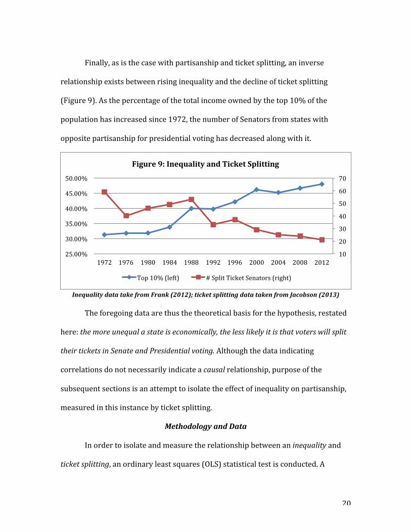
Finally, as is the case with partisanship and ticket splitting, an inverse
relationship exists between rising inequality and the decline of ticket splitting
(Figure 9). As the percentage of the total income owned by the top 10% of the
population has increased since 1972, the number of Senators from states with
opposite partisanship for presidential voting has decreased along with it.
Inequality data take from Frank (2012); ticket splitting data taken from Jacobson (2013)
The foregoing data are thus the theoretical basis for the hypothesis, restated
here: the more unequal a state is economically, the less likely it is that voters will split
their tickets in Senate and Presidential voting. Although the data indicating
correlations do not necessarily indicate a causal relationship, purpose of the
subsequent sections is an attempt to isolate the effect of inequality on partisanship,
measured in this instance by ticket splitting.
Methodology and Data
In order to isolate and measure the relationship between an inequality and
ticket splitting, an ordinary least squares (OLS) statistical test is conducted. A
10
20
30
40
50
60
70
25.00%
30.00%
35.00%
40.00%
45.00%
50.00%
1972 1976 1980 1984 1988 1992 1996 2000 2004 2008 2012
Figure 9: Inequality and Ticket Splitting
Top 10% (left) # Split Ticket Senators (right)

21
number of control variables that have been found to contribute to ticket splitting
have been added to the model in order to isolate the effect of inequality on the
dependent variable, ticket splitting.
Dependent Variable – Ticket Splitting
The dependent variable, ticket splitting, is measured by tabulating the
percentage of years that a state was represented by a Senator(s) from the party
opposite to that of which it voted in elections from 2001-‐2013. Thus a state is ‘red’
or ‘blue’ if it voted either Republican or Democratic in every election during that
time span. Any state that voted for both a Republican and Democratic candidate
between 2001-‐2013 is dropped from the analysis.49 The percentage of ticket
splitting is calculated by dividing the number of years an opposite party Senator
held the seat by 26 (13 years, multiplied by two seats for each state). Figures 9 and
10 illustrate the breakdown of ticket splitting in red and blue states, respectively.
The proportion of ‘blue state Republicans’ ranges from 96.2% (Maine) to 0% (10
states) (Figure 11). Similarly, the proportion of ‘red state Democrats’ ranges from
100% (West Virginia) to 0% (10 states) (Figure 12).
49 Nate Silver, “Party-‐Line Voting Makes Scott Brown Part of a Dying Breed in the Senate,” 538 Politics, Feb. 4, 2013, URL: http://fivethirtyeight.com/features/party-‐line-‐voting-‐makes-‐scott-‐brown-‐part-‐of-‐a-‐dying-‐breed-‐in-‐the-‐senate/, accessed on: 10/05/14, note that there are 40 total red and blue states, 10 ‘purple’ states are omitted from the analysis.

22
Figure 10: Republican Senators in Blue States (2001-‐2013)
Data taken from Silver (2013)
Figure 11: Democratic Senators in Red States (2001-‐2013)
Data taken from Silver (2013)
This analysis focuses only on Senate races for a number of reasons. First,
previous scholarship has found that individuals tend to have more familiarity with

23
Senate races than those in the House because the elections are more prominent.50
Secondly, fewer Senators run unopposed, and thus the elections tend to be more
competitive overall.51 Finally, since this analysis is focusing on statewide
characteristics, focusing on an office in which the entire state is the constituency
lends more validity to the methodology. House races may provide diverging insights
regarding candidate characteristics and geographical sorting effects; however,
analyzing Senate races enables one to test the inequality hypothesis put forward
here more effectively.
Independent Variable -‐ Inequality
The primary independent variable, income inequality, is measured by the
percentage of the income owned by the wealthiest 10% within each state. Data was
collected from Mark W. Frank’s database; income shares are calculated by dividing
top income series by total personal income.52 Aside from the convenience of data
collection, the ‘top 10%’ measure is widely used and accepted by economists and
political scientists alike. Although the primary strength of the measurement is its
ability to delineate among types of income sources (which is not the purpose here),
it is also highly correlative with other commonly used inequality measures like the
GINI coefficient and the top 1% income share. A state-‐by-‐state breakdown of income
inequality is presented in Figure 12. The value of each state’s inequality is derived
from its average percentage from the years 2001-‐2012. Values range from about
50 From Campbell and Sumners, “Presidential Coattails in Senate Elections” (1990) 51 Abramowitz, “Explaining Senate Election Outcomes” (1988) 52 Mark W. Frank, “U.S. State-‐Level Income Inequality Data,” URL: http://www.shsu.edu/eco_mwf/inequality.html, accessed on 10/20/14; Thomas Piketty and Emmanuel Saez, “The Evolution of Top Incomes: A Historical and International Perspective,” American Economic Association Papers and Proceedings, Vol. 96, No. 2 (2006) pp. 200-‐205.

24
50% (New York) to 41% (Utah and Alaska), with a higher percentage representing
greater inequality.
Control Variables
A number of control variables that have been found to be influential in
explaining ticket splitting in previous scholarship are also added to the model. In
order to account for the ideological strength within each state, data is extracted from
a pooled CBS News and New York Times poll, which measures the percentage of
individuals who identify as liberals and conservatives in each state from 1993-‐
1999.53 One would expect states with a higher proportion of individuals identifying
as either liberals or conservative to be less likely to split their ticket. Partisanship is
measured with Cook’s PVI, a common metric that attempts to capture the strength
of a state’s preference for either the Republican or Democratic Party.54 Population
density, measured by a state’s population per square mile, is also added to the model
53 Gerald C. Wright, Robert Erikson, and John P. McIver, Statehouse Democracy. Cambridge University Press (1993). 54 Cook’s Political Report (2013)
0.4
0.42
0.44
0.46
0.48
0.5
0.52
NY LA TX CA GA MA NJ AR PA RI MO OR KS MD MT MN NE HI WI AK
Figure 12: Inequality in the States (2001-‐2012)

25
to account for variation as a result of smaller population states in which
‘incumbency bumps’ may be stronger.55 The logic behind this assertion is that
residents of rural states may have a stronger ‘personal connection’ with their
Senators and may be more inclined to cross partisan lines to support an incumbent
they are personally familiar with. Finally, in order to account for the ‘Southern
Effect’, a dummy variable is created to ensure test whether those in the South are
more or less likely to split their tickets, as was the case in previous decades.
OLS Results
Table 1 summarizes the results of the OLS regression, with ticket splitting as
the dependent variable. The entire model predicts about 20% of the variation of
ticket splitting in the states in years 2001-‐2013 (R2 = 0.205), although it is not
statistically significant as a whole (F = 1.417; p-‐value = 0.238). Interestingly, the
only variable that is statistically significant is inequality (90% confidence). As
inequality decreases across the states, the probability of an opposite party Senator
occupying one or both of the states increases, controlling for other sources of
variation. In other words, moving from Utah or Alaska (the lowest inequality) to
New York (the highest inequality) decreases the probability of a state being
represented by an opposite party Senator(s) by about 27.65%.
55 Population density data obtained from 2005 US Census Bureau; Abramowitz, “Explaining Senate Outcomes” (1988) pp. 387; John R. Hibbing and Sara L. Brandes, “State Population and the Electoral Success of U.S. Senators. American Journal of Political Science, Vol. 25 (1981) pp. 808-‐819.

26
Also noteworthy, none of the other variables are found to be statistically
significant, although the standardized coefficient of partisanship nearly matches
inequality (-‐.28 and -‐.27 respectively). Although certain states may have a higher
proportion of individuals who identify as either liberal or conservative, this
ideological identity does not seem to influence a state electorate’s propensity to split
its ticket. Similarly, population density (and the corresponding ‘personal connection’
that theoretically comes along with it) does not influence whether a state splits its
ticket between Senate and presidential voting. Finally, the ‘Southern Effect’ seems to
have disappeared over the past few decades, as southerners are not more or less
likely to vote for candidates of opposite parties for Senate and presidential elections.
Limitations and Future Research
Despite the intriguing results, one must proceed with caution before
declaring inequality as the primary culprit in the decline of ticket splitting. First, the
duration of the data examined is limited to elections over a 13-‐year period of which

27
ticket splitting had already been in decline for about 10 years. Measuring the
number of years an opposite party Senator occupied a state’s seat tells us something
about that specific time frame, but extending the data beyond the current era of
polarization and partisan sorting would present a more thorough depiction of this
phenomenon. Senate terms are six years long, and thus one split ticket outcome may
drastically influence the results over such short time duration. Future research
should examine ticket splitting from the time of its ascension in 1972 (or even since
the inception of popular voting for Senate in 1912), and examine it through the
years of decline. In order for the findings of this analysis to maintain their validity,
one must demonstrate that at different points in time, states with lower inequality
more frequently split their ticket.
It is likely, that the control variables would also become more predictive if
the duration of the study allowed for more variation of the dependent variable.
Ticket splitting had already started its decline by 2001, and thus the few states left
continuing to split their tickets could be considered holdovers with strong
incumbents, as was likely the case in North Dakota’s three Democrat congressional
delegation from 1992-‐2008. The state currently boasts two Republicans and one
Democrat in its delegation (one of each in the Senate), and it remains unclear
whether the cause of this is increased inequality (from the oil boom), or simply
strong incumbents deciding to retire (only one of the Democrats lost a reelection
bid). Expanding the data set would prevent a single strong incumbent from skewing
the results drastically, as may have been the case in a number of states in this
analysis.

28
Finally, a number of limitations with regards to data collection are present as
well. Population density is but a one-‐year measure (2005), and ideology is an average
of the years 1993-‐1999. Although it is likely that neither has fluctuated greatly from
2001-‐2013, a more rigorous approach would identically match the time frames of
the data. Time constraints and data access limitations prevent this analysis from
employing the amount of rigor and validity required for this type of undertaking.
Future efforts at explaining ticket splitting should take these limitations into
account and develop more sophisticated methods of operationalizing the variables.
Conclusion
Despite the foregoing limitations, the results here are encouraging and do
support the hypothesis. Similar to what is theorized by McCarty, Poole, and
Rosenthal, economic inequality does tend to ‘breed polarizing politics’, or more
accurately characterized as inducing more tribal partisan attachments. In states in
which these economic disparities are more pronounced, voters cling more strongly
to partisan and ideological identities, and thus are less willing to vote across party
lines for different offices. As a higher proportion of the populace can be
characterized as genuinely ‘middle class’, the electorate generally is more open to
the idea of voting for different parties for different elective offices.
The results contribute to the growing body of literature regarding the causes
polarization, partisan sorting, and in particular, ticket splitting. However, as
mentioned previously, one must be reticent when attributing causal processes to
such a complex phenomenon. Although the correlation between inequality and
partisanship is highly suggestive, it is highly possible that the partisanship increase

29
occurred first, only to be followed by inequality. Indeed, the contention put forward
by McCarty, Poole, and Rosenthal emphasizes the lack of responsiveness on the part
of Congressional leaders to address inequality, as some have theorized: as more
people become worse off, relatively speaking, they would tend to prefer a higher
degree of redistribution in regards to economic policies. They argue that this has not
happened because those who are worse off economically are less likely to vote or
ineligible (illegal immigrants and felons), and thus the voting public is skewed
towards those who oppose redistributive economic policies.56 This may very well be
the case, but the question remains as to whether geographical areas with lower
degrees of inequality have residents with weaker partisan attachments, and are thus
more likely to split their tickets. This analysis provides some initial insights to
clarifying the economic inequality effect on partisanship.
Recent scholarship has additionally examined the effect of divided
government (which may or may not be the result of ticket splitting) during highly
polarized times.57 One would expect to see less divided government when fewer
voters are splitting their tickets; however, divided government has been the norm in
recent elections, with the President and Congress representing opposite parties in
12 of the last 22 years (55%). This trend is likely to continue, not because of ticket
splitting, but to due to a partisan advantage favoring Republicans in House races, in
addition to a similar Electoral College favoring Democrats for the presidency.58 It is
56 McCarty, Poole, and Rosenthal, Polarized America (2006) pp. 165-‐190. 57 Binder, Stalemate (2003); David Mayhew, Divided We Govern, Party Control, Lawmaking, and Investigations, 1946-‐1990. New Haven, London: Yale University Press (1991). 58Jowei Chen and Jonathan Rodden, “Unintentional Gerrymandering: Political Geography and Electoral Bias in Legislatures.” Quarterly Journal of Political Science. Vol. 8 (2013) pp. 239–269; Ben Highton, “A big Electoral College advantage for the Democrats is looming,” Washington Post Monkey

30
one thing for democracy when a government is divided because voters prefer it that
way in order to moderate policy; it is quite another when it results from
institutional vagaries that exaggerate seat allocation in Congress or Electoral Vote
support for the White House.59 We are experiencing the consequences of these
trends in the form of constant threats of government shutdowns and the habitual
use of continuing resolutions to fund the government, rather than more
comprehensive and predictable budgetary practices.
Additionally, if the conclusions presented here do indeed withstand further
scrutiny and testing, it indicates yet another troubling development for income
inequality in a society. Aside from the moral implications, many claim that
exorbitant inequality may slow economic growth, decrease social mobility, worsen
social relations, and perhaps most troubling, facilitate the arrival of a genuine
‘plutocracy’ in America (these implications are interrelated).60 In recent years, social
movements on the left (Occupy Wall Street) and the right (Tea Party) that
emphasize inequality and government corruption have gained momentum.
However, a vicious cycle seems to have developed in the process: as the electorate
becomes more cynical about economic inequality, they exacerbate it by becoming
more strongly attached to their partisan and ideological identities, thus
Cage Blog, Apr. 28, 2014. URL: http://www.washingtonpost.com/blogs/monkey-‐cage/wp/2014/04/28/a-‐big-‐electoral-‐college-‐advantage-‐for-‐the-‐democrats-‐is-‐looming/, accessed on 11/25/14. 59 Jacobson, The Electoral Origin of Divided Government: Competition in U.S. House Elections, 1946-‐1988 (1990); Alesina and Rosenthal, Partisan Politics, Divided Government, and the Economy (1995). 60 Eduardo Porter, “Income Equality: A Search for Consequences,” New York Times, March 25, 2014, URL: http://www.nytimes.com/2014/03/26/business/economy/making-‐sense-‐of-‐income-‐inequality.html, accessed on: 11/25/14. Martin Gilens and Benjamin I. Page, “Testing Theories of American Politics: Elites, Interest Groups, and Average Citizens,” Perspectives in Politics, Vol. 12, No. 3 (2014).

31
incentivizing lawmakers to ignore the issue. Short of restructuring the governing or
party system, it is not entirely clear what the potential remedies are to improve
these troubling trends. The findings of this analysis do indicate, however, that
extreme economic inequality has consequences beyond that of social mobility and
economic growth – it impacts how people think about partisan attachments, and
thus how a democracy functions as well.

32
References:
Abramowitz, Alan I. (1988) “Explaining Senate Election Outcomes,” The American Political Science Review, Vol. 82, No. 2, pp. 385-‐403.
Abramowitz, Alan I. Kile L and Saunders (2008) “Is Polarization a Myth?” The
Journal of Politics, Vol. 70, No. 2, 542–555. Alesina, Alberto and Howard Rosenthal, (1995) Partisan Politics, Divided
Government, and the Economy, Cambridge University Press. Bawn, Kathleen; Cohen, Martin; Karol, David; Masket, Seth; Noel, Hans; and John
Zaller (2012) “A Theory of Political Parties: Groups, Policy Demands and Nominations in American Politics, “ Perspectives in Politics, Vol. 10, pp 571-‐597.
Binder, Sarah (2003) Stalemate: Causes and Consequences of Legislative Gridlock,
Washington, DC: Brookings Institution. Bishop, Bill (2009) The Big Sort: Why the Clustering of Like-‐Minded America is
Tearing Us Apart. Mariner Books. Campbell, James E. and Joe A. Sumners, (1990) “Presidential Coattails in Senate
Elections,” The American Political Science Review, Vol. 84, No. 2, pp. 513-‐524. Chen, Jowei and Jonathan Rodden, (2013) “Unintentional Gerrymandering: Political
Geography and Electoral Bias in Legislatures.” Quarterly Journal of Political Science. Vol. 8, pp. 239–269.
Converse, Philip E. (1983) “The Concept of the ‘Normal Vote’”, in Elections and the
Political Order, ed. Angus Campbell, Philip E. Converse, Warren E. Miller and Donald E. Stokes. New York: Wiley (1966); Steven J. Rosenstone, Forecasting Presidential Elections. Yale University Press, New Haven.
Cook Political Report (2014) “Partisan Voter Index by State, 1994-‐2014,” The Cook
Political Report. Downs, Anthony (1957) Economic Theory of Democracy. Harper and Row, First Ed. Fiorina, Morris P. and Samuel J. Abrams (2008) “Political Polarization in the
American Public,” Annual Review of Political Science. Vol. 11:563–588. Fiorina, Abrams and Pope (2008) “Polarization in the American Public:
Misconceptions and Misreadings,” The Journal of Politics, Vol. 70, No. 2, 556–560.

33
Frank, Mark W. (2014) “U.S. State-‐Level Income Inequality Data,” URL: http://www.shsu.edu/eco_mwf/inequality.html, accessed on 10/20/14.
Gerber, Elizabeth and Adam Many, (1996) “Incumbency-‐Led Ideological Balancing:
A Hybrid Model of Split-‐Ticket Voting,” Presented at the annual meeting of Midwest Political Science Association, Chicago.
Gerber, Elisabeth R; and Rebecca B. Morton (1998). “Primary Election Systems and
Representation.” Oxford University Press. Gilens, Martin and Benjamin I. Page (2014)“Testing Theories of American Politics:
Elites, Interest Groups, and Average Citizens,” Perspectives in Politics, Vol. 12, No. 3.
Green, John C.; Coffey, Daniel J.; and David B. Cohen, (2014) The State of the Parties:
The Changing Role of Contemporary American Parties, Rowman & Littlefield Publishers; 7th Edition.
Hassell, Hans (2013). “The Non-‐existent Primary-‐Ideology Link, or Do Open
Primaries Actually Limit Party Influence in Primary Elections?” Presentation at the 2013 State Politics and Policy Conference, University of Iowa, Iowa City, Iowa.
Hibbing, John R. and Sara L. Brandes (1981) “State Population and the Electoral
Success of U.S. Senators. American Journal of Political Science, Vol. 25, pp. 808-‐819.
Highton, Ben (2014) “A big Electoral College advantage for the Democrats is
looming,” Washington Post Monkey Cage Blog, Apr. 28, 2014. URL: http://www.washingtonpost.com/blogs/monkey-‐cage/wp/2014/04/28/a-‐big-‐electoral-‐college-‐advantage-‐for-‐the-‐democrats-‐is-‐looming/, accessed on 11/25/14.
Ingraham, Christopher (2014) “Inequality and political polarization have been rising
in tandem for three decades,” Washington Post Wong Blog, May, 27, 2014. URL: http://www.washingtonpost.com/blogs/wonkblog/wp/2014/05/27/inequality-‐and-‐political-‐polarization-‐have-‐been-‐rising-‐in-‐tandem-‐for-‐three-‐decades/, accessed on: 11/25/14.
Jacobson, Gary (1990) The Electoral Origin of Divided Government: Competition in
U.S. House Elections, 1946-‐1988. Westview Press. Jacobson, Gary C. (2013) “Partisan Polarization in American Politics: A Background
Paper,” Presidential Studies Quarterly, Vol. 43. No. 4, pp. 688-‐708.

34
Katz, Elihu and Paul Lazarsfeld (2005) Personal Influence: The Part Played by People in the Flow of Mass Communications. Transaction Publishers, 2nd Ed.
Key, V.O. (1949). Southern Politics in State and Nation. New York: A. A. Knopf. Levendusky, Matthew (2009) The Partisan Sorty: How Liberals Became Democrats
and Conservatives Became Republicans. University of Chicago Press. Lewis-‐Beck, Michael S. and Tom W. Rice, (1985)"Are Senate Election Outcomes
Predictable?" PS: Political Science & Politics, Vol. 18., No. 4, pp. 745-‐754. Mann, Thomas E.; and Norman J. Ornstein (2012) It’s Even Worse Than It Looks:
Howl the American Constitutional System Collided with the New Politics of Extremism. Basic Books.
Mayhew, David (1991) Divided We Govern, Party Control, Lawmaking, and
Investigations, 1946-‐1990. New Haven, London: Yale University Press. McCarty, Poole, Rosenthal (2006) Polarized America: The Dance of Ideology and
Unequal Riches. MIT Press. Ostermeier, Eric (2011) “Which States Have the Most Split-‐Ticket Voting in
Presidential-‐U.S. Senate Election Cycles?” University of Minnesota Humphrey School of Public Policy, Oct. 5, 2011, URL: http://blog.lib.umn.edu/cspg/smartpolitics/2011/04/which_states_have_the_most_spl.php, accessed on: 11/02/14.
Pew Research Center (2014) “Political Polarization in the American Public,” Pew
Research Center. Piketty, Thomas and Emmanuel Saez, (2006) “The Evolution of Top Incomes: A
Historical and International Perspective,” American Economic Association Papers and Proceedings, Vol. 96, No. 2, pp. 200-‐205.
Pildes, Richard H. (2011) “Why the Center Does Not Hold: The Causes of
Hyperpolarized Democracy in America,” California Law Review, Vol. 99 273, 288.
Polsby, Nelson W. (2004) How Congress Evolves: Social Bases of Institutional Change.
Oxford University Press. Poole, Keith (2014) Voteview, URL: www.voteview.com. Accessed on 11/10/14. Poole, Keith (2014) “An Update on Political Polarization through the 112th Congress”,
URL: http://voteview.com/blog/?p=726, accessed on 11/10/14.

35
Porter, Eduardo (2014) “Income Equality: A Search for Consequences,” New York Times, March 25, 2014, URL: http://www.nytimes.com/2014/03/26/business/economy/making-‐sense-‐of-‐income-‐inequality.html, accessed on: 11/25/14
Prior, Markus (2007) Post-‐Broadcast Democracy: How Media Choice Increases
Inequality in Political Involvement and Polarizes Elections. Cambridge Studies in Public Opinion and Political Psychology.
Silver, Nate (2012). “As Swing Districts Dwindle, Can a Divided House Stand?” The
New York Times. 27 Dec. 2012. Nov. 15, 2013. Silver, Nate (2014) “Party-‐Line Voting Makes Scott Brown Part of a Dying Breed in
the Senate,” 538 Politics, Feb. 4, 2013, URL: http://fivethirtyeight.com/features/party-‐line-‐voting-‐makes-‐scott-‐brown-‐part-‐of-‐a-‐dying-‐breed-‐in-‐the-‐senate/, accessed on: 10/05/14.
Southwell, Priscilla (1986) “The Politics of Disgruntlement: Nonvoting and Defection
among Supporters of Nomination Losers, 1968-‐1984,” Political Behavior, Vol. 8, pp. 81-‐95.
Sunquist, James L. (1983) Dynamics of the Party System: Alignment and Realignment
of Political Parties in the United States, The Brookings Institution, Washington, D.C..
Theriault, Sean M. and David W. Rohde (2011) “The Gingrich Senators and Party
Polarization in the U.S. Senate,” The Journal of Politics, Vol. 73, No. 4, Pp. 1011–1024.
US Census Bureau (2005), “U.S. Census Bureau, Statistical Abstract of the United
States: 2004-‐2005,” US Census Bureau. Walsh, Deirdre (2014) “Last white Democrat from Deep South loses Congressional
seat,” Nov. 5, 2014. URL: http://www.cnn.com/2014/11/05/politics/last-‐southern-‐white-‐democrat-‐in-‐congress/; accessed on 11/20/14.
Wattenberg, Martin P. (1991) The Rise of Candidate-‐Centerted Politics: Presidential
Elections of the 1980s. Harvard University Press, Cambridge, MA. Wright, Gerald C.; Erikson, Robert; and John P. McIver (1993) Statehouse Democracy.
Cambridge University Press.