7HPLGLGLVFXVVLRQHGHO 6HUYL]LR 6WXGL

,QGXVWULDO 'LVWULFWV DQG /RFDO %DQNV�'R WKH 7ZLQV (YHU 0HHW"

E\ $� %DIILJL� 0� 3DJQLQL DQG )� 4XLQWLOLDQL

1XPEHU ��� �� 0DUFK ����

7KH SXUSRVHRI WKH´7HPL GL GLVFXVVLRQHµ VHULHV LV WR SURPRWH WKH FLUFXODWLRQ RIZRUNLQJSDSHUV SUHSDUHG ZLWKLQ WKH %DQN RI ,WDO\ RU SUHVHQWHG LQ %DQN VHPLQDUV E\ RXWVLGHHFRQRPLVWV ZLWK WKH DLP RI VWLPXODWLQJ FRPPHQWV DQG VXJJHVWLRQV�

7KH YLHZV H[SUHVVHG LQ WKH DUWLFOHV DUH WKRVH RI WKH DXWKRUV DQG GR QRW LQYROYH WKHUHVSRQVLELOLW\ RI WKH %DQN�

(GLWRULDO %RDUG�0$66,02 52&&$6� &$5/2 0217,&(//,� *,86(33( 3$5,*,� 52%(572 5,1$/',� '$1,(/(

7(5/,==(6(� 3$2/2 =$))$521,� 6,/,$ 0,*/,$58&&, �(GLWRULDO $VVLVWDQW��

,1'8675,$/�',675,&76�$1'�/2&$/�%$1.6�'2�7+(�7:,16�(9(5�0((7"

di Alberto Baffigi*, Marcello Pagnini** and Fabio Quintiliani**

$EVWUDFW

The paper offers theoretical and empirical insights into the links between banks andfirms in industrial districts and to the way investment is financed.

Theoretically, it is assumed that district-banking localism is embedded in the industrialdistricts’ social context. District banks should thus be distinguished by such features asgreater concentration of lending, greater concentration of market shares and the cooperativelegal form. Counteracting forces (e.g. excessive risk taking, higher monitoring costs and thecooperative’s typical dilution of power among members) may nonetheless preventdistrict-banking localism from arising.

The empirical analysis crosses an Istat dataset on local labour systems and industrialdistricts with banking supervisory data as of the end of 1991. Cooperative banks are found toconcentrate their lending and to acquire larger market shares in industrial districts, thoughthe evidence is not clear-cut. Mutual banks, on the other hand, generally concentrate theirlending to small local labour systems, thereby indicating that their role as local banks isplayed not only in industrial districts but in non-district areas as well. Finally, in a regressionanalysis we find that investment by firms operating in industrial districts is more closelycorrelated with their cash-flow than those of non-district firms, although the pattern variesacross regions and economic sectors.

The conclusion is that the rise of district banking localism cannot be taken for grantedand that IDs do not seem to be homogeneous entities even as far as bank-firm relationshipsare concerned.

* Bank of Italy, Research Department.**Bank of Italy, Bologna Main Branch, Economic Research Unit.

&RQWHQWV

1. Introduction..................................................................................................................92. Industrial districts in Italy ..........................................................................................12

2.1 Definition ............................................................................................................122.2 Empirical and structural aspects of the definition of industrial districts ............14

3. Industrial districts as credit markets ..........................................................................223.1 Double concentration condition: an overview ....................................................233.2 Concentration of loan portfolio...........................................................................233.3 Concentration of credit supply............................................................................253.4 Mutual banks and IDs .........................................................................................26

4. An empirical analysis of credit markets in district and non-district areas.................284.1 Introduction.........................................................................................................284.2 The geographical composition of the four bank categories’ loan portfolio ........304.3 The concentration of credit supply in the 4 area types........................................33

5. Patterns of banking localism in IDs...........................................................................366. Investment and liquidity constraints in industrial districts ........................................38Appendix I: The empirical definition of IDs..................................................................48Appendix II: A note on the Italian banking system........................................................50Appendix III: Tables and summary statistics.................................................................53References .....................................................................................................................66

1. �,QWURGXFWLRQ1

Localism is a widespread phenomenon in the Italian economic system. In some parts of

Italy, especially in the northern and central regions, firms and workers tend to agglomerate in

self-contained and restricted areas. Links to those areas frequently have important effects on

the allocation of resources and on the well-being of the resident population. The literature on

this topic has taken two distinct routes: one referring to LQGXVWULDO�GLVWULFWV and the other to

ORFDO�EDQNV.

Industrial districts (IDs henceforth) are networks of small firms operating in a limited

area. Each firm specialises in one phase in the production process of a district-specific final

good. Thanks to district level co-ordination mechanisms, these firms can benefit from

intensive division of labor yet avoid the costs associated with small size.

Local banks have recently been the subject of renewed interest on the part of Italian

economists, and a burgeoning literature has emerged.2 Far from considering local banks as

inefficient economic units, these authors argue that they can play an essential role in

financing small firms and in fostering industrial take-off in relatively backward areas.

The aim of this paper is to offer some theoretical and empirical insights into the links

between IDs’ real and credit markets and the way investment is financed. In particular, we

carry out - for the first time to our knowledge - an empirical comparison of district versus

non-district areas, exploiting a mass of financial and real statistics, namely:

− 1991 dataset on industrial districts (Istat, the Italian central statistical office);

− municipal data from the 1991 population and industry censuses (Istat);

1 This is a revised version of the paper presented at the XXXVII ERSA conference in Rome on 28 August

1997. The views expressed are those of the authors only and in no way involve the responsibility of the Bank ofItaly. We would like to thank Istat and in particular Franco Lorenzini for kindly providing us with the industrialdistrict dataset, without which this paper could have never been written. We would also like to thank LuigiBuzzacchi, Luigi Cannari, Davide Conti, Giuseppe Garofalo, Marcello Messori, Guido Pellegrini, AchillePuggioni, Massimo Roccas, Irene Valsecchi and an anonymous referee for their helpful comments and advice.The responsibility for any errors is of authors’ alone. E-mail: faquinti@tin.it.

2 See Angelini, Di Salvo and Ferri (1997), Cannari and Signorini (1996, 1997), Cesarini, Ferri andGiardino (1997),�Cesari (1996), Conti and Ferri (1997) and Ferri and Di Salvo (1994), to name a few.

10

− banking supervisory returns on loans and on bank branches by individual banks and

municipalities, as of the end of 1991;

− balance sheet data as reported by the Italian Company Accounts Data Service (Centrale

dei bilanci);

− data on real per capita provincial income (1952-1992) as estimated by Fabiani and

Pellegrini (1997).

From a theoretical point of view, we emphasise the attributes of social interaction inside

IDs and their possible consequences for credit markets. Industrial-district scholars have

stressed that economic behaviour is HPEHGGHG in the districts’ social context (Harrison,

1992). Thus, in dealing with the role of banks in IDs a question immediately arises: are the

banks that operate in IDs fully integrated into the socio-economic network? Is their

behaviour HPEHGGHG�in the social context?

We define a bank E as embedded in an ID G socio-economic context if two conditions

are met (GRXEOH� FRQFHQWUDWLRQ� FRQGLWLRQ�� DCC�: 1) E concentrates its loans in G

(FRQFHQWUDWLRQ� RI� OHQGLQJ�; 2) E holds a large market share in G’s credit market

(FRQFHQWUDWLRQ� RI� FUHGLW� PDUNHW). More loosely, E is said to be embedded in G’s socio-

economic context if E is important to G and G is important to E. We argue also that

embeddedness will be strengthened if E has a FRRSHUDWLYH� OHJDO� IRUP�� Concentration of

lending (condition 1) signals the district-local banks’ commitment to the local economy,

allowing them to benefit from the district’s cooperative behaviour. Holding large credit

market shares (condition 2) enables such banks to obtain useful information on the web of

relationships among firms. Cooperative legal form increases the ability to check the

behaviour of local borrowers, due to reciprocal monitoring by members.

However, there are forces that can constrain the advantages of double concentration

and of cooperative legal form. There is a trade-off between the advantages of having a large

stake in the district and the disadvantages of excessive risk-taking and monitoring costs,

which would arise if banks concentrated their loans in ID areas and if they acquired a great

share of the IDs’ credit markets. There is also a trade-off between the advantages and

disadvantages of the cooperative form: excessive membership dilution and the “one head-

one vote” rule can reduce the incentives for reciprocal monitoring among members. Thus,

11

the existence of differences between district-local banking and local banking as such may not

be theoretically generalised. Whether district banking localism arises or not is in part an

empirical question.

From an empirical point of view, we try to check whether district banking localism, as

defined above, actually emerges in IDs. First, we carry out a comparative static analysis of

the banking structure in�district and in non-district areas at national and at “macro-regional”

level. We find that there is some evidence indicating that cooperative banks (known as

“popular” banks in Italy: henceforth POP) show greater aggregate specialisation of lending to

ID areas, especially in the North-East. They also tend to have larger market shares in district

than in non-district areas. Data also show that the role of the other banks that operate mainly

at local level (savings banks and mutual banks) is not limited to IDs but is also particularly

important in small QRQ�GLVWULFW areas with no provincial capital.

Second, we check whether DCC obtains in IDs. We assume that double concentration

exists if: i) the fraction of a bank’s loan portfolio is greater than the quadratic mean of all

portfolio shares and ii) a bank’s credit market share is greater than the quadratic mean of all

credit market shares. We discover that only 58 out of the 199 IDs designated by Istat satisfy

the DCC. These IDs� include the best known and oldest district areas (Carpi, Biella, Prato,

etc.). This suggests that district banking localism tends to be stronger in more mature IDs. As

to the banks that operate there, we find that mutual banks (in Italian Banche di credito

cooperativo, BCC) match the DCC condition more frequently than the other categories.

Finally, we try to assess the magnitude of financing constraints on ID firms as

compared to firms that do not operate in district areas. In a regression analysis based on a

panel of firms, we find that ID firms’ investment tends to be PRUH sensitive to cash flow than

non-ID firms’. This finding could suggest that the lack of close ties with the banking system

is particularly costly for firms EHORQJLQJ to IDs. Running the same regression by region and

sector of economic activity, however, the results are different, at least in part. In particular,

the cash flow sensitivity of investment is lower for ID firms located in Marche, Tuscany and

Emilia-Romagna and for the food and beverage and above all textile, clothing and leather

industries. Again, these findings underscore the different ways IDs’ finance their economies.

12

Our conclusion is that the rise of district banking localism cannot be taken for granted and that IDs

do not seem to be homogeneous entities even as far as bank-firm relationships are concerned.

The paper is organised as follows. Section 2 sketches the relevant theoretical and empirical aspects of

IDs and describes the importance of districts to Italy’s industrial system, their geographical and sectoral

distribution, and their long-run growth profiles. In Section 3 we discuss the theoretical underpinnings of the

supposedly stronger bank-firm relationship at ID level and the factors that may prevent the emergence of

district banking localism. In Section 4 we present an empirical analysis of credit markets in district and

non-district areas. In Section 5 we address the issue of whether some bank categories may typically qualify as

GLVWULFW banks. Finally, Section 6 compares the financing of investment in district versus non-district areas.

��� �,QGXVWULDO�GLVWULFWV�LQ�,WDO\

���� �'HILQLWLRQ

A salient feature of Italian industry is the very widespread presence of small firms.

Until recently, many economists saw this as a weakness, since small firms could not exploit

economies of scale, and their survival could only be guaranteed by protecting them from

market competition. However, the relatively good performance of the Italian economy in a

long-term perspective and the crisis of the Fordist type of production in the late sixties and

seventies induced some economists to examine Italian small firms more closely. Becattini

(1987, 1991, 1996), among others, changed the perspective of the debate on the efficient

scale of production. He argued that, owing to long-term historical processes, small firms

tended to aggregate in marshallian-type IDs in some regions of Italy. In order to assess the

efficiency of these firms, however, the traditional conceptual tool of the single representative

firm is of little help. The focus should be shifted to the QHWZRUN of firms making up the IDs

and on the peculiar allocative mechanisms that are at work within district areas.

From this new perspective, economic relationships cannot be considered apart from the

social context within district areas, and IDs are treated as complex entities involving

interrelated sociological, historical and economic aspects, whose main characteristics can be

summed up in three points:

13

a) $ VRFLR�WHUULWRULDO� DVSHFW. IDs are communities of people and firms acting in spatially

concentrated areas (see Sforzi, 1987). Geographical proximity favours socio-economic

interaction. The members of these communities have common values and attitudes

resulting from long historical processes in which many institutions (the family, political

parties, etc.) contributed to their spread and perpetuation within the local community.

Loyalty towards the community and its values is also an important element affecting the

economic behaviour of agents.3

b) 3URGXFWLYH� HIILFLHQF\. Looking at the production process, IDs can be seen as groups of

small firms, each specialised in a single phase of the productive process of a

district-specific final good.4 IDs are thus partially spontaneous mechanisms that help

co-ordinate all the phases of the process, thereby fostering the development of economies

of scale that are external to firms but internal to the districts. Individual firms benefit from

very high degrees of specialisation and overcome the disadvantages of being small. To use

the terminology of transaction cost economics, IDs reduce transaction costs both

compared to the usual market relationships and compared to cases in which all production

takes place in a single vertically-integrated firm.

c) 6WUDWHJLF�LQWHUDFWLRQ. Exchanges in production share some aspects of market transactions,

since firms are legally independent, but repeated exchanges favour the accumulation of

“reputational capital”, thereby increasing the incentives of the parties to transact. Personal

acquaintance and mutual trust, moreover, encourage cooperation, which becomes

necessary when the activities of different economic agents must be co-ordinated to a

common productive aim. Long-run cooperative equilibria can be also achieved and

sustained through the threat of punishment for deviant behaviour. The role of the

community in making this threat credible is crucial: free riding by some firms can be

sanctioned through social ostracism. Long-lasting interactions among firms will favour

3 Another feature of IDs is a relatively high degree of VRFLDO�PRELOLW\ in the district, due to the spread ofinformation and of technical competence through social and economic interaction. Workers often start their ownbusiness, after learning the job as employees with other entrepreneurs.

4 The single phases of the process may either consist in the production of an intermediate good or in theconstruction of machinery that will subsequently be used to manufacture the final product or anotherintermediate good.

14

specific investment in the transactions, thereby making them highly relational

(Williamson, 1979).

These characteristics of district areas show that economic interaction is an integral part

of the complex social context existing in IDs: we can say that economic behaviour is

HPEHGGHG in social relations within district areas (Harrison, 1992).5

���� �(PSLULFDO�DQG�VWUXFWXUDO�DVSHFWV�RI�WKH�GHILQLWLRQ�RI�LQGXVWULDO�GLVWULFWV

This complex theoretical definition of IDs makes their empirical identification rather

difficult. In particular, the interaction between the socio-territorial features of IDs and the

economic and industrial variables cannot be easily assessed. One approach to the problem is

the VSDWLDO� LGHQWLILFDWLRQ�PHWKRG employed by Sforzi (1987, 1997) and Istat (1994, 1995),

based on a complex multi-step algorithm. A brief account of the procedure is as follows.6

First, the national territory is divided into ORFDO� ODERXU� V\VWHPV (LLS), i.e. territorial

groupings of municipalities marked by a certain degree of commuting to work. Next, an LLS

is defined as an ID if it has: i) a proportion of employment in manufacturing greater than the

national average; ii) a higher-than-average proportion of employment in small local

productive units (i.e. industrial plants with no more than the EU threshold of 250 employees;

see Brusco and Paba, 1997) in at least one manufacturing subsector in which the LLS is

specialised; iii) a proportion of employment in a subsector satisfying condition ii) above 50

per cent of total LLS’ manufacturing employment.

This procedure has its drawbacks, however. First of all, it accounts only marginally for

the social aspects that the industrial district literature cites as typical. Secondly, the

concentration thresholds may be too rigid: units with 250 employees, for instance, may still

be larger than the average for Italian manufacturing. Despite these problems, we think that

Istat dataset usefully captures many of the main features of IDs and can be used as a basis for

our discussion.

5 Harrison borrows the concept of HPEHGGHGQHVV from Granovetter (1985).6 See Appendix I for a more detailed description of this procedure. The spatial identification method,

which is at the basis of the procedure followed by Istat (1994, 1995), is described in Sforzi (1987, 1997, ch. 9).

15

Using the 1991 census data, Istat divided Italy’s territory into 784 local labour systems

and, by Sforzi-Istat methodology, identified 199 IDs. Henceforth, the unit of our analyses

will be the LLS and we will also refer to 199 IDs found by Istat as GLVWULFW�DUHDV, and to the

remaining 585 LLSs as QRQ-GLVWULFW�DUHDV.

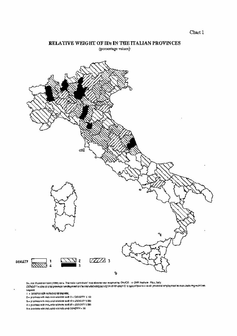
The geographical distribution of IDs in 1991 is extremely uneven (see Chart 1).

Lombardy is the Italian region with the highest number of IDs.7 Over 80 per cent of the

districts are in Lombardy, Piedmont, Veneto, Emilia-Romagna, Marche and Tuscany. By

contrast, Molise, Basilicata, Sicily and Sardinia have none, and IDs are only marginally

present in Lazio, Calabria and Puglia. In short, IDs are mainly concentrated in Northern and

Central Italy (see also Tables A1 and A2 in Appendix 3). In particular, they are found either

in regions whose high degree of development originated in the earlier years of Italian

industrialisation (such as Lombardy), or in areas of late industrialisation which have only

recently achieved high levels of per capita income (such Veneto, Marche and, to a lesser

degree, Abruzzo).8

7 The Italian territory is administratively divided into 20 UHJLRQV. Each region is formed by SURYLQFHV

which are then divided into PXQLFLSDOLWLHV (FRPXQL). Generally speaking, the largest municipality tend to giveits name to the province. We refer to this city as the SURYLQFLDO�FDSLWDO. In 1991, there were 95 provinces and8,100 municipalities in Italy. This implies that in our dataset there are 95 LLSs including a provincial capital(19 of these are district areas: see Table A1 in the Appendix).

8 With regard to the scarcity of IDs in southern Italy, Brusco and Paba (1997) show that in 1951 IDs weremainly present in southern regions and that these districts disappeared in the following decades, as a result ofthe competition of other IDs in the northern and central regions and of the loss of human capital in the south,following massive migration. Rates of ID formation were high between 1951 and 1991 in Lombardy and inCentral and North-Eastern Italy.

17

The population of ID municipalities amounts to over 24 per cent of Italy’s population.

IDs are present mainly in relatively small communities (Figure 1). The largest city located in

ID is Padua (215,000 inhabitants in 1991). Only nine ID municipalities have as many as

100,000 inhabitants. The average population is about 5,550 in ID municipalities, as opposed

to over 7,500 in non-district ones.

Looking at the structure of employment (Table 1), we see that district manufacturing

employment in the sub-sectors in which districts are specialised is about 18 per cent of

national manufacturing employment and 41 per cent of total manufacturing employment in

district areas.9

Figure 1

�3238/$7,21�',675,%87,21�,1�121�',675,&7�$1'�,1�',675,&7�$5($6%<�6,=(�2)�081,&,3$/�3238/$7,21�(1)

(percentage values)

0

5

10

15

20

25

30

35

0-4999 5000-10000 10001-20000 20001-50000 50001-100000 over 100000

residents in non-district areas

residents in district areas

Source: Based on Istat population census data.

(1) Municipalities have been grouped into six population classes, as shown on the horizontal axis. White histograms represent the percentage shares of total

population in non-ID municipalities; black histograms represent the corresponding shares in ID.

9 Notice that, as a consequence of the considerations developed in Section 2.1 point b), employees not

working in each ID’s sector of specialisation have not been included in IDs’ total employment.

18

Table 1

,1'8675,$/�',675,&76$1'�0$18)$&785,1*�,1'8675<�,1�,7$/<�%<�6(&725�(1)

(absolute figures and percentages)

SectorsNumber ofdistricts per

sector(03

GM/(03

G(03

PM/(03

PSpecialisation

index (2)(03

GM/(03

PM

Food, beverage and tobacco industry products 17 2.9 9.2 0.3 5.5

Textile products and clothing 69 34.5 15.9 2.2 38.1

Leather, leather and hide articles, footwear 27 10.6 4.7 2.3 39.4

Wood and wooden furniture, construction materials, baked

clay products, glass, non-metal mineral based products

39 15.6 13.2 1.2 20.8

Metal products excluding machinery 1 0.0 2.5 0.0 0.3

Agricultural and industrial machinery, office equipment,

computers, precision instruments, motor vehicles and

related engines

32 32.5 39.7 0.8 14.4

Petroleum and plastic products, chemical products, artificial

and synthetic fibres, rubber products

4 1.5 8.7 0.2 3.1

Paper and publishing 6 0.5 5.5 0.1 1.6

Other products of manufacturing industries 4 1.9 0.6 3.2 52.2

TOTAL 199 100.0 100.0 - 17.6

Source: Based on Irpet-Istat data.

(1) (03

GM

represents the sum of employees in sector M�in all IDs specialised in that sector. (03

G

is total employment in all IDs in their respective sector of specialisation.

(03

PM

is overall national employment in the M-th manufacturing sector, while (03

P

represents the overall national manufacturing employment. – (2) The specialisation

index is given by the ratio ((03

GM

��

/(03

G

)/((03

PM��

/(03

P

.).

Table 1 shows the sectoral distribution of Italian IDs. Over 90 per cent of

manufacturing employment in district areas is concentrated in 4 sectors: textiles and clothing,

machinery, wood and minerals, leather (see column, (03GM

/(03G in Table 1). If we look at

the specialisation index (fifth column in Table 1),10 we see that Italian IDs are specialised,

10 The fifth column of Table 1 shows an ID specialisation index we have constructed referring to

employment: ((03GM�/(03G) / ((03PM�/(03

P). It compares two fractions. The numerator represents the

fraction of employment, at GLVWULFW�OHYHO, in the manufacturing sub-sector in which each ID is specialised out oftotal manufacturing employment in the district ((03GM/(03G). The denominator shows the analogous fractionat QDWLRQDO� OHYHO between national manufacturing employment in the sectors in which districts are specialisedand overall national manufacturing employment ((03

PM/(03

P).

19

relative to the Italian manufacturing employment, in “traditional”, less capital-intensive

industries (leather, textiles and wood products) whose productive processes can be

fragmented over many small units and co-ordination can be achieved through informal

agreements and cooperative strategies, rather than through hierarchical decision-making

structures. On the contrary, single large firms can be expected to perform more efficiently in

those sectors (such as chemicals or paper and publishing) in which indivisibilities and

economies of scale prevail at the firm level.

Nonetheless, “traditional” industries are not necessarily backward. The organisation of

productive factors in ID markets frequently involves a high degree of know-how and skill.

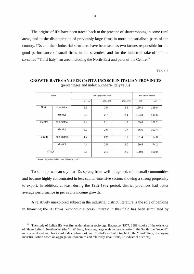
As far as long-run performance is concerned, we compared post-war growth rates in ID

and non-ID provinces. By GLVWULFW�SURYLQFH we mean a province including at least one district

municipality in 1991. If a district encompasses more than one province, we split the group of

municipalities by province.

Table 2 reports real SHU�FDSLWD�income levels and their percentage growth rates, in ID and

QRQ-ID provinces located in the North, Centre and South of Italy.11 In the early fifties, ID

provinces in northern and central regions were behind non-district ones in those regions. In the

four decades from 1952 to 1992, however, ID provinces experienced an industrial take-off and

grew faster than the others. By the end of the period, the gap had been closed in the North,

while in the Centre and especially in the South, ID provinces exhibited higher capita incomes.

However, provinces including district areas did not grow faster than the others from 1982 to

1992, suggesting that IDs’ economies may have reached a certain degree of maturity.

11 The aim of the exercise reported in Table 2 is merely indicative. We simply compare the pattern ofgrowth of 1991 IDs vis-à-vis other Italian areas regardless of the fact that some groups of municipalities madeup an ID in 1952 but not in 1991, and viceversa. Our results are consistent with recent findings by Brusco andPaba (1997) on the evolution of employment in ID areas. These authors use a different methodology to defineIDs. First of all, they use a Sforzi-Istat algorithm on the 1981 census data and, on the basis of certainassumptions, they reconstruct the features that the LLSs they obtain had in the census years 1951-1991. Theyalso define small plants as up to 100 employees. Finally, they adopt wider classes of economic activity, in orderto cope with differences of classification in the census data spanning from 1951 to 1991. On the basis of thismethodology, the authors show that the share of total employment in the manufacturing sector in district areasalways increased in the period 1951-1991, including the 1981-1991 decade.

20

The origins of IDs have been traced back to the practice of sharecropping in some rural

areas, and to the disintegration of previously large firms in more industrialised parts of the

country. IDs and their industrial structures have been seen as two factors responsible for the

good performance of small firms in the seventies, and for the industrial take-off of the

so-called “Third Italy”, an area including the North-East and parts of the Centre.12

Table 2

�*52:7+�5$7(6�$1'�3(5�&$3,7$�,1&20(�,1�,7$/,$1�3529,1&(6(percentages and index numbers- Italy=100)

Areas Average growth rates Per capita income

1952-1992 1972-1992 1982-1992 1952 1992

North non-district 2.9 2.5 2.5 155.2 119.8

district 3.5 2.7 2.1 124.3 119.6

Centre non-district 3.4 2.1 1.8 109.8 102.2

district 3.9 2.6 1.7 86.5 103.4

South non-district 4.2 2.2 1.9 51.4 67.8

district 4.4 2.5 2.0 50.5 74.2

ITALY 3.5 2.4 2.0 100.0 100.0

Source: Based on Fabiani and Pellegrini (1997).

To sum up, we can say that IDs sprang from well-integrated, often small communities

and became highly concentrated in less capital-intensive sectors showing a strong propensity

to export. In addition, at least during the 1952-1982 period, district provinces had better

average performance in per capita income growth.

A relatively unexplored subject in the industrial district literature is the role of banking

in financing the ID firms’ economic success. Interest in this field has been stimulated by

12 The study of Italian IDs was first undertaken in sociology. Bagnasco (1977, 1988) spoke of the existence

of “three Italies”: North-West (the “first” Italy, featuring large scale industrialisation); the South (the “second”,mostly rural and with backward industrialisation); and North-East-Centre (or NEC, the “third” Italy, displayingindustrialisation based on aggregation economies and relatively small firms, i.e industrial districts).

21

recent theoretical work that emphasises the importance of small local banks for small local

firms. Nakamura (1994), among others, posits that small local banks enjoy an LQIRUPDWLRQDO

DGYDQWDJH over big banks in financing small local businesses. Direct handling of local firms’

checking accounts and of local depositors’ savings accounts generates information on the

local economy’s well-being that cannot be easily obtained by big banks.13 As a consequence,

small banks should have a comparative advantage over larger ones in financing small firms

operating in spatially concentrated areas.

In the case of IDs, we might expect the nexus between small local banks operating in

district areas and small local businesses to be stronger than in areas that do not display the

typical features of IDs. Intuitively, the advantage of being part of an ID community and the

benefits accruing from positive externalities in district areas should add to the advantages

that small local banks obtain from long-term customer relationships with small

district-located firms. For these reasons, banking localism in IDs may be expected to display

a high concentration of local banks’ loans to ID firms as well as large credit-market shares

held by local banks in the district.

However, the rise of close customer relationships between small local banks (or indeed

any bank) and small local firms in district areas cannot be taken for granted. As will become

clear in the ensuing discussion, there may be counteracting forces that limit the concentration

of lending and the market power of local banks. Banks may not be interested in concentrating

their loans on local district firms, if counterbalancing forces outweigh the benefits of

long-run customer relationships in ID areas. Therefore, whether banking localism in IDs

arises or not is in part an empirical matter.

In the following sections we address these issues in a more systematic way. First of all,

we will concentrate on the theoretical features of IDs as credit markets (Section 3),

examining the factors that favour and those that impede banking localism in IDs. Then, we

will look at some empirical traits of the bank-firm interaction at ID level, to check whether

there is evidence of banking localism in district areas (Section 4). Finally, we carry out a

13 The reasoning behind Nakamura’s argument is quite straightforward. Since small local firms seldom

branch far from their head quarters and since local depositors transact regularly, checking and savings accountsare immediate sources of information about purchase payments and sales receipts. As a result, a small bank thatmanages to collect deposits in large amounts from local savers and to concentrate its lending to local

22

regression to assess whether ID firms’ investment is less dependent on self-financing due to

possible tighter links with local banks (Section 5).

��� �,QGXVWULDO�GLVWULFWV�DV�FUHGLW�PDUNHWV

Despite the large body of literature on IDs, only a few recent papers study the

interaction between finance and the real economy at district level. Becattini (1991) pointed

out that locally established banks are important members of the ID community because their

managers have direct knowledge of the banks’ customers. Informational asymmetries and

agency problems are consequently reduced. Conti and Ferri (1997) strengthen Becattini’s

remark, observing that separation of banking and industry, which until recently was one of

the pillars of the Italian banking regime (see Appendix II), is partially overcome at the local

level: managers of local banks often sit on the boards of local firms and viceversa.

Dei Ottati (1992) further extends the analysis of the financial mechanisms in IDs

emphasising the importance of subcontracting and FUHGLW� LQWHUOLQNDJHV that develop within

IDs: these are seen as the pillars of the peculiar financial structures in those areas. A firm

offering credit to one of its subcontractors ends up with a stake in the latter. Financial

relationships and repeated dealings between the two parties will create a ORFN-LQ process,

through which both the firm and its subcontractor tend to carry out specific investment.14

In Dei Ottati’s financial model of IDs, the entrepreneurs who supply credit to other

firms are usually the owners of medium-sized older firms for which financial resources are

more readily available. They are generally firms at the end of the IDs’ vertically integrated

process, specialising in marketing the final products. In this framework, local banks play a

crucial role. They are the first link in the ID-specific chain of financial relationships, since

they supply funds to the relatively larger terminal firms, thereby allowing the IDs’ internal

capital market to work.

entrepreneurs can obtain information that is unavailable to large banks (see Nakamura, 1994).14 In this sort of strategic interaction, the firm offering credit will not change its partner, even if better

opportunities may arise outside the relationship, because this would impair the subcontractor’s probability torepay his/her debt. On the other hand, the subcontractor will not decide to weaken the partnership because of itsfinancial dependence on the other party. This ORFN-LQ process will be another source of accumulation of WUXVWFDSLWDO, upon which the whole ID architecture is based (Marshall, 1875).

23

In these authors’ contributions, however, economic forces that explain why close

financial and banking relationships develop or fail to develop in IDs are left partially

unanalysed. In the remaining parts of this section, we present a theoretical discussion of the

factors leading towards or away from GRXEOH� FRQFHQWUDWLRQ�and FRRSHUDWLYH� OHJDO� IRUP in

district-local banking.

���� �'RXEOH�FRQFHQWUDWLRQ�FRQGLWLRQ��DQ�RYHUYLHZ

Traditionally, theorists have identified “local banks” with small banks acting in narrow

geographical areas (Drèze, 1997). However, since economic activity in district areas is

embedded in the districts’ social context (as illustrated in Section 2.1), GLVWULFW� EDQNLQJ

ORFDOLVP may be expected to display additional features as well. In particular, due to the

strong ties among firms, banking localism in districts should imply greater concentration

than in non-district areas. We define a bank as local in a district if it shows:

i) a relatively KLJK�FRQFHQWUDWLRQ�RI�LWV�ORDQ�SRUWIROLR in the ID;

ii) a relatively�ODUJH�FUHGLW�PDUNHW�VKDUH in the ID.

We will refer to conditions i) and ii) as the GRXEOH�FRQFHQWUDWLRQ�FRQGLWLRQ (DCC).

Provided that double condition holds, a sort of bilateral monopoly between the

district’s banking system and its industrial system emerges. Condition i) can be seen as a

credible FRPPLWPHQW�RI� ORFDO�EDQNV� WRZDUGV� WKH� ,'�FRPPXQLW\. Condition ii), on the other

hand, leads to the development of long-lasting FXVWRPHU�UHODWLRQVKLSV�EHWZHHQ� ORFDO�EDQNV

DQG�GLVWULFW�ILUPV. In exchange for this commitment to the local community, these banks will

benefit from the district’s cooperative atmosphere and, if condition ii) applies as well, they

will probably refrain from exploiting their market power to extract rents from local firms

through high interest rates.

���� �&RQFHQWUDWLRQ�RI�ORDQ�SRUWIROLR

One tenet of the ID literature is that long-term interaction among ID firms gives rise to

cooperative equilibria sustained through the threat of social sanctions in case of deviant

behaviour. We can then imagine that a bank may benefit from operating in a district’s

socio-economic setting. First of all, its lending will be protected against local enterprises’

24

free-riding by social sanctions that are not available to outside banks. Secondly, members of

the community, as depositors, may decide to open accounts with the local bank even if they

could get higher returns from outside banks, because they enjoy the positive externalities

accruing from the lending activity of the bank to the community.

,Q�RUGHU�WR�EHQHILW�IURP�FRRSHUDWLYH�EHKDYLRXU�LQ�WKH�,'��D�EDQN�KDV�WR�EH�UHFRJQLVHG

DV� D� PHPEHU� RI� WKH� ORFDO� FRPPXQLW\�� 7KH� PDLQ� LQVWUXPHQW� IRU� D� EDQN� WR� VLJQDO� LWV

FRPPLWPHQW� WR�EHLQJ�DQ� ,'�PHPEHU� LV� WR�JHW�D�ELJ� VWDNH� LQ� WKH�GLVWULFW� E\� OHWWLQJ� LWV� WRWDO

OHQGLQJ�WR�,'�ILUPV�UHSUHVHQW�D�ODUJH�VKDUH�RI�LWV�ORDQ�SRUWIROLR.

One implication of this condition is that the bank’s loan portfolio should not greatly

exceed the ID credit market. This does not automatically rule out the possibility that a big

bank may signal its commitment toward cooperative behaviour. Through its branches in the

,'�DUHD, this bank could try to build a local reputation by charging low interest rates and/or

by providing ID firms with more credit. Now, reputational capital requires SHUVRQDO

knowledge and VWDELOLW\ of the economic actors; but a common feature of big banks is the

high turnover of their branch managers (Ferri, 1997). This can be explained by the big banks’

worry that local management may collude with local customers. As a result, big banks cannot

guarantee a long-lasting presence of personnel at local branches and cannot get effectively

involved in customer relationships with local firms.

However, there are forces that can FRXQWHUEDODQFH the factors for high concentration of

loan portfolios in the district. In particular, if a bank concentrates its loans in IDs, WKH

ULVNLQHVV� RI� LWV� DFWLYLW\� ZLOO� LQFUHDVH. IDs are usually specialised in single phases of a

vertically-integrated productive network. So if loans to ID firms represent a large share of the

bank’s overall loan portfolio, the bank’s performance and stability would be at risk if the

market for the good contracted. In addition, IDs are often characterised by a concentration of

firms specialising in the production of investment goods or intermediate goods that are

subsequently used by other district firms to manufacture a district-specific final product. The

economic life of such firms is therefore strongly linked with the success of the firms that

produce or market the ID-specific final good. It follows that if a local bank concentrates its

lending on ID firms, it can still face high risks of default on loans, in case of a decrease in the

demand for the final good.

25

Thus, D�WUDGH�RII�HPHUJHV�EHWZHHQ�WKH�DGYDQWDJH�WR�D�EDQN�RI�FRQFHQWUDWLQJ� LWV� ORDQ

SRUWIROLR�RQ� WKH� ORFDO�HFRQRP\�� WKHUHE\�VLJQDOOLQJ� LWV�FRPPLWPHQW� WR� WKH� ORFDO� FRPPXQLW\�

DQG�WKH�QHHG�IRU�GLYHUVLILFDWLRQ�DV�WKH�PHDQV�WR�EHWWHU�ULVN�PDQDJHPHQW�

���� �&RQFHQWUDWLRQ�RI�FUHGLW�VXSSO\

Concentration of credit supply in ID credit markets can be explained by two peculiar

features of IDs: the VPDOO�VL]H�RI�ILUPV and the dense QHWZRUN of socio-economic relations.

A long-established district area usually features high rates of business formation and

the presence of more mature small and medium-sized firms. These two characteristics can be

associated with highly concentrated ID�credit markets. Petersen and Rajan (1995) show that

young firms have a better chance to be financed in more concentrated credit markets than in

competitive ones. According to their view, the banks’ monopolistic power represents a sort

of a stake in the future profits of their client firms. Now while monopolistic banks can trade

current profits for future profits, those acting in competitive markets must break even in each

period. Young firms characteristically have low current cash flow but good future profit

prospects. A monopolistic bank can thus decide to subsidise these firms in periods of low

cash flow, and recover the missed profits by exploiting its market power in the future.

More mature small firms, on the other hand, usually have higher cash flow than young

enterprises. Yet, they may still face problems in signalling their creditworthiness, so that they

may still need strong links with some monopolistic banks. Therefore, the small size of firms

helps explain why a greater loan market concentration should be expected in IDs.

The district-specific web of relations reinforces this conclusion. Under asymmetric

information, a bank will spend resources to screen and monitor customers in order to reduce

adverse selection and moral hazard. However, the creditworthiness of a single ID firm cannot be

properly assessed unless its whole ZHE of productive relations is considered. Assessing such ties

UDLVHV�VFUHHQLQJ�DQG�PRQLWRULQJ�FRVWV and specific ID investment by the bank becomes necessary.

Since investment in screening and monitoring is district-specific, local banks can redeploy their

monitoring technology elsewhere only to a limited extent and therefore incur sunk costs.

Once a bank decides to sink these costs, it will have incentives to operate in the district

and to acquire local market power, thereby reaping the benefits of economies of scale. In

26

particular, it will have incentives to spread fixed screening and monitoring costs by offering

credit to a large number of firms in the district. Thanks to the strong interdependence among

ID firms, lending to many ID businesses will benefit the bank, since observing the behaviour

of single borrowers will provide information on the others at lower cost. Sunk costs and the

propensity of the bank to operate at district level will also create entry barriers, thereby

making credit markets in ID less contestable.

Hence, WKH�VPDOO�VL]H�RI�,'�ILUPV�DQG�WKHLU�VWURQJ�LQWHUGHSHQGHQFH�FDOO�IRU�D�UHODWLYHO\

KLJK� GHJUHH� RI� PDUNHW� FRQFHQWUDWLRQ� DFURVV� OHQGHUV� LQ� RUGHU� WR� RYHUFRPH� WKH� W\SLFDO

LQIRUPDWLRQ�SUREOHPV�RI�,'V.

In this case too, however, there may be forces that diminish the degree of concentration. In

particular, investing in monitoring the ID network of relationships may be too costly. If a bank’s

volume of activity does not greatly exceed the size of the ID�credit market, average costs may

increase considerably, while average returns may not increase as much. The bank’s profitability

would then be impaired. On the other hand, monitoring and screening investment can be too

costly for big banks as well. These banks usually screen and monitor their customers using

standardised credit scoring techniques, which can be inadequate to catch the specific nature of the

district network of relationships among firms. As a consequence, WKHUH�H[LVWV�DQ�XSSHU�ERXQG�WR

WKH�GHJUHH�RI�FUHGLW�PDUNHW�FRQFHQWUDWLRQ�DFURVV�OHQGHUV�LQ�GLVWULFW�DUHDV.

���� �0XWXDO�EDQNV�DQG�,'V

It is difficult to say what category of banks may give rise to strong ties with district

firms. However, the embeddedness of economic behaviour in IDs’�social settings can entail

that community members may prefer to set up a FRRSHUDWLYH�EDQN rather than dealing with

other kinds of banks.

By PXWXDO�EDQN we mean a credit cooperative such that: a) each member is entitled to a

single vote regardless of capital shareholding and can participate in the management of the

enterprise;15 b) a large share of its total credit offering goes to its members.

15 Generally speaking, legal provisions also restrict the number of shares that each member of a mutual

27

We said before that screening and monitoring ID firms tends to be more costly to a bank

because of the firms’ small size and of the network of productive relations they are involved in. A

cooperative bank can effectively overcome these informational problems. First of all, cooperative

membership can work as a selection device, thereby contributing to the solution of adverse

selection problems. Secondly, cooperative legal form can induce mutual monitoring by its

members (SHHU� PRQLWRULQJ� DVVXPSWLRQ; see Varian, 1990, and Stiglitz, 1990). Incentives to

monitor other members can be explained by the fact that free riding can damage the mutual bank

as a whole, thereby impairing reciprocal trust and the opportunity for other members to have

access to a privileged source of credit. Notice that reciprocal monitoring will be relatively easier

for ID firms, since they are strongly and reciprocally interlinked through the production process

and probably know each other as well as the nature of their transactions.

Apart from informational advantages, a mutual bank can also exploit the positive

externalities accruing from being a community member. Borrowers from the mutual bank

will be members of both the ID community and the mutual itself. Hence, this intermediary

will benefit from social sanctions against fraudulent behaviour not otherwise available to

ordinary banks (Banerjee, Besley and Guinnane, 1994; Besley and Coate, 1995).

We can say that D�PXWXDO�EDQN�ZLOO� KDYH� WZR�GLIIHUHQW�DGYDQWDJHV�RYHU�DQ�RUGLQDU\

EDQN�� EHWWHU� PRQLWRULQJ� FDSDELOLW\� DQG� EHWWHU� DELOLW\� WR� WKUHDW� DQG� SXQLVK� ERUURZHUV¶

misconduct (see Pagano and Panunzi, 1997). 7KHVH� DGYDQWDJHV� ZLOO� EH� FRPSDUDWLYHO\

JUHDWHU� LQ� GLVWULFWV�� JLYHQ� WKH� HFRQRPLF� DFWRUV¶� UHFLSURFDO� NQRZOHGJH� DQG� WKHLU� VWURQJ

DWWDFKPHQW�WR�WKH�FRPPXQLW\.

However, the peculiar allocation of property rights in mutual banks can generate

specific costs. Due to the “one-head-one-vote” rule, members may have insufficient

incentive to monitor the management.16 Hence, managers can behave opportunistically and

finance only low-risk investment projects, since they are aware that their performance will

bank can hold. There are consequently two property limits in cooperative banks: i) the “one head-one vote”constraint and ii) the shareholding constraint.

16 For this peculiar form of separation of property from control in the Italian cooperatives see De Bonis,Manzone and Trento (1994) and Buzzacchi and Pagnini (1997).

28

not be judged on the basis of the mutual’s profitability (see Pagano and Panunzi, 1997).

These agency costs will increase with the number of members because, as the membership

increases, the incentives to monitor management are further reduced. The costs of

monitoring borrowers can also rise as their number increases, thereby exacerbating the

adverse incentive effects. Hence, D� WUDGH�RII� EHWZHHQ� DOORFDWLYH� DQG� RSHUDWLRQDO� HIILFLHQF\

FDQ�HPHUJH��HFRQRPLHV�RI�VFDOH�LQ�EDQNLQJ�ZRXOG�SXVK�PXWXDO�EDQNV�WR�LQFUHDVH�WKHLU�VL]H�

EXW�WKLV�ZRXOG�ORZHU�WKHLU�DGYDQWDJH�LQ�WHUPV�RI�DOORFDWLYH�HIILFLHQF\.

��� �$Q�HPSLULFDO�DQDO\VLV�RI�FUHGLW�PDUNHWV�LQ�GLVWULFW�DQG�QRQ�GLVWULFW�DUHDV

���� �,QWURGXFWLRQ

In this section we illustrate the locational and structural patterns of Italian banks in

district and non-district areas. Generally speaking, three kinds of banks have traditionally

concentrated their business in local credit markets in Italy:

- Banche popolari (POP), or cooperative banks;

- Banche di credito cooperativo (BCC) or mutual banks;

- Savings banks (SAV).

The first two categories of banks (POPs and BCCs) are both cooperatives but they are

quite different entities; the operating range of BCCs is much narrower than that of POPs.

Under the supervisory provisions, BCCs can only operate in a restricted number of

municipalities, and at least 50 per cent of their lending must go to their members. This

constraint does not hold for POPs, which in this respect are more similar to SAVs, even

though the latter are not cooperatives.

These three groups of banks have traditionally played an important role in financing

small firms in local markets. Padoa-Schioppa (1993, 1997) argues that, despite their limited

size, POPs, SAVs and especially BCCs behave like “micro giants” in many small local

markets.

29

Besides these three categories, we consider a further composite group of banks (BIGs),

all the other Italian banks which mostly operate nationwide.17

Our approach to the analysis of the role of local banking in IDs is essentially VWDWLF. We

take IDs already in place showing a given degree of maturity. Then we draw some

conclusions as to the working of credit markets in these areas, comparing them with credit

markets in non-district areas. We do� QRW deal with the role of credit intermediaries in

fostering the birth and industrial take-off of IDs or with the nexus between the districts’ life-

cycle and the role of the banking system.

There are both practical and theoretical reasons for this choice. Firstly, the Istat

industrial-district dataset refers to one year only (1991); hence, we lack the necessary data to

follow the evolution of IDs through time. Secondly, although the statistical definition of district

areas has some limitations (see Section 2.2), the methodology employed by Istat to identify them

guarantees a certain degree of homogeneity in their definition. In particular, the requirement for a

relatively high degree of industrialisation rules out regions at an early stage of development, while

that for a relatively widespread presence of small firms excludes cases in which districts have

evolved towards a more hierarchical structure and in which big companies play a major role.

This is not to deny the importance of dynamic analysis for a good assessment of the

interaction between the banking industry and the evolution of ID firms. Yet the dynamic

approach does not completely overshadow the merits of static analysis, since explaining the

rise of some particular forms of economic organisation is not equivalent to studying them

once in place. The two issues should be addressed separately, thereby leaving room for

comparative-static analysis.

To carry out our study, we match the Istat dataset on LLSs and IDs, based on the 1991

industrial census, with the banking supervisory returns at municipal level on outstanding

credit and bank branches in those areas in 1991. The focus is on the locational pattern and to

the market position of banks, as captured by their degree of “double concentration”.

17 For a brief sketch of the Italian banking system, see Appendix II. In 1991, the Italian banking system was

made up of 12833 branches, 11.9 per cent of which pertained to BCCs, 17.7 to POPs, 10.9 to SAV and 59.4 toBIGs.

30

Note that a proper comparison between the bank-firm relationship at district and

non-district level can be made only if we take account of the urban or rural character of the

area. A big city tends to act as a “gravitational pole”, shaping LLS’s territories on a

hierarchical rather than a network pattern. In order to control, at least to some extent, for the

presence of a big city in the areas and to compare more homogeneous sets of municipalities,

we proxy the urban effect with the presence (or the absence) of a provincial capital in district

and non-district areas. As a result, we identify four area types: QRQ�GLVWULFW� DUHDV� ZLWK

SURYLQFLDO� FDSLWDO; QRQ�GLVWULFW� DUHDV� ZLWK� QR� SURYLQFLDO� FDSLWDO; GLVWULFW� DUHDV� ZLWK

SURYLQFLDO�FDSLWDO; GLVWULFW�DUHDV�ZLWK�QR�SURYLQFLDO�FDSLWDO. Proper comparisons can then be

made only between the first and the third or between the second and the fourth types.

The four area types and the four bank categories provide us with a useful tool to

interpret the empirical verification of the “double concentration condition”, implemented in

paragraph 5. As a preliminary, however, let us first describe the Italian banking system

according to this geographical and institutional classification.

In particular, in the following two sections we consider: the geographical composition

of each bank category aggregate loans’ portfolio (4.2), the market share held by each bank

category in each area type (4.3), and the average market concentration, as measured by the

Herfindahl index, in LLSs’ credit markets�in each area type (4.3).

���� �7KH�JHRJUDSKLFDO�FRPSRVLWLRQ�RI�WKH�IRXU�EDQN�FDWHJRULHV¶�ORDQ�SRUWIROLR

Table 3 shows the distribution of the four bank categories’ loan portfolios across the

four area types. More than 73 per cent of the banking system’s lending goes to non-district

LLSs; that is only 26.7 per cent goes to IDs (Table 3), which is by and large consistent with

the relative weight of IDs and non-district areas in the economy.

The highest concentration of lending to IDs is that of BCCs (40 per cent), whereas

POPs and SAVs concentrate in district areas 38 and 35 per cent respectively. BIGs are much

more specialised in non-district areas featuring a provincial capital (67.7 per cent), while

their lending to ID areas is well below POPs’ share.

The specialisation index compares the relative weight of aggregate loans granted by

each bank category in each area type with the banking system’s average in the same areas

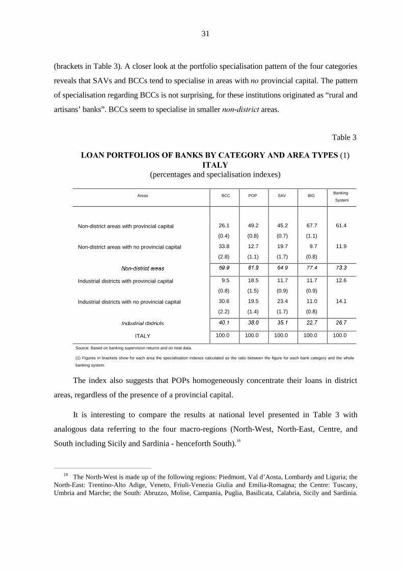
31

(brackets in Table 3). A closer look at the portfolio specialisation pattern of the four categories

reveals that SAVs and BCCs tend to specialise in areas with QR provincial capital. The pattern

of specialisation regarding BCCs is not surprising, for these institutions originated as “rural and

artisans’ banks”. BCCs seem to specialise in smaller QRQ-GLVWULFW areas.

Table 3

/2$1�3257)2/,26�2)�%$1.6�%<�&$7(*25<�$1'�$5($�7<3(6�(1),7$/<

(percentages and specialisation indexes)

Areas BCC POP SAV BIGBanking

System

Non-district areas with provincial capital 26.1

(0.4)

49.2

(0.8)

45.2

(0.7)

67.7

(1.1)

61.4

Non-district areas with no provincial capital 33.8

(2.8)

12.7

(1.1)

19.7

(1.7)

9.7

(0.8)

11.9

1RQ�GLVWULFW�DUHDV

���� ���� ���� ���� ����

Industrial districts with provincial capital 9.5

(0.8)

18.5

(1.5)

11.7

(0.9)

11.7

(0.9)

12.6

Industrial districts with no provincial capital 30.6

(2.2)

19.5

(1.4)

23.4

(1.7)

11.0

(0.8)

14.1

,QGXVWULDO�GLVWULFWV

���� ���� ���� ���� ����

ITALY 100.0 100.0 100.0 100.0 100.0

Source: Based on banking supervision returns and on Istat data.

(1) Figures in brackets show for each area the specialisation indexes calculated as the ratio between the figure for each bank category and the whole

banking system.

The index also suggests that POPs homogeneously concentrate their loans in district

areas, regardless of the presence of a provincial capital.

It is interesting to compare the results at national level presented in Table 3 with

analogous data referring to the four macro-regions (North-West, North-East, Centre, and

South including Sicily and Sardinia - henceforth South).18

18 The North-West is made up of the following regions: Piedmont, Val d’Aosta, Lombardy and Liguria; the

North-East: Trentino-Alto Adige, Veneto, Friuli-Venezia Giulia and Emilia-Romagna; the Centre: Tuscany,Umbria and Marche; the South: Abruzzo, Molise, Campania, Puglia, Basilicata, Calabria, Sicily and Sardinia.

32

Tables B1-B5 in Appendix 3 show that POPs lend more to IDs than to non-district

areas in those regions where IDs are most commonly found, namely North-West, North-East

and to a lesser extent Central Italy.

It is noteworthy that in North-Eastern Italy (Table B2) over 64 per cent of POPs’

lending goes to IDs; in no other macro-regions do POPs supply so much credit to IDs. In

addition, we notice that BIGs allot over 50 per cent of their overall loans to IDs rather than to

non-district areas, whereas BCCs’ and SAVs’ lending to IDs is slightly less than the national

average (compare Tables 3 and B2).

This great concentration of POPs’ loan portfolios in IDs could be interpreted as the

result of a comparatively greater concentration of IDs in North-Eastern Italy than in the rest

of the country. However, Tables A1 and A2� (Appendix III) show that this is only a partial

explanation. As displayed in Table A1, 32.7 per cent of district areas are located in

North-Eastern Italy, YLV�j�YLV about 30 in both North-Western and Central Italy. On the other

hand, Table A2 shows that 45.5 per cent of LLSs in North-Eastern Italy can be defined as

IDs, according to the Sforzi-Istat criteria. In the North-West and in the Centre the fraction of

district areas reduces to 42.1 and 44.1 per cent respectively. Therefore, even if district areas

are more numerous in the North-East, the difference is slight and cannot by itself explain the

high concentration of POPs’ loans to IDs.

Looking at other areas, we note that the pattern of banking localism in Central Italy is

partly similar to what we found in the North-East. In the Centre, though, BCCs play a greater

role: 56 per cent of their overall lending goes to district areas, as opposed to 52 per cent of

POPs’ and 51 per cent of SAVs’. However, while POPs seem to specialise in larger ID areas,

BCCs (and to a lesser extent SAVs) mainly lend to district areas with no provincial capital.

In North-Western Italy (Table B1), BCCs concentrate much of their lending in district

areas (70.4 per cent), particularly in IDs with no provincial capital. POPs and SAVs, on the

other hand, concentrate only a relatively small part of their portfolios in ID areas. However,

POPs’ degree of specialisation in districts is higher than in non-district areas.

We consider Lazio in isolation due to the scarcity of ID areas in this region and to the fact that data are biased bythe presence of Rome, where BIGs are enormously overrepresented. Data for Lazio are nonetheless given inseparate tables.

33

In the South, with its scarcity of IDs, all bank categories concentrate their lending in

non-district areas (Table B4). BCCs show a high degree of specialisation in smaller

non-district areas, due to their rural character. As to district areas, SAVs play a more

important role than the other bank categories.

In conclusion, with the possible exception of POPs there is not much evidence of greater

concentration of local banks’ loan portfolios in district than in non-district areas. In particular,

BCCs’ and SAVs’ activity is not limited to ID areas; rather, it applies mainly to non-district

areas, whereas POPs uniformly show a great specialisation of their loan portfolios in IDs.

���� �7KH�FRQFHQWUDWLRQ�RI�FUHGLW�VXSSO\�LQ�WKH���DUHD�W\SHV

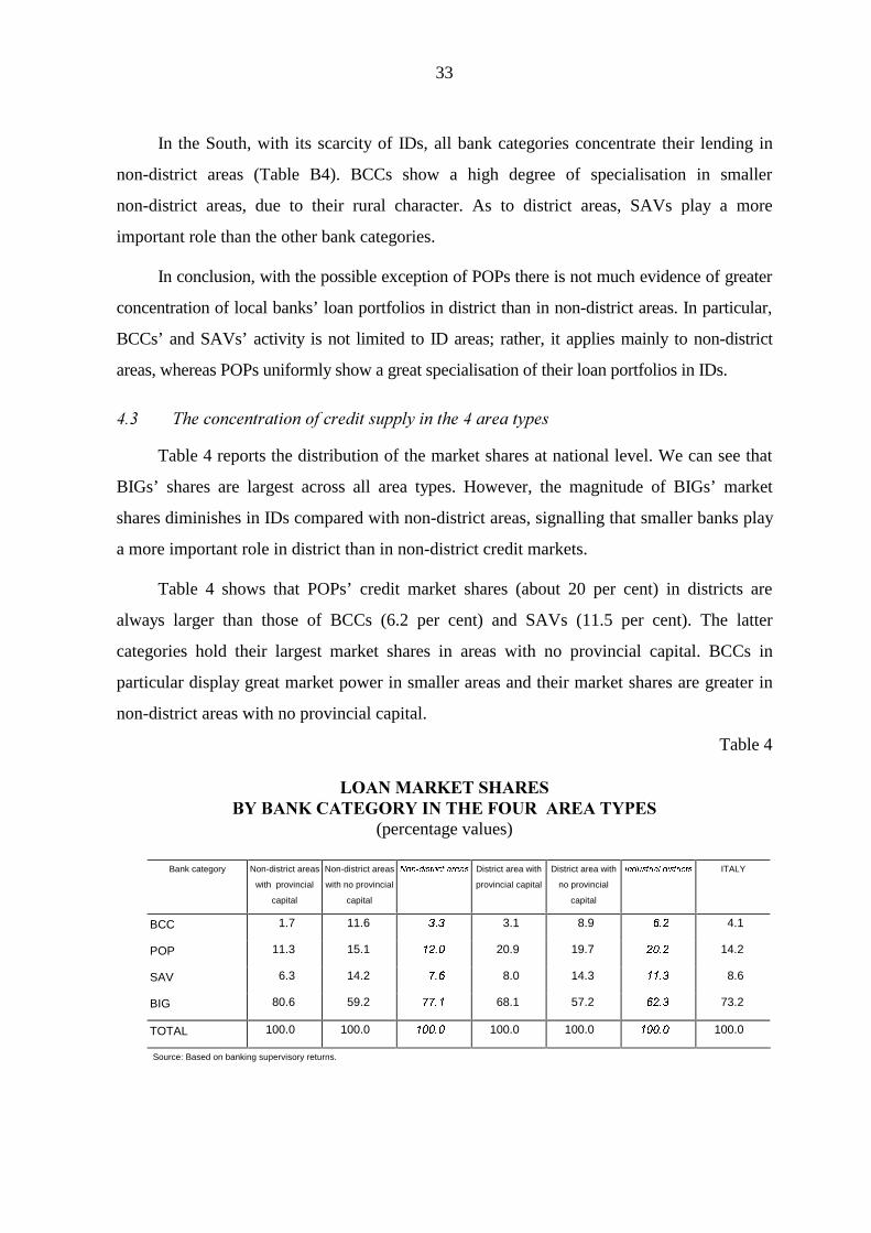
Table 4 reports the distribution of the market shares at national level. We can see that

BIGs’ shares are largest across all area types. However, the magnitude of BIGs’ market

shares diminishes in IDs compared with non-district areas, signalling that smaller banks play

a more important role in district than in non-district credit markets.

Table 4 shows that POPs’ credit market shares (about 20 per cent) in districts are

always larger than those of BCCs (6.2 per cent) and SAVs (11.5 per cent). The latter

categories hold their largest market shares in areas with no provincial capital. BCCs in

particular display great market power in smaller areas and their market shares are greater in

non-district areas with no provincial capital.

Table 4

/2$1�0$5.(7�6+$5(6%<�%$1.�&$7(*25<�,1�7+(�)285��$5($�7<3(6

(percentage values)

Bank category Non-district areas

with provincial

capital

Non-district areas

with no provincial

capital

1RQ�GLVWULFW�DUHDV District area with

provincial capital

District area with

no provincial

capital

,QGXVWULDO�GLVWULFWV ITALY

BCC 1.7 11.6 ��� 3.1 8.9 ��� 4.1

POP 11.3 15.1 ���� 20.9 19.7 ���� 14.2

SAV 6.3 14.2 ��� 8.0 14.3 ���� 8.6

BIG 80.6 59.2����

68.1 57.2����

73.2

TOTAL 100.0 100.0�����

100.0 100.0�����

100.0

Source: Based on banking supervisory returns.

34

Looking at credit market concentration at macro-regional level (see Appendix 3,

Tables C1-C5), we see that POPs hold the largest market shares in Northern IDs, particularly

in North-Eastern Italy, where they hold over 23 per cent of credit markets in district areas but

less than 14 per cent in non-district areas (Table C2). BCCs too appear to have significant

market shares in North-Eastern Italy, especially in non-district areas.

In Central Italy, POPs’ and BCCs’ market shares are much lower (Table C3).

Conversely, SAVs tend to have greater market power in district areas of Central Italy (43.3

per cent). It is interesting to note that BIGs’ market shares in this part of the country are the

lowest, not only in district areas (42.2 per cent) but also in non-district areas (55.4 per cent).

A description of the territorial pattern of the Italian banking system may benefit, for

our purposes, from an evaluation of the degree of average market concentration in the

different geographical areas. Market concentration is commonly measured by the Herfindahl

index of banks’ loan-market shares and of their branches. The simple means of this index at

LLS�level shows that concentration is not greater in IDs than in non-district areas (Table 5).

Considering the distribution of branches by area, again we find that concentration is not

higher in district credit markets.

Table 5

+(5),1'$+/�,1'(;�)25�/2$16�$1'�%5$1&+(6�(1)(simple means by area type)

Loans Branches

Non-district areas with provincial capital 0.16

(76)

0.15

(76)

Non-district areas with no provincial capital 0.45

(501)

0.40

(502)

Industrial districts with provincial capital 0.13

(19)

0.14

(19)

Industrial districts with no provincial capital 0.31

(179)

0.28

(179)

ITALY 0.38

(775)

0.34

(776)

Source: Based on banking supervisory returns and on Istat data. The Herfindahl index is equal to the sum of

the squares of market shares.

(1) Figures in brackets indicate the number of LLSs featuring loans granted by at least one bank or with at least

a branch of a bank. Differences between corresponding numbers of municipalities are due to the different

phenomena observed.

35

Similar results generally apply if we consider market concentration as measured by the

average Herfindahl index at municipal level by macro-regions both with respect to loans and

to branches (Appendix 3, Tables D1-D5). For Central Italy, however, Table D3 reveals that

market concentration is higher than average in district areas; for non-district areas the

evidence is mixed. In the South, higher-than-average market shares can be found in LLSs

without provincial capitals.

Results do not change if we look at other concentration indexes, such as the simple

mean of the largest market shares held at municipal level and the distribution of market

leadership across bank categories and area-types.19

On the basis of this evidence, with the possible exception of POPs, there seems to be

no category that can be seen as typical of district-local banks. But we do get an interesting

insight into the pattern of BCCs’ territorial specialisation. As Padoa-Schioppa argues, a

“BCCs’ Italy” exists in which “each of these banks, albeit very small in relation to the

national system, plays a prominent role in its own local market space” (Padoa-Schioppa,

1997, p. 522). According to our analysis it appears that this “BCCs’ Italy” is not concentrated

in district areas: these banks seem capable of finding their own market niches in non-district

contexts as well. BCCs’ localism is in many respects linked to their being mutual banks. As

we saw in Section 3, mutuals may elicit incentives that help overcome adverse selection and

moral hazard (i.e., the SHHU� PRQLWRULQJ� K\SRWKHVLV� DQG� ORQJ�WHUP� LQWHUDFWLRQ)20 Such

mechanisms do not necessarily require that mutual banks operate in IDs. Therefore, BCCs’

localism is not necessarily equivalent to ID localism.

19 The first index shows that banks do not hold larger market shares in district areas than in non-district

areas, with the sole exception of Central Italy, where IDs display higher market concentration (see Appendix 3,Table E1). As for the frequency distribution of LLS market leadership across bank categories, BCCs show atendency to be leaders (i.e. to retain the biggest share of the local market) in smaller areas, whereas POPs tendto be leaders mainly in larger IDs (see Appendix 3, Table E2). BCCs hold market leadership more frequently(26.3 per cent) than POPs (15.8 per cent) not only in small IDs, but also in district areas with provincialcapitals. Finally, considering the frequency distribution of LLS market leadership across area-types, BCCs andPOPs are market leaders more frequently in non-district areas than in IDs, while POPs tend to be market leadersmainly in smaller LLSs (district and non-district) rather than larger ones (see Appendix 3, Table E3).

20 Cf. Banerjee, Besley and Guinnane (1994), Stiglitz (1990), Varian (1990). Angelini, Di Salvo and Ferri(1997) find empirical evidence consistent with the peer monitoring hypothesis. In particular their results showthat, on average, BCC members enjoy better conditions than non-member clients. They accordingly reject theiralternative hypothesis: the long-term interaction hypothesis. According to the latter, the most importantincentive mechanism derives from the cooperative outcome of a sort of repeated game.

36

��� �3DWWHUQV�RI�EDQNLQJ�ORFDOLVP�LQ�,'V

In this section, we give empirical content to the “double concentration condition”. In

order to test whether a bank is an ID bank or not, consider a bank E (E = 1, ..., %) that offers

credit to a local labour system V (V = 1, ..., 6). We start with the following definition.

DEFINITION� (,'� EDQN).� A bank “E” is said to be a ORFDO� EDQN in ID� “V´ if the

following two conditions simultaneously hold (GRXEOH�FRQFHQWUDWLRQ�FRQGLWLRQ):

(1) TEV

≥ T

EV

TVE

≥ T

VE

where TEV

is the credit market share held by bank E� in LLS�V;�TVE� is the share of bank E’s

loan portfolio supplied to V; T

EV is the TXDGUDWLF�PHDQ of all credit market shares T

EV,; T

VE is

the quadratic mean of all loan portfolio shares TVE. If the conditions (1) are respected, we say

that the banking system is HPEHGGHG in the district’s socio-economic context.

The reasons for choosing the quadratic mean will become clear if we formally develop

condition (1). We obtain:

(2) TT

161

+ TT

1%1

+EV

EV

EV

%6 %6

6VE

VE

VE

%6 %6

%≥ = ⋅ ≥ = ⋅∑∑ ∑∑2 2

^ ^

where 6 represents the total number of local labour systems with at least one bank granting

credit; % is the total number of banks granting credit to the V-th local labour system; 1%6

is

equal to the non-empty intersection between the set of banks and that of local labour

systems; + 6

^

is the mean value of the Herfindahl indexes measuring market concentration in

each LLS; + %

^

is the mean value of the Herfindahl indexes measuring banks’ loan portfolio

concentration for each bank.

37

Simple means of TEV

and TVE

are equal to 6

1%6

and %1

%6

, respectively the reciprocal of

the average number of banks per LLS and of LLSs per bank. These fractions do not take

account of the different size of local labour systems and of banks, so we correct them by the

average Herfindahl indexes. Finally we compute mean values in (2) according to the

different geographical area to which LLS belong and according to their including a

provincial capital or not.

According to our methodology, only 58 out of 199 IDs have an embedded banking

system (Table 6). The need for the bank to diversify risk, thereby reaping the benefits from

scale economies, and the firms’ desire to free their decisions from the influence of

quasi-monopolistic banks set limits on the degree of banking localism.

Districts with an embedded banking system do not show any special difference from

other district areas, as far as the distribution by sector and the geographical area is concerned.

It is worth noting IDs with banking embeddedness include Biella, Prato, Carpi, Reggio

Emilia, Pesaro and Fermo, probably among the best known, and the earliest to be studied of

Italy’s district areas; this may explain a sort of observational bias in the literature in favour of

the natural link between districts and local banks.

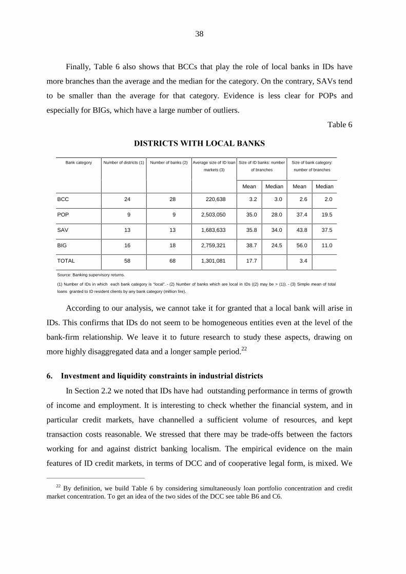
BCCs present the highest absolute frequency of banking embeddedness in IDs. They

pass our test in 28 cases and for 24 districts.21 As to the other bank categories, BIGs satisfy

the DCC 18 times, SAVs 13 and POPs only 9. In fact, the 24 IDs in which BCCs are “local”

represent 17.9 percent of all the IDs in which BCCs operate. The percentage diminishes to

11.1, 8.7 and 6.1 for SAVs, BIGs and POPs, respectively. This indicates that BCCs are more

capable of getting embedded in IDs. But, as was shown in the previous section, BCCs play

the role of local banks in non-ID areas as well. Furthermore, the embeddedness of BCCs is

concentrated in smaller districts: the ID credit markets in which BCCs are embedded are

much smaller, on average, than those of the other categories (see Table 6).

21 Note that our methodology does not rule out cases in which more than one bank per district can pass the

test.

38

Finally, Table 6 also shows that BCCs that play the role of local banks in IDs have

more branches than the average and the median for the category. On the contrary, SAVs tend

to be smaller than the average for that category. Evidence is less clear for POPs and

especially for BIGs, which have a large number of outliers.

Table 6

',675,&76�:,7+�/2&$/�%$1.6

Bank category Number of districts (1) Number of banks (2) Average size of ID loan

markets (3)

Size of ID banks: number

of branches

Size of bank category:

number of branches

Mean Median Mean Median

BCC 24 28 220,638 3.2 3.0 2.6 2.0

POP 9 9 2,503,050 35.0 28.0 37.4 19.5

SAV 13 13 1,683,633 35.8 34.0 43.8 37.5

BIG 16 18 2,759,321 38.7 24.5 56.0 11.0

TOTAL 58 68 1,301,081 17.7 3.4

Source: Banking supervisory returns.

(1) Number of IDs in which each bank category is “local”. - (2) Number of banks which are local in IDs ((2) may be > (1)). - (3) Simple mean of total

loans granted to ID resident clients by any bank category (million lire).

According to our analysis, we cannot take it for granted that a local bank will arise in

IDs. This confirms that IDs do not seem to be homogeneous entities even at the level of the

bank-firm relationship. We leave it to future research to study these aspects, drawing on

more highly disaggregated data and a longer sample period.22

��� �,QYHVWPHQW�DQG�OLTXLGLW\�FRQVWUDLQWV�LQ�LQGXVWULDO�GLVWULFWV

In Section 2.2 we noted that IDs have had outstanding performance in terms of growth

of income and employment. It is interesting to check whether the financial system, and in

particular credit markets, have channelled a sufficient volume of resources, and kept

transaction costs reasonable. We stressed that there may be trade-offs between the factors

working for and against district banking localism. The empirical evidence on the main

features of ID credit markets, in terms of DCC and of cooperative legal form, is mixed. We

22 By definition, we build Table 6 by considering simultaneously loan portfolio concentration and credit

market concentration. To get an idea of the two sides of the DCC see table B6 and C6.

39

have not so far investigated the net effect of those trade-offs on the extent credit rationing

vis-à-vis ID firms. In this section, we carry out an empirical analysis to this purpose.

In imperfect capital markets there are many different reasons why firms may choose

internal sources to finance their investment. First of all, asymmetries of information between

lenders and borrowers entail agency costs. If these costs are passed on to debtors, the latter

may seek to avoid them by resorting to internal finance (see Jensen and Meckling, 1976;

Myers and Majluf, 1984). Secondly, internal and external sources can also be matched with

the alternative governance structures they are associated with (Williamson, 1988). Financing

through debt or capital markets involves sharing residual rights of control with lenders and

capital holders, while internal sources avoid it and keep all power with the incumbents. Such

a governance structure could have lower transaction costs than external financing, which

may explain why internal sources are preferred.

A quite clear-cut implication then is that, with imperfect capital markets, investment

will be positively correlated with current cash flow or, more in general, with some measure

of the firm’s liquidity. In a neoclassical world with perfect capital markets it would only

depend on the stream of future expected profits.

Starting from the seminal paper by Fazzari, Hubbard and Petersen (1988) an entire

stream of literature has argued that as the bank-firm relationship becomes closer, the

sensitiveness of investment to measures of liquidity decreases. Hoshi, Kashyap and

Scharfstein (1991), for instance, show that Japanese firms belonging to groups called

NHLUHWVX are less liquidity-constrained than non-affiliated firms. That is due to the presence of

a main bank in the group with which other group firms establish very strong ties, thereby

reducing information asymmetries and agency costs.

In a recent and very provocative paper, Kaplan and Zingales (1997) argue that capital

market imperfections can certainly explain why cash flow is positively correlated with

investment, but that an increasing degree of these imperfections cannot explain greater

sensitivity of investment to liquidity measures. They offer a very simple theoretical model in

which, under reasonable assumptions about production and cost functions, greater capital

market imperfection leads to lower sensitivity of investment to the availability of internal

resources. They also provide empirical evidence that the firms which are most likely to be

40

rationed, according to a reasonable D�SULRUL classification, are those with lower, not higher,

sensitivity of investment to liquidity measures.

Although we cannot discuss this paper in detail, two critical remarks are appropriate.

From a theoretical point of view, the conceptual framework within which the model is valid

is too narrow.23 As for the empirical analysis, most of the findings refer to a sample of listed

companies, which can raise external funds to finance investment. This circumstance actually

complicates the role of cash flow, so that the latter can no longer be a mere source of

investment financing. When we consider small firms, as in IDs, external sources to finance

investment consist essentially in bank loans. Imperfections in credit markets can then explain

the different sensitivity of investment to liquidity measures.

For these reasons, we propose to carry out an experiment in which we compare the

sensitivity of investment to liquidity measures in IDs with respect to other areas. We

interpret the results of this experiment as a measure of the different degree of credit rationing

of ID versus non-ID companies.

Our data comes from the Italian Company Account Data Service (Centrale dei bilanci),

which reports data on the balance sheets of over 40,000 companies, for the years 1982-1995.

Albeit very detailed, this sample is partially biased: it mostly includes medium-to-large firms

and reports data for limited liability companies only, ruling out sole proprietorships and

partnerships.

The sample used in the regression analysis is selected by filtering data according to

different criteria. In particular, we choose firms that in the initial year of analysis had fewer

than 250 employees, in order to account for the small size of ID firms. We excluded firms

belonging to groups, since the availability of an internal capital market for these firms may

affect the results. We also ruled out those companies reporting irregular data and those for

which the growth rate of sales differed from the average value by more than twice the

standard deviation. As a result we obtain a sample of more than 4,000 companies reporting

data for the entire period 1985-1994. The main statistics are reported in Table 7.

23 In particular, their model is static and does not allow for endogeneity of the amount of funds raised in the

market with respect to the cost differential between internal and external sources.

41

A bit less than 25 per cent of this sample is made up of firms located in IDs. We did

not count as district firms those located in a district but operating in sectors other than that in

which the district specialises. Median values are quite similar between the two groups,

although ID firms on average tend to have higher growth rates of sales and accumulation of

capital, higher cash flow, and more debt. Differences between the two groups are rather

modest. So it is better to use multivariate analysis in order to go more deeply into the issue.

The reported data actually start from 1988, since we use lags in the regression.

There are several alternative ways in which investment behaviour can be associated

with liquidity measures. We could approach the issue via Tobin’s T model augmented by a

cash-flow variable. Since most of the companies in our sample are not listed, we cannot have

data on their market value, and Tobin’s T cannot be computed. Another approach can be

based on Euler’s equation, in which investment behaviour is explicitly designed as a

dynamic optimisation problem. Again, this model can be augmented by financial variables,

in order to check their possible impact on investment. We think, however, that this approach

is based on a number of restrictive assumptions that are very difficult to control empirically.

We therefore prefer using an DG� KRF dynamic model of investment based on the

DFFHOHUDWRU� SULQFLSOH�with adjustment costs augmented by cash flow and initial stock of

liquid assets.

Our basic equation is then as follows:

(1),

.D D

,

.D

&)

.D

/

.D

)

.YW

W

W

W

W

W

W

W

W

W

LW

−

−

− −

−

− −

= + + + + +1

0 11

22

13

1

14

1

∆

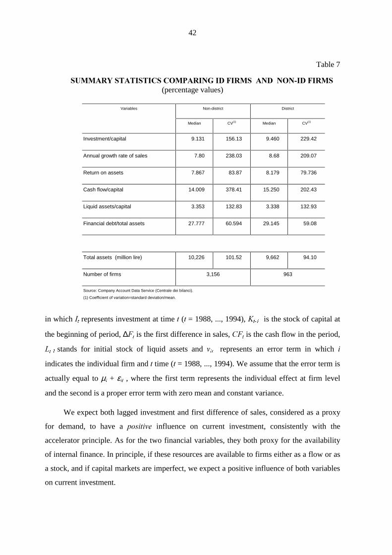
42

Table 7

6800$5<�67$7,67,&6�&203$5,1*�,'�),506��$1'��121�,'�),506(percentage values)

Variables Non-district District

Median CV(1) Median CV(1)

Investment/capital 9.131 156.13 9.460 229.42

Annual growth rate of sales 7.80 238.03 8.68 209.07

Return on assets 7.867 83.87 8.179 79.736

Cash flow/capital 14.009 378.41 15.250 202.43

Liquid assets/capital 3.353 132.83 3.338 132.93

Financial debt/total assets 27.777 60.594 29.145 59.08

Total assets (million lire) 10,226 101.52 9,662 94.10

Number of firms 3,156 963

Source: Company Account Data Service (Centrale dei bilanci).

(1) Coefficient of variation=standard deviation/mean.

in which ,W�represents investment at time W (W = 1988, ..., 1994), .

W��� is the stock of capital at

the beginning of period, ∆)W is the first difference in sales, &)

W is the cash flow in the period,

/W��

stands for initial stock of liquid assets and YLW represents an error term in which L

indicates the individual firm and W time (W = 1988, ..., 1994). We assume that the error term is

actually equal to µL + ε

LW , where the first term represents the individual effect at firm level

and the second is a proper error term with zero mean and constant variance.

We expect both lagged investment and first difference of sales, considered as a proxy

for demand, to have a SRVLWLYH influence on current investment, consistently with the

accelerator principle. As for the two financial variables, they both proxy for the availability

of internal finance. In principle, if these resources are available to firms either as a flow or as

a stock, and if capital markets are imperfect, we expect a positive influence of both variables

on current investment.

43

In order to estimate this dynamic panel data model, we take first differences and then

proceed with an instrumental variable estimation, due to the presence of a lagged dependent

variable among the regressors. As instrument we use ,W�2/.W�3. In this way we should get at

least a consistent estimation of parameters, although there could be problems with

efficiency.24 All the data are at book value. We then run this regression for the two groups of

firms: those belonging to IDs and the others. Notice also that we deal with a balanced panel,

with a constant number of firms. Results are reported in Table 8.

The most important piece of evidence is that the values of parameters for liquidity

measures are much KLJKHU for ID firms than for non-ID firms;25 the cash-flow parameter for

ID firms, in particular, is QHDUO\�WHQ�WLPHV�that for non-ID firms. The other results from the

table are quite clear: all the parameters show the expected sign and all the regressors are

highly significant.

Can we conclude, then, that agency costs in ID credit markets are such that district

firms are more severely liquidity-constrained than other firms? Before accepting this

conclusion, we have to go more deeply into this matter and address a number of issues.

24 See Baltagi (1995), including survey of the literature.25 In a recent paper, Pagnini (1998) obtained exactly the same result using completely different methodology

and source of data. In particular, he used unauthorised overdrafts as a percentage of total credit lines as a proxyfor the magnitude of financial constraints in different areas. Descriptive statistics and regression analysisconsistently indicate that this percentage is higher in ID than in non-ID areas. The conclusions reached in thepresent paper are not restricted to the validity of the test used in this paper which is based on the correlationbetween real investment and cash flow.

44

Table 8

Dependent variable: investment/lagged capital

(standard errors in parenthesis)

Regressors Total Non-district District

Lagged investment 0.00407639 0.100646 0.039012

(0.0015852) (0.008321) (0.01388)

Cash flow 0.045819 0.035352 0.285493

(0.0023555) (0.0022539) (0.01315)

Lagged short term securities 0.295574 0.277468 0.379710

(0.03108) (0.03354) (0.07939)

First difference of sales 0.023443 0.016526 0.027605

(0.0008992) (0.001052) (0.0022845)

Number of firms 4,119 3,156 963

1) Cash flow could proxy for profit opportunities. Hence, a greater sensitivity of investment

to this variable may not necessarily signal the degree of financial constraint. To control

for this factor we introduce a proxy for profits. The results do not change significantly: the

sensitivity of investment to liquidity measures remains much higher for ID firms.

2) Greater sensitivity to liquidity measures may signal that ID firms are specialised in sectors

of economic activity with better growth opportunities. Looking at the sectoral

composition of the two samples, it turns out that non-district firms are more concentrated

in sectors such as food and beverages, petroleum and chemical products and paper and

publishing. It is not clear whether these have higher growth rates. In any case, we run a

regression by selecting only those sectors in which IDs are mostly concentrated (textiles,

leather and footwear, wood and wood products, glass, non-metal mineral-based-products,

machinery). The results do not change radically.

3) We also carried out sensitivity analysis by changing the threshold for the maximum size

of firms in the initial year. The effects of liquidity measures on investment in IDs remain

significantly greater. To better qualify the influence of size, we also introduce the

logarithm of the number of employees. We obtain the same result.

45

4) The geographical composition of the two samples is rather different: the frequency of

non-district firms is higher among southern than among northern firms. Southern

companies, in particular, are usually considered as more liquidity-constrained than the

others; hence, the different sample composition should act in the opposite direction with

respect to our main result. In any case, even when we run the regression excluding

southern firms, the sensitivity of investment to liquidity measures turns out to be greater

in the district areas.

We offer two alternative interpretations for this evidence. On the one hand, greater

cash-flow sensitivity in ID areas may genuinely signal the existence of agency problems in

ID credit markets. This conclusion may be better qualified, however, if we look at the

characteristics of our sample. As we have seen, the Company Account Data Service panel

consists overwhelmingly of medium-to-large firms. Very small firms are not included.

Furthermore, we have taken only firms reporting data for the entire period 1988-1994,

thereby probably further reducing the proportion of small firms.

As was explained in Section 3, district areas may also have internal capital markets in

which comparatively bigger firms, responsible for marketing the final product, apply for bank

credit on behalf of smaller firms operating in the intermediate stages of production. Now, due

to the lack of strong ties with the banking system, these larger firms may suffer from the sort of

agency problems we mentioned before. At the same time, it may be economic for these firms to

alleviate liquidity problems for smaller firms in the district by channelling funds to them

through internal capital markets. So our results could be due to a sort of selection bias. In other

words, because of the over-representation of larger firms in the Company Account Data Service

sample, we may have only observed firms applying for credit on behalf of the whole district

and bearing the bulk of the agency costs. At the same time, however, we cannot observe the

smaller firms that benefit most from access to internal capital markets.

On the other hand, a different interpretation is also available. So far, the level of

aggregation chosen has been a sort of representative district. But industrial districts can differ

in their banking relations, stage of industrialisation, local conditions and so on (see Sections

3 and 4). In this respect, our conclusion that investment is more sensitive to cash-flow

measures in IDs may have been influenced by the characteristics of a subset of districts.

46

In order to carry out the analysis at a higher level of disaggregation, we run equation

(1) by alternatively considering: a) districts classified by the nature of their banking relations;

b) the regions to which district and non-district companies belong to; c) the sectors of

economic activity of ID and non-ID companies. We restrict our analysis to those cases for

which we have a sufficient sample size.

To investigate the extent of the banking relationship in ID areas, we run two different

regressions for districts with a local bank, according to the definition given in Section 3, and

for the others; surprisingly, there is no difference in the sensitivity of investment to liquidity

measures. This suggests a need to go more deeply into the analysis of bank-firm relationships

and also consider other indicators of their nature.

We also run regression (1) for different sectors of economic activity (see Figure 4).

Here, the results are quite different from those of the aggregate analysis. Whereas in the case

of machinery and furniture the correlation between investment and cash flow is actually

stronger in ID areas, this is not true for the food-and-beverage sector and especially for the

textile, clothing and leather sector. This seems to confirm that the nature of banking

relationships and the way investment is financed in the districts depends heavily on the

nature of the productive process.

Finally, we replicate our regression at regional level (Figure 5). Again, the results are

quite different across regions. While in northern regions like Lombardy and Veneto, ID firms

seem to be more financially constrained than non-district firms, the opposite holds for

Emilia-Romagna, Tuscany and Marche.

All these results suggest that we should abandon the concept of a representative district

and move toward more disaggregate levels of analysis.

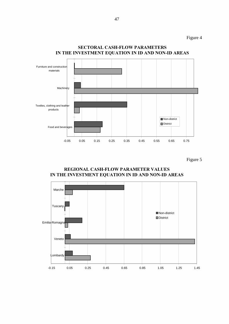
47

Figure 4

6(&725$/�&$6+�)/2:�3$5$0(7(56,1�7+(�,19(670(17�(48$7,21�,1�,'�$1'�121�,'�$5($6

-0.05 0.05 0.15 0.25 0.35 0.45 0.55 0.65 0.75

Food and beverages

Textiles, clothing and leather

products

Machinery

Furniture and construction

materials

Non-district

District

Figure 5

5(*,21$/�&$6+�)/2:�3$5$0(7(5�9$/8(6,1�7+(�,19(670(17�(48$7,21�,1�,'�$1'�121�,'�$5($6

-0.15 0.05 0.25 0.45 0.65 0.85 1.05 1.25 1.45

Lombardy

Veneto

Emilia-Romagna

Tuscany

Marche

Non-district

District

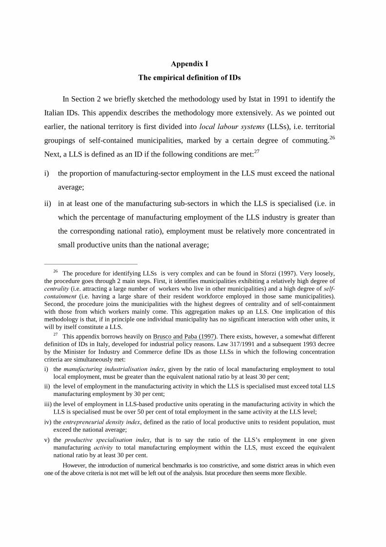
$SSHQGL[�,

7KH�HPSLULFDO�GHILQLWLRQ�RI�,'V

In Section 2 we briefly sketched the methodology used by Istat in 1991 to identify the

Italian IDs. This appendix describes the methodology more extensively. As we pointed out

earlier, the national territory is first divided into ORFDO�ODERXU�V\VWHPV (LLSs), i.e. territorial

groupings of self-contained municipalities, marked by a certain degree of commuting.26

Next, a LLS is defined as an ID if the following conditions are met:27

i) the proportion of manufacturing-sector employment in the LLS must exceed the national

average;

ii) in at least one of the manufacturing sub-sectors in which the LLS is specialised (i.e. in

which the percentage of manufacturing employment of the LLS industry is greater than

the corresponding national ratio), employment must be relatively more concentrated in

small productive units than the national average;

26 The procedure for identifying LLSs� is very complex and can be found in Sforzi (1997). Very loosely,

the procedure goes through 2 main steps. First, it identifies municipalities exhibiting a relatively high degree ofFHQWUDOLW\ (i.e. attracting a large number of workers who live in other municipalities) and a high degree of VHOI�FRQWDLQPHQW (i.e. having a large share of their resident workforce employed in those same municipalities).Second, the procedure joins the municipalities with the highest degrees of centrality and of self-containmentwith those from which workers mainly come. This aggregation makes up an LLS. One implication of thismethodology is that, if in principle one individual municipality has no significant interaction with other units, itwill by itself constitute a LLS.

27 This appendix borrows heavily on Brusco and Paba (1997). There exists, however, a somewhat differentdefinition of IDs in Italy, developed for industrial policy reasons. Law 317/1991 and a subsequent 1993 decreeby the Minister for Industry and Commerce define IDs� as those LLSs in which the following concentrationcriteria are simultaneously met:

i) the PDQXIDFWXULQJ� LQGXVWULDOLVDWLRQ� LQGH[, given by the ratio of local manufacturing employment to totallocal employment, must be greater than the equivalent national ratio by at least 30 per cent;

ii) the level of employment in the manufacturing activity in which the LLS is specialised must exceed total LLSmanufacturing employment by 30 per cent;

iii) the level of employment in LLS-based productive units operating in the manufacturing activity in which theLLS is specialised must be over 50 per cent of total employment in the same activity at the LLS level;

iv) the HQWUHSUHQHXULDO�GHQVLW\�LQGH[, defined as the ratio of local productive units to resident population, mustexceed the national average;

v) the SURGXFWLYH� VSHFLDOLVDWLRQ� LQGH[, that is to say the ratio of the LLS’s employment in one givenmanufacturing DFWLYLW\ to total manufacturing employment within the LLS, must exceed the equivalentnational ratio by at least 30 per cent.

However, the introduction of numerical benchmarks is too constrictive, and some district areas in which evenone of the above criteria is not met will be left out of the analysis. Istat procedure then seems more flexible.

49

iii) the degree of concentration of manufacturing employment in small local productive

units (i.e. industrial plants with no more than 250 employees) must be greater than the

national average;

iv) employment in one of the subsectors satisfying condition ii) must exceed 50 per cent of

total manufacturing employment in the same LLS�

Thus, each ID is associated to a manufacturing sector which in the text we refer to

as its “sector of specialisation” or “sector in which an ID is specialised”.

$SSHQGL[�,,

$�QRWH�RQ�WKH�,WDOLDQ�EDQNLQJ�V\VWHP

In this paper we use the 1991 banking data. In that year the 1936 Banking Law was still

in force28 and had not yet been replaced by the 1993 Banking Law. In this appendix we give

some information as to the types of banks that existed under the old law.

The old banking law framed the Italian banking structure within a rigid regulatory

system in which the supervisory institution had pervasive structural powers. In particular,

any new banks had to be authorised first, and a different authorisation was also necessary for

the newly formed bank to begin its activity. Branching also required prior authorisation.

Moreover, the old banking regime featured IXQFWLRQDO, VHFWRUDO and WHUULWRULDO specialisation.

)XQFWLRQDO� VSHFLDOLVDWLRQ consisted in the definite separation of the fund-raising

activities that could be undertaken by commercial banks (D]LHQGH�GL�FUHGLWR) from those that

could be carried out by long-term special credit institutions (LVWLWXWL� GL� FUHGLWR� VSHFLDOH).

More specifically, whereas commercial banks could raise sight deposits, short-term deposits

(meaning deposits with less than 18 months maturity) and medium-to-long-term maturity

funds, VSHFLDO�FUHGLW�LQVWLWXWLRQV could generally raise funds featuring long-term maturities.29

A functional subdivision of commercial banks was also in force. Accordingly,

commercial banks were divided into:30

i) public law banks (Banco di Napoli, Banco di Sicilia, Banca Nazionale del Lavoro,

Istituto Bancario San Paolo di Torino, Monte dei Paschi di Siena and from 1944 Banco

di Sardegna);

28 The 1936 Banking Law resulted from two governmental acts: i) royal decree 375/1936 and (Liii) royal

decree 1400/1937. These decrees were subsequently and respectively transposed into parliamentary acts141/1938 and 636/1938 and successively modified and integrated by act 933/1940. Although other changestook place in the years between 1938 and 1992-93 (such as Legislative Decree 350/1985, which adapted theItalian banking law to the norms of EC directive 77/780 of 1977 - “First Banking Directive”), the main body ofthe Italian banking law remained substantially.

29 This complex system was developed to overcome a series of banking crises towards the end of thetwenties and the beginning of the thirties.

30 Notice, however, that public law banks and savings banks could collect medium-term funds and grantlong-term loans through some “special sections” specifically set up to deal with specific long-term lending activities.

51

ii) banks of national interest (Banca Commerciale Italiana, Istituto di Credito Italiano and

Banco di Roma);

iii) limited company banks;

iv) popular cooperative banks (banche popolari) - POPs;

v) savings banks - SAVs;

vi) first and second class pledge banks;

vii) rural and artisans’ mutual banks - BCCs;

viii) branches of foreign banks.

Some of these categories were also disciplined by some specific legal provisions

which, among other things, restricted their operations.

3XEOLF� ODZ� EDQNV were credit institutions whose main feature was the public legal

form. They were generally organised in the form of foundations. The composition of the

boards of directors and chief executives and their salaries were often determined by central

government authorities.

%DQNV�RI�QDWLRQDO�LQWHUHVW were large public banks organised as stock corporations. Their

shares were concentrated in the hands of IRI as a result of their precarious financial situation

during the thirties. The purpose of this provision was to prevent the acquisition of dominant

positions by non-public bodies. “National interest” was defined on the basis of their vast territorial

organisation (as determined by the existence of branches in at least 30 provinces).

6$9V, 323V�and %&&V�were originally set up in order to provide for the financial needs

of local communities of entrepreneurs and/or farmers and artisans.31 Whereas savings banks

were generally set up in the form of moral institutions and foundations,32 both popular banks

and rural and artisans’ banks were credit cooperatives with mutual-aid features. However,

some distinctive features gradually emerged between popular and savings banks on the one

31 In many cases, the savings banks date back to the 18th century, whereas popular banks and rural and

artisans’ mutual banks began to spread in the second half of the 19th century. However, whereas savings banksoriginated from the initiative of the middle classes, both popular and artisans’ banks were initially formed byless wealthier social classes and often had religious roots.

32 Substantially similar to savings banks, the first and second class pledge banks were created with a viewto granting credit to small otherwise-would-be rationed savers and to fight usury beginning in the 15th and 16thcenturies.

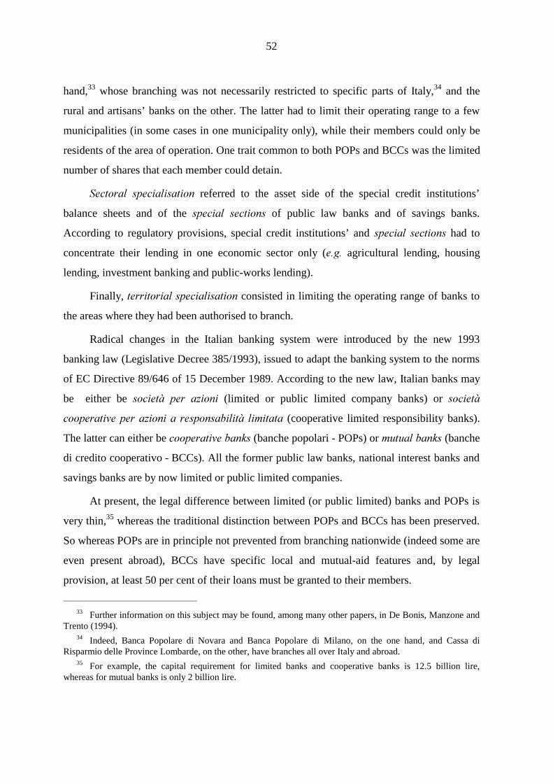
52

hand,33 whose branching was not necessarily restricted to specific parts of Italy,34 and the

rural and artisans’ banks on the other. The latter had to limit their operating range to a few

municipalities (in some cases in one municipality only), while their members could only be

residents of the area of operation. One trait common to both POPs and BCCs was the limited

number of shares that each member could detain.

6HFWRUDO� VSHFLDOLVDWLRQ referred to the asset side of the special credit institutions’

balance sheets and of the VSHFLDO� VHFWLRQV of public law banks and of savings banks.

According to regulatory provisions, special credit institutions’ and VSHFLDO� VHFWLRQV had to

concentrate their lending in one economic sector only (H�J� agricultural lending, housing

lending, investment banking and public-works lending).

Finally, WHUULWRULDO�VSHFLDOLVDWLRQ consisted in limiting the operating range of banks to

the areas where they had been authorised to branch.

Radical changes in the Italian banking system were introduced by the new 1993

banking law (Legislative Decree 385/1993), issued to adapt the banking system to the norms

of EC Directive 89/646 of 15 December 1989. According to the new law, Italian banks may

be either be VRFLHWj� SHU� D]LRQL (limited or public limited company banks) or VRFLHWj

FRRSHUDWLYH�SHU�D]LRQL�D� UHVSRQVDELOLWj� OLPLWDWD (cooperative limited responsibility banks).

The latter can either be FRRSHUDWLYH�EDQNV (banche popolari - POPs) or PXWXDO�EDQNV (banche

di credito cooperativo - BCCs). All the former public law banks, national interest banks and

savings banks are by now limited or public limited companies.

At present, the legal difference between limited (or public limited) banks and POPs is

very thin,35 whereas the traditional distinction between POPs and BCCs has been preserved.

So whereas POPs are in principle not prevented from branching nationwide (indeed some are

even present abroad), BCCs have specific local and mutual-aid features and, by legal

provision, at least 50 per cent of their loans must be granted to their members.

33 Further information on this subject may be found, among many other papers, in De Bonis, Manzone and

Trento (1994).34 Indeed, Banca Popolare di Novara and Banca Popolare di Milano, on the one hand, and Cassa di

Risparmio delle Province Lombarde, on the other, have branches all over Italy and abroad.35 For example, the capital requirement for limited banks and cooperative banks is 12.5 billion lire,

whereas for mutual banks is only 2 billion lire.

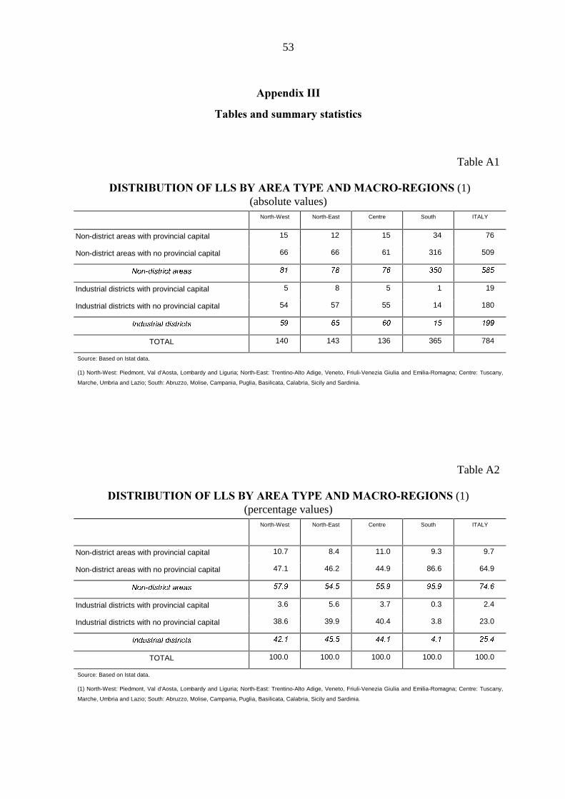
53

$SSHQGL[�,,,

7DEOHV�DQG�VXPPDU\�VWDWLVWLFV

Table A1

�',675,%87,21�2)�//6�%<�$5($�7<3(�$1'�0$&52�5(*,216�(1)(absolute values)

North-West North-East Centre South ITALY

Non-district areas with provincial capital 15 12 15 34 76

Non-district areas with no provincial capital 66 66 61 316 509

1RQ�GLVWULFW�DUHDV

�� �� �� ��� ���

Industrial districts with provincial capital 5 8 5 1 19

Industrial districts with no provincial capital 54 57 55 14 180

,QGXVWULDO�GLVWULFWV

�� �� �� �� ���

TOTAL 140 143 136 365 784

Source: Based on Istat data.

(1) North-West: Piedmont, Val d’Aosta, Lombardy and Liguria; North-East: Trentino-Alto Adige, Veneto, Friuli-Venezia Giulia and Emilia-Romagna; Centre: Tuscany,

Marche, Umbria and Lazio; South: Abruzzo, Molise, Campania, Puglia, Basilicata, Calabria, Sicily and Sardinia.

Table A2

',675,%87,21�2)�//6�%<�$5($�7<3(�$1'�0$&52�5(*,216�(1)(percentage values)

North-West North-East Centre South ITALY

Non-district areas with provincial capital 10.7 8.4 11.0 9.3 9.7

Non-district areas with no provincial capital 47.1 46.2 44.9 86.6 64.9

1RQ�GLVWULFW�DUHDV

���� ���� ���� ���� ����

Industrial districts with provincial capital 3.6 5.6 3.7 0.3 2.4

Industrial districts with no provincial capital 38.6 39.9 40.4 3.8 23.0

,QGXVWULDO�GLVWULFWV

���� ���� ���� ��� ����

TOTAL 100.0 100.0 100.0 100.0 100.0

Source: Based on Istat data.

(1) North-West: Piedmont, Val d’Aosta, Lombardy and Liguria; North-East: Trentino-Alto Adige, Veneto, Friuli-Venezia Giulia and Emilia-Romagna; Centre: Tuscany,

Marche, Umbria and Lazio; South: Abruzzo, Molise, Campania, Puglia, Basilicata, Calabria, Sicily and Sardinia.

54

Table A3

�',675,%87,21�2)�081,&,3$/,7,(6�%<�$5($�7<3(�$1'�0$&52�5(*,216�(1)(number of non-district areas)

North-West North-East Centre South ITALY

Non-district areas with provincial capital 541 234 267 632 1674

Non-district areas with no provincial capital 1236 494 382 1835 3947

1RQ�GLVWULFW�DUHDV

���� ��� ��� ���� ����

Industrial districts with provincial capital 281 201 37 22 541

Industrial districts with no provincial capital 1006 552 315 65 1938

,QGXVWULDO�GLVWULFWV

���� ��� ��� �� ����

TOTAL 3064 1481 1001 2554 8100

Source: Based on Istat data.

(1) North-West: Piedmont, Val d’Aosta, Lombardy and Liguria; North-East: Trentino-Alto Adige, Veneto, Friuli-Venezia Giulia and Emilia-Romagna; Centre: Tuscany,

Marche, Umbria and Lazio; South: Abruzzo, Molise, Campania, Puglia, Basilicata, Calabria, Sicily and Sardinia.

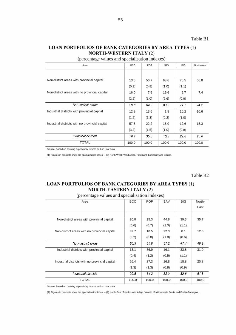
55

Table B1

�/2$1�3257)2/,26�2)�%$1.�&$7(*25,(6�%<�$5($�7<3(6�(1)1257+�:(67(51�,7$/<�(2)

(percentage values and specialisation indexes)Area BCC POP SAV BIG North-West

Non-district areas with provincial capital 13.5

(0.2)

56.7

(0.8)

63.6

(1.0)

70.5

(1.1)

66.8

Non-district areas with no provincial capital 16.0

(2.2)

7.6

(1.0)

19.6

(2.6)

6.7

(0.9)

7.4

1RQ�GLVWULFW�DUHDV

���� ���� ���� ���� ����

Industrial districts with provincial capital 12.8

(1.2)

13.6

(1.3)

1.8

(0.2)

10.2

(1.0)

10.6

Industrial districts with no provincial capital 57.6

(3.8)

22.2

(1.5)

15.0

(1.0)

12.6

(0.8)

15.3

,QGXVWULDO�GLVWULFWV

���� ���� ���� ���� ����

TOTAL 100.0 100.0 100.0 100.0 100.0

Source: Based on banking supervisory returns and on Istat data.

(1) Figures in brackets show the specialisation index. – (2) North-West: Val d’Aosta, Piedmont, Lombardy and Liguria.

Table B2

/2$1�3257)2/,26�2)�%$1.�&$7(*25,(6�%<�$5($�7<3(6�(1)1257+�($67(51�,7$/<�(2)

(percentage values and specialisation indexes)Area BCC POP SAV BIG North-

East

Non-district areas with provincial capital 20.8

(0.6)

25.3

(0.7)

44.8

(1.3)

39.3

(1.1)

35.7

Non-district areas with no provincial capital 39.7

(3.2)

10.5

(0.8)

22.3

(1.8)

8.1

(0.6)

12.5

1RQ�GLVWULFW�DUHDV ���� ���� ���� ���� ����

Industrial districts with provincial capital 13.1

(0.4)

36.9

(1.2)

16.1

(0.5)

33.8

(1.1)

31.0

Industrial districts with no provincial capital 26.4

(1.3)

27.3

(1.3)

16.8

(0.8)

18.8

(0.9)

20.8

,QGXVWULDO�GLVWULFWV ���� ���� ���� ���� ����

TOTAL 100.0 100.0 100.0 100.0 100.0

Source: Based on banking supervisory returns and on Istat data.

(1) Figures in brackets show the specialisation index. – (2) North-East: Trentino-Alto Adige, Veneto, Friuli-Venezia Giulia and Emilia-Romagna.

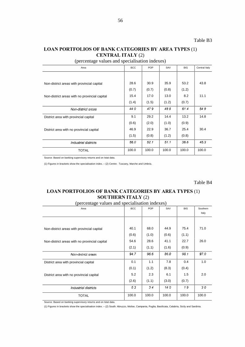
56

Table B3

/2$1�3257)2/,26�2)�%$1.�&$7(*25,(6�%<�$5($�7<3(6�(1)&(175$/�,7$/<�(2)

(percentage values and specialisation indexes)Area BCC POP SAV BIG Central Italy

Non-district areas with provincial capital 28.6

(0.7)

30.9

(0.7)

35.9

(0.8)

53.2

(1.2)

43.8

Non-district areas with no provincial capital 15.4

(1.4)

17.0

(1.5)

13.0

(1.2)

8.2

(0.7)

11.1

1RQ�GLVWULFW�DUHDV

���� ���� ���� ���� ����

District area with provincial capital 9.1

(0.6)

29.2

(2.0)

14.4

(1.0)

13.2

(0.9)

14.8

District area with no provincial capital 46.9

(1.5)

22.9

(0.8)

36.7

(1.2)

25.4

(0.8)

30.4

,QGXVWULDO�GLVWULFWV

���� ���� ���� ���� ����

TOTAL 100.0 100.0 100.0 100.0 100.0

Source: Based on banking supervisory returns and on Istat data.

(1) Figures in brackets show the specialisation index. – (2) Centre: Tuscany, Marche and Umbria.

Table B4

/2$1�3257)2/,26�2)�%$1.�&$7(*25,(6�%<�$5($�7<3(6�(1)6287+(51�,7$/<�(2)

(percentage values and specialisation indexes)Area BCC POP SAV BIG Southern

Italy

Non-district areas with provincial capital 40.1

(0.6)

68.0

(1.0)

44.9

(0.6)

75.4

(1.1)

71.0

Non-district areas with no provincial capital 54.6

(2.1)

28.6

(1.1)

41.1

(1.6)

22.7

(0.9)

26.0

1RQ�GLVWULFW�DUHDV

���� ���� ���� ���� ����

District area with provincial capital 0.1

(0.1)

1.1

(1.2)

7.8

(8.3)

0.4

(0.4)

1.0

District area with no provincial capital 5.2

(2.6)

2.3

(1.1)

6.1

(3.0)

1.5

(0.7)

2.0

,QGXVWULDO�GLVWULFWV

��� ��� ���� ��� ���

TOTAL 100.0 100.0 100.0 100.0 100.0

Source: Based on banking supervisory returns and on Istat data.

(1) Figures in brackets show the specialisation index. – (2) South: Abruzzo, Molise, Campania, Puglia, Basilicata, Calabria, Sicily and Sardinia.

57

Table B5

/2$1�3257)2/,26�2)�%$1.�&$7(*25,(6�%<�$5($�7<3(6�(1)/$=,2�(2)

(percentage values and specialisation indexes)Area BCC POP SAV BIG Lazio

Non-district areas with provincial capital 68.4

(0.7)

80.3

(0.9)

84.0

(0.9)

94.2

(1.0)

92.4

Non-district areas with no provincial capital 31.6

(4.4)

19.1

(2.7)

16.0

(2.2)

5.4

(0.8)

7.2

1RQ�GLVWULFW�DUHDV

����� ���� ����� ���� ����

District area with provincial capital (3) 0.0

-

0.0

-

0.0

-

0.0

-

0.0

District area with no provincial capital 0.0

(0.0)

0.6

(1.3)

0.0

(0.0)

0.4

(1.0)

0.4

,QGXVWULDO�GLVWULFWV

��� ��� ��� ��� ���

TOTAL 100.0 100.0 100.0 100.0 100.0

Source: Based on banking supervisory returns and on Istat data.

(1) Figures in brackets show the specialisation index. – (2) Lazio was considered on its own, because of the relatively scarce presence of district areas

in the region and its peculiar banking structure, with huge presence of big banks mainly concentrated in Rome and in its province. – (3) According to

the Sforzi-Istat algorithm, Lazio had no ID area with provincial capital in 1991.

Table B6$9(5$*(�6+$5(�2)�/2&$/�0$5.(76�,1�/2$1�3257)2/,26

2)�,1',9,'8$/�%$1.6�,1�63(&,),&�$5($�7<3(6�(1)(simple means; percentage values)

Area BCC POP SAV BIG Bankingsystem

Non-district areas with provincial capital 84.7 14.8 20.0 12.4 22.3

Non-district areas with no provincial capital 75.5 7.1 4.8 2.9 16.8

1RQ�GLVWULFW�DUHDV

���� ��� ��� ��� ����

District area with provincial capital (3) 73.1 9.9 15.4 4.2 13.8

District area with no provincial capital 66.5 4.2 6.7 3.1 15.2

,QGXVWULDO�GLVWULFWV

���� ��� ��� ��� ����

ITALY 74.8 8.3 8.9 5.9 17.6

Source: Based on banking supervisory returns and on Istat data.

(1) The figure in the first line, first column indicates, for instance, that, in non-ID areas with a provincial capital, on average individual BCCs have ashare of 84.7 per cent of the local market.

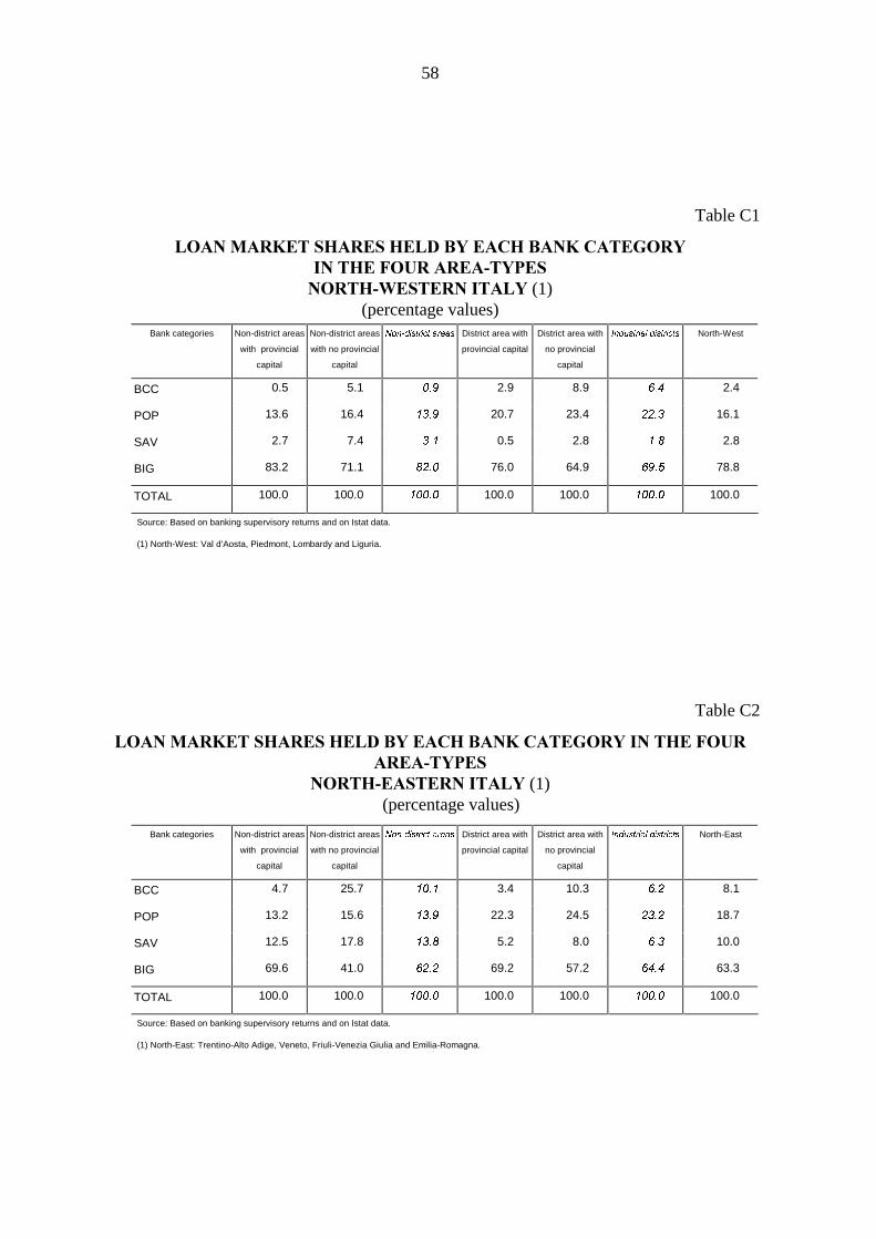
58

Table C1

/2$1�0$5.(7�6+$5(6�+(/'�%<�($&+�%$1.�&$7(*25<,1�7+(�)285�$5($�7<3(61257+�:(67(51�,7$/<�(1)

(percentage values)Bank categories Non-district areas

with provincial

capital

Non-district areas

with no provincial

capital

1RQ�GLVWULFW�DUHDV District area with

provincial capital

District area with

no provincial

capital

,QGXVWULDO�GLVWULFWV North-West

BCC 0.5 5.1 ��� 2.9 8.9 ��� 2.4

POP 13.6 16.4 ���� 20.7 23.4 ���� 16.1

SAV 2.7 7.4 ��� 0.5 2.8 ��� 2.8

BIG 83.2 71.1 ���� 76.0 64.9 ���� 78.8

TOTAL 100.0 100.0 ����� 100.0 100.0 ����� 100.0

Source: Based on banking supervisory returns and on Istat data.

(1) North-West: Val d’Aosta, Piedmont, Lombardy and Liguria.

Table C2

/2$1�0$5.(7�6+$5(6�+(/'�%<�($&+�%$1.�&$7(*25<�,1�7+(�)285$5($�7<3(6

1257+�($67(51�,7$/<�(1)(percentage values)

Bank categories Non-district areas

with provincial

capital

Non-district areas

with no provincial

capital

1RQ�GLVWULFW�DUHDV District area with

provincial capital

District area with

no provincial

capital

,QGXVWULDO�GLVWULFWV North-East

BCC 4.7 25.7 ���� 3.4 10.3 ��� 8.1

POP 13.2 15.6 ���� 22.3 24.5 ���� 18.7

SAV 12.5 17.8 ���� 5.2 8.0 ��� 10.0

BIG 69.6 41.0 ���� 69.2 57.2 ���� 63.3

TOTAL 100.0 100.0�����

100.0 100.0�����

100.0

Source: Based on banking supervisory returns and on Istat data.

(1) North-East: Trentino-Alto Adige, Veneto, Friuli-Venezia Giulia and Emilia-Romagna.

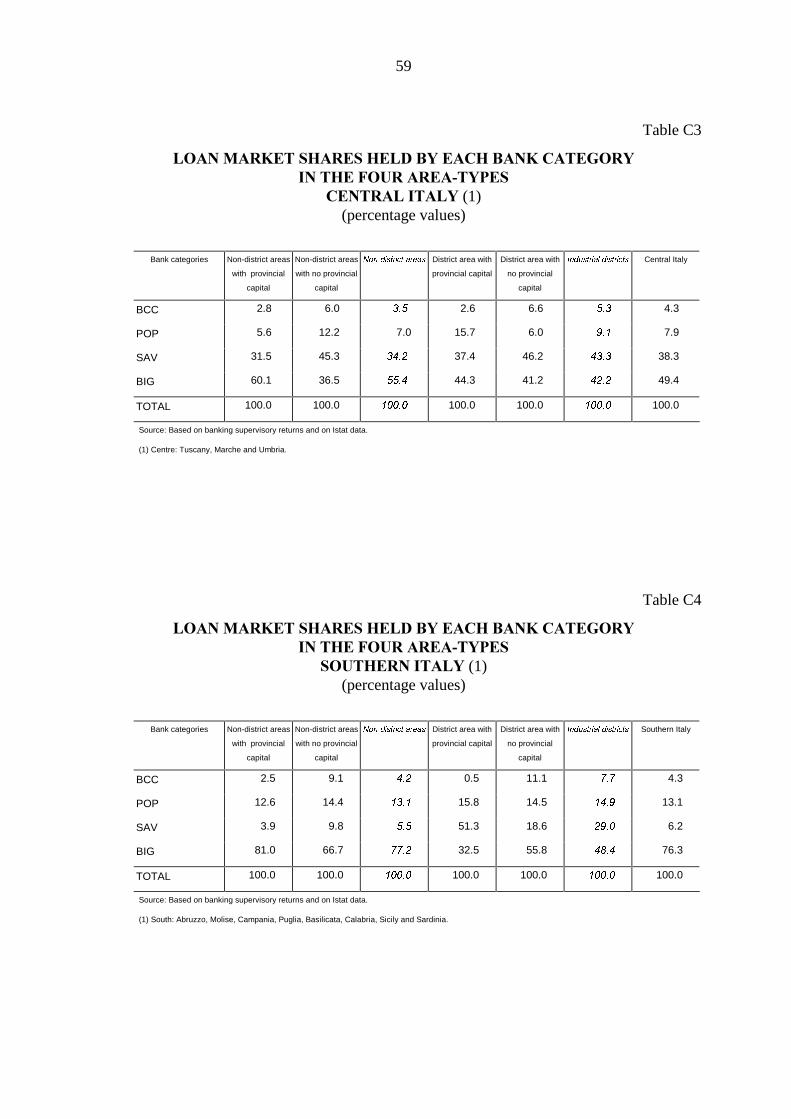
59

Table C3

/2$1�0$5.(7�6+$5(6�+(/'�%<�($&+�%$1.�&$7(*25<,1�7+(�)285�$5($�7<3(6

&(175$/�,7$/<�(1)(percentage values)

Bank categories Non-district areas

with provincial

capital

Non-district areas

with no provincial

capital

1RQ�GLVWULFW�DUHDV District area with

provincial capital

District area with

no provincial

capital

,QGXVWULDO�GLVWULFWV Central Italy

BCC 2.8 6.0 ��� 2.6 6.6 ��� 4.3

POP 5.6 12.2 7.0 15.7 6.0 ��� 7.9

SAV 31.5 45.3 ���� 37.4 46.2 ���� 38.3

BIG 60.1 36.5 ���� 44.3 41.2 ���� 49.4

TOTAL 100.0 100.0 ����� 100.0 100.0 ����� 100.0

Source: Based on banking supervisory returns and on Istat data.

(1) Centre: Tuscany, Marche and Umbria.

Table C4

/2$1�0$5.(7�6+$5(6�+(/'�%<�($&+�%$1.�&$7(*25<,1�7+(�)285�$5($�7<3(6

6287+(51�,7$/<�(1)(percentage values)

Bank categories Non-district areas

with provincial

capital

Non-district areas

with no provincial

capital

1RQ�GLVWULFW�DUHDV District area with

provincial capital

District area with

no provincial

capital

,QGXVWULDO�GLVWULFWV Southern Italy

BCC 2.5 9.1 ��� 0.5 11.1 ��� 4.3

POP 12.6 14.4 ���� 15.8 14.5 ���� 13.1

SAV 3.9 9.8 ��� 51.3 18.6 ���� 6.2

BIG 81.0 66.7 ���� 32.5 55.8 ���� 76.3

TOTAL 100.0 100.0 ����� 100.0 100.0 ����� 100.0

Source: Based on banking supervisory returns and on Istat data.

(1) South: Abruzzo, Molise, Campania, Puglia, Basilicata, Calabria, Sicily and Sardinia.

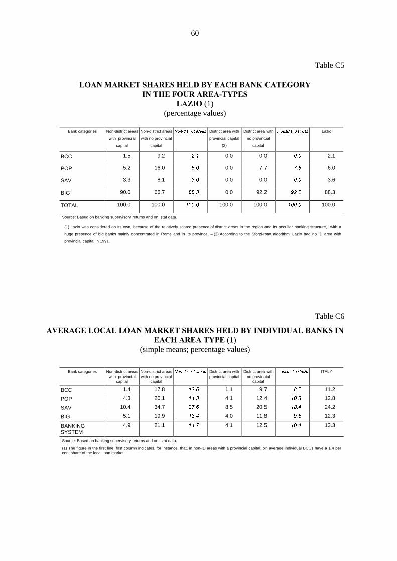
60

Table C5

/2$1�0$5.(7�6+$5(6�+(/'�%<�($&+�%$1.�&$7(*25<,1�7+(�)285�$5($�7<3(6

/$=,2�(1)(percentage values)

Bank categories Non-district areas

with provincial

capital

Non-district areas

with no provincial

capital

1RQ�GLVWULFW�DUHDV District area with

provincial capital

(2)

District area with

no provincial

capital

,QGXVWULDO�GLVWULFWV Lazio

BCC 1.5 9.2 ��� 0.0 0.0 ��� 2.1

POP 5.2 16.0 ��� 0.0 7.7 ��� 6.0

SAV 3.3 8.1 ��� 0.0 0.0 ��� 3.6

BIG 90.0 66.7 ���� 0.0 92.2 ���� 88.3

TOTAL 100.0 100.0 ����� 100.0 100.0 ����� 100.0

Source: Based on banking supervisory returns and on Istat data.

(1) Lazio was considered on its own, because of the relatively scarce presence of district areas in the region and its peculiar banking structure, with a

huge presence of big banks mainly concentrated in Rome and in its province. – (2) According to the Sforzi-Istat algorithm, Lazio had no ID area with

provincial capital in 1991.

Table C6

$9(5$*(�/2&$/�/2$1�0$5.(7�6+$5(6�+(/'�%<�,1',9,'8$/�%$1.6�,1($&+�$5($�7<3(�(1)

(simple means; percentage values)

Bank categories Non-district areaswith provincial

capital

Non-district areaswith no provincial

capital

1RQ�GLVWULFW�DUHDV District area withprovincial capital

District area withno provincial

capital

,QGXVWULDO�GLVWULFWV ITALY

BCC 1.4 17.8 ���� 1.1 9.7 ��� 11.2

POP 4.3 20.1 ���� 4.1 12.4 ���� 12.8

SAV 10.4 34.7 ���� 8.5 20.5 ���� 24.2

BIG 5.1 19.9 ���� 4.0 11.8 ��� 12.3

BANKINGSYSTEM

4.9 21.1 ���� 4.1 12.5 ���� 13.3

Source: Based on banking supervisory returns and on Istat data.

(1) The figure in the first line, first column indicates, for instance, that, in non-ID areas with a provincial capital, on average individual BCCs have a 1.4 percent share of the local loan market.

61

Table D1

+(5),1'$+/�,1'(;�)25�/2$16�$1'�%5$1&+(6�(1)1257+�:(67(51�,7$/<�(2)

(simple means by area type)Loans Branches

Non-district areas with provincial capital 0.16

(16)

0.18

(16)

Non-district areas with no provincial capital 0.34

(68)

0.29

(68)

Industrial districts with provincial capital 0.10

(5)

0.12

(5)

Industrial districts with no provincial capital 0.26

(55)

0.23

(55)

NORTH-WEST 0.28

(144)

0.25

(144)

Source: Based on banking supervisory returns and on Istat data.

(1) Number of LLSs with at least one bank’s loans or branches in brackets. Differences between corresponding

numbers of municipalities are due to the different phenomena observed. – (2) North-West: Val d’Aosta,

Piedmont, Lombardy and Liguria.

Table D2

+(5),1'$+/�,1'(;�)25�/2$16�$1'�%5$1&+(6�(1)1257+�($67(51�,7$/<�(2)

(simple means by area type)Loans Branches

Non-district areas with provincial capital 0.15

(12)

0.13

(12)

Non-district areas with no provincial capital 0.32

(64)

0.28

(64)

Industrial districts with provincial capital 0.11

(8)

0.12

(8)

Industrial districts with no provincial capital 0.26

(56)

0.23

(56)

NORTH-EAST 0.27

(140)

0.24

(140)

Source: Source: Based on banking supervisory returns and on Istat data.

(1) Number of LLSs with at least one bank’s loans or branches in brackets. Differences between corresponding

numbers of municipalities are due to the different phenomena observed. – (2) North-East: Trentino-Alto Adige,

Veneto, Friuli-Venezia Giulia and Emilia-Romagna.

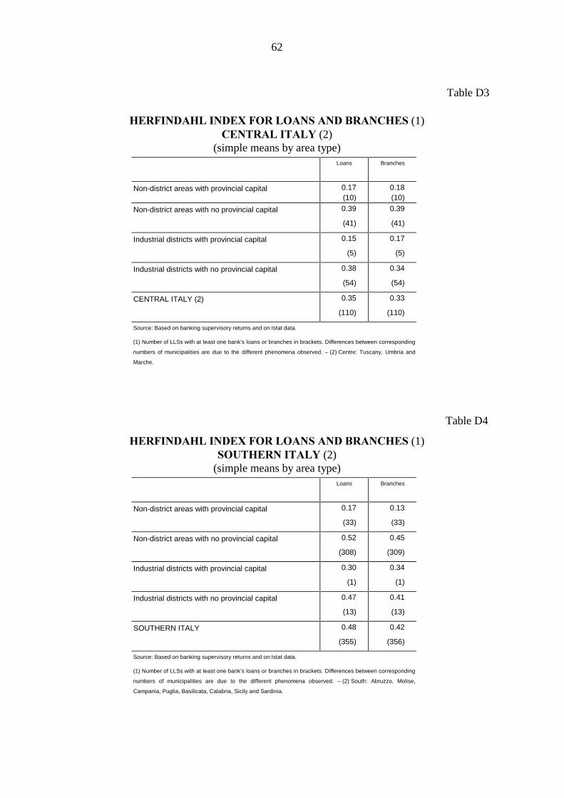
62

Table D3

+(5),1'$+/�,1'(;�)25�/2$16�$1'�%5$1&+(6�(1)&(175$/�,7$/<�(2)

(simple means by area type)Loans Branches

Non-district areas with provincial capital 0.17(10)

0.18(10)

Non-district areas with no provincial capital 0.39

(41)

0.39

(41)

Industrial districts with provincial capital 0.15

(5)

0.17

(5)

Industrial districts with no provincial capital 0.38

(54)

0.34

(54)

CENTRAL ITALY (2) 0.35

(110)

0.33

(110)

Source: Based on banking supervisory returns and on Istat data.

(1) Number of LLSs with at least one bank’s loans or branches in brackets. Differences between corresponding

numbers of municipalities are due to the different phenomena observed. – (2) Centre: Tuscany, Umbria and

Marche.

Table D4

+(5),1'$+/�,1'(;�)25�/2$16�$1'�%5$1&+(6�(1)6287+(51�,7$/<�(2)

(simple means by area type)Loans Branches

Non-district areas with provincial capital 0.17

(33)

0.13

(33)

Non-district areas with no provincial capital 0.52

(308)

0.45

(309)

Industrial districts with provincial capital 0.30

(1)

0.34

(1)

Industrial districts with no provincial capital 0.47

(13)

0.41

(13)

SOUTHERN ITALY 0.48

(355)

0.42

(356)

Source: Based on banking supervisory returns and on Istat data.

(1) Number of LLSs with at least one bank’s loans or branches in brackets. Differences between corresponding

numbers of municipalities are due to the different phenomena observed. – (2) South: Abruzzo, Molise,

Campania, Puglia, Basilicata, Calabria, Sicily and Sardinia.

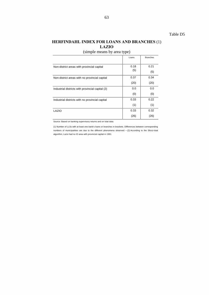
63

Table D5

+(5),1'$+/�,1'(;�)25�/2$16�$1'�%5$1&+(6�(1)/$=,2

(simple means by area type)Loans Branches

Non-district areas with provincial capital 0.18(5)

0.21

(5)

Non-district areas with no provincial capital 0.37

(20)

0.34

(20)

Industrial districts with provincial capital (2) 0.0

(0)

0.0

(0)

Industrial districts with no provincial capital 0.33

(1)

0.22

(1)

LAZIO 0.33

(26)

0.32

(26)

Source: Based on banking supervisory returns and on Istat data.

(1) Number of LLSs with at least one bank’s loans or branches in brackets. Differences between corresponding

numbers of municipalities are due to the different phenomena observed. – (2) According to the Sforzi-Istat

algorithm, Lazio had no ID area with provincial capital in 1991.

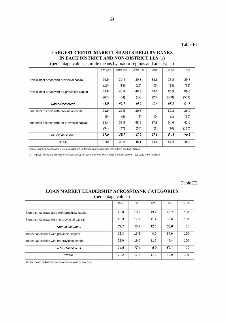
64

Table E1

/$5*(67�&5(',7�0$5.(7�6+$5(6�+(/'�%<�%$1.6,1�($&+�',675,&7�$1'�121�',675,&7�//6�(1)

(percentage values; simple means by macro-regions and area types)North-West North-East Centre (2) Lazio South ITALY

Non-district areas with provincial capital 29.9

(15)

30.4

(13)

30.3

(10)

33.6

(5)

28.8

(33)

29.8

(76)

Non-district areas with no provincial capital 45.9

(67)

44.4

(64)

48.5

(42)

48.3

(20)

60.5

(308)

55.0

(501)

1RQ�GLVWULFW�DUHDV

���� ���� ���� ���� ���� ����

Industrial districts with provincial capital 21.9

(5)

22.5

(8)

30.6

(5)

-

(0)

50.3

(1)

26.0

(19)

Industrial districts with no provincial capital 38.4

(54)

37.5

(57)

48.5

(54)

37.8

(2)

54.6

(14)

42.5

(180)

,QGXVWULDO�GLVWULFWV

���� ���� ���� ���� ���� ����

TOTAL 0.40 39.2 46.1 44.8 57.4 48.9

Source: Banking supervisory returns, calculations performed on municipalities with at least one bank branch.

(1) Figures in brackets indicate the number of LLSs in each area type with at least one bank branch. – (2) Lazio is not included.

Table E2

/2$1�0$5.(7�/($'(56+,3�$&5266�%$1.�&$7(*25,(6(percentage values)

BCC POP SAV BIG TOTAL

Non-district areas area with provincial capital 25.0 13.2 13.2 48.7 100

Non-district areas with no provincial capital 18.3 17.7 11.4 52.6 100

1RQ�GLVWULFW�DUHDV

���� ���� ���� ���� ���

Industrial districts with provincial capital 26.3 15.8 0.0 57.9 100

Industrial districts with no provincial capital 22.9 19.0 11.7 46.4 100

,QGXVWULDO�GLVWULFWV

���� ���� ��� ���� ���

TOTAL 20.2 17.5 11.3 50.9 100

Source: Based on banking supervisory returns and on Istat data.

65

Table E3

/2$1�0$5.(7�/($'(56+,3�$&5266�$5($�7<3(6(percentage values)

BCC POP SAV BIG Banking

System

Non-district area with one provincial capital 12.1 7.4 11.4 9.4 9.8

Non-district area with no provincial capital 58.6 65.4 64.8 66.8 64.7

1RQ�GLVWULFW�DUHDV

���� ���� ���� ���� ����

District area with one provincial capital 3.2 2.2 0.0 2.8 2.4

District area with no provincial capital 26.1 25.0 23.9 21.0 23.1

,QGXVWULDO�GLVWULFWV

���� ���� ���� ���� ����

TOTAL 100.0 100.0 100.0 100.0 100.0

Source: Based on banking supervisory returns and on Istat data.

5HIHUHQFHV

Angelini, P., R. Di Salvo and G. Ferri G. (1997), “Availability and Cost of Credit for SmallBusinesses: Customer Relationships and Credit Cooperatives”, in Cesarini, Ferri andGiardino (1997).

Bagnasco, A. (1977), 7UH�,WDOLH��OD�SUREOHPDWLFD�GHOOR�VYLOXSSR�LWDOLDQR, Bologna, Il Mulino.

Bagnasco, A. (1988), /D�FRVWUX]LRQH�VRFLDOH�GHO�PHUFDWR, Bologna, Il Mulino.

Baltagi, B. H. (1995), (FRQRPHWULF�$QDO\VLV�RI�3DQHO�'DWD, New York, Wiley.

Banerjee, A. V., T. Besley and T. W. Guinnane (1994), “Thy Neighbor’s Keeper: The Designof a Credit Cooperative with Theory and a Test”, 4XDUWHUO\� -RXUQDO� RI� (FRQRPLFV,Vol. 109, No. 2, pp. 491-516.

Barca, F. (ed.) (1997), OO�FDSLWDOLVPR�LWDOLDQR�GDO�GRSRJXHUUD�D�RJJL, Roma, Donzelli.

Becattini, G. (ed.) (1987), 0HUFDWR�H�IRU]H�ORFDOL��LO�GLVWUHWWR�LQGXVWULDOH, Bologna, Il Mulino.

Becattini, G. (1991), “Il distretto industriale marshalliano come concetto socio-economico”,4XDGHUQL�GHOOD�%DQFD�7RVFDQD, No. 34, pp. 51-65.

Becattini, G. (1996), “I sistemi locali nello sviluppo economico italiano”, 6YLOXSSR� ORFDOH,Vol. 2-3, No. 2-3, pp. 5-25.

Besley, T. and S. Coate (1995), “Group Lending, Repayment Incentives and SocialCollateral”, -RXUQDO�RI�(FRQRPLF�'HYHORSPHQW, Vol. 46, No. 1, pp. 1-18.

Brusco, S. (1991), “La genesi dell’idea di distretto industriale”, 4XDGHUQL� GHOOD� %DQFD7RVFDQD, No. 34, pp. 25-34.

Brusco, S. and S. Paba (1997), “Per una storia dei distretti industriali italiani dal secondodopoguerra agli anni novanta”, in Barca (1997).

Brusco, S., G. Cainelli, F. Forni, M. Franchi, A. Malusardi and R. Righetti (1996), “TheEvolution of Local Productive Systems in Emilia-Romagna”, in Cossentino, Pyke andSengenberger (1996).

Buzzacchi, L. and M. Pagnini (1997), “Equità ed efficienza: una comparazione tracooperative e imprese capitalistiche in Italia”, 6WXGL�H�1RWH�GL�(FRQRPLD, No. 3, pp. 79-112.

Cannari, L. and L. F. Signorini (1996), “Localismo, spirito cooperativo ed efficienza:elementi per un’analisi economica delle banche di credito cooperativo”, Banca d’Italia,Temi di discussione, No. 274.

67

Cannari, L. and L. F. Signorini (1997), “Rischiosità e razionamento: un’analisidell’efficienza allocativa delle banche di credito cooperativo e dei divari Nord-Sud”, inCesarini (1997).

Carboni, C. (1996), “Distretti industriali e governo socioeconomico locale”, Cespe Paper,No. 9.

Cesari, R. (1996), “Ci sono troppe banche locali in Italia? Un’analisi empirica su banche edimensione”, &RRSHUD]LRQH�GL�&UHGLWR, Vol. 48, No. 154, pp. 585-615.

Cesarini, F., G. Ferri and M. Giardino (eds.) (1997), &UHGLWR� H� VYLOXSSR�� EDQFKH� ORFDOLFRRSHUDWLYH�H�LPSUHVH�PLQRUL, Bologna, Il Mulino.

Conti, G. and G. Ferri (1997), “Banche locali e sviluppo economico decentrato”, mimeo.

Cossentino, F., F. Pyke and W. Sengenberger (eds.) (1996), /RFDO�DQG�5HJLRQDO�5HVSRQVH�WR*OREDO�3UHVVXUH��7KH�&DVH�RI�,WDO\�DQG�,WV�,QGXVWULDO�'LVWULFWV, IILS Research Series,No. 103; It. trans.: /H� ULVSRVWH� ORFDOL� H� UHJLRQDOL� DOOD� SUHVVLRQH� JOREDOH�� LO� FDVRGHOO¶,WDOLD�H�GHL�VXRL�GLVWUHWWL�LQGXVWULDOL, Bologna, Il Mulino, 1997.

De Bonis, R., B. Manzone and S. Trento (1994), “La proprietà cooperativa: teoria, storia e ilcaso delle banche popolari”, Banca d’Italia, Temi di discussione, No. 238.

De Gregorio, J. (1997), “Il ruolo della banca locale: un confronto internazionale”, in Cesarini(1997).

Dei Ottati, G. (1992), “Fiducia, transazioni intrecciate e credito nel distretto industriale”,(FRQRPLF� 1RWHV, Vol. 23, No. 1-2, pp. 1-30; see also &DPEULGJH� -RXUQDO� RI(FRQRPLFV, Vol. 18, No. 6, 1994, pp. 529-46.

Drèze, J. (1997), “Piccolo è bello anche per le banche. Potrà durare?”, in Cesarini (1997).

Fabiani, S. and G. Pellegrini (1997), “Education, Infrastructures, Geography and Growth: AnEmpirical Analysis of the Development of Italian Provinces”, Banca d’Italia, Temi didiscussione, No� 323.

Fabiani, S., G. Pellegrini, E. Romagnano and L. F. Signorini (1998), “L’efficienza delleimprese nei distretti industriali”, Banca d’Italia, mimeo.

Fazzari, S., R. G. Hubbard and B. C. Petersen (1988), “Financing Constraints and CorporateInvestment”, %URRNLQJV�3DSHUV�RQ�(FRQRPLF�$FWLYLW\, No. 1, pp. 141-95.

Fazzari, S., R. G. Hubbard and B. C. Petersen (1996), “Financing Constraints and CorporateInvestment: Response to Kaplan and Zingales”, NBER Working Paper, No. 5462.

Ferri, G. (1997), “Mobilità dei dirigenti ed efficienza allocativa: banche locali e nazionali”,in Banca Nazionale del Lavoro, 3URSULHWj��FRQWUROOR�H�JRYHUQR�GHOOH�EDQFKH, Quadernodi Moneta e Credito, Supplement to No. 197, pp. 245-65.

68

Ferri, G. and R. Di Salvo (1994), “Credito cooperativo, finanziamento alle piccole e medieimprese e sviluppo decentrato: valutazioni teoriche e primi riscontri empirici”,&RRSHUD]LRQH�GL�&UHGLWR, Vol. 46, No. 146, pp. 309-69.

Granovetter, M. (1985), “Economic Action and Social Structure: The Problem ofEmbeddedness”, $PHULFDQ�-RXUQDO�RI�6RFLRORJ\, Vol. 91, pp. 481-510.

Harrison, B. (1992), “Industrial Districts: Old Wine in New Bottles?”, 5HJLRQDO�6WXGLHV, Vol.26, No. 5, pp. 469-83.

Hoshi, T., A. Kashyap and D. Scharfstein (1991), “Corporate Structure, Liquidity, andInvestment: Evidence from Japanese Industrial Groups”, 4XDUWHUO\� -RXUQDO� RI(FRQRPLFV, Vol. 106, No. 1, pp. 33-60.

Irpet and Istat (1994), ,�VLVWHPL�ORFDOL�GHO�ODYRUR�LQ�,WDOLD, Milano, Angeli.

Istat (1994, 1995), 5DSSRUWR�DQQXDOH��OD�VLWXD]LRQH�GHO�3DHVH, Roma.

Jensen, M. C. and H. W. Meckling (1976), “Theory of the Firm: Managerial Behavior,Agency Costs, and Ownership Structure”, -RXUQDO�RI�)LQDQFLDO�(FRQRPLFV, Vol. 3, No.4, pp. 305-60.

Kaplan, S. N. and L. Zingales (1997), “Do Investment Cash-Flow Sensitivities ProvideUseful Measures of Financing Constraints”, 4XDUWHUO\� -RXUQDO� RI� (FRQRPLFV, Vol.112, No. 1, pp. 169-215.

Marshall, A. (1875), “Some Features of American Industry”, in J. Whitaker (ed.), 7KH�(DUO\(FRQRPLF�:ULWLQJV�RI�$OIUHG�0DUVKDOO����������, London, Macmillan, 1975.

Myers, S. and N. Majluf (1984), “Corporate Financing and Investment Decisions WhenFirms Have Information That Investors Do Not”, -RXUQDO�RI�)LQDQFLDO�(FRQRPLFV, Vol.13, No. 2, pp. 187-221.

Nakamura, L. I. (1994), “Small Borrowers and the Survival of the Small Bank: Is MouseBank Mighty or Mickey?”, )HGHUDO� 5HVHUYH� %DQN� RI� 3KLODGHOSKLD� %XVLQHVV� 5HYLHZ,November-December, pp. 3-15.

Padoa-Schioppa, T. (1994), “Profili di diversità nel sistema bancario italiano”, in Bancad’Italia, %ROOHWWLQR�(FRQRPLFR,�No. 22, pp. 27*-43*.

Padoa-Schioppa, T. (1997), “Il credito cooperativo in Italia: realtà e problemi”, in Cesarini(1997).

Pagano, M. and F. Panunzi (1997), “Banche cooperative e banche commerciali: qual è ladifferenza?”, Proceedings of IRCEL’s 3rd Annual Convention on “Motivations andObjectives in the Local Cooperative Bank: An Interdisciplinary Discussion”, Rome,27-28 February.

69

Pagnini, M. (1998), ,� YLQFROL� ILQDQ]LDUL� SHU� OH� LPSUHVH� GLVWUHWWXDOL�� XQD� DQDOLVL� VX� GDWLEDQFDUL, paper prepared for the XIX Associazione Italiana Scienze Regionali (AISRe)Conference, L’Aquila, 7-9 October.

Petersen, M. A. and R. G. Rajan (1995), “The Effect of Credit Market Competition onLending Relationships”, 4XDUWHUO\�-RXUQDO�RI�(FRQRPLFV, Vol. 110, No. 2, pp. 407-44.

Sforzi, F. (1987), “L’identificazione spaziale”, in Becattini (1987).

Sforzi, F. (ed.) (1997), ,�VLVWHPL�ORFDOL�GHO�ODYRUR�����, Roma, Istat.

Stiglitz, J. E. (1990), “Peer Monitoring in Credit Markets”, :RUOG�%DQN�(FRQRPLF�5HYLHZ,Vol. 4, pp. 351-66.

Varian, H. R. (1990), “Monitoring Agents with Other Agents”, -RXUQDO�RI�,QVWLWXWLRQDO�DQG7KHRUHWLFDO�(FRQRPLFV, Vol. 146, pp. 153-74.

Williamson, O. E. (1979), “Transaction-Cost Economics: The Governance of ContractualRelations”, -RXUQDO�RI�/DZ�DQG�(FRQRPLFV, Vol. ""�XXII, pp. 233-61; repr. in O. E.Williamson, (FRQRPLF�2UJDQL]DWLRQ, Brighton, Harvester-Wheatsheaf, 1986.

Williamson, O. E. (1988), “Corporate Finance and Corporate Governance”, -RXUQDO� RI)LQDQFH, Vol. 43, No. 2, pp. 567-91.

5(&(17/< 38%/,6+(' ´7(0,µ � �

1R� ��� ³ /RQJ��7HUP ,QWHUHVW 5DWH &RQYHUJHQFH LQ (XURSH DQG WKH 3UREDELOLW\ RI (08� E\,� $1*(/21, DQG 5� 9,2/, �1RYHPEHU ������

1R� ��� ³ (GXFDWLRQ� ,QIUDVWUXFWXUH� *HRJUDSK\ DQG *URZWK� $Q (PSLULFDO $QDO\VLVRI WKH 'HYHORSPHQW RI ,WDOLDQ 3URYLQFHV� E\ 6� )$%,$1, DQG *� 3(//(*5,1,�1RYHPEHU ������

1R� ��� ³ 3URSHUWLHV RI WKH 0RQHWDU\ &RQGLWLRQV ,QGH[� E\ *� *5$1'( �'HFHPEHU ������

1R� ��� ³ 6W\OH� )HHV DQG 3HUIRUPDQFH RI ,WDOLDQ (TXLW\ )XQGV� E\ 5� &(6$5, DQG )� 3$1(77$�-DQXDU\ ������

1R� ��� ³ $GYHUVH 6HOHFWLRQ RI ,QYHVWPHQW 3URMHFWV DQG WKH %XVLQHVV &\FOH� E\ 3� 5(,&+/,1DQG 3� 6,&212/), �)HEUXDU\ ������

1R� ��� ³ ,QWHUQDWLRQDO 5LVN 6KDULQJ DQG (XURSHDQ 0RQHWDU\ 8QLILFDWLRQ� E\ %� (�6�5(16(1 DQG 2� <26+$ �)HEUXDU\ ������

1R� ��� ³ 7KH %HKDYLRXU RI WKH 'ROODU DQG ([FKDQJH 5DWHV LQ (XURSH� (PSLULFDO (YLGHQFHDQG3RVVLEOH([SODQDWLRQV� E\3�'(/*,29$1( DQG$� )� 32==2/2 �)HEUXDU\ ������

1R� ��� ³ 5LVXOWDWL H SUREOHPL GL XQ TXLQTXHQQLR GL SROLWLFD GHL UHGGLWL� XQD SULPD YDOXWD]LRQHTXDQWLWDWLYD� E\ 6� )$%,$1,� $� /2&$512� *� 21(72 DQG 3� 6(67,72 �0DUFK ������

1R� ��� ³ /D SUREOHPDWLFD GHOOD FUHVFHQWH IUDJLOLWj QHOOD ´LSRWHVL GL LQVWDELOLWj ILQDQ]LDULDµGD XQD SURVSHWWLYD NDOHFNLDQD� E\ *� &25%,6,(52 �0DUFK ������

1R� ��� ³ 5HVHDUFK DQG 'HYHORSPHQW� 5HJLRQDO 6SLOORYHUV� DQG WKH /RFDWLRQ RI (FRQRPLF$FWLYLWLHV� E\ $� )� 32==2/2 �0DUFK ������

1R� ��� ³ &HQWUDO %DQN ,QGHSHQGHQFH� &HQWUDOL]DWLRQ RI :DJH %DUJDLQLQJ� ,QIODWLRQ DQG8QHPSOR\PHQW� 7KHRU\ DQG (YLGHQFH� E\$� &8.,(50$1 DQG )� /,33, �$SULO ������

1R� ��� ³ /D GRPDQGD GL ILQDQ]LDPHQWL EDQFDUL LQ ,WDOLD H QHOOH GLYHUVH DUHH GHO 3DHVH������������� E\ '� )2&$5(//, DQG 3� 5266, �0D\ ������

1R� ��� ³ /D SROLWLFD ILVFDOH QHL SDHVL GHOO·8QLRQH HXURSHD QHJOL DQQL QRYDQWD� E\ 3� &$6(//,DQG 5� 5,1$/', �-XO\ ������

1R� ��� ³ 6LJQDOLQJ )LVFDO 5HJLPH 6XVWDLQDELOLW\� E\ )� '58', DQG $� 35$7, �6HSWHPEHU������

1R� ��� ³ )LVFDO &RQVROLGDWLRQV XQGHU)L[HG ([FKDQJH5DWHV� E\ 3�&$6(//, �2FWREHU ������

1R� ��� ³ ,QYHVWLPHQWL GLUHWWL DOO·HVWHUR H FRPPHUFLR� FRPSOHPHQWL R VRVWLWXWL"� E\ $� 025,DQG 9� 52//, �2FWREHU ������

1R� ��� ³ 1RQOLQHDU 9$5� 6RPH 7KHRU\ DQG DQ $SSOLFDWLRQ WR 86 *13 DQG 8QHPSOR\PHQW�E\ )� $/7,66,02 DQG *� /� 9,2/$17( �2FWREHU ������

1R� ��� ³ 7KH 3UREDELOLW\ 'HQVLW\ )XQFWLRQ RI ,QWHUHVW 5DWHV ,PSOLHG LQ WKH 3ULFH RI 2SWLRQV�E\ )� )251$5, DQG 5� 9,2/, �2FWREHU ������

1R� ��� ³ +HWHURJHQHRXV ´&UHGLW &KDQQHOVµ DQG 2SWLPDO 0RQHWDU\ 3ROLF\ LQ D 0RQHWDU\8QLRQ� E\ /� *$0%$&257$ �2FWREHU ������

1R� ��� ³ ´(QHP\ RI1RQH EXW D&RPPRQ)ULHQG RI $OOµ"$Q ,QWHUQDWLRQDO 3HUVSHFWLYH RQ WKH/HQGHU��RI��/DVW��5HVRUW )XQFWLRQ� E\ &� *,$11,1, �'HFHPEHU ������

1R� ��� ³ (QHUJ\ &RQVXPSWLRQ� 6XUYH\ 'DWD DQG WKH 3UHGLFWLRQ RI ,QGXVWULDO 3URGXFWLRQ LQ,WDO\� E\ '� -� 0$5&+(77, DQG *� 3$5,*, �'HFHPEHU ������

1R� ��� ³ :KDW &DXVHG WKH $VLDQ &XUUHQF\ DQG )LQDQFLDO &ULVLV"� E\ *� &256(77,�3� 3(6(17, DQG 1� 528%,1, �'HFHPEHU ������

1R� ��� ³ ,QYHVWPHQW DQG WKH ([FKDQJH 5DWH� E\ )� 18&&, DQG $� )� 32==2/2 �'HFHPEHU������

1R� ��� ³ 5HDOORFDWLRQ DQG /HDUQLQJ RYHU WKH %XVLQHVV &\FOH� E\ )� 6&+,9$5', �'HFHPEHU������

1R� ��� ³ 8QD ULFRVWUX]LRQH RPRJHQHD GL GDWL UHJLRQDOL� FRQWL HFRQRPLFL H UHGGLWRGLVSRQLELOH GHOOH IDPLJOLH ����������� E\ 3� %(55(7721,� 5� '(/2*8� &�3$33$/$5'2 DQG 3� 3,6(//, �)HEUXDU\ ������

� � 5HTXHVWV IRU FRSLHV VKRXOG EH VHQW WR�%DQFD G·,WDOLD �� 6HUYL]LR 6WXGL �� 'LYLVLRQH %LEOLRWHFD H SXEEOLFD]LRQL �� 9LD 1D]LRQDOH� �� �� ����� 5RPH�ID[ ���� �� ���������