1

Indication of a species in an extinction vortex: the ocellated turkey on the Yucatan 1

Peninsula, Mexico 2

3

Christian KAMPICHLER * 4

Universidad Juárez Autónoma de Tabasco, División de Ciencias Biológicas, Carretera 5

Villahermosa-Cárdenas km. 0.5 s/n, C.P. 86150, Villahermosa, Tabasco, Mexico, 6

and Vogeltrekstation – Dutch Centre for Avian Migration and Demography, NIOO-7

KNAW, P. O. Box 40, 6666 ZG Heteren, The Netherlands. E-mail: 8

christian.kampichler@web.de 9

10

Sophie CALMÉ 11

El Colegio de la Frontera Sur, Unidad Chetumal, Avenida del Centenario km. 5.5, C.P. 12

77900, Chetumal, Quintana Roo, Mexico, and Université de Sherbrooke, Département 13

de biologie, 2500 boulevard de l’Université, Sherbrooke, Quebec, J1K 2R1 Canada. E-14

mail: sophie.calme@usherbrooke.ca 15

16

Holger WEISSENBERGER 17

El Colegio de la Frontera Sur, Unidad Chetumal, Avenida del Centenario km. 5.5, C.P. 18

77900, Chetumal, Quintana Roo, Mexico. E-mail: holgerweissen@ecosur.mx 19

20

Stefan Louis ARRIAGA-WEISS 21

Universidad Juárez Autónoma de Tabasco, División de Ciencias Biológicas, Carretera 22

Villahermosa-Cárdenas km. 0.5 s/n, C.P. 86150, Villahermosa, Tabasco, Mexico. E-23

mail: slaw2000@prodigy.net.mx 24

25

* Corresponding author. Vogeltrekstation – Dutch Centre for Avian Migration and 26

Demography, NIOO-KNAW, P. O. Box 40, 6666 ZG Heteren, The Netherlands. E-mail: 27

christian.kampichler@web.de; Tel +31 (0)26 479 1234; Fax +31 (0)26 472 3227 28

2

Indication of a species in an extinction vortex: the ocellated turkey on the Yucatan 29

Peninsula, Mexico 30

31

Christian KAMPICHLER, Sophie CALMÉ, Holger WEISSENBERGER, Stefan Louis 32

ARRIAGA-WEISS 33

34

Abstract 35

The ocellated turkey Meleagris ocellata (OT) is a large, unmistakable endemic bird of 36

the Yucatan peninsula. The species has suffered a considerable loss of distributional 37

area as well as local abundance between 1980 and 2000 and is classified as endangered 38

according to Mexican norms. We applied Classification Trees and Random Forests in 39

order to determine the factors that most closely explain the observed patterns of 40

distribution and abundance loss, and to develop hypotheses that may guide measures for 41

the protection of the OT. Among the most important predictors of change were variables 42

corresponding to aspects of forest cover and variables on human population and small 43

settlements. OT abundance in 1980, however, was by far the most important predictor 44

for OT abundance change. This is an indication that the OT dynamics are governed by 45

internal rather than by external factors. Medium and low abundances in 1980 inevitably 46

led to a further decrease during the following years, which gives rise to the conclusion 47

that the OT might find itself in an extinction vortex. We suggest the following 48

hypothetical scenario for OT decline: migrant people from other Mexican states colonise 49

forested regions in Yucatan; they establish small settlements; bushmeat hunting is 50

important for their survival; the naïve OT is easy prey; hunting—together with 51

beginning deforestation—reaches a certain level, and local OT abundance falls below a 52

3

critical threshold; OT continues declining regardless of current social and environmental 53

changes except where there is total protection of both the species and its habitat. 54

55

Keywords 56

57

Human migration, Land use change, Machine Learning, Subsistence hunting, Tropical 58

forest 59

4

1. Introduction 60

61

The ocellated turkey Meleagris ocellata (henceforth, OT) is a large (3-5 kg), 62

unmistakable bird endemic to the Yucatan peninsula. Its geographic range encompasses 63

the Mexican states of Yucatán, Campeche and Quintana Roo, as well as the Guatemalan 64

department of El Petén, and the Northern portion of Belize (Howell and Webb, 1995). 65

This region, especially along the borders between countries, represents the last 66

agricultural frontier in Central America (Turner et al., 2001). Despite the scale and rate 67

of land use change throughout its geographic range, little is known about the actual 68

distribution of OT. The first comprehensive assessment of its distribution in Mexico 69

was performed by Calmé and co-workers (Calmé and Sanvicente, 2000; Calmé et al., in 70

press); previously, only anecdotal distributional data had been collected (e.g., Brodkorb, 71

1943; Leopold, 1948). 72

73

The lack of attention to the status of the OT is surprising since it has been a 74

longstanding cultural symbol of life among peninsular Maya (De la Garza, 1995). The 75

OT has also long been recognised as an important gallinaceous species for subsistence 76

hunting in poor rural areas (Escamilla et al., 2000; Jorgenson, 1993; Quijano-Hernández 77

and Calmé, 2002). González et al. (1998a) reported that two-thirds of the subsistence 78

hunters in northern Guatemala had hunted OT, with one-third killing more than 10 79

individuals per year. Moreover, like the North American wild turkey Meleagris 80

gallopavo, the OT is a prized game species for Mexican and American sport hunters, 81

who hunt for trophy males (Branton and Berryhill, 2007; NWTF, 2005). 82

83

5

The OT is very similar in its biology, ecology and behaviour to the wild turkey 84

(González et al., 1998a, 1998b; Sugihara and Heston, 1981; Steadman et al., 1977). Like 85

wild turkey, OT is gregarious, except for nesting females during incubation and early 86

chick life. Unlike wild turkey, the OT is prey for a suite of very diverse predators, 87

ranging from snakes and birds of prey to canids and felines (González et al., 1998a). 88

Also, the OT is presently an endangered species, unlike the wild turkey. 89

90

In the most recent IUCN Red List of Threatened Species (IUCN, 2009), the OT has been 91

assigned “nearly threatened” status. This listing is mostly due to the lack of recent 92

information on the precarious situation of the species. According to the Mexican list of 93

endangered species (NOM-059-SEMARNAT-2001, 2002), the OT is indeed 94

“endangered.” To support this classification, the assessment by Calmé et al. (in press) 95

demonstrated considerable losses of distributional area and decreases in local abundance 96

of the OT between 1980 and 2000, except for a few notable exceptions (Table 1, Fig. 1). 97

Over this 20-year time period, the species vanished from 114 (16.6%), and its local 98

abundance decreased in 238 (34.6%) of 688 map grid cells (10 x 10 km) with available 99

data. We hypothesise that this is mostly due to corresponding changes in land 100

occupation by migrant peasants. The most obvious example is southern Yucatan, which 101

experienced increasing human colonisation between the early 1970’s and late 1990’s 102

(Ericson et al., 1999). The largest corresponding rates of deforestation came in the late 103

1980’s when the Calakmul Biosphere Reserve (CBR) was close to being established 104

(Turner et al., 2001). Settlers from all over Mexico have settled in the southern 105

peninsula because of land scarcity, lack of employment, ecological disasters or social 106

unrest in their original communities (Ericson et al., 1999). Their settlements have been 107

6

characterised by fast population growth and extreme poverty, and bushmeat is an 108

important component of their diet. Within the same region, another unexpected change 109

occurred: OT abundance increased in the CBR, at least in the vicinity of archaeological 110

sites. Here, any extractive activity was prohibited after the reserve was declared. 111

Therefore, it can be assumed that ongoing habitat loss and forest fragmentation, together 112

with increased levels of subsistence hunting, are most likely responsible for the decrease 113

of the OT. However, there has been no attempt to closely analyse the relationships 114

between these factors and OT abundance and distribution. 115

116

The tool box available for the identification of species distributions and species-habitat 117

relationships has recently been augmented by a number of novel methods, which come 118

from artificial intelligence and machine learning (see comparisons of methods by 119

Benito-Garzón et al., 2006; Segurado and Araújo, 2004; Kampichler et al., in press; 120

among others). In the present study, we make use of a classical method, the automated 121

induction of classification trees (Breiman et al., 1984; De'ath and Fabricius, 2000), and 122

proceed with its further development into an ensemble forecasting method, which is 123

called random forests (Breiman, 2001; Cutler et al., 2007; Hastie et al., 2009). While 124

classification trees have the appeal of explicitly representing the relationships between 125

the state variable (for example, local abundance class) and its explanatory variables in 126

an intuitively comprehensible tree-like structure, random forests are superior to 127

classification trees with regard to accuracy of model predictions and stability (Breiman, 128

2001; Kampichler et al., in press). Instead of specifying explicit relationships between 129

variables, random forests yield a ranked list of explanatory variables according to their 130

importance in predicting the state variable. The generalisation error converges to a limit 131

7

as the number of trees in the forest gets large; therefore, in contrast to other machine-132

learning methods, overfitting is not a problem in random forests (Breiman, 2001). Both 133

methods are non-parametric approaches and do not depend on statistical distributions of 134

the explanatory variables, and are able to model noisy and non-linear relationships in 135

high-dimension data sets. Random forests are competitive with the best available 136

classification methods and can outcompete most of the commonly used ones (Cutler et 137

al., 2007; Prasad et al., 2006). 138

139

In this paper, we applied classification trees and random forests to determine which 140

factors most closely explained the observed patterns of distribution and abundance loss 141

of the OT. We are aware that these factors are not necessarily the proximate causes of 142

the observed losses since the relationships between distribution and abundance of the 143

OT and the explanatory variables are purely correlative. Nevertheless, the modelling 144

results permitted us to develop testable hypotheses, and may guide measures for the 145

protection of the OT. 146

147

2. Materials and Methods 148

149

2.1. Data origin and definition of response and explanatory variables 150

151

2.1.1. Ocellated Turkey 152

Data were collected between February and November 1999 in the Yucatan Peninsula of 153

Mexico, which encompasses the states of Yucatán, Quintana Roo and Campeche. We 154

8

covered the study region with a reference grid of 10 10 km cells, which was the basis 155

for data collection. This resolution is commonly used to map species distributions in 156

bird atlases. Moreover, female OT dispersal remains within the resolution of the 10 x 10 157

km cells (Gonzalez et al., 1998b). Information was gathered for cells corresponding to 158

human settlements (e.g., communally owned land, private ranches, ranger stations). 159

More details on how information was obtained can be found in Calmé et al. (in press). 160

Because the purpose of our study was to obtain reliable information within a short time 161

frame and at low cost, we used the local ecological knowledge of the subsistence 162

hunters and peasants whom we interviewed. Confidence in the information was based 163

on the fact that OT is well-known and unmistakable (Howell and Webb, 1995), and 164

because local rural people, especially hunters and gum-tappers, make use of the whole 165

territory to which they have access during the course of their numerous activities 166

(González-Abraham et al. 2007). The interview was divided into two sections. The first 167

section allowed us to evaluate the validity of answers provided by informants, while the 168

second was designed to collect information on sightings of OT over the past two years 169

(present) and 20 years ago. Informants were asked about the presence of the species and 170

the maximum number of birds in flocks, among other information. The maximum 171

number of birds in flocks was used as a surrogate for species abundance, as group size 172

varies with local abundance in gregarious species. Detailed information on the rationale 173

for using local ecological knowledge, and how informants were approached and 174

information was validated, is provided by Calmé et al. (in press). Also, recent studies 175

have found that local ecological knowledge of well-known, conspicuous species is more 176

efficient, and as exact in determining distributional and abundance changes, compared 177

9

to traditional ecological methods (Anadón et al., 2009; Liu et al., 2009). We defined the 178

response variable “change in OT abundance between 1980 and 2000” in two ways: (1) 179

we classified abundance changes in three classes (increase, decrease, no change), 180

irrespective of prior abundance in 1980. For example, a cell with low OT abundance in 181

1980 that went extinct falls into the same class “decrease” as does a cell with high OT 182

abundance in 1980 that dropped to medium abundance. (2) We resolved abundance 183

changes at a finer grain, using 16 classes, with each one defined by abundance classes 184

absent, low, medium, or high in 1980 and by abundance classes absent, low, medium, or 185

high in 2000. The corresponding abbreviations are derived by their first letters; 186

abundance change class ML, for example, means that the OT decreased from medium 187

abundance in 1980 to low abundance in 2000. There were no observations for classes 188

AH and LM, so the number of classes was actually 14. We have referred to the two 189

approaches as the “coarse” (3 abundance change classes) and the “fine” (14 abundance 190

change classes) models, respectively, throughout the paper. 191

192

2.1.2. Environmental and social data 193

Due to our hypothesis, we limited the range of explanatory variables to vegetation 194

properties and land use types, and to characteristics of the human population. Climate 195

and physiography were not considered since temperature and elevation gradients across 196

the Yucatan peninsula appeared to be negligible (Mexican National Meteorological 197

Service, URL http://smn.cna.gob.mx/climatologia/normales/normales.htm; Soler-Bientz 198

et al., 2010). Moreover, meteorological data were scarce, spatially irregular, and at a 199

scale much coarser than the 10 x 10 km cell unit. Main data sources were the results of 200

the Mexican national forest inventories of 1980 and 2000 (URL 201

10

http://www.conafor.gob.mx), and the human population census of 2000 (INEGI, 2002). 202

Earlier censuses (the Mexican population is counted every 10 years) were not available 203

in digital form and could not be included in the analysis. All data were converted to a 10 204

x 10 km grid format corresponding to the OT distribution maps. For every explanatory 205

variable, we determined the local value, i.e., in each 10 x 10 km cell (100 km2), and the 206

corresponding mean value for the Moore neighbourhood, i.e., the lattice of eight cells 207

that surrounds the first, thereby characterising the regional level (800 km2) in which the 208

local cell is embedded. To include relationships between local abundance and regional 209

status of the OT, we included OT data from the Moore neighbourhood in 1980 to the 210

explanatory variables. We added geographic variables (coordinates of the cells within 211

the grid) to identify regions where the chosen predictors were not efficient enough for a 212

successful classification of OT abundance change. The complete list of explanatory 213

variables is presented in Table A (electronic supplementary material). 214

215

2.2. Modelling 216

217

A total of 688 cells of the grid contained complete information on OT abundance 218

changes and explanatory variables and were used for the induction of classification trees 219

and random forests. 220

221

We applied the R packages tree (Ripley, 2007; R Development Core Team, 2008) for 222

classification tree (CT in the rest of the paper) induction and randomForest (Liaw 223

and Wiener, 2002) for growing the random forests (RF in the rest of the paper). Briefly, 224

CT represents the relationships between the attributes (i.e., the environmental and social 225

11

variables in a given cell) and the class of an object (i.e., abundance class of OT in that 226

cell) as a dichotomously branching tree (Breiman et al., 1984; De'ath and Fabricius, 227

2000), which is intuitively easy to understand. Each node (or internal branching point) 228

of the CT is defined by one of the attributes, which best partitions the data into two 229

purer subsets as measured by the Gini index or entropy (Breiman et al., 1984). The 230

algorithm continues by hierarchical, recursive binary partitioning of subsequent nodes 231

until further subdivision does not reduce the Gini index (or entropy). RF constitutes a 232

substantial modification of the CT approach towards ensemble learning: many 233

classifiers are constructed and predict a class by a majority vote (Breiman, 2001; Liaw 234

and Wiener, 2002). Each tree is grown independently by using a bootstrap sample (with 235

replacement) of the entire data set, a procedure called bootstrap aggregating, or bagging 236

for short (Breiman, 1996). Aside from the use of bootstrap samples, RFs are special in 237

their construction in that each node is split using only a subset of the explanatory 238

variables chosen randomly for each node. Breiman (2001) showed that the error of RF 239

converges on a limit as the number of trees in a forest becomes larger; thus, the method 240

is robust against overfitting. This property makes RF an extremely useful tool in 241

ecological modelling. In addition, there is no need to set aside test data for the 242

estimation of the error on unseen data, since at each bootstrap iteration the prediction for 243

the cases not included in the bootstrap sample (the so-called out-of-bag cases, or OOB 244

cases, for short) can be compared with the observed data. All OOB predictions of a RF 245

are aggregated and yield the OOB estimate of error rate, that is, the proportion of cases 246

that are not correctly classified. The parameters that have to be tuned for growing a RF 247

are the number of attributes chosen at each split (mtry) and the number of trees to be 248

grown (ntree). For a given number of trees (in this study: ntree = 2000), the 249

12

randomForest package permits the search for an optimal number of randomly 250

selected explanatory variables per tree (in this study: mtry = 15). 251

252

Each RF differs from the next because of the process of bootstrap sampling during 253

induction, and consequently, each differs in its predictive success. We grew ten RF and 254

saved the best one. To determine predictive success, we evaluated the confusion matrix 255

C obtained for each RF by determining the OOB estimate of error rate. 256

257

Variable importance was determined for the best RF (one for the coarse, one for the fine 258

model) and evaluated in randomForest by looking at prediction error increases when 259

the OOB data were permuted for a certain variable, while keeping all others constant. 260

Among the various possible criteria for variable importance, we selected the mean 261

decrease in accuracy from splitting on the variable, averaged over all trees. 262

263

Model residuals were mapped onto the grid of 10 x 10 km cells of the Yucatan 264

Peninsula and checked for spatial autocorrelation. We used Moran's I adjusted for a 265

ranked continuous variable (Bivand et al., 2008) by applying the R package spdep 266

(Bivand et al., 2007). 267

268

3. Results 269

270

Both the fine and the coarse RF models classified all 688 grid cells into the correct 271

abundance change classes; thus, all residuals were equal to zero. The fine and coarse CT 272

13

models yielded a less efficient classifier, but still 72% (coarse model) and 54% (fine 273

model) of the cells were correctly classified (see Table B, electronic supplementary 274

material, for confusion matrices). CT model residuals were spatially autocorrelated for 275

neither the coarse nor the fine model (Moran's I, p > 0.05). 276

277

In both fine and coarse RF models, OT abundance in 1980 was by far the most 278

important predictor of OT abundance changes between 1980 and 2000 (Fig. 2); all other 279

explanatory variables had considerably less predictive power. Among the ten most 280

important variables, most were regional variables corresponding to various aspects of 281

forest cover (Fig. A.I, electronic supplementary material). Two variables that were 282

related to human population were of some importance in both the fine and coarse 283

models, i.e., total regional human population and the number of small settlements with 284

10 or fewer inhabitants (Fig. 2). The probability of OT population decline increased 285

sharply with human population size at already very moderate densities of less than 20 286

individuals per square kilometre (Fig.A.II, electronic supplementary material). The 287

geographical coordinate variables were among the ten most important predictors, 288

indicating that in certain parts of Yucatan OT abundance changes could not be modelled 289

by considering the environmental and social variables alone. Closer examination of the 290

relationships between these predictors and OT abundance change revealed that the 291

corresponding regions were the southeast of the study area (where OT suffered extreme 292

losses, Fig. 1) and the northernmost parts of the peninsula (Fig. A.III, electronic 293

supplementary material). 294

295

CT explicitly illustrated the relationships between explanatory variables and OT 296

14

abundance changes. In the fine model, no explanatory variables other than OT 297

abundance in 1980 were necessary to classify those cells where OT abundance in 1980 298

was medium or less: existing populations were predicted to decrease, and cells without 299

OT were predicted to remain without it (Fig. 3A). Forest and human population-related 300

variables were relevant only in case of high OT abundance in 1980; threshold levels of 301

forest cover and local settlement cover were required that would allow the persistence of 302

large OT populations and resembled the results of the fine RF model. The inclusion of a 303

geographic coordinate (the position of a cell on the East-West gradient is measured in 304

km from the easternmost to the westernmost extension of the study area) again hints of a 305

region where the environmental and human-related variables were not sufficient to 306

predict OT change successfully; OT abundance decreased in that region (southeastern 307

part of the Yucatan Peninsula). The coarse CT model differed from the fine one insofar 308

as the main bifurcation at the root of the tree distinguishes only between cells with and 309

without OT in 1980 (Fig. 3B); however, the rest of the coarse CT showed elements 310

similar to the fine CT model. OT abundance was constant only when forest cover did 311

not fall below a minimum threshold (total cover 81%, cover of low forest 62%) and 312

settlement cover did not exceed a maximum threshold (0.2%) (Fig. 3B). 313

314

4. Discussion 315

316

4.1. Importance of forest cover thresholds 317

318

Between 1980 and 2000, total forest cover in the study area decreased by 14%, 319

according to data collected by CONAFOR (the Mexican National Forest Commission). 320

15

Most of the 1209 grid cells (10 x 10 km each) showed a decrease in forest cover of less 321

than 10%; some, however, were completely deforested (Fig. B, electronic 322

supplementary material). Increased forest cover was only observed in 190 grid cells, 323

which was mostly due to natural succession after land-use changes. These changes 324

included cessation of henequen (agave fibre) production in Yucatan state (Mizrahi-325

Perkulis et al., 1997), and the general trend of decreasing areas under maize cultivation 326

after the 1994 North American Free Trade Agreement (NAFTA) caused a marked 327

decline in maize prices (Schmook and Vance, 2009). 328

329

Although OT uses savannah and other open vegetation types during courtship, it 330

remains within forested areas the rest of the time, especially during nesting and brood-331

rearing (S. Calmé, pers. obs. 1999-2002; Gonzalez et al., 1998b). Most nests are directly 332

on the ground and are found within dense forest, where nesting females remain 333

inconspicuous. During brood-rearing, young hide from predators and find abundant 334

sources of insects on the forest floor of mature forests (Gonzalez et al., 1998b). In 335

contrast, adults feed in the forest on fruits and leaves, as well as on seeds and flowers of 336

herbs and vines found in forest clearings, and even forage along the edges of cultivated 337

areas, picking bean flowers in summer and maize in fall (Williams et al., 2010). While 338

OT behaves as a generalist, it also depends on forest habitat for many critical resources. 339

340

Very detailed knowledge about the closely related wild turkey provides even more 341

information regarding habitat requirements of OT. In the former species, optimal habitat 342

consists of at least 40% forest with the remainder consisting of other vegetation types, 343

including pastures and croplands (Backs and Eisfelder, 1990; Donovan, 1985). 344

16

Schroeder (1985) also determined that wild turkeys are reluctant to cross open areas of 345

more than 180 m wide. Forest cover and connectivity among patches are thus important 346

landscape characteristics which allow wild turkeys to persist. 347

348

The fine CT model that showed OT cannot persist below 50% forest cover in the 349

landscape (Fig. 3A) hints at the negative relationship between forest cover in the 350

Yucatan and other variables such as forest connectivity and human density, together 351

with their own respective ensembles of associated variables (see Harrison and Bruna, 352

1998). One of these effects is increased predation by both humans and medium-sized, 353

generalist predators such as the grey fox Urocyon cinereoargentus (Tewksbury et al., 354

1998; Thogmartin and Schaeffer, 2000), which are favoured by the disappearance of 355

large predators such as the jaguar Panthera onca (Sieving and Karr, 1997; Terborgh and 356

Winter, 1980). It might well be that, in our 100 km2 “landscapes,” forest behaves as an 357

ecological trap (sensu Gates and Gysel, 1978) when its cover decreases below 50%, 358

even if the amount of forest is large enough to support flocks. 359

360

4.2. Importance of small settlements 361

362

The importance of very small settlements and low human population density in the 363

models corroborates our expectation that subsistence hunting causes a major threat to 364

OT populations. Whereas in larger settlements (> 1000 inhabitants) or towns there are 365

several possibilities guaranteeing more stable family income and nourishment 366

(employment or informal work contracts), the small settlements were characterised by 367

considerable poverty and a strong reliance on bushmeat (Escamilla et al., 2000; 368

17

Jorgenson, 1993; Quijano-Hernández and Calmé, 2002). 369

370

There is additional evidence that the founding of new settlements affected OT 371

distribution, based on the relationship between settlement age and the minimum walking 372

distance from the settlement required to encounter an OT (Fig. C, electronic 373

supplementary material). Although there is large variation for any given settlement age, 374

an upper limit can be fitted to the data. For settlements > 30-years-old, there appeared to 375

be a constant upper distance threshold of 15 km (except for very old settlements, 376

including larger towns with highly impacted surroundings), whereas for recently 377

founded settlements, there was a distinct and statistically significant relationship (Fig. C, 378

electronic supplementary material). Immediately following settlement establishment, 379

OT can be found in the immediate vicinity; with increasing settlement age and 380

corresponding increases in hunting pressure and decreases in prey naiveté, the minimum 381

distance threshold for OT encounter progressively increases to 15 km. In this context, 382

settlers act like alien predators that prey upon a naïve prey species and which have the 383

potential for heavily affecting the prey population (Banks and Dickman, 2007; Cox and 384

Lima, 2006). Although we did not directly observe what the respondents reported (i.e., 385

OT appearing almost within village boundaries, being easy prey, and progressive 386

disappearance from closer areas and increased wariness), we observed that OT became 387

less wary in CBR after the hunting ban of 1989. Consequently, some flocks now remain 388

almost permanently stationed around human installations, such as the residences of CBR 389

personnel or touristic infrastructure. 390

391

4.3. Indications of an extinction vortex 392

18

393

OT abundance in 1980 was expected a priori to be the most important explanatory 394

variable in the fine models. This is due to the fact that information on prior abundance 395

appears as a part of the abundance change classes. If OT abundance in 1980 was H, for 396

example, then the only possible abundance change classes were HH, HM, HL and HA. 397

OT abundance in 1980 was also the most important explanatory in the coarse models, 398

where information regarding prior abundance was not integrated into the abundance 399

change classes. In both the fine and the coarse models, classification accuracy decreased 400

considerably when OT abundance in 1980 was excluded from the list of explanatory 401

variables: in the fine RF model, for example, the OOB error rate increased from 42.88% 402

to 59.30%, while in the coarse RF model it increased from 26.60% to 37.06%. 403

404

All conclusions based on the importance of OT abundance as a predictor depend heavily 405

on the reliability of the data, particularly when they were collected in recent inquiries 406

regarding the status of a bird population 20 years ago. Despite having no way to 407

corroborate these data which otherwise would not exist, we would like to stress that: 1) 408

interviewees had no cues to determine whether it would be better or worse to report a 409

positive or a negative trend; 2) each interview was led as an informal conversation in 410

which most information was provided by the informant prior to even being asked; and 411

3) present day data that were verified in the field proved to be accurate. Also, using 412

categories rather than exact numbers of maximum bird number per flock made the data 413

more robust to errors. 414

415

The preeminent importance of OT abundance in 1980 as an explanatory variable for 416

19

abundance changes between 1980 and 2000 (Figs. 1 and 2) indicates that OT dynamics 417

have been governed by internal rather than by external factors. Medium and low 418

abundances in 1980 inevitably led to a further decrease during subsequent years, which 419

leads us to conclude that the OT might well find itself in what Gilpin and Soulé (1986) 420

have termed an extinction vortex. When human colonisation, subsequent hunting, and 421

habitat loss reach certain thresholds (Fig. 3; Fig. A.I and A.II, electronic supplementary 422

material), OT abundance would decrease so that its populations become increasingly 423

small and isolated. These populations are thus vulnerable to processes such as reduction 424

in gene flow, genetic drift, inbreeding, the Allee effect, or environmental stochasticity, 425

all of which reinforce the trend towards extinction. 426

427

Conservation biology traditionally has concentrated on the extinction risk of small 428

populations (Fagan and Holmes, 2006; Primack, 1998). However, Oborny et al. (2005) 429

showed through simulation that low abundances also can be dangerous. They pointed 430

out that, below critical thresholds, a population spontaneously fragments into discrete 431

subpopulations even if the population is very large and that this fragmentation is an 432

abrupt rather than a steady process. This situation might well apply to OT, which still is 433

distributed over the entire Yucatan Peninsula and far from being a “small population.” 434

The observed population thinning between 1980 and 2000 (Fig. 1) and the lack of an 435

obvious relationship between environmental/social variables and population decline 436

correspond quite well to the kind of population erosion modelled by Oborny et al. 437

(2005). 438

439

The model proposed by Osborny et al. (2005) is based on the dispersal abilities of a 440

20

species: the lower the dispersal ability, the higher the critical threshold. Turkeys are not 441

considered good dispersers (Schroeder, 1985). Consequently, failures of wild turkey 442

reintroductions are often due to their limited capacity in reaching more favourable parts 443

of the North American landscape (Backs and Eisfelder, 1990). For OT, the few data that 444

exist for females come from the protected area of Tikal, Guatemala, where the species is 445

not exposed to human predators. While one female dispersed eight km from her nest, 446

the average distance travelled by radio-collared female OTs is only 2.4 km (Gonzalez et 447

al., 1998b), thereby characterising the OT as a weak disperser. Since female OT 448

dispersal remains within the resolution of the 10 x 10 km grain we applied, dispersal 449

would be very rare to observe at the spatial scale of our study. 450

451

An extinction vortex is only averted with the complete cessation of hunting and 452

deforestation, and when species and habitats are effectively protected. This is the case in 453

the conversion of Calakmul to CBR, with the result that OT abundance increased from 454

medium to high abundance (Fig. 1) in 1989. Another example is the forest reserve of the 455

communal area of Laguna Om (Fig. A, electronic supplementary material). This 456

community was founded more than 80 years ago for gum tappers, but eventually its 457

forest was depleted by bad management practices in the 1960’s and 1970’s. Most of its 458

inhabitants turned to cattle ranching and let the vegetation recover in the forest reserve, 459

thereby permitting OT populations to re-establish. 460

461

462

5. Conclusions 463

464

21

Our survey results suggest a hypothetical scenario for OT decline, as follows: migrants 465

from other Mexican states settle forested regions in Yucatan; they establish small 466

settlements, and in their initial phase, bushmeat hunting is important for survival; the 467

naïve OT is easy prey; when hunting, together with the initiation of land-use changes 468

(deforestation), reaches a certain level, local OT abundance falls below a critical 469

threshold and enters an extinction vortex; and finally, OT keeps declining over its entire 470

distribution regardless of current social and environmental changes, according to the 471

Oborny population thinning model, except when there is complete protection of both the 472

species and its habitat. 473

474

As a consequence of abundance decreases and the loss of distributional area, hunting of 475

OT has been officially forbidden since 2001, except in dedicated wildlife management 476

units. However, subsistence hunting persists and is widespread. Moreover, deforestation 477

and conversion of forests to agricultural land and cattle ranches has not halted. Since 478

large parts of the distributional area of the OT have already shown low or medium 479

abundances in 2000, we suspect that the OT has continued to decrease since then. If the 480

OT actually finds itself in an extinction vortex and OT decrease goes on, then only a 481

network of well-protected reserves will be able to locally conserve the species. 482

483

Acknowledgements 484

485

We thank Volker Bahn for advice on the analysis of spatial autocorrelation and Bill 486

Parsons for linguistic revision of the manuscript. This research was financed by the 487

Mexican Programa de Mejoramiento del Profesorado PROMEP (project number 488

22

UJATAB-PTC-030, Promep/103.5/04/1401 and Promep/103.5/08/1232) and the 489

Comisión Nacional para el Uso y Conocimiento de la Biodiversidad CONABIO 490

(project R114). This is publication xxxx of the Netherlands Institute of Ecology (NIOO-491

KNAW). 492

493

References 494

495

Anadón, J.D., Giménez, A., Ballestar, R., Pérez, I., 2009. Evaluation of local ecological

knowledge as a method for collecting extensive data on animal abundance. Conserv.

Biol. 23, 617-625.

Backs, S.E., Eisfelder, C.H., 1990. Criteria and guidelines for wild turkey release

priorities in Indiana. Proceedings National Wild Turkey Symposium 6, 134-143.

Banks, P.B., Dickman, C.R., 2007. Alien predation and the effects of multiple levels of

prey naiveté. Trends Ecol. Evol. 22, 229-230.

Benito-Garzón, M., Blazek, R., Neteler, M., Sánchez-de Dios, R., Sainz-Ollero, H.,

Furlanello, C., 2006. Predicting habitat suitability with machine learning models: The

potential area of Pinus sylvestris L. in the Iberian Peninsula. Ecol. Modell. 197, 383-

393.

Bivand, R., Anselin, L., Berke, O., Bernat, A., Carvalho, M., Chun, Y., Dormann, C.,

Dray, S., Halbersma, R., Lewin-Koh, N., Millo, G., Mueller, W., Ono, H., Peres-

23

Neto, P., Reder, M., Tiefelsdorf, M., Yu, D., 2007. The spdep Package. R package

version 0.4-2. http://CRAN.R-project.org/.

Bivand, R.S., Pebesma, E.J., Gómez-Rubio, V., 2008. Applied Spatial Data Analysis

with R. Springer, New York.

Branton, S., Berryhill, R., 2007. Pavo! Pavo! The Odyssey of Ocellated Turkey Hunting.

Bang Printing, Brainerd.

Breiman, L., 1996. Bagging predictors. Mach. Learn. 24, 123-140.

Breiman, L., 2001. Random forests. Mach. Learn. 45, 5-32.

Breiman, L., Friedman, J., Olsen, R., Stone, C., 1984. Classification and Regression

Trees. Chapman & Hall/CRC, Boca Raton.

Brodkorb, P., 1943. Birds from the gulf lowlands of southern Mexico. Miscellaneous

Publications of the Museum of Zoology of the University of Michigan No. 55. Ann

Arbor.

Calmé, S., Sanvicente, M., 2000. Distribución actual, estado poblacional y evaluación

del estado de protección del pavo ocelado (Agriocharis ocellata). Unpublished

Report. El Colegio de la Frontera Sur, Chetumal, Mexico.

http://www.conabio.gob.mx/institucion/proyectos/resultados/InfR114.pdf

24

Calmé, S., Sanvicente, M., Weissenberger, H., in press. Changes in the distribution of

the Ocellated Turkey (Meleagris ocellata) in Mexico as documented by evidences of

mixed origins. Stud. Avian Biol.

Cox, J.G., Lima, S.L., 2006. Naiveté and an aquatic-terrestrial dichotomy in the effects

of introduced predators. Trends Ecol. Evol. 21, 674-680.

Cutler, D.R., Edwards Jr., T.C., Beard, K.H., Cutler, A., Hess, K.T., Gibson, J., Lawler,

J.J., 2007. Random forests for classification in ecology. Ecology 88, 2783-2792.

De la Garza, M., 1995. Aves sagradas de los Mayas. Facultad de Filosofía y Letras and

Centro de Estudios Mayas del Instituto de Investigaciones Filológicas, UNAM,

Mexico City.

Donovan, M.L., 1985. A turkey habitat suitability model utilizing the Michigan resource

information system (MIRIS). M.S. Thesis. University of Michigan, Ann Arbor.

Ericson, J., Freudenberger, M.S., Boege, E., 1999. Population dynamics, migration, and

the future of the Calakmul Biosphere Reserve. Occasional Papers No. 1. Program on

Population and Sustainable Development, American Association for the

Advancement of Science, Washington, DC.

Escamilla, A., Sanvicente, M., Sosa, M., Galindo-Leal, C., 2000. Habitat mosaic,

25

wildlife availability and hunting in the tropical forest of Calakmul, Mexico. Conserv.

Biol. 14, 1592-1601.

Fagan, W.F., Holmes, E.E., 2006. Quantifying the extinction vortex. Ecol. Lett. 9, 51-

60.

Gates, J.E., Gysel, L.W., 1978. Avian nest dispersion and fledging success in field-

forest ecotones. Ecology 59, 871-883.

Gilpin, M.E., Soulé, M.E., 1986. Minimum viable populations: processes of species

extinction, in: Soulé, M.E. (Ed.), Conservation Biology: The Science of Scarcity and

Diversity. Sinauer, Sunderland, pp. 19-34.

González, M.J., Quigley, H.B., Taylor, C.I., 1998a. Habitat use, reproductive behaviour,

and survival of ocellated turkeys in Tikal National Park, Guatemala. National Wild

Turkey Symposium 7, 193-199.

González, M.J., Quigley, H.B., Taylor, C.I., 1998b. Habitat use and reproductive

ecology of the ocellated turkey in Tikal National Park. Wilson Bull. 110, 505-510.

González-Abraham, A., Schmook, B., Calmé, S., 2007. Distribución espacio-temporal

de las actividades extractivas y su relación con la conservación de los recursos

naturales. El caso del ejido Caoba al Sur de Quintana Roo. Investigaciones

Geograficas 62, 69-86.

26

Harrison, S., Bruna, E., 1999. Habitat fragmentation and large-scale conservation: What

do we know for sure? Ecography 22, 225-232.

Hastie, T., Tibshirani, R., Friedman, J., 2009. The Elements of Statistical Learning, 496

second ed. Springer, New York. 497

498

Howell, S.N.G., Webb, S., 1995. A Guide to the Birds of Mexico and Northern Central

America. Oxford University Press, Oxford.

INEGI, 2002. XII Censo de población y vivienda 2000. Instituto de Estadística

Geografía e Informática, Mexico City.

IUCN, 2009. IUCN Red List of Threatened Species. IUCN, Gland.

http://www.iucnredlist.org/.

Jorgenson, J., 1993. Gardens, wildlife densities, and subsistence hunting by Maya

Indians in Quintana Roo, Mexico. Ph.D. Thesis, University of Florida, Gainesville.

Kampichler, C., Wieland, R., Calmé, S., Weissenberger, H., Arriaga-Weiss, S., in press. 499

Classification in conservation biology: a comparison of five machine-learning 500

methods. Ecol. Inf. 501

Lawler, J.J., White, D., Nelson, R.P., Blaustein, A.R., 2006. Predicting climate-induced

27

range shifts: model differences and model reliability. Glob. Chang. Biol. 12, 1568-

1584.

Leopold, A.S., 1948. The wild turkeys of Mexico. Transactions of the North American

Wildlife Conference 13, 393-400.

Liaw, A., Wiener, M., 2002. Classification and regression by randomForest. R

News 2, 18-22.

Liu, F., McShea, W., Garshelis, D., Zhu, X., Wang, D., Gong, J., Chen, Y., 2009.

Spatial distributions as a measure of conservation needs: an example with Asiatic

black bears in south-western China. Divers. Distrib. 15, 649-659.

Mizrahi-Perkulis, A., Ramos-Prado, J.M., Jiménez-Osornio, J.J., 1997. Composition,

structure and management potential of secondary dry tropical vegetation in two

abandoned henequen plantations of Yucatan, Mexico. For. Ecol. Manage. 94, 79-88.

NOM-059-SEMARNAT-2001, 2002. Norma Oficial Mexicana NOM-059-ECOL-2001,

Protección ambiental - Especies nativas de México de flora y fauna silvestres -

Categorías de riesgo y especificaciones para su inclusión, exclusión o cambio - Lista

de especies en riesgo. http://www.conabio.gob.mx/informacion/catalogo_

autoridades/NOM-059-SEMARNAT-2001/NOM-059-SEMARNAT-2001.pdf.

NWTF (National Wild Turkey Federation), 2005. Delivering Guatemala -- The

28

Ocellated turkey has Guatemalan villagers counting dollars they never thought they'd

see. http://www.nwtf.org/nwtf_newsroom/press_releases.php?id=11570.

Oborny, B., Meszéna, G., Szabó, G., 2005. Dynamics of populations on the verge of

extinction. Oikos 109, 291-296.

Peters, J., De Baets, B., Verhoest, N.E.C., Samson, R., Degroeve, S., De Becker, P.,

Huybrechts, W., 2007. Random forests as a tool for ecohydrological distribution

modelling. Ecol. Modell. 207, 304-318.

Prasad, A.M., Iverson, L.R., Liaw, A., 2006. Newer classification and regression tree

techniques: bagging and random forests for ecological prediction. Ecosystems 9, 181-

199.

Primack, R., 1998. Essentials of conservation biology. Sinauer, Sunderland.

Quijano-Hernández, E., Calmé, S., 2002. Aprovechamiento y conservación de la fauna

silvestre en una comunidad maya de Quintana Roo. Etnobiologia 2, 1-18.

R Development Core Team, 2008. R: A language and environment for statistical

computing. http://www.R-project.org.

Ripley, B.D., 1996. Pattern Recognition and Neural Networks. Cambridge University

Press, Cambridge.

29

Ripley, B.D., 2007. tree: classification and regression trees. R package version 1.0-26.

http://CRAN.R-project.org/.

Schmook, B., Vance, C., 2009. Agricultural policy, market barriers, and deforestation.

World Dev. 37, 1015-1025.

Schroeder, R.L., 1985. Habitat suitability index models: Eastern Wild Turkey. U.S. Fish

and Wildlife Service, Biological Report 82 (10.106).

Segurado, P., Araújo, M.B., 2004. An evaluation of methods for modelling species

distributions. J. Biogeogr. 31, 1555-1568.

Sieving, K.E., Karr, J.R., 1997. Avian extinction and persistence mechanisms in

lowland Panama, in: Laurance, W.F., Bierregaard, R.P. (Eds.), Tropical forest

remnants: ecology, management, and conservation of fragmented communities.

Chicago University Press, Chicago, pp.156-170.

Soler-Bientz, R., Watson, S., Infield, D., 2010. Wind characteristics on the Yucatán

Peninsula based on short-term data from meteorological stations. Energy Convers.

Manage. 51, 754-764.

Steadman, D.W., Stull, J., Eaten, S.W., 1979. Natural history of the ocellated turkey.

World Pheasant Association Journal 4, 15-37.

30

Sugihara, G., Heston, K., 1981. Notes on winter flocks of the ocellated turkey

(Agriocharis ocellata). Auk 98, 398-400.

Terborgh, J., Winter, B., 1980. Some causes of extinction, in: Terborgh, J., Winter, B.,

Soulé, M.E., Wilcox, B.A. (Eds.), Conservation Biology: an Evolutionary-Ecological

Perspective. Sinauer, Sunderland, pp. 119-133.

Tewksbury, J.J., Hejl, S.J., Martin, T.E., 1998. Breeding productivity does not decline

with increasing fragmentation in a western landscape. Ecology 79, 2890-2903.

Thogmartin, W.E., Schaeffer, B.A., 2000. Landscape attributes associated with 502

mortality events of Wild Turkeys in Arkansas. Wildl. Soc. Bull. 28, 865-874. 503

Turner II, B.L., Cortina-Villar, S., Foster, D., Geoghegan, J., Keys, E., Klepeis, P.,

Lawrence, D., Macario-Mendoza, P., Manson, S., Ogneva-Himmelberger, Y.,

Plotkin, A.B., Pérez-Salicrup, D.R., Roy-Chowdhury, R., Savitsky, B., Schneider, L.,

Schmook, B., Vance, C., 2001. Deforestation in the Southern Yucatán peninsular

region: An integrative approach. For. Ecol. Manage. 154, 353-370.

Williams, L.E., Jr., Baur, E.H., Eichholz, N.F., 2010. The Ocellated Turkey: In the land

of the Maya. Real Turkeys Publishers, Cedar Key.

31

Table 1. Abundance change matrix of the Ocellated Turkey (OT) on the Yucatan 504

Peninsula between 1980 and 2000 in 688 cells of a 10 x 10 km grid. For example, of the 505

130 squares without OT in 1980, there was no change observed in 118, an increase to 506

low abundance in nine, an increase to medium abundance in three squares, and an 507

increase to high abundance in none of them. 508

509

2000 1980

Absent Low

abundance

Medium

abundance

High

abundance

Row total

Absent 118 30 30 54 232

Low abundance 9 26 63 59 157

Medium abundance 3 0 34 116 153

High abundance 0 1 9 136 146

Column total 130 57 136 365 688

510

32

Figure captions 511

512

Figure 1. Distribution of the Ocellated Turkey (Meleagris ocellata) in the Yucatan 513

Peninsula in (A) 1980 and (B) 2000 on a grid of 10 x 10 km cells (after Calmé et al., 514

in press). ◦, OT absent; •, low abundance; , medium abundance; , high abundance; 515

empty cells, no data available. State borders between Yucatán (N), Campeche (W) 516

and Quintana Roo (E) are shown. CBR, core area of the southern part of the 517

Calakmul Biosphere Reserve; LO, Laguna Om communal farming system. 518

519

Figure 2. Importance of explanatory variables in the (A) coarse and (B) fine random 520

forest models of decrease in the distribution and abundance of the Ocellated Turkey 521

(Meleagris ocellata) in the Yucatan Peninsula between 1980 and 2000. Only the 10 522

most important variables are shown. 523

524

Figure 3. Classification trees modelling the decrease in distribution and abundance of 525

the Ocellated Turkey (Meleagris ocellata) in the Yucatan Peninsula between 1980 526

and 2000. (A) coarse model (3 classes of abundance change); (B) fine model (14 527

classes of abundance change). 528

529

530

531

532

33

Figure captions for electronic supplementary material 533

534

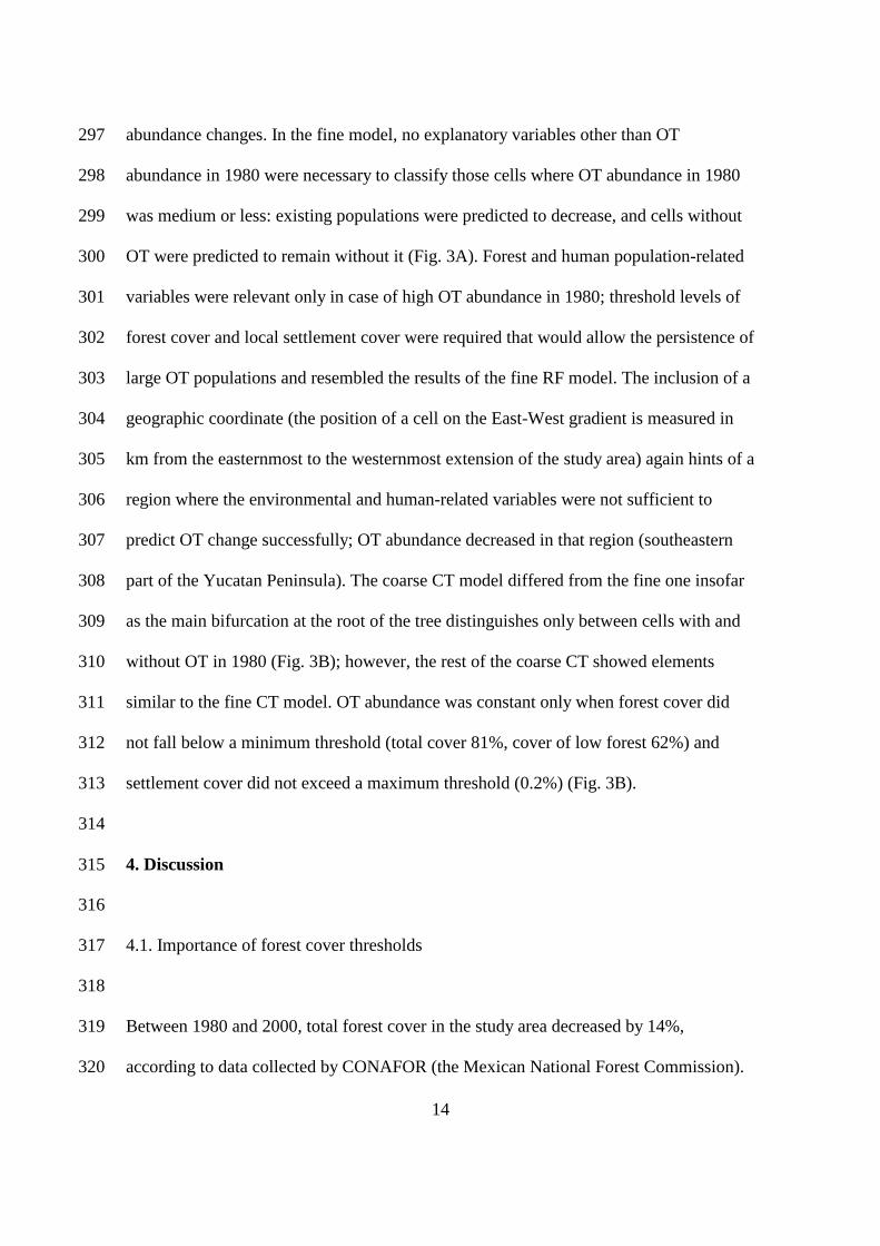
Figure A. Partial dependence plots characterising the relationships between selected 535

predictors and predicted probabilities of abundance change. The partial dependence of 536

the classification function f(X) = f(X1, X2, X3, … Xs), where X = (X1, X2, …, Xs) are the 537

predictor variables, on the variable Xj is the expectation of f with respect to all the 538

variables except Xj. It can be estimated by using equally spaced values in the range of Xj 539

and averaging the prediction function over all possible combinations among the 540

observed values of the other predictors. The values on the y-axis correspond to log pk(X) 541

- Σj log pj(X) /K, where pk is the probability of membership in the k-th class given the 542

predictors and K is the number of classes (here, K=4 for the coarse and K=14 for the fine 543

model, respectively) (Cutler et al., 2007; Hastie et al., 2009). 544

I. Relationship between regional tropical forest cover in 2000 and the predicted 545

probability of OT population decline from high to low abundance. The probability of 546

decline decreases above a threshold of ca. 80% forest cover. 547

II. Relationship between local human population size and the predicted probability of 548

the abundance change classes “decrease” and “no change”. The probability of OT 549

population decline increases rapidly at already very low human population densities. 550

III. Relationship between “Position of the cell on the East-West gradient” and “Position 551

of the cell on the North-South gradient” (measured in km from the easternmost to the 552

westernmost and from the northernmost to the southernmost extension of the study area, 553

respectively) and predicted probabilities of the abundance change classes HA (high 554

abundance in 1980, absent in 2000) and HL (high abundance in 1980, low abundance in 555

2000). The probability of being classified as HL increases steeply towards the eastern 556

34

150 km and the southern 150 km of the study area; the probability of HA is high in the 557

easternmost as well as in the northernmost parts of the Yucatan Peninsula. 558

Cutler, D.R., Edwards, T.C.Jr., Beard, K.H., Cutler, A., Hess, K.T., Gibson, J., Lawler, 559

J.J., 2007. Random forests for classification in ecology. Ecology 88, 2783–2792. 560

Hastie, T., Tibshirani, R., Friedman, J., 2009. The Elements of Statistical Learning, 561

second ed. Springer, New York. 562

563

Figure B. Losses of forest cover on 1395 grid cells (10 x 10 km each) on Yucatan 564

Peninsula between 1980 and 2000. Since each cell has a size of 100 km², the loss of km² 565

of forest per cell corresponds to percentage loss. 566

567

Figure C. Relationship between settlement age and minimum distance from the 568

settlement necessary for encountering Ocellated Turkeys (Meleagris ocellata). The 569

slope of the upper limit for settlements < 30-years-old was fitted by determining the 570

maximum value for every settlement age, calculating the moving average over each 571

value and its immediate neighbours, and calculating a least square regression (slope = 572

0.6, p<0.001). The horizontal line of the envelope was fitted by eye. 573