Income and Bargaining Effects on Education and Health in Brazil

Vladimir Ponczek ∗

Sao Paulo School of Economics - Getulio Vargas Foundation.

Abstract

In this paper, we examine the impacts of the reform in the rural pension system in Brazil in 1991 onschooling and health indicators. In addition, we use the reform to investigate the validity of the unitarymodel of household allocation by testing if there were uneven impacts on those indicators depending onthe gender of the recipient. The main conclusion of the paper is that the reform had significantly posi-tive effects on the outcomes of interest, especially on those co-residing with a male pensioner, indicatingthat the unitary model is not a well-specified framework to understand family allocation decisions. Thehighest impacts were on school attendance for boys, literacy for girls and illness for middle-age people.We explore a collective model as defined by Chiappori (1992) as one possible alternative representationfor the decision-making process of the poor rural Brazilian families. In the cooperative Nash equilibrium,the reform effects can be divided into two pieces: a direct income effect and bargaining power effect. Thedata support the existence of these two different effects. [JEL=O15, I12, I28]

Keywords: Education, Health, Bargaining Power

Resumo

Nesse artigo, examinamos os impactos da reforma no sistema de previdencia rural no Brasil em 1991 emeducacao e saude. Alem, utilizamos a reforma para analisar a validade do modelo unitario de alocacaointra-familiar testando se existiram impactos desiguais dependendo do genero do pensionista. A principalconclusao do artigo e que a reforma afetou significativamente os indicadores observados, especialmentenaqueles que moravam com pensionistas do sexo masculino, sugerindo que o modelo unitario nao e umaboa abordagem para entendermos decisoes alocativas dentro da famılia. Os maiores impactos foram emfrequencia escolar para meninos, alfabetizacao para meninas e doenca para pessoas de meia idade. Nosexploramos o modelo coletivo definido por Chiappori (1992) como uma possıvel representacao alterna-tiva do processo de decisao alocativa para famılias rurais pobres no Brasil. Em um equilıbrio de Nashcooperativo, os efeitos da reforma podem ser divididos em duas partes: um efeito-renda direto e umefeito poder de barganha. Os dados apontam para a existencia desses dois efeitos.

Palavras-chaves: Educacao, Saude, Poder de Barganha

Area ANPEC: Economia Social e Demografia Economica - 11

∗Rua Itapeva, 474 12 andar. Sao Paulo, SP Brazil 01332-000 vladimir.ponczek@fgv.br .

1 Introduction

In the past decades, the economic literature has shown evidence that the household cannot be character-ized as a unit with individuals sharing the same preferences or pooling their resources. Within the familyunit different individuals may have different concerns about how to spend their total family income andthe decision-making process of the resource allocation may be affected by the difference in preferences.This paper intends to take advantage of variation in social security system rules in Brazil to estimatethe impact of a change in family income on socio-economic outcomes and uses that to investigate thedecision-making process of the affected families.

Fully understanding the decision process is important in order to make better and more efficienttransfer policies. Using the unitary model of the household as a guideline for policy prescriptions maybe misleading, since the effect of public transfers may differ depending on the identity of the incomerecipient. Therefore, targeting transfers to the household may not result in the desired consequences,given that transfers directed to the head of the family, to the spouse or to elderly people may have differentimpacts over the family. For example, if the receiver of the transfer were an elderly person, there couldbe a larger fraction of the transfer allocated to health care. In the same way, if the beneficiary were themother instead of the father, the income augment might cause a reduction on her labor supply, sinceshe might now want to allocate more of her time raising the children. Hence, an increase in the familyincome may have uneven impacts on different members of the household depending on the characteristicsof the transfer recipient.

In many developing countries, the pension system is the most important source of public transfersto poor families. Therefore, a major change in the rules of the social security system in a continentalcountry is an excellent opportunity to understand how income is allocated within household members.We will take advantage of the Brazilian social security reform that occurred in 1991 to measure the extentto which the impacts of an unanticipated increase in pension income depend on the characteristics of thepensioner.

To many families, especially in rural Brazil, pensions are the only stable source of income, even inhouseholds not headed by a pensioner. Indeed, a considerable number of household units are formedby pensioners, adults and children. A change in the eligibility rules as well as in the pension valuesmay modify the balance of power over the allocation decisions in favor of the pensioner’s preferences.Therefore, if the pensioner’s preferences about education, health, and leisure are different from those ofother family members, the modification in the social security system may cause a massive change in intra-household allocations. For instance, if female pensioners are concerned more about children education,a change in the pension rules that allows spouses to also be a recipient may cause an important boost inschooling for children living with an elderly female. In this case, the impact would be even higher thanone caused by a male beneficiary. Thus, estimating uneven impacts of the reform on different familymembers creates a possibility to better understand how intra-household allocations are designed. In thisresearch, we plan to concentrate the analysis of the impact of changes in the pension system rules ontwo different outcomes: education and health. Both issues are important to the design of policies withthe goal of enhancing the quality of life of poor families and reducing inequality in developing countries.

Since Becker published his seminal works1 on family behavior, there has been a great number oftheoretical and applied research interested in the analysis of intra-household allocation. The neoclassicaltraditional view, the unitary model of intra-household allocation, assumes that the family behaves as asingle agent. An important implication of this model is that the expenditure on family’s public good(e.g. children’s schooling, health, etc) depends only on the total family income and redistribution ofincome among family members has no effect on the provision of the public good. The literature definesthis property as a “neutrality” result.2 As discussed by Ermisch (2003), the “neutrality” conditioncan be also obtained even in a framework where individuals within a family have different preferencesand are allowed to make distinct decisions about consumption. In this case, we have to assume thatindividuals do not cooperate in making decisions, i.e., each member chooses his contribution to the publicgood to maximize his own welfare, taking the contribution of the other members as given and also that

1See Becker (1964), Becker (1974) and Becker (1981).2The main characteristics of the unitary model are also described in the common preference model where the family’s

members have identical preferences.

1

preferences are convex. In the case of interior solutions, where each individual contributes a non-zeroamount of public good and care only about the private consumption and the total amount of publicgood, the “neutrality” condition holds. Another characteristic of the non-cooperative outcome is thePareto inefficiency.

On the other hand, in a cooperative Nash equilibrium, adults maximize their utility function con-strained by given levels of utility achieved by the other adult members. Therefore, the equilibrium shouldbe Pareto-Efficient, in the sense that in the equilibrium allocation of public and private goods, no adultcan be better off without making at least one of the others worse off. This is called the “collectivemodel” by Chiappori (1992). In this situation, for types of preferences usually assumed in economicanalysis, a redistribution of resources among the family members will potentially affect the amount ofpublic good, and it will increase or decrease depending on the preferences of the receiving adult.3 Theresult works as if there was an income sharing rule, i.e., each member has a share of the total familyincome and chooses his contribution to the public good based on his own preferences and the share ofincome. Chiappori (1992) interprets the share as a reflection of the bargaining power within the family.Therefore, an increase in a member’s income will generate two separate effects: (i) a direct income effectthat increases the provision of the public good as long as it is a normal good; (ii) a bargaining effectwhich reinforces the income effect if the member who received the extra income has stronger preferencesin favor of the public good compared to the other members.

The empirical investigation about the unitary model of intra-household allocation is a recurrent topicin the literature. A classic study by Thomas (1990) which also uses Brazilian data, tests whether themother’s unearned income has a different impact on family health than the father’s. He finds differentialeffects for child survival, and thus rejects the neoclassical model. He also observes that mothers favortheir daughters, and fathers their sons in terms of nutritional intakes. Duflo (2003) uses the South Africansocial pension program to study whether the impact of cash transfer on child nutritional status is affectedby the gender of the recipient. The author claims that pensions received by women have an impact onthe anthropometrics status (height) of girls but little effect on boys. However, she could not find a similareffect for pensions received by men. Emerson and Souza (2007) study the existence of uneven impactsof parent’s socio-economic characteristics on school attendance and child labor for boys and girls. Theirresults show that the father’s characteristics such as years of schooling, non-labor income, and the agehe first began working have a greater impact on sons than on daughters while mother’s characteristicshave are greater effect on daughters. Moreover, the authors find that both non-labor income of mothersand fathers affect the son’s schooling attendance more than they affect daughter’s attendance.

Delgado (1997) and Delgado (1999) descriptively report the impacts of the reform on socio-economicindicators such as poverty, personal and regional income distribution and find a significant reduction ofpoverty and income redistribution for families affected by the reform. Carvalho (2000) and Carvalho(2001) also focus on the 1991 Brazilian reform. He studies the impact of the income variation causedby the social security changes on schooling decisions, child labor, retirement decisions and labor marketresponses. In the first paper, the author finds a reduction in child labor for both girls and boys andpositive impact on schooling enrollment for both genders, but does not focus on intra-household allocationor bargaining power. In the second paper, he also observes a reduction in the retirement age among thoseaffected by the reform.

In summary, the literature from developing countries has used social security reforms to investigatewhether pension income is associated with better outcomes for individuals who live with pensionersand to explore whether characteristics of pensioners affect the allocation of resources in the household.The restructuring in the Brazilian social security system presents itself as a valuable opportunity tounderstand the individual and family responses to unanticipated income shocks. This study intends toexplore the exogenous variation in income caused by the rural pension system reform in Brazil to estimatethe impact on the cited social outcomes (education and health). Our primary objective in this paper isto test whether an extra amount of family income coming from the social security benefits creates unevenimpacts on different members depending on the gender of the beneficiary.

The empirical strategy consists of estimating whether the variation in income driven by the social3This result is sensitive to the utility function used. Bergstgrom and Cornes (1981) and Bergstgrom (1983) have shown

that when the preference of each member has the Gorman form, public good allocation in a cooperative equilibrium isindependent of income distribution and the “neutrality” property holds.

2

security reform generated a different impact on the demand for the public goods (schooling and health)depending on the gender of the eligible member, and also whether the pension income was spent likeany other non-pension income or not. If the “neutrality” property holds, it is expected that the pensionincome is spent like income from any other source and also that the gender of the pensioner will not besignificantly related to the provision of the public good.

This paper is organized as follows: Section 2 discusses about the dataset used in this paper. Section3 explains the details of the reform. Identification strategies are discussed in section 4. The results areanalyzed in section 5 and show a positive impact on schooling and health status for boys living withmale pensioners suggesting that the unitary model is not valid. Section 6 concludes.

2 Data

The data used in this research come from the Pesquisa Nacional por Amostra de Domicılios (PNAD)database. The PNAD is an annual household survey, with sample size equal to 1/500 of the Brazilianpopulation (about 100,000 households) and is designed to produce a picture of the social-economicconditions of the Brazilian population. It covers all urban and almost all rural areas, except the Amazonregion. It has been conducted on a regular basis since 1981 by IBGE (the Brazilian Census Bureau)except in years in which census data was collected (1991 and 2000) and in 1994 when there was abudgetary crisis. PNAD contains also extensive data on personal and household information. For eachperson, information about age, schooling attendance, literacy, migration, labor participation, retirementand income sources (including amounts) is available. Moreover, periodically questions about some otherspecial topics (the “Supplements”) are included in the survey. For instance, in the 1970’s, questions aboutmigration were included; in the 1980’s the special topics were heath education, labor market and socialsecurity; in the 1990’s, migration, fertility and child labor. To study the schooling outcomes (literacyand attendance), we will use the 1988, 1989 and 1990 PNAD’s for years before the reform took place(1991), and the 1992, 1993 and 1995 surveys for years after the reform. We will analyze the impact onchildren between 6 and 18 years old who live in rural areas. In the case of health indicators, we willuse the PNAD supplements’ information collected prior the reform (1986) and from one collected afterthe reform (1988). Two indicators will be evaluated: reported illness and the search for any health careservice in the past two weeks prior to the interview. We study the effects of the reform on those twohealth indicators for different subgroups (everyone, children - between 0 and 14 years old) and middle-agepeople - men between 40 and 55; and women between 40 and 50 years old).

3 The Reform

In October of 1988, the new Brazilian Constitution was promulgated. The Constitution establishedmany changes in the principles of the entire social security system. In addition, it also determined thatthe Congress should approve Ordinary Laws, which should implement all changes. The main guidingprinciples stipulated by the Constitution were: extension of old-age benefits to anyone who was not ahousehold head; no benefit should be smaller than one minimum wage; reduction in the minimum age ofold-age eligibility; length-of-service eligibility to rural workers.4 The Congress passed the Ordinary Laws5 on July 24 of 1991 and the reforms went into effect. The new main rules sanctioned by the law were:(i) New minimum age eligibility equal to 60 for men and 55 for women compared to 65 years for bothmen and women before the reform;(ii)anyone who reached the minimum age requirement could be eligiblein the household;(iii) the minimum benefit was increased to 100% of the minimum wage; (iv) the valueof the benefit is calculated based on previous earnings against a flat benefit of 50% of minimum wagebefore the reform; (v) length-of-service pension available after 30 years of services for men and 25 yearsfor women. The value of the benefit is also calculated based on previous earnings.

4Beltrao et al. (2003) and Delgado (1997) have more details about the constitutional new rules concerning the ruralpension system.

5Laws # 8212 and 8213, available athttp://www010.dataprev.gov.br/sislex/paginas/42/1991/8212.htmhttp://www010.dataprev.gov.br/sislex/paginas/42/1991/8213.htm .

3

Beyond minimum age, eligibility to a rural pension requires from the worker proof of residence ina rural area and engagement in one of the rural activities defined by the law (farmers, fishers, miners,loggers, etc.) for at least 60 months prior to the application. Proving previous engagement in a ruralactivity was extremely easy, since many documents were accepted as sufficient proof, such as individuallabor contracts, tenancy contracts and sharecropping agreement, among others.

Although the law stipulated an earning-based benefit, the great majority of the rural pensionersreceived the minimum wage at least until 1997 because almost all rural workers did not keep a documentedrecord of previous earnings. For instance, the average rural benefit paid in 1997 was around R$ 121,while the minimum wage was R$ 120. For the same reason, the proportion of length-of-service retireesin the rural system is insignificant, less than 0.1% of the total number of pensioners.6 Therefore, we donot worry about any kind of endogeneity caused by differences in the value of the benefit or in the ageof retirement.

The increase in the minimum benefit for the current pensioners was instantaneous. The income ofthose who were pensioners in the old system doubled right after July of 1991. However, for those whoare now eligible or decided to apply after the change in the rules, the entire process of registration tookseveral months due to administrative delays. Therefore, for the entire group of people who became eligibleafter the reform, the impact was not automatic. Beside, since the worker should apply to be registeredin the system, concerns about selectivity bias, especially about the timing of the reform impacts, arise.Probably many newly eligible workers in a first moment ignored the new rules of the system and it ispossible that unobservables correlated to the ignorance of the new rules are also correlated with someoutcome of interest. That is one of the reasons why we use datasets until 1995 in order to let the take-upprocess for the newly eligible complete. In our dataset, the proportion of pensioners among the newlyeligible before the reform was around 15%7 and increases to 50% before stabilizing after 1995.

4 Identification Strategies

Consistently estimating the effect of income variations on different family members is not a simple task.Using disparity of income across families from a single cross-section may introduce many identificationproblems in the regressions. A family’s unobserved characteristics might be correlated with family’sincome and also with investment in schooling and health. This situation could lead to several misinter-pretations of the data. Based on the results of such simple regressions, one could argue, for example,that an extra amount income would imply an increase on schooling attendance, when, in reality, it isthe intellectual level of the parents, which is correlated with the family income, that drives the decisionabout the child schooling. An exogenous source of income variation is a sine qua non condition forhaving consistent and reliable results. Hence, the modification in the Brazilian social security system in1991 is an excellent source of income variation to be explored, since it is not correlated with any familyunobserved characteristics.

However, using total income that comes from the benefits or even a direct indicator if the family hasa person that is a pensioner is also problematic. The value received from the pension (when it is notthe minimum value) is derived from the past labor earnings and could possibly also be correlated withunobservable characteristics. Directly including a dummy variable indicating if the person is a pensionermight also generate inconsistent results, since the decision to apply (and when to apply) to the benefitcould potentially be endogenous. For instance, rich people might not be willing to go to a post office andstay in the line in order to apply for the pension, since their extra income utility could not compensatethe burden of applying to the pension. In this case, a selectivity bias problem could arise. Therefore,we will pursue a intent-to-treat approach, in which actual treatment is replaced by eligibility in order toavoid the selectivity problem.8

Moreover, the use of variation across households in social security income to identify the impactof earnings on social outcomes requires adequate control of the effects of living with an elderly personunrelated to their social security revenue. Families who co-reside with an elderly person may differ from

6Data from the social security administration.7This number is not zero probably because of migration of previous urban workers to rural areas or public employees

who have their own pension system.8Nonetheless, we will refer to families with an eligible people as the treated group.

4

other families for several reasons. Elderly people may have different preferences over the importance ofchildren education compared to the other family members, or concern more about their own health, or,in general, the presence of an elderly person may be correlated with other unobserved characteristicsthat are also correlated with the outcomes of interest. Therefore, from one single cross-section, it isimpossible to disentangle the direct income effect of coming from the old-age pension from the impactsof living with an elderly person. An exogenous reform in social security, however, permits the separationof theses effects.

Nevertheless, the comparison between the cross-sectional patterns of outcomes before and after thereform would identify the effect of the changes in social security income only in the absence of any ongoingtrend. In the presence of such trend a before and after estimator would be upward or downward biaseddepending whether the trend is positive or negative sloped. In order to control for the time trend effect,we will use a difference-in-difference approach. The difference-in-difference estimator will be consistentas long as the time variation on the outcome of interest would be the same for both treated and controlgroup in the absence of the treatment, i.e., only if both groups have the same time trend. If the controlgroup has a different time pattern from the treated, the difference-in-difference estimator will be biased.Suppose Yit,0 and Yit,1 are, respectively, the outcomes for the non-treated and treated individual i attime t and they are modeled by the following equations:

Yit,0 = βi,0 + δt,0 + εit

Yit,1 = βi,1 + δt,1 + α + εit.

where βi, . are the fixed effects, δt,. are the time effects and α indicates the true effect of the treatment.Let t = b, a ((b)efore and (a)fter the treatment). For simplicity, we will assume that δb,1 = δb,0 = 0.The difference-in-difference estimator will only be unbiased if δa,1 = δa,0, i.e., if both treated and controlgroups have the same time pattern.

E[αDD] = E[Yia,1 − Yib,1]− E[Yia,0 − Yib,0]= α + δa,1 − δa,0 = α if δa,1 = δa,0.

Assuming nowδe=1a,. = δe=0

a,. + ∆e. (1)

where e = 1 indicates if the individual has an elderly member in her family. More specifically, we areassuming that the potential difference in the time trend of the treatment and control group (∆e) doesnot come only from the treatment per se, but also from the presence of an elderly person in the family.An unobservable shock could have affected only families with an elderly member in the same moment ofthe pension reform. Therefore, in order to obtain an unbiased estimator of the true treatment effect, weneed a control group that has an elderly member (e = 1), but was not affected by the reform.

We plan to use families with an almost-eligible person – man between 55 years and 60 years oldand/or women between 50 years and 55 years old– as the control group9 in order to disentangle the truetreatment effect from the specific elderly trend effect.

Furthermore, the reform is also an extraordinary opportunity to check whether the “neutrality”property characterizes the intra-household allocation process. Testing the validity of the unitary modelwithout an exogenous income variation may also lead to erroneous conclusions. Most studies in theliterature use only the variation across families of unearned income in the hands of different member (forexample mothers and fathers) to identify the allocation process within households. They usually regressthe children outcomes (health, schooling, anthropometrics, nutrient intakes, etc) on parent’s unearnedincome. By comparing the coefficient of each parent income, those studies gauge the consistency of theunitary model. However, since the difference between unearned incomes of distinct members in the familyis not likely to be orthogonal to unobserved characteristics in the family that also affect the outcomeof interest, the conclusion based on those estimated coefficients may be invalid. For instance, supposefamilies that depend more on unearned income care less (both fathers and mothers) about education. In

9From now on, every time we refer to the control group, we will be mentioning about families with an almost-eligiblemember.

5

addition, it is possible that the fact that they need more this extra money induces the member of thefamily who works to also search for these alternative resources. In this case, the difference in unearnedincome between the working and non-working member of the family would be higher for such familiesand could lead to a spurious correlation with the outcome of interest. Since the income variation causedby the reform was out of the family’s control and therefore orthogonal to any unobserved characteristicthat could be correlated to the provision of the public good, we will test the validity of the unitary modelby examining if the reform had uneven impacts on the outcome of interest conditioning on the gender ofthe eligible person.

The benchmark regression is the following:

E[Y | Tm,f , Cm,fPost,W

]= β0 + βm

1 Tm + βf1 T f + βm

2 Cm + βf2 Cf + β3Post

+βm4 Tm × Post + βf

4 T f × Post + βm5 Cm × Post + βf

5 Cf × Post + Wγ (2)

where Y is the outcome of interest (explicitly, schooling and health indicators); T j (for both j = (m)aleor (f)emale) is a binary variable which is 1 if individual’s family has the presence of at least one eligibleperson in the new system rules [(Tm) man 60 years or older or (T f ) woman 55 years or older], i.e.,the “treated” group; Cm,f indicates whether the individual co-resides with at least one male (Cm) orfemale (C f ) almost-eligible person, i.e., if she is part of the control group; W is a vector of household andpersonal characteristics such as age, age squared10, education attainment of the head of household, head’sgender, age and race, number of family members and number of children in family; Post is a dummydenoting post-reform years (after 1991). Tm, T f , Cm and Cf also enter in the equation interacted withPost .

With this specification and assuming a linear probability model, βj4 (the coefficients of the interaction

terms between T j and Post) will be the difference-in-difference estimators of the treated against thereference group, which is, in this case, everyone who resides in the rural areas and does not co-residewith an eligible or an almost-eligible person. βj

4 is consistent as long as ∆e = 0 in equation (1), i.e., bothtreated and reference groups have the same time trend.

Comparing βj4 with βj

5 allows us to check if βj4 are indeed capturing the reform effect driven by the

increase in benefits11 or if it is just reveling an elderly presence trend effect. βj4 − βj

5 is the difference-in-difference estimator when the comparison is the control group. In this case, both treated and controlgroups have an elderly member in their family. Therefore, even if there is a specific time trend relatedto the presence of an elderly person, βj

4 − βj5 will consistently estimate the true treatment effect.

Finally, we analyze the validity of the “neutrality” property by testing if βm4 = βf

4 . Assuming thatthe direct income impact of the reform was uniform across families with male and female pensioners,difference in the effects on the provision of the public good must be caused by changes in the bargainingpower within the household. In other words, if bargaining power has an important role on the allocationdecisions, extra income given to men should impact the outcomes of interest differently than incomegiven to women, therefore, βm

4 6= βf4 , violating the “neutrality” property and consequently rules out the

unitary model as a good specification of the allocation process.

New × old eligibility

Since the decision about applying to the benefit is potentially endogenous, the results based on specifica-tion (2) have to be carefully interpreted. As explained in section (3), the reduction in the age eligibilitydoes not guarantee an extra amount of income for families with a newly eligible person right after thereform in the system. Depending on how important the extra income is for the eligible member and herfamily, the decision of whether and when to apply to the benefit could be different from family to family.And if the source of this “application” heterogeneity was correlated to the outcome of interest, the resultestimated would have to be understood differently than if it was not the case. Each βj

4 in equation 2captures the average impact of the reform on the entire group of potentially “treated” families.

10We also tried a specification including dummies for each year of birth in order to capture any cohort effect. The resultswere qualitatively very similar to those presented here and are available upon request.

11Actually, in this specification, βj4 is also capturing the effect of the reduction in age eligibility. Below, we will disentangle

the outcome of those two change in the rural pension system.

6

Moreover, even disregarding the possible heterogeneity problem exposed above, work with just onetreatment effect could create another problem, since the impact of the reform on families with a newlyeligible was different on those with an old eligible member. More specifically, for those families that havea newly eligible member who now receives the minimum benefit, the amount of benefit received was zerobefore and increased to one minimum wage after the reform. On the other hand, for those who werealready beneficiaries, the reform impact was half as much as on the first group. Therefore, again, βj

4

would capture an “average” effect that could underestimate or overestimate the true impact on each oneof those two treatment groups.

In order to disentangle the effect of the increase in the minimum benefits and the change in eligibilityage we estimate the following:

E[Y | T j

k , Post,W]

= β0 +∑

j=m,f

[2∑

k=1

(βj

1,kTjk

)+ βj

2Cj

]+

β3Post +∑

j=m,f

[2∑

k=1

(βj

4,kTjkPost

)+ βj

5CjPost

]+ W.γ (3)

where T j ′i s are: (k = 1) the presence of an individual eligible in the old system rules – 65 years or older

person – this term captures the impact of the increase in the minimum benefits values from 50% of theminimum wage to 100% of it.; (k = 2) the presence of a newly eligible individual in the new system rules(between 60 years and 65 years old for men or between 55 years and 65 years old for women) this termalso captures the effect of reduction in the age requirement.

In this case, βj4,k=1 and βj

4,k=2 will be, respectively, the difference-in-difference estimators of the

treated group 1 and 2 against the reference group. Again, testing βj4,k=1 = βj

5 and βj4,k=2 = βj

5 allows usto check if the effect is coming from the reform or a specific characteristic of families with elderly people.

Again, testing if βm4,k=1 = βf

4,k=1 and βm4,k=2 = βf

4,k=2 indicates the unitary model validity.

5 Results

Impacts on Income

Before attempting to measure any effect of the changes of the pension system on social-economic out-comes, it is important to be sure that the social security reform has an impact on families’ total incomein rural areas.

Table 3 shows the results of an OLS regression of model (3) where the dependent variable is the totalfamily income in logs. All control variable coefficients are statistically significant and have the expectedsign. The total family income is higher if the head is older (with concavity), more educated, male andwhite; families with more children also tend to have lower income. It is also worthy noticing that all“treated” are poorer compared to the reference group, indicating that the reform mostly impacted familiesin the bottom of the income distribution. Looking now at the difference-in-difference coefficients, we thatthe “treated” families have experienced a significant growth in their income after the reform. All βj

4,i arestrongly significantly different from zero and from their respective counterpart in the control group (βj

5).Moreover, the coefficients of the “old eligible” groups (for both male and female pensioners) (βj

4,k=2) are

statistically significantly higher than the “newly eligible” ones (βj4,k=1). Once more, this could be an

illustration of the new registration delays which occurred after the reduction in the eligibility rule. Asexpected both βf

4,k=1 and βf4,k=2 are significantly bigger than βm

4,k=1 and βm4,k=2, indicating a stronger

effect on income from the presence of an eligible females compared to the presence of an eligible male.This was due to the new rules concerning the benefits of spouses.

Impacts on Schooling and Health

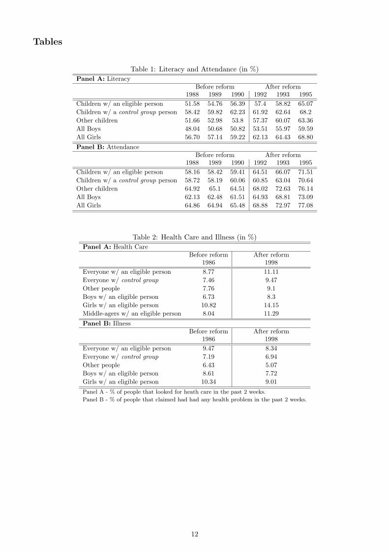
Table (1) shows the evolution of the literacy and attendance and dispicts the improvement of theseschooling indicators in Brazil during the period for all groups of families. It illustrates the fact that

7

Brazil has been considerably improving its educational performance, especially in the elementary levelof schooling, since the beginning of the last decade.

In Brazil, the constitution establishes that the primary level of education (up to 8 years of schooling)should be freely provided by the municipalities and secondary level (9 to 11 years of schooling) bythe states. Although it was possible for almost all children to find a public school within the state,transportation, uniform and other supplies costs impeded the access of a considerable part of the childrenpopulation. Moreover, since child labor was not a rare phenomenon in rural Brazil, the opportunity costof the forgone income was also significant. Therefore, we believe that the social security reform whichhad a significant impact on the families’ budget constraints is also behind the progress of those indicatorsfor the treated families. The increase of the schooling standards in Brazil reinforces the importance ofhaving a control group that correctly mimics the behavior of the treatment group in the absence of thereform in order to consistently estimate its effects.

Table 4 has the results of specification (3) with schooling attendance or literacy as the dependentvariables. Columns (1a) and (1b) show the results for regressions with the entire sample of childrenbetween 6 and 18 years old who live in rural areas. As expected, children living in treated families are ingeneral less likely to be literate and attending school, since they are on average poorer families.

The difference-in-difference coefficients show that the presence of an eligible male in the family had apositive and significant effect on the schooling achievements. Children living with a newly eligible male(Tm

k=1) are 2.6% and 2.7% more likely to be literate and attending school, respectively, while childrenwith an old eligible male (Tm

k=2) are also significantly more likely to attend school (2.7%). On the otherhand, despite causing a bigger increase in the family income, the presence of an eligible female does notseem to have improved the schooling outcome of the children. Neither the presence of a newly (T f

k=1) oran old (T f

k=2) eligible females has a positive effect on literacy or attendance. Actually, the presence ofan old eligible female seems to decrease the likelihood of being literate.

Breaking the sample between boys and girls, we find positive effects in attendance for both Tmk=1 and

Tmk=2 boys. On the other hand, Tm

k=1 girls is positive, suggesting that the there was a benefit in terms ofliteracy. Again, neither boys or girls benefited form living with an eligible female.

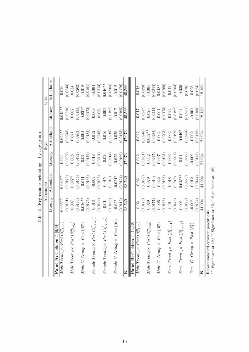
Table 5 shows the results after splitting the sample into two different subgroups: younger childrenbetween 6 and 14 and older children between 14 and 18. It is clear that the first group benefited muchmore from the reform than the second, especially the Tm

k=1 children; however, Tmk=2 older boys also suffered

a significantly positive effect on attendance. Again, children with an eligible female seem to have notbenefited from the reform, at least compared to those in the reference group.

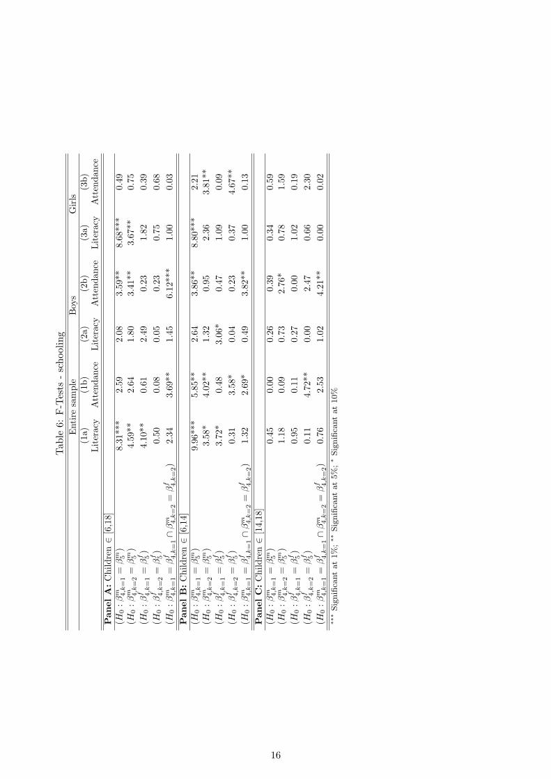
The last rows of each panel show the joint F-test if the presence of an eligible male is significantdifferent from the presence of an eligible female in the family. Panel (A) shows the results for theregressions with the entire sample; Panel (B) and (C) show the results for children between 6 and 14;and 14 and 18, respectively. We can see that in all samples the presence of an eligible male had asignificantly bigger effect than the presence of a female, especially for boys’ attendance. These resultsindicate that the families are not pooling their income and deciding the provision of those public goodsbased on the total family income; if that were the case there would be no reason why the presence of aneligible male would have a different impact on schooling than the presence of an eligible female. Thus,the findings contradict the core of the unitary model, i.e., the “neutrality” property.

Table 2) shows the proportion of people self-reported as ill and the proportion who have looked forany health care service in two points of time, before and after the reform. Like the schooling indicators,it displays a clear improvement on the heath indicators. In 1991, the Brazilian government created theSUS (The Universal Health System), which proposed to offer free health care for virtually every citizenin the entire country. Before that, only workers (and their dependents) who contributed to the socialsecurity system had access to the public health system. Since the implementation of the SUS coincideswith the reform in the social security, our results could be very sensitive to it. The consistency of ourestimation hinges on the assumption that the impact of the SUS creation was uniform across treated andcontrol groups. Once again, this example also testifies to the importance of having a control group (likethe almost-eligible families) as similar as possible to the treatment one.

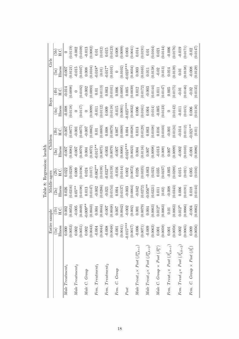
Table 8 displays the results of specification (2) having both health indicators (illness and search forhealth care) as dependent variables. Again, the impact of the reform can be measured by the difference-in-difference coefficients (βj

4,k). Looking at the results, we can see that the only significant impact of

8

the reform was in the likelihood of being sick only for middle-agers who live with an old eligible male.Compared to the reference group, all other groups seem to have suffered no effect from any of the othertreatment groups.

The last row of table (9) tests whether there were different effects from the presence of eligible malesand females. Once more, middle-age people who live with an eligible male significantly12 benefited morethan those living with an eligible female.

Robustness Checks

As mentioned in section 4, the difference-in-difference estimator is consistent only if reference group hasthe same trend process as the treatment group in the absence of the treatment. For that reason, weincluded in the regressions a difference-in-difference estimator for the control group - families with analmost-eligible member - in order to capture a possible trend associated with the presence of an elderlyperson in the family.

Table 6 shows the F-tests comparing the difference-in-difference coefficients of both treatment againstthe control groups. Panel A has the tests for the entire sample while panels (B) and (C) displays the testsfor children between 6 and 14, and 14 and 18 years old, respectively. Looking across the three differentpanels, we observe that the results are, in general, similar to those found when comparing to the referencegroup. The presence of eligible males seems more valuable than eligible females; and children between6 and 14 years old benefited more from the reform than the older ones. In the same way, the resultsshown on table 9 corroborate the findings about health: middle-agers living with a newly eligible maleare significantly less likely to be ill after the reform.

One possible caveat of the intent-to-treat approach rises if the take-up ratios for males and femalesare very different from each other. In this case, all uneven impacts of males and females shown in themain results could be driven by differences in the take-up ratios. One way to test if that is the case isto see the effects of the true treatment and compare to the intent-to-treat ones. Defining a treated groupas the families that have a member who is an eligible pensioner (i.e. there is a person in the family whoreceives a pension and matches the age eligibility criteria), we run specification 2 regressions using bothdefinitions of treatment. For both health and schooling, there is no significant difference between thosetwo strategies. The results are qualitatively very similar, showing again a much bigger effect from themale presence compared to the female. The results are available upon request.

Income × Bargaining Effects

Case and Deaton (1998) show that one way to test if the pension income has the same impact as anyother income source is by doing the following decomposition of total family income effect on the outcomeof interest:

ln[In + φIp] = ln[I + (φ− 1)Ip] ≈ ln(I) + (φ− 1)Ip/I (4)

where In is the family non-pension income; Ip is the pension income; and, I is the total family income.We then need to test if the coefficient of the pension income share over the total family income (Ip/I)

is different from zero. If that is the case, φ 6= 1 and, thus, the pension money has a different effect on thepublic good provision than the rest of the family income. Moreover, this specification is also a direct testof the “neutrality” property of the public good. Non-zero coefficients on the income shares confirm theinfluence of the bargaining power in the decision-making process over the public good allocation withinthe family.

Table 7 shows the results of a regression with schooling attendance as the dependent variable andtotal family income, male pension share, female pension share and all other control variables. We cansee that indeed the fractions of income provided by the pensioner have a positive effect on attendance,indicating the double impact of the reform on attendance by, firstly, increasing total family income andsecondly, increasing the bargaining power of the pensioner, defined by her share on total family income.The results shed light on the impact differences of the reform depending on the gender of the recipient.

12at 10% of significance.

9

It seems that, although both men and women pensioners care more about education than the averageadult member of the family, especially for boys, eligible males manage to transform bargaining powerin actual provision more efficiently than females. This result is even more evident when we reduce oursample to only treated families as shown in Panel (B). This could be driven not only by differences inpreferences, but it also possible that social norms or cultural models make the male income share morerelevant for concrete bargaining power inside the family. It is possible that the results are capturingsystematic difference between families that have only male pensioners compare to those that have onlyfemale pensioners. Nevertheless, narrowing down our sample only to families with both female and malepensioners (Panel (C)) does not change the main conclusion that male pension share is more importantfor schooling attendance, especially for boys.

In the case of illness, the same conclusions arise. As expected total family income has a negative effecton the likelihood of being ill, and the male pension income share has a significant and bigger impact onthe reduction of illness for middle-agers (table 10). Reducing the sample only to treated families (Panel(B)) diminishes the precision of the estimators without changing their signs.13 The same occurs in thesample including only families with both male and female pensioners (Panel (C)).

6 Conclusion

The social security reform occurred in 1991 in Brazilian rural pension system has led to an increasein schooling indicators for young children living with an eligible male. Boys are more likely to attendschool and girls to be literate. The reform has also negatively impacted the probability of being ill onmiddle-age people living with a male pensioner. These uneven results for the presences of male andfemale recipients are evidence that the unitary model of household resource allocation does not representthe Brazilian poor rural families’ decision-making process over their budget. The income is not pooledand provision of education and health is not made based upon the total family resources. Moreover, wefind an indication that the impact of the pension income on the schooling and health was higher thanthe rest of the family resources. The increase in the bargaining power of the elderly, especially males,may explain these findings, suggesting that they have stronger preferences toward those outcomes. Theresults show the importance of targeting specific family members in cash transfer programs in order tomaximize the effect on desirable outcomes. Although families with an elderly person have on average lowschooling and health indicator levels, cash transfers to those members of the family have significantlylarger effects than unconditional transfers. In addition, since more than 10% of all children in rural areaslive with an eligible person, it is very plausible to attribute part of the success Brazil has achieved in thepast 15 years in education and health, specially for poor families, to the social security reform of 1991.

The findings have also great consequences for the design of conditional cash transfer programs, suchas Bolsa Familia. Those programs directly create incentives for schooling by requiring attendance.They set the mother as the receiver of the transfer. To the best of my knowledge, there is no studyproviding evidence that this is the most efficient away (in the sense of maximizing the outcome ofinterest). Therefore, a more profound study with the targeted families is necessary to identify specificmembers who may boost the direct income effect on schooling outcomes, enhancing the effectiveness ofthe programs.

A straightforward extension for this paper is to measure the impact of the reform on many othersocial outcomes, like child labor, fertility, anthropometrics, and other finer health indicators.

References

Becker, G. S. (1964) Human capital. Columbia Press University.

Becker, G. S. (1974) “A Theory of Social Interactions.” Journal of Political Economy 82(6): pp.1063–93. Available at http://ideas.repec.org/a/ucp/jpolec/v82y1974i6p1063-93.html.

Becker, G. S. (1981) A Treatise on the Family. Harvard University Press.13Except the coefficient of the female pension share on the sample with only children.

10

Beltrao, K. I., et al. (2003) “The 1988 Constitution and Acess to Social Security in Rural Brazil:Towards Universalization.”

Bergstgrom, T. (1983) “Independence of Allocative Efficiency from Distribution in the Theory ofPublic Goods.” Econometrica 51: pp. 1753–1766.

Bergstgrom, T. and Cornes, R. (1981) “Gorman and Musgrave are Dual: An Antipodean Thoeremon Public Goods.” Economic Letters pp. 371–378.

Carvalho, I. E. (2000) “Old-age benefits and the labor supply of rural elderly in Brazil.” Mimeo.

Carvalho, I. E. (2001) “Household Income as a Determinant of child Labor and School Enrollment inBrazil: Evidennces from a Social Security Reform.” Boston University Working Paper Series.

Case, A. and Deaton, A. (1998) “Large Cash Transfers to the Elderly in South Africa.” The EconomicJournal 108: pp. 1330–1361.

Chiappori, P.-A. (1992) “Collective Labor Supply and Welfare.” Journal of Political Economy 100(3):pp. 437–67. Available at http://ideas.repec.org/a/ucp/jpolec/v100y1992i3p437-67.html.

Delgado, G. C. (1997) “Previdencia Rural - Relatorio de Avaliacao Socio-economica.” Texto paraDiscussao - IPEA 477.

Delgado, G. C. E. (1999) “Experiencias Exitosas de Combate a Pobreza Rural: Licoes para Reorien-tacoes de Politicas.” Projeto FAO Pobreza - LOA 98290/RLC.

Duflo, E. (2003) “Grandmothers and Granddaughters: Old-Age Pensions and Intrahousehold Al-location in South Africa.” World Bank Economic Review 17(1): pp. 1–25. Available athttp://ideas.repec.org/a/oup/wbecrv/v17y2003i1p1-25.html.

Emerson, P. M. and Souza, A. P. (2007) “Bargaining over Sons and Daughters: Child Labor, SchoolAttendance and Intra-Household Gender Bias in Brazil.” World Bank Economic Review (0213).Available at http://ideas.repec.org/p/van/wpaper/0213.html (forthcoming).

Ermisch, J. (2003) An Economic Analysis of the Family. Princeton Univerity Press.

Thomas, D. (1990) “Intra-Household Resource Allocation: An Inferential Approach.” Journal of HumanResources 25: pp. 635–664.

11

Tables

Table 1: Literacy and Attendance (in %)Panel A: Literacy

Before reform After reform1988 1989 1990 1992 1993 1995

Children w/ an eligible person 51.58 54.76 56.39 57.4 58.82 65.07Children w/ a control group person 58.42 59.82 62.23 61.92 62.64 68.2Other children 51.66 52.98 53.8 57.37 60.07 63.36All Boys 48.04 50.68 50.82 53.51 55.97 59.59All Girls 56.70 57.14 59.22 62.13 64.43 68.80Panel B: Attendance

Before reform After reform1988 1989 1990 1992 1993 1995

Children w/ an eligible person 58.16 58.42 59.41 64.51 66.07 71.51Children w/ a control group person 58.72 58.19 60.06 60.85 63.04 70.64Other children 64.92 65.1 64.51 68.02 72.63 76.14All Boys 62.13 62.48 61.51 64.93 68.81 73.09All Girls 64.86 64.94 65.48 68.88 72.97 77.08

Table 2: Health Care and Illness (in %)Panel A: Health Care

Before reform After reform1986 1998

Everyone w/ an eligible person 8.77 11.11Everyone w/ control group 7.46 9.47Other people 7.76 9.1Boys w/ an eligible person 6.73 8.3Girls w/ an eligible person 10.82 14.15Middle-agers w/ an eligible person 8.04 11.29Panel B: Illness

Before reform After reform1986 1998

Everyone w/ an eligible person 9.47 8.34Everyone w/ control group 7.19 6.94Other people 6.43 5.07Boys w/ an eligible person 8.61 7.72Girls w/ an eligible person 10.34 9.01Panel A - % of people that looked for heath care in the past 2 weeks.

Panel B - % of people that claimed had had any health problem in the past 2 weeks.

12

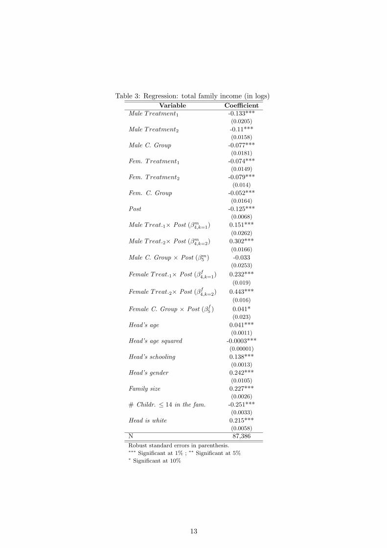
Table 3: Regression: total family income (in logs)Variable Coefficient

Male Treatment1 -0.133***(0.0205)

Male Treatment2 -0.11***(0.0158)

Male C. Group -0.077***(0.0181)

Fem. Treatment1 -0.074***(0.0149)

Fem. Treatment2 -0.079***(0.014)

Fem. C. Group -0.052***(0.0164)

Post -0.125***(0.0068)

Male Treat.1× Post (βm4,k=1) 0.151***

(0.0262)

Male Treat.2× Post (βm4,k=2) 0.302***

(0.0166)

Male C. Group × Post (βm5 ) -0.033

(0.0253)

Female Treat.1× Post (βf4,k=1) 0.232***

(0.019)

Female Treat.2× Post (βf4,k=2) 0.443***

(0.016)

Female C. Group × Post (βf5 ) 0.041*

(0.023)

Head’s age 0.041***(0.0011)

Head’s age squared -0.0003***(0.00001)

Head’s schooling 0.138***(0.0013)

Head’s gender 0.242***(0.0105)

Family size 0.227***(0.0026)

# Childr. ≤ 14 in the fam. -0.251***(0.0033)

Head is white 0.215***(0.0058)

N 87,386Robust standard errors in parenthesis.∗∗∗ Significant at 1% ; ∗∗ Significant at 5%∗ Significant at 10%

13

Tab

le4:

Reg

ress

ion:

scho

olin

gA

llsa

mpl

eB

oys

Gir

ls(1

a)(1

b)(2

a)(2

b)(3

a)(3

b)Lit

erac

yA

tten

danc

eLit

erac

yA

tten

danc

eLit

erac

yA

tten

danc

eM

ale

Tre

atm

ent 1

-0.0

67**

*-0

.08*

**-0

.068

***

-0.0

62**

*-0

.064

***

-0.0

95**

*(0

.0089)

(0.0

096)

(0.0

124)

(0.0

129)

(0.0

126)

(0.0

145)

Mal

eT

reatm

ent 2

-0.0

97**

*-0

.079

***

-0.0

95**

*-0

.056

***

-0.0

97**

*-0

.1**

*(0

.0081)

(0.0

087)

(0.0

114)

(0.0

116)

(0.0

114)

(0.0

131)

Mal

eC

.G

roup

-0.0

16**

-0.0

47**

*-0

.016

*-0

.035

***

-0.0

12-0

.055

***

(0.0

065)

(0.0

073)

(0.0

093)

(0.0

098)

(0.0

09)

(0.0

111)

Fem

.T

reatm

ent 1

-0.0

41**

*-0

.017

**-0

.046

***

-0.0

21**

-0.0

36**

*-0

.012

(0.0

074)

(0.0

08)

(0.0

104)

(0.0

106)

(0.0

104)

(0.0

122)

Fem

.T

reatm

ent 2

-0.0

31**

*-0

.008

-0.0

3**

0.01

9-0

.032

**-0

.034

**(0

.0081)

(0.0

091)

(0.0

118)

(0.0

125)

(0.0

111)

(0.0

133)

Fem

.C

.G

roup

-0.0

21**

*-0

.005

-0.0

2**

0.00

4-0

.02*

*-0

.016

(0.0

061)

(0.0

068)

(0.0

086)

(0.0

089)

(0.0

086)

(0.0

104)

Pos

t0.

04**

*0.

063*

**0.

036*

**0.

06**

*0.

045*

**0.

066*

**(0

.0024)

(0.0

027)

(0.0

035)

(0.0

038)

(0.0

034)

(0.0

038)

Mal

eT

reat.

1×

Pos

t(β

m 4,k

=1)

0.02

6**

0.02

7**

0.01

90.

032*

0.03

6**

0.02

2(0

.0119)

(0.0

131)

(0.0

168)

(0.0

175)

(0.0

167)

(0.0

197)

Mal

eT

reat.

2×

Pos

t(β

m 4,k

=2)

0.01

40.

026*

*0.

015

0.02

9*0.

014

0.02

4(0

.0108)

(0.0

116)

(0.0

151)

(0.0

155)

(0.0

152)

(0.0

173)

Mal

eC

.G

roup

×Pos

t(β

m 5)

-0.0

150.

002

-0.0

1-0

.002

-0.0

22*

0.00

5(0

.0092)

(0.0

105)

(0.0

131)

(0.0

139)

(0.0

127)

(0.0

159)

Fem

ale

Tre

at.

1×

Pos

t(β

f 4,k

=1)

0.00

70.

002

0.00

6-0

.009

0.00

90.

016

(0.0

101)

(0.0

111)

(0.0

144)

(0.0

148)

(0.0

14)

(0.0

166)

Fem

ale

Tre

at.

2×

Pos

t(β

f 4,k

=2)

-0.0

08-0

.004

-0.0

17-0

.027

0.00

40.

022

(0.0

117)

(0.0

126)

(0.0

17)

(0.0

174)

(0.0

158)

(0.0

182)

Fem

ale

C.G

roup

×Pos

t(β

f 5)

-0.0

18**

-0.0

09-0

.022

*-0

.017

-0.0

130.

003

(0.0

086)

(0.0

095)

(0.0

121)

(0.0

125)

(0.0

119)

(0.0

146)

14

Tab

le5:

Reg

ress

ion:

scho

olin

g-

byag

egr

oup

All

sam

ple

Boy

sG

irls

Lit

erac

yA

tten

danc

eLit

erac

yA

tten

danc

eLit

erac

yA

tten

danc

ePan

elA

:C

hild

ren∈

[6,1

4]M

ale

Tre

at.

1×

Pos

t(β

m 4,k

=1)

0.03

5**

0.03

9**

0.02

40.

052*

*0.

049*

*0.

026

(0.0

161)

(0.0

172)

(0.0

227)

(0.0

243)

(0.0

226)

(0.0

243)

Mal

eT

reat.

2×

Pos

t(β

m 4,k

=2)

0.00

70.

027*

0.00

80.

021

0.00

70.

034

(0.0

136)

(0.0

143)

(0.0

192)

(0.0

203)

(0.0

191)

(0.0

202)

Mal

eC

.G

roup

×Pos

t(β

m 5)

-0.0

26**

-0.0

11-0

.02

-0.0

04-0

.031

*-0

.018

(0.0

125)

(0.0

133)

(0.0

179)

(0.0

185)

(0.0

173)

(0.0

191)

Fem

ale

Tre

at.

1×

Pos

t(β

f 4,k

=1)

0.01

3-0

.009

0.01

8-0

.012

0.00

9-0

.004

(0.0

144)

(0.0

153)

(0.0

204)

(0.0

218)

(0.0

2)

(0.0

213)

Fem

ale

Tre

at.

2×

Pos

t(β

f 4,k

=2)

-0.0

10.

015

-0.0

2-0

.016

-0.0

010.

046*

*(0

.0145)

(0.0

15)

(0.0

214)

(0.0

219)

(0.0

197)

(0.0

205)

Fem

ale

C.G

roup

×Pos

t(β

f 5)

-0.0

2*-0

.021

*-0

.025

-0.0

29-0

.017

-0.0

12(0

.0119)

(0.0

124)

(0.0

169)

(0.0

173)

(0.0

165)

(0.0

179)

N93

,539

93,5

3947

,973

47,9

7345

,566

45,5

66

Pan

elB

:C

hild

ren∈

[14,

18]

Mal

eT

reat.

1×

Pos

t(β

m 4,k

=1)

0.02

0.02

0.02

20.

022

0.01

70.

018

(0.0

178)

(0.0

198)

(0.0

251)

(0.0

246)

(0.0

237)

(0.0

328)

Mal

eT

reat.

2×

Pos

t(β

m 4,k

=2)

0.02

90.

029

0.03

20.

052*

*0.

026

-0.0

01(0

.0177)

(0.0

19)

(0.0

247)

(0.0

234)

(0.0

244)

(0.0

314)

Mal

eC

.G

roup

×Pos

t(β

m 5)

0.00

60.

022

0.00

70.

004

0.00

10.

048*

(0.0

135)

(0.0

163)

(0.0

193)

(0.0

203)

(0.0

173)

(0.0

269)

Fem

.T

reat.

1×

Pos

t(β

f 4,k

=1)

0.01

0.01

80.

003

0.00

20.

022

0.04

2(0

.0145)

(0.0

16)

(0.0

207)

(0.0

199)

(0.0

192)

(0.0

263)

Fem

.T

reat.

2×

Pos

t(β

f 4,k

=2)

0.00

1-0

.045

**-0

.01

-0.0

49*

0.02

4-0

.036

(0.0

193)

(0.0

225)

(0.0

278)

(0.0

284)

(0.0

251)

(0.0

36)

Fem

.C

.G

roup

×Pos

t(β

f 5)

-0.0

060.

012

-0.0

090.

002

-0.0

010.

028

(0.0

124)

(0.0

144)

(0.0

175)

(0.0

179)

(0.0

166)

(0.0

24)

N41

,094

41,0

9421

,934

21,9

3419

,160

19,1

60R

obust

standard

erro

rsin

pare

nth

esis

.∗∗∗

Sig

nifi

cant

at

1%

;∗∗

Sig

nifi

cant

at

5%

;∗

Sig

nifi

cant

at

10%

15

Tab

le6:

F-T

ests

-sc

hool

ing

Ent

ire

sam

ple

Boy

sG

irls

(1a)

(1b)

(2a)

(2b)

(3a)

(3b)

Lit

erac

yA

tten

danc

eLit

erac

yA

tten

danc

eLit

erac

yA

tten

danc

ePan

elA

:C

hild

ren∈

[6,1

8](H

0:β

m 4,k

=1

=β

m 5)

8.31

***

2.59

2.08

3.59

**8.

68**

*0.

49(H

0:β

m 4,k

=2

=β

m 5)

4.59

**2.

641.

803.

41**

3.67

**0.

75(H

0:β

f 4,k

=1

=β

f 5)

4.10

**0.

612.

490.

231.

820.

39(H

0:β

f 4,k

=2

=β

f 5)

0.50

0.08

0.05

0.23

0.75

0.68

(H0

:βm 4,k

=1

=β

f 4,k

=1∩

βm 4,k

=2

=β

f 4,k

=2)

2.34

3.69

**1.

456.

12**

*1.

000.

03Pan

elB

:C

hild

ren∈

[6,1

4](H

0:β

m 4,k

=1

=β

m 5)

9.96

***

5.85

**2.

643.

86**

8.80

***

2.21

(H0

:βm 4,k

=2

=β

m 5)

3.58

*4.

02**

1.32

0.95

2.36

3.81

**(H

0:β

f 4,k

=1

=β

f 5)

3.72

*0.

483.

06*

0.47

1.09

0.09

(H0

:βf 4,k

=2

=β

f 5)

0.31

3.58

*0.

040.

230.

374.

67**

(H0

:βm 4,k

=1

=β

f 4,k

=1∩

βm 4,k

=2

=β

f 4,k

=2)

1.32

2.69

*0.

493.

82**

1.00

0.13

Pan

elC

:C

hild

ren∈

[14,

18]

(H0

:βm 4,k

=1

=β

m 5)

0.45

0.00

0.26

0.39

0.34

0.59

(H0

:βm 4,k

=2

=β

m 5)

1.18

0.09

0.73

2.76

*0.

781.

59(H

0:β

f 4,k

=1

=β

f 5)

0.95

0.11

0.27

0.00

1.02

0.19

(H0

:βf 4,k

=2

=β

f 5)

0.11

4.72

**0.

002.

470.

662.

30(H

0:β

m 4,k

=1

=β

f 4,k

=1∩

βm 4,k

=2

=β

f 4,k

=2)

0.76

2.53

1.02

4.21

**0.

000.

02∗∗∗

Sig

nifi

cant

at

1%

;∗∗

Sig

nifi

cant

at

5%

;∗

Sig

nifi

cant

at

10%

16

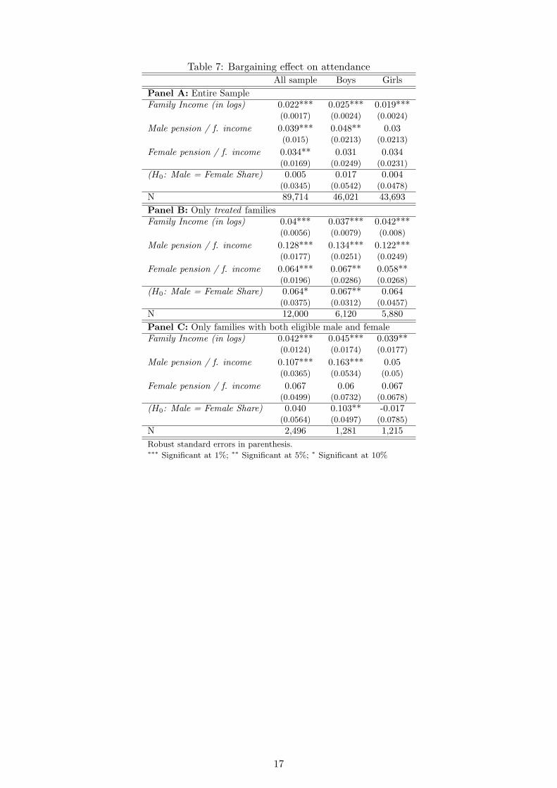
Table 7: Bargaining effect on attendanceAll sample Boys Girls

Panel A: Entire SampleFamily Income (in logs) 0.022*** 0.025*** 0.019***

(0.0017) (0.0024) (0.0024)

Male pension / f. income 0.039*** 0.048** 0.03(0.015) (0.0213) (0.0213)

Female pension / f. income 0.034** 0.031 0.034(0.0169) (0.0249) (0.0231)

(H0: Male = Female Share) 0.005 0.017 0.004(0.0345) (0.0542) (0.0478)

N 89,714 46,021 43,693Panel B: Only treated familiesFamily Income (in logs) 0.04*** 0.037*** 0.042***

(0.0056) (0.0079) (0.008)

Male pension / f. income 0.128*** 0.134*** 0.122***(0.0177) (0.0251) (0.0249)

Female pension / f. income 0.064*** 0.067** 0.058**(0.0196) (0.0286) (0.0268)

(H0: Male = Female Share) 0.064* 0.067** 0.064(0.0375) (0.0312) (0.0457)

N 12,000 6,120 5,880Panel C: Only families with both eligible male and femaleFamily Income (in logs) 0.042*** 0.045*** 0.039**

(0.0124) (0.0174) (0.0177)

Male pension / f. income 0.107*** 0.163*** 0.05(0.0365) (0.0534) (0.05)

Female pension / f. income 0.067 0.06 0.067(0.0499) (0.0732) (0.0678)

(H0: Male = Female Share) 0.040 0.103** -0.017(0.0564) (0.0497) (0.0785)

N 2,496 1,281 1,215Robust standard errors in parenthesis.∗∗∗ Significant at 1%; ∗∗ Significant at 5%; ∗ Significant at 10%

17

Tab

le8:

Reg

ress

ion:

heal

thE

ntir

esa

mpl

eM

iddl

e-ag

ers

Chi

ldre

nB

oys

Gir

ls(1

a)(1

b)(2

a)(2

b)(3

a)(3

b)(4

a)(4

b)(5

a)(5

b)Illn

ess

H.C

.Illn

ess

H.C

.Illn

ess

H.C

.Illn

ess

H.C

.Illn

ess

H.C

.M

ale

Tre

atm

ent 1

0.00

00.

002

0.02

60.

022

-0.0

07-0

.007

-0.0

08-0

.014

-0.0

070

(0.0

053)

(0.0

053)

(0.0

216)

(0.0

229)

(0.0

084)

(0.0

077)

(0.0

118)

(0.0

098)

(0.0

121)

(0.0

119)

Mal

eT

reatm

ent 2

0.00

2-0

.005

0.05

**0.

009

-0.0

07-0

.001

00

-0.0

15-0

.002

(0.0

051)

(0.0

049)

(0.0

198)

(0.0

196)

(0.0

079)

(0.0

075)

(0.0

117)

(0.0

102)

(0.0

107)

(0.0

109)

Mal

eC

.G

roup

0.00

2-0

.009

**0.

013

0.02

40.

004

-0.0

070

-0.0

020.

008

-0.0

13(0

.0043)

(0.0

043)

(0.0

147)

(0.0

17)

(0.0

072)

(0.0

062)

(0.0

099)

(0.0

093)

(0.0

104)

(0.0

082)

Fem

.T

reatm

ent 1

-0.0

040.

004

-0.0

02-0

.062

**-0

.015

**0.

01-0

.011

0.01

-0.0

18*

0.01

(0.0

044)

(0.0

044)

(0.0

266)

(0.0

198)

(0.0

075)

(0.0

083)

(0.0

112)

(0.0

113)

(0.0

1)

(0.0

12)

Fem

.T

reatm

ent 2

-0.0

08-0

.007

-0.0

21-0

.032

**-0

.003

0.00

80.

009

0.00

3-0

.017

*0.

015

(0.0

048)

(0.0

048)

(0.0

154)

(0.0

159)

(0.0

079)

(0.0

079)

(0.0

118)

(0.0

101)

(0.0

101)

(0.0

123)

Fem

.C

.G

roup

-0.0

010.

007

0.00

4-0

.016

-0.0

070.

007

-0.0

150.

006

00.

008

(0.0

041)

(0.0

042)

(0.0

137)

(0.0

144)

(0.0

068)

(0.0

069)

(0.0

091)

(0.0

095)

(0.0

102)

(0.0

099)

Pos

t-0

.015

***

-0.0

02-0

.003

0.00

2-0

.024

***

0.00

4-0

.025

***

0.00

5-0

.023

***

0.00

3(0

.0017)

(0.0

02)

(0.0

064)

(0.0

072)

(0.0

023)

(0.0

028)

(0.0

032)

(0.0

039)

(0.0

034)

(0.0

041)

Mal

eT

reat.

1×

Pos

t(β

m 4,k

=1)

-0.0

060.

001

-0.0

420.

026

0.00

40.

013

0.00

60.

012

0.00

30.

014

(0.0

071)

(0.0

079)

(0.0

272)

(0.0

335)

(0.0

116)

(0.0

129)

(0.0

161)

(0.0

172)

(0.0

165)

(0.0

191)

Mal

eT

reat.

2×

Pos

t(β

m 4,k

=2)

-0.0

090.

004

-0.0

56**

-0.0

030.

007

0.00

30.

004

-0.0

030.

011

0.01

(0.0

063)

(0.0

063)

(0.0

221)

(0.0

23)

(0.0

098)

(0.0

108)

(0.0

14)

(0.0

144)

(0.0

138)

(0.0

164)

Mal

eC

.G

roup

×Pos

t(β

m 5)

0.00

10.

012*

0.01

10.

035

-0.0

130.

016

-0.0

050.

011

-0.0

20.

021

(0.0

059)

(0.0

063)

(0.0

2)

(0.0

237)

(0.0

09)

(0.0

103)

(0.0

123)

(0.0

147)

(0.0

13)

(0.0

144)

Fem

.T

reat.

1×

Pos

t(β

f 4,k

=1)

0.00

10.

01-0

.008

-0.0

050.

007

-0.0

010

0.00

50.

014

-0.0

06(0

.0058)

(0.0

063)

(0.0

343)

(0.0

288)

(0.0

099)

(0.0

124)

(0.0

142)

(0.0

175)

(0.0

139)

(0.0

176)

Fem

.T

reat.

2×

Pos

t(β

f 4,k

=2)

0.00

20.

012*

0.00

60.

015

-0.0

02-0

.014

-0.0

11-0

.01

0.01

-0.0

19(0

.0065)

(0.0

066)

(0.0

191)

(0.0

21)

(0.0

103)

(0.0

112)

(0.0

15)

(0.0

146)

(0.0

138)

(0.0

171)

Fem

.C

.G

roup

×Pos

t(β

f 5)

0.00

9-0

.004

0.01

80.

005

-0.0

01-0

.021

**0.

006

-0.0

2-0

.008

-0.0

2(0

.0056)

(0.0

062)

(0.0

144)

(0.0

16)

(0.0

086)

(0.0

1)

(0.0

116)

(0.0

135)

(0.0

129)

(0.0

147)

18

Tab

le9:

F-T

ests

-he

alth

Ent

ire

sam

ple

Mid

dle-

ager

sC

hild

ren

Boy

sG

irls

(1a)

(1b)

(2a)

(2b)

(3a)

(3b)

(4a)

(4b)

(5a)

(5b)

Illn

ess

H.C

.Illn

ess

H.C

.Illn

ess

H.C

.Illn

ess

H.C

.Illn

ess

H.C

.(H

0:β

m 4,k

=1

=β

m 5)

0.58

1.18

2.82

*0.

061.

540.

050.

350

1.34

0.11

(H0

:βm 4,k

=2

=β

m 5)

1.53

0.74

5.66

**1.

472.

440.

840.

210.

52.

79*

0.27

(H0

:βf 4,k

=1

=β

f 5)

1.22

2.87

*0.

490.

080.

581.

790.

141.

491.

580.

43(H

0:β

f 4,k

=2

=β

f 5)

0.59

3.07

*0.

280.

140

0.18

0.93

0.26

0.94

0(H

0:β

m 4,k

=1

=β

f 4,k

=1∩

βm 4,k

=2

=β

f 4,k

=2)

1.21

0.83

2.76

*0.

050.

061.

290.

360.

160.

091.

44∗∗∗

Sig

nifi

cant

at

1%

;∗∗

Sig

nifi

cant

at

5%

;∗

Sig

nifi

cant

at

10%

19

Table 10: Bargaining effect on illnessAll sample Middle-agers Children

Panel A: Entire SampleFamily Income (in logs) -0.014*** -0.021*** -0.009***

(0.0003) (0.0009) (0.0003)

Male pension / f. income -0.002 -0.033** 0.006(0.0049) (0.0163) (0.0079)

Female pension / f. income 0.013** -0.012 -0.001(0.0054) (0.0203) (0.0076)

(H0: Male = Female Share) -0.015* -0.021** 0.007(0.0094) (0.0112) (0.0023)

N 126,208 13,704 48,483Panel B: Only treated familiesFamily Income (in logs) -0.022*** -0.02*** -0.008***

(0.0007) (0.0025) (0.0011)

Male pension / f. income -0.009 -0.024 0.008(0.0055) (0.0189) (0.0088)

Female pension / f. income 0.005 -0.005 0.006(0.0062) (0.0238) (0.0089)

(H0: Male = Female Share) -0.014 -0.019* 0.002(0.0105) (0.0119 (0.0231)

N 28,714 2,092 5,302Panel C: Only families with both eligible male and femaleFamily Income (in logs) -0.024*** -0.025*** -0.009***

(0.0012) (0.0083) (0.0025)

Male pension / f. income -0.019** -0.063 0.019(0.0084) (0.0563) (0.0197)

Female pension / f. income 0.039*** 0.002 0.005(0.0123) (0.0837) (0.0238)

(H0: Male = Female Share) -0.058** -0.065* 0.014(0.0249) (0.0380) (0.0523)

N 10,426 271 1,045Robust standard errors in parenthesis.∗∗∗ Significant at 1%; ∗∗ Significant at 5%; ∗ Significant at 10%

20