Journal of Pharmacokinetics and Pharmacodynamics, Vol. 28, No. 3, 2001

In Vivo–In Vitro Correlation (IVIVC) ModelingIncorporating a Convolution Step

T. O’Hara,1,2 S. Hayes,2 J. Davis,3 J. Devane,1 T. Smart,3 and A. Dunne2,4

Received May 22, 2000—Final February 5, 2001

The purpose of in vivo–in vitro correlation (IVIVC) modeling is described. These models areusually fitted to deconûoluted data rather than the raw plasma drug concentration�time data.Such a two-stage analysis is undesirable because the deconûolution step is unstable and becausethe fitted model predicts the fraction of a dosage unit dissolûed/absorbed in vivo which generallyis not the primary focus of our attention. Interest usually centers on the plasma drug concentrationor some function of it (e.g., AUC, Cmax). Incorporation of a conûolution step into the modeloûercomes these difficulties. Odds, hazards, and reûersed hazards models which include a conûol-ution step are described. The identity model (which states that aûerage in vivo and in vitrodissolution/time curûes are coincident or directly superimposable) is a special case of these mod-els. The odds model and the identity model were fitted to data sets for two different productsusing nonlinear mixed effects model fitting software. Results show that the odds model describesboth data sets reasonably well and is a significantly better fit than the identity model in each case.

KEY WORDS: in ûiûo–in ûitro correlation; deconvolution; convolution; odds; hazards;reversed hazards.

INTRODUCTION

In an in ûitro dissolution study the fraction (or percentage) of the dosedissolved under stated conditions at a set of predetermined time points ismeasured for each of a number of dosage units. These studies are routinelyperformed as part of the quality assurance procedure in the process ofmanufacturing solid oral drug dosage forms because they help to ensure thatthe manufacturing process has not deviated significantly from a particularstandard. Such studies do not necessarily assume that the in ûitro dissolutiondata tell us anything about drug dissolution�absorption in ûiûo. However,

1Elan Corporation plc, Athlone, Ireland.2Department of Statistics, University College Dublin, Ireland.3Pfizer Central Research, Sandwich, England.4To whom correspondence should be addressed. E-mail: Adrian.Dunne@UCD.ie

277

1567-567X�01�0600-0277$19.50�0 2001 Plenum Publishing Corporation

O’Hara et al.278

in ûitro dissolution studies can be used for applications other than qualityassurance of manufactured product if they can be used to predict the in ûiûoperformance of the product. For example, in certain circumstances an inûitro dissolution study can form the basis of a bioequivalence (BE) assess-ment without the need for human BE studies (1,2) or it could be used in theevaluation of a dosage form during the process of product development (3).Another application is in setting dissolution specifications that are moremeaningful in that a product that is within specification can be said to haveparticular in ûiûo properties (1,2,4). These applications constitute a consider-able widening of the potential impact of in ûitro dissolution studies in thepharmaceutical industry. For this reason, considerable effort has gone intothe development of models relating in ûiûo performance to in ûitro dissol-ution. These models describe the relationship between in ûiûo and in ûitrocharacteristics and are known in the literature as in ûiûo–in ûitro correlation(IVIVC) models. IVIVC models are divided into four categories known aslevels A, B, C, and D (1). Level A applies to a model that can predict theentire in ûiûo time course from the in ûitro data. The other levels use anumber of tablet�capsule formulations and relate summary statistics for thein ûitro and in ûiûo behavior of the drug. Because levels B, C, and D arebased on summary statistics that do not uniquely reflect the time depen-dence of the data, they are not considered to be as useful as level A (1,5).The majority of level A IVIVC models consider the relationship between inûitro dissolution and either in ûiûo dissolution or absorption. The modelsused range from the simple identity model which assumes that in ûitro dissol-ution mirrors in ûiûo dissolution�absorption exactly (2,5–9, 20–22), to moresophisticated models which express a more complex relationship betweenthe two (10,11). One of the problems with all of these models is that theymodel the fraction (or percentage) of the dosage form dissolved�absorbedin ûiûo despite the fact that this variable is not directly observable. Theobserved variable is the plasma drug concentration and a deconvolutionstep is required in order to transform it to estimated fraction of dosage formdissolved�absorbed in ûiûo (12). Whether the deconvoluted data representdissolution or absorption in ûiûo depends on the way in which the deconvol-ution is implemented. If the deconvolution involves oral administration ofa reference solution or immediate release (IR) tablet then the deconvoluteddata represent the in ûiûo dissolution of the test product. On the other hand,a bolus intravenous reference will result in the deconvoluted data rep-resenting the in ûiûo dissolution followed by absorption of the orally admin-istered product. A Wagner–Nelson deconvolution (12) also results indeconvoluted data that represent the combined effects of dissolution fol-lowed by absorption. For the sake of brevity in the remainder of this paper,the in ûiûo process being studied is henceforth referred to as dissolution with

In Vivo–In Vitro Correlation Modeling 279

the understanding that the same considerations and models could be appliedto in ûiûo dissolution�absorption.

The necessity to transform the data by deconvoluting the plasma drugconcentrations before the model can be fitted is a serious disadvantage ofthe current modeling approach. It involves a two-stage data analysis withthe first stage consisting of the deconvolution of the in ûiûo plasma drugconcentration�time data to produce in ûiûo dissolution�time data. In thesecond stage the IVIVC model is fitted to the deconvoluted in ûiûo data andthe in ûitro dissolution�time data. Deconvolution is an unstable process (13)because it essentially involves derivatives which can exhibit appreciablechanges in response to small changes in the data. This instability is not afeature of a particular method of deconvoluting but is a property of thesolutions to integral equations of the first kind (13). Another serious disad-vantage is that the model predicts the fraction of the dosage form dissolvedin ûiûo which is generally not the primary focus of our attention. Instead,we are usually more interested in the plasma drug concentration or somefunction of it (e.g., AUC or Cmax). Hence a further data-processing stage isrequired because the model predictions have to be convoluted in order totransform them into the variable of interest. In addition the two-stage pro-cess is more cumbersome than a single stage data analysis. A differentmodeling approach that overcomes these limitations, involves the incorpor-ation of a convolution step into the model and has been advocated by Gille-spie (14). This paper considers the extension of some previously reportednonlinear level A IVIVC models (10,11) to incorporate a convolution step.The basic models are very similar to those described before (10,11) butincorporate additional random effects not previously considered. For thisreason and for the sake of clarity and inclusiveness, a complete descriptionof the models is included in this paper. As stated above, the idea of incorpo-rating a convolution step into the model is not new but has never beenapplied to these particular models. This paper shows how this can beachieved and demonstrates that it can be implemented by means of twoexamples.

MODEL

Let Fi1(t) represent the true fraction of drug dissolved at time t fromthe ith dosage unit in ûitro and let Fi2k (t) represent the true fraction of drugdissolved at time t from the ith dosage unit in the kth subject in ûiûo. Oneinterpretation of Fi1(t) and Fi2k (t) is that they are the distribution functionsfor random variables T1 and T2 which are the times at which a drug mole-cule enters solution from the ith dosage unit in ûitro and in ûiûo in the kthsubject respectively. The essence of any IVIVC model is that it describes a

O’Hara et al.280

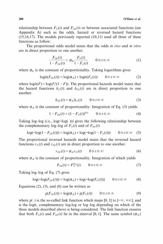
relationship between Fi1(t) and Fi2k (t) or between associated functions (seeAppendix A) such as the odds, hazard or reversed hazard functions(15,16,17). The models previously reported (10,11) used all three of thesefunctions as follow:

The proportional odds model states that the odds in ûiûo and in ûitroare in direct proportion to one another.

Fi2k(t)

1AFi2k(t)Gαik

Fi1(t)

1AFi1(t)0⁄ t⁄S (1)

where αik is the constant of proportionality. Taking logarithms gives

logit(Fi2k(t))Glog(α ik)Clogit(Fi1(t)) 0⁄ t⁄S (2)

where logit(F )Glog(F�(1AF )). The proportional hazards model states thatthe hazard functions hi1(t) and hi2k (t) are in direct proportion to oneanother.

hi2k (t)Gα ikhi1(t) 0⁄ t⁄S (3)

where α ik is the constant of proportionality. Integration of Eq. (3) yields

1AFi2k(t)G(1AFi1(t))α ik 0⁄ t⁄S (4)

Taking log–log (i.e., log(−log( · ))) gives the following relationship betweenthe complementary log–log of Fi1(t) and of Fi2k (t)

log(−log(1AFi2k(t)))Glog(α ik)Clog(−log(1AFi1(t))) 0⁄ t⁄S (5)

The proportional reversed hazards model states that the reversed hazardfunctions ri1(t) and ri2k (t) are in direct proportion to one another.

ri2k (t)Gα ik ri1(t) 0⁄ t⁄S (6)

where α ik is the constant of proportionality. Integration of which yields

Fi2k(t)GFα iki1 (t) 0⁄ t⁄S (7)

Taking log–log of Eq. (7) gives

log(−log(Fi2k(t)))Glog(α ik)Clog(−log(Fi1(t))) 0⁄ t⁄S (8)

Equations (2), (5), and (8) can be written as

g(Fi2k(t))Glog(α ik)Cg(Fi1(t)) 0⁄ t⁄S (9)

where g( · ) is the so-called link function which maps [0, 1] to [−S, +S], andis the logit, complementary log-log or log–log depending on which of thethree models described above is being considered. The link function ensuresthat both Fi1(t) and Fi2k (t) lie in the interval [0, 1]. The same symbol (α ik)

In Vivo–In Vitro Correlation Modeling 281

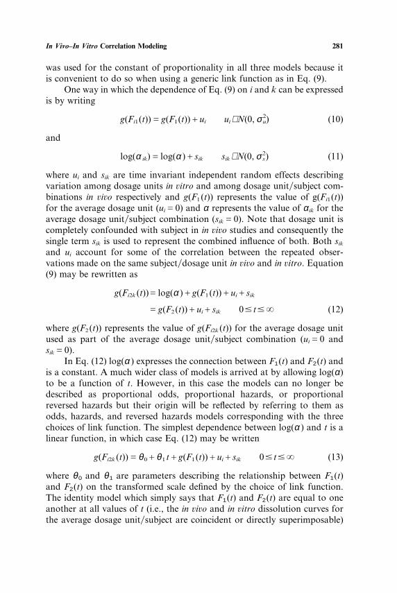
was used for the constant of proportionality in all three models because itis convenient to do so when using a generic link function as in Eq. (9).

One way in which the dependence of Eq. (9) on i and k can be expressedis by writing

g(Fi1(t))Gg(F1(t))Cui ui ∼ N(0, σ2u) (10)

and

log(α ik)Glog(α )Csik sik ∼ N(0, σ2s) (11)

where ui and sik are time invariant independent random effects describingvariation among dosage units in ûitro and among dosage unit�subject com-binations in ûiûo respectively and g(F1(t)) represents the value of g(Fi1(t))for the average dosage unit (uiG0) and α represents the value of αik for theaverage dosage unit�subject combination (sikG0). Note that dosage unit iscompletely confounded with subject in in ûiûo studies and consequently thesingle term sik is used to represent the combined influence of both. Both sik

and ui account for some of the correlation between the repeated obser-vations made on the same subject�dosage unit in ûiûo and in ûitro. Equation(9) may be rewritten as

g(Fi2k (t))Glog(α )Cg(F1(t))CuiCsik

Gg(F2(t))CuiCsik 0⁄ t⁄S (12)

where g(F2(t)) represents the value of g(Fi2k (t)) for the average dosage unitused as part of the average dosage unit�subject combination (uiG0 andsikG0).

In Eq. (12) log(α ) expresses the connection between F1(t) and F2(t) andis a constant. A much wider class of models is arrived at by allowing log(α)to be a function of t. However, in this case the models can no longer bedescribed as proportional odds, proportional hazards, or proportionalreversed hazards but their origin will be reflected by referring to them asodds, hazards, and reversed hazards models corresponding with the threechoices of link function. The simplest dependence between log(α ) and t is alinear function, in which case Eq. (12) may be written

g(Fi2k (t))Gθ0Cθ1 tCg(F1(t))CuiCsik 0⁄ t⁄S (13)

where θ0 and θ1 are parameters describing the relationship between F1(t)and F2(t) on the transformed scale defined by the choice of link function.The identity model which simply says that F1(t) and F2(t) are equal to oneanother at all values of t (i.e., the in ûiûo and in ûitro dissolution curves forthe average dosage unit�subject are coincident or directly superimposable)

O’Hara et al.282

corresponds with the case where both θ0 and θ1 are zero irrespective of thelink function.

Equation (13) describes a relationship between F1(t) and F2(t) withoutdescribing how either of them depends on time. Since the in ûitro data areconcerned with the dependence of F1(t) on time, it is necessary to modelhow F1(t) depends on time. The most general form that can be used definesa separate parameter for each observation time and consequently makes noassumption whatsoever about the shape of F1(t), it is

F1(tm)Gφm mG1, 2, . . . (14)

where tm represents the mth observation time and φm is a parameter.The measured fraction of drug dissolved from the ith dosage unit in

ûitro at time t is written as Yi1(t) and is related to Fi1(t) by

Yi1(t)GFi1(t)Cε i1(t) ε i1(t) ∼ N(0, σ21) (15)

where the independent random error term ε i1(t) includes measurementerrors. Since Yi1(t) is expressed as the measured amount of drug dissolveddivided by a constant (e.g., label claim) it is not necessarily less than orequal to unity and consequently Eq. (15) imposes no such constraint.

The measured drug concentration at time t in the plasma of the kthsubject following administration of the i th dosage unit is denoted by Yi2k (t)and may be written using the convolution integral (12) as

Yi2k (t)G�t

0

cδk (tAτ )F ′i2k (τ ) dτCε i2k (t) ε i2k (t) ∼ N(0, σ22) (16)

where cδk (t) represents the plasma concentration unit impulse response forthe kth subject, F ′i2k (t) (the prime denotes the derivative with respect totime) represents the in ûiûo dissolution rate at time t for the ith dosage unitin the kth subject and ε i2k (t) represents independent in ûiûo errors. The inûitro and in ûiûo errors (ε i1(t) and εi2k (t)) have different variances becausethe in ûitro data would be expected to be more precise than the in ûiûo dataand also because these measurements are on different scales. All the randomeffects ui , sik , ε i1(t) and ε i2k (t) are assumed to be independent of one another.

Combining Eqs. (10), (13), (14), (15), and (16) provides a model forFi2k (t) at the observation times but does not specify it in between thosetimes. Consequently, F ′i2k (t) is not specified by the model described above.If we assume that the dissolution rate is piecewise constant between theobservation times then we can write

F ′i2k (t)GFi2k (tm)AFi2k (tmA1)

tmAtmA1

tmA1Ft⁄ tm (17)

In Vivo–In Vitro Correlation Modeling 283

Equations (10), (14), and (15) together define a model for in ûitro data. Inaddition the combination of Eqs. (10), (11), (13), (14), (16), and (17) definea model for in ûiûo data.

METHOD

The models described above with the logit link function were tested byfitting them to data sets for a number of different extended release (ER)drug products. Two of these data sets were selected for presentation below.

Product A

The in ûitro study consisted of dissolution studies of 12 tablets using aUSP 2 apparatus with phosphate buffer at pH 7.2 and a paddle speed of50 rpm. Aliquots of the dissolution medium were removed at 0.5, 1, 2, 3, 4,5, 6, 7, 8, 10, 12, and 24 hr and assayed for drug content. The amount ofdrug dissolved at each time point for each tablet was expressed as a fractionof label claim.

The in ûiûo study consisted of a crossover design with each of 10 healthyhuman volunteers being administered an IR tablet during one of the treat-ment periods and the test ER formulation during the other treatmentperiod. Blood was collected at 0.5, 1, 2, 3, 4, 5, 6, 7, 8, 10, 12, and 24 hrfollowing each drug administration and assayed for plasma drugconcentration.

Product B

The in ûitro study consisted of dissolution studies of six tablets using aUSP 1 apparatus in aqueous 0.01 M hydrochloric acid at pH 2. Aliquots ofthe dissolution medium were removed at 0.25, 0.5, 0.75, 1, 1.5, 2, 2.5, 3, 3.5,4, 4.5, 5, 5.5, 6, 6.5, 7, 7.5, 8, 8.5, and 9 hr and assayed for drug content. Theamount of drug dissolved at each time point for each tablet was expressed asa fraction of label claim.

The in ûiûo study consisted of a crossover design with each of 9 healthyhuman volunteers being administered an IR reference tablet during one ofthe treatment periods and the test ER formulation during the other treat-ment period. Blood was collected at 0.25, 0.5, 1, 2, 3, 4, 6, 8, 9, 10, 12, 15,18, 24, 36, 48, and 60 hr following each drug administration and assayedfor plasma drug concentration.

Analysis

The plasma concentration–time data collected following administrationof the reference formulation was modeled using a two-compartment pharm-acokinetic (PK) model with first-order absorption and the parameters esti-mated separately for each subject using WINNONLIN (Product A) and

O’Hara et al.284

PROC NLIN in SAS (Product B). After scaling for the reference dose, thisPK model together with the individual subject parameter estimates treatedas known parameter values was used as the unit impulse response in Eq.(16) above when fitting models to the in ûiûo ER data.

The IVIVC model [Eqs. (10)–(17) inclusive] with the logit link wasfitted simultaneously to the in ûitro and the in ûiûo ER data. Details of themodel as fitted to the data are given in Appendix B.

Due to the current emphasis placed on the identity model which statesthat the in ûiûo dissolution profile is identical with that in ûitro (θ0 and θ1

both constrained to be zero) it was also fitted to the same data for compari-son purposes.

Apart from the PK modeling of the in ûiûo IR reference data, all othermodel fitting was performed using an approximation to maximumlikelihood implemented by the nonlinear mixed-effects modeling programNONMEM (18). The NONMEM code is available on request.

RESULTS

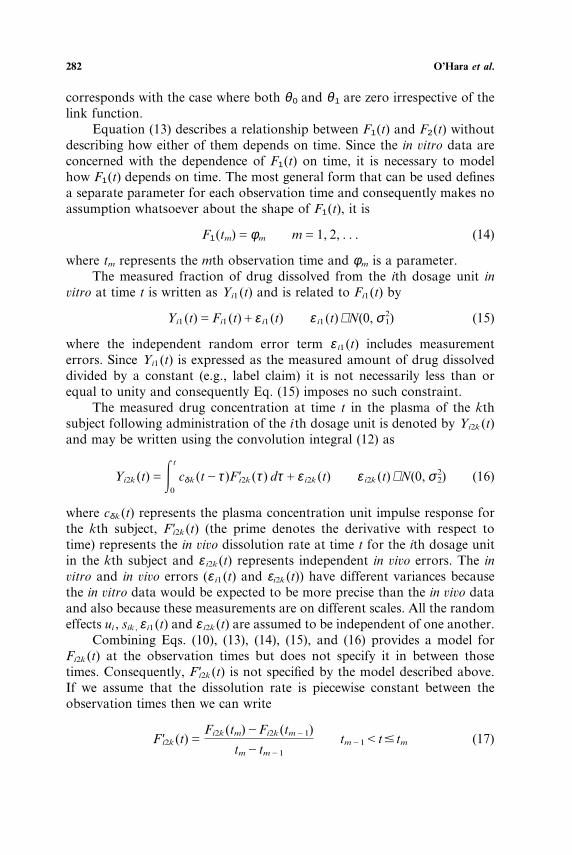
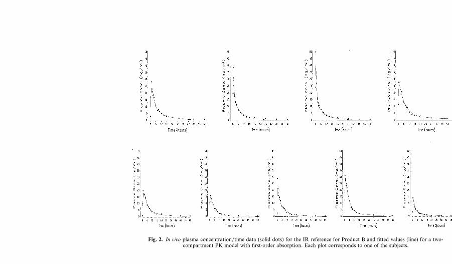
For each subject the plasma concentration�time data for the referencedose together with the fitted two-compartment PK model are illustrated inFigs. 1 and 2 which show that this PK model adequately describes thesedata.

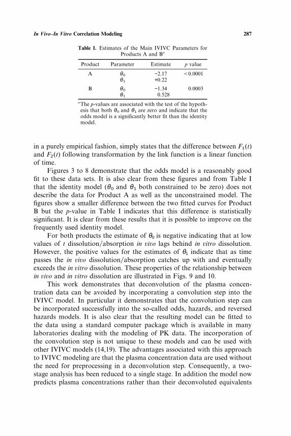
The estimates of θ0 and θ1 are tabulated in Table I which also reportsthe p-value for the difference between the odds model and the identity modelfor each product.

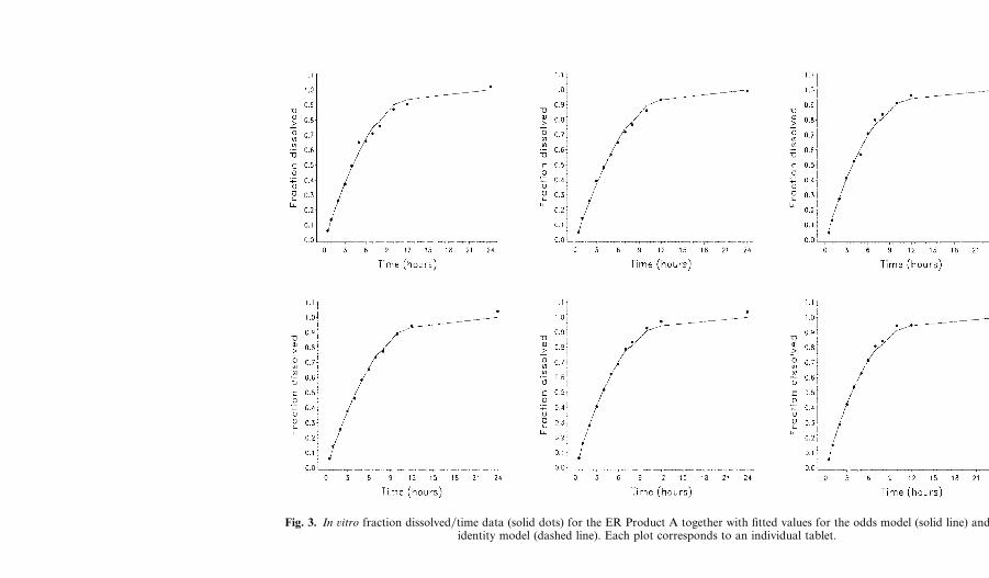
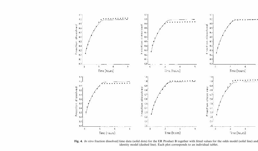
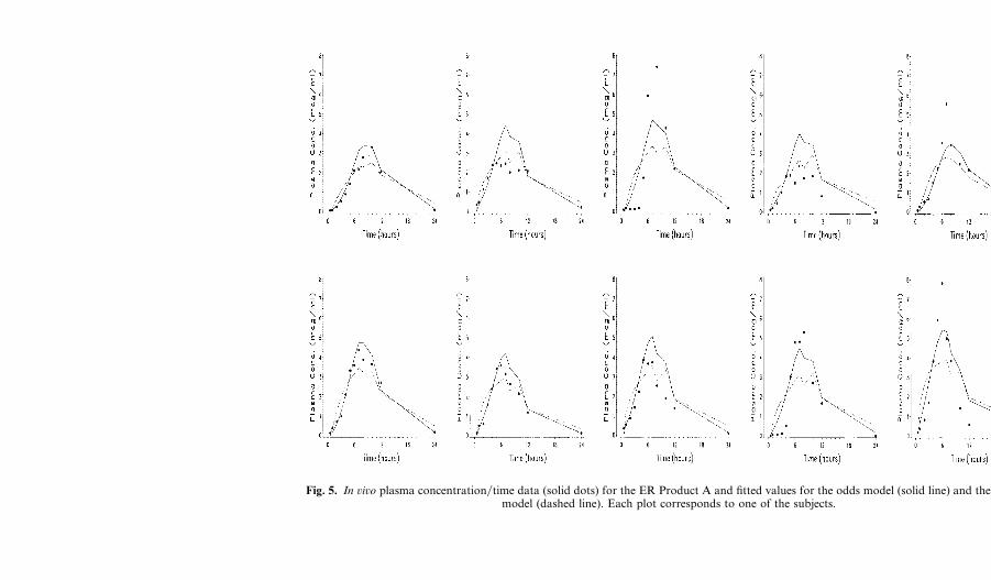
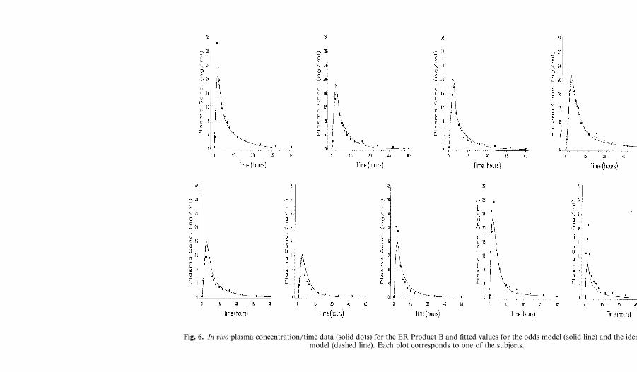
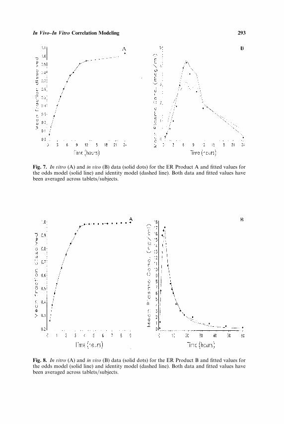
The fraction dissolved in ûitro is plotted versus time for each tablet inFigs. 3 and 4 together with the fitted values from the odds model and theidentity model. The plasma concentration�time data for the ER formu-lations for each subject together with the fitted values from the odds modeland the identity model are illustrated in Figs. 5 and 6. These data and fittedvalues were averaged across tablets and across subjects and the averagesplotted vs. time in Figs. 7 and 8. For comparison purposes Figs. 9 and 10show plots of F̂1(t) (estimated in ûitro dissolution for the average dosageunit) and F̂2(t) (estimated in ûiûo dissolution for the average dosage unit�subject combination) vs. time. The relationship between in ûiûo and in ûitrodissolution is illustrated by plotting F̂1(t) against F̂2(t) in Figs. 9 and 10 forproducts A and B, respectively.

DISCUSSION

Equation (13) is the core of the IVIVC model because it expresses thelink between F1(t) and F2(t). This equation, which currently is being used

InV

ivo–InV

itroC

orrelationM

odeling285

Fig. 1. In ûiûo plasma concentration�time data (solid dots) for the IR reference for Product A and fitted values (line) for a two-compartment PK model with first-order absorption. Each plot corresponds to one of the subjects.

O’H

araet

al.286

Fig. 2. In ûiûo plasma concentration�time data (solid dots) for the IR reference for Product B and fitted values (line) for a two-compartment PK model with first-order absorption. Each plot corresponds to one of the subjects.

In Vivo–In Vitro Correlation Modeling 287

Table I. Estimates of the Main IVIVC Parameters forProducts A and Ba

Product Parameter Estimate p value

A θ0 −2.17 F0.0001θ1 +0.22

B θ0 −1.34 0.0003θ1 0.528

aThe p-values are associated with the test of the hypoth-esis that both θ0 and θ1 are zero and indicate that theodds model is a significantly better fit than the identitymodel.

in a purely empirical fashion, simply states that the difference between F1(t)and F2(t) following transformation by the link function is a linear functionof time.

Figures 3 to 8 demonstrate that the odds model is a reasonably goodfit to these data sets. It is also clear from these figures and from Table Ithat the identity model (θ0 and θ1 both constrained to be zero) does notdescribe the data for Product A as well as the unconstrained model. Thefigures show a smaller difference between the two fitted curves for ProductB but the p-value in Table I indicates that this difference is statisticallysignificant. It is clear from these results that it is possible to improve on thefrequently used identity model.

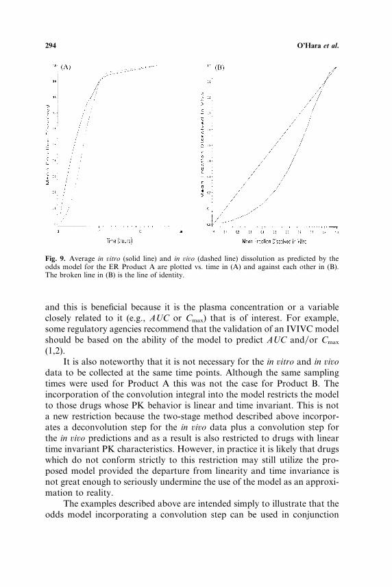
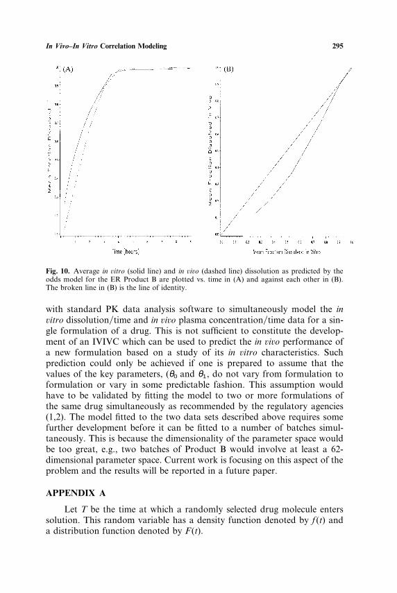
For both products the estimate of θ0 is negative indicating that at lowvalues of t dissolution�absorption in ûiûo lags behind in ûitro dissolution.However, the positive values for the estimates of θ1 indicate that as timepasses the in ûiûo dissolution�absorption catches up with and eventuallyexceeds the in ûitro dissolution. These properties of the relationship betweenin ûiûo and in ûitro dissolution are illustrated in Figs. 9 and 10.

This work demonstrates that deconvolution of the plasma concen-tration data can be avoided by incorporating a convolution step into theIVIVC model. In particular it demonstrates that the convolution step canbe incorporated successfully into the so-called odds, hazards, and reversedhazards models. It is also clear that the resulting model can be fitted tothe data using a standard computer package which is available in manylaboratories dealing with the modeling of PK data. The incorporation ofthe convolution step is not unique to these models and can be used withother IVIVC models (14,19). The advantages associated with this approachto IVIVC modeling are that the plasma concentration data are used withoutthe need for preprocessing in a deconvolution step. Consequently, a two-stage analysis has been reduced to a single stage. In addition the model nowpredicts plasma concentrations rather than their deconvoluted equivalents

O’H

araet

al.288

Fig. 3. In ûitro fraction dissolved�time data (solid dots) for the ER Product A together with fitted values for the odds model (solid line) and theidentity model (dashed line). Each plot corresponds to an individual tablet.

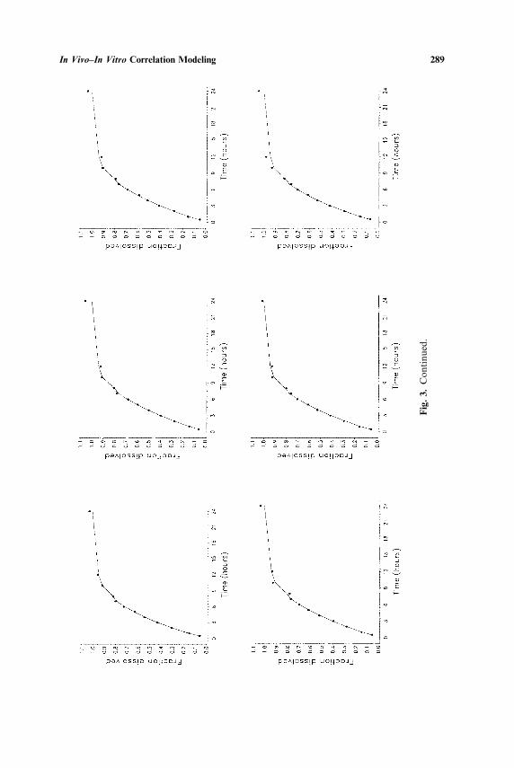
In Vivo–In Vitro Correlation Modeling 289

Fig

.3.

Con

tinu

ed.

O’H

araet

al.290

Fig. 4. In ûitro fraction dissolved�time data (solid dots) for the ER Product B together with fitted values for the odds model (solid line) and theidentity model (dashed line). Each plot corresponds to an individual tablet.

InV

ivo–InV

itroC

orrelationM

odeling291

Fig. 5. In ûiûo plasma concentration�time data (solid dots) for the ER Product A and fitted values for the odds model (solid line) and the identitymodel (dashed line). Each plot corresponds to one of the subjects.

O’H

araet

al.292

Fig. 6. In ûiûo plasma concentration�time data (solid dots) for the ER Product B and fitted values for the odds model (solid line) and the identitymodel (dashed line). Each plot corresponds to one of the subjects.

In Vivo–In Vitro Correlation Modeling 293

Fig. 7. In ûitro (A) and in ûiûo (B) data (solid dots) for the ER Product A and fitted values forthe odds model (solid line) and identity model (dashed line). Both data and fitted values havebeen averaged across tablets�subjects.

Fig. 8. In ûitro (A) and in ûiûo (B) data (solid dots) for the ER Product B and fitted values forthe odds model (solid line) and identity model (dashed line). Both data and fitted values havebeen averaged across tablets�subjects.

O’Hara et al.294

Fig. 9. Average in ûitro (solid line) and in ûiûo (dashed line) dissolution as predicted by theodds model for the ER Product A are plotted vs. time in (A) and against each other in (B).The broken line in (B) is the line of identity.

and this is beneficial because it is the plasma concentration or a variableclosely related to it (e.g., AUC or Cmax) that is of interest. For example,some regulatory agencies recommend that the validation of an IVIVC modelshould be based on the ability of the model to predict AUC and�or Cmax

(1,2).It is also noteworthy that it is not necessary for the in ûitro and in ûiûo

data to be collected at the same time points. Although the same samplingtimes were used for Product A this was not the case for Product B. Theincorporation of the convolution integral into the model restricts the modelto those drugs whose PK behavior is linear and time invariant. This is nota new restriction because the two-stage method described above incorpor-ates a deconvolution step for the in ûiûo data plus a convolution step forthe in ûiûo predictions and as a result is also restricted to drugs with lineartime invariant PK characteristics. However, in practice it is likely that drugswhich do not conform strictly to this restriction may still utilize the pro-posed model provided the departure from linearity and time invariance isnot great enough to seriously undermine the use of the model as an approxi-mation to reality.

The examples described above are intended simply to illustrate that theodds model incorporating a convolution step can be used in conjunction

In Vivo–In Vitro Correlation Modeling 295

Fig. 10. Average in ûitro (solid line) and in ûiûo (dashed line) dissolution as predicted by theodds model for the ER Product B are plotted vs. time in (A) and against each other in (B).The broken line in (B) is the line of identity.

with standard PK data analysis software to simultaneously model the inûitro dissolution�time and in ûiûo plasma concentration�time data for a sin-gle formulation of a drug. This is not sufficient to constitute the develop-ment of an IVIVC which can be used to predict the in ûiûo performance ofa new formulation based on a study of its in ûitro characteristics. Suchprediction could only be achieved if one is prepared to assume that thevalues of the key parameters, (θ0 and θ1, do not vary from formulation toformulation or vary in some predictable fashion. This assumption wouldhave to be validated by fitting the model to two or more formulations ofthe same drug simultaneously as recommended by the regulatory agencies(1,2). The model fitted to the two data sets described above requires somefurther development before it can be fitted to a number of batches simul-taneously. This is because the dimensionality of the parameter space wouldbe too great, e.g., two batches of Product B would involve at least a 62-dimensional parameter space. Current work is focusing on this aspect of theproblem and the results will be reported in a future paper.

APPENDIX A

Let T be the time at which a randomly selected drug molecule enterssolution. This random variable has a density function denoted by f (t) anda distribution function denoted by F (t).

O’Hara et al.296

The odds of a randomly chosen molecule entering solution during theinterval [0, t] are

F (t)

1AF (t)(A1)

The hazard function describes the probability that a molecule which has notentered solution prior to time t, doing so immediately following time t. Itcan be written

h(t)Gf (t)

1AF (t)(A2)

The reversed hazard function describes the probability that a moleculewhich has entered solution prior to time t, having done so immediately priorto time t. It can be written

r(t)Gf (t)

F (t)(A3)

APPENDIX B

The odds model (with a two-compartment PK model) which was fittedto the two data sets described above can be written as follows: for the inûitro data

Yi1(tm)Galogit(logit(φm)Cui)Cε i1(tm)

iG1, 2, . . . , nd mG1, 2, . . . , nt1 (B1)

and for the in ûiûo data

Yi2k (tm)G ∑m

lG1

fi2k (tl)�Ak

ak

ek1lCBk

bk

ek2lA(AkCBk)

ck

ek3l�Cε i2k (tm)

iGkG1, 2, . . . , ns mG1, 2, . . . , nt2 (B2)

where

ek1lG(exp(−ak (tmAtl)Aexp(−ak (tmAtlA1))

ek2lG(exp(−bk (tmAtl)Aexp(−bk (tmAtlA1)) (B3)

ek3lG(exp(−ck (tmAtl)Aexp(−ck (tmAtlA1))

In Vivo–In Vitro Correlation Modeling 297

fi2k (tl)Galogit(θ0Cθ1tlClogit(φl)CuiCsik)

tllG1

G

alogit(θ0Cθ1tlClogit(φl)CuiCsik)

Aalogit(θ0Cθ1tlA1Clogit(φlA1)CuiCsik)

tlAtlA1

lH1 (B4)

alogit is the inverse of the logit function (the antilogit), nd is the number ofdosage units studied in ûitro, nt1 is the number of time points at which inûitro dissolution was measured, ns is the number of subjects�dosage unitsstudied in ûiûo, nt2 is the number of time points at which plasma drug con-centration was measured for the ER dosage form, t0G0, and the unitimpulse IR response for the kth subject is modeled by

Ak exp(−akt)CBk exp(−bkt)A(AkCBk) exp(−ckt) (B5)

REFERENCES

1. Food and Drug Administration. Guidance for Industry, Extended Release Oral DosageForms; Deûelopment, Eûaluation and Application of In Vitro�In Viûo Correlations. Foodand Drug Administration, Rockville, Md., 1997.

2. European Agency for the Evaluation of Medicinal Products. Note for Guidance on Qualityof Modified Release Products: A: Oral Dosage Forms B: Transdermal Dosage Forms SectionI (Quality), European Agency for the Evaluation of Medicinal Products, London, U.K.,1999.

3. J. Devane. Impact of IVIVR on product development. In D. Young, J. Devane, and J.Butler (eds.), Adûances in Experimental Medicine and Biology, Vol. 423, In Vitro–In ViûoCorrelations, Plenum Press, New York, 1997, pp. 241–259.

4. D. A. Piscitelli and D. Young. Setting dissolution specifications for modified-release dosageforms. In D. Young, J. Devane, and J. Butler (eds.), Adûances in Experimental Medicineand Biology, Vol. 423, In Vitro–In Viûo Correlations, Plenum Press, New York, 1997, pp.159–166.

5. United States Pharmacopeia. In Vitro and In Viûo Evaluation of Dosage Forms. Pharma-cop. Forum 19:5366–5379 (1993).

6. Z. Hussein and M. Friedman. Release and absorption characteristics of novel theophyllinesustained-release formulations. In ûitro–in ûiûo correlation. Pharm. Res. 7:1167–1171(1990).

7. P. Mojaverian, E. Radwanski, C. C. Lin, P. Cho, W. A. Vadino, and J. M. Rosen. Corre-lation of in ûitro release rate and in ûiûo absorption characteristics of four chlorpheniraminemaleate extended-release formulations. Pharm. Res. 9:450–456 (1992).

8. J. M. Cardot and E. Beyssac. In ûitro�in ûiûo correlations: Scientific implications and stan-dardization. Eur. J. Drug Metab. Pharmacokin. 8:113–120 (1983).

9. S. S. Hwang, J. Gorsline, J. Louie, D. Dye, D. Guinta, and L. Hamel. In ûitro and in ûiûoevaluation of a once-daily controlled-release pseudoephedrine product. J. Clin. Pharmacol.35:259–267 (1995).

10. A. Dunne, T. O’Hara, and J. Devane. Level A in ûiûo–in ûitro correlation: Nonlinearmodels and statistical methodology. J. Pharm. Sci. 86:1245–1249 (1997).

11. A. Dunne, T. O’Hara, and J. Devane, J. A new approach to modeling the relationshipbetween in ûitro and in ûiûo drug dissolution�absorption. Statist. Med. 18:1865–1876 (1999).

12. J. Gabrielsson and D. Weiner. Pharmacokinetic and Pharmacodynamic Data Analysis: Con-cepts and Applications, Swedish Pharmaceutical Press, Sweden, 1997.

O’Hara et al.298

13. G. M. Wing. A Primer on Integral Equations of the First Kind—The Problem of Deconûol-ution and Unfolding, Society for Industrial and Applied Mathematics, Philadelphia, 1991.

14. W. R. Gillespie. Convolution-based approaches for in ûiûo–in ûitro correlation modeling.In Adûances in Experimental Medicine and Biology, Vol. 423, In Vitro–In Viûo Correlations,Plenum Press, New York, 1997, pp. 53–65.

15. A. Agresti. Categorical Data Analysis, Wiley, New York, 1990.16. E. T. Lee. Statistical Methods for Surûiûal Data Analysis, Wiley, New York, 1992.17. M. Shaked and J. G. Shantikumar. Stochastic Orders and their Applications, Academic

Press, London, 1994.18. S. L. Beal and L. B. Sheiner. NONMEM User’s Guides, NONMEM Project Group, Univer-

sity of California, San Francisco, 1992.19. M. Pitsiu, G. Sathyan, S. Gupta, and D. Verotta. A semi-parametric deconvolution model

to establish in ûiûo–in ûitro correlation applied to OROS Oxybutynin. J. Pharm. Sci. (inpress).

20. C. Caramella, F. Ferrari, M. C. Bonferron, M. E. Sangalli, M. De Bernardi Di Valserra,F. Feletti, and M. R. Galmozzi. In ûitro–in ûiûo correlation of prolonged release dosageforms containing diltiazem HCl. Biopharm. Drug. Dispos. 14:143–160 (1993).

21. H. Humbert, M. D., Cabiac, and H. Bosshardt. In ûitro–in ûiûo correlation of a modified-release oral form of ketotifen: In ûitro dissolution rate specification. J. Pharm. Sci. 83:131–136 (1994).

22. J. E. Polli, J. R. Crison, and G. L. Amidon. Novel approach to the analysis of In ûitro–inûiûo relationships. J. Pharm. Sci. 85:753–759 (1996).