In Defence Of A Naıve Conditional Epistemology

Draft: 20/06/2012, Updated: 13/05/2013

Abstract

Numerous triviality results have been directed at a collection of viewsthat identify the probability of a conditional sentence with the conditionalprobability of the consequent on its antecedent. In this paper I argue thatthis identification makes little sense if conditional sentences are contextsensitive. The best alternative, I argue, is a version of the thesis whichstates that someone whose total evidence is E should have the same con-ditional credence in B given A as they have credence in the propositionexpressed by ‘if A then B’ in a context where E is salient. The biggestchallenge to this thesis comes from the ‘static’ triviality arguments devel-oped by Stalnaker, and Hajek and Hall. It is argued that these argumentsrely on invalid principles of conditional logic and that the thesis is consis-tent with a reasonably strong logic that does not include the principles inquestion.

Imagine that a coin has been selected at random from a bag containing three20p coins, five 5p coins, six 1p coins, and four 2p coins.1 Given that no coin hasa better chance of being selected than any other, what is the probability that

(i) The selected coin is 5p if it’s silver?

(ii) The selected coin is 20p if it’s silver?

(iii) The selected coin is 1p if it’s copper?

(iv) The selected coin is 2p if it’s copper?

Intuitively the answer to these questions are: (i) 58 (ii) 3

8 (iii) 610 and (iv) 4

10 .For example, to work out (i), i.e. to calculate the probability that if the coinis silver it’s 5p, we consider the proportion of silver coins which are 5p coins.Since five out of seven silver coins are 5p coins we conclude that 5

8 is the answerto (i).

This simple account cannot be the whole story. For example not only doesthe answer to questions (i-iv) depend on what your evidence is, but sometimeswhich question is being asked depends on your evidence; indicative conditionalsare notoriously context sensitive.

1For those not familiar with British currency the first two kinds of coins are silver colouredwhile the latter two are copper coloured.

1

To see this we might consider a variant of the ‘Sly Pete’ examples describedby Gibbard [10]. Suppose that, unbeknownst to Alice, the coin is a 1p coin,and, furthermore, she has been told that the selected coin is not a 20p coin.Alice reasons, quite correctly, that

If it’s silver then it’s a 5p coin (1)

On the other hand Bob has been told only that the selected coin is not a 5pcoin. Bob reasons, again quite correctly, that

If it’s silver then it’s a 20p coin (2)

Some theorists have taken examples such as these to show that conditionalsdo not have truth conditions at all (indeed this is Gibbards own response.)However, assuming conditionals do have truth conditions, and assuming thatthe propositions asserted by (1) and (2) in a single context are inconsistent withone another, it seems inevitable that conditionals must exhibit some degree ofcontext sensitivity. If Alice’s utterance of (1) and Bob’s utterance of (2) bothexpress true propositions, it follows that which proposition is expressed by anutterance of (1) or (2) is sensitive to the context of utterance. In particular,since the only relevant difference between the context of Alice’s utterance and ofBob’s is the total evidence they have, it follows that the proposition expressedby an utterance of (1) or (2) may depend on a contextually salient piece ofevidence.2

Bearing in mind that what question you are asking in (i-iv) may depend onyour current evidence, it is natural to ask: what general principle guides ourjudgments in (i-iv)? If the reported judgments in (i-iv) are in fact correct then,since they were calculated in a uniform manner, one would expect there to besome general explanation of them.

Probability judgments involving conditionals, such as those reported in (i-iv), are determined by two pieces of evidence: one piece of evidence determineswhich proposition is asserted by an utterance of the conditional, the other de-termines the probability function with which we make the actual judgmentsof probability; the former determines the proposition to be evaluated, and thelatter determines how probable that proposition is. My proposal, then, is thatwhen these two peices of evidence are identical then the probability of the con-ditional and the conditional probability coincide. In other words, if one’s totalevidence is Γ then the evidential probability of a conditional that’s evaluatedwhen the evidence Γ is salient is identical to the conditional evidential probabil-ity of the consequent on the antecedent. The conditional probability of B given

A, written Pr(B | A), is determined by the ratio Pr(A∧B)Pr(A) .3

2I do not want to limit myself to the claim that an utterance of a conditional alwaysdepends on the utterer’s evidence – it may be some amalgamation of the evidence of theparticipants of the conversation or some other contextually salient piece of evidence.

3We might compare this to van Fraassen’s denial of ‘metaphysical realism’ in [37] in whichthe interpretation of the conditional itself depends on the probability function you are eval-uating it with respect to. However, unlike van Fraassen’s metaphysical claim, the contextualdependence I am positing is quite respectable.

2

Although a simple and appealing theory of the epistemology of conditionals,we shall see that many philosophers argue, citing triviality results, that this styleof explanation must be incorrect – at least, if conditionals of this sort are to havetruth conditions at all (see [12] for a representative example.) This position,however, raises a whole host of difficult questions. For example: what should wemake of our intuitive probability judgments about conditionals? One reactionwould be to take these highly theoretical arguments as reasons to reject thesejudgments. Needless to say, I think this would be unwise – triviality resultsdo not cast doubt on particular probability judgments such as those reportedin (i-iv). They merely refute a general theory that predicts those judgments –the judgments themselves do not imply the refuted theory. Furthermore, if theanswers I listed to (i-iv) are not correct then this theorist owes us an answerto the question: what are the correct answers to these particular questions?Another reaction, my own, would be to accept judgments such as (i-iv) andpropose an alternative theory that predicts them. In my opinion no-one has yetgiven a satisfactory answer to these questions which does not invoke the relationbetween conditionals and conditional probabilities.

Let us write A →Γ B for the proposition expressed by an utterance of aconditional relative to evidence Γ, whose antecedent expresses A and consequentexpresses B. The main technical result of this paper is that the below principle,CP – a formal rendering of the principle outlined above – is consistent, and holdsfor a large range of non-trivial probability functions.

CP Pr(ψ | Γ ∪ {φ}) = Pr(φ→Γ ψ | Γ).

Here Γ ranges over sets of propositions which could, in some possible world,be some agent’s total evidence. For now it will not matter if we allow Γ tobe any consistent set of propositions whatsoever. Pr ranges over rational ini-tial probability functions, sometimes called ‘priors’ or ‘ur-priors’ – the rationalcredences of a completely uninformed agent. There is nothing particularly mys-terious about ur-priors – in order to have informed rational credences at allthere has to be credences it would be permissible to have if you had no evidencewhatsoever. I shall make the standard assumption that ur-priors are regularin the sense that no possibility is ruled out by the function a priori – formallyspeaking, that the function takes value 0 only on the inconsistent proposition.The evidential probability of an agent at a given time can therefore be identi-fied with the result of conditioning her ur-prior on her total evidence at thattime, Pr(· | Γ). This would not make sense if the agent is able to initiallyrule out some of her later evidence a priori, which is the reason regularity mustbe assumed. CP is compatible with the thesis that there is exactly one prior,E, representing the evidential probability prior to investigation (see Williamson[38].) Nothing I say in this paper relies on there being only one rational prior,so my defence of the thesis is left at a general level. It is important to notethat sometimes ‘prior probability’, or ‘initial probability’, is used to mean thecredence of an informed rational agent before undergoing some episode – thisuse should be carefully distinguished from ours.

A special case of CP, when Γ = ∅, is the claim

3

CP∅ Pr(ψ | φ) = Pr(φ→ ψ) for every rational ur-prior Pr.

Throughout this paper I shall adopt a shorthand of writing → to mean →∅;informally I shall refer to →∅ as the ‘ur-conditional’. Most of the literature onprobabilities of conditionals focus on principles which have the same form asCP∅, so the primary focus of this paper is CP∅ and not the seemingly strongerCP.4 Once again, Pr ranges over rational initial probability functions and Γover possible evidence.

A number of principles have been proposed in the literature relating proba-bilities of conditionals to conditional probabilities that look very much like CP∅.In this tradition two have been widely discussed: Adams’ thesis that the asserta-bility of a conditional is the conditional probability of the consequent on theantecedent (see [1]) and Stalnaker’s thesis that the probability of a conditionalsentence is the conditional probability of the consequent on the antecedent (seeStalnaker [34].) Van Fraassen, McGee and others discuss versions of these the-ses with restrictions on what kinds of proposition can be substituted into theprinciple. These usually involve sentences in some way – a proposition obeys therelevant form of the principle only if it is expressed by a conditional that doesnot have conditionals embedded in it in certain ways. CP and CP∅ are closelyrelated to some of these theses, but there are some important differences.

CP∅, for example, has the same form as Stalnaker’s thesis except there isa restriction that Pr be an initial probability function. The restriction in CP∅weakens Stalnaker’s thesis, telling us only about the conditional opinions of aperson with no evidence whatsoever. To allow Pr to be substituted for a prob-ability function representing the evidential probability or credences of someonewith evidence would lead to a number of triviality results which we shall rehearsein the next section. CP∅ on the other hand seems stronger than principles dis-cussed by McGee and van Fraassen since there is no restriction to non-iteratedconditionals.

As we have already mentioned there are a great number of impossibility re-sults aimed at principles like CP∅. My treatment of this literature shall thereforebe far from comprehensive. The main line of defence against all of these kindsof arguments is the aforementioned technical argument that CP (and thus CP∅)is consistent across a large class of ur-priors. However this response is not veryilluminating, and it often pays to see how particular triviality arguments fail,and furthermore, it is important to show how the premises of these argumentsare not philosophically motivated. The triviality results are often divided intotwo kinds – the ‘dynamic’ kind, which show the identity must fail under certainways of updating probability functions, and ‘static’ results, which apply to asingle probability function but which make assumptions about the conditionallogic. In sections 1 and 2 I will address what I take to be the main versions ofthese two problems: Lewis’s impossibility result [18], based on the assumptionthat the range of probabilities to which CP∅ applies is closed under conditioning,and Stalnaker’s impossibility result that appeals to his logic C2. The upshot ofthese sections is that there is a very natural logic and semantics for conditionals

4However we show both principles to be consistent in the appendix.

4

which, for all these results show, are compatible with CP∅ and CP. In section3 the tenability result is proved – I provide a model of CP∅ and CP within thesemantic framework motivated in the earlier sections.

Before we start let me introduce some notation. I shall always use Pr todenote a rational ur-prior, i.e. a function representing a degree of confidence itwould be rational to have if you have no evidence whatsoever. I shall use Cr todenote a rational credence function, i.e. a function which represents the degreeof confidence it is rational for an agent to have on her evidence. Γ will be usedto denote a set of propositions (or, equivalently, the conjunction of that set)which could possibly be some agent’s total evidence and → shall always mean→∅. When A is a proposition and Γ a set of propositions I shall write Pr(A | Γ)for the conditional probability of A given the conjunction of the members of Γ.I shall often abuse notation by omitting set brackets – for example by writingPr(A | B) instead of Pr(A | {B}), Pr(A | B,C) instead of Pr(A | {B,C}), andso on.

1 Stalnaker’s thesis

‘Stalnaker’s thesis’ is often understood as the claim that the credence one shouldhave in an indicative sentence, ‘if A then B’, is the same as the conditionalcredence one should have in B given A, provided the latter is defined.

Stalnaker’s Thesis: For any rational credence function, Cr, Cr(B |A) = Cr(A→ B) whenever Cr(A) > 0.

Since Stalnaker does not distinguish between the different connectives one mightexpress with the indicative conditional, I shall temporarily relax reference tosubscripts (we will worry about this soon enough.)

Stalnaker’s thesis has been the subject a number of disproofs beginning withLewis’s [18]. But before I turn to these arguments I want to discuss another morebasic problem with the thesis. Consideration of this problem should hopefullylead us to reconsider the data supposedly in support of Stalnaker’s thesis, andto a better formulation of the thesis which explains the data but is not subjectto disproof.

The problem is this. It is generally acknowledged among theorists work-ing on conditionals that if indicative conditionals are to have truth conditionswhich are not truth functional, they must be context sensitive (Stalnaker [31],Gibbard [10], Nolan [24].) This is demonstrated, for instance, by the ‘Sly Pete’example we outlined in (1) and (2) above. Which proposition is expressed by aconditional sentence depends on the context in which it is uttered.

The probability of a conditional sentence is therefore context sensitive in thefollowing sense: the probability of a conditional sentence varies from context tocontext as the proposition it expresses varies. Thus, for example, the probabilityof the sentence ‘I will live until I’m eighty five’ is context sensitive – when it isuttered by someone with a healthy lifestyle they express a proposition with agreater probability than when it is uttered by an unhealthy person.

5

An indicative conditional, ‘if A then B’, can be context sensitive even whenneither A nor B are context sensitive. In such cases neither the probability of‘A and B’ nor the probability of A are context sensitive (‘and’ is not usually asource of context sensitivity.) So the number you get by dividing the probabilityof the proposition expressed by ‘A and B’ in a certain context by the probabilityof the proposition expressed by A in that context will be the same as the numberobtained by performing the same calculation relative to any other context. Thequestion ‘what is the conditional probability of B given A?’ has a quite definite,context invariant answer whereas the question ‘what is the probability of ifA then B’ does not. We cannot therefore expect an arbitrary utterance ofStalnaker’s thesis to be true: the number flanking one side of the identity willchange from context to context whereas the number flanking the other sidewon’t.

This raises a serious question about what claim Stalnaker’s thesis is in-tended to state. Perhaps it states that the relevant conditional probability isthe probability of the proposition expressed by the sentence ‘if A then B’ insome particular context: the context Stalnaker found himself in when he wrote[34], or at least the context we find ourselves in when we read [34]. On thisinterpretation we should read Stalnaker’s thesis as making a very local claimabout Stalnaker’s own evidence when he wrote [34], namely that the probabilityof the proposition that is expressed by this use of ‘if A then B’ is the same as theprobability of the proposition expressed by B given the proposition expressedby A in this context. I think it is clear that Stalnaker intended to capturesomething much more general than an autobiographical fact about himself so itis safe, I think, to disregard this possibility in what follows.

Stalnaker’s thesis is context sensitive – it states that a context sensitiveprobability is the same as a context insensitive conditional probability – andprovides no sensible context at which to evaluate it. Considerations such asthese have led me to think that Stalnaker’s thesis, at least as stated, cannotthe correct theory of the probabilities of conditional sentences. However, it alsoseems obvious to me that our intuitions about the probabilities of conditionalsin particular contexts, including those reported in (i)-(iv), are in some wayconnected to the corresponding conditional probability. The task, therefore, isto isolate this truth about the way we evaluate conditionals from Stalnaker’sthesis.

Let me now formulate two revisions of Stalnaker’s thesis in which the con-text sensitivity of conditional sentences is explicitly taken into account. I shallthroughout assume that each context, c, provides a salient set of evidence, Γ,and as explained earlier I shall use P →Γ Q for the proposition expressed inc by a conditional whose antecedent expresses P in c and whose consequentexpresses Q in c. I shall also assume, following Lewis, that it is rational for anagent to be Bayesian. That is, that if Pr is a rational initial probability, andit is possible for Γ to be someone’s total evidence, then Pr(· | Γ) is a rationalcredence function – i.e. a credence it is rational for some possible agent to havegiven their evidence. When we also assume that all rational people are Bayesianwe can effectively eliminate talk of rational credences and just talk of functions

6

of the form Pr(· | Γ) for rational ur-priors Pr and evidence Γ.One principle that might do justice to the generality of Stalnaker’s thesis

says that Stalnaker’s thesis holds of every rational credence function (i.e. everyfunction of the form Pr(· | Γ)) in every context. That is:

ST∀ Pr(ψ | Γ ∪ {φ}) = Pr(φ→Σ ψ | Γ) for every ur-prior Pr.

where Σ a set of propositions provided by any context you like and Γ anyset of propositions which could be an agent’s total evidence. In other wordsthe connective →Σ obeys the statement of Stalnaker’s thesis for any rationalcredence, Pr(· | Γ).

It would of course be a miracle if Stalnaker’s thesis were true in all contexts.Since the left hand side is sometimes context insensitive it could only be trueif the propositions expressed by the right hand side in different contexts allhappened to have the same probability for any agent. In my view the principlethat best accounts for the data Stalnaker’s thesis was supposed to account forsays that when your total evidence is Γ (and, therefore, your credences are ofthe form Pr(· | Γ) for some ur-prior Pr) the probability of a conditional ina context where the evidence Γ is salient is the conditional probability of theconsequent on the antecedent. In our formalism we get:

CP Pr(ψ | Γ ∪ {φ}) = Pr(φ→Γ ψ | Γ).

Note that CP is entailed by ST∀ (just set Σ = Γ) but is strictly weaker.It is important to get clear what the data is that our answers to (i)-(iv) re-

port. In the context in which those questions are asked a single piece of evidenceis salient, the evidence of the subject, and we are evaluating these condition-als by her credences, which are, given our Bayesian assumptions, a rationalur-prior conditioned on this same piece of evidence. The answers reported to(i)-(iv) therefore confirm instances of CP. CP only predicts a relation betweenconditional credences and credences in conditionals when the agent’s evidenceand the contextually salient propositions are the same. Indeed, it is not hard tosee why most of the data purportedly in support of Stalnaker’s thesis are actu-ally instances of the weaker principle CP: in most contexts the salient evidenceis the utterer’s evidence.

(i)-(iv) are also predicted by the stronger principle ST∀. In order to evaluatethe extra strength of ST∀ one has to consider more contrived examples where thecontextual evidence and the subject’s evidence are different. It is thus hard tofind counterexamples to ST∀ since most of our judgments about the probabilitiesof conditionals come about when the evidence that is salient at the time of thejudgment is the evidence the determines what the relevant probabilities are. Inorder to see why ST∀ fails we must look to more theoretical arguments, suchas the triviality results. The fact that it is hard to refute ST∀ with a directcounterexample points in favour of our current diagnosis; the cases where ourjudgments about probabilities of conditionals are at their firmest are the caseswhere ST∀ and CP coincide.

7

1.1 Lewis’s triviality result

In [18] Lewis famously showed that no binary connective satisfies Stalnaker’sthesis throughout a class of probability functions closed under conditioning un-less the probability of a conditional is always the same as the probability of itsconsequent in that class. We say that a class is closed under conditioning ifwhenever Cr is in the class and Cr(A) > 0 then Cr(· | A) is also in the class.The result doesn’t straightforwardly apply in this context since A→Γ B is beingtreated as a ternary connective. However the result can be stated and discussedin this framework in terms of the binary connective →∅, which we shorten to→.5

Here we present Lewis’s triviality result in a way that does not require any-thing as strong as Stalnaker’s thesis. It requires only the substantially weakerthesis:

You may be conditionally certain in B given A only if you are certain thatif A then B.

While this principle sounds initially intuitive it suffers from the same defect asStalnaker’s thesis: its truth is context sensitive. For example, in the last sectionwe argued that a principle like this can be false in a context in which all thesalient evidence is tautologous (so that we may formalise ‘if A then B’ withA→ B) and where the agent in question has non-tautologous evidence. Lewis’sresult in effect establishes this fact directly.

Let us assume, then, that for any rational credence with Cr(φ) > 0, ifCr(ψ | φ) = 1 then Cr(φ → ψ) = 1. Reformulating this explicitly in terms ofur-priors gives us

1. If Pr(ψ | Γ ∪ {φ}) = 1 then Pr(φ → ψ | Γ) = 1 for every rational initialprobability Pr and evidence Γ provided Pr(φ | Γ) > 0.

Note that (1) entails the principle (*): if Pr(ψ | Γ ∪ {φ}) = 0 then Pr(φ→ ψ |Γ) = 0 when Pr(φ | Γ) > 0. The argument makes use of the uncontroversialinference from φ→ ¬ψ to ¬(φ→ ψ) when φ is (epistemically) possible.6

Now we make two simple observations. Trivially Pr(B | A,B) = 1 so itfollows by (1) that Pr(A → B | B) = 1. Equally trivially Pr(B | A,¬B) = 0,so it follows that Pr(A→ B | ¬B) = 0 by (*). Therefore:

i. Pr(A → B) = Pr(A → B | B)Pr(B) + Pr(A → B | ¬B)Pr(¬B) byprobability theory.

ii. Pr(A→ B | B)Pr(B) +Pr(A→ B | ¬B)Pr(¬B) = 1.P r(B) + 0.P r(¬B)by the two observations above.

5There is a further reason why we focus on →∅ in what follows: in our eventual semanticsA →{E} B is equivalent to A ∧ E → B so we can in fact take the binary connective →∅ asprimitive.

6Suppose Pr(φ | Γ) > 0 (so φ is epistemically possible). Then Pr(ψ | Γ ∪ {φ}) = 0, soPr(¬ψ | Γ ∪ {φ}) = 1. By 1 it follows that Pr(φ → ¬ψ | Γ) = 1. By the inference fromφ→ ¬ψ to ¬(φ→ ψ), Pr(¬(φ→ ψ) | Γ) = 1 and finally Pr(φ→ ψ | Γ) = 0 as required.

8

iii. 1.P r(B) + 0.P r(¬B) = Pr(B)

This result is disastrous: we have shown that if 1 is true the probability ofany conditional is the same as the probability of its consequent. Any theory ofprobabilities of conditionals that commits us to 1 has to go.

What can we conclude about our two theories, ST∀ and CP? Both CP andST∀ have special consequences for the connective →∅, which for ease of use Ishall name ST∀∅ and CP∅:

ST∀∅ Pr(ψ | Γ ∪ {φ}) = Pr(φ→ ψ | Γ) for every ur-prior Pr.

CP∅ Pr(ψ | φ) = Pr(φ→ ψ) for every ur-prior Pr.

Note the difference between ST∀∅ and CP∅. ST∀∅ applies to conditional ur-priors – to the credences of an informed agent – whereas CP∅ only applies tour-priors. This marks a crucial difference between the two theses. CP∅ places abasic constraint on the rationality of your initial credences – provided you obeythis constraint you will continue to be rational no matter what you update on.ST∀∅, on the other hand, tries to constrain your credences as you update byconditioning, and turns out to be inconsistent.7

Lewis’s result is a problem for ST∀∅ but not for CP∅. It is easy to see thatST∀∅ has 1 as a consequence whereas CP∅ only has the weaker principle 2.

1. If Pr(ψ | Γ ∪ {φ}) = 1 then Pr(φ → ψ | Γ) = 1 for every rational initialprobability Pr and evidence Γ.

2. If Pr(ψ | φ) = 1 then Pr(φ→ ψ) = 1 for every rational initial probabilityPr.

To put it in Lewis’s original language, the range of probabilities CP∅ and 2apply to are not closed under conditioning. They apply only to initial evidentialprobability functions representing permissible evidential probabilities of agentswith no evidence at all. If the initial probability distributions were not regularthen they would represent the possibility of an agent who has been able to ruleout some contingent or empirical hypothesis a priori without having receivedany evidence. To rule out an emprical hypothesis without evidence is irrational.No set of regular probability functions is closed under conditioning since theresult of conditioning a probability function on a contingent proposition is neverregular.

7Unfortunately it appears to be quite easy to mistake a principle formulated in terms ofur-priors for one formulated in terms of a rational agent’s current credences. For example,a common mistake regarding the Principal Principle, according to Meacham, ‘replaces thereasonable initial credence function that appears in Lewis’ original formulation with a subject’scurrent credence function’ ([23]) The mistake is just as disastrous in this case and leads toinconsistencies. The Principal Principle, like CP∅, are in some sense a priori constraints andshould not rule out an agents recieving this or that piece of empirical evidence.

9

1.2 Conditional proof

According to the theory we endorse certain modes of inference are acceptable forpeople who have no evidence which are unacceptable for people who have partic-ular evidence. This is seen, for example, from the fact that we endorse 2 but not1 (and CP∅ but not ST∀∅.) When one has no evidence at all one should evaluatethe probability of A →∅ B as the same as the probability of B on A, but oncefurther evidence E is in this connection may not hold (although a similar con-nection between the conditional probability and the probability of A →{E} Bwill hold.) Other writers have suggested that to correctly capture conditionalreasoning we must keep track of which background suppositions or which back-ground evidence is in place (see for example McGee [22] and Humberstone [14]§7.16.) For example, conditional logics typically distinguish between conditionalproof with side premises and conditional proof without, usually treating only thelatter as valid. In this section I show how this phenomenon is closely connectedwith the conditional epistemology defended here.

Let’s start by highlighting an analogy between the two probabilistic princi-ples we have been discussing, namely:

1. If Pr(ψ | Γ ∪ {φ}) = 1 then Pr(φ → ψ | Γ) = 1 for every rational initialprobability Pr and evidence Γ.

2. If Pr(ψ | φ) = 1 then Pr(φ→ ψ) = 1 for every rational initial probabilityPr.

and two logical principles which state versions of conditional proof, with andwithout side premises:

1′. If Γ, φ ` ψ then Γ ` φ→ ψ

2′. If φ ` ψ then ` φ→ ψ

1′ says that if you can validly infer ψ from Γ ∪ {φ} then you can validly inferφ→ ψ from Γ, whereas 1 says that if you’re conditionally certain in ψ given φagainst background evidence Γ, you should be certain in φ→ ψ with backgroundΓ. 2′ says that if you can validly infer ψ from φ you can always validly inferφ→ ψ from no assumptions whereas 2 says that if you are conditionally certainin ψ given φ, when you have no evidence, you should be certain in φ→ ψ. 2 and2′ are special cases of 1 and 1′ respectively (let Γ = ∅.) It is very natural to thinkthat these two pairs of principles are closely related. For example, if 1 is truethen 1′ represents a good form of argument in the following sense: if your initialcredences recommend being fully confident in ψ conditional on the premisesΓ ∪ {φ} then they will recommend being fully confident in φ → ψ conditionalon Γ. Similarly if 2 is true then 2′ also represents a good form of inference inthe sense that if you’re initial credences recommend being conditionally certainin ψ given φ they will recommend being certain that φ→ ψ simpliciter.

What about the converse connection? For example, if 2′ is a valid form ofinference must 2 be true? The matter is less straightforward, but I think an

10

argument can be made. Suppose that Pr is a rational initial probability andPr(ψ | φ) = 1. It follows by calculation that Pr(φ ∧ ¬ψ) = 0. Since Pr isregular, in the sense that it assigns every possibility a non-zero value, it followsthat φ ∧ ¬ψ is not a genuine possibility, i.e. φ ` ψ. By 2′ it follows that φ→ ψis valid, so Pr(φ → ψ) = 1.8 A similar argument could be made for 1 on thebasis of 1′.

There is an interesting difference between 1′ and 2′, however, which shedssome light on the difference between 1 and 2. 2′ is valid and 1′ is not. Thecase for the validity of 2′ is both intuitive and evidenced by the fact that it isvalidated on all the standard possible world semantics for conditionals. Puttingaside irrelevant differences between the possible world theories, they all say, giveor take, that a conditional is true at a world if the consequent is true at theclosest world (or worlds) to it at which the antecedent is true. So if every φworld is a ψ world then, for any world, the closest φ world to it is a ψ world.

1′, however, is invalid. The case for this is again supported by intuition andthe possible world semantics. We’ll begin with the latter. Note that in anymodel, φ and ψ entail φ (i.e. every φ and ψ world is a φ world) so if 1 were asound rule we should have that ψ entails φ→ ψ. This is not so; there could bea ψ world which is not a φ world, and where the closest φ world is not ψ either.Intuitive counter examples to 1 abound. For example note that:

I will wake up at 7am on Saturday, I drink a bottle of vodka on Fridaynight; therefore I will wake up at 7am on Saturday

is a valid inference, whereas the following is patently false:

I will wake up at 7am on Saturday; therefore if I drink a bottle of vodkaon Friday night I will wake up at 7am on Saturday.

I may well wake up at 7am on Saturday, but not if I drink a bottle of vodka thenight before. The presence of side premises in 1′ therefore marks an importantdifference between 1′ and 2′.

There is therefore a principled reason why we should accept 2 and reject 1.2, unlike 1, is in fact guaranteed by general norms governing the way in whichour conditional confidence is regulated by validity: as we have argued 2′ is valid,and that if 2′ is valid then 2 is true. On the other hand 1 appears to inherit thecounterexamples to 1′: I should not be fully confident, even conditional on thesupposition that I wake up at 7 on Saturday, that I’ll wake up at 7 on Saturdayif I drink a bottle of vodka the night before.9 This directly contradicts 1 sincemy conditional confidence that I’ll wake up at 7 given I’ll wake up at 7 and Idrink a bottle vodka is, of course, 1.

8The potentially controversial step is where we inferred that φ ` ψ from the fact thatφ ∧ ¬ψ is false in all possibilities. I have tacitly assumed that a rational initial probabilityis one which assigns every logical possibility a non-zero value. If this is assumed is then 2′

entails 2 (and similarly 1′ entails 1.)9Although I concede, and predict, that this judgment is context sensitive. In a context in

which I somehow have knowledge that I’ll wake up at 7 I am much less inclined to assign alow conditional probability to this sentence.

11

However, notice that there is a second reading of the above counterexamplewhich is slightly harder to get, but which can be accounted for by taking thecontext sensitivity of conditional statements into account. Suppose, now, thatthe fact that I will wake up at 7am on Saturday is really part of my evidence– let’s suppose some completely reliable oracle has told me that I’d wake up at7. Now it seems OK to say ‘look, the oracle told me that I’d wake up at 7. So,whatever happens tonight, even if I drink a bottle of vodka, I’ll wake up at 7.’If we add the proposition that I wake up at 7 on Saturday to the evidence weevaluate the conditional with respect to we can infer that if I drink a bottle ofvodka on Friday, I’ll wake up at 7 tomorrow, in the contextually salient senseof ‘if’. In our current notation we can capture this form of reasoning by thefollowing version of conditional proof:

3′ If Γ, φ ` ψ then Γ ` φ→Γ ψ

This version of conditional proof is, as with 1′ 2′, closely connected to a proba-bilistic principle, namely

3. If Pr(ψ | Γ ∪ {φ}) = 1 then Pr(φ→Γ ψ | Γ) = 1 for every rational initialprobability Pr.

3 is a consequence of CP.Conditional proof is also closely related to the infamous ‘or-to-if’ argument.

Consider the following instance of 3′

φ ∨ ψ,¬φ ` ψ

Therefore φ ∨ ψ ` ¬φ→φ∨ψ ψ

The conclusion sequent is an instance of ‘or-to-if’ reasoning, and is often moti-vated by examples such as the following: either the butler did it or the gardenerdid; therefore if the butler did not do it the gardener did. Traditional formula-tions of the ‘or-to-if’ argument employ a binary connective, which, on the basisof this inference, can be shown to be equivalent to the material conditional (as-suming also modus ponens.) However, if we accept that the conclusion of thisargument is context sensitive in the way I have suggested, the current formu-lation seems to fare better, and indeed does not collapse the conditional intomaterial implication.10

In short, then, we see that CP∅ evades Lewis’s results due to its restriction tour-priors. However, we have argued that this restriction is not ad hoc: it is partof a general theory (CP) for evaluating probabilities of context sensitive condi-tional statements, and is also motivated by accepted principles of conditionallogic in a way in which the unrestricted version (ST∀∅) isn’t.

Unfortunately, however, there are other triviality results which do not relyon 1. These use the logic of conditionals to cause problems, and it is to these Inow turn.

10For the origin of this sort of response to the ‘or-to-if’ argument see Stalnaker [31], whoendorses ‘or-to-if’ speechs as pragmatically justified, albeit formally invalid. Here we give‘or-to-if’ its due, as a formally valid inference by explicitly treating the conditional as a threeplace relation.

12

2 Stalnaker’s impossibility result

In [32] Stalnaker, rejecting the thesis he once held, provided another trivialityresult which did not rely on Lewis’s closure assumption. This is a ‘static’ trivial-ity result: unlike Lewis’s result, which required Stalnaker’s thesis to continue tohold under various ways of updating probabilities, Stalnaker’s argument showsthat no single probability function can satisfy the thesis. Unlike Lewis’s result,this kind of argument seems to be directly applicable to CP∅. However thisargument also relies on contentious principles of conditional logic.

Stalnaker’s argument was later refined by Hajek and Hall in [12] who isolatedprinciples of Stalnaker’s C2 that are sufficient for the proof. One of these prin-ciples represents a weakening of transitivity, ((φ→ ψ) ∧ (ψ → φ) ∧ (ψ → χ)) ⊃(φ → χ), which is often referred to as CSO. Here → represents the indicativeconditional and ⊃ the material conditional.

Indeed, CSO appears to be the primary culprit for this result, which can beseen from inspecting the assumptions of Hajek and Hall’s result.

Theorem 2.1. Suppose that CP∅ holds and that the following principles arevalid

MP φ, φ→ ψ ` ψ

CC φ→ ψ, φ→ χ ` φ→ (ψ ∧ χ)

CSO ((φ→ ψ) ∧ (ψ → φ) ∧ (ψ → χ)) ⊃ (φ→ χ)

Then no more than two disjoint consistent propositions have positive probabilityfor any rational ur-prior.

For the argument see [12]. I take it that modus ponens is non-negotiable11

and that CC is equally self-evident. So the upshot of theorem 2.1 is clear: eitherCP∅ goes or CSO goes. The case against CP∅ is therefore only as good as thecase for weakened transitivity.

What does weakened transitivity have to recommend itself? It is a bit hardto say what its intuitive rationale is without appealing to the transitivity of →.(That CSO is a weakening of the transitivity of→ can be seen by deleting ψ → φfrom the antecedent.) This would be a bad basis on which to justify weakenedtransitivity since transitivity is itself considered to be invalid by many, includingStalnaker himself (see [30].) For example, suppose we know that an experimentinvolving a match has taken place, although we do not know whether the matchwas struck. We agree that if the match was struck then it lit. Furthermore, weclearly agree that if the match was soaked in water and struck, it was struck,since the antecedent entails the consequent. But transitivity would allow us toinfer that if the match was soaked in water and struck then it lit. In other wordstransitivity allows us to commit the error of strengthening the antecedent.12

11Although for scepticism about modus ponens see McGee [21].12Stalnaker also provides direct counterexamples to transitivity which do not involve an-

tecedent strengthening.

13

In the following subsections I shall make a case for the view that CSO is notvalid on the basis of independent, non-probabilistic considerations. I shall thenargue that, while CSO is validated in many standard possible world semantics(see Lewis [17], Stalnaker [30], Pollock [26]), which appeal to what happensat the closest antecedent-worlds to the world of evaluation, one can constructa slightly different possible worlds semantics that can accommodate the coun-terexamples without detracting much from the theoretical simplicity of theseaccounts.

We should think of the following counterexamples as prima facie casesagainst CSO and related principles. The purpose of this paper, however, isto defend the tenability of CP, not to conclusively refute CSO, and I shall ac-cordingly not spend much time considering potential responses one could maketo these counterexamples. My purpose is to rather motivate alternatives toStalnaker’s semantics.

2.1 Counterexamples: subjunctives

It is worth noting that CSO is one of the more controversial commitments of theinfluential Lewis-Stalnaker account conditionals. Indeed, there is a small butsubstantial body of underdiscussed papers in which counterexamples to thisprinciple have been suggested (see [35], Stalnaker [REF], [20], Tooley [36] andAhmed [2].13) In addition to these counterexamples there are general theoreti-cal reasons for dropping CSO (see, for example, analyses of conditionals whichtake the notion of causal independence seriously: Kvart [16], Martensson [20],Schaffer [28], Edgington [9].)

In this section I’ll present my own counterexample to the subjunctive versionof CSO. In the next section I’ll consider the indicative version. In both cases, Ihope, the countexamples ought to make it clear how Stalnaker’s semantics failsand how it can be modified.

In order to state his formal semantics (which we shall describe shortly) Stal-naker introduces a selection function, f(A, x), mapping a proposition, A, anda world, x, to another world. Neutrally speaking, f(A, x) represents the worldthat would have obtained (instead of x) had A obtained. Somewhat less neu-trally, Stalnaker identifies f(A, x) with the closest world to x at which A obtains,on a certain technical understanding of ‘close’. On this second interpretation itfollows that if f(A, x) is a B-world (a world in which B obtains) and f(B, x)is an A-world then f(A, x) = f(B, x) – if the closest A-world is a B-world andthe closest B-world is an A-world then the closest A-world is the closest B-world. It is exactly this property of Stalnaker’s selection function that ensuresthe validity of CSO in the formal semantics.

But now consider the set up in figure 1. Here is how things would havegone if A had toppled: A would have rolled down the slope, up the oppositeslope toppling B from its perch. Here is how things would have gone if B had

13It’s worth also noting Pollock [27] p254 in this regard. Pollock presents a counterexampleto a principle that is a consequence of CSO and conditional excluded middle.

14

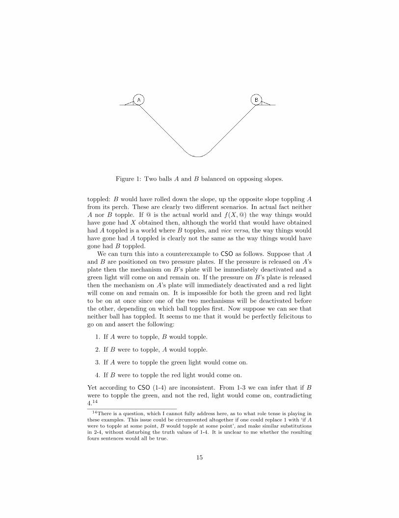
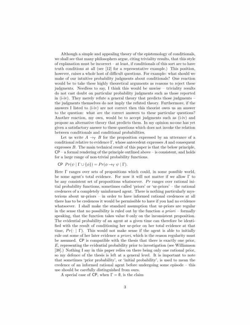
Figure 1: Two balls A and B balanced on opposing slopes.

toppled: B would have rolled down the slope, up the opposite slope toppling Afrom its perch. These are clearly two different scenarios. In actual fact neitherA nor B topple. If @ is the actual world and f(X,@) the way things wouldhave gone had X obtained then, although the world that would have obtainedhad A toppled is a world where B topples, and vice versa, the way things wouldhave gone had A toppled is clearly not the same as the way things would havegone had B toppled.

We can turn this into a counterexample to CSO as follows. Suppose that Aand B are positioned on two pressure plates. If the pressure is released on A’splate then the mechanism on B’s plate will be immediately deactivated and agreen light will come on and remain on. If the pressure on B’s plate is releasedthen the mechanism on A’s plate will immediately deactivated and a red lightwill come on and remain on. It is impossible for both the green and red lightto be on at once since one of the two mechanisms will be deactivated beforethe other, depending on which ball topples first. Now suppose we can see thatneither ball has toppled. It seems to me that it would be perfectly felicitous togo on and assert the following:

1. If A were to topple, B would topple.

2. If B were to topple, A would topple.

3. If A were to topple the green light would come on.

4. If B were to topple the red light would come on.

Yet according to CSO (1-4) are inconsistent. From 1-3 we can infer that if Bwere to topple the green, and not the red, light would come on, contradicting4.14

14There is a question, which I cannot fully address here, as to what role tense is playing inthese examples. This issue could be circumvented altogether if one could replace 1 with ‘if Awere to topple at some point, B would topple at some point’, and make similar substitutionsin 2-4, without disturbing the truth values of 1-4. It is unclear to me whether the resultingfours sentences would all be true.

15

Let me first concede that it is possible to prime the audience to read 3 (or,indeed, 4) in a way that makes it less acceptable. I might say to you: ‘look,when A topples because it’s hit by B the green light will not come on because itsmechanism has been deactivated. So if A were to topple, the green light mightnot come on (because B toppled first) so we should not accept 3.’ This argumentrelies on a controversial connection between ‘might’ and ‘would’ counterfactuals,but an assumption I am willing to grant for the sake of argument.

The kind of reasoning described above is sometimes called ‘backtracking’.I am inclined to agree with Lewis [19], and many after him, that the contextsin which backtracking is legitimate are somewhat special contexts. As Lewisputs it: ‘A counterfactual saying that the past would be different if the presentwere somehow different may come out true under the special resolution of itsvagueness, but false under the standard resolution.’ The same distinction appliesto the ‘might’ counterfactual we used in the above argument.15

It must be stressed, however, that our case against CSO does not depend onthe possibility of contexts in which backtracking is legitimate. We only need1-4 to be simultaneously true in one context to complete our case against CSO,which deems them jointly inconsistent. It does not matter if there are alsocontexts in which some or all of 1-4 are false.

2.2 Counterexamples: indicatives

To what extent do these counterexamples generalise to indicative conditionals?Given the assumption that indicative and subjunctive conditionals have thesame logic, it is clear that the above counterexample has a direct bearing onindicatives. For what it is worth, my view is that this assumption is entirelyreasonable, even given the differences between the two classes. However, I don’twant to rest my case on this assumption so I shall consider the indicative caseseparately here.

There is one straightforward sense in which these counterexamples gener-alise. People have often noted that if I say now ‘if A topples, B will topple’you can later report my speech by saying ‘[XXXX] said that if A had toppled,B would have toppled’ (see Dudman [8].) Thus subjunctive conditionals oftenexpress in the past tense what a ‘forward looking’ indicative conditional (i.e. aconditional containing the future modal ‘will’ in the consequent) can be used toexpress at an earlier time. Thus if in figure 1 what I say now with the sentences1-4 can be said at an earlier time by uttering appropriate indicative conditionalsthen the counterexample clearly generalises to the indicative case.

Perhaps all this shows is that the distinction between indicative and sub-junctive doesn’t cut at the semantic joints. Another question that is worthinvestigating is whether these counterexamples generalise to bare indicatives –indicatives with no visible modal in the consequent (‘will’, ‘must’, ‘should’ etcetera.) Suppose that we know that a system was set up as in figure 1 an hour

15Indeed, according to the logics containing conditional excluded middle there is little dif-ference between ‘would’ and ‘might’ counterfactuals assuming, as we did above, that they areduals of one another.

16

ago, but we don’t know how the state of the system has changed since. Then itseems that the following four conditionals may, for all I know, be all true:

1. If A toppled, B toppled.

2. If B toppled, A toppled.

3. If A toppled the green light came on.

4. If B toppled the red light came on.

However, according to CSO, these are inconsistent and therefore cannot, for allI know, be simultaneously true.

The consistency of 1-4 is one thing, whether they are ever jointly assertableis another. Here is an argument that 1-4 are jointly assertable only if you knowtheir antecedents to be false:

I cannot assert 3 unless I can rule out the possibility that A toppledand the green light didn’t come on.16 But I know that any worldwhere B toppled initially, later colliding with A, is a world where Atoppled and the green light doesn’t come on, so I can rule out thatB toppled first. By symmetrical reasoning I know that I can assert4 only if I can rule out the possibility that A toppled first. So I mayassert 3 and 4 only if I know that neither A nor B toppled.

However if the antecedents of 1-4 are known to be false this ruins the example asindicatives whose antecedents are known to be false are not usually assertable.17

This problem does not generalise to subjunctives: it is perfectly fine to assert,for example, that if A had toppled B would have toppled, even when you knowthat A hasn’t toppled. The most this proves is that the pragmatics of indicativeand subjunctive conditionals are different. Indeed I want to go further andsuggest that although the indicative form of CSO is not semantically valid itstates an important constraint on the kind of inferences that are pragmaticallyappropriate. Say that an inference from sentences A1 . . . An to the sentence B ispragmatically appropriate iff, whatever the context of utterance, the conjunctionof A1 . . . An is less probable for the agent of that context than B is in thatcontext. It follows that if the inference from A1 . . . An to B is pragmaticallyappropriate then A1 . . . An,¬B cannot all have probability 1 in a context ofutterance. Assumping CP it is possible to show that CSO is pragmaticallyappropriate.

16I cannot assert that if A toppled then B toppled unless I know it. So every epistemicallypossible world is a world where B toppled if A did, and thus, there are no epistemicallypossible worlds where A toppled and B didn’t.

17Sometimes it is possible to read conditionals whose antecedents are known to be false asvacuously true. For example, if I know that A won’t topple I can assert: if A topples then I’ma monkey’s uncle. In contexts where the conditionals are vacuously true, however, we cannotinfer ‘it’s not the case that if B toppled the green light came on’ from ‘if B toppled the redlight came on’ so the counterexample to CSO fails.

17

2.3 Conditional Logic and Semantics

I do not want to claim that these examples spell the end for Stalnaker’s theory;there is still room for manoeuvre and considerations to be made in its favour.My aim, more modestly, is to dislodge the idea that CSO is an incontrovertibleprinciple of conditional logic.

I would conjecture that CSO is not accorded this status on the basis ofdirect intuitions about its validity, but rather on the basis of more holistictheoretical considerations. One point in favour of the principles is that it isvalidated by a well known semantics that promises to give a general theory ofconditionals. If we are to reject this theory we had better offer an alternative.In the following sections I’ll suggest a couple of ways to develop a possibleworld semantics, formally similar to Stalnaker’s, which does not validate theproblematic principles.

We shall work with a toy modal propositional language, L, consisting ofthe usual truth functional connectives, ¬ and ⊃ from which the other truthfunctional connectives are definable, and a special binary modal connective rep-resenting the ur-conditional,→. A frame for L is a pair 〈W, f〉 where W is a setof worlds and f : P(W )×W → P(W ) – f is called the ‘ur-selection function’.18

A model is a pair 〈F , J·K〉 where F is a frame and J·K maps propositional lettersto subsets of W . J·K extends to a function from the rest of L to P(W ) as follows:

• J¬φK = W \ JφK

• Jφ ⊃ ψK = (W \ JφK) ∪ JψK

• Jφ→ ψK = {w | f(JφK, w) ⊆ JψK}

Logics based on this semantics can described quite neatly. Here are someprinciples which we shall be focusing on.

RCN if ` ψ then ` φ→ ψ

RCEA if ` φ ≡ ψ then ` (φ→ χ) ≡ (ψ → χ)

CK (φ→ (ψ ⊃ χ)) ⊃ ((φ→ ψ) ⊃ (φ→ χ))

ID φ→ φ

MP (φ→ ψ) ⊃ (φ ⊃ ψ)

C1 (φ→ ψ) ⊃ ((ψ → ⊥) ⊃ (φ→ ⊥))

CEM (φ→ ψ) ∨ (φ→ ¬ψ)

CA ((φ→ χ) ∧ (ψ → χ)) ⊃ (φ ∨ ψ → χ)

RCA (φ ∨ ψ → χ) ⊃ ((φ→ χ) ∨ (ψ → χ))

18See Chellas [6]. One can define the selection function for other conditional connectives ofthe form →Γ as fΓ(A, x) = f(

⋂Γ ∩A, x).

18

VLAS (φ→ ψ) ⊃ ((φ→ χ) ⊃ (φ ∧ ψ → χ))

LT (φ→ ψ) ⊃ ((φ ∧ ψ → χ) ⊃ (φ→ χ))

CSO ((φ→ ψ) ∧ (ψ → φ) ∧ (φ→ χ)) ⊃ (ψ → χ)

The logic CK denotes the logic consisting of the rules RCN, RCEA and the axiomCK. CK is validated in every frame, and is analagous to the smallest normalmodal logic K.19 Indeed, we can consider it as a multi-modal logic in which φ→is a normal modal operator for each substitution of φ.

Stalnaker’s logic C2 includes all of the above principles, and Lewis all exceptfor CEM. Stalnaker guarantees this by placing further constraints on the functionf , namely:

F1. w ∈ f(A,w) whenever w ∈ A

F2. f(A,w) ⊆ A

F3. f(A,w) ⊆ {x} for some x

F4. if f(A,w) ⊆ B and f(B,w) ⊆ A then f(A,w) = f(B,w)

F1 ensures the validity of MP, F2 ensures ID, F3 ensures CEM and F4 ensures theweakened transitivity axiom, CSO. F4 also guarantees that the weaker principlesCA, RCA, LT and VLAS are valid.20 In the presence of F3 we can modify thesemantics in to Stalnaker’s original form so that f maps us from a world, w,and a set of worlds, A, to a single possible world (namely x if f(A,w) = {x} inthe general semantics) or the unique impossible world λ (if f(A,w) = ∅) in thegeneral semantics) at which every sentence is stipulated to be true.

In the next sections we shall focus on two problems with Stalnaker’s seman-tics. Both, I argue, require relaxing the constraint F4 and giving up CSO. Thefirst problem is that the relevant aspects of similarity rarely ever pick out aunique world maximally similar to the actual world. While Lewis and othershave given up constraint F3 in order to accommodate this, this strategy hasrecently been shown to give the wrong predictions in non-deterministic worlds.I shall argue that the best way to accommodate these issues is to keep F3 andrelax F4 instead. The second problem is that Stalnaker’s semantics validatesCSO and therefore cannot accommodate the putative counterexamples we havedescribed for subjunctives and indicatives.

19As with K we use the same name for the logic and its characteristic axiom.20Stalnaker also stipulates that f(A,w) = ∅ only if A = ∅. This is there for a technical

reason: it ensures that the notion of epistemic possibility can be modelled by a universalaccessibility relation. However, since any reasonable notion of epistemic necessity will notiterate in an S5 fashion this constraint does not seem to be particularly motivated and I shallignore it in what follows.

19

2.3.1 Non-determinism

For us it is the last restriction, F4, that is responsible for the problematicprinciples we have been considering. On Stalnaker’s preferred reading f(A, x)denotes the closest world to x at which A is true: f(A, x) is a a world in whichA is true but which differs minimally from x in respects of law and particularfact. F4 states that if the closest A world is a B world and if the closest B worldis an A world then the closest A world is the closest B world. This principleought to be obviously true if we are thinking of f(A, x) as denoting the closestA world to x, where ‘closeness’ here denotes an independent ordering that doesnot depend on the proposition A being evaluated.

However, there is a well known objection to Stalnaker’s semantics. Whyshould there be a unique closest world at which A is true? Surely there couldbe multiple worlds equally close with respect to the relevant factors? For thisreason Lewis drops condition F3 in the general semantics and allows f(A, x) tosometimes denote a set with two or more members.21 I shall focus on the caseof counterfactuals in what follows, since that is how the debate has been framed(although, as before, the discussion generalises to indicatives.)

Lewis’s response involves relinquishing the principle CEM, a principle I taketo be highly desirable (although this is not the place to defend it.) This is prob-lematic for those moved by the kinds of epistemological considerations outlinedhere since CEM is probabilistically valid given CP∅.22

There are, however, more pressing problems with Lewis’s response. Accord-ing to Lewis, a conditional is false if any of the closest antecedent worlds isnot a consequent world. However a number of authors (Hawthorne [13], Hajek[11]) have noted that if the laws are chancy, as predicted by quantum mechan-ics say, there will be, among the closest worlds, all kinds of wild possibilities.For example, worlds where a plate is dropped and, instead of hitting the floor,floats upwards, represent no more of a departure from actual laws than a worldin which it falls and hits the ground. The claim that the plate would break ifdropped seems to be highly probable, even granting the laws are this way, be-cause although not impossible it is very improbable that the plate would floatupwards. The claim that the plate would break if dropped seems to be at leastas probable as the claim that the plate will break, asserted after the plate isdropped and before it breaks (or floats upwards!) Lewis’s analysis, however,predicts that this conditional is outright false: if the plate floats upward in anyof the closest worlds then the counterfactual is false. If I am certain that amongthe closest worlds there are worlds where the plate floats upwards, as I shouldbe if I believe quantum mechanics, I should reject the claim that the plate wouldbreak if dropped – I should be certain it is false.

There is, however, another way to respond to the problem for Stalnaker’s

21This modification does not address the problem of there being no closest world due tothere being an infinite succession of closer and closer worlds. Lewis addresses this in otherpapers.

22For example, if φ is consistent, Pr((φ → ψ) ∨ (φ → ¬ψ)) = Pr(φ → ψ) + Pr(φ →¬ψ) − Pr((φ → ψ) ∧ (φ → ¬ψ)) = Pr(ψ | φ) + Pr(¬ψ | φ) − 0 = 1 for every rational initialprior Pr, and therefore = 1 for every informed prior with Cr(φ) > 0 too.

20

theory: instead of giving up the constraint F3 relinquish F4.23 We agree withLewis that, in the relevant sense of closeness (keeping in accordance with par-ticular matter of fact, respecting natural laws, and so on) there will typicallybe multiple closest worlds to the actual world at which a proposition is true.However, we agree with Stalnaker that there’s a particular way things wouldhave turned out if A had obtained. In order to evaluate a conditional, A→ B,in such a case, we look to the world that would have obtained if A had obtained,and this will be a single member of this set. (It is particularly hard to denyconditional excluded middle for indicative conditionals. Either the coin landedheads if it was flipped, or it didn’t; there just doesn’t seem to be room for athird option.)

On this proposal we therefore sever the straightforward connection betweenthe function f(A, x), which is used in the formal semantics, and counterfactualsimilarity. f(A, x) represents the world that would have obtained instead ofx if A had obtained. If there is exactly one closest world, w, then the waythings would have gone had A obtained is just w. However, when there aremultiple worlds that are equally close in the relevant respects (for example, ifthe laws are chancy) then the way things would have gone had A obtained isnot determined by the closeness facts. If, for example, x is a chancy world,then there will be an element of randomness – the way things would have gonewill certainly be one of the closest worlds, but due to the element of chancethis cannot be deterministically calculated from non-counterfactual facts aboutwhat’s happened at x and closeness facts. Thus, according to this alternative,the world f(A, x) which is selected is not determined by the closeness facts –it is primitively counterfactual and it is an irreducibly chancy matter which,among the closest worlds, this world is.

It is clear why this does better than Lewis’s theory. On this semanticsthe claim that the plate would break if dropped is highly probable, and is asassertable as anything is in a quantum world, whereas for Lewis it is false withprobability 1. Even for Stalnaker, it seems, the conditional is indeterminatewith probability one, thus also unassertable (assuming that it is not permissibleto assert something you’re certain is indeterminate.)

Finally, this semantics also allows us to see why F4 is refuted and why CSOis invalid. Suppose that the closest A worlds are B worlds and that the closestB worlds are A worlds. It follows by simple facts about closesness that theclosest A worlds are the closest B worlds (this is what motivates principle F4in the Lewis/Stalnaker semantics.) Call the set of closest A/B worlds X. Nownote that the member of X that would have obtained if A had obtained isnon-deterministically selected from X and thus might not be the same as themember of X that would have obtained had B obtained. Thus f(A, x) need notbe the same as f(B, x) in cases like this, even though the world that would have

23The idea behind this semantics is due to Moritz Schulz [REF]. Schulz’s theory places a lotof emphasis on the theory of arbitrary reference and epsilon terms which I am not followingclosely here. However, the basic idea – that f(A, x) represents a randomly selected world fromthe closest A worlds to x – is the same. Schulz, however, prefers to add the constraint F4 bybrute force, even though it does not appear to be motivated by his semantics.

21

obtained if A had obtained, f(A, x), is a B world, since by hypothesis all theclosest A worlds are B worlds, and also the world that would have obtained ifB had obtained, f(B, x), is an A world, since we know the closest B worlds areA worlds. In other words, f(A, x) ∈ B and f(B, x) ∈ A even though f(A, x)may not be identical to f(B, x).

The proposal extends to indicatives in a similar way. f(A, x) represents theway the world will turn out if A happens. Even on an epistemic interpretationof ‘closeness’ there will be cases where there are multiple equally close worlds.In these cases the world that will obtain if A obtains is one of these worlds, butnot any particular one with evidential probability 1.

2.3.2 Determinism

The counterexamples we have discussed (and those mentioned by Tichy, Pollock,Martensson, Tooley and Ahmed) all appear to be compatible with determinismso it is unclear whether the suggestion above is the best way to accommodatethese examples. A number of people have suggested that we instead relativisethe notion of closeness to the antecedent of the conditional (see Ahmed [2] andNoordhof [25].) According to this proposal a conditional A→ B is true only ifB is true at the A-worlds which are closest according to an ordering determinedin part by A.

As an example of an antecedent relative theory Ahmed [2] points us tothe theory of Edgington [9] which is tied to a tradition of taking causation asprimitive in the analysis of counterfactuals (see also Kvart [16], Martensson [20],Schaffer [28], [9] all of whom seem to endorse antecedent relativity of some sortor other.) In listing what counts for closeness Schaffer, who is quite up frontabout the invalidity of CSO, writes that among other things we should try to“maximize the region of perfect match, from those regions causally independentof whether or not the antecedent obtains.”24

In fact the thought that the similarity relation depends on the antecedent isquite pervasive in the literature on counterfactuals for the reason that on mostaccounts similarity depends on the time of the antecedent. On such accountsa subjunctive conditional A → C is true when and only when C is true at theA-worlds that are like the actual world in matters of particular fact up to theantecedent time and continue according to the causal laws after the antecedenttime. According to Bennett this ‘general idea has been accepted by all analystsof subjunctive conditionals in the ‘worlds’ tradition, and by most others as well.’[4] p198.25

The consensus seems to be that differences of particular fact after the an-tecedent time count for very little compared to differences before the antecedent

24See also Cross [7] for a discussion of the formal semantics (albeit from an unsympatheticperspective.)

25Whether this idea makes its way into the semantics endorsed by these theorists is anothermatter. For Lewis, for example, the dependence on an antecedent time is provided by thepragmatics. See Bennett [4] §118 for discussion.

22

time, when it comes to counterfactual similarity. This fact is nicely demon-strated by Fine’s example:

If Nixon had pressed the button, then there would have been a nuclearholocaust.

Worlds where there has been a nuclear holocaust are dramatically different fromour own, although the difference manifests itself only after the antecedent time.Nonetheless, in the relevant sense the closest worlds where Nixon pressed thebutton are worlds where there is a nuclear holocaust – this is possible becausethe relevant notion of closeness is one which places little weight to differencesof particular fact after the antecedent time. This notion of closeness is one thatvaries from antecedent to antecedent.

The upshot is that if we interpret f(A, x) in the formal semantics as ‘theA-closest A-world’, where ‘A-closesness’ may depend on A, constraints F1-F3remain intact while the problematic constraint F4 is no longer forced on us andCSO is not validated.

Stalnaker considers this response to Tichy’s counterexample to CSO, writ-ing: ‘call a selection function which is based on some antecedent-independentordering of possible worlds a regular selection function. The issue is whether oneshould describe the situation in terms of a single irregular selection function, orin terms of a contextual shifts from one regular selection function to another.’Stalnaker concedes, however, that the issue may be in part a matter of prefer-ence, not substance, regarding how best to distribute the burden of explanationbetween pragmatics and semantics. If this is so then, far from being the coreof the Stalnakerian theory of conditionals, the principle CSO is more of a sideissue. If CSO is a casualty of adopting a systematic epistemology of conditionalstatements then perhaps this is not so bad after all.

2.3.3 Conditional Logic without Stalnaker’s constraint

What happens if we remove F4? Call the class of frames in which the selectionfunction satisfies F1-F3 C. Then C is sound and complete with respect to thelogic CK with the addition of the principles ID, MP and CEM.26 If we additionallystipulate that the frames satisfy

F5. If f(A, x) ⊆ B and f(B, x) = ∅, f(A, x) = ∅.

then we also validate C1.27 Note, however, that one can satisfy F5 withoutsatisfying F4, and indeed one can have all the principles listed except for CSOin a semantics of the kind described.

The logic CK consists of the principles CK, RCN and RCEA. Call the resultof adding ID, MP and CEM to the logic CK, L1 and let L2 be the logic resulting

26This is a simple application of the canonical model style of argument outlined in Chellas[6].

27C1 is a principle governing the conditions under which conditionals are vacuously true.F5 is roughly equivalent to saying that f(A, x) = ∅ just in case A is true in none of the worldsaccessible to x (where y is accessible to x iff f({y}, x) 6= ∅.)

23

from adding C1 to L1. There is a sense in which L1 is simply the logic you getwhen you drop CSO from Stalnaker’s logic since L1+ CSO has exactly the sametheorem’s as Stalnaker’s logic C2.28

In order to compare L2 to other systems of conditional logic note that, forexample, L2 is the result of replacing VLAS with CEM in Pollock’s logic ofconditionals SS. Removing CEM from L2 and adding CSO, the principle ((φ→ψ)∧¬(φ→ ¬χ))→ (φ∧χ→ ψ) (a strengthening of VLAS) and φ∧ψ → (φ→ ψ)(which is already theorem of L2) results in Lewis’s VC (see [3].)

It is worth pointing out that adding any of CSO, CA, RCA, VLAS or LT to L2results in a system equivalent to Stalnaker’s.29 Thus out of logics consisting ofthe principles we have listed, L2 is the strongest system containing CEM whichdoes not collapse into Stalnaker’s.

3 The tenability of CP

In this section we will construct a model for CP∅ and CP within the logic L2.While models of CP∅ based on the semantics of section 2.3.1 seem worth in-vestigating we shall limit our attention here to models based on the semanticswe discussed in section 2.3.2, utilising an antecedent relative closeness ordering.We begin by defining the kind of model we are aiming for

Definition 3.0.1. A probabilistic frame is a quintuple 〈W,F, P, f, λ〉 where

• W is a set (the set of worlds.)

• F ⊂ P(W ) is a σ-algebra, i.e., a set containing the empty-set which isclosed under complements in W and countable unions which is also closedunder the operation X ⇒ Y := {w | f(X,w) ∈ Y }.

• P is a non-empty set of probability measures over F . I.e. Pr : F → [0, 1]for Pr ∈ P .

• f : P(W )×W →W is called the selection function.

• λ 6∈W is the impossible world.

A probabilistic frame is adequate iff for every Pr ∈ P , A,B ∈ F , Pr(A⇒ B) =Pr(B | A) whenever Pr(A) > 0. Here A⇒ B := {w | f(A,w) ∈ B}. (It followsthat in an adequate frame A ⇒ B is measurable if A and B are, otherwise theleft-hand side of this equation would not be defined.)

In effect an adequate probabilistic frame consists of an interpretation of theconditional plus a set of ur-priors (the set P ) which obey CP∅ on measurable

28Lewis’s axiomatisation of C2 consists of L1, CSO and the complicated principle (A∨B →A) ∨ (A ∨ B → B) ∨ ((A ∨ B → C) ≡ (A → C) ∧ (B → C)). The last principle is actuallyredundant (i.e. is provable in L1+CSO) but does not appear to be a theorem of L1 (althoughit is a theorem of L2.)

29For proofs of these facts see [XXXX], to appear.

24

sets. The more interesting frames are ones in which P represents a rich set ofprobability functions.

Intuitively there are two kinds of propositions: those which are not hypo-thetical at all, such as, for example, the proposition that a particular coin, C,landed heads, and those which are hypothetical, such as the proposition that ifC is flipped it will land heads. The latter kind of proposition is often associatedwith a curious epistemic phenomenon: it does not seem to be possible to knowwhether the latter proposition is true if the coin isn’t flipped. For example, if youaccept conditional excluded middle then either C will land heads if it is flipped,or it will land tails, but in worlds where the coin is not flipped it is impossibleto obtain further evidence to settle the question of which way it would landif flipped. Philosophers subscribing to the law of conditional excluded middlehave conjectured that hypothetical propositions like this are a special source ofindeterminacy (e.g. [33].) Whether or not this is so we can certainly agree thatwe must be ignorant in the scenario described, much as we would be in the faceof vagueness or indeterminacy. In our model the non-hypothetical (completelydeterminate) propositions are represented by a Boolean algebra B, which is asubalgebra of a larger space of propositions, B′, consisting of all propositionshypothetical or not. The basic intuition is that one can have any credence youlike regarding the completely determinate non-hypothetical facts, but once youhave fixed your credences in those propositions your credences over the restof the space of propositions is fixed. For example, if you know that C is fairand will not be flipped, then you are forced to have a credence of a half in theproposition that C will land heads if flipped. The situation here is similar tothe analogous situation with vague propositions. Once you know someone has acertain borderline number of hairs, N , you are forced to be uncertain, to somedegree, in the proposition that that person is bald.

3.1 The construction

Despite the impossibility results there have been a number of results to theeffect that, under certain restrictions, one can have Stalnaker’s thesis (see forexample, van Fraassen [37], McGee [22], Stalnaker and Jeffrey [29], Kaufmann[15], Bradley [5].) However, in general, these constructions fall short of the fullgenerality of a principle like CP∅ as they do not deal with certain embeddedconditionals. The closest thing to the project attempted here is found in vanFraassen’s [37], where a model of CP∅ is presented. In this paper van Fraassenprovides, for each probability function, Pr, a model of the logic L1 such thatPr(A→ B) = Pr(B | A) whenever Pr(A) > 0. Unfortunately this constructionis not suitable for our purposes. Van Frassen constructs a different conditionalfor each choice of probability function Pr, so this construction is not a sat-isfactory model of CP∅ except in the limiting case in which there is only one‘Carnapian’ ur-prior. Furthermore, it is not a model of the general principleCP. (There are also a number of technical limitations on the construction: (i)the construction only generates models where the number of measurable sets iscountable (it is therefore also not a σ-algebra) (ii) the semantics is not based

25

on selection functions and subsequently has an unnatural quantificational logic(for example the principle ∀x(φ → ψ) ⊃ (φ → ∀xψ), when x is not free inφ, is invalid)30 (iii) the conditional operator is not defined on unmeasurablepropositions (thus given (i), the conditional is only defined on countably manypropositions) (iv) as far as I can see van Fraassen shows that CP∅ holds over afield of sets, but not over the σ-algebra it generates.)

In that same paper van Fraassen provides a distinct model for a restrictionof CP∅ in which the antecedent and consequent, A and B, do not involve anyconditionals themselves (see the ‘Bernoulli-Stalnaker’ models of [37].) Howevervan Fraassen’s construction does not allow iterated conditionals, and it validatesthe undesirable logic C2. The approach here extends the idea of the ‘Bernoulli-Stalnaker’ models to validate the full strength of CP, iterations and all.

The construction begins with an initial set of possible worlds W , whichrepresent maximally specific things that can be said about the world withoutmentioning conditional facts – facts about what will happen if this or that hap-pens. The set W∞ then extends this set, dividing members of W into epistemicpossibilities according to the kind of hypothetical distinctions you can make. Inthe Bernoulli-Stalnaker models of van Fraassen we can think of W∞ as pairs ofmembers of W and well-orderings of the universe W . The well-ordering repre-sents the closeness facts at that possible world. Even if we know exactly whichworld obtains you might be ignorant about the hypothetical facts, encoded bywhich well orderings obtain at that world.

Note that the space of worlds just described gives a poor representation ofthe conditional facts at a world since it only well-orders the possible worlds, notthe epistemically possible worlds. What we want, rather, is a space of worldsW∞ such that each member of W∞ determines a well-ordering of W∞, not W(actually, in our setting it’s slightly more complicated because the ordering isantecedent dependent.) This is potentially problematic for cardinality reasons:W∞ cannot be the same same size as the set of well-orderings over W∞. Tosolve this we restrict our attention to well-orderings of some fixed collection oforder types. For simplicity this is just ω.

Let us put this into practice. Assume that the initial set of states, W , thatdo not involve conditional facts is given and is countable. The set of worlds inour model will be the set W∞ = Wω1 = {π | π : ω1 →W}. Let B∞ = P(W∞).

Given our initial space W , define the following sequence of sets for α < ω1

• Wα = Wωα

That is, Wα represents the set of all ωα sequences of members of W . Sinceωα < ω1 whenever α < ω1 it follows that an element of Wα will be isomorphicto an initial section of a member of W∞. Note also the following consequencesof this definition:

• W0 = W

• Wα+1∼= Wω

α

30Although, since this is effectively the limit assumption, perhaps this isn’t so bad.

26

In what follows we shall adopt a practice of identifying products which areisomorphic to subsets of W∞, allowing us, for example, to identify A × W∞with a subset of W∞ whenever A is contained in some Wα.

The sets Wα for α < ω1 help us describe the measurable sets.

Definition 3.0.2. Suppose X is a set of subsets of W∞. Then cl(X) is theclosure of X under the operations of countable unions and intersections, andcomplements relative to W∞.

The measurable sets, which we shall denote F∞, can be thought of as beingapproximated by an infinite sequence of σ-algebras, Fα ⊂ B∞ for α < ω1.

• F0 = {A×W∞ | A ⊆W}

• Fα+1 = cl{A0 × . . .×An ×W∞ | Ai ×W∞ ∈ Fα for 0 ≤ i ≤ n}

• Fγ = cl(⋃α<γ Fα)

Note that Fα+1 is generated by sets of the form A0 × . . . × An ×W∞ whereAi ⊆Wα. Each of these generating sets consists of an ω1 sequence such that aninitial finite number of elements belong to Wα and the rest belong to W . This is,of course, just equivalent to an ω1 sequence of elements of W whenever α < ω1:it is just equivalent to n successive ωα-sequences of elements of W followed byan ω1-sequence of elements of W , which is itself an ω1-sequence of elements ofW . Bearing this equivalence in mind we can see from the construction thatan arbitrary member of Fα will be of the form A ×W∞ where A ⊆ Wα. It isstraightforward to show

Proposition 3.1. Fα ⊆ Fβ if α ≤ β

Now we turn to our definition of F∞, the set of measurable sets.

Definition 3.1.1. A set A ∈ B∞ is measurable iff A ∈ Fα for some α. Wedenote the set of measurable sets F∞ :=

⋃α<ω1

Fα.

It should now become apparent why we chose the ordinal ω1 in our defini-tions: it is due to this choice that our measurable sets are closed under countableunions so that F∞ is a σ-algebra.

Definition 3.1.2. If A is measurable then the rank of A is the smallest α suchthat A ∈ Fα. We shall write this: rank(A) = α. If A is not measurable thenrank(A) =∞.

For any ordinal α < ω1 and ω1 sequence, π, let π[α] be the ω1 sequencestarting from π’s αth element. I.e. π[α](β) = π(α+β). For each ordinal α < ω1

and element π ∈W∞ we can define a well-ordering of W∞.

τ ≤α,π σ if and only if for some i, j ∈ ω τ = π[ωα.i], σ = π[ωα.j] andi ≤ j.

27

We identify ≤∞,π arbitrarily with ≤0,π

It is now time to define the selection function for a A ∈ B∞ of rank α(possibly identical to ∞)

f(A, π) =

{the ‘smallest’ A-world under the ordering ≤α,π if such a world existsλ otherwise

By the ‘smallest’ A-world I just mean a world τ such that τ is in the domainof ≤α,π, τ ∈ A and for any other σ in the domain of ≤α,π and in A, τ ≤α,π σ.Note that, like in Stalnaker’s semantics, f(A, π) represents the closest world toπ which belongs to A – the crucial difference is that the notion of closeness atplay here depends on the antecedent, A – this accords with the semantics ofsection 2.3.2. Note that f(A, π) ∈ A and f(A, π) = π whenever π ∈ A. Thusthis frame validates the logic L1.

Proposition 3.2. ∅ is measurable and if A, B and A0, A1, A2, . . . are measur-able then so is W∞ \A, A⇒ B and

⋃nAn.

We now define the set, P , of ur-priors. For simplicity we shall assume thatW is countable so that every subset of W can be treated as a measurable set(although it would be simple enough to drop this assumption and work with aninitial σ-algebra over W instead.) We shall show that every regular countablyadditive probability function Pr on the powerset algebra on W extends to themeasurable sets over B∞. We then identify P with the set of all such probabilityfunctions generated this way.

Suppose that Pr is a regular countably additive probability function on B.For α ≤ ω1 we define Prα over Fα as follows.

• Pr0 = Pr

• Prα+1(A0 × . . .×An ×W∞) = Prα(A0 ×W∞) . . . P r(An ×W∞); Prα+1

extends to the rest of Fα+1 via Caratheodory’s extension theorem.

• Prγ(A) = Prα(A) when A ∈ Fα for α < γ. This extends to the rest of Fγby Caratheodory’s extension theorem.

Write Pr∞ for Prω1. Observe, from the construction of Pr∞, that for any α <

ω1 and A0, . . . , Ak ⊂Wα Pr∞(A0×. . .×Ak×W∞) = Pr∞(A0×W∞)Pr∞(A1×W∞) . . . P r∞(Ak ×W∞)

We are now in a position to prove our main theorem.

Theorem 3.3. The frame 〈W∞, F∞, P, f, λ〉 is adequate.In particular, if Pr is a countably additive regular probability function over

W then Pr∞ ∈ P and Pr∞(A ⇒ B) = Pr∞(B | A) whenever A and B aremeasurable.

Proof. Suppose that rank(A) = α so that A = A′ ×W∞ for some A′ ⊆Wα.According to our definition π ∈ A ⇒ B if and only if the smallest A world

in the sequence (π[ωα.i])i is a B world. In other words, if and only if π[ωα.0] =

28

π ∈ A ∩ B or π 6∈ A but π[ωα.1] ∈ A ∩ B or π[ωα.0] 6∈ A, π[ωα.1] 6∈ A andπ[ωα.2] ∈ A ∩B or ... or π[ωα.i] 6∈ A for any i.

Let R be the set of π with f(A, π) = λ. Thus A ⇒ B = (A ∩ B) ∪ (A′ ×(A ∩ B)) ∪ (A′ × A′ × (A ∩ B)) ∪ ... ∪ R =

⋃n(A′n × (A ∩ B)) ∪ R. Here I am

using X to denote the complement of X.Note that R ⊆ (A′)ω ×W∞ which has probability 0 whenever Pr∞(A) > 0.

Since we are calculating a union of disjoint sets we have

Pr∞(A⇒ B) =∑n<ω

(Pr∞(A)n·Pr∞(A∩B)) =Pr∞(A ∩B)

1− Pr∞(A)=Pr∞(A ∩B)

Pr∞(A)= Pr∞(B | A)

It is fairly straightforward now to model CP. Let Γ be a set of propositions.Then we now define the selection function, fΓ, for the connective→Γ as follows.

Firstly we define ≤Γ,α,π=≤α,π ∩(⋂

Γ×⋂

Γ). Suppose that rank(⋂

Γ∩A) =α.

fΓ(A, π) =

{the ‘smallest’ A-world under the ordering ≤Γ,α,π if such a world existsλ otherwise

The next question we must settle is: what kind of proposition could be anagent’s total evidence? A natural answer is suggested by our model: propo-sitions that correspond to a set of possible worlds in W (i.e. a proposition ofthe form A×W∞ for A ⊂W .) A proposition that carves out finer distinctionsthan a set of possible worlds would is an essentially hypothetical proposition.For example, the proposition that a certain coin will land heads if flipped is ahypothetical proposition. It can certainly be entailed or ruled out by our evi-dence (for example, if we knew that the coin was flipped and landed heads orif we knew that the coin was flipped and landed tails.) In these cases, however,the proposition would not be our total (i.e. our strongest) evidence; it is sim-ply impossible, I have argued, for our strongest evidence to be a hypotheticalproposition.

If we let E be the conjunction of the evidence in Γ then our definition ofA⇒Γ B above effectively amounts to: A ∩ E ⇒ B. We shall now demonstratethat CP holds in this model.

Theorem 3.4. If E ∈ F0 then PrE(A⇒ B) = Pr(AB | E)+Pr(A | E)Pr(B |A) where PrE(·) = Pr(· | E).

Proof. Suppose that E = E′ ×W∞ where E′ ⊆W . Then in general, for any α,and A0 . . . Ak ⊆ Wα, (A0 × . . . × Ak ×W∞) ∩ E = (A0 ∩ (E′ ×Wα)) × A1 ×. . .×Ak ×W∞.

From theorem 3.3 we know that PrE(A ⇒ B) = ΣnPrE((A′)n× AB) =

1Pr(E)ΣnPr((A)n ×AB) ∩ E).

Expanding this sum and applying the observation above we get = 1Pr(E) (Pr(ABE)+

Pr(AE)Σn(Pr(A)nPr(AB)) = 1Pr(E)Pr(ABE) + 1

Pr(E)Pr(AE)Pr(B | A)) =

Pr(AB | E) + Pr(A | E)Pr(B | A)

29

Now since A ⇒Γ B = AE ⇒ B where E is the conjunction of Γ, we getPr(A ⇒Γ B) = Pr(ABE | E) + Pr(AE | E)Pr(B | AE) = Pr(B | AE) =Pr(B | {A} ∪ Γ).

Finally we must address the matter of the principle C1 which is not validatedin this current construction, but is highly desirable. It is a simple matter, in fact,to modify the construction to validate C1. It is sufficient merely to ensure thatthe domain of ≤α,π, which we shall write dom(≤α,π), is the same as the domainof ≤β,π for any α and β. For each world, π, let Dπ be the union

⋃α dom(≤α,π).

Then, for each α simply add all the elements of Dπ \dom(≤α,π) on to the end ofthe ordering ≤α,π in some order or other, it does not matter which, to make alonger ordering whose domain is Dπ. The probability calculation goes throughas in theorem 3.3 except in this case R denotes the set of worlds, π, where noneof the first ω worlds (in the ≤α,π ordering) is an antecedent world; as beforethis set has measure zero.

3.2 A small refinement of Hajek and Hall’s theorem

Here we weaken the assumption CSO of [12] to VLAS. While VLAS and CSO areequivalent in L2, VLAS is strictly weaker in L1. Note that in the other directionCSO entails VLAS given CC, ID and CK.

To see that VLAS is strictly weaker in L1, here is a frame validating L1+VLASbut which does not validate L1+CSO. Let W = N. If A contains primes thenf(A, i) = {j} where j is the smallest number ≥ i with j ∈ A, and = ∅ if thereis no such number. If A does not contain i or any primes then f(A, i) = ∅, andif A contains i then f(A, i) = {i}. It’s simple to verify that if f(A, x) ⊆ B thenf(A∩B, x) ⊆ f(A, x), ensuring the validity of VLAS. However, let A = {2} andB = {2, 3}, so f(A, 1) = ∅ and f(B, 1) = {2}. So f(A, 1) 6= f(B, 1) even thoughf(A, 1) ⊆ B and f(B, 1) ⊆ A.

Theorem 3.5. Suppose that CP∅ holds for at least one ur-prior, Pr, and thatthe following facts are true of the model

MP A ∩ (A→ B) ⊆ B

CC (A→ B) ∩ (A→ C) ⊆ (A→ (B ∩ C)

VLAS ((A→ B) ∩ (A→ C)) ⊆ ((A ∩B)→ C)

Then there are no more than two disjoint consistent propositions.

Proof. Suppose AB, AB and A are three disjoint consistent propositions. Theytherefore all have positive probability by the regularity assumption. Let C =A ∪ (A→ B). Now note that the following chain of entailments hold (i.e. eachproposition is a subset of the next):

1. C → AB

2. ⊆ (C → AB) ∩ (C → A) ∩ (C → B) by CC

30

3. ⊆ (C → AB) ∩ (CA→ B) by VLAS

4. ⊆ (C → AB) ∩ (A→ B) since CA = A

5. ⊆ (C → AB) ∩ C since (A→ B) ⊆ C

6. ⊆ ABC by MP

So C → AB ⊆ ABC and thus Pr(C → AB) ≤ Pr(ABC). Now the argumentproceeds as in [12]:

1. Pr(AB | C) ≤ Pr(ABC), by CP∅

2. So Pr(C) = 1 by probability theory.

3. Pr(A ∩ (A→ B)) = 0 by some fiddling (see P5 in [12].)

4. Pr(AB) = Pr(A ∩ (A→ B) = Pr(A→ B) by 3 and MP.

5. Pr(B | A) = Pr(AB), i.e. Pr(AB) = Pr(A)(AB) which is impossiblesince Pr(A) < 1 and Pr(AB) > 0.

In fact, both the Hajek and Hall result, Stalnaker’s and the above can beseen as a special instance of an observation Stalnaker makes in [32].

Consider the following rule of proof:

RS If ` (φ→ ψ) ⊃ φ then ` φ.

If L is conditional logic that is, in a sense, not only sound but ‘complete’ for CP∅then SR must be an admissible rule in the sense of Lorenzen: i.e. the result ofclosing L under RS leaves you with L again, (or, in other words, RS is a derivedrule of the logic.)

Theorem 3.6. Assuming MP, RS is probabilistically valid in the sense that itpreserves probability 1 in any model where Pr(A→ B) = Pr(B | A), stipulatingthat Pr(B | A) = 1 when Pr(A) = 0.

Proof. Suppose that Pr((A→ B) ⊃ A) = 1. Then Pr(A→ B) ≤ Pr(A∩ (A→B)) by probability theory, which is ≤ Pr(A ∩B) by MP.

Since Pr(A → B) = Pr(B | A), Pr(B | A) ≤ Pr(A ∩ B) so that Pr(A) =1

However, RS is not admissible in C2, nor MP+CC+CSO, nor MP+CC+VLAS.In the former case the system you get by closing under RS collapses → into thematerial conditional (which is incompatible with CP∅ and the existence of threedisjoint consistent propositions), and similarly for the latter two systems if weadd CEM or (φ ∧ ψ) ⊃ (φ → ψ) to either (which are both guaranteed by CP∅anyway.)31

31Since we can prove (C → A∧B) ⊃ C, where C = A∨(A→ B), it follows that A∨(A→ B)is a theorem for arbitrary A and B. Since A ⊃ B,¬A ` A → B, and A ⊃ B,A ` A → B wehave A ⊃ B ` A→ B (the converse is MP.)

31

References

[1] E.W. Adams. The logic of conditionals: An application of probability todeductive logic, volume 86. Springer, 1975.

[2] A. Ahmed. Walters on conjunction conditionalization. In Proceedings of theAristotelian Society (Hardback), volume 111, pages 115–122. Wiley OnlineLibrary, 2011.

[3] H. Arlo-Costa. The logic of conditionals. 2007.

[4] J.F. Bennett. A philosophical guide to conditionals. Oxford UniversityPress, 2003.

[5] R. Bradley. Multidimensional possible-world semantics for conditionals.Philosophical Review, 121(4), 2011.

[6] B.F. Chellas. Basic conditional logic. Journal of philosophical logic,4(2):133–153, 1975.

[7] C.B. Cross. Antecedent-relative comparative world similarity. Journal ofPhilosophical Logic, 37(2):101–120, 2008.

[8] V.H. Dudman. Conditional interpretations of if-sentences. Australian Jour-nal of Linguistics, 4(2):143–204, 1984.

[9] D. Edgington. Counterfactuals and the benefit of hindsight. Causation andCounterfactuals. London: Routledge, pages 12–27, 2004.

[10] A. Gibbard. Two recent theories of conditionals. Ifs: Conditionals, Belief,Decision, Chance and Time, WL Harper, R. Stalnaker & G Pearce (eds.).D. Reidel Publ. Co., Dordrecht, pages 211–248, 1981.

[11] A. Hajek. Most counterfactuals are false. MS.

[12] A. Hajek and N. Hall. The hypothesis of the conditional construitl ofconditional probability. Probability and conditionals: belief revision andrational decision, page 75, 1994.

[13] J. Hawthorne. Chance and counterfactuals1. Philosophy and Phenomeno-logical Research, 70(2):396–405, 2005.

[14] L. Humberstone. The connectives. MIT Press, 2011.

[15] S. Kaufmann. Conditional predictions. Linguistics and Philosophy,28(2):181–231, 2005.

[16] I. Kvart. A theory of counterfactuals. Hackett Publishing Company, 1986.

[17] D. Lewis. Counterfactuals oxford, 1973.

32

[18] D. Lewis. Probabilities of conditionals and conditional probabilities. Thephilosophical review, 85(3):297–315, 1976.

[19] D. Lewis. Counterfactual dependence and time’s arrow. Nous, pages 455–476, 1979.

[20] J. Martensson. Subjunctive conditionals and time: A defense of the classicalapproach, 1999.

[21] V. McGee. A counterexample to modus ponens. The Journal of Philosophy,82(9):462–471, 1985.

[22] V. McGee. Conditional probabilities and compounds of conditionals. ThePhilosophical Review, 98(4):485–541, 1989.

[23] C.J.G. Meacham. Two mistakes regarding the principal principle. TheBritish Journal for the Philosophy of Science, 61(2):407–431, 2010.

[24] D. Nolan. Defending a possible-worlds account of indicative conditionals.Philosophical Studies, 116(3):215–269, 2003.

[25] P. Noordhof. Tooley on backward causation. Analysis, 63(278):157–162,2003.

[26] J.L. Pollock. Subjunctive reasoning. Reidel Dordrecht, 1976.

[27] J.L. Pollock. A refined theory of counterfactuals. Journal of PhilosophicalLogic, 10(2):239–266, 1981.

[28] J. Schaffer. Counterfactuals, causal independence and conceptual circular-ity. Analysis, 64(284):299–308, 2004.

[29] Jeffrey R. Stalnaker, R. Conditionals as random variables. Probability andconditionals: belief revision and rational decision, page 31, 1994.

[30] R. Stalnaker. A theory of conditionals. Studies in logical theory, 2:98–112,1968.

[31] R. Stalnaker. Indicative conditionals. Philosophia, 5(3):269–286, 1975.

[32] R. Stalnaker. Letter to van fraassen. WL Harper and CA Hooker (1976),pages 302–306, 1976.

[33] R. Stalnaker. A defense of conditional excluded middle. Ifs: Conditionals,belief, decision, chance, and time, pages 87–104, 1981.

[34] R.C. Stalnaker. Probability and conditionals. Philosophy of Science, pages64–80, 1970.

[35] P. Tichy. A new theory of subjunctive conditionals. Synthese, 37(3):433–457, 1978.

33

[36] M. Tooley. Backward causation and the stalnaker-lewis approach to coun-terfactuals. Analysis, 62(275):191–197, 2002.

[37] B.C. Van Fraassen. Probabilities of conditionals. Foundations of probabilitytheory, statistical inference, and statistical theories of science, 1:261–308,1976.

[38] T. Williamson. Knowledge and its Limits. Oxford University Press, 2000.

34