JOURNAL OF OPTIMIZATION THEORY AND APPLICATIONS: Vol. 81, No. 3, JUNE 1994

Impulsive Control Systems Without Commutativity Assumptions

A. BRESSAN, JR. 1 AND F. R A M P A Z Z O 2

Communicated by R. Conti

Abstract. This paper is concerned with optimal control problems for an impulsive system of the form

~(t)=f(t,x,u)+ ~ gi(t,x,u)fti, u(t)~U, i=1

where the measurable control u(- ) is possibly discontinuous, so that the trajectories of the system must be interpreted in a generalized sense. We study in particular the case where the vector fields gi do not commute. By integrating the distribution generated by all the iterated Lie brackets of the vector fields g/, we first construct a local factoriza- tion A1 x A 2 of the state space. If (x ~, x 2) are coordinates on Aj • A2,

we derive from (1) a quotient control system for the single state variable x 1, with u, x 2 both playing the role of controls. A density result is proved, which clarifies the relationship between the original system (1) and the quotient system. Since the quotient system turns out to be commutative, previous results valid for commutative systems can be applied, yielding existence and necessary conditions for optimal trajectories. In the final sections, two examples of impulsive systems and an application to a mechanical problem are given.

Key Words. Lie brackets, local integral manifolds, optimal impulsive controls.

1. Introduction

This pape r is concerned with impulsive control system o f the fo rm

Yc(t) =f(t, x, u) + ~, gi(t, x, u)tii, (1) i=1

'Professor, Scuola Internazionale Superiore di Studi Avanzati, Trieste, Italy. 2Associate Professor, Dipartimento di Matematica Pura e Applicata, Universitfi di Padova, Padova, Italy.

435 0022-3239/94/0600-0435507.00/0 �9 1994 Plenum Publishing Corporation

436 JOTA: VOL. 81, NO. 3, JUNE 1994

x(0)=ff , u(0)=ff, (2)

where x ~ R" and the measurable control function u ranges inside a fixed closed convex set U c R". Due to the presence of the time derivatives fig on the right-hand side of (1), (2), a solution x(. ) can be interpreted in the usual Carath6odory sense only when u is absolutely continuous. In the case of u measurable, various definitions of generalized trajectories have been intro- duced in the literature. This can be done by considering suitable limits of classical solutions, under key assumptions involving either the total varia- tion of u (Refs. 1 -3) or the commutativity of the vector fields gi (Refs. 4-7).

The aim of this paper is to investigate the dynamics of (1) and some related optimum problems when the above hypotheses on the variation of u or the commutativity of the fields gi are removed. We remark that Eq. (1) is considerably more general than in the impulsive control equations studied in Refs. 8-10, where the fields g; do not depend on the state variable x. Actually, the dependence of the fields gi on x is quite natural in some physical applications. Indeed, under suitable assumptions on the geometry of the constraint manifold, a Lagrangian mechanical system driven by additional time-dependent constraints can be locally described by equations of the form (1); see Refs. 11-16.

The impulsive structure of the system accounts for some features which are not shared by a standard control problem. In particular, the set reachable with absolutely continuous controls is not necessarily closed or bounded. Therefore, the existence of a solution for an optimal control problem will be achieved only within a generalized class of controls (looping controls), as described in Sections 2-3; see in particular the examples in Section 6.

The picture that emerges from our analysis is as follows. Under fairly general assumptions, in a coordinate neighborhood of each point x one can consider a product structure A ~ x A 2, where for every x l ~ A ~ {x 1} x .4 2 is a local integral manifold of the distribution A defined by

A(x) = span{h(x); h e d } ,

~r being the Lie algebra generated by all the Lie brackets of the vector fields gl- Such integral manifolds can be thought of as classes of instanta- neous controllability. If y, z belong to the same integral submanifold {x 1 } x A 2, this means that they can be connected by a path which is the limit of trajectories defined on arbitrarily small time intervals and generated by controls which loop faster and faster around circuits shrinking to a single point.

On the quotient space (A I x A2)/A 2 with coordinates (x 1, x2), we then define a quotient system, with x I as state variable and the couple (u, x 2) as

JOTA: VOL. 81, NO. 3, JUNE 1994 437

control, here called looping control. This auxiliary control system turns out to be still impulsive; yet it has the considerable advantage that the new vector fields g~ commute. Most of the results obtained for the commutative case (see Ref. 6) can thus be applied to it. In particular, the quotient system can in turn be reduced to an ordinary control system, where the time derivatives fi,. do not appear (see Ref. 6).

The density of the set of Carathrodory trajectories of the original system on the set of generalized trajectories of the quotient system is proved in Section 3. This shows that looping controls can be regarded as generalizations of ordinary controls, much in the same way as chattering controls are.

In Sections 4 and 5, a class of optimization problems related to the control system (1) is reformulated in a generalized sense for the quotient system. In the same context, necessary conditions for optimal (looping) controls are stated.

In Section 6, we present two simple examples showing the nonexis- tence of optimal controls within the class of absolutely continuous func- tions. On the other hand, the corresponding extended variational problems do admit an optimal looping control. Finally in Section 7, we provide a mechanical application, concerning a Lagrangian system where two of the three state parameters are used as controls.

2. Quotient Control System

Throughout this paper, we shall consider the system

=f(x) + ~ gi(x)tii, (3) i=l

x(0) = )z, u(0) = 0, (4)

where f, g~ . . . . , g.~ are smooth vector fields on ~" and the measurable control u = (u~ . . . . . u..) takes values inside a fixed closed convex set U c R m with nonempty interior, Observe that the more general system (1), (2) can be reduced to (3), (4) by introducing the additional variables

xO-~-t~xn+i~ui, i= l , . . . ,m,

with the corresponding equations

&o= 1, &n+i= fii.

Due to the presence of the time derivatives fii on the right-hand side of (3), the solutions corresponding to discontinuous controls u require a careful

438 JOTA: VOL. 81, NO. 3, JUNE 1994

definition. To study the set of absolutely continuous trajectories of (3), (4), let ~ be the Lie algebra generated by all Lie brackets of the vector fields g~, i = 1 . . . . . m, having length >_ 2, and define the distribution A by setting

A(y) = span{h(y); h ~ ~ } .

By construction, A is involutive, i.e., [h,k]eA whenever h , k~A . If the dimension q of A(y) is constant in a neighborhood of 37, then by the Frobenius theorem one can find two open subsets A ~ _ R p, A 2 _ Rq, with p + q = n, and a local system of coordinates,

(y l ,y2) = ((Yl . . . . . Yp), (Yp+l . . . . . yp+q))~A 1 x A 2,

such that

A(y) = span{(O/Oy p+ i)(y) . . . . , (~/~yp+q)(y) },

for every y ~A ~ x A 2. Coordinates with this property are called A-adapted. With obvious meaning of the notations, we have the following lemma.

Lemma 2.1. In a system of A-adapted coordinates (yl , y2), Eqs. (3), (4) take the form

~ =f~(y~,y2) + ~ g~ (y~)ft~, i = 1

.~z = f2 (y l , y2) + ~ g~ (yl , y2)fti ' i = 1

y(O) = 37, u(O) = O,

with 1 1 I [gi, g~ ](Y ) = 0,

for every i , j = 1 . . . . , m and y l~A1.

(5)

(6)

(7)

(8)

Proof . By assumption, for j = p + 1 . . . . . p + q, the constant vector field ej = O]Oy/can be locally written as a linear combination,

q

ej = ~ ca(y)h~(y), a = l

where the vector fields h a lie in ~r and c a are suitable coefficients. We then have

q q q

(a/t~yj)g,= E [caha,g,] = ~ ca[ha, g , ] - ~, (Vca, gi)ha. (9) a=l a=l a=l

Both terms on the right-hand side of (9) lie in A, hence (O/dy~)g~ = 0; therefore, the components g~ do not depend on y 2 = (yp+~ . . . . . yp+q).

JOTA: VOL. 81, NO. 3, JUNE 1994

To prove (8), observe that, using the column representation

= fg] ] for every i,j, g' Lg~J'

one has

439

is the following control system on AI:

.f,J =f(y,,yZ) + ~ g](yl)ft, i = 1

yl = (0)371, y2(0 ) = )72, u(0) = 0. (13)

Here, xl is the state variable, while both u and y2 are regarded as controls. The pair of measurable functions

(u, y2): [0, T] ~ U x A 2

is called a looping control.

Remark 2.1. The system (12) still has an impulsive behavior, but the vector fields gJ now commute. Solutions corresponding to measurable controls can thus be constructed as in Ref. 6. Consider the vector field

] : ( [ s ] ) u,g] (~), y2 (14) F(~, y2, u) = exp i=l --(uig)) 1 exp t i

(12)

g) g~ [[o] f0]]+[[0] +[[o] [:,]]+[[o] ,l,)

By the identity

(O/OyOg] =0 , j = p + 1 , . . . ,p + q ,

all terms in (11), except possibly the first on the right-hand side, have zero component along the tangent subspace TAI. Hence, (10) and (11) imply (8). []

We now introduce an auxiliary control system on the quotient space

AI ~(A1 x A2)/A z.

Definition 2.1. The quotient control system corresponding to (5 ) - (7)

440 JOTA: VOL. 81, NO. 3, JUNE 1994

Here, as usual, by exp(th)(~) we denote the value at time t of the solution of the Cauchy problem

= h(x ) , x (O) = ~,

while [exp h], denotes the Jacobian of the map ~ ~[exp h](~). For any smooth control (y2, u), calling y~ the corresponding solution (12), (13) and setting

~(t)= Iexp J=~ (-ui(t))g , ~'(t), (15)

one checks that

~(t) = F(r y2, u). (16)

Therefore, for measurable controls (y2, u), one can define

y~(t) = [ e x p i=, ~ ui(t)g, l(~(t)), (17)

where ~(. ) is the solution of (16). Optimal control problems for impulsive systems of the form (12) were also considered in Ref. 6. Some of the results contained therein will be used in Section 5 in order to deduce necessary conditions for optimization problems involving looping controls.

3. Density Theorem

The definition of the quotient system is primarily motivated by the fact that every solution of (12), (13) can be approximated in the Le~-norm by absolutely continuous solutions of the original system (5)-(7).

Theorem 3.1. Assume that A-adapted coordinates are defined on open, connected sets A ~ ~_ ~P and A 2 _~ g~q. Let (u, y2): [0, T ] ~ U x A 2 be a looping control, let y~ be the corresponding solution of (12), (13), and assume that the closures of the sets

V 2 = {y2(t); te[0, r]} are compact and contained inside A ~, .,t 2, respectively. Then, for every �9 > 0, there exists a Lipschitz continuous control fi such that the corre- sponding solution ()~l, ~2) of (5)-(7) satisfies

lip' -y ' [ l~ , < �9 [lyZ-y2[l~, < ~,

IjT'(r) - y ' ( r ) l < �9 [y2(T) - y 2 ( r ) 1 < �9

JOTA: VOL. 81, NO. 3, JUNE 1994 441

Proof. We first observe that the solution ~ of (16) depends continu- ously on the looping control (y2, u). More precisely, the map (y2, u) ~ ~ is continuous from ~1 into ego, as long as y2, u, ~ remain inside compact sets. Recalling (17), this implies that y l varies continuously with y2, u, in the s It is therefore not restrictive to assume that u, y2 are Lipschitz continuous functions on [0, T].

By continuity and compactness, there exists 6 e(0, E] such that, if,92, are Lipschitz continuous looping controls such that

1.92(0 -y2 ( t ) I < 6, l~7(t) - u(t)l < 6, gt E[0, Z], (18)

this implies that the corresponding solution 91 of (12), (13) satisfies

I.9'(0 - y ' ( t ) l < E, vt ~[0, T]. (19)

Given a Lipschitz control U, we shall inductively construct a new control z7 such that the corresponding solution jT~,j7 z of (5)-(7) satisfies (18). At the kth step, assume that ~ has been defined on some interval [0, t~], with

a(O) = u(O), a(t~) = u(t~), Ip2(tk) - y2(tOI _< 6/3,

and assume that (18) holds for t~[0, t~]. Extend ~7 to [0, T] by setting

~(t) = u(t), for t > tk.

If the corresponding solution .gz of (5)- (7) satisfies (18) on the entire interval [0, T], we are done. Otherwise, let t ~(tk, T] be the first time at which

1)72(t) _ yZ(t)[ = 26/3.

Let y: [0, 1] ~ B ( V 2, 6) be a smooth path such that

y(0) =.92(0, y(1) = y2(t).

Recalling that the tangent space to A 2 at every point is spanned by Lie brackets of the vector fields g.2 having length > 2, by Theorem 2 in Ref. 17 there exists a Lipschitz control v: [0, 1] ~-~ U, with Iv(s) - tT(t)l < 6/2 for all s, such that the solution of the Cauchy problem

P = ~. g~(Y)f;i, y(0) =.9(t), i = I

satisfies

lye(s) -~(s) I <a/4, vs~[o, 1].

442 JOTA: VOL. 81, NO. 3, JUNE 1994

By choosing al > 0 sufficiently small, and redefining

~v[(t - ~)/a, ], .)[(z + 261 - t)/al]u(z) if t~[z, z + al],

tT(t) = ] + [ ( t - z - a l ) / a l ] u ( z +260 , if te[z +6~,z +2611,

[u(t), i f t > z +261,

we obtain a new control ~ whose corresponding solution )71, 3~ z of (5)-(7) satisfies (18) on some larger interval [0, t~+ 1] = [0, tk]. By compactness and by the Lipschitz continuity of u, in a finite number of steps we obtain a control fi Such that (18) holds on the entire interval [0, T]. This in turn implies (19), proving the theorem. []

4. Optimal Looping Controls

We wish to study a variational problem of Mayer type for the impulsive system (1), (2). For simplicity, let us assume that our system has been already reduced to the form (5)-(7). Given a smooth function ~: Rn +m__+ ~, we consider the minimization problem

(P) min{y(yl (T) , y2(t), u(T)), u~ql},

where ( j l , y 2 ) represent the solution of (5)-(7) corresponding to the control u, and the set of admissible controls ag is defined by

q /= {u E W"| T], Rm), u(t) ~ U, Vt ~[0, T], u(0) = 0}.

It is not difficult to see (Section 5) that in general an optimal control does not exist for problem (P). Yet, motivated by the density result proved in the previous section, one can embed (P) into a commutative problem (P'), which can be studied by means of the methods provided in Ref. 6. Furthermore, if (P') admits a looping optimal control, the corresponding value of the cost function coincides with the infimum for problem (P).

To begin with, we write the quotient control system (12), (13) in the form

.f, =f l (y l ,y2) + ~ g) (yl)fti ' (20) i=1

p2 = ~, ~ ' = a, (21)

(y I, y2, y3)(0) = (.)71,)72, 0), (22)

where the pair (v, u) is a looping control, i.e., it belongs to

W = {(v, u): [0, T] ~ A 2 x U, u, v measurable, u(0) = 0, v(0) =372}.

JOTA: VOL. 81, NO. 3, JUNE 1994 443

Remark 4.1. The vector fields gi, defined on N" + q + m by ~; = (g], 0, 0), commute. Hence as we pointed out in Remark 2.1, one can construct a solution (yl , yZ, y3)((v ' u)," ) of (20)-(22) corresponding to a control (v,u)~W. It is clear that y~ coincides with the solution of (12)-(13) corresponding to the control (y2, u) = (v, u), while the pair (y2, y3) coin- cides with (v, u). This solution is defined up to L I-equivalence and it is pointwise defined at T if (v, u) is pointwise defined at T.

Furthermore, it is a robust solution: in particular, if a sequence (un, v~)~N of smooth controls converge to (u, v) in the Ll-norm and pointwise at T, then also the solutions of (20)-(22) corresponding to the (v,, un) converge to the solution corresponding to (u, v) in the L l-norm and pointwise at T (see Ref. 6).

As a straightforward consequence of Theorem 3.1, we have the following corollary.

Corollary 4.1. For every looping control (v, u)e W, there exists a sequence of Lipschitz continuous controls un s U such that u, converges to u in Ll([0, T], R n) and the corresponding solutions (yl,y2)(Un, ") of (5)- (7) satisfy

7((Y 1 y 2)(un ' T), u, (T)) ~ 7((Y l, y 2, y 3)((/), b/), T)). (23)

Define the extended minimum problem (P') as

(P') min{7((y l, y2, y3)((v ' u), T)), (u, v) ~ W}.

Definition 4.1. A generalized control (9, 2) e W is said to be optimal for the extended problem (P') if

7((Y 1, y2 y3)(/3 ' 2)) T)) _~ 7((Y In y2 y3)((v ' u), T)),

for every (v, u) e W.

We recall that a triplet (yl , v, u) is the solution of (20)-(22) corre- sponding to the looping control (v, u) ~ W if and only if the map

~(t)[exp i~ 1 (--ui(t))g])l(t)

solves the ordinary (i.e., nonimpulsive) Cauchy problem

~(t) = F(((t), v(t), u(t)), r =371,

where F is defined as in (14). Let ~((v, u), ") denote the solution of the latter Cauchy problem

corresponding to the control pair (v, u) ~ W, and define the scalar function

444

v: RJ' + q + m __, ~ by setting

v(4, v, u ) - 7 ( ~ e x p \1_

JOTA: VOL. 81, NO. 3, JUNE 1994

One then easily checks that the nonimpulsive control problem

(P}) min{v({((v, u), T), v(T), u(T)), (v, u) ~ W}

is equivalent to (P'); i.e., a control (v, u) is optimal for (P') if and only if it is optimal for (P{) and the corresponding minimum values of the cost functions coincide.

5. Maximum Principle for Impulsive Systems

On the basis of the results in Ref. 6, we deduce a necessary condition for an optimal control of the extended control problem (P'). This condition has the form of a maximum principle, which will be stated both in a strong form and in a weak form.

In order to state the maximum principle, we need the following definition; see Ref. 6.

Definition 5.1. F o r every ( y l , y2, y 3 ) E A I x A 2 x U ~ ~P x ~q x ~m

and u E ~", the p-dimensional we set

[Gv,,)f,l(y~, y2, y3)..=

[ ],S'(Ee ] ) [ - ( u , - y ~ ) ] g ] xp ( ~ ' e x P i i i=l - - (Y i ) )g i (Yl), v �9

We are now ready to apply Theorem 4.1 in Ref. 6. As a corollary we shall obtain a maximum principle for the extended minimum problem (e').

Theorem 5.1. Let 03, ~)e W be an optimal looping control for the extended problem (P'). Let ((391, 39 2, 333), (Pl,/~2, P3)) be the solution of the two-point boundary-value problem

01 =f,(y,,y2) + ~ g~ (y,)~i, (24) i=l

~2 = ~, P = L (251

JOTA: VOL. 81, NO. 3, JUNE 1994 445

1)'=--P'" ( Vytf'(y''y2) + i=, ~ VY'gi(Y')~ti) ' (26)

,62= --Pl "Vy2fl(Y',Y2), /)3 =0 , (27)

(yl , y2, y3) = (171, .172, 0), (28)

(P,, P2, P3)(T) = V,(P l(T), o(r); ~(r)).

Then, if ( . , - ) stands for the usual inner product, the inequality

(p,(t), [~v,uvrl]O~'(t), ~3(0, ~(t)) - f ' (~'(O, ~(t))) < 0 (29)

holds for almost every t ~ [0, t] and for every (v, u)~A 2 x U. Moreover, for any t~[0, T], let a: [t, T] -*A 2, fl: [t, T] ~ U, be maps with bounded varia- tion, right continuous at t, left continuous at T, and satisfying

(~2, /~)(Z) "J- (O'a, af l ) ( ' f ) ~--4 2 • U, for every ze[t, T] and every a t [0 , 1].

Then, one has

(p,(t), i= , ~ g~ ('91(t))fli(t) ) + (P2(t)' a(t)) + (p3(t), fl(t) )

<_ (p2(s), ~(s)) as + @3(s), ~(s)) as, (30)

for every re[0, T]; the first and the second integral on the right-hand side are the integral ofpz w.r.t, the vector Radon measure ~ and the integral of P3 w.r.t, the vector Radon measure/~, respectively. Finally, the inequality

holds for every (v, u)sA 2 x U.

Corollary 5.1. Maximum Principle for the Extended Problem (P'). Let ((9~,~2 93), (/~,/~2,fl3)) be as in Theorem 5.1. Then, the inequalities

~',/~1 (t), [ff'~(v,u)/I]()3 l(t), ~l(t), /3(t), ~(t)) __fl(fil(t), ~3(t))) ~ O, (32)

4,13, (t),f'(,9 I(t), v) - - f ' (p'(t), g(t)) ) < 0 (33)

almost every re[0, T] and for every (v, u)~A 2 • U. Moreover, one hold for has

( , , , ) p, = g](p(t)) .p ' +(V~3~,(p'(T),9(T),a(T)),~)<_O, (34)

446 JOTA: VOL. 81, NO. 3, JUNE 1994

for almost every t and for every vector fl~ ~m that satisfies z~(z) + aft E U as soon as a z > t and o'~[0, 1]. Also, one has

p2(t) = 0, (35)

almost everywhere in [0, T], and

p3(t) = Vy37() ~ ( T ) , ~(T), a(T)), (36)

identically in [0, T]. Finally, the inequalities

)'(fl(T)'v(T)'u(T))<~([exp~(-u(t)+u)g~l(Y'(t));v'u)'i=l (37)

y(fi '(T), ~3(T), a(T)) _< y(fil(T), v, a(T)) (38)

hold for every (v, u)eA 2 x U. In particular, (38) implies

Vy2~(p~(T), ~3(T), a(T)) = 0. (39)

Remark 5.1. The notion of solution of the differential system (24)- (28) in the statements of Theorem 5.1 and Corollary 5.1 is meaningful, because the commutativity of the system (20) implies the commutativity of (24)-(26) (see Ref. 6).

Remark 5.2. The equalities (35) and (39) put in evidence the fact that the control v ranges on an open set.

Proof of Corollary 5.1. Inequalities (32) and (37) coincide with (29) and (31) of Theorem 5.1, respectively. Inequality (33) follows from (32), because

~v.a(o)f (Y l, y2, ~(t)) = f (y t , v),

for every (yL, y2)6A1 • A 2 and v6A 2. The equality (34) is obtained from (30) simply by setting

�9 (s) = 0, /~(s) = /~ ,

identically on [t, T]. To prove (35), observe that there exist an r > 0 such that

p2(t) + o'o~ ~A 2,

for every t~[0, T], every vector ~ R m such that I~1 ~< r. Hence, by setting

~(s) = ~, /~(s) = 0,

identically on [t, T], (30) yields

(P2(t), o~> _< 0; (40)

JOTA: VOL. 81, NO. 3, JUNE 1994 447

since a varies in {r ~R", Ir ~ r}, (40) implies (35). The conservation of p3, stated by (36), is straightforward. Finally, (38) follows from (31) as soon as one sets u = ~(T); and (38) implies (39), because v can range in an open neighborhood of ~(T). []

6. Examples

In this section, we provide two examples of minimization problems which can be solved only by generalized controls. In both examples, the optimal looping controls can be considered as the limit of ordinary controls which loop faster and faster around suitable squares, which is turn shrink asymptotically to a point. As is known, this looping behavior generates a limiting motion of the state variables along certain Lie brackets. In the former example, the controls loop during the whole time interval [0, 1]; on the contrary, in the latter example, the looping time interval tends to concentrate at the instant t = 1/2, so that the corresponding limit control can be called an impulsive looping control.

Example 6.1. Let U = [ 0 , 1] x [0, 1], and let 0// be the family of admissible controls defined by

~e = {u~ w',~ 1], ~") , u(O) -- (o, o), u(t)~u, vt ~[o, 1]}.

Consider the impulsive control system

(xl, :~2, x3) = 0il, fi2, ( 1/2)(xl fi2 -- x2fil ), (41)

(x,, x2, x3)(0) = (0, 0, 0), (ul, u2)(0) = (0, 0), (42)

and the associated minimization problem

(P) min{J(u), uEq/},

where J(u) is defined by means of the solution (xl, x2, x3)(' ) corresponding to u as follows:

J(u) [(x 3 (t) - t) 2 + (Xl (t)) 2 + (x 2 (t)) 21 at.

By introducing the new equations

&4=(x3--xs)2 +(xl)Z +(xz) 2, .~s= 1,

and the initial conditions

(x4, xs)(o) = (o, o),

448 JOTA: VOL. 81, NO. 3, JUNE 1994

we obtain the control system

2 = f ( x ) + gl (x)fil + g2(x)/J2,

x(O) = (o, o, o, o, o), u(O) = (o, o),.

where

f(x)'-

[-0

0

0

(X 3 - - X5) 2 "~ (X l ) 2 -F- (X2) 2

1

v 0

1

g 2 ( x ) - x l /2

0

0

(43)

(44)

0

0

g l ( x ) - --x2/2 ,

0

0

[gl, g2] = (0, 0, 1, 0, 0), (45)

and all the Lie brackets having length > 2 are zero, as in Section 4 we can associate the minimization problem (P) with the extended problem defined by

(P') min{xa((V, u), 1), (v, u) ~ W},

(21,22, 2s, 24, 25) = (ul, ti2, b, (x3 - xs) 2 + (xl) 2 + (x2) 2, 1), (46)

x(O) = (0, O, O, O, 0), (v, u~, u2)(O) = (0, O, 0), (47)

where x((v, u), �9 ) denotes the solution of (46), (47) corresponding to the looping control (v, u), and

W = {(v, u): [0, 1] ~ B~ x U, u, v measurable, v(O) =0, u(O) =(0, 0)}.

(P) min{x4(u, 1), u~ql}.

Since

Moreover, if x(u, �9 ) denotes the solution of (43), (44) corresponding to the control u, (P) is equivalent to

JOTA: VOL. 81, NO. 3, JUNE 1994 449

Clearly, the triplet 03, ~,, t~2)( �9 ) defined by

(13, t~l, a2)( t ) = (1, 0, 0),

for every t ~[0, 1], is an optimal looping control. Indeed,

x4((v, u), 1) _> 0,

for every (v, u) e W, and

x4((13, a), 1) = 0.

According to Theorem 3.1 there exists a minimizing sequence for (P), i.e., a sequence (u.).~u, u. eq/, such that

J(u , ) -~o = x4((13, a), 1).

Actually, we can find explicitly such a minimizing sequence. Indeed, for a given n > 1, consider the parti t ion of [0, 1] into 4" - ' congruent intervals,

[0, 1/4"- ' ] , [1/4 n - ' , 2 / 4 " - ' ] , . . . , [(4 " - l - 1)/4 n- l , 11;

define the control u. on the first interval [0, 1 /4"- ' ] by setting

u.(t)-'= (2" + 't, 0),

u.(t) := (1 /2" - ' , 2 "+ t(t -- 1/4")),

u.(t) -'= (2 "+ '(3/4" -- t), 1/2" - ' ) ,

u.(t) ,=(0, 2 "+ 1(1/4"- ' -- t)),

and extend it to [0, 1] by periodicity.

if te[O, 1/4"[,

if t e[1/4", 2/4~[,

if t ~[2/4", 3/4.[,

if t~[3/4", 1/4"- ' ] ,

I f ((x,) . , (x2),, (X3)n) denotes the solution of (41), (42) corresponding to u., one can easily verify that

( X 3 ) n ( q / 4 . - I ) = q/4" -l,

for every q = 0 . . . . . 4 " - ' . Since (x3). is a nondecreasing function, it follows that

Ir(x3).(t) -tll - 0, and hence

1 ( (X3)n( t ) __ -~ t) 2 dt O.

Furthermore, a brief calculation shows that

' [((xl ). (t)) + ((x2). (t)) = O ( / 2 " ) , 2 2] dt 1

450 JOTA: VOL. 81, NO. 3, JUNE 1994

where O( 1/2") denotes an infinitesimal of the same order as 1/2". Hence, we obtain

J ( u n ) ---~0 = (X4(/3 , a, 1))

i.e., (u,) ,~v is actually a minimizing sequence for (P).

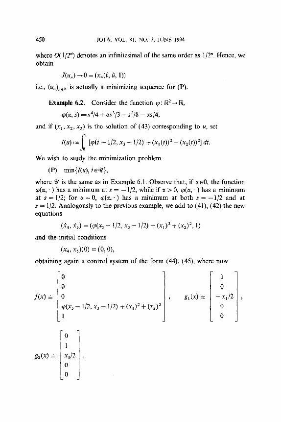
Example 6.2. Consider the function ~o: ~2"-4" ~ ,

~o(~, s ) ,=s4 /4 + ~s3/3 - s 2 / 8 - ~s/4,

and if (Xl, x2, x3) is the solution of (43) corresponding to u, set

I(u) ,= [tp(t - 1/2, x3 - 1/2) + (x, (t)) 2 + (x2 (t)) 2] dt.

We wish to study the minimizat ion problem

(P) min{I(u), ieq/},

where q / i s the same as in Example 6.1. Observe that, if ~E0, the funct ion q~(~, �9 ) has a min imum at s = - 1/2, while if ~ > 0, ~o(~, �9 ) has a min imum at s = 1/2; for ~ = 0, ~p(~,. ) has a minimum at bo th s = - 1 / 2 and at s = 1/2. Analogously to the previous example, we add to (41), (42) the new equations

(2~4,)C5) = (~O(X5 -- 1/2, x 3 - 1/2) + (xl) 2 + (x2) 2, 1)

and the initial condit ions

(m, xs)(O) = (0, 0),

obtaining again a control system of the form (44), (45), where now

-0

0

f ( x ) - 0 , g l ( x ) - ,

rp(x5 - 1/2, x3 - 1/2) + (xl) 2 + (x2) 2

1

0

1

g2(x) - xd2

0

0

1

0

- x l / 2

0

0

JOTA: VOL. 81, NO. 3, JUNE 1994 451

Then, (P) is equivalent to

(P) min{x4(u, 1), ueq/).

As in Example 6.1, the only nonvanishing Lie bracket is [gl, g2], given by (45). Hence, the extended control problem becomes

(P') min{x4((v, u), 1), (v, u) E W),

(-~1,3~2,)C3,3~4,3~5) ~--- (/gl, /~2, U, q)(X5 -- 1/2, X 3 - - 1/2) 71- (X 1 )2 .q_ (X2)2, 1), (48)

x(0) = (0, 0, 0, 0, 0), (v, u,, u2)(0 ) = (0, 0, 0), (49)

where W has the same meaning as in Example 6.1. By the properties of the map q~, it is clear that the impulsive, looping

control (~, ul, u2) e W defined by

(~, ~ , ~2)(t).'= (0, 0, 0), if t~[0, 1/2[,

(t3, ~ , fi2)(t),=(1, 0, 0), if t ~[1/2, 1],

is optimal for the extended problem (P'). Again, we obtain a corresponding minimizing sequence (W.).~N, Wn eqg,

for the original problem (P) by setting

w.( t ) = (o, o),

w.(t) = u.(n(t - 1/2 + l/n)),

w.( t ) = (o, o),

if te[0, I / 2 - I/n[,

if te[1/2 - 1/n, 1/2],

if t~]I/2, 0],

where (u,,),,~N is the sequence defined in Example 6.1.

7. Mechanical Application

The theory of hyperimpulsive motions (see Refs. 11-14, 15, 16, 7) in Lagrangian mechanics motivates our interest for impulsive control systems. In fact, within this theory, the controls are identified with some of the state parameters of a given Lagrangian system. Under suitable assumptions on the Riemannian structure of the constraint manifold (see Refs. 15, 16, 7), the differential system for the remaining state coordinates and their conju- gate momenta have the form of the impulsive control system (1), (2). However, because of the lack of analytical theory, up to now only examples concerning scalar controls have been considered (see Ref. 12).

In fact, if the control is scalar, an impulsive optimal control problem can be transformed into an ordinary control problem by means of a suitable change of coordinates. If the vector fields g,- in the control system

452 JOTA: VOL. 81, NO. 3, JUNE 1994

(1), (2) commute, the same procedure can be applied in the case of measurable vector-valued controls (see Ref. 6).

On the contrary, the results of the previous sections allow us to treat control problems for mechanical systems with vector-valued controls and without commutativity assumptions. As an illustration, we present here an example concerning a double pendulum, where the length of the second pendulum and the angle formed by the two pendulums are regarded as controls.

Precisely, consider the mechanical system formed by two mass points A and B, where A is constrained to move without friction on a vertical plane rc and to keep a fixed distance from a center of rotation 0, and B is connected to A by a rod, which has variable length and is allowed to rotate without friction around A on the plane zt.

Let m~ and mB be the masses of A and B, respectively, and suppose that the mass of the rod is negligible. It is trivial to check that, if the rod has a symmetry w.r.t, the axis AB, then the problem with nonnegligible mass is equivalent to a problem with negligible mass, up to a suitable translation of B along A B and a suitable adjustment of m A . The system has three degrees of freedom: as Lagrangian parameters, we choose the coun- terclockwise counted angle 0 between the half ray descending from 0 and the segment 0A, the counterclockwise counted angle u, determined by the segments 0A and AB, and the length u2 = lAB[; see Fig. 1. After rescaling the masses and the lengths, we can assume l = 1 and rnA = 1. Then, we can write simply m in place of mB. The kinetic energy H of the system is expressed by

n = (1/2)(0, ill, fi2)" A. (0, fir, fi2) t,

where the superscript t denotes transposition and A = A(O, u~, u2) is the positive-definite matrix defined by

I -1 + m(1 + u~ + 2u 2 cos u~)

(Aij)is = 1,2,3 = muz(cos ul + u2)

L m sin ul

mu2(cos ul +u2) m sinu,-]

mu~ 0 J. 0 m

According to the theory of hyperimpulsive motions, we regard the parame- ters ul, u2 as controls, which in turn have to be dynamically implemented as frictionless moving constraints. Then, one obtains a Lagrangian system parametrized by 0, which is governed by the equations

6 = OHIt3p, fJ = - O H I O 0 - (1 + m)g sin 0 - u2mg sin(0 + ul), (50)

where

p "- 3HI ,O, (51)

JOTA: VOL. 81, NO. 3, JUNE 1994 453

0

ml " m2

Q,

\ *$

\ "o

Fig. 1. Controls u~ and u2.

to 0, H is regarded and by the invertibility of (51) with respect function of 0, ul, u2, p, ~ , u2. Setting by (50)

Xj = 0 , x z = p , X3=Ul, X4:U2,

we obtain the impulsive control system

2 = f ( x ) + g, (x)fi I + g2(x)fi2,

where the vector fields f g~, g2 are defined by

f ( x ) - (x2/[l + m(1 - x4 z + 2x4 cos x3)], - ( 1 + m)g sin x~

- x4mg sin(x1 + x3), 0 0) t,

gl(x) - ( -mx4(x4+cosx3)/[1 +m(1 +m(1 + x]+ 2x4cosx3)], O, 1, O) t,

g2 (x) - ( - m sin x3/[1 + m(1 + x] + 2x4 cos x3)], 0, 0, 1)t.

as a

(52)

454 JOTA: VOL. 81, NO. 3, JUNE 1994

For a given pair (us u+), u y > us > 0, we assume that the controls u I and u2 satisfy the bounds

ul~[-rt/2, rc/2], uzE[us u~].

Set U = [-re/2, r~/2] x [us u~-] and let

o-//= {u ~ W1'~ T], ~n), u(t)~ U, u(0) = (rr]2, u~-)}

be the set of admissible controls. For the initial conditions

x~(0) = x/4, x2(0) = s x3(0) = 7r/2, x4(0) = us (53)

with

g2 < [ - ( 1 + m)g - u~mg]T, (54)

we consider the following control problem:

(P1) Find a control such that the absolute value of the correspond- ing final momentum p(T) is minimum.

Our system may be considered as a model for a swing carrying a man who can influence the oscillation by his movements. This model is some- what more realistic than the one in Ref. 12, where the man is only capable of a one-dimensional movement along the half ray 0A (pendulum with variable length). On the contrary, here the man has two degrees of freedom, for he can also rotate around the point A in the vertical plane passing through 0A.

Once we have solved (P1), with a slight modification we will be able to solve also the following constrained control problem:

(P2) Find a possibly looping control such that, at the final time t = T, the absolute value of the momentum p is minimum and the point A lies at 0 = 0.

Problem (P1) can be formally expressed by

(P) min{(x2(u, T))2, uaql},

where (x,. (u, . ))i ~ 1....4 denotes the solution of (52) corresponding to the control ue~//. According to Section 4, we embed (P) into an extended problem, provided the distribution generated by the Lie brackets of the g; of length > 2 is nonsingular. Actually, one has

"h(x3, x4) -

[g~, g2] - - 0 0 0

JOTA: VOL. 81, NO. 3, JUNE 1994 455

where

h(x3, x4) = mx4/[1 q- m(1 + 2x4 cos X 3 q- X2)] 2,

and every other bracket formed with the gi's has the three last components equal to zero. Since

h(x3, x4) __- m u 2 > 0, V(x3, X4) ~ U,

we obtain the quotient control system

2, = ~, (55)

22 = - ( 1 + m)g sin xl - x 4 m g sin(x1 + x3), (56)

23 = ~,, (57)

24 = zi2, (58)

where the looping control (v, ul, u2) belongs to the family

W = {(v, uj, u2): [0, T] ~ N x U, v, ul, u2 measurable,

(v, u,, u2)(0) = (re/4, ~r/2, u2)}.

Hence, the state xj can be considered as a control. Because of the form of Eqs. (55)-(58), it is clearly not restrictive to assume that the control v - x ~ ranges on the compact subset K = [ - r t / 2 , zt/2]. Therefore, our optimal control problem is equivalent to the problem for the ordinary control system

22 = - ( 1 + m)g sin v - u l m g sin(v + ul), (59)

where (v, u)( - ) is a map belonging to

W x = {(v, u): [0, T] --+[-re/2, 7r/2] x U, v, Ul, Uz measurable,

(v, ul, u2)(0) = (re/4, ~z[2, u~) }.

By standard existence results, there exist an optimal control (0, ~/)(. ) in WK. And by applying the Pontryagin maximum principle, we have

[l(v, u) - l(O(t), a(t)) l - x2((•, z3), T) < 0, (60)

for almost every ts [0 , 1] and every (v, u ) e K x U, where

l(v, u) = - ( 1 + m)g sin v - u2mg sin(v + ul ).

Since (54)-(58) imply that

x2 ((v, u), T) < O,

456 JOTA: VOL. 81, NO. 3, JUNE 1994

for every (v, u)(" ) < W~, (60) yields

[l(v, u) - l(~(t), a(t))] >_ 0, (61)

for almost every t~[0, 1] and every (v, u ) ~ K x U. Clearly, the map (t3, 2)(. ) defined by

03, a)(t) = (7z/4, 7z/2, u~), if t = 0,

(e, a)(t) = ( - n / 2 , O, u~) , if t~]0, 1],

satisfies (61). It is straightforward to verify that (t3, 2)(. ) is actually a looping optimal control for the extended problem corresponding to (P), and that no ordinary control ueq / i s optimal.

Finally, the map if, ~)(. ) defined by

(~, ~)(t) = (~, ~)(t), if t~[0, 1[,

(~, ~)(t) = (0, 0, u2), if t = 1,

is obviously a looping optimal control for the constrained problem (P2).

References

1. BRESSAN, A., JR., and RAMPAZZO, F., On Differential Systems with Vector- Valued Impulsive Controls, Bollettino dell'Unione Matematica Italiana, Series B, Vol. 3, pp. 641-656, 1988.

2. RAMPAZZO, F., Optimal Impulsive Controls with a Constraint on the Total Variation, New Trends in Systems Theory, Edited by G. Conte, A. M. Perdon, and B. F. Wyman, Birkhauser, Boston, Massachussets, pp. 606-613, 1991.

3. DALMASO, G., and RAMPAZZO, F., On Systems of Ordinary Differential Equations with Measures as Controls, Differential and Integral Equations, Vol. 4, pp. 739-765, 1991.

4. SUSSMANN, H. J., On the Gap between Deterministic and Stochastic Ordinary Differential Equations, Annals of Probability, Vol. 6, pp. 17-41, 1978.

5. BRESSAN, A., JR., On Differential Systems with Impulsive Controls. Rendiconti del Seminario Matematico dell' Universit~ di Padova, Vol. 78, pp. 227-236, 1987.

6. BRESSAN, A., JR., and RAMPAZZO, F., Impulsive Control Systems with Commu- tative Vector Fields, Journal of Optimization Theory and Applications, Vol. 71, pp. 67-83, 1991.

7. RAMPAZZO, F., Some Remarks on the Use of Constraints as Controls in Rational Mechanics, Rendiconti del Seminario Matematico dell' Universit~ e Politecnico di Torino, Vol. 48, pp. 367-382, 1990.

8. RISHEL, R. W., An Extended Pontryagin Maximum Principle for Control Systems Whose Control Laws Contain Measures, SIAM Journal on Control, Series A, Voi. 3, pp. 191-205, 1965.

JOTA: VOL. 81, NO. 3, JUNE 1994 457

9. SCHMAEDEKE, W. W., Optimal Control Theory for Nonlinear Differential Equations Containing Measures, SIAM Journal on Control, Series A, Vol. 3, pp. 231-280, 1965.

10. VINTER, R. B., and PEREIRA, F. M. F. L., A Maximum Principle for Optimal Processes with Discontinuous Trajectories, SIAM Journal on Control and Optimization, Vol. 26, pp. 205-229, 1988.

l l. BRESSAN, A., Hyperimpulsive Motions and Controllizable Coordinates for La- grangian Systems, Atti della Accademia' Nazionale dei Lincei, Memorie della Classe di Scienze Fisiche, Matematiche e Naturali, Series 8, Vol. 19, pp. 197-246, 1989.

12. BRESSAN, A., On Some Control Problems Concerning the Ski and the Swing, Atti della Accademia Nazionale dei Lincei, Memorie della Classe di Scienze Fisiche, Matematiche e Naturali, Series 9, Vol. 1, pp. 149-196, 1991.

13. BRESSAN, A., On Some Recent Results in Control Theory and Their Applications to Lagrangian Systems, Atti della Accademia Nazionale dei Lincei, Memorie della Classe di Scienze Fisiche, Mathematiche e Naturali (to appear).

14. BRESSAN, A., On the Applications of Control Theory to Certain Problems for Lagrangian Systems and Hyperimpulsive Motions for These, Parts 1 and 2, Atti della Accademia Nazionale dei Lincei, Rendiconti della Classe di Scienze Fisiche, Matematiche e Naturali, Vol. 82, pp. 91-118, 1988.

15. RAMPAZZO, F., On Lagrangian Systems with Some Coordinates as Controls, Atti della Accademia Nazionale dei Lincei, Rendiconti delia Classe di Scienze Fisiche, Matematiche e Naturali, Vol. 82, pp. 685-695, 1988.

16. RAMPAZZO, F., On The Riemannian Structure of a Lagrangian System and the Problem of Adding Time-Dependent Constraints as Controls, European Journal of Mechanics, A/Solids, Vol. 10, pp. 405-431, 1991.

17. HAINES, G. W., and HERMES, H., Nonlinear Controllability via Lie Theory. SIAM Journal on Control, Vol. 8, pp. 450-460, 1970.

18. AUBIN, J. P., and CELLINA, A., Differential Inclusions, Springer, Berlin, Ger- many, 1984.