University of Illinois at Urbana-Champaign

Air Conditioning and Refrigeration Center A National Science Foundation/University Cooperative Research Center

Improving the Accuracy and Scope of Control-Oriented Vapor Compression

Cycle System Models

B. D. Eldredge and A. G. Alleyne

ACRC TR-246 August 2006

For additional information:

Air Conditioning and Refrigeration Center University of Illinois Mechanical & Industrial Engineering Dept. 1206 West Green Street Urbana, IL 61801 Prepared as part of ACRC Project #175 Dynamic Grey Box Modeling for Vapor Compression Cycle Systems (217) 333-3115 A. G. Alleyne, Principal Investigator

The Air Conditioning and Refrigeration Center was founded in 1988 with a grant from the estate of Richard W. Kritzer, the founder of Peerless of America Inc. A State of Illinois Technology Challenge Grant helped build the laboratory facilities. The ACRC receives continuing support from the Richard W. Kritzer Endowment and the National Science Foundation. The following organizations have also become sponsors of the Center. Arçelik A. S. Behr GmbH and Co. Carrier Corporation Cerro Flow Products, Inc. Copeland Corporation Daikin Industries, Ltd. Danfoss A/S Delphi Thermal and Interior Embraco S. A. General Motors Corporation Hill PHOENIX Honeywell, Inc. Hydro Aluminum Precision Tubing Ingersoll-Rand/Climate Control Lennox International, Inc. LG Electronics, Inc. Manitowoc Ice, Inc. Matsushita Electric Industrial Co., Ltd. Modine Manufacturing Co. Novelis Global Technology Centre Parker Hannifin Corporation Peerless of America, Inc. Samsung Electronics Co., Ltd. Sanden Corporation Sanyo Electric Co., Ltd. Tecumseh Products Company Trane Visteon Automotive Systems Wieland-Werke, AG For additional information: Air Conditioning & Refrigeration Center Mechanical & Industrial Engineering Dept. University of Illinois 1206 West Green Street Urbana, IL 61801 217 333 3115

iii

Abstract

The benefits of applying advanced control techniques to vapor compression cycle systems are well know.

The main advantages are improved performance and efficiency, the achievement of which brings both economic and

environmental gains. One of the most significant hurdles to the practical application of advanced control techniques

is the development of a dynamic system level model that is both accurate and mathematically tractable. Previous

efforts in control-oriented modeling have produced a class of heat exchanger models known as moving-boundary

models. When combined with mass flow device models, these moving-boundary models provide an excellent

framework for both dynamic analysis and control design. This thesis contains the results of research carried out to

increase both the accuracy and scope of these system level models.

The improvements to the existing vapor compression cycle models are carried out through the application

of various modeling techniques, some static and some dynamic, some data-based and some physics-based. Semi-

empirical static modeling techniques are used to increase the accuracy of both heat exchangers and mass flow

devices over a wide range of operating conditions. Dynamic modeling techniques are used both to derive new

component models that are essential to the simulation of very common vapor compression cycle systems and to

improve the accuracy of the existing compressor model. A new heat exchanger model that accounts for the effects

of moisture in the air is presented. All of these model improvements and additions are unified to create a simple but

accurate system level model with a wide range of application. Extensive model validation results are presented,

providing both qualitative and quantitative evaluation of the new models and model improvements.

iv

Table of Contents

Page

Abstract......................................................................................................................... iii List of Figures ............................................................................................................. vii List of Tables ................................................................................................................. x

List of Abbreviations.................................................................................................... xi Chapter 1. Introduction................................................................................................. 1

1.1 Motivation........................................................................................................................................ 1 1.1.1 Vapor Compression Cycle Systems .......................................................................................................1 1.1.2 Efficiency ...............................................................................................................................................2 1.1.3 Advantages of Feedback Control ...........................................................................................................2 1.1.4 Model-based Control..............................................................................................................................2 1.1.5 Industry Need .........................................................................................................................................3

1.2 Objectives........................................................................................................................................ 3 1.3 Literature Review............................................................................................................................ 3

1.3.1 Finite Difference Models........................................................................................................................3 1.3.2 Moving-boundary Models ......................................................................................................................3 1.3.3 Model Validation....................................................................................................................................4

1.4 Organization.................................................................................................................................... 4 Chapter 2. Previous VCC Modeling ............................................................................. 6

2.1 Moving-boundary Heat Exchanger Modeling .............................................................................. 6 2.2 Static Valve Modeling..................................................................................................................... 8 2.3 Static Compressor Modeling......................................................................................................... 8 2.4 Modeling Challenges...................................................................................................................... 9

2.4.1 Accurate Model Parameters ...................................................................................................................9 2.4.2 Atmospheric Conditions.......................................................................................................................10 2.4.3 Expanding Operating Conditions .........................................................................................................10 2.4.4 Dynamic Compressor Shell Model.......................................................................................................10 2.4.5 Large Transient Simulation ..................................................................................................................10

Chapter 3. Semi-empirical Models ............................................................................. 11 3.1 External Heat Transfer Coefficients ........................................................................................... 11

3.1.1 Empirical Heat Transfer Model............................................................................................................11 3.1.2 Sources of Empirical Heat Transfer Data.............................................................................................11 3.1.3 Implementation in Thermosys ..............................................................................................................13

3.2 Performance Mapping.................................................................................................................. 15 3.2.1 Valves...................................................................................................................................................17 3.2.2 Compressor...........................................................................................................................................24 3.2.3 Implementation in Thermosys ..............................................................................................................26

Chapter 4. Atmospheric Conditions Modeling ........................................................ 30 4.1 Air Temperature Condensation Method..................................................................................... 30

v

4.1.1 Modified Energy Balances ...................................................................................................................31 4.1.2 Heat Transfer Rates ..............................................................................................................................34 4.1.3 Implementation in Thermosys ..............................................................................................................34

4.2 Wall Temperature Condensation Method .................................................................................. 35 4.2.1 Individual Region Mass and Energy Balances .....................................................................................36 4.2.2 Outlet Humidity Calculations...............................................................................................................37 4.2.3 Mixing of Region Outputs....................................................................................................................38 4.2.4 Implementation in Thermosys ..............................................................................................................39

Chapter 5. Dynamic Modeling ................................................................................... 40 5.1 Motivation...................................................................................................................................... 40

5.1.1 Heat exchangers with Receivers/Accumulators ...................................................................................40 5.1.2 Compressor Shell Capacitance .............................................................................................................40 5.1.3 Dynamic Mass Flow Correction...........................................................................................................40 5.1.4 Compressor Cycling Simulation...........................................................................................................40

5.2 Heat Exchangers with Receivers/Accumulators....................................................................... 41 5.2.1 Challenge of Receiver/Accumulator Modeling ....................................................................................41 5.2.2 Receiver Model ....................................................................................................................................41 5.2.3 Accumulator Model..............................................................................................................................42 5.2.4 Nonlinear Condenser with Receiver.....................................................................................................43 5.2.5 Nonlinear Evaporator with Accumulator .............................................................................................45 5.2.6 Pseudo-Quality and Mean Void Fraction .............................................................................................46

5.3 Compressor Shell Thermal Capacitance Dynamic ................................................................... 48 5.3.1 Implementation in Thermosys ..............................................................................................................49

5.4 Identified Compressor Mass Flow Model................................................................................... 51 5.4.1 Compressor Mass Flow Dynamics Isolation ........................................................................................51 5.4.2 Identification of Isolated Dynamics .....................................................................................................52

5.5 Compressor Cycling Dynamics .................................................................................................. 52 5.5.1 Literature Review.................................................................................................................................52 5.5.2 Current Thermosys Model Cycling Capabilities ..................................................................................54

5.6 Future Work................................................................................................................................... 59 5.6.1 Cycling Simulation...............................................................................................................................59 5.6.2 Start-up Simulation...............................................................................................................................59 5.6.3 Improved Compressor Mass Flow Prediction ......................................................................................60

Chapter 6. Experimental System .............................................................................. 61 6.1 General Description ..................................................................................................................... 61 6.2 Sensors.......................................................................................................................................... 63

6.2.1 Temperature, Pressure, Mass Flow, and Power Measurement .............................................................64 6.2.2 Humidity Measurement ........................................................................................................................65

6.3 Actuators ....................................................................................................................................... 65 6.3.1 Compressor, Fans, and Valves .............................................................................................................65 6.3.2 Humidifier ............................................................................................................................................66

6.4 Data Acquisition ........................................................................................................................... 67

vi

6.5 Components.................................................................................................................................. 67 6.5.1 Heat Exchangers...................................................................................................................................67 6.5.2 Auxiliary Components .........................................................................................................................67

6.6 Physical Parameters .................................................................................................................... 68 Chapter 7. Model Validation ...................................................................................... 69

7.1 Single-Step Model Validation Scenario...................................................................................... 69 7.1.1 System Inputs .......................................................................................................................................69 7.1.2 System Output ......................................................................................................................................71 7.1.3 Quantified Modeling Improvements ....................................................................................................76

7.2 Drive Cycle Model Validation Scenario ...................................................................................... 77 7.2.1 System Inputs .......................................................................................................................................78 7.2.2 System Outputs ....................................................................................................................................79

7.3 Atmospheric Conditions Model Validation Scenario................................................................ 81 7.3.1 System Inputs .......................................................................................................................................82 7.3.2 System Outputs ....................................................................................................................................83 7.3.3 Simulation Analysis .............................................................................................................................85

Chapter 8. Conclusions and Future Work................................................................. 89 8.1 Summary of Research Contributions......................................................................................... 89

8.1.1 Model Developments ...........................................................................................................................89 8.1.2 Model Validation..................................................................................................................................89

8.2 Future Work................................................................................................................................... 90 8.2.1 Model Development................................................................................................................... 90

8.2.2 Model Validation..................................................................................................................................90 8.2.3 Model Applications .............................................................................................................................90

List of References ....................................................................................................... 91

Appendix A. Sample Code.......................................................................................... 94 H.1 Condenser j Factor Correlation................................................................................................. 94 H.2 Evaporator j Factor Correlation................................................................................................. 95 H.3 EEV Performance Map................................................................................................................ 96 H.4 AEV Performance Map ............................................................................................................... 98 H.5 TEV Performance Map................................................................................................................ 99 H.6 Capillary Tube Performance Map............................................................................................ 103 H.7 Volumetric Efficiency Performance Map................................................................................ 105 H.8 Adiabatic Efficiency Performance Map .................................................................................. 106

Appendix B. Operating Conditions.......................................................................... 109

vii

List of Figures

Page Figure 1.1 Components of the basic vapor compression cycle......................................................................................1 Figure 2.1 Evaporator fluid regions...............................................................................................................................7 Figure 3.1 The experimentally obtained j factor plot for surface CF-8.72 from [25] ..................................................12 Figure 3.2 Experimental system condenser j factor from correlation..........................................................................12 Figure 3.3 Experimental system evaporator j factor from correlation .........................................................................12 Figure 3.4 Example calculation of heat exchanger flow length...................................................................................13 Figure 3.5 Plane of maximum flow constriction used in calculation of the minimum free flow area .........................14 Figure 3.6 Block diagram of heat transfer coefficient calculation from j factor data ..................................................15 Figure 3.7 Compressor speed and valve opening settings ...........................................................................................16 Figure 3.8 Range of operating conditions covered by performance maps...................................................................16 Figure 3.9 Comparison of 2-input and 3-input EEV models with experimental data..................................................18 Figure 3.10 Flow coefficient map for an EEV with black points representing experimental data ..............................19 Figure 3.11 Schematic of an AEV [1] .........................................................................................................................19 Figure 3.12 Flow coefficient performance map and data points for an AEV ..............................................................20 Figure 3.13 Schematic of a TEV and example values for superheat regulation [2].....................................................21 Figure 3.14 TEV discharge coefficient performance map and generating data...........................................................22 Figure 3.15 TEV area map...........................................................................................................................................23 Figure 3.16 Capillary tube flow coefficient data points and best fit performance map ...............................................24 Figure 3.17 A two input performance map of volumetric efficiency...........................................................................25 Figure 3.18 A two-input adiabatic efficiency map with experimental data .................................................................26 Figure 3.19 2-D lookup table block and Block Parameters interface ..........................................................................27 Figure 3.20 3-D lookup table block and Block Parameters interface ..........................................................................28 Figure 3.21 Performance map portion of the 2-input EEV component GUI showing data structure field names.......29 Figure 4.1 Water saturation pressure as a function of saturation temperature .............................................................30 Figure 4.2 Water saturated liquid enthalpy as a function of temperature ....................................................................30 Figure 4.3 Control volume for humid air mass and energy balances under non-condensing conditions.....................31 Figure 4.4 Control volume for humid air mass and energy balances under condensing conditions ............................33 Figure 4.5 Data for a condensing conditions test with the air temperature well above the dew point temperature.....35 Figure 4.6 Divided air-side control volumes ...............................................................................................................36 Figure 5.1 Two possible steady-state condenser with receiver operating conditions ..................................................41 Figure 5.2 A possible transient condenser with receiver operating condition .............................................................41 Figure 5.3 Control volume for receiver model ............................................................................................................42 Figure 5.4 Control volume for accumulator model .....................................................................................................42 Figure 5.5 Mean void fraction for two-phase flows operating at 900 kPa (condenser) and 320 kPa (evaporator)

as a function of the outlet quality ........................................................................................................................48 Figure 5.6 Compressor shell and refrigerant outlet temperature data for system shutdown from 1600 RPM.............49 Figure 5.7 Block diagram of Equation 5.23.................................................................................................................49 Figure 5.8 Compressor outlet temperature data (blue) and small time constant model output (green) .......................50

viii

Figure 5.9 Compressor outlet temperature model output for various time constants ..................................................50 Figure 5.10 Compressor mass flow dynamics isolation procedure..............................................................................51 Figure 5.11 Receiver mass inventory showing numerical instability ..........................................................................54 Figure 5.12 Pressures...................................................................................................................................................55 Figure 5.13 Condenser fluid region lengths.................................................................................................................55 Figure 5.14 Evaporator fluid region lengths with the superheat length vanishing.......................................................55 Figure 5.15 Receiver mass inventory ..........................................................................................................................55 Figure 5.16 Evaporator superheat................................................................................................................................56 Figure 5.17 System pressure data ................................................................................................................................56 Figure 5.18 System evaporator superheat data ............................................................................................................57 Figure 5.19 System pressures ......................................................................................................................................57 Figure 5.20 Condenser lengths ....................................................................................................................................57 Figure 5.21 Evaporator lengths....................................................................................................................................58 Figure 5.22 Evaporator superheat................................................................................................................................58 Figure 5.23 System pressure data ................................................................................................................................58 Figure 5.24 System evaporator superheat data ............................................................................................................59 Figure 6.1 Experimental system schematic .................................................................................................................62 Figure 6.2 Photograph of the relative humidity sensor at the evaporator inlet ............................................................65 Figure 6.3 Humidifier and tubing bringing moist air output to the evaporator inlet....................................................66 Figure 7.1 Valve input signal.......................................................................................................................................70 Figure 7.2 Compressor input signal.............................................................................................................................70 Figure 7.3 Condenser air mass flow rate input signal..................................................................................................70 Figure 7.4 Evaporator mass flow rate input signal ......................................................................................................70 Figure 7.5 Condenser with receiver pressure...............................................................................................................72 Figure 7.6 Condenser with receiver outlet air temperature..........................................................................................72 Figure 7.7 Condenser with receiver refrigerant outlet temperature .............................................................................72 Figure 7.8 Evaporator pressure....................................................................................................................................73 Figure 7.9 Evaporator superheat..................................................................................................................................73 Figure 7.10 Static volumetric efficiency map (surface) and volumetric efficiency generated from mass flow

correction (line) ...................................................................................................................................................74 Figure 7.11 Condenser pressure ..................................................................................................................................75 Figure 7.12 Condenser air outlet temperature..............................................................................................................75 Figure 7.13 Evaporator pressure..................................................................................................................................75 Figure 7.14 Evaporator air outlet temperature.............................................................................................................76 Figure 7.15 Evaporator superheat................................................................................................................................76 Figure 7.16 Compressor speed ....................................................................................................................................78 Figure 7.17 Condenser air mass flow rate ...................................................................................................................78 Figure 7.18 Valve opening ..........................................................................................................................................79 Figure 7.19 Valve mass flow data and compressor mass flow models........................................................................79 Figure 7.20 Condenser pressure data and models........................................................................................................79

ix

Figure 7.21 Condenser outlet air temperature data and models...................................................................................80 Figure 7.22 Evaporator pressure data and models .......................................................................................................80 Figure 7.23 Evaporator superheat data and models .....................................................................................................80 Figure 7.24 Evaporator outlet air temperature data and models ..................................................................................80 Figure 7.25 Components used in humidity model validation ......................................................................................82 Figure 7.26 Inlet relative humidity data.......................................................................................................................82 Figure 7.27 Photograph on the inlet and outlet evaporator pipes with condensation on the inlet (lower) pipe ...........83 Figure 7.28 Outlet relative humidity data and model ..................................................................................................83 Figure 7.29 Condensate mass flow rate model ............................................................................................................84 Figure 7.30 Evaporator outlet air temperature and model ...........................................................................................84 Figure 7.31 Accumulated condensation measurements and model prediction ............................................................85 Figure 7.32 Inlet relative humidity ..............................................................................................................................86 Figure 7.33 Dew point temperature and model wall temperatures ..............................................................................86 Figure 7.34 Outlet relative humidity model.................................................................................................................86 Figure 7.35 Condensate mass flow rate model ............................................................................................................87 Figure 7.36 Outlet evaporator air temperature model..................................................................................................87 Figure 7.37 Evaporator pressure model.......................................................................................................................88 Figure A.1 Diagram of TEV geometry.....................................................................................................................103

x

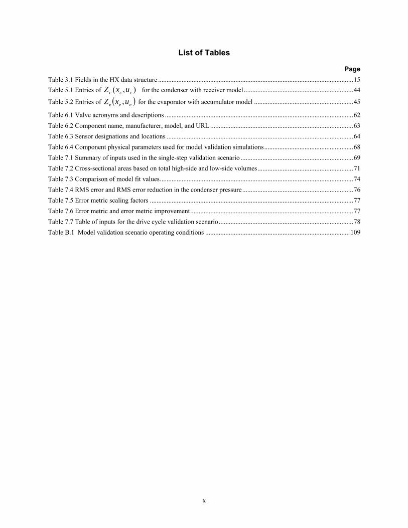
List of Tables

Page Table 3.1 Fields in the HX data structure ....................................................................................................................15 Table 5.1 Entries of ),( ccc uxZ for the condenser with receiver model .................................................................44 Table 5.2 Entries of ( )eee uxZ , for the evaporator with accumulator model ...........................................................45 Table 6.1 Valve acronyms and descriptions ................................................................................................................62 Table 6.2 Component name, manufacturer, model, and URL .....................................................................................63 Table 6.3 Sensor designations and locations ...............................................................................................................64 Table 6.4 Component physical parameters used for model validation simulations.....................................................68 Table 7.1 Summary of inputs used in the single-step validation scenario ...................................................................69 Table 7.2 Cross-sectional areas based on total high-side and low-side volumes.........................................................71 Table 7.3 Comparison of model fit values...................................................................................................................74 Table 7.4 RMS error and RMS error reduction in the condenser pressure..................................................................76 Table 7.5 Error metric scaling factors .........................................................................................................................77 Table 7.6 Error metric and error metric improvement.................................................................................................77 Table 7.7 Table of inputs for the drive cycle validation scenario................................................................................78 Table B.1 Model validation scenario operating conditions ......................................................................................109

xi

List of Abbreviations

AEV – automatic expansion valve EES – Engineering Equation Solver EEV – electronic expansion valve HVAC – heating, ventilation, and air-conditioning ILC – iterative learning control MIMO – multiple-input multiple-output NREL – National Renewable Energy Laboratory ODE – ordinary differential equation PDE – partial differential equation RMS – root mean square RPM – revolutions per minute SISO – single-input single-output TEV – thermostatic expansion valve VCC – vapor compression cycle VFD – variable frequency drive

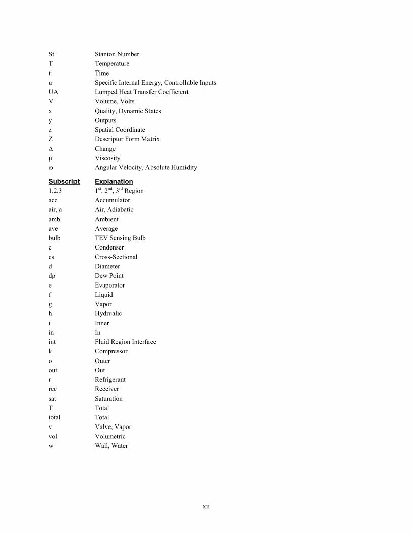
List of Symbols

Variable Explanation α Heat Transfer Coefficient η Efficiency γ Void Fraction γ Mean Void Fraction m& Mass Flow Rate ρ Density γ̂ Pseudo Mean Void Fraction

φ Relative Humidity A Area C Coefficient Cp Specific Heat e Error G Maximum Mass Velocity, Transfer Function h Specific Enthalpy j Colburn j factor L Length m Mass P Pressure p Perimeter Pr Prandtl Number Q& Heat Transfer Rate

Re Reynold’s Number S Slip Ratio s Specific Entropy sh Superheat

xii

St Stanton Number T Temperature t Time u Specific Internal Energy, Controllable Inputs UA Lumped Heat Transfer Coefficient V Volume, Volts x Quality, Dynamic States y Outputs z Spatial Coordinate Z Descriptor Form Matrix Δ Change μ Viscosity ω Angular Velocity, Absolute Humidity

Subscript Explanation 1,2,3 1st, 2nd, 3rd Region acc Accumulator air, a Air, Adiabatic amb Ambient ave Average bulb TEV Sensing Bulb c Condenser cs Cross-Sectional d Diameter dp Dew Point e Evaporator f Liquid g Vapor h Hydrualic i Inner in In int Fluid Region Interface k Compressor o Outer out Out r Refrigerant rec Receiver sat Saturation T Total total Total v Valve, Vapor vol Volumetric w Wall, Water

1

Chapter 1. Introduction

1.1 Motivation Vapor compression cycle (VCC) systems are now an essential part of life, providing critical temperature

control through air-conditioning and refrigeration machines. These complex thermo-fluid systems have increased in

efficiency as they have increased in usage [15]. Great efforts have been expended in optimizing the design of

individual VCC components. Most of this component-based research has focused on steady-state performance.

This work, in contrast, examines the transient behavior and performance of vapor compression cycles at the system

level. An understanding of the system dynamic behavior opens the door for the application of advanced feedback

control techniques. Feedback control promises further improvements in efficiency, resulting in both economic and

environmental benefits.

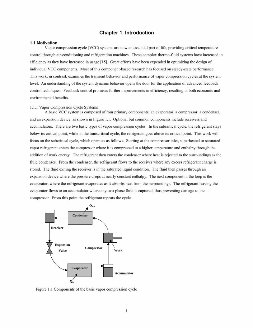
1.1.1 Vapor Compression Cycle Systems A basic VCC system is composed of four primary components: an evaporator, a compressor, a condenser,

and an expansion device, as shown in Figure 1.1. Optional but common components include receivers and

accumulators. There are two basic types of vapor compression cycles. In the subcritical cycle, the refrigerant stays

below its critical point, while in the transcritical cycle, the refrigerant goes above its critical point. This work will

focus on the subcritical cycle, which operates as follows. Starting at the compressor inlet, superheated or saturated

vapor refrigerant enters the compressor where it is compressed to a higher temperature and enthalpy through the

addition of work energy. The refrigerant then enters the condenser where heat is rejected to the surroundings as the

fluid condenses. From the condenser, the refrigerant flows to the receiver where any excess refrigerant charge is

stored. The fluid exiting the receiver is in the saturated liquid condition. The fluid then passes through an

expansion device where the pressure drops at nearly constant enthalpy. The next component in the loop is the

evaporator, where the refrigerant evaporates as it absorbs heat from the surroundings. The refrigerant leaving the

evaporator flows to an accumulator where any two-phase fluid is captured, thus preventing damage to the

compressor. From this point the refrigerant repeats the cycle.

Figure 1.1 Components of the basic vapor compression cycle

Accumulator

Compressor

Evaporator

Receiver

Condenser

Expansion Valve

Qin

Qout

Work

2

1.1.2 Efficiency A 2004 National Renewable Energy Laboratory (NREL) study found that the United States uses 7 billion

gallons (26.4 billion Liters) of fuel per year for light-duty vehicle air-conditioning alone, equivalent to 5.5% of the

total national light-duty vehicle fuel use. It would take 9.5% of the U.S. imported oil to produce this much gasoline

[37].

Statistics compiled by the Energy Information Administration for 2001 indicate that 82.9 million US

households have some type of air-conditioning system. One hundred eighty-three (183) billion kWh of home

electricity were consumed to power these home air-conditioners. That energy consumption is equivalent to 15.94

billion dollars. Trends indicate that air-conditioning is being used in more homes and is being used more often [15].

Data from 1999 showed commercial energy use for cooling required energy expenditures of 72.2 billion dollars.

Refrigeration energy expenditures exceeded 40 billion dollars [14]. Considering the huge expenditures associated

with air-conditioning and refrigeration, even modest gains in VCC system efficiency will result in substantial

reductions in energy usage on a national scale. The associated economic and environmental benefits are clear.

1.1.3 Advantages of Feedback Control The application of advanced feedback control techniques to VCC systems is motivated by the desire to

increase system efficiency. Feedback control allows the system to match its capacity to a required load without

cycling the compressor on and off. Variable speed or variable displacement continuous compressor operation has

been shown to be more efficient than compressor cycling [27]. Control also allows for the regulation of the level of

superheat at the evaporator outlet. By maintaining a low level of superheat, the evaporator operates in its most

efficient wet condition, and the compressor is not slugged with liquid refrigerant. The current industry standard for

superheat control is the thermostatic expansion valve. These valves regulate superheat, but are only effective near a

single operating condition. Feedback control used in conjunction with an electronic expansion valve and variable

speed compressor allows for superheat and capacity regulation over the entire system operating range through

techniques such as gain scheduling [41].

1.1.4 Model-based Control Vapor compression cycles are frequently used as multiple-input multiple-output (MIMO) systems. The

inputs, or actuators, could include the expansion device, the compressor, and the heat exchanger fans. The outputs

to be controlled are typically superheat and capacity. Research has shown that coordinated MIMO control of these

two outputs is more effective than separate single-input single-output (SISO) control loops [42, 21]. Due to the

highly coupled nature of these systems, SISO control loops will fight one another, an effect that is very detrimental

to performance.

In order to effectively design and evaluate MIMO control techniques, an accurate system level dynamic

VCC model is required. Such a model is available in Thermosys, a MATLAB toolbox developed at the University of

Illinois under the auspices of the Air-Conditioning and Refrigeration Center. Thermosys contains low-order

dynamic models of heat exchangers and static models of the other basic components of VCC systems. The heat

exchangers are modeled with a moving-boundary approach, which produces models of lower dynamic order than the

more common finite difference approach. The individual component models are combined in Simulink to create an

overall system level model. The linearized system model is a valuable tool for the control designer. The state of

3

Thermosys at the commencement of this research effort is described in Chapter 2, as well as model additions and

improvements that will be covered in this thesis.

1.1.5 Industry Need To the author’s knowledge, no software package incorporating low-order moving-boundary dynamic heat

exchanger models is commercially available. Numerous researchers have developed moving-boundary models, but

the models have not been made available as software to either the industrial or the academic community. The

HVAC industry stands in need of a software tool capable of simulating the dynamics of VCC cycles. Many finite

difference modeling tools are on the market, but Thermosys is the only available tool containing compact, control-

oriented moving-boundary heat exchanger models.

1.2 Objectives The main objective of the research presented in this thesis is to advance the state-of-the-art of system level

VCC models based on the moving-boundary paradigm. Increased simulation accuracy is achieved by incorporating

improvements and additions to both static and dynamic models, including the addition of environmental effects

(humid air) on heat exchanger behavior.

The secondary objective is to increase confidence in the moving-boundary models through presentation of

extensive model validation results. Model validation results are one area of moving-boundary model research that

has been lacking in the literature. All modeling improvements and additions presented in this work are validated

with experimental data as much as time and resources permit.

1.3 Literature Review Modeling of VCC systems can be divided into two general paradigms: finite difference (spatially

dependent) models and moving-boundary models [4]. The following sections give a brief discussion of finite

difference modeling and an examination of existing moving-boundary models. A more detailed examination of the

deficiencies of previous moving-boundary models is found in Chapter 2.

1.3.1 Finite Difference Models In the finite difference paradigm, the conservation equations are approximated with a finite difference

technique and applied to a number of elements in the heat exchanger [33]. Each element contains its own dynamic

states and is independent of fluid phase. As the number of elements increases, model accuracy increases as well.

However, the increased number of elements results in a dynamically large model that may be computationally

expensive and is unsuitable for model-based control design [3]. Gruhle and Isermann presented this method in 1984

[18], and it has been utilized by numerous researchers. Finite difference models are available in a number of

commercial software packages.

1.3.2 Moving-boundary Models In the moving-boundary modeling approach, the heat exchangers are divided into regions based on the fluid

phase in each region. The complex heat exchanger geometry is reduced to an equivalent single pipe. Model

parameters are lumped together in each region. The location of the boundary between regions is allowed to be a

dynamic variable, thereby capturing the essential two-phase flow dynamics. The resulting models are of low

dynamic order, making them very well suited for control design. The moving-boundary models give the model

4

developer and control designer physical insight into the dynamic behavior of the plant. In comparison to the finite

difference models, the compact nature of the moving-boundary models is assumed to reduce accuracy, although no

direct model validation comparison is available in the literature. Grald and MacArthur (1992) showed that a

spatially dependent model and a moving-boundary model for an evaporator have very similar dynamic responses

[17].

Moving-boundary models have been under development since 1979 [11]. A review of the literature shows

that they have been applied to a variety of VCC systems with many variations in the details of the modeling

approach [4]. Broersen and van der Jagt (1980) developed a moving-boundary model of an evaporator to analyze

hunting behavior in thermostatic expansion valves [6]. Validation of the model is not presented. Kapadia (1984)

presented very limited validation for a moving-boundary condenser model in a Rankine cycle [24]. Grald and

MacArthur (1992) developed a moving-boundary model of an evaporator as part of a heat pump model. Model

validation results are again limited [17]. He (1997) presented linearized moving-boundary models for both an

evaporator and a condenser, with the stated purpose of designing feedback controllers. Adequate model validation

results were included [20, 21]. Numerous authors have presented similar models to those discussed, but with some

extensions to the modeling framework [23, 47, 38]. Rasmussen (2004) derived moving-boundary models for

transcritical cycles, while previous authors have focused on sub-critical cycles [42].

1.3.3 Model Validation The models presented in this work are applicable to both dynamic analysis and control. The intended

application dictates the necessary level of accuracy. The model validation process attempts to determine if the given

model meets the specified level of accuracy, where accuracy is determined by comparing model output to

experimental data. A good overview of various model validation approaches is found in [12]. Strictly speaking, a

model can not be validated by a finite set of data [39], only invalidated. However, each successful validation effort

increases the user’s confidence in the model.

The process of model validation can be used to answer two questions. The first is a qualitative question:

does the model accurately describe the essential characteristics of the system? The second is a quantitative question:

What is the level of agreement between the model and the real system? The qualitative question is typically

addressed first in the model development process. Pursuing quantitative model validation makes little sense if the

model obviously does not capture the salient dynamic behavior of the system. Once the qualitative accuracy

requirement has been satisfied, quantitative model accuracy may be addressed. By quantifying accuracy,

researchers can compare models, evaluate the value of changes to the model, and track progress. The quantitative

validation results presented in this work use RMS error and similar metrics to compare the accuracy of various

models.

1.4 Organization Chapter 2 describes previous moving-boundary modeling work, with specific emphasis placed on the

models developed within the Alleyne Research Group. In examining the existing state-of-the-art, areas for potential

improvement are identified. Chapter 3 describes various semi-empirical methods for improving model accuracy,

including improved static mass flow models and heat transfer models. Modeling of environmental conditions is

5

described in Chapter 4. New dynamic models and dynamic additions to existing static models are described in

Chapter 5. Chapter 6 gives an overview of the experimental system used to generate data for model validation tests.

The model validation results for the various static and dynamic modeling improvements and additions are presented

in Chapter 7. The thesis concludes in Chapter 8 with a summary of the results and directions for future research.

6

Chapter 2. Previous VCC Modeling

Vapor compression cycle system modeling has been an ongoing research topic within the Alleyne Research

Group since 2000. Industry interest in the initial modeling efforts led to the creation of the Thermosys Toolbox for

MATLAB. This chapter will first review the status of Thermosys as of Fall 2004 [40, 44], with some comparisons to

the moving-boundary models developed by other researchers. An overview of modeling needs addressed in this

thesis is then presented.

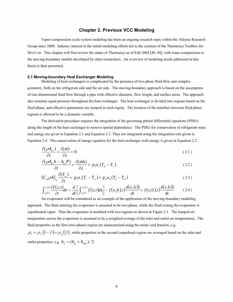
2.1 Moving-boundary Heat Exchanger Modeling Modeling of heat exchangers is complicated by the presence of two-phase fluid flow and complex

geometry, both on the refrigerant side and the air side. The moving-boundary approach is based on the assumption

of one-dimensional fluid flow through a pipe with effective diameter, flow length, and surface areas. The approach

also assumes equal pressure throughout the heat exchanger. The heat exchanger is divided into regions based on the

fluid phase, and effective parameters are lumped in each region. The location of the interface between fluid phase

regions is allowed to be a dynamic variable.

The derivation procedure requires the integration of the governing partial differential equations (PDEs)

along the length of the heat exchanger to remove spatial dependence. The PDEs for conservation of refrigerant mass

and energy are given in Equation 2.1 and Equation 2.2. They are integrated using the integration rule given in

Equation 2.4. The conservation of energy equation for the heat exchanger wall energy is given in Equation 2.3.

( ) ( ) 0=∂∂

+∂

∂zm

tAcs &ρ

( 2.1 )

( ) ( ) ( )rwiicscs TTp

zhm

tPAhA

−=∂

∂+

∂−∂

αρ &

( 2.2 )

( ) ( ) ( ) ( )waoowriiw

wp TTpTTpt

TAC −+−=

∂∂

ααρ ( 2.3 )

( )( )

( ) ( )( )

( ) ( )( ) ( )( ) ( )( ) ( )( )dt

tzdttzf

dttzd

ttzfdztzfdtddz

ttzf tz

tz

tz

tz1

12

2 ,,,, 2

1

2

1

+−⎥⎦⎤

⎢⎣⎡=

∂∂

∫∫ ( 2.4 )

An evaporator will be considered as an example of the application of the moving-boundary modeling

approach. The fluid entering the evaporator is assumed to be two-phase, while the fluid exiting the evaporator is

superheated vapor. Thus the evaporator is modeled with two regions as shown in Figure 2.1. The lumped air

temperature across the evaporator is assumed to be a weighted average of the inlet and outlet air temperatures. The

fluid properties in the first (two-phase) region are characterized using the mean void fraction, e.g.

( ) ( )γργρρ gf +−= 11 , while properties in the second (superheat) region are averaged based on the inlet and

outlet properties, e.g. 2/)(2 outg hhh += .

7

Two-Phase Superheat

L1(t) L2(t)

LTotal

)(thm outout&ininhm&

xin > 0P(t)

Twall,1(t) Twall,2(t)

x = 1

Two-Phase Superheat

L1(t) L2(t)

LTotal

L1(t) L2(t)

LTotal

)(thm outout& )(thm outout&ininhm&

xin > 0ininhm&

xin > 0P(t)

Twall,1(t) Twall,2(t)

x = 1

Figure 2.1 Evaporator fluid regions

Integration of the three conservation equations for each region results in six equations that can be

simplified into a nonlinear state space form, ( ) ( )uxfxuxZ ,, =⋅ & , where the elements of ( )uxZ , and ( )uxf ,

are nontrivial and presented in detail in [40]. The states of the evaporator model, which are a result of the derivation

procedure, are the length of two-phase flow, the evaporation pressure, the outlet enthalpy, and the two lumped wall

temperatures, shown symbolically in Equation 2.5. The inputs to each of the component models are generally

outputs of other component models. The inputs to the evaporator model are the inlet and outlet refrigerant mass

flow rates (outputs of the valve and compressor models), the inlet enthalpy (output of the valve model), and the

temperature and mass flow rate of air (inputs to the overall system), given symbolically in Equation 2.6

[ ]Tewewouteeee TThPLx 21,1= ( 2.5 )

[ ]Taireinaireineouteinee mThmmu ,,,,,, &&&= ( 2.6 )

Industry interest in the moving-boundary models developed within the Alleyne Research Group led to the

creation of Thermosys, a MATLAB Toolbox. Thermosys contains linear and nonlinear Simulink models of the basic

components of VCC systems, including heat exchangers, compressors, and expansion devices. Individual

Thermosys component models are connected in Simulink to create a complete system. The component models are

added to the system model using Simulink’s drag-and-drop functionality. Model users set physical parameters and

initial conditions through component graphical user interfaces.

When the research presented in this thesis was initiated, Thermosys contained moving-boundary heat

exchanger models of an evaporator, a condenser, and a gas cooler. Both linear and nonlinear versions of these

models were available. In addition, a lumped-parameter internal counter-flow heat exchanger was included in the

model library. This collection of heat exchanger models was fairly comprehensive when compared to the models

produced by other researchers (see Chapter 1 literature review). The heat exchangers could be used in subcritical,

transcritical, and multi-evaporator cycles. Notably absent from the Thermosys model library were receivers and

8

accumulators. At least one of these two components has also typically been absent from many other moving-

boundary modeling efforts as well [20, 47, 23, 17, 11, 9].

An inherent feature of moving-boundary models is the connection between the number of dynamic states

and the number of fluid regions in the heat exchanger model. If system transients cause a fluid region to appear or

disappear, then the number of states in the model changes. Handling the mathematical effects of adding and

removing states is challenging. Some researchers [11, 47] have proposed a modeling-switching scheme whereby

multiple modeling frameworks are used in a single simulation. At the commencement of this research, the

Thermosys models did not have the ability to simulate heat exchangers with a changing number of fluid regions.

This situation occurs frequently in heat exchangers connected with receivers or accumulators and always occurs

during system start-up and shut-down.

2.2 Static Valve Modeling The only expansion device available in Thermosys was an electronic expansion valve. Since the models

were originally developed as a control design tool, including a valve suited to electronic control made sense. The

valve model required some restrictive assumptions. The mass flow rate model is given in Equation 2.7.

( )[ ] 21outinvvvv PPCAm −= ρ& ( 2.7 )

The valve area, Av, was assumed to be linearly related to the control input, uv, as shown in Equation 2.8.

vv uA 21 ββ += ( 2.8 )

The discharge coefficient, Cv, was assumed to be a function of the Reynolds number in Equation 2.9.

⎟⎠⎞

⎜⎝⎛ +=

Re1 4

3β

βvC ( 2.9 )

The framework described above is somewhat restrictive to the model user. If an industrial user had an alternate

theoretical valve modeling framework or an empirical modeling framework, that framework would be excluded

from use in Thermosys. All model users were required to identify the three parameters in Equation 2.8 and Equation

2.9 for their valves. Other moving-boundary model developers have generally not included valve modeling details,

such as calculation of the discharge coefficient, in their publications.

2.3 Static Compressor Modeling Like the valve, the variable speed compressor was modeled as a static component based on empirical

parameters. Some researchers have attempted to model compressor dynamics [11, 47], while others [20, 23] assume

a static model. The mass flow equation for the compressor model is given in Equation 2.10.

volkkkk Vm ηρω=& ( 2.10 )

The volumetric efficiency was calculated from the assumed function of pressure ratio shown in Equation 2.11.

n

in

outkkvol P

PDC

1

1 ⎟⎟⎠

⎞⎜⎜⎝

⎛−+=η ( 2.11 )

9

The compressor outlet enthalpy was calculated from Equation 2.12.

( )[ ]11, −+= ainisentropicout

aout hhh η

η ( 2.12 )

The adiabatic efficiency was also assumed to be a function of pressure ratio, as given in Equation 2.13.

kin

outka B

PP

A +⎟⎟⎠

⎞⎜⎜⎝

⎛=η ( 2.13 )

In similarity to the valve models, the volumetric and adiabatic efficiencies were based on equations whose

structure was predetermined by the model developers. A user’s existing compressor modeling framework was

precluded from application in Thermosys.

2.4 Modeling Challenges During the course of the research, the following areas were identified as modeling challenges, or areas

where the existing Thermosys models could be expanded or improved. Some of the modeling challenges are

specific to Thermosys, while others are challenges that have faced numerous moving-boundary model developers.

The incorporation of semi-empirical techniques for describing model parameters is an improvement to the existing

Thermosys models that has been used frequently be other model developers. Modeling humidity effects is common

practice in steady-state VCC modeling, but, to the author’s knowledge, this work demonstrates the first application

of humidity effects to moving-boundary models. The incorporation of receiver/accumulator models is not new to

moving-boundary modeling. This work, however, presents a unique approach than does not require switching

model structures during simulation. The compressor shell dynamic has been included in other models; it is

considered to be a necessary improvement to the Thermosys Toolbox. Finally, the simulation of very large

transients is a challenge to all moving-boundary models. Most researchers use a switching scheme when simulating

large transients. This work evaluates the approaches of other model developers as well as the current capabilities of

Thermosys for large transient simulation.

2.4.1 Accurate Model Parameters Potential improvements in model parameter estimation were identified in both the heat exchangers and the

mass flow devices. In the existing heat exchanger models, the initial air-side heat transfer coefficients were either

assumed by the user or calculated from other initial conditions (with necessary assumptions). During simulation, the

air-side heat transfer coefficient was found by simply scaling the initial value with changes in the mass flow rate of

air across the heat exchanger, as shown in Equation 2.14.

n

initialair

airinitialoo m

m⎟⎟⎠

⎞⎜⎜⎝

⎛=

,, &

&αα ( 2.14 )

A more rigorous approach to predicting this dominant thermal parameter was encouraged by industry sponsors of

the project.

The key model parameters in the valve are the area and the discharge coefficient. In the compressor, the

key model parameters are the volumetric efficiency and the adiabatic efficiency. As discussed above, in the original

Thermosys models, users were constrained to use the equation structure for these parameters that was provided by

10

the developers. These parameters were identified as being very critical to system level model accuracy. A semi-

empirical approach that blends the first-principles models with performance maps was employed to make the models

more flexible as well as more accurate over a large range of operating conditions. The semi-empirical heat transfer

and static mass flow device modeling improvements are described in Chapter 3.

2.4.2 Atmospheric Conditions A fundamental limitation of the original heat exchanger models was the assumption that the air passing

over the heat exchangers was completely dry. This condition would seldom exist in reality, and the prediction of

dehumidification effects and the onset of condensation are important application issues. The only air-side

parameters affecting the models were air mass flow rate and inlet air temperature. Relative humidity of the inlet air

also has an effect on system performance. Chapter 4 describes humidity modeling efforts.

2.4.3 Expanding Operating Conditions The original Thermosys Toolbox contained neither receiver nor accumulator models. Shah [44] presented

one approach to modeling these components. However, the models were not distributed with Thermosys because

they were very complex and not adequately robust. The majority of VCC systems contain a receiver, an

accumulator, or both components. Without robust models of these components, a large number of practical systems

could not be simulated by Thermosys. The derivation of unique first-principles condenser with receiver and

evaporator with accumulator models is presented in Chapter 5.

2.4.4 Dynamic Compressor Shell Model The original compressor model assumed the refrigerant outlet enthalpy to be determined by a static

relationship, as shown in Equation 2.12. Observations from experimental data indicated that this assumption was

not adequate. The simulation outlet enthalpy response was consistently much faster than the actual response to

compressor steps. Chapter 5 contains the description of a simple dynamic addition to the compressor outlet enthalpy

model that accounts for the compressor shell thermal capacitance.

2.4.5 Large Transient Simulation Attempts to validate models with large compressor step inputs revealed that the models were not capable of

accurately predicting critical outputs. Chapter 5 presents an iterative learning control (ILC) method for reducing

pressure prediction errors caused by large input steps. Mass flow rate prediction errors are identified as the likely

source of significant pressure prediction errors occurring during large transients. Potential sources of mass flow

errors include the compressor or unmodeled components such as the oil separator. Due to the lack of a high side

mass flow sensor, the compressor model is one of the most uncertain components in the system. Finally, an

evaluation of possible methods for handling the challenges of compressor cycling and start-up/shut-down transients

are presented, as well as an examination of current cycling simulation capabilities.

11

Chapter 3. Semi-empirical Models

Semi-empirical models combine first-principles component models with experimental data to improve the

system level simulation accuracy. By using data-driven correlations, accuracy is increased without increasing the

model’s dynamic complexity.

3.1 External Heat Transfer Coefficients A critical heat exchanger design parameter is the overall thermal resistance between the internal and the

external fluids. In the case of refrigerant-to-air heat exchangers, the air-side heat transfer coefficient is often the

dominating component of this thermal resistance. A heat exchanger model should be able to accurately predict the

air-side heat transfer coefficient through the entire feasible range of air mass flow rates. An accurate external heat

transfer coefficient contributes to the model’s ability to transition to a correct steady-state operating condition

following a change in the model inputs.

3.1.1 Empirical Heat Transfer Model A semi-empirical modeling approach is applied to increase the accuracy of air-side heat transfer coefficient

predictions. A more accurate air-side heat transfer coefficient prediction results in an improved model of the flow of

energy from the heat exchanger wall to the surrounding air, and therefore, an improved model of the overall system

dynamics. The semi-empirical model used here is the Colburn j factor. The j factor provides a means of correlating

experimentally determined heat transfer characteristics of a heat exchanger with the Reynolds number of air flowing

through the heat exchanger [22]. The correlation is of the form given in Equation 3.1.

32StPrj = ( 3.1 ) The Stanton number in Equation 3.1 is based on the air-side heat transfer coefficient, αo:

p

o

CGSt

⋅=

α ( 3.2 )

The maximum mass velocity, G, is a function of the mass flow rate of air through the heat exchanger; Cp is

the specific heat of air. By combining Equation 3.1 and Equation 3.2, we arrive at an expression for the external

heat transfer coefficient, as given in Equation 3.3.

32PrCGj p

O

⋅⋅=α ( 3.3 )

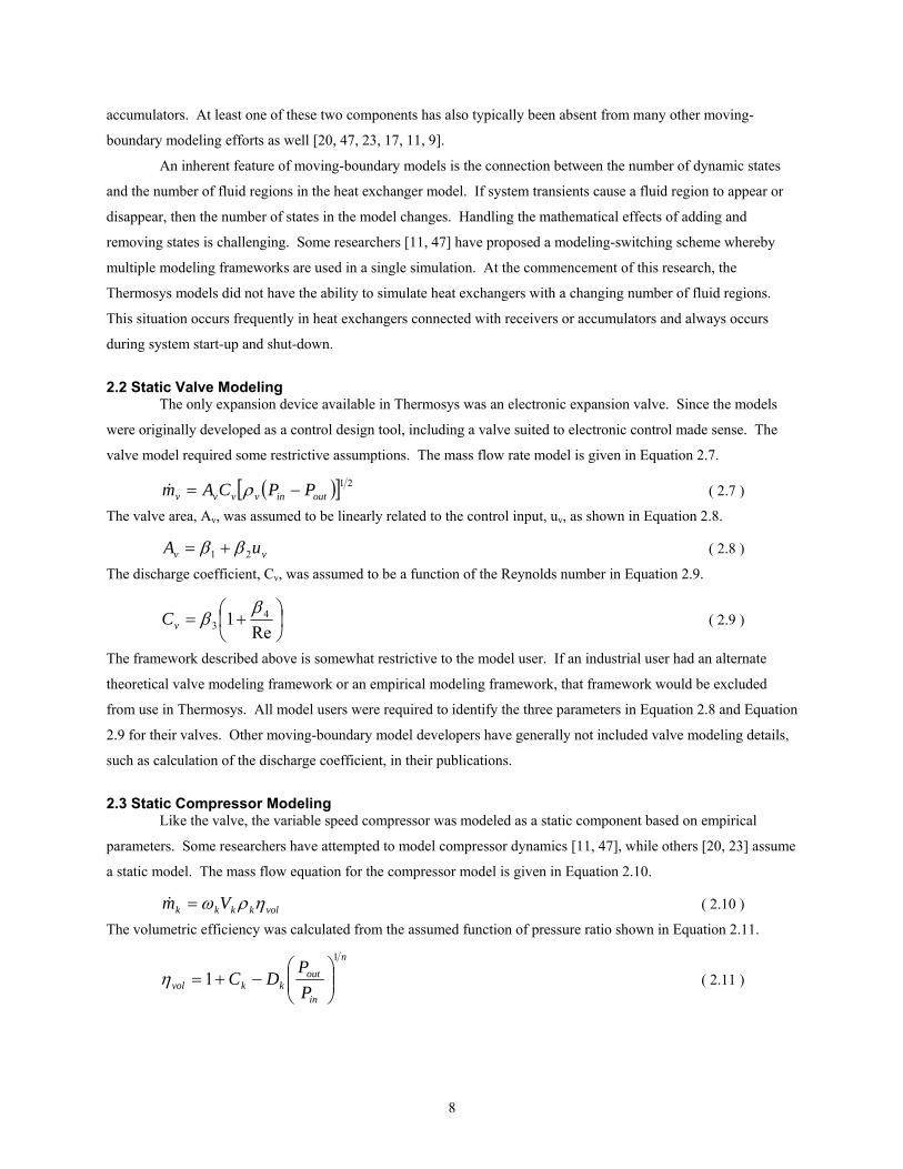
3.1.2 Sources of Empirical Heat Transfer Data A heat exchanger’s j factor data as a function of Reynolds number is typically presented graphically or in

tabular form, as in the classic work of Kays and London [25]. Figure 3.1 shows an example of a typical j factor vs.

Reynolds number plot. Correlations for determining the j factor of various heat exchanger geometries are available

in the literature.

12

103

10−2

Air−side Reynolds Number

j

Figure 3.1 The experimentally obtained j factor plot for surface CF-8.72 from [25]

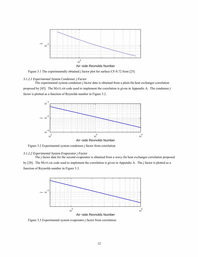
3.1.2.1 Experimental System Condenser j Factor The experimental system condenser j factor data is obtained from a plain-fin heat exchanger correlation

proposed by [45]. The MATLAB code used to implement the correlation is given in Appendix A. The condenser j

factor is plotted as a function of Reynolds number in Figure 3.2.

102

103

104

10−3

10−2

10−1

Air−side Reynolds Number

j

Figure 3.2 Experimental system condenser j factor from correlation

3.1.2.2 Experimental System Evaporator j Factor The j factor data for the second evaporator is obtained from a wavy-fin heat exchanger correlation proposed

by [28]. The MATLAB code used to implement the correlation is given in Appendix A. The j factor is plotted as a

function of Reynolds number in Figure 3.3.

103

104

10−2

Air−side Reynolds Number

j

Figure 3.3 Experimental system evaporator j factor from correlation

13

3.1.3 Implementation in Thermosys During simulation of a heat exchanger, the mass flow rate of air is assumed to be a known input. Using this

mass flow rate, an air-side Reynolds number is calculated and used to find a j factor value from the experimental

data. The Reynolds number is found from Equation 3.4.

μhDG ⋅

=Re ( 3.4 )

The air viscosity, μ, is found from a lookup table with an average air temperature input. The hydraulic diameter, Dh,

is a property of the heat exchanger geometry as defined in Equation 3.5.

AA

LD ch ⋅= 4 ( 3.5 )

The flow length, L, is defined as the distance the air travels through the heat exchanger from the leading edge of the

first row of tubes to the leading edge of an additional fictitious row of tubes located at one longitudinal tube pitch

behind the last row of tubes. For example, in Figure 3.4, the heat exchanger flow length would be L = 3 inches.

Leading tube row Last tube row Fictitious tube row

1" 1" 1"

Figure 3.4 Example calculation of heat exchanger flow length

The parameter A in Equation 3.5 is the total heat transfer area. In a tube-and-fin heat exchanger, this parameter

would be found from the combined surface area of all external tube walls and fins. The parameter Ac is the

minimum free flow area. To determine this parameter, first find the plane in the heat exchanger where air flow is

the most constricted. At this plane, subtract the cross-sectional area of all flow obstructions (tubes and fins) from

the total frontal area of the heat exchanger. An example is given in Figure 3.5.

14

Plane of maximumflow constriction

Subtract these cross-sectional

areas from the total frontal area

Figure 3.5 Plane of maximum flow constriction used in calculation of the minimum free flow area

Unfortunately, the hydraulic diameter (Equation 3.5) is not used consistently in the literature. Some

authors prefer to develop correlations based on the collar diameter, such as the correlation [28] used for the

experimental system’s second evaporator. The collar diameter is defined in Equation 3.6, where oD is the tube

outside diameter and fδ is the fin thickness.

foc DD δ2+= ( 3.6 )

The simulation Reynolds number must be calculated from the same diameter, hD or cD , that was used to reduce

experimental heat transfer data to a j factor correlation.

Returning to Equation 3.4, the only remaining parameter to be calculated is G, the maximum mass velocity.

This parameter is found from Equation 3.7.

fr

air

Am

G⋅

=σ&

( 3.7 )

Afr is the frontal area and σ, the constriction ratio, is the ratio of the minimum free flow area, Ac, to the frontal area.

An empirically-based external heat transfer coefficient is calculated from Equation 3.3 at each time step of

the simulation. A Simulink block diagram of the calculations carried out in Thermosys is shown in Figure 3.6.

15

Figure 3.6 Block diagram of heat transfer coefficient calculation from j factor data

The j factor and Reynolds number data points for a variety of heat exchanger geometries from [25] are

stored in a MATLAB data structure called HX. The structure also contains the geometric information necessary for

calculating a heat transfer coefficient from the j factor. The structure fields and their contents are summarized in

Table 3.1. Thermosys developers and users can easily add additional data to the HX structure.

Table 3.1 Fields in the HX data structure

Field Name Field Contents Core name of the core geometry assigned by Kays and London Num number indicating the location of the heat exchanger in the HX structure

Redat row vector of Reynolds number data points jHdat row vector of j factor data points sigma the constriction ratio

Dh the air-side hydraulic diameter

Results presented in Chapter 7 demonstrate the increase in system level model accuracy obtained by using

this semi-empirical modeling approach in the heat exchangers. Incorporating empirical results in this fashion

improves model fidelity without increasing the dynamic complexity of the model.

3.2 Performance Mapping The performance mapping approach presented here is based on the availability of large amounts of

component experimental data. The data is used to characterize the key parameters in the mass flow models with

performance maps. Performance maps can also be generated from other modeling frameworks. For example, if a

strictly first-principles approach is used to model a component, then the model output could be treated as data and

used to generate a performance map. Figure 3.7 shows the range of valve and compressor settings used to generate

16

the electronic expansion valve performance map and the compressor efficiency maps for the experimental system

described in Chapter 6. The operating conditions produced by these inputs are shown in Figure 3.8. Similar inputs

are used to generate data for mapping the other components described in this section. The experimental system that

is the source of the performance mapping data is described in Chapter 6.

6 8 10 12 14 16 180

500

1000

1500

2000

2500

3000

Valve Opening [%]

RP

M

Low

Eva

pora

tor

Pre

ssur

e

Low Evaporator Superheat

High Compressor Power

Figure 3.7 Compressor speed and valve opening settings

1.5 2 2.5 3 3.5 4 4.5 5 5.5 60

500

1000

1500

2000

2500

3000

(Pko

/Pki

) [kPa]

RP

M

6 8 10 12 14 16 18250

300

350

400

450

500

550

600

650

700

Valve Opening [%]

ΔP [

kPa]

100 150 200 250 300 350 400 450650

700

750

800

850

900

950

1000

Pe [kPa]

Pc [

kPa]

Figure 3.8 Range of operating conditions covered by performance maps

17

The changes in system inputs should be sufficiently slow that each operating condition can be considered nearly

steady-state. The steady-state operating conditions should cover the feasible range of high side and low side

pressures for the system.

The mapping approach discussed here provides greater flexibility to the model user when compared to the

equation-based approach previously implemented in Thermosys. If a user has an existing model, it can be utilized in

Thermosys by simply converting it to a performance map form. The only restriction is that the user model has the

same inputs as the Thermosys performance map. The performance mapping approach is applied to valve flow

coefficients and compressor volumetric and adiabatic efficiencies.

3.2.1 Valves Thermosys valve models provide a mass flow rate for the condenser outlet and the evaporator inlet. Due to

time scale separation [41], the valve mass flow may be modeled with algebraic relationships. The basic valve mass

flow model is given in Equation 3.8. Assuming a sharp orifice, the models presented here use n = 2 in Equation 3.8.

The main challenge of modeling the valves is determining the discharge coefficient, Cv.

( )[ ] noutinvvvv PPCAm

1−= ρ& ( 3.8 )

The orifice tube and the capillary tube have a fixed valve opening area. The thermostatic expansion valve

(TEV), automatic expansion valve (AEV), and electronic expansion valve (EEV) have a variable valve opening

area. The variable area valves are differentiated by the means of controlling the valve opening area. In situations

where the valve area is variable or unknown, the valve area and discharge coefficient are lumped into a single

parameter referred to as the valve flow coefficient, Cf.

( )outinvfv PPCm −= ρ& ( 3.9 )

Solve Equation 3.9 for the flow coefficient to obtain Equation 3.10.

( )outinv

vf PP

mC

−=

ρ&

( 3.10 )

If the valve area is known, the discharge coefficient may be obtained directly from Equation 3.11.

( )outinvv

vv PPA

mC

−=

ρ&

( 3.11 )

Using experimental measurements of mass flow rate, inlet refrigerant density, inlet pressure, and outlet pressure, the

flow coefficient or discharge coefficient is calculated for a large number of steady-state operating conditions.

Once the flow coefficient data points are obtained, an equation model is then fit to the data. This equation

fitting is carried out using a least-squares linear regression method. The best fit equation is then used to generate a

lookup table for implementation in Thermosys. The quality of the model may be judged by such metrics as the

RMS error between model coefficients and data coefficients or the R2 value returned by MATLAB’s linear regression

command.

3.2.1.1 Mapping Procedure for the Electronic Expansion Valve The valve opening area of the EEV is typically controlled by a stepper motor. The precise relationship

between stepper motor position and valve area is often unknown. Therefore, the flow coefficient is used in place of

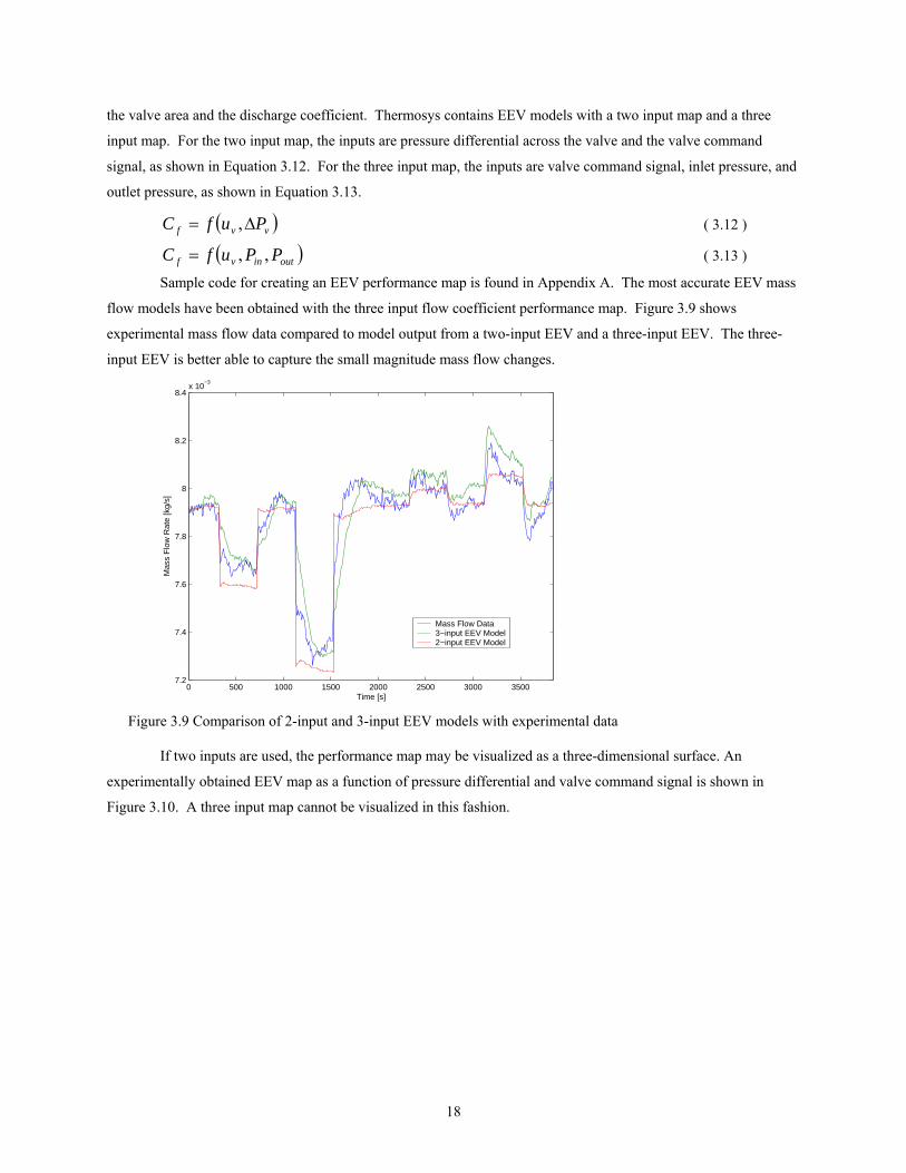
18

the valve area and the discharge coefficient. Thermosys contains EEV models with a two input map and a three

input map. For the two input map, the inputs are pressure differential across the valve and the valve command

signal, as shown in Equation 3.12. For the three input map, the inputs are valve command signal, inlet pressure, and

outlet pressure, as shown in Equation 3.13.

( )vvf PufC Δ= , ( 3.12 )

( )outinvf PPufC ,,= ( 3.13 )

Sample code for creating an EEV performance map is found in Appendix A. The most accurate EEV mass

flow models have been obtained with the three input flow coefficient performance map. Figure 3.9 shows

experimental mass flow data compared to model output from a two-input EEV and a three-input EEV. The three-

input EEV is better able to capture the small magnitude mass flow changes.

0 500 1000 1500 2000 2500 3000 35007.2

7.4

7.6

7.8

8

8.2

8.4x 10

−3

Time [s]

Mas

s F

low

Rat

e [k

g/s]

Mass Flow Data3−input EEV Model2−input EEV Model

Figure 3.9 Comparison of 2-input and 3-input EEV models with experimental data

If two inputs are used, the performance map may be visualized as a three-dimensional surface. An

experimentally obtained EEV map as a function of pressure differential and valve command signal is shown in

Figure 3.10. A three input map cannot be visualized in this fashion.

19

200300

400500

600700

6

8

10

12

14

16

180

2

4

6

8

10

12

14

(Pvi

−Pvo

) [kPa]Valve Opening [%]

Flo

w C

oef

fici

ent

[10−6

]

Cf (10−6) = (−9.5984) + (2.0481)u

v + (0.0054106)ΔP + (−0.00074909)u

vΔP + (−0.037775)u

v2

Figure 3.10 Flow coefficient map for an EEV with black points representing experimental data

3.2.1.1 Mapping Procedure for the Automatic Expansion Valve Automatic expansion valves maintain a constant pressure in either the evaporator or the condenser,

depending on the type of valve used. In order to maintain constant pressure, the valve opening area is based on the

force balance of a spring and the inlet or outlet pressure on a diaphragm. Therefore, the inlet or outlet pressure is

roughly equivalent to the valve command signal in the EEV. Figure 3.11 shows a schematic of an AEV with the

spring, diaphragm, and refrigerant flow path visible.

Figure 3.11 Schematic of an AEV [1]

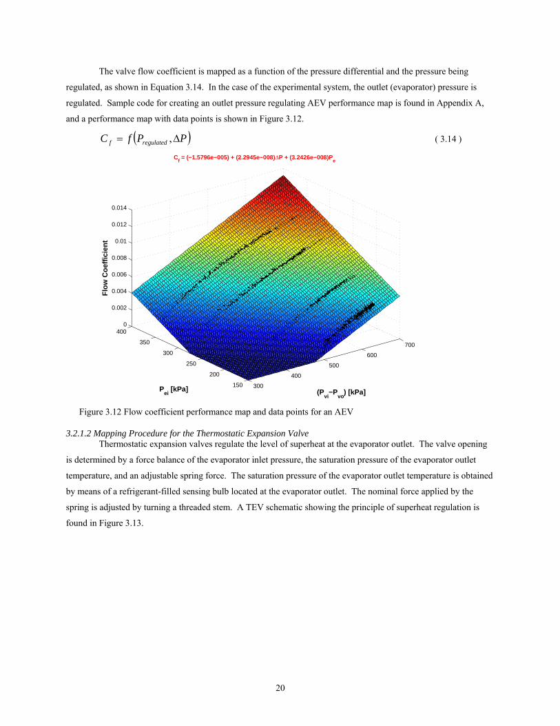
20

The valve flow coefficient is mapped as a function of the pressure differential and the pressure being

regulated, as shown in Equation 3.14. In the case of the experimental system, the outlet (evaporator) pressure is

regulated. Sample code for creating an outlet pressure regulating AEV performance map is found in Appendix A,

and a performance map with data points is shown in Figure 3.12.

( )PPfC regulatedf Δ= , ( 3.14 )

300

400

500

600

700

150

200

250

300

350

4000

0.002

0.004

0.006

0.008

0.01

0.012

0.014

(Pvi

−Pvo

) [kPa]Pei

[kPa]

Cf = (−1.5796e−005) + (2.2945e−008)ΔP + (3.2426e−008)P

e

Flo

w C

oef

fici

ent

Figure 3.12 Flow coefficient performance map and data points for an AEV

3.2.1.2 Mapping Procedure for the Thermostatic Expansion Valve Thermostatic expansion valves regulate the level of superheat at the evaporator outlet. The valve opening

is determined by a force balance of the evaporator inlet pressure, the saturation pressure of the evaporator outlet

temperature, and an adjustable spring force. The saturation pressure of the evaporator outlet temperature is obtained

by means of a refrigerant-filled sensing bulb located at the evaporator outlet. The nominal force applied by the

spring is adjusted by turning a threaded stem. A TEV schematic showing the principle of superheat regulation is

found in Figure 3.13.

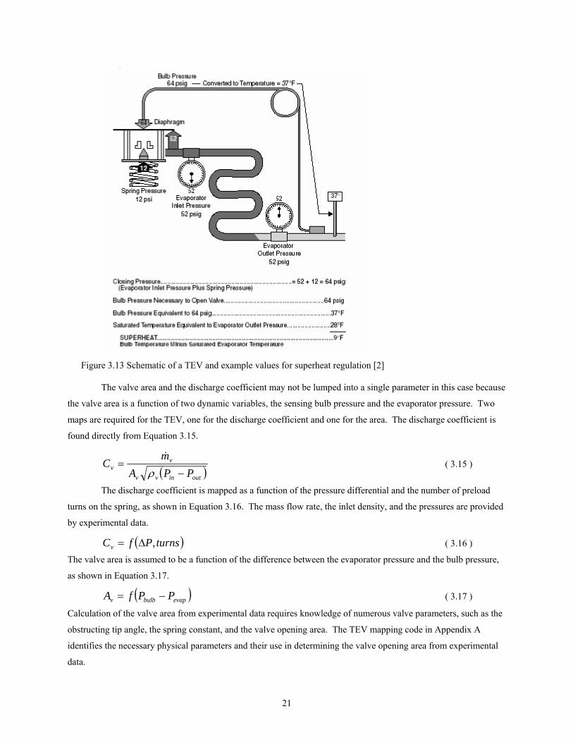
21

Figure 3.13 Schematic of a TEV and example values for superheat regulation [2]

The valve area and the discharge coefficient may not be lumped into a single parameter in this case because

the valve area is a function of two dynamic variables, the sensing bulb pressure and the evaporator pressure. Two

maps are required for the TEV, one for the discharge coefficient and one for the area. The discharge coefficient is

found directly from Equation 3.15.

( )outinvv

vv PPA

mC

−=

ρ&

( 3.15 )

The discharge coefficient is mapped as a function of the pressure differential and the number of preload

turns on the spring, as shown in Equation 3.16. The mass flow rate, the inlet density, and the pressures are provided

by experimental data.

( )turnsPfCv ,Δ= ( 3.16 )

The valve area is assumed to be a function of the difference between the evaporator pressure and the bulb pressure,

as shown in Equation 3.17.

( )evapbulbv PPfA −= ( 3.17 )

Calculation of the valve area from experimental data requires knowledge of numerous valve parameters, such as the

obstructing tip angle, the spring constant, and the valve opening area. The TEV mapping code in Appendix A

identifies the necessary physical parameters and their use in determining the valve opening area from experimental

data.

22

For simulation purposes, a time constant, τbulb, is needed to account for the dynamic associated with the

transfer of energy from the evaporator outlet refrigerant through the pipe wall to the sensing bulb. During

simulation, the bulb pressure is found by integrating the bulb pressure derivative, shown in Equation 3.18. The bulb

time constant, which is chosen by the user, is not needed in the mapping process because steady-state data is used to

generate the maps.

( )bulb

bulboutevapsatbulb

PTPP

τ−

= ,& ( 3.18 )

The sample code in Appendix A uses valve geometry and parameter assumptions to generate a discharge coefficient

map and an area map. The sample code approach loosely follows that of [31].

A discharge coefficient map generated using the assumed valve parameters is shown in Figure 3.14; the

corresponding valve area map is shown in Figure 3.15. The sample maps may not be a numerically accurate

reflection of the system TEV, but the qualitative behavior should be captured by the model. Finding TEV physical

parameters is a non-trivial challenge. Manufacturers generally do not provide detailed valve geometry. For that

reason, the Thermosys TEV model has not been validated.

200

300

400

500

600

700

6

7

8

9

10

11

0

0.2

0.4

0.6

0.8

1

Number of TurnsPressure Differential [kPa]

Cd = (0.46662) + (0.002973)ΔP + (−1.9067e−006)ΔP2 + (−0.095859)Turns

Dis

char

ge

Co

effi

cien

t

Figure 3.14 TEV discharge coefficient performance map and generating data

23

60 80 100 120 140 160 180 2000.4

0.6

0.8

1

1.2

1.4

1.6x 10

−5

Pbulb

− Pevap

[kPa]

Are

a m

2

Figure 3.15 TEV area map

3.2.1.3 Mapping Procedure for Fixed Area Expansion Devices Capillary tubes and orifice tubes are fixed area expansion devices. If the valve area is known, the discharge

coefficient can be calculated from Equation 3.15. If the valve area is unknown, the flow coefficient is used as with

the other valve models. In either case, the performance map is a function of the pressure differential across the

expansion device.

( )PfC fd Δ=, ( 3.19 )

Sample code for generating a capillary/orifice tube performance map is found in Appendix A for the unknown area

case. Figure 3.16 below shows an example of a capillary tube flow coefficient map.

24

250 300 350 400 450 500 550 600 650 700

5.6

5.8

6

6.2

6.4

6.6

6.8

7

7.2

7.4

(Pvi

−Pvo

) [kPa]

Flo

w C

oef

fici

ent

Cf = (0.018742) + (−7.7665e−005)ΔP + (1.4969e−007)ΔP2 + (−8.9518e−011)ΔP3

Figure 3.16 Capillary tube flow coefficient data points and best fit performance map

3.2.2 Compressor The Thermosys compressor model provides a mass flow rate for the evaporator outlet and a mass flow rate

and enthalpy for the condenser inlet. As with the expansion devices, the compressor is generally considered to be a

static component. The compressor mass flow rate is modeled by Equation 3.20, where Vk is the compressor

displacement volume per revolution, ωk is the compressor speed, ρk is the inlet density, and ηvol is the compressor

volumetric efficiency.

volkkkk Vm ηρω=& ( 3.20 )

The outlet enthalpy is based on an adiabatic efficiency, as shown in Equation 3.21, where hout,isentropic is the

outlet enthalpy assuming isentropic compression, hin is the inlet enthalpy, and ηa is the compressor adiabatic

efficiency.

( )[ ]11, −+= ainisentropicout

aout hhh η

η ( 3.21 )

Determining the volumetric and adiabatic efficiency is the main challenge of compressor modeling. The

flexible performance map approach is again applied to find the best model over a large range of operating

conditions.

25

3.2.2.1 Mapping Procedure for Volumetric Efficiency Equation 3.20 may be solved for volumetric efficiency. Given steady-state measurements of mass flow rate

and inlet density, Equation 3.22 allows for the calculation of volumetric efficiency values. The steady-state

measurements should cover the expected range of high side and low side pressures for the system.

kkk

kvol V

mρω

η&

= ( 3.22 )

Thermosys contains two-input and three-input performance map compressor models. In the two-input model, the

volumetric efficiency is a function of the pressure ratio across the compressor and the compressor speed, as shown

in Equation 3.23. The volumetric efficiency of the three-input model is assumed to be a function of the compressor

speed, the inlet pressure, and the outlet pressure, as shown in Equation 3.24. Sample code for the creation of a

three-input volumetric efficiency map is found in Appendix A. The three input performance map cannot be

visualized, but a two input map with generating data is shown in Figure 3.17.

( )krvol Pf ωη ,= ( 3.23 )

( )outinkvol PPf ,,ωη = ( 3.24 )

12

34

56

0

1000

2000

30000.2

0.4

0.6

0.8

1

(Pko

/Pki

) [kPa]RPM

+ (3.0221e−005)*RPM*Pr + (−1.1905e−007)*RPM2 + (−0.0081256)*P

r2

ηvol

= (0.65127) + (0.00027681)*RPM + (−0.031338)*Pr

η vol

Figure 3.17 A two input performance map of volumetric efficiency

3.2.2.2 Mapping Procedure for Adiabatic Efficiency Equation 3.21 may be solved for adiabatic efficiency to obtain Equation 3.25.

inout

inisentropicouta hh

hh−

−= ,η ( 3.25 )

Using steady-state measurements of inlet enthalpy, outlet enthalpy, and the calculated isentropic outlet enthalpy, this

equation provides a means for calculating adiabatic efficiency values. As with the volumetric efficiency, the

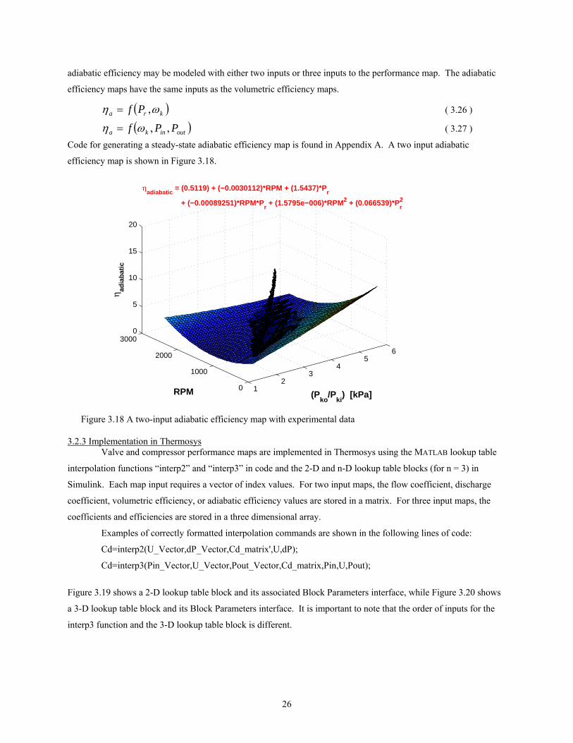
26

adiabatic efficiency may be modeled with either two inputs or three inputs to the performance map. The adiabatic

efficiency maps have the same inputs as the volumetric efficiency maps.

( )kra Pf ωη ,= ( 3.26 )

( )outinka PPf ,,ωη = ( 3.27 )

Code for generating a steady-state adiabatic efficiency map is found in Appendix A. A two input adiabatic

efficiency map is shown in Figure 3.18.

12

34

56

0

1000

2000

30000

5

10

15

20

(Pko

/Pki

) [kPa]RPM

+ (−0.00089251)*RPM*Pr + (1.5795e−006)*RPM2 + (0.066539)*P

r2

ηadiabatic

= (0.5119) + (−0.0030112)*RPM + (1.5437)*Pr

η adia

bat

ic

Figure 3.18 A two-input adiabatic efficiency map with experimental data

3.2.3 Implementation in Thermosys Valve and compressor performance maps are implemented in Thermosys using the MATLAB lookup table

interpolation functions “interp2” and “interp3” in code and the 2-D and n-D lookup table blocks (for n = 3) in

Simulink. Each map input requires a vector of index values. For two input maps, the flow coefficient, discharge

coefficient, volumetric efficiency, or adiabatic efficiency values are stored in a matrix. For three input maps, the

coefficients and efficiencies are stored in a three dimensional array.

Examples of correctly formatted interpolation commands are shown in the following lines of code:

Cd=interp2(U_Vector,dP_Vector,Cd_matrix',U,dP);

Cd=interp3(Pin_Vector,U_Vector,Pout_Vector,Cd_matrix,Pin,U,Pout);

Figure 3.19 shows a 2-D lookup table block and its associated Block Parameters interface, while Figure 3.20 shows

a 3-D lookup table block and its Block Parameters interface. It is important to note that the order of inputs for the

interp3 function and the 3-D lookup table block is different.

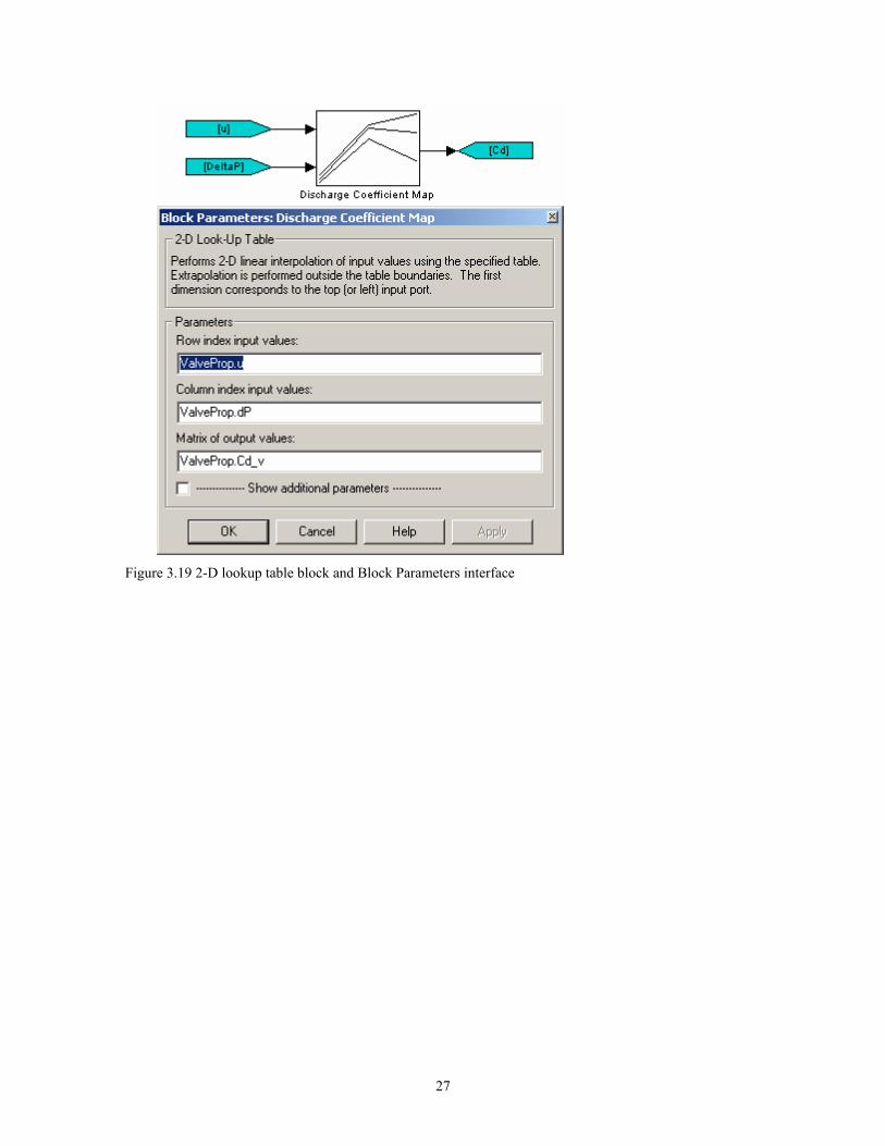
27

Figure 3.19 2-D lookup table block and Block Parameters interface

28

Figure 3.20 3-D lookup table block and Block Parameters interface

Flow coefficients, efficiencies, and input index vectors are stored in MATLAB data structures. For use in

simulation, the data structures are first loaded into the MATLAB workspace. Then the appropriate data structure field

names are entered in the component GUI, as shown in Figure 3.21 below. The GIU m-file loads the field names into

the Block Parameters interface of the blocks in the Simulink model.

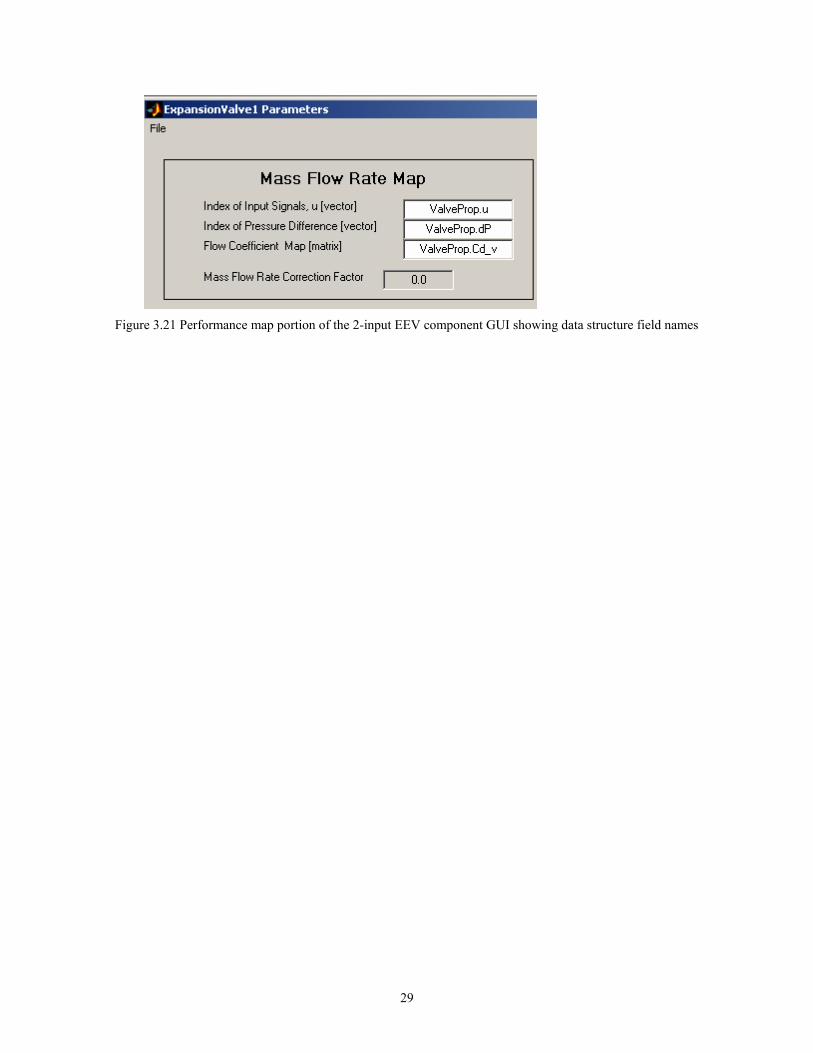
29

Figure 3.21 Performance map portion of the 2-input EEV component GUI showing data structure field names

30

Chapter 4. Atmospheric Conditions Modeling

Original Thermosys heat exchanger air-side mass and energy balances assumed dry air entering the heat

exchangers. This chapter details the model modifications necessary to take into account the effects of the water

vapor which is nearly always present to some degree in atmospheric air. Two modeling approaches are presented.

The first approach is based on condensation occurring when the bulk air temperature reaches the dew point. The

second approach assumes that condensation begins when the heat exchanger wall temperature reaches the dew point.

The mass and energy balances follow from the discussion in [7].

Some equations appearing in the derivations represent fluid property functions. Due to the complex nature

of the functions, they are not given explicitly in this thesis. For simulation purposes, the fluid property functions are

implemented as lookup tables in Thermosys. The data contained in the tables was generated from the fluid property

functions provided with the software package Engineering Equation Solver (EES) [29]. The EES documentation

contains the details of the specific equations of state used for the various fluid properties. Plots for two common

fluid properties, saturation pressure as a function of saturation temperature and saturated liquid enthalpy as a

function of temperature, are shown in Figure 4.1 and Figure 4.2.

−80 −60 −40 −20 0 20 40 60 80 100 1200

50

100

150

Temperature [C]

Pre

ssur

e [k

Pa]

Figure 4.1 Water saturation pressure as a function of saturation temperature

−80 −60 −40 −20 0 20 40 60 80 100 120−500

0

500

Temperature [C]

Ent

halp

y [k

J/kg

]

.

Figure 4.2 Water saturated liquid enthalpy as a function of temperature

4.1 Air Temperature Condensation Method The air temperature condensation method assumes that condensation occurs when the bulk average air

temperature is lower than the dew point. This highly idealized model does not take into account the spatial variation

of air temperatures around the heat exchanger.

31

4.1.1 Modified Energy Balances To properly model air-side behavior, mass and energy balances should take into account both air and water

vapor entering the evaporator. Two distinct situations are possible. Water vapor may pass through the evaporator

either with or without some condensation on the surface of the evaporator. The two conditions require different

mass and energy balances. The non-condensing equations are presented first.

4.1.1.1 Non-condensing Conditions Figure 4.3 shows a control volume containing the air around an evaporator. Air enters and exits the control

volume at a known rate, airm& . The inlet temperature, inlet enthalpy, and inlet relative humidity of the air are known

quantities. Heat is transferred from the air to the evaporator wall. The variables to be determined are the outlet

temperature, the outlet enthalpy, and the outlet relative humidity of the air. We assume that no condensation occurs

and that the outlet relative humidity is less than one. The conservation of mass is given in Equation 4.1. The

conservation of energy is given in Equation 4.2.

inairT ,

inair ,φ

inairoutair TT ,, <

1, <outairφ

inh outh

Figure 4.3 Control volume for humid air mass and energy balances under non-condensing conditions

outairinair mm ,, && = ( 4.1 )

( )outinairinwall hhmQ −= &&, ( 4.2 )

The inlet enthalpy is a combination of the dry air enthalpy and the enthalpy of water vapor in the air, as

shown in Equation 4.3. A constant specific heat assumption results in errors less than 0.2 percent between -10 and

50°C. The inlet absolute humidity is calculated from Equation 4.4. The enthalpy of the water vapor (in kJ/kg) is

approximated with Equation 4.5. The approximation error is again insignificant between -10 and 50°C. The inlet

saturation pressure of water is a function of the inlet air temperature, as shown in Equation 4.6. Thus, with

knowledge of inairT , and the ambient air pressure, the enthalpy of the air entering the control volume may be

determined.

ingininairairpin hTCh ,,, ω+= ( 4.3 )

32

inginair

inginin PP

P

,

,622.0φφ

ω−

= ( 4.4 )

inairing Th ,, 82.13.2501 += ( 4.5 )

( )inairsating TPP ,, = ( 4.6 )

The outlet enthalpy is calculated from the energy balance for air, as shown in Equation 4.7. The heat

transfer rate from the air to the evaporator is assumed to be a known quantity. As with the inlet air, the enthalpy of

the outlet air is found from the dry air enthalpy and the water vapor enthalpy. Recognizing that the non-

condensation condition implies that the inlet and outlet absolute humidity are equivalent, Equation 4.8 is obtained

for the outlet enthalpy. Substituting the water vapor enthalpy approximation yields Equation 4.9. Solving for the

outlet air temperature gives Equation 4.10.

air

inwallinout m

Qhh

&

&,−= ( 4.7 )

outginoutairairpout hTCh ,,, ω+= ( 4.8 )

( )outairinoutairairpout TTCh ,,, 82.13.2501 ++= ω ( 4.9 )

inairp

inoutoutair C

hT

ωω

82.13.2501

,, +

−= ( 4.10 )

The outlet saturation pressure is a function of the outlet air temperature, as in Equation 4.11. Using this

pressure, the outlet relative humidity is found from Equation 4.12.

( )outairsatoutg TPP ,, = ( 4.11 )

( )inoutg

airinout P

Pω

ωφ

+=

622.0,

( 4.12 )

Equations 4.7, 4.10, and 4.12 give the three outlet variables of interest. As a final step, the outlet air

temperature is compared to the dew point temperature to verify that the non-condensation assumption is correct.

The dew point is the saturation temperature of water at the water vapor partial pressure. The water vapor partial

pressure is given in Equation 4.13. The dew point is then a function of the partial pressure, as shown in Equation

4.14. If the outlet air temperature is above the dew point, the non-condensation assumption is correct.

inginv PP ,φ= ( 4.13 )

( )vsatdp PTT = ( 4.14 )

4.1.1.2 Condensing Conditions Figure 4.4 shows a control volume for humid air under condensing conditions. The two major differences

between this control volume and the non-condensing conditions control volume are the saturated air outlet condition

and the presence of liquid water leaving the control volume. The liquid water is assumed to have the same

temperature as the outlet air. The conservation of mass equation for the air is given in Equation 4.1. The

conservation of mass for water is given in Equation 4.15, and the conservation of energy is found in Equation 4.16.

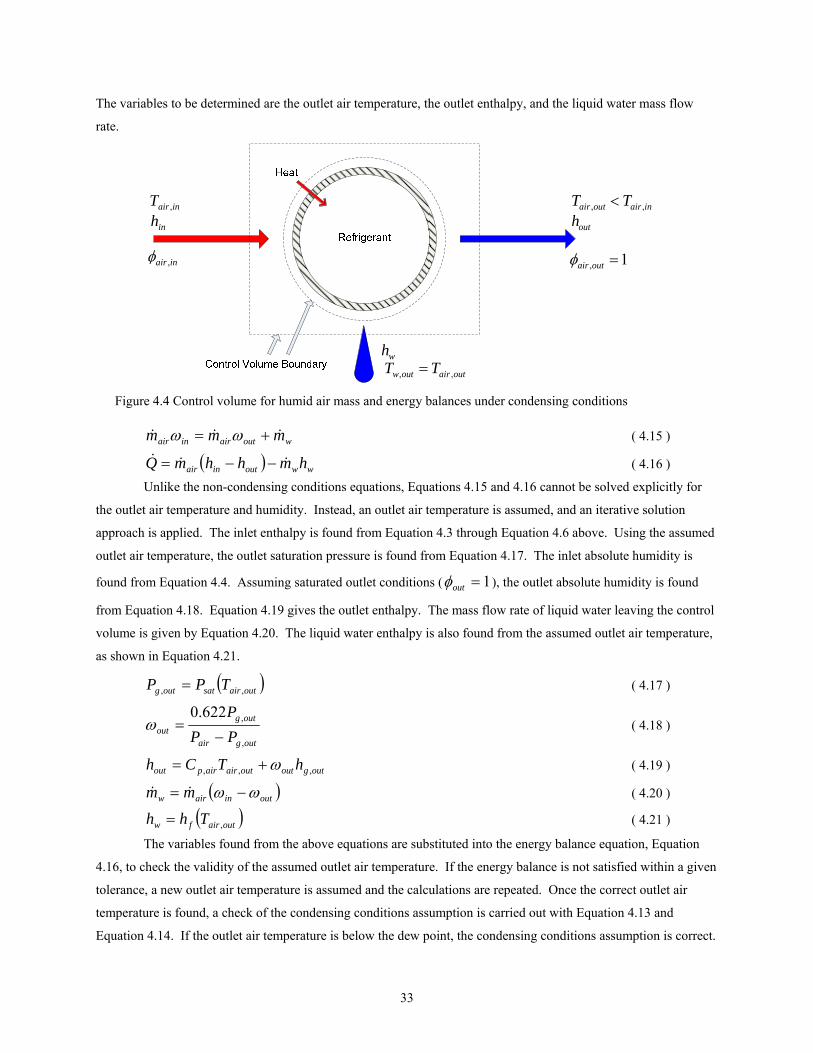
33

The variables to be determined are the outlet air temperature, the outlet enthalpy, and the liquid water mass flow

rate.

inairT ,

inair ,φ

inairoutair TT ,, <

1, =outairφ

inh outh

whoutairoutw TT ,, =

Figure 4.4 Control volume for humid air mass and energy balances under condensing conditions

woutairinair mmm &&& += ωω ( 4.15 )

( ) wwoutinair hmhhmQ &&& −−= ( 4.16 )

Unlike the non-condensing conditions equations, Equations 4.15 and 4.16 cannot be solved explicitly for

the outlet air temperature and humidity. Instead, an outlet air temperature is assumed, and an iterative solution

approach is applied. The inlet enthalpy is found from Equation 4.3 through Equation 4.6 above. Using the assumed

outlet air temperature, the outlet saturation pressure is found from Equation 4.17. The inlet absolute humidity is

found from Equation 4.4. Assuming saturated outlet conditions ( 1=outφ ), the outlet absolute humidity is found

from Equation 4.18. Equation 4.19 gives the outlet enthalpy. The mass flow rate of liquid water leaving the control

volume is given by Equation 4.20. The liquid water enthalpy is also found from the assumed outlet air temperature,

as shown in Equation 4.21.

( )outairsatoutg TPP ,, = ( 4.17 )

outgair

outgout PP

P

,

,622.0−

=ω ( 4.18 )

outgoutoutairairpout hTCh ,,, ω+= ( 4.19 )

( )outinairw mm ωω −= && ( 4.20 )

( )outairfw Thh ,= ( 4.21 )

The variables found from the above equations are substituted into the energy balance equation, Equation

4.16, to check the validity of the assumed outlet air temperature. If the energy balance is not satisfied within a given

tolerance, a new outlet air temperature is assumed and the calculations are repeated. Once the correct outlet air

temperature is found, a check of the condensing conditions assumption is carried out with Equation 4.13 and

Equation 4.14. If the outlet air temperature is below the dew point, the condensing conditions assumption is correct.

34

4.1.2 Heat Transfer Rates 4.1.2.1 Non-condensing Conditions

The equation for inwallQ ,& is dependent on the presence or absence of condensation. Under non-condensing

conditions, the heat transfer rate to the heat exchanger wall is found from Equation 4.22, where oα is the air-side

heat transfer coefficient, oA is the external heat exchanger area, aT is the average air temperature, and wT is the

lumped wall temperature.

( )waooinwall TTAQ −= α,& ( 4.22 )

4.1.2.2 Condensing Conditions If condensation is occurring, the original heat transfer equation, Equation 4.22, must be modified to account

for the energy released by the phase change of water from a vapor to a liquid. The result is Equation 4.23. The

latent heat, fgh , is found at the average air temperature, aT .

( ) fgwwaooinwall hmTTAQ && +−= α, ( 4.23 )

4.1.2.3 Wet Conditions Heat Transfer Coefficients The presence of water droplets or a film of water on the evaporator changes the air-side heat transfer

characteristics. Korte and Jacobi (2001) [30] studied plain fin heat exchangers under wet conditions. They found

that there were clear trends when comparing dry and wet j factor data, but the differences were almost within the

experimental uncertainty. Mirth and Ramadhyani [35] studied wavy fin heat exchangers. They found that the effect

of condensation on the air-side heat transfer coefficient was unclear. Sometimes the wet surface heat transfer

coefficients were higher than the dry surface coefficients. Sometimes the relationship was reversed. The authors

claimed to demonstrate that “it is possible to predict heat transfer rates under a wide range of wet-surface conditions

with good accuracy using only dry-surface heat transfer correlations.” Based on the findings of these researchers,

adjustments to heat transfer coefficients under wet conditions are not included in the Thermosys model.

4.1.3 Implementation in Thermosys The humid air functionality requires the user to supply the model with the inlet air temperature and the inlet

relative humidity at the initial condition and at each subsequent time step. In addition, the user must supply an

initial condition for the outlet air temperature. The ambient air pressure and the specific heat of air are assumed to

be constants. The evaporator with humid air is implemented in a new, and as yet unreleased, version of Thermosys

referred to as Thermosys Academic. In Thermosys Academic, the component models are based on MATLAB

functions rather than Simulink block diagrams. This shift to code-based component models facilitates the

incorporation of new, more complex models such as the evaporator with humid air.

The humid air outlet conditions solution is divided into two sections of code, a non-condensing section and

a condensing section. The two sections are contained within a while loop. When one of the two sections

successfully finds an outlet air temperature and verifies the condensing or non-condensing assumption, a flag is set

to force an exit from the while loop. The code also sets a flag that indicates which assumption (non-condensing or

condensing) to try first on the next iteration. For instance, if the current time step finds condensing conditions, the

next time step will execute the condensing section first.

35

The iterative solution of the condensing conditions energy balance is carried out with the fmincon function,

part of the Control Systems Toolbox. The initial guess for the outlet air temperature is the outlet air temperature

found from the previous time step. The energy balance equation, Equation 4.24Error! Reference source not

found., is found by combining Equation 4.16 and Equation 4.23. The objective function for the minimization,

Equation 4.25, is found by squaring the left side of Equation 4.24.

( ) ( ) ( ) 0=−−+−− waoofgwwoutina TTAhhmhhm α&& ( 4.24 )

( ) ( ) ( )( )2waoofgwwoutina TTAhhmhhmF −−+−−= α&& ( 4.25 )

The iterative approach to solving the condensing conditions energy balances and to determining the condensing

condition does not produce a noticeable slow-down in simulation speed.

4.2 Wall Temperature Condensation Method Initial validation of the air temperature condensation method revealed that condensation occurred on the

experimental evaporator when the outlet air temperature, and therefore the bulk average air temperature, was above

the dew point. For example, the plot in Figure 4.5 shows dew point and outlet air temperature data for a test during

which condensation was observed in the evaporator.

100 150 200 250

10

12

14

16

Time [s]

Tem

pera

ture

[C] Dew Point

Outlet Air

Figure 4.5 Data for a condensing conditions test with the air temperature well above the dew point temperature

This observation indicated that significant spatial air temperature variations were present in the heat exchanger. For

this condition, which is common in compact heat exchangers, the air temperature condensation model is inadequate

because it will not accurately predict the onset of condensing conditions. To address this inadequacy, an evaporator

model was created that assumes a condensing condition when the heat exchanger wall temperature is less than the

dew point. In this model, a mass transfer coefficient is used to determine the condensate mass flow rate. In

addition, the model incorporates a higher level of detail by considering condensation in the different fluid regions of

the evaporator. The general control volumes are the same as those used in the previous derivation, but they are

separated by region, as shown in Figure 4.6. The control volume boundaries contain the air surrounding the heat

exchanger and are only used for derivation purposes.

36

airm&

1,airm& 2,airm&

inairT ,inω

2,outω1,outω

inh

2,outh1,outh

outh outω outairT ,

1,,inwallQ 2,,inwallQ

1,wm& 2,wm&1,wh 2,wh

Figure 4.6 Divided air-side control volumes

4.2.1 Individual Region Mass and Energy Balances As with the previous modeling approach, the model outputs of interest are the heat exchanger outlet air

temperature and outlet relative humidity, which are obtained from the outlet enthalpy and the outlet absolute

humidity. The outlet enthalpy in each region is found by rearranging the energy balance equation, Equation 4.16.

This equation was previously used only for condensing conditions, but in this derivation it will be taken as a general

energy balance for both condensing and non-condensing conditions. The equation for outlet enthalpy is given in

Equation 4.26, where numeric subscripts denote individual fluid regions. The mass balance relations are given in

Equation 4.27 through Equation 4.29. The derivation assumes an evaporator with a two-phase region (1) and a

superheat region (2). Adding additional fluid regions to the derivation is trivial.

2,1,

2,1,,2,1,

2,1,

2,1,2,1,

air

inwallw

air

winout m

Qh

mm

hh&

&

&

&−−= ( 4.26 )

outairinairair mmm ,1,,1,1, &&& == ( 4.27 )

outairinairair mmm ,2,,2,2, &&& == ( 4.28 )

2,1, airairair mmm &&& += ( 4.29 )

Solution of Equation 4.26 requires an air mass flow rate across each region. The overall air mass flow rate

is divided into two parts based on the length of each region, as shown in Equation 4.30 and Equation 4.31.

37

airTotal

air mL

Lm && 11, = ( 4.30 )

airTotal

air mLLm && 2

2, = ( 4.31 )

The heat transfer rates, inwallQ ,& , are found in the manner previously described for the air temperature condensation

method derivation. Other key variables in Equation 4.26 are the mass flow rates of condensate leaving the control

volume. These mass flow rates are found from Equation 4.32. The determination of the outlet absolute humidity

terms is discussed in the following section.

( )inoutairw mm ωω −= 2,1,2,1,2,1, && ( 4.32 )

4.2.2 Outlet Humidity Calculations Equation 4.33 provides a relationship between the outlet absolute humidity and the air mass flow rate in

each region. The left hand side of Equation 4.33 gives the condensate mass flow rate based on the change in inlet

and outlet absolute humidity. The right hand side of Equation 4.33 gives the condensate mass flow rate based on a

mass transfer coefficient, a fin efficiency, and a log mean humidity difference. The log mean humidity difference

approach is taken from [34].

( ) ( ) ( )

⎟⎟⎟⎟⎟

⎠

⎞

⎜⎜⎜⎜⎜

⎝

⎛

⎟⎟⎠

⎞⎜⎜⎝

⎛

−

−

−−−=−

2,1,2,1,

2,1,

2,1,2,1,2,1,2,1,2,1,

lnwallout

outin

walloutwallinoominoutair Am

ωωωω

ωωωωηαωω& ( 4.33 )

Solving for the outlet absolute humidity yields Equation 4.34.

2,1,2,1,

2,1,

2,1,

2,1,wall

mA

wallinout

air

oom

e

ωωω

ωηα

+−

=⎟⎟⎠

⎞⎜⎜⎝

⎛

&

( 4.34 )

Under condensing conditions, the absolute humidity at the wall, ωwall, is the absolute humidity of saturated water at

the wall temperature. The humidity is assumed to be uniform around the tube. The external heat transfer area, Ao,

and the inlet absolute humidity, ωin, are known parameters.

The amount of mass transfer is governed by the mass transfer coefficient, αm. The mass transfer coefficient

is often assumed to be a function of the heat transfer coefficient [13]. Equation 4.35 for the mass transfer coefficient

assumes a Lewis number of one.

airpair

om C ,ρ

αα = ( 4.35 )

The specific heat of dry air is taken to be a constant at 1.005 kJ/kg-K, and the air density is considered to be a

function of temperature according to the ideal gas law.

The general expression for the overall surface effectiveness is given in Equation 4.36.

38

( )fino

fino A

Aηη −−= 11 ( 4.36 )

The fin efficiency parameter, ηfin, in Equation 4.36 requires detailed analysis of the heat exchanger geometry. The

following discussion is specific to wavy-fin heat exchangers similar to that of the experimental system and is taken

from [46]. Other heat exchanger geometries require different expressions for the fin efficiency. The wavy-fin

efficiency is calculated from Equation 4.37.

( )θθη

mrmr

fintanh

= ( 4.37 )

The parameter m is defined in Equation 4.38, and the parameter θ is defined in Equation 4.39.

finfin

o

km

δα2

= ( 4.38 )

⎥⎥⎦

⎤

⎢⎢⎣

⎡⎟⎟⎠

⎞⎜⎜⎝

⎛+⎟⎟

⎠

⎞⎜⎜⎝

⎛−=

rR

rR eqeq ln35.011θ ( 4.39 )

In Equation 4.38, kfin is the fin material conductivity and δfin is the fin thickness. The equivalent radius parameter is

given in Equation 4.40, where r is the tube inside radius which is also used in Equation 4.37.

5.0

3.027.1 ⎟⎟⎠

⎞⎜⎜⎝

⎛−=

M

LMeq X

XXR ( 4.40 )

Equation 4.40 contains two additional geometric parameters, XM and XL, which are defined in Equation 4.41 and

Equation 4.42. The parameters Pt and Pl are the transverse and longitudinal tube pitches, respectively.

2t

MP

X = ( 4.41 )

22

22lt

LPP

X +⎟⎠⎞

⎜⎝⎛= ( 4.42 )

4.2.3 Mixing of Region Outputs Once the humidity and enthalpy outputs from each region have been determined, a single lumped outlet

condition is found. Equation 4.43 for the adiabatic mixing of airstreams [7] relates the air mass flow rates and the

outlet conditions of each region to the mixed outlet conditions.

1,

2,

1,

2,

2,

1,

outout

outout

outout

woutout

air

air

hhhh

mm

−

−=

−

−=

ωωωω

&

& ( 4.43 )

Solving for the mixed outlet enthalpy yields Equation 4.44, while solving for the mixed outlet absolute humidity

gives Equation 4.45.

39

2,

1,

2,

1,1,2,

1air

air

air

airoutout

out

mm

mm

hhh

&

&

&

&

+

⎟⎟⎠

⎞⎜⎜⎝

⎛+

= ( 4.44 )

2,

1,

2,

1,1,2,

1air

air

air

airoutout

out

mm

mm

&

&

&

&

+

⎟⎟⎠

⎞⎜⎜⎝

⎛+

=

ωωω ( 4.45 )

The outlet air temperature is found from Equation 4.46 as a function of both the mixed enthalpy and absolute

humidity. The outlet relative humidity is found from Equation 4.47, where Pg,out was given in Equation 4.11.

Finally, the total condensate mass flow rate is the sum of the condensate mass flow rate found for each region, as

shown in Equation 4.48.

outairp

outoutoutair C

hT

ωω

82.13.2501

,, +

−= ( 4.46 )

( ) outgout

airoutout P

P

,622.0 ωω

φ+

= ( 4.47 )

2,1, www mmm &&& += ( 4.48 )

4.2.4 Implementation in Thermosys The general implementation is similar to that described previously for the air temperature condensation

model. The model inputs are the same, and the wall temperature condensation model is also implemented as a

MATLAB function.

The code that calculates air-side outlet conditions is divided into two sections, one for each fluid region.

The condensation condition in each region is first determined by checking the region wall temperature. If the wall

temperature is above the dew point, the region absolute outlet humidity is set equal to the inlet absolute humidity

and the region condensate mass flow rate is set to zero. The outlet condition is then found from Equation 4.26. If

the wall temperature is below the dew point, the region outlet absolute humidity is determined from Equation 4.34.

The condensate mass flow rate is found from Equation 4.32. Finally, the outlet enthalpy is again found from

Equation 4.26. Once the outlet conditions of each region have been determined, the lumped outlet enthalpy and

absolute humidity are found from Equation 4.44 and Equation 4.45. The outputs of interest, outlet air temperature,

outlet relative humidity, and condensate mass flow rate, are then calculated with Equation 4.46 through Equation

4.48. Unlike the air temperature condensation method, an iterative solution procedure is not required for the

condensing conditions case.

40

Chapter 5. Dynamic Modeling

5.1 Motivation The overall motivation for the developments described in this chapter is to improve the accuracy and

applicability of the Thermosys models through dynamic modeling techniques. Both first-principles and system

identification modeling techniques are applied, depending on the situation. The first-principles approach is applied

when the underlying physics is well understood, while the system identification approach is applied when the

appropriate model structure is unknown or overly complex. This chapter also examines possible future extensions to

dynamic simulation capabilities with emphasis on compressor cycling simulation.

5.1.1 Heat exchangers with Receivers/Accumulators Heat exchangers with receivers/accumulators are found in the majority of VCC systems. These critical

components were not included in previous distributions of Thermosys, severely limiting the types of systems and

operating conditions that could be modeled. While the modeling of these components is challenging in the moving-

boundary framework, employing a first-principles dynamic modeling approach gives the model developer the ability

to apply assumptions in the derivation process that allow the models to run under varying fluid phase outlet

conditions without using a model switching scheme. The new components are a necessary addition to Thermosys,

allowing for simulation of a large range of common systems and operating conditions.

5.1.2 Compressor Shell Capacitance The dynamic effects of the compressor shell thermal capacitance were not included in the original

compressor model. Early validation results revealed that the static compressor outlet enthalpy model output did not

match the experimental data. The static outlet enthalpy performance map accurately predicted the correct enthalpy

for a given operating condition, but it could not account for the transients associated with transitions between

operating conditions. A first-order dynamic model with a user-specified time constant was chosen as a means for

capturing the dynamic effects of the compressor shell thermal capacitance and slowing the response speed of the

model.

5.1.3 Dynamic Mass Flow Correction Model validation results also suggested that the inaccurate prediction of the compressor mass flow rate was

causing large errors in evaporator pressure and other model outputs. The mass flow rate errors could be caused by

inadequacy of the static compressor model or by unmodeled components and component interactions. The

compressor dynamic behavior is not well understood because the experimental system cannot directly measure the

compressor mass flow rate. Because the sources of the modeling errors are not well understood, a system

identification approach was applied. A combination of model output and system data was used to find a dynamic

compressor mass flow rate correction model.

5.1.4 Compressor Cycling Simulation A common control practice, and likely direction for future research, is compressor cycling. An analysis of

current compressor cycling simulation capabilities is presented. Compressor cycling drives models towards

conditions that violate the assumptions used in deriving the moving-boundary models. The results presented here

give comparisons of model output and system data to demonstrate that the models qualitatively capture system

41

behavior under compressor cycling conditions. The extent to which cycling conditions cause violations of the

modeling assumptions is also examined.

5.2 Heat Exchangers with Receivers/Accumulators The majority of VCC systems include a receiver or an accumulator. The receiver is connected to the

condenser outlet and stores excess refrigerant charge. The accumulator is connected to the evaporator outlet and

captures liquid phase refrigerant, preventing it from damaging the compressor. These two components ensure safe

and reliable operation over a wide range of conditions. The nonlinear model derivations are presented in the

following sections. Linear models of the same components are available in [41].

5.2.1 Challenge of Receiver/Accumulator Modeling The main challenge presented by the presence of receivers/accumulators is the possibility of multiple fluid

phase conditions at the heat exchanger outlet. At steady-state conditions, a condenser with receiver will operate

with saturated liquid or two-phase fluid at the outlet, as shown in Figure 5.1. During transients, the condenser outlet

fluid condition could deviate to subcooled outlet conditions, as shown in Figure 5.2. Similarly, an evaporator with

accumulator will operate with saturated vapor or two-phase fluid at the outlet. Transients could cause the evaporator

outlet fluid condition to deviate to superheated vapor conditions.

Figure 5.1 Two possible steady-state condenser with receiver operating conditions

Figure 5.2 A possible transient condenser with receiver operating condition

The creation of a subcooled region in the condenser or a superheated region in the evaporator presents the

problem of the creation of new dynamic states, as fluid region lengths and wall temperatures are states in the

moving-boundary framework. When the system transients die out, the models face the problem of disappearing

states. In the traditional moving-boundary framework, multiple model structures would be needed to capture the

dynamics of heat exchangers operating with the possibility of multiple fluid phase conditions at the outlet. Previous

work [11, 47] used a model switching approach to accommodate multiple modeling frameworks in one simulation.

In the following heat exchanger derivations, an extended definition of quality is used to capture the transient

behavior of heat exchangers with receivers/accumulators and avoid the complications of switching model structures

during simulation.

5.2.2 Receiver Model High side receivers provide a volume for storing excess refrigerant charge and ensuring liquid flow into the

expansion device. The receiver is modeled as a simple control volume with refrigerant entering and exiting the

42

control volume boundary. Heat transfer may occur between the walls of the receiver and the surroundings. The

entering refrigerant is either two-phase, saturated liquid, or subcooled, and the exiting refrigerant is assumed to be

saturated liquid, as shown in Figure 5.3. The receiver pressure is assumed to be the condenser pressure.

Figure 5.3 Control volume for receiver model

The conservation of mass and energy for the receiver are written as Equation 5.1 and Equation 5.2.

outinrec mm

dtdm

&& −= ( 5.1 )

( ) ( )recamboutoutininrecrec TTUAhmhm

dtumd

−+−= && ( 5.2 )

Expanding the time derivative term of Equation 5.2 results in a conservation of refrigerant energy equation

in terms of recm& and recP& . Thus Equation 5.1 and Equation 5.3 form the governing differential equations for the

receiver.

( )ambrecrecoutoutrecfg

ffgg

cfc

fg

c

g

fg

ffggff

c

fgg

c

gff

c

fgg

c

g

TTUAhmhmmuu

PVdPd

VdPduu

VdPdu

VdPdu

uVdPd

uVdPd

−−−=⎥⎥⎦

⎤

⎢⎢⎣

⎡

−

−+

⎥⎥⎦

⎤

⎢⎢⎣

⎡⎟⎟⎠

⎞⎜⎜⎝

⎛+⎟

⎟⎠

⎞⎜⎜⎝

⎛

−

−−⎟⎟

⎠

⎞⎜⎜⎝

⎛+++

&&&

&

intintρρρρ

ρρρρρρ

ρρρρ

( 5.3 )

5.2.3 Accumulator Model Low side accumulators protect compressors from “slugging” by capturing two-phase refrigerant and

allowing only vapor to exit the accumulator and enter the compressor. The only difference between the accumulator

model and the receiver model is the inlet and outlet conditions. For the accumulator, the entering refrigerant is

either two-phase, saturated vapor, or superheated, and the exiting fluid is assumed to be saturated vapor, as shown in

Figure 5.4. The accumulator pressure is assumed to be the evaporator pressure.

gouthm&( )thm intint&Pevap

ff hm

gghm

gouthm&( )thm intint&Pevap

ff hm

gghm

Figure 5.4 Control volume for accumulator model

fouthm&

( )t hm 2 int2 int&Pcond

f f hm gg hm

fouthm&

( )t hm 2 int2 int&Pcond

f f hm gg hm

43

The equations for the accumulator are obtained by replacing the receiver terms with accumulator terms and

the condenser terms with evaporator terms in Equation 5.1 and Equation 5.3.

5.2.4 Nonlinear Condenser with Receiver Nominally, the condenser is assumed to have two fluid regions (superheat and two-phase), as shown in

Figure 5.1. The derivation here follows the method presented in [41]. The starting point is the governing PDEs for

mass and energy, Equation 5.4 and Equation 5.5. Integrating along the length of the heat exchanger and applying

the lumped parameter assumptions gives the conservation of mass in Equation 5.6 and Equation 5.7 and the

conservation of energy in Equation 5.8 and Equation 5.9 for the superheat and two-phase regions of the heat

exchanger.

( ) ( ) 0=∂∂

+∂

∂zm

tAcs &ρ

( 5.4 )

( ) ( ) ( )rwiicscs TTp

zhm

tPAhA

−=∂

∂+

∂−∂

αρ &

( 5.5 )

( ) 1int1111

11

1

11

21

21 mmLAhLA

hPLA

dPdh

hP icsgicsccsc

g

c

&&&&& −=−+⎟⎟⎠

⎞⎜⎜⎝

⎛∂∂

+⎟⎟⎠

⎞⎜⎜⎝

⎛∂∂

+∂∂ ρρρρρ

( 5.6 )

( )( ) ( ) ( ) ( ) 2int1int221 11 mmLAPLAdPd

dPd

LA csfgccsc

g

c

fcsfg &&&&& −=−+⎟⎟

⎠

⎞⎜⎜⎝

⎛+−+−− γρργ

ργ

ργρρ ( 5.7 )

( )

( )111

11int

1111111

1111

1

11

21

211

21

21

rwT

iigii

csggicsccsc

g

c

g

c

TTLLAhmhm

LAhhhLAhh

PLAdPdh

hdPdh

hP

−⎟⎟⎠

⎞⎜⎜⎝

⎛+−=

−+⎥⎥⎦

⎤

⎢⎢⎣

⎡⎟⎠⎞

⎜⎝⎛+⎟⎟

⎠

⎞⎜⎜⎝

⎛∂∂

+⎥⎥⎦

⎤

⎢⎢⎣

⎡−⎟⎟

⎠

⎞⎜⎜⎝

⎛+⎟⎟

⎠

⎞⎜⎜⎝

⎛∂∂

+∂∂

α

ρρρρρρρ

&&

&&& ( 5.8 )

( )( ) ( ) ( )( ) ( )( )

( )222

22int2int1int

221 111

rwT

iig

ccsc

gg

c

ffcsffggcsffgg

TTLLAhmhm

PLAdP

hddP

hdLAhhLAhh

−⎟⎟⎠

⎞⎜⎜⎝

⎛+−=

⎟⎟⎠

⎞⎜⎜⎝

⎛−+−+−+−−

α

γρ

γρ

γρργρρ

&&

&&&

( 5.9 )

The heat exchanger wall energy conservation equations are given as Equation 5.10 and Equation 5.11.

( ) ( ) ( )111111

211 waoowrii

wwwwP TTATTAL

LTTTVC −+−=⎟⎟

⎠

⎞⎜⎜⎝

⎛ −+ ααρ && ( 5.10 )

( ) ( ) ( )22222 waoowriiwwP TTATTATVC −+−= ααρ & ( 5.11 )

Equations 5.6 through 5.11 together with Equations 5.1 and 5.3 from the receiver are combined to eliminate

the variables 1intm& and 2intm& , resulting in a model with six states: [ ]Twwreccc TTmPLx 211 γ= .

The model inputs are defined as [ ]Tambaircinaircincoutcincc TmThmmu ,,,,,, &&&= . The resulting model is

given in Equation 5.12 in descriptor form, ( ) ( )ccccccc uxfxuxZ ,, =⋅ & , with the elements of the ),( ccc uxZ

matrix found in Table 5.1.

44

( ) ( )

( ) ( )

( ) ( )( ) ( )( ) ( ) ⎥

⎥⎥⎥⎥⎥⎥⎥⎥⎥

⎦

⎤

⎢⎢⎢⎢⎢⎢⎢⎢⎢⎢

⎣

⎡

−+−−+−−−−

−

−⎟⎟⎠

⎞⎜⎜⎝

⎛+−

−⎟⎟⎠

⎞⎜⎜⎝

⎛+−

=

⎥⎥⎥⎥⎥⎥⎥⎥

⎦

⎤

⎢⎢⎢⎢⎢⎢⎢⎢

⎣

⎡

⎥⎥⎥⎥⎥⎥⎥⎥

⎦

⎤

⎢⎢⎢⎢⎢⎢⎢⎢

⎣

⎡

2222

1111

2int

222

22int

111

1

2

1

1

66

5551

4442

34333231

24232221

1211

000000000000000000000

waoowrii

waoowrii

ambrecrecfo

oi

rwTotal

iigo

rwTotal

iigii

w

w

rec

c

TTATTATTATTA

TTUAhhmmm

TTLL

Ahhm

TTL

LAhhm

TTm

PL

zzz

zzzzzzzzzz

zz

αααα

α

α

γ

&

&&

&

&

&

&

&

&

&

&

( 5.12 )

Table 5.1 Entries of ),( ccc uxZ for the condenser with receiver model

11z ( ) csg Ahh 111 ρρ −

12z ( ) 1111

11 121

21 LA

dPdh

hhdPdh

hP csc

gg

c

g

c⎥⎦

⎤⎢⎣

⎡−⎟⎟

⎠

⎞⎜⎜⎝

⎛+−⎟⎟

⎠

⎞⎜⎜⎝

⎛∂∂

+∂∂ ρρρ

21z ( )( ) csffgf Ahh γρρ −− 1

22z ( )( ) ( ) ( ) 2111 LAh

dPd

hdPd

dPhd

dPhd

csgc

gg

c

f

c

gg

c

ff⎟⎟⎠

⎞⎜⎜⎝

⎛−−−−+− γ

ργ

ργ

ργ

ρ

23z

( ) 2LAhh csffgf ρρ −

24z ( )ghh −2int

31z ( )[ ] csgf Aγργρρ −−− 11

32z

( ) csc

g

cc

g

c

f ALdPdh

hPL

dPd

dPd

⎥⎦

⎤⎢⎣

⎡⎟⎟⎠

⎞⎜⎜⎝

⎛∂∂

+∂∂

+⎟⎟⎠

⎞⎜⎜⎝

⎛+− 1

1

112 2

11 ρργρ

γρ

33z

( ) 2LAcsfg ρρ −

34z 1

42z ⎟⎟⎠

⎞⎜⎜⎝

⎛+⎟

⎟⎠

⎞⎜⎜⎝

⎛

−

−−+++ f

c

fg

c

g

fg

ffgg

c

ff

c

ggff

c

fgg

c

g VdPd

VdPduu

dPdu

mdPdu

muVdPd

uVdPd ρρ

ρρρρρρ

44z ⎟⎟⎠

⎞⎜⎜⎝

⎛−

−

−2inth

uu

fg

ffgg

ρρρρ

51z

( ) ⎟⎟⎠

⎞⎜⎜⎝

⎛ −

1

21

LTT

Vc wwwpρ

55z

( )wp Vc ρ

66z

( )wp Vc ρ

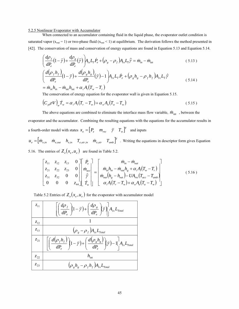
45

5.2.5 Nonlinear Evaporator with Accumulator When connected to an accumulator containing fluid in the liquid phase, the evaporator outlet condition is

saturated vapor (xout = 1) or two-phase fluid (xout < 1) at equilibrium. The derivation follows the method presented in

[42]. The conservation of mass and conservation of energy equations are found in Equation 5.13 and Equation 5.14.

( ) ( ) ( ) int1 mmLAPLAdPd

dPd

inTcsfgeTcse

g

e

f &&&& −=−+⎟⎟⎠

⎞⎜⎜⎝

⎛+− γρργ

ργ

ρ ( 5.13 )

( )( ) ( )( ) ( )

( )rwiiinin

TcsffggeTcse

gg

e

ff

TTAhmhm

LAhhPLAdP

hddP

hd

−+−=

−+⎟⎟⎠

⎞⎜⎜⎝

⎛−+−

α

γρργρ

γρ

intint

11

&&

&& ( 5.14 )

The conservation of energy equation for the evaporator wall is given in Equation 5.15.

( ) ( ) ( )waoowriiwwp TTATTATVC −+−= ααρ & ( 5.15 )

The above equations are combined to eliminate the interface mass flow variable, intm& , between the

evaporator and the accumulator. Combining the resulting equations with the equations for the accumulator results in

a fourth-order model with states [ ]Twrecee TmPx γ= and inputs

[ ]Tambaireinaireineouteinee TmThmmu ,,,,,, &&&= . Writing the equations in descriptor form gives Equation

5.16. The entries of ( )eee uxZ , are found in Table 5.2.

( )( ) ( )( ) ( ) ⎥

⎥⎥⎥

⎦

⎤

⎢⎢⎢⎢

⎣

⎡

−+−−−−−+−

−

=

⎥⎥⎥⎥⎥

⎦

⎤

⎢⎢⎢⎢⎢

⎣

⎡

⎥⎥⎥⎥

⎦

⎤

⎢⎢⎢⎢

⎣

⎡

waoowrii

ambaccrecoutgout

rwiigoutinin

outin

w

acc

e

TTATTATTUAhhmTTAhmhm

mm

T

mP

zzz

zzzzzz

αα

αγ &

&&

&&

&

&

&

&

44

3231

232221

131211

0000000

( 5.16 )

Table 5.2 Entries of ( )eee uxZ , for the evaporator with accumulator model

11z ( ) ( ) Totalcse

g

e

f LAdPd

dPd

⎥⎥⎦

⎤

⎢⎢⎣

⎡⎟⎟⎠

⎞⎜⎜⎝

⎛+−⎟⎟

⎠

⎞⎜⎜⎝

⎛γ

ργ

ρ1

12z 1

13z ( ) Totalcsfg LAρρ −

21z ( ) ( ) ( ) ( ) Totalcse

gg

e

ff LAdP

hddP

hd⎥⎦

⎤⎢⎣

⎡−⎟⎟

⎠

⎞⎜⎜⎝

⎛+−⎟⎟

⎠

⎞⎜⎜⎝

⎛11 γ

ργ

ρ

22z inth

23z ( ) Totalcsffgg LAhh ρρ −

46

31z

⎟⎟⎠

⎞⎜⎜⎝

⎛+⎟

⎟⎠

⎞⎜⎜⎝

⎛

−

−−

⎟⎟⎠

⎞⎜⎜⎝

⎛+++

fe

fg

e

g

fg

ffgg

ffe

fgg

e

gff

e

fgg

e

g

VdPd

VdPduu

VdPdu

VdPdu

uVdPd

uVdPd

ρρρρρρ

ρρρρ

32z

⎟⎟⎠

⎞⎜⎜⎝

⎛−

−

−inth

uu

fg

ffgg

ρρρρ

44z ( )wp VC ρ

5.2.6 Pseudo-Quality and Mean Void Fraction The mean void fraction, γ , was chosen in the condenser with receiver and evaporator with accumulator

derivations as a dynamic state. The mean void fraction is used to determine the fluid properties at the outlet of the

heat exchanger. A Slip-Ratio [43] void fraction correlation relates the void fraction to the quality at any point in the

two phase region, as shown in Equation 5.17, where Sf

gs ⎟

⎟⎠

⎞⎜⎜⎝

⎛=

ρρ

μ .

( ) sxxx

μγ

−+=

1 ( 5.17 )

The mean void fraction, Equation 5.18, results from integrating Equation 5.17 from xin to xout. This equation relates

the mean void fraction to the inlet and outlet quality of the two-phase region. Once the outlet quality is obtained, all

other outlet conditions may be calculated.

( ) ( )( )( )

( ) ( )( )⎥⎦⎤

⎢⎣

⎡−−+−+

−+

−−+

−=

SinoutSinS

SinS

Sinout

S

S xxxx

xx μμμμμ

μμ

μγ

111

ln11

12

( 5.18 )

5.2.6.1 Condenser with Receiver Outlet Quality At steady-state, the inlet fluid of the condenser with receiver two-phase region is saturated vapor (xin = 1)

and the outlet fluid is saturated liquid (xout = 0) or two-phase liquid (xout > 0). We would like to use Equation 5.18 to

obtain the outlet quality for small deviations from saturated liquid conditions, but the equation is transcendental in

outlet quality. Assuming small deviations from saturated liquid outlet conditions, we set xout = 0 outside of the

natural log to arrive at Equation 5.19. Solving for xout yields Equation 5.20, where s

saμ

μ−

=1

and s

bμ−

=1

1.

( ) ( ) .1

1ln11

12 ⎥

⎦

⎤⎢⎣

⎡−+−

−−

≈soutss

s

s x μμμμ

μγ ( 5.19 )

abex abb

out −=⎟⎠⎞

⎜⎝⎛ −γ

( 5.20 )

5.2.6.2 Evaporator with Accumulator Outlet Quality As with the condenser with receiver derivation, the mean void fraction is a dynamic state of the evaporator

with accumulator model. Equation 5.18 again provides the means of relating mean void fraction to quality. We

47

assume small deviations from saturated vapor outlet conditions, setting xout = 1 inside of the natural log to arrive at

Equation 5.21. Solving for xout yields Equation 5.22.

( )( )( )[ ]sins

sinout

s

s

xxx

μμμ

μμ

γ −+−−

+−

≈ 1ln11

12 ( 5.21 )

( )[ ]( ) ( ) in

SS

SinSSout x

xx +

−−−

−+=

μγμμμμ

111ln

2 ( 5.22 )

5.2.6.3 Pseudo-Quality During simulation, some transients will cause the condenser outlet fluid to deviate towards subcooled

conditions or the evaporator outlet fluid to deviate towards superheated conditions. When quality is calculated from

the mean void fraction, Equation 5.20 and Equation 5.22, these deviations result in heat exchanger outlet quality

values less than zero (condenser) and greater than one (evaporator). We therefore define a “pseudo-quality” that

exists outside the normal bounds on quality, [ ]1,0∈x . This pseudo-quality is defined as

( ) ( )[ ]εε +∪−∈ 1,10,0x̂ , where 10 <<< ε . By using the two-phase property relationships with the pseudo-

quality, outlet property approximations that capture the gross property behavior are obtained. This approach avoids

the complications of switching between multiple model structures during simulation.

5.2.6.4 Validity of Pseudo-Quality Assumptions This section addresses the validity of two key assumptions: the small deviation assumption used to derive

Equation 5.19 and Equation 5.21 and the assumption that approximate refrigerant properties calculated from the

pseudo-quality capture the basic behavior of the true refrigerant properties with sufficient accuracy for dynamic

modeling purposes.

Figure 5.5 compares the mean void fraction of Equation 5.18 with the mean void fraction resulting from

application of the condenser and evaporator small outlet quality deviation assumptions; see Equation 5.19 and

Equation 5.21.

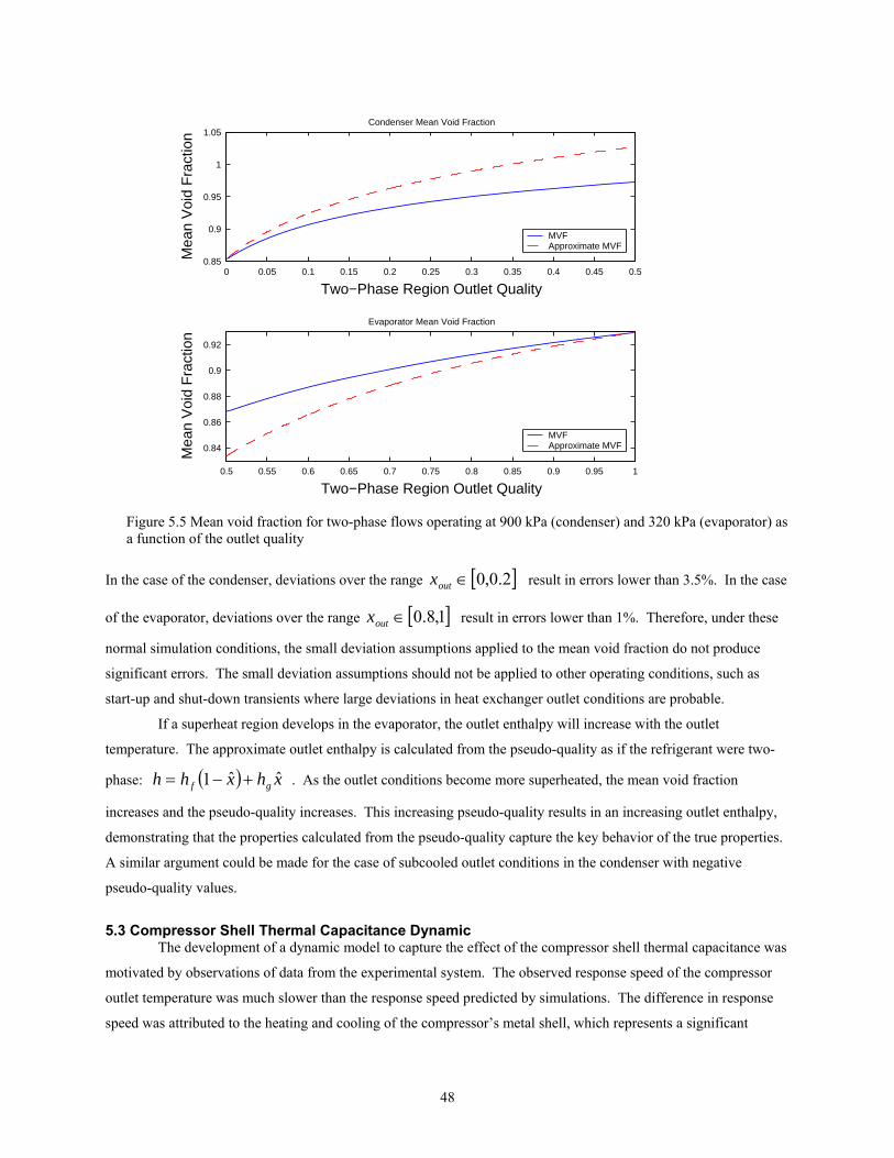
48

0 0.05 0.1 0.15 0.2 0.25 0.3 0.35 0.4 0.45 0.50.85

0.9

0.95

1

1.05

Two−Phase Region Outlet Quality

Mea

n V

oid

Fra

ctio

n

Condenser Mean Void Fraction

MVFApproximate MVF

0.5 0.55 0.6 0.65 0.7 0.75 0.8 0.85 0.9 0.95 1

0.84

0.86

0.88

0.9

0.92

Two−Phase Region Outlet Quality

Mea

n V

oid

Fra

ctio

n

Evaporator Mean Void Fraction

MVFApproximate MVF

Figure 5.5 Mean void fraction for two-phase flows operating at 900 kPa (condenser) and 320 kPa (evaporator) as a function of the outlet quality

In the case of the condenser, deviations over the range [ ]2.0,0∈outx result in errors lower than 3.5%. In the case

of the evaporator, deviations over the range [ ]1,8.0∈outx result in errors lower than 1%. Therefore, under these

normal simulation conditions, the small deviation assumptions applied to the mean void fraction do not produce

significant errors. The small deviation assumptions should not be applied to other operating conditions, such as

start-up and shut-down transients where large deviations in heat exchanger outlet conditions are probable.

If a superheat region develops in the evaporator, the outlet enthalpy will increase with the outlet

temperature. The approximate outlet enthalpy is calculated from the pseudo-quality as if the refrigerant were two-

phase: ( ) xhxhh gf ˆˆ1 +−= . As the outlet conditions become more superheated, the mean void fraction

increases and the pseudo-quality increases. This increasing pseudo-quality results in an increasing outlet enthalpy,

demonstrating that the properties calculated from the pseudo-quality capture the key behavior of the true properties.

A similar argument could be made for the case of subcooled outlet conditions in the condenser with negative

pseudo-quality values.

5.3 Compressor Shell Thermal Capacitance Dynamic The development of a dynamic model to capture the effect of the compressor shell thermal capacitance was

motivated by observations of data from the experimental system. The observed response speed of the compressor

outlet temperature was much slower than the response speed predicted by simulations. The difference in response

speed was attributed to the heating and cooling of the compressor’s metal shell, which represents a significant

49

thermal capacitance. Temperature data such as that shown in Figure 5.6 indicates that a first-order dynamic model

would be sufficiently accurate to capture the effect of the compressor shell thermal capacitance on the outlet

temperature. In [11], the authors point out that the temperatures in the compressor shell converge very slowly to a

steady-state value due to the high thermal capacity of the metal and oil in the shell. They also use a thermal

capacitance model to account for the compressor shell dynamics.

2000 4000 6000 8000 10000 12000 14000 16000 18000

30

40

50

60

70

Time [s]

Tem

pera

ture

[C] Compressor Shell

Outlet Refrigerant

Figure 5.6 Compressor shell and refrigerant outlet temperature data for system shutdown from 1600 RPM

Using the data in Figure 5.6, time constants may be found for both the refrigerant temperature decay and

the shell temperature decay. The time constant of the shell temperature decay is approximately 4490 seconds, and

the time constant of the refrigerant temperature decay is approximately 610 seconds. The refrigerant temperature

was measured with an immersion thermocouple, while the compressor shell temperature shell temperature was

measured with a contact thermocouple.

5.3.1 Implementation in Thermosys The desired first-order response is achieved by filtering the semi-empirical model’s static enthalpy

prediction. The filter transfer function is given in Equation 5.23, where τ is the chosen time constant for the first-

order response.

11

, +=

− shh

empiricalsemiout

out

τ ( 5.23 )

The transfer function is depicted in block diagram form in Figure 5.7.

Figure 5.7 Block diagram of Equation 5.23

In the Thermosys framework, dynamic component models calculate state derivates which are then

integrated to find the states. The time derivative of the compressor outlet enthalpy is found by examination of

Figure 5.7 to be the following:

50

τoutempiricalsemiout

out

hhh

−= −,& ( 5.24 )

The time constant is set by the user in the compressor graphical user interface.

The following plots compare output of compressor models for various time constant values. Figure 5.8

shows the compressor outlet temperature data for a test with numerous large compressor steps. Note the different

scales of the temperature data (blue, left side) and the model output (green, right side). The data shows minimal

temperature fluctuations compared to those of the model. The model output was generated with a time constant of

0.5 seconds, approximating a model without the compressor shell dynamic. Similar results motivated the

development of the thermal capacitance model. Figure 5.9 shows the same temperature data with model output

generated by various compressor shell time constants. The results indicate that a time constant between 1200

seconds and 1500 seconds is appropriate. These time constants fall between the shell and refrigerant temperature

decay time constants observed from system data.

3000 3050 3100 3150 3200 3250 3300 3350 340050

55

60

Time [s]

Tem

pera

ture

[C]

3000 3050 3100 3150 3200 3250 3300 3350 34000

100

200

Figure 5.8 Compressor outlet temperature data (blue) and small time constant model output (green)

3000 3050 3100 3150 3200 3250 3300 3350 340052

54

56

58

60

62

64

66

Time [s]

Tem

pera

ture

[C] Data

τ = 300τ = 600τ = 900τ = 1200τ = 1500

Figure 5.9 Compressor outlet temperature model output for various time constants

51

5.4 Identified Compressor Mass Flow Model While the previous section dealt with improving the transient compressor enthalpy prediction, this section

addresses the accuracy of the compressor mass flow rate prediction. In the case of the compressor mass flow

prediction, early model validation efforts revealed that the static compressor performance map model was not

adequately predicting true system behavior during transients. The inaccuracy of the mass flow model caused

significant inaccuracy in other model outputs, particularly the evaporator pressure. Possible causes of the

discrepancies could be deficiencies in the compressor model itself, unmodeled components such as the oil separator,

or interactions between the various component models. Since no physical understanding of the source of the model

errors is available, a system identification approach was chosen to find a mass flow correction. The necessary mass

flow correction is first isolated from simulation and system data using an iterative learning control (ILC) algorithm.

Standard system identification techniques are then used to find a simple model for the mass flow correction.

5.4.1 Compressor Mass Flow Dynamics Isolation The first step in this identification method is the isolation of the mass flow correction from simulation

output and experimental system data. The static, semi-empirical compressor model is the baseline compressor

model. An iterative learning control algorithm [36,5] is used to identify a compressor mass flow rate correction.

The ILC algorithm adjusts the compressor mass flow rate to reduce the error in one of the model outputs, in this case

the evaporator pressure. Figure 5.10 shows a schematic of the isolation procedure.

Compressor Model

Evaporator ModelValve Model

Condenser Model

Off-line IterativeLearning Control

Algorithm

EvaporatorPressure Data

RPMSimulation

Feed-forwardMass flow correction

SimulationVariables

Evaporator Pressure

Evaporator PressureError

m&

correctedm&

Compressor Model

Evaporator ModelValve Model

Condenser Model

Off-line IterativeLearning Control

Algorithm

EvaporatorPressure Data

RPMSimulation

Feed-forwardMass flow correction

SimulationVariables

Evaporator Pressure

Evaporator PressureError

m&

correctedm&

Figure 5.10 Compressor mass flow dynamics isolation procedure

For the first run of the simulation, the baseline static compressor model produces a compressor mass flow

rate prediction. This mass flow rate is passed to the other component models which, in turn, generate additional

model outputs. After the simulation has finished, the evaporator pressure model output is compared to evaporator

pressure data to generate an evaporator pressure error signal. This error signal is passed to the PD-type ILC

52

algorithm given in Equation 5.25, where P and D are tunable gains on the evaporator pressure error and pressure

error derivative, j is the iteration number, and T is the data length.

( ) ( ) ( ) ( ) [ ]TtteDtePtmtm jjjcorrectionjcorrection ,0111,, ∈⋅+⋅+= −−− &&& ( 5.25 )

The ILC algorithm produces a feed-forward mass flow rate correction signal that is applied to the mass flow rate

predicted by the static compressor model during the next iteration of the simulation. Iterations continue until the

evaporator pressure RMS error reaches an acceptably small value. At the final iteration, the mass flow rate

correction signal represents an isolation of the compressor mass flow rate dynamics not captured by the static

compressor model.

5.4.2 Identification of Isolated Dynamics After isolation of the compressor mass flow dynamics, a model is identified to capture the dynamic

behavior in simulation. Any standard system identification technique could be applied to this problem; see [32] for

examples. MATLAB’s System Identification Toolbox has been more than adequate for identifying the dynamic mass

flow correction model. Two examples of the application of this technique are found in Chapter 7.

5.5 Compressor Cycling Dynamics While it is not an efficient capacity control method [27], compressor cycling is frequently used in vapor

compression cycle systems with fixed-speed compressors. Compressor cycling produces very large transients that

cause substantial difficulties in the moving-boundary modeling framework. As with the heat exchanger with

receiver/accumulator model, the main challenge is the destruction and creation of dynamic states due to a changing

number of fluid regions in the heat exchangers. The cycling transients are so severe that they cannot be handled

with the modeling assumptions applied to the heat exchanger with receiver/accumulator models. A compressor

cycling model also requires an accurate prediction of mass flow behavior for the expansion device and the

compressor at very low mass flow rates. A similar but more challenging problem is system start-up. In addition to

the cycling difficulties already mentioned, modeling start-up transients requires knowledge of the initial distribution

of refrigerant charge in the system. Modeling start-up transients is a difficult challenge for even the well-developed

commercial modeling tools. This work will focus on possible solutions to the slightly less challenging compressor

cycling problems. Overcoming the compressor cycling challenges will be a first step towards modeling start-up

transients. A review of current Thermosys model capabilities in regards to cycling transients is provided as a

starting point for future research.

5.5.1 Literature Review Two papers based on the moving-boundary framework have discussed modeling techniques appropriate for

capturing compressor cycling behavior. In the follow sections, the work of Dhar and Soedel [11] is briefly

described, followed by a discussion of the work of Pettit, Willatzen, and Ploug-Sorensen [47, 38].

5.5.1.1 Dhar and Soedel Dhar and Soedel present the component models necessary to simulate a complete VCC system. Three

condenser models are presented: a superheated model, a two-phase model, and a subcooled model. The three

models may be combined to form a condenser model with multiple fluid regions. Only one evaporator model is

presented. Logic statements are used in the main simulation program to call the correct heat exchanger subroutine.

53

Simulation results indicate that the models were used for a system start-up simulation that should require model

switching. The paper does not indicate how potential discontinuities and numerical difficulties are handled, but the

simulation output appears to be free of discontinuities. The lack of multiple evaporator model structures raises

questions as to the applicability of the model to start-up transients. It is expected that the evaporator would operate

with different combinations of fluid regions during the severe start-up transients.

5.5.1.2 Willatzen, Pettit, and Ploug-Sorensen Willatzen, Pettit, and Ploug-Sorensen derive a generic moving-boundary heat exchanger model very similar

to those of [19]. They do not include expansion device or compressor models.

The authors go to great length to explain their approach for handling the discontinuities and numerical

challenges associated with switching model structures during simulation. The models are implemented in ACSL, a

modeling environment for continuous dynamic systems. This platform was chosen because it allows for event-

driven procedures and user access to integrator properties.

The evaporator model is given as an example of their approach. Four model structures are considered: a

subcool/two-phase/superheat model, a subcool/two-phase model, a two-phase model, and a two-phase/superheat

model. The models are made up of explicit equations for the state derivatives. The major contribution of the paper

is the discussion of what to do with these state derivatives when the physical entities that they represent are no

longer active in the model. Two guiding principles are presented. First, if a state going to zero will adversely affect

numerics, do not allow the state to go all the way to zero. Second, force inactive states to track a meaningful

physical value. The value to be tracked is determined by the desired state value at the time of its reactivation in the

model. For example, consider the case of an evaporator switching from a subcool/two-phase/superheat model to a

two-phase/superheat model. As the model structure switch occurs, the subcooled region length goes to zero and the

subcooled region wall temperature state becomes inactive. The length is prevented from reaching zero by changing

the original length derivative equation to Equation 5.26 when a model switch is imminent.

( )ε−−= 11 ee LL& ( 5.26 )

The inactive wall temperature is forced to track the adjacent active wall temperature by replacing the original

temperature state derivative equation with Equation 5.27. The parameter k is a time constant that controls how

quickly the inactive wall temperature converges to the value of the active wall temperature.

( )121 ewewew TTkT −=& ( 5.27 )

Using this method, if the subcooled region is reactivated in the model, the length will start from a small non-zero

value and the subcooled region wall temperature will start with the same value as the adjacent two-phase region wall

temperature.

The model structure switching is based on the inlet and outlet refrigerant enthalpy. If the inlet enthalpy is

less than the saturated liquid enthalpy, the subcooled region is included. If the outlet enthalpy is greater than the

saturated vapor enthalpy, the superheat region is included.

No model validation results are presented in the papers, but simulation results are presented for a number of

model outputs. The model inputs are shaped such that switching between various model structures occurs during the

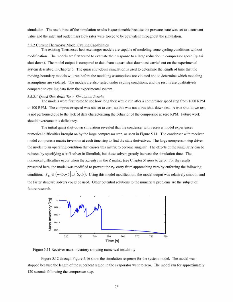
54

simulation. The usefulness of the simulation results is questionable because the pressure state was set to a constant

value and the inlet and outlet mass flow rates were forced to be equivalent throughout the simulation.

5.5.2 Current Thermosys Model Cycling Capabilities The existing Thermosys heat exchanger models are capable of modeling some cycling conditions without

modification. The models are first tested to evaluate their response to a large reduction in compressor speed (quasi

shut-down). The model output is compared to data from a quasi shut-down test carried out on the experimental

system described in Chapter 6. The quasi shut-down simulation is used to determine the length of time that the

moving-boundary models will run before the modeling assumptions are violated and to determine which modeling

assumptions are violated. The models are also tested under cycling conditions, and the results are qualitatively

compared to cycling data from the experimental system.

5.5.2.1 Quasi Shut-down Test: Simulation Results The models were first tested to see how long they would run after a compressor speed step from 1600 RPM

to 100 RPM. The compressor speed was not set to zero, so this was not a true shut-down test. A true shut-down test

is not performed due to the lack of data characterizing the behavior of the compressor at zero RPM. Future work

should overcome this deficiency.

The initial quasi shut-down simulation revealed that the condenser with receiver model experiences

numerical difficulties brought on by the large compressor step, as seen in Figure 5.11. The condenser with receiver

model computes a matrix inversion at each time step to find the state derivatives. The large compressor step drives

the model to an operating condition that causes this matrix to become singular. The effects of the singularity can be

reduced by specifying a stiff solver in Simulink, but these solvers greatly increase the simulation time. The

numerical difficulties occur when the z44 entry in the Z matrix (see Chapter 5) goes to zero. For the results

presented here, the model was modified to prevent the z44 entry from approaching zero by enforcing the following

condition: ( ] [ )∞∪−∞−∈ ,55,44z . Using this model modification, the model output was relatively smooth, and

the faster standard solvers could be used. Other potential solutions to the numerical problems are the subject of

future research.

720 730 740 750 760 770 780 790

0.2

0.4

0.6

0.8

1

Time [s]

Mas

s In

vent

ory

[kg]

Figure 5.11 Receiver mass inventory showing numerical instability

Figure 5.12 through Figure 5.16 show the simulation response for the system model. The model was

stopped because the length of the superheat region in the evaporator went to zero. The model ran for approximately

120 seconds following the compressor step.

55

720 740 760 780 800 820 840200

400

600

800

1000

Time [s]

Pre

ssur

e [k

Pa]

CondenserEvaporator

Figure 5.12 Pressures

720 740 760 780 800 820 8400

0.2

0.4

0.6

0.8

1

Time [s]

% o

f Tot

al L

engt

h SuperheatTwo−Phase

Figure 5.13 Condenser fluid region lengths

720 740 760 780 800 820 8400

0.2

0.4

0.6

0.8

1

Time [s]

% o

f Tot

al L

engt

h Two−PhaseSuperheat

Figure 5.14 Evaporator fluid region lengths with the superheat length vanishing

720 740 760 780 800 820 8400.7

0.75

0.8

0.85

0.9

0.95

1

1.05

Time [s]

Mas

s In

vent

ory

[kg]

Figure 5.15 Receiver mass inventory

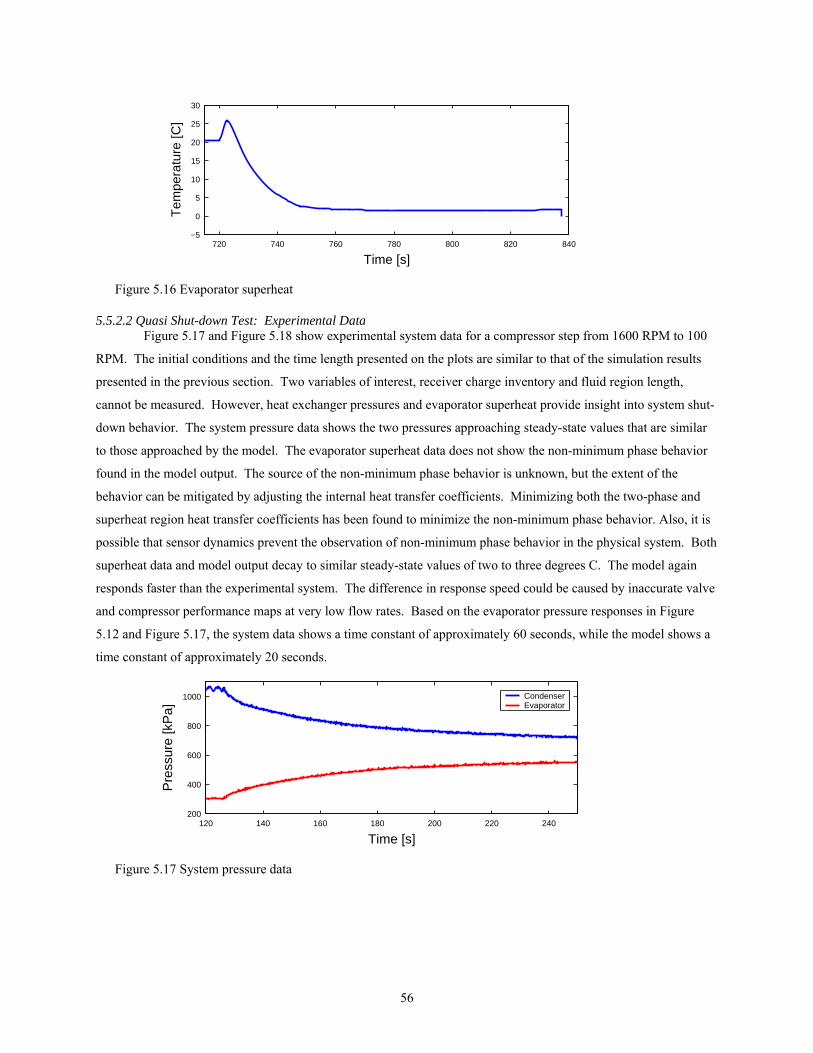
56

720 740 760 780 800 820 840−5

0

5

10

15

20

25

30

Time [s]

Tem

pera

ture

[C]

Figure 5.16 Evaporator superheat

5.5.2.2 Quasi Shut-down Test: Experimental Data Figure 5.17 and Figure 5.18 show experimental system data for a compressor step from 1600 RPM to 100

RPM. The initial conditions and the time length presented on the plots are similar to that of the simulation results

presented in the previous section. Two variables of interest, receiver charge inventory and fluid region length,

cannot be measured. However, heat exchanger pressures and evaporator superheat provide insight into system shut-

down behavior. The system pressure data shows the two pressures approaching steady-state values that are similar

to those approached by the model. The evaporator superheat data does not show the non-minimum phase behavior

found in the model output. The source of the non-minimum phase behavior is unknown, but the extent of the

behavior can be mitigated by adjusting the internal heat transfer coefficients. Minimizing both the two-phase and

superheat region heat transfer coefficients has been found to minimize the non-minimum phase behavior. Also, it is

possible that sensor dynamics prevent the observation of non-minimum phase behavior in the physical system. Both

superheat data and model output decay to similar steady-state values of two to three degrees C. The model again

responds faster than the experimental system. The difference in response speed could be caused by inaccurate valve

and compressor performance maps at very low flow rates. Based on the evaporator pressure responses in Figure

5.12 and Figure 5.17, the system data shows a time constant of approximately 60 seconds, while the model shows a

time constant of approximately 20 seconds.

120 140 160 180 200 220 240200

400

600

800

1000

Time [s]

Pre

ssur

e [k

Pa]

CondenserEvaporator

Figure 5.17 System pressure data

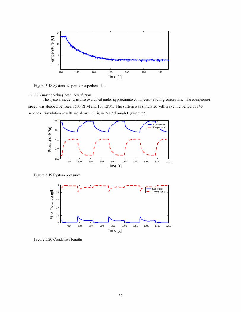
57

120 140 160 180 200 220 240

0

5

10

15

Time [s]

Tem

pera

ture

[C]

Figure 5.18 System evaporator superheat data

5.5.2.3 Quasi Cycling Test: Simulation The system model was also evaluated under approximate compressor cycling conditions. The compressor

speed was stepped between 1600 RPM and 100 RPM. The system was simulated with a cycling period of 140

seconds. Simulation results are shown in Figure 5.19 through Figure 5.22.

750 800 850 900 950 1000 1050 1100 1150 1200200

400

600

800

1000

Time [s]

Pre

ssur

e [k

Pa]

CondenserEvaporator

Figure 5.19 System pressures

750 800 850 900 950 1000 1050 1100 1150 12000

0.2

0.4

0.6

0.8

1

Time [s]

% o

f Tot

al L

engt

h SuperheatTwo−Phase

Figure 5.20 Condenser lengths

58

750 800 850 900 950 1000 1050 1100 1150 12000.1

0.2

0.3

0.4

0.5

0.6

0.7

0.8

Time [s]

% o

f Tot

al L

engt

h Two−PhaseSuperheat

Figure 5.21 Evaporator lengths

750 800 850 900 950 1000 1050 1100 1150 12000

5

10

15

20

25

30

Time [s]

Tem

pera

ture

[C]

Figure 5.22 Evaporator superheat

5.5.2.4 Quasi Cycling Test: Experimental Data The experimental system was run under cycling conditions similar to those used in the simulation. The

system pressures and superheat data are found in Figure 5.23 and Figure 5.24. The qualitative aspects of the

pressure model and data are very similar. The model again responds to compressor steps faster than the data. The

pressure data does not reach a steady-state value between steps, so an evaluation of steady-state accuracy is not

possible. The superheat data and model output are significantly different. The data shows a loss of superheat

following the first compressor speed increase. The evaporator is subsequently unable to consistently regain a level

of superheat. The model does not predict this loss of superheat; it shows large fluctuations in superheat for each

compressor step. Very short cycling periods were also tested, but superheat was always lost. Shortening the cycling

period delayed the onset of superheat loss.

150 200 250 300 350 400 450 500 550 600 650 700200

400

600

800

1000

Time [s]

Pre

ssur

e [k

Pa]

CondenserEvaporator

Figure 5.23 System pressure data

59

150 200 250 300 350 400 450 500 550 600 650 700−5

0

5

10

15

20

25

Time [s]

Tem

pera

ture

[C]

Figure 5.24 System evaporator superheat data

5.6 Future Work Many opportunities for continued work in dynamic modeling of VCC systems are readily available. The

dynamic modeling goals of greatest interest are the simulation of cycling conditions, the simulation of start-up

conditions, and the improvement of the compressor mass flow rate prediction.

5.6.1 Cycling Simulation The model output and data presented in the preceding sections showed that the current Thermosys models

capture many of the qualitative features of the transient response associated with compressor cycling. However,

some aspects of the data, such as the loss of the superheat in the evaporator, were not captured by the model. This

loss of superheat behavior demonstrates the need for switching between model structures during simulation. Loss of

superheat in a simulation should result in the evaporator model changing from a two-phase/superheat structure to

two-phase only structure.

The approach presented by [38] could be applied to the Thermosys models. Some modifications to the

existing models would be needed. The Thermosys models currently perform a matrix inversion at each time step to

find the state derivatives. In the approach of [38], this matrix inversion is performed symbolically. This approach

provides explicit expressions for the state derivatives. These expressions can then be manipulated to account for

model switching numeric issues. Using this approach in Thermosys would require a significant amount of

modification to the Simulink component models, but the change is not conceptually challenging. In addition to

finding explicit state derivative expressions, new derivations of heat exchangers with different active fluid regions

would be required. These new derivations would be very similar to both previous Thermosys derivations and

derivations available in the literature. A final, and perhaps most time consuming challenge, is accurately

characterizing the behavior of the expansion device and compressor at extremely low mass flow rates. But this

challenge must be overcome regardless of the chosen method for dealing with compressor cycling.

5.6.2 Start-up Simulation System start-up simulation will build upon the results of the cycling simulation efforts. Developing cycling

simulation capabilities will provide the model switching structure necessary for start-up simulation as well as

characterize the mass flow devices under very low flow conditions.

The additional difficulty presented by start-up simulation is the determination of the proper initial

conditions. The behavior of a system during start-up is largely dependent on the location of the refrigerant charge.

60

The mechanisms governing the migration of charge while the system is not operating are not well understood. In

addition, the migration of charge may continue over a long period of time. For example, a system’s start-up

transients could be significantly different if it has not been operated for one day as opposed to one week. This

behavior has been observed in the experimental system described in Chapter 6.

5.6.3 Improved Compressor Mass Flow Prediction The compressor mass flow prediction could be improved in a number of ways. One possibility is the

development of a first-principles dynamic compressor model. Other moving-boundary model developers have taken

this approach. Another possibility is the inclusion of oil flow modeling. The presence of oil in the compressor

pistons affects the amount of refrigerant mass expelled during each compressor revolution. Oil circulation is also of

interest to industry due to its effects on heat transfer and compressor reliability. A third approach is directly

identifying a dynamic compressor mass flow model. This approach would be the simplest from a modeling point of

view but would require the addition of a new sensor capable of measuring the mass flow rate of a fluid in the gas

phase.

61

Chapter 6. Experimental System

The model validation results presented in this thesis were obtained using data from an experimental air-

conditioning system. This chapter contains an overview of the experimental system sensors, actuators, data

acquisition, and components. A detailed description of the experimental system is found in [41]. This chapter will

describe significant changes to the system carried out since [41] was written.

6.1 General Description The experimental system is a modified dual-evaporator industrial air-conditioning trainer system. The

major components are two tube-and-fin evaporators, a tube-and-fin condenser, an internal heat exchanger, a liquid-

line receiver, a suction-line accumulator, a semi-hermetic compressor, and a variety of expansion devices. The

system is instrumented with a number of sensors, allowing for detailed observation of system transients. Manual

valves allow for the selection of multiple system configurations. A schematic of the system is shown in Figure 6.1.

The valve acronyms are defined in Table 6.1. The manufacturer and model number for each component are given in

Table 6.2.

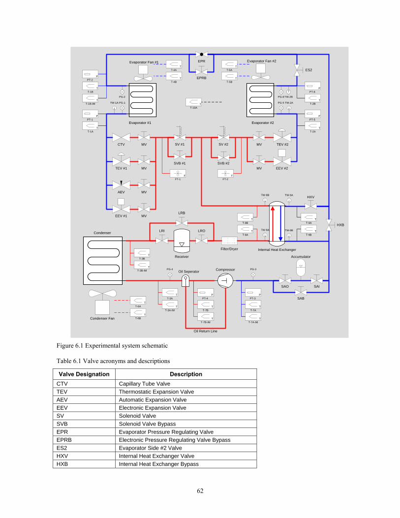
62

Evaporator #2Evaporator #1

CTV

AEV

Accumulator

Condenser

PG-4

TW-1A

Oil Seperator Compressor

FFT-1

Filter/Dryer

TEV #1

EEV #1

SV #2

SAB

SVB #2

EPRB

HXB

LRB

EPR

TEV #2

EEV #2

Evaporator Fan #1 Evaporator Fan #2

SV #1

SVB #1

Condenser Fan

HXV

Internal Heat Exchanger

MV

MV

MV

MV

MV

MV

ES2

PG-3

PG-5

PG-6

PG-1

PG-2

TW-2A

TW-2B

TW-9ATW-8B

TW-9BTW-8A

FFT-2

PPT-4

PPT-3

PPT-1

PPT-2

PPT-6

PPT-5

TT-7B

TT-7A

TT-7A-IM

TT-3A

TT-3A-IM

ReceiverTT-3B

TT-3B-IM

TT-6A

TT-6B

TT-4A

TT-4B

TT-5A

TT-5B

TT-1B-IM

TT-1A

TT-2B

TT-2A

TT-1B

TT-10A

TT-9B

TT-9A

TT-8A

TT-8B

TT-7B-IM

SAISAO

LROLRI

Oil Return Line

Figure 6.1 Experimental system schematic

Table 6.1 Valve acronyms and descriptions

Valve Designation Description CTV Capillary Tube Valve TEV Thermostatic Expansion Valve AEV Automatic Expansion Valve EEV Electronic Expansion Valve SV Solenoid Valve SVB Solenoid Valve Bypass EPR Evaporator Pressure Regulating Valve EPRB Electronic Pressure Regulating Valve Bypass ES2 Evaporator Side #2 Valve HXV Internal Heat Exchanger Valve HXB Internal Heat Exchanger Bypass

63

LRI Liquid Line Receiver Inlet LRO Liquid Line Receiver Outlet LRB Liquid Line Receiver Bypass SAI Suction Line Accumulator Inlet SAO Suction Line Accumulator Outlet SAB Suction Line Accumulator Bypass MV Manual Valve

Table 6.2 Component name, manufacturer, model, and URL

Component Manufacturer Model URL Evaporator Fan and Casing Larkin (HeatCraft) VAK-17A www.heatcraftrpd.com Evaporator #1 HeatCraft 52601301 (VAK-17A) www.heatcraftrpd.com Evaporator #2 Blissfield BH517 www.blissfield.com Condenser and Fan Tecumseh (Blissfield) 50803-1 (66001-3) www.blissfield.com Internal Heat Exchanger Superior (Sherwood) HXSV-1/2 www.sherwoodvalve.com Liquid Line Receiver AC&R Components, Inc. (Henry Tech.) S-8064 www.henrytech.com Suction Line Accumulator AC&R Components, Inc. (Henry Tech.) S-7043 www.henrytech.com Oil Separator AC&R Components, Inc. (Henry Tech.) S-5581 www.henrytech.com Compressor Copeland KANA-006E-TAC-800 www.copeland-corp.com Variable Frequency Drive Baldor ID15J101-ER www.baldor.com Capillary Tubing Sealed Unit Parts Co., Inc. BC-4 www.supco.com TEV Sporlan Valve Co. FJ ¼ C www.sporlan.com AEV Parker-Hannefin A2 www.parker.com EEV Sporlan Valve Co. SEI-0.5 www.sporlan.com EPR Sporlan Valve Co. ORIT 6-0/50-1/2” www.sporlan.com Manual Valves Mueller Brass Co. 14838, 14841 www.muellerindustries.com Filter-Dryer Sporlan Valve Co. C-052 www.sporlan.com Sight Glasses Sporlan Valve Co. SA-14S, SA-12FM www.sporlan.com Pressure Transducers Cole-Palmer 07356-53, 07356-54 www.coleparmer.com Pressure Gauges Ritchie Engineering Co., Inc. 49051, 49052 www.yellowjacket.com Mass Flow Transducers McMillan Company 102-6P www.mcmflow.com Immersion Thermocouple Omega GTMQSS-062U-6 www.omega.com Welded Thermocouple Omega FF-T-20-100 www.omega.com Watt Meter Ohio Semitronics, Inc. GW5-019D www.ohiosemitronics.com Pressure Switches Ranco 010-1402, 011-1711 www.ranco.invensys.com Line Reactors MTE (Galco Industrial Electronics) MTE RL-00402 www.galco.com Analog Input Board Measurement Computing, Inc. PCI-DAS1200/JR www.measurementcomputing.com Analog Output Board Measurement Computing, Inc. PCI-DDA-08/12 www.measurementcomputing.com Thermocouple Board Measurement Computing, Inc. PCI-DAS-TC www.measurementcomputing.com Signal Conditioners Omega OM5 Series www.omega.com Humidifier Hunter 33222 www.hunterfan.com

6.2 Sensors The experimental system is equipped with sensors to measure temperatures, pressures, mass flow rates,

power, and humidity. Table 6.3 gives the location of these sensors on the system.

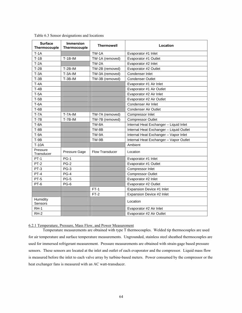
64

Table 6.3 Sensor designations and locations

Surface Thermocouple

Immersion Thermocouple Thermowell Location

T-1A TW-1A Evaporator #1 Inlet T-1B T-1B-IM TW-1A (removed) Evaporator #1 Outlet T-2A TW-2A Evaporator #2 Inlet T-2B T-2B-IM TW-2B (removed) Evaporator #2 Outlet T-3A T-3A-IM TW-3A (removed) Condenser Inlet T-3B T-3B-IM TW-3B (removed) Condenser Outlet T-4A Evaporator #1 Air Inlet T-4B Evaporator #1 Air Outlet T-5A Evaporator #2 Air Inlet T-5B Evaporator #2 Air Outlet T-6A Condenser Air Inlet T-6B Condenser Air Outlet T-7A T-7A-IM TW-7A (removed) Compressor Inlet T-7B T-7B-IM TW-7B (removed) Compressor Outlet T-8A TW-8A Internal Heat Exchanger – Liquid Inlet T-8B TW-8B Internal Heat Exchanger – Liquid Outlet T-9A TW-9A Internal Heat Exchanger – Vapor Inlet T-9B TW-9B Internal Heat Exchanger – Vapor Outlet T-10A Ambient Pressure Transducer Pressure Gage Flow Transducer Location

PT-1 PG-1 Evaporator #1 Inlet PT-2 PG-2 Evaporator #1 Outlet PT-3 PG-3 Compressor Inlet PT-4 PG-4 Compressor Outlet PT-5 PG-5 Evaporator #2 Inlet PT-6 PG-6 Evaporator #2 Outlet FT-1 Expansion Device #1 Inlet FT-2 Expansion Device #2 Inlet Humidity Sensors

Location

RH-1 Evaporator #2 Air Inlet RH-2 Evaporator #2 Air Outlet

6.2.1 Temperature, Pressure, Mass Flow, and Power Measurement Temperature measurements are obtained with type T thermocouples. Welded tip thermocouples are used

for air temperature and surface temperature measurements. Ungrounded, stainless steel sheathed thermocouples are

used for immersed refrigerant measurement. Pressure measurements are obtained with strain-gage based pressure

sensors. These sensors are located at the inlet and outlet of each evaporator and the compressor. Liquid mass flow

is measured before the inlet to each valve array by turbine-based meters. Power consumed by the compressor or the

heat exchanger fans is measured with an AC watt-transducer.

65

6.2.2 Humidity Measurement To validate new heat exchanger models that incorporate humidity calculations, two humidity sensors were

added to the experimental system. The sensors were placed at the inlet and outlet of the second evaporator.

The inlet sensor is a Honeywell model HIH-3610, and the outlet sensor is a Honeywell model HIH-4000.

Each sensor consists of a thermoset polymer capacitive sensing element with on-chip integrated signal conditioning.

They are powered by the data acquisition computer’s 5 V power supply and provide a voltage output as a function of

relative humidity. Using a manufacturer specified curve, the voltage output is converted to relative humidity. The

conversion includes temperature compensation for deviations from the calibration temperature, 25°C. The HIH-

3610 conversion is given in Equation 6.1. The HIH-4000 conversion is given in Equation 6.2. The HIH-3610 has a

stated accuracy of 2% relative humidity. The HIH-4000 claims 3.5% relative humidity accuracy. Figure 6.2 shows

the inlet relative humidity sensor; the outlet sensor is very similar in appearance. The sensors are approximately

4.27 mm by 9.47 mm by 2.03 mm in size.

inair

out

in T

VV

,

supply

00216.00546.1

16.00062.01

−

⎟⎟⎠

⎞⎜⎜⎝

⎛−

=φ ( 6.1 )

( )2

,,

2,,

0000011.0000044.00305.0000040.00041.09237.0

outairoutair

outairoutairoutout TT

TTV−+

+−−=φ ( 6.2 )

Figure 6.2 Photograph of the relative humidity sensor at the evaporator inlet

6.3 Actuators The experimental system is designed for computer control of compressor speed, fan speeds, and electronic

expansion valve opening. The other expansion devices operate as mechanical feedback devices or with no control.

6.3.1 Compressor, Fans, and Valves The compressor is a semi-hermetic reciprocating machine. The pistons are driven by a crankshaft which is

connected directly to an electric motor in the compressor shell. Compressor speed control is achieved with a

variable frequency drive (VFD). The VFD converts single phase 120 VAC to the three-phase 240 VAC required by

the compressor. The VFD uses pulse width modulation to control the compressor speed.

66

The three heat exchanger fans are powered by fan control boards than take in a DC command signal and

output an AC signal to the fan motor. Air mass flow rate maps were generated by measuring the average air

velocity over a range of locations and fan speeds.

The experimental system may be configured to use one of four expansion devices: an electronic expansion

valve (EEV), a thermostatic expansion valve (TEV), an automatic expansion valve (AEV), and a capillary tube. The

EEV uses a stepper motor to vary the size of the valve opening. The stepper motor is computer controlled, allowing

the EEV to be used in feedback control schemes. The TEV uses a thermo-mechanical feedback system to regulate

superheat at the evaporator outlet. The AEV regulates the evaporator at a constant pressure. Unlike the other three

expansion devices, which incorporate variable area valves, the capillary tube geometry is fixed. It is therefore the

simplest expansion device, but also the most limited in capabilities.

6.3.2 Humidifier Validation of the humidity models requires the experimental system to run under conditions in which

condensation occurs on the external evaporator surfaces. During drier seasons of the year, condensation will not

naturally occur, and the relative humidity of the air entering the evaporator must be artificially raised to ensure that

condensation will occur. To achieve elevated inlet air relative humidity, a small room humidifier was added to the

system. The humidifier is a model 33222 from Hunter. The output of the humidifier is ducted directly to the

evaporator inlet where it is mixed with room air before entering the evaporator, as shown in Figure 6.3. The

humidifier has three speed settings, allowing for model validation to include step changes in inlet relative humidity.

Figure 6.3 Humidifier and tubing bringing moist air output to the evaporator inlet

67

6.4 Data Acquisition Data acquisition and control are carried out with a 16 channel thermocouple board, an 8 channel 12-bit

analog output board, and a 16 channel 12-bit analog input board from Measurement Computing. Models are

interfaced with a PC using WinCon and the Real Time Workshop. For details on the wiring and the individual

components of the data acquisition system, see [26].

6.5 Components The experimental system contains four heat exchangers and a number of auxiliary components.

6.5.1 Heat Exchangers Both evaporators are tube-and-fin models with copper tubes and aluminum fins. The first evaporator is a

VAK17A from Larkin. The second evaporator is similar in size to the first evaporator, but has an alternative tube

configuration. In the first evaporator, fluid enters at the top of the heat exchanger, flows back and forth down the

front face, and then flows back and forth up the back face to exit at the top. This configuration effectively gives the

first evaporator a “two-slab” configuration. Because this configuration is more difficult to model in the Thermosys

framework, a “single-slab” design was chosen for the second evaporator. In this tube configuration, refrigerant

enters at the top and exits at the bottom, flowing back and forth as it descends. The second evaporator was provided

by Blissfield Manufacturing Company. The model validation results presented in this work were obtained from tests

using the second evaporator.

The condenser, Tecumseh model #50803-1, is also a tube-and-fin design. Both the tubes and the fins are

steel.

The internal heat exchanger is a Superior model HXSV-1/2. This component facilitates heat exchange

between cold vapor exiting the evaporator and hot liquid exiting the condenser or the receiver. The internal heat

exchanger makes it less likely that liquid will enter the compressor and two-phase flow will enter the expansion

device, thus preventing slugging and choking. This component was not used for the tests described herein.

6.5.2 Auxiliary Components The experimental system contains a receiver at the condenser outlet and an accumulator at the evaporator

outlet. Both components are manufactured by AC&R Components, Inc. The receiver is a model S-8064 and the

accumulator is a model S-7043. The receiver stores excess refrigerant charge and ensures that flow into the valve

will not be two-phase. The accumulator captures liquid in the suction line, allowing only vapor to flow to the

compressor. In the model validation tests presented in the next chapter, the receiver and the accumulator are both

included in the system. However, the accumulator is not included in the models because it only contains vapor and

therefore acts as an additional pipe volume.

The other auxiliary components are an oil separator, a filter/dryer, sight glasses, and hand valves. The oil

separator, a model S-5581 from AC&R Components, captures oil from the discharge line and returns it to the

compressor. The Sporlan C-052 Catch-All filter-dryer removes potentially damaging moisture, acids, and

particulates from the system. This component is located between the receiver and the valves. At various locations

throughout the system, sight glasses are included for visual monitoring of the fluid condition. The sight glasses

contain a color-changing element that serves as an indication of excessive moisture in the system. Sporlan See-All

68

models SA-12FM and SA-14S are used. Manual valves (Mueller models 14838 and 14841) are used to isolate

various sections of the system. They allow for multiple system configurations, such as single evaporator and dual

evaporator operation.

6.6 Physical Parameters Each component used in model validation must be characterized by physical parameters. Table 6.4 below

shows the baseline physical parameter values for the components used in model validation simulations. They were

obtained through a combination of manufacturer provided technical drawings and measurements of components.

Table 6.4 Component physical parameters used for model validation simulations

Component Parameter Value Units Comments

Heat Exchanger Mass 4.656 kg Calculated Heat Exchanger Specific Heat 0.467 kJ/kg-K Steel Heat Exchanger Frontal Area 0.0898 m^2 From Manufacturer Hydraulic Diameter of Tubes 0.008103 m Measured Internal Volume 0.00055716 m^3 From Manufacturer Internal Surface Area 0.274993 m^2 Calculated External Surface Area 2.7927 m^2 Calculated Total Fluid Flow Length 10.6895 m Calculated Flow Cross Sectional Area 0.00005156 m^2 Calculated

Con

dens

er

Receiver Volume 0.0007732 m^3 Measured Heat Exchanger Mass 2.7438 kg Calculated Heat Exchanger Specific Heat 0.4877 kJ/kg-K Aluminum and Copper Heat Exchanger Frontal Area 0.0584 m^2 Calculated Hydraulic Diameter of Tubes 0.0081026 m From Manufacturer Internal Volume 0.000591 m^3 From Manufacturer Internal Surface Area 0.29166 m^2 Calculated External Surface Area 3.068 m^2 Calculated Total Fluid Flow Length 11.45794 m Calculated Flow Cross Sectional Area 0.00005156 m^2 Calculated

Eva

pora

tor 2

Accumulator Volume 0.0028665 m^3 Measured Rising Slew Rate 12.5 %/s From Manufacturer Falling Slew Rate -12.5 %/s From Manufacturer

EE

V

Input Delay 0.5 s Estimated Volume 0.0000304 m^3 From Manufacturer Rising Slew Rate 1000 rpm/s Estimated Falling Slew Rate -1000 rpm/s Estimated

Com

pres

sor

Compressor to Condenser 4.04 m Measured Condenser to Valve 4.79 m Measured Valve to Evaporator 1.63 m Measured Evaporator to Compressor 6.53 m Measured

Pip

e Le

ngth

Hydraulic Diameter 9.5 mm Estimated

69

Chapter 7. Model Validation

This chapter addresses one of the key challenges of the model development process, model validation.

While a model cannot be validated by a finite amount of data, the model user’s confidence in the model may be

increased through the model validation process. In this chapter, particular attention will paid to the validation of the

modeling techniques discussed in previous chapters, namely, the addition of semi-empirical modeling tools, the

incorporation of heat exchanger with receiver/accumulator models, the use of a dynamic compressor mass flow

correction, and the incorporation of humidity in the evaporator model. Extensive model validation has been lacking

in the moving-boundary literature, as demonstrated in [41]; this work attempts to increase confidence in the moving-

boundary modeling approach by presenting numerous comparisons of experimental data and simulation output.

Model validation results are presented for three test scenarios: single-step validation, drive cycle validation, and

atmospheric conditions validation.

7.1 Single-Step Model Validation Scenario The single-step model validation scenario serves two main purposes: the validation of the condenser with

receiver model and the validation of the semi-empirical modeling tools. The system identification technique for

compressor mass flow correction was also applied to this validation scenario in a separate set of simulations. The

experimental system was used to generate data containing a relatively small step in each of the system actuators.

The liquid receiver at the condenser outlet was included in the experimental system, necessitating the use of the

condenser with receiver component model. To quantify the accuracy improvements obtained through the use of the

semi-empirical modeling and dynamic mass flow correction tools, the model outputs of various system simulations

were compared. Each system simulation used a different subset of the available modeling tools.

7.1.1 System Inputs Data was taken from the experimental system described in Chapter 6. Step inputs were applied to the

compressor speed, the valve opening, the condenser fan speed, and the evaporator fan speed, as summarized in

Table 7.1. Plots of the inputs are shown in Figure 7.1 through Figure 7.4.

Table 7.1 Summary of inputs used in the single-step validation scenario

Input Step Time Before Step After Step Percent of Range Valve Open Command 1000 s 13 14.5 9.4 % Compressor RPM 1400 s 1600 RPM 1800 RPM 14.3 % Condenser Air Mass Flow 1800 s 0.2938 kg/s 0.2858 kg/s 2.7 % Evaporator Air Mass Flow 2200 s 0.1568 kg/s 0.1363 kg/s 13.1 %

70

800 1000 1200 1400 1600 1800 2000 2200 2400 260012.5

13

13.5

14

14.5

15

Time [s]

Val

ve P

erce

nt O

pen

Figure 7.1 Valve input signal

800 1000 1200 1400 1600 1800 2000 2200 2400 2600

1600

1650

1700

1750

1800

Time [s]

Com

pres

sor

Spe

ed [r

pm]

Figure 7.2 Compressor input signal

800 1000 1200 1400 1600 1800 2000 2200 2400 2600

0.286

0.288

0.29

0.292

0.294

Time [s]

Mas

s F

low

Rat

e [k

g/s]

Figure 7.3 Condenser air mass flow rate input signal

800 1000 1200 1400 1600 1800 2000 2200 2400 26000.135

0.14

0.145

0.15

0.155

0.16

Time [s]

Mas

s F

low

Rat

e [k

g/s]

Figure 7.4 Evaporator mass flow rate input signal

71

7.1.2 System Output Before presenting the model validation results, it should be noted that tables containing the user-specified

initial conditions for each component are found in Appendix B for each validation scenario discussed in this chapter.

Refer to [41] for a complete description of the physical parameters and initial conditions associated with each

component. Two parameters, the air-side heat transfer coefficient and the cross-sectional area for refrigerant flow,

merit additional discussion.

The initial value of the air-side heat transfer coefficient was determined by two methods to examine the

effect of the j factor semi-empirical modeling technique. When the j factor semi-empirical approach was used, the

initial condition for the air-side heat transfer coefficient was calculated from the j factor based on the user-supplied

air mass flow rate and inlet air temperature. When the j factor approach was not used, the model steady-state solver

calculated an initial air-side heat transfer coefficient based on the assumption that the lumped air temperature was

the mean of the user-supplied inlet air temperature and outlet air temperature.

The equivalent pipe cross-sectional area was also considered to be a tunable physical parameter. This

parameter has a significant effect on the general speed of response of the heat exchanger models. Model validation

results demonstrated that a cross-sectional area larger than that calculated from the heat exchanger tube diameter

was necessary to match the model response speed with the data response speed, particularly in the pressure output.

Increasing the cross-sectional area effectively increases the volume of the heat exchanger equivalent pipe model.

Considering that the pipe lengths between components participate in the pressure dynamics and are not currently

modeled to account for those pressure dynamics, it is logical to include the volume of the pipes in the heat

exchanger models. Table 7.2 shows estimates of the heat exchanger cross-sectional areas that could be used to

account for the pipe volume by lumping it into the heat exchanger volumes. The cross-sectional areas are found by

dividing the total high-side and low-side volumes by the condenser flow length and the evaporator flow length,

respectively. The modified condenser cross-sectional area is approximately seven times larger than the tube cross-

sectional area. The modified evaporator cross-sectional area is approximately three times larger than the tube cross-

sectional area. Increased cross-sectional area values were used to generate all model validation results presented in

this chapter.

Table 7.2 Cross-sectional areas based on total high-side and low-side volumes

High-Side (Condenser) Low-Side (Evaporator 2)

Component Volumes [m^3] Condenser 0.00055716 Evaporator 0.000590806 Receiver 0.002866511 Accumulator 0.000773225 Condenser to Valve Pipe 0.000339354 Compressor to Evaporator Pipe 0.000462626 Compressor to Condenser Pipe 0.000286219 Valve to Evaporator Pipe 0.000115479 Total Volume 0.004049243 Total Volume 0.001942137

Heat Exchanger Lengths [m] Condenser 10.6895493 Evaporator 11.4582

Cross-Sectional Areas [m^2] Condenser 0.000378804 Evaporator 0.000169498

72

7.1.2.1 Semi-empirical Results Figure 7.5 through Figure 7.9 compare the experimental data with model output from a model utilizing all

of the semi-empirical modeling techniques. The major dynamic effects associated with each input step are captured

in the model outputs. The condenser with receiver model outputs match the system data very well, giving increased

confidence in the receiver/accumulator modeling approach presented in Chapter 5. It should be noted that for these

smaller transients the condenser with receiver model does not suffer from the same numerical problems encountered

in the shut-down simulations presented in Chapter 5. The evaporator pressure prediction is less accurate, a result

that is consistent across all model validation scenarios. The inaccuracy in the evaporator model is attributed to the

fact that the evaporator model is more sensitive to errors in the compressor mass flow rate prediction. In addition,

the evaporator on the experimental system is mounted on a plate in such a way that air flow out of the evaporator is

restricted. The effects of the resulting changes in air flow patterns and temperatures in the evaporator cannot be

captured by the model.

800 1000 1200 1400 1600 1800 2000 2200 2400 2600960

970

980

990

1000

1010

1020

1030

Time [s]

Pre

ssur

e [k

Pa]

DataModel

Figure 7.5 Condenser with receiver pressure

800 1000 1200 1400 1600 1800 2000 2200 2400 2600

30

30.5

31

31.5

Time [s]

Tem

pera

ture

[C]

DataModel

Figure 7.6 Condenser with receiver outlet air temperature

800 1000 1200 1400 1600 1800 2000 2200 2400 260036.5

37

37.5

38

38.5

39

39.5

Time [s]

Tem

pera

ture

[C]

DataModel

Figure 7.7 Condenser with receiver refrigerant outlet temperature

73

800 1000 1200 1400 1600 1800 2000 2200 2400 2600260

270

280

290

300

310

Time [s]

Pre

ssur

e [k

Pa]

DataModel

Figure 7.8 Evaporator pressure

800 1000 1200 1400 1600 1800 2000 2200 2400 260015

16

17

18

19

20

21

22

Time [s]

Tem

pera

ture

[C]

DataModel

Figure 7.9 Evaporator superheat

7.1.2.2 Mass Flow Correction Results Although this validation scenario was not the original motivation for the development of the system

identification mass flow correction method, the method was also applied to the single-step validation models. The

input to the ILC algorithm was the evaporator pressure error. The mass flow correction isolated by the ILC

algorithm was modeled as shown in Equation 7.1, where G1, G2, and G3 are the transfer functions defined in

Equation 7.2 through Equation 7.4. The transfer function inputs were deviations from the initial values of

compressor inlet pressure, outlet pressure and speed.

[ ]⎥⎥⎥

⎦

⎤

⎢⎢⎢

⎣

⎡

ΔΔΔ

=

k

out

in

correctionk PP

GGGmω

321,& ( 7.1 )

07181.010014.910698.8 77

1 +⋅+⋅

=−−

ssG ( 7.2 )

01232.010923.410893.4 88

2 +⋅−⋅−

=−−

ssG ( 7.3 )

08469.010659.110591.1 77

3 +⋅+⋅

=−−

ssG ( 7.4 )

The transfer functions were generated using the MATLAB System Identification Toolbox. The model

structure was the linear time-invariant output error model described in [32]. The metric for comparison is the

percentage of output variations captured by the model. The models and their model fit metric values are shown in

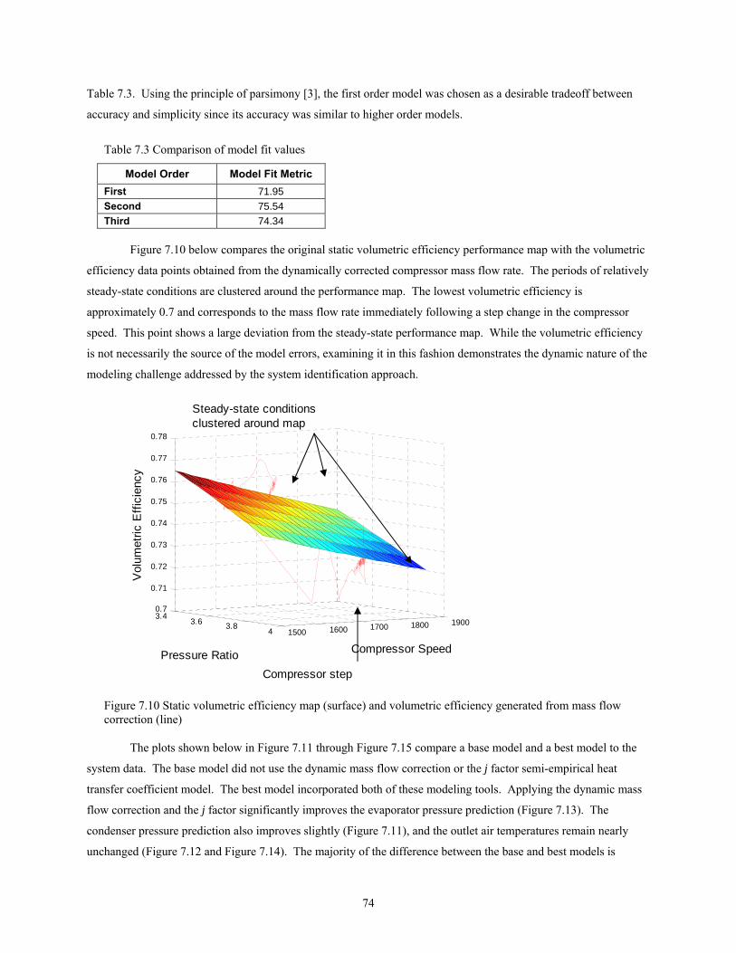
74

Table 7.3. Using the principle of parsimony [3], the first order model was chosen as a desirable tradeoff between

accuracy and simplicity since its accuracy was similar to higher order models.

Table 7.3 Comparison of model fit values

Model Order Model Fit Metric First 71.95 Second 75.54 Third 74.34

Figure 7.10 below compares the original static volumetric efficiency performance map with the volumetric

efficiency data points obtained from the dynamically corrected compressor mass flow rate. The periods of relatively

steady-state conditions are clustered around the performance map. The lowest volumetric efficiency is

approximately 0.7 and corresponds to the mass flow rate immediately following a step change in the compressor

speed. This point shows a large deviation from the steady-state performance map. While the volumetric efficiency

is not necessarily the source of the model errors, examining it in this fashion demonstrates the dynamic nature of the

modeling challenge addressed by the system identification approach.

3.43.6 3.8

4 1500 1600 1700 1800 1900

0.7

0.71

0.72

0.73

0.74

0.75

0.76

0.77

0.78

Compressor SpeedPressure Ratio

Vol

umet

ric E

ffici

ency

Steady-state conditionsclustered around map

Compressor step

Figure 7.10 Static volumetric efficiency map (surface) and volumetric efficiency generated from mass flow correction (line)

The plots shown below in Figure 7.11 through Figure 7.15 compare a base model and a best model to the

system data. The base model did not use the dynamic mass flow correction or the j factor semi-empirical heat

transfer coefficient model. The best model incorporated both of these modeling tools. Applying the dynamic mass

flow correction and the j factor significantly improves the evaporator pressure prediction (Figure 7.13). The

condenser pressure prediction also improves slightly (Figure 7.11), and the outlet air temperatures remain nearly

unchanged (Figure 7.12 and Figure 7.14). The majority of the difference between the base and best models is

75

attributed to the dynamic mass flow correction, as demonstrated by the quantitative results presented in the

following section. These results demonstrate the high sensitivity from the evaporator outlet mass flow model input

to the evaporator pressure model output. The effect of modifying the compressor mass flow rate is much more

pronounced in the evaporator than in the condenser. The evaporator superheat plot (Figure 7.15) actually shows a

decrease in accuracy for the best model. Recognizing that the superheat model output is closely tied to the

evaporator pressure model output and that the pressure model output of the best model is very accurate, the clear

conclusion is that errors must be present in the other component of the superheat prediction, the evaporator

refrigerant outlet temperature.

800 1000 1200 1400 1600 1800 2000 2200 2400 2600960

970

980

990

1000

1010

1020

1030

Time [s]

Pre

ssur

e [k

Pa]

DataBase ModelBest Model

Figure 7.11 Condenser pressure

800 1000 1200 1400 1600 1800 2000 2200 2400 2600

30

30.5

31

31.5

Time [s]

Tem

pera

ture

[C]

DataBase ModelBest Model

Figure 7.12 Condenser air outlet temperature

800 1000 1200 1400 1600 1800 2000 2200 2400 2600260

270

280

290

300

310

Time [s]

Pre

ssur

e [k

Pa]

DataBase ModelBest Model

Figure 7.13 Evaporator pressure

76

800 1000 1200 1400 1600 1800 2000 2200 2400 260014.5

15

15.5

16

16.5

17

17.5

18

Time [s]

Tem

pera

ture

[C] Data

Base ModelBest Model

Figure 7.14 Evaporator air outlet temperature

800 1000 1200 1400 1600 1800 2000 2200 2400 260014

16

18

20

22

Time [s]

Tem

pera

ture

[C]

DataBase ModelBest Model

Figure 7.15 Evaporator superheat

7.1.3 Quantified Modeling Improvements 7.1.3.1 Semi-empirical Accuracy Improvements

For the initial single-step model validation, the RMS error was chosen as the metric for comparing the

models that did and did not use the semi-empirical modeling techniques. As this validation scenario represented the

initial attempt at implementing the condenser with receiver model, the condenser pressure was chosen as the output

of interest for RMS error comparisons. The system simulation was run in six configurations. The base model

contained none of the semi-empirical modeling improvements described in Chapter 3, namely the j factor and the

mass flow component maps. The other simulation models used various combinations of the semi-empirical

modeling techniques. The condenser pressure RMS error and percent reduction in RMS error for each simulation

are summarized in Table 7.4.

Table 7.4 RMS error and RMS error reduction in the condenser pressure

Semi-empirical models in system RMS Error Percent Change in RMS Error from Base Model

Base—no semi-empirical models 7.55 -- Evaporator j factor 7.41 1.84 Condenser j factor 7.16 5.17 Condenser and Evaporator j factor 7.03 6.97 Valve and Compressor mass flow 6.02 20.31 All semi-empirical models—mass flow and j factor 5.62 25.64

77

Table 7.4 shows that, as expected, the largest error reduction comes from incorporating all of the semi-

empirical modeling techniques. The largest individual error reduction comes from including the detailed valve and

compressor performance maps generated from experimental system components. Validation results consistently

demonstrate that accurate refrigerant mass flow rate prediction is essential to system level model accuracy.

7.1.3.2 Mass Flow Correction Accuracy Improvements The effect of the dynamic mass flow correction method was also quantitatively compared to the effect of

the j factor semi-empirical model. A new error metric was defined to capture the impact of the two modeling

techniques on multiple model outputs, as shown in Equation 7.5. The chosen model outputs are those judged to be

of greatest importance in control design: evaporator pressure, condenser pressure, evaporator superheat, and

evaporator outlet air temperature.

( ) 212

42

32

22

1 ∞∞∞∞+++= TeaoTeshPcPe eeeecErrorMetri αααα ( 7.5 )

The weighting terms, α1 through α4, are used to normalize by the mean value of each output. Table 7.5

gives the scaling factor values. Table 7.6 summarizes the percent reduction in the error metric achieved by using

both the mass flow correction and the j factor modeling techniques. By far, the largest percentage error reductions

come from incorporating the dynamic mass flow correction, again showing the importance of accurate mass flow

prediction. The gains from incorporating the j factor are marginal compared to those from incorporating the

dynamic mass flow correction.

Table 7.5 Error metric scaling factors

Scaling Factor (1/mean) α1 0.003597 α2 0.000998 α3 0.055301 α4 0.061596

Table 7.6 Error metric and error metric improvement

Model Error Metric

Percent Improvement

Base-no j factor, no dynamic mass flow correction 1.3167 --

Dynamic mass flow correction 0.8523 35.2720 Dynamic mass flow correction and condenser j factor 0.8521 35.2878

Dynamic mass flow correction and evaporator j factor 0.8118 38.3479

Dynamic mass flow correction, condenser and evaporator j factor 0.8109 38.4179

7.2 Drive Cycle Model Validation Scenario The drive cycle validation scenario is based on a standard EPA emissions test, the SFTP-SCO3 [16]. This

test is of interest because it specifies that the vehicle air conditioning system must be operating while tailpipe

emissions are measured. Therefore the efficiency of the air conditioner becomes critical for a vehicle to perform

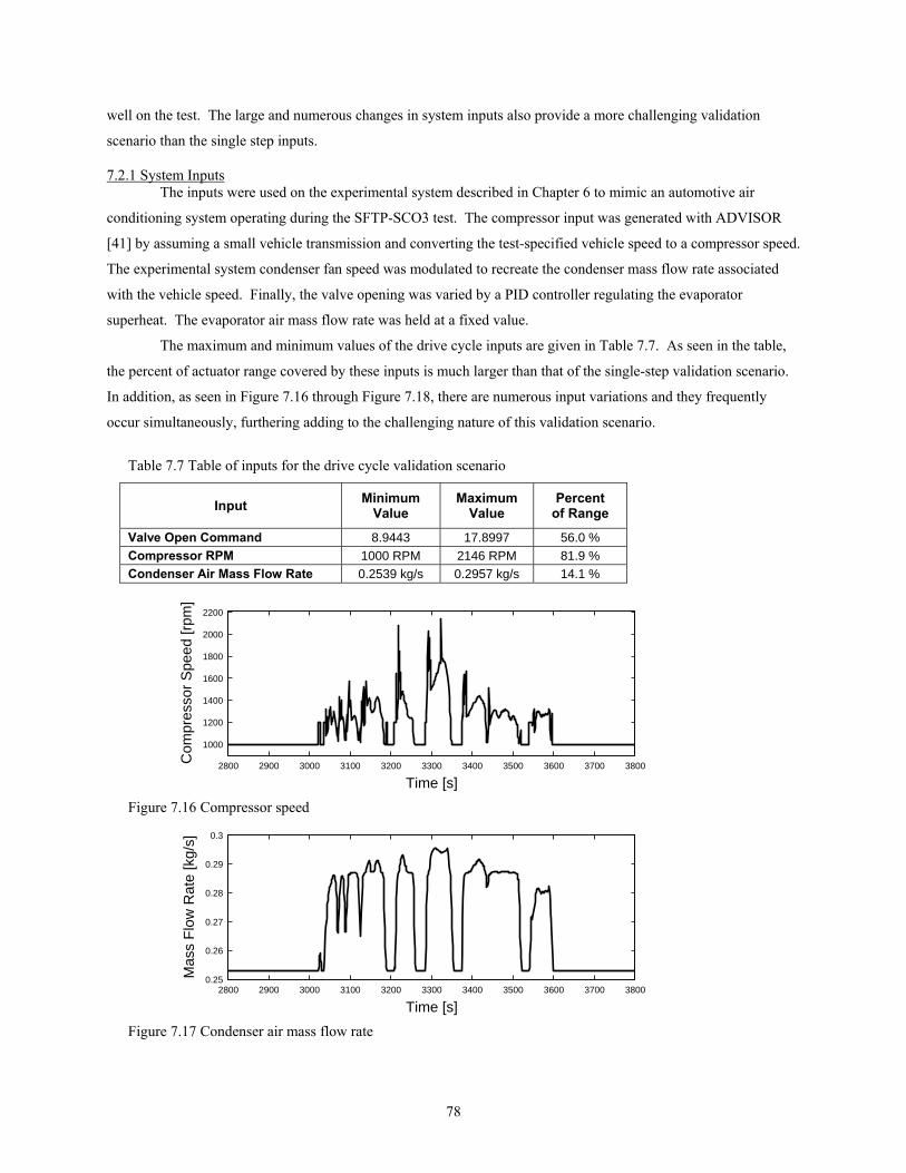
78

well on the test. The large and numerous changes in system inputs also provide a more challenging validation

scenario than the single step inputs.

7.2.1 System Inputs The inputs were used on the experimental system described in Chapter 6 to mimic an automotive air

conditioning system operating during the SFTP-SCO3 test. The compressor input was generated with ADVISOR

[41] by assuming a small vehicle transmission and converting the test-specified vehicle speed to a compressor speed.

The experimental system condenser fan speed was modulated to recreate the condenser mass flow rate associated

with the vehicle speed. Finally, the valve opening was varied by a PID controller regulating the evaporator

superheat. The evaporator air mass flow rate was held at a fixed value.

The maximum and minimum values of the drive cycle inputs are given in Table 7.7. As seen in the table,

the percent of actuator range covered by these inputs is much larger than that of the single-step validation scenario.

In addition, as seen in Figure 7.16 through Figure 7.18, there are numerous input variations and they frequently

occur simultaneously, furthering adding to the challenging nature of this validation scenario.

Table 7.7 Table of inputs for the drive cycle validation scenario

Input Minimum Value

Maximum Value

Percent of Range

Valve Open Command 8.9443 17.8997 56.0 % Compressor RPM 1000 RPM 2146 RPM 81.9 % Condenser Air Mass Flow Rate 0.2539 kg/s 0.2957 kg/s 14.1 %

2800 2900 3000 3100 3200 3300 3400 3500 3600 3700 3800

1000

1200

1400

1600

1800

2000

2200

Time [s]

Com

pres

sor

Spe

ed [r

pm]

Figure 7.16 Compressor speed

2800 2900 3000 3100 3200 3300 3400 3500 3600 3700 38000.25

0.26

0.27

0.28

0.29

0.3

Time [s]

Mas

s F

low

Rat

e [k

g/s]

Figure 7.17 Condenser air mass flow rate

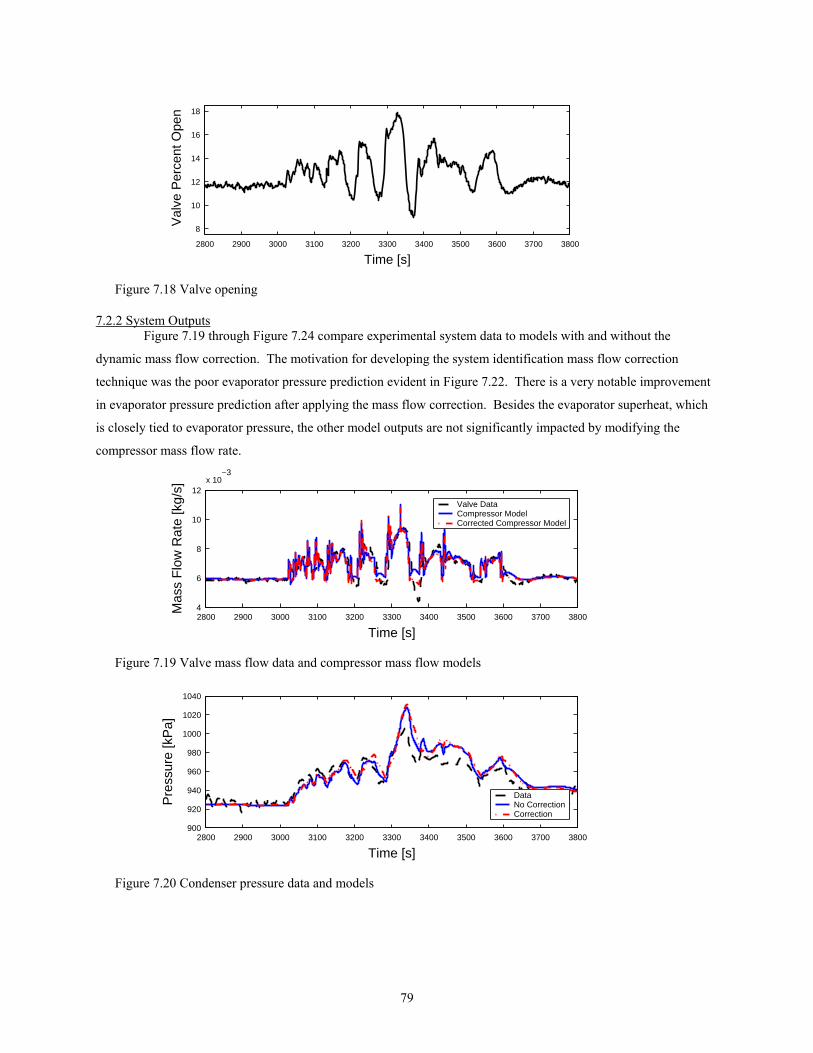
79

2800 2900 3000 3100 3200 3300 3400 3500 3600 3700 3800

8

10

12

14

16

18

Time [s]

Val

ve P

erce

nt O

pen

Figure 7.18 Valve opening

7.2.2 System Outputs Figure 7.19 through Figure 7.24 compare experimental system data to models with and without the

dynamic mass flow correction. The motivation for developing the system identification mass flow correction

technique was the poor evaporator pressure prediction evident in Figure 7.22. There is a very notable improvement

in evaporator pressure prediction after applying the mass flow correction. Besides the evaporator superheat, which

is closely tied to evaporator pressure, the other model outputs are not significantly impacted by modifying the

compressor mass flow rate.

2800 2900 3000 3100 3200 3300 3400 3500 3600 3700 38004

6

8

10

12x 10

−3

Time [s]

Mas

s F

low

Rat

e [k

g/s]

Valve DataCompressor ModelCorrected Compressor Model

Figure 7.19 Valve mass flow data and compressor mass flow models

2800 2900 3000 3100 3200 3300 3400 3500 3600 3700 3800900

920

940

960

980

1000

1020

1040

Time [s]

Pre

ssur

e [k

Pa]

DataNo CorrectionCorrection

Figure 7.20 Condenser pressure data and models

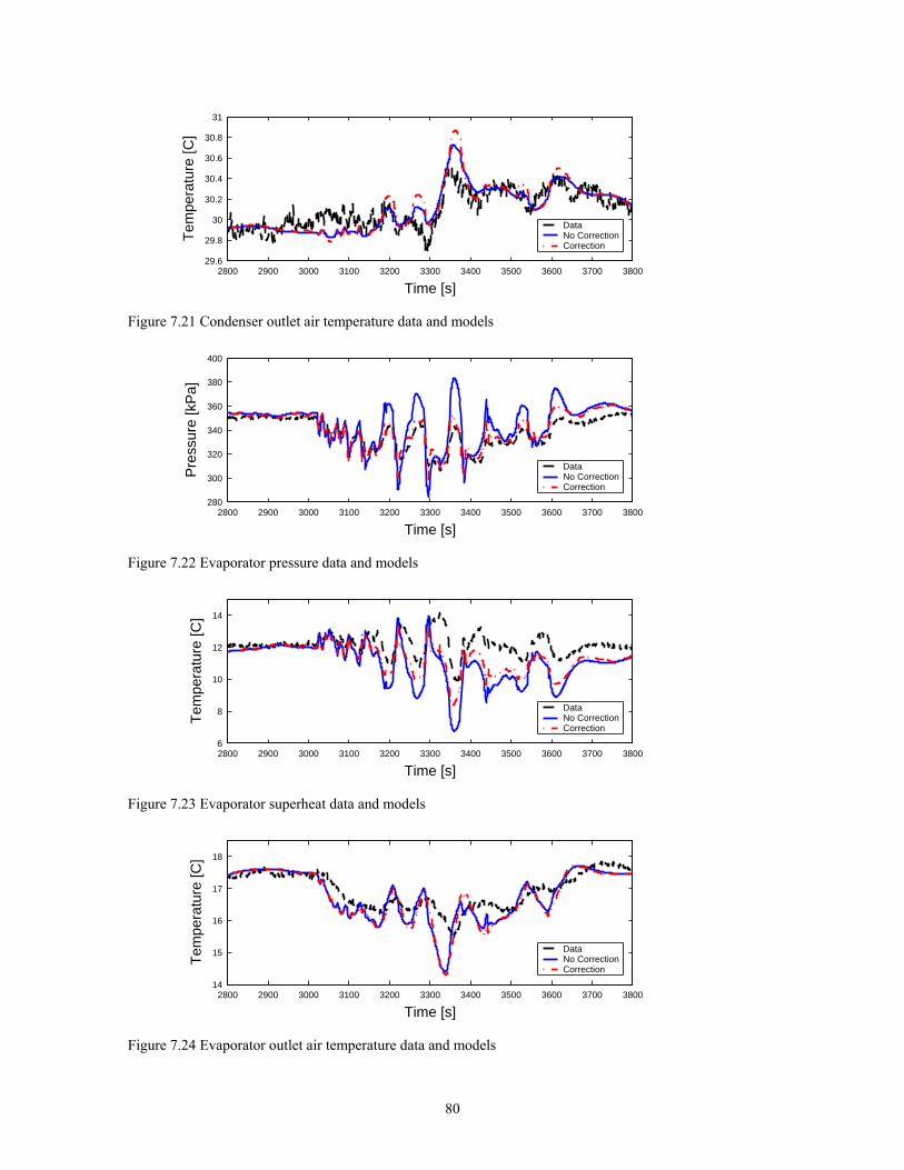
80

2800 2900 3000 3100 3200 3300 3400 3500 3600 3700 380029.6

29.8

30

30.2

30.4

30.6

30.8

31

Time [s]

Tem

pera

ture

[C]

DataNo CorrectionCorrection

Figure 7.21 Condenser outlet air temperature data and models

2800 2900 3000 3100 3200 3300 3400 3500 3600 3700 3800280

300

320

340

360

380

400

Time [s]

Pre

ssur

e [k

Pa]

DataNo CorrectionCorrection

Figure 7.22 Evaporator pressure data and models

2800 2900 3000 3100 3200 3300 3400 3500 3600 3700 38006

8

10

12

14

Time [s]

Tem

pera

ture

[C]

DataNo CorrectionCorrection

Figure 7.23 Evaporator superheat data and models

2800 2900 3000 3100 3200 3300 3400 3500 3600 3700 380014

15

16

17

18

Time [s]

Tem

pera

ture

[C]

DataNo CorrectionCorrection

Figure 7.24 Evaporator outlet air temperature data and models

81

The mass flow correction factor is defined in Equation 7.6, where G1 and G2 are the transfer functions

given in Equation 7.7 and Equation 7.8. The transfer functions were generated with the MATLAB System

Identification Toolbox. The model structure is the ARMAX model described in [32]. The inputs to the correction

model are the deviations from the initial conditions of compressor speed and valve opening. These inputs were

chosen because they are the cause of most dynamic events in the system. However, using these inputs required the

selection of a high-order model to capture the dynamics isolated by the ILC algorithm. For reasons of minimizing

model complexity, the inputs used in the single-step validation scenario (compressor inlet pressure, outlet pressure,

and speed) are probably more advantageous than the inputs used here.

[ ] ⎥⎦

⎤⎢⎣

⎡ΔΔ

=Valve

GGm kcorrectionk

ω21,& ( 7.6 )

00056.00045.0109.0111.0104101.5108.2107

234

1010210311

1 ++++×−×−×−×−

=−−−−

sssssssG ( 7.7 )

00056.00045.0109.0111.0104.41033.11057.1104.5

234

872738

2 ++++×−×+×+×

=−−−−

sssssssG ( 7.8 )

Figure 7.19 shows the original compressor mass flow rate and the corrected compressor mass flow rate. By

examining the compressor RPM plot and the mass flow rate plot, it is readily noted that the mass flow correction

momentarily decreases the compressor mass flow following increases in the compressor speed. In other words, the

static compressor model over-predicts the mass flow rate of refrigerant exiting the evaporator and entering the

condenser following step increases in speed. A similar under-prediction of mass flow rate occurs for step decreases

in speed. The source of these unmodeled dynamics has not been determined, but the dynamic mass flow correction

provides a method for compensating for them. Possible sources of the unmodeled dynamics include the compressor

model itself and the oil separator component, or some interaction between these components and others in the

system.

7.3 Atmospheric Conditions Model Validation Scenario To obtain a clear evaluation of the evaporator with humidity model, the atmospheric conditions model

validation scenario was carried out with just the compressor model, the evaporator model, and a connecting pipe

model. The evaporator and compressor inputs that would normally come from other components were replaced with

experimental data. For example, the valve mass flow rate input to the evaporator model was replaced with

experimental system mass flow rate data. The component models and inputs are shown in Figure 7.25.

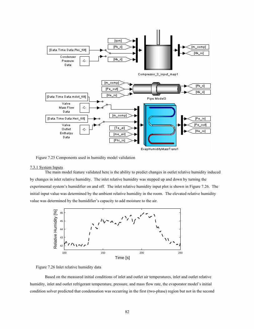
82

Figure 7.25 Components used in humidity model validation

7.3.1 System Inputs The main model feature validated here is the ability to predict changes in outlet relative humidity induced

by changes in inlet relative humidity. The inlet relative humidity was stepped up and down by turning the

experimental system’s humidifier on and off. The inlet relative humidity input plot is shown in Figure 7.26. The

initial input value was determined by the ambient relative humidity in the room. The elevated relative humidity

value was determined by the humidifier’s capacity to add moisture to the air.

100 150 200 250

42

43

44

45

46

Time [s]

Rel

ativ

e H

umid

ity [%

]

Figure 7.26 Inlet relative humidity data

Based on the measured initial conditions of inlet and outlet air temperatures, inlet and outlet relative

humidity, inlet and outlet refrigerant temperature, pressure, and mass flow rate, the evaporator model’s initial

condition solver predicted that condensation was occurring in the first (two-phase) region but not in the second

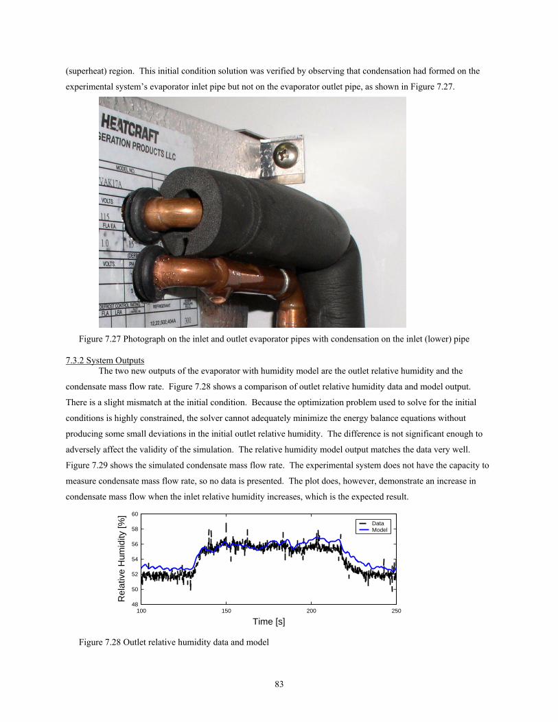
83

(superheat) region. This initial condition solution was verified by observing that condensation had formed on the

experimental system’s evaporator inlet pipe but not on the evaporator outlet pipe, as shown in Figure 7.27.

Figure 7.27 Photograph on the inlet and outlet evaporator pipes with condensation on the inlet (lower) pipe

7.3.2 System Outputs The two new outputs of the evaporator with humidity model are the outlet relative humidity and the

condensate mass flow rate. Figure 7.28 shows a comparison of outlet relative humidity data and model output.

There is a slight mismatch at the initial condition. Because the optimization problem used to solve for the initial

conditions is highly constrained, the solver cannot adequately minimize the energy balance equations without

producing some small deviations in the initial outlet relative humidity. The difference is not significant enough to

adversely affect the validity of the simulation. The relative humidity model output matches the data very well.

Figure 7.29 shows the simulated condensate mass flow rate. The experimental system does not have the capacity to

measure condensate mass flow rate, so no data is presented. The plot does, however, demonstrate an increase in

condensate mass flow when the inlet relative humidity increases, which is the expected result.

100 150 200 25048

50

52

54

56

58

60

Time [s]

Rel

ativ

e H

umid

ity [%

]

DataModel

Figure 7.28 Outlet relative humidity data and model

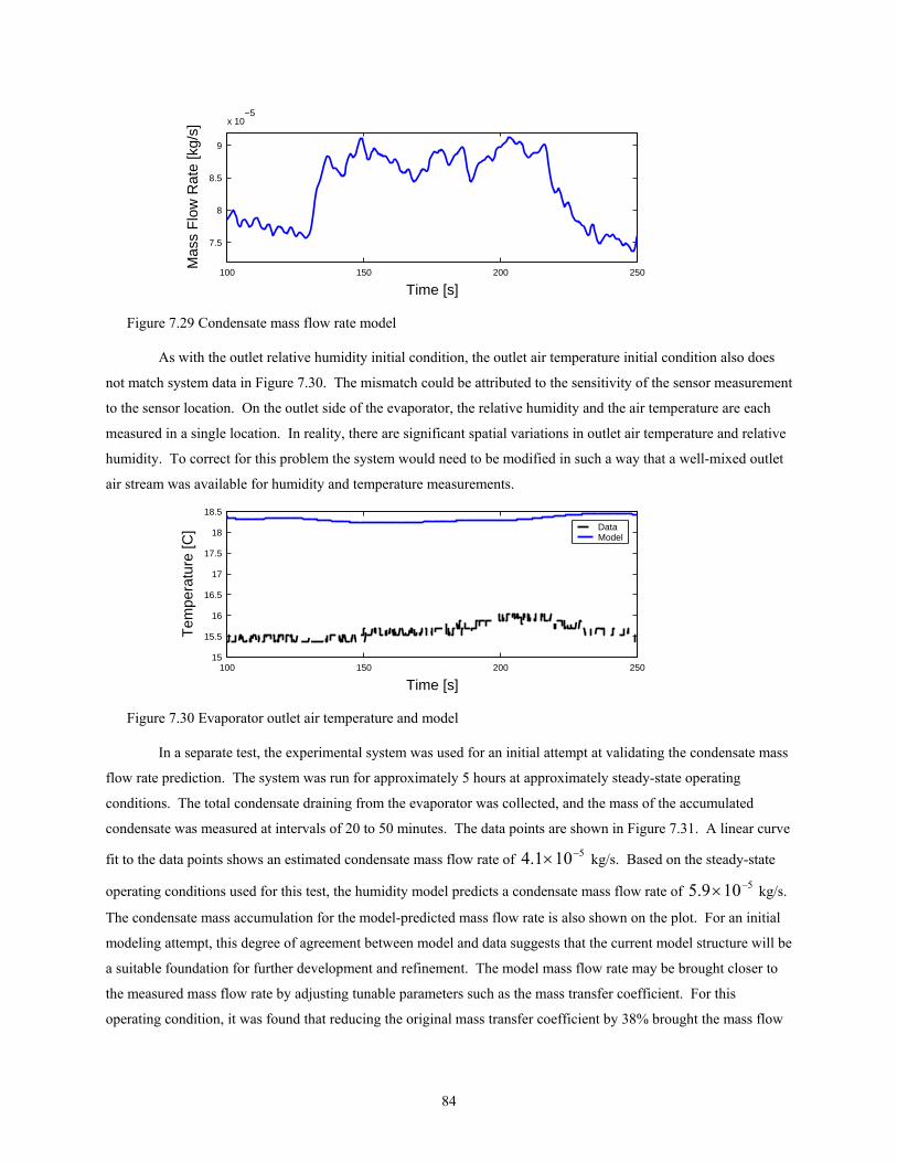
84

100 150 200 250

7.5

8

8.5

9

x 10−5

Time [s]

Mas

s F

low

Rat

e [k

g/s]

Figure 7.29 Condensate mass flow rate model

As with the outlet relative humidity initial condition, the outlet air temperature initial condition also does

not match system data in Figure 7.30. The mismatch could be attributed to the sensitivity of the sensor measurement

to the sensor location. On the outlet side of the evaporator, the relative humidity and the air temperature are each

measured in a single location. In reality, there are significant spatial variations in outlet air temperature and relative

humidity. To correct for this problem the system would need to be modified in such a way that a well-mixed outlet

air stream was available for humidity and temperature measurements.

100 150 200 25015

15.5

16

16.5

17

17.5

18

18.5

Time [s]

Tem

pera

ture

[C] Data

Model

Figure 7.30 Evaporator outlet air temperature and model

In a separate test, the experimental system was used for an initial attempt at validating the condensate mass

flow rate prediction. The system was run for approximately 5 hours at approximately steady-state operating

conditions. The total condensate draining from the evaporator was collected, and the mass of the accumulated

condensate was measured at intervals of 20 to 50 minutes. The data points are shown in Figure 7.31. A linear curve

fit to the data points shows an estimated condensate mass flow rate of 5101.4 −× kg/s. Based on the steady-state

operating conditions used for this test, the humidity model predicts a condensate mass flow rate of 5109.5 −× kg/s.

The condensate mass accumulation for the model-predicted mass flow rate is also shown on the plot. For an initial

modeling attempt, this degree of agreement between model and data suggests that the current model structure will be

a suitable foundation for further development and refinement. The model mass flow rate may be brought closer to

the measured mass flow rate by adjusting tunable parameters such as the mass transfer coefficient. For this

operating condition, it was found that reducing the original mass transfer coefficient by 38% brought the mass flow

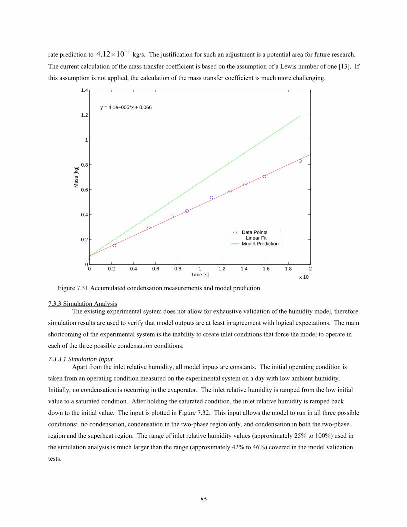
85

rate prediction to 51012.4 −× kg/s. The justification for such an adjustment is a potential area for future research.

The current calculation of the mass transfer coefficient is based on the assumption of a Lewis number of one [13]. If

this assumption is not applied, the calculation of the mass transfer coefficient is much more challenging.

0 0.2 0.4 0.6 0.8 1 1.2 1.4 1.6 1.8 2

x 104

0

0.2

0.4

0.6

0.8

1

1.2

1.4

Time [s]

Mas

s [k

g]

y = 4.1e−005*x + 0.066

Data Points Linear FitModel Prediction

Figure 7.31 Accumulated condensation measurements and model prediction

7.3.3 Simulation Analysis The existing experimental system does not allow for exhaustive validation of the humidity model, therefore

simulation results are used to verify that model outputs are at least in agreement with logical expectations. The main

shortcoming of the experimental system is the inability to create inlet conditions that force the model to operate in

each of the three possible condensation conditions.

7.3.3.1 Simulation Input Apart from the inlet relative humidity, all model inputs are constants. The initial operating condition is

taken from an operating condition measured on the experimental system on a day with low ambient humidity.

Initially, no condensation is occurring in the evaporator. The inlet relative humidity is ramped from the low initial

value to a saturated condition. After holding the saturated condition, the inlet relative humidity is ramped back

down to the initial value. The input is plotted in Figure 7.32. This input allows the model to run in all three possible

conditions: no condensation, condensation in the two-phase region only, and condensation in both the two-phase

region and the superheat region. The range of inlet relative humidity values (approximately 25% to 100%) used in

the simulation analysis is much larger than the range (approximately 42% to 46%) covered in the model validation

tests.

86

100 120 140 160 180 200 220 240 260 280 300 32020

40

60

80

100

Time [s]

Rel

ativ

e H

umid

ity [%

]

Figure 7.32 Inlet relative humidity

7.3.3.2 Simulation Output Figure 7.33 shows the evaporator dew point temperature and the wall temperature of each fluid region.

Condensation in a region occurs when the wall temperature is below the dew point temperature. As the inlet relative

humidity increases, the dew point temperature increases as well, meaning that condensation will occur at higher

temperatures due to the elevated moisture content in the air.

100 120 140 160 180 200 220 240 260 280 300 3200

5

10

15

20

25

Time [s]

Tem

pera

ture

[C] Dew Point

Twall,1

Twall,2

Figure 7.33 Dew point temperature and model wall temperatures

Figure 7.34 shows the outlet relative humidity prediction. The outlet relative humidity increases and

decreases in roughly the same fashion as the inlet relative humidity. Small discontinuities are present when the

condensation condition of a fluid region changes. One noteworthy feature of Figure 7.34 is that the outlet relative

humidity reaches values greater than 100%. As explained in [8], this condition is referred to as super-saturation.

The physical explanation for super-saturation is that some water vapor is condensing out of the air but not depositing

on the evaporator pipes. Therefore the outlet fluid consists of a mixture of saturated air and tiny water droplets.

100 120 140 160 180 200 220 240 260 280 300 32020

40

60

80

100

120

Time [s]

Rel

ativ

e H

umid

ity [%

]

Figure 7.34 Outlet relative humidity model

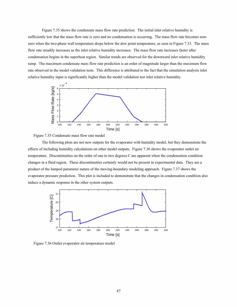
87

Figure 7.35 shows the condensate mass flow rate prediction. The initial inlet relative humidity is

sufficiently low that the mass flow rate is zero and no condensation is occurring. The mass flow rate becomes non-

zero when the two-phase wall temperature drops below the dew point temperature, as seen in Figure 7.33. The mass

flow rate steadily increases as the inlet relative humidity increases. The mass flow rate increases faster after

condensation begins in the superheat region. Similar trends are observed for the downward inlet relative humidity

ramp. The maximum condensate mass flow rate prediction is an order of magnitude larger than the maximum flow

rate observed in the model validation tests. This difference is attributed to the fact that the simulation analysis inlet

relative humidity input is significantly higher than the model validation test inlet relative humidity.

100 120 140 160 180 200 220 240 260 280 300 3200

1

2

3

4

5

6x 10

−4

Time [s]

Mas

s F

low

Rat

e [k

g/s]

Figure 7.35 Condensate mass flow rate model

The following plots are not new outputs for the evaporator with humidity model, but they demonstrate the

effects of including humidity calculations on other model outputs. Figure 7.36 shows the evaporator outlet air

temperature. Discontinuities on the order of one to two degrees C are apparent when the condensation condition

changes in a fluid region. These discontinuities certainly would not be present in experimental data. They are a

product of the lumped parameter nature of the moving-boundary modeling approach. Figure 7.37 shows the

evaporator pressure prediction. This plot is included to demonstrate that the changes in condensation condition also

induce a dynamic response in the other system outputs.

100 120 140 160 180 200 220 240 260 280 300 32017

18

19

20

21

Time [s]

Tem

pera

ture

[C]

Figure 7.36 Outlet evaporator air temperature model

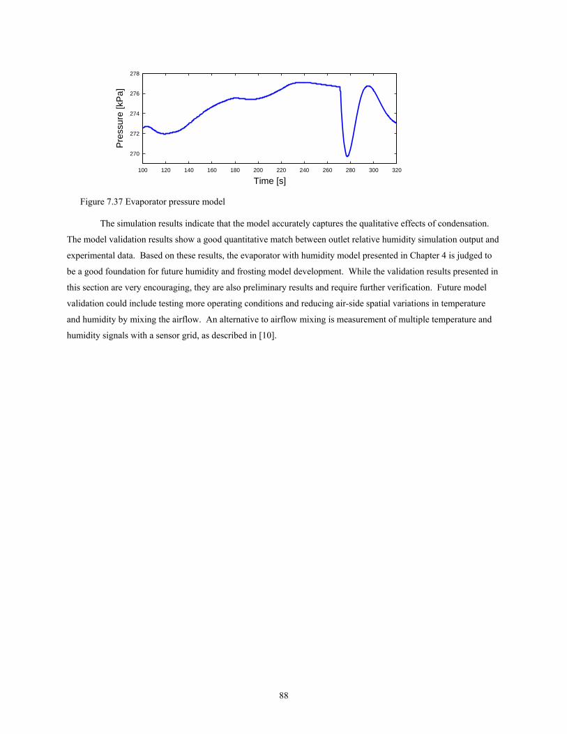
88

100 120 140 160 180 200 220 240 260 280 300 320

270

272

274

276

278

Time [s]

Pre

ssur

e [k

Pa]

Figure 7.37 Evaporator pressure model

The simulation results indicate that the model accurately captures the qualitative effects of condensation.

The model validation results show a good quantitative match between outlet relative humidity simulation output and

experimental data. Based on these results, the evaporator with humidity model presented in Chapter 4 is judged to

be a good foundation for future humidity and frosting model development. While the validation results presented in

this section are very encouraging, they are also preliminary results and require further verification. Future model

validation could include testing more operating conditions and reducing air-side spatial variations in temperature

and humidity by mixing the airflow. An alternative to airflow mixing is measurement of multiple temperature and

humidity signals with a sensor grid, as described in [10].

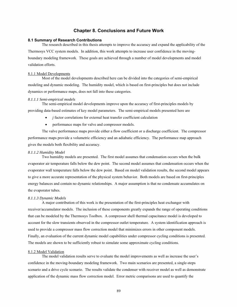
89

Chapter 8. Conclusions and Future Work

8.1 Summary of Research Contributions The research described in this thesis attempts to improve the accuracy and expand the applicability of the

Thermosys VCC system models. In addition, this work attempts to increase user confidence in the moving-

boundary modeling framework. These goals are achieved through a number of model developments and model

validation efforts.

8.1.1 Model Developments Most of the model developments described here can be divided into the categories of semi-empirical

modeling and dynamic modeling. The humidity model, which is based on first-principles but does not include

dynamics or performance maps, does not fall into these categories.

8.1.1.1 Semi-empirical models The semi-empirical model developments improve upon the accuracy of first-principles models by

providing data-based estimates of key model parameters. The semi-empirical models presented here are

• j factor correlations for external heat transfer coefficient calculation

• performance maps for valve and compressor models.

The valve performance maps provide either a flow coefficient or a discharge coefficient. The compressor

performance maps provide a volumetric efficiency and an adiabatic efficiency. The performance map approach

gives the models both flexibility and accuracy.

8.1.1.2 Humidity Model Two humidity models are presented. The first model assumes that condensation occurs when the bulk

evaporator air temperature falls below the dew point. The second model assumes that condensation occurs when the

evaporator wall temperature falls below the dew point. Based on model validation results, the second model appears

to give a more accurate representation of the physical system behavior. Both models are based on first-principles

energy balances and contain no dynamic relationships. A major assumption is that no condensate accumulates on

the evaporator tubes.

8.1.1.3 Dynamic Models A major contribution of this work is the presentation of the first-principles heat exchanger with

receiver/accumulator models. The inclusion of these components greatly expands the range of operating conditions

that can be modeled by the Thermosys Toolbox. A compressor shell thermal capacitance model is developed to

account for the slow transients observed in the compressor outlet temperature. A system identification approach is

used to provide a compressor mass flow correction model that minimizes errors in other component models.

Finally, an evaluation of the current dynamic model capabilities under compressor cycling conditions is presented.

The models are shown to be sufficiently robust to simulate some approximate cycling conditions.

8.1.2 Model Validation The model validation results serve to evaluate the model improvements as well as increase the user’s

confidence in the moving-boundary modeling framework. Two main scenarios are presented, a single-steps

scenario and a drive cycle scenario. The results validate the condenser with receiver model as well as demonstrate

application of the dynamic mass flow correction model. Error metric comparisons are used to quantify the

90

improvements obtained through application of the semi-empirical modeling techniques. Results consistently

demonstrate the importance of the compressor mass flow rate prediction. The humidity model is also shown to

provide a reasonably accurate prediction of both the outlet relative humidity and the condensate mass flow rate.

8.2 Future Work Future work in both modeling and model validation will improve the quality of the moving-boundary

models and their acceptance in academia and industry. As the models improve and user confidence increases, the

models will be useful in numerous applications.

8.2.1 Model Development Opportunities for future model development are numerous. Possible directions for future research are

given in the following list. The list is ordered according to a suggested priority for the research directions.

• Develop a model switching scheme. Completion of this task is essential for successful simulation of cycling and start-up conditions. In addition, the behavior of the mass flow devices at very low flow rates will need to be characterized.

• Develop a dynamic model to improve the compressor mass flow rate prediction, as this model output has a significant effect on the accuracy of other component models. Improvements in the mass flow rate prediction could be achieved by creating a first-principles dynamic compressor model, including oil flow modeling, or directly identifying a compressor mass flow rate model.

• Improve the semi-empirical modeling approach presented here by evaluating additional performance map structures and inputs. The semi-empirical approach could be applied to other VCC system components which contain parameters that are best described with data-driven correlations.

• Improve the humidity model by taking into account the effects of condensate retention on the heat exchanger tubes. This task will likely require a blending of first-principles dynamic modeling and semi-empirical parameter estimates.

8.2.2 Model Validation Additional successful model validation results will always increase user confidence in the accuracy of the

moving-boundary models. Future model validation could focus on validating the system models on a larger range of

operating conditions. Some system configurations have yet to be validated, such as systems including models of the

accumulator, the capillary tube, the automatic expansion valve, and the thermostatic expansion valve. The humidity

model validation could be improved by validating a range of conditions that includes no condensation, condensation

on the two-phase region, and condensation on both the two-phase and the superheat regions. Eliminating spatial

variation in the air-side humidity and temperature measurements (through air flow mixing or spatially distributed

sensor arrays) would also be an improvement to the results presented here.

8.2.3 Model Applications An accurate and tractable dynamic model of VCC systems has numerous application areas. The most

obvious is dynamic analysis for improved system level design. The low-order nature of the moving-boundary

models makes them especially useful for control design. Control design based on moving-boundary models is

already an active research area and should yield significant improvements in system efficiency [41, 20]. Fault

detection is also being explored as a possible application of these models [26].

91

List of References

[1] “Parker Bulletin 21-02D,” Parker Hannifin, Cleveland, OH.

[2] “Sporlan Bulletin 10-9,” Sporlan Valve Company, Washington, MO, June 2001.

[3] Anderson, B.D.O., “Controller Design: Moving From Theory to Practice,” IEEE Control Systems Magazine, vol. 13, no. 4, pp. 16-25, Aug, 1993.

[4] Bendapudi, S. and Braun, J.E., “A Review of Literature on Dynamic Models of Vapor Compression Equipment,” ASHRAE Report #4036-5, May, 2002.

[5] Bristow, D.A., Tharayil, M., and Alleyne, A., “A Survey of Iterative Learning Control,” IEEE Control Systems Magazine, vol. 26, no. 3, pp. 96-114, Jun, 2006.

[6] Broersen, P.M.T. and van der Jagt, M.F.G., "Hunting of Evaporators Controlled by a Thermostatic Expansion Valve," ASME Journal of Dynamic Systems Measurement & Control, vol. 102, no. 2, pp. 130-135, Jun, 1980.

[7] Cengel, Y. A. and Boles, M. A. Thermodynamics: An Engineering Approach, Boston, MA: WCB McGraw-Hill, 1998.

[8] Chen, H., Thomas, L, and Besant, R., “Fan Supplied Heat Exchanger Performance Under Frosting Conditions,” International Journal of Refrigeration, vol. 26, no. 1, pp. 140-149, Jan, 2003.

[9] Chi, J. and Didion, D., "A Simulation Model of the Transient Performance of a Heat Pump," International Journal of Refrigeration, vol. 5, no. 3, pp. 176-184, May, 1982.

[10] Dane, M., Miller, N., Alleyne, A., Bullard, C., and Hrnjak, P., “Investigation of Control Strategies for Reducing Mobile Air Conditioning Power Consumption,” Air Conditioning and Refrigeration Center, University of Illinois at Urbana-Champaign, ACRC TR-199, Aug, 2002.

[11] Dhar, M. and Soedel, W., "Transient Analysis of a Vapor Compression Refrigeration System," in Proceedings of the XVth International Congress of Refrigeration, Venice, Italy, vol. 2, 1979 , pp. 1031-1067.

[12] Eborn, J., “On Model Libraries for Thermo-hydraulic Applications,” Department of Automatic Control, Lund Institute of Technology, Lund, Sweden, Mar. 2001.

[13] Eckert, E.R.G. and Drake, R.M., Analysis of Heat and Mass Transfer, New York, NY: McGraw-Hill, 1972.

[14] Energy Information Administration, 1999 CBECS Detailed Tables, http://www.eia.doe.gov/emeu/cbecs/detailed_tables_1999.html#ce

[15] Energy Information Administration, Residential Energy Consumption Survey 2001 Consumption and Expenditure Data Tables, http://www.eia.doe.gov/emeu/recs/recs2001/detailcetbls.html

[16] Federal Register, “Part II Environmental Protection Agency. Motor Vehicle Emissions Federal Test Procedure Revisions: Final Regulations,” 40 CFR Part 86, Oct. 1996.

[17] Grald, E.W. and MacArthur, J.W., "A Moving-Boundary Formulation for Modeling Time-Dependent Two-Phase Flows," International Journal of Heat & Fluid Flow, vol. 13, no. 3, pp. 266-272, Sep, 1992.

[18] Gruhle, W.D. and Isermann, R., "Modeling and Control of a Refrigerant Evaporator," ASME Journal of Dynamic Systems Measurement & Control, vol. 107, no. 4, pp. 235-240, Dec, 1985.

[19] He, X., Liu, S., and Asada, H., “Moving-Interface Model of Two-Phase Flow Heat Exchanger Dynamics for Control of Vapor Compression Cycle,” ASME Advanced Energy Systems, vol. 32, pp. 69-75, 1994.

[20] He, X.D., Asada, H., Liu, S., and Itoh, H., "Multivariable Control of Vapor Compression Systems," HVAC&R Research, vol. 4, no. 3, pp. 205-230, Jul, 1998.

[21] He, X.D., Liu, S., and Asada, H., “Modeling of Vapor Compression Cycles for Multivariable Feedback Control of HVAC Systems,” ASME Journal of Dynamic Systems, Measurement, and Control, vol. 119, no. 2, pp. 183-191, Jun, 1997.

[22] Incropera, F. P. and DeWitt, D. P. Fundamentals of Heat and Mass Transfer, New York: John Wiley & Sons, 1996.

92

[23] Jensen, J.M. and Tummescheit, H., "Moving Boundary Models for Dynamic Simulations of Two-Phase Flows," in Proceedings of the 2nd International Modelica Conference, 2002, pp. 235-244.

[24] Kapadia, M. and Wolgemuth, C.H., "A Dynamic Model of a Condenser in a Closed Rankine Cycle Power Plant," in Proceedings of the 1984 American Control Conference, New York, NY, vol. 1, 1984, pp. 79-84.

[25] Kays, W. M. and London, A. L. Compact Heat Exchangers, New York: McGraw-Hill Book Company, 1984.

[26] Keir, M., “Dynamic Modeling, Control and Fault Detection in Vapor Compression Systems,” Dept. of Mechanical and Industrial Engineering, University of Illinois, Urbana, IL, Aug, 2006.

[27] Keir, M., Rasmussen, B.P., and Alleyne, A., “Improving Energy Efficiency in Automotive Vapor Compression Cycles through Advanced Control Design,” SAE 2006 World Congress and Exposition, Detroit, MI, Apr, 2006.

[28] Kim, N.-H., Yun, J.-H., and Webb, R.L., “Heat Transfer and Friction Correlations for Wavy Plate Fin-and-Tube Heat Exchangers,” ASME Journal of Heat Transfer, vol. 119, no. 3, pp. 560-567, Aug, 1997.

[29] Klein, S.A. and Alvarado, F.L., EES-Engineering Equation Solver, F-Chart Software, Middleton, WI, 2002.

[30] Korte, C. and Jacobi, A.M., “Condensate Retention Effects on the Performance of Plain-Fin-and-Tube Heat Exchangers: Retention Data and Modeling,” ASME Journal of Heat Transfer, vol. 123, no. 5, pp. 926-936, Oct, 2001.

[31] Lenger, M.J., Jacobi, A.M., and Hrnjak, P.S., "Superheat Stability of an Evaporator and Thermostatic Expansion Valve," Air Conditioning and Refrigeration Center, University of Illinois at Urbana Champaign, ACRC TR-138, Jul 1998.

[32] Ljung, L., System Identification, Prentice Hall, New Jersey, 1999.

[33] MacArthur, J.W. and Grald, E.W., “Unsteady Compressible Two-Phase Flow Model for Predicting Cyclic Heat Pump Performance and a Comparison With Experimental Data,” International Journal of Refrigeration, vol. 12, no. 1, pp. 29-41, Jan, 1989.

[34] McQuiston, F.C., “Fin Efficiency with Combined Heat and Mass Transfer,” ASHRAE Transactions, vol. 81, no. 1, pp. 350-355, 1975.

[35] Mirth, D.R. and Ramadhyani, S., “Prediction of Cooling-Coil Performance Under Condensing Conditions,” International Journal of Heat and Fluid Flow, vol. 14, no. 4, pp. 391-400, Dec, 1993.

[36] Moore, K. L., Iterative Learning Control for Deterministic Systems, Springer-Verlag London, 1993.

[37] National Renewable Energy Laboratory, Ancillary Loads Reduction, http://www.nrel.gov/vehiclesandfuels/ancillary_loads/ac_emissions.html

[38] Pettit, N.B.O.L., Willatzen, M., and Ploug-Sorensen, L, “A General Dynamic Simulation Model for Evaporators and Condensers in Refrigeration. Part II: Simulation and Control of an Evaporator,” International Journal of Refrigeration, vol. 21, no. 5, pp. 404-414, Aug, 1998.

[39] Popper, K.R., Logik der Forschung, Julius Springer, Vienna, Austria, 1935.

[40] Rasmussen, B.P., "Control-Oriented Modeling of Transcritical Vapor Compression Systems," Dept. of Mechanical and Industrial Engineering, University of Illinois, Urbana, IL, Oct. 2002.

[41] Rasmussen, B.P., “Dynamic Modeling and Advanced Control of Air Conditioning and Refrigerating Systems,” Dept. of Mechanical and Industrial Engineering, University of Illinois, Urbana, IL, Dec, 2005.

[42] Rasmussen, B.P. and Alleyne, A., “Control-Oriented Modeling of Transcritical Vapor Compression Systems,” ASME Journal of Dynamic Systems, Measurement, and Control, vol. 126, no. 1, pp. 54-64, Mar, 2004.

[43] Rice, C.K., "Effect of Void Fraction Correlation and Heat Flux Assumption on Refrigerant Charge Inventory Predictions," ASHRAE Transactions, vol. 93, no. 1, pp. 341-367, 1987.

[44] Shah, R., “Dynamic Modeling and Control of Single and Multi-Evaporator Subcritical Vapor Compression Systems,” Dept. of Mechanical and Industrial Engineering, University of Illinois, Urbana, IL, Aug. 2003.

93

[45] Wang, C., Chi, K., and Chang, C., “Heat Transfer and Friction Characteristics of Plain Fin-and-Tube Heat Exchangers, Part II: Correlation,” International Journal of Heat and Mass Transfer, vol. 43, no. 15, pp. 2641-2823, Aug, 2000.

[46] Wang, C., Lin, Y., Lee, C., and Chang, Y., “Investigation of Wavy Fin-and-Tube Heat Exchangers: A Contribution to Databank,” Experimental Heat Transfer, vol. 12, no. 1, pp. 73-89, Jan-Mar, 1993.

[47] Willatzen, M., Pettit, N.B.O.L., and Ploug-Sorensen, L., "General Dynamic Simulation Model for Evaporators and Condensers in Refrigeration. Part I: Moving-Boundary Formulation of Two-Phase Flows with Heat Exchange," International Journal of Refrigeration, vol. 21, no. 5, pp. 398-403, Aug, 1998.

94

Appendix A. Sample Code

H.1 Condenser j Factor Correlation % This file generates the experimental system j factor information to be % stored in the data structure HX. The information includes Reynolds % number data points, j factor data points, the constriction ratio % (sigma) and the air-side hydraulic diameter (Dh). % The j factor correlation is from the following article: % International Journal of Heat and Mass Transfer Volume 43, Issue 15, % Pages 2641-2823 (1 August 2000) % Create a Reynolds number vector (stored in HX structure) Re = [100 200 300 400 500 600 700 800 900 1000 ... 2000 3000 4000 5000 6000 7000 8000 9000 10000]; % Number of tube rows in the condenser N = 3; % Fin pitch (distance between fins) in inches Fp = .1429; % Tube outside diameter in inches Do = .375; % Fin thickness in inches Ft = .0093; % Fin collar outside diameter in inches (fin collar is defined as tube % diameter plus twice the fin thickness) Dc = Do + 2*Ft; % Longitudinal tube pitch (distance between tube centers in direction of % air flow) in inches Pl = .956; % Flow length in inches (flow length is explained in Chapter 3) L = 3*.956; % Flow cross-sectional area, also known as the minimum free flow area, in % square inches % Flow cross-sectional area = Frontal Area - Tube Diameter*Number of % Tubes at cross section*Tube_Length - Fin thinkness*Fin height*Number of % Fins Ac = (10.656*13.062) - .375*10*13.062 - .0093*10*89; % Total heat transfer area in square inches, provided by manufacturer A = 4328.64; % Air-side hydraulic diameter in inches as defined by Kays and London Dh = 4*L*Ac/A; % Transverse tube pitch in inches (distance between tube centers in % direction transverse to air flow) Pt = 1;

95

% Powers used in the j factor correlation P3 = -.361 - (.042*N./log(Re)) + .158*log(N*(Fp/Dc)^.41); P4 = -1.224 - (.076*(Pl/Dh)^1.42)./(log(Re)); P5 = -.083 + (.058*N)./(log(Re)); P6 = -5.735 + 1.21*log(Re/N); % Colburn j factor correlation (stored in HX structure) j_cond = .086.*Re.^P3.*N.^P4.*(Fp./Dc).^P5.*(Fp/Dh).^P6*(Fp./Pt).^-.93; % Calculate the frontal area in square inches Afr = (10.656*13.062); % Calculate the constriction ratio (stored in HX structure) sigma = Ac/Afr; % Convert Dh from inches to meters (stored in HX structure) DhSI = Dh*0.0254;

H.2 Evaporator j Factor Correlation % This file generates the experimental system j factor information to be % stored in the data structure HX. The information includes Reynolds % number data points, j factor data points, the constriction ratio % (sigma) and the air-side hydraulic diameter (Dh). % The j factor correlation is from the following article: % International Journal of Heat and Mass Transfer Volume 43, Issue 15, % Pages 2641-2823 (1 August 2000) % Create a Reynolds number vector (stored in HX structure) Re = [100 200 300 400 500 600 700 800 900 1000 ... 2000 3000 4000 5000 6000 7000 8000 9000 10000]; % Number of tube rows in the condenser N = 3; % Fin pitch (distance between fins) in inches Fp = .1429; % Tube outside diameter in inches Do = .375; % Fin thickness in inches Ft = .0093; % Fin collar outside diameter in inches (fin collar is defined as tube % diameter plus twice the fin thickness) Dc = Do + 2*Ft; % Longitudinal tube pitch (distance between tube centers in direction of % air flow) in inches Pl = .956; % Flow length in inches (flow length is explained in Chapter 3) L = 3*.956; % Flow cross-sectional area, also known as the minimum free flow area, in

96

% square inches % Flow cross-sectional area = Frontal Area - Tube Diameter*Number of % Tubes at cross section*Tube_Length - Fin thinkness*Fin height*Number of % Fins Ac = (10.656*13.062) - .375*10*13.062 - .0093*10*89; % Total heat transfer area in square inches, provided by manufacturer A = 4328.64; % Air-side hydraulic diameter in inches as defined by Kays and London Dh = 4*L*Ac/A; % Transverse tube pitch in inches (distance between tube centers in % direction transverse to air flow) Pt = 1; % Powers used in the j factor correlation P3 = -.361 - (.042*N./log(Re)) + .158*log(N*(Fp/Dc)^.41); P4 = -1.224 - (.076*(Pl/Dh)^1.42)./(log(Re)); P5 = -.083 + (.058*N)./(log(Re)); P6 = -5.735 + 1.21*log(Re/N); % Colburn j factor correlation (stored in HX structure) j_cond = .086.*Re.^P3.*N.^P4.*(Fp./Dc).^P5.*(Fp/Dh).^P6*(Fp./Pt).^-.93; % Calculate the frontal area in square inches Afr = (10.656*13.062); % Calculate the constriction ratio (stored in HX structure) sigma = Ac/Afr; % Convert Dh from inches to meters (stored in HX structure) DhSI = Dh*0.0254;

H.3 EEV Performance Map % This file creates a EEV flow coefficient performance map with inputs of % inlet pressure, outlet pressure, and valve command signal. The % experimental system data is stored in the workspace in a structure % called Data. % The start and finish variables are used to select the range of data % that will be used to generate the map start = 2500; finish = 3800; % Store the selected range of data in new variables % MDOT = mass flow rate % PI = valve inlet pressure % PO = valve outlet pressure % EEV = valve command signal % TIME = time values MDOT = Data.mdot(start:finish); PI = Data.Pko(start:finish); PO = Data.Pei_2(start:finish); EEV = Data.EEV_ref(start:finish); TIME = Data.Time(start:finish);

97

% Calculate the inlet fluid density, assuming the inlet fluid is % saturated vapor RHO_V = interp1(FluidProp.Psat,FluidProp.Rhof,PI); % Calculate the flow coefficient (valve area * discharge coefficient) CF = MDOT./(sqrt(RHO_V.*(PI-PO))); % Form input matrix X, assuming a model structure X = [ones(size(MDOT)) EEV PI.^.5 PO.^.5 PI.*PO]; % Find model coefficients using left matrix division (approximate matrix % inverse) a = X\CF % Find the flow coefficient values predicted by the model CF_model = X*a; % Find the error (difference between data and model flow coefficient) error = (CF_model-CF); % Find the maximum error value, used to evaluate model structure MaxErr = max(abs(error)); % Find the average error value, used to evaluate model structure AveErr = mean(error); % Find the RMS error, used to evaluate model structure RMS = norm(error)/sqrt(length(MDOT)) % Plot the error as a function of time, used to evaluate model structure plot(TIME,error) % Clear the variables used for map generation % Pi = inlet pressure % Po = outlet pressure % eev = valve command signal % Cf_map = lookup table array clear Pi clear Po clear eev clear Cf_map % Define input variable vectors Pi = 700:20:1100; Po = 100:25:500; eev = 0:1:25; % Generate the lookup table using a for loop for each input, equation % should match the model structure chosen for the X matrix for c1 = 1:length(eev) for c2 = 1:length(Pi) for c3 = 1:length(Po) Cf_map(c1,c2,c3) = a(1) + a(2).*eev(c1) + a(3).*Pi(c2)^.5 ... + a(4).*Po(c3)^.5+ a(5)*Pi(c2)*Po(c3); end

98

end end % Store the input vectors and lookup table array in a structure ValveProp.Pi = Pi; ValveProp.Po = Po; ValveProp.u = eev; ValveProp.Cf_v = Cf_map;

H.4 AEV Performance Map % This file creates a AEV flow coefficient performance map with inputs of % pressure differential and evaporator pressure. The experimental system % data is stored in the workspace in a structure called Data. % The start and finish variables are used to select the range of data % that will be used to generate the map start = 2500; finish = 3800; % Store the selected range of data in new variables % MDOT = mass flow rate % PI = valve inlet pressure % PO = valve outlet pressure % PDELTA = pressure differential % TIME = time values MDOT = Data.mdot(start:finish); PI = Data.Pko(start:finish); PO = Data.Pei_2(start:finish); PDELTA = PI - PO; TIME = Data.Time(start:finish); % Calculate the inlet fluid density, assuming the inlet fluid is % saturated vapor RHO_V = interp1(FluidProp.Psat,FluidProp.Rhof,PI); % Calculate the flow coefficient (valve area * discharge coefficient) CF = MDOT./(sqrt(RHO_V.*(PI-PO))); % Form input matrix X, assuming a model structure X = [ones(size(MDOT)) PDELTA PO]; % Find model coefficients using left matrix division (approximate matrix % inverse) a = X\CF % Find the flow coefficient values predicted by the model CF_model = X*a; % Find the error (difference between data and model flow coefficient) error = (CF_model-CF); % Find the maximum error value, used to evaluate model structure MaxErr = max(abs(error)); % Find the average error value, used to evaluate model structure AveErr = mean(error);

99

% Find the RMS error, used to evaluate model structure RMS = norm(error)/sqrt(length(MDOT)) % Plot the error as a function of time, used to evaluate model structure plot(TIME,error) % Clear the variables used for map generation % dP = pressure differential % Po = outlet pressure % Cf_map = lookup table array clear dP clear Po clear Cf_map % Define input variable vectors dP = 300:5:700; Po = 150:5:400; % Generate the lookup table using a for loop for each input, equation % should match the model structure chosen for the X matrix for c1 = 1:length(dP) for c2 = 1:length(Po) Cf_map(c1,c2) = a(1) + a(2).*dP(c1) + a(3).*Po(c2); end end % Store the input vectors and lookup table array in a structure ValveProp.dP = dP; ValveProp.Po = Po; ValveProp.Cf_v = Cf_map;

H.5 TEV Performance Map % This file creates a TEV discharge coefficient performance map with % inputs of valve stem turns and pressure drop. An area map with an % input of the difference between sensing bulb pressure and evaporator % pressure is also created. The experimental system data is stored in % the workspace in multiple data structures. Each data structure % corresponds to a different valve turn setting. Many of the physical % parameters used in this file are estimates. % Store the selected range of data in new variables. The data is divided % based on the number of valve stem turns % MDOT = mass flow rate % PEI = valve inlet pressure % PDELTA = valve pressure differential % TERO = evaporator outlet temperature % TURNS = number of valve stem turns MDOT = [TEV_6_Data.mdot(1:3645); TEV_7_Data.mdot(1:3690);... TEV_8_Data.mdot(1:3755); TEV_9_Data.mdot(1:3925);... TEV_10_Data.mdot(1:3960); TEV_11_Data.mdot(1:4125);... TEV_12_Data.mdot(1:4100)]; PEI = [TEV_6_Data.Pei(1:3645); TEV_7_Data.Pei(1:3690);... TEV_8_Data.Pei(1:3755); TEV_9_Data.Pei(1:3925);... TEV_10_Data.Pei(1:3960); TEV_11_Data.Pei(1:4125);... TEV_12_Data.Pei(1:4100)];

100

PDELTA = [TEV_6_Data.Pdelta(1:3645); TEV_7_Data.Pdelta(1:3690);... TEV_8_Data.Pdelta(1:3755); TEV_9_Data.Pdelta(1:3925);... TEV_10_Data.Pdelta(1:3960); TEV_11_Data.Pdelta(1:4125);... TEV_12_Data.Pdelta(1:4100)]; TERO = [TEV_6_Data.Tero_im(1:3645); TEV_7_Data.Tero_im(1:3690);... TEV_8_Data.Tero_im(1:3755); TEV_9_Data.Tero_im(1:3925);... TEV_10_Data.Tero_im(1:3960); TEV_11_Data.Tero_im(1:4125);... TEV_12_Data.Tero_im(1:4100)]; TURNS = [6*ones(3645,1); 7*ones(3690,1); 8*ones(3755,1);... 9*ones(3925,1); 10*ones(3960,1); 11*ones(4125,1);... 12*ones(4100,1)]; % Calculate the pressure in the sensing bulb PBULB = interp1(FluidProp.Tsat,FluidProp.Psat,TERO); % Calculate the inlet fluid density, assuming the inlet fluid is % saturated liquid RHO_V = interp1(FluidProp.Psat,FluidProp.Rhof,PEI); % Find the pressure applied by the spring, based on a force balance on % the valve diaphragm Spring = PBULB - PEI; % Plot the pressure applied by the spring. This plot is used to % determine the range over which the spring can be treated as a linear % spring. In this case, the spring appears linear over the 7, 8, 9, and % 10 turns data sets. figure(1) plot(Spring) % Assume linear spring (use data from 7,8,9,10). This section finds the % average spring pressure (P_spring) over the four valve turn data sets. % The x# variables are indexes used when calculating P_spring. turns_used = [7 8 9 10]; x0 = 3645; x1 = 3645+3690; x2 = 3645+3690+3755; x3 = 3645+3690+3755+3925; x4 = 3645+3690+3755+3925+3960; P_spring = [mean(Spring(x0+1:x1)) mean(Spring(x1+1:x2))... mean(Spring(x2+1:x3)) mean(Spring(x3+1:x4))]; % Assume a valve diaphragm area in m^2, the actual value is unknown Ad = 10e-6; % Plot the spring force (diaphragm area * spring pressure) as a function % of turns figure(2) plot(turns_used,Ad*P_spring); % Applying a linear curve fit to the previous plot shows that the spring % force = 0.000172 (turns) - 1.25*10^-6 % Assume that 1 turn corresponds to a specified travel length in meters, % actual parameter is unknown travel_length = 0.0001;

101

% The spring constant is found by dividing the spring force per turn by % the travel length per turn K = 0.000172/travel_length; % Find the spring compression X = (PBULB-PEI)*Ad/K; % Assume an unobstructed valve opening area in m^2, the actual parameter % value is unknown A_out = 0.0001; % Assume an obstructing pin tip angle in degrees, the actual parameter % value is unknown alpha = 50; % assume an initial (valve closed) spring compression X0 = 3e-6; % Calculate delta, the difference between current and initial spring % compression delta = X - X0; % Calculate AB, see Figure X AB = delta*sin(.5*alpha*pi/180); % Calculate the opening radius (also the large cone radius) r_l = sqrt(A_out/pi); % Calculate the large cone height h_l = r_l*tan(.5*alpha*pi/180); % Calculate the large cone area area_l = pi*r_l*sqrt(r_l^2 + h_l^2); % Calculate the small cone radius r_s = r_l - cos(.5*alpha*pi/180).*AB; % Calculate the small cone height h_s = h_l - sin(.5*alpha*pi/180).*AB; % Calculate small cone area area_s = pi.*r_s.*sqrt(r_s.^2 + h_s.^2); % Calculate the valve opening area A = area_l - area_s; % Plot the area to see if it is reasonable figure(3) plot(A) % Calculate the discharge coefficient CV = MDOT./(A.*(sqrt(RHO_V).*PDELTA.^0.5)); % Form input matrix X, assuming a model structure B = [ones(size(MDOT)) PDELTA PDELTA.^2 TURNS];

102

% Find model coefficients using left matrix division (approximate matrix % inverse) a = B\CV % Find the flow coefficient values predicted by the model CV_model = B*a; % Find the error (difference between data and model flow coefficient) error = (CV_model-CV); % Find the maximum error value, used to evaluate model structure MaxErr = max(abs(error)); % Find the average error value, used to evaluate model structure AveErr = mean(error); % Find the RMS error, used to evaluate model structure RMS = norm(error)/sqrt(length(MDOT)); % Clear the variables used for map generation % dP = pressure differential % turn = number of valve stem turns % Pb_Pe = bulb pressure minus evaporator pressure % Cd_map = lookup table array for discharge coefficient % area = lookup vector for valve opening area clear dP clear turn clear Pb_Pe clear Cd_map clear area % Define input variable vectors dP = 250:10:700; turn = 6.5:0.25:10.5; Pb_Pe = 60:1:190; % Generate the valve opening area map. First find the spring compression % values associated with the Pb - Pe values. Then find the valve % displacement values associated with the spring compression values. % Then find the valve opening area values associated with the valve % displacement values. This process involves repeating the valve area % calculations from above that are a function of displacement, delta. X_map = (Pb_Pe)*Ad/K; delta_map = X_map - X0; AB_map = delta_map*sin(.5*alpha*pi/180); r_s_map = r_l - cos(.5*alpha*pi/180).*AB_map; h_s_map = h_l - sin(.5*alpha*pi/180).*AB_map; area_s_map = pi.*r_s_map.*sqrt(r_s_map.^2 + h_s_map.^2); area_map = area_l - area_s_map; % Generate the lookup table using a for loop for each input, equation % should match the model structure chosen for the X matrix for c1 = 1:length(turn) for c2 = 1:length(dP) Cd_map(c1,c2) = a(1) + a(2).*dP(c2) + a(3).*dP(c2)^2 + a(4).*turn(c1);

103

end end % Store the input vectors, lookup vector, and lookup table array in a % structure ValveProp.dP = dP; ValveProp.turn = turn; ValveProp.PbPe = Pb_Pe; ValveProp.area = area_map; ValveProp.Cd_v = Cd_map;

rl

rs

A

Bδ

hl

hs

α/2

RefrigerantFlowPath

Large Cone

Small Cone

AB

Center Line

Figure A.1 Diagram of TEV geometry

H.6 Capillary Tube Performance Map % This file creates a capillary tube flow coefficient performance map a % pressure differential input. The experimental system data is stored in % the workspace in a structure called Data. % The start and finish variables are used to select the range of data % that will be used to generate the map start = 2500; finish = 3800; % Store the selected range of data in new variables % MDOT = mass flow rate % PI = valve inlet pressure % PO = valve outlet pressure % PDELTA = pressure differential % TIME = time values

104

MDOT = Data.mdot(start:finish); PI = Data.Pko(start:finish); PO = Data.Pei_2(start:finish); PDELTA = PI - PO; TIME = Data.Time(start:finish); % Calculate the inlet fluid density, assuming the inlet fluid is % saturated vapor RHO_V = interp1(FluidProp.Psat,FluidProp.Rhof,PI); % Calculate the flow coefficient (valve area * discharge coefficient) CF = MDOT./(sqrt(RHO_V.*(PI-PO))); % Form input matrix X, assuming a model structure X = [ones(size(MDOT)) PDELTA PDELTA.^2 PDELTA.^3]; % Find model coefficients using left matrix division (approximate matrix % inverse) a = X\CF % Find the flow coefficient values predicted by the model CF_model = X*a; % Find the error (difference between data and model flow coefficient) error = (CF_model-CF); % Find the maximum error value, used to evaluate model structure MaxErr = max(abs(error)); % Find the average error value, used to evaluate model structure AveErr = mean(error); % Find the RMS error, used to evaluate model structure RMS = norm(error)/sqrt(length(MDOT)) % Plot the error as a function of time, used to evaluate model structure plot(TIME,error) % Clear the variables used for map generation % dP = pressure differential % Cf_map = lookup table vector clear dP clear Cf_map % Define input variable vectors dP = 450:5:700; % Generate the lookup table using a for loop for each input, equation % should match the model structure chosen for the X matrix for c1 = 1:length(dP) Cf_map(c1) = a(1) + a(2).*dP(c1) + a(3).*dP(c1)^2 + a(4).*dP(c1)^3; end % Store the input vector and lookup table vector in a structure ValveProp.dP = dP; ValveProp.Cf_v = Cf_map;

105

H.7 Volumetric Efficiency Performance Map % This file creates a compressor volumetric efficiency performance map % with inputs of inlet pressure, outlet pressure, and compressor speed. % The experimental system data is stored in the workspace in a structure % called AllData. % The start and finish variables are used to select the range of data % that will be used to generate the map start = 4000; finish = 10000; % Store the selected range of data in new variables % MDOT = mass flow rate % V = compressor displacement % RPS = compressor speed in revolutions per second % RPM = compressor speed in revolutions per minute % TKRI = inlet temperature % PKI = inlet pressure % PKO = outlet pressure % TIME = time values MDOT = AllData.mdot(start:finish); V = 3.0416e-5; RPS = AllData.RPM(start:finish)./60; RPM = AllData.RPM(start:finish); TKRI = AllData.Tkri_im(start:finish); PKI = AllData.Pki(start:finish); PKO = AllData.Pko(start:finish); TIME = AllData.Time(start:finish); % Calculate the inlet fluid density RHO_K = interp2(FluidProp.T,FluidProp.P,FluidProp.Rho_pt,TKRI,PKI); % Calculate the volumetric efficiency ETA_V = MDOT./(V.*RPS.*RHO_K); % Form input matrix X, assuming a model structure X = [ones(size(PKI)) RPM PKI PKO PKI.*RPM PKO.*RPM PKI.*PKO]; % Find model coefficients using left matrix division (approximate matrix % inverse) a = X\ETA_V; % Find the volumetric efficiency values predicted by the model ETA_V_model = X*a; % Find the error (difference between data and model volumetric efficiency) error = (ETA_V_model-ETA_V); % Find the maximum error value, used to evaluate model structure MaxErr = max(abs(error)); % Find the average error value, used to evaluate model structure AveErr = mean(error); % Find the RMS error, used to evaluate model structure rms = norm(error)/sqrt(length(PKI))

106

% Plot the error as a function of time, used to evaluate model structure plot(TIME,error) % Clear the variables used for map generation % Pi = inlet pressure % Po = outlet pressure % rpm = compressor speed % eta_v_map = lookup table array clear Pi clear Po clear rpm clear eta_v_map % Define input variable vectors Po = 880:.5:930; Pi = 305:.5:340; rpm = 900:10:1100; % Generate the lookup table using a for loop for each input, equation % should match the model structure chosen for the X matrix for c1 = 1:length(rpm) for c2 = 1:length(Pi) for c3 = 1:length(Po) eta_v_map(c1,c2,c3) = a(1) + a(2).*rpm(c1) + a(3)*Pi(c2)... + a(4).*Po(c3) + a(5).*Pi(c2)*rpm(c1)... + a(6).*Po(c3)*rpm(c1) + a(7).*Pi(c2)*Po(c3); end end end % Store the input vectors and lookup table array in a structure CompProp.Pi = Pi; CompProp.rpm = rpm; CompProp.Po = Po; CompProp.eta_v = eta_v_map;

H.8 Adiabatic Efficiency Performance Map % This file creates a compressor adiabatic efficiency performance map % with inputs of inlet pressure, outlet pressure, and compressor speed. % The experimental system data is stored in the workspace in a structure % called AllData. % The start and finish variables are used to select the range of data % that will be used to generate the map start = 4000; finish = 10000; % Store the selected range of data in new variables % RPS = compressor speed in revolutions per second % RPM = compressor speed in revolutions per minute % TKRI = inlet temperature % TKRO = outlet temperature % PKI = inlet pressure % PKO = outlet pressure % TIME = time values

107

RPS = AllData.RPM(start:finish)./60; RPM = AllData.RPM(start:finish); TKRI = AllData.Tkri_im(start:finish); TKRO = AllData.Tkro_im(start:finish); PKI = AllData.Pki(start:finish); PKO = AllData.Pko(start:finish); TIME = AllData.Time(start:finish); % Calculate the inlet fluid enthalpy HIN = interp2(FluidProp.T,FluidProp.P,FluidProp.H_pt,TKRI,PKI); % Calculate the outlet fluid enthalpy HOUT = interp2(FluidProp.T,FluidProp.P,FluidProp.H_pt,TKRO,PKO); % Calculate the inlet fluid entropy S = interp2(FluidProp.H,FluidProp.P,FluidProp.S_ph,HIN,PKI); % Calculate the isentropic outlet fluid enthalpy HOUTS = interp2(FluidProp.S,FluidProp.P,FluidProp.H_ps,S,PKO); % Calculate the adiabadic efficiency ETA_A = (HOUTS - HIN)./(HOUT-HIN); % Form input matrix X, assuming a model structure X = [ones(size(PKI)) PKI PKO RPM PKI.^2 PKO.^2 RPM.^2]; % Find model coefficients using left matrix division (approximate matrix % inverse) a = X\ETA_A; % Find the volumetric efficiency values predicted by the model ETA_A_model = X*a; % Find the error (difference between data and model volumetric efficiency) error = (ETA_A_model-ETA_A); % Find the maximum error value, used to evaluate model structure MaxErr = max(abs(error)); % Find the average error value, used to evaluate model structure AveErr = mean(error); % Find the RMS error, used to evaluate model structure rms = norm(error)/sqrt(length(PKI)) % Plot the error as a function of time, used to evaluate model structure plot(TIME,error) % Clear the variables used for map generation % Pi = inlet pressure % Po = outlet pressure % rpm = compressor speed % eta_a_map = lookup table array clear Pi clear Po clear rpm

108

clear eta_a_map % Define input variable vectors Po = 880:.5:930; Pi = 305:.5:340; rpm = 900:10:1100; % Generate the lookup table using a for loop for each input, equation % should match the model structure chosen for the X matrix for c1 = 1:length(rpm) for c2 = 1:length(Pi) for c3 = 1:length(Po) eta_a_map(c1,c2,c3) = a(1) + a(2).*Pi(c2) + a(3)*Po(c3)... + a(4).*rpm(c1) + a(5).*Pi(c2)*Pi(c2)... + a(6).*Po(c3)*Po(c3) + a(7).*rpm(c1)*rpm(c1); end end end % Store the input vectors and lookup table array in a structure CompProp.Pi = Pi; CompProp.rpm = rpm; CompProp.Po = Po; CompProp.eta_a = eta_a_map;

109

Appendix B. Operating Conditions

Table B.1 Model validation scenario operating conditions

UnitsSingle Steps Single Steps

with System IDDrive Cycle Humidity

EvaporatorPressure [kPa] 270.4 273.128823 354 273.2356Inlet Enthalpy [kJ/kg] 105.92509 105.92509 102.48 104.1116Outlet Refrigerant Temperature [C] 18.25 18.25 17.1 15.7Refrigerant Mass Flow Rate [kg/s] 0.00713 0.00713 0.00594637 0.0065Slip Ratio 4.6 4.6 4.2 4.39Inlet Air Temperature [C] 23.9819834 23.9819835 23.7227308 23.1194Outlet Air Temperature [C] 17.04 17.04 17.38 17.908Air Mass Flow Rate [kg/s] 0.15685995 0.15685995 0.15685995 0.1569Two-phase HTC [kW/m^2-K] 2 2 2 1Superheat HTC [kW/m^2-K] 0.04 0.04 0.04 0.3Air-side HTC 1 (From Data) [kW/m^2-K] 0.139622 0.141077 0.068438 0.0195Air-side HTC 2 (From j factor) [kW/m^2-K] 0.058341 NA 0.083905 NAInlet Relative Humidity [%] NA NA NA 0.4216Outlet Relative Humidity [%] NA NA NA 0.515Air Pressure [kPa] NA NA NA 101.325Condenser with ReceiverPressure [kPa] 970 970 925 NAInlet Refrigerant Temperature [C] 59.65 59.65 49.5 NARefrigerant Mass Flow Rate [kg/s] 0.00713 0.00713 0.00594637 NASlip Ratio 2.9 2.9 2.9 NAInlet Air Temperature [C] 25.669659 25.669659 25.54463148 NAOutlet Air Temperature [C] 30.44 30.44 29.93 NAAir Mass Flow Rate [kg/s] 0.29382712 0.29382712 0.2529559 NASuperheat HTC [kW/m^2-K] 0.38791 0.38791 0.1 NATwo-phase HTC [kW/m^2-K] 1 1 2 NAAir-side HTC 1 (From Data) [kW/m^2-K] 0.086822 0.086822 0.112912 NAAir-side HTC 2 (From j factor) [kW/m^2-K] 0.12583 NA 0.071374 NAReceiver Refrigerant Mass [kg] 0.8 0.8 0.4 NAReceiver Ambient Temperature [C] 27 27 25 NAElectronic Expansion ValveInlet Pressure [kPa] 975 975 925 NAOutlet Pressure [kPa] 296.5 296.5 365.77 NAInlet Temperature [C] 37.13 37.13 35.77 NARefrigerant Mass Flow Rate [kg/s] 0.00713 0.00713 0.00594637 NAInput Signal [%] 13 13 11.714527 NACompressorInlet Pressure [kPa] 263.5 263.5 347.24 273.2356Outlet Pressure [kPa] 975 975 914.93 944.1639Inlet Temperature [C] 21.91 21.91 21.44 20.45Outlet Temperature [C] 64.42 64.42 54.16 64.8Refrigerant Mass Flow Rate [kg/s] 0.00713 0.00713 0.00594637 0.0065Compressor Speed [RPM] 1600 1600 1000 1600

Validation Scenario