IMPLEMENTINGSIX SIGMA

Smarter Solutions� UsingStatistical Methods

Second Edition

FORREST W. BREYFOGLE IIIFounder and PresidentSmarter Solutions, Inc.www.smartersolutions.comAustin, Texas

JOHN WILEY & SONS, INC.

IMPLEMENTING SIX SIGMA

IMPLEMENTINGSIX SIGMA

Smarter Solutions� UsingStatistical Methods

Second Edition

FORREST W. BREYFOGLE IIIFounder and PresidentSmarter Solutions, Inc.www.smartersolutions.comAustin, Texas

JOHN WILEY & SONS, INC.

This book is printed on acid-free paper. ��

Copyright � 2003 by Forrest W. Breyfogle III. All rights reserved.

Published by John Wiley & Sons, Inc., Hoboken, New JerseyPublished simultaneously in Canada.

No part of this publication may be reproduced, stored in a retrieval system or transmitted inany form or by any means, electronic, mechanical, photocopying, recording, scanning orotherwise, except as permitted under Section 107 or 108 of the 1976 United States CopyrightAct, without either the prior written permission of the Publisher, or authorization throughpayment of the appropriate per-copy fee to the Copyright Clearance Center, Inc., 222Rosewood Drive, Danvers, MA 01923, (978) 750-8400, fax (978) 750-4470, or on the web at

Permissions Department, John Wiley & Sons, Inc., 111 River Street, Hoboken, NJ 07030, (201)748-6011, fax (201) 748-6008, e-mail: permcoordinator@wiley.com.

Limit of Liability /Disclaimer of Warranty: While the publisher and author have used their bestefforts in preparing this book, they make no representations or warranties with respect to theaccuracy or completeness of the contents of this book and specifically disclaim any impliedwarranties of merchantability or fitness for a particular purpose. No warranty may be created orextended by sales representatives or written sales materials. The advice and strategies containedherein may not be suitable for your situation. You should consult with a professional whereappropriate. Neither the publisher nor author shall be liable for any loss of profit or any othercommercial damages, including but not limited to special, incidental, consequential, or otherdamages.

For general information on our other products and services or for technical support, pleasecontact our Customer Care Department within the United States at (800) 762-2974, outside theUnited States at (317) 572-3993 or fax (316) 572-4002.

Wiley also publishes its books in a variety of electronic formats. Some content that appears inprint may not be available in electronic books. For more information about Wiley products,visit our web site at www.wiley.com.

Library of Congress Cataloging-in-Publication Data:

Breyfogle, Forrest W., 1946–Implementing Six Sigma: smarter solutions using

statistical methods /Forrest W. Breyfogle III.—2nd ed.p. cm.

Includes bibliographical references and index.ISBN 0-471-26572-1 (cloth)1. Quality control—Statistical methods. 2. Production

management—Statistical methods. I. Title.TS156.B75 2003658.5�62—dc21 2002033192

Printed in the United States of America.

10 9 8 7 6 5 4 3 2 1

www.copyright.com. Requests to the Publisher for permission should be addressed to the

To a great team at Smarter Solutions, Inc., which is helping organizationsimprove their customer satisfaction and bottom line!

vii

CONTENTS

PREFACE xxxi

PART I S4/IEE DEPLOYMENT AND DEFINE PHASEFROM DMAIC 1

1 Six Sigma Overview and S4/IEE Implementaton 3

1.1 Background of Six Sigma, 41.2 General Electric’s Experiences with Six Sigma, 61.3 Additional Experiences with Six Sigma, 71.4 What Is Six Sigma and S4/IEE?, 101.5 The Six Sigma Metric, 121.6 Traditional Approach to the Deployment of Statistical

Methods, 151.7 Six Sigma Benchmarking Study, 161.8 S4/IEE Business Strategy Implementation, 171.9 Six Sigma as an S4/IEE Business Strategy, 191.10 Creating an S4/IEE Business Strategy with Roles and

Responsibilities, 221.11 Integration of Six Sigma with Lean, 311.12 Day-to-Day Business Management Using S4/IEE, 321.13 S4/IEE Project Initiation and Execution Roadmap, 331.14 Project Benefit Analysis, 361.15 Examples in This Book That Describe the Benefits and

Strategies of S4/IEE, 381.16 Effective Six Sigma Training and Implementation, 411.17 Computer Software, 43

viii CONTENTS

1.18 Selling the Benefits of Six Sigma, 441.19 S4/IEE Difference, 451.20 S4/IEE Assessment, 481.21 Exercises, 51

2 Voice of the Customer and the S4/IEE Define Phase 52

2.1 Voice of the Customer, 532.2 A Survey Methodology to Identify Customer Needs, 552.3 Goal Setting and Measurements, 572.4 Scorecard, 592.5 Problem Solving and Decision Making, 602.6 Answering the Right Question, 612.7 S4/IEE DMAIC Define Phase Execution, 612.8 S4/IEE Assessment, 632.9 Exercises, 64

PART II S4/IEE MEASURE PHASE FROM DMAIC 65

3 Measurements and the S4/IEE Measure Phase 71

3.1 Voice of the Customer, 713.2 Variability and Process Improvements, 723.3 Common Causes versus Special Causes and Chronic

versus Sporadic Problems, 743.4 Example 3.1: Reacting to Data, 753.5 Sampling, 793.6 Simple Graphic Presentations, 803.7 Example 3.2: Histogram and Dot Plot, 813.8 Sample Statistics (Mean, Range, Standard Deviation,

and Median), 813.9 Attribute versus Continuous Data Response, 853.10 Visual Inspections, 863.11 Hypothesis Testing and the Interpretation of Analysis of

Variance Computer Outputs, 873.12 Experimentation Traps, 893.13 Example 3.3: Experimentation Trap—Measurement

Error and Other Sources of Variability, 903.14 Example 3.4: Experimentation Trap—Lack of

Randomization, 923.15 Example 3.5: Experimentation Trap—Confused

Effects, 933.16 Example 3.6: Experimentation Trap—Independently

Designing and Conducting an Experiment, 943.17 Some Sampling Considerations, 963.18 DMAIC Measure Phase, 96

CONTENTS ix

3.19 S4/IEE Assessment, 973.20 Exercises, 99

4 Process Flowcharting/Process Mapping 102

4.1 S4/IEE Application Examples: Flowchart, 1034.2 Description, 1034.3 Defining a Process and Determining Key Process Input/

Output Variables, 1044.4 Example 4.1: Defining a Development Process, 1054.5 Focusing Efforts after Process Documentation, 1074.6 S4/IEE Assessment, 1074.7 Exercises, 109

5 Basic Tools 111

5.1 Descriptive Statistics, 1125.2 Run Chart (Time Series Plot), 1135.3 Control Chart, 1145.4 Probability Plot, 1155.5 Check Sheets, 1155.6 Pareto Chart, 1165.7 Benchmarking, 1175.8 Brainstorming, 1175.9 Nominal Group Technique (NGT), 1195.10 Force-Field Analysis, 1195.11 Cause-and-Effect Diagram, 1205.12 Affinity Diagram, 1225.13 Interrelationship Digraph (ID), 1235.14 Tree Diagram, 1245.15 Why-Why Diagram, 1255.16 Matrix Diagram and Prioritization Matrices, 1255.17 Process Decision Program Chart (PDPC), 1275.18 Activity Network Diagram or Arrow Diagram, 1295.19 Scatter Diagram (Plot of Two Variables), 1305.20 Example 5.1: Improving a Process That Has

Defects, 1305.21 Example 5.2: Reducing the Total Cycle Time of a

Process, 1335.22 Example 5.3: Improving a Service Process, 1375.23 Exercises, 139

6 Probability 141

6.1 Description, 1416.2 Multiple Events, 1426.3 Multiple-Event Relationships, 143

x CONTENTS

6.4 Bayes’ Theorem, 1446.5 S4/IEE Assessment, 1456.6 Exercises, 146

7 Overview of Distributions and Statistical Processes 148

7.1 An Overview of the Application of Distributions, 1487.2 Normal Distribution, 1507.3 Example 7.1: Normal Distribution, 1527.4 Binomial Distribution, 1537.5 Example 7.2: Binomial Distribution—Number of

Combinations and Rolls of Die, 1557.6 Example 7.3: Binomial—Probability of Failure, 1567.7 Hypergeometric Distribution, 1577.8 Poisson Distribution, 1577.9 Example 7.4: Poisson Distribution, 1597.10 Exponential Distribution, 1597.11 Example 7.5: Exponential Distribution, 1607.12 Weibull Distribution, 1617.13 Example 7.6: Weibull Distribution, 1637.14 Lognormal Distribution, 1637.15 Tabulated Probability Distribution: Chi-Square

Distribution, 1637.16 Tabulated Probability Distribution: t Distribution, 1657.17 Tabulated Probability Distribution: F Distribution, 1667.18 Hazard Rate, 1667.19 Nonhomogeneous Poisson Process (NHPP), 1687.20 Homogeneous Poisson Process (HPP), 1687.21 Applications for Various Types of Distributions and

Processes, 1697.22 S4/IEE Assessment, 1717.23 Exercises, 171

8 Probability and Hazard Plotting 175

8.1 S4/IEE Application Examples: Probability Plotting, 1758.2 Description, 1768.3 Probability Plotting, 1768.4 Example 8.1: PDF, CDF, and Then a Probability

Plot, 1778.5 Probability Plot Positions and Interpretation of

Plots, 1808.6 Hazard Plots, 1818.7 Example 8.2: Hazard Plotting, 1828.8 Summarizing the Creation of Probability and Hazard

Plots, 183

CONTENTS xi

8.9 Percentage of Population Statement Considerations, 1858.10 S4/IEE Assessment, 1858.11 Exercises, 186

9 Six Sigma Measurements 188

9.1 Converting Defect Rates (DPMO or PPM) to SigmaQuality Level Units, 188

9.2 Six Sigma Relationships, 1899.3 Process Cycle Time, 1909.4 Yield, 1919.5 Example 9.1: Yield, 1919.6 Z Variable Equivalent, 1929.7 Example 9.2: Z Variable Equivalent, 1929.8 Defects per Million Opportunities (DPMO), 1929.9 Example 9.3: Defects per Million Opportunities

(DPMO), 1939.10 Rolled Throughput Yield, 1949.11 Example 9.4: Rolled Throughput Yield, 1959.12 Example 9.5: Rolled Throughput Yield, 1969.13 Yield Calculation, 1969.14 Example 9.6: Yield Calculation, 1969.15 Example 9.7: Normal Transformation (Z Value), 1979.16 Normalized Yield and Z Value for Benchmarking, 1989.17 Example 9.8: Normalized Yield and Z Value for

Benchmarking, 1999.18 Six Sigma Assumptions, 1999.19 S4/IEE Assessment, 1999.20 Exercises, 200

10 Basic Control Charts 204

10.1 S4/IEE Application Examples: Control Charts, 20510.2 Satellite-Level View of the Organization, 20610.3 A 30,000-Foot-Level View of Operational and Project

Metrics, 20710.4 AQL (Acceptable Quality Level) Sampling Can Be

Deceptive, 21010.5 Example 10.1: Acceptable Quality Level, 21310.6 Monitoring Processes, 21310.7 Rational Sampling and Rational Subgrouping, 21710.8 Statistical Process Control Charts, 21910.9 Interpretation of Control Chart Patterns, 22010.10 and R and and s Charts: Mean and Variabilityx x

Measurements, 22210.11 Example 10.2: and R Chart, 223x

xii CONTENTS

10.12 XmR Charts: Individual Measurements, 22610.13 Example 10.3: XmR Charts, 22710.14 and r versus XmR Charts, 229x10.15 Attribute Control Charts, 23010.16 p Chart: Fraction Nonconforming Measurements, 23110.17 Example 10.4: p Chart, 23210.18 np Chart: Number of Nonconforming Items, 23510.19 c Chart: Number of Nonconformities, 23510.20 u Chart: Nonconformities per Unit, 23610.21 Median Charts, 23610.22 Example 10.5: Alternatives to p-Chart, np-Chart,

c-Chart, and u-Chart Analyses, 23710.23 Charts for Rare Events, 23910.24 Example 10.6: Charts for Rare Events, 24010.25 Discussion of Process Control Charting at the Satellite

Level and 30,000-Foot Level, 24210.26 Control Charts at the 30,000-Foot Level: Attribute

Response, 24510.27 XmR Chart of Subgroup Means and Standard Deviation:

An Alternative to Traditional and R Charting, 245x10.28 Notes on the Shewhart Control Chart, 24710.29 S4/IEE Assessment, 24810.30 Exercises, 250

11 Process Capability and Process Performance Metrics 254

11.1 S4/IEE Application Examples: Process Capability/Performance Metrics, 255

11.2 Definitions, 25711.3 Misunderstandings, 25811.4 Confusion: Short-Term versus Long-Term

Variability, 25911.5 Calculating Standard Deviation, 26011.6 Process Capability Indices: Cp and Cpk, 26511.7 Process Capability/Performance Indices: Pp and

Ppk, 26711.8 Process Capability and the Z Distribution, 26811.9 Capability Ratios, 26911.10 Cpm Index, 26911.11 Example 11.1: Process Capability/Performance

Indices, 27011.12 Example 11.2: Process Capability/Performance Indices

Study, 27511.13 Example 11.3: Process Capability/Performance Index

Needs, 27911.14 Process Capability Confidence Interval, 282

CONTENTS xiii

11.15 Example 11.4: Confidence Interval for ProcessCapability, 282

11.16 Process Capability/Performance for Attribute Data, 28311.17 Describing a Predictable Process Output When No

Specification Exists, 28411.18 Example 11.5: Describing a Predictable Process Output

When No Specification Exists, 28511.19 Process Capability/Performance Metrics from XmR

Chart of Subgroup Means and Standard Deviation, 29011.20 Process Capability/Performance Metric for Nonnormal

Distribution, 29011.21 Example 11.6: Process Capability/Performance Metric

for Nonnormal Distributions: Box-CoxTransformation, 292

11.22 Implementation Comments, 29711.23 The S4/IEE Difference, 29711.24 S4/IEE Assessment, 29911.25 Exercises, 300

12 Measurement Systems Analysis 306

12.1 MSA Philosophy, 30812.2 Variability Sources in a 30,000-Foot-Level Metric, 30812.3 S4/IEE Application Examples: MSA, 30912.4 Terminology, 31012.5 Gage R&R Considerations, 31212.6 Gage R&R Relationships, 31412.7 Additional Ways to Express Gage R&R

Relationships, 31612.8 Preparation for a Measurement System Study, 31712.9 Example 12.1: Gage R&R, 31812.10 Linearity, 32212.11 Example 12.2: Linearity, 32312.12 Attribute Gage Study, 32312.13 Example 12.3: Attribute Gage Study, 32412.14 Gage Study of Destructive Testing, 32612.15 Example 12.4: Gage Study of Destructive Testing, 32712.16 A 5-Step Measurement Improvement Process, 33012.17 Example 12.5: A 5-Step Measurement Improvement

Process, 33512.18 S4/IEE Assessment, 34112.19 Exercises, 341

13 Cause-and-Effect Matrix and Quality Function Deployment 347

13.1 S4/IEE Application Examples: Cause-and-EffectMatrix, 348

xiv CONTENTS

13.2 Quality Function Deployment (QFD), 34913.3 Example 13.1: Creating a QFD Chart, 35413.4 Cause-and-Effect Matrix, 35613.5 Data Relationship Matrix, 35813.6 S4/IEE Assessment, 35913.7 Exercises, 359

14 FMEA 360

14.1 S4/IEE Application Examples: FMEA, 36114.2 Implementation, 36214.3 Development of a Design FMEA, 36314.4 Design FMEA Tabular Entries, 36614.5 Development of a Process FMEA, 36914.6 Process FMEA Tabular Entries, 37114.7 Exercises, 381

PART III S4/IEE ANALYZE PHASE FROM DMAIC(OR PASSIVE ANALYSIS PHASE) 383

15 Visualization of Data 385

15.1 S4/IEE Application Examples: Visualization ofData, 386

15.2 Multi-vari Charts, 38615.3 Example 15.1: Multi-vari Chart of Injection-Molding

Data, 38715.4 Box Plot, 38915.5 Example 15.2: Plots of Injection-Molding Data, 39015.6 S4/IEE Assessment, 39115.7 Exercises, 392

16 Confidence Intervals and Hypothesis Tests 399

16.1 Confidence Interval Statements, 40016.2 Central Limit Theorem, 40016.3 Hypothesis Testing, 40116.4 Example 16.1: Hypothesis Testing, 40416.5 S4/IEE Assessment, 40516.6 Exercises, 405

17 Inferences: Continuous Response 407

17.1 Summarizing Sampled Data, 40717.2 Sample Size: Hypothesis Test of a Mean Criterion for

Continuous Response Data, 408

CONTENTS xv

17.3 Example 17.1: Sample Size Determination for a MeanCriterion Test, 408

17.4 Confidence Intervals on the Mean and Hypothesis TestCriteria Alternatives, 409

17.5 Example 17.2: Confidence Intervals on the Mean, 41117.6 Example 17.3: Sample Size—An Alternative

Approach, 41317.7 Standard Deviation Confidence Interval, 41317.8 Example 17.4: Standard Deviation Confidence

Statement, 41317.9 Percentage of the Population Assessments, 41417.10 Example 17.5: Percentage of the Population

Statements, 41517.11 Statistical Tolerancing, 41717.12 Example 17.6: Combining Analytical Data with

Statistical Tolerancing, 41817.13 Nonparametric Estimates: Runs Test for

Randomization, 42017.14 Example 17.7: Nonparametric Runs Test for

Randomization, 42017.15 S4/IEE Assessment, 42117.16 Exercises, 421

18 Inferences: Attribute (Pass/Fail) Response 426

18.1 Attribute Response Situations, 42718.2 Sample Size: Hypothesis Test of an Attribute

Criterion, 42718.3 Example 18.1: Sample Size—A Hypothesis Test of an

Attribute Criterion, 42818.4 Confidence Intervals for Attribute Evaluations and

Alternative Sample Size Considerations, 42818.5 Reduced Sample Size Testing for Attribute

Situations, 43018.6 Example 18.2: Reduced Sample Size Testing—Attribute

Response Situations, 43018.7 Attribute Sample Plan Alternatives, 43218.8 S4/IEE Assessment, 43218.9 Exercises, 433

19 Comparison Tests: Continuous Response 436

19.1 S4/IEE Application Examples: Comparison Tests, 43619.2 Comparing Continuous Data Responses, 43719.3 Sample Size: Comparing Means, 43719.4 Comparing Two Means, 438

xvi CONTENTS

19.5 Example 19.1: Comparing the Means of TwoSamples, 439

19.6 Comparing Variances of Two Samples, 44019.7 Example 19.2: Comparing the Variance of Two

Samples, 44119.8 Comparing Populations Using a Probability Plot, 44219.9 Example 19.3: Comparing Responses Using a

Probability Plot, 44219.10 Paired Comparison Testing, 44319.11 Example 19.4: Paired Comparison Testing, 44319.12 Comparing More Than Two Samples, 44519.13 Example 19.5: Comparing Means to Determine If

Process Improved, 44519.14 S4/IEE Assessment, 45019.15 Exercises, 451

20 Comparison Tests: Attribute (Pass/Fail) Response 455

20.1 S4/IEE Application Examples: Attribute ComparisonTests, 455

20.2 Comparing Attribute Data, 45620.3 Sample Size: Comparing Proportions, 45620.4 Comparing Proportions, 45620.5 Example 20.1: Comparing Proportions, 45720.6 Comparing Nonconformance Proportions and Count

Frequencies, 45820.7 Example 20.2: Comparing Nonconformance

Proportions, 45920.8 Example 20.3: Comparing Counts, 46020.9 Example 20.4: Difference in Two Proportions, 46120.10 S4/IEE Assessment, 46220.11 Exercises, 462

21 Bootstrapping 465

21.1 Description, 46521.2 Example 21.1: Bootstrapping to Determine Confidence

Interval for Mean, Standard Deviation, Pp and Ppk, 46621.3 Example 21.2: Bootstrapping with Bias Correction, 47121.4 Bootstrapping Applications, 47121.5 Exercises, 472

22 Variance Components 474

22.1 S4/IEE Application Examples: VarianceComponents, 474

CONTENTS xvii

22.2 Description, 47522.3 Example 22.1: Variance Components of Pigment

Paste, 47622.4 Example 22.2: Variance Components of a Manufactured

Door Including Measurement System Components, 47822.5 Example 22.3: Determining Process Capability/

Performance Using Variance Components, 47922.6 Example 22.4: Variance Components Analysis of

Injection-Molding Data, 48022.7 S4/IEE Assessment, 48122.8 Exercises, 482

23 Correlation and Simple Linear Regression 484

23.1 S4/IEE Application Examples: Regression, 48523.2 Scatter Plot (Dispersion Graph), 48523.3 Correlation, 48523.4 Example 23.1: Correlation, 48723.5 Simple Linear Regression, 48723.6 Analysis of Residuals, 49223.7 Analysis of Residuals: Normality Assessment, 49223.8 Analysis of Residuals: Time Sequence, 49323.9 Analysis of Residuals: Fitted Values, 49323.10 Example 23.2: Simple Linear Regression, 49323.11 S4/IEE Assessment, 49623.12 Exercises, 496

24 Single-Factor (One-Way) Analysis of Variance (ANOVA) andAnalysis of Means (ANOM) 500

24.1 S4/IEE Application Examples: ANOVA andANOM, 501

24.2 Application Steps, 50124.3 Single-Factor Analysis of Variance Hypothesis

Test, 50224.4 Single-Factor Analysis of Variance Table

Calculations, 50324.5 Estimation of Model Parameters, 50424.6 Unbalanced Data, 50524.7 Model Adequacy, 50524.8 Analysis of Residuals: Fitted Value Plots and Data

Transformations, 50624.9 Comparing Pairs of Treatment Means, 50724.10 Example 24.1: Single-Factor Analysis of Variance, 50724.11 Analysis of Means, 511

xviii CONTENTS

24.12 Example 24.2: Analysis of Means, 51224.13 Example 24.3: Analysis of Means of Injection-Molding

Data, 51324.14 Six Sigma Considerations, 51424.15 Example 24.4: Determining Process Capability Using

One-Factor Analysis of Variance, 51624.16 Nonparametric Estimate: Kruskal–Wallis Test, 51824.17 Example 24.5: Nonparametric Kruskal–Wallis Test, 51824.18 Nonparametric Estimate: Mood’s Median Test, 51924.19 Example 24.6: Nonparametric Mood’s Median Test, 52024.20 Other Considerations, 52024.21 S4/IEE Assessment, 52124.22 Exercises, 521

25 Two-Factor (Two-Way) Analysis of Variance 524

25.1 Two-Factor Factorial Design, 52425.2 Example 25.1: Two-Factor Factorial Design, 52625.3 Nonparametric Estimate: Friedman Test, 53025.4 Example 25.2: Nonparametric Friedman Test, 53125.5 S4/IEE Assessment, 53125.6 Exercises, 532

26 Multiple Regression, Logistic Regression, and IndicatorVariables 533

26.1 S4/IEE Application Examples: MultipleRegression, 533

26.2 Description, 53426.3 Example 26.1: Multiple Regression, 53426.4 Other Considerations, 53626.5 Example 26.2: Multiple Regression Best Subset

Analysis, 53726.6 Indicator Variables (Dummy Variables) to Analyze

Categorical Data, 53926.7 Example 26.3: Indicator Variables, 53926.8 Example 26.4: Indicator Variables with Covariate, 54126.9 Binary Logistic Regression, 54226.10 Example 26.5: Binary Logistic Regression, 54326.11 Exercises, 544

PART IV S4/IEE IMPROVE PHASE FROM DMAIC (ORPROACTIVE TESTING PHASE) 547

27 Benefiting from Design of Experiments (DOE) 549

27.1 Terminology and Benefits, 550

CONTENTS xix

27.2 Example 27.1: Traditional Experimentation, 55127.3 The Need for DOE, 55227.4 Common Excuses for Not Using DOE, 55327.5 Exercises, 554

28 Understanding the Creation of Full and Fractional Factorial2k DOEs 555

28.1 S4/IEE Application Examples: DOE, 55528.2 Conceptual Explanation: Two-Level Full Factorial

Experiments and Two-Factor Interactions, 55728.3 Conceptual Explanation: Saturated Two-Level

DOE, 55928.4 Example 28.1: Applying DOE Techniques to a

Nonmanufacturing Process, 56128.5 Exercises, 570

29 Planning 2k DOEs 571

29.1 Initial Thoughts When Setting Up a DOE, 57129.2 Experiment Design Considerations, 57229.3 Sample Size Considerations for a Continuous Response

Output DOE, 57429.4 Experiment Design Considerations: Choosing Factors

and Levels, 57529.5 Experiment Design Considerations: Factor Statistical

Significance, 57729.6 Experiment Design Considerations: Experiment

Resolution, 57829.7 Blocking and Randomization, 57829.8 Curvature Check, 57929.9 S4/IEE Assessment, 58029.10 Exercises, 580

30 Design and Analysis of 2k DOEs 582

30.1 Two-Level DOE Design Alternatives, 58230.2 Designing a Two-Level Fractional Experiment Using

Tables M and N, 58430.3 Determining Statistically Significant Effects and

Probability Plotting Procedure, 58430.4 Modeling Equation Format for a Two-Level DOE, 58530.5 Example 30.1: A Resolution V DOE, 58630.6 DOE Alternatives, 59930.7 Example 30.2: A DOE Development Test, 60330.8 S4/IEE Assessment, 60730.9 Exercises, 609

xx CONTENTS

31 Other DOE Considerations 613

31.1 Latin Square Designs and Youden Square Designs, 61331.2 Evolutionary Operation (EVOP), 61431.3 Example 31.1: EVOP, 61531.4 Fold-Over Designs, 61531.5 DOE Experiment: Attribute Response, 61731.6 DOE Experiment: Reliability Evaluations, 61731.7 Factorial Designs That Have More Than Two

Levels, 61731.8 Example 31.2: Creating a Two-Level DOE Strategy

from a Many-Level Full Factorial Initial Proposal, 61831.9 Example 31.3: Resolution III DOE with Interaction

Consideration, 61931.10 Example 31.4: Analysis of a Resolution III Experiment

with Two-Factor Interaction Assessment, 62031.11 Example 31.5: DOE with Attribute Response, 62231.12 Example 31.6: A System DOE Stress to Fail Test, 62231.13 S4/IEE Assessment, 62731.14 Exercises, 629

32 Robust DOE 630

32.1 S4/IEE Application Examples: Robust DOE, 63132.2 Test Strategies, 63132.3 Loss Function, 63232.4 Example 32.1: Loss Function, 63432.5 Robust DOE Strategy, 63532.6 Analyzing 2k Residuals for Sources of Variability

Reduction, 63632.7 Example 32.2: Analyzing 2k Residuals for Sources of

Variability Reduction, 63732.8 S4/IEE Assessment, 64032.9 Exercises, 640

33 Response Surface Methodology 643

33.1 Modeling Equations, 64333.2 Central Composite Design, 64533.3 Example 33.1: Response Surface Design, 64733.4 Box-Behnken Designs, 64933.5 Mixture Designs, 65033.6 Simplex Lattice Designs for Exploring the Whole

Simplex Region, 65233.7 Example 33.2: Simplex-Lattice Designed Mixture

Experiment, 654

CONTENTS xxi

33.8 Mixture Designs with Process Variables, 65633.9 Example 33.3: Mixture Experiment with Process

Variables, 65833.10 Extreme Vertices Mixture Designs, 66133.11 Example 33.4: Extreme Vertices Mixture

Experiment, 66133.12 Computer-Generated Mixture Designs/Analyses, 66133.13 Example 33.5: Computer-Generated Mixture Design/

Analysis, 66333.14 Additional Response Surface Design

Considerations, 66333.15 S4/IEE Assessment, 66533.16 Exercises, 666

PART V S4/IEE CONTROL PHASE FROM DMAIC ANDAPPLICATION EXAMPLES 667

34 Short-Run and Target Control Charts 669

34.1 S4/IEE Application Examples: Target ControlCharts, 670

34.2 Difference Chart (Target Chart and NominalChart), 671

34.3 Example 34.1: Target Chart, 67134.4 Z Chart (Standardized Variables Control Chart), 67334.5 Example 34.2: ZmR Chart, 67434.6 Exercises, 675

35 Control Charting Alternatives 677

35.1 S4/IEE Application Examples: Three-Way ControlChart, 677

35.2 Three-Way Control Chart (Monitoring within- andbetween-Part Variability), 678

35.3 Example 35.1: Three-Way Control Chart, 67835.4 CUSUM Chart (Cumulative Sum Chart), 68035.5 Example 35.2: CUSUM Chart, 68335.6 Example 35.3: CUSUM Chart of Bearing

Diameter, 68535.7 Zone Chart, 68635.8 Example 35.4: Zone Chart, 68635.9 S4/IEE Assessment, 68735.10 Exercises, 687

xxii CONTENTS

36 Exponentially Weighted Moving Average (EWMA) andEngineering Process Control (EPC) 690

36.1 S4/IEE Application Examples: EWMA and EPC, 69036.2 Description, 69236.3 Example 36.1: EWMA with Engineering Process

Control, 69236.4 Exercises, 701

37 Pre-control Charts 703

37.1 S4/IEE Application Examples: Pre-control Charts, 70337.2 Description, 70437.3 Pre-control Setup (Qualification Procedure), 70437.4 Classical Pre-control, 70537.5 Two-Stage Pre-control, 70537.6 Modified Pre-control, 70537.7 Application Considerations, 70637.8 S4/IEE Assessment, 70637.9 Exercises, 706

38 Control Plan, Poka-yoke, Realistic Tolerancing, and ProjectCompletion 708

38.1 Control Plan: Overview, 70938.2 Control Plan: Entries, 71038.3 Poka-yoke, 71638.4 Realistic Tolerances, 71638.5 Project Completion, 71738.6 S4/IEE Assessment, 71838.7 Exercises, 718

39 Reliability Testing/Assessment: Overview 719

39.1 Product Life Cycle, 71939.2 Units, 72139.3 Repairable versus Nonrepairable Testing, 72139.4 Nonrepairable Device Testing, 72239.5 Repairable System Testing, 72339.6 Accelerated Testing: Discussion, 72439.7 High-Temperature Acceleration, 72539.8 Example 39.1: High-Temperature Acceleration

Testing, 72739.9 Eyring Model, 72739.10 Thermal Cycling: Coffin–Manson Relationship, 72839.11 Model Selection: Accelerated Testing, 72939.12 S4/IEE Assessment, 730

CONTENTS xxiii

39.13 Exercises, 732

40 Reliability Testing/Assessment: Repairable System 733

40.1 Considerations When Designing a Test of a RepairableSystem Failure Criterion, 733

40.2 Sequential Testing: Poisson Distribution, 73540.3 Example 40.1: Sequential Reliability Test, 73740.4 Total Test Time: Hypothesis Test of a Failure Rate

Criterion, 73840.5 Confidence Interval for Failure Rate Evaluations, 73940.6 Example 40.2: Time-Terminated Reliability Testing

Confidence Statement, 74040.7 Reduced Sample Size Testing: Poisson Distribution, 74140.8 Example 40.3: Reduced Sample Size Testing—Poisson

Distribution, 74140.9 Reliability Test Design with Test Performance

Considerations, 74240.10 Example 40.4: Time-Terminated Reliability Test

Design—with Test Performance Considerations, 74340.11 Posttest Assessments, 74540.12 Example 40.5: Postreliability Test Confidence

Statements, 74640.13 Repairable Systems with Changing Failure Rate, 74740.14 Example 40.6: Repairable Systems with Changing

Failure Rate, 74840.15 Example 40.7: An Ongoing Reliability Test (ORT)

Plan, 75240.16 S4/IEE Assessment, 75340.17 Exercises, 754

41 Reliability Testing/Assessment: Nonrepairable Devices 756

41.1 Reliability Test Considerations for a NonrepairableDevice, 756

41.2 Weibull Probability Plotting and Hazard Plotting, 75741.3 Example 41.1: Weibull Probability Plot for Failure

Data, 75841.4 Example 41.2: Weibull Hazard Plot with Censored

Data, 75941.5 Nonlinear Data Plots, 76141.6 Reduced Sample Size Testing: Weibull

Distribution, 76441.7 Example 41.3: A Zero Failure Weibull Test

Strategy, 76541.8 Lognormal Distribution, 766

xxiv CONTENTS

41.9 Example 41.4: Lognormal Probability PlotAnalysis, 766

41.10 S4/IEE Assessment, 76841.11 Exercises, 769

42 Pass/Fail Functional Testing 771

42.1 The Concept of Pass/Fail Functional Testing, 77142.2 Example 42.1: Automotive Test—Pass/Fail Functional

Testing Considerations, 77242.3 A Test Approach for Pass/Fail Functional Testing, 77342.4 Example 42.2: A Pass/Fail System Functional Test, 77542.5 Example 42.3: A Pass/Fail Hardware/Software System

Functional Test, 77742.6 General Considerations When Assigning Factors, 77842.7 Factor Levels Greater Than 2, 77842.8 Example 42.4: A Software Interface Pass/Fail

Functional Test, 77942.9 A Search Pattern Strategy to Determine the Source of

Failure, 78142.10 Example 42.5: A Search Pattern Strategy to Determine

the Source of Failure, 78142.11 Additional Applications, 78542.12 A Process for Using DOEs with Product

Development, 78642.13 Example 42.6: Managing Product Development Using

DOEs, 78742.14 S4/IEE Assessment, 79042.15 Exercises, 790

43 S4/IEE Application Examples 792

43.1 Example 43.1: Improving Product Development, 79243.2 Example 43.2: A QFD Evaluation with DOE, 79443.3 Example 43.3: A Reliability and Functional Test of an

Assembly, 80043.4 Example 43.4: A Development Strategy for a Chemical

Product, 80943.5 Example 43.5: Tracking Ongoing Product Compliance

from a Process Point of View, 81143.6 Example 43.6: Tracking and Improving Times for

Change Orders, 81343.7 Example 43.7: Improving the Effectiveness of Employee

Opinion Surveys, 81543.8 Example 43.8: Tracking and Reducing the Time of

Customer Payment, 816

CONTENTS xxv

43.9 Example 43.9: Automobile Test—Answering the RightQuestion, 817

43.10 Example 43.10: Process Improvement and Exposing theHidden Factory, 823

43.11 Example 43.11: Applying DOE to Increase WebsiteTraffic—A Transactional Application, 826

43.12 Example 43.12: AQL Deception and Alternative, 82943.13 Example 43.13: S4/IEE Project: Reduction of Incoming

Wait Time in a Call Center, 83043.14 Example 43.14: S4/IEE Project: Reduction of Response

Time to Calls in a Call Center, 83743.15 Example 43.15: S4/IEE Project: Reducing the Number

of Problem Reports in a Call Center, 84243.16 Example 43.16: S4/IEE Project: AQL Test

Assessment, 84743.17 Example 43.17: S4/IEE Project: Qualification of Capital

Equipment, 84843.18 Example 43.18: S4/IEE Project: Qualification of

Supplier’s Production Process and OngoingCertification, 851

43.19 Exercises, 852

PART VI S4/IEE LEAN AND THEORY OF CONSTRAINTS 855

44 Lean and Its Integration with S4/IEE 857

44.1 Waste Prevention, 85844.2 Principles of Lean, 85844.3 Kaizen, 86044.4 S4/IEE Lean Implementation Steps, 86144.5 Time-Value Diagram, 86244.6 Example 44.1: Development of a Bowling Ball, 86444.7 Example 44.2: Sales Quoting Process, 86744.8 5S Method, 87244.9 Demand Management, 87344.10 Total Productive Maintenance (TPM), 87344.11 Changeover Reduction, 87644.12 Kanban, 87644.13 Value Stream Mapping, 87744.14 Exercises, 885

45 Integration of Theory of Constraints (TOC) in S4/IEE 886

45.1 Discussion, 88745.2 Measures of TOC, 887

xxvi CONTENTS

45.3 Five Focusing Steps of TOC, 88845.4 S4/IEE TOC Application and the Development of

Strategic Plans, 88945.5 TOC Questions, 89045.6 Exercises, 891

PART VII DFSS AND 21-STEP INTEGRATIONOF THE TOOLS 893

46 Manufacturing Applications and a 21-Step Integrationof the Tools 895

46.1 A 21-Step Integration of the Tools: ManufacturingProcesses, 896

47 Service/Transactional Applications and a 21-StepIntegration of the Tools 901

47.1 Measuring and Improving Service/TransactionalProcesses, 902

47.2 21-Step Integration of the Tools: Service/TransactionalProcesses, 903

48 DFSS Overview and Tools 908

48.1 DMADV, 90948.2 Using Previously Described Methodologies within

DFSS, 90948.3 Design for X (DFX), 91048.4 Axiomatic Design, 91148.5 TRIZ, 91248.6 Exercise, 914

49 Product DFSS 915

49.1 Measuring and Improving Development Processes, 91649.2 A 21-Step Integration of the Tools: Product DFSS, 91849.3 Example 49.1: Notebook Computer Development, 92349.4 Product DFSS Examples, 924

50 Process DFSS 926

50.1 A 21-Step Integration of the Tools: Process DFSS, 927

PART VIII MANAGEMENT OF INFRASTRUCTURE ANDTEAM EXECUTION 933

CONTENTS xxvii

51 Change Management 935

51.1 Seeking Pleasure and Fear of Pain, 93651.2 Cavespeak, 93851.3 The Eight Stages of Change and S4/IEE, 93951.4 Managing Change and Transition, 94351.5 How Does an Organization Learn?, 944

52 Project Management and Financial Analysis 946

52.1 Project Management: Planning, 94652.2 Project Management: Measures, 94852.3 Example 52.1: CPM/PERT, 95152.4 Financial Analysis, 95352.5 S4/IEE Assessment, 95552.6 Exercises, 955

53 Team Effectiveness 957

53.1 Orming Model, 95753.2 Interaction Styles, 95853.3 Making a Successful Team, 95953.4 Team Member Feedback, 96353.5 Reacting to Common Team Problems, 96353.6 Exercise, 966

54 Creativity 967

54.1 Alignment of Creativity with S4/IEE, 96854.2 Creative Problem Solving, 96854.3 Inventive Thinking as a Process, 96954.4 Exercise, 970

55 Alignment of Management Initiatives and Strategieswith S4/IEE 971

55.1 Quality Philosophies and Approaches, 97155.2 Deming’s 7 Deadly Diseases and 14 Points for

Management, 97355.3 Organization Management and Quality Leadership, 97855.4 Quality Management and Planning, 98155.5 ISO 9000:2000, 98255.6 Malcolm Baldrige Assessment, 98455.7 Shingo Prize, 98555.8 GE Work-Out, 98655.9 S4/IEE Assessment, 98755.10 Exercises, 987

xxviii CONTENTS

Appendix A: Supplemental Information 989

A.1 S4/IEE Project Execution Roadmap, 989A.2 Six Sigma Benchmarking Study: Best Practices

and Lessons Learned, 989A.3 Choosing a Six Sigma Provider, 1001A.4 Agenda for Management and Employee

S4/IEE Training, 1005A.5 8D (8 Disciplines), 1006A.6 ASQ Black Belt Certification Test, 1011

Appendix B: Equations for the Distributions 1014

B.1 Normal Distribution, 1014B.2 Binomial Distribution, 1015B.3 Hypergeometric Distribution, 1015B.4 Poisson Distribution, 1016B.5 Exponential Distribution, 1016B.6 Weibull Distributions, 1017

Appendix C: Mathematical Relationships 1019

C.1 Creating Histograms Manually, 1019C.2 Example C.1: Histogram Plot, 1020C.3 Theoretical Concept of Probability

Plotting, 1021C.4 Plotting Positions, 1022C.5 Manual Estimation of a Best-Fit Probability

Plot Line, 1023C.6 Computer-Generated Plots and Lack of

Fit, 1026C.7 Mathematically Determining the c4

Constant, 1026

Appendix D: DOE Supplement 1028

D.1 DOE: Sample Size for Mean FactorEffects, 1028

D.2 DOE: Estimating Experimental Error, 1030D.3 DOE: Derivation of Equation to Determine

Contrast Column Sum of Squares, 1030D.4 DOE: A Significance Test Procedure for

Two-Level Experiments, 1032D.5 DOE: Application Example, 1033D.6 Illustration That a Standard Order DOE Design

from Statistical Software Is Equivalent to aTable M Design, 1039

CONTENTS xxix

Appendix E: Reference Tables 1040

List of Symbols 1092

Glossary 1098

References 1125

Index 1139

xxxi

PREFACE

This book provides a roadmap for the creation of an enterprise system inwhich organizations can significantly improve both customer satisfaction andtheir bottom line. The described techniques help manufacturing, development,and service organizations become more competitive and/or move them tonew heights. This book describes a structured approach for the tracking andattainment of organizational goals through the wise implementation of tradi-tional Six Sigma techniques and other methodologies—throughout the wholeenterprise of an organization.

In the first edition of this book I described a Smarter Six Sigma Solutions(S4) approach to the wise implementation and integration of Six Sigma meth-odologies.* Within this edition, we will go well beyond traditional Six Sigmamethods to an enhanced version of the S4 method described in the first edition.

With this enhanced version of S4 we integrate enterprise measures andimprovement methodologies with tools such as lean and theory of constraints(TOC) in a never-ending pursuit of excellence. This enhanced version of S4

also serves to integrate, improve, and align with other initiatives such as totalquality management (TQM), ISO 9000, Malcolm Baldrige Assessments, andthe Shingo Prize. Because of this focus, I coined the term Integrated Enter-prise Excellence (IEE, I double E) to describe this enhanced version of S4.In this book, I will refer to this ‘‘beyond traditional Six Sigma methodology’’as S4/IEE.

Keith Moe, retired Group VP from 3M, defines the high-level goal ofbusiness as ‘‘creating customers and cash.’’ This book describes an approach

*Satellite-Level, 30,000-Foot-Level, 50-Foot-Level, Smarter Six Sigma Solutions, and S4 are ser-vice marks of Smarter Solutions, Inc. Smarter Solutions is a registered service mark of SmarterSolutions, Inc.

xxxii PREFACE

that helps for-profit and nonprofit organizations achieve this objective. Thedescribed organizational enterprise cascading measurement system (ECMS)helps companies avoid the measurement pitfalls experienced by many com-panies today. It also helps organizations create meaningful metrics at a levelwhere effective improvements can be targeted, the operational level. Theseoperational metrics can be tracked and improved upon by using the describedS4/IEE strategy, which has alignment with customer needs and bottom-linebenefits.

Through Six Sigma, many companies have achieved billions of dollars inbottom-line benefits and improved customer relationships. However, not allorganizations have experienced equal success. Some organizations have hadtrouble jump-starting the effort, others in sustaining the momentum of theeffort within their companies. The described S4/IEE methods in this bookhelp organizations overcome these difficulties by implementing a statistical-based, cascading measurement system that leads to the creation of S4/IEEprojects whenever improvements in business or operational metrics areneeded. This is in contrast to the creation of Six Sigma/lean projects thatmay or may not be aligned with the overall needs of the business.

This book describes how to select and track the right measures within acompany so that lean/Six Sigma efforts better meet the strategic needs of thebusiness and reduce the day-to-day firefighting activities of the organization.In addition, the described S4/IEE project execution roadmap illustrates howto execute lean/Six Sigma projects wisely so that the most appropriate leanor Six Sigma tool is used when executing both manufacturing and transac-tional projects. Organizations of all sizes can reap very large benefits fromthis pragmatic approach to implementing Six Sigma, no matter whether theorganization is manufacturing, service, or development.

This second edition is a major revision. Described are some techniquesthat have evolved while conducting Six Sigma training and coaching atSmarter Solutions, Inc. I have noted that our process for implementing andexecuting Six Sigma has evolved into much more than the traditional imple-mentation of Six Sigma. One example of this S4/IEE difference is thesatellite-level, 30,000-foot-level, and 50-foot-level metrics. In this book wewill describe how these metrics can, for example, help organizations dramat-ically reduce the amount of their day-to-day firefighting activities. Anotherexample is the seamless integration of methodologies such as lean manufac-turing, theory of constraints (TOC), and ISO 9000 within S4/IEE. A thirdexample is the integration of S4/IEE with an organization’s strategic planningprocess. This S4/IEE strategy helps organizations develop and execute theirstrategic plan, as well as track their progress against the organizational goalsof the plan.

This book describes not only the tools and roadmap for executing S4/IEEprocess improvement/reengineering projects but also the infrastructure forselecting and managing projects within an organization. It provides manypractical examples and has application exercises. In addition, it offers a class-

PREFACE xxxiii

room structure in which students can learn practical tools and a roadmap forimmediate application.

Since the first edition of this book there has been a proliferation of SixSigma books. The primary focus of these books is on the importance ofhaving executive management drive and orchestrate the implementation ofSix Sigma. I agree that the success of Six Sigma is a function of managementbuy-in. Within Managing Six Sigma (Breyfogle et al. 2001) we elaborate onthe importance of and strategies to gain executive buy-in. In this book, Ielaborate more on this important topic and discuss strategies to gain both thisbuy-in and organizational buy-in. However, I think that the success of SixSigma is also a function of an organization’s having a pragmatic statistical-based project execution roadmap, which I think is not given nearly as muchattention as it should in most Six Sigma books, conference presentations, andpapers.

The primary roadmap described in this book falls under the traditionaldefine-measure-analyze-improve-control (DMAIC) Six Sigma strategy; how-ever, we have added more structure and tools to the basic DMAIC approach.With the S4/IEE approach we start by viewing and measuring the organizationas an enterprise system. To make improvements to this overall system, weidentify processes and then focus our attention on improving or reengineeringthese processes through S4/IEE projects. In addition to DMAIC, Chapters48–50 discuss design for Six Sigma (DFSS) and execution roadmaps thatutilize the tools and techniques from earlier chapters in this book.

Since the first edition of this book, the described S4/IEE approach hasadded more structure to the alignment of Six Sigma improvement activitieswith the measures of the business. This concept and integration of tools isdescribed in more detail in an easy-to-read book, Wisdom on the Green:Smarter Six Sigma Business Solutions (Breyfogle et al. 2001b). In this book,we use golf as a metaphor for the game of life and business, with its com-plexities and challenges, challenging conditions, chances for creativity, pen-alties, and rewards. This book can be used to understand better the power ofwisely applied Six Sigma/Lean methodologies and then explain the concepts/benefits to others by giving them a copy of the book. This explanation canbe initiated by an employee giving copies to executive management to obtaintheir buy-in or by executive management giving copies to all their employeesso they can better understand Six Sigma/Lean during its rollout within theircompany.

The sequence of chapters in this edition has not been changed from thefirst edition. A significant amount of effort was given to correcting typograph-ical errors and improving sentence structure. This second edition has manyadditions, including:

• Inclusion of the Smarter Solutions, Inc. high-level, nine-step DMAICproject execution roadmap (see Figure A.1), where steps of the roadmapreference sections and chapters of book for how-to execute methods.

xxxiv PREFACE

Sections and chapters of this book reference steps of the DMAIC road-map so the reader can see where the tool could be applied in the roadmap.

• Integrating lean and TOC within the overall S4/IEE roadmaps.• How to execute Design for Six Sigma (DFSS) roadmaps.• Descriptions for all American Society for Quality (ASQ) black belt body

of knowledge topics (ASQ 2002), which are also referenced in the book’sindex (see Section A.6 in the Appendix).

• Many new examples.• A summary of my observations and lessons learned from an APQC Six

Sigma benchmarking study, in which I was the Six Sigma Subject MatterExpert (SME).

• A description of the benefits and use of an S4/IEE measurement strategythat consists of high-level, satellite-level, and 30,000-foot-level views ofbusiness and operational key process output variables (KPOVs). Thesemetrics can be used to track and quantify the success of S4/IEE projectsand reduce everyday firefighting activities at the day-to-day operationallevel.

• A description of the benefits and use of 50-foot-level metrics as part ofthe control phase to quickly identify for resolution special-cause condi-tions for key process input variables (KPIVs) within an overall S4/IEEstrategy.

• Description and illustration of the benefits of linking Six Sigma/Leanprojects to high-level, satellite-level metrics.

• Addition of application examples at the front of many chapters and ex-amples, which help bridge the gap between textbook examples and real-life situations. These application examples could be encountered by avariety of organizations such as service, development, or manufacturing.I usually chose to put these illustrations at the beginning of the chapters(e.g., Section 10.1) and examples (e.g., Section 10.13) so that the readercould scan the application benefits before reading the chapter or section.My reason for doing this was to help the reader see how he or she coulduse and benefit from the described technique(s). After reading the chapteror section, he or she can then reread the various applications for furtherreinforcement of potential applications. I believe that a generic ‘‘howcould I use this methodology?’’ before introducing the concept can fa-cilitate the application learning process.

• Addition of a phase checklist at the beginning of each part of the bookthat describes a DMAIC phase.

• Addition of a five-step measurement improvement process.• Addition of nonparametric estimates.• Summary of the activities and thought process for several S4/IEE

projects.• Addition of Chapter 54, which shows the integration of S4/IEE with

ISO 9000:2000, Malcolm Baldrige Assessment, Shingo Prize, and ad-vanced quality planning (AQP).

PREFACE xxxv

• Addition of 10 chapters, which have the following additional part group-ings:• Part VI describes lean and theory of constraints and their S4/IEE

integration.• Part VII describes Design for Six Sigma (DFSS) techniques for both

products and processes. In addition, 21-step integration of the tools androadmaps is described for manufacturing, service, process DFSS, andproduct DFSS.

• Part VIII describes change management, project management, financialanalysis, team effectiveness, creativity, and the alignment of S4/IEEwith various business initiatives. Note: I positioned these topics in thelast part of the book so the S4/IEE tool application flow in earlierchapters would not be disrupted by the introduction of these methods.Readers should initially scan these chapters to build awareness of thecontent so that they can later reference topics when needed.

• Addition of many S4/IEE project examples.• A description of how S4/IEE provides an instrument for executing the

8-step transformation change steps described by Kotter (1995).• Illustrations showing why some classical approaches can lead to the

wrong activity. For example:• Section 1.18 describes why the requirement that all Six Sigma projects

have a defined defect can lead to the wrong activity and why a sigmaquality level metric calculation can be very time-consuming and leadto playing games with the numbers.

• Section 11.23 illustrates why Cp, Cpk, Pp, Ppk metrics can cause con-fusion, costing companies a great deal of money because of inappro-priate decisions. This section also describes an alternative method ofcollecting data and describing the capability/performance of a process.

• Example 43.12 describes why acceptable quality level (AQL) samplingprocedures can be a deceptive metric and why organizations can benefitif they were able to eliminate the techniques from their internal andsupplier/customer procedures. Example 43.16 describes the strategy foran S4/IEE project to assess the value of the AQL method within anorganization.

• Section 10.25 describes why the selection of traditional control chartingcan often lead to an inappropriate activity.

• Description of techniques that can significantly improve business oper-ations. For example:• Example 43.2 describes an alternative approach to reliability mean time

between failures (MTBF) assessments in development.• Example 43.7 describes alternative considerations for employee sur-

veys.• Example 43.10 describes an alternative to tracking and improving the

hidden factory of an organization.

xxxvi PREFACE

• Example 43.12 describes an S4/IEE project to reduce incoming waittime in a call center.

• Example 43.13 describes an S4/IEE project to reduce the response timein a call center.

• Example 43.17 describes an S4/IEE project for the qualification ofcapital equipment.

• Example 43.18 describes an S4/IEE project for the qualification ofsupplier’s production process and on-going certification.

This book can be useful in many situations, fulfilling needs such as the fol-lowing:

• An executive is considering the implementation of Six Sigma within his/her company. He or she can read Chapters 1 and 2 to get a basicunderstanding of the benefits and how-to implementation process. Byscanning the rest of the book, the executive can get a feel for the sub-stance of the S4/IEE methodology and how to ask questions that lead tothe ‘‘right’’ activities (see checklists in Parts I–V).

• An organization needs a book to use in its Six Sigma workshops.• Book topics not covered during black belt training (see Section A.4)

could be referenced during the training for later reading. Also, blackbelts can use book examples to illustrate to suppliers, customers, orpeers how they are using an approach which can yield more informa-tion with less effort.

• A subset of book topics could be used during green belt training. Afterthe training, green belts can later reference the book to expanding theirknowledge about Six Sigma methods.

• An organization wants a practical approach that offers technical optionswhen implementing DFSS.

• A practitioner, confused by the many aspects and inconsistencies of im-plementing a Six Sigma business strategy, wants a description of alter-native approaches enabling him/her to choose the best approach for thesituation at hand. This understanding also reduces the likelihood of a SixSigma requirement/ issue misunderstanding with a supplier/customer.

• A university wants to offer a practical course in which students can seethe benefits and wise application of statistical techniques to their chosenprofession.

• A high-level manager wants to read parts of a book to see how his/herorganization might benefit from a Six Sigma business strategy and sta-tistical techniques. From this investigation the manager might want tosee the results of more statistical design of experiments (DOE) beforecertain issues are considered resolved (in lieu of previous one-at-a-time

PREFACE xxxvii

experiments). The manager might also have a staff person use this bookas a guide for an in-depth reevaluation of the traditional objectives, def-initions, and procedures in his or her organization.

• An engineer or technician who has minimal statistical training wants todetermine how to address such issues as sample size requirements easilyand perhaps find an alternative approach that better addresses the realissue.

• Individuals want a concise explanation of design of experiments (DOE),response surface methods (RSM), reliability testing, statistical processcontrol (SPC), quality function deployment (QFD), and other statisticaltools in one book. They also desire a total problem solution involving ablend of all these techniques that can lead to smart execution.

This book is divided into eight parts:

Part I: S4/IEE Deployment and Define Phase from DMAICPart II: S4/IEE Measure Phase from DMAICPart III: S4/IEE Analyze Phase from DMAICPart IV: S4/IEE Improve Phase from DMAICPart V: S4/IEE Control Phase from DMAIC and Application ExamplesPart VI: S4/IEE Lean and Theory of ConstraintsPart VII: DFSS and 21-Step Integration of the ToolsPart VIII: Management of Infrastructure and Team Execution

Part I describes the deployment of the S4/IEE implementation with aknowledge-centered activity (KCA) focus and the benefits. Describes the de-fine phase of DMAIC and how the wise application and integration of SixSigma tools along with S4/IEE project definition leads to bottom-line im-provement. Parts II–V describe the measure-analyze-improve-control phasesof DMAIC. Parts VI–VIII describe other aspects for a successful S4/IEEimplementation.

The S4/IEE strategies and techniques described in this book are consistentwith the philosophies of such quality authorities as W. Edwards Deming, J. M.Juran, Walter Shewhart, Genichi Taguchi, Kaoru Ishikawa, and others. Chap-ter 54 discusses this alignment along with the integration of S4/IEE withinitiatives such as ISO 9000, Malcolm Baldrige Assessments, Shingo Prize,and GE Work-Out.

To meet the needs of a diverse audience and improve the ease of use, thefollowing has been done structurally in this book:

xxxviii PREFACE

• Chapters and sections are typically short, descriptive, and example-laden.The detailed table of contents is especially useful in quickly locatingtechniques and examples to help solve a particular problem.

• The glossary and list of symbols are useful references for understandingunfamiliar statistical terms or symbols.

• Detailed mathematical explanations and tables are presented in the ap-pendices to prevent disrupting the flow of the chapters and provide easierreference.

• S4/IEE assessment sections appear at the end of many chapters to directattention to alternative beneficial approaches.

• Examples describe the mechanics of implementation and applicationalong with the integration of techniques that lead to bottom-line benefits.

CLASSICAL TRAINING AND TEXTBOOKS

Many engineers believe that statistics apply only to baseball and do not ad-dress their needs because too many samples are always required. Bill Sang-ster, past Dean of the Engineering School at Georgia Tech, states: ‘‘Statisticsin the hands of an engineer is like a lamppost to a drunk. They’re used morefor support than illumination’’ (The Sporting News 1989).

It is unfortunate that in the college curriculum of many engineering dis-ciplines only a small amount of time is allocated to training in statistics. Inthese classes and other crash courses, students are rarely shown how statisticaltechniques can be helpful in solving problems in their discipline.

Statistical books normally identify techniques to use when solving classicalproblems of various types. A practitioner could use a book to determine, forexample, the sample size that is needed to check a failure rate criterion.However, the practitioner may find this simple test plan impossible to executebecause the low failure rates of today require a very large sample size andvery long test duration. Instead of blindly running this type of test, this booksuggests other considerations that may make the test more manageable andmeaningful. Effort needs to be expended to develop a basic strategy and todefine problems that focus on meeting the real needs of customers with lesstime, effort, and cost.

This book breaks from the traditional bounds maintained by many books.In this guide, emphasis is given to defining the right question, identifyingtechniques for restructuring the original question, and then designing a moreinformative test plan/procedure requiring fewer samples and providing moreinformation with less test effort.

Development and manufacturing engineers, as well as service providers,need effective training in the application of statistics to their jobs with a ‘‘doit smarter’’ philosophy. Managers need effective training so that they candirect their employees to accomplish tasks in the most efficient manner and

PREFACE xxxix

present information in a concise fashion. If everyone in an organization wereto apply S4/IEE statistical techniques, many meetings for the purpose of prob-lem discussion would either be avoided or yield increased benefits with moreefficiency. Engineering management and general problem solvers need to havestatistical concepts presented to them in an accessible format so that they canunderstand how to use these tools. This guide addresses these needs.

Because theoretical derivations and manual statistical analysis procedurescan be laborious and confusing, this guide provides minimal discussion ofsuch topics, which are covered sufficiently in other books. This informationwas excluded to make the book more accessible to a diverse audience. In lieuof theory, illustrations are sometimes included to show why the conceptswork. Computer analysis techniques, rather than manual analysis concepts,are discussed because most practitioners would implement the concepts usingone of the many commercially available computer packages.

This guide also has a ‘‘keep-it-simple’’ (KIS) objective. To achieve maxi-mum effectiveness for developing or manufacturing a product, many quicktests, in lieu of one ‘‘big’’ test, could be best for a given situation. Engineersdo not have enough time to investigate statistical literature to determine, forexample, the best theoretically possible DOE strategy to use for a given sit-uation. An engineer needs to spend his or her time choosing a good overallstatistical strategy assessment that minimizes the risk of customer dissatisfac-tion. These strategies often require a blend of statistical approaches with tech-nical considerations.

Classical statistical books and classes usually emphasize a topic such asDOE, statistical process controls (SPC), or reliability testing. This guide il-lustrates that a combination of all these techniques and more with brainstorm-ing yields very powerful tools for developing and producing high-qualityproducts in a timely fashion. Engineers and others need to be equipped withall of these skills in order to maximize effective job performance. This guideemphasizes defining the best problem to solve for a given situation. Individ-uals should continually assess their work environment by addressing the issueof whether we are answering the right question and using the best basic test,development, manufacturing, and service-process strategies.

Examples in this book presume that samples and trials can be expensive.The book focuses on using a minimum number of samples or trials to get themaximum amount of useful information. Many examples illustrate the blend-ing of engineering judgment and experience with statistics as part of a deci-sion process.

Finally, within this book I am attempting to help the reader through thesix levels of cognition from Bloom’s taxonomy (Bloom 1956) for S4/IEE. Asummary of the ranking for these levels from the least complex is:

• Knowledge level: Ability to remember or recognize terminology• Comprehensive level: Ability to understand descriptions, reports, tables,

etc.

xl PREFACE

• Application level: Ability to apply ideas, procedures, methods• Analysis: Ability to subdivide information into its parts and recognize

relationship of one part to other• Synthesis: Ability to put parts together so that a pattern or structure which

was not defined previously is apparent• Evaluation: Ability to make judgments regarding ideas and methods

It is my intent that readers can develop their areas of expertise in S4/IEEthrough initial training using this book as a guide. They can later referencethe book to review and gain additional insight on how they can benefit fromthe concepts within their profession. Readers can also help others such assuppliers, customers, peers, and managers through these six levels, using thisbook as a reference, so that they too can see how they can benefit from S4/IEE and apply the techniques.

NOMENCLATURE AND SERVICE MARKS

I have tried to be consistent with other books when assigning characters toparameters (e.g., � represents mean or average). However, nomenclaturesused in different areas of statistics overlap, and because this guide spans manyareas of statistics, compromises had to be made. The symbols section inAppendix E summarizes the assignments that are used globally in this guide.

Both continuous data response and reliability analyses are discussed in thisbook. The independent variable x is used in models that typically describecontinuous data responses, while t is used when time is considered the in-dependent variable in reliability models.

ACKNOWLEDGMENTS

I want to thank those who have helped with the evolution of this edition.David Enck (who contributed Sections 12.16, 12.17, and 44.7), Jewell Parker,Jerri Saunders, and Becki Meadows from the Smarter Solutions team helpedwith the refinement of some S4/IEE methodologies and the creation of someillustrations. David Enck contributed the five-step measurement improvementprocess section and Example 44.2. Bill Scherkenbach provided valuable input.Bryan Dodson provided many exercises. Dorothy S. Stewart and Devin J.Stewart did a great job correcting typographical errors and improving thesentence structure of topics carried over from the first edition. My wife, Becki,helped compile figures and tables from previous manuscripts. Lori Crichtonincorporated the publisher’s hardcopy edit changes from the first edition intoa soft copy. Stan Wheeler, Herman Goodwin, and Louis McDaniels provided

PREFACE xli

helpful inputs to specific topics. Minitab provided some data sets. Thanksalso goes to P. N. Desai, Rob Giebitz, Manuel Pena, Kenneth Pipke, SusanMay, Dan Rand, Jim Whelan, David Yules, Shashui Zhai, and other readerswho took the time to make me aware of typographical errors that they foundin the first edition and/or offer improvement suggestions. Finally I would liketo thank those who gave helpful improvement suggestions to my manuscriptfor this edition: Manry Ayrer, Wes Breyfogle, Joe Knecht, Nanci Malinfeck,Monte Massongill, Janice Shade, Frank Shines, and Bill Scherkenbach.

WORKSHOP MATERIAL AND ITS AVAILABILITY

I get a high when I see someone’s ‘‘light bulb turn on’’ to how they canachieve a dramatic benefit from a unique approach or strategy that they dis-covered during S4/IEE training. I have seen this in both novice and experi-enced statistical practitioners. It is true that a novice and a very experiencedpractitioner will typically benefit differently from S4/IEE training. The novicemight learn about application of the tools to his/her job, while an experiencedblack belt might discover a different spin on how some tools could be appliedor integrated and/or how to increase management’s Six Sigma buy-in. We atSmarter Solutions take pride in creating an excellent learning environment forthe wise application of Six Sigma. Our S4/IEE approach and handout materialare continually being refined and expanded.

I once attended management training conducted by a very large, well-known, and respected company. The training class kept your interest; how-ever, the training did not follow the training material handout. We jumped allover within the handout material. In addition, before the end of the class theclass instructor stated that we would never pick up this training material againand the training manual would get dusty on our shelf. He then stated theimportance of each student’s describing one take-away from the workshop. Istopped to think about what the instructor had said. He was right: I wouldnever pick up that training manual again. When thinking about his statementmore, it occurred to me that I could not remember a time when I referencedtraining material that I previously experienced.

I believe that there is a lesson here. Most training material is written insuch a way that one cannot reference and use the material later. After stop-ping to think about it, I realized the differences between the S4/IEE trainingmaterial of Smarter Solutions, Inc. and traditional training material. Our train-ing material is written so that later it can be referenced and used in con-junction with our books to timely resolve problems. This differentiatorcan have a large impact on the success of Six Sigma within a company.Licensing inquiries for S4/IEE training material can be directed throughwww.smartersolutions.com.

xlii PREFACE

ABOUT SMARTER SOLUTIONS, INC: CONTACTING THEAUTHOR AND ADDITIONAL MATERIAL

Your comments and suggestions for improvements to this book are greatlyappreciated. Any suggestions you give will be seriously considered for futureeditions (I work at practicing what I preach). In addition, I along with otherson the Smarter Solutions, Inc. team conduct both public and in-house S4/IEEworkshops from this book. Contact me if you would like information aboutthese workshops or need catapults to conduct the team exercises described.My email address is forrest@smartersolutions.com. You might also findthe articles, additional implementation ideas, and newsletter at www.smartersolutions.com beneficial. This website also offers solutions manual forthe exercises and a CD called the Six Sigma Study Guide available for salethat generates additional questions with solutions and can be used to preparefor black belt certification. A number of questions contained in this bookwere taken from the Six Sigma Study Guide 2002 and are referenced as suchwhere they occur in the book.

FORREST W. BREYFOGLE III

Smarter Solutions, Inc.Austin, Texaswww.smartersolutions.com

PART I

S4/IEE DEPLOYMENT AND DEFINEPHASE FROM DMAIC

Part I (Chapters 1 and 2) discusses the meaning and benefits of a wiselyimplementing Six Sigma. Benefits of an S4/IEE implementation and executionstrategy are discussed. S4/IEE implementation and project execution roadmapis presented.

Also within this part of the book, the DMAIC define steps, which aredescribed in Section A.1 (part 1) of the Appendix, are discussed. A checklistfor the completion of the define phase is:

Define Phase Checklist

Description Questions Yes/No

Tool /MethodologyProject Selection Matrix Does the project clearly map to business

strategic goals /customer requirements?Is this the best project to be working on at

this time and supported by business leaders?COPQ/CODND Was a rough estimate of COPQ/CODND used

to determine potential benefits?Is there agreement on how hard/soft financial

benefits will be determined?Project Description Completed a problem statement, which focuses

on symptoms not solutions?Completed a gap analysis of what the

customer of the process needs versus whatthe process is delivering?

2 S4 / IEE DEPLOYMENT AND DEFINE PHASE FROM DMAIC

Define Phase Checklist (continued )

Description Questions Yes/No

Project Description(continued )

Completed a goal statement with measurabletargets?

Created an SIPOC which includes the primarycustomer and key requirements of theprocess?

Completed a drill down from a high-levelprocess map to the focus area for theproject?

Completed a visual representation of how theproject’s 30,000-foot-level metrics alignwith the organizations satellite-level metrics

Project Charter Are the roles and goals of the team clear to allmembers and upper management?

Has the team reviewed and accepted thecharter?

Is the project scoped sufficiently?Communication Plan Is there a communication plan for

communicating project status and results toappropriate levels of the organization?

Has the project been recorded in an S4 / IEEproject database?

TeamResources Does the team include cross-functional

members /process experts?Are all team members motivated and

committed to the project?Is the process owner supportive of the project?Has a kickoff team meeting been held?

Next PhaseApproval to Proceed Did the team adequately complete the above

steps?What is the detailed plan for the measure

phase?Are barriers to success identified and planned

for?

3

1SIX SIGMA OVERVIEW ANDS4/IEE IMPLEMENTATION

As business competition gets tougher, there is much pressure on product de-velopment, manufacturing, and service organizations to become more pro-ductive and efficient. Developers need to create innovative products in lesstime, even though the products may be very complex. Manufacturing orga-nizations feel growing pressure to improve quality while decreasing costs andincreasing production volumes with fewer resources. Service organizationsmust reduce cycle times and improve customer satisfaction. A Six Sigmaapproach, if conducted wisely, can directly answer these needs. Organizationsneed to adopt an S4/IEE implementation approach that is linked directly tobottom-line benefits and the needs of customers. One might summarize thisas:

S4 / IEE is a methodology for pursuing continuous improvement in customer sat-isfaction and profit that goes beyond defect reduction and emphasizes businessprocess improvement in general.

One should note that the word quality does not appear in this definition.This is because the word quality often carries excess baggage. For example,often it is difficult to get buy-in throughout an organization when Six Sigmais viewed as a quality program that is run by the quality department. Wewould like S4/IEE to be viewed as a methodology that applied to all functionswithin every organization, even though the Six Sigma term orginated as aquality initiative to reduce defects and much discussion around Six Sigmanow includes the quality word.

The term sigma (�), in the name Six Sigma, is a Greek letter used todescribe variability, in which a classical measurement unit consideration ofthe initiative is defects per unit. Sigma quality level offers an indicator ofhow often defects are likely to occur: a higher sigma quality level indicatesa process that is less likely to create defects. A Six Sigma quality level issaid to equate to 3.4 defects per million opportunities (DPMO), as describedin Section 1.5.

4 SIX SIGMA OVERVIEW AND S4 / IEE IMPLEMENTATION

An S4/IEE business strategy involves the measurement of how well busi-ness processes meet their organizational goal and offers strategies to makeneeded improvements. The application of the techniques to all functions re-sults in a very high level of quality at reduced costs with a reduction in cycletime, resulting in improved profitability and a competitive advantage. Orga-nizations do not necessarily need to use all the measurement units often pre-sented within a Six Sigma. It is most important to choose the best set ofmeasurements for their situation and to focus on the wise integration of sta-tistical and other improvement tools offered by an S4/IEE implementation.

Six Sigma directly attacks the cost of poor quality (COPQ). Traditionally,the broad costing categories of COPQ are internal failure costs, external fail-ure costs, appraisal costs, and prevention costs (see Figure 1.21). Within SixSigma, the interpretation for COPQ has a less rigid interpretation and perhapsa broader scope. COPQ within Six Sigma addresses the cost of not performingwork correctly the first time or not meeting customer expectations. To keepS4/IEE from appearing as a quality initiative, I prefer to reference this metricas the cost of doing nothing different (CODND), which has even broadercosting implications than COPQ. It needs to be highlighted that within atraditional Six Sigma implementation a defect is defined, which impactsCOPQ calculations. Defect definition is not a requirement within an S4/IEEimplementation or CODND calculation. Not requiring a defect for financialcalculations has advantages since the non-conformance criteria placed onmany transactional processes and metrics such as inventory and cycle timesare arbitrary. Within a Six Sigma implementation, we want to avoid arbitrarydecisions. In this book I will make this reference as COPQ/CODND.

Quality cost issues can very dramatically affect a business, but very im-portant issues are often hidden from view. Organizations can be missing thelargest issues when they focus only on the tip of the iceberg, as shown inFigure 1.1. It is important for organizations to direct their efforts so thesehidden issues, which are often more important than the readily visible issues,are uncovered. Wisely applied Six Sigma techniques can help flatten manyof the issues that affect overall cost. However, management needs to ask theright questions so that these issues are effectively addressed. For managementto have success with Six Sigma they must have a need, vision, and plan.

This book describes the S4/IEE business strategy: executive ownership andleadership, a support infrastructure, projects with bottom-line results, full-timeblack belts, part-time green belts, reward/motivation considerations, financeengagement (i.e., to determine the COPQ/CODND and return on investmentfor projects), and training in all roles, both ‘‘hard’’ and ‘‘soft’’ skills.

1.1 BACKGROUND OF SIX SIGMA

Bill Wiggenhorn, senior Vice President of Motorola, contributed a forewordto the first edition of Implementing Six Sigma. The following is a condensedversion of his historical perspective about the origination of Six Sigma atMotorola.

BACKGROUND OF SIX SIGMA 5

Maintenance cost

Prevention costAppraisal cost

Litigation

SS TitanicManagement

Reruncost

Projectrework

cost

Lostcredibility

cost

Lostbusiness,

goodwill costLost opportunityLost assets cost

Lost managementtime cost

FIGURE 1.1 Cost of poor quality. (Reproduced with permission: Johnson, Allen,‘‘Keeping Bugs Out of Software (Implementing Software Reliability),’’ ASQ Meeting,Austin, TX, May 14, 1998. Copyright � RAS Group, Inc., 1998.)

The father of Six Sigma was the late Bill Smith, a senior engineer and scientist.It was Bill who crafted the original statistics and formulas that were the begin-ning of the Six Sigma culture. He took his idea and passion for it to our CEOat the time, Bob Galvin. Bob urged Bill to go forth and do whatever was neededto make Six Sigma the number one component in Motorola’s culture. Not longafterwards, Senior Vice President Jack Germaine was named as quality directorand charged with implementing Six Sigma throughout the corporation. So heturned to Motorola University to spread the Six Sigma word throughout thecompany and around the world. The result was a culture of quality that per-meated Motorola and led to a period of unprecedented growth and sales. Thecrowning achievement was being recognized with the Malcolm Baldrige Na-tional Quality Award (1988).

In the mid-1990s, Jack Welsh, the CEO of General Electric (GE), initiatedthe implementation of Six Sigma in the company so that the quality improve-ment efforts were aligned to the needs of the business. This approach toimplementing Six Sigma involves the use of statistical and nonstatistical toolswithin a structured environment for the purpose of creating knowledge thatleads to higher-quality products in less time than the competition. The selec-tion and execution of project after project that follow a disciplined executionapproach led to significant bottom-line benefits to the company. Many otherlarge and small companies have followed GE’s stimulus by implementingvarious versions for Six Sigma (see Six Sigma benchmarking study in SectionA.2).

This book describes the traditional methodologies of Six Sigma. However,I will also challenge some of these traditional approaches and expand on othertechniques that are typically beyond traditional Six Sigma boundaries. It hasbeen my observation that many Six Sigma implementations have pushed proj-

6 SIX SIGMA OVERVIEW AND S4 / IEE IMPLEMENTATION

ects (using a lean manufacturing term) into the system. This can lead toprojects that do not have value to the overall organization. The described S4/IEE approach in this book expands upon traditional balanced scorecard tech-niques so that projects are pulled (using another lean term) into the system.This can lead to all levels of management asking for the creation of Six Sigmaprojects that improve the numbers against which they are measured. Thisapproach can help sustain Six Sigma activities, a problem many companieswho have previously implemented Six Sigma are now confronting. In addi-tion, S4/IEE gives much focus to downplaying a traditional Six Sigma policythat all Six Sigma projects must have a defined defect. I have found that thispolicy can lead to many nonproductive activities, playing games with thenumbers, and overall frustration. This practice of not defining a defect makesthe S4/IEE strategy much more conducive to a true integration with generalworkflow improvement tools that use lean thinking methods.

Various steps have been proposed by organizations when executing SixSigma. Motorola frequently referenced a 6-step approach to implementingSix Sigma. I have seen several versions to these 6 steps. I referenced a 10-step Motorola approach in Statistical Methods for Testing Development andManufacturing (Breyfogle 1992), which I preferred over their 6-step ap-proach, since this roadmap linked the steps with statistical and nonstatisticalapplication tools.

Most of the chapters in this book focus on using the S4/IEE project exe-cution roadmap for process improvement/reengineering projects. This road-map is described in Section A.1. Chapters 48–50 discuss both product DFSSand process DFSS along with applicable roadmaps, which utilize the toolsand techniques described in earlier chapters.

The statistical community often comments that most of the Six Sigmastatistical procedures that are suggested in these roadmaps are not new. I donot disagree. However, the Six Sigma name has increased the awareness ofupper-level management to the value of using statistical concepts, and thestructure of the S4/IEE roadmap provides an efficient linkage of the tools thathelp novice and experienced practitioners utilize Six Sigma tools effectively.

1.2 GENERAL ELECTRIC’S EXPERIENCES WITH SIX SIGMA

General Electric (GE) CEO Jack Welch describes Six Sigma as ‘‘the mostchallenging and potentially rewarding initiative we have ever undertaken atGeneral Electric’’ (Lowe 1998). The GE 1997 annual report states that SixSigma delivered more than $300 million to its operating income. GE listedin their annual report the following to exemplify these Six Sigma benefits(GE 1997):

ADDITIONAL EXPERIENCES WITH SIX SIGMA 7

• ‘‘Medical Systems described how Six Sigma designs have produced aten-fold increase in the life of CT scanner x-ray tubes, increasing the‘uptime’ of these machines and the profitability and level of patient caregiven by hospitals and other health care providers.’’

• ‘‘Superabrasives, our industrial diamond business, described how SixSigma quadrupled its return on investment and, by improving yields, isgiving it a full decade’s worth of capacity despite growing vol-ume—without spending a nickel on plant and equipment capacity.’’

• ‘‘Our railcar leasing business described a 62% reduction in turnaroundtime at its repair shops: an enormous productivity gain for our railroadand shipper customers and for a business that’s now two or three timesfaster than its nearest rival because of Six Sigma improvements. In thenext phase across the entire shop network, black belts and green belts,working with their teams, redesigned the overhaul process, resulting ina 50% further reduction in cycle time.’’

• ‘‘The plastics business, through rigorous Six Sigma process work, added300 million pounds of new capacity (equivalent to a ‘free plant’), saved$400 million in investment, and will save another $400 million by 2000.’’

More recent annual reports from GE describe an increase in monetarybenefits from Six Sigma, along with a greater focus on customer issues.

1.3 ADDITIONAL EXPERIENCES WITH SIX SIGMA

A USA Today article presented differences of opinions about the value of SixSigma in ‘‘Firms Air for Six Sigma Efficiency’’ (Jones 1998). One statedopinion was Six Sigma is ‘‘malarkey,’’ while Larry Bossidy, CEO ofAlliedSignal, counters: ‘‘The fact is, there is more reality with this (SixSigma) than anything that has come down in a long time in business. Themore you get involved with it, the more you’re convinced.’’ Other quotesfrom the article include:

• ‘‘After four weeks of classes over four months, you’ll emerge a SixSigma ‘black belt.’ And if you’re an average black belt, proponents sayyou’ll find ways to save $1 million each year.’’

• ‘‘Six Sigma is expensive to implement. That’s why it has been a large-company trend. About 30 companies have embraced Six Sigma includingBombardier, ABB (Asea Brown Boveri) and Lockheed Martin.’’

• ‘‘[N]obody gets promoted to an executive position at GE without SixSigma training. All white-collar professionals must have started trainingby January. GE says it will mean $10 billion to $15 billion in increasedannual revenue and cost savings by 2000 when Welch retires.’’

8 SIX SIGMA OVERVIEW AND S4 / IEE IMPLEMENTATION

• ‘‘Raytheon figures it spends 25% of each sales dollar fixing problemswhen it operates at four sigma, a lower level of efficiency. But if it raisesits quality and efficiency to Six Sigma, it would reduce spending on fixesto 1%.’’

• ‘‘It will keep the company (AlliedSignal) from having to build an $85million plant to fill increasing demand for caprolactam used to makenylon, a total savings of $30–$50 million a year.’’

• ‘‘Lockheed Martin used to spend an average of 200 work-hours tryingto get a part that covers the landing gear to fit. For years employees hadbrainstorming sessions, which resulted in seemingly logical solutions.None worked. The statistical discipline of Six Sigma discovered a partthat deviated by one-thousandth of an inch. Now corrected, the companysaves $14,000 a jet.’’

• ‘‘Lockheed Martin took a stab at Six Sigma in the early 1990s, but theattempt so foundered that it now calls its trainees ‘program managers,’instead of black belts to prevent in-house jokes of skepticism. . . . SixSigma is a success this time around. The company has saved $64 millionwith its first 40 projects.’’

• ‘‘John Akers promised to turn IBM around with Six Sigma, but the at-tempt was quickly abandoned when Akers was ousted as CEO in 1993.’’

• ‘‘Marketing will always use the number that makes the company lookbest. . . . Promises are made to potential customers around capabilitystatistics that are not anchored in reality.’’

• ‘‘Because managers’ bonuses are tied to Six Sigma savings, it causesthem to fabricate results and savings turn out to be phantom.’’

• ‘‘Six Sigma will eventually go the way of other fads, but probably notuntil Welch and Bossidy retire.’’

• ‘‘History will prove those like [Brown] wrong, says Bossidy, who hasbeen skeptical of other management fads. Six Sigma is not more fluff.At the end of the day, something has to happen.’’

Example projects with the expected annual return on investment (ROI) if afull-time black belt were to complete three projects per year:

Projects Benefits

Standardization of hip and knee joint replacements in hospital $1,463,700

Reduction of job change down time $900,000

Reduction of forge cracks $635,046

Computer storage component test and integration $1,000,000

Reducing post class survey defects regarding instructorexpertise

$462,400

ADDITIONAL EXPERIENCES WITH SIX SIGMA 9

Projects Benefits

Reducing the manufacturing/brazing costs of tail coneassembly

$194,000

Reducing defects ppm to cell phone manufacturer $408,000

Reducing power button fallout $213,000

Thermal insulator pad improvement $207,400

Wave solder process improvements $148,148

Reduction of specific consumption of fuel gas in the crackingfurnaces

$1,787,000

Decreased disposal cost of the dirty solvent $330,588

Analyzing help desk ticket volume $384,906

Laser test time cycle reduction $500,000

Reduction of fuel gas consumption through efficiencyimprovement into furnaces

$195,000

Increase productivity by reducing cycle time of paint batches $119,000

Inside sales quote turnaround project $43,769

Interactive voice recognition service (IVRS) programdevelopment, cycle

$1,241,600

Improve delivery credibility / reduce past due orders $1,040,000

Reduction of nonuse material in end bar $221,000

Wash water generation reduction at manufacturing facility $83,690

Reduction in loss on the transportation of propane to thechemical plant

$606,800

Reduce fuel oil consumed by using natural gas in utilityunit’s boilers

$353,000

Electricity consumption reduction at aromatics unit $265,000

Local contract renewal project and product profitability $1,400,000

Average project value $568,122

Number of projects per year 3

Annual investment $200,000

ROI 900%

I believe that Six Sigma implementation can be the best thing that everhappened to a company. Or a company can find Six Sigma to be a dismalfailure. It all depends on implementation. The S4/IEE roadmap within this

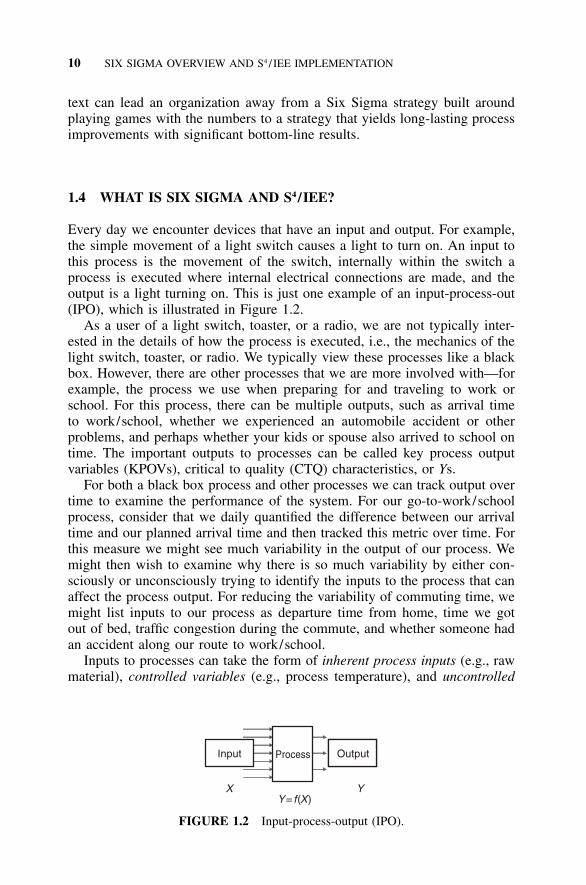
10 SIX SIGMA OVERVIEW AND S4 / IEE IMPLEMENTATION

ProcessInput OutputOutput

YXY=f(X)

FIGURE 1.2 Input-process-output (IPO).

text can lead an organization away from a Six Sigma strategy built aroundplaying games with the numbers to a strategy that yields long-lasting processimprovements with significant bottom-line results.

1.4 WHAT IS SIX SIGMA AND S4/IEE?

Every day we encounter devices that have an input and output. For example,the simple movement of a light switch causes a light to turn on. An input tothis process is the movement of the switch, internally within the switch aprocess is executed where internal electrical connections are made, and theoutput is a light turning on. This is just one example of an input-process-out(IPO), which is illustrated in Figure 1.2.

As a user of a light switch, toaster, or a radio, we are not typically inter-ested in the details of how the process is executed, i.e., the mechanics of thelight switch, toaster, or radio. We typically view these processes like a blackbox. However, there are other processes that we are more involved with—forexample, the process we use when preparing for and traveling to work orschool. For this process, there can be multiple outputs, such as arrival timeto work/school, whether we experienced an automobile accident or otherproblems, and perhaps whether your kids or spouse also arrived to school ontime. The important outputs to processes can be called key process outputvariables (KPOVs), critical to quality (CTQ) characteristics, or Ys.

For both a black box process and other processes we can track output overtime to examine the performance of the system. For our go-to-work/schoolprocess, consider that we daily quantified the difference between our arrivaltime and our planned arrival time and then tracked this metric over time. Forthis measure we might see much variability in the output of our process. Wemight then wish to examine why there is so much variability by either con-sciously or unconsciously trying to identify the inputs to the process that canaffect the process output. For reducing the variability of commuting time, wemight list inputs to our process as departure time from home, time we gotout of bed, traffic congestion during the commute, and whether someone hadan accident along our route to work/school.

Inputs to processes can take the form of inherent process inputs (e.g., rawmaterial), controlled variables (e.g., process temperature), and uncontrolled

WHAT IS SIX SIGMA AND S4 / IEE? 11

noise variables (e.g., raw material lots). For our go-to-work/school processa controllable input variable might be setting the alarm clock, while an un-controllable input variable might be whether someone had an accident on ourroute that affected our travel time. By examining our arrival times as a func-tion of the time departing home, we might find that if we left the house 5minutes earlier we could reduce our commute time by 25 minutes. For thissituation, departure time is a key process input variable (KPIV) that is animportant X, which affects our arrival time. When this KPIV is controlled inour go-to-work/school process, we can reduce the amount of variability inour arrival time at work/school (KPOV).

Another tactic to reduce the variability of our arrival time is to change ourprocess so that we can reduce the commute time or make our process robustto uncontrollable/noise input variables. For example, we might change ourtravel route to work or school such that our travel time is reduced during thehigh-traffic hours of the day. This change could also reduce the likelihood oflengthy delays from accidents; i.e., we made our process robust to the oc-currence of accidents, which was a noise input variable.

Similarly, within business and other organizations we have processes orsystems. For the go-to-work/school process the identification of inputs andpotential process changes that would positively impact our process output isnot too difficult. Easy fixes can also occur within business processes whenwe view our process systematically through a Six Sigma or S4/IEE strategy.However, the identification and improvement systems for some business pro-cess can be more involved. For these more complex situations within S4/IEE,I view this search for KPIVs and process improvement strategies as a murdermystery where we use a structured S4/IEE approach for the uncovering ofclues that leads us to how we can improve our process outputs.

Let us now consider the following example KPOVs (Ys) that a companycould experience along with one, of perhaps many, KPIV (Xs) for each ofthese processes:

Ys or KPOVs Xs or KPIVs

1 Profits Actions taken to improve profits2 Customer satisfaction Out of stock items3 Strategic goal Actions taken to achieve goal4 Expense Amount of WIP5 Production cycle time Amount of internal rework6 Defect rate Inspection procedures7 Critical dimension on a part Process temperature

These Ys are at various levels within an organization’s overall system ofdoing business. Within S4/IEE, a cascading measurement system can be cre-ated, which aligns metrics to the overall needs of the organization. The track-ing of these measurements over time can then pull (using a lean term) for thecreation of S4/IEE projects, which addresses common cause variability im-provement needs for the process output. Through this pragmatic approach,

12 SIX SIGMA OVERVIEW AND S4 / IEE IMPLEMENTATION

where no games are played with the numbers, organizations have a systematicway to improve both customer satisfaction and their bottom line. S4/IEE ismuch more than a quality initiative; it is a way of doing business.

I will be using the term 30,000-foot-level metric (see Sections 1.8 and10.3) to describe a Six Sigma KPOV, CTQ, or Y variable response that isused in S4/IEE to describe a high-level project or operation metric that hasinfrequent subgrouping/sampling such that short-term variations, which mightbe cause by KPIVs, will result in charts that view these perturbations ascommon cause issues. A 30,000-foot-level XmR chart can reduce the amountof firefighting in an organization when used to report operational metrics.

1.5 THE SIX SIGMA METRIC

The concepts described in this section will be covered in greater depth laterin this book (see Chapter 9). This section will give readers who have somefamiliarity with the normal distribution a quick understanding of the sourcefor the Six Sigma metric. Section 1.19 describes some shortcomings andalternatives to this metric.

First, let us consider the level of quality that is needed. The ‘‘goodnesslevel’’ of 99% equates to

• 20,000 lost articles of mail per hour• Unsafe drinking water almost 15 minutes per day• 5,000 incorrect surgical operations per week• Short or long landing at most major airports each day• 200,000 wrong drug prescriptions each year• No electricity for almost 7 hours per month (Harry 1987)

I think that most of us agree that this level of ‘‘goodness’’ is not close tobeing satisfactory. An S4/IEE business strategy, among other things, can offera measurement for ‘‘goodness’’ across various products, processes, and ser-vices.

The sigma level (i.e., sigma quality level) sometimes used as a measure-ment within a Six Sigma program includes a �1.5� value to account for‘‘typical’’ shifts and drifts of the mean. This sigma quality level relationshipis not linear. In other words, a percentage unit improvement in parts-per-million (ppm) defect rate does not equate to the same percentage improvementin the sigma quality level.

Figure 1.3 shows the sigma quality level associated with various services(considering the 1.5� shift of the mean). From this figure we note that thesigma quality level of most services is about four sigma, while world classis considered six. A goal of S4/IEE implementation is continually to improveprocesses and become world class.

Figures 1.4 to 1.6 illustrate various aspects of a normal distribution as itapplies to Six Sigma program measures and the implication of the 1.5� shift.

THE SIX SIGMA METRIC 13

FIGURE 1.3 Implication of the sigma quality level. Parts per million (ppm) rate forpart or process step.

FIGURE 1.4 Normal distribution curve illustrates the Three Sigma and Six Sigmaparametric conformance. (Copyright of Motorola, Inc., used with permission.)

Figure 1.4 illustrates the basic measurement concept of Six Sigma accordingto which parts are to be manufactured consistently and well within their spec-ification range. Figure 1.5 shows the number of parts per million that wouldbe outside the specification limits if the data were centered within these limitsand had various standard deviations. Figure 1.6 extends Figure 1.4 to non-central data relative to specification limits, in which the mean of the data isshifted by 1.5�. Figure 1.7 shows the relationship of ppm defect rates versussigma quality level for a centered and 1.5� shifted process, along with a

14 SIX SIGMA OVERVIEW AND S4 / IEE IMPLEMENTATION

FIGURE 1.5 With a centered normal distribution between Six Sigma limits, onlytwo devices per billion fail to meet the specification target. (Copyright of Motorola,Inc., used with permission.)

±1 σ±2 σ±3 σ±4 σ±5 σ±6 σ

Spec. limit30.2369.1393.3299.379099.9767099.999660

Percent697700308700668106210233

3.4

Defective ppm

–6σ –5σ –4σ –3σ –2σ –1σ X +1σ +2σ +3σ +4σ +5σ +6σ

Lowerspecification

limit

Normal DistributionShifted 1.5σ

Upperspecification

limit

FIGURE 1.6 Effects of a 1.5� shift where only 3.4 ppm fail to meet specifications.(Copyright of Motorola, Inc., used with permission.)

TRADITIONAL APPROACH TO THE DEPLOYMENT OF STATISTICAL METHODS 15

FIGURE 1.7 Defect rates (ppm) versus sigma quality level.

quantification for the amount of improvement needed to change a sigma qual-ity level.

A metric that describes how well a process meets requirements is processcapability. A Six Sigma quality level process is said to translate to processcapability index values for Cp and Cpk requirement of 2.0 and 1.5, respectively(see Chapter 11). To achieve this basic goal of a Six Sigma program mightthen be to produce at least 99.99966% quality at the process step and partlevel within an assembly; i.e., no more than 3.4 defects per million parts orprocess steps if the process mean were to shift by as much as 1.5�. If, forexample, there were on the average 1 defect for an assembly that contained40 parts and four process steps, practitioners might consider that the assemblywould be at a four sigma quality level from Figure 1.7, because the numberof defects in parts per million is: (1⁄160)(1 � 106) � 6250.

1.6 TRADITIONAL APPROACH TO THE DEPLOYMENT OFSTATISTICAL METHODS

Before the availability and popularity of easy-to-use statistical software, mostcomplex statistical analysis was left to a statistical consultant within an or-ganization. An engineer needs to know what questions to ask of a statisticalconsultant. If the engineer does not realize the power of statistics, he or shemight not solicit help when statistical techniques are appropriate. If an en-gineer who has no knowledge of statistics approaches a statistical consultantfor assistance, the statistician should learn all the technical aspects of the

16 SIX SIGMA OVERVIEW AND S4 / IEE IMPLEMENTATION

dilemma in order to give the best possible assistance. Most statisticians donot have the time, background, or desire to understand all engineering dilem-mas within their corporate structure. Therefore, engineers need to have at aminimum some basic knowledge of the concepts in this book so that theycan first identify an application of the concepts and then solicit help, ifneeded, in an effective manner.

In any case, detailed knowledge transfer to statisticians can be very time-consuming and in most cases will be incomplete. Engineers who have knowl-edge of basic statistical concepts can intelligently mix engineering conceptswith statistical techniques to maximize test quality and productivity. Earlierproblem detection and better quality can then be expected when testing isconsidered as an integral part of the design and manufacturing process de-velopment.

Now easy-to-use statistical software has made the whole process of statis-tical analyses more readily available to a larger group of people. However,the issue of problem definition and dissemination of the wise use of statisticaltechniques still exists. Even though great accomplishments may be occurringthrough the use of statistical tools within an organization, there is often a lackof visibility of the benefits to upper management. Because of this lack ofvisibility, practitioners often have to fight for funds and may be eliminatedwhenever times get rough financially.

Typically in this situation, executive management does not ask questionsthat lead to the wise application of statistical tools; hence, an internal statis-tical consultant or practitioner has to spend much of his or her time trying tosell others on how basic problems could be solved more efficiently usingstatistical methods. In addition, internal statistical consultants or practitionerswho help others will only have the time or knowledge to assist with problemresolution as it is currently defined. In a purely consultant role, statisticalpractitioners will often not be involved in project or problem definition. Inaddition, the benefits of good statistical work that has been accomplished arenot translated into the universal language understood by all executives—namely, money. Hence, the benefits of wisely applying statistical techniquesare limited to small areas of the business, do not get recognition, and are notaccepted as general policy.

1.7 SIX SIGMA BENCHMARKING STUDY

In addition to learning from traditional statistical method deployments, thereare also lessons to be learned from previous organizational deployments ofSix Sigma. Because of this, I am now noting a Six Sigma benchmarkingstudy that I was involved with.

I was selected as the Subject Matter Expert (SME) for an APQC Six Sigmabenchmarking study that was conducted in 2001. In September 2001 I gavea presentation during the knowledge transfer section, which summarized my

S4 / IEE BUSINESS STRATEGY IMPLEMENTATION 17

30,000-foot-level

Satellite-level

FIGURE 1.8 Satellite-level and 30,000-foot-level metrics.

observations during the study. A summary of this presentation is included inSection A.2.

1.8 S4/IEE BUSINESS STRATEGY IMPLEMENTATION

Organizations create strategic plans and policies. They also create organiza-tional goals that describe the intent of the organization. These goals shouldhave measurable results, which are attained through defined action plans. Thequestion of concern is: How effective and aligned are these managementsystem practices within an organization? An improvement to this system candramatically impact an organization’s bottom line.

An S4/IEE approach measures the overall organization at a high level usingsatellite-level and 30,000-foot-level metrics as illustrated in Figure 1.8. Physi-cally, these metrics can take on many responses, as illustrated in Figure 1.9.Satellite-level and 30,000-foot-level metrics (see Chapter 10) permit manage-ment with the right information. An organization can use theory of constraints(TOC) metrics (see Chapter 45) and/or traditional business measures for theirsatellite-level metrics, where measures are tracked monthly using an XmR chart(see Chapter 10) that is not bounded by any quarterly or annual time frame.

More information can be gleaned from business data presented in the S4/IEE format at the satellite level, as opposed to comparing quarterly results ina tabular format. This approach tracks the organization as a system, which canlead to focused improvement efforts and a reduction of firefighting activities.Data presented in this format can be useful for executives when creating theirstrategic plans and then tracking the results of these strategic plans. With anS4/IEE strategy, action plans to achieve organizational goals center around thecreation and implementation of S4/IEE projects, as illustrated in Figure 1.10.

The following S4/IEE results orchestration (RO) process to select projectsthat are aligned with the business needs is called an enterprise business plan-ning methodology (EBPM):

18 SIX SIGMA OVERVIEW AND S4 / IEE IMPLEMENTATION

DividendPayment

StockPrice

Increase

ROEStockholders (Value adds Interest)

Stock Analysts &Board Members

& CEO

SalesGrowth

OIGrowth

Earningper

Share

P/ERatio

EconomicProfit ROIC/ROE

DebtServiceCharge People

Development

P&LOptimization

MetricsCorporateExecutive

AssetManagement

Metrics

PeopleDevelopment

Factory Metrics(Percent Yield, Run Time

Productivity, etc.)

Supply ChainMetrics

SalespersonProductivity

New ProductIntroduction

SafetySupplier Metrics (Cost,

Quality, Service)Patents

ROE = Return on Equity; OI = Operating Income; P/E = Price to Earnings; ROIC = Return on Invested CapitalP&L = Profit & Loss

Satellite-LevelSatellite-Level

30,000-Foot-Level30,000-Foot-Level

FIGURE 1.9 Satellite-level and 30,000-foot-level metrics.

30,000-foot-level

Satellite-Level

Projects

Strategic Plans

Business Measures and Goals

Identify High Potential Areas

FIGURE 1.10 Aligning improvement activities with business needs.

• Create satellite-level metrics for the past two to five years.• Select goals that are in alignment with improvement desires for the sat-

ellite-level metrics.• Select strategies that are in alignment with goals.• Examine supply chain process map.• Choose high-potential areas for focusing improvement efforts using goals

and supply chain process map to help guide the selection process.• Select and create 30,000-foot-level operational metrics that are in align-

ment with the high potential areas for improvements.• Select S4/IEE project areas that are in alignment with operational metrics.

SIX SIGMA AS AN S4 / IEE BUSINESS STRATEGY 19

• Drill down project areas to well-scoped projects (project scope) that arenot too large or too small.

• Create 30,000-foot-level project metrics for base-lining projects andtracking impact from S4/IEE project work.

S4/IEE 30,000-foot-level metrics are high-level operational or Six Sigma/lean project metrics. The right metrics are needed for the orchestration of theright activities. The above-described EBPM process accomplishes this bylinking Six Sigma improvement activities to business strategies and goals.

As noted in Figure 1.9, traditional business metrics that could be classifiedas satellite-level metrics are capital utilization, growth, revenue, equity valu-ation, and profit. Traditional operational metrics at the 30,000-foot level aredefective/defect rates, cycle time, waste, days sales outstanding, customersatisfaction, on-time delivery, number of days from promise date, number ofdays from customer-requested date, dimensional property, inventory, and headcount. Organizations can find it to be very beneficial when they decide toalign project selection with satellite-level measures from theory of constraint(TOC) metrics; i.e., TOC throughput (see Glossary for definition), investment/inventory, and operating expense.

Within S4/IEE the alignment and management of metrics throughout anorganization is called an enterprise cascading measurement methodology(ECMM). With ECMM meaningful measurements are statistically trackedover time at various functional levels of the business. This leads to a cascadingand alignment of important metrics throughout the organization from thesatellite-level business metrics to high-level KPOV operational metrics, whichcan be at the 30,000-foot level, 20,000-foot level, or 10,000-foot level (infre-quent subgrouping/sampling), to KPIVs at the 50-foot level (frequentsubgrouping/sampling). The metrics of ECMM can then be used to run thebusiness so that organizations get out of the firefighting mode and pull (usedas a lean term) for the creation of projects whenever improvements are neededto these operational metrics.

An S4/IEE business strategy helps organizations understand and improvethe key drivers that affect the metrics and scorecards of their enterprise.

1.9 SIX SIGMA AS AN S4/IEE BUSINESS STRATEGY

We do things within a work environment. A response is created when thingsare done, but the way we do things may or may not be formally documented.One response to doing something is how long it takes to complete the task.Another response might be the quality of the completed work. We call theimportant responses from a process key process output variables (KPOVs),sometimes called the Ys of the process (see Section 1.4).

Sometimes the things that are completed within a work environment causea problem to our customers or create a great deal of waste (e.g., overproduc-tion, waiting, transportation, inventory, overprocessing, motion, and defects),which can be very expensive to an organization.

20 SIX SIGMA OVERVIEW AND S4 / IEE IMPLEMENTATION

FIGURE 1.11 Example process with a key process output variable.

Organizations often work to solve this type of problem. However, whenthey do this work, organizations do not often look at their problems as theresult of current process conditions. If they did, their work activities mightnot be much different from Figure 1.11. They might also have a variety ofKPOVs, such as a critical dimension, overall cycle time, a DPMO rate (i.e.,a defect-per-million opportunities rate could expose a ‘‘hidden factory’’ re-work issue that is not currently being reported), customer satisfaction, and soon.

SIX SIGMA AS AN S4 / IEE BUSINESS STRATEGY 21

DefineProject

ControlMeasurePassiveAnalysis

ProactiveTesting

Foundation Integration

Champion and Black Belt with TeamSteering

TeamSteering

Team

Plan Project

and Metrics

Wisdomof the

OrganizationMSA

BaselineProject

ConsiderLeanTools

D M A I C

FIGURE 1.12 S4 / IEE DMAIC project execution roadmap.

For this type of situation, organizations often react over time to the up-and-down movements of the KPOV level in a firefighting mode, fixing theproblems of the day. Arbitrary tweaks to controllable process variables thatare made frequently and noise (e.g., material differences, operator-to-operatordifferences, machine-to-machine differences, and measurement imprecision)can cause excess variability and yield a large nonconforming proportion forthe KPOV. Practitioners and management might think that their day-to-dayproblem-fixing activities are making improvements to the system. In reality,these activities often expend many resources without making any improve-ments to the process. Unless long-lasting process changes are made, the pro-portion of noncompliance, as shown in the figure, will remain approximatelythe same.

Organizations that frequently encounter this type of situation have muchto gain from the implementation of an S4/IEE business strategy. They canbetter appreciate this potential gain when they consider all the direct andindirect costs associated with their current level of nonconformance.

The S4/IEE methodology described in this book is not only a statisticalmethodology but also a deployment system of statistical and other techniquesthat follows the high-level S4/IEE project execution roadmap depicted in Fig-ure 1.12 and further described in Section A.1 in the Appendix. In this exe-cution roadmap, one might note that S4/IEE follows the traditional Six SigmaDMAIC roadmap. In addition to the project execution roadmap shown inFigure A.1, there is a 21-step integration of the tools roadmaps for the fol-lowing disciplines:

• Manufacturing processes: Section 46.1• Service/transactional processes: Section 47.2• Product DFSS: Section 49.2• Process DFSS: Section 50.1

In S4/IEE and a traditional DMAIC, most Six Sigma tools are applied inthe same phase. However, the S4/IEE project execution roadmap offers theadditional flexibility of breaking down the measure phase to the componentsnoted in the figure. In addition, the term passive analysis is often used in S4/

22 SIX SIGMA OVERVIEW AND S4 / IEE IMPLEMENTATION

IEE to describe the analyze phase, where process data are observed passively(i.e., with no process adjustments) in an attempt to find a causal relationshipbetween input and output variables. Finally, the descriptive term proactivetesting is often used within S4/IEE to describe the tools associated with theimprove phase. The reason for this is that within the improve DMAIC phasedesign of experiments (DOE) tools are typically used. In DOE you can makemany adjustments to a process in a structured fashion, observing/analyzingthe results collectively (i.e., proactively testing to make a judgment). It shouldbe noted that improvements can be made in any of the phases. If low-hangingfruit is identified during a brainstorming session in the measure phase, thisimprovement can be made immediately, which could yield a dramatic im-provement to the 30,000-foot-level output metric.

In an S4/IEE business strategy, a practitioner applies the project executionroadmap either during a workshop or as a project after a workshop, as de-scribed in Figures 1.13 and 1.14. From this effort, Figure 1.15 illustrates howthe process has been simplified, designed to require less testing, and designedto become more robust or indifferent to the noise variables of the process.This effort can result in an improvement shift of the mean along with reducedvariability leading to quantifiable bottom-line monetary benefits.

For an S4/IEE business strategy to be successful, it must have upper-levelmanagement commitment and the infrastructure that supports this commit-ment. Deployment of the S4/IEE techniques is most effective through indi-viduals, sometimes called black belts or agents, who work full time on theimplementation of the techniques through S4/IEE projects selected on busi-ness needs (i.e., they have a very beneficial ROI). Direct support needs to begiven by an executive management committee that has high-level managerswho champion S4/IEE projects.

1.10 CREATING AN S4/IEE BUSINESS STRATEGY WITH ROLESAND RESPONSIBILITIES

For Six Sigma to become a successful business strategy, it needs to haveexecutive management support and an effective organizational structure. SixSigma needs to become a business process management system that:

1. Understands and addresses process components and boundaries2. Identifies and collectively utilizes process owners, internal customers/

external customers, and other stakeholders effectively3. Creates an environment for effective project management where the

business achieves maximum benefits4. Establishes project measures that include key performance metrics with

appropriate documentation

23

Def

ine

• Mea

sure

•A

naly

ze •

Impr

ove

• Con

trol

Freq

uenc

y of

non-

conf

orm

anceC

usto

mer

need

s

Freq

uenc

y of

non-

conf

orm

anceCus

tom

erne

eds

30,0

00-F

oot-L

evel

Met

ric

Bot

tom

-line

ben

efit

isth

e tra

nsla

tion

of th

ese

diffe

renc

es in

to m

oney

Key

Pro

cess

Out

put

Var

iabl

e

Def

ine

Proj

ect

Con

trol

Mea

sure

Pass

ive

Ana

lysis

Proa

ctiv

eTe

stin

g

Plan

Pro

ject

and

Met

rics

Wis

dom

of th

eO

rgan

izatio

nM

SABa

selin

ePr

ojec

t

Con

sider

Lean

Tool

s

DM

AI

C

FIG

UR

E1.

13S4

/IE

Epr

ojec

ttr

acki

ng,

exec

utio

n,an

dth

ebe

nefit

s:co

ntin

uous

data

.

24 SIX SIGMA OVERVIEW AND S4 / IEE IMPLEMENTATION

Frequency ofnon-conformance

30,000-Foot-Level Metric

Bottom-line benefit isthe translation of thesedifferences into money

Key ProcessOutput Variable

DefineProject

ControlMeasurePassiveAnalysis

ProactiveTesting

Plan Project

and Metrics

Wisdomof the

OrganizationMSA

BaselineProject

ConsiderLeanTools

D M A I C

Define •Measure •Analyze •Improve •Control

FIGURE 1.14 S4 / IEE project tracking, execution, and the benefits: attribute data.

A force field analysis (see Section 5.10) can be conducted to highlight thedriving and restraining forces for a successful implementation of S4/IEEwithin your organization. Action plans need to be created to address largerestraining forces.

S4/IEE projects need to focus on areas of the business that can yield ahigh ROI and address the needs of customers. Project black belt implementersare typically expected to deliver annual benefits of between $500,000 and$1,000,000, on average, through four to six projects per year. The value ofmaintaining and improving customer satisfaction must not be overlooked byorganizations within their S4/IEE activities.

To achieve success, organizations must wisely address Six Sigma metricsand its infrastructure. The success of Six Sigma is linked to a set of cross-functional metrics that lead to significant improvements in customer satisfac-tion and bottom-line benefits. Companies experiencing success with SixSigma have created an infrastructure to support the strategy.

The affinity diagram in Figure 5.3 shows a grouping of issues that a teambelieved was important to address when creating an S4/IEE business strategy.The interrelationship digraph (ID) in Figure 5.4 shows a further subdivisionof issues and the interrelationship of these issues:

• Executive leadership and involvement• Delivered results• Customer focus• Strategic goals• Project selection• Training and execution

CREATING AN S4 / IEE BUSINESS STRATEGY 25

FIGURE 1.15 Example process improvement and impact to a key process outputvariable.

26 SIX SIGMA OVERVIEW AND S4 / IEE IMPLEMENTATION

B lack B e lt

S p on sor/P rocess O wn er

B lack B e lt

S p on sor/P rocess O wn er

S B U # 1C h ampion

B lack B elt

S p on sor/P rocess O w n er

B lack B elt

S p on sor/P rocess O wn er

S B U # 2C h ampion

B lack B e lt

S p on sor/P rocess O wn er

B lack B e lt

S p on sor/P rocess O wn er

S B U # nC h ampion

O rg an iza tion a l L ead er

FIGURE 1.16 Possible S4 / IEE organizational interrelationship.

• Resources• Black belt selection• Communications• Culture• Metrics (and feedback)• Planning

Within an S4/IEE infrastructure, several roles and responsibilities need tobe addressed. Some of these roles and possible technical and organizationalinterrelationships are shown in Figures 1.16 and 1.17. These roles and re-sponsibilities for the organizational structure include:

• Executive:• Motivate others toward a common vision.• Set the standard, demonstrate the behaviors.• Use satellite-level and 30,000-foot-level metrics.• Ask the right questions.• Use S4/IEE tools in day-to-day operations.• Be visible.• Give a short presentation for each S4/IEE training wave.• Attend project-completion presentations conducted by S4/IEE team.• Stay involved.

• Steering team:• Same as executive roles and responsibilities, plus:• Develop project selection criteria.• Set policies for accountability for project results.• Develop policies for financial evaluation of project benefits.• Establish internal and external communication plan.• Identify effective training and qualified trainers.• Develop human resource policies for S4/IEE roles.

CREATING AN S4 / IEE BUSINESS STRATEGY 27

Team M em b ers

B lack /G reen B elt

Team M em b ers

B lack /G reen B elt

S B U # 1M aster B lack B elt

Team M em b ers

B lack /G reen B elt

Team M em b ers

B lack /G reen B elt

S B U # 2M aster B lack B elt

Team M em b ers

B lack /G reen B elt

Team M em b ers

B lack /G reen B elt

S B U # nM aster B lack B elt

Q u ality L ead er

FIGURE 1.17 Possible S4 / IEE technical relationships.

• Determine computer hardware and software standards.• Set policies for team reward and recognition.• Identify high potential candidates for S4/IEE roles.

• Champion:• Remove barriers to success.• Develop incentive programs with executive team.• Communicate and execute the S4/IEE vision.• Determine project-selection criteria with executive team.• Identify and prioritize projects.• Question methodology and project-improvement recommendations.• Verify completion of phase deliverables.• Drive and communicate results.• Approve completed projects.• Leverage project results.• Reward and recognize team members.

• Master black belt:• Function as change agents.• Conduct and oversee S4/IEE training.• Coach black belts/green belts.• Leverage projects and resources.• Formulate project-selection strategies with steering team.• Communicate the S4/IEE vision.• Motivate others toward a common vision.• Approve completed projects.

• Black belt:• Lead change.• Communicate the S4/IEE vision.• Lead the team in the effective utilization of the S4/IEE methodology.• Select, teach, and use the most effective tools.• Develop a detailed project plan.

28 SIX SIGMA OVERVIEW AND S4 / IEE IMPLEMENTATION

• Schedule and lead team meetings.• Oversee data collection and analysis.• Sustain team motivation and stability.• Deliver project results.• Track and report milestones and tasks.• Calculate project savings.• Interface between finance and information management (IM).• Monitor critical success factors and prepare risk-abatement plans.• Prepare and present executive-level presentations.• Complete four to six projects per year.• Communicate the benefit of the project to all associated with the pro-

cess.• Green belt: Similar to black belt except they typically:

• Address projects that are confined to their functional area.• Have less training than black belts.• Are involved with S4/IEE improvement in a part-time role.

• Sponsor:• Function as change agents.• Remove barriers to success.• Ensure process improvements are implemented and sustained.• Obtain necessary approval for any process changes.• Communicate the S4/IEE vision.• Aid in selecting team members.• Maintain team motivation and accountability.

• Other recommended team resources:• Overall quality leader to deploy and monitor the S4/IEE business strat-

egy on a broad level.• Information management support to aid hardware and software pro-

curement and installation for black belts and teams, to establish data-collection systems that are easily reproducible and reliable.

• Finance support to approve monetary calculations.• Human resources—employee career path and job descriptions.• Communications—internal and external.• Training—to coordinate S4/IEE training for the organization and to

implement training recommended by black belt teams.

Some larger companies have both deployment and project champion roles.Within this book I will make reference to black belt as the S4/IEE practitioner.However, many of the tasks could similarly be executed by green belts.

When implementing S4/IEE, organizations need to create a plan that ad-dresses these issues and their interrelationship. For this to occur, an organi-

CREATING AN S4 / IEE BUSINESS STRATEGY 29

zation needs to be facilitated through the process of creating all the internalprocess steps that address these issues, as illustrated within Figure 1.18.Within this strategy, it is also very beneficial to integrate Six Sigma strategieswith existing business incentives such as lean manufacturing, total qualitymanagement (TQM), Malcolm Baldrige Assessments, and ISO-9000:2000 im-provements (Breyfogle et al. 2001b). This integration with lean is describedin the next section, while the other topics are discussed in Chapter 54.

Let us now address an issue that I believe is important to the success ofimplementing Six Sigma within an organization. It has been my experiencethat within many Six Sigma programs projects are pushed (used as a leanmanufacturing term) into the system through the Six Sigma infrastructure.This approach creates an environment in which it is difficult for Six Sigmato sustain its effectiveness. I believe a much better approach is to create anenvironment that has satellite-level metrics and 30,000-foot-level metrics thatare cascaded throughout the organization. All levels of management wouldthen ask questions of their subordinates as to what they are doing to improvetheir processes; i.e., address common cause issues, as described in Chapter3. This question, as opposed to the typical firefighting question of what areyou doing to fix today’s problems, can lead to pulling (used as a lean term)for the creation of S4/IEE projects that address issues that are important tothe success of the business.

It needs to be emphasized that S4/IEE black belts need to be selected whonot only have the capability of learning and applying statistical methodologiesbut also are proactive people good at the so-called soft skills of working withpeople. S4/IEE black belts will not only need to analyze information and usestatistical techniques to get results but will also need to be able to work withothers through mentoring, teaching, coaching, and selling others on how theycan benefit from S4/IEE techniques. Six skills I think are important to con-sider when selecting a black belt are:

• Fire in the belly: They have an unquenchable desire to improve the wayan organization does its business.

• Soft skills: They have the ability to work effectively with people in teamsand other organizations.

• Project management: They have the ability to get things done well andon time.

• Multitasking: They can manage multiple tasks at one time and maintainfocus.

• Big picture: They don’t focus on insignificant details, losing sight of thebig picture.

• Analytical skills: They have good analytical skills.

The first five characteristics are very difficult to teach since these traits areclosely linked with personalities. The statistical methodologies used withinS4/IEE can be easily taught if a person has good analytical skills. Whenimplementing an S4/IEE business strategy, organizations need to create a

30

Executive Management Steering CommitteeChampions (Business

Unit Managers) Project Teams

Allo

cate

re

sou

rces

De

fine

a s

et o

f cr

oss-

fun

ctio

nal,

stra

tegi

c m

etri

cs

to d

rive

p

roje

cts

(CO

PQ

)

Tie

Six

S

igm

a to

ov

era

ll b

usi

nes

sst

rate

gy

Dev

elo

pin

cent

ive

pla

ns

Est

ablis

ha

ccou

nta

bili

ty

Exp

and

in

volv

emen

t to

a

ddit

iona

l a

ssoc

iate

s

Iden

tify

p

ote

ntia

l p

roje

cts

Def

ine

ap

roje

ct

sele

ctio

n p

roce

ss

Pri

ori

tize

pro

ject

s

Cre

ate

an

ove

rall

tra

inin

g p

lan

Eva

luat

e

cultu

ral

obs

tacl

es

and

fa

cilit

ate

chan

ge

Na

rrow

sc

ope

Pro

vid

e a

ppro

pria

te

uni

vers

al

com

mun

ica

tion

to

ols

Su

pply

p

roje

ct

repo

rt o

ut

tem

pla

tes

dat

es

Sh

are

bes

tp

ract

ices

Det

erm

ine

stra

teg

icg

oals

and

o

bjec

tives

De

fine

p

roje

ct

"Def

ine"

Incl

ude

s th

e V

OC

?E

stab

lish

cust

ome

r fe

edba

ck

pro

cess

es

No

Yes

Se

lect

ch

ampi

ons

a

nd t

eam

le

ader

s

Se

lect

ke

y p

roje

cts

with

le

ader

ship

b

uy-i

n

Iden

tify

cr

oss-

func

tion

al

team

m

embe

rs

Man

age

pro

ject

s

Mot

ivat

e a

nd s

ust

ain

ch

ange

Pla

n p

roje

ct

met

rics

"Mea

sure

"

Bas

elin

ep

roje

ct

"Mea

sure

"

Co

nsi

der

le

an to

ols

"M

easu

re"

MS

A

"Mea

sure

"W

isd

om

of

the

org

aniz

atio

n "M

easu

re"

Pas

sive

anal

ysis

"An

alyz

e"

Pro

activ

e

test

ing

"Im

pro

ve"

Oth

erev

alu

atio

ns

"Con

trol

"

FIG

UR

E1.

18S4

/IE

Ein

fras

truc

ture

road

map

.

INTEGRATION OF SIX SIGMA WITH LEAN 31

process for selecting black belts. Organizations initially need to create theirown skill set needs for black belts with a prioritization of these skills (seeFigure 5.6). One means to rank black belt candidates is then to use a priori-tization matrix/cause-and-effect matrix (see Sections 5.16 and 13.4).

A rule of thumb for the number of black belts within an organization is1–2% of the total number of employees. Black belts are supported technicallythrough a master black belt and through the management chain of an orga-nization by way of a champion. Individuals who are given S4/IEE training toa lesser extent and support black belts are called green belts.

When an organization chooses to implement Six Sigma, it should use agroup outside its company to help it get started. This group can help withsetting up a deployment strategy, conducting initial training, and providingproject coaching. The decision on which group is chosen can dramaticallyaffect the success of the implementation of Six Sigma. However, choosingthe best group to help an organization implement Six Sigma can be a chal-lenge. Some items for consideration are covered in Section A.3 of the Ap-pendix.

1.11 INTEGRATION OF SIX SIGMA WITH LEAN

There has been much contention between Six Sigma and lean functions. Iwill use lean or lean thinking to describe the application of lean manufactur-ing, lean production, and/or lean enterprise principles to all processes. Peoplefrom the Six Sigma community typically say that Six Sigma comes first oris above lean, relative to application within an organization. People from alean discipline typically say that lean comes first or is above Six Sigma,relative to application within an organization.

The S4/IEE approach integrates the two concepts, where high-level SixSigma metrics dictate which of the lean or Six Sigma tools should be usedwithin an S4/IEE define-measure-analyze-improve-control (DMAIC) road-map. The application of lean tools is a step within this execution roadmap,as illustrated within Figure 1.12. When a lean methodology is used to achievethe goal of a project, the 30,000-foot-level metrics will quantify the benefitof the change statistically on a continuing basis.

One reason why this integration works especially well within the S4/IEEapproach is that this Six Sigma approach does not require the definition of adefect for a project. This is very important because lean metrics involve var-ious waste measures, such as inventory or cycle time, that do not have truespecification criteria like manufactured components. Defect definitions forthese situations can lead to playing games with the numbers.

It is beneficial to dissolve any separate Six Sigma and lean functions thatexist, having the same person work using the most appropriate tool for anygiven situation, whether the tool is lean or Six Sigma.

32 SIX SIGMA OVERVIEW AND S4 / IEE IMPLEMENTATION

1.12 DAY-TO-DAY BUSINESS MANAGEMENT USING S4/IEE

Organizations often experience much firefighting where they react to the prob-lems of the day (see Example 3.1). These organizations need a system wherethey can replace much of their firefighting activities with fire prevention. Thiscan be accomplished by way of an S4/IEE cascading measurement strategy.

With this strategy, metrics are orchestrated through a statistical-based high-level measurement system. Through the alignment of 30,000-foot-level withsatellite-level and other high-level metrics, organizations can yield meaningfulmetrics at the operational level, which have a direct focus on the needs ofthe business. The wise use of these metrics can improve the orchestration ofday-to-day activities for organizations.

When we view our system using a set of cascading high-level XmR chartsthat has infrequent subgrouping/sampling (see Section 10.3), behaviorscan change. Often previous situations had individual day-to-day out-of-specification conditions, which were caused by common-cause variability,were fought as a special-cause event fires. These fires needed immediate at-tention and often only later reappeared after the extinguishing.

When there are common cause variability problems such that a specifica-tion is not consistently met, the overall process needs to be changed in orderto improve the metrics. Long-lasting improvements can be accomplishedthrough S4/IEE projects that address the overall system’s process steps andits metrics, including the measurement system itself and a control mechanismfor the process that keeps it from returning to its previous unsatisfactory state.

With the S4/IEE approach, process management teams might meet weeklyto discuss their high-level 30,000-foot-level operational metrics. When anXmR chart that has infrequent subgrouping/sampling shows a predictable pro-cess that does not yield a satisfactory capability/performance (see Chapter11) measurement level, an S4/IEE project can be created; i.e., the S4/IEEproject is pulled (using a lean term) by the need to improve the metrics.

This S4/IEE project could become a green belt project that is executed bya part-time S4/IEE project practitioner who is within a function. Alternatively,the project might become a larger black belt project that needs to addresscross-functional issues. When improvements are made to the overall systemthrough the S4/IEE project, the 30,000-foot-level operational metric shouldchange to an improved level.

Awareness of the 30,000-foot-level metrics and the results of S4/IEE pro-ject improvement efforts should be made available to everyone, includingthose in the operations of the process. This information could be routinelyposted using the visual factory concept typically encountered within lean im-plementations (see Chapter 44). This posting of information can improve theawareness and benefits of S4/IEE throughout the organization, which can leadmore buy-in to the S4/IEE methodology throughout the function. This canresult in the stimulation of other improvement efforts, resulting in a dramaticimprovement in the overall satellite-level measures.

S4 / IEE PROJECT INITIATION AND EXECUTION ROADMAP 33

With this approach to the tracking of metrics and the creation of improvingactivities, management can change its focus, which might currently be on theproblems of the day. This approach can lead to asking questions about thestatus of S4/IEE projects that will improve the overall capability/performanceof their operational metrics. That is, focus will be changed from firefightingto fire prevention.

1.13 S4/IEE PROJECT INITIATION AND EXECUTION ROADMAP

S4 /IEE DMAIC Application: Appendix Section A.1, Project ExecutionRoadmap, Steps 1.2, 1.3, 1.5, 1.7, 2.2, and 9.9

One problem frequently encountered by organizations when implementing SixSigma is that all activities can become Six Sigma projects. Organizations needa process for addressing the classification of projects. The S4/IEE roadmapclarifies this decision-making process of what is and what is not a projectthrough the subprocess shown in Figure 1.19, which is a drill down of aprocess step shown in Figure 1.18 for the champion. This subprocess alsohelps determine whether a project should follow a product design for SixSigma (DFSS) or process DFSS execution roadmap (see Chapters 46–49).

Upon completion of the decision that a project will be undertaken, it iscritical that the stakeholders (finance, managers, people who are working inthe process, upstream/downstream departments, suppliers, and customers)agree to a project problem statement as part of the S4/IEE define phase.

The project scope needs to be sized correctly and documented in a projectcharter format. Pareto charts (see Section 5.6) can help prioritize drill-downopportunities, which often occur when scoping a project. Theory of con-straints (TOC) (see Chapter 45) techniques can also help identify bottleneckimprovement opportunities, which can dramatically affect the overall systemoutput.

The project scope should be aligned with improvement needs of its high-level supply chain map; e.g., the supply chain process decision program chart(PDPC) shown in Figure 5.8. An SIPOC (suppliers, inputs, process, outputs,and customers) diagram is a high-level process map that adds supplier andcustomer to the IPO described earlier. SIPOC can be useful as a communi-cation tool that helps team members view the project the same way and helpsmanagement know where the team is focusing its efforts. For each categoryof SIPOC, the team creates a list. For example, the input portion of SIPOCwould have a list of inputs to the process. The process portion of SIPOCshould be high-level, containing only four to seven high-level steps (see Chap-ter 4). How the SIPOC diagram aligns with the high-level supply chain mapand its needs should be demonstrated.

An example S4/IEE DMAIC project charter format is shown in Figure1.20. All involved must agree to the objectives, scope, boundaries, resources,

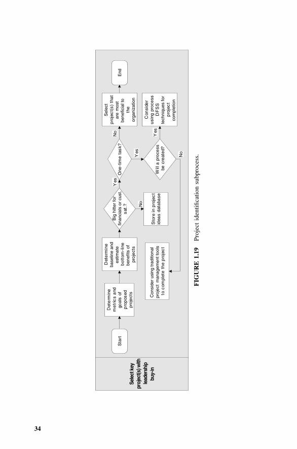
34

Sele

ct k

ey

proj

ect(s

) with

le

ader

ship

bu

y-in

Sta

rt

Det

erm

ine

m

etr

ics

and

go

als

of

pro

pos

ed

pro

ject

s

Det

erm

ine

ba

selin

e an

des

timat

e

bo

ttom

-line

be

nefit

s of

pro

ject

s

Big

hitt

er fo

rfin

anci

als

or c

ust.

sat

.?

Sto

re i

n p

roje

ct

idea

s d

ata

base

No

One

-tim

e t

ask?

Yes

End

No

Will

a p

roce

ss b

e c

reat

ed?

Yes

Con

side

r us

ing

trad

ition

alpr

oje

ct m

anag

emen

t too

lsto

com

plet

e t

he

pro

jec

t

No

Con

side

r u

sing

pro

cess

D

FS

S

tech

niqu

es fo

rp

roje

ct

com

plet

ion

Yes

Sel

ect

pro

jec

t(s

) th

at

are

mos

tbe

nefic

ial t

o

the

or

gani

zatio

n

FIG

UR

E1.

19Pr

ojec

tid

entifi

catio

nsu

bpro

cess

.

S4 / IEE PROJECT INITIATION AND EXECUTION ROADMAP 35

Wisdom of the organization deliverables and report out dateWisdom of the Org.

MSA deliverables and report out dateMSA

Consider lean tools deliverables and report out dateConsider Lean Tools

Baseline project deliverables and report out dateBaseline Project

Plan project and metrics phase deliverables and report out datePlan Project and Metrics

Control

Improve

Analyze

Define

Internal Productivity

Financial

Customer

Black be lt, team members and rolesTeam Members

Sponsor, champion, MBB, process owner, financial analystTeam Support

Control phase deliverables and report out date

Proactive testing deliverables and report out date

Passive analysis deliverables and report out date

Define phase deliverables and report out date

Phase Milestones

Describe the expected business performance improvement

Estimated financial impact to the business

Describe the impact and benefits to the final customer

Benefits

Describe improvement goals for these metricsGoal

Include RTY, DPMO as needed Secondary Metrics

30,000-foot-level, COPQ/CODND, process capability metric Primary Metrics

Identify KPOVs that will be used for process metricsBaseline Metrics

Project kick-off date and completion dateStart and Completion Date

Project name and problem statementProject Description

S /IEE Project Charter4

FIGURE 1.20 S4 / IEE project charter.

project transition, and closure. The details on this charter should be updatedas the project proceeds within the overall S4/IEE execution roadmap. Thechampion needs to work with the black belt so that the project status issufficiently documented within a corporate database that can be convenientlyaccessed by others.

At the beginning stages of an S4/IEE project, the champion needs to workwith the black belt and process owner so that the right people are on theteam. Team selection should result in team members being able to give dif-ferent insights and provide the skills (e.g., self-facilitation, technical/subjectmatter expert) needed to the completion of the project in a timely fashion.

The champion, belt belt, and team need to agree on the gap that currentlyexists between the process output and the expectations of the customer of theprocess, along with a tangible project improvement goal. A drill down froma high-level process map is to show the area of project focus. A visual rep-resentation of the project’s 30,000-foot-level metrics needs to show alignmentwith the satellite-level metrics for the organization.

36 SIX SIGMA OVERVIEW AND S4 / IEE IMPLEMENTATION

Chapter 53 summarizes project management issues that need to be ad-dressed for timely project completion. Upon project completion, the championneeds to work with the black belt to get a final project report that is timelyposted in their organization’s project tracking database.

Figure 1.12 showed the S4/IEE high-level project execution roadmap thataddresses the overall DMAIC roadmap, while Section A.1 in the Appendixshows the next-level drill-down from this roadmap. However, when executinga project, novices can have difficulty determining the next step to take whenworking on projects. Also, they can have difficulty determining what SixSigma tool to use for the various situations that they encounter. To aid usersof this book, I make reference to where tools that are described in this bookfit into this overall roadmap, which is shown in Figure A.1. Shadowed boxesidentify subprocesses that have a further description in another flowchart,which is covered within our training/coaching at Smarter Solutions, Inc.

Although there are many effective problem-solving tools, the use andapplication benefits from them are not often linked to the overall businessneeds or objectives. Because of this, teams that completed valuable projectsoften do not get the credit and recognition that they deserve. Many traditionalproblem-solving tools are described as part of the overall S4/IEE roadmap.When the application of these tools is part of an S4/IEE infrastructure, thebenefits for making improvements can have more visibility throughout theorganization. This visibility can be very desirable to a team that applied thetechniques, as well as to the organization, since success builds on success.

1.14 PROJECT BENEFIT ANALYSIS

S4 /IEE DMAIC Application: Appendix Section A.1, Project ExecutionRoadmap Steps 1.6, 3.7, and 9.6

Traditional COPQ calculations look at costs across the entire company usingthe categories of prevention, appraisal, internal failure, and external failure,as described in Figure 1.21. Organizations often do not disagree with thesecategories, but they typically do not expend the effort to determine this costingfor their particular situations.

Organizations need to determine how they are going to determine the ben-efit of projects. The procedure that they use can affect how projects are se-lected and executed. I think that other categories need to be considered whenmaking these assessments. Hence, I prefer the term cost of doing nothingdifferent (CODND) to COPQ. The reason I have included the term differentis that organizations often are doing something under the banner of processimprovements. These activities could include lean manufacturing, TQM, ISO9000, and so on.

Let’s use a Days Sales Outstanding (DSO) S4/IEE project example to il-lustrate two options for conducting a project benefit analysis. For an individ-

PROJECT BENEFIT ANALYSIS 37

PREVENTION

Training

Capability Studies

Vendor Surveys

Quality Design

APPRAISAL

Inspection and Test

Test Equipment and Maintenance

Inspection and Test Reporting

Other Expense Reviews

INTERNAL FAILURE

Scrap and Rework

Design Changes

Retyping Letters

Late Time Cards

Excess Inventory Cost

EXTERNAL FAILURE

Warranty Costs

Customer Complaint Visits

Field Service Training Costs

Returns and Recalls

Liability Suits

FIGURE 1.21 Traditional quality cost categories and examples.

ual invoice, its DSO would be from the time the invoice was created untilpayment was received. CODND considerations could include the monetaryimplications of not getting paid immediately (e.g., costs associated with in-terest charges on the money due and additional paperwork charges) whileCOPQ calculations typically involve the monetary implications beyond a cri-terion (e.g., costs associated with interest charges on the money due after thedue date for the invoice and additional paperwork/activity charges beyondthe due date).

One might take the position that we should not consider incurred costsuntil the due date of an invoice since this is the cost of doing business. Thiscould be done. However, consider that some computer companies actually getpaid before products are built for their Internet on-line purchases and theirsuppliers are paid much later for the parts that are part of the product assem-bly process. If we look at the total CODND opportunity costs, this could leadto out-of-the-box thinking. For example, we might be able to change our sales

38 SIX SIGMA OVERVIEW AND S4 / IEE IMPLEMENTATION

and production process so that we too can receive payment at the time of anorder.

I like the categories that Iomega used to determine the benefits of projects:

• Bottom-line hard dollar:• Decreases existing business costs• Example: defects, warranty, maintenance, labor, freight• Takes cost off the books or adds revenue to the books

• Cost avoidance:• Avoids incremental costs that have not been incurred but would have

occurred if project were not performed• Example: enhanced material or changes that would affect warranty

work• Lost profit avoidance:

• Avoids lost sales that have not been incurred, but would have occurredif project had not occurred

• Example: a project reduces frequency of line shutdowns• Productivity:

• Increases in productivity which improves utilization of existing re-sources

• Example: redeployment of labor or assets to better use• Profit enhancement:

• Potential sales increase, which would increase gross profit• Example: change that was justifiable through a survey, pilots, or as-

sumptions• Intangible:

• Improvements to operations of business which can be necessary tocontrol, protect, and or enhance company assets but are not quantifiable

• Example: Administrative control process that could result in high legalliability expense if not addressed

Further financial analysis basics will be described in the Project Manage-ment chapter of this book (see Chapter 52).

1.15 EXAMPLES IN THIS BOOK THAT DESCRIBE THEBENEFITS AND STRATEGIES OF S4/IEE

Many examples included in this book illustrate the benefits of implementingS4/IEE techniques through projects. The following partial list of examples isincluded to facilitate the reader’s investigation and/or give a quick overview

EXAMPLES OF S4 / IEE 39

of the benefits and implementation methodologies for use within S4/IEE train-ing sessions.

• Generic Process Measurement and Improvement• Process measurement and improvement within a service organization:

Example 5.3.• A 20:1 return on investment (ROI) study leads to a methodology that

has a much larger benefit through the changing or even the eliminationof the justification process for many capital equipment expenditures:Example 5.2.

• Tracking a product to a specification and then fixing the problem doesnot reduce the frequency of product nonconformance but can cost agreat deal of money. A better summary view of the process, as opposedto only measuring the product, can give direction for design improve-ments and poka-yoke: Example 43.5.

• Improving internal employee surveys to get more useful results withless effort. The procedure described would also work with externalsurveys: Example 43.7.

• A described technique better quantifies the output of a process, includ-ing variability, in terms that everyone can understand. The process isa business process that has no specifications: Example 11.5.

• The bottom line can be improved through the customer invoicing pro-cess: Example 43.8.

• An improvement in the tracking metric for change order times can givedirection to more effective process change needs. Example 43.6.

• Illustrating how the application of S4/IEE techniques improves thenumber in attendance at a local ASQ section meeting. The same meth-odology would apply to many process measurement and improvementstrategies: Example 11.5 and Example 19.5.

• Improving product development: Example 43.1.• A conceptual example can help with a problem that frequently is not

addressed, such as answering the right question: Example 43.9.• Design of Experiments (DOE)

• A DOE strategy during development uses one set of hardware com-ponents in various combinations to represent the variability expectedfrom future production. A follow-up stress to fail test reveals that de-sign changes reduce the exposure to failure: Example 31.5.

• Several DOEs are conducted to understand and fix a manufacturingproblem better. A follow-up experiment demonstrates that the imple-mented design changes not only improve average performance but alsoreduce the variability in performance between products: Examples 19.1,19.2, 19.3, 19.4.

40 SIX SIGMA OVERVIEW AND S4 / IEE IMPLEMENTATION

• The integration of quality functional deployment (QFD) and DOE leadsto better meeting customer needs: Example 43.2.

• Implementing a DOE strategy within development can reduce the num-ber of no-trouble-founds (NTFs) later reported after the product isavailable to customers: Example 30.2.

• Testing Products and Product Reliability• Improving a process that has defects: Example 5.1.• A DOE expedites the testing process of a design change: Example 30.1.• A strategy to capture combinational problems of hardware and software

can quickly identify when design problems exist. The strategy alsoprovides a test coverage statement: Example 42.4.

• An expensive reliability test strategy requiring many prototype ma-chines is replaced by a test that gives much more useful results in ashorter period of time. The results from this test reveal design issuesthat could have been diagnosed as NTF, which in many organizationscan cost manufacturing a great deal of money: Example 43.3.

• A customer ongoing-reliability test (ORT) requirement is created tosatisfy a customer requirement so that the activity gives more timelyinformation leading to process improvement with less effort than typ-ical ORT plans: Example 40.7.

• A reduced test of preproduction machines indicates that in order tohave 90% confidence that the failure criterion will be met, a total num-ber of 5322 test hours is needed during which two failures are permit-ted: Example 40.3.

• An accelerated reliability test consisting of seven components indicatesa wear-out failure mode according to which 75% of the units are ex-pected to survive the median life specifications. Example 41.1.

• Data from the field indicate a nonconstant failure rate for a repairablesystem: Example 40.6.

• Product Design for Six Sigma (DFSS)• Defining a development process: Example 4.1.• 21-step integration of the tools for product DFSS: Section 49.2.• Notebook computer development: Example 49.1.• An illustration of integration of lean and Six Sigma methods in devel-

oping a bowling ball: Example 44.1.• A reliability and functional test of an assembly, which yields more

information with less traditional testing: Example 43.3.• In a DFSS DOE one set of hardware components is configured in

various combinations to represent the variability expected from futureproduction. A follow-up stress-to-fail test reveals that design changesreduce the exposure to failure: Example 31.5.

EFFECTIVE SIX SIGMA TRAINING AND IMPLEMENTATION 41

• The integration of quality functional deployment (QFD) and a DOEleads to better meeting customer needs and the identification of man-ufacturing control variables: Example 43.2.

• Implementing a DFSS DOE strategy within development can reducethe number of no-trouble-founds (NTFs) later reported after the productis available to customers: Example 30.2.

• Conducting a reduced sample size test assessment of a system failurerate: Example 40.3.

• Postreliability test confidence statements: Example 40.5.• Reliability assessment of systems that have a changing failure rate:

Example 40.6.• Zero failure Weibull test strategy: Example 41.3.• Pass/fail system functional testing: Example 42.2.• Pass/fail hardware/software system functional test: Example 42.3.• A development strategy for a chemical product: Example 43.4.• A stepper motor development test that leads to a control factor for

manufacturing: Example 30.1.

1.16 EFFECTIVE SIX SIGMA TRAINING ANDIMPLEMENTATION

Section A.4 in the Appendix exemplifies a basic agenda using the topics inthis book to train executives (leadership), champions, black belts, green belts,and yellow belts. However, there are many additional issues to be consideredin training sessions.

For successful implementation of Six Sigma techniques, the training ofblack belt candidates needs to be conducted so that attendees can apply theconcepts to their project soon after the techniques are covered in the S4/IEEworkshop. An effective approach to the training of the Six Sigma conceptsdescribed in this book is four weekly modules spread over four months. Be-tween workshop sessions, attendees apply to their projects the concepts pre-viously learned. During this time they also get one-on-one coaching of theapplication of the S4/IEE techniques to their project.

In this training process, it is also very important that attendees have theresources to learn the concepts quickly and to apply the concepts to theirprojects. A portable computer should be assigned to all black belts with thefollowing software installed:

• An easy-to-use statistical program• Office suite (programs for word processing, spreadsheets, and presenta-

tions)• Process flowcharting program

42 SIX SIGMA OVERVIEW AND S4 / IEE IMPLEMENTATION

The most effective basic format to deliver the concepts is as follows:

• Present a topic using a computer projector system in conjunction with apresentation software package.

• Show an example (e.g., using the statistical software).• Present application exercise in which each student is to analyze a given

set of data on his/her computer in the class.• Periodically present an application exercise in which teams in the class

work together on a generic application of the concepts recently described;e.g., four or five team members collect and analyze data from a catapultexercise; students use this teaching tool that was developed by TexasInstruments to shoot plastic golf balls and measure the distance they wereprojected. [Note: Team catapult exercises will be described as exercisesthroughout this book. See the Glossary for a description of the catapult.]

• Periodically discuss how the techniques are applicable to the projects.

I have found that it is very beneficial for participants to create a presen-tation of how they applied S4/IEE techniques to their projects. Each persongives a presentation of his/her project using a computer projector system andpresentation software during weeks 2, 3, and 4. The instructor can evaluatethe presentation and give the presenter written feedback.

Each organization needs to create a process that establishes guidelines forthe selection, execution, and reporting of projects. Some things to considerand related issues when determining these guidelines are the following:

• Metrics and Monetary Issues:• Consider how to quantify and report in simple terms how the process

is doing relative to customer and business needs (see Section 1.19).Consider also how defects-per-million opportunities (DPMO) would bereported if this metric were beneficial. With an S4/IEE strategy, we donot force measurements on projects that do not make sense.

• Decisions must be made relative to how monetary S4/IEE project ben-efits are determined. Consider whether hard, soft, or both types of sav-ings will be tracked; e.g., hard savings have to show an impact to theaccounting balance sheet before reported. Soft savings would includean efficiency improvement that in time would save money becausefewer people would later be required to conduct the task. Before mak-ing this decision, I suggest first reviewing Examples 5.2 and 5.3. Ibelieve that it is important to have a measurement that encourages theright activity. For the black belts, one of the primary measurementsshould be a monetary saving. When a strict accounting rule of only‘‘hard money’’ is counted, the wrong message can be sent. A true hardmoney advocate would probably not allow for cost avoidance. For ex-

COMPUTER SOFTWARE 43

ample, a black belt who reduced the development cycle time by 25%would get no credit because the savings were considered soft money.

• Target S4/IEE Project Completion Dates and Stretch Goals:• Consider having a somewhat flexible amount of time, one to three

months, after the last S4/IEE workshop session, to account for projectcomplexity.

• Consider having stretch goals for projects, both individually and col-lectively. It is very important that management not try to drive im-provement only through these numbers. Management must insteadorchestrate efforts that lead to the most effective activities that canpositively affect these metrics.

• Recognition/Certification:• Consider the certification process for someone to become a black belt.

Perhaps she should have demonstrated a savings of at least $100,000in projects, obtained a level of proficiency using S4/IEE tools, andgiven good documentation of project results in a format that could bepublished.

• Consider how black belts and others involved within an S4/IEE imple-mentation will be recognized.

1.17 COMPUTER SOFTWARE

Most tedious statistical calculations can now easily be relegated to a computer.I believe that for a Six Sigma business strategy to be successful, practitionersmust have good versatile statistical software used in their training and readilyavailable for use between and after training sessions. The use of statisticalsoftware in training sessions expedites the learning of techniques and appli-cation possibilities. The availability and use of a common statistical softwarepackage in an organization following a training session will improve the fre-quency of application of the techniques and communications within/betweenorganizations and their suppliers/customers.

An organization should choose a common computer program that offersmany statistical tools, ease of use, good pricing, and technical support. QualityProgress (a magazine published by the American Society for Quality [ASQ],Milwaukee, WI) periodically publishes an article describing the features ofcomputer program packages that can aid the practitioner with many of thesetasks. The charts, tables, and analyses produced in this book were createdwith Minitab or Excel.

Reiterating, I believe that black belt workshops should include only theminimal number of manual exercises needed to convey basic understanding.Typically, we no longer do manual manipulation of statistical data; hence, amajority of instruction within an S4/IEE workshop should center around use

44 SIX SIGMA OVERVIEW AND S4 / IEE IMPLEMENTATION

of this computer program on a laptop computer assigned to the individual.After workshop sessions are complete, the student will then have the tools toefficiently apply S4/IEE techniques immediately.

It needs to be emphasized that even though computer software packagesare now very powerful, problem solutions and process improvements are nota result of statistical computer programs. Unfortunately, computer programpackages do not currently give the practitioner the knowledge to ask the rightquestion. This book addresses this most important task along with giving thebasic knowledge of how to use computer program packages most effectively.

1.18 SELLING THE BENEFITS OF SIX SIGMA

All the CEOs of partnering companies within the Six Sigma benchmarkingstudy described in Section A.2 in the Appendix were a driving force for theinitiation of Six Sigma within their company. However, there are many situ-ations in which someone in an organization believes in the methodology butdoes not have top executive buy-in. For this case, consider the followingstrategies to gain executive buy-in:

Strategy 1: Present the alternatives.Strategy 2: Illustrate an application.

With strategy 1 the monetary impact of the following alternatives is deter-mined and presented to influential managers within the company.

• Do nothing different: This might be the best alternative, but before mak-ing this decision the cost of doing nothing different (CODND) needs tobe determined and compared to the cost-of-doing-something. When cal-culating the CODND, consider future trends that might even drive acompany out of business.

• Implement Six Sigma as a business strategy: With this approach, an in-frastructure is created, in which key improvement projects follow a struc-tured methodology and are tied to strategic business metrics. Executivesupport is a necessary element! The Six Sigma business strategy has themost benefit, if it is executed wisely.

• Implement Six Sigma as a program: With this approach, there is focuson the training of Six Sigma tools and their application. Applicationproject selection does not necessarily align with the needs of the business.This approach is easier than implementing Six Sigma as a business strat-egy but risks becoming the ‘‘flavor of the month’’ and does not capturethe buy-in necessary to reap large bottom-line benefits.

S4 / IEE DIFFERENCE 45

With strategy 2 a highly visible situation is chosen. The selected situationshould have caused much anguish and firefighting within a company overtime. Data are then collected and presented in a high-level (30,000-foot-level)control chart. The following topics are included in a presentation to influentialmanagers.

• COPQ/CODND, including costs of firefighting and implications of futuretrends if something is not done different

• Roadmap of how this situation could be improved through the wise im-plication of Six Sigma techniques

For companies, improvement messages, strategies, or discussions with ex-ecutives need to be undertaken when the timing is right. We need to have apull (used as a lean term) for a solution attitude, as opposed to pushinginformation. That usually occurs when the pain is so great that the feeling isthat something has to be done for survival.

1.19 S4/IEE DIFFERENCE

I am including this section early in this book so the practitioner can easilysee the differences and advantages of the S4/IEE over traditional Six Sigmastrategies. A novice to the techniques may wish to only scan this section sincehe or she may encounter terms that are unfamiliar, which will be discussedlater.

Traditionally, within Six Sigma effort is given to identifying critical toquality (CTQ) characteristics issues (or process Y outputs), which are to bein alignment to what the customer wants. A defect is then considered anyinstance or event in which the product or process fails to meet a customerrequirement. One problem with this approach is that Six Sigma is viewed asa quality program, which can lead to playing games with the numbers if thereis no undisputable definition for what a defect truly is.

Six Sigma should be viewed as more than a quality improvement program.The methodologies of Six Sigma should be an integral part of the operationsand measurements of a company. A Six Sigma business strategy should leadto projects that can involve either simple process improvements or complexreengineering that is aligned to business needs.

In lieu of defining a CTQ parameter for each project, I prefer to identifyan important process output variable generically as a key process output vari-able (KPOV). When this is done, the implication to others is that Six Sigmais more than a quality initiative.

An S4/IEE strategy would track the KPOV metric at a high level, e.g.,30,000-foot level. This would be the Y output of a process that is expressed

46 SIX SIGMA OVERVIEW AND S4 / IEE IMPLEMENTATION

as Y � ƒ(x); i.e., Y is a function of x. In S4/IEE, an important x in thisequation is referred to as a key process input variable (KPIV). In S4/IEE, thetracking of this metric would be at a 50-foot level.

S4/IEE discourages the use of the commonly used metric, sigma qualitylevel; e.g., a 3.4 parts per million defect rate equals a six sigma quality level.There are several reasons for taking this position. One issue is that this metricis a quality metric. To apply this metric to the other measures of the business,such as a reduction of cycle time and waste, one has to define a specification.This creation of a specification often leads to playing games with a value inorder to make the sigma quality level number look good. This is one reasonwhy many organizations are having trouble integrating Six Sigma with leanmethodologies; i.e., cycle time and waste do not really have specificationlimits as manufactured products do. In addition, the logistics and cost tocalculate this metric, which has little if any value, can be very expensive. SeeExample 43.10 for a more in-depth discussion of these issues.

I will next describe the approach for measurements within S4/IEE. Withthe S4/IEE methodology, key business enterprise metrics such as ROI andinventory (as a TOC metric) are tracked at a high level; e.g., XmR statisticalcontrol chart (see Chapter 10), where there is a subgrouping/sampling ratethat is infrequent, perhaps monthly (see infrequent subgrouping/sampling de-scription in Glossary). Our satellite-level measurement strategy for these high-level business metrics separates common cause variability from special causevariability. The separation of these two variability types offers organizationsa means to get out of the firefighting mode, where common cause variabilityissues can be treated as though they were special cause.

When common cause variability with a satellite-level metric is unsatisfac-tory, the organization should then define a Six Sigma project(s) leading toimprovement of this business measurement. With an S4/IEE strategy, the out-put from the processes that these projects are to improve would be trackedusing a 30,000-foot-level measurement strategy. With this strategy, at leastone key process output variable (KPOV) metric for each project is trackedusing an XmR statistical control chart that has an infrequency subgrouping/sampling period, e.g., perhaps one unit or group of units collective analyzedper day or week on an XmR statistical control chart.

The purpose of a Six Sigma project is to find key process input variables(KPIVs) that drive the KPOV. For example, temperature (KPIV) in a plasticinjection-molding machine affects the overall dimension of a part (KPOV).With an S4/IEE strategy, we would focus on what should be done to controlthis KPIV through our 50-foot-level measurement and improvement strategy.The tracking of this metric would utilize an XmR statistical control chart thathas a frequent sampling period, e.g., one unit sampled, measured, and trackedevery minute or hour.

When an improvement is made to our process, the 30,000-foot-level mea-surement should show a sustainable shift to a new level of common cause

S4 / IEE DIFFERENCE 47

variability for the KPOV of the project. In addition, the satellite-level metricshould in time be impacted favorably. This approach creates a linkage andfeedback methodology between processes and the enterprise system as awhole.

Within a Six Sigma business strategy, we are trying to determine the pulseof the business, which requires more than just a snapshot of the latest resultsfrom a process or business metric. There is a real need to create a continuouspicture that describes key outputs over time, along with other metrics thatgive insight to focus areas for improvement opportunities. Unfortunately, or-ganizational policy often encourages practitioners to compile data in a formatthat does not lead to useful information. This problem is overcome when anorganization follows the S4/IEE methodology and uses the described mea-surement strategy.

In addition to discouraging the use of the sigma quality level metric, I alsohighlight the confusion that can result from common process capability/per-formance indices such as Cp, Cpk, Pp, and Ppk. I realize that customers oftenask for these metrics; hence, you may need to calculate these metrics andsupply these numbers to your customers. Chapter 11 describes alternativesfor making these calculations, as well as how these metrics can be very de-ceiving and why I believe that these metrics should not be used to driveimprovement activities within organizations. Chapter 11 also discusses why Ibelieve that a better metric is simply an estimate for the percentage or partsper million (ppm) beyond a desired response. Perhaps you can ask your cus-tomer to read sections of this book that describe my argument for why theCp, Cpk, Pp, and Ppk metrics can be deceptive and expensive in that they canlead to the wrong activities. Perhaps this suggestion can be the stimulus forthe creation of a new set of measures that you supply your customer.

I think that it can be a very detrimental requirement that all Six Sigmaprojects must define a defect. One reason for making this requirement with aSix Sigma initiative is that this is a requirement for a sigma quality level tobe calculated. An attractive selling point for making this requirement is thatnow all organizations can be compared through this one metric, sigma qualitylevel. This might sound good, but it is not practical. Consider how we mightdefine the opportunity for a defect on a sheet of titanium metal. Would thisbe the number of defects per square inch, foot, meter, or millimeter? Consideralso: how might we define a defect for days sales outstanding (DSO) for aninvoice? Should we consider the specification to be 30 days late or 90 dayslate? These two situations are quite different. For the first situation, an S4/IEE approach would suggest choosing a convenient area opportunity for thetitanium sheet, tracking over time this defect rate, and translating this rateinto monetary and customer dissatisfaction terms. For DSO, we could trackthis metric as a continuous response using a 30,000-foot-level metric samplingstrategy. We could then quantify from a probability plot (see Chapter 8) theestimated percentage beyond our desired response, perhaps the number of

48 SIX SIGMA OVERVIEW AND S4 / IEE IMPLEMENTATION

days beyond the due date of an invoice, where this due date could be 30, 60,or 90 days. Note that this probability plot could be from normal, log-normal,Weibull, or multiple distributions (see Chapter 9).

The S4/IEE approach to Six Sigma implementation leads to other oppor-tunities. Consider customer relationship management (CRM). Integratingsales, marketing, and customer service channels is important to an organiza-tion. Historically, implementing these CRM applications can cost more thanrealized in time, money, and lost opportunities. Companies want to automatekey customer-facing business functions to deliver greater efficiencies and pro-vide better customer service. We need to work on fire prevention rather thanfirefighting when working with customers. To do this, we need to have metricsand a process improvement strategy that drives the right type of activities.An S4/IEE implementation of Six Sigma can address these needs.

Another application for the S4/IEE methodology is a structured improve-ment methodology required for ISO 9000:2000. An organization could ad-dress the requirement by stating that the processes that it would be focusingon for improvement would be identified by the S4/IEE implementation infra-structure. The project execution would then follow the S4/IEE roadmap.

It is best if the CEO of a company embraces Six Sigma methods from thestart. However, we have found this is not a prerequisite to initiate Six Sigma.Sometimes a CEO or other management wants to experience the success ofSix Sigma first before committing to a organization-wide deployment. Forthis situation, whether the company is large or small, we have found that acompany can send one to five people to a public black belt workshop andwork from there with their deployment. True, this is typically a harder pathfor the black belt. However, we have seen that if an influential executive whotruly wants to assess Six Sigma sponsors the black belt, this approach canwork. For this rollout model, we conduct on-site executive and infrastructurebuilding workshops either in the same time frame or upon completion of theblack belt training. Sometimes with this approach, especially in small com-panies, the black belt can have multiple Six Sigma roles.

1.20 S4/IEE ASSESSMENT

Often people suggest that Six Sigma is the same as total quality management(TQM). I disagree. However, before making any generalities about the ad-vantages of Six Sigma over TQM, emphasis needs to be given that there havebeen implementation and success/failure differences for both TQM and SixSigma. Some generic advantages of using an S4/IEE implementation are:

• Focus is given to bottom-line benefits for organizations, where projectmonetary benefits are verified by finance. At the executive level thisbreeds excitement since improvement work is being aligned to the pri-mary measure of success.

S4 / IEE ASSESSMENT 49

• A support infrastructure is created where specific roles exist for peopleto be full-time practitioners (black belts) and to fill other support/ lead-ership roles (e.g., champions, green belts, etc.).

• Practitioners follow a consistent project execution roadmap, i.e., DMAIC.• Rather than a quality program it is a business strategy that helps drive

the business to the right activities.• Projects are pulled (used as a lean term) for creation by the metrics that

drive the business. However, I must note that often companies push (usedas a lean term) when creating Six Sigma projects, which may not be thebest utilization of resources.

• Voice-of-the-customer focus is given at both the satellite-level businessmetrics and 30,000-foot-level project execution metrics.

When implementing Six Sigma we need to capitalize on the lessons learnedfrom other implementations (see Section A.2). My experiences are consistentwith the summary of common case study attributes from Snee and Hoerl(2003):

Very Successful Case Studies Less Successful Case Studies• Committed leadership• Use of top talent• Supporting infrastructure

• Formal project selection process• Formal project review process• Dedicated resources• Financial system integration

• Supportive leadership• Use of whoever was available• No supporting infrastructure

• No formal project selectionprocess

• No formal project reviewprocess

• Part-time resources• Not integrated with financial

system

When organizations are considering making a change, they will considerassociated costs but will not give adequate focus to the cost of not making achange. When organizations are considering the costs of implementing an S4/IEE business strategy, they should look not only at direct costs of implemen-tation but also at the costs associated with not implementing S4/IEE, i.e.,CODND.

S4/IEE projects need to be of a manageable size, with consideration of theimpact on the overall system and bottom-line improvements. Consider alsoincluding cost avoidance and soft savings in the bottom-line improvement ofprojects.

In development, S4/IEE techniques can lead to earlier problem detectionand fewer problem escapes, with reduced development time. In manufactur-ing, these techniques can lead to a reduced number of problem escapes, theproblem being fixed the first time, and better process understanding. The

50 SIX SIGMA OVERVIEW AND S4 / IEE IMPLEMENTATION

ProductDesign

ProcessEngineering

ProductEngineering

Production Sales

Product DFSS DMAIC

FIGURE 1.22 Product DFSS with DMAIC.

economics associated with these results can be very significant. Figure 1.22shows how product DFSS and DMAIC align with a product’s life cycle(Scherkenbach 2002). Chapters 48 and 49 discuss the product DFSS process,which uses many of the DMAIC tools only in a different sequence (see Sec-tion 49.4).

It is important that management not only drive through the metrics, butalso focus on asking the right questions leading to the right activity. A SixSigma program can fail because emphasis is only on output measurements,not on real process improvement. For example, the type of management focusthat reprimands workers when they do not meet an arbitrarily set target willsurely make the numbers look good while real process improvement falls bythe wayside. Consider making the primary focus of a Six Sigma businessstrategy a structured strategy for improvement, not a bureaucratic system fordata collection and reporting. When creating the organizational infrastructurethat supports a Six Sigma business strategy, it is important to utilize Deming’s14 points (see Section 54.2).

Finally, let us consider communications between practitioners and execu-tives. The quality community for years has complained that management hasnot listened and supported its quality initiatives. The quality professionalsblame management. I do not agree. In my opinion, we in the quality andprocess improvement field are to blame because in the past we often showeda lack of ability to communicate well in terms that executives understand.

To illustrate my point, consider traveling to a country and not speaking thelanguage of that country. We should not expect everyone in the country tolearn our language to communicate with us. We either have to learn thelanguage or figure out an alternative way to communicate through a commonlanguage, like hand gestures. Similarly, a quality professional should not ex-pect executives to take the time to learn everything there is to know aboutthe language of the quality profession. The quality practitioner often needsto do a better job of communicating to executives using a language that theyunderstand, namely, money.

One might argue that this communication strategy in money terms cannotbe done and should not be done in all situations. The statement might be

EXERCISES 51

made that there are many activities that cannot be translated into money. Iwill not agree or disagree. However, I do believe that more issues can betranslated into monetary terms than are currently receiving this translation.More importantly, consider a situation in which there are no communicationproblems between practitioners and the right things are getting done. For thissituation, there is no reason to address changing the communication structure.However, if communication problems do exist between executive manage-ment and practitioners, perhaps more issues (and Six Sigma project work)should be communicated in monetary terms. Because of this change, a prac-titioner could receive more recognition for his or her accomplishments andadditional support for future efforts.

Peter Senge (1990) writes that learning disabilities are tragic in childrenbut fatal in organizations. Because of them, few corporations live even halfas long as a person—most die before they reach the age of 40. ‘‘Learningorganizations’’ defy these odds and overcome learning disabilities to under-stand threats and recognize new opportunities. If we choose to break a com-plex system into many elements, the optimization of each element does nottypically lead to total system optimization; e.g., optimizing purchasing costsby choosing cheaper parts can impact manufacturing costs through an increasein defect rates. One focus of S4/IEE is on avoiding optimizing subsystems atthe expense of the overall system. With systems thinking we do not lose sightof the big picture. The methodologies of S4/IEE offer a roadmap for changingdata into knowledge that leads to new opportunities. With S4/IEE, organiza-tions can become learning organizations!

1.21 EXERCISES

1. Define satellite-level metrics for a for-profit company, nonprofit organi-zation, school, religious organization, or political organization.

2. Create a strategic plan for improving a set of satellite-level metrics forone of the categories noted in Exercise 1.

3. Create a set of 30,000-foot-level operational metrics that are aligned withthe Satellite-level metrics described in Exercise 1 and the strategic planthat is described in Exercise 2.

4. Describe an S4/IEE project as a problem statement that you would expectwould be pulled from the activities described in Exercises 1, 2, and 3.

52

2VOICE OF THE CUSTOMER ANDS4/IEE DEFINE PHASE

A basic theme of this book is that the key system outputs of an organizationshould be tracked as a process. When improvements are needed to the systemmetrics, focus should be given to improving the processes that are mostaligned with these metrics.

One output that should be important to all systems at both the satellitelevel and 30,000-foot level is customer satisfaction. However, this voice ofthe customer (VOC) output can sometimes be difficult to quantify meaning-fully, remembering that we want to do things smarter, not play games withthe numbers. In this chapter I will discuss some strategies for collecting thevoice of the customer, while Chapter 13 elaborates on quality function de-ployment (QFD), a tool that can also help with these objectives.

Leaders in an organization need to ask the right questions leading to thewise use of statistical and other techniques for the purpose of obtaining knowl-edge from facts and data. Leaders need to encourage the wise application ofstatistical and other techniques for a Six Sigma implementation to be suc-cessful. This book suggests periodic process reviews and projects based onS4/IEE assessments leading to a knowledge-centered activity (KCA) focus in

VOICE OF THE CUSTOMER 53

all aspects of the business, where KCA describes efforts for wisely obtainingknowledge and then wisely utilizing this knowledge within organizations andprocesses. KCA can redirect the focus of business so that efforts are moreproductive. To accomplish this, we need to have a strategy for measurementand improvement. This chapter discusses goals and the S4/IEE define phase(see Section 2.7).

2.1 VOICE OF THE CUSTOMER

Consider products that a customer has purchased that do not meet his or herexpectations. Perhaps a product has many ‘‘bells and whistles’’ but does notmeet his or her basic needs. Or perhaps the product is not user-friendly orhas poor quality. Will a customer take the time to complain about the productor service? Will the customer avoid purchasing products from the same com-pany in the future? The importance of achieving customer satisfaction is animportant attribute of an S4/IEE implementation.

Important marketplace phenomena that apply to many consumer and in-dustrial products are (Goodman 1991):

• Most customers do not complain if a problem exists (50% encounter aproblem but do not complain; 45% complain at the local level; 5% com-plain to top management).

• On problems with loss of over $100 and where the complaint has beenresolved, only 45% of customers will purchase again (only 19% if thecomplaint has not been resolved).

• Word-of-mouth behavior is significant. If a large problem is resolved tothe customer’s satisfaction, about 8 persons will be told about the ex-perience; if the customer is dissatisfied with the resolution, 16 other per-sons will be told.

These realities of business make it important to address customer satisfac-tion, along with customer retention and loyalty. A calculation for the eco-nomic worth of a loyal customer is the combination of revenue projectionswith expenses over the expected lifetime of repeated purchases. The economicworth is calculated as the net present value (NPV) of the net cash flow (prof-its) over the time period. This NPV is the value expressed in today’s moneyof the profits over time (see Chapter 52).

With regard to customers, it should be emphasized that the end user of aproduct is not the only customer. For example, a supplier that manufacturesa component part of a larger assembly has a customer relationship with thecompany responsible for the larger assembly. Procedures used to determinethe needs of customers can also be useful to define such business proceduraltasks as office physical layout, accounting procedures, internal organization

54 VOICE OF THE CUSTOMER AND S4 / IEE DEFINE PHASE

FIGURE 2.1 Kano diagram: Satisfied feeling versus condition.

structure, and product test procedures. Focusing on the needs of customersgoes hand in hand with ‘‘answering the right question’’ and the S4/IEE as-sessments throughout this book. Within an S4/IEE strategy, the voice of thecustomer is assessed at two levels: the high level of the organization (satellitelevel) and the project level (e.g., 30,000-foot level).

Customer needs are dynamic. Product features that were considered wowfeatures in the past are now taken for granted. For example, a person seeingfor the first time a car that does not need a crank start would consider this awow change; however, electronic starters are now taken for granted. NoritakiKano’s description of this is illustrated conceptually in the Kano diagramshown in Figure 2.1.

The arrow in the middle, one-dimensional quality, shows the situation inwhich the customers tell the producer what they want and the producer sup-plies this need. The lower arrow represents the items that are expected. Cus-tomers are less likely to mention them but will be dissatisfied if they do notreceive them. Safety is an example in this category. The top arrow representswow quality. These are the items that a normal customer will not mention.Innovative individuals within the producer’s organization or leading edgeusers need to anticipate these items, which must be satisfiers, not dissatisfiers.

To capture VOC at the satellite level, organizations need input from avariety of sources, such as audits, management systems, unbiased surveys andfocus groups, interviews, data warehouse, and complaints. Organizations needa process that captures and integrates this information so that they are goingin the right direction and have the best focus relative to customer require-ments. This assessment can lead to improvement opportunities that result inS4/IEE projects.

A SURVEY METHODOLOGY TO IDENTIFY CUSTOMER NEEDS 55

TABLE 2.1 Example Questionnaire Format That Can Give a PerceptualMap Response

The products produced by our company are reliable. (Please comment on any spe-cific changes that you believe are needed.)

What is the importance of this require-ment to you?

What is your level of satisfaction thatthis requirement is met?

5 Very important 5 Very satisfied4 Important 4 Satisfied3 Neither important nor unimportant 3 Neither satisfied nor unsatisfied2 Unimportant 2 Unsatisfied1 Very unimportant 1 Very unsatisfied

Response: Response

Comments:

2.2 A SURVEY METHODOLOGY TO IDENTIFYCUSTOMER NEEDS

Situations often do not necessarily require all the outputs from a formal QFD,noting that an accurate QFD investigation can be useless if it is not conductedand compiled in a timely fashion.

This section describes an approach that utilizes brainstorming techniquesalong with surveys to quantify the needs of customers. The following stepsdescribe an approach to determine the questions to ask and then quantify andprioritize needs, as perceived by the customer.

1. Conduct brainstorming session(s) where a wish list of features, problemresolutions, and so forth are identified.

2. If there are many different brainstorming sessions that contain too manyideas to consider collectively in a single survey, it may be necessary torank the individual brainstorming session items. A secret ballot ratingfor each topic by the attendees could be done during or after the ses-sions. The items that have the highest rankings from each brainstormingsession are then considered as a survey question consideration.

3. A set of questions is then determined and worded from a positive pointof view. Obviously, care needs to be exercised with the wording of thesequestions so as not to interject bias. The respondent to the question isasked to give an importance statement and a satisfaction statement rel-ative to the question. The question takes the form shown in Table 2.1.

4. The information from this type of survey can be plotted in a perceptualmap (Urban and Hasser 1980) format.

56 VOICE OF THE CUSTOMER AND S4 / IEE DEFINE PHASE

FIGURE 2.2 Coordinate system and example data for a perceptual map.

A plot of this type can be created for each respondent to the survey, wherethe plot point that describes a particular question could be identified as itssurvey question number, as illustrated in Figure 2.2. Areas that need workare those areas that are judged important with low satisfaction (i.e., questions8 and 4).

The average question response could similarly be plotted; however, withany analysis approach of this type, care must be exercised not to lose indi-vidual response information that might be very important. An expert may ratesomething completely differently from the rest of the group because he orshe has much more knowledge of an area. Some effort needs to be given toidentify these people so that they can be asked more questions individuallyfor additional insight that could later prove to be very valuable; i.e., let usnot miss the important issues by ‘‘playing games’’ with the numbers.

Determining the areas that need focus from such a plot would not berigorous because the response has two-dimensional considerations (impor-tance and satisfaction). To address a more rigorous approach, consider firstthe extreme situation where a question is thought to be very important (i.e.,a 5) with low satisfaction (i.e., a 1). The difference between the importanceand satisfaction numbers could be used to create a number that is used forthe purpose of determining which areas have the largest opportunity for im-provement. A large number difference (i.e., 4) indicates an area that has alarge amount of potential for improvement, while lower numbers have lesspotential (a negative number is perhaps meaningless) (Wheeler 1990). Thesedifferences could then be ranked. From this ranking, a better understandingof where opportunities exist for improvement can result. From this ranking,we might also rank important questions, which can be grouped to get a betteridea of what areas should have the most focus for change.

This survey procedure is usually associated with determining the needs andwishes of the end users of a product. However, good customer-supplier re-lationships should exist within a company. Consider, for example, two stepsof a process in a manufacturing line. People involved with the second step of

GOAL SETTING AND MEASUREMENTS 57

the process are customers of the people who are involved with the first stepof the process.

A customer-supplier relationship can also be considered to exist betweenthe employees of an organization and the procedures that they use, for ex-ample, to develop a product. The methodology described in this section couldbe used to identify bureaucratic procedures that hamper productive activitiesof employees. After these areas are identified, additional brainstorming ses-sions could be conducted to improve the areas of processes that need to bechanged.

2.3 GOAL SETTING AND MEASUREMENTS

We are trained to think that goals are very important, and they are. Goals areto be SMART: simple, measurable, agreed to, reasonable, and time-based.However, these guidelines are often violated. Arbitrary goals set for individ-uals or organizations can be very counterproductive and very costly. To il-lustrate my point, consider two situations in your personal life.

Situation 1

You have a great deal of work that needs to get done around your house orapartment. A goal to get more work done on a Saturday can be very useful.Consider two scenarios relative to this desire:

• You can set a goal for the number of tasks you would like to accomplish,create a plan on how to accomplish these tasks most efficiently, and trackhow well you are doing during the day to meet your goal. You wouldprobably get more done with this strategy than just randomly attackinga list of to-do items.

• Your spouse or friend can set an arbitrary goal for the number of tasksyou are to accomplish. If he/she does not create a plan and the goals areset arbitrarily, you will probably not accomplish as much as you wouldunder the previous scenario because there is no plan and you do notnecessarily have to buy into the tasks that are to be accomplished.

Situation 2

You would like to make 50% return on your investment next year. Considertwo scenarios relative to this desire:

• You choose some mutual funds that have tracked well over the last fewyears; however, their yield was not as large as you desired. Because this

58 VOICE OF THE CUSTOMER AND S4 / IEE DEFINE PHASE

goal is important to you, you decide to track the yield of your portfoliodaily and switch money in and out of the funds, always keeping in mindyour 50% return on investment goal.

• You evaluate some quality index mutual funds that have tracked wellover the last few years. You decide that your goal was too aggressivebecause these funds have not had the yield that you would like to obtain.You alter your plan and choose an investment plan of buying and holdinga balanced portfolio of quality index mutual funds with minimal switch-ing of funds.

Situations 1 and 2 are very different relative to goal setting. In the firstsituation, goal setting can be useful because you do have some control overthe outcome—if there is buy-in by the person doing the implementation. Inthe second situation, goal setting could be very counterproductive becauseyou do not directly control the outcome of the process (i.e., how well thestock market will do next year). The first option scenario to situation 2 willprobably add additional variability to your investment process and can causesignificant losses. The second plan to address this goal is better because youdid research choosing the best process for your situation and took the resultingyield, even though you might not achieve your goal.

Management can easily get into the trap of setting arbitrary goals for peo-ple in which the outcome is beyond the scope of control of the employee. Toillustrate this point, consider a manufacturing process that has 90% of itsproblems from supplier quality issues. Often the approach to meet aggressivegoals for this situation is to monitor suppliers closely and hold them account-able whenever quality problems occur or to add inspection steps. These maybe the only courses of action that manufacturing employees can take and willnot be very productive with regard to meeting any improvement goals.

However, if management extends the scope of what employees can do tofix a problem, then things can change. Perhaps manufacturing employees canbe more involved with the initial supplier selection. Or perhaps manufacturingemployees can work with engineering to conduct a DOE for the purpose ofchanging settings of the manufacturing process (e.g., process temperature orpressure) so that high-quality product can be achieved with raw material oflesser quality.

Note that I do not mean to imply that stretch goals are not useful, becausethey are. Stretch goals can get people to think ‘‘out of the box.’’ However,goals alone without a real willingness to change and a road map to conductchange can be detrimental.

There is another consideration when setting goals: the scorecard. VinceLombardi said, ‘‘If you are not keeping score, you are just practicing.’’ Ascorecard worksheet can be useful for metric development when organization,product, process, and people are each assessed against performance, schedule,and cost. The implication of this is that organizations should not just measureagainst sigma quality levels and/or process output defect rates.

SCORECARD 59

FINANCIAL

Inventory levels Cost per unit Hidden factory Activity-based costing Cost of poor quality Cost of doing nothing different Overall project savings

CUSTOMER

Customer satisfaction (CTQ) On-time delivery Product quality (KPOV) Safety Communications

INTERNAL PROCESS

Defects: inspection data, DPMO, Sigma quality level On-time shipping Rolled throughput yield Supplier quality Cycle time Volume hours Baseline measurements KPIVs

LEARNING AND GROWTH

Six Sigma tool utilization Quality of training Meeting effectiveness Lessons leaned Number of employees trained in Six Sigma Project schedule vs. actual completion dates Number of project completed Total dollars saved on Six Sigma projects to date

FIGURE 2.3 Balance scorecard.

2.4 SCORECARD

Often organizations can spend much resource developing balanced scorecardmetrics throughout their organization. Balanced scorecard is often organizedaround the four distinct performance perspectives of financial, customer, in-ternal business process, and learning and growth (Kaplan and Norton 1996).

The status of any balanced scorecard metrics could then be reported as asingle number within a dashboard of dials. Someone would then be assignedthe task of fixing the problem whenever the position of needle on the dial isin a red region, which indicates a nonconformance state. Metrics within theyellow state are to be observed more closely since they are in the warningregion, while everything is considered okay when the needle is in the greenregion.

Reporting and reacting to metrics in this manner can lead to the same typesof problems described in Example 3.1. A tracking and reporting procedurethat uses 30,000-foot-level control charts and process capability/performancenon-conformance rate assessment of important operational metrics for bothvariables and attribute measures, can lead to S4/IEE projects, when appro-priate, that are aligned with the needs of the business. If one wishes to usetraditional balanced scorecard criteria, Figure 2.3 shows how the metrics ofSix Sigma can be categorized into balanced scorecard metrics.

How much success an S4/IEE business strategy achieves can depend uponhow goals are set and upon any boundaries that are given relative to meetingthese objectives. In addition, if scorecards are not balanced across an orga-nization, people can be driving their activities toward a metric goal in one

60 VOICE OF THE CUSTOMER AND S4 / IEE DEFINE PHASE

area, adversely affecting another metric or area. The result is that even thoughthe person appears successful since he/she met his/her goal, the overall or-ganization can suffer.

2.5 PROBLEM SOLVING AND DECISION MAKING

One process for problem solving or decision making is:

• Become aware of a problem or needed action.• Define the problem or needed action.• Consider alternatives and their consequences.• Select an approach.• Implement the approach.• Provide feedback.

This may not be an all-inclusive list; however, often deviations from theflow are large. For example, someone may determine a quick fix to a crisisin the manufacturing line. The person may have created other problems withthe quick fix because he or she did not discuss the alternatives with otherindividuals. In addition, there may be no feedback to determine whether theproblem fix was effective for future production.

An additional concern arises in that the wrong basic problem is oftensolved; this is often called a type III error. Type I and type II errors, discussedin depth later (see Sections 3.8 and 16.3), address (�) the risk of rejecting anull hypothesis when it is true and (�) the risk of failing to reject the nullhypothesis when it is not true.

To address this type III issue, consider a manufacturing facility that pro-duces printed circuit boards. This company may need to reduce its total defectrate at final test. Without proper understanding and investigation, the problemmay be defined initially as follows: How should we get the assembly lineemployees to work more carefully so that they will reduce variability at theirstations? However, perhaps a better starting point would be to state the prob-lem as being too high of a defective rate at the end of the manufacturingprocess. From this more general definition, Pareto charts can be used to directefforts toward the sources that are causing most of the failures. The S4/IEEroadmap can then be used to consider alternatives and possible experimentsfor data collection as part of the decision-making process that leads to quan-tifiable improvement.

Shewhart developed the plan-do-check-act (PDCA) cycle as a process im-provement flowchart. Deming later called the improvement methodologyplan-do-study-act (PDSA). Actions for this management cycle from Demingare steps, as the names imply. First, it is important to plan what is to be done,i.e., determine what steps are to be completed to achieve the objectives of

S4 / IEE DMAIC DEFINE PHASE EXECUTION 61

the plan by the target date. Second, the plan is executed (do). Third, studythe results, arriving at conclusions. Finally, act on what was concluded fromthe study phase. The PDSA is a simplification of other more elaborateproblem-solving methodologies.

A standardized problem-solving process used by Chrysler, Ford and Gen-eral Motors is 8 disciples (8D) or steps described in Section A.5 in the Ap-pendix. The techniques could be used within an overall S4/IEE strategy. Forexample, an S4/IEE 30,000-foot-level metric could initiate the 8D processwhen quick containment of a problem is needed. Tools that are later describedin this book, such as design of experiments (DOE), are referenced within the8D process to help identify and then verify fixes to problems as part of theverification process. In addition, statistical tests could be used as part of thevalidation process.

The basic PDSA, 8D, and other problem-solving philosophies are con-tained within the overall structure of the S4/IEE methodology described inthis book.

2.6 ANSWERING THE RIGHT QUESTION

Sometimes practitioners of Six Sigma techniques need to consider a differentapproach to a problem or project in order to resolve the issue most effectively.The S4/IEE assessment sections at the end of many chapters can help withthe creation of a do-it-smarter approach for a given situation. This sectionoffers some additional thoughts on the topic.

Large objectives can be achieved by considering the methodologies de-scribed within the S4/IEE assessment sections, but there is a price to pay:Objectives may need redefinition. The unwise application of classical statis-tical problem definitions might assume no engineering knowledge; e.g., willthis product meet the failure rate criterion? Typically, within any product orprocess development there are individuals who have engineering knowledgeof where product risks exist. Combining all sources of knowledge structurallyis important to problem redefinition and an S4/IEE philosophy. If test effortsare directed toward these risk areas, favorable customer satisfaction andhigher product quality can result with less test effort.

2.7 S4/IEE DMAIC DEFINE PHASE EXECUTION

S4 /IEE DMAIC Application: Appendix Section A.1 Project ExecutionRoadmap Steps 1.2–1.7

Chapter 1 discussed the overall infrastructure of S4/IEE, which included pro-ject selection and the basic project execution roadmap structure. Chapter 2touched on the importance of obtaining the VOC at both the enterprise andproject execution level, along with some strategies to obtain this feedback. Inaddition, this chapter also discussed goal setting and problem solving, along

62 VOICE OF THE CUSTOMER AND S4 / IEE DEFINE PHASE

with the importance of problem definition. All of these issues need consid-eration when you are defining and scoping an S4/IEE project. The objectiveof the define phase is to describe the CTQ/business issue, the customer, andthe involved core business process. During the define phase a problem state-ment is formulated. Customer requirements are gathered, and a project charteris created, where the project scope is determined by the team with the supportof management. Other activities during this phase include: definition of theCTQ/30,000-foot-level metric; identification of both internal and externalcustomers; identification and definition of what is to be improved (e.g., defector cycle time); estimation of COPQ/CODND; development of high-level pro-cess map; initiation of SIPOC.

The success of a project also depends on communication. The project char-ter and periodic report-outs provide an effective means for communication sothat there is no misunderstanding of the objectives and status of a project.

The following list describes focus areas for the define phase of an S4/IEEproject, which is an expansion of the items initially described in Section 1.13.

• A two-to-three sentence problem statement needs to focus on the symp-toms and not the possible solution. Customer and business impact infor-mation should be included along with current DPMO or other baselineinformation, data sources for problem analysis, and a COPQ/CODNDestimate. Example (see Example 43.13): Companies are dissatisfied withthe customer service call wait time in our XYZ office. Our service re-cords show an estimated median wait time of 80 seconds with 80% ofwait times between 25 and 237 seconds. Note: This example illustrateshow a 30,000-foot-level operational metric within an S4/IEE enterprisecan pull (using a lean term) for the creation of a project.

• Stakeholders (finance, managers, people who are working in the process,upstream/downstream departments, suppliers, and customers) need toagree to the usefulness of the project and its problem statement.

• The financial liaison should work closely with the project leader andchampion to create a cost-benefit analysis for the project. This couldinclude expense reduction, revenue enhancements, loss avoidance, re-duced costs, or other COPQ/CODND benefits.

• The project scope needs to be sized correctly and documented in a projectcharter format (see Figure 1.20). All involved need to agree to the ob-jectives, scope, boundaries, resources, project transition, and closure ofthe project charter. The details of this charter should be updated as theproject proceeds through the overall S4/IEE execution roadmap.

• Projects should be aligned with the improvement needs of its high-levelsupply chain map; e.g., the supply chain process decision program chart(PDPC) shown in Figure 5.8. Constraints and assumptions should beincluded.

• Projects should be large enough to justify the investment of resourcesbut small enough to ensure problem understanding and development of

S4 / IEE ASSESSMENT 63

sustainable solutions. The scope should accurately define the bounds ofthe project so project creep, a major cause for missed deadlines, isavoided. Example: Reduce the hold time of calls at the XYZ office withthe intention of leveraging success to other call centers.

• Targeted improvement goals should be measurable. These goals shouldbe tied to COPQ/CODND benefits when appropriate. Example: Reducethe median call wait time to 40 seconds or less, yielding a $200,000 peryear benefit at the XYZ office.

• Measurements should be described. If defects are at the 30,000-foot-levelmetric, what constitutes a defect and how it will be tracked should bedescribed. If cycle time is the metric, the plans for cycle-time quantifi-cation and tracking should be described. Note: Some organizations maychoose to report a sigma quality level metric; however, as noted in Sec-tion 1.19, this is not recommended within an S4/IEE implementation.

• The categories of an SIPOC should have been addressed, where the pro-cess portion of SIPOC is at a high level, containing only four to sevenhigh-level steps (see Chapter 4). How the SIPOC diagram aligns withthe high-level supply chain map and its needs should be demonstrated,along with the gap between voice of the process and VOC.

• Team members should be selected by the champion and project leader(e.g., black belt) such that they provide different insights and skills (e.g.,self-facilitation, technical/subject matter expert) needed for the success-ful completion of the project in a timely fashion.

• Names, roles, and amount of time for project dedication should be ad-dressed for each team member.

• The champion needs to work with the project leader so that the projectstatus is sufficiently documented within a corporate database that can beconveniently accessed by others.

2.8 S4/IEE ASSESSMENT

An S4/IEE philosophy means directing efforts toward objectives that have themost benefit by compiling and converting data into knowledge. If this is notdone, development and manufacturing work can have much misdirection. Ef-forts must be taken to avoid magnifying the small and missing the big. Moreemphasis also needs to be placed on having a product that is satisfactory toall customers, as opposed to certifying an average criterion; i.e., a value-addactivity versus a non-value-add activity. Sometimes only very simple changesare needed to make a process much better.

When setting up tests using an S4/IEE strategy, some problems can bebroken up into subgroupings for statistical assessment. However, for this strat-egy to be successful, all areas of management in an organization must havean appreciation for the value of statistical concepts. If an S4/IEE strategy isincorporated, fewer emergencies testing and fixing in both product develop-

64 VOICE OF THE CUSTOMER AND S4 / IEE DEFINE PHASE

ment and the manufacturing process can be expected. One might say, ‘‘Usestatistics for fire prevention.’’ Constant job pressure to fix individual problemsimmediately can be very stressful. With less firefighting, there could be lessemployee stress, leading to healthier and happier employees.

2.9 EXERCISES

1. Describe a situation in which you think management, organizations, orsociety is addressing the wrong problem.

2. Explain how the techniques presented in this chapter are useful and canbe applied to S4/IEE projects.

3. Describe customers for the organization chosen in Exercise 1.1 (Exercise1 in Chapter 1). Build a strategy for determining the VOC and trackinghow well their needs are fulfilled.

PART II

S4/IEE MEASURE PHASEFROM DMAIC

Part II (Chapters 3–14) addresses process definition, process performance,and the quantification of variability. Potential key process input variables(KPIVs) and key process output variables (KPOVs) are identified throughconsensus. Included in this section are basic analysis tools: Six Sigma mea-sures, measurement systems analysis, failure mode and effects analysis(FMEA), and quality function deployment (QFD).

Also within this part of the book, the DMAIC measure steps, which aredescribed in Section A.1 (part 2) of the Appendix, are discussed. I havegrouped the tools of the measurement phase into several related components,adding a ‘‘consider lean tools’’ component. Because of this, within S4/IEEthere are five components to the measure phase:

• Plan project and metrics• Baseline project• Consider lean tools• MSA• Wisdom of the organization

Checklists for the completion of each of these measure phase componentsare:

66 S4 / IEE MEASURE PHASE FROM DMAIC

Measure Phase: Plan Project and Metrics Checklist

Description Questions Yes/No

Tool /MethodologyKPOV Are the key process output variables clearly

defined?Were the most appropriate metrics chosen in order

to give insight into the process (continuous vs.attribute)?

Was continuous data used when available?Secondary Metrics Are any secondary metrics such as DPMO and

RTY going to be used?Financial Metrics Have you finalized with Finance how financial

benefits will be calculated?Does the project include any cost avoidance,

improved efficiency, improved customersatisfaction, or other soft money considerations?

Voice of theCustomer

Did the team identify key internal and externalcustomers of the project process?

Did the team speak with customers of the projectprocess?

Has this customer input been included in theproject description and scope?

Project Plan Are project milestones identified?Is the project time line reasonable and acceptable?

TeamResources Are team members and key stakeholders identified?

Are all team members motivated and committed tothe project?

Next PhaseApproval to

ProceedDid the team adequately complete the above steps?Has the project database been updated and

communication plan followed?Are barriers to success identified and planned for?Is the team tracking with the project schedule?Have schedule revisions been approved?

S4 / IEE MEASURE PHASE FROM DMAIC 67

Measure Phase: Baseline Project Checklist

Description Questions Yes/No

Tool /Methodology30,000-foot-level

Control ChartWere project metrics compiled in a 30,000-foot-

level control chart with an infrequentsubgrouping sampling plan so that typicalprocess noise occurs between samples?

Was historical data used when initiating the 30,000-foot-level control chart?

Is the 30,000-foot-level control chart now beingupdated regularly?

Is the process in control /predictable?Have special cause issues been resolved?

Process Capability /PerformanceMetric

If specification limits exist for continuous data, wasthe process capability /performance metricestimated as a percentage or ppm ofnoncompliance?

If data are attribute, has the process capability beenshown as the centerline of a 30,000-foot-levelcontrol chart?

Probability Plot /Dot Plot

If data are continuous, were probability plots and/or dot plots used to show process capability /performance metric?

Was the appropriate probability plot used?Are the data normally distributed?If there is more than one distribution, were the data

separated for further analysis?Pareto Chart If KPOV data are classified by failure type, was a

Pareto chart used to prioritize failure types?Data Collection Has the team collected and reviewed the current

standard operating procedures?Are the data you are using good and truly

representative of the process?Do you know how much data you will need?Is your data collection plan satisfactory to all

stakeholders?COPQ/CODND Now that the process capability /performance metric

has been determined, given the refined COPQ/CODND estimate, is this still the right project towork on?

TeamResources Are all team members motivated and committed to

the project?Is there a plan for executive management to

interface with the team to keep motivation aliveand commitment visible?

68 S4 / IEE MEASURE PHASE FROM DMAIC

Measure Phase: Baseline Project Checklist (continued )

Description Questions Yes/No

Next PhaseApproval to

ProceedDid the team adequately complete the above steps?Has the project database been updated and

communication plan followed?Is the team considering lean tools?Have barriers to success been identified and

resolved?Is the team tracking with the project schedule?Have schedule revisions been approved?

Measure Phase: Consider Lean Tools Checklist

Description Questions Yes/No

Tool /MethodologyLean Tools Is the KPOV a lean metric, like cycle time?

If so, are you planning to use lean tools?Have you defined value add, non-value add but

necessary, and waste?Have you identified the benefits you expect to gain

from their use?If cycle time is a KPOV, have you done a time-

value analysis?Assessment Were any process improvements made?

If so, were they statistically verified with theappropriate hypothesis test?

Did you describe the change over time on a30,000-foot-level control chart?

Did you calculate and display the change inprocess capability /performance metrics (in unitssuch as ppm)?

Have you documented and communicated theimprovements?

Have you summarized the benefits and annualizedfinancial benefits?

TeamResources Are all team members motivated and committed to

the project?Next PhaseApproval to

ProceedDid the team adequately complete the above steps?Has the project database been updated and

communication plan followed?Should an MSA be conducted for this project?Is the team tracking with the project schedule?Have schedule revisions been approved?Are barriers to success identified and planned for?

S4 / IEE MEASURE PHASE FROM DMAIC 69

Measure Phase: Measurement System Analysis Checkist

Description Questions Yes/No

Tool /MethodologyData Integrity Is there an operational definition for the data being

collected that reflects the needs of the customer?Are the recorded data representative of the actual

process?Have you taken appropriate steps to error proof the

data collection process?Gage R&R Was an MSA needed?

If so, is the measurement system satisfactory?If the measurement system was not satisfactory,

have improvements been implemented to make itsatisfactory, or has the data collection plan beenrevised?

Assessment Were any process improvements made?If so, were they statistically verified with the

appropriate hypothesis test?Did you describe the change over time on a

30,000-foot-level control chart?Did you calculate and display the change in

process capability /performance metrics (in unitssuch as ppm)?

Have you documented and communicated theimprovements?

Have you summarized the benefits and annualizedfinancial benefits?

TeamResources Are all team members motivated and committed to

the project?

Next PhaseApproval to

ProceedDid the team adequately complete the above steps?Has the project database been updated and

communication plan followed?Is there a detailed plan for collecting wisdom of

the organization?Are barriers to success identified and planned for?Is the team tracking with the project schedule?Have schedule revisions been approved?

70 S4 / IEE MEASURE PHASE FROM DMAIC

Measure Phase: Wisdom of the Organization Checklist

Description Questions Yes/No

Tool /MethodologyProcess Flowchart Was a process map created at the appropriate level

of detail?Does the flowchart include critical suppliers and

end customers?Cause and Effect

DiagramWas a brainstorming session held with a cross-

functional team to collect the wisdom of theorganization inputs?

Cause and EffectMatrix

Were the results of the cause-and-effect diagramprioritized with the C&E matrix?

Were there any ‘‘low hanging fruit’’ opportunitiesthat can be fixed immediately?

FMEA Was an FMEA conducted with resulting actionitems?

Assessment Were any process improvements made?If so, were they statistically verified with the

appropriate hypothesis test?Did you describe the change over time on a

30,000-foot-level control chart?Did you calculate and display the change in

process capability /performance metrics (in unitssuch as ppm)?

Have you documented and communicated theimprovements?

Have you summarized the benefits and annualizedfinancial benefits?

TeamResources Are all team members motivated and committed to

the project?

Next PhaseApproval to

ProceedDid the team adequately complete the above steps?Has the project database been updated and

communication plan followed?Should this project proceed to the passive analysis

phase?Is there a detailed plan for the passive analysis

phase?Are barriers to success identified and planned for?Is the team tracking with the project schedule?Have schedule revisions been approved?

71

3MEASUREMENTS AND THE S4/IEEMEASURE PHASE

An objective of the measure phase is the development of a reliable and validmeasurement system of the business process identified in the define phase.This chapter describes some issues that need to be addressed within theS4/IEE measure phase. Presented is a discussion on how an inappropriatetracking methodology can lead to the wrong activity, including firefighting.Described also is an overview of some basic descriptive statistics or enumer-ative studies used when sampling from a population. Some of the method-ologies discussed are data gathering, presentation, and simple statistics. Thereis an introductory discussion of confidence level and hypothesis testing, bothof which will be discussed in more depth later (see Section 16.3). Also, thereis discussion about attribute versus continuous data and the ineffectiveness ofvisual inspections.

To get a valid answer, care must be exercised when performing experimentsand conducting analyses. This chapter also includes examples of experimenttraps that need to be avoided consciously.

3.1 VOICE OF THE CUSTOMER

S4 /IEE DMAIC Application: Appendix Section A.1, Project ExecutionRoadmap Step 2.1

VOC assessment is needed up front when executing S4/IEE projects at the30,000-foot level. Steps for this execution are:

72 MEASUREMENTS AND THE S4 / IEE MEASURE PHASE

• Define your customer.• Obtain customer wants, needs, and desires.• Ensure that focus of project is addressing customer needs.

Graphical, statistical, and qualitative tools described later in this book shouldbe used to understand customer feedback.

Important customer key process output categories are sometimes classifiedwith regard to their area of impact—that is, critical to quality (CTQ) (e.g.,flatness, diameter, or electrical characteristic), critical to delivery (CTD), crit-ical to cost (CTC), and critical to satisfaction (CTS). Important key processinput issues are sometimes classified as critical to process (CTP).

The format of a tree diagram (see Section 5.14) can be useful to helpensure that a linkage exists between customer requirements and process per-formance metrics. A tree diagram can describe the transition: need → drivers→ CTQs. It can also be used to describe the hierarchy of critical to (CT)categories at the satellite level, operational 30,000-foot level, and project30,000-foot level. This hierarchy can give direction to the assessment ofwhether current measures are in alignment with the needs of customers, orjust collected and reported against internal standards; e.g., a metric is reportedonly because it is easy to capture. In addition, the tree diagram can givedirection for improvement activities.

An example CTS tree is shown in Figure 3.1, where the categories of priceand quality could have a similar drill-down to the illustrated drill-down fordelivery. This drill-down graphic can also be useful to capture categories thatwill be collected and analyzed further to see if they significantly affect the30,000-foot-level response of an S4/IEE project and warrant further investi-gation for improvement opportunities.

Quality function deployment (QFD) (see Chapter 13) is a tool that can helpcollectively examine the VOC. QFD can be used in many different areas ofthe business: planning, testing, engineering, manufacturing, distribution, mar-keting, and service. However, it must be understood that great effort may berequired to perform a formal QFD evaluation.

3.2 VARIABILITY AND PROCESS IMPROVEMENTS

Variability is everywhere. Consider a person who parks his/her car inside his/her garage. The final position of the car is not the same exact place day afterday. The driver has variability when parking the car. Variability in parkingposition can be measured over time. When nothing unusual occurs, thesources of variability in parking position are considered common cause. How-ever, if a cat were to jump in front of the car during parking, this mightdistract the driver and cause additional variability, i.e., special cause.

If his/her variability, either common or special cause, when parking is toolarge from the center parking position in the garage, he/she could hit the

73

Cus

tom

er o

n

Tim

e D

eliv

ery

Lat

e D

eliv

ery

Ear

ly D

eliv

ery

Doc

umen

tati

onP

O D

iscr

epan

cyC

ompl

ete

On

Tim

e

Item

Typ

eSu

pplie

rL

ocat

ion

Cle

vela

ndC

inci

nnat

iH

oust

onC

harl

otte

Cle

vela

nd

Ser

vice

Sho

p G

ener

ates

Mos

t Def

ects

Wit

h A

Fai

lure

Rat

e of

89%

Lat

e D

eliv

erie

sC

leve

lan

d S

ervi

ce S

hop

Gen

erat

es M

ost D

efec

ts w

ith

aFa

ilure

Rat

e of

89%

Lat

e D

eliv

erie

s

Sour

ces

of V

aria

tion

Pri

ceD

eliv

ery

Qua

lity

FIG

UR

E3.

1C

ritic

alto

satis

fact

ion

tree

.

74 MEASUREMENTS AND THE S4 / IEE MEASURE PHASE

garage door frame. If parking variability is too large because of special causes,e.g., the cat, attempts need to be made to avoid the source of special cause.If parking variability is too large from common cause, the process of parkingneeds to be changed.

For the purpose of illustration, consider a person who wants to determinehis/her average parking position and the consistency he/she has in parkinghis/her car inside the garage. It is not reasonable to expect that he/she wouldneed to make measurements every time that the car is parked. During someperiod of time (e.g., one month) he/she could periodically take measurementsof the parked position of the car. These measurements would then be used toestimate, for example, an average parking position for that period of time.

Similarly, all automobiles from a manufacturing line will not be manufac-tured exactly the same. Automobiles will exhibit variability in many differentways. Manufacturers have many criteria or specifications that must beachieved consistently. These criteria can range from dimensions of parts inthe automobile to various performance specifications. An example criterionis the stopping distance of the automobile at a certain speed. To test thiscriterion, the automobile manufacturer obviously cannot test every vehicleunder actual operating conditions to determine whether it meets this criterion.In lieu of this, the manufacturer could test against this criterion using a samplefrom the population of automobiles manufactured.

3.3 COMMON CAUSES VERSUS SPECIAL CAUSES ANDCHRONIC VERSUS SPORADIC PROBLEMS

J. M. Juran (Juran and Gryna 1980) considers the corrective action strategyfor sporadic and chronic problems, while W. Edwards Deming addresses thisbasic issue using a nomenclature of special causes and common causes (Dem-ing 1986). Process control charts are tools that can be used to distinguishthese two types of situations.

Sporadic problems are defined as unexpected changes in the normal op-erating level of a process, while chronic problems exist when the process isat a long-term unacceptable operating level. With sporadic problems the cor-rective action is to bring the process back to the normal operating level, whilethe solution to chronic problems is a change in the normal operating level ofthe process. Solving these two types of problems involves different basicapproaches.

The Juran’s control sequence (Juran and Gryna 1980) is basically a feed-back loop that involves the following steps:

1. Choose the control subject (i.e., what we intend to regulate).2. Choose a unit of measure.3. Set a standard or goal for the control subject.

EXAMPLE 3.1: REACTING TO DATA 75

4. Choose a sensing device that can measure the control subject in termsof unit of measure.

5. Measure actual performance.6. Interpret the difference between the actual and standard.7. Take action, if any is needed, on the difference.

Process control charting techniques discussed in this book are useful tools tomonitor the process stability and identify the existence of both chronic andsporadic problems in the process.

Chronic problems often involve extensive investigation time and resources.Juran describes the following breakthrough sequence for solving this type ofproblem:

1. Convince those responsible that a change in quality level is desirableand feasible.

2. Identify the vital few projects; that is, determine which quality problemareas are most important.

3. Organize for breakthrough in knowledge; that is, define the organizationmechanisms for obtaining missing knowledge.

4. Conduct the analysis; that is, collect and analyze the facts that are re-quired and recommend the action needed.

5. Determine the effect of proposed changes on the people involved andfind ways to overcome the resistance to change.

6. Take action to institute the changes.7. Institute controls to hold the new level.

The Pareto chart (see Section 5.6) is a tool that is used to identify the mostlikely candidates or areas for improvement. Within a given area of improve-ment, DOE techniques can often be used to determine efficiently which ofthe considered changes are most important for implementation within theprocess.

It is important to note that special causes (sporadic problems) usually re-ceive more attention because of high visibility. However, more gains can oftenbe made by continually working on common cause (i.e., chronic problems).The terms common cause and special cause will be used in the remainingportion of this book.

3.4 EXAMPLE 3.1: REACTING TO DATA

An organization collects data and reacts whenever an out-of-specification con-dition occurs or a goal is not met. The following example dialogue is whatcould happen with this approach, where attempts are made to fix all out-of-

76 MEASUREMENTS AND THE S4 / IEE MEASURE PHASE

specification problems whenever they occur within a manufacturing or serviceenvironment. This scenario could apply equally to a business service processwhenever the goals of an organization are not being met.

Consider a product that has specification limits of 72–78. We will nowdiscuss how an organization might react to collected data.

• First datum point: 76.2• Everything is OK.

• Second datum point: 78.2• Joe, go fix the problem.

• Data points: 74.1, 74.1, 75.0, 74.5, 75.0, 75.0• Everything OK—Joe must have done a good job!

• Next datum point: 71.8• Mary, fix the problem.

• Data points: 76.7, 77.8, 77.1, 75.9, 76.3, 75.9, 77.5, 77.0, 77.6, 77.1,75.2, 76.9• Everything OK; Mary must have done a good job!

• Next datum point: 78.3• Harry, fix the problem.

• Next data points: 72.7, 76.3• Everything OK; Harry must have fixed the problem.

• Next datum point: 78.5• Harry, seems like there still is a problem.

• Next data points: 76.0, 76.8, 73.2• Everything OK; the problem must be fixed now.

• Next datum point: 78.8• Sue, please fix the problem that Harry could not fix.

• Next data points: 77.6, 75.2, 76.8, 73.8, 75.6, 77.7, 76.9, 76.2, 75.1, 76.6,76.6, 75.1, 75.4, 73.0, 74.6, 76.1• Everything is great; give Sue an award!

• Next datum point: 79.3• Get Sue out there again. She is the only one who knows how to fix

the problem.• Next data points: 75.9, 75.7, 77.9, 78

• Everything is great again!

A plot of this information is shown in Figure 3.2. From this plot we can seethat the previously described reaction to out-of-specification conditions doesnot improve the process or likelihood of having problems in the future. Figure3.3 shows a replot of the data as an XmR control chart (see Chapter 10). The

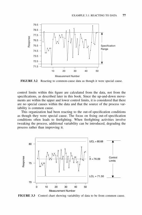
EXAMPLE 3.1: REACTING TO DATA 77

5040302010

79.5

78.5

77.5

76.5

75.5

74.5

73.5

72.5

71.5

Measurement Number

Res

pons

e

RangeSpecification

FIGURE 3.2 Reacting to common-cause data as though it were special cause.

0 10 20 30 40 50

70

75

80

Measurement Number

X = 76.09

UCL = 80.68

LCL = 71.50

Res

pons

e

LimitsControl

FIGURE 3.3 Control chart showing variability of data to be from common cause.

control limits within this figure are calculated from the data, not from thespecifications, as described later in this book. Since the up-and-down move-ments are within the upper and lower control limits, it is considered that thereare no special causes within the data and that the source of the process var-iability is common cause.

This organization had been reacting to the out-of-specification conditionsas though they were special cause. The focus on fixing out-of-specificationconditions often leads to firefighting. When firefighting activities involvetweaking the process, additional variability can be introduced, degrading theprocess rather than improving it.

78 MEASUREMENTS AND THE S4 / IEE MEASURE PHASE

Both public and private organizations frequently look at human and ma-chine performance data similar to the situation just described and then makejudgments based on the data. Production supervisors might constantly reviewproduction output by employee, by machine, by work shift, by day of theweek, by product line, and so forth. In the service sector, an administrationassistant’s output of letters and memos produced per day may be monitored.In call centers around the world, the average time spent per call is monitoredand used to counsel low-performing employees. The efficiency of computerprogrammers could be monitored through the tracking of lines of code pro-duced per day. In the legal department the number of patents secured on thecompany’s behalf during the last fiscal year could be compared to previousannual rates. Whenever an organization reacts to individual situations that donot meet requirements/specifications and does not look at the system of doingwork as a whole, it could be reacting to common cause situations as thoughthey were special cause.

To illustrate this point further, I will use an example in which an organi-zation monitored the frequency of safety memos. Consider that a safety memowas written indicating that the number of accidents involving injuries duringthe month of July was 16, up by 2 units from 14 such injuries a year ago inJuly. The memo declares this increase in accidents to be unacceptable andrequires all employees to watch a mandatory 30-minute safety video by theend of August. At an average wage rate of $10 per hour, the company payrollof 1500 employees just affected the August bottom line by $7500 plus wastedtime getting to and from the conference room. This does not even considerthe time spent issuing memos reminding people to attend, reviewing atten-dance rosters looking for laggards, and so forth.

I am not saying that safety and productivity are not important to an or-ganization. I am saying, as did Dr. Deming, that perhaps 94% of the outputof a person or machine is a result of the system that management has put inplace for use by the workers. If performance is poor, 94% of the time it isthe system that must be modified for improvements to occur. Only 6% of thetime is problems due to special causes. Knowing the difference between spe-cial and common cause variation can affect how organizations react to dataand the success they achieve using the methods of a Six Sigma strategy. Forsomeone to reduce the frequency of safety accidents from common cause, anorganization would need to look at its systems collectively over a long periodto determine what should be done to processes that lead to safety problems.Reacting to an individual month that does not meet a criterion can be bothcounterproductive and very expensive.

One simple question that should be repeated time and time again as S4/IEE implementation proceeds is this: ‘‘Is the variation I am observing ‘com-mon cause’ or ‘special cause’ variation?’’ The answer to this simple questionhas a tremendous impact on the action managers and workers take in responseto process and product information. And those actions have a tremendousimpact on worker motivation and worker self-esteem.

SAMPLING 79

Common cause variability of the process might or might not cause a prob-lem relative to meeting the needs of customers. We will not know until wecompare the process output collectively relative to the specification. This ismuch different than reacting to individual points that do not meet specificationlimits. When we treat common cause data collectively, focus is placed onwhat should be done to improve the process. When reaction is taken to anindividual point that is beyond specification limits for a common cause situ-ation, focus is given to what happened relative to this individual point asthough it were a ‘‘special’’ condition, not to the process information collec-tively.

Reiterating, variation of the common cause variety resulting in out-of-spec-ification conditions does not mean that one cannot or should not do anythingabout it. What it does mean is that you need to give focus on improvingthe process, not just firefight individual situations that happen to be out-of-specification. However, it is first essential to identify whether the conditionis common or special cause. If the condition is common cause, data are usedcollectively when comparisons are made relative to the frequency of how theprocess will perform relative to specification needs. If an individual point orpoints are determined to be special cause from a process point of view, wethen need to address what was different about this/ these individual point(s).

One of the most effective quality tools for distinguishing between commoncause and special cause variation is the simple-to-learn and easy-to-use con-trol chart. The problem with control charts is that they are so simple thatmany managers and workers misunderstand and misuse them to the detrimentof product and process quality. In Chapter 10 I will elaborate on the satellite-level and 30,000-foot-level control charting procedures, which can greatlyenhance the success of Six Sigma within an organization. The charts canreduce the frustration and expense associated with firefighting activities withinan organization.

3.5 SAMPLING

A sample is a portion of a larger aggregate or population from which infor-mation is desired. The sample is observed and examined, but information isdesired about the population from which the sample is taken. A sample canyield information that can be used to predict characteristics of a population;however, beginning experimenters often have a misconception about the de-tails of performing such a test. They might consider taking a sample (e.g.,10) from today’s production, making a measurement, averaging the results,and then reporting this value to management (for the purpose of making adecision).

Arbitrary sampling plans such as this can yield erroneous conclusions sincethe test sample may not accurately represent the population of interest. Asample that is not randomly selected from a population can give experimental

80 MEASUREMENTS AND THE S4 / IEE MEASURE PHASE

bias, yielding a statement that is not representative of the population that isof interest. A sample of automobiles to address some criterion characteristic,for example, should be taken over some period of time with the considerationof such parameters as production shifts, workers, and differing manufacturinglines (i.e., a random sample without bias). A response (x) from samples takenrandomly from a population is then said to be a random variable.

If there is much variability within a population, then there may not bemuch confidence in the value that is reported (e.g., average or mean response).A confidence interval statement quantifies the uncertainty in the estimate sincethe width of the interval is a function of both sample size and sample vari-ability. When a population characteristic such as the mean is noted to bewithin a confidence interval, the risk of the true value being outside this rangeis a quantifiable value.

Still another point not to overlook when evaluating data is that there areother estimates besides the mean that can be a very important part of ex-pressing the characteristic of a population. One of these considerations is thestandard deviation of a population, which quantifies the variability of a pop-ulation. Another consideration is the capability/performance of a process ora population-percentage value compliance statement.

3.6 SIMPLE GRAPHIC PRESENTATIONS

It can be meaningful to present data in a form that visually illustrates thefrequency of occurrence of values. This display of data can be accomplishedusing a dot plot or histogram.

A dot plot is a simple procedure to illustrate data positioning and its var-iability. Along a numbered line, a dot plot displays a dot for each observation.Dots are stacked when data are close together. When too many points existvertically, each dot may represent more than one point. Figure 15.4 showsdot plots within a marginal plot.

A histogram is another form of plot to make such illustrations. To createa histogram when the response only takes on certain discrete values, a tallyis made each time a discrete value occurs. After a number of responses istaken, the tally for the grouping of occurrences can then be plotted in histo-gram form. For example, Figure 3.4 shows a histogram of 200 rolls of twodice, in which the sum of the dice for 8 of these rolls was two.

However, when making a histogram of response data that are continuous,the data need to be placed into classes (i.e., groups or cells). For example, ina set of data there might be six measurements that fall between the numbersof 0.501 and 1.500; these measurements can be grouped into a class that hasa center value of 1. Many computer programs internally handle this grouping.Section C.1 in the Appendix discusses a manual approach. A stem-and-leafdiagram is constructed much like a tally column for creating a histogram,except that the last digit of the data value is recorded in the plot instead of atally mark.

SAMPLE STATISTICS (MEAN, RANGE, STANDARD DEVIATION, AND MEDIAN) 81

FIGURE 3.4 Histogram: 200 rolls of two dice.

It should be noted that even though histograms are commonly used toillustrate data, the probability plotting techniques described in a later chaptercan often give a more informative visual illustration about the population fromwhich the data is sampled.

3.7 EXAMPLE 3.2: HISTOGRAM AND DOT PLOT

A sample yields the following 24 data points, ranked low to high value:

2.2 2.6 3.0 4.3 4.7 5.2 5.2 5.3 5.4 5.7 5.8 5.85.9 6.3 6.7 7.1 7.3 7.6 7.6 7.8 7.9 9.3 10.0 10.1

A computer-generated histogram plot of this data is shown in Figure 3.5. Adot plot is shown in Figure 3.6.

3.8 SAMPLE STATISTICS (MEAN, RANGE, STANDARDDEVIATION, AND MEDIAN)

S4 /IEE Application Examples

• Random sample of last year’s invoices, where the number of days beyondthe due date was measured and reported (i.e., days sales outstanding[DSO])

• Random sample of parts manufactured over the last year, where the di-ameter of the parts were measured and reported

82 MEASUREMENTS AND THE S4 / IEE MEASURE PHASE

FIGURE 3.5 Histogram of the data.

109876543

Values

FIGURE 3.6 Dot plot of the data.

A well-known statistic for a sample is the mean ( ). The mean is a measurexof central tendency. It is the arithmetic average of the data values (x1, x2, x3,. . . , xi), which is mathematically expressed in the following equation usinga summation sign � for sample size (n) as:

n

x� ii�1x �

n

A sample yields an estimate for the true mean of a population � fromxwhich the sample is randomly drawn. Consider, for example, the time it takesto respond to a telephone inquiry. Six randomly selected phone conversationswere closely monitored, where the duration of the phone conversation was 6,2, 3, 3, 4, and 5 min. An estimate for the mean duration of phone inquiriesis:

6 � 2 � 3 � 3 � 4 � 5x � � 3.83

6

Range is a statistic that describes data dispersion. It is simply the difference

SAMPLE STATISTICS (MEAN, RANGE, STANDARD DEVIATION, AND MEDIAN) 83

between the highest and lowest value of a set of data. The range for theprevious set of data is 4 (i.e., 6 � 2 � 4). Range values can give a quickassessment of data variability; however, values are dependent upon the samplesize and outlier data can give distorted results. A better measure of datavariability is standard deviation.

Standard deviation is a statistic that quantifies the dispersion of data. Amanager would not only be interested in the average duration of phone con-versations but also the variability of the length of conversation. One equationform for the standard deviation mean(s) of a sample is:

n1/22(x � x)� i

i�1� �s �n � 1

A sample yields an estimate s for the true population standard deviation�. When data have a bell-shaped distribution (i.e., are normally distributed),approximately 68.26% of the data is expected to be within a plus or minusone standard deviation range around the mean. For this example, the standarddeviation estimate of the duration of phone inquiries would be

1/22(6 � 3.83) � � � �s � � 1.472� �6 � 1

It should be noted that the standard deviation of a population when all thedata is available is calculated using a denominator term n, not n � 1. Somecalculators offer both standard deviation calculation options. The n � 1 termin the denominator of the previous equation is commonly called degrees offreedom. This term will be used throughout this book and is assigned theGreek letter � (pronounced ‘‘nu’’). The number of degrees of freedom is afunction of the sample size and is a tabular input value often needed to makevarious statistical calculations.

Variance is the square of the standard deviation. Variance is equivalent tomoment of inertia, a term encountered in engineering. For this illustration,the sample variance s2 is:

2 2s � 1.472 � 2.167

Range, standard deviation, and variance are measures of dispersion. An-other measure of dispersion is coefficient of variation, which equals thestandard deviation divided by the mean and is expressed as a percentage.

The curves shown in Figure 3.7 have a frequency distribution shape thatis often encountered when smoothing histogram data. The mathematicalmodel corresponding to the frequency distribution is the probability density

84 MEASUREMENTS AND THE S4 / IEE MEASURE PHASE

FIGURE 3.7 PDF: Effects of population variability.

function (PDF). Each of these density function curves is bell-shaped and iscalled a normal probability density function.

For a given sample size, a smaller standard deviation yields more confi-dence in the results of the experiment. This is pictorially illustrated in Figure3.7, which shows that case 2 has more variability than case 1, which willcause more uncertainty in any estimated population parameter mean. Calcu-lation of the confidence interval that quantifies this uncertainty will be dis-cussed in a later chapter (see Chapter 17).

The sample median is the number in the middle of all the data. It can berepresented as x50 or . The 50 denotes that 50% of the measurements arex̃lower than the x value. Similarly, x30 indicates the 30th percentile. To deter-mine the median of data, the data first need to be ranked. For the precedingset of data, the median is the mean of the two middle values, because thereis an even number of data points, which is

3 � 42 3 3 4 5 6:median � � 3.5

2

However, if the data were 1 2 4 5 6, the sample median would be 4, themiddle of an odd number of data points.

As described, the mean and median quantify the central tendency of mea-surements, while the range and standard deviation describe variability of mea-surements. Throughout this book, mean and standard deviation metrics willhave various applications. For example, we can use these metrics collectivelyin a process to determine estimates for percentage nonconformance beyondspecification limits. Another application is statistical tests for equality of themean and standard deviation of input parameters (e.g., machines or raw ma-terial), which could affect the desirability of a KPOV.

ATTRIBUTE VERSUS CONTINUOUS DATA RESPONSE 85

3.9 ATTRIBUTE VERSUS CONTINUOUS DATA RESPONSE

The data discussed in the previous section are continuous, or variables, data.Continuous data can assume a range of numerical responses on a continuousscale, as opposed to data that can assume only discrete levels, whereas at-tribute, or discrete, data have the presence or absence of some characteristicin each device under test (e.g., proportion nonconforming in a pass/fail test).

An example of continuous data is the micrometer readings of a sample ofparts. Examples of attribute data are which operator or machine manufactureda part. Another example of attribute data is the number of defects on a partrecorded by an inspector. Still another example of attribute data is the outputof an inspection process in which parts are either passed or failed (as opposedto measuring and recording the dimension of the part).

One should strive for continuous data information over attribute informa-tion whenever possible since continuous data gives more information for agive sample size. Sometimes people who build the infrastructure within anorganization for how a Six Sigma business strategy will be implemented losesight of this metric because ppm and DPMO are attribute measurements.

Another type of response is covered within this book. I call this responselogic pass/fail. This type of response is most common in the computer in-dustry when certain machine configurations will not work together. The pre-sumption is that they will always not work together because there perhaps isa logic problem in the software; hence the term logic. This is not to beconfused with the attribute response when a conformance is measured innoncompliance rates or proportions. The logic pass/fail response is discussedin Chapter 42 on pass/fail functional testing.

S4 /IEE Attribute Application Examples

• Transactional workflow metric (could similarly apply to manufacturing;e.g., inventory or time to complete a manufacturing process): Randomsample of last year’s invoices where the number of days beyond the duedate was measured and reported (i.e., days sales outstanding [DSO]). Ifan invoice was beyond 30 days late, it was considered a failure or de-fective transaction. The number of nonconformances was divided by thesample size to estimate the nonconformance rate of the overall process.Note that this procedure would not be the recommended strategy withinS4 /IEE, since much information is lost in the translation between con-tinuous and attribute data.

• Transactional quality metric: Random sample of last year’s invoices,where the number of defects in filling out the form were measured andreported. The number of defective transactions was divided by the samplesize to estimate the defective rate of the process.

• Transactional quality metric: Random sample of last year’s invoices,where the invoices were examined to determined if there were any errors

86 MEASUREMENTS AND THE S4 / IEE MEASURE PHASE

when filling out the invoice. Multiple errors or defects could occur onone invoice. The total number of defects was divided by the sample sizeto estimate the defect rate of the process.

• Transactional quality metric: Random sample of last year’s invoices,where the invoices were examined to determined if there were any errorswhen filling out the invoice or within any other step of the process.Multiple errors or defects could occur when executing an invoice. Thetotal number of defects when the invoice was executed was divided bythe total number of opportunities for failure to estimate the defect permillion opportunity rate of the process.

• Manufacturing quality metric: Random sample of parts manufacturedover the last year, where the diameter of the parts were measured andreported. If the part was beyond specification limits, it was considered adefective part or a ‘‘failure.’’ The number of nonconformances was di-vided by the sample size to estimate the nonconformance rate of theoverall process. Note that this procedure would not be the recommendedstrategy within S4 /IEE, since much information is lost in the translationbetween continuous and attribute data.

• Manufacturing quality metric: Random sample of printed circuit boardsover the last year, where the boards were tested for failure. The numberof defective boards was divided by the sample size to estimate the defec-tive rate of the process.

• Manufacturing quality metric: Random sample of printed circuit boardsover the last year, where the boards were tested for failure. Multiplefailures could occur on one board. The total number of defects wasdivided by the sample size to estimate the defect rate of the process.

• Manufacturing quality metric: Random sample of printed circuit boardsover the last year, where the boards were tested for failure. Multiplefailures could occur on one board. The total number of defects on theboards was divided by the total number of opportunities for failure (sumof the number of components and solder joints from the samples) toestimate the defect per million opportunity rate of the process.

3.10 VISUAL INSPECTIONS

Visual inspections still often remain a very large single form of inspectionactivity to determine if a product is satisfactory. However, characteristics oftendo not completely describe what is needed, and inspectors need to make theirown judgment. When inspections are required, standards need to be set up sothat consistent decisions are made.

Another problem that can occur is that a visual inspection does not addressthe real desires of the customer. A classified defect found within a manufac-turing organization may or may not be a typical customer issue. Also, there

HYPOTHESIS TESTING AND ANALYSIS OF VARIANCE COMPUTER OUTPUTS 87

can be issues that a customer thinks are important which are not consideredby the test.

Visual inspections often lead to the thinking that quality can be inspectedinto a product. This can be a very expensive approach. In addition, peopletypically believe that a test does better at capturing defects than it really does.An exercise at the end of this chapter and also the measurement systemsanalysis chapter illustrate the typical ineffectiveness of these tests.

Whether the inspections are visual or not, the frequency of defects andtypes of defects need to be communicated to the appropriate area for processimprovement considerations. The techniques described later within this bookcan improve the effectiveness of these tests and reduce the frequency of whenthey are needed.

3.11 HYPOTHESIS TESTING AND THE INTERPRETATION OFANALYSIS OF VARIANCE COMPUTER OUTPUTS

This section gives a quick overview of hypothesis testing and how it relatesto the interpretation of analysis of variance outputs. Both hypothesis testingand analysis of variance methods are described in more depth later. The pur-pose for discussing these concepts now is twofold. First, this explanation cangive management a quick overview of the concepts. Secondly, a basic under-standing of the concepts is needed for some topics, such as measurementsystems analysis, covered before a more formal explanation.

Hypothesis tests are used when decisions need to be made about a popu-lation. Hypothesis tests involve a null hypothesis (H0) and an alternative hy-pothesis (Ha). Example hypotheses are as follows:

• Null (H0): Mean of population equals the criterion. Alternative (Ha):Mean of population differs from the criterion.

• Null (H0): Mean response of machine A equals mean response of ma-chine B. Alternative (Ha): Mean response of machine A differs frommachine B.

• Null (H0): Mean response from the proposed process change equals themean response from the existing process. Alternative (Ha): Mean re-sponse from proposed process change does not equal the mean responsefrom the existing process.

• Null (H0): There is no difference in fuel consumption between regularand premium fuel. Alternative (Ha): Fuel consumption with premium fuelis less.

Two risks can be involved within a hypothesis test. These risks are typicallyassigned the nomenclature � and � (see Chapter 16). Within this section wewill only consider the � risk.

88 MEASUREMENTS AND THE S4 / IEE MEASURE PHASE

TABLE 3.1 Analysis of Variance Output Illustration

Source df Seq SS Adj SS Adj MS F P

A 1 0.141 0.141 0.141 0.34 0.575B 1 31.641 31.641 31.641 75.58 0.000C 1 18.276 18.276 18.276 43.66 0.000D 1 0.331 0.331 0.331 0.79 0.395E 1 0.226 0.226 0.226 0.54 0.480Error 10 4.186 4.186 0.419Total 15 54.799

Assume that we collect data and wanted to determine if there is a differencebetween the mean response of two machines or two departments. Our nullhypothesis would be that the mean responses of the two machines or depart-ments are equal, while the alternative hypothesis would be that the meanresponse of the two machines or departments are not equal.

When analyzing the data, we have the intent of showing a difference. Inall likelihood, the means of the sampled data from our two populations willnot be exactly the same whether there is in fact a true difference between thepopulations or not. The question is whether the difference of sample meansis large enough so that we can consider that there is a difference in thepopulation means.

If we conducted a statistical analysis that indicated that there is a differ-ence, then we would say that we reject the null hypothesis (i.e., that the twomeans of the population are the same) at an � risk of being in error. This �risk addresses the possibility, assuming random sampling techniques are fol-lowed, that a large enough difference occurred between our samples bychance. However, in fact there was no difference in the population means.Hence, if we rejected the null hypothesis with an � risk of 0.05, there wouldbe one chance in 20 that our decision was not correct.

Many types of hypothesis test will be discussed later in this book. Thestatistical method used when making the hypothesis test will vary dependingupon the situation. We will later discuss how one experiment can addressmany hypotheses at once. To illustrate this multiple-hypothesis testing, whichwill help with interpretation of analysis of variance tables, consider that adesign of experiments (DOE) evaluation was to assess the impact of five inputvariables, or factors. These factors are designated as factor A, factor B, factorC, factor D, and factor E. Each of these factors had two levels (e.g., machine1 vs. machine 2, operator 1 vs. operator 2, day 1 vs. day 2, machine tem-perature 1 vs. machine temperature 2). An experiment was then conducted,and the results were analyzed using a statistical computer software packageto give the output shown in Table 3.1.

For now we will consider only the values designated as p within the tablefor each of the five factors, which correspond to � in our previous discussion.

EXPERIMENTATION TRAPS 89

TABLE 3.2 Estimated Effects and Coefficients Output Illustration

Term Effect Coefficient SD Coefficient T P

Constant 4.844 0.1618 29.95 0.000A �0.187 �0.094 0.1618 �0.58 0.575B �2.812 �1.406 0.1618 �8.69 0.000C 2.138 1.069 0.1618 6.61 0.000D �0.288 �0.144 0.1618 �0.89 0.395E �0.238 �0.119 0.1618 �0.73 0.480

Basically, with this analysis there are five null hypotheses, each taking theform that there is no difference between the two levels of the factor. Considerthat we set a criterion of � � 0.05. That is, if our analysis indicated a lessthan 1 chance in 20 of being wrong, we would reject the null hypothesis.From this table, we note that the p value for factors B and C are much lessthan this criterion; hence, for these factors we would reject the null hypoth-esis. However, for factors A, D, and E the p value is not less than 0.05; hence,we can say that we do not have enough information to reject the null hy-pothesis at � � 0.05.

As discussed earlier, there is a statistical procedure used by the computerprogram to calculate these probability values. The statistic used to calculatethese values is the F statistic (see Section 7.17). Sometimes there is morethan one statistical approach to analyze data. Table 3.2 shows the output usinganother statistic, the t statistic (see Section 7.16). As you can see, many ofthe table outputs are different; however, the probability (p) values are thesame.

Using this type of Six Sigma analysis tool, we can gain a lot of knowledgeabout our process. We know that if process improvement is needed, we shouldfocus on factors B and C (not A, D, and E).

3.12 EXPERIMENTATION TRAPS

Randomization is used in experiments when attempting to avoid experimentalbias. However, there are other traps that can similarly yield erroneous con-clusions. For example, erroneous statements can result from not consideringrational subgroups, sampling scheme, measurement error, poor experimentdesign strategy, erroneous assumptions, and/or data analysis errors.

Invalid conclusions can easily result when good statistical experimentationtechniques are not followed. Perhaps more erroneous conclusions occur be-cause of this than from inherent risks associated with the probability of gettinga sample that is atypical. The next four sections illustrate examples associatedwith poor experiment methodology. These problems emphasize the risksassociated with not considering measurement error, lack of randomization,

90 MEASUREMENTS AND THE S4 / IEE MEASURE PHASE

confused effects, and not tracking the details of the implementation of anexperiment design.

3.13 EXAMPLE 3.3: EXPERIMENTATION TRAP—MEASUREMENT ERROR AND OTHER SOURCESOF VARIABILITY

Consider that the data in Table 3.3 are the readings (in 0.001 of cm) of afunctional gap measured between two mechanical parts. The design specifi-cations for this gap were 0.008 � 0.002 cm. This type of data could beexpected from the measurements in a manufacturing line, when the 16 randomsamples were taken over a long period of time.

However, there are two areas that are often not considered in enough detailwhen making such an evaluation: first, how samples are selected when makingsuch an assessment of the capability/performance of the response; second,the precision and accuracy of the measurement system are often overlooked.

Relative to sampling methodology, consider the experimenter who is beingpressed for the characterization of a process. He/she may take the first productparts from a process and consider this to be a random sample of future processbuilds. This type of assumption is not valid because it does not consider themany other variabilities associated with processes (e.g., raw material lot-to-lot variability that might occur over several days).

Relative to the measurement systems analysis, it is often assumed thatgages are more precise than they really are. It is typically desirable to havea measurement system that is at least 10 times better than the range of theresponse that is of interest. Measurement error can cause ambiguities duringdata analysis. The basic sources for error need to be understood to manageand reduce their magnitude and to obtain clear and valid conclusions. Thevariability from a measurement tool can be a large term in this equation,leading to erroneous conclusions about what should be done to reduce processvariability.

The measured variability of parts can have many sources, such as repeat-ability, the variability associated with the ability of an appraiser to get asimilar reading when given the same part again (� ); reproducibility, the var-2

1

iability associated with the ability of differing appraisers obtaining a similarreading for the same part ( ); and measurement tool-to-tool ( ), within lots2 2� �2 3

( ), and between lots ( ). The total variability (� ) for this example would2 2 2� �4 5 T

be equal to the sum of the variance components, which is

2 2 2 2 2 2� � � � � � � � � � �T 1 2 3 4 5

Measurements will include all these sources of variability. The precision ofthe measurements of parts is dependent on � . In addition, the accuracy de-2

T

pends upon any bias that occurs during the measurements.

91

TA

BL

E3.

3T

enR

ando

mSa

mpl

ings

from

aN

orm

alP

DF

Whe

re�

�6

and

��

2

With

in-G

roup

Sam

ple

Num

ber

Sam

plin

gG

roup

Num

bers

12

34

56

78

910

12.

997.

889.

806.

864.

554.

875.

317.

178.

953.

402

6.29

6.72

4.04

4.76

5.19

8.03

7.73

5.04

4.58

8.57

32.

655.

884.

826.

148.

759.

148.

904.

645.

772.

424

10.1

17.

655.

073.

244.

525.

716.

902.

426.

775.

595

5.31

7.76

2.18

8.55

3.18

6.80

4.64

10.3

66.

159.

926

5.84

7.61

6.91

3.35

2.45

5.03

6.65

4.17

6.11

4.63

72.

177.

074.

184.

087.

957.

522.

866.

875.

747.

488

4.13

5.67

8.96

7.48

7.28

9.29

8.15

8.28

4.91

8.55

97.

298.

938.

895.

323.

427.

918.

266.

606.

366.

1010

5.20

4.94

7.09

3.82

7.43

5.96

6.31

4.46

5.27

6.42

115.

807.

177.

095.

795.

806.

988.

647.

085.

264.

4612

5.39

2.33

3.90

4.45

6.45

6.94

1.67

6.97

5.37

7.02

1310

.00

3.62

5.68

5.19

7.72

7.77

7.49

4.06

2.54

5.86

149.

297.

167.

185.

573.

537.

126.

1410

.01

6.69

4.80

154.

749.

397.

144.

427.

693.

712.

982.

207.

899.

6016

5.19

7.98

2.36

7.74

5.98

9.91

7.11

5.18

5.67

5.92

x5.

776.

745.

965.

425.

747.

046.

235.

975.

886.

30s

2.41

1.86

2.30

1.59

1.97

1.69

2.19

2.38

1.42

2.14

92 MEASUREMENTS AND THE S4 / IEE MEASURE PHASE

FIGURE 3.8 Plot of the first set of experimental data.

Someone in manufacturing could be confronted with the question ofwhether to reject initial product parts, given the information from any columnof Table 3.3. With no knowledge about the measurement system, a largereproducibility term, for example, can cause good parts to be rejected andbad parts to be accepted. Variance components and measurement systemsanalysis (see Chapters 12 and 22) can provide an estimate of the parametersin this equation.

3.14 EXAMPLE 3.4: EXPERIMENTATION TRAP—LACKOF RANDOMIZATION

The following measurements were made sequentially to assess the effect ofpressure duration on product strength:

TestNumber

Durationof Pressure

(sec)Strength

(lb)

1 10 1002 20 1483 30 1924 40 2045 50 2126 60 208

From the data plot of Figure 3.8, strength appears to have increased withduration; however, from the preceding table it is noted that the magnitude ofpressure duration was not randomized relative to the test number.

EXAMPLE 3.5: EXPERIMENTATION TRAP—CONFUSED EFFECTS 93

FIGURE 3.9 Plot of the second set of experimental data.

The collection of data was repeated in a random fashion to yield the follow-ing:

TestNumber

Durationof Pressuremean (sec)

Strength(lb)

1 30 962 50 1513 10 1904 60 2005 40 2106 20 212

From the data plot in Figure 3.9, strength does not now appear to increasewith duration. For an unknown reason, the initial data indicate that strengthincreases with the test number. Often such unknown phenomena can cloudtest results. Perhaps the first two samples of the initial experiment were takenwhen the machine was cold, and this was the real reason that the strengthwas lower. Randomization reduces the risk of an unknown phenomenon af-fecting a response, leading to an erroneous conclusion.

3.15 EXAMPLE 3.5: EXPERIMENTATIONTRAP—CONFUSED EFFECTS

The following strategy was used to determine if resistance readings on wafersare different when taken with two types of probes and/or between automatic

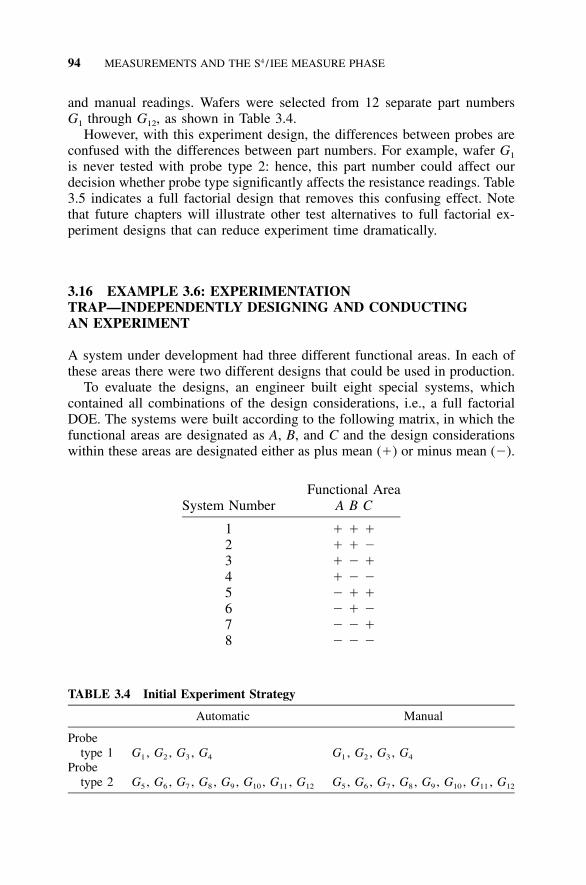
94 MEASUREMENTS AND THE S4 / IEE MEASURE PHASE

TABLE 3.4 Initial Experiment Strategy

Automatic Manual

Probetype 1 G1 , G2 , G3 , G4 G1 , G2 , G3 , G4

Probetype 2 G5 , G6 , G7 , G8 , G9 , G10 , G11 , G12 G5 , G6 , G7 , G8 , G9 , G10 , G11 , G12

and manual readings. Wafers were selected from 12 separate part numbersG1 through G12, as shown in Table 3.4.

However, with this experiment design, the differences between probes areconfused with the differences between part numbers. For example, wafer G1

is never tested with probe type 2: hence, this part number could affect ourdecision whether probe type significantly affects the resistance readings. Table3.5 indicates a full factorial design that removes this confusing effect. Notethat future chapters will illustrate other test alternatives to full factorial ex-periment designs that can reduce experiment time dramatically.

3.16 EXAMPLE 3.6: EXPERIMENTATIONTRAP—INDEPENDENTLY DESIGNING AND CONDUCTINGAN EXPERIMENT

A system under development had three different functional areas. In each ofthese areas there were two different designs that could be used in production.

To evaluate the designs, an engineer built eight special systems, whichcontained all combinations of the design considerations, i.e., a full factorialDOE. The systems were built according to the following matrix, in which thefunctional areas are designated as A, B, and C and the design considerationswithin these areas are designated either as plus mean (�) or minus mean (�).

System NumberFunctional Area

A B C

1 � � �2 � � �3 � � �4 � � �5 � � �6 � � �7 � � �8 � � �

EXAMPLE 3.6: EXPERIMENTATION TRAP—DESIGN AND EXPERIMENT 95

TABLE 3.5 Revised Experiment Strategy

Auto

Probe 1 Probe 2

Manual

Probe 1 Probe 2

G1 —a — — —G2 — — — —

� � � � �� � � � �� � � � �

G11 — — — —G12 — — — —

a A dash indicates the tabular position of a datum point.

The engineer then gave the eight systems to a technician to perform anaccelerated reliability test. The engineer told the technician to note the timewhen each system failed and to call him after all the systems had failed. Theengineer did not tell the technician that there were major differences betweeneach of the test systems. The technician did not note any difference becausethe external appearance of the systems was similar.

After running the systems for one day, the technician accidentally knockedone of the systems off the table. There was no visible damage; however, thesystem now made a different sound when operating. The technician chose notto mention this incident because of the fear that the incident might affect hiswork performance rating. At the end of the test, the technician called theengineer to give the failure times for the eight systems.

During the analysis, the engineer did not note that one of the systems hadan early failure time with an unexpected mode of failure. Because of schedulepressures from management, the engineer’s decision was based only on‘‘quick and dirty’’ statistical analysis of the mean effects of the factors withoutconducting a residual analysis (see Section 23.6). Unknown to the engineer,the analytical results from this experiment led to an erroneous and very costlydecision.

This type of experiment trap can occur in industry in many forms. It isimportant for the person who designs a test to have some involvement in thedetails of the test activity. When breaking down the communication barrierthat exists in this example, the test designer may also find some other un-known characteristic of the design/process that is important. This knowledgealong with some interdepartmental brainstorming can yield a better overallbasic test strategy.

Wisely applied DOE techniques can be very beneficial to improve thebottom line. A DOE does not have to investigate all possible combinationsof the factor levels. This book will later describe how seven two-level factorscan be assessed in only eight trials (see Chapter 29).

96 MEASUREMENTS AND THE S4 / IEE MEASURE PHASE

3.17 SOME SAMPLING CONSIDERATIONS

Readers might find it hard to believe that they could ever fall into one ormore of the preceding example traps. However, within an individual experi-ment these traps can be masked; they may not be readily identifiable to in-dividuals who are not aware of the potential pitfalls.

The reader may conclude from the previous examples that this book willsuggest that all combinations of the parameters or factors need direct exper-imental assessment during test. This is not usually true; experimental designtechniques are suggested that are manageable within the constraints of in-dustry. This objective is achieved by using design matrices that yield muchinformation for each test trial.

Random sampling plans are based on the assumption that errors are in-dependent and normally distributed. In real data this independence assumptionis often invalid, yielding serious inaccuracies. If appropriate, randomizationis introduced as an approximation alternative when conducting an experiment.The adoption of the randomization approach has the advantage that it doesnot require information about the nature of dependence. However, there aresituations where randomization is not appropriate. To illustrate this, considerstock market prices. The magnitude of the closing price on a given day isdependent on its closing price the previous day.

One approach to this data-dependence issue is that of a specific model fordependence. If such a model is valid, it is possible to develop procedures thatare more sensitive than those that depend only on randomization. Box et al.(1978) illustrate with elementary examples that the ability to model depend-ence using time series can lead to problem solutions in the areas of forecast-ing, feedback control, and intervention analysis.

The sampling plans discussed later in this book assume that the process isstable. If the measurements are not from a stable process, the test method-ology and confidence statements can be questionable. Even if an experimentstrategy is good, the lack of stability can result in erroneous conclusions.

3.18 DMAIC MEASURE PHASE

For S4/IEE projects, black belts need to work with their team to determinewhere focus should be given relative to addressing any gap needs of theprocess to internal/external customers and the needs of the business.

Measurements are important. However, often organizations measure whatis convenient, as opposed to what is important to customer and the needs ofthe business. Also, there can be arbitrary goals or policy-dictated measuresthat might make no sense. It is important that S4/IEE projects have measuresand activities that are aligned with these needs.

Within an S4/IEE project, one can address the particulars of measurementsand the details of data collection using the following procedures (Pande et al.2000):

S4 / IEE ASSESSMENT 97

• Select what to measure: Consider the questions that need to be answeredand the data that will help answer these questions. Consider also the finaland internal customers to the process and how the measures will betracked and reported.

• Develop operational definitions: Consider how to clearly describe whatis being measured to ensure that there is no miscommunications.

• Identify data source(s): Consider where someone can obtain data andwhether historical data can be used.

• Prepare collection and sampling plan: Consider who will collect andcompile the data and the tools that are necessary to capture the data.Create a data-sampling plan that addresses any potential data integrityissues.

• Implement and refine measurement: Consider what could be done toassess an initial set of measures and procedures for collecting the databefore expending a lot of resource collecting/compiling questionabledata. To ensure ongoing data integrity, consider what procedures will befollowed to monitor data-collection practices over time.

3.19 S4/IEE ASSESSMENT

It is important that management ask questions encouraging the collection andanalyses of data so that much can be gained from the efforts of employees.If care is not exercised, an experimenter may simply collect data, compile thedata using traditional statistical techniques, and then report the results in aform that leads to firefighting or one-at-a-time fix attempts. For example, thedirection of management might lead an experimenter to collect data and reportthe following with no suggestions on what steps should be taken to improveunfavorable results:

• Confidence interval on the population mean and standard deviation• Hypothesis statement relative to an average criterion• Process capability/performance metric statement relative to a specifica-

tion

When unfavorable results exist, there are many other issues that should beconsidered. These issues can be more important to consider than the simplereporting of the results from randomly collected data. Unfortunately, theseissues can involve how the data are initially collected. Many resources canbe wasted if forethought is not given to the best approach to take whenworking to resolve an unsatisfactory situation.

For example, understanding the source of the variability in measurementsmay be more beneficial. A random effects model or variance componentsanalysis could be used in an experiment design having such considerations.

98 MEASUREMENTS AND THE S4 / IEE MEASURE PHASE

Or perhaps there should be an emphasis on understanding what factors affectthe average response output of an experiment.

Another possibility for inefficient data collection is the proportion of prod-uct that either passes or fails a specification. An experimenter may want tomake a confidence statement about the population of this attribute informa-tion. Another application of an attribute statistic is the comparison of twopopulations (e.g., two machine failure rates). In these cases, it is often easyfor a practitioner to overlook how he/she could have benefited more by con-sidering a change from traditionally reported attribute statistics to a variableassessment, so that more information could be obtained about a process withless effort.

In developing and maintaining processes, emphasis should be given toreducing manufacturing variability, preferably during initial design stages ofthe development effort. If there is less variability in the process, there will befewer defects and fewer problems to fix. Simple experiments in critical pro-cess steps initially can be very beneficial to reducing variability.

Consider the situation in which a product failure rate criterion is to becertified before first customer shipment. Samples that are taken should not beassumed to represent a random sample of future machine builds. Randomsamples can only be presumed to represent the population from which theyare taken. With an early production sample, the production volume may notbe much larger than the sample used in the test. In addition, the lack ofprecision of acceleration test factors that may be used in a test adds to theuncertainty about confidence statements relative to certifying that a failurecriterion is not exceeded.

Instead of taking a random sample of the first production builds, an S4/IEE strategy may be to make the sample represent future builds with config-urations, part tolerances, and/or process tolerances that are typical of what isexpected to be within a customer environment. DOE designs are useful whenimplementing such a test strategy. With this approach, many manufacturingand design factors are structurally changed to assess whether the product willperform satisfactorily within the designed or manufactured space. The inputparameters to a DOE can be set to specification limits and the output responsethen evaluated to determine if it is acceptable. This basic test approach oftenrequires more initial planning and effort but typically leads to a much betterunderstanding of the process and to early improvements, resulting in a smallernumber of future firefights. Overall, this strategy can yield higher quality withreduced costs.

In addition to input differences with this philosophy, other output consid-erations beyond a defect rate can give more statistical power and insight tothe process and design; e.g., the amount of temperature increase a machinecould withstand before failure. In addition, in an established process, surpris-ing conclusions may often result from looking at the data differently. Dataanalysis paralysis should be avoided. For example, a DOE analysis may in-dicate that a factor affects the response; however, this may have no practical

EXERCISES 99

importance if all DOE trial responses are well within specification (seeDCRCA strategy described in Section 30.5). Also, consider how informationis presented to others. Graphical techniques cannot only be very powerful infurnishing additional knowledge, but can also be a form that is useful inpresentations to management.

A high-level view, e.g., daily defect rate, might help us see that most ofour day-to-day problems are common causes. With this knowledge we canthen create an S4/IEE team that leads the effort toward quantifiable results.At a lower-level view, perhaps temperature was identified through DOE to bea key process input variable (KPIV). A control chart could then be used totrack process temperature. When temperature goes out of control, the processshould be shut down for problem resolution immediately before many poor-quality production parts are manufactured.

When choosing an effective test strategy, one needs to gain an appreciationof the fact that when several factors are considered in one experiment, a DOEis a tool that can often help solve problems more quickly than a one-at-a-time approach. When developing a process or product or fixing a problem,and there is an attempt for a quick solution, the ‘‘let’s try this next’’ or one-at-a-time strategy often prevails. This type of test strategy can yield erroneousconclusions and the problems may never really get fixed. Individuals should,in general, consider the more efficient alternative of evaluating several factorssimultaneously using a DOE strategy.

Another S4/IEE consideration may be to assess the design or manufactur-ing safety factor. With this technique, stress factors are changed until failuresoccur. Probability plotting techniques are then used to project failure ratesback to nominal conditions. This technique can be considered either withrandom samples or structurally with fractional factorial experiment designs.True randomization of the current build vintage will be sacrificed when usingDOE concepts with this approach; however, a more desirable output of earlierproblem detection and resolution may be achieved by reconsidering the testobjective. This, in combination with good data analyses, can yield a moreuseful test result.

For a given situation, defining the best problem to solve and convincingothers that this is the best problem to solve can be much more difficult thanthe analytical portion of the problem. It is hoped that the examples discussedin this book can be used as a model for you to help define and convinceothers of the best problem to solve for your specific situation.

3.20 EXERCISES

1. Describe a situation in which you or your organization exhibits variabil-ity.

2. Roll two dice 10 times and create a histogram. Roll two dice 50 timesand create a histogram. Comment on the shape of the distributions.

100 MEASUREMENTS AND THE S4 / IEE MEASURE PHASE

3. Manually calculate the mean, standard deviation, variance, and medianof the following four data sets. Comment on the results.a. 100 100 100 100 100b. 50 75 100 125 150c. 50 100 100 100 150d. 75 75 75 100 175

4. Count the number of times the sixth letter of the alphabet occurs in thefollowing paragraph and compare to others within the S4/IEE workshop.Save the results from the counts of all members of the workshop.

The farmer found that his field of alfalfa had a certain type of fungus onit. The fungus was part of a family of parasitic microbes. The only answerthat the farmer had found to fight the feisty fungus was spraying his fieldswith a toxic chemical that was not certified. It was the only method thatoffered him any hope of success. Unfortunately, when the farmer began tospray his fields, the federal agent from the FDA was in the area. The federalagent’s opinion of the fungus was that it was not at a stage of significantconcern. He offered the farmer a choice: Stop the contamination of the floraof the region or face a fine of substantial amount. The farmer halted thespraying of his alfalfa fields.

5. Manually calculate the mean, median, standard deviation, and varianceof the class results for exercise 4. Show the position of these parameterson a histogram.

6. Describe a television or radio commercial that could be questioned be-cause of the wording in its claim.

7. Describe what affects the magnitude of the level of confidence in theresults given a sample that has continuous data response outputs.

8. Describe the source of measurement variability of a plastic part. Describeother sources of variability if the part were made from a cavity of amulticavity tool in which there are many multicavity tools and manyinjection molding machines.

9. A potential problem exists with machines that are stored within a largewarehouse, where the shipping boxes are stacked high and packed closetogether. Management wants a test conducted on a sample of the productto assess the magnitude of the problem. Describe a major physical prob-lem with implementing the task.

10. Describe a nonmanufacturing application of DOE.

11. Describe how you could personally apply control charting and DOE tech-niques at work or at home.

12. Describe the type of product variability, i.e., common or special cause,which is consistent but at an undesirable high level of 10%.

EXERCISES 101

13. Describe a situation in which a process exhibits a special cause problem.

14. Describe past instances when an existing process exhibited a break-through for process improvement.

15. Describe tools that can help initiate breakthrough change.

16. Even when all brainstorming rules are followed, what is a common ex-ecution problem when preparing and executing a brainstorming session?

17. Over time a process has experienced consistent variability, but a largeramount than desired. Should management be told that the process is outof control? Explain.

18. A new operator did not understand his job within manufacturing. Thefirst day of employment, he made more mistakes than other operatorswho performed a similar task. Describe the type of cause for recent prob-lems within this process.

19. Describe the type of problem existing when a reporter justifies daily theclosing price of the stock market.

20. A company needs to reduce its product development time to be compet-itive. Describe a basic strategy for making process improvements.

21. Explain how the techniques presented in this chapter are useful and canbe applied to S4/IEE projects.

22. List visual inspections which can yield questionable results in organiza-tions.

23. For the data set shown in Exercise 10.17, determine the overall samplemean and standard deviation. Determine also the sample mean and stan-dard deviation for each of the machines (see Example 19.12 for a com-piling of the data by machine). Comment on results.

24. Consider that an airplane’s departure time is classified late if its entrydoor is not closed within 15 minutes of its scheduled departure time.Discuss whether this type of airline data are attribute/discrete orcontinuous/variables data and what might be done differently to betterdescribe departure time of flights relative to customer expectations.

102

4PROCESS FLOWCHARTING/PROCESS MAPPING

S4 /IEE DMAIC Application: Appendix Section A.1, Project ExecutionRoadmap Steps 1.4, 6.1, and 6.2

For quality systems, it is advantageous to represent system structure and re-lationships using flowcharts. A flowchart provides a picture of the steps thatare needed to create a deliverable. The process flowchart document can main-tain consistency of application, identify opportunities for improvement, andidentify key process input variables. It can also be very useful to train newpersonnel and describe activities expediently during audits.

A flowchart provides a complete pictorial sequence of what happens fromstart to finish of a procedure. Applications include procedure documentation,manufacturing processes, work instructions, and product development steps.Flowcharting can minimize the volume of documentation, including ISO 9000documentation.

However, organizations can sometimes spend a very large amount of re-sources in creating flowcharts that are never referenced or used for insightinto process improvement. In lieu of a major process documentation effortwithin an organization, it can be better to create flowcharts after unsatisfactorybaseline measurements of the overall process are identified. The overall mea-surement outputs from a process can give insight to the level of detail andhow the flow charting process should be conducted. In addition, this baselinemeasurement should be used to quantify the monetary benefits of the S4/IEEprojects.

DESCRIPTION 103

Flowcharting of key processes for S4/IEE projects should lead to the es-tablishment and documentation of a standard operating procedure (SOP), ifone does not currently exist, that is used by all. A standard operating pro-cedure that is documented can dramatically reduce variability and cycle time,as well as improve the product quality. In addition, a flowchart can giveinsight to process improvement focus areas and other measurement needs.

An alternative or supplement to a detailed process flowchart is a high-levelprocess map that shows only a few major process steps as activity symbols.For each of these symbols key process input variables (KPIVs) to the activityare listed on one side of the symbol, while key process output variables(KPOVs) to the activity are listed on the other side of the symbol. The KPIVsand KPOVs can then be used as inputs to a cause-and-effects matrix, whichis described in Chapter 13.

As noted earlier, a SIPOC (suppliers, inputs, process, outputs, and custom-ers) is a high-level process map that adds supplier and customer to the IPOdescribed earlier. SIPOC can be useful as a communication tool that helpsteam members view the project the same way and helps management knowwhere the team is focusing its efforts. For each category of SIPOC the teamcreates a list. For example, the input portion of SIPOC would have a list ofinputs to the process. The process portion of SIPOC should be high-level,containing only four to seven high-level steps.

When executing an S4/IEE project in the measure phase, the black beltworks with a team to review and develop process flowcharts. Process workinstructions, standard operating procedures (SOPs), and the process flowchartscan help the team gain insight to where their efforts should focus.

4.1 S4/IEE APPLICATION EXAMPLES: FLOWCHART

S4/IEE application examples of flowcharts are:

• An S4/IEE project was created to improve the 30,000-foot-level metric,for days sales outstanding (DSO). A process flowchart was created todescribe the existing process.

• An S4/IEE project was created to improve the 30,000-foot-level metricfor the diameter of a manufactured part. A process flowchart was createdto describe the existing process.

4.2 DESCRIPTION

Figure 4.1 exemplifies the form of a process flowchart. Frequently used sym-bols to describe the activities associated with a process map are:

104 PROCESS FLOWCHARTING/PROCESS MAPPING

FIGURE 4.1 Process flowchart.

�� Terminal: Symbol that defines start and end of a flowchart.� Activity symbol: Symbol that contains a description of a step of the

process.� Decision symbol: Symbol that contains a question following an activ-

ity symbol (e.g., passes test?). The process branches into two or morepaths. Each path is labeled to correspond to the answer of the question.

� On-page connector: Symbol identifies the connection points in a loopor the continuation in a flow. Tie-in symbols contain the same letter.Off-page connector: Initiating symbol contains a letter or number inthe form ‘‘to page x,’’ while the receiving symbol contains a letter ornumber in the form ‘‘from page y.’’

An arrowhead on the line segments that connect symbols shows directionof flow. The conventional overall flow direction of a flowchart is top to bottomor left to right. Usually the return loop flow is left and up. When a loop feedsinto a box, the arrowhead may terminate at the top of the box, at the side ofthe symbol, or at the line connecting the previous box. The use of on-pageconnectors on a page can simplify a flowchart by reducing the number ofinterconnection lines.

An illustration of a process can proceed down the left side of a page andthen proceed down the right side of a page. A line or on-page connector canconnect the last box of the left column with the first box of the right column.Boxes should be large enough to contain all necessary information to describewho does what. Notes can contain nondirective information.

4.3 DEFINING A PROCESS AND DETERMINING KEY PROCESSINPUT/OUTPUT VARIABLES

First consider and describe the purpose and the process that is to be evaluated.Much time can be wasted trying to formally document every process withinan organization. Reasons to formally document and evaluate a process includethe reduction of cycle time, reduction of defects, improved consistency of

EXAMPLE 4.1: DEFINING A DEVELOPMENT PROCESS 105

operators, reduction of new operator training time, reduction of product var-iability, and reduction of hidden factory reworks. When defining the purpose,consider the bottom-line benefits of the activity. Consider also the potentialimpact of the process that is to be evaluated to the high-level metrics that areimportant to management. Start with processes that have the most impact ondeliverables, and then work downward from there.

Define all steps to create a product or service deliverable. This can be doneseveral different ways. One common approach is conducting a meeting ofthose familiar with a process. The team then describes the sequence of stepson a wall or poster chart using self-stick removable notes. Each process stepis described on one self-stick removable note. With this approach the teamcan easily add and rearrange process steps. After the meeting, one persontypically documents and distributes the results.

I prefer to use another approach when documenting and defining new pro-cesses. When conducting a team meeting to either define or review a process,I prefer to use a computer process flowcharting program in conjunction witha projector that projects the computer image to a screen. This approach cansignificantly reduce time, greatly improve accuracy, and dramatically diminishthe reworking of process description. Computer process charting programsoffer the additional benefit of easy creation and access to subprocesses. Thesesubprocesses can be shown as a process step that is highlighted and accessedby double-clicking with a mouse.

After the process is described, brainstorming sessions can be conducted tolist ideas for improvement. For the process, value-add and no-value-add stepscan be identified along with key process input variables and key processoutput variables. These ideas can then be prioritized and action plans created.

4.4 EXAMPLE 4.1: DEFINING A DEVELOPMENT PROCESS

A computer manufacturer wants to define and improve its functional tests ofa new computer design during development.

Often this type of activity is not viewed as a process because the processoutput crosses product boundaries. When evaluating a new product, the de-velopers tend to determine what should be done to test a new specific com-puter design. They often think that a new product design differs greatly fromthe previous product design and needs special considerations.

The structure of management and of its roles and responsibilities oftendiscourages viewing situations as processes. A new product typically willhave a product manager. His/her responsibility will be to get the productthrough the various phases of development as quickly as possible. The productmanager’s personal rewards will reflect how well he/she conducted this ac-tivity. These personal measurements often do not involve processes at all.When we look at the situation from this point of view, it is not hard to

106 PROCESS FLOWCHARTING/PROCESS MAPPING

understand why he/she might not view the situation as a process. Even if thesituation were seen as a process, the ‘‘what’s in it for me’’ impetus for changewould not be very strong.

The point that someone makes about a new product being different fromthe previous one can be very true; however, often the previous product differsgreatly from its predecessor. Viewing the process at a higher level can changeour point of view. At a very high level, we might consider the process cyclesimply as four steps: design, test, manufacture, and customer use. If we dothis, product-to-product differences could simply be considered as noise tothe process. We could then consider differences between product-to-producttechnology, individuals on development team, and so on, as common causenoise to the process unless something special occurs; e.g., a dramaticallydifferent design or an unusually major change was made to the developmentcycle. This perspective on the basic situation can completely change how weview the metrics of a product and what should be done differently to improve.

The original problem of concern was functional testing of a computer de-sign. The following implementation steps for defining a process, basically aprocess in itself, presume that a nondocumented process previously has beenconducted for earlier vintage products and that the process inputs/outputs tothe process are known.

Using a computer process flow program, create a process flow that givesa high-level view of the functional test process. This process flowchart mightonly list the various test phases as Phase 1, Phase 2, . . . , Phase 6.

Representatives who are familiar with the process are invited to a meeting,usually lasting two hours, during which the creation of the process is facili-tated using a computer process flow program and projection system. Whendefining the process steps, keep the view at a fairly high level. Define sub-process steps that need further expansion off-line with other teams. Documentthe process as it currently exists. Describe entry requirements and deliverablesto the various test phases processes. Create a list of any suggested changesto the process for future reference. The overall process meeting may takemore than one session.

Between meetings, the facilitator cleans up the process flowcharts and dis-tributes them to attendees for their review and comments. Subprocess meet-ings are similarly conducted as needed. Upon completion of all process andsubprocess meetings and reviews, the facilitator compiles the work and putsit into a document.

Process improvement brainstorming sessions can then be conducted. Forthe process, value-add and no-value-add steps can be identified along withkey process input variables and key process output variables. During thesesessions, each step of the process can be reviewed to stimulate either minorprocess improvement or more major process reengineering possibilities. Ameeting can then be conducted to discuss the process change brainstormingissues and prioritize the improvement ideas. Action items and responsibilitiescan then be assigned. Customers and suppliers can then be asked what they

S4 / IEE ASSESSMENT 107

think should be done to improve the process. Monetary implication of changesshould be made whenever possible.

4.5 FOCUSING EFFORTS AFTER PROCESS DOCUMENTATION

Many organizations are now documenting processes. Often an organizationalready has a structured approach leading to the next step after the documen-tation of a process is complete. However, organizations need to have a meth-odology leading them not only to focus areas for process improvement orreengineering but also to the quantification of bottom-line benefits.

An approach that some Six Sigma teams use to focus efforts effectively isto assess all process steps to determine whether the step is value-add or no-value-add to the end result of the process. Within this assignment, steps suchas inspection would be given an assignment of no-value-add. These assign-ments can then indicate where to direct improvement efforts.

Another consideration is a cause-and-effect diagram made immediatelyupon the completion of a process flow diagram. The items within a cause-and-effect diagram of a response variable, problem, goal, or objective are thenaddressed. Each item can be assigned a classification of control or noise. Allstandard operating procedures for the process are then examined to minimizethe impact of the identified causes.

Spagon (1998) suggested the use of activity-based costing (ABC) for pro-cess steps, which offers the added flexibility of combining costs with processsteps within a computer model to prioritize focus areas for improvement op-portunities and to quantify return on investment (ROI) for process changes.

4.6 S4/IEE ASSESSMENT

It might sound like a worthy goal to document all processes within an or-ganization. However, before initiating such a task, assess the amount of effortinvolved to create initially and then maintain the documentation. Consider thelevel of detail to include within the documentation, and also consider theorder in which the various processes will be described. Then honestly assessthe value of the overall effort upon completion relative to employees actuallyreferencing and following the documented processes.

An initial assessment to document all processes may not indicate as muchvalue as expected. This does not mean that time spent documenting currentprocesses and defining improvement opportunities is not beneficial. Largerewards can be expected when the effort is spent wisely. Much value can begained if process definition activities are linked with process metrics. Thisfocus can also lead to the prioritization of process documentation activities.This approach often starts with a high-level view of the processes. Drill-downsfrom this vantage point can be prioritized so that problematic areas are ad-

108 PROCESS FLOWCHARTING/PROCESS MAPPING

dressed first. After processes are developed, put them in a place where theycan be referenced easily. Electronic filing of the information on a readilyavailable medium such as a website can be very beneficial.

Whether the consideration of a process improvement activity originatedfrom an ISO 9000 requirement or from an S4/IEE project, it is important toget buy-in at all levels. Practitioners need to determine the best way to getthe right people involved within a team environment during the process cre-ation. In addition to the definition of process steps, input is needed to keyprocess input variables and key process output variables. If people who areinvolved within the process are a part of the documentation-and-refinementprocess, they will more likely follow that process and the process definitionwill be more precise. This is different from the common practice of creatingin a nonteam environment a process that is later reviewed for input. Thispractice is analogous to the ineffective manufacturing method of testing qual-ity into a product, when the product is the document that was created.

When team meetings are conducted to create processes, it is essential tobe considerate of the time of attendees. As with all meetings, the facilitatorshould be well prepared. This is especially important for the practitioner be-cause he/she wants to build the reputation of having efficient and effectivemeetings. If a good reputation is established, more attendees will attend andhelp during future meetings.

A projector displaying the images from a computer process flowchartingprogram can be very valuable to improve meeting efficiency. Consider havingmeetings of one or two hours’ duration, depending upon the complexity ofthe process. Start and complete the meetings on time. Keep the meeting flow-ing with a focus on the objectives of the meeting. Many organizations havetoo many meetings that are inefficiently conducted. The facilitator should notfall into this trap.

Perhaps the process of preparing and conducting meetings is an area wheremany organizations should focus some of their initial process documentationand improvement activities. If you agree with this thought, consider how youcould sell the idea to others. Consider what metrics are appropriate and dosome informal data collection; e.g., track the number of hours per week thatyou are attending meetings or estimate how much time is wasted in meetingsbecause people arrived late or the presenter was not prepared. Even withlimited data, perhaps you can present this information to your manager in acharting format using monetary terms to get him/her thinking of the impli-cations and possibilities. You might then get the task of working with yourcolleagues to create a process that will be followed preparing and conductingeach meeting. This work initiative by you could be the best thing the companydoes for the year. Think of the benefits to you. You might get some form ofmonetary reward or at least the good feeling that you are not wasting as muchtime in meetings!

EXERCISES 109

4.7 EXERCISES

1. Catapult Exercisea. Executing a process: Teams are handed a tape measure, a golf ball,

and a catapult that has previously been set up. They can use no otherequipment. They are told that each person is to shoot five shots, andthe time between shots is not to exceed 10 seconds. The distancefrom the catapult base to impact is recorded. Operators and inspectorof shot distances are rotated until a total of 100 shots is completed.The range of shot distances is noted and compared to a range spec-ification, e.g., 6 in., determined by the instructor. The data are savedin a time series format for future exercises. Note in the data whowas the operator and inspector for each shot. Compare the range ofshot distances for each catapult to the objective.

b. Process documentation: Teams are to create a flowchart of the cat-apult process, list potential improvement ideas, and then repeat theprevious exercise. They are given the option of using additional ma-terial. For example, a carbon paper and blank paper combination (oraluminum foil) could aid the identification of the projection impactpoint. Or talcum powder could be put onto the ball before the ballis shot, to aid in marking ball impact position. In addition, tape isprovided to hold the catapult and tape measure to the floor. Mea-surements are to be made as precisely as possible, to the nearest 0.1in., for example. Compare the range of shot distances to the previousresults. Save the data in a time series format for future exercises.For each show, record who on your team was the operator and in-spector. Compare the range of these shot distances for each catapultto an objective provided by instructor (e.g., 6 in.). Also comparerange of distances to previous exercise.

2. Catapult Exercise COPQ/CODND: Create histograms for the two setsof data created from shooting the catapult. Determine the center of theprocess and then establish upper and lower specification limits from thecenter using a distance specified by the instructor (e.g., �3 in. frommean projection distance). A part can be reworked if it is outside thespecification but close to the limit (e.g., 1 in.), as specified by instructor.Compute the COPQ/CODND for each set of data given the followingunit costs: inspection costs of $10, defect costs of $20, rework costs of$100, and scrap costs of $200. Estimate annual savings from processchange, considering 10,000 catapult projections are made annually.

3. Catapult Exercise Data Analysis: Consider how an activity-based cost-ing procedure could be used to compare the two processes for shootingand measuring the projection distance. Compare this methodology tothe previously described cost of poor-quality procedure.

110 PROCESS FLOWCHARTING/PROCESS MAPPING

4. Create a process flowchart that describes your early morning activities.Consider the day of the week in the process flowchart. List key processinput variables and key process output variables. Identify steps that addvalue and steps that do not add value. Consider what could be done toimprove the process.

5. Create a process flowchart that describes the preparation and conductingof a regular meeting that you attend. List key process input variablesand key process output variables. Identify steps that add value and stepsthat do not add value. Consider what could be done to improve theprocess.

6. List a process that impacts you personally at school or work. Considerwhat metrics could be created to get focus on how much the processneeds improvement.

7. Describe how you are going to document a process for your S4/IEEproject.

111

5BASIC TOOLS

Among other topics, Chapters 2 and 3 discussed histograms, sample mean,sample standard deviation, attribute/continuous data, and special /commoncause. This chapter continues the discussion of basic techniques and offers acollection of data analysis, data presentation, and improvement alternatives.

In this chapter a wide variety of tools are briefly described for the purposeof aiding with the efficient building of strategies for collecting and compilinginformation that leads to knowledge. With this knowledge we can make betterdecisions.

Descriptive statistics help pull useful information from data, whereas prob-ability provides, among other things, a basis for inferential statistics and sam-pling plans. The mechanics of implementing many of the topics describedwithin this chapter will be utilized throughout this book.

This chapter describes the 7 management tools (7M tools) or 7 manage-ment and planning tools (7 MP tools). The tools described are affinity dia-grams, interrelationship digraphs, tree diagrams, prioritization matrices,matrix diagrams, process decision program charts (PDPC), and activity net-work diagrams.

The chapter also describes what is often called the 7 quality control tools.These tools are cause-and-effect diagram, check sheet, scatter diagram, flow-chart, Pareto chart, histogram, and control chart.

We could divide the tools in this chapter into two categories: working withideas and working with numbers:

• Working with ideas: activity network diagrams, affinity diagram, bench-marking, brainstorming, cause-and-effect diagram, flowchart, force field,

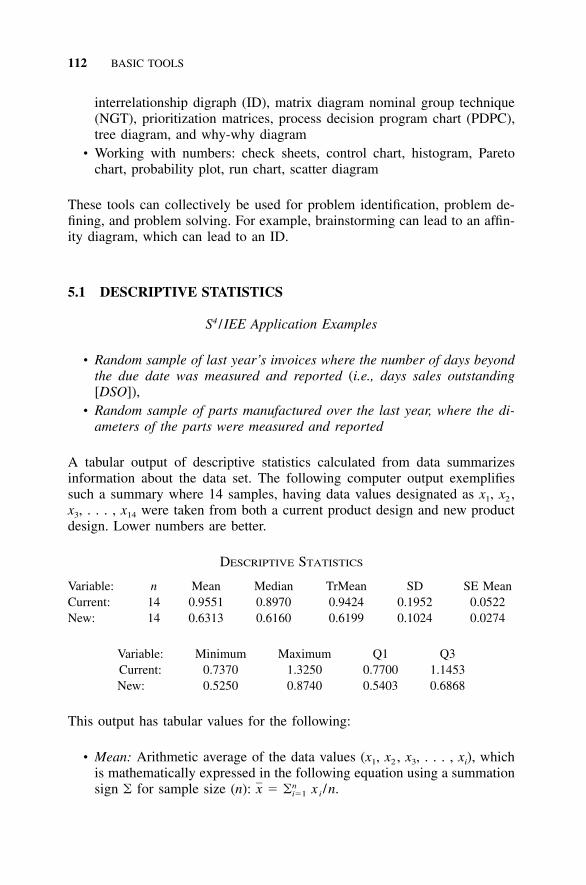
112 BASIC TOOLS

interrelationship digraph (ID), matrix diagram nominal group technique(NGT), prioritization matrices, process decision program chart (PDPC),tree diagram, and why-why diagram

• Working with numbers: check sheets, control chart, histogram, Paretochart, probability plot, run chart, scatter diagram

These tools can collectively be used for problem identification, problem de-fining, and problem solving. For example, brainstorming can lead to an affin-ity diagram, which can lead to an ID.

5.1 DESCRIPTIVE STATISTICS

S4 /IEE Application Examples

• Random sample of last year’s invoices where the number of days beyondthe due date was measured and reported (i.e., days sales outstanding[DSO]),

• Random sample of parts manufactured over the last year, where the di-ameters of the parts were measured and reported

A tabular output of descriptive statistics calculated from data summarizesinformation about the data set. The following computer output exemplifiessuch a summary where 14 samples, having data values designated as x1, x2 ,x3, . . . , x14 were taken from both a current product design and new productdesign. Lower numbers are better.

DESCRIPTIVE STATISTICS

Variable: n Mean Median TrMean SD SE MeanCurrent: 14 0.9551 0.8970 0.9424 0.1952 0.0522New: 14 0.6313 0.6160 0.6199 0.1024 0.0274

Variable: Minimum Maximum Q1 Q3Current: 0.7370 1.3250 0.7700 1.1453New: 0.5250 0.8740 0.5403 0.6868

This output has tabular values for the following:

• Mean: Arithmetic average of the data values (x1, x2 , x3, . . . , xi), whichis mathematically expressed in the following equation using a summationsign � for sample size (n): � � xi /n.nx i�1

RUN CHART (TIME SERIES PLOT) 113

• Median: The data of n observations are ordered from smallest to largest.For an odd sample size, median is the ordered value at (n � 1)/2. Foran even sample size, median is the mean of the two middle orderedvalues.

• TrMean (trimmed mean): Average of the values remaining after both 5%of the largest and smallest values, rounded to the nearest integer areremoved.

• SD: Sample standard deviation of data, which can be mathematicallyexpressed as 2��(x � x) /(n � 1).

• SE mean (standard error of mean): SD/ .�n• Minimum: Lowest number in data set.• Maximum: Largest number in data set.• Q1 and Q3: The data of n observations are ordered from smallest to

largest. The observation at position (n � 1)/4 is the first quartile (Q1).The observation at position 3(n � 1)/4 is the third quartile (Q3).

5.2 RUN CHART (TIME SERIES PLOT)

S4 /IEE DMAIC Application: Appendix Section A.1, Project ExecutionRoadmap Step 3.1

S4 /IEE Application Examples

• One random paid invoice was selected each day from last year’s invoiceswhere the number of days beyond the due date was measured and re-ported (i.e., days sales outstanding [DSO]). The DSO for each samplewas plotted in sequence of occurrence on a run chart.

• One random sample of a manufactured part was selected each day overthe last year, where the diameters of the parts were measured and re-ported. The diameter for each sample was plotted in sequence of occur-rence on a run chart.

A run chart or time series plot permits the study of observed data for trendsor patterns over time, where the x-axis is time and the y-axis is the measuredvariable. A team can use a run chart to compare a performance measurementbefore and after a solution implementation to measure its impact. Generally,20–25 points are needed to establish patterns and baselines.

Often a problem exists with the interpretation of run charts. There is atendency to see all variation as important (i.e., reacting to each point as aspecial cause). Control charts offer simple tests that are to identify special-cause occurrences from common-cause variability through the comparison of

114 BASIC TOOLS

individual datum points and trends to an upper control limit (UCL) and alower control limit (LCL).

5.3 CONTROL CHART

S4 /IEE DMAIC Application: Appendix Section A.1, Project ExecutionRoadmap Steps 3.1 and 9.3

S4 /IEE Application Examples

• One paid invoice was randomly selected each day from last year’s in-voices where the number of days beyond the due date was measured andreported (i.e., days sales outstanding [DSO]). The DSO for each samplewas plotted in sequence of occurrence on a control chart.

• One random sample of a manufactured part was selected each day overthe last year, where the diameters of the parts were measured and re-ported. The diameter for each sample was plotted in sequence of occur-rence on a control chart.

Control charts offer the study of variation and its source. Control charts cangive not only process monitoring and control but also direction for improve-ments. Control charts can separate special from common cause issues of aprocess. This is very important because the resolution approach is very dif-ferent for these two types of situations. Reacting to fix the problem of theday when it is a common cause issue as though it were a special cause addslittle if any value to the long-term performance of the process.

A typical explanation of the value for control charts is that they can giveearly identification of special causes so that there can be timely resolutionbefore many poor-quality parts are produced. This can be a benefit; however,organizations often focus only on the output of a process when applyingcontrol charts. This type of measurement is not really controlling the processand may not offer timely problem identification. To control a process usingcontrol charts, the monitoring should be of key process input variables, andthe process flow is stopped for resolution when this variable goes out ofcontrol (becomes unpredictable; see Section 10.28).

I also like to use control charts when examining a process from a higherviewpoint. In my opinion, this application may offer more value to an orga-nization than using process control charts to truly control processes throughthe observation and reaction to key process input variables data. Deming(1986) states that 94% of the troubles belong to the system (common cause);only 6% are special cause. A control chart might illustrate to managementand others that firefighting activities have been the result of common causeissues. Because most of these issues were not special cause issues, this ex-

CHECK SHEETS 115

pensive approach to issue resolution had no lasting value. An argument canthen be made to track the day-to-day issues using control chart. If the processis shown to be in-control/predictable (see Section 10.28), issues should belooked at collectively over some period of time, and issues occurring mostfrequently resolved first, using overall process improvement techniques.

The construction and interpretation of the many types of control charts,for both attribute and continuous data, are described in Chapter 10. Thischapter illustrates how upper and lower control limits, UCL and LCL, arecalculated for various types of data. These control limits are a function ofdata variability, not specification limits.

5.4 PROBABILITY PLOT

S4 /IEE DMAIC Application: Appendix Section A.1, Project ExecutionRoadmap Steps 3.3 and 7.4

Probability plots are most often associated with tests to assess the validity ofnormality assumptions. When data are a straight line on a normal probabilityplot, the data are presumed to be from a normal distribution, or bell-shapedcurve. Probability plots similarly apply to other distributions, such as theWeibull distribution.

Probability plots can also be used to make percentage of population state-ments. This procedure can be very useful in describing the performance ofbusiness and other processes. Probability plotting techniques are describedlater in this book (see Chapter 8).

5.5 CHECK SHEETS

S4 /IEE DMAIC Application: Appendix Section A.1, Project ExecutionRoadmap Step 7.1

Check sheets contain the systematic recording and compiling of data fromhistorical or current observations. This information can indicate patterns andtrends. After agreement is reached on the definition of events or conditions,data are collected over a period of time and presented in tabular form similarto the following:

Problem

Week

1 2 3 Total

A III IIIII II 10B I II II 5C IIII I I 6

116 BASIC TOOLS

We can create a confirmation check sheet to confirm that the steps in a processhave been completed.

5.6 PARETO CHART

S4 /IEE DMAIC Application: Appendix Section A.1, Project ExecutionRoadmap Steps 3.5 and 7.1

S4 /IEE Application Examples

• Transactional workflow metric (could similarly apply to manufacturing;e.g., inventory or time to complete a manufacturing process): Randomsample of last year’s invoices where the number of days beyond the duedate was measured and reported (i.e., days sales outstanding [DSO]). Ifan invoice was beyond 30 days late, it was considered a failure or de-fective transaction. A Pareto chart showed the frequencies of delinquen-cies by company invoiced.

• Transactional quality metric: Random sample of last year’s invoices,where the invoices were examined to determine if there were any errorswhen filling out the invoice or within any other step of the process.Multiple errors or defects could occur when executing an invoice. Thetotal number of defects when the invoice was executed was divided bythe total number of opportunities for failure to estimate the defect permillion opportunity rate of the process. A Pareto chart showed the fre-quencies of delinquencies by type of failure.

• Manufacturing quality metric: Random sample of printed circuit boardsover the last year, where the boards were tested for failure. The numberof defective boards was divided by the sample size to estimate the defec-tive rate of the process. A Pareto chart showed the frequencies of defec-tive units by printed circuit board type.

• Manufacturing quality metric: Random sample of printed circuit boardsover the last year, where the boards were tested for failure. Multiplefailures could occur on one board. The total number of defects on theboards was divided by the total number of opportunities for failure (sumof the number of components and solder joints from the samples) toestimate the defect per million opportunity rate of the process. A Paretochart showed the frequencies of defects by failure type.

Pareto charts are a tool that can be helpful in identifying the source of chronicproblems/common causes in a manufacturing process. The Pareto principlebasically states that a vital few of the manufacturing process characteristicscause most of the quality problems on the line, while a trivial many of themanufacturing process characteristics cause only a small portion of the qualityproblems.

BRAINSTORMING 117

A procedure to construct a generic Pareto chart is as follows:

1. Define the problem and process characteristics to use in the diagram.2. Define the period of time for the diagram—for example, weekly, daily,

or shift. Quality improvements over time can later be made from theinformation determined within this step.

3. Total the number of times each characteristic occurred.4. Rank the characteristics according to the totals from step 3.5. Plot the number of occurrences of each characteristic in descending

order in a bar graph form along with a cumulative plot of the magni-tudes from the bars. Sometimes, however, Pareto charts do not have acumulative percentage overlay.

6. Trivial columns can be lumped under one column designation; however,care must be exercised not to forget a small but important item.

Note that a Pareto chart may need to consider data from different per-spectives. For example, a Pareto chart of defects by machine may not beinformative while a Pareto chart of defects by manufacturing shifts couldillustrate a problem source. Example 5.1 exemplifies use of a Pareto chart.

5.7 BENCHMARKING

S4 /IEE DMAIC Application: Appendix Section A.1, Project ExecutionRoadmap Step 6.4

With benchmarking we learn from others. Benchmarking involves the searchof an organization for the best practices, adaptation of the practices to itsprocesses, and improving with the focus of becoming the best in class. Bench-marking can involve comparisons of products, processes, methods, and strat-egies. Internal benchmarking makes comparisons between similar operationswithin an organization. Competitive benchmarking makes comparisons withthe best direct competitor. Functional benchmarking makes comparisons ofsimilar process methodologies. Generic benchmarking makes comparisons ofprocesses with exemplary and innovative processes of other companies.Sources of information for benchmarking include the Internet, in-house pub-lished material, professional associations, universities, advertising, and cus-tomer feedback.

5.8 BRAINSTORMING

S4 /IEE DMAIC Application: Appendix Section A.1, Project ExecutionRoadmap Steps 6.5 and 6.6

A brainstorming session is a very valuable means of generating new ideasand involving a group. There are many ways both to conduct a brainstorming

118 BASIC TOOLS

session and to compile the information from the session. The generation ofideas can be generated formally or informally. Flexibility should exist whenchoosing an approach because each team and group seems to take a person-ality of its own. Described next is a formal process, which can be modifiedto suit specific needs.

To begin this process of gathering information by brainstorming, a groupof people is assembled in a room with tables positioned in a manner to en-courage discussion, in the shape of a U, for example. The participants shouldhave different perspectives on the topic to be addressed. The problem orquestion is written down so that everyone can see it. The following basicrules of the exercise are followed by the facilitator and explained to the mem-bers.

1. Ask each member in rotation for one idea. This continues until all ideasare exhausted. It is acceptable for a member to pass a round.

2. Rule out all evaluations or critical judgments.3. Encourage wild ideas. It may be difficult to generate them; hence, wild

ideas should not be discouraged because they encourage other wildideas. They can always be tamed down later.

4. Encourage good-natured laughter and informality.5. Target for quantity, not quality. When there are many ideas, there is

more chance of a good idea surfacing.6. Look for improvements and combinations of ideas. Participants should

feel free to modify or add to the suggestions of others.

For the most effective meeting the leader should consider the followingguidelines:

1. The problem needs to be simply stated.2. Two or more people should document the ideas in plain sight so that

the participants can see the proposed ideas and build on the concepts.3. The name of the participant who suggested the idea should be placed

next to it.4. Ideas typically start slowly and build speed. Change in speed often

occurs after someone proposes an offbeat idea. This change typicallyencourages others to try to surpass it.

5. A single session can produce over 100 ideas, but many will not bepractical.

6. Many innovative ideas can occur after a day or two has passed.

A follow-up session can be used to sort the ideas into categories and rankthem. When ranking ideas, members vote on each idea that they think hasvalue. For some idea considerations it is beneficial to have a discussion of

FORCE FIELD ANALYSIS 119

the pros and cons about the idea before the vote. A circle is drawn aroundthe ideas that receive the most votes. Through sorting and ranking, manyideas can be combined while others are eliminated.

Brainstorming can be a useful tool for a range of questions, from definingthe right question to ask to determining the factors to consider within a DOE.Brainstorming sessions can be used to determine, for example, a more effec-tive general test strategy that considers a blend of reliability testing, SPC, andDOE. The cause-and-effect diagramming tool, as discussed later in this chap-ter, can be used to assemble thoughts from the sessions. I like to facilitatebrainstorming sessions using a computer projector system. This approach canexpedite the recording of ideas and dissemination of information after thesession.

Computers are sometimes now used with specialized software in a networkto aid in administering brainstorming sessions. This tool can be a very effec-tive means to gather honest opinions whenever participants might be hesitantto share their views when management or some influential peers are presentin the room.

5.9 NOMINAL GROUP TECHNIQUE (NGT)

S4 /IEE DMAIC Application: Appendix Section A.1, Project ExecutionRoadmap Step 6.6

Nominal group technique expedites team consensus on relative importance ofproblems, issues, or solutions. A basic procedure for conducting an NGTsession is described below; however, voting procedures can differ dependingupon team preferences and the situation.

An NGT is conducted by displaying a generated list of items, perhaps froma brainstorming session, on a flipchart or board. Eliminating duplications andmaking clarifications then creates a final list. The new final list is made byeliminating duplications and making clarifications. The new final list of state-ments is then prominently displayed, each item is assigned a letter, A, B, . . .Z. On a sheet of paper, each person ranks the statements, assigning the mostimportant a number equal to the number of statements and the least importantthe value of one. Results from the individual sheets are combined to create atotal overall prioritization number for each statement.

5.10 FORCE FIELD ANALYSIS

S4 /DMAIC Application: Appendix Section A.1, Project Execution RoadmapStep 6.6

Force field analysis can be used to analyze what forces in an organization aresupporting and driving toward a solution and which are restraining progress.

120 BASIC TOOLS

FIGURE 5.1 Force field analysis for a successful S4 / IEE implementation.

The technique forces people to think together about the positives and nega-tives of a situation and the various aspects of making a change permanent.

After an issue or problem is identified, a brainstorming session is con-ducted to create a list of driving forces and then a list of restraining forces.A prioritization is then conducted of the driving forces that could be strength-ened. There is then a prioritization of the restraining forces that could bereduced to better achieve the desired result. An example presentation formatfor this information is shown in Figure 5.1, which employs the weight of theline to indicate the importance of a force. Table 5.1 shows example actionplans that could be created for restraining forces identified in a force fieldanalysis.

5.11 CAUSE-AND-EFFECT DIAGRAM

S4 /IEE DMAIC Application: Appendix Section A.1, Project ExecutionRoadmap Step 6.5

S4 /IEE Application Examples

• An S4 /IEE project was created to improve the 30,000-foot-level metricdays sales outstanding (DSO). A process flowchart was created to de-scribe the existing process. A team created a cause-and-effect diagramin a brainstorming session to trigger a list of potential causal inputs andimprovement ideas.

• An S4 /IEE project was created to improve the 30,000-foot-level metric,the diameter of a manufactured part. A process flow chart was createdto describe the existing process. A team created a cause-and-effect dia-gram in a brainstorming session to trigger a list of potential causalinputs and improvement ideas.

CAUSE-AND-EFFECT DIAGRAM 121

TABLE 5.1 Action Items for Restraining Forces for a Successful S4 /IEEImplementation Identified in Force Field Analysis

Restraining Forces Action Items

Programs reinforce the old Create reward and recognitionprograms that reinforce the new

People do not have skills sets neededto succeed

Create training programs so that peoplehave the opportunity to learn newskills

Phrases still refer to the old Introduce new vocabulary so peopleknow you are speaking of the new

Current cultural supports staying thesame

Change culture so that it supports thenew

People concerned about makingmistakes

Reassure them that mistakes arelearning opportunities and failurewill not be punished

People concerned how changes affecttheir job

Provide information that clarifies howperformance will be evaluated

People isolated in the ways they aregoing about the new

Celebrate successes

People wonder how serious thecompany is about this change

Provide consistent communications thatclarify how serious the company isabout completing this change

An effective tool as part of a problem-solving process is the cause-and-effectdiagram, also known as an Ishikawa diagram (after its originator Karoru Ishi-kawa) or fishbone diagram. This technique is useful to trigger ideas and pro-mote a balanced approach in group brainstorming sessions in whichindividuals list the perceived sources (causes) of a problem (effect). The tech-nique can be useful, for example, to determine the factors to consider withina regression analysis or DOE.

A cause-and-effect diagram provides a means for teams to focus on thecreation of a list of process input variables that could affect key process outputvariables. With this strategy, we can address strata issues based on key char-acteristics (e.g., who, what, where, and when). The analysis of this stratifi-cation later through both graphical and analytical techniques can provideneeded insight for pattern detection, which provides an opportunity for fo-cused improvement efforts.

When constructing a cause-and-effect diagram, it is often appropriate toconsider six areas or causes that can contribute to a characteristic responseor effect, materials, machine, method, personnel, measurement, and environ-

122 BASIC TOOLS

Why isn't a standard process forsourcing being followed?

Lack of training

Purchase cards

Face approvals

T&L cards

FIGURE 5.2 Completed cause-and-effect diagram.

ment. Each one of these characteristics is then investigated for subcauses.Subcauses are specific items or difficulties that are identified as a factual orpotential cause to the problem (effect).

There are variations to creating a cause-and-effect diagram. A team maychoose to emphasize the most likely causes by circling them. These causescould, for example, be used as initial factor considerations within a DOE.Besides the identification of experimental factors within the cause-and-effectdiagram, it can also be beneficial to identify noise factors (n) (e.g., ambientroom temperature and a raw material characteristic that cannot be controlled)and factors that can be controlled (c) (e.g., process temperature or speed) byplacing the letter n or c next to the named effect. Figure 5.2 shows anotheroption where focus was given to targeted categories for the effect and animportance and ease-of-resolution matrix was included.

5.12 AFFINITY DIAGRAM

S4 /IEE DMAIC Application: Appendix Section A.1, Project ExecutionRoadmap Step 6.6

Using an affinity diagram a team can organize and summarize the naturalgrouping from a large number of ideas and issues that could have been createdduring a brainstorming session. From this summary, teams can better under-stand the essence of problems and breakthrough solution alternatives.

To create an affinity diagram, boldly record each brainstorming idea indi-vidually on a self-stick removable note, using at a minimum a noun and verbto describe each item. An affinity diagram often addresses 40–60 items butcan assess 100–200 ideas. Next, place the self-stick removable note on a walland ask everyone, without talking, to move the notes to the place where they

INTERRELATIONSHIP DIGRAPH (ID) 123

Infrastructure Align projects with business needs Create system to pull projects from business metrics needsEstablish project accountabilityPlan steering committee meetingsSelect champions, sponsors, and team leadersDetermine strategic projects and metricsCommunication plansIncentive plansSchedule project report outsChampion/sponsor trainingCompile lessons learned from past projects

Project ExecutionProject scopingProject approvalPhase report outsProject closureProject leveraging into

other areas of the business

TrainingChampion trainingBlack belt trainingGreen belt trainingUse training material

that has a good implementation strategy/roadmap

CultureCreate buy-inEvaluate obstacles and

facilitate changeIntegrate Six Sigma into

daily activitiesCreate communication

plans

FIGURE 5.3 Affinity diagram: Essential elements of an S4 / IEE implementationplan.

think the issue best fits. Upon completion of this sorting, create a summaryor header sentence for each grouping. Create subgroups for large groupingsas needed with a subhead description. Connect all finalized headers with theirgroupings by drawing lines around the groupings, as illustrated in Figure 5.3.

5.13 INTERRELATIONSHIP DIGRAPH (ID)

S4 /IEE DMAIC Application: Appendix Section A.1, Project ExecutionRoadmap Step 6.6

An interrelationship digraph, as illustrated in Figure 5.4, permits systematicidentification, analysis, and classification of cause-and-effect relationships, en-abling teams to focus on key drivers or outcomes to determine effective so-lutions.

To create an ID, assemble a team of four to six members who have intimateknowledge of the subject. Arrange the 5–25 items or statements from anothertool (e.g., an affinity diagram) in a circular pattern on a flipchart. Draw re-lationship between the items by choosing any one of the items as a startingpoint, with a stronger cause or influence indicated by the origination of anarrow. Upon the completion of a chart, get additional input from others andthen tally the number of outgoing and input arrows for each item. A highnumber of outgoing arrows indicates that the item is a root cause or driverthat should be addressed initially. A high number of incoming arrows indi-

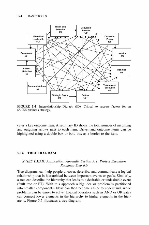
124 BASIC TOOLS

ExecutiveLeadership

11/1

Resources4/2

Project Selection

4/3

Planning1/4

Communications

1/2

Culture1/7

DeliveredResults

1/11

Black Belt Selection

2/5

Strategic Goals 6/2

Training and Execution

4/2

Metrics2/3

Customer Focus

5/1

FIGURE 5.4 Interrelationship Digraph (ID): Critical to success factors for anS4 / IEE business strategy.

cates a key outcome item. A summary ID shows the total number of incomingand outgoing arrows next to each item. Driver and outcome items can behighlighted using a double box or bold box as a border to the item.

5.14 TREE DIAGRAM

S4 /IEE DMAIC Application: Appendix Section A.1, Project ExecutionRoadmap Step 6.6

Tree diagrams can help people uncover, describe, and communicate a logicalrelationship that is hierarchical between important events or goals. Similarly,a tree can describe the hierarchy that leads to a desirable or undesirable event(fault tree or FT). With this approach a big idea or problem is partitionedinto smaller components. Ideas can then become easier to understand, whileproblems can be easier to solve. Logical operators such as AND or OR gatescan connect lower elements in the hierarchy to higher elements in the hier-archy. Figure 5.5 illustrates a tree diagram.

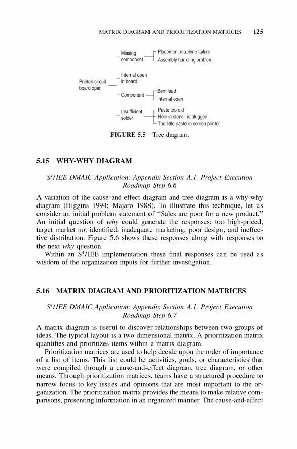
MATRIX DIAGRAM AND PRIORITIZATION MATRICES 125

Printed circuitboard open

Insufficientsolder

Component

Internal openin board

Missingcomponent

Too little paste in screen printerHole in stencil is pluggedPaste too old

Bent lead

Internal open

Placement machine failure

Assembly handling problem

FIGURE 5.5 Tree diagram.

5.15 WHY-WHY DIAGRAM

S4 /IEE DMAIC Application: Appendix Section A.1, Project ExecutionRoadmap Step 6.6

A variation of the cause-and-effect diagram and tree diagram is a why-whydiagram (Higgins 1994; Majaro 1988). To illustrate this technique, let usconsider an initial problem statement of ‘‘Sales are poor for a new product.’’An initial question of why could generate the responses: too high-priced,target market not identified, inadequate marketing, poor design, and ineffec-tive distribution. Figure 5.6 shows these responses along with responses tothe next why question.

Within an S4/IEE implementation these final responses can be used aswisdom of the organization inputs for further investigation.

5.16 MATRIX DIAGRAM AND PRIORITIZATION MATRICES

S4 /IEE DMAIC Application: Appendix Section A.1, Project ExecutionRoadmap Step 6.7

A matrix diagram is useful to discover relationships between two groups ofideas. The typical layout is a two-dimensional matrix. A prioritization matrixquantifies and prioritizes items within a matrix diagram.

Prioritization matrices are used to help decide upon the order of importanceof a list of items. This list could be activities, goals, or characteristics thatwere compiled through a cause-and-effect diagram, tree diagram, or othermeans. Through prioritization matrices, teams have a structured procedure tonarrow focus to key issues and opinions that are most important to the or-ganization. The prioritization matrix provides the means to make relative com-parisons, presenting information in an organized manner. The cause-and-effect

126 BASIC TOOLS

Sales are poorfor a new product

Too high priced

No interest inproduct

Inadequate promotion

Poor product acceptance

Ineffective distribution

Manufacturing costs are too

high

Economy is poor

Distribut ion costs are too

high

Target market not identified

Target marketchanged

Insufficient advertising

dollars

Too small sales force

No buy-in bymarketing

department

Poor quality

Too long oflead time for

orders

Usability problems

Ineffective distribution channels

Manufacturing problems

FIGURE 5.6 Why-why diagram, modified from Higgins (1995).

PROCESS DECISION PROGRAM CHART (PDPC) 127

matrix and quality function deployment (QFD) are two examples of the ap-plication of prioritization matrices or relational matrices (see Chapter 13).

Within a prioritization matrix we can assign relative importance weightsresponses. Sometimes these weights are simply assigned by the organizationor team. However, there are several techniques for more objectively estab-lishing these prioritization criteria. The analytical hierarchy process (AHP) isone of these techniques (Canada and Sullivan 1989). Within the AHP ap-proach, a number of decision-makers can integrate their priorities into a singlepriority matrix using a pairwise fashion. This result of this matrix is a prior-itization of the factors.

Figure 5.7 shows the result of a paired comparison of all characteristicsthat are being considered within the selection of black belts. Within this AHP,for example, the cell response of B2 when comparing factor ‘‘A: Fire in thebelly’’ with factor ‘‘B: Soft skills’’ would indicate that the team thought factorB was more important than factor A at a medium level. After completing thematrix, the team sums values for all factors and then normalizes these valuesto a scale, for example, 100.

This procedure could be used to quantify the importance category used inthe creation of a cause-and-effect matrix (see Table 13.4).

5.17 PROCESS DECISION PROGRAM CHART (PDPC)

S4 /IEE DMAIC Application: Appendix Section A.1, Project ExecutionRoadmap Step 1.2

A process decision program chart (PDPC) helps with the organization andevaluation of processes and the creation of contingency plans. PDPC can helpthe evaluation of process implementation at a high level early in the planningstage. PDPC can help anticipate deviations from expected events and provideinsight to the creation of effective contingency plans.

PDPC can help determine the impact of problems or failures on projectschedules. From this, specific actions can be undertaken for problem preven-tion or mitigation of impact when they do occur. Subjective probabilities ofoccurrence can be assigned to each probability. These probabilities can thenbe used for the assignment of priorities.

One form for a PDPC resembles an annotated tree diagram, while anotherresembles an annotated flowchart. Figure 5.8 shows a simplified supply chainPDPC, which provides a basic look at the process with several deviationsindicated. A plan should be created to address contingency issues.

Berger et al. (2002) highlight the following steps, which are common toall PDPC formats:

• Identify the process purpose.• Identify the basic activities and related events associated with the process.• Annotate the basic activities and related events.

128

Des

crip

tion

Sco

reP

erce

ntB

: S

oft s

kills

C: P

roje

ct m

anag

emen

tD

: Ana

lytic

ski

llsE

: S

tatis

tical

kno

wle

dge

B:

Sof

t ski

lls8

38A

: F

ire

in th

e be

llyB

2A

2A

2A

3A

: F

ire

in th

e be

lly7

33B

: S

oft s

kills

B1

B2

B3

C: P

roje

ct m

anag

emen

t4

19C

: Pro

ject

man

agem

ent

C1

C3

D: A

naly

tic s

kills

210

D: A

naly

tic s

kills

D2

E:

Sta

tistic

al k

now

ledg

e0

01

Low

2M

ediu

m3

Hi g

h

FIG

UR

E5.

7A

naly

tical

hier

arch

ypr

oces

s(A

HP)

for

cate

gori

esw

ithin

prio

ritiz

atio

nm

atri

x:bl

ack

belt

sele

ctio

npr

o-ce

ss.

ACTIVITY NETWORK DIAGRAM OR ARROW DIAGRAM 129

SupplierReceiving & inspection

Warehouse Assembly Customer

Build line orderInventory update

Damaged?

Order correct?

Rework? Defects?

Built on time?

Part shortage?

Late delivery?

Unsatisfactory quality?

FIGURE 5.8 Process decision program chart (PDPC) for a simplified supply chain(PDPC in annotated process flowchart format).

1

4

2 6

3 5 7 80 1

4

2 6

3 5 7 80

FIGURE 5.9 Arrow diagram.

• Superimpose the possible (conceivable) deviations.• Annotate the possible deviations.• Identify and annotate contingency activities.• Weight the possible contingencies.

5.18 ACTIVITY NETWORK DIAGRAM OR ARROW DIAGRAM

S4 /IEE DMAIC Application: Appendix Section A.1, Project ExecutionRoadmap Step 2.4

Activity network diagrams, sometimes called arrow diagrams, help with thedefinition, organization, and management of activities with respect to time.The arrow diagram is used in program evaluation and review technique(PERT) and critical path method (CPM) methodologies, which is discussedmore in Chapter 52.

Figure 5.9 shows an arrow diagram. Activities are displayed as arrows,while nodes represent the start and finish of activities.

130 BASIC TOOLS

5.19 SCATTER DIAGRAM (PLOT OF TWO VARIABLES)

S4 /IEE DMAIC Application: Appendix Section A.1, Project ExecutionRoadmap Step 7.1

S4 /IEE Application Examples

• An S4 /IEE project was created to improve the 30,000-foot-level metricdays sales outstanding (DSO). A process flowchart was created to de-scribe the existing process. A team created a cause-and-effect diagramin a brainstorming session to trigger a list of potential causal inputs andimprovement ideas. One input that the team thought could be an impor-tant cause was the size of the invoice. A scatter diagram of DSO versussize of invoice was created.

• An S4 /IEE project was created to improve the 30,000-foot-level metric,the diameter of a manufactured part. A process flowchart was created todescribe the existing process. A team created a cause-and-effect diagramin a brainstorming session to trigger a list of potential causal inputs andimprovement ideas. One input that the team thought could be an impor-tant cause was the temperature of the manufacturing process. A scatterdiagram of part diameter versus process temperature was created.

A scatter diagram, or plot to assess the relationship between two variables,offers a follow-up procedure to assess the validity of a consensus relationshipfrom a cause-and-effect diagram. When creating a scatter diagram, 50 to 100pairs of samples should be plotted so that the independent variable is on thex-axis while the dependent variable is on the y-axis.

A scatter diagram relationship does not predict a true cause-and-effect re-lationship. The plot only shows the strength of the relationship between twovariables, which may be linear, quadratic, or some other mathematical rela-tionship. The correlation and regression techniques described in a later chaptercan be used to test the statistical significance of relationships (see Chapter23).

5.20 EXAMPLE 5.1: IMPROVING A PROCESS THATHAS DEFECTS

Note: Example 43.10 discusses alternative tracking metrics and improvementstrategies for the described situation.

As noted earlier, process control charts are useful to monitor the processstability and identify the point at which special-cause situations occur. Aprocess is generally considered to be in control/predictable whenever it issampled periodically and the measurements from the samples are within theupper control limit (UCL) and lower control limit (LCL), which are positioned

EXAMPLE 5.1: IMPROVING A PROCESS THAT HAS DEFECTS 131

around a centerline (CL). Note that these control limits are independent ofany specification limits.

Consider that the final test of a printed circuit-board assembly in a man-ufacturing facility yielded the fraction nonconforming control chart shown inFigure 5.10. This chart, which describes the output of this process, could alsobe presented in percent nonconforming units. A run chart without controllimits could cause the organization to react to the individual ups and downof the chart as special cause.

In addition, organizations can react to limited data and draw erroneousconclusions. Consider what conclusion an organization might arrive at aftercollecting only the first four points on the chart if the x-axis and y-axis datawere considered continuous. Someone might create a scatter diagram con-cluding that the downward trend was significant with this limited data. How-ever, a regression analysis would indicate that there was not enoughinformation to reject the null hypothesis that the slope was zero (see Chapters16 and 23).

In the process control chart it is noted that sample number 1 had a defectrate approximately equal to 0.18, while the overall average defect rate was0.244. This process is in control/predictable; i.e., no special causes are noted.However, the defect rate needs to be reduced so that there will be less reworkand scrap (i.e., reduce the magnitude of common causes). A team was thenformed. The team noted the following types of production defects for the3200 manufactured printed circuit boards (Messina 1987):

440 Insufficient solder120 Blowholes

80 Unwetted64 Unsoldered56 Pinholes40 Shorts

800

From the Pareto chart of the solder defects shown in Figure 5.11, itbecomes obvious that focus should first be given to the insufficient soldercharacteristic. A brainstorming session with experts in the field (engineers,technicians, manufacturing workers, chemists, management, etc.) could thenbe conducted to create a cause-and-effect diagram for the purpose of identi-fying the most likely sources of the defects. Regression analysis (see Chapter23) followed by a DOE might then be most appropriate to determine whichof the factors has the most impact on the defect rate. This group of technicalindividuals can perhaps also determine a continuous data response to use inaddition to or in lieu of the preceding attribute response consideration. Onecan expect that a continuous data response output would require a muchsmaller sample size.

132 BASIC TOOLS

FIGURE 5.10 Initial control chart.

FIGURE 5.11 Pareto chart of solder defects.

EXAMPLE 5.2: REDUCING THE TOTAL CYCLE TIME OF A PROCESS 133

After changes are made to the process and improvements are demonstratedon the control charts, a new Pareto chart can then be created. Perhaps theimprovements will be large enough to the insufficient solder characteristicthat blowholes may now be the largest of the vital few to be attacked next.Process control charts could also be used to track insufficient solder individ-ually so that process degradation from the fix level can be identified quickly.

Changes should then be made to the manufacturing process after a confir-mation experiment verifies the changes suggested by the experiments. Thedata pattern of the control chart should now shift downward in time to anotherregion of stability. As part of a continuing process improvement program, thepreceding steps can be repeated to identify other areas to improve.

One final note for this example: I have seen people try to establish a timeseries trend line where there was limited data (e.g., three to four points).Consider what one would project for a failure rate if a line were drawnthrough the first four points in Figure 5.10. In Chapter 23 we will discussregression techniques where we can test the hypothesis that the slope of theline equals zero.

5.21 EXAMPLE 5.2: REDUCING THE TOTAL CYCLE TIMEOF A PROCESS

Sometimes individuals are great at fixing the small problems but miss the bigpicture. This example addresses a big-picture issue.

Consider the development cycle time of a complex product that needsshortening so that the needs of the customer can be met more expediently.The total development process is described in Figure 5.12.

The total development cycle time of a product can be two to three years.Because absolute numbers were not available from previous development cy-cles, brainstorming sessions were conducted to identify possible sources ofimprovement. Several sessions were conducted to identify processes thatcould be targeted for improvement. Consider that after all the group sessionswere completed, the total list was presented to each group for quantificationin the form of a survey. Such a survey might ask for the amount of perceivedimprovement for each of the items, resulting in a Pareto chart.

Management might be surprised to learn that an item such as the procure-ment of standard equipment and components was the biggest deterrent to ashortened development cycle time. Management might have expected to hearsomething more complex, such as availability of new technology.

A team was then formed for the purpose of improving the procurementcycle. The team, as shown in Figure 5.13, defined the current procurementprocess.

To understand the existing process better, the team considered a samplesituation: an employee in her office needs a new piece of computer equipmentcosting $1000. There should be much improvement in work efficiency after

134 BASIC TOOLS

FIGURE 5.12 Current process.

the equipment item is installed. An overhead rate of $100/hr exists (i.e., itcosts the company $100 for the employee’s salary, benefits, space allotment,etc.), and an improvement in efficiency of 1⁄8 is expected when the equipmentis available for use (i.e., 5 hr for every 40-hr week). The estimated cost toprocure the item is noted in the following breakdown. Because the cost isover $500, the approval process is lengthy. The itemized costs include lostefficiency because of the time it takes to receive the item; e.g., consider thatthe company might not have to spend so much money subcontracting outwork if the employee could get more done in less time.

Because of this process, time expenditures and lost revenue increased thepurchase price by a factor larger than 20; i.e., $22,100 compared to $1000(see Table 5.2). This process flow encourages the purchase of antiquatedequipment. To illustrate this point, consider that during the 36 weeks of jus-tification and the creation of a new budget a new more expensive piece ofequipment is marketed. This equipment offers the opportunity of having muchmore productivity, which would be cost effective. But if the purchase of thisequipment required additional delays, the employee would probably opt topurchase the obsolete piece of equipment in lieu of going through anotherjustification and budget cycle. This action could cause a decrease in productquality and/or an increase in product development time.

In addition, the team noted that with this process it becomes only naturalto play games. A department may often justify equipment with the anticipa-

EXAMPLE 5.2: REDUCING THE TOTAL CYCLE TIME OF A PROCESS 135

FIGURE 5.13 The procurement process.

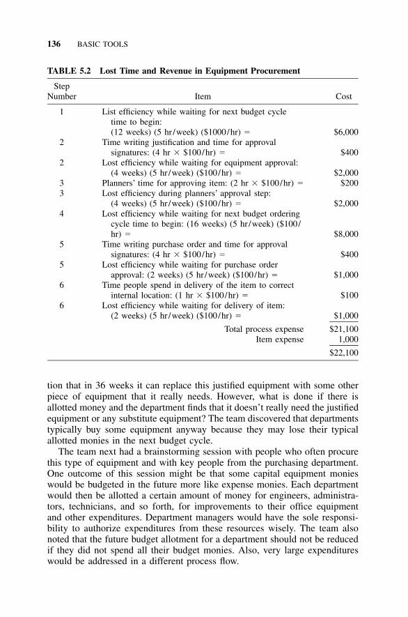
136 BASIC TOOLS

TABLE 5.2 Lost Time and Revenue in Equipment Procurement

StepNumber Item Cost

1 List efficiency while waiting for next budget cycletime to begin:(12 weeks) (5 hr /week) ($1000/hr) � $6,000

2 Time writing justification and time for approvalsignatures: (4 hr � $100/hr) � $400

2 Lost efficiency while waiting for equipment approval:(4 weeks) (5 hr /week) ($100/hr) � $2,000

3 Planners’ time for approving item: (2 hr � $100/hr) � $2003 Lost efficiency during planners’ approval step:

(4 weeks) (5 hr /week) ($100/hr) � $2,0004 Lost efficiency while waiting for next budget ordering

cycle time to begin: (16 weeks) (5 hr /week) ($100/hr) � $8,000

5 Time writing purchase order and time for approvalsignatures: (4 hr � $100/hr) � $400

5 Lost efficiency while waiting for purchase orderapproval: (2 weeks) (5 hr /week) ($100/hr) � $1,000

6 Time people spend in delivery of the item to correctinternal location: (1 hr � $100/hr) � $100

6 Lost efficiency while waiting for delivery of item:(2 weeks) (5 hr /week) ($100/hr) � $1,000

Total process expense $21,100Item expense 1,000

$22,100

tion that in 36 weeks it can replace this justified equipment with some otherpiece of equipment that it really needs. However, what is done if there isallotted money and the department finds that it doesn’t really need the justifiedequipment or any substitute equipment? The team discovered that departmentstypically buy some equipment anyway because they may lose their typicalallotted monies in the next budget cycle.

The team next had a brainstorming session with people who often procurethis type of equipment and with key people from the purchasing department.One outcome of this session might be that some capital equipment monieswould be budgeted in the future more like expense monies. Each departmentwould then be allotted a certain amount of money for engineers, administra-tors, technicians, and so forth, for improvements to their office equipmentand other expenditures. Department managers would have the sole responsi-bility to authorize expenditures from these resources wisely. The team alsonoted that the future budget allotment for a department should not be reducedif they did not spend all their budget monies. Also, very large expenditureswould be addressed in a different process flow.

EXAMPLE 5.3: IMPROVING A SERVICE PROCESS 137

5.22 EXAMPLE 5.3: IMPROVING A SERVICE PROCESS

Consider an S4/IEE project was to reduce cycle time problems in a claimprocessing center, accounts payable organization, or typing center. Measure-ment data may not be recorded at all within the organization. If there isdocumentation, periodic reporting may only be a set of numbers from one ortwo periods of time.

A first step for a black belt would be to work with management and ateam from the area to determine a set of measurements that reflects the needsof customers and the business. The team might agree to a daily or weeklyreporting time period. Example metrics determined by the team for these timeperiods might include the number of forms processed, the average number offorms processed per individual, the rejection rate of forms from the finalcustomer, the rejection rate of forms that are found unsatisfactory beforedelivery of the document, and the time from initial request to final deliveryto complete a form. Some of these rejection rates could be converted to aDPMO rate, e.g., by considering an estimation of the number of opportunities,perhaps keystroke entries into a form. Monetary implications should be esti-mated for these measurements whenever possible. These measurements couldbe tracked over time in a control chart format.

The black belt could then work with the team to describe the process, asexemplified in Figure 5.14. The team could then create a cause-and-effectdiagram to aid in the identification of process improvement opportunities.During this session, team members most familiar with the process were askedto quantify the benefit of how they thought the proposed process changewould benefit efficiency. Figure 5.15 is a Pareto chart that illustrates the rel-ative magnitude of these items. Note that tasks 1, 2, and 3 in the Pareto chartaffected other areas of the business; hence, they were not included in theprevious process flowchart.

The implication of the issue of purchasing two additional printers, forexample, needs to be addressed next because this is perceived as the mostimportant change to make. To address this issue, it was noted that if twoprinters were purchased, each operator could have a dedicated printer, whichwas thought to be much more efficient than the current queuing of jobs onthe shared printers. The operators spent a lot of time walking to the printersand sorting through printer outputs to find their jobs. The cost for two printerswould be

Cost for two printers � (2 printers)($2000/printer) � $4000

Given 40% efficiency and the additional factors of a 160-hr work monthfor five employees at a company burden rate of $100/hr, the estimated annualcost savings after purchasing the equipment would be

138 BASIC TOOLS

Coordinator notifiescustomer of

job completion

Workcoordinator

checksjob

Operatorchecks

job

Operator waits for job tocomplete printing

Operatorprints

outputs

Operator does job

Originator fills out job track form

~~

Not OK

Not OK

OK

OK

FIGURE 5.14 Current process in the service center.

0.40(160 hr/month)(12 month/yr)($100/hr)(5 people) � $384,000

The percentile estimates made by the operators could have considerableerror and yet the purchase of these printers would still be cost effective. It isalso expected that there will be fewer operator errors after the purchase ofthe printers because the removal of job queuing and sorting of printer outputswill eliminate one major source of frustration in the center. A similar analysismight also be done of the lesser ‘‘leverage’’ items that were mentioned in thebrainstorming session.

After the purchase of the equipment, we would expect that a control chartof our metrics would indicate a statistically significant improvement in per-formance of the process. After this change is implemented, we could betterquantify from these metrics the true cost savings to the process from thechanges.

EXERCISES 139

FIGURE 5.15 Pareto chart of opportunities for improvement.

5.23 EXERCISES

1. Catapult Exercise: Using the catapult exercise data sets from Chapter 4,create or determine the following for each set of data: run chart, histo-gram, mean, standard deviations, median, quartile 1, and quartile 3.

2. Catapult Exercise: Create a cause-and-effect diagram of factors that affectthrow distance. Label the factors as noise, controllable, or experimental.Select an experimental factor from the control chart (e.g., arm length).Make adjustments to this factor and monitor the projection distance. Col-lect 20 data points. Consider how the experiment will be executed (e.g.,randomized or not). Create a scatter diagram. Save the data for a futureexercise.

3. M&M’s Candy Exercise: Open a bag of M&M’s, count the number ofeach color, and present information in a Pareto chart. Save the data fora future analysis.

4. Determine the mean, standard deviation, variance, median, and numberof degrees of freedom for the following sampled sequential data:

9.46, 10.61, 8.07, 12.21, 9.02, 8.99, 10.03, 11.73, 10.99, 10.56

5. Create a run chart of data in the previous exercise.

140 BASIC TOOLS

6. Create a scatter diagram of the following data. Describe the results.

Temp. Strength Temp. Strength Temp. Strength

140.6 7.38 140.5 6.95 142.1 3.67140.9 6.65 139.7 8.58 141.1 6.58141.0 6.43 140.6 7.17 140.6 7.42140.8 6.85 140.1 8.55 140.5 7.53141.6 5.08 141.1 6.23 141.2 6.28142.0 3.80 140.9 6.27 142.2 3.46141.6 4.93 140.6 7.54 140.0 8.67140.6 7.12 140.2 8.27 141.7 4.42141.6 4.74 139.9 8.85 141.5 4.25140.2 8.70 140.2 7.43 140.7 7.06

7. Explain how the techniques presented in this chapter are useful and canbe applied to S4/IEE projects.

8. Estimate the proportion defective rate for the first four points in Figure5.10. Using only these four points, project what the failure rate would bein 10 days. Comment on your results.

9. Create a force field analysis for the implementation of S4/IEE within theorganization identified in Exercise 1.1.

10. Describe how and show where the tools described in this chapter fit intothe overall S4/IEE roadmap described in Figure A.1 in the Appendix.

141

6PROBABILITY

Processes are created to deliver product, either meeting or exceeding the ex-pectations of their customers. However, the output of many processes is sub-ject to the effects of chance. Because of this, companies need to considerchance, or probability, when they make assessments of how well they fulfillcustomer expectations. This chapter gives a very brief description of somebasic probability concepts and the applicability to techniques described withinthis book.

6.1 DESCRIPTION

Data can originate as samples of measurements from production samples (e.g.,closing force for car doors) or a business process (e.g., invoice paymenttimes). Measurements can also result from experimental evaluation (e.g., howan increase in the temperature of the process affects the yield of the process).In all these cases if the experiment were repeated, we should get a comparablevalue to an initial response; however, we probably would not get exactly thesame response. Because of this, we need to assess occurrence probabilitieswhen making decisions from data (e.g., should we increase the temperatureof the process to improve yield?).

When conducting an experiment or making an evaluation in which resultswill not be essentially the same even though conditions may be nearly iden-tical, the experiment is called a random experiment. Random events can beassociated with flip of a coin and the roll of a die. In these cases the proba-bility of an event is known, assuming the coin and die are fair. In the case

142 PROBABILITY

of a flip of the coin there is one chance in two that the flip will result inheads (probability � 1/2 � 0.5). Similarly, with a six-sided die there is onechance in six that a two will occur on a single roll of the die (probability �1/6 � 0.167).

In manufacturing we might similarly have a nonconformance rate of 1 ina 100. Hence, any given customer would have a 1/100 (or 0.01) probabilityof obtaining a product that is nonconforming. The difference between the rollof a die and this scenario is that for the manufacturing situation we typicallydo not know the probability of the underlying population from which we aresampling. This uncertainty relative to sampling needs consideration when wemake decisions about process characterization and improvements.

These situations could also be described using a percent of populationstatement rather than the probability of occurrence of a single event. In thecase of the flip of the coin, we could state that 50% of the time a flip of thecoin would be heads. Similarly, we could state that 16.67% of the time a twowould occur with the roll of the die. In the case of the roll of the die, wecould expand our population percentage statement to a region of values. Forexample, 33.3% of the time a two or less will occur with the roll of the die;i.e., 16.67% for a roll of 1 plus 16.67% for a roll of 2.

If P(A) represents the probability of A occurring, P(A�) � 1 � P(A) rep-resents the probability of A not occurring; i.e., the complementation rule. Inthe above example the probability was 0.33 of rolling a two or less; hence,the probability of not rolling a two or less is 0.67 (which is the same as theprobability of rolling a 3, 4, 5, or 6).

Sample space is a set that consists of all possible outcomes of a randomexperiment. A sample space that is countable is said to be discrete samplespace (e.g., roll of die), while one which is not countable is to be a continuoussample space (e.g., viscosity of incoming raw material to a production pro-cess).

6.2 MULTIPLE EVENTS

If A and B are events, the following describes possible outcomes:

• Union (A � B) is the event ‘‘either A or B or both.’’• Intersection (A � B) is the event ‘‘both A and B.’’• Negation or opposite of A (A�) is the event ‘‘not A.’’• Difference A � B is the event ‘‘A but not B.’’

Consider the situation in which, for two flips of a coin, A is the event at leastone head (H) occurs and B the event the second toss results in a tail (T).These events can be described as the sets

MULTIPLE-EVENT RELATIONSHIPS 143

A � {HT, TH, HH}

B � {HT, TT}

For this situation we note the space describing possible outcomes as

(A � B) � {HT, TH, HH, TT}

Other events within this space are described as

(A � B) � {HT}

A� � {TT}

A � B � {TH, HH}

6.3 MULTIPLE-EVENT RELATIONSHIPS

If A and B are two events that cannot occur simultaneously, the events aremutually exclusive or disjoint events. For this situation the probability thatevent A or event B will occur is

P(A � B) � P(A) � P(B)

If A and B are two events that can occur simultaneously, then the proba-bility that event A or event B will occur is

P(A � B) � P(A) � P(B) � P(A � B)

To illustrate the application of this equation, consider that a process has twosteps, where the probability of failure for the first step is 0.1 and the proba-bility of failure at the second step is 0.05. The probability of failure fromeither step within the process is

P(A � B) � P(A) � P(B) � P(A � B) � 0.1 � 0.05 � (0.1)(0.05) � 0.145

If the occurrence of A influences the probability that event B will occur,then the probability that event A and event B will occur simultaneously is thefollowing: P(B�A) is the probability of B given that A has occurred (i.e.,general multiplication rule):

P(A � B) � P(A) � P(B�A)

To illustrate the application of this equation, consider that the probability ofdrawing two aces from a deck of cards is

144 PROBABILITY

P(A � B) � P(A) � P(B�A) � (4/52)(3/51) � 0.0045

If A and B are two statistically independent events (i.e., there is indepen-dence between the events), then the probability that events A and B will occursimultaneously is

P(A � B) � P(A) � P(B)

To illustrate the application of this equation, consider again the above processthat had steps, in which the probability of failure for the first step is 0 (i.e.,yield is 0.9) and the probability of failure at the second step is 0.05 (i.e.,yield is 0.95). The overall yield of the process is

P(A � B) � P(A) � P(B) � (1 � 0.1)(1 � 0.05) � 0.855

Note that this answer is consistent with the earlier calculation; i.e., 0.855 �1 � 0.145.

6.4 BAYES’ THEOREM

When there are two possible events A and B, the probability of Z occurringcan be described by the theorem of total probability, which takes the form

P(Z) � [P(A) � P(Z �A)] � [P(B) � P(Z �B)]

A relationship that is often very useful is Bayes’ theorem (the formal defi-nition for conditional probability), which takes the form

P(A � Z)P(A�Z) �

P(Z)

To address the application of this theorem, consider the following. A pro-duction process has a product nonconformance rate of 0.5%. There is a func-tional test for nonconformance. A failed test response is supposed to indicatethat a defect exists; however, the test is not perfect. For a product that has adefect, the test misses the defect 2% of the time (i.e., it reports a false productconformance). For machines without the defect, the test incorrectly indicates3% of the time that they have the defect (i.e., it reports a false product non-conformance).

The probability that a sampled machine picked at random will test satis-factorily equates to the summation of the appropriate legs of the tree diagramshown in Figure 6.1, which is

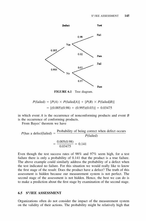
S4 / IEE ASSESSMENT 145

FIGURE 6.1 Tree diagram.

P(failed) � [P(A) � P(failed�A)] � [P(B) � P(failed�B)]

� [(0.005)(0.98) � (0.995)(0.03)] � 0.03475

in which event A is the occurrence of nonconforming products and event Bis the occurrence of conforming products.

From Bayes’ theorem we have

Probability of being correct when defect occursP(has a defect�failed) �

P(failed)

0.005(0.98)� � 0.141

0.03475

Even though the test success rates of 98% and 97% seem high, for a testfailure there is only a probability of 0.141 that the product is a true failure.The above example could similarly address the probability of a defect whenthe test indicated no failure. For this situation we would really like to knowthe first stage of the result: Does the product have a defect? The truth of thisassessment is hidden because our measurement system is not perfect. Thesecond stage of the assessment is not hidden. Hence, the best we can do isto make a prediction about the first stage by examination of the second stage.

6.5 S4/IEE ASSESSMENT

Organizations often do not consider the impact of the measurement systemon the validity of their actions. The probability might be relatively high that

146 PROBABILITY

the product they reject is satisfactory, while the product they pass is unsat-isfactory. Gage R&R studies and Bayes’ theorem can quantify these risks.This information could lead to a concentrated effort on improving the mea-surement system, resulting in improvement to the bottom line; i.e., less sat-isfactory product being rejected and fewer product returns from customersbecause of nonconforming product.

6.6 EXERCISES

1. Your friend wants to have a friendly wager with you. He/she wants to bet$10.00 that two people within your organization of 30 have the samebirthday; for example, May 15 might be the birthday of two people in theorganization. Determine whether it would be wise to take this wager bycalculating the probability of occurrence.

2. A process had three steps. The probability of failure for each step equatedto the roll of two dice. The probability of failure for the first step wasequivalent to rolling two ones (i.e., ‘‘snake eyes’’). The probability offailure for the second step was the equivalent of the roll of a 7. Theprobability of failure for the third step was the equivalent of rolling 11 orhigher. Determine the probability of a part being manufactured with nofailure.

3. For the described Bayes’ example determine the probability there was ac-tually a defect when it passes the test.

4. A production process has a product nonconformance rate of 1%. There isa functional test for nonconformance. A failed test response is supposedto indicate that a defect exists; however, the test is not perfect. For productthat has a defect, the test misses the defect 3% of the time (i.e., it reportsa false product conformance). For machines without the defect, the testincorrectly indicates 4% of the time that they have the defect; i.e., it reportsa false product nonconformance. Determine the probability of a defectwhen no defect was indicated by the test.

5. Explain how the techniques presented in this chapter are useful and canbe applied to S4/IEE projects.

6. Consider that you have two automobiles and the probability of startingeach of them is 0.8 on cold mornings. Determine the expected number ofdays neither car will start during the year if there are 100 cold days duringthe year.

7. The following appeared as a question to Marilyn Vos Savant in the ParadeMagazine (Savant 1991): ‘‘Suppose you’re on a game show, and you’regiven a choice of three doors. Behind one is a car; behind the others,goats. You pick a door—say, No. 1—and the host, who knows what’s

EXERCISES 147

behind the doors, opens another door—say, No. 3—which has a goat. Hethen says to you, ‘Do you want to change your selection to door No. 2?’’’Decide whether it is to your advantage to switch your choice.

148

7OVERVIEW OF DISTRIBUTIONSAND STATISTICAL PROCESSES

A practitioner does not need an in-depth understanding of all the detailedinformation presented in this chapter to solve most types of problems. Areader may choose to scan this chapter and then refer to this informationagain as needed in conjunction with the reading of other chapters in this book.

This chapter gives an overview of some statistical distributions (e.g., nor-mal PDF) that are applicable to various engineering situations. In some sit-uations a general knowledge of distributions can be helpful when choosing agood test /analysis strategy to answer a specific question. Detailed analysistechniques using these distributions are discussed in later chapters. Additionalmathematics associated with these distributions is found in Sections B.1–B.6in the Appendix.

Hazard rate, the homogeneous Poisson process (HPP), and the nonhomo-geneous Poisson process (NHPP) with Weibull intensity are also discussed inthis chapter. The hazard rate is the instantaneous failure rate of a device as afunction of time. The HPP and NHPP are used later in this book to modelthe failure rate for repairable systems. The HPP can be used to model situa-tions where a failure rate is constant with respect to time. The NHPP can beused to model situations in which the failure rate increases or decreases withtime.

7.1 AN OVERVIEW OF THE APPLICATION OF DISTRIBUTIONS

The population of a continuous variable has an underlying distribution. Thisdistribution might be represented as a normal, Weibull, or lognormal distri-

AN OVERVIEW OF THE APPLICATION OF DISTRIBUTIONS 149

bution. This distribution is sometimes called the parent distribution. From apopulation, samples can be taken with the objective of characterizing a pop-ulation. A distribution that describes the characteristic of this sampling iscalled the sampling distribution or child distribution.

The shape of the distribution of a population does not usually need to beconsidered when making statements about the mean because the samplingdistribution of the mean tends to be normally distributed; i.e., the central limittheorem, which is discussed later (see Section 16.2). However, often a betterunderstanding of the percentiles of the population yields more useful knowl-edge relative to the needs of the customer. To be able to get this information,knowledge is needed about the shape of the population distribution. Insteadof representing continuous data response data using a normal distribution, thethree-parameter Weibull distribution or lognormal distribution may, for ex-ample, better explain the general probability characteristics of the population.

The normal distribution is often encountered within statistics. This distri-bution is characterized by the bell-shaped Gaussian curve. The normal PDFis applicable to many sampling statistical methodologies when the responseis continuous.

The binomial distribution is another common distribution. In this distri-bution an attribute pass/fail condition is the response that is analogous to aflip of the coin (one chance in two of passing) or a roll of a die (one chancein six of getting a particular number, which could equate to either a passingor failing probability). An application for the hypergeometric distribution issimilar to the binomial distribution, except this distribution addresses the sit-uation in which the sample size is large relative to the population. Thesedistributions are compared further in the binomial/hypergeometric distribu-tion section of this chapter.

In addition to a continuous output or a pass/fail response, another attributeoutput possibility is that multiple defects or failures can occur on a sample.The Poisson distribution is useful to design tests when the output takes thisform.

Reliability tests are somewhat different from the previously noted samplingplans. For a reliability test, the question of concern is how long the samplewill perform before failure. Initial start-up tests can be binomial; i.e., sampleseither pass or fail start-up. If the sample is not DOA (dead on arrival), thena reliability test model can be used to analyze the failure times from thesamples.

If reliability test samples are not repairable (e.g., spark plugs in an auto-mobile), the response of interest is percentage failure as a function of usage.The Weibull and lognormal distributions, discussed later in this chapter cantypically model this scenario.

If the reliability test samples are repairable (e.g., an automobile), the nat-ural response of interest is a failure rate model (i.e., intensity function). Inthis type of test, systems are repaired and placed back on test after failureshave occurred. The HPP is used to describe system failure rate when it has

150 OVERVIEW OF DISTRIBUTIONS AND STATISTICAL PROCESSES

FIGURE 7.1 Normal PDF.

a constant (i.e., a constant intensity function) value that is independent ofusage that the system has previously experienced. The NHPP can be used tomodel system failure rate when the instantaneous failure rate (i.e., intensityfunction) either increases or decreases as a function of system usage. Both ofthese models use the Poisson distribution to calculate the probability of seek-ing a certain number of failures during a fixed interval of time.

The following discussion in this chapter expands on the preceding over-view. The mathematics associated with these distributions is found in SectionsB.1–B.6 in the Appendix. This chapter also contains a discussion on theapplication of other frequently encountered sampling distributions, which arederived from the parent distribution by random sampling. Probability valuesfor these distributions are in tables at the end of this book. Later chaptersin this book expand upon the practical application of these distributions/processes.

7.2 NORMAL DISTRIBUTION

The following two scenarios exemplify data that follow a normal distribution.

A dimension on a part is critical. This critical dimension is measured daily ona random sample of parts from a large production process. The measurementson any given day are noted to follow a normal distribution.

A customer orders a product. The time it takes to fill the order was noted tofollow a normal distribution.

Figure 7.1 illustrates the characteristic bell shape of the normal probabilitydensity function (PDF), while Figure 7.2 shows the corresponding S shape of

NORMAL DISTRIBUTION 151

FIGURE 7.2 Normal CDF.

the normal cumulative distribution function (CDF). These curves were gen-erated for � � 0 and � � 1. The area shown under the PDF corresponds tothe ordinate value of the CDF. Any normal X variable governed by X � N(�;�2) (a shorthand notation for a normally distributed random variable x withmean � and variance �2) can be converted into variable Z � N(0;1) using therelationship

X � �Z �

�

A commonly applied characteristic of the normal distribution is the rela-tionship of percent of population to the standard deviation. To illustrate thisrelationship, it can be noted from the normal PDF equation in Section B.1 inthe Appendix that the CDF is dependent only on the mean � and standarddeviation �. Figure 7.3 pictorially quantifies the percent of population as afunction of standard deviation.

In Appendix E, area under the standardized normal curve is shown inTables A, B, and C. To illustrate conceptually the origin of these tables, thereader can note from Table B that U� � U0.05 � 1.645, which is the areashaded in Figure 7.1. Also, the quantity for U� is noted to equal the double-sided value in Table C when � � 0.10; i.e., the single-sided probability ismultiplied by two. In addition, the single-sided value equates to the value thatcan be determined from Table A for Z� � Z0.05, i.e., a more typical tableformat.

As an additional point to illustrate the preceding concept, the reader canalso note that the 2� value of 95.46% from Figure 7.3 equates to a double-tail (�) area of approximately 0.05; i.e., (100 � 95.46)/100 � 0.05. For an

152 OVERVIEW OF DISTRIBUTIONS AND STATISTICAL PROCESSES

FIGURE 7.3 Properties of a normal distribution.

� � 0.05, Table C yields a value of 1.960, which approximately equates tothe � value of 2.0 shown in Figure 7.3; i.e., � 2� contains approximately95% of the population.

As a side note, most books consider only one type of table for each dis-tribution. The other table forms were included in this book so that the prac-titioner can more readily understand single- and double-tail probabilityrelationships and determine the correct tabular value to use when solving thetypes of problems addressed in this book.

The reader should be aware of the methods by which a book or computerprogram computes a Z statistic. The area for a Z value is sometimes computedfrom the center of the distribution.

7.3 EXAMPLE 7.1: NORMAL DISTRIBUTION

The diameter of bushings is � � 50 mm with a standard deviation of � �10 mm. Let’s estimate the proportion of the population of bushings that havea diameter equal to or greater than 57 mm.

For P(X � 57 mm), the value of Z is

X � � 57 mm � 50 mmZ � � � 0.7

� 10 mm

Table A yields P(X � 57 mm) � P(Z � 0.7) � 0.2420, i.e., 24.20%.

BINOMIAL DISTRIBUTION 153

7.4 BINOMIAL DISTRIBUTION

A binomial distribution is useful when there are only two results in a randomexperiment: pass or failure, compliance or noncompliance, yes or no, presentor absent. The tool is frequently applicable to attribute data. Altering the firstscenario discussed under the normal distribution section to a binomial distri-bution scenario yields the following:

A dimension on a part is critical. This critical dimension is measured daily ona random sample of parts from a large production process. To expedite theinspection process, a tool is designed either to pass or fail a part that is tested.The output now is no longer continuous. The output is now binary; pass or failfor each part; hence, the binomial distribution can be used to develop an attributesampling plan.

Other S4/IEE application examples are as follows:

• Product either passes or fails test; determine the number of defectiveunits.

• Light bulbs work or do not work; determine the number of defectivelight bulbs.

• People respond yes or no to a survey question; determine the proportionof people who answer yes to the question.

• Purchase order forms are filled out either incorrectly or correctly; deter-mine the number of transactional errors.

• The appearance of a car door is acceptable or unacceptable; determinethe number of parts of unacceptable appearance.

The following binomial equation could be expressed using either of thefollowing two expressions:

• The probability of exactly x defects in n binomial trials with probabilityof defect equal to p is [see P(X � x) relationship]:

• For a random experiment of sample size n in which there are two cate-gories of events, the probability of success of the condition x in onecategory, while there is n � x in the other category, is:

n x n�xP(X � x) � p (q) x � 0, 1, 2, . . . , n� �xwhere (q � 1 � p) is the probability that the event will not occur. Also,the binomial coefficient gives the number of possible combinations withrespect to the number of occurrences, which equates to

154 OVERVIEW OF DISTRIBUTIONS AND STATISTICAL PROCESSESP

(x)

P(x

)

P(x

)P

(x)

FIGURE 7.4 Binomial PDF.

n!n� C �� � n xx x!(n � x)!

From the binomial equation it is noted that the shape of a binomial distri-bution is dependent on the sample size (n) and proportion of the populationhaving a characteristic (p); e.g., proportion of the population that is not incompliance. For an n of 8 and various p values (i.e., 0.1, 0.5, 0.7, and 0.9),Figure 7.4 illustrates these four binomial distributions, for the probability ofan occurrence P, while Figure 7.5 shows the corresponding cumulative dis-tributions.

When the number of occurrences of the event is zero (x � 0), the binomialequation becomes

n! x n�x n nP(X � 0) � p q � q � (1 � p)x!(n � x)!

P(X � 0) has application as a Six Sigma metric and sometimes called firsttime yield (YFT) and equates to YFT � qn � (1 � p)n

EXAMPLE 7.2: BINOMIAL DISTRIBUTION 155

Cum

ulat

ive

P(x

)

Cum

ulat

ive

P(x

)

Cum

ulat

ive

P(x

)

Cum

ulat

ive

P(x

)

FIGURE 7.5 Binomial CDF.

7.5 EXAMPLE 7.2: BINOMIAL DISTRIBUTION—NUMBER OFCOMBINATIONS AND ROLLS OF DIE

The number of possible combinations of three letters from the letters of theword ‘‘quality’’ (i.e., n � 7 and x � 3) is

n! 7! 7 � 6 � 5 � 4 � 3 � 2C � � � � 35n r x!(n � x)! 3! � 4! 3 � 2 � 4 � 3 � 2

Consider now that the probability of having the number 2 appear exactly threetimes in seven rolls of a six-sided die is

n x n�x 3 7�3P(X � 3) � p (1 � p) � (35)(0.167) (1 � 0.167) � 0.0784� �xwhere the number 35 was determined previously under a similar set of nu-meric values and 0.167 is the probability of a roll of 2 occurring (i.e., 1/6 �0.167). Hence, the probability of getting the number 2 to occur exactly threetimes in seven rolls of a die is 0.0784.

156 OVERVIEW OF DISTRIBUTIONS AND STATISTICAL PROCESSES

Similarly, we could calculate the probability of 2 occurring for other fre-quencies besides three out of seven. A summary of these probabilities (e.g.,probability of rolling a 2 one time is 0.390557) is as follows:

P(X � 0) � 0.278301

P(X � 1) � 0.390557

P(X � 2) � 0.234897

P(X � 3) � 0.078487

P(X � 4) � 0.015735

P(X � 5) � 0.001893

P(X � 6) � 0.000126�6P(X � 7) � 3.62 � 10

The probabilities from this table sum to one. From this summary we note thatthe probability, for example, of rolling the number 2 two, three, four, five,six, or seven times is 0.096245: 0.078487 � 0.015735 � 0.001893 �0.000126 � 3.62256 � 10�6.

7.6 EXAMPLE 7.3: BINOMIAL—PROBABILITY OF FAILURE

A part is said to be defective if a hole that is drilled into it is less or greaterthan specifications. A supplier claims a failure rate of 1 in 100. If this failurerate were true, the probability of observing exactly one defective part in 10samples would be

n! 10!x n�x 1 10�1P(X � 1) � p q � (0.01) (0.99) � 0.091x!(n � x)! 1!(10 � 1)!

The probability of having exactly one defect in the test is only 0.091.This exercise has other implications. An organization might choose a sam-

ple of 10 to assess a criterion failure rate of 1 in 100. The effectiveness ofthis test is questionable because the failure rate of the population would needto be much larger than 1/100 for there to be a good chance of having adefective test sample. That is, the test sample size is not large enough to doan effective job. When making sample size calculations, we need to includethe chance of having zero failures and other frequencies of failures. Thesample size calculations shown in Chapter 18 address this need.

POISSON DISTRIBUTION 157

7.7 HYPERGEOMETRIC DISTRIBUTION

Use of the hypergeometric distribution in sampling is similar to that of thebinomial distribution except that the sample size is large relative to the pop-ulation size. To illustrate this difference, consider that the first 100 parts of anew manufacturing process were given a pass/fail test in which one partfailed. A later chapter shows how a confidence interval for the proportion ofdefects within a process can be determined given the one failure in a sampleof 100. However, in reality the complete population was tested; hence, thereis no confidence interval. The experimenter is 100% confident that the failurerate for the population that was sampled (i.e., the 100 parts) is 0.01 (i.e.,1/100). This illustration considers the extreme situation where the samplesize equals the population size. The hypergeometric distribution should beconsidered whenever the sample size is larger than approximately 10% of thepopulation. Section B.3 in the Appendix shows the mathematics of this dis-tribution.

7.8 POISSON DISTRIBUTION

A random experiment of a discrete variable can have several events, and theprobability of each event is low. This random experiment can follow thePoisson distribution. The following two scenarios exemplify data that canfollow a Poisson distribution.

There are a large number of critical dimensions on a part. Dimensions are mea-sured on a random sample of parts from a large production process. The numberof out-of-specification conditions is noted on each sample. This collective num-ber-of-failures information from the samples can often be modeled using a Pois-son distribution.

A repairable system is known to have a constant failure rate as a function ofusage (i.e., follows an HPP). In a test a number of systems are exercised andthe number of failures are noted for the systems. The Poisson distribution canbe used to design/analyze this test.

Other application examples are estimating the number of cosmetic non-conformances when painting an automobile, projecting the number of indus-trial accidents for next year, and estimating the number of unpopped kernelsin a batch of popcorn.

The probability of observing exactly x events in the Poisson situation isgiven by the Poisson PDF

158 OVERVIEW OF DISTRIBUTIONS AND STATISTICAL PROCESSES

P(x

)P

(x)

P(x

)P

(x)

FIGURE 7.6 Poisson PDF.

�� x �np xe � e (np)P(X � x) � � , x � 0, 1, 2, 3, . . .

x! x!

where e is a constant of 2.71828, x is the number of occurrences, and � canequate to a sample size multiplied by the probability of occurrence, i.e., np.P(X � 0) has application as a Six Sigma metric for yield, which equates toY � P(X � 0) � e�� � e�D / U � e�DPU, where D is defects, U is unit, andDPU is defects per unit.

The probability of observing a or fewer events is

a

P(X � a) � P(X � x)�x�0

The Poisson distribution is dependent only on one parameter, the mean (�)of the distribution. Figure 7.6 shows Poisson distributions, or the probabilityof an occurrence P, for the mean values of 1, 5, 8, and 10, while Figure 7.7shows the corresponding cumulative distributions.

EXPONENTIAL DISTRIBUTION 159

Cu

mu

lati

ve P

(x)

Cu

mu

lati

ve P

(x)

Cu

mu

lati

ve P

(x)

Cu

mu

lati

ve P

(x)

FIGURE 7.7 Poisson CDF.

7.9 EXAMPLE 7.4: POISSON DISTRIBUTION

A company observed that over several years they had a mean manufacturingline shutdown rate of 0.10 per day. Assuming a Poisson distribution, deter-mine the probability of two shutdowns occurring on the same day.

For the Poisson distribution, � � 0.10 occurrences/day and x � 2 resultsin the probability

�� x �0.1 2e � e 0.1P(X � 2) � � � 0.004524

x! 2!

7.10 EXPONENTIAL DISTRIBUTION

The following scenario exemplifies a situation that follows an exponentialdistribution:

A repairable system is known to have a constant failure rate as a function ofusage. The time between failures will be distributed exponentially. The failureswill have a rate of occurrence that is described by an HPP. The Poisson distri-

160 OVERVIEW OF DISTRIBUTIONS AND STATISTICAL PROCESSES

FIGURE 7.8 Exponential PDF.

bution can be used to design a test in which sampled systems are tested for thepurpose of determining a confidence interval for the failure rate of the system.

The PDF for the exponential distribution is simply

�x / �ƒ(x) � (1/�)e

Integration of this equation yields the CDF for the exponential distribution

�x / �F(x) � 1 � e

The exponential distribution is dependent on only one parameter (�), whichis the mean of the distribution (i.e., mean time between failures). The instan-taneous failure rate (i.e., hazard rate) of an exponential distribution is constantand equals 1/�. Figure 7.8 illustrates the characteristic shape of the PDF,while Figure 7.9 shows the corresponding shape for the CDF. The curveswere generated for a � value of 1000.

7.11 EXAMPLE 7.5: EXPONENTIAL DISTRIBUTION

The reported mean time between failure rate of a system is 10,000 hours. Ifthe failure rate follows an exponential distribution, the time when F(x) is 0.10can be determined from substitution into the relationship

�x / � �x / 10,000F(x) � 1 � e � 0.10 � 1 � e

which is 1054 hours.

WEIBULL DISTRIBUTION 161

FIGURE 7.9 Exponential CDF.

7.12 WEIBULL DISTRIBUTION

The following scenario exemplifies a situation that can follow a two-parameterWeibull distribution.

A nonrepairable device experiences failures through either early-life, intrinsic,or wear-out phenomena. Failure data of this type often follow the Weibull dis-tribution.

The following scenario exemplifies a situation in which a three-parameterWeibull distribution is applicable:

A dimension on a part is critical. This critical dimension is measured daily ona random sample of parts from a large production process. Information is desiredabout the ‘‘tails’’ of the distribution. A plot of the measurements indicates thatthey follow a three-parameter Weibull distribution better than they follow a nor-mal distribution.

As illustrated in Figures 7.10 and 7.11, the Weibull distribution has shapeflexibility; hence, this distribution can be used to describe many types of data.The shape parameter (b) in the Weibull equation defines the PDF shape.Another parameter is k (scale parameter or characteristic life), which describesconceptually the magnitude of the x-axis scale. The other parameter containedwithin the three-parameter model is the location parameter (x0), which is thex-axis intercept equating to the value where there is zero probability of lesservalues.

For reliability models, x0 usually equals zero. The proportion of failuresF(x) at a certain time reduces to simply

162 OVERVIEW OF DISTRIBUTIONS AND STATISTICAL PROCESSES

FIGURE 7.10 Weibull PDF.

FIGURE 7.11 Weibull CDF.

bxF(x) � 1 � exp �� � � �k

Section B.6 in the Appendix has more detailed information on the math-ematical properties of the Weibull distribution.

TABULATED PROBABILITY DISTRIBUTION: CHI-SQUARE DISTRIBUTION 163

7.13 EXAMPLE 7.6: WEIBULL DISTRIBUTION

A component has a characteristic life of 10,000 hours and a shape parameterof 1. Ninety percent of the systems are expected to survive x hours determinedby substitution

b 1x xF(x) � 1 � exp � � 0.10 � 1 � exp �� � � � � � � �k 10,000

which is 1054 hours. Note that this is the same result as the exponentialdistribution example. The parameters within this example are a special caseof the Weibull distribution, which equates to the exponential distribution. Herethe scale parameter of the Weibull distribution equates to the mean of theexponential distribution.

7.14 LOGNORMAL DISTRIBUTION

The following scenario exemplifies a situation that can follow a lognormaldistribution:

A nonrepairable device experiences failures through metal fatigue. Time of fail-ure data from this source often follows the lognormal distribution.

Like the Weibull distribution, the log-normal distribution exhibits manyPDF shapes, as illustrated in Figures 7.12 and 7.13. This distribution is oftenuseful in the analysis of economic, biological, life data (e.g., metal fatigueand electrical insulation life), as well as the repair times of equipment. Thedistribution can often be used to fit data that have a large range of values.

The logarithm of data from this distribution is normally distributed; hence,with this transformation, data can be analyzed as if they came from a normaldistribution. Note in Figures 7.12 and 7.13 that � and � are determined fromthe transformed data.

7.15 TABULATED PROBABILITY DISTRIBUTION:CHI-SQUARE DISTRIBUTION

The chi-square distribution is an important sampling distribution. One appli-cation of this distribution is one in which the chi-square distribution (TableG in Appendix E) is used to determine the confidence interval for the standarddeviation of a population.

164 OVERVIEW OF DISTRIBUTIONS AND STATISTICAL PROCESSES

FIGURE 7.12 Lognormal PDF.

FIGURE 7.13 Lognormal CDF.

If xi, where i � 1, 2, . . . , �, are normally and independently distributedwith means �i and variances �i

2, the chi-square variable can be defined as

2� x � �i i2 (�) � � � ��i�1 i

TABULATED PROBABILITY DISTRIBUTION: t DISTRIBUTION 165

FIGURE 7.14 Chi-square PDF for various degrees of freedom.

In Figure 7.14 the chi-square distribution is shown to be a family of dis-tributions that is indexed by the number of degrees of freedom (�). The chi-square distribution has the characteristics � � � and �2 � 2�.

Table G gives percentage points of the chi-square distribution. For example,from this table � � 63.17, which is illustrated pictorially in Figure2 2 �;� 0.10;50

7.14.

7.16 TABULATED PROBABILITY DISTRIBUTION:t DISTRIBUTION

Another useful sampling distribution is the t distribution or Student’s t dis-tribution. This distribution was discovered by W. S. Gosset (Student 1908)and perfected by R. A. Fisher (Fisher 1926).

Applications of the t distribution include the confidence interval of thepopulation mean and confidence statistics when comparing sampled popula-tion means. In these equations, probability values from the t distribution (seeTables D and E in Appendix E) are used to determine confidence intervalsand comparison statements about the population mean(s).

In Figure 7.15 the t distribution is shown to be a family of distributionsthat is indexed by the number of degrees of freedom (�). The distribution issymmetrical; hence, t1��;� � �t�;�. Tables D and E give probability points ofthe t distribution. Table D considers the single-sided probability of the distri-bution tail, while Table E contains the probability of both tails (i.e., double-sided). From Table D, for example, t�;� � t0.10;1 � 3.078, which is illustrated

166 OVERVIEW OF DISTRIBUTIONS AND STATISTICAL PROCESSES

FIGURE 7.15 t PDF for various degrees of freedom.

pictorially in Figure 7.15. A double-sided value equates to the single-sidedvalue when the single-sided probability is multiplied by 2. For example, thedouble-sided 0.20 level equates to the 0.10 single-sided value; i.e., from TableE [t�;� (double-sided) � t0.20;1 � 3.078] equates to the preceding value.

As the number of degrees of freedom approaches infinity, the distribu-tion approaches a normal distribution. To illustrate this, note that from TableD, t0.10;� � 1.282, which equates to the value U0.10 in Table B and Z0.10 inTable A.

7.17 TABULATED PROBABILITY DISTRIBUTION:F DISTRIBUTION

The F distribution is another useful sampling distribution. An application ofthe F distribution (see Table F in Appendix E) is the test to determine if twopopulation variances are different in magnitude.

The F distribution is a family of distributions defined by two parameters,�1 and �2. Figure 7.16 shows example shapes for this distribution. Table Fgives percentage points of the F distribution. From this table, for example,

� F0.10;40;40 � 1.51, which is illustrated pictorially in Figure 7.16.F�;� ;�1 2

7.18 HAZARD RATE

Hazard rate is the probability that a device on test will fail between (t) andan additional infinitesimally small increment unit of time (i.e., t � dt), if the

HAZARD RATE 167

FIGURE 7.16 F PDF for various degrees of freedom.

FIGURE 7.17 Bathtub curve with Weibull shape parameters.

device has already survived up to time (t). The general expression for thehazard rate (�) is

ƒ(t)� �

1 � F(t)

where ƒ(t) is the PDF of failures and F(t) is the CDF of failures at time t.The [1 � F(t)] quantity is often described as the reliability of a device attime t, i.e., survival proportion.

The hazard or failure rate can often be described by the classical reliabilitybathtub curve shown in Figure 7.17. For a nonrepairable system, the Weibulldistribution can be used to model portions of this curve. In the Weibull equa-tion a value of b � 1 is characteristic of early-life manufacturing failures, a

168 OVERVIEW OF DISTRIBUTIONS AND STATISTICAL PROCESSES

value of b � 1 is characteristic of a wear-out mechanism, and a value ofb � 1 is characteristic of a constant failure rate mode, also known as intrinsicfailure period.

The hazard rate equations for the exponential and Weibull distributions areshown in Sections B.5 and B.6 in the Appendix.

7.19 NONHOMOGENEOUS POISSON PROCESS (NHPP)

The Weibull distribution can be used to estimate the percent of the populationthat is expected to fail by a given time. However, if the unit under test isrepaired, then this percentage value does not have much meaning. A moredesirable unit of measure would result from monitoring the system failurerate as a function of usage. For a repairable system, this failure rate model iscalled the intensity function. The NHPP with Weibull intensity is a modelthat can consider system repairable failure rates that change with time. Thefollowing scenario exemplifies the application of this NHPP.

A repairable system failure rate is not constant as a function of usage. The NHPPwith Weibull intensity process can often be used to model this situation whenconsidering the general possibilities of early-life, intrinsic, or wear-out charac-teristics.

The NHPP with Weibull intensity function can be expressed mathemati-cally as

b�1r(t) � �bt

where r(t) is instantaneous failure rate at time t and � is the intensity of thePoisson process.

7.20 HOMOGENEOUS POISSON PROCESS (HPP)

This model considers that the failure rate does not change with time (i.e., aconstant intensity function). The following scenario exemplifies the applica-tion of the HPP.

A repairable system failure rate is constant with time. The failure rate is said tofollow an HPP process. The Poisson distribution is often useful when designinga test of a criterion that has an HPP.

The HPP is a model that is a special case of the NHPP with Weibullintensity, where b equals 1. With this substitution the HPP model is noted to

APPLICATIONS FOR VARIOUS TYPES OF DISTRIBUTIONS AND PROCESSES 169

have a constant failure rate. It can be noted that the intensity of the HPPequates to the hazard rate of the exponential distribution (i.e., they both havea constant failure rate).

r(t) � �

7.21 APPLICATIONS FOR VARIOUS TYPES OF DISTRIBUTIONSAND PROCESSES

Table 7.1 summarizes the application of distributions and processes to solvea variety of problems found in this book.

For engineering applications the previous sections of this chapter haveshown common density functions for continuous responses and the discretedistribution function for a binary response. In addition, this discussion hasshown some models to describe the instantaneous failure rate of a process.

The equation forms for the discrete distributions noted in Sections B.2 andB.4 in the Appendix are rather simple to solve even though they might ini-tially look complex. By knowing the sample size and the percentage of goodparts, the mechanics of determining the probability or chance of getting a bador good individual sample involves only simple algebraic substitution. Un-fortunately in reality the percent of good parts is the unknown quantity, whichcannot be determined from these equations without using an iterative solutionapproach.

An alternative approach to this binomial criterion validation dilemma isthe use of another distribution that closely approximates the shape of thebinomial distribution. As mentioned earlier, the Poisson distribution is appli-cable to address exponential distribution problems. The Poisson distributioncan also be used for some binomial problems. The method can be betterunderstood by noting how the binomial distribution shape in Figure 7.4 skewstoward the shape of the exponential distribution in Figure 7.8 when the pro-portion defective (p) is a low number. However, when the proportions of goodparts approach 0.5, the normal distribution can be utilized. This again can beunderstood conceptually by comparing the distribution shapes between Figure7.4, when p is near 0.5, and Figure 7.1.

Table 7.2 gives some rules of thumb to determine when the precedingapproximations can be used, along with determining whether the binomialdistribution is applicable in lieu of the hypergeometric distribution.

The distributions previously discussed are a few of the many possible al-ternatives. However, these distributions are, in general, sufficient to solve mostindustrial engineering problems.

An exception to this statement is the multinomial distribution, in which thepopulation can best be described with more than one distribution (e.g., bi-modal distribution). This type of distribution can occur, for example, when a

170 OVERVIEW OF DISTRIBUTIONS AND STATISTICAL PROCESSES

TABLE 7.1 Distribution/Process Application Overview

Distribution or Process Applications Examples

Normal distribution Can be used to describevarious physical,mechanical, electrical, andchemical properties.

Part dimensionsVoltage outputsChemical composition

levelBinomial distribution Can be used to describe the

situation where anobservation can either passor fail.

Part sampling planwhere the part meetsor fails to meet aspecification criterion

Hypergeometricdistribution

For pass / fail observationsprovides an exact solutionfor any sample size from apopulation.

Pass / fail testing wherea sample of 50 israndomly chosenfrom a population ofsize 100

Lognormal distribution Shape flexibility of densityfunction yields an adequatefit to many types of data.Normal distributionequations can be used inthe analysis.

Life of mechanicalcomponents that failby metal fatigue

Describes repair timesof equipment

Weibull distribution(2-parameter)

Shape flexibility of densityfunction convenientlydescribes increasing,constant, and decreasingfailure rates as a functionof usage (age).

Life of mechanical andelectrical components

Weibull distribution(3-parameter)

Shape flexibility of two-parameter distribution withthe added flexibility thatthe zero probability pointcan take on values that aregreater than zero.

Mechanical part tensilestrength

Electrical resistance

Exponential distribution Shape can be used to describedevice system failure ratesthat are constant as afunction of usage.

MTBF or constantfailure rate of asystem

Poisson distribution Convenient distribution to usewhen designing tests thatassumes that the underlyingdistribution is exponential.

Test distribution todetermine whether aMTBF failurecriterion is met

HPP Model that describesoccurrences that happenrandomly in time.

Modeling of constantsystem failure rate

NHPP Model that describesoccurrences that eitherdecrease or increase infrequency with time.

System failure ratemodeling when therate increases ordecreases with time

EXERCISES 171

TABLE 7.2 Distribution Approximations

DistributionApproximateDistribution Situation

Hypergeometric Binomial 10n � population size (Miller and Freund 1965)Binomial Poisson n � 20 and p � 0.05. If n � 100, the

approximation is excellent as long as np � 10(Miller and Freund 1965)

Binomial Normal np and n(1 � p) are at least 5 (Dixon andMassey 1969)

n � sample size; p proportion (e.g., rate of defective parts)

supplier sorts and distributes parts that have a small plus or minus toleranceat an elevated piece price. The population of parts that are distributed to thelarger plus or minus tolerance will probably have a bimodal distribution.

A specific example of this situation is the distribution of resistance valuesfor resistors that have a �10% tolerance. A manufacturer may sort and re-move the �1% parts that are manufactured, thereby creating a bimodal sit-uation for the parts that have the larger tolerance.

7.22 S4/IEE ASSESSMENT

When there is an alternative, attribute sampling inspection plans are not, ingeneral, as desirable as a continuous sampling plan, which monitors the mea-surement values. For the parts in the above sampling plan, no knowledge isgained as to the level of goodness or badness of the dimension relative to thecriterion. Attribute test plans can often require a much larger sample size thansampling plans that evaluate measurement values.

7.23 EXERCISES

1. Catapult Data Analysis: Using the catapult exercise data sets from Chap-ter 4, determine Z for an X value that is specified by the instructor, e.g.,78 in. Determine the probability of a larger value. Show this probabilityrelationship in a histogram plot of the data.

2. M&M’s Candy Data Analysis: In an exercise within Chapter 5 a bag ofM&M’s candy was opened. Compile the total number of brown colorsfrom all attendees. Plot the data. Estimate the number of browns expected80% of the time.

3. The diameter of a shaft has � � 75 mm with a standard deviation of� � 8 mm. Determine the proportion of the population of bushings thathas a diameter less than 65 mm.

172 OVERVIEW OF DISTRIBUTIONS AND STATISTICAL PROCESSES

4. Determine the proportion of the population described in the previousexercise that has a diameter between 55 mm and 95 mm.

5. An electronic manufacturer observed a mean of 0.20 defects per board.Assuming a Poisson distribution, determine the probability of three de-fects occurring on the same board.

6. Give an example application of how each of the following distributionscould be applicable to your personal life: normal, binomial, hypergeo-metric, Poisson, exponential, Weibull, lognormal, NHPP, HPP.

7. List the important parameters for each of the following: Normal distri-bution (e.g., mean and standard deviation), binomial distribution, Poissondistribution, exponential distribution, two-parameter Weibull distribution,lognormal distribution, NHPP, HPP.

8. Determine the following values from the appropriate table:U (one-sided): probability � 0.10U (two-sided): probability � 0.20Z: probability � 0.10Chi-square: probability � 0.10, degrees of freedom � 20t distribution, one-sided: probability � 0.05, degrees of freedom � 5t distribution, two-sided: probability � 0.10, degrees of freedom � 5F distribution: probability � 0.05, degrees of freedom in numerator �10, degrees of freedom in denominator � 5

9. One hundred computers were randomly selected from 10,000 manufac-tured during last year’s production. The times of failure were noted foreach system. Some systems had multiple failures, while others did notwork initially when the customer tried to use the system. Determine whatmodeling distribution(s) could be appropriate to describe the failures.

10. Note the distribution(s) that could be expected to describe the following:(a) Diameters produced for an automobile’s piston(b) Time to failure for the brake lining of an automobile(c) A random sample of 10 electronic computer cards from a population

of 1000 that either pass or fail test(d) A random sample of 10 cards from a population of 50 that either

pass or fail test(e) Test evaluating a computer system MTBF rate(f) Distribution of automobile failures that has a constant failure rate(g) The time to failure of an inexpensive watch

11. An electronic subassembly is known to have a failure rate that follows aWeibull distribution in which the shape parameter is 2.2 and its characterlife is 67 months. Determine the expected failure percentage at an annualusage of 12 months.

EXERCISES 173

12. At 10,000 hr, 20% of an electrical component type fail. Determine itsreliability at 10,000 hr.

13. A component has a Weibull probability plot with a slope of 0.3 and thenlater changes to 2.0. Describe what physically happened.

14. A repairable system has an intensity of 0.000005 and a b constant of 1.3.Determine its failure rate at 1500 hr.

15. Explain how the techniques presented in this chapter are useful and canbe applied to S4/IEE projects.

16. Given that the data below were selected from a log-normal distribution,determine the value when the probability is 0.20 of being less than thisvalue. (Six Sigma Study Guide 2002.)1.64 1.31 5.52 4.24 3.11 8.46 3.42

17. Given a normally distributed population with mean 225 and standarddeviation 35: Determine the value where the probability is .90 of beingless than the value.

18. Given an exponentially distributed population with mean 216.24: Deter-mine the probability of a random selected item having a value between461.1 and 485.8. (Six Sigma Study Guide 2002.)

19. Determine the probability that a randomly selected item from a popula-tion having a Weibull distribution with shape parameter of 1.6 and a scaleparameter of 117.1 has a value between 98.1 and 99.8. (Six Sigma StudyGuide 2002.)

20. A complex software system averages 7 errors per 5,000 lines of code.Determine the probability of exactly 2 errors in 5,000 lines of randomlyselected lines of code. (Six Sigma Study Guide 2002.)

21. The probability of a salesman making a successful sales call is 0.2 when8 sales calls are made in a day. Determine the probability of makingexactly 3 successful sales calls in a day. Determine the probability ofmaking more than 2 successful sales calls in a day. (Six Sigma StudyGuide 2002.)

22. A complex software system averages 6 errors per 5,000 lines of code.Determine the probability of less than 3 errors in 2,500 lines of randomlyselected lines of code. Determine the probability of more than 2 errorsin 2,500 lines of randomly selected lines of code. (Six Sigma Study Guide2002.)

23. Fifty items are submitted for acceptance. If it is known that there are 4defective items in the lot, determine the probability of finding exactly 1defective item in a sample of 5. Determine the probability of finding lessthan 2 defective items in a sample of 5.

174 OVERVIEW OF DISTRIBUTIONS AND STATISTICAL PROCESSES

24. From sampled data, state the distribution that is used when calculating(a) The confidence interval on the mean(b) The confidence interval on the standard deviation(c) Comparing two sampled variances

175

8PROBABILITY PLOTTING ANDHAZARD PLOTTING

S4 /IEE DMAIC Application: Appendix Section A.1, Project ExecutionRoadmap Steps 3.3 and 7.4

Chapter 7 discussed various types of probability density functions (PDFs) andtheir associated cumulative distribution functions (CDFs). This chapter illus-trates the concepts of PDF, CDF, probability plotting, and hazard plotting.

When sampling from a population, a probability plot of the data can oftenyield a better understanding of the population than traditional statements madeonly about the mean and standard deviation.

8.1 S4/IEE APPLICATION EXAMPLES:PROBABILITY PLOTTING

S4/IEE application examples of probability plotting are:

• One random paid invoice was selected each day from last year’s invoices,where the number of days beyond the due date was measured and re-ported (i.e., days sales outstanding [DSO]). The DSO for each samplewas plotted in sequence of occurrence on a control chart. No specialcauses were identified in the control chart. A normal probability plot ofthe sample data had a null hypothesis test of population normality beingrejected at a level of 0.05. A lognormal probability plot fits the data well.From the lognormal probability plot, we can estimate the percentage ofinvoices from the current process that are beyond a 30-day criterion.

176 PROBABILITY PLOTTING AND HAZARD PLOTTING

• One random sample of a manufactured part was selected each day overthe last year, where the diameter of the parts were measured and reported.The diameter for each sample was plotted in sequence of occurrence ona control chart. No special causes were identified in the control chart. Anormal probability plot of the sample data failed to reject the null hy-pothesis of population normality at a level of 0.05. From a normal prob-ability plot we can estimate the percentage of parts that the customerreceives from the current process that are beyond a specification limit.

8.2 DESCRIPTION

Percent characteristics of a population can be determined from the cumulativedistribution function, CDF, which is the integration of the probability densityfunction (PDF). Probability and hazard plots are useful in visually assessinghow well data follow distributions and in estimating from data the unknownparameters of a PDF/CDF. These plots can also be used to estimate thepercent less than (or greater than) characteristics of a population.

A basic concept behind probability plotting is that if data plotted on aprobability distribution scale follow a straight line, then the population fromwhich the samples are drawn can be represented by that distribution. (For anormal probability paper, see Table Q1 in Appendix E.) When the distributionof data is noted, statements can be made about percentage values of thepopulation, which can often be more enlightening than the mean and standarddeviation statistics.

There are many different types of probability papers, or coordinate systems,to address data from differing distributions (e.g., normal PDF or WeibullPDF). Some computer programs can generate probability plots convenientlyand yield precise parameter estimations. However, manual plots can also begenerated using probability paper, which can be obtained from sources suchas TEAM. Some blank probability papers are included near the end of thisbook so that the reader will have the opportunity to immediately apply thispowerful tool to a variety of problems even if they do not have a computerprogram that supports these functions (see Tables Q1–R3 in Appendix E).

Probability and hazard plots of the same data are interchangeable for prac-tical purposes (Nelson 1982). For ease of manual calculations, this book willuse probability plotting when the data are not censored (e.g., all componentfailure times are available from a reliability test), while hazard plotting willbe used when there are censored data (e.g., all the components did not failduring a reliability test).

8.3 PROBABILITY PLOTTING

When creating a histogram, data are grouped into intervals. A PDF can de-scribe the shape of a histogram, in which the area under the PDF is equal to

EXAMPLE 8.1: PDF, CDF, AND THEN A PROBABILITY PLOT 177

TABLE 8.1 Data Groupings

ResponseTest Dataa

(number of items)

Test Datab

Integration(number of itemsless than or equal

to a value)

3.6–4.5 1 14.6–5.5 7 85.6–6.5 12 206.6–7.5 4 247.6–8.5 1 25

a For Figure 8.1.b For Figure 8.2.

100% of the population. The median of the variable described by a PDF, forexample, is the value where the area under the curve is split 50/50 (i.e., 50%of the population is less than or greater than the median value). Other per-centiles of population values can similarly be determined; however, becausethis percentage value is the area under a curve, it is difficult to get an accuratevalue for any given value of the variable on the abscissa of a PDF.

As noted earlier, the PDF is integrated to yield the CDF, which graphicallyyields population percentile (less than or greater than) values on one axis ofthe plot. However, drawing a line through test data to determine populationcharacteristics is not accurate because the data do not typically follow astraight line on commonly used graph papers.

To address this nonlinear plotting situation, probability paper can be usedbecause the axes are transformed such that a particular CDF shape will appearas a straight line if the data are from that distribution. The mathematics behindthis transformation is illustrated for the Weibull PDF (see Section B.6 in theAppendix). The following example illustrates this transformation from a con-ceptual point of view.

8.4 EXAMPLE 8.1: PDF, CDF, AND THEN A PROBABILITY PLOT

Consider the following 25 measurements, ranked low to high:

3.8 4.6 4.6 4.9 5.2 5.3 5.3 5.4 5.6 5.6 5.7 5.8 5.9

6.0 6.1 6.1 6.3 6.3 6.4 6.5 6.6 6.8 7.0 7.4 7.6

In these data there is, for example, one output response between 3.6 and 4.5,while there are seven between 4.6 and 5.5. These ranked values can begrouped into cells (see Table 8.1) and then be plotted to create the histogramshown in Figure 8.1. These measurements form a bell-shaped PDF that is

178 PROBABILITY PLOTTING AND HAZARD PLOTTING

FIGURE 8.1 Frequency distribution and normal PDF.

FIGURE 8.2 Cumulative frequency distribution and CDF.

characteristic of a normal distribution. Figure 8.2 illustrates an integrationplot of the data from Figure 8.1, yielding the characteristic S-shaped curveof the normal CDF.

Figure 8.3 next illustrates a transformation of the raw data via a normalprobability plot. To make this plot, the following probability plot coordinatepositions were used in conjunction with the original data set. The origin ofthese positions will be discussed in the next section of this chapter.

179

FIG

UR

E8.

3N

orm

alpr

obab

ility

plot

.

180 PROBABILITY PLOTTING AND HAZARD PLOTTING

Data point: 3.8 4.6 4.6 4.9 5.2 5.3 5.3 5.4 5.6 5.6Plot position: 2.0 6.0 10.0 14.0 18.0 22.0 26.0 30.0 34.0 38.0

Data point: 5.7 5.8 5.9 6.0 6.1 6.1 6.3 6.3 6.4 6.5Plot position: 42.0 46.0 50.0 54.0 58.0 62.0 66.0 70.0 74.0 78.0

Data point: 6.6 6.8 7.0 7.4 7.6Plot position: 82.0 86.0 90.0 94.0 98.0

8.5 PROBABILITY PLOT POSITIONS AND INTERPRETATIONOF PLOTS

Probability paper has one axis that describes percentage of the population,while the other axis describes the variable of concern. For example, a straightline on probability paper intersecting a point having the coordinates 30% (lessthan) and 2.2 can be read as ‘‘30% of the population is estimated to havevalues equal to or less than 2.2.’’ Note that this could mean that 30% of thedevices exhibit failure before a usage of 2.2 or that a measurement is expectedto be less than 2.2 for 30% of the time. The precise statement wording de-pends on the type of data under consideration.

Consider an evaluation in which components were to be tested to failure;however, some of the samples had not yet experienced a failure at the testtermination time. Only measured data (e.g., failure times) can be plotted onprobability paper. Individual censored datum points (i.e., times when com-ponents were removed from test without failure) cannot be plotted. Whenthere are censored data, these data affect the percentage value plot consider-ations of the uncensored data. Because the adjustment of these plot positionsutilizes a cumbersome and difficult algorithm, this book will use hazard plots,as discussed later in this chapter, to address the manual analysis of data thatcontain some censored data points.

With uncensored data, the coordinate position of each plot point relates tothe measured value and a percentage value. For a sample of uncensored data,a simple generic form commonly used to determine the percentage value forranked data, Fi (Nelson 1982), is

100(i � 0.5)F � i � 1, 2, . . . , ni n

where n is the sample size and i is the ranking number of the data points.For convenience, values from this equation are tabulated within Table P inAppendix E for sample sizes up to 26. Section C.4 in the Appendix discussessome other probability plot position equations that may, in general, yield amore precise plot position for a given set of data.

HAZARD PLOTS 181

There are many types of probability paper. Within this book, normal, log-normal, and Weibull are discussed. Data from a distribution follow a straightline when plotted on a probability paper created from that distribution. Hence,if a distribution is not known, data can be plotted on different papers in anattempt to find the probability paper distribution that best fits the data. In lieuof a manual plot, a computer program could be used to generate a probabilityplot and make a lack-of-fit assessment of how the data fit the model.

Probability plots have many applications. These plots are an excellent toolto gain better insight into what may be happening physically in an experiment.A probability plot tells a story. For example, a straight line indicates that aparticular distribution may adequately represent a population, while a ‘‘knee’’can indicate that the data are from two (or more) distributions. One data pointthat deviates significantly from an otherwise straight line on a probability plotcould be an outlier that is caused, for example, by an erroneous reading. Laterchapters of this book discuss the application of probability plotting relativeto measured data, utilize the technique to determine the reliability of a device,and discuss applications relative to DOE analyses.

Other books discuss the mathematics that is used to perform the variousformal lack-of-fit tests. A manual lack-of-fit check procedure is discussed inSection C.5 in the Appendix. However, in many situations a simple visualexamination can be adequate if care is taken not to overreact and concludethat a distribution assumption is not valid because the data do not visually fita straight line well enough. Visually assessing data fit is further illustrated byDaniel and Wood (1980), who display 40 normal probability plots of 16independent standard normal deviates (� � 0 and � � 1) that contain moredispersion than may intuitively be expected.

8.6 HAZARD PLOTS

Most nonlife data are complete, i.e., not censored. Reliability test of life datamay also be complete when the time to failure of each sample is noted.However, reliability tests of this type commonly contain failure times forsome samples and cumulative usages for other test samples that have notexperienced failure. There are several types of censoring possible (Nelson1982); however, this book considers only multiple time censoring in whichfailure times are noted and test samples may be removed from test at anytime; in general, some can be removed earlier than others. Graphically, thisis shown in Figure 8.4.

As noted earlier, this problem is addressed manually in this book usinghazard plots. The following procedure can be used to plot data on hazardpaper (see Tables R1 to R3 in Appendix E for blank normal, lognormal, andWeibull hazard papers).

182 PROBABILITY PLOTTING AND HAZARD PLOTTING

FIGURE 8.4 Multiple censored test.

1. Ranked data are assigned a reverse rank number ( j), which is indepen-dent of whether the data points were from censoring or failure. A �sign indicates that the device has not yet failed at the noted time.

2. A hazard value (100/ j) for each failure point is determined, where j isthe reverse ranking.

3. Cumulative hazard values are determined for these failure points. Thisvalue is the sum of the current hazard value and the previous failedcumulative hazard value. These hazard values may exceed 100%.

4. The cumulative hazards are plotted with the failure times on hazardplotting paper.

If the data follow a straight line on the hazard plot, the data are from thedistribution described by that paper. The example in the next section illustratesthe creation of a hazard plot.

8.7 EXAMPLE 8.2: HAZARD PLOTTING

Consider that the ranked data from the previous example were from an ac-celerated reliability test that had some censoring. In Table 8.2 the data areshown along with the results from applying the steps noted in the previoussection. Censored data are noted by a � sign.

Time of failure data from a nonrepairable device often follow a Weibulldistribution. From the hazard plot of this data in Figure 8.5, it is noted thatthe data can be modeled by a Weibull distribution since the data follow astraight line on Weibull hazard paper. Percentage values for a failure time arethen estimated by using the upper probability scale. For example, 90% of thepopulation is expected to have a value less than 7.0. An example of a relia-bility statement given these numbers from a test would be as follows: a bestestimate is that 90% of the devices will fail in the customer’s office before ausage of 7.0 years. A later chapter has more discussion about the applicationof hazard plots to reliability data.

SUMMARIZING THE CREATION OF PROBABILITY AND HAZARD PLOTS 183

TABLE 8.2 Hazard Plot Data/Calculations

Time of Failure orCensoring Time (yr)

ReverseRank ( j)

Hazard(100/ j)

CumulativeHazard

3.8 25 4.0 4.04.5 24 4.2 8.24.6 23 4.3 12.5b

4.9 22 4.5 17.05.2�a 215.3 20 5.0 22.05.3 19 5.3 27.35.4� 185.6 17 5.9 33.25.6 16 6.3 39.55.7 15 6.7 46.25.8� 145.9 13 7.7 53.96.0 12 8.3 62.26.1 11 9.1 71.36.1 10 10.0 81.36.3� 096.3 08 12.5 93.86.4 07 14.3 108.16.5 06 16.7 124.86.6 05 20.0 144.86.8� 047.0 03 33.3 178.17.4 02 50.0 228.17.6� 01

a Censoring times are identified by a � sign.b For example, 12.5 � 8.2 � 4.3.

8.8 SUMMARIZING THE CREATION OF PROBABILITY ANDHAZARD PLOTS

A histogram is a graphical representation of a frequency distribution deter-mined from sample data. The empirical cumulative frequency distribution isthen the accumulation of the number of observations less than or equal to agiven value.

Both the frequency distribution and cumulative frequency distribution aredetermined from sample data and are estimates of the actual population dis-tribution. Mathematically, the PDF and CDF are used to model the probabilitydistribution of the observations. The PDF is a mathematical function thatmodels the probability density reflected in the histogram. The CDF evaluatedat a value x is the probability that an observation takes a value less than orequal to x. The CDF is calculated as the integral of the PDF from minus

184

FIG

UR

E8.

5W

eibu

llha

zard

plot

.

S4 / IEE ASSESSMENT 185

infinity to x. The procedure often used to determine a PDF for a given set ofdata is first to assume that the data follow a particular type of distributionand then observe whether the data can be adequately modeled by the selecteddistribution shape. This observation of data fit to a distribution can be eval-uated using a probability plot or hazard plot.

Chapter 7 gave an overview of the common PDFs that describe sometypical frequency distribution shapes and summarized the application of dis-tributions and processes to solve a variety of problems found in this book.

8.9 PERCENTAGE OF POPULATIONSTATEMENT CONSIDERATIONS

Sections C.4 and C.5 in the Appendix discusses other things to consider tomake when generating either manual or computer probability plots. Discussedare techniques for determining the best-fit line on a probability plot andwhether this line (i.e., the PDF) adequately describes the data.

Confidence interval statements relative to a percent of population plot cantake one of two general forms. For example, in Figure 8.3 the following twoquestions could be asked:

1. The population percentile estimate below 7.0 is 90%. What are the 95%confidence bounds for this percentile estimate?

2. The 90% population percentile is estimated to have a value of 7.0. Whatare the 95% confidence bounds around this estimate?

This book does not address the confidence interval calculations for per-centiles. Nelson (1982) includes an approximation for these limits, while King(1980b) addresses this issue by using graphical techniques with tabular plotpositions. Statistical computer programs can offer confidence intervals forprobability plots.

This book focuses on the normal, Weibull, and lognormal distributions tosolve common, industrial problems. Nelson (1982) and King (1980b, 1981)discuss other distributions that may be more appropriate for a given set ofdata.

8.10 S4/IEE ASSESSMENT

The most frequent application of probability plots is the test for data nor-mality. This can be beneficial; however, a probability plot can also describepercentage statements. This approach can be especially useful to describe thetransactional processes (e.g., 80% of the time orders take 2–73 days to fulfill)where specifications often do not exist. This can be more meaningful than

186 PROBABILITY PLOTTING AND HAZARD PLOTTING

fabricating criteria so that a process capability/performance index can becreated for this business process. A two-parameter Weibull plot is often veryuseful for this situation because this distribution is truncated at zero, whichis often the case when time (e.g., delivery time) is the reported metric.

8.11 EXERCISES

1. Catapult Exercise Data Analysis: Using the catapult exercise data setsfrom Chapter 4, create two normal probability plots. Assess how well datafit a normal distribution and whether there are any outliers. Determine fromthe chart the probability of a larger value than the value use (e.g., 75 in.)in the previous exercise. Estimate from the probability plot the range ofvalues expected 80% of the time. Determine these values mathematicallyusing the Z table (i.e., Table A in Appendix E).

2. Consider a situation where a response equal to or greater than 12.5 wasundesirable. The collection of data was very expensive and time-consuming; however, a team was able to collect the following set of ran-dom measurements: 9.46, 10.61, 8.07, 12.21, 9.02, 8.99, 10.03, 11.73,10.99, 10.56.(a) Conduct an attribute assessment.(b) Make a visual assessment of data normality using a histogram. From

the plot, estimate the mean and percentage of time 12.5 or larger.(c) Make a visual assessment of data normality using a normal probability

plot. From this plot, estimate the median and percentage of time 12.5or larger. Estimate the response level where 10% is below. Estimatethe response level that 10% of the population does not exceed. Esti-mate the range of response exhibited by 80% (i.e., �40% from themedian) of the population.

(d) Use the Z table (i.e., Table A in Appendix E) to refine these estimates.

3. Describe a business process application and/or S4/IEE project applicationof the normal probability plot that can improve the explanation and un-derstanding of a process output; e.g., 80% of invoice payments are between5 and 120 days delinquent.

4. Give an example of censored data from a reliability test and a nonreliabilitytest.

5. Explain how the techniques presented in this chapter are useful and canbe applied to S4/IEE projects.

6. Consider that the 31 observations in Exercise 10.13 were a random samplefrom a population. Determine the estimated 80% frequency of occurrencerange. Determine the estimated proportion below a lower specificationlimit of 120 and an upper specification limit of 150.

EXERCISES 187

7. Consider that the 48 observations in Exercise 10.14 were a random samplefrom a population. Determine the estimate for 80% frequency of occur-rence range. Determine the expected proportion below a lower specifica-tion limit of 95 and an upper specification limit of 130.

8. Create a probability plot of the overall data shown in Exercise 10.17.Create also probability plots of the data for each machine (see Example19.12 for a compiling of the data by machine). Comment on results.

9. Describe how and show where the tools described in this chapter fit intothe overall S4/IEE roadmap described in Figure A.1 in the Appendix.

188

9SIX SIGMA MEASUREMENTS

S4 /IEE DMAIC Application: Appendix Section A.1, Project ExecutionRoadmap Step 2.3

This chapter summarizes metrics that are often associated with Six Sigma(Harry 1994a, 1994b). It is not suggested that an organization utilize all thedescribed metrics, some of which are very controversial. The real value of anS4/IEE business strategy is the process of continuous improvement that pro-duces good results despite the possible shortcoming of some of its metrics.

The intent of this chapter is to provide a concise overview of Six Sigmametric alternatives so that an organization can better select metrics and cal-culation techniques that are most appropriate for its situation. Even if anorganization does not utilize the described methodologies, a basic knowledgeis still needed so that there is good communication with other organizations,suppliers, and customers that might be using or developing their applicationof Six Sigma techniques. Improved communication of the described metricscould make a very significant impact to the bottom line of an organizationby reducing the chance for misunderstandings that lead to defects.

9.1 CONVERTING DEFECT RATES (DPMO OR PPM) TO SIGMAQUALITY LEVEL UNITS

Chapter 1 showed the sigma quality level relationship from a normal distri-bution to a parts-per-million (ppm) defect rate. This discussion also described

SIX SIGMA RELATIONSHIPS 189

the impact of a shift of the mean by 1.5�, which is often assumed within aSix Sigma program to account for typical process drifting.

Sometimes organizations calculate a ppm defect rate or defects per millionopportunities (DPMO) rate and then convert this rate to a Six Sigma mea-surement unit that considers this 1.5� shift. Table S in Appendix E describesthe relationship of ppm defect rates to sigma quality level units with andwithout the shift the by 1.5�. This sigma quality level relationship with thel.5� shift can be approximated (Schmidt and Launsby 1997) by the equation

Sigma quality level � 0.8406 � �29.37 � 2.221 � ln(ppm)

A classical Six Sigma definition is that world-class organizations are thoseconsidered to be at 6� performance in the short term or 4.5� in the long term.Average companies are said to show a 4� performance. The difference be-tween 4� and 6� performance means producing 1826 times fewer defects andincreasing profit by at least 10%.

9.2 SIX SIGMA RELATIONSHIPS

Th following summarizes Six Sigma nomenclature, basic relationships, yieldrelationships, and standardized normal distribution relationships for Z that willbe described throughout this chapter:

Nomenclature

• Number of operation steps � m• Defects � D• Unit � U• Opportunities for a defect � O• Yield � Y

Basic Relationships

• Total opportunities: TOP � U � O

• Defects per unit: DPU �DU

• Defects per unit opportunity: DPO � �DPU D

O U � O• Defects per million opportunity: DPMO � DPO � 106

Yield Relationships

• Throughput yield: YTP � e�DPU

• Defects per unit: DPU � �ln(Y)

190 SIX SIGMA MEASUREMENTS

• Rolled throughput yield: YRT � YTPim�i�1

• Total defects per unit: TDPU � �ln(YRT)• Normalized yield: Ynorm �

m

�YRT

• Defects per normalized unit: DPUnorm � �ln(Ynorm)

Standardized Normal Distribution Relationships for Z

• Zequiv � Z � N(0;1)• Z long-term: ZLT � Zequiv

• Z short-term relationship to Z long-term with 1.5 standard deviation shift:ZST � ZLT � 1.5shift

• Z Benchmark: Zbenchmark � � 1.5ZYnorm

9.3 PROCESS CYCLE TIME

The time it takes for a product to go through an entire process is defined asprocess cycle time. Process cycle time is an important parameter relative tomeeting the needs of customers. The inspection, analysis, and repair of defectsextend the process cycle time.

Within a manufacturing just-in-time environment, process cycle time couldbe calculated as the time it takes for material arriving at the receiving dockto become a final product received by the customer. An objective of a SixSigma business strategy might be to reduce this cycle time significantly.

Real process cycle time includes the waiting and storage time between andduring operations. Theoretical process cycle time does not include waiting,shutdown, and preparation time. Real daily operating time equates to the timewhen processes are functioning; e.g., calendar time is reduced for mainte-nance periods and rest periods. The relationship between real daily operatingtime and theoretical process cycle time is

real daily operating timeTheoretical process cycle time �

number of units required daily

Process-cycle-time analysis consists of comparing real and theoretical pro-cess cycle times. Factors that constitute additional steps to the theoreticalprocess cycle time include inspection, shipping, testing, analysis, repair, wait-ing time, storage, operation delays, and setup times. The identification andresolution of causal differences can reduce the real process cycle time. Pos-sible solutions include improved work methods, changed production se-quence, transfer of part inspection ownership to production employees, andreduction in batch size.

EXAMPLE 9.1: YIELD 191

Measurement

Specificationlimit

Yield = e–DPU

Probabilityof defect=1 –e–DPU

FIGURE 9.1 Yield plot.

Reducing real process cycle time can reduce the number of defective unitsand improve process performance. Other advantages include the reduction ininventory costs, reduction in production costs, increased internal/external cus-tomer satisfaction, improved production yields, and reduction in floor spacerequirements. Process-cycle-time reductions have advantages but must not beachieved by jeopardizing product quality. Hence, quality assessments shouldbe made before implementing process-cycle-time reduction changes.

9.4 YIELD

Yield is the area under the probability density curve between tolerances. Fromthe Poisson distribution, this equates to the probability with zero failures.Mathematically, this relationship is

�� xe ��� �D / U �DPUY � P(x � 0) � � e � e � e

x!

where � is the mean of the distribution and x is the number of failures. Thisrelationship is shown pictorially in Figure 9.1.

9.5 EXAMPLE 9.1: YIELD

Five defects are observed in 467 units produced. The number of defects perunit, DPU, is 0.01071 (i.e., 5/467). The probability of obtaining units withzero defects (yield) is

�DPU �0.01071Y � P(x � 0) � e � e � 0.98935

192 SIX SIGMA MEASUREMENTS

9.6 Z VARIABLE EQUIVALENT

The Poisson distribution can be used to estimate the Z variable. This is ac-complished by determining the Z value for the defects per unit (DPU) fromthe normal distribution table. This Z value is defined as the Z variable equiv-alent (Zequiv) and is sometimes expressed using the following relationshipswith Z long-term (ZLT) and Z short-term (ZST).

Z � ZLT equiv

Z � Z � 1.5ST LT shift

The value for ZST can be converted to a part-per-million (ppm) defect rate byuse of the ‘‘conversion of Z variable to ppm’’ table (Table S).

9.7 EXAMPLE 9.2: Z VARIABLE EQUIVALENT*

For the previous example the DPU was calculated as 0.01071. DetermineZequiv and ZST. Estimate the ppm defect rate.

From a normal distribution table (Table A in Appendix E) a DPU valueof 0.01071 results in a Zequiv value of 2.30. The resulting value for ZST is

Z � Z � 1.5 � 2.30 � 1.5 � 3.8ST LT shift

The process is then said to be at a 3.8 sigma quality level. Converting the Zvariable to ppm using the shifted value within Table S yields a ppm rate of10,724.

9.8 DEFECTS PER MILLION OPPORTUNITIES (DPMO)

Some organizations give focus only to the rate of defects at the end of aprocess. For example, if there were 200 units produced and 10 units failedthe test, the reported defect rate is 5%, i.e., (10/200)100 � 5.

A defect-per-unit calculation can give additional insight into a process byincluding the number of opportunities for failure. A defect-per-unit metricconsiders the number of opportunities for failure within the calculations. Toillustrate the methodology, consider a process where defects were classifiedby characteristic type and the number of opportunities for failure (OP) werenoted for each characteristic type. The number of defects (D) and units (U)

*S. Zinkgraf developed and contributed this exercise.

EXAMPLE 9.3: DEFECTS PER MILLION OPPORTUNITIES (DPMO) 193

are then monitored for the process over some period of time. Calculations forthe metrics in spreadsheet format are as follows:

CharacteristicType Defects Units Opportunities

TotalOpportunities

DefectsperUnit

Defectsper Total

Opportunities

Defectsper Million

Opportunities

Description D U OP TOP� U � OP

DPU� D / U

DPO� D / TOP

DPMO� DPO � 1,000,000

An application example might have 15 or 20 different description types.Totals could then be determined for the defects (D) and total opportunities(O) columns for each description type. The overall defects per total oppor-tunities (DPO) and defects per million opportunities (DPMO) could then becalculated from these totals. A Pareto chart of the defect characteristic typeby DPMO can determine the focus of process improvement efforts.

An electronic industry application example of DPMO is the soldering ofcomponents onto printed circuit boards. For this case, the total number ofopportunities for failure could be the number of components plus the numberof solder joints (sometimes insertion is also included as a opportunity forfailure). A benefit of using DPMO for this situation is that many differentpart numbers pass through a printed circuit-board assembly process. Each ofthese part numbers typically contain a different number of solder joints andcomponents. With a DPMO metric we can now have a uniform measurementfor the process, not just the product. Measurements that focus on the process,as opposed to the product, lead more directly to effective process improve-ment activities.

9.9 EXAMPLE 9.3: DEFECTS PER MILLIONOPPORTUNITIES (DPMO)

A process had defects described as type A, B, C, D, E, and F. Exampleoriginations for these data include the manufacturing of printed circuit boardsand the generation of purchase orders. Data were collected over some periodof time for defects (D), units (U), and opportunities per unit (OP). Theseinput data and calculations are

Characteristic D U OP TOP DPU DPO DPMO

Type A 21 327 92 30,084 0.064 0.0007 698Type B 10 350 85 29,750 0.029 0.0003 336Type C 8 37 43 1,591 0.216 0.0050 5,028Type D 68 743 50 37,150 0.092 0.0018 1,830Type E 74 80 60 4,800 0.925 0.0154 15,417Type F 20 928 28 25,984 0.022 0.0008 770

Totals: 201 129,359 0.0016 1,554

194 SIX SIGMA MEASUREMENTS

FIGURE 9.2 DPMO by failure type.

Calculations for totals are

DPO � 201/129,359 � 0.0016

DPMO � DPO � 1,000,000 � 1554 (difference is due to round-off error)

Figure 9.2 shows a Pareto chart of DPMO by characteristic type.

9.10 ROLLED THROUGHPUT YIELD

When organizations focus on a defect rate at the end of a process, they canlose sight of reworks that occur within processes. Reworks within an operationhave no value and comprise what is termed the hidden factory. Rolledthroughput yield (RTY) measurements can give visibility to process steps thathave high defect rates and/or rework needs.

One method to determine the rolled throughput yield is to determine theyield for each process operation. Multiply these process operation step yieldsto get the rolled throughput yield for a process. A cumulative throughputyield up through a process step can be determined by multiplying the yieldof the current step by the yields of previous steps.

Process yield can be described pictorially using two plots on one chart. Inboth cases the x-axis lists the step numbers sequentially. One of the plotsshows yield for each process step, while the other plot shows degradation inyield with the progression of process steps.

Rolled throughput yield could be calculated from the number of defectsper unit (DPU) through the relationship

�DPUY � eRT

where the number of defects per unit within a process is the total of thedefects for each operation divided by the number of units produced.

EXAMPLE 9.4: ROLLED THROUGHPUT YIELD 195

Y1 = 0.92

Y6 = 0.93

Y2 = 0.82

Y7 = 0.92

Y3 = 0.95

Y8 = 0.91

Y4 = 0.82

Y9 = 0.83

Y5 = 0.84

Y10 = 0.85

FIGURE 9.3 Yields of process steps.

FIGURE 9.4 Rolled throughput yield.

9.11 EXAMPLE 9.4: ROLLED THROUGHPUT YIELD

A process has 10 operation steps Y1–Y10 shown pictorially in Figure 9.3.Example sources for these data are a manufacturing assembly operation andthe administrative steps for the execution of a purchase order. A summary ofthese yields and calculated cumulative rolled throughput yields is as follows:

Y1 Y2 Y3 Y4 Y5 Y6 Y7 Y8 Y9 Y10

Oper. Yield 0.92 0.82 0.95 0.82 0.84 0.93 0.92 0.91 0.83 0.85Cum. Yield 0.92 0.75 0.72 0.59 0.49 0.46 0.42 0.38 0.32 0.27

The rolled throughput yield of the process is 0.27. Figure 9.4 is a plot of thisinformation showing both operation steps and cumulative rolled throughputyields.

196 SIX SIGMA MEASUREMENTS

9.12 EXAMPLE 9.5: ROLLED THROUGHPUT YIELD

A process produces a total of 400 units and has a total of 75 defects. Deter-mine RTY.

DPU � 75/400 � 0.1875�DPU �0.1875Y � e � e � 0.829029RT

9.13 YIELD CALCULATION

A process had D defects and U units within a period of time for operationsteps (m). The following exemplifies table entries to determine rolled through-put yield and defects per unit:

Operation Defects Units DPU Operation Throughput Yield

Step Number D U DPU � D / U YTPi � e�DPU � e�D / U

Summations: Sum ofdefects

Sum of units Sum of DPUs m

Y � Y�RT TPii�1

Averages: Average of thenumber ofdefects peroperation

Average of thesum ofunits peroperations

Average of DPUsper operation

TDPU � �ln(YRT)

9.14 EXAMPLE 9.6: YIELD CALCULATION

A process has 10 operation steps. Shown is a summary of the number ofdefects and units produced over time. Calculated for each step is DPU andoperation yield along with rolled throughput yield (YTPi) and defects per unit(DPU). Summary calculations are total defects per unit (TDPU) and rolledthroughput yield (YRT).

EXAMPLE 9.7: NORMAL TRANSFORMATION (Z VALUE) 197

Operation Defects Units DPU Throughput Yield

1 5 523 0.00956 0.990492 75 851 0.08813 0.915643 18 334 0.05389 0.947534 72 1202 0.05990 0.941865 6 252 0.02381 0.976476 28 243 0.11523 0.891167 82 943 0.08696 0.916728 70 894 0.07830 0.924699 35 234 0.14957 0.86108

10 88 1200 0.07333 0.92929

Sum of operationsteps �

479 6676 0.73868

0.47774 � YRT

(rolledthroughputyield)

Avg. ofoperation steps�

47.9 667.6 0.073870.73868 � TDPU

(total defectsper unit)

Example calculations are as follows:

For Step 1

DPU � 5/523 � 0.00956�0.00956Operation yield � e � 0.99049

For Operation Yield Totals

Y � rolled throughput yield � 0.99049 � 0.91564 � � � � � 0.92929RT

� 0.47774

TDPU � total defects per unit � �ln(0.47774) � 0.73868

9.15 EXAMPLE 9.7: NORMAL TRANSFORMATION (Z VALUE)

Some Six Sigma calculations involve the transformation of yields into Zvalues. Standardized normal distribution relationships for Z can be determinedusing a standardized normal curve table, spreadsheet equations, or statisticalprograms.

The yields for the operation steps described in an earlier example were asfollows:

198 SIX SIGMA MEASUREMENTS

M1 M2 M3 M4 M5 M6 M7 M8 M9 M10

Oper. Yield: 0.92 0.82 0.95 0.82 0.84 0.93 0.92 0.91 0.83 0.85Oper. Z Value: 1.4051 0.9154 1.6449 0.9154 0.9945 1.4758 1.4051 1.3408 0.9542 1.0364

To exemplify the conversion of yield to Z, consider process step 1. For theStandardized Normal Curve table in Table A in Appendix E the table entryvalue is 0.08, (i.e., 1.00 � 0.92 � 0.08). This value yields an interpolated Zvalue between 1.4 and 1.41. The above-tabled value of 1.4051 was determinedmathematically using a statistical program. This value is consistent with theStandardized Normal Curve computation approach.

9.16 NORMALIZED YIELD AND Z VALUEFOR BENCHMARKING

Typically, yields for each of the m steps within a process differ. Rolledthroughput yield (YRT) gives an overall yield for the process. A normalizedyield value (Ynorm) for the process steps is expressed as

m

Y � �Ynorm RT

The defects per normalized unit (DPUnorm) is

DPU � �ln(Y )norm norm

The following Six Sigma relationships are used to determine a benchmarkvalue for Z (Zbenchmark). The normality approximation for Z equivalent (Zequiv)and the relationship of Z equivalent to Z long term (ZLT) are expressed as

Z � Z � N(0;1)equiv

Z � Zequiv LT

The Z long-term to Z short-term (ZST) relationship with a 1.5 standard devi-ation shift is

Z � Z � 1.5ST LT shift

The Z value for benchmarking (Zbenchmark) is then

Z � Z � 1.5benchmark Ynorm

S4 / IEE ASSESSMENT 199

9.17 EXAMPLE 9.8: NORMALIZED YIELD AND Z VALUEFOR BENCHMARKING

A previous example had a rolled throughput yield of 0.47774 for 10 opera-tions. The following shows calculations to determine normalized yield (Ynorm)defects per normalized unit (DPUnorm), and Zbenchmark.

m 10

Y � �Y � �0.47774 � 0.92879norm RT

DPU � �ln(Y ) � �ln(0.92879) � 0.07387norm norm

Z � Z � 1.5 � 1.47 � 1.5 � 2.97benchmark Ynorm

9.18 SIX SIGMA ASSUMPTIONS

The validity of several assumptions can affect the accuracy of many of theSix Sigma metrics described in this chapter and process capability/perform-ance indices discussed later in this book. A very significant consideration isthe characterization of each process parameter by a normal distribution. Aquestion is then, How common is the normal distribution in the real world?Gunther (1989) states that there are certainly many situations in which anonnormal distribution is expected and describes these two situations:

• Skewed distribution with a one-sided boundary is common for processesin which process measurements clustered around low values with a heavytail to the right.

• Heavy-tailed distributions in which the tails have a larger proportion ofthe values than for a normal distribution. These tails can be caused bynatural variation from a variety of sources.

Another Six Sigma calculation assumption is a frequent drift /shift of theprocess mean by 1.5� for its nominal specification. In addition, it is assumedthat the process mean and standard deviation are known and that the processcapability parameters Cp and Cpk are point values that everybody calculatesusing the same methodology. Also, it is assumed that defects are randomlydistributed throughout units and that there is independence between part /process steps.

9.19 S4/IEE ASSESSMENT

A variety of responses can be expected when many are asked their perceptionof Six Sigma. Among other things, responses will depend upon a person’s

200 SIX SIGMA MEASUREMENTS

background and position within an organization. One possible response in-volves the unique metrics of Six Sigma. Another possible response is that SixSigma can offer a methodology to integrate meaningful metrics with effectiveprocess improvements.

I have seen organizations get very frustrated and then drop a Six Sigmainitiative because management tried to drive improvement through the met-rics. Another common problem with the implementation of Six Sigma is cre-ating Six Sigma metrics using very limited data that do not represent thepopulation of interest. In addition, the comparison of suppliers by examiningonly reported Six Sigma metrics without an understanding of how the metricswere originated can lead to distorted results because the data might not havebeen similarly obtained.

It is difficult, expensive, and time-consuming to collect good data andcreate a metric that is meaningful. This task can be even more difficult ifmetrics are forced into a one-size-fits-all Six Sigma format. Metrics are im-portant; however, some formats are more beneficial for a given situation.

Metrics that convey monetary issues get the most visibility and should beconsidered a part of an overall measurement strategy. However, metrics byitself does not fix anything. If a metric chart is used only for information andhas no backup chart that gives insight to what should be done differently,perhaps this chart should be eliminated from regular meetings.

Organizations should not lose sight that charts and measurements costmoney. If organizations spend a lot of time and money collecting data andcreating some Six Sigma charts that do not add value, there will surely comea time when management will question the effectiveness of its Six Sigmaprogram and perhaps drop the effort.

The major value-add of a Six Sigma program should be to determine, usingstatistical techniques, what should be done differently to improve. If this isthe focus of a Six Sigma initiative, customer satisfaction, cycle times, defectrates, and so on will improve; i.e., Six Sigma metrics will improve.

9.20 EXERCISES

1. Catapult Exercise Data Analysis: Using the catapult exercise data setsfrom Chapter 4, determine the process yields and ppm defect rates forspecifications supplied by the instructor (e.g., 75 � 3 in.).

2. Cards Exercise: The purpose of this exercise is to demonstrate the impactof process variation on rolled throughput yield, product cost, and cycletime. Each team of 4–12 people needs three poster chart sheets as targets,one deck of 52 cards, a stopwatch, three pads of paper, and a tally sheet.There are three process steps, during which good products advance to thenext process step while defects are recycled. At each process step anoperator drops a card, which is held vertically or, as specified by instruc-tor, at arm’s length parallel to the floor at shoulder’s height. If the card

EXERCISES 201

lands completely within the poster chart, a material handler moves thecard to the next process step. If the card does not land correctly, it isconsidered a defect and returned to the operator. A recorder documentsperformance data for the step. Each team will need a timekeeper whomeasures time to completion, a customer who receives/counts the numberof cards completed satisfactory, and a data entry clerk to tally the results.

Each team starts with a full deck of 52 cards and stops when 25 goodunits are received. The following is used within the computations andpresented to the group: total good units moved to subsequent step orcustomer, total drops at each step, total number of cards never used byfirst operator and total time from first drop to customer order completion.Recycled units will need to be segregated from never-used units. Teamsare given a trial run of five units, and cards are returned to first operator.Each team is to maximize yield while minimizing scrap and rework, totalcost, and total cycle time. Teams determine these metrics from the fol-lowing relationships: Yield � materials yield � shipment quantity/ totalinput into step 1, RTY � multiplication of yield (units in spec/totaldrops) for all three process steps costs. Materials cost $5 per unit intro-duced into step 1, process cost is $2 per drop, scrap is $1 per unit inprocess at end of game, and cycle time � total time/number of unitsshipped to customer. Upon completion, give an assessment of the processrelative to variability and control. Consider how this affects the metrics(Zinkgraf 1998).

3. Six defects are observed in 283 units produced. Determine the probabilityof obtaining units with zero defects (yield).

4. For a DPU value of 0.02120, determine Zequiv and ZST. Estimate the ppmdefect rate.

5. The following data were collected over time. Create a table showing TOP,DPU, DPO, and DPMO for each characteristic along with the grandDPMO. Create a Pareto chart for characteristic type ranked by DPMOvalues. Describe manufacturing, business process, and/or Six Sigma pro-ject situations for the origination of these data. Include characteristics tomonitor.

Characteristic D U OP

Type A 56 300 88Type B 44 350 75Type C 30 55 32Type D 83 50 60Type E 95 630 70Type F 53 800 40

6. A process has 10 steps with yields

202 SIX SIGMA MEASUREMENTS

Y1 Y2 Y3 Y4 Y5 Y6 Y7 Y8 Y9 Y10

0.82 0.81 0.85 0.78 0.87 0.80 0.88 0.83 0.89 0.90

Create a table that shows operation step yields and cumulative rolledthroughput yields. Determine the overall process rolled throughput yield.Plot the results. Describe manufacturing, business process, and/or SixSigma project situations for the origination of this data. Include exampleoperation steps to monitor.

7. A process has 10 steps with the following data:

Operation Defects Units

1 12 3802 72 9433 22 2204 85 15055 23 1556 23 2557 102 10238 93 8439 55 285

10 68 1132

Calculate DPU and operation yield for each step. Determine the rolledthroughput yield and total defects per unit. Describe manufacturing, busi-ness process, and/or Six Sigma project situations for the origination ofthese data. Include example operation steps to monitor.

8. A process produces a total of 300 units and has a total of 80 defects.Determine the number units it would take to produce 100 conformingunits.

9. Determine the Z value for each of the following 10 process steps thathad the following yields:

Y1 Y2 Y3 Y4 Y5 Y6 Y7 Y8 Y9 Y10

0.82 0.81 0.85 0.78 0.87 0.80 0.88 0.83 0.89 0.90

10. A process had a rolled throughput yield of 0.38057 for 10 opera-tions. Determine normalized yield (Ynorm), defects per normalized unit(DPUnorm), and Zbenchmark.

11. You are given the following information for analysis with the purpose ofselecting the best supplier that is to manufacture to a specification of 85–115. Suppliers claimed the following: supplier 1— � 100, s � 5; sup-x

EXERCISES 203

plier 2— � 95, s � 5; supplier 3— � 100, s � 10; supplier 4— �x x x95, s � 10. Determine ppm noncompliance rates and yields. Discuss anyconcerns you have about making a decision with just the information.

12. Explain how the techniques presented in this chapter are useful and canbe applied to S4/IEE projects.

13. Determine the failure rate of a company that is said to operate at a 4.5sigma quality level. Comment on your result.

14. Determine the total defects per unit for a process given four sequentialsteps of yields of 99.7, 99.5, 96.3, and 98.5.

15. A product could exhibit one or more of six different types of failures. Asample of 1000 units experienced 70 defects. Determine the number ofdefects expected in a million opportunities. Determine the expected sigmaquality level. Comment on your results.

16. Describe how and show where the tools described in this chapter fit intothe overall S4/IEE roadmap described in Figure A.1 in the Appendix.

204

10BASIC CONTROL CHARTS

S4 /IEE DMAIC Application: Appendix Section A.1, Project ExecutionRoadmap Steps 3.1 and 9.3

Example 3.1 illustrated how firefighting can occur when we don’t track dataover time, reporting information in a format that separates common causevariability from special cause. In Section 5.3, the control chart was describedbriefly as one of the 7 basic quality tools. Chapter 10 will elaborate more onthe alternatives and mechanics when creating a control chart.

In the second half of the 1920s, Dr. Walter A. Shewhart of Bell TelephoneLaboratories developed a theory of statistical quality control. He concludedthat there were two components to variations that were displayed in all man-ufacturing processes. The first component was a steady component (i.e., ran-dom variation) that appeared to be inherent in the process. The secondcomponent was an intermittent variation to assignable causes. He concludedthat assignable causes could be economically discovered and removed withan effective diagnostic program but that random causes could not be removedwithout making basic process changes. Dr. Shewhart is credited with devel-oping the standard control chart test based on 3� limits to separate the steadycomponent of variation from assignable causes. Shewhart control charts cameinto wide use in the 1940s because of war production efforts. Western Electricis credited with the addition of other tests based on sequences or runs (West-ern Electric 1956).

Deming (1986) notes: ‘‘A fault in the interpretation of observations, seeneverywhere, is to suppose that every event (defect, mistake, accident) is at-tributable to someone (usually the one nearest at hand), or is related to some

S4 / IEE APPLICATION EXAMPLES: CONTROL CHARTS 205

special event. The fact is that most troubles with service and production liein the system.’’ Deming adds: ‘‘Confusion between common causes and spe-cial causes leads to frustration of everyone, and leads to greater variabilityand to higher costs, exactly contrary to what is needed. I should estimate thatin my experience most troubles and most possibilities for improvement addup to proportions something like this: 94% belong to the system (responsi-bility of management), 6% special.’’

In an earlier chapter it was noted that Juran classifies manufacturing pro-cess problems into two categories: sporadic and chronic. Similarly, there wasdiscussion about Deming’s categorization of process situations that resultfrom common causes and special causes. It was emphasized that correctiveaction can be very different depending on which of the two categories existsin a given situation. The process control charts discussed in this chapter aretools that can identify when common or special causes (i.e., sporadic orchronic problems) exist so that the appropriate action can be taken.

The techniques covered in this chapter are normally associated with man-ufacturing processes. However, these analysis techniques can be used to assessparameters in other areas of the business (e.g., the time required to processan invoice). Also, these techniques can be very beneficial to get both a high-level and low-level view of the process.

Some additional control charting techniques are described in later chaptersof this book. The material in this chapter is covered in weeks 1 and 2 ofS4/IEE black belt training, while the topics within the later chapters are cov-ered during the fourth week of the training.

10.1 S4/IEE APPLICATION EXAMPLES: CONTROL CHARTS

S4/IEE application examples of control charts are:

• Satellite-level metric: The last three-year’s ROI for a company was re-ported monthly in a control chart.

• Transactional 30,000-foot-level metric: One random paid invoice was se-lected each day from last year’s invoices, where the number of daysbeyond the due date was measured and reported (i.e., days sales outstand-ing [DSO]) The DSO for each sample was reported in a control chart.

• Transactional 30,000-foot-level metric: The mean and standard deviationof DSOs was tracked using a weekly subgroup. An XmR control chartwas used for each chart in lieu of an and s chart (reason described inxthis chapter).

• Manufacturing 30,000-foot-level metric (KPOV): One random sample ofa manufactured part was selected each day over the last year. The di-ameter of the part was measured and plotted in an XmR control chart.

206 BASIC CONTROL CHARTS

• Transactional and manufacturing 30,000-foot-level cycle time metric (alean metric): One randomly selected transaction was selected each dayover the last year, where the time from order entry to fulfillment wasmeasured and reported in an XmR control chart.

• Transactional and manufacturing 30,000-foot-level inventory metric orsatellite-level TOC metric (a lean metric): Inventory was tracked monthlyusing an XmR control chart.

• Manufacturing 30,000-foot-level quality metric: The number of printedcircuit boards produced weekly for a high-volume manufacturing com-pany is similar. The weekly failure rate of printed circuit boards is trackedon an XmR control chart rather than a p chart (reason described in thischapter).

• Transactional 50-foot-level metric (KPIV): An S4/IEE project to improvethe 30,000-foot-level metrics for DSOs identified a KPIV to the process,the importance of timely calling customers to ensure that they receiveda company’s invoice. A control chart tracked the time from invoicing towhen the call was made, where one invoice was selected hourly.

• Product DFSS: An S4/IEE product DFSS project was to reduce the30,000-foot-level MTBF (mean time between failures) of a product byits vintage (e.g., laptop computer MTBF rate by vintage of the computer).A control chart tracked the product MTBF by product vintage. Categoriesof problems for common cause variability were tracked over the longhaul in a Pareto chart to identify improvement opportunities for newlydeveloped products.

• S4/IEE infrastructure 30,000-foot-level metric: A steering committeeuses an XmR control chart to track the duration of projects.

10.2 SATELLITE-LEVEL VIEW OF THE ORGANIZATION

Organizations often evaluate their business by comparing their currently quar-terly profit or another business measure to the quarterly figures from a pre-vious year or a previous month. From this comparison one often describeswhether the business is either up or down to the compared time frame. Withinthis type of analysis, business metrics from previous fiscal years are not typ-ically carried over to the current year in a time-series chart. Action plansmight be created from these simple months or quarterly comparisons, whichare not dissimilar from the firefighting activities described in Example 2.1.

Measurements should lead to the right activity. However, the procedure ofevaluating a current response without systematically looking at previous re-sponses in a time-series chart, which separates common cause from specialcause, can lead to activities that are very costly and not effective. The monthlyor quarterly comparison tracking procedure that was initially described is notlooking at the organization as a system that can have ups and downs in itsmetrics caused by common cause variability. The magnitude of these fluctu-

A 30,000-FOOT-LEVEL VIEW OF OPERATIONAL AND PROJECT METRICS 207

ations is a function of the business and how the business is run. Changes tothese perturbations need to be resolved by looking at the system as a whole,not by reacting to individual monthly or quarterly comparisons.

With the S4/IEE approach we create satellite-level metrics that view theorganization as a system. Over time we expect to see variation within thissystem (e.g., month-to-month). To assess whether our system is experiencingany special cause events or trends we will use an XmR control chart, asdescribed later within this chapter (see Section 10.13). This chart can give usa very different view of the business when we compare quarters or some otherperiod of time.

With the satellite-level metric we are viewing the organization as a systemor a process. From this view, we can make projections when there is commoncause variability, we expect the next month to be within a range, unless some-thing different occurs, either positive or negative. This charting technique canalso be modified to address trending or seasonal issues. We can also proba-bility plot the data from common cause variability to describe the expectedvariability from the system at the satellite level, e.g., 80% of the months weare experiencing an ROI annualized rate from 5 to 12% (see Section 11.17).

Within S4/IEE, when change is needed to a common cause response, weimprove the system by creating and executing S4/IEE projects, as illustratedin Figures 1.13 and 1.14. It is important to note that with this procedure weare pulling (using a lean term) Six Sigma projects from the system as opposedto pushing (using a lean term) Six Sigma projects into the system. This ap-proach to managing the business helps create a learning organization, as de-scribed by Senge (1990). This approach also provides a stimulus for initiatingSix Sigma and a system for the sustaining of Six Sigma through S4/IEEimprovement projects that are aligned with the needs of the business.

10.3 A 30,000-FOOT-LEVEL VIEW OF OPERATIONAL ANDPROJECT METRICS

Consider the view from an airplane. When the airplane is at an elevation of30,000 feet, passengers see a big-picture view of the landscape. However,when the airplane is at 50 feet during landing, passengers view a much smallerportion of the landscape. Similarly, a 30,000-foot-level control chart gives amacro view of a process KPOV, CTQ, or Y, while a 50-foot-level controlchart gives more of a micro view of some aspect of the process (i.e., KPIVor X of the process). Within an S4/IEE organization we might also describethe drill-down of 30,000-foot-level KPOVs measures to other high levels, suchas 20,000-foot level, 15,000-foot level, and 10,000-foot level, noting that the50-foot level is reserved for the KPIV designation.

Within training sessions, control charts are typically taught to timely iden-tify special causes within the control of a process at a low level. Within S4/IEE, I would describe this as the 50-foot level. An example of this form ofcontrol is to timely identify when temperature within a process goes out of

208 BASIC CONTROL CHARTS

control (becomes unpredictable) so that the process can be stopped and thetemperature variable problem fixed before a large amount of product is pro-duced with unsatisfactory characteristics.

However, control charts are also very useful at a higher level where focusis given to directing activities away from firefighting the problems of the day.I suggest using these charts to prevent the attacking of common cause issuesas though they were special cause. I want to create a measurement systemsuch that fire-prevention activities are created to address common cause issueswhere products do not consistently meet specification needs, in lieu of theday-to-day firefighting of noncompliance issues. The S4/IEE roadmap givesa structured approach for fire prevention through the wise use and integrationof process improvement/reengineering tools as needed within process im-provement activities.

Unlike 50-foot-level control charts, the S4/IEE measurements at a highlevel suggest infrequent subgrouping/sampling to capture how the process isperforming relative to overall customer needs. When the sampling frequencyis long enough to span all short-term process noise inputs, such as typicalraw material differences between days or daily cycle differences, I will callthis a high-level control chart, e.g., a 30,000-foot-level control chart. At thissampling frequency we might examine only one sample or a culmination ofprocess output data, plotting the response on an XmR control chart, notingthat transformations may be needed for certain types of data.

Examples of infrequent subgrouping/sampling are: (1) ROI was trackedmonthly over the last 3 years on an XmR chart. (2) One paid invoice wasrandomly selected daily and the difference between payment receipt date anddue date was tracked for the last year using an XmR chart, where the datahad a lognormal transformation). (3) The mean and standard deviation (logof standard deviation was plotted) for all DSO invoices collected was trackedfor the last year using XmR charts, where approximately the same number ofinvoices were received daily. (4) Daily the number of defects was divided bythe opportunities and plotted on an XmR chart (no transformation wasneeded), where approximately the same number of opportunities occurreddaily.

When someone is first introduced to this concept of infrequentsubgrouping/sampling, a typical concern expressed is that this measurementdoes not give any insight to what we should do to improve. This observationis true: the purpose of this measurement is not to determine what should bedone to improve. The two intents for this infrequent subgrouping/sampleapproach are:

• To determine if we have special cause or common cause conditions froma 30,000-foot-level vantage point.

• To compile and analyze data such that they provide a long-term view ofthe capability/performance of our process relative to meeting the needsof customers.

A 30,000-FOOT-LEVEL VIEW OF OPERATIONAL AND PROJECT METRICS 209

At the initial state of evaluating a situation, the S4/IEE approach does notsuggest that practitioners get bogged down trying to collect a lot of data withthe intent of hopefully identifying a cause-and-effect relation that can fix theirproblem. The S4/IEE approach does suggest that this form of data collectionshould occur after a problem has been identified relative to meeting a cus-tomer requirement KPOV, where the improvement team identifies the priori-tization of effort for further evaluation.

Teams identify focus items for further investigation during brainstormingactivities within the S4/IEE measure phase. These items can be monitoredwith the intent of determining if there is a cause-and-effect relationship.Within S4/IEE this gathering of wisdom of the organization includes activitiessuch as process mapping, cause-and-effect diagram, cause-and-effect matrix,and failure mode and effects analysis (FMEA).

To reiterate, when selecting a rational subgroup to create a 30,000-foot-level control chart, the practitioner needs to create a sampling plan that willgive a long-term view of process variability. A sampling plan to create abaseline of a process might be to select randomly one daily KPOV responsefrom a historical data set during the last year. An individual control chartcould then identify whether the process has exhibited common cause or spe-cial cause conditions.

If there are many special cause conditions spread throughout the time frameof the chart, it might be appropriate to see what the chart would look likewhen examined at a less frequent rate. If the chart now consists of commoncause variability, we might conclude that the previous subgrouping had var-iability between the subgroups, which should later be investigated by the teamfor the purpose of gaining insight into what might be done to improve theoverall process.

When many special cause conditions appear on a control chart with toofrequent sampling, these special cause conditions could be viewed as noiseto the system when examined using a less frequent sampling approach. Ibelieve that long-term regular perturbations should often be viewed as a com-mon cause variability of the system/process and should be dealt with ac-cordingly if they impact KPOV conditions adversely relative to specificationlimits or business needs. That is, they should be addressed looking at theprocess inputs/outputs collective rather than as individual special cause con-ditions.

For processes that exhibit common cause variability, the next step is toassess the KPOV relative to the needs of customers. This assessment is mosttypically made relative to specification requirements or other desired out-comes. One example of this is that the process capability/performance indicessuch as Cp, Cpk, Pp, and Ppk do not meet customer requirements, noting thatthese types of indices can be deceiving, as described within Chapter 11. Aprobability plot of the data can be a good supplementary tool to better un-derstand and describe pictorially expected variability (see Figure 11.11). Thisform of output can also be very beneficial in describing the process capability/performance percent frequency of occurrence range of a transactional/service

210 BASIC CONTROL CHARTS

process. A probability plot for this instance might indicate that for the currentprocess 80% of the time it takes between two days and six weeks to fulfillour orders. For an S4/IEE project in this area, someone might then estimatethe cost impact of this process variability on an organization and/or generalcustomer dissatisfaction level. These values could then be the baseline fromwhich S4/IEE projects are measured against.

When this measurement and process improvement strategy is implemented,a statistical alteration to the 30,000-foot-level control chart appearance servesas an indicator that change occurred. We want to monitor this chart as timeproceeds with the intent of detecting a shift or change in the control chartpattern toward the better as a result of implemented S4/IEE changes.

In addition, the 30,000-foot-level control chart could be considered a usefulpart of the control phase upon project completion. After project completion,something new could happen within the process to cause the control chart togo out of control (unpredictable process). The 30,000-foot-level control chartcould identify that this change occurred, which might lead to the reinvesti-gation of a particular process. This information could be very useful to anorganization, even though its feedback might not be timely.

10.4 AQL (ACCEPTABLE QUALITY LEVEL) SAMPLING CANBE DECEPTIVE

The intent of this section is not to give instruction on how to create an ac-ceptable quality level (AQL) sampling plan. There are many other sourcesfor this type of information. The intent of this section is rather to show howan AQL pass/fail sample lot test strategy for product is not effective. A moreeffective approach is to monitor the process, using techniques such as controlcharts within an overall S4/IEE infrastructure.

With AQL sampling plans, a lot is inspected to determine whether it shouldbe accepted or rejected. Sampling plans are typically determined from tablesas a function of an AQL criterion and other characteristics of the lot. Pass/fail decisions for an AQL evaluated lot are based only on the lot’s perform-ance, not on previous product performance from the process. AQL samplingplans do not give a picture of how a process is performing.

AQL sampling plans are inefficient and can be very costly, especially whenhigh levels of quality are needed. Often, organizations think that they willachieve better quality with AQL sampling plans than they really can. Thetrend is that organizations are moving away from AQL sampling plans; how-ever, many organizations are slow to make the transition. The following de-scribes the concepts and shortcomings of AQL sampling plans.

When setting up an AQL sampling plan, much care needs to be exercisedin choosing samples. Samples must be a random sample from the lot. Thiscan be difficult to accomplish. Neither sampling nor 100% inspection guar-antees that every defect will be found. Studies have shown that 100% in-spection is at most 80% effective.

AQL (ACCEPTABLE QUALITY LEVEL) SAMPLING CAN BE DECEPTIVE 211

1

0

0.5

0.02Lot fraction defective (p)

Goodlot

Pa = 1.00

Pro

babi

lity

of a

ccep

tanc

e (P

a)

Bad lot: Pa = 0

Criterion (e.g., 0.02)

FIGURE 10.1 Ideal operating curve.

There are two kinds of sampling risks:

• Good lots can be rejected.• Bad lots can be accepted.

The operating characteristic (OC) curve for sampling plans quantifies theserisks. Figure 10.1 shows an ideal operating curve. Because we cannot achievean ideal OC curve, we describe OC curves using the following terms:

Acceptable Quality Level (AQL)

• AQL is typically considered to be the worst quality level that is stillconsidered satisfactory. It is the maximum percent defective that for pur-poses of sampling inspection can be considered satisfactory as a processaverage.

• The probability of accepting an AQL lot should be high. A probabilityof 0.95 translates to an � risk of 0.05.

Rejectable Quality Level (RQL) (Sometimes called Lot TolerancePercent Defective [LTPD])

• This is considered to be unsatisfactory quality level.• This consumer’s risk has been standardized in some tables as 0.1.• The probability of accepting an RQL lot should be low.

Indifference Quality Level (IQL)

• Quality level is somewhere between AQL and RQL.• This is frequently defined as quality level having probability of accep-

tance of 0.5 for a sampling plan.

212 BASIC CONTROL CHARTS

FIGURE 10.2 An operating characteristic curve. n � 150, c � 3.

An OC curve describes the probability of acceptance for various values ofincoming quality. Pa is the probability that the number of defectives in thesample is equal to or less than the acceptance number for the sampling plan.The hypergeometric, binomial, and Poisson distributions describe the proba-bility of acceptance for various situations.

The Poisson distribution is the easiest to use when calculating probabilities.The Poisson distribution can often be used as an approximation for the otherdistributions. The probability of exactly x defects [P(x)] in n samples is

�np xe (np)P(x) �

x!

For a allowed failures, P(x � a) is the sum of P(x) for x � 0 to x � a.Figure 10.2 shows an AQL operating characteristic curve for an AQL level

of 0.9%. Someone who is not familiar with the operating characteristic curvesof AQL would probably think that passage of this AQL 0.9% test wouldindicate goodness. Well, this is not exactly true, because from this operatingcurve it can be seen that the failure rate would have to be actually about 2.5%to have a 50%/50% chance of rejection.

AQL sampling often leads to activities that are associated with attempts totest quality into a product. AQL sampling can reject lots that are a result ofcommon-cause process variability. When a process output is examined asAQL lots and a lot is rejected because of common cause variability, customerquality does not improve.

In lieu of using AQL sampling plans to inspect periodically the output ofa process, more useful information can be obtained by using control chartsfirst to identify special cause issues. Process capability/performance noncon-formance rate studies can then be used to quantify the common cause of the

MONITORING PROCESSES 213

process. If a process is not capable, something needs to be done differentlyto the process to make it more capable.

10.5 EXAMPLE 10.1: ACCEPTABLE QUALITY LEVEL

For N (lot size) � 75 and AQL � 4.0%, MIL-STD-105E (replaced by ANSI/ASQC Z1.4-1993) yields for a general inspection level II a test plan in which

• Sample size � 13• Acceptance number � 1• Rejection number � 2

From this plan we can see how AQL sampling protects the producer. Thefailure rate at the acceptance number is 7.6% [i.e., (1/13)(100) � 7.6%],while the failure rate at the rejection number is 15.4% [i.e., (2/13)(100) �15.4%].

10.6 MONITORING PROCESSES

This chapter describes both the traditional selection methods for various con-trol charts, as illustrated in Figure 10.3, and alternative approaches that canlead to better sampling and chart selection decisions.

A process is said to be in statistical control when special causes do notexist. Figure 10.4 illustrates both an out-of-control (unpredictable) and an in-control process (predictable) condition. When a process is in statistical con-trol, this does not imply that the process is producing the desired quality ofproducts relative to specification limits. The overall output of a process canbe in statistical control and still be producing defects at a rate of 20%. Thishigh defective rate is considered a process capability/performance metric is-sue, not a process control issue. A process can be in statistical control andnot be capable of consistently producing product that is within specificationlimits, as shown in Figure 10.5. This can occur because the process mean isshifted excessively from the nominal target value, or because the variabilityis excessive. Process capability/performance metric studies can be used toassess this situation. This type of problem is a fault of the system (i.e., aDeming description) and needs to be addressed as a common-cause problem.

We would like to be able to create a control charting strategy for a processin which we can separate special-cause events from common-cause events(i.e., a fault of the system). The question of concern is whether for a givenprocess one person might set up a control charting strategy that indicates thatthe system is out of control/unpredictable while another sets up a control

214

Con

stru

ct b

asi

c co

ntro

l cha

rt

Var

iabl

esor

att

ribu

tes?

n =

1X

mR

char

tY

es

n <

10

No

Var

iabl

es

char

tx–

Rch

art

No

2< =

n <

= 9

Def

ect

s or

defe

ctiv

es ?

Attr

ibut

es

Con

stan

tsa

mpl

esi

ze a

nd t

rack

ing

tota

l def

ect

ives

Def

ect

ives

pch

art

No

np c

har

t

C

ons

tant

are

a

of o

ppor

tun

ity

Def

ect

s

Yes

cch

art

uch

art

Yes

No

x–S

FIG

UR

E10

.3T

radi

tiona

lse

lect

ion

ofco

ntro

lch

arts

.Not

e:Se

ctio

ns10

.14

and

10.2

2de

scri

bech

artin

gal

tern

ativ

esth

atca

nbe

mor

eap

prop

riat

eth

anth

ose

show

nfo

rm

any

situ

atio

ns.

MONITORING PROCESSES 215

FIGURE 10.4 Process control. [Reprinted with permission from the SPC Manual(Chrysler, Ford, General Motors Supplier Quality Requirements Task Force).]

FIGURE 10.5 Process capability. [Reprinted with permission from the SPC Manual(Chrysler, Ford, General Motors Supplier Quality Requirements Task Force).]

charting strategy that indicates that the system is in control/predictable. Theanswer is an affirmative one. Think about the significance of this. For a givenprocess, one control charting planner can indicate the occurrence of manyspecial-cause problems, perhaps leading to many firefighting activities, whilethe other person would be working on common-cause issues (i.e., process

216 BASIC CONTROL CHARTS

improvement) if the process capability/performance nonconformance ratewere not adequate.

To illustrate how this could happen, consider a manufacturing process thatproduces a widget (although the same methodology would apply to businessprocesses). There is one dimension on this widget that is considered veryimportant and needs to be monitored by way of a control chart. Consider thatnew raw material is supplied daily and that the measurement of this part isquite expensive.

Using a traditional sampling approach, one person might choose to dailycollect a sample of five parts, where the parts are manufactured consecutively,while another person might create a sampling plan where five parts are se-lected every week (i.e., one sample is collected randomly each day). In eachcase a more frequent sampling plan was thought to be too expensive.

Consider now that both of these people plotted information on and Rxcharts (described later) using a subgroup size of five, and the process was notcapable of consistently producing an adequate dimension because (it was laterdiscovered) of variability between raw material lot, which changed daily. Thequestion is whether the two control charting strategies would lead to the samebasic actions. The answer is no. The upper and lower control chart limits thatare to identify special cause and common cause are not determined fromtolerances. They are determined from the variability of the process. The sam-pling of five consecutive parts would typically have a lower standard deviationthan the sampling of five parts throughout the week; hence, the control chartsthat used five consecutive parts could be out of control (indicate an unpre-dictable process) frequently because of the variability from daily changes inraw material. For this situation there could be frequent panic because, whenthis occurs, the production line is supposed to stop until the problem is re-solved. In addition, the next obvious question is what should be done withthe parts produced since the previous inspection a day earlier. Do we need toinstitute a sorting plan for today’s production? On the next day, since thematerial changed, the process might be within the control limits, so everybodytakes a sigh of relief that the problem is fixed now—until another batch ofmaterial arrives that adversely affects the widget.

The sampling plan of five parts weekly would not indicate an out-of-controlcondition (i.e., a predictable process exists); however, a process capability/performance nonconformance rate study might not be satisfactory, indicatingthat a common-cause problem exists. This process study might indicate thatthere is an overall 10% problem (i.e., 10% of the widgets produced are notconforming to specification). This problem then could be translated into mon-etary and customer satisfaction terms that everyone can understand. A teamcould then tackle this problem by collecting data that give more insight intowhat could cause the problem. Many ideas could be mentioned, one of whichis raw material. The collection of data and then analysis using the techniquesdescribed later in this book would indicate that there is a system problemwith raw material. A quick fix might be to sort for satisfactory raw materialand work with the supplier to tighten tolerances.

RATIONAL SAMPLING AND RATIONAL SUBGROUPING 217

A potentially more desirable solution might be to conduct a DOE to de-termine whether there are process settings that would make the process morerobust to the variability of raw material characteristics. Perhaps through thisexperiment we would find that if process temperature were increased, rawmaterial variability would no longer affect widget quality. We have nowgained knowledge about our process, in which a control chart should beconsidered for temperature at the 50-foot level, because it is a KPIV. A fre-quent sampling plan should be considered for this measure because the qualityof the process output depends on the performance of this KPIV. When thisupstream process measurement goes out of control (becomes unpredictable),the process should be shut down immediately to resolve this KPIV problem.

Consider how control charts were used initially in the above illustration.For the sampling plan of five parts weekly, the overall measurement was ata high level. It considered material variability as common cause to the system.The more frequent plan treated the material variability as special cause. Noteveryone in the statistical community agrees as to whether material variabilityfor this example should be considered special or common cause. When mak-ing this decision for yourself, consider that Deming described system prob-lems to be common cause that needed to be addressed by management. Thequestion is whether you consider the typical day-to-day variability of rawmaterial as a system problem, as opposed to a problem that was caused bysomething outside the system. The later description of temperature monitoringusing control charts had a lower-level (e.g., 50-foot-level) view of the process.This key process input variable was chosen through DOE techniques to beimportant to the quality of the process. This low-level measurement was notchosen arbitrarily (e.g., by someone implementing an overall SPC systemthroughout the company). Because of this, we should take it seriously whenthe temperature control chart indicates a special cause condition.

Within the above illustration, we compared the results from the two sam-pling plans using and R charts. For an S4/IEE strategy we typically wouldxuse an XmR chart to identify special-cause conditions, where an appropriatedata transformation is made when data cannot often be represented by a nor-mal distribution (e.g., count data, failure rates, and many transactional envi-ronments that are log-normally distributed).

10.7 RATIONAL SAMPLING AND RATIONAL SUBGROUPING

The effective use of control charts is dependent upon both rational samplingand subgrouping. Efforts should focus on using the simplest technique thatprovides the best analysis.

Rational sampling involves the best selection of the best what, where, how,and when for measurements. Traditionally, sampling frequency has been con-sidered rational if it is frequent enough to monitor process changes; however,the previous section addressed other issues to consider. Still more issues in-clude the creation of both product and process measurements that either di-

218 BASIC CONTROL CHARTS

rectly or indirectly affect internal/external customer satisfaction. Samplingplans should lead to analyses that give insight, not just present numbers.

Traditionally, rational subgrouping issues involve the selection of samplesthat yield relatively homogeneous conditions within the subgroup for a smallregion of time or space, perhaps five in a row. For the and R chart describedxin this chapter, the within-subgroup variation defines the limits of the controlchart on how much variation should exist between the subgroups. For a givensituation, differing subgrouping methodologies can dramatically affect themeasured variation within subgroups, which in turn affects the width of thecontrol limits.

Subgrouping can affect the output and resulting decisions from and Rxcharts. Average charts identify differences between subgroups, while the rangecharts identify inconsistency within the subgroups. The variation within sub-groups determines the sensitivity of the control charts. Because of this, it isimportant to consider the sources of variation for the measurement and thenorganize the subgroups accordingly.

Consider the hourly sampling of five parts created one after another froma single-cavity mold. This subgroup size is five and the frequency of samplingis hourly. Sources of variability are cycle-to-cycle and hour-to-hour. A processcould have low variability between cycles in conjunction with raw materialvariability that affects the hour-to-hour measurements. The measurement offive consecutive pieces for this process yields control limits that are small.Concerns for immediate investigation can then result from many apparentlyout-of-control conditions (unpredictable process indication). However, if thisprocess consistently meets the needs of the customer, even with many out-of-control points, perhaps it would be wiser to spend resources on other areasof the business. Perhaps the business would benefit more from an effort tochange the current sampling plan because the hour-to-hour variability in rawmaterial did not jeopardize overall customer satisfaction.

Sometimes the decisions for sampling and subgrouping are more involved.Consider, for example, a four-cavity molding process that has an hourly sam-pling frequency of five parts. A sampling plan to create a control chart forthis situation should consider cavity-to-cavity, cycle-to-cycle, and hour-to-hour variations. Inappropriate activities can result when these sources are notconsidered collectively within sampling plans. Section 35.2 offers a samplingalternative for this situation.

One object of the S4/IEE 30,000-foot-level and satellite-level metrics is toget out of the firefighting mode, where common-cause issues cause reactionas though they were special-cause events. If, for example, daily raw materialchanges impact our process, within S4/IEE we view this as a process problem,not a special-cause event. With an S4/IEE strategy this type of variabilityshould be reflected within the control limits.

Reiterating, for the high-level metrics of S4/IEE, we want infrequentsubgrouping/sampling so that short-term variations caused by KPIV pertur-bations are viewed as common-cause issues. A 30,000-foot-level XmR chartcreated with infrequent subgrouping/sampling can reduce the amount of fire-

STATISTICAL PROCESS CONTROL CHARTS 219

FIGURE 10.6 Shewhart control chart format.

fighting in an organization. However, this does not mean a problem does notexist within the process. Chapter 11 describes some approaches to view thecapability/performance of our process, or how well the process meets cus-tomer specifications or overall business needs. When process capability/per-formance metric improvements are needed for these metrics, we can initiatean S4/IEE project; i.e., S4/IEE projects are pulled (used as a lean term) intothe system as they are needed by the metrics.

Section 35.1 describes another rational subgrouping alternative when weneed to track within and between part variability.

10.8 STATISTICAL PROCESS CONTROL CHARTS

Shewhart control charts (Shewhart 1931) track processes by plotting data overtime in the form shown in Figure 10.6. This chart can track either variablesor attribute process parameters. The types of variable charts discussed withinthis book are process mean range (R), standard deviation (s), and indi-(x),vidual values (X). The attribute types discussed are proportion nonconforming(p), number of nonconforming items (np), number of nonconformities (c),and nonconformities per unit (u). Figure 10.3 describes the typical applicationof these charts.

The typical control limits are plus and minus three standard deviation lim-its, where the standard deviation value is a function of the sampling plan.Typically, we desire at least 20 data points; however, some illustrative ex-amples in this book have less data. When a point falls outside these limits,the process is said to be out of control (i.e., the process is unpredictable).Interpretations of other control chart patterns are discussed in the next section.It should be emphasized that the process, not the specification, determines theprocess control limits noted in the following sections.

The terms variable data and continuous data describe the same situation.These situations involve measurements such as cycle time, weight, tempera-ture, and size. A rough rule of thumb is to consider data as continuous if at

220 BASIC CONTROL CHARTS

FIGURE 10.7 Shewhart control chart zones.

least 10 different values occur and no more than 20% of the data set arerepeat values.

10.9 INTERPRETATION OF CONTROL CHART PATTERNS

When a process is in control/predictable, the control chart pattern shouldexhibit ‘‘natural characteristics’’ as if it were from random data. Unnaturalpatterns involve the absence of one or more of the characteristics of a naturalpattern. Some example unnatural patterns are mixture, stratification, and in-stability.

Unnatural patterns classified as mixture have an absence of points near thecenterline. These patterns can be the combination of two different patterns onone chart: one at a high level and one at a low level. Unnatural patternsclassified as stratification have up-and-down variations that are very small incomparison to the control limits. This pattern can occur when samples aretaken consistently from widely different distributions. Unnatural patterns clas-sified as instability have points outside the control limits. This pattern indi-cates that something, either ‘‘goodness’’ or ‘‘badness,’’ has changed withinthe process.

Consider further the analysis approach to determine whether there is in-stability in the process. It should be remembered that whenever the processis stated to be out of control/unpredictable there is a chance that the statementwas made in error because there is a chance that either abnormally ‘‘good’’or ‘‘bad’’ samples were drawn. This chance of error increases with the intro-duction of more criteria when analyzing the charts. When using the followingpattern criteria, this chance of error should be considered before making aprocess out-of-control statement.

INTERPRETATION OF CONTROL CHART PATTERNS 221

FIGURE 10.8 Control charts: zone tests.

Because the upper and lower control limits each are 3�, consider a controlchart that is subdivided into three 3� regions, as noted in Figure 10.7. Whilestatistical computer analysis programs may offer other tests, tests for out-of-control conditions relative to these zones are as follows:

1. One point beyond zone A.2. Two out of three points in zone A or beyond.3. Four out of five points in zone B or beyond.4. Eight points in zone C or beyond.

In Figure 10.8 the out-of-control data points are identified with the applicablecondition number.

Another test is the runs test, which indicates that the process has shifted.Sequential data are evaluated relative to the centerline. A shift has occurredif:

1. At least 10 out of 11 sequential data points are on the same side of thecenterline.

2. At least 12 out of 14 sequential data points are on the same side of thecenterline.

3. At least 14 out of 17 sequential data points are on the same side of thecenterline.

4. At least 16 out of 20 sequential data points are on the same side of thecenterline.

Other patterns within a control chart can tell a story. For example, a cyclicpattern that has large amplitude relative to the control limits may indicate thatsamples are being taken from two different distributions. This could occurbecause of operator or equipment differences.

222 BASIC CONTROL CHARTS

The above battery of runs test is commonly suggested in books; however,there is a cost in terms of decreasing the average run length (ARL) of thechart. Lloyd Nelson has noted that he prefers to use nine consecutive points,all on the same side of the centerline, as the only test of this type (Nelson1993).

10.10 AND R AND AND s CHARTS: MEAN ANDx xVARIABILITY MEASUREMENTS

Consider that a rational subgrouping of m samples of size n is taken oversome period of time. The number of m samples should be at least 20 to 25,where n will often be smaller and either 4, 5, or 6. For each sample of sizen, a mean and range can be determined, where range is the difference betweenhigh and low readings.

For a process variable to be in statistical control, both the mean and range(or standard deviation) of the process must be in control. For a new processtypically the process mean is not known; hence, it has to be calculated(x)using the equation

x � x � � � � � x1 2 mx �m

Similarly the mean range value (R) of the m subgroups is

R � R � � � � � R1 2 mR �m

For small sample sizes a relatively good estimate for the population stan-dard deviation is (see Table J in Appendix E for factor d2)(�̂)

R�̂ �

d2

In general, it is better to use the standard deviation from each subgroupinstead of the range when tracking variability. This was more difficult in thepast before the advent of on-line computers and calculators. However, whensample sizes for n are of a magnitude of 4 to 6, the range approximation issatisfactory and typically utilized.

When the sample size n for the subgroup is moderately large, say (n � 10to 12), the range method for estimating � loses efficiency. In these situationsit is best to consider using and s charts, where s, the sample standardxdeviation, can be determined using the relationship

EXAMPLE 10.2: x̄ AND R CHART 223

n1 / 22(x � x)� i

i�1� �s �n � 1

For m subgroups, can then be determined using the equations

s � s � � � � � s1 2 ms �m

The upper control limit (UCL) and lower control limit (LCL) around acenterline (CL) for and (R or s) can be determined from the followingxequations, where the constants (e.g., A2 and D3) are taken from Table J:

UCL � x � A R LCL � x � A R2 2

x: CL � x orUCL � x � A s LCL � x � A s3 3

R: CL � R UCL � D R LCL � D R4 3

s: s UCL � B s LCL � B s4 3

If successive group values plotted on the s or R charts are in control, controlstatements can then be made relative to a chart.x

When it is possible to specify the standard values for the process mean(�) and standard deviation (�), these standards can be used to establish thecontrol charts without the analysis of past data. For this situation the followingequations are used, where the constants are again taken from Table J:

x: CL � � UCL � � � A� LCL � � � A�

R: CL � d � UCL � D � LCL � D �2 2 1

s: CL � c � UCL � B � LCL � B �4 6 5

Care must be exercised when using this approach because the standards maynot be applicable to the process, which can result in many out-of-controlsignals.

10.11 EXAMPLE 10.2: AND R CHARTx

S4 /IEE Application Examples

• Transactional: Five sequentially paid invoices were randomly selectedeach hour. The number of days past the invoice due date was trackedusing an and R chart.x

224 BASIC CONTROL CHARTS

TABLE 10.1 - and R-Chart Datax

SampleNumber Subgroup Measurements Mean x

Range(R)

1 36 35 34 33 32 34.0 42 31 31 34 32 30 31.6 43 30 30 32 30 32 30.8 24 32 33 33 32 35 33.0 35 32 34 37 37 35 35.0 56 32 32 31 33 33 32.2 27 33 33 36 32 31 33.0 58 23 33 36 35 36 32.6 139 43 36 35 24 31 33.8 19

10 36 35 36 41 41 37.8 611 34 38 35 34 38 35.8 412 36 38 39 39 40 38.4 413 36 40 35 26 33 34.0 1414 36 35 37 34 33 35.0 415 30 37 33 34 35 33.8 716 28 31 33 33 33 31.6 517 33 30 34 33 35 33.0 518 27 28 29 27 30 28.2 319 35 36 29 27 32 31.8 920 33 35 35 39 36 35.6 6

� 33.55x � 6.2R

• Cycle time (manufacturing and transactional): Each hour, five sequentialtransactions were randomly selected. Cycle time for completing the trans-actions was tracked using an and R chart.x

A grinding machine is to produce treads for a hydraulic system of an aircraftto a diameter of 0.4037 � 0.0013 in. Go/no-go thread ring gages are cur-rently used in a 100% test plan to reject parts that are not within the toleranceinterval specification. In an attempt to understand better the process variabilityso that the process can be improved, variables data were taken for the process.Measurements were taken every hour on five samples using a visual com-parator that had an accuracy of 0.0001. The averages and ranges from thistest are noted in Table 10.1 (Grant and Leavenworth 1980).

The and R chart parameters are (values are expressed in units of 0.0001xin. in excess of 0.4000 in.) as follows.

For chart:x

CL � x � 33.6 UCL � x � A R � 33.6 � 0.577(6.2) � 37.182

LCL � x � A R � 33.6 � 0.577(6.2) � 30.022

EXAMPLE 10.2: x̄ AND R CHART 225

40

35

30

0 10 20

20

10

0

Subgroup

Sam

ple

mea

nS

ampl

e ra

nge

UCL = 37.13

X = 33.55

LCL = 29.97

1

11

=

UCL = 13.11

R = 6.200

LCL = 0.000

1

1

–

FIGURE 10.9 and R control chart example.x

For R chart:

CL � R � 6.2

UCL � D R � 2.114(6.2) � 13.1 LCL � D R � 0(6.2) � 04 3

Computer-generated and R control charts are shown in Figure 10.9. Bothxthe (points 10, 12, and 18) and R (points 9 and 13) charts show lack ofxcontrol. These points should have an assignable cause for being outside thecontrol limits. However, in general, determining the real cause after someperiod of time may be impossible. In addition, often not much can be doneabout these past causes besides creating some awareness of trying to preventa certain type of problem in the future. However, this chart gives evidencethat there is opportunity to reduce the variability of the current process. Forthis example the previously noted abnormal variation in the mean was deter-mined to be from the machine setting, while abnormal variation in the rangewas determined to be from operator carelessness. After isolating specialcauses, these points should then, in general, be removed from the data tocreate new control charts with new limits.

If we assume an average range value of 0.0006, the tolerance of �0.0013could be consistently obtainable with a stable process that is centered withinthe specification, if there are no operator and machine problems. However,the chart indicates that the process mean is shifted from the nominal spec-xification. An example in Chapter 11 quantifies the measurement of this pro-cess capability/performance metric.

Whenever natural tolerances are found to be consistently within specifi-cation limits, consideration should be given to replacing a 100% inspection

226 BASIC CONTROL CHARTS

plan with periodic variable measurements of samples. For this example, thiscan mean the replacement of the 100% go/no-go test with periodic measure-ments and control charting of the actual dimensions of five samples, as longas the control chart is in control/predictable and has an acceptable level forthe process capability/performance metric. Often this change can yield botha significant savings and improvement in quality, because the process is betterunderstood.

A practitioner might have chosen a different approach to set up this controlchart plan. For example, someone might have chosen to use a single valuerather than a subgroup size of five. The resulting control chart would then bean XmR chart, as described in the next section. The creation of XmR chartsfrom these data is an exercise at the end of this chapter.

10.12 XmR CHARTS: INDIVIDUAL MEASUREMENTS

A chart of individual values is typically referred to as an I chart or an X chart.A moving range chart often accompanies these charts; hence, the designationI-MR or XmR chart. I will use the XmR nomenclature.

The criteria of and R charts consider sample sizes greater than one withinxthe sampling groups. For some situations, such as chemical batch processes,only a sample size of one is achievable. Individual measurements of this typecan be monitored using X charts. For other situations, someone can choosewhich type of chart to use.

For an individual-measurement control chart the process average is simplythe mean of the n data points, which is

n

x� ii�1x �

n

Most frequently, adjacent values are used to determine the moving range;however, someone could use a larger duration when making this calculation.The constants shown would need to be adjusted accordingly. When usingadjacent values, moving ranges (MRs) are determined from the data using theequations

MR � �x � x � MR � �x � x �, . . . ,1 2 1 2 3 2

The average moving range is the average MR value for the n values(MR)described by

EXAMPLE 10.3: XmR CHARTS 227

m

MR� i (MR ) � (MR ) � (MR ), . . . , (MR )i�1 1 2 3 mMR � �m m

Charting parameters for the individual values chart are

3(MR)CL � x UCL � x � � x � 2.66(MR)

d2

3(MR)LCL � x � � x � 2.66(MR)

d2

The 2.66 factor is 3/d2, where 3 is for three standard deviations and d2 isfrom Table J for a sample size of 2 (i.e., 3/1.128 � 2.66). This relationshipcan be used when the moving range is selected to expand beyond the adjacentsamples. For this situation the value for d2 would be adjusted accordingly.

When using two adjacent values to determine moving range, the chartingparameters for the moving range chart are

CL � MR UCL � D MR � 3.267(MR)4

The 3.267 factor D4 is from Table J for a sample size of 2.Some practitioners prefer not to construct moving range charts because any

information that can be obtained from the moving range is contained in theX chart, and the moving ranges are correlated, which can induce patterns ofruns or cycles (ASTM STP15D). Because of this artificial autocorrelation, theassessment of moving range charts (when they are used) should not involvethe use of run tests for out-of-control conditions.

10.13 EXAMPLE 10.3: XmR CHARTS

S4 /IEE Application Examples

• Transactional: One paid invoice was randomly selected each day. Thenumber of days past the invoice due date was tracked using an XmRchart.

• Cycle time (manufacturing and transactional): One transaction was ran-domly selected daily. Cycle time for completing the transaction wastracked using an XmR chart.

The viscosity of a chemical mixing process has the centipoise (cP) measure-ments noted in Table 10.2 for 20 batches (Messina 1987). Within a service

228 BASIC CONTROL CHARTS

TABLE 10.2 XmR-Chart Data

BatchNumber

Viscosity(cP)

MovingRange (MR)

1 70.10 —2 75.20 5.103 74.40 0.804 72.07 2.335 74.70 2.636 73.80 0.907 72.77 1.038 78.17 5.409 70.77 7.40

10 74.30 3.5311 72.90 1.4012 72.50 0.4013 74.60 2.1014 75.43 0.8315 75.30 0.1316 78.17 2.8717 76.00 2.1718 73.50 2.5019 74.27 0.7720 75.05 0.78

� 74.200x � 2.267MR

organization these data could be thought of as the time it takes to completea process such as a purchase order request.

The MRs are determined from the relationship

MR � �x � x � � �70.10 � 75.20� � 5.101 2 1

MR � �x � x � � �74.40 � 75.20� � 0.80, . . .2 3 2

The process mean and moving range mean are calculated and used to deter-mine the individual-measurement control chart parameters of

CL � x UCL � x � 2.66(MR) LCL � x � 2.66(MR)

CL � 74.200 UCL � 74.200 � 2.66(2.267) LCL � 74.200 � 2.66(2.267)

UCL � 80.230 LCL � 68.170

The moving range chart parameters are

x̄ AND R VERSUS XmR CHARTS 229

80

75

70

0 10Subgroup

20

876543210

Indi

vidu

al v

alue

Mov

ing

rang

e

UCL = 80.23

LCL = 68.17

LCL = 0.000

UCL = 7.406

R = 2.267

X = 74.20=

–

FIGURE 10.10 XmR control chart example.

CL � MR � 2.267 UCL � 3.267(MR) � 3.267(2.267) � 7.406

The XmR computer plots shown in Figure 10.10 indicate no out-of-controlcondition for these data (i.e., a predictable process). If we consider that the20 batch readings are a random sample of the process, we could make aprobability plot of the raw data to determine the expected range of viscositiesthat will be experienced by the customer. We also could make processcapability/performance metric assessments relative to specification require-ments.

10.14 AND R VERSUS XmR CHARTSx

Wheeler (1995a) favors the XmR chart for most real-time applications involv-ing periodic data collection. He suggests the following:

• Charting individual values to achieve a timely response to any shift inprocess location.

• Charting moving average values when it is more important to know aboutrecent trends than it is to respond to sudden changes.

For an and R chart, short-term variability is estimated from the variabilityxwithin a subgroup (see Figure 11.12), while in an XmR chart variability isestimated from the moving range. If between-subgroup variability is much

230 BASIC CONTROL CHARTS

larger than within-subgroup variability (perhaps caused by raw material lotchanges between subgroups), the short-term standard deviation determinedfrom an and R chart will be lower than it would be if one value werexselected from each subgroup and plotted using an XmR chart. For this secondscenario, standard deviation would be determined from the moving range ofthe XmR chart. Many of the comments within the rational subgroup sectionof this chapter are also applicable to the selection of chart type.

Section 10.27 discusses alternatives to and R charts, which have multiplexsamples within a subgroup.

10.15 ATTRIBUTE CONTROL CHARTS

The standard deviation used to calculate control chart limits for variables datais computed from the data. However, if one examines the binomial and Pois-son distribution equations noted in Sections B.2 and B.4 in the Appendix,one will find that standard deviation is dependent on the mean of the data(not data dispersion, as with variables data). Because of this, the standarddeviation for an attribute control that uses the binomial or Poisson distributionwill be derived from a formula based on the mean.

For the binomial distribution-based and Poisson distribution-based controlcharts we assume that when a process is in statistical control the underlyingprobabilities remain fixed over time. This does not happen very often and canhave a dramatic impact on the binomial distribution-based and Poisson dis-tribution-based control chart limits when the sample size gets large. For largesample sizes batch-to-batch variation can be greater than the prediction oftraditional theory because of the violation of an underlying assumption. Thisassumption is that the sum of one or more binomial distributed random var-iables will follow a binomial distribution. This is not true if these randomvariables have differing values (Wheeler 1995a). The implication of this isthat with very large sample sizes, classical control chart formulas squeezelimits toward the centerline of the charts and can result in many points fallingoutside the control limits. The implication is that the process is out of controlmost of the time (unpredictable process), when in reality the control limitsdo not reflect the true common-cause variability of the process.

The usual remedy for this problem is to plot the attribute failure rates asindividual measurements. One problem with this approach is that the failurerate for the time of interest can be very low. For this situation the controlchart limit might be less than zero, which is not physically possible. Oneapproach to get around this problem is to use XmR charts to track time be-tween failures and/or to make an appropriate transformation to the data (seeSection 10.23).

Another problem with plotting failure rates directly as individual measure-ments is that there can be a difference in batch sample size. A way to addressthis problem is to use a Z chart. However, this has the same problem as

p CHART: FRACTION NONCONFORMING MEASUREMENTS 231

previously described relative to variability being just a function of the mean.Laney (1997) suggests combining the approaches of using an XmR chart witha Z chart to create Z&MR charts for this situation (see Section 10.22).

The following two sections describe and illustrate the application of clas-sical p charts, and Section 10.22 describes, through example, the mechanicsof executing the XmR and Z&MR analysis alternatives for an attribute anal-ysis.

10.16 p CHART: FRACTIONNONCONFORMING MEASUREMENTS

Consider m rational subgroups where each subgroup has n samples with xnonconformities or defective units. The fraction nonconforming (p) for a sub-group is

xp �

n

The process average nonconforming for the m subgroups isp

m

p� ii�1p �

m

where in general m should be at least 20 to 25. The chart parameters for thisbinomial scenario are

p(1 � p)CL � p UCL � p � 3 � n

p(1 � p)LCL � p � 3� n

An LCL cannot be less than zero; hence, this limit is set to zero whenever alimit is calculated below zero.

One of the problems that occur with this type of chart is that sample sizesare often not equal. One approach to solve this problem is to use the averagesample size with a p value that is most typically determined as the totalnumber of defects from all the samples divided by the total number of samplesthat are taken. These charts are easy to interpret since the control limits areat the same level for all samples. However, this approach is not very satis-factory when there are large differences in sample sizes. A better way to

232 BASIC CONTROL CHARTS

create this chart, but resulting in a more difficult chart to interpret, is to adjustthe control chart limits for each sample. For this chart we have

m

D� ii�1p � m

n� ii�1

where Di is the number of nonconformances within the ith sample of m totalsamples. Control limits for the ith sample are then

p(1 � p)CL � p UCL � p � 3� ni

p(1 � p)LCL � p � 3� ni

There is another approach to address unequal subgroup sample sizes butstill get constant control limits. The approach is to perform a Z transformationon the data. Section 10.22 describes this technique.

10.17 EXAMPLE 10.4: p CHART

S4 /IEE Application Examples

• Transactional workflow metric (could similarly apply to manufacturing;e.g., inventory or time to complete a manufacturing process): The numberof days beyond the due date was measured and reported for all invoices.If an invoice was beyond 30 days late it was considered a failure ordefective transaction. The number of nonconformances for total trans-actions per day was plotted using a p chart (see Section 10.22 for al-ternative approach)

• Transactional quality metric: The number of defective recorded invoiceswas measured and reported. The number of defective transactions wascompared daily to the total number of transactions using a p chart (seeSection 10.22 for alternative approach).

A machine manufactures cardboard cans used to package frozen orangejuice. Cans are then inspected to determine whether they will leak when filledwith orange juice. A p chart is initially established by taking 30 samples of50 cans at half-hour intervals within the manufacturing process, as summa-rized in Table 10.3 (Montgomery 1985). Within a service organization thesedata could be considered defect rates for the completion of a form, such as

EXAMPLE 10.4: p CHART 233

TABLE 10.3 Data for p -Chart Example

SampleNumber

Number ofNonconformances

SampleNonconforming

Fraction

1 12 0.242 15 0.303 8 0.164 10 0.205 4 0.086 7 0.147 16 0.328 9 0.189 14 0.28

10 10 0.2011 5 0.1012 6 0.1213 17 0.3414 12 0.2415 22 0.4416 8 0.1617 10 0.2018 5 0.1019 13 0.2620 11 0.2221 20 0.4022 18 0.3623 24 0.4824 15 0.3025 9 0.1826 12 0.2427 7 0.1428 13 0.2629 9 0.1830 6 0.12

whether a purchase order request was filled out correctly. Note that in thisexample there was no assessment of the number of errors that might be onan individual form (this would involve a c or u chart). An alternative analysisapproach for this data is described in Example 10.5.

The process average is

m p 0.24 � 0.30 � 0.16, . . .ip � � � 0.2313�m 30i�1

The chart parameters are then

234 BASIC CONTROL CHARTS

FIGURE 10.11 p-Chart example.

0.2313(1 � 0.2313)CL � 0.2313 UCL � 0.2313 � 3 � 0.4102� 50

0.2313(1 � 0.2313)LCL � 0.2313 � 3 � 0.0524� 50

The p chart of the data is shown in Figure 10.11. Samples 15 and 23 arebeyond the limits in the control chart; hence, the process is considered tohave out-of-control conditions or is unpredictable (see Section 10.28). If in-vestigation indicates that these two points were caused by an adverse condi-tion (e.g., a new batch of raw material or an inexperienced operator), theprocess control limits can be recalculated without the data points. Wheneverout-of-control conditions exist that cannot be explained, these data pointsshould typically not be removed from the control limit computations. If thisinitial process control chart also does not have any abnormal patterns, thecontrol limits are used to monitor the current production on a continuing basis.

For an in-control/predictable process the magnitude of the average failurerate should be examined for acceptability. A reduction in the overall averagetypically requires a more involved overall process or design change (i.e., acommon-cause issue). Pareto charts and DOE techniques can be a powerfulapproach to aid in determining which changes are beneficial to improving theprocess.

This section described the traditional control chart analysis approach forthis type of problem. See Example 10.5 for alternative approaches to theanalysis of these data.

c CHART: NUMBER OF NONCONFORMITIES 235

10.18 np CHART: NUMBER OF NONCONFORMING ITEMS

An alternative to the p chart when the sample size (n) is constant is a npchart. In this chart the number of nonconforming items is plotted instead ofthe fraction nonconforming (p). The chart parameters are

CL � np UCL � np � 3�np(1 � p) LCL � np � 3�np(1 � p)

where is determined similar to a p chart. See Example 10.5 for alternativepanalysis considerations for these types of data.

10.19 c CHART: NUMBER OF NONCONFORMITIES

S4 /IEE Application Example

• Transactional quality metric: The number of daily transactions is con-stant. The number of defects in filling out invoices was measured andreported, where there can be more than one defect on a transaction.Daily the number of defects on transactions was tracked using a c chart(see Section 10.22 alternative approach).

In some cases the number of nonconformities or defects per unit is a moreappropriate unit of measure than the fraction nonconforming. An example ofthis situation is one in which a printed circuit board is tested. If the inspectionprocess considered the board as a pass/fail entity, then a p chart or np chartwould be appropriate. However, a given printed circuit board can have mul-tiple failures; hence, it may be better to track the total number of defects perunit of measure. For a printed circuit board the unit of measure could be thenumber of solder joints in 100 cards, while the unit of measure when man-ufacturing cloth could be the number of blemishes per 100 square yards.

The c chart can be used to monitor these processes, if the Poisson distri-bution is an appropriate model. As noted earlier, the Poisson distribution canbe used for various analysis considerations if the number of opportunities fornonconformities is sufficiently large and the probability of occurrence of anonconformity at a location is small and constant. The chart parameters forthe c chart are

CL � c UCL � c � 3�c LCL � c � 3�c

where is the mean of the occurrences and the LCL is set to zero if theccalculations yield a negative number. See Example 10.5 for alternative anal-ysis considerations for these types of data.

236 BASIC CONTROL CHARTS

10.20 U CHART: NONCONFORMITIES PER UNIT

S4 /IEE Application Example

• Transactional quality metric: The number of daily transactions is notconstant. The number of defects in filling out invoices was measured andreported, where there can be more than one defect on a transaction. Thenumber of defects on transactions relative to total transactions wastracked daily using a u chart (see Section 10.22 alternative approach).

A u chart plots defects that can be used in lieu of a c chart when the rationalesubgroup size is not constant. This occurs, for example, when defects aretracked daily and production volume has daily variation. For a sample size nthat has a total number of nonconformities c, u equates to

u � c /n

The control chart parameters for the u chart are then

CL � u UCL � u � 3�u /n LCL � u � 3�u /n

where is the mean of the occurrences. See Example 10.5 for alternativeuanalysis considerations for these types of data.

10.21 MEDIAN CHARTS

Median charts and and R charts are similar. However, within a median chartxall points are plotted and the median value is circled. Circled medians arethen connected within the graph. Since average calculations are not needed,the charts are a little easier to use; however, they are considered statisticallysomewhat less sensitive to detecting process instability than and R charts.xThe control limit formulas are the same as the and R chart where A2 isxdetermined from

Median Charts A2mValue

Sample size 2 3 4 5 6 7 8 9

A2 value 1.88 1.19 0.8 0.69 0.55 0.51 0.43 0.41

EXAMPLE 10.5: ALTERNATIVES 237

10.22 EXAMPLE 10.5: ALTERNATIVES TO p-CHART, np-CHART,c-CHART, AND u-CHART ANALYSES

S4 /IEE Application Examples

• Transactional and manufacturing 30,000-foot-level metric: A companyhad a large number of transactions completed daily, where the numberof daily transactions was similar. The number of defective recorded trans-actions was measured and reported. It was proposed that daily the num-ber of defective transactions could be compared to the total number oftransactions and tracked using a p chart. An XmR chart can be a betteralternative for this situation.

• Transactional and manufacturing 30,000-foot-level metric: The numberof daily transactions is approximately the same, but not exactly. Thenumber of defects in filling out invoices is large. It was proposed thatdaily the number of defects on transactions (there can be more than onedefect on a transaction) to total transactions could be tracked using a uchart. An XmR chart can be a better alternative for this situation.

Earlier some potential problems with a classical p-chart analysis were de-scribed. This section will illustrate the mechanics of various analysis alter-natives using the data in Table 10.3. The implication of these alternativeanalytical approaches become more dramatic when the sample size is muchlarger and there are differing sample sizes between samples. The basic alter-natives described within this section could be considered for a variety ofsituations, including DPMO tracking.

When creating a p chart the number both of opportunities and defects isconsidered within the calculations made for each sample. An XmR analysisof attribute data needs only response for each sample. This response couldtake differing forms to describe each trial, such as failure rate for each trial,inverse of failure rate, and the total number of failures for each trial (i.e., annp value). For this illustration I have chosen to use the proportion that failedfor each trial; i.e., the failure rate for each trial. The results of this XmRanalysis are shown in Figure 10.12.

We note that the results of this XmR analysis of the Table 10.3 data arevery different from the previous p-chart analysis. This analysis shows no out-of-control points. With this analysis we now would consider the out-of-controlpoints determined in the p-chart analysis to be common cause, not specialcause. The reason for differing results between these two analytical ap-proaches is that the XmR control chart analysis considers variability betweensamples when determining control limits. A p-chart analysis (also for np-chart, c-chart, and u-chart analysis) assumes that dispersion is a function oflocation and uses theoretical limits. The XmR chart makes no such assumptionand uses empirical limits. Wheeler (1995a) states that theoretical limits only

238 BASIC CONTROL CHARTS

0.60.50.40.30.20.10.0

–0.1

0.4

0.3

0.2

0.1

0.0

0 10 20Subgroup

30

Indi

vidu

al v

alue

Mov

ing

rang

e

UCL = 0.5285

UCL = 0.3650

LCL = 0.000

X = 0.2313

R = 0.1117

LCL = 0.0658

=

–

FIGURE 10.12 p-Chart alternative example: XmR chart.

offer a larger number of degrees of freedom. However, if the theory is correct,an XmR chart will be about the same. However, if the theory is wrong, thetheoretical limits will be wrong, yet the empirical limits will still be correct.

However, some issues often need to be addressed when conducting an XmRanalysis for this type of situation. First, an XmR analysis is not bounded byphysical restraints that might be present. For example, the XmR computerprogram analysis has a lower control limit below zero, which is not physicallypossible. Hence, this limit needs to be adjusted to zero. Sometimes this prob-lem can be overcome by reassessing our rational subgrouping or viewing thedata differently. We might also consider plotting the total number of failures(i.e., an np-chart alternative) or the reciprocal of the failure rate instead offailure rate itself.

Another potential issue with the XmR analysis approach for this situationis that this analysis does not consider that there could be differing subgroupsample sizes. If these differences are not large, this issue might not be im-portant; however, if the differences are large, they can adversely affect theanalysis.

To address the differing sample size issue for an XmR analysis of thissituation, Laney (1997) suggests analyzing the data using a Z&MR chart,where a Z transformation is made of the nonconformance rates. This trans-formation is then analyzed as an individual measurement. For this procedure

p � p p � p 0.24 � 0.2313i 1Z � for example: Z � � � 0.145i 1�̂ �̂ 0.05963p pi 1

where pi is the nonconformance proportion at the ith sample and the valuefor is determined from the relationship�̂pi

CHARTS FOR RARE EVENTS 239

5

0

–5

76543210

Indi

vidu

al v

alue

Mov

ing

rang

e

0 10 20Subgroup

30

UCL = 4.983

LCL = 4.983

LCL = 0.000

UCL = 6.121

X = 0.000

R = 1.873

=

FIGURE 10.13 p-Chart alternative example: Z&MR chart.

0.2313(1 � 0.2313)p(1 � p)�̂ � for example: �̂ � � 0.05963p pi 1� � 50ni

A Z chart could be created from these calculations where the centerline wouldbe zero and the upper/ lower control limits would be �3 standard deviations.However, this does not resolve the previously discussed problem of limitsbeing calculated from dispersion of the mean. The solution to this dilemmais to analyze the Z-score transformed data as though they were individualmeasurements. This Z&MR chart has limits that are calculated the same asXmR charts, except Z values replace the original data values. Figure 10.13shows the results of this analysis. We note that this control chart is verysimilar in appearance to Figure 10.12; however, we do not have the problemof having a zero bound with this chart. We should note that in general therecould be large differences between these two plots when there are samplesize differences between subgroups.

10.23 CHARTS FOR RARE EVENTS

S4 /IEE Application Example

• Transactional quality metric: Thirty customers were contacted daily byphone and asked if their shipment was complete. A p chart frequentlybounced off zero and was not very informative. A time between failurerecording and tracking using an XmR chart is often more informative.

240 BASIC CONTROL CHARTS

Imagination is the only limitation to Shewhart’s charts. Shewhart charts areapplicable to a wide variety of situations; however, the key is to implementthe charts wisely. Consider the need to create a plan for control charting thefollowing scenarios:

1. An organization has an occasional safety problem such as a spill or aninjury. Much effort was spent to eliminate the problems, but problemsstill occur on the average of every seven months.

2. A company requires that a supplier conducts an ongoing reliability test(ORT) of an electronic product that the supplier manufacturers. Thecompany later integrates this product into a larger system within itsmanufacturing facility. Through this ORT the supplier is to determinewhen changes are occurring in such a way that they expect the fre-quency of failure to degrade within a final customer environment. Thesupplier is most interested in weekly performance; however, because ofsampling costs and constraints, failure is expected to occur only onceevery seven weeks. The supplier estimated this frequency of occurrenceby dividing the total usage, adjusting for any acceleration factors, perweek into the expected mean time between failure (MTBF) rate for his/her product. Note: The supplier could have determined this expectedfrequency of failure from a bottoms-up analysis of historical failurerates of the components comprising the product that he/she manufac-tures.

Even though these two scenarios are quite different, the analysis challengesand approaches are very similar. In scenario 1 the unit of time was months,while in scenario 2 the unit of time was weeks. Both scenarios involve countdata, which can often be represented by a Poisson distribution. For both sce-narios a plot count contained the number of failures within their respectivetime periods. The following description exemplifies the first scenario; how-ever, the same methodology would apply also to the second scenario.

Typically, plots for these scenarios are in the form of c charts. If the du-ration of time examined is small relative to the frequency of failure, the plotpositions for most data points are zero. Whenever even one rare problem orfailure occurs during a month, the plot point shifts to one. This occasionalshift from zero to one for low failure rates (e.g., 1/7 failures per month) giveslittle information. A better alternative to the c chart is the XmR chart, whichexamines the change in failure rate between failure occurrences.

10.24 EXAMPLE 10.6: CHARTS FOR RARE EVENTS

A department occasionally experiences a spill, which is undesirable (Wheeler1996). Everything possible is done to prevent spills; however, over the last

EXAMPLE 10.6: CHARTS FOR RARE EVENTS 241

1.5

1.0

0.5

0.0

0 10 20 30

Sample number

40 50 60

Sam

ple

coun

t

UCL = 1.290

LCL = 0.000

C = 0.1455–

FIGURE 10.14 c-Chart example.

few years a spill occurs on the average about once every 7 months. Thefollowing describes two methods to analyze infrequent occurrences.

The first spill occurred on February 23 of year 1. The second occurred onJanuary 11 of year 2. The third occurred on September 15 of year 2. Thenumber of days between the first and second spill is 322 days, or an equivalentrate of 1.13 spills per year. The number of days between the second spill andthird spill is 247 days, or an equivalent rate of 1.48 spills per year. Dates ofoccurrence, time between spills, and annual spill rates for these and otheroccurrences are summarized as follows:

Date ofOccurrence

TimeBetween

SpillsAnnual

Spill Rate

2/23/901/11/91 322.00 1.139/15/91 247.00 1.48

7/5/92 294.00 1.242/17/93 227.00 1.619/28/93 223.00 1.643/19/94 172.00 2.127/12/94 115.00 3.17

A c-chart analysis for these data, in which the time of failure occurrences isconverted to the number defects that occurred each month, is shown in Figure10.14. This chart shows no out-of-control condition (indicates a predictableprocess), while the XmR chart analysis shown in Figure 10.15 suggests an

242 BASIC CONTROL CHARTS

3.5

2.5

1.5

1.5

1.0

0.5

0.5

0.0

Indi

vidu

al v

alue

Mov

ing

rang

e

21 3 4Subgroup

5 6 7

1UCL = 2.887

UCL = 1.372

X = 1.770

R = 0.4200

LCL = 0.6530

LCL = 0.000

=

–

FIGURE 10.15 XmR chart analysis alternative to c-chart.

increase in spill rate that should be investigated. Counts of rare events are noexception to the rule that count information is generally weaker than mea-surement data. This example illustrates that the times between undesirablerare events are best charted as rates.

10.25 DISCUSSION OF PROCESS CONTROL CHARTING AT THESATELLITE LEVEL AND 30,000-FOOT LEVEL

I believe that 30,000-foot-level control charting should be an important con-sideration when implementing a Six Sigma strategy; however, some readersmay feel uncomfortable with the approach since it has some differences fromtraditional control charting techniques. Because of this concern, this sectionwill reiterate and further elaborate on the technique.

Classically it is stated when creating control charts that subgroups shouldbe chosen so that opportunities for variation among the units within a sub-group are small. The thought is that if variation within a subgroup representsthe piece-to-piece variability over a very short period of time, then any un-usual variation between subgroups will reflect changes in the process thatshould be investigated for appropriate action. The following will discuss thelogic of this approach.

Let us consider a process that has one operator per shift and batch-to-batchraw material changes that occur daily. Consider also that there are some slightoperator-to-operator differences and raw material differences from batch tobatch, but raw material is always within specification limits. If a control chartis established where five pieces are taken in a row for each shift, the variability

DISCUSSION OF PROCESS CONTROL CHARTING 243

NNoo ttiimmeesseeqquueenncciinngg

ooff ddaattaa

TTiimmee sseeqquueenncciinnggooff ddaattaa

Lowerspec.limit

Upperspec.limit

FIGURE 10.16 Control charting and process capability /performance metric assess-ment at the 30,000-foot level.

used to calculate and R control chart limits does not consider operator-to-xoperator and batch-to-batch raw material variability. If the variability betweenoperators and batch-to-batch is large relative to five pieces in a row, theprocess could appear to be going out of control very frequently (i.e., anunpredictable process). We are often taught that when a process goes out ofcontrol (becomes unpredictable) we should ‘‘stop the presses’’ and fix thespecial-cause problem. Much frustration can occur in manufacturing whentime is spent to no avail trying to fix a problem that one may have little, ifany, control over.

One question that someone might ask is whether the manufacturing lineshould be shut down because of such a special cause. Someone could evenchallenge whether out-of-control conditions caused by raw material shouldbe classified as special cause. Note that this point does not say that rawmaterial is not a problem to the process even though it is within tolerance.The point is whether the variability in raw material should be treated as aspecial cause. It seems that there is a very good argument for treating thistype of variability as common cause. If this is the case, control limits shouldthen be created to include this variability.

To address this, we suggest tracking the measurement from only one uniton an XmR control chart, noting that a transformation of the data may beappropriate if the type of data does not follow a normal distribution. To ad-dress whether the batch-to-batch variability or other variability sources arecausing a problem, the long-term variability of the process could then becompared to specification needs as illustrated in Figure 10.16. Mathematically,this comparison could be expressed in process capability/performance indexunits such as Cp, Cpk, Pp, Ppk (see Section 11.23 for why these units can causeconfusion and problems). In addition, this variability could be described aspercent beyond specification or in parts-per-million (ppm) defect rates. Ifthere is no specification, as might be the case in transactional or serviceprocesses, variability could be expressed in percent of occurrence. An ex-

244 BASIC CONTROL CHARTS

Raw material day 1

Between-day variability

Within-dayvariability

Raw material day 2

Raw material day 4

Raw material day 3

Lowerspec.limit

Upperspec.limit

22

21

2total σσσ +=

FIGURE 10.17 Potential sources for output variability.

ample of this application is when 80% of the time a purchase order takesbetween 10 days and 50 days to fill.

If the process is not capable of meeting specification needs, an S4/IEEproject can be created, as illustrated in Figure 1.13. Further analysis of theprocess using the other tools will show that the process is not robust to rawmaterial batch-to-batch variations, as illustrated in Figure 10.17. Graphicaltools described later in this book can give insight to these differences (e.g.,multi-vari charts, box plots, and marginal plots). Analytical tools describedlater in this book mathematically examine the significance of these observeddifferences (e.g., variance components analysis, analysis of variance, andanalysis of means).

When we react to the problem of the day, we are not structurally assessingthis type of problem. With an S4/IEE strategy we integrate structural brain-storming techniques (e.g., process flowcharting, cause-and-effect diagram, andFMEA), passive analyses (e.g., multi-vari analysis, ANOVA, regression anal-ysis), proactive testing/experimentation (e.g., DOE), and control (e.g., error-

XmR CHART OF SUBGROUP MEANS AND STANDARD DEVIATION 245

proofing, control charting at the 50-foot level, and creation of a meaningfulcontrol plan) to identify and fix the process problem and prevent its reoc-currence.

It should be noted that the above dialogue does not suggest that an infre-quent subgrouping/sampling plan using individual charting is the best ap-proach for all processes. What it does suggest is that perhaps we often needto step back and look at the purpose and value of how many control chartsare being used. Surely control charts can be beneficial to give direction whena process needs to be adjusted before a lot of scrap is produced. However,control charts can also be very beneficial at a higher plane of vision thatreduces day-to-day firefighting of common-cause problems as though theywere special-cause.

10.26 CONTROL CHARTS AT THE 30,000-FOOT LEVEL:ATTRIBUTE RESPONSE

The previous section described a continuous data response situation. Let usnow consider an attribute response situation. Care must be exercised whencreating a 30,000-foot-level control chart. In general, I like a control chartmethodology such that control limits are determined by the variability thatoccurs between subgroups. Example 10.5 illustrated how an XmR controlchart can often be more appropriate than a traditional p chart, noting that atransformation of the data may be appropriate if the type of data does notfollow a normal distribution (see Tables 7.2 and 24.2).

Figure 10.18 shows a situation where the best estimate for the capability/performance (reference Chapter 11) of the process at the 30,000-foot level isthe mean of the control chart, which could be expressed in ppm units. If theprocess capability/performance level is unsatisfactory, an S4/IEE project canbe created as illustrated in Figure 1.14. The Pareto chart shown within thisfigure can give an indicator of where we should focus our efforts for im-provement. However, we should exercise care when making decisions fromsuch graphical tools. Statistical significance such as a chi-square statisticaltest (see Section 20.4) should be used to test for statistical significance ofdifferences between the categories.

10.27 XmR CHART OF SUBGROUP MEANS AND STANDARDDEVIATION: AN ALTERNATIVE TO TRADITIONAL ANDxR CHARTING

S4 /IEE Application Examples

• Transactional workflow metric (could similarly apply to manufacturing;e.g., inventory or time to complete a manufacturing process): The numberof days beyond the due date was measured and reported for all invoices.

246

Oth

ers

Pinh

oles

Uns

olde

red

Unw

ette

d

Blow

hole

s

Insu

ffici

ents

olde

r

40

56

64

80

12

04

40

5.0

7.0

8.0

10

.01

5.0

55

.01

00

.0 9

5.0

88

.0 8

0.0

70

.0 5

5.0

800

700

600

500

400

300

200

100 0

100

80 60 40 20 0

Def

ect

Cou

ntPe

rcen

tC

um %

Percent

Count

Par

eto

Cha

rt o

f S

olde

r D

efec

ts

3020

100

0.4

0.3

0.2

0.1

0.0

We

ek

Num

be

r

Proportion

P=

0.20

96

UC

L=0.

3823

LCL=

0.03

694

FIG

UR

E10

.18

Con

trol

char

tsat

the

30,0

00-f

oot

leve

l:at

trib

ute

resp

onse

.

NOTES ON THE SHEWHART CONTROL CHART 247

If an invoice was beyond 30 days late it was considered a failure ordefective transaction. Someone suggested using a p chart to track thenumber of nonconformances to total transactions per day. An approachthat can yield more information is XmR plots of the mean and standarddeviation of DSO transactions for the subgroupings.

Infrequent subgrouping/sampling of one datum point from a process foreach subgroup has a lot of advantages from separating process common-causevariability from special-cause variability when compared to an and R strat-xegy. However, when a lot of data is available for each subgroup (e.g., ERPsystem that captures days sales outstanding for all invoices), we might wantto use more data when making decisions.

An alternative procedure to implement the infrequent subgrouping/sam-pling approach is to take a large sample for each subgroup. This sample sizefor each subgroup should be approximately the same size. Two XmR chartsare then created. The mean of each subgroup is tracked along with the stan-dard deviation of subgroup. Typically it would be better to track the logarithmof the standard deviation because of the lack of robustness to nonnormalityfor the XmR chart. Data in this format can lead to a variance componentsanalysis for the source of variability (see Chapter 22).

It should be emphasized that this control charting procedure can lead tovery different set of control limits than an and s chart. Control limits forxthe above-described procedure are calculated by quantifying between sub-group variability, as opposed the and s procedure, which calculates limitsxfrom within subgroup variability.

10.28 NOTES ON THE SHEWHART CONTROL CHART

Nelson (1999) noted that the following statements are incorrect. In this sectionI will summarize some of the thoughts presented in this article.

Incorrect Statements

• Shewhart charts are a graphical way of applying a sequential statisticalsignificance test for an out-of-control condition.

• Control limits are confidence limits on the true process mean.• Shewhart charts are based on probabilistic models.• Normality is required for the correct application of an chart.x• The theoretical basis for the Shewhart control chart has some obscurities

that are difficult to teach.

Shewhart control charts are used to indicate the presence of causes thatproduce important deviations from the stable operation of a process. Shewhart

248 BASIC CONTROL CHARTS

(1931) called these causes ‘‘assignable,’’ while Deming (1986) called thesecauses ‘‘special’’ causes. When special causes no longer are indicated, theprocess is said to be ‘‘in statistical control.’’ ‘‘In control’’ does not imply thatonly random causes remain, nor does it imply that the remaining values arenormally distributed.

Wheeler (1997) makes a nomenclature point, which I have adopted in thisbook: ‘‘As long as people see a Shewhart chart as a manual process-controlalgorithm, they will be blinded to its use for continual improvement. In keep-ing with this I have been using ‘predictable process’ and ‘unpredictable pro-cess,’ rather than the more loaded phrases ‘in-control process’ and‘out-of-control process.’ I find this helpful in two ways—predictability is whatit is all about, and many people use ‘in-control’ as a synonym for‘conforming.’’’

Tukey (1946) points out that the Shewhart control chart is not a methodfor detecting deviations from randomness. He writes: ‘‘This was not She-whart’s purpose, and it is easy to construct artificial examples where non-randomness is in control or randomness is out of control. A state of control,in Shewhart’s basic sense, is reached when it is uneconomic to look for as-signable causes, and experience that shows that the compactness of the dis-tribution associated with a good control chart implies this sort of control.’’ Acontrol chart tests for the practical significance of an effect, which is differentthan a statistical significance despite the fact that the word significance canbe used for both. Shewhart charts are not based on any particular probabilisticmodel. He did not base his choice of the 3� limit on any particular statisticaldistribution.

It is sometimes suggested that data can be improved by transforming thedata so it behaves as though it came from a normal distribution (see Section11.20). This can be appropriate if the nonnormal distribution to be trans-formed is known (Nelson 1994). However, there could be problems if it hasto be estimated from preliminary data. Many skewed distributions can betraced from two normally distributed sources with different parameters.

If one were to view the control chart as a statistical significance test foreach point in succession, the question would then become, what is the sig-nificance of the test? This calculation does not make sense for a situationwhere the test is continued repeatedly until a significant result is obtained,even though there are no special causes present. Similarly, when a controlchart is not a statistical significance test, the upper and lower limits do notform a confidence interval. The control chart was developed empirically byShewhart. Its applicability has withstood the test of time.

10.29 S4/IEE ASSESSMENT

People often lose sight of the fact that the purpose of measurements is togather data from which information can be derived. The methods presented

S4 / IEE ASSESSMENT 249

in this chapter can be used to help determine the best way of viewing thesystem and processes. This view can help determine what questions to askand what important factors or constraints to measure in order to answer them,and how to improve a method by integrating techniques.

With the typical low failure rates of today, AQL sampling is not an effectiveapproach to identify lot defect problems. However, often it can be difficult toconvince others that AQL does not add much value and should be replacedby a better process monitoring system. If AQL testing is commonplace withinan organization, consider viewing the AQL’s department activity as a processwhere input to the process is various types of batches that enter this process(see Example 43.16). The output to this process is whether the lot failed ornot. Next, calculate p for some period of time (e.g., weekly) by dividing thenumber of lots that failed by the number of lots that were tested. Next, plotthese p values on an XmR chart and assess the frequency of lots. A Paretochart could then be created to summarize overall the types of failure capturedwithin the AQL department. To grasp better how many unacceptable lots thatare perhaps missed by the AQL department because of a low sample size,resampling of some lots that failed can give valuable insight. (I suspect thatmany of the failed lots would pass the second time. If this is the case, onewould suspect that many of the lots that passed might fail if they were re-tested). This information collectively could be very valuable in obtaining abetter overall picture of the value of the department and determining whereimprovements could be made.

The presentation of time series data can give insight into when and howprocess improvements should be conducted. However, it is important to selectthe best chart and sampling frequency for the given situation. Control chartsare most often associated with the identification of special causes within thecontrol of a process. However, these charts are also very useful at a higherlevel where focus is given to direct activities ranging from the firefighting ofdaily problems (i.e., common-cause issues being attacked as though they werespecial-cause) to fire-prevention activities (i.e., common-cause issues beingresolved through process-improvement activities). When selecting a rationalsubgrouping for a high level, consider a sampling plan that will give a long-term view of variability (e.g., one sample daily). A probability plot of thedata can be a good supplementary tool to better understand and describepictorially expected variability (e.g., 80% of the time it takes between twodays and six weeks to fill our orders). When this measurement and process-improvement strategy is implemented, true change can be detected as a shiftof the Shewhart chart. It is hoped that this shift in the control chart will betoward the better, perhaps caused through the change resulting from a DOEor improved operator awareness.

A process that is in control/predictable does not indicate that no problemsexist. When analyzing the average failure rate of a stable process, considerthe acceptability of the expected failure rate. A reduction in the overall av-erage typically requires a more involved overall process or design change

250 BASIC CONTROL CHARTS

because the nonconformances are considered chronic-problem or common-cause issues. A Pareto chart in conjunction with a DOE can often be a verypowerful approach to aid in determining which changes are beneficial to im-proving the process. A control chart tracking of the largest Pareto chart itemscan give us insight into when our process improvements focused on theseitems are effective (i.e., should go out of control to the better). We shouldalso consider translating any of these quantifiable defect rate improvementsto monetary benefits for presentation to management.

10.30 EXERCISES

1. Catapult Exercise Data Analysis: Combine the catapult exercise data setsfrom Chapter 4 to create an and R chart that shows the impact of thexprocess change. Describe the results.

2. M&Ms’ Candy Data Analysis: In Chapter 5 an exercise was described inwhich bags of M&Ms were opened by S4/IEE workshop attendees. Thenumber of each color was counted and documented. Create a p chart andc chart for the number for each color of M&M’s. Comment on the resultsand which chart seems to be most appropriate for the given situation.

3. Create a control chart of the data in the chart below (AIAG 1995b).Comment.

Measurement

Subgroup 1 2 3 4 5

1 0.65 0.70 0.65 0.65 0.852 0.75 0.85 0.75 0.85 0.653 0.75 0.80 0.80 0.70 0.754 0.60 0.70 0.70 0.75 0.655 0.70 0.75 0.65 0.85 0.806 0.60 0.75 0.75 0.85 0.707 0.75 0.80 0.65 0.75 0.708 0.60 0.70 0.80 0.75 0.759 0.65 0.80 0.85 0.85 0.75

10 0.60 0.70 0.60 0.80 0.6511 0.80 0.75 0.90 0.50 0.8012 0.85 0.75 0.85 0.65 0.7013 0.70 0.70 0.75 0.75 0.7014 0.65 0.70 0.85 0.75 0.6015 0.90 0.80 0.80 0.75 0.8516 0.75 0.80 0.75 0.80 0.65

EXERCISES 251

4. Make an assessment of the statistical control of a process using XmRcharts: 3.40, 8.57, 2.42, 5.59, 9.92, 4.63, 7.48, 8.55, 6.10, 6.42, 4.46,7.02, 5.86, 4.80, 9.60, 5.92.

5. Consider someone decided to use an XmR strategy in lieu of the andxR strategy described in Example 10.l. Consider five scenarios for theresulting data as the five columns of Table 10.1. That is, one set of XmRdata would be 36, 31, 30, . . . , 35, 33, while another data set would be35, 31, 30, . . . , 36, 35. Compare and describe result differences fromExample 10.1.

6. Discuss the concepts of special and common cause relative to Shewhartcharts. Describe the statistical meaning of the term in control. Describea nonmanufacturing application of control charts.

7. A process produces an output that is measured as a continuous response.The process is consistent from day to day.(a) Given only this information, comment on what can be said, if any-

thing, about the capability/performance of the process.(b) Give an example of a service, manufacturing, and personal process

where this might apply.

8. Management initially wanted the evaluation of a random sample to assessa process that is considered a problem whenever the response is largerthan 100. Management believes that an unsatisfactory rate of 2% is tol-erable but would like a rate not to exceed 3%. Describe control chartingalternatives that could have been used earlier within the process to givethe requested response. Describe the advantages of the alternative strat-egies over the currently proposed single-sample approach.

9. A manufacturing company was conducting a go/no-go test on a criticaldimension that had a specification of 0.100 � 0.002 in. The companythought it was getting a reject rate of 10%. Describe what, if anything,could be done differently within the sampling plan to understand theprocess better.

10. Manufactured parts experience a high-temperature burn-in test of 6–12hours before shipment. The parts either pass or fail the test. Create a planthat distinguishes special from common causes and also gives manufac-turing feedback into common-cause issues. Describe a strategy that couldbe used to reduce the frequency of manufacturing common-cause failures.Describe what could be done to assess the effectiveness of the test relativeto capturing the types of problems encountered within a customer envi-ronment.

11. Explain how the techniques presented in this chapter are useful and canbe applied to S4/IEE projects.

252 BASIC CONTROL CHARTS

12. Weekly 100,000 transactions were made, where the number of defectiveunits by week for the last 30 weeks was:

883 900 858 611 763 754 737 643 683 613 867 554 593663 757 475 865 771 855 978 961 837 640 976 840739 731 648 955 670

Create a control chart to track the output of this process at the 30,000-foot level. Determine whether the process in in-control/predictable. Dis-cuss the results, including alternatives for control charting this data.

13. Determine the upper and lower control limits for the following thirty-onedaily observations, i.e., 30,000-foot-level data. Determine upper andlower control limits and make a statement about whether the process isin control/predictable. (Six Sigma Study Guide 2002.)

141.9 124.8 131.7 126.5 129.0 136.0 134.3 144.9 140.5 134.1 137.0 147.1 126.6155.5 133.4 120.7 138.8 125.0 133.0 142.4 146.0 137.4 120.8 145.2 125.0127.0 118.3 137.1 136.5 105.8 136.9

14. Determine the upper and lower control limits for the following forty-eight daily observations, i.e., 30,000-foot-level data. Determine upper andlower control limits and make a statement about whether the process isin control/predictable. (Six Sigma Study Guide 2002.)

125.3 100.9 90.5 106.0 117.8 100.5 100.0 126.3 106.9 110.2 101.0 115.7 108.893.4 121.2 115.3 108.9 126.9 107.2 114.0 111.3 101.8 117.2 105.2 109.4

123.7 102.8 118.9 127.8 114.3 113.9 112.3 109.8 103.1 105.6 97.0 105.2111.3 97.2 105.8 121.5 101.1 103.7 94.2 109.5 116.9 105.9 125.2

15. Given the historical non-conformance proportion of 0.77 and a subgroupsample size of 21, determine the upper control limit for a p chart. (SixSigma Study Guide 2002.) Determine whether this limit is a function ofthe variabiliy between subgroups and the implication of this issue.

16. Given that the historical average for number of non-conformities per unithas been 2.13, determine the upper control limit for a c chart. (Six SigmaStudy Guide 2002.) Determine whether this limit is a function of thevariability between subgroups and the implication of this issue.

17. The output of a process is produced by two machines. Create a 30,000-foot-level response for the overall time series output of this process,which does not consider the effect of machine.

EXERCISES 253

109.40 Machine A83.03 Machine A

120.75 Machine B89.20 Machine A

121.26 Machine A121.47 Machine B85.77 Machine A84.22 Machine A

111.30 Machine B99.70 Machine A

135.74 Machine A151.01 Machine B135.18 Machine A130.88 Machine A108.80 Machine B120.56 Machine A

126.12 Machine A119.45 Machine B84.65 Machine A

102.22 Machine A135.68 Machine B98.47 Machine A

116.39 Machine A118.55 Machine B

103.39 Machine A89.52 Machine A

101.22 Machine B107.78 Machine A119.43 Machine A78.53 Machine A84.47 Machine A

106.84 Machine A

18. The KPOV from a process yielded the following:

subgroup sample 1 sample 2 sample 3 sample 4 sample 5

1 98.731 98.943 97.712 107.912 97.2662 87.394 96.018 98.764 100.563 98.3053 113.910 109.791 115.205 116.298 116.8374 120.052 111.994 110.041 119.676 119.2425 107.035 105.492 111.519 114.119 100.4686 98.436 102.282 92.957 100.247 107.2147 89.928 90.444 98.230 89.860 88.1378 104.424 102.700 97.119 101.723 102.1689 93.209 98.536 102.683 111.545 105.954

10 89,059 91.914 91.172 95.646 105.60811 106.586 100.760 106.271 108.019 105.28812 103.583 122.339 110.341 107.661 111.15713 103.785 100.825 95.790 104.117 108.51214 109.769 109.791 110.307 106.365 99.33615 112.115 111.952 109.979 124.777 110.93516 88.464 95.487 91.104 100.842 85.60617 110.206 103.991 110.982 109.633 113.92518 94.751 102.563 101.663 98.483 88.96319 103.387 108.197 105.230 103.677 95.46920 96.668 97.482 102.466 101.277 103.000

Conduct a COPQ/CODND assessment relative to a one-sided upper spec-ification limit of 115 considering the following current policies withinthe company:

• Whenever a response greater than 115 is encountered it costs thebusiness $50.00.

• Next year’s annual volume is 1,000,000 units for the 220 days ofproduction. Assume that the 20 days in the data set are representativeof the entire year.

• The current procedure for tracking this metric is to test five samplesper day. If any one of the five samples is beyond 115, a root causeinvestigation team is assembled to fix the problem. On average thecosts for this fixing activity is $50,000 per occurrence, which con-siders people’s time and lost output.

19. Describe how and show where the tools described in this chapter fit intothe overall S4/IEE roadmap described in Figure A.1 in the Appendix.

254

11PROCESS CAPABILITY ANDPROCESS PERFORMANCEMETRICS

S4 /IEE DMAIC Application: Appendix Section A.1, Project ExecutionRoadmap Step 3.2

Traditionally, process capability/performance index studies are conducted toassess a process relative to specification criteria. Statisticians often challengehow well commonly used capability indices do this. I will address some ofthese very important issues within this chapter and suggest procedures toovercome these deficiencies. However, the fact remains that customers oftenrequest these indices when communicating with their suppliers. A customermight set process capability/performance indices targets and then ask sup-pliers to report on how well they meet these targets.

The equations for process capability/performance indices discussed in thischapter are quite simple but are very sensitive to the input value for standarddeviation (�). Unfortunately, there can be differences of opinion on how todetermine standard deviation in a given situation. This chapter will discusssome of these alternatives and their differences.

The equations presented in this chapter apply to normally distributed data.Computer programs can often address data not originating from a normallydistributed population.

PROCESS CAPABILITY/PERFORMANCE METRICS 255

11.1 S4/IEE APPLICATION EXAMPLES: PROCESS CAPABILITY/PERFORMANCE METRICS

S4/IEE application examples of process capability/performance metrics are:

• Satellite-level metric: The last three years’ ROI for a company was re-ported monthly in a control chart. No special causes or trends wereidentified. Monthly ROIs were plotted on a normal probability plot,where a null hypothesis (see Sections 3.8 and 16.3) for normality wasnot rejected. The capability/performance of the system was reported onthe probability plot as a best-estimate 80% interval, which describedcommon-cause variability. Organizational goals were set to improve thismetric. A strategic plan was created that was in alignment with the or-ganizational goal to improve this metric, and 30,000-foot-level opera-tional metrics were then chosen that would be the focus of improvementefforts. S4/IEE projects were then chosen to improve these metrics.

• Transactional 30,000-foot-level metric: One random paid invoice was se-lected each day from last year’s invoices where the number of days be-yond the due date was measured and reported (i.e., days sales outstanding[DSO]). The DSO for each sample was reported in an XmR control chart,where no reason was identified for a couple of special-cause data points.These data were plotted on a normal probability plot, where a null hy-pothesis (see Section 16.3) for normality was rejected. A lognormal plotfit the data well. An XmR chart of the lognormal data did not indicateany special-cause conditions. The lognormal probability plot was used toestimate the proportion of invoices beyond 30, 60, and 90 days. An S4/IEE project was initiated to improve the DSO metric.

• Transactional 30,000-foot-level metric: The mean and standard deviationof all DSOs were tracked using two XmR charts with a weekly subgroup-ing, where the standard deviation values had a log transformation. Nospecial causes were identified. The long-term capability/performance ofthe process was reported as percentage nonconformance beyond 30, 60,and/or 90 days, using variance of components techniques (see Chapter22) or a statistical program that reports this metric under their and sxprocess capability/performance option.

• Manufacturing 30,000-foot-level metric (KPOV): One random sample ofa manufactured part was selected each day over the last year. The di-ameter of the part was measured and plotted in a control chart. No specialcauses were identified. A null hypothesis for normality could not berejected. The long-term process capability/performance metric was re-ported as the estimated ppm rate beyond the specification limits.

• Transactional and manufacturing 30,000-foot-level cycle-time metric (alean metric): One randomly selected transaction was selected each day

256 PROCESS CAPABILITY AND PROCESS PERFORMANCE METRICS

over the last year, where the time from order entry to fulfillment wasmeasured. The differences between these times relative to their due datewere reported in an XmR chart. No special causes were identified. A nullhypothesis for normality could not be rejected. The long-term processcapability/performance metric was reported as the estimated ppm ratebeyond the due date for the transactions.

• Transactional and manufacturing 30,000-foot-level inventory metric orsatellite-level TOC metric (a lean metric): Inventory was tracked monthlyusing a control chart. No special causes were identified. A null hypothesisfor normality could not be rejected. The long-term process capability/performance nonconformance rate was reported as an equal to or lessthan frequency of occurrence level of 80% for month-to-month inventorylevels and the associated monetary implications.

• Manufacturing 30,000-foot-level quality metric: The number of printedcircuit boards produced weekly for a high-volume manufacturing com-pany is similar. The weekly failure rate of printed circuit boards is trackedon an XmR. No special causes were identified. The centerline ppm rateof the XmR chart was reported as the capability/performance of the pro-cess.

• Transactional 50-foot-level metric (KPIV): An S4/IEE project to improvethe 30,000-foot-level metrics for DSOs identified a KPIV to the process,the importance of timely calling customers to ensure that they receiveda company’s invoice. A control chart tracked the time from invoicing towhen the call was made, where one invoice was selected hourly. Nospecial cause was identified. A hypothesis for normality could not berejected. The long-term percentage of instances beyond the objective‘‘specification,’’ identified during the S4/IEE project was the reportedcapability/performance of this input variable.

• Product DFSS: An S4/IEE product DFSS project was to reduce the30,000-foot-level MTBF (mean time between failures) of a product byits vintage (e.g., laptop computer MTBF rate by vintage of the computer).A control chart tracked the product MTBF by product vintage. Thecapability/performance of the system was reported on the probability plotas a best-estimate 80% interval, which described common-cause varia-bility and what might be expected for MTBF rates in the future unlesssomething were done differently to change the design process. Categoriesof problems were tracked over the long haul in a Pareto chart to identifyimprovement opportunities for newly developed products.

• S4/IEE infrastructure 30,000-foot-level metric: A steering committeeuses a control chart to track the duration of projects. The processcapability/performance metric of the system was reported as a best-estimate 80% interval on a probability plot.

DEFINITIONS 257

11.2 DEFINITIONS

It is important to note that the following definitions, presented in AIAG(1995b), are not used by all organizations. Differences of opinion about theseterms are discussed at the end of this section.

Inherent Process Variation. The portion of process variation due to com-mon causes only. This variation can be estimated from control chartsby , among other things (e.g., .R /d s /c )2 4

Total Process Variation. Process variation due to both common and spe-cial causes. This variation may be estimated by s, the sample standarddeviation, using all of the individual readings obtained from either adetailed control chart or a process study; that is,

n 2(x � x)is � � �̂� s� (n � 1)i�1

where xi is an individual reading, is the average of individual readings,xand n is the total number of all of the individual readings.

Process Capability. The 6� range of a process’s inherent variation; forstatistically stable processes only, where � is usually estimated by

[‘‘Process capability is broadly defined as the ability of a processR /d .2

to satisfy customer expectations’’ Bothe (1997).]Process Performance. The 6� range of a process’s total variation, where

� is usually estimated by s, the sample standard deviation.

AIAG (1995b) defines these indices:

Cp. The capability index, defined as the tolerance width divided by theprocess capability, irrespective of process centering.

Cpk. The capability index, which accounts for process centering. It relatesthe scaled distance between the process mean and the closest specifi-cation limit to half the total process spread.

Pp. The performance index, defined as the tolerance width divided by theprocess performance, irrespective of process centering. Typically, it isexpressed as the tolerance width divided by six times the sample stan-dard deviation. It should be used only to compare to Cp and Cpk and tomeasure and prioritize improvement over time.

Ppk. The performance index, which accounts for process centering. Itshould be used only to compare to or with Cp and Cpk and to measureand prioritize improvement over time.

258 PROCESS CAPABILITY AND PROCESS PERFORMANCE METRICS

As noted earlier, it is important to understand that these definitions are notfollowed by all organizations.

• Some organizations interpret the process capability index as a measureof how well a product performs relative to customer needs (i.e., speci-fication). This interpretation is closer to the definition given above forprocess performance index.

• Some organizations require/assume that processes are in control beforeconducting process capability/performance index assessments. Other or-ganizations lump all data together, which results in special-cause dataincreasing the value for long-term variability.

• The term process performance index is not always used to describe Pp

and Ppk.

11.3 MISUNDERSTANDINGS

Practitioners need to be very careful about the methods they use to calculateand report process capability/performance indices. I have seen a customerask for Cp and Cpk metrics when the documentation really stipulated the useof a long-term estimate for standard deviation. The supplier was initiallyoperating under the assumption that Cp and Cpk measure short-term variability.A misunderstanding of this type between customer and supplier could be verycostly.

Another possible source of confusion is the statistical computer programpackage used to calculate these indices. I have seen a supplier enter randomlycollected data into a computer program, thinking that the usual samplingstandard deviation formula would be the source of the standard deviationvalue used in the capability computations. The computer program presumedby default that the data were collected sequentially. The computer programestimated a short-term standard deviation by calculating the average movingrange of the sequential entries and then converting this moving range valueto a standard deviation. The program listed the response as Cp and Cpk. Thepractitioner thought he had used the program correctly because the output (Cp

and Cpk) was consistent with the customer’s request. However, the data werenot generated in sequence. If he had reentered the same data in a differentsequence, a different Cp and Cpk metric would probably have resulted. Fornonsequentially generated data, the practitioner should limit his/her calcula-tions to options of this program that lead to a Pp and Ppk-type computation.The underlying assumption with this approach is that the data are collectedrandomly over a long period of time and accurately describe the populationof interest.

Process capability/performance index metrics require good communicationand agreement on the techniques used for calculation. These agreements

CONFUSION: SHORT-TERM VERSUS LONG-TERM VARIABILITY 259

should also include sample size and measurement considerations. Within anS4/IEE strategy, we can avoid many of these issues by reporting in estimatedprocess capability/performance noncompliance rate units for both continuousand attribute data (see Figures 1.13 and 1.14).

11.4 CONFUSION: SHORT-TERM VERSUSLONG-TERM VARIABILITY

A great deal of confusion and difference of opinion exist relative to the termsshort-term and long-term variability. The following summarizes the basic dif-ferences in two main categories.

Opinion 1

Process capability describes the ‘‘capability,’’ or the best a process couldcurrently be expected to work. It does not address directly how well a processis running relative to the needs of the customer. Rather, it considers short-term variability. A long-term variability assessment attempts to address di-rectly how well the process is performing relative to the needs of thecustomer. Typically, analysis focuses on determining short-term variabilitywith an assumed adjustment of 1.5� to compensate for drifts to get long-termvariability. Special causes, which have the most impact on long-term varia-bility estimates, from a control chart might be included in the analyses. Somemight object that predictions cannot be made without process stability. Pro-cesses can appear to be out of control from day-to-day variability effects suchas raw material, which, they would argue, is common-cause variability.

Standard deviation input to process capability and process performanceequations can originate from short-term or long-term considerations. In de-termining process capability indices from and R control chart data, thexstandard deviation within subgroups is said to give an estimate of the short-term variability of the process, while the standard deviation of all the datacombined is said to give an estimate of its long-term variability.

In a manufacturing process, short-term variability typically does not in-clude, for example, raw material lot-to-lot variability and operator-to-operatorvariability. Within a business process, short-term variability might not include,for example, day-to-day variability or department-to-department variability.Depending upon the situation, these long-term variability sources might beconsidered special causes and not common causes.

Process capability indices Cp and Cpk typically assess the potential short-term capability by using a short-term standard deviation estimate, while Pp

and Ppk typically assess overall long-term capability by using a long-termstandard deviation estimate. Sometimes the relationship Pp and Ppk is referredto as process performance.

260 PROCESS CAPABILITY AND PROCESS PERFORMANCE METRICS

Some organizations require or assume that processes are in control beforeconducting process capability/performance index assessments. Other organi-zations lump all data together, which results in special-cause data increasingthe estimates of long-term variability. These organizations might try to restrictthe application of control charts to monitoring process inputs.

Opinion 2

Process capability describes how well a process is executing relative to theneeds of the customer. The terms short-term and long-term are not typicallyconsidered separately as part of a process capability assessment.

The quantification for the standard deviation term within process capabilitycalculations describes the overall variability of a process. When determiningprocess capability indices from and R control chart data, an overall standardxdeviation estimate would be used in the process capability equations. Calcu-lation procedures for standard deviations differ from one practitioner to an-other, ranging from lumping all data together to determining total standarddeviation from a variance components model.

This opinion takes a more long-term view of variability. It involves a dif-ferent view of factors in an in-control process. In manufacturing, raw materiallot-to-lot variability and operator-to-operator variability are more likely con-sidered common causes. In a business process, day-to-day variability anddepartment-to-department variability are more likely considered commoncauses.

Process capability indices Cp and Cpk typically address the needs of cus-tomers and have a total standard deviation estimate within the calculations.Pp and Ppk are not typically used as a metric in this approach.

11.5 CALCULATING STANDARD DEVIATION

This section addresses confusion encountered with regard to the calculationof the seemingly simple statistic standard deviation. Though standard devia-tion is an integral part of the calculation of process capability, the methodused to calculate it is rarely adequately scrutinized. In some cases it is im-possible to get a specific desired result if data are not collected in the appro-priate fashion. Consider the following three sources of continuous data(Method 6 gives other alternatives for data collection and analyses):

• Situation 1. An and R control chart with subgroups of sample size of 5.x• Situation 2. An X chart with individual measurements.• Situation 3. A random sample of measurements from a population.

All three are real possible sources of information, but no one method is correctfor obtaining an estimate of standard deviation � in all three scenarios. Py-

CALCULATING STANDARD DEVIATION 261

Moving Median

)~

(Moving047.1ˆ R=σ

M eth od 1"lon g -te rm "

M eth od 2"s hor t-te rm "

M eth od 3"sh ort -te rm "

M eth od 4"sh ort -te rm "

M eth od 5"sh ort -term "

M etho d 6"sh ort- te rm "

C alcu la tin g S tan d ard D eviat ion

∑= −

−=

n

i

i

n

xx

1

2

1

)(σ̂

2

ˆd

R=σ

4

ˆc

s=σ

( )

∑

∑∑

=

= =

−

−

=m

ii

m

i

n

jiij

p

n

xx

s

1

1 1

2

)1(

128.1ˆ

2

RM

d

RM ==σ

FIGURE 11.1 Various ways to calculate standard deviation.

zedek (1998) presents five methods of calculating standard deviation. Figure11.1 illustrates six approaches to making this calculation, while the followingelaborates more on each of these techniques.

Method 1

Long-Term Estimate of �. One approach for calculating the standard devi-ation of a sample (s) is to use the formula

n 2(x � x)i�̂ � �� n � 1i�1

where is the average of all data, xi is the data values, and n is the overallxsample size.

Sometimes computer programs apply an unbiasing term to this estimate,dividing the above by c4(n � 1) (Minitab 1998). Tabulated values for c4 at n� 1 can be determined from Table J in Appendix E or by using the mathe-matical relationship described in Section C.7 in the Appendix.

• Situation 1. When data come from an and R chart, this traditionalxestimate of standard deviation is valid only when a process is stable,though some use this method even when processes are not stable. She-whart shows that this method overestimates scatter if the process is in-fluenced by a special cause. This estimate should never be used tocalculate control limits. Control limits are calculated using sampling dis-tributions.

• Situation 2. When data are from an XmR chart, this approach can givean estimate of process variability from the customer’s point of view.

• Situation 3. For a random sample of data from a population, this is theonly method that makes sense, because the methods presented below allrequire the sequence of part creation.

262 PROCESS CAPABILITY AND PROCESS PERFORMANCE METRICS

Method 2

Short-Term Estimate of �. A standard method for estimating standard de-viation from and R control chart data isx

R�̂ �

d2

where is the average of the subgroup range values from a control chart andRd2 is a value from Table J that depends upon subgroup sample size.

• Situation 1. When data come from an and R chart, this estimator al-xleviates the problem of the standard deviation being inflated by specialcauses because it does not include variation between time periods. She-whart proposed using a rational subgroup to achieve this, where the sub-group sample is chosen such that the opportunity for special causes isminimized. Often this is accomplished by selecting consecutively pro-duced units from a process. The method of analysis is inefficient whenrange is used to estimate standard deviation because only two data valuesare used from each subgroup. This inefficiency increases as the subgroupsize increases. Efficiency increases when subgroup standard deviation isused.

• Situation 2. When data are from an XmR chart, this calculation is notdirectly possible because the calculation of for a subgroup size of oneRis not possible.

• Situation 3. For a random sample of data from a population, this calcu-lation is not possible because the sequence of unit creation is not known.

Method 3

Short-Term Estimate of �. The following equation derives from the equationused to determine the centerline of a control chart when the process standarddeviation is known:

s�̂ �

c4

where is the average of the subgroup standard deviation values from ascontrol chart and c4 is a value from Table J, which depends upon subgroupsample size. Subgroup standard deviation values are determined by the for-mula shown in Method 1.

• Situation 1. When data are from an and R or s chart, the commentsxrelative to this situation are similar to the comments in Method 2. In

CALCULATING STANDARD DEVIATION 263

comparison to Method 2, this approach is more involved but more effi-cient.

• Situation 2. When data are from an XmR chart, this calculation is notpossible because the calculation of for a subgroup size of one is notspossible.

• Situation 3. For a random sample of data from a population this calcu-lation is not possible since the sequence of unit creation is not known.

Method 4

Short-Term Estimate of �. The following relationship is taken from one ofthe equation options used to determine the centerline of an individual controlchart:

˜�̂ � 1.047 (Moving R)

where a correction factor of 1.047 is multiplied by the median of the movingrange (Moving ).R̃

• Situation 1. When data are from an and R chart, this approach is notxdirectly applicable.

• Situation 2. When data are from an XmR chart, this calculation is analternative. If the individual chart values are samples from a process, wewill expect a higher value if there is less variability from consecutivelycreated units when compared to the overall variability experienced bythe process between sampling periods of the individuals control chart.Research has recently indicated that this approach gives good results fora wide variety of out-of-control patterns.

• Situation 3. For a random sample of data from a population, this calcu-lation is not possible because the sequence of unit creation is not known.

Method 5

Short-Term Estimate of �. The following equation derives from one of theequations used to determine the centerline of an individual control chart:

MR MR�̂ � �

d 1.1282

where is the moving range between two consecutively produced unitsMRand d2 is a value from the table of factors for constructing control charts usinga sample size of two.

264 PROCESS CAPABILITY AND PROCESS PERFORMANCE METRICS

• Situation 1. When data are from an and R chart, this approach is notxdirectly applicable.

• Situation 2. When data are from an XmR chart, this calculation is analternative. Most of the Method 4 comments for this situation are simi-larly applicable. This is the method suggested in AIAG (1995b). Somepractitioners prefer Method 4 over Method 5 (Pyzedek 1998).

• Situation 3. For a random sample of data from a population this calcu-lation is not possible because the sequence of unit creation is not known.

Method 6

Short-Term Estimate of �. The following relationship is sometimes used bycomputer programs to pool standard deviations when there are m subgroupsof sample size n:

sp�̂ �

c (d)4

where c4(d) is a value that can be determined from Table J or the equationin Section C.7 and

m n2(x � x )� � ij i

i�1 j�1s � mp � (n � 1)� ii�1

and

m

d � n � m � 1�� �ii�1

The purpose of using c4(d) when calculating is to reduce bias to this esti-�̂mate.

• Situation 1. When data come from an and R or s chart, the commentsxrelative to this situation are similar to the comments in Methods 2 and3. If all groups are to be weighed the same regardless of the number ofobservations, the (or ) approach is preferred. If the variation is to bes Rweighted according to subgroup size, the pooled approach is appropriate.

PROCESS CAPABILITY INDICES: Cp AND Cpk 265

• Situation 2. When data are from an XmR chart, this calculation is notdirectly possible because the calculation of for subgroup size of oneRis not possible.

• Situation 3. For a random sample of data from a population, this calcu-lation is not possible because the sequence of unit creation is not known.

Other Methods

The following methods are discussed in greater detail later in this book. Forthese approaches, data need to be collected in a manner different from thatof the three situations discussed above:

• Long-term estimate of � (could also obtain a short-term estimate). Var-iance components analysis using total variability from all consideredcomponents.

• Short-term or long-term estimate of �. Single-factor analysis of variance.• Short-term or long-term estimate of �. Two-factor analysis of variance.

11.6 PROCESS CAPABILITY INDICES: Cp AND Cpk

The process capability index Cp represents the allowable tolerance intervalspread in relation to the actual spread of the data when the data follow anormal distribution. This equation is

USL � LSLC �p 6�

where USL and LSL are the upper specification limit and lower specificationlimit, respectively, and 6� describes the range or spread of the process. Datacentering is not taken into account in this equation. Options for standarddeviation (�) are given later in this section.

Figure 11.2 illustrates graphically various Cp values relative to specificationlimits; Cp addresses only the spread of the process; Cpk is used concurrentlyto consider the spread and mean shift of the process, as graphically illustratedin Figure 11.3. Mathematically, Cpk can be represented as the minimum valueof the two quantities

USL � � � � LSLC � min ,� �pk 3� 3�

The relationship of Cpk to Cp is

266 PROCESS CAPABILITY AND PROCESS PERFORMANCE METRICS

FIGURE 11.2 Cp examples.

FIGURE 11.3 Cpk example; Cpk � 1.00, Cp � 1.67.

C � C (1 � k)pk p

The k factor quantifies the amount by which the process is off center andequates to

�m � ��k �

(USL � LSL)/2

PROCESS CAPABILITY/PERFORMANCE INDICES: Pp AND Ppk 267

where m � [(USL � LSL)/2] is the midpoint of the specification range and0 � k � 1.

Computer programs can offer appropriate options for the methods dis-cussed above. Strategies for estimating standard deviation (�) for these equa-tions include the following:

• Short-term view for �. From an and R chart the following estimatesxare made: , (AIAG 1995b).�̂ � s � R /d �̂ � x2

• Long-term view for �. Total standard deviation from a variance compo-nents analysis is now used in Motorola University’s Continuous Improve-ment Curriculum (CIC) training program (Spagon 1998).

A minimum acceptable process capability index often recommended (Juranet al. 1976) is 1.33 (4�); however, Motorola, in its Six Sigma program, pro-poses striving to obtain a minimum individual process step Cp value of 2.0and a Cpk value of 1.5.

11.7 PROCESS CAPABILITY/PERFORMANCE INDICES:Pp AND Ppk

These indices are sometimes referred to as long-term process capability/per-formance indices. Not all organizations report information as Pp and Ppk.Some organizations calculate Cp and Cpk such that they report informationthat is similar to Pp and Ppk.

The relationship between Pp and Ppk is similar to that between Cp and Cpk.The process capability index Pp represents the allowable tolerance spreadrelative to the actual spread of the data when the data follow a normal dis-tribution. This equation is

USL � LSLP �p 6�

where USL and LSL are the upper specification limit and lower specificationlimit, respectively. No quantification for data centering is described withinthis Pp relationship. Calculation alternatives for � are given below. Pictoriallythe relationship between Pp and Ppk is similar to that between Cp and Cpk

relative to specification limits. Differences can be the spread of the distribu-tion for given process.

Mathematically, Ppk can be represented as the minimum value of the twoquantities

USL � � � � LSLP � min ,� �pk 3� 3�

268 PROCESS CAPABILITY AND PROCESS PERFORMANCE METRICS

Computer programs offer appropriate options from the methods presentedhere. Suggested strategies to estimate standard deviation (�) for these equa-tions include the following:

• From an and R chart the following estimates are made (AIAG 1995b):xand�̂ � x

n 2(x � x)i�̂ � �� n � 1i�1

where xi is individual readings from a process that has n total samples(including subgroup samples) and is the process mean from the controlxchart.

• Pp and Ppk indices are no longer used in the Motorola University trainingprogram. Cp and Cpk address total variability (Spagon 1998).

11.8 PROCESS CAPABILITY AND THE Z DISTRIBUTION

Capability can be represented using the distance of the process average fromspecification limits in standard deviation units (Z from the standard normalcurve). Consider the noncentering of a process relative to specification limitsas process capability. Equations for these process capability relationships areas follows:

• Unilateral Tolerance: Z � or Z � ,USL � � � � LSL

� �whichever is appropriate

• Bilateral Tolerances: ZUSL � ZLSL �USL � � � � LSL

� �Zmin � Minimum of ZUSL or ZLSL.

When a process is in statistical control and is normally distributed, cal-culated Z values can be used to estimate the proportion of output beyond anyspecification. This computation is made from either a statistical computerprogram or a standard normal curve table (Table A). For unilateral tolerance,this estimated proportion is simply the proportion value corresponding to theZ value. For bilateral tolerance, determine the proportions above and belowthe tolerance limits and add these proportions together. This proportion canbe changed to a parts-per-million (ppm) defect rate by multiplying the valueby one million.

An expression for Cpk in terms of Z is

Cpm INDEX 269

ZminC �pk 3

From this equation we note the following: A Zmin value of 3 for a processequates to a Cpk value of 1.00, a Zmin value of 4 for a process equates to aCpk value of 1.33, a Zmin value of 5 for a process equates to a Cpk value of1.67, and a Zmin value of 6 for a process equates to a Cpk value of 2.00.

For Motorola’s original Six Sigma program a process was said to be at asix sigma quality level when Cp � 2.00 and Cpk � 1.5. This program consid-ered that on average processes had a mean shift of 1.5�. This 1.5� adjustmentis considered an average adjustment from short-term to long-term variability.Using the above relationship between Cpk and Zmin, a Z shift of 1.5 wouldequate to a change in Cpk of 0.5. This shift of 0.5 is the difference betweenMotorola’s Six Sigma program’s Cp value of 2.00 and the Cpk value of 1.5.Section 24.14 in the single-factor analysis of variance chapter discusses short-term and long-term variability calculations further.

11.9 CAPABILITY RATIOS

Sometimes organizations use the following ‘‘capability ratios’’ to describetheir processes (AIAG 1995b). These ratios are defined as

1CR �

Cp

1PR �

Pp

11.10 Cpm INDEX

Some state that Cp and Cpk do not adequately address the issue of processcentering (Boyles 1991). Taguchi advocated an alternative metric, and laterauthors introduced the name Cpm for the Taguchi index (Chan et al. 1988).The index of Cpm is

USL � LSLC �pm 2 26�(� � T) � �

where target (T) is the added consideration.This equation for Cpm is based on the reduction of variation from the target

value as the guiding principle to quality improvement, an approach champi-

270 PROCESS CAPABILITY AND PROCESS PERFORMANCE METRICS

oned by Taguchi. It is consistent with his philosophy relative to the lossfunction and monetary loss to the customer and society in general when prod-ucts do not meet the target exactly. These concepts are discussed in greaterdetail later in this book.

From this equation we note the following:

• More importance is given to target (T).• Less importance is given to specification limits.• Variation from target is expressed as two components, namely, process

variability (�) and process centering (� � T).

11.11 EXAMPLE 11.1: PROCESSCAPABILITY/PERFORMANCE INDICES

S4 /IEE Application Examples

• Transactional: Five sequentially paid invoices were randomly selectedeach hour. The number of days past the invoice due date was trackedusing a and R chartx

• Cycle time (manufacturing and transactional): Each hour five sequentialtransactions were randomly selected. Cycle time for completing the trans-actions was tracked using a and R chart.x

In an earlier and R control chart example, we concluded that data from axprocess were out of control/unpredictable. The data from that process areshown in Table 11.1 with some additional computations. Some would arguethat the process needs to be brought into statistical control before processcapability is determined. The purpose of this example is to illustrate the var-ious methods of computation, not to enter into debate over this issue. Anexercise at the end of this chapter addresses the analysis of these data whenthe out-of-control points are removed because of special-cause resolution.

For this process, specifications are 0.4037 � 0.0013 (i.e., 0.4024 to0.4050). Tabular and calculated values will be in units of 0.0001 (i.e., thespecification limits will be considered 24 to 50).

Method 1 (Long-Term View): Using Individual Data Points

The standard deviation estimate is

n 1002 2(x � x) (x � 33.55)i i�̂ � � � 3.52874� �� �n � 1 100 � 1i�1 i�1

EXAMPLE 11.1: PROCESS CAPABILITY/PERFORMANCE INDICES 271

TABLE 11.1 Data and Calculations for Assessment of ProcessCapability Indices

Sample Sum ofNumber Subgroup Measurements Mean Range SD Squares

1 36 35 34 33 32 34.0 4 1.5811 10.02 31 31 34 32 30 31.6 4 1.5166 9.23 30 30 32 30 32 30.8 2 1.0954 4.84 32 33 33 32 35 33.0 3 1.2247 6.05 32 34 37 37 35 35.0 5 2.1213 18.06 32 32 31 33 33 32.2 2 0.8367 2.87 33 33 36 32 31 33.0 5 1.8708 14.08 23 33 36 35 36 32.6 13 5.5045 121.29 43 36 35 24 31 33.8 19 6.9785 194.8

10 36 35 36 41 41 37.8 6 2.9496 34.811 34 38 35 34 38 35.8 4 2.0494 16.812 36 38 39 39 40 38.4 4 1.5166 9.213 36 40 35 26 33 34.0 14 5.1478 106.014 36 35 37 34 33 35.0 4 1.5811 10.015 30 37 33 34 35 33.8 7 2.5884 26.816 28 31 33 33 33 31.6 5 2.1909 19.217 33 30 34 33 35 33.0 5 1.8708 14.018 27 28 29 27 30 28.2 3 1.3038 6.819 35 36 29 27 32 31.8 9 3.8341 58.820 33 35 35 39 36 35.6 6 2.1909 19.2

Totals: 671.0 124.0 49.9532 702.4Averages: 33.55 6.2 2.4977

If we chose to adjust this standard deviation for bias, the results would be

3.529 3.529�̂ � � � 3.53776adjusted c (99) 0.99754

producing

USL � LSL 50 � 24P � � � 1.22p 6�̂ 6(3.53776)

USL � �̂ �̂ � LSLP � min ,� �pk 3�̂ 3�̂

50.00 � 33.55 33.55 � 24.00� min ,� �3(3.53776) 3(3.53776)

� min[1.55, 0.90] � 0.90

272 PROCESS CAPABILITY AND PROCESS PERFORMANCE METRICS

Calculating ppm from Z values using Table A in Appendix E yields

USL � �̂ 50.00 � 33.55Z � � � 4.65USL �̂ 3.53776

�̂ � LSL 33.55 � 24.00Z � � � 2.70LSL �̂ 3.53776

6 6ppm � �(Z ) � 10 � �(4.65) � 10 � 1.7USL USL

6 6ppm � �(Z ) � 10 � �(2.70) � 10 � 3472.7LSL LSL

ppm � ppm � ppm � 1.7 � 3472.7 � 3474.4total USL LSL

Method 2 (Short-Term View): Using R

Converting into � yieldsR

�̂ � R/d � 6.2/2.326 � 2.665522

which results in

USL � LSL 50 � 24C � � � 1.63p 6�̂ 6(2.66552)

USL � �̂ �̂ � LSLC � min ,� �pk 3�̂ 3�̂

50.00 � 33.55 33.55 � 24.00� min ,� �3(2.66552) 3(2.66552)

� min [2.06, 1.19] � 1.19

Calculating ppm from Z values yields

USL � �̂ 50.00 � 33.55Z � � � 6.17USL �̂ 2.66552

�̂ � LSL 33.55 � 24.00Z � � � 3.58LSL �̂ 2.66552

6 6ppm � �(Z ) � 10 � �(6.17) � 10 � 0USL USL

6 6ppm � �(Z ) � 10 � �(3.58) � 10 � 170LSL LSL

EXAMPLE 11.1: PROCESS CAPABILITY/PERFORMANCE INDICES 273

ppm � ppm � ppm � 0 � 170 � 170total USL LSL

Method 3 (Short-Term View): Using s

Converting into sigmas

s 2.4977�̂ � � � 2.6571

c 0.94004

which results in

USL � LSL 50 � 24C � � � 1.63p 6�̂ 6(2.6571)

USL � �̂ �̂ � LSLC � min ,� �pk 3�̂ 3�̂

50.00 � 33.55 33.55 � 24.00� min ,� �3(2.6571) 3(2.6571)

� min[2.06, 1.20] � 1.20

Calculating ppm from Z values yields

USL � �̂ 50.00 � 33.55Z � � � 6.19USL �̂ 2.6571

�̂ � LSL 33.55 � 24.00Z � � � 3.59LSL �̂ 2.6571

6 6ppm � �(Z ) � 10 � �(6.19) � 10 � 0USL USL

6 6ppm � �(Z ) � 10 � �(3.59) � 10 � 170LSL LSL

ppm � ppm � ppm � 0 � 170 � 170total USL LSL

Methods 4 and 5

These do not apply since data are not from an XmR chart.

274 PROCESS CAPABILITY AND PROCESS PERFORMANCE METRICS

Method 6 (Short-Term View): Pooled Standard Deviation

m n2(x � x )� � ij i 702.4i�1 j�1s � � � 2.963106mp �20 � 4� (n � 1)� i

i�1

m

d � n � m � 1 � (20 � 5) � 20 � 1 � 81�� �ii�1

s s 2.963106p p�̂ � � � � 2.97238

c (d) c (81) 0.99694 4

which results in

USL � LSL 50 � 24C � � � 1.46p 6�̂ 6(2.97238)

USL � �̂ �̂ � LSLC � min ,� �pk 3�̂ 3�̂

50.00 � 33.55 33.55 � 24.00� min ,� �3(2.97238) 3(2.97238)

� min [1.84, 1.07] � 1.07

Calculating ppm from Z values yields

USL � �̂ 50.00 � 33.55Z � � � 5.53USL �̂ 2.97238

�̂ � LSL 33.55 � 24.00Z � � � 3.21LSL �̂ 2.97238

6 6ppm � �(Z ) � 10 � �(5.53) � 10 � 0USL USL

6 6ppm � �(Z ) � 10 � �(3.21) � 10 � 657LSL LSL

ppm � ppm � ppm � 0 � 657 � 657total USL LSL

Some organizations also convert the ppmtotal rates calculated from short-termvariability into sigma quality level, taking into account a 1.5� shift. This canbe done using Table S in Appendix E.

This example illustrates the different calculations that can arise betweenorganizations given the same set of data. For some data sets they could bemuch larger. Therefore, it is important to agree on the procedures to be fol-

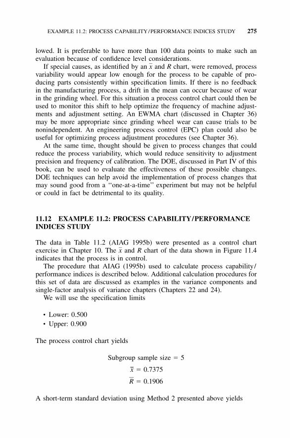
EXAMPLE 11.2: PROCESS CAPABILITY/PERFORMANCE INDICES STUDY 275

lowed. It is preferable to have more than 100 data points to make such anevaluation because of confidence level considerations.

If special causes, as identified by an and R chart, were removed, processxvariability would appear low enough for the process to be capable of pro-ducing parts consistently within specification limits. If there is no feedbackin the manufacturing process, a drift in the mean can occur because of wearin the grinding wheel. For this situation a process control chart could then beused to monitor this shift to help optimize the frequency of machine adjust-ments and adjustment setting. An EWMA chart (discussed in Chapter 36)may be more appropriate since grinding wheel wear can cause trials to benonindependent. An engineering process control (EPC) plan could also beuseful for optimizing process adjustment procedures (see Chapter 36).

At the same time, thought should be given to process changes that couldreduce the process variability, which would reduce sensitivity to adjustmentprecision and frequency of calibration. The DOE, discussed in Part IV of thisbook, can be used to evaluate the effectiveness of these possible changes.DOE techniques can help avoid the implementation of process changes thatmay sound good from a ‘‘one-at-a-time’’ experiment but may not be helpfulor could in fact be detrimental to its quality.

11.12 EXAMPLE 11.2: PROCESS CAPABILITY/PERFORMANCEINDICES STUDY

The data in Table 11.2 (AIAG 1995b) were presented as a control chartexercise in Chapter 10. The and R chart of the data shown in Figure 11.4xindicates that the process is in control.

The procedure that AIAG (1995b) used to calculate process capability/performance indices is described below. Additional calculation procedures forthis set of data are discussed as examples in the variance components andsingle-factor analysis of variance chapters (Chapters 22 and 24).

We will use the specification limits

• Lower: 0.500• Upper: 0.900

The process control chart yields

Subgroup sample size � 5

x � 0.7375

R � 0.1906

A short-term standard deviation using Method 2 presented above yields

276

TA

BL

E11

.2D

ata

for

Ass

essm

ent

ofP

roce

ssC

apab

ility

/Per

form

ance

Indi

ces

Subg

roup

s

12

34

56

78

910

1112

1314

1516

Sam

ples

:

1 2 3 4 5

0.65

0.70

0.65

0.65

0.85

0.75

0.85

0.75

0.85

0.65

0.75

0.80

0.80

0.70

0.75

0.60

0.70

0.70

0.75

0.65

0.70

0.75

0.65

0.85

0.80

0.60

0.75

0.75

0.85

0.70

0.75

0.80

0.65

0.75

0.70

0.60

0.70

0.80

0.75

0.75

0.65

0.80

0.85

0.85

0.75

0.60

0.70

0.60

0.80

0.65

0.80

0.75

0.90

0.50

0.80

0.85

0.75

0.85

0.65

0.70

0.70

0.70

0.75

0.75

0.70

0.65

0.70

0.85

0.75

0.60

0.90

0.80

0.80

0.75

0.85

0.75

0.80

0.75

0.80

0.65

Mea

n:0.

700.

770.

760.

680.

750.

730.

730.

720.

780.

670.

750.

760.

720.

710.

820.

75R

ange

:0.

200.

200.

100.

150.

200.

250.

150.

200.

200.

200.

400.

200.

050.

250.

150.

15

EXAMPLE 11.2: PROCESS CAPABILITY/PERFORMANCE INDICES STUDY 277

0.85

0.80

0.75

0.70

0.65

0.60

0.4

0.3

0.2

0.1

0.0

Sam

ple

mea

nS

ampl

e ra

nge

0 5 10Subgroup

15

UCL=0.8475

UCL = 0.4031

X = 0.7375

R = 0.1906

LCL = 0.6275

LCL = 0.000

=

–

FIGURE 11.4 Example x̄ and R chart.

R 0.1906� � s � � � 0.0819R/d2 d 2.3262

For the bilateral tolerances, Z values and Cpk are as follows:

USL � �̂ 0.900 � 0.7375Z � � � 1.9831USL � 0.0819R/d2

�̂ � LSL 0.7375 � 0.500Z � � � 2.8983LSL � 0.0819R/d2

Z 1.98307975minC � � � 0.6610pk 3 3

Proportion out-of-specification calculations are

�(Z ) � 0.0237USL

�(Z ) � 0.0019LSL

�(total) � 0.0256 (Note: This equates to a 25554 ppm defect rate,from a ‘‘short-term’’ variability perspective.)

It can also be determined that

278 PROCESS CAPABILITY AND PROCESS PERFORMANCE METRICS

USL � LSL 0.9 � 0.5C � � � 0.8136p 6� 0.0819R/d2

The long-term standard deviation using Method 1 with the mean equal to thecontrol chart average yields

n 802 2(x � x ) (x � 0.7375)i i� � s � � � 0.0817� �sample � �n � 1 80 � 1i�1 i�1

Using this standard deviation estimate, we can determine

USL � LSL 0.9 � 0.5P � � � 0.8159p 6� 6(0.081716)sample

USL � x x � LSLP � min ,� �pk 3� 3�sample sample

0.900 � 0.7375 0.7375 � 0.500� min ,� �3(0.0817) 3(0.0817)

� min [0.6629, 0.9688] � 0.6629

The following should be noted:

• Process capability and process performance metrics are noted to be al-most identical.

• Calculations for short-term variability were slightly larger than long-termvariability, which is not reasonable because short-term variability is acomponent of long-term variability. Using range as described in Method2 is not as statistically powerful as Method 3 (because only the highestand lowest data points are considered), which yields the better estimatefor short-term variability (slightly smaller estimate than long-term stan-dard deviation in this case) of

s 0.07627613s � � � 0.0811

c 0.944

• The discussion above follows the basic approach described in AIAG(1995b), focuses on the use of short-term variability metrics. Some or-ganizations prefer to focus on long-term standard deviation and ppmmetrics. These data will be analyzed again as an example in the vari-ance components and single-factor analysis of variance chapters (Chap-ters 22 and 24) to illustrate alternative methods of determining processcapability/performance index metrics.

EXAMPLE 11.3: PROCESS CAPABILITY/PERFORMANCE INDEX NEEDS 279

FIGURE 11.5 Five parts to assemble.

11.13 EXAMPLE 11.3: PROCESS CAPABILITY/PERFORMANCEINDEX NEEDS

Management has given the mandate (all too frequently we have to deal withmanagers who are not schooled in the principles of Deming) that processsteps are to have process indices of Cp � 2.0 and Cpk � 1.5. Consider thefive parts in Figure 11.5 that are to be manufactured and then assembled. Thetolerances of the dimensions on the parts were believed achievable usingconventional manufacturing practices. We will also consider that Cp and Cpk

are expressions of long-term capability (equating to Pp and Ppk).

280 PROCESS CAPABILITY AND PROCESS PERFORMANCE METRICS

For purposes of achieving final measurements that meet customer needs,should each dimension be given equivalent monitoring effort relative to theprocess indices? What procedure would be followed to correct manufacturingprocesses if the parts were shown not to meet the process capability objective?Because quality cannot be measured into a product, it might be better torephrase the initial question to address how S4/IEE techniques can be appliedto better meet the needs of the customer.

Measurements considered should include other parameters besides just thefinal characteristics of the part (e.g., final part dimension considerations).Effort should be made to create a process that consistently produces productsas close to the nominal specification as possible (not ones that just meetspecification).

Determining many capability/performance indices in a process over timecan be very expensive. Often it may be more important to monitor a keyprocess parameter (e.g., a pressure prevalent in a manufacturing tool) than tomonitor the final specification considerations of the manufactured part. Thisbasic manufacturing strategy can result in the detection of process degradationshifts before a large volume of ‘‘bad’’ parts is produced.

If the philosophy of striving for nominal considerations during develop-ment is stressed, the chance of meeting the desired process capability/per-formance indices initially will be higher. For this example, effort should beexpended on making tools and identifying economical processes that manu-facture the parts with precision and consistency along with an emphasis oncontinual process improvement in the areas that are important from the per-spective of the customer.

Back to the initial question of concern: It may not be necessary, from acustomer’s point of view, to collect enough information to calculate the pro-cess indices for all dimensions. Assume that the 0.005 tolerance (in inches)for a dimension is easy to achieve consistently with the current process, ifthe manufacturing processes is initially shown via a tool sample to producethis dimension well within specification. For this dimension, only periodicmeasurements may be needed over time.

However, the tolerance of the B dimensions may require a special operationthat is more difficult to achieve on a continuing basis. For the process thatwas chosen initially, assume that the B dimensions are shown to be in control/predictable over time for all the B-value considerations. For the purpose ofillustration, consider also that the processes had a mean value equal to thenominal specification (i.e., Cpk � Cp), but the Cp values for these dimensionsranged from 1.0 to 1.33 for the five parts. A brainstorming session was thenconducted because the Cp values were less than the objective of 2.0. Theconsensus of opinion from this session was that a new, expensive processwould be required to replace the existing process in order to achieve a higherCp value.

The question of concern is now whether this new process should be de-veloped in order to reduce the B-dimensional variability. Before making this

EXAMPLE 11.3: PROCESS CAPABILITY/PERFORMANCE INDEX NEEDS 281

FIGURE 11.6 Five assembled parts.

decision, the group considered first how these parts are used when they areassembled. The important dimension from a customer’s perspective is theoverall dimensional consideration of B, which after the assembly process ispictorially shown in Figure 11.6.

Consider that the manufactured B dimensions conformed to a straight linewhen plotted on normal probability paper (i.e., the parts are distributed nor-mally). In addition, the mean value for each part equaled the nominal spec-ification value and a 3� limit equaled the tolerance of 0.001 (i.e., Cp � Cpk

� 1.0).When these parts are assembled in series, a low dimension for B1 can be

combined with a high dimension for B2, and so on; hence, it would not bereasonable to just add the tolerance considerations of the individual parts toget the overall tolerance consideration. Because the individual part dimensionsare normally distributed, an overall tolerance can be determined as the squaresof the individual; hence, the overall assembled expected tolerance for B wouldbe

2 2 2 2 1/ 2B tolerance � �(0.001 � 0.001 � 0.001 � 0.001 )

� �(0.00224)

Because 0.00224 describes 3�, we can see that

USL � LSL 0.010C � � � 2.23p 6� 2(0.00224)

Because the Cp � 2.0, this process index target is met on the overalldimension even though the individual measurements do not meet the targetof 2.0.

The purpose of this example is to illustrate that care must be taken not tospend resources unwisely by striving for the tightening of tolerances that maynot have much benefit to the customer. There are many ways to determinewhich parameters should be tracked (e.g., through experience, historical data,

282 PROCESS CAPABILITY AND PROCESS PERFORMANCE METRICS

or statistically significant factors from a DOE). Efforts must also be directedtoward continually improving processes in those areas that benefit the cus-tomer the most. Playing games with the numbers should be avoided.

11.14 PROCESS CAPABILITY CONFIDENCE INTERVAL

Confidence intervals are discussed in greater detail in Chapter 16, but a briefdiscussion of major uncertainties that can occur when calculating this statisticseems warranted here.

A process capability index calculated from sample data is an estimate ofthe population process capability index. It is highly unlikely that the truepopulation index is the exact value calculated. A confidence interval adds aprobability range for the true population value given the results of the sample,including sample size. The confidence interval for Cpk and Ppk is difficult tocalculate directly (later bootstrapping will be used to give an estimate); how-ever, the confidence interval for Cp and Pp is not difficult. The 100(1 � �)percent confidence interval expressed in terms of Cp is

2 2� �1��/ 2;n�1 �/ 2;n�1ˆ ˆC � C � Cp p p� �n � 1 n � 1

11.15 EXAMPLE 11.4: CONFIDENCE INTERVAL FORPROCESS CAPABILITY

An organization wants to create a table that can be used to give a quick 95%confidence interval for a population Cp given the sample size and calculatedCp. When creating this table, consider assigning Cp value of 1.0 to calculatethe following relationship, with a sample size of 10 for illustration:

2 2� �1��/ 2;n�1 �/ 2;n�1ˆ ˆC � C � Cp p p� �n � 1 n � 1

2 2� �1�0.05/ 2;10�1 0.05/ 2;10�1(1.0) � C � (1.0)p� �10 � 1 10 � 1

2.70 19.02� C �p� �9 9

0.55 � C � 1.45p

A 95% confidence interval table including other sample sizes would be

PROCESS CAPABILITY/PERFORMANCE FOR ATTRIBUTE DATA 283

n

Cp LowerConfidence

Multiple

Cp UpperConfidence

Multiple

10 0.55 1.4520 0.68 1.3130 0.74 1.2640 0.78 1.2250 0.80 1.2060 0.82 1.1870 0.83 1.1780 0.84 1.1690 0.85 1.15

100 0.86 1.14

From this table we can then determine the Cp confidence interval for a sampleof 10 that had a calculated Cp of 1.5:

(1.5)(0.55) � C � (1.5)(1.45)p

0.82 � C � 2.18p

11.16 PROCESS CAPABILITY/PERFORMANCE FORATTRIBUTE DATA

S4 /IEE Application Examples

• Transactional and manufacturing 30,000-foot-level metric: A companyhad a large number of transactions completed daily, where the numberof daily transactions was similar. The number of defective recorded trans-actions were measured and reported. An XmR chart of the defective hadno special causes. The capability/performance of the process was re-ported as the centerline of the chart.

• Transactional and manufacturing 30,000-foot-level metric: The numberof daily transactions is approximately the same, but not exact. The num-ber of defects in filling out invoices is unsatisfactory. An XmR chart ofthe defect rate had no special causes. The capability/performance of theprocess was reported as the centerline of the chart.

The p chart and other attribute control charts are different from variables datain that each point can be directly related to a proportion or percentage ofnonconformance relative to customer requirements, while points on a varia-bles chart indicate a response irrespective of specification needs.

284 PROCESS CAPABILITY AND PROCESS PERFORMANCE METRICS

AIAG (1995b) defines capability as follows: ‘‘For attribute charts, capa-bility is defined simply as the average proportion or rate of nonconformingproduct, whereas capability for variables charts refers to the total (inherent)variation ( ) yielded by the (stable) process, with and/or without ad-6�̂R / d2

justments for process centering to specification targets.’’AIAG (1995b) also states: ‘‘If desired, this can be expressed as the pro-

portion conforming to specification (i.e., 1 � ). For a preliminary estimatepof process capability, use historical data, but exclude data points associatedwith special causes. For a formal process capability study, new data shouldbe run, preferably for 25 or more periods, with the points all reflecting sta-tistical control. The for these consecutive in-control periods is a betterpestimate of the process’s current capability.’’

Attribute assessments are not only applicable to pass/fail tests at the endof a manufacturing line. They can also be used to measure the ‘‘hidden factor’’using a DPMO scale. Process improvement efforts for stable processes havingattribute measurements can originate with a Pareto chart of the types of non-conformance. Efforts to reduce the most frequent types of defects could per-haps then utilize DOE techniques.

11.17 DESCRIBING A PREDICTABLE PROCESS OUTPUT WHENNO SPECIFICATION EXISTS

Specification requirements are needed to determine Cp, Cpk, Pp, and Ppk.Sometimes, however, the output of a process does not have a specification.This happens frequently with business or service processes. Measurementsfor these situations can be cycle time and costs. Sometimes organizations willuse targets as a specification; however, the results can be deceptive.

A measurement approach I have found useful for this type of situation isto describe the overall response as expected percentage of occurrences. Thisapproach is outlined here in three figures. Figure 11.7 shows an X chart andhow time-sequenced data can be conceptually accumulated to create a distri-bution of nonsequenced data. Figure 11.8 then illustrates how 80% of theoccurrence are expected to be between response levels A and B. However, itis difficult to determine percentage of populations from a histogram. Figure11.9 shows how this percentage can be more easily shown using a probabilityplot and how it relates to a probability density function and histogram plot.

For a given set of data a percentage value can be determined mathemati-cally using a Z table (Table A) or a statistical computer program. The pre-sentation of this type of information with a normal probability can give agood baseline view of the process. Quick estimations are offered through theplot response estimates at differing percentage levels and percentage estimatesat differing response levels. This same approach has application flexibility toother probability plots where the distribution is non-normal. I have found thetwo-parameter Weibull distribution very useful for describing many situations

EXAMPLE 11.5: DESCRIBING A PREDICTABLE PROCESS OUTPUT 285

FIGURE 11.7 Conceptual change from time-sequenced data to no time sequencingof data.

FIGURE 11.8 Conceptual view of a percentage of population statement.

where, for example, time (e.g., cycle time) is the metric and values belowzero are not possible.

11.18 EXAMPLE 11.5: DESCRIBING A PREDICTABLE PROCESSOUTPUT WHEN NO SPECIFICATION EXISTS

S4 /IEE Application Examples

• Satellite-level metric: The last three years’ ROI for a company was re-ported monthly in a control chart. No special causes or trends wereidentified. Monthly ROIs were plotted on a normal probability plot, wherea null hypothesis (see Sections 3.8 and 16.3) for normality was not re-

286 PROCESS CAPABILITY AND PROCESS PERFORMANCE METRICS

FIGURE 11.9 Conceptual view of a percent of population statement using a normalprobability plot.

jected. The capability/performance of the system was reported on theprobability plot as a best-estimate 80% frequency of occurrence interval,which described common-cause variability. Goals were set to improvethis metric. A strategic plan was created that was in alignment with thegoal to improve this metric. The 30,000-foot-level operational metricswere then chosen that would be the focus of improvement efforts. S4/IEEprojects were then chosen to improve these metrics.

• Transactional 30,000-foot-level metric: One random paid invoice wasselected each day from last year’s invoices where the number of daysbeyond the due date was measured and reported (i.e., days sales out-standing [DSO]). The DSO for each sample was reported in an XmRcontrol chart, where no reason was identified for a couple special-causedata points. These data were plotted on a normal probability plot, where

EXAMPLE 11.5: DESCRIBING A PREDICTABLE PROCESS OUTPUT 287

a null hypothesis (see Sections 3.11 and 16.3) for normality was rejected.We often expect that this type of data would follow a log-normal distri-bution. A lognormal probability plot fit the data well. An XmR chart ofthe lognormal data did not indicated any special-cause conditions. Alognormal probability plot was used to describe the capability/perform-ance of the process as a best-estimate 80% frequency of occurrence in-terval, which described common-cause variability.

• Transactional and manufacturing 30,000-foot-level cycle time metric (alean metric): One randomly selected transaction was selected each dayover the last year, where the time from order entry to fulfillment wasmeasured. The differences between these times relative to their due datewere reported in an XmR chart. No special causes were identified. A nullhypothesis for normality could not be rejected. The long-term processcapability/performance metric was reported as the best-estimate 80%interval, which described the common-cause variability of the system.

• Transactional and manufacturing 30,000-foot-level inventory metric orsatellite-level TOC metric (a lean metric): Inventory was tracked monthlyusing a control chart. No special causes were identified. A null hypothesisfor normality could not be rejected. The long-term process capability/performance was reported as the best-estimate 80% frequency of occur-rence interval for month-to-month inventory levels, along with associatedmonetary implications.

• Transactional 50-foot-level metric (KPIV): An S4/IEE project to improvethe 30,000-foot-level metrics for DSOs identified a KPIV to the process,the importance of timely calling customers to ensure that they receiveda company’s invoice. A control chart tracked the time from invoicing, towhen the call was made, where one invoice was selected hourly. Nospecial cause was identified. A hypothesis for normality could not berejected. The long-term process capability/performance metric was re-ported as the best-estimate 80% interval, which described common-causevariability.

• Product DFSS: An S4/IEE product DFSS project was to reduce the30,000-foot-level MTBF (mean time between failures) of a product by itsvintage (e.g., laptop computer MTBF rate by vintage of the computer).A control chart tracked the product MTBF by product vintage. Thecapability/performance of the system was reported on the probabilityplot as a best-estimate 80% interval, which described common-causevariability and what might be expected for MTBF rates in the futureunless something were done different to change the design process. Cat-egories of problems were tracked over the long haul in a Pareto chartto identify improvement opportunities for newly developed products.

• S4/IEE infrastructure 30,000-foot-level metric: A steering committee usesa control chart to track the duration of projects. The capability/perform-ance of the system was reported on the probability plot as a best-estimate80% interval.

288 PROCESS CAPABILITY AND PROCESS PERFORMANCE METRICS

People’s busy schedules and other factors can make it very difficult to getgood attendance at professional society meetings. An average monthly atten-dance of 10% of the membership is considered very good. As the new localASQ section chair in Austin, Texas, I thought attendance was important andchose this metric as a measure of success for my term. My stretch goal wasto double average monthly attendance from the level experienced during theprevious six years.

The process of setting up and conducting a professional society sessionmeeting with program is more involved than one might initially think. Stepsin this process include guest speaker/ topic selection, meeting room arrange-ments, meeting announcements, and many other issues. I wanted to create abaseline that would indicate expected results if nothing was done differentlyfrom our previous meeting creation process. Later I also wanted to test thetwo process means to see if there was a significance difference of the pro-cesses at an � level of 0.05.

This situation does not differ much from a metric that might be expectedfrom business or service processes. A process exists and a goal has been set,but there are no real specification limits. Setting a goal or soft target as aspecification limit for the purpose of determining process capability/perform-ance indices could yield very questionable results. The records indicated thatour previous section meeting attendance had been as follows (we do not meetduring the summer months, and a term is from July 1 to June 30):

9 / 9 / 93 10 / 14 / 93 11 / 11 / 93 12 / 9 / 93 1 / 13 / 94 2 / 17 / 94 3 / 10 / 94 4 / 14 / 94 5 / 12 / 94

66 45 61 36 42 41 46 44 47

9 / 8 / 94 10 / 13 / 94 11 / 10 / 94 12 / 8 / 94 1 / 12 / 95 2 / 16 / 95 3 / 9 / 95 4 / 3 / 95 5 / 16 / 95

46 51 42 42 61 57 47 46 28

9 / 14 / 95 10 / 12 / 95 11 / 9 / 95 12 / 14 / 95 1 / 11 / 96 2 / 8 / 96 3 / 14 / 96 4 / 11 / 96 5 / 9 / 96

45 37 45 42 58 49 39 53 58

9 / 12 / 96 10 / 10 / 96 11 / 14 / 96 12 / 12 / 96 1 / 9 / 97 2 / 13 / 97 3 / 13 / 97 4 / 10 / 97 5 / 8 / 97

44 37 52 33 43 45 35 29 33

An XmR chart of the data shown in Figure 11.10 indicates that the processis stable. A process capability/performance 80% frequency of occurrencemetric shown in Figure 11.11 could be used to describe the expected responsevariability from the process. Management and others can then assess if thisresponse range is acceptable. For this example the figure indicates an esti-mation that 80% of the time attendance would be between 34 and 57. Otherpercentage of population estimates can similarly be taken from this chart.

If an improved response is desired from a stable process, process improve-ments are needed. An example in the comparison test chapter (see Chapter19) shows some changes that were implemented to encourage better atten-

EXAMPLE 11.5: DESCRIBING A PREDICTABLE PROCESS OUTPUT 289

70

60

50

40

30

20

30

20

10

0

Indi

vidu

al v

alue

Mov

ing

rang

e

0 10 20Subgroup

30 40

UCL = 69.68

LCL = 20.59

LCL = 0.000

UCL = 30.15

R = 9.229

X = 45.14=

–

FIGURE 11.10 XmR chart of previous attendance.

FIGURE 11.11 Normal probability plot of previous attendance.

290 PROCESS CAPABILITY AND PROCESS PERFORMANCE METRICS

dance. The example also shows the results of a comparison test that comparedprevious meeting mean attendance to the mean attendance response from thenew process.

11.19 PROCESS CAPABILITY/PERFORMANCE METRICSFROM XmR CHART OF SUBGROUP MEANSAND STANDARD DEVIATION

S4 /IEE Application Examples

• Transactional 30,000-foot-level metric: The mean and standard deviationof all DSOs were tracked using two XmR charts with a weekly subgroup-ing, where the standard deviation values had a log transformation. Nospecial causes were identified. The long-term capability/performance ofthe process was reported as percentage nonconformance beyond 30, 60,and/or 90 days, using variance of components techniques (see Chapter22) or a statistical program that reports this metric under their and sxprocess capability option.

Section 10.27 described a situation where a process mean and standarddeviation was tracked over time using XmR control charts. Again I suggestreporting an estimated nonconformance percentage or ppm rate that addressesthe underlying distribution shape for the population, rather than reporting Cp,Cpk, Pp, and Ppk process capability/performance indices.

In order to determine this long-term percentage or ppm nonconformancerate we could use variance components techniques (see Chapter 22) or acomputer program that combines within and between variability from theoriginal data set when determining an overall long-term ppm. In both casesit may be necessary to transform the data as described in the next section.

11.20 PROCESS CAPABILITY/PERFORMANCE METRIC FORNONNORMAL DISTRIBUTION

S4 /IEE Application Examples

• Transactional 30,000-foot-level metric: One random paid invoice wasselected each day from last year’s invoices where the number of daysbeyond the due date was measured and reported (i.e., days sales out-standing [DSO]). The DSO for each sample was reported in an XmRcontrol chart, where no reason was identified for a couple special-causedata points. These data were plotted on a normal probability plot, wherea null hypothesis (see Sections 3.8 and 16.3) for normality was rejected.A lognormal plot fit the data well. An XmR chart of the lognormal datadid not indicate any special-cause conditions. The lognormal probability

NONNORMAL DISTRIBUTION 291

plot was used to estimate the proportion of invoices beyond 30, 60, and90 days. An S4 /IEE project was initiated to improve the DSO metric.

• Transactional 30,000-foot-level metric: The mean and standard deviationof all DSOs were tracked using two XmR charts with a weekly subgroup-ing, where the standard deviation values had a log transformation. Nospecial causes were identified. The long-term capability/performance ofthe process was reported as percentage nonconformance beyond 30, 60,and/or 90 days, using variance of components techniques (see Chapter22) or a statistical program that reports this metric under their and sxprocess capability option.

Nonnormality is common for measurements such as flatness, roundness, andparticle contamination. The capability/performance measures described aboveare for normal distributions. One approach to address nonnormal data is tonormalize the data using a transformation. A transformation can be appro-priated if the nonnormal distribution to be transformed is known. However,there could be problems if it has to be estimated from preliminary data. Manyskewed distributions can be traced from two normally distributed sources withdifferent parameters (Nelson 1999a). Table 24.2 describes transformations forvarious situations.

A general approach for transforming data is a Box-Cox transformation(Box et al. 1977), where values (Y) are transformed to the power of � (i.e.,Y�). This relationship has the following characteristics:

� � �2 Y transformed � 1/Y2

� � �0.5 Y transformed � 1/�Y� � 0 Y transformed � ln(Y)� � 0.5 Y transformed � �Y� � 2 Y transformed � Y2

Maximum likelihood value for � is when the residual sum of squares fromthe fitted model is minimized, as shown in Example 11.6.

An alternative approach when data can be represented by a probability plot(e.g., Weibull distribution) is to use the 0.135 and 99.865 percentiles fromthis plot to describe the spread of the data. This method is applicable whenall individual measurements are combined from an in-control/predictable pro-cess to determine a long-term capability/performance. The capability/per-formance indices from this procedure are sometimes termed equivalent indicesbecause they use the equivalent percentile points from the normal distribution.Both observed and expected long-term ppm nonconformance rates can bedetermined using this method.

Statistical software can expedite calculations and give better estimates be-cause calculations can be based upon maximum likelihood estimates of thedistribution parameters. For example, for the Weibull distribution these esti-

292 PROCESS CAPABILITY AND PROCESS PERFORMANCE METRICS

TABLE 11.3 Amount of Residue by Period

Period Residue Period Residue Period Residue Period Residue

1 0.027 26 0.015 51 0.018 76 0.0102 0.027 27 0.013 52 0.034 77 0.0413 0.064 28 0.011 53 0.014 78 0.0154 0.042 29 0.009 54 0.013 79 0.0295 0.019 30 0.011 55 0.011 80 0.0286 0.019 31 0.015 56 0.025 81 0.0247 0.019 32 0.027 57 0.016 82 0.0118 0.016 33 0.016 58 0.091 83 0.0309 0.024 34 0.019 59 0.018 84 0.052

10 0.032 35 0.016 60 0.025 85 0.01911 0.015 36 0.017 61 0.015 86 0.01612 0.025 37 0.027 62 0.012 87 0.02213 0.007 38 0.018 63 0.012 88 0.02414 0.072 39 0.010 64 0.029 89 0.04615 0.023 40 0.013 65 0.015 90 0.02416 0.018 41 0.021 66 0.012 91 0.01217 0.019 42 0.015 67 0.013 92 0.02318 0.019 43 0.015 68 0.026 93 0.01619 0.016 44 0.021 69 0.013 94 0.03120 0.019 45 0.013 70 0.010 95 0.02521 0.035 46 0.035 71 0.011 96 0.01822 0.021 47 0.012 72 0.028 97 0.01323 0.015 48 0.011 73 0.03524 0.019 49 0.021 74 0.01625 0.012 50 0.014 75 0.023

mates would be based on the shape and scale parameters, rather than meanand variance estimates as in the normal case.

11.21 EXAMPLE 11.6: PROCESS CAPABILITY/PERFORMANCEMETRIC FOR NONNORMAL DISTRIBUTIONS:BOX-COX TRANSFORMATION

A chemical process has residue, as shown in Table 11.3, with a specificationupper limit of 0.02. There is a no lower limit; however, there is a naturalbound of 0.

Figure 11.12 shows a control chart of the data with no transformation. Noreason was identified for the special-cause points identified in the plot. Figure11.13 shows a process capability/performance analysis, while Figure 11.14shows a normal probability plot. From this normal probability plot it is nosurprise that the null hypothesis of normality is rejected (see Sections 3.8 and16.3) since the process has a physical boundary of 0. Because of this lack ofnormality, the above process capability/performance metrics are not valid.

EXAMPLE 11.6: BOX-COX TRANSFORMATION 293

100908070605040302010Subgroup 0

0.10

0.05

0.00

11

1

Mean = 0.02168

UCL = 0.05293

LCL = –9.6E-03

0.080.070.060.050.040.030.020.010.00

1

1

11

R = 0.01175

UCL = 0.03839

LCL =0

Indi

vidu

al v

alue

Mov

ing

rang

e

FIGURE 11.12 XmR chart for amount of residue, without transformation.

0 .1 00 .0 80 .0 60 .0 40 .0 20 .0 0

USLLB

PPM Total

PPM > USL

PPM < LB

PPM Total

PPM > USL

PPM < LB

PPM Total

PPM > USL

PPM < LB

Ppk

PPL

PPU

Pp

Cpm

Cpk

CPL

CPU

Cp

StDev (Overall )

St Dev (Within)

Sample NMean

Lower BoundTarget

USL

551243.21

551243.21

*

563680.61

563680.61

*

402061.86

402061.86

0.00

-0.04

*

-0.04

*

*

-0.05

*

-0.05

*

0.0130464

0.0104824

97

0.0216804

0.0000000 *

0.0200000

Exp. "Overall " PerformanceExp. "Within" PerformanceObserved PerformanceOverall Capability

Potent ia l (Wi th in ) Capab i l i t y

Process Data

Within

Overall

FIGURE 11.13 Process capability analysis, assuming data are normally distributed.

Figure 11.15 shows a Box-Cox plot. The minimum plot value is the bestestimate for �; i.e., we estimate � � �0.674. Figure 11.16 shows a normalprobability plot of the transformed data. The transformed data looks wellbehaved. Figure 11.17 shows a control chart of the transformed data, wherethere is still one condition that could be further investigated. However, the

294 PROCESS CAPABILITY AND PROCESS PERFORMANCE METRICS

P-value: 0.000A-squared: 6.188

Anderson-Darling Normality Test

97St Dev: 0.0130125Average: 0.0216804

0.0950.0700.0450.020

.999

.99

.95

.80

.50

.20

.05

.01

.001

Pro

babi

lity

Amount of Residue

N:

FIGURE 11.14 Normal probability plot of residue, without transformation.

1.00.50.0–0.5–1.0–1.5–2.0–2.5–3.0–3.5–4.0–4.5–5.0

0.03

0.02

0.01

95% Confidence Interval

St D

ev

Lambda

Last Iteration Info

0.008

0.008

0.008

–0.617

–0.674

–0.730

St DevLambda

Up

Est

Low

FIGURE 11.15 Box-Cox plot for amount of residue.

EXAMPLE 11.6: BOX-COX TRANSFORMATION 295

P-va lue: 0.633A-squared: 0.281

Anderson-Darling Normality Test

97St Dev: 2.28740Average: 9.50462

15105

.999

.99

.95

.80

.50

.20

.05

.01

.001

Pro

babi

lity

Transformed values

N:

FIGURE 11.16 Normal probability plot of transformed residue data, Box-Cox � �� 0.674.

100908070605040302010Subgroup 0

30

20

10

0

Indi

vidu

al V

alue

1

Mean = 15.01

UCL = 27.25

LCL = 2.767

20

10

0

Mov

ing

Ran

ge 1

1

R = 4.602

UCL = 15.04

LCL = 0

FIGURE 11.17 XmR chart for amount of residue, with Box-Cox transformationwhere � � � 0.674.

296 PROCESS CAPABILITY AND PROCESS PERFORMANCE METRICS

5004003002001000

USL* LB*

PPM TotalPPM < USL*PPM > LB*

PPM TotalPPM < USL*PPM > LB*

PPM TotalPPM > USLPPM < LB

PpkPPLPPU

Pp

Cpm

Cpk

CPLCPUCp

St Dev* (Overall)St Dev (Overall)St Dev* (Within)St Dev (Within)Sample NMean*MeanLower Bound*Lower BoundTarget*TargetUSL*USL

404424.58404424.58

*

399440.73399440.73

*

402061.86402061.86

0.00

0.08*

0.08

*

*

0.08*

0.08 *

4.297160.013054.079870.01042

97 15.007 0.022496.592 0.000

* *

13.967 0.020

Exp. "Overall" PerformanceExp. "Within" PerformanceObserved PerformanceOverall Capability

Potential (Within) Capability

Process Data

Within

Overall

FIGURE 11.18 Process capability analysis, with Box-Cox transformation where �� � 0.674.

transforming of this process output to create an XmR plot seems appropriate.This plot also seems to describe a predictable process.

Figure 11.18 shows the capability/performance of the process. To createthis plot I adjusted the lower bound a very small distance of 0.001, since zeroor negative values are not permissible with this modeling (in general we mightneed to offset our data so there are no zero or negative values). In this plotthe data transformation caused the upper and lower specification limits toswitch.

I believe that a process capability/performance nonconformance rate esti-mate of 404,000 ppm, which is in the lower right corner of this figure, bettergives a description of the common cause output of this process than a Cpk orPpk value of 0.8, noting that Cp and Pp values cannot be determined since thespecification is one-sided. The plot in the upper left corner of Figure 11.18shows a histogram of the nontransformed data. An estimated 404,000 ppmrate is consistent with this plot. Note also that this ppm estimate from Figure11.18 of 404,000 is a better estimate than the ppm estimate from Figure 11.13of 551,000, which was based on an underlying normal distribution assump-tion.

THE S4 / IEE DIFFERENCE 297

ResponseLevel

Time

Within-subgroupvariability

Overallvariability

FIGURE 11.19 Within-subgroup (short-term variability) and overall variability(long-term variability) of a process’s output.

11.22 IMPLEMENTATION COMMENTS

AIAG (1995b) states that ‘‘the key to effective use of any process measurecontinues to be the level of understanding of what the measure truly repre-sents. Those in the statistical community who generally oppose how Cpk num-bers, for instance, are being used are quick to point out that few real worldprocesses completely satisfy all of the conditions, assumptions, and parame-ters within which Cpk has been developed. Further, it is the position of thismanual that, even when all conditions are met, it is difficult to assess or trulyunderstand a process on the basis of a single index or ratio number.’’

AIAG (1995b) further comments that it is strongly recommended thatgraphical analysis be used in conjunction with process measures. A finalprecaution is given that all capability/performance assessments should beconfined to a single process characteristic. It is never appropriate to combineor average the capability/performance results for several processes into oneindex.

Organizations might be tempted to ask suppliers to report their currentprocess capability/performance indices. The results from this effort can bevery deceptive because these indices vary over time, even if the processeswere exactly the same. Wheeler (1995a) suggests the use of an XmR chartto report process indices, where the supplier is meeting the target whenthe central line meets or exceeds the target and capability indices are incontrol/predictable. I am in ageement with this approach.

11.23 THE S4/IEE DIFFERENCE

Figure 11.19 shows the output of a process where within-day variability isless than between-day variability. If someone were to sample from this pro-

298 PROCESS CAPABILITY AND PROCESS PERFORMANCE METRICS

cess and then create an and R chart, the process could have many out-of-xcontrol signals (unpredictable process indictators) since the control limits arecalculated from within-day variability. From this sampling plan, Cp and Cpk

indices, using a statistical software program such as Minitab, would be de-termined from a within-day standard deviation, while Pp and Ppk would bedetermined from an overall standard deviation. In addition, for this type ofsituation there are typically other within-day variance components that coulddramatically affect the results depending upon how someone chose to samplefrom the process.

Minitab statistical software uses the above procedure to differentiate be-tween short-term and long-term variability. However, other statistical softwarepackages and calculation procedures do not necessarily make this differenti-ation. This confusion becomes amplified when we consider the differencesthat can result from how frequently a process is sampled to make the calcu-lation. Because of these differences, a company can make a wrong decisionthrough the determination, interpretation, and comparison of these indices.

Other issues compound this confusion. The described equations are fornormally distributed data. Some computer programs can address situationswhere data are not from a normal distribution; however, this is often not donein practice and the omission can affect the accuracy of the reported metrics.In addition, sample size, confidence intervals, and not having samples takenfrom the time period of interest can distort results. Finally, these indices arenot appropriate when data are attribute, which is typically expressed as a part-per-million (ppm) defect rate or a percent defective rate.

It is important for organizations to build awareness of the exposures whenusing these metrics within their Six Sigma training and coaching. I have foundthat most people find it much easier to visualize and interpret an estimatedppm rate (or percentage of nonconformance) beyond customer objectives/specifications than a process capability/performance index value. Because ofthis, within S4/IEE I encourage organizations to utilize this metric with ap-propriate data transformations, in lieu of Cp, Cpk, Pp, and Ppk process metrics.Another benefit of this approach is that there can now be a single unit ofmeasure for both attribute and continuous situations within manufacturing,development, and transactional processes.

Many times people have asked me for a procedure to convert the failurerate of an attribute process into a Cpk metric. This conversion makes no phys-ical sense. Apparently these people are confronted with a policy that theymust report a single metric—Cpk. Note that if a process had a continuousresponse and there were upper and lower specification limits we would alsoneed to report Cp. I hope you see how the policy of using the processcapability/performance indices of Cp, Cpk, Pp, and Ppk can cause confusionwithin an organization and between suppliers/customers. This is another ar-gument to use an estimated ppm rate or nonconformance percentage rate asa single metric for both attribute and continuous data.

S4 / IEE ASSESSMENT 299

One last point about this set of metrics. I have been asked Cp /Cpk /Pp /Ppk

questions by many people who have very solid statistical backgrounds. OftenI respond to them by asking: If you are confused, what do you think is thelevel of understanding of others who have less statistical background? Theyinvariably respond that the metric does create a lot of confusion. I believethat we should report metrics that everybody understands and can picture intheir minds. People can picture a metric that relates to a nonconformance rate.With this approach, even though our estimates may not be perfect for manyreasons, the reporting of a nonconformance rate gives us a picture of relativeconformance to criteria.

Within S4/IEE an infrequent subgrouping/sampling strategy for the crea-tion of a 30,000-foot-level control chart avoids these problems. This chartoffers a time series baseline from which a process capability/performancenoncomplaince rate can be determined. These metrics can be used for bothoperational metrics and the establishment of a baseline for S4 / IEE projects.From this capability/performance measure the COPQ/CODND can be estab-lished. The COPQ/CODND metric, along with any customer satisfaction is-sues, can then be assessed to determine whether improvement efforts arewarranted.

Some Six Sigma programs have a standard practice where black belts com-pare short-term process capability to long-term process performance directlyfor all Six Sigma projects, where short-term variability is considered the en-titlement of a process. Since these differences would be fallout from our S4/IEE project execution roadmap if this difference had statistical significance,there is nothing to gain by making such a routine comparison, which can bevery costly and be highly dependent on the sampling procedure that was usedto determine the metrics.

Finally, with the S4/IEE approach I also do not recommend convertingppm rates to sigma quality levels because the results lead to confusion. The1.5 standard deviation shift that is buried within a sigma quality level metricis confusing to many and distorts interpretations and comparisons betweenother process metrics. In addition, this conversion can become a very largeissue when organizations must fabricate specification requirements in orderto determine their sigma quality levels for various processes (e.g., transac-tional processes).

Six Sigma can help organizations improve their bottom-line and customersatisfaction; however, its effectiveness is a function of how wisely the metricsand project execution strategy are implemented.

11.24 S4/IEE ASSESSMENT

This chapter discusses, among other things, the often overlooked aspect ofprocess capability/performance index equations—the method used to deter-

300 PROCESS CAPABILITY AND PROCESS PERFORMANCE METRICS

mine standard deviation. For some situations large differences in this metriccan occur depending on how data are collected and analyzed. Organizationsneed to determine the best metric for their particular situation. Also, thereneeds to be good communication between organizations and their supplier/customers up front to avoid any costly misunderstandings.

Important considerations when conducting a process capability/perform-ance metric assessment include:

• Keep priorities balanced. The collection and reporting of data can beexpensive. Process capability/performance metrics alone do not directlyadd value; they are only an estimate of what is expected from the process.Hence, it is important not to spend a large amount of resources just todetermine a precise process capability/performance metric value at theexpense of process-improvement efforts.

• When reporting process measurements, don’t forget to consider the lan-guage spoken by all—money. Converting the cost of cycle time andaverage defect costs (direct and indirect impact) to money can be eye-opening.

• Consider the impact of sample size on process capability/performancemetric calculations.

• A variance-components analysis approach cannot only quantify a stan-dard deviation to use within process capability/performance metric cal-culations, but can also suggest where process improvement efforts shouldbe focused. It can also be used whenever time series data are limited.

• If variability is greater than desired, consider the impact of the measure-ment system. One customer of mine had a situation where the contri-bution from measurement uncertainty was one half of the total variabilityof the product output that he was using to determine whether he shouldship a product or not.

• Make sure that you and your customer/supplier are in agreement whetherreported metrics are to reflect short-term or long-term variability. Ra-tional subgrouping considerations can make a big difference in processcapability/performance index calculations.

• Consider the impact of forcing a specification where one does not exist.I have seen some organizations spend a lot of time creating a very ques-tionable metric by arbitrarily adding a specification value where one wasnot really appropriate—so they could make a Cpk metric. This situationcan often occur in business and service processes. Consider using thedescribed probability plotting reporting procedure for this situation.

11.25 EXERCISES

1. Catapult Exercise Data Analysis: Using the catapult exercise data setsfrom Chapter 4, determine the process capability/performance metrics of

EXERCISES 301

each data set using specifications supplied by the instructor (e.g., 75 �inches). Compare the results using different calculation procedures.

2. The example and R chart in Chapter 10 indicated that samples num-xbered 8, 9, 10, 12, 13, and 18 were out of control (i.e., an unpredictableprocess). The process specifications are 0.4037 � 0.0013 (i.e., 0.4024 to0.4050). Tabular and calculated values will be in units of 0.0001 (i.e., thespecification limits will be considered 24 to 50). Assume that for eachof these data points, circumstances for an out-of-control response wereidentified and will be avoided in future production. Determine the processcapability/performance metrics of the remaining 14 subgroups, which areas follows:

Measurements

1 36 35 34 33 322 31 31 34 32 303 30 30 32 30 324 32 33 33 32 355 32 34 37 37 356 32 32 31 33 337 33 33 36 32 318 34 38 35 34 389 36 35 37 34 33

10 30 37 33 34 3511 28 31 33 33 3312 33 30 34 33 3513 35 36 29 27 3214 33 35 35 39 36

3. Determine the process capability/performance metrics of a process thathad a lower specification of 2 and an upper specification of 16 withresponses: 3.40, 8.57, 2.42, 5.59, 9.92, 4.63, 7.48, 8.55, 6.10, 6.42, 4.46,7.02, 5.86, 4.80, 9.60, 5.92 (data were collected sequentially). Determinethe 95% confidence interval for Cp.

4. A company is incorporating a Six Sigma program. A process is said tobe capable of producing a response of 36 �12. Someone compiled thefollowing responses from the process, which were not collected in timesequence: 41.3, 30.8, 38.9 33.7, 34.7, 20.4, 28.3, 35.1, 37.9, 32.6. De-termine best-estimate and 95% confidence intervals for capability/per-formance indices that can be calculated. List any concerns or questionsyou have about the data.

5. A machine measures the peel-back force necessary to remove the pack-aging for electrical components. A tester records an output force thatchanges as the packaging is separated. Currently, one random sample istaken from three shifts and compared to a � specification limit that

302 PROCESS CAPABILITY AND PROCESS PERFORMANCE METRICS

reflects the customer needs for a maximum and minimum peel-back forcerange. Whenever a measurement exceeds the specification limits, thecause is investigated.(a) Evaluate the current plan and create a sampling plan utilizing control

charts.(b) Assume that the peel-back force measurements are in control/pre-

dictable. Create a plan to determine if the process is capable of meet-ing the � specifications.

(c) Discuss alternative sampling considerations.

6. A supplier quotes a Cp value of 1.7. After a discussion with representa-tives, you determine that they are calculating standard deviation as youdesire, but you are concerned that they had a sample size of only 20.Determine a 95% confidence interval for the population Cp.

7. An organization requires a Cp value of 2.00. Given a sample size of 30determine the minimum level for a sampled Cp value in order to be 97.5%confident that the Cp population value is 2.00 (i.e., a one-sided confidenceinterval).

8. In an exercise in Chapter 11 you were presented the following informa-tion for analysis in order to select the best supplier to manufacture to aspecification of 85–115. Suppliers claimed the following: supplier 1, �x100 and s � 5, supplier 2, � 95 and s � 5, supplier 3, � 100 andx xs � 10, supplier 4, � 95 and s � 10. You were to determine ppmxnoncompliance rates and yields. Because of concerns about the lack ofinformation supplied about the raw data used to make these computations,you asked each supplier for additional information. They could not supplyyou with the raw data, but all suppliers said their raw data were normallydistributed and from a process that was in control. In addition, you didget the following information from them: for supplier 1, results weredetermined from five samples produced consecutively: for supplier 2,results were determined from 10 samples, where one sample was pro-duced every day for 10 days: for supplier 3, results were from 60 samplestaken over 30 days; for supplier 4, results were from 10 samples takenover two days. Determine confidence intervals for Cp and Pp. Commenton the selection of a supplier and what else you might ask to determinewhich supplier is the best selection. Comment on what you would askthe purchasing department to do different in the future relative to supplierselection.

9. List issues that organizations often ignore when addressing capability/performance issues.

10. Explain how the techniques presented in this chapter are useful and canbe applied to S4/IEE projects.

11. For the data in Exercise 10.17, estimate the overall process capability/performance metrics and then the process capability/performance by ma-

EXERCISES 303

chine type. (See Example 19.12 for a compiling of the data by machine.)Comment on results.

12. A chemical process has a specification upper limit of 0.16 and physicallower limit of 0.10 for the level of contaminant. Determine the estimatedprocess capability/performance of the process, which had the followingoutput:

Period Level Period Level Period Level

1 0.125 40 0.135 81 0.142 0.18 41 0.125 82 0.133 0.173 42 0.12 83 0.1324 0.1215 43 0.135 84 0.1415 0.1515 44 0.1195 85 0.3256 0.139 45 0.1265 86 0.217 0.144 46 0.115 87 0.1358 0.205 47 0.115 88 0.1359 0.1785 48 0.12 89 0.144510 0.1625 49 0.12 90 0.15511 0.17 50 0.13 91 0.16612 0.13 51 0.16 92 0.147513 0.18 52 0.17 93 0.141514 0.11 53 0.12 94 0.13315 0.14 54 0.16 95 0.12616 0.14 55 0.14 96 0.11117 0.14 56 0.115 97 0.1318 0.1365 57 0.225 98 0.1319 0.1385 58 0.154 99 0.13520 0.1365 59 0.126 100 0.13521 0.1395 60 0.1075 101 0.1322 0.135 61 0.128 102 0.126523 0.135 62 0.13 103 0.1424 0.135 63 0.13 104 0.15725 0.14 64 0.121 105 0.1726 0.1525 65 0.1145 106 0.19527 0.155 66 0.14 107 0.1628 0.18 67 0.142 108 0.17529 0.184 68 0.135 109 0.1430 0.1625 69 0.115 110 0.13531 0.18 70 0.1115 111 0.11932 0.175 71 0.115 112 0.133 0.17 72 0.12 113 0.12834 0.184 73 0.115 114 0.13535 0.165 74 0.1025 115 0.12536 0.1525 75 0.1215 116 0.12537 0.1535 76 0.1335 117 0.128538 0.1355 77 0.165 118 0.121539 0.135 78 0.14 119 0.118540 0.135 79 0.1541 0.125 80 0.14

304 PROCESS CAPABILITY AND PROCESS PERFORMANCE METRICS

13. Individuals from a team are to toss a coin toward a wall with the objectiveof having the coin rest as close to the wall as possible. The coin mustlie flat or the throw is not included in the data set. The throw distance is15 feet. Team members are to rotate such that each team member makesfive consecutive throws and each person throws twice. Measurement dis-tance is to the center of the coin. Estimate the process capability/per-formance metrics for this process using an upper specification limit of10 inches.

14. In exercise 10.12 a control chart was created for defective rates, wherethere were 100,000 transactions for each subgroup. Estimate thecapability/performance metrics and the sigma quality level for this pro-cess. Comment on the results and analysis.

15. At the 30,000-foot level a process had time series responses of 25, 27,23, 30, 18, 35, and 22. Estimate the process capability/performance met-rics relative to a one-sided upper specification limit of 36.

16. A process with a one-sided specification has a Cpk of 0.86. Determine theproportion of production that is expected to fall beyond the specificationlimit. Assume that long-term standard deviation was used when calcu-lating the process capability index. (Six Sigma Study Guide 2002.)

17. Given a mean of 86.4 and an upper specification limit of 94.4, determinethe maximum standard deviation if a Cpk greater than 1.67 is required.Assume that long-term standard deviation was used when calculating theprocess capability index. (Six Sigma Study Guide 2002.)

18. Estimate the capability/performance indices of a process that had the30,000-foot-level data determined in Exercise 10.13, where the lower andupper specifications were 120 and 150. Determine from these indices theexpected proportion beyond the upper and lower specification limits forthe process. Compare these results to the results from a probability plot.Calculate sigma quality level and comment on this metric relative to theother process capability metrics.

19. Estimate the capability/performance indices of a process that had the30,000-foot-level data determined in Exercise 10.14, where the lower andupper specifications were 95 and 130. Determine from these indices theproportion beyond the upper and lower specification limits. Comparethese results to the results from a probability plot. Calculate sigma qualitylevel and comment on this metric relative to the other process capabilitymetrics.

20. A sales force had an eleven-step process, where each step tracked thesuccess to input ratio. Consider that the values in Table 10.3 were thenumber of weekly successes for a subprocess step, where there wereapproximately 1000 weekly leads. Consider that the cost of each unsuc-cessful lead was $500. Estimate the COPQ/CODND. Comment on yourresults.

EXERCISES 305

21. The number of weekly Product Dead on Arrival (DOA) units is noted inTable 10.3. Approximately 50 products are shipped weekly. Estimate theCOPQ/CODND considering that each DOA costs the business about$500.

22. Accounts receivables were considered late if payment was not receivedwithin 75 days. Consider that the viscosity column in Table 10.2 was theDSO for a daily random sampled invoice. Determine if the process hasany special causes. Determine the estimate for percentage of invoices thatare beyond 75 days. Estimate the COPQ/CODND if the average invoiceis $10,000 and the interest rate that could be achieved on money is 6%for the 1000 invoices made per year.

23. Often customers ask for a Cp or Cpk value for their new product from asupplier. Discuss alternatives, confusion, and what could better addresstheir underlying need.

24. In Exercise 1.3, a set of 30,000-foot-level operational metrics was createdthat was aligned with the satellite-level metrics described in Exercise 1.1and the strategic plan that is described in Exercise 1.2. Describe a planto track one of these operational metrics over time. Consider the fre-quency of reporting and how the capability of the process will be de-scribed.

25. A supplier was requested by a customer to produce information concern-ing their Cpk level. They were to estimate the expected percentage offailures that would occur if Cpk falls below 1.33. Consider how you wouldanswer this question, assuming that there are both upper and lower spec-ification limits.

26. Describe how and show where the tools described in this chapter fit intothe overall S4/IEE roadmap described in Figure A.1 in the Appendix.

27. For the 50 time-sequenced observations in Table 36.4 labeled Yt, createa control chart and calculate process capability/performance indices.Randomly rearrange the data. Create a control chart for this data andcalculate process capability/performance indices. Compare the processcapability/performance indices. Comment on the results and the impli-cations of the results.

28. The following time series registration data was obtained for a device.

0.1003 0.0990 0.0986 0.1009 0.0983 0.0995 0.0994 0.0998 0.0990 0.1000 0.1010 0.0977

0.0999 0.0998 0.0991 0.0988 0.0990 0.0989 0.0996 0.0996 0.0996 0.0986 0.1002

0.0979 0.1008 0.1005 0.0982 0.1004 0.0982 0.0994 0.1008 0.0984 0.0996 0.0993

0.1008 0.0977 0.0998 0.0991 0.0988 0.0999 0.0991 0.0996 0.0993 0.0991 0.0999

Determine whether the process appears predictable. Describe how wellthe process is doing relative to a specification of 0.1000 in. �0.003.

306

12MEASUREMENTSYSTEMS ANALYSIS

S4 /IEE DMAIC Application: Appendix Section A.1, Project ExecutionRoadmap Steps 5.1–5.8

As part of executing and S4/IEE project, data integrity needs to be addressed.Data integrity assessments are often considered a part of Six Sigma measure-ment systems analysis (MSA) studies. Within this activity we should firstconsider whether we are measuring the right thing. For example, a customermight require delivery within one week; however, we are tracking to whenthe order was received by the service group to when the transaction wasshipped by our company. For this case, we did not consider all the time ittook for all steps of the process relative to the needs of the customer (e.g.,time for the shipment to arrive). Another example of the lack of data integrityis when a wrong number is recorded into a database that is used by othersfor analyses. For example, because of the layout of a facility, people mightnot have time to walk the distance required to record an accurate time relativeto when a product was actually received at the receiving dock.

After any data integrity issues are resolved within an S4/IEE project, thenext step within MSA is the assessment of any measuring devices. The re-maining portion of this chapter will focus on this evaluation.

Manufacturing uses many forms of measuring systems when making de-cisions about how well a product or process conforms to specifications re-quirements. (Definitions for the following terms are in the Glossary.) Anorganization might create an attribute screen that assesses every part or systemproduced and ships only those that meet conformance requirements. Orga-

MEASUREMENT SYSTEMS ANALYSIS 307

nizations may routinely use gage blocks, calipers, micrometers, optical com-parators, or other devices as part of their measurement system. Through theuse of various measurement devices, organizations make decisions about thedimensions or tensile strength of a part or the titration of a chemical process.

However, organizations sometimes do not even consider that their mea-surement might not be exact. Such presumptions and inadequate considera-tions can lead to questionable analyses and conclusions. Organizations needto consider the impact of not having a quality measurement system.

Measurement system issues are not unique to manufacturing. Transactionalor service processes can have MSA issues. Consider, for example, the annualperformance appraisal system of people within an organization. Consider anorganization that had a scale of 1–5, where 1 is the best an employee couldbe rated. One might believe that an employee would have received a differentranking if a different manager evaluated the employee. When you think theremight be a difference, you would then believe the performance appraisalsystem (a type of measurement tool) has some measurement system issues.

As part of their metrology, organizations need to understand the implica-tions of measurement error for decisions they make about their products andprocesses. To ensure the integrity of the responses given by their measurementsystems, organizations need to have effective calibration standards and sys-tems. Organizations also need to have processes in place that result in goodcontrol and integrity of calibration standards and measurement devices.

Organizations frequently overlook the impact of not having quality mea-surement systems. Organizations sometimes do not even consider that theirmeasurements might not be exact. Such presumptions and inadequate consid-erations can lead to questionable analyses and conclusions.

When appraisers/operators do not measure a part consistently, the expenseto a company can be very great: satisfactory parts are rejected and unsatis-factory ones are accepted. In addition, a poor measurement system can makethe process capability/performance metric assessment of a satisfactory pro-cess appear unsatisfactory. Sales are lost and unnecessary expenses incurredin trying to fix a manufacturing or business process when the primary sourceof variability is from the measurement system.

Traditionally, the tool to address the appraiser/operator consistency is agage repeatability and reproducibility (R&R) study, which is the evaluationof measuring instruments to determine capability to yield a precise response.Gage repeatability is the variation in measurements considering one part andone operator. Gage reproducibility is the variation between operators mea-suring one part.

This chapter presents procedural guidelines for assessing the quality of ameasurement system for both nondestructive testing and destructive testing,where AIAG (2002) refers to destructive testing as nonreplicable testing. GageR&R and other issues that affect an overall MSA system are discussed.

308 MEASUREMENT SYSTEMS ANALYSIS

12.1 MSA PHILOSOPHY

As pointed out by Down et al. (2002), the focus and scope for MSA describedin AAIG (2002) has changed from previous editions. Highlights of this re-focus are:

• A move from a focus on compliance to system understanding andimprovement. This involves measurement strategy and planning alongwith measurement source development.

• Measurement is a lifelong process, not a single snapshot.• Focus should be given to more than just the appraiser/operator and ma-

chine in a gage R&R study (see Section 12.4). Temperature, humidity,dirt, training, and other conditions should be consided as part of a sys-temic analysis.

• The initial purchase of measurement systems should be addressed as partof an overall advanced product quality planning (APQP) system.

I agree with these points. Within S4/IEE a practitioner can address these MSApoints using one or more of the systematic tools described in this book; e.g.,five-step measurement system improvement (see Section 12.16), variancecomponents (see Chapter 22), DOE techniques (see Chapters 27–32), andDFSS strategies related to the purchase of equipment (see Chapter 49).

12.2 VARIABILITY SOURCES IN A 30,000-FOOT-LEVEL METRIC

Consider that a 30,000-foot-level metric that has a continuous response doesnot have a satisfactory level of capability/performance because of excessvariability. This variability ( ) can have many components such as those2�T

described in the previous section and Section 3.13. For now I will focus onthe measurement systems component to this variability.

Mathematically, measurement systems analysis involves the understandingand quantification of measurement variance, as described in the followingequation, in relation to process variability and tolerance spread:

2 2 2� � � � �T p m

where

�2�T total variance�2�p process variance�2�m measurement variance

S4 / IEE APPLICATION EXAMPLES: MSA 309

Accuracy is the degree of agreement of individual or average measure-ments with an accepted reference value or level. Precision is the degree ofmutual agreement among individual measurements made under prescribedlike conditions (ASTM 1977).

MSA assesses the statistical properties of repeatability, reproducibility,bias, stability, and linearity. Gage R&R (repeatability and reproducibility)studies address the variability of the measurement system, while bias, stability,and linearity studies address the accuracy of the measurement system.

This chapter focuses on measurement systems in which readings can berepeated on each part, but includes destructive test situations as well. Thegage R&R methodologies presented are applicable to both initial gage as-sessments and studies that help determine whether a measurement system iscontributing a large amount to an unsatisfactory reported process capability/performance index.

12.3 S4/IEE APPLICATION EXAMPLES: MSA

S4/IEE application examples of MSA are:

• Satellite-level metric: Focus was to be given to creating S4/IEE projectsthat improved a company’s ROI. As part of a MSA assessment the teamdecided effort was to be given initially to how the satellite-level metricwas calculated. It was thought that there might be some month-to-monthinconsistencies in how this metric was being calculated and reported.

• Satellite-level metric: S4/IEE projects were to be created that improvethe company’s customer satisfaction. Focus was given to ensure that theprocess for measuring customer satisfaction gave an accurate response.

• Transactional 30,000-foot-level metric: DSO reduction was chosen anS4/IEE project. Focus was given to ensuring that DSO entries accuratelyrepresented what happened within the process.

• Manufacturing 30,000-foot-level metric (KPOV): An S4/IEE project wasto improve the capability/performance of the diameter for a manufac-tured product (i.e., reduce the number of parts beyond the specificationlimits). An MSA was conducted of the measurement gage.

• Transactional and manufacturing 30,000-foot-level cycle time metric (alean metric): An S4/IEE project was to improve the time from order entryto fulfillment was measured. Focus was given to ensure that the cycletime entries accurately represented what happened within the process.

• Transactional and manufacturing 30,000-foot-level inventory metric orsatellite-level TOC metric (a lean metric): An S4/IEE project was toreduce inventory. Focus was given to ensure that entries accurately rep-resented what happened within the process.

310 MEASUREMENT SYSTEMS ANALYSIS

• Manufacturing 30,000-foot-level quality metric: An S4/IEE project wasto reduce the number of defects in a printed circuit board manufacturingprocess. An MSA was conducted to determine if defects were both iden-tified and recorded correctly into the company’s database.

• Transactional 50-foot-level metric (KPIV): An S4/IEE project to improvethe 30,000-foot-level metrics for DSOs identified a KPIV to the process.An MSA was conduced to determine the metric is reported accurately.

• Product DFSS: An S4/IEE product DFSS project was to reduce the30,000-foot-level MTBF (mean time between failures) of a product byits vintage (e.g., laptop computer MTBF rate by vintage of the computer).As part of an MSA the development test process was assessed. It wasdiscovered that much of the test process activities was not aligned withthe types of problems typically experienced by customers.

12.4 TERMINOLOGY

There are inconsistencies in MSA terminology. AIAG (2002) provides thefollowing definitions.

• Accuracy is the closeness of agreement between an observed value andthe accepted reference value.

• Precision is the net effect of discrimination, sensitivity, and repeatabilityover the operating range (size, range, and time) of the measurement sys-tem. In some organizations, precision is used interchangeability with re-peatability. In fact, precision is most often used to describe the expectedvariation of repeated measurements over the range of measurement; thatrange may be size or time. The use of the more descriptive componentterms is generally preferred over the term precision. Minitab (2002) hasa different description for precision, which is described at the end of thissection.

• Part variation (PV), as related to measurement systems analysis, repre-sents the expected part-to-part and time-to-time variation for a stableprocess.

• Measurement system error is the combined variation due to gage bias,repeatability, reproducibility, stability, and linearity.

• Bias is the difference between the observed average of measurements(trials under repeatability conditions) and a reference value; historicallyreferred to as accuracy. Bias is evaluated and expressed at a single pointwith the operating range of the measurement system.

• Repeatability is the variability resulting from successive trials under de-fined conditions of measurement. It is often referred to as equipment

TERMINOLOGY 311

variation (EV), which can be a misleading term. The best term for re-peatability is within-system variation, when the conditions of measure-ment are fixed and defined (i.e., fixed part, instrument, standard, method,operator, environment, and assumptions). In addition to within-equipmentvariation, repeatability will include all within variation from the condi-tions in the measurement error model.

• Reproducibility is the variation in the average of measurements causedby a normal condition(s) of change in the measurement process. Typi-cally, it has been defined as the variation in average measurements of thesame part (measurand) between different appraisers (operators) using thesame measurement instrument and method in a stable environment. Thisis often true for manual instruments influenced by the skill of the oper-ator. It is not true, however, for measurement processes (i.e., automatedsystems) where the operator is not a major source of variation. For thisreason, reproducibility is referred to as the average variation between-systems or between-conditions of measurement.

• Appraiser variation (AV) is the average measurements of the same partbetween different appraisers using the same measuring instrument andmethod in a stable environment. AV is one of the common sources ofmeasurement system variation that results from difference in operatorskill or technique using the same measurement system. Appraiser vari-ation is commonly assumed to be the reproducibility error associatedwith a measurement, this is not always true (as described under repro-ducibility).

• Stability refers to both statistical stability of measurement process andmeasurement stability over time. Both are vital for a measurement systemto be adequate for its intended purpose. Statistical stability implies apredictable, underlying measurement process operating within commoncause variation. Measurement drift addresses the necessary conformanceto the measurement standard or reference over the operating life (time)of the measurement system.

Minitab (2002) definition for precision differs from AIAG. Precision, ormeasurement variation, can be broken down into two components:

• Repeatability is the variation due to the measuring device. It is the var-iation observed when the same operator measures the same partrepeatedly with the same device.

• Reproducibility is the variation due to the measurement system. It is thevariation observed when different operators measure the same parts usingthe same device.

312 MEASUREMENT SYSTEMS ANALYSIS

12.5 GAGE R&R CONSIDERATIONS

In a gage R&R study the following characteristics are essential:

• The measurement must be in statistical control, which is referred to asstatistical stability. This means that variation from the measurement sys-tem is from common causes only and not special causes.

• Variability of the measurement system must be small compared with boththe manufacturing process and specification limits.

• Increments of measurement must be small relative to both process vari-ability and specification limits. A common rule of thumb is that theincrements should be no greater than one-tenth of the smaller of eitherthe process variability or specification limits.

The purpose of a measurement system is to better understand the sourcesof variation that can influence the results produced by the system. A mea-surement is characterized by location and spread, which are impacted by thefollowing metrics:

• Location: bias, stability, and linearity metrics• Spread: repeatability and reproducibility

Bias assessments need an accepted reference value for a part. This canusually be done with tool room or layout inspection equipment. A referencevalue is derived from readings and compared with appraisers observed aver-ages. The following describes such an implementation method:

• Measure one part in a tool room.• Instruct one appraiser to measure the same part 10 times, using the gage

being evaluated.• Determine measurement system bias using the difference between the

reference value and observed average.• Express percent of process variation for bias as a ratio of bias to process

variation multiplied by 100.• Express percent of tolerance for bias as a ratio of bias to tolerance mul-

tiplied by 100.

Measurement system stability is the amount of total variation in system’sbias over time on a given part or master part. One method of study is to plotthe average and range of repeated master or master part readings on a regularbasis. Care must be given to ensure that the master samples taken are rep-resentative (e.g., not just after morning calibration).

GAGE R&R CONSIDERATIONS 313

Linearity graphs are a plot of bias values throughout the expected operatingrange of the gage. Later sections of this chapter describe how to implementthis gage assessment method.

Various measures of evaluating the acceptability of the measurement sys-tem spread are as follows:

• Percent of tolerance• Percent of process variation• Number of distinct data categories

Percent of population metrics equate to standard deviation units from agage R&R study multiplied by a constant. This book uses a multiple of 5.15,where the 5.15 multiple converts to 99% of the measurements for a normaldistribution. Sometimes companies instead use a value of 6.00.

When selecting or analyzing a measurement system, the primary concernis discrimination. Discrimination or resolution of a measurement system is itscapability to detect and faithfully indicate even small changes in the measuredcharacteristic. Because of economic and physical limitations, measurementsystems cannot perceive infinitesimal separate or different measured charac-teristics of parts or a process distribution. Measured values of a measuredcharacteristic are instead grouped into data categories. For example, the in-cremental data categories using a rule might be 0.1 cm, while a micrometermight be 0.001 cm. Parts in the same data category have the same value forthe measured characteristic.

When the discrimination of a measurement system is not adequate, theidentification of process variation or individual part characteristic values isquestionable. This situation warrants the investigation of improved measure-ment techniques. The recommended discrimination is at most one-tenth of sixtimes the total process standard deviation.

Discrimination needs to be at an acceptable level for analysis and control.Discrimination needs to be able both to detect the process variation for anal-ysis and to control for the occurrence of special causes. The number of dis-tinct data categories determined from a gage R&R study is useful for thisassessment. Figure 12.1 illustrates how the number of categories affects con-clusions about control and analysis.

Unacceptable discrimination symptoms can also appear in a range chart,which describes the repeatability of operators within a gage R&R study.When, for example, the range chart shows only one, two, or three possiblevalues for the range within the control limits, the discrimination for the mea-surements is inadequate. Another situation of inadequate discrimination is onein which the range chart shows four possible values for the range withincontrol limits, and more than one-fourth of the ranges are zero.

314 MEASUREMENT SYSTEMS ANALYSIS

FIGURE 12.1 Impact of nonoverlapping data categories of the process distributionon control and analysis activities. [Reprinted with permission from the MSA Manual(Chrysler, Ford, General Motors Supplier Quality Requirements Task Force).]

12.6 GAGE R&R RELATIONSHIPS

For illustration, let’s consider a manual gage used by operators. A measure-ment process is said to be consistent when the results for operators are re-peatable and the results between operators are reproducible. A gage is ableto detect part-to-part variation whenever the variability of operator measure-ments is small relative to process variability. The percent of process variationconsumed by the measurement (% R&R) is then determined once the mea-surement process is consistent and can detect part-to-part variation.

When describing % R&R mathematically, first consider

2 2� � �� � �m e o

where

�m � Measurement system standard deviation�e � Gage standard deviation�o � Appraiser standard deviation

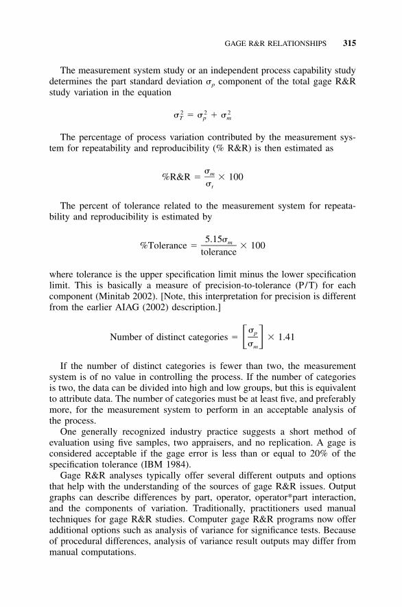
GAGE R&R RELATIONSHIPS 315

The measurement system study or an independent process capability studydetermines the part standard deviation �p component of the total gage R&Rstudy variation in the equation

2 2 2� � � � �T p m

The percentage of process variation contributed by the measurement sys-tem for repeatability and reproducibility (% R&R) is then estimated as

�m%R&R � � 100�t

The percent of tolerance related to the measurement system for repeata-bility and reproducibility is estimated by

5.15�m%Tolerance � � 100tolerance

where tolerance is the upper specification limit minus the lower specificationlimit. This is basically a measure of precision-to-tolerance (P/T) for eachcomponent (Minitab 2002). [Note, this interpretation for precision is differentfrom the earlier AIAG (2002) description.]

�pNumber of distinct categories � � 1.41� ��m

If the number of distinct categories is fewer than two, the measurementsystem is of no value in controlling the process. If the number of categoriesis two, the data can be divided into high and low groups, but this is equivalentto attribute data. The number of categories must be at least five, and preferablymore, for the measurement system to perform in an acceptable analysis ofthe process.

One generally recognized industry practice suggests a short method ofevaluation using five samples, two appraisers, and no replication. A gage isconsidered acceptable if the gage error is less than or equal to 20% of thespecification tolerance (IBM 1984).

Gage R&R analyses typically offer several different outputs and optionsthat help with the understanding of the sources of gage R&R issues. Outputgraphs can describe differences by part, operator, operator*part interaction,and the components of variation. Traditionally, practitioners used manualtechniques for gage R&R studies. Computer gage R&R programs now offeradditional options such as analysis of variance for significance tests. Becauseof procedural differences, analysis of variance result outputs may differ frommanual computations.

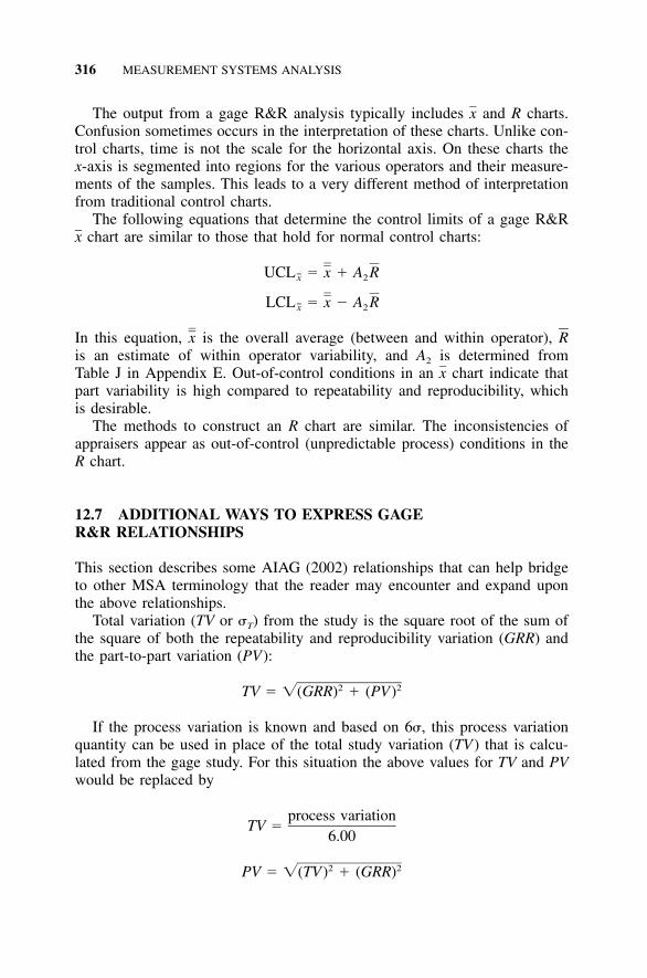
316 MEASUREMENT SYSTEMS ANALYSIS

The output from a gage R&R analysis typically includes and R charts.xConfusion sometimes occurs in the interpretation of these charts. Unlike con-trol charts, time is not the scale for the horizontal axis. On these charts thex-axis is segmented into regions for the various operators and their measure-ments of the samples. This leads to a very different method of interpretationfrom traditional control charts.

The following equations that determine the control limits of a gage R&Rchart are similar to those that hold for normal control charts:x

UCL � x � A Rx 2

LCL � x � A Rx 2

In this equation, is the overall average (between and within operator),x Ris an estimate of within operator variability, and A2 is determined fromTable J in Appendix E. Out-of-control conditions in an chart indicate thatxpart variability is high compared to repeatability and reproducibility, whichis desirable.

The methods to construct an R chart are similar. The inconsistencies ofappraisers appear as out-of-control (unpredictable process) conditions in theR chart.

12.7 ADDITIONAL WAYS TO EXPRESS GAGER&R RELATIONSHIPS

This section describes some AIAG (2002) relationships that can help bridgeto other MSA terminology that the reader may encounter and expand uponthe above relationships.

Total variation (TV or �T) from the study is the square root of the sum ofthe square of both the repeatability and reproducibility variation (GRR) andthe part-to-part variation (PV):

2 2TV � �(GRR) � (PV)

If the process variation is known and based on 6�, this process variationquantity can be used in place of the total study variation (TV) that is calcu-lated from the gage study. For this situation the above values for TV and PVwould be replaced by

process variationTV �

6.00

2 2PV � �(TV) � (GRR)

PREPARATION FOR A MEASUREMENT SYSTEM STUDY 317

Repeatability is sometimes called equipment variation (EV or �E). The percentof equipment variation (%EV) to total variation is

EV%EV � 100 � �TV

Similarly, other percent relationships for appraiser variation (AV), gageR&R (GRR), and part variation (PV) can be determined.

AV%AV � 100 � �TV

GRR%GRR � 100 � �TV

PV%PV � 100 � �TV

Results from the percent total variation are assessed to determine the accept-ability of the measurement system for the intended application.

For an analysis based on tolerance instead of process variation, %EV, %AV,%GRR, and %PV are calculated by substituting the value of tolerance dividedby six for TV. Either process or tolerance analysis (or both) can be used,depending on the intended use of the measurement system and customer de-sires.

The number of distinct categories (ndc) that can reliably distinguished bythe measurement system is

PVndc � 1.41

GRR

The ndc is truncated to the integer and should be greater than or equal to 5.

12.8 PREPARATION FOR A MEASUREMENT SYSTEM STUDY

Sufficient planning and preparation should be done prior to conducting ameasurement system study. Typical preparation prior to study includes thefollowing steps:

1. Plan the approach. For instance, determine by engineering judgment,visual observations, or gage study if there is appraiser influence in cal-ibrating or using the instrument. Reproducibility can sometimes be con-sidered negligible—for example, when pushing a button.

318 MEASUREMENT SYSTEMS ANALYSIS

2. Select number of appraisers, number of sample of parts, and number ofrepeat reading. Consider requiring more parts and/or trials for circledimensions. Bulky or heavy parts may dictate fewer samples. Considerusing at least 2 operators and 10 samples, each operator measuring eachsample at least twice (all using the same device). Select appraisers whonormally operate the instruments.

3. Select sample parts from the process that represent its entire operatingrange. Number each part.

4. Ensure that the instrument has a discrimination that is at least one-tenthof the expected process variation of the characteristic to be read. Forexample, if the characteristic’s variation is 0.001, the equipment shouldbe able to read a change of 0.0001.

Ensure that the measuring method of the appraiser and instrument is fol-lowing the defined procedure. It is important to conduct the study properly.All analyses assume statistical independence of all readings. To reduce thepossibility of misleading results, do the following:

1. Execute measurements in random order to ensure that drift or changesthat occur will be spread randomly throughout the study.

2. Record readings to the nearest number obtained. When possible, makereadings to nearest one-half of the smallest graduation (e.g., 0.00005for 0.0001 graduations).

3. Use an observer who recognizes the importance of using caution whenconducting the study.

4. Ensure that each appraiser uses the same procedure when taking mea-surements.

12.9 EXAMPLE 12.1: GAGE R&R

S4 /IEE Application Example

• Manufacturing 30,000-foot-level metric (KPOV): An S4 /IEE project wasto improve the capability /performance of the diameter for a manufac-tured product. An MSA was conducted of the measurement gage.

Five samples selected from a manufacturing process are to represent thenormal spread of the process. Two appraisers who normally do the measure-ments are chosen to participate in the study. Each part is measured three timesby each appraiser. Results of the test are shown in Table 12.1 (AIAG 1995a).

The computer output for a gage R&R study is shown next where Figure12.2 shows the computer graphical output. An analysis discussion then fol-lows.

EXAMPLE 12.1: GAGE R&R 319

TABLE 12.1 Measurements for Gage R&R Example

Trials

Appraiser 1

Part 1 Part 2 Part 3 Part 4 Part 5

1 217 220 217 214 2162 216 216 216 212 2193 216 218 216 212 220

Avg. 216.3 218.0 216.3 212.7 218.3Range 1.0 4.0 1.0 2.0 4.0

Average of averages � 216.3

Trials

Appraiser 2

Part 1 Part 2 Part 3 Part 4 Part 5

1 216 216 216 216 2202 219 216 215 212 2203 220 220 216 212 220

Avg. 218.3 217.3 215.7 213.3 220.0Range 4.0 4.0 1.0 4.0 0.0

Average of averages � 216.9

X Chart by Operator

Gage R & R (ANOVA) for Resp Gage name:Date of study:Reported by:Tolerance:Misc:

Operator*Part Interaction

R Chart by Operator By Operator

1 2 3 4 5

Components of Variation By Part

3.0SL = 219.2

3.0SL = 6.436

% Total Var

% Study Var

R = 2.500

–3.0SL = 0.000

221220

220219218217216215214213212

220219218217216215214213212

220219218217216215214213212

219218217216215214213212

76543210

10090

8070

6050

4030

2010

Gage R&R Repeat Reprod Part-to-Part0

–3.0SL = 214.2

x = 216.6

Per

cent

Sam

ple

rang

eS

ampl

e m

ean

Ave

rage

Operator

1

12

2

Part ID

Oper ID

Part ID 1 2 3 4 5

–

–

–

FIGURE 12.2 Gage R&R plots.

320 MEASUREMENT SYSTEMS ANALYSIS

Gage R&R Computer Output

Gage R&R Study—Analysis of Variance MethodAnalysis of Variance Table with Operator*PartInteraction

Source DF SS MS F P

Parts 4 129.467 32.3667 13.6761 0.01330Operators 1 2.700 2.7000 1.1408 0.34565Oper*Part 4 9.467 2.3667 0.9221 0.47064Repeatability 20 51.333 2.5667Total 29 192.967

Analysis of Variance Table Without Operator*PartInteraction

Source DF SS MS F P

Parts 4 129.467 32.3667 12.7763 0.0000Operators 1 2.700 2.7000 1.0658 0.3122Repeatability 24 60.800 2.5333Total 29 192.967

Gage R&R

Source VarComp StdDev 5.15*Sigma

Total Gage R&R 2.5444 1.59513 8.2149Repeatability 2.5333 1.59164 8.1970Reproducibility 0.0111 0.10541 0.5429Operator 0.0111 0.10541 0.5429

Part-to-Part 4.9722 2.22985 11.4837Total Variation 7.5167 2.74165 14.1195

Source %Contribution %Study Var

Total Gage R&R 33.85 58.18Repeatability 33.70 58.05Reproducibility 0.15 3.84Operator 0.15 3.84

Part-to-Part 66.15 81.33Total Variation 100.00 100.00

Number of Distinct Categories � 2

EXAMPLE 12.1: GAGE R&R 321

Gage R&R Output Interpretation

The first analysis of variance results considered both operators and opera-tor*part interaction. The second analysis of variance results did not considerthe operator*part interaction. From these analyses, operator and operator*partinteraction were not found to have statistical significance because the prob-ability of significance values (P) for operator or operator*part interaction werenot small (e.g., not less than 0.05).

A recreation of the computer output calculations for the ratio variancecomponent to total variance estimates is

Variance componentVariance component % � � 100

Total variance

2.5444Gage variance component % � � 100 � 33.85%

7.5167

4.9722Part-to-part variance component % � � 100 � 66.15%

7.5167

These results indicate a need to improve the measurement system, becauseapproximately 34% of the total measured variance is from repeatability andreproducibility of the gage.

The following shows a similar recreation of the previous computer outputcalculations, that the ratio of variance component to total variance is nowexpressed in 99 percentile units.

5.15 � standard deviationof component

% Study ratio � � 100Total of 5.15 � standard

deviation of all components

8.2149R&R % study Var � � 100 � 58.18

14.1195

11.4837Part-to-part % Var study � � 100 � 81.33

14.1195

Concern is again appropriate because about 58% of the 99% spread of vari-ability is estimated as coming from the measurement system.

The gage R&R computer output shows only two distinct categories, an-other indication that the gage is not effective. With only two distinct cate-gories, the data can be divided into high and low groups, which is equivalentto attribute data.

322 MEASUREMENT SYSTEMS ANALYSIS

Graphical outputs associated with a gage R&R study can give additionalinsight into a gage and opportunities for improvement. In a gage R&R studythe control chart address measurement variability relative to part-to-partxvariation. The limits for a control chart in a gage R&R study relate to part-to-part variation. The control limits for these charts are based on repeatabilityinconsistencies, not part-to-part variation. For this study, the chart by op-xerator plot had only 30%, or less than half, of the averages outside the limits.The measurement system in this example is concluded to be inadequate todetect part-to-part variations, assuming that the parts used in the study trulyrepresent the total process variation. An adequate measurement system ispresent when a majority of part averages fall outside the limits and appraisersagree on which parts fall outside the limits.

When the R chart of a gage R&R study is in control/predictable, the in-spection process by appraisers is similar. If one appraiser has an out-of-controlcondition, his/her method differs from the others. If all appraisers have someout-of-control ranges, the measurement system is apparently sensitive to ap-praiser technique and needs improvement to obtain useful data. For this ex-ample there does not appear to be any inconsistency within and betweenoperators.

Other output graphs from a gage R&R study can give additional insight tosources of variability (e.g., part-to-part, operator, operator*part interaction,and components of variance). These charts for this example do not appear tocontain any additional information that was already determined through othermeans.

This example did not include a percent part tolerance; however, similarcalculations to the percent study ratio could be made for this calculation. Forthe percent part tolerance calculations, part tolerance spread replaces the prod-uct of 5.15 times part-to-part standard deviation.

12.10 LINEARITY

Linearity is the difference in the bias values through the expected operatingrange of the gage. For a linearity evaluation, one or more operators measureparts selected throughout the operating range of the measurement instrument.For each of the chosen parts, the average difference between the referencevalue and the observed average measurement is the estimated bias. Sourcesfor reference values of the parts include tool room or layout inspection equip-ment.

If a graph between bias and reference values follows a straight linethroughout the operating rate, a regression line slope describes the best fit ofbias versus reference values. This slope value is then multiplied by the processvariation (or tolerance) of the parts to determine an index that represents thelinearity of the gage. Gage linearity is converted to a percentage of processvariation (or tolerance) when multiplied by 100 and divided by process var-

ATTRIBUTE GAGE STUDY 323

TABLE 12.2 Measurements for Linearity Example

Part:Reference Value:

12.00

24.00

36.00

48.00

510.00

1 2.70 5.10 5.80 7.60 9.102 2.50 3.90 5.70 7.70 9.303 2.40 4.20 5.90 7.80 9.504 2.50 5.00 5.90 7.70 9.305 2.70 3.80 6.00 7.80 9.406 2.30 3.90 6.10 7.80 9.507 2.50 3.90 6.00 7.80 9.508 2.50 3.90 6.10 7.70 9.509 2.40 3.90 6.40 7.80 9.60

10 2.40 4.00 6.30 7.50 9.2011 2.60 4.10 6.00 7.60 9.3012 2.40 3.80 6.10 7.70 9.40

Part average: 2.49 4.13 6.03 7.71 9.38Bias: �0.49 �0.13 �0.03 �0.29 �0.62Range: 0.4 1.3 0.7 0.3 0.5

iation (or tolerance). A scatter diagram of the best-fit line using graphicaltechniques can give additional insight to linearity issues.

12.11 EXAMPLE 12.2: LINEARITY

The five parts selected for the evaluation represent the operating range of themeasurement system based upon the process variation. Layout inspection de-termined the part reference values. Appraisers measured each part 12 timesin a random sequence. Results are shown in Table 12.2 (AIAG 2002).

Figure 12.3 shows the results of a computer analysis of the data. Thedifference between the part reference value and the part average yielded bias.Inferences of linear association between the biases (accuracy measurements)and reference value (master part measurement) use the goodness-of-fit (R2)value. Conclusions are then drawn from this to determine if there is a linearrelationship. Linearity is determined by the slope of the best-fit line, not thegoodness-of-fit (R2). If there is a linear relationship, a decision needs to bemade to determine if the amount is acceptable. Generally a lower slope in-dicates better gage linearity.

12.12 ATTRIBUTE GAGE STUDY

The following is a short method for conducting an attribute gage study. Anattribute gage either accepts or rejects a part after comparison to a set of

324 MEASUREMENT SYSTEMS ANALYSIS

2 3 4 5 6Master Part Measurement

LinearityP

erce

ntAcc

urac

y av

erag

e

Percent of Process Variation

Gage LinearityLinearity:

% Linearity:

R-Squared:

0.79

13.167

0.978

Accuracy:

% Accuracy:

5.33 × 10–2

0.889

Gage Linearity Study for Resp.

Gage Accuracy

Accuracy7 8 9 10

14

1

0

–1

1210

86420

Tolerance:Misc:

Gage name:Date of study:Reported by:

FIGURE 12.3 Plots for gage linearity.

limits. Unlike a variable gage, an attribute gage cannot quantify the degreeto which a part is good or bad.

A short attribute gage study can be conducted by first selecting 20 parts.Choose parts, if possible, so that some parts are slightly below and someabove specification limits. Use two appraisers and conduct the study in amanner to prevent appraiser bias. Appraisers inspect each part twice, decidingwhether the part is acceptable or not.

If all measurements agree (four per part), the gage is accepted. Gage needsimprovement or reevaluation if measurement decisions do not agree or arenot consistent with an established standard or correct answer (master at-tribute). Choose an alternative measurement system if gage cannot be im-proved since the measurement system is unacceptable (AIAG 2002).

Some statistical programs offer an analysis approach for an attribute gagestudy.

12.13 EXAMPLE 12.3: ATTRIBUTE GAGE STUDY

A company is training five new appraisers for the written portion of a stan-dardized essay test. The ability of the appraiser to rate essays relative tostandards needs to be assessed. Fifteen essays were rated by each appraiseron a five-point scale (�2, �1, 0, 1, 2). Table 12.3 shows the results of thetest. A statistical computer MSA analysis yielded:

325

TA

BL

E12

.3E

xam

ple

12.4

:A

ttri

bute

Gag

eSt

udy

Dat

a(M

init

ab13

)

App

rais

erSa

mpl

eR

atin

gA

ttrib

ute

App

rais

erSa

mpl

eR

atin

gA

ttrib

ute

App

rais

erSa

mpl

eR

atin

gA

ttrib

ute

Sim

pson

12

2Si

mps

on6

11

Sim

pson

11�

2�

2M

ontg

omer

y1

22

Mon

tgom

ery

61

1M

ontg

omer

y11

�2

�2

Hol

mes

12

2H

olm

es6

11

Hol

mes

11�

2�

2D

unca

n1

12

Dun

can

61

1D

unca

n11

�2

�2

Hay

es1

22

Hay

es6

11

Hay

es11

�1

�2

Sim

pson

2�

1�

1Si

mps

on7

22

Sim

pson

120

0M

ontg

omer

y2

�1

�1

Mon

tgom

ery

72

2M

ontg

omer

y12

00

Hol

mes

2�

1�

1H

olm

es7

22

Hol

mes

120

0D

unca

n2

�2

�1

Dun

can

71

2D

unca

n12

�1

0H

ayes

2�

1�

1H

ayes

72

2H

ayes

120

0Si

mps

on3

10

Sim

pson

80

0Si

mps

on13

22

Mon

tgom

ery

30

0M

ontg

omer

y8

00

Mon

tgom

ery

132

2H

olm

es3

00

Hol

mes

80

0H

olm

es13

22

Dun

can

30

0D

unca

n8

00

Dun

can

132

2H

ayes

30

0H

ayes

80

0H

ayes

132

2Si

mps

on4

�2

�2

Sim

pson

9�

1�

1Si

mps

on14

�1

�1

Mon

tgom

ery

4�

2�

2M

ontg

omer

y9

�1

�1

Mon

tgom

ery

14�

1�

1H

olm

es4

�2

�2

Hol

mes

9�

1�

1H

olm

es14

�1

�1

Dun

can

4�

2�

2D

unca

n9

�2

�1

Dun

can

14�

1�

1H

ayes

4�

2�

2H

ayes

9�

1�

1H

ayes

14�

1�

1Si

mps

on5

00

Sim

pson

101

1Si

mps

on15

11

Mon

tgom

ery

50

0M

ontg

omer

y10

11

Mon

tgom

ery

151

1H

olm

es5

00

Hol

mes

101

1H

olm

es15

11

Dun

can

5�

10

Dun

can

100

1D

unca

n15

11

Hay

es5

00

Hay

es10

21

Hay

es15

11

326 MEASUREMENT SYSTEMS ANALYSIS

Each Appraiser vs Standard

Assessment Agreement

Appraiser # Inspected # Matched Percent (%) 95.0% CIDuncan 15 8 53.3 (26.6, 78.7)Hayes 15 13 86.7 (59.5, 98.3)Holmes 15 15 100.0 (95.2,100.0)Montgomery 15 15 100.0 (95.2,100.0)Simpson 15 14 93.3 (68.1, 99.8)

# Matched: Appraiser’s assessment across trials agreeswith standard.

Between Appraisers

Assessment Agreement

# Inspected # Matched Percent (%) 95.0% CI15 6 40.0 (16.3, 67.7)

# Matched: All appraisers’ assessments agree with eachother.

All Appraisers vs Standard

Assessment Agreement

# Inspected # Matched Percent (%) 95.0% CI15 6 40.0 (16.3, 67.7)

# Matched: All appraisers’ assessments agree withstandard.

Figure 12.4 shows a plot of the results.

12.14 GAGE STUDY OF DESTRUCTIVE TESTING

Unlike nondestructive tests, destructive tests cannot test the same unit re-peatedly to obtain an estimate for pure measurement error. However, an upperbound on measurement error for destructive tests is determinable using thecontrol chart technique described (Wheeler 1990).

When testing is destructive, it is impossible to separate the variation of themeasurements themselves from the variation of the product being measured.However, it is often possible to minimize the product variation between pairs

EXAMPLE 12.4: GAGE STUDY OF DESTRUCTIVE TESTING 327

SimpsonMontgomeryHolmesHayesDuncan

100

90

80

70

60

50

40

30

20

Appraiser

Per

cent

Appraiser vs. Standard

Assessment AgreementDate of study:Reported by:Name of product:Misc:

[ , ] 95.0% CI

Percent

FIGURE 12.4 Attribute MSA.

TABLE 12.4 Destructive Testing Example: Calculations for Range Chart

Lot: 1 2 3 4 5 6 7Sample 1: 20.48 19.37 20.35 19.87 20.36 19.32 20.58Sample 2: 20.43 19.23 20.39 19.93 20.34 19.30 20.68Range: 0.05 0.14 0.04 0.06 0.02 0.02 0.10

of measurements through the careful choice of the material that is to bemeasured. Through repeated duplicate measurements on material that isthought to minimize product variation between the two measurements, anupper bound is obtainable for the variation due to the measurement process.The simple control chart method illustrated in the following example showsthe application of this procedure.

12.15 EXAMPLE 12.4: GAGE STUDY OF DESTRUCTIVETESTING

The data in Table 12.4 are viscosity measurements by lot (Wheeler 1990).For this measurement systems analysis study, consider that the readings for

328 MEASUREMENT SYSTEMS ANALYSIS

FIGURE 12.5 Range chart of difference between two samples for destructive test.

the samples represent duplicate measurements because they were obtainedusing the same methods, personnel, and instruments. Because each lot isseparate, it is reasonable to interpret the difference between the two viscositymeasurements as the primary component of measurement error. To illustratethe broader application of this approach, consider that these data could alsorepresent a continuous process where the measurements are destructive. Ifthis were the case, measurements would need to be taken so that the samplesare as similar as possible. This selection often involves obtaining samples asclose together as possible from the continuous process.

Figure 12.5 shows a range chart for these data. These duplicate readingsshow consistency because no range exceeds the control limit of 0.2007. Anestimate for the standard deviation of the measurement process is

R 0.0614� � � � 0.054m d 1.1282

where is average range and d2 is from Table J in Appendix E, where n �R2.

These calculated ranges do not reflect batch-to-batch variation and shouldnot be used in the construction of the control limits for average viscosity.When tracking the consistency of the process, it is best to use the average ofthe duplicate readings with an individual chart and a moving range chart (i.e.,XmR chart), as in Table 12.5. The grand average is 20.045 and the averagemoving range is 0.9175. The XmR chart in Figure 12.6 indicates no incon-sistency in the process.

Both types of control charts are needed. The range chart checks for con-sistency within the measurement process, while the XmR chart checks forconsistency of the production process.

EXAMPLE 12.4: GAGE STUDY OF DESTRUCTIVE TESTING 329

TABLE 12.5 Destructive Testing Example: Calculations for XmR Chart

Lot: 1 2 3 4 5 6 7Sample 1: 20.48 19.37 20.35 19.87 20.36 19.32 20.58Sample 2: 20.43 19.23 20.39 19.93 20.34 19.30 20.68:x 20.455 19.300 20.370 19.900 20.350 19.310 20.630

MR 1.155 1.07 0.47 0.45 1.04 1.32

23

22

21

20

1918

171 2 3 4

Subgroup5 6 7

3

2

1

0

Indi

vidu

al v

alue

Mov

ing

rang

e

UCL = 22.49

UCL = 2.998

LCL = 17.60

LCL = 0.000

X = 20.04

R = 0.9175

=

–

FIGURE 12.6 XmR chart of mean of two samples for destructive test.

From the individual chart, an estimate for the standard deviation of theproduct measurements is

R 0.9175� � � � 0.813p d 1.1282

where is average range and d2 is from Table J, where n � 2.RThe estimated number of distinct categories is then

� 0.813pNumber of distinct categories � � 1.41 � � 1.41 � 21.2� �� 0.054m

The magnitude for number of distinct categories suggests that the measure-ment process adequately detects product variation.

In summary, the pairing of units such that sample-to-sample variation isminimized can give a reasonable estimate of the measurement process usinga simple control chart approach. Estimates from these calculations are useful

330 MEASUREMENT SYSTEMS ANALYSIS

to then determine an estimate for the number of distinct categories for themeasurement process.

12.16 A 5-STEP MEASUREMENT IMPROVEMENT PROCESS*

Gage R&R studies are useful for quantifying the variation in a measurementsystem; however, this is only part of the problem (Enck 2002). Once thevariation is identified, the team needs a method to reduce it. In addition, fora complete assessment of the measurement system, teams need to address theimportant issues of accuracy and long-term stability. This section provides anoverview of a 5-step measurement system analysis and improvement processthat addresses these measurement system issues. This methodology has beensuccessfully used in a variety of industries, from semiconductor to medicaldevice manufacturing, to improve and control their measurement systems.

Previously the standard breakdown of the measurement variance for a gageR&R study was described as the variance of the gage plus the variance ofthe operator. In order to reduce the measurement variation this general break-down needs to be further refined so specific sources of variation can be iden-tified and removed. The described approach provides a simple and effectivemethod for identifying and helping the practitioner reduce measurement var-iation.

The following 5-step method assesses sources of variation in stages. Ateach stage the practitioner is responsible for hypothesizing the potentialsources of variation and developing methods to remove them if the measure-ment system variation for that stage is too large. The following provides anapplied view of the 5-step methodology. Each step has the purpose, accep-tance criteria, method to conduct the test, and comments. Documentation isan important part of the analysis. Documentation should be such that practi-tioners conducting future studies will know the measurement relevance, whatequipment was used, what measurements were taken, and the procedure usedto make those measurements.

Terminology and relationships used in the 5-step measurement improve-ment process sections are:

• NPV � natural process variation, T � tolerance, P � precision• SMS � standard deviation of measurement system• STotal � standard deviation of total variability of measurements over time

from true value variabilities and measurement error• P /T � (5.15 � SMS) /Tolerance• P /NPV � (5.15 � SMS) /(5.15 � Stotal) � SMS /Stotal

*David Enck contributed this section.

A 5-STEP MEASUREMENT IMPROVEMENT PROCESS 331

1. Machine Variation

This step tries to reduce the impact of external sources of variation on themeasurement system so that the experimenter can study variation due only togage variables, short-term environmental variables, and possibly some oper-ator variables.

Sources of Variation. Machine variation, short-term environmental, possibleoperator variables, and unstable fixture.

How to Conduct this Test

1. Take 20 to 30 sequential measurements of a typical part.2. Do not touch the part or adjust the gage during the measurements.3. Use one operator.

Acceptance Criteria

1. Plot the observations on a control chart and determine that there are nosignificant out-of-control patterns.

2. If there are fewer than five distinct measurement values the controllimits will be slightly narrow due to rounding.• This needs to be considered for any control chart run rules (see Sec-

tion 10.9).• If an observation is outside the control limits, but within one resolu-

tion increment, the process may not be out of control (i.e., a predict-able process).

3. The P /T (P /NPV) ratio is less than 5% (10%) unless operator decisionsare involved in the measurement, in which case it may go as high as10% (15%).

Comments

1. Twenty to 30 measurements were used because the machine variationmeasurements are typically easy to collect. If the measurements aredifficult to obtain, a minimum is usually 16.

2. The ratio targets are typical standards and may be modified based oncircumstances.

3. Conduct a blind study.• An operator measures the part, but is not allowed to see or hear the

final measured value.• A second person records the measurements.

332 MEASUREMENT SYSTEMS ANALYSIS

2. Fixture Study

This step evaluates the variation added due to the part being refixtured. Formeasurement systems that are manual, variation seen in the fixture studyimpacts between operator differences as well, so any improvements to themeasurement process can impact reproducibility as well as repeatability.Rather than running the whole gage R&R study and finding that the fixturemethod adds a lot of variation, this step allows a shorter test to be used tofix any problems that you find prior to conducting the larger gage R&R study.

Sources of Variation. Same as machine variation, with refixturing included.

How to Conduct This Test

1. Take 16 measurements of a typical part.2. Remove the part from the gage and replace it for each measurement.3. Use one operator.

Acceptance Criteria

1. Plot the observations on a control chart and determine that there are nosignificant out-of-control patterns.

2. The P /T (P /NPV) ratio is less than 15 to 20% (20 to 25%). This isflexible and it depends on what the final goal is. However, the largerthe values the less likely it is to reach the final goal.

Comments

1. If the results are unacceptable, use technical knowledge and organiza-tional wisdom to change the system and retest. Once the variation inthis stage is satisfactory, move on to the next test.

3. Accuracy (Linearity)

This step determines whether the measurement system is biased across thetolerance range of the parameter being measured.

How to Conduct This Test

1. Take 16 measurements of a traceable standard.2. Do not adjust the gage during the measurements.3. Remove the standard from the gage and replace it for each measure-

ment.

A 5-STEP MEASUREMENT IMPROVEMENT PROCESS 333

4. Repeat this for three standards (low, middle, high) across the range ofthe natural process variation of the parts.

5. Use one operator.

Acceptance Criteria

1. Plot the observations on a control chart and determine that there are nosignificant out-of-control patterns.

2. Ninety-five percent confidence intervals contain the certified standardvalue for each of the three standards.

3. Regression analysis shows an insignificant slope from a practical pointof view (e.g., the bias may be increasing; however, if the largest biasis less than 5% of the specification range, you should also compare thebias to the natural process variation).

4. The P /T ratio for an accuracy study will be close to the P /T for thefixture variation study. Since the measurements are on standards thatmay be different than the parts being measured, this metric is not crit-ical.

4. Repeatability and Reproducibility

This step (the traditional ‘‘R&R’’) will use additional experiments to quantifythe total variation of the measurement system. Further, we will be able toisolate between operator, part, and within operator variation. If the total var-iation for the measurement system is unacceptable, the isolated sources ofvariation will provide a guide to where the best opportunities for improvementlie.

Sources of Variation. Same as refixturing with time, operator, and operator-by-part variation included.

How to Conduct This Test

1. Develop a measurement plan based on the sources of variation to bestudied and the hypothesized importance of each source of variation.Below are some possible ranges to use when selecting the measurementplan:• Four to six operators• Four to six parts• Three to four measurements per day• Three to five days

2. Do not adjust the gage during the measurements. If it is known that thegage is incapable of remaining stable over time, fix this source of var-

334 MEASUREMENT SYSTEMS ANALYSIS

iation prior to conducting the gage R&R. If it is not possible, use thestandard preparation method during the gage R&R stage.

3. Set up a measurement schedule that randomizes the order of the oper-ators and the order in which the parts are measured. This is used to tryto spread the effects of any unknown factors between all assignablesources of variation equally.

4. Have the operators’ record factors that may affect the measurements,such as temperature, gage settings, condition of part, and observationsabout anything unusual. These can be written down on the data sheets.

5. Analyze the data as described previously.

Acceptance Criteria

1. Refer to gage R&R section.2. P /T and P /NPV are less than the targets.

5. Long-Term Stability

This step will monitor the measurement system on an ongoing basis in orderto verify that the system is operating in the same manner (i.e., stable andconsistent) over time. This can also be used to provide information on whena gage may need to be calibrated.

How to Conduct This Test

1. Obtain one to two parts that can be used as internal reference parts.2. Meet with the operators and discuss the importance of this part of the

MCA. With the operators’ input, create a measurement plan that coversall shifts and all operators. This sampling plan is important in that itwill provide information about the whole measurement system.

3. Measure the parts at least once a day over a 20–30-day period for aminimum of 20 to 30 measurements.

4. After the initial measurements, implement a sampling plan to monitorthe measurement system continually as long as it is being used. Basedon the results of the initial measurements, the sampling plan may bereduced if the process is stable. Even with a reduced sampling plan thephilosophy of complete system coverage should be maintained.

5. Document the conditions during the measurements. Document variablesthat are thought to be important:• Operator• Any important gage settings• Any important environmental conditions

EXAMPLE 12.5: A 5-STEP MEASUREMENT IMPROVEMENT PROCESS 335

Acceptance Criteria

1. Plot the observations on a control chart and determine that there are nosignificant out-of-control patterns.

2. The P/T and P/NPV ratios are satisfactory (meet the previously spec-ified criteria).

Comment

1. If the process goes out of control and cannot be brought back so thatit is in control/predictable, the measurement system needs to be recal-ibrated.

2. As long as the process is in control, the variation and calibration havenot changed.

3. Consider using this control process as part of the calibration process.

12.17 EXAMPLE 12.5: A 5-STEP MEASUREMENTIMPROVEMENT PROCESS

The following example will provide a brief description of the machine vari-ation, fixture variation, linearity, gage R&R, and long-term stability studiesfor an optical microscope (Enck 2002).

A company used an optical microscope to measure part widths. A total of30 operators used the measurement technique on a daily basis. An S4/IEEteam was working on reducing the defect rate for this particular KPOV. Afterbaselining and calculating the process capability for this parameter, they con-ducted a five-step measurement system analysis. Organizational wisdom in-dicated that the measurement system had a lot of variation; however, it hadnever been quantified using a P /T ratio. In order to keep the project on track,the objective of the measurement system analysis was to develop a testmethod that had a P /T and P /NPV ratio that was less than 30%. Any furtherimprovements would be handled by another team at a later date. The parttolerance was 1.2 mils and the historical process standard deviation was 0.21mils.

The measurement process consisted of aligning the part with the centerlineof the screen, zeroing out the micrometer, rolling the stage until the centerlinewas aligned with the opposite side of the part, and recording the measurement.Figure 12.7 shows the optical microscope screen.

1. Machine Variation

The machine variation phase consisted of placing a part on the microscopestage and measuring it 30 times without touching the part. An XmR control

336 MEASUREMENT SYSTEMS ANALYSIS

14 in.

FIGURE 12.7 Optical microscope screen.

FIGURE 12.8 XmR chart for machine variation phase.

chart and P /T ratio were used to analyze the results. Figure 12.8 shows thecontrol chart.

All measurements collected in this 5-step study were taken in a blind man-ner. A piece of paper was placed over the gage display and the operatorconducted the measurement as stated in the SOP. When the measurement was

EXAMPLE 12.5: A 5-STEP MEASUREMENT IMPROVEMENT PROCESS 337

Variation inmeasurements fromoptical comparator

Method Machine

Personnel Materials

** Poor edge selection

Stage slop relative to gagePart fixtured with edge not parallel towhisker** Poor operational definition of "edge"** Poor operational definition of how toselect the part edge with the centerline

Edge not well defined

FIGURE 12.9 Highlights from a cause-and-effect diagram to identify potentialcauses of excess variation.

completed a second person looked under the paper and recorded the mea-surement without telling the operator the result.

The measurements were in-control/predictable; however, the P /T ratio was15.8%. When operators make decisions about where to start and stop mea-surements, the measurement variation tends to be high. The team wanted toreduce the variation so that when more operators were included the P /T ratiowould remain acceptable.

Figure 12.9 highlights the results from a cause-and-effect diagram, whichwas used to identify potential causes of excess variation in the optical micro-scope measurement process. Edge selection was selected as having the largestpotential impact on the measurement variation. An improved edge selectionprocess was then developed, which used the left side of the centerline as thestarting point and ending point for the measurement.

The 30 measurements for the machine variation study were repeated withthe new process. An XmR chart indicated that the process was in-control/predictable and the P /T ratio had been reduced to 7.08%. A statistical testthat compared the initial process variance to the new process variance showeda significant difference with a p value less than 0.001. The measurementvariation at this stage was deemed acceptable so the team proceeded to thefixture variation study.

2. Fixture Variation

The fixture variation study consisted of picking the part up, placing it on thestage, measuring the part, and repeating the process. This procedure wasrepeated 16 times. An XmR chart was generated and P /T ratio was deter-mined. The control chart was in-control/predictable with a P /T ratio of15.46%. Part orientation was considered the most likely candidate for theincrease in variation. The standard operating procedure for the measurement

338 MEASUREMENT SYSTEMS ANALYSIS

NIST Std

Dev

from

Std

FIGURE 12.10 Regression analysis of the deviation from target for 16 measure-ments that were taken for each standard versus the stated value of the standard.

was then modified to improve part alignment. The team believed that mostof the variation of the measurement process was represented by the fixturevariation study and that difference between operators would be small. Becauseof this, the team felt comfortable moving to the next step of the 5-step mea-surement system analysis with the improved SOP.

3. Linearity Study

The linearity study assessed the bias across the range of part widths of inter-est. There was a concern that if a single operator were used, any bias wouldreflect bias of the operator and that this would differ between operators. Itwas decided to pick the most experienced operator and assume that any biasobserved would be from the gage rather than the operator. If there was adifference between operators, it would show up in the gage R&R study asexcessive variation from differences between operators.

Standards were selected at the low, medium, and high levels of the rangeof interest. Figure 12.10 shows the regression analysis of the deviation fromtarget for 16 measurements that were taken for each standard versus the statedvalue of the NIST standard. The relationship is statistically significant; how-

EXAMPLE 12.5: A 5-STEP MEASUREMENT IMPROVEMENT PROCESS 339

FIGURE 12.11 Gage R&R study, part 1.

ever, when using the average deviation from target, the maximum bias for thethree standards was less than 5% of the specification range. Given the rela-tively small bias over the range of interest the bias was considered not tohave practical significance.

4. Repeatability and Reproducibility

The gage R&R study consisted of three operators measuring each of threeparts three times a day for four days. The SOPs developed during the machineand fixture variation studies were used for this study. Each operator wastrained on the SOP and was required to conduct a 16-run fixture study achiev-ing a 20% P /T ratio prior to being certified for the measurement system.Once the operators were certified the gage R&R study was conducted. Theanalysis, as seen in Figures 12.11 and 12.12, follows from the previous dis-cussion on gage R&R studies. There were statistical differences observedbetween operators, however, the differences were not of practical importanceto the team’s goal. The P /T ratio was 20.13%, and the P /NPV was 22.83%.These results met the stated goals so the team moved on to the next phase ofthe five-step measurement system analysis.

The objective of this team was to develop a test method that had a P /Tratio and P /NPV ratio that were less than 30%. If they had wanted to quantify

340 MEASUREMENT SYSTEMS ANALYSIS

P/NPV = 22.33%(historical sigma)

P/T = 20.13%

FIGURE 12.12 Gage R&R study, part 2.

the improvement in the measurement system they would have conducted agage R&R study prior to starting the five-step measurement system analysisso they would have had a baseline to compare their results with.

5. Long-Term Stability

The team selected a single part for the long-term stability control chart. Abaseline of 20 days was established, with the part being measured once a day.The shift and operator were randomly selected and recorded. The part thatwas measured was called the golden part and was kept in a nitrogen box nextto the measurement gage. The long-term stability control chart was used todetect any change in the measurement process that might cause an increasein the measurement system variation or a change in the accuracy.

Summary

This section provided a five-step measurement system analysis and a simpleexample. This method can be used as part of an S4/IEE project or as anintegrated part of how measurement systems are set up in either a manufac-turing plant or research and development lab.

EXERCISES 341

12.18 S4/IEE ASSESSMENT

Organizations often overlook the importance of conducting a measurementsystems analysis. Much money can be wasted trying to fix a process whenthe major source of variability is the measurement system. Practitioners oftenneed to give more consideration to the measurement system before beginningexperimentation work. To illustrate the importance of pretest measurementsystems analysis, consider a DOE. When the measurement system is poor,significance tests can detect only factors with very large effects. There mightbe no detection of important smaller factor effects. The importance of a mea-surement system is also not often considered when making sample size andconfidence interval calculations. An unsatisfactory measurement system canaffect these calculations dramatically.

This chapter describes procedures to determine whether a measurementsystem is satisfactory. The measurement system is only one source of varia-bility found when a product or process is measured. Other possible sourcesof variability are differences between raw material, manufacturing lines, andtest equipment. In some experiments it is advantageous to consider these othersources of variability in addition to operator variability within the experiment.The techniques described in Chapter 22 use a nested design structure that canquantify the variance components not only of a process but also of measure-ment system parameters. Knowing and then improving the sources of varia-bility for a measurement system improve the bottom line in an expedientmanner. Note that a measurement systems analysis may need reanalysis asthe capability/performance of a process improves.

12.19 EXERCISES

1. Machine Screws Exercise: Teams are to conduct a gage R&R study ofthe length measurement of machine screws. Five machine screws (ap-proximately 2 in. long) will be supplied to each team for analysis. Thesemachine screws were previously filed or ground so that the lengths ofscrews within a set span a certain range (e.g., 0.030 in.). Teams areinstructed to conduct a gage R&R using two appraisers where each partis measured twice by each appraiser. Measurements are to be recordedto the nearest one-tenth of the smallest increment on the rule.

2. M&M’s Candy Exercise: A team sets up the procedure to conduct anexperiment in which 20 M&M’s candies are taken from a bag. For eachteam there will be two or three appraisers examining the candies. One tothree people will collect and compile the results in a table like the fol-lowing table:

342 MEASUREMENT SYSTEMS ANALYSIS

Sample

Appraiser 1

Test 1: OK? Test 2: OK?

Appraiser 2

Test 1: OK? Test 2: OK?

Appraiser 3

Test 1: OK? Test 2: OK?

Overall

All Agree?

1

2

�

�

�

19

20

% Time operconsistenta

Answer: Answer: Answer:

% overallConsistentb

Answer:

a 100 times number of times in agreement for each pair of columns divided by 20.b 100 times number of times ‘‘yes’’ in ‘‘all agree’’ column divided by 20.

3. In an exercise in Chapter 3 a paragraph of a book was examined. Thetimes the sixth character occurs was counted. Discuss this visual inspec-tion process. What you think should be done to increase awareness ofany deficiencies and approaches for making process improvements?

4. Conduct a gage R&R study of the following data, where five parts areevaluated twice by three appraisers.

Part

Appraiser A

1 2 3 4 5

Appraiser B

1 2 3 4 5

Appraiser C

1 2 3 4 5

1 113 113 71 101 113 112 117 82 98 110 107 115 103 110 131

2 114 106 73 97 130 112 107 83 99 108 109 122 86 108 90

5. For the following data, conduct a gage R&R study to assess whether thegage is acceptable, may be acceptable, or is unacceptable. A specificationtolerance is 0.004 (i.e., for a specification of 0.375 � 0.002, where mea-surement unit is 0.0001). A table value of 56, for example, equates to ameasurement of 0.3700 � (56 � 0.0001) � 0.3756 (IBM 1984).

EXERCISES 343

Appraiser

SampleNo.

1

1stTrial

2ndTrial

3rdTrial

2

1stTrial

2ndTrial

3rdTrial

3

1stTrial

2ndTrial

3rdTrial

1 56 55 57 57 58 56 56 57 56

2 63 62 62 64 64 64 62 64 64

3 56 54 55 57 55 56 55 55 55

4 57 55 56 56 57 55 56 57 55

5 58 58 57 59 60 60 57 60 60

6 56 55 54 60 59 57 55 57 56

7 56 55 56 58 56 56 55 55 57

8 57 57 56 57 58 57 57 58 57

9 65 65 64 64 64 65 65 64 65

10 58 57 57 61 60 60 58 59 60

6. Describe how the techniques in this chapter are useful and can be appliedto S4/IEE projects.

7. Determine an estimate for bias given the following set of measurementsand a reference value of 19.919: 20.5513, 20.1528, 20.6246, 19.9609,and 20.7493. (Six Sigma Study Guide 2002.)

8. Conduct an MSA of the following data. State the level of significance ofthe interaction between part and appraiser. Describe equipment variationas a percent of process variation. Describe appraiser variation as a per-centage of process variation. (Six Sigma Study Guide 2002.)

Part Appraiser Trial Measurement

1 1 1 7.7831 1 2 8.0121 1 3 7.7181 1 4 7.9551 2 1 8.5821 2 2 8.1921 2 3 8.4381 2 4 8.2052 1 1 12.3622 1 2 12.3272 1 3 12.5782 1 4 12.6922 2 1 13.366

344 MEASUREMENT SYSTEMS ANALYSIS

Part Appraiser Trial Measurement

2 2 2 13.6572 2 3 13.2622 2 4 13.3643 1 1 9.7243 1 2 9.9303 1 3 9.2033 1 4 10.1073 2 1 10.1823 2 2 10.4603 2 3 10.3603 2 4 10.7104 1 1 15.7344 1 2 14.9794 1 3 14.8174 1 4 14.4894 2 1 15.4214 2 2 15.6224 2 3 15.7894 2 4 15.6615 1 1 11.2205 1 2 12.3555 1 3 11.8375 1 4 12.1265 2 1 12.1485 2 2 12.5085 2 3 13.1935 2 4 11.9866 1 1 17.1236 1 2 17.1916 1 3 17.7316 1 4 17.0796 2 1 18.8056 2 2 18.9486 2 3 19.5706 2 4 19.2447 1 1 15.6437 1 2 16.2947 1 3 16.2557 1 4 16.1617 2 1 17.2117 2 2 17.1597 2 3 17.4307 2 4 17.699

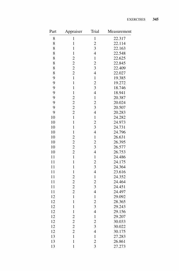
EXERCISES 345

Part Appraiser Trial Measurement

8 1 1 22.3178 1 2 22.1148 1 3 22.1638 1 4 22.5488 2 1 22.6258 2 2 22.8458 2 3 22.4098 2 4 22.0279 1 1 19.3859 1 2 19.2729 1 3 18.7469 1 4 18.9419 2 1 20.3879 2 2 20.0249 2 3 20.5079 2 4 20.283

10 1 1 24.28210 1 2 24.97310 1 3 24.73110 1 4 24.79610 2 1 26.63110 2 2 26.39510 2 3 26.57710 2 4 26.75311 1 1 24.48611 1 2 24.17511 1 3 24.36411 1 4 23.61611 2 1 24.35211 2 2 24.46411 2 3 24.45111 2 4 24.49712 1 1 29.09212 1 2 28.36512 1 3 29.24312 1 4 29.15612 2 1 29.20712 2 2 30.03312 2 3 30.02212 2 4 30.17513 1 1 27.28313 1 2 26.86113 1 3 27.273

346 MEASUREMENT SYSTEMS ANALYSIS

Part Appraiser Trial Measurement

13 1 4 26.71713 2 1 29.74213 2 2 29.24613 2 3 29.80813 2 4 29.60514 1 1 35.69314 1 2 35.95114 1 3 35.65014 1 4 35.78914 2 1 35.61614 2 2 35.83214 2 3 35.95814 2 4 35.97315 1 1 34.37415 1 2 34.27815 1 3 34.25015 1 4 34.47815 2 1 37.09315 2 2 38.10015 2 3 37.27115 2 4 37.706

9. Describe how and show where the tools described in this chapter fit intothe overall S4/IEE roadmap described in Figure A.1 in the Appendix.

10. Discuss the implication of MSA issues within your country’s court oflaw system.

11. Discuss the implication of MSA issues within the medical profession.

347

13CAUSE-AND-EFFECT MATRIXAND QUALITYFUNCTION DEPLOYMENT

Processes have inputs and outputs. Some outputs are more important to cus-tomers than others. The output of a process might be a product or service.Output variables can include delivery time or a dimension on a part. Inputvariables to a process can affect output variables.

Example input variables are operators, machines, process temperatures,time of day, and raw material characteristics. Some output variables to aprocess are more important to customers (internal and external) of the processthan others. The performance of these key output variables can be affectedby process input variables. However, all process-input variables do not affectkey output variables equally. To improve a process we need to determinewhat the key process input variables are, how they affect key process outputvariables, and what, if anything, should be done differently with these vari-ables (e.g., control them).

This chapter presents tools that can help assess the relationships betweenkey process input and key process output variables. Quality function deploy-ment (QFD) was discussed previously in Chapter 2 as a tool that could beused when organizations obtain VOC inputs. QFD is a powerful tool, but itcan require a great deal of time and resources to use. Other simpler-to-usetools such as the cause-and-effect matrix are described later in this chapter,which is also an integral part of the overall S4/IEE project execution roadmap(see Section A.1).

After a practitioner has identified potential key process input variables forthe output(s) of a process using a cause-and-effect diagram or other wisdomof the organization tool, he/she can use a cause-and-effect matrix in a teammeeting to prioritize the perceived importance of input variables.

348 CAUSE-AND-EFFECT MATRIX

13.1 S4/IEE APPLICATION EXAMPLES:CAUSE-AND-EFFECT MATRIX

S4/IEE application examples of a cause-and-effect matrix are:

• Satellite-level metric: S4/IEE projects were to be created that improvethe company’s ROI. A cause-and-effect diagram was created to generateideas for improving the metrics. A cause-and-effect matrix was createdto prioritize the importance of these items.

• Satellite-level metric: S4/IEE projects were to be created that improvethe company’s customer satisfaction. A cause-and-effect diagram wascreated to generate ideas for improving customer satisfaction. A cause-and-effect matrix was used to prioritize the importance of these items.

• Transactional 30,000-foot-level metric: DSO reduction was chosen as anS4/IEE project. The team used a cause-and-effect matrix to prioritizeitems from a cause-and-effect diagram.

• Manufacturing 30,000-foot-level metric (KPOV): An S4/IEE project wasto improve the capability/performance of the diameter of a manufacturedproduct (i.e., reduce the number of parts beyond the specification limits).The team used a cause-and-effect matrix to prioritize items from a cause-and-effect diagram.

• Transactional and manufacturing 30,000-foot-level cycle time metric (alean metric): An S4/IEE project that was to improve the time from orderentry to fulfillment was measured. The team used a cause-and-effect ma-trix to prioritize items from a cause-and-effect diagram.

• Transactional and manufacturing 30,000-foot-level inventory metric orsatellite-level TOC metric (a lean metric): An S4/IEE project was toreduce inventory. The team used a cause-and-effect matrix to prioritizeitems from a cause-and-effect diagram.

• Manufacturing 30,000-foot-level quality metric: An S4/IEE project wasto reduce the number of defect in a printed circuit board manufacturingprocess. The team used a cause-and-effect matrix to prioritize items froma cause-and-effect diagram.

• Product DFSS: An S4/IEE product DFSS project was to reduce the30,000-foot-level metric of the number of product phone calls generatedfor newly developed products. The team used a cause-and-effect matrixto prioritize items from a cause-and-effect diagram.

• Process DFSS: A team was to create a new call center. A process flow-chart of the planned call center process was created. The team used acause-and-effect matrix to prioritize items from cause-and-effect dia-grams on what should be included within the call center.

• S4/IEE infrastructure: A steering committee uses a cause-and-effect ma-trix as part of their black belt selection process.

QUALITY FUNCTION DEPLOYMENT (QFD) 349

13.2 QUALITY FUNCTION DEPLOYMENT (QFD)

S4 /IEE DMAIC Application: Appendix Section A.1, Project ExecutionRoadmap Step 2.1

Quality function deployment, or the house of quality, a term coined in QFDbecause of the shape of its matrix, is a tool that can aid in meeting the needsof the customer and in translating customer requirements into basic require-ments that have direction. It is a communication tool that uses a team concept,breaking down organizational barriers (e.g., sales, manufacturing, and devel-opment) so that product definition and efforts are directly focused on theneeds of the customer. A QFD chart can be used to organize, preserve, andtransfer knowledge. It can also be used in conjunction with DOE (see Ex-ample 43.2).

Many problems can be encountered when conducting a QFD. If extremecare is not exercised, one can reach the wrong conclusions. For example, biascan easily be injected into a survey through the way the questions are asked,the procedure that is used to conduct the survey, or the type of people whoare asked questions. Practitioners might ask themselves if they would expectto get the same results if the survey were conducted again (i.e., perhaps theexperimental error in the results is too high, and a forced comparison surveyprocedure should have been used). Erroneous conclusions also result fromthe data analysis—for example, the technical importance calculations that aremade in step 7 of the generic procedures described in the next section. In agiven situation it may be more important to weight responses by the impor-tance of overall secondary or primary customer requirements. Perhaps themost important benefit that can result from creating a QFD is via personalinterviews with customers. The comments resulting from these discussionscan perhaps give the best (although not numerically tangible) direction(Brown 1991).

An overall product QFD implementation strategy involves first listing thecustomer expectations (voice of the customer). These ‘‘whats’’ are then tab-ulated along with the list of design requirements (‘‘hows’’) related to meetingthese customers’ expectations (‘‘hows’’). The important ‘‘hows’’ can then betransferred to ‘‘whats’’ of another QFD matrix within a complete QFD matrix-to-matrix process flow. For example, consider the customer requirement ofincreasing the years of durability for a car. This matrix-to-matrix flow isexemplified in Table 13.1.

To determine accurate ‘‘whats’’ for the requirement matrix (i.e., accurateone-dimensional quality projections and anticipated attractive quality addi-tions), personal interviews with customers may first be appropriate. Surveysshould use the words of the customer when determining these ‘‘what’’ items.These ‘‘whats’’ can then be compiled into primary, secondary, and even ter-tiary requirements. Follow-up surveys can then be done using test summariesto get importance ratings (e.g., 1–5) for each ‘‘what’’ item. Opinions aboutcompetitive products can also be compiled during these surveys.

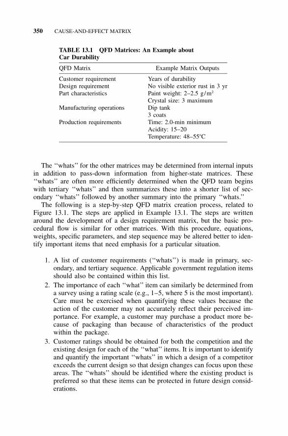
350 CAUSE-AND-EFFECT MATRIX

TABLE 13.1 QFD Matrices: An Example aboutCar Durability

QFD Matrix Example Matrix Outputs

Customer requirement Years of durabilityDesign requirementPart characteristics

No visible exterior rust in 3 yrPaint weight: 2–2.5 g/m2

Crystal size: 3 maximumManufacturing operations Dip tank

3 coatsProduction requirements Time: 2.0-min minimum

Acidity: 15–20Temperature: 48–55�C

The ‘‘whats’’ for the other matrices may be determined from internal inputsin addition to pass-down information from higher-state matrices. These‘‘whats’’ are often more efficiently determined when the QFD team beginswith tertiary ‘‘whats’’ and then summarizes these into a shorter list of sec-ondary ‘‘whats’’ followed by another summary into the primary ‘‘whats.’’

The following is a step-by-step QFD matrix creation process, related toFigure 13.1. The steps are applied in Example 13.1. The steps are writtenaround the development of a design requirement matrix, but the basic pro-cedural flow is similar for other matrices. With this procedure, equations,weights, specific parameters, and step sequence may be altered better to iden-tify important items that need emphasis for a particular situation.

1. A list of customer requirements (‘‘whats’’) is made in primary, sec-ondary, and tertiary sequence. Applicable government regulation itemsshould also be contained within this list.

2. The importance of each ‘‘what’’ item can similarly be determined froma survey using a rating scale (e.g., 1–5, where 5 is the most important).Care must be exercised when quantifying these values because theaction of the customer may not accurately reflect their perceived im-portance. For example, a customer may purchase a product more be-cause of packaging than because of characteristics of the productwithin the package.

3. Customer ratings should be obtained for both the competition and theexisting design for each of the ‘‘what’’ items. It is important to identifyand quantify the important ‘‘whats’’ in which a design of a competitorexceeds the current design so that design changes can focus upon theseareas. The ‘‘whats’’ should be identified where the existing product ispreferred so that these items can be protected in future design consid-erations.

QUALITY FUNCTION DEPLOYMENT (QFD) 351

FIGURE 13.1 A QFD chart format.

4. Engineering first compiles a list of design requirements that are nec-essary to achieve the market-driven ‘‘whats.’’ The design team listsacross the top of the matrix the design requirements (‘‘hows’’) thataffect one or more of the customer attributes. Each design requirementshould describe the product in measurable terms and should directlyaffect customer perceptions. For example, within a design require-ments matrix, the closing force of a car door may be noted, in contrastto the thickness of the metal within the door, which may be noted ina future parts characteristics matrix. The arrow at the top of the designrequirements listing indicates the direction for improvement (e.g., adownward-pointing error indicates that a lower value is better, while

[Image not available in this electronic edition.]

352 CAUSE-AND-EFFECT MATRIX

a zero indicates that a target is desired). Each ‘‘what’’ item is system-atically assessed for specific measurement requirements. Vague andtrivial characteristics should be avoided.

5. Cell strengths within the matrix are determined to quantify the impor-tance of each ‘‘how’’ item relative to getting each ‘‘what’’ item. Sym-bols describing these relationships include �, which indicates muchimportance or a strong relationship, �, which indicates some impor-tance or relationship, �, which indicates a small importance or rela-tionship, and no mark, which indicates no relationship or importance.The symbols are later replaced by weights (e.g., 9, 3, 1, and 0) to givethe relationship values needed to make the technical importance cal-culations. Initially, the symbols are used to clarify the degree of im-portance attributed to the relationships and weightings. From thisvisual representation, it is easier to determine where to place criticalresources. If a current quality control measurement does not affect anycustomer attribute, either it is not necessary or a ‘‘what’’ item is miss-ing. ‘‘How’’ items may need to be added so that there is at least one‘‘how’’ item for each ‘‘what’’ requirement.

6. From technical tests of both competitive products and our existingproduct design, objective measurements are added to the bottom of thehouse beneath each ‘‘how’’ item. Note that if the customer perception‘‘what’’ of the competition does not correlate to the ‘‘how’’ engineeringcharacteristic competition measurement, either the measurements arein error, the ‘‘how’’ measurement characteristic is not valid for this‘‘what,’’ or a product has an image perception problem.

7. The technical importance of each design requirement is determined bythe following equations. The two sets of calculations are made for each‘‘how’’ consideration given a total of n ‘‘whats’’ affecting the relation-ship matrix. An equation to determine an absolute measurement fortechnical importance is

n

Absolute � relationship value � customer importance�i�1

To get a relative technical importance number, rank the results fromthis equation, where 1 is the highest ranking. It should be noted thatother equations and/or procedures found in books or articles may bemore appropriate for a given situation (e.g., for each ‘‘how’’ determinean overall percentage value of the total of all absolute technical im-portances).

8. The technical difficulty of each ‘‘how’’ design requirement is docu-mented on the chart so focus can be given to important ‘‘hows’’ thatmay be difficult to achieve.

QUALITY FUNCTION DEPLOYMENT (QFD) 353

FIGURE 13.2 QFD chart example. (Adapted and reprinted by permission of Har-vard Business Review. From ‘‘House of Quality’’ by John R. Hauser and Don Clausing,May–June 1988. Copyright � 1988 by Harvard Business School Publishing Corpo-ration; all rights reserved.)

9. The correlation matrix is established to determine the technical inter-relationships between the HOWs. These relationships can be denotedby the following symbols: �, high positive correlation; �, positivecorrelation; �, high negative correlation; �, negative correlation, anda blank, no correlation (see Figure 13.2).

354 CAUSE-AND-EFFECT MATRIX

10. New target values are, in general, determined from the customer rat-ings and information within the correlation matrix. Trend charts andsnapshots are very useful tools to determine target objective values forkey items. DOE techniques are useful to determine targets that needto be compromised between ‘‘hows.’’

11. Areas that need concentrated effort are selected. Key elements areidentified for follow-up matrix activity. The technical importance andtechnical difficulty areas are useful to identify these elements.

As previously noted above, this discussion was written around a designrequirement matrix. Information within the ‘‘how much’’ (see Figure 13.1)area can vary depending on the type of matrix. For example, the matrix mayor may not have adjusted target specification values for the ‘‘hows,’’ technicalanalyses of competitive products, and/or degree of technical difficulty.

13.3 EXAMPLE 13.1: CREATING A QFD CHART

A fraction of one QFD chart is directed toward determining the design re-quirements for a car door. The following describes the creation of a QFDchart for this design (Hauser and Clausing 1988).

Customer surveys and personal interviews led to the QFD chart inputsnoted in items 1 to 3 in the previous section. The remaining items were thesteps used to determine the technical aspects of achieving these ‘‘whats.’’

1. A partial list of customer requirements (‘‘whats’’) for the car door isnoted in Table 13.2. A government impact resistance requirement wasalso a ‘‘what’’ item, but it is not shown in this list.

2. In Figure 13.2 an importance rating to the customer is noted for each‘‘what’’ item. For example, the ease of closing the door from the out-side was given an importance rating of 5.

3. A rating (1–5, where 5 is best) of two competitor products and thecurrent design is noted in Figure 13.2 for each ‘‘what’’ item. For ex-ample, the customer perceives our existing design to be the worst (i.e.,1.5) of the three evaluated in the area of ‘‘easy to close’’; however,when making any design changes to change this rating, care must begiven to protect the favorable opinion customers have about our currentdesign in the area of road noise.

4. The engineering team addresses the design requirements (‘‘hows’’)necessary to achieve the market-driven ‘‘whats’’ for the car door. Forexample, ‘‘Energy to close door’’ is a ‘‘how’’ to address the ‘‘what,’’‘‘Easy to close from outside.’’ The arrow indicates that a lower energyis better.

EXAMPLE 13.1: CREATING A QFD CHART 355

TABLE 13.2 List of ‘‘Whats’’ for Car Door Example

Primary Secondary Tertiary

Good operation and use

Easy to openand close door�

Isolation

Stays open on hillEasy to open from insideEasy to open from outsideEasy to close from inside�Easy to close from outsideDoesn’t kick back

Doesn’t leakNo road noiseNo wind noiseDoesn’t rattle�Crash impact resistance

Good appearance

Arm rest

Interior trim�Clean

SoftCorrect position�Durable

Material won’t fade�Attractive

Easy to clean�No grease from door

5. The relationship of the ‘‘hows’’ in meeting the customer’s requirements(‘‘whats’’) is noted. For example, an important measurement (�) toaddress the customer ‘‘what,’’ ‘‘Easy to close from outside,’’ is the‘‘how,’’ ‘‘Torque to close door.’’

6. Objective measurements are noted for both customer requirements andour existing product (i.e., a competitive survey). For example, our cardoor currently measures 11 ft-lb closing torque.

7. Absolute technical importance of the design requirements is then de-termined within the ‘‘how much’’ area. For example, the absolute tech-nical importance (see Figure 13.2, second-to-last row) of door sealresistance would be 5(9) � 2(3) � 2(9) � 2(9) � 1(3) � 90 (seeFigure 13.2, seventh column from left). Because this was the highestof those numbers shown, it had the highest ranking; hence, it is givena ‘‘1’’ relative ranking because it was the most import ‘‘how’’ in meet-ing the needs of the customer.

8. The technical difficulty requirements are determined. For example, thetechnical difficulty of water resistance is assessed the most difficultand is given a rating of 5.

9. The correlation matrix is established to determine the technical inter-relationships between the ‘‘hows.’’ For example, the � symbol indi-

356 CAUSE-AND-EFFECT MATRIX

cates that there is a high negative correlation between ‘‘Torque to closedoor’’ and ‘‘Closing force on level ground.’’ The customer wants thedoor to be easy to close from outside while being able to stay openon a hill (i.e., two opposite design requirement needs).

10. Because our car door had a relatively poor customer rating for the‘‘what’’ ‘‘Easy to close from outside,’’ a target value was set that wasbetter than the measured values of the competition (i.e., 7.5 ft-lb).Trade-offs may be necessary when determining targets to address re-lationships within the correlation matrix and relative importance rat-ings.

11. Important issues can be carried forward to ‘‘whats’’ of another‘‘house’’ that is concerned with the detailed product design. For ex-ample, the engineering requirement of minimizing the torque (ft-lb) toclose the door is important and can become a ‘‘what’’ for anothermatrix that leads to part characteristics such as weather stripping prop-erties or hinge design.

This survey procedure described in Section 2.2 is soliciting some of thesame type of information from customers that is solicited in a QFD. In Figure13.1 the ‘‘customer satisfaction rating’’ and ‘‘customer importance’’ both werea numerical query issue for each ‘‘what’’ item in a QFD. Figure 2.2 illustratesa perceptual map of this type information.

13.4 CAUSE-AND-EFFECT MATRIX

S4 /IEE DMAIC Application: Appendix Section A.1, Project ExecutionRoadmap Step 6.7

The cause-and-effect matrix (or characteristic selection matrix) is a tool thatcan aid with the prioritization of importance of process input variables. Thisrelational matrix prioritization by a team can help with the selection of whatwill be monitored to determine if there is a cause and effect relationship andwhether key process input controls are necessary. The results of a cause-andeffect matrix can lead to other activities such as FMEA, multi-vari charts,correlation analysis, and DOE.

To construct a cause-and-effect matrix, do the following:

1. List horizontally the key process output variables that were identifiedwhen documenting the process (see Chapter 4). These variables are torepresent what the customer of the process considers important andessential.

2. Assign a prioritization number for each key process output variable,where higher numbers have a larger priority (e.g., using values from 1to 10). These values do not need to be sequential. Figure 5.7 shows the

CAUSE-AND-EFFECT MATRIX 357

TABLE 13.3 Characteristic Selection Matrix Example

Key Process Output Variables(with Prioritization)

A5

B3

C10

D8

E7

F6 Results Percentage

Keyprocessinputvariables

123456789

1011

410

4

5

6

4

3

4

6

3

2

4

9

4

34

36

5

5

4

4

96

5

2

2

6

8

2

5

5

53174

0241

6252

10062744096

5.56%18.24%

0.00%25.26%

6.50%5.45%

10.48%6.50%7.76%4.19%

10.06%

result of a paired comparison of all characteristics that are being con-sidered within the selection of black belts. This procedure could be usedto quantify the importance category used in the creation of a cause-and-effect matrix.

3. List vertically on the left side of the cause-and-effect matrix all keyprocess input variables that may cause variability or nonconformanceto one or more of the key process output variables.

4. Reach by consensus the amount of effect each key process input vari-able has on each key process output variable. Rather than use valuesfrom 1 to 10 (where 10 indicates the largest effect), consider a scaleusing levels 0, 1, 3, and 5 or 0, 1, 3, and 9.

5. Determine the result for each process input variable by first multiplyingthe key process output priority (step 2) by the consensus of the effectfor the key process input variable (step 4) and then summing theseproducts.

6. The key process input variables can then be prioritized by the resultsfrom step 5 and/or a percentage of total calculation.

Table 13.3 exemplifies a cause-and-effect selection matrix, which indicatesa consensus that focus should be given to key process input variables num-bered 2 and 4.

The results from a cause-and-effect matrix can give direction for

• The listing and evaluation of KPIVs in a control plan summary• The listing and exploration of KPIVs in an FMEA

358 CAUSE-AND-EFFECT MATRIX

13.5 DATA RELATIONSHIP MATRIX

A cause-and-effect matrix is a tool that helps quantify team consensus onrelationships that are thought to be between key input and key output varia-bles. This section describes a matrix that can be created to summarize howdata are collected to assess these theorized relationships.

Key process input variables can be affected by

• Temporal variation (over time)—for example, shift-to-shift, day-to-day,week-to-week.

• Positional variation (on the same part)—for example, within-part varia-tion, variation between departments, variation between operators.

• Cycling variation (between parts)—for example, part-to-part variation,lot-to-lot variation.

Key process input variables can be discrete (attribute) or continuous. Exam-ples are

• Attribute—for example, machine A or machine B, batch 1 or batch 2,supplier 1 or supplier 2.

• Continuous—for example, pressure, temperature, time.

A data relationship then can be created for each key process in the exampleform:

Data Relationship MatrixKey process variable: Flatness

No.WithinPiece

Type(attributeor cont.)

Pieceto

Piece

Type(attributeor cont.)

Timeto

Time

Type(attributeor cont.)

1 Positionon part att Inspector att

shift toshift att

2 Pressure cont

3 Operator att

A plan might then be created to collect flatness measurements as afunction of the key process variables, which would be recorded in the follow-ing form:

EXERCISES 359

Measurement Position Inspector Pressure Operator Shift Flatness

1 1 1 1148 1 1 0.005

2 2 2 1125 1 1 0.007

3 3 1 1102 2 2 0.009

4 1 2 1175 2 2 0.008

5 2 1 1128 1 3 0.010

6 3 2 1193 1 3 0.003

Once the data are collected, graphical or statistical analysis tools describedin the following chapters can be used to determine which key process inputvariables affect the key process output variables the most. It should be notedthat these data are collected under normal process operation and that at least30 data points should be collected.

13.6 S4/IEE ASSESSMENT

Organizations can spend a lot of time trying to make sense of data that orig-inated under questionable circumstances. Often more time needs to be spentdeveloping the best strategy for conducting brainstorming sessions (e.g., whoshould attend and how the session will be conducted) and/or how measureddata are to be collected.

13.7 EXERCISES

1. Catapult Exercise: Create a cause-and-effect matrix and relationship ma-trix of key process input and key process output variables. Consider out-puts of cycle time, projection distance from catapult base, and distance ofprojection from tape measure.

2. Document and/or research a process in work, school, community, or per-sonal life. List key process input variables, key process output variables,and appropriate metrics. Examples include the criminal conviction process,your investment strategy, a manufacturing process, and college admissionprocess.

3. Explain how the techniques presented in this chapter are useful and canbe applied to S4/IEE projects.

4. Describe how and show where the tools described in this chapter fit intothe overall S4/IEE roadmap described in Figure A.1 in the Appendix.

360

14FMEA

S4 /IEE DMAIC Application: Appendix Section A.1, Project ExecutionRoadmap Step 6.8

To remain competitive, organizations must continually improve. Potential fail-ure mode and effects analysis (FMEA) is a method that facilitates processimprovement. Using FMEAs, organizations can identify and eliminate con-cerns early in the development of a process or design and provide a form ofrisk analysis. The quality of procured parts or services can improve whenorganizations work with their suppliers to implement FMEAs within theirorganization. Properly executed FMEAs can improve internal and externalcustomer satisfaction in addition to the bottom line of organizations.

Discussed in this chapter are design and process FMEAs. Design FMEA(DFMEA) applications include component, subsystem, and main system. Pro-cess FMEA (PFMEA) applications include assembly, machines, workstations,gages, procurement, training of operators, and tests.

Benefits of a properly executed FMEA include:

• Improved product functionality and robustness• Reduced warranty costs• Reduced day-to-day manufacturing problems• Improved safety of products and implementation processes• Reduced business process problems

S4 / IEE APPLICATION EXAMPLES: FMEA 361

14.1 S4/IEE APPLICATION EXAMPLES: FMEA

S4/IEE application examples of FMEA are:

• Transactional 30,000-foot-level metric: DSO reduction was chosen as anS4/IEE project. The team used a cause-and-effect matrix to prioritizeitems from a cause-and-effect diagram. An FMEA was conducted of theprocess steps and/or highest categories from the cause-and-effect matrix.

• Manufacturing 30,000-foot-level metric (KPOV): An S4/IEE project wasto improve the capability/performance of a process that affected the di-ameter of a manufactured product (i.e., reduce the number of parts be-yond the specification limits). The team used a cause-and-effect matrixto prioritize items from a cause-and-effect diagram. An FMEA was con-ducted of the process steps and/or highest categories from the cause-and-effect matrix.

• Transactional and manufacturing 30,000-foot-level cycle time metric (alean metric): An S4/IEE project was to improve the time from order entryto fulfillment was measured. The team used a cause-and-effect matrix toprioritize items from a cause-and-effect diagram. An FMEA was con-ducted of the process steps and/or highest categories from the cause-and-effect matrix.

• Transactional and manufacturing 30,000-foot-level inventory metric orsatellite-level TOC metric (a lean metric): An S4/IEE project was toreduce inventory. The team used a cause-and-effect matrix to prioritizeitems from a cause-and-effect diagram. An FMEA was conducted of theprocess steps and/or highest categories from the cause-and-effect matrix.

• Manufacturing 30,000-foot-level quality metric: An S4/IEE project wasto reduce the number of defects in a printed circuit board manufacturingprocess. The team used a cause-and-effect matrix to prioritize items froma cause-and-effect diagram. An FMEA was conducted of the processsteps and/or highest categories from the cause-and-effect matrix.

• Product DFSS: An S4/IEE product DFSS project was to reduce the30,000-foot-level metric of number of product phone calls generated fornewly developed products. The team used a cause-and-effect matrix toprioritize items from a cause-and-effect diagram. An FMEA was con-ducted of the process steps when developing a product and/or highestcategories from the cause-and-effect matrix. One process-improvementidea for the development process was to establish a product designFMEA procedure.

• Process DFSS: A team was to create a new call center. A process flow-chart of the planned call center process was created. An FMEA wasconducted to assess risks for steps within this process and then createaction plans to address identified issues.

362 FMEA

14.2 IMPLEMENTATION

Timeliness and usefulness as a living document are important aspects of asuccessful FMEA. To achieve maximum benefit, organizations need to con-duct FMEAs before a failure is unknowingly instituted into a process ordesign.

FMEA input is a team effort, but one individual typically is responsible,by necessity, for its preparation. It is the role of the responsible engineer toorchestrate the active involvement of representatives from all affected areas.FMEAs should be part of design or process concept finalization that acts asa catalyst for the stimulation and interchange of ideas between functions. AnFMEA should be a living document that is updated for design changes andthe addition of new information.

Important FMEA implementation issues include the following:

• Use as a living document with periodic review and updates.• Conduct early enough in development cycle to

• Design out potential failure modes by eliminating root causes.• Reduce seriousness of failure mode if elimination is not possible.• Reduce occurrence of the failure mode.

Implementation benefits of an FMEA include the following:

• Early actions in the design cycle save time and money.• Thorough analysis with teams creates better designs and processes.• Complete analysis provides possible legal evidence.• Previous FMEAs provide knowledge leading to current design or product

FMEAs.

Team interaction is an important part of executing an FMEA. Organizationsshould consider using outside suppliers in an FMEA and creating the teamso that it consists of five to seven knowledgeable, active members. Whenexecuting an FMEA, teams work to identify potential failure modes for designfunctions or process requirements. They then assign a severity to the effectof this failure mode. They also assign a frequency of occurrence to the po-tential cause of failure and likelihood of detection. Organizations can differin approach to assigning numbers to these factors (i.e., severity, frequency ofoccurrence, and likelihood of detection—sometimes called SOD values), withthe restriction that higher numbers are worse. After these numbers are deter-mined, teams calculate a risk priority number (RPN), which is the product ofthese three numbers. Teams use the ranking of RPNs to focus process im-provement efforts.

DEVELOPMENT OF A DESIGN FMEA 363

An effective roadmap to create FMEA entries is as follows:

• Note an input to a process or design (e.g., process step, key input iden-tified in a cause-and-effect matrix, or design function).

• List two or three ways input/function can go wrong.• List at least one effect of failure.• For each failure mode, list one or more causes of input going wrong.• For each cause list at least one method of preventing or detecting cause.• Enter SOD values.

14.3 DEVELOPMENT OF A DESIGN FMEA

Within a design FMEA, manufacturing and/or process engineering input isimportant to ensure that the process will produce to design specifications. Ateam should include knowledgeable representation from design, test, reliabil-ity, materials, service, and manufacturing/process organizations.

A design FMEA presumes the implementation of manufacturing/assemblyneeds and design intents. A design FMEA does not need to include potentialfailure modes, causes, and mechanisms originating from manufacturing/as-sembly when their identification, effect, and control is covered by a processFMEA. However, a design FMEA team may choose to consider some processFMEA issues. Design FMEAs do not rely on process controls to overcomepotential design weaknesses, but do consider technical and physical limits ofthe manufacturing/assembly process.

When beginning a design FMEA, the responsible design engineer compilesdocuments that give insight into the design intent. Design intent is expressedas a list of what the design is expected to do and what it is not expected todo. Quality function deployment (QFD) and manufacturing/assembly require-ments are sources for determining the design wants and needs of customers.The identification of potential failure modes for corrective action is easiestwhen the design intent is clear and thorough.

A block diagram of the system, subsystem, and/or component at the be-ginning of a design FMEA is useful to improve the understanding of the flowof information and other characteristics for the FMEA. Blocks are the func-tions, while the deliverables are the inputs and outputs of the blocks. Theblock diagram shows the relationship between analysis items and establishesa logical order for analysis. The documentation for an FMEA should includeits block diagram. Figure 14.1 provides one example of a relational blockdiagram; other types of block diagrams may be more useful, depending onthe specific items considered in the analysis.

Table 14.1 shows a blank FMEA form. A team determines the designFMEA tabular entries following guidelines as described in the next section.

364 FMEA

FIGURE 14.1 Relational block diagram example. [Reprinted with permission fromthe FMEA Manual (Chrysler, Ford, General Motors Supplier Quality RequirementsTask Force).]

365

TA

BL

E14

.1B

lank

FM

EA

For

m

POT

EN

TIA

L

FAIL

UR

EM

OD

EA

ND

EFF

EC

TS

AN

ALY

SIS

FME

ATy

pe(D

esig

nor

Proc

ess)

:Pr

ojec

tN

ame

/Des

crip

tion:

Dat

e(O

rig.

):

Res

pons

ibili

ty:

Prep

ared

By:

Dat

e(R

ev.)

:

Cor

eTe

am:

Dat

e(K

ey):

Des

ign

FME

A(I

tem

/Fu

nctio

n)Pr

oces

sFM

EA

(Fun

ctio

n/

Req

uire

men

ts)

Pote

ntia

lFa

ilure

Mod

e

Pote

ntia

lE

ffec

t(s)

ofFa

ilure

S e v

C l a s s

Pote

ntia

lC

ause

(s)/

Mec

hani

sm(s

)of

Failu

re

O c c u r

Cur

rent

Con

trol

sPr

even

tion

Cur

rent

Con

trol

sD

etec

tion

D e t e c

R P NR

ecom

men

ded

Act

ions

Res

pons

ibili

ty&

Targ

etC

ompl

etio

nD

ate

Act

ions

Take

n

S e v

O c c u r

D e t e c

R P N

366 FMEA

14.4 DESIGN FMEA TABULAR ENTRIES

A design FMEA in the format of Table 14.1 contains the following:

• Header Information. Documents the system/subsystem/component (un-der project name/description) and supplies other information about whenand who created the FMEA.

• Item/Function. Contains the name and number of the item to be ana-lyzed. Includes a concise, exact, and easy-to-understand explanation ofa function of the item task or response that is analyzed to see whetherit meets the intent of the design. Includes information regarding the tem-perature, pressure, and other pertinent system operating conditions. Whenthere is more than one function, it lists each function separately, withdifferent potential failure modes.

• Potential Failure Mode. Describes ways a design might fail to performits intended function. May include the cause of a potential failure modein a higher-level subsystem or process step. May also be the effect of afailure in a lower-level component or process step. Contains, for eachitem/function, a list of potential failure modes given the assumption thatthe failure might occur. Items considered are previous problems and newissues from brainstorming sessions. Consideration is given to problemsthat could arise only under certain operation conditions, such as hightemperature and high humidity. Descriptions are in physical or technicalterms, not symptoms. Includes failure modes such as fractured, electricalshort-circuited, oxidized, and circuit logic failed.

• Potential Effect(s) of Failure. Describes the effects of the failure modeon the function from an internal or external customer point of view.Highlights safety or noncompliance with regulation issues. Expressed interms of the specific system, subsystem, or component hierarchical re-lationship that is analyzed. Includes failure effects such as intermittentoperation, lost computer data, and poor performance.

• Severity. Assesses the seriousness of the effect of the potential failuremode to the next component, subsystem, or system. Design change usu-ally strives to reduce severity levels. Estimation is typically based on a1 to 10 scale where the team agrees to a specific evaluation criteria foreach ranking value. Table 14.2 shows example evaluation criteria for theautomotive industry.

• Classification. Includes optional information such as critical character-istics requiring additional process controls. An appropriate character orsymbol in this column indicates the need for an entry in the recom-mended action column and special process controls within the processFMEA.

• Potential Causes(s) of Failure. Indicates a design weakness that causesthe potential failure mode. Contains a concise, clear, and comprehensive

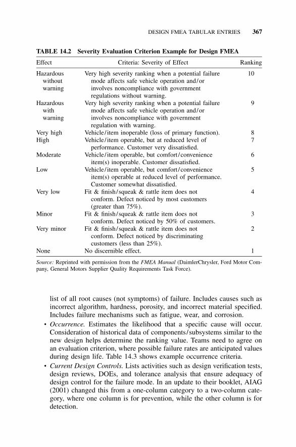
DESIGN FMEA TABULAR ENTRIES 367

TABLE 14.2 Severity Evaluation Criterion Example for Design FMEA

Effect Criteria: Severity of Effect Ranking

Hazardouswithoutwarning

Very high severity ranking when a potential failuremode affects safe vehicle operation and/orinvolves noncompliance with governmentregulations without warning.

10

Hazardouswithwarning

Very high severity ranking when a potential failuremode affects safe vehicle operation and/orinvolves noncompliance with governmentregulation with warning.

9

Very high Vehicle / item inoperable (loss of primary function). 8High Vehicle / item operable, but at reduced level of

performance. Customer very dissatisfied.7

Moderate Vehicle / item operable, but comfort /convenienceitem(s) inoperable. Customer dissatisfied.

6

Low Vehicle / item operable, but comfort /convenienceitem(s) operable at reduced level of performance.Customer somewhat dissatisfied.

5

Very low Fit & finish/squeak & rattle item does notconform. Defect noticed by most customers(greater than 75%).

4

Minor Fit & finish/squeak & rattle item does notconform. Defect noticed by 50% of customers.

3

Very minor Fit & finish/squeak & rattle item does notconform. Defect noticed by discriminatingcustomers (less than 25%).

2

None No discernible effect. 1

Source: Reprinted with permission from the FMEA Manual (DaimlerChrysler, Ford Motor Com-pany, General Motors Supplier Quality Requirements Task Force).

list of all root causes (not symptoms) of failure. Includes causes such asincorrect algorithm, hardness, porosity, and incorrect material specified.Includes failure mechanisms such as fatigue, wear, and corrosion.

• Occurrence. Estimates the likelihood that a specific cause will occur.Consideration of historical data of components/subsystems similar to thenew design helps determine the ranking value. Teams need to agree onan evaluation criterion, where possible failure rates are anticipated valuesduring design life. Table 14.3 shows example occurrence criteria.

• Current Design Controls. Lists activities such as design verification tests,design reviews, DOEs, and tolerance analysis that ensure adequacy ofdesign control for the failure mode. In an update to their booklet, AIAG(2001) changed this from a one-column category to a two-column cate-gory, where one column is for prevention, while the other column is fordetection.

368 FMEA

TABLE 14.3 Occurrence Evaluation Criterion Example for Design FMEA

Probability of Failure Possible Failure Rates Ranking

Very high: Persistent failures �100 per thousand vehicles / items50 per thousand vehicles / items

109

High: Frequent failures 20 per thousand vehicles / items10 per thousand vehicles / items

87

Moderate: Occasional failures 5 per thousand vehicles / items2 per thousand vehicles / items1 per thousand vehicles / items

654

Low: Relatively few failures 0.5 per thousand vehicles / items0.1 per thousand vehicles / items

32

Remote: Failure is unlikely �0.010 per thousand vehicles / items 1

Source: Reprinted with permission from the FMEA Manual (DaimlerChrysler, Ford Motor Com-pany, General Motors Supplier Quality Requirements Task Force).

• Detection. Assessment of the ability of the current design control to de-tect the subsequent failure mode or potential cause of design weaknessbefore releasing to production. Table 14.4 shows example detection cri-teria.

• Risk Priority Number (RPN). Product of severity, occurrence, and detec-tion rankings. The ranking of RPN prioritizes design concerns; however,problems with a low RPN still deserve special attention if the severityranking is high.

• Recommended Action(s). This entry proposes actions intended to lowerthe occurrence, severity, and/or detection rankings of the highest RPNfailure modes. Example actions include DOE, design revision, and testplan revision. ‘‘None’’ indicates that there are no recommended actions.

• Responsibility for Recommended Action. Documents the organization andindividual responsible for recommended action and target completiondate.

• Actions Taken. Describes implementation of recommended action andeffective date.

• Resulting RPN. Contains the recalculated RPN resulting from correctiveactions that affected previous severity, occurrence, and detection rank-ings. Blanks indicate no action taken.

The responsible design engineer follows up to ensure the adequate imple-mentation of all recommended actions. An FMEA should include designchanges and other relevant actions, even after the start of production. Table14.5 exemplifies a completed process FMEA.

DEVELOPMENT OF A PROCESS FMEA 369

TABLE 14.4 Detection Evaluation Criterion Example for Design FMEA

DetectionCriteria: Likelihood of Detection

by Design Control Ranking

Absolute uncertainty Design control will not and/or cannot detect apotential cause/mechanism and subsequentfailure mode; or there is no design control.

10

Very remote Very remote chance the design control willdetect a potential cause/mechanism andsubsequent failure mode.

9

Remote Remote chance the design control will detect apotential cause/mechanism and subsequentfailure mode.

8

Very low Very low chance the design control will detect apotential cause/mechanism and subsequentfailure mode.

7

Low Low chance the design control will detect apotential cause/mechanism and subsequentfailure mode.

6

Moderate Moderate chance the design control will detecta potential cause/mechanism and subsequentfailure mode.

5

Moderately high Moderately high chance the design control willdetect a potential cause/mechanism andsubsequent failure mode.

4

High High chance the design control will detect apotential cause/mechanism and subsequentfailure mode.

3

Very high Very high chance the design control will detecta potential cause/mechanism and subsequentfailure mode.

2

Almost certain Design control will almost certainly detect apotential cause/mechanism and subsequentfailure mode.

1

Source: Reprinted with permission from the FMEA Manual (DaimlerChrysler, Ford Motor Com-pany, General Motors Supplier Quality Requirements Task Force).

14.5 DEVELOPMENT OF A PROCESS FMEA

For a process or assembly FMEA, design engineering input is important toensure the appropriate focus on important design needs. An effort of the teamshould include knowledgeable representation from design, manufacturing/process, quality, reliability, tooling, and operators.

A process FMEA presumes the product meets the intent of the design. Aprocess FMEA does not need to include potential failure modes, causes, and

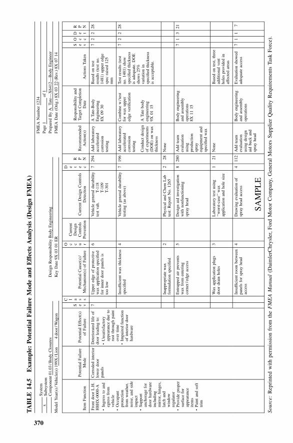
370

TA

BL

E14

.5E

xam

ple:

Pot

enti

alF

ailu

reM

ode

and

Eff

ects

Ana

lysi

s(D

esig

nF

ME

A)

Syst

emSu

bsys

tem

x

Com

pone

nt01

.03

/Bod

yC

losu

res

Des

ign

Res

pons

ibili

tyB

ody

Eng

inee

ring

FME

AN

umbe

r12

34

Page

1of

1

Prep

ared

By

A.

Tate

—X

6412

—B

ody

Eng

inee

r

Mod

elY

ear(

s)/V

ehic

le(s

)19

9X/L

ion

4do

or/W

agon

Key

Dat

e9X

0301

ER

FME

AD

ate

(Ori

g.)

8X03

22(R

ev.)

8X07

14

Item

Func

tion

Pote

ntia

lFa

ilure

Mod

ePo

tent

ial

Eff

ect(

s)of

Failu

re

S e v

C l a s sPo

tent

ial

Cau

se(s

)/M

echa

nism

(s)

ofFa

ilure

O c c u r

Cur

rent

Des

ign

Con

trol

sPr

even

tion

Cur

rent

Des

ign

Con

trol

sD

etec

tion

D e t e c

R P NR

ecom

men

ded

Act

ion(

s)

Res

pons

ibili

tyan

dTa

rget

Com

plet

ion

Dat

eA

ctio

nsTa

ken

S e v

O c c

D e t

R P N

Fron

tdo

orL

.H.

H8H

X-0

000-

A

•In

gres

sto

and

egre

ssfr

omve

hicl

e•

Occ

upan

tpr

otec

tion

from

wea

ther

,no

ise,

and

side

impa

ct•

Supp

ort

anch

orag

efo

rdo

orha

rdw

are

incl

udin

gm

irro

r,hi

nges

,la

tch

and

win

dow

regu

lato

r•

Prov

ide

prop

ersu

rfac

efo

rap

pear

ance

item

s•

Pain

tan

dso

fttr

im

Cor

rode

din

teri

orlo

wer

door

pane

ls

Det

erio

rate

dlif

eof

door

lead

ing

to:

•U

nsat

isfa

ctor

yap

pear

ance

due

toru

stth

roug

hpa

int

over

time

•Im

pair

edfu

nctio

nof

inte

rior

door

hard

war

e

7U

pper

edge

ofpr

otec

tive

wax

appl

icat

ion

spec

ified

for

inne

rdo

orpa

nels

isto

olo

w

Insu

ffici

ent

wax

thic

knes

ssp

ecifi

ed

Inap

prop

riat

ew

axfo

rmul

atio

nsp

ecifi

ed

Ent

rapp

edai

rpr

even

tsw

axfr

omen

teri

ngco

rner

/edg

eac

cess

6 4 2 5

Veh

icle

gene

ral

dura

bilit

yte

stva

h.T-

118

T-10

9T-

301

Veh

icle

gene

ral

dura

bilit

yte

stin

g(a

sab

ove)

Phys

ical

and

Che

mL

abte

st:

Rep

ort

No.

1265

Des

ign

aid

inve

stig

atio

nw

ithno

nfun

ctio

ning

spra

yhe

ad

7 7 2 8

294

196 28 280

Add

labo

rato

ryac

cele

rate

dco

rros

ion

test

ing

Add

labo

rato

ryac

cele

rate

dco

rros

ion

test

ing

Con

duct

desi

gnof

expe

rim

ents

(DO

E)

onw

axth

ickn

ess

Non

e

Add

team

eval

uatio

nus

ing

prod

uctio

nsp

ray

equi

pmen

tan

dsp

ecifi

edw

ax

ATa

te-B

ody

Eng

inee

ring

8X09

30

Com

bine

w/t

est

for

wax

uppe

red

geve

rific

atio

n

ATa

tebo

dyen

gine

erin

g9X

0115

Bod

yen

gine

erin

gan

das

sem

bly

oper

atio

ns8X

1115

Bas

edon

test

resu

lts(t

est

no.

1481

)up

per

edge

spec

rais

ed12

5m

m

Test

resu

lts(t

est

no.

1481

)sh

owsp

ecifi

edth

ickn

ess

isad

equa

te.

DO

Esh

ows

25%

vari

atio

nin

spec

ified

thic

knes

sis

acce

ptab

le.

7 7 7

2 2 1

2 2 3

28 28 21

Wax

appl

icat

ion

plug

sdo

ordr

ain

hole

s3

Lab

orat

ory

test

usin

g‘‘

wor

st-c

ase’

’wax

appl

icat

ion

and

hole

size

121

Non

eB

ased

onte

st,

thre

ead

ditio

nal

vent

hole

spr

ovid

edin

affe

cted

area

s

Insu

ffici

ent

room

betw

een

pane

lsfo

rsp

ray

head

acce

ss

4D

raw

ing

eval

uatio

nof

spra

yhe

adac

cess

411

2A

ddte

amev

alua

tion

usin

gde

sign

aid

buck

and

spra

yhe

ad

Bod

yen

gine

erin

gan

das

sem

bly

oper

atio

ns

Eva

luat

ion

show

edad

equa

teac

cess

71

17

SAM

PLE

Sour

ce:

Rep

rint

edw

ithpe

rmis

sion

from

the

FM

EA

Man

ual

(Dai

mle

rChr

ysle

r,Fo

rdM

otor

Com

pany

,G

ener

alM

otor

sSu

pplie

rQ

ualit

yR

equi

rem

ents

Task

Forc

e).

PROCESS FMEA TABULAR ENTRIES 371

mechanisms originating from the design, though a process FMEA team maychoose to include some design issues. The design FMEA covers the effectand avoidance of these issues. A process FMEA can originate from a flow-chart that identifies the characteristics of the product/process associated witheach operation. Included are appropriate product effects from available designFMEA. The documentation for an FMEA should include its flowchart.

Table 14.1 shows a blank FMEA form. A team determines the processFMEA tabular entries following the guidelines presented in the next section.

14.6 PROCESS FMEA TABULAR ENTRIES

A process FMEA in the format of Table 14.1 contains the following:

• Header Information. Documents the process description and suppliesother information about when and who created the FMEA.

• Process Function/Requirements from a Process FMEA. Contains a sim-ple description of the process or operation analyzed. Example processesinclude assembly, soldering, and drilling. Concisely indicates the purposeof the analyzed process or operation. When numeric assembly operationsexist with differing potential failure modes, the operations may be listedas separate processes.

• Potential Failure Mode. Describes how the process could potentially failto conform to process requirements and/or design intent at a specificoperation. Contains for each operation or item/function a list of eachpotential failure mode in terms of the component, subsystem, system, orprocess characteristic. Consider how the process/part fails to meet spec-ifications and/or customer expectations. Subsequent or previous opera-tions can cause these failure modes; however, teams should assume thecorrectness of incoming parts and materials. Items considered are pre-vious problems and new issues foreseen by brainstorming. Includes fail-ure modes such as broken, incorrect part placement, and electricalshort-circuited.

• Potential Effect(s) of Failure. Describes the effects of the failure modeon the function from an internal or external customer point of view.Considers what the customer experiences or the ramifications of thisfailure mode either from the end-user point of view or from subsequentoperation steps. Example end-user effects are poor performance, inter-mittent failure, and poor appearance. Example subsequent operation ef-fects are ‘‘does not fit,’’ ‘‘cannot mount,’’ and ‘‘fails to open.’’

• Severity. Assesses the seriousness of the effect of the potential failuremode to the customer. Estimation is typically based on a 1 to 10 scalewhere the team agrees to a specific evaluation criterion for each rankingvalue. Table 14.6 shows example evaluation criterion for the automotiveindustry.

372

TA

BL

E14

.6Se

veri

tyE

valu

atio

nC

rite

rion

Exa

mpl

efo

rP

roce

ssF

ME

A

Eff

ect

Cri

teri

a:Se

veri

tyof

Eff

ect

Thi

sra

nkin

gre

sults

whe

na

pote

ntia

lfa

ilure

mod

ere

sults

ina

final

cust

omer

and

/or

am

anuf

actu

ring

/ass

embl

ypl

ant

defe

ct.

The

final

cust

omer

shou

ldal

way

sbe

cons

ider

edfir

st.

Ifbo

thoc

cur,

use

the

high

erof

the

two

seve

ritie

s.

Cus

tom

erE

ffec

tM

anuf

actu

ring

/Ass

embl

yE

ffec

tR

anki

ng

Haz

ardo

usw

ithou

tw

arni

ng

Ver

yhi

ghse

veri

tyra

nkin

gw

hen

apo

tent

ial

failu

rem

ode

affe

cts

safe

vehi

cle

oper

atio

nan

d/o

rin

volv

esno

ncom

plia

nce

with

gove

rnm

ent

regu

latio

nw

ithou

tw

arni

ng.

Or

may

enda

nger

oper

ator

(mac

hine

oras

sem

bly)

with

out

war

ning

.10

Haz

ardo

usw

ithw

arni

ng

Ver

yhi

ghse

veri

tyra

nkin

gw

hen

apo

tent

ial

failu

rem

ode

affe

cts

safe

vehi

cle

oper

atio

nan

d/o

rin

volv

esno

ncom

plia

nce

with

gove

rnm

ent

regu

latio

nw

ithw

arni

ng.

Or

may

enda

nger

oper

ator

(mac

hine

oras

sem

bly)

with

war

ning

.9

Ver

yhi

ghV

ehic

le/i

tem

inop

erab

le(l

oss

ofpr

imar

yfu

nctio

n).

Or

100%

ofpr

oduc

tm

ayha

veto

besc

rapp

ed,

orve

hicl

e/ite

mre

pair

edin

repa

irde

part

men

tw

itha

repa

irtim

egr

eate

rth

anon

eho

ur.

8

Hig

hV

ehic

le/i

tem

oper

able

but

ata

redu

ced

leve

lof

perf

orm

ance

.C

usto

mer

very

diss

atis

fied.

Or

prod

uct

may

have

tobe

sort

edan

da

port

ion

(les

sth

an10

0%)

scra

pped

,or

vehi

cle/

item

repa

ired

inre

pair

depa

rtm

ent

with

are

pair

time

betw

een

aha

lf-h

our

and

anho

ur.

7

Mod

erat

eV

ehic

le/i

tem

oper

able

but

com

fort

/con

veni

ence

item

(s)

inop

erab

le.

Cus

tom

erdi

ssat

isfie

d.O

ra

port

ion

(les

sth

an10

0%)

ofth

epr

oduc

tm

ayha

veto

besc

rapp

edw

ithno

sort

ing,

orve

hicl

e/ite

mre

pair

edin

repa

irde

part

men

tw

itha

repa

irtim

ele

ssth

ana

half

-hou

r.

6

Low

Veh

icle

/ite

mop

erab

lebu

tco

mfo

rt/c

onve

nien

ceite

m(s

)op

erab

leat

redu

ced

leve

lof

perf

orm

ance

.O

r10

0%of

prod

uct

may

have

tobe

rew

orke

d,or

vehi

cle/

item

repa

ired

off-

line

but

does

not

goto

repa

irde

part

men

t.

5

373

Ver

ylo

wFi

tan

dfin

ish

/squ

eak

and

rattl

eite

mdo

esno

tco

nfor

m.

Def

ect

notic

edby

mos

tcu

stom

ers

(gre

ater

than

75%

).

Or

the

prod

uct

may

have

tobe

sort

ed,

with

nosc

rap,

and

apo

rtio

n(l

ess

than

100%

)re

wor

ked.

4

Min

orFi

tan

dfin

ish

/squ

eak

and

rattl

eite

mdo

esno

tco

nfor

m.

Def

ect

notic

edby

50%

ofcu

stom

ers.

Or

apo

rtio

n(l

ess

than

100%

)of

the

prod

uct

may

have

tobe

rew

orke

d,w

ithno

scra

p,on

-lin

ebu

tou

t-of

-sta

tion.

3

Ver

ym

inor

Fit

and

finis

h/s

quea

kan

dra

ttle

item

does

not

conf

orm

.D

efec

tno

ticed

bydi

scri

min

atin

gcu

stom

ers

(les

sth

an25

%).

Or

apo

rtio

n(l

ess

than

100%

)of

the

prod

uct

may

have

tobe

rew

orke

d,w

ithno

scra

p,on

-lin

ebu

tin

-st

atio

n.

2

Non

eN

odi

scer

nibl

eef

fect

.O

rsl

ight

inco

nven

ienc

eto

oper

atio

nor

oper

ator

,or

noef

fect

.1

Sour

ce:

Rep

rint

edw

ithpe

rmis

sion

from

the

FM

EA

Man

ual

(Dai

mle

rChr

ysle

r,Fo

rdM

otor

Com

pany

,G

ener

alM

otor

sSu

pplie

rQ

ualit

yR

equi

rem

ents

Task

Forc

e).

374 FMEA

TABLE 14.7 Occurrence Evaluation Criterion Example for Process FMEA

Probability Likely Failure Rates Ranking

Very high: Persistent failures �100 per thousand pieces50 per thousand pieces

109

High: Frequent failures 20 per thousand pieces10 per thousand pieces

87

Moderate: Occasional failures 5 per thousand pieces2 per thousand pieces1 per thousand pieces

654

Low: Relatively few failures 0.5 per thousand pieces0.1 per thousand pieces

32

Remote: Failure unlikely �0.01 per thousand pieces 1

Source: Reprinted with permission from the FMEA Manual (DaimlerChrysler, Ford Motor Com-pany, General Motors Supplier Quality Requirements Task Force).

• Classification. Includes optional information that classifies special pro-cess characteristics that may require additional process controls. Applieswhen government regulations, safety, and engineering specificationconcerns exist for the product and/or process. An appropriate charac-ter or symbol in this column indicates the need for an entry in therecommended action column to address special controls in the controlplan.

• Potential Causes(s) of Failure. Describes how failure could occur interms of a correctable or controllable item. Contains a concise, descrip-tive, and comprehensive list of all root causes (not symptoms) of failure.The resolution of some causes directly affects the failure mode. In othersituations a DOE determines the major and most easily controlled rootcauses. Includes causes such human error, improper cure time, and miss-ing part.

• Occurrence. Estimates the frequency of occurrence of failure withoutconsideration of detecting measures. Gives the number of anticipatedfailures during the process execution. Consideration of statistical datafrom similar processes improves the accuracy of ranking values. Alter-native subjective assessments use descriptive words to describe rankings.Table 14.7 shows example occurrence criteria.

• Current Process Controls. Describes controls that can prevent failuremode from occurring or detect occurrence of the failure mode. In anupdate to their booklet, AIAG (2001) changed this from a one-columncategory to a two-column category, where one column is for prevention,while the other column is for detection. Process controls includes controlmethods such as SPC and poka-yoke (fixture error proofing) at the sub-

PROCESS FMEA TABULAR ENTRIES 375

ject or subsequent operations. The preferred method of control is pre-vention or reduction in the frequency of the cause/mechanism to thefailure mode/effect. The next preferred method of control is detection ofthe cause/mechanism, which leads to corrective actions. The least pre-ferred method of control is detection of the failure mode.

• Detection. Assesses the probability of detecting a potential cause/mech-anism from process weakness or the subsequent failure mode before thepart /component leaves the manufacturing operation. Ranking values con-sider the probability of detection when failure occurs. Table 14.8 showsexample detection evaluation criteria.

• Risk Priority Number (RPN). Product of severity, occurrence, and detec-tion rankings. The ranking of RPN prioritizes design concerns; however,problems with a low RPN still deserve special attention if the severityranking is high.

• Recommended Action(s). This entry is proposed actions intended to lowerthe occurrence, severity, and/or detection rankings of the highest RPNfailure modes. Example actions include DOE to improve the understand-ing of causes and control charts to improve the focus of defectprevention/continuous improvement activities. Teams should focus onactivities that lead to the prevention of defects (i.e., occurrence rankingreduction) rather than improvement of detection methodologies (i.e., de-tection ranking reduction). Teams should implement corrective action toidentified potential failure modes where the effect is a hazard tomanufacturing/assembly personnel. Severity reduction requires a revisionin the design and/or process. ‘‘None’’ indicates that there are no rec-ommended actions.

• Responsibility for Recommended Action. Documents the organization andindividual responsible for recommended action and target completiondate.

• Actions Taken. Describes implementation of recommended action andeffective date.

• Resulting RPN. Contains the recalculated RPN resulting from correctiveactions that affected previous severity, occurrence, and detection rank-ings. Blanks indicate no action taken.

The responsible process engineer follows up to ensure the adequate imple-mentation of all recommended actions. An FMEA should include designchanges and other relevant actions even after the start of production. Table14.9 provides an example of a completed process FMEA that has an RPNtrigger number of 150, along with a severity trigger number of 7. Table 14.10is another example of a completed FMEA with an action RPN trigger numberof 130.

376

TA

BL

E14

.8D

etec

tion

Eva

luat

ion

Cri

teri

aE

xam

ple

for

Pro

cess

FM

EA

Det

ectio

nC

rite

ria

Insp

ectio

nTy

pe

AB

CSu

gges

tion

Ran

geof

Det

ectio

nM

etho

dsR

anki

ng

Alm

ost

impo

ssib

leA

bsol

ute

cert

aint

yof

nond

etec

tion.

XC

anno

tde

tect

oris

not

chec

ked.

10

Ver

yre

mot

eC

ontr

ols

will

prob

ably

not

dete

ct.

XC

ontr

olis

achi

eved

with

indi

rect

orra

ndom

chec

kson

ly.

9

Rem

ote

Con

trol

sha

vepo

orch

ance

ofde

tect

ion.

XC

ontr

olis

achi

eved

with

visu

alin

spec

tion

only

.8

Ver

ylo

wC

ontr

ols

have

poor

chan

ceof

dete

ctio

n.X

Con

trol

isac

hiev

edw

ithdo

uble

visu

alin

spec

tion

only

.7

Low

Con

trol

sm

ayde

tect

.X

XC

ontr

olis

achi

eved

with

char

ting

met

hods

,su

chas

SPC

(Sta

tistic

alPr

oces

sC

ontr

ol).

6

Mod

erat

eC

ontr

ols

may

dete

ct.

XC

ontr

olis

base

don

vari

able

gaug

ing

afte

rpa

rts

have

left

the

stat

ion,

orG

o/N

oG

oga

ugin

gpe

rfor

med

on10

0%of

the

part

saf

ter

part

sha

vele

ftth

est

atio

n.

5

Mod

erat

ely

high

Con

trol

sha

vea

good

chan

ceto

dete

ct.

XX

Err

orde

tect

ion

insu

bseq

uent

oper

atio

ns,

OR

gaug

ing

perf

orm

edon

setu

pan

dfir

st-p

iece

chec

k(f

orse

tup

caus

eson

ly).

4

Hig

hC

ontr

ols

have

ago

odch

ance

tode

tect

.X

XE

rror

dete

ctio

nin

-sta

tion,

orer

ror

dete

ctio

nin

subs

eque

ntop

erat

ions

bym

ultip

lela

yers

ofac

cept

ance

:su

pply

,se

lect

,in

stal

l,ve

rify

.C

anno

tac

cept

disc

repa

ntpa

rt.

3

Ver

yhi

ghC

ontr

ols

alm

ost

cert

ain

tode

tect

.X

XE

rror

dete

ctio

nin

-sta

tion

(aut

omat

icga

ugin

gw

ithau

tom

atic

stop

feat

ure)

.C

anno

tpa

ssdi

scre

pant

part

.2

Ver

yhi

ghC

ontr

ols

cert

ain

tode

tect

.X

Dis

crep

ant

part

sca

nnot

bem

ade

beca

use

item

has

been

erro

r-pr

oofe

dby

proc

ess/

prod

uct

desi

gn.

1

Insp

ectio

nTy

pes:

A.

Err

or-p

roof

ed;

B.

Gau

ging

;C

.M

anua

lIn

spec

tion.

Sour

ce:

Rep

rint

edw

ithpe

rmis

sion

from

the

FM

EA

Man

ual

(Dai

mle

rChr

ysle

r,Fo

rdM

otor

Com

pany

,G

ener

alM

otor

sSu

pplie

rQ

ualit

yR

equi

rem

ents

Task

Forc

e).

377

TA

BL

E14

.9E

xam

ple:

Pot

enti

alF

ailu

reM

ode

and

Eff

ects

Ana

lysi

s(P

roce

ssF

ME

A)

FME

ATy

pe(D

esig

nor

Proc

ess)

:Pr

oces

sPr

ojec

tN

ame

/Des

crip

tion:

Che

etah

/Cha

nge

surf

ace

finis

hof

part

Dat

e(O

rig.

):4

/14

Res

pons

ibili

ty:

Paul

aH

inke

lPr

epar

edB

y:Pa

ula

Hin

kel

Dat

e(R

ev.)

:6

/15

Cor

eTe

am:

Sam

Smith

,H

arry

Ada

ms,

Hilt

onD

ean,

Har

ryH

awki

ns,

Sue

Wat

kins

Dat

e(K

ey):

Des

ign

FME

A(I

tem

/Fu

nctio

n)Pr

oces

sFM

EA

(Fun

ctio

n/

Req

uire

men

ts)

Pote

ntia

lFa

ilure

Mod

ePo

tent

ial

Eff

ect(

s)of

Failu

re

S e v

C l a s s

Pote

ntia

lC

ause

(s)/

Mec

hani

sm(s

)of

Failu

re

O c c u rC

urre

ntC

ontr

ols

D e t e c

R P NR

ecom

men

ded

Act

ions

Res

pons

ibili

tyan

dTa

rget

Com

plet

ion

Dat

eA

ctio

nsTa

ken

S e v

O c c u r

D e t e c

R P N

Sold

erdi

ppin

gE

xces

sive

sold

er/

sold

erw

ire

prot

rusi

on

Shor

tto

shie

ldco

ver

9Fl

uxw

ire

term

inat

ion

610

0%in

spec

tion

316

2A

utom

atio

n/D

OE

/10

0%ch

kw

ithgo

/no

goga

ge

Sam

Smith

6/4

Don

e9

42

72

Inte

rloc

kba

seda

mag

eV

isua

lde

fect

s7

Lon

gso

lder

time

8A

utom

atic

sold

erto

ol3

168

Aut

omat

ion

/DO

E/

defin

evi

sual

crite

ria

Har

ryA

dam

s5

/15

Don

e7

42

56

7H

igh

tem

p8

Aut

omat

icso

lder

tool

/SP

C3

168

Aut

omat

ion

/DO

EH

ilton

Dea

n5

/15

Don

e7

42

56

Del

amin

atio

nof

inte

rloc

kba

seV

isua

lde

fect

s7

See

inte

rloc

kba

seda

mag

e8

Aut

omat

icso

lder

tool

/SP

C3

168

Aut

omat

ion

/DO

ESu

eW

atki

ns5

/15

Don

e7

42

56

7M

oist

ure

inin

terl

ock

base

5N

o7

245

Info

rmsu

pplie

rto

cont

rol

mol

ding

cond

.H

arry

Haw

kins

5/1

5D

one

72

798

Oxi

diza

tion

ofgo

lden

plat

ing

pins

Con

tact

prob

lem

/no

sign

al8

Not

bein

gcl

eane

din

time

7C

lean

in30

min

utes

afte

rso

lder

dip

528

0Im

prov

equ

ality

ofpl

atin

gde

fine

crite

ria

with

cust

omer

Sam

Smith

5/1

5D

one

82

580

Mar

king

Mar

king

perm

anen

cyte

stL

egib

lem

arki

ng/

cust

omer

unsa

tisfa

ctio

n

6 6 6

Mar

king

ink

Cur

ing

Smoo

thm

arki

ngsu

rfac

e

4 5 8

SPC

UV

ener

gyan

dSP

C

Non

e

2 3 6

48 90 288

Non

e

Non

e

Rou

ghsu

rfac

eSa

mSm

ith5

/15

Cha

nge

inte

rloc

kte

xtur

esu

rfac

e

63

610

8

Sour

ce:

Puls

e,a

Tech

nitr

olC

ompa

ny,

San

Die

go,

CA

(Jim

Fish

and

Mar

yM

cDon

ald)

.

378

TA

BL

E14

.10

Exa

mpl

e:P

oten

tial

Fai

lure

Mod

ean

dE

ffec

tsA

naly

sis

(Pro

cess

FM

EA

)FM

EA

Type

(Des

ign

orPr

oces

s):

Proj

ect

Nam

e/D

escr

iptio

n:B

usin

ess

oper

atio

nsof

Ato

Zim

port

sD

ate

(Ori

g.):

6/1

1

Res

pons

ibili

ty:

Prep

ared

By:

KC

Dat

e(R

ev.)

:7

/31

Cor

eTe

am:

KC

,JG

,L

MD

ate

(Key

):

Des

ign

FME

A(I

tem

/Fu

nctio

n)Pr

oces

sFM

EA

(Fun

ctio

n/

Req

uire

men

ts)

Pote

ntia

lFa

ilure

Mod

ePo

tent

ial

Eff

ect(

s)of

Failu

re

S e v

C l a s s

Pote

ntia

lC

ause

(s)/

Mec

hani

sm(s

)of

Failu

re

O c c u rC

urre

ntC

ontr

ols

D e t e c

R P NR

ecom

men

ded

Act

ions

Res

pons

ibili

tyan

dTa

rget

Com

plet

ion

Dat

eA

ctio

nsTa

ken

S e v

O c c u r

D e t e c

R P N

Bus

ines

sO

pera

tions

Shut

dow

nL

oss

ofin

com

e/

bank

rupt

cy9

Torn

ado

hits

loca

tion

3N

one

1027

0In

stal

lw

eath

erch

anne

lra

dio

inst

ore,

and

keep

ondu

ring

stor

eho

urs

JG7

/8In

stal

led

and

test

ed9

32

54

9L

awsu

itby

visi

tor

hurt

inst

ore

duri

ngvi

sit

3In

sura

nce

cove

rage

agai

nst

acci

dent

sin

stor

e

254

Non

e

9L

awsu

itby

visi

tor

owin

gto

faul

tym

erch

andi

se

5W

arni

ngla

bels

onm

erch

andi

se2

90N

one

9E

lect

rica

lfir

ebu

rns

dow

nst

ore

2Fi

reex

tingu

ishe

rsan

dsp

rink

lers

1018

0In

stal

lgr

ound

faul

tin

terr

upto

rs,a

ndov

erlo

ad/t

herm

alpr

otec

tion

onal

lhi

ghw

atta

gefix

ture

s

LM

6/2

8In

stal

led

GFI

san

dth

erm

alpr

otec

tion

92

118

9IR

Sau

dit

show

sm

isre

port

ing

offin

ance

s

5C

PAau

dits

acco

unts

atta

xtim

e

418

0C

hang

epr

oced

ure

toal

low

clos

ing

ofbo

oks

ever

y6

mon

ths,

and

CPA

toau

dit

the

sam

e

KC

7/1

5Pr

oced

ure

chan

ged,

acco

untin

gpe

rson

nel

and

CPA

info

rmed

92

236

9E

xces

sive

com

petit

ion

5A

gree

men

tw

ithpr

oper

tyow

ners

onlim

iting

num

ber

ofim

port

stor

es

290

Non

e

379

9L

oss

ofle

ase

10R

enta

lag

reem

ent

onm

onth

tom

onth

basi

s,au

tom

atic

ally

rene

ws

1090

0N

egot

iate

with

leas

ing

com

pany

toch

ange

leas

eag

reem

ent

toye

arly

KC

7/1

9Ta

lked

mat

ter

over

with

prop

erty

owne

rs,

obta

ined

verb

alas

sura

nce,

but

leas

est

ays

mon

thto

mon

th

910

1090

0

Ear

ning

sgr

owth

does

not

mee

tta

rget

s

Del

ayed

loan

repa

ymen

ts6

Sale

sst

aff

impo

lite

4Jo

bin

terv

iew

attim

eof

hiri

ng5

120

Inst

itute

sale

str

aini

ngof

new

hire

sfo

rha

lfda

yin

addi

tion

toex

istin

gtr

aini

ng.

Do

not

assi

gnto

floor

ifca

ndid

ate’

spe

rfor

man

cein

sale

str

aini

ngis

susp

ect

KC

8/2

Sale

str

aini

ngm

odul

ead

ded

toex

istin

gtr

aini

ngpa

ckag

e

62

224

6E

xces

sive

com

petit

ion

5A

gree

men

tw

ithpr

oper

tyow

ners

onlim

iting

num

ber

ofim

port

stor

es

260

Non

e

6Su

pplie

rde

lays

owin

gto

late

paym

ents

3N

one

1018

0C

ondu

ctFM

EA

onth

isca

use,

trea

ting

itas

afa

ilure

mod

eits

elf

6L

ocal

econ

omy

slow

s5

Non

e10

300

Mon

itor

area

grow

thth

ruqu

arte

rly

chec

ksw

ithth

elo

cal

Cha

mbe

rof

Com

mer

ce

JG7

/15

Obt

aine

dpo

pula

tion

grow

thfo

rci

ty,

and

inco

me

stat

istic

sfo

rqu

arte

ren

ding

Mar

ch31

st.

65

260

6St

ore

untid

y9

Em

ploy

ees

have

stan

ding

orde

rsto

atte

ndcu

stom

ers

first

;an

dup

keep

ofst

ore

seco

nd.

154

Non

e

380

TA

BL

E14

.10

(Con

tinue

d)

Des

ign

FME

A(I

tem

/Fu

nctio

n)Pr

oces

sFM

EA

(Fun

ctio

n/

Req

uire

men

ts)

Pote

ntia

lFa

ilure

Mod

ePo

tent

ial

Eff

ect(

s)of

Failu

re

S e v

C l a s s

Pote

ntia

lC

ause

(s)/

Mec

hani

sm(s

)of

Failu

re

O c c u rC

urre

ntC

ontr

ols

D e t e c

R P NR

ecom

men

ded

Act

ions

Res

pons

ibili

tyan

dTa

rget

Com

plet

ion

Dat

eA

ctio

nsTa

ken

S e v

O c c u r

D e t e c

R P N

6D

elay

edor

lost

ship

men

tsfr

omsu

pplie

r

7Fr

eigh

tfo

rwar

der

faxe

sbi

llof

ladi

ngw

hen

mer

chan

dise

islo

aded

onsh

ip/

air.

Nex

tco

ntac

tis

whe

ngo

ods

arri

veat

dest

inat

ion

1042

0R

equi

refr

eigh

tfo

rwar

der

toin

timat

est

atus

ofsh

ipm

ent

ever

y3

days

KC

7/2

8G

otag

reem

ent

with

frei

ght

forw

arde

r;ad

ditio

nal

char

geof

2.5%

onfr

eigh

tag

reed

upon

67

312

6

6D

efec

tive

mer

chan

dise

4In

spec

tion

prio

rto

putti

ngm

erch

andi

seon

shel

ves

248

Non

e

6T

heft

ofca

shby

empl

oyee

sfr

omca

shre

gist

ers

7L

ogs

ofem

ploy

eena

mes

man

agin

gca

sh,

byda

tean

dtim

e

1042

0Su

perv

isor

sto

star

tac

coun

ting

for

cash

with

empl

oyee

sw

hen

they

star

tw

ork

and

atev

ery

chan

geov

er.

KC

8/3

Proc

edur

espu

tin

plac

eto

acco

mpl

ish

cash

man

agem

ent

asre

com

men

ded

62

224

6T

heft

ofm

erch

andi

se5

Stor

eat

tend

ants

tom

onito

rcu

stom

ers

whe

nfe

asib

le

824

0In

stal

lm

agne

ticth

eft

prev

entio

nta

gson

mer

chan

dise

and

dete

ctor

sat

stor

een

tran

ce

LM

8/1

5C

ompl

eted

onite

ms

with

ticke

tpr

ices

over

$20;

rest

will

beco

mpl

eted

by8

/15

65

130

6W

rong

mer

chan

dise

lead

ing

tosl

ower

inve

ntor

ytu

rns

5V

isit

who

lesa

lem

arke

tstw

ice

/yea

rto

keep

upw

ithcu

rren

ttr

ends

390

Non

e

6A

ccou

ntin

ger

rors

5B

ooks

audi

ted

byC

PAat

tax

time

412

0N

one

Sour

ce:

Rai

Cho

wdh

ary.

EXERCISES 381

14.7 EXERCISES

1. Catapult Exercise: Create an FMEA for the catapult shot process. Considerthat an operator injury will occur if the ball drops out of the holder duringloading, and machine damage will occur if a rubber band breaks. There isan additional specification of the right and left distance from the tapemeasure (e.g., �2 in.).

2. Conduct an FMEA of a pencil. Consider that the function is to make ablack mark. Requirements could include that it is to make a mark, it marksa black color, and it intermittently fails to mark. Failure modes would thenbe that it makes no mark at all, mark is not black in color, and it marksintermittently.

3. Conduct an FMEA on implementing Six Sigma within an organization.

4. Discuss the value of the techniques presented in this chapter and explainhow they can be applied to S4/IEE projects.

5. Describe how and show where the tools described in this chapter fit intothe overall S4/IEE roadmap described in Figure A.1 in the Appendix.

383

PART III

S4/IEE ANALYZE PHASEFROM DMAIC (OR PASSIVEANALYSIS PHASE)

Starting with the process map in conjunction with the cause-and-effect dia-gram, cause-and-effect matrix, and FMEA, we can look for information sys-tems that currently collect desired data. This data can be transformed intoinformation through the reviewing of reports and data analysis. When appro-priate data sources are not present, we can interview subject matter expertsand/or collect our own data.

Part III (Chapters 15–26) addresses the analysis of data for the purpose oflearning about causal relationships. Information gained from this analysis canprovide insight into the sources of variability and unsatisfactory performance,and help improve processes. Within S4/IEE this phase is often referred to asthe passive analysis phase. The reason for this is that within this phase thelevel of input variables from the wisdom of the organization is observedpassively to see if a relationship can be detected between them. If there is arelationship observed, this knowledge can help focus improvement efforts.Note, proactive testing when input variable levels are changed is coveredusing DOE techniques within the DMAIC improvement phase.

Tools included within this section include visualization of data, inferencetesting, variance components, regression, and analysis of variance. Improve-ments can be made in any phase of DMAIC. Tools in this phase can be usedto statistically quantify and pictorially show the amount of improvementmade.

Within this part of the book, the DMAIC analyze steps, which are de-scribed in Section A.1 (part 3) of the Appendix, are discussed. A checklistfor the completion of the analyze (passive analysis) phase is:

384 S4 / IEE ANALYZE PHASE FROM DMAIC

Analyze Phase: Passive Analysis Checklist

Description Questions Yes /No

Tool /MethodologyBox Plots, Marginal

Plots, andMulti-vari Charts

Was the appropriate visualization of data technique usedin order to gain process insight to the process?

Pareto Charts If data are discrete, were Pareto charts used to drilldown to the KPIVs?

Chi-Squarep Chart /u Chart

If input data and output data are both discrete, was achi-square test used to test for statistical significanceand a p chart (u chart for count data) used to assessindividual difference from the overall mean?

Scatter Plots If data are continuous, were scatter plots used to displaythe relationship beween KPIVs and a KPOV?

Comparison Tests Were statistical significance tests used to gain processinsight?

VarianceComponents

If output data are continuous and inputs are in ahierarchy, were variance components considered togain insight?

Regression Analysis For continuous input and output data, was regressionanalysis used to compare the relationship betweeninputs and the output(s)?

ANOVA/ANOMBartlett’s /Levene

For discrete KPIVs and continuous KPOV data, was theappropriate tool used to compare samples from thedifferent levels of KPIVs?

Assessment Were any process improvements made?If so, were they statistically verified with the

appropriate hypothesis test?Did you describe the change over time on a 30,000-

foot-level control chart?Did you calculate and display the change in process

capability (in units such as ppm)?Have you documented and communicated the

improvements?Have you summarized the benefits and annualized

financial benefits?TermResources Are all team members motivated and committed to the

project?Next PhaseApproval to

ProceedDid the team adequately complete the above steps?Has the project database been updated and

communication plan followed?Is DOE needed?If so, should this project proceed to the proactive

testing phase?Is there a detailed plan for the proactive testing phase?Has the team considered improvements to both the

process mean and process variation?Are barriers to success identified and planned for?Is the team tracking with the project schedule?Have schedule revisions been approved?

385

15VISUALIZATION OF DATA

S4 /IEE DMAIC Application: Appendix Section A.1, Project ExecutionRoadmap Step 7.1

Previous chapters presented graphical techniques used to quantify informationvisually. These techniques included histograms, time series plots, scatter di-agrams, probability plotting, control charts, cause-and-effect diagrams, andPareto charts. Chapter 14 described techniques for determining by consensuskey process input and output variables. Chapter 14 also discussed the collec-tion of data to assess relationships between key process input variables andkey process output variables.

This chapter presents additional graphical and charting techniques that cangive visual insight into the relationships between key process input variablesand key process output variables. Through these exploratory data analysis(EDA) tools, we can divide data into groups or strata based on key charac-teristics; e.g., who, what, where, and when. The visualization of this stratifi-cation can help detect a pattern which provides an opportunity forimprovement efforts focus. The hypothesis testing described in Chapter 16tests for the statistical significance of these relationships.

The visualization offered by these techniques allows us to assess a greatdeal of information about the process without modifying it and to determinewhere to focus efforts for improvement.

We can look for differences between samples, interrelationships betweenvariables, and change over time. Hypothesized relationships noticed couldthen be tested statistically. Knowledge gained from these tests can suggestmodifications of the process, key process input variable control needs, andDOE opportunities.

386 VISUALIZATION OF DATA

15.1 S4/IEE APPLICATION EXAMPLES:VISUALIZATION OF DATA

S4/IEE application examples of visualization of data are:

• Transactional 30,000-foot-level metric: DSO reduction was chosen as anS4/IEE project. A cause-and-effect matrix ranked company as an impor-tant input that could affect the DSO response; i.e., the team thought somecompanies were more delinquent in payments than other companies. Abox plot and marginal plot were created from sampled data to visuallyshow similarities and differences in DSO response times by company.

• Manufacturing 30,000-foot-level metric: An S4/IEE project was to im-prove the capability/performance of the diameter of a manufacturedproduct; i.e., reduce the number of parts beyond the specification limits.A cause-and-effect matrix ranked cavity of the mold as an importantinput that could be yielding different part diameters. A box plot andmarginal plot were created from the sampled data to visually show sim-ilarities and differences in part diameter by cavity.

• Transactional and manufacturing 30,000-foot-level cycle time metric (alean metric): An S4/IEE project was to improve the time from order entryto fulfillment was measured. A cause-and-effect matrix ranked depart-ment as an important input that could affect the overall order entry timeresponse; i.e., the team thought some departments did not process ordersas quickly as others. A box plot and marginal plot were created fromsampled data to visually show similarities and differences in order entrytimes by department.

• Transactional and manufacturing 30,000-foot-level inventory metric orsatellite-level TOC metric (a lean metric): An S4/IEE project was toreduce inventory. A cause-and-effect matrix ranked WIP by productionline as an input that could affect the overall inventory response. A boxplot and marginal plot were created from sampled data to visually showsimilarities and differences in WIP by production line.

• Transactional 30,000-foot-level metric: An S4/IEE project was to reducewait time for incoming calls in a call center. A cause-and-effect matrixranked time of call as an important input that could affect the overallwait time. Sampled hierarchical data were collected and presented in amulti-vari chart. This chart showed variability within hours of a 12-hourworkday, between hours, between days of the week, and between weeksof the month. The multi-vari chart showed a consistent long wait timearound noon on Fridays.

15.2 MULTI-VARI CHARTS

Leonard Seder (1950) can be given credit for introducing the multi-vari chart,which is described in this section.

EXAMPLE 15.1: MULTI-VARI CHART OF INJECTION-MOLDING DATA 387

Within a discrete manufacturing environment, contributing factors to over-all variability of a response include differences between time periods, pro-duction tool differences, part-to-part variations, and within-part variability.Within a continuous flow manufacturing process, contributing factors to over-all variability include within shifts, across shifts, and across days/weeks/months. Multi-vari charts allow visual decomposition into components andthe identification of the component that affects variability the most.

Considerations when constructing a multi-vari chart are as follows:

• If there are many measurements within a part, the average, highest, andlowest values could be used.

• Reconstruction of the chart using various arrangements for the axes canaid in the detection of patterns and relationships.

• Connecting mean values on the chart can aid the visual representation.

Visual observations can lead to the use of other analytical tools that testhypotheses. These techniques include variance component analysis and anal-ysis of means, discussed in Chapters 22 and 24. Information gained fromthese analyses can lead to effective targeting of process improvement efforts.

15.3 EXAMPLE 15.1: MULTI-VARI CHART OFINJECTION-MOLDING DATA

An injection-molding process made plastic cylindrical connectors (Taylor1991). Every hour for three hours, two parts were selected from each of fourmold cavities. Measurements were made at each end and the middle. Thedata are shown in Table 15.1, and the multi-vari chart is shown in Figure15.1.

From observation of the multi-vari chart it appears that:

• Any difference between time periods appears to be small.• Differences occur between cavities for a given time period (largest var-

iation source).

Cavities 2, 3, and 4 appear to have thicker ends, while cavity 1 has a slighttaper. Sixteen of the 18 parts from cavities 2, 3, and 4 exhibit a ‘‘V’’ pattern.

Another option for presentation of multi-vari information is to use a meaneffects plot of each variable source consideration.

These data will later be analyzed in Chapters 24 and 22 as a statisticalhypothesis using analysis of means and variance of components techniques.

388

TA

BL

E15

.1M

ulti

-var

iC

hart

ofIn

ject

ion-

Mol

ding

Dat

a

Tim

e

1

Cav

ity

2

Cav

ity

3

Cav

ity

Part

Loc

atio

n1

23

41

23

41

23

4

Top

0.25

220.

2501

0.25

100.

2489

0.25

180.

2498

0.25

160.

2494

0.25

240.

2488

0.25

110.

2490

1M

iddl

e0.

2523

0.24

970.

2507

0.24

810.

2512

0.24

840.

2496

0.24

850.

2518

0.24

860.

2504

0.24

79B

otto

m0.

2518

0.25

010.

2516

0.24

850.

2501

0.24

920.

2507

0.24

920.

2512

0.24

970.

2503

0.24

88

Top

0.25

140.

2501

0.25

080.

2485

0.25

200.

2499

0.25

030.

2483

0.25

170.

2496

0.25

030.

2485

2M

iddl

e0.

2513

0.24

940.

2495

0.24

780.

2514

0.24

950.

2501

0.24

820.

2509

0.24

870.

2497

0.24

83B

otto

m0.

2505

0.24

950.

2507

0.24

840.

2513

0.25

010.

2504

0.24

910.

2513

0.25

00.

2492

0.24

95

BOX PLOT 389

0.2525

0.2510

0.2495

0.2480

0.2525

0.2510

0.24952

1

Part

0.2480

1 2 3 4 1 2 3Cavity

2Time

31

4 1 2 3 4bottomPosition

middletop

FIGURE 15.1 Multi-vari chart for diameter by position within part.

FIGURE 15.2 Box plot characteristics.

15.4 BOX PLOT

A box plot (or box-and-whisker plot) is useful for describing various aspectsof data pictorially. Box plots can visually show differences between charac-teristics of a data set.

Figure 15.2 shows the common characteristics of a box plot. The boxdisplays the lower and upper quartiles (the 25th and 75th percentiles), andthe median (the 50th percentile) appears as a horizontal line within the box.The whiskers are then often extended to

390 VISUALIZATION OF DATA

FIGURE 15.3 Box plot of diameter versus cavity.

Lower limit: Q1 � 1.5(Q3 � Q1)Upper limit: Q3 � 1.5(Q3 � Q1)

In this case, points outside the lower and upper limits are considered to beoutliers and are designated with asterisks (*).

15.5 EXAMPLE 15.2: PLOTS OF INJECTION-MOLDING DATA

This example expands upon the multi-vari chart analysis of data in Table15.1. Techniques applied are box plot, marginal plot, main effects plot, andinteraction plot.

The box plot in Figure 15.3 shows the differences in the sample by cavity.The marginal plot of the data stratification in Figure 15.4 permits the visu-alization of the distribution of data in both the x and y direction. The maineffects plot in Figure 15.5 quantifies the average difference noted betweencavities.

From the multi-vari chart it appears that parts from cavity 2, 3, and 4 werewider at the ends, while cavity 1 had a taper. This observation indicates aninteraction between cavity and position, an effect that shows up in an inter-action plot (see Section 27.1) as lines out of parallel. The interaction plot inFigure 15.6 is consistent with this multi-vari observation since the lines areslightly out of parallel. The center dimension is lowest for cavities 2, 3, and4, while the center measurement in cavity 1 is midway. From this plot we geta pictorial quantification of the average difference between these three cavitiesas a function of position.

S4 / IEE ASSESSMENT 391

FIGURE 15.4 Marginal plot of diameter versus cavity.

FIGURE 15.5 Main effects plot of cavity differences.

15.6 S4/IEE ASSESSMENT

Presenting information in the form of graphs and charts can be very enlight-ening. Visual representation of data can alert the analyst to erroneous datapoints or the invalidity of some statistical tests. It can give information thatleads to the discovery and implementation of important process improve-ments. In addition, visual representations can be used to present informationin a form quickly understood by others.

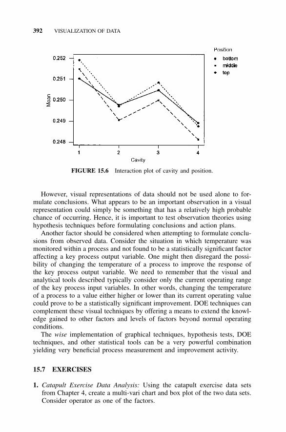
392 VISUALIZATION OF DATA

FIGURE 15.6 Interaction plot of cavity and position.

However, visual representations of data should not be used alone to for-mulate conclusions. What appears to be an important observation in a visualrepresentation could simply be something that has a relatively high probablechance of occurring. Hence, it is important to test observation theories usinghypothesis techniques before formulating conclusions and action plans.

Another factor should be considered when attempting to formulate conclu-sions from observed data. Consider the situation in which temperature wasmonitored within a process and not found to be a statistically significant factoraffecting a key process output variable. One might then disregard the possi-bility of changing the temperature of a process to improve the response ofthe key process output variable. We need to remember that the visual andanalytical tools described typically consider only the current operating rangeof the key process input variables. In other words, changing the temperatureof a process to a value either higher or lower than its current operating valuecould prove to be a statistically significant improvement. DOE techniques cancomplement these visual techniques by offering a means to extend the knowl-edge gained to other factors and levels of factors beyond normal operatingconditions.

The wise implementation of graphical techniques, hypothesis tests, DOEtechniques, and other statistical tools can be a very powerful combinationyielding very beneficial process measurement and improvement activity.

15.7 EXERCISES

1. Catapult Exercise Data Analysis: Using the catapult exercise data setsfrom Chapter 4, create a multi-vari chart and box plot of the two data sets.Consider operator as one of the factors.

EXERCISES 393

2. An experiment was conducted where each student recorded his or herheight, weight, gender, smoking preference, usual activity level, and restingpulse. Then they all flipped coins, and those whose coins came up headsran in place for one minute. Then the entire class recorded their pulsesonce more (Minitab 1998).

Create a multi-vari chart that provides insight into the effect of factors.

Column Name Count Description

Cl Pulse 1 92 First pulse rateC2 Pulse 2 92 Second pulse rateC3 Ran 92 1 � ran in place

2 � did not run in placeC4 Smokes 92 1 � smokes regularly

2 � does not smoke regularlyC5 Sex 92 1 � male 2 � femaleC6 Height 92 Height in inchesC7 Weight 92 Weight in poundsC8 Activity 92 Usual level of physical activity:

1 � slight2 � moderate3 � a lot

Pulse 1 Pulse 2 Ran Smokes Sex Height Weight Activity

64 88 1 2 1 66.00 140 258 70 1 2 1 72.00 145 262 76 1 1 1 73.50 160 366 78 1 1 1 73.00 190 164 80 1 2 1 69.00 155 274 84 1 2 1 73.00 165 184 84 1 2 1 72.00 150 368 72 1 2 1 74.00 190 262 75 1 2 1 72.00 195 276 118 1 2 1 71.00 138 290 94 1 1 1 74.00 160 180 96 1 2 1 72.00 155 292 84 1 1 1 70.00 153 368 76 1 2 1 67.00 145 260 76 1 2 1 71.00 170 362 58 1 2 1 72.00 175 366 82 1 1 1 69.00 175 270 72 1 1 1 73.00 170 368 76 1 1 1 74.00 180 272 80 1 2 1 66.00 135 370 106 1 2 1 71.00 170 274 76 1 2 1 70.00 157 266 102 1 2 1 70.00 130 270 94 1 1 1 75.00 185 2

394 VISUALIZATION OF DATA

Pulse 1 Pulse 2 Ran Smokes Sex Height Weight Activity

96 140 1 2 2 61.00 140 262 100 1 2 2 66.00 120 278 104 1 1 2 68.00 130 282 100 1 2 2 68.00 138 2

100 115 1 1 2 63.00 121 268 112 1 2 2 70.00 125 296 116 1 2 2 68.00 116 278 118 1 2 2 69.00 145 288 110 1 1 2 69.00 150 262 98 1 1 2 62.75 112 280 128 1 2 2 68.00 125 262 62 2 2 1 74.00 190 160 62 2 2 1 71.00 155 272 74 2 1 1 69.00 170 262 66 2 2 1 70.00 155 276 76 2 2 1 72.00 215 268 66 2 1 1 67.00 150 254 56 2 1 1 69.00 145 274 70 2 2 1 73.00 155 374 74 2 2 1 73.00 155 268 68 2 2 1 71.00 150 372 74 2 1 1 68.00 155 368 64 2 2 1 69.50 150 382 84 2 1 1 73.00 180 264 62 2 2 1 75.00 160 358 58 2 2 1 66.00 135 354 50 2 2 1 69.00 160 270 62 2 1 1 66.00 130 262 68 2 1 1 73.00 155 248 54 2 1 1 68.00 150 076 76 2 2 1 74.00 148 388 84 2 2 1 73.50 155 270 70 2 2 1 70.00 150 290 88 2 1 1 67.00 140 278 76 2 2 1 72.00 180 370 66 2 1 1 75.00 190 290 90 2 2 1 68.00 145 192 94 2 1 1 69.00 150 260 70 2 1 1 71.50 164 272 70 2 2 1 71.00 140 268 68 2 2 1 72.00 142 384 84 2 2 1 69.00 136 274 76 2 2 1 67.00 123 268 66 2 2 1 68.00 155 284 84 2 2 2 66.00 130 261 70 2 2 2 65.50 120 264 60 2 2 2 66.00 130 3

EXERCISES 395

Pulse 1 Pulse 2 Ran Smokes Sex Height Weight Activity

94 92 2 1 2 62.00 131 260 66 2 2 2 62.00 120 272 70 2 2 2 63.00 118 258 56 2 2 2 67.00 125 288 74 2 1 2 65.00 135 266 72 2 2 2 66.00 125 284 80 2 2 2 65.00 118 162 66 2 2 2 65.00 122 366 76 2 2 2 65.00 115 280 74 2 2 2 64.00 102 278 78 2 2 2 67.00 115 268 68 2 2 2 69.00 150 272 68 2 2 2 68.00 110 282 80 2 2 2 63.00 116 176 76 2 1 2 62.00 108 387 84 2 2 2 63.00 95 390 92 2 1 2 64.00 125 178 80 2 2 2 68.00 133 168 68 2 2 2 62.00 110 286 84 2 2 2 67.00 150 376 76 2 2 2 61.75 108 2

3. Create a box plot of the previous data set with pulse 2 as the responseand sex as the category.

4. Discuss the value of the techniques presented in this chapter and explainhow they can be applied to S4/IEE projects.

5. Select various tools to visually describe the data from the two machinesthat are in Example 10.17. (See Example 19.12 for a compiling of the databy machine.) Comment on results.

6. The COPQ/CODND for the situation described in Exercise 10.18 wasexcessive. An S4/IEE wisdom of the organization study for this improve-ment project yield potential KPIVs as inspector, machine, process tem-perature, material lot, and day-to-day variability relative to within-dayvariability. The data below was collected to assess these relationships. Usevisualization of data techniques to describe differences between inspectors,machines, material lot, and day-to-day variability relative to within-dayvariability.

SubgroupWithinSubgroup KPOV Temperature Machine Inspector

MaterialLotNumber

1 1 96.73 88.3954 1 1 211 2 98.94 81.4335 2 2 211 3 97.71 74.9126 3 1 21

396 VISUALIZATION OF DATA

SubgroupWithinSubgroup KPOV Temperature Machine Inspector

MaterialLotNumber

1 4 107.91 79.0657 1 2 211 5 97.27 76.5458 2 1 2122222

12345

87.3996.0298.76

100.5698.31

74.912272.100582.717177.031886.3016

31231

21212

5555555555

33333

12345

113.91109.79115.21116.3116.84

81.360590.965680.888978.64981.4751

23123

12121

1010101010

44444

12345

120.05111.99110.04119.68119.24

78.357773.951671.014187.635878.8888

12312

21212

3333333333

55555

12345

107.04105.49111.52114.12100.47

83.636881.913373.830780.430177.4916

31231

12121

2626262626

66666

12345

98.44102.28

92.96100.25107.21

84.375182.035680.101380.554778.7169

23123

21212

2929292929

77777

12345

89.9390.4498.2389.8688.14

81.330277.641478.969280.361380.282

12312

12121

4545454545

88888

12345

104.42102.7

97.12101.72102.17

82.652688.082374.235478.96275.926

31231

21212

2222222222

99999

12345

93.2198.54

102.68111.55105.95

88.149673.181682.800779.661381.8933

23123

12121

6767676767

101010

123

89.0691.9191.17

80.172983.842682.3181

123

212

888

EXERCISES 397

SubgroupWithinSubgroup KPOV Temperature Machine Inspector

MaterialLotNumber

1010

45

95.65105.61

80.674681.7851

12

12

88

1111111111

12345

106.59100.76106.27108.02105.29

85.640680.595584.134782.559281.927

31231

12121

102102102102102

1212121212

12345

103.58122.34110.34107.66111.16

90.095786.046988.511581.270372.8305

23123

21212

33333

1313131313

12345

103.79100.83

95.79104.12108.51

82.628381.208581.269475.906289.9129

12312

12121

8888888888

1414141414

12345

109.77109.79110.31106.37

99.34

85.402287.665483.725178.149688.5317

31231

21212

6767676767

1515151515

12345

112.12111.95109.98124.78110.94

81.832683.836790.602378.775580.0546

23123

12121

7676767676

1616161616

12345

88.4695.4991.1

100.8485.61

79.365474.051686.908882.263385.141

12312

21212

5555555555

1717171717

12345

110.21103.99110.98109.63113.93

96.084575.336486.555883.559467.5415

31231

12121

9090909090

1818181818

12345

94.75102.56101.66

98.4888.96

80.98277.457788.329283.641986.0019

23123

21212

8787878787

191919

123

103.39108.2105.23

77.576382.194878.6831

123

121

656565

398 VISUALIZATION OF DATA

SubgroupWithinSubgroup KPOV Temperature Machine Inspector

MaterialLotNumber

1919

45

103.6895.47

75.505888.4383

12

21

6565

2020202020

12345

96.6797.48

102.47101.28103

75.682584.641372.989478.571282.8468

31231

21212

1313131313

7. Describe how and show where the tools described in this chapter fit intothe overall S4/IEE roadmap described in Figures A.1 and A.3 in the Ap-pendix.

399

16CONFIDENCE INTERVALSAND HYPOTHESIS TESTS

S4 /IEE DMAIC Application: Appendix Section A.1, Project ExecutionRoadmap Steps 7.2, 7.4, and 8.9

Descriptive statistics help pull useful information from data, whereas proba-bility provides, among other things, a basis for inferential statistics and sam-pling plans. Within this chapter, focus will be given to inferential statistics,where we will bridge from sample data to statements about the population.That is, properties of the population are inferred from the analysis of samples.

Samples can have random sampling with replacement and random sam-pling without replacement. In addition, there are more complex forms ofsampling, such as stratified random sampling. For this form of sampling acertain number of random samples are drawn and analyzed from divisions ofthe population space. We can also have systematic sampling, where a samplemight be taken after 20 parts are manufactured. We can also have subgroupsampling, where five units might be drawn every hour.

From a random sample of a population we can estimate characteristics ofthe population. For example, the mean of a sample ( ) is a point estimate ofxthe population mean (�). This chapter introduces the topic of confidenceintervals that give probabilistic ranges of values for true population charac-teristics from sampled data. Application of the central limit theorem to thissituation will also be illustrated.

This chapter expands upon the topic of hypothesis testing, discussed inSection 3.11. Hypothesis tests address the situation where we need to makea selection between two choices from sampled data (or information). Becausewe are dealing with sampled data, there is always the possibility that our

400 CONFIDENCE INTERVALS AND HYPOTHESIS TESTS

sample was not an accurate representation of the population. Hypothesis testsaddress this risk. The techniques described in this chapter provide the basisfor statistical significance tests of stratifications that were thought importantby teams when executing S4/IEE projects.

One thing we need to keep in mind is that something can be statisticallysignificant but have no practical significance. For example, a study of 10,000transactions determined that a new procedure reduced the time to complete atransaction from 90 minutes to 89 minutes and 59 seconds. The difference of1 second may be statistically significant but have no practical significance tothe process. Note that a difference can be found to be statistically significantif the sample size is large enough. This is one of the reasons we need toblend statistical analysis with pictures of the data so we can maximize ourinsight to information that can be gleaned from the data.

When a parametric distribution is assumed during analyses, parametricestimates result. When no parametric distribution is assumed during analyses,nonparametric estimates result. Focus in this book is given to parametricestimates; however, nonparametric estimates are also discussed.

16.1 CONFIDENCE INTERVAL STATEMENTS

As noted earlier, the mean of a sample does not normally equate exactly tothe mean of the population from which the sample is taken. An experimenterhas more confidence that a sample mean is close to the population meanwhen the sample size is large, and less confidence when a sample size issmall. Statistical procedures quantify the uncertainty of a sample through aconfidence interval statement.

A confidence interval can be single-sided or double-sided. A confidenceinterval statement can also relate to other characteristics besides mean values(e.g., population variance). The following statements are examples of single-and double-sided confidence interval statements about the mean.

� � 8.0 with 95% confidence

2.0 � � � 8.0 with 90% confidence

Similar statements can be made about standard deviation and other populationcharacteristics. The mechanics of determining confidence intervals for varioussituations are discussed in Chapters 17 and 18.

16.2 CENTRAL LIMIT THEOREM

The central limit theorem is an important theoretical basis of many statisticalprocedures, such as calculation of the confidence interval of a sample mean.It states that a plot of sampled mean values from a population tends to benormally distributed. Figure 16.1 indicates that a plot of the 10 sample mean

HYPOTHESIS TESTING 401

FIGURE 16.1 Plot of sample mean values.

values from Table 3.3 has the shape of a normal distribution. The distributionof mean values taken from a population will tend to be normal even whenthe underlying distribution is not normal. The standard deviation of this sam-pling distribution is s / , where s is the sample standard deviation and n is�nthe sample size. For a given standard deviation, the spread of the samplingdistribution decreases when sample size increases (i.e., we have more confi-dence in our results when sample size is large).

16.3 HYPOTHESIS TESTING

In industrial situations, we frequently want to decide whether the parametersof a distribution have particular values or relationships. That is, we may wishto test a hypothesis that the mean or standard deviation of a distribution hasa certain value or that the difference between two means is zero. Hypothesistesting procedures are used for these tests. Here are some practical examples:

1. A manufacturer wishes to introduce a new product. In order to make aprofit, he needs to be able to manufacture 1200 items during the 200hours available in the next 5 weeks. The product can be successfullymanufactured if the mean time that is required to manufacture an itemis no more than 6 hours. The manufacturer can evaluate manufactura-bility by testing the hypothesis that the mean time for manufacture isequal to 6 hours.

2. The same manufacturer is planning to modify the process to decreasethe mean time required to manufacture another type of product. Themanufacturer can evaluate the effectiveness of the change by testing the

402 CONFIDENCE INTERVALS AND HYPOTHESIS TESTS

hypothesis that the mean manufacturing time is the same before andafter the process change.

Both of these situations involve tests on the mean values of populations.Hypothesis tests may also involve the standard deviations or other parameters.

A statistical hypothesis has the following elements:

• A null hypothesis (H0) that describes the value or relationship beingtested

• An alternative hypothesis (Ha)• A test statistic, or rule, used to decide whether to reject the null hypoth-

esis• A specified probability value (noted as �) that defines the maximum

allowable probability that the null hypothesis will be rejected when it istrue

• The power of the test, which is the probability (noted as [1 � �]) that anull hypothesis will be rejected when it is false

• A random sample of observations to be used for testing the hypothesis

The null and alternative hypotheses arise from the problem being ad-dressed. In example 1, the null hypothesis is that the mean time to manufac-ture an item is equal to six. The item cannot be successfully manufactured ifthe mean time is larger than six, so the alternative hypothesis is that the meanis greater than six. The mean time to manufacture is noted as �, and theshorthand notation for the null and alternative hypotheses is

H : � � � and H : � � �0 0 a 0

where �0 � 6. The hypothesis in the second example concerns the relationshipbetween two mean values. The null hypothesis is that the mean time to man-ufacture the item is the same before and after the change. Because the man-ufacturer wishes to establish the effectiveness of the change, the alternativehypothesis is that the mean time is shorter after the change. If the mean timeto manufacturer before the change is �1 and the mean time to manufactureafter the change is �2. The shorthand notation is

H : � � � and H : � � �0 1 2 a 1 2

where no values need to be specified for �1 and �2. Table 16.1 gives examplesof various hypothesis formats.

The rule used to test the hypothesis depends on the type of hypothesisbeing tested. Consider example 1, where the usual rule is to reject the nullhypothesis if the average of an appropriate sample of manufacturing times issufficiently larger than six. How much larger depends on the allowable prob-ability of making an error.

HYPOTHESIS TESTING 403

TABLE 16.1 Hypothesis Testing: Single- andDouble-Sided Tests on Population Mean

Single-SidedH0: � � �0 H0: � � �0

orHa : � � �0 Ha : � � �0

Double-SidedH0: � � �0 H0: �1 � �2

orHa : � � �0 Ha : �1 � �2

FIGURE 16.2 Hypothesis testing error types.

The result of a hypothesis test is a decision either to reject or not rejectthe null hypothesis; that is, the hypothesis is either rejected or we reservejudgment about it. In practice, we may act as though the null hypothesis isaccepted if it is not rejected. Because we do not know the truth, we can makeone of the following two possible errors when running a hypothesis test:

1. We can reject a null hypothesis that is in fact true.2. We can fail to reject a null hypothesis that is false.

The first error is called a type I error, and the second is called a type IIerror. This relationship is shown in Figure 16.2. Hypothesis tests are designedto control the probabilities of making either of these errors; we do not knowthat the result is correct, but we can be assured that the probability of makingan error is within acceptable limits. The probability of making a type I erroris controlled by establishing a maximum allowable value of the probability,called the level of the test, usually noted as �. The specific rule used to governthe decision to accept or reject the null hypothesis is determined by selectinga particular value of �.

Selecting an appropriate sample size usually controls the probability ofmaking a type II error. Consider example 1 again. If the true mean time tomanufacture an item is not six, it can have one of any number of possiblevalues. It could be 6.01, 6.1, 7, 20, 100, etc. To design the hypothesis testproperly, the manufacturer selects a possible value that is to be protected

404 CONFIDENCE INTERVALS AND HYPOTHESIS TESTS

against and specifies the probability that the hypothesis should be rejected ifthe true mean equals the selected value. For example, the manufacturer maydecide that the hypothesized mean is 6 and should be rejected with probability0.85 if the true mean time is 8 or with probability 0.98 if the true time is 9hours. In common notation these differences of 2 (i.e., 8 � 6 � 2) and 3(i.e., 9 � 6 � 3) correspond to values for �. The probability of rejecting fora given value of � is called the power of the test at �, and it is one minusthe probability of making a type II error (�) at �. The manufacturer designsthe test by selecting a sample size that ensures the desired power at thespecified alternative value. Sample size selection is discussed in Sections 17.2,18.2, 19.3, and 20.3.

After a rule for rejecting the null hypothesis and a sample size are selected,a random sample is selected and used for the test. Statistical statements aboutpopulation means are robust to the data not being normally distributed, whilestatistical evaluations about population standard deviations may not be robustto a lack of normality.

The parameters �, �, and � are sometimes referred to as producer’s risk,consumer’s risk, and an acceptable amount of uncertainty, respectively.

16.4 EXAMPLE 16.1: HYPOTHESIS TESTING

Consider that someone is on trial in a court of law for murder. The personeither committed the crime or did not commit the crime. This situation takesthe form of a hypothesis test where the null hypothesis is that the person isinnocent (i.e., not guilty) and the alternative hypothesis is that he or she isguilty.

Evidence (information) is presented to the jury. The jury then deliberatesto decide whether the person is guilty or not. If the jury makes the decisionthat the person is innocent, there is � risk of error (i.e., the jury is failing toreject the null hypothesis that the person is innocent). If the jury makes thedecision that the person is guilty, there is � risk of error (i.e., the jury rejectsthe null hypothesis that the person is innocent).

To quantify these two risks conceptually within the current court of legalsystem of a country, consider a random selection of 10,000 murder cases inwhich the suspect was found innocent and 10,000 murder cases in which thesuspect was found guilty. If we could determine the real truth (whether theydid in fact commit murder or not), the risks associated with our current ju-dicial system would be

u v� � � �

10,000 10,000

where u is the number of people found guilty who were in fact innocent andv is the number of people not found guilty who were in fact guilty.

EXERCISES 405

16.5 S4/IEE ASSESSMENT

It is good practice to visualize the data in conjunction with making mathe-matical computations. Probability plotting is a good tool to use when makingsuch an observation. After looking at the data, the analyst might determinethat the wrong question was initially asked; e.g., a statement about the per-centage of population would be more meaningful than a statement about themean of a population.

It is unfortunate (Hoerl 1995) that the vast majority of works in statisticalbooks and papers focus almost exclusively on deduction (i.e., testing hypoth-esis or an estimation of parameters in an assumed model). Very little existsin print on how to use induction to revise subject matter theory based onstatistical analysis. Deductive reasoning begins with premises (theory) andinfers through analysis what should be seen in practice, whereas induction isreasoning from particulars to the general.

While both types of reasoning are required by scientific methods, statisticaleducation focuses primarily on deduction because it lends itself more to math-ematics. As a result, most books teach rigorous adherence to preset rules fordecision making when covering hypothesis testing. For example, if the nullhypothesis is rejected, the possibility of questioning the original assumptionsbased on what is seen in the data is never mentioned. However, the primaryneeds of engineers and scientists are inductive. They need to use data to creategeneral rules and statements, which explains why statistical techniques arenot more widely used in these disciplines.

This book suggests various approaches to creating hypotheses. The S4/IEEassessment sections at the ends of subsequent chapters challenge the under-lying assumptions of many hypothesis tests. When analyzing data and inte-grating the statistical techniques described here, practitioners should not losesight of the need to challenge the underlying assumptions of hypothesis tests.It is very important to ask the right question before determining an answer.

16.6 EXERCISES

1. Catapult Exercise Data Analysis: Describe the wording of various hypoth-eses that could be assessed relative to the data that were collected in Chap-ter 4.

2. Dice Exercise: Each person in an S4/IEE workshop rolls a die 25 times,records the number of times each number appears, and calculates an av-erage value. The instructor collects from attendees the total number oftimes each number is rolled and plots the information. Average values fromall attendees are collected and plotted in a histogram format. Note theshape of each curve.

3. Card Exercise: Each team is given a deck of 52 cards and told to removethe 8’s, 9’s, and 10’s. The cards are shuffled. Five cards are removed. The

406 CONFIDENCE INTERVALS AND HYPOTHESIS TESTS

face value of these cards are averaged (jack � 11, queen � 12, king �13, and ace � 1). This is repeated 25 times by each team (removed cardsare returned to deck before reshuffling). Plot the distribution of the meanvalues. Describe results and explain what would happen to the shape ofthe distribution if 10 card values had been averaged instead of 5.

4. From the curve of average rolls of the die (or averages of card draws),estimate the range of roll mean values that are expected for 25 rolls of thedie 90% of the time. Describe how the distribution shape of mean valueswould change if there were 50 rolls of the die.

5. Is the null hypothesis one-sided or two-sided in a test to evaluate whetherthe product quality of two suppliers is equal?

6. Describe a decision that you make within your personal life that could bephrased as a hypothesis test.

7. Discuss the usefulness of the techniques presented in this chapter andexplain how they can be applied to S4/IEE projects.

407

17INFERENCES:CONTINUOUS RESPONSE

S4 /IEE DMAIC Application: Appendix Section A.1, Project ExecutionRoadmap Steps 7.2, 7.3, and 8.9

This chapter covers random sampling evaluations from a population that hasa continuous response. An example of a continuous response is the amountof tire tread that exists after 40,000 kilometers (km) of automobile usage.One tire might, for example, have 6.0 millimeters (mm) of remaining treadwhile another tire might measure 5.5 mm.

In this chapter the estimation of population mean and standard deviationfrom sampled data is discussed in conjunction with probability plotting.

17.1 SUMMARIZING SAMPLED DATA

The classical analysis of sampled data taken from a continuous response pop-ulation has focused on determining a sample mean ( and standard deviationx)(s), along with perhaps confidence interval statements that can relate both ofthese sampled characteristics to the actual population values (� and �, re-spectively). Experimental considerations of this type answer some basic ques-tions about the sample and population. However, analysts responsible foreither generating a criterion specification or making a pass/fail decision oftendo not consider the other information that data analyses can convey. Forexample, an experiment might be able to indicate that 90% of the automobilesusing a certain type of tire will have at least 4.9 mm of tire tread after 40,000

408 INFERENCES: CONTINUOUS RESPONSE

km. Such a statement can be more informative than a statement that onlyrelates to the mean tire tread after 40,000 km.

17.2 SAMPLE SIZE: HYPOTHESIS TEST OF A MEANCRITERION FOR CONTINUOUS RESPONSE DATA

One of the most traditional questions asked of a statistical consultant is,‘‘What sample size do I need (to verify this mean criterion)?’’ The followingequation (Diamond 1989) can be used to determine the sample size (n) nec-essary to evaluate a hypothesis test criterion at given values for �, �, and �(i.e., producer’s risk, consumer’s risk, and an acceptable amount of uncer-tainty, respectively). Sometimes the population standard deviation (�) isknown from previous test activity; however, this is not generally true. For thissecond situation, � can be conveniently expressed in terms of �:

2�2n � (U � U )� � 2�

In this equation, U� is determined from the single-sided Table B in AppendixE. If the alternative hypothesis is single-sided (e.g., � � criterion), U� is alsodetermined from Table B; however, if the alternative hypothesis is double-sided (e.g., � � or � criterion), U� is determined from Table C.

If the standard deviation is not known, the sample size should be adjustedusing (Diamond 1989):

2s2n � (t � t )� � 2�

In this equation, t� is determined from the single-sided Table D. If thealternative hypothesis is single-sided (e.g., � � criterion), t� is also deter-mined from Table D; however, if the alternative hypothesis is double-sided(e.g., � � or � criterion), t� is determined from Table E.

An alternative approach for sample size calculations is described later inthis chapter.

17.3 EXAMPLE 17.1: SAMPLE SIZE DETERMINATION FOR AMEAN CRITERION TEST

A stereo amplifier output power level is desired to be on the average at least100 watts (W) per channel. Determine the sample size that is needed to verifythis criterion given the following:

CONFIDENCE INTERVALS ON THE MEAN AND HYPOTHESIS TEST 409

� � 0.1, which from Table B yields U� � 1.282.� � 0.05, which from Table B yields U� � 1.645.� � 0.5�.

Substitution yields

2�2n � (1.282 � 1.645) � 34.262(0.5�)

Rounding up to a whole number yields a sample size of 35.If the standard deviation is not known, this sample size needs to be ad-

justed. Given that the number of degrees of freedom for the t-table valueequals 34 (i.e., 35 � 1), interpolation in Table D yields to t0.1;34 � 1.307 andt0.05;34 � 1.692; hence,

2s2n � (1.692 � 1.307) � 35.952(0.5s)

Rounding up to a whole number yields a sample of 36.Because individuals want to make sure that they are making the correct

decision, they often specify very low � and � values, along with a low �value. This can lead to a sample size that is unrealistically large with normaltest time and resource constraints. When this happens, the experimenter mayneed to accept more risk than he or she was originally willing to tolerate.The sample size can then be recalculated permitting the larger risks (a higher� and/or � value) and/or an increase in uncertainty (i.e., a higher � value).

17.4 CONFIDENCE INTERVALS ON THE MEAN ANDHYPOTHESIS TEST CRITERIA ALTERNATIVES

After sample mean and standard deviation (s) are determined from the(x)data, Table 17.1 summarizes the equations used to determine from these pop-ulation estimates the intervals that contain the true mean (�) at a confidencelevel of [(1 � �)100]. The equations in this table utilize the t tables (asopposed to the U tables) whenever the population standard deviation is notknown. Because of the central limit theorem, the equations noted in this tableare robust even when data are not from a normal distribution.

If a sample size is calculated before conducting the experiment using de-sired values of �, �, and �, the null hypothesis is not rejected if the criterionis contained within the appropriate confidence interval for �. This decision ismade with the � risk of error that was used in calculating the sample size(given the underlying � input level of uncertainty). However, if the criterion

410 INFERENCES: CONTINUOUS RESPONSE

TABLE 17.1 Mean Confidence Interval Equations

Single-Sided Double-Sided

� Known

� � �U ��x�n

or

� � �U ��x�n

� � � � �U � U �� �x x�n �n

� Unknown

� � �t s�x�n

or

� � �t s�x�n

� � � �t s t s� �x � x�n �n

Using reference tables U : Table B�

at : Table D�

U : Table C�

at : Table E�

a � � n � 1 (i.e., the number of degrees of freedom used in the t table is equal to one less thanthe sample size).

is not contained within the interval, then the null hypothesis is rejected. Thisdecision is made with � risk of error.

Other methods can be used when setting up a hypothesis test criterion.Consider, for example, the alternative hypothesis (Ha) of � � �a, where �a

is a product specification criterion. From Table 17.1 it can be determined that

t s�x � � �criterion a �n

When is greater than the test the null hypothesis is rejected. Whenx x ,criterion

is less than the null hypothesis is not rejected. An alternative ap-x x ,criterion

proach for this problem is to use the equation form

(x � � )�nat �0 s

where the null hypothesis is rejected if t0 � t�.The equations above apply to planned statistical hypothesis testing where

prior to testing itself �, �, and � were chosen. However, in reality, data areoften taken without making these pretest decisions. The equations presented

EXAMPLE 17.2: CONFIDENCE INTERVALS ON THE MEAN 411

here are still useful in making an assessment of the population, as seen in thefollowing example.

17.5 EXAMPLE 17.2: CONFIDENCE INTERVALS ON THE MEAN

Consider the 16 data points from sample 1 of Table 3.3, which had a samplemean of 5.77 and a sample standard deviation of 2.41. Determine the various90% confidence statements that can be made relative to the true populationmean, that the standard deviation is 2.0 and then treating it as an unknownparameter.

Given that � is 2.0, the single-sided and double-sided 90% confidence (i.e.,� � 0.1) interval equations are as shown below. The U� value of 1.282 isfrom the single-sided Table B, given � � 0.1. The U� value of 1.645 is fromthe double-sided Table C, given � � 0.1.

Single-Sided Scenarios:

U � U �� �� � x � � � x ��n �n

1.282(2.0) 1.282(2.0)� � 5.77 � � � 5.77 �

�16 �16

� � 5.77 � 0.64 � � 5.77 � 0.64

� � 6.41 � � 5.13

Double-Sided Scenario:

U � U �� �x � � � � x ��n �n

1.615(2.0) 1.645(2.0)5.77 � � � � 5.77 �

�16 �16

5.77 � 0.82 � � � 5.77 � 0.82

4.95 � � � 6.59

If the standard deviation is not known, the resulting equations for single- anddouble-sided 90% confidence intervals are the following. The t� value of1.341 is from the single-sided Table D, given � � 0.1 and v � 16 � 1 �15. The t� value of 1.753 is from the double-sided Table E, given � � 0.1and v � 16 � 1 � 15.

412 INFERENCES: CONTINUOUS RESPONSE

Single-Sided Scenarios:

t s t s� �� � x � � � x ��n �n

(1.341)(2.41) (1.341)(2.41)� � 5.77 � � � 5.77 �

�16 �16

� � 5.77 � 0.81 � � 5.77 � 0.81

� � 6.58 � � 4.96

Double-Sided Scenario:

t s t s� �x � � � � x ��n �n

1.753(2.41) 1.753(2.41)5.77 � � � � 5.77 �

�16 �16

5.77 � 1.06 � � � 5.77 � 1.06

4.71 � � � 6.83

Computer programs can provide confidence intervals for continuous responsedata. In addition, these computer programs can test null hypotheses. For thedouble-sided interval calculated above, where 6 is the mean criterion, a com-puter analysis yielded

One-Sample T: Sampling 1

Test of mu � 6 vs mu not � 6

Variable N Mean StDev SE MeanSampling 1 16 5.774 2.407 0.602

Variable 90.0% CI T PSampling 1 ( 4.720, 6.829) �0.37 0.713

This confidence interval is similar to the above manual calculations, wheredifferences are from round-off error. For a hypothesis risk criterion of 0.05,the p value of 0.713 indicates that we would fail to reject the null hypothesisthat the mean is equal to 6.

The mean and standard deviation used in the preceding calculations wererandomly created from a normal distribution where � � 6.0. Note that thistrue mean value is contained in these confidence intervals. When the confi-dence interval is 90%, we expect the interval to contain the true value 90%of the time that we take random samples and analyze the data.

EXAMPLE 17.4: STANDARD DEVIATION CONFIDENCE STATEMENT 413

17.6 EXAMPLE 17.3: SAMPLE SIZE—AN ALTERNATIVE APPROACH

The equation given above for sample size included the risk levels for both �and �. An alternative approach can be used if we want to determine a meanvalue within a certain � value and level of confidence (e.g., �4 at 95%confidence). To determine the sample size for this situation, consider theequation

U ��� � x ��n

It then follows that

U � 1.96��4 � ��n �n

or

2 2(1.96) � 2n � � 0.24�24

17.7 STANDARD DEVIATION CONFIDENCE INTERVAL

When a sample of size n is taken from a population that is normally distrib-uted, the double-sided confidence interval equation for the population’s stan-dard deviation (�) is

1 / 2 1 / 22 2(n � 1)s (n � 1)s� � �� � � �2 2 � / 2; � (1�� / 2; �)

where s is the standard deviation of the sample and the 2 values are takenfrom Table G with � /2 risk and � degrees of freedom equal to the samplesize minus 1. This relationship is not robust for data from a nonnormal dis-tribution.

17.8 EXAMPLE 17.4: STANDARD DEVIATIONCONFIDENCE STATEMENT

Consider again the 16 data points from sample 1 of Table 3.3, which had amean of 5.77 and a standard deviation of 2.41. Given that the standard de-

414 INFERENCES: CONTINUOUS RESPONSE

viation was not known, the 90% confidence interval for the standard deviationof the population would then be

1 / 2 1 / 22 2(16 � 1)(2.41) (16 � 1)(2.41)� � �� � � �2 2 (0.1 / 2;[16�1]) (1�[0.1 / 2];[16�1])

1 / 2 1 / 287.12 87.12� � �� � � �25.00 7.26

1.87 � � � 3.46

The standard deviation used in this calculation was from a random sampletaken from a normal distribution where � � 2.0. Note that this true standarddeviation value is contained in this confidence interval. When the confidenceinterval is 90%, we would expect the interval to contain the true value 90%of the time that we take random samples and analyze the data.

17.9 PERCENTAGE OF THE POPULATION ASSESSMENTS

Criteria are sometimes thought to apply to the mean response of the product’spopulation, with no regard to the variability of the product response. Oftenwhat is really needed is that all of the product should have a response that isless than or greater than a criterion.

For example, a specification may exist that a product should be able towithstand an electrostatic discharge (ESD) level of 700 volts (V). Is the intentof this specification that the mean of the population (if tested to failure) shouldbe above 700 V? Or should all products built be able to resist a voltage levelof 700 V?

It is impossible to be 100% certain that every product will meet such acriterion without testing every product that is manufactured. For criteria thatrequire much certainty and a 100% population requirement, 100% testing toa level that anticipates field performance degradation may be required. How-ever, a reduced confidence level may be acceptable with a lower percentconfidence requirement (e.g., 95% of the population). Depending on the sit-uation, the initial criterion may need adjustment to reflect the basic test strat-egy.

Other books present approaches to this situation such as K factors (Natrella1966) using tables and equations that consider both the mean and standarddeviation of the sample. However, with this approach the assumption of nor-mality is very important and the sample size requirements may often be toolarge.

Another possible approach is a ‘‘best estimate’’ probability plot, which cangive visual indications to population characteristics that may not otherwisebe apparent. A probability plot may indicate, for example, that data outliers

EXAMPLE 17.5: PERCENTAGE OF THE POPULATION STATEMENTS 415

TABLE 17.2 Ranked Data and Plot Positions

Original SampleNumber

RankedSample Value

PercentagePlot Position

7 2.17 3.13 2.65 9.41 2.99 15.68 4.13 21.9

15 4.74 28.116 5.19 34.410 5.20 40.6

5 5.31 46.912 5.39 53.111 5.80 59.4

6 5.84 65.62 6.29 71.99 7.29 78.1

14 9.29 84.413 10.00 90.6

4 10.11 96.9

are present or that a normal distribution assumption is not appropriate. Inaddition, some computer software packages include confidence intervals intheir probability plots.

17.10 EXAMPLE 17.5: PERCENTAGE OF THEPOPULATION STATEMENTS

Consider again the first sample from Table 3.3 that yielded a mean value of5.77 and a standard deviation of 2.41. This time let’s create a normal prob-ability of the data. Table 17.2 has the ranked sample values matched with thepercentage plot position taken from Table P for the sample size of 16. Thesecoordinates can then be manually plotted on normal probability paper (seeTable Q1). Figure 17.1 is a computer-generated normal probability plot of thedata.

From this plot one notes that evaluating only the mean value for this samplemay yield deceiving conclusions because the standard deviation is rather largecompared to the reading values. In addition, the normal distribution can beused to represent the population, because the data tend to follow a straightline. If a criterion of 20 were specified for 95% of the population (given thata low number indicates goodness), an individual would probably feel com-fortable that the specification was met because the best-estimate plot estimatesthat 95% of the population is less than 9.5. However, if the criterion were 10for this percentage of the population, we would probably conclude that the

416 INFERENCES: CONTINUOUS RESPONSE

FIGURE 17.1 Normal probability plot.

manufacturing process might need to be examined for possible improvements.Regression and/or DOE might be appropriate to assess which of those par-ameters considered (perhaps from a brainstorming session) are statisticallysignificant in reducing the mean and/or standard deviation of the process.

Probability plots of data can often be enlightening. From these plots onemay find, for example, that the data are not normally distributed. If there isa knee in the curve, this may indicate that there are two distributions in theprocess (i.e., a bimodal distribution). In this case it might be beneficial to tryto determine why one sample is from one distribution while another sampleis from another distribution. This may happen, for example, because one oftwo suppliers produces a better part than the other. Another possibility is thatthe normal probability plot has curvature and may be better fitted to someother distribution (e.g., a three-parameter Weibull distribution).

As a minimum, when choosing a sample size for making a decision aboutthe percentage of population, extrapolation should be avoided to reach thedesired percentage value. In this example, one notes from the tabulated valuesthat the percentage plot position extremes are 3.1% and 96%. This meansthat a probability plot of the 16 data points has no extrapolation when single-sided (high-value) statements are made about 95% of the population. Thepercentage plot positions in Table P indicate that 26 data points are neededto yield nonextrapolated single-sided statements about 98% of the population.

Another valid concern can emerge from this type of experiment. If thesample is drawn from a process over a short period of time, this sample doesnot necessarily represent what the process will do in the future. DOE tech-niques again can be used as a guide to adjust parameters used to manufacturethe parts. The procedure described within this example could then still beapplied to get a ‘‘big-picture spatial representation’’ (i.e., the data are fromthe factorial trials and are not a true random sample of a population) of what

STATISTICAL TOLERANCING 417

could be expected of the process in the future (see Example 43.3). In addition,any statistically significant parameters could then be focused on, perhaps toimprove the process mean and/or reduce the process variability. The processthen could be continually monitored via control charts for drifts of the processmean and standard deviation.

17.11 STATISTICAL TOLERANCING

The quality of a product’s output (or whether the assembly will work or fail)can depend on the tolerances of the component parts used in the assemblyprocess. A pencil-and-paper worst-case tolerance analysis is sometimes ap-propriate to make sure that tolerances do not ‘‘stack,’’ causing an overall out-of-specification condition. However, if there are many components in theassembly process, it may be impossible to ensure that the completed productwill perform satisfactorily if all the component tolerances were at worst-caseconditions.

The overall effect of a component is often considered to follow a normaldistribution, with �3� bounds equivalent to the component tolerance limits(or other tighter limits), where the mean (�) of the distribution is the midpointbetween the tolerance limits.

Consider that measurements for n components that are each centered atmean (�i) of a normal distribution with plus or minus tolerances (Ti) aroundthis mean value. The worst-case overall tolerance (Tw) for this situation issimply the addition of these tolerances.

n

T � � T � �(T � T � � � � � T )�w i 1 2 ni�1

The serial 3� combination of the component tolerances yields an overallproduct 3� tolerance (T3�) of

1 / 2n2 2 2 2 1 / 2T � � T � �(T � T � � � � � T )�� �3� i 1 2 n

i�1

Care must be exercised when using this equation. Normality is very im-portant. In some situations, the assumption that each component follows anormal distribution will not be valid. For example, a �10% tolerance resistormay follow a bimodal, truncated, and/or skewed, distribution because the bestparts can be sorted out and sold at a higher price, with a �1% or �5%tolerance. Another situation where the normality assumption may be invalidis where a manufacturer initially produces a part at one tolerance extreme,anticipating tool wear in the manufacturing process.

418 INFERENCES: CONTINUOUS RESPONSE

FIGURE 17.2 Diagram showing specification limits.

An alternative approach to using this equation is to estimate a distributionshape for each component. Then, by computer, conduct a Monte Carlo sim-ulation, randomly choosing a component characteristic from each distribution;then combine these values to yield an overall expected output. A computercan easily simulate thousands of assemblies to yield the expected overalldistribution of the combined tolerances.

17.12 EXAMPLE 17.6: COMBINING ANALYTICAL DATA WITHSTATISTICAL TOLERANCING

An automatic sheet feed device is to load a sheet of paper into a printer suchthat the first character printed on the paper will be 1.26 � 1.26 mm from theedge of the paper (Figure 17.2).

In this problem there are two variabilities that need consideration: first,variability within machines and then the variability between machines. Forsome problem types, when there is only one output for the device, only var-iability between machines will be needed. In this situation each machine willhave multiple outputs because each printed page is an output.

In industry, this type of question may need to be addressed early within adevelopment cycle when few models are available for testing. The followingwill consider three alternatives given this physical test constraint. In the firstapproach, all tolerances, including some measurement data, will be combinedto yield a worst-case analysis (i.e., Tw). In the second approach, the populationwill be all sheets of paper produced on all printers manufactured. The thirdapproach to determine whether 99.7% (�3�) of the sheets printed on 99.7%of the printers will be within the tolerance limits.

The design group determined that there were 14 tolerances involved witheither (a) the placement of the page within the printer or (b) the printing ofthe character on the page. The tolerance analyses also indicated a nominalcharacter position of 1.26 mm. All the tolerances were plus or minus values;hence, the tolerances can be algebraically combined as shown below. Theplus or minus tolerances (Ti) (i � 1 to 14) are

0.1, 0.2, 0.2, 0.03, 0.34, 0.15, 0.05, 0.08, 0.1, 0.1, 0.1, 0.1, 0.06, 0.1

When a machine is assembled, it takes on a value within the range. How-

EXAMPLE 17.6: COMBINING ANALYTICAL DATA 419

ever, for various reasons, the first print character will not always be positionedin the same position. Things that could affect this positioning are paper type,platen imperfections, initial loading of the paper tray, and so forth. A DOEassessment may be necessary to take all these considerations into account.Assume that this experiment was performed and that it was concluded fromthe test that a machine repeatability (�r) estimate of 0.103 mm would be usedfor any further calculations.

1. In a worst-case analysis approach, the worst-case machine tolerances(TA) are combined with the 3� limits of machine repeatability to yield

n

T � � T � 3��A i ri�1

� �(0.1 � 0.2 � � � 0.1) � 3(0.103)

� �1.71 � 0.31 � �2.02

Because �2.02 is greater than the specification �l.26 tolerance, theassembly is not expected to perform satisfactorily.

2. If the specification is taken as addressing 99.7% of all pages producedon all printers, it follows that

0.5n2 2T � � T � (3�)��� � �B i

i�1

2 2 2 2 0.5� �{(0.1 � 0.2 � � � 0.1 ) � [3(0.103)] }

� �0.622

This combination yields a favorable result because �0.622 is less thanthe specification tolerance of �1.26. However, consider the person whohas a printer with manufacturing tolerances at a 3� limit. This individualwill still experience the full effects of variations when loading the paperin addition to the adverse printer tolerance considerations. Hence, thisapproach may yield a conclusion that is too optimistic from a user’sperspective.

3. Considering that the specification should be met on 99.7% of the sheetsproduced on a ‘‘statistical worst-case’’ machine (i.e., 3� combination),this yields

0.5n2T � � T � (3�)�� �C i

i�1

2 2 2 0.5� �(0.1 � 0.2 � � � 0.1 ) � [3(0.103)]

� �0.85

420 INFERENCES: CONTINUOUS RESPONSE

This approach yields a favorable result because �0.85 is less than thespecification tolerance of �1.26.

This example illustrates the combination of experimental results with atolerance analysis. It also shows that the basic analysis strategy can changedepending on the definition of the problem. Chapter 32, on Taguchi contri-butions, will take this a step further. This chapter will challenge the historicallogic of assuming that an assembly that just meets a criterion is good, whilean assembly that just misses the criterion is bad (for this example, a �1.25value around the criterion would be considered ‘‘good,’’ while a �1.27 valuearound the criterion would be considered ‘‘bad’’).

17.13 NONPARAMETRIC ESTIMATES: RUNS TESTFOR RANDOMIZATION

A run is defined as a group of consecutive observations either all greater thanor less than some value. To assess whether data are in random order using aruns test, data are evaluated in terms of the number of runs above and belowthe median. Within this nonparametric test no assumption is required aboutthe population distribution.

17.14 EXAMPLE 17.7: NONPARAMETRIC RUNS TESTFOR RANDOMIZATION

Forty people are selected randomly. Each person is asked a question, whichhas five possible answers that are coded 1–5. A gradual bias in the questionphrasing or a lack of randomization when selecting people would cause non-randomization of the respnses. The responses were

1 1 2 1 1 1 1 1 1 2 3 3 2

0 0 0 0 1 1 3 3 4 4 5 5

5 5 2 1 1 2 2 2 1 1 3 3

3 3 2

The following statistical analysis indicates that the null hypothesis of a ran-dom response is rejected at a p level less than 0.0000.

EXERCISES 421

Runs Test: Response

K � 2.0500

The observed number of runs � 7The expected number of runs � 19.200014 Observations above K 26 below

The test is significant at 0.0000

17.15 S4/IEE ASSESSMENT

This chapter illustrates techniques in which random samples are used forhypothesis testing or confidence interval statements. This type of assessmentmight be suggested during initial problem definition; however, one mightconsider the following questions to determine if there is an S4/IEE alternative.

1. Is the sample really taken from the population of interest? If, for ex-ample, a sample is taken from the start-up of a manufacturing process,the sample output will not necessarily represent future machine builds.Hence, a machine failure rate test during this early phase of productionmay not yield a failure rate similar to later experience by the customer.

2. Is the process that is being sampled stable? If it is not, then the testmethods and confidence statements cannot be interpreted with muchprecision. Process control charting techniques can be used to determinethe stability of a process.

3. What is going to be done if the process does not meet a test criterion?Are the parts going to be shipped anyway, as long as the output is‘‘reasonable’’?

4. Would a DOE be more useful than a random sample taken at somepoint in time? A DOE test strategy can yield information indicatingwhere the process/design may be improved.

Let’s not play games with the numbers. Future chapters will illustrate ap-proaches that can be more helpful in answering the real questions: How canwe design, build, or test this product smarter to give the customer the bestpossible product at the lowest possible price?

17.16 EXERCISES

1. Catapult Exercise Data Analysis: Using the catapult exercise data setsfrom Chapter 4, determine the 95% confidence interval of the mean andstandard deviation.

422 INFERENCES: CONTINUOUS RESPONSE

2. From sampled data, state the distribution used to calculate the confidenceinterval on the mean. Also, state the distribution that is used to calculatethe confidence interval on the standard deviation.

3. The following data give the difference between actual arrival time andscheduled arrival time for the 12 monthly flights someone made into his/her resident city during the previous year (plus values indicate the numberof minutes the flight was late). The traveler was always scheduled toarrive at the same time on the last Wednesday of the month.

June July Aug Sep Oct Nov Dec Jan Feb Mar Apr May

0.1 3.2 18.4 2.5 15.6 90.9 102.1 0.8 20.2 31.3 1.4 21.9

(a) Determine the sample mean and standard deviation.(b) Estimate the 95% confidence intervals for the population mean and

standard deviation. Note any assumptions.(c) Display data in a histogram format.(d) Create a normal probability plot of the data.(e) Estimate arrival time range for 90% of the flights (using normal prob-

ability plot and Z table (Table A). Comment on analysis.(f) Interpret the plots and describe any further investigation.(g) If someone was to make a general inference about the arrival times

of all passengers into the airport, state a key underlying assumptionthat is violated.

(h) Explain the potential problem with making inferences about nextyear’s arrival times from the current year’s arrival times.

4. A random sample yielded the measurements 9.4, 10.6, 8.1, 12.2, 15.9,9.0, 9.1, 10.0, 11.7, 11.0.(a) Determine the sample mean and the 95% confidence interval for the

population mean.(b) Determine the sample standard deviation and the 95% confidence

interval for the population standard deviation.(c) Display the data using a histogram and normal probability plots.(d) Estimate the response that is exceeded 10% of the time (using prob-

ability plot and Z table (Table A). Comment on the validity of theanalysis and results.

(e) Create a process capability/performance report for a specification of10.0 � 4.0. Comment on the validity of the analysis and results.

5. The following random sampled data was submitted for analysis: 33.4,42.2, 37.1, 44.2, 46.0, 34.0, 32.6, 42.7, 32, 39.5.(a) Determine the sample mean and the 95% confidence interval for the

population mean.

EXERCISES 423

(b) Determine the sample standard deviation and the 95% confidenceinterval for the population standard deviation.

(c) Display the data using a histogram and normal probability plots.(d) Using the plots and Z table (i.e., Table A) estimate the range of

responses expected 90% of the time. Comment on the validity of theanalysis and results.

(e) Estimate process capability/performance metrics for a specificationof 40.0 � 7.0. Comment on the validity of the analysis and results.

(f) Describe possible sources for this data.

6. A 10 random-sample evaluation of the specification 75 � 3 yielded read-ings of 77.1, 76.8, 76.3, 75.9, 76.1, 77.7, 76.7, 75.7, 76.9, 77.4.(a) Determine the sample mean and the 95% confidence interval for the

population mean.(b) Determine the sample standard deviation and the 95% confidence

interval for the population standard deviation.(c) Display the data using a histogram and normal probability plots.(d) Using plots and Z table (Table A), estimate the proportion beyond

the specification limits. Determine the process capability/perform-ance indices. Comment on the validity of the analysis and results.

(e) Determine where emphasis should be given to make the process morecapable of meeting specifications (reducing variability or shiftingmean).

(f) Give an example from manufacturing, development, and servicewhere these data might have originated.

7. A sample of 10 was taken from an in-control process. A variance of 4.2and a mean of 23.2 were calculated. Determine the 95% confidence in-terval on the mean and standard deviation. Explain any potential problemswith this analysis.

8. A sample from an in-control/predictable process had a variance of 4.2and a mean of 23.2. Determine the 90% lower confidence bound on themean and standard deviation. Describe any potential problems with thisanalysis.

9. To address some customer problem reports, management wants a randomsample evaluation to assess the products currently produced. Determinethe sample size needed to assess a mean response criterion of 75 if risksare at a level of 0.05. Consider that � equals the standard deviation ofthe process response. State the test hypothesis. Discuss how well the basictest strategy will probably assess the needs of the customer.

10. A product design consists of five components that collectively affect aresponse. Four of the component dimensions are 4.0 � 0.1 mm, 3.0 �0.1 mm, 6.0 � 0.1 mm, and 2.0 � 0.1 mm. If the dimensions for each

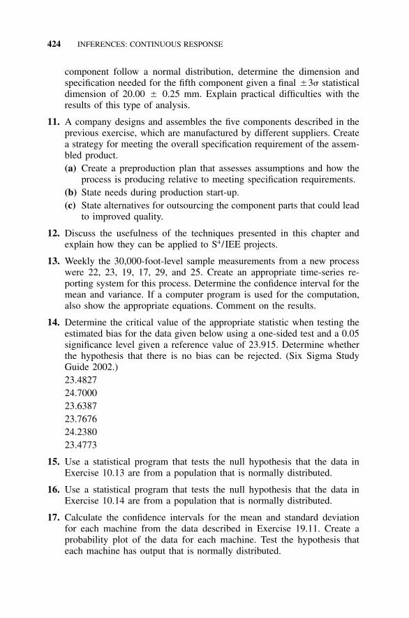
424 INFERENCES: CONTINUOUS RESPONSE

component follow a normal distribution, determine the dimension andspecification needed for the fifth component given a final �3� statisticaldimension of 20.00 � 0.25 mm. Explain practical difficulties with theresults of this type of analysis.

11. A company designs and assembles the five components described in theprevious exercise, which are manufactured by different suppliers. Createa strategy for meeting the overall specification requirement of the assem-bled product.(a) Create a preproduction plan that assesses assumptions and how the

process is producing relative to meeting specification requirements.(b) State needs during production start-up.(c) State alternatives for outsourcing the component parts that could lead

to improved quality.

12. Discuss the usefulness of the techniques presented in this chapter andexplain how they can be applied to S4/IEE projects.

13. Weekly the 30,000-foot-level sample measurements from a new processwere 22, 23, 19, 17, 29, and 25. Create an appropriate time-series re-porting system for this process. Determine the confidence interval for themean and variance. If a computer program is used for the computation,also show the appropriate equations. Comment on the results.

14. Determine the critical value of the appropriate statistic when testing theestimated bias for the data given below using a one-sided test and a 0.05significance level given a reference value of 23.915. Determine whetherthe hypothesis that there is no bias can be rejected. (Six Sigma StudyGuide 2002.)23.482724.700023.638723.767624.238023.4773

15. Use a statistical program that tests the null hypothesis that the data inExercise 10.13 are from a population that is normally distributed.

16. Use a statistical program that tests the null hypothesis that the data inExercise 10.14 are from a population that is normally distributed.

17. Calculate the confidence intervals for the mean and standard deviationfor each machine from the data described in Exercise 19.11. Create aprobability plot of the data for each machine. Test the hypothesis thateach machine has output that is normally distributed.

EXERCISES 425

18. Determine the sample statistic value and note the table(s) that is appro-priate when determining the confidence interval on the mean when thestandard deviation is not known.

426

18INFERENCES: ATTRIBUTE(PASS/FAIL) RESPONSE

S4 /IEE DMAIC Application: Appendix Section A.1, Project ExecutionRoadmap Steps 7.2, 7.3, and 8.9

This chapter discusses the evaluation of defective count data (go/no-go at-tribute information). An example of an attribute (pass/fail or pass/noncon-formance) response situation is that of a copier that fed or failed to feedindividual sheets of paper satisfactorily (i.e., a copier may feed 999 sheetsout of 1000 sheets of paper on the average without a jam). The purpose ofthese experiments may be to assess an attribute criterion or evaluate the pro-portion of parts beyond a continuous criterion value (e.g., 20% of the elec-trical measurements are less than 100,000 ohms).

Samples are evaluated to determine whether they will either pass or fail arequirement (a binary response). Experiments of this type can assess the pro-portion of a population that is defective through either a confidence intervalstatement or a hypothesis test of a criterion.

As illustrated later, tests of pass/fail attribute information can require amuch larger sample size than tests of a continuous response. For this reason,this chapter also includes suggestions on how to change an original attributetest approach to a continuous response test alternative, often allowing morerelevant information to be obtained with greatly reduced sample size require-ments.

The binomial distribution is used for this type of analysis, given that thesample size is small relative to the size of the population (e.g., less than 10%of the population size). A hypergeometric distribution (see Section B.3 in theAppendix) can be used when this assumption is not valid.

HYPOTHESIS TEST OF AN ATTRIBUTE CRITERION 427

18.1 ATTRIBUTE RESPONSE SITUATIONS

The equation forms for the binomial and hypergeometric distributions shownin Sections B.2 and B.3 in the Appendix might initially look complex; how-ever, they are rather mathematically simple to apply. Simply by knowing thesample size and the percentage of ‘‘good’’ parts, it is easy to determine theprobability (chance) of getting a ‘‘bad’’ or ‘‘good’’ sample part.

However, a typical desired response is to determine whether a criterion ismet with a manageable risk of making the wrong decision. For example, theexperimenter may desire to state that at least 99% of the parts are satisfactorywith a risk of only 0.10 of making the wrong decision. Or an experimentermay desire the 90% confidence interval for the defective proportion of thepopulation.

The binomial equation can be used to assess this situation using an iterativecomputer routine; however, care must be taken when writing the program toavoid computer number size limitation problems. The Poisson or the normaldistribution can be used to approximate the binomial distribution under thesituations noted in Table 7.2. Because failure rates typically found in industryare low, the Poisson distribution is often a viable alternative for these attributetests.

18.2 SAMPLE SIZE: HYPOTHESIS TEST OF ANATTRIBUTE CRITERION

The following equation is a simple approximation of the sample size neededto make a hypothesis test using the binomial distribution with � and � risks(Diamond 1989), where the failure rate at which � applies is ��, while thefailure rate at which � applies is ��.

21 / 2 1 / 2(U )[(� )(1 � � )] � (U )[(� )(1 � � )]� � � � � �n � � �� � �� �

U� is the value from Table B or C (depending on whether Ha is single- ordouble-sided) and U� is from the single-sided Table B. After the test, if thefailure rate falls within the confidence bounds (see Section 18.4), the nullhypothesis is not rejected with � risk of error.

For readers who are interested, this sample size equation assumes that anormality approximation to the binomial equation is appropriate. In general,this is valid because the sample size required for typical � and � levels ofrisk is high enough to approximate normality, even though the failure criterionis low. The example in the next section illustrates this point. Alternative ap-proaches for sample size calculations are presented later in this chapter.

428 INFERENCES: ATTRIBUTE (PASS/FAIL) RESPONSE

18.3 EXAMPLE 18.1: SAMPLE SIZE—A HYPOTHESIS TEST OFAN ATTRIBUTE CRITERION

A supplier manufactures a component that is not to have more than 1 defectevery 1000 parts (i.e., a 0.001 failure rate criterion). They want to determinea test sample size for assessing this criterion.

The failure rate criterion is to be 1/1000 (0.001); however, the sample sizerequires two failure rates (�� and ��). To determine values for �� and ��,assume that a shift of 200 was thought to be a minimal ‘‘important increment’’from the above 1000-part criterion, along with � � � � 0.05. The value for�� would then be 0.00125 [i.e., 1/(1000 � 200)], while the value for �� wouldbe 0.000833 [i.e., 1/(1000 � 200)]. For this single-sided problem the valuesare determined from Table B. Substitution yields

21 / 2 1 / 2(1.645)[(0.000833)(1 � 0.000833)] � (1.645)[(0.00125)(1 � 0.00125)]n � � �0.00125 � 0.000833

n � 64,106

Are you ready to suggest this to your management? There goes your nextraise! This is not atypical of sample size problems encountered when devel-oping an attribute sampling plan. These calculations could be repeated forrelaxed test considerations for �, �, ��, and/or ��. If these alternatives stilldo not appeal to you, consider the reduced sample size testing alternative andthe S4/IEE assessment for Smarter Solutions described later in this chapter.

As stated above, the sample size equation that we used was based on anormal distribution approximation. To illustrate why this approximation isreasonable for this test situation, first note from Table 7.2 that normality isoften assumed if np � 5 and n(1 � p) � 5. In the example, � � 0.001 andN � 64,106, which yields an np value of 64.106 [64,106 � 0.001], which isgreater than 5, and n(1 � p) value of 64,042 [64,106 � 0.999], which is alsogreater than 5.

18.4 CONFIDENCE INTERVALS FOR ATTRIBUTE EVALUATIONSAND ALTERNATIVE SAMPLE SIZE CONSIDERATIONS

If there are r failures from a sample size of n, one way to make a double-sided confidence interval statement for this pass/fail test situation is to useClopper and Pearson (1934) charts. However, these tables are difficult to readfor low failure rates, which often typify the tests of today’s products.

In lieu of using a computer algorithm to determine the confidence interval,the Poisson distribution can often be used to yield a satisfactory approxima-tion. Given this assumption and a small number of failures, Table K can beused to calculate a confidence interval for the population failure rate more

CONFIDENCE INTERVALS FOR ATTRIBUTE EVALUATIONS 429

simply. A rule of thumb is that we should have at least five failures beforedetermining attribute confidence intervals.

If a normal distribution approximation can be made (e.g., a large samplesize), the confidence interval for the population proportion (�) can be deter-mined from the equation

pq pqp � U � � � p � U� �� �n n

where p � r/n, q � 1 � p, and U� is taken from a two-sided U table (i.e.,Table C). As in the approach mentioned earlier for continuous data, a samplesize may be determined from this equation. To do this, we can rearrange theequation as

pq� � p � U� � n

For a desired proportion � confidence interval of �p and a proportion rateof , we notep

p(1 � p)�p � U� � n

Solving for n yields

2U�n � (p)(1 � p)� ��p

Computer programs can provide attribute confidence intervals that require noapproximating distributions. In addition, these computer programs can test anull hypothesis.

For example, if we had an upper failure rate criterion of 0.01 units andencounter 8 defective transactions out of a random sample of 1000 transac-tions, our sample failue rate would be 0.008 (i.e., 8/1000). A one-sided con-fidence interval failure rate and hypothesis test from a computer programyielded:

Test and CI for One Proportion

Test of p � 0.01 vs. p � 0.01

Sample X N Sample p95.0%

Upper BoundExact

p-Value

1 8 1000 0.008000 0.014388 0.332

430 INFERENCES: ATTRIBUTE (PASS/FAIL) RESPONSE

If for this example we chose an � � 0.05 decision criterion, we would failto reject the null hypothesis that the failure rate is equal to 0.01. Our 95%upper bound confidence interval is 0.014, which is larger than our criterion.

18.5 REDUCED SAMPLE SIZE TESTING FORATTRIBUTE SITUATIONS

The sample size calculation presented above in Section 18.3 protects both thecustomer and the producer. A reduced sample size may be used for a criterionverification test when the sample size is chosen such that the criterion is setto a confidence interval limit with a given number of allowed failures (i.e.,the failure rate criterion will be equal to or less than the limit at the desiredconfidence level).

The example in the next section illustrates the simple procedure to usewhen designing such a test; it also shows that in order to pass a test of thistype the sample may be required to perform at a failure rate that is muchbetter than the population criterion. This method also applies to the certifi-cation of a repairable system failure rate.

If the Poisson distribution is an appropriate approximation for this binomialtest situation, sample size requirements can be determined from Table K. Atabular value (B) can be determined for the chosen number of permissiblefailures (r) and desired confidence value (c). This value is then substitutedwith the failure rate criterion (�a) into the following equation to yield a valuefor T, the necessary test sample size (T is used in this equation for consistencywith the reliability application equation discussed in Section 40.7, where Tsymbolizes time).

T � B /�r;c a

18.6 EXAMPLE 18.2: REDUCED SAMPLE SIZETESTING—ATTRIBUTE RESPONSE SITUATIONS

Given the failure rate criterion (�a) of 0.001 (1/1000) from the previous ex-ample, determine a zero failure test sample size such that a 95% confidenceinterval bound will have

� � 0.001

From Table 7.2 it is noted that the Poisson approximation seems to be areasonable simplification because the failure rate criterion of 0.001 is muchless than 0.05 and the test will surely require a sample size larger than 20.

From Table K, B0;0.95 equals 2.996. The sample size is then

EXAMPLE 18.2: REDUCED SAMPLE SIZE TESTING 431

T � B /� � 2.996/0.001 � 29960;0.95 a

The sample size for this example is much less than that calculated in theprevious example (i.e., 64,106); however, this example does not consider both� and � risks. With a zero failure test strategy, there is a good chance thatthe samples will not perform well enough to pass the test objectives, unlessthe actual failure rate (which is unknown to the experimenter) is much betterthan the criterion.

To see this, consider, for example, that only one failure occurred whiletesting the sample of 2996. For this sample the failure rate is lower than the0.001 criterion (i.e., 1/2996 � 0.00033). However, from Table K, B1;0.95

equals 4.744 for one failure and a level equal to 0.95. The single-sided 95%confidence interval for the failure rate given information from this test usingthe relationship shown at the bottom of Table K is

� � B /T � 4.744/2996 � 0.00158 (i.e., � � 0.00158)1;0.95

The 0.001 failure rate criterion value is contained in the above 95% confi-dence bounds. The original test objectives were not met (i.e., a failure oc-curred during test); hence, from a technical point of view, the product did notpass the test. However, from a practical point of view, the experimenter maywant to determine (for reference only) a lesser confidence interval (e.g., 80%confidence) that would have allowed the test to pass had this value beenchosen initially.

From Table K, the single-sided 80% confidence for the failure rate is

� � B /T � 2.994/2996 � 0.0009993 (i.e., � � 0.0009993)1;0.95

The 0.001 criterion is now outside the single-sided 80% confidence interval.A major business decision may rest on the outcome of this test. From apractical point of view, it seems wise for the experimenter to report this lowerconfidence interval information to management and others along with thecause of the failure and a corrective action strategy (i.e., don’t we really wantto have zero failures experienced by the customer?). The experimenter mightalso state that a DOE is being planned to determine the changes that shouldbe made to improve the manufacturing process so that there is less chancethat this type of failure will occur again. From this information, it may bedecided that a limited shipment plan is appropriate for the current product.Note that the same general method could be used if more than one failureoccurred during the test. Other confidence statements that might also be ap-propriate under certain situations are a double-sided confidence interval state-ment and a single-sided statement where (� � a value).

The experimenter may be surprised to find that one failure technicallymeans that the test done was not passed, even though the sample failure rate

432 INFERENCES: ATTRIBUTE (PASS/FAIL) RESPONSE

was much better than the criterion. Section 40.9 illustrates how a test per-formance ratio can be used to create pretest graphical information that canbe an aid when choosing the number of permissible failures and test confi-dence interval level. A lower level than initially desired may be needed inorder to create a reasonable test.

18.7 ATTRIBUTE SAMPLE PLAN ALTERNATIVES

The preceding discussion assumes that the sample size is small relative to thepopulation size. If the sample size is greater than one-tenth of the populationsize, the hypergeometric distribution should be considered.

It is important to emphasize that the sample must be randomly selectedfrom the population and that the outcome of the experiment only characterizesthe population from which the sample is taken. For example, a sample takenfrom an initial production process may be very different from the character-istics of production parts manufactured in the future and sent to the customer.

American National Standards Institute (ANSI) documents could be used toselect an alternative approach to choosing an attribute-sampling plan. Forexample,

• ANSI/ASQC Z1.4-1993 (canceled MIL-STD-105): Sampling proceduresand tables for inspection by attributes

• ANSI/ASQC Z1.9-1993 (canceled MIL-STD-414): Sampling proceduresand tables for inspection by variables for percent nonconforming

Still another approach is to consider sequential binomial test plans, whichare similar in form to those shown in Section 40.2 for the Poisson distribution.Ireson (1966) gives the equations necessary for the application of this method,originally developed by Wald (1947). However, with the low failure rate cri-teria of today, this sequential test approach is not usually a realistic alternative.

18.8 S4/IEE ASSESSMENT

When determining a test strategy, the analyst needs to address the questionof process stability. If a process is not stable, the test methods and confidencestatements cannot be interpreted with much precision. Process control chart-ing techniques can be used to determine the stability of a process.

Consider also what actions will be taken when a failure occurs in a par-ticular attribute-sampling plan. Will the failure be ‘‘talked away’’? Often noknowledge is obtained about the ‘‘good’’ parts. Are these ‘‘good parts’’ closeto ‘‘failure’’? What direction can be given to fixing the source of failure sothat failure will not occur in a customer environment? One should not play

EXERCISES 433

games with numbers! Only tests that give useful information for improvingthe manufacturing process continually should be considered.

The examples in this chapter illustrate that test sample size often can be-come very large when verifying low failure criteria. To make matters worse,large sample sizes may actually be needed for each lot that is produced.

Fortunately, however, many problems that are initially defined as attributetests can be redefined to continuous response output tests. For example, atester may reject an electronic panel if the electrical resistance of any circuitis below a certain resistance value. In this example, more benefit could bederived from the test if actual resistance values were evaluated. With thisinformation, percent of population projections for failure at the resistancethreshold could then be made using probability plotting techniques. After anacceptable level of resistance is established in the process, resistance couldthen be monitored using control chart techniques for variables. These chartsthen indicate when the resistance mean and standard deviation is decreasingor increasing with time, an expected indicator of an increase in the percentagebuilds that are beyond the threshold requirement.

Additionally, DOE techniques could be used as a guide to manufacture testsamples that represent the limits of the process. This test could perhaps yieldparts that are more representative of future builds and future process varia-bility. These samples will not be ‘‘random’’ from the process, but this tech-nique can potentially identify future process problems that a random samplefrom an initial ‘‘batch’’ lot would miss.

18.9 EXERCISES

1. Catapult Exercise Data Analysis: Using the catapult exercise data setsfrom Chapter 4, reassess the data using an attribute criterion describedby the instructor (e.g., 75 � 3 in. or � 3 in. from the mean projectiondistance). Determine the confidence interval for the failure rate.

2. M&M’s Candy Data Analysis: In the exercises at the end of Chapter 5 abag of M&M’s candy was to be opened. A count of each color was made.Determine from this count data the confidence interval of the true pop-ulation percentage of brown.

3. Determine the 95% confidence interval for a population defective rategiven a sample of 60 with 5 defectives.

4. A 10 random-sample evaluation of the specification 75 � 3 yielded read-ings of 77.1, 76.8, 76.3, 75.9, 76.1, 77.7, 76.7, 75.7, 76.9, 77.4. Make abest-estimate attribute assessment of the population relative to the spec-ification limits. Suggest an S4/IEE analysis approach.

5. The following data give the difference between actual arrival time andthe scheduled arrival time for the 12 monthly flights that someone made

434 INFERENCES: ATTRIBUTE (PASS/FAIL) RESPONSE

into his/her resident city during the last year (positive values indicate thenumber of minutes the flight was late). The traveler always used the sameairline and was scheduled to arrive at the same time on the last Wednes-day of the month.

June July Aug Sep Oct Nov Dec Jan Feb Mar Apr May

0.1 3.2 18.4 2.5 15.6 90.9 102.1 0.8 20.2 31.3 1.4 21.9

(a) Give conclusions if a flight was considered ‘‘on time’’ when it arrivedwithin 20 minutes.

(b) Give S4/IEE considerations.

6. A process is considered to have an unsatisfactory response whenever theoutput is greater than 100. A defective rate of 2% is considered tolerable;however, a rate of 3% is not considered tolerable.(a) Calculate a sample size if all risk levels are 0.05.(b) Give examples from manufacturing, development, and service where

this type of question might have originated.(c) Explain potential implementation problems and S4/IEE considera-

tions.

7. A part is not to exceed a failure rate of 3.4 failures in one million.(a) Determine the sample size needed for a hypothesis test of the equality

of this failure rate to a 3.4 parts per million failure rate. Use risks of0.05 and an uncertainty of � 10% of the failure rate target.

(b) Determine the sample size if one failure were permitted with a 95%confidence statement (using a reduced sample size testing approach).

(c) Determine the failure rate of the sample if two failures occurred dur-ing the test (using a reduced sample size testing approach).

(d) Comment on your results and implementation challenges. List S4/IEE opportunities.

8. Earlier, the results of an AQL � 4.0% sampling plan for lot size 75 andinspection level II yielded a sample size of 13 with acceptance number� 1 and rejection number � 2. If we considered the sample size to besmall relative to the population, determine the confidence interval of thepopulation failure rate if one failure occurred for this sample size. Repeatthis calculation for the case when two failures occurred.

9. A random sample of 100 units was selected from a manufacturing pro-cess. These units either passed or failed a tester in the course of themanufacturing process. A record was kept so that each unit could laterbe identified as to whether it passed or failed the manufacturing test.Each unit was then thoroughly tested in the laboratory to determinewhether it should have passed or failed. The result of this laboratory

EXERCISES 435

evaluation was that a correct assessment was performed in manufacturingon 90 out of the 100 samples tested. Determine the 95% confidenceinterval for the test’s effectiveness.

10. Explain how the techniques presented in this chapter are useful and canbe applied to S4/IEE projects.

436

19COMPARISON TESTS:CONTINUOUS RESPONSE

S4 /IEE DMAIC Application: Appendix Section A.1, Project ExecutionRoadmap Steps 7.3 and 7.4

This chapter focuses on continuous response situations (e.g., do two machinesmanufacture, on average, the diameter of a shaft to the same dimension?).The next chapter focuses on attribute response situations (e.g., does the failurefrequencies of completing a purchase order differ between two departments?).

19.1 S4/IEE APPLICATION EXAMPLES: COMPARISON TESTS

S4/IEE application examples of visualization of data are:

• Transactional 30,000-foot-level metric: DSO reduction was chosen as anS4/IEE project. A cause-and-effect matrix ranked company as an impor-tant input that could affect the DSO response; i.e., the team thought thatCompany A was more delinquent in payments than other companies.From randomly sampled data, a t test was conducted to test the hypoth-esis of equality of mean DSO of Company A to the other companies.

• Manufacturing 30,000-foot-level metric (KPOV): An S4/IEE project wasto improve the capability/performance of the diameter of a manufacturedproduct; i.e., reduce the number of parts beyond the specification limits.A cause-and-effect matrix ranked cavity of the two-cavity mold as an

SAMPLE SIZE: COMPARING MEANS 437

important input that could be yielding different part diameters. Fromrandomly sampled data, a t test was conducted to test the hypothesisof mean diameter equality for cavity 1 and cavity 2. An F test wasconducted to test the hypothesis of variability equality for cavity 1 andcavity 2.

• Transactional and manufacturing 30,000-foot-level cycle time metric (alean metric): An S4/IEE project to improve the time from order entry tofulfillment was measured. A low-hanging fruit change was made to theprocess. Using the 30,000-foot-level control chart data, a confidence in-terval was created to describe the impact of the change in the system’scycle time.

• Manufacturing 30,000-foot-level quality metric: The number of printedcircuit boards produced weekly for a high-volume manufacturing com-pany is similar. Printed circuit board failure rate reduction was chosenas an S4/IEE project. A cause-and-effect matrix ranked product type asan important input that could affect the overall failure rate. A chi-squaretest was conducted of the null hypothesis of equality of failure rate byproduct type.

19.2 COMPARING CONTINUOUS DATA RESPONSES

The methods discussed in this chapter can be used, for example, to comparetwo production machines or suppliers. Both mean and standard deviation out-put can be compared between the samples to determine whether a differenceis large enough to be statistically significant. The comparison test of meansis robust to the shape of the underlying distribution not being normal; how-ever, this is not true when comparing standard deviations. Nonparametricstatistical comparisons may be used when underlying distribution issues areof concern.

The null hypothesis for the comparison test is that there is no difference,while the alternative hypothesis is that there is a difference. The basic com-parison test equations apply also to the analyzing DOEs and analysis of var-iance, which are treated in more detail later in this book (see Chapters 24and 30).

19.3 SAMPLE SIZE: COMPARING MEANS

Brush (1988) gives graphs that can be used to aid with the selection of samplesizes. Diamond (1989) multiplies the appropriate single-sampled populationequation by 2 to determine a sample size for each of the two populations.

438 COMPARISON TESTS: CONTINUOUS RESPONSE

TABLE 19.1 Significance Tests for the Difference Betweenthe Means of Two Samples

2 2� � �1 22 2� � �1 2

� Known

�x � x �1 2U �01 1

� ��n n1 2

Reject H0 if U0 � U�

�x � x �1 2U �02 2� �1 2��n n1 2

Reject H0 if U0 � U�

� Unknown

�x � x �1 2t �01 1

s ��n n1 2

2 2(n � 1)s � (n � 1)s1 1 2 2s � � n � n � 21 2

Reject H0 if t0 � t� where� � n1 � n2 � 2

�x � x �1 2t �02 2s s1 2��n n1 2

Reject H0 if t0 � t� where

2 2 2[(s /n ) � (s /n )]1 1 2 2� � � 22 2 2 2(s /n ) (s /n )1 1 2 2�n � 1 n � 11 2

Reference Tables

Ha

�1 � �2

�1 � �2 (if �x x )1 2

or�1 � �2 (if �x x )1 2

U� t�

Table C Table E

Table B Table D

19.4 COMPARING TWO MEANS

When comparing the means of two samples, the null hypothesis is that thereis no difference between the population means, while the alternative hypoth-esis is that there is a difference between the population means. A differencebetween two means could be single-sided (i.e., �1 � �2 or �1 � �2) or double-sided (i.e., �1 � �2). Table 19.1 summarizes the equations and tables to usewhen making these comparisons to determine whether there is a statisticallysignificant difference at the desired level of risk. The null hypothesis rejectioncriterion is noted for each of the tabulated scenarios.

EXAMPLE 19.1: COMPARING THE MEANS OF TWO SAMPLES 439

19.5 EXAMPLE 19.1: COMPARING THE MEANS OFTWO SAMPLES

S4 /IEE Application Examples

• Transactional 30,000-foot-level metric: Hypothesis test of equality ofmean DSO of Company A to Company B.

• Manufacturing 30,000-foot-level metric (KPOV): Hypothesis test ofequality of diameters from the two cavities of a plastic injection mold.

A problem existed within manufacturing where the voice quality of a portabledictating machine was unsatisfactory. It was decided to use off-line DOEs toassess the benefit of design and process changes before implementation, ratherthan using the common strategy of implementing changes and examining theresults using a one-at-a-time strategy.

Over 20 changes were considered in multiple DOEs, but only three designchanges were found beneficial. A comparison experiment was conducted toconfirm and quantify the benefit of these three design changes. The resultsfrom the test were as follows (a lower number indicates that a machine hasbetter voice quality):

Sample Number

Current Design(Voice QualityMeasurement)

New Design(Voice QualityMeasurement)

1 1.034 0.5562 0.913 0.8743 0.881 0.6734 1.185 0.6325 0.930 0.5436 0.880 0.7487 1.132 0.5328 0.745 0.5309 0.737 0.678

10 1.233 0.67611 0.778 0.55812 1.325 0.60013 0.746 0.71314 0.852 0.525

The mean ( ) and standard deviation (s) of the 14 samples arex

Current Design New Design

x � 0.9551

s � 0.9151

x � 0.6312

s � 0.1022

440 COMPARISON TESTS: CONTINUOUS RESPONSE

From the sample data the mean level from the new design is better thanthat of the current design; however, the question of concern is whether thedifference is large enough to be considered statistically significant. Becausethe standard deviations are unknown and are thought to be different, it followsthat

�x � x � �0.955 � 0.631�1 2t � � � 5.5102 2 2 2s s (0.195) (0.102)1 2� �� �n n 14 141 2

Reject H0 if t0 � t�, where the degrees of freedom for t� are

2 2 2 2 2 2[(s /n ) � (s /n )] [(0.195 /14) � (0.102 /14)]1 1 2 2� � � 2 � � 2 � 14.72 2 2 2 2 2 2 2(s /n ) (s /n ) (0.195 /14) (0.102 /14)1 1 2 2� �n � 1 n � 1 14 � 1 14 � 11 2

Assume that the changes will be made if this confirmation experiment showssignificance at a level of 0.05. For 15 degrees of freedom, Table D in Ap-pendix E yields a �t� � t0.05 value of 1.753.

The test question is single-sided (i.e., whether the new design is better thanthe old design). It does not make sense for this situation to address whetherthe samples are equal (double-sided scenario). Money should only be spentto make the change if the design changes show an improvement in voicequality. Because 5.51 � 1.753 (i.e., t0 � t�), the design changes should bemade.

19.6 COMPARING VARIANCES OF TWO SAMPLES

A statistical significance test methodology to determine whether a samplevariance is larger than another sample variance is first to determine2 2(s ) (s )1 2

2s1 2 2F � s � s0 1 22s2

For significance this ratio needs to be larger than the appropriate tabular valueof the F distribution noted in Table F in Appendix E. From this one-sidedtable is taken F�;�1;�2 , where �1 is the number of degrees of freedom (samplesize minus one) of the sample with the largest variance, while �2 is the numberof degrees of freedom of the smallest variance. A variance ratio that is largerthan the tabular value indicates that there is a statistically significant differ-ence between the variances at the level of �.

EXAMPLE 19.2: COMPARING THE VARIANCE OF TWO SAMPLES 441

Without a prior reason to anticipate inequality of variance, the alternativeto the null hypothesis is two-sided. The same equation applies; however, thevalue from Table F would now be F� / 2;�1;�2 (Snedecor and Cochran 1980).

Unlike the test for differing means, this test is sensitive to the data beingfrom a normal distribution. Care must be exercised when doing a variancecomparison test because a statistically significant difference may in realityresult from a violation of the underlying assumption of normality. A proba-bility plot of the data can yield information useful for making this assessment.Some statistical computer programs offer the Levene’s test for the analysis ifdata are not normally distributed.

19.7 EXAMPLE 19.2: COMPARING THE VARIANCE OFTWO SAMPLES

S4 /IEE Application Examples

• Transactional 30,000-foot-level metric: Hypothesis test of equality ofDSO variance of Company A to Company B.

• Manufacturing 30,000-foot-level metric (KPOV): Hypothesis test ofequality of diameter variance from the two cavities of a plastic injectionmold.

The standard deviations of the two samples of 14 in Example 19.1 were 0.195for the current design and 0.102 for the new design. The designers had hopedthat the new design would produce less variability. Is there reason to believe(at the 0.05 significance level) that the variance of the new design is less?

2 2s 0.1951F � � � 3.6330 2 2s 0.1022

The number of degrees of freedom is

�1 � 14 � 1 � 13 �2 � 14 � 1 � 13

With these degrees of freedom, interpolation in Table F yields

F�;�1;�2 � F0.05; 13; 13 � 2.58

Because 3.633 � 2.58 (i.e., F0 � F�;�1;�2), we conclude that the variability ofthe new design is less than the old design at a significance level of 0.05.

442 COMPARISON TESTS: CONTINUOUS RESPONSE

FIGURE 19.1 Normal probability plot comparison.

19.8 COMPARING POPULATIONS USING A PROBABILITY PLOT

Probability plots of experimental data can supplement traditional comparisontests. These plots can show information that may yield a better basic under-standing of the differences between the samples. Two probability plots on oneset of axes can indicate graphically the differences in means, variances, andpossible outliers (i.e., data points that are ‘‘different’’ from the other values;there may have been an error when recording some of the data). This typeof understanding can often be used to help improve the manufacturing pro-cesses.

19.9 EXAMPLE 19.3: COMPARING RESPONSES USING APROBABILITY PLOT

Consider the data presented in Example 19.1. The normal probability plotsof these data in Figure 19.1 show graphically the improvement in mean andstandard deviation (increased slope with new design). The data tend to followa straight line on the normal probability paper. However, the experimenter ingeneral should investigate any outlier points, slope changes (e.g., the highest‘‘new design’’ value should probably be investigated), and other distributionpossibilities.

Additional information can be obtained from the normal probability plot.If, for example, a final test criterion of 1.0 exists, the current design wouldexperience a rejection rate of approximately 40%, while the new design wouldbe close to zero.

The probability plot is a powerful tool, but management may not be fa-miliar with the interpretation of the graph. Because the data seem to follow

EXAMPLE 19.4: PAIRED COMPARISON TESTING 443

FIGURE 19.2 Comparison of estimated PDFs.

a normal distribution, a final presentation format could use the sample meansand standard deviations to draw the estimated PDFs in order to convey theresults in an easily understood manner. These graphs can then be illustratedtogether as shown in Figure 19.2 for comparative purposes.

19.10 PAIRED COMPARISON TESTING

When possible, it is usually advantageous to pair samples during a comparisontest. In a paired comparison test, a reduction in experimental variability canpermit the detection of smaller data shift; even though the total number ofdegrees of freedom is reduced since the sample size now is the number ofcomparisons.

An example of this type of test is the evaluation of two pieces of inspectionequipment to determine whether there is a statistically significant differencebetween the equipment. With this technique, products could be inspected oneach piece of equipment. The differences between the paired trials are statis-tically tested against a value of zero using the equations noted in Table 17.1.Note that the sample size now becomes the number of comparisons and thedegrees of freedom is minus one the number of comparisons.

19.11 EXAMPLE 19.4: PAIRED COMPARISON TESTING

The data in Example 19.1 were previously considered as two separate exper-iments. However, the data were really collected in a paired comparison fash-ion. Fourteen existing drive mechanisms were labeled 1 through 14. The voicequality was measured in a machine using each of these drives. The drives

444 COMPARISON TESTS: CONTINUOUS RESPONSE

were then rebuilt with the new design changes. The voice quality was notedagain for each drive, as shown:

Sample NumberCurrentDesign

NewDesign

Change(Current � New)

1 1.034 0.556 0.4782 0.913 0.874 0.0393 0.881 0.673 0.2084 1.185 0.632 0.5535 0.930 0.543 0.3876 0.880 0.748 0.1327 1.132 0.532 0.6008 0.745 0.530 0.2159 0.737 0.678 0.059

10 1.233 0.676 0.55711 0.778 0.558 0.22012 1.325 0.600 0.72513 0.746 0.713 0.03314 0.852 0.525 0.327

x � 0.324s � 0.229

For the alternative hypothesis that the new design is better than the existingdesign, we need to conduct a one-sided test. Noting that t0.05 � 1.771 in thesingle-sided Table D for v � 13 (i.e., n � 1) degrees of freedom, the changein voice quality for each drive sample for this single-sided 95% confidenceinterval is the following:

t s�� � x ��n

1.771(0.229)� � 0.324 � � 0.216

�14

The lower side of the single-sided 95% confidence interval is greater thanzero, which indicates that the new design is better than the current design.Another way to determine whether there is a statistically significant differenceis to consider

t s 1.771(0.216)�Test criterion � � � 0.102�n �14

Because 0.324 � 0.102, there is a statistically significant difference in thepopulation means (i.e., the new design is better than the old design) at the

EXAMPLE 19.5: COMPARING MEANS 445

FIGURE 19.3 Normal probability plot indicating the expected difference betweenthe new and old design.

0.05 level. The normal probability plot of the change data, as shown in Figure19.3, can help show the magnitude of improvement as it relates to percent ofpopulation. In addition, a best estimate of the PDF describing the expectedchange, as shown in Figure 19.4, can serve as a useful pictorial presentationto management. This PDF was created using the and s estimates for thexchange because the normal probability plot followed a straight line.

19.12 COMPARING MORE THAN TWO SAMPLES

Subsequent chapters will discuss techniques for comparing the means of morethan two populations. Analysis of variance techniques can assess the overalldifferences between factor level or treatments. Analysis of means can testeach factor level or treatment against a grand mean.

Some computer programs offer Bartlett’s test for comparing multiple var-iances if the data are normal. If the data are not normal, a Levene’s test canbe used.

19.13 EXAMPLE 19.5: COMPARING MEANS TO DETERMINE IFPROCESS IMPROVED

Example 11.5 described a situation where I was the newly elected chair ofan ASQ section and wanted to increase monthly meeting attendance duringmy term. The example illustrated what attendance should have been expectedif nothing were done differently. This example lists the process changes that

446 COMPARISON TESTS: CONTINUOUS RESPONSE

FIGURE 19.4 PDF indicating the expected difference between the new and olddesign.

were made in an attempt to improve attendance. It also shows the resultingattendance and analyses to see whether the objective was met.

I set a stretch goal to double attendance at our monthly meeting (but Iwould have been happy with a 50% increase in attendance). I knew that thestretch goal was going to be exceptionally difficult to meet since we had toreduce the frequency of our newsletter to every other month because of recentcash flow problems. My focus was not on trying to drive improved attendancethrough the measurement (i.e., team go out and do better because our atten-dance is not up to my goal). Instead I worked with our executive committeeon implementing the following process changes that it was thought wouldimprove attendance. Note that I had some control over the implementation ofprocess changes but had no control over how many people would actuallydecide to attend the meeting. The process changes that I focused on imple-menting with the executive committee team were as follows:

• Work with program chair to define interesting programs and getcommitments from all presenters before the September meeting.

• Create an email distribution list for ASQ members and others. Send no-tice out the weekend before the meeting.

• Create a website.• Submit meeting notices to newspaper and other public media• Videotape programs for playing on cable TV.• Add door prizes to meeting.• Send welcome letters to visitors and new members.

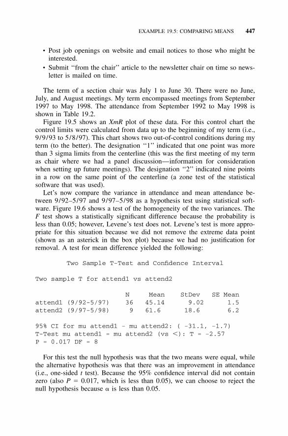
EXAMPLE 19.5: COMPARING MEANS 447

• Post job openings on website and email notices to those who might beinterested.

• Submit ‘‘from the chair’’ article to the newsletter chair on time so news-letter is mailed on time.

The term of a section chair was July 1 to June 30. There were no June,July, and August meetings. My term encompassed meetings from September1997 to May 1998. The attendance from September 1992 to May 1998 isshown in Table 19.2.

Figure 19.5 shows an XmR plot of these data. For this control chart thecontrol limits were calculated from data up to the beginning of my term (i.e.,9/9/93 to 5/8/97). This chart shows two out-of-control conditions during myterm (to the better). The designation ‘‘1’’ indicated that one point was morethan 3 sigma limits from the centerline (this was the first meeting of my termas chair where we had a panel discussion—information for considerationwhen setting up future meetings). The designation ‘‘2’’ indicated nine pointsin a row on the same point of the centerline (a zone test of the statisticalsoftware that was used).

Let’s now compare the variance in attendance and mean attendance be-tween 9/92–5/97 and 9/97–5/98 as a hypothesis test using statistical soft-ware. Figure 19.6 shows a test of the homogeneity of the two variances. TheF test shows a statistically significant difference because the probability isless than 0.05; however, Levene’s test does not. Levene’s test is more appro-priate for this situation because we did not remove the extreme data point(shown as an asterick in the box plot) because we had no justification forremoval. A test for mean difference yielded the following:

Two Sample T-Test and Confidence Interval

Two sample T for attend1 vs attend2

N Mean StDev SE Meanattend1 (9/92-5/97) 36 45.14 9.02 1.5attend2 (9/97-5/98) 9 61.6 18.6 6.2

95% CI for mu attend1 � mu attend2: ( �31.1, �1.7)T-Test mu attend1 � mu attend2 (vs �): T � �2.57P � 0.017 DF � 8

For this test the null hypothesis was that the two means were equal, whilethe alternative hypothesis was that there was an improvement in attendance(i.e., one-sided t test). Because the 95% confidence interval did not containzero (also P � 0.017, which is less than 0.05), we can choose to reject thenull hypothesis because � is less than 0.05.

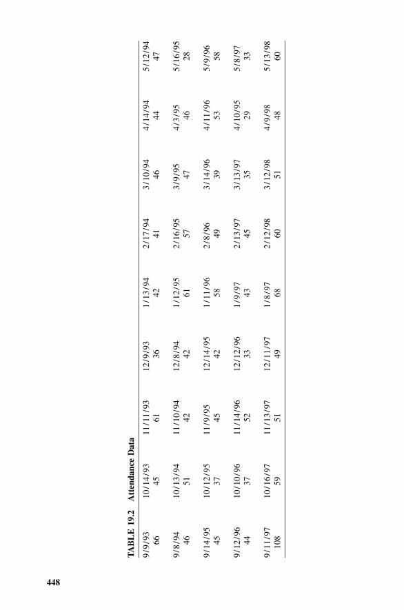
448

TA

BL

E19

.2A

tten

danc

eD

ata

9/9

/93

6610

/14

/93

4511

/11

/93

6112

/9/9

336

1/1

3/9

442

2/1

7/9

441

3/1

0/9

446

4/1

4/9

444

5/1

2/9

447

9/8

/94

4610

/13

/94

5111

/10

/94

4212

/8/9

442

1/1

2/9

561

2/1

6/9

557

3/9

/95

474

/3/9

546

5/1

6/9

528

9/1

4/9

545

10/1

2/9

537

11/9

/95

4512

/14

/95

421

/11

/96

582

/8/9

649

3/1

4/9

639

4/1

1/9

653

5/9

/96

58

9/1

2/9

644

10/1

0/9

637

11/1

4/9

652

12/1

2/9

633

1/9

/97

432

/13

/97

453

/13

/97

354

/10

/95

295

/8/9

733

9/1

1/9

710

810

/16

/97

5911

/13

/97

5112

/11

/97

491

/8/9

768

2/1

2/9

860

3/1

2/9

851

4/9

/98

485

/13

/98

60

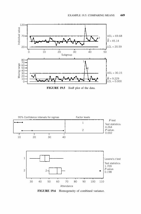
EXAMPLE 19.5: COMPARING MEANS 449

120

70

20

0 10 20

2

Subgroup30

1

1

1

2

40 50

8070605040302010

0

Indi

vidu

al v

alue

Mov

ing

rang

e

UCL = 69.68

LCL = 20.59

UCL = 30.15

LCL = 0.000

X = 45.14

R = 9.229

=

–

FIGURE 19.5 XmR plot of the data.

95% Confidence intervals for sigmas Factor levels

1

2

22

1

10

30 40 50 60 70

Attendance

80 90 100 110

20 30 40

F-test

Test statistics:4.264P-value:0.002

Levene's t test

Test statistics: 1.709P-value:0.198

FIGURE 19.6 Homogeneity of combined variance.

450 COMPARISON TESTS: CONTINUOUS RESPONSE

From this output we are also 95% confident that our process changes im-proved mean attendance between 2 and 31 people per meeting. Our bestestimate for percentage improvement is

61.6 � 45.14Best estimate for percent improvement in attendance � (100)

45.14

� 36.5%

My stretch goal of doubling meeting attendance was not met; however,attendance was shown (at a significance level of 0.05) to improve during myterm as chair with a best estimate of 36.5%. I felt good about the results ofthe executive team’s effort to improve attendance. I am confident that theresults would have been even better had we been able to print our newsletterat our previous frequency rate of once monthly.

An additional observation from the attendance plot is that attendance mayhave been on the decline immediately preceding my term. An exercise at theend of this chapter addresses the null hypothesis that there was no changebetween my term and the previous year.

19.14 S4/IEE ASSESSMENT

Whenever conducting a comparison test, consider whether the test could beconducted using paired comparison techniques. In general, fewer samples arerequired if the test objective can be met in this way, as opposed to comparisontests between samples. In addition, probability plotting techniques can be atool for understanding the data. A probability plot of the data may revealsomething worth investigating that was not obvious from a comparison ofmean or standard deviation values.

Problems may occur when making comparisons. For example, the qualityof parts that supplied by two sources may be compared. A problem with thistype of test is that the samples that are drawn do not necessarily representparts to be manufactured in the future. Also, the samples need to be takenfrom processes that are stable. If the processes are not stable, the test con-clusion may not be valid.

For this situation an S4/IEE consideration might be to have the suppliermanufacture (and label) specially made parts that reflect normal boundariesexperienced in their processes. A DOE design structure can be used to de-scribe how these specially built parts are to be manufactured, where one ofthe factors under consideration might be supplier A versus supplier B. Otherfactors to consider are new versus experienced operator, first shift versussecond shift, raw material supply source A versus B, high versus low machine

EXERCISES 451

tolerance limits, manufacturing line A versus B, tester A versus B, and soforth. This comparison test build strategy can also indicate what factors arecausing a degraded response so that these problems can get fixed.

For added insight into the range of variability that might be expected fromthe current process, a probability plot could be made of all the DOE trialdata. Care should be taken in interpreting this type of plot because the dataare not random.

After a supplier is qualified using the procedure above, process controlcharts should be implemented for the purpose of tracking and stopping theprocess should degradation later occur. A DOE strategy may again be neededin the future to discover the source of any degradation.

19.15 EXERCISES

1. Catapult Exercise Data Analysis: Using the catapult exercise data setsfrom Chapter 4, conduct a hypothesis test of the equality of means andvariance of the two different times the catapult was shot. Document thesignificance probabilities.

2. From sampled data, note the distribution used when(a) Calculating the confidence interval on the mean(b) Calculating the confidence interval on the standard deviation(c) Comparing two sampled variances

3. In the example given in this chapter, compare the attendance of myterm as ASQ chair to the previous year, as opposed to attendance since1992.

4. The difference between the actual arrival time and scheduled arrival timefor 20 trips made into Dallas was noted. The flights were on the sameairline at approximately the same time of day; however, half of theflights were from St. Louis (denoted as ‘‘S’’) while the other half werefrom New York (denoted as ‘‘N’’). Plus values indicate the number ofminutes the flight was late. The times were 11.1 (S), 8.7 (S), 14.3 (N),11.1 (S), 10.4 (N), 6.4 (N), 11.2 (S), 6.3 (N), 13.3 (S), 8.9 (N), 11.0 (S),8.5 (N), 9.4 (S), 10.2 (N), 10.0 (N), 8.7 (S), 9.1 (S), 13.2 (N), 16.5 (N),9.6 (S).(a) Determine at a significance level of 0.05 whether the variability in

arrival times were longer for the New York flight.(b) Determine at a significance level of 0.05 whether on the average the

arrival time from New York was longer than that from St. Louis.(c) To save parking fees, estimate when a friend should meet the traveler

at the pickup/drop-off area. Assume that the distribution of these

452 COMPARISON TESTS: CONTINUOUS RESPONSE

arrival times is representative of future flights. Consider that it takes10 minutes to walk from the gate to the load zone and that the friendshould wait only 5% of the times.

5. It is important that the mean response from a manufacturing process beincreased, but any change to the process is expensive to implement. Ateam listed some changes that they thought would be beneficial. Theyconducted a test with the current process settings and the new settings.They wanted to be certain that the change would be beneficial beforeimplementing it. For this reason, they decided to keep the current processunless they could prove that the new process would be beneficial at alevel of significance of 0.01. Discuss results and assess what should bedone.Current process readings: 98.1, 102.3, 98.5, 101.6, 97.7, 100.0, 103.1,99.1, 97.7, 98.5New process readings: 100.9, 101.1, 103.4, 85.0, 103.4, 103.6, 100.0,99.7, 106.4, 101.2

6. In 1985 a manufacturing company produced televisions in both Japan andthe United States. A very large random sample of products was taken toevaluate the quality of picture relative to a standard (which was a goodmeasurement for picture quality). It was found that all the US-manufactured products had no defects, while the Japan-built products hadsome defects. However, customers typically preferred the picture qualityof Japanese-manufactured televisions. Explain this phenomenon.

7. A manufacturer wants to determine if two testers yield a similar response.Ten parts were measured on machine A and another 10 parts were mea-sured on machine B.Machine A: 147.3, 153.0, 140.3, 161.0, 145.1, 145.0, 150.1, 158.7, 154.9,152.8Machine B: 149.6, 155.5, 141.3, 162.1, 146.7, 145.5, 151.6, 159.3, 154.8,152.7(a) Determine if there is a statistically significant difference in the mean

response at a level of 0.05.(b) If the data were collected such that 10 parts were evaluated on each

of the two machines with the pairing as noted. For example, the firstpart yielded a value of 147.3 on machine A, while it yielded 149.6on machine B. Determine if there is a statistically significant differ-ence in the mean.

(c) For the paired evaluation, use a normal probability plot to pictoriallyquantify the best estimate for the difference that would be expected80% of the time. Determine the value using a Z table (i.e., Table Ain Appendix E).

EXERCISES 453

8. Given the data sets:Data set A: 35.8, 40.4, 30.3, 46.8, 34.1, 34.0, 38.1, 45.0, 41.9, 40.2Data set B: 40.9, 35.7, 36.7, 37.3, 41.8, 39.9, 34.6, 38.8, 35.8, 35.6(a) Determine if there is a difference in the means at a level of 0.05 for

the data.(b) Determine if the variability of data set A is larger.(c) Describe manufacturing, development, and service examples from

which the data could have originated.

9. Explain how the techniques presented in this chapter are useful and canbe applied to S4/IEE projects.

10. Given the data below determine if there is a significant difference betweenscale A and B. Report the value of the computed statistic in the hypoth-esis test (Six Sigma Study Guide 2002).

Part Scale A Scale B

1 256.93 256.842 208.78 208.823 245.66 245.614 214.67 214.755 249.59 249.696 226.65 226.577 176.57 176.49

11. Test for a significance difference between sample 1 and sample 2. Com-ment.

Sample 1: 10, 15, 12, 19Sample 2: 15, 19, 18, 22

12. Compare the mean and variance of Machine A and B. State the teststatistics and their values that were used in making these comparisons(Six Sigma Test Guide 2002). This is the same data as that shown inExercise 10.17. Comment on the results.

Machine A Machine B

109.4 120.7583.03 121.4789.2 111.3

121.26 151.0185.77 108.884.22 119.4599.7 135.68

135.74 118.55135.18 101.22

454 COMPARISON TESTS: CONTINUOUS RESPONSE

Machine A Machine B

130.88120.56126.12

84.65102.22

98.47116.39103.39

89.52107.78119.43

78.5384.47

106.84

13. Exercise 15.6 showed data that was collected passively for the purposeof better understanding what might be done to improve the KPOV de-scribed in Exercise 10.18. Test for a significant difference between in-spectors.

14. Describe how and show where the tools described in this chapter fit intothe overall S4/IEE roadmap described in Figures A.1 and A.2 in theAppendix.

455

20COMPARISON TESTS: ATTRIBUTE(PASS/FAIL) RESPONSE

S4 /IEE DMAIC Application: Appendix Section A.1, Project ExecutionRoadmap Steps 7.3 and 7.4

This chapter focuses on attribute response situations (e.g., does the failurefrequencies of completing a purchase order differ between departments?).

20.1 S4/IEE APPLICATION EXAMPLES: ATTRIBUTECOMPARISON TESTS

S4/IEE application examples of attribute comparison tests:

• Manufacturing 30,000-foot-level quality metric: An S4/IEE project is toreduce the number of defects in a printed circuit board manufacturingprocess. A highly ranked input from the cause-and-effect matrix wasinspector; i.e., the team thought that inspectors could be classifying fail-ures differently. A null hypothesis test of equality of defective rates re-ported by inspector indicated that the difference was statisticallysignificant.

• Transactional 30,000-foot-level metric: DSO reduction was chosen as anS4/IEE project. A cause-and-effect matrix ranked a possible importantinput was that there was a difference between companies in the numberof defective invoices reported or lost. The null hypothesis test of equality

456 COMPARISON TESTS

of defective invoices by company indicated that there was a statisticallysignificant difference.

20.2 COMPARING ATTRIBUTE DATA

The methods presented in this chapter can be used, for example, to comparethe frequency of failure of two production machines or suppliers. The nullhypothesis for the comparison tests is there is no difference, while the alter-native hypothesis is there is a difference.

20.3 SAMPLE SIZE: COMPARING PROPORTIONS

Natrella (1966) gives tables for sample size selection when comparing theattribute response of two populations. Brush (1988) gives graphs that can beused to aid with the selection of sample sizes. Diamond (1989) multiplies theappropriate single-sampled population calculation by 2 to determine a samplesize for each of two populations. One rule of thumb that does not structurallyassess � and � levels is that there should be at least five failures for eachcategory.

20.4 COMPARING PROPORTIONS

The chi-square distribution can be used to compare the frequency of occur-rence for discrete variables. Within this test, often called a �2 goodness-of-fittest, we compare an observed frequency distribution with a theoretical distri-bution. An example application is that a company wants to determine if in-spectors categorize failure similarly. Consider that inspectors are described asA1, A2, and so forth, while types of failures are B1, B2, and so forth. The chi-square test assesses the association (lack of independency) in a two-way clas-sification. This procedure is used when testing to see if the probabilities ofitems or subjects being classified for one variable depend on the classificationof the other variable.

Data compilation and analysis is in the form of the following contingencytable, in which observations are designated as Oij and expected values arecalculated to be Eij. Expected counts are printed below observed counts. Thecolumn totals are the sum of the observations in the columns; the row totalsare the sum of the observations in the rows.

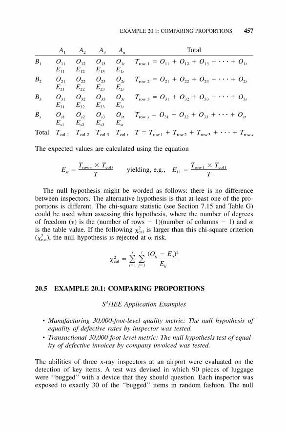
EXAMPLE 20.1: COMPARING PROPORTIONS 457

A1 A2 A3 An Total

B1 O11

E11

O12

E12

O13

E13

O1t

E1t

Trow 1 � O11 � O12 � O13 � � � � � O1t

B2 O21

E21

O22

E22

O23

E23

O2t

E2t

Trow 2 � O21 � O22 � O23 � � � � � O2t

B3 O31

E31

O32

E32

O33

E33

O3t

E3t

Trow 3 � O31 � O32 � O33 � � � � � O3t

Bs Os1

Es1

Os2

Es2

Os3

Es3

Ost

Est

Trow s � O31 � O32 � O33 � � � � � Ost

Total Tcol 1 Tcol 2 Tcol 3 Tcol t T � Trow 1 � Trow 2 � Trow 3 � � � � � Trow s

The expected values are calculated using the equation

T � T T � Trow s col t row 1 col 1E � yielding, e.g., E �st 11T T

The null hypothesis might be worded as follows: there is no differencebetween inspectors. The alternative hypothesis is that at least one of the pro-portions is different. The chi-square statistic (see Section 7.15 and Table G)could be used when assessing this hypothesis, where the number of degreesof freedom (�) is the (number of rows � 1)(number of columns � 1) and �is the table value. If the following is larger than this chi-square criterion2�cal

( ), the null hypothesis is rejected at � risk.2��,�

s t 2(O � E )ij ij2� � � �cal Ei�1 j�1 ij

20.5 EXAMPLE 20.1: COMPARING PROPORTIONS

S4 /IEE Application Examples

• Manufacturing 30,000-foot-level quality metric: The null hypothesis ofequality of defective rates by inspector was tested.

• Transactional 30,000-foot-level metric: The null hypothesis test of equal-ity of defective invoices by company invoiced was tested.

The abilities of three x-ray inspectors at an airport were evaluated on thedetection of key items. A test was devised in which 90 pieces of luggagewere ‘‘bugged’’ with a device that they should question. Each inspector wasexposed to exactly 30 of the ‘‘bugged’’ items in random fashion. The null

458 COMPARISON TESTS

hypothesis is that there is no difference between inspectors. The alternativehypothesis is that at least one of the proportions is different (Wortman 1990).

lnsp 1 lnsp 2 lnsp 3Treatment

Total

Detected 27 25 22 74Undetected 3 5 8 16Sample total 30 30 30 90

A computer analysis of these data yielded the following:

Chi-Square Test

Expected counts are printed below observed counts

Insp 1 Insp 2 Insp 3 Total1 27 25 22 74

24.67 24.67 24.67

2 3 5 8 165.33 5.33 5.33

Total 30 30 30 90

Chi-Sq � 0.221 � 0.005 � 0.288 �

1.021 � 0.021 � 1.333 � 2.889

DF � 2, P-Value � 0.236

The value for was 2.889, which is not larger than � � 5.99;2 2 2� � �cal �,� 2,0.05

hence, there is not sufficient evidence to reject the null hypothesis at � �0.05. Similarly, we can see from the computer output that the P value of0.236 is not less than an � criterion of 0.05.

20.6 COMPARING NONCONFORMANCE PROPORTIONS ANDCOUNT FREQUENCIES

Consider the situation in which an organization wants to evaluate the non-conformance rates of several suppliers to determine if there are differences.The chi-square approach just explained could assess this situation from anoverall point of view; however, the methodology does not identify whichsupplier(s) might be worse than the overall mean.

EXAMPLE 20.2: COMPARING NONCONFORMANCE PROPORTIONS 459

321

0.4

0.3

0.2

0.1

0.0

Sample Number

Pro

port

ion

P=0.1778

UCL=0.3872

LCL=0

FIGURE 20.1 p-Chart comparison test.

A simple approach to address this problem is to plot the nonconformancedata in a p-chart format, where each supplier would replace the typical p-chart subgroupings. Obviously, no zone tests would be applicable because theorder sequence of plotting the supplier information is arbitrary. The onlyapplicable test occurs when a supplier exceeds either the upper or lowercontrol limit (i.e., decision level for the test). Similarly a u chart could beused when there are count data. These tests are not technically a hypothesistest since decision levels are calculated using control charting methods.

For this analysis there are some statistical programs that contain a meth-odology similar to the analysis of means (ANOM) procedure for continuousdata described in Section 24.11, for both proportion and count data when thesample size between categories is the same. This method provides statisticalsignificance-based decision levels for the above binomial (comparing propor-tions) and Poisson (comparing count frequency) situations. The null hypoth-esis statement for these tests is that the rate from each category equates tothe overall mean.

20.7 EXAMPLE 20.2: COMPARINGNONCONFORMANCE PROPORTIONS

For the data in Example 20.1, compare each inspector nonconformance rateto the overall mean nonconformance rate using the p-chart procedure and abinomial ANOM statistical significance test.

Figure 20.1 shows the results for a p-chart analysis procedure, while Figure20.2 shows the one-way binomial ANOM statistical significance test proce-

460 COMPARISON TESTS

321

0.3

0.2

0.1

0.314220

0.041336

0.177778

Sample Number

Pro

port

ion

Def

ectiv

e

FIGURE 20.2 One-way binomial ANOM.

dure. In both cases we do not have enough information to suggest that thereis a difference in individual inspector rates to the overall mean. Note thatdecision bounds are wider for the p chart, which does not consider the numberof comparisons that are being made to the overall mean when creating thedecision levels.

20.8 EXAMPLE 20.3: COMPARING COUNTS

Ten inspectors evaluated the same number of samples from a process duringthe last month. Inspections were visual, where multiple defects could occuron one unit. The number of logged defects was

Inspector 1 2 3 4 5 6 7 8 9 10

Defects 330 350 285 320 315 390 320 270 310 318

Figure 20.3 shows the results of a one-way Poisson ANOM, where the hy-pothesis of equality of the defect rate to the overall average was rejected forinspectors 6 and 8. An S4/IEE project team could use the information fromthis analysis to address next why there appeared to be differences in inspec-tion results; perhaps inspectors were using a different inspection criterion fortheir decisions.

EXAMPLE 20.4: DIFFERENCE IN TWO PROPORTIONS 461

10987654321

380

330

280

320.8

368.496

273.104

Sample Number

Num

ber

of D

efec

ts

FIGURE 20.3 One-way Poisson ANOM.

20.9 EXAMPLE 20.4: DIFFERENCE IN TWO PROPORTIONS

A team believed that they made improvements to a process. They need to testthis hypothesis statistically and determine the 95% confidence interval for theimprovement in ppm rate given the following data.

Before improvement: 6290 defects out of 620,000After improvement: 4661 defects out of 490,000

A computer analysis yielded

Test and Confidence Interval for Two Proportions

Sample X N Sample p

1 6290 620000 0.0101452 4661 490000 0.009512

Estimate for p(1) � p(2): 0.00063291695% CI for p(1) � p(2): (0.000264020, 0.00100181)Test for p(1) � p(2) � 0 (vs. not � 0): Z � 3.36, P value � 0.001

From this analysis we can reject the null hypothesis that no improvement wasmade. The 95% confidence interval for the ppm improvement rate is 264 to1001.

462 COMPARISON TESTS

20.10 S4/IEE ASSESSMENT

The methods included in this chapter are traditionally used to compare sup-pliers, machines, and so forth by taking samples from the populations. Ingeneral, when designing a test, the analyst attempts to use a continuous re-sponse output, as opposed to an attribute response, whenever possible. Forexample, a particular part may be considered a failure when it tests beyonda certain level. Instead of analyzing what proportion of parts are beyond thislevel, fewer samples are required if the actual measurement data are recorded.

Let’s revisit the example where a test was conducted to see if there was adifference between inspectors. If we only assessed the results of our hypoth-esis test deductively, we would stop our investigation because the null hy-pothesis could not be rejected. However, if we used inductive reasoning, wewould learn from these data to challenge previous understandings or create anew hypothesis. Using inductive reasoning, we probably should be concernedthat the overall detection rate for the ‘‘bugs’’ we applied for the x-ray in-spectors was only 82% (i.e., [74/90] � 100). From a practical point of view,the overall detection process needs to be investigated and improved. Perhapsa control chart program should be implemented as a means to track progress,where bugs are periodically applied and monitored for detection.

20.11 EXERCISES

1. Catapult Exercise Data Analysis: Using the catapult exercise data setsfrom Chapter 4, conduct a hypothesis test of the equality of the attributeresponses of the two different times the catapult was shot (e.g., 45 outof 100 failed first time against 10 out of 100 failed the second time tobe within 75 � 3 in. of the medians). Document the probability level.

2. M&M’s Candy Data Analysis: In an exercise at the end of Chapter 5, abag of M&M’s candy was opened. A count of each color was made.Attendees at the S4/IEE workshop are to pair up to compare data. Com-pare the proportion of browns counted in your bags of M&M’s. Comparethe proportion of browns in one bag to the proportion of blues in anotherbag. Explain the applicability of this analysis approach to data you mightencounter in your project. Also note any shortcomings due to the type ofdata used.

3. M&M’s Candy Data Analysis: In an exercise used at the end of Chapter5, a bag of M&M’s candy was opened. A count of each color was made.Compare the proportions of browns that each person had, except for oneperson who is to submit his/her proportion of blues). Explain the appli-cability of this analysis approach to data you might encounter in yourproject. Also note any shortcomings due to the type of data used.

4. A manufacturer wants to select only one supplier of a key part that isused in the manufacturing process. The cost for parts from supplier A is

EXERCISES 463

greater than that for supplier B. A random sample of 1000 parts wastaken from each of the suppliers’ processes. The output from each samplewas compared to the specification. Supplier A had 10 parts beyond thespecification limits, while supplier B had 15.(a) Determine if there is a significance difference at a level of 0.1.(b) Comment on findings and make recommendations.

5. Explain how the techniques presented in this chapter are useful and canbe applied to S4/IEE projects.

6. Assess whether a difference can be claimed in the following supplier non-conformance rates. Comment on results and the applicability to othersituations within business.

Supplier 1 Supplier 2 Supplier 3 Supplier 4

20% 40% 60% 20%

7. Assess whether a difference can be claimed in the following suppliernonconformance rates. Compare the results to the assessment in Exercise6 and comment on the use of statistical analyses to make decisions.

Supplier 1 Supplier 2 Supplier 3 Supplier 4

Defectives 1 2 3 1Sample Size 5 5 5 5

8. Assess whether a difference can be claimed in the following suppliernonconformance rates. Compare the results to the assessments in Exer-cises 6 and 7 and comment on the use of statistical analyses to makedecisions.

Supplier 1 Supplier 2 Supplier 3 Supplier 4

Defectives 10 20 30 10Sample Size 50 50 50 50

9. A team believed that they made improvements to a process. They needto test this hypothesis statistically and determine the 95% confidenceinterval for the improvement in ppm rate for the following data.Before improvement: 6290 defects out of 620,000After improvement: 466 defects out of 49,000Comment on these results relative to the results in Example 20.4.

10. In Exercise 19.4 the difference between the actual arrival times and thescheduled arrival times for 20 trips into Dallas was noted. Consider thatflights are considered on time if they arrive no later than 15 minutes aftertheir scheduled arrival time, as compiled in the following table.

464 COMPARISON TESTS

Origination Number of Flights On Time Number of Flights Late

N 9 1S 10 0

Determine if there is a significant difference between the arrival timesfor flights from St. Louis (S designation) and New York (N designation).Comment on the analysis.

11. Using Figure A.2 in the Appendix, determine the tools that could be usedto assess a potential KPIV for a visual inspection process where parts areeither accepted or rejected. If all operators made a similar judgment fora part, their rejetion rates should be approximately the same. Suggest astrategy to make a passive analysis which tests for differences betweenappraisers. Create a dummy set of data and make such an analysis.

465

21BOOTSTRAPPING

S4/IEE DMAIC Application: Appendix Section A.1, Project ExecutionRoadmap Steps 3.2 and 7.2

Bootstrapping is a resampling technique. It is a simple but effective methodfor describing the uncertainty associated with a summary statement withoutconcern for the complexity of the chosen summary or the exact distributionfrom which data are calculated (Gunther 1991, 1992; Efron and Tibshirani1993). This chapter will illustrate how bootstrapping can be used to determinethe confidence interval for Cpk and/or Ppk.

21.1 DESCRIPTION

Bootstrapping involves the treatment of samples as though they were theunderlying population of data. Consider, for example, selecting and makinga measurement from 50 samples of a stable process. Now take many samples(1000 is typical) from these measurements where sampling is conducted withreplacement. Compute the mean and other statistics of interest (e.g., medianstandard deviation, and percent of population) for each of the 1000 samples.Rank each statistic of interest. Determine the confidence interval for the sta-tistic by choosing the value at the appropriate ranking level. For example, the90% confidence interval for the ranking of 1000 mean values would be thevalues at the 50 or 950 ranking levels.

Bootstrapping frees practitioners from arbitrary assumptions and limitingprocedures of classical methods that are based on normal theory. The method

466 BOOTSTRAPPING

provides an intuitively appealing, statistically rigorous, and potentially auto-matic way for the assessment of uncertainty of estimates from sampled datathat are taken from a variety of processes. However, a computer is needed toperform the random sampling. The technique can be used to determine aconfidence interval for Cpk. /Ppk.

Like all confidence interval calculations, the approach has meaning onlywhen the process is stable. Without stability, the results from current samplingcannot give information about future sampling because we are not able todetermine whether value changes are caused by what is being measured orchanges in the process. However, the technique can still be useful for tworeasons. First, confidence intervals give us a snapshot of what will happenshould current behavior continue. Second, these confidence intervals can dis-courage basing decisions on inadequate data.

Bootstrapping is easy to understand, is automatic, gives honest estimates(i.e., stringent assumptions are not required), and has good theoretical prop-erties. It has potential for many applications beyond simple sampling statis-tics. However, sometimes confidence intervals are not quite right when thebootstrap distribution is biased. For these situations the estimate from thesample is not near enough to the median of the distribution of the bootstrapestimates. However, Bradley Efron developed a simple bias correction pro-cedure to fix this problem (Gunther 1991, 1992; Efron and Tibshirani 1993).Efron’s bias correction procedure is described in Example 21.2.

Bootstrapping does not give valid statistical inferences on everything.Dixon (1993), Hall (1992), Efron and Tibshirani (1993), and Shao and Tu(1995) describe limitations of bootstrapping and other technical considera-tions.

21.2 EXAMPLE 21.1: BOOTSTRAPPING TO DETERMINECONFIDENCE INTERVAL FOR MEAN, STANDARD DEVIATION,Pp AND Ppk

The data in Table 11.2 were used previously to illustrate procedures to de-termine Pp and Ppk (I am using this terminology instead of Cp and Cpk so thatthere is no doubt that we are taking a long-term view of variability). In thisexample we will calculate confidence intervals for these statistics along withconfidence intervals for the mean and standard deviation using bootstrappingtechniques. Comparison will be made to applicable formulas when appropri-ate.

Statistics determined from the sample were: � 0.7375, s � 0.0817, Pp �x0.8159, and Ppk � 0.6629. Bootstrap samples are then taken from the sample,where the 80 samples are resampled with replacement. The first bootstrapsamples were

EXAMPLE 21.1: BOOTSTRAPPING TO DETERMINE CONFIDENCE LEVEL 467

0.70 0.80 0.75 0.70 0.75 0.65 0.85 0.70 0.75 0.80 0.70 0.65 0.850.80 0.50 0.85 0.80 0.65 0.60 0.75 0.80 0.65 0.85 0.70 0.850.70 0.65 0.65 0.80 0.65 0.85 0.70 0.85 0.85 0.65 0.75 0.800.75 0.85 0.75 0.80 0.75 0.60 0.90 0.85 0.80 0.75 0.75 0.700.80 0.85 0.80 0.75 0.70 0.75 0.70 0.80 0.70 0.85 0.60 0.850.50 0.65 0.65 0.75 0.65 0.80 0.70 0.60 0.90 0.65 0.85 0.850.60 0.70 0.80 0.70 0.65 0.70 0.85

while the second bootstrap samples were

0.70 0.75 0.65 0.60 0.60 0.90 0.70 0.75 0.75 0.80 0.70 0.75 0.750.85 0.75 0.85 0.70 0.75 0.75 0.80 0.65 0.70 0.80 0.65 0.650.70 0.80 0.75 0.65 0.80 0.90 0.80 0.75 0.85 0.85 0.90 0.650.75 0.80 0.75 0.70 0.75 0.65 0.65 0.65 0.75 0.70 0.75 0.650.75 0.65 0.85 0.70 0.75 0.75 0.85 0.65 0.75 0.65 0.80 0.600.85 0.75 0.85 0.60 0.80 0.80 0.70 0.80 0.85 0.75 0.80 0.850.60 0.85 0.80 0.60 0.60 0.75 0.70

This resampling was repeated 1000 times using a computer program. For eachexample the mean, standard deviation, Pp, and Ppk were determined. Table21.1 contains some of the ranked results for each of the four calculated sta-tistics. Because there were 1000 bootstrap samples, the pertinent values fromthis table to determine the 90% confidence interval are as follows:

Ranked No. Mean SD Pp Ppk

50 0.722500 0.070641 0.729374 0.579831500 0.737500 0.080975 0.822926 0.669102950 0.752500 0.091368 0.943406 0.775125

The 90% confidence interval for the mean, for example, would be 0.7225 �� � 0.7525.

We do not need to use bootstrapping to determine a confidence intervalfor the mean, standard deviation, and Pp statistic because these values can bedetermined mathematically (see Sections 17.4 and 17.7). However, it is notso easy to determine a confidence interval for Ppk and other statistics such aspercent of population. The mean, standard deviation, and Pp statistic wereincluded in this so that comparisons could be made between bootstrap andcalculated values.

The confidence interval for the mean calculation is

468

TA

BL

E21

.1A

Sele

ctio

nof

Ran

ked

Boo

tstr

apR

esul

tsfr

om10

00Sa

mpl

es

Ran

ked

No.

Mea

nSD

Pp

Pp

k

Ran

ked

No.

Mea

nSD

Pp

Pp

k

10.

7068

750.

0595

210.

6563

750.

5055

4150

40.

7375

000.

0810

430.

8236

960.

6692

642

0.70

9375

0.06

3367

0.66

5732

0.50

5798

505

0.73

7500

0.08

1043

0.82

3721

0.66

9647

400.

7218

750.

0700

790.

7249

930.

5756

9550

60.

7375

000.

0810

430.

8237

210.

6696

9741

0.72

2500

0.07

0236

0.72

4993

0.57

6120

940

0.75

1875

0.09

0699

0.93

8218

0.76

7487

420.

7225

000.

0702

500.

7256

050.

5763

5894

10.

7518

750.

0906

990.

9384

020.

7684

9443

0.72

2500

0.07

0250

0.72

5962

0.57

6936

942

0.75

1875

0.09

0914

0.93

9249

0.77

1415

440.

7225

000.

0703

040.

7267

810.

5771

9494

30.

7518

750.

0909

770.

9392

490.

7718

4345

0.72

2500

0.07

0416

0.72

7328

0.57

7194

944

0.75

1875

0.09

0977

0.93

9286

0.77

2424

460.

7225

000.

0704

420.

7274

650.

5773

4094

50.

7518

750.

0910

010.

9404

310.

7727

6947

0.72

2500

0.07

0442

0.72

8151

0.57

7631

946

0.75

1875

0.09

1001

0.94

0765

0.77

4240

480.

7225

000.

0704

610.

7282

710.

5778

1394

70.

7518

750.

0911

230.

9413

580.

7746

6049

0.72

2500

0.07

0461

0.72

8340

0.57

8178

948

0.75

1875

0.09

1140

0.94

1655

0.77

4743

500.

7225

000.

0706

410.

7293

740.

5798

3194

90.

7525

000.

0913

250.

9429

580.

7747

4351

0.72

2500

0.07

0666

0.72

9651

0.57

9891

950

0.75

2500

0.09

1368

0.94

3406

0.77

5125

520.

7225

000.

0706

990.

7299

960.

5800

7695

10.

7525

000.

0914

030.

9437

430.

7753

3053

0.72

3125

0.07

0797

0.73

1472

0.58

1249

952

0.75

2500

0.09

1532

0.94

6146

0.77

5777

540.

7231

250.

0708

200.

7316

120.

5815

5695

30.

7525

000.

0915

410.

9461

460.

7764

5155

0.72

3125

0.07

0864

0.73

2590

0.58

1646

954

0.75

2500

0.09

1556

0.94

6410

0.77

6982

469

440

0.73

6250

0.07

9950

0.81

5103

0.65

8464

955

0.75

2500

0.09

1642

0.94

6410

0.77

7119

441

0.73

6250

0.07

9950

0.81

5465

0.65

9058

980

0.75

5625

0.09

4045

0.96

6055

0.80

0214

442

0.73

6250

0.07

9992

0.81

5465

0.65

9181

981

0.75

5625

0.09

4098

0.97

2540

0.80

0831

443

0.73

6250

0.08

0029

0.81

5489

0.65

9258

982

0.75

5625

0.09

4197

0.97

2540

0.80

2667

444

0.73

6250

0.08

0029

0.81

5851

0.65

9276

983

0.75

6250

0.09

4365

0.97

3524

0.80

3572

445

0.73

6250

0.08

0029

0.81

5851

0.65

9423

984

0.75

6250

0.09

4381

0.97

9156

0.80

5523

446

0.73

6250

0.08

0049

0.81

5876

0.65

9423

985

0.75

6250

0.09

4635

0.98

0119

0.81

1029

447

0.73

6250

0.08

0101

0.81

6069

0.65

9423

986

0.75

6875

0.09

4668

0.98

1168

0.81

2090

448

0.73

6250

0.08

0101

0.81

6238

0.65

9585

987

0.75

6875

0.09

4699

0.98

4548

0.81

7541

449

0.73

6250

0.08

0111

0.81

6335

0.65

9640

988

0.75

7500

0.09

4749

0.98

6892

0.81

7541

450

0.73

6250

0.08

0128

0.81

6335

0.65

9884

989

0.75

7500

0.09

4935

0.98

7749

0.81

9210

493

0.73

7500

0.08

0897

0.82

2604

0.66

7719

990

0.75

8125

0.09

5459

1.00

3200

0.82

3103

494

0.73

7500

0.08

0914

0.82

2604

0.66

7827

991

0.75

8750

0.09

5599

1.00

7404

0.82

6522

495

0.73

7500

0.08

0934

0.82

2604

0.66

7885

992

0.75

9375

0.09

5630

1.01

0467

0.82

7803

496

0.73

7500

0.08

0934

0.82

2604

0.66

7889

993

0.75

9375

0.09

6053

1.01

2909

0.83

1789

497

0.73

7500

0.08

0936

0.82

2604

0.66

7889

994

0.76

0000

0.09

6119

1.02

0391

0.83

2379

498

0.73

7500

0.08

0936

0.82

2604

0.66

9021

995

0.76

0625

0.09

6382

1.02

0911

0.83

9950

499

0.73

7500

0.08

0973

0.82

2728

0.66

9053

996

0.76

1250

0.09

6710

1.02

8573

0.84

4865

500

0.73

7500

0.08

0975

0.82

2926

0.66

9102

997

0.76

1250

0.09

6765

1.03

1540

0.84

7229

501

0.73

7500

0.08

1012

0.82

3299

0.66

9102

998

0.76

5000

0.09

9166

1.04

8303

0.86

7720

502

0.73

7500

0.08

1031

0.82

3323

0.66

9253

999

0.76

7500

0.10

0140

1.05

2066

0.91

7047

503

0.73

7500

0.08

1043

0.82

3696

0.66

9253

1000

0.76

8125

0.10

1568

1.12

0057

0.92

5201

470 BOOTSTRAPPING

t s t s� �x � � � � x ��n �n

1.99(0.0817) 1.99(0.0817)0.7375 � � � � 0.7375 �

�80 �80

0.7375 � 0.0182 � � � 0.7375 � 0.0182

0.7193 � � � 0.7557

The results from the confidence interval calculation are comparable to thebootstrap interval of 0.7225 � � 0.7525. If we were to run another 1000bootstrap samples, our confidence interval should differ by some smallamount. Let’s now compare the results for standard deviation using the re-lationship

1/2 1/22 2(n � 1)s (n � 1)s� � �� � � �2 2� �� / 2;n�1 (1�� / 2;n�1)

1/2 1/22 2(80 � 1)(0.0817) (80 � 1)(0.0817)� � �� � � �2 2� �(0.1 / 2;[80�1]) (1�[0.1 / 2];[80�1])

1/2 1/20.5273 0.5273� � �� � � �105.4727 56.3089

0.0707 � � � 0.0968

These confidence interval results are again comparable to the bootstrap inter-val of 0.0706 � � � 0.0914. Let’s now compare the results for the confidenceinterval for Pp.

2 2� �1�� / 2;n�1 � / 2;n�1ˆ ˆP � P � Pp p p� �n � 1 n � 1

56.3089 105.47270.8159 � P � 0.8159p� �80 � 1 80 � 1

0.6888 � P � 0.9427p

Because the results are comparable to the bootstrap interval for Pp of0.7294 � Pp � 0.9434, we would probably be fairly comfortable reportingalso the Ppk 95% confidence bootstrap interval of 0.5798 � Ppk � 0.7751,which we cannot determine through a simple mathematical relationship.

BOOTSTRAPPING APPLICATIONS 471

21.3 EXAMPLE 21.2: BOOTSTRAPPING WITHBIAS CORRECTION

This example illustrates application of Efron’s bias correction method for thebootstrap interval estimate. In this example the 95% confidence interval of Pp

will be determined and compared to the values determined in the previousexample; other situations may need this bias correction procedure more.

To adjust for bias, we first note that we previously determined Pp � 0.8159from the original data set. From Table 21.1 we determine a proportion ofsamples that are less than or equal to this sample value. From this table wenote the following:

Ranked No. Mean SD Pp Ppk

445 0.736250 0.080029 0.815851 0.659423446 0.736250 0.080049 0.815876 0.659423447 0.736250 0.080101 0.816069 0.659423

The ranking number of 446 is used to determine this percentage because thevalue of Pp for this ranking number is 0.815876, which is less than or equalto 0.8159, and the Pp value of 0.816069 for ranking number 447 is greaterthan the Pp sample value of 0.8159. This proportion then equates to 0.446(i.e., 446/1000).

The Z value (Z0) for this proportion is then determined to be 0.1358 (fromTable A or a computer program). For a 95% confidence interval, � � 0.025and Z� � 1.96, the upper and lower values are determined from the relation-ship of 2 � Z0 � z�. These equations yield lower and upper values of �1.6884and 2.2315, which correspond to normal CDF values of 0.0457 and 0.98721.A lower bootstrap value is then determined such that its value is as close aspossible but no larger than the 0.0457 value. An upper bootstrap value is alsodetermined such that its value is as close as possible but no smaller than0.9872. This relationship yields a lower bootstrap value of 45 (i.e., 1000 �0.0457 � 45.7) and an upper bootstrap value of 988 (i.e., 1000 � 0.09872� 987.2). From Table 21.1 for these bootstrap values we can determine anunbiased bootstrap estimate of 0.7273 � Pp � 0.9869.

21.4 BOOTSTRAPPING APPLICATIONS

Bootstrapping can be applied to situations beyond those described in thischapter (e.g., time series). Let’s consider three extensions of the strategy de-scribed here.

First, a confidence interval for the median, a statistic not readily availablewith standard theory, can be easily obtained using bootstrapping techniques.A median value can often give more insight into the characteristics of apopulation for a skewed distribution. For example, the median value of houses

472 BOOTSTRAPPING

within an area typically gives more insight than the mean value of houses. Afew high-valued houses can increase a mean a lot, giving a distorted percep-tion of typical house values. This problem does not occur when a medianvalue is reported.

Second, consider calculating a mean and standard deviation for bootstrapsand then combine these values to estimate a ‘‘percentage less than value,’’ forexample, three standard deviations from the sample mean. A confidence in-terval can then be obtained for this ‘‘percentage less than value.’’ An extensionof this method is to transform nonnormal data before applying the technique.

Third, consider a reliability test in which the failure times of sample com-ponents are determined. It might be desired to determine the percentage ex-pected to survive a particular amount of usage. From the data a maximumlikelihood estimate for this percentage could be obtained for the sample usinga computer program (or a manual estimate could be determined from a prob-ability plot of the data). A confidence interval for this survival percentage canbe determined using bootstrapping techniques by resampling the sample, de-termining the maximum likelihood (or manual) estimate of the desired valuefor each sample, and then determining a confidence interval using the sameprocedure described above.

21.5 EXERCISES

1. Catapult Exercise Data Analysis: For the catapult exercise data sets fromChapter 4, use bootstrapping to determine the confidence intervals formean, standard deviation, Pp, and Ppk (i.e., long-term process capability/performance index). Consider that the specification limits are �3 in. fromthe data median.

2. A previous exercise asked for the calculation of process capability/per-formance metrics from the following set of data. Determine now using acomputer the bootstrap confidence interval for the mean, standard deviation(of all data combined), Pp, and Ppk (without and with bias correction).Compare bootstrap values to calculated values whenever possible. Theorigination of the data is as follows: An and R chart in Example 10.2xindicated that samples numbered 8, 9, 10, 12, 13, and 18 were out ofcontrol (i.e., the process is unpredictable). The process specifications are0.4037 � 0.0013 (i.e., 0.4024 to 0.4050). Tabular and calculated valueswill be in units of 0.0001; i.e., because of this transformation, the speci-fication limits will not be 24 and 50. Assume that for each of these datapoints, circumstances for an out-of-control response were identified andwill be avoided in future production. The 14 subgroups and measurementsare

EXERCISES 473

Measurements

1 36 35 34 33 322 31 31 34 32 303 30 30 32 30 324 32 33 33 32 355 32 34 37 37 356 32 32 31 33 337 33 33 36 32 318 34 38 35 34 389 36 35 37 34 33

10 30 37 33 34 3511 28 31 33 33 3312 33 30 34 33 3513 35 36 29 27 3214 33 35 35 39 36

3. Determine the confidence interval for Ppk for the data set in Table 21.1using the bias correction procedure. Compare this interval to the noncor-rected interval determined as an example in this chapter.

4. Explain how the techniques presented in this chapter are useful and canbe applied to S4/IEE projects.

474

22VARIANCE COMPONENTS

S4 /IEE DMAIC Application: Appendix Section A.1, Project ExecutionRoadmap Step 7.4

The methodology described in this chapter is a random effects model orcomponents of variance model, as opposed to a fixed-effects model as de-scribed in Chapter 24. The statistical model for the random effects or com-ponents of variance model is similar to that of the fixed effects model. Thedifference is that in the random effects model the levels (or treatments) couldbe a random sample from a larger population of levels. For this situation wewould like to extend conclusions, based on sample of levels, to all populationlevels whether explicitly considered or not. In the situation the test attemptsto quantify the variability from factor levels.

22.1 S4/IEE APPLICATION EXAMPLES: VARIANCECOMPONENTS

S4/IEE application examples of variance components tests:

• Manufacturing 30,000-foot-level metric (KPOV): An S4/IEE project wasto improve the capability/performance metric for the diameter of a man-ufactured product (i.e., reduce the number of parts beyond the specifi-cation limits). A cause-and-effect matrix ranked the variability ofdiameter within a part and between the four-cavity molds as importantinputs that could be affecting the overall 30,000-foot-level part diametermetric. A variance component analysis was conducted to test significanceand estimate the components.

DESCRIPTION 475

FIGURE 22.1 A 5 � 3 � 2 hierarchical design. (From Statistics for Experimenters,by George E. P. Box, William G. Hunter, and J. Stuwart Hunter, copyright � 1978 byJohn Wiley & Sons, Inc. Reprinted by permission of John Wiley & Sons, Inc.)

• Transactional 30,000-foot-level metric: DSO reduction was chosen as anS4/IEE project. A cause-and-effect matrix ranked company as an impor-tant input that could affect the DSO response. The team wanted to esti-mate the variability in DSO between and within companies. A variancecomponent analysis was conducted to test signifiance and estimate thecomponents.

22.2 DESCRIPTION

Earlier we discussed the impact that key process input variables can have onthe output of a process. A fixed-effects model assesses how the level of keyprocess input variables affects the mean response of key process outputs,while a random effects model assesses how the variability of key processinput variables affect the variability of key process outputs.

A key process output of a manufacturing process could be the dimensionor characteristic of a product. A key process output of a service or businessprocess could be time from initiation to delivery. The total affect of n variancecomponents on a key process output can be expressed as the sum of thevariances of each of the components:

2 2 2 2 2� � � � � � � � � � � � �total 1 2 3 n

The components of variance within a manufacturing process could bematerial, machines, operators, and the measurement system. In service orbusiness processes the variance components can be the day of the month therequest was initiated, department-to-department variations when handling arequest, and the quality of the input request. An important use of variancecomponents is the isolation of different sources of variability that affect prod-uct or system variability. This problem of product variability frequently arisesin quality assurance, where the isolation of the sources for this variability canoften be very difficult.

A test to determine these variance components often has the nesting struc-ture as exemplified in Figure 22.1. Other books describe in detail the analysisof variance method for estimating variance components. In this procedure theexpected mean squares of the analysis of variance table are equated to theirobserved value in the analysis of variance table and then solved for the vari-

476 VARIANCE COMPONENTS

FIGURE 22.2 Three components of variance in the final moisture reading. (a) Dis-tribution of batch means about the process mean �. (b) Distribution of sample meansabout the batch mean. (c) Distribution of analytical test results about sample mean.(From Statistics for Experimenters, by George E. P. Box, William G. Hunter, andJ. Stuwart Hunter, copyright � 1978 by John Wiley & Sons, Inc. Reprinted by permis-sion of John Wiley & Sons, Inc.)

ance components. In this text a statistical computer analysis program will beused for computations.

Occasionally, variance components analyses yield negative estimates. Neg-ative estimates are viewed with concern because it is obvious that, by defi-nition, variance components cannot be negative. For these situations, it hasintuitive appeal to accept the negative estimate and use it as evidence that thetrue value is zero. This approach suffers from theoretical difficulties becauseusing a zero in place of the negative estimates can affect the statistical prop-erties of the other estimates. Another approach is to use an alternative cal-culating technique that yields a nonnegative estimate. Still another approachis to consider that this is evidence that the linear model is incorrect and theproblem needs to be reexamined.

An output often included with a computer variance component analyses isthe expected mean-square values. Although not discussed in this book, thesevalues can be used to determine confidence intervals for variance componentsor percent contribution.

22.3 EXAMPLE 22.1: VARIANCE COMPONENTS OFPIGMENT PASTE

Consider that numerous batches of a pigment paste are sampled and testedonce. We would like to understand the variation of the resulting moisturecontent as a function of those components shown pictorially in Figure 22.2(Box et al. 1978).

In this figure, � is shown to be the long-run process mean for moisturecontent. In this figure, process variation is shown to be the distribution ofbatch means about this process mean, sampling variation is shown to be the

EXAMPLE 22.1: VARIANCE COMPONENTS OF PIGMENT PASTE 477

distribution of samples about the batch mean, and analytical variation isshown to be the distribution of analytical test results about the sample mean.

The overall error (ε � y � �) will contain the three separate error com-ponents (i.e., ε � εt � εs � εb), where εt is the analytical test error, εs is theerror made in taking the samples, and εb is the batch-to-batch error. By thesedefinitions the mean of the error components (i.e., εt, εs, and εb) have zeromeans. The assumption is made that the samples are random (independent)from normal distributions with fixed variances 2 2 2� , � , � .t s b

Consider now the following data that were collected using the hierarchicaldesign shown in Figure 22.1:

Batch

Sample Subsample 1 2 3 4 5 6 7 8 9 10 11 12 13 14 15

1 1 40 26 29 30 19 33 23 34 27 13 25 29 19 23 392 39 28 28 31 20 32 24 34 27 16 23 29 20 24 37

2 1 30 25 14 24 17 26 32 29 31 27 25 31 29 25 262 30 26 15 24 17 24 33 29 31 24 27 32 30 25 28

A variance components analysis for this set of experimental data is shownbelow. For now, let’s concentrate only on the outputs from this table as de-scribed below. Section 24.4 describes the mathematical relationships from asingle-factor ANOVA table. However, one major difference between the AN-OVA table calculations in Chapter 24 and this ANOVA table is that the prob-ability calculations for a variance components analysis is dependent upon thedesign hierarchy; e.g., the probability calculation for ‘‘batch’’ is the statisticalcomparison of ‘‘sample’’ to ‘‘batch,’’ not ‘‘error’’ to ‘‘batch.’’

Fully Nested Analysis of Variance

Analysis of Variance for Moisture

Source DF SS MS F PBatch 14 1210.9333 86.4952 1.492 0.226Sample 15 869.7500 57.9833 63.255 0.000Error 30 27.5000 0.9167Total 59 2108.1833

Variance Components

Source Var Comp. % of Total StDevBatch 7.128 19.49 2.670Sample 28.533 78.01 5.342Error 0.917 2.51 0.957Total 36.578 6.048

478 VARIANCE COMPONENTS

FIGURE 22.3 Diagrammatic summary of results of experiment to determine com-ponents of variance. (From Statistics for Experimenters, by George E. P. Box, WilliamG. Hunter, and J. Stuwart Hunter, copyright � 1978 by John Wiley & Sons, Inc.Reprinted by permission of John Wiley & Sons, Inc.)

For this analysis the ‘‘sample’’ is nested in ‘‘batch.’’ The variance componentsestimated in the model are

Analytical test variance � 0.92 (standard deviation � 0.96)Sample variance (within batches) � 28.5 (standard deviation � 5.3)Process variance (between batches) � 7.1 (standard deviation � 2.6)

The square roots of these variances are estimates of the standard deviationsthat are pictorially compared in Figure 22.3. These results indicate that thelargest individual source for variation was the error arising in chemical sam-pling. Investigators given this information then discovered and resolved theproblem of operators not being aware of the correct sampling procedure.

22.4 EXAMPLE 22.2: VARIANCE COMPONENTS OF AMANUFACTURED DOOR INCLUDING MEASUREMENTSYSTEM COMPONENTS

When a door is closed, it needs to seal well with its mating surface. Sometwist of the manufactured door can be tolerated because of a seal that isattached to the door. However, a large degree of twist cannot be toleratedbecause the seal would not be effective, excessive force would be required to

EXAMPLE 22.3: VARIANCE COMPONENTS 479

close the door, and excessive load on the door latching mechanism could intime cause failure.

Let’s consider this situation from the point of view of the supplier of thedoor. The burden of how well a door latches due to twist does not completelylie with the supplier of the door. If the mating doorframe is twisted, there canbe a customer problem, no matter how well the door is manufactured. Thesupplier of the door never sees the doorframe and hence cannot check thequality of the overall assembly. Also, the doors are supposed to be inter-changeable between frames.

The customer of the door supplier often rejects doors. The supplier of thedoor can only manufacture to the specification. The question then arises ofhow to measure the door twist. Drawing specifications indicate that the areawhere the door is to seal has a 0.031-in. tolerance. Currently, this dimensionis measured in the fixture that manufacturers the door. However, it has beennoticed that the door tends to spring into a different position after leaving thefixture. Because of this it was concluded that there needed to be built ameasurement fixture for checking the door which simulated where the doorwould be mounted on hinges in taking the measurements that assess how itseals.

A nested experiment was then planned where other issues of concern werealso included (e.g., measurement system). There was only one manufacturingjig and one inspection jig. The following sources of variability were consid-ered: week-to-week, shift-to-shift, operator-to-operator, within-part variability,inspector measurement repeatability, and inspector measurement reproduci-bility.

22.5 EXAMPLE 22.3: DETERMINING PROCESS CAPABILITY/PERFORMANCE METRICS USING VARIANCE COMPONENTS

The following set of data (AIAG 1995b) was presented initially as Exercise3 in Chapter 10 on control charts. Example 11.2 described a procedure usedto calculate process capability/performance metrics for this in-control/pre-dictable process. This chapter gives an additional calculation procedure fordetermining standard deviations from the process. Additional procedures forprocess capability/performance metrics calculations are treated in the single-factor analysis of variance chapter (see Chapter 24).

Subgroups

1 2 3 4 5 6 7 8 9 10 11 12 13 14 15 16

1 0.65 0.75 0.75 0.60 0.70 0.60 0.75 0.60 0.65 0.60 0.80 0.85 0.70 0.65 0.90 0.752 0.70 0.85 0.80 0.70 0.75 0.75 0.80 0.70 0.80 0.70 0.75 0.75 0.70 0.70 0.80 0.80

Samples 3 0.65 0.75 0.80 0.70 0.65 0.75 0.65 0.80 0.85 0.60 0.90 0.85 0.75 0.85 0.80 0.754 0.65 0.85 0.70 0.75 0.85 0.85 0.75 0.75 0.85 0.80 0.50 0.65 0.75 0.75 0.75 0.805 0.85 0.65 0.75 0.65 0.80 0.70 0.70 0.75 0.75 0.65 0.80 0.70 0.70 0.60 0.85 0.65

480 VARIANCE COMPONENTS

This control chart data has samples nested within the subgroups. A random-effects model would yield the following computer analysis results:

Fully Nested Analysis of Variance

Analysis of Variance for Data

Source DF SS MS F PSubgrp 15 0.1095 0.0073 1.118 0.360Error 64 0.4180 0.0065Total 79 0.5275

Variance Components

Source Var Comp. % of Total StDevSubgrp 0.000 2.30 0.012Error 0.007 97.70 0.081Total 0.007 0.082

An interpretation of this output is that the long-term standard deviation wouldbe the total component of 0.082, while the short-term standard deviation com-ponent would be the error component of 0.081. These values for standarddeviation are very similar to the values determined using the approach pre-sented in Chapter 11.

Variance components technique can be useful for determining processcapability/performance metrics when a hierarchy of sources affects processvariability. The strategy will not only describe the variability of the processfor process capability/performance metrics calculations, but will also indicatewhere process improvement focus should be given to reduce the magnitudeof component variabilities.

22.6 EXAMPLE 22.4: VARIANCE COMPONENTS ANALYSIS OFINJECTION-MOLDING DATA

From the multi-vari analysis in Example 15.1 of the injection-molding datadescribed in Table 15.1 it was thought that differences between cavities af-fected the diameter of parts. A variance components analysis of the factorsyielded the following results, where the raw data were multiplied by 10,000so that the magnitude of the variance components would be large enough tobe quantified on the computer output.

S4 / IEE ASSESSMENT 481

Fully Nested Analysis of Variance

Analysis of Variance for Diameter

Source DF SS MS F PTime 2 56.4444 28.2222 0.030 0.970Cavity 9 8437.3750 937.4861 17.957 0.000Part 12 626.5000 52.2083 1.772 0.081Position 48 1414.0000 29.4583Total 71 10534.3194

Variance Components

Source Var Comp. % of Total StDevTime �37.886* 0.00 0.000Cavity 147.546 79.93 12.147Part 7.583 4.11 2.754Position 29.458 15.96 5.428Total 184.588 13.586

In this analysis, variability between position was used to estimate error.Using position measurements to estimate error, the probability value for cavityis the only factor less than 0.05. We estimate that the variability betweencavities is the largest contributor, at most 80% of total variability. We alsonote that the percentage value for position has a fairly high percentage valuerelative to time. This could indicate that there are statistically significant dif-ferences in measurements across the parts, which is consistent with our ob-servation from the multi-vari chart. Variance component factors need to beadjusted by the 10,000 multiple initially made to the raw data.

22.7 S4/IEE ASSESSMENT

Variability is often the elusive enemy of manufacturing processes. Variancecomponents analysis can aid in the identification of the major contributors tothis variability.

As noted earlier, variance components techniques can be used for processcapability/performance metrics assessments. When variability in a product orprocess is too large and the source for this variability is understood, perhapsonly a few simple changes are necessary to reduce its magnitude and improvequality.

In other cases there may not be good insight on how a large detrimentalvariance component can be reduced. In this case it could be appropriate tonext use a DOE strategy that considers various factors that could contributeto the largest amount of variability in the area of concern. Output from this

482 VARIANCE COMPONENTS

experiment could better indicate what changes should be made to the processin order to reduce variability. Perhaps this analysis can lead to the develop-ment of a process that is more robust to the variability of raw material.

Before conducting a gage R&R study, as discussed in Chapter 12, considerreplacing the study with a variance components analysis, which can give moreinsight into the sources of variability for process improvement efforts. Thisanalysis may show that the measurement procedure is causing much varia-bility and needs to be improved.

22.8 EXERCISES

1. Catapult Exercise: Conduct a variance components analysis of the catapultconsidering bands (3 bands), mount of bands (2 remounts of bands), re-peatability of shots (2 replications), and reproducibility of measurements(2 people measuring the distance). There will be a total of 24 recordingsfor this experiment; however, there will be only 12 shots because twopeople will be making a shot measurement at the same time. The sequenceof events is as follows:• Choose a rubber band, mount the band, take a shot, and measure the

distance twice by two spotters.• Take another shot and measure the distance with two spotters.• Remount the rubber bands, take a shot, and measure the distance twice

with two spotters.• Take another shot and measure the distance with two spotters.• Select another rubber band, mount the band, take a shot, and measure

the distance twice with two spotters.• Repeat the above until a total of 24 readings (12 shots) are completed.

Estimate the variance components and assess the significance of the fac-tors.

2. Fabric is woven on a large number of looms (Montgomery 1997). It issuspected that variation can occur both within samples from fabric fromthe same loom and between different looms. To investigate this, four loomswere randomly selected and four strength determinations were made onthe fabric that was produced. Conduct a variance of components analysisof the data:

Observations

Looms 1 2 3 4

1 98 97 99 962 91 90 93 923 96 95 97 954 95 96 99 98

EXERCISES 483

3. Example 22.3 described a variance components strategy to measure thetwist of a door. Build a plan to execute this strategy. Include the numberof samples for each factor considered.

4. Describe how the techniques within this chapter are useful and can beapplied to S4 projects.

5. Describe how and show where the tools described in this chapter fit intothe overall S4/IEE roadmap described in Figures A.1 and A.2 in the Ap-pendix.

484

23CORRELATION AND SIMPLELINEAR REGRESSION

S4 /IEE DMAIC Application: Appendix Section A.1, Project ExecutionRoadmap Step 7.4

In processes there is often a direct relationship between two variables. If astrong relationship between a process input variable is correlated with a keyprocess output variable, the input variable could then be considered a keyprocess input variable. The equation Y � ƒ(x) can express this relationshipfor continuous variables, where Y is the dependent variable and x is the in-dependent variable. Parameters of this equation can be determined using re-gression techniques.

After the establishment of a relationship, an appropriate course of actionwould depend upon the particulars of the situation. If the overall process isnot capable of consistently meeting the needs of the customer, it may beappropriate to initiate tighter specifications or to initiate control charts for thiskey process input variable. However, if the variability of a key process inputvariable describes the normal variability of raw material, an alternative courseof action might be more appropriate. For this case it could be beneficial toconduct a DOE with the objective of determining other factor settings thatwould improve the process output robustness to normal variabilities of thiskey process input variable.

The mathematical equations presented in this chapter focus on linear re-lationships. Correlation between two variables can be quadratic or even cubic.When investigating data it is important to plot the data. If the relationshiprepeats to be nonlinear, other models can be investigated for a fit using acommercially available statistical analysis program.

CORRELATION 485

23.1 S4/IEE APPLICATION EXAMPLES: REGRESSION

S4/IEE application examples of regression analysis:

• An S4/IEE project was created to improve the 30,000-foot-level metricdays sales outstanding (DSO). One input that surfaced from a cause-and-effect diagram was the size of the invoice. A scatter plot and regressionanalysis of DSO versus size of invoice was created.

• An S4/IEE project was created to improve the 30,000-foot-level metric,the diameter of a manufactured part. One input that surfaced from acause-and-effect diagram was the temperature of the manufacturing pro-cess. A scatter plot of part diameter versus process temperature wascreated.

23.2 SCATTER PLOT (DISPERSION GRAPH)

A scatter plot or dispersion graph pictorially describes the relationship be-tween two variables. It gives a simple illustration of how one variable caninfluence the other. Care must be exercised when interpreting dispersiongraphs. A plot that shows a relationship does not prove a true cause-and-effect relationship (i.e., it does not prove causation). Happenstance data cancause the appearance of a relationship. For example, the phase of the mooncould appear to affect a process that has a monthly cycle.

When constructing a dispersion graph, first clearly define the variables thatare to be evaluated. Next collect at least 30 data pairs (50 or 100 pairs isbetter). Plot data pairs using the horizontal axis for probable cause and usingthe vertical axis for probable effect.

23.3 CORRELATION

A statistic that can describe the strength of a linear relationship between twovariables is the sample correlation coefficient (r). A correlation coefficient cantake values between �1 and �1. A �1 indicates perfect negative correlation,while a �1 indicates perfect positive correlation. A zero indicates no corre-lation. The equation for the sample correlation coefficient (r) of two variablesis

(x � x)(y � y)� i ir �

2 2(x � x) (y � y)� �i i�where (xi, yi) are the coordinate pairs of evaluated values and and are thex y

486 CORRELATION AND SIMPLE LINEAR REGRESSION

FIGURE 23.1 Correlation coefficients.

averages of the x and y values, respectively. Figure 23.1 shows four plotswith various correlation characteristics. It is important to plot the analyzeddata. Two data variables may show no linear correlation but may still have aquadratic relationship.

The hypothesis test for the correlation coefficient (�) to equal zero is

H : � � 00

H : � � 0A

If the x and y relationships are jointly normally distributed, the test statisticfor this hypothesis is

r�n � 2t �0 2�1 � r

where the null hypothesis is rejected if �t0� � using a one-sided t-tablet� / 2,n�2

value.Coefficient of determination (R2) is simply the square of the correlation

coefficient. Values for R2 describe the percentage of variability accounted forby the model. For example, R2 � 0.8 indicates that 80% of the variability inthe data is accounted for by the model.

SIMPLE LINEAR REGRESSION 487

23.4 EXAMPLE 23.1: CORRELATION

The times for 25 soft drink deliveries (y) monitored as a function of deliveryvolume (x) is shown in Table 23.1 (Montgomery and Peck 1982). The scatterdiagram of these data shown in Figure 23.2 indicates that there probably is astrong correlation between the two variables. The sample correlation coeffi-cient between delivery time and delivery volume is determined through useof a computer program or equation to be

(x � x)(y � y)� i i 2473.34r � � � 0.96

�(1136.57)(5784.54)2 2(x � x) (y � y)� �i i�

Testing the null hypothesis that the correlation coefficient equals zero yields

r�n � 2 0.96�25 � 2t � � � 17.560 2 2�1 � r �1 � 0.96

Using a single-sided t-table (i.e., Table D) at � /2, we can reject H0 since�t0� � , where � 2.069. Or, we could use a two-sided t-tablet t� / 2,n�2 0.05 / 2,23

(i.e., Table E) at �. This data are discussed again in Example 23.2.

23.5 SIMPLE LINEAR REGRESSION

Correlation only measures association, while regression methods are usefulto develop quantitative variable relationships that are useful for prediction.For this relationship the independent variable is variable x, while the depen-dent variable is y. This section gives focus to regression models that containlinear variables; however, regression models can also include quadratic andcubic terms (i.e., model contains nonlinear parameters).

The simple linear regression model (i.e., with a single regressor x) takesthe form

Y � � � � x � ε0 1

where �0 is the intercept, �1 is the slope, and ε is the error term. All datapoints do not typically fall exactly on the regression model line. The errorterm ε makes up for these differences from other variables such as measure-ment errors, material variations in a manufacturing operation, and personnel.Errors are assumed to have mean zero and unknown variance �2, and they

488

TA

BL

E23

.1D

eliv

ery

Tim

eD

ata

Num

ber

ofC

ases

(x)

Del

iver

yT

ime

(y)

Num

ber

ofC

ases

(x)

Del

iver

yT

ime

(y)

Num

ber

ofC

ases

(x)

Del

iver

yT

ime

(y)

Num

ber

ofC

ases

(x)

Del

iver

yT

ime

(y)

Num

ber

ofC

ases

(x)

Del

iver

yT

ime

(y)

716

.68

718

.11

1640

.33

1029

.00

1017

.90

311

.50

28.

0010

21.0

06

15.3

526

52.3

23

12.0

37

17.8

34

13.5

07

19.0

09

18.7

54

14.8

830

79.2

46

19.7

53

9.50

819

.83

613

.75

521

.50

924

.00

1735

.10

410

.75

SIMPLE LINEAR REGRESSION 489

FIGURE 23.2 Plot of number of cases versus delivery time.

are not correlated. When the magnitude of the coefficient of determination(R2) is large, the error term is relatively small and the model has a good fit.

When a linear regression model contains only one independent (regressoror predictor) variable, it is called simple linear regression. When a regressionmodel contains more than one independent variable, it is called a multiplelinear regression model. The focus of this chapter is on simple linear regres-sion.

The primary purpose of regression analysis is the determination of theunknown parameters in a regression model. We determine these regressioncoefficients through the method of least squares. Least squares minimizes thesum of squares of the residuals (which are described below). The fitted simplelinear regression model that gives a point estimate of the mean of y for aparticular x is

ˆ ˆŷ � � � � x0 1

where the regression coefficients are

n n

y x� �� �� �i in ni�1 i�1

y x �� y (x � x)i i � i iS ni�1xy i�1�̂ � � � n1 2nSxx 2(x � x)�x i�� �in i�1i�12x �� i ni�1

ˆ ˆ� � y � � x0 1

The difference between the observed value yi and the corresponding fittedvalue ŷi is a residual. The ith residual is

490 CORRELATION AND SIMPLE LINEAR REGRESSION

e � y � ŷi i i

Residuals are important in the investigation of the adequacy of the fittedmodel along with detecting the departure of underlying assumptions. Residualanalysis techniques are described in the next section.

Statistical regression programs can calculate the model and plot the least-square estimates. Programs can also generate a table of coefficients and con-duct an analysis of variance. Significance tests of the regression coefficientsinvolve either the t distribution for the table of coefficients or the F distri-bution for analysis of variance. One null hypothesis is that �0 is constant, andthe alternative hypothesis is that it is not constant. Another null hypothesis isthat �1 is zero, and the alternative hypothesis is that it is not zero. In bothcases � � 0.05 corresponds to a computer probability p value of 0.05; prac-titioners often use this value as a level of significance to reject the null hy-pothesis.

For the analysis of variance table, total variation is broken down into thepieces described by the sum of squares (SS):

SS � SS � SStotal regression error

where

2SS � (y � y)�total i

2SS � ( ŷ � y)�regression i

2SS � (y � ŷ )�error i i

Each sum of squares has an associated number of degrees of freedom equalto

Sum ofSquares

Degrees ofFreedom

SStotal n � 1SSregression 1SSerror n � 2

When divided by the appropriate number of degrees of freedom, the sumsof squares give good estimates of the source of variability (i.e., total, regres-sion, and error). This variability is analogous to a variance calculation and iscalled mean square. If there is no difference in treatment means, the twoestimates are presumed to be similar. If there is a difference, we suspect thatthe regressor causes the observed difference. Calculating the F-test statistictests the null hypothesis that there is no difference because of the regressor:

MSregressionF �0 MSerror

SIMPLE LINEAR REGRESSION 491

TABLE 23.2 The Analysis of Variance Table for Simple Regression

Source ofVariation

Sum ofSquares

Degrees ofFreedom

MeanSquare F0

Regression SSregression 1 MSregression

MSregressionF �0 MSerror

Error SSerror n � 2 MSerror

Total SStotal n � 1

Using an F table, we should reject the null hypothesis and conclude that theregressor causes a difference, at the significance level of �, if

F � F0 �,1,n�2

Alternatively, a probability value could be calculated for F0 and compared toa criterion (e.g., � � 0.05). The null hypothesis is rejected if the calculatedvalue is less than the criterion. This approach is most appropriate when acomputer program makes the computations. This test procedure is summa-rized through an analysis of variance table, as shown in Table 23.2.

The coefficient of determination (R2) is a ratio of the explained variationto total variation, which equates to

2( ŷ � y)�SS iSS regressionerror2R � 1 � � � 2SS SS (y � ŷ)�total total i

The multiplication of this coefficient by 100 yields the percentage variationexplained by the least-squares method. A higher percentage indicates a betterleast-squares predictor.

If a variable is added to a model equation, R2 will increase even if thevariable has no real value. A compensation for this is an adjusted value, R2

(adj), which has an approximate unbiased estimate for the population R2 of

SS / (n � p)error2R (adj) � 1 �SS / (n � 1)total

where p is the number of terms in the regression equation and n is the totalnumber of degrees of freedom.

The correlation coefficient of the population (�) and its sample estimate(r) are connected intimately with a bivariate population known as the bivariatenormal distribution. This distribution is created from the joint frequency dis-tributions of the modeled variables. The frequencies have an elliptical con-centration.

492 CORRELATION AND SIMPLE LINEAR REGRESSION

23.6 ANALYSIS OF RESIDUALS

For our analysis, modeling errors are assumed to be normally and indepen-dently distributed with mean zero and a constant but unknown variance. Anabbreviation for this assumption is NID(0, �2).

An important method for testing the NID(0, �2) assumption of an experi-ment is residual analysis (a residual is the difference between the observedvalue and the corresponding fitted value). Residual analyses play an importantrole in investigating the adequacy of the fitted model and in detecting depar-tures from the model.

Residual analysis techniques include the following:

• Checking the normality assumption through a normal probability plotand/or histogram of the residuals.

• Check for correlation between residuals by plotting residuals in timesequence.

• Check for correctness of the model by plotting residuals versus fittedvalues.

23.7 ANALYSIS OF RESIDUALS: NORMALITY ASSESSMENT

If the NID(0, �2) assumption is valid, a histogram plot of the residuals shouldlook like a sample from a normal distribution. Expect considerable departuresfrom a normality appearance when the sample size is small. A normal prob-ability plot of the residuals can similarly be conducted. If the underlying errordistribution is normal, the plot will resemble a straight line.

Commonly a residual plot will show one point that is much larger orsmaller than the others. This residual is typically called an outlier. One ormore outliers can distort the analysis. Frequently, outliers are caused by theerroneous recording of information. If this is not the case, further analysisshould be conducted. This data point may give additional insight to whatshould be done to improve a process dramatically.

To perform a rough check for outliers, substitute residual error eij valuesinto

eijd �ij �MSE

and examine the standardized residuals values. About 68% of the standardizedresiduals should fall within a dij value of �1. About 95% of the standardizedresiduals should fall within a dij value of �2. Almost all (99%) of the stan-dardized residuals should fall within a dij value of �3.

EXAMPLE 23.2: SIMPLE LINEAR REGRESSION 493

23.8 ANALYSIS OF RESIDUALS: TIME SEQUENCE

A plot of residuals in time order of data collection helps detect correlationbetween residuals. A tendency for positive or negative runs of residuals in-dicates positive correlation. This implies a violation of the independenceassumption. An individual chart of residuals in chronological order by ob-servation number can verify the independence of errors. Positive autocorre-lation occurs when residuals do not change signs as frequently as should beexpected, while negative autocorrelation is indicated when the residualsfrequently change signs. This problem can be very serious and difficult tocorrect. It should be avoided initially. An important step in obtainingindependence is conducting proper randomization initially.

23.9 ANALYSIS OF RESIDUALS: FITTED VALUES

For a good model fit, this plot should show a random scatter and have nopattern. Common discrepancies include the following:

• Outliers, which appear as points that are either much higher or lowerthan normal residual values. These points should be investigated. Perhapssomeone recorded a number wrong. Perhaps an evaluation of this sampleprovides additional knowledge that leads to a major process improvementbreakthrough.

• Nonconstant variance, where the difference between the lowest and high-est residual values either increases or decreases for an increase in thefitted values. A measurement instrument could cause this where error isproportional to the measured value.

• Poor model fit, where, for example, residual values seem to increase andthen decrease with an increase in the fitted value. For the described sit-uation, a quadratic model might possibly be a better fit than a linearmodel.

Transformations (see Table 24.2) are sometimes very useful for addressingthese problems mentioned above.

23.10 EXAMPLE 23.2: SIMPLE LINEAR REGRESSION

S4 /IEE Application Examples

• Regression analysis of DSO versus size of invoice.• Regression analysis of part diameter versus processing temperature.

494 CORRELATION AND SIMPLE LINEAR REGRESSION

Consider the data shown in Table 23.1 that was used for the correlation Ex-ample 23.1. The output from a regression analysis computer program is asfollows:

Regression Analysis

The regression equation isDelivery Time (y) � 3.32 � 2.18 Cases

Predictor Coef StDev T PConstant 3.321 1.371 2.42 0.024Cases 2.1762 0.1240 17.55 0.000S � 4.181 R � Sq � 93.0% R-Sq(adj) � 92.7%

Analysis of Variance

Source DF SS MS F PRegression 1 5382.4 5382.4 307.85 0.000Residual Error 23 402.1 17.5Total 24 5784.5

Unusual Observations

Obs Cases Delivery Fit StDev Fit Residual St Resid9 30.0 79.240 68.606 2.764 10.634 3.39RX

22 26.0 52.320 59.901 2.296 �7.581 �2.17RXR denotes an observation with a large standardizedresidual.X denotes an observation whose X value gives it largeinfluence.

Figure 23.3 shows a plot of this model along with the 95% predictionbands and confidence bands. The confidence bands reflect the confidenceintervals on the equation coefficients. The prediction bands reflect the confi-dence interval for responses at any given level of the independent variable.Figure 23.4 shows various residual analysis plots.

The tabular value of 92.7% for R2 would initially give us a good feelingabout our analysis. However, when we examine the data we notice that mostreadings were 0–10 cases. The values beyond 10 could almost be considered

EXAMPLE 23.2: SIMPLE LINEAR REGRESSION 495

80

70

60

50

40

30

20

10

0

0 10 20Cases

30

Del

iver

y ti

me

Regression

95% Cl

95% Pl

FIGURE 23.3 Regression plot of number of cases versus delivery time. Y � 3.32� 2.18X; R2 � 93.0%; CI � confidence interval; PI � prediction interval.

FIGURE 23.4 Residual model diagnostics for regression analysis.

an extrapolation to the majority of data used fitting this model. In addition,the plots indicate that these values are not fitting the general model very well.The residuals versus fitted plot indicates that there could also be an increasein the variability of delivery time with an increase in the number of cases.

496 CORRELATION AND SIMPLE LINEAR REGRESSION

At this point in time the practitioner needs to stop and reflect back on thereal purpose of the analysis. The model does not fit real well, and Montgom-ery and Peck (1982) discuss further analysis such as the number of casesversus distance. This type of analysis may be appropriate, and there could beother additional factors to consider, such as operator, time of day of delivery,and weather.

However, let’s not forget that data collection and analysis takes time, andour time is valuable. If the general model response meets the needs of cus-tomers and is economically satisfactory, perhaps we should do no furtheranalysis and move on to some other problem. However, if we need to reducedelivery time, then our actions need to reflect this objective.

23.11 S4/IEE ASSESSMENT

Correlation and regression techniques can be very valuable; however, careneeds to be exercised when using the methodologies. Some things to considerare the following:

• The regression model describes the region for which it models and maynot be an accurate representation for extrapolated values.

• It is difficult to detect a cause-and-effect relationship if measurementerror is large.

• A true cause-and-effect relationship does not necessarily exist when twovariables are correlated.

• A process may have a third variable that affects the process such thatthe two variables vary simultaneously.

• Least-squares predictions are based on history data, which may not rep-resent future relationships.

• An important independent variable to improve a process may be disre-garded for further considerations because a study did not show correla-tion between this variable and the response that needed improvement.However, this variable might be shown to be important within a DOE ifthe variable were operated outside its normal operating range.

23.12 EXERCISES

1. Catapult Exercise Data Analysis: Conduct correlation and regressionanalyses of the catapult exercise data sets from Chapter 5.

2. Two variables within a process were thought to be correlated. Generatea scatter plot, determine the value of the coefficient of correlation, con-duct a significance test on the coefficient of correlation, and estimate thevariability in y thought to be caused by x.

EXERCISES 497

x Y X Y X y

27.02 50.17 43.09 50.09 57.07 49.8030.01 49.84 43.96 49.77 59.07 49.9133.10 50.00 46.14 49.61 59.96 50.2034.04 49.79 46.99 49.86 61.05 49.9735.09 49.99 48.20 50.18 61.88 50.1635.99 49.97 49.87 49.90 63.08 49.9736.86 49.93 51.92 49.84 63.87 50.1237.83 49.94 53.97 49.89 66.10 50.0539.13 50.10 55.02 50.02 67.17 50.2039.98 50.09 55.97 49.81 68.01 50.19

3. The strength of a part was monitored as function of temperature withina process. Generate a scatter plot, determine the value of the coefficientof correlation, conduct a significance test on the coefficient of correlation,determine the regression equation, generate a residual diagnostic plot, andestimate the percentage of variability in strength caused by temperature.

Temp. Strength Temp. Strength Temp. Strength

140.6 7.38 140.5 6.95 142.1 3.67140.9 6.65 139.7 8.58 141.1 6.58141.0 6.43 140.6 7.17 140.6 7.42140.8 6.85 140.1 8.55 140.5 7.53141.6 5.08 141.1 6.23 141.2 6.28142.0 3.80 140.9 6.27 142.2 3.46141.6 4.93 140.6 7.54 140.0 8.67140.6 7.12 140.2 8.27 141.7 4.42141.6 4.74 139.9 8.85 141.5 4.25140.2 8.70 140.2 7.43 140.7 7.06

4. The dependent variable y was monitored as a function of an independentvariable x. Conduct a regression analysis and comment.

x y x y x y x y x y

2.19 47.17 10.45 48.93 47.17 10.45 31.2 52.8 40.46 55.200.73 47.43 11.38 49.14 47.43 11.38 28.83 52.95 44.29 55.393.95 47.16 10.72 49.50 47.16 10.72 35.64 53.31 36.68 55.446.85 47.44 13.42 49.69 47.44 13.42 34.5 53.8 50.75 55.611.81 47.83 12.35 49.78 47.83 12.35 29.35 53.77 37.99 55.774.49 47.94 13.91 49.92 47.94 13.91 33.87 54.16 49.02 56.033.71 48.20 9.43 50.29 48.20 9.43 40.08 54.17 45.66 56.14

11.21 48.19 21.76 50.17 48.19 21.76 38.72 54.52 43.55 56.256.02 48.59 19.92 50.78 48.59 19.92 34.86 54.88 48.00 56.538.42 48.77 19.45 50.41 48.77 19.45 38.47 54.85 49.00 57.01

498 CORRELATION AND SIMPLE LINEAR REGRESSION

5. Suggest/ list manufacturing and business process application of correla-tion and regression techniques.

6. Explain how the techniques presented in this chapter are useful and canbe applied to S4/IEE projects.

7. Estimate the proportion defective rate for the first four points in Figure5.9. Using only these four points as a continuous response, project whatthe response would be in 10 days using simple regression analysis tech-niques. Comment on this response. Describe a null hypothesis to testwhether change occured over time. Conduct a test of this null hypothesis.Comment on your results.

8. Analyze and comment on the following data relationship:

Input (X): 2 4 1 5 1.5 6Output (Y): 18 20 15 20 17 50

9. Conduct a regression analysis of the following data. Determine the ex-pected value for Y given X � 93.1 (Six Sigma Study Guide 2002).

X Y

78.4 �9.089.9 �18.254.2 �33.558.3 �25.698.3 �1.557.8 �9.066.0 �35.267.1 �20.397.3 �40.376.5 0.386.1 �16.163.7 4.162.7 �8.781.9 �5.588.0 �14.960.9 �19.860.7 0.970.1 �38.586.7 �5.894.4 �33.761.5 �38.472.4 �26.263.9 �3.197.4 �43.6

EXERCISES 499

10. Create a linear model. Determine the lower 80% confidence interval (one-sided) for the predicted vaue of y when x � 100. (Six Sigma Study Guide2002.)

X Y

84.4 307.0388 304.7471.5 276.0559.9 225.88

11. Describe how and who where the tools described in this chapter fit intothe overall S4/IEE roadmap described in Figures A.1 and A.2 in theAppendix.

500

24SINGLE-FACTOR (ONE-WAY)ANALYSIS OF VARIANCE (ANOVA)AND ANALYSIS OF MEANS (ANOM)

S4 /IEE DMAIC Application: Appendix Section A.1, Project ExecutionRoadmap Step 7.4

Previously we discussed methods for comparing two conditions or treatments.For example, the voice quality of a portable recording machine involved twodifferent designs. Another analysis approach for this type of experiment is asingle-factor analysis of variance experiment (or one-way analysis of vari-ance) with two levels (or treatments), where the factor is machine design andthe two levels are design 1 (old) and design 2 (new). Experiments of this typecan involve more than two levels of the factor. This chapter describes single-factor analysis of variance experiments (completely randomized design) withtwo or more levels (or treatments).

This method is based on a fixed effects model (as opposed to a randomeffects model or components of variance model) and tests the null hypothesisthat the different processes give an equal response. The statistical model forthe fixed effects model is similar to that of the random effects model orcomponents of variance model. The difference is that with the fixed effectsmodel the levels are specifically chosen by the experimenter. For this situationthe test hypothesis is about the mean response effects due to factor levels,and conclusions apply only to the factor levels considered in the analysis.Conclusions cannot be extended to similar levels not explicitly considered.The term analysis of variance originates from a partitioning of total variabilityinto its component parts for the analysis; however, for fixed effects modelthis partitioning of variability (or variance) is only a method for assessingmean effects of the factor levels.

APPLICATION STEPS 501

24.1 S4/IEE APPLICATION EXAMPLES: ANOVA AND ANOM

S4/IEE application examples of ANOVA and ANOM are:

• Transactional 30,000-foot-level metric: DSO reduction was chosen as anS4/IEE project. A cause-and-effect matrix ranked company as an im-portant input that could affect the DSO response (i.e., the team thoughtthat some companies were more delinquent in payments than other com-panies). From randomly sampled data, a statistical assessment was con-ducted to test the hypothesis of equality of means for the DSOs of thesecompanies.

• Manufacturing 30,000-foot-level metric (KPOV): An S4/IEE project wasto improve the capability/performance of the diameter of a manufacturedproduct (i.e., reduce the number of parts beyond the specification limits).A cause-and-effect matrix ranked cavity of the four-cavity mold as animportant input that could be yielding different part diameters. Fromrandomly sampled data, statistical tests were conducted to test the hy-potheses of mean diameter equality and equality of variances for thecavities.

• Transactional and manufacturing 30,000-foot-level cycle time metric (alean metric): An S4/IEE project was to improve the time from orderentry to fulfillment. The WIP at each process step was collected at theend of the day for a random number of days. Statistical tests were con-ducted to test the hypothesis that the mean and variance of WIP at eachstep was equal.

24.2 APPLICATION STEPS

Steps to consider when applying a single factor analysis of variance:

1. Describe the problem using a response variable that corresponds to thekey process output variable or measured quality characteristic. Ex-amples include the following:a. Customer delivery time is sometimes too long.b. The dimension on a part is not meeting specification.

2. Describe the analysis. Examples include the following:a. Determine if there is a difference in the mean delivery time of five

departments.b. Determine if there is a difference in the dimension of a part when

a particular setting on a machine is changed to five different levels.3. State the null and alternative hypotheses. Examples include the follow-

ing:

502 SINGLE-FACTOR (ONE-WAY) ANOVA AND ANOM

a. H0: �1 � �2 � �3 � �4 � �5 HA: �1 � �2 � �3 � �4 � �5,where �x is the mean delivery time of department x.

b. H0: �1 � �2 � �3 � �4 � �5 HA: �1 � �2 � �3 � �4 � �5,where �x is the mean part dimension from machine setting x.

4. Choose a large enough sample and conduct the experiment randomly.5. Generate an analysis of variance table.6. Test the data normality and equality of variance hypothesis.7. Make hypothesis decisions about factors from analysis of variance ta-

ble.8. Calculate (if desired) epsilon squared (ε2), as discussed in Section

24.14.9. Conduct an analysis of means (ANOM).

10. Translate conclusions from the experiment into terms relevant to theneeds of the problem or the process in question.

24.3 SINGLE-FACTOR ANALYSIS OF VARIANCEHYPOTHESIS TEST

A single-factor analysis of variance problem can be represented graphicallyby a box plot, scatter diagram, and/or mean effects plot of the data. A plotmight visually indicate differences between samples. Analysis of varianceassesses the differences between samples taken at different factor levels todetermine if these differences are large enough relative to error to concludethat the factor level causes a statistically significant difference in response.

For a single-factor analysis of variance, a linear statistical model can de-scribe the observations of a level with j observations taken under level i(i � 1, 2, . . . , a; j � 1, 2, . . . , n):

y � � � � � εij i ij

where yij is the (ij)th observation, � is the overall mean, � is the ith leveleffect, and εij is random error.

In an analysis of variance hypothesis test, model errors are assumed to benormally and independently distributed random variables with mean zero andvariance �2. This variance is assumed constant for all factor levels.

An expression for the hypothesis test of means is

H : � � � � � � � � �0 1 2 a

H : � � � for at least one pair (i, j)A i j

When H0 is true, all levels have a common mean �, which leads to an equiv-alent expression in terms of �:

SINGLE-FACTOR ANALYSIS OF VARIANCE TABLE CALCULATIONS 503

H : � � � � � � � � � � 00 1 2 a

H : � � 0 (for at least one i)A i

Hence, we can describe a single-factor analysis of variance test as assessingthe equality of level means or whether the level effects (�i) are zero.

24.4 SINGLE-FACTOR ANALYSIS OF VARIANCETABLE CALCULATIONS

The total sum of squares of deviations about the grand average (sometimesyreferred to as the total corrected sum of squares) represents the overall vari-ability of the data:

a n2SS � (y � y)� �total ij

i�1 j�1

This equation is intuitively appealing because a division of SStotal by theappropriate number of degrees of freedom would yield a sample variance ofy’s. For this situation, the overall number of degrees of freedom is an � 1 �N � 1.

Total variability in data as measured by the total corrected sum of squarescan be partitioned into a sum of two elements. The first element is the sumof squares for differences between factor level averages and the grand aver-age. The second element is the sum of squares of the differences of obser-vations within factor levels from the average of factorial levels. The firstelement is a measure of the differences between the means of the levels,whereas the second element is due to random error. Symbolically, this rela-tionship is

SS � SS � SStotal factor levels error

where SSfactor levels is called the sum of squares due to factor levels (i.e., be-tween factor levels or treatments), and SSerror is called the sum of squares dueto error (i.e., within factor levels or treatments):

a2SS � n (y � y)�factor levels i

i�1

a n2SS � (y � y )� �error ij i

i�1 j�1

When divided by the appropriate number of degrees of freedom, these sumsof squares give good estimates of the total variability, the variability between

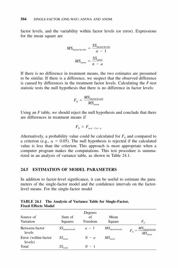
504 SINGLE-FACTOR (ONE-WAY) ANOVA AND ANOM

TABLE 24.1 The Analysis of Variance Table for Single-Factor,Fixed Effects Model

Source ofVariation

Sum ofSquares

Degreesof

FreedomMeanSquare F0

Between-factorlevels

SSfactor levels a � 1 MSfactor levels MSfactor levelsF �0 MSerror

Error (within-factorlevels)

SSerror N � a MSerror

Total SStotal N � 1

factor levels, and the variability within factor levels (or error). Expressionsfor the mean square are

SSfactor levelsMS �factor levels a � 1

SSerrorMS �error n � a

If there is no difference in treatment means, the two estimates are presumedto be similar. If there is a difference, we suspect that the observed differenceis caused by differences in the treatment factor levels. Calculating the F-teststatistic tests the null hypothesis that there is no difference in factor levels:

MSfactor levelsF �0 MSerror

Using an F table, we should reject the null hypothesis and conclude that thereare differences in treatment means if

F � F0 �,a�1,n�a

Alternatively, a probability value could be calculated for F0 and compared toa criterion (e.g., � � 0.05). The null hypothesis is rejected if the calculatedvalue is less than the criterion. This approach is most appropriate when acomputer program makes the computations. This test procedure is summa-rized in an analysis of variance table, as shown in Table 24.1.

24.5 ESTIMATION OF MODEL PARAMETERS

In addition to factor-level significance, it can be useful to estimate the para-meters of the single-factor model and the confidence intervals on the factor-level means. For the single-factor model

MODEL ADEQUACY 505

y � � � � � �ij i ij

estimates for the overall mean and factor-level effects are

�̂ � y

�̂ � y � y, i � 1, 2, . . . , ai i

These estimators have intuitive appeal. The grand average of observation es-timates the overall mean and the difference between the factor levels and theoverall mean estimates the factor-level effect.

A 100(1 � �) percent confidence interval estimate on the ith factor levelis

y � t �MS /ni �,N�a E

where t values for � are from a two-sided t table.

24.6 UNBALANCED DATA

A design is considered unbalanced when the number of observations in thefactor levels is different. For this situation, analysis of variance equationsneed only slight modifications. For an unbalanced design the formula forSSfactor levels becomes

a2SS � n (y � y)�factor levels i i

i�1

A balanced design is preferable to an unbalanced design. With a balanceddesign the power of the test is maximized and the test statistic is robust tosmall departures from the assumption of equal variances. This is not the casefor an unbalanced design.

24.7 MODEL ADEQUACY

As discussed in the correlation and simple regression chapter (see Chapter23), valid analysis of variance results require that certain assumptions besatisfied. As experimenters we collect and then statistically analyze data.Whether we think about it or not, model building is often the center of sta-tistical analysis. The validity of an analysis also depends on basic assump-tions. One typical assumption is that errors are normally and independentlydistributed with mean zero and constant but unknown variance NID(0, �2).

To help with meeting the independence and normal distribution require-ment, an experimenter needs to select an adequate sample size and randomly

506 SINGLE-FACTOR (ONE-WAY) ANOVA AND ANOM

conduct the trials. After data are collected, computer programs offer routinesto test the assumptions. Generally, in a fixed effects analysis of variancemoderate departures from normality of the residuals are of little concern.Because the F test is only slightly affected, analysis of variance and relatedprocedures of fixed effects is said to be robust to the normality assumption.Nonnormality affects the random effects model more severely.

In addition to an analysis of residuals, there is also a direct statistical testfor equality of variance. An expression for this hypothesis is

2 2 2H : � � � � � � � � �0 1 2 a

2H : above not true for at least one �A i

Bartlett’s test is frequently used to test this hypothesis when the normalityassumption is valid. Levene’s test can be used when the normality assumptionis questionable. An example later in this chapter includes a computer outputusing these test statistics.

24.8 ANALYSIS OF RESIDUALS: FITTED VALUE PLOTS ANDDATA TRANSFORMATIONS

Residual plots should show no structure relative to any factor included in thefitted response; however, trends in the data may occur for various reasons.One phenomenon that may occur is inconsistent variance. One example ofthis situation is that the error of an instrument may increase with larger read-ings because the error is a percentage of the scale reading. If this is the case,the residuals will increase as a function of scale reading.

Fortunately, a balanced fixed effects model is robust to variance not beinghomogeneous. The problem becomes more serious for unbalanced designs,situations in which one variance is much larger than others, and for the ran-dom effects model. A data transformation may then be used to reduce thisphenomenon in the residuals, which would yield a more precise significancetest.

Another situation occurs when the output is count data, where a squareroot transformation may be appropriate, while a lognormal transformation isoften appropriate if the trial outputs are standard deviation values and a logitmight be helpful when there are upper and lower limits. A summary of com-mon transformations is given in Table 24.2.

As an alternative to the transformations included in the table, Box (1988)describes a method for eliminating unnecessary coupling of dispersion effectsand location effects by determining an approximate transformation using alambda plot. Montgomery (1997) and Box et al. (1978) discuss transforma-

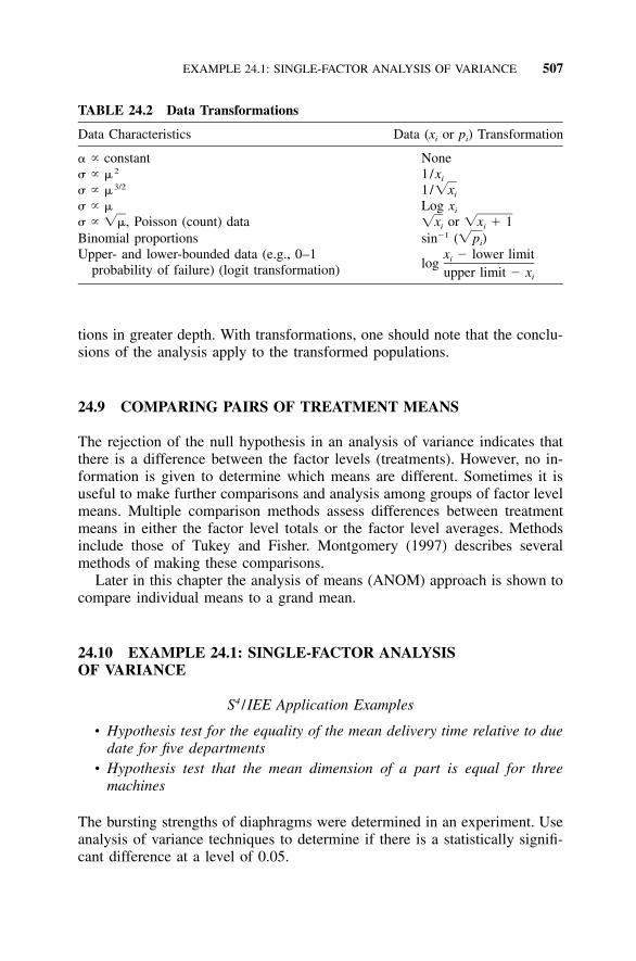
EXAMPLE 24.1: SINGLE-FACTOR ANALYSIS OF VARIANCE 507

TABLE 24.2 Data Transformations

Data Characteristics Data (xi or pi) Transformation

� � constant None� � � 2 1 /xi

� � � 3/2 1 /�xi

� � � Log xi

� � , Poisson (count) data�� orx �x � 1� i i

Binomial proportions sin�1 (�p )iUpper- and lower-bounded data (e.g., 0–1

probability of failure) (logit transformation)x � lower limitilogupper limit � xi

tions in greater depth. With transformations, one should note that the conclu-sions of the analysis apply to the transformed populations.

24.9 COMPARING PAIRS OF TREATMENT MEANS

The rejection of the null hypothesis in an analysis of variance indicates thatthere is a difference between the factor levels (treatments). However, no in-formation is given to determine which means are different. Sometimes it isuseful to make further comparisons and analysis among groups of factor levelmeans. Multiple comparison methods assess differences between treatmentmeans in either the factor level totals or the factor level averages. Methodsinclude those of Tukey and Fisher. Montgomery (1997) describes severalmethods of making these comparisons.

Later in this chapter the analysis of means (ANOM) approach is shown tocompare individual means to a grand mean.

24.10 EXAMPLE 24.1: SINGLE-FACTOR ANALYSISOF VARIANCE

S4 /IEE Application Examples

• Hypothesis test for the equality of the mean delivery time relative to duedate for five departments

• Hypothesis test that the mean dimension of a part is equal for threemachines

The bursting strengths of diaphragms were determined in an experiment. Useanalysis of variance techniques to determine if there is a statistically signifi-cant difference at a level of 0.05.

508 SINGLE-FACTOR (ONE-WAY) ANOVA AND ANOM

FIGURE 24.1 Box plots by response type. Means are indicated by solid circles.

Type 1 Type 2 Type 3 Type 4 Type 5 Type 6 Type 7

59.0 65.7 65.3 67.9 60.6 73.1 59.462.3 62.8 63.7 67.4 65.0 71.9 61.665.2 59.1 68.9 62.9 68.2 67.8 56.365.5 60.2 70.0 61.7 66.0 67.4 62.7

These data could also be measurements from

• Parts manufactured by 7 different operators• Parts manufactured on 7 different machines• Time for purchase order requests from 7 different sites• Delivery time of 7 different suppliers

The box plot and dot plot shown in Figure 24.1 and Figure 24.2 indicate thatthere could be differences between the factor levels (or treatments). However,these plots do not address the question statistically.

An analysis of variance tests the hypothesis for equality of treatment means(i.e., that the treatment effects are zero), which is expressed as

H : � � � � � � � � � � 00 1 2 a

H : � � 0 (for at least one i)A i

The resulting analysis of variance table is as follows:

EXAMPLE 24.1: SINGLE-FACTOR ANALYSIS OF VARIANCE 509

FIGURE 24.2 Dot plots by type. Group means are indicated by lines.

One-Way Analysis of Variance

Analysis of Variance for Response

Source DF SS MS F PType 6 265.34 44.22 4.92 0.003Error 21 188.71 8.99Total 27 454.05

Level N Mean StDev

Individual 95% CIs for Mean

Based on Pooled StDev-------�-------�-------�-------

1 4 63.000 3.032 (-----*-----)2 4 61.950 2.942 (-----*-----)3 4 66.975 2.966 (-----*-----)4 4 64.975 3.134 (-----*-----)5 4 64.950 3.193 (-----*-----)6 4 70.050 2.876 (-----*-----)7 4 60.000 2.823 (------*------)

-------�-------�-------�-------Pooled StDev � 2.998 60.0 65.0 70.0

This analysis indicates that rejection of the null hypothesis is appropriatebecause the p-value is lower than 0.05. Figure 24.3 shows tests of the modelassumptions. The probability values for the test of homogeneity of variances

510 SINGLE-FACTOR (ONE-WAY) ANOVA AND ANOM

20

43

6 43210

–1–2–3–4–5

–5

5

0

543210

210

–1–2–3–4–5

–2

–4 –3 –2 –1 0 1 2 3 60 65 704

–1 0 0 10 20 30Normal scores

Normal Plot of Residuals I Chart of Residuals

Observation number

Res

idua

l

Res

idua

lR

esid

ual

Freq

uenc

y

Histogram of Residuals Residuals vs. fits

Residual Fit

1 2

Factor Levels1

Bartlett's Test

Test Statistic: 0.064P-Value : 1.000

Levene's Test

Test Statistic: 0.080P-Value : 0.998

2

3

4

5

6

7

95% Confidence Intervalsfor Sigmas

100

3.0SL = 6.329

3.0SL = 6.329

X = 0.000

Homogeneity of Variance Test for Response

Residual Model Diagnostics

=

FIGURE 24.3 Single-factor analysis of variance: tests of the model.

indicate that there is not enough information to reject the null hypothesis ofequality of variances. No pattern or outlier data are apparent in either the‘‘residuals versus order of the data’’ or ‘‘residuals versus fitted values.’’ Thenormal probability plot and histogram indicate that the residuals may not benormally distributed. A transformation of the data might improve this fit, butit is doubtful that any difference would be large enough to be of practicalimportance. These data will be further analyzed as an analysis of meansexample.

ANALYSIS OF MEANS 511

24.11 ANALYSIS OF MEANS

Analysis of means (ANOM) is a statistical test procedure in a graphical for-mat, which compares k groups of size n. Consider the following xij data formatwhere there are j observations in k groups.

Groups

1 2 3 � � � k

Observationsx11 x21 x31 � � � xk1

x12 x22 x32 � � � xk2

x13 x23 x33 � � � xk3

......

......

...

x1j x2j x3j � � � xkj

x1 x2 x3 � � � xi

s1 s2 s3 � � � si

The grand mean of the group means ( i) is simply the average of thesex xmean values, which is written

k

x� ii�1x �

k

The pooled estimate for the standard deviation is the square root of the av-erage of the variances for the individual observations.

k2s� i

i�1s � � k

The lower and upper decision lines (LDL and UDL) are

k � 1 k � 1LDL � x � h s UDL � x � h s� �� �kn kn

where h� is from Table I for risk level �, number of means k, and degrees offreedom [(n � 1)k]. The means are then plotted against the decision lines. Ifany mean falls outside the decision lines, there is a statistically significantdifference for this mean from the grand mean.

512 SINGLE-FACTOR (ONE-WAY) ANOVA AND ANOM

If normality can be assumed, analysis of means is also directly applicableto attribute data. It is reasonable to consider a normality approximation ifboth np and n(1 � p) are at least 5. For a probability level p of 0.01, thiswould require a sample size of 500 [i.e., 500(0.01) � 5].

24.12 EXAMPLE 24.2: ANALYSIS OF MEANS

The analysis of variance example above indicated that there was a statisticallysignificant difference in the bursting strengths of seven different types ofrubber diaphragms (k � 7). We will now determine which diaphragms differfrom the grand mean. A data summary of the mean and variance for eachrubber type, each having four observations (n � 4), is

ith Sample Number

1 2 3 4 5 6 7

xi 63.0 62.0 67.0 65.0 65.0 70.0 60.02si 9.2 8.7 8.8 9.8 10.2 8.3 8.0

The overall mean is

k

x� i 63 � 62 � 67 � 65 � 65 � 70 � 60i�1x � � � 64.57k 7

The pooled estimate for the standard deviation is

k2s� i

i�1s � � k1 / 29.2 � 8.7 � 8.8 � 9.8 � 10.2 � 8.3 � 8.0

� � �7

� 3.0

The number of degrees of freedom is (n � 1)k � (4 � 1)(7) � 21. For asignificance level of 0.05 with 7 means and 21 degrees of freedom, it isdetermined by interpolation from Table I that h0.05 � 2.94. The upper andlower decision lines are then

EXAMPLE 24.3: ANALYSIS OF MEANS OF INJECTION-MOLDING DATA 513

FIGURE 24.4 Analysis of means for diaphragm strength by type.

k � 1 7 � 1UDL � x � h s � 64.57 � (2.94)(3.0) � 68.65� � �kn 7(4)

k � 1 7 � 1LDL � x � h s � 64.57 � (2.94)(3.0) � 60.49� � �kn 7(4)

An ANOM chart with the limits and measurements is shown in Figure 24.4.This plot illustrates graphically that and have a statistically significantx x6 7

difference from the grand mean.

24.13 EXAMPLE 24.3: ANALYSIS OF MEANS OFINJECTION-MOLDING DATA

From the Example 15.1 multi-vari analysis and the Example 22.4 variancecomponents analysis of the injection-molding data described in Table 15.1, itwas concluded that differences between cavities affected the diameter of thepart. However, the variance components analysis did not indicate how thecavities differed. The computer analysis of means output shown in Figure24.5 for cavities addresses these needs, where the level of significance for thedecision lines is 0.05.

From this analysis we conclude that the differences between cavity 1 and4 are the main contributors to this source of variability.

514 SINGLE-FACTOR (ONE-WAY) ANOVA AND ANOM

FIGURE 24.5 Analysis of means for diameter by cavity.

24.14 SIX SIGMA CONSIDERATIONS

This section presents some of the controversial metrics and methods of SixSigma. I am including these topics here in hopes of clarifying some aspectsof these methods. Even if an organization chooses not to use these techniques,it should be aware of them because its suppliers or customers may be usingthem for their metrics. Awareness of these techniques and alternatives canreduce the possibility of misunderstandings, which could be very expensive.The author emphasizes that by including these methods, he is not suggestingthat they should all be used.

Much controversy about Six Sigma revolves around whether there shouldbe both a short-term and long-term process capability/performance indexmetric. In addition, there is much controversy about the reporting of a SixSigma metric that includes a 1.5 standard deviation shift. This section de-scribes a methodology to calculate these metrics that is built upon the tech-niques describe within this chapter.

A comparison of the proportion of total variability of the factor levels (orprocess) to the error term could be made in percentage units using a contro-versial epsilon square relationship:

SSfactor2� � 100 �factor level SStotal

SSerror2� � 100 �error SStotal

SIX SIGMA CONSIDERATIONS 515

This relationship is sometimes presented in a pie chart format.Consider the situation in which a process was randomly sampled using

conventional, rational sampling practices and there was a rational subgroupsize between 4 and 6. Consider also that there were between 25 and 100 setsof samples taken over time. A commonly employed combination might be asubgroup size of 5 with 50 periodical samples yielding a total of 250 samples.Using the terms discussed in this chapter, this would equate to a factor of 50levels having a within level sample size of 5. Note that this type of infor-mation could be generated to describe the common cause variability of datataken from a control chart that was in-control/predictable.

For this type of data the sums of squares from an analysis of variance tablecan be used to break down total variability into two parts. The division ofthese sums of squares by the correct number of degrees of freedom yieldsestimates for the different sources of variation. From these sources we canobtain an estimate of the total variation, the variation between subgroups, andthe variation within subgroups. The estimator of total variability gives anestimate for long-term capability/performance, while the estimator of within-group variability gives an estimate for short-term capability.

These concepts of variability can be used to represent the influence of timeon a process. They may also be used to provide understanding when calcu-lating Six Sigma measurements for continuous data. The short-term and long-term standard deviation estimates from an analysis of variance table are

a n2(y � y)� � ij

i�1 j�1�̂ � �lt na � 1

a n2(y � y )� � ij i

i�1 j�1�̂ � �st a(n � 1)

where the numerator terms are sum of squares and the denominator terms areappropriate degrees of freedom.

These two estimators are useful in calculating the long-term and short-termcapability/performance of the process. The variable used to measure thiscapability/performance is Z. Short-term Z values for the process are

LSL � T USL � TZ � Z �LSL,st USL,st�̂ �̂st st

where LSL and USL are the lower and upper specification limit, respectively,and T is the target. The nominal specification T value is used in this equationfor Zst because it represents the potential capability/performance of the pro-

516 SINGLE-FACTOR (ONE-WAY) ANOVA AND ANOM

cess, which implies that the process is considered to conform to the specifi-cation limits and is centered.

Long-term Z values for the process are

LSL � �̂ USL � �̂Z � Z �LSL,lt USL,lt�̂ �̂lt lt

where the estimated process average is . Zlt describes the process over sev-�̂eral time periods. The estimator is used because the process is not assumed�̂to be centered for this long-term case.

Probability values can then be obtained from the normal distribution tablefor the different values of Z. These probabilities correspond to the frequencyof occurrence beyond specification limits or the probabilities of having adefect. The two probabilities for each situation are added to give the totalprobability of a defect for short-term and the total probability of a defect forlong-term. The multiplication of these two probabilities by one million givesDPMO (defects per million opportunities). From this information Zbench couldalso be calculated. In addition, Zshift could be estimated and then comparedto the 1.5 value in the Zst � Zlt � 1.5 shift equation.

24.15 EXAMPLE 24.4: DETERMINING PROCESS CAPABILITYUSING ONE-FACTOR ANALYSIS OF VARIANCE

The following set of data (AIAG 1995b) was presented initially as a controlchart exercise in Chapter 10 (Exercise 3). Example 11.2 shows a procedurethat AIAG (1995b) used to calculate process capability/performance metricsfor this in-control/predictable process. Example 22.3 in the chapter on vari-ance components used a random effects model to determine standard devia-tion values for use in process capability/performance metric equations. Thisexample introduces a single-factor analysis of variance approach to quantifyprocess capability/performance metrics.

Subgroups

1 2 3 4 5 6 7 8 9 10 11 12 13 14 15 16

1 0.65 0.75 0.75 0.60 0.70 0.60 0.75 0.60 0.65 0.60 0.80 0.85 0.70 0.65 0.90 0.752 0.70 0.85 0.80 0.70 0.75 0.75 0.80 0.70 0.80 0.70 0.75 0.75 0.70 0.70 0.80 0.80

Samples 3 0.65 0.75 0.80 0.70 0.65 0.75 0.65 0.80 0.85 0.60 0.90 0.85 0.75 0.85 0.80 0.754 0.65 0.85 0.70 0.75 0.85 0.85 0.75 0.75 0.85 0.80 0.50 0.65 0.75 0.75 0.75 0.805 0.85 0.65 0.75 0.65 0.80 0.70 0.70 0.75 0.75 0.65 0.80 0.70 0.70 0.60 0.85 0.65

EXAMPLE 24.4: DETERMINING PROCESS CAPABILITY 517

For the single-factor analysis of variance approach, we will consider thesubgroups as different factor levels. A computer-generated output for thisanalysis is as follows:

One-Way Analysis of Variance

Analysis of Variance for Data

Source DF SS MS F Psubgrp 15 0.10950 0.00730 1.12 0.360Error 64 0.41800 0.00653Total 79 0.52750

From this analysis of variance table we can determine

a n2(y � y)� � ij 0.52750i�1 j�1

�̂ � � � 0.081714�lt �na � 1 (5)(16) � 1

a n2(y � y )� � ij i 0.41800i�1 j�1

�̂ � � � 0.080816�st �a(n � 1) 16(4)

These estimates for long-term and short-term are similar to the results ofprevious calculations using different approaches. However, Section 24.14 of-fers additional alternatives for calculating process capability/performancemetrics. The methods from Section 24.14 yield

LSL � T 0.5 � 0.7Z � � � �2.4747LSL,st �̂ 0.080816st

USL � T 0.9 � 0.7Z � � � 2.4747USL,st �̂ 0.08016st

LSL � �̂ 0.5 � 0.7375Z � � � � 2.9065LSL,lt �̂ 0.081714lt

USL � �̂ 0.9 � 0.7375Z � � � 1.9886USL,lt �̂ 0.081714lt

518 SINGLE-FACTOR (ONE-WAY) ANOVA AND ANOM

The probabilities for these Z values can then be determined by using a sta-tistical program or a standardized normal distribution curve (Table A). Com-bining and converting to a ppm defect rate yield the following long-term andshort-term results:

Proportion out-of-spec calculations (long-term) are

P(Z ) � P(1.9886) � 0.023373USL long-term

P(Z ) � P(2.9065) � 0.001828LSL long-term

P(total) � 0.023373 � 0.001828 � 0.02520long-term

(equates to a ppm rate of 25,201)

Proportion out-of-spec calculations (short-term) are

P(Z ) � P(2.4747) � 0.006667USL short-term

P(Z ) � P(2.4747) � 0.006667LSL short-term

P(total) � 0.006667 � 0.006667 � 0.013335short-term

(equates to a ppm rate of 13,335)

24.16 NONPARAMETRIC ESTIMATE: KRUSKAL-WALLIS TEST

A Kruskal-Wallis test provides an alternative to a one-way ANOVA. This testis a generalization of Mann-Whitney test procedure. The null hypothesis isall medians are equal. The alternative hypothesis is the medians are not allequal. For this test, it is assumed that independent random samples takenfrom different populations have a continuous distribution with the same shape.For many distributions the Kruskal-Wallis test is more powerful than Mood’smedian test (described later), but it is less robust against outliers.

24.17 EXAMPLE 24.5: NONPARAMETRICKRUSKAL-WALLIS TEST

The yield per acre for four methods of growing corn was (Conover 1980)

NONPARAMETRIC ESTIMATE: MOOD’S MEDIAN TEST 519

Method

1 2 3 4

83 91 101 7891 90 100 8294 81 91 8189 83 93 7789 84 96 7996 83 95 8191 88 94 8092 91 8190 89

84

The following computer output indicates the difference to be statistically sig-nificant

Kruskal-Wallis Test on Yield Per Acre versus Method

Method N Median Ave Rank Z

Method 1 9 91.00 21.8 1.52Method 2 10 86.00 15.3 �0.83Method 3 7 95.00 29.6 3.60Method 4 8 80.50 4.8 �4.12Overall 34 17.5

H � 25.46 DF � 3 P � 0.000H � 25.63 DF � 3 P � 0.000 (adjusted for ties)

24.18 NONPARAMETRIC ESTIMATE: MOOD’S MEDIAN TEST

Like the Kruskal-Wallis test, a Mood’s median test (sometimes called a me-dian test or sign scores test) is a nonparametric alternative to ANOVA. In thischi-square test, the null hypothesis is the population medians are equal. Thealternative hypothesis is the medians are not all equal.

For this test, it is assumed that independent random samples taken fromdifferent populations have a continuous distribution with the same shape. TheMood’s median test is more robust to outliers than the Kruskal-Wallis test.The Mood’s median is less powerful than the Kruskal-Wallis for data frommany distributions.

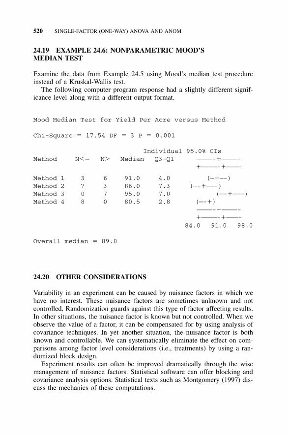
520 SINGLE-FACTOR (ONE-WAY) ANOVA AND ANOM

24.19 EXAMPLE 24.6: NONPARAMETRIC MOOD’SMEDIAN TEST

Examine the data from Example 24.5 using Mood’s median test procedureinstead of a Kruskal-Wallis test.

The following computer program response had a slightly different signif-icance level along with a different output format.

Mood Median Test for Yield Per Acre versus Method

Chi-Square � 17.54 DF � 3 P � 0.001

Individual 95.0% CIsMethod N�� N� Median Q3-Q1 ————-�————-

�————-�———-

Method 1 3 6 91.0 4.0 (—�—-)Method 2 7 3 86.0 7.3 (—-�——-)Method 3 0 7 95.0 7.0 (—-�———)Method 4 8 0 80.5 2.8 (—-�)

————-�————-�————-�———-

84.0 91.0 98.0

Overall median � 89.0

24.20 OTHER CONSIDERATIONS

Variability in an experiment can be caused by nuisance factors in which wehave no interest. These nuisance factors are sometimes unknown and notcontrolled. Randomization guards against this type of factor affecting results.In other situations, the nuisance factor is known but not controlled. When weobserve the value of a factor, it can be compensated for by using analysis ofcovariance techniques. In yet another situation, the nuisance factor is bothknown and controllable. We can systematically eliminate the effect on com-parisons among factor level considerations (i.e., treatments) by using a ran-domized block design.

Experiment results can often be improved dramatically through the wisemanagement of nuisance factors. Statistical software can offer blocking andcovariance analysis options. Statistical texts such as Montgomery (1997) dis-cuss the mechanics of these computations.

EXERCISES 521

24.21 S4/IEE ASSESSMENT

Factors involved in a single-factor analysis of variance can be quantitative orqualitative. Quantitative factors are those levels that can be expressed on anumerical scale, such as time or temperature. Qualitative factors such as ma-chine or operator cannot be expressed on a numerical scale.

When there are several levels of a factor and the factors are quantitative,the experimenter is often interested in developing an empirical model equationfor the response variable of the process that is being studied. When startingthis investigation, it is good practice first to create a scatter diagram of thedata. This plot can give insight into the relationship between the response andfactor levels. Perhaps this relationship is nonlinear. The fit of the model thencould be conducted using regression analysis. This procedure makes no sensewhen the factor levels are qualitative.

It is unfortunate that an organization might choose not to embrace a SixSigma methodology because of some controversial metrics. Many organiza-tions use the basic approach of Six Sigma without including the controversialmetrics. With S4/IEE, the positive aspects of a Six Sigma approach are usedto integrate statistical techniques wisely to organizations. This approach canlead to dramatic bottom-line improvements.

Important aspects of Six Sigma metrics that are often not addressed aresample size and method of selection. First, the sample must be a randomsample of the population of interest. Second, the sample size must be largeenough to give adequate confidence in the metric. Neither of these needs iseasy to achieve. Making supplier and other comparative decisions on the valueof a metric alone can cause problems. When an organization reports a SixSigma metric or process capability/process index, consider how it determinedthe value. Consider also asking the organization about the details of the pro-cess measurement and improvement program. This second query may providemore insight than any Six Sigma metric.

24.22 EXERCISES

1. Catapult Exercise Data Analysis: Using the catapult exercise data setsfrom Chapter 4, conduct single-factor analysis of variance and ANOMof the operator factor.

2. Catapult Exercise Data Analysis: Using the catapult exercise data setsfrom Chapter 4, determine the long-term and short-term processcapabilities/performances. Use a subgroup size of 5, which was the num-ber of shots made by each operator before their rotation.

3. For the following data conduct an analysis of variance and ANOM. As-sess significance levels at 0.05.

522 SINGLE-FACTOR (ONE-WAY) ANOVA AND ANOM

MachineNumber Samples

1.0 35.8 40.4 30.3 46.8 34.1 34.0 38.1 45.0 41.9 40.22.0 40.9 35.7 36.7 37.3 41.8 39.9 34.6 38.8 35.8 35.63.0 36.0 38.3 47.9 35.9 38.1 35.8 31.5 37.4 40.3 44.04.0 44.8 40.0 43.9 43.3 38.8 44.9 42.3 51.8 44.1 45.25.0 37.5 40.4 37.6 34.6 38.9 37.4 35.9 41.0 39.4 28.96.0 33.1 43.4 43.4 43.3 44.3 38.4 33.9 34.5 40.1 33.77.0 37.5 41.9 43.7 38.6 33.2 42.7 40.5 36.1 38.3 38.0

4. The normal probability plot of residuals for the analysis of variance ex-ercise in this chapter had some curvature. Repeat the analysis using anatural logarithm transformation of the data. Give the results and explainwhether the transformation leads to any change in conclusion.

5. When conducting an ANOM, determine the value to use if a significancelevel of 0.05 is desired. There are 5 levels, where each has 7 samples.

6. Explain how the techniques presented in this chapter are useful and canbe applied to S4/IEE projects.

7. Wisdom of the organization thought operator could affect a response.Conduct an analysis and comment.

Oper 1 Oper 2 Oper 3

50 58 4945 52 5547 53 2853 59 3552 60 25

8. Given the factor level output below analyze the data for significance. (SixSigma Study Guide 2002.)

Level 1 Level 2 Level 3 Level 4

34.6 90.1 124.4 71.8103.1 82.1 75.4 35.8102.9 61.8 112.8 61.931.2 24.3 47.9 47.631.7 26.0 45.0 42.668.1 72.4 115.1 70.264.3 67.6 114.0 43.2

102.8 104.7 108.4 75.775.2 101.6 95.6 66.996.9 80.1 91.9 96.240.9 56.0 123.1 93.6

EXERCISES 523

Level 1 Level 2 Level 3 Level 4

52.4 82.3 87.9 64.481.4 104.9 61.4 106.822.9 31.5 106.3 83.756.4 37.2 69.5 34.950.5 58.1 104.6 54.078.3 100.1 91.5 122.5

9. Given the factor level output below analyze the data for significance. (SixSigma Study Guide 2002.)

Level 1 Level 2 Level 3 Level 4 Level 5

51.9 46.5 44.9 115.2 33.6120.2 82.7 68.1 26.7 43.942.4 79.6 90.9 27.7 48.762.9 91.4 88.7 86.6 45.634.0 92.0 65.6 118.1 65.142.1 50.9 57.2 118.3 44.597.3 85.8 45.3 77.3 63.262.1 65.2 26.0 89.9 42.270.1 118.5 42.6 77.3 76.256.9 53.1 35.2 58.4 33.7

108.1 59.1 73.4 28.6 76.489.1 30.3 79.8 46.1 45.236.0 93.2 91.3 103.2 79.243.8 41.4 84.1 122.5 48.3

118.6 101.8 67.4 96.9 98.368.9 35.9 100.6 94.7 54.887.6 81.5 45.6 109.7 62.341.4 95.994.1 32.662.0 28.674.8 116.1

105.8 45.4

10. Exercise 15.6 showed data that was collected passively for the purposeof better understanding what might be done to improve the KPOV de-scribed in Exercise 10.18. Using the appropriate statistical tools, test forstatistical significant differences between inspector, machines, processtemperature, material lot, and day-to-day variability relative to within-dayvariability. Compare these results in a graphical assessment.

11. Describe how and show where the tools described in this chapter fit intothe overall S4/IEE roadmap described in Figure A.1 and A.2 in the Ap-pendix.

524

25TWO-FACTOR (TWO-WAY)ANALYSIS OF VARIANCE

S4 /IEE DMAIC Application: Appendix Section A.1, Project ExecutionRoadmap Step 7.4

Experiments often involve the study of more than one factor. Factorial designsare most efficient for the situation in which combinations of levels of factorsare investigated. These designs evaluate the change in response caused bydifferent levels of factors and the interaction of factors.

This chapter focuses on two-factor analysis of variance or two-way analysisof variance of fixed effects. The following chapters (see Chapters 27–33)describe factorial experiments in which there are more than two factors.

25.1 TWO-FACTOR FACTORIAL DESIGN

The general two-factor factorial experiment takes the form shown in Table25.1, in which design is considered completely randomized because obser-vations are taken randomly. In this table response, factor A has levels rangingfrom 1 to a, while factor B has levels ranging from 1 to b, and the replicationshave replicates 1 to n. Responses for the various combinations of factor Awith factor B take the form yijk , where i denotes the level of factor A, j notesthe level of factor B, and k represents the replicate number. The total numberof observations is then abn.

A description of the fixed linear two-factor model is then

TWO-FACTOR FACTORIAL DESIGN 525

TABLE 25.1 General Arrangement for a Two-Factor Factorial Design

Factor B

1 2 . . . b

Factor A

12�

a

y � � � � � � � (��) � εijk i j ij ijk

where � is the overall mean effect, � i is the effect of the i th level of A (rowfactor), �j is the effect for the j th level of B (column factor), (��)ij is theeffect of the interaction, and εij k is random error.

For a two-factor factorial, both row and column factors (or treatments) areof equal interest. The test hypothesis for row factor effects is

H : � � � � � � � � � � 00 1 2 a

H : at least one � � 0A i

The test hypothesis for column factor effects is

H : � � � � � � � � � � 00 1 2 b

H : at least one � � 0A j

The test hypothesis for the interaction of row and column factor effects is

H : (��) � 0 for all values of i, j0 ij

H : at least one (��) � 0A ij

As in one-factor analysis of variance the total variability can be partitionedinto the sum of the sum of squares from the elements of the experiment,which can be represented as

SS � SS � SS � SS � SST A B AB e

where SST is the total sum of squares, SSA is the sum of squares from factorA, SSB is the sum of squares from factor B, SSAB is the sum of squares from

526 TWO-FACTOR (TWO-WAY) ANALYSIS OF VARIANCE

TABLE 25.2 Two-Factor Factorial Analysis of Variance Table for FixedEffects Model

SourceSum ofSquares

Degrees ofFreedom Mean Square F0

Factor A

Factor B

Interaction

Error

Total

SS A

SSB

SS AB

SS E

SS T

a � 1

b � 1

(a � 1)(b � 1)

ab(n � 1)

abn � 1

SS AMS �A a � 1

SSBMS �B b � 1

SS ABMS �AB (a � 1)(b � 1)

SS EMS �E ab(n � 1)

MS AF �0 MS E

MSBF �0 MS E

MS ABF �0 MS E

the interaction of factor A with factor B, and SSe is the sum of squares fromerror. These sums of squares have the following degrees of freedom:

EffectDegrees ofFreedom

A a � 1B b � 1AB interaction (a � 1)(b � 1)Error ab(n � 1)Total abn � 1

Mean square and F0 calculations are also similar to one-factor analysis ofvariance. These equations for the two-factor factorial are given in Table 25.2.

The difference between a two-factor analysis of variance approach and arandomized block design on one of the factors is that the randomized blockdesign would not have the interaction consideration.

25.2 EXAMPLE 25.1: TWO-FACTOR FACTORIAL DESIGN

A battery is to be used in a device subjected to extreme temperature varia-tions. At some point in time during development, an engineer can select oneof only three plate material types. After product shipment, the engineer hasno control over temperature; however, he/she believes that temperature coulddegrade the effective life of the battery.

The engineer would like to determine if one of the material types is robustto temperature variations. Table 25.3 gives the observed effective life (in

EXAMPLE 25.1: TWO-FACTOR FACTORIAL DESIGN 527

TABLE 25.3 Life Data (in hours) for Battery Two-Factorial Design

Material Type

Temperature (�F)

15 70 125

1 13074

155180

3480

4075

2082

7058

2 150159

188126

136106

122115

2558

7045

3 138168

110160

174150

120139

9682

10460

hours) of the battery at controlled temperatures in the laboratory (Montgom-ery 1997).

The two-factor analysis of variance output is

Two-Way Analysis of Variance

Analysis of Variance for Response

Source DF SS MS F PMaterial 2 10684 5342 7.91 0.002Temp 2 39119 19559 28.97 0.000Interaction 4 9614 2403 3.56 0.019Error 27 18231 675Total 35 77647

Using an � � 0.05 criterion, we conclude that there is a statistically significantinteraction between material types and temperature because its probabilityvalue is less than 0.05 [and F0 � (F0.05,4,27 � 2.73)]. We also conclude thatthe main effects of material type and temperature are also statistically signif-icant because each of their probabilities are less than 0.05 [and F0 � (F0.05,2,27

� 3.35)].A plot of the average response at each factor level is shown in Figure 25.1,

which aids the interpretation of experimental results. The significance of theinteraction term in our model shows up as the lack of parallelism of theselines. From this plot we note a degradation in life with an increase in tem-perature regardless of material type. If it is desirable for this battery to ex-perience less loss of life at elevated temperature, type 3 material seems to bethe best choice of the three materials.

Whenever there is a difference in the rows’ or columns’ means, it can beuseful to make additional comparisons. This analysis shows these differences,but the significance of the interaction can obscure comparison tests. One ap-

528 TWO-FACTOR (TWO-WAY) ANALYSIS OF VARIANCE

FIGURE 25.1 Mean battery life as a function of material and temperature.

FIGURE 25.2 Analysis of means for life at 70�F.

proach to address this situation is to apply the test at only one level of afactor at a time.

Using this strategy, let us examine the data for statistically significant dif-ferences at 70�F (i.e., level 2 of temperature). We can use ANOM techniquesto determine factor levels relative to the grand mean. The ANOM outputshown in Figure 25.2 indicates that material types 1 and 3 differ from thegrand mean.

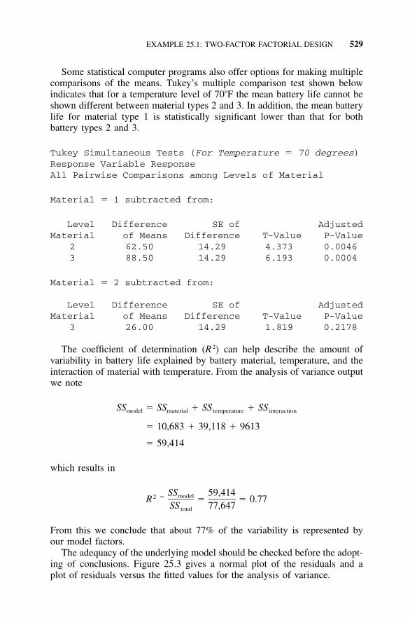
EXAMPLE 25.1: TWO-FACTOR FACTORIAL DESIGN 529

Some statistical computer programs also offer options for making multiplecomparisons of the means. Tukey’s multiple comparison test shown belowindicates that for a temperature level of 70�F the mean battery life cannot beshown different between material types 2 and 3. In addition, the mean batterylife for material type 1 is statistically significant lower than that for bothbattery types 2 and 3.

Tukey Simultaneous Tests (For Temperature � 70 degrees)Response Variable ResponseAll Pairwise Comparisons among Levels of Material

Material � 1 subtracted from:

LevelMaterial

Differenceof Means

SE ofDifference T-Value

AdjustedP-Value

2 62.50 14.29 4.373 0.00463 88.50 14.29 6.193 0.0004

Material � 2 subtracted from:

Level Difference SE of AdjustedMaterial of Means Difference T-Value P-Value

3 26.00 14.29 1.819 0.2178

The coefficient of determination (R2) can help describe the amount ofvariability in battery life explained by battery material, temperature, and theinteraction of material with temperature. From the analysis of variance outputwe note

SS � SS � SS � SSmodel material temperature interaction

� 10,683 � 39,118 � 9613

� 59,414

which results in

SS 59,414model2 �R � � 0.77SS 77,647total

From this we conclude that about 77% of the variability is represented byour model factors.

The adequacy of the underlying model should be checked before the adopt-ing of conclusions. Figure 25.3 gives a normal plot of the residuals and aplot of residuals versus the fitted values for the analysis of variance.

530 TWO-FACTOR (TWO-WAY) ANALYSIS OF VARIANCE

Residual

Temperature

Res

idua

lN

orm

al s

core

–50

2

1

0

50

0

–50

–1

–2

0 50

Fitted Value

Residuals Versus Temperature Residuals Versus Material

Normal Probability Plot of the Residuals Residuals Versus the Fitted Values

Material

Res

idua

lR

esid

ual

–50 100 150

50

0

–50

50

0

–50

100 1 2 3

0 50

FIGURE 25.3 Residual plots for analysis of variance results of battery life.

The normal probability plot of the residuals does not reveal anything ofparticular concern. The residual plot of residuals versus fitted values seemsto indicate a mild tendency for the variance of the residuals to increase asbattery life increases. The residual plots of battery type and temperature seemto indicate that material type 1 and low temperature might have more varia-bility. However, these problems do not appear to be large enough to have adramatic impact on the analysis and conclusions.

25.3 NONPARAMETRIC ESTIMATE: FRIEDMAN TEST

A Friedman test is a nonparametric analysis of a randomized block experi-ment. This test, which is a generalization of the paired sign test, provides analternative to the two-way ANOVA. The null hypothesis is all treatment ef-fects are zero. The alternative hypothesis is that not all treatment effects arezero.

Additivity is the sum of treatment and block effects. ANOVA possessesadditivity. That is, the fit of the model is the sum of treatment and blockeffects. Within the Friedman test, additivity is not required for the test; how-ever, it is required when estimating the treatment effects.

S4 / IEE ASSESSMENT 531

25.4 EXAMPLE 25.2: NONPARAMETRIC FRIEDMAN TEST

The effect of a drug treatment on enzyme activity was evaluated within arandomized block experiment. Three different drug therapies were given tofour animals. Each animal belonging to a different litter. The null hypothesiswas all treatment effects are zero. The alternative hypothesis was not alltreatment effects are zero (Minitab 2000).

Therapy

1 2 3

Litter

1

2

3

4

0.15

0.26

0.23

0.99

0.55

0.26

�0.22

0.99

0.55

0.66

0.77

0.99

From the following computer output we could not reject the null hypothesesat a level of 0.05.

Friedman Test for Enzyme Activity by Therapy Blockedby Litter

S � 2.38 DF � 2 P � 0.305

S � 3.80 DF � 2 P � 0.150 (adjusted for ties)

Therapy NEst

MedianSum ofRanks

1 4 0.2450 6.5

2 4 0.3117 7.0

3 4 0.5783 10.5

Grand median � 0.3783

25.5 S4/IEE ASSESSMENT

Two-factor factorial experiments offer more information than one-factor ex-periments. The two-factor factorial experiment is often the best approach fora given situation. The method gives information about interactions and canapply to both manufacturing and business processes. However, in some situ-

532 TWO-FACTOR (TWO-WAY) ANALYSIS OF VARIANCE

ations the experiment can be very costly because it requires many test trials.It addition, it does not address other factors that may significantly affect aprocess. The normal approach for dealing with other process factors not con-sidered in the experiment is either to hold them constant or let them exhibit‘‘normal’’ variability. In many situations, neither of these alternatives is verydesirable.

Before conducting a two-factor factorial, it is best to reflect on the objectiveof the experiment and important aspects of the situation. Often it is best toexecute this reflection in a team setting in which attendees have differentperspectives on the situation. Initially, the situation should be crisply defined,and what is desired from the experimental analysis should be determined.Next the group should use brainstorming techniques to create a list of allfactors that can affect the situation. The group can then prioritize these factorsand list any test constraints.

Reflection on the issues in this team meeting may indicate that a two-factorfactorial approach is the best for the particular situation, but, if there are manyfactors, then a DOE approach (discussed in Chapters 27–33) may be a betteralternative.

25.6 EXERCISES

1. Catapult Exercise: Each team is to select two continuous variable factorsto vary on the catapult (e.g., arm length and start angle). Three levels arechosen for each factor. Conduct a randomized experiment of projectiondistance with one replication for each level setting of the factors. Therewill be a total of 18 measurements. Conduct a two-factor analysis of var-iance.

2. The breaking strength of a fiber is studied as a function of four machinesand three operators using fiber from one batch. Using computer software,analyze the following data and draw conclusions. Comment on how thesevariables could be related to a transactional process (Montgomery 1997).

Operator

Machine

1 2 3 4

1 109110

110115

108109

110108

2 110112

110111

111109

114112

3 116114

112115

114119

120117

3. Explain how the techniques presented in this chapter are useful and canbe applied to S4/IEE projects.

533

26MULTIPLE REGRESSION,LOGISTIC REGRESSION, ANDINDICATOR VARIABLES

S4 /IEE DMAIC Application: Appendix Section A.1, Project ExecutionRoadmap Step 7.4

The previous chapter presented the simple regression model, used to estimatea response as a function of the magnitude of one regressor variable. Thischapter discusses using multiple regressor variables to build a multiple re-gression model. In addition, categorical data such as location, operator, andcolor are modeled using indicator or dummy variables.

26.1 S4/IEE APPLICATION EXAMPLES:MULTIPLE REGRESSION

S4/IEE application examples of multiple regression are:

• An S4/IEE project was created to improve the 30,000-foot-level metricDSO. Two inputs that surfaced from a cause-and-effect diagram were thesize of the invoice and the number of line items included within theinvoice. A multiple regression analysis was conducted for DSO versussize of invoice and number of line items included in invoice.

• An S4/IEE project was created to improve the 30,000-foot-level metric,the diameter of a manufactured part. Inputs that surfaced from a cause-and-effect diagram were the temperature, pressure, and speed of the man-ufacturing process. A multiple regression analysis of diameter versustemperature, pressure, and speed was conducted.

534 MULTIPLE AND LOGISTIC REGRESSIONS, AND INDICATOR VARIABLES

26.2 DESCRIPTION

A general model includes polynomial terms in one or more variables such as

2 2Y � � � � x � � x � � x � � x � � x x � ε0 1 1 2 2 3 1 4 2 5 1 2

where �’s are unknown parameters and ε is random error. This full quadraticmodel of Y on x1 and x2 is of great use in DOE.

For the situation without polynomial terms where there are k predictorvariables, the general model reduces to the form

Y � � � � x � � � � � � x � ε0 1 1 k k

The object is to determine from data the least squares estimates (b0, b1, . . . ,bk) of the unknown parameters (�0, �1, . . . , �k) for the prediction equation

Ŷ � b � b x � � � � � b x0 1 1 k k

where is the predicted value of Y for given values of x1, . . . , xk. ManyŶstatistical software packages can perform these calculations. The followingexample illustrates this type of analysis.

26.3 EXAMPLE 26.1: MULTIPLE REGRESSION

S4 /IEE Application Examples

• Analysis of DSO versus invoice amount and the number of line items inthe invoice

• Analysis of part diameter versus temperature, pressure, and speed of amanufacturing process

An investigator wants to determine the relationship of a key process outputvariable, product strength, to two key process input variables, hydraulic pres-sure during a forming process and acid concentration. The data are given inTable 26.1 (Juran 1988), which resulted in the following analysis:

Regression Analysis

The regression equation isstrength � 16.3 � 1.57 pressure � 4.16 concent

Predictor Coef StDev T PConstant 16.28 44.30 0.37 0.718Pressure 1.5718 0.2606 6.03 0.000Concent 4.1629 0.3340 12.47 0.000

S � 15.10 R-Sq � 92.8% R-Sq(adj) � 92.0%

EXAMPLE 26.1: MULTIPLE REGRESSION 535

TABLE 26.1 Data for Multiple Regression Modelof Product Strength

Strength Pressure Concentration

665 110 116618 119 104620 138 94578 130 86682 143 110594 133 87722 147 114700 142 106681 125 107695 135 106664 152 98548 118 86620 155 87595 128 96740 146 120670 132 108640 130 104590 112 91570 113 92640 120 100

Analysis of Variance

Source DF SS MS F PRegression 2 50101 25050 109.87 0.000Residual Error 17 3876 228Total 19 53977

Source DF Seq SSPressure 1 14673Concent 1 35428

Some of the entries in this output are more important than others. I willnow highlight some of the more important aspects of this table. The predictorand coefficient (coeff) describe the prediction model (strength � 16.3 � 1.57pressure � 4.16 concent). The P columns give the significance level for eachmodel term. Typically, if a P value is less than or equal to 0.05, the variableis considered statistically significant (i.e., null hypothesis is rejected). If a Pvalue is greater than 0.10, the term is removed from the model. A practitionermight leave the term the model if the P value is the gray region between

536 MULTIPLE AND LOGISTIC REGRESSIONS, AND INDICATOR VARIABLES

these two probability levels. Note that these probability values for the modelparameters are determined from the t-statistic values shown in the output.

The coefficient of determination (R2) is presented as R-Sq and R-Sq(adj)in the output. This value represents the proportion of the variability accountedfor by the model, where the R2(adj) adjusts for the degrees of freedom. Whena variable is added to an equation the coefficient of determination will getlarger, even if the added variable has no real value. R2(adj) is an approximateunbiased estimate that compensates for this. In this case the model accountsfor a very large percentage of the variability because the R2(adj) value is92%.

In the analysis of variance portion of this output the F value is used todetermine an overall P value for the model fit. In this case the resulting Pvalue of 0.000 indicates a very high level of significance. The regression andresidual sum of squares (SS) and mean square (MS) values are interim stepstoward determining the F value. Standard error is the square root of the meansquare.

No unusual patterns were apparent in the residual analysis plots. Also, nocorrelation was shown between hydraulic pressure and acid concentration.

26.4 OTHER CONSIDERATIONS

Regressor variables should be independent within a model (i.e., completelyuncorrelated). Multicollinearity occurs when variables are dependent. A mea-sure of the magnitude of multicollinearity that is often available in statisticalsoftware is the variance inflation factor (VIF). VIF quantifies how much thevariance of an estimated regression coefficient increases if the predictors arecorrelated. Regression coefficients can be considered poorly estimated whenVIF exceeds 5 or 10 (Montgomery and Peck 1982). Strategies for breakingup multicollinearity include collecting additional data or using different pre-dictors.

Another approach to data analysis is the use of stepwise regression (Draperand Smith 1966) or of all possible regressions of the data when selecting thenumber of terms to include in a model. This approach can be most usefulwhen data derives from an experiment that does not have experiment struc-ture. However, experimenters should be aware of the potential pitfalls result-ing from happenstance data (Box et al. 1978).

A multiple regression best subset analysis is another analysis alternative.Consider an analysis of all possible regressions for the data shown in Table30.3. Table 26.2 illustrates a computer output with all possible regressions.This approach first considers only one factor in a model, then two, and soforth (Table 26.2, notes and ). The R2 value is then considered for each� �1 2of the models (Table 26.2, note ); only factor combinations containing the�3highest two R2 values are shown in Table 26.2. For example, if one were toconsider a model containing only one factor, the factor to consider would be

EXAMPLE 26.2: MULTIPLE REGRESSION BEST SUBSET ANALYSIS 537

TABLE 26.2 Summary from All Possible Regressions Analysis

N � 16

Number inModel �1

Regression Models for Dependent Variable:Timing Model: Model 1

R-Square �3 C(P) �4 Variables in Model �2

1 0.33350061 75.246939 MOT ADJ1 0.57739025 43.320991 ALGOR2 0.58342362 44.531203 ALGOR EXT ADJ2 0.91009086 1.664676 ALGOR MOT ADJ3 0.91500815 3.125709 ALGOR MOT ADJ SUP VOLT3 0.91692423 2.874888 ALGOR MOT ADJ EXT ADJ4 0.91949041 4.538967 ALGOR MOT ADJ EXT ADJ MOT TEMP4 0.92104153 4.335921 ALGOR MOT ADJ EXT ADJ SUP VOLT5 0.92360771 6.000000 ALGOR MOT ADJ EXT ADJ SUP VOLT MOT TEMP

algor. Likewise, if one were to consider a model containing only two factors,the factors to consider would be algor with mot adj.

The Mallows Cp statistic [C(P) in Table 26.2, note ] is useful to deter-�4mining the minimum number of parameters that best fits the model. Techni-cally this statistic measures the sum of the squared biases plus the squaredrandom errors in Y at all n data points (Daniel and Wood 1980).

The minimum number of factors needed in the model occurs when theMallows Cp statistic is a minimum. From this output the pertinent MallowsCp statistic values under consideration as a function of a number of factorsin this model are

Number in Model Mallows Cpa

1 43.322 1.673 2.874 4.335 6.00

a The Mallows Cp is not related to the process indices Cp.

From this summary it is noted that the Mallows Cp statistic is minimizedwhenever there are two parameters in the model. The corresponding factorsare algor and mot adj. This conclusion is consistent with the analysis inExample 30.1.

26.5 EXAMPLE 26.2: MULTIPLE REGRESSION BEST SUBSETANALYSIS

The results from a cause-and-effect matrix lead to a passive analysis of factorsA, B, C, and D on Thruput. In a plastic molding process, for example, the

538 MULTIPLE AND LOGISTIC REGRESSIONS, AND INDICATOR VARIABLES

thruput response might be shrinkage as a function of the input factors tem-perature 1, temperature 2, pressure 1, and hold time.

A B C D Thruput

7.13 3.34 3.20 146.74 19.257.36 3.31 3.17 147.89 19.328.05 3.06 3.15 144.67 19.347.13 2.92 3.17 153.87 19.376.90 3.06 3.20 160.31 19.417.13 3.08 3.50 161.00 20.338.05 2.81 3.43 166.06 20.567.13 2.81 3.52 169.97 20.728.05 2.97 3.50 160.08 20.758.28 2.81 3.40 166.52 20.828.05 2.92 3.70 149.27 21.398.28 2.92 3.66 170.89 21.418.28 2.83 3.57 172.04 21.46

A best subsets computer regression analysis of the collected data assessingthe four factors yielded:

Vars R-SqAdj.R-Sq Cp s A B C D

1 92.1 91.4 38.3 0.25631 X1 49.2 44.6 294.2 0.64905 X2 96.3 95.6 14.9 0.18282 X X2 95.2 94.3 21.5 0.20867 X X3 98.5 98.0 4.1 0.12454 X X X3 97.9 97.1 7.8 0.14723 X X X4 98.7 98.0 5.0 0.12363 X X X X

For this computer output format, an ‘‘X’’ is placed in the column(s) for thevariable(s) considered in the model.

We would like to create a model that provides a good estimate with thefewest number of terms. From this output we note:

• R-Sq: Look for the highest value when comparing models with the samenumber of predictors (vars).

• Adj. R-Sq: Look for the highest value when comparing models withdifferent numbers of predictors.

• Cp: Look for models where Cp is small and close to the number ofparameters in the model, e.g., look for a model with Cp close to four for

EXAMPLE 26.3: INDICATOR VARIABLES 539

a three-predictor model that has an intercept constant (often we just lookfor the lowest Cp value).

• s: We want s, the estimate of the standard deviation about the regression,to be as small as possible.

The regression equation for a 3-parameter model from a computer programis:

Thruput � 3.87 � 0.393 A � 3.19 C � 0.0162 DPredictor Coef SE Coef T P VIF

Constant 3.8702 0.7127 5.43 0.000A 0.39333 0.07734 5.09 0.001 1.4C 3.1935 0.2523 12.66 0.000 1.9D 0.016189 0.004570 3.54 0.006 1.5

S � 0.1245 R-Sq � 98.5% R-Sq(adj) � 98.0%

The magnitude of the VIFs is satisfactory, i.e., not larger than 5–10. In ad-dition, there were no observed problems with the residual analysis.

26.6 INDICATOR VARIABLES (DUMMY VARIABLES) TOANALYZE CATEGORICAL DATA

Categorical data such as location, operator, and color can also be modeledusing simple and multiple linear regression. It is not generally correct to usenumerical code when analyzing this type of data within regression, since thefitted values within the model will be dependent upon the assignment of thenumerical values. The correct approach is through the use of indicator vari-ables or dummy variables, which indicate whether a factor should or shouldnot be included in the model.

If we are given information about two variables, we can calculate the third.Hence, only two variables are needed for a model that has three variables,where it does not matter which variable is left out of the model. After indi-cator or dummy variables are created, indicator variables are analyzed usingregression to create a cell means model.

If the intercept is left out of the regression equation, a no intercept cellmeans model is created. For the case where there are three indicator variables,a no intercept model would then have three terms where the coefficients arethe cell means.

26.7 EXAMPLE 26.3: INDICATOR VARIABLES

Revenue for Arizona, Florida, and Texas is shown in Table 26.3 (Bower2001). This table also contains indicator variables that were created to rep-resent these states. One computer analysis possibility is:

540 MULTIPLE AND LOGISTIC REGRESSIONS, AND INDICATOR VARIABLES

TABLE 26.3 Revenue By State

Revenue Location AZ FL TX Revenue Location AZ FL TX Revenue Location AZ FL TX

23.487 AZ 1 0 0 35.775 FL 0 1 0 48.792 TX 0 0 120.650 AZ 1 0 0 33,978 FL 0 1 0 52.829 TX 0 0 122.500 AZ 1 0 0 30.985 FL 0 1 0 48.591 TX 0 0 124.179 AZ 1 0 0 30.575 FL 0 1 0 49.826 TX 0 0 126.313 AZ 1 0 0 34.700 FL 0 1 0 52.484 TX 0 0 123.849 AZ 1 0 0 34.107 FL 0 1 0 43.418 TX 0 0 125.052 AZ 1 0 0 31.244 FL 0 1 0 44.406 TX 0 0 125.647 AZ 1 0 0 32.769 FL 0 1 0 45.899 TX 0 0 125.014 AZ 1 0 0 31.073 FL 0 1 0 53.997 TX 0 0 121.443 AZ 1 0 0 29.655 FL 0 1 0 42.590 TX 0 0 125.690 AZ 1 0 0 32.161 FL 0 1 0 48.041 TX 0 0 131.274 AZ 1 0 0 26.651 FL 0 1 0 48.988 TX 0 0 126.238 AZ 1 0 0 32.825 FL 0 1 0 47.548 TX 0 0 132.253 AZ 1 0 0 30.567 FL 0 1 0 44.999 TX 0 0 122.084 AZ 1 0 0 34.424 FL 0 1 0 44.212 TX 0 0 121.565 AZ 1 0 0 29.600 FL 0 1 0 48.615 TX 0 0 129.800 AZ 1 0 0 25.149 FL 0 1 0 41.634 TX 0 0 123.248 AZ 1 0 0 34.342 FL 0 1 0 47.562 TX 0 0 129.785 AZ 1 0 0 28.557 FL 0 1 0 44.616 TX 0 0 128.076 AZ 1 0 0 31.490 FL 0 1 0 47.660 TX 0 0 118.606 AZ 1 0 0 38.966 FL 0 1 0 50.278 TX 0 0 122.876 AZ 1 0 0 31.129 FL 0 1 0 48.802 TX 0 0 126.688 AZ 1 0 0 36.983 FL 0 1 0 51.430 TX 0 0 125.910 AZ 1 0 0 36.940 FL 0 1 0 46.852 TX 0 0 128.320 AZ 1 0 0 36.318 FL 0 1 0 48.704 TX 0 0 122.192 AZ 1 0 0 32.802 FL 0 1 0 53.289 TX 0 0 125.048 AZ 1 0 0 28.994 FL 0 1 0 43.165 TX 0 0 127.056 AZ 1 0 0 31.236 FL 0 1 0 53.987 TX 0 0 125.312 AZ 1 0 0 35.703 FL 0 1 0 51.484 TX 0 0 129.996 AZ 1 0 0 38.738 FL 0 1 0 49.923 TX 0 0 122.902 AZ 1 0 0 35.032 FL 0 1 0 49.618 TX 0 0 126.942 AZ 1 0 0 27.430 FL 0 1 0 46.043 TX 0 0 121.384 AZ 1 0 0 29.046 FL 0 1 0 47.716 TX 0 0 123.952 AZ 1 0 0 34.942 FL 0 1 0 46.465 TX 0 0 121.793 AZ 1 0 0 36.624 FL 0 1 0 54.701 TX 0 0 126.664 AZ 1 0 0 34.198 FL 0 1 0 48.776 TX 0 0 123.886 AZ 1 0 0 33.307 FL 0 1 0 47.817 TX 0 0 123.242 AZ 1 0 0 33.644 FL 0 1 0 54.188 TX 0 0 127.764 AZ 1 0 0 34.063 FL 0 1 0 51.947 TX 0 0 129.126 AZ 1 0 0 33.558 FL 0 1 0 54.657 TX 0 0 123.734 AZ 1 0 0 35.538 FL 0 1 0 50.777 TX 0 0 118.814 AZ 1 0 0 31.162 FL 0 1 0 53.390 TX 0 0 124.544 AZ 1 0 0 30.260 FL 0 1 0 51.147 TX 0 0 122.632 AZ 1 0 0 27.638 FL 0 1 0 44.404 TX 0 0 125.184 AZ 1 0 0 32.833 FL 0 1 0 45.515 TX 0 0 122.869 AZ 1 0 0 35.859 FL 0 1 0 49.694 TX 0 0 126.900 AZ 1 0 0 38.767 FL 0 1 0 49.716 TX 0 0 124.870 AZ 1 0 0 34.535 FL 0 1 0 48.896 TX 0 0 125.490 AZ 1 0 0 28.816 FL 0 1 0 45.447 TX 0 0 123.652 AZ 1 0 0 31.324 FL 0 1 0 51.111 TX 0 0 1

EXAMPLE 26.4: INDICATOR VARIABLES WITH COVARIATE 541

The regression equation isRevenue � 48.7 � 24.1 AZ � 16.0 FL

Predictor Coef SE Coef T PConstant 48.7325 0.4437 109.83 0.000AZ �24.0826 0.6275 �38.38 0.000FL �15.9923 0.6275 �25.49 0.000

S � 3.137 R-Sq � 91.2% R-Sq(adj) � 91.1%

Calculations for various revenues would be:

Texas Revenue � 48.7 � 24.1(0) � 16.0(0) � 48.7

Arizona Revenue � 48.7 � 24.1(1) � 16.0(0) � 24.6

Florida Revenue � 48.7 � 24.1(0) � 16.0(1) � 32.7

A no intercept cell means model from a computer analysis would be

The regression equation is

Revenue � 24.6 AZ � 32.7 FL � 48.7 TXPredictorNoconstant Coef SE Coef T PAZ 24.6499 0.4437 55.56 0.000FL 32.7402 0.4437 73.79 0.000TX 48.7325 0.4437 109.83 0.000

S � 3.137

Note how the coefficients, when rounded off, equate to the previous calculatedrevenues.

26.8 EXAMPLE 26.4: INDICATOR VARIABLESWITH COVARIATE

Consider the following data set, which has created indicator variables and acovariate. This covariate might be a continuous variable such as process tem-perature or dollar amount for an invoice.

542 MULTIPLE AND LOGISTIC REGRESSIONS, AND INDICATOR VARIABLES

Response Factor 1 Factor 2 A B High Covariate

1 A High 1 0 1 112 A Low 1 0 �1 73 A High 1 0 1 54 A Low 1 0 �1 65 B High 0 1 1 66 B Low 0 1 �1 37 B High 0 1 1 148 B Low 0 1 �1 209 C High �1 �1 1 2

10 C Low �1 �1 �1 1711 C High �1 �1 1 1912 C Low �1 �1 �1 14

A computer regression analysis yields

The regression equation is

Response � 5.62 � 3.18 A � 0.475 B � 0.883 High� 0.0598 Covariate

Predictor Coef SE Coef T PConstant 5.6178 0.3560 15.78 0.000A �3.1844 0.2550 �12.49 0.000B �0.4751 0.2374 �2.00 0.086High �0.8832 0.1696 �5.21 0.001Covariat �0.05979 0.03039 �1.97 0.090

S � 0.5808 R-Sq � 97.6% R-Sq(adj) � 96.2%

Similar to Example 26.2, an estimated response can be calculated for variouscategorical and discrete variable situations.

26.9 BINARY LOGISTIC REGRESSION

Binary logistic regression is applicable when the response is pass or fail andinputs are continuous variables. To illustrate the application, consider the fol-lowing example.

EXAMPLE 26.5: BINARY LOGISTIC REGRESSION 543

26.10 EXAMPLE 26.5: BINARY LOGISTIC REGRESSION

Ingots prepared with different heating and soaking times are tested for read-iness to be rolled:

Sample Heat Soak ReadyNotReady Sample Heat Soak Ready

NotReady

1 7 1.0 10 0 11 27 1.0 55 12 7 1.7 17 0 12 27 1.7 40 43 7 2.2 7 0 13 27 2.2 21 04 7 2.8 12 0 14 27 2.8 21 15 7 4.0 9 0 15 27 4.0 15 16 14 1.0 31 0 16 51 1.0 10 37 14 1.7 43 0 17 51 1.7 1 08 14 2.2 31 2 18 51 2.2 1 09 14 2.8 31 0 19 51 4.0 1 0

10 14 4.0 19 0

The results of a statistical analysis program are:

Binary Logistic Regression

Link Function: Normit

Response Information

Variable Value CountReady Success 375Not read Failure 12Total 387

Logistic Regression Table

Predictor Coef SE Coef Z PConstant 2.8934 0.5006 5.78 0.000Heat �0.03996 0.01185 �3.37 0.001Soak �0.0363 0.1467 �0.25 0.805

Log-Likelihood � �47.480Test that all slopes are zero: G � 12.029,DF � 2, P-Value � 0.002

Heat would be considered statistically significant. Let’s now address the ques-tion of which levels are important. Rearranging the data by heat only, we get

544 MULTIPLE AND LOGISTIC REGRESSIONS, AND INDICATOR VARIABLES

1 2 3 4

0.0

0.1

0.2

Levels of heat

Pro

por

tion

P=0.03125

3.0SL=0.1760

-3.0SL=0.000

FIGURE 26.1 p Chart for levels of heat.

Heat

NotReady by

HeatSample

Size

7 0 5514 3 15727 6 15951 3 13

From the p chart in Figure 26.1 of this data it appears that heat at the 51level causes a larger portion of not readys.

26.11 EXERCISES

1. Catapult Exercise Data Analysis: Using the catapult exercise data setsfrom Chapter 25, conduct a multiple regression analysis.

2. Conduct a multiple regression analysis of the continuous input pulse datapreviously presented as Exercise 2 in Chapter 15. Comment on the results.

3. Explain how the techniques presented in this chapter are useful and canbe applied to S4/IEE projects.

4. Analyze Example 26.2 three times with different indicator variables leftout of the model for each analysis. Demonstrate how the same results areobtained for the three analyses.

5. Analyze Example 26.3 with different indicator variable conditions. Com-pare the results for the setting Factor 1 � C, Factor 2 � Low, Covariate� 10.

EXERCISES 545

6. Conduct a multiple regression analysis of the four factors on cycle time.Comment on the results.

A B C D Cycle Time

63.8 30.13 26.11 25.60 442.7564.3 30.36 26.10 25.36 444.3662.9 31.05 26.02 25.20 444.8266.9 30.13 25.97 25.36 445.5169.7 29.90 26.02 25.60 446.4370.0 30.13 26.03 28.00 467.5972.2 31.05 25.94 27.44 472.8873.9 30.13 25.94 28.16 476.5669.6 31.05 25.99 28.00 477.2572.4 31.28 25.94 27.20 478.8664.9 31.05 25.97 29.60 491.9774.3 31.28 25.97 29.28 492.4374.8 31.28 25.94 28.56 493.58

7. Conduct a multiple regression analysis of the five factors on the response.(Six Sigma Study Guide 2002.) Replace the final reading for E of 1443.3with 14433.0 and reanalyze. Comment on the results.

A B C D E Result

144.1 124.6 124.3 150.0 81.6 2416.9122.8 51.1 71.9 104.0 50.2 1422.6130.3 80.4 146.6 125.2 129.2 1842.982.5 71.4 105.6 66.9 149.0 1276.7

117.0 138.1 63.9 65.0 148.3 1795.9108.4 92.3 79.5 107.1 91.5 1777.8125.8 55.7 61.5 101.2 89.7 1437.5120.7 56.4 140.5 110.8 115.9 1526.463.1 51.5 67.4 146.5 129.5 1796.265.2 139.5 132.0 130.0 51.8 2365.158.5 55.7 115.6 70.7 57.6 1174.6

115.2 64.1 119.9 121.3 72.2 1683.6129.4 87.0 135.8 102.1 92.4 1704.398.2 138.8 144.7 110.2 69.2 2190.869.8 53.7 66.8 54.4 119.5 1016.7

147.0 122.5 97.4 80.3 56.5 1798.664.4 81.0 96.3 78.1 55.8 1447.176.7 113.1 121.9 87.0 95.5 1784.8

127.7 61.8 124.5 137.2 138.8 1801.486.0 61.6 140.7 96.6 146.8 1443.3

546 MULTIPLE AND LOGISTIC REGRESSIONS, AND INDICATOR VARIABLES

8. Describe how and show where the tools described in this chapter fit intothe overall S4/IEE roadmap described in Figures A.1 and A.2 in the Ap-pendix.

PART IV

S4/IEE IMPROVE PHASE FROMDMAIC (OR PROACTIVETESTING PHASE)

The tools of design of experiments (DOE) typically reside in the DMAICimprovement phase, as shown within the S4/IEE roadmap in Section A.1 ofthe Appendix. Within S4/IEE this phase is often referred to as the proactivetesting phase since the levels of input factors are proactively changed to ob-serve the effect on an output variable. Improvements can be made in anyphase of DMAIC. If a DOE is not appropriate for a project, this phase isskipped.

Part IV (Chapters 27–33) addresses the use of DOE to gain process knowl-edge by structurally changing the operating levels of several factors in aprocess simultaneously. This information can help identify the setting of keyvariables for process optimization and change opportunities. I believe thatanyone who is considering making an adjustment to see what happens to aprocess should consider DOE.

Within this part of the book, the DMAIC improve steps, which are de-scribed in Section A.1 (part 4) of the Appendix, are discussed. A checklistfor the completion of the improve (proactive testing) phase is:

548

Improve Phase: Proactive Testing Checklist

Description Questions Yes/No

Tool /MethodologyDOE Was a DOE needed? If so, was the DOE carefully

planned, selecting the appropriate factors, levels,and response (mean and variance)?

Was appropriate randomization used?Were results analyzed appropriately to determine

KPIVs?Is a follow-up DOE necessary?Is response surface methodology needed?Was a confirmation experiment conducted?

ImprovementRecommendations

Are improvement recommendations well thoughtout?

Do improvement recommendations address theKPIVs determined in the analyze phase?

Is there an action plan for implementation ofimprovements with accountabilities and deadlinesspecified?

Assessment Were any process improvements made?If so, were they statistically verified with the

appropriate hypothesis test?Did you describe the change over time on a

30,000-foot-level control chart?Did you calculate and display the change in

process capability (in units such as ppm)?Have you documented and communicated the

improvements?Have you summarized the benefits and annualized

financial benefits?

TeamTeam Members Are all team members motivated and committed to

the project?Process Owner Does the process owner support the recommended

improvements?

Next PhaseApproval toProceed

Did the team adequately complete the above steps?Has the project database been updated and

communication plan followed?Should this project proceed to the control phase?Is there a detailed plan for the control phase?Are barriers to success identified and planned for?Is the team tracking with the project schedule?Have schedule revisions been approved?

549

27BENEFITING FROM DESIGN OFEXPERIMENTS (DOE)

S4 /IEE DMAIC Application: Appendix Section A.1, Project ExecutionRoadmap Step 8.1

Analysis of variance and regression techniques are useful for determining ifthere is a statistically significant difference between treatments and levels ofvariables. Example analysis of variance assessments include tests for differ-ences between departments, suppliers, or machines. Regression techniques areuseful for describing the effects of temperature, pressure, delays, and otherkey process inputs on key process outputs such as cycle time and dimensionson a production part.

Analysis of variance and regression techniques help determine the sourceof differences without making changes to the process. However, analysis ofvariance and regression results sometimes do not describe the most effectiveprocess improvement activities. For example, a regression analysis might notindicate that temperature affects the output of a process. Because of thisanalysis a practitioner might choose not to further investigate a change tem-perature setting to improve the response of a process. The deception can occurbecause the normal variability of temperature in the process is not largeenough to be detected as a statistically significant effect. This limitation isovercome with design of experiments (DOE).

George Box has a statement that is often quoted: ‘‘To find out what happensto a system when you interfere with it you have to interfere with it (not justpassively observe it)’’ (Box 1966). DOE techniques are useful when a prac-titioner needs to ‘‘kick’’ a process so it can give us insight into possibleimprovements. DOE techniques offer a structured approach for changing

550 BENEFITING FROM DESIGN OF EXPERIMENTS (DOE)

many factor settings within a process at once and observing the data collec-tively for improvements/degradations. DOE analyses not only yield a signif-icance test of the factor levels but also give a prediction model for theresponse. These experiments can address all possible combinations of a setof input factors (a full factorial) or a subset of all combinations (a fractionalfactorial).

A Forbes article by Koselka (1996) refers to this concept as multivariabletesting (MVT). DOE techniques yield an efficient strategy for a wide rangeof applications. In DOE the effects of several independent factors (variables)can be considered simultaneously in one experiment without evaluating allpossible combinations of factor levels.

In the following chapters, various experiment design alternatives are dis-cussed with emphasis on two-level fractional factorial designs, as opposed tofull factorial designs that consider all possible combinations of factor levels.Also treated are (a) a simple illustration why two-level fractional factorialexperiments work and (b) the mechanics of setting up and conducting anexperiment. The focus is on continuous response designs; attribute data arealso discussed.

DOE techniques offer an efficient, structured approach for assessing themean effects between factor levels for a response. However, often the realneed is the reduction of variability. Chapter 32 addresses the use of DOE forvariability reduction.

27.1 TERMINOLOGY AND BENEFITS

There are many benefits to DOE. Koselka (1996) lists the following appli-cations:

• Reducing the rejection rate of a touch-sensitive computer screen from25% to less then 1% within months.

• Maintaining paper quality at a mill while switching to a cheaper gradeof wood.

• Reducing the risks of misusing a drug in a hospital by incorporating astandardized instruction sheet with patient–pharmacist discussion.

• Reducing the defect rate of the carbon-impregnated urethane foam usedin bombs from 85% to zero.

• Improving the sales of shoes by using an inexpensive arrangement ofshoes by color in a showcase, rather than an expensive, flashy alternative.

• Reducing errors on service orders while at the same time improvingresponse time on service calls.

• Improving bearing durability by a factor of five.

EXAMPLE 27.1: TRADITIONAL EXPERIMENTATION 551

55° Bake

45° Bake

Additive (%)

Spe

ed o

f ph

otoc

ond

uct

or

1 3

1.2

0.8

1

3

2

4

0.4

0

FIGURE 27.1 Interaction of factors (test sequence noted).

27.2 EXAMPLE 27.1: TRADITIONAL EXPERIMENTATION

A one-at-a-time experiment was conducted when there was interest in reduc-ing the photoconductor speed of a process. Bake temperature and percentadditive were the factors under consideration, and each experimental trial wasexpensive.

The experimenter first chose to set bake temperature and percent additiveto their lowest level setting because this was the cheapest manufacturing al-ternative. The percent additive was then increased while the bake temperatureremained constant. Because the photoconductor speed degraded (i.e., a highernumber resulted), the bake temperature was next increased while the percentadditive was set to its original level. This combination yielded the lowestresults; hence, the experimenter suggested this combination to managementas the ‘‘optimum combination.’’ A summary of this sequence is as follows:

Test Results as a Function of Factor Levels

SequenceNumber

BakeTemperature

(�C)

PercentAdditive

(%)Speed of

Photoconductor

1 45 1 1.12 45 3 1.23 55 1 1.0

From this summary of results it is obvious that one combination of baketemperature with additive percentage was not evaluated. Consider now thatanother trial was added to address this combination of parameters and theresulting photoconductor speed was measured as 0.6. The two factors, baketemperature and percent additive, interact to affect the output level. Figure27.1 shows an interaction plot of these data where the lowest (best) speed ofconductor is obtained by adjusting both parameters concurrently.

552 BENEFITING FROM DESIGN OF EXPERIMENTS (DOE)

The straight line interconnecting the points assumes a linear relationshipbetween the test point combinations, which may not be precise. However, thisis surely a better initial test evaluation than using the original one-at-a-timeapproach.

As an example of a two-factor interaction, consider how copiers mighthave a higher failure rate when both temperature and humidity are high. Thefailure rate was not higher because of increased temperature or increasedhumidity levels alone. Temperature and humidity interacted to cause an in-crease in the failure rate. Failure rate models must consider temperature andhumidity collectively. A one-at-a-time approach evaluating the failure of acopier could miss this point if the factors were not considered collectively.

27.3 THE NEED FOR DOE

To be competitive in today’s markets, companies need to execute design,manufacturing, and business processes with aggressive cost and schedule con-straints. To meet these challenges, organizations need efficient experimenta-tion techniques that provide useful information. DOE techniques are tools thatcan help satisfy these needs.

In manufacturing and design verification it is natural, because of time con-straints, to focus experiment evaluations on nominal operating conditions.However, customers rarely receive a ‘‘nominally’’ built machine or use aproduct under ‘‘nominal operating conditions.’’ Similarly, a manufacturingprocess rarely produces products under nominal tolerance conditions. DOEtechniques can aid in the development of quality products that meet the needsof customers even though they might have a variety of different applications.DOE techniques can also help manufacturing with process parameters andother considerations so that they create quality products on a continuing basis.

Factors to consider in an experiment to determine whether a product willperform satisfactorily in a customer environment include such considerationsas environmental conditions, external loads, product tolerances, and generalhuman factors. Factors for experimental consideration in the manufacturingprocess are part tolerances, process parameter tolerances, supplier sources,and manufacturing personnel. Factors to consider in a business process in-clude departments, time of day, days of the week, and personnel.

If factors (e.g., part tolerances and environmental conditions) are assessed,it is natural to set up an experiment that monitors change in an output as afunction of factors changed individually while holding all other factors con-stant. However, experiments performed at nominal conditions and then atother conditions using a one-at-a-time assessment for factor levels are inef-ficient and can lead to erroneous conclusions. It is important to understandthe effect that factors have collectively on a product so that appropriatechanges can be made to reduce variability and deliver a price-competitiveproduct.

COMMON EXCUSES FOR NOT USING DOE 553

In product development, a test strategy needs to give early problem detec-tion and isolation while promoting a reduced product development cycle timealong with a low-cost basic design. In manufacturing, quick problem detectionand resolution are most important. In addition, efficient techniques are neededto help maintain and continually improve the manufacturing process. In trans-actional or business processes, the identification and quantification of processimprovement opportunities can help weigh the monetary trade-offs betweensavings of implementation and cost of implementation. DOE techniques canprovide major benefits to development, manufacturing, and business/ trans-actional processes.

Traditional one-at-a-time approaches can miss interactions and are ineffi-cient. However, much effort can be wasted if two-factor interactions are notinvestigated wisely. For example, consider the number of trials needed toassess all combination of seven two-level factors. There would be 128 trials(i.e., 27 � 128). Such tests can become very expensive. Wisely applied DOEtechniques can require only a small subset of all possible combinations andstill give information about two-factor interactions.

As mentioned, DOE techniques are often associated with manufacturingprocesses illustrated. For example, the setting of 15 knobs could initially beassessed in 16 trials. However, the techniques are also applicable to devel-opment tests. For example, an improved development test strategy could re-duce the amount of no trouble found (NTF) encountered from field returns.The techniques are also applicable to service processes—for example, reduc-ing absenteeism of students in high school.

27.4 COMMON EXCUSES FOR NOT USING DOE

I believe that DOEs can be very powerful. However, not everybody agreeswith me. The following are actual responses to the question of why an indi-vidual does not use DOE.

• Fifteen minutes with a statistician never helped before.• Don’t use statistical techniques because of schedules.• Statistically designed experiments take too much time.• We only have one or two more experiments to run.• Statistically designed experiments take too many samples.• It’s only applicable where rigid specs are already defined.• It’s only applicable when nothing is defined.• We already know all the variables and interactions from previous exper-

iments.• Intuition gets quicker results.• It takes away the creative ability of the engineer.

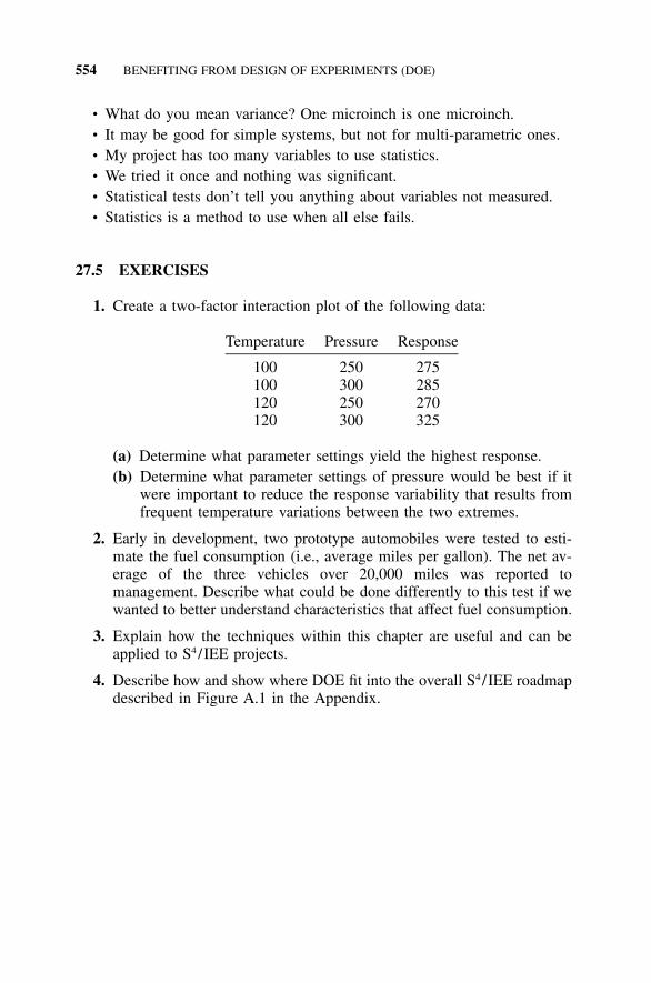
554 BENEFITING FROM DESIGN OF EXPERIMENTS (DOE)

• What do you mean variance? One microinch is one microinch.• It may be good for simple systems, but not for multi-parametric ones.• My project has too many variables to use statistics.• We tried it once and nothing was significant.• Statistical tests don’t tell you anything about variables not measured.• Statistics is a method to use when all else fails.

27.5 EXERCISES

1. Create a two-factor interaction plot of the following data:

Temperature Pressure Response

100 250 275100 300 285120 250 270120 300 325

(a) Determine what parameter settings yield the highest response.(b) Determine what parameter settings of pressure would be best if it

were important to reduce the response variability that results fromfrequent temperature variations between the two extremes.

2. Early in development, two prototype automobiles were tested to esti-mate the fuel consumption (i.e., average miles per gallon). The net av-erage of the three vehicles over 20,000 miles was reported tomanagement. Describe what could be done differently to this test if wewanted to better understand characteristics that affect fuel consumption.

3. Explain how the techniques within this chapter are useful and can beapplied to S4/IEE projects.

4. Describe how and show where DOE fit into the overall S4/IEE roadmapdescribed in Figure A.1 in the Appendix.

555

28UNDERSTANDING THE CREATIONOF FULL AND FRACTIONALFACTORIAL 2k DOEs

S4 /IEE DMAIC Application: Appendix Section A.1, Project ExecutionRoadmap Step 8.1

This chapter provides a conceptual explanation of two-level factorial experi-ments. It uses a nonmanufacturing example to illustrate the application of thetechniques.

It should be noted that the DOE designs describe in this book are not in‘‘standard order.’’ This was done to avoid possible confusion with the uniqueTables M and N. Section D.6 illustrates the standard order and compares astandard order design to that determined from Table M.

28.1 S4/IEE APPLICATION EXAMPLES: DOE

S4/IEE application examples of DOE are:

• Transactional 30,000-foot-level metric: An S4/IEE project was to reduceDSO for an invoice. Wisdom of the organization and passive analysis ledthe creation of a DOE experiment that considered factors: size of order(large versus small), calling back within a week after mailing invoice(yes versus no), prompt paying customer (yes versus no), originationdepartment (from passive analysis: least DSO versus highest DSO av-erage), stamping ‘‘past due’’ on envelope (yes versus no).

556 CREATION OF FULL AND FRACTIONAL FACTORIAL 2k DOEs

• Transactional and manufacturing 30,000-foot-level metric: An S4/IEEproject was to improve customer satisfaction for a product or service.Wisdom of the organization and passive analysis led to the creation of aDOE experiment that considered factors: type of service purchased (Aversus B), size of order (large versus small), department that sold service(from passive analysis: best versus worst), experience of person selling/delivering service (experienced versus new).

• Manufacturing 30,000-foot-level metric: An S4/IEE project was to im-prove the process capability/performance metrics for the diameter of aplastic part from an injection-molding machine. Wisdom of the organi-zation and passive analysis led to the creation of a DOE experiment thatconsidered factors: temperature (high versus low), pressure (high versuslow), hold time (long versus short), raw material (high side of toleranceversus low side of tolerance), machine (from passive analysis: best per-forming versus worst performing), and operator (from passive analysis:best versus worst).

• Manufacturing 30,000-foot-level metric: An S4/IEE project was to im-prove the process capability/performance metrics for the daily defect rateof a printed circuit board assembly diameter of a plastic part from aninjection-molding machine. Wisdom of the organization and passive anal-ysis led to the creation of a DOE experiment that considered factors:board complexity (complicated versus less complicated), manufacturingline (A versus B), processing temperature (high versus low), solder type(new versus current), and operator (A versus B).

• Product DFSS: An S4/IEE project was to improve the process capability/performance metrics for the number of notebook computer design prob-lems uncovered during the product’s life. A DOE test procedure assessingproduct temperature was added to the test process, where factors andtheir levels would be various features of the product. Each trial computerconfiguration would experience, while operational, an increase in tem-perature until failure occurs. The temperature at failure would be theresponse for the DOE (as measured with temperature sensing devicesthat are placed on various components within computer). Wisdom of theorganization and passive analysis led to the creation of a DOE experimentthat considered factors: hard drive size (large versus small), speed ofprocessor (fast versus slow), design (new versus old), test case (highstress on machine processing versus low stress on machine processing),modem (high speed versus low speed).

• Product DFSS: An S4/IEE project was to improve the process capability/performance metrics for the number of daily problem phone calls re-ceived within a call center. Passive analysis indicated that product setupwas the major source of calls for existing products/services. A DOE testprocedure assessing product setup time was added to the test process fornew products. Wisdom of the organization and passive analysis led to

TWO-LEVEL FACTORIAL EXPERIMENTS AND TWO-FACTOR INTERACTIONS 557

TABLE 28.1 Two-Level Full FactorialExperiment Design

Trial No.

Factor Designation

A B CExperimentResponse

1 � � � x1

2 � � � x2

3 � � � x3

4 � � � x4

5 � � � x5

6 � � � x6

7 � � � x7

8 � � � x 8

the creation of a DOE experiment that considered factors: features ofproducts or services, where factors and their levels would be variousfeatures of the product/service, along with various operator experience,include as a factor special setup instruction sheet in box (sheet includedversus no sheet included).

28.2 CONCEPTUAL EXPLANATION: TWO-LEVEL FULLFACTORIAL EXPERIMENTS AND TWO-FACTOR INTERACTIONS

This section discusses two-level full factorial experiment designs. The nextsection illustrates why fractional factorial design matrices ‘‘work.’’

When executing a full factorial experiment, a response is achieved for allcombinations of factor levels. The three-factor experiment design in Table28.1 is a two-level full factorial experiment. For analyzing three factors, eighttrials are needed (i.e., 23 � 8) to address all assigned combinations of thefactor levels. The plus/minus notation illustrates the high/low level of thefactors. When a trial is performed, the factors are set to the noted plus/minuslimits (levels) and a response value is then noted for the trial.

In this experiment design, each factor is executed at its high and low levelan equal number of times. Note that there are an equal number of plus andminus signs in each column. The best estimate factor effects can be assessedby noting the difference in the average outputs of the trials. The calculationof this number for the factor A effect is

x � x � x � x x � x � x � x1 2 3 4 5 6 7 8[(x ) � (x )] � �� �[A ] [A ] 4 4

The result is an estimate of the average response change from the high to

558 CREATION OF FULL AND FRACTIONAL FACTORIAL 2k DOEs

TABLE 28.2 Full Factorial Experiment Design with Interaction Considerations

Trial No.

Factors and Interactions

A B C AB BC AC ABCExperimentResponse

1 � � � � � � � x1

2 � � � � � � � x2

3 � � � � � � � x3

4 � � � � � � � x4

5 � � � � � � � x5

6 � � � � � � � x6

7 � � � � � � � x7

8 � � � � � � � x 8

the low level of A. The other factor effects can be calculated in a similarfashion.

Interaction effects are a measurement of factor levels working together toaffect a response (e.g., a product’s performance degrades whenever temper-ature is high in conjunction with low humidity). In addition to the maineffects, all interaction effects can be assessed given these eight trials withthree factors, as shown in Table 28.2. ‘‘Interaction columns’’ can be generatedin the matrix by multiplying the appropriate columns together and noting theresultant sign using conventional algebraic rules. In this table the third trialsign, in the AB column, for example, is determined by multiplying the A sign(�) by the B sign (�) to achieve an AB sign (�).

Two-factor interaction effects are noted similarly. For the AB interaction,the best estimate of the effect can be determined from

x � x � x � x x � x � x � x1 2 7 8 3 4 5 6[(x ) � (x )] � �� �[AB ] [AB ] 4 4

A question of concern in a factorial experiment is whether the calculatedeffects are large enough to be considered statistically significant. In otherwords, we need to determine whether the result of the two previous calcu-lations is a large number relative to differences caused by experimental error.

If a two-factor interaction is found statistically significant, more informa-tion about the interaction is shown using a plot such as that shown in Figure28.1. From this plot it is noted that there are four combinations of the levelsof the AB factors (AB levels: ��, ��, ��, ��). To make the interactionplot, the average value for each of these combinations is first calculated [e.g.,AB � � � effect is (x1 � x2) /2]. The averages are then plotted. In this plotA�B� yields a high-output response, while A�B� yields a low-output response:the levels of these factors interact to affect the output level.

CONCEPTUAL EXPLANATION: SATURATED TWO-LEVEL DOE 559

FIGURE 28.1 A two-factor interaction plot.

If there is no interaction between factors, the lines on an interaction plotwill be parallel. The overall effect initially determined for the interaction

is a measure of the lack of parallelism of the lines.(x � x )� �[AB ] [AB ]

28.3 CONCEPTUAL EXPLANATION: SATURATED TWO-LEVEL DOE

When many factors are considered, full factorials can yield a very large testsample size, whereas a saturated fractional factorial can require a much re-duced sample size. For example, an eight-trial saturated fractional factorialexperiment can assess seven two-level factors, while it would take 128 trialsas a full factorial.

The basic saturated fractional factorial experiment design is illustrated inTable 28.3. In this table, the calculated interaction columns give the levels offour additional factors, making the total number of two-level factor consid-erations seven in eight trials.

The disadvantage of this saturated fractional factorial experiment is theconfounding of two-factor interaction effects and main effects. There is con-founding of the AB interaction and the main effect D; however, there is alsoconfounding of factor D and other two-factor interactions because of theintroduction of the additional factors D, E, F, and G.

Because each column can now have more than one meaning, it is assigneda number, the contrast column number (see Tables M1 to M5 and N1 to N3).

It may be hard for the reader to believe that all main effect information ofseven two-level factors can be obtained in only eight trials. There may be aconcern that the significance of one factor could affect the decision aboutanother factor. To address this concern, assume that E is the only statisticallysignificant factor and that there are no interactions. The question of concern,

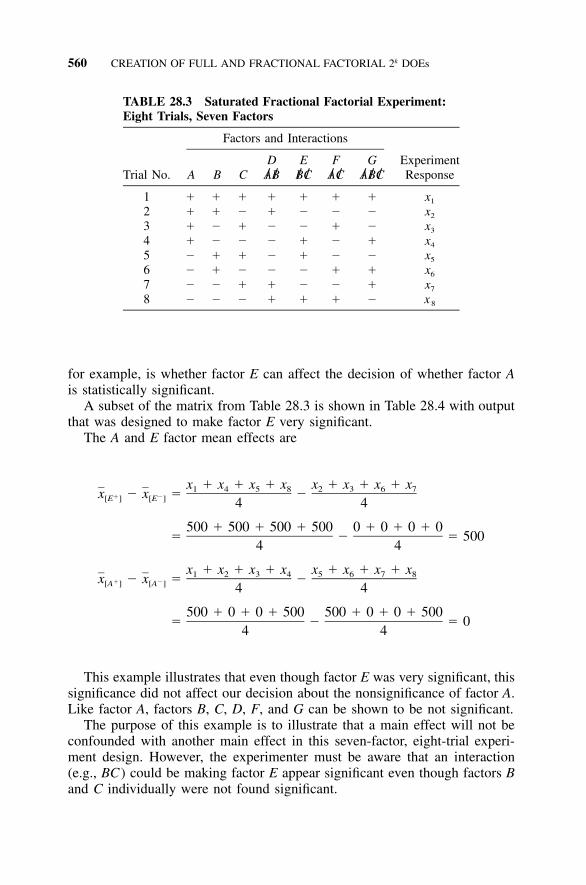
560 CREATION OF FULL AND FRACTIONAL FACTORIAL 2k DOEs

TABLE 28.3 Saturated Fractional Factorial Experiment:Eight Trials, Seven Factors

Trial No.

Factors and Interactions

A B CD/A /B

E/B /C

F/A /C

G/A /B /C

ExperimentResponse

1 � � � � � � � x1

2 � � � � � � � x2

3 � � � � � � � x3

4 � � � � � � � x4

5 � � � � � � � x5

6 � � � � � � � x6

7 � � � � � � � x7

8 � � � � � � � x 8

for example, is whether factor E can affect the decision of whether factor Ais statistically significant.

A subset of the matrix from Table 28.3 is shown in Table 28.4 with outputthat was designed to make factor E very significant.

The A and E factor mean effects are

x � x � x � x x � x � x � x1 4 5 8 2 3 6 7x � x � �� �[E ] [E ] 4 4

500 � 500 � 500 � 500 0 � 0 � 0 � 0� � � 500

4 4

x � x � x � x x � x � x � x1 2 3 4 5 6 7 8x � x � �� �[A ] [A ] 4 4

500 � 0 � 0 � 500 500 � 0 � 0 � 500� � � 0

4 4

This example illustrates that even though factor E was very significant, thissignificance did not affect our decision about the nonsignificance of factor A.Like factor A, factors B, C, D, F, and G can be shown to be not significant.

The purpose of this example is to illustrate that a main effect will not beconfounded with another main effect in this seven-factor, eight-trial experi-ment design. However, the experimenter must be aware that an interaction(e.g., BC) could be making factor E appear significant even though factors Band C individually were not found significant.

EXAMPLE 28.1: NONMANUFACTURING PROCESS 561

TABLE 28.4 Example Output from Table 28.3 Design

Trial No. A EExperimentResponse

1 � � 5002 � � 03 � � 04 � � 5005 � � 5006 � � 07 � � 08 � � 500

28.4 EXAMPLE 28.1: APPLYING DOE TECHNIQUES TO ANONMANUFACTURING PROCESS

This example gives an overview of the thought process involved in setting upa DOE experiment and illustrates the application of these techniques. Con-sider that a high-school administration wants to reduce absenteeism of stu-dents in high school.

Many factors can affect school absenteeism. These factors, perhaps iden-tified in a brainstorming session, include the following:

• Student: age, sex, ethnic background, etc.• School: location, teacher, class, etc.• Time: day of week, class period, etc.

Consider how you might approach the problem if you were a consultantcommissioned to assist with this effort. A typical approach would be to re-gress factors on the response to determine which factors significantly affectthe output. A regression approach might indicate that there was a differencein the amount of absenteeism depending upon the sex of the student. Considerwhat should now be done with the system to reduce absenteeism. Difficult,isn’t it? The information from this experiment might be interesting to reportin the news media, but suggesting what should be done differently to reduceabsenteeism given this information would be pure conjecture.

There are several problems with a pure regression approach. First, regres-sion only observes the factors and levels of factors that occur naturally in thesystem; for example, it would not detect that an increase in pressure beyondnormal operating conditions could dramatically improve product quality. Sec-ond, it does not assess new factors (e.g., a call-back program). Third, theconclusion could be happenstance; for example, the phase of the moon might

562 CREATION OF FULL AND FRACTIONAL FACTORIAL 2k DOEs

look significant within a regression model because some other factor had amonthly cycle.

After an initial regression assessment, consider using a DOE approach withthe following factor designations A–G:

A: Day of the weekB: Call-back when absentC: SchoolD: Class periodE: Mentor if missed a lotF: Contract if already missed a lot of classesG: Sex of the student

Consider what two fundamental differences exist between these factors.Some factors are observations while other factors are improvement possibil-ities. Day of the week, school, class period, and sex of student are observa-tions, while call-back when absent, assignment of a mentor if class is missedoften, and contract if a great many classes have already been missed areimprovement possibilities. Normally a student would fail if he/she missedmore than a certain number of days. This ‘‘contract’’ improvement possibilitywould offer the student a second chance if he/she agreed to attend all classesthe remaining portion of the semester.

Choose now how to address the levels for each factor. The tendency is toassign many levels to each factor, but this could add much complexity to theexperiment. We should always ask whether the additional level is helpful foraddressing the problem at hand, determining what should be done to reducestudent absenteeism. Consider the number of trials that would be needed ifthe following levels were assigned to each factor:

A: Day of the week: Monday versus FridayB: Call-back when absent: Yes versus noC: School: Locations 1, 2, 3, 4D: Class period: 1, 2, 3E: Mentor if missed a lot: Yes versus noF: Contract if already missed a lot of classes: Yes versus noG: Sex of student: Male versus female

The total number of combinations for a full factorial is (2 � 2 � 4 �3 � 2 � 2 � 2 � 384). This number of trials is impossible for many situa-tions. To reduce the number of trials for the full factorial, consider alteringthe number of levels to two. To do this, consider the question at hand. Perhapsit can be satisfactorily addressed, for example, by choosing only two schools:

EXAMPLE 28.1: NONMANUFACTURING PROCESS 563

the one with the best attendance record and the other with the worst atten-dance record. A two-level assessment would reduce the number of trials to27 �128 trials for a full factorial design. This could be further reduced to 64,32, 16, or 8 trials using a fractional factorial structure. For fractional DOEs,the alternatives of 64, 32, 16, or 8 trials gives varying resolution of factorinformation. Resolution is related to the management of two-factor interac-tions. Two-factor interactions may or may not be confounded (aliased) witheach other or main effects. To illustrate a two-factor interaction, consider thatthere was a difference between absenteeism caused by day of the week (Fri-day versus Monday) and call-back program (yes versus no), so that the call-back program was much more effective in reducing absenteeism on Friday,perhaps because students would be corrected by parent after weekend calls.

When reducing the number of factors to two levels, quantitative factorssuch as pressure would be modeled as a linear relationship. For qualitativefactors such as suppliers, schools, operators, or machines, consider choosingthe sources that represent the extremes.

For purposes of illustration, consider initially only three of the two-levelfactors:

• Day of week: Monday versus Friday• Call-back when absent: Yes versus no• School: 1 versus 2

Eight trials can assess all possible combinations of the levels of threefactors (i.e., 23 � 8).

The factors and levels could have the following designation:

Factor

Level

� �

A: Day of week Friday MondayB: Call-back when absent Yes NoC: School 1 2

One experiment design and response approach might be to select 800 stu-dents randomly from two schools. Students would then be randomly placedinto one of the eight trial categories, 100 students in each trial. The totalnumber of days absent from each category for the 100 students would be theresponse for the analysis.

This approach offers some advantages over a more traditional regressionanalysis. New factors are assessed that could improve the process, such as acall-back program. Effects from happenstance occurrences are lessened. Theeight-trial combinations are as follows:

564 CREATION OF FULL AND FRACTIONAL FACTORIAL 2k DOEs

Trial No.

Factor Designation

A B C Response

1 � � � x1

2 � � � x2

3 � � � x3

4 � � � x4

5 � � � x5

6 � � � x6

7 � � � x7

8 � � � x8

Consider trial 2 the response would be the total absenteeism of 100 stu-dents on Monday with no call-back for school 1. We also note from the initialdesign matrix that there are four levels for each factors for the experiment;that is, four trials had C at a ‘‘�’’ level and four trials had A at a ‘‘�’’ level.The effect for a factor would be the average for that factor at the ‘‘�’’ levelminus the average for that factor at the ‘‘�’’ level.

Consider that this experiment yielded the following results (these data werecreated such that there was an interaction between factors A and B).

Trial No.

Factor Designation

A B C Response

1 � � � 1982 � � � 2033 � � � 1694 � � � 1725 � � � 1836 � � � 1817 � � � 948 � � � 99

The estimated main effects are

A: Day of week �46.25B: Call-back when absent �57.75C: School �2.75

By observation the magnitude of the school effect seems small. The signof the other two factors indicates which level of the factor is best. In thiscase, lower numbers are best; hence, Friday and call-back are best. However,this model does not address the interaction.

EXAMPLE 28.1: NONMANUFACTURING PROCESS 565

As mentioned earlier, a two-factor interaction causes a lack of parallelismbetween the two lines in a two-factor interaction plot. When sample data areplotted, the lines typically will not be exactly parallel. The question for apractitioner is whether the degree of out-of-parallelism between two linesfrom an interaction plot is large enough to be considered as originating fromtrue interaction opposed to chance. This issue is addressed through the cal-culation of an interaction effect.

An interaction contrast column is created by multiplying the level desig-nations of all main effect contrast columns to create new contrast columns ofpluses and minuses:

Trial No.

Factor Designation

A B C AB BC AC ABC Response

1 � � � � � � � x1

2 � � � � � � � x2

3 � � � � � � � x3

4 � � � � � � � x4

5 � � � � � � � x5

6 � � � � � � � x6

7 � � � � � � � x7

8 � � � � � � � x8

Again, there are four pluses and four minuses in each contrast column.The magnitude of the effect from an interaction contrast column (e.g., AB)relative to other contract column effects can be used to assess the likelihoodof an interaction. Hence, all possible two-factor interaction plots do not needto be plotted. Only those two-factor interactions that are thought to be suffi-ciently large need to be plotted.

Entering our trial responses in this format yields the following:

Trial No.

Factor Designation

A B C AB BC AC ABC Response

1 � � � � � � � 1982 � � � � � � � 2033 � � � � � � � 1694 � � � � � � � 1725 � � � � � � � 1836 � � � � � � � 1817 � � � � � � � 948 � � � � � � � 99

The interaction effects are determined in a similar fashion to main effects.

566 CREATION OF FULL AND FRACTIONAL FACTORIAL 2k DOEs

For example, the AB interaction is determined as follows: (198 � 203 � 94� 99)/4 �(169 � 172 � 183 � 181)/4 � 27.75. The following summarizesthese results for all main effects and interactions:

A: Day of week 46.25 (Friday is best)B: Call-back when absent 57.75 (call back is best)C: School �2.75 (not significant)AB: Day*call-back 27.75 (significant)BC: Call-back*school 1.25 (not significant)AC: Call-back*school �1.25 (not significant)ABC: Day*call-back*school �2.25 (not significant)

This summary indicates that the A, B, and AB effects are large relative tothe other effects, which are presumed to be the result of experimental error.That is, the magnitude of the day*call-back interaction looks significant. Wecannot talk about ‘‘day of the week’’ and ‘‘call-back’’ without talking aboutthe two-factor interaction. A two-factor interaction plot shows which factorlevels are most beneficial. A reduction of this table to create an AB interactionplot is

Trial No. A B AB Response

1 � � � 1982 � � � 2033 � � � 1694 � � � 1725 � � � 1836 � � � 1817 � � � 948 � � � 99

A plot of the average of the four response combinations for AB (i.e.,AB � ��, AB � ��, AB � ��, and AB � ��) shown in Figure 28.2shows out-of-parallelism of the two lines. The plot indicates that the call-back program helps more on Friday than on Monday. A call-back when astudent is absent on Friday results in a reduction in absenteeism. The call-back program for absenteeism on Monday does not appear to reduce absen-teeism.

To illustrate how the magnitude of an effect helps assesses the out-of-parallelism of a two-factor interaction plot, let’s examine the appearance of

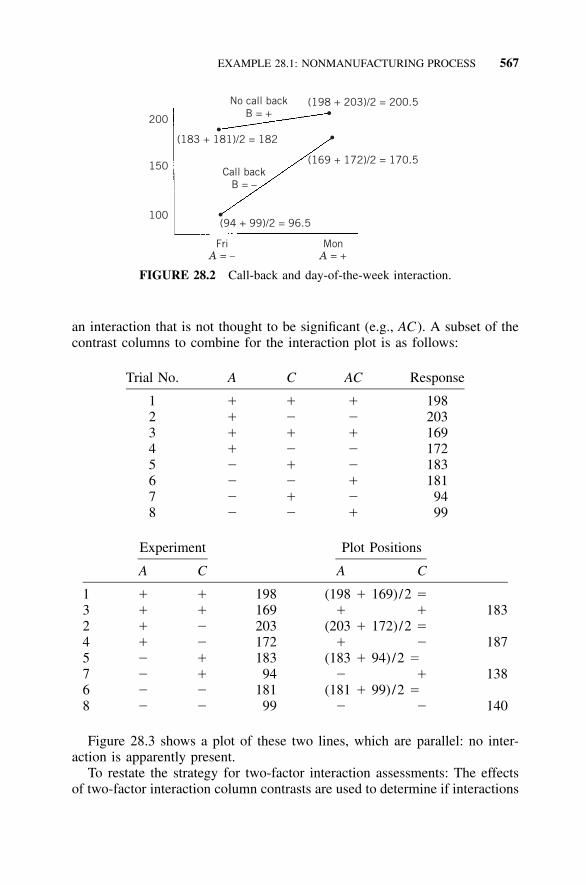
EXAMPLE 28.1: NONMANUFACTURING PROCESS 567

No call backB = +

Call backB = –

200

100

150

FriA = –

MonA = +

(183 + 181)/2 = 182

(94 + 99)/2 = 96.5

(169 + 172)/2 = 170.5

(198 + 203)/2 = 200.5

•

•

•

•

FIGURE 28.2 Call-back and day-of-the-week interaction.

an interaction that is not thought to be significant (e.g., AC). A subset of thecontrast columns to combine for the interaction plot is as follows:

Trial No. A C AC Response

1 � � � 1982 � � � 2033 � � � 1694 � � � 1725 � � � 1836 � � � 1817 � � � 948 � � � 99

Experiment Plot Positions

A C A C

1 � � 198 (198 � 169)/2 �3 � � 169 � � 1832 � � 203 (203 � 172)/2 �4 � � 172 � � 1875 � � 183 (183 � 94)/2 �7 � � 94 � � 1386 � � 181 (181 � 99)/2 �8 � � 99 � � 140

Figure 28.3 shows a plot of these two lines, which are parallel: no inter-action is apparently present.

To restate the strategy for two-factor interaction assessments: The effectsof two-factor interaction column contrasts are used to determine if interactions

568 CREATION OF FULL AND FRACTIONAL FACTORIAL 2k DOEs

200

100

150140

138

FriA = –

MonA = +

School 2C = +

School 1C = –

187

183

••

••

FIGURE 28.3 Interaction plot where factor interaction is not significant.

are statistically significant. Two-factor interaction plots are used to get a pic-ture of what factor levels are best.

Reflecting again on the differences between this strategy and a regressionapproach, we were able to identify what should be done different and quantifythe effects. We can also think about how to modify the current call-backmethod to improve the effect on Mondays.

The number of trials can increase dramatically if we follow a similar pro-cedure for an increased number of factors. For example, if we similarly assessseven (not three) two-level factors, the resulting number of trials is 128 (27

� 128). Consider now the addition of four factors to our original design withthe noted levels:

A: Day of the week: Friday versus MondayB: Call-back when absent: Yes versus noC: School: Locations 1 versus 2D: Class period: 1 versus 2E: Mentor if missed a lot: Yes versus NoF: Contract if already missed a lot of classes: Yes versus noG: Sex: Male versus female

A 128-trial seven-factor experiment contains very high factor interactions.It contains other interactions: three-factor, four-factor, five-factor, six-factor,and seven-factor. Typically, we assume that any interactions above two aresmall, if they exist at all; hence, we don’t need this many trials. A fractionalDOE is an alternative to a full factorial DOE.

Consider again the eight-trial two-level full factorial design with all inter-actions. An assignment of the four additional factors to the interaction contrastcolumns yields the following:

EXAMPLE 28.1: NONMANUFACTURING PROCESS 569

Factor Designation

A B C D E F G Output

1 � � � � � � � x1

2 � � � � � � � x2

3 � � � � � � � x3

4 � � � � � � � x4

5 � � � � � � � x5

6 � � � � � � � x6

7 � � � � � � � x7

8 � � � � � � � x8

This seven-factor, eight-trial two-level factorial saturated design minimizessample size, assesses main factor information, and confounds two-factor in-teractions with main effects. A summary of the main and two-factor inter-action effects are as follows:

A: Day of week (1 versus 2) 46.25 (Friday is best)B: Call-back (yes versus no) 57.75 (Call-back is best)C: School (1 versus 2) �2.75 (not significant)D: Class period (1 versus 2) 27.75 (significant)E: Mentor (yes versus no) 1.25 (not significant)F: Contract (yes versus no) �1.25 (not significant)G: Sex (male versus female) �2.25 (not significant)

From the analysis of main effects the expectation now for factor D is thatclass period 2 has more absenteeism than class period 1 (about 27.75 days ina semester for 100 students). Strategies discussed later will address concernsthat two-factor interaction confounding with main effects will distort conclu-sions (see Section 31.9).

The example above illustrates a nonmanufacturing example of DOE tech-niques. For eight trials the extremes discussed are as follows:

• Three two-level factors (full factorial)• Seven two-level factors (saturated factorial)

For eight trials, the confounding of two-factor interactions are as follows:

• Three two-level factors (full factorial)—all interactions are determined.• Seven two-level factors (saturated factorial)—two-factor interactions are

confounded with main effects.

570 CREATION OF FULL AND FRACTIONAL FACTORIAL 2k DOEs

For eight trials, the resolution designation is as follows:

• Three two-level factors (full factorial): V�

• Seven two-level factors (saturated factorial): III

However, there are other choices for the number of factors in eight trialsinstead of three or seven factors. There could be four, five, or six two-levelfactors examined in eight trials. This additional number of factors can leadto other resolution levels besides III and V�. Resolution IV designs confoundtwo-factor interactions with each other but not with main effects. ResolutionV designs do not confound two-factor interactions with other two-factor in-teractions or with main effects. Table M shows various resolution alternatives,number of factors for 8, 16, 32, and 64 trials, and design matrices.

28.5 EXERCISES

1. Catapult Exercise: Teams are to create a two-level catapult DOE. Thecause-and-effect diagram created in Exercise 2 in Chapter 5 should beused to help determine the factors and level of factors that will be assessedduring the experiment. Select at least six factors indicating ball type andarm length.

2. Create a 16-trial full factorial where the factors have two levels. Determinethe contrast columns for all interactions and list them with the factorialdesign. Comment on the frequency of the �’s and �’s in each column.

3. Explain the setup of a DOE for a nonmanufacturing situation.

4. Explain how the techniques presented in this chapter are useful and canbe applied to S4/IEE projects.

571

29PLANNING 2k DOEs

S4 /IEE DMAIC Application: Appendix Section A.1, Project ExecutionRoadmap Steps 8.2 and 8.3

Executing a DOE is not difficult, but time and resources can be wasted if theexperiment is not set up wisely. This chapter discusses thoughts to considerwhen setting up a DOE.

29.1 INITIAL THOUGHTS WHEN SETTING UP A DOE

One major obstacle in implementing an efficient fractional factorial designtest strategy is that the initial problem definition may not imply that fractionalfactorial design concepts are appropriate, when in fact they are the best al-ternative.

It is often most effective to combine fractional factorial statistical methodswith the skills of experts in a field of concern. Because of their structure,DOE techniques are conducive to evaluating in one experiment a collectionof agreed-upon conditions determined by team brainstorming sessions. Thisteam management strategy tool can be dramatically more efficient than one-at-a-time experiments conducted by many individuals independently.

When designing an experiment, it is most important to first agree upon aclear set of objectives and criteria. An S4/IEE practitioner needs to considerhistorical information and ask detailed questions before deciding the detailsof an experiment. Brainstorming and cause-and-effect diagram techniques canhelp with collecting this information.

572 PLANNING 2k DOEs

The S4/IEE practitioner should strive to identify all relevant sources ofinformation about factors, their levels, and ranges. Factors that are believedto be important need to be included in an experiment design in order toproduce meaningful results. Factor effects that are not of primary interest inan experiment should be held constant or blocked (as described later). Inaddition, the sequence of experiment trials should be randomized in order toreduce the risk of an unknown/unexpected occurrence jeopardizing accurateconclusions. Care should be exercised to ensure that there is minimal errorin the measurements for each trial.

After an experiment is determined, its structure is conducive to an individ-ual or team presentation to management and other organizations. The pro-posed factors, levels of factors, and outputs in the experiment can be presentedin a fashion that makes the test strategy easily understood. Perhaps this pre-sentation will provoke a constructive critique that results in a better imple-mentation strategy.

29.2 EXPERIMENT DESIGN CONSIDERATIONS

Examples in this book propose using unreplicated two-level fractional facto-rial design matrices in Tables Ml to M5. Other experiment design matricesare also available in tabular form in other books, journals, or computer pro-grams. The basic experiment design strategy suggested in this book is alsoapplicable to many of these design matrix alternatives.

To most people it seems appropriate to have factors with many levels,which can make an experiment become very cumbersome and unreasonableto conduct. Reducing the number of factor levels and listing associated as-sumptions can change an experiment’s feasibility dramatically.

The next task is to determine what resolution is desired. I often suggest asingle replication of a 2k design, which is sometimes called an unreplicatedfactorial. There is no internal estimate of error (i.e., pure error). One approachfor the analysis of unreplicated factorials is to assume that high-order inter-actions are negligible and to combine mean squares to estimate error. A jus-tification for this is the sparsity of effects principle, which states the following:Main effects dominate most systems and low-order interactions, and mosthigh-order interactions are negligible.

In addition, many experiment design considerations fall into two generalclassifications. The first type needs to optimize a process (or help give direc-tion toward a basic problem’s resolution), while the second type needs toconsider how a product will perform under various situations relative to meet-ing a specification.

Factor interaction considerations may be more important for the first typeof classification than for the second type. In the second type a continuousresponse may have many factors that are statistically significant, but if the

EXPERIMENT DESIGN CONSIDERATIONS 573

product is well within criterion, additional analysis may not be necessary. Ifthe statistically significant factor information will not lead to a cost reductionor a reduction in manufacturing variability, the experimenter should avoidanalysis paralysis and move on to the next problem/investigation.

In a fractional factorial experiment as opposed to an experiment that has‘‘too small a sample size,’’ there may be a higher probability of problemsfrom unconscious experimental bias or data collection techniques that intro-duce large amounts of error. Good techniques can reduce these problems.First, the sequence in which the experimental trials are performed should berandom. Second, external experimentation factors should be blocked to avoidconfusion between them and experimental factor effects.

Note that for some factors, randomization may be very difficult to imple-ment. Whenever the experiment is not randomized, care must be taken toconsider that a bias could be the real reason that a factor is statistically sig-nificant.

At the end of a fractional factorial experiment, a confirmation experimentshould be performed to quantify and confirm the magnitude of statisticallysignificant effects more accurately. A comparison test may, for example, beappropriate to compare the old design with new design considerations thatwere found statistically significant within the experiment.

The following is a checklist of items to consider when designing a two-level DOE. Note that both a team brainstorming session and historical infor-mation should be considered when addressing these issues.

• List the objectives of the experiment. Consider whether the intent of theDOE is the understanding of factor mean effects or variability reduction.

• List the assumptions.• List factors that might be considered in the experiment.• Choose factors and their levels to consider in the experiment.• List what other factors will not be evaluated in the experiment and will

be held constant.• Reduce many-level factors to two-level factors.• Choose the number of trials and resolution of the experiment.• Determine if any of the factors will need to be blocked.• If possible, change attribute response considerations to continuous re-

sponse considerations.• Determine if any design center points will be used to check for curvature.• Choose a fractional factorial design.• Determine if trials will be replicated or repeated (see Chapter 32).• Choose a sample size for the number of repetitions per trial and the

number of replications needed. Adjust number of trials and experimentresolution as needed.

574 PLANNING 2k DOEs

• Determine a random order trial sequence to use.• Determine what can be done to minimize experimental error.• Plan a follow-up experiment strategy (e.g., a higher-resolution follow-up

experiment or confirmation experiment).• Plan the approach to be used for the analysis.

The difference between the approximation model and the truth is some-times referred to a lack-of-fit or model bias. Two approaches historically usedto protect from lack of fit are to include special runs for detection (e.g.,addition of center points, described in Section 29.8) and to decrease the rangeof settings, where this second approach does not quantify the amount of lackof fit.

Design efficiency is the amount of information per trial in relationship toa model. Efficiency and the lack-of-fit protection compete. When a designmaximizes efficiency, there is no room for the detection of lack of fit (i.e.,we are implying that the model is adequate).

I prefer DOE matrices that have two levels, where two-factor interactionswill be managed. This leads to designs that have 2n trials, where n is aninteger (e.g., 4, 8, 16, 32, and 64). A resolution III design for these trialalternatives is considered a screening design. There are other DOE experimentoptions, such as Plackett-Burman designs. These designs offer additional trialalternatives such as 12, 20, 24, 28, 36, 40, 44, and 48 trials; i.e., 4(i) trialswhere i is an integer and the number of trials is not 2n. Plackett-Burmandesigns loose information about where the 2-factor interactions are con-founded. DOE Taguchi methodologies suggested offer other design alterna-tives that contain more than two levels; e.g., L9 and L27, which have 9 and27 trials for three levels of the factors. These design alternatives which canhave several levels also do not address two-factor interactions.

29.3 SAMPLE SIZE CONSIDERATIONS FOR A CONTINUOUSRESPONSE OUTPUT DOE

Section D.1 in the Appendix discusses a mathematical method for determininga sample size to use when conducting a fractional factorial experiment. Overthe years I have found the following procedure and rationale satisfactory formany industrial experiments that have a continuous response output, wherethe DOE is to assess the significance of mean effects of a response. Note thatthis discussion does not address sample size issues when the focus of theexperiment is to understand and reduce the variability of a response (seeChapter 32).

Many industry experiments can be structured such that they have either 16or 32 trials, normally with no trial replication and only two-level factor con-siderations. Obviously, if trials are cheap and time is not an issue, more trialsare better.

CHOOSING FACTORS AND LEVELS 575

The following discussion illustrates the logic behind this conclusion. Withtwo-level experiment designs advantages are achieved relative to two-factorinteraction assessments when the number of trials are 2n (i.e., those containingthe number of trials in Tables Ml to M5), where n is a whole number. Thiswill then yield 2, 4, 8, 16, 32, 64, 128, . . . trial experiment design alternatives.Experiments with 2, 4, and 8 trials are in general too small to give adequateconfidence in the test results. Experiments with 64 and higher numbers oftrials are usually too expensive. Also, when larger experiments require muchmanual data collection, the person responsible for this work may becomefatigued, causing sloppy data collection. Sloppy data collection can cause highexperimental error, which can mask factors that have a relatively small butimportant effect on the response. In addition, any individual trial mistake thatgoes undetected can jeopardize the accuracy of all conclusions. Sixteen- and32-trial fractional factorial designs are a more manageable size but can usuallyaddress the number of factors of interest with sufficient accuracy. Consideralso that a series of shorter tests that give quick feedback can sometimes bemore desirable than one long test.

It is perhaps more important than getting a large sample size to do every-thing possible to achieve the lowest possible measurement error. Often ex-perimental error can be reduced by simple operator awareness. For an indi-vidual experiment, there is typically a trade-off among the number of factors,number of trials, experiment resolution, and number of possible follow-upexperiments.

A 16-trial experiment may appear to be ‘‘too much testing’’ to someonewho has not been introduced to design experiment concepts. An eight-trialexperiment, still much better than a one-at-a-time strategy, can be a moreviable alternative.

29.4 EXPERIMENT DESIGN CONSIDERATIONS: CHOOSINGFACTORS AND LEVELS

The specific situations to which a DOE is being applied will affect how factorsand levels are chosen. In a manufacturing environment, data analysis maysubject the best factors and levels to use in an experiment to relate key processinput variables to key process output variables. In development, there may befew data to give direction, so that a DOE may be begun without much pre-vious data analysis. However, in both cases a major benefit of the DOE struc-ture is that it gives teams direct input into the selection of factors and thelevels of factors.

Factor levels also can take different forms. Levels can be quantitative orqualitative. A quantitative level is when the factor can take on one of manydifferent values (e.g., the temperature input in a manufacturing process step),while qualitative levels take on discrete values (e.g., material x versus materialy). The results obtained from the two-level manual fractional factorial analysistechniques discussed in this book are the same. However, the effect from two

576 PLANNING 2k DOEs

levels of a quantitative factor can be used to interpolate an output responsefor other magnitudes of the factor, assuming that a linear relationship existsbetween the two-level factors.

There is often a strong desire to conduct an initial DOE with factors thathave more than two levels. Initial experiments that have more than two levelscan add a much unnecessary time, expense, and complexity to the testingprocess. Before beginning a multilevel experiment, the question should beasked: Why increase the levels of a factor beyond two? When we analyzethe response to this question, the initial reasons for having more than twolevels often disappear.

In some situations this transition down from many-level to two-level con-siderations can require much thought. For example, instead of consideringhow a process operates at three temperatures, an experiment could first onlybe conducted at the tolerance extremes of temperature. If there were concernthat the end condition levels of the factor have similar effects and the midpointshowed a statistically significant difference, one tolerance extreme versus anominal condition could be used in an initial experiment. If this factor is stillconsidered important after the first experiment, the second tolerance extremecan be addressed in another experiment in conjunction with the nominal con-dition or another factor level setting. When the number of factors is not large,a response surface design may be an appropriate alternative.

If a factor has many levels (e.g., four supplier sources), perhaps previousknowledge can be used to choose the two extreme scenarios in the initialexperiment considerations (realizing that there is a trade-off between the riskof making a wrong decision relative to the selection of suppliers and theimplications of a larger sample size). If there appears to be a difference be-tween these two levels, additional investigation of the other levels may thenbe appropriate.

When only two levels are considered, the possibility of nonlinearity mayraise concern. It is generally best to consider a multiple-experiment DOEapproach initially and then to use mathematical modeling during the analysis.Curvature can be checked by the addition of center points. If curvature existsin the region of concern, this can be quantified later through another experi-ment that is set up using response surface methods. The curvature relationshipcan then be described in a mathematical model. It is sometimes better toreduce the differences between levels in one experiment so that the responsebetween levels can be approximately modeled as a linear relationship.

There may be concern that there is a difference between three machineswhere machine is one factor in the test. One of the main purposes for con-ducting a DOE is to identify improvement opportunities through structuredchoices. Other techniques treated in this book are useful for determining anddescribing differences between such factors as machines, suppliers, and op-erators. To create a DOE, consider initially identifying the best and worstmachine and using these as levels for the machine factor. This approach couldlead to an interaction, which could end up determining why the best machineis getting more desirable results.

FACTOR STATISTICAL SIGNIFICANCE 577

Another situation, which might arise: one factor can either perform at hightolerance, perform at low tolerance, or be turned off. If we take this factor asinitially described into consideration, we are forced to consider its levels asqualitative because one of the levels is ‘‘off.’’ In addition to the added com-plexity of a three-level experiment, this initial experiment design does notpermit us to model the expected response directly at different ‘‘on’’ settingswithin the tolerance extremes.

To address this situation better, consider two experiment designs in whicheach experiment considers each factor at two levels. The first experiment leadsto a 16-trial experiment where the two levels of the factor are the toleranceextremes when the factor is ‘‘on.’’ The ‘‘off’’ factor condition is then consid-ered by the addition of eight trials to the initial design. The other factorsettings for a given trial in the ‘‘off’’ level setting are similar to those usedat either the high or low factor setting for the ‘‘on’’ experiment design. Thisresults in 24 total trials, which should be executed in random order.

After the responses from the 24 trials are collected, the data can be ana-lyzed using several approaches. Three simple techniques are as follows. Thefirst 16 trials, where the described factor level is quantitative, can be analyzedseparately. If this factor is found to have statistical significance, the modelequation can be used to predict the response at other settings besides toleranceextremes. Second, the 8 trials for the ‘‘off’’ level can be analyzed in con-junction with the appropriate 8 trials from the 16 trials that gives a DOEmatrix. This analysis will test the significance of the ‘‘on’’ versus ‘‘off’’ levelsof this factor. Third, the data can be analyzed collectively using multipleregression analysis techniques.

29.5 EXPERIMENT DESIGN CONSIDERATIONS: FACTORSTATISTICAL SIGNIFICANCE

For fractional factorial designed experiments, continuous outputs, as opposedto attribute outputs, are normally desired. A typical fractional factorial con-clusion is ‘‘voltage is significant at a level of 0.05.’’ If voltage was a two-level factor in the experiment, this statement means that a response is affectedby changing the voltage from one level to another, and there is only an � riskof 0.05 that this statement is not true. Statements can also be made about theamount of change in output that is expected between levels of factors. Forexample, a best estimate for a statistically significant factor might be thefollowing: A shift from the high tolerance level of the voltage factor to itslow tolerance level will cause an average output timing change of 4 millisec-onds (msec).

The next chapter discusses methods for testing for factor significance givenan estimate for error. If a factor is statistically significant (i.e., we reject thenull hypothesis that the factor levels equally affect our response), the state-ment is made with an � risk of being wrong. However, the inverse is not trueabout factors not found to be statistically significant. In other words there is

578 PLANNING 2k DOEs

not an � risk of being wrong when these factors are not found to be statis-tically significant. The reason for this is that the second statement has a �risk (i.e., not rejecting the null hypothesis, which is a function of the samplesize and �). Section D.1 in the Appendix discusses an approach where thesample size of a factorial experiment is made large enough to address the �risk of not rejecting the null hypothesis when it is actually false.

29.6 EXPERIMENT DESIGN CONSIDERATIONS:EXPERIMENT RESOLUTION

Full factorial designs are used to assess all possible combinations of the factorlevels under consideration. These designs provide information about all pos-sible interactions of the factor levels. For example, a full factorial experimentconsisting of seven two-level factors will require 128 trials (27 � 128). It willprovide information about all possible interactions, including whether allseven factors work in conjunction to affect the output (defined as a seven-factor interaction), as well as information about lower factor interactions—that is, any combination of 6, 5, 4, 3, and 2 factors.

In many situations, three-factor and higher interaction effects can be con-sidered small relative to the main effects and two-factor interaction effects.Therefore, interactions higher than two can often be ignored. In such cases,a smaller number of trials are needed to assess the same number of factors.A fractional factorial design can assess the factors with various resolutions(see instructions in Table Ml). A resolution V design evaluates the main ef-fects and two-factor interactions independently. A resolution IV design eval-uates main effects and confounded or mixed up two-factor interactions (i.e.,there is aliasing of the two-factor interactions). A resolution III design eval-uates the main effects, which are confounded with the two-factor interactions.Tables Ml to M5 will later be used to give test alternatives for each of theseresolutions. Plackett and Burman (1946) give other resolution III design al-ternatives, but the way in which two factor interactions are confounded withmain effects is often complicated.

29.7 BLOCKING AND RANDOMIZATION

Many experiments can inadvertently give biased results. For example, errorcan occur in the analysis of experimental data if no consideration is givenduring the execution of an experiment to the use of more than one piece ofequipment, operator, and/or test days. Blocking is a means of handling nui-sance factors so that they do not distort the analysis of the factors that are ofinterest.

Consider, for example, that the experiment design in Table 28.3 is con-ducted sequentially in the numeric sequence shown over a two-day period

CURVATURE CHECK 579

(trials 1–4 on day 1 and trials 5–8 on day 2). Consider that, unknown to thetest designer, humidity conditions affected the process results dramatically.As luck would have it, the weather conditions changed and it started rainingvery heavily on the second day. Results from the experiment would lead theexperimenter to believe that factor A was very statistically significant becausethis factor was � on the first day and � on the second day, when in fact thehumidity conditions caused by the rain were the real source of significance.

There are two approaches to avoiding this unplanned confounding: In thefirst approach the experimental trials are randomized. This should always bethe goal. If this were done for the above scenario, the differences betweendays would not affect our decision about factor significance, and the varia-bility between day differences would show up as experimental error. Anotherapproach is to block the experimental trials. This is a better approach forfactors that we do not want to consider within our model but that could affectour results (e.g., operators, days, machines, ovens, etc.).

An application example for blocking in Table 28.3 is that ‘‘day’’ couldhave been blocked using the ABC interaction column. The trial numbers 1,4, 6, and 7 could then be performed in random sequence the first day, whilethe other four trials could be exercised in random sequence on the secondday. If the block on ‘‘day’’ was shown to be statistically significant, then theconclusion would be that something changed from day 1 to day 2; however,the specific cause of the difference may not be understood to the experimenterfrom a basic data analysis. More importantly, this confounding would notaffect decisions made about the other factors of interest.

High-factor interaction contrast columns can be used for the assignmentof blocks when there are only two-level blocks to consider, as noted earlier.However, care must be exercised when there are more than two levels in ablock. Consider that four ovens are to be used in an experiment. Undesirableconfounding can result if two high-factor interaction contrast columns arearbitrarily chosen to describe the trials that will use each of the ovens(i.e.,� � � oven 1, � � � oven 2, � � � oven 3, and � � � oven 4).Commercially available computer statistical packages often offer variousblocking alternatives.

29.8 CURVATURE CHECK

In a two-level experiment design, linearity is assumed between the factor levelextremes. When factors are from a continuous scale, or a quantitative factor(e.g., factor A is an adjustment value that can take on any value from 1 to10, as opposed to discrete levels, or a qualitative factor such as supplier 1versus supplier 2), a curvature check can be made to evaluate the validity ofthis assumption by adding center points to the design matrix. To illustrate thisprocedure, the average of the four response trials for a 22 full factorial(i.e., ��, ��, ��, and ��) can be compared to the average of the trials

580 PLANNING 2k DOEs

that were taken separately at the average of levels of each of the factor ex-tremes. The difference between these two numbers can then be compared tosee if there is a statistically significant difference in their magnitudes, in whichcase a curvature exists. In lieu of a manual approach, some computer pro-grams can perform a statistical check for curvature. The examples discussedin this chapter do not have trials set up to make a curvature check, but thistopic will be addressed in the discussion of response surface in Chapter 33.

29.9 S4/IEE ASSESSMENT

Many ‘‘what ifs’’ can often be made about experimental designs proposed byothers. A good way to overcome challenges is to bring potential challengingparties and/or organization into a brainstorming session when planningDOEs. One of the main benefits of a DOE is that the selection of factors andlevels of factors is the ideal topic for a brainstorming session. Better designstypically result from this activity. In addition, there will be more buy-in tothe basic strategy and results when they become available.

When planning a DOE, write down the options. For example, considerwhether suppliers should be considered a controlled or noise factor within thedesign (see Chapter 32). Also, consider the cost of doing nothing; a DOEmay not be the right thing to do.

When planning the execution of a DOE where experimental trials are ex-pensive, it might be advantageous to begin with trials that are the least ex-pensive and evaluate the trial results as they occur. These findings might givedirection to a solution before all trials are completed.

29.10 EXERCISES

1. The position of the leads on an electronic component is important forgetting a satisfactory solder mount of the component to an electronicprinted circuit board. There is concern that an electronic tester of the com-ponent function is bending the component leads. To monitor physicalchanges from tester handling, the leads from a sample of components arenoted before and after the tester.(a) Create a plan for implementing a DOE that assesses what should be

done differently to reduce the amount of bending on each component.Consider the selection of measurement response, selection of factors,and results validation.

(b) Create a plan that could be used in the future for a similar machinesetup.

2. A machine measures the peel-back force necessary to remove the pack-aging for electrical components. The tester records an output force that

EXERCISES 581

changes as the packaging is separated. The process was found to be in-capable of consistently meeting specification limits. The average peel-backforce needed to be reduced.(a) Create a DOE plan to determine what should be done to improve the

capability/performance of the process.(b) Create a plan that the company could use in the future to set up similar

equipment to avoid this type of problem.

3. Half of the trials for an experiment need to be conducted on Monday,while the remaining trials need to be conducted on Tuesday. Describe whatshould be done to avoid potential changes from Monday to Tuesday af-fecting conclusions about the other factors.

4. Explain how the techniques presented in this chapter are useful and canbe applied to S4/IEE projects.

5. Create a list of items that are important for a successful DOE and anotherlist of things that can go wrong with a DOE.

6. In Example 26.2 a multiple regression analysis created a best subset modelfrom the consideration of four input factors. Plan the factors and the levelsof the factors for a DOE, given that the desired throughput is to be at least25. A new design is to also be considered within the DOE, along withplant location. Maximum acceptable ranges for the input variables areA: 6–9B: 1–5C: 3–4D: 135–180E: Design (old versus new)F: Plant (location 1 versus location 2)

582

30DESIGN AND ANALYSIS OF 2k DOEs

S4 /IEE DMAIC Application: Appendix Section A.1, Project ExecutionRoadmap Steps 8.4–8.7

This chapter describes design alternatives and analysis techniques for con-ducting a DOE. Tables M1 to M6 in Appendix E can be used to easily createtest trials. These test trials are similar to those created by many statisticalsoftware packages. Section D.6 in the Appendix illustrates the equivalence ofa test design from Table M to that of a statistical software package.

The advantage of explaining the creation of test cases using these tablesis that the practitioner gains quick understanding of the concept of designresolution. A good understanding of this concept enables the practitioner tocreate better experiment designs.

30.1 TWO-LEVEL DOE DESIGN ALTERNATIVES

It was illustrated above how a saturated fractional factorial experiment designcould be created from a full factorial design. However, there are other alter-natives between full and saturated fractional factorial designs, which can givediffering resolutions to the experiment design. The question of concern ishow to match the factors to the interaction columns so that there is minimalconfounding (e.g., of main effects and two-factor interactions).

Tables M1 to M5 manages this issue by providing the column selectionsfor the practitioner, while Tables N1 to N3 shows the confounding with two-

TWO-LEVEL DOE DESIGN ALTERNATIVES 583

TABLE 30.1 Number of Two-Level Factor Considerations Possible for VariousFull and Fractional Factorial Design Alternatives in Table M

Number of Trials

Experiment Resolution

V� V IV III

4 2 38 3 4 5–7

16 4 5 6–8 9–1532 5 6 7–16 17–3164 6 7–8 9–32 33–63

where resolution is defined as

V�: Full two-level factorial.V: All main effects and two-factor interactions are unconfounded with either main

effects or two-factor interactions.IV: All main effects are unconfounded by two-factor interactions. Two-factor

interactions are confounded with each other.III: Main effects confounded with two-factor interactions.

factor interaction. Another alternative to the manual creation of a test designusing these tables is to create the design using a statistical software package.However, as described earlier, the novice to DOE techniques gains knowledgequickly by using these tables initially.

Table 30.1 and Table M1 indicate test possibilities for 4, 8, 16, 32, and 64two-level factor designs with resolution V�, V, IV, and III. To illustrate theuse of these tables, consider the eight-trial test alternatives that are shown. Ifan experiment has three two-level factors and is conducted in eight trials, allcombinations are executed; it is a full factorial. This test alternative is shownin the table as 3 (number of factors) at the intersection of the V� column(full factorial) and the row designation 8 (number of trials).

Consider now an experiment in which there are seven factors in eight trials.Table 30.1 shows that it is a resolution III design, which confounds two-factorinteractions and main effects. For example, the significance of a contrast couldtechnically be caused by a main effect such as D, its aliased interaction AB,or other aliased interactions. In a resolution III test, technically a screeningdesign, the experimenter normally initially assumes that the D level is statis-tically significant and then confirms/rejects this theory through a confirmationexperiment. This table shows that designs with five, six, or seven factors ineight trials produce a resolution III design.

Table 30.1 also shows that a resolution IV design is possible for accessingfour two-level factors in eight trials. In this test, there is no confounding ofmain effects and two-factor interaction effects, but two-factor interaction ef-fects are confounded with each other. This table also shows resolution Vexperiment alternatives where there is no confounding either of the main

584 DESIGN AND ANALYSIS OF 2k DOEs

effects with two-factor interaction effects, or of two-factor interaction effectswith each other. This is possible in a test of five factors in 16 trials.

The next section shows how the experiment trials noted in Table 30.1 canbe obtained from Table M.

30.2 DESIGNING A TWO-LEVEL FRACTIONAL EXPERIMENTUSING TABLES M AND N

This section explains the method used to create two-level full and fractionalfactorial design alternatives from Tables M1–M5. The confounding structureof these designs is shown in Tables N1–N3. These designs may look differentfrom the two-level design matrices suggested in other books, but they areactually very similar. Diamond (1989) describes the creation of these matricesfrom the Hadamard matrix. I have taken the 4, 8, 16, 32, and 64 designs fromthis work and put the designs into the tabular format shown in Tables M1–M5.

In Tables M1 to M5 the rows of the matrix define the trial configurations.Sixteen rows mean that there will be 16 trials. The columns are used to definethe two-level states of the factors for each trial, where the level designationsare � or �. Step-by-step descriptions for creating an experiment design usingthese tables are provided in Table M1.

After the number of factors, resolution, and number of trials are chosen, adesign can then be determined from the tables by choosing columns from leftto right using those identified by an asterisk (*) and the numbers sequentiallyin the header, until the number of columns equals the number of factors inthe experiment. The contrast column numbers are then assigned sequentialalphabetic characters from left to right. These numbers from the originalmatrix are noted and cross-referenced with Tables N1 to N3 if information isdesired about two-factor interactions and two-factor interaction confounding.

30.3 DETERMINING STATISTICALLY SIGNIFICANT EFFECTSAND PROBABILITY PLOTTING PROCEDURE

Analysis of variance techniques has traditionally been used to determine thesignificant effects in a factorial experiment. The t-test for assessing signifi-cance gives the same results as analysis of variance techniques but can bemore appealing because the significance assessment is made against the mag-nitude of the effect, which has more physical meaning than a mean squarevalue, would be calculated in an analysis of variance.

DOE techniques are often conducted with a small number of trials to savetime and resources. Experimental trials are often not replicated, which leadsto no knowledge about pure experimental error. When this occurs, other anal-ysis methods are needed. One approach is to use nonsignificant interaction

MODELING EQUATION FORMAT FOR A TWO-LEVEL DOE 585

terms (or nonsignificant main effect terms) to estimate error for these signif-icance tests. A method is needed to identify the terms that can be combinedto estimate experimental error.

This method is an alternative to a formal significance test in which a prob-ability plot of the contrast column effects is created. For the two-level factorialdesigns included in this book, a contrast column effect, �, can be determinedfrom the equation

n nhigh lowx xhigh i low i� � �� �� � � �n ni�1 i�1high low

where xhigh i and x are the response values of each of the i responses fromlow i

the total of nhigh and nlow trials [for high (�) and low (�) factor-level condi-tions, respectively]. A plot of the absolute values of the contrast columneffects is an alternative plotting approach (i.e., a half-normal probability plot).

Main effect or interaction effect is said to be statistically significant if itsmagnitude is large relative to the other contrast column effects. When theplot position of an effect is beyond the bounds of a ‘‘straight line’’ throughthe ‘‘nonsignificant’’ contrast column effects, this effect is thought to be sta-tistically significant. Because this is not a rigorous approach, there can bedifferences of opinions as to whether some effects are really statistically sig-nificant.

Computer programs are available to create this probability plot of effects,but the task can be executed manually by using the percentage plot positionsfrom Table P and normal probability paper (Table Q1). The contrast columnsnot found to be statistically significant can then be combined to give anestimate of experimental error for a significance test of the other factors.

30.4 MODELING EQUATION FORMAT FOR A TWO-LEVEL DOE

If an experimenter has a situation where ‘‘lower is always better’’ or ‘‘higheris always better,’’ the choice of the statistically significant factor levels to useeither in a conformation or follow-up experiment may be obvious after somesimple data analysis. However, in some situations a mathematical model isneeded for the purpose of estimating the response as a function of the factor-level considerations.

For a seven-factor two-level test, the modeling equation, without interac-tion terms, would initially take the form

y � b � b x � b x � b x � b x � b x � b x � b x0 1 1 2 2 3 3 4 4 5 5 6 6 7 7

where y is the response and b0 is the average of all the trials. In this equation

586 DESIGN AND ANALYSIS OF 2k DOEs

b1 to b7 are half of the calculated effects of the factors x1 (factor A) to x7

(factor G), noting that x1 to x7 would take on values of �1 or �1.The reader should not confuse the x1 to x7 nomenclature used in this equa-

tion with the output response nomenclature shown previously (e.g., in Table28.1).

The model resulting from the experimental responses shown in Table 28.4would be

y � 250 � 0(x ) � 0(x ) � 0(x ) � 0(x ) � 250(x ) � 0(x ) � 0(x )1 2 3 4 5 6 7

Because b5 is the E factor or x5 factor consideration coefficient, it will have avalue of 250. This equation reduces to y � 250 � 250(x5). We then note thatwhen factor E is high (i.e., x5 � 1), the response y is equal to 500 and whenE is low (i.e., x5 � �1) the response y is equal to zero.

This equation form assumes that the factor levels have a linear relationshipwith the response. Center points may have been included in the basic exper-iment design to check this assumption. The results from one or more two-level fractional factorial experiments might lead a practitioner fromconsidering many factors initially to considering a few factors that may needto be analyzed further using response surface techniques.

Interaction terms in a model are added as the product of the factors, asillustrated in the equation

y � b � b x � b x � b x x0 1 1 1 2 12 1 2

If an interaction term is found statistically significant, the hierarchy rule statesthat all main factors and lower interaction terms that are a part of the statis-tically significant interaction should be included in the model.

30.5 EXAMPLE 30.1: A RESOLUTION V DOE

The settle-out time of a stepper motor was a critical item in the design of adocument printer. The product development group proposed a change to thestepping sequence algorithm that they believed would improve the settle-outcharacteristics of the motor. Note that this wording is typical in industry. Bothspecification vagueness and engineering change evaluation exist. (Note: Sec-tion D.5 in the Appendix describes an alternative analysis approach for theDOE experiment data presented below.)

One approach to this problem would be to manufacture several motors andmonitor their settle-out time. If we assume that these motors are a randomsample, a confidence interval on the average settle-out characteristics of themotor can then be determined. Another approach could also be to determinethe percentage of population characteristics by using probability plotting tech-

EXAMPLE 30.1: A RESOLUTION V DOE 587

niques. However, the original problem did not mention any specification. Onecould also object that the sample would not necessarily be representative offuture product builds.

What the development organization was really proposing was an improveddesign. This could lead one to perform a comparison test between the olddesign and new design, perhaps conducted as a paired comparison test. Be-cause several adjustments and environmental conditions could affect this com-parison, test conditions for making this comparison would have to bedetermined. To address this question and perhaps get more information thanjust ‘‘between algorithm effects,’’ a fractional factorial experiment design isuseful.

Consider that a team brainstorming technique was conducted to determinewhich factors would be considered in the experiment relative to the response(i.e., motor settle-out time). The resulting factor assignments and associatedlevels were as follows:

Levels

Factors and Their Designations (�) (�)

A: Motor temperature (mot temp) Cold HotB: Algorithm (algor) Current design Proposed redesignC: Motor adjustment (mot adj) Low tolerance High toleranceD: External adjustment (ext adj) Low tolerance High toleranceE: Supply voltage (sup volt) Low tolerance High tolerance

The development and test group team agreed to evaluate these five two-level factors in a resolution V design. This factorial design sometimes calleda half-fraction since 16 trials of the 32 full factorial trials are evaluated. Itcan also be given the designation of 25�1 since

5 �1 5 5 �1 5�11⁄2 (2 ) � 2 2 � 2 2 � 2

Table 30.1 (or instructions on Table M1) shows that 16 test trials are neededto get this resolution with the 5 two-level factors. Table 30.2 illustrates theprocedure for extracting the design matrix trials from Table M3. Table 30.3shows the resulting resolution V design matrix with trial response outputs.From Table N it is noted for this design that all the contrast columns containeither a main or two-factor interaction effect. There are no contrast columnswith three-factor and higher interactions that could be used to estimate ex-perimental error.

From this experimental design it is noted that trial 5, for example, wouldbe exercised with

588 DESIGN AND ANALYSIS OF 2k DOEs

TABLE 30.2 Fractional Factorial Experiment Design Creation

Contrast column numbers

Applicable contrast columnsfor factors as a function ofexperiment resolution

Contrast column numbers

Contrast column numbers

1 2 3 4

* * * 4

5 6 7 8 9 0 1 2 3

5

4

6 7 8

5

1 2 3 4 5 6 7 8 9 0 1 2 3 4 5

+ – – – + – – + + – + – + + ++ + – – – + – – + + – + – + ++ + + – – – + – – + + – + – ++ + + + – – – + – – + + – + –– + + + + – – – + – – + + – ++ – + + + + – – – + – – + + –– + – + + + + – – – + – – + ++ – + – + + + + – – – + – – ++ + – + – + + + + – – – + – –– + + – + – + + + + – – – + –– – + + – + – + + + + – – – ++ – – + + – + – + + + + – – –– + – – + + – + – + + + + – –– – + – – + + – + – + + + + –– – – + – – + + – + – + + + +– – – – – – – – – – – – – – –

1 1 1 1 1 1

1 2 3 4 5 6 7 8 9 0 1 2 3 4 51 1 1 1 1 1

9 0 1 2 3 4 51 1 1 1 1 1

1 1 1 1 1 1

Resolution V designmatrix columns

*RESOLUTION

V+

* * * *V

* * * * *IV

* * * * * * * *III

TRIALS

12345678910111213141516

EXAMPLE 30.1: A RESOLUTION V DOE 589

TABLE 30.3 Test Design with Trial Responses

A B C D E

Number of Trial Input Factors

mot temp algor mot adj ext adj sup voltOutput timing

(msec)

1 � � � � � 5.62 � � � � � 2.13 � � � � � 4.94 � � � � � 4.95 � � � � � 4.16 � � � � � 5.67 � � � � � 1.98 � � � � � 7.29 � � � � � 2.4

10 � � � � � 5.111 � � � � � 7.912 � � � � � 5.313 � � � � � 2.114 � � � � � 7.615 � � � � � 5.516 � � � � � 5.3

1 2 3 4 13 Table M3contrastcolumnnumbers

Mot temp (�) � cold temperature

algor (�) � proposed redesignmot adj (�) � high tolerance

ext adj (�) � high tolerance

sup volt (�) � high tolerance

The interaction assignment associated with each contrast column numbernoted from Table N is

1 2 3 4 5 6 7 8 9 10 11 12 13 14 15

*A *B *C *D AB BC CD ABD AC BD ABC BCD ABCD ACD ADCE DE AE *E BE

We note that all the contrast columns either have a two-factor interactionor main-effect consideration. It should also be noted that the factors are high-lighted with an asterisk (*) and that the higher-order terms that were used togenerate the design are also shown.

590 DESIGN AND ANALYSIS OF 2k DOEs

A probability plot of the effects from the contrast columns is shown inFigure 30.1. The normal score for each data point is shown in this plot. Theycan be related to percentage values through the Z table (Table A). A Paretochart of these contrast column effects created from a computer program isalso shown in Figure 30.2, with an � � 0.05 decision line. When the mag-nitude of an effect is beyond this line, this factor is thought to be statisticallysignificant. From these plots it is quite apparent that factors B and C aresignificant.

This plot suggests that we should now build a model using only factors Band C with no two-factor interaction terms. However, in this type of situationI prefer first to examine a model with all the main effects. The results of thisanalysis are as follows:

Fractional Factorial Fit

Estimated Effects and Coefficients for resp (coded units)

Term Effect Coef StDev Coef T PConstant 4.844 0.1618 29.95 0.000mot temp �0.187 �0.094 0.1618 �0.58 0.575algor �2.812 �1.406 0.1618 �8.69 0.000mot adj 2.138 1.069 0.1618 6.61 0.000ext adj �0.288 �0.144 0.1618 �0.89 0.395sup volt �0.238 �0.119 0.1618 �0.73 0.480

Analysis of Variance for resp (coded units)

Source DF Seq SS Adj SS Adj MS F PMain Effects 5 50.613 50.613 10.1226 24.18 0.000ResidualError

10 4.186 4.186 0.4186

Total 15 54.799

Unusual Observations for resp

Obs resp Fit StDev Fit Residual St Resid6 5.60000 6.96250 0.39621 �1.36250 �2.66R

R denotes an observation with a large standardized re-sidual

EXAMPLE 30.1: A RESOLUTION V DOE 591

FIGURE 30.1 Normal probability plot of the effects.

FIGURE 30.2 Pareto chart of the effects.

The P value from this analysis again indicates that factors B and C, algor andmot adj , have a high degree of statistical significance, and the other factorsare not significant (i.e., because their P values are not equal to or less than0.05). Let’s now examine an analysis of the model where only the two sta-tistically significant terms are evaluated.

592 DESIGN AND ANALYSIS OF 2k DOEs

Fractional Factorial Fit

Estimated Effects and Coefficients for resp (coded units)

Term Effect Coef StDev Coef T PConstant 4.844 0.1532 31.61 0.000algor �2.812 �1.406 0.1532 �9.18 0.000mot adj 2.137 1.069 0.1532 6.98 0.000

Analysis of Variance for resp (coded units)

Source DF Seq SS Adj SS Adj MS F PMain Effects 2 49.9163 49.9163 24.9581 66.44 0.000Residual Error 13 4.8831 4.8831 0.3756Lack of Fit 1 0.9506 0.9506 0.9506 2.90 0.114Pure Error 12 30.9325 30.9325 0.3277

Total 15 54.7994

Unusual Observations for resp

Obs resp Fit StDev Fit Residual St Resid6 5.60000 7.31875 0.26539 �1.71875 �30.11R

R denotes an observation with a large standardized re-sidual

In this output effect represents the difference from going to two levels ofa factor. The sign indicates direction. For example, the effect �2.812 esti-mates that the proposed algorithm reduces the settle-out time of the selectionmotor by 2.812 msec (on average). Figure 30.3 shows these factor effectsgraphically. If we accept this model and data, we can create from the coef-ficients the estimated mean response model of

Motor settle-out time � 4.844 � 1.406(algorithm)

� 1.069(motor adjustment)

where the coded values used in the equation are algorithm � �1 (currentdesign), algorithm � � 1 (proposed redesign), motor adjustment � �1 (lowtolerance), and motor adjustment � �1 (high tolerance).

The accuracy of these significance tests and best-estimate assessments de-pend on the accuracy of the assumption that the errors are normal and inde-pendently distributed with mean zero and constant but unknown variance.

EXAMPLE 30.1: A RESOLUTION V DOE 593

FIGURE 30.3 Main effect plots of significant factors.

TABLE 30.4 Experimental Data with Model Predictions and Residuals

Trial No. mot temp algor mot adj ext adj sup volt resp Fits Residuals

1 1 �1 �1 �1 1 5.6 5.18125 0.418752 1 1 �1 �1 �1 2.1 2.36875 �0.268753 1 1 1 �1 1 4.9 4.50625 0.393754 1 1 1 1 �1 4.9 4.50625 0.393755 �1 1 1 1 1 4.1 4.50625 �0.406256 1 �1 1 1 1 5.6 7.31875 �1.718757 �1 1 �1 1 �1 1.9 2.36875 �0.468758 1 �1 1 �1 �1 7.2 7.31875 �0.118759 1 1 �1 1 1 2.4 2.36875 0.03125

10 �1 1 1 �1 �1 5.1 4.50625 0.5937511 �1 �1 1 1 �1 7.9 7.31875 0.5812512 1 �1 �1 1 �1 5.3 5.18125 0.1187513 �1 1 �1 �1 1 2.1 2.36875 �0.2687514 �1 �1 1 �1 1 7.6 7.31875 0.2812515 �1 �1 �1 1 1 5.5 5.18125 0.3187516 �1 �1 �1 �1 �1 5.3 5.18125 0.11875

These assumptions are not generally exact, but it is wise to ensure that thereare not any large deviations from them. Violations of some basic assumptionscan be investigated by examining the residuals of the model. The residual foreach trial is the difference between the trial output and the model predictionvalue. If these assumptions are valid, the data have balanced scatter and nopatterns. If there is much deviation from the assumptions, a data transfor-mation may be necessary to get a more accurate significance test.

The statistical software package output of the data indicates that there isan unusual observation. Table 30.4 shows the residuals and predicted valuesfor each trial. The residual plots of these data in Figures 30.4 and 30.5 are

594 DESIGN AND ANALYSIS OF 2k DOEs

FIGURE 30.4 Residuals versus fitted values.

FIGURE 30.5 Normal probability plot of residuals.

consistent with this computer software package analysis in showing that ob-servation 6 does not fit the model well. Consider now that we examined ourdata and concluded that there was something wrong with observation 6. Acomputer analysis of the data without this data point yields

EXAMPLE 30.1: A RESOLUTION V DOE 595

FIGURE 30.6 Residuals versus fitted values (second analysis).

Fractional Factorial Fit

Estimated Effects and Coefficients for resp (coded units)

Term Effect Coef StDev Coef T PConstant 4.976 0.08364 59.49 0.000algor �30.077 �1.538 0.08364 �18.39 0.000mot adj 2.402 1.201 0.08364 14.36 0.000

Analysis of Variance for resp (coded units)

Source DF Seq SS Adj SS Adj MS F PMain Effects 2 52.9420 52.9420 26.4710 254.67 0.000Residual Error 12 1.2473 1.2473 0.1039Lack of Fit 1 0.2156 0.2156 0.2156 2.30 0.158Pure Error 11 1.0317 1.0317 0.0938

Total 14 54.1893

This model does not indicate any unusual observations, which is consistentwith the residual plots in Figures 30.6 and 30.7. For this model and data wecan create from the coefficients the estimated mean response model of

Motor settle-out time � 4.976 � 1.538(algorithm)

� 1.20(motor adjustment)

the coefficients of which are slightly different than those of the previousmodel.

596 DESIGN AND ANALYSIS OF 2k DOEs

FIGURE 30.7 Normal probability plot of the residuals (second analysis).

The initial purpose of the experiment was to determine whether a newalgorithm should be used to move a stepper motor. The answer to this questionis yes; the new algorithm can be expected to improve the motor settle-outtime by approximately 2.81 msec. We have also learned that the motor ad-justment can also affect settle-out time.

A couple of additional steps can be useful for addressing questions beyondthe initial problem definition and put the data in better form for presentation.Dissecting and presenting the data in a clearer form can have hidden benefitsthat may be useful in reducing overall product costs. These additional con-siderations may point to a tolerance that should be tightened to reduce overallmanufacturing variability, resulting in fewer customer failures and/or com-plaints. Another possibility is that a noncritical tolerance may be increased,causing another form of cost reduction.

In this experiment the settle-out time was shown to be affected by motoradjustment in addition to algorithm level; a �1 level of motor adjustment onthe average increases the settle-out time by 2.1 msec. To understand thisphysical effect better, determine from the raw data the mean values for thefour combinations of algorithm (algor) and motor adjustment (mot adj):

New algorithm Motor adjustment low tolerance 2.125New algorithm Motor adjustment high tolerance 4.75Old algorithm Motor adjustment low tolerance 5.425Old algorithm Motor adjustment high tolerance 7.075

Assuming that the decision is made to convert to the new algorithm, asettle-out time of about 4.75 msec with the �1 level of the motor adjustmentis expected. This time should be about 2.12 msec with the �1 level of thatfactor (a settle-out time difference of 2.25 msec). Obviously, it would be better

EXAMPLE 30.1: A RESOLUTION V DOE 597

987654321

99

95

90

80

7060504030

20

10

5

1

Settle-out time

Per

cent

FIGURE 30.8 DCRCA of settle-out time.

if the motor adjustment factor could always be adjusted near the low toler-ance. However, the cost to achieve this could be large.

Let’s now illustrate what I call a DOE collective response capability as-sessment (DCRCA). In this study we evaluate the overall responses of theDOE to specification limits. Figure 30.8 shows a probability plot of all thedata from the 16 trials. This type of plot can be very useful when attemptingto project how a new process would perform relative to specification limits.If the levels of the DOE factors were chosen to be the tolerance extremes forthe new process and the response was the output of the process, this proba-bility plot gives an overall picture of how we expect the process to laterperform relative to specification limits. Obviously the percentage of occur-rence would provide only a very rough picture of what might occur in thefuture since the data that were plotted are not random future data from theprocess. Note again that there is no historical data from which a future as-sessment can be made.

This DCRCA plot can be useful in a variety of situations; however, in thisexample our future process would not experience the two algorithm extremes.Only one of the two algorithms would be used when setting up the process.Because of this and the understanding that motor adjustment is also statisti-cally significant, I have chosen to create a DCRCA plot by specific factorlevels, as shown in Figure 30.9. This probability plot shows the four scenariosand provides a clearer understanding of alternatives. This plot clearly indicates

598 DESIGN AND ANALYSIS OF 2k DOEs

FIGURE 30.9 DCRCA of the four combinations of algorithm and motor adjustment.

FIGURE 30.10 PDF ‘‘sizing’’ of the four combinations of algorithm and motoradjustment.

that combination 4 is superior. The outlier data point from the previous anal-ysis (lowest value for situation 1) again does not appear to fit the model aswell as the other data points.

Similarly, using the means and standard deviation values from each of thefour combinations, the probability density function shown in Figure 30.10

DOE ALTERNATIVES 599

gives a graphical sizing illustrating the potential effects in another format.Care needs to be exercised when drawing specific conclusions from thesegraphs because they only indicate trends from the calculated estimates anddo not represent a random sample of a population with such characteristics.

The experimenter’s next step depends on the settle-out time requirementsfor the product design. If a settle-out time less than 15 msec, for example,presents no chance of causing a machine failure, the best decision may be tosimply accept the new algorithm with no special considerations about themotor adjustment. However, to obtain additional safety factors for unknownvariabilities (e.g., motor-to-motor differences), a tightening of the motor ad-justment tolerance toward the low tolerance should perhaps be considered. If,however, the settle-out time requirement was less than 6 msec, for example,then another experiment seems appropriate to assess other factors along withthe other statistically significant factor, motor adjustment, in order to reducethis variability. Perhaps a further extremity below the current low tolerancelevel could be considered.

A confirmation experiment should be considered before using fractionalfactorial information in the manufacturing process. For the previous examplea comparison experiment might be appropriate using several motors (e.g., 10),where the settle-out time characteristics of old algorithm/motor adj � �1 iscompared to new algorithm/motor adj � �1. In addition to statistically com-paring mean and variance of the two situations, probability plots of the tim-ings for the 10 ‘‘new’’ and ‘‘old’’ motors could be very enlightening.

Example 35.2 continues the discussion on what could be done in the man-ufacturing environment to track the settle-out time of motors being built. Inthis example a CUSUM control chart is used to monitor for degradation ofthe motor’s performance.

30.6 DOE ALTERNATIVES

This section provides examples of DOE experiment alternatives for 16 trialtests. Three examples will be illustrated that have different resolutions for 16trials. The confounding of main effects and interactions will be discussed.Situation X will be a five-factor 16-trial experiment, situation Y will be aneight-factor 16-trial experiment, and situation Z will be a 15-factor 16-trialexperiment. Table 30.5 shows how these designs can be determined fromTable M3.

Situation X, which has five factors in 16 trials, is a resolution V design.From Table 30.5 we note that the design uses contrast columns 1, 2, 3, 4,and 13. From Table N1 we can determine the aliasing structure of the 15contrast columns for this design to be

600 DESIGN AND ANALYSIS OF 2k DOEs

TABLE 30.5 DOE Matrix Alternatives

1 1 1 1 1 11 2 3 4 5 6 7 8 9 0 1 2 3 4 5

* * * 4* * * * 5* * * * * 6 7 8

1 1 1 1 1 1* * * * * * * * 9 0 1 2 3 4 5

1 1 1 1 1 11 2 3 4 5 6 7 8 9 0 1 2 3 4 5+ – – – + – – + + – + – + + ++ + – – – + – – + + – + – + +

– – – + – – + + – + – + + + +– – – – – – – – – – – – – – –

TRIALS

V+VIV

III

12

1516

XY

Z

1 2 3 4 5 6 7 8

A B C D AB BC CD ABDCE

9 10 11 12 13 14 15

AC BD ABC BCD ABCD ACD ADDE AE E BE

We note from this summary that all contrast columns either have no morethan one main effect or one two-factor interaction. This is a characteristic ofa resolution V design. The first row of the contrast column indicates how itwas created. Because this is a 16-trial design, four columns are needed tocreate the 15 contrast columns (i.e., the first columns A, B, C, and D). Eachof the remaining contrast columns is a multiple of these first four contrastcolumns (may include a minus one multiple). For example, contrast column13 is the multiple of A � B � C � D. For this design the fifth factor E wasplaced in the 13 contrast column. The result of this is the other two-factorinteraction combinations that contain E (e.g., contrast column 12 has a patternthat is the multiple of A times E).

When conducting an analysis (probability plot or t test), we are assessingthe magnitude of each contrast column relative to error. If a two-factor inter-action contrast column is large relative to error, our conclusion is that aninteraction exists. We would then create a two-factor interaction plot to de-termine which set of conditions is most advantageous for our particular sit-

DOE ALTERNATIVES 601

uation. In the model equation for a balanced design, one-half of the effectwould be the coefficient of the multiple of the two factor levels.

Situation Y, which has eight factors in 16 trials, is a resolution IV design.From Table 30.5 we note that the design uses contrast columns 1, 2, 3, 4, 8,11, 12, and 14. From Table N2 we can determine the aliasing structure of the15 contrast columns for this design to be

1 2 3 4 5 6 7 8

*A *B *C *D AB BC CD ABDDE AF EF *ECF DG BGGH EH AH

9 10 11 12 13 14 15

AC BD ABC BCD ABCD ACD ADBF AE *F *G CE *H BEEG CG DF FGDH FH AG CH

BH

We note from this summary that all contrast columns either have one maineffect or two-factor interactions. This is a characteristic of a resolution IVdesign. If the design has less than eight factors, the inappropriate two-factorinteractions are not considered part of the aliasing structure. If, for example,there were only seven factors (i.e., A, B, C, D, E, F, and G), two-factorinteractions with H would make no sense (e.g., CH in contrast column 15).

Situation Z, which has 15 factors in 16 trials, is a resolution III design.From Table 30.5 we note that the design uses all the contrast columns. FromTable N3 we can determine the aliasing structure of the 15 contrast columnsfor this design to be

1 2 3 4 5 6 7 8

*A *B *C *D AB BC CD ABDBE AE BF CG *E *F *G DECI CF DG EH DH EI FJ *HHJ DJ AI BJ FI GJ HK AJFK IK EK FL CK AK BL GKLM GL JL KM GM DL EM ILGN MN HM IN LN HN AN CMDO HO NO AO JO MO IO FN

BO

602 DESIGN AND ANALYSIS OF 2k DOEs

9 10 11 12 13 14 15

AC BD ABC BCD ABCD ACD ADEF FG CE DF EG AG BH*I AH AF BG CH FH GIBK *J GH HI IJ DI EJHL CL BI CJ DK JK KLJM IM *K *L AL EL FMDN KN DM AM *M BM CNGO EO JN EN BN *N *OBO LO KO FO CO

We note from this summary that these contrast columns have main effectsconfounded with two-factor interactions. This is a characteristic of a resolu-tion III design. This particular design is a saturated design because it has 15factors in 16 trials.

An experiment with enough trials to address all interaction concerns isdesirable, but the costs of performing such a test may be prohibitive. Instead,experimenters may consider fewer factors. This leads to less confounding ofinteractions but yields no information about the factors not considered withinthe experiment.

Concerns about missing statistically significant factors during an initialexperiment of reasonable size can be addressed by using a multiexperimenttest strategy. A screening experiment (perhaps 25% of the resource allotmentfor the total experimental effort) should weed out small effects so that moredetailed information can be obtained about the large effects and their inter-actions through a higher-resolution experiment. A resolution III or IV designcan be used for a screening experiment.

There are situations where an experimenter would like a resolution III orIV design but yet manage a ‘‘few’’ two-factor interactions. This is achievableby using Tables M1 to M5 and N1 to N3 collectively when designing anexperiment. When using Tables M1 to M5, if there are columns remainingabove the number of main effect assignments, these columns can be used forinteraction assignments. This is done by using Tables N1 to N3 to assign thefactor designations so that the interactions desired appear in the open col-umns. It should be noted that in Tables N1 to N3 the lower tabular interactionconsiderations are dropped if they are not possible in the experiment. Forexample, an AO interaction should be dropped from the list of confoundeditems if there is no O main effect in the design.

Much care needs to be exercised when using this pretest interaction as-signment approach because erroneous conclusions can result if a statisticallysignificant interaction was overlooked when setting up the experiment. Thisis especially true with resolution III experiment designs. When interaction

EXAMPLE 30.2: A DOE DEVELOPMENT TEST 603

information is needed, it is best to increase the number of trials to capturethis information. The descriptive insert to Table M1 is useful, for example,for determining the resolution that is obtainable for six two-level factors whenthe test size is increased to 32 or 64 trials.

Even thought there is much confounding in a resolution III design, inter-action information can sometimes be assessed when technical information iscombined with experimental results. For example, if factors A, B, and E arestatistically significant, one might suspect that a two-factor interaction is prev-alent. It is possible that a two-factor interaction does not contain statisticallysignificant main effects (an ‘‘X’’ pattern on a two-factor interaction plot), butthis occurs rarely. From the above aliasing pattern we note that factor E isconfounded with the AB interaction, factor A is confounded with BE, andfactor B is confounded with AE. For this situation we might plot all threeinteractions during the analysis to see if any of the three make any technicalsense. This could give us additional insight during a follow-up experiment.

30.7 EXAMPLE 30.2: A DOE DEVELOPMENT TEST

The techniques of DOE are often related to process improvement. This ex-ample presents a method that can be used in the development process to assesshow well a design performs.

Consider that a computer manufacturer determines that ‘‘no trouble found(NTF)’’ is the largest category of returns that they get from their customers.For this category of problem a customer had a problem and returned thesystem; however, the manufacturer could not duplicate the problem (hencethe category description NTF). This manufacturer did some further investi-gation to determine that there was a heat problem in the system. Whenevera system heated up, circuit timing would start to change and eventually causea failure. When the system cooled down, the failure mode disappeared.

A fix for the problem in manufacturing would be very difficult because theproblem was design-related. Because of this it was thought that this potentialproblem in the design process should be focused on so that new productswould not exhibit similar problems. A test was desired that could check thecurrent design before first customer shipment.

The problem description is a new computer design that can fail whenevermodule temperature exceeds a value that frequently occurs in a customerenvironment with certain hardware configurations and software applications.The objective is to develop a strategy that identifies both the problem andrisk of failure early in the product development cycle.

Computers can have different configurations depending upon customerpreferences. Some configurations are probably more likely to cause failurethan others. Our direction will be first to identify the worst-case configuration

604 DESIGN AND ANALYSIS OF 2k DOEs

using DOE techniques and then stress a sample of these configured machinesto failure to determine the temperature guardband.

From a brainstorming session the following factors and levels were chosen:

Factor

Level

�1 1

System type New OldProcessor speed Fast SlowHard-drive size Large SmallCard No card 1 cardMemory module 2 extra 0 extraTest case Test case 1 Test case 2Battery state Full charge Charging

Table 30.6 shows the design selected. Temperature was measured at threedifferent positions within the product. An analysis of the data for processortemperature yielded the following mean temperature model:

Processor temp. (est.) � 73.9 � 3.3(system type) � 3.5(processor speed)

� 0.9(memory module) � 0.8(test case)

Consider that we want to determine the configuration that causes the high-est temperature and estimate the mean component temperature at thisconfiguration. From the modeling equation for the processor the mean overalltemperature is 73.9�F. Temperature is higher for some configurations. Forexample, the processor module temperature would increase 3.3�F if systemtype were at the �1 level (i.e., old system type). The worst-case levels andtemperatures are

Average 73.9System type � 1 (old) 3.3Processor speed � �1 (fast) 3.5Memory module � �1 (2 extra) 0.9Test case � �1 (test case 1) 0.8

Total 82.4

In this model we need to note that mean temperature is modeled as afunction of various configurations. Product-to-product variability has a distri-bution around an overall mean. If the mean temperature of a configuration isclose to an expected failure temperature, additional product-to-product eval-uation is needed.

We now have to select a worst-case configuration to evaluate further. Inthis model we note that the new system type has a lower temperature than

605

TA

BL

E30

.6D

esig

nof

Exp

erim

ent

Res

ults

Tri

alSy

stem

Type

Proc

esso

rSp

eed

Har

d-D

rive

Size

Car

dM

emor

yM

odul

eTe

stC

ase

Bat

tery

Stat

eTe

mpe

ratu

rePr

oces

sor

Tem

pera

ture

Har

d-D

rive

Cas

e

Tem

p.V

ideo

Chi

p

1�

1�

1�

1�

1�

1�

1�

176

.058

.572

.82

11

�1

�1

�1

1�

173

.763

.371

.33

�1

�1

1�

1�

11

173

.867

.275

.24

11

1�

1�

1�

11

74.8

58.3

73.2

51

�1

�1

1�

11

181

.366

.270

.96

�1

1�

11

�1

�1

167

.056

.169

.17

1�

11

1�

1�

1�

184

.161

.169

.78

�1

11

1�

11

�1

67.5

63.6

71.7

91

�1

�1

�1

1�

11

79.4

58.2

65.5

10�

11

�1

�1

11

165

.662

.369

.611

1�

11

�1

11

�1

78.7

59.2

68.1

12�

11

1�

11

�1

�1

68.6

61.3

71.5

13�

1�

1�

11

11

�1

71.6

64.6

74.5

141

1�

11

1�

1�

173

.756

.869

.815

�1

�1

11

1�

11

74.4

64.2

74.2

161

11

11

11

72.3

57.4

69.5

606 DESIGN AND ANALYSIS OF 2k DOEs

FIGURE 30.11 Potential product-to-product processor temperature variability.

the old system type. Because we are most interested in new products, wewould probably limit additional evaluations to this area. We also need toconsider that failure from temperature might be more sensitive in other areasof the product (e.g., hard drive).

The model created from the DOE experiment is a mean temperature model.For any configuration we would expect product-to-product temperature vari-ability as shown in Figure 30.11. However, we would not expect all productsto fail at a particular temperature because of the variability of electrical char-acteristics between assemblies and other factors. Hence, there would be an-other distribution that describes temperature at failure because of thisvariability of product parameters. The difference between these distributionswould be the margin of safety for a machine, as shown in Figure 30.12 (wherethe zero value for temperature is an expected customer ambient temperature).This figure indicates that roughly 5% of the products would fail when theinternal operating temperatures of the worst-case configured machines reacha steady-state temperature (i.e., approximately 5% of the area of the curve isbelow the zero value, which is ambient temperature).

We need next to build a plan that estimates this margin of safety for tem-perature. One approach would be to select randomly a sample of machinesthat have a worst-case configuration. This sample could then be placed in atemperature chamber. The chamber could be initially set below the normalambient temperature chosen. All machines would then be exercised continu-

S4 / IEE ASSESSMENT 607

FIGURE 30.12 Product design margin for temperature.

ally with an appropriate test case. After the machines reach their normalinternal operating temperature, the chamber temperature would then be grad-ually increased. Chamber temperature is then documented when each machinefails. Ambient temperature is subtracted from these temperatures at failure foreach of the products under test. A normal probability plot of these data canyield the percentage value shown conceptually in Figure 30.12. The resultingpercentage is an estimate of the margin of safety for temperature. This infor-mation can help determine whether changes are needed.

30.8 S4/IEE ASSESSMENT

I have found that sorting fractional factorial experiment trials by level ofresponse can be an effective tool when looking at the data given by traditionalstatistical analyses for the purpose of gaining additional insight. Diamond(1989) refers to this approach as ‘‘analysis of goodness.’’ This method mayhelp identify factors or combinations of factors that affect the response butdo not show significance in a formal analysis. In addition, this approach canlead to the identification of a bad data point that distorted the formal statisticalanalysis. Obviously, conclusions from this type of evaluation usually needfurther consideration in a follow-up confirmation experiment.

Practitioners sometimes do not consider the amount of hidden informationthat might be included in data obtained from a fractional factorial experiment,

608 DESIGN AND ANALYSIS OF 2k DOEs

even when no factors are found statistically significant. It is obvious that ifno factors are found to be statistically significant and a problem still exists,it may be helpful to consider having another brainstorming session to deter-mine other factors to consider and/or how the measurement technique mightbe improved to give a more reliable response in another experiment. Thereare situations when looking at the trial response data can be very enlightening.Consider the following:

• If all the response data are ‘‘good,’’ then perhaps the experimenter isdone with the specific task at hand.

• A ranking of the fractional factorial trials according to the level of aresponse can sometimes yield additional insight into other important in-teraction possibilities.

• If much of the response data are ‘‘bad’’ but a few trials were especially‘‘good,’’ unusual setup or other conditions should be investigated forthese good trials so that these conditions might be mimicked.

• If factors with levels consistent with those used in the manufacturingprocess were not found statistically significant, these tolerances might berelaxed as part of a cost-reduction effort.

• A probability plot of the raw experiment data could be useful for showingpictorially the variability of the overall response when the factors varywithin the levels set in the fractional factorial experiment.

• A ‘‘sizing’’ for the process capability/performance metrics could bemade from the raw data information.

Often the output from a DOE is only considered at one point in time, butin many applications a DOE can be considered a part of a process improve-ment effort. This was illustrated in Example 30.2, where a DOE was part ofa process to estimate temperature design margin for a product design. If weconsider the creation of product as an output to a development and test pro-cess, we could track the design margin over time for similar product vintages.This tracking could indicate whether (and what) changes might be needed inthe development process. Example metrics that could be tracked in this matterare electromagnetic emission levels, acoustic emissions, and electrostatic dis-charge levels.

It is important not only to decide upon an efficient test strategy, but alsofor the experimenter (and team) to become involved in the data collection. Ifthis is not done, the data might be faulty because of a misunderstanding,which can lead to erroneous conclusions and/or a waste of resources.

Confirmation experiments should be used to assess the validity and quan-tify the benefits of changes resulting from DOE activities. It is always a good

EXERCISES 609

practice to document the results of experimental work and present the benefitsin monetary terms so that others (including all levels of management) canappreciate the results. This work will make the justification of similar effortsin the future much easier.

30.9 EXERCISES

1. Catapult Exercise: For the factors and levels from the catapult DOE ex-periment that was set up in Chapter 28, create a 16-trial randomizeddesign.

2. Catapult Exercise: Execute the catapult two-level DOE trials test thatwas designed in the previous exercise. Analyze the data, build a modelof statistically significant factors, and create a set of factor levels that areestimated to give a projection distance specified by instructor (e.g., 75in.). Set up catapult to these settings and take five shots. Make refinementadjustments using the model, if necessary. Execute 20 shots at this setting.Make process capability/performance metric assessments relative to aspecification given by the instructor (e.g., 75 �3 in.). Work with theteam to create a list of what they would do different if they had theopportunity of redoing the experiment.

3. A five-factor, two-level, 16-trial fractional factorial design is needed.(a) List the experimental trials in nonrandom order(b) List the main and two-factor interaction effects in each contrast col-

umn.(c) Note the experiment resolution and explain what this level of reso-

lution means.(d) Describe possible applications of this experiment to both a manufac-

turing problem and a service problem. Include potential responsesand factors.

4. A seven-factor, two-level, 16-trial fractional factorial design is needed.(a) List the experimental trials in nonrandom order.(b) List the main and two-factor interaction effects in each contrast col-

umn.(c) Note the experiment resolution and describe what this level of res-

olution means.

5. An 11-factor, two-level, 16-trial fractional factorial design is needed.(a) List the experimental trials in non-random order.(b) List the main and two-factor interaction effects in each contrast col-

umn.

610 DESIGN AND ANALYSIS OF 2k DOEs

(c) Note the experiment resolution and explain what this level of reso-lution means.

6. A factorial design is needed to assess 10 factors.(a) Create a two-level, 16-trial factorial design matrix.(b) Note the experiment resolution and explain what this level of reso-

lution means.(c) Describe any main or two-factor interaction aliasing with the AB

interaction.(d) If this is the first experiment intended to fix a problem, note the

percentage of resources often suggested for this type of experiment.(e) Suggest a procedure for determining the factors and levels of factors

to use in the experiment.(f) Consider that the analysis indicated the likelihood of a C*D inter-

action. Draw a conceptual two-factor interaction plot where C � �and D � � yielded a high value, while the other combinationsyielded a low value.

7. The resources for an experiment are limited to 16 trials. There are 14factors (factor designations are A–N); however, there is concern aboutthe interaction of the temperature and humidity factors. Describe an ap-propriate assignment of the temperature and humidity factors.

8. Create an eight-trial unreplicated two-level fractional factorial experi-ment. List the trials in the sequence planned for investigation.(a) Include the effects of four factors: A—150 to 300; B—0.2 to 0.8;

C—22 to 26; D—1200 to 1800.(b) Add five center points.(c) Your manager insists that the best combination is when A � 150,

B � 0.8, C � 26, and D � 1800. If the above design does not containthis combination, make adjustments so that this combination will oc-cur in the experiment.

9. Conduct a DOE analysis of the processor temperature data in Example30.2. Recreate the model and list /record any assumptions.

10. Conduct an analysis of the hard-drive case temperature response shownin Table 30.6. Create a model. List any assumptions or further investi-gation needs.

11. Conduct an analysis of the video chip temperature response shown inTable 30.6. Create a model. List any assumptions or further investigationneeds.

12. Analyze the following DOE data:

EXERCISES 611

A B C D E Response

�1 �1 �1 �1 1 38.91 �1 �1 �1 �1 35.3

�1 1 �1 �1 �1 36.71 1 �1 �1 1 45.5

�1 �1 1 �1 �1 35.31 �1 1 �1 1 37.8

�1 1 1 �1 1 44.31 1 1 �1 �1 34.8

�1 �1 �1 1 �1 34.41 �1 �1 1 1 38.4

�1 1 �1 1 1 43.51 1 �1 1 �1 35.6

�1 �1 1 1 1 37.11 �1 1 1 �1 33.8

�1 1 1 1 �1 36.01 1 1 1 1 44.9

(a) Determine if there are any outlier data points. Comment on the tech-niques used to make the assessment.

(b) Determine what factors (if any) are statistically significant and to whatsignificance level.

(c) Determine if there are any two-factor interactions. Determine and il-lustrate the combinations from any interactions that give the greatestresults.

(d) Write a model equation with the statistically significant terms.(e) If B high (i.e., �) was 30 volts and B low (i.e., �) was 40 volts,

determine from the model equation the expected output at 32 volts ifall other factors are set to nominal conditions.

13. Explain how the techniques presented in this chapter are useful and canbe applied to S4/IEE projects.

14. A machine needs to be improved. A DOE was planned with factors tem-perature 1, speed, pressure, material type, and temperature 2. Create a16-trial DOE. Fabricate data such that there is a pressure and speed in-teraction. Analyze the data and present results.

15. A DOE was created to obtain an understanding of how a color responsecould be minimized with reduced variability in the response. Analyze thedata for the purpose of determining the optimum settings. Describe anyquestions you would like to ask someone who is technically familiar withthe process.

612 DESIGN AND ANALYSIS OF 2k DOEs

RunOrder

FILMTHIC

DRYTIME DELAY

TESTSPOTS

DOOROPENINGS

OVENPOSITION CENTRIFUGE SHAKE

COLORRESPONSE

1 1 1 1 1 1 1 1 1 0.13

2 �1 �1 1 �1 1 1 1 �1 0.07

3 �1 1 1 1 1 �1 �1 �1 0.26

4 �1 1 �1 1 �1 1 1 �1 0.31

5 1 �1 �1 1 1 �1 1 �1 0.19

6 1 1 1 �1 �1 �1 1 �1 0.25

7 �1 1 1 �1 �1 1 �1 1 0.30

8 1 �1 �1 �1 �1 1 1 1 0.11

9 1 �1 1 �1 1 �1 �1 1 0.11

10 �1 �1 �1 1 1 1 �1 1 0.24

11 1 �1 1 1 �1 1 �1 �1 0.14

12 1 1 �1 �1 1 1 �1 �1 0.19

13 �1 �1 1 1 �1 �1 1 1 0.25

14 1 1 �1 1 �1 �1 �1 1 0.27

15 �1 1 �1 �1 1 �1 1 1 0.34

16 �1 �1 �1 �1 �1 �1 �1 �1 0.16

16. Three factors (A, B, and C) were evaluated within one DOE, where eachfactor was evaluated at high and low levels. Document the null and al-ternative hypotheses that would be considered for each factor within theDOE. Upon completion of the experiment, the level of significance foreach factor wasFactor A: p � 0.04Factor B: p � 0.37Factor C: p � 0.97Using hypothesis statement terminoliogy, describe the results of this ex-periment relative to a desired significance level of 0.05.

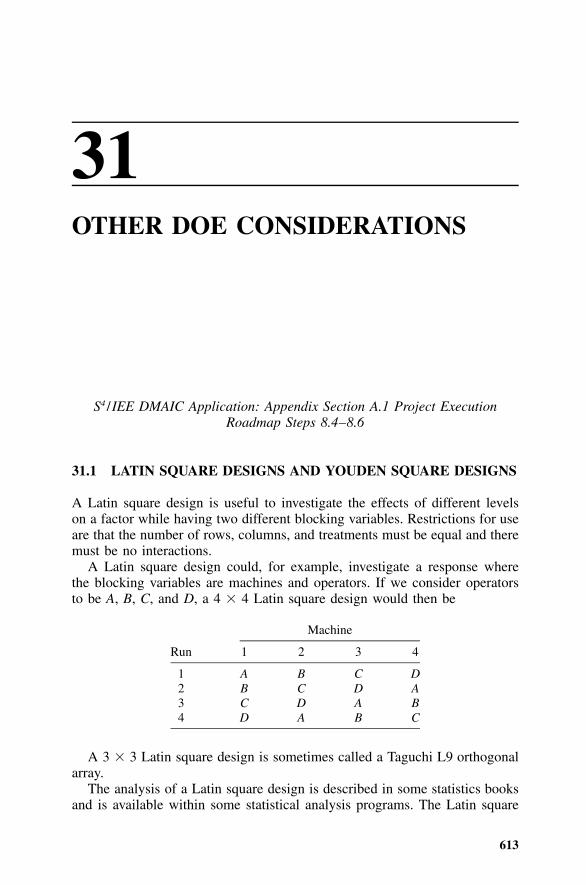
613

31OTHER DOE CONSIDERATIONS

S4 /IEE DMAIC Application: Appendix Section A.1 Project ExecutionRoadmap Steps 8.4–8.6

31.1 LATIN SQUARE DESIGNS AND YOUDEN SQUARE DESIGNS

A Latin square design is useful to investigate the effects of different levelson a factor while having two different blocking variables. Restrictions for useare that the number of rows, columns, and treatments must be equal and theremust be no interactions.

A Latin square design could, for example, investigate a response wherethe blocking variables are machines and operators. If we consider operatorsto be A, B, C, and D, a 4 � 4 Latin square design would then be

Run

Machine

1 2 3 4

1 A B C D2 B C D A3 C D A B4 D A B C

A 3 � 3 Latin square design is sometimes called a Taguchi L9 orthogonalarray.

The analysis of a Latin square design is described in some statistics booksand is available within some statistical analysis programs. The Latin square

614 OTHER DOE CONSIDERATIONS

design is not considered to be a factorial design since the design does notallow for interactions between separate factors composing the design. Hunter(1989a) warns of some dangers that can arise from misuse of Latin squaredesigns.

Youden square designs are similar to Latin square designs; however, theyare less restrictive in that Youden designs have a fairly wide choice of thenumber of rows as design possibilities.

31.2 EVOLUTIONARY OPERATION (EVOP)

Evolutionary operation (EVOP) is an analytical approach targeted at securingdata from a manufacturing process where process conditions are varied in aplanned factorial structure from one lot to another without jeopardizing themanufactured product. It is an ongoing mode of utilizing the operation of afull-scale process such that information on ways to improve the process isgenerated from simple experiments while production continues. Analyticaltechniques are then used to determine what process changes to make forproduct improvement (Box et al. 1978).

For previously described DOEs it is typically desirable to include as manyfactors as possible in each design, which keeps the factors studied-to-runsratio as high as possible. However, the circumstances when conducting anEVOP are different. Box et al. (1978) provides the following suggestionswhen conducting an EVOP:

• Because the signal/noise ratio must be kept low, a large number of runsis usually necessary to reveal the effects of changes.

• However, these are manufacturing runs that must be made anyway andresult in very little additional cost.

• In the manufacturing environment things need to be simple, and usuallyit is practical to vary only two or three factors in any given phase of theinvestigation.

• In these circumstances it makes sense to use replicated 22 or 23 factorialdesigns, often with an added centerpoint.

• As results become available, averages and estimates of effects are con-tinually updated and displayed on an information board as a visual fac-tory activity in the area under investigation.

• The information board must be located where the results are visible tothose responsible for running the process.

• In consultation with an EVOP committee, the process supervisor usesthe information board as a guide for better process conditions.

FOLD-OVER DESIGNS 615

31.3 EXAMPLE 31.1: EVOP

A study was conducted to decrease the cost per ton of a product in a petro-chemical plant (Jenkins 1969; Box et al. 1978). For one stage of the inves-tigation two variables believed important were:

• Reflux ratio of a distillation column• Ratio of recycle flow to purge flow

Changes to the magnitude of the input variables were expected to cause tran-sients, which would subside in about 6 hours. Measurements for the studywould be made during an additional 18 hours of steady operation.

Figure 31.1 shows the posting at the end of each of the three phases, wherethe recorded response was the average cost per ton recorded to the nearestunit. The design was a 22 factorial with a center point. Phase I results are theaverages of five cycle replications. Upon completion of phase I it was believedsufficient evidence existed to justify a move to the lower reflux ratio andhigher recycle/purge ratio in phase II. The five cycles from phase II suggestedthat this move did lower costs as expected, while further suggesting assessingeven higher values of recycle/purge ratio assessment in phase III. Phase IIIwas terminated after four cycles with the conclusion that the lowest cost ofapproximately £80 was achieved when the reflux ratio was close to 6.3 andthe recycle/purge ratio was about 8.5.

The cost for the described 41⁄2-month program was £6,000, which resultedin a per-ton cost reduction from £92 to £80. This annualized savings was£100,000.

31.4 FOLD-OVER DESIGNS

Consider the situation in which a resolution III experiment is conducted. Afterlooking at the results, the experimenters wished that they had conducted aresolution IV experiment initially because they were concerned about theconfounding of two-factor interactions with the main effect.

A technique called fold-over can be used to create a resolution IV designfrom a resolution III design. To create a fold-over design, simply include withthe original resolution III design a second fractional factorial design with allthe signs reversed. This fold-over process can be useful in the situation wherethe experimenter has performed a resolution III design initially and nowwishes to remove the confounding of the main and two-factor interactioneffects.

616

FIG

UR

E31

.1A

ppea

ranc

eof

the

info

rmat

ion

boar

dat

the

end

ofph

ases

I,II

,an

dII

I,pe

troc

hem

ical

plan

tda

ta.

Res

pons

eis

aver

age

cost

per

ton.

[Fro

mB

ox,

etal

.(1

978)

,w

ithpe

rmis

sion

.]

FACTORIAL DESIGNS THAT HAVE MORE THAN TWO LEVELS 617

31.5 DOE EXPERIMENT: ATTRIBUTE RESPONSE

The previous chapter described DOEs with continuous response outputs. Insome situations the appropriate response for a trial may be, for example, thatthere were two failures out of 300,000 tested solder joints.

If the sample size is the same for each trial, the attribute data can beanalyzed using the proportion defect rate as a response for each trial, but adata transformation may be needed when doing this analysis. The accuracyof such an analysis can become questionable whenever the sample size issuch that many trials have no failures.

An alternative approach is to use a computer categorical data modelingroutine that is offered by some statistical software packages. In some cases,additional insight may be achieved by looking at the data after they areranked; however, an attribute test to evaluate the proportion of failures foreach trial should not begin with the intent of relying solely on such an analysisstrategy.

31.6 DOE EXPERIMENT: RELIABILITY EVALUATIONS

In some situations it is beneficial when doing a reliability evaluation to buildand test devices/systems using a DOE structure. This strategy can be bene-ficial when deciding on what design changes should be implemented to fix aproblem. This strategy can also be used to describe how systems are built /configured when running a generic reliability test during early stages of pro-duction. In this type of test, if all trials experience failures, a failure rate ortime of failure could be the response that is used for the DOE analysis, withtransformation considerations.

31.7 FACTORIAL DESIGNS THAT HAVE MORE THANTWO LEVELS

A multiple-experiment strategy that builds on two-level fractional factorialscan be a very useful approach for gaining insight into what is needed to betterunderstand and improve a process. Usually nonlinear conditions can be ad-dressed by not being too bold when choosing factorial levels. If a descriptionof a region is necessary, a response surface design such as Box-Behnken orcentral composite design (CCD) can be beneficial (see Chapter 33). Statisticalsoftware packages can offer other alternatives.

Tables M1 to M5 can be used to create designs for these test considera-tions. To do this, combine the contrast columns of the designs in Tables M1to M5 for these test considerations (e.g., � � � source W, � � � source X,� � � source Y, � � � source Z). However, an additional contrast column

618 OTHER DOE CONSIDERATIONS

needs to be preserved in the case of four levels, because there are threedegrees of freedom with 4 levels (4 levels � 1 � 3 degrees of freedom). Thecontrast column to preserve is normally the contrast column that contains thetwo-factor interaction effect of the two contrast columns selected to representthe four levels. For example, if the A and B contrast columns were combinedto define the levels, the AB contrast column should not be assigned a factor.These three contrast columns contain the four-level main effect information.

Again, I believe that for test efficiency most factor-level considerationsabove the level of 2 should be reduced to the value of 2 during an initialDOE experiment. Higher-level considerations that cannot be eliminated fromconsideration can still be evaluated in a test strategy that consists of multipleexperiments. When the factors that significantly affect a response are reducedto a manageable number through two-level experiments, response surfaceanalysis techniques can be used to find the factor levels that optimize aresponse.

31.8 EXAMPLE 31.2: CREATING A TWO-LEVEL DOESTRATEGY FROM A MANY-LEVEL FULL FACTORIALINITIAL PROPOSAL

Consider two-level factorial experiments where possible. However, it is some-times not very obvious how to make the change from an experiment designof many-level considerations to two-level considerations. This example illus-trates a basic thought process that can be used to address this transition.

An experiment is proposed that considers an output as a function of thefollowing factors with various level considerations.

Factors Number of Levels

A 4B 3C 2D 2E 2F 2

where the A factor may be temperature at four temperature levels and B to Fmay consider the effects from other process or design factor tolerances.

To use an experiment design that considers all possible combinations ofthe factors (i.e., a full-factorial experiment), there would need to be 192 ex-periment trials (4 � 3 � 2 � 2 � 2 � 2 � 192). In reality, this experimenttypically would never be performed, since the number of trials would makeit too expensive and time-consuming for most industrial situations.

EXAMPLE 31.3: RESOLUTION III DOE WITH INTERACTION CONSIDERATION 619

Again, an experiment that considers all possible combinations of the factorstypically contains more information than is needed for engineering decisions.By changing all factors to two levels and reducing the amount of interactionoutput information, a design alternative can be determined using Tables M1to M5. This experiment can then be performed in 8, 16, or 32 trials dependingon the desired resolution.

The first of two basic arguments against restructuring such an example testis that the factor levels cannot be changed to two levels. In some cases areduction to a two-level experiment is not possible, but in many situations itis. For example, perhaps only two temperatures are assessed initially, andthen, if significance is found, further investigation through another experimentmay be appropriate for other temperature effects. The specific temperaturevalues to use in an experiment can be dependent on the test objectives. If thetest is to determine whether a product is to have a satisfactory output withina temperature range, the levels of temperature may be the two tolerance ex-tremes. However, if a test is to determine the sensitivity of a process totemperature input, a smaller difference in temperature range may be appro-priate. Even factors that appear impossible to change to a two-level consid-eration can often initially be made two levels with the understanding that iffactor significance is found, additional investigation of the other levels willbe made in another experiment.

The second argument is the what-if doldrums. These questions can takenumerous basic forms. Limiting assumptions should be listed and critiquedbefore performing experiments so that appropriate modifications suggested byothers can be incorporated into the initial experiment strategy.

If reasonable limiting assumptions are not made, a ‘‘test-all-combinations’’strategy will probably make the test too large and thus not performed. A one-at-a-time test strategy can then occur, which is inefficient and may in the endrequire more test time than a fractional factorial experiment. In addition, aone-at-a-time strategy has a higher risk of not yielding the desired informa-tion.

A series of two-level experiments, perhaps with a screening experiment, isa more efficient test strategy. Experiment resolution should be chosen so thattwo-factor interactions may be confounded but are managed. After the sig-nificant parameters are identified, a follow-up experiment is made at a reso-lution that better assesses main effects and the two-factor interactions of thesefactors.

31.9 EXAMPLE 31.3: RESOLUTION III DOE WITHINTERACTION CONSIDERATION

An experimenter wants to assess the effects of 14 two-level factors (A–N) onan output. Two of these factors are temperature and humidity. Each test trial

620 OTHER DOE CONSIDERATIONS

is very expensive; hence, only a 16-trial resolution III screening experimentis planned. However, the experimenter is concerned that temperature and hu-midity may interact.

From Table M3 it is noted that for a 14-factor experiment, the 15th contrastcolumn is not needed for any main effect consideration. This column couldbe used to estimate experimental error or the temperature-humidity interactionthat is of concern. To make the temperature-humidity interaction term appearin this column, the factor assignments must be managed such that the tem-perature and humidity assignments are consistent with an interaction noted inthis column. From Table N3 it is noted that there are several assignmentalternatives (i.e., AD, BH, GI, EJ, KL, FM, and CN). For example, tempera-ture could be assigned an A while humidity is assigned a D, or humiditycould be assigned a B while temperature is assigned an H.

This method could be extended to address more than one interaction con-sideration for both resolution III and IV designs, as long as the total numberof two-level factors and interaction contrast column considerations does notexceed one less than the number of trials.

31.10 EXAMPLE 31.4: ANALYSIS OF A RESOLUTION IIIEXPERIMENT WITH TWO-FACTORINTERACTION ASSESSMENT

A resolution III experiment was conducted to determine if a product wouldgive a desirable response under various design tolerance extremes and oper-ating conditions. The experiment had 64 trials with 52 two-level factors (A–Z, a–z). The experiment design format from Table M5 is shown in Table 31.1.

Consider that an analysis conducted indicated that only contrast columns6, 8, and 18 were found statistically significant, which implies that factors F,H, and R are statistically significant. However, if Table N3 is examined, it isnoted that contrast column 6 (i.e., factor F) also contains the HR interaction,while contrast column 8 (i.e., factor H) also contains the FR interaction andcontrast column 18 (i.e., factor R) also contains the FH interaction. Hence, itcould be that instead of the three factors each being statistically significant,one of three two-factor interactions might be making the third contrast columnstatistically significant. To assess which of these scenarios is most likely froma technical point of view, interaction plots can be made of the possibilitiesassuming that each of them are true. Engineering judgment could then beused to assess which interaction is most likely or whether the three factorsindividually are the most probable cause of significance.

This example only illustrates a procedure to be used for determining pos-sible sources of significance. A confirmation experiment is necessary to con-firm or dispute any theories. Many circumstances can cause contrast columnsignificance in a resolution III experiment. For example, any of the interactionconsiderations in a contrast column could be the source for significance with-

621

TA

BL

E31

.1D

OE

Exp

erim

enta

lT

rial

s

Fact

ors

� →A

BC

DE

FG

HI

JK

LM

NO

PQ

RS

TU

VW

XY

Za

bc

de

fg

hi

jk

lm

no

pq

rs

tu

vw

xy

z

Con

tras

tco

lum

n—

→�

11

11

11

11

11

22

22

22

22

22

33

33

33

33

33

44

44

44

44

44

55

51

23

45

67

89

01

23

45

67

89

01

23

45

67

89

01

23

45

67

89

01

23

45

67

89

01

2

1�

��

��

��

��

��

��

��

��

��

��

��

��

��

��

��

��

��

��

��

��

��

��

��

��

��

�

2�

��

��

��

��

��

��

��

��

��

��

��

��

��

��

��

��

��

��

��

��

��

��

��

��

��

�

3�

��

��

��

��

��

��

��

��

��

��

��

��

��

��

��

��

��

��

��

��

��

��

��

��

��

�

* * *

63�

��

��

��

��

��

��

��

��

��

��

��

��

��

��

��

��

��

��

��

��

��

��

��

��

��

�

64�

��

��

��

��

��

��

��

��

��

��

��

��

��

��

��

��

��

��

��

��

��

��

��

��

��

�

622 OTHER DOE CONSIDERATIONS

out the main effect being statistically significant. However, with the initialproblem definition, if all the trial responses are well within a desirable outputrange, then it may not be important to have a precise analysis to determinewhich factor(s) are statistically significant.

31.11 EXAMPLE 31.5: DOE WITH ATTRIBUTE RESPONSE

A manufacturing surface mount processes and assembles electrical compo-nents onto a printed circuit board. A visual quality assessment at severallocations on the printed circuit board assesses residual flux and tin (Sn) re-sidual. A lower value for these responses is most desirable. A DOE wasconducted with the following factors;

Factor

Levels

�1 �1

A Paste age Fresh ‘‘Old’’B Humidity Ambient HighC Print-reflow time Short LongD IR temperature Low HighE Cleaning temperature Low HighF Is component present? No Yes

Inspectors were not blocked within the experiment though they should havebeen. Table 31.2 shows the results of the experiment along with the experi-mental trials.

Consider first an analysis of the flux response. There are many zeros forthis response, which makes a traditional DOE analysis impossible. However,when we rank the responses, as shown in Table 31.3, there are seven nonzerovalues. The largest six of these values are with C � �1 (i.e., long print-reflowtime). However, there is concern that all of these assessments were made bythe same inspector. From this result, one might inquire whether a gage R&Rstudy had been conducted, and one may also inquire about the results of thestudy. Also, these boards should be reassessed to make sure that the docu-mented results are valid. If there is agreement that the results are valid, onewould conclude that the �1 level for C is best (i.e., short print-reflow time).

Consider next an analysis of the tin (Sn) response. This response does nothave as many zeros and lends itself to regular DOE analysis techniques.Because the response is count data, a transformation should be considered.Analysis of these data is an exercise at the end of this chapter.

31.12 EXAMPLE 31.6: A SYSTEM DOE STRESS TO FAIL TEST

During the development of a new computer a limited amount of test hardwareis available to evaluate the overall design of the product. Four test systems

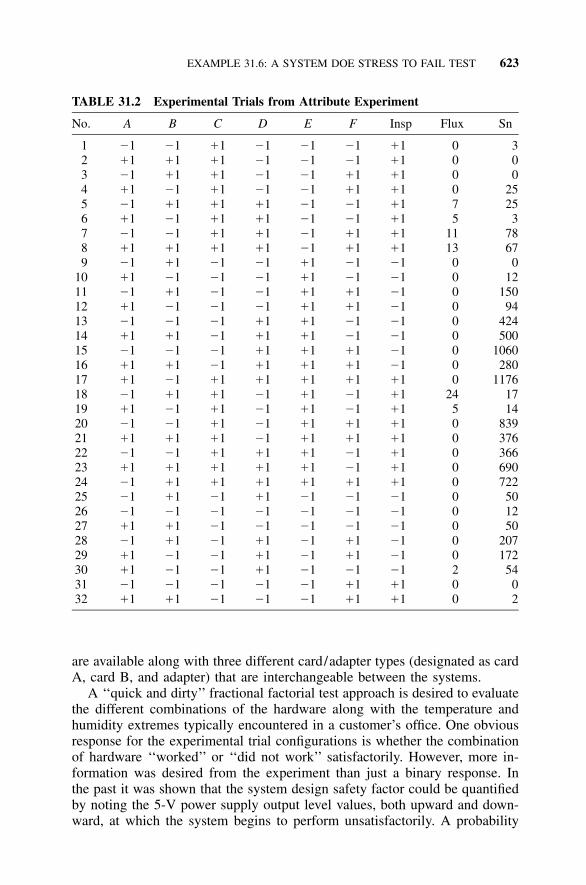
EXAMPLE 31.6: A SYSTEM DOE STRESS TO FAIL TEST 623

TABLE 31.2 Experimental Trials from Attribute Experiment

No. A B C D E F Insp Flux Sn

1 �1 �1 �1 �1 �1 �1 �1 0 32 �1 �1 �1 �1 �1 �1 �1 0 03 �1 �1 �1 �1 �1 �1 �1 0 04 �1 �1 �1 �1 �1 �1 �1 0 255 �1 �1 �1 �1 �1 �1 �1 7 256 �1 �1 �1 �1 �1 �1 �1 5 37 �1 �1 �1 �1 �1 �1 �1 11 788 �1 �1 �1 �1 �1 �1 �1 13 679 �1 �1 �1 �1 �1 �1 �1 0 0

10 �1 �1 �1 �1 �1 �1 �1 0 1211 �1 �1 �1 �1 �1 �1 �1 0 15012 �1 �1 �1 �1 �1 �1 �1 0 9413 �1 �1 �1 �1 �1 �1 �1 0 42414 �1 �1 �1 �1 �1 �1 �1 0 50015 �1 �1 �1 �1 �1 �1 �1 0 106016 �1 �1 �1 �1 �1 �1 �1 0 28017 �1 �1 �1 �1 �1 �1 �1 0 117618 �1 �1 �1 �1 �1 �1 �1 24 1719 �1 �1 �1 �1 �1 �1 �1 5 1420 �1 �1 �1 �1 �1 �1 �1 0 83921 �1 �1 �1 �1 �1 �1 �1 0 37622 �1 �1 �1 �1 �1 �1 �1 0 36623 �1 �1 �1 �1 �1 �1 �1 0 69024 �1 �1 �1 �1 �1 �1 �1 0 72225 �1 �1 �1 �1 �1 �1 �1 0 5026 �1 �1 �1 �1 �1 �1 �1 0 1227 �1 �1 �1 �1 �1 �1 �1 0 5028 �1 �1 �1 �1 �1 �1 �1 0 20729 �1 �1 �1 �1 �1 �1 �1 0 17230 �1 �1 �1 �1 �1 �1 �1 2 5431 �1 �1 �1 �1 �1 �1 �1 0 032 �1 �1 �1 �1 �1 �1 �1 0 2

are available along with three different card/adapter types (designated as cardA, card B, and adapter) that are interchangeable between the systems.

A ‘‘quick and dirty’’ fractional factorial test approach is desired to evaluatethe different combinations of the hardware along with the temperature andhumidity extremes typically encountered in a customer’s office. One obviousresponse for the experimental trial configurations is whether the combinationof hardware ‘‘worked’’ or ‘‘did not work’’ satisfactorily. However, more in-formation was desired from the experiment than just a binary response. Inthe past it was shown that the system design safety factor could be quantifiedby noting the 5-V power supply output level values, both upward and down-ward, at which the system begins to perform unsatisfactorily. A probability

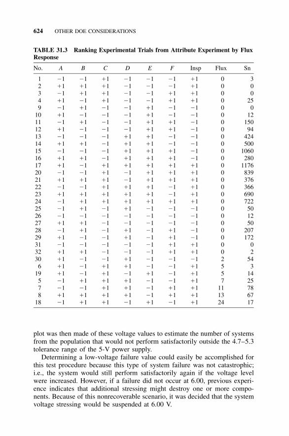
624 OTHER DOE CONSIDERATIONS

TABLE 31.3 Ranking Experimental Trials from Attribute Experiment by FluxResponse

No. A B C D E F Insp Flux Sn

1 �1 �1 �1 �1 �1 �1 �1 0 32 �1 �1 �1 �1 �1 �1 �1 0 03 �1 �1 �1 �1 �1 �1 �1 0 04 �1 �1 �1 �1 �1 �1 �1 0 259 �1 �1 �1 �1 �1 �1 �1 0 0

10 �1 �1 �1 �1 �1 �1 �1 0 1211 �1 �1 �1 �1 �1 �1 �1 0 15012 �1 �1 �1 �1 �1 �1 �1 0 9413 �1 �1 �1 �1 �1 �1 �1 0 42414 �1 �1 �1 �1 �1 �1 �1 0 50015 �1 �1 �1 �1 �1 �1 �1 0 106016 �1 �1 �1 �1 �1 �1 �1 0 28017 �1 �1 �1 �1 �1 �1 �1 0 117620 �1 �1 �1 �1 �1 �1 �1 0 83921 �1 �1 �1 �1 �1 �1 �1 0 37622 �1 �1 �1 �1 �1 �1 �1 0 36623 �1 �1 �1 �1 �1 �1 �1 0 69024 �1 �1 �1 �1 �1 �1 �1 0 72225 �1 �1 �1 �1 �1 �1 �1 0 5026 �1 �1 �1 �1 �1 �1 �1 0 1227 �1 �1 �1 �1 �1 �1 �1 0 5028 �1 �1 �1 �1 �1 �1 �1 0 20729 �1 �1 �1 �1 �1 �1 �1 0 17231 �1 �1 �1 �1 �1 �1 �1 0 032 �1 �1 �1 �1 �1 �1 �1 0 230 �1 �1 �1 �1 �1 �1 �1 2 54

6 �1 �1 �1 �1 �1 �1 �1 5 319 �1 �1 �1 �1 �1 �1 �1 5 14

5 �1 �1 �1 �1 �1 �1 �1 7 257 �1 �1 �1 �1 �1 �1 �1 11 788 �1 �1 �1 �1 �1 �1 �1 13 67

18 �1 �1 �1 �1 �1 �1 �1 24 17

plot was then made of these voltage values to estimate the number of systemsfrom the population that would not perform satisfactorily outside the 4.7–5.3tolerance range of the 5-V power supply.

Determining a low-voltage failure value could easily be accomplished forthis test procedure because this type of system failure was not catastrophic;i.e., the system would still perform satisfactorily again if the voltage levelwere increased. However, if a failure did not occur at 6.00, previous experi-ence indicates that additional stressing might destroy one or more compo-nents. Because of this nonrecoverable scenario, it was decided that the systemvoltage stressing would be suspended at 6.00 V.

EXAMPLE 31.6: A SYSTEM DOE STRESS TO FAIL TEST 625

TABLE 31.4 Experimental System Data

Temperature(�F)

Humidity(%)

System(#)

Card A(#)

Card B(#)

Adapter(#)

5 V (error types,a

voltages)

ElevatedVoltage

LoweredVoltage

95 50 1 4 1c 4 E1 5.92 E2 4.4195 50 3b 3 3 2 sus 6.00 E3 4.6095 50 4 1 2 1 sus 6.00 E2 4.5095 50 2 2 4 3 sus 6.00 E2 4.4155 20 1 4 1c 1 sus 6.00 E2 4.3455 20 2 1 4 2 sus 6.00 E2 4.4155 20 3ad 2 3 3 sus 6.00 E2 4.4555 20 4 3 2 4 sus 6.00 E2 4.5155 85 1 1 2 2 sus 6.00 E2 4.5255 85 2 4 3 1 sus 6.00 E2 4.4555 85 3b 2 4 4 sus 6.00 E3 4.6255 85 4 3 1c 3 E1 5.88 E2 4.5895 20 1 1 2 3 sus 6.00 E2 4.5195 20 2 3 3 4 sus 6.00 E2 4.4495 20 3ad 4 4 1 sus 6.00 E2 4.4195 20 4 2 1c 2 E1 5.98 E2 4.41

a sus � suspended test at noted voltage.b Lowering 5 V caused an E3 error.c Lowering 5 V caused a different error type (i.e., E1) three out of four times when cardB � 1.d 3a � new system planar board installed.

A 16-trial test matrix is shown in Table 31.4 along with measured voltagelevels. Note that the trial fractional factorial levels of this type can be createdfrom Tables M1 to M5 where four levels of the factors are created by com-bining contrast columns (e.g., � � � 1, � � � 2, � � � 3, and � �� 4). It should be noted that the intent of the experiment was to do a quickand dirty test at the boundaries of the conditions to assess the range of re-sponse that might be expected when parts are assembled in different patterns.Because of this, no special care was taken when picking the contrast columnsto create the four levels of factors; hence, there will be some confounding ofthe effects. Obviously a practitioner needs to take more care when choosinga design matrix if he/she wishes to make an analysis that addresses theseeffect considerations.

From Table 31.4 it is noted that the system 3 planar board was changedduring the experiment (denoted by a postscript a). Changes of this type shouldbe avoided during a test; however, if an unexpected event mandates a change,the change should be documented. It is also noted that the trials containingsystem 3 with the original system planar resulted in a different error messagewhen the 5-V power supply was lowered to failure. It is also noted that the

626 OTHER DOE CONSIDERATIONS

FIGURE 31.2 Normal probability plot of the 5-V stress to fail responses (first designtest).

only ‘‘elevated voltage’’ failures occurred (three out of four times) when cardB number I was installed. General conclusions from observations of this typemust be made with extreme caution because aliasing and experimental mea-surement errors can lead to erroneous conclusions. Additional investigationbeyond the original experiment needs to be performed for the purpose ofeither confirming or rejecting such theories.

Since the failures only occurred when the voltage was varied outside itslimits, some people might conclude that there is no problem. It is true thatthese observations and failure voltage levels may not be indicative of futureproduction problems. However, the basic strategy behind this type of exper-iment is to assess the amount of safety factor before failure with a limitedamount of hardware. A design that has a small margin of safety may expe-rience problems in the future if the manufacturing process experiences anyslight change. In addition, it is good general practice to make other appro-priate evaluations on any cards and devices that have peculiar failures for thepurpose of assessing whether there is a potential design problem.

The DCRCA plot in Figure 31.2 can give some idea of the safety factorin the design. We need to keep in mind that this probability plot of the trialresponses is not a probability plot of random data. However, we can get arelative picture of how we might expect to perform relative to specificationconditions in the future if we assume that the factor levels represent thevariability of our future process. From this plot a best-estimate projection isthat about 99.9% of the systems will perform at the low-voltage tolerancevalue of 4.7.

S4 / IEE ASSESSMENT 627

Consider next that a similar experiment is performed with a new level ofhardware. The results from this experiment are shown in Table 31.5. Abnor-malities that occurred in Card A did not occur in Card B. A probability plotof the low-voltage stress values is shown in Figure 31.3. One of the pointsin this probability plot could be an outlier. This data measurement should beinvestigated for abnormalities. Another observation from this plot is that thereis a larger percentage projection at the 4.7-V specification limit than from theearlier set of data; this later design appears to have a larger safety factor.

Figure 31.4 gives a pictorial presentation of this comparison using theestimated normal probability density functions (PDFs) from each set of data.From this figure it is noted that the average values of the density functionsare approximately the same, but there was a reduction in measurement vari-ability in the later design level. This is ‘‘goodness,’’ but, if the situation werereversed and the newer design had greater variability, then there might beconcern that things could degrade more in the future.

In manufacturing it is feasible for the preceding test strategy to be repeatedperiodically. Data could then be monitored on x and R control charts fordegradation/improvement as a function of time.

31.13 S4/IEE ASSESSMENT

In some situations efforts should be to understand the magnitude of effectsfrom statistically significant factors. Follow-up experiments can be designedto yield additional information leading to an optimal solution. Understandingthe levels of factors that did not affect the output significantly is also impor-tant because this knowledge can lead to relaxed tolerances that are easier toachieve.

In many instances the overall understanding of the process through frac-tional factorial experiments can be combined with general cost considerationsto determine the changes that are ‘‘best’’ in order to supply the customer witha high-quality/ low-cost product. In other instances, fractional factorial exper-iments can be used to structure a test strategy so that the test efficientlyevaluates a product relative to meeting the needs of the customer.

When deciding what should be done next, consider the real purpose of theexperiment. If the primary objective is to determine whether a satisfactoryoutput is achieved within the operational extremes of environmental and tol-erance conditions and all the responses are ‘‘very good,’’ the significance ofeffects may be of little practical importance. A probability plot of the exper-imental outputs for each trial can be a ‘‘picture’’ to assess variabilities in this‘‘operational space’’—perhaps with only one prototype system. It should benoted, however, that this would not be a random sample (of future produc-tion); the percentage of population values is not necessarily representative ofthe true population. Nevertheless, this procedure can often give a more mean-

628 OTHER DOE CONSIDERATIONS

TABLE 31.5 Experiment Data with New Hardware

Temperature(�F)

Humidity(%)

System(#)

Card A(#)

Card B(#)

Adapter(#)

5 V (error types,a

voltages)

ElevatedVoltage

LoweredVoltage

95 50 1 4 1 1 sus 6.00 E2 4.4895 20 2 1 4 2 sus 6.00 E2 4.4895 20 3 2 3 3 sus 6.00 E2 4.4595 20 4 3 2 4 sus 6.00 E2 4.4255 85 1 1 2 2 sus 6.00 E2 4.5655 85 2 4 3 1 sus 6.00 E2 4.4655 85 3 2 4 4 sus 6.00 E2 4.4555 85 4 3 1 3 sus 6.00 E2 4.4355 20 1 1 2 3 sus 6.00 E2 4.4555 20 2 3 3 4 sus 6.00 E2 4.4655 20 3 4 4 1 sus 6.00 E3 4.4255 20 4 2 1 2 sus 6.00 E2 4.4895 50 1 4 1 4 sus 6.00 E2 4.4595 50 3 2 4 3 sus 6.00 E2 4.4995 50 4 3 3 2 sus 6.00 E2 4.4595 50 2 1 2 1 sus 6.00 E2 4.49

a sus � suspended test at noted voltage.

FIGURE 31.3 Normal probability plot of the 5-V stress to fail responses (seconddesign test).

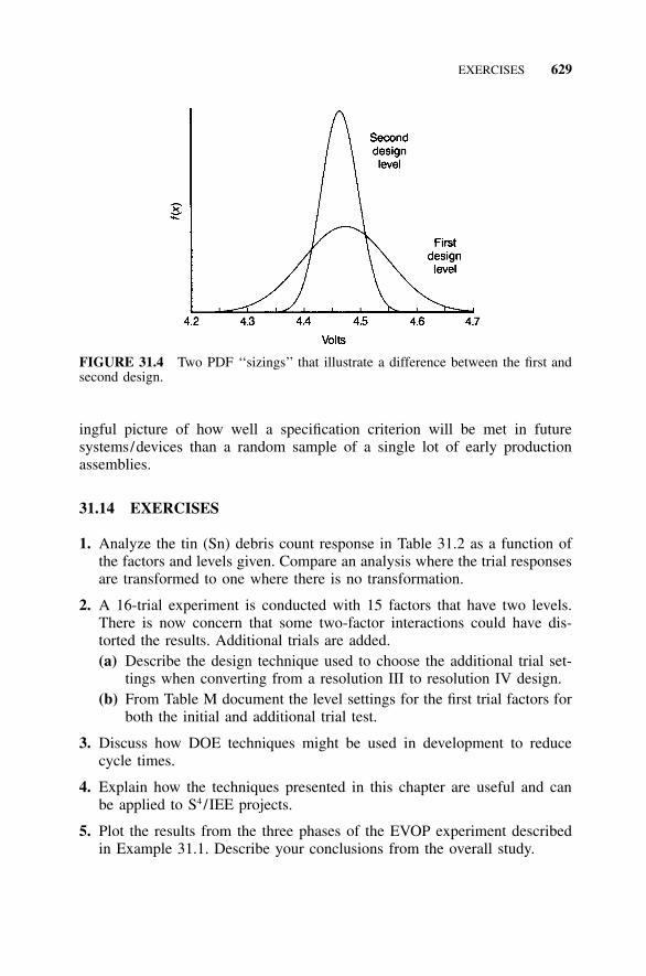
EXERCISES 629

FIGURE 31.4 Two PDF ‘‘sizings’’ that illustrate a difference between the first andsecond design.

ingful picture of how well a specification criterion will be met in futuresystems/devices than a random sample of a single lot of early productionassemblies.

31.14 EXERCISES

1. Analyze the tin (Sn) debris count response in Table 31.2 as a function ofthe factors and levels given. Compare an analysis where the trial responsesare transformed to one where there is no transformation.

2. A 16-trial experiment is conducted with 15 factors that have two levels.There is now concern that some two-factor interactions could have dis-torted the results. Additional trials are added.(a) Describe the design technique used to choose the additional trial set-

tings when converting from a resolution III to resolution IV design.(b) From Table M document the level settings for the first trial factors for

both the initial and additional trial test.

3. Discuss how DOE techniques might be used in development to reducecycle times.

4. Explain how the techniques presented in this chapter are useful and canbe applied to S4/IEE projects.

5. Plot the results from the three phases of the EVOP experiment describedin Example 31.1. Describe your conclusions from the overall study.

630

32ROBUST DOE

S4 /IEE DMAIC Application: Appendix Section A.1 Project ExecutionRoadmap Steps 8.2, 8.5, 8.6, and 8.7

The experiment procedures proposed by Genichi Taguchi (Taguchi andKonishi 1987; Ross 1988) have provoked both acclaim and criticism. Somenonstatisticians like the practicality of the techniques, while statisticians havenoted problems that can lead to erroneous conclusions. However, most stat-isticians would agree that Taguchi has increased the visibility of DOE. Inaddition, most statisticians and engineers would probably agree with Taguchithat more direct emphasis should have been given in the past to the reductionof process variability and the reduction of cost in product design and manu-facturing processes.

I will use the term robust DOE to describe the S4/IEE implementation ofkey points from the Taguchi philosophy. Robust DOE is an extension ofpreviously discussed DOE design techniques that focuses not only on meanfactor effects but on expected response variability differences from the levelsof factors. Robust DOE offers us a methodology where focus is given tocreate a process or product design that is robust or desensitized to inherentnoise input variables.

This chapter gives a brief overview of the basic Taguchi philosophy as itrelates to the concepts discussed in this book. The loss function is also dis-cussed, along with an approach that can be used to reduce variability in themanufacturing process. In addition, the analysis of 2k residuals is discussedfor assessing potential sources of variability reduction.

TEST STRATEGIES 631

32.1 S4/IEE APPLICATION EXAMPLES: ROBUST DOE

S4/IEE application examples of robust DOE are:

• Transactional 30,000-foot-level metric: An S4/IEE project was to reduceDSO for invoices. Wisdom of the organization and passive analysis ledto the creation of a robust DOE experiment that considered factors: sizeof order (large versus small), calling back within a week after mailinginvoice (yes versus no), prompt-paying customer (yes versus no), origi-nation department (from passive analysis: least DSO versus highest DSOaverage), stamping ‘‘past due’’ on envelope (yes versus no). The DSOtime for 10 transactions for each trial will be recorded. The average andstandard deviation of these responses will be analyzed in the robust DOE.

• Manufacturing 30,000-foot-level metric: An S4/IEE project was to im-prove the process capability/performance metrics for the diameter of aplastic part from an injection-molding machine. Wisdom of the organi-zation and passive analysis led to the creation of a DOE experiment thatconsidered factors: temperature (high versus low), pressure (high versuslow), hold time (long versus short), raw material (high side of toleranceversus low side of tolerance), machine (from passive analysis: best-performing versus worst-performing), and operator (from passive analy-sis: best versus worst). The diameter for 10 parts manufactured for eachtrial will be recorded. The average and standard deviation of these re-sponses will be analyzed in the robust DOE.

• Product DFSS: An S4/IEE project was to improve the process capability/performance metrics for the number of daily problem phone calls re-ceived within a call center. Passive analysis indicated that product setupwas the major source of calls for existing products/services. A DOE testprocedure assessing product setup time was added to the test process fornew products. Wisdom of the organization and passive analysis led tothe creation of a DOE experiment that considered factors: features ofproducts or services, where factors and their levels would be variousfeatures of the product/service, including as a factor special setup in-struction sheet in box (sheet included versus no sheet included). Thesetup time for three operators was recorded for each trial. The averageand standard deviation of these responses will be analyzed in the robustDOE.

32.2 TEST STRATEGIES

Published Taguchi (Taguchi and Konishi 1987) orthogonal arrays and lineargraphs contain both two- and three-level experiment design matrices. In gen-

632 ROBUST DOE

eral, I prefer a basic two-level factor strategy for most experiments, withfollow-up experiments to address additional levels of a factor or factors. Theresponse surface techniques described in Chapter 33 could also be used, insome cases, as part of that follow-up effort.

The basic two-level Taguchi design matrices are equivalent to those inTable M (Breyfogle 1989e), where there are n trials with n � 1 contrastcolumn considerations for the two-level designs of 4, 8, 16, 32, and 64 trials.Table N contains the two-factor interaction confounding for the design ma-trices found in Table M.

One suggested Taguchi test strategy consists of implementing one experi-ment (which can be rather large) with a confirmation experiment. Taguchiexperiment analysis techniques do not normally dwell on interaction consid-erations that are not anticipated before the start of test. If care is not takenduring contrast column selection when choosing the experiment design ma-trix, an unnecessary or a messy interaction confounding structure may result,which can lead the experimenter to an erroneous conclusion (Box et al. 1988).

This book suggests first considering what initial experiment resolution isneeded and manageable with the number of two-level factors that are present.If a resolution is chosen that does not directly consider interactions, someinteraction concerns can be managed by using the techniques described ear-lier. After this first experiment analysis, one of several actions may next beappropriate, depending on the results. First, the test may yield dramatic con-clusions that answer the question of concern. For this situation, a simpleconfirmation experiment would be appropriate. The results from another ex-periment may lead testers to plan a follow-up experiment that considers otherfactors in conjunction with those factors that appear statistically significant.Still another situation may suggest a follow-up experiment of statisticallysignificant factors at a higher resolution for interaction considerations.

Again, if interactions are not managed properly in an experiment, confu-sion and erroneous action plans can result. In addition, the management ofthese interactions is much more reasonable when three-level factors are notinvolved in the fractional factorial experiment design.

32.3 LOSS FUNCTION

The loss function is a contribution of Genichi Taguchi (Taguchi 1978). Thisconcept can bridge the language barrier between upper management and thoseinvolved in the technical details. Upper management best understands money,while those involved in the technical arena better understand product varia-bility. Classical experiment design concepts do not directly translate the re-duction of process variability and into economical considerations understoodby all management.

The loss function describes the loss that occurs when a process does notproduce a product that meets a target value. Loss is minimized when there is

LOSS FUNCTION 633

FIGURE 32.1 Traditional method of interpreting manufacturing limits.

‘‘no variability’’ and the ‘‘best’’ response is achieved in all areas of the productdesign.

Traditionally, manufacturing has considered all parts that are outside spec-ification limits to be equally nonconforming and all parts within specificationto be equally conforming. The loss function associated with this way of think-ing is noted in Figure 32.1.

In the Taguchi approach, loss relative to the specification limit is not as-sumed to be a step function. To understand this point, consider whether it isrealistic, for example, to believe that there is no exposure of having anyproblems (i.e., loss) when a part is barely within the specification limit andthat the maximum loss level is appropriate whenever the part is barely outsidethese limits. Most people would agree that this is not normally true.

Taguchi addresses variability in the process using a loss function. The lossfunction can take many forms. A common form is the quadratic loss function

2L � k(y � m)

where L is the loss associated with a particular value of the independentvariable y. The specification nominal value is m, while k is a constant de-pending on the cost and width of the specification limits. Figure 32.2 illus-trates this loss function graphically. When this loss function is applied to asituation, more emphasis will be put on achieving the target as opposed tojust meeting specification limits. This type of philosophy encourages, for ex-ample, a television manufacturer to strive continually to manufacture routinelyproducts that have a very high quality picture (i.e., a nominal specificationvalue), as opposed to accepting and distributing a quality level that is ‘‘goodenough.’’

634 ROBUST DOE

FIGURE 32.2 Taguchi loss function.

32.4 EXAMPLE 32.1: LOSS FUNCTION

Given that the cost of scrapping a part is $10.00 when it deteriorates from atarget by �0.50 mm, the quadratic loss function given m (the nominal value)of 0.0 is

2$10.00 � k(0.5 � 0.0)

Hence,

2 2k � 10.00/0.25 � $40.00 per mm (i.e., $25,806 per in. )

This loss function then becomes

2L � 40(y � 0)

The loss function can yield different conclusions from decisions based onclassical ‘‘goalpost’’ specification limits. For example, a different decision canresult relative to frequency of maintenance for a tool that wears in a manu-facturing process. In addition, this loss function can help make economicdecisions to determine whether the expense to implement a new process thatcan yield a tighter tolerance should be implemented.

ROBUST DOE STRATEGY 635

32.5 ROBUST DOE STRATEGY

Again, most practitioners of statistical techniques agree with Taguchi that itis important to reduce variability in the manufacturing process. To do this,Taguchi suggests using an inner and outer array (i.e., fractional factorial de-sign structure) to address the issue. The inner array addresses the items thatcan be controlled (e.g., part tolerances), while the outer array addresses factorsthat cannot necessarily be controlled (e.g., ambient temperature and humid-ity). To analyze the data, he devised a signal-to-noise ratio technique, whichBox et al. (1988) show can yield debatable results. However, Box (1988)states that it can be shown that use of the signal-to-noise ratio concept canbe shown equivalent to an analysis that uses the logarithm of the data.

The fractional factorial designs included in this book can be used to addressreducing manufacturing variability with the inner/outer array experimentationstrategy. To do this, simply categorize the factors listed into controllable andnoncontrollable factors. The controllable factors can be fit into a design struc-ture similar to those illustrated in the previous chapters on DOE, while thenoncontrollable factors can be set to levels determined by another fractionalfactorial design. All the noncontrollable factor experimental design trialswould be performed for each trial of the controllable factor experimentationdesign. Note, however, that in using this inner/outer experimentation strategya traditional design of 16 trials might now contain a total of 64 trials if theouter experiment design contains 4 test trials.

Now both a mean and standard deviation value can be obtained for eachtrial and analyzed independently. The trial mean value can be directly ana-lyzed using the DOE procedures described above. The standard deviation (orvariance) for each trial should be given a logarithm transformation to nor-malize standard deviation data.

If the Taguchi philosophy of using an inner and outer array were followedin the design of the stepper motor fractional factorial experiment, the tem-perature factor would probably be considered in an outer array matrix. Thiscould be done, perhaps along with other parameters, remembering that themean value needs to be optimized (minimized to meet this particular testobjective) in addition to minimizing variability.

Obviously a practitioner is not required to use the inner/outer array ex-periment design approach when investigating the source of variability. It maybe appropriate, for example, to construct an experiment design where eachtrial is repeated and (in addition to the mean trial response) the variance (orstandard deviation) between repetitions is considered a trial response. Datamay need a log transformation. The sample size for each trial repetition needsto be large enough so that detection of the magnitude of variability differencesis possible. If the number of repetitions is small, the range in response rep-etitions can yield a better estimate than the variance.

636 ROBUST DOE

TABLE 32.1 Experiment Design and Results

Trial A B C D Response Factors

Level

� �

1 �1 �1 �1 �1 5 A Temperature 295 3252 1 �1 �1 �1 11 B Clamp time 7 93 �1 1 �1 �1 3.5 C Resin flow 10 204 1 1 �1 �1 9 D Closing time 15 305 �1 �1 1 �1 0.56 1 �1 1 �1 87 �1 1 1 �1 1.58 1 1 1 �1 9.59 �1 �1 �1 1 6

10 1 �1 �1 1 12.511 �1 1 �1 1 812 1 1 �1 1 15.513 �1 �1 1 1 114 1 �1 1 1 615 �1 1 1 1 516 1 1 1 1 5

32.6 ANALYZING 2k RESIDUALS FOR SOURCES OFVARIABILITY REDUCTION

A study of residuals from a single replicate of a 2k design can give insightinto process variability, because residuals can be viewed as observed valuesof noise or error (Montgomery 1997; Box and Meyer 1986). When the levelof a factor affects variability, a plot of residuals versus the factor levels willindicate more variability of the residuals at one factor level than at the otherlevel.

The magnitude of contrast column dispersion effects in the experiment canbe tested by calculating

2 �s (i )F* � ln i � 1, 2, . . . , ni 2 �s (i )

where n is the number of contrast columns for an experiment. Also, thestandard deviation of the residuals for each group of signs in each contrastcolumn is designated as s2(i�) and s2(i�). This statistic is approximately nor-mally distributed if the two variances are equal. A normal probability plot ofthe dispersion effects for the contrast columns can be used to assess thesignificance of a dispersion effect.

EXAMPLE 32.2: ANALYZING 2k RESIDUALS 637

FIGURE 32.3 Normal probability plot of the factor effects.

FIGURE 32.4 Plot of residuals versus clamp time (B).

32.7 EXAMPLE 32.2: ANALYZING 2k RESIDUALS FOR SOURCESOF VARIABILITY REDUCTION

The present defect rate of a process producing internal panels for commercialaircraft is too high (5.5 defects per panel). A four-factor, 16-trial, 2k singlereplicate design was conducted and yielded the results shown in Table 32.1for a single press load (Montgomery 1997).

638

TA

BL

E32

.2C

alcu

lati

onof

Dis

pers

ion

Eff

ects

Tri

alA

BC

DA

BA

CB

CA

BC

AD

BD

�A

BD

CD

AC

DB

CD

AB

CD

Res

idua

l

1�

��

��

��

��

��

��

��

�0.

942

��

��

��

��

��

��

��

��

0.69

3�

��

��

��

��

��

��

��

�2.

444

��

��

��

��

��

��

��

��

2.69

5�

��

��

��

��

��

��

��

�1.

196

��

��

��

��

��

��

��

�0.

567

��

��

��

��

��

��

��

��

0.19

8�

��

��

��

��

��

��

��

2.06

9�

��

��

��

��

��

��

��

0.06

10�

��

��

��

��

��

��

��

0.81

11�

��

��

��

��

��

��

��

2.06

12�

��

��

��

��

��

��

��

3.81

13�

��

��

��

��

��

��

��

�0.

6914

��

��

��

��

��

��

��

��

1.44

15�

��

��

��

��

��

��

��

3.31

16�

��

��

��

��

��

��

��

�2.

44s(

i�)

2.25

2.72

1.91

2.24

2.21

1.81

1.80

1.80

2.05

2.28

1.97

1.93

1.52

2.09

1.61

s(i�

)1.

850.

822.

201.

551.

862.

242.

262.

241.

931.

612.

111.

582.

161.

892.

33F

* i0.

392.

39�

0.29

0.74

0.35

�0.

43�

0.45

�0.

440.

130.

69�

0.14

0.40

�0.

710.

20�

0.74

EXAMPLE 32.2: ANALYZING 2k RESIDUALS 639

FIGURE 32.5 Normal probability plot of the dispersion effects.

A normal probability plot of the factor effects in Figure 32.3 (page 637)indicates that factors A and C are statistically significant. From this analysiswe conclude that lower temperature (A) and higher resin flow (C) woulddecrease the frequency of panel defects.

However, careful analysis of the residuals gives other insight. For a modelcontaining factors A and C no abnormalities were shown from a normal prob-ability plot of the residuals, but a plot of the residuals versus each of factors(A, B, C, and D) yielded the pattern shown in Figure 32.4 (page 637) for B.The B factor was not shown to affect the average number of defects per panel,but appears to be very important in its effect on process variability. It appearsthat a low clamp time results in less variability in the average number ofdefects per panel.

The magnitude of the B contrast column dispersion effect in the experimentis

2 � 2s (B ) (2.72)F* � ln � � 2.39B 2 � 2s (B ) (0.82)

Table 32.2 shows the result of this dispersion effect calculation for allcontrast columns. The normal probability plot of these contrast column dis-persion effects in Figure 32.5 clearly confirms our early observation of theimportance of the B factor with respect to process dispersion.

640 ROBUST DOE

32.8 S4/IEE ASSESSMENT

The mechanics of implementing some of the Taguchi concepts discussed inother books are questionable, but Taguchi has gotten management’s attentionon the importance of using DOE techniques. He has also shown on the im-portance of reducing variability. The process index Cp addresses the effectsthat variability can have on the consistency of a process toward meetingspecification objectives. Fractional factorial experiment concepts with stan-dard deviation as a response can be used to improve Cp. In addition, anassessment of residuals in a 2k design can help identify sources for the re-duction of variability.

32.9 EXERCISES

1. Catapult Exercise: Set up, conduct, and then analyze a DOE similar to theone executed in Chapter 30. However, this time repeat each trial threetimes. Analyze the mean and standard deviation of each trial response.Evaluate the residuals of the standard deviation to determine if a datatransformation is needed. Consider factors that not only adjust the meanresponse (e.g., arm length) but also could affect response variability. In-clude a measurement method factor, where one level of the factor is avisual recording of the distance with no marking (i.e., no carbon paper ortalcum powder to mark ball impact point) and the other is using somemethod to mark the ball position at impact. Consider how the factor levelswill be chosen (e.g., high ball projection arc or flat projection arc). Con-sider also whether the factor levels are going to be chosen so that therewill be much variability between throw distances or so that the throwdistances will be more clustered around the target (i.e., very bold or notso bold selection of factor levels).

2. A test had the objective of studying the effects of four factors on airflowthrough a valve that is used in an automobile air pollution control device.The factors and levels are noted below, along with the response for testtrials. Analyze all responses and summarize conclusions (Moen et al. 1991;Bisgaard and Fuller 1995):

Factors �1 1

Length of armature 0.595 in. 0.605 in.Spring load 70 g 100 gBobbin length 1.095 in. 1.105 in.Tube length 0.500 in. 0.510 in.

EXERCISES 641

TrialArm

LengthSpringLoad

BobbinDepth

TubeLength y S s2 ln(s2)

1 �1 �1 �1 �1 0.46 0.04 0.0016 �6.442 1 �1 �1 �1 0.42 0.16 0.0256 �3.673 �1 1 �1 �1 0.57 0.02 0.0004 �7.824 1 1 �1 �1 0.45 0.1 0.0100 �4.615 �1 �1 1 �1 0.73 0.02 0.0004 �7.826 1 �1 1 �1 0.71 0.01 0.0001 �9.217 �1 1 1 �1 0.7 0.05 0.0025 �5.998 1 1 1 �1 0.7 0.01 0.0001 �9.219 �1 �1 �1 1 0.42 0.04 0.0016 �6.44

10 1 �1 �1 1 0.28 0.15 0.0225 �3.7911 �1 1 �1 1 0.6 0.07 0.0049 �5.3212 1 1 �1 1 0.29 0.06 0.0036 �5.6313 �1 �1 1 1 0.7 0.02 0.0004 �7.8214 1 �1 1 1 0.71 0.02 0.0004 �7.8215 �1 1 1 1 0.72 0.02 0.0004 �7.8216 1 1 1 1 0.72 0.01 0.0001 �9.21

3. Reconsider how the following situation, presented as an exercise in Chap-ter 29, could be conducted using a DOE centered around the reduction ofvariability: The position of the leads on an electronic component is im-portant to get a satisfactory solder mount of the component to an electronicprinted circuit board. There is concern that in manufacturing, an electronictester of the component function is bending the component leads. To mon-itor physical changes from tester handling, the leads from a sample ofcomponents are noted examined before and after the tester.(a) Create a plan for implementing a DOE that assesses what should be

done differently to reduce the amount of bending on each component.Consider the selection of measurement response, selection of factors,and results validation.

(b) Create a plan that could be used in the future for a similar machinesetup.

4. Reconsider how the following situation, presented as an exercise in Chap-ter 29, could be conducted using a DOE centered around the reduction ofvariability: A machine measures the peel-back force necessary to removethe packaging for electrical components. The tester records an output forcethat changes as the packaging is separated. The process was found notcapable of consistently meeting specification limits. The average peel-backforce needed to be reduced.(a) Create a DOE plan to determine what should be done to improve the

capability/performance of the process.(b) Create a plan that the company could use in the future to set up similar

equipment to avoid this type of problem.

642 ROBUST DOE

5. A manufacturing process has 15 controllable and 3 uncontrollable factorsthat could affect the output of a process.(a) Create an inner/outer array test plan if the three uncontrollable factors

are ambient temperature, humidity, and barometric pressure.(b) Describe difficulties that may be encountered when conducting the

experiment.

6. Early in development, three prototype automobiles were used to estimateaverage miles per gallon. The net average of the three vehicles over 20,000miles was reported to management. Suggest what might be done differentlyif the objective of the test was to understand the characteristics of thevehicles better relative to sensitivity of different operators.

7. Explain how the techniques presented in this chapter are useful and canbe applied to S4/IEE projects.

8. Explain robust DOE setup alternatives for Exercise 2 in Chapter 27.

9. Describe how and show where robust DOE fits into the overall S4/IEEroadmap described in Figure A.1 in the Appendix.

643

33RESPONSE SURFACEMETHODOLOGY

S4 /IEE DMAIC Application: Appendix Section A.1, Project ExecutionRoadmap Step 8.8

Response surface methodology (RSM) is used to determine how a responseis affected by a set of quantitative variables/factors over some specified re-gion. This information can be used to optimize the settings of a process togive a maximum or minimum response, for example. Knowledge of the re-sponse surface can help in choosing settings for a process so that day-to-dayvariations typically found in a manufacturing environment, which will havea minimum effect on the degradation of product quality.

For a given number of variables, response surface analysis techniques re-quire more trials than the two-level fractional factorial design techniques;hence, the number of variables considered in an experiment may first need tobe reduced through either technical considerations or fractional factorial ex-periments.

This chapter explains how to apply central composite rotatable and Box–Behnken designs for determining the response surface analysis of variables.It discusses extreme vertices and simplex lattice designs along with computeralgorithm designs for mixture designs.

33.1 MODELING EQUATIONS

The DOE chapters above covering two-level fractional factorial experimen-tation considered main effects and interaction effects. For these designs the

644 RESPONSE SURFACE METHODOLOGY

response was assumed to be linear between the levels considered for thefactors. The general approach of investigating factor extremes addresses prob-lems expediently with a minimal number of test trials. This form of experi-mentation is adequate in itself for solving many types of problems, but thereare situations in which a response needs to be optimized as a function of thelevels of a few input factors/variables. This chapter focuses on such situa-tions.

The prediction equation for a two-factor linear main-effect model withoutthe consideration of interactions takes the form

y � b � b x � b x0 1 1 2 2

where y is the response, b0 is the y-axis intercept, and (b1, b2) are the coef-ficients of the factors. For a balanced experiment design with factor-levelconsiderations for x1 and x2, respectively, equal to �1 and �1, the b1 and b2

coefficients equate to one-half of the effect and b0 is the average of all theresponses. For a given set of experimental data, computer programs can de-termine these coefficients by such techniques as least squares regression.

If there is an interaction consideration, the equation model will then takethe form

y � b � b x � b x � b x x0 1 1 2 2 12 1 2

The number of terms in the equation represents the minimum number ofexperimental trials needed to determine the model. For example, the equationabove has four terms; a minimum of four trials is needed to calculate thecoefficients. The two-level DOE significance tests discussed in previous chap-ters were to determine which of the coefficient estimates were large enoughto have a statistically significant affect on the response (y) when changedfrom a low (�1) level to a high (�1) level.

Centerpoints can be added to the two-level fractional factorial design todetermine the validity of the linearity assumption of the model. When usinga regression program on the coded effects, the fractional factorial levelsshould take on symmetrical values around zero (i.e., �1 and �1). To deter-mine if the linearity assumption is valid, the average response of the center-points can be compared to the overall average of the two-level fractionalfactorial experiment trials.

If the first-degree polynomial approximation does not fit the process data,a second-degree polynomial model may adequately describe the curvature ofthe response surface as a function of the input factors. For two-factor consid-erations, this model takes the form

2 2Y � b � b x � b x � b x � b x � b x x0 1 1 2 2 11 1 22 2 12 1 2

CENTRAL COMPOSITE DESIGN 645

FIGURE 33.1 Central composite design for two factors.

33.2 CENTRAL COMPOSITE DESIGN

To determine the additional coefficients of a second-degree polynomial, ad-ditional levels of the variables are needed between the end-point levels. Anefficient test approach to determine the coefficients of a second-degree poly-nomial is to use a central composite design. Figure 33.1 shows this designfor the two-factor situation.

An experiment design is said to be rotatable if the variance of the predictedresponse at some point is a function of only the distance of the point fromthe center. The central composite design is made rotatable when [a �(F)1 / 4], where F is the number of points used in the factorial part of thedesign. For two factors F � 22 � 4; hence, a � (4)1 / 4 � 1.414. A usefulproperty of the central composite design is that the additional axial points canbe added to a two-level fractional factorial design as additional trials after thecurvature is detected from initial experimental data.

With a proper number of center points, the central composite design canbe made such that the variance of the response at the origin is equal to thevariance of the response at unit distance from the origin (i.e., a uniformprecision design). This characteristic in the uniform precision design is im-portant because it gives more protection against bias in the regression coef-ficients (because of the presence of third-degree and higher terms in the truesurface) than does the orthogonal design. Table 33.1 shows the parametersneeded to achieve a uniform precision design as a function of the number ofvariables in the experiment. From this table, for example, a design assessingfive variables along with all two-factor interactions plus the curvature of allvariables would be that shown in Table 33.2. Data are then analyzed usingregression techniques to determine the output response surface as a functionof the input variables.

646 RESPONSE SURFACE METHODOLOGY

TABLE 33.1 Uniform Precision Central Composite Rotatable Designs

Numberof

Variables

Numberof

FactorialTrials

Numberof

AxialTrials

Numberof

CenterTrials a

TotalNumberof Trials

2 4 4 5 1.4142 133 8 6 6 1.6820 204 16 8 7 2.0000 315 16 10 6 2.0000 326 32 12 9 2.3780 537 64 14 14 2.8280 92

TABLE 33.2 Response Surface Design Matrix for Five Variables

A B C D E

�1�1�1�1�1�1�1�1�1�1�1�1�1�1�1�1

�1�1�1�1�1�1�1�1�1�1�1�1�1�1�1�1

�1�1�1�1�1�1�1�1�1�1�1�1�1�1�1�1

�1�1�1�1�1�1�1�1�1�1�1�1�1�1�1�1

�1�1�1�1�1�1�1�1�1�1�1�1�1�1�1�1

Fractional factorial design fromTable M3

�2�2

00000000

00

�2�2

000000

0000

�2�2

0000

000000

�2�2

00

00000000

�2�2

Axial trialswith levelsconsistentwithTable 33.1

000000

000000

000000

000000

000000

Center point trialsconsistent withTable 33.1

EXAMPLE 33.1: RESPONSE SURFACE DESIGN 647

TABLE 33.3 Responses in Central Composite Design

Natural Variables

u1 u2

Coded Variables

v1 v2

Responses

Yieldy1

Viscosityy2

Molecularweight

y3

80 170 �1 �1 76.5 62 294080 180 �1 1 77.0 60 347090 170 1 �1 78.0 66 368090 180 1 1 79.5 59 389085 175 0 0 79.9 72 348085 175 0 0 80.3 69 320085 175 0 0 80.0 68 341085 175 0 0 79.7 70 329085 175 0 0 79.8 71 350092.07 175 1.414 0 78.4 68 336077.93 175 �1.414 0 75.6 71 302085 182.07 0 1.414 78.5 58 363085 167.93 0 �1.414 77.0 57 3150

Cornell (1984), Montgomery (1997), and Box et al. (1978) discuss ana-lytical methods to determine maximum points on the response surface usingthe canonical form of the equation. The coefficients of this equation can beused to describe the shape of the surface (ellipsoid, hyperboloid, etc.). Analternative approach is to understand the response surface by using a computercontour plotting program, as illustrated in the next example. Determining theparticular contour plot may help determine/change process factors to yield adesirable/ improved response output with minimal day-to-day variation.

Creating a contour representation for the equation derived from an RSMcan give direction for a follow-up experiment. For example, if the contourrepresentation does not capture a peak that we are interested in, we couldinvestigate new factor levels, which are at right angles to the contours thatappear to give a higher response level. This is called direction of steepestascent. When searching for factor levels that give a lower response, a similardirection of steepest descent approach could be used.

33.3 EXAMPLE 33.1: RESPONSE SURFACE DESIGN

A chemical engineer desires to determine the operating conditions that max-imize the yield of a process. An earlier two-level factorial experiment of manyconsiderations indicated that reaction time and reaction temperature were theparameters that should be optimized. A central composite design was chosenand yielded the responses shown in Table 33.3 (Montgomery 1997). A sec-ond-degree model can be fitted using the natural levels of the variables (e.g.,

648 RESPONSE SURFACE METHODOLOGY

time � 80) or the coded levels (e.g., time � �1). A statistical analysis ofyield in terms of the coded variables is as follows:

Response Surface Regression

The analysis was done using coded variables.

Estimated Regression Coefficients for y1 (yield)

Term Coef StDev T PConstant 79.940 0.11909 671.264 0.000v1 (time) 0.995 0.09415 10.568 0.000v2 (temperature) 0.515 0.09415 5.472 0.001v1*v1 �1.376 0.10098 �13.630 0.000v2*v2 �1.001 0.10098 �9.916 0.000v1*v2 0.250 0.13315 1.878 0.103

S � 0.2663 R-Sq � 98.3% R-Sq(adj) � 97.0%

Analysis of Variance for y1

Source DF Seq SS Adj SS Adj MS F PRegression 5 28.2467 28.2467 5.64934 79.67 0.000Linear 2 10.0430 10.0430 5.02148 70.81 0.000Square 2 17.9537 17.9537 8.97687 126.59 0.000Interaction 1 0.2500 0.2500 0.25000 3.53 0.103

Residual Error 7 0.4964 0.4964 0.07091Lack-of-Fit 3 0.2844 0.2844 0.09479 1.79 0.289Pure Error 4 0.2120 0.2120 0.05300

Total 12 28.7431

A statistical analysis of yield in terms of natural variables is as follows:

Response Surface Regression

The analysis was done using natural variables.

Estimated Regression Coefficients for y1 (yield)

Term Coef StDev T PConstant �1430.69 152.851 �9.360 0.000u1 (time) 7.81 1.158 6.744 0.000u2 (temperature) 13.27 1.485 8.940 0.000u1*u1 �0.06 0.004 �3.630 0.000u2*u2 �0.04 0.004 �9.916 0.000u1*u2 0.01 0.005 1.878 0.103

S � 0.2663 R-Sq � 98.3% R-Sq(adj) � 97.0%

BOX-BEHNKEN DESIGNS 649

Analysis of Variance for y1

Source DF Seq SS Adj SS Adj MS F PRegression 5 28.2467 28.2467 5.64934 79.67 0.000Linear 2 10.0430 6.8629 3.43147 48.39 0.000Square 2 17.9537 17.9537 8.97687 126.59 0.000Interaction 1 0.2500 0.2500 0.25000 3.53 0.103

Residual Error 7 0.4964 0.4964 0.07091Lack-of-Fit 3 0.2844 0.2844 0.09479 1.79 0.289Pure Error 4 0.2120 0.2120 0.05300

Total 12 28.7431

From this analysis, the second-degree model in terms of the coded levelsof the variables is

2 2ŷ � 79.940 � 0.995v � 0.515v � 1.376v � 0.250v v � 1.001v1 2 1 1 2 2

This equates to an equation for the natural levels of

2 2ŷ � �1430.69 � 7.81u � 13.27u � 0.06u � 0.01 u u � 0.04u1 2 1 1 2 2

These equations will yield the same response value for a given input datastate. The advantage of using the coded levels is that the importance of eachterm can be compared somewhat by looking at the magnitude of the coeffi-cients because the relative magnitude of the variable levels is brought to asingle unit of measure.

When projections are made from a response surface, it is obviously im-portant that the model fit the initial data satisfactorily. Erroneous conclusionscan result when there is lack of fit. The computer analysis did not indicatethat there was lack of fit; hence, the second-degree polynomial model is ac-cepted. The natural form of this polynomial equation is shown as a contourplot in Figure 33.2 and a response surface plot in Figure 33.3.

33.4 BOX-BEHNKEN DESIGNS

When estimating the first- and second-order terms of a response surface, Boxand Behnken (1960) give an alternative to the central composite design ap-proach. They present a list of 10 second-order rotatable designs covering 3,4, 5, 6, 7, 9, 10, 11, 12, and 16 variables. However, in general, Box-Behnkendesigns are not always rotatable nor are they block orthogonal.

One reason that an experimenter may choose this design over a centralcomposite design is physical test constraints. This design requires only threelevels of each variable, as opposed to five for the central composite design.Figure 33.4 shows the test points for this design approach given three designvariables.

650 RESPONSE SURFACE METHODOLOGY

FIGURE 33.2 Contour plot of yield response.

80.579.5

78.577.5

76.5

75.574.5

73.5

Yield

8085

Time0

170175 Temperature

180

FIGURE 33.3 Response surface plot of the yield response.

33.5 MIXTURE DESIGNS

The experiment designs discussed previously in this book apply to discreteand/or continuous factors, where the levels of each factor are completelyindependent from the other factors. However, consider a chemist who mixesthree ingredients together. If the chemist wishes to increase the percentageof one ingredient, the percentage of another ingredient must be adjusted ac-cordingly. Mixture experiment designs are used for this situation, where thecomponents (factors/variables) under consideration take levels that are aproportion of the whole.

The next few sections of this chapter explain the concept of mixture de-signs. A textbook experiment design approach to this type of problem is often

MIXTURE DESIGNS 651

FIGURE 33.4 Box-Behnken design space for three factors.

not practical. Computer-generated designs and analyses are usually better formost realistic mixture problems.

In the general mixture problem the measured response depends only onthe proportions of the components present in the mixture and not on the totalamount of the mixture. For three components this can be expressed as

x � x � x � 11 2 3

To illustrate the application of this equation consider that a mixture consistsof three components: A, B, and C. If component A is 20% and B is 50%, Cmust be 30% to give a total of 100% (i.e., 0.2 � 0.5 � 0.3 � 1).

When three factors are considered in a two-level full factorial experiment(23), the factor space of interest is a cube. However, a three-component mix-ture experiment is represented by an equilateral triangle. The coordinate sys-tem for these problems is called a simplex coordinate system. Figure 33.5shows the triangle for three components whose proportions are x1, x2, and x3.A four-component experiment would similarly take on the space of a tetra-hedron.

With three components, coordinates are plotted on equilateral triangulargraph paper that has lines parallel to the three sides of the triangle. Eachvertex of the triangle represents 100% of one of the components in the mix-ture. The lines away from a vertex represent decreasing amounts of the com-ponent represented by that vertex. The center of the equilateral trianglerepresents, for example, a mixture with equal proportions (1⁄3, 1⁄3, 1⁄3) fromeach of the components.

In a designed mixture experiment, several combinations of components arechosen within the spatial extremes defined by the number of components (e.g.,an equilateral triangle for three components). In one experiment all possible

652 RESPONSE SURFACE METHODOLOGY

FIGURE 33.5 Three-component simplex factor space. [From Cornell (1983), withpermission.]

combinations of the components can be considered as viable candidates fordetermining an ‘‘optimal’’ response. However, in many situations some com-binations of the components are not reasonable or may even cause a danger-ous response (e.g., an explosion).

In this chapter, simplex lattice designs will be used when all combinationsof the components are under consideration, while extreme vertices designswill be used when restrictions are placed on the proportions of the compo-nents.

33.6 SIMPLEX LATTICE DESIGNS FOR EXPLORING THEWHOLE SIMPLEX REGION

The simplex lattice designs (Scheffé 1958) in this section address problemswhere there are no restrictions on the limits of the percentages of compoundscomprising the total 100% composition.

A simplex lattice design for q components consists of points defined bythe coordinates (q, m), where the proportions assumed by each componenttake m � 1 equally spaced values from 0 to 1 and all possible combinationsof the components are considered. Figure 33.6 illustrates pictorially the spatialtest consideration of several lattice design alternatives for three and four com-ponents. Cornell (1983) notes that the general form of a regression functionthat can be fitted easily to data collected at the points of a (q, m) simplexlattice is the canonical form of the polynomial. This form is then modifiedby applying the restriction that the terms of a polynomial sum to 1. Thesimplified expression for three components yields the first-degree model form

y � b x � b x � b x1 1 2 2 3 3

The second-degree model form is

SIMPLEX LATTICE DESIGNS FOR EXPLORING THE WHOLE SIMPLEX REGION 653

FIGURE 33.6 Some simplex lattice designs for three and four components. [FromCornell (1983), with permission.]

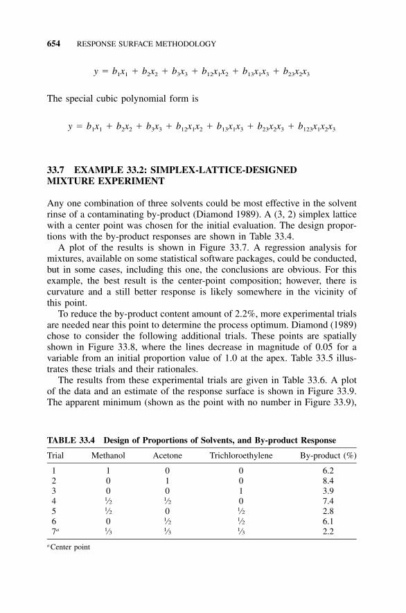
654 RESPONSE SURFACE METHODOLOGY

TABLE 33.4 Design of Proportions of Solvents, and By-product Response

Trial Methanol Acetone Trichloroethylene By-product (%)

1 1 0 0 6.22 0 1 0 8.43 0 0 1 3.94 1⁄2 1⁄2 0 7.45 1⁄2 0 1⁄2 2.86 0 1⁄2 1⁄2 6.17a 1⁄3 1⁄3 1⁄3 2.2

a Center point

y � b x � b x � b x � b x x � b x x � b x x1 1 2 2 3 3 12 1 2 13 1 3 23 2 3

The special cubic polynomial form is

y � b x � b x � b x � b x x � b x x � b x x � b x x x1 1 2 2 3 3 12 1 2 13 1 3 23 2 3 123 1 2 3

33.7 EXAMPLE 33.2: SIMPLEX-LATTICE-DESIGNEDMIXTURE EXPERIMENT

Any one combination of three solvents could be most effective in the solventrinse of a contaminating by-product (Diamond 1989). A (3, 2) simplex latticewith a center point was chosen for the initial evaluation. The design propor-tions with the by-product responses are shown in Table 33.4.

A plot of the results is shown in Figure 33.7. A regression analysis formixtures, available on some statistical software packages, could be conducted,but in some cases, including this one, the conclusions are obvious. For thisexample, the best result is the center-point composition; however, there iscurvature and a still better response is likely somewhere in the vicinity ofthis point.

To reduce the by-product content amount of 2.2%, more experimental trialsare needed near this point to determine the process optimum. Diamond (1989)chose to consider the following additional trials. These points are spatiallyshown in Figure 33.8, where the lines decrease in magnitude of 0.05 for avariable from an initial proportion value of 1.0 at the apex. Table 33.5 illus-trates these trials and their rationales.

The results from these experimental trials are given in Table 33.6. A plotof the data and an estimate of the response surface is shown in Figure 33.9.The apparent minimum (shown as the point with no number in Figure 33.9),

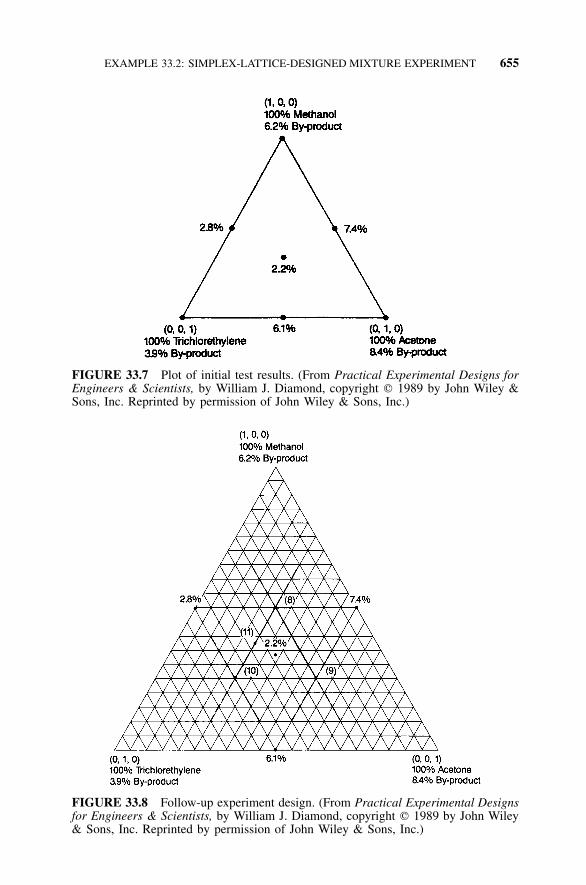
EXAMPLE 33.2: SIMPLEX-LATTICE-DESIGNED MIXTURE EXPERIMENT 655

FIGURE 33.7 Plot of initial test results. (From Practical Experimental Designs forEngineers & Scientists, by William J. Diamond, copyright � 1989 by John Wiley &Sons, Inc. Reprinted by permission of John Wiley & Sons, Inc.)

FIGURE 33.8 Follow-up experiment design. (From Practical Experimental Designsfor Engineers & Scientists, by William J. Diamond, copyright � 1989 by John Wiley& Sons, Inc. Reprinted by permission of John Wiley & Sons, Inc.)

656 RESPONSE SURFACE METHODOLOGY

TABLE 33.5 Experimental Points and Their Rationales

ExperimentalPoint Number Rationale

8, 9, 10 (3,1) simplex lattice design vertices around the best responsewith the noted diagonal relationship to the original datapoints.

11 Because point 5 is the second best result, another data pointwas added in that direction.

12 Repeat of the treatment combination that was the best in theprevious experiment and is now the centroid of this follow-upexperiment.

TABLE 33.6 Results of Experimental Trials

Trial Methanol Acetone Trichloroethylene By-product (%)

8 1⁄2 1⁄4 1⁄4 3.39 1⁄4 1⁄2 1⁄4 4.8

10 1⁄4 1⁄4 1⁄2 1.411 3⁄8 1⁄4 3⁄8 1.212 1⁄3 1⁄3 1⁄3 2.4

along with the results from an additional trial setting at this value are asfollows:

Trial Methanol Acetone Trichloroethylene By-product (%)

13 0.33 0.15 0.52 0.45

Additional simplex design trials around this point could yield a yet smalleramount of by-product. However, if the by-product percentage is ‘‘lowenough,’’ additional experimental trials might not serve any economic purpose.

33.8 MIXTURE DESIGNS WITH PROCESS VARIABLES

Consider the situation where a response is a function not only of a mixturebut also of its process variables (e.g., cooking temperature and cooking time).For the situation where there are three components to a mixture and threeprocess variables, the complete simplex-centroid design takes the form shownin Figure 33.10.

In general, the number of experimental trial possibilities can get very largewhen there are many variable considerations. Cornell and Gorman (1984)discuss fractional factorial design alternatives. Cornell (1990) discusses the

MIXTURE DESIGNS WITH PROCESS VARIABLES 657

FIGURE 33.9 Plot of all data with contour lines. (From Practical ExperimentalDesigns for Engineers & Scientists, by William J. Diamond, copyright � 1989 byJohn Wiley & Sons, Inc. Reprinted by permission of John Wiley & Sons, Inc.)

FIGURE 33.10 Complete simplex centroid � 23 factorial design. [From Cornell andGorman (1984), with permission.]

658 RESPONSE SURFACE METHODOLOGY

TABLE 33.7 Results of Mixture Experiment with Process Variables

Texture Readings

CodedProcessVariables

z1 z2 z3

Mixture Composition (x1, x2, x3)

(1,0,0) (0,1,0) (0,0,1) (1⁄2,1⁄2,0) (1⁄2,0,1⁄2) (0,1⁄2,1⁄2) (1⁄3,1⁄3,1⁄3)

�1 �1 �1 1.84 0.67 1.51 1.29 1.42 1.16 1.591 �1 �1 2.86 1.10 1.60 1.53 1.81 1.50 1.68

�1 1 �1 3.01 1.21 2.32 1.93 2.57 1.83 1.941 1 �1 4.13 1.67 2.57 2.26 3.15 2.22 2.60

�1 �1 1 1.65 0.58 1.21 1.18 1.45 1.07 1.411 �1 1 2.32 0.97 2.12 1.45 1.93 1.28 1.54

�1 1 1 3.04 1.16 2.00 1.85 2.39 1.60 2.051 1 1 4.13 1.30 2.75 2.06 2.82 2.10 2.32

embedding of mixture experiments inside factorial experiments. Algorithmdesigns, discussed in Section 33.12, can also reduce the number of test trials.

33.9 EXAMPLE 33.3: MIXTURE EXPERIMENT WITHPROCESS VARIABLES

The data in Table 33.7 are the average of a replicated texture reading inkilogram force required to puncture fish patty surfaces (Cornell 1981; Cornelland Gorman 1984; Gorman and Cornell 1982) that were prepared under pro-cess conditions that had code values of �1 and �1 for

z1: cooking temperature (�1 � 375�F, �1 � 425�F)z2: cooking time (�1 � 25 min, �1 � 40 min)z3: deep fat frying time (�1 � 25 sec, �1 � 40 sec)

The patty was composed of three types of fish that took on compositionratios of 0, 1/3, 1/2, or 1. The fish designations are

x1: mulletx2: sheepsheadx3: croaker

The desired range of fish texture (in the noted scaled units) for customersatisfaction is between 2.0 and 3.5. Other characteristics, not discussed here,were also considered in the actual experiment. A computer analysis of thesedata yielded the coefficient estimates shown in Table 33.8. The standard error

EXAMPLE 33.3: MIXTURE EXPERIMENT WITH PROCESS VARIABLES 659

TABLE 33.8 Coefficient Estimates from Computer Analysis

Mean z1 z2 z3 z1z2 z1z3 z2z3 z1z2z3 SE

x1 2.87a 0.49a 0.71a �0.09 0.07 �0.05 0.10 0.04 0.05x2 1.08a 0.18a 0.25a �0.08 �0.03 �0.05 �0.03 �0.04 0.05x3 2.01a 0.25a 0.40a 0.01 0.00 0.17a �0.05 �0.04 0.05x1 x2 �1.14a �0.81a �0.59 0.10 �0.06 0.14 �0.19 �0.09 0.23x1 x3 �1.00a �0.54 �0.05 �0.03 �0.06 �0.27 �0.43 �0.12 0.23x2 x3 0.20 �0.14 0.07 �0.19 0.23 �0.25 0.12 0.27 0.23x1 x2 x3 3.18 0.07 �1.41 0.11 1.74 �0.71 1.77 �1.33 1.65

a Individual estimates thought to be significant.

(SE) for this example was determined using all the original data and wastaken from Cornell (1981).

In the data analysis of the averages, there were 54 data inputs and the samenumber of estimates; hence, a regression analysis cannot give any significancetest on the variables. A half-normal probability plot of the effects is notmathematically helpful because the SE is not consistent between the esti-mates.

However, using the SE terms (where the number of degrees of freedomfor error is 56; i.e., �error � 56) that were noted in Cornell (1981), the asteriskshows those items that are thought to be different from zero. To illustrate this,the effect level for significance for a variable with an SE of 0.05 is as shownbelow (see Table E for interpolated t value):

Effect level criterion � (SE)(t ) � (SE)(t ) � 0.05(2.667) � 0.13�;� 0.01;56

Any of the effects noted in the table that have an SE of 0.05 are statisticallysignificant at the 0.01 level if their magnitude is greater than 0.13. A highlystatistically significant probability level of 0.01 for this problem is appropriatebecause the parameter effect estimates are not independent; hence, the indi-vidual t tests are not independent.

Various characteristics of fish patty hardness can be determined by evalu-ating the main effect and interaction considerations in the preceding table.However, another alternative for evaluating the characteristics is to isolate theindividual blend characteristics at each of the eight process variable treat-ments.

The equation to consider, for example, where z1 � �1, z2 � �1, and z3 ��1 is

y � a x � a x z � � � � � 2.87x � 0.49x (�1) � � �1 1 2 1 1 1 1

Various x1, x2, and x3 values are then substituted to create a contour plotin a simplex coordinate system for each of the eight variable treatments, as

660 RESPONSE SURFACE METHODOLOGY

FIGURE 33.11 Contour plots of the texture. (From The Analysis of Mixture Data,by John A. Cornell, copyright � 1981 by John Wiley & Sons, Inc. Reprinted bypermission of John Wiley & Sons, Inc.)

noted in Figure 33.11. The shaded area in this figure shows when the desirableresponse range of 2.0 to 3.5 (nominal � 2.75) is achieved. This figure illus-trates that a z2 � 1 level (i.e., 40 min cooking time) is desirable. However,many other combinations of the other parameters at z2 � 1 can yield a sat-isfactory texture reading. To maximize customer satisfaction, effort should bedirected toward achieving the nominal criterion on the average with minimumvariability between batches.

At this point in the analysis, perhaps other issues should be considered.For example, it may be desirable to make the composition of the fish pattyso that its sensitivity is minimized relative to deep fat frying time. In a homekitchen it may be relatively easy to control the cooking temperature; however,a person frying patties in a fast-food restaurant may be too busy to removethem immediately when the timer sounds. To address this concern, it appearsthat a z1 � �1 level (i.e., 375�F cooking temperature) may be most desirablewith a relative high concentration of mullet in the fish patty composition.

Other considerations to take into consideration when determining the‘‘best’’ composition and variable levels are economics (e.g., cost of each typeof fish) and other experimental output response surface plots (e.g., taste eval-

COMPUTER-GENERATED MIXTURE DESIGNS/ANALYSES 661

uation of fish patties). To aid in the decision-making process, a similar outputto that of Figure 33.11 could be made for a mathematical combination of theseveral responses weighted by importance.

33.10 EXTREME VERTICES MIXTURE DESIGNS

Extreme vertices designs can take on most of the nice properties of the matrixdesigns discussed above (Diamond 1989). This type of design is explained inthe following example.

33.11 EXAMPLE 33.4: EXTREME VERTICESMIXTURE EXPERIMENT

A chemist wishes to develop a floor wax product. The following range ofproportions of three ingredients is under consideration along with the notedproportion percentage limitations. The response to this experiment takes onseveral values: level of shine, scuff resistance, and so forth.

Wax: 0–0.25 (i.e., 0%–25%)Resin: 0–0.20 (i.e., 0%–20%)Polymer: 0.70–0.90 (i.e., 70%–90%)

Again, mixture experiment trial combinations are determined by using asimplex coordinate system. This relationship is noted in Figure 33.12, wherethe lines leaving a vertex decrease by a magnitude of 0.05 proportion froman initial proportion value of 1.

The space of interest is noted by the polygon shown in the figure. Table33.9 shows test trials for the vertices along with a center point. The logicused in Example 33.1 for follow-up experiments can similarly be applied tothis problem in an attempt to optimize the process.

33.12 COMPUTER-GENERATED MIXTURE DESIGNS/ANALYSES

The concepts behind algorithm design were introduced by Wynn (1970) andFedorov (1972). With these designs a computer program creates a list ofpossible trials to fit the model, calculates the standard deviation of the valuepredicted by the polynomial for each trial, and picks the trial with the largeststandard deviation as the next trial to include in the design. The coefficientsof the polynomial are then recalculated using this new trial and the processis repeated. The designs that are best are those having the largest varianceproportional to the number of terms in the polynomial (B. Wheeler 1989).

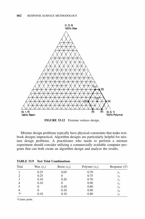
662 RESPONSE SURFACE METHODOLOGY

FIGURE 33.12 Extreme vertices design.

TABLE 33.9 Test Trial Combinations

Trial Wax (x1) Resin (x2) Polymer (x3) Response (Y )

1 0.25 0.05 0.70 y1

2 0.25 0 0.75 y2

3 0.10 0.20 0.70 y3

4 0.10 0 0.90 y4

5 0 0.20 0.80 y5

6 0 0.10 0.90 y6

7a 0.10 0.10 0.80 y7

a Center point.

Mixture design problems typically have physical constraints that make text-book designs impractical. Algorithm designs are particularly helpful for mix-ture design problems. A practitioner who needs to perform a mixtureexperiment should consider utilizing a commercially available computer pro-gram that can both create an algorithm design and analyze the results.

ADDITIONAL RESPONSE SURFACE DESIGN CONSIDERATIONS 663

The following example illustrates the application of a computer programto generate a design matrix and then analyze the results.

33.13 EXAMPLE 33.5: COMPUTER-GENERATED MIXTUREDESIGN/ANALYSIS

An improvement is needed in the paste used to attach electronic componentswhen manufacturing surface-mounted printed circuit cards. Viscosity of thepaste was one desired response as a function of the proportion of the fivemixture components, which had the following ranges:

Component Proportion

Compl 0.57–0.68Comp2 0.15–0.21Comp3 0.03–0.08Comp4 0.05–0.10Comp5 0.04–0.06

ECHIP, a computer program (B. Wheeler 1989), was used to create analgorithm design given the above constraints. The mixture proportions for thisresulting design along with the experimental viscosity measurement responses(in units of pascal-seconds) are shown in Table 33.10.

From the analysis, three variables were found to be statistically significant(Comp1, Comp2, and Comp3). Figure 33.13 shows three pictorial views thengenerated to understand the relationship of these variables better, whereComp4 was set to a proportion of 0.077 and Comp5 was set to a proportionof 0.050. It should be noted that the program highlights the bounds of thelevels of the variables used in the experiment so that the interpreter of theplots will know when to exercise caution because the predictions are extrap-olated.

33.14 ADDITIONAL RESPONSE SURFACEDESIGN CONSIDERATIONS

When no linear relationship exists between the regressors, they are said to beorthogonal. For these situations the following inferences can be made rela-tively easily:

• Estimation and/or prediction.• Identification of relative effects of regressor variables.• Selection of a set of variables for the model.

664 RESPONSE SURFACE METHODOLOGY

TABLE 33.10 Input Variable Levels and Viscosity Response

Comp1 Comp2 Comp3 Comp4 Comp5 Viscosity

1a 0.5700 0.2100 0.0800 0.1000 0.0400 7.62 0.6800 0.1500 0.0600 0.0500 0.0600 32.63 0.6700 0.2100 0.0300 0.0500 0.0400 20.54 0.6800 0.1500 0.0300 0.1000 0.0400 13.95 0.6000 0.2100 0.0300 0.1000 0.0600 12.26 0.6000 0.2100 0.0800 0.0500 0.0600 13.67 0.6100 0.1500 0.0800 0.1000 0.0600 15.88 0.6800 0.1500 0.0800 0.0500 0.0400 21.49 0.6200 0.2100 0.0300 0.1000 0.0400 12.5

10 0.6200 0.2100 0.0800 0.0500 0.0400 14.811 0.6300 0.1500 0.0800 0.1000 0.0400 7.012 0.6650 0.1800 0.0300 0.0650 0.0600 19.313 0.6750 0.1800 0.0550 0.0500 0.0400 15.214 0.6200 0.2100 0.0550 0.0750 0.0400 11.615 0.6600 0.2100 0.0300 0.0500 0.0500 16.416 0.5700 0.2100 0.0800 0.0800 0.0600 7.817 0.6600 0.1500 0.0300 0.1000 0.0600 19.318 0.5700 0.2100 0.0600 0.1000 0.0600 9.619 0.5900 0.1800 0.0800 0.1000 0.0500 6.820 0.6800 0.1500 0.0450 0.0750 0.0500 20.5

1a 0.5700 0.2100 0.0800 0.1000 0.0400 7.82 0.6800 0.1500 0.0600 0.0500 0.0600 35.53 0.6700 0.2100 0.0300 0.0500 0.0400 20.74 0.6800 0.1500 0.0300 0.1000 0.0400 12.65 0.6000 0.2100 0.0300 0.1000 0.0600 11.0

a Some variable level combinations are repeated.

However, conclusions from the analysis of response surface designs maybe misleading because of dependencies between the regressors. When near-linear dependencies exist between the regressors, multicollinearity is said tobe prevalent. Other books (e.g., Montgomery and Peck 1982) discuss diag-nostic procedures for this problem (e.g., variance inflation factor) along withother procedures used to better understand the output from regression analyses(e.g., detecting influential observations).

Additional textbook design alternatives to the central composite and Box–Behnken designs are discussed in Cornell (1984), Montgomery (1997), andKhuri and Cornell (1987). ‘‘Algorithm’’ designs can also be applied to non-mixture problems, as discussed in B. Wheeler (1989), where, as previouslynoted, algorithm designs are ‘‘optimized’’ to fit a particular model (e.g., linearor quadratic) with a given set of factor considerations.

S4 / IEE ASSESSMENT 665

GFFF

EEEE

DDDDDDDDDD

CCCCCCCCCCCCCC

CCBBBBBBBBBBBBBBBBB

BBBBBBBB

BBBBBBBBBBBBBBBBBBBBB

BBBBBBBBBBBBBBBB

BBBBB CC CCCCCC

BBBBBBBBBBBBBBBBBBBBBBBBBBBBBBBBBBBB

CCCCCCCCCCCCCCCCCCCCCC DDDDCCCCCCCC D

AAA

0.270.03

0.240.06

0.210.09

0.180.12

0.150.15

0.630.600.57 0.66 0.69

A = 5.000 = 7.333B = 9.667

= 12.000C = 14.333

= 16.667D = 19.000

= 21.333E = 23.667

= 26.000F = 28.333

= 30.667G = 33.000

= 35.333H = 37.667

= 40.000

.

.

.

.

,

,

,

,

Comp4 = 0.077Comp5 = 0.050

Com

p3

Comp2

Comp1

Comp1

Comp2Co

mp3

Comp3 Com

p2

FIGURE 33.13 Contour and response surface outputs.

33.15 S4/IEE ASSESSMENT

If there are several response outputs to the trials, it may be necessary tocompromise the optimum solution for each response to get an overall optim-ization. Several response outputs can be collectively weighted to yield a com-bined response output for consideration.

An overall implementation strategy for continuous-response variables canbe first to implement a linear model design (i.e., a two-level fractional fac-torial design for a nonmixture test) with center-points. The center-points areused to determine if there is adequate fit. If the model does not fit well andan ‘‘optimum’’ response is needed, then additional trials can be added inconsideration of higher-order model terms (e.g., second-order polynomial).After the initial test, factor considerations that were not found important canbe removed to make the response surface experiment more manageable in size.

666 RESPONSE SURFACE METHODOLOGY

B. Wheeler (1989) notes that ‘‘boldness’’ should be used when choosingthe levels of the variables so that the desired maximum or minimum is likelyto be contained within the response surface design. When building a responsesurface, a basic strategy is first to choose bold factor levels consistent with asimple model and then make lack-of-fit tests. If the model does not fit, ad-ditional trials can then be added to the original design consistent with thevariable levels needed to add higher-order terms.

An evaluation of the magnitude of the center points relative to the fractionalfactorial end points may indicate that the initial selection of the magnitudeof the variables did not have enough ‘‘boldness’’ to contain the optimumvalue. The surface outside these bounds can be quite different from the ex-trapolated value. A multiexperiment response surface test strategy may beneeded to evaluate possible process improvements outside the bounds initiallyconsidered in the experiment. The variable levels to consider in the nextexperiment can be determined by evaluating the direction for improvement(i.e., the path of steepest ascent of the response curve, assuming that highernumbers are better, as described in Section 33.2).

33.16 EXERCISES

1. Catapult Exercise: Create, conduct, and analyze a central composite designof the catapult process using three factors. Discuss and document whatwas learned from the experiment relative to the catapult process and ex-ecution of the experiment.

2. Create a three-factor central composite response surface design.

3. Create a three-factor Box-Behnken response surface design.

4. Conduct a response surface analysis of the viscosity response shown inTable 33.3.

5. Conduct a response surface analysis of the molecular weight responseshown in Table 33.3.

6. Explain how the techniques presented in this chapter are useful and canbe applied to S4/IEE projects.

7. Describe how and show where RSM fits into the overall S4/IEE roadmapdescribed in Figure A.1 in the Appendix.

667

PART V

S4/IEE CONTROL PHASEFROM DMAIC ANDAPPLICATION EXAMPLES

This part (Chapters 34–44) addresses the implementation of a control plan,along with other DMAIC tools. Project success at one point in time does notnecessarily mean that the changes will stick after the project leader moves onto another project. Because of this, the control phase is included in DMAIC.

This part also describes engineering process control, 50-foot-level controlcharts, precontrol, and error-proofing (poka-yoke). This part also discussesreliability assessments, pass/fail functional testing, and application examples,which have broader implementation possibilities than often initially perceived.

Within this part of the book, the DMAIC control steps, which are describedin Section A.1 (part 5) of the Appendix, are discussed. A checklist for thecompletion of the control phase is:

Control Phase Checklist

Description Questions Yes/No

Tool /MethodologyProcess Map/

SOPS/FMEAWere process changes and procedures documented

with optimum process settings?Mistake Proofing Were mistake proofing options considered?Control Plan Were control charts created at the 50-foot level on

appropriate KPIVs?Was the appropriate control chart used for the input

variable data type?Is the sampling plan sufficient?

668 S4 / IEE CONTROL PHASE FROM DMAIC

Control Phase Checklist (continued )

Description Questions Yes/No

Tool /Methodology(continued )

Is a plan in place to maintain the 30,000-foot-levelcontrol chart using this metric and the processcapability /performance metric as operationalmetrics?

Has the responsibility for process monitoring beenassigned?

Is there a reaction plan for out-of-controlconditions?

Assessment Were any process improvements made?If so, were they statistically verified with the

appropriate hypothesis tests?Did you describe the change over time on a

30,000-foot-level control chart?Did you calculate and display the change in

process capability /performance metric (in unitssuch as ppm)?

Have you documented and communicated theimprovements?

Have you summarized the benefits and annualizedfinancial benefits?

CommunicationPlan

Has the project been handed off to the processowner?

Are the changes to the process and improvementsbeing communicated appropriately throughout theorganization?

Is there a plan to leverage project results to otherareas of the business?

TeamTeam Members Were all contributing members of the team

acknowledged and thanked?Change

ManagementHas the team considered obstacles to making this

change last?Has the project success been celebrated?

Next PhaseFinal Approval and

ClosureIs there a detailed plan to monitor KPIV and

KPOV metrics over time to ensure that change issustained?

Have all action items and project deliverables beencompleted?

Has a final project report been approved?Was the project certified and the financial benefits

validated?Has the project database been updated?

669

34SHORT-RUN AND TARGETCONTROL CHARTS

S4 /IEE DMAIC Application: Appendix Section A.1, Project ExecutionRoadmap Steps 3.1 and 9.3

A control chart is often thought to be a technique to control the characteristicsor dimensions of products, the thought being that a controlled process willyield products that are more consistent. However, the dimension of a part, forexample, is the end result of a process. It is typically more useful to focuson key product characteristics and their related process parameters than on asingle product characteristic. Brainstorming techniques can help with this se-lection activity. The most effective statistical process control (SPC) programuses the minimum number of charts and at the same time maximizes theirusefulness.

General application categories for short-run charts include the following:

• Insufficient parts in a single production run• Small lot sizes of many different parts• Completion time that is too short for the collection and analysis of data,

even though the production size is large

Someone might initially think that control charting techniques are not use-ful for his/her situation for one or more of these categories. If we examinethe wording of these three application scenarios, we note that focus is givento product measurements. The perception about the applicability of controlcharting to these situations changes when we use a method that bridges these

670 SHORT-RUN AND TARGET CONTROL CHARTS

product scenarios to process measurements. The control charting techniquespresented in this chapter can help us make this transition. Future part numbersfrom a process can benefit from the work of today in a process, where wiselyapplied control charting and process improvements were conducted. The wiseapplication of SPC techniques to the categories above can reduce futurefirefighting through todays fire prevention.

Manufacturing and business process applications for short-run charts in-clude the following:

• Solder thickness for circuit boards• Inside diameter of extrusion parts• Cycle time for purchase orders• Delivery time for parts

The following should be considered during the initial phases of a process. Ifstandard control limits are used when there are only a small number of sub-groups, there is a greater likelihood of erroneously rejecting a process that isactually in control/predictable. Pyzdek (1993) includes tables that can be usedto adjust control limits when there are a small number of subgroups. Theexamples included here do not consider this adjustment.

34.1 S4/IEE APPLICATION EXAMPLES: TARGETCONTROL CHARTS

S4/IEE application examples of target control charts are:

• Transactional 30,000-foot-level metric: An S4/IEE project was to reduceDSO for invoices. Instead of total DSO for an invoice, could make com-parison to different due dates.

• Transactional and manufacturing 30,000-foot-level metric: An S4/IEEproject was to improve customer satisfaction for a product or service.Could combine satisfaction surveys that have different criteria or scales(1–5 versus 1–10).

• Manufacturing 30,000-foot-level metric: An S4/IEE project was to im-prove the process capability/performance metrics for the diameter of aplastic part from an injection-molding machine. Could compare differentdiameter parts off the same molding machine by plotting differencesrelative to center of specification.

• Product DFSS: An S4/IEE project was to improve the process capability/performance metrics for the number of daily problem phone calls re-ceived within a call center. Can record differences to optimum numberof calls that could handle because of different call center sizes.

EXAMPLE 34.1: TARGET CHART 671

34.2 DIFFERENCE CHART (TARGET CHART ANDNOMINAL CHART)

Difference charts (also known as target chart and nominal chart) permit thevisualization of underlying process even though it has short runs of differingproducts. The nominal value that is to be subtracted from each value observedis specific to each product. This value can either be a historic grand mean foreach product or a product target value.

Specification targets depend upon the type of specification. Symmetricalbilateral tolerances such as 1.250 � 0.005 would have the nominal value asthe target. Unilateral tolerances such as 1.000 maximum could have any de-sired value—for example, 0.750.

Historical targets focus on the actual target value of the process with lessemphasis on specifications. The definition of historical target is the averageoutput of the process. Applications include situations where the target valueis preferred over the specification or there is a single specification (maximumor minimum) limit.

General application rules of the difference chart are as follows:

• Constant subgroup size• Twenty data points for control limits• Same type of measurement• Similar part-to-part range

If the average ranges for the products are dramatically different or the typesof measurements are different, it is better to use a Z chart.

34.3 EXAMPLE 34.1: TARGET CHART

Possible sources for the following set of data are as follows: the length ofthree part types after a machining operation, the number of days late fordiffering order types, and the thickness of solder paste on a printed circuitboard. Table 34.1 shows the measurements from three parts designated as a,b, and c that have different targets. The subgroup measurements for each partare designated as M1, M2, and M3. Measurement shifts from the target aredesignated as M1 shift, M2 shift, and M3 shift. The method for calculatingthese control limits is similar to that for typical and R charts.x

The control chart in Figure 34.1 indicates that the process is in control/predictable. Process capability/performance metric assessments can also bemade from these data.

672

TA

BL

E34

.1T

arge

tC

ontr

olC

hart

Dat

aan

dC

alcu

lati

ons

Sequ

ence

Part

Targ

etM

1M

2M

3M

1Sh

ift

M2

Shif

tM

3Sh

ift

xR

ange

1 2 3 4 5 6 7 8 9 10 11 12

a a b b b b c c c c c c

3.25

03.

250

5.50

05.

500

5.50

05.

500

7.75

07.

750

7.75

07.

750

7.75

07.

750

3.49

33.

450

6.02

85.

639

5.79

05.

709

8.11

57.

885

7.93

28.

142

7.90

77.

905

3.49

63.

431

5.66

85.

690

5.75

75.

743

7.99

28.

023

8.07

87.

860

7.95

17.

943

3.53

33.

533

5.92

25.

634

5.73

55.

661

7.95

68.

077

7.95

87.

934

7.94

78.

091

0.24

30.

200

0.52

80.

139

0.29

00.

209

0.36

50.

135

0.18

20.

392

0.15

70.

155

0.24

60.

181

0.16

80.

190

0.25

70.

243

0.24

20.

273

0.32

80.

110

0.20

10.

193

0.28

30.

283

0.42

20.

134

0.23

50.

161

0.20

60.

327

0.20

80.

184

0.19

70.

341

0.25

70.

221

0.37

30.

154

0.26

10.

204

0.27

10.

245

0.23

90.

229

0.18

50.

230

0.04

00.

102

0.36

00.

056

0.05

50.

082

0.15

90.

192

0.14

60.

282

0.04

40.

186

Z CHART (STANDARDIZED VARIABLES CONTROL CHART) 673

FIGURE 34.1 and R chart of shift from target.x

34.4 Z CHART (STANDARDIZED VARIABLES CONTROL CHART)

A plot of the standard values (Z) can be a useful control chart for somesituations. With this chart, multiple processes can be examined at the sametime. For example, the hardness, profile, and surface finish can all be trackedon the same chart. A chart can even be set up to track a part as it goesthrough its manufacturing operation. This charting technique can be used tomonitor the same chart measurements that have different units of measureand standard deviations. The control limits are also fixed, so that they neverneed recomputing (the plot points are standardized to the limits, typically �3units).

However, caution should be exercised when applying these charts becausemore calculations are required for each point. In addition, they require fre-quent updating of historical process values. Also, the value that is tracked onthe chart (Z value) is not the unit of measure (e.g., dimension of a part), andthe user can become distant from individual processes.

This charting technique is based on the transformation

Sample statistic � Process averageZ �

Process standard deviation

The method can apply to both attribute and continuous data, but only the ZmRchart will be shown here.

Short-run charts can pool and standardize data in various ways. The mostgeneral way assumes that each part or batch produced by a process has aunique average and standard deviation. If the average and standard deviation

674 SHORT-RUN AND TARGET CONTROL CHARTS

can be obtained, the process data can be standardized by subtracting the meanand dividing the result by the standard deviation. When using a ZmR chart,consider the following when determining standard deviation:

• When all output has the same variance regardless of size of measurement,consider using a pooled estimate of the standard deviation across all runsand parts to obtain a common standard deviation estimate.

• When the variance increases fairly constantly as the measurement sizeincreases, consider using a natural log transformation to stabilize varia-tion.

• When runs of a particular part or product have the same variance, con-sider using an estimate that combines all runs of the same part or productto estimate standard deviation.

• When you cannot assume that all runs for a particular product or parthave the same variance, consider using an independent estimate for stan-dard deviation from each run.

34.5 EXAMPLE 34.2: ZmR CHART

The following observations were taken in a paper mill for different grades ofpaper made in short runs (Minitab 1998):

Sequence Grade Thickness

1 B 1.4352 B 1.5723 B 1.4864 A 1.8835 A 1.7156 A 1.7997 B 1.5118 B 1.4579 B 1.548

10 A 1.76811 A 1.71112 A 1.83213 C 1.42714 C 1.34415 C 1.404

The ZmR chart shown in Figure 34.2 was calculated where standard deviationwas determined by pooling all runs of the same part. This chart shows noout-of-control condition (i.e., a predictable process).

EXERCISES 675

FIGURE 34.2 ZmR chart.

34.6 EXERCISES

1. Create a difference chart for the following set of data (Wheeler 1991):

Sample Product Target Value Sample Product Target Value Sample Product Target Value

1 A 35 33 18 B 24 22 35 B 24 242 A 35 37 19 A 35 33 36 B 24 233 B 24 24 20 A 35 36 37 A 35 344 A 35 35 21 A 35 38 38 A 35 345 B 24 22 22 B 24 22 39 A 35 346 B 24 23 23 B 24 21 40 B 24 217 B 24 25 24 B 24 23 41 B 24 238 B 24 23 25 A 35 35 42 A 35 349 A 35 32 26 B 24 26 43 A 35 30

10 A 35 34 27 A 35 35 44 B 24 2211 A 35 33 28 B 24 24 45 B 24 2512 A 35 37 29 A 35 33 46 A 35 3513 B 24 26 30 B 24 21 47 A 35 3614 A 35 36 31 A 35 35 48 A 35 3715 A 35 35 32 B 24 27 49 A 35 3516 B 24 23 33 B 24 26 50 B 24 2517 B 24 26 34 B 24 25

2. Create a ZmR chart for the data in Example 34.2 with the additional knowl-edge that variation in the process is proportional to thickness of paperproduced.

3. Explain how the techniques presented in this chapter are useful and canbe applied to S4/IEE projects.

676 SHORT-RUN AND TARGET CONTROL CHARTS

4. Repeat the individual short runs analysis from Example 34.2 for a newvariable called ‘‘altered.’’ This new variable is to have the same thicknessfor grades A and B; however, grade C is to be increased by 10. Comparethe results to Example 34.2.

5. Described how and show where the tools described in this chapter fit intothe overall S4/IEE roadmap described in Figure A.1 in the Appendix.

677

35CONTROL CHARTINGALTERNATIVES

S4 /IEE DMAIC Application: Appendix Section A.1, Project ExecutionRoadmap Steps 3.1 and 9.3

This chapter discusses the three-way control chart, the cumulative sum(CUSUM) control chart, and the zone chart. The three-way (or Shewhart)control chart is useful for tracking both within- and between-part variability.One application example is the following. An electrical component has manyleads and an important criterion to the customer is that the leads should notbe bent. Variability for bent leads has both within- and between-part varia-bility. Another application is the flatness readings that are made when man-ufacturing an aircraft cargo door. Flatness measurements that are taken atseveral points across a door have both within-part and between-part variabil-ity.

An alternative to Shewhart control charts is the CUSUM control chart.CUSUM charts can detect small process shifts faster than Shewhart controlcharts. A zone chart is a hybrid between an or X chart and a CUSUM chart.x

35.1 S4/IEE APPLICATION EXAMPLES: THREE-WAYCONTROL CHART

S4/IEE application examples of three-way control charts:

• Manufacturing 30,000-foot-level metric: An S4/IEE project was to im-prove the process capability/performance metrics for the diameter of a

678 CONTROL CHARTING ALTERNATIVES

plastic part from an injection-molding machine. A three-way controlchart could track over time not only the part-to-part variability but withinpart variability over the three positions within the length of the part.

• Transaction 30,000-foot-level metric: An S4/IEE project was to improvethe process capability/performance metrics for the duration of phonecalls received within a call center. A three-way control chart could trackover time within-person and between-person variability by randomly se-lecting three calls for five people for each subgroup.

35.2 THREE-WAY CONTROL CHART (MONITORINGWITHIN- AND BETWEEN-PART VARIABILITY)

Consider that a part is sampled once every hour, where five readings are madeat specific locations within the part. Not only can there be hour-to-hour partvariability, but the measurements at the five locations within a part can beconsistently different in all parts. One particular location, for example, mightconsistently produce either the largest or smallest measurement.

For this situation the within-sample standard deviation no longer estimatesrandom error. Instead this standard deviation is estimating both random errorand location effect. The result from this is an inflated standard deviation,which causes control limits that are too wide, and the plot position of mostpoints are very close to the centerline. An XmR–R(between/within) chart cansolve this problem through the creation of three separate evaluations of pro-cess variation.

The first two charts are an individuals chart and a moving-range chart ofthe mean from each sample. Moving ranges between the consecutive meansare used to determine the control limits. The distribution of the sample meanswill be related to random error. The moving range will estimate the standarddeviation of the sample means, which is similar to estimating the randomerror component alone. Using only the between-sample component of varia-tion, these two charts in conjunction track both process location and processvariation. The third chart is an R chart of the original measurements. Thischart tracks the within-sample component of variation.

The combination of the three charts provides a method of assessing thestability of process location, between-sample component of variation, andwithin-sample component of variation.

35.3 EXAMPLE 35.1: THREE-WAY CONTROL CHART

Plastic film is coated onto paper. A set of three samples is taken at the endof each roll. The coating weight for each of these samples is shown in Table35.1 (Wheeler 1995a).

679

TA

BL

E35

.1T

hree

-Way

Con

trol

Cha

rtD

ata

ofF

ilmC

oati

ngW

eigh

ts

Posi

tion

Rol

lN

umbe

r

12

34

56

78

910

1112

1314

15

Nea

rsi

de26

927

426

828

028

827

830

630

330

628

327

928

527

426

526

9M

iddl

e30

627

529

127

728

828

828

429

229

230

330

027

927

827

827

6Fa

rsi

de27

930

230

830

629

831

330

830

730

729

729

929

329

728

228

6

680 CONTROL CHARTING ALTERNATIVES

FIGURE 35.1 Three-way chart.

Figure 35.1 shows the three-way control chart. The individuals chart forsubgroup means shows roll-to-roll coating weights to be out of control (i.e.,an unpredictable process). Something in this process allows film thickness tovary excessively. The sawtooth pattern on the moving-range chart suggeststhat larger changes in film thickness have a tendency to occur every otherroll. The sample-range chart indicates stability between rolls, but the mag-nitude of this positional variation is larger than the average moving rangebetween rolls (an opportunity for improvement).

35.4 CUSUM CHART (CUMULATIVE SUM CHART)

An alternative to Shewhart control charts is the CUSUM control chart.CUSUM charts can detect small process shifts faster than Shewhart controlcharts. The form of a CUSUM chart can be ‘‘v mask’’ or ‘‘decision intervals.’’The decision interval approach will be discussed here.

The following scenario is for the consideration where smaller numbers arebetter (single-sided case). For a double-sided situation, two single-sided in-tervals are run concurrently. The three parameters considered in CUSUManalyses are n, k, and h, where n is the sample size of the subgroup, k is thereference value, and h is the decision interval. The two parameters h and kare often referred to as the ‘‘CUSUM plan.’’

Consider a situation where it is desirable for a process to operate at a targetvalue � [an acceptable quality level (AQL)] with desired protection against

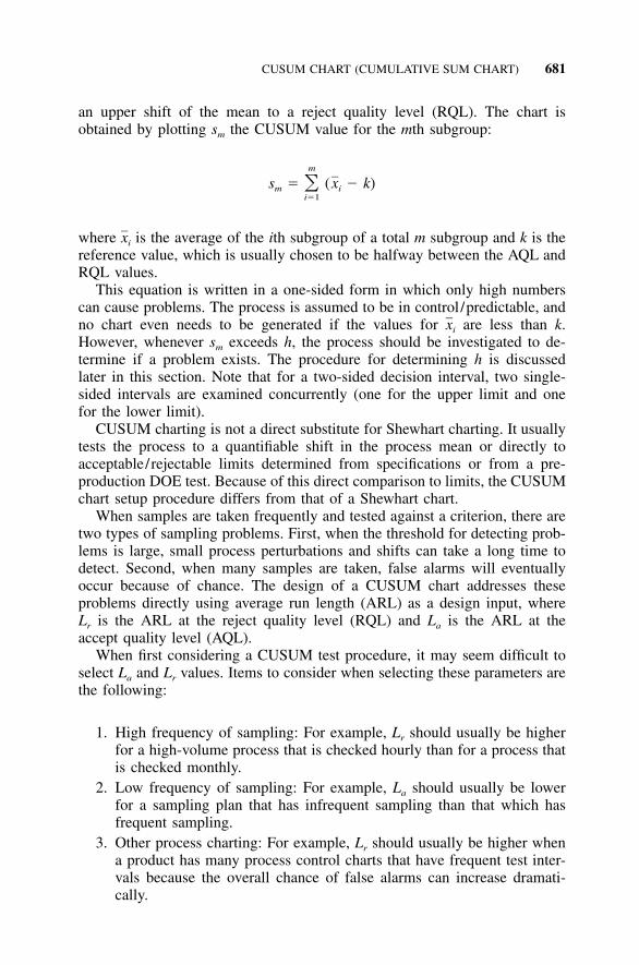
CUSUM CHART (CUMULATIVE SUM CHART) 681

an upper shift of the mean to a reject quality level (RQL). The chart isobtained by plotting sm the CUSUM value for the mth subgroup:

m

s � (x � k)�m ii�1

where is the average of the ith subgroup of a total m subgroup and k is thexi

reference value, which is usually chosen to be halfway between the AQL andRQL values.

This equation is written in a one-sided form in which only high numberscan cause problems. The process is assumed to be in control/predictable, andno chart even needs to be generated if the values for are less than k.xi

However, whenever sm exceeds h, the process should be investigated to de-termine if a problem exists. The procedure for determining h is discussedlater in this section. Note that for a two-sided decision interval, two single-sided intervals are examined concurrently (one for the upper limit and onefor the lower limit).

CUSUM charting is not a direct substitute for Shewhart charting. It usuallytests the process to a quantifiable shift in the process mean or directly toacceptable/rejectable limits determined from specifications or from a pre-production DOE test. Because of this direct comparison to limits, the CUSUMchart setup procedure differs from that of a Shewhart chart.

When samples are taken frequently and tested against a criterion, there aretwo types of sampling problems. First, when the threshold for detecting prob-lems is large, small process perturbations and shifts can take a long time todetect. Second, when many samples are taken, false alarms will eventuallyoccur because of chance. The design of a CUSUM chart addresses theseproblems directly using average run length (ARL) as a design input, whereLr is the ARL at the reject quality level (RQL) and La is the ARL at theaccept quality level (AQL).

When first considering a CUSUM test procedure, it may seem difficult toselect La and Lr values. Items to consider when selecting these parameters arethe following:

1. High frequency of sampling: For example, Lr should usually be higherfor a high-volume process that is checked hourly than for a process thatis checked monthly.

2. Low frequency of sampling: For example, La should usually be lowerfor a sampling plan that has infrequent sampling than that which hasfrequent sampling.

3. Other process charting: For example, Lr should usually be higher whena product has many process control charts that have frequent test inter-vals because the overall chance of false alarms can increase dramati-cally.

682 CONTROL CHARTING ALTERNATIVES

FIGURE 35.2 Nomogram for designing CUSUM control charts. (The labeling re-flects the nomenclature used in Implementing Six Sigma.) [From Kemp (1962), withpermission.]

4. Importance of specification: For example, La should usually be lowerwhen the specification limit is important for product safety and relia-bility.

The final input requirement to the design of a CUSUM chart is the processstandard deviation (�). A preproduction experiment is a possible source forthis information. Note that after the CUSUM test is begun, it may be nec-essary to readjust the sampling plan because of an erroneous assumption oran improvement, with time, of the parameter of concern.

The nomogram in Figure 35.2 can now be used to design the samplingplan. By placing a ruler across the nomogram corresponding to La and Lr ,values for the following can be determined:

�n�� � k�

�

h�n

�

At the reject quality level, � � k is a known parameter; n can be deter-

EXAMPLE 35.2: CUSUM CHART 683

mined from the first equation. With this n value, the second equation can thenbe used to yield the value of h. The data are then plotted with the controllimit h using the equation presented above:

m

s � (x � k)�m ii�1

35.5 EXAMPLE 35.2: CUSUM CHART

An earlier example described a preproduction DOE of the settle-out time ofa selection motor. In this experiment it was determined that an algorithmchange (which had no base machine implementation costs) was important,along with an inexpensive reduction in a motor adjustment tolerance. As aresult of this work and other analyses, it was determined that there would beno functional problems unless the motors experienced a settle-out time greaterthan 8 msec. A CUSUM control charting scheme was desired to monitor theproduction process to assess this criterion on a continuing basis.

If we consider the 8-msec tolerance to be a single-sided 3� upper limit,we need to subtract the expected 3� variability from 8 to get an upper meanlimit for our CUSUM chart. Given an expected production 3� value of 2 (i.e.,� � 2⁄3), the upper accepted mean criterion could be assigned a value of 6(8 � 2 � 6). However, because of the importance of this machine criterionand previous test results, the designers decided to set the upper AQL at 5 andthe RQL at 4. The value for k is then determined to be 4.5, which is themidpoint between these extremes.

Given an Lr of 3 and an La of 800, from Figure 35.2 this leads to

�n�� � k� � 1.11

�

Substitution yields

�n�5.0 � 4.5� � 1.11 so n � 2.19

2/3

Being conservative, n should be rounded up to give a sample size of 3. Inaddition, from Figure 35.2 we can determine

h�n� 2.3

�

Substitution then yields

684 CONTROL CHARTING ALTERNATIVES

FIGURE 35.3 CUSUM chart.

h�3� 2.3 so h � 0.89

2/3

In summary, the overall design is as follows. The inputs were an RQL of4.0 with an associated Lr (ARL) of 3, an AQL of 4.0 with an associated La

(ARL) of 800, and a process standard deviation of 2⁄3. Rational subgroupsamples of size 3 should be taken where a change in the process is declaredwhenever the cumulative sum above 4.5 exceeds 0.89—that is, whenever

m

s � (x � 4.5) � 0.89�� �m ii�1

A typical conceptual plot of this information is shown in Figure 35.3. Intime, enough data can be collected to yield a more precise estimate for thestandard deviation, which can be used to adjust the preceding proceduralcomputations. In addition, it may be appropriate to adjust the k value to themean of the sample that is being assessed, which can yield an earlier indicatorto determine when a process change is occurring.

Other supplemental tests can be useful when the process is stable to un-derstand the data better and to yield earlier problem detection. For example,a probability plot of data by lots could be used to assess visually whetherthere appears to be a percentage of population differences that can be detri-mental. If no differences are noted, one probability plot might be made of allcollected data over time to determine the percentage of population as a func-tion of a control parameter.

EXAMPLE 35.3: CUSUM CHART OF BEARING DIAMETER 685

FIGURE 35.4 Zone chart for viscosity.

35.6 EXAMPLE 35.3: CUSUM CHART OF BEARING DIAMETER

This example illustrates and discusses the output of a statistical computerprogram’s CUSUM analysis.

The data shown in Table 36.1 (Wheeler 1995b; Hunter 1995) are the bear-ing diameters of 50 camshafts collected over time. Figure 36.1 shows a plotof this data as an XmR chart. The data are then analyzed using EWMA andEPC alterntives; however, let’s now analyze this data using CUSUM tech-niques.

A computer analysis yielded for a target of 50 and h � 4.0, k � 0.5 theCUSUM chart shown in Figure 35.4. This chart tracks the cumulative sumsof the deviations of each sample value from the target value. The two one-sided CUSUM chart shown uses the upper CUSUM to detect upward shiftsin the process, while the lower CUSUM detects downward shifts. The UCLand LCL determine out-of-control conditions. This chart is based on individ-ual observations; however, plots can be based on subgroup mean. For an in-control/predictable process, the CUSUM chart is good at detecting smallshifts from the target.

With this plot we note:

• Two one-sided CUSUMs, where the upper CUSUM is to detect upwardshifts in the level of the process and the lower CUSUM is for detectingdownward shifts.

• h is the number of standard deviations between the centerline and controllimits for the one-sided CUSUM.

• k is the allowable ‘‘stack’’ in the process.

686 CONTROL CHARTING ALTERNATIVES

Mean

-2 sigma

-1 sigma

+1 sigma

+2 sigma

-3 sigma

+3 sigma

68.1712

70.1808

72.1904

74.2000

76.2096

78.2192

80.2288

8

4

2

0

0

2

4

8

5 10 15 20

Observation

Weights

4

0 0

2

0

0 0

2

2

0

0 0

0 0 0

2

2

0

0 0

FIGURE 35.5 CUSUM chart of bearing diameters.

• Constant magnitude region when the slope is the same.• Process has shifted at slope change, steeper slope indicates larger change.

35.7 ZONE CHART

A zone chart is a hybrid between an or X chart and a CUSUM chart. Inxthis chart the cumulative score is plotted, based on 1, 2, and 3 samplingstandard deviation zones from the centerline. An advantage of zone chartsover and X charts is its simplicity. A point is out of control simply, byxdefault, if its score is greater than or equal to 8.

With zone charts there is no need to recognize patterns associated withnonrandom behavior as on a Shewhart chart. The zone chart methodology isequivalent to using four of the standard tests for special causes or X chart.xThe zone chart can have a weighting scheme that provides the sensitivityneeded for a specific process.

35.8 EXAMPLE 35.4: ZONE CHART

In Example 10.3, individual viscosity readings from Table 10.2 were plottedto create the XmR chart shown in Figure 10.10. Compare this figure to thezone chart of the data, which is shown in Figure 35.5.

From Figure 35.5 we note:

EXERCISES 687

• Weights are assigned to each zone, which typically equate to 0, 2, 4,and 8.

• Each circle contains the cumulative score for each subgroup or obser-vation.

• The cumulative score is set to zero when the next plotted point crossesover the centerline.

• Weights for points on the same size of the centerline are added. Withthe above-noted weights, the cumulative score of 8 indicates an out-of-control process.

Since no circled value was greater than 8, there are no out-of-control signals.

35.9 S4/IEE ASSESSMENT

CUSUM charting has some basic differences from Shewhart charts. Addi-tional considerations for Shewhart versus CUSUM chart selection are thefollowing:

1. When choosing a control chart strategy using Shewhart techniques, vari-able sample sizes can be difficult to manage when calculating controllimits, while this is not a concern with CUSUM techniques.

2. Shewhart charts handle a number of nonconforming items via p charts,while CUSUM can consider this a continuous variable (e.g., number of‘‘good’’ samples selected before a ‘‘bad’’ sample is found).

3. CUSUM charting does not use many rules to define an out-of-controlcondition, while, in the case of Shewhart charting it can lead to anincrease in false alarms (Yashchin 1989).

35.10 EXERCISES

1. Catapult Exercise: Analyze the exercise catapult data from Chapter 4 usingCUSUM and zone chart techniques.

2. To monitor physical changes from tester handling, the leads of 21 elec-tronic chips in a tray are scanned for bent leads. The average and standarddeviation of the worst dimensions on the 21 parts are noted. A test handlerthen places the parts in position; good parts are placed in one tray and badparts are placed in another. The lead scanner test is repeated. Twenty lotsare evaluated per day and reported on the following worksheets (Spec.max. delta is 0.3).(a) Create a control charting plan.(b) The delta (before-to-after test) for average and standard deviation of

worst dimension on the 21 parts is determined for bent leads and

688 CONTROL CHARTING ALTERNATIVES

recorded in the table format noted below. Create a plan to determineif the process is capable of meeting the maximum allowed specifica-tion limit of 0.3.

(c) Describe S4/IEE possibilities.

Post-test Pre-test Delta

Average of bent leads

Standard deviation of bent leads

3. Explain how the techniques presented in this chapter are useful and canbe applied to S4/IEE projects.

4. Create XmR CUSUM, and zone chart of the following data, where thereis a specification target of 4500 (Wheeler 1995a). Comment on results.

Seq Resistance Seq Resistance

1 4430.00 27 4366.252 4372.50 28 4222.503 3827.50 29 4367.504 3912.00 30 4495.005 5071.25 31 3550.006 4682.50 32 4498.757 4557.50 33 4476.258 4725.00 34 4528.759 4733.75 35 4550.00

10 4372.50 36 3701.2511 4943.75 37 4030.0012 4722.50 38 4781.2513 4278.75 39 4797.5014 4242.50 40 4887.5015 4007.50 41 4760.0016 4006.25 42 4853.7517 4606.25 43 4925.0018 4647.50 44 5041.2519 4441.25 45 4835.0020 4566.25 46 4555.0021 4548.75 47 4566.2522 3846.25 48 4842.5023 4572.50 49 4343.7524 4470.00 50 4361.2525 4676.25 51 5100.0026 4710.00

EXERCISES 689

5. In Example 11.5, I described my desire as the newly elected ASQ sectionchair to increase the attendance at our monthly meetings. Example 19.5described the process changes that were made in preparation of my 9-month term. The XmR chart in Figure 19.5 indicated an increase in atten-dance was accomplished since an out of control conditon and shift in theprocess mean occurred during the last 9 meeting dates on the plot, whichwas when I was chair of the section. The t test in Example 19.5 showedthis difference to be statistically significant. For this exercise create aCUSUM chart of the data in Table 19.2. Consider where it would be bestto set the target since the purpose of the chart would be to determinequickly if a process shift has occurred after the new term has begun.

6. Repeat Exercise 5 using a zone chart. Compare results to an XmR andCUSUM chart.

7. Sheets of manufactured metal are to meet a thickness tolerance throughoutits surface. Create a 30,000-foot-level tracking and reporting strategy. Gen-erate some data according to this strategy and then analyze it. Commenton your results.

8. Describe how and show where the tools described in this chapter fit intothe overall S4/IEE roadmap described in Figure A.1 in the Appendix.

690

36EXPONENTIALLY WEIGHTEDMOVING AVERAGE (EWMA) ANDENGINEERING PROCESSCONTROL (EPC)

S4 /IEE DMAIC Application: Appendix Section A.1, Project ExecutionRoadmap Steps 3.1 and 9.3

Under the Shewhart model for control charting, it is assumed that the meanis constant. Also, errors are to be normal, independent, with zero mean andconstant variance �2. In many applications this assumption is not true. Ex-ponentially weighted moving average (EWMA) techniques offer an alternativebased on exponential smoothing (sometimes called geometric smoothing).

The computation of EWMA as a filter is done by taking the weightedaverage of past observations with progressively smaller weights over time.EWMA has flexibility of computation through the selection of a weight factorand can use this factor to achieve balance between older data and more recentobservations.

EWMA techniques can be combined with engineering process control(EPC) to indicate when a process should be adjusted. Application examplesfor EWMA with EPC include the monitoring of parts produced by a tool thatwears and needs periodic sharpening, adjustment, or replacement.

Much of the discussion in this chapter is a summary of the discussion ofHunter (1995, 1996).

36.1 S4/IEE APPLICATION EXAMPLES: EWMA AND EPC

S4/IEE application examples of EWMA and EPC are:

DESCRIPTION 691

• Manufacturing 30,000-foot-level metric: An S4/IEE project was to de-crease the within- and between-part thickness capability/performance ofmanufactured titanium metal sheets. A KPIV to this process, which washighlighted during the project, is the acid concentration of a chemical-etching step (pickling), which removes metal from the sheet. As part ofthe control phase of the project, an EWMA with EPC procedure wasestablished that would identify when additional acid should be added tothe etching tank.

• Manufacturing 30,000-foot-level metric: An S4/IEE project was to de-crease the within- and between-part variability of the diameter of a metalpart, which was ground to dimension. As part of the control phase of theproject, an EWMA with EPC procedure was established that would iden-tify when adjustments should be made to the grinding wheel because ofwear.

36.2 DESCRIPTION

Consider a sequence of observations Y1, Y2, Y3, . . . , Yt . We could examinethese data using any of the following procedures, with the differences noted:

• Shewhart—no weighting of previous data• CUSUM—equal weights for previous data• Moving average—weight, for example, the five most recent responses

equally as an average• EWMA—weight the most recent reading the highest and decrease

weights exponentially for previous readings

A Shewhart, CUSUM, or moving average control chart for these variablesdata would all be based on the model

Y � � � mt t

where the expected value of the observations E(Yt) is a constant � and mt isNID(0, ). For the Shewhart model the mean and variance are both constant,2�m

with independent errors. Also with the Shewhart model the forecast for thenext observation or average of observations is the centerline of the chart (�0).

An EWMA is retrospective when plotted under Shewhart model conditions.It smoothes the time trace, thereby reducing the role of noise which can offerinsight into what the level of the process might have been, which can behelpful when identifying special causes. Mathematically, for 0 � � � 1 thiscan be expressed as

692 EXPONENTIALLY WEIGHTED MOVING AVERAGE

ˆ ˆEWMA � Y � �Y � �Y where � � (1 � �)s,t t s,t�1

This equation can be explained as follows: At time t the smoothed value ofthe response equals the multiple of lambda times today’s observation plustheta times yesterday’s smoothed value. A more typical plotting expressionfor this relationship is

ˆ ˆ ˆEWMA � Y � Y � �e where e � Y � Yt�1 t t t t t

This equation can be explained as follows: The predicted value for tomorrowequals the predicted value of today plus a ‘‘depth of memory parameter’’(lambda) times the difference between the observation and the current day’sprediction. For plotting convenience, EWMA is often put one unit ahead ofYt. Under certain conditions, as described later, EWMA can be used as aforecast.

The three sigma limits for an EWMA control chart are

�3� � �� / (2 � �) [�3� ]EWMA Shewhart

When there are independent events, an EWMA chart with � � 0.4 yieldsresults almost identical to the combination of Western Electric rules, wherethe control limits are exactly half of those from a Shewhart chart (Hunter1989b).

The underlying assumptions for a Shewhart model are often not true inreality. Expected values are not necessarily constant, and data values are notnecessarily independent. An EWMA model does not have this limitation. AnEWMA can be used to model processes that have linear or low-order timetrends, cyclic behavior, and a response that is a function of an external factor,nonconstant variance, and autocorrelated patterns.

The following example illustrates the application of EWMA and EPC.

36.3 EXAMPLE 36.1: EWMA WITH ENGINEERINGPROCESS CONTROL

The data shown in Table 36.1 (Wheeler 1995b; Hunter 1995) are the bearingdiameters of 50 camshafts collected over time. A traditional XmR chart ofthese data shown in Figure 36.1 indicates that there are many out-of-controlconditions. However, this example illustrates how underlying assumptions forapplication of the XmR chart to this data set are probably violated. EWMAand EPC alternatives are then applied.

First we will check for nonindependence. To do this we will use time seriesanalysis techniques. If data meander, each observation tends to be close to

EXAMPLE 36.1: EWMA WITH ENGINEERING PROCESS CONTROL 693

TABLE 36.1 Camshaft Bearing Diameters

SequenceDiameter

150

251

350.5

449

550

643

742

845

947

1049

SequenceDiameter

1146

1250

1352

1452.5

1551

1652

1750

1849

1954

2051

SequenceDiameter

2152

2246

2342

2443

2545

2646

2742

2844

2943

3046

SequenceDiameter

3142

3243

3342

3445

3549

3650

3751

3852

3954

4051

SequenceDiameter

4149

4250

4349.5

4451

4550

4652

4750

4848

4949.5

5049

FIGURE 36.1 XmR chart of camshaft bearing diameters.

the previous observation and there is no correlation between successive ob-servations. That is, there is no autocorrelation (i.e., correlation with itself).

If observations are independent of time, their autocorrelation should equalzero. A test for autocorrelation involves regressing the current value on pre-vious values of the time series to determine if there is correlation. The termlag quantifies how far back comparisons are made. Independence of dataacross time can be checked by estimation of the lag autocorrelation coeffi-cients �k, where k � 1, 2, . . . . Statistical software packages can performthese calculations. Examples of lag values are

694 EXPONENTIALLY WEIGHTED MOVING AVERAGE

Data Lag 1 Lag 2 Lag 3 Lag 4 Lag 5 Lag 6 Lag 7 Lag 8 Lag 9 Lag 10

50 * * * * * * * * * *51 50 * * * * * * * * *50.5 51 50 * * * * * * * *49 50.5 51 50 * * * * * * *50 49 50.5 51 50 * * * * * *43 50 49 50.5 51 50 * * * * *42 43 50 49 50.5 51 50 * * * *45 42 43 50 49 50.5 51 50 * * *47 45 42 43 50 49 50.5 51 50 * *49 47 45 42 43 50 49 50.5 51 50 *46 49 47 45 42 43 50 49 50.5 51 5050 46 49 47 45 42 43 50 49 50.5 5152 50 46 49 47 45 42 43 50 49 50.552.5 52 50 46 49 47 45 42 43 50 49

� � � � � � � � � � �� � � � � � � � � � �� � � � � � � � � � �

For example, the correlation coefficient between the original and the lag 1data is 0.74. The estimates of the autocorrelation coefficients are then

r1 � 0.74 r6 � �0.02r2 � 0.55 r7 � �0.09r3 � 0.34 r8 � �0.23r4 � 0.24 r9 � �0.23r5 � 0.13 r10 � �0.34

For the hypothesis that all �k � 0 the approximate standard error of rk is, which leads to an approximate 95% confidence interval for �1 of1/�n

, which results in 0.74 � 0.28. Because zero is not containedr � 2/�n1

within this interval, we reject the null hypothesis. The implication of corre-lation is that the moving-range statistic does not provide a good estimate ofstandard deviation to calculate the control limits.

George Box (Hunter 1995; Box and Luceno 1997) suggests using a var-iogram to check adequacy of the assumptions of constant mean, indepen-dence, and constant variance. It checks the assumption that data derive froma stationary process. A variogram does this by taking pairs of observations1, 2, or m apart to produce alternative time series. When the assumptions arevalid, there should be no difference in the expectation of statistics obtainedfrom these differences. For the standardized variogram

EXAMPLE 36.1: EWMA WITH ENGINEERING PROCESS CONTROL 695

Var(Y � Y )t�m tG �m Var(Y � Y )t�1 t

the ratio Gm equals 1 for all values of m, if the data have a constant mean,independence, and constant variance. For processes that have an ultimate con-stant variance (i.e., stationary process), Gm will increase at first but soonbecome constant. When the level and variance of a process grows withoutlimit (i.e., nonstationary processes), Gm will continually increase. For pro-cesses that increase as a straight line, an EWMA gives a unique model.

A simple method to compute Gm is to use the moving-range computationsfor standard deviations. Table 36.2 shows the computations for moving range,while Table 36.3 shows the results of the calculations for each of the sepa-ration steps m. The plot of Gm versus the interval m shown in Figure 36.2 isan increasing straight line, which suggests that an EWMA model is reason-able. An estimate for � can be obtained from the slope of the line. Becausethe line must pass through G(m) � 1 and m � 1, the slope can be obtainedfrom the equation

� xy � [m � 1][G(m) � 1]b � �2 2� x [m � 1]

0(0) � 1(0.552) � 2(1.445) � � � � � 9(5.330)� 2 2 2 20 � 1 � 2 � � � � � 9

155.913� � 0.547

285

An interactive solution of the relationship, where b � 0.547

2�b � 21 � (1 � �)

yields � � 0.76. The limits of the EWMA control chart are determined bythe equation

�3� � �� / (2 � �) [�3� ]EWMA Shewhart

� �0.76/(2 � 0.76)(53.74 � 48.20)

� 0.783 � 5.54 � 4.33

The resulting control limits are then 52.53 and 43.87 (i.e., 48.20 � 4.33 and48.20 � 4.33). The EWMA control chart in Figure 36.3 shows these adjustedcontrol limits from �.

696

TA

BL

E36

.2M

ovin

g-R

ange

Cal

cula

tion

s

Sequ

ence

Bea

ring

Dia

met

erM

Rm

�1

MR

m�

2M

Rm

�3

MR

m�

4M

Rm

�5

MR

m�

6M

Rm

�7

MR

m�

8M

Rm

�9

MR

m�

10

150

251

13

50.5

0.5

0.5

449

1.5

21

550

10.

51

06

437

67.

58

77

421

87

8.5

98

845

32

54

5.5

65

947

25

43

23.

54

310

492

47

61

01.

52

111

463

11

43

43

4.5

54

1250

41

35

87

01

0.5

113

522

63

57

109

23

1.5

1452

.50.

52.

56.

53.

55.

57.

510

.59.

52.

53.

5• • •

• • •

• • •

• • •

• • •

• • •

• • •

• • •

• • •

• • •

• • •

• • •

MR

2.08

2M

R2.

594

MR

3.25

5M

R3.

391

MR

3.68

9M

R4.

045

MR

4.20

9M

R4.

393

MR

4.79

3M

R5.

238

EXAMPLE 36.1: EWMA WITH ENGINEERING PROCESS CONTROL 697

TABLE 36.3 Variogram Computations

m

MovingRange( )MR d2 � � /d2MRYm

� 2Ym

G (m) �2�Ym

2�Y1

1 2.082 1.128 1.845 3.406 1.0002 2.594 1.128 2.299 5.287 1.5533 3.255 1.128 2.886 8.329 2.4464 3.391 1.128 3.006 9.039 2.6545 3.689 1.128 3.270 10.695 3.1406 4.045 1.128 3.586 12.862 3.7777 4.209 1.128 3.732 13.925 4.0898 4.393 1.128 3.894 15.166 4.4539 4.793 1.128 4.249 18.053 5.301

10 5.238 1.128 4.643 21.559 6.331

7

6

5

4

3

2

1

0

0 1 2 3 4 5m

6 7 8 9 10

G(m

) ra

tio

of v

aria

nces

FIGURE 36.2 Variogram plot.

The resulting fitted EWMA model is

ˆ ˆ ˆ ˆ ˆY � Y � 0.76(Y � Y ) � 0.76Y � 0.24Y � 0.76Y � 0.24Yt�1 t t t t t t t

Let us now consider employing the fitted EWMA model. If we let the targetvalue for the camshaft diameters be � � 50 and let the first prediction be

, the fitted EWMA gives the prediction values and errors in TableŶ � 501

36.4. From this table we can determine

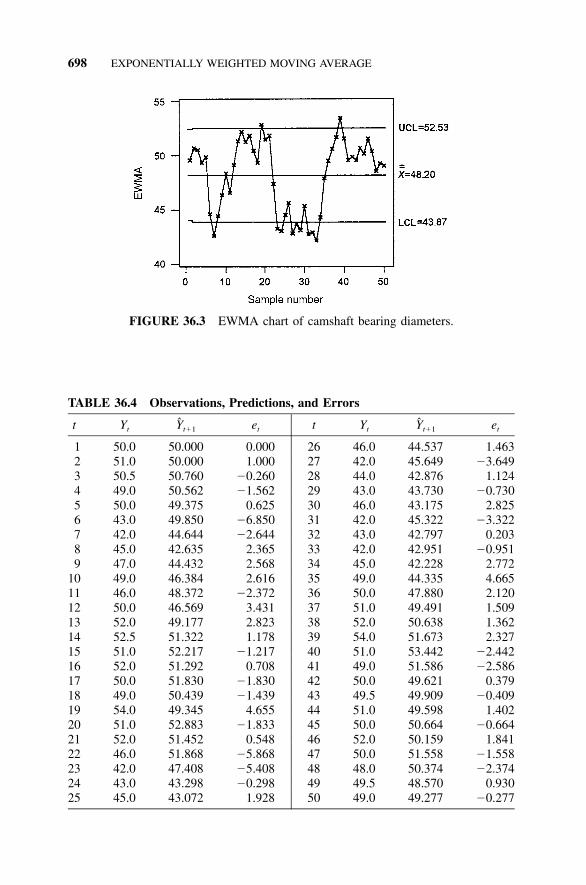
698 EXPONENTIALLY WEIGHTED MOVING AVERAGE

FIGURE 36.3 EWMA chart of camshaft bearing diameters.

TABLE 36.4 Observations, Predictions, and Errors

t Yt Ŷt�1 et t Yt Ŷt�1 et

1 50.0 50.000 0.000 26 46.0 44.537 1.4632 51.0 50.000 1.000 27 42.0 45.649 �3.6493 50.5 50.760 �0.260 28 44.0 42.876 1.1244 49.0 50.562 �1.562 29 43.0 43.730 �0.7305 50.0 49.375 0.625 30 46.0 43.175 2.8256 43.0 49.850 �6.850 31 42.0 45.322 �3.3227 42.0 44.644 �2.644 32 43.0 42.797 0.2038 45.0 42.635 2.365 33 42.0 42.951 �0.9519 47.0 44.432 2.568 34 45.0 42.228 2.772

10 49.0 46.384 2.616 35 49.0 44.335 4.66511 46.0 48.372 �2.372 36 50.0 47.880 2.12012 50.0 46.569 3.431 37 51.0 49.491 1.50913 52.0 49.177 2.823 38 52.0 50.638 1.36214 52.5 51.322 1.178 39 54.0 51.673 2.32715 51.0 52.217 �1.217 40 51.0 53.442 �2.44216 52.0 51.292 0.708 41 49.0 51.586 �2.58617 50.0 51.830 �1.830 42 50.0 49.621 0.37918 49.0 50.439 �1.439 43 49.5 49.909 �0.40919 54.0 49.345 4.655 44 51.0 49.598 1.40220 51.0 52.883 �1.833 45 50.0 50.664 �0.66421 52.0 51.452 0.548 46 52.0 50.159 1.84122 46.0 51.868 �5.868 47 50.0 51.558 �1.55823 42.0 47.408 �5.408 48 48.0 50.374 �2.37424 43.0 43.298 �0.298 49 49.5 48.570 0.93025 45.0 43.072 1.928 50 49.0 49.277 �0.277

EXAMPLE 36.1: EWMA WITH ENGINEERING PROCESS CONTROL 699

Y � 48.2t�1

7752(Y � �) � 775.00 hence s � � 3.98� t � �50 � 1

6132(Y � Y) � 613.00 hence S � � 3.54� t Y �50 � 1

312.472 2ˆ(Y � Y ) � e � 312.47 hence s � � 2.53� �t t t e �50 � 1

From this it seems possible that use of the EWMA as a forecast to controlthe process could result in a very large reduction in variability (i.e., sum ofsquares from 775.00 to 312.47).

A comparison of the autocorrelation coefficients of the original observa-tions with the residuals et after fitting the EWMA model is as follows:

Original Observations Yt EWMA Residuals et

r1 � 0.74 r6 � �0.02 r1 � 0.11 r6 � �015r2 � 0.55 r7 � �0.09 r2 � �0.01 r7 � 0.02r3 � 0.34 r8 � �0.23 r3 � �0.19 r8 � �0.24r4 � 0.24 r9 � �0.23 r4 � �0.03 r9 � 0.13r5 � 0.13 r10 � �0.34 r5 � 0.09 r10 � �0.10

The residuals suggest independence and support our use of EWMA as areasonable model providing useful forecast information of process perform-ance.

Consider now what can be done to take active control. We must be willingto accept a forecast for where a process will be in the next instant of time.When a forecast falls too distant from a target �, an operator can then changesome influential external factor Xt to force the forecast to equal target �. Thisdiffers from the Shewhart model discussed above in that the statistical ap-proach is now not hypothesis testing but instead estimation.

The application of process controls from an external factor can be con-ducted periodically when the response reaches a certain level relative to thespecification. However, for this example we will consider that adjustmentsare made after each reading and that full consequences of taking correctiveaction can be accomplished within the next time interval. Table 36.5 sum-marizes the calculations, which can be explained as follows. Let us considerthat Xt is the current setting of a control factor, where is the forecast.Ŷt�1

Also, we can exactly compensate for a discrepancy of by mak-ˆz � Y � �t t�1

ing the change xt � Xt�1 � Xt. When bringing a process back to its target,we set gxt � �zt, where g is the adjuster gain.

700

TA

BL

E36

.5E

ngin

eeri

ngP

roce

ssC

ontr

olR

esul

ts

tO

rigi

nal

Obs

erva

tion

Adj

ustm

ent

toO

rigi

nal

Obs

erva

tion

New

Obs

erva

tion

EW

MA

e(t

)0.

76�

e(t

)t

Ori

gina

lO

bser

vatio

n

Adj

ustm

ent

toO

rigi

nal

Obs

erva

tion

New

Obs

erva

tion

EW

MA

e(t

)0.

76�

e(t

)

150

0.00

50.0

050

.00

0.00

0.00

2646

5.46

51.4

651

.38

1.46

1.11

251

0.00

51.0

050

.76

1.00

0.76

2742

4.35

46.3

547

.56

�3.

65�

2.77

350

.5�

0.76

49.7

449

.98

�0.

26�

0.20

2844

7.12

51.1

250

.27

1.12

0.85

449

�0.

5648

.44

48.8

1�

1.56

�1.

1929

436.

2749

.27

49.5

1�

0.73

�0.

555

500.

6350

.63

50.1

90.

630.

4830

466.

8252

.82

52.0

32.

822.

156

430.

1543

.15

44.8

4�

6.85

�5.

2131

424.

6846

.68

47.9

6�

3.32

�2.

527

425.

3647

.36

46.7

5�

2.64

�2.

0132

437.

2050

.20

49.6

60.

200.

158

457.

3752

.37

51.0

22.

371.

8033

427.

0549

.05

49.2

0�

0.95

�0.

729

475.

5752

.57

52.2

02.

571.

9534

457.

7752

.77

51.9

12.

772.

1110

493.

6252

.62

52.5

22.

621.

9935

495.

6754

.67

54.0

04.

673.

5511

461.

6347

.63

48.8

0�

2.37

�1.

8036

502.

1252

.12

52.5

72.

121.

6112

503.

4353

.43

52.3

23.

432.

6137

510.

5151

.51

51.7

61.

511.

1513

520.

8252

.82

52.7

02.

822.

1538

52�

0.64

51.3

651

.46

1.36

1.04

1452

.5�

1.32

51.1

851

.54

1.18

0.89

3954

�1.

6752

.33

52.1

22.

331.

7715

51�

2.22

48.7

849

.45

�1.

22�

0.93

4051

�3.

4447

.56

48.6

5�

2.44

�1.

8616

52�

1.29

50.7

150

.40

0.71

0.54

4149

�1.

5947

.41

47.7

1�

2.59

�1.

9717

50�

1.83

48.1

748

.71

�1.

83�

1.39

4250

0.38

50.3

849

.74

�0.

380.

2918

49�

0.44

48.5

648

.60

�1.

44�

1.09

4349

.50.

0949

.59

49.6

3�

0.41

�0.

3119

540.

6554

.65

53.2

04.

653.

5444

510.

4051

.40

50.9

81.

401.

0720

51�

2.88

48.1

249

.34

�1.

88�

1.43

4550

�0.

6649

.34

49.7

3�

0.66

�0.

5021

52�

1.45

50.5

550

.26

0.55

0.42

4652

�0.

1651

.84

51.3

31.

841.

4022

46�

1.87

44.1

345

.60

�5.

87�

4.46

4750

�1.

5648

.44

49.1

4�

1.56

�1.

1823

422.

5944

.59

44.8

3�

5.41

�4.

1148

48�

0.37

47.6

347

.99

�2.

37�

1.80

2443

6.70

49.7

048

.53

�0.

30�

0.23

4949

.51.

4350

.93

50.2

20.

930.

7125

456.

9351

.93

51.1

11.

931.

4750

490.

7249

.72

49.8

4�

0.28

�0.

21

EXERCISES 701

FIGURE 36.4 XmR chart of camshaft bearing diameters (after EPC).

The controlling factor is initially set to zero and the first forecast is 50, thetarget. The table contains the original observations and new observations,which differ from original observations by the amount shown. The differencebetween the new observation and the target of 50 is shown as e(t), while 0.76e(t) represents the new amount of adjustment needed. EWMA is determinedfrom the equation .ˆ ˆY � 0.76Y � 0.24Yt�1 t t

We can see that the XmR chart of the new observations shown in Figure36.4 is now in control/predictable. The estimated implications of control tothe process are as follows:

MeanStandardDeviation

No control 48.20 3.54Every observation control 49.98 2.53

It should be noted that for this situation a chart could be created from theEWMA relationship that describes how an operator in manufacturing shouldadjust a machine depending on its current output.

36.4 EXERCISES

1. Catapult Exercise Data Analysis: Using the catapult exercise data setsfrom Chapter 4, conduct EWMA analyses. Assess whether there is anyvalue in using an EWMA chart and whether an EPC plan should be con-sidered.

702 EXPONENTIALLY WEIGHTED MOVING AVERAGE

2. Repeat the example with process control such that the operator leaves theprocess alone whenever the forecast is within the interval 47.5 �Ŷt�1

� 52.5. If the forecast falls beyond these limits, the process is to beŶt�1

adjusted back to a target of 50.

3. Explain how the techniques presented in this chapter are useful and canbe applied to S4/IEE projects.

4. A manufacturing process produces quality products whenever a grindingwheel is well maintained. Describe how EWMA/EPC could be used inthis process.

5. A manufacturing process that produces sheet metal, which has a tightlytoleranced thickness requirement. The process consistently produces qual-ity product whenever the bath for an etching process step has the correctlevel of acid. Describe how an EWMA/EPC could be used in this process.

6. Describe how and show where the tools described in this chapter fit intothe overall S4/IEE roadmap described in Figure A.1 in the Appendix.

703

37PRE-CONTROL CHARTS

S4 /IEE DMAIC Application: Appendix Section A.1, Project ExecutionRoadmap Step 9.3

A team in 1953 from Rath & Strong, Inc., developed pre-control as an easieralternative to Shewhart control charts. Pre-control (sometimes called stoplightcontrol) monitors test units in manufacturing by classifying them into one ofthree groups (green, yellow, or red). From a small sample the number ofgreen, yellow, and red units observed determines when to stop and adjust theprocess. Since its initial proposal, at least three different versions of pre-control have been suggested. This chapter discusses the classical, two-stage,and modified versions.

37.1 S4/IEE APPLICATION EXAMPLES: PRE-CONTROL CHARTS

S4/IEE application examples of pre-control charts:

• Transactional 30,000-foot-level metric: An S4/IEE project was to reduceDSO for invoices. As part of the control phase for the project, somepredetermined adjustment would be made if a pre-control chart of aKPIV indicated action was needed per specifications for the KPIV, whichwere determined during the project.

• Manufacturing 30,000-foot-level metric: An S4/IEE project was to im-prove the process capability/performance metrics for the diameter of a

704 PRE-CONTROL CHARTS

plastic part from an injection-molding machine. As part of the controlphase for the project, the temperature of a mold would be changed if apre-control chart of mold temperature indicated action was needed perspecifications that were determined during the project.

37.2 DESCRIPTION

Classical pre-control refers to the original method proposed. Two-stage pre-control involves taking an additional sample if initial sample results are am-biguous. Modified pre-control attempts to compromise between the Shewhartcontrol chart type of method and the simplicity of applying pre-control.

The schemes of pre-control are defined by their group classification, de-cision, and qualification procedures. The setup or qualification procedure de-fines the required results of an initial sampling scheme to determine ifpre-control is appropriate for the situation. For all three of these options aprocess passes qualification if five consecutive green units are observed. Dif-ferences between the three versions of pre-control are most substantial in theirmethods of group classification. Classical and two-stage pre-control base theclassification of units on specification limits, while modified pre-control clas-sifies units according to control limits, as defined by Shewhart control charts.

After qualification or setup, a unit is classified as green if its quality char-acteristic is within the central half of the tolerance range (for classical or two-stage pre-control) or control chart limits (for modified pre-control). A yellowunit has a quality characteristic within the remaining tolerance range (forclassical or two-stage pre-control) or control chart limits (for modified pre-control). A red unit has a quality characteristic that is outside the tolerancerange (for classical or two-stage pre-control) or control chart limits (for mod-ified pre-control).

37.3 PRE-CONTROL SETUP (QUALIFICATION PROCEDURE)

Before conducting classical, two-stage, or modified pre-control on a ‘‘run-ning’’ basis, a setup needs to be passed. A unit is classified as green if itsquality characteristic is within the central half of the tolerance range. A yellowunit has a quality characteristic within the remaining tolerance. A red unithas a quality characteristic that is outside the tolerance range. The setup rulesare as follows (Shainin and Shainin 1989):

Setup. OK to run when five pieces in a row are green:A. If one yellow, restart count.B. If two yellows in a row, adjust.C. Return to setup after adjustment, tool change, new operator, or ma-

terial.

MODIFIED PRE-CONTROL 705

37.4 CLASSICAL PRE-CONTROL

With classical pre-control, a unit is classified as green if its quality charac-teristic is within the central half of the tolerance range. A yellow unit has aquality characteristic within the remaining tolerance range. A red unit has aquality characteristic that is outside the tolerance range.

When the setup or qualification rules are satisfied, the following rules areapplied (Shainin and Shainin 1989):

Running. Sample two consecutive pieces, A and B:A. If A is green, continue to run.B. If A is yellow, check B.C. If A and B are yellow, stop.D. If A or B are red, stop.

Average six sample pairs between consecutive adjustment:

Average Time BetweenProcess Adjustments

SamplingInterval

8 hours Every 80 minutes4 hours Every 40 minutes2 hours Every 20 minutes1 hour Every 10 minutes

37.5 TWO-STAGE PRE-CONTROL

Two-stage pre-control has the same red, yellow, and green rules as classicalpre-control. However, with two-stage pre-control, when the setup or qualifi-cation rules are satisfied, the following rules are applied (Steiner 1997):

Sample two consecutive parts.

• If either part is red, stop process and adjust.• If both parts are green, continue operation.• If either or both of the parts are yellow, continue to sample up to three

more units. Continue operation if the combined sample contains threegreen units, and stop the process if three yellow units or a single red unitis observed.

37.6 MODIFIED PRE-CONTROL

With modified pre-control a unit is classified as green if its quality charac-teristic is within the central half of the �three standard deviation control

706 PRE-CONTROL CHARTS

limits defined by Shewhart control charts. A yellow unit has a quality char-acteristic within the remaining control chart bounds. A red unit has a qualitycharacteristic that is outside the control chart limits. When the setup or qual-ification rules are satisfied, the following rules are applied (Steiner 1997):

Sample two consecutive parts.

• If either part is red, stop process and adjust.• If both parts are green, continue operation.• If either or both of the parts are yellow, continue to sample up to three

more units. Continue operation if the combined sample contains threegreen units, and stop the process if three yellow units or a single red unitare observed.

37.7 APPLICATION CONSIDERATIONS

Classical and two-stage pre-control do not require estimates of the currentprocess mean and standard deviation; hence, they are easier to set up than amodified pre-control chart. It has been suggested that pre-control and two-stage pre-control are only applicable if the current process spread of six stan-dard deviations covers less than 88% of the tolerance range (Traver 1985).Modified pre-control has the same goal as an chart but has an excessivelyxlarge false alarm rate and is not recommended (Steiner 1997).

The advantage of the more complicated decision procedure for two-stageand modified pre-control over classical pre-control is that decision errors areless likely. However, the disadvantage is that, on the average, large samplesizes are needed to make decisions about the state of the process.

37.8 S4/IEE ASSESSMENT

Pre-control charting is a technique that causes much debate. Some companiesspecifically state that pre-control charting should not be used. As with alltools (statistical or not), there are applications where a particular tool is bestfor an application, OK for an application, or not right for an application. Pre-control charting can complement a strategy that wisely integrates Shewhartcontrol charts, gage R&R studies, DOE experimentation, FMEA, and so on.Pre-control techniques can also be appropriate when there are auto-correlateddata.

37.9 EXERCISES

1. Explain how the techniques presented in this chapter are useful and canbe applied to S4/IEE projects.

EXERCISES 707

2. A manufacturing process produces quality products whenever a grindingwheel is well maintained. Describe how a pre-control chart could be usedin this process.

3. A manufacturing process produces sheet metal, which has a tightly toler-anced thickness requirement. The process consistently produces qualityproduct whenever the bath for an etching process step has the correct levelof acid. Describe how a pre-control chart could be used in this process.

4. Describe how and show where the tools described in this chapter fit intothe overall S4/IEE roadmap described in Figure A.1 in the Appendix.

708

38CONTROL PLAN, POKA-YOKE,REALISTIC TOLERANCING, ANDPROJECT COMPLETION

S4/IEE DMAIC Application: Appendix Section A.1, Project ExecutionRoadmap Steps 9.1, 9.2, 9.5, and 9.7–9.10

In Section 1.4 IPO was discussed, while SIPOC was discussed in Section1.13. In Section 1.4 process inputs were described using a go-to-school/workprocess as follows:

Inputs to processes can take the form of inherent process inputs (e.g., raw ma-terial), controlled variables (e.g., process temperature), and uncontrolled noisevariables (e.g., raw material lots). For our go-to-work/school process a con-trollable input might be setting the alarm clock, while an uncontrollable inputvariable is whether someone had an accident on our route that affected our traveltime.

The setting of the alarm is indeed a controllable variable, as I described it.However, what we really want is an alarm to sound at a certain point in timefor us to get out of bed so we can leave the house on time, which in turnshould get us to work/school on time.

The question of concern is whether this process is error-proof or mistake-proof. An FMEA of this process would indicate that it is not. For example,we might forget to set the alarm, the power to an electric alarm clock mightbe interrupted during the night, or we might turn off the alarm and go backto sleep.

If KPIV levels are subject to errors, this can be a very large detriment toachieving a consistent system response output over time. To make our processmore error-proof, we might purchase two clocks, one electric and the other

CONTROL PLAN: OVERVIEW 709

battery operated, and place them on the opposite side of the room from thebed so that we have to get up to turn off the alarms. However, we might stillforget to set the alarms. Perhaps this is where a technology solution wouldbe appropriate; e.g., a seven-day programmable clock for wake-up times couldreduce the risk of this error type.

Similarly, it is important to control KPIVs within organizational systems.However, this control mechanism can be more difficult when many peopleare involved in the process. Because of this, we create a control plan thatdocuments this low-level, but important, activity—making the control mech-anism as mistake-proof as possible.

Tracking of KPIVs is at the 50-foot level. This control chart tracking in-volves frequent sampling and reporting such that changes to input levels arequickly detected. Timely corrective action can then be made following theprocedure described in the reaction plan section of the control plan. Thistimely resolution of important process input issues minimizes the unsatisfac-tory impact to 30,000-foot-level output metrics of the process.

This chapter discusses control plans, error-proofing, realistic tolerances,and S4/IEE project completion.

38.1 CONTROL PLAN: OVERVIEW

A control plan is a written document created to ensure that processes are runso that products or services meet or exceed customer requirements at all times.It should be a living document that is updated with both additions and dele-tions of controls based on experience from the process. A control plan mayneed approval of the procuring organization(s).

A control plan is an extension of the control column of an FMEA. TheFMEA is an important source for the identification of KPIVs that are includedwithin a control plan. Other sources for the identification of KPIVs are pro-cess maps, cause-and-effect matrices, multi-vari studies, regression analysis,DOE, and S4/IEE project execution findings.

A control plan offers a systematic approach to finding and resolving out-of-control conditions. It offers a troubleshooting guide for operators throughits documented reaction plan. A good control plan strategy should reduceprocess tampering, provide a vehicle for the initiation/implementation of pro-cess improvement activities, describe the training needs for standard operatingprocedures, and document maintenance schedule requirements. Control plansshould reduce the amount of firefighting and save money through fire-prevention activities.

Control plans should be created from the knowledge gained from otherS4/IEE phases and use not only control charts but also error-proofing. Keyprocess input variables considerations should include monitoring procedures,frequency of verification, and selection of optimum targets/specifications. Un-controllable noise inputs considerations should include their identification,control procedures, and robustness of the system to the noise. Standard op-

710 CONTROL PLAN

erating procedure issues include documentation, ease-of-use, applicability,utilization, updating, and training. Maintenance procedure issues include iden-tification of critical components, scheduling frequency, responsibility, train-ing, and availability of instructions.

AIAG (1995a) lists three types of control plans: prototype, pre-launch, andproduction. A prototype control plan is a description of measurements, ma-terial, and performance tests that are to occur during the building of proto-types. A pre-launch control plan is a description of measurements, material,and performance tests that are to occur after prototype and before normalproduction. A production control plan is a comprehensive documentation ofproduct/process characteristics, process controls, tests, and measurement sys-tems occurring during normal production.

38.2 CONTROL PLAN: ENTRIES

Control plans should be available electronically within the organization. Com-panies often tailor control plans to address their specific needs. Categoriesthat AIAG (1995a) includes in a control plan are noted below. The generalcontrol plan layout is shown in Table 38.1, where the term characteristics inthe table means a distinguishing feature, dimension, or property of a processor its output (product) on which variable or attribute data can be collected.

Header Information

1. Control plan type: Prototype, pre-launch, production.2. Control plan number: A tracking number, if applicable.3. Part number/latest change: Number to describe the system, subsystem

or component that is to be controlled, along with any revision number.4. Part name or description: Name and description of the product or pro-

cess that is to be controlled.5. Supplier/plant: Name of company and appropriate division, plant, or

department that is preparing the control plan.6. Supplier code: Procurement organization identification number.7. Key contact and phone: Name and contact information for primary

person who is responsible for control plan.8. Core team: Names and contact information for those responsible for

preparing the control plan and its latest revision.9. Supplier/plant approval date: If required, obtain approval from re-

sponsible facility.10. Date (original): Date the original control plan was compiled.11. Date (revision): Date of latest update to the control plan.12. Customer engineering approval and date: If required, obtain the ap-

proval of the responsible engineer.

711

TA

BL

E38

.1C

ontr

olP

lan

Ent

ry

No.

Pro

duct

Pro

cess

Siz

eF

req.

Cha

ract

eris

tics

Sam

ple

Con

trol

Met

hod

Rea

ctio

n P

lan

Eva

luat

ion/

Mea

sure

men

t T

echn

ique

Pro

duct

/Pro

cess

S

peci

ficat

ion/

Tol

eran

ceS

peci

al

Cha

r. C

lass

Met

hods

Mac

hine

, Dev

ice,

Jig

, T

ools

for

Mfg

.

Pro

cess

N

ame/

Ope

ratio

n D

escr

iptio

nP

art/P

roce

ss N

umbe

r

Hea

der

Info

rmat

ion

1516

1 to

14

1718

1920

2122

23

24

2526

Sour

ce:

Rep

rint

edw

ithpe

rmis

sion

from

the

AP

QP

Man

ual

(Dai

mle

rChr

ysle

r,Fo

rdM

otor

Com

pany

,an

dG

ener

alM

otor

sSu

pplie

rQ

ualit

yR

equi

rem

ents

Task

Forc

e).

712 CONTROL PLAN

13. Customer quality approval and date: If required, obtain approval ofsupplier quality representative.

14. Other approvals and dates: If required, obtain approvals.

Line-by-Line Items

15. Part or process number: Usually referenced from process flowchart.When there are multiple assembled parts, list individual part numbers.

16. Process name/operation description: All steps in the manufacturing ofa system, subsystem, or component, which are described in a processflow diagram. This line entry contains the process/operation name thatbest describes the activity that is addressed.

17. Machine, device, jig, tools for manufacturing: Identification of theprocessing equipment for each described operation; e.g., machine, de-vice, jig, or other tools for manufacturing.

18. Number characteristic: Cross-reference number from which all appli-cable documents can be referenced; e.g., FMEA.

19. Product characteristic: Features or properties of a part component, orassembly that are described on drawings or other primary engineeringinformation. All special characteristics need to be listed in the controlplan, while other product characteristics for which process controls areroutinely tracked during normal operations may be listed.

20. Process characteristic: Process characteristics are the process input var-iables that have a cause-and-effect relationship with the identifiedproduct characteristics. A process characteristic can only be measuredat the time it occurs. The core team should identify process charac-teristics for which variation must be controlled to minimize productvariation. There could be one or more process characteristics listed foreach product characteristic. In some processes one process character-istic may affect several product characteristics.

21. Special characteristic classification: Customers may use unique sym-bols to identify important characteristics such as those affecting safety,compliance with regulations, function, fit, or appearance. These char-acteristics can be determined, for example, critical, key, safety, or sig-nificant.

22. Product/process specification/tolerance: Sources can include variousengineering documents such as drawings, design reviews, materialstandard, computer-aided design data, manufacturing, and/or assemblyrequirements.

23. Evaluation/measurement technique: Identifies measurement systemthat is used. Could include gages, fixtures, tools, and/or test equipmentthat is required to measure the part /process/manufacturing equipment.An analysis of linearity, reproducibility, repeatability, stability, and ac-curacy of the measurement system should be completed prior to re-

CONTROL PLAN: ENTRIES 713

lying on a measurement system, where improvements are made asapplicable.

24. Sample size and frequency: Identifies sample size and frequency whensampling is required.

25. Control method: Contains a brief description of how the operation willbe controlled, including applicable procedure numbers. The describedcontrol method should be based on the type of process and an effectiveanalysis of the process. Example operational controls are SPC, in-spection, mistake-proofing, and sampling plans. Descriptions shouldreflect the planning and strategy that is being implemented in the pro-cess. Elaborate control procedures typically reference a procedure orprocedure number. Control methods should be continually evaluatedfor their effectiveness in controlling the process. Significant changesin the process or its capability/performance should lead to an evalu-ation of the control method.

26. Reaction plan: Specifies the corrective actions that are necessary toavoid producing nonconforming products or operating out of control(having an unpredictable process). The people closest to the processshould normally be responsible for the actions. This could be the op-erator, jobsetter, or supervisor, which is clearly designated in the plan.Provisions should be made for documenting reactions. Suspect andnonconforming products must be clearly identified and quarantined,and disposition made by the responsible person who is designated inthe reaction plan. Sometimes this column will make reference to aspecific reaction plan number identifying the responsible person.

Example control plan entries using this format are shown in Table 38.2.A control plan checklist is given below (AIAG 1995a). Any negative com-

ment is to have an associated comment and/or action required along withresponsible part and due date.

1. Were the above control plan methods used in preparing the controlplan?

2. Have all known customer concerns been identified to facilitate theselection of special product/process characteristics?

3. Are all special product/process characteristics included in the controlplan?

4. Were the appropriate FMEA techniques used to prepare the controlplan?

5. Are material specifications that require inspection identified?6. Are incoming material and component packaging issues addressed?7. Are engineering performance-testing requirements identified?8. Are required gages and test equipment available?

714

TA

BL

E38

.2E

xam

ple

Con

trol

Pla

nE

ntri

es

No.

Pro

duct

Pro

cess

Siz

eF

req.

3P

last

ic in

ject

ion

mol

ding

Mac

h N

o. 1

-518

App

eara

nce

*F

ree

of b

lem

ishe

sV

isua

l ins

pect

on10

0%C

ontin

uous

100%

insp

Not

ify

supe

rvis

orN

obl

emis

hes

Flo

wlin

es1s

t pie

ce b

uy-o

ffC

heck

she

etA

djus

t/re-

chec

kS

ink

mar

ks1s

t pie

ce b

uy-o

ffC

heck

she

etA

djus

t/re-

chec

k

Mac

hine

No.

1-5

19M

ount

ing

hole

loc.

*H

ole

"X"

loca

tion

Fix

ture

#10

1st p

iece

Buy

-off

per

ru

nC

heck

she

etA

djus

t/re-

chec

k

25 +

/- 1

mm

5 pc

sH

rx-

bar

& R

cha

rtQ

uara

ntin

ean

d ad

just

Mac

hine

No

1-5

20D

imen

sion

*G

ap 3

+/-

.5 m

mF

ixtu

re #

101s

t pie

ceB

uy-o

ff p

er

run

Che

ck s

heet

Adj

ust a

nd

rech

eck

Fix

ture

#10

21P

erim

ente

r fit

*G

ap 3

+/-

.5m

mC

heck

gap

to

fixtu

re 4

loca

tions

5 pc

sH

rx-

bar

& R

cha

rtQ

uara

ntin

e an

d ad

just

Mac

hine

No

1-5

22

Set

-up

of

mol

d m

achi

neS

ee a

ttac

hed

set-

up

card

Rev

iew

of

set-

up

card

and

mac

hine

se

tting

sE

ach

set-

up1s

t pie

ce b

uy-o

ffA

djus

t and

res

et

mac

hine

Insp

ecto

r ve

rifie

s se

tting

No.

Pro

duct

Pro

cess

Siz

eF

req.

3S

olde

ring

conn

ectio

nsW

ave

sold

er

mac

hine

Wav

e so

lder

he

ight

*2.

0 +

/- 0

.25m

cS

enso

r co

ntin

uity

ch

eck

100%

Con

tinuo

us

Aut

omat

ed

insp

ectio

n (e

rror

pr

oofin

g)A

djus

t and

re

test

Flu

x co

ncen

tra

tion

Sta

ndar

d #3

02B

Tes

t sam

plin

g la

b en

viro

nmen

t1

pc4

hour

sx-

MR

cha

rtS

egre

gate

and

re

test

Sam

ple

Con

trol

Met

hod

Par

t/Pro

cess

Num

ber

Pro

cess

N

ame/

Ope

ratio

n D

escr

iptio

nM

achi

ne, D

evic

e, J

i g,

Too

ls fo

r M

f g.

Cha

ract

eris

tics

Spe

cial

C

har.

Cla

ss

Met

hods

Rea

ctio

n P

lan

Pro

duct

/Pro

cess

S

peci

ficat

ion/

Tol

eran

ceE

valu

atio

n/M

easu

rem

ent

Tec

hniq

ue

Par

t/Pro

cess

Num

ber

Pro

cess

N

ame/

Ope

ratio

n D

escr

iptio

nM

achi

ne, D

evic

e, J

ig,

Too

ls fo

r M

f g.

Cha

ract

eris

tics

Spe

cial

C

har.

Cla

ss

Met

hods

Rea

ctio

n P

lan

Pro

duct

/Pro

cess

S

peci

ficat

ion/

Tol

eran

ceE

valu

atio

n/M

easu

rem

ent

Tec

hniq

ue

Sam

ple

Con

trol

Met

hod

Hea

der

Info

rmat

ion

Hea

der

Info

rmat

ion

r

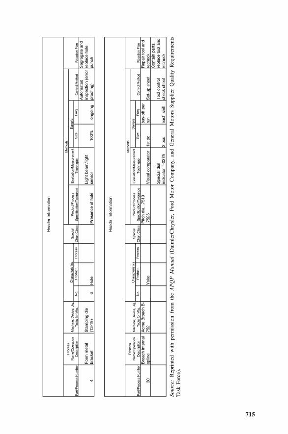
715

No.

Pro

duct

Pro

cess

Siz

eF

req.

4F

orm

met

al

brac

ket

Sta

mpi

ng d

ie

(13-

19)

6H

ole

Pre

senc

e of

hol

eLi

ght b

eam

/ligh

t se

nsor

100%

ongo

ing

Aut

omat

ed

insp

ectio

n (e

rror

pr

oofin

g)

Seg

rega

te a

nd

repl

ace

hole

pu

nch

No.

Pro

duct

Pro

cess

Siz

eF

req.

30B

roac

h in

tern

al

splin

eA

cme

Bro

ach

B-

752

Yok

eP

itch

dia.

.75

10

.752

5V

isua

l com

para

tor

1st p

cbu

y-of

f pe

r ru

nS

et-u

p sh

eet

Rep

air

tool

and

re

chec

k

Spe

cial

dia

l in

dica

tor

T-0

375

2 pc

sea

ch s

hift

Too

l con

trol

ch

eck

shee

t

Con

tain

par

ts,

repl

ace

tool

and

re

chec

k

Sam

ple

Con

trol

Met

hod

Par

t/Pro

cess

Num

ber

Pro

cess

N

ame/

Ope

ratio

n D

escr

iptio

nM

achi

ne, D

evic

e, J

ig,

Too

ls fo

r M

f g.

Cha

ract

eris

tics

Spe

cial

C

har.

Cla

ss

Met

hods

Rea

ctio

n P

lan

Pro

duct

/Pro

cess

S

peci

ficat

ion/

Tol

eran

ceE

valu

atio

n/M

easu

rem

ent

Tec

hniq

ue

Pro

duct

/Pro

cess

S

peci

ficat

ion/

Tol

eran

ceE

valu

atio

n/M

easu

rem

ent

Tec

hniq

ue

Sam

ple

Con

trol

Met

hod

Par

t/Pro

cess

Num

ber

Pro

cess

N

ame/

Ope

ratio

n D

escr

iptio

nM

achi

ne, D

evic

e, J

ig,

Too

ls fo

r M

f g.

Cha

ract

eris

tics

Spe

cial

C

har.

Cla

ss

Met

hods

Rea

ctio

n P

lan

Hea

der

Info

rmat

ion

Hea

deIn

form

atio

n

Sour

ce:

Rep

rint

edw

ithpe

rmis

sion

from

the

AP

QP

Man

ual

(Dai

mle

rChr

ysle

r,Fo

rdM

otor

Com

pany

,an

dG

ener

alM

otor

sSu

pplie

rQ

ualit

yR

equi

rem

ents

Task

Forc

e).

716 CONTROL PLAN

9. If required, has there been customer approval?10. Are gage methods compatible between supplier and customer?

The above guidelines are consistent with the basic S4/IEE method. However,I would suggest including 30,000-foot-level KPOVs wherever appropriate.Obviously S4/IEE project results can have a major influence on the details ofthe control plan as they currently exist within an organization.

38.3 POKA-YOKE

A poka-yoke (pronounced POH-kah YOH-kay) device is a mechanism thateither prevents a mistake from occurring or makes a mistake obvious at aglance. As an industrial engineer at Toyota, Shigeo Shingo was credited withcreating and formalizing zero quality control (ZQC), an approach that reliesheavily on poka-yoke (mistake-proofing or error-proofing).

To understand a poka-yoke application, consider an operator who createscustomized assemblies from small bins in front of him. One approach to thetask would be to give the operator a list of parts to assemble, taking the partsas needed from the bins. This approach can lead to assembly errors by theoperator. He/she might either forget to include a part or add parts that arenot specified. A poka-yoke solution might be to include lights on all bins.When the operator is to create a new assembly, the bins that contain thespecified parts for the assembly light up. The operator then systematicallyremoves one part from each bin and places it in front of himself/herself untilone part has been removed from each bin. The operator knows that theirassembly is complete when no parts remain in front of him/her.

Poka-yoke offers solutions to organizations that experience frequent dis-crepancies in the packaging of their products (e.g., someone forgot to includethe instructions or a mounting screw). Poka-yoke devices can be much moreeffective than simple demands on workers to ‘‘be more careful.’’

38.4 REALISTIC TOLERANCES

Consider that the S4/IEE methods presented earlier identified a critical KPOVand then characterized KPIVs. Consider also that mistake-proofing methodswere not found effective. We would like to create an SPC method to controlthe process inputs, which are continuous.

We can track process inputs through automation or manual techniques. Thistracking can involve monitoring or control. Often we monitor KPOVs onlybecause we are unable to control process inputs. When we can control KPIVcharacteristics, we can predict output capability/performance. Hence, we cancontrol the process through these inputs.

PROJECT COMPLETION 717

When the KPIV-to-KPOV relationship is understood, the establishment ofoptimum levels for KPIVs can be accomplished through the following ap-proach:

1. Identify the target and specification for a critical KPOV.2. Select from previous S4/IEE activities KPIVs that have been shown to

affect the KPOV.3. Explain what has been learned from previous S4/IEE activities (e.g.,

the DOE activities) about the levels of each KPIV that are thought toyield an optimum KPOV response.

4. Plot the relationship between each KPIV and the KPOV on an x–y plotdescribing not only the best-fit line but also the 95% prediction intervalbounds. An approach to do this is to create 30 samples over the rangeof the KPIVs thought to optimize the KPOV. Plot then the relationshipof each KPIV to the KPOV using statistical software to determine the95% prediction bounds for individual points. When creating these re-lationships, consider not only the effect from each KPIV but also thesimultaneous impact of other KPIVs.

5. Draw two parallel lines horizontally from the specification bounds ofthe KPOV to the upper and lower prediction limits.

6. Draw two parallel lines vertically from the intersection of the previouslydrawn lines and the prediction limits.

7. Determine the maximum tolerance permitted for each KPIV by observ-ing the x-axis intersection points of the two vertical lines.

8. Compare the determined KPIV tolerance to existing operating levels.9. Implement changes to the standard operating procedures as required,

documenting changes in the FMEA and control plan.

38.5 PROJECT COMPLETION

Before a project is complete, the process owner needs to agree to the conclu-sions of the S4/IEE project and be willing to take over any responsibilitiesresulting from the project. Organizations need to establish a process for thistransfer of ownership.

One approach to accomplish this transfer is for the black belt to scheduleand then lead a project turnover meeting. If the project owner accepts theproject, the black belt works with the owner to finalize the presentation slides.The process owner and project team then presents the results. However, if theprocess owner rejects the project results/conclusions, the process owner, blackbelt, and champion need to discuss the project. If they agree to continue theproject, agreement needs to be reach as to what specifics need to be addressedwithin the DMAIC procedure. Other options for this meeting are for theproject to be redefined or placed on hold.

718 CONTROL PLAN

Other items that need to be addressed are:

• To maximize gains, a process needs to be established that leverages theresults of a project to other areas of the business. A communicationprocess needs to be established between organizations.

• Organizations need to encourage the documentation of projects such thatothers can understand and use the information learned. A repositoryneeds to be established for storing project information such that otherscan easily search and learn from the project findings.

• Organizations need to check after some period of time to ensure thatproject gains are sustained after the project is completed.

38.6 S4/IEE ASSESSMENT

S4/IEE complements the traditional approach that creates control plans. Pro-cesses that are well established and have no problems using their existingcontrol procedures would not be good S4/IEE project candidates. However,processes that are experiencing problems can be the target of S4/IEE work ifthese processes impact the 30,000-foot-level and satellite-level metrics of theorganization. Results from this S4/IEE work can then directly impact thecontrol plan for this process.

38.7 EXERCISES

1. Explain how the techniques presented in this chapter are useful and canbe applied to S4/IEE projects.

2. In Example 26.2 a multiple regression model was created for cycle time.Create a specification for the KPIV ‘‘D’’ given a cycle time that was tobe between 460 and 500, treating the other factors as noise.

3. Catapult Exercise: Create a control plan for the catapult process.

4. Describe 50-foot-level metrics that could be KPIVs for the S4/IEE projectdescribed in Exercise 1.4. Describe how these metrics would be trackedand/or made error-proof.

5. Describe how and show where the tools described in this chapter fit intothe overall S4/IEE roadmap described in Figure A.1 in the Appendix.

719

39RELIABILITY TESTING/ASSESSMENT: OVERVIEW

S4 /IEE DMAIC Application: Appendix Section A.1, Project ExecutionRoadmap Step 9.4

This chapter is an introduction to the two chapters that follow, which discussthe reliability testing of repairable systems and nonrepairable devices, re-spectively. In this book the Weibull and lognormal distributions are used fornonrepairable device analyses, while the Poisson distribution and nonhomo-geneous Poisson process (NHPP) are used for repairable system analyses.

A test that evaluates the frequency of failure for systems (or the time offailure for devices) can take a long time to complete when the failure ratecriterion is low (or the average life is high). To complete a test in a reasonableperiod of time, the sample may need to be tested in an environment thataccelerates usage. Alternatives for achieving this acceleration in the electron-ics industry include tests at high temperature, high humidity, thermal cycling,vibration, corrosive environments, and increased duty cycle. This chaptercovers some accelerated testing models and a general accelerated reliabilitytest strategy.

39.1 PRODUCT LIFE CYCLE

The ‘‘bathtub’’ curve shown in Figure 39.1 describes the general life cycle ofa product. The downward-sloping portion of the curve is considered to be the‘‘early-life’’ portion, where the chance of a given product failing during a

720 RELIABILITY TESTING/ASSESSMENT: OVERVIEW

FIGURE 39.1 Bathtub curve.

unit of time decreases with usage. The flat portion is the portion of the cyclewhere the failure rate does not change with additional usage. Finally, theincreasing slope portion is the ‘‘wear-out’’ region, where the chance of failureover a unit of time increases as the product’s usage increases.

An automobile is a repairable system that can experience a bathtub lifecycle. New car owners may have to return the vehicle several times to thedealer to remove the ‘‘bugs.’’ Failures during this time are typically due tomanufacturing workmanship problems; a customer may experience problemswith a wheel alignment adjustment, a door not closing properly, or a rattle inthe dashboard. During this early-life period, the frequency of returning thevehicle decreases with vehicle age. After these initial bugs are removed, thecar will usually approach a relatively constant failure rate. When the constantfailure rate portion of life is reached, the vehicle may experience, for example,a mean time between failures (MTBF) rate of 6 months or 10,000 miles.Failures during this period will normally differ from early-life failures for anautomobile; problems may occur with the water pump bearings, wheel bear-ings, brake linings, or exhaust system. Note that at the device level the partsmay be wearing out, but at the system level the overall failure rate may beconstant as a function of usage of the vehicle. However, with usage an au-tomobile then may start to experience an overall increasing failure rate. Dur-ing this period, the frequency of component wear-out and requiredadjustments increases with time. This period of time may contain many ofthe same failures as the constant failure rate period; however, now the fre-quency of repair will be increasing with the addition of wear-out from othercomponents. Wear-out might now involve such components as the steeringlinkage, differential, suspension, and valve lifters.

As discussed earlier, there are repairable systems and nonrepairable de-vices. The automobile is obviously a repairable system because we don’tthrow the vehicle away after its first failure. Other items are not so obvious.For example, a water pump may be repairable or nonrepairable. The mostfrequent failure mode for a water pump may be its bearings. If a water pump

REPAIRABLE VERSUS NONREPAIRABLE TESTING 721

is repaired (rebuilt) because of a bearing failure, then that water pump couldbe considered a repairable system. If a water pump that has never been rebuiltis discarded after a failure, then this device will be considered a nonrepairabledevice.

Other devices are easier to classify as a nonrepairable device. These de-vices include brake pads, headlights, wheel bearings, exhaust pipe, muffler,and the bearings of the water pump. They are discarded after failure.

39.2 UNITS

Even though a failure rate is not constant over time, a single average numberis often reported to give an average failure rate (AFR) over an interval (T1,T2). Because the failure rates of electronic components are so small, they areoften expressed in terms of failures per thousand hours (%/K) rather thanfailures per hour. Another popular scale for expressing the reliability of com-ponents is parts per million (ppm) per thousand hours (ppm/K); ppm/K isoften expressed as FIT (failures in time). A summary of conversions for afailure rate r(t) and AFR is the following (Tobias and Trindade 1995):

5Failure rate in %/K � 10 � r(t)5AFR in %/K � 10 � AFR (T , T )1 2

9Failure rate in FITs � 10 � r(t)9AFR in FITs � 10 � AFR (T , T )1 2

39.3 REPAIRABLE VERSUS NONREPAIRABLE TESTING

Consider first a nonrepairable device. Assume that 10 tires were randomlyselected from a warehouse and tested to wear-out or failure. In this situation,input to an analysis may simply be 10 customer equivalent mileage numbersreflecting when the tire treads decreased to 2.0 mm. From this informationan ‘‘average life’’ (e.g., 60,000 km) and other characteristics could be deter-mined (e.g., 90% of the tires are not expected to fail by 40,000 km). Chapter41 addresses this problem type (reliability of nonrepairable devices) usingWeibull or lognormal analysis techniques.

Consider now a repairable system such as an overall automobile failurerate. The data from this test analysis might be in the following form:

2,000 km: repaired electronic ignition, idling problems8,000 km: pollution device replacement, acceleration problems18,000 km: dashboard brake light repair30,000 km: water pump bearing failure40,000 km: test terminated

722 RELIABILITY TESTING/ASSESSMENT: OVERVIEW

This summary may apply to one of 10 cars monitored for similar infor-mation. Because multiple failures can occur on each test device, a Weibullprobability plot, for example, is not an appropriate direct analysis tool. Forthis situation we are not interested in the percentage of population that failsat a given test time or an average life number; we are interested in the failurerate of the car (or the time between failures).

Extending this conceptual automobile failure example further, consider thefollowing. If the failure rate is believed not to be dependent on the age of theautomobile, then in the example above we may estimate that the failure ratefor the vehicle during a 40,000-km test would be on the average 0.0001failures/km (4 failures/40,000 km � 0.0001) or 10,000 km MTBF (40,000km/4 failures � 10,000) (note that this is a biased estimate for MTBF).However, the ‘‘constant failure rate’’ assumption seems questionable, becausethe time between each succeeding failure seems to be increasing. Chapter 40addresses this type of problem (reliability of repairable systems with constantand decreasing/increasing failure rates) using the Poisson distribution or theNHPP with Weibull intensity.

39.4 NONREPAIRABLE DEVICE TESTING

The two-parameter Weibull distribution is often used for the analysis of non-repairable device failure times because it can model any one of the threesituations commonly encountered as a function of device age: reducingchance of failure, constant chance of failure, and increasing chance of failurefor a time increment.

The Weibull cumulative distribution function takes the form

bF(t) � 1 � exp[� (t /k) ]

where t represents time, b is the shape parameter, and k is the scale parameter(or characteristic life). If both k and b are known, a cumulative failure value[F(t)] can be determined for any value of time (t). For example, F(100,000hr) � 0.9 indicates that 90% of the population is expected to fail before ausage of 100,000 hr. The purpose of a test and corresponding data analysesthen becomes a means to estimate the unknown parameters of the equation.

Much can be understood about a device failure mode if the shape parameterb is known. The probability density function (PDF) for several shape para-meters is shown in Figure 39.2. Numerically, this shape parameter b indicatesthe following relative to Figure 39.1:

b � 1: early life, decreasing failure rate with usageb � 1: random or intrinsic failures, constant failure rate with usageb � 1: wear-out mode, increasing failure rate with usage

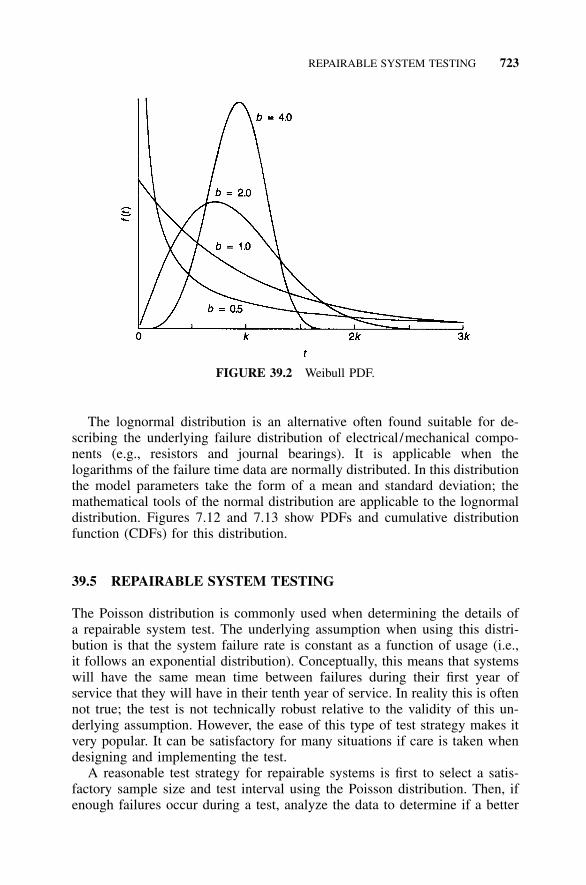
REPAIRABLE SYSTEM TESTING 723

FIGURE 39.2 Weibull PDF.

The lognormal distribution is an alternative often found suitable for de-scribing the underlying failure distribution of electrical/mechanical compo-nents (e.g., resistors and journal bearings). It is applicable when thelogarithms of the failure time data are normally distributed. In this distributionthe model parameters take the form of a mean and standard deviation; themathematical tools of the normal distribution are applicable to the lognormaldistribution. Figures 7.12 and 7.13 show PDFs and cumulative distributionfunction (CDFs) for this distribution.

39.5 REPAIRABLE SYSTEM TESTING

The Poisson distribution is commonly used when determining the details ofa repairable system test. The underlying assumption when using this distri-bution is that the system failure rate is constant as a function of usage (i.e.,it follows an exponential distribution). Conceptually, this means that systemswill have the same mean time between failures during their first year ofservice that they will have in their tenth year of service. In reality this is oftennot true; the test is not technically robust relative to the validity of this un-derlying assumption. However, the ease of this type of test strategy makes itvery popular. It can be satisfactory for many situations if care is taken whendesigning and implementing the test.

A reasonable test strategy for repairable systems is first to select a satis-factory sample size and test interval using the Poisson distribution. Then, ifenough failures occur during a test, analyze the data to determine if a better

724 RELIABILITY TESTING/ASSESSMENT: OVERVIEW

fit could be made using the NHPP model, which can consider failure rate asvarying as a function of usage.

When designing a test to certify a criterion (failures/unit time or MTBF)using the Poisson distribution, the design consideration to determine is thetotal test time. For example, a test criterion for an automobile might be 7000km MTBF or 1/7000 failures/km. From Table K (using the concepts illus-trated in Section 40.7), it can be determined that a proposed test to verifythat the 90% confidence interval (i.e., for � � 1/7000 failures/km), whilepermitting eight failures, would be a total test time of about 90,965 km.

Because the underlying assumption is that the failure rate does not changeas a function of usage, two extremes for the physical test are either to testone automobile for 90,965 km or to test 90,965 automobiles for 1 km. Thefirst test alternative is perhaps physically achievable; however, by the timethe test is completed, knowledge gained from the test relative to its criterionmay be too late to affect the design. These test results may then be used forinformation only. The alternative extreme of a 90,963 sample size is notrealistic because it is too large for a complex system test. Both these testextremes would be very sensitive to the accuracy of the underlying assump-tion of a constant failure rate.

Chapter 40 discusses realistic compromises between the sample size andthe test duration for individual systems. That chapter also analyzes the results,taking into account that the failure rate changes as a function of usage.

Another test consideration that might be applicable and advantageous toconsider is the modeling of the positive improvement displayed during reli-ability tests resulting from changes in product design or in the manufacturingprocess. US Department of Defense (1980, 1981a), Crow (1975), and Dwaine(1964) discuss the modeling of ‘‘reliability growth.’’

39.6 ACCELERATED TESTING: DISCUSSION

Reliability certification of electronic assemblies can be difficult because fail-ure rate criteria are low and time and resource constraints are usually ag-gressive. Accelerated testing techniques are often essential to completecertification within a reasonable time and with reasonable resources. However,care must be exercised when choosing an accelerated test strategy. A modelthat does not closely follow the characteristics of a device can result in aninvalid conclusion. The following sections give a general overview of accel-erated test models.

Product technology, design, application, and performance objectives needto be considered when choosing stress tests for a product. After the stresstests are chosen, stress levels must not change the normal product failuremodes. Without extensive model validation in the proposed experiment, anacceleration model should be technically valid for the situation and imple-mented wisely for sample size and test duration limitations. Unfortunately,because of test constraints, model applicability may only be speculative. In

HIGH-TEMPERATURE ACCELERATION 725

addition, the results from a lack-of-fit analysis might not very decisive be-cause of test sample size constraints.

Often a simple form of acceleration is implemented without any awarenessthat the test is being accelerated. For example, a device under test may besubjected to a reliability test 24 hours per day, 7 days a week (i.e., 168 hoursper week). If we believe that a customer will only use the device 8 hours aday, 5 days a week (i.e., 40 hours per week), our test has a customer usagetime acceleration of 4.2 (i.e., 168/40). Even with this simple form of accel-eration, traps can be encountered. This test assumes that the sample is testedexactly as a customer uses the product. This assumption may not be valid;for example, on/off cycling may be ignored during the test. This cyclingmight cause thermal or electrical changes that contribute significantly to fail-ures in the customer environment. Or perhaps even zero run time in thecustomer’s facility causes a significant number of failures because of corrosiveor high-humidity conditions. Again, care must be exercised to protect againstperforming an accelerated test that either ignores an underlying phenomenonthat can cause a significant number of failures or has an erroneous accelera-tion factor. Perhaps too much emphasis is often given to the confidence levelthat the product will be equal to or better than the criteria, as opposed to thebasic assumptions that are made in the test design.

Accelerated tests can use one or more of many stress test environments(e.g., high temperature, thermal cycling, power cycling, voltage, high current,vibration, high humidity, and mechanical stress). The following discussionincludes model considerations for elevated temperature and thermal cyclingtests.

39.7 HIGH-TEMPERATURE ACCELERATION

A common acceleration model used in the electronics industry is the Arrhe-nius equation. This model suggests that degradation leading to componentfailure is governed by a chemical and physical process reaction rate. Thishigh-temperature model yields a temperature acceleration factor (At) of

A � exp[(E /k)(1/T � 1/T )]t a u s

whereEa � activation energy (eV), function of device type/technology/mecha-

nismk � Boltzmann’s constant, 8.617 � 105 (eV/K)

Tu � unstress temperature (K)Ts � stress temperature (K)K � 273.16 � �C

This equation was originally generated to predict the rate of chemical re-actions. It is often applied to electronic component testing because many

726 RELIABILITY TESTING/ASSESSMENT: OVERVIEW

FIGURE 39.3 An example of the effects from activation energy assumptions.

failure mechanisms are dependent on such reactions. A key parameter in thisequation is the activation energy, which commonly ranges from 0.3 to 0.7 eV,depending on the device. Jensen and Petersen (1982) summarize activationenergies that have been found applicable for certain device types, while Figure39.3 illustrates the sensitivity of the equation to activation energy constantassumptions.

Multiple temperature stress cells can be used to determine the activationenergy using the following equation, which is in a form conducive to a simpleanalysis of a two-cell temperature test T1 and T2. To use this equation, firstdetermine the 50% failure point for each cell ( ) using Weibull orT and T50 501 2

other analysis techniques discussed in this text (note that it is not requiredthat 50% of the sample fail to make a T50 estimate). The ratio of isT /T50 501 2

the best estimate for the acceleration factor (At). The activation energy (Ea)can then be determined using the equation (Tobias and Trindad 1995)

�1T 1 1501E � k ln � T � T� � ��� �a 2 1T T T50 1 22

Assembly testing offers the additional challenge of multiple component typeswith various activation energies. One approach for such a test is to determinean overall activation energy for the assembly. Jensen and Petersen suggestthat ‘‘at the present time, and lacking further information, we would, forintegrated circuits, be inclined to follow Peck and Trapp (1978) and suggesta value of 0.4 eV for an otherwise unspecified freak population failure,’’ where

EYRING MODEL 727

a freak population is produced by random occurrences in the manufacturingprocess. To add more uncertainty to the number, Jensen and Petersen statethat activation is not necessarily constant as a function of test temperature.

In addition to an activation energy constant, the Arrhenius equation needstemperature inputs. In component tests these inputs should be measured indegrees Kelvin on the component where the failure process is taking place.In an assembly, temperature varies as a function of component position, type,and usage; for practical considerations, some test designers use the moduleambient temperature.

Additional discussion of the application of the Arrhenius equation is foundin Nelson (1990), Tobias and Trindade (1995), Jensen and Petersen (1982),and Sutterland and Videlo (1985).

39.8 EXAMPLE 39.1: HIGH-TEMPERATURE ACCELERATIONTESTING

The life criterion of an electronic component needs verification using a high-temperature test. Given an ambient operating temperature of 35�C, a stresstemperature of 85�C, and an activation energy of 0.6, determine the test ac-celeration (At).

Converting the centigrade temperatures to degrees Kelvin yields

T � 35 � 273 � 3080

T � 85 � 273 � 358s

Substitution yields

A � exp[(E /k)(1/T � 1/T )]t a u s

�5� exp[(0.6/8.617 � 10 )(1/308 � 1/358)]

� exp[6963(1/308 � 1/358)] � 23.5

39.9 EYRING MODEL

Most of the well-known acceleration functions can be considered special casesof the general Eyring acceleration function. This model also offers a generalsolution to the problem of combining additional stresses.

The Arrhenius model is an empirical equation that justifies its use by thefact that it ‘‘works’’ in many situations. The Eyring model has the addedstrength of having a theoretical derivation based on chemical reaction ratetheory and quantum mechanics. For the time to fail of 50% of the population(T50), the generalized form of the Eyring model equation is

728 RELIABILITY TESTING/ASSESSMENT: OVERVIEW

ZT � AT [exp(E /kT)]{exp[B � (C /T)]S }50 a 1

where temperature (T) is one stress and S1 is a second stress; A, B, C, and Zare constants. Several notes should be made about this equation:

1. The Eyring model equation describes failures at one condition. A testacceleration factor can be calculated by taking the ratio of two of theseequations with different input conditions. When this mathematical op-eration is performed, the A constant will cancel.

2. Many expressions originate from an Eyring model, but do not finallyappear to do so. For example, the temperature/voltage stress model inthe following equation is thought to apply under a certain situation.

BT � A[exp(E /kT)](V )50 a

The generalized two-stress Eyring equation reduces to this form by substi-tuting Z � 0, C � 0, and S1 in V (where V is in volts).

3. T50 represents the time when 50% of the test units will fail. Other per-centiles can be represented similarly.

4. The term TZ[exp(Ea /kT)] models the effect of temperature and compareswith the Arrhenius model if Z is close to 0.

5. Additional stresses (S2) can be added as factors in the following form:

T50 � ATZ[exp (Ea /kT)]{exp [B � (C /T)]S1}{exp [D � (E/T)]S2}

Each additional set of factors adds two more unknown constants (e.g., Dand E), making the model more difficult to work with in a general state. Anexperiment requires at least as many separate stress cells as there are unknownconstants in the model.

6. Choosing the units to use in a model equation can be a problem. Tem-perature is in degrees Kelvin. But, for example, how should voltage orhumidity be calculated? The theoretical model derivation does not spec-ify units. The experimenter must either (a) work it out by trial and erroror (b) derive an applicable model using arguments from physics andstatistics.

39.10 THERMAL CYCLING: COFFIN–MANSON RELATIONSHIP

The inverse power law is used to model fatigue failure of metals subjectedto thermal cycling. For the purpose of accelerated testing, this model is calledthe Coffin–Manson equation (Coffin 1954, 1974; Manson 1953, 1966) andcan be expressed in the form

MODEL SELECTION: ACCELERATED TESTING 729

At � (�TS /�Tu)B

where At is the acceleration factor and B is a constant characteristic of themetal, test method, and cycle. �Tu is the temperature change under normaloperation, while �TS is the temperature change under stress operation. Theconstant B is near 2 for metals, while Nelson (1990) states that for plasticencapsulates for microelectronics, B is near 5.

An application of this equation is in the electronics industry. Heating/cooling conditions often occur inside the covers of a product because ofsimple on/off cycling. Thermal changes cause expansion/contraction in aproduct. If solder joints are weak and the thermal change is sufficiently large,stresses can then occur in solder joints, causing fractures which can lead toproduct failure.

In the electronics industry, modifications are sometimes needed to the basicCoffin–Manson equation. For example, Norris and Landzberg (1969) notedthat for tin-lead solders used in C-4 (controlled collapse chip connections),joints at room temperature are at about 50% of their absolute melting tem-perature. They state: ‘‘The Coffin–Manson equation was found to be inade-quate for projecting the thermal failure of solder interconnections; inlaboratory experiments it was found to yield very pessimistic estimates offatigue lifetimes.’’ They add a frequency-dependent term and an Arrheniustemperature-dependent term to form a ‘‘modified Coffin–Manson’’ equation.

Tummala and Rymaszewski (1989) present a modified Coffin–Mansonequation of

0.3 1.9ƒ �Tu SA � exp[(0.123/k)(1/T � 1/T )]� � � �t u S ƒ �Ts u

where the added terms ƒu and ƒS reflect the frequency of cyclic changes inuse and stress conditions, respectively. Tu and TS represent the maximum useand stress temperature in the cycles in degrees Kelvin; k is Boltzmann con-stant.

Other treatments of the Coffin–Manson equation are Engelmaier (1985),Goldmann (1969), Tobias and Trindade (1995), Nachlas (1986), and Nishi-mura et al. (1987). Saari et al. (1982) have an additional discussion on thermalcycle screening strengths in a manufacturing environment.

39.11 MODEL SELECTION: ACCELERATED TESTING

Previous sections in this chapter included only a handful of the acceleratedfailure test alternatives suggested in the literature. Other stresses, such ashumidity, voltage, current, corrosive gas, and vibration, are sometimes usedin industry for accelerated tests.

730 RELIABILITY TESTING/ASSESSMENT: OVERVIEW

In choosing an accelerated test strategy for reliability certification, keep inmind that model selection and test strategy can dramatically affect a productpass-versus-fail test position. In order to be valid, the accelerated test meth-odology must not change the failure mode of the component. Care must beexercised when making a confidence interval assessment after using an ac-celerated test model because, in reality, much unknown error can exist in the‘‘acceleration factor number.’’

Each model is most appropriate for a specific component failure mecha-nism. Assemblies can contain many components with different failure mech-anisms, which makes the selection of test models even more difficult.Additional discussion on the application of acceleration models is providedin Nelson (1990) and in Tobias and Trindade (1995). These references alsodiscuss step stress testing where, for example, the temperature stress on a setof test components is increased periodically and the time to failure is notedat each temperature level.

39.12 S4/IEE ASSESSMENT

When choosing a basic test strategy for a given situation, consider the fol-lowing:

1. Determine whether the units under test are repairable or nonrepairable.2. Determine through consultation and a literature search the most accurate

accelerated test modeling strategy that will suffice for the test con-straints yet capture the failure modes that the customer might experi-ence. Note, for example, that a test that constantly exercises acomponent only at an accelerated high-temperature environment is notevaluating possible failure modes caused by thermal cycling.

3. Determine a sample size, test duration (per unit), and number of per-missible failures using detailed test strategies discussed in the next twochapters.

4. List all the test assumptions.

Reliability tests are usually performed to verify that the frequency of failuresof a component or assembly is below a criterion. Often this test is performedduring initial model builds or initial production.

One of the major assumptions that is often compromised in a typical re-liability test is that the sample is randomly taken from the population ofinterest. Often with qualification tests the population of interest is really futureproduct production. For this situation a better strategy may be to test a productspecially manufactured to represent the variability ‘‘space’’ of a productionprocess. Special test samples can be manufactured according to DOE consid-erations. This strategy has the added advantage that a major process problem

S4 / IEE ASSESSMENT 731

can be detected before mass production is begun; i.e., when a manufacturingfactor is at its low tolerance setting, the product failure rate is significantlyincreased. This advantage can outweigh the sacrifice in a loss of randomi-zation given that ‘‘random’’ sample from an early manufacturing process maybe far from representative of the product that the customer will actually re-ceive.

DOE can also have reliability test output considerations for each trial. Forexample, consider that the failure rate of a system needs to be reduced inorder to increase customer satisfaction. A fractional factorial experiment couldbe used to evaluate proposed design changes, where special systems wouldbe built according to the trial factor considerations. If all test units wereoperated to failure, the time of failure or a failure rate could be analyzed asa response for each trial. Note that a data transformation may be required.However, it may be difficult to test long enough for all test units to fail. Forthis reason, it would be advantageous to monitor periodically during the testsome response that typically degrades in unison with the life characteristicsof the device. For this response, the factors that appear to be statisticallysignificant would then be presumed to affect the system failure rate signifi-cantly. The factor levels that are found to be best from this experiment shouldthen be considered important when making changes to the design.

In some system situations it might be assumed erroneously that the majorsource of customer problems is component failures. It is common for thecustomer to experience a problem that depends on how he or she used theproduct. When the inherent failure rate of components is very low, it is verydifficult to quantify a reliability failure rate. Perhaps more effort should bemade to ensure that the product meets the real needs of the customer, in lieuof a simple ‘‘build them and test them’’ strategy.

In the electronics industry, systems or components are often run-in orburned-in (i.e., screened) to capture early-life failures before the productreaches the customer’s office. However, it is not reasonable to expect that thistest will capture all problem escapes of the manufacturing process. If theproduct does experience an early-life failure mode, it is reasonable to expectthat the quality experienced by the customer will be better because of theburn-in/run-in test.

After a burn-in/run-in test time is determined, a failure rate tracking chartcan be used to monitor over time the proportion that fails during the test.When special causes are identified in the chart, it is reasonable to expect thatthe customer will also have an increased failure rate because, as noted earlier,all individual machine problems will not normally be captured during thistest. In a stable process over some period of time, a list of failure causes canbe generated and presented in a Pareto chart. Reduction of the vital few causescan then be addressed using fractional factorial experiment techniques or per-haps by making some obvious changes to the process. Statistically significantimprovements that reduce the number of the causes of failures in the manu-facturing process could later be detected as an out-of-control condition (for

732 RELIABILITY TESTING/ASSESSMENT: OVERVIEW

the better) in the overall failure rate control chart of the burn-in station. Thisprocedure can then be repeated for further improvements.

In time it is desirable to improve the basic manufacturing process enoughto produce a dramatic, consistent reduction in the overall failure rate. If thishappens, it might be appropriate to change the 100% burn-in/run-in procedureto a sampling plan for the detection of special causes. It should be noted,however, that even though the burn-in/run-in (i.e., screen) test may experienceno failures, customers may be having many difficulties. A Pareto chart of thecause of field problems can be illuminating. Perhaps the burn-in/run-in testis evaluating the wrong things and missing many of the problems experiencedby customers. The tester function may need to be changed to capture thesetypes of problems.

39.13 EXERCISES

1. Explain how the techniques presented in this chapter are useful and canbe applied to S4/IEE projects.

2. Describe how and show how reliability testing fits and overall productfield reliability measurements fit into the overall S4/IEE roadmap describedin Figure A.1 in the Appendix.

733

40RELIABILITY TESTING/ASSESSMENT: REPAIRABLESYSTEM

S4/IEE DMAIC Application: Appendix Section A.1, Project ExecutionRoadmap Step 9.4

This chapter explores the problem of ‘‘certifying’’ the failure rate criterion(failures per unit of time, �a) or mean time between failures (MTBF) criterionof a system, where a system is defined as a collection of components andcomponents are replaced or repaired whenever a failure occurs.

Both constant and changing failure rate situations are considered. The Pois-son distribution can be used when the system failure rate is constant as afunction of the age of a system. The nonhomogeneous Poisson process(NHPP) with Weibull intensity can often be used when the failure ratechanges as a function of system usage.

40.1 CONSIDERATIONS WHEN DESIGNING A TEST OF AREPAIRABLE SYSTEM FAILURE CRITERION

One of several test design alternatives could be chosen to certify a repairablesystem failure rate criterion. In this chapter, classical test design alternativesare discussed along with some extensions and S4/IEE assessments.

The techniques discussed in this chapter address the rate at which systemsexperience failures as a function of time. Criteria expressed in units of MTBFneed to be transformed by a simple reciprocal conversion. For example, anMTBF rate of 10,000 hours can be converted to a failure rate criterion of0.0001 failures/hour (1/10,000 � 0.0001).

734 RELIABILITY TESTING/ASSESSMENT: REPAIRABLE SYSTEM

Reliability tests can be either sequential or fixed-length. With the sequentialapproach, test termination generally occurs after either the product has ex-hibited few enough failures by some point in time during test for a ‘‘pass’’decision (with � risk of error) or enough failures have occurred to make a‘‘fail’’ decision (with � risk of error). The other alternatives are either fixed-length or fixed-failure tests. Because fixed-failure tests are not terminated untila predetermined number of failures has occurred and most test situations haveschedule/time constraints, time-terminated tests are the normal choice forfixed-length test strategies.

System failure rate test designs often initially assume that the failure rateis constant as a function of system age. This can lead to the selection of thePoisson distribution for these test designs and analyses. With the Poissondistribution, total usage on all systems is the parameter of concern; it theo-retically does not matter how many units are on the test to achieve this totaltest usage value. For example, in a 15,000-hour fixed-length test, it does nottechnically matter if one unit is exercised for 15,000 hours or 15,000 unitsare exercised for 1 hour.

Theoretically, these scenarios may be the same, but in reality the two testextremes may yield quite different results. If one of these two extremes werechosen, dramatic differences can be expected if the ‘‘constant failure rate’’assumption is invalid. This type of test evaluation is not robust to the under-lying assumption not being valid. The following discussion considers teststrategies that can be used to reduce the risk of getting an answer that hasminimal value.

Technically, before using the Poisson distribution for test design, the ana-lyst should determine that the failure rate of the system is a known constant(flat part of a bathtub curve) for the time of concern (product warranty orproduct useful life). However, process problems can cause more early-lifefailures, while wear-out phenomena can cause the instantaneous system fail-ure rate to increase as a function of usage on the product. In reality, theexperimenter does not know for sure that this response will be constant. How-ever, if care is exercised when making initial decisions relative to sample sizeversus individual sample usage, error due to unknown information about theshape of this intensity function can be minimized.

When a test is being designed, consideration must be given to the realobjective or concern. If concerns are about capturing wear-out problems, asmall number of systems need to be tested for a long period of time. Ifconcern is whether manufacturing or early-life problems exist, a larger num-ber of samples should be tested for a shorter period of time. If there areconcerns about early life and wear out, it may be most cost-effective to ex-ercise a large sample for a short period and then continue the test for a subsetof machines to product life usage to assess system wear-out exposures.

If a warranty or maintenance criterion needs to be assessed to ensure thatfailures will not exceed targets, then it may be best for the test duration perunit to equal the warranty or maintenance agreement period. If a sufficientnumber of failures occurs during this test, then the NHPP can be used to

SEQUENTIAL TESTING: POISSON DISTRIBUTION 735

determine if and how failure rates are changing as a function of usage onindividual systems.

Failure rate tests during product development are sometimes expected togive an accurate confidence interval assessment of what the failure rate willbe when the product is built in production. If there is concern about designand manufacturing problems, does it make sense to take a ‘‘random’’ sampleof the first parts that are produced to certify a criterion? A random sample offuture products is needed to test for design and manufacturing problems.Assemblies produced within the same short time period tend to be similar;these samples do not necessarily represent the product ‘‘space’’ (i.e., boundarylimits) of design tolerances and manufacturing variability.

In lieu of classical reliability testing, other economical alternatives maycapture the problems that can haunt a manufacturer later during production.Initial lot sampling may not expose design and process problems that in factexist, because the sample is representative only of the current lot population.Example 43.2 discusses alternatives to replace or supplement this classicaltest approach in capturing such elusive problems earlier in the product designand manufacturing processes.

Again, fixed-length and sequential test plans (US Department of Defense1986, 1987) are the two general types of test strategies applicable to systemfailure rate certification. Fixed-length test plans are more commonly used, butsequential test plan alternatives are also discussed. The results from thesetests can also give a confidence interval for the failure rate of the productpopulation from which the sample is drawn. It is assumed in this test that themanufacturing process is stable and that there will be no design changes tothe product during test. In addition, it is assumed for the tests described thatsample size is small relative to population size. For this last assumption tobe true, it is best that the ratio of sample size to population size not exceed10%.

A sequential test plan is considered the best test alternative when it is arequirement to either accept or reject predetermined failure rate values (�0

and �1) with predetermined risks of error (� and �). With sequential testing,uncertainty must be expected with regard to total test time.

A fixed-length test plan is appropriate when the total test time must beknown in advance. In this chapter, two alternatives for this type of test arediscussed. Section 40.2 discusses sample size for hypothesis test where both� and � risks are considered, while Section 40.7 offers a reduced sample sizetesting strategy option. This second test approach can be used to certify sys-tem criteria, with the understanding that the real test purpose is to obtain aconfidence interval for the true failure rate and then compare the single-sidedlimit to the criterion.

40.2 SEQUENTIAL TESTING: POISSON DISTRIBUTION

For sequential plans, in addition to both � and � risks, two failure rates (�0

and �1) are needed as input. If a system has only one criterion (�a) and this

736 RELIABILITY TESTING/ASSESSMENT: REPAIRABLE SYSTEM

criterion is be certified with a consumer risk �, the highest failure rate �1

should probably be set equal to the criterion. Perhaps the easiest way to selecta �0 which relates to � risk is to first select a discrimination ratio (d) thatrelates the two failure rate test extremes (US Department of Defense 1987).This ratio can be defined as the ratio of a higher failure rate (�1) to a lowerfailure rate (�0):

�1d � � � �1 0�0

The discrimination ratio input is a key parameter, along with � and �,when determining the specifics of the test. Before the test, all concernedgroups need to agree to all parameter inputs.

A sequential probability ratio plan for repairable systems can then be ex-pressed as two straight lines with coordinates of failures (r) and total testtime (T):

ln[� / (1 � �)] (� � � ) ln(C(1 � �) /� (� � � )1 0 1 0� T � r � � Tln(� /� ) ln(� /� ) ln(� /� ) ln(� /� )1 0 1 0 1 0 1 0

where C � 1 when there is no test truncation time. The actual test failuresare then plotted versus time. The test is terminated when this plot intersectseither the pass or fail line determined from the equation.

The factor C in this equation takes on the value ([1 � d] /2d) when thefollowing test truncation procedure is used (US Department of Defense 1987).In this procedure, the parallel lines from the equation have truncation linesadded at T0 and r0. To determine r0, an appropriate value of r is first deter-mined to be the smallest integer so that

2� (1 � �);2r �0�2� ��;2r 1

In this equation, values are then determined for the numerator and denom-inator by searching the chi-square tables (see Table G) until the ratio of thevariables is equal to or greater than �0 /�1. The number of degrees of freedomr0 will be half of this value; values for r0 are rounded up to the next integer.The test truncation time T0 is then determined to be

2�(1��);2r0T �0 2�0

EXAMPLE 40.1: SEQUENTIAL RELIABILITY TEST 737

40.3 EXAMPLE 40.1: SEQUENTIAL RELIABILITY TEST

1. A sequential test is to assess whether a criterion of 1000 hr MTBF (i.e.,0.001 failures/hr) is met on a system given the following:a. � � 0.1 for �1 � criterion � 0.001b. Discrimination ratio � d � 1.6c. � � 0.05

Hence, � � � /d � 0.001/1.6 � 0.0006250 1

C � (1 � 1.6)/(2[1.6]) � 0.81252. The test was then conducted. The accumulated usages on the systems

when there was a system failure are 2006, 3020, 6008, 8030, and 9010.With a given total test time of 12,268 hr it was necessary to determinewhat action should be taken (i.e., continue test, pass test, or fail test).

Substitution yields the following sequential decision lines:

ln[0.1/(1 � 0.05)] (0.001 � 0.000625)� T � r

ln(0.001/0.000625) ln(0.001/0.000625)

�4.790 � 0.000798T � r

ln[0.8125(1 � 0.1)/0.05] (0.001 � 0.000625)r � � T

ln(0.001/0.000625) ln(0.001/0.000625)

r � 5.708 � 0.000798T

Using the procedure described above for termination time, Table G yieldsthe following because �0 /�1 � 0.000625/0.001 � 0.625:

2� 60.39[(1�0.05);80] � � 0.6253 � 0.6252� 96.58[0.1;80]

It then follows that r0 � 40 failures (i.e., 80/2) and

2� 60.39(1��);2r0T � � � 48,3120 2� 0.001250

Figure 40.1 illustrates the plotting of these sequential test boundary con-ditions with the failure data. The test indicates that the systems ‘‘passed’’ atthe test usage of 12,268 hr: that is, from the first equation above, T � [(5 �4.79)/0.000798] � 12,268.

738 RELIABILITY TESTING/ASSESSMENT: REPAIRABLE SYSTEM

FIGURE 40.1 Sequential reliability test.

At the ‘‘passed test’’ time of 12,268 hr for this example, the product samplewas performing at a failure rate of 0.00041 (i.e., 5/12,268 � 0.00041), whichis 41% of the 0.001 criterion. If the test system had actually performed closeto the specification limit, the test duration time could have been much larger.

In general, a sequential test strategy will yield a shorter test duration thana fixed test strategy with the same � and �. However, planning terminationtimes before the ‘‘truncation time’’ can make accurate scheduling difficult.

40.4 TOTAL TEST TIME: HYPOTHESIS TEST OF A FAILURERATE CRITERION

When the underlying distribution is Poisson, the total run time (in the caseof a reliability test) for a hypothesis test about one population is

21 / 2 1 / 2(U )(� ) � (U )(� )� � � �T � � �� � �� �

where T is the total test time given the failure rates �� and �� that relate tothe null (H0) and alternative (Ha) hypotheses, respectively. U� is the valuefrom Table B or C, depending on whether Ha is single or double-sided, andU� is from Table B. T represents sample size when the Poisson distributionis used to approximate the binomial distribution in an attribute hypothesistest. To see this point, consider the units of these two types of failure rates.A reliability failure rate criterion could be 0.0001 failures/hour, while an

CONFIDENCE INTERVAL FOR FAILURE RATE EVALUATIONS 739

attribute criterion could be 0.0001 jams/sheet of paper loaded. In the secondexample the experimenter is interested in determining the total number ofsheets of paper to load into devices.

40.5 CONFIDENCE INTERVAL FOR FAILURE RATEEVALUATIONS

The following confidence interval equation is for time-terminated tests wherethe failure rate is constant. For a failure-terminated test the lower confidenceinterval remains the same, but the number of degrees of freedom for the upperconfidence interval changes from (2r � 2) to 2r:

2 2� �2r;(1�c) / 2 2r�2;(1�c) / 2� � �2T 2T

whereT � total cumulative usager � number of failures

�2 � chi-square value from Table G for 2r � 2 or 2r degrees of freedomc � level of confidence selected expressed in decimal form

For a time-terminated test an alternative approach is to use Table K with theequation

A Br;(1�c) / 2 r;(1�c) / 2� � �T T

whereB � factor from Table K with r failures and [(1 � c) /2] decimal confi-

dence valueA � factor from Table K with r failures and [(1 � c) /2] decimal confi-

dence value

The single-sided confidence statement takes a similar form using the dec-imal confidence value directly. If r � 0 at the test termination time, only asingle-sided confidence interval is possible.

The format for the chi-square equation shown earlier in this section canbe used for a similar problem. Consider there were 10 units broken during amove, the confidence intervals for the frequency of occurrence could be cal-culated from the equation:

2 2� �2r;(1�c) / 2 2r�2;(1�c) / 2� Number of occurrences �2 2

where

740 RELIABILITY TESTING/ASSESSMENT: REPAIRABLE SYSTEM

r � number of failures�2 � chi-square value from Table G for 2r � 2 or 2r degrees of freedomc � level of confidence selected expressed in decimal form

40.6 EXAMPLE 40.2: TIME-TERMINATED RELIABILITYTESTING CONFIDENCE STATEMENT

Ten systems are tested for 1000 equivalent customer usage hours each. Whena failure occurs, the system is repaired and placed back in the test. Ten failuresoccurred during the time-terminated test. The 90% confidence interval for thefailure rate can be determined using either of the following two procedures.

Substitution yields

2 2� �[(2)(10)];[(1 � 0.9) / 2] [(2)(10) � 2];[1 � 0.9) / 2]� � �2[(10)(1000)] 2[(10)(1000)]

from the chi-square distribution (Table G)

2 2� � 10.85 � � 33.9220;0.95 22;0.05

Substitution yields

0.0005425 � � � 0.001696

Similarly, Table K could be used to get the same answer:

A B10;(1�0.9) / 2 10;(1�0.9) / 2� � �(10)(1000) (10)(1000)

5.425 16.962� � �

10,000 10,000

0.0005425 � � � 0.0016962

Since the objective is usually to ensure the upper limits of the failure rate,the double-sided 90% confidence interval above can be expressed as a single-sided 95% confidence level of

� � 0.001696

EXAMPLE 40.3: REDUCED SAMPLE SIZE TESTING—POISSON DISTRIBUTION 741

40.7 REDUCED SAMPLE SIZE TESTING: POISSONDISTRIBUTION

The sample size procedure presented above protects both the customer (with� risk) and the producer (with � risk). The objective of the plan here is onlyto ‘‘certify’’ that the product does not exceed a criterion �a. This single-sidedtest strategy yields a test plan similar to those proposed by commerciallyavailable reliability slide rules. Fewer than r failures must occur within a totaltest time T for ‘‘certification.’’

When this strategy is used, the total test time is chosen so that the criterionis set to a bound of the confidence interval with a given number of allowedfailures. The failure rate of the population is equal to or less than the criterionfailure rate at the desired confidence level.

To get the total test duration required for such an evaluation, Br;c can bedetermined using Table K for the chosen number of permissible failures anddesired confidence interval value. Br;c is then substituted with the failure ratecriterion (�a) to yield a value for T, the total test time.

Br;cT ��a

The following example illustrates the simple procedure to use when de-signing such a test. In order to pass a test of this type, the sample may berequired to perform at a failure rate much better than the population criterion.

40.8 EXAMPLE 40.3: REDUCED SAMPLE SIZETESTING—POISSON DISTRIBUTION

Product planning states that a computer system is to have a failure rate (i.e.,a failure rate criterion) not higher than 0.001 failures/hour (i.e., �a � 0.001).The projected annual customer usage of the system is 1330 hr. A test durationis desired such that two failures are acceptable and a 90% confidence intervalbound on the failure rate will be

� � 0.001

Table K is used to determine that B2;0.90 � 5.322. It then follows that

B B 5.322r;c 2;0.90T � � � � 5322 hr� 0.001 0.001a

As just noted, for this type of test one system could be tested for 5322 hr

742 RELIABILITY TESTING/ASSESSMENT: REPAIRABLE SYSTEM

or 5322 systems for 1 hr. A compromise, although a potentially very expen-sive approach, is to test 4 units 1330 hr each [i.e., (4)(1330) � 5322 totalhr]. In this scenario each unit would experience usage equal to the annualwarranty usage of 1330 hr. If a total of two or less failures occur on the testmachines, the test is ‘‘passed.’’

40.9 RELIABILITY TEST DESIGN WITH TEST PERFORMANCECONSIDERATIONS

The test strategy discussed in the preceding section does not consider howdifficult it might be for a product to pass a given test design. Consider whatposition should be taken if a zero-failure, 99% confidence bound test planhad 1 failure, 2 failures, 10 failures. Technically, the test was failed in allthese cases because the zero-failure objective was not met, but care needs tobe exercised with this failed test position. It seems unreasonable to take anequal failed test position in the three posttest scenarios. With a 99% confi-dence bound test plan and one or two failures at test completion, the samplefailure rate (number of failures divided by total test time) would be betterthan the criterion. However, if 10 failures occurred, the sample failure ratewould be much worse than the criterion. The following discussion proposesa method to guide the experimenter in making better test input decisions.

In corporations, test groups can have an adversarial relationship with themanufacturing and development communities. Testers want certainty that cri-teria objectives are met, while other groups are most concerned with meetingschedule and production volume requirements. Posttest confrontation betweentesters and others can be expected when certifying aggressive failure criteriawith a fixed-length test design that permits only a small number of failuresand a high amount of confidence that the criterion will be met. If the producthad one too many failures, the development or manufacturing organizationsmay take the position that the product should be considered satisfactory be-cause the test failure rate was better than specification. There is some meritto this position, because with this type of test strategy the development/manufacturing organizations are taking the full impact of test uncertaintyresulting from the test requirements of a high pass test confidence level anda small number of permissible failures.

One alternative to this uncertainty dilemma is to design a test that willaddress both � and � risks collectively. The disadvantage to this strategy isthat the test sample size and duration are normally too large.

A compromise to this approach is to address hypothetical scenarios upfront with possible outcomes before the test is begun. To aid this pretestscenario process, I suggest considering the test performance ratio (P) factorof various test alternatives before the test starts.

To explain this factor, consider a test alternative that permits r failures withT total test time. The sample failure �t rate for this test design would then be

EXAMPLE 40.4: TIME-TERMINATED RELIABILITY TEST DESIGN 743

r� �t T

This test design failure rate (�t) is a function of both the number of allow-able failures and desired percent confidence interval consideration for thechosen scenario. The test performance ratio (P) is then used to compare thistest design failure rate (�t) to the criterion (�a) by the equation

�tP ��a

Note that low values for P indicate that the product will need to performat a failure rate much better than the criterion to achieve a pass test position.For example, if P is equal to 0.25, for a pass test position to occur the productwill need to perform four times better than specification during the test. Ifthis ratio is assessed before the test, perhaps tests that are doomed to failurecan be avoided. In this example the development organization may state thatthe proposed test is not feasible because it is highly unlikely that the productsample will perform four times better than the criterion.

The following example illustrates the application of the test performanceratio to help achieve test design inputs that are agreeable to all concernedorganizations before test initiation.

40.10 EXAMPLE 40.4: TIME-TERMINATED RELIABILITY TESTDESIGN—WITH TEST PERFORMANCE CONSIDERATIONS

A test performance ratio graph can aid in the selection of the number ofpermissible test failures to allow when verifying a criterion. The failure cri-terion in this example was 0.001 failures/hour with a test 90% confidenceinterval bound.

From Table K the following B values for 90% confidence given 0, 1, 2,and 3 failure(s) scenarios are

r: 0 1 2 3

B: 2.303 3.890 5.322 6.681

These tabular values yield a total test time (T) (e.g., 5.322/0.001 � 5322)for the differing failure scenarios of

r: 0 1 2 3

T: 2303 3890 5322 6681

For these scenarios, �t is determined by dividing the number of failures bythe total test time (e.g., 2/5322 � 0.0003758) to achieve

744 RELIABILITY TESTING/ASSESSMENT: REPAIRABLE SYSTEM

FIGURE 40.2 Test performance ratio versus total test time for various test scenarios.

r: 0 1 2 3

� 0 0.0002571 0.0003758 0.0004490t:

For the failure criterion of 0.001, the test performance ratio (P) for eachtest possibility becomes (e.g., 0.0002571/0.001 � 0.2571)

r: 0 1 2 3

P: 0 0.2571 0.3758 0.4490

This table indicates how much better than criterion the sample needs toperform for the 90% confidence interval bounded tests. For example, a one-failure test requires that the sample failure rate be at least 3.89 times (�1/0.2571) better than criterion for passage, while a three-failure test needs tobe a multiple of 2.23 (�1/0.4490). Obviously a product will have a betterchance of passing a three-failure test; however, the price to pay is additionaltesting. To get a better idea of the test alternatives, test performance ratio (P)can be plotted versus the corresponding test times for each failure, as shownin Figure 40.2.

Each of the points on the graph represents a test plan alternative. This plotis not ‘‘half’’ of a sequential test plot. A zero-failure test requires usage of2303 hr, while the previous sequential test plan in the example above requires6003. This difference exists because with a fixed-length test a decision is tobe made after test time (T), while a sequential test plan will normally becontinued for a much longer time, until a decision can be made with eitheran � or � risk.

Figure 40.2 addresses a test performance ratio that relates a ‘‘pass test’’failure rate to a criterion. The plot shown in Figure 40.3 indicates, in addition

POSTTEST ASSESSMENTS 745

FIGURE 40.3 Test performance ratio versus total test time for various test scenarios.

to the preceding curve, a test performance ratio curve that is appropriate ifeach possible test failure objective is exceeded by one, the minimal numberof failures that is considered for a ‘‘failed test’’ decision.

The plot form shown in Figure 40.4 is useful to assess the effects of variousinput confidence level alternatives on the test performance ratio (P). With thisinformation a more realistic and cost-effective pass/fail test can often bechosen.

40.11 POSTTEST ASSESSMENTS

More failures than originally permitted may occur in a reliability test, butmanagement may not be willing to stop the production build process purelyon the test position that the targeted failure rate cannot be passed with thedesired confidence level. Management may want to know what future failurerate can be expected with minimal process changes. Management may evenbe willing to accept the risk of a higher customer failure rate exposure forsome period of time until long-term fixes can be incorporated into the designor manufacturing process. The question of concern for making this decisionbecomes: What customer failure rate can be expected with the given test data,given minor product alterations?

To address this question, each failure in the test should be evaluated todetermine whether a fix can be made to eliminate future failures of this type.Many of the problems experienced may be talked away by either future design

746 RELIABILITY TESTING/ASSESSMENT: REPAIRABLE SYSTEM

FIGURE 40.4 Test design alternatives (60, 80, 90, and 95% confidence criterionbounded interval)

change proposals or process changes. Care must be exercised with this strat-egy because a retest may experience additional process or design problemsthat did not occur with the initial test sample, resulting in an overall failurerate that did not decrease to the extent expected.

A confidence interval could be calculated to illustrate the probabilisticrange of failure rate for the population with a given test failure scenario.However, two problems can occur with this strategy. First, differing organi-zations in a corporation often do not agree on the number of failures thatshould be counted from the test data. Also, the confidence level to be reportedmay not be subject to general agreement.

40.12 EXAMPLE 40.5: POSTRELIABILITY TEST CONFIDENCESTATEMENTS

Consider that in the earlier example the three-failure test of the 0.001 failures/hour criterion was chosen. A total test time of 6681 hours was planned toverify the criterion, but the test did not actually stop until a total customerequivalent usage time of 7000 hours was achieved. This time-terminated testexperienced a total of eight failures.

The eight failures were analyzed to determine what would be necessary toprevent future occurrences of each failure type. Representatives from all con-cerned organizations agreed that three of the failure types could happen again

REPAIRABLE SYSTEMS WITH CHANGING FAILURE RATE 747

because the cost to alter the manufacturing process to eliminate these differingfailure types would currently be cost-prohibitive. These representatives alsoagreed that two of the failures would be transparent to a customer and shouldnot be considered a failure. The manufacturing and development organizationsbelieved that the other three could be fixed by an engineering change to eitherthe process or the design; if this test were performed again with these changes,there would probably be three failures. The test organization was not so op-timistic about these fixes, and they believed that other types of failures mightsurface if the test were repeated. They estimated six failures until provenotherwise.

To assess the business risk relative to the 0.001 criterion better, the follow-ing failure rate table was created for various confidence levels using Table K:

Three Failures Six Failures

Sample failure rate 3/7000 � 0.00043 6/7000 � 0.0008670% upper limit 4.762/7000 � 0.00068 8.111/7000 � 0.0011690% upper limit 6.681/7000 � 0.00095 10.532/7000 � 0.0015

Cost factors can be an appropriate extension of this table to aid with thebusiness decision process.

The preceding discussion was relative to the goal of meeting a criterion.However, neither testers nor management should play games with the num-bers. A customer wants no failures to occur. Emphasis should be given tocontinually improving the process by eliminating first the sources of majorproblems and then the sources of smaller problems, with the eventual targetof zero failures. Brainstorming, Pareto charts, DOE, and other S4/IEE toolscan be very useful for improving processes.

40.13 REPAIRABLE SYSTEMS WITH CHANGING FAILURERATE

A Weibull probability plot yields an estimate for the percentage of populationfailed as a function of device usage. For a system a question of concern iswhether the ‘‘instantaneous’’ failure rate (e.g., failures/hour) changes as afunction of usage. The NHPP model, often applicable to this situation, canbe expressed as

r(t) � �b(t)b�1

If � and b are known, then the equation gives the system failure rate, r(t), asa function of time.

748 RELIABILITY TESTING/ASSESSMENT: REPAIRABLE SYSTEM

Consider that time-of-failure data are available either from a test or froma database containing information about system failures in a customer’s office.If we consider that these systems had multiple start times, iterative solutionsare needed to determine the estimators for this model. The equations are inclosed form in the special case when the systems are considered to have thesame start time (see Crow 1974); hence, this scenario does not require aniterative solution.

For a time-truncated scenario the conditional maximum-likelihood esti-mates and � when all the systems start at the same time are given by theb̂following equations. These equations can be used to estimate the unknownquantities b and �.

K

N� qq�1b̂ � K Nq Tqln� �

Xq�1 i�1 iq

K

N� qq�1�̂ � K

b̂T� qq�1

whereK � total number of systems on testq � system number (1, 2, . . . , K)

Nq � the number of failures exhibited by qth systemTq � the termination time for qth systemXiq � age of the q system for the ith occurrence of failure

The following example illustrates how the NHPP can be used to assess asystem failure rate as a function of usage. The data in this example couldhave been collected from a failure criterion test, from field tracking infor-mation, or from an in-house stress screen test, if we assume that the systemshave the same start time.

40.14 EXAMPLE 40.6: REPAIRABLE SYSTEMS WITHCHANGING FAILURE RATE

A manufacturing process is to produce systems that are to be tested beforeshipment in an accelerated test environment. This screening test is to be longenough to capture most quality problems. Twenty systems were tested toduration longer than the planned normal stress screen duration. This testyielded the results shown in Table 40.1, where the accelerated test usage wasconverted to expected ‘‘customer usage’’ values. Figure 40.5 illustrates these

EXAMPLE 40.6: REPAIRABLE SYSTEMS WITH CHANGING FAILURE RATE 749

TABLE 40.1 System Failure Times

SystemNumber

Failure Times(‘‘Customer Days’’)

Termination Time(‘‘Customer Days’’)

1 0.3 582 14, 42 613 20 274 1, 7, 15 545 12, 25 276 0.3, 6, 30 357 6 408 24 319 1 42

10 26 5411 0.3, 12, 31 4612 10 2513 3 3514 5 2515 None 6716 None 4017 None 4318 None 5519 None 4620 None 31

FIGURE 40.5 Pictorial representation of system failure times.

750 RELIABILITY TESTING/ASSESSMENT: REPAIRABLE SYSTEM

FIGURE 40.6 Intensity function.

failures on the individual systems. Note that the following discussion assumesthat multiple failures occur on a system by chance. In general, an experi-menter should try to determine if, and then understand why, some systemsperform significantly better/worse than others.

Substitution yields

K

N� q 1 � 2 � 1 � 3 � ���q�1b̂ � � � 0.54K Nq T 58 61 61 27qln ln � ln � ln � ln � ���� �X 0.3 14 42 20q�1 i�1 iq

K

N� q 1 � 2 � 1 � 3 � ���q�1�̂ � � � 0.15K 0.54 0.54 0.54 0.5458 � 61 � 27 � 54 � ���b̂T� qq�1

The expected individual system failure rate is then

b�1 0.54�1 �0.46r(t) � �b(t) � (0.15)(0.54)t � 0.081t

This intensity function is illustrated in Figure 40.6, where, for example, thefailure rate at 10 days was determined to be

EXAMPLE 40.6: REPAIRABLE SYSTEMS WITH CHANGING FAILURE RATE 751

FIGURE 40.7 Average failures per system.

�0.46r(10) � 0.081(10) � 0.028 failures/day

One visual representation of the model fit to the data is a plot for each ofthe 22 failures of the average system cumulative failure rate as a function ofusage. Figure 40.7 shows the fitted equation along with these data points.

To determine the raw data plot positions in this figure, consider, for ex-ample, the plot position for the eighth data point in ascending rank. From theoriginal data set, the failure time for both the eight and ninth data point was6 days, which would be the abscissa value for both these points. The ordinatevalue for the eighth data point would be the average failure rate of the systemsunder test at this point in time. For the eighth data point the ordinate valueis

8 total failures� 0.4 failures/system

20 systems in test

The rapidly decreasing intensity function curve shown in this figure indi-cates a decreasing failure rate. The test is detecting early-life problems, whichare often production quality issues. There does not appear to be a knee in thecurve of the average failures per system plot, which leads us to believe thatour test duration is not getting past the early-life problems in the population.

From Figure 40.6 it appears that a 10-day customer usage test screen re-duces the initial failure rate from approximately 0.10 failures/day to 0.02failures/day. Additional test time does not have as much benefit as this initialtest period; a 10-day customer equivalent usage test may initially seem to bea reasonable starting point for a production screen. Other economic factorscould be added to this decision process, but a 10-day screen will not capture

752 RELIABILITY TESTING/ASSESSMENT: REPAIRABLE SYSTEM

all the failures from the original data set. It might be appropriate to critiquethe screening procedure to determine if a better scheme can be found to getfailures to occur sooner. Perhaps a vibration screen should be considered foruse in conjunction with a thermal cycling screen.

After the specifics and duration of a screen test are established, a processcontrol chart could then be used to monitor this manufacturing process stepfor future changes in failure rate characteristics. An increase in the failurerate detected by the screen might be an indicator that the process has degraded(i.e., a special-cause situation) and that customers might also be expected tobegin experiencing an increase in the failure rate. Early problem identificationthrough use of a control chart allows action to be taken to fix this degradationbefore it impacts the customer appreciably.

For most products the noted failure rate would be too high to tolerate ona continuing basis (i.e., a common-cause situation). A problem determinationprogram should be used to find the cause of the failures. If the process ischanged to minimize the number of problems that occur in this test, there isless risk of these problems occurring in a customer’s office.

Pareto charts, DOE, and other Six Sigma tools can be combined to identifyand reduce the number of problems. Control charts could be used to determinewhen the process is creating fewer failures, an indicator that the fixes arebeneficial.

A significant reduction (or increase) in the process control chart mean valuemight also be considered as a trigger to repeat the above test to ‘‘reoptimize’’the screening procedure. It may be later determined, for example, that ourstress screen duration can be reduced appreciably, thus reducing costs.

40.15 EXAMPLE 40.7: AN ONGOING RELIABILITY TEST (ORT)PLAN

Consider that the customer requires an ongoing reliability test (ORT) of anelectronic assembly that a company produces. If care is not exercised whendeveloping this plan, considerable resources can be spent without much value-add.

Typically, ORT plans are exercised at elevated temperatures, but the plandeveloper thought that an elevated temperature test was not worth the expense.Also, this supply company had no available temperature chamber. A plan wasdesired that would stress the conditions that could be controlled. Elevatedtemperatures typically address intrinsic failure rates of components, whichwere not under the control of the company. It was thought that a power cycletest would be more valuable for identifying marginal design issues and solderjoint problems.

The goal behind this ORT plan is to identify in timely fashion manufac-turing and supplier problems that could adversely degrade product mean timebetween failure (MTBF) performance from initial projections determinedfrom a bottom-up analysis, where reported component failure rates are com-

S4 / IEE ASSESSMENT 753

bined using computer software. If failures occur during ORT, the process willbe evaluated for improvements that could reduce the possibility of reoccurr-ence of similar failures.

The ORT will stress the system through power cycling at ambient condi-tions. In a customer environment, units are typically under constant power.The increased frequency of heating and cooling of units under test will me-chanically stress solder joints created by the manufacturing process. Similarly,frequent power cycling of the units will stress circuit timings. The likelihoodof failures increases during power cycling when component parameters areeither initially unsatisfactory or degrade with usage.

If production volumes exceed 100 per week, sampling for the ORT willconsist of randomly choosing one unit per week. If production volumes areless than 100 per week, a sample will be drawn for every 100 produced.Sampling and putting a new unit in ORT will occur according to the aboveplan until there are 10 units on test. Whenever a new sample makes the ORTsample size 11, the unit under test that has been running the longest will beremoved from test.

Units under test will experience a power-on cycle that lasts for one hour.Units will then be powered down and remain off for 20 minutes. A tester willcontrol the powering cycles and monitor the units under test for failures. Thetester will record any failure times. Logs will be maintained showing the serialnumbers of units tested along with their test performance. Total time of theunits under test will be tracked weekly.

The frequency of failures, if any, will be tracked over time using controlcharts that monitor rare events. XmR charts will track the total time of allunits tested since the last failure of any one unit. The average of the X chartwill be used as MTBF estimate for the units under test. Individual ORTfailures will be evaluated to estimate the acceleration factor for that failure.This information will be used to assist process improvement.

If more than one failure occurs, the nonhomogeneous Poisson process withWeibull intensity will be used to estimate the intensity function of the re-pairable device. The intensity function can help determine whether the prob-lem is early-life, intrinsic, or wear-out. This information can assist processimprovement efforts.

In addition to ORT, 10 other units will be immediately placed on a lifetest. These units will be tested for failure under long-term usage. The totalusage from all units will be recorded weekly. Failures, if any, will be inves-tigated for root cause and process improvement opportunities. If more thanone failure occurs, the intensity function of the units under test will be esti-mated using the nonhomogeneous Poisson process.

40.16 S4/IEE ASSESSMENT

The reliability tests discussed in this chapter can be an important part of theprocess of getting a quality product to the customer, but are only part of the

754 RELIABILITY TESTING/ASSESSMENT: REPAIRABLE SYSTEM

total process. A false sense of security can result from a favorable reliabilitytest at the beginning of production. Future production units may be quitedifferent, and customer usage may differ a great deal from that simulated bythe test driver, causing a higher field failure rate than anticipated. In addition,results of these tests typically come late in the process; problems discoveredcan be very difficult and expensive to fix. Reliability tests often can only beused as a sanity check, not as a means to ‘‘inspect in quality’’ (point 3 ofDeming’s 14 points). DOEs early in the development and manufacturing pro-cess are usually a more effective means of creating quality in the product andin its manufacturing process. Statistical process control charts then providean effective tool for monitoring the manufacturing process for sporadic prob-lems that could degrade product quality.

Determining the changing failure rate of a repairable system in tests in amanufacturing facility can be difficult because there may not be enough fail-ures in the allotted test time to fit a model. However, the NHPP can be auseful tool for tracking a product in the customer environment if there is anaccurate method of determining time to failure. This information might helpdetermine a better screen to capture similar problems before units leave themanufacturing facility.

40.17 EXERCISES

1. You are told to certify a 500,000-hour MTBF failure rate criteria.(a) Determine the total test time if two failures are allowed and a 90%

confidence level is desired.(b) If the true MTBF of the population is 600,000 hours, determine and

justify whether the product will most likely pass or fail test.(c) Create a test performance ratio chart that lists various test alternatives.(d) Select one of the following regions where the product failure rate is

presumed to lie for the analysis above to be valid (early life, flat partof bathtub curve, or wear-out).

2. An automobile manufacturer randomly chose 10 vehicles for which tomonitor the number of service calls in one year. There was a total numberof 22 service calls.(a) Estimate the MTBF.(b) Calculate the MTBF 90% confidence interval.(c) List issues that need clarification for a better assessment of ways to

reduce the frequency of defects.

3. A test is needed to verify a 300,000-hour MTBF product criterion. Theproduct is typically used 24 hours per day by customers.(a) If five failures are allowed and a 90% confidence interval statement is

desired, determine the total number of test hours.

EXERCISES 755

(b) Create a test performance ratio chart that lists various test alternatives.(c) Consider test alternatives (e.g., a DOE strategy).

4. Explain how the techniques presented in this chapter are useful and canbe applied to S4/IEE projects.

5. An interval recorded 13 occurrences. Determine the one-sided 99% lowerconfidence limits for the number of occurrences in an interval (Six SigmaStudy guide 2002).

756

41RELIABILITY TESTING/ASSESSMENT: NONREPAIRABLEDEVICES

S4 /IEE DMAIC Application: Appendix Section A.1, Project ExecutionRoadmap Step 9.4

This chapter is an extension of the concepts discussed in Chapter 39 relativeto reliability tests performed on nonrepairable devices. The techniques dis-cussed in this chapter concern random samples of a product monitored forfailure times, assuming that samples that fail are not placed back on test afterfailure (i.e., a nonrepairable test plan). These techniques are applicable to thereliability testing of such devices as electronic modules, television displays,and automobile tires. In the test situations described here, accelerated stressconditions are noticed on the devices under test or the acceleration factor isknown.

41.1 RELIABILITY TEST CONSIDERATIONS FOR ANONREPAIRABLE DEVICE

In this chapter the Weibull distribution is most often used when assessing thereliability of nonrepairable devices. However, many of the concepts applysimilarly to the lognormal distribution, which is also discussed. The Weibulldistribution is often appropriate for analyzing this type of problem because itcan model the three usage-sensitive characteristics commonly encountered ina nonrepairable device: improving failure rate, constant failure rate, and de-

WEIBULL PROBABILITY PLOTTING AND HAZARD PLOTTING 757

grading failure rate. The lognormal distribution is an alternative approach formodeling these characteristics.

The unit of time considered in the data analysis can be chosen after ac-celeration factor adjustments are made to the test times. For example, a 1-hour test with an acceleration factor of 20 can yield a test time input to theWeibull model of 20 hr.

In the preceding chapter the Poisson distribution was used to design testsfor repairable systems assumed to experience a constant failure rate. For agiven set of test requirements, Table K was used to determine the total testtime, which could be divided among several test machines. For a nonrepair-able device following the Weibull distribution, however, the constant failurerate assumption is not appropriate; the test time cannot be divided arbitrarilyamong the devices under test. The test time for each unit needs to be consid-ered in conjunction with the sample size. To illustrate this point, consider thata wear-out problem would occur at 10,000 hr. Ten units tested to 1000 hrwould not detect this problem, but one unit tested to 10,000 hr could.

From an analysis point of view, it is best to test long enough to have afailure time for each device under test. When this is done, the data can beanalyzed using probability plotting techniques. However, often, all devices inthis type of test do not experience a failure before test termination. Data fromthis type of test can be analyzed manually using hazard plotting techniques,if no computer program is available to analyze the data using probabilityplotting techniques.

Both of these test alternatives can involve a lot of test time. A test alter-native discussed later in this chapter can be used when the shape of theunderlying Weibull distribution is known or can be assumed. With this ap-proach probability plots are not anticipated since the test is often planned topermit no failures. This section also illustrates how trade-off can be madebetween the sample size and test duration for the individual samples.

41.2 WEIBULL PROBABILITY PLOTTING ANDHAZARD PLOTTING

When planning a reliability test for a nonrepairable device, a sample size andtest duration need to be considered along with a method of determining thetime of failures during test. An accelerated test environment may be neededso that the test can be completed in a reasonable period of time. The failuretime data from such a test can be plotted on Weibull probability paper (seeTable Q3) or Weibull hazard paper (see Table R3) for the data analysis.

When making a trade-off between sample size and test duration, the realtest objective should be considered. If wear-out is of concern, perhaps asmaller number of units will suffice, but the test time for these devices could

758 RELIABILITY TESTING/ASSESSMENT: NONREPAIRABLE DEVICES

be very lengthy (e.g., the expected average life of the device or expected lifeusage in a customer’s office). However, if early-life failures are of concern,more devices need to be tested for a shorter period of time (e.g., 1 to 6 monthsequivalent ‘‘customer’s usage’’).

Again, it is desirable from an analysis point of view for the test to be longenough so that all test samples fail. The mechanics of this analysis was dis-cussed in the chapter on probability and hazard plotting, while the followingexample illustrates the probability plot procedure for reliability tests. How-ever, this type of test is often not realistic; test analyses often must be doneon data that have a mixture of failure and no failure (censored data) times.

If all the test samples have not failed, it is best that they have a consistenttest termination time beyond the last failure point; however, other censoringtimes can be accommodated. The mechanics of manual hazard plotting anal-ysis is described in the chapter on probability and hazard plotting and alsoin Example 43.2.

A probability plot of the data from a Weibull distribution yields a slopeequal to the shape parameter (b), and the 63.2% cumulative failure pointequates to the characteristic life (k) (see Section B.6 in the Appendix foradditional mathematical relationships). The cumulative frequency distributionis then given by the following equation, where t is used to represent time

bF(t) � 1 � exp [�(t /k) ]

The following examples illustrate how the two unknown parameters of theWeibull distribution equation can be estimated using a probability plot orhazard plot approach. Manual analysis techniques were used in these exam-ples, but available computer programs can give more accurate graphical il-lustration and parameter computations.

For a manual plot of the data, Section C.5 in the Appendix gives a methodof determining a best-fit line. Computer-generated probability plots can bemore accurate because the estimates are determined mathematically (e.g.,maximum-likelihood estimators).

41.3 EXAMPLE 41.1: WEIBULL PROBABILITY PLOT FORFAILURE DATA

Seven printwheel components were tested and failed with the following num-ber of months of usage: 8.5, 12.54, 13.75, 19.75, 21.46, 26.34, and 28.45.

The ranked data along with the Table P percentage plot positions for asample size of seven yields the following:

EXAMPLE 41.2: WEIBULL HAZARD PLOT WITH CENSORED DATA 759

Ranked Life Data Percentage Plot Position8.5 7.1

12.54 21.413.75 35.719.75 50.021.46 64.326.34 78.628.45 92.9

The ranked life data values are then plotted with the corresponding per-centage plot position values on Weibull probability paper to create a best-fitline represented by the solid line shown in Figure 41.1.

From the slope of the curve the shape parameter (b) is determined to be3.1 by drawing a line parallel to the best-fit line through a key found on theWeibull probability paper. The characteristic life (k) is determined by notingthe usage value corresponding to a 63.2% percentage point, which yields anapproximate value of 21.0. These values for b and k are considered the bestestimates for the unknown parameters.

From the graph we can tell, for example, that the best estimate for B25 isapproximately 14.0 (i.e., 75% of the components are expected to survive ausage of 14.0 without failure) and that the best estimate for the median lifeB50 is approximately 18.6.

Because the Weibull distribution is not generally symmetrical, the averagelife of a Weibull plot is not normally the 50% failure point. Table L is usefulfor determining the percentage value that relates to the average life as afunction of Weibull shape parameters (Lipson and Sheth 1973). This tableyields a value of 50.7%, only slightly larger than the median value for thisparticular shape parameter. When all the devices tested fail, an average (mean)life and confidence interval can be determined using the techniques describedabove, but this approach is not appropriate with censored data. It cannot giveinformation about the tails of the distribution.

41.4 EXAMPLE 41.2: WEIBULL HAZARD PLOT WITHCENSORED DATA

Assume that the printwheel life failure times from the preceding example alsocontained four censored times of 13.00, 20.00, 29.00, and 29.00 (i.e., theywere taken off the test at these times). These times are represented in thefollowing table by a plus sign.

For ease of manual calculations, this book uses hazard plot techniques forcensored data. Application of the probability and hazard plotting proceduredescribed above yields the following cumulative hazard plot percentagevalues:

760

FIG

UR

E41

.1W

eibu

llpr

obab

ility

plot

.

NONLINEAR DATA PLOTS 761

Time ofFailure

ReverseRank (1)

Hazard(100/ j)

CumulativeHazard

8.50 11 9.1 9.112.54 10 10.0 19.113.00� 913.75 8 12.5 31.619.75 7 41.3 45.920.00� 621.46 5 20.0 65.926.34 4 25.0 90.928.45 3 33.3 124.229.00� 229.00� 1

The time-to-failure values are then plotted with the corresponding cumu-lative hazard values on Weibull hazard paper to create the plot shown inFigure 41.2. The percentage probability value readings can then be noted andinterpreted. A comparison of the results from the analysis with censored datato that with noncensored data yields the following:

Data b k B50 B25

7 failures � 4 censored points 2.3 26.0 22.0 15.07 failures 3.1 21.0 18.6 41.0

The characteristic life (k) is obviously larger with the censored data set,and this is also reflected in the values for B50 and B25.

41.5 NONLINEAR DATA PLOTS

When the data do not follow a straight line on a Weibull probability or hazardplot, the data are not from a Weibull distribution. In this case the probabilityor hazard plot may be telling us a story, indicating something important aboutthe device failure modes. For example, when the probability plot has a kneein the curve, the data may come from two different distributions. A knee maybe prevalent in a plot when, for example, a device experiences a definitetransition between early-life failures to a constant failure rate.

To describe more accurately the overall frequency of cumulative failuresas a function of usage when multiple distributions are present, the data canbe split into groups from the differing distributions. The data are then ana-lyzed in these groups and combined mathematically using the equation:

762

FIG

UR

E41

.2W

eibu

llha

zard

plot

.

NONLINEAR DATA PLOTS 763

FIGURE 41.3 Freak and main distribution.

F(t) � 1 � {[1 � F (t)] � [1 � F (t)] � � � � � [1 � F (t)]}1 2 n

This equation does not require F1(t), F2(t), and so on all to be from a Weibulldistribution. Data should be split into groups of various distributions that makephysical sense, but in reality it is often difficult to run a large enough testeffort to be able to get to this level of detail in the analysis.

The knee characteristic of a Weibull plot can be used in a basic test strat-egy. For example, a test can be designed to optimize the duration of a screenthat is going to be installed in a manufacturing process (Navy 1979). Thescreen should last until the knee occurs in the curve so that the early-lifeproblems are detected and fixed in the manufacturing plant, as opposed to inthe customer’s office. This situation can take the form described by Jensenand Petersen (1982) and illustrated by the situation where a small number ofpoor parts is from a freak distribution, while a larger portion of parts is fromthe main distribution (see Figure 41.3). The parts in the freak distributioncould have a Weibull slope indicating wear-out tendencies.

Another situation in which one overall Weibull distribution may not beapplicable is when test data indicate that a mechanism experienced severaldistinctly different failure modes. In this situation the data might again besplit up, analyzed separately, and then combined with the equation above.

Still another common occurrence is for the data to have a convex shape.Often with this scenario the data can be fitted by transforming the data intoa three-parameter Weibull model. This can be done by subtracting from allthe data points a constant (i.e., location parameter, t0) of such a magnitudethat a two-parameter Weibull plot of the adjusted data follows a straight line.Mathematically, this equation is

bt � t0F(t) � 1 � exp �� � � �k � t0

Transformation to a three-parameter Weibull distribution can make sense ifthe data are to describe a physical phenomena where the probability of failing

764 RELIABILITY TESTING/ASSESSMENT: NONREPAIRABLE DEVICES

at any value from zero up to the shift value is zero. This is not usually areasonable physical restriction to make in the case of a reliability test becausethe device always has a chance of failing the instant after it has begun toperform its intended function (not taking into account dead on arrival devices).

However, there are situations where a three-parameter Weibull distributionmay be applicable. For example, when considering the tensile strength of amaterial, it is reasonable to assume that there is zero chance for a steel barto break until some axial force much larger than zero is applied. This physicalvalue of shift for the expected zero probability point is the location parameter(i.e., t0) within the three-parameter Weibull distribution.

41.6 REDUCED SAMPLE SIZE TESTING: WEIBULLDISTRIBUTION

It is best to test many components long enough so that there are many failurepoints to plot using Weibull analysis. However, because of economic con-straints, it is not often possible to have a large number of devices under testfor a long period of time.

This section proposes a test strategy that can be used to assess the feasi-bility of a mean life criterion if the failure distribution is Weibull and thepractitioner is able and willing to assume a value for the shape parameter (b).

For data ti the transformed values come from the exponential dis-bU � ti i

tribution with mean � � kb (Nelson 1982), where k is the characteristic lifeconstant. From these equations the methods for exponential data can be usedto obtain estimates, confidence limits, and predictions, noting that the preci-sion of this approach is dependent on the accuracy of b.

Consider a test that is to have no failures and in which the resultant meanlife Td confidence interval is to have the form Td � criterion. Td can then betranslated to a characteristic life criterion using the equation

Tdk ��(1 � 1/b)

where the gamma function value �(1 � 1/b) is determined from Table H.From the exponential distribution that has a mean (�) of

b� � k

the individual transformed test times are

1 / bt � Ui i

From Table K it is noted that the total test time (T) to obtain a confidenceinterval for � (i.e., 1/� in Table K) is

EXAMPLE 41.3: A ZERO FAILURE WEIBULL TEST STRATEGY 765

T � (B )�r;c

For a zero failure test strategy it then follows that when n units are on testfor an equal time period, Ui would be

U � [(B )(�)] /ni r;c

Substitution then yields

b 1 / bt � {[(B )(k )] /n}i r;c

Reducing this equation results in the following equation, which can be usedto determine the amount of individual test time (ti) that (n) devices need toexperience during a ‘‘zero failure permissible’’ test:

1 / bt � k[(B ) /n]i r;c

41.7 EXAMPLE 41.3: A ZERO FAILURE WEIBULLTEST STRATEGY

A reliability test presented earlier indicated that the Weibull shape parameterwas 2.18 for an automobile clutch. How long should a test consisting of 1,2, 3, or 10 samples be tested to yield an 80% confidence bound that the meanlife (Td) is greater than or equal to 100,000 km of automobile usage, giventhat no failures occur?

The � function in Table H can be used to determine k from the relationship

Tdk ��(1 � 1/b)

The 100,000-km mean life criterion then equates to a characteristic life cri-terion of

T 100,000 100,000 100,000dk � � � � � 112,918�(1 � 1/b) �(1 � 1/2.18) �(1.459) 0.8856

For an 80% confidence interval with no permissible failures, Table K yieldsB0;0.8 � 1.609. If there is only one device on the test, it follows that

1 / b 1 / 2.18B (1.609)r;ct � k � 112,918 � 140,447� � � �i n 1

A summary of the individual test time requirements with no device failuresfor 1, 2, 3, and 10 sample size alternatives is as follows:

766 RELIABILITY TESTING/ASSESSMENT: NONREPAIRABLE DEVICES

Sample SizeIndividual

Device Test Time

1 140,4472 102,1943 84,850

10 48,843

In general, the shape parameter estimate needs to be accurate in order forthe unit test times to be accurate. However, this accuracy requirement de-creases as the test time for each unit approaches the average life criterion.Hence, when assessing wear-out concerns, it is normally better to test asmaller number of units to the approximate mean life usage than to test alarge number to only a portion of this usage. When there is uncertainty aboutthe accuracy of the shape parameter estimate, the sample size can be calcu-lated for several different shape parameters. This information can yield betterunderstanding of the sensitivity of this underlying assumption when choosinga sample size.

The objective of this test approach is that no failures occur; however, atthe completion of a test, many more failures may occur than originally antic-ipated. Times-of-failure data from a test can then be analyzed using proba-bility or hazard plotting techniques to determine an experimental value forthe shape parameter, and so forth.

41.8 LOGNORMAL DISTRIBUTION

The lognormal distribution can be a good analysis alternative to the Weibulldistribution. If this distribution is applicable, the equations for the normaldistribution are appropriate through a log transformation. Data can also beplotted on lognormal probability paper (see Table Q2) or hazard paper (seeTable R2) using the plot positions noted in Table P.

41.9 EXAMPLE 41.4: LOGNORMAL PROBABILITYPLOT ANALYSIS

The noncensored printwheel failure times (i.e., 8.5, 12.54, 13.75, 19.75, 21.46,26.34, and 28.45) that were presented above will now be analyzed using log-normal probability plotting techniques.

Table P is used to yield the same percentage plot position values as thosefrom the example above; however, this time the data are plotted on lognormalprobability paper to create Figure 41.4. It may be difficult from a manual plotto determine whether the Weibull or lognormal distribution fits the data better.With computer programs, lack-of-fit output parameters can be compared to

767

FIG

UR

E41

.4L

ogno

rmal

prob

abili

typl

ot.

768 RELIABILITY TESTING/ASSESSMENT: NONREPAIRABLE DEVICES

choose the best distribution. A comparison of conclusions from the two man-ual Weibull and lognormal plots yields the following:

Analysis B50 B25

Lognormal 17.0 13.0Weibull 18.6 41.0

41.10 S4/IEE ASSESSMENT

When planning a reliability test for a device, the practitioner needs to remem-ber that in order to plot a point on Weibull or lognormal probability paper, afailure must occur. With the reliability of components improving with tech-nology, the task of quantifying the reliability of these components during testis becoming increasingly difficult. To address this issue, acceleration modelscan be used to accelerate failure modes. Step stress testing is another testalternative that can be considered, and even with accelerated testing methods,test durations can be very long. Another method of addressing this problemis to monitor another response while noting when the device fails completely.From experience it might be ‘‘known’’ for a certain device that whenever aparticular output signal degrades 10%, the device has reached 20% of its lifeexpectancy. To project the expected device failure usage, the practitionercould then multiply five by the amount of usage that the device had experi-enced whenever the signal degraded 10%.

If there are wear-out exposures, testing a small number of samples for along period of time is more effective than testing a large number of samplesfor a short period. The test duration for the components should be at least tothe usage of concern (e.g., life of the assembly that will contain the device).If early-life problems are anticipated, a large number of parts from a manu-facturing process should be tested for a relatively ‘‘short’’ period of time tocapture these failures. In some situations it may be best to conduct both typesof tests, possibly concurrently, to evaluate the characteristics of both failuremodes.

Time-to-failure data from a screen test of components on the manufacturingline are tracked using control charting techniques. Information from a Weibullanalysis of the failure data (from a stable screen test) can be used to optimizethe duration of a manufacturer’s in-house burn-in test supposed to captureearly-life failures before customer shipment. It should be noted, however, thata burn-in of all manufactured components does not preclude efforts made toimprove the manufacturing process so that the number of defects found duringthe screen test is lower in the future.

EXERCISES 769

41.11 EXERCISES

1. A sample of 7 electronic components was tested to failure in an environ-ment that represented customer usage. All seven components failed. Fail-ure times were 89.6, 109.2, 79.2, 54.6, 83.0, 86.5, and 29.1 months. Usethe Weibull distribution to estimate the usage when 75% of the populationis expected to experience failure.

2. A computer component life test of four randomly selected modems hadfailure times of 1.2, 2.7, 3.4, and 5.1 years.(a) Create a Weibull probability plot.(b) Estimate when 25% of the population will fail.(c) Estimate the parameters of the distribution.(d) State the most likely failure mode (i.e., early-life, intrinsic, wear-out).

3. A computer component life test of 10 assemblies tested to 6 years equiv-alent customer usage exhibited failures of five units at 1.2, 2.7, 3.4, and5.1 years.(a) Create a Weibull probability plot.(b) Estimate when 25% of the population will fail.(c) Estimate the parameters of the distribution.(d) State the most likely failure mode (i.e., early-life, intrinsic, wear-out).

4. A sample of 10 electronic components was tested to a customer usage of110 months. Seven of the ten components failed at times 89.6, 109.2, 79.2,54.6, 83.0, 86.5, and 29.1 months.(a) Create a Weibull probability plot.(b) Estimate when 30% of the population will not have failed.(c) Estimate the parameters of the distribution.(d) State the most likely failure mode (i.e., early-life, intrinsic, wear-out).

5. A tire design has a Weibull shape parameter of 3.2. Fifty percent of thefailures are estimated to occur on or before 27,000 miles.(a) Estimate when 90% of the tires will fail.(b) Determine the failure mode (i.e., early-life, intrinsic, wear-out).

6. An electronic subassembly is known to have a failure rate that follows aWeibull distribution where the slope of the Weibull probability plot is 2.2and the usage when 63.2% failed is 67 months. Determine the percentageis expected to fail at an annual usage of 12 months.

7. Parts are subjected to an accelerated test before customer shipment. Createa plan to determine an effective test that captures typical customer prob-lems before shipment.

8. Explain how the techniques presented in this chapter are useful and canbe applied to S4/IEE projects.

770 RELIABILITY TESTING/ASSESSMENT: NONREPAIRABLE DEVICES

9. A reliability evaluation had failures at component usage times:55.8 41.3 74.2 78.2 9.6 103 15.1 280.8 277.8 14.9 28.9 59.3Three units did not experience failures at: 21.6 519.2 142.2Conduct a reliability analysis. Describe the failure mode as early life, con-stant failure rate, or wear out. Estimate the 90% reliability level.

771

42PASS/FAIL FUNCTIONAL TESTING

S4 /IEE DMAIC Application: Appendix Section A.1, Project ExecutionRoadmap Step 9.4

It is often impossible to test all possible combinations of input parameterswhen trying to ensure that no one combination can cause a failure. Thischapter explains how fractional factorial design matrices can be used to designan efficient test of a pass/fail logic response for multiple combinational con-siderations. The strategy suggests that a small, carefully selected subset ofpossible factor combinations can yield a satisfactory test of combinationaleffects (not to be confused with interaction effects). In addition, an expected‘‘test coverage’’ is quantifiable for a given test matrix and given factor con-siderations.

42.1 THE CONCEPT OF PASS/FAIL FUNCTIONAL TESTING

Consider a situation in which a product will be put together (i.e., configured)in many different ways by a customer. Because of possible design flaws, it isof interest to discover when things will not work together during an in-housetest (i.e., a ‘‘logic’’ failure situation). If the number of configuration possibil-ities is not large, a test person should simply evaluate all possible combina-tions to assess whether there are any design problems. However, in somesituations the number of combinational possibilities can be very large (e.g.,tens of thousands). For these situations it becomes very difficult, if not im-possible, to test all possible combinations.

772 PASS/FAIL FUNCTIONAL TESTING

This chapter presents a test strategy for the situation in which the numberof test scenarios needs to be much less than all possible combinations. Thisapproach is used to determine a small subset of test configurations that willidentify the types of problems found in many situations.

Consider, for example, the electromagnetic interference (EMI) emissionsof a product. Compliance with government specifications is important becausenoncompliance can result in legal actions by the Federal CommunicationsCommission (FCC). However, each EMI test setup and measurement can bevery time-consuming; to test all possible configurations of a complex systemcan be virtually impossible.

To understand the type of EMI problem that this approach will capture,consider that, unknown to the experimenter, a new computer design onlyemits unacceptably high EMI levels whenever a certain type of display mon-itor is used in conjunction with a power supply with an optional ‘‘long size’’cable manufactured by a certain supplier.

In lieu of testing all possible combinations, an EMI test strategy that eval-uates factors one at a time would probably not detect this type of combina-tional problem. A nonstructural test alternative that evaluates a few commontypical configurations might miss important factor considerations because theyare not typical. In addition, this type of test typically involves no mention ofcoverage at its completion.

The test strategy discussed in this chapter aims to identify efficiently cir-cumstances where a combinational problem exists. This identification focuseson how problems are defined. In this problem a group size of three factorlevels caused a combinational problem. This is a typical manner in whichproblems are identified. An example below illustrates a simple test designstrategy for evaluating this logic pass/fail situation using a minimal numberof test scenarios. The example also addresses a measurement for the testcoverage achieved when using such a test strategy.

42.2 EXAMPLE 42.1: AUTOMOTIVE TEST—PASS/FAILFUNCTIONAL TESTING CONSIDERATIONS

To understand the concept of pass/fail functional testing, consider the ficti-tious example where a catastrophic failure situation involves the combinationof three factor levels. The test described in Table 42.1 was designed fromTable M2.

Assume that elderly drivers always cause accidents when driving a newautomotive vehicle on curved roads. The question of concern is whether thisexperiment would detect this fact. The answer is yes, because this combina-tion is covered in trial 6 (elderly driver: D � �, new vehicle: E � �, roadcurved: F � �).

Most of the three-factor combinations of any of the factor levels (i.e., groupsize equaling three) are covered in this experiment. This level of test coverage

A TEST APPROACH FOR PASS/FAIL FUNCTIONAL TESTING 773

TABLE 42.1 Experimental Design for Automotive Test

TrialNumber A B C D E F

1 ������ where2 ������ (�) (�)3 ������ A � weather Wet Dry4 ������ B � alcohol None Legal limit5 ������ C � speed 40 mph 70 mph6 ������ D � age of driver 20–30 60–707 ������ E � vehicle Current New8 ������ F � road curvature None Curved

TABLE 42.2 Illustrationof Three-Factor Coverage

D E F Trial Number

��� 8��� 3��� 2��� 7��� 4��� 1��� 5��� 6

is shown conceptually in that all combinations of DEF are included in thedesign matrix in Table 42.2. The following section and example discuss testcoverage further.

42.3 A TEST APPROACH FOR PASS/FAIL FUNCTIONALTESTING

Fractional factorial designs are classically used to assess continuous responseoutputs as a function of factor-level considerations. However, there are in-stances where a more appropriate experimental task is to determine a logicpass/fail (binary) result that will always occur relative to machine functionor configuration. This section explains how fractional factorial designs canalso be used to give an efficient test strategy for this type of evaluation.

With pass/fall functional testing, test trials from a fractional factorial de-sign are used to define configurations and/or experimental conditions, whiletest coverage is used to describe the percentage of all possible combinationsof the factor levels (C) tested for various group sizes (G). In the EMI problem

774 PASS/FAIL FUNCTIONAL TESTING

noted earlier, the levels from a group size of three factors were identified (i.e.,display type, power supply manufacturer, and power supply cable length).Using the strategy described in this chapter, the following example showshow a test coverage of 90% can be expected for a group of size three givena logic pass/fail output consideration of seven two-level factors in eight testtrials.

The desired output from a fractional factorial design matrix using this teststrategy is that all experimental trials pass. The percent coverage as a functionof group size and the number of test trials can be determined from Table O.It should be noted, however, that when a trial fails, the source of the problemmight not be identified by any statistical analysis technique. If additionalengineering analyses do not identify the problem source, trials can be addedto assist the experimenter in determining the cause of failure.

The percentage test coverage C possible from a fractional factorial designexperiment in which F two-level factors are assessed in T trials is

TC(F) � � 100 C(F) � 100%F2

For example, if T � 32, the maximum number of factors yielding completecoverage (C � 100%) is F � 5.

It may be interesting to know, besides the total coverage of the experiment,the coverage of a particular subclass or group of G factors chosen out of thetotal F factors that comprise the experiment under consideration. Theoreti-cally, the equation is still valid if G replaces F, but for a generic group of Gfactors the fractional factorial design is not guaranteed against pattern repe-titions. Therefore we expect to have

TC(G) � � 100 G � T � 1G2

This equation gives us a theoretical maximum coverage value in a very gen-eral case. The mean percent coverage of all the possible G groups from Ffactors can be calculated using a computer for a representative sample ofresolution III fractional factorial design matrices for 2n trials, where n � 3,4, 5, and 6 (see Tables Ml to M5). Results from this study indicate that thereis only a slight variation in the value of coverage (C) as a function of thenumber of factors (F). When ignoring these differences we can determinethe approximate percentage coverage by using Table O. The aliasing structurecould have been examined to determine this coverage in lieu of using a com-puter program.

The number of P possible G groups of factors is determined from thebinomial coefficient formula

EXAMPLE 42.2: A PASS/FAIL SYSTEM FUNCTIONAL TEST 775

F!FP � �� �G G!(F � G)!

The N total number of possible combinations of the two-level factors thenbecomes

FGN � 2 � �G

The value C determined from Table O is the test percent coverage of Npossible combinations of the factor levels for group size G.

A step-by-step method for implementing this procedure for two-level factorconsiderations is as follows

• List the number of two-level factors (F).• Determine the minimum number of trials (T) (i.e., 8, 16, 32, or 64 trials)

that is at least one larger than the number of factors. Higher test coveragecan be obtained by using a fractional factorial design with more trials.

• Choose a fractional factorial design from Tables M1 to M5 (or someother source). Use Table O to determine the test percent coverage (C)for 3, 4, 5, 6, . . . two-level group sizes (G) with number of trials (T).

• Determine the number of possible combinations (N) for each group size(G) considered (e.g., 1, 2, and 3).

• Tabulate the percent coverage with possible combinational effects to un-derstand better the effectiveness of the test.

Often, determining the right problem to solve is more difficult than per-forming the mechanics of solving the problem. The next three examples havetwo purposes. The first purpose is to present more applications of pass/failfunctional testing. The second purpose is to illustrate issues that typically areencountered when choosing factors and their levels. Though the reader maynot find these examples directly relevant to his/her job, it is hoped that thisdiscussion will promote additional insight into the techniques for applyingthis method.

42.4 EXAMPLE 42.2: A PASS/FAIL SYSTEM FUNCTIONAL TEST

A computer is to be tested where a logic pass/fail response is thought to bea function of the two-level considerations of seven factors shown in Table42.3. A minimal number of test trials is needed for a high level of test cov-erage. (Note: A similar approach can be applied to a test situation with many

776 PASS/FAIL FUNCTIONAL TESTING

TABLE 42.3 Factors and Levels of Computer Test

FactorDesignation

Contrast Column Level

(�) (�)

A Display type X Display type YB Memory size, small Memory size, largeC Power supply vendor X Power supply vendor YD Power cable length, short Power cable length, longE Printer type X Printer type YF Hardfile size, small Hardfile size, largeG Modem, yes Modem, no

TABLE 42.4 Test Matrix fromTable M2

Trial Number A B C D E F G

1 �������2 �������3 �������4 �������5 �������6 �������7 �������8 �������

more factors involved. For example, 63 two-level factors could be assessedin a 64-trial design.)

Using the procedure above, this test can be designed to include the follow-ing eight trials, taken from Table M2, shown in Table 42.4. From Table Oand the equation presented earlier the information in Table 42.5 can be cal-culated for N.

With only eight trials, there is 90% coverage for the number of groups ofsize three, which contains 280 possibilities! If this coverage is not satisfactory,Table O can be consulted to determine the increase in coverage if the numberof fractional factorial experimental trials is doubled, for example, to 16.

To illustrate the type of problem that this test can detect, consider that thefollowing failure condition exists (unknown to the test person):

Display type X: A � �

Power supply supplier Y: C � �

Power supply cable length, long: D � �

This combination of factor levels occurs in trial 4. In this case, trial 4would be the only test trial to fail. As noted earlier, an experimenter would

EXAMPLE 42.3: A PASS/FAIL HARDWARE/SOFTWARE TEST 777

TABLE 42.5 Percent Coverage and Number of Possible Combinations

Number of Groups

2 3 4 5 6 7

Percentage coverage 100a 90 50 25 12 6Number of possible combinations 84 280b 560 672 448 128

aExample coverage statement: 100% coverage of two combinations of the seven two-level factors.bExample calculation: When the number of groups � 3 and the number of factors � 7, it follows

7!7� � 35� �3 3!(7 � 3)!

which yields

73Number of possible combinations � 2 � 8(35) � 280� �3

not know from the pass/fail information of the trials (i.e., trial 4 was the onlytrial that failed) what specifically caused the failure (i.e., the ACD combinationof � � � caused the failure). This information cannot be deduced becausemany combinations of factor levels could have caused the problem; however,with this test strategy, the tester was able to identify that a problem existswith a minimal number of test case scenarios. For the experimenter to deter-mine the root cause of failure, a simple technical investigation may be theonly additional work that is necessary. If the cause cannot be determined fromsuch an investigation, additional trial patterns may need to be performed tofind the root cause.

42.5 EXAMPLE 42.3: A PASS/FAIL HARDWARE/SOFTWARESYSTEM FUNCTIONAL TEST

A company is considering buying several new personal computers to replaceits existing equipment. The company has some atypical configurations for itscomputers, and the company wishes to run a ‘‘quick and dirty’’ test to verifythat the product will work with its existing peripheral equipment and software.

The company believes that there will probably be no future problems if nocombination of the levels of three factors causes a failure. The followingdiscussion describes their test concerns.

Four different types of printers are used, but it is believed that two of thefour ‘‘special’’ printers can assess the ‘‘space’’ of the printer applications.Some of the company users have an application in which two displays arerun concurrently on one computer. Two different word processor packagesare often used with two different database managers and two different spread-sheet programs. Some individuals use a plotter, while others do not. In ad-

778 PASS/FAIL FUNCTIONAL TESTING

TABLE 42.6 Factors and Levels in Computer Assessment

Factor (�) (�)

A Printer X Printer YB One display Two displaysC Word processor X Word processor YD Database manager X Database manager YE Spreadsheet X Spreadsheet YF No plotter PlotterG Network X Network Y

dition, the company has two basic network systems interconnecting thecomputers.

The seven factors and associated levels can take the form shown in Table42.6. Because 23 � 8, an eight-trial experiment can then be used to test mostof the combinational possibilities of group size three. Derived from TablesMl to M5, the appropriate test matrix is shown in Table 42.7.

One approach to executing this experiment is first to build various config-urations and applications and then to perform test cases that stress the productapplication. In addition to a pass/fail output scenario, one may include per-formance test cases that realistically assess the performance improvementexpected because of the new computer.

The percentage test coverage of the factor levels for this test is similar tothat found in the preceding example; if no failures are noted, the companywill probably feel more secure with the purchase. An example below illus-trates a search method for determining the cause of failures that occur in thetest.

42.6 GENERAL CONSIDERATIONS WHEN ASSIGNING FACTORS

For a given test, some groups of G factors can have 100% coverage whileothers have 50% coverage for the 2n trial designs in Tables Ml to M5. Insteadof arbitrarily assigning factors, an experimenter may wish to make assign-ments so that factor combinational considerations that are thought to be im-portant will have 100% test coverage. Combinational considerations to avoidfor these factors are identity elements (Diamond 1989; Box et al. 1978; Mont-gomery 1997) or multiple identity elements of the design matrix.

42.7 FACTOR LEVELS GREATER THAN 2

Two-level factors are generally desirable in a fractional factorial experiment,but fractional factorial design matrices containing more than two levels can

EXAMPLE 42.4: A SOFTWARE INTERFACE PASS/FAIL FUNCTIONAL TEST 779

TABLE 42.7 Test Matrix fromTable M2

Trial Number A B C D E F G

1 �������2 �������3 �������4 �������5 �������6 �������7 �������8 �������

still be used to efficiently detect the type of functional problems discussed inthis chapter. If no design matrices are available to represent the desired num-ber of factor levels of interest, a two-level fractional factorial matrix designcan be used to create a design matrix. For pass/fail functional testing contrastcolumn selection is not as important as it is when the response is continuous(relative to addressing the problem of confounded effects). For this reason, Isometimes (e.g., when test resources are limited) do not preserve additionalcontrast columns when creating these greater-than-two-level designs fromTables MI to M5.

For this test situation, the procedure above using Tables Ml to M5 can beused with some modification to determine test coverage. However, when thereare several factors of multiple levels, it seems more applicable to chooserandomly many different configurations of a group size and examine whetherthese configurations were tested. The test percentage coverage (C) could thenbe calculated and plotted versus group size (G) to represent the coverage forthe particular test pictorially.

There is a computer program that creates test cases for any number offactors with any number of levels. Readers can contact me to discuss thisprogram.

42.8 EXAMPLE 42.4: A SOFTWARE INTERFACE PASS/FAILFUNCTIONAL TEST

A program was written so that a computer terminal could interface with alink attached to a computer network. A structured test strategy was desiredto assess combinational problems directly with only a relatively small numberof test cases and hardware configurations. The test cases need to check forcombinational problems and abnormal situations that could cause a problemfor customers.

780 PASS/FAIL FUNCTIONAL TESTING

TABLE 42.8 Factors and Levels in Software Interface Test

Factors

Levels

(�) (�)

A Send data Large data block (32K) Small control message(8 bytes)

B Receive data Large data block (32K) Small control message(8 bytes)

C Interrupt No YesD Link type Switched circuit Leased lineE Type of cable

interface betweenthe terminal andmodem

Slow Minimum baud rate Fast Maximum baud rate

F Throughputnegotiations

No: use default baud rate Yes: different baud ratethen default rate

G Loading/utilization ofsystem

Multiple sessions Single session

H Personal computerprocessor type

Fast type Slow type

I Personal computerinternal clock speed

Fastest Slowest

J Abnormalsituations

None Connection broken

M Upstream link tomainframecomputer

No Yes

K and L Networkadapters

�� Only one type X network adapter�� Two type X network adapters�� One type X and one type Y network adapter�� One type X and one type Z network adapter

The following assumptions were made when creating the test cases. A testcase scenario was defined using a fractional factorial matrix design fromTables Ml to M5. The test case was written to stress the level combinationsof the factors.

• If two extreme levels of factors pass, the levels between these extremeswill be assumed to pass.

• If an abnormal situation causes a failure, the trial will be reassessedwithout the abnormal situation.

The factors and factor levels considered in the experiment design are shownin Table 42.8. The experimental design matrix, derived from Table M3, isshown in Table 42.9.

EXAMPLE 42.5: A SEARCH PATTERN TO DETERMINE FAILURE 781

TABLE 42.9 Test Matrix from Table M3

Trial Number A B C D E F G H I J K L M

1 �������������2 �������������3 �������������4 �������������5 �������������6 �������������7 �������������8 �������������9 �������������

10 �������������11 �������������12 �������������13 �������������14 �������������15 �������������16 �������������

42.9 A SEARCH PATTERN STRATEGY TO DETERMINE THESOURCE OF FAILURE

When a failure occurs in the matrix test strategy above, the problem sourcemay be obvious, from a physical point of view. However, sometimes a causecannot be determined and a search pattern is needed to understand the failuremode better.

A diagnostic search pattern strategy begins with noting the trials that hada common failure mode. Next, factors that obviously do not affect the outputare removed from consideration. A logical assessment of the combinationalpass/fail conditions can be done to determine additional test trials to be con-ducted, or additional trials can be set by reversing the level states of theoriginal matrix design (i.e., a fold-over design). These two techniques areillustrated in the following example.

42.10 EXAMPLE 42.5: A SEARCH PATTERN STRATEGY TODETERMINE THE SOURCE OF FAILURE

If no failures were found in Example 42.3, the company would probably becomfortable in purchasing the product, because most three-factor combina-tions were considered in the test and there was no reason to expect any failure.

However, if one or more trials do fail for an unknown reason, the experi-menter may not understand the cause. The following illustrates, using threedifferent scenarios, a logic search pattern to diagnose a single-source com-

782 PASS/FAIL FUNCTIONAL TESTING

binational problem of factor levels that results in a failure condition for certaintrials.

Consider first that the experiment design had failures with trials 2, 3, 4,and 6, as noted by the �’s:

Trial Number A B C D E F G

1 �������2 ������� �3 ������� �4 ������� �5 �������6 ������� �7 �������8 �������

The trials with failures are noted as follows:

Trial Number A B C D E F G

2 ������� �3 ������� �4 ������� �6 ������� �

Assuming that problems originate from a single source, this pass/fail pat-tern leads us to conclude that the failure is caused by B � �, because thelevel B � � had no failures (i.e., the computer does not work with twodisplays).

Consider now that trials 2 and 3 were the only two that had failures.

Trial Number A B C D E F G

1 �������2 ������� �3 ������� �4 �������5 �������6 �������7 �������8 �������

The trials with failure are noted as follows:

EXAMPLE 42.5: A SEARCH PATTERN TO DETERMINE FAILURE 783

Trial Number A B C D E F G

2 ������� �3 ������� �

This pass/fail pattern leads us to conclude initially that the failure couldbe caused by ABD � ���. However, consider the subset of all possiblecombinations of ABD that were run in this test:

A B D Trial Numbers

��� 7,8���

* ������ 4,6������ 1,5��� 2,3

* ���

As noted earlier, not all combinations of three factors are covered in 23 �8 test trials. Approximately 90% of all possible combinations are coveredwhen there are seven two-level factors in eight trials. For this particular com-bination of factors (ABD), there is 50% coverage. To determine the cause ofthe failure, the other subset combinations of ABD need to be considered.

To determine whether the problem is from an ABD � � �� effect or acombinational consideration that has one less factor, consider a test of thecombinations that contain a single-factor-level change from the state of � �� to levels not previously tested. The two combinational considerations notpreviously tested that meet this single-factor-level change are noted by anasterisk. If, for example, the problem was really caused by AB � � �, thenthe ABD � ��� trial would fail while the ABD � � � � combinationwould pass. Further step reductions in the number of factors would not benecessary because these combinations passed previously.

Consider now that trial 3 was the only trial that failed. The failure patternfor this trial is as follows:

Trial Number A B C D E F G

3 ������� �

There are many reasons why this one trial could have failed; several testtrials are needed to assess the failure source further.

Consider that the real cause was from the combinational effect BCD � �� (i.e., two displays with word processor Y and database manager X). How-

784 PASS/FAIL FUNCTIONAL TESTING

ever, the experimenter did not know the cause and wanted to determine thereason for failure.

Sometimes obvious factors can be removed from further consideration,leading to a significant reduction in test effort. However, let’s assume in thisexample that no engineering/programming knowledge could eliminate anyfactor considerations. A good beginning strategy to consider is a fold-overdesign. In this approach, all the levels are changed to the opposite level con-dition. These trials are then tested. The additional trials to execute would thenbe as follows:

Trial Number A B C D E F G

9 ������� �10 �������11 �������12 �������13 �������14 �������15 �������16 �������

Trial 9 would now be the only failure because it is the only trial with BCD� � � �. The trials that failed collectively are now as follows:

Trial Number A B C D E F G

3 ������� �9 ������� �

From the information obtained at this point, effects A, E, and F can be re-moved from consideration because these factors occurred at both high andlow levels for the failure conditions. The reduced combinational factor ef-fect considerations are then

Trial Number B C D G

3 ���� �9 ���� �

At this point it is not known that a BCDG combinational relationship or asubset of these effects causes the failure. These trials can then be listed todetermine which combinations were/were not run. By examination, the com-binations of BCDG run in the proceeding two experiments are shown in Table42.10.

To determine whether the problem is from an BCDG � � � �� effector a subset that has one less factor level consideration, note the combinations

ADDITIONAL APPLICATIONS 785

TABLE 42.10 Listing of BCDG Combinations andTrials

B C D G Trial Numbers

���� 8, 12������������ 1, 11

* �������� 7, 14���� 5, 10����

* �������� 2, 13���� 6, 15�������� 3, 9a

* ����* ����

���� 4, 16

a9 was the previously failed scenario.

that contain a single-factor-level change from the BCDG state of � � �� tothose levels not previously tested. The four preceding combinational consid-erations not previously tested that meet this single-factor-level change areagain noted by an asterisk. Because BCD � � �� is the ‘‘real’’ problem,the BCDG � � ��� combination fails, while the other combinations pass.Because all smaller group sizes of these factor levels were already testedwithout failure, the experimenter then correctly concludes that the problemwas caused by BCD � � �� (i.e., two displays, word processor Y, anddatabase manager X).

In this last single failure scenario, this procedure was able to design athree-level combinational test in 8 trials and then isolate the source of theproblem in only 12 more trials, given the combinational possibilities of seventwo-level factors.

In general, it is good experimental practice to run a confirmation experi-ment because multiple combinational effects or other experimental problemscan sometimes cause erroneous conclusions.

42.11 ADDITIONAL APPLICATIONS

Pass/fail functional testing procedures can also apply to the situation wherea problem is noted within an assembly; suspected bad part components canbe exchanged in a structured fashion with an assembly that has good parts.The objective of this test is to determine a particular part type or combination

786 PASS/FAIL FUNCTIONAL TESTING

FIGURE 42.1 Typical information flow in a product development cycle.

of part types that causes a problem. For this situation each part type becomesa factor with a level that indicates whether it was from a good or bad assem-bly. However, in this type of situation, trial replication may be necessary todetermine whether, for example, a consistent pass/fail response occurs forthe combination consideration. This is important because the assembly pro-cess may be a major source of the problem.

Pass/fail search patterns can also be useful to indicate why some attributefractional factorial trials are very good and others are not very good, evenwhen attribute fractional factorial testing procedures showed no statisticallysignificant differences in terms of the mean effect analysis. Insight can some-times be gained by ranking the trials from good to bad. Sometimes there isan obvious change in the failure rate between the ranked trials. For example,trials 7 and 9 may have had no failures, while all the other trials had between6 and 10 failures. Perhaps something unique can then be identified for thesetrials (e.g., a pass/fail logic condition) by looking at the patterns of �’s and�’s. Obviously any theories that are developed would need further evaluationin a confirmation experiment.

42.12 A PROCESS FOR USING DOEs WITH PRODUCTDEVELOPMENT

Competitive pressures in many industries are driving for improved qualityand reduced costs while requiring state-of-the-art technology with a shorterdevelopment cycle time. Historical product development processes are notadequate for creating a product that is competitive.

Consider a development strategy where a product is to be conceived bydevelopers and then tested by a ‘‘design test’’ organization. After the test iscomplete, the product design is then given to the manufacturing organizationthat will mass produce the product under the supervision of a quality depart-ment. Information flow in this approach is graphically depicted in Figure 42.1.

This review approach may be satisfactory for small projects that are noton aggressive development and build programs. However, it is impractical fora test organization of a complex product to know as much detail about theproduct as the developers and to choose a reasonable test approach withouttheir aid. However, a developer cannot define a thorough test strategy alone

EXAMPLE 42.6: MANAGING PRODUCT DEVELOPMENT USING DOEs 787

because he or she can become too close to the design and may not recognizepotential problems that can occur when the design interfaces with those ofother developers.

Organizations might state that Figure 42.1 does not represent their situationbecause the testing and manufacturing organizations review the work plansof the previous group. I do not believe that the review of plans is often aseffective as one would like to believe. How might a review/test process struc-ture be improved so as to increase its effectiveness between organizations andproduce a higher-quality product more expediently?

A common language to aid communication between all organizationsshould be used to remove any walls between test activities and organizationfunction. For the best overall test strategy, all organizations might need togive input (e.g., brainstorming) to a basic test strategy and limiting assump-tions that assess product performance relative to needs of the customer. Thislanguage needs to be high enough for effective communication and still lowenough to give adequate details for the experiment(s).

The analysis techniques presented earlier in this book are useful after thebasic problem is defined, but determining the best test strategy is often moreimportant and more difficult than analyzing the data. This challenge increaseswhen developing a complex product because a multiple experimental teststrategy that promotes both test efficiency and early problem detection shouldbe considered.

This book has often encouraged the use of fractional factorial experimentdesign matrices when possible to address questions that initially take a dif-ferent form, because this powerful approach to problem-solving assesses sev-eral factors (i.e., variables) in one experiment. In addition, the format of thesedesigns can aid in bridging communication barriers between departments inan organization.

The experimental strategy illustrated in the following example contains alayering of planned fractional factorial experiments in the product develop-ment cycle. The fractional factorial experiments can have structural inputsfrom other organizations (via brainstorming and cause-and-effect diagrams)to improve test effectiveness, achieve maximum coverage, and detect prob-lems early in the product development cycle.

42.13 EXAMPLE 42.6: MANAGING PRODUCT DEVELOPMENTUSING DOEs

Consider the design cycle and integration testing of a complex computersystem. Figure 42.2 pictorially illustrates an approach where example con-cerns are expressed from each organization to yield a collaborative generaltest strategy for evaluating the development of a computer.

This unified test strategy can reduce a product’s development cycle time,resource requirements, and solution costs while improving test effectiveness.

788 PASS/FAIL FUNCTIONAL TESTING

FIGURE 42.2 A unified test strategy.

Product cycles and resource requirements can be reduced by eliminating re-dundant testing and by improved test efficiency, while solution costs are re-duced by early detection of problems and minimizing the chance of problemescapes.

Inputs for test consideration should emphasize meeting the needs of thecustomer with more than criterion validation of noncritical areas (that arecurrently being performed because ‘‘that is the way it has been done in thepast’’). For this to happen, the original test objective may need reassessmentand redefinition.

Figure 42.3 shows a basic experiment design building process for thisproduct development cycle. The product is first broken down into functionalareas that will have individual fractional factorial experiments. Also at thistime, plans should be made for pyramiding functional area experiments toassess the interrelationships between areas. Initial ‘‘rough’’ factor plans shouldbe made at this time for experimental designs at all levels of the pyramid.Factor selection for higher-level pyramid designs should consider those fac-tors and levels that can cause interrelationship problems, because lower-leveldesigns will consider the factors as independent entities. However, the higher-level design factors and levels will be subject to change because informationfrom earlier experiments can be combined with initial thoughts on these se-lections.

EXAMPLE 42.6: MANAGING PRODUCT DEVELOPMENT USING DOEs 789

FIGURE 42.3 A structured test strategy.

The following steps should be considered for this process flow:

1. Assemble representatives of affected areas to determine the functionalarea and hierarchical structure, as noted in Figure 42.3.

2. Use brainstorming techniques to determine, for each functional area, thefollowing:a. Test objectiveb. Limiting assumptionsc. Outputsd. Factors with respective levels

790 PASS/FAIL FUNCTIONAL TESTING

3. Perform experiments and analyze results.4. Draw conclusions, assemble, and then publish results.5. Adjust other higher hierarchical structure experimental plans, which

may change depending on earlier experiments.6. Repeat the process as needed throughout the hierarchy of experiments.

42.14 S4/IEE ASSESSMENT

Obviously, when using a fractional factorial design strategy, it is importantnot to exclude factors or factor levels that are important relative to the re-sponse of interest. One major advantage to the test strategy discussed in thischapter is that this risk can be minimized by using brainstorming techniquesto choose the test factors and factor levels. In addition, the concepts lendthemselves to a structured pyramid test strategy that can be used in the de-velopment of products.

It is often impossible to test all combinations of factor levels because ofthe staggering number of combinational possibilities. However, by determin-ing the number of factor groupings that realistically should be assessed andthen testing the combinations of factor levels within a fractional factorialdesign structure, an impossible situation can become quite manageable. Inaddition, the test coverage effectiveness can be reported. It should also beremembered that fractional factorial design matrices can have more than oneresponse. A pass/fail functional response in addition to multiple continuousresponse outputs can be a very powerful basic test strategy.

The basic test strategy described in this chapter can also be used to assesssoftware and microcode effectiveness when the number of factors and desiredtrials could exceed the matrix designs given in this book. Larger design ma-trices, where there are 2n trials, could be generated for this situation by com-bining the � /� patterns of columns with a computer program. The methoddescribed in Section 42.7 could then be used to determine test coverage (Brey-fogle 1991).

42.15 EXERCISES

1. One system (A) was having failures that occurred every hour, while an-other system (B) was experiencing no problems. It was thought that acombination of two things might be causing a problem to occur. A bigpicture was needed for the investigation because many one-at-a-timechanges gave no indication of the origin of the problem. A brainstormingsession yielded the following six possible causal factors: hard file hard-ware, processor card (a difference between component tolerances couldaffect a critical clock speed), network interface card, system software (wasthought to be the same but there might be some unknown internal setup

EXERCISES 791

differences), a software internal address of the system, and the remainingcomponents of the system hardware.(a) Design a two-level test such that 100% of all two-factor level com-

binations would be evaluated.(b) Determine the test coverage for three-factor combinations and four-

factor combinations.

2. Several new software levels (i.e., word processor, spreadsheet, and fax)offer better functionality than existing software. A customer should be ableto use these levels in any combination. It is desired to evaluate whetherthe programs work satisfactorily when the levels are combined in anyfashion and also work with other software.(a) List 15 factors and their levels in a 16-trial test plan that assesses

combinational problems. Choose the factors and levels according toyour projected use of a particular word processor package. Note thespecific hardware and software that will not be changed during thetest. (e.g., model and speed of computer).

(b) Determine the percent test coverage of two- and three-factor combi-nations.

3. Explain how the techniques presented in this chapter are useful and canbe applied to S4/IEE projects.

792

43S4/IEE APPLICATION EXAMPLES

This chapter gives examples that combine the techniques of several chaptersand illustrate nontraditional applications of Six Sigma tools.

43.1 EXAMPLE 43.1: IMPROVING PRODUCT DEVELOPMENT

This section was originally published in the first edition of Statistical Methodsfor Testing, Development, and Manufacturing (Breyfogle 1992) as a roadmapfor Six Sigma implementation in product development (Lorenzen 1990). I ampresenting the method again, but with a different intent. In this edition myintent is to stimulate thoughts on creating projects in the development processas this is where Six Sigma benefits can be the greatest, i.e., DFSS.

Statistical techniques can be an integral part of the product developmentprocess, and not just a tool for improving the processes:

1. Provide education in statistical methodologies. The fundamental meth-ods of statistical process control, design of experiments (DOE),brainstorming, and quality function deployment (QFD) must be used bymany individuals to develop, manufacture, and deliver the best possibleproducts to customers at competitive prices.

2. Identify and optimize key process and product parameters. Defining allprocesses and creating flowcharts that describe their steps can provideinsight not otherwise apparent. The list of processes needs to includeexisting basic internal processes in development. Brainstorming and Pa-reto chart techniques can help to determine which processes need to be

EXAMPLE 43.1: IMPROVING PRODUCT DEVELOPMENT 793

changed and how these processes can be improved. For example, abrainstorming session may identify a source as simple as the currentprocurement procedure for standard components as the major contrib-utor to long development cycles. Another brainstorming session thatbridges departmental barriers may then indicate the changes needed toimprove this process so that it better meets the business’s overallneeds. It is also important to establish processes that can identify theparameters that affect product performance and quality early in the de-sign and development phase. DOE, response surface experiments, andpass/fail functional testing should be an integral part of these processes.

3. Define tolerances on key parameters. QFD is a tool that can be helpfulwhen defining limits relative to meeting the needs of the customer. DOEand statistical tolerancing techniques can also be useful tools for deter-mining tolerance levels. For example, a DOE on one prototype early inthe development cycle could indicate that the tolerancing of only oneof four areas under consideration needs to be closely monitored in themanufacturing process.

4. Construct control charts, establish control limits, and determine processcapability/performance metrics. Initial identification and tracking pro-cedures for key parameters need to begin in development. Continuousresponse outputs should be used wherever possible. Data collectionshould begin as part of the development process.

5. Implement statistical process controls in the development line with amanagement system to assure compliance. Functional statistical processcontrol (SPC, not just control charts) can monitor the key product par-ameters as a function of time. An implementation process is needed toaddress both sporadic/special (i.e., out-of-control) conditions andchronic/common conditions (e.g., the number of defects is consistentfrom day to day, but the amount of defects is too high). An implemen-tation process must be created that encourages continual process im-provement, as opposed to fixing all the problems via firefightingtechniques.

6. Demonstrate process capability/performance metrics for key processes.For an accurate quantification of common-cause variability, the processcapability/performance metrics need to be calculated from data thatwere taken from a stable process over time. However, it is beneficial tomake an estimate of the process capabilities for key parameters andtheir tolerances with early data. Results from this activity can yield aprioritized list of work to be done, where a DOE strategy is used foroptimization and the reduction of product variability. To meet variabilityreduction needs, it may be necessary in some cases to change the designor process. Additional key parameters can be identified from the knowl-edge gained from this work. Periodic review and updates of the para-meters and their tolerances need to be made.

794 S4 / IEE APPLICATION EXAMPLES

7. Transfer the responsibility for continuing process improvement to man-ufacturing. The manufacturing organization should be involved in de-velopment activities, but in most organizations when the ownership ofthese processes needs to be transferred to manufacturing at some point.Care must be taken to avoid hand-off problems. SPC charting needs tobe conducted on all key parameters with an emphasis on making con-tinual process improvements where required.

43.2 EXAMPLE 43.2: A QFD EVALUATION WITH DOE

A company (the customer) purchased metallized glass plates from a supplierfor additional processing in an assembly (Lorenzen 1989). The quality ofthese parts was unsatisfactory. The current supplier process of sputtering thinfilms of chrome/copper/chrome onto glass substrates caused yields that weretoo low and costs that were too high. The information for this example wastaken from an experiment that was conducted in the early 1980s before QFDand Taguchi concepts became popular; hence, some of the analyses cannotbe recreated with the rigor suggested in the procedure. However, this exampleillustrates how DOE techniques align with and can quantify parameters withina QFD matrix. In addition, this example illustrates the application of DOEwithin a product DFSS strategy.

There are many trade-offs to consider when attempting to improve thisprocess. For this example a QFD approach is used. The discussion that fol-lows addresses how some of the information provided in Figure 43.1 wasdetermined.

The primary QFD ‘‘what’’ (desires/needs) of the customer was first deter-mined to be high yield/low cost. The secondary customer ‘‘whats’’ were theproblems encountered in meeting these primary desires. These secondary‘‘what’’ considerations were then determined to be superior adhesion to elim-inate peeling lines, uniform line widths to improve electrical operating mar-gins, and no open electrical circuit paths. Tertiary ‘‘whats’’ then follow,addressing these desires along with an importance rating. The process/designrequirements thought necessary to meet these tertiary ‘‘what’’ items are thenlisted as the ‘‘hows’’ across the top of this matrix. The following discussiongives the thought process used to determine the other parameters of this‘‘house of quality.’’

The next step is to define the relationship between the ‘‘whats’’ and‘‘hows.’’ One option is to assign a value from a known or assumed relationshipof fundamental principles; however, this relationship may be invalid. Anotherapproach is to use a fractional factorial experiment. When taking this secondapproach, consider a ‘‘what’’ (e.g., ‘‘target thickness’’) as the output of afractional factorial experiment with the 10 ‘‘how’’ factors and levels, as shownin Table 43.1.

One glass substrate would be manufactured according to a fractional fac-torial design matrix that sets the 10 factor levels for each sample that is

EXAMPLE 43.2: A QFD EVALUATION WITH DOE 795

FIGURE 43.1 QFD chart.

TABLE 43.1 ‘‘How’s’’ for Glass Plates

Factor

Level

(�) (�)

A: Belt speed 2.2 rpm 1.1 rpmB: Argon sputter pressure 4 mtorr 14 mtorrC: Glow discharge atmosphere Dry WetD: Target current 4 amperes 8 amperesE: Glow discharge plate geometry Flat EdgeF: Background pressure 8 � 10�6 torr 5 � 10�5 torrG: Plate cool-down time 2 min 10 minH: Shields With WithoutI: Number of layers 1 3J: Glow discharge time 10 min 20 min

796 S4 / IEE APPLICATION EXAMPLES

TABLE 43.2 A ‘‘What’’ Output Versus ‘‘How’’ Factors

TrialNumber

‘‘Hows’’Factors

A B C D E F G H I J(‘‘What’’)Thickness

TrialNumber

‘‘Hows’’Factors

A B C D E F G H I J(‘‘What’’)Thickness

1 ���������� 1405 33 ���������� 13002 ���������� 1122 34 ���������� 10743 ���������� 895 35 ���������� 10704 ���������� 1915 36 ���������� 13605 ���������� 2060 37 ���������� 13406 ���������� 1985 38 ���������� 15307 ���������� 1050 39 ���������� 8708 ���������� 2440 40 ���������� 14809 ���������� 960 41 ���������� 1920

10 ���������� 1260 42 ���������� 97511 ���������� 1110 43 ���������� 213012 ���������� 1495 44 ���������� 77013 ���������� 1810 45 ���������� 121014 ���������� 482 46 ���������� 180015 ���������� 1040 47 ���������� 45016 ���������� 2620 48 ���������� 138017 ���������� 910 49 ���������� 136018 ���������� 545 50 ���������� 84019 ���������� 3650 51 ���������� 102020 ���������� 2430 52 ���������� 118021 ���������� 1065 53 ���������� 98022 ���������� 1260 54 ���������� 47023 ���������� 1976 55 ���������� 77024 ���������� 2000 56 ���������� 132025 ���������� 430 57 ���������� 82026 ���������� 2070 58 ���������� 142427 ���������� 780 59 ���������� 62028 ���������� 570 60 ���������� 50029 ���������� 3600 61 ���������� 101030 ���������� 495 62 ���������� 54531 ���������� 620 63 ���������� 60032 ���������� 2520 64 ���������� 590

produced. The 64-trial experiment design shown in Table 43.2 (created fromTable M5) is a resolution IV design. It gives unconfounded information aboutthe main effects with two-factor interactions; however, the two-factor inter-actions are confounded with each other.

For purposes of illustration, consider the target thickness ‘‘what’’ that hada value of 1600 angstroms, with a customer tolerance of 300 angstroms. This

EXAMPLE 43.2: A QFD EVALUATION WITH DOE 797

thickness measurement response is noted in Table 43.2 for each of the 64trials. The other ‘‘whats’’ can similarly have an output level for each trial.

The results of a computer analysis are shown in Table 43.3, where thefactors and interactions are noted as contrast columns (i.e., cont1–cont63).This nomenclature is consistent with Table N2. The contrast columns notnoted in the computer output were used by the program to estimate experi-mental error because only factors A–J and their two-factor interaction contrastcolumns were defined in this resolution IV experiment design model.

For this design the interaction effects are confounded. Table 43.3 includesthe results of the engineering judgment used to determine which of the in-teractions noted from Table N2 probably caused the contrast column to bestatistically significant. A confirmation experiment will later be needed toassess the validity of these assumptions.

Results of this data analysis provide quantitative information on the natureof the relationships between the customer ‘‘wants’’ and the ‘‘hows’’ for theprocess/design requirements noted in Figure 43.1. When computing impor-tance for the QFD chart, a 5 (�) indicates a very strong relationship (P �0.001), a 3 (�) represents a strong relationship (P � 0.01), and a 1 (�)indicates a weak relationship (P � 0.05). A ↑ indicates that the value of thecustomer ‘‘want’’ improves as factor levels used in the process requirementincreases, while ↓ indicates that lower values are better and � indicates thatthere was a preferred target value. Statistically significant interactions areindicated in the correlation matrix with the noted significance levels (the ‘‘roofof the house’’ in QFD chart).

A strategy could now be adopted to evaluate parameter design and toler-ance design considerations from a ‘‘target thickness’’ point of view. Themodel parameter coefficients could be used to determine target parametersfor each design requirement. However, in lieu of this procedure, consider thesummary of statistically significant factor interactions shown in Table 43.4.When statistically significant main effects are involved in interactions, themain effects must be discussed in terms of other factors (for example, theaverage of all the 16 thickness responses where A � 1 and B � 1 was1535.68750).

Of the interactions noted in this table, first consider the A*B interaction.Given the target objective of 1300 to 1900 (i.e., 1600 � 300), it is inferredthat the process should have A and B both near the �1 level. From the A*Dinteraction, A should be near the �1 level with D approximately halfwaybetween its two test extremes. From the H*I interaction, H should be at alevel near the �1 level with I also at a �1 level. Finally, the D*H interactioninformation does not invalidate the conclusions for our previously selectedfactor levels.

A summary of the conclusions is as follows: A � �, B � �, D � halfwaybetween high and low, H � �, and I � �. From the raw data consider nowthe thickness output for the trials with the combination levels above:

798

TA

BL

E43

.3C

ompu

ter

Out

put

(Sig

nific

ance

Cal

cula

tion

s)ANALYSISOFVARIANCEPROCEDURE

DEPENDENTVARIABLE:THICKNESS

SOURCE

DF

MODEL

41

ERROR

22

CORRECTEDTOTAL

63

SOURCE

DF

CONT1

1CONT2

1CONT3

1CONT4

1CONT5

1CONT6

1CONT7

1CONT8

1CONT9

1CONT10

1CONT11

1CONT12

1CONT13

1CONT14

1CONT15

1CONT16

1CONT17

1CONT18

1CONT19

1CONT20

1CONT21

1CONT22

1CONT23

1CONT25

1CONT26

1CONT31

1CONT33

1CONT34

1CONT35

1CONT39

1CONT40

1CONT42

1CONT43

1CONT45

1CONT48

1CONT52

1CONT55

1CONT56

1CONT59

1CONT61

1CONT63

1

SUMOFSQUARES

30235649.12500000

1459141.81250000

31694790.93750000

ANOVASS

13619790.25000000

1180482.25000000

40200.25000000

10107630.56250000

88655.06250000

5112.25000000

530348.06250000

1207.56250000

110.25000000

57960.56250000

17030.25000000

529.00000000

637.56250000

39006.25000000

5256.25000000

11025.00000000

962851.56250000

284089.00000000

6.25000000

25680.06250000

249750.06250000

32761.00000000

378840.25000000

83810.25000000

3937.56250000

57600.00000000

1400672.25000000

2070.25000000

5365.56250000

362705.06250000

88209.00000000

85.56250000

15813.06250000

65025.00000000

127627.56250000

5550.25000000

38220.25000000

8742.25000000

226338.06250000

15067.56250000

89850.06250000

MEANSQUARE

FVALUE

PR

�F

737454.85670732

11.12

0.0001

66324.62784091

ROOTMSE

257.53568266

FVALUE

PR

�F

205.35

0.0001

←A:BeltSpeed

17.80

0.0004

←B:ArgonSputterPressure

0.61

0.4445

152.40

0.0001

←D:TargetCurrrent

1.34

0.2600

0.08

0.7839

8.00

0.0098

←A*B:BeltSpeed*ArgonPressure

0.02

0.8939

0.00

0.9678

0.87

0.3600

0.26

0.6174

0.01

0.9296

0.01

0.9228

0.59

0.4513

0.08

0.7809

0.17

0.6874

14.52

0.0010

←H:TargetShields

4.28

0.0504

←I:NumberofMetalLayers

0.00

0.9923

0.39

0.5402

3.77

0.0652

0.49

0.4895

5.71

0.0258

←H*I:TargetShields*NumberofLayers

1.26

0.2731

0.06

0.8098

0.87

0.3615

21.12

0.0001

←A*D:BeltSpeed*TargetCurrent

0.03

0.8614

0.08

0.7787

5.47

0.0289

←D*H:TargetCurrent*TargetShields

1.33

0.2612

0.00

0.9717

0.24

0.6302

0.98

0.3329

1.92

0.1793

0.08

0.7751

0.58

0.4558

0.13

0.7200

3.41

0.0782

0.23

0.6383

1.35

0.2569

R-SQUARE

0.953963

C.V.

19.7919

THICKNESSMEAN

1301.21875000

EXAMPLE 43.2: A QFD EVALUATION WITH DOE 799

TABLE 43.4 Result from Computer Output (Mean Interaction Effectsfrom Data)

Note 1: A*B Interaction

A B Na Thickness

11

�1�1

1�1

1�1

16161616

1535.687501989.37500

795.12500884.68750

* Conclude that A and B should be near�1 level.

Note 2: A*D Interaction

A D N Thickness

11

�1�1

1�1

1�1

16161616

2307.875001217.187501089.37500

590.43750

* Conclude that D should be nearhalfway point between �1 and �1levels given A � �1.

Note 3: H*I Interaction

H I N Thickness

11

�1�1

1�1

1�1

16161616

1567.437501280.312501168.250001188.87500

* Conclude that H and I should be near�1 level.

Note 4: D*H Interaction

D H N Thickness

11

�1�1

1�1

1�1

16161616

1896.562501500.68750

951.18750856.43750

* Conclude that previous D and Hlevels look reasonable.

aN is the number of trials that were averaged to get the thickness response.

Trial A B D H I

6 � � � � � 1985 We would20 � � � � � 2430 → average 2007.5 if D expect an

→ were halfway → output of21 � � � � � 1065 → average 1183 approx.33 � � � � � 1300 1595.25

The expected value of 1595.25 is close to the desired target value of 1600.A confirmation experiment should be performed to verify this conclusion. A

800 S4 / IEE APPLICATION EXAMPLES

response surface design could also be used to gain more information aboutthe sensitivity of the output response to the factor levels.

Note that these are the target considerations given that thickness toleranceis the only output. There may be conflict between ‘‘what’’ items, causing acompromise for these levels.

The thought process just described parallels what other books on Taguchitechniques call parameter design. In a Taguchi strategy, the next step wouldbe a tolerance design (i.e., an experiment design to determine the toleranceof the parameters). It can be easy to assign a tolerance value to nonsignificantfactors. From the analysis above for thickness and other ‘‘what’’ analyses notdiscussed, the cooling time from 2 mm (the experimental low level) to 10mm (the high level) had no affect on the ‘‘what’’ items. Hence, it is probablysafe to use the test extremes as tolerance extremes. Likewise, the backgroundpressure can vary from its experimental level settings of 8 to 5 � 10�5 torr,and the glow discharge atmosphere can be wet or dry. However, to speculateabout a reasonable tolerance for the other critical parameters from the givendata could yield questionable conclusions. More information would be neededto determine satisfactory tolerance limits for these factors.

The five parameters noted earlier affect thickness individually and throughtwo-factor interactions. Let’s consider economics first. I suggest first deter-mining what tolerance can be maintained without any additional expendituresto the process. An experiment can then be conducted similar to that shownaround the ‘‘new’’ nominal values. From Table M3 a 16-trial experiment canbe designed to assess all two-factor interactions of five factors. A 16-trial testwhere the two factors are evaluated at their tolerance extremes represent the‘‘space’’ (i.e., assessment of boundary conditions) of the tolerances expected.If these data are plotted on probability paper, a picture of the extreme oper-ating range can be determined. If this plot is centered and the 0.1%–99.9%probability plot positions are well within the tolerance extremes, then it isreasonable to conclude that the tolerances are adequate. If this is not true,then the fractional factorial information needs to be analyzed again using thelogic explained above so that the tolerance of critical factors can be tightenedwhile less important factors maintain loose tolerance limits. A response sur-face design approach can be used to optimize complex process parameters.

After process parameters are determined, control charting techniquesshould be used to monitor the important process factors in the manufacturingprocess. In addition, sampling should be performed as necessary along withcontrol charting to monitor the other entire primary and secondary ‘‘what’’factors.

43.3 EXAMPLE 43.3: A RELIABILITY AND FUNCTIONAL TESTOF AN ASSEMBLY

A power supply has sophisticated design requirements. In addition, the spec-ification indicates an aggressive MTBF (mean time between failures) criterion

EXAMPLE 43.3: A RELIABILITY AND FUNCTIONAL TEST OF AN ASSEMBLY 801

of 10 � 106 hr. A test organization is to evaluate the reliability and functionof the nonrepairable power supply. This example illustrates the application ofDOE within a product DFSS strategy.

Tests of this type emphasize testing the failure rate criterion by exercisingenough units long enough to verify it. Considering that the failure rate of theunits is constant with age, as the criterion implies, Table K can yield a factorused to determine the total number of test hours needed. If we desire 90%confidence with a test design that allows no failures, then the factor wouldbe 2.303, yielding a total test time of

6 6T � 2.303 (10 � 10 ) � 23.03 � 10 hr

The number of units could range from 23.03 � 106 units for 1 hr or one unitfor 23.03 � 106 hr. It is unlikely that many products would survive the single-unit test length without failure because of some type of wear-out mechanism.Actually, it is not very important that a single product would last this long,because for continual customer usage it would require 114 years to accu-mulate 1� 106 hr of usage. For this test a single product would need to survive2636 years without failure before passing the test. This test approach is ri-diculous.

In addition, the wording of this criterion is deceptive from another pointof view. Whenever a nonrepairable device fails, it needs to be replaced. Thewording for the above criterion implies a repairable device (mean time be-tween failures). What is probably intended by the criterion is that the failurerate should not exceed 0.0000001 failures/hr (i.e., 1/[10 � 106 hr/failure]).From a customer point of view, where the annual usage is expected to be5000 hr and there is a 5-year expected life, this would equate to 0.05% ofthe assemblies failing after 1 year’s usage and 0.25% of the assemblies after5 years’ usage. If the criterion were quoted with percentages of this type,there would be no confusion about the reliability objectives of the product.

Two percentage values are often adequate for this type of criterion, onegiving maximum fail percentage within a warranty period and the other givingmaximum fail percentage during the expected product life.

Consider that the expected annual number of power-on hours for the powersupply is 5000 hr, and each unit is tested to this expected usage. This testwould require 4605 (i.e., 23.026 � 106/5000 � 4605) units, while a 5-yeartest would require 921 units [i.e., 23.026 � 106/(5000)(5) � 921]). For mostscenarios involving complex assemblies, neither of these alternatives is rea-sonable because the unit costs would be prohibitive, the test facilities wouldbe very large, the test would be too long, and information obtained late inthe test would probably come too late for any value added. Accelerated testalternatives can help reduce test duration, but the same basic problems stillexist with less magnitude.

Even if the time and resources are spent on running this test and no failureoccurs, customer reliability problems can still exist. Two basic assumptionsare often overlooked with the preceding test strategy. The first assumption is

802 S4 / IEE APPLICATION EXAMPLES

that the sample is a random sample of the population. If this test were per-formed early in the manufacturing process, the sample may be the first unitsbuilt, which is not a random sample of future builds that will go to thecustomer. Problems can occur later in the manufacturing process and causefield problems that this test will not detect. The second assumption is that thetest replicates customer usage. If a test does not closely replicate customersituations, real problems may not be detected. For example, if the customerturns off a system unit that contains the power supply each evening, whiletest units are run continuously, the test may miss thermal cycling componentfatigue failures. Or the customer might put more electrical load on the systemthan is put on the test system, and the test might miss a failure mode causedby the additional load. A fractional factorial test strategy might better definehow the power supplies should be loaded and run when trying to identifycustomer reliability problems.

It is easy to fall into the trap of playing games when testing to verify afailure rate criterion. Consider S4/IEE alternatives. Reflect on problems ofother products found during previous tests or in the user environment. Testsshould be designed to give the customer the best possible product.

Single-lot initial production testing that treats the product as a black boxcan involve great effort but fail to detect important problems. To maximizetest effectiveness, consider the following: Should more emphasis be placedon monitoring the component selection/design considerations as opposed torunning them and counting the number of failures? Should more emphasis begiven to monitoring the manufacturing process (i.e., control charting, processcapability/performance metrics, etc.)? Should more fractional factorial ex-periments be used in the design process of the mechanism, with stress tofailure considerations as an output?

Consider also the real purpose of a reliability test. For the product testcriterion, what should really happen if a zero failure test plan had one, two,three, . . . failures? It is hoped that the process or design would be fixed sothat the failures would not occur again. It is doubtful that time would permitanother sample of the ‘‘new design/process’’ every time a failure was de-tected. Typically, the stated objective may be to verify a criterion, but the realintent may be to determine and then fix problems.

Now, if the real objective is to identify and fix problems, instead of playinggames with numbers, test efforts should be directed to ways of doing thisefficiently. An efficient test would not be to turn on 4605 units for a 5000-hrtest and monitor them once a week for failures. An efficient approach couldinclude querying experts for the types of failure expected and monitoringhistorical field data so that test efforts can be directed toward these consid-erations and new technology risks. For example, a test without power on/offswitching and heating/cooling effects does not make sense if previous powersupplies experience 70% of their field failures during the power-on cycling(e.g., a failure mode often experienced when turning on a light bulb), or if10% of the time the power supply does not start the first time it is usedbecause handling during shipment caused out-of-box failures.

EXAMPLE 43.3: A RELIABILITY AND FUNCTIONAL TEST OF AN ASSEMBLY 803

S4/IEE considerations may indicate that more fractional factorial experi-ments should be used in the development process. For a preproduction test,the experimenter may decide to test only three units at an elevated temperaturefor as long as possible to determine if there are any wear-out surprises. Theperson who conducts the test may also plan to run some units in a thermalcycle chamber and a thermal shock chamber. Plans may also consider a ship-ping test and an out-of-box vibration stress to failure test for some units.

In addition, the experimenter should work with the manufacturing groupto obtain time-of-failure information during production preshipment run-intests. Data from these tests could be used to determine early-life character-istics of the product, which could possibly be projected into the customerenvironment. The experimenter would also like to ensure that any run-in testtime in manufacturing is optimized.

A good reliability test strategy has a combination of test considerationsthat focus on efficiently capturing the types of failures that would be expe-rienced by the customer. It is not a massive test effort that ‘‘plays games withnumbers.’’ In addition to reliability considerations, the experimenter needs toalso address functional considerations in the customer environment. Fractionalfactorial testing is an efficient method for meeting these needs.

For the preceding test, one preproduction unit could be tested functionallyat the extremes of its operating environment using a fractional factorial teststrategy. The following is such a strategy where input factors are evaluatedfor their effect on the various important output characteristic requirements ofthe power supply; it is summarized in Table 43.5.

From Table M4 a 32-trial resolution IV design was chosen. With this de-sign the main effects would not be confounded with two-factor interactions,but there would be confounding of two-factor interactions with each other.The 11 contrast columns from Table M4 were assigned alphabetical factordesignations from left to right (A–K). These test trials along with two of theexperimental trial outputs (�12- and 3.4-V output levels) are noted in Table43.6.

The effect of the �12-V loading (factor F), for example, on the �12-Voutput level is simply the difference between average output response for thetrials at the high load and those at low load:

Average effect on �12-V output by �12-V load (F effect)

(�11.755 � 11.702, . . .) (12.202 � 12.200, . . .)� �

16 16

� �0.43 V

The main effect and interaction considerations, which are (given the con-founding noted in Table N2) plotted on a half-normal probability paper, areshown in Figure 43.2, where a half-normal probability plot plots absoluteeffect values. The 0.43-V effect is a large outlier from any linear relationships;

804 S4 / IEE APPLICATION EXAMPLES

TABLE 43.5 Summary of Test Strategy

Inputs

Factors

Levels

(�) (�)

A: Ambient temperature 47�C 25�CB: Input ac voltage range 110 V 220 VC: Mode on programmable output 3.4 V 5.1 VD: ac line voltage (within range in B) Min MaxE: Frequency at ac input Min MaxF: Load on �12 V output Min MaxG: Load on �5 V output Min MaxH: Load on 12 V output Min MaxI: Load on 5.1 V output Min MaxJ: Load on 3.4 V output Min MaxK: Load on programmable output Min Max

Outputs

Output voltage on each output (�12 V, �5 V, 12 V, 5.1 V, 3.4 V, programmablevolt output)

Ripple /noiseNoiseInput (power factor)EfficiencyLine currentLine power

it is concluded that the loading of the �12-V output significantly affects the�12-V output (best estimate value of 0.43 V). Other less statistically signif-icant effects are noted.

The results of statistical analyses are commonly presented as significancestatements. However, a practitioner may be interested in the overall effectsrelative to specification limits. As described previously in this book, aDCRCA plot addresses this desire. A DCRCA probability plot of the outputsof the 32 trials includes the specification limits on the plot; note that this plotis not a true random sample plot of a population. Figure 43.3 illustrates sucha plot for the �12-V source; the magnitude of the loading effect is noticeableas a discontinuity in the line. This plot reflects the variability of one machinegiven various worst-case loading scenarios. Because the distribution tails arewithin the specification limits of 12 � 1.2 V, it might be concluded that thereare no major problems if the variability from machine to machine is not largeand there is no degradation with usage.

Consider now the 3.4-V output. A half-normal probability plot of the 3.4-V effects is shown in Figure 43.4. The 3.4-V loading effect appears moststatistically significant when followed by the temperature effect. The third

EXAMPLE 43.3: A RELIABILITY AND FUNCTIONAL TEST OF AN ASSEMBLY 805

TABLE 43.6 DOE Design with Two of the Output Responses

Trial

Input Matrix

A B C D E F G H I J K �12 V 3.4 V

1 � � � � � � � � � � � �11.755 3.14652 � � � � � � � � � � � �11.702 3.39653 � � � � � � � � � � � �12.202 3.14704 � � � � � � � � � � � �11.813 3.40385 � � � � � � � � � � � �11.761 3.15376 � � � � � � � � � � � �12.200 3.18617 � � � � � � � � � � � �12.325 3.19028 � � � � � � � � � � � �12.292 3.39809 � � � � � � � � � � � �11.872 3.1498

10 � � � � � � � � � � � �11.819 3.191411 � � � � � � � � � � � �11.685 3.408412 � � � � � � � � � � � �11.763 3.421713 � � � � � � � � � � � �11.780 3.424914 � � � � � � � � � � � �12.223 3.140315 � � � � � � � � � � � �12.344 3.178216 � � � � � � � � � � � �11.909 3.197217 � � � � � � � � � � � �11.834 3.190218 � � � � � � � � � � � �12.181 3.184719 � � � � � � � � � � � �11.801 3.406320 � � � � � � � � � � � �12.146 3.418421 � � � � � � � � � � � �12.355 3.140122 � � � � � � � � � � � �11.891 3.182623 � � � � � � � � � � � �12.146 3.404424 � � � � � � � � � � � �12.337 3.143525 � � � � � � � � � � � �12.280 3.397526 � � � � � � � � � � � �12.275 3.423027 � � � � � � � � � � � �11.852 3.145928 � � � � � � � � � � � �12.131 3.390029 � � � � � � � � � � � �11.819 3.428130 � � � � � � � � � � � �12.134 3.419331 � � � � � � � � � � � �11.846 3.422632 � � � � � � � � � � � �12.261 3.4203

most statistically significant effect is suspension between loading and tem-perature.

This interaction effect is suspected because two-factor interactions are con-founded in this resolution IV experiment design. This probability point is inreality contrast column 15 (see the design matrix in Table M4). Table N2indicates that contrast 15 represents many confounded interactions. However,the number of interaction possibilities is reduced because this experiment hadonly 11 factors (designated A through K). The number of possibilities isreduced to EF, GH, AJ, and BK. Engineering then technically considered

806 S4 / IEE APPLICATION EXAMPLES

FIGURE 43.2 Half-normal probability plot of the contrast column effects (�12-Voutput).

FIGURE 43.3 DCRCA normal probability plot of the �12-V responses.

which of these interaction possibilities [frequency at ac input/ load on �12-Voutput (EF), load on �5-V output/ load on 12-V output (GH), ambienttemperature/load on 3.4-V output (AJ), and input ac voltage range/load onprogrammable output (BK)] would be most likely to affect the �12-V outputlevel. Engineering concluded that the most likely interaction was temperature/load on �12-V output (AJ). Obviously, if it is important to be certain aboutthis contrast column effect, a confirmation experiment will need to be con-ducted.

A DCRCA probability plot of the 32 trial outputs, similar to the �12-Vanalyses, is shown in Figure 43.5. This plot illustrates the previously sus-

EXAMPLE 43.3: A RELIABILITY AND FUNCTIONAL TEST OF AN ASSEMBLY 807

FIGURE 43.4 Half-normal probability plot of the contrast column effects (3.4-Voutput).

FIGURE 43.5 DCRCA normal probability plot of the 3.4-V responses.

pected two-factor interaction by the grouping of the data. When comparingto the specifications of 3.4 � 0.34, we note that many of the data points fallat the lower specification limit. It appears that the supplier adjusts the powersupply to a 3.4-V output under a low-load condition. However, with additionalload, the output decreases to a value close to the specification limit. It isapparent from the out-of-specification condition that the voltage adjustmentprocedure at the supplier should be changed to center the high/low loadingconditions within the specification limits.

Figure 43.6 shows an estimate of the PDFs for the four different scenarios.With this format, the findings from the experiment can be more easily pre-

808 S4 / IEE APPLICATION EXAMPLES

FIGURE 43.6 DCRCA: Four PDF ‘‘sizing’’ for the 3.4-V output.

sented to others who are not familiar with probability plots. Note that this isa very rough estimate because the data were not a random sample consistingof many units.

The next question of concern is whether any other parameters should beconsidered. One possible addition to the variability conditions is circuitry driftwith component age. Another is variability between power supply assemblyunits.

To address the between-assemblies condition, multiple units can be usedfor these analyses. However, the test duration and resource requirements couldbe much larger. An alternative is to consider an addition derived from his-torical information, but such information is seldom available. Another alter-native is to evaluate a sample of parts held at constant conditions. This canalso serve as a confirmation experiment to assess whether the conclusionsdrawn from the fractional factorial experiment are valid.

In Figure 43.7 the test data for 10 power supply assemblies are plotted.The test data consist of two points for each assembly (taken at low and highload on the 3.4-V output and at low temperature). The plot indicates thatapproximately 99.8% of the population variability is within a 0.1-V range.Therefore, if we assume the same machine-to-machine variability at hightemperatures, allowance should be made for this 0.1-V variation in the 3.4-V analyses. This type of plot should be constructed for each level of voltagebecause the variation will probably be different for other outputs.

After the power supply qualification test process is completed satisfactorily,the information it provides can be used to determine which parameters needto be monitored in the manufacturing process using process control charttechniques. If this problem escaped development tests, manufacturing would

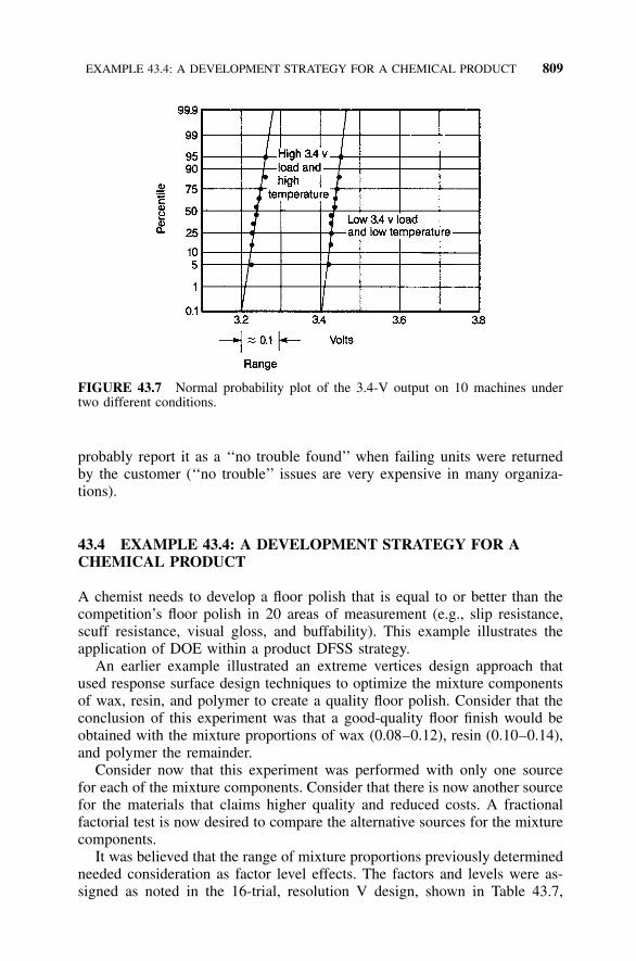
EXAMPLE 43.4: A DEVELOPMENT STRATEGY FOR A CHEMICAL PRODUCT 809

FIGURE 43.7 Normal probability plot of the 3.4-V output on 10 machines undertwo different conditions.

probably report it as a ‘‘no trouble found’’ when failing units were returnedby the customer (‘‘no trouble’’ issues are very expensive in many organiza-tions).

43.4 EXAMPLE 43.4: A DEVELOPMENT STRATEGY FOR ACHEMICAL PRODUCT

A chemist needs to develop a floor polish that is equal to or better than thecompetition’s floor polish in 20 areas of measurement (e.g., slip resistance,scuff resistance, visual gloss, and buffability). This example illustrates theapplication of DOE within a product DFSS strategy.

An earlier example illustrated an extreme vertices design approach thatused response surface design techniques to optimize the mixture componentsof wax, resin, and polymer to create a quality floor polish. Consider that theconclusion of this experiment was that a good-quality floor finish would beobtained with the mixture proportions of wax (0.08–0.12), resin (0.10–0.14),and polymer the remainder.

Consider now that this experiment was performed with only one sourcefor each of the mixture components. Consider that there is now another sourcefor the materials that claims higher quality and reduced costs. A fractionalfactorial test is now desired to compare the alternative sources for the mixturecomponents.

It was believed that the range of mixture proportions previously determinedneeded consideration as factor level effects. The factors and levels were as-signed as noted in the 16-trial, resolution V design, shown in Table 43.7,

810 S4 / IEE APPLICATION EXAMPLES

TABLE 43.7 Design Factors and Levels

Factors

Levels

(�) (�)

A: Polymer brand Original source New sourceB: Wax brand Original source New sourceC: Wax proportion amount 0.08 0.12D: Resin brand New source Original sourceE: Resin proportion amount 0.14 0.10

TABLE 43.8 Design Matrix for 16-Trial Test

Trial Number A B C D E

1 � � � � �2 � � � � �3 � � � � �4 � � � � �5 � � � � �6 � � � � �7 � � � � �8 � � � � �9 � � � � �

10 � � � � �11 � � � � �12 � � � � �13 � � � � �14 � � � � �15 � � � � �16 � � � � �

where the amount of polymer used in a mixture trial would be the amountnecessary to achieve a total proportion of 1.0 with the given proportions ofresin and wax specified for each trial.

From Table M3 the design matrix for five factors would be as shown inTable 43.8. From this design, two-factor interaction effects can be determined.After the 16 formulations are prepared, the test environment and trial re-sponses can also be considered. Do we expect the response to vary as afunction of the weather (temperature and humidity), application equipment,application techniques, and/or type of flooring? If so, we can choose aTaguchi strategy of assigning these factors to an outer array. This inner/outerarray test strategy will require more trials, but it can help us avoid developinga product that works well in a laboratory environment but not well in acustomer situation. As an alternative to an inner/outer array strategy, theseconsiderations can be managed as factors in the experiment design consid-erations.

EXAMPLE 43.5: TRACKING ONGOING PRODUCT COMPLIANCE 811

Another concern that can be addressed is the relationship of our new prod-uct composition to that of the competition. To make a competitive assessment,competitive products could be evaluated in a similar ‘‘outer array’’ test en-vironment during initial testing. From this information, comparisons could bemade during and after the selection of the final chemical composition.

After the chemical composition is determined, stability is needed in themanufacturing process so that a quality product is produced on a continuingbasis. An XmR chart is useful for monitoring key parameters in a batch chem-ical manufacturing process.

43.5 EXAMPLE 43.5: TRACKING ONGOING PRODUCTCOMPLIANCE FROM A PROCESS POINT OF VIEW

An organization is periodically required to sample product from manufactur-ing to assess ongoing compliance to government requirements. The test istime-consuming and is known to have considerable error, but this error hasnot been quantified. Many products produced by the company must undergothis test. These products are similar in nature but have different designrequirements and suppliers. To address the government requirements, theorganization periodically samples the manufacturing process and tests tospecifications. If the product does not meet requirements, corrective action istaken within manufacturing. When the failure frequency is higher than de-sired, manufacturing needs to be notified for issue resolution.

Current tests are attribute (pass or fail), and measurements focus on theproduct. When samples are outside of specification, the reaction is that theproblem is due to special cause (i.e., go to the manufacturing and fix theproblem). Let’s look at the situation from a higher viewpoint and examinethe data as continuous from process. All products go through the same basicprocess of design, design qualification test, and manufacturing. From thispoint of view we can assess whether the failures are special cause or commoncause. If the failures are common cause, we might be able to determine whatshould be done differently in the process to reduce the overall frequency offailure. The variables data of measurements relative to specification limits arethe following, where zero is the specification and positive values indicate theamount the measurement is beyond specification.

�9.4 �9.4�9.5�6.7

�6.4�2.6

�10

�7.7�6.9

3.6

�9.711.2

�0.2

�8.6�9.5�7.6

�4.7�9.3

1.9

�4.7�7.8

�6.2�12.4

�0.3�3.2

3�4.9

0.6�16.3

�8.8�3.5

The XmR control chart of the variable shown in Figure 43.8 indicates onlyone special cause, while Figure 43.9 shows a normal probability plot of alldata. This plot is to be recreated without the special cause data point as part

812 S4 / IEE APPLICATION EXAMPLES

10

0

–10

–20

20

10

0

Indi

vidu

al v

alue

Mov

ing

rang

e

0 10 20Subgroup

UCL=8.866

UCL=1864

LCL=21.47

LCL=0.000

X=6.304

R=5.704

=

FIGURE 43.8 Control chart tracking relative to the specification.

99

95

90

80706050403020

10

5

1

Per

cent

–10 0 10Data

ML EstimatesMean: –6.30385SD: 5.33129

FIGURE 43.9 Normal probability plot of all data.

of an exercise. This plot indicates that our overall process is not very capableof meeting the test requirements consistently. The plot indicates that we mightexpect a 10%–20% failure rate unless we do something differently (the math-ematical estimation of this rate and other statistical calculations are givenlater as an exercise).

EXAMPLE 43.6: TRACKING AND IMPROVING TIMES FOR CHANGE ORDERS 813

From a process improvement point of view, we would next like to assesswhat should be done differently in the process. With existing data we couldcreate a Pareto chart of what should be done to bring the previous out-of-specification product back into compliance. Perhaps there is some commonthread between the different product types that are being measured. Thisinformation could be passed on to development and manufacturing with em-phasis on improving the robustness of the design in the future and poka-yoke.

So far we have only looked at data differently (i.e., no additional mea-surements have been made). The next process improvement effort that seemsto be appropriate is to understand our measurement system better (i.e., con-duct a gage R&R). After this, a DOE might be appropriate to determine whatcould be done differently in the process.

43.6 EXAMPLE 43.6: TRACKING AND IMPROVING TIMES FORCHANGE ORDERS

An organization would like engineering change orders to be resolved quickly.Time series data showing the number of days to complete change order werecollected as follows:

18 2 0 0 0 0 0 0 0 0 0 0 00 0 0 0 0 14 0 0 7 3 0 410 0 0 0 0 0 0 0 17 0 0 00 0 0 0 0 0 0 0 0 0 0 00 1 0 0 0 0 0 0 11 0 0 17

26 0 0 0 0 0 0 21 0 0 0 06 0 0 17 0 0 0 0 0 0 0 0

The XmR chart of these data shown in Figure 43.10 explains little aboutthe process because there are so many zeros. A histogram of these data in-dicates that it might be better to consider the situation bimodal—that is, lessthan one day (i.e., 0) as one distribution and one day or more as anotherdistribution. An estimate of the proportion of instances it takes one day ormore is 14/85 � 0.16. The control chart of the one or greater values shownin Figure 43.11 does not indicate any trends or special causes when durationtakes longer than one day. The normal probability plot shown in Figure 43.12indicates the variability expected when a change order takes one day orlonger.

We can combine these two distributions to give an estimate of the per-centage of change orders beyond a criterion. To illustrate this, consider acriterion of 10 days. The estimated percentage of engineering change orderstaking longer than 10 days is 100(0.16)(.65) � 11% (where 0.65 is the esti-

814 S4 / IEE APPLICATION EXAMPLES

40

30

20

10

40

30

20

10

0

0

–10

Indi

vidu

al v

alue

Mov

ing

rang

e

0 10 20 30 40Subgroup

50 60 70 80 90

UCL=13.13

UCL=13.22

X=2.365

R=4.048

LCL=8.400

LCL=0.000

=

–

11

1

1 1

11

1

111

1

11

1

111

1

11

FIGURE 43.10 XmR chart of the time taken to process engineering change orders.

605040302010

0–10–20–30

0 5 10Subgroup

15

50

40

30

20

10

0

Indi

vidu

al v

alue

Mov

ing

rang

e

UCL=49.75

UCL=43.48

LCL=0.000

LCL=21.04

X=14.36

R=13.31

=

FIGURE 43.11 XmR chart of nonzero values.

mate proportion [1 – 0.35 � 0.065] from the figure). With this informationwe could categorize the characteristics of change orders that take a longperiod of time. From this information we could create a Pareto chart thatwould give a visual representation that leads to focus areas for process im-provement efforts.

EXAMPLE 43.7: IMPROVING EMPLOYEE OPINION SURVEYS 815

99

95

90

80706050403020

10

5

1

–10 0 10 20Data

30 40

Per

cent

ML EstimatesMean: 14.3571SD: 10.4171

FIGURE 43.12 Normal probability plot of nonzero values.

43.7 EXAMPLE 43.7: IMPROVING THE EFFECTIVENESS OFEMPLOYEE OPINION SURVEYS

The method discussed here was originally developed for a company employeeopinion survey, but the approach can be applied in other situations.

Many employee opinion surveys are conducted periodically (e.g., an-nually). These surveys can use a Likert scale with the associated numericalresponses of strongly agree (5), agree (4), uncertain (3), disagree (2), andstrongly disagree (1). Much time and effort can be expended in interpretingthe results. After all this effort we might question the value of the survey.When interpreting these results, one might ask several questions:

1. Are these response levels okay?2. Is there any improvement trends?3. Might the results be different if the survey were taken a month later

(e.g., a gloomy time of year might yield a less favorable response thana bright time of year.)

4. What should be done differently?

Let’s examine what might be done differently to address these issues. Thissurvey strategy will focus on understanding company internal processes, as

816 S4 / IEE APPLICATION EXAMPLES

opposed, for example, to the ranking of departmental results and taking cor-rective action as required.

Because the absolute number of a 1–5 Likert response has bounds, it isdifficult to determine if opinions have changed (e.g., if one were to get all5’s for a year in a category, how could improvement be measured for futureyears?). To address this issue, consider phrasing the questions relative tochanges from last year with response levels of: a lot of improvements (5),some improvements (4), no change (3), a bit worse (2), and a lot worse (1).Much more flexibility is offered with this approach because there is no upperbound. For example, management could set a stretch goal (that is consistentfrom year to year) of an average response of 0.5, with 80% of those surveyedbelieving improvement has been made. Because of the phrasing of the ques-tion, people would obviously need to be employed for one year or more inthe area before they could take the survey.

To address the issue of both trends in the response levels and biases inresults because of ‘‘noise considerations’’ (e.g., weather, fear of layoffs, datewhen survey was taken), consider having surveys conducted monthly using asampling strategy whereby each person is surveyed once annually. A controlchart could then be used to evaluate overall and specific question responses.Other Six Sigma tools, such as normal probability plotting and ANOM, canexamine variability and areas that need focus.

The organization that is conducting the survey would like to get an as-sessment of what should be done differently. Good information for improve-ment opportunities is often provided in the comment section of surveys, butthis information is often very hard to quantify relative to perceived value. Toaddress this, consider adding a section that lists ‘‘improvement ideas.’’ Eachperson can ‘‘vote’’ on a certain number of ideas. This information can thenbe presented in a Pareto chart format. The improvement ideas list can comefrom previous write-in comments and an off-line committee that evaluatesthese comments and other ideas to create a list that will be used during theupcoming year. (Note: different areas could have different lists.)

43.8 EXAMPLE 43.8: TRACKING AND REDUCING THE TIME OFCUSTOMER PAYMENT

For this study the measurement was changed from attribute (i.e., the invoicewas paid on time or not) to a continuous measurement relative to due date(i.e., the company changed its tracking policy for timeliness of payments).

A yearly 30,000-foot-level control chart of the number of days a sampleof invoices were overdue showed no special causes. A histogram of the num-ber of days a sample of invoices were overdue is shown in Figure 43.13(negative numbers indicate payment was made before due date).

The data does not appear to be normally distributed. If all the days’ overduedata were available and we considered the customers who paid the invoicesas noise to our process, we could estimate the overall percentage of invoices

EXAMPLE 43.9: AUTOMOBILE TEST—ANSWERING THE RIGHT QUESTION 817

FIGURE 43.13 Histogram showing the number of days invoices are delinquent.

that would not be paid beyond 60 days or any other criterion we might choose(i.e., the capability/performance metric of our collection process). Since nospecial-cause conditions were prevalent from the 30,000-foot-level controlchart, we would consider our process predictable and would expect a similarresponse in future payments unless something changed within our process,our customers’ processes, or an outside event. Obviously we would like tochange our process such that our company receives payment more timely.

When the data were collected, other characteristics were recorded at thesame time (e.g., company that was invoiced, amount of invoice, whether in-voice had errors upon submittal, and whether any payment incentives weregiven to the customer). From these data the cost of delinquency could bedetermined for the existing process of invoicing and collection (i.e., the base-line for an S4/IEE project).

Analysis of variance and analysis of means (ANOM) studies indicated thatthe size of invoice did not significantly affect the delinquency, but certaincompanies were more delinquent in payment. Also, invoices were often re-jected because of errors, which caused payment delays. In addition, a costlypayment incentive given to some customers had no value add. With this in-formation the team started documenting the current process and then deter-mined what should be done differently to addresses these problem areas.

43.9 EXAMPLE 43.9: AUTOMOBILE TEST—ANSWERING THERIGHT QUESTION

Consider a hypothetical situation in which the insurance industry and theautomotive industry want to work together to determine whether the averageaccident rate of an automobile with an innovative steering and braking mech-

818 S4 / IEE APPLICATION EXAMPLES

anism will be higher than with the previous design (one accident every fiveyears). This initial question form is similar to a mean time between failure(MTBF) criterion test of a product. This example illustrates a product DFSSstrategy. (Note: This is only a conceptual example that illustrates how a prob-lem can be redefined for the purpose of S4/IEE considerations. All resultsand conclusions from this experiment were fabricated for illustration only.)

One can use the techniques discussed earlier in this book to determine thenumber of prototype vehicles to build and then the number of miles to testdrive a random sample. For these test vehicles the desired accident rate mustbe achieved with some level of belief that the customer will not exceed thecriterion after shipment. The test will require a large random sample of au-tomobiles, typical drivers, and test time. The experimenter will probably alsorequire that the cause of accidents be investigated to note if a design problemcaused the accident. However, with the current definition, this problem di-agnosis is not a formal requirement of the experiment.

When reassessing the problem definition, it seems that the real question ofconcern may not be addressed by the test. Perhaps the test should directlyassess whether this new design is going to increase the chance of accidentsunder varying road and driver situations. For example, if the initial test wasperformed in a locality during dry months, design problems that can causeaccidents on wet pavements might not be detected. Other concerns may alsobe expressed. For example, speed, driver’s age, sex of driver, alcohol contentin driver, traffic conditions, and road curvature are not formally consideredindividually or in combination. Care needs to be given to create driving sce-narios that match the frequency of customer situations during such a ‘‘ran-dom’’ test strategy. Often it is not practical to consider a random samplingplan that covers all infrequent situations in a test, but a very serious problemcould be overlooked because it was considered a rare event and was not tested.When such a rare event occurs later to a customer, a serious problem mightoccur. In lieu of verifying an overall failure criterion, a test alternative is toforce various situations structurally, in order to assess whether a problemexists with the design. A fractional factorial experiment design offers such astructure.

Next, alternative responses should be considered because the sole outputof ‘‘accidents’’ is expensive and can be catastrophic. In this example, twopossible output alternatives to the experiment are operator and vehicle re-sponse time to a simulated adverse condition. These outputs can be assessedrelative to each other for a simulated obstacle to determine if an accidentwould have occurred. If the accident was avoided, the ‘‘safety factor’’ timecould also then be determined for each adverse condition.

Reflect on the original problem definition. The validation question for thefailure rate criterion was changed to a test that focused directly on meetingthe needs of the customer. A test strategy that attempted to answer the originalquestion would not focus on the different customer situations that might causea problem or hazardous situation for some users. The redefined questionwould also save money because the test could be conducted earlier in the

EXAMPLE 43.9: AUTOMOBILE TEST—ANSWERING THE RIGHT QUESTION 819

TABLE 43.9 Initial Proposal

ObjectiveTest operators under simulated road hazards to

assess their reaction time along with automobileperformance to determine if the new design willperform satisfactorily in various customer drivingsituations.

Limiting AssumptionsNo passingFlat terrainNo traffic

OutputsOperator response time to adverse conditionAutomobile response characteristics to operator

inputPass / fail expectation

FactorConsideration

Factor-Level Conditons

(�) (�)

Weather Wet DryAlcohol None Legal limitSpeed 40 mph 70 mphSex Male Female

development cycle with fewer test systems. This earlier test strategy wouldpermit more expedient (and less costly) fixes to the problems identified duringthe test.

So far this automobile test description illustrates the logic behind changingfrom failure rate criterion tests to a fractional factorial experiment approach(i.e., to answer the right question). Consider now how brainstorming andcause-and-effect techniques can aid with the selection of factors and theirlevels.

A group of people might initially choose factors and factor levels alongwith test assumptions as shown in Table 43.9 for the fractional factorial ex-periment, in which factor levels are indicated by a � or �. Next, a meetingof peers from all affected areas would be conducted to consider expansion/deletion of selected factors, outputs, and limiting assumptions for the exper-iment.

In the meeting, inputs to the basic test design will depend on the experienceand perspective of each individual. It is unlikely that everyone will agree tothe initial proposal. The following scenario could typify such a meeting.

Someone indicates that historically there is no difference in driving ability be-tween men and women; he suggests using men for the test because there is ashortage of women workers in the area. The group agrees to this change as well

820 S4 / IEE APPLICATION EXAMPLES

TABLE 43.10 Revised Proposal

ObjectiveTest operators under simulated road hazards to

assess their reaction time along with automobileperformance to determine if the new design willperform satisfactorily in customer drivingsituations.

Limiting assumptionsNo passingFlat terrainNo trafficOperators will have one hour to get accustomed to

the car before experiencing any hazards.Only male drivers will be used since previous

testing indicates that there is no differencebetween male and female drivers.

OutputsOperator response time to adverse conditionAutomobile response characteristics to operator

inputPass / fail expectation

FactorConsideration

Factor Level Conditions

(�) (�)

Weather Wet DryAlcohol None Legal limitSpeed 40 mph 70 mphAge of driver 20–30 years 70–80 yearsCar design Current NewRoad curvature None Curved

as to suggestions that automobile performance on curves and operator age beincluded. The group thinks that operator age should be considered because theydo not want to jeopardize the safety of elderly people who might have troubleadapting to the new design. Also, it is suggested that a comparison be madebetween the new design and the existing vehicle design within the same exper-iment to determine whether the new vehicle caused a difference in responseunder similar conditions. It is agreed that operators should have one hour to getexperience operating the new vehicle design before experiencing any simulatedhazards. The revised test design shown in Table 43.10 was created, in whicheach factor would be tested at either a � or � factor level condition, as men-tioned below.

Note that this is a conceptual example to illustrate the power of usingfactorial tests versus a random test strategy. In reality, for this particular sit-uation there would be other statistical concerns for the factor levels. For ex-

EXAMPLE 43.9: AUTOMOBILE TEST—ANSWERING THE RIGHT QUESTION 821

TABLE 43.11 An Eight-Trial Test Design

Trial Number A B C D E F Where (�) (�)

1 ������ A � Weather Wet Dry2 ������ B � Alcohol None Legal limit3 ������ C � Speed 40 mph 70 mph4 ������ D � Age of driver 20–30 years 70–80 years5 ������ E � Vehicle Current New6 ������ F � Road curvature None Curved7 ������8 ������

ample, it would be unreasonable to assume that one elderly driver couldaccurately represent the complete population of elderly drivers. Several driv-ers would be needed for each trial to determine whether they all respondedfavorably to the test situation.

Let’s consider what has happened so far. Initially a failure rate criteriontest was changed to a fractional factorial test strategy because this strategywould better meet the needs of the customer. Next the brainstorming processwas used to choose the experiment factors and their levels. This examplediscusses the creation of a fractional factorial experiment design.

An eight-trial resolution III design alternative was chosen from Table M2and is noted in Table 43.11 with the experiment factors and their levels. Inthis conceptual example the two-factor interactions would be confounded withthe main effects.

The output response for each trial could be one or more measurements.For example, it could be the electronically measured response times of thevehicle and the driver to various obstacles placed in the path of the operatorin a simulated test environment, similar to that given to airline pilots duringtraining.

Instead of having a random sample of people driving automobiles undertheir normal operating conditions as proposed in the original problem defi-nition, this test philosophy considers the range of operator types along witha range of operating conditions, the thought being that if there is satisfactoryperformance under extreme conditions (i.e., factor levels are set to boundaryconditions), then there will probably be satisfactory performance under lessextreme conditions.

Consider the hypothetical situation shown in Figure 43.14, where, unknownto the experimenter, ‘‘age of driver’’ interacts with ‘‘vehicle design.’’ Exper-iments are performed in order to identify improvements to the design or tothe manufacturing process. This plot indicates that elderly drivers have a highreaction time when operating the new vehicle design. This information sup-poses that a design change may need to be made to improve the safety ofthis vehicle for elderly people. Detection of this type of problem is most

822 S4 / IEE APPLICATION EXAMPLES

FIGURE 43.14 Two-factor interaction plot.

TABLE 43.12 Two-Factor Interaction Confounding from Table N3a

Contrast Column Number

1 2 3 4 5 6 7

*ABDEFCG

*BADCEFG

*CBEDFAG

AB*DCFEG

BC*EAFDG

ABCCDAE*FBG

ACDEBF*G

aMain effects are denoted by an asterisk.

important early in the development cycle, not after the new automobile designis in production.

Resolution III designs such as the one shown in Table 43.11 are not nor-mally used to determine two-factor interactions, but Table N3 can be used toshow how the two-level factors are confounded with two-factor interactions.The confounding in the contrast columns for this design is noted in Table43.12.

In this experiment the age of the driver was factor D, and the vehicle designwas E. The DE interaction effect would be represented in contrast column 7.Consider that a probability plot of contrast column effects noted that absolutevalue effect from contrast column 7 was statistically significant compared tothe other effects. Because there were only six factors in this experiment (i.e.,

EXAMPLE 43.10 EXPOSING THE HIDDEN FACTORY 823

there was no G factor), there was no confounding of this interaction effectwith any main effects. If other considerations were important, at test comple-tion the experimenter might speculate that this interaction (or one of the otherinteractions in this column) was statistically significant. Obviously any of thechosen theories would need to be verified in a confirmation experiment.

A fractional factorial test strategy can have much greater power than arandom test strategy. As noted previously, there are other practical concernsfor this experiment design. For example, it would be unreasonable to assumethat one elderly driver would accurately represent the complete population ofelderly drivers. Generally, several drivers should be considered for each trialassessment. An alternative response for this type of test would be an attributeresponse (i.e., a certain portion of drivers did not respond satisfactorily). Toillustrate this situation, consider that 3 out of 10 people had a reaction timethat was not quick enough to avoid a simulated obstacle; these people wereclassified as having an accident for this trial. Example 42.1 illustrates anotherconceptual analysis possibility for this example. In this analysis the trials areconsidered to yield a logic pass/fail response.

The purpose of this automobile example is to illustrate the importance ofanswering the right question. With the initial test strategy of verifying a cri-terion, someone could easily end up playing games with the numbers to cer-tify one accident in five years as the failure criterion before shipment. Whatdo you expect would be done if the day before shipment it was discoveredthat the automobile did not meet its failure criterion? Next, a customer-driventest strategy combines the knowledge that exists in several organizations towork to reach a common goal early in the development cycle.

These examples illustrate how a few early development models (or a sim-ulator) could be used to evaluate a product design. This test could be betterthan a larger random sample that was simply run against a failure rate crite-rion. With this approach, multiple applications are assessed concurrently toassess interaction or combinational affects, which are very difficult, if notimpossible, to detect when assessing each factor individually (i.e., a one-at-a-time test strategy). Problems detected early in product development withthis strategy can be resolved with less cost and schedule impacts. It must beemphasized repeatedly that the original question often needs redefinition.

43.10 EXAMPLE 43.10: PROCESS IMPROVEMENT ANDEXPOSING THE HIDDEN FACTORY

A company assembles surface mount components on printed circuit boards(see Example 5.1). This company might report their defective failure rate inthe format shown in Figure 5.10. This type of chart would be better than arun chart where there was a criterion, which could induce the firefighting ofcommon cause variability as though it were special cause. The centerline ofthis control chart could be used to describe the capability/performance metric

824 S4 / IEE APPLICATION EXAMPLES

for this process, which would be 0.244. Given that a 24.4% defective rate isconsidered acceptably high, a Pareto chart as shown in Figure 5.11 can giveinsight to where process improvements should be focused. From this chart itbecomes obvious that the insufficient solder characteristic should be attackedfirst.

A brainstorming session with experts in the field could then be conductedto create a cause-and-effect diagram for the purpose of identifying the mostlikely sources of the defects. Regression, ANOVA, and/or other statisticalanalyses followed by a DOE might then be most appropriate to determinewhich of the factors has the most impact on the defect rate. This group oftechnical individuals can perhaps also determine a continuous response to usein addition to or in lieu of the preceding attribute response consideration. Onecan expect that a continuous response output would require a much smallersample size.

After changes are made to the process and improvements are demonstratedon the control charts, a new Pareto chart can then be created. Perhaps theimprovements to the insufficient solder noncompliance characteristic will belarge enough that blowholes might now be the largest of the vital few to beattacked next. Process control charts could also be used to track insufficientsolder individually so that process degradation from the ‘‘fix level’’ can beidentified quickly.

Changes should then be made to the manufacturing process after a confir-mation experiment verifies the changes suggested by the experiments. Thedata pattern of the control chart should now shift downward in time becauseof these changes, to another region of stability. As part of a continuing processimprovement, the preceding steps can be repeated to identify other areas toimprove.

The previously described approach is one way to define the process mea-surement and improvement strategy. However, often for this type of situationeach manufacturing line within a company typically assembles various prod-uct types, which consist of differing circuit layouts, component types andnumber of components. For this situation one might create a measurementsystem and improvement strategy as described above for each product type.A major disadvantage of the previous approach is that emphasis is now givento measuring the product versus measuring the process. Since most manufac-turing improvements are made through adjustments to the process, as opposedto the product, a measurement system is needed that focuses on the processand what can be done to improve the process. Two Six Sigma metrics canprove to be very valuable for this situation: dpmo and rolled throughput yield.

Let us consider dpmo first. This metric can both bridge product type andexpose the hidden factory of reworks. As described earlier, the defects peropportunity (DPO) calculation can give additional insight into a process byincluding the number of opportunities for failure. A defects per opportunitymetric considers the number of opportunities for failure within the calcu-lations. Consider, for example, that there were 1,000 opportunities for

EXAMPLE 43.10 EXPOSING THE HIDDEN FACTORY 825

failure on an assembly, which consisted of the number of solder joints andnumber of assembly components. If 23 defects were found within the assem-bly process after assembling 100 boards over a period of time, the estimatedppm rate for the process for that period of time would be 230 (i.e.,1,000,000{23/[100 � 1,000]} � 230). If someone were to convert this ppmrate to a sigma quality level, he/she would report a 5.0 sigma quality levelfor the process, using Table S. The magnitude of this sigma quality level of5 initially seems good since average companies are considered at a 4.0 sigmaquality level, as noted in Figure 1.3. However, if these defects were evenlydistributed throughout the 100 assemblies produced such that no more thatone defect occurred on each assembly, 23% ([23/100]100) of the assemblieswould exhibit a defect somewhere within the manufacturing process. I believethat most readers would consider this an unsatisfactory failure rate for themanufacturing process. This is one reason why I discourage the reporting anduse of the sigma quality level metric to drive improvement activities.

However, I do believe that a reported ppm rate can be a very beneficialmetric in that it can create a bridge from product to process and can exposethe hidden factory of reworks. We should note that it would be difficult toexamine the magnitude of this metric alone to quantify the importance of S4/IEE project activities within this area. For example, the manufacturing of acomputer chip might have millions of junctions that could be consideredopportunities for failure. For this situation we might report a sigma qualitylevel that is much better than a six sigma quality level and still have an overalldefective rate of the assembled unit of 50%. Another situation might onlyhave a few parts within an assembly that are considered opportunities forfailure. For this situation we might report a sigma quality level that is 4.0 buthave an overall defective rate of the assembled unit of 0.1%. Because of this,I suggest the consideration of tracking ppm rates directly over time using acontrol chart. When a process exhibits common-cause variability, centerlineof the control chart can be used to describe the capability/performance of theprocess. COPQ/CODND calculations can then be made using this value andthe cost associated with the types of defects experienced within the manufac-turing process. This COPQ/CODND can be used to determine if an S4/IEEproject should be undertaken. In addition, this COPQ/CODND can be usedas a baseline for determining the value of process improvement activitiesresulting from an S4/IEE project.

Rolled throughput yield is another metric that can be beneficial for thissituation. This metric can quantify the likelihood of product progressingthrough a process without failure, as well as expose major sources reworkswithin a factory. To create this metric, the process would be subdivided intoprocess steps such as pick-and-place components, wave solder, and so forth.The yield for each step would be multiplied together to determine rolledthroughput yield. Steps that have low yields are candidates for initial S4/IEEprocess improvement efforts. A disadvantage of this metric is that the logisticsto collect the data could be time-consuming.

826 S4 / IEE APPLICATION EXAMPLES

TABLE 43.13 Website Hit Rate Data

Week Number of Hits

11/7/99 418511/14/99 396211/21/99 333411/28/99 4176

12/5/99 388912/12/99 397012/19/99 259112/26/99 2253

1/2/00 40531/9/00 5357

1/16/00 53051/23/00 48871/30/00 5200

2/6/00 43902/13/00 46752/20/00 47362/27/00 4993

Other areas of this manufacturing process that could also be consideredfor S4/IEE projects are inventory accuracy, frequency and cause of customerfailures, expense reduction, effectiveness of functional tests, and functionaltest yields.

43.11 EXAMPLE 43.11: APPLYING DOE TO INCREASE WEBSITETRAFFIC—A TRANSACTIONAL APPLICATION

A company was unhappy with how many hits it received on its website andwhere the website listed in search engine rankings. The company formed anS4/IEE improvement team to increase the traffic on its website. Upper man-agement gave the team a budget and an aggressive goal of doubling thenumber of hits within the next four months.

The team compiled hit-rate data in time series format from the website.They looked at hit rates by week over the past three months. The data usedfor the project are shown in Table 43.13. A 30,000-foot-level XmR controlchart of these data is shown in Figure 43.15. Weeks 4 and 5 are beyond thecontrol limits. Investigation into these two data points showed that this re-flected website activity during the last two weeks of December, when websitetraffic was lower due to the holiday season. Since a clear reason could beassigned, the two points were removed from the data and the control chartswere recreated.

Next, the team held a brainstorming session to create a cause-and-effectdiagram. They came up with many factors that might increase the number of

EXAMPLE 43.11: APPLYING DOE TO INCREASE WEBSITE TRAFFIC 827

0Subgroup 5 10 15

2000

3000

4000

5000

6000

Indi

vidu

al V

alue

11

Mean=4233

UCL=5742

LCL=2724

0

1000

2000

Mo

ving

Ran

ge

R=567.4

UCL=1854

LCL=0

FIGURE 43.15 A 30,000-foot-level control chart of website hit rates.

page requests on their website. To rank the list of factors and begin to deter-mine the KPIVs, the team utilized a cause-and-effect matrix similar to Table43.14.

No data were available on the relationships of the KPIVs to the websitehit rate, so the team decided to run an experiment. In order to test the criticalfactors, they established different gateway pages with links back to the mainsite. Instead of testing these factors one at a time, the black belt decided touse a DOE approach. He knew that through utilizing a DOE, the team wouldbe more efficient. The DOE would help them gain a better understanding ofhow the critical factors affected website hit rate and also interacted with eachother.

To reduce the size of the experiment and the number of doorway pagesneeded, the team reviewed the list of factors from the cause-and-effect matrixand took care to only include factors that would yield valuable insight abouttheir web page traffic. A meeting of peers from all affected areas was thenconducted to consider expansion/deletion of selected factors, outputs and lim-iting assumptions for the experiment. The team then determined levels foreach of the factors and reduced the number of factors to two levels; theychose to represent the extremes of each setting. The revised list with settingsis shown in Table 43.15.

The black belt used the matrix in Table M2 and came up with the testmatrix shown in Table 43.16. Eight gateway pages were created, each pagerepresenting one of the trials listed in this table. Hit rates could then becollected on a weekly basis to determine which combination of factors pro-duced the most Web traffic.

From the results the team could determine which factors were importantto improve. Results of the experiment could, for example, test the hypothesis

828 S4 / IEE APPLICATION EXAMPLES

TABLE 43.14 Cause-and-Effect Matrix: Factors That Affect Website Traffic

IncreaseWebsite Hit

RateEasy to

Implement ����Process Outputs

10 10 ��������Importance

Process InputCorrelation of Input

to Output Total

Number of keywords 9 9 180

Type of keywords 9 9 180

Length of description 9 9 180

URL 3 9 120

Frequency of updates 9 3 120

Description 3 9 120

Free gift 9 1 100

Search engine used 3 3 60

Contest 3 1 40

Text size and font 1 3 40

Links from other sites 3 1 40

Banner advertising 1 1 20

TABLE 43.15 Factors and Levels of Website Hit Rate Test

FactorDesignation � Setting � Setting

A URL title, new URL title, oldB Length of descriptions: Long Length of description: ShortC Number of keywords: Many

(10 words)Number of keywords: Short(2 words)

D Types of keywords: New Types of keywords: OldE Site updates: Weekly Site updates: monthlyF Location of keywords in title:

40th characterLocation of keywords in title:

75th characterG Free gift: yes Free gift: no

that Web Consulting Honolulu addresses the most important things to do inorder to increase website traffic (Web Consulting Honolulu 1999). They be-lieve in having the right/ important key words and offering something special(e.g., gift, download, and so forth).

EXAMPLE 43.12: AQL DECEPTION AND ALTERNATIVE 829

TABLE 43.16 DOE Test Matrix

Trial Number A B C D E F G

1 �������2 �������3 �������4 �������5 �������6 �������7 �������8 �������

As part of the control plan, the team might choose weekly to check theranking of the website against other sites using a combination of keywordsthat are important to the site. Whenever the site ranking degrades adjustmentsshould be considered and/or another DOE conducted to address any newtechnology issues that might have recently occurred.

43.12 EXAMPLE 43.12: AQL DECEPTION AND ALTERNATIVE

An E-mail Inquiry I Received

I have the following question on AQL. Hope you can help.

For AQL: 0.65Lot size: 15000Sampling: SingleInspection level: II

The sample size code I got is M and the MIL-STD-105D (replaced by ANSI/ASQC Z1.4-1993) indicated that the sample size should be 315 with 5 acceptand 6 reject.

Question: What is the probability that a bad lot is accepted with this sam-pling plan? If one changes to a sampling plan of 20 with 0 accept and 1reject, what is the probability that a bad lot is accepted?

Thanks in advance for your help.

My Response

I think that AQL sampling can be very deceiving. For example, it is not clearto me what is a ‘‘bad’’ lot.

A reduced sample size test procedure along with its implications is shownin Section 18.6; however, I believe one can gain an appreciation of the di-

830 S4 / IEE APPLICATION EXAMPLES

lemma confronted when trying to make lot pass/fail decisions by looking atconfidence intervals.

When we assume the sample size is small relative to the population size,a 95% confidence interval calculation for the population failure rate � is:

5 failures from a sample of 315: 0.005173 � � � 0.0366526 failures from a sample of 315: 0.007021 � � � 0.0409960 failures from a sample of 20: 0.000000 � � � 0.1391081 failure from a sample of 20: 0.001265 � � � 0.248733

As you can see, even with a relatively large sample size the confidenceinterval is larger that you might expect. With this confidence interval you areprobably not getting the acceptance risk level for the test that you really want.

For the low failure rates of today, we can get much more information withless work when we measure the process that produces the product on a con-tinuing basis, not as to whether an individual batch meets an AQL criterionor not. Section 10.4 elaborates more on this.

It is more beneficial when customers ask their supplier questions that leadto the right activity. AQL testing has a ‘‘testing quality into the product’’connotation. Instead of AQL testing, the S4/IEE approach would be for thesupplier to measure a KPOV of the process that produces the product on anongoing basis. This measure would assess the quality of the product as allcustomers receive it, then tracking the response using a 30,000-foot-levelcontrol chart. If the response could not be changed to a continuous response,the centerline of attribute control chart could be viewed as the best estimatefor the capability/performance of the product.

It would be much better if the 30,000-foot-level response could be quan-tified as a continuous variable. For this case all common-cause data could beexamined collectively to estimate the percentage expected beyond specifica-tion limits. A probability plot could be used to make such assessment.

Within companies there is a cultural difference between accepting the AQLprocedure approach and the S4/IEE alternative. The AQL procedure has afirefighting mentality—that is, everything is okay until a lot is rejected. Whenthis occurs, someone is then assigned the task of fixing the problem of today.With the S4/IEE approach, we would view the overall output of the process.If the process has an unacceptable level of common-cause nonconformance,we then establish an S4/IEE team to look at all data collectively to makeimprovements and establish control measures for KPIVs to the process.

43.13 EXAMPLE 43.13: S4/IEE PROJECT: REDUCTION OFINCOMING WAIT TIME IN A CALL CENTER

The satellite-level metrics of an organization led to a project to shorten waittimes for incoming calls in a call center. The project goal was to reduce wait

EXAMPLE 43.13: S4 / IEE PROJECT 831

0Subgroup 10 20 30

1

23

4

5

6

78

Indi

vidu

al V

alue

Mean=4.353

UCL=7.084

LCL=1.623

0

1

2

3

Mov

ing

Ran

ge

R=1.027

UCL=3.354

LCL=0

FIGURE 43.16 The 30,000-foot-level XmR chart of wait time (seconds) with naturallog transformation of data—process baseline.

time by 50%. An estimated annual benefit for the project was $100,000, asoft savings resulting from improved customer image.

Each day one phone call was randomly selected. The wait time durationfor the phone call was recorded and tracked as a 30,000-foot-level controlKPOV (Y variable) metric. At least 30 data points from historical data wouldestablish a baseline for this process metric.

A project charter was created. The project charter showed the linkage tosatellite-level business metrics. The black belt facilitated the creation of aproject plan that she tracked progress against. The team decided that therewas no value to quantify any secondary metrics such as RTY.

It was anticipated that response time would be lognormally distributedsince it was impossible to experience a duration that was negative. Also, mostcalls would be clustered around a median and some calls would probablyhave a very long wait time. An analysis of historical data could not reject thehypothesis that the response time was lognormally distributed. An XmR chartof the untransformed data set did have a point that was beyond the controllimits, which could be expected when samples are taken from a populationthat is lognormally distributed.

The 30,000-foot-level XmR chart in Figure 43.16 shows no special causeoccurrences for the lognormal transformed wait time data. Figure 43.17 showslognormal probability plot of the data. Since there was no specification forthe process, we might describe a best estimate capability/performance metric

832 S4 / IEE APPLICATION EXAMPLES

100010010

99

95

90

80

7060504030

20

10

5

1

Wait Time

Per

cent

25-237

FIGURE 43.17 Lognormal probability plot of wait time in seconds, showing bestML estimate for 80% of occurrences and 95% CI.

for the process as 80% of the time customers experience a wait time of 25–237 seconds. A monetary impact estimate for this level of wait time was$216,000 per year.

The team documented the process and created a time-value diagram. Theycreated a cause-and-effect diagram, which had some improvement ideas. Across-functional team created a cause-and-effect matrix that prioritized wis-dom of the organization improvement ideas. One input variable (an x variable)thought to be important was that delays might be longer during lunch (12:00PM–1:00 PM). An FMEA matrix created by a cross-functional team identifiedseveral potential failure modes that had high RPN numbers. These issues wereto be resolved through several action plans. For example, a snowstorm couldsignificantly disrupt service when call center operators could not arrive atwork on time. A team was created to resolve this exposure.

A marginal plot of our original data set of 30 readings, shown in Figure43.18, indicates that the wait time during lunch could be longer. A randomsample from the last year’s data was taken, where 75 samples from nonlunchtimes and 25 samples from lunch times were selected. The dot plot of thisdata in Figure 43.19 indicates that there could be a difference in mean waittimes. An analysis of the 100 samples by sampled time period yielded

EXAMPLE 43.13: S4 / IEE PROJECT 833

0

100

200

300

400

500W

ait T

ime

20

5

2

2

1

Lunch TimeNot- Lunch Time1 2

FIGURE 43.18 Marginal plot of 30,000-foot-level wait time data in seconds for not-lunch time and lunch time.

6005004003002001000

TimeDuringLu

TimeNotLunch

FIGURE 43.19 Dot plots for wait time during not-lunch time period (75 randomsamples) and lunch time (25 random samples).

Two-sample T for TimeLunch1 N Mean StDev SE Mean

1 75 83.0 62.4 7.22 25 313 157 31

Difference � mu (1) � mu (2)Estimate for difference: �230.195% CI for difference: (�296.3, �163.8)T-Test of difference � 0 (vs not �): T-Value � �7.14P-Value � 0.000 DF � 26

A statistically significant difference was indicated with a p value less than0.000. The 95% confidence interval for the estimated difference was 163.0 to296.3 seconds.

834 S4 / IEE APPLICATION EXAMPLES

5040302010Subgroup 0

87

6

5

4

32

1

Indi

vidu

al V

alue

2

Mean=4.460

UCL=7.196

LCL=1.724

3

2

1

0

Mov

ing

Ran

ge

2

R=1.029

UCL=3.361

LCL=0

FIGURE 43.20 The 30,000-foot-level control chart before and after first change.Control limits established for the first 34 data points, which was before change im-plementation. The number 2 is a detection sign of a process shift, since nine pointswere in a row on the same side of the centerline.

The team came up with a log-hanging-fruit idea, which improved the stag-gering of lunch periods. This process change was then implemented. Figure43.20 shows the 30,000-foot-level control chart before and after the firstchange was implemented. Control limits were established for the first 34 datapoints since the process point was made at the 35th data point. The number2 in the chart is a detection sign of a process shift, since nine points were ina row on the same side of the centerline. A t-test showed a statistical differ-ence between the before to after change. Figure 43.21 shows a readjustmentof the control limits at process change.

Visual descriptions for the process capability/performance metrics im-provement are the dot plot shown in Figure 43.22 and the probability plotshown in Figure 43.23. The new 80% occurrence capability/performance es-timate for the process is shown in Figure 43.24. A monetary estimate for thereduction in wait time was $108,500. A control mechanism was establishedto ensure that the new lunch scheduling process was later followed. Theprocess owner agreed to these changes and the continual monitoring andreporting of the 30,000-foot-level metric to his management.

Further improvements in the call wait time KPOV were desired. Anotherhighly ranked potential KPIV from the wisdom of the organization evaluationwas the time it took to respond to a previous call. Figure 43.25 and thefollowing analysis support this hypothesis.

EXAMPLE 43.13: S4 / IEE PROJECT 835

0Subgroup 10 20 30 40 50

1

23

4

5

6

78

Indi

vidu

al V

alue

Mean=3.823

UCL=5.853

LCL=1.793

0

1

2

3

Mov

ing

Ran

ge

R=0.7632

UCL=2.494

LCL=0

Process Change Implemented

FIGURE 43.21 The 30,000-foot-level control chart before and after first change.Control limits changed after process change was implemented.

0 100 200 300 400 500

Wait Time

After Change

Before Change

FIGURE 43.22 Dot plot describing distribution of expected wait times before andafter the first change.

The regression equation is

WaitTimeAfte � -35.7525 � 0.237708 TimeAnsPrevQ

S � 14.1910 R-Sq � 72.9 % R-Sq(adj) � 72.7 %

Analysis of Variance

Source DF SS MS F PRegression 1 53222.2 53222.2 264.281 0.000Error 98 19735.7 201.4Total 99 72958.0

836 S4 / IEE APPLICATION EXAMPLES

Before Change

After Change

10 100 1000

1

5

10

20

3040506070

80

90

95

99

Wait Time

Per

cent

FIGURE 43.23 Lognormal probability plot comparing before change to afterchange.

10010

99

95

90

80

7060504030

20

10

5

1

Wait Time

Per

cent

23-92

FIGURE 43.24 Lognormal base e probability plot of wait time after first change inseconds, showing ML best estimate for 80% of occurrences and 95% CI.

EXAMPLE 43.14: S4 / IEE PROJECT 837

200 300 400 500 600 700 800

0

20

40

60

80

100

120

140

160

180

Time Answer Previous Question

Wai

t Tim

e

WaitTimeAfte = -35.7525 + 0.237708 TimeAnsPrevQ

S = 14.1910 R-Sq = 72.9 % R-Sq(adj) = 72.7 %

FIGURE 43.25 Regression analysis of wait time versus time to answer previousquestion.

Since this effort required a different focus, it was taken on as a separateproject (Example 43.14).

43.14 EXAMPLE 43.14: S4/IEE PROJECT: REDUCTION OFRESPONSE TIME TO CALLS IN A CALL CENTER

The project described in Example 43.13 was a stimulus to creating this pro-ject. An estimated annual financial benefit of $150,000 is expected from im-proved utilization of people’s problem response time in the call center.

Each day one phone call was randomly selected. The response durationfor the phone call was recorded and tracked as a 30,000-foot-level KPOV (Yvariable) metric. At least 30 data points from historical data established abaseline for this process metric, which was tracked using an XmR chart. Notethat if all data were available, the subgroup means and standard deviationcould be tracked (see Section 10.27).

A project charter was created. The project charter showed the linkage tosatellite-level business metrics. The black belt facilitated the creation of aproject plan that she tracked progress against. The team decided that therewas no value to quantify any secondary metrics such as RTY.

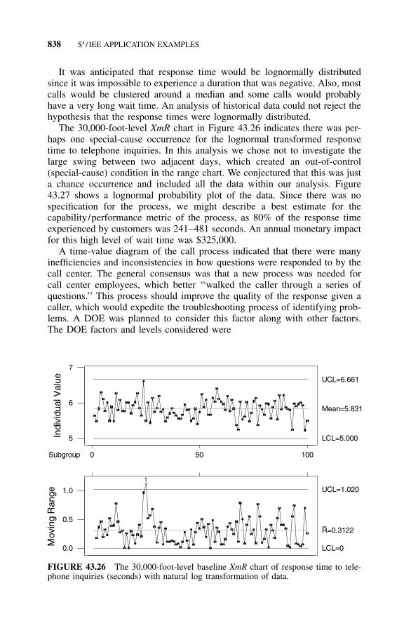
838 S4 / IEE APPLICATION EXAMPLES

10050Subgroup 0

7

6

5Indi

vidu

al V

alue

Mean=5.831

UCL=6.661

LCL=5.000

1.0

0.5

0.0

Mov

ing

Ran

ge

1

R=0.3122

UCL=1.020

LCL=0

FIGURE 43.26 The 30,000-foot-level baseline XmR chart of response time to tele-phone inquiries (seconds) with natural log transformation of data.

It was anticipated that response time would be lognormally distributedsince it was impossible to experience a duration that was negative. Also, mostcalls would be clustered around a median and some calls would probablyhave a very long wait time. An analysis of historical data could not reject thehypothesis that the response times were lognormally distributed.

The 30,000-foot-level XmR chart in Figure 43.26 indicates there was per-haps one special-cause occurrence for the lognormal transformed responsetime to telephone inquiries. In this analysis we chose not to investigate thelarge swing between two adjacent days, which created an out-of-control(special-cause) condition in the range chart. We conjectured that this was justa chance occurrence and included all the data within our analysis. Figure43.27 shows a lognormal probability plot of the data. Since there was nospecification for the process, we might describe a best estimate for thecapability/performance metric of the process, as 80% of the response timeexperienced by customers was 241–481 seconds. An annual monetary impactfor this high level of wait time was $325,000.

A time-value diagram of the call process indicated that there were manyinefficiencies and inconsistencies in how questions were responded to by thecall center. The general consensus was that a new process was needed forcall center employees, which better ‘‘walked the caller through a series ofquestions.’’ This process should improve the quality of the response given acaller, which would expedite the troubleshooting process of identifying prob-lems. A DOE was planned to consider this factor along with other factors.The DOE factors and levels considered were

EXAMPLE 43.14: S4 / IEE PROJECT 839

100 1000

1

510

20304050607080

9095

99

Response Time to Telephone Inquiries

Per

cent

241-481

FIGURE 43.27 Lognormal probability plot for the phone inquiry response time withML estimates and 95% CI. Best estimate for 80% of response times is between 241and 481 seconds.

�1 �1New process for call center No YesExperienced operator No YesService center location 1 2Time of week Monday WednesdayShift of work First Second

The output of the DOE analysis was

Estimated Effects and Coefficients for Resp1 (codedunits)

Term Effect Coef SE Coef T PConstant 452.9 19.06 23.76 0.000NewProce �217.7 �108.8 19.06 �5.71 0.000Experien �218.3 �109.2 19.06 �5.73 0.000Location �21.0 �10.5 19.06 �0.55 0.595Time of 64.0 32.0 19.06 1.68 0.127Shift 103.6 51.8 19.06 2.72 0.024NewProce*Experien 255.6 127.8 19.06 6.71 0.000

840 S4 / IEE APPLICATION EXAMPLES

No Yes

YesNo

800

700

600

500

400

300

Experienced

NewProcess

Mea

n

FIGURE 43.28 Two-factor interaction plot of the new process and operator expe-rience.

These results indicate that focus should be given to the New Pro-cess*Experience interaction. Figure 43.28 shows this interaction plot. Theinteraction plot for average duration in response to call indicated that the newprocess helped those who were not experienced by over 400 seconds on theaverage.

Figure 43.29 shows a control chart of the KPOV, duration of response tocall (log to base e), indicates a change occurred after new procedures wereimplemented. The dot plot in Figure 43.30 shows the before-change and after-change distribution of data. The output from a statistical analysis comparingthe mean response was

Two-sample T for time response, where subset 2 is afterprocess change

subset N Mean StDev SE Mean1 100 353.2 97.5 9.82 30 219.0 98.5 18

Difference � mu (1) � mu (2)Estimate for difference: 134.295% CI for difference: (93.0, 175.4)T-Test of difference � 0 (vs not �): T-Value � 6.56P-Value � 0.000 DF � 47

The analysis shows that there was a statistically significant decrease in theaverage duration of response to inquiry call after the process improvement

EXAMPLE 43.14: S4 / IEE PROJECT 841

10050Subgroup 0

7

6

5

4Indi

vidu

al V

alue

1

Mean=5.276

UCL=6.648

LCL=3.904

2

1

0

Mov

ing

Ran

ge

1

1

R=0.5159

UCL=1.686

LCL=0

Process Change Implemented

FIGURE 43.29 XmR chart for the log to base e of inquiry response time for beforeand after process change implementation.

75065055045035025015050

Time (sec)

Before Change

After Change

FIGURE 43.30 Dot plots for time response to phone inquiry.

change was made with a p value of 0.000 and a 95% confidence interval of93–175.4 seconds. However, from Figure 43.31 we could not reject the nullhypothesis that the before-change and after-change variance in call time du-ration was the same.

For the project control phase, a procedure was established for updating thecomputer-assisted prompts, which operators followed when answering tele-phone inquiries. For this procedure, someone identified the five longest callsduring each day. For each of these calls, someone contacted the customerwho initiated these calls to better understand why duration of the responsewas lengthy and what changes should be made to the computer-assistedprompts so that the duration of future calls of this time would be less. Weeklychanges were planned to the computer-assisted application program. The pro-

842 S4 / IEE APPLICATION EXAMPLES

140130120110100908070

95% Confidence Intervals for Sigmas

1

2

8007006005004003002001000

Boxplots of Raw Data

Time to Respond

P-Value : 0.702Test Statistic: 0.147

Levene's Test

P-Value : 0.902Test Statistic: 0.980

F-Test

Factor Levels

2

1

FIGURE 43.31 Test for equal variances, where number 1 is before change andnumber 2 is after change.

cess owner of the call center signed up for this new procedure. He also agreedto own the 30,000-foot-level control chart; he agreed to create, use, and pe-riodically report this metric to his management. He also committed to respondto statistically out-of-control (special cause) conditions in a timely manner.

Because of these improvements, fewer people were hired to cover the in-creased number of calls, which were a result of business growth. The esti-mated annual savings are $427,000.

43.15 EXAMPLE 43.15: S4/IEE PROJECT: REDUCING THENUMBER OF PROBLEM REPORTS IN A CALL CENTER

The satellite-level metrics of an organization led to a project for the reductionof the number of problem reports in a call center. Each week we would totalthe number of weekly calls within a call center and divide by the number ofsales that would use the call center if a problem were to occur. Week waschosen as an infrequent subgrouping/sampling plan for the 30,000-foot-levelKPOV (Y response) chart since the team thought that day of the week might

EXAMPLE 43.15: S4 / IEE PROJECT 843

5040302010Subgroup 0

0.03

0.02

0.01

Indi

vidu

al V

alue

Mean=0.02215

UCL=0.03264

LCL=0.01167

0.015

0.010

0.005

0.000

Mov

ing

Ran

ge

R=0.003941

UCL=0.01288

LCL=0

FIGURE 43.32 XmR of failure rate by week.

affect the volume of calls. Data from the previous 52 weeks were used as abaseline within the chart. Figure 43.32 is an XmR chart of the failure rate.An XmR charted was select over a p chart since we wanted the variabilitybetween subgroups to affect the calculation of the control chart limits and thenumber of weekly calls was approximately the same (see Section 10.22).Since the data are discrete, the centerline of the control chart is an estimatefor the capability/performance metric of the process, which is approximately2.2%.

A project charter was created. The project charter showed the linkage tosatellite-level business metrics. A goal was set to reduce the number of prob-lem reports by 10% with projected savings of $350,000. The team decidedthat there was no value to quantify any secondary metrics such as RTY. Theblack belt facilitated the creation of a project plan, which she tracked progressagainst.

A sample of 100 calls was monitored closely so that reasons for the callscould be categorized. A Pareto chart of this data, shown in Figure 43.33,indicates that setup problems are the most frequent reason for calls. Hardwareand software problems seemed to be the source of fewer problems. The pro-ject was rescoped so that focus was given to reducing the setup problem callrate. The 30,000-foot-level KPOV (Y response) for this project is shown inFigure 43.34. We might consider this at a 20,000-foot-level chart since thisis still a high-level response output but at a lower level than our original30,000-foot-level metric, which tracked the frequency of all calls within thecall center.

The team documented the process and time-value diagram. They createda cause-and-effect diagram that had some improvement ideas. A cross-

844 S4 / IEE APPLICATION EXAMPLES

SwProb

HwProb

Instruc

tions

Setup

1317294113.017.029.041.0

100.0 87.0 70.0 41.0

100

50

0

100

80

60

40

20

0

Defect

CountPercentCum %

Per

cent

Cou

nt

FIGURE 43.33 Pareto chart of call type.

5040302010Subgroup 0

0.014

0.009

0.004

Mean=0.0088

UCL=0.01318

LCL=0.00457

0.006

0.005

0.004

0.003

0.002

0.001

0.000

Mov

ing

Ran

geIn

divi

dual

Ran

ge

R=0.001618

UCL=0.00528

LCL=0

FIGURE 43.34 XmR chart of weekly call rate for product setup.

functional team created a cause-and-effect matrix that prioritized wisdom ofthe organization improvement ideas. The item that ranked highest was thatthere was no methodology that highlighted the setup procedure when the boxwas initially opened.

EXAMPLE 43.15: S4 / IEE PROJECT 845

70605040302010Subgroup 0

0.015

0.010

0.005

0.000

Mean=0.00197UCL=0.002955

LCL=9.95E-04

Process Change Implemented

0.006

0.005

0.004

0.003

0.002

0.001

0.000

Mov

ing

Ran

geIn

divi

dual

Ran

ge

R=3.68E-04

UCL=0.001204

LCL=0

FIGURE 43.35 XmR chart of the weekly call rate for product setup, before and afterthe implemented process change.

An FMEA matrix created by a cross-functional team identified severalpotential failure modes that had high RPN numbers. These issues were to beresolved through several action plans. A highly ranked RPN issue was thatnewly developed products did not build upon the experience of previous prod-ucts. This new S4/IEE project opportunity was passed onto the S4/IEE steer-ing committee.

The team implemented a low-hanging-fruit idea of including a piece ofpaper, giving updates to setup procedures, which was to be placed on top ofthe equipment before it was packaged. Figure 43.35 shows the process shift.A statistical test comparing the attribute failure rates is

Expected counts are printed below observed counts

Failed Opportun TotalPrevious Process 923 104000 04923

725.04 1.04E�05New Process 79 40000 40079

276.96 39802.04Total 1002 144000 145002

846 S4 / IEE APPLICATION EXAMPLES

Chi-Sq � 54.047 � 0.376 �141.490 � 0.985 � 196.898

DF � 1, P-Value � 0.000

This chi-square test indicated that the null hypothesis of equality of failurerates should be rejected with a p value of 0.000.

A two-proportion statistical test yielded:

Test and CI for Two Proportion

Sample X N Sample p

1 923 104000 0.008875

2 79 40000 0.001975

Estimate for p(1) � p(2): 0.0069

95% CI for p(1) � p(2): (0.00618292, 0.00761708)

Test for p(1) � p(2) � 0 (vs not � 0): Z � 18.86P-Value � 0.000

From this test we are 95% confident that our failure rate improved by aproportion of 0.0062 to 0.0076, or 0.62% to 0.766%.

A procedure was established to track and report status using a 30,000-foot-level control chart for the occurrence rate of setup issues. Action would betaken when the control chart indicates an unsatisfactory change in the non-conformance rate.

A tracking and reporting system was also established for the type of callsreceived. This report would go to development so they can focus their effortson reducing these types of failures on future products. Development manage-ment was to address the creation of new procedures for developing new prod-ucts that addressed previous high-frequency call issues.

A new S4/IEE project was initiated that looked into the creation of a newprocess step within development where a DOE was conducted to assess op-erational instructions of equipment before first customer shipment. The DOEfactors were to include setup instructions and operating instructions.

Project benefits were estimated to be $1,200,000 annually, without consid-eration of the design process improvements, which could exhibit dramaticimprovements for future products.

EXAMPLE 43.16: S4 / IEE PROJECT: AQL TEST ASSESSMENT 847

5040302010Subgroup 0

110

100

90

Mean=99.09

UCL=109.3

LCL=88.85

15

10

5

0

Mov

ing

Ran

geIn

divi

dual

Ran

ge

R=3.851

UCL=12.58

LCL=0

FIGURE 43.36 XmR showing time between AQL inspection failures.

43.16 EXAMPLE 43.16: S4/IEE PROJECT:AQL TEST ASSESSMENT

The satellite-level metrics of an organization led to the assessment of productfailure rates. The assessment of these failure rates through the wisdom of theorganization led to the evaluation of current AQL test procedures. Each weekthe number of AQL tests for a variety of products that failed was divided bythe total number of AQL tests performed. The initial plan was to track thisratio over time as a KPOV (Y response) for the process. However, when thefrequency of failure for AQL tests was observed to be only about 1%, whilethe number of AQL test performed weekly was about 50, it was decided totrack the time between AQL failure test as a baseline. From this plot shownin Figure 43.36, the time between AQL test failure rate was estimated to beabout 99.09, which translates to approximately 1% of the products testedfailed.

A project charter was created. The project charter showed the linkage tosatellite-level business metrics. It was thought that the AQL function mightbe eliminated within the company, which would result in about $1,000,000savings annually. The team decided that there was no value to quantify anysecondary metrics such as RTY. The black belt facilitated the creation of aproject plan that she tracked progress against.

The team documented the test process and time-value diagram. They cre-ated a cause-and-effect diagram, which had some improvement ideas. A cross-functional team created a cause-and-effect matrix that prioritized wisdom of

848 S4 / IEE APPLICATION EXAMPLES

the organization improvement ideas. The item that ranked largest was theeffectiveness of the AQL sampling procedure as an effective means of cap-turing incoming part failures.

The next 10 lots that failed the AQL test were retested. In 9 out of 10cases a second sample from the lot passed the test. Because of this it wasconcluded that the AQL test process could not serve as an effect incomingproduct screen. One question that was not resolved was how many AQL teststhat were passed would have failed if there had been a second sample.

The team changed the policy of the organization such that quality engineersnow would ask suppliers for their 30,000-foot-level control charts andcapability/performance analysis, along with what S4/IEE projects they wereimplementing, to address any quality or on-time-delivery issues.

The savings for this one facility were $1,000,000, not counting the ex-pected improvement in quality from the new procedure. The result of thisproject is now being leveraged within the companies’ other facilities, whichcould result in a total $10,000,000 annual corporate savings.

43.17 EXAMPLE 43.17: S4/IEE PROJECT: QUALIFICATION OFCAPITAL EQUIPMENT

The satellite-level metrics of an organization led to assessing the proceduresthat were followed for the qualification of capital equipment. The time it tookto get equipment up and running satisfactorily was tracked using a 30,000-foot-level control chart, as shown in Figure 43.37. A probability plot of thecapability/performance of the process is shown in Figure 43.38. This metricconsisted not only of the in-house qualification time for testing the equipmentbut also the time it took to resolve startup problems.

A project charter was created. The project charter showed the linkage tosatellite-level business metrics. The potential value for the project was esti-mated to be $2,000,000. Categories for this calculation were not only thevalue of the time but also the cost implications for initial quality problems.The team decided that there was no value to quantify any secondary metricssuch as RTY. The black belt facilitated the creation of a project plan, whichshe tracked progress against.

The team documented the test process and time-value diagram. They cre-ated a cause-and-effect diagram, which had some improvement ideas. A cross-functional team created a cause-and-effect matrix that prioritized wisdom ofthe organization improvement ideas. An FMEA assessment had a high RPNassignment to the failure of capturing problems that resulted from the com-bination of typical factor extremes that occurred within the process.

The process was changed to include a DOE collective response capabilityassessment (DCRCA) strategy that would be used to qualify the equipmentat the supplier. We would work with the supplier on the selection of the input

EXAMPLE 43.17: S4 / IEE PROJECT: QUALIFICATION OF CAPITAL EQUIPMENT 849

15105Subgroup 0

110100908070605040

Mean=77.87

UCL=107.9

LCL=47.85

40

30

20

10

0

Mov

ing

Ran

geIn

divi

dual

Ran

ge

R=11.29

UCL=36.87

LCL=0

FIGURE 43.37 The 30,000-foot-level control chart of the number of days to qualifyequipment.

P-Value: 0.743A-Squared: 0.236

Anderson-Darling Normality Test

N: 15StDev: 11.8314Average: 77.8667

9585756555

93.9

675

61.7

658

0.90000

0.10000

.90 99

.990

.950

.800

.500

.200

.00 5

.00 1

.00 01

Pro

babi

lity

Time (Days)

FIGURE 43.38 Normal probability plot capability assessment of the number of daysto quality equipment, ML estimates—95% CI.

850 S4 / IEE APPLICATION EXAMPLES

2010Subgroup 0

100

50

0Mean=8.467UCL=26.32

LCL=-9.390

Process Change Implemented

40

30

20

10

0

Mov

ing

Ran

geIn

divi

dual

Ran

ge

R=6.714

UCL=21.94

LCL=0

FIGURE 43.39 The 30,000-foot-level control chart of the number of days to qualifyequipment.

variables for the test, which would include the variability extremes of setupconditions and raw material extremes. The supplier would need to share theresults of the test and the process they used to resolve any issues.

After this test, process change was implemented. The 30,000-foot-levelKPOV chart shown in Figure 43.39 went out of control to the better (changedto an improved level of conformance). The dot plot in Figure 43.40 showsthe improvement in capability/performance metric. A statistical analysis com-paring the mean of the previous process with the new process is

Two-sample T for Equipment Qualification

N Mean StDev SE MeanPrevious Process 11 76.8 10.1 3.0New Process 15 8.47 5.13 1.3

Difference � mu (1) � mu (2)

Estimate for difference: 68.35

95% CI for difference: (61.20, 75.50)

T-Test of difference � 0 (vs not �): T-Value � 20.66P-Value � 0.000 DF � 13

EXAMPLE 43.18: S4 / IEE PROJECT 851

9080706050403020100Time (Days)

After Change

Before Change

FIGURE 43.40 Dot plot showing the impact of the process change on the processoutput.

The 95% confidence interval for the reduction in time to qualify equipmentis 61.20–75.50 days. The remaining time now was mostly due to machinesetup, which was being considered as another project that would utilize leantools. Annual benefits for the project were estimated to be $2,200,000. Thisamount did not include the opportunities that existed to leverage the use ofthis change in procedures to other locations within the company.

43.18 EXAMPLE 43.18: S4/IEE PROJECT: QUALIFICATIONOF SUPPLIER’S PRODUCTION PROCESS ANDONGOING CERTIFICATION

The satellite-level metrics of an organization led to assessing the proceduresthat were used to initially qualify and then evaluate suppliers for ongoingquality. The 30,000-foot-level chart tracked the amount of resources spent tomonitor supplier quality.

A project charter was created. The project charter showed the linkage tosatellite-level business metrics. The potential value for the project was esti-mated. The team decided that there was no value to quantify any secondarymetrics such as RTY. The black belt facilitated the creation of a project plan,which he tracked progress against.

The team documented the test process and the time-value diagram. Theycreated a cause-and-effect diagram, which had some improvement ideas. Across-functional team created a cause-and-effect matrix, which prioritizedwisdom of the organization improvement ideas. An FMEA assessment had ahigh RPN assignment that challenged the calculation and using the processcapability/performance indices of Cp, Cpk, Pp, and Ppk to test both initialsupplier quality and ongoing compliance (see Section 11.23).

An MSA of the process capability/performance measurement and reportingprocedure indicated that there were problems with this metric, which includedthe following issues:

• Sampling procedural inconsistencies: Some companies sampled a fewproducts that were produced sequentially, while others pulled individualsamples from their process periodically.

852 S4 / IEE APPLICATION EXAMPLES

• Some companies reported capability by sampling a few sampled in arow. This would not necessarily represent what we, the customer, wouldactually be receiving.

• Some companies reporting capability using short-term variability calcu-lations within statistical programs, while others used long-term variabil-ity.

• Some companies used normal distribution calculation procedures whendata were not normal.

• Sample size was inconsistent between suppliers.

A new process was established that required suppliers to furnish electron-ically 30,000-foot-level metrics of KPOVs per an S4/IEE implementationplan. Percentage or ppm estimates of common-cause variability for noncon-formance of common-cause variability were also to be reported using all datafrom the 30,000-foot-level metric since any process shift occurred. Supplierswere to implement an S4/IEE business strategy.

Project savings were reported. The procedural changes from this projectwere being considered as the standard operating procedure throughout thecompany.

43.19 EXERCISES

1. For the data in Example 43.5, assume the special-cause data point wasidentified. Remove this data point and create an XmR and normal proba-bility plot of the data. Determine if the data appear normal. Use the Zdistribution to give a better estimate of the percentage of time an out-of-specification condition will occur. Use the Z distribution to determine theexpected range of values 80% of the time. Show this range on the prob-ability plot. Calculate Cpk and Ppk.

2. Recalculate the probability of failure in Example 43.6 for a criterion of 15days. Rather than estimating the probability value from a normal proba-bility plot, use the Z distribution to determine the estimate.

3. A mail-in customer survey identified the following responses: 500 favor-able, 300 neutral, 300 unfavorable. The only written comment that oc-curred more than once was that the price of the product should be reduced.(a) Suggest how this information could be reported.(b) Explain what might be done differently to get better feedback.

4. Explain how the techniques discussed in this chapter are useful and canbe applied to S4/IEE projects.

5. The cycle time of an accounts receivable process is a 30,000-foot-levelmetric. Twelve random samples from invoices were selected over the

EXERCISES 853

year—one random sample selected for each month. One of two invoicingdepartments was noted for each invoice. The monetary value for eachinvoice was also noted. Determine the confidence interval for the meancycle time and conduct other appropriate analyses.

Sample Cycle Time (days) Department Value for Invoice

1 47 1 24,0002 28 2 12,0003 45 1 22,0004 51 1 30,0005 47 1 23,0006 56 1 28,0007 55 1 75,0008 54 1 22,0009 59 1 33,000

10 30 2 22,00011 48 1 78,00012 33 2 24,000

6. Describe what might be done to improve the measurement and improve-ment strategy for a company that has an alloy sheet manufacturing processwith three material reduction stages: hot rolling, grinding, pickling. Thecompany currently only inspects for thickness of alloy sheets after pick-ling. They take 45 readings per sheet. They currently do not take readingsin the same locations. If one reading fails, the entire sheet is reworked.They are wondering what type of data collection makes sense for theirprocess. They picked a sample of 45 per sheet because somebody calcu-lated it as statistically significant for their process.

PART VI

S4/IEE LEAN AND THEORYOF CONSTRAINTS

Part VI (Chapters 44–45) addresses lean and theory of constraints (TOC).Since these chapters are new to this edition, I have listed these topics asseparate chapters within this new part. However, it is important that theseconcepts be integrated within the overall S4/IEE infrastructure and projectexecution.

Example applications are:

• TOC techniques can be useful to the selection of projects.• When project focus is to reduce a KPOV (or Y response) 30,000-foot-

level metric such as cycle time or waste in general, lean tools can bevery useful.

857

44LEAN AND ITS INTEGRATIONWITH S4/IEE

S4 /IEE DMAIC Application: Appendix Section A.1, Project ExecutionRoadmap Steps 4.1–4.4 and 9.2

Lean methods assess the operation of the factory and supply chain with anemphasis for the reduction of wasteful activities like waiting, transportation,material hand-offs, inventory, and overproduction. It collocates the process insequential order and, in so doing, can give emphasis to the reduction ofvariation associated with manufacturing routings, material handling, storage,lack of communication, batch production, and so forth. Lean can reduce in-ventory value by reducing WIP, which can be tracked as a 30,000-foot-levelmetric. This can be accomplished by focusing on smaller job sizes and quickerprocessing times. By decreasing WIP on the floor, inventory is turned overmore rapidly (i.e., inventory turns are increased).

However, the implementation of lean without Six Sigma could lead to anactivity focus that is misdirected relative to the big picture. The S4/IEE strat-egy does not suggest that Six Sigma be implemented before lean or that leanbe implemented before Six Sigma. Lean and Six Sigma need to be imple-mented at the same time. The S4/IEE strategy places the satellite-level and30,000-foot-level metrics (Ys or KPOVs) of Six Sigma above the lean andSix Sigma application tools. From a 30,000-foot-level view of a KPOV, a SixSigma black belt can pick the right tool for the right situation when workinga project. When a particular 30,000-foot-level metric involves the cycle timeof a process, lean manufacturing tools are a very likely candidate to use withinthis improvement process, along with other Six Sigma tools that may beappropriate.

858 LEAN AND ITS INTEGRATION WITH S4 / IEE

Companies that only choose to embrace lean manufacturing without SixSigma concepts are missing out and can have the following problems:

• They may not pick the best projects to work on, which could result ineither suboptimizing the system or making the system worse.

• They typically do not formally consider the application of Six Sigmatools such as design of experiments (DOE).

44.1 WASTE PREVENTION

If we consider that waste is being generated anywhere work is accomplished,we can create a vehicle through which organizations can identify and reduceit. The goal is total elimination of waste through the process of defining waste,identifying its source, planning for its elimination, and establishing permanentcontrol to prevent reoccurrence.

Seven elements to consider for the elimination of ‘‘muda’’ (a Japanese termfor waste) are correction, overproduction, processing, conveyance, inventory,motion, and waiting. Initiatives to consider for reducing waste include the 5Smethod, which focuses on improvements through sorting (cleaning up), stor-age (organizing), shining (cleaning), standardize (standardizing), and sustain-ing (training and discipline). 5S is described more in a later section in thischapter.

44.2 PRINCIPLES OF LEAN

The principles of lean are define customer value, focus on the value stream,make value flow, let the customer pull product, and relentless pursuit of per-fection. Lean is an answer to a customer need or desire. The product orservice is provided in a timely manner and at an appropriate price. You or Idon’t determine value; value is in the eyes of the customer.

Within lean we identify the value stream. This might be a process or seriesof processes steps from concept to launch to production, order to delivery todisposition, or raw materials to customer receipt to disposal. It consists ofsteps that add value to a product. Within lean we eliminate steps that do notadd value, where a product can be tangible or intangible.

When working on the product/service, we start at receipt of customerrequest and end at delivery to customer. We strive for no interruptions. Thatis, we strive for no muda. We work to avoid batch processing and strive forone-piece flow. We want a pattern of processing that accomplishes smoothflow through the process without stacking of material between process steps.We want to minimize WIP and develop standard work processes.

We strive to have just in time (JIT) workflow, which yields exactly theright product in exactly the right place at exactly the right time. With this

PRINCIPLES OF LEAN 859

approach nothing is produced until the downstream customer requests it. Anapplication example is a made-to-order sandwich shop versus a fast foodhamburger shop that makes a batch of hamburgers in anticipation of customerdemand.

Waste is anything other than the minimum amount of people, effort,material / information, and equipment necessary to add value to the product.We will now consider the following attributes of waste: value added, requirednon-value-added, manufacturing waste, waste in design, and waste in admin-istration. We will also consider what we might do hunting for waste.

When there is value-added activities the customer recognizes its impor-tance and is willing to pay for it. It transforms the product in form, fit, orfunction, where the product could be information or physical product. Workis done right the first time. Required non-value-added activities do not in-crease customer-defined value. However, the activity may be a required busi-ness necessity (e.g., accounting), employee necessity (e.g., payroll), or processnecessity (e.g., inspection).

Manufacturing wastes include:

• Overproduction: Make more than you need• Waiting: People or product waiting• Transportation: Move materials• Inventory: Have more than you need• Overprocessing: Unnecessary steps• Motion: People moving• Defects: Making it wrong, fixing it

Waste in design includes:

• Overproduction: Unlaunched designs• Waiting: Waiting for signatures, approvals, data• Transportation: Handoffs to other organizations• Inventory: Backlogs, outdated designs• Overprocessing: Approval routings, excessive analysis• Motion: Obtaining forms, paperwork• Defects: Incorrect drawings, data

Waste in administration includes:

• Overproduction: Excessive reports• Waiting: Waiting for signatures, approvals, data• Transportation: Handoffs to other organizations• Inventory: Backlogs• Overprocessing: Approval routings, signature requirements

860 LEAN AND ITS INTEGRATION WITH S4 / IEE

• Motion: Obtaining forms, paperwork• Defects: Incorrect data, missing data

Within lean an organization might form hunting parties to identify waste.One party can use its notepad to identify and record waste in their assignedarea, sharing its findings with the team.

Metrics at the 30,000-foot level give insight to where lean improvementefforts should focus. Lean metrics include:

• Inventory• Finished goods (FG)• WIP• Raw material (RM)• Scrap• Headcount• Product changeover time• Setup time• Distance traveled• Yield• Cycle time: Time from customer order to delivery• Takt time: Customer demand rate (e.g., available work time per shift

divided by customer demand rate per shift)• Span time: Cycle time for specific task• Lead time: Setup time to start a process

Another aspect of lean is the visual factory, which involves managementby sight. The creation of a visual factory involves the collection and displayof real-time information to the entire workforce at all times. Work cell bulletinboards and other easily seen media might report information about orders,production schedules, quality, deliver performance, and financial health ofbusiness.

Continuous flow manufacturing (CFM) within lean consists of the efficientutilization of operations and machines to build parts. Non-value-added activ-ities in the operation are eliminated. Flexibility is a substitute for work-in-process inventory. A product focus is established in all areas of operation.Through CFM, organizations have simplified manufacturing operation intoproduct or process flows, organized operations so that there is similarity be-tween days, and established flow or cycle times.

44.3 KAIZEN

The Japanese word kaizen literally means continuous improvement. The hall-mark of kaizen is its empowerment of people, fostering their creativity.

S4 / IEE LEAN IMPLEMENTATION STEPS 861

Through the work of Taiichi Ohno, the Toyota Production System (TPS) hasbecome synonymous with kaizen, embodying the philosophy and applyingthe principles. Some companies use a kaizen event or kaizen blitz to fixspecific problem or workflow issue within their organization. S4/IEE inte-grates with this activity through 30,000-foot-level metrics, where a kaizenevent is created when there is a need to improve a particular aspect of thebusiness, as identified by this metric, and a kaizen event is a tool that can beused to accomplish this. Rother and Shook (1999) suggest that there are twokinds of kaizen. Process kaizen addresses the elimination of waste, which hasa focus at the front lines, while flow kaizen addresses value stream improve-ments, which have focus from senior management.

Kaizen and the TPS are based on quantitative analysis. Ohno says ‘‘At ourfactory, we start our Kaizen efforts by looking at the way our people do theirwork, because it doesn’t cost anything.’’ A starting point for the identificationof waste can be the study of motion. In the late 19th and early 20th centuries,Frederick W. Taylor set the foundation for industrial engineering. The initialobjectives were to set work standards by quantifying times and motions ofthe routine tasks performed by workers, which gave a basis for compensation.This resulted in a method according to which work could be analyzed andwasted motion eliminated. The scientific management approach was broadlyadopted but was perceived by many as inhumane, although Taylor did respectthe workers and undoubtedly intended the system to benefit both employersand employees.

Taylor’s primary tool of time study remains a basis tool for kaizen. Thedifference between Taylor’s original implementation and the implementationof today is the source of inputs to work methods (i.e., process). Taylor’s workstandards were set by the standards department with no worker input, but nowkaizen provides the worker both the opportunity and means to find betterways to do his/her job.

The implementation of S4/IEE involves not only good quantitative mea-surements but also humanism. Abraham Maslow describes self-actualizationas the development of an individual to the fullest or the process of growththat unfolds and frees what is already within the individual. This is the highestlevel of Maslow’s hierarchy of needs; physiological (lowest), safety, belong-ingness and love, esteem, self-actualization (highest). Kaizen has been de-scribed as a new manifestation of achievement motivation.

The management styles of Taylor and Maslow, once thought to be opposite,can share common ground with a kaizen approach (Cheser 1994).

44.4 S4/IEE LEAN IMPLEMENTATION STEPS

Within an S4/IEE roadmap lean tools should be considered if the 30,000-foot-level metric (Y variable or KPOV) implies the need for improved work-flow; for example, the time it takes to complete a task or reduce WIP. Leanprocess steps to consider are process observation, logic flow map, spaghetti

862 LEAN AND ITS INTEGRATION WITH S4 / IEEIn O

utpu

ts

puts

Transportationto assembly

Assemblyof parts

Transportationto inspection

station

Transportationto work area

Storagein work

area

Machiningof parts

Operation/Activity

Inspection

Delay

Legend

Value Add

Non value add(necessary)

Waste

Inspection

Transport

Storage

FIGURE 44.1 Logic flow map.

diagram, time-value diagram, cause-and-effect diagram, and the five whys/fault tree analysis. The remaining portion of this section elaborates on allthese tools, except time-value diagram, which is described in the next section.

The first step, process observation, involves walking the actual process.During this activity a form should be filled out. This form lists for each stepa description, distance from last step, estimated task time, observations, andreturn rate.

Figures 44.1 and 44.2 illustrate a logic flow map and spaghetti diagramexample. These tools, along with a cause-and-effect diagram and the valuestream mapping method described in a later section, can help a black beltgain insight into the process and opportunities for improvement.

Insight can be gained into why a particular procedure is followed by asking‘‘why’’ repeatedly five times. This procedure is called the ‘‘five whys.’’ Anexample fault tree analysis from five whys is shown in Figure 44.3.

44.5 TIME-VALUE DIAGRAM

In a time-value diagram, times for process steps can be considered as calendartime, work time, and value-added time. With this information, focused effortis given to what changes should be made to reduce non-value-added times,which result in an improvement in the overall cycle time.

Figure 44.4 shows one format of a time-value diagram. Steps to createsuch a diagram are:

TIME-VALUE DIAGRAM 863

IMDIMD

Elec.

Quality

“A” Cover #1

“A” Cover #2

Leo # 3

W.S.

W.S.

Tools

Trimming

CABShelf

NewEquip.

Reel Boxes

Lne

Tools

Mfg. PartsandSupplies

Assortment ofnew rawmaterial, QA,boxes, finishedgoods, etc.

Rework

FIGURE 44.2 Spaghetti diagram.

Engine Sputtersand/or Dies

Out of GasFuel Flow

FailureFuel Injector

Failure

Son failedto fill tank

GaugeFailure

PoorCommunication Bad

Genes

CloggedJet

FaultyJet

BlockedFuel

IcedLines

Fuel PumpFailure

OR

OR OROR

AND

FIGURE 44.3 Five whys (three levels shown).

1. Determine total cycle time.2. Determine queue times between steps.3. Create step segments proportional to the task times.4. Place steps and queues along the line segment in the order they happen:

864 LEAN AND ITS INTEGRATION WITH S4 / IEE

Q u e u e / Wa i tT i m e = 1 6 8 0

P ro c e ss i n g tim e = 1 1 8

V a lu e =A d d e d = 6 3

N o n- v a lu e =A d d e d (n e ce s s a ry ) = 2 0

W a s te = 3 5

C usto m e rO rd er

L ea d T im eT h ro u g h p u t T im e

T h ro u g h p u tT im e

P r o ce ss in gT im e

W a it toS ta r t

C usto m e rR e ceip t

1 0 % 2 7 %2 0 % 5 0 %

T hese are thetim e va lue

relationships

T hese are thetime-value

relationships

FIGURE 44.4 One form of a time-value diagram.

• Place value-adding steps above the line.• Place non-value-adding steps below the line.• Separate with queue times.

5. Draw in rework loops and label with rework percentage (items sentback/items that reach that step).

6. Indicate percentage of time in queue versus time in activity.7. Indicate percentage of activity time that is value added versus non-value

added.

When a time-value diagram includes the distribution of times for each step,simulation models can be built to better understand the impact of variousprocess conditions on the overall output. This information can help determinewhere improvement efforts should be made.

44.6 EXAMPLE 44.1: DEVELOPMENT OF A BOWLING BALL

This example shows both the integration of lean and Six Sigma, along withan application of product DFSS.

An eight-month development process of bowling balls is to be reduced. Atime-value diagram with calendar times and work times is shown in Figure44.5. In such a figure one might also indicate value-added activities with a‘‘VA’’ designation.

From Figure 44.6, we note that the S4/IEE team reduced the developmentcycle time by 1 months (i.e., 8 months � 6.25 months � 1.75 months). The3–4

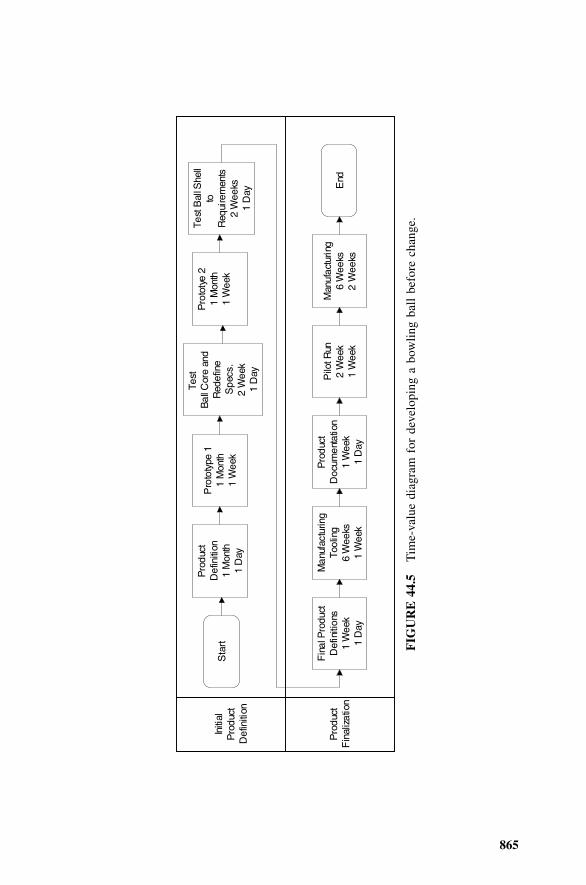
865

Initi

al

Pro

duct

D

efin

ition

Pro

duct

F

inal

izat

ion

Pro

duct

D

efin

ition

1 M

onth

1 D

ay

Pro

toty

pe 1

1 M

onth

1 W

eek

Test

B

all C

ore

and

Red

efin

e S

pecs

.2

Wee

k1

Day

Pro

toty

e 2

1 M

onth

1 W

eek

Test

Bal

l She

ll to

R

equi

rem

ents

2 W

eeks

1 D

ay

Fin

al P

rodu

ct

Def

initi

ons

1 W

eek

1 D

ay

Man

ufac

turin

g To

olin

g6

Wee

ks1

Wee

k

Pro

duct

D

ocum

enta

tion

1 W

eek

1 D

ay

Pilo

t Run

2 W

eek

1 W

eek

Man

ufac

turin

g6

Wee

ksW

2ee

ks

Sta

rt

End

FIG

UR

E44

.5T

ime-

valu

edi

agra

mfo

rde

velo

ping

abo

wlin

gba

llbe

fore

chan

ge.

866

Initi

alP

rodu

ct

Def

initi

on

Pro

duct

F

inal

izat

ion

Pro

duct

D

efin

ition

1 M

onth

1 D

ay

Pro

toty

pe 1

1 M

onth

1 W

eek

Test

Bal

l Cor

e an

d S

hell u

sing

DO

E

2 W

eek

1 D

ay

Man

ufac

turin

gTo

olin

g6

Wee

ks1

Wee

k

Pro

duct

D

ocum

enta

tion

1 W

eek

1 D

ay

Pilo

t Run

2 W

eek

1 W

eek

Man

ufac

turin

g6

Wee

ksW

2ee

ks

Sta

rt

End

FIG

UR

E44

.6T

ime-

valu

edi

agra

mfo

rde

velo

ping

abo

wlin

gba

llaf

ter

chan

ge.

EXAMPLE 44.2: SALES QUOTING PROCESS 867

team combined two prototype definition steps through DOE statistical tech-niques. This DOE step optimized the bowling ball core and shell requirementssimultaneously. By considering manufacturing factors within this develop-ment DOE, we can also expect to produce a ball that has less variability. Ifthe development process cycle time needs further reduction, one should thenassess other non-value-added steps or steps that have a large discrepancybetween calendar and work time.

44.7 EXAMPLE 44.2: SALES QUOTING PROCESS

The following example shows how the S4/IEE approach can be applied tothe quoting process within the sales function (Enck 2002). This applicationillustrates how nonmanufacturing or transactional processes within a businesscan greatly benefit from S4/IEE. Transactional business activities do not man-ufacture a household product; however, as seen in the example below, theseactivities typically have greater visibility to the customer than many manu-factured products.

Company ABC is a small electronic components supplier. It makes plasticconnectors that are used by computer manufacturers and high-tech Internethardware providers. One particular product line had been floundering for anumber of months. It has been facing a weak market for the past six monthswith sales at 50% of forecast. It has been losing sales of existing productsand has been winning a low percentage of new product requests. The man-agers responsible for this product line met with a black belt, to determinewhether S4/IEE could help them improve their situation within the currentmarket and prepare for the future.

At first the discussion focused on product quality and delivery time, whichwere both poor due to a recent change in manufacturing sites. To make surethey were considering the entire value stream, the team studied a flowchartof their supply chain from high level, as shown in Figure 44.7.

From the supply chain map it became clear that the first opportunity tolose potential customers existed in all of the transactional interactions thattook place prior to the customer placing an order. After requesting a quote,the sale could be lost due to the quote taking too long, inability to meetspecifications, price, or long manufacturing lead times. After making somephone calls, the team determined that the quoting lead times, which wereexpected to be hours, were in fact days. The team decided to work on quotingand manufacturing lead times in parallel. This example covers the quotingprocess.

The number of customers lost to long lead times was not known. However,after talking to some customers, the team decided that the lead time neededto be less than two days. The customers they spoke with indicated that com-petitors were quoting within one day and if they didn’t have their quote inwithin one or two days customers felt they didn’t have their act together.

868 LEAN AND ITS INTEGRATION WITH S4 / IEE

New Product Development

Supplier Plant Freight Carrier

Sales Rep

Customer

MarketingCustomer

Service Reps

Customer Complaints

Waste, Rework,

Obsolete Inv

Supplier Complaints

FIGURE 44.7 Supply chain flowchart for component assembly business.

0S u b g ro u p 5 1 0 1 5 2 0 2 5

0

5

1 0

1 5

Quo

te T

ime

Sample Number

1

Me a n =6 .66 7

U C L =12 .1 9

L C L =1 .1 42 2

FIGURE 44.8 A 30,000-foot-level metric for customer quote.

In order to understand the current process, a baseline control chart of 30quote times was produced; one quote was randomly sampled per day overthe previous 30 days, as shown in Figure 44.8. Next the team developed atime-value map of the quoting process to identify the high potential areas forreducing the quoting time, as shown in Figure 44.9.

It was clear from the time-value diagram that the outsource manufacturingwas the reason for the long quote times. The quoting specialists had oftencomplained that the outsource manufacturer delayed their quoting process.However, they were never able to get management within their company orthe outsource company to work on the process. The time-value diagram wassent to management at both companies. Within a week the black belt teamhad a meeting with the chief operating officer (COO) and the managers re-sponsible for quoting at the outsource manufacturer.

EXAMPLE 44.2: SALES QUOTING PROCESS 869

Collect Information from Customer

3 hours1 day

Generate Quote0.5 hours2 hours

Negotiate Price1 day3 days

Enter Order

0.25 hrs1 day

Assemble & Deliver1 week

10 weeks

Start

End

C

Quoting Process

ollect Information from Outsource on Mfg Cost

0.25 hours5 days

FIGURE 44.9 Quoting process time-value diagram.

At the meeting they created as-is and future-state flowcharts for the quotingprocess, as shown in Figure 44.10. Management at both companies wasamazed at the convoluted process for quoting. The current quoting processevolved in the rush to get the process established when the outsourcing com-pany was first contracted to do the work. The team that selected the outsourcemanufacturer focused on their manufacturing abilities. Once the contract wassigned, the marketing people realized that the costing information resided inSan Francisco, so the process was set up with the agreement that the costrequests would be answered within one day. Once the business started, peopleon both ends were scrambling to keep up with their daily activities alongwith the new costing requirements and the process was not capable of meetingthe one-day agreement.

With the support of the COO of the outsourcing company, the future-statequoting process was implemented within two weeks. The plan was to userandomly sampled quotes over the next 30 days to verify that the process hadimproved. At the time of this printing 10 quotes were available. Figures 44.11,44.12, and 44.13 can be used to evaluate the improvements.

Figure 44.11 shows an obvious improvement in the average quoting times.A statistical comparison of the old and new process yielded:

Two-sample T for Old vs New Quoting Process

N Mean St Dev SE Mean

Old 30 5.66 2.16 0.39New 10 1.637 0.139 0.044

Difference � mu Old � mu NewEstimate for difference: 4.02395% lower bound for difference: 3.349T-Test of difference � 0 (vs �): T-Value � 10.14P-Value � 0.000 DF � 29

870 LEAN AND ITS INTEGRATION WITH S4 / IEE

As-is Process Map

Future State Process Map

Component Company

Outsource Manufacturer

Outsource Mfg San Francisco

Office

StartCompile and

send request to outsource

Send to San Francisco

Office

Process request

Send back to Outsource

plant

Compile information

Assemble quote

Send

Component Company

Outsource Manufacturer

StartCompile request

Use standard costing table

Assemble quote

Send

Maintain costingtables

FIGURE 44.10 As-is and future-state process map.

The process control chart showed a new level of process performancearound an average of 1.6 days. The dot plot in Figure 44.12 is a simple wayto convey the capability of the new quoting process relative to the old quotingsystem. The probability plot shown in Figure 44.13 can be used to estimatethe percentage of time the quotes will be made within two days. The teamwas 95% confident that the quoting process would be less than two days 97%of the time.

While there was still some work to be done on this process, the black beltand the team had essentially achieved their objective of reducing the quoting

EXAMPLE 44.2: SALES QUOTING PROCESS 871

0S ubgroup 5 10 15 20 25 30 35

0

5

10

15In

divi

dual

Val

ue

Sample Number

1

Mean=1.640UCL=2.151

LCL=1.129

Curren t Cus to m er Quote Tim e Im proved Curren t Cus tom e r Quote

FIGURE 44.11 The 30,000-foot-level metric for current customer quote.

1 272

Before Change

Time (Days)

After Change

FIGURE 44.12 Customer quote time, before and after change.

time to less than two days. The process owners (marketing and sales) wouldwork to make sure that all quotes were made in less than two days while theblack belt moved on to other more pressing problems within the organization.

Some people might view this as a problem that should have easily beenfixed by management and was not in need of an S4/IEE project. This argu-ment would miss the point that S4/IEE not only provides a process to improvebusiness, it also provides a methodology to help better manage business. Busi-nesses have so many problems that not all can be addressed at any giventime. S4/IEE provides a way to assess the important business processes anddecide what needs to be worked on and how to fix it. In other words, S4/IEEprovides a structure to help management structure and improve its manage-ment activities.

In this particular example they broadened their view of the problem andpicked problems to work on given the data that was available. There arecertainly many other opportunities within this quoting process. However, thisproject focused on the high potential areas, which is what businesses need todo to increase their effectiveness.

There was a tremendous improvement in the quoting process as a resultof this project. This transaction is very important because it is seen by thecustomer long before any product is purchased and can cause the loss, justbecause they had a poor quoting experience, of customers who would prefer

872 LEAN AND ITS INTEGRATION WITH S4 / IEE

2.051.951.851.751.651.551.451.351.25

99

95

90

80

70

60504030

20

10

5

1

New Quote Time (Days)

Per

cent

97

2.00

e

FIGURE 44.13 Normal probability plot for quote time with ML estimates—95%CI.

your product. The team decided that this quoting process was a core com-petence that had to exist for survival. This project, as with many other trans-actional projects, can certainly provide large opportunities in increasing salesand reducing costs for any type of company.

44.8 5S METHOD

The basic housekeeping discipline for both the shop floor and office is 5S(sort, straighten, shine, standardize, sustain). 5S should be considered in twoways: as an everyday continuous improvement activity for individuals andsmall groups, or as a KPIV that should impact a 30,000-foot-level project/operational metric. When the 30,000-foot-level metric indicates cycle time,quality, or safety issues, 5S should be considered as an execution strategy.The sustain portion of 5S should be part of the control phase within a DMAICroadmap. Activities for each of these activities is:

• Sort: The needed tools, supplies, and materials are clearly separated fromthe unneeded.

• Straighten: All items in the work area have a marked place, and a placeexists for everything to allow for easy and immediate retrieval.

TOTAL PRODUCTIVE MAINTENANCE (TPM) 873

• Shine: The work area is cleaned and straightened regularly as you work.• Standardize: Work method, tools, and identification markings are stan-

dard and recognizable throughout the factory. 5S methods are appliedconsistently in a uniform and disciplined manner.

• Sustain: 5S is a regular part of work and continuous actions are taken toimprove work. Established procedures are maintained by checklist.

44.9 DEMAND MANAGEMENT

The system works best when there is a uniform flow of product within thesystem. The policies of a company should encourage stability. Unfortunately,this often does not happen. For example, the reward system for product salesmight create a spike in manufacturing demands at the end of each month.This can lead to supply chain amplification in the form of inaccurate productforecast when these signals are read incorrectly. Also, accounting procedurescan encourage management to produce excess inventory in order to make thenumber that they are evaluated on look better.

Improvements to the supply chain are expected when there is first a re-duction in response time, which leads to more accurate forecasting, and sec-ondly there is a sharing of information along the supply chain so uniformschedules can then be agreed on.

44.10 TOTAL PRODUCTIVE MAINTENANCE (TPM)

As implementation programs with a company, lean and TPM have similarities.The TPM description within this section describes TPM and its linkage to anoverall S4/IEE implementation strategy.

TPM is productive maintenance carried out by all employees through smallgroup activities. Like TQC, which is company-wide total quality control, TPMis equipment maintenance performed on a company-wide basis (Nakajima1998).

Sources for the schedule downtime of a machine are maintenance, breaks,and lunch. Sources for unscheduled downtime include machine breakdown,setup time, and part shortages. Equipment needs to be available and functionproperly when needed. TPM emphasizes not only prevention but also im-provement in productivity. To achieve this we need the participation of bothexperts and operators with a feeling of ownership for this process.

Focus is given within TPM to eliminating the obstacles to the effectivenessof equipment. These six big losses can be broken down into three categories:

874 LEAN AND ITS INTEGRATION WITH S4 / IEE

• Downtime:1. Equipment failure from breakdowns2. Setup and adjustment from die changes, etc.

• Speed losses:3. Idling and minor stoppages due to abnormal sensor operation, etc.4. Reduced speed due to discrepancies between the design and actual

operational speed• Defect:

5. Process defects in process due to scrap and reworks6. Reduced yield from machine startup to stable production

From an equipment point of view:

• Load time and operating time are impacted by losses numbered 1 and 2.• Net operating time is impacted by losses numbered 3 and 4.• Valuable operating time is impacted by losses numbered 5 and 6.

Metrics within TPM can be tracked at the 30,000-foot level, where improve-ment projects are initiated when the metrics are not satisfactory. The highest-level TPM metric is overall equipment effectiveness (Nakajima 1988):

Overall equipment effectiveness � availability � Performance efficiency� Rate of quality products

where the downtime loss metric (loss 1 from equipment failure and loss 2from setup and adjustment) is

Operation time Loading time � DowntimeAvailability � �

Loading time Loading time

and the speed loss metric (loss 3 from idling and minor stoppages and loss4 from reduced speed) is

Ideal cycle time � Processed amountPerformance efficiency � � 100

Operating time

and the defect loss metric (loss 5 from defects in process and loss 6 fromreduced yield) is

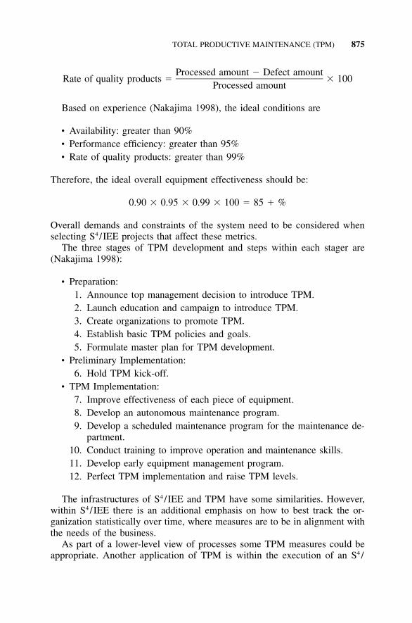
TOTAL PRODUCTIVE MAINTENANCE (TPM) 875

Processed amount � Defect amountRate of quality products � � 100

Processed amount

Based on experience (Nakajima 1998), the ideal conditions are

• Availability: greater than 90%• Performance efficiency: greater than 95%• Rate of quality products: greater than 99%

Therefore, the ideal overall equipment effectiveness should be:

0.90 � 0.95 � 0.99 � 100 � 85 � %

Overall demands and constraints of the system need to be considered whenselecting S4/IEE projects that affect these metrics.

The three stages of TPM development and steps within each stager are(Nakajima 1998):

• Preparation:1. Announce top management decision to introduce TPM.2. Launch education and campaign to introduce TPM.3. Create organizations to promote TPM.4. Establish basic TPM policies and goals.5. Formulate master plan for TPM development.

• Preliminary Implementation:6. Hold TPM kick-off.

• TPM Implementation:7. Improve effectiveness of each piece of equipment.8. Develop an autonomous maintenance program.9. Develop a scheduled maintenance program for the maintenance de-

partment.10. Conduct training to improve operation and maintenance skills.11. Develop early equipment management program.12. Perfect TPM implementation and raise TPM levels.

The infrastructures of S4/IEE and TPM have some similarities. However,within S4/IEE there is an additional emphasis on how to best track the or-ganization statistically over time, where measures are to be in alignment withthe needs of the business.

As part of a lower-level view of processes some TPM measures could beappropriate. Another application of TPM is within the execution of an S4/

876 LEAN AND ITS INTEGRATION WITH S4 / IEE

IEE project where the project situation suggests the application of a uniqueTPM tool.

44.11 CHANGEOVER REDUCTION

Let’s consider a 30,000-foot-level metric (Y variable or KPOV) that has alead time reduction goal. For this situation we would consider a lean toolapplication since one major objective of lean is the reduction of lead time.To achieve this, the size of batches often needs reduction, which creates afocus for improving changeover reduction. (Changeover time is the time fromthe last piece of one batch to the first piece of the next batch.)

Changeover time can have several components. Internal changeover timeis the time when the machine is stopped. External changeover time involvespreparation.

Other types of changeover besides machine changeover that can need re-duction include line changeover, maintenance operations, vehicle loading/unloading of vehicles, and many office operations. The classic changeoveranalogy is the Grand Prix pit stop. Another example is the loading and un-loading of an airplane. For changeover it is important not only to reduce themean changeover time but also the variability in changeover time using astandardized process.

Within Shingo’s classic single-minute exchange of die (SMED), internaland external activities are classified within a flowchart of the changeover. Itis desirable to move internal activities to external activities when possible.Doing this permits more uptime of the machine since the maximum amountof preparation is accomplished before the machine is stopped. Example ap-plications for the improvement of external activities are placing tools on cartsnear the die and using color codes to avoid confusion. Example applicationsfor the improvement of internal activities are quick-change nuts and the stan-dardization of activities.

Consider recording and plotting on a visible run chart all changeover times,asking for improvement suggestions.

44.12 KANBAN

A system that creates product that is then sold after it is produced is calleda push system. If there is no mechanism to keep WIP below some level, theprocess will not be controllable.

The Japanese word kanban refers to the pulling of product through a pro-duction process (i.e., a pull system). The intent of kanban is to signal apreceding process that the next process needs parts/material. Because a bot-tleneck is the slowest operation in a chain of operations, it will pace the output

VALUE STREAM MAPPING 877

of the entire line. Buffers in high-volume manufacturing serve to affect linebalance among bottlenecks and product-specific operations. It is very impor-tant that bottleneck operations be supplied with the necessary WIP at theappropriate time and that poorly sequenced work not interfere with the workthat is to be accomplished at these operations.

Rules to consider when operating an effective kanban are as follows:

• No withdrawal of parts is to occur without a kanban where subsequentprocesses are to withdraw only what is needed.

• Defective parts are not to be sent to subsequent processes.• Preceding processes are to produce only the exact quantity of parts with-

drawn by subsequent processes.• Variability in the demand process should be minimized as much as pos-

sible.

If production requirements drop off, the process must be stopped. An in-crease in production requirements is addressed through overtime and S4/IEEprocess improvement activities.

Kanban can dramatically improve a process that produces few defectswithin workstations. However, if there are workstations that have high defectrates (i.e., a hidden factory), the system can become starved for parts. Thisproblem could be avoided by integrating kanban with S4/IEE measurementsand implementation methods.

44.13 VALUE STREAM MAPPING

When the 30,000-foot-level measures for cycle time and other lean metricsare not satisfactory, the value stream mapping approach described in thissection can create insight into where efforts should be placed to improve theoverall enterprise. Focused S4/IEE projects can result from this activity.

In Toyota, value stream mapping is know as ‘‘material and informationflow mapping.’’ In the Toyota Production System, current and future states/ideal states are depicted by practitioners when they are developing plans toinstall lean systems. Much attention is given to establishing flow, eliminatingwaste, and adding value. Toyota views manufacturing flows as material, in-formation, and people/process. The value stream mapping methodology de-scribed in this section covers the first two of these three items (Rother andShook 1999). This section is an overview of the methodology that is describedin that reference.

A value stream map can trace both product and information flow acrossorganizational boundaries of a company. A value stream manager, who isresponsible for the entire value stream and reports to senior management, canbe a great asset to an organization. This person can take ownership of the

878 LEAN AND ITS INTEGRATION WITH S4 / IEE

overall system metric (30,000-foot-level metric) and lead a focus effort toimproving the overall system, even though this might mean suboptimizingindividual processes. The value stream manager can be responsible for theprioritization and orchestration of S4/IEE projects, which have a specific fo-cus to improve the overall value stream.

The type of value stream map described in this section utilizes symbolssuch as those illustrated in Figure 44.14. These symbols represent variousactivities when conducting value stream mapping.

Before addressing value stream improvements, a current-state value streammap needs to be created. When creating a current-state map, such as thatshown in Figure 44.15, someone needs to walk the actual pathways of ma-terial and information flow, beginning with a quick walk through the entirevalue stream. One should start at the end and work upstream, mapping theentire value stream firsthand using a pencil and paper for documentation anda stopwatch to record times that were personally observed.

When creating a future state map for a value stream, one should keep inmind some important lean principles. Overproduction can be created with abatch-and-push mass production system. This can occur when production iscreated by commands from production control instead of needs of the down-stream customer of the process. Defects can remain as part of the hiddenfactory until discovered downstream in the process. This can result in the totaltime for a part to get through the production process being very long andvalue-added time for producing the product very small. The most significantsource of waste is overproduction, which can cause various types of wastes,from part storages, additional part handling, additional sorting, and rework toshortages at some production steps, because they need to produce parts tomaintain their efficiency, even though no parts are needed. Mass productionthinking implies that it is cheaper to produce if you produce more and faster.However, this is only true from traditional accounting practices where thereis a direct-cost-per-item perspective that ignores all other real costs associatedwith direct and indirect production costs.

A lean value stream has some characteristics that should be strived for:

1. Produce to takt time. For industries such as distribution, customer prod-ucts, and process industries, a unit of customer demand for a takt timecalculation could be the amount of work that can be accomplished bythe process bottleneck during a fixed time interval (e.g., 1 hour).

2. Whenever possible, develop continuous flow, that is, the production ofone piece at a time and the immediate passing of this part to the nextstep. It might be best to have a combination of continuous flow with aFIFO (first-in-first-out) pull system.

3. A supermarket is an inventory of parts that are controlled for the pro-duction scheduling of an upstream process. When continuous flow does

VALUE STREAM MAPPING 879

FIGURE 44.14 Material flow, information flow, and general icons. [From Rotherand Shook (1999), with permission.]

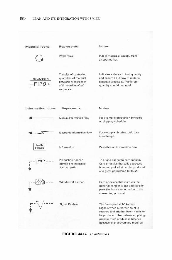
880 LEAN AND ITS INTEGRATION WITH S4 / IEE

FIGURE 44.14 (Continued )

VALUE STREAM MAPPING 881

FIGURE 44.14 (Continued )

882 LEAN AND ITS INTEGRATION WITH S4 / IEE

FIGURE 44.15 Current state value stream example. [From Rother and Shook (1999),with permission.]

not extend upstream, use supermarkets to control production. This mightbe needed when a machine creates several part numbers, supplier’s lo-cation is distant, or there is a long lead time or unreliable process in-terface. Control by scheduling to downstream needs, as opposed to anindependent scheduling function. A production kanban should triggerthe production of parts, while a withdrawal kanban instructs the materialhandler to transfer parts downstream.

4. Attempt customer scheduling to only one production process or sub-process in the overall production process (i.e., the pacemaker process).Frequently this process is the most downstream continuous flow processin the value stream.

5. Use load leveling at the pacemaker process so that there is an evendistribution of production of different products over time. This improves

VALUE STREAM MAPPING 883

FIGURE 44.15 (Continued )

the flexibility of the overall process to have a short lead time whenresponding to different customer requirements, while keeping finishedgood inventory and upstream supermarkets low.

6. Release and withdraw small consistent work increments at the pace-maker process. This creates a predictable production flow, which canyield to quick problem identification and resolution. When a largeamount of work is released to the shop floor, each process can shuffleorders, which results in increased lead time and the need for expediting.

7. In fabrication processes that are upstream from the pacemaker process,create the ability to make every part every day (i.e., EPE day). Wewould then like to reduce EPE to shorter durations (e.g., shift). Thiscan be accomplished by shortening changeover times and runningsmaller batches in upstream fabrication processes. An approach to de-termining initial batch size at fabrication processes is to determine howmuch time remains in a day to make changeovers. A typical target isthat there is 10% of the time available for changeovers.

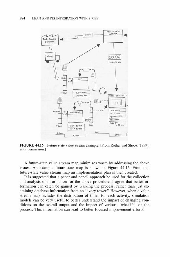
884 LEAN AND ITS INTEGRATION WITH S4 / IEE

FIGURE 44.16 Future state value stream example. [From Rother and Shook (1999),with permission.]

A future-state value stream map minimizes waste by addressing the aboveissues. An example future-state map is shown in Figure 44.16. From thisfuture-state value stream map an implementation plan is then created.

It is suggested that a paper and pencil approach be used for the collectionand analysis of information for the above procedure. I agree that better in-formation can often be gained by walking the process, rather than just ex-amining database information from an ‘‘ivory tower.’’ However, when a valuestream map includes the distribution of times for each activity, simulationmodels can be very useful to better understand the impact of changing con-ditions on the overall output and the impact of various ‘‘what-ifs’’ on theprocess. This information can lead to better focused improvement efforts.

EXERCISES 885

FIGURE 44.16 (Continued )

44.14 EXERCISES

1. Conduct and apply 30,000-foot-level measurements and S4/IEE strategiesto the ‘‘beer game,’’ which is described in Chapter 3 of Senge (1990).

2. Describe how and show where the tools described in this chapter fit intothe overall S4/IEE roadmap described in Figure A.1 in the Appendix.

886

45INTEGRATION OF THEORY OFCONSTRAINTS (TOC) IN S4/IEE

S4 /IEE DMAIC Application: Appendix Section A.1, Project ExecutionRoadmap Steps 4.1 and 4.4

The outputs of a system are a function of the whole system, not just individualprocesses. When we view our system as a whole, we realize that the outputis a function of the weakest link. The weakest link of the system is theconstraint. If care is not exercised, we can be focusing on a subsystem that,even though it is improved, does not impact the overall system output. Weneed to focus on the orchestration of efforts such that we optimize the overallsystem, not individual pieces. Unfortunately, organization charts lead to work-flow by function, which can result in competing forces within the organiza-tion. With TOC, systems are viewed as a whole and work activities are to bedirected such that the whole system performance measures are improved.

The TOC system chain extends from market demand through the organi-zation chain to suppliers. Let’s consider an example when this high-level viewof the overall system is not addressed. An organization works at improvinginternal process efficiencies. Capacity then increases. Excess inventory wasthen created because there was not sufficient demand. It was then discoveredthat the constraint was really the sales and marketing process.

Within an organization there are often constraints that we may or may notthink about. Types of constraints include market, resource, material, supplier,financial, and knowledge/competency. We need to look at the rules (i.e., pol-icies) that drive the constraints.

MEASURES OF TOC 887

45.1 DISCUSSION

TQM has often been implemented by dividing the system into processes andthen optimizing the quality of each process. This approach is preferable tochasing symptoms, but new problems can be created if the individual processis not considered in concert with other processes that it affects.

The theory of constraints presented by Goldratt (1992) focuses on reducingsystem bottlenecks as a means to continually improve the performance of theentire system. Rather than viewing the system in terms of discrete processes,TOC addresses the larger systematic picture as a chain or grid of interlinkedchains. The performance of the weakest link determines the performance ofthe whole chain. According to Goldratt, the vast majority of constraints resultfrom policies (e.g., rules, training, and other measures), while few constraintsare physical (e.g., machines, facilities, people, and other tangible resources).For example, a large portion of highway road repair seems initially to bephysically constrained by traffic flow. But the real constraint is governmentacquisition policy, which mandates the award of contracts to the lowest bidder.This drives contractors to the use of low-quality materials with shorter life inan effort to keep costs down and remain competitive.

TOC considers three dimensions of system performance in the followingorder: throughput (total sales revenues minus the total variable costs for pro-ducing a product or service), inventory (all the money a company invests initems it sells), and operating expense (money a company spends transforminginventory into throughput). Focusing on these dimensions can lead a companyto abandon traditional management cost accounting while at the same timecausing an improvement in competitive price advantage.

45.2 MEASURES OF TOC

Traditional financial measures (net profit, ROI, and cash flow) do not tell uswhat to do daily at the operational level. It is not easy for first- or second-line managers to decide how their actions might affect net profit, ROI, or cashflow. The TOC measures of throughput, inventory, and operating expense aremore easily understood in relationship to operational decisions. Within theS4/IEE approach we can view these as satellite-level metrics that drive projectselection.

Throughput (T) as a TOC measure is the rate of generating money in anorganization. This is a financial value-added metric that equates to revenuesminus variable costs. Levels of measures/assessments are unit, product, andorganization. Investment or inventory (I) as a TOC measure is money tied upwithin an organization. This includes facilities, capital assets, equipment, andmaterials. Operating expense (OE) is the money flowing out of the system to

888 INTEGRATION OF THEORY OF CONSTRAINTS (TOC) IN S4/IEE

generate throughput. This is the fixed expense, that is, the overhead of theorganization. These TOC metrics have the relationships

T � OEReturn on investment �

I

Net profit � T � OE

Cash flow (CF) � T � OE � �I

Throughput is limited by the system constraints. Operating expense is pri-marily generated by nonconstraints. Using a TOC approach, focus is given toimproving the overall system by making changes to the constraint.

45.3 FIVE FOCUSING STEPS OF TOC

The five focusing steps of TOC for addressing constraints (Schragenheim andDettmer 2001) are

1. Identify2. Exploit3. Subordinate4. Elevate5. Go back to step 1, but beware of the inertia

Step 1: Identify the system’s constraint. Consider what is limiting the per-formance of the system. Determine whether the restraint is inside (resourceor policy) or outside the system (market or supplier). Assess the difficulty ofbreaking the constraint. If the constraint can easily be broken, break it andthen look for the next constraint. If it is hard to break the constraint, proceedto step 2.

Step 2: Decide how to exploit the system’s constraint, where exploit meansto get the most from the constraining element without additional investment.Consider what operational changes can be made to maximize productivityfrom the constraining element. For example, for a market demand constraint,cater to the market to win more sales. If there is a resource constraint, deter-mine the best approach to maximize its contribution to profit.

Step 3: After making a decision on how to exploit the system, subordinateeverything else to that decision. This requires that other parts of the systembe put in second place relative to their own measures of success. All non-constraints are to be placed in a support role to the constraint, which can bedifficult to accomplish. For example, if market demand is the only constraint,

S4 / IEE TOC APPLICATION AND THE DEVELOPMENT OF STRATEGIC PLANS 889

incoming orders should trigger the release of material. If there are no neworders entering the system, manufacturing managers often want to continueworking so that their efficiencies remain high. For this situation, the materialrelease process must be subordinated to the needs of the constraint.

Step 4: If the system constraint is broken by subordination, go back tostep 1. If the system constraint is not broken, determine other ways to elevatethe constraint, where elevate means to increase capacity. For example, if theconstraint is internal, additional capacity for the resource could be achievedthrough acquiring more machines or people or through the addition of over-time. If there is a market demand constraint (i.e., lack of sales), elevationmight be achieved through an advertising campaign.

Step 5: Even when subordination does not break the constraint, elevationwill likely break it, unless there is a conscious effort to stop short of breakingit. After the subordinate or elevate steps are completed, step 1 needs to berepeated to determine the location of the new constraints. Sometimes a con-straint moves not as a result of our intentional actions but because there isan environmental change. An example of this is the change in market demandfor product mixes. One must not become complacent with their actions sinceinertia can change things. When a constraint moves, previous actions forsubordination and elevation may no longer be the best solution. Other alter-natives might need to be investigated.

45.4 S4/IEE TOC APPLICATION AND THE DEVELOPMENT OFSTRATEGIC PLANS

Theory of constraints (TOC) can be useful to help organizations get out ofthe firefighting mode. TOC measures can be the satellite-level metrics thatdrive S4/IEE projects. In lieu of attempting to drive improvements throughtraditional measures of capital utilization, growth, revenue, a TOC satellite-level metrics strategy would focus on throughput, investment/ inventory, andoperating expense.

Organizations can have satellite-level metrics, which are in alignment with

• 30,000-foot-level operational metrics such as defective/defect rates, cycletime, waste, days sales outstanding (DSO), customer satisfaction, on-timedelivery, number of days from promise date, number of days from cus-tomer requested date, dimensional property, inventory, and headcount

• A methodology to build strategic plans and then track how well resultsare achieved against this plan

• The S4/IEE project selection process

Perhaps you have seen balance scorecard metrics for an organization pre-sented as a dashboard metrics. Dashboard metrics can present what the or-

890 INTEGRATION OF THEORY OF CONSTRAINTS (TOC) IN S4/IEE

ganization is doing at any point in time in the format of a dial. If the needleon the dial is within the green area, no action is to be taken. If the needle isin the yellow area, caution should be taken since the current response is nearspecification limits. If the needle is in the red region, corrective action shouldbe taken since specification limits are not being met. Data presented in thismanner tends to firefighting activities in that common cause, treating them asthough they were special cause.

An S4/IEE strategy using a TOC approach would be to tracking balancescorecard metrics using TOC satellite-level measures. These measures wouldlead to a strategy for improvement. Operational 30,000-foot-level controlchart measures would then be created and tracked. S4/IEE projects would beprioritized and then selected based upon a screening criteria that is to yieldprojects that have a high likelihood of success of achieving significant bottom-line and improved customer satisfaction benefits.

45.5 TOC QUESTIONS

We can use the following questions to help determine if local decisions arebeing made positively relative to overall system success TOC measures(Schragenheim 2001).

Positive response will improve throughput:

• Will the decision result in a better use of the worst constrained resource?• Will it make full use of the worst constrained resource?• Will it increase total sales?• Will it speed up delivery to customers?• Will it provide a characteristic of product or service that our competitors

don’t have?• Will it win repeat business for us?• Will it reduce scrap or rework?• Will it reduce warranty or replacement costs?

Positive response will decrease inventory or investment:

• Will we need fewer raw materials or purchased parts?• Will we be able to keep less material on hand?• Will it reduce work-in-process?• Will we need less capital facilities or equipment to do the same work?

Positive response will decrease operating expense:

EXERCISE 891

• Will overhead go down?• Will payments to vendors decrease?• Will we be able to divert some people to do other throughput-generating

work?

The TOC described by Goldratt (1992) presents a system thinking processwhere the focus is on the system’s bottlenecks. This results in continual im-provement of the performance of the entire system. Rather than viewing thesystem in terms of discrete processes, TOC addresses the larger systematicpicture as a chain or grid of interlinked chains. The performance of the wholechain is determined by the performance of its weakest link.

45.6 EXERCISE

1. Describe how TOC fits into the overal S4/IEE strategy.

PART VII

DFSS AND 21-STEP INTEGRATIONOF THE TOOLS

This part (Chapters 46–50) describes DFSS techniques for both products andprocesses. In addition, the 21-step integration of the tools roadmaps is de-scribed for manufacturing, service, process DFSS, and product DFSS, withexamples.

895

46MANUFACTURING APPLICATIONSAND A 21-STEP INTEGRATION OFTHE TOOLS

Six Sigma techniques are applicable to a wide variety of manufacturing pro-cesses. The following examples illustrate how Smarter Solutions, Inc. hasassisted customers in benefiting from the wise application of Six Sigma tools.

• Customer 1 (computer chip company): Developed a control charting mea-surement system and a DOE strategy to improve the consistency of peel-back force necessary to remove packaging for electrical components.Results: The approach directly assessed customer needs by consideringboth within- and between-product variability.

• Customer 2 (computer chip company): Developed a technique to monitorand reduce the amount of damage from control handlers. Results: Thecontrol chart test strategy considered sampled continuous data informa-tion to monitor the existing process in conjunction with DOE techniquesthat assess process improvement opportunities.

• Customer 3 (plastic molding company): Applied DOE techniques to aninjected molded part. Results: Part-to-part variability decreased. Com-pany now routinely uses DOE techniques to better understand and im-prove processes.

• Customer 4 (computer company): Used DOE techniques to reduceprinted circuit board defects. Results: Determined the manufacturing pro-cess settings that reduced the number of bridges, insufficient solders, andnon-wet conditions.

• Customer 5 (environmental equipment company): Used a DOE strategyto improve manufacturing product yield. Results: A small number ofexperimental trials uniquely assessed design and manufacturing param-

896 APPLICATIONS AND A 21-STEP INTEGRATION OF THE TOOLS

eters in conjunction with other factors that could affect test accuracy andprecision.

• Customer 6 (telephone equipment company): Implemented DOE tech-niques to improve the manufacturing of a critical plastic component.Results: The analysis approach identified important factor settings thatimproved the process capability/performance metric for flatness.

• Customer 7 (satellite equipment interface company): Developed a fieldreporting methodology. Result: The field tracking system quantified prod-uct failure rate as a function of time and identified the best area to focusimprovement efforts.

• Customer 8 (video conferencing company): Created a strategy to deter-mine where to focus improvement efforts for product burn-in. Result: Amultiple control chart strategy of both the burn-in and field failure ratesis combined with Pareto charting to identify common and special causesalong with opportunities for improvement.

These examples illustrate the many implementation strategies and uniquetool combinations available for manufacturing processes. Through S4/IEEtechniques organizations can also achieve significant benefits when they canbridge their measurement and improvement activities from products to a man-ufacturing process that creates various product types. In addition Six Sigmaprovides a means to expose the hidden factory of reworks and helps organi-zations quantify the cost of doing nothing. Through the wise application ofSix Sigma techniques, organizations can focus on the big picture and thendrill down when it is appropriate. This chapter includes thoughts on whatcould be done when measuring manufacturing processes, an overall applica-tion strategy, and S4/IEE application examples.

46.1 A 21-STEP INTEGRATION OF THE TOOLS:MANUFACTURING PROCESSES

There are many possible alternatives and sequencing of Six Sigma tools forS4/IEE manufacturing projects. From our S4/IEE project execution roadmapwe can create a 21-step integration of the tools that has some general appli-cation. Shown below is a concise sequencing of how Six Sigma tools can belinked/considered for manufacturing projects. This roadmap can be refer-enced to give insight on how individual tools can fit into the big picture.Presentation of a project plan into this format can aid with creating an im-proved project plan. Specific tools are highlighted in bold print to aid thereader in later locating where a tool could be applied. The Glossary in theback of this book can aid with term clarifications.

A 21-STEP INTEGRATION OF THE TOOLS: MANUFACTURING PROCESSES 897

21-Step Integration of the Tools: Manufacturing Processes

Step Action Participants Source of Information

1 Drill down from satellite-level metricto a business need. Identify criticalcustomer requirements from a30,000-foot-level measurementpoint of view. Define the scope ofprojects. Create a project charter.Identify KPOVs that will be usedfor project metrics.

Black belt andchampion

Organization wisdom

2 Identify team of key stakeholders forthe project. Address any projectformat and frequency of statusreporting issues. Conduct initialteam meeting. Address problemstatement, gap analysis of processto customer needs, goal statement,SIPOC diagram, drill down fromhigh-level process map to focusarea, and visual representation ofproject’s 30,000-foot-level metricsalignment with satellite-levelmetrics.

Black belt, champion,process owner, andteam

Organization wisdom

3 Describe business impact. Addressfinancial measurement issues ofproject. Estimate COPQ/CODND.

Black belt, champion,and finance

Organization wisdom

4 Collect VOC needs for the project.Define, as needed, secondarymetrics that will be compiled (e.g.,RTY). Plan overall project.Consider using this 21-stepintegration of tools to help withthe creation of a projectmanagement Gantt chart.

Team, champion, andsponsor

Organization wisdom

5 Start compiling project metrics intime series format with infrequentsampling / subgrouping. Create30,000-foot-level control chartsor run charts of KPOVs. Controlcharts at this level can reduceamount of firefighting.

Black belt and team Current and collecteddata

6 Determine long-term processcapability /performance metricsfor KPOVs from 30,000-foot-levelcontrol charts. Quantifynonconformance proportion.Compile nonconformance issues inPareto chart format. RefineCOPQ/CODND estimates.

Black belt and team Current and collecteddata

898 APPLICATIONS AND A 21-STEP INTEGRATION OF THE TOOLS

Step Action Participants Source of Information

7 Create a process flowchart /processmap of the current process at alevel of detail that can give insightto what should be done differently.Consider using lean tools.

Black belt and team Organization wisdom

8 Create a cause-and-effect diagramto identify variables that can affectthe process output. Use theprocess flowchart and Paretochart of nonconformance issues tohelp with the identification ofentries within the diagram.

Black belt and team Organization wisdom

9 Create a cause-and-effect matrixassessing strength of relationshipsbetween input variables andKPOVs. Input variables for thismatrix could have been identifiedinitially through a cause-and-effect diagram.

Black belt and team Organization wisdom

10 Assess the integrity of the data.Conduct a measurement systemsanalysis. Consider a variancecomponents analysis thatconsiders repeatability andreproducibility along with othersources such as machine-to-machine within the sameassessment.

Black belt and team Proactiveexperimentation

11 Rank importance of input variablesfrom the cause-and-effect matrixusing a Pareto chart. From thisranking create a list of variablesthat are thought to be KPIVs.

Black belt and team Organization wisdom

12 Prepare a focused FMEA. Considercreating the FMEA from a systemspoint of view, where item/ functioninput items are the largest rankedvalues from a cause-and-effectmatrix. Assess current controlplans. Implement agreed toprocess improvement changes.

Black belt and team Organization wisdom

13 Create a data collection plan. Collectdata for assessing the KPIV/KPOV relationships that arethought to exist.

Black belt and team Collected data

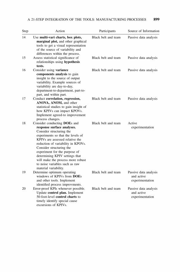
A 21-STEP INTEGRATION OF THE TOOLS: MANUFACTURING PROCESSES 899

Step Action Participants Source of Information

14 Use multi-vari charts, box plots,marginal plot, and other graphicaltools to get a visual representationof the source of variability anddifferences within the process.

Black belt and team Passive data analysis

15 Assess statistical significance ofrelationships using hypothesistests.

Black belt and team Passive data analysis

16 Consider using variancecomponents analysis to gaininsight to the source of outputvariability. Example sources ofvariability are day-to-day,department-to-department, part-to-part, and within part.

Black belt and team Passive data analysis

17 Conduct correlation, regression,ANOVA, ANOM, and otherstatistical studies to gain insight ofhow KPIVs can impact KPOVs.Implement agreed-to improvementprocess changes.

Black belt and team Passive data analysis

18 Consider conducting DOEs andresponse surface analyses.Consider structuring theexperiments so that the levels ofKPIVs are assessed relative thereduction of variability in KPOVs.Consider structuring theexperiment for the purpose ofdetermining KPIV settings thatwill make the process more robustto noise variables such as rawmaterial variability.

Black belt and team Activeexperimentation

19 Determine optimum operatingwindows of KPIVs from DOEsand other tools. Implementidentified process improvments.

Black belt and team Passive data analysisand activeexperimentation

20 Error-proof KPIs whenever possible.Update control plan. Implement50-foot-level control charts totimely identify special causeexcursions of KPIVs.

Black belt and team Passive data analysisand activeexperimentation

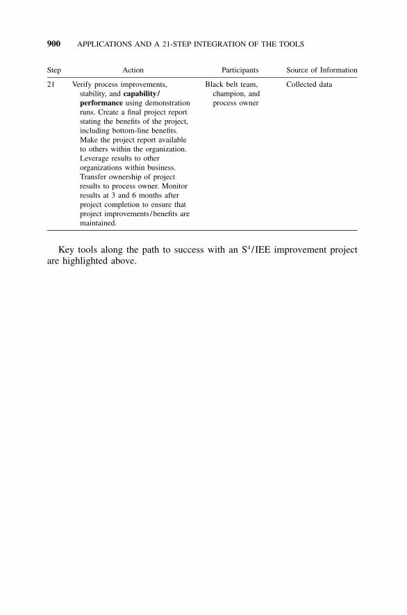
900 APPLICATIONS AND A 21-STEP INTEGRATION OF THE TOOLS

Step Action Participants Source of Information

21 Verify process improvements,stability, and capability /performance using demonstrationruns. Create a final project reportstating the benefits of the project,including bottom-line benefits.Make the project report availableto others within the organization.Leverage results to otherorganizations within business.Transfer ownership of projectresults to process owner. Monitorresults at 3 and 6 months afterproject completion to ensure thatproject improvements /benefits aremaintained.

Black belt team,champion, andprocess owner

Collected data

Key tools along the path to success with an S4/IEE improvement projectare highlighted above.

901

47SERVICE/TRANSACTIONALAPPLICATIONS AND A 21-STEPINTEGRATION OF THE TOOLS

A key lesson that many companies have learned when implementing SixSigma is that successful outcomes are not limited to manufacturing processes.Many of our clients have had great success when applying the S4/IEE meth-odology to improve their key service/transactional processes. Consider thefollowing cases:

• Customer 1 (software company): Implemented control charting and pro-cess capability/performance measurement strategies in their customerorder fulfillment process. Results: Subprocess owners in assembly, ma-terials, planning, purchasing, shipping, and testing identified importantmeasurements and process improvement opportunities using controlcharting, Pareto charting, normal probability plotting, and DOE tools.

• Customer 2 (pharmaceutical testing company): Created a strategy usingSPC techniques to track iterations of paperwork. Result: Control chartsand Pareto charts in conjunction with brainstorming could then indicatethe magnitude of common-cause variability and opportunities for im-provement.

• Customer 3 (aerospace service company): Created a strategy to reducethe warranty return rate after servicing products. Results: Control charttechniques could monitor the proportion of returns over time, while Pa-reto charts could monitor the types of failures. Efforts could then bedirected to improve processes on the ‘‘big hitter’’ items.

• Customer 4 (city government): Created a strategy to evaluate the differ-ences among city home inspectors. Result: Random sampling and controlcharting techniques could quantify the differences over time. Through

902 SERVICE/TRANSACTIONAL APPLICATIONS

Pareto charting and brainstorming techniques, opportunities for improve-ment could be identified.

• Customer 5 (school district): Created a fractional factorial DOE strategyto assess the factors that could affect attendance and what could be donedifferent to improve.

These examples illustrate the many implementation strategies and uniquetool combinations available for S4/IEE service/transactional projects. Thischapter includes thoughts on what could be done when measuring service-type processes, an overall application strategy, and two S4/IEE applicationexamples where teams have effectively utilized the S4/IEE methodology toimprove key service/transactional processes.

47.1 MEASURING AND IMPROVING SERVICE/TRANSACTIONAL PROCESSES

Collecting insightful metrics is sometimes a challenge when effectively ap-plying the S4/IEE methodology to service/transactional processes. Projectsof this type sometimes lack objective data. When data do exist, the practi-tioner is usually forced to work with attribute data such as pass/fail require-ments or number of defects. Teams should strive for continuous data overattribute data whenever possible. Continuous data provide more options forstatistical tool usage and yield more information about the process for a givensample size. A rough rule of thumb is to consider data as continuous if atleast 10 different values occur and no more than 20% of the data set arerepeat values.

Frequently in service/transactional projects, a process exists and a goal hasbeen set but there are no real specification limits. Setting a goal or soft targetas a specification limit for the purpose of determining process capability/performance indices could yield very questionable results. Some organizationsspend a lot of time creating a very questionable metric by arbitrarily addinga specification value where one was not really appropriate. Consider the im-pact of forcing a specification limit where one does not exist. Instead, considerusing probability plotting to gain insight into the capability/performance ofa process expressed in units of frequency of occurrence. Chapter 11 givesmore detailed information on planning, performing, and analyzing the resultsof process capability/performance measurement studies for this type of sit-uation.

Even service/transactional processes should consider the benefit of con-ducting a measurement systems analysis (MSA). Data integrity can be a prob-lem with some of these processes. If attribute data is gathered, one shouldnot overlook the importance of performing a measurement system analysis todetermine the amount of variability the gage is adding to the total processvariation. Attribute gage studies can also be conducted by comparing how

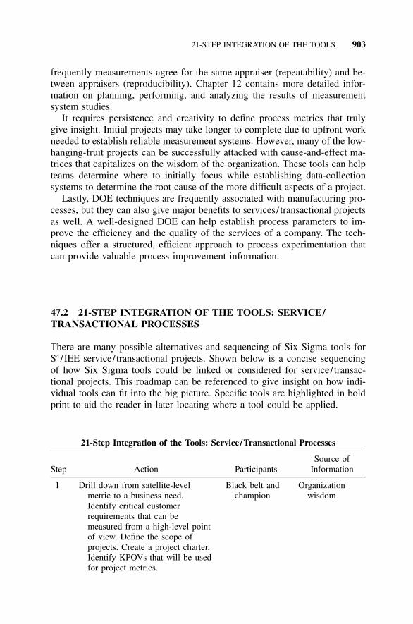
21-STEP INTEGRATION OF THE TOOLS 903

frequently measurements agree for the same appraiser (repeatability) and be-tween appraisers (reproducibility). Chapter 12 contains more detailed infor-mation on planning, performing, and analyzing the results of measurementsystem studies.

It requires persistence and creativity to define process metrics that trulygive insight. Initial projects may take longer to complete due to upfront workneeded to establish reliable measurement systems. However, many of the low-hanging-fruit projects can be successfully attacked with cause-and-effect ma-trices that capitalizes on the wisdom of the organization. These tools can helpteams determine where to initially focus while establishing data-collectionsystems to determine the root cause of the more difficult aspects of a project.

Lastly, DOE techniques are frequently associated with manufacturing pro-cesses, but they can also give major benefits to services/ transactional projectsas well. A well-designed DOE can help establish process parameters to im-prove the efficiency and the quality of the services of a company. The tech-niques offer a structured, efficient approach to process experimentation thatcan provide valuable process improvement information.

47.2 21-STEP INTEGRATION OF THE TOOLS: SERVICE/TRANSACTIONAL PROCESSES

There are many possible alternatives and sequencing of Six Sigma tools forS4/IEE service/transactional projects. Shown below is a concise sequencingof how Six Sigma tools could be linked or considered for service/transac-tional projects. This roadmap can be referenced to give insight on how indi-vidual tools can fit into the big picture. Specific tools are highlighted in boldprint to aid the reader in later locating where a tool could be applied.

21-Step Integration of the Tools: Service/Transactional Processes

Step Action ParticipantsSource of

Information

1 Drill down from satellite-levelmetric to a business need.Identify critical customerrequirements that can bemeasured from a high-level pointof view. Define the scope ofprojects. Create a project charter.Identify KPOVs that will be usedfor project metrics.

Black belt andchampion

Organizationwisdom

904 SERVICE/TRANSACTIONAL APPLICATIONS

Step Action ParticipantsSource of

Information

2 Identify team of key stakeholdersfor project. Address any projectformat and frequency of statusreporting issues. Conduct initialteam meeting. Address problemstatement, gap analysis of processto customer needs, goalstatement, SIPOC diagram, drilldown from high-level processmap to focus area, and visualrepresentation of project’s30,000-foot-level metricsalignment with satellite-levelmetrics.

Black belt andchampion

Organizationwisdom

3 Describe business impact. Addressfinancial measurement issues ofproject. Estimate COPQ/CODND.

Black belt andfinance

Organizationwisdom

4 Collect VOC needs for the project.Define secondary metrics, asneeded, that will be compiled,(e.g. RTY). Plan overall project.Consider using this 21-stepintegration of tools to help withthe creation of a projectmanagement Gantt chart.

Team andchampion

Organizationwisdom

5 Start compiling project metrics intime series format with infrequentsampling/subgrouping. Create30,000-foot-level control chartsor run charts of KPOVs.Control charts at this level canreduce amount of firefighting.

Black belt andteam

Current andcollected data

21-STEP INTEGRATION OF THE TOOLS 905

Step Action ParticipantsSource of

Information

6 Since specifications are nottypically appropriate fortransactional processes, describelong-term process capability /performance metrics for KPOVsin percentage beyond desiredvalue (e.g., on-time delivery) orfrequency of occurrence units(80% of the time a KPOVresponse is within a particularrange). Describe implication inmonetary terms. Use this value asbase-line performance. Paretochart types of nonconformanceissues.

Black belt andteam

Current andcollected data

7 Create a process flowchart /processmap of the current process at alevel of detail that can giveinsight to what should be donedifferently. Consider theapplication of lean tools.

Black belt andteam

Organizationwisdom

8 Create a cause-and-effect diagramto identify variables that canaffect the process output. Use theprocess flowchart and Paretochart of nonconformance issuesto help with the identification ofentries within the diagram.

Black belt andteam

Organizationwisdom

9 Create a cause-and-effect matrixassessing strength of relationshipsbetween input variables andKPOVs. Input variables for thismatrix might have been identifiedinitially through a cause-and-effect diagram.

Black belt andteam

Organizationwisdom

10 Assess the integrity of the dataintegrity within an MSA.Consider an attributemeasurement systems analysisstudy if people, for example, maynot be classifyingnonconformance similarly.

Black belt andteam

Activeexperimentation

906 SERVICE/TRANSACTIONAL APPLICATIONS

Step Action ParticipantsSource of

Information

11 Rank importance of input variablesfrom the cause-and-effect matrixusing a Pareto chart. From thisranking create a list of variablesthat are thought to be KPIVs.

Black belt andteam

Organizationwisdom

12 Prepare a focused FMEA. Considercreating the FMEA from asystems point of view, whereitem/function input items are thelargest ranked values from acause-and-effect matrix. Assesscurrent control plans.

Black belt andteam

Organizationwisdom

13 Create a data collection plan.Implement agreed-to processimprovement changes. Collectdata for assessing the KPIV/KPOV relationships that arethought to exist.

Black belt andteam

Collected data

14 Use multi-vari charts, box plots,marginal plots, and othergraphical tools to get a visualrepresentation of the source ofvariability and differences withinthe process.

Black belt andteam

Passive dataanalysis

15 Assess statistical significance ofrelationships using hypothesistests.

Black belt andteam

Passive dataanalysis

16 Consider using variancecomponents analysis to gaininsight to the source of outputvariability. Example sources ofvariability are day-to-day anddepartment-to-departmentdifferences.

Black belt andteam

Passive dataanalysis

17 Conduct correlation, regression,ANOVA, ANOM, and otherstatistical studies to gain insightof how KPIVs can impactKPOVs. Implement agreed-toprocess improvement changes.

Black belt andteam

Passive dataanalysis

21-STEP INTEGRATION OF THE TOOLS 907

Step Action ParticipantsSource of

Information

18 Consider conducting DOEs toassess the impact of processchange considerations within aprocess. This assessmentapproach can give insight tointeractions that may exist, forexample, between noise factorsand change considerations.

Black belt andteam

Activeexperimentation

19 Determine optimum operatingwindows of KPIVs from DOEsand other tools. Implementidentified process improvements.

Black belt andteam

Passive dataanalysis andactiveexperimentation

20 Error-proof KPIVs wheneverpossible. Update control plan.Implement 50-foot-level controlcharts to timely identify special-cause excursions of KPIVs.

Black belt andteam

Passive dataanalysis andactiveexperimentation

21 Verify process improvements,stability, and capability /performance metrics usingdemonstration runs. Create a finalproject report stating the benefitsof the project, including bottom-line benefits. Make the projectreport available to others withinthe organization. Leverage resultsto other organizations withinbusiness. Transfer ownership ofproject results to process owner.Monitor results at 3 and 6months after project completionto ensure that projectimprovements /benefits aremaintained.

Black belt,team,champion,and processowner

Collected data

908

48DFSS OVERVIEW AND TOOLS

Figure 1.22 showed how product DFSS and DMAIC align with a product’slife cycle. This chapter presents an overview of DFSS in general and relatedtools, while the focus of the following two chapters is on the linkage of toolsto product DFSS and process DFSS applications.

In the product DFSS chapter, Six Sigma tools are linked to address newtypes of products that build upon the knowledge gained from previously de-veloped products (e.g., the development of a new vintage notebook computer).In the process DFSS chapter, Six Sigma tools are linked to the developmentof a new process that has never been done previously by an organization (e.g.,creation of a call center within a company).

For DFSS the basic thought process differs from a DMAIC strategy. Thisthought process, sometimes called DMADV (define-measure-analyze-design-verify), will be described in this chapter.

Traditionally, the products and processes were designed based on know-how and trial-and-error. However, the experiences of a designer are limited,which can lead to costly mistakes. Axiomatic design (AD) and theory ofinventive problem-solving (TRIZ), described briefly within this chapter, weredeveloped to aid the design decision-making process.

In addition, often there were oversights or lack of focus on important needsof the overall development process. Concurrent engineering is an approach toimprove new product development where the product and its associated pro-cesses are developed in parallel. The design for X techniques described inthis chapter focuses on the details needed within concurrent engineering.

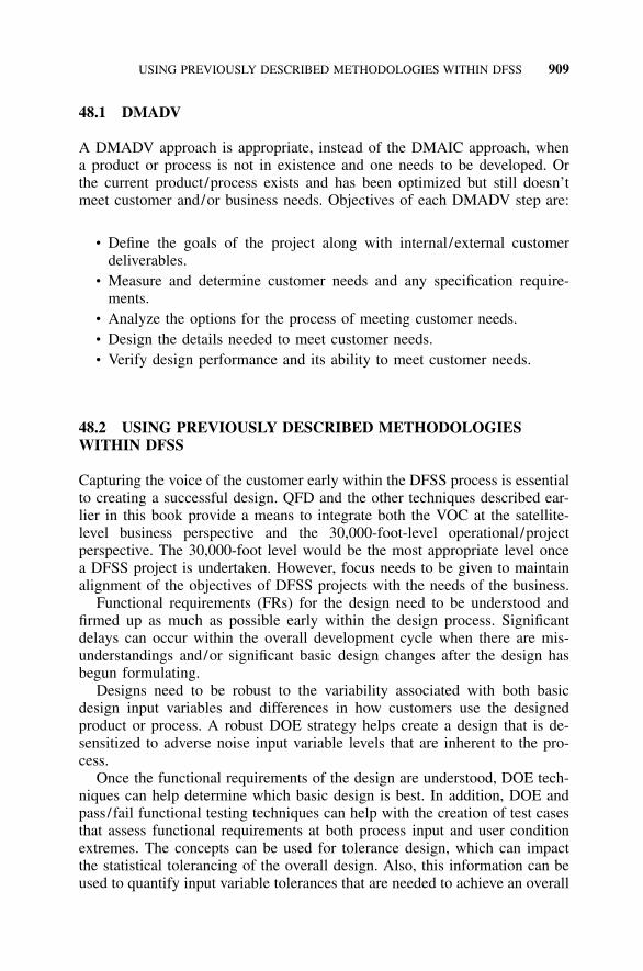
USING PREVIOUSLY DESCRIBED METHODOLOGIES WITHIN DFSS 909

48.1 DMADV

A DMADV approach is appropriate, instead of the DMAIC approach, whena product or process is not in existence and one needs to be developed. Orthe current product/process exists and has been optimized but still doesn’tmeet customer and/or business needs. Objectives of each DMADV step are:

• Define the goals of the project along with internal/external customerdeliverables.

• Measure and determine customer needs and any specification require-ments.

• Analyze the options for the process of meeting customer needs.• Design the details needed to meet customer needs.• Verify design performance and its ability to meet customer needs.

48.2 USING PREVIOUSLY DESCRIBED METHODOLOGIESWITHIN DFSS

Capturing the voice of the customer early within the DFSS process is essentialto creating a successful design. QFD and the other techniques described ear-lier in this book provide a means to integrate both the VOC at the satellite-level business perspective and the 30,000-foot-level operational/projectperspective. The 30,000-foot level would be the most appropriate level oncea DFSS project is undertaken. However, focus needs to be given to maintainalignment of the objectives of DFSS projects with the needs of the business.

Functional requirements (FRs) for the design need to be understood andfirmed up as much as possible early within the design process. Significantdelays can occur within the overall development cycle when there are mis-understandings and/or significant basic design changes after the design hasbegun formulating.

Designs need to be robust to the variability associated with both basicdesign input variables and differences in how customers use the designedproduct or process. A robust DOE strategy helps create a design that is de-sensitized to adverse noise input variable levels that are inherent to the pro-cess.

Once the functional requirements of the design are understood, DOE tech-niques can help determine which basic design is best. In addition, DOE andpass/fail functional testing techniques can help with the creation of test casesthat assess functional requirements at both process input and user conditionextremes. The concepts can be used for tolerance design, which can impactthe statistical tolerancing of the overall design. Also, this information can beused to quantify input variable tolerances that are needed to achieve an overall

910 DFSS OVERVIEW AND TOOLS

satisfactory level for process capability/performance metrics using techniquessuch as DCRCA.

48.3 DESIGN FOR X (DFX)

In previous decades it was thought that the efficiency of manufacturing wasa prerequisite to achieve a competitive edge within the marketplace. Withinthis approach focus was given to minimizing manufacturing costs, while max-imizing product quality. More recently focus has changed from the manufac-turing perspective to the product perspective. Now it is believed thatcompanies who can efficiently introduce more new products while reactingfaster to market/ technology changes in their development of superior productswill excel against their competitors. Concurrent engineering or simultaneousengineering is an approach to improve new product development where theproduct and its associated processes are developed in parallel. This approachconsiders, early within the product development project, the cross-functionalinvolvement of organizations such as manufacturing, distribution, and service,which develop their processes in parallel.

Within the concurrent engineering philosophy, a number of approacheshave evolved to increase the efficiency of elements of the product develop-ment process. These approaches have become known as design for X, whereX is a process that is related to product development.

Often during the design cycle, focus is placed on the final product and notthe process used to manufacture the product. Within a DFX strategy, thedesign is continually reviewed for the purpose of finding ways to improveproduction and other nonfunctional aspects of the process. The aspects ofDFX are not new. They are common sense documented techniques that canbe used within the overall design process.

When focus is given to the various aspects of DFX, the created design canbenefit through a reduction in production times and steps. There can be morestandardization of parts, smaller parts inventory, and simpler designs. Thetechniques can be a significant piece of the concurrent engineering effort ofan organization. Examples of DFX (Dodd 1992) are design for assembly,design for performance, design for ergonomics, design for recyclability, de-sign for redesign, design for reliability, design for quality, design for main-tainability, and design for test. Example nomenclature for DFX are design formanufacturability (DFM) and design for assembly (DFA).

The success or failure of a multidisciplinary, multi-team design activitydepends upon the management and control of the various design activities.Different activities that are being carried out at different times and for dif-ferent purposes need to provide information and fulfill their tasks at particulartimes for the design process to be effective.

AXIOMATIC DESIGN 911

48.4 AXIOMATIC DESIGN

In AD theory (Yang and Zhang 2000a), the design process is the developmentand selection of a means to satisfy objects that are subject to constraints.There is a series of activity steps where inputs are transformed to an output.The design object is something that a customer needs, which may be a phys-ical object, manufacturing process, software, or an organization. AD carefullyemphasizes the importance of recognizing the hierarchical nature of design.AD strives to ensure that the process of iteration between functional require-ments and design parameters are carried out systematically.

The design process can be considered to consist of several steps (Yang andZhang 2000b):

• Establish design objectives that satisfy a given set of customer attributes.• Generate ideas to create plausible solutions.• Analyze the solution alternatives that best satisfies the design objectives.• Implement the selected design.

Decisions made within each design process step profoundly affect bothproduct quality and manufacturing productivity. AD theory is to aid in thedesign decision-making process. AD approaches the execution of the aboveactivities through the following five concepts (Yang and Zhang 2000b):

1. There are four domains within design: customer domain, functional do-main, physical domain, and process domain. Customer needs areidentified in the customer domain and stated in a form that is requiredof a product in the functional domain. The design parameters that satisfythe functional requirements are in the physical domain. The manufac-turing variables define how the product will be produced in the processdomain. Within AD the whole design process is to address structurallythe continuous processing of information between the four distinct do-mains.

2. Solution alternatives are created through the mapping of requirementsthat are specified in one domain to a set of characteristic parameters inan adjacent domain. Concept design is considered to be the mappingbetween customer and functional domains. Product design is consideredto be the mapping between functional and physical domains. Processdesign is considered to be the mapping between physical and processdomains.

3. Mathematically the mapping process can be expressed in terms of thecharacteristic vectors that define the design goals and design solution.

4. The output of each domain evolves from concepts that are abstract todetailed information in a hierarchical, top-down manner. Hierarchical

912 DFSS OVERVIEW AND TOOLS

decomposition in one domain cannot be performed independently ofother domains. Decomposition follows a zigzagging mapping betweenadjacent domains.

5. Two design axioms provide a rational basis for the evaluation of pro-posed alternative solutions, which is to lead to the best alternative. Thefirst axiom is independence, which states that sections of the designshould be separable so that changes in one have no, or as little aspossible, effect on the other. The second axiom is information, whichstates that the information inherent in a product design should be min-imized.

In product design, the creation or synthesis phase of design involves map-ping the functional requirements (FRs) in the functional domain to the designparameters (DPs). The complexity of the solution process increases with thenumber of FRs. Because of this, it is important to describe the perceiveddesign needs using the minimum set of independent requirements. One FRthat is equivalent should replace two or more dependent FRs.

In process design, mapping the DPs in the physical domain to the processdomain creates a set of process variables (PVs). The PVs specify the manu-facturing methods for which the DPs are produced.

Because of its broad scope and inclusivity, AD fits well with concurrentengineering (Tate 2000). Using partial derivative concepts and matrix math-ematics, what-if questions can be asked and answered and determinativesolutions can be based on the quality of the model. For highly complex prob-lems, this can be very useful.

48.5 TRIZ

TRIZ states that some design problems may be modeled as technical contra-diction. Creativity is required when attempts to improve some functional at-tributes lead to deterioration of other functional attributes. Design problemsassociated with a pair of functional contradiction can be made by makingtrade-offs or by overcoming the obstacle. TRIZ stresses that an ideal designsolution overcomes the conflict, as opposed to making a trade-off.

Problems can be grouped into those with generally known solutions andthose with unknown solutions. Solutions to problems come in levels:

• Standard: Uses methods well known in the profession.• Improvement: Uses methods from inventor’s own industry and technol-

ogy. Improves an existing system.• Within existing paradigm: Uses methods from other fields and technol-

ogies. Improves an existing system.

TRIZ 913

• Outside existing paradigm: Uses little-known and understood physicaleffects (physics, chemistry, geometry).

• Discovery: Goes beyond contemporary scientific knowledge. Creates anew discovery or new science.

Those with known solutions can usually be solved by currently availableinformation. Those with no known solution are called inventive problems.These problems often contain contradictory requirements.

TRIZ is an acronym for a Russian phrase meaning ‘‘theory of inventiveproblem-solving.’’ Genrich Altshuller, a Russian mechanical engineer, is cred-ited with the creation of TRIZ. While analyzing patents for the Russian Navy,Altshuller noticed patterns in the inventive process, which he developed intoa set of tools and techniques for solving inventive problems.

Instead of classifying patents by industry, such as automotive or aerospace,Altshuller removed the subject matter to uncover the problem-solving process.Altshuller found that often the same problems had been solved over and overagain using 1 of only 40 fundamental inventive principles (e.g., transformationof properties, self-service, do it in reverse, and nesting).

Altshuller also classified engineering system development into eight laws:

• Law of completeness of the system: Systems derive from synthesis ofseparate parts into a functional system.

• Law of energy transfer in the system: Shaft, gears, magnetic fields,charged particles, which are the heart of many inventive problems.

• Law of increasing ideality: Function is created with minimum complex-ity, which can be considered a ratio of system usefulness to its harmfuleffects. The ideal system has the desired outputs with no harmful effects,i.e., no machine, just the function(s).

• Law of harmonization: Transferring energy more efficiently.• Law of uneven development of parts: Not all parts evolve at the same

pace. The least will limit the overall system.• Law of transition to a super system: Solution system becomes subsystem

of larger system.• Law of transition from macro to micro: Using physically smaller solu-

tions (e.g., electronic tubes to chips).• Law of increasing substance-field involvement: Viewing and modeling

systems as composed of two substances interacting through a field.

Most effective solutions come from resolving contradictions without com-promise. When improving some part or characteristic of our system causesdeterioration in another, that’s contradiction. Altshuller states that inventionsurmounts the contradiction by moving both characteristics in a favorable

914 DFSS OVERVIEW AND TOOLS

direction. For example, to increase the capacity of an air conditioner, we canincrease weight, price, and power consumed. However, a better solution is touse a new technology that improves efficiency and capacity.

Altshuller thought that if only later inventors had knowledge of earlierwork, solutions could have been discovered more quickly and efficiently. Hisapproach was to use the principle of abstraction to map the problems tocategories of solutions outside of a particular field of study. Conflict can beresolved through the principle of abstraction, that is, classification of problemsin order to map the problems to categories of solutions.

When solving problems, typically some feature or parameter is selectedand then changed to improve the process feature of the problem. TRIZ for-malizes this thought process by starting with a list of 39 parameters/featuressuch as waste of time, force, speed, and shape.

TRIZ then facilitates the solution process through abstraction. Problemsare stated in terms of a conflict between two attributes (e.g., parts, character-istics, functions, and features). This allows seeing generic solutions that mayalready be documented in other industries or fields of study. This also allowsfor a better search in the global patent collection.

48.6 EXERCISE

1. You have a pizza delivery business. Your customers want their pizzas hotwhen delivered. Your cardboard boxes have a problem: they must hold theheat in but not the condensation. When they get damp from condensation,they become weakened and make the pizza crust soggy. Resolve the prob-lem, where designing a better box is one possible solution. Assume thatwe are going to pursue the better-box solution, using TRIZ techniques;describe the features and contradictions along with the inventive principlesthat can be used.

915

49PRODUCT DFSS

Six Sigma techniques are applicable to a wide variety of situations, includingdevelopment. The application of Six Sigma techniques within the develop-ment process is often called DFSS. When we are referring to the design ofproducts, I prefer to call this Six Sigma application product DFSS, whichdifferentiates the methodology from process DFSS. My definition for processDFSS is using Six Sigma methodologies when creating a process initially tobest meet customer needs while minimizing the time it takes to reduce thetime and resources it takes to create the process.

The following examples illustrate how Smarter Solutions, Inc. has assistedcustomers in benefiting from the wise application of Six Sigma tools.

• Customer 1 (hardware/software integration test organization): Used aunique test strategy for evaluating the interfaces of new computer de-signs. Result: The methodology was more effective and efficient in de-termining if a computer would have functional problems when interfacingwith various customer hardware and software configurations.

• Customer 2 (product mixture development organization): Used a mixtureDOE design to develop a solder paste. Results: The analysis identifiedstatistically significant mixture components and opportunities for im-provement.

• Customer 3 (reliability test organization): Developed a unique reliabilitytest DOE strategy to evaluate preship product designs. Result: Monetarysavings from the detection of combination manufacturing and design is-sues before first customer shipment.

• Customer 4 (printer design organization): Used DOE techniques to as-sess the validity of a design change that was to reduce the settle-out time

916 PRODUCT DFSS

of a stepper motor. Result: The DOE validated the design change andthe amount of improvement. In addition, the DOE indicated the signifi-cance of another adjustment.

• Customer 5 (computer company): Created a unique metric feedback strat-egy within system test. Result: Improved feedback loops when testing aproduct, between product evaluations, and field to design failure mech-anisms would show a statistically significant decrease in expensesthrough failure prevention.

• Customer 6 (government certification test organization): Improved elec-tromagnetic interference (EMI) testing. Results: An efficient approachwas developed that considered both within and between machine varia-bility.

• Customer 7 (hardware design test organization): Created an improvedreliability test strategy for a complex power supply. Result: A less ex-pensive DOE-based reliability strategy identified exposures that a tradi-tional reliability test would not capture.

• Customer 8 (reliability organization): Used DOE techniques in a stresstest environment to improve design reliability. Result: The componentlife was projected to increase by a factor of 100.

These examples illustrate the many implementation strategies and uniquetool combinations available for development processes. This chapter includesthoughts on what could be done when measuring development processes, anoverall application strategy, and S4/IEE application examples.

49.1 MEASURING AND IMPROVING DEVELOPMENTPROCESSES

Within product DFSS I suggest, whenever possible, the bridging of devel-opment process measurements across the various products that go sequentiallythrough the development process. Product-to-product differences could thenbe viewed as noise to the development process measurements. Even whenthis measurement technique for the development process is not used, the tech-niques described within this chapter are still applicable.

Consider, for example, that the functional test area for new computer de-signs is to be measured and then improved. This situation is often not viewedas a process where the output of the process crosses product boundaries.Typical focus is on the created product, not the process that develops theproduct. Information is often not compiled to quantify the effectiveness ofcurrent methodologies in creating new products that are developed timely tomeet manufacturing needs along with the quality and functional needs of theend user. Much can be gained if this way of thinking is altered such that afeedback and measurement system is created, as illustrated within Figure 49.1,where the chronicle sequence unit within the control chart is products thatwere developed over time.

917

FIG

UR

E49

.1M

easu

rem

ents

acro

sspr

oduc

tsde

velo

ped

over

time

with

info

rmat

ion

feed

back

from

man

u-fa

ctur

ing

tode

velo

pmen

t.

918 PRODUCT DFSS

Within DFSS most Six Sigma tools still are applicable. However, strategiesand the sequence of use of these tools can be very different than what mightbe expected within manufacturing or service/transactional processes. For ex-ample, fractional factorial DOEs within manufacturing are often used to fixproblems; however, within development the use of structured fractional fac-torial DOEs could be used as a control measure for achieving a high-qualityproduct design. A measure for the effectiveness of a design FMEA within adevelopment process could be considered a control measure for creating aproduct that consistently meets or exceeds the needs of customers.

The following 21-step integration of the tools illustrates the foundation forbuilding an S4/IEE product DFSS implementation. This roadmap can be ex-panded to include detailed implementation aspects of an organization’s tac-tical quality plan. Organizations can use this format to create specific tasksfor an advanced quality plan (AQP) that which defines key activities and thetasks that are to be completed as the project advances through the develop-ment cycle. These tasks would have a schedule along with methods and re-sponsibilities for the purpose of ensuring that the new product or servicemeets or exceeds customer expectations.

49.2 A 21-STEP INTEGRATION OF THE TOOLS: PRODUCT DFSS

There are many possible alternatives and sequencing of Six Sigma tools forS4/IEE development projects. Shown below is a concise sequencing of howSix Sigma tools could be linked/considered for development projects. Thisroadmap can be referenced to give insight on how individual tools can fit intothe big picture, starting with obtaining functional requirements for a design.Specific tools are highlighted in bold print to aid the reader in later locatingwhere a tool could be applied. The Glossary in the back of this book can aidwith term clarifications.

21-Step Integration of the Tools: Development Processes

Step Action ParticipantsSource of

Information

1 Drill down from satellite-level metric to abusiness need to determine anenhancement and /or expansion ofexisting portfolio of products.Brainstorm for linkages to previousproducts that were developed for thepurpose of creating a set of 30,000-foot-level measurements that can bridge fromthe development of a product to theprocess of developing products. Create aproject charter.

Black belt andchampion

Organizationwisdom

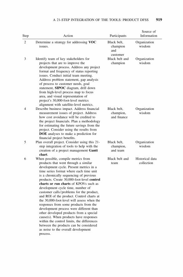
A 21-STEP INTEGRATION OF THE TOOLS: PRODUCT DFSS 919

Step Action ParticipantsSource of

Information

2 Determine a strategy for addressing VOCissues.

Black belt,championandcustomer

Organizationwisdom

3 Identify team of key stakeholders forprojects that are to improve thedevelopment process. Address any projectformat and frequency of status reportingissues. Conduct initial team meeting.Address problem statement, gap analysisof process to customer needs, goalstatement, SIPOC diagram, drill downfrom high-level process map to focusarea, and visual representation ofproject’s 30,000-foot-level metricsalignment with satellite-level metrics.

Black belt andchampion

Organizationwisdom

4 Describe business impact. Address financialmeasurement issues of project. Addresshow cost avoidance will be credited tothe project financials. Plan a methodologyfor estimating the future savings from theproject. Consider using the results fromDOE analyses to make a prediction forfinancial project benefits.

Black belt,champion,and finance

Organizationwisdom

5 Plan overall project. Consider using this 21-step integration of tools to help with thecreation of a project management Ganttchart.

Black belt,champion,and team

Organizationwisdom

6 When possible, compile metrics fromproducts that went through a similardevelopment cycle. Present metrics in atime series format where each time unitis a chronically sequencing of previousproducts. Create 30,000-foot-level controlcharts or run charts of KPOVs such asdevelopment cycle time, number ofcustomer calls /problems for the product,and ROI of the product. Control charts atthe 30,000-foot-level will assess when theresponses from some products from thedevelopment process were different thanother developed products from a specialcause(s). When products have responseswithin the control limits, the differencesbetween the products can be consideredas noise to the overall developmentprocess.

Black belt andteam

Historical datacollection

920 PRODUCT DFSS

Step Action ParticipantsSource of

Information

7 When measuring the development process,specifications are not typicallyappropriate. Long-term process capability /performance metrics for KPOVs canthen be described in frequency ofoccurrence units. For example, 80% ofthe time the development cycle time of aproduct is between 6.1 and 9.2 months.Another example: 80% of the time thenumber of reported problems for adeveloped product is between 2.8 and 4.3calls per unit sold. Describe implicationin monetary terms. Use this value as abaseline for the project. Pareto charttypes of nonconformance issues fromprevious products that were developed.This Pareto chart might indicate thatresponses to customer questions aboutproduct setup were more of a financialimpact to the business than productreliability service issues.

Black belt andteam

Current andcollected data

8 Create a process flowchart /process map ofthe current development process at a levelof detail that can give insight to whatshould be done differently. Note howVOC inputs are obtained and how theyimpact the design process. Theapplication of lean tools such as valuestream analysis / time-value diagram canbe very useful to identify cycle timeissues.

Black belt andteam

Organizationwisdom

9 Create a cause-and-effect diagram toidentify variables that can affect theprocess output. Use the processflowchart and Pareto chart ofnonconformance issues to help with theidentification of entries within thediagram.

Black belt andteam

Organizationwisdom

10 Create a cause-and-effect matrix assessingstrength of relationships between inputvariables and KPOVs. Input variables forthis matrix might have been identifiedinitially through a cause-and-effectdiagram.

Black belt andteam

Organizationwisdom

11 Rank importance of input variables from thecause-and-effect matrix using a Paretochart. From this ranking create a list ofvariables that are thought to be KPIVs.

Black belt andteam

Organizationwisdom

A 21-STEP INTEGRATION OF THE TOOLS: PRODUCT DFSS 921

Step Action ParticipantsSource of

Information

12 Prepare a focused process FMEA where theitem/ function inputs are steps of thedevelopment process. Consider alsocreating the FMEA from a systems pointof view, where item/ function input itemsare the largest ranked values from acause-and-effect matrix. Assess currentcontrol plans. Within FMEA considerrisks of current development tests andmeasurement systems. Conductmeasurement systems analyses whereappropriate. Implement agreed-to processimprovement changes. Consider a betterutilization of historical information fromprevious products (see steps 13–17).Consider also using or better applyingdesign FMEA, DOE optimation,DCRCA, pass / fail functional testing,TRIZ, and VOC input strategies (e.g.,simplified QFD) (see steps 18–20).Consider also how the use of creativityand innovation tools can be betterintegrated in the development process.

Black belt andteam

Organizationwisdom

13 Collect data from previous developmentprojects to assess the KPIV/KPOVrelationships that are thought to exist.

Black belt andteam

Collected data

14 When enough data exist from previouslydeveloped products, use multi-varicharts, box plots, marginal plots, andother graphical tools to get a visualrepresentation of the source of variabilityand differences within the process.

Black belt andteam

Passive dataanalysis

15 When enough data exist from previouslydeveloped products, assess statisticalsignificance of relationships usinghypothesis tests.

Black belt andteam

Passive dataanalysis

16 When enough data exists from previouslydeveloped products, consider usingvariance components analysis to gaininsight to the source of output variability.Example sources of variability aresupplier-to-supplier and plant-to-plantvariability.

Black belt andteam

Passive dataanalysis

17 When enough data exist from previouslydeveloped products, conduct correlation,regression, ANOVA, ANOM, and otherstatistical studies to gain insight of howKPIVs can impact KPOVs.

Black belt andteam

Passive dataanalysis

922 PRODUCT DFSS

Step Action ParticipantsSource of

Information

18 Conduct fractional factorial DOEs, pass /fail functional testing, and responsesurface analyses as needed to assessKPOVs considering factors that aredesign, manufacturing, and supplier innature. Consider structuring experimentsso that the levels of KPIVs are assessedrelative the reduction of variability inKPOVs when the product will later beproduced within manufacturing. Considerstructuring the experiment for the purposeof determining manufacturing KPIVsettings that will make the process morerobust to noise variables such as rawmaterial variability. Consider how wiselyapplied DOE techniques can replace and /or complement existing pre-productionreliability tests that have beenquestionable in predicting future productfailure rates. DOE within developmentcould be used and considered a SixSigma control methodology for thedevelopment process.

Black belt andteam

Activeexperimentation

19 Determine from DOEs and other toolsoptimum operating windows of KPIVsthat should be used within manufacturing.

Black belt andteam

Passive data anal-ysis and activeexperimen-tation

20 Update control plan noting that fractionalfactorial DOE experiments, pass / failfunctional testing methodologies, andwisely applied reliability assessments canbe an integral part of the control plan ofthe development process. Consider alsowithin this control plan the involvementof development and other organizationswhenever field problems occur for thepurpose of immediate problem resolutionand improvements to the overall develop-ment process for future products.

Black belt andteam

Passive data anal-ysis and activeexperimen-tation

21 Verify process improvements, stability, andcapability /performance over time. Cre-ate a final project report stating the bene-fits of the project, including bottom-linebenefits. Make the project report availableto others within the organization. Con-sider monitoring the execution and resultsclosely for the next couple of projects af-ter project completion to ensure that pro-ject improvements /benefits aremaintained.

Black belt andteam

Active experi-mentation

EXAMPLE 49.1: NOTEBOOK COMPUTER DEVELOPMENT 923

49.3 EXAMPLE 49.1: NOTEBOOK COMPUTER DEVELOPMENT

Product reliability is important to a company that develops and manufacturesnotebook computers. Customer product problems are expensive to resolve andcan impact future sales. One KPOV measure for this type of product was thenumber of machine problem phone calls and/or failures per machine over itsproduct life.

The frequency of this metric was tracked using a 30,000-foot-level controlchart where the chronological sequencing of the chart was type of product.The frequency of this KPOV was judged to be too large. An S4/IEE projectwas defined to reduce the magnitude of this number.

As part of the S4/IEE project a Pareto chart was created. This chart indi-cated that the source of most customer problems was customer setup followedby no trouble found. A no-trouble-found condition exists whenever a cus-tomer states that a problem existed; however, the failure mode could not berecreated when the machine was returned to a service center of the company.

To reduce the number of customer setup problems, a team was created toidentify the current process used to establish customer setup instructions. Acause-and-effect diagram was then created to solicit ideas on what might bedone to improve the current process for the purpose of reducing the amountof confusion a customer might have when setting up a newly purchased ma-chine. A cause-and-effect matrix was then created to rank the importance ofthe items with the cause-and-effect diagram. From this session there was somelow-hanging fruit identified which could be implemented immediately to im-prove the process of creating customer setup instructions. An FMEA was thenused to establish controls to the largest ranked items from the cause-and-effect matrix. As part of the improvement effort and control mechanism whendeveloping new instruction procedures, a DOE matrix would be used to con-duct the testing of new instructions where the factors from the DOE matrixwould include such items as experience of the person setting up the newcomputer design.

For the second-highest category, no trouble found, in the Pareto chart acause-and-effect diagram, a cause-and-effect matrix, and then FMEA alsoindicated other control measures that should be in place. Examples of thesetypes of control measures within this book that could be identified throughS4/IEE projects are:

• Testing for thermal design problems that are causing NTF: Example 30.2• Creating a more effective test for reliability issues using less resources

through DOEs: Example 43.2• Improving software/hardware interface testing: Example 42.4• Managing product development of software: Example 42.6• Tracking of change orders: Example 43.6• Creating a more effective ORT test strategy: Example 40.7

924 PRODUCT DFSS

• Using a system DOE stress to fail test to quantify design margins: Ex-ample 31.5

• Using a DOE strategy to size the future capability/performance of aproduct by testing a small number of pre-production samples. Method-ology also can determine if any key process manufacturing parametersshould be monitored or have a tightened tolerance: Example 30.1

• Using a QFD in conjunction with a DOE to determine manufacturingsettings: Example 43.2

49.4 PRODUCT DFSS EXAMPLES

Within this section I will compile some of the product DFSS concepts de-scribed throughout this book. The listed figures, examples, and illustrationscan give insight to how the various S4/IEE techniques can be integrated andapplied to other situations.

An overview of the product DFSS thought process is described in:

• Figure 1.2 shows the input-process-output (IPO) model, which also ap-plies to product DFSS.

• Example 4.1 describes developing a development process.• Section 49.1 and Figure 49.1 describe measurements across products de-

veloped over time with information feedback from manufacturing to de-velopment.

• Section 49.2 describes a 21-step integration of the tools for productDFSS.

Product DFSS example applications are:

• Notebook computer development: Example 49.1.• An illustration of integration of lean and Six Sigma methods in devel-

oping a bowling ball: Example 44.1.• A reliability and functional test of an assembly that yields more infor-

mation with less traditional testing: Example 43.3.• In a DFSS DOE one set of hardware components in various combinations

to represent the variability expected from future production. A follow-upstress to fail test reveals that design changes reduce the exposure tofailure: Example 31.5.

• The integration of quality functional deployment (QFD) and a DOE leadsto better meeting customer needs: Example 43.2.

• Implementing a DFSS DOE strategy within development can reduce thenumber of no-trouble-founds (NTFs) later reported after the product isavailable to customers: Example 30.2.

PRODUCT DFSS EXAMPLES 925

• Conducting a reduced sample size test assessment of a system failurerate: Example 40.3.

• Postreliability test confidence statements: Example 40.5.• Reliability assessment of systems that have a changing failure rate: Ex-

ample 40.6.• Zero failure Weibull test strategy: Example 41.3.• A pass/fail system functional test: Example 42.2.• Pass fail hardware/software system functional test: Example 42.3.• A development strategy for a chemical product: Example 43.4.• A stepper motor development test that leads to a control factor for man-

ufacturing: Example 30.1.

926

50PROCESS DFSS

Six Sigma techniques can expedite the development of processes such thatthere are fewer problems both when creating and later executing the process.This approach can lead to the reduction of future firefighting that often occurswithin processes both initially and over time.

I call this Six Sigma application process S4/IEE process DFSS. Whenusing this approach, organizations can better meet customer needs while min-imizing the process implementation time along with the amount of resourcesneeded to create the process.

Example applications of process DFSS are:

• Developing a new call center• Developing a new warehouse• Building a new road• Developing a new store• Developing a new office• Installing an ERP system

The following 21-step integration of the tools illustrates the foundation forbuilding an S4/IEE process DFSS implementation. This roadmap can be ex-panded to include detailed implementation aspects of an organization’s tac-tical quality plan. Organizations can use this format to create specific tasksfor an AQP. These tasks would have a schedule along with methods andresponsibilities for the purpose of ensuring that the new process will meet orexceed customer expectations.

A 21-STEP INTEGRATION OF THE TOOLS: PROCESS DFSS 927

50.1 A 21-STEP INTEGRATION OF THE TOOLS: PROCESS DFSS

There are many possible alternatives and sequencing of Six Sigma tools forS4/IEE process DFSS. The following chart is a concise sequencing of howSix Sigma tools could be linked/considered when designing new processesand their layouts. This roadmap can be referenced to give insight on howindividual tools can fit into the big picture. Specific tools are highlighted inbold print to aid the reader in later locating where a tool could be applied.

21-Step Integration of the Tools: Process DFSS

Step Action Participants Source of Information

1 A drill-down from asatellite-level metricindicated that there wasa business need tocreate a new processthat had never beendone before by thecompany. CreateProject charter.Include projectmanagementimplementation planusing this 21-stepintegration of the toolsroadmap as a guideline.Determine how financialand other benefits forthis implementationprocess will bequantified. Establishteam.

Black belt, champion,and finance

Organization wisdom

928 PROCESS DFSS

Step Action Participants Source of Information

2 Define customers ofprocess, both internaland external. Conductinitial team meeting.Address problemstatement, gap analysisof process to customerneeds, goal statement,SIPOC diagram, drilldown from high-levelprocess map to focusarea, and visualrepresentation ofproject’s 30,000-foot-level metrics alignmentwith satellite-levelmetrics.

Black belt, team, andchampion

Organization wisdom

3 Establish KPOVs that willbe tracked at the30,000-foot-level.Consider the types ofdefects that will betracked and how overallthroughput time for theprocess should betracked.

Black belt, team, andchampion

Organization wisdom

4 Obtain and documentVOC needs and desiresfor the process usingQFD and other VOCtools. Establishcustomer conformancedesires for 30,000-foot-level metric.

Black belt and team Organization wisdom

5 Benchmark similarprocesses.

Black belt and team Organization wisdom

6 Create a flowchart thataddresses the needs ofthe process.

Black belt and team Organization wisdom

7 Apply lean tools such aslogic flow map,spaghetti chart, andtime-value diagram.Change process asneeded.

Black belt and team Organization Wisdom

A 21-STEP INTEGRATION OF THE TOOLS: PROCESS DFSS 929

Step Action Participants Source of Information

8 Start forming a projectmanagement plan tocreate the process.Discuss implications ofproject executiontimeline.

Black belt and team Organization wisdom

9 Develop a model of theprocess using a processmodeling computerprogram.

Black belt and team Organization wisdom

10 Conduct a process FMEA.Make appropriatechanges to the process.

Black belt and team Organization wisdom

11 List variables that areanticipated to beKPIVs.

Black belt and team Organization wisdom

12 Conduct a DOE and/orpass/ fail functionaltest using processmodeling computerprogram to simulate theprocess. Extreme valuesfor KPIVs should bepart of the considerationfor factors for DOE.KPOVs of the processare responses for theDOE.

Black belt and team Proactiveexperimentation

13 Conduct a DCRCA. Forthe DCRCA create aprobability plot of theDOE responsescollectively and thencompare against thecustomer requirementsfor the process. Forexample, compare aprobability plot of allsimulated throughputtimes from the DOE toVOC desires and needs.

Black belt and team Proactiveexperimentation

930 PROCESS DFSS

Step Action Participants Source of Information

14 If the desired percentagepoints from aprobability plot of DOEresponses are not wellwithin conformancelevels, analyze DOEusing traditionalprocedures.

Black belt and team Proactiveexperimentation

15 Adjust process design asrequired usingknowledge gained fromDOE such that afollow-up DOE givesdesired results.

Black belt and team Proactiveexperimentation

16 Create a control plan forthe initially anticipatedKPIVs of the processthat were foundstatistically significantfrom DOE.

Black belt and team Organization wisdom

17 Finalize plan to trackKPOVs at the 30,000-foot level.

Black belt and team Organization wisdom

18 Create a plan to collectand compile KPOVs asa function of KPIVs sothat data are available ifcausal investigation islater required.

Black belt and team Organization wisdom

19 Update and follow theproject managementplan for creating theprocess.

Black belt and team Organization wisdom

20 Run pilot for completedprocess, trackingKPOVs at the 30,000-foot level.

Black belt and team Passive data analysis

A 21-STEP INTEGRATION OF THE TOOLS: PROCESS DFSS 931

Step Action Participants Source of Information

21 Compare capability /performance of processto desired level. Ifcapability /performanceis not at the desiredlevel, follow an S4 / IEEDMAIC strategy forprocess improvement.Document results andstrategy of this processDFSS. Leverage resultsand strategies to otherareas of the business.

Black belt and team Passive data analysis

PART VIII

MANAGEMENT OFINFRASTRUCTURE ANDTEAM EXECUTION

This part (Chapters 51–55) describes some leadership tools that are veryimportant to achieve success with S4/IEE. Change management, project man-agement, team effectiveness, and the alignment of management initiativeswith S4/IEE are discussed.

935

51CHANGE MANAGEMENT

S4 /IEE DMAIC Application: Appendix Section A.1, Project ExecutionRoadmap Step 1.4

Fundamental changes in how a business is conducted are important to helpcope with a market environment that continually becomes more complex andchallenging. Companies need to face this head-on or they will not survive.

To address this companies have undertaken various initiatives over theyears in an attempt to make constructive change to their organization. Someorganizations have had great success with these initiatives; however, othershave been very disappointing.

To better understand the implication of change, let’s consider the last NewYear’s resolution you made. If you are like the vast majority of New Year’sresolution makers, the desired change you resolved to make did not occur, atleast for any length of time. Similarly, organizations have difficulty withchange and reaping expected benefits through their business change initia-tives.

Leaders who are implementing S4/IEE within an organization need to be-come change agents. They need to be able to manage change, overcomeorganizational roadblocks, negotiate/resolve conflicts, motivate others, andcommunicate to overcome organizational barriers for success. When imple-menting S4/IEE, it is important to address both initial and sustaining changemanagement issues. This chapter addresses some strategies that can be usedto achieve this.

936 CHANGE MANAGEMENT

51.1 SEEKING PLEASURE AND FEAR OF PAIN

The motivational speaker Tony Robbins has suggested that the reason peoplechange is to either seek pleasure or avoid pain. The more powerful of thesetwo forces for achieving change, Robbins says, is the fear of pain. (I need tonote that this fear of pain does not refer to the periodic infliction of pain onsomeone by yelling at him or her to do something different.) Let’s considerthese two points from a personal level and then a business level.

At a personal level, I think most people will agree that people in the UnitedStates need to eat less fat and exercise more. Let’s now consider what driveschange on a personal level for someone who should improve his diet andexercise program. A seeking-pleasure motivation would be encouragementfrom a loved one saying you will feel better if you exercise more and eat lessfat, while a fear of pain motivation would be the fear of having another heartattack. Consider which of these motivational forces is more effective. Unfor-tunately, my observation is that the answer is the latter.

At a business, a seeking-pleasure motivation could be the promise of ayearly bonus if corporate objectives are met. A fear-of-pain motivation couldbe fear of being fired for not improving processes within one’s area, therealism of this fear being reinforced when a friend did lose his job becausehe was not making long-lasting improvements within his area of the business.Again, consider which one of these motivational forces is the most effectivein driving day-to-day activities.

I believe that the reason Six Sigma was so successful within GE was thatthey used the fear-of-pain stimulus described above as their primary drivingforce, with a secondary driving of the seeking-pleasure stimulus through fi-nancial benefits and recognition that were tied to Six Sigma project benefits.

I believe that it is important to include both the fear-of-pain and the seek-ing-pleasure motivation within an S4/IEE business strategy. I think that GEdid an excellent job using the fear-of-pain motivation for driving changewithin their organization. In my opinion, most people within GE believed thatthey needed to embrace Six Sigma and the concepts of Six Sigma or theywould lose their jobs.

However, I am not so sure how well GE and others have accomplished theseeking-pleasure piece of the puzzle. This piece is much harder to implementthroughout an organization since the day-to-day interface between levels ofmanagement and management to employee needs to be changed for this mo-tivation to be successful. I say this because I believe that day-to-day pats onthe back for small tasks well done are perhaps a better driving force in generalthan the hope of a bonus because of some arbitrary organizational goal setby high-level management. Changing this level of behavior can be very dif-ficult. In some organizations, I believe, the day-to-day motivational benefitsfrom quarterly or yearly bonuses that are linked to organizational goals canbe from peer pressure to those who are not executing their jobs well.

SEEKING PLEASURE AND FEAR OF PAIN 937

Whenever I think about the changing of day-to-day behavior, I think aboutthe time my wife and I enrolled our dog in dog obedience school. I believethat I learned more than the dog did.

In this school a choker chain was used as a stimulus to change the dog’sbehavior. (To some who are not familiar with the process this might soundcruel, but it isn’t when the choker chain is used correctly.)

I will use the training of one command to illustrate the training process.When walking, a dog is to heel on your left side and move at the same pacethat you do. When you stop, the dog is to stop and then sit at your left sidewithout any command being given. This behavior needs to be trained sinceit is not natural for the dog.

The training procedure that I learned from class was to start walking withthe dog heeling at your left. When you stop walking, wait to see if the dogstops and sits with no command given. If the dog does not sit, lightly jerkthe choke chain once. If the dog still does not sit, push down on the rump ofthe dog until it sits down. When the dog does sits, compliment the dog bypetting it and saying nice things to it. Then repeat the procedure. It may takea few times, but the dog will sit when the choker chain is jerked after stoppingfrom a walk. At this point during the training you should really complimentthe dog when it achieves this next level of achievement. Our dog then quicklyproceeded to the next level, where it would sit after stopping from a walkwith no choker chain jerk. Again, the compliments should flow to the dog.

Since my encounter with dog training and its utilization of positive rein-forcement, I have wondered how we might use these techniques more inperhaps the most challenging and important role many people ever encoun-ter—parenting. When raising children, it is easy to get in the habit of cor-recting children for everything they don’t do correctly as opposed to praisingthem for things they do right (e.g., picking up one toy and returning it to itstoy box when finished). If the primary stimulus in parenting a child is neg-ative, it should be no surprise that an early word out of the mouth of a youngchild is ‘‘no.’’

My conclusion is that the process of parenting would be improved if cou-ples bought a dog and took the dog to training before they had any children.Hopefully they would learn from their dog the power of positive reinforce-ment and then later apply the techniques to their children.

I think that this timely positive feedback technique is useful in many areas.My wife is very good at this. She will give me a timely thank you or affectioncomment. For example, I have noted that my wife, when returning to thehouse, will thank me for putting a few dishes into the dishwasher that man-aged somehow to accumulate in the sink. This type of behavior from heraffects my behavior. Because of her actions I am more likely to redo and saythings that make her feel good, which she expresses through her positivefeedback. This type of relationship is far superior to the nagging wife orhusband.

938 CHANGE MANAGEMENT

Similarly, I think that many companies could dramatically improve theirculture through this model by the giving of timely reinforcements to peopleeven when the tasks they completed are small but aligned with the needs ofthe business. This type of feedback can reinforce behaviors within people sothat they can achieve greater things.

One challenge with this timely positive reinforcement model is that thequality of implementation of this skill by someone is not easy to measure.Hence, it is often not given the emphasis needed. Often the visibility withinan organization is given to the firefighters who fix the problem of the dayrather than the people who worked effectively together getting the job doneright the first time.

One final point needs to be made. GE had a ranking system for employeeswhere they periodically eliminated the lower percentage of ranked people.Ranking systems can have severe problems for many reasons. One reason isthat the people making the decision on the ranking of an individual often donot know all the details or may have a personality issue with the person.However, we cannot ignore the fact that some people will not change theirbehaviors to better meet the needs of the business no matter how much fear-of-pain and seeking-pleasure stimulus they are given. For these people, ter-mination or relocation to a different position is perhaps the only answer. Atthe same time we do this, let’s consider whether our termination/assessmentprocess and hiring process should be focused upon improvement opportuni-ties.

The following sections describe other tools and approaches for changemanagement.

51.2 CAVESPEAK

Someone who is resisting change typically uses one or several of the follow-ing, ‘‘cavespeak’’ statements. Lockheed created a pocket-sized card listing 50of these statements. Referencing the card can lighten situations where changeis being resisted.

1. We tried that before.2. Our place is different.3. It costs too much.4. That’s not my job.5. They’re too busy to do that.6. We don’t have the time.7. Not enough help.8. It’s too radical a change.

9. The staff will never buy it.10. It’s against company policy.11. The union will scream.12. Runs up our overhead.13. We don’t have the authority.14. Let’s get back to reality.15. That’s not our problem.16. I don’t like the idea.

THE EIGHT STAGES OF CHANGE AND S4 / IEE 939

17. You’re right, but . . .18. You’re two years ahead of your

time.19. We’re not ready for that.20. It isn’t in the budget.21. Can’t teach an old dog new

tricks.22. Good thought, but impractical.23. Let’s give it more thought.24. We’ll be the laughingstock.25. Not that again.26. Where’d you dig that one up?27. We did all right without it.28. It’s never been tried before.29. Let’s put that one on the back

burner.30. Let’s form a committee.31. I don’t see the connection.32. It won’t work in our plant/

office.

33. The committee would never gofor it.

34. Let’s sleep on it.35. It can’t be done.36. It’s too much trouble to change.37. It won’t pay for itself.38. It’s impossible.39. I know a person who tried it.40. We’ve always done it this way.41. Top management won’t buy it.42. We’d lose money in the long

run.43. Don’t rock the boat.44. That’s all we can expect.45. Has anyone else ever tried it?46. Let’s look into it further (later).47. Quit dreaming.48. That won’t work in our school.49. That’s too much ivory tower.50. It’s too much work.

The other side of the card has the following description of Lockheed Mar-tin’s lean thinking model:

• Precisely specify/define VALUE through the eyes of the customer.• Identify the VALUE STREAM for each product; i.e., the properly se-

quenced, irreducible set of actions required to bring the product frominception into the hands of the customer.

• Make value FLOW continuously without detours, backflows, or interrup-tions.

• Let the customer PULL value from the producer; i.e., no one upstreamshould produce a good or service until the downstream customer asksfor it.

• Pursue PERFECTION through the relentless elimination of waste.

51.3 THE EIGHT STAGES OF CHANGE AND S4/IEE

Kotter (1995) lists the following eight stages for a successful change process.We will discuss the linkages of these steps to an S4/IEE implementationstrategy and how-to’s of execution.

940 CHANGE MANAGEMENT

1. Establishing a sense of urgency2. Forming a powerful guiding coalition3. Creating a vision4. Communicating the vision5. Empowering others to act on the vision6. Planning for and creating short-term wins7. Consolidating improvements and producing still more change8. Institutionalizing new approaches

1. Establishing a Sense of Urgency

Typically, change efforts begin after some individuals become aware ofthe need for change through their assessment of their organization’s compe-titive/market/ technology position and/or financial situation. To build thisawareness for change throughout their organization, they need to find waysthat communicate these issues so that motivation for change is stimulated. Ifmotivation is not created, efforts will stall from lack of support.

Within S4/IEE the satellite-level measures of a company provide an over-view of the KPOVs of a company that is not restricted to accounting periods.This statistical time-series view and process capability/performance metricsof the organization establish a baseline and can offer some insight into wherethe company has been, is, and is going. A satellite-level metric plot is alsouseful to identify when there has been either a positive or negative changewithin the overall system.

A focused VOC examination then can give timely insight to the realitiesfrom the competition and the overall direction of the market. Wisdom-of-the-organization tools can help identify both potential crises and major opportu-nities.

After this information is compiled and then presented to the managementteam, a high rate for urgency must be created. (This act is creating the pain,as described in an earlier section.) Kotter (1995) considers that this rate ofurgency is high enough when about 75% of the company’s management hon-estly is convinced that business as usual is totally unacceptable.

2. Forming a Powerful Guiding Coalition

Typically one or two people start major renewal efforts within an organization.When transformations are successful this effort must grow over time. Thehead of the organization must share the commitment of excellent performancewith 5 to 15 people, depending upon the size of the organization.

Within the S4/IEE infrastructure this guiding coalition would be the ex-ecutive steering committee. Their tasks are described in Figure 1.18. This step

THE EIGHT STAGES OF CHANGE AND S4 / IEE 941

within S4/IEE would lead to the creation of a steering committee that ad-dresses many of the infrastructure issues relative to S4/IEE.

3. Creating a Vision

A picture of the future must be created that is easy to describe to stockholders,customers, and employees. Plans and directives that have no vision and focuscan be counterproductive.

In S4/IEE the executive committee and steering committee can create avision that is aligned with their satellite-level metrics. A strategic plan toaccomplish this vision is then created by drilling down from the satellite-levelmetrics using the techniques described earlier within this book. The satellite-level metrics and their aligned 30,000-foot-level metrics are useful to trackthe success of implementation to the strategic plan.

The vision for the transformation should be communicated crisply. Thisvision can be communicated not only through words but also using graphicalrepresentations. This description must get a reaction that conveys both un-derstanding and interest.

4. Communicating the Vision

Communication of the vision is more than one-shot presentations given to themasses, where management retains old behavior patterns that are not consis-tent with the vision. Executives and those down from the executives mustincorporate messages in their hour-by-hour activities. They must discuss howday-to-day activities either are in alignment or not in alignment with thevision. They must walk the talk. Company newsletters and other communi-cation channels must continually convey this vision.

In S4/IEE one form of communications is through day-to-day operationalmetrics at the 30,000-foot level. This form of reporting can create an envi-ronment where firefighting activities are reduced through the institution offire-prevention activities. When there is common-cause variability, questionsfrom these charts can lead to the inquiries about an S4/IEE project initiationor the status of existing projects that are to improve those metrics. Emphasisshould be given whenever possible how these metrics are aligned with thesatellite-level metrics and vision of the organization. S4/IEE project successesshould be communicated throughout the organization where credit is given tothe effectiveness of the team and how the effort aligns with the organizationalsatellite-level metrics and vision of the organization.

5. Empowering Others to Act on the Vision

Organizations that are undergoing transformation need to remove the obsta-cles for change. For example, job categories that are too narrow can seriously

942 CHANGE MANAGEMENT

undermine improvement efforts in productivity and customer interactions. An-other example is compensation and the system for making performance ap-praisals lead people to choose an interest that better suits them rather thanaligning with the vision. Systems that seriously undermine the vision need tobe change. The taking of risks and execution of nontraditional actions needto be encouraged.

In S4/IEE one form of empowerment is through the execution of projects.Traditional functional boundaries within an organization can be lowered whenstrategically aligned projects that bridge traditional barriers are implementedin a cooperative environment. The benefits of these successes need to becommunicated so that the cross-functional team that executed the project ex-ecution is given visible recognition for their work and the benefits of thework. S4/IEE projects that have high-level support can improve systems thatare undermining the implementation of changes that are inconsistent with thetransformation vision.

6. Planning for and Creating Short-Term Wins

Victories that are clearly recognizable within the first year or two of thechange effort bring the doubters of the change effort more in line with theeffort. There is often the reluctance to the forcing of short-term wins onmanagers. However, this pressure can be a beneficial piece of the changeeffort. This is one way to overcome the problem of the realization that thetime it takes to produce long-term gain is long, which results in a lack ofurgency level.

In an S4/IEE strategy the creation of well-focused projects that are inalignment with the vision and satellite-level metrics of an organization createsan environment where many short-term wins combine to make statisticallysignificant long-term wins for the organization. Short-term wins from projectsthat are in areas sponsored by managers who are reluctant to the change effortcan be very instrumental in changing their view of the benefits of the work.

7. Consolidating Improvements and Producing Still More Change

When statistically significant changes have been made, it can be catastrophicto declare victory, thereby halting the transformation efforts. Replace the vic-tory celebration with a short-term win celebration that reinforces the efforts.Because of the credibility gained from short-term wins, bigger problems cannow be addressed.

In an S4/IEE strategy the tracking and reporting of satellite-level and30,000-foot-level day-to-day operational/project metrics that are aligned en-courage the asking of questions that lead to improvements within the overallsystem on a continuing basis. One challenge of implementation is having aproject tracking and operational metric reporting system that is available and

MANAGING CHANGE AND TRANSITION 943

used by all levels of management and employees in the company. At variouspoints within the transformation process it is important to celebrate short-termoverall wins. Reinforcement of the long-term vision should be given wherefuture efforts can be directed toward problems and systems that can be moredifficult and time-consuming to improve.

8. Institutionalizing New Approaches

For change to sustain, new behaviors need to be rooted as the social normsand as the shared values of the organization. Until this happens, behaviorsare subject to degradation whenever pressure is relieved. When institutional-izing change it is important to show people how the new approaches havehelped improve performance. Also, it is important for the next generation oftop management to personify with the methodology. Replacements at theexecutive management need to be in alignment with the approach to change.Because of this, members of the board of directors need to be in tune withthe details of the transformation process so that executive replacements donot undermine the changes that have been made.

In the S4/IEE DMAIC project roadmap, the final step is ‘‘C’’ for control.For a project to be satisfactorily completed, there needs to be a control mech-anism that prevents degradation. Similarly, within an overall Six Sigma im-plementation there should be some form of control mechanism. However, thiscontrol mechanism does not seem to exist within many Six Sigma imple-mentations. There seems to be the creation of projects and the reporting ofbenefits but not an overall system that pulls (similar to what might be donewithin a lean manufacturing process) Six Sigma projects from the overallmetric needs of the business. Typically, projects are ‘‘pushed’’ into the SixSigma system. I have seen Six Sigma implementations stall out because ofthis.

Within an S4/IEE infrastructure, satellite-level and 30,000-foot-level met-rics should become a way of life. When these measures degrade or indicatean improvement is needed, this should trigger the need for a Six Sigma projectby the process owner. That is, the process owner ‘‘pulls’’ a project request toaddress his/her specific metric need. This level of awareness of aligned met-rics and associated improvement strategy needs to extend up to the board ofdirectors. Executives who are brought in must align with this way of doingbusiness; otherwise the previously achieved transformation efforts will be injeopardy.

51.4 MANAGING CHANGE AND TRANSITION

Five stages occur when a SEE (significant emotional event) occurs in bothprofessional and personal lives:

944 CHANGE MANAGEMENT

1. Shock or denial2. Flood of emotion, usually anger3. Bargaining4. Depression or grief5. Intellectual/emotional acceptance

Working through the five stages takes a minimum of one and a half years.The results of not dealing with change in two years are burnout/quitting job,becoming difficult, or becoming emotionally/physically ill (Bissell and Shirah1992).

Critical steps in dealing with change involve understanding that what isoccurring is normal, that the five stages are feelings and not behavior, thatpeople need to have ways to deal with anger, that low morale is an angerproblem, that all change produces fear, that there is a need to increase infor-mation flow, that perceptions are distorted in times of change, that initiativemust be taken to ask for something that is needed, and that it is importantnot to distort the truth.

During change it is important to keep things familiar since people need tofeel stable when encountering change. Grieving is normal and necessary. Itis also important to build a new support system of people who are healthyfor you.

To cope with the stress of change, people need to take care of themselvesboth physically and mentally. Physical signals that accompany stress signalsare breathing problems (a tendency either to hold one’s breath or hyperven-tilate), increased eating pace, and irregular sleeping patterns. During times ofstress it is important to play.

51.5 HOW DOES AN ORGANIZATION LEARN?

During a presentation on new trends in teaching elementary statistics, JessicaUtts asked the audience to either write down or remember their responses tothe following questions. While reading this book, I suggest that the readeralso stop to reflect on his or her solution to these questions.

1. What do you know how to do very well?2. What do you know is true?3. What do you remember from grades 1 to 5?4. How would you explain to a student the probability of flipping a penny,

then a dime, where both land heads up?

Responses to these questions typically have a pattern. Question 1 involvessomething where there was much practice. Question 2 is something that was

HOW DOES AN ORGANIZATION LEARN? 945

seen to be true many times. Question 3 is something that had a high emotionalimpact tied to it. Question 4 describes how you teach. For example, somewould respond to this question as drawing pictures, while others would havemathematical relations.

From this pattern of responses we can infer what needs to occur duringtraining. From this exercise we could conclude that training needs to involvepractice, a lot of experience, emotion, and diversity, since people learn dif-ferently.

Peter Senge (1990) talks about the learning organization. I think that thereare similarities to student learning and organization learning. Within an or-ganization, the success of S4/IEE depends on how well these learning attri-butes were addressed within all the levels of an organization during initialrollout and on a sustaining basis.

946

52PROJECT MANAGEMENT ANDFINANCIAL ANALYSIS

Project management is the management, allocation, and timely use of re-sources for the purpose of achieving a specific goal. Within project manage-ment, focus should be placed on the efficient utilization of resources andminimization of execution time. To meet schedule requirements and objec-tives, project managers need to integrate and balance technical, financial, andhuman resources.

Successful Six Sigma projects begin with an initial definition and charterthat has good scope. The black belt then needs to work with his/her championand process owner to create due dates for the various phases and activitieswithin the project. The black belt works with the project champion to createa plan to check on the status of the project. They also need to create a planto report the progress of the project to various levels of management andproject stakeholders, including personnel within the operations of the process.

This chapter describes briefly some basic project management and financialanalysis tools. These tools can are applicable to both Six Sigma project ex-ecutions and the infrastructure management of Six Sigma.

52.1 PROJECT MANAGEMENT: PLANNING

S4 /IEE DMAIC Application: Appendix Section A.1, Project ExecutionRoadmap Step 2.4

The three pillars of project management are project objectives, resources, andtime. Project management involves the balancing of these pillars. For exam-ple, a team could increase resources in order to reduce the time it takes to

PROJECT MANAGEMENT: PLANNING 947

XProjectObjectives

XResources

XTime

LeastFlexible

ModeratelyFlexible

MostFlexibile

FIGURE 52.1 Project flexibility matrix.

meet objectives, or the team could extend the time for project completion toreduce resources and still meet objectives. The champion and team need tounderstand the flexibility that a project has for each pillar.

A project flexibility matrix helps management and teams decide upon andthen communicate the prioritization of these pillars to others. Figure 52.1shows a project flexibility matrix. It is important for teams to discuss theseissues with management prior to the initiation of a project so that a team willknow the needs and priorities of the organization. Management needs to re-alize it cannot have it all. Sometimes trade-off needs to occur. It is good toinclude a project flexibility matrix, signed off by management, within theproject charter.

Errors in estimating costs or time allocations can cause projects to fail.Vital tasks that are forgotten or have no owner or completion date can resultin project failure. For Six Sigma projects, these pitfalls are avoided whenproject tasks follow a work breakdown structure that is aligned with the S4/IEE nine-step DMAIC project execution roadmap.

Within a work breakdown structure, a project is broken down into easilydigestible parts. This methodology systematically maps out the detail of pathsand tasks needed to accomplish a project. A work breakdown structure canreveal the real level of complexity involved in the achievement of any goal.Potentially overwhelming projects can then become manageable, and un-known complexity can be uncovered. Planning teams move from theory tothe real world relative to project scope and due dates. In addition, a workbreakdown structure gives both participants and reviewers outside the team apresentation structure that can be checked for logical links and completenessat each level of the detailed plan. Figure 52.2 shows an example project workbreakdown structure.

Resources for a project need to be determined and then managed. Projectmanagers need to consider the skills and time commitments of personnel whoare needed for a project. A team-member-skill matrix (illustrated at the topof Figure 52.3) pictorially describes how each team member fulfills the skillsand expertise requirement for the project. From this matrix, the project man-ager can determine any additional resource needs or whether some plannedresources can be freed up. A work-breakdown-activity and team-member ma-

948 PROJECT MANAGEMENT AND FINANCIAL ANALYSIS

Goal Phase Deliverable Responsible Date

Project Goal

Define

Plan Project

Baseline

Lean Tools

Problem StatementReviewed CharterFirst Team MeetingInitial Estimate of Financial Benefits

Process DescriptionMetricsData Collection PlanProject Plan/Timeline

Baseline PerformanceProcess Capability

Lean Tool Assessment

Don JayDon JayDon Jay/TeamDon Jay February 8

February 7February 6February 6

FIGURE 52.2 Project breakdown structure.

trix (illustrated at the bottom of Figure 52.3) pictorially describes how eachteam member fulfills activities needed for project completion. This matrixalso can include time estimates for the task, where O is optimistic time, R isrealistic time, and P is pessimistic time, along with a weighted average (WA)of these numbers. Project managers sometimes use a WA relationship of

O � 4R � PWA �

6

Historical information should be used whenever possible when estimatingrecorded time commitments; however, wisdom-of-the-organization techniquescan also be used to determine the estimates. These estimates should be refinedas the project work progresses. Before a S4/IEE project is begun, the blackbelt and champion should agree on resource needs and investment expendi-tures. The needs list and budget need to be approved. Costs should be trackedthroughout the project.

52.2 PROJECT MANAGEMENT: MEASURES

S4 /IEE DMAIC Application: Appendix Section A.1, Project ExecutionRoadmap Step 2.4

A simple Gantt chart, as illustrated in Figure 52.4, can show the planned andactual start and completion dates/ times for a Six Sigma project. Gantt charts

949

Tea

m M

embe

r 1

Tea

m M

embe

r 2

Tea

m M

embe

r 3

Tea

m M

embe

r 4

Ski

ll Jo

hnJi

llM

axM

ary

Sta

tistic

s5

33

1

Peo

ple

skill

s3

15

3

Pro

cess

35

52

Tec

h w

riti

ng

13

35

John

Jill

Max

Mar

yT

ime

Est

imat

esT

ime

Est

imat

esW

B A

ctiv

ityT

ime

need

edT

ime

need

edT

ime

need

edT

ime

need

edO

ptim

istic

Rea

listic

Pes

sim

istic

Wei

ghte

d A

vg(O

+4*R

+P

)/6

Des

ign

form

s5

00

15

68

6.2

Tra

in o

pera

tors

15

10

78

108.

2

Gat

her

data

10

71

911

1511

.3

Ana

lyze

dat

a10

13

318

1920

19.0

FIG

UR

E52

.3E

xam

ple,

proj

ect

reso

urce

need

s.O

isop

timis

tictim

e,R

isre

alis

tictim

e,an

dP

ispe

ssim

istic

time,

alon

gw

ithan

over

all

wei

ghte

dav

erag

e(W

A)

that

som

epr

ojec

tm

anag

ers

use

for

thes

ees

timat

es.

950 PROJECT MANAGEMENT AND FINANCIAL ANALYSIS

Activity 1

Activity 2

Activity 3

Activity 4

Jan Feb M ar A pr May

Planned Actual

FIGURE 52.4 Gantt chart with planned and actual start dates.

are easy to understand and simple to change. Gantt charts can track progressversus goals and checkpoints; however, these charts do not show interdepen-dencies or details of activities.

The success of large projects depends upon rigorous planning and coor-dination. Formal procedures to accomplish this are based on networks. PERT(program evaluation and review technique) and CPM (critical path method)procedures offer the structure for this network analysis. Historically, activitytime estimates in PERT were probabilistic, while they were assumed to bedeterministic in CPM. Today CPM and PERT are typically considered as oneapproach.

A PERT-CPM chart can give insight into the chronological sequence oftasks that require the greatest expected accomplishment time and can identifythe critical path. The critical path method can provide valuable informationon early forecasting of problems, interrelationships, responsibility identifica-tion, and allocation/allocation leveling of resources. An arrow diagram (seeFigure 5.9) can be used to describe PERT-CPM activity relationships, whereactivities are displayed as arrows, while nodes represent the start and finishof activities. The arrows can have the activity described along with its sched-ule completion time. A dashed arrow describes a dummy activity, which isthe situation where one activity must wait for another activity with no inter-vention on any other activity.

When boxes are used within a PERT-CPM analysis, the activity is notedwithin the box. Figure 52.5 illustrates how tasks that can be done at the sametime are listed together and numbered the same. Time estimates for each taskcan also be included: ES (estimated start), EF (estimated finish), AS (actualstart), and AF (actual finish). This diagram can indicate what is possible,which can be adapted to fit available resources. For example, we can offercompletion times that depend upon how many workers are cleaning the ga-rage.

The completion time for each activity is assumed to follow a beta distri-bution while, because of the central limit theorem, the duration for the entireproject follows a normal distribution. As noted earlier, each activity is to have

EXAMPLE 52.1: CPM/PERT 951

CleanGarage

2

Sweep out garage, prep forrestocking

ES: AS: EF: AF:

O, R, P time:

1

Move mess to driveway

ES: AS: EF: AF:

O, R, P time:

2

Organize mess in driveway

ES: AS: EF: AF:

O, R, P time:

3

Return organized mess to garage

ES: AS: EF: AF:

O, R, P time:

FIGURE 52.5 Example network diagram with boxes.

an estimate for the optimistic time (O), pessimistic time (P), and most likelytime (R). The estimated duration for each activity is

� � (O � 4R � P) /6

The estimated standard deviation for each activity is

� � (P � O) /6

The estimated duration for the project is the sum of the durations for theactivities on the critical path. The estimated variance for the project is thesum of the variances for the activities on the critical path.

PERT-CPM project scheduling consists of planning, scheduling, improving,and controlling. Within the planning phase, the project is segmented intoactivities along with completion times. Activities are then linked through anetwork diagram. Within the schedule phase, the start and completion timesfor activities are assessed, along with any critical activities that must be com-pleted on time to keep the project on schedule. Within the improving phase,activities that are considered critical should be highlighted as implementationimprovement opportunities. Within the control phase, the network diagramand Gantt chart are assessed for the purpose of giving timely feedback andmaking timely adjustments.

Controlling a project involves track costs, expected savings, and schedule,noting any gaps. The alignment of team members and their skills with projectgoals is important. Risk analysis should be conducted at all steps. The projectmanager needs to stay in the proactive mode, providing honest and meaning-ful feedback to team, sponsor, and management.

52.3 EXAMPLE 52.1: CPM/PERT

Given the data below, we want to determine the critical path, project duration,probability of completing the project in 10 units of time or less, and the

952 PROJECT MANAGEMENT AND FINANCIAL ANALYSIS

2 51

3

4

A

B D

C E

FIGURE 52.6 Example arrow diagram.

probability of completing the project in 14 or more units of time (Six SigmaStudy Guide 2002).

Activity PredecessorOptimistic

TimeMost Likely

TimePessimistic

Time

A None 2 3 4B A 4 5 8C A 2 4 5D B 3 4 5E C 1 2 4

The duration, standard deviation, and variance for each activity are

Activity PredecessorOptimistic

Time

MostLikelyTime

PessimisticTime

EstimatedMean

EstimatedStandardDeviation

EstimatedVariance

A None 2 3 4 3.00 0.33 0.11B A 4 5 8 5.33 0.66 0.44C A 2 4 5 3.83 0.50 0.25D B 3 4 5 4.00 0.33 0.11E C 1 2 4 2.17 0.50 0.25

From the narrow diagram shown in Figure 52.6 we observe that there aretwo paths in this project: ABD and ACE. The duration for path ABD is 12.5and the duration for path ACE is 9. Thus, ABD is the critical path and theproject duration is 12.5. The estimated variance for the critical path is 0.11� 0.44 � 0.11 � 0.66. The estimated standard deviation for the critical pathis the square root of the variance, which is 0.81.

To determine the probability of completing the project in 10 or fewer timeunits, we need to calculate the area under the normal PDF to the left of 10.To do this we can calculate Z from the relationship

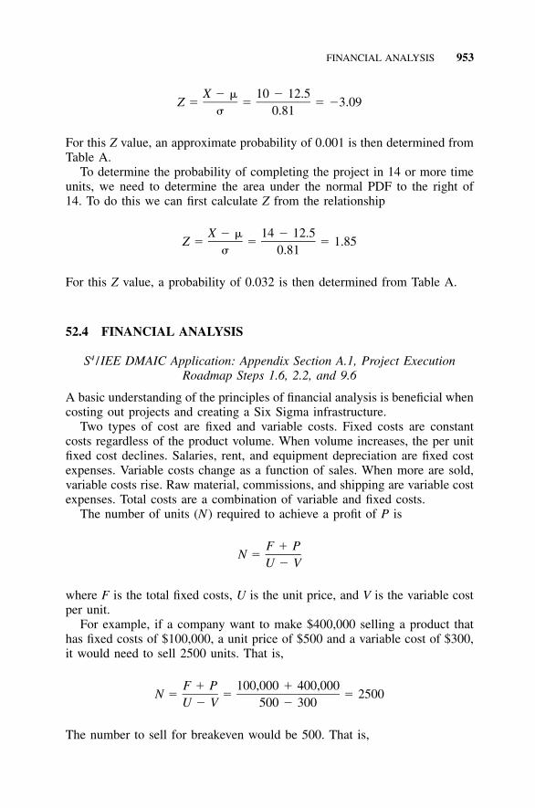
FINANCIAL ANALYSIS 953

X � � 10 � 12.5Z � � � �3.09

� 0.81

For this Z value, an approximate probability of 0.001 is then determined fromTable A.

To determine the probability of completing the project in 14 or more timeunits, we need to determine the area under the normal PDF to the right of14. To do this we can first calculate Z from the relationship

X � � 14 � 12.5Z � � � 1.85

� 0.81

For this Z value, a probability of 0.032 is then determined from Table A.

52.4 FINANCIAL ANALYSIS

S4 /IEE DMAIC Application: Appendix Section A.1, Project ExecutionRoadmap Steps 1.6, 2.2, and 9.6

A basic understanding of the principles of financial analysis is beneficial whencosting out projects and creating a Six Sigma infrastructure.

Two types of cost are fixed and variable costs. Fixed costs are constantcosts regardless of the product volume. When volume increases, the per unitfixed cost declines. Salaries, rent, and equipment depreciation are fixed costexpenses. Variable costs change as a function of sales. When more are sold,variable costs rise. Raw material, commissions, and shipping are variable costexpenses. Total costs are a combination of variable and fixed costs.

The number of units (N) required to achieve a profit of P is

F � PN �

U � V

where F is the total fixed costs, U is the unit price, and V is the variable costper unit.

For example, if a company want to make $400,000 selling a product thathas fixed costs of $100,000, a unit price of $500 and a variable cost of $300,it would need to sell 2500 units. That is,

F � P 100,000 � 400,000N � � � 2500

U � V 500 � 300

The number to sell for breakeven would be 500. That is,

954 PROJECT MANAGEMENT AND FINANCIAL ANALYSIS

F � P 100,000 � 0N � � � 500

U � V 500 � 300

If you deposit $1000 into a money market account, you expect your depositto grow as a function of time. Because of this, we say that money has timevalue. Present value and future value describe the time value of money andhave the relationship

FV � PV(1 � i)

where PV is the present value of money, FV is the future value of money,and i is the interest rate expressed as a proportion.

If interest were to be credited monthly to an account that had a deposit of$1000, the monetary value of the account would be compounding during eachmonthly compounding period. For N accounting periods, future value couldnow be expressed as

NFV � PV(1 � i)

Repeat purchases by a loyal customer can be very large over the years.For example, a frequent flyer of an airline might spend $100,000 in threeyears. The economic worth of this customer can be determined by combiningrevenue projections with expenses over some period of time. The net presentvalue (NPV) of the net cash flow, that is, profits, describes this economicworth. NPV describes the value of the profits over time in terms of today’sdollars. The knowledge of NPV can lead to the evaluation of alternative mar-keting and other strategies to attract and retain customers.

NPV calculations can also be used within the selection process of SixSigma project and the determination of the value for these projects. However,often both costs and benefits have a cash flow stream, rather than lump sums.In addition, these cash flow streams can be uneven. These added complexitiesmake the calculation for NPV tedious. However, most spreadsheets have afunction to address these calculations. For example, someone could enter adesired rate of return along with the net revenue (e.g., yearly benefits lesscosts) for several years, and could then execute a function that calculates theNPV for these inputs.

Interest rate paid on a loan and rate of return (ROI) are both computationsfrom the annual cost of money expressed in percentage units. However, theydiffer in that one is the investor and the other is the borrower. For an invest-ment period of one year the computation is simply

S � PROI �

P

where S is the amount collected or paid back and P is the amount borrowed

EXERCISES 955

or invested. Computations for ROI increase when other factors are considered,such as number of interest periods increase, compounding of interest, andtaxes. Companies can use complex models to make this calculation.

Internal rate of return (IRR) is the rate of return that equates the presentvalue of future cash flows with investment costs. IRR can be determined usingan IRR function within many spreadsheets. For example, annual price andcash flows for a project can be entered into a spreadsheet, where expendituresare minus and receipts are positive. The IRR function would then make it-erative calculations to determine the project IRR. Another application of IRRis within the project selection process, where projects are prioritized accordingto their expected IRR.

Payback period is the time necessary for net financial benefits (inflows) toequate to the net costs (outflows). The equations are simplistic, where typi-cally the time value of money is ignored. Projects can be compared usingthis approach; however, financial benefits beyond the payback period are notaddressed. When there is an initial investment and an inflow of cash that isfixed, the payback period can be calculated from (Johnson and Melicher 1982)

Initial (and incremental) investmentPayback period �

Annual (or monthly) cash inflow

52.5 S4/IEE ASSESSMENT

Project management is very important when executing Six Sigma projects.However, the efficient completion of tasks should not be overlooked whenmanaging Six Sigma project tasks. For example, consider the creation of aprocess flowchart for a project. It can be much more efficient to use a com-puter projector with a flowcharting program to dynamically create a processflowchart within a team meeting, rather than positioning sticky-back note padson the wall to represent process steps.

The financial quantification of projects is very important within the SixSigma infrastructure of an organization. However, organizations should notoverlook the value from soft savings and improved customer satisfaction.Also, organizations should consider TOC methodologies within the overallfinancial measurement strategy of an organization.

52.6 EXERCISES

1. Create a project management flexibility table for your project.

2. Create a work breakdown structure for your project, laying out the nine-step DMAIC.

3. Construct a Gantt chart for your project showing your project activities’planned start and end dates.

956 PROJECT MANAGEMENT AND FINANCIAL ANALYSIS

4. Create an arrow chart for your project. Discuss how to establish reasonabletime estimates for activities. Discuss how historical data could be used todetermine time ranges.

5. Calculate the expected IRR for your project.

6. A project requires an initial investment of $23,000 and training costs of$6,000, which are spread over six months. Beginning with the third month,the expected monthly project savings is $3,000. Ignoring interest and taxes,determine the payback period (Quality Council of Indiana 2002).

7. Given the data below determine the critical path, project duration, andslack time, where slack time is the amount of time an activity can bedelayed without delaying the project. (Six Sigma Study Guide 2002.)

Activity Predecessor Duration

A None 3B A 5C A 4D B 4E C 2

8. For the activities below, determine the probability of completing the projectin 48 or more time units. (Six Sigma Study 2002.)

ActivityPreceded

byOptimistic

TimeExpected

TimePessimistic

Time

A None 10.17 12.06 15.42B None 14.81 15.84 18.53C A and B 12.45 15.31 16.72D C 11.79 14.54 17.74E C 10.63 12.56 15.34

9. For the activities below determine the probability of completing the projectin 28.3 or more time units. (Six Sigma Study Guide 2002.)

ActivityPreceded

byOptimistic

TimeExpected

TimePessimistic

Time

A None 14.27 16.69 18.81B None 11.93 13.47 14.52C A and B 10.07 11.09 12.11D A and B 11.17 12.86 14.84

957

53TEAM EFFECTIVENESS

S4 /IEE DMAIC Application: Appendix Section A.1, Project ExecutionRoadmap Step 1.4

Within an S4/IEE implementation there is infrastructure building, infrastruc-ture management, and project execution. The success of these tasks dependsupon transforming a group of diverse individuals into a team that is productiveand highly functional.

The range of commitment levels that stakeholders can have during projectdefinition is: enthusiastic, will lend support, compliant, hesitant, indifferent,uncooperative, opposed, and hostile. An expectation for enthusiastic supportby all team members for all projects is not realistic. However, team leaderscan do a stakeholder analysis and quantify where each member is in thatrange, keeping in mind the importance of moving team members toward theenthusiastic level.

This section describes a commonly used and easy-to-follow model that canimprove the effectiveness of teams.

53.1 ORMING MODEL

It is commonly agreed that teams go through stages to become a highlyeffective team. In addition, it is generally agreed that teams can improve thequality of their interactions when each member of the team is aware of thesestages. Tuckman (1965) describes the four stages of team development as

958 TEAM EFFECTIVENESS

forming, storming, norming, and performing. These team stages are oftencollectively referenced as the orming model. Successful teams are those thatmake transitions back and forth between these stages when circumstanceschange. Adjourning and recognition can be considered as the final stages ofthe team stages.

Within the forming stage the team leader needs to provide structure for theteam, clarifying expectations about the initiation of team processes. The workthat needs to be accomplished is team member introduction, team resourceassessment, and objective definition. Issues that need to be overcome are theteam leader taking on most of the work, team members not organized arounda common objective, and team not taking advantage of all the team resources.The status of the team execution process at this stage is a wait-and-see atti-tude, where the team process is usually noticed but avoided.

Within the storming stage the team leader coaches the team in the main-taining of a focus on the goals and expectations, managing the team processand conflict resolution, generating ideas, and explaining of decisions. Thework that needs to be accomplished is identifying team member expectations,discussing differences, and conflict management. Issues that surface are teammembers feeling unsatisfied, overburdened, and lack of contribution. Thestatus of the team execution process at this stage is the formation of cliquesbecause the general perception is that the effort does not require teamwork.

Within the norming stage the team leader primarily acts as a facilitatorwho provides encouragement, helps with consensus building, and gives feed-back. Work needs to be given to resolving differences through establishingground rules, developing trust, and discussing directly how to better worktogether. Issues that arise are ongoing disagreements between team membersand team members working at cross-purposes. The status of the team exe-cution process at this stage is general support for leadership, with the sharingof leadership among the team.

Within the performing stage the team leader facilitates the team process,where there is a delegation of tasks and objectives. Work needs to be givento objective achievement, team member satisfaction, and collaboration. Issuesthat surface are unfinished work and not celebrating success. The status ofthe team execution process at this stage is members are not dependent on thedesignated leaders, where everyone shares the responsibility for initiating anddiscussing team process issues.

53.2 INTERACTION STYLES

Teams are made up of individuals who have different styles. Individuals maybe more task-oriented or more people-oriented. Some team members preferto focus more on the job at hand, while others focus on relationships. Peoplealso tend to be thinkers or doers. Thinkers reflect on their work, while doerstend to discuss their work more openly. Everybody strikes his or her balance

MAKING A SUCCESSFUL TEAM 959

between these characteristics. This yields a distinctive profile for each indi-vidual on a team.

The inherent dynamics can be quite different between teams since thestyles for members of the team can be quite different. The success of a teamis dependent upon how well differences between individuals are understoodand capitalized upon. Teams need to have profile diversity, but the individualsin a team also need to be able to work together.

The question of concern is what should be done to make the teams withinan S4/IEE implementation most effective. Those who are involved in creatingthe team should consider the interaction styles of people and how well thesepeople’s skills and styles will complement each other toward the commongoal of the team. Secondly, after the team is formed it is important that eachteam member understand and consider the difference in interaction stylesamong the team members so that he/she knows how best to interface withthe team as a whole and with individuals within the team.

There are many tests to assess the personality of individuals (e.g., Myers-Briggs). It can be advantageous to study the results of these tests to determinewhat members of the team needs to do to interact better with the team as awhole or with other individuals who have personality styles that can easilyconflict with their own.

One model describes the interaction styles of people as they relate to teams.These styles are driver, enthusiast, analyzer, or affiliator (Teamwork 2002):

• Drivers take charge. They focus on results. They exert a strong influenceto get things done.

• Enthusiasts are social specialists. They express opinions and emotionseasily. They prefer a strong interaction with people.

• Analyzers like to be well organized and think things out. They preferspecific projects and activities. They enjoy putting structure into ideas.

• Affiliators are adaptive specialists. They have a high concern for goodrelationships. They seek stability and predictability. They want to be apart of the bigger picture.

The potential strengths and potential weaknesses of each style are noted inTable 53.1.

53.3 MAKING A SUCCESSFUL TEAM

When initiating teams it is important to have members who have the appro-priate skill sets (e.g., self-facilitation and technical/subject-matter expertise).The teams should have an appropriate number of members and representation.When launching a team it is important to have a clear purpose, goals, com-mitment, ground rules, roles, and responsibilities set for the team members.

960 TEAM EFFECTIVENESS

TABLE 53.1 Potential Strengths and Weaknesses of Styles

Style Strengths Weaknesses

Driver *Determined *Thorough*Decisive *Efficient*Direct

*Dominating *Unsympathetic*Demanding *Critical*Impatient

Enthusiast *Personable *Stimulating*Enthusiastic *Innovative

*Opinionated *Undependable*Reactionary

Analyzer *Industrious *Persistent*Serious *Orderly *Methodical

*Indecisive *Uncommunicative*Critical

Affiliator *Cooperative *Supportive*Dependable *Helpful

*Conforming *Uncommitted*Hides true feeling

Schedules, support from management, and team empowerment issues mustalso be addressed.

Team dynamics and performance issues must also be addressed, such as:

1. Team-building techniques that address goals, roles, responsibilities, in-troductions, and stated/hidden agenda.

2. Team facilitation techniques that include applying coaching, mentoring,and facilitation techniques to guide a team to overcome problems suchas overbearing, dominant, or reluctant participants and the unquestionedacceptances of opinions as facts, feuding, floundering, rush to accom-plishment, attribution, digressions, tangents, etc.

3. Measurement of team performance in relationship to goals, objectives,and metrics.

4. Use of team tools such as nominal group technique, force-field analysis,and other team tools described in Chapter 5.

Ten ingredients for a successful team have been described as (Scholtes1988):

1. Clarity in team goals2. An improvement plan3. Clearly defined roles4. Clear communication5. Beneficial team behaviors6. Well-defined decision procedures7. Balanced participation8. Established ground rules9. Awareness of the group process

10. Use of the scientific approach

MAKING A SUCCESSFUL TEAM 961

I will address each of these 10 points as they apply to the execution of aproject within S4/IEE. However, these ingredients also apply to the executiveteam and steering team.

1. Clarity of Team Goals

All team members should understand and maintain focus on the goals of theproject as expressed within the S4/IEE team charter. During the execution ofprojects there will be times when it is best to redirect or rescope a project.There will be other times when new project opportunities arise or it appearsthat it would be best to abort further work on the project. All these situationscan occur within a project’s execution. Within S4/IEE it is important to informthe project champion and others about these issues. Until formal alterationsare made to the project charter, it is important that the team maintain focuson the current project chart definition.

2. An Improvement Plan

A project execution plan should be made from the S4/IEE project executionroadmap. This plan guides the team to determine schedules and identify mile-posts. Reference is made to these documents when there are discussions aboutwhat direction to take next and resource/training needs.

3. Clearly Defined Roles

The efficiency and effectiveness of teams is dependent upon how well eve-ryone’s talents are tapped. It is also important for members to understandwhat they are to do and who is responsible for various issues and tasks.Ideally there are designated roles for all team members. The pecking orderof an organization should not dictate the roles and duty assignments withina team.

4. Clear Communication

The effectiveness of discussions is based upon how well information is trans-ferred between members of the team. Team members need to speak withclarity and directness. They need to actively listen to others, avoiding inter-ruptions and talking when they speak.

5. Beneficial Team Behaviors

Within teams there should be encouragement to use the skills and method-ologies that make discussions and meetings more effective. Each team meet-ing should use an agenda. Within the meeting there should be a facilitatorwho is responsible for keeping the meeting focused and moving. Someone

962 TEAM EFFECTIVENESS

should take minutes for each meeting. There should be a draft of the nextagenda and evaluation of the meeting. Everyone should give his or her fullattention to the meeting. No one should leave the meeting unless there is trulyan emergency. During a meeting members should initiate discussions, seekinformation, and clarify/elaborate on ideas. Focus should be given, avoidingdigressions.

6. Well-Defined Decision Procedures

A team should be aware and flexible to execute the different ways to reacha decision. Discussions should be made to determine when a poll or consensusis most appropriate. Many of the decision-making procedures are part of theS4/IEE project execution roadmap.

7. Balanced Participation

Every team member should participate in discussions and decisions. Teammembers should share in the contribution of their talents and be committedto the success of the project. There should ideally be balanced participationwith the building of the styles offered by each team member.

8. Established Ground Rules

Every team should establish ground rules that address how meetings will berun. Norms should be set for how members are to interact and what kind ofbehavior is acceptable. Some important ground rules for meetings are highpriority on attendance, promptness for meeting start /stop times with full at-tendance, and meeting place and time along with how this notification iscommunicated.

9. Awareness of the Group Process

Team members should be aware of how the team works together where at-tention is given to the content of the meeting. Members should be sensitiveto nonverbal communication. They should be sensitive to the group dynamics.They should feel free to comment and intervene when appropriate to correcta process problem of the group.

10. Use of the Scientific Approach

Teams need to focus on how they can best use the S4/IEE project executionroadmap for their particular situation. They should focus on when and howto implement the best tool for every given situation.

REACTING TO COMMON TEAM PROBLEMS 963

53.4 TEAM MEMBER FEEDBACK

A teams needs to work both smart and hard at completing its task. However,the team needs to support the needs of individual members. To understandthe needs of team members, there needs to be feedback. The most commonform of this feedback is a one-on-one conversation.

We want feedback to be constructive. We must acknowledge the need forfeedback, give both positive and negative feedback, understand the context,know when to give feedback, know how to give feedback, and know how toreceive feedback (Scholtes 1988).

Feedback should be descriptive, relating objectively to the situation andgiving examples whenever possible. The basic format for such a statementfollows. Descriptive words can be changed for the particular situation.

When you are late for meetings, I get angry because I think it is wasting thetime of all the other team members and we are never able to get through ouragenda items. I would like you to consider finding some way of planning yourschedule that lets you get to these meetings on time. That way we can be moreproductive at the meetings and we can all keep to our tight schedules.

Additional guidelines for giving feedback are: don’t use labels such asimmature, don’t exaggerate, don’t be judgmental, speak for yourself, and talkabout yourself, not about the other person. In addition, phrase the issue as astatement, not a question, restrict feedback to things you know for certain,and help people hear/accept your compliments when positive feedback isgiven.

Guidelines for receiving feedback are: breathe to relax, listen careful, askquestions for clarification, acknowledge the understanding of the feedback,acknowledge the validity of points, and, when appropriate, take time out tosort what you heard before responding.

Within a team it is best to anticipate and prevent problems whenever pos-sible. However, when a problem does occur, it should be thought of as a teamproblem. It is important to neither under- nor overreact to problems. Typicaldecisions that need to be made by the team leader for problems are: donothing, off-line conversation, impersonal group time (e.g., start of meetingdescribing the problem with no mention of name), off-line confrontation, in-group confrontation, and expulsion from the group, an option that should notbe used. These options are listed in order of preference and sequence ofexecution. That is, off-line confrontation will typically be used only if a lessforceful off-line conversation earlier did not work.

53.5 REACTING TO COMMON TEAM PROBLEMS

Ten common group problems have been described as (Scholtes 1988):

964 TEAM EFFECTIVENESS

1. Floundering2. Overbearing participants3. Dominating participants4. Reluctant participants5. Unquestioned acceptance of opinions as facts6. Rush to accomplishment7. Attribution8. Discounted9. Wanderlust: digression and tangents

10. Feuding members

1. Floundering

Teams often experience trouble starting a project, ending a project, and/oraddressing various stages of the project. When problems occur at the begin-ning of a project, they can indicate that the team is unclear or overwhelmedby its task. When this occurs, specific questions should be asked and ad-dressed by the team, such as: ‘‘Let’s review our project charter and make sureit’s clear to everyone.’’ ‘‘What do we need to do so we can move on?’’

2. Overbearing Participants

Because of their position of authority or expertise area on which they basetheir authority, some members wield a disproportionate amount of influence.This can be detrimental to the team when they discourage discussion in theirarea. When this occurs, the team leader can reinforce the agreement that noarea is sacred and a team policy of ‘‘In God we trust. All others must havedata!’’

3. Dominating Participants

Some team members talk too much, using long anecdotes when a concisestatement would do. These members may or may not have any authority orexpertise. When this occurs, the leader can structure discussions that encour-age equal participation, using such tools as nominal group technique. Theleader may need to practice gate-keeping, using such statements as ‘‘Paul,we’ve heard from you on this. I’d like to hear what others have to say.’’

4. Reluctant Participants

Some team members rarely speak. A group can have problems when thereare no built-in activities that encourage introverts to participate and extrovertsto listen. When this occurs, the leader may need to divide the tasks into

REACTING TO COMMON TEAM PROBLEMS 965

individual assignments with reports. A gate-keeping approach would be toask the silent person a direct question about his/her experience in the areaunder consideration.

5. Unquestioned Acceptance of Opinions as Facts

Team members sometime express a personal belief with such confidence thatlisteners assume that what they are hearing is fact. When this occurs, theleader can ask a question such as ‘‘Is your statement an opinion or fact? Doyou have data?’’

6. Rush to Accomplishment

Often teams have at least one member who is either impatient or sensitive tothe outside pressures to such a level that he/she feels the team must dosomething now. If this pressure gets too great, the team can be led to unsys-tematic efforts to make improvements, leading to chaos. When this occurs,the leader can remind the members of the team that they are to follow thesystematic S4/IEE roadmap, which allows for the possibility of executingquick low-hanging-fruit fixes when these fixes are appropriate for a project.

7. Attribution

We tend to attribute motives to people when we disagree with or don’t un-derstand their behavior. Statements such as ‘‘They won’t get involved sincethey are waiting their time out to collect their pensions’’ can lead to hostilitywhen aimed at another team member or someone outside the team. When thisoccurs, the leader can respond by saying, ‘‘That might well explain why thisis occurring. But how do we know for sure? Has anyone seen or heard some-thing that indicates this is true? Are there any data that supports this state-ment?’’

8. Discounted

We all have certain values and perspectives that may consciously or uncon-sciously be important to them. When these values are ignored or ridiculed,we feel discounted. A discounted statement ‘‘plop’’ occurs when someonemakes a statement that no one acknowledges and discussion picks up on asubject totally irrelevant to the statement. The speaker then wonders why therewas no response. The speaker needs feedback on whether such a statementis or is not relevant to the conversation. When this occurs, the leader caninterject conversation that supports the discounted person’s statement. If ateam member frequently discounts people, the leader might give off-line con-structive feedback.

966 TEAM EFFECTIVENESS

9. Wanderlust: Digression and Tangents

Unfocused conversations that ramble from one topic to another are wanderlustconversations. When this happens, team members can wonder where the timewent for the meeting. To deal with this problem, the team leader can writean agenda that has time estimates for each item, referencing the time whendiscussions deviate too far from the current topic.

10. Feuding Members

Sometimes there are team members who have been having feuds since longbefore the team creation. Their behavior can disrupt a team. Interaction byother team members could be viewed as taking sides with one of the com-batants. It is best that feuding members not be placed on the same team.When this is not possible, the leader may need to have off-line discussionswith both individuals at the onset of the team’s creation.

53.6 EXERCISE

1. Consider the following meeting dynamics of a Six Sigma team in theanalyze phase. The team is behind schedule and has a presentation due toupper management next week. An agenda has been set to determine whereto focus improvements and calculate the COPQ/CODND. The last fewmeetings have seemed like reruns with no clear direction on where to drilldown and focus low-hanging-fruit improvements. During the meeting var-ious group members share conflicting opinions about what area of theprocess should be the point of focus for improvements. Team member arecomplaining that nothing is getting done and are losing momentum to workon the project. The team leader will not budge on the direction he thinksthe team should go in, although most members are in disagreement. Dis-cuss and record what went wrong, how the facilitator could have acteddifferently in order to gain team consensus, and what tools/actions aremost appropriate for this scenario.

967

54CREATIVITY

S4 /IEE DMAIC Application: Appendix Section A.1, Project ExecutionRoadmap Step 6.5

Creativity is the process of creating unusual associations among mental ob-jects. Invention is a result of creative problem-solving. Creativity can some-times result when there is an association of the right combination of objects.One frequently described example of association effect of the right objects isthe exhaustive search of Thomas Edison during the development of a durablefilament for the light bulb. In other cases the objects are known but an unusualassociation type becomes creative. An example of this is the creation of musicfrom a fixed set of notes.

Value is the sufficiency for creativity. Without some metric for value, cre-ativity will not be recognized. We need to note that this value might bedeveloped years later when the work is recognized as creative. People otherthan the person creating often describe this value.

Organizations need to have value in order to grow and stay in business.To create value, we need creativity. From a how-to-create perspective, Jones(1999) states that to encourage creativity we need to put ourselves in theplace of most potential. The question then becomes how organizations cancreate an environment that encourages creativity such that more value is gen-erated for the organization.

968 CREATIVITY

54.1 ALIGNMENT OF CREATIVITY WITH S4/IEE

Jones (1999) list nine points for creativity:

1. Creativity is the ability to look at the ordinary and see the extraordinary.2. Every act can be a creative one.3. Creativity is a matter of perspective.4. There’s always more than one right answer.5. Reframe problems into opportunities.6. Don’t be afraid to make mistakes.7. Break the pattern.8. Train your technique.9. You’ve got to really care.

The S4/IEE approach described within this book aligns with these points.S4/IEE creates an environment that encourages the implementation of creativesolutions that are aligned with the needs of the business. Satellite-level metricscan track overall value to an organization from both a financial and a customerpoint of view. A closer view of the value from processes can then be obtainedfrom operational and project 30,000-foot-level metrics. Creativity activitiescan then be a very integral part of the S4/IEE project execution roadmap.

This S4/IEE implementation process is a procedure for putting ourselvesin the place of most potential for the execution of projects that create valuefor the organization and its customers. One example of this occurrence iswhen a colleague of mine executed a DOE that I designed for him in twostages because a new assembly factor was not available. The first stage hadthe old assembly, while the second stage had a new assembly. An analysis ofthis DOE indicated that the statistically significant difference between the twotypes of assemblies was large. I raised suspicions about the execution of thisexperiment when a follow-up experiment did not indicate significance of thisfactor. Upon further investigation, my colleague discovered that the first testhad been executed using a different procedure for mounting the machine. Mycolleague was very apologetic about his oversight. I indicate that this was ablessing in disguise since a testing problem was uncovered that we wouldlater have had within manufacturing. From this test we discovered, beforeproduction start-up, that the test fixture yielded an erroneous response relativeto how a customer would experience the machine function. Though the exe-cution of this DOE we put ourselves in a place of most potential for discovery/creativity.

54.2 CREATIVE PROBLEM SOLVING

Teams might find that a less rigid creative approach to solving problems yieldsthe best solutions (Teamwork 2002). With this association of ideas approach

INVENTIVE THINKING AS A PROCESS 969

one needs to understand the factors that make creative thinking work best.Through this process, imagination feeds off memory and knowledge, whichresults in one idea leading to another.

This creative thinking process is dependent upon the execution of the fol-lowing factors within the process:

• Suspend judgment: An open mind is an important contributor to thesuccess of this process.

• Self-assessment: It may be helpful for team members to conduct a self-evaluation of their tendency to cling to dogmatic ideas and opinions sothat they can better assess how much work they need to do in this area.

• Develop a positive attitude: We need to develop an attitude that all ideasare good ideas.

• Use checklists: All ideas should be written down. This sends the messagethat all ideas are good. It also ensures that nothing is forgotten.

• Be self-confident: Great ideas often can initially be ridiculed. Be confi-dent in ideas that are different than the traditional approach.

• Encourage others: The fuel for creativity is praise and encouragement.

Five steps to solving problems creatively are:

1. Orientation: Set the stage for a productive session.2. Preparation and analysis: Gather facts without getting into too much

detail. Research for successful past solutions to problems that are sim-ilar.

3. Brainstorming: Conduct a brainstorming session where there are manyideas created.

4. Incubation: Disperse the group for a period of time to let ideas grow.This time could be over a lunch break or a good night’s sleep.

5. Synthesis and verification: Construct a whole out of the ideas generatedby brainstorming. To stimulate this process, the team might create a listof the desirable and undesirable qualities of the solutions. Another ap-proach is to synthesize ideas through the creation of an outline or group-ing of ideas together with similar ideas assigned to the same group.Relationships between these groups can then be mapped out.

54.3 INVENTIVE THINKING AS A PROCESS

Within this book we suggest creating and using processes wherever possible.The purpose of this section is to present some background information thatmight be used to initiate the creation of a more rigorous inventive processwithin organizations.

970 CREATIVITY

System inventive thinking is a problem-solving methodology developed inIsrael and inspired by the Russian TRIZ methodology. Innovations wereadded that simplified the learning and application of the problem-solvingmethodology. These included the closed-world diagram, the qualitative-change graph, the particles method (an improvement on the ‘‘smart little peo-ple’’ of the TRIZ method), and a simplified treatment of the solutiontechniques (which the Israelis call ‘‘tricks’’). Whereas TRIZ stresses the useof databases of effects, the Israeli method stresses making the analyst anindependent problem-solver (Sickafus 1997).

Structured inventive thinking (SIT) is a modified version of the Israelisystematic inventive thinking problem-solving methodology. The methodol-ogy is sometimes referenced in the 8D problem-solving methodology. It is amethod of developing creative solutions to technical problems that are con-ceptual. The problem-solver focuses on the essence of the problem. Themethod is to efficiently overcome psychological barriers to creative thinking,enabling the discovery of inventive solutions.

Unified structured inventive thinking (USIT) was developed by E. N. Sick-afus while teaching an elementary course in SIT at Ford Motor Company inDearborn, Michigan (Sickafus 1997).

54.4 EXERCISE

1. Given six equal-length sticks, determine how you can arrange them tocreate four equal-sided triangles.

971

55ALIGNMENT OF MANAGEMENTINITIATIVES AND STRATEGIESWITH S4/IEE

Management needs to ask the right questions leading to the wise use of sta-tistical techniques for the purpose of obtaining knowledge from facts and data.Management needs to encourage the wise application of statistical techniquesfor a Six Sigma implementation to be successful. It needs to operate underthe cliché: ‘‘In God we trust. All others must have data.’’

This book suggests periodic process reviews and projects based on S4/IEEassessments leading to a knowledge-centered activity (KCA) focus on allaspects of the business, where KCA describes efforts for wisely obtainingknowledge and then wisely utilizing this knowledge within organizations andprocesses. KCA can redirect the focus of business so that efforts are moreproductive.

The strategies and techniques described in this book are consistent andaligned with the philosophies of such quality authorities as W. Edwards Dem-ing, J. M. Juran, Walter Shewhart, Genichi Taguchi, Kaoru Ishikawa, andothers. This chapter discusses, as a point of reference, the steps to both Dem-ing’s 14 points of management philosophy and Juran’s control sequence andbreakthrough sequence. Also described is the integration of S4/IEE with in-itiatives such as ISO 9000, Malcolm Baldrige assessments, Shingo Prize, andGE Work-Out.

55.1 QUALITY PHILOSOPHIES AND APPROACHES

This section highlights some quality philosophies and approaches over theyears (Berger et al. 2002).

972 ALIGNMENT OF MANAGEMENT INITIATIVES AND STRATEGIES WITH S4 / IEE

• Early 1900s: Frederick Taylor developed work specialization. Specializedinspectors were created.

• Late 1920s: Walter Shewhart developed the control chart and statisticalprocess control (SPC).

• 1940s: The United States during World War II required quality charting,which brought operators back to looking at their quality. However, manyorganizations continued to rely on inspectors.

• 1951: Armand Feigenbaum published Total Quality Control, which ini-tiated the total quality management (TQM) movement.

• 1960s and 1970s: quality circles and employee involvement were utilized.• 1980s: SPC had a resurgence.• 1990s: Focus was placed on the International Organization for Standard-

ization’s (ISO) quality management system (QMS), ISO 9000, and Mal-colm Baldrige National Quality Award assessments.

• 1980s and 1990s: Additional methodologies utilized included valueanalysis/value engineering, lean manufacturing, kaizen, poka-yoke, the-ory of constraints (TOC), and Six Sigma.

A few of the top-rated people and a very brief highlight of their contri-butions are

• Philip B. Crosby: Wrote the best-selling Quality Is Free. American ex-ecutives absorbed his ‘‘do it right the first time’’ philosophy. His 14-stepcost-of-quality method gave explicit guidance to managers. His four ab-solutes of quality management were: quality is conformance to require-ments, quality is caused by prevention, the performance standard is nodefects, and the measure of quality is the price of nonconformance.

• W. Edwards Deming: In recognition of his contribution to the post-warrecovery, the Japanese Union of Scientists and Engineers (JUSE) estab-lished the Deming Prize, an annual award for quality achievements. Heemphasized that the key to quality improvement was in the hands ofmanagement since most problems are the result of the system and not ofemployees. He used statistical quality control techniques to identifyspecial- and common-cause conditions, in which common-cause condi-tions were the result of systematic variability, while special-cause con-ditions were erratic and unpredictable. He described the seven deadlydiseases of the workplace and 14 points for management.

• George D. Edwards: Was the first president of ASQ from 1946 to 1948.His work as head of the inspection engineering department of Bell Tele-phone Laboratories and Bell’s director of quality assurance (a term hecoined) gained him reputation in the quality control discipline. In 1960the ASQ established the Edwards Medal in his honor.

• Armand V. Feigenbaum: Argued that total quality management (TQM)was necessary to achieve productivity, market penetration, and competi-

DEMING’S 7 DEADLY DISEASES AND 14 POINTS FOR MANAGEMENT 973

tive advantage. This involves four essential actions: (1) setting standards,(2) appraising conformance, (3) acting when necessary, and (4) planningfor improvement. His Nine M’s of quality are markets, money, manage-ment, men, motivation, materials, machines and mechanization, moderninformation methods, and mounting product requirements. He believedthat it was important to place a strong emphasis on identifying the qualityrequirements of the customer so that the customer was satisfied when hereceived the product.

• Kaoru Ishikawa: Popularized total quality control in Japan. He introducedthe problem diagnosis tool called Ishikawa diagrams, cause-and-effectdiagrams, or fishbone diagrams. In the early 1960s he developed thequality circle concept. The quality circle decentralized problem-solvingto work groups that included the workers when solving quality problemsin their own work.

• Joseph M. Juran: Traveled to Japan in the 1950s to teach quality man-agement. His definition of quality was ‘‘fitness for use by the customer,’’where fitness was based on the availability, reliability, and maintainabilityof the product. He emphasized the necessity of management’s hands-oninvolvement in the quality effort. Juran’s trilogy had three major qualityprocesses: (1) quality control, and the control sequence for sporadic prob-lems; (2) quality improvement and the breakthrough sequence for chronicproblems; and (3) quality planning and an annual quality program toinstitutionalize managerial control and review.

• Walter A. Shewhart: Considered the father of modern quality control,Shewart brought together the disciplines of statistics, engineering, andeconomics. His Economic Control of Quality of Manufactured Product(1931) is regarded as a complete and detailed explanation of the basicprinciples of quality control. For most of his professional career he wasan engineer at Western Electric and Bell Telephone Laboratories.

• Genichi Taguchi: Was well known by 1950 in Japan for his statisticalmethods applications through his work at the Ministry of Public Healthand Welfare. In 1962 he published Design of Experiments, in which heintroduced the signal-to-noise ratio measurement. In 1982 the AmericanSupplier Institute first introduced Dr. Taguchi and his methods to theUnited States.

The S4/IEE strategy orchestrates the most powerful points of these qualityexperts with powerful methodologies described by other continuous improve-ment experts in fields such as TOC and lean.

55.2 DEMING’S 7 DEADLY DISEASES AND 14 POINTS FORMANAGEMENT

Deming had a great influence on the rise of quality and productivity in Japan.The Japanese have embraced his concepts and have named their highest qual-

974 ALIGNMENT OF MANAGEMENT INITIATIVES AND STRATEGIES WITH S4 / IEE

ity award after him. Based on many years of experience, I agree with Dem-ing’s basic philosophy and believe that many companies need to make thechanges proposed by Deming in order to become more competitive. This bookis a how-to guide for the implementation of many of Deming’s concepts.

The following are Deming’s 7 deadly diseases:

1. Lack of constancy of purpose in planning product and service that willhave a market, keep the company in business, and provide jobs.

2. Emphasis on short-term profits: short-term thinking (just the oppositeof constancy of purpose to stay in business), fed by fear of unfriendlytakeover and by push from bankers and owners for dividends.

3. Evaluation of performance, merit rating, or annual review.4. Mobility of management: job hopping.5. Management by use only of visible figures, with little or no consider-

ation of figures that are unknown or unknowable.6. Excessive medical costs.7. Excessive cost of liability, swelled by lawyers who work on contingency

fees.

The following are Deming’s original 14 points for management with dis-cussion (Deming 1982):

1. ‘‘Create constancy of purpose toward improvement of product andservice, with the aim to become competitive and to stay in businessand to provide jobs.’’ For the company that wants to stay in business,the two general types of problems that exist are the problems of todayand the problems of tomorrow. It is easy to become wrapped up withthe problems of today, but the problems of the future demand, firstand foremost, constancy of purpose and dedication to keep the com-pany alive. Decisions need to be made to cultivate innovation, fundresearch and education, and improve the product design and service,remembering that the customer is the most important part of the pro-duction line.

2. ‘‘Adopt the new philosophy. We are in a new economic age. Westernmanagement must awaken to the challenge, must learn their respon-sibilities, and take on leadership for change.’’ Government regulationsand antitrust activities need to be changed to support the well-beingof people. Commonly accepted levels of mistakes and defects can nolonger be tolerated. People must receive effective training so that theyunderstand their job and also understand that they should not be afraidto ask for assistance when it is needed. Supervision must be adequateand effective. Management must be rooted in the company and mustnot job-hop between positions within a company.

DEMING’S 7 DEADLY DISEASES AND 14 POINTS FOR MANAGEMENT 975

3. ‘‘Cease dependence on inspection to achieve quality. Eliminate theneed for inspection on a mass basis by building quality into the prod-uct in the first place.’’ Inspection is too late, ineffective, and costlyto improve quality. It is too late to react to the quality of a productwhen the product leaves the door. Quality comes not from inspectionbut from improving the production process. Corrective actions are notinspection, scrap, downgrading, and rework on the process.

4. ‘‘End the practice of awarding business on the basis of price tag.Instead, minimize total cost. Move toward a single supplier for anyone item, on a long-term relationship of loyalty and trust.’’ Price andquality go hand in hand. Trying to drive down the price of anythingpurchased without regard to quality and service can drive good sup-pliers and good service out of business. Single-source suppliers aredesirable for many reasons. For example, a single-source supplier canbecome innovative and develop an economy in the production processthat can only result from a long-term relationship with its purchaser.Lot-to-lot variability within a one-supplier process is often enough todisrupt the purchaser’s process. Only additional variation can be ex-pected with two suppliers. To qualify a supplier as a source for partsin a manufacturing process, perhaps it is better first to discard man-uals that may have been used as guidelines by unqualified examinersto rate suppliers. Instead suppliers could be asked to present evidenceof active involvement of management encouraging the application ofmany of the S4/IEE concepts discussed in this book. Special noteshould be given to the methodology used for continual process im-provement.

5. ‘‘Improve constantly and forever the system of production and ser-vice, to improve quality and productivity, and thus constantly de-crease costs.’’ There is a need for constant improvement in testmethods and a better understanding of how the customer uses andmisuses a product. In the past, American companies have often wor-ried about meeting specifications, while the Japanese have worriedabout uniformity, i.e., reducing variation about the nominal value.Continual process improvement can take many forms. For example,never-ending improvement in the manufacturing process means thatwork must be done continually with suppliers to improve their pro-cesses. It is important to note that, like depending on inspection,putting out fires is not a process improvement.

6. ‘‘Institute training on the job.’’ Management needs training to learnabout all aspects of the company, from incoming materials to cus-tomer needs, including the impact that process variation has on whatis done within the company. Management must understand the prob-lems the worker has in performing his or her tasks satisfactorily. Alarge obstacle exists in training and leadership when there are flexible

976 ALIGNMENT OF MANAGEMENT INITIATIVES AND STRATEGIES WITH S4 / IEE

standards for acceptable work. The standard may often be most de-pendent on whether a foreperson is having difficulty in meeting adaily production quota. It should be noted that money and time spentwill be ineffective unless the inhibitors to good work are removed.

7. ‘‘Institute leadership. The aim of supervision should be to help peopleand machines and gadgets to do a better job. Supervision of manage-ment is in need of overhaul, as well as supervision of productionworkers.’’ Management should lead, not supervise. Leaders mustknow the work that they supervise. They must be empowered anddirected to communicate and to act on conditions that need correction.They must learn to fix the process, not react to every fault as if itwere a special-cause problem, which can lead to a higher defect rate.

8. ‘‘Drive out fear, so that everyone may work effectively for the com-pany.’’ No one can give his/her best performance unless he/she feelssecure. Employees should not be afraid to express their ideas or askquestions. Fear can take many forms, resulting in impaired perform-ance and padded figures. Industries should embrace new knowledgebecause it can yield better job performance, not be fearful of thisknowledge because it could disclose some of our failings.

9. ‘‘Break down barriers between departments. People in research, de-sign, sales, and production must work as a team to foresee problemsof production and in use that may be encountered with the productor service.’’ Teamwork is needed throughout the company. Everyonein design, sales, manufacturing, etc. can be doing superb work, andyet the company can be failing. Why? Functional areas are suboptim-izing their own work and not working as a team for the company.Many types of problems can occur when communication is poor. Forexample, service personnel working with customers know a great dealabout their products, but there is often no routine procedure for dis-seminating this information.

10. ‘‘Eliminate slogans, exhortations, and targets for the work force ask-ing for zero defects and new levels of productivity. Such exhortationsonly create adversary relationships, as the bulk of the causes of lowquality and low productivity belong to the system and thus lie beyondthe power of the work force.’’ Exhortations, posters, targets, and slo-gans are directed at the wrong people, causing general frustration andresentment. Posters and charts do not consider the fact that mosttrouble comes from the basic process. Management needs to learnthat its main responsibility should be to improve the process andremove any special causes for defects found by statistical methods.Goals need to be set by an individual for the individual, but numericalgoals set for other people without a roadmap to reach the objectivehave an opposite effect.

11a. ‘‘Eliminate work standards (quotas) on the factory floor. Substituteleadership.’’ Never-ending improvement is incompatible with a quota.

DEMING’S 7 DEADLY DISEASES AND 14 POINTS FOR MANAGEMENT 977

Work standards, incentive pay, rates, and piecework are manifesta-tions of management’s lack of understanding, which leads to inap-propriate supervision. Pride of workmanship needs to be encouraged,while the quota system needs to be eliminated. Whenever work stan-dards are replaced with leadership, quality and productivity increasesubstantially and people are happier on their jobs.

11b. ‘‘Eliminate management by objective. Eliminate management bynumbers, numerical goals. Substitute leadership.’’ Goals such as ‘‘im-prove productivity by 4% next year’’ without a method are a bur-lesque. The data tracking these targets are often questionable.Moreover, a natural fluctuation in the right direction is often inter-preted as success, while small fluctuation in the opposite directioncauses a scurry for explanations. If the process is stable, a goal is notnecessary because the output level will be what the process produces.A goal beyond the capability/performance of the process will not beachieved. A manager must understand the work that is to be done inorder to lead and manage the sources for improvement. New man-agers often short-circuit this process and focus instead on outcome(e.g., getting reports on quality, proportion defective, inventory, sales,and people).

12a. ‘‘Remove barriers that rob the hourly worker(s) of their right to prideof workmanship. The responsibility of supervisors must be changedfrom sheer numbers to quality.’’ In many organizations the hourlyworker becomes a commodity. He/she may not even know whetherhe/she will be working next week. Management can face decliningsales and increased costs of almost everything, but it is often helplessin facing the problems of personnel. The establishment of employeeinvolvement and participation plans has been a smokescreen. Man-agement needs to listen and to correct process problems that are rob-bing the worker of pride of workmanship.

12b. ‘‘Remove barriers that rob people in management and in engineeringof their right to pride of workmanship. This means, inter alia, abol-ishment of the annual or merit rating and of managing by objective.’’Merit rating rewards people who are doing well in the system; how-ever, it does not reward attempts to improve the system. The per-formance appraisal erroneously focuses on the end product, notleadership to help people. People who are measured by counting aredeprived of pride of workmanship. The indexes for these measure-ments can be ridiculous. For example, an individual is rated on thenumber of meetings he or she attends; hence, in negotiating a con-tract, the worker increases the number of meetings needed to reacha compromise. One can get a good rating for firefighting because theresults are visible and quantifiable, while another person only satisfiedminimum requirements because he or she did the job right the firsttime; in other words, mess up your job and correct it later to become

978 ALIGNMENT OF MANAGEMENT INITIATIVES AND STRATEGIES WITH S4 / IEE

a hero. A common fallacy is the supposition that it is possible to ratepeople by putting them in rank order from last year’s performance.There are too many combinations of forces involved: the worker,coworkers, noise, and confusion. Apparent differences in the rankingof personnel will arise almost entirely from these factors in the sys-tem. A leader needs to be not a judge but a colleague and counselorwho leads and learns with his/her people on a day-to-day basis. Inthe absence of numerical data, a leader must make subjective judg-ments when discovering who, if any, of his/her people are outsidethe system, either on the good or the bad side, or within the system.

13. ‘‘Institute a vigorous program of education and self-improvement.’’An organization needs good people who are improving with educa-tion. Management should be encouraging everyone to get additionaleducation and engage in self-improvement.

14. ‘‘Put everybody in the company to work to accomplish the transfor-mation. The transformation is everybody’s job.’’ Management needsto take action to accomplish the transformation. To do this, first con-sider that every job and activity is part of a process. A flow diagrambreaks a process into stages. Questions then need to be asked aboutwhat changes could be made at each stage to improve the effective-ness of other upstream or downstream stages. An organizational struc-ture is needed to guide continual improvement of quality. Statisticalprocess control (SPC) charts are useful to quantify chronic problemsand identify sporadic problems. Everyone can be a part of the teameffort to improve the input and output of the stages. Everyone on ateam has a chance to contribute ideas and plans. A team has an aimand goal toward meeting the needs of the customer.

55.3 ORGANIZATION MANAGEMENT AND QUALITYLEADERSHIP

Management structure can discourage effective decision-making (Scholtes1988). American managers have often conducted much of their businessthrough an approach that is sometimes called management by results. Thistype of management tends to focus only on the end result: process yield,gross margin, sales dollars, and return on investment. Emphasis is placed ona chain of command with a hierarchy of standards, objectives, controls, andaccountability. Objectives are translated into work standards or quotas thatguide the performance of employees. Use of these numerical goals can causeshort-term thinking, misdirected focus on fear (e.g., of a poor job performancerating), fudging the numbers, internal conflict, and blindness to customer con-cerns. This type of management is said to be like trying to keep a dog happyby forcibly wagging its tail.

ORGANIZATION MANAGEMENT AND QUALITY LEADERSHIP 979

FIGURE 55.1 Historical management structure.

Quality leadership is an alternative that emphasizes results by working onmethods. In this type of management every work process is studied and con-stantly improved so that the final product or service not only meets but alsoexceeds customer expectations. The principles of quality leadership are cus-tomer focus, obsession with quality, effective work structure, a balance ofcontrol and freedom (i.e., management in control of employees yet freedomgiven to employees), unity of purpose, process defect identification, team-work, and education and training. These principles are more conducive tolong-term thinking, correctly directed efforts, and a keen regard for the cus-tomer’s interest.

Quality leadership has a positive effect on the return on investment. In1950 Deming described the chain reaction of getting a greater return on in-vestment as: improve quality → decrease costs → improve productivity →decrease prices → increase market share in business → provide jobs → in-crease return on investment. Quality is not something that can be delegatedto others. Management must lead the transformation process.

To give quality leadership, the historical hierarchical management structureof Figure 55.1 needs to be changed to a team structure that has a more unifiedpurpose, as represented in Figure 55.2. A single person can make some dif-ference in an organization. However, one person rarely has enough knowledgeor experience to understand everything within a process. Major gains in bothquality and productivity can often result when a team of people pools theirskills, talents, and knowledge using an S4/IEE strategy.

Teams need to have a systematic plan to improve the process that createsmistakes/defects, breakdowns/delays, inefficiencies, and variation. For a

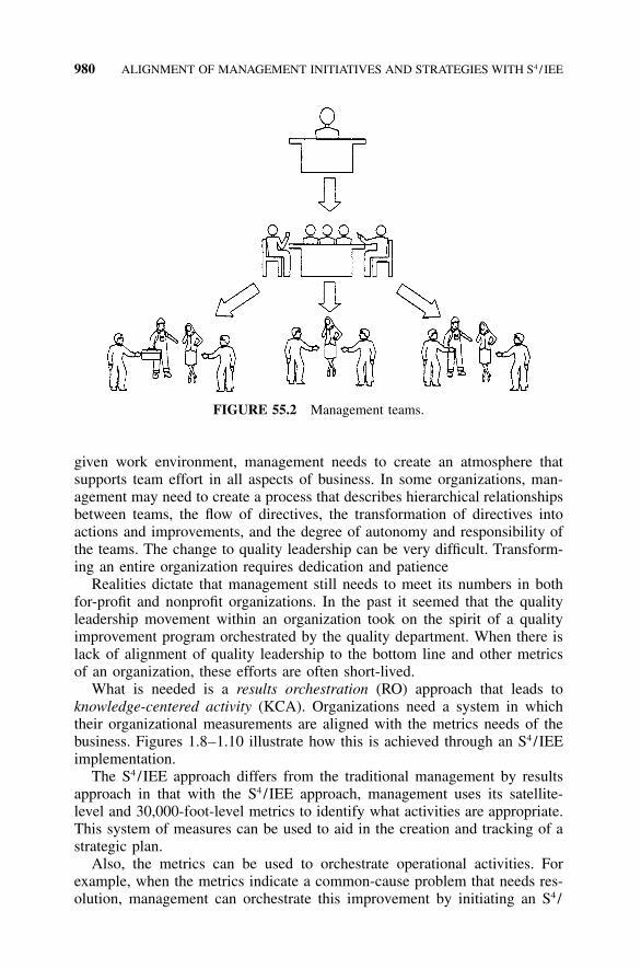
980 ALIGNMENT OF MANAGEMENT INITIATIVES AND STRATEGIES WITH S4 / IEE

FIGURE 55.2 Management teams.

given work environment, management needs to create an atmosphere thatsupports team effort in all aspects of business. In some organizations, man-agement may need to create a process that describes hierarchical relationshipsbetween teams, the flow of directives, the transformation of directives intoactions and improvements, and the degree of autonomy and responsibility ofthe teams. The change to quality leadership can be very difficult. Transform-ing an entire organization requires dedication and patience

Realities dictate that management still needs to meet its numbers in bothfor-profit and nonprofit organizations. In the past it seemed that the qualityleadership movement within an organization took on the spirit of a qualityimprovement program orchestrated by the quality department. When there islack of alignment of quality leadership to the bottom line and other metricsof an organization, these efforts are often short-lived.

What is needed is a results orchestration (RO) approach that leads toknowledge-centered activity (KCA). Organizations need a system in whichtheir organizational measurements are aligned with the metrics needs of thebusiness. Figures 1.8–1.10 illustrate how this is achieved through an S4/IEEimplementation.

The S4/IEE approach differs from the traditional management by resultsapproach in that with the S4/IEE approach, management uses its satellite-level and 30,000-foot-level metrics to identify what activities are appropriate.This system of measures can be used to aid in the creation and tracking of astrategic plan.

Also, the metrics can be used to orchestrate operational activities. Forexample, when the metrics indicate a common-cause problem that needs res-olution, management can orchestrate this improvement by initiating an S4/

QUALITY MANAGEMENT AND PLANNING 981

IEE project. This can lead to a different set of management activities. Insteadof criticizing someone about not meeting a numbers goal, management caninquire about the status of the project, perhaps offering helpful suggestionsfor how organizational barriers can be overcome to achieve a timelier projectcompletion.

With this RO approach we are pulling (using a lean term) for the creationof Six Sigma projects, rather than pushing (using a lean term) for projectcreation. This approach for implementing Six Sigma provides a continuingstimulus for the sustaining of Six Sigma within an organization, overcominga problem many companies have experienced with a traditional rollout of SixSigma.

The overall S4/IEE structure still allows for immediate problem contain-ment, when needed, using such tools as 8D, which is described in SectionA.5 in the Appendix. The advantage of using the overall S4/IEE structure isthat this approach encourages the creation of system improvements that yieldlong-lasting improvements. This activity can be viewed as fire prevention,which leads to a reduction in firefighting.

The RO approach helps reduce the problems often associated with tradi-tional management by results. With RO, management focuses not only oncreating activities that are in alignment with the needs of this business but onactively considering the capability/performance of the system before actionsare created. This refocus can help organizations avoid the problems oftenassociated with management by results: short-term thinking, misguided focus,internal conflict, fudging the figures, greater fear, and blindness to customerconcerns.

55.4 QUALITY MANAGEMENT AND PLANNING

Quality management is to achieve, monitor, control, and improve the func-tional, financial, and human relationship performance of the enterprise. Pro-cedures include mechanisms for allocating, organizing, and improvingresources. Quality management procedures should incorporate quantitativemetrics and other report card criteria that monitor and evaluate the perform-ance of the units and personnel of the organization (Juran and Godfrey 1999).

The purpose of traditional quality planning is the prevention of defects andvalidation of designs (Berger et al. 2002). Broad groupings for quality plan-ning are strategic plans, tactical plans, and operational plans. For the businessneeds, these groupings can have timelines of:

• Strategic quality plan: three to five years• Tactical quality plan: product development that aligns with strategic goals• Operational quality plan: short-term day-to-day needs; can include inter-

nal audits, inspection, equipment calibration, testing, and training courses

982 ALIGNMENT OF MANAGEMENT INITIATIVES AND STRATEGIES WITH S4 / IEE

Within strategic quality planning, organizational strengths, weaknesses, op-portunities, and threats (SWOT) should be assessed. With this strategic riskanalysis, organizations can leverage the strength of the organization, improveany weaknesses, exploit opportunities, and minimize the potential impact ofthreats. Strategic planning should then create the vision, broad goals, andobjectives for an organization. Through this risk assessment, organizationscan then optimize their system as a whole. Organizations should avoid theoptimization of subprocesses, which can be detrimental to the system as awhole. A strategic plan then leads to a tactical quality plan.

Within tactical quality planning, organizations create specific tasks thathave schedules, along with methods and responsibilities. These plans aresometimes called advanced quality planning (AQP) or advanced product qual-ity planning (APQP). The purpose of AQP is to ensure that a new product orservice will meet customer expectations. The process DFSS and productDFSS chapters of this book (see Chapters 46–49) describe a roadmap toaccomplish this.

With an S4/IEE implementation, strategic planning leads to doing the rightthings and tactical planning leads to doing the things right. In addition, thisapproach leads to a closed-loop assessment, resulting in effective knowledgemanagement of the overall system document objectives achieved and managelessons learned for the identification and creation of additional opportunities.Results from strategic planning can be tracked using a satellite-level metric,while tactical and operational results can be tracked at the 30,000-foot level.An S4/IEE strategy is useful not only to implement the plan through SixSigma projects but also to help create a strategic and tactical plan that isaligned with these metrics.

55.5 ISO 9000:2000

ISO 9000:2000 standards are based on eight quality management principles.ISO chose these principles because they can be used to improve organiza-tional performance and to achieve success (Praxiom 2002).

1. Focus on your customers. Organizations rely on customers. Therefore:• Organizations must understand customer needs.• Organizations must meet customer requirements.• Organizations must exceed customer expectations.

2. Provide leadership. Organizations rely on leaders. Therefore:• Leaders must establish a unity of purpose and set the direction the

organization should take.• Leaders must create an environment that encourages people to achieve

the organization’s objectives.

ISO 9000:2000 983

3. Involve your people. Organizations rely on people. Therefore:• Organizations must encourage the involvement of people at all levels.• Organizations must help people to develop and use their abilities.

4. Use a process approach. Organizations are more efficient and effectivewhen they use a process approach. Therefore:• Organizations must use a process approach to manage activities and

related resources.5. Take a system approach. Organizations are more efficient and effective

when they use a system approach. Therefore:• Organizations must identify interrelated processes and treat them as a

system.• Organizations must use a systems approach to manage their interre-

lated processes.6. Encourage continual improvement. Organizations are more efficient and

effective when they continually try to improve. Therefore:• Organizations must make a permanent commitment to continually im-

prove their overall performance.7. Get the facts before you decide. Organizations perform better when their

decisions are based on facts. Therefore:• Organizations must base decisions on the analysis of factual infor-

mation and data.8. Work with your suppliers. Organizations depend on their suppliers to

help them create value. Therefore:• Organizations must maintain a mutually beneficial relationship with

their suppliers.

An organization may ask what it should do to pass the new ISO 9000:2000audit. The problem with this attitude is that the organization will probablyspend a great deal of money trying to make things look good enough to pass,as opposed to focusing on what should be done to make changes to theiroverall system that are in alignment with these categories.

A better approach is to step back and look at each of the above categoriesas a whole. I think that most would agree that their company could greatlybenefit if they truly achieved all these items as part their ISO 9000:2000efforts.

The next question is how to achieve this so that the ISO 9000:2000 activ-ities actually become an investment. That is, we want to get a high ROI sincebusiness improvements through installing such a system should far exceedany administration costs. The S4/IEE infrastructure and roadmaps provide astructure for achieving each of these ISO 9000:2000 facets while at the sametime obtaining significant bottom-line and customer satisfaction benefits.

984 ALIGNMENT OF MANAGEMENT INITIATIVES AND STRATEGIES WITH S4 / IEE

55.6 MALCOLM BALDRIGE ASSESSMENT

The Malcolm Baldrige National Quality Award is given by the President ofthe United States to businesses—manufacturing and service, small andlarge—and education and health care organizations that apply and are judgedto be outstanding in seven areas: leadership, strategic planning, customer andmarket focus, information and analysis, human resource focus, process man-agement, and business results. (See www://www.quality.nist.gov.)

The award is named for Malcolm Baldrige, who served as Secretary ofCommerce from 1981 until his tragic death in a rodeo accident in 1987.Baldrige was credited with managerial excellence that contributed to long-term improvement in efficiency and effectiveness of government.

The U.S. Congress established the award program in 1987 to recognizeU.S. organizations for their achievements in quality and performance and toraise awareness about the importance of quality and performance excellenceas a competitive edge. The award is not given for specific products or services.Three awards may be given annually in each of these categories: manufac-turing, service, small business, and, starting in 1999, education and healthcare.

The following shows the 1000-point system breakdown for each category/item in the evaluation process. Many companies use these criteria as a Bald-rige assessment to evaluate their company without formally applying for theaward.

1. Leadership: 1201.1. Organizational leadership: 801.2. Public responsibility and citizenship: 40

2. Strategic planning: 852.1. Strategy development: 402.2. Strategy deployment: 45

3. Customer market focus: 853.1. Customer market knowledge: 403.2. Customer relationships and satisfaction: 45

4. Information and analysis: 904.1. Measurement and analysis of organizational performance: 504.2. Information management: 40

5. Human resource focus: 855.1. Work systems: 355.2. Employee education, training, and development: 255.3. Employee well-being and satisfaction: 25

SHINGO PRIZE 985

6. Process management: 856.1. Product and service processes: 456.2. Business processes: 256.3. Support processes: 15

7. Business results: 4507.1. Customer-focused results: 1257.2. Financial and market results: 1257.3. Human resource results: 807.4. Organizational effectiveness results: 120

The comments made at the end of the ISO 9000:2000 section are generallyapplicable here, too. I believe that companies that are truly aligned with theS4/IEE roadmap will fulfill these categories by default. The question thenbecomes whether they want to expend the extra effort to apply for this awardor another award that is similar in many states and cities.

55.7 SHINGO PRIZE

The Shingo Prize was established in 1988 to promote an awareness of leanmanufacturing concepts and to recognize companies that achieve world-classmanufacturing status. The prize is presented to manufacturing sites that haveachieved dramatic performance improvements.

The prize is named for Shigeo Shingo, a Japanese industrial engineer whodistinguished himself as one of the world’s leading experts in improving man-ufacturing processes. Dr. Shingo helped create and described in his books themany aspects of the manufacturing practices that comprise the renowned Toy-ota Production System (TPS).

The 1000-point ranking system is broken down into enablers, core opera-tions, results, and feedback. In the following point system, section I is theenablers’ category, sections II and III are core operations, section IV is results,and section V is feedback to all systems.

I. Leadership culture and infrastructure: 150A. Leadership: 75B. Empowerment: 75

II. Manufacturing strategies and system integration: 425A. Manufacturing vision and strategy: 50B. Innovations in market service and product: 50C. Partnering with suppliers/customers and environmental practices:

75D. World-class manufacturing operations and processes: 250

986 ALIGNMENT OF MANAGEMENT INITIATIVES AND STRATEGIES WITH S4 / IEE

III. Nonmanufacturing support functions: 125IV. Quality, cost, and delivery: 225

A. Quality and quality improvement: 75B. Cost and productivity improvement: 75C. Delivery and service improvement: 75

V. Customer satisfaction and profitability: 75

The comments made at the end of the ISO 9000:2000 and Malcolm Bald-rige sections are generally applicable here. Again, I believe that companiesthat are truly aligned with the S4/IEE roadmap will fulfill these categories bydefault.

55.8 GE WORK-OUT

In 1988 GE coined the term Work-Out. In 1992 and 1993 change accelerationprocess (CAP) was created to build on Work-Out. A major commitment oftime and talent is required for Work-Out since an event is a workshop lastinganywhere from one to three days and involving up to 80 people—or evenmore. Within Work-Out there are three stages: plan, conduct, implement (Ul-rich et al. 2002).

The plan stage has three steps. Step 1 is selecting a business problem,where the estimated impact and improvement opportunities are listed, alongwith a 12-week or shorter timeline for implementation. Step 2 is getting theorganization and a senior manager to sponsor the activities and be ready foropen improvement suggestions at a town meeting, making a decision on thespot of whether the suggestions will be implemented or not. Other activitiesfor the sponsor or delegate representative are organizing a design team to planthe Work-Out session and recruiting cross-functional teams of employees andmanagers who are close to the problem. Step 3 is planning the logistics ofthe Work-Out event.

The conduct stage typically has five sessions, which take place over oneto three days. This stage has five steps. Step 1 is an introduction whereparticipants are briefed on the business strategy, goals, rules (no sacred cows),and agenda for the Work-Out, along with the culminating town meeting event.Step 2 consists of brainstorming where multiple cross-functional teams eachbrainstorm on a different aspect of the problem, creating a top 10 list of ideasfor achieving the assigned goal. Step 3 is the gallery of ideas, where partic-ipants vote on the 3 or 4 ideas most worth implementing of the 10 team ideaspresented by teams. Step 4 is the generation of action plans for the selectedideas (each has a owner), along with the preparation of a presentation re-questing for approval from the sponsor at the town meeting. Step 5 is thetown meeting, where teams present their recommendations to the sponsor,who makes a yes/no decision after dialog with the team, participants, andaffected managers.

EXERCISES 987

Within the implementation stage there are five steps. Step 1 is the projectowners and teams implementing recommendations by the established goal,which is no longer than 12 weeks. Step 2 is the sponsors organizing a reviewprocess to track progress, assisting with any encountered problems. Step 3 isthe communication of the Work-Out progress along the way to the entireorganization. Step 4 is the assessing of accumulated impacts from all actionrecommendations. Step 5 is holding a closure work session where next stepsfor extended improvements are decided and communicated.

Ulrich et al. (2002) says, ‘‘In the later 1990s, Work-Out became the basisfor GE’s companywide push into Six Sigma Quality.’’ To reemphasize a pointthat was made earlier in this book, S4/IEE is not a quality initiative. S4/IEEdoes not require the definition of a defect, which is typically a requirementfor Six Sigma projects in GE and many other companies that are followinga similar model for implementing Six Sigma.

The methodology of Work-Out is very consistent with S4/IEE and couldbe used as an option for implementation of projects in some areas of thebusiness within an S4/IEE implementation. That is, we want to work on aproblem that is beneficial to the business, as identified within the S4/IEEsatellite-level/30,000-foot-level cascading measurement framework that isaligned with business goals and the strategic plan. A variety of methodologiesthat are beneficial to the overall system can be used to execute projects thatare pulled by the metrics of an S4/IEE framework. The structure of the S4/IEE DMAIC roadmap typically encompasses the tools of most strategies, withthe flexibility for quick execution when there is low-hanging fruit and com-plex analyses when wisdom-of-the-organization knowledge does not take usas far as we need to go.

55.9 S4/IEE ASSESSMENT

Management in recent years has encouraged the use of teams. Teams can bevery powerful, but process improvement teams sometime do not operate undera roadmap that leads them to quick success. A wisely applied S4/IEE imple-mentation process can be a very effective methodology that orchestrates andexpedites beneficial change.

Even organizations that have been trained in statistical process control tech-niques (SPC) are often guilty of reacting to the problems of the day as thoughthey were special-cause problems. Consider using control-charting techniquesat various levels within an organization. When this is done, the control chartcan serve a different purpose.

55.10 EXERCISES

1. List some compensation issues that need to be addressed in teamworkenvironments and with S4/IEE implementation leads and teams.

988 ALIGNMENT OF MANAGEMENT INITIATIVES AND STRATEGIES WITH S4 / IEE

2. Deming’s fourth point suggests working with a small number of suppliers.Describe what should be looked for when evaluating a supplier.

3. Describe positive and negative aspects of ranking employees.

989

APPENDIX A

SUPPLEMENTAL INFORMATION

This section includes information that was not included within the main bodyof this book since it might have disrupted the flow of dialogue.

A.1 S4/IEE PROJECT EXECUTION ROADMAP

Most organizations follow a define-measure-analyze-improve-control(DMAIC) roadmap when executing Six Sigma projects. The S4/IEE approachhas extensions to this roadmap, which are illustrated in Figures 1.12–1.14.Sections 46.1, 47.1, and 49.2 provide 21-step integration of the tools road-maps for implementing S4/IEE in manufacturing, development, and serviceorganizations. In this section Figures A.1–A.3 present a more generic high-level view of the S4/IEE roadmap. This roadmap can be referenced whenreading this book so insight is not lost into how individual tools can fit intothe big picture of project execution. The Glossary and List of Symbols in theback of this book can aid with the clarification of terms that are describedwithin the roadmap.

A.2 SIX SIGMA BENCHMARKING STUDY: BEST PRACTICESAND LESSONS LEARNED

The American Productivity and Quality Center (APQC, http://apqc.org) con-ducted a national Six Sigma benchmarking study in 2001, and I was selectedto be the Subject Matter Expert (SME) for the study. The study consisted ofpartner companies who agreed to share openly their Six Sigma experiences

990

Def

ine

pro

ject

with

ind

efin

ep

ha

se

Sta

rt1.

1

Est

imat

e

finan

ciha

rd/s

oft

al

bene

fits

(CO

PQ

or

CO

DN

D)

Sec

. 1.

13,

52.4

1.6

Doc

umen

t pro

blem

sta

tem

ent

and

esta

blis

h ch

arte

r with

cha

mpi

on.

Dem

onst

rate

pro

ject

alig

nmen

t to

busi

ness

sta

tellit

e-le

vel m

etric

s,

stra

tegi

es, a

nd o

vera

ll su

pply

cha

in

need

s (e

.g.,

PD

PC

)S

ec.

1.13

, 5.

17

1.2

Sel

ect

team

m

embe

rs w

ith

cham

pion

Sec

. 1.

13

1.3

Team

revi

ews

scop

e of

pr

ojec

t with

cham

pion

and

proc

ess

owne

ran

d ad

dres

ses

gap

betw

een

voic

e of

pro

cess

& V

OC

Sec

. 1.1

31.5

Con

duct

initi

alte

am m

eetin

g.C

reat

e S

IPO

Cdi

agra

m a

nd a

dd-

ress

oth

er d

efin

eph

ase

deliv

erab

les.

Cha

p. 4

, 51,

& 5

3S

ec. 1

.131.

4

Rec

ord

proj

ect

in p

roje

ct

trac

king

da

taba

seS

ec1.

13

1.7

FIG

UR

EA

.1a

S4/I

EE

proj

ect

exec

utio

nro

adm

ap,

defin

eph

ase.

991

Pla

n p

roje

ctan

dm

etri

csw

ithin

m

ea

sure

ph

ase

Bas

elin

e p

roje

ct w

ithin

me

asu

rep

ha

se

Con

side

r le

an to

ols

with

in

me

asu

rep

ha

se

Link

fina

ncia

l m

easu

res

to

prim

ary

proj

ect

met

rics

Sec

. 1.

14,

52.4

2.2

Cre

ate

seco

ndar

y S

ix

Sig

ma

met

rics

as n

eede

dC

hap.

9

2.3

Cre

ate

over

all

proj

ect

plan

and

G

antt

cha

rtS

ec.

5.18

and

52

.1, 5

2.22.

4

Com

pile

pr

ojec

t m

etric

s in

a

30,0

00-

foot

leve

lco

ntro

l cha

rt,

run

char

tC

hap.

5,

10,

34,

35, 3

63.1

Est

imat

e pr

oces

s ca

pabi

lity/

perfo

rman

cem

etric

s at

the

30,0

00

foot

leve

lC

hap.

11 3.

2

Rev

ise

estim

ate

for

CO

PQ

/CO

DN

DS

ec.

1.14

, 52

.4

3.7

Are

failu

res

cate

goric

al

3.4

No

Cre

ate

Par

eto

Cha

rtS

ec.

5.63.

5

Yes

App

rove

d to

pr

ocee

d to

nex

t ph

ase?

3.8

Red

o un

satis

fact

ory

step

s or

sto

p pr

ojec

t, a

dd t

o lis

t of

low

- pr

iorit

y pr

ojec

ts

3.9

No

Col

lect

voic

e o

f th

ecu

stom

erS

ec.

2.1,

3.1

,13

.2

2.1

For

con

tinuo

us

data

des

crib

e pr

oces

s ca

pabi

lity/

per-

form

ance

usin

g a

prob

abili

ty

and/

or d

ot p

lot

Cha

p. 8

, 11

Sec

. 3

.6, 5

.43.3

Lean

tool

s or

TOC

nee

ded

Ch &

45

ap. 4

4

4.1

No

Def

ine

valu

e-

ad

de

d,

no

n-

valu

e-a

dd

ed

and

wa

ste

Sec

. 44

.24.2

Yes

Impl

emen

t ag

reed

-to

"lo

w-h

angi

ng-

fruit"

lean

impr

ovem

ent

idea

s

4.5

Con

side

r pr

oces

s si

mul

atio

n a

nd/o

r TO

C

asse

ssm

ent

Cha

p. 4

4 &

45

4.4

diag

ram

and

proc

ess

anal

ysis

Tim

e-va

lue

Sec

. 44

. 2-44

.54.3

App

rove

d to

pr

ocee

d to

nex

t ph

ase?

2.5

Red

o un

satis

fact

ory

step

s or

sto

p pr

ojec

t, a

dd t

o lis

t of

low

-prio

rity

proj

ects

2.6

No

Yes

App

rove

d to

pr

ocee

d to

nex

t ph

ase?

4.6

Red

o un

satis

fact

ory

step

s or

sto

p pr

ojec

t, a

dd t

o lis

t of

low

-pr

iorit

y pr

ojec

ts

4.7

No

Yes

Yes

Res

cope

pro

ject

to

a la

rge

Par

eto

cate

gory

Sec

. 1.

133.6

No

Yes

FIG

UR

EA

.1b

S4/I

EE

proj

ect

exec

utio

nro

adm

ap,

mea

sure

phas

e(p

art

1).

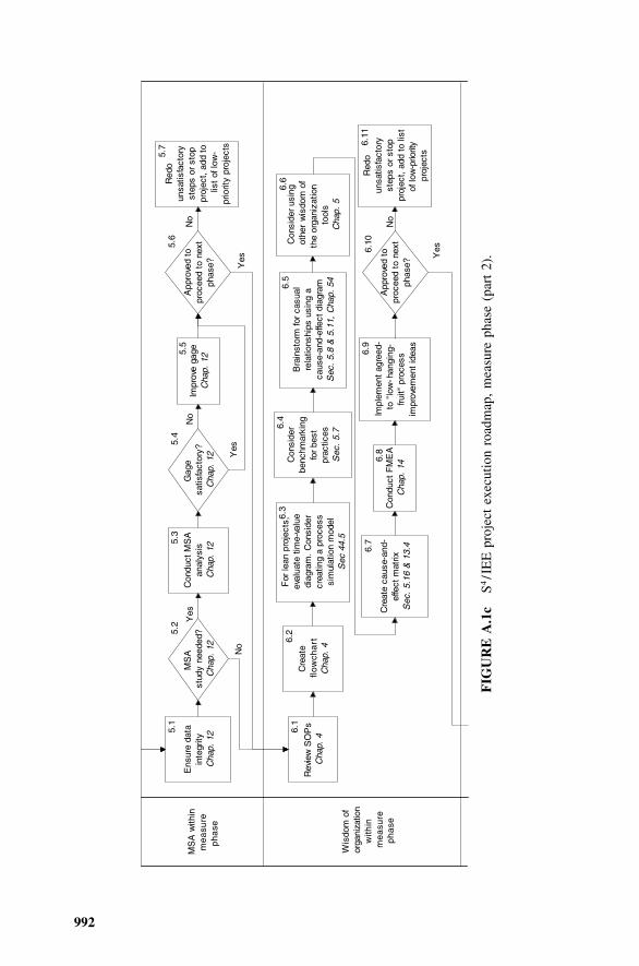
992

MS

A w

ithin

m

ea

sure

ph

ase

Wis

dom

of

orga

niza

tion

with

inm

ea

sure

ph

ase

Bra

inst

orm

for

casu

al

rela

tions

hips

usi

ng a

ca

use-

and-

effe

ct d

iagr

amS

ec.

5.8

& 5

.11,

Cha

p. 5

4

6.5

Cre

ate

caus

e-an

d-ef

fect

mat

rixS

ec.

5.16

& 1

3.46.7

Cre

ate

flow

cha

rtC

hap.

4

6.2

Con

duct

FM

EA

Cha

p. 1

46.8

MS

A

stud

y ne

eded

?C

hap.

12

5.2

Con

duct

MS

A

anal

ysis

Cha

p. 1

25.3

Yes

Gag

e sa

tisfa

ctor

y?C

hap.

12

5.4

No

Impr

ove

gage

Cha

p. 1

25.5

Con

side

r us

ing

othe

r w

isdo

m o

f th

e or

gani

zatio

nto

ols

Cha

p. 5

6.6

Impl

emen

t ag

reed

-to

"lo

w- h

angi

ng-

fruit"

pro

cess

im

prov

emen

t id

eas

6.9

Rev

iew

SO

Ps

Cha

p. 4

6.1

App

rove

d to

pr

ocee

d to

nex

t ph

ase?

5.6

Red

o un

satis

fact

ory

step

s or

sto

p pr

ojec

t, a

dd t

o lis

t of

low

-pr

iorit

y pr

ojec

ts

5.7

No

Ens

ure

data

in

tegr

ityC

hap.

125.

1

No

Yes

Yes

App

rove

d to

pr

ocee

d to

nex

t ph

ase?

6.10

Red

o un

satis

fact

ory

step

s or

sto

p pr

ojec

t, a

dd t

o lis

t of

low

-prio

rity

proj

ects

6.11

No

Yes

For

lean

pro

ject

s,

eval

uate

tim

e-va

lue

diag

ram

. C

onsi

der

crea

ting

a pr

oces

s si

mul

atio

n m

odel

Sec

44.

5

6.3

Con

side

r be

nchm

arki

ng

for

best

prac

tices

Sec

. 5.

76.4

FIG

UR

EA

.1c

S4/I

EE

proj

ect

exec

utio

nro

adm

ap,

mea

sure

phas

e(p

art

2).

993

Pas

sive

an

alys

isw

ithin

a

na

lyze

phas

e

Use

vis

ualiz

atio

n of

dat

a te

chni

ques

to

gai

n in

sigh

t to

pro

cess

es

Cha

p. 5

& 1

5S

ee F

igur

e A

2:

Vis

ualiz

atio

n of

dat

ase

lect

ion

tre

e

7.1

Con

duct

hy

poth

esis

tes

ts

Cha

p. 1

6, 1

9–26

See

Fig

ure

A3:

H

ypot

hesi

s te

stse

lect

ion

tre

e7.4

Use

vis

ualiz

atio

n of

da

ta t

echn

ique

s to

de

scrib

e st

atis

tical

fin

ding

s to

oth

ers

Cha

p. 5

& 1

5

7.5

Impl

emen

t ag

reed

-to

proc

ess

impr

ovem

ent

findi

ngs

7.6

Con

duct

infe

rent

ial

stat

istic

al t

ests

and

co

nfid

ence

inte

rval

ca

lcul

atio

ns o

n in

divi

dual

KP

OV

sC

hap.

16–

18

7.2

Con

duct

ap

prop

riate

sa

mpl

e si

ze

calc

ulat

ions

Cha

p. 1

7–207.

3

App

rove

d to

pr

ocee

d to

nex

t ph

ase?

7.7

Red

o un

satis

fact

ory

step

s or

sto

p pr

ojec

t, a

dd t

o lis

t of

low

-prio

rity

proj

ects

7.8

No

Yes

FIG

UR

EA

.1d

S4/I

EE

proj

ect

exec

utio

nro

adm

ap,

anal

yze

phas

e.Se

eFi

gure

sA

.2an

dA

.3fo

rfu

rthe

rdr

ill-d

owns

ofst

eps

7.1

and

7.4.

994

Pro

activ

e te

stin

gw

ithin

im

pro

vep

ha

se

Nee

d a

DO

E?

Cha

p. 2

7, 2

88.1

No

Yes

Ana

lyze

DO

EC

hap.

30-

328.6

Con

side

r co

nduc

ting

a re

spon

sesu

rfa

ce d

esi

gn

Cha

p. 3

38.8

Sel

ect

fact

ors

and

leve

ls o

f fa

ctor

sC

hap.

298.

3

Con

duct

a

conf

irmat

ion

expe

rimen

tC

hap.

16–

188.9

Set

up

exp

eri

me

nt

Cha

p. 3

0, 3

18.4

Con

duct

a fo

llow

-up

DO

E w

ith im

prov

ed

reso

lutio

n?C

hap.

30–

32

8.7 N

o

Con

duct

DO

EC

hap.

30,

318.5

Des

crib

e pu

rpos

e of

DO

E a

nd b

uild

te

st/a

naly

sis

stra

tegy

Cha

p. 2

9, 3

28.2

App

rove

d to

pr

ocee

d to

nex

t ph

ase?

8.10

Red

oun

satis

fact

ory

step

s or

sto

p pr

ojec

t, a

dd t

o lis

t of

low

-pr

iorit

ypr

ojec

ts

8.11

No

Yes

Yes

FIG

UR

EA

.1e

S4/I

EE

proj

ect

exec

utio

nro

adm

ap,

impr

ove

phas

e.

995

Oth

er

eva

lua

tion

s an

d co

ntr

ol

ph

ase

Con

side

r w

hat

coul

d be

don

e to

er

ror

proo

f pro

cess

an

d/or

impr

ove

wor

kflo

w u

sing

to

ols

such

as

lean

m

fg.

and

5S t

ools

Cha

p. 3

8, 4

4 9.2

Ver

ify p

roce

ss

impr

ovem

ents

hav

e be

en

mai

ntai

ned

seve

ral m

onth

s af

ter

proj

ect

com

plet

ion

Cha

p. 3

8

9.10

Doc

umen

t op

timum

pr

oces

s se

ttin

gs,

cond

ition

s, a

nd

KP

IVs

Cha

p. 3

89.1

Doc

umen

t co

ntro

l m

easu

res

Cha

p. 3

89.5

Impl

emen

t ap

prop

riate

50-

foot

-leve

l con

trol

char

t m

etric

s fo

r K

PIV

s C

hap.

5, 1

0, 3

4–379.

3C

onsi

der

usin

g ot

her

stat

istic

al t

estin

g an

d ev

alua

tion

tool

s su

ch a

s re

liabi

lity

test

ing

and

pass

/fail

func

tiona

l tes

ting

Cha

p. 3

9–42

9.4

Cre

ate

final

rep

ort

and

post

in o

rgan

izat

ion'

spr

ojec

t da

taba

seS

ec.

1.12

, C

hap.

389.9

Com

mun

icat

e an

d le

vera

ge p

roje

ct r

esul

ts

with

in o

ther

are

as o

f th

e bu

sine

ssC

hap.

38

9.8

End

9.11

Com

plet

e fin

anci

al

valid

atio

nS

ec.

1.13

, 52

.4

9.6

Turn

ove

rpr

ojec

t to

pr

oces

s ow

ner

Cha

p38

9.7

FIG

UR

EA

.1e

S4/I

EE

proj

ect

exec

utio

nro

adm

ap,

cont

rol

phas

e.

996

Vis

ualiz

atio

n of

dat

a: T

wo

or m

ore

varia

bles

Out

put:

Dis

cret

e

Out

put:

Con

tinuo

us

Inpu

t: D

iscr

ete

Inpu

t: C

ontin

uous

Inpu

t: D

iscr

ete

Par

eto

char

tC

hap.

5

Obs

ervi

ng

rela

tions

hip

of t

wo

varia

bles

Obs

ervi

ng

effe

ct o

f inp

ut

leve

ls

Obs

ervi

ng

hier

arch

ial

rela

tions

hip

of

two

or m

ore

varia

bles

Sca

tter

plo

tC

haps

. 5,

23

Mul

ti-va

ri ch

art

Cha

p. 1

5

Prio

ritiz

tion

type

s of

eve

nts

Box

plo

tD

ot p

lot

Mar

gina

l plo

tC

hap.

15

Obs

ervi

ng

hier

arch

ial

rela

tions

hip

of

two

or m

ore

varia

bles

Mul

ti-va

ri ch

art

Cha

p. 1

5

FIG

UR

EA

.2V

isua

lizat

ion

ofda

tase

lect

ion

tree

invo

lvin

gtw

oor

mor

eva

riab

les.

997

Hyp

othe

sis

test

invo

lvin

gtw

o or

mor

e va

riabl

es

Out

put:

Dis

cret

e

Out

put:

Con

tinuo

us

Inpu

t:C

ontin

uous

Inpu

t: D

iscr

ete

Inpu

t: C

ontin

uous

Inpu

t: D

iscr

ete

Logi

stic

re

gres

sion

Cha

p. 2

3

Chi

-squ

are

test

/ p-c

hart

asse

ssm

ent

Cha

p. 2

0

Reg

ress

ion

Cha

p. 2

3, 2

6

Var

ianc

e eq

ualit

y te

st

Var

ianc

e co

mpo

nent

sC

hap.

22

Mea

n eq

ualit

y te

st

Two

sam

ples

:t t

est

Cha

p. 1

9

Two-

sam

ple

com

paris

ons

(nor

mal

ly

dist

ribut

ed):

F te

stC

hap.

19

Non

orm

ally

dist

ribut

ed

com

paris

ons:

Le

vene

's te

stC

hap.

24

Mul

tiple

sa

mpl

e co

mpa

rison

s (n

orm

ally

di

strib

uted

): B

artle

tt's

test

Cha

p. 2

4

Two

or m

ore

sam

ples

: A

NO

VA

, A

NO

M,

com

paris

ions

Cha

p. 2

4, 2

5

Inpu

t:C

ontin

uous

/ D

iscr

ete

Ana

lysi

s us

ing

indi

cato

r va

riabl

esC

hap.

26m

ultip

le

FIG

UR

EA

.3H

ypot

hesi

ste

stse

lect

ion

tree

invo

lvin

gtw

oor

mor

eva

riab

les.

Thi

sch

art

does

not

incl

ude

nonp

aram

etri

cal

tern

ativ

es.

Com

para

tive

test

sof

mea

nsar

ety

pica

llyro

bust

tono

nnor

mal

ity.

998 APPENDIX A: SUPPLEMENTAL INFORMATION

during an on-site visit to their companies. During a kick-off meeting, thecompanies that financially sponsored the study selected six companies tostudy, called benchmarking partners. Deliverables from the study included atwo-day knowledge transfer session (KTS) and a final report. Below is mysummary of highlights from the study, which I presented at the KTS.

For all the partners studied, the initial thought of undertaking Six Sigmaapparently came from the CEO or another member of the leadership team. Ineach case, even though the desire to implement Six Sigma came from anexecutive, it appeared that the CEO delegated the details of implementationto a department or business unit once the decision was made. It seemed tome that this caused some problem with buy-in between functional silos ateach of the companies. Lessons learned from other successful implementa-tions showed that continued CEO involvement helped to overcome this issue.For example, Larry Bossidy, CEO of Allied Signal, thought it was importantfor him to appear personally at some black belt training sessions. This visibleexecutive support and involvement is important in gaining acceptance at alllevels.

Rollout

The initial rollout of Six Sigma in a company is essential. This rollout canfollow one of three tactics:

Tactic 1: Going it alone as a company with minimal direction.Tactic 2: Compiling a methodology of your own by observing methodol-

ogies from several Six Sigma providers who may or may not be usinga classical Six Sigma methodology (i.e., companyize Six Sigma).

Tactic 3: Select one Six Sigma provider and go with its strategy (changingit later if needed).

Using tactic 1 a company could create a Six Sigma program by readingsome books and perhaps putting together some of the training material thatit used previously to teach statistics and other methodologies. Companiestypically find that this approach takes a lot more effort than they initiallythought since they need to follow copyright laws. The first set of trainingmaterials invariably needs a lot of refinement; hence, students are typicallyunhappy with the first waves of training. The executive who chooses thisapproach will probably be scrambling to recover from initial startup problems.This can jeopardize the success of Six Sigma within the organization. Com-panies often initially think they are saving money using this approach; how-ever, they later typically realize that the largest investment in Six Sigma ispeople’s time when they implement Six Sigma. Hence, they need to investresources for doing the best possible training so that the utilization of people’stime is maximized. None of the benchmarking partner companies in the studyfollowed this route.

SIX SIGMA BENCHMARKING STUDY 999

When companies use tactic 2, they put their spin on Six Sigma by con-sulting with several companies who have different approaches and then build-ing their own approach to Six Sigma. I refer to this as companyizing SixSigma. This approach again involves more effort than originally anticipated,since they need to not only create training material but also invent an effectiveimplementation strategy, which can take many years of trial and error. Also,details of how the strategy is put together are typically a function of the peoplewho are to invent the strategy. For example, strong TQM people have TQMas the driver for their Six Sigma strategy and strong lean manufacturing peo-ple have lean as the driver. Later these companies realize that it is better tobuild upon the experiences of others and not reinvent the wheel. Two of thesix benchmarking partners chose this route.

When companies use tactic 3 they select an experienced Six Sigma con-sulting firm and follow the basic strategy of this company. One company saidit traditionally has tried to redo every initiative it has tried in the past. It saidthat these initiatives failed because of this and the company was not going toreinvent Six Sigma. However, I noticed with this approach that the decisionof which Six Sigma provider to use is made at the executive level, where notmuch investigation is made into the details of what the Six Sigma provider’simplementation strategy or project execution roadmap looks like. These or-ganizations may find that the executive presentation comes off well but thereis not as much substance under these presentations. Hence, the organizationwill later look to other providers for course material. These companies laterrealize they should have been concerned about the practical details of imple-menting before choosing a Six Sigma provider. Four of the six benchmarkingpartners used this tactic.

Black Belts

The practitioner who leads Six Sigma project teams is the black belt. I listthree essential considerations from the benchmarking study below:

Consideration 1: Selection of black belts.Consideration 2: Some companies had part-time black belts, while others

had full-time black belts.Consideration 3: Some companies had four-weeks of training or more over

four months or longer, while other companies had a shorter duration.

With consideration 1 companies need to create a reliable process for theselection of black belts. Effective black belts are critical to the success of SixSigma in an organization. In the study I saw a variety of selection methods,from a formal application and a screening process to management ‘‘tappingsome key people on the shoulder.’’ Characteristics to consider in the selectionprocess are: fire in belly; good at soft skills; ability to manage projects; abilityto multi-task; ability to see the big picture; basic analytical skills.

1000 APPENDIX A: SUPPLEMENTAL INFORMATION

For consideration 2 it was noted that full-time black belts typically aremore successful at completing projects. Part-time black belts are often tornbetween their responsibility to complete Six Sigma projects and their day-to-day work. With the downsizing of companies, people are stretched to thelimit. When faced with choices between day-to-day activities/crises and SixSigma projects, the short-term tasks usually win.

In consideration 3 it is my conclusion that less than four weeks for blackbelt training is not sufficient to give insight into the best use of all statisticaltools. Organizations often state that black belts are not using many of the SixSigma techniques previously taught; hence, they are saving money by notteaching the concepts. Problems can result from this approach because SixSigma techniques such as analysis of variance (ANOVA) and regression anal-ysis are often not conducted properly with less than four weeks of training.A better approach is to deliver the full black belt training content and havemore green belts working on projects with coaching from fully trained blackbelts.

Duration of Training

Training duration for black belts took two forms:

Tactic 1: Less than four weeks of trainingTactic 2: Four weeks of training or more

With tactic 1 less than four weeks of training time is not enough for moststudents to acquire an in-depth understanding of the wise implementation ofstatistical methodologies. With only a superficial understanding of statisticalmethodologies, black belts can make decisions that are incorrect and costly.Proponents of reduced training state that many projects do not need a lot ofstatistical analyses. I will not disagree that there is much low-hanging fruitthat requires little sophistication in statistical analysis. In my opinion, projectsof this type can be executed using green belts, who have only two-weeks oftraining and know when to ask black belts for assistance when more sophis-ticated statistical techniques are needed.

With tactic 2 four weeks of training delivered over four months give sub-stance to the methodologies. I believe that it is important to teach integrationwith other methods like lean manufacturing, facilitation skills, and projectmanagement techniques in the training. Also, the attendee will present theirproject results to the class three times during weeks 2, 3, and 4.

Company Integration

All benchmarking partners studied wanted to integrate Six Sigma into theircorporate culture and make it the way the work gets done. Two tactics usedto accomplish this are:

SIX SIGMA BENCHMARKING STUDY 1001

Tactic 1: Full-time dedicated black belts are rotated back into their previousroles after a two- to three-year assignment. The thought with this strat-egy is that these people will embrace and understand the Six Sigmamethods and will later be promoted to more influential positions withinthe company, taking this knowledge with them.

Tactic 2: Part-time black belts learn how to apply the techniques to theirjob through projects. The implication with this strategy is that Six Sigmatechniques will then become a way of life since many will have beenexposed to the techniques first-hand.

With tactic 1 organizations can select projects that are tied across the func-tions of their business. Full-time black belts gain insight into what can bedone differently within the system. These people can be very beneficial tothe organization when they are rotated back into a higher-level non-full-timeblack belt position within the company. They could then perhaps do a betterjob of asking the right questions of those who work with them as employeesor team members. Resulting from this should be less day-to-day firefightingand more constructing improvements.

With tactic 2 black belts learn how to apply techniques to their job throughprojects. However, a project that improves a particular job assignment is notnecessarily the best project for the company as a whole. These non-cross-functional projects can optimize the subsystem but degrade the overall system,which would be detrimental to the company as a whole. When cross-functional projects are identified using this tactic, it can be difficult to get thededicated resources and support for the bridging of functional silos within thecompany.

Roadmap

All benchmarking partners had an overall roadmap for executing Six Sigmaprojects. Two tactics to accomplish this are:

Tactic 1: Apply a define-measure-analyze-improve-control (DMAIC) road-map.

Tactic 2: Develop a unique strategy for the company.

With tactic 1 organizations build upon the methodologies others have used.However, care needs to be exercised with the applied metrics. For example,sigma quality level units can be misleading and process capability indices canbe misinterpreted, as was elaborated in this book. When implementing SixSigma it is important to use the best metric for the situation, add a controlmechanism to maintain benefits, and leverage projects to other areas of thebusiness.

1002 APPENDIX A: SUPPLEMENTAL INFORMATION

With tactic 2 organizations do not get the benefits of lessons learned fromother organizations. Not using the same roadmap as their customers or sup-pliers can cause confusion with communications and terminology.

Project Benefit Analysis

All benchmarking partners had finance involved with the costing of projectbenefits. The tactics for costing were:

Tactic 1: Report the monetary benefit from projects as it impacts the com-pany’s financial statement, often referred to as hard savings.

Tactic 2: Report both hard savings and soft savings as separate entities.

With tactic 1 reported savings taken from future budgets could not bedisputed when the amounts are derived through black belts working with thefinancial department. Financial benefits could be reported annually or rolledinto future years. When focus is given only to hard savings, projects thatimprove customer satisfaction are often not given much emphasis, which canresult in a bottom-line impact that is hard to quantify. Also, cost-avoidanceprojects are not typically considered, which indirectly can have a major im-pact to the bottom line, but is hard sometimes to quantify.

With tactic 2 both hard savings and soft savings are considered with theinput of a financial person. With this approach both customer satisfaction andcost avoidance issues are addressed.

A.3 CHOOSING A SIX SIGMA PROVIDER

All Six Sigma implementations are not created equal. I suggest that you askthe following questions of groups that you are considering using to help starta Six Sigma implementation within your organization:

Strategy and Implementation

• Describe your Six Sigma implementation strategy and flow. It is impor-tant to have a strategy that makes sense, where there is no playing gameswith the numbers. The strategy should have a wise integration of SixSigma measurements, Six Sigma tools, and lean tools.

• Describe the strategy you would use to measure and then execute threeexample projects that we have. There should be a good strategy for cre-ating metrics that tracks the three described projects over time. The de-scribed strategy should follow a roadmap that includes when the variousSix Sigma tools should be applied.

CHOOSING A SIX SIGMA PROVIDER 1003

• What book do you use that follows the material taught within the course?Having a book that can be referenced for project execution details duringand after the workshop sessions is very beneficial. Participants need abook where they can obtain further explanation during the workshop andcan review a concept at a later date. Also, the book should have examplesthat can be used to explain the implementation strategies to others thathave not taken a Six Sigma course (e.g., peers, suppliers, and customers).

• What is the basic format of your Six Sigma course for executive andchampion training? The training should have substance, not just successstories. Training needs to illustrate how executives and champions willbenefit from Six Sigma projects, along with how Six Sigma will helpthem achieve their measurement goals.

• How do you address business and service processes? An execution road-map that has good integration with lean methods is important for businessprocesses. A Six Sigma execution strategy should not force the creationof metrics and specifications that make no sense (e.g., the creation ofspecification limits so that Cp, Cpk, Pp, and Ppk can be calculated).

• How do you address defect definition for a Six Sigma project? I thinkthat the policy of requiring a defect definition for all projects can be verycostly and can often lead to the wrong activities within a Six Sigmaimplementation. See Section 1.19 for more explanation.

• How do your clients use the sigma quality level metric? I think that thismetric can lead to the wrong activities. See Section 1.18 for more ex-planation.

• How do you select Six Sigma projects? I think that it is most beneficialto view the business as a process and have Six Sigma metrics that providefeedback to how well this process is doing. A Six Sigma infrastructureprocess should be created that aligns Six Sigma project selections withthe needs of the business. It is important that the Six Sigma infrastructurepull for the creation of projects (using a lean term) according to the needsof the business, as opposed to pushing projects (using a lean term) intothe organization, i.e., executing projects that may or may not be beneficialto the business.

Course Material

• What topics do you cover in your black belt workshops? It is importantto cover both statistical and nonstatistical topics in the workshop so thatstudents understand how to apply the information to their projects. Thereneeds to be a good project execution roadmap that guides the practitionerto the selection of the right tool and approach for both manufacturingand transactional applications.

1004 APPENDIX A: SUPPLEMENTAL INFORMATION

• How frequently do your past students reference the workshop handoutmaterial for the how-to’s of project execution? Students need a good setof workshop material that is useful for later reference.

• How do you address the licensing of your instructional material? At somepoint in time companies need to be able to use the material on their ownthrough the licensing of the training material.

• What strategy do you use so that others can teach your material? Sinceblack belt training is four weeks long, I have found that there needs tobe enough explanation in the slides that instructors who are knowledge-able of the topics can teach the material without difficulty.

Computers and Software

• Are attendees required to have computers? This is essential for black beltand green belt training.

• What software do you use? I suggest using a general-purpose statisticalsoftware package such as Minitab.

• Does the software that you use in your training offer other functionsbesides those taught during the workshop? I think that it is important tohave software that offers more sophisticated techniques than those taughtduring the workshop. This offers the flexibility for workshop attendeesto use more sophisticated techniques later.

Exercises

• Describe the type and frequency of exercises (i.e., manual, computersoftware, and other hands-on exercises) within the black belt workshop.There should be many meaningful hands-on exercises that align with thethe application of the techniques to real situations and their projects.

• How do you address application of the techniques to real-world situa-tions? I have found that it is important to have exercises where teamswork the application of the concepts to both real and generic projects.

• How do you address adult learning needs? The course material needs tohave many team and individual exercises.

Experience of Course Developer(s)/Trainer(s)• What is the experience of the person(s) responsible for developing the

courseware? It is important that the developers of the course materialalso teach the course for the companies.

• What companies have you helped utilize Six Sigma tools and method-ologies? I suggest asking many of the above questions to references thatare provided.

AGENDA FOR MANAGEMENT AND EMPLOYEE S4 / IEE TRAINING 1005

References

• What have others said about your courses and consulting in the appli-cation of Six Sigma tools? I suggest looking between the lines of feed-back quotes to better understand how the company addresses the aboveissues.

A.4 AGENDA FOR MANAGEMENT AND EMPLOYEE S4/IEETRAINING

A one-day S4/IEE executive or leadership training program could use selectedtopics from Chapters 1 to 3, where exercises are created so executives seehow the techniques are directly applicable to them and their organization.

A three-day S4/IEE champion training course should give an overview ofthe topics and strategies covered in the four-week black belt training that isdescribed below. This training is to help champions ask the right question oftheir black belts, as opposed to how to use a statistical computer program toconduct the analysis. Emphasis should also be given to the management andselection of projects and the process of black belt candidate selection. Some-one from finance should be involved with these sessions.

A four-week training program for black belts focusing on the four topicsof define, measure, analyze, improve, and control is described below. In afour-week S4/IEE black belt workshop it is difficult to tailor the material sothat each of the MAIC themes from DMAIC fits neatly into one week. Thematerial from weeks 1 and 2 may flow over into later weeks. Topics such asreliability and pass/fail functional testing are optional. The program could bereduced to two or three weeks if measurement systems analysis, DOE, andsome other tools are not considered applicable to the processes of attendees(e.g., some transactional processes).

Week 1 (S4/IEE define and measure): Chapters 1–14Week 2 (S4/IEE analyze): Chapters 15–26Week 3 (S4/IEE improve): Chapters 27–33Week 4 (S4/IEE control): Chapters 34–43Topics covered within various weeks: Chapters 44–54

The Six Sigma black belt public and in-house training that we conduct atSmarter Solutions, Inc. does not include all the topics within this book. Duringworkshops we reference sections of this book for further reading when ap-propriate. We believe that it is important that students have a reference thatthey can later use to help them address various situations that they encounter.Over the years we have developed modules that build upon each other withmany hands-on application exercises that make learning fun. Our training is

1006 APPENDIX A: SUPPLEMENTAL INFORMATION

very sensitive to the capacity of the student’s comprehension. Also, our pro-ject execution roadmap has more detailed drill-down steps than those listedin Section A.1.

During week 1 of a two-week green belt training, many of the topicscovered during week 1 of black belt training are included. During week 2,however, I believe that it is more important to describe lean techniques andwhen to apply specific statistical techniques as opposed to how to apply eachtechnique. I have seen many of the more advanced statistical tools used in-correctly because of lack of training and hands-on time with the tools.

Three-day yellow belt training gives an overview of Six Sigma and themore commonly used metrics and measurement strategies within S4/IEE. Ithink that lean techniques should be an integral part of this training sinceworkflow improvement activities are needed at all levels within organizations.

A two-week master black belt training session can involve the expansionof topics within this book that are not covered within the black belt training,along with other related topics not included in the normal black belt training.The training of master black belts can involve the critique of their training ofblack belts.

A.5 8D (8 DISCIPLINES)

The 8D process strives for the definition and understanding of a problem.Within the 8D methodology, one initially asks why a process is operatingbeyond its target range. 8D then provides a mechanism for the identificationof root cause and implementation of an appropriate corrective action. The 8Dprocess can also lead to a system change such that the problem and similarproblems are prevented from recurring (Ford 1998).

The criteria for 8D consideration: The symptom has been defined andquantified. The customer(s) of the 8D who experienced the symptom(s), alongwith affected parties when appropriate, have been identified. A performancegap was demonstrated by measurements that were taken to quantify the symp-tom(s) and/or the symptoms of the priority (severity, urgency, or growth)warrant initiation of 8D. The cause is not known. There is a commitment bymanagement to dedicating the necessary resources to fix the problem at theroot-cause level and prevent recurrence. The complexity of the symptom ex-ceeds the ability of one person to resolve the problem.

The 8D process steps:

D0: Prepare for the 8D processD1: Establish the teamD2: Describe the problem

8D (8 DISCIPLINES) 1007

D3: Develop the interim containment actionD4: Define and verify root cause and escape pointD5: Choose and verify permanent corrective actions (PCAs)D6: Implement and validate permanent corrective actions (PCAs)D7: Prevent recurrenceD8: Recognize team and individual contributions

D0 (Prepare for the 8D Process)

The purpose of D0 is to evaluate the need for the 8D process. 8D addressesquantifiable events or effects experienced by customers that may indicate theexistence of one or more problems. An emergency response action (ERA) isto be provided if necessary to protect the customer and initiate the 8D pro-cedures.

The tools suggested for use within D0 are a trend or run chart, a Paretochart, and a Paynter chart. The trend chart shows performance over time,while the Pareto chart show the rankings based on frequency. Paynter chartsare to show the effectiveness of corrective actions (i.e., before and after actiontaken).

In a Paynter chart, increments of time (e.g., months) are on the horizontalaxis. In the vertical axis there are customer problem classifications. At theintersection of the horizontal and vertical axes the number of problem clas-sification occurrences for the time period is noted. Any emergency responseaction (ERA), interim containment action (ICA), or permanent corrective ac-tion (PCA) that occurs during a time period is also noted at the intersection.Year-to-date totals for each problem type are summarized at the right.

D0 process: The input to D0 is awareness of the symptom. The outputfrom D0 is 8D is initiated.

D0 steps: Define/quantify symptom identifying customer and affected par-ties. If an emergency response action (ERA) is required, select/validateERA and then develop action plan implementing/validating ERA.Gather and review available data. Initiate the 8D process if the proposed8D meet the application criteria and do not duplicate an existing 8D.

D1 (Establish the Team)

The purpose of D1 is to establish a small team. Team members are to haveknowledge of the process/product, time allotment, authority, and requiredtechnical discipline skills to solve problems and implement corrective actions.Teams need someone to champion the work and another person to lead theteam. Within D1 the team-building process is initiated.

1008 APPENDIX A: SUPPLEMENTAL INFORMATION

D1 process input/output: The input is an 8D initiation from D0. The outputis that the team is established.

D1 steps: Identify champion. Identify team leader. Determine skills andknowledge team will need. Select team members. Establish team goalsand membership roles. Establish operating procedures and working re-lationships of the team.

D2 (Describe the Problem)

The purpose of D2 is to describe the problem in quantifiable terms, whetherit is internal or external. The function of D2 is to identify the object anddefect and act as a database for the problem description or problem statement.

The first step in developing a problem statement is to address what (i.e.,defect) is wrong with what (i.e., object). The second step is to ask, ‘‘Why isthat happening to that object?’’ For this step use the repeated whys (or 5-whys) technique, where the question is asked over and over again until thequestion can no longer be answered with certainty. The problem statement isthe last object and defect with an unknown cause.

The problem description defines problem boundaries in terms of what it isand what is not but could be. Within D2 a problem-solving worksheet iscreated for the problem statement. ‘‘Is’’ and ‘‘is not’’ (Is/Is not) statementsare made for each of the categories ‘‘what’’ (contains categories object anddefect), ‘‘where,’’ ‘‘when,’’ and ‘‘how big.’’

Tools used within D2 are process flowcharting, cause-and-effect diagram,check sheets, SPC data, sampling plans, run charts, scatter diagrams, internal/external customer surveys/interviews. Supplemental tools include FMEA,control charts, histogram, process capabilities, and scatter diagram.

D2 process input/output: The input to this process step is that a team isestablished from D1. The output is a problem description.

D2 steps: Review available data. If the symptom can be subdivided, go toD0 for each symptom. State symptom as an object and defect. If thecause is not known, document the problem statement. Initiate develop-ment of problem description (‘‘is’’ and ‘‘is not’’). Identify process flow.Identify additional data requirements. Collect and analyze additionaldata. When the problem describes something that has changed or a newsituation, consider supplemental tools such as DOE. Review problemdescription with customer and affected parties.

D3 (Develop the Interim Containment Action)

The purpose of D3 is the definition, verification, and implementation of in-terim containment action (ICA). The ICA is to isolate the problem from any

8D (8 DISCIPLINES) 1009

internal/external customer until the implementation of permanent correctiveactions (PCA). The effectiveness of containment action is validated in D3.

The tools suggested for use with D3 are the PDSA management cycle andPaynter chart. The PDSA includes an action plan sheet to address action planelements, including the activity (what), who, and due date.

D3 process input/output: The input is the problem description from D2.The output is established ICAs.

D3 steps: If an ICA is required, evaluate ERA. Identify and choose thebest ICA and verify. Develop action plan, implement and validate ICA.If the ICA passes validation, continue monitoring the effectiveness ofthe ICA.

D4 (Define and Verify Root Cause and Escape Point)

The first purpose of D4 is the isolation and verification of the root cause.This is accomplished through the testing of root cause theories against theproblem description and test data. The second purpose of D4 is the isolationand verification of the escape point in the process, where the effect of theroot cause was not detected and contained.

Within D4 data are used to determine if ‘‘something changed’’ or the pro-cess has ‘‘never been there’’ (S4/IEE 30,000-foot-level control charts andprocess capability/performance metric assessments are useful to address theseissues). If something changed, identification is made as to whether the changewas gradual or abrupt.

Within D4 a cause-and-effect diagram describes how an effect may occur.A theory based on available data describes the most likely cause for theproblem description. A verified cause that accounts for the problem is theroot cause, which is verified passively and actively by making the problemcome and go.

The tools suggested for use within D4 are cause-and-effect diagram andDOE.

D4 process input/output: The input is the ICA implemented from D3. Afteracknowledgment of root causes, the output is the verification of theescape point and possible need for an improved control system.

D4 steps: Identify differences, changes, and develop theories. Test theoriesagainst problem description. If the theory explains all the know data andthe problem can be made to come and go away, acknowledge the rootcause. If there is more than one root cause, consider creating a separate8D for each root cause or evaluation using alternative methods such asDOE (may cause the suspension of further 8D process activity) for thepurpose of later acknowledging root causes. Review process flowcharts

1010 APPENDIX A: SUPPLEMENTAL INFORMATION

and identify control points for root causes(s). If a control system doesnot exist to detect the problem, acknowledge the control system is notcapable and needs improvement. If a control system is capable but didnot detect problem, acknowledge the control point as the verified escapepoint.

D5 [Choose and Verify Permanent Corrective Actions (PCAs) for RootCause and Escape Point]

The purpose of D5 is to select the best permanent corrective action thatremoves the root cause and addresses escape point. Verify that decisions aresuccessful upon implementation and do not cause undesirable effects.

The tools suggested for use within D5 are FMEA, cause-and-effect dia-gram, and design verification plan/report. Other tools to be considered areDOE, process flowcharting, process capability/performance metric analysis,branstorming, benchmarking, force-field analysis, Weibull analysis, and robustDOE methods.

D5 process input/output: The input is either a verified root cause or verifiedescape point/acknowledged need for improved control system. Outputis either verified for PCA root cause or verified for PCA escape point.

D5 steps: Establish decision criteria. Identify possible actions. Choose thePCA that is best. If testing verifies the PCA, either reevaluate ICA/PCAfor escape point or identify possible actions that improve ICA. If cham-pion does not concur in PCA selection, return to step 1 of D5.

D6 [Implement and Validate Permanent Corrective Actions (PCA)]

The purpose of D6 is to plan and implement PCAs, remove ICA, and monitorresults long-term.

D6 supplemental tools and techniques include PERT chart, Gantt chart,process flowchart, creativity, FMEA, QFD, DFM, DFA, IS/IS/NOT, SPC,Paynter chart, customer surveys, and process capability/performance metricreports.

D6 process input/output: The input is either a verified PCA for root causeor verified escape point. The output is implemented PCAs and validationdata.

D6 steps: Develop action plan for PCA. Implement PCA plan. RemoveICA and evaluate PCA for escape point when a new root cause wasdetermined. Perform validation. Confirm with customer that the symp-tom has been eliminated.

ASQ BLACK BELT CERTIFICATION TEST 1011

D7 (Prevent Recurrence)

The purpose and function of D7 is to modify the necessary systems to preventrecurrence of this problem and similar ones. This modification can includechanging policies, practices, and procedures.

D7 supplemental tools and techniques include repeated whys, benchmark-ing, creativity, process flowcharting, FMEA, QFD, subject matter expert(SME) inteviews, VOC, and force-field analysis.

D7 process input/output: The input is implemented PCAs and validationdata. The output is preventative actions for present/similar problems andsystematic preventive recommendations. Technical lessons learned areto be inputted to organization’s lessons learned system.

D7 steps: Review the history of the problem. Analyze how the problemoccurred and then escaped. Identify the parties that were affected andthe opportunities for problems that are similar to occur and escape.Identify the policies, practices, and procedures of the system that al-lowed the problem to occur and escape to the customer. Analyze howthere can be similar problems to address. Identify and then choose pre-ventive actions. Verify the effectiveness of preventive actions. Developan action plan that the champion agrees to. Implement the preventiveactions and validate. Develop and present systematic preventive rec-ommendations to owner.

D8 (Recognize Team and Individual Contributions)

The purpose of D8 is to complete the team experience and celebrate, recog-nizing both team and individual contributions.

D8 process input/output: Inputs are preventive actions for present problem,preventive actions for similar problems, and systemic preventive rec-ommendations. Output 8D is completed and there was closure for team.

D8 steps: Select key documents and provide for their retention. Reviewthe process used by the team and document lessons learned. Collectivelyrecognize the efforts of the entire team in solving the problem. Mutuallyrecognize all contributions made to the problem-solving process. Cele-brate the task completion of the team.

A.6 ASQ BLACK BELT CERTIFICATION TEST

ASQ offers a Six Sigma black belt certification test. The test categories (ASQ2002) and where these topics are generally covered in this book are:

1012 APPENDIX A: SUPPLEMENTAL INFORMATION

I. Enterprisewide DeploymentA. Enterprise view: Chapter 1B. Leadership: Chapter 1C. Organizational goals and objectives: Chapter 1D. History or organizational improvement/foundations of Six

Sigma: Chapter 55II. Business Process Management

A. Process, versus functional view: Chapters 1, 4, and 52B. Voice of the customer: Chapters 2 and 3C. Business results: Chapters 5, 9, 10, 11, and 52

III. Project ManagementA. Project charter and plan: Chapters 1 and 52B. Team leadership: Chapters 1 and 53C. Team dynamics and performance: Chapters 5 and 53D. Change agent: Chapter 51E. Management and planning tools: Chapter 5

IV. Six Sigma Improvement Methodology and Tools—DefineA. Project scope: Chapter 1B. Metrics: Chapters 1, 2, 5, 9, 10, and 11C. Problem statement: Chapter 1

V. Six Sigma Improvement Methodology and Tools—MeasureA. Process analysis and documentation: Chapters 4, 5, 13, and 14B. Probability and statistics: Chapters 3, 6, and 16C. Collecting and summarizing data: Chapters 5, 12, and 15D. Properties and applications of probability distributions: Chapters

7 and 8E. Measurement systems: Chapter 12F. Analyzing process capability: Chapter 11

VI. Six Sigma Improvement Methodology and Tools—AnalyzeA. Exploratory data analysis: Chapters 15, 22, 23, and 24B. Hypothesis testing: Chapters 16–26

VII. Six Sigma Improvement Methodology and Tools—ImproveA. Design of experiments (DOE): Chapters 27–32B. Response surface methodology: Chapter 33

VIII. Six Sigma improvement methodology and tools—ControlA. Statistical process control (SPC): Chapters 10 and 37B. Advanced statistical process control: Chapters 34–36C. Lean tools for control: Chapter 44D. Measurement system reanalysis: Chapter 12

IX. Lean EnterpriseA. Lean concepts: Chapters 44 and 45B. Lean tools: Chapters 38 and 44C. Total productive maintenance: Chapter 44

ASQ BLACK BELT CERTIFICATION TEST 1013

X. Design for Six Sigma (DFSS)A. Quality function deployment: Chapter 13B. Robust design and process: Chapters 32, 48, 49, and 50C. Failure mode and effects analysis (FMEA): Chapter 14D. Design for X (DFX): Chapter 48E. Special design tools: Chapter 48

I have made every attempt to cover all topics in the body of knowledge (BOK)for the black belt certification test. To help students locate information effi-ciently during the open-book examination, keywords taken from the BOK arelisted in the index.

1014

APPENDIX B

EQUATIONS FOR THEDISTRIBUTIONS

This appendix contains equations associated with many of the distributionsdiscussed in this book. In this book, t replaces x when the independent vari-able considered is time. In the following equations, ƒ(x) is used to denote thePDF, F(x) is used to denote the CDF, and the P(X � x) format is used todenote probability. The relationship of F(x) and P(x) to ƒ(x) is

x

F(x) � P(X � x) � � ƒ(x) dx�x

where the capital letter X denotes the distribution, which can be called arandom variable.

B.1 NORMAL DISTRIBUTION

The normal PDF is

21 (x � �)ƒ(x) � exp � � � � x � � �� �22���2�

where � � mean and � � standard deviation. The CDF is

x 21 (x � �)F(x) � � exp � dx� �2

�� 2���2�

HYPERGEOMETRIC DISTRIBUTION 1015

B.2 BINOMIAL DISTRIBUTION

The probability of exactly x defects in n binomial trials with probability ofdefect equal to p is

n x n�xP(X � x) � p (1 � p) x � 0, 1, 2, . . . , n� �x

where

n!n�� �x x!(n � x)!

The mean (�) and standard deviation (�) of the distribution are

� � np

� � �np(1 � p)

The probability of observing a or fewer defects is

a

P(X � a) � P(X � x)�x�0

B.3 HYPERGEOMETRIC DISTRIBUTION

The probability of observing exactly x defects when n items are sampledwithout replacement from a population of N items containing D defects isgiven by the hypergeometric distribution

D N � D� �� �x n � xP(X � x) � x � 0, 1, 2, . . . , n

N� �n

The probability of observing a or fewer defects is

a

P(X � a) � P(X � x)�x�0

1016 APPENDIX B: EQUATIONS FOR THE DISTRIBUTIONS

B.4 POISSON DISTRIBUTION

The probability of observing exactly x events in the Poisson situation is givenby the Poisson PDF:

�� xe �P(X � x) � x � 0, 1, 2, 3, . . .

x!

The mean and standard deviation are, respectively,

� � �

� � ��

The probability of observing a or fewer events is

a

P(X � a) � P(X � x)�x�0

B.5 EXPONENTIAL DISTRIBUTION

The PDF of the exponential distribution is

1�x / �ƒ(x) � e� �

�

The exponential distribution has only one parameter (�), which is also themean and equates to the standard deviation. The exponential CDF is

x 1�x / �F(x) � � e dx� �

0 �

�x / �� 1 � e

For the exponential distribution, substitution into the hazard rate equationdescribed earlier (t is replaced by an x) yields a constant hazard rate of

�x / �ƒ(x) (1/�)e 1� � � �

�x / �1 � F(x) 1 � (1 � e ) �

WEIBULL DISTRIBUTIONS 1017

B.6 WEIBULL DISTRIBUTIONS

The PDF of the three-parameter Weibull distribution is

b�1 bb x � x x � x0 0ƒ(x) � exp �� � � �� � � � �k � x k � x k � x0 0 0

and the CDF is

bx � x0F(x) � 1 � exp �� � � �k � x0

The three-parameter Weibull distribution reduces to the two-parameter dis-tribution when x0 (i.e., location parameter) equals zero, as is commonly donein reliability analysis. The PDF of the two-parameter Weibull distribution is

b�1 bb x xƒ(x) � exp �� � � �� � � � �k k k

and the CDF is

bxF(x) � 1 � exp �� � � �k

For the two-parameter Weibull distribution the probability that a device willfail at the characteristic life k or less is 0.632, as illustrated by the followingsubstitution:

bk 1F(k) � 1 � exp � � 1 � � 0.632� � � �k e

One could restate this as follows: The characteristic life (k) of a device is theusage probability plot coordinate value that corresponds to the percentage lessthan 63.2%.

The characteristic life (k) is also related to the median life (B50) since theCDF at B50 � 0.5 is

bB50F(B ) � 0.50 � 1 � exp �� � � �50 k

or

1018 APPENDIX B: EQUATIONS FOR THE DISTRIBUTIONS

bB500.5 � exp �� � � �k

which gives

bB50ln 2 � � �k

and finally

B50k � 1 / b(0.693)

It can also be shown that the characteristic life k is related to the Weibullmean (Td) by the equation (Nelson 1982)

Tdk ��(1 � 1/b)

where the gamma function value �(1 � 1/b) is determined from Table H.The hazard rate of the two-parameter Weibull distribution is

ƒ(x) b b�1� � � (x)b1 � F(x) k

When the shape parameter b equals 1, this reduces to a constant failurerate � � 1/k. Because the Weibull with b � 1 is an exponential distribution,it can be shown that � � 1/k � 1/�. The values of b less than 1 are notedto have a hazard rate that decreases with x (early-life failures), while b valuesgreater than 1 have a hazard rate that increases with x (wear-out failures).The classical reliability bathtub curve describes this characteristic.

1019

APPENDIX C

MATHEMATICAL RELATIONSHIPS

This appendix extends the earlier discussion on histogram and probabilityplotting, focusing on the details of manual histogram plotting, the theoreticalconcept of probability plotting, and alternative probability plotting positions.

Probability plots can be determined either manually or by using a computerpackage. With regard to each of these approaches, this appendix also dis-cusses how to determine the best-fit probability line and how to determine ifthis line (i.e., the estimated PDF) adequately represents the data.

C.1 CREATING HISTOGRAMS MANUALLY

When making a histogram of response data that are not continuous, one mustfirst place the data in groups (i.e., cells). Many computer programs handlethis grouping internally; however, a practitioner may have to create this group-ing manually if no program is available.

For manual data plotting, it should be noted that the group size or classwidth is important to give meaningful results to the plot. King (1981) suggestsgrouping data according to Sturges’s rule (Freund 1960). This rule gives amethod of determining the number of groups, cells (K), and cell width (W)to use when tallying the results for a graphic summary. Using this rule, theoptimum number of cells for sample size N is first calculated to be

K � 1 � 3.3 log N

From the range of data (R), the class width to be assigned each cell is thendetermined to be

1020 APPENDIX C: MATHEMATICAL RELATIONSHIPS

RW �

K

Example C.1 illustrates the application of this approach. There is anothercommon alternative approach where the number of classes is the square rootof the sample size (i.e., K � ), with upward rounding, and the class width�Nis also the range divided by the number of classes.

C.2 EXAMPLE C.1: HISTOGRAM PLOT

An earlier example had samples that yielded the following 24 ranked (low tohigh value) data points:

2.2 2.6 3.0 4.3 4.7 5.2 5.2 5.3 5.4 5.7 5.8 5.8 5.9 6.3 6.77.1 7.3 7.6 7.6 7.8 7.9 9.3 10.0 10.1

To create a histogram, a starting point for the grouping can be determined tobe

K � 1 � 3.3 log N � 1 � 3.3 log (24) � 5.55

For a sample of 24, the number of cells falls between 5 and 6. The range ofdata is 7.9(10.1 � 2.2 � 7.9). With a basic unit size of 0.1, this range is 79units. Consequently, we have the following:Using five cells:

79W � � 15.8 (16 rounded off)

5

Using six cells:

79W � � 13.2 (13 rounded off)

6

Either number of units is acceptable. After this rounding-off the number ofcells calculates to be the following:

Using 16 units:

79�Number of cells � � 4

16

THEORETICAL CONCEPT OF PROBABILITY PLOTTING 1021

Using 13 units:

79�Number of cells � � 6

13

Consider now positioning the cell boundaries by balancing the end points.The number of units required to display the range is 80 units (i.e., 79 � 1).If we choose 13 units per cell, then 7 cells will take 91 units (i.e., 7 � 13 �91). There will be 11 units (i.e., 91 � 80 � 11) that need to be split betweenthe two end points. Five or 6 units could then be subtracted from the lowestvalue to begin the increment sequencing. If we subtract 6 units from thelowest point to get the first minimum cell value (i.e., 2.2 � 0.6 � 1.6), theincrements will then be

Minimum cell values � 1.6, 2.9, 4.2, 5.5, 6.8, 8.1, 9.4

Because the cell size is 1.3 (i.e., 13 units per cell with a basic unit size of0.1), it then follows from these values that

Maximum cell values � 2.9, 4.2, 5.5, 6.8, 8.1, 9.4, 10.7

A histogram of these data is shown in Figure 3.5. Despite the rigor of theprocedure used in this example, the practitioner should note that another in-crement could yield a better histogram pictorial representation of the data.This procedure should perhaps be considered when determining a startingpoint before doing a more traditional select-and-view procedure.

C.3 THEORETICAL CONCEPT OF PROBABILITY PLOTTING

Consider the Weibull CDF equation

bF(x) � 1 � exp [�(x /k) ]

The rearrangement and transformation of this equation yields

b1 x� exp � �1 � F(x) k

b1 xln �� � � �1 � F(x) k

1ln ln � b ln x � b ln k� �1 � F(x)

1022 APPENDIX C: MATHEMATICAL RELATIONSHIPS

This equation is in the form of a straight line (Y � mX � c), where

1Y � ln ln

1 � F(x)m � bX � ln xc � �b ln k

Weibull probability paper has incorporated these X and Y transformations.Hence, data plotted on Weibull probability paper that follow a straight linecan be assumed to be from a unimodal Weibull density function.

The unknown parameters for the population (k and b for the Weibull dis-tribution) can also be estimated from the plot. Because of the resulting trans-formation formats, the slope of the line yields an estimate for b (Weibullshape parameter). Given the Y-axis intercept (c) and shape parameter (b), theother unknown parameter k (characteristic life) can be determined.

Similar transformations are done to create the scale for the probability axesfor other functions such as the normal and lognormal distributions.

C.4 PLOTTING POSITIONS

An equation to determine the midpoint plotting position on probability paperfor an ith-ranked data point is

100(i � 0.5)F � i � 1, 2, . . . , ni n

Nelson (1982) describes the motivation for using the equation; however, healso notes that different plotting positions have been zealously advanced.Some of these alternative plotting positions are as follows.

The mean plotting position is a popular alternative:

100iF � i � 1, 2, . . . , ni n � 1

King (1981) suggests using the equation noted by Cunnane (1978):

100(i � a)F � i � 1, 2, . . . , ni n � 1 � 2a

where a is a distribution-related constant with values of

MANUAL ESTIMATION OF A BEST-FIT PROBABILITY PLOT LINE 1023

0.375 for the normal and logarithmic normal distributions0.44 for type I extreme value distributions0.5 for types II and III (Weibull) extreme value distributions0.4 as a compromise for other nonnormal distributions

Johnson (1964) advocates and tabulates median plotting positions that arewell approximated by

100(i � 0.3)F � i � 1, 2, . . . , ni n � 0.4

Nelson (1982) states that plotting positions differ little compared with therandomness of the data. For convenience, I chose to use and tabulate (i.e.,Table P in Appendix E) the plotting positions, which are consistent withNelson. However, a reader may choose to use another set of plotting positionsand still apply the concepts presented in this book.

C.5 MANUAL ESTIMATION OF A BEST-FIT PROBABILITYPLOT LINE

There are inconsistencies when determining a best-fit line for a manual plot.To obtain consistent results for a given set of data, King (1981) promotes thefollowing technique. [This section is reproduced from King (1981) with per-mission of the author.]

Ferrell (1958) proposed the use of a median regression line to be fitted toa set of data points plotted on probability paper in order to characterize thedata in a manner that allows subsequent estimation of the distribution para-meters directly from the probability plot. The Ferrell best-fit line divides thedata plot into two halves in which half of the data points are above the fittedline and half are below the line, which is a classical definition of a median.It is obtained as follows:

1. Divide the data set into two parts to obtain a lower half and an upperhalf, as indicated in Figure C.1. If the number of points is even, theneach half is unique and distinct such that no overlap occurs. When thenumber of points is odd, the middle point is plotted on the 50% verticalline and it is not clear to which half it belongs. There are two choices:(a) Ignore the odd point or (b) treat the odd point as though it belongsto each half until a preference can be determined. We recommendchoice (b).

2. Place a sharp pencil on the lowest point of the plot, as shown in FigureC.1. Then place a transparent straight-edge against the pencil point and

1024 APPENDIX C: MATHEMATICAL RELATIONSHIPS

FIGURE C.1 Drawing a median regression line. [From King (1981), with permis-sion.]

rotate the straight-edge until the upper half of the data points is sub-divided into two equal parts. This is accomplished simply by countinguntil 50% of the upper points are above the edge of the straight-edge.

3. Mark a second reference point on the graph somewhere beyond thehighest plotted point. Transfer the pencil to this point and, again rotatingthe straight-edge against the pencil, divide the lower half of the datapoints into two equal halves.

4. Make another reference point toward the lower left corner of the plotand repeat steps 2 and 3 until both the upper and lower halves of thedata points are equally divided by the same position of the straight-edge. Using this final split, draw in the best-fit line.

Lack of fit of the line to the data can then be assessed by the followingtechnique (King 1981): After a Ferrell median regression line is obtained, the

MANUAL ESTIMATION OF A BEST-FIT PROBABILITY PLOT LINE 1025

TABLE C.1 Approximate 95% Critical Values for the Number of Runs aboveand below the Median Regression Line

SampleSize Limits

SampleSize Limits

SampleSize Limits

4 2–4 28 4–14 48 6–198 3–7 30 4–14

12 3–9 32 5–1516 3–11 36 5–1620 4–12 40 5–1724 4–13 44 5–18

a Created by Stan Wheeler. Based on simulation with 3000 trials per sample size.

fit of this line is checked by two simple tests. The first test is to check theaccuracy with which the lower and upper halves of the data set were dividedby counting the number of points above the median regression line and thenumber of points below it. The difference in the number of points on eitherside of the line should not exceed �2�; otherwise the line should be redrawn.

If the count difference is satisfactory, the second test is to count the numberof runs above and below the line. (A run is any group of consecutive pointson the same side of the line.) Any point which lies on the fitted line countsas the end of a run. After the number of runs is determined, refer to TableC.1, which gives the approximate 95% confidence limits for the number ofruns to be expected from different sample sizes, assuming that only randomsampling variation occurs in the sample. Limits for sample sizes not givenmay be approximated by simple linear interpolation.

When the number of runs above and below the fitted line is too few, thereis good evidence that the data are not homogeneous—that is, that they didnot come from a stable or consistent process, given that the data are plottedon an appropriate probability paper. Such knowledge usually comes fromprior experience or from technical considerations. If one is not sure that theappropriate probability paper is being used, a simple test of the data is toplace a straight-edge across the lowest and highest points on the plot. If allremaining data points fall on either side of the straight-edge, then it is likelythat the wrong probability paper has been used. When this occurs, also placethe straight-edge across the second lowest and the second highest points. Ifall the remaining points are still on the same side of the straight-edge, thenit is highly likely that the wrong paper was used.

On a second check, if some points now fall on either side of the straight-edge, there may be a problem due to the incomplete data caused by suchactivities as inspection, sorting, and/or test used to remove certain portionsof the original or intrinsic population for special uses or for failure to conformto a governing specification.

Finally, if there are too many runs above and below the line, then there isevidence that the sample was not randomly selected and that the samplingprocedures should be reviewed to prevent similar results in the future.

1026 APPENDIX C: MATHEMATICAL RELATIONSHIPS

C.6 COMPUTER-GENERATED PLOTS AND LACK OF FIT

As part of a computer-generated plot, a best-fit line can be determined byusing approaches that can be computationally intensive (e.g., maximum like-lihood). In these programs, lack-of-fit calculations of the line fit to the datamay be available in the program package. The program could use statisticaltests such as chi-square goodness-of-fit (Duncan 1986; Tobias and Trindade1995), Kolmogorov–Smirnov (KS) (Massey 1951; Jensen 1982); constanthazard rate test, Cramer–Von Mises (Crow 1974), and Shapiro–Wilk (Shapiroand Wilk 1965). More information is contained in D’Agostino and Stephens(1986).

When determining whether a model is adequate using these techniques,one should presume that the data fit the model until proven otherwise by alack-of-fit significance test. In a nonfit statement, risks have type I error (e.g.,� risk at a level of 0.05).

If the distribution test is for data normality, a skewness calculation can bemade to measure the sidedness of the distribution, while a kurtosis calculationcan be used to measure heaviness of tails (Duncan 1986; Ramsey and Ramsey1990).

Over the years lack-of-fit tests have been discussed at great length. Eachtest has benefits under certain situations; however, there is no one universalbest test. In addition, some tests can require more than 30 to 50 data pointsto be valid and can be quite conservative.

C.7 MATHEMATICALLY DETERMINING THE c4 CONSTANT

The c4 constant (Table J in Appendix E) is sometimes used to remove biasfrom standard deviation estimates. Values for c4 are listed in Table J, butfrequently values not listed in the table are needed. This section illustrates amathematical procedure for computing this constant using a function oftenfound in statistical computer packages. Using the � function, the c4 constantfor a value of d can be determined from the relationship

2 �(d /2)c (d) � � �4 �d � 1 �((d � 1)/2)

When d becomes large, direct computations for this equation may result incomputer overflow conditions because of the nature of the � function. Toavoid this problem, computer programs may offer the natural log of the �function. The difference between these two natural log values raised to the

MATHEMATICALLY DETERMINING THE c4 CONSTANT 1027

power of e (i.e., 2.718282) yields the same result as the above ratio of two� functions. To understand this procedure, consider

2c (6) � exp[(ln(�(6/2))) � (ln �((6 � 1)/2))]4 �6 � 1

� (0.6325) exp[0.6931 � 0.2847] � 0.9515

This value is consistent with the Table J value for c4.

1028

APPENDIX D

DOE SUPPLEMENT

This appendix discusses other considerations to be taken into account whenconducting a DOE. Included are sample size calculation methodologies andalternative analysis methodologies.

D.1 DOE: SAMPLE SIZE FOR MEAN FACTOR EFFECTS

A 16- or 32-trial DOE experiment used to evaluate mean effects can be sat-isfactory for many situations. However, for some situations a more rigorousapproach that assesses the power (1 � �) of the test is needed to determinesample size. Note that this section does not address sample size needs relativeto assessing the impact of factor levels on the variability of a response (seeChapter 32).

Sample size is a common question encountered when designing a fractionalfactorial experiment. Unfortunately, there is no generally agreed-upon ap-proach to address the question. Even though there is no procedure to deter-mine the ‘‘right’’ sample size for a given situation, the question is still a realissue for the practitioner. The following methodology and discussion arebased on an approach discussed in Diamond (1989).

Methods of testing for factor significance of error have been estimatedabove. If a factor is found statistically significant (i.e., the decision is to rejectthe null hypothesis), the statement is made with an � risk of error. However,the inverse is not true about factors not found to be statistically significant.In other words, there is no � risk of being wrong when these factors are notshown statistically significant. The reason for this is that the second statementrelates to a � risk (i.e., the decision was not to reject the null hypothesis,which is a function of the sample size and �).

DOE: SAMPLE SIZE FOR MEAN FACTOR EFFECTS 1029

To make a statement relative to the risk of error when stating that there isno statistically significant difference (between the levels of factors), considere, which is defined as the ratio of an acceptable amount of uncertainty to thestandard deviation.

e � � /�

where � is related to making �-risk statements and � is the standard deviationof error (se). If the parameter (e) is too large, then additional trials should beconsidered for the experiment design.

The total number of trials to use in a two-level fractional factorial exper-iment at each level can be determined by the relationship (Diamond 1989)

2 2� �2 2n � 2(t � t ) � 2(t � t )� � � �2 2� (e�)

Solving for e yields

2 1 / 2[2(t � t ) ]� �e ��n

which reduces to

1.414(t � t )� �e ��n

Consider the situation where � � 0.1, � � 0.1 and nhigh � nlow � 8 (i.e.,eight trials are conduced at the high level and eight trials at the low level ofthe factors). For seven degrees of freedom, t� � 1.415 (from Table D inAppendix E) and t� � 1.895 (from Table E in Appendix E), respectively, theequation then yields

1.414(1.415 � 1.895)e � � 1.65

�8

Because of the given assumptions and analyses, the risk is 0.10 that thenonsignificant factor levels do not alter the response by 1.65 times the stan-dard deviation (se). For comparison, consider the amount that e would de-crease if there were 32 trials instead of 16 (i.e., 16 at each factor level). Thene would become

1.414(1.34 � 1.753)e � � 1.09

�16

It could then be stated that doubling the number of trials from 16 to 32

1030 APPENDIX D: DOE SUPPLEMENT

improves the nonsignificance statements by about 34% {i.e., 100 [(1.65 �1.09)/1.65]}. Increasing the sample size may be necessary to get better res-olution when setting up an experiment to evaluate interactions; however, thecost to double the sample size from 16 to 32 using trial replications to get amore accurate response is often not justifiable. Instead of striving to get alarger sample size, it may be more feasible to devise a measurement schemethat yields a smaller amount error relative to the amount of change consideredimportant. As noted earlier in this book, a test strategy of several information-building small factorial experiments is often more advantageous than a largefactorial experiment that may technically have a better sample size.

D.2 DOE: ESTIMATING EXPERIMENTAL ERROR

Given a set of continuous trial outputs, statistics are used to determine whetherthe differences between the levels of the factors on the response (i.e., factoreffect) is large enough to be statistically significant (e.g., was the differencebetween the mean response of factor A at the plus level and the minus levellarge enough to be considered statistically significant?). To make this deter-mination, one needs an estimate of error.

Sometimes trials are replicated to give an estimate for this error. Unfor-tunately, this approach is often not practical because the total number ofexperimental trials would double for one replication. An alternative is to de-sign the experiment with a resolution so those extra contrast columns containinteractions higher than those the design is to capture. The information inthese contrast columns can then be used to estimate the amount of experi-mental error. Another alternative is to replicate one or more trials severaltimes within the sequence of random trial selection. These approaches toexperimental error can be handled directly via the data input by some com-puter programs. An alternative is to use historical information and combinethe error estimates from different sources. A methodology that uses this es-timate of error to assess factor significance is described in the following sec-tions.

D.3 DOE: DERIVATION OF EQUATION TO DETERMINECONTRAST COLUMN SUM OF SQUARES

This section describes a technique to determine manually the sum of squaresof the column contrasts for the two-level fractional factorial unreplicated de-signs originating from Tables M1 to M5 in Appendix E. It illustrates how amore typical format found in other books reduces to the simplified format inthis equation (for the fractional factorial test design approach proposed here).The significance test method illustrated in the following example could also

DOE TO DETERMINE SUM OF SQUARES 1031

be used if knowledge exists about experimental error outside the experimentaltrials.

Sometimes the contrast column sum of squares (SS) used to create ananalysis of variance table is described as having a crude treatment SS that isadjusted by a correction factor to yield a desired between-treatment SS. Thiscan be expressed as

k 2 2T (�x)tSS (between-treatment) � ��n nt�1 t

where Tt is the total for each treatment (i.e., factor level), nt is the number ofobservations (i.e., responses) comprising this total, x is the observations, n isthe total number of observations, and k is the number of treatment classifi-cations (i.e., number of levels).

For a two-level fractional factorial consideration where half of the trialsare at a ‘‘high’’ level and the other half are at a ‘‘low’’ level, this equationcan be rewritten as

2 22T (T � T )Thigh high lowlowSS (contrast column) � � �� �n /2 n /2 n

where for a contrast column Thigh and Tlow are the totals of the responses atthe high and low levels, respectively, and n is the total number of trials. Thisequation then can be rearranged to

2 2 2 22T � 2T � T � 2T T � Thigh low high low high lowSS (contrast column) �n

which reduces to

2(T � T )high lowSS (contrast column) �n

This equation may be expressed as

2n

w�� �ii�1

(SS) �j n

where wi is the trial response value preceded by either a � or � sign, de-pending on the level designation that is in the contrast column j (i.e., a high� or a low � level).

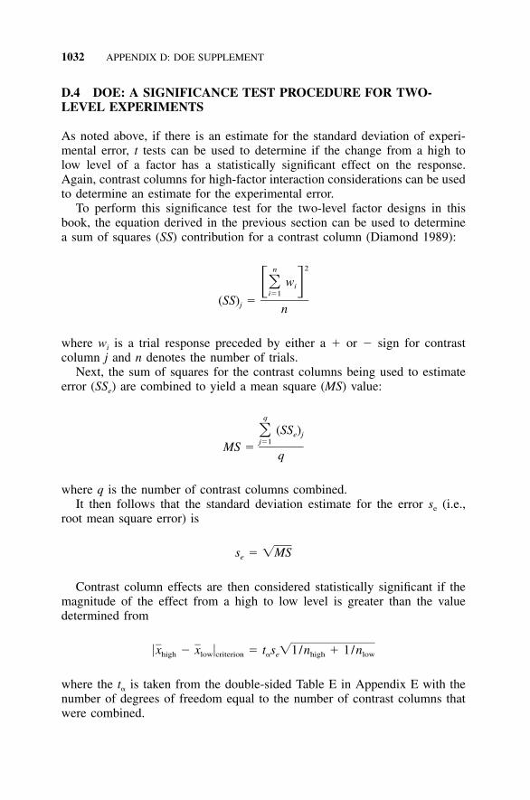
1032 APPENDIX D: DOE SUPPLEMENT

D.4 DOE: A SIGNIFICANCE TEST PROCEDURE FOR TWO-LEVEL EXPERIMENTS

As noted above, if there is an estimate for the standard deviation of experi-mental error, t tests can be used to determine if the change from a high tolow level of a factor has a statistically significant effect on the response.Again, contrast columns for high-factor interaction considerations can be usedto determine an estimate for the experimental error.

To perform this significance test for the two-level factor designs in thisbook, the equation derived in the previous section can be used to determinea sum of squares (SS) contribution for a contrast column (Diamond 1989):

2n

w�� �ii�1

(SS) �j n

where wi is a trial response preceded by either a � or � sign for contrastcolumn j and n denotes the number of trials.

Next, the sum of squares for the contrast columns being used to estimateerror (SSe) are combined to yield a mean square (MS) value:

q

(SS )� e jj�1MS �

q

where q is the number of contrast columns combined.It then follows that the standard deviation estimate for the error se (i.e.,

root mean square error) is

s � �MSe

Contrast column effects are then considered statistically significant if themagnitude of the effect from a high to low level is greater than the valuedetermined from

�x � x � � t s �1/n � 1/nhigh low criterion � e high low

where the t� is taken from the double-sided Table E in Appendix E with thenumber of degrees of freedom equal to the number of contrast columns thatwere combined.

DOE: APPLICATION EXAMPLE 1033

D.5 DOE: APPLICATION EXAMPLE

The method described in the previous section will now be applied to the datafrom Example 30.1. In this example the following factors and level assign-ments were made for an experiment that was to provide an understanding of(with an intent to minimize) the settle-out time of a stepper motor when itwas stopped.

Levels

Factors and Their Designations (�) (�)

A: Motor temperature (mot temp) Cold HotB: Algorithm (algor) Current design Proposed redesignC: Motor adjustment (mot adj) Low tolerance High toleranceD: External adjustment (ext adj) Low tolerance High toleranceE: Supply voltage (sup volt) Low tolerance High tolerance

The experiment yielded the trial responses shown in Table D.1 along withthe noted input factor levels. In general, standard analysis of variance or t-test techniques could be used to determine the statistical significant factors.However, if two-factor interactions are considered in the model, no columnsremain to assess experimental error.

An alternative analysis approach to a formal significance test is to createa probability plot of the mean contrast column effects. A probability plot ofthe main and interaction effects (i.e., all the contrast column effects fromTable M3) can be used to determine the statistically significant effects pic-torially. For this resolution V design, the interaction considerations for eachcontrast column are noted from Table N1.

Computer programs are available to perform this task, but this exampledescribes a manual procedure utilizing normal probability paper (Table Q1)with percentage plot points (Fi) determined from Table P. The following pro-cedure can be used to manage the numbers when creating such a probabilityplot.

Table D.2 is first created when the plus/minus signs of the experimentdesign are combined with the response value for each trial. The mean contrastcolumn effect for factor A (contrast column 1) is then, for example,

5.6 � 2.1 � 4.9 � . . . 4.1 � 1.9 � 5.1� � �0.188

8 8

When using the two-level fractional factorial designs in Table M, an alter-native approach is simply to divide the contrast column summation by halfthe total sample size. For factor A this would be

1034 APPENDIX D: DOE SUPPLEMENT

TABLE D.1 Design Matrix with Outputs

A B C D E

Number of Trial Input Factors

mot temp algor mot adj ext adj sup voltOutput Timing

(msec)

1 � � � � � 5.62 � � � � � 2.13 � � � � � 4.94 � � � � � 4.95 � � � � � 4.16 � � � � � 5.67 � � � � � 1.98 � � � � � 7.29 � � � � � 2.4

10 � � � � � 5.111 � � � � � 7.912 � � � � � 5.313 � � � � � 2.114 � � � � � 7.615 � � � � � 5.516 � � � � � 5.3

1 2 3 4 13 Table M3contrast columnnumbers

�1.5/8 � �0.188

Similarly, the mean effects for all 15 factors can be determined. Theseresults are shown in Table D.3. Next, the values of these effects can be rankedand plotted with the percent plot positions noted from Table P to make anormal probability plot. These ranked effects and corresponding plot coor-dinates are shown in Table D.4.

A computer-generated normal probability plot of these values is shown inFigure D.1. The conclusion from this plot is that factors B and C (contrastcolumn numbers 2 and 3) are statistically significant. The ‘‘best estimates’’for the magnitude of the difference (with no regard to sign) from a high levelto low level for these factors are �2.813 for B and 2.138 for C. Because ofthe procedure used to calculate the estimates, the �2.138 mean effect formot adj indicates that the low tolerance value [(�) level for C] yields asmaller settle-out time for the motor by approximately 2.138 msec, while the�2.812 mean effect for the algorithm [(�) level for B] indicates that theproposed algorithm redesign yields a smaller settle-out time by approximately2.812 msec. No other main effects or interactions were considered to bestatistically significant.

1035

TA

BL

ED

.2E

xper

imen

tR

espo

nse

Val

ues

wit

hL

evel

Con

side

rati

ons

and

Con

tras

tC

olum

nT

otal

s

Con

tras

tC

olum

nN

umbe

r/Fa

ctor

Des

igna

tion

1 A2 B

3 C4 D

5 AB

6 BC

7 CD

8 CE

9 AC

10 BD

11 DE

12 AE

13 E14 B

E15 ND

�5.

6�

5.6

�5.

6�

5.6

�5.

6�

5.6

�5.

6�

5.6

�5.

6�

5.6

�5.

6�

5.6

�5.

6�

5.6

�5.

6�

2.1

�2.

1�

2.1

�2.

1�

2.1

�2.

1�

2.1

�2.

1�

2.1

�2.

1�

2.1

�2.

1�

2.1

�2.

1�

2.1

�4.

9�

4.9

�4.

9�

4.9

�4.

9�

4.9

�4.

9�

4.9

�4.

9�

4.9

�4.

9�

4.9

�4.

9�

4.9

�4.

9�

4.9

�4.

9�

4.9

�4.

9�

4.9

�4.

9�

4.9

�4.

9�

4.9

�4.

9�

4.9

�4.

9�

4.9

�4.

9�

4.9

�4.

1�

4.1

�4.

1�

4.1

�4.

1�

4.1

�4.

1�

4.1

�4.

1�

4.1

�4.

1�

4.1

�4.

1�

4.1

�4.

1�

5.6

�5.

6�

5.6

�5.

6�

5.6

�5.

6�

5.6

�5.

6�

5.6

�5.

6�

5.6

�5.

6�

5.6

�5.

6�

5.6

�1.

9�

1.9

�1.

9�

1.9

�1.

9�

1.9

�1.

9�

1.9

�1.

9�

1.9

�1.

9�

1.9

�1.

9�

1.9

�1.

9�

7.2

�7.

2�

7.2

�7.

2�

7.2

�7.

2�

7.2

�7.

2�

7.2

�7.

2�

7.2

�7.

2�

7.2

�7.

2�

7.2

�2.

4�

2.4

�2.

4�

2.4

�2.

4�

2.4

�2.

4�

2.4

�2.

4�

2.4

�2.

4�

2.4

�2.

4�

2.4

�2.

4�

5.1

�5.

1�

5.1

�5.

1�

5.1

�5.

1�

5.1

�5.

1�

5.1

�5.

1�

5.1

�5.

1�

5.1

�5.

1�

5.1

�7.

9�

7.9

�7.

9�

7.9

�7.

9�

7.9

�7.

9�

7.9

�7.

9�

7.9

�7.

9�

7.9

�7.

9�

7.9

�7.

9�

5.3

�5.

3�

5.3

�5.

3�

5.3

�5.

3�

5.3

�5.

3�

5.3

�5.

3�

5.3

�5.

3�

5.3

�5.

3�

5.3

�2.

1�

2.1

�2.

1�

2.1

�2.

1�

2.1

�2.

1�

2.1

�2.

1�

2.1

�2.

1�

2.1

�2.

1�

2.1

�2.

1�

7.6

�7.

6�

7.6

�7.

6�

7.6

�7.

6�

7.6

�7.

6�

7.6

�7.

6�

7.6

�7.

6�

7.6

�7.

6�

7.6

�5.

5�

5.5

�5.

5�

5.5

�5.

5�

5.5

�5.

5�

5.5

�5.

5�

5.5

�5.

5�

5.5

�5.

5�

5.5

�5.

5�

5.3

�5.

3�

5.3

�5.

3�

5.3

�5.

3�

5.3

�5.

3�

5.3

�5.

3�

5.3

�5.

3�

5.3

�5.

3�

5.3

Tota

ls�

1.5

�22

.5�

17.1

�2.

3�

3.7

�3.

9�

2.3

�3.

9�

2.7

�0.

5�

2.9

�0.

1�

1.9

�0.

9�

0.9

1036 APPENDIX D: DOE SUPPLEMENT

TABLE D.3 Mean Effects of Contrasts Columns

Column Contrast Number, Factor Designation, and Mean Effect

1 2 3 4 5 6 7 8

A B C D AB BC CD CE�0.188 �2.813 �2.138 �0.288 �0.463 �0.488 �0.288 �0.488

9 10 11 12 13 14 15

AC BD DE AE E BE AD�0.338 �0.063 �0.363 �0.013 �0.238 �0.113 �0.113

TABLE D.4 Ranking of Mean Effects with PlotPositions

ContrastColumn

FactorDesignation

MeanEffect

PercentagePlot Position

12 AE 0.013 3.310 BD �0.063 10.014 BE �0.113 16.715 AD 0.113 23.3

1 A �0.188 30.013 E �0.238 36.7

4 D �0.288 43.37 CD 0.288 50.09 AC 0.338 56.7

11 DE 0.363 63.35 AB �0.463 70.06 BC �0.488 76.78 CE 0.488 83.33 C 2.138 90.02 B �2.813 96.7

Because there appear to be no interaction terms, for the purpose of illus-tration we will leave all the main effects in the model and use the contrastcolumns to make an estimate of error. To do this manually, refer to TableD.2. The SS value for each contrast column that is used to estimate error canthen be determined (i.e., all contrast columns except 1, 2, 3, 4, and 13). Forexample, the SS for contrast column 5 is

2 2(�w ) (�3.7)iSS � � � 0.855616 16

The results of the SS calculations for the contrast columns that will be used

DOE: APPLICATION EXAMPLE 1037

-2 -1 0 1 2

1

5

10

20

3040506070

80

90

95

99

Time (msec)

Per

cent

Contrastcolumn 2(factor B)

Contrastcolumn 3(factor C)

Othereffects

FIGURE D.1 Normal probability plot of the contrast column effects.

to estimate experimental error (i.e., two-factor interaction contrast columns)are

5 6 7 8 9 10 11 12 14 15

0.8556 0.9506 0.3306 0.9506 0.4556 0.0156 0.5256 0.0006 0.0506 0.0506

It follows that MS is then

0.8556 � 0.9506 � � � � � 0.0506 � 0.0506MS �

10

� 0.4186

The standard deviation estimate for experimental error (se) is (with 10 degreesof freedom)

s � �0.4186 � 0.647e

The factors are then considered to be statistically significant if the outputeffect from high to low is greater than that determined in the following man-ner. From the double-sided t table (Table E in Appendix E), the t� values forvarious � values with 10 degrees of freedom are as follows, with the notedsignificance criteria calculations:

1038

TA

BL

ED

.5C

ompa

riso

nof

Tab

leM

Des

ign

toa

Com

pute

r-G

ener

ated

Stan

dard

Ord

erD

esig

n

Stan

dard

Ord

erD

esig

nfr

omC

ompu

ter

Tabl

eM

3D

esig

n

Tr#

AB

CD

ET

r#A

1A

2A

3A

4A

5R

esp

1�

1�

1�

1�

11

41

11

1�

14.

92

1�

1�

1�

1�

15

�1

11

11

4.1

3�

11

�1

�1

�1

61

�1

11

15.

64

11

�1

�1

111

�1

�1

11

�1

7.9

5�

1�

11

�1

�1

91

1�

11

12.

46

1�

11

�1

17

�1

1�

11

�1

1.9

7�

11

1�

11

121

�1

�1

1�

15.

38

11

1�

1�

115

�1

�1

�1

�1

15.

59

�1

�1

�1

1�

13

11

1�

11

4.9

101

�1

�1

11

10�

11

1�

1�

15.

111

�1

1�

11

18

1�

11

�1

�1

7.2

121

1�

11

�1

14�

1�

11

�1

17.

613

�1

�1

11

12

11

�1

�1

�1

2.1

141

�1

11

�1

13�

11

�1

�1

12.

115

�1

11

1�

11

1�

1�

1�

11

5.6

161

11

11

16�

1�

1�

1�

1�

15.

3

ILLUSTRATION THAT A STANDARD ORDER DOE DESIGN 1039

� t� �x � x �high low criterion

0.10 1.812 0.586a

0.05 2.228 0.7210.01 3.169 1.025

a �x � x � � t s �1 /n � 1 /n � 1.812(0.647)�1 /8 � 1 /8 � 0.586high low criterion a � high low

A comparison of the absolute values for the A, B, C, D, and E mean effectsfrom Table D.3 (�0.188, �2.813, 2.138, �0.288, and 0.238, respectively) tothe preceding tabular values yields B (algor) and C (mot adj) statisticallysignificant at the 0.01 level, while the other three main effects cannot beshown statistically significant at the 0.10 level.

D.6 ILLUSTRATION THAT A STANDARD ORDER DOE DESIGNFROM STATISTICAL SOFTWARE IS EQUIVALENT TO A TABLEM DESIGN

The DOE designs shown in Table M in Appendix E are similar to the designsgenerated by computers. Table D.5 is an illustrative example where the onlydifference is the change in sign.

1040

APPENDIX E

REFERENCE TABLES

TABLE A Area under the Standardized Normal Curve

APPENDIX E: REFERENCE TABLES 1041

TABLE A (Continued)

Source: Croxton (1953).

Z �

�

a .05541 means .00000541.Note 1: The same information can be obtained from Tables B and C; however, this table format is different.Note 2: In this text the tabular value corresponds to Z�, where � is the value of probability associated with the distribution area pictorially represented as

1042 APPENDIX E: REFERENCE TABLES

TABLE B Probability Points of the Normal Distribution: Single-Sided (Variance Known)

U �

�

U �

�

Source: Diamond (1989), with permission.

TABLE C Probability Points of the Normal Distribution: Double-Sided (Variance Known)

Source: Diamond (1989), with permission.

Note 1: The same information can be obtained from Table A; however, this table format is different.Note 2: In this text the tabular value corresponds to U�,where � is the value of probability associated with the distribution area pictorially represented as

Note 1: The same information can be obtained from Table A; however, this table format is different.Note 2: In this text the tabular value corresponds to U�,where � is the value of probability associated with the distribution area pictorially represented as

APPENDIX E: REFERENCE TABLES 1043

TABLE D Probability Points of the t Distribution: Single-Sided

t �;�

�

�

�

Note: In this text the tabular value corresponds to t�;�, where � is the number of degrees of freedom and � is the value of probability associated with the distribution area pictorially represented as

Source: Pearson and Hartley (1958), with permission. Parts of the table are also taken from Table III of Fisher and Yates (1953), with permission.

1044 APPENDIX E: REFERENCE TABLES

TABLE E Probability Points of the t Distribution: Double-Sided

APPENDIX E: REFERENCE TABLES 1045

TABLE E (Continued)

t �;�

�

Note: In this text the tabular value corresponds to t�;�, where � is the number of degrees of freedom and � is the value of probability associated with the distribution area, pictorially represented as

Source: Snedecor and Cochran (1989), with permission.

1046

TA

BL

E F

Pro

babi

lity

Poi

nts

of t

he V

aria

nce

Rat

io (

F D

istr

ibut

ion)

1047

1048

TA

BL

E F

(Con

tinue

d)

1049

F�

;�1;

�2

�

Not

e: T

he t

abul

ar v

alue

cor

resp

onds

to

F�

;�1;

�2, w

here

�1

is t

he n

umbe

r of

deg

rees

of

free

dom

of

the

larg

er v

alue

in

the

num

erat

or, �

2 is

the

num

ber

of d

egre

es o

f fr

eedo

m

of th

e sm

alle

r va

lue

in th

e de

nom

inat

or, a

nd �

is th

e va

lue

of p

roba

bilit

y as

soci

ated

with

the

dist

ribu

tion

area

pic

tori

ally

rep

rese

nted

as

Sour

ce: T

able

V o

f Fi

sher

and

Yat

es (

1953

), w

ith p

erm

issi

on. (

The

labe

ling

refl

ects

the

nom

encl

atur

e us

ed in

this

text

.)

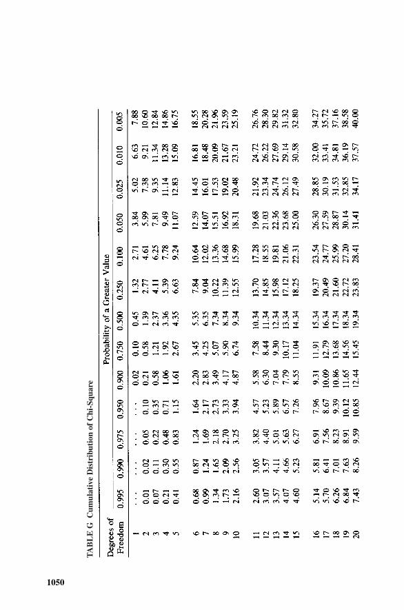
1050

TA

BL

E G

Cum

ulat

ive

Dis

trib

utio

n of

Chi

-Squ

are

1051

Not

e: I

n th

is te

xt th

e ta

bula

r va

lue

corr

espo

nds

to �

2 ,

whe

re �

is th

e nu

mbe

r of

deg

rees

of

free

dom

and

� is

the

valu

e of

pro

babi

lity

asso

ciat

ed w

ith th

e di

stri

butio

n ar

ea p

icto

rial

ly r

epre

sent

ed a

s

Sour

ce: S

nede

cor

and

Coc

hran

(19

89),

with

per

mis

sion

.

�;�

��

;�

�

2

1052 APPENDIX E: REFERENCE TABLES

TABLE H Gamma Function

Source: Lipson and Sheth (1973), with permission.

Tabulation of Value of �(n) versus n

0

1053

TA

BL

E I

Exa

ct C

riti

cal V

alue

s fo

r U

se o

f th

e A

naly

sis

of M

eans

1054

TA

BL

E I

(Con

tinue

d)

1055

1056

TA

BL

E I

(Con

tinue

d)

1057

1058

TA

BL

E I

(Con

tinue

d)

Sour

ce: N

elso

n (1

983)

, with

per

mis

sion

of

the

Am

eric

an S

ocie

ty f

or Q

ualit

y C

ontr

ol.

1059

TA

BL

E J

Fac

tors

for

Con

stru

ctin

g V

aria

bles

Con

trol

Cha

rts

Sour

ce: M

ontg

omer

y (1

985)

, with

per

mis

sion

.

1060

TA

BL

E K

Poi

sson

Dis

trib

utio

n F

acto

rs

1061

App

lica

tion

s of

Tab

le K

Tota

l tes

t tim

e: T

= B

r;c/

� a f

or �

≤� a

whe

re �

a is

a f

ailu

re r

ate

crite

rion

, r is

allo

wed

num

ber

of te

st f

ailu

res,

and

c is

a c

onfi

denc

e fa

ctor

.C

onfi

denc

e in

terv

al s

tate

men

ts (

time-

term

inat

ed te

st);

� ≤

Br;

c/T

� ≥

Ar;

c/T

Exa

mpl

es:

1 fa

ilure

test

for

a 0

.000

1 fa

ilure

s/ho

ur c

rite

rion

(i.e

., 10

,000

-hr

MT

BF)

95%

con

fide

nce

test

: Tot

al te

st ti

me

= 4

7,44

0 hr

(i.e

., 4.

744/

0.00

1)5

failu

res

in a

tota

l of

10,0

00 h

r95

% c

onfi

dent

: �≤

0.00

1051

3 fa

ilure

s/ho

ur (

i.e.,

10,5

13/1

0,00

0)95

% c

onfi

dent

: �≥

0.00

0197

0 fa

ilure

s/ho

ur (

i.e.,

1.97

0/10

,000

)90

% c

onfi

denc

e: 0

.000

1970

≤�

≤ 0.

0010

513

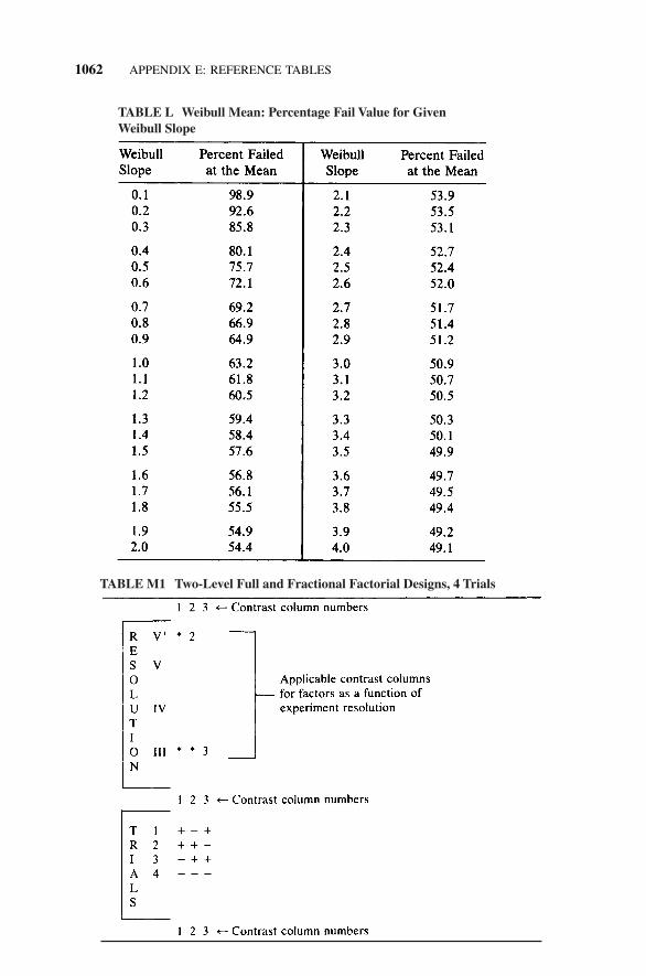
1062 APPENDIX E: REFERENCE TABLES

TABLE L Weibull Mean: Percentage Fail Value for Given Weibull Slope

TABLE M1 Two-Level Full and Fractional Factorial Designs, 4 Trials

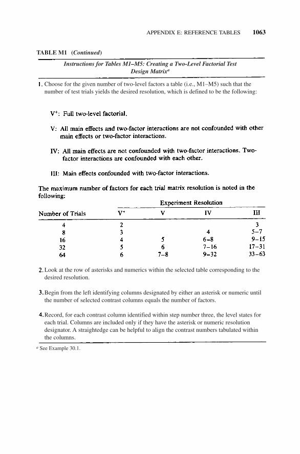
APPENDIX E: REFERENCE TABLES 1063

TABLE M1 (Continued)

a See Example 30.1.

Look at the row of asterisks and numerics within the selected table corresponding to the desired resolution.

Choose for the given number of two-level factors a table (i.e., M1–M5) such that the number of test trials yields the desired resolution, which is defined to be the following:

Begin from the left identifying columns designated by either an asterisk or numeric until the number of selected contrast columns equals the number of factors.

Record, for each contrast column identified within step number three, the level states for each trial. Columns are included only if they have the asterisk or numeric resolution designator. A straightedge can be helpful to align the contrast numbers tabulated within the columns.

Instructions for Tables M1–M5: Creating a Two-Level Factorial TestDesign Matrixa

1064 APPENDIX E: REFERENCE TABLES

TABLE M2 Two-Level Full and Fractional Factorial Designs, 8 Trialsa

a Table usage instructions are noted following Table M1.The 8, 16, 32, and 64 trial matrices in Tables M2–M5 were created from a computer program described by Diamond (1989).

APPENDIX E: REFERENCE TABLES 1065

TABLE M3 Two-Level Full and Fractional Factorial Design, 16 Trialsa

a Table usage instructions are noted following Table M1.

1066

TA

BL

E M

4T

wo-

Lev

el F

ull a

nd F

ract

iona

l Fac

tori

al D

esig

n, 3

2 T

rial

sa

1067

a Tab

le u

sage

inst

ruct

ions

are

not

ed f

ollo

win

g Ta

ble

M1.

1068

TA

BL

E M

5T

wo-

Lev

el F

ull a

nd F

ract

iona

l Fac

tori

al D

esig

n, 6

4 T

rial

sa

1069

1070

TA

BL

E M

5(C

ontin

ued)

a

1071

a Tab

le u

sage

inst

ruct

ions

are

not

ed f

ollo

win

g Ta

ble

M1.

1072

TA

BL

E N

1T

wo-

Fac

tor

Inte

ract

ion

Con

foun

ding

in t

he C

ontr

ast

Col

umns

of

the

Tabl

es M

1–M

5 R

esol

utio

ns V

Fra

ctio

nal F

acto

rial

Des

igns

a

a The

hig

her-

orde

r te

rms

wer

e us

ed w

hen

gene

ratin

g th

e de

sign

. Mai

n ef

fect

s ar

e de

note

d by

an

aste

risk

.

1073

TA

BL

E N

2T

wo-

Fac

tor

Inte

ract

ion

Con

foun

ding

in t

he C

ontr

ast

Col

umns

of

the

Tabl

es M

1–M

5 R

esol

utio

ns I

V F

ract

iona

l Fac

tori

al D

esig

nsa

1074

TA

BL

E N

2(C

ontin

ued)

a

1075

a The

hig

her-

orde

r te

rms

wer

e us

ed w

hen

gene

ratin

g th

e de

sign

. Mai

n ef

fect

s ar

e de

note

d by

an

aste

risk

.

1076

TA

BL

E N

3T

wo-

Fac

tor

Inte

ract

ion

Con

foun

ding

in t

he C

ontr

ast

Col

umns

of

the

Tabl

es M

1–M

5 R

esol

utio

ns I

II F

ract

iona

l Fac

tori

al D

esig

nsa

1077

1078

TA

BL

E N

3(C

ontin

ued)

a

1079

1080

TA

BL

E N

3(C

ontin

ued)

a

a The

hig

her-

orde

r te

rms

wer

e us

ed w

hen

gene

ratin

g th

e de

sign

. Mai

n ef

fect

s ar

e de

note

d by

an

aste

risk

.

APPENDIX E: REFERENCE TABLES 1081

TABLE O Pass/Fail Functional Test Matrix Coverage

1082

TA

BL

E P

Gen

eric

Per

cent

Plo

t P

osit

ions

(F

i) fo

r P

roba

bilit

y P

aper

s [F

i = 1

00(i

– 0.

5)/n

]

1083

1084

TA

BL

E Q

1N

orm

al P

roba

bilit

y P

aper

Rep

rodu

ced

with

per

mis

sion

of

man

ufac

ture

r. Ph

otoc

opie

s of

illu

stra

ted

grap

h pa

pers

sho

uld

be u

sed

for

sim

ple

illus

trat

ive

purp

oses

onl

y. P

hoto

copy

dis

tort

ions

cha

nge

the

mat

hem

atic

al r

elat

ions

hips

bet

wee

n ho

rizo

ntal

and

ver

tical

sca

le g

rids

whi

ch th

enca

uses

err

ors

in p

aram

eter

est

imat

es ta

ken

from

the

grap

h.

1085

TA

BL

E Q

2L

ogno

rmal

Pro

babi

lity

Pap

er

Rep

rodu

ced

with

per

mis

sion

of

man

ufac

ture

r. Ph

otoc

opie

s of

illu

stra

ted

grap

h pa

pers

sho

uld

be u

sed

for

sim

ple

illus

trat

ive

purp

oses

only

. Pho

toco

py d

isto

rtio

ns c

hang

e th

e m

athe

mat

ical

rel

atio

nshi

ps b

etw

een

hori

zont

al a

nd v

ertic

al s

cale

gri

ds w

hich

the

n ca

uses

err

ors

in p

aram

eter

est

imat

es ta

ken

from

the

grap

h.

1086

TA

BL

E Q

3W

eibu

ll P

roba

bilit

y P

aper

Rep

rodu

ced

with

per

mis

sion

of

man

ufac

ture

r. Ph

otoc

opie

s of

illu

stra

ted

grap

h pa

pers

sho

uld

be u

sed

for

sim

ple

illus

trat

ive

purp

oses

only

. Pho

toco

py d

isto

rtio

ns c

hang

e th

e m

athe

mat

ical

rel

atio

nshi

ps b

etw

een

hori

zont

al a

nd v

ertic

al s

cale

gri

ds w

hich

then

cau

ses

erro

rs in

pa

ram

eter

est

imat

es ta

ken

from

the

grap

h.

1087

TA

BL

E R

1N

orm

al H

azar

d P

aper

Rep

rodu

ced

with

per

mis

sion

of

man

ufac

ture

r. Ph

otoc

opie

s of

illu

stra

ted

grap

h pa

pers

sho

uld

be u

sed

for

sim

ple

illus

trat

ive

purp

oses

onl

y. P

hoto

copy

dis

tort

ions

cha

nge

the

mat

hem

atic

al r

elat

ions

hips

bet

wee

n ho

rizo

ntal

and

ver

tical

sca

le g

rids

whi

ch

then

cau

ses

erro

rs in

par

amet

er e

stim

ates

take

n fr

om th

e gr

aph.

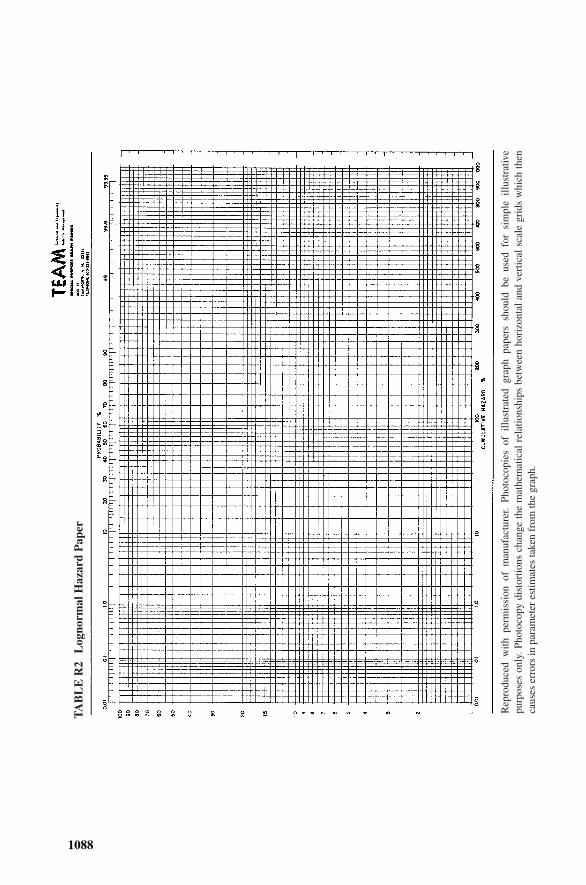
1088

TA

BL

E R

2L

ogno

rmal

Haz

ard

Pap

er

Rep

rodu

ced

with

per

mis

sion

of

man

ufac

ture

r. Ph

otoc

opie

s of

illu

stra

ted

grap

h pa

pers

sho

uld

be u

sed

for

sim

ple

illus

trat

ive

purp

oses

onl

y. P

hoto

copy

dis

tort

ions

cha

nge

the

mat

hem

atic

al r

elat

ions

hips

bet

wee

n ho

rizo

ntal

and

ver

tical

sca

le g

rids

whi

ch t

hen

caus

es e

rror

s in

par

amet

er e

stim

ates

take

n fr

om th

e gr

aph.

1089

TA

BL

E R

3W

eibu

ll H

azar

d P

aper

Rep

rodu

ced

with

per

mis

sion

of

man

ufac

ture

r. Ph

otoc

opie

s of

illu

stra

ted

grap

h pa

pers

sho

uld

be u

sed

for

sim

ple

illus

trat

ive

purp

oses

onl

y. P

hoto

copy

dis

tort

ions

cha

nge

the

mat

hem

atic

al r

elat

ions

hips

bet

wee

n ho

rizo

ntal

and

ver

tical

sca

le g

rids

whi

ch th

enca

uses

err

ors

in p

aram

eter

est

imat

es ta

ken

from

the

grap

h.

1090 APPENDIX E: REFERENCE TABLES

TABLE S Conversion Between ppm and Sigma

� /�Sigma

Level atSpec.

Limit*

Percentwithin Spec.:

CenteredDistribution

Defectiveppm:

CenteredDistribution

Percentwithin Spec.:

1.5 SigmaShifted

Distribution

Defectiveppm: 1.5

SigmaShifted

Distribution

1 68.2689480 317310.520 30.232785 697672.151.1 72.8667797 271332.203 33.991708 660082.921.2 76.9860537 230139.463 37.862162 621378.381.3 80.6398901 193601.099 41.818512 581814.881.4 83.8486577 161513.423 45.830622 541693.781.5 86.6385542 133614.458 49.865003 501349.971.6 89.0401421 109598.579 53.886022 461139.781.7 91.0869136 89130.864 57.857249 421427.511.8 92.8139469 71860.531 61.742787 382572.131.9 94.2567014 57432.986 65.508472 344915.282 95.4499876 45500.124 69.122979 308770.212.1 96.4271285 35728.715 72.558779 274412.212.2 97.2193202 27806.798 75.792859 242071.412.3 97.8551838 21448.162 78.807229 211927.712.4 98.3604942 16395.058 81.589179 184108.212.5 98.7580640 12419.360 84.131305 158686.952.6 99.0677556 9322.444 86.431323 135686.772.7 99.3065954 6934.046 88.491691 115083.092.8 99.4889619 5110.381 90.319090 96809.102.9 99.6268240 3731.760 91.923787 80762.133 99.7300066 2699.934 93.318937 66810.633.1 99.8064658 1935.342 94.519860 54801.403.2 99.8625596 1374.404 95.543327 44566.733.3 99.9033035 966.965 96.406894 35931.063.4 99.9326038 673.962 97.128303 28716.973.5 99.9534653 465.347 97.724965 22750.353.6 99.9681709 318.291 98.213547 17864.533.7 99.9784340 215.660 98.609650 13903.503.8 99.9855255 144.745 98.927586 10724.143.9 99.9903769 96.231 99.180244 8197.564 99.9936628 63.372 99.379030 6209.704.1 99.9958663 41.337 99.533877 4661.234.2 99.9973292 26.708 99.653297 3467.034.3 99.9982908 17.092 99.744481 2555.194.4 99.9989166 10.834 99.813412 1865.884.5 99.9993198 6.802 99.865003 1349.974.6 99.9995771 4.229 99.903233 967.674.7 99.9997395 2.605 99.931280 687.204.8 99.9998411 1.589 99.951652 483.484.9 99.9999040 0.960 99.966302 336.985 99.9999426 0.574 99.976733 232.67

APPENDIX E: REFERENCE TABLES 1091

TABLE S (Continued )

� /�Sigma

Level atSpec.

Limit*

Percentwithin Spec.:

CenteredDistribution

Defectiveppm:

CenteredDistribution

Percentwithin Spec.:

1.5 SigmaShifted

Distribution

Defectiveppm: 1.5

SigmaShifted

Distribution

5.1 99.9999660 0.340 99.984085 159.155.2 99.9999800 0.200 99.989217 107.835.3 99.9999884 0.116 99.992763 72.375.4 99.9999933 0.067 99.995188 48.125.5 99.9999962 0.038 99.996831 31.695.6 99.9999979 0.21 99.997933 20.675.7 99.9999988 0.012 99.998665 13.355.8 99.9999993 0.007 99.999145 8.555.9 99.9999996 0.004 99.999458 5.426 99.9999998 0.002 99.999660 3.40

*Sometimes referred to as sigma level or sigma quality level when considering process shift.

1092

LIST OF SYMBOLS

Some symbols used locally in the book are not shown.

Ar;c Factor from the Poisson distribution that is tabulated inTable K

ABC Activity based costingAD Axiomatic designAFR Average failure rateAHP Analytical hierarchy processAIAG Automotive Industry Action GroupANOM Analysis of meansANOVA Analysis of varianceAPQP Advanced product quality planningAQL Accept quality levelAQP Advanced quality planningARL Average run lengthASQ American Society for Quality (Previously ASQC, American

Society for Quality Control)ASTM American Society for Testing and MaterialsAV Appraiser variationAt Acceleration test factorBr;c Factor from the Poisson distribution tabulated in Table Kb Weibull distribution shape parameter (slope of a Weibull

probability plot); a parameter used in the NHPP withWeibull intensity model

BOK Body of knowledgec Confidence factor used in Table K

LIST OF SYMBOLS 1093

c chart Control chart for nonconformities�C Celsius temperatureCCD Central composite designCI Confidence intervalCL Centerline in an SPC chartCDF Cumulative distribution functionCFM Continuous flow manufacturingCAP Change acceleration processCp Capability index (AIAG 1995b) (In practice, some calculate

using short-term standard deviation, others calculate usinglong-term standard deviation)

Cpk Capability index (AIAG 1995b) (In practice, some calculateusing short-term standard deviation, others calculate usinglong-term standard deviation)

cP Centipoise (measure of fluid viscosity)CPM Critical path methodCRM Customer relationship managementCUSUM Cumulative sum (control chart approach)C4 Controlled collapse chip connection points within electronic

chip componentsC&E Cause and effect (diagram)C/O Change overCODND Cost of doing nothing differentCOPQ Cost of poor qualityC/T Cycle timeCTC Critical to costCTD Critical to deliveryCTP Critical to processCTQ Critical to qualityd Discrimination ratio (Poisson distribution sequential testing)DCRCA DOE collective response capability assessment.df Degrees of freedomDFA Design for assembly (Example of DFX)DFM Design for manufacturability (Example of DFX)DFMEA Design failure mode and effects analysisDFX Design for a characteristic (e.g., DFA or DFM)DMAIC Define-measure-analyze-improve-controlDMADV Define-measure-analyze-design-verifyDOA Dead on arrivalDOE Design of experimentsDP Design parameterDPMO Defects per million opportunitiesDPU Defects per unitDSO Days sales outstanding (a metric that quantifies the length of

time for invoice payment)

1094 LIST OF SYMBOLS

dt Calculus expression used to describe an infinitesimally smallincrement of time t

e 2.71828EBPM Enterprise business planning methodologyECMM Enterprise cascading measurement methodologyEDA Exploratory data analysis8D 8 DisciplinesEPE Every part every (batch size) (e.g., EPE day)ERA Emergency response actionERP Enterprise resource planningEVOP Evolutionary operationEWMA Exponentially weighted moving averageexp(x) � ex � (2.71828 . . .)x

�F Fahrenheit temperatureF0 Test criterion value from the F distribution (Table F)Fa,�1; �2 Value from the F distribution for � risk and �1 and �2

degrees of freedom (Table F)Fi Probability plot positions determined from Table PFIFO First-in-first-outFG Finished goodsFIT Failures in timeFMEA Failure mode and effects analysisFR Functional requirementFT Fault treeFV Future valueF(x) Describes the CDF where the independent variable is xƒ(x) Describes the PDF where the independent variable is xGage R&R Gage repeatability and reproducibilityGDT Geometric dimensioning and tolerancingGLM General linear modelingH0 Null hypothesisHa Alternative hypothesisHPP Homogeneous Poisson processICA Interim containment actionIEE Integrated enterprise excellencein. InchesI-MR chart Individuals chart and moving range (Same as XmR chart)IPO Input-process-outputJIT Just in timeK Temperature in degrees Kelvin (273.16 � �C); Boltzmann’s

constantk Characteristic life or scale parameter in the Weibull

distributionKCA Knowledge-centered activityKTS Knowledge-transfer sessions

LIST OF SYMBOLS 1095

KPIV Key process input variableKPOV Key process output variableLr Length run for AQL (in CUSUM charting)LCL Lower control limit (in SPC)LDL Lower decision level (in ANOM)L/T Lead timeln loge � log2.718 . . .log 1og10

Lr Length run for RQL (in CUSUM charting)ML Maximum likelihoodMP Maintenance preventionmph Miles per hourMR Moving range (in SPC)MS Mean squareMSA Measurement systems analysismsec MillisecondsMTBF Mean time between failuresMu Greek letter �, which often symbolizes the mean of a

populationn Sample sizendc Number of distinct categories, in measurement systems

analysisnp (chart) SPC chart of number of nonconforming itemsNGT Nominal group techniqueNHPP Nonhomogeneous Poisson processNID(0,�2) Modeling errors are often assumed to be normally and

independently distributed with mean zero and a constantbut unknown variance

NIST National Institute of Standards and TechnologyNPV Natural process variation, net present valueNTF No trouble foundOC Operating characteristic curveOEM Original equipment manufacturer (customers)ORT Ongoing reliability testp (chart) SPC chart of fraction nonconformingP Probability, test performance ratio (�t /�a)PCA Permanent corrective actionsPDCA Plan-do-check-actPDF Probability density functionPDPC Process decision program chartsPDSA Plan-do-study-actPERT Program evaluation and review techniquePFMEA Process failure mode and effects analysisPI Prediction intervalPP&E Plant property and equipment

1096 LIST OF SYMBOLS

ppm Parts per million (defect rate)PM Preventive maintenance, productive maintenancePp Performance index (AIAG 1995b) (calculated using long-

term standard deviation)Ppk Performance index (AIAG 1995b) (calculated using long-

term standard deviation)PV Part variation, Present valueQFD Quality function deploymentROI Return on investmentRQL Reject quality levelR Range (in SPC)RM Raw materialRMR Rejected material reviewRPN Risk priority number (in FMEA)RO Results orchestrationROI Return on investmentRSM Response surface methodologyRTY Rolled throughput yieldr Number of failures, correlation coefficientR2 Coefficient of determinationr(t) System failure rate at time (t) for the NHPP models Standard deviation of a sampleSIPOC Supplier-input-process-output-customerSIT Structured inventive thinkingSME Subject matter expertSMED Single-minute exchange of dieSOD Severity, occurrence, and detection (used in FMEA)SOP Standard operating procedureSPC Statistical process controlSS Sum of squaresSWOT Strengths, weaknesses, opportunities, and threatsS4 Smarter Six Sigma SolutionsT Total test time used in Table Kt TimeTPM Total productive maintenanceTQC Total quality controlt0 Test criterion value from the t distribution (Tables D or E)Tq q% of the population is expected to be below this value for a

populationt�; � Value from the t distribution for � risk and v degrees of

freedom (Tables D and E)UCL Upper control limit (SPC)UDL Upper decision level (ANOM)U0 Test criterion value from the normal distribution (Table B or

C)U� Value from the normal distribution for � risk (Table B or C)

LIST OF SYMBOLS 1097

U� Value from the normal distribution for � risk (Table B or C)u (chart) SPC chart of number of nonconformity’s per unitUSIT Unified structured inventive thinkingVA time Value added timeVIF Variance inflation factorVOC Voice of customerWIP Work in process, Work in progressXmR (chart) SPC chart of individual and moving range measurementsx0 Three-parameter Weibull distribution location parameterx Mean of a variable x

chartx SPC chart of means (i.e., chart)xx̃ Median of variable xZD Zero defectsZ� Normal distribution value for � risk (Table A)� Alpha, risk of rejecting the null hypothesis erroneously� Beta, risk of not rejecting the null hypothesis erroneously� Delta, effect of contrast column Delta, an acceptable amount of uncertainty Theta, the parameter in the exponential distribution equation

(mean of the distribution)� Lambda, hazard rate; intensity term in the NHPP equation� Mu, population true mean�̂ Estimate of population mean� Nu, degrees of freedom� Rho, actual failure rate of population, correlation coefficient

between two variables�a A single failure rate test criterion�t The highest failure rate that is to be exhibited by the samples

in a time-terminated test before a ‘‘pass test’’ statementcan be given

�1 Higher failure rate (failures/unit time) involving � risk inPoisson sequential testing (typically assigned equality tofailure rate criterion �a)

�0 Lower failure rate (failures/unit time involving � risk inPoisson sequential testing

�� Used when calculating sample size for a fixed length test; thefailure rate at which � is to apply

�� Used when calculating sample size for a fixed length test; thefailure rate at which � is to apply

� Mathematical summation� Sigma, population standard deviation�̂ Estimate of population standard deviation

2 �;� Chi-square value from the chi-square distribution for � riskand � degrees of freedom (Table G)

2 o Test criterion value from the chi-square distribution (Table G)� Mathematical symbol used to denote the absolute value of a

quantity

1098

GLOSSARY

Abscissa: The coordinate representing the distance from the y-axis in a two-dimensional plot.

Accelerated testing: The testing of equipment in an environment so that thetime will be shortened for failures to occur. For example, high temperatureis often used to create failures sooner during a reliability test of electroniccomponents. The acceleration test factor (At) is the expected normal usagetime that the test is putting on the device under test divided by the testtime used to perform the accelerated testing

Accept quality level (AQL): The maximum proportion of defective units ina sampling plan that can be considered satisfactory as the process average.

Accuracy: The closeness of agreement between an observed value and theaccepted reference value (AIAG 2002).

Activation energy (E0): A constant in the Arrhenius equation that is a func-tion of the type of failure mechanism during a high-temperature acceleratedtest of electrical components.

Active experimentation: Experiments are conducted where variable levelsare changed to assess their impact on responses.

Advanced quality planning (AQP) or Advanced product quality planning(APQP): The act of ensuring that a new product or service will meetcustomer expectations.

Affinity diagram: A methodology where a team can organize and summarizethe natural grouping from a large number of ideas and issues.

Algorithm design: A method for choosing experiment design trials whenfitting a model (e.g., quadratic). With these designs a computer creates a

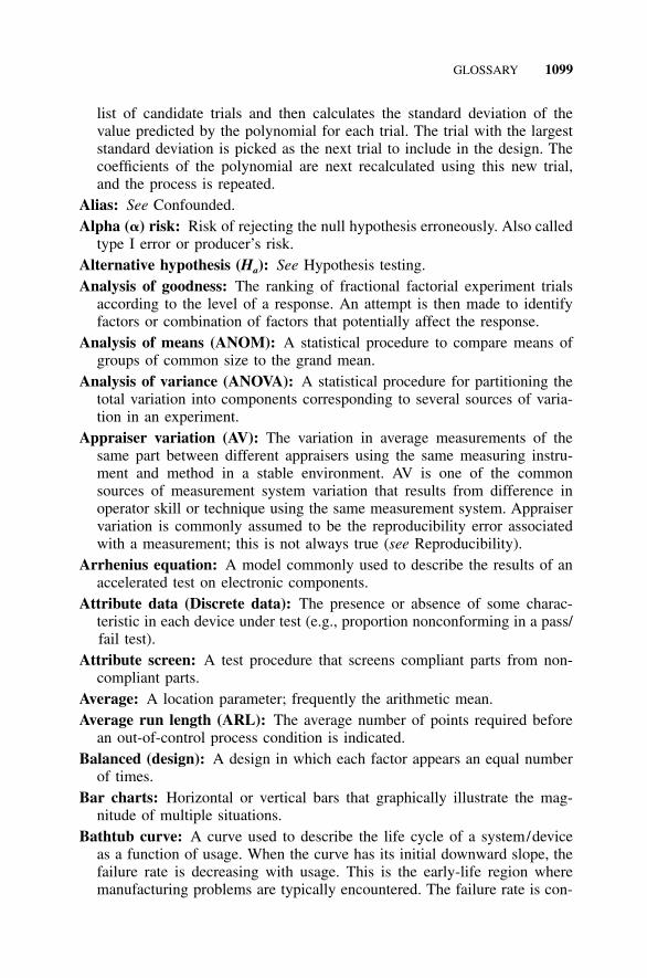
GLOSSARY 1099

list of candidate trials and then calculates the standard deviation of thevalue predicted by the polynomial for each trial. The trial with the largeststandard deviation is picked as the next trial to include in the design. Thecoefficients of the polynomial are next recalculated using this new trial,and the process is repeated.

Alias: See Confounded.Alpha (�) risk: Risk of rejecting the null hypothesis erroneously. Also called

type I error or producer’s risk.Alternative hypothesis (Ha): See Hypothesis testing.Analysis of goodness: The ranking of fractional factorial experiment trials

according to the level of a response. An attempt is then made to identifyfactors or combination of factors that potentially affect the response.

Analysis of means (ANOM): A statistical procedure to compare means ofgroups of common size to the grand mean.

Analysis of variance (ANOVA): A statistical procedure for partitioning thetotal variation into components corresponding to several sources of varia-tion in an experiment.

Appraiser variation (AV): The variation in average measurements of thesame part between different appraisers using the same measuring instru-ment and method in a stable environment. AV is one of the commonsources of measurement system variation that results from difference inoperator skill or technique using the same measurement system. Appraiservariation is commonly assumed to be the reproducibility error associatedwith a measurement; this is not always true (see Reproducibility).

Arrhenius equation: A model commonly used to describe the results of anaccelerated test on electronic components.

Attribute data (Discrete data): The presence or absence of some charac-teristic in each device under test (e.g., proportion nonconforming in a pass/fail test).

Attribute screen: A test procedure that screens compliant parts from non-compliant parts.

Average: A location parameter; frequently the arithmetic mean.Average run length (ARL): The average number of points required before

an out-of-control process condition is indicated.Balanced (design): A design in which each factor appears an equal number

of times.Bar charts: Horizontal or vertical bars that graphically illustrate the mag-

nitude of multiple situations.Bathtub curve: A curve used to describe the life cycle of a system/device

as a function of usage. When the curve has its initial downward slope, thefailure rate is decreasing with usage. This is the early-life region wheremanufacturing problems are typically encountered. The failure rate is con-

1100 GLOSSARY

stant during the flat part of the curve. When the curve begins slopingupward, the failure rate is increasing with usage. This region describeswear-out of a product.

Benchmarking: To provide a standard against which something can be as-sessed.

Beta (�) risk: Chance of not rejecting a false null hypothesis. Also calledtype II error or consumer’s risk.

Bias: The difference between the observed average of measurements (trialsunder repeatability conditions) and a reference value; historically referredto as accuracy. Bias is evaluated and expressed at a single point with theoperating range of the measurement system (AIAG 2002).

Bimodal distribution: A distribution that is a combination of two differentdistributions resulting in two distinct peaks.

Binomial distribution: A distribution that is useful to describe discrete var-iables or attributes that have two possible outcomes (e.g., a pass/fail pro-portion test, heads/tails outcome from flipping a coin, defect/no defectpresent).

Black box: an electronic component where its constituents or circuitry areunknown or irrelevant but whose function is understood.

Blocking: For large experiments it may be desirable to divide the experi-mental units into smaller, more homogeneous groups. These groups arecalled blocks.

Boldness: The term used to describe the choosing of the magnitude of thevariable levels to use within a response surface design. The concept sug-gests that the magnitudes of variables should be large enough to capturethe minimum and maximum responses of the process under test.

Boltzmann’s constant: A constant of 8.617 � l0�5 eV/K used in the Arrhe-nius equation for high-temperature accelerated testing.

Bootstrapping: A resampling technique that provides a simple but effectivemethod to describe the uncertainty associated with a summary statementwithout concern about details of complexity of the chosen summary orexact distribution from which data are calculated.

Bottleneck: The slowest operation in a chain of operations; it will pace theoutput of the entire line.

Bottom line: The final profit or loss that a company experiences at the endof a given period of time.

Brainstorming: Consensus-building among experts about a problem or issueusing group discussion.

Bugs: A slang term used to describe problems that may occur in a processor in the use of a product. These problems can result from errors in thedesign or the manufacturing process.

GLOSSARY 1101

Burn-in: Stress screen at perhaps high temperature or elevated voltages con-ducted on a product for the purpose of capturing failures inside the man-ufacturing facility and minimizing early-life field failures. See Screen.

Calibration: A set of operations that establishes, under specified conditions,the relationship between a measuring device and a traceable standard ofknown reference value and uncertainty. Calibration may also include stepsto detect, correlate, report, or eliminate by adjustment any discrepancy inaccuracy of the measuring device being compared (AIAG 2002).

Calipers: An instrument consisting of a pair of movable, curved legs fastenedtogether at one end. It is used to measure the thickness or diameter ofsomething. There are both inside and outside calipers.

Canonical form: A transformed form of a response surface equation to anew coordinate system such that the origin is at the maximum, minimum,or saddle point and the axis of the system is parallel to the principal axisof the fitted quadratic response surface.

Capability, Process: See Process capability.Catapult: A teaching aid originally developed by Texas Instruments (TI).

With this device, teams of students project plastic golf balls and the dis-tance from the catapult at impact is the response. There are many adjust-ments on the catapult that affect the throw distance. Contact the author forinformation about availability.

Cause-and-effect diagram (C&E diagram): This is a technique that is use-ful in problem-solving using brainstorming sessions. With this technique,possible causes from such sources as materials, equipment, methods, andpersonnel are typically identified as a starting point to begin discussion.The technique is sometimes called an Ishikawa diagram or fishbone dia-gram.

Cell: A grouping of data that, for example, comprise a bar in a histogram.Censored datum: The sample has not failed at a usage or stress level.Central composite rotatable design: A type of response surface experiment

design.Central limit theorem: The means of samples from a population will tend

to be normally distributed around the population mean.Certification: A test to determine whether, for example, a product is ex-

pected to meet or be better than its failure rate criterion.Changeover: The time from the last piece of one batch to the first piece of

the next batch.Characteristic life (k): A parameter that is contained in the Weibull distri-

bution. In a reliability test, the value of this parameter equates to the usagewhen 63.2% of the devices will fail.

Checks sheets: The systematic recording and compiling of data from histor-ical or current observations.

1102 GLOSSARY

Chronic problem: A description of the situation where a process SPC chartmay be in control/predictable; however, the overall response is not satis-factory (i.e., common causes yield an unsatisfactory response). For ex-ample, a manufacturing process has a consistent ‘‘yield’’ over time;however, the average yield number is not satisfactory.

Class variables: Factors that have discrete levels.Coded levels: Regression analysis of factorial or response surface data can

be performed where the levels are described in the natural levels of thefactors (e.g., 5.5 and 4.5 V) or the coded levels of the factors (e.g., �l and�1).

Coefficient: See Regression analysis.Coefficient of determination (R2): The square of the correlation coefficient.

Values for R2 describe the percentage of variability accounted for by themodel. For example, R2 � 0.8 indicates that 80% of the variability in thedata is accounted for by the model.

Coefficient of variation: A measure of dispersion where standard deviationis divided by the mean and is expressed as a percentage.

Combinational problem: A term used in this book to describe a type ofproblem where the occurrences of a combination of factor levels cause alogic failure. Pass/fail functional testing is a suggested procedure to iden-tify whether such a problem exists in a unit under test. This term is verydifferent from the term interaction.

Common causes: See Chronic problem.Component: A device that is one of many parts of a system. Within this

book components are considered to be nonrepairable devices.Concurrent engineering: An approach to the development of new products

where the product and all its associated processes, such as manufacturing,distribution, and service, are all developed in parallel.

Confidence interval: The region containing the limits or band of a parameterwith an associated confidence level that the bounds are large enough tocontain the true parameter value. The bands can be single-sided to describean upper/ lower limit or double-sided to describe both upper and lowerlimits.

Confounded: Two factor effects that are represented by the same comparisonare aliases of one another (i.e., different names for the same computedeffect). Two effects that are aliases of one another are confounded (orconfused) with one another. Although the word ‘‘confounded’’ is com-monly used to describe aliases between factorial effects and block effects,it can more generally be used to describe any effects that are aliases ofone another.

Consumer’s risk: See Beta (�) risk.Contingency tables: If each member of a sample is classified by one char-

acteristic into S classes and by a second characteristic into R classes, the

GLOSSARY 1103

data may be presented by a contingency table with S rows and R columns.Statistical independence of characteristics can also be determined by con-tingency tables.

Continuous data (Variables data): Data that can assume a range of nu-merical responses on a continuous scale, as opposed to data that can as-sume only discrete levels.

Continuous distribution: A distribution used in describing the probabilityof a response when the output is continuous. See Response.

Continuous data response: See Response.Continuous flow manufacturing (CFM): Within CFM operations and ma-

chines are efficiently used to build parts. Non-value-added activities in theoperation are eliminated. Flexibility is a substitute for work-in-process in-ventory. A product focus is established in all areas of operation.

Contrast column effects: The effect in a contrast column, which might haveconsiderations that are confounded.

Control chart: A procedure used to track a process with time for the purposeof determining if sporadic or chronic problems (common or special causes)exist.

Control: ‘‘In control’’ or predictable is used in process control charting toindicate when the chart shows there are no indications that the process isnot predictable.

Correlation coefficient (r): A statistic that describes the strength of a rela-tionship between two variables is the sample correlation coefficient. Acorrelation coefficient can take values between �1 and �1. A �1 indicatesperfect negative correlation, while a �1 indicates perfect positive correla-tion. A zero indicates no correlation.

Cost of doing nothing different (CODND): To keep S4/IEE from appearingas a quality initiative, I prefer to reference the Six Sigma metric COPQ asthe cost of doing nothing different (CODND), which has even broadercosting implications than COPQ. In this book I refer to COPQ/CODND.

Cost of poor quality (COPQ): Traditionally, cost of quality issues have beengiven the broad categories of internal failure costs, external failure costs,appraisal costs, and prevention costs. Within Six Sigma, COPQ addressesthe cost of not performing work correctly the first time or not meetingcustomers’ expectations.

Covariate: A quantitative variable that can be included within an ANOVAmodel. May be a variable where the level is measured but not controlledas part of the design. For this situation, when the covariate is entered intothe model the error variance would be reduced. A covariate may also bea quantitative variable where its levels were controlled as part of the ex-periment. For both situations, the statistical model contains a coefficientfor the covariate, which would be interpreted as a predictor in a regressionmodel.

Coverage: See Test coverage.

1104 GLOSSARY

Cumulative distribution function (CDF) [F(x)]: The calculated integral ofthe PDF from minus infinity to x. This integration takes on a characteristic‘‘percentage less than or percentile’’ when plotted against x.

Cumulative sum (CUSUM) (control chart): An alternative control chartingtechnique to Shewhart control charting. CUSUM control charts can detectsmall process shifts faster than Shewhart control charts can.

Customer: Someone for whom work or a service is performed. The end userof a product is a customer of the employees within a company that man-ufactures the product. There are also internal customers in a company.When an employee does work or performs a service for someone else inthe company, the person who receives this work is a customer of thisemployee.

Cycle time: Frequency that a part /product is completed by process. Also,time it takes for operator to go through work activities before repeatingthe activities. In addition, cycle time can be used to quantify customerorder to delivery time.

DOE-collective-response-capability-assessment (DCRCA): Consider a DOEwhere the factors were chosen to be the tolerance extremes for a newprocess and the response was the output of the process. Consider also thatthere were no historical data that could be used to make a capability/performance metric statement for the process. A probability plot of theDOE responses can give an overall picture of how we expect the processto perform later relative to specification limits or other desired conformancetargets. This type of plot can be very useful when attempting to projecthow a new process would perform relative to specification limits (i.e., aDCRCA assessment). Obviously the percentage of occurrence would pro-vide only a very rough picture of what might occur in the future since thedata that were plotted are not random future data from the process.

Dead on arrival (DOA): A product that does not work the first time it isused or tested. The binomial distribution can often be used to statisticallyevaluate DOA (i.e., it works or does not work) scenarios.

Decision tree: A graphical decision-making tool that integrates for a definedproblem both uncertainties and cost with the alternatives to decide on the‘‘best’’ alternative.

Defect: A nonconformity or departure of a quality characteristic from itsintended level or state.

Defective: A nonconforming item that contains at least one defect or has acombination of several imperfections causing the unit not to satisfy in-tended requirements.

Descriptive statistics: Descriptive statistics help pull useful information fromdata, whereas probability provides among other things a basis for infer-ential statistics and sampling plans.

GLOSSARY 1105

Discrete data (Attribute data): The presence or absence of some charac-teristic in each device under test (e.g., proportion nonconforming in a pass/fail test).

DMAIC: Define-measure-analyze-improve-control Six Sigma roadmap.DMADV: Define-measure-analyze-design-verify DFSS roadmap.Degrees of freedom (df or �): Number of measurements that are indepen-

dently available for estimating a population parameter. For a random sam-ple from a population, the number of degrees of freedom is equal to thesample size minus one.

Delphi technique: A method of predicting the future by surveying expertsin the area of concern.

Design of experiments (DOE): Used in studies in which the influences ofseveral factors are studied.

Discrete distribution: A distribution function that describes the probabilityfor a random discrete variable.

Discrete random variable: A random variable that can only assume discretevalues.

Discrimination (of a measurement system): Alias, smallest readable unit,discrimination is the measurement resolution, scale limit, or smallest de-tectable unit of the measurement device and standard. It is an inherentproperty of gage design and reported as a unit of measurement or classi-fication. The number of data categories is often referred to as the discrim-ination ratio (not to be confused with the discrimination ratio used inPoisson sequential testing) since it describes how many classifications canbe reliably distinguished given the observed process variation (AIAG2002).

Discrimination ratio (d): Poisson sequential testing relationship of failurerate considerations (�1 /�0).

Distinct data categories: The number of data classifications (ndc) or cate-gories that can be reliably distinguished, which is determined by the ef-fective resolution of the measurement system and part variation from theobserved process for a given application (AIAG 2002).

Distribution: A pattern that randomly collected numbers from a populationfollow. The normal, Weibull, Poisson, binomial, and lognormal distribu-tions discussed in this book are applicable to the modeling of variousindustrial situations.

Double-sided test: A statistical consideration where, for example, an alter-native hypothesis is that the mean of a population is not equal to a criterionvalue. See Single-sided test.

DPMO: When using the nonconformance rate calculation of defects per mil-lion opportunities (DPMO) one needs to first describe what the opportu-

1106 GLOSSARY

nities for defects are in the process (e.g., the number of components andsolder joints when manufacturing printed circuit boards). Next the numberof defects is periodically divided by the number of opportunities to deter-mine the DMPO rate.

Early-life failures: See Bathtub curve.Effect: The main effect of a factor in a two-level factorial experiment is the

mean difference in responses between the two levels of the factor, whichis averaged over all levels of the other factors.

Efficiency: A concept due to R. A. Fisher, who said that one estimator ismore efficient than another if it has a smaller variance. Percentage effi-ciency is 100 times the ratio of the variance of the estimator with minimumvariance to the variance of the estimator in question.

Enterprise business planning methodology (EBPM): A method where S4/IEE improvement projects are created so that they are in alignment withthe business measures and strategic goals.

Enterprise cascading measurement methodology (ECMM): A systemwhere meaningful measurements are statistically tracked over time at var-ious functional levels of the business. This leads to a cascading and align-ment of important metrics throughout the organization.

Error (experimental): Ambiguities during data analysis caused from suchsources as measurement bias, random measurement error, and mistake.

Escape: Failure of a control system that allowed advancement of a productor service that was substandard.

Evolutionary operation (EVOP): An analytical approach where processconditions are changed in a manufacturing process (e.g., using a fractionalfactorial experiment design matrix) for the purpose of analytically deter-mining changes to make for product improvement.

Experimental error: Variations in the experimental response under identicaltest conditions. Also called residual error.

Exploratory data analysis (EDA): The examination of the appearance ofdata for the purpose of gaining insight to the development of a theory ofcause-and-effect.

Factorial experiment: See Full factorial experiment and Fractional factorialexperiment.

Factors: Variables that are studied at different levels in a designed experi-ment.

Failure: A device is said to fail when it no longer performs its intendedfunction satisfactorily.

Failure mode and effects analysis (FMEA): Analytical approach directedtoward problem prevention through the prioritization of potential problemsand their resolution. Opposite of fault tree analysis.

Failure rate: Failures/unit time or failures/units of usage (i.e., l /MTBF).Sample failure rates are: 0.002 failures/hour, 0.0003 failures/auto miles

GLOSSARY 1107

traveled, 0.01 failures/1000 parts manufactured. Failure rate criterion (�a)is a failure rate value that is not to be exceeded in a product. Tests todetermine if a failure rate criterion is met can be fixed or sequential induration. With fixed-length test plans, the test design failure rate (�t) is thesample failure rate that cannot be exceeded in order to certify the criterion(�a) at the boundary of the desired confidence level. With sequential testplans, failure rates �1 and �0 are used to determine the test plans.

Fault tree analysis: A schematic picture of possible failure modes and as-sociated probabilities. Opposite of failure mode effects analysis.

50-foot level: A low-level view of a key process input variable to a process(e.g., process temperature when manufacturing plastic parts). This type ofchart can involve frequent sampling since special-cause issues need timelyidentification so that problems can be quickly resolved without jeopardiz-ing the quality or timeliness of the outgoing product or service.

Firefighting: An expression used to describe the process of performing emer-gency fixes to problems.

Fixed-effects model: A factorial experiment where the levels of the factorsare specifically chosen by the experimenter (as opposed to a random effectsor components of variance model).

Fold-over: Resolution IV designs can be created from resolution III designsby the process of fold-over. To fold-over a resolution III design, simplyadd to the original fractional factorial design matrix a second fractionalfactorial design matrix with all the signs reversed.

Force-field analysis: Representation of the forces in an organization whichare supporting and driving toward a solution and which are restrainingprogress.

Fractional factorial experiment: A designed experiment strategy that as-sesses several factors/variables simultaneously in one test, where only apartial set of all possible combinations of factor levels are tested to moreefficiently identify important factors. This type of test is much more effi-cient than a traditional one-at-a-time test strategy.

Freak distribution: A set of substandard products that are produced by ran-dom occurrences in a manufacturing process.

Full factorial experiment: Factorial experiment where all combinations offactor levels are tested.

Gage: Any device used to obtain measurements. The term is frequently usedto refer specifically to shop floor devices, including go/no-go devices.

Gage blocks: Precision standards used for calibrating other measuring de-vices.

Gage repeatability and reproducibility (R&R) study: The evaluation ofmeasuring instruments to determine capability to yield a precise response.Gage repeatability is the variation in measurements considering one partand one operator. Gage reproducibility is the variation between operatorsmeasuring one part.

1108 GLOSSARY

General linear modeling (GLM): A statistical procedure for univariate anal-ysis of variance with balanced/unbalanced designs, analysis of covariance,and regression.

Geometric dimensioning and tolerancing (GDT): A technical approachthrough which product design and manufacturing personnel can commu-nicate via drawings in order to provide a uniform interpretation of therequirements for making a product. The approach uses standard symbolsthat refer to a universal code, the ASME Y14.5M-1994 Dimensioning andTolerancing Standard, an international symbolic engineering language.

Goodness-of-fit tests: A type of test to compare an observed frequency dis-tribution with a theoretical distribution such as the Poisson, binomial, ornormal. See Lack of fit.

Go/no-go: A technique often used in manufacturing where a device is testedwith a gage that is to evaluate the device against its upper/ lower specifi-cation limit. A decision is made that the device either meets or does notmeet the criterion. Go/no-go gages provide a rapid means of giving a pass/fail assessment to whether a part is beyond a conformance limit.

Group size: A term used in this book to describe how many factors areconsidered when making a combinational ‘‘test coverage’’ statement withina pass/fail functional test.

Groupthink: The tendency where highly cohesive groups can lose their crit-ical evaluative capabilities (Janis 1971).

Half-normal probability plot: A normal probability plot where the absolutedata measurements are plotted.

Hard savings: Savings that directly impact the bottom line.Hazard paper: Specialized graph paper (see Tables R1 to R3 in Appendix

E) that yields information about populations similar to that of probabilitypaper. In this book this paper is used to plot data that contain censoredinformation.

Hazard rate (�): The probability that a device will fail between times x andx � dx after it has survived time (usage) x (i.e., a conditional probabilityof failure given survival to that time). At a given point in time, the hazardrate and instantaneous failure rate are equivalent.

Hidden factory: Reworks within an organization that have no value and areoften not considered within the metrics of a factory.

Histogram: A frequency diagram in which bars proportional in area to theclass frequencies are erected on the horizontal axis. The width of eachsection corresponds to the class interval of the variate.

Homogeneous Poisson process (HPP): A model that considers that failurerate does not change with time.

Hoshin: Japanese name for policy deployment. Used by some lean compa-nies to guide their operations strategy.

GLOSSARY 1109

Hypergeometric distribution: A distribution of a discrete variate usuallyassociated with sampling without replacement from a finite population.

Hypothesis testing: Consists of a null hypothesis (H0) and alternative hy-pothesis (Ha) where, for example, a null hypothesis indicates equality be-tween two process outputs and an alternative hypothesis indicatesnonequality. Through a hypothesis test a decision is made whether to rejecta null hypothesis or not reject a null hypothesis. When a null hypothesisis rejected, there is � risk of error. Most typically there is no risk assign-ment when we fail to reject the null hypothesis. However, an appropriatesample size could be determined such that failure to reject the null hy-pothesis is made with � risk of error.

Indifference quality level (IQL): Quality level is somewhere between AQLand RQL in acceptance sampling.

Inner array: The structuring in a Taguchi-style fractional factorial experi-ment of the factors that can be controlled in a process (as opposed to anouter array).

In control: The description of a process where variation is consistent overtime (i.e., only common causes exist). The process is predictable.

Inferential statistics: From the analysis of samples we can make statementsabout the population using inferential statistics. That is, properties of thepopulation are inferred from the analysis of samples.

Infrequent subgrouping/sampling: Traditionally, rational subgrouping is-sues involve the selection of samples that yield relatively homogeneousconditions within the subgroup for a small region of time or space, perhapsfive in a row. For an and R chart, the within-subgroup variation definesxthe limits of the control chart on how much variation should exist betweenthe subgroups. For a given situation, differing subgrouping methods candramatically affect the measured variation within subgroups, which in turnaffects the width of the control limits. For the high-level metrics of S4/IEE we want infrequent subgrouping/sampling so that short-term varia-tions caused by KPIV perturbations are viewed as common cause issues.

Integrated enterprise excellence (IEE, I double E): A roadmap for thecreation of an enterprise system in which organizations can significantlyimprove both customer satisfaction and their bottom lines. IEE is a struc-tured approach that guides organizations through the tracking and attain-ment of organizational goals. This is accomplished through the wiseimplementation of traditional Six Sigma techniques and other methodolo-gies throughout the whole enterprise of an organization.

Intensity function: A function that was used to describe failure rate as afunction of time (usage) in the NHPP.

Interaction: A description for the measure of the differential comparison ofresponse for each level of a factor at each of the several levels of one ormore other factors.

1110 GLOSSARY

Interrelationship digraph (ID): A methodology that permits systematicidentification, analysis, and classification of cause-and-effect relationships.From these relationships, teams can focus on key drivers or outcomes todetermine effective solutions.

Knowledge-centered activity (KCA): A term used that means striving toobtain knowledge wisely and utilize it wisely.

Lack of fit: A value determined by using one of many statistical techniquesstating probabilistically whether data can be shown not to fit a model. Lackof fit is used to assess the goodness-of-fit of a model to data.

Lambda plot: A technique to determine a data transformation when analyz-ing data.

Lean: Improving operations and the supply chain with an emphasis for thereduction of wasteful activities such as waiting, transportation, materialhand-offs, inventory, and overproduction.

Least squares: A method used in regression to estimate the equation coef-ficients and constant so that the sum of squares of the differences betweenthe individual responses and the fitted model is minimized.

Lead time: Time for one piece to move through a process or a value stream.Can also describe the set-up time to start a process.

Levels: The settings of factors in a factorial experiment (e.g., high and lowlevels of temperature).

Linearity: The condition of being representable by a first-order model.Location parameter (x0): A parameter in the three-parameter Weibull dis-

tribution that equates to the minimum value for the distribution.Logic pass/fail response: See Response.Logit (transformation): A type of data transformation sometimes advanta-

geous in factorial analysis when data have an upper and lower bound re-striction (e.g., 0–1 proportion defective).

Loss function: A continuous Taguchi function that measures the cost impli-cations of product variability.

Main distribution: The main distribution is centered around an expectedvalue of strengths, while a smaller freak distribution describes a smallerset of substandard products that are produced by random occurrences in amanufacturing process.

Main effect: An estimate of the effect of a factor measured independentlyof other factors.

Mallows Cp statistic: A value used to determine the smallest number ofparameters that should be used when building a model. The number ofparameters corresponding to the minimum of this statistic is the minimumnumber of parameters to include during the model-building process.

Maximum likelihood estimator (MLE): Maximum likelihood estimates arecalculated through maximizing the likelihood function. For each set of

GLOSSARY 1111

distribution parameters, the likelihood function describes the chance thatthe true distribution has the parameters based on the sample.

Mean: The mean of a sample ( ) is the sum of all the responses divided byxthe sample size. The mean of a population (�) is the sum of all responsesof the population divided by the population size. In a random sample of apopulation, is an estimate of the � of the population.x

Mean square: Sum of squares divided by degrees of freedom.Mean time between failures (MTBF): A term that can be used to describe

the frequency of failures in a repairable system with a constant failure rate.MTBF � 1/failure rate.

Measurement systems: The complete process of obtaining measurements.This includes the collection of equipment, operations, procedures, software,and personnel that affect the assignment of a number to a measurementcharacteristic.

Measurement systems analysis: See Gage repeatability and reproducibility(R&R).

Measurement system error: The combined variation due to gage bias, re-peatability, reproducibility, stability, and linearity (AIAG 2000).

Median: For a sample, the number that is in the middle when all observationsare ranked in magnitude. For a population, the value at which the cumu-lative distribution function is 0.5.

Metrology: The Greek root of the word means ‘‘measurement science.’’ Thatportion of measurement science used to provide, maintain, and disseminatea consistent set of units; to provide support for the enforcement of equityin trade by weights and measurement laws; or to provide data for qualitycontrol in manufacturing (Simpson 1981).

Micrometer calipers: Calipers with a finely threaded screw of definite pitchwith a head graduated to show how much the screw has been moved in orout.

Mil: Unit of linear measurement equivalent to one thousandth of an inch.Mixture experiments: Variables are expressed as proportions of the whole

and sum to unity. Measured responses are assumed to depend only on theproportions of the ingredients and not on the amount of the mixture.

Multicollinearity: When there exists near linear dependencies between re-gressors, the problem of multicollinearity is said to exist. See Varianceinflation factor (VIF).

Multimodal distribution: A combination of more than one distribution thathas more than one distinct peak.

Multi-vari chart: A chart that is constructed to display the variation withinunits, between units, between samples, and between lots.

Natural tolerances of a process: Three standard deviations on either sideof the mean.

1112 GLOSSARY

Nested data: An experiment design where the trials are not fully randomizedsets. In lieu of full randomization, trials are structured such that some factorconsiderations are randomized within other factor considerations.

Nominal group technique (NGT): A voting procedure to expedite team con-sensus on relative importance of problems, issues, or solutions.

Nonhomogenous Poisson process (NHPP) with Weibull intensity: A math-ematical model that can often be used to describe the failure rate of arepairable system that has a decreasing, constant, or increasing rate.

Nonrepairable device: A term used to describe something that is discardedafter it fails to function properly. Examples of a nonrepairable device area tire, a spark plug, and the water pump in an automobile (if it is notrebuilt after a failure).

Nonreplicable testing: Destructive testing (AIAG 2002).Nonstationary process: A process with a level and variance that can grow

without limit.Normal distribution: A bell-shaped distribution that is often useful to de-

scribe various physical, mechanical, electrical, and chemical properties.Null hypothesis (H0): See Hypothesis testing.Optical comparator: device to evaluate a part through the enlargement of

its image.One-at-a-time experiment: An individual tries to fix a problem by making

a change and then executing a test. Depending on the findings, somethingelse may need to be tried. This cycle is repeated indefinitely.

One-sided test: See Single-sided test.One-way analysis of variance: See Single-factor analysis of variance.Ordinal: Possesses natural ordering.Ordinate: The coordinate representing the distance from the x-axis in a two-

dimensional plot.Orming model: Tuckman (1965) described the four stages of team devel-

opment as forming, storming, norming, and performing. These stages areoften referenced as the orming model.

Orthogonal: An experimental design is called orthogonal if observed vari-ates or linear combinations of them are independent.

Outlier: A data point that does not fit a model because of an erroneousreading or some other abnormal situation.

Outer array: The structuring in a Taguchi-style fractional factorial experi-ment of the factors that cannot be controlled in a process (as opposed toan inner array).

Out of control: Control charts exhibit special-cause conditions. The processis not predictable.

GLOSSARY 1113

Pareto chart: A graphical technique used to quantify problems so that effortcan be expended in fixing the ‘‘vital few’’ causes, as opposed to the ‘‘trivialmany.’’ Named after Vilfredo Pareto, an Italian economist.

Pareto principle: Eighty percent of the trouble comes from 20% of the prob-lems (i.e., the vital few problems).

Part variation (PV): Related to measurement systems analysis, PV repre-sents the expected part-to-part and time-to-time variation for a stable pro-cess (AIAG 2002).

Pass/fail functional test: A test strategy described in this book to determinewhether a failure will occur given that the response is a logic pass/failsituation. See Response.

Passive analysis: In S4/IEE and a traditional DMAIC, most Six Sigma toolsare applied in the same phase. However, the term passive analysis is oftenused in S4/IEE to describe the analyze phase, where process data are ob-served passively (i.e., with no process adjustments) in an attempt to find acausal relationship between input and output variables. It should be notedthat improvements can be made in any of the phases. If there is ‘‘low-hanging fruit’’ identified during a brainstorming session in the measurephase, this improvement can be made immediately, which could yield adramatic improvement in the 30,000-foot-level output metric.

Path of steepest ascent: A methodology used to determine different factorlevels to use in a follow-up experiment such that the expected responsewill be close to optimum than previous responses.

Paynter chart: In this chart, increments of time, e.g., months, are on thehorizontal axis. In the vertical axis there are customer problem classifica-tions. At the intersection of the horizontal and vertical axes the number ofproblem classification occurrences for the time period is noted.

Percent (%) R&R: The percentage of process variation related to the mea-surement system for repeatability and reproducibility.

Performance, Process: See Process performance.Point estimate: An estimate calculated from sample data without a confi-

dence interval.Poisson distribution: A distribution that is useful, for example, to design

reliability tests, where the failure rate is considered to be constant.Population: The totality of items under consideration.Precision: The net effect of discrimination, sensitivity, and repeatability over

the operating range (size, range, and time) of the measurement system. Insome organizations, precision is used interchangeably with repeatability. Infact, precision is most often used to describe the expected variation ofrepeated measurements over the range of measurement; that range may besize or time. The use of the more descriptive component terms is generallypreferred over the term ‘‘precision’’ (AIAG 2002).

1114 GLOSSARY

Proactive Testing: In S4/IEE and a traditional DMAIC, most Six Sigmatools are applied in the same phase. The descriptive term proactive testingis often used within S4/IEE to describe the improve phase. The reason forthis is that within the improve DMAIC phase design of experiments (DOE)tools are typically used. In DOE you can make many adjustments to aprocess in a structured fashion, observing/analyzing the results collectively(i.e., proactively testing to make a judgment). It should be noted that im-provements can be made in any of the phases. If there is low-hanging fruitidentified during a brainstorming session in the measure phase, this im-provement can be made immediately, which could yield a dramatic im-provement to the 30,000-foot-level output metric.

Probability (P): A numerical expression for the likelihood of an occurrence.Probability density function (PDF) [f(x)]: A mathematical function that can

model the probability density reflected in a histogram.Probability paper: Various types of graph papers (see Tables Ql to Q3 in

Appendix E) where a particular CDF will plot as a straight line.Probability plot: Data are plotted on a selected probability paper coordinate

system (e.g., Tables Q1 to Q3) to determine if a particular distribution isappropriate (i.e., the data plots as a straight line) and to make statementsabout percentiles of the population.

Problem-solving: The process of determining the cause from a symptom andthen choosing an action to improve a process or product.

Process: A method to make or do something that involves a number of steps.A mathematical model such as the HPP (homogeneous Poisson process).

Process capability indices (Cp and Cpk): Cp is a measurement of the allow-able tolerance spread divided by the actual 6� data spread. Cpk has a similarratio to that of Cp except that this ratio considers the shift of the meanrelative to the central specification target.

Process capability: AIAG (1995b) definition for the variables data case is6� range of a process’s inherent variation; for statistically stable processes,where � is usually estimated by /d2. For the attribute data case it isRusually defined as the average proportion or rate of defects or defectives(e.g., center of an attribute control chart). Bothe’s (1997) definition is:‘‘Process capability is broadly defined as the ability of a process to satisfycustomer expectations.’’

Process performance: The AIAG (1995b) definition is the 6� range of aprocess’s total variation, where � is usually estimated by s, the samplestandard deviation.

Process flow diagram (chart): Path of steps of work used to produce or dosomething.

Producer’s risk: See Alpha (�) risk.Pull: A lean term that results in an activity when a customer or downstream

process step requests the activity. A homebuilder that builds houses only

GLOSSARY 1115

when an agreement is reached on the sale of the house is using a pullsystem. See Push.

Push: A lean term that results in an activity that a customer or downstreamprocess step has not specifically requested. This activity can create exces-sive waste and/or inventory. A homebuilder that builds houses on the spec-ulation of sale is using a push system. If the house does not sell promptlyupon completion, the homebuilder has created excess inventory for hiscompany, which can be very costly. See Pull.

p value or p: The significance level for a term in a model.

Qualitative factor: A factor that has discrete levels. For example, productorigination where the factor levels are supplier A, supplier B, and supplierC.

Quantitative factor: A factor that is continuous. For example, a product canbe manufactured with a process temperature factor between 50�C and 80�C.

Quality function deployment (QFD): A technique that is used, for example,to get the ‘‘voice of the customer’’ in the design of a product.

Randomizing: A statistical procedure used to avoid bias possibilities as theresult of influence of systematic disturbances, which are either known orunknown.

Random: Having no specific pattern.

Random effects (or components of variance) model: A factorial experi-ment where the variance of factors is investigated (as opposed to a fixedeffects model).

Range: For a set of numbers, the absolute difference between the largest andsmallest value.

Ranked sample values: Sample data that are listed in order relative to mag-nitudes.

Reference value: A measurand value that is recognized and serves as anagreed upon reference or master value for comparisons. Can be a theoret-ical or established value based on scientific principles; an assigned valuebased on some national or international organization; a consensus valuebased on collaborative experimental work under the auspices of a scientificor engineering group; or for a specific application an agreed upon valueobtained using an accepted reference method. A value that is consistentwith the definition of a specific quantity and accepted, sometimes by con-vention, as appropriate for a given purpose. Other terms used synony-mously with reference value are accepted reference value, accepted value,conventional value, conventional true value, assigned value, best estimateof the value, master value, and master measurement (AIAG 2002).

Regression analysis: Data collected from an experiment are used to empir-ically quantify through a mathematical model the relationship that existsbetween the response variable and influencing factors. In a simple linear

1116 GLOSSARY

regression model, y � b0 � b1x � ε, x is the regressor, y is the expectedresponse, b0 and b1 are coefficients, and ε is random error.

Regressor: See Regression analysis.Reject quality level (RQL): The level of quality that is considered unsatis-

factory when developing a test plan.Reliability: The proportion surviving at some point in time during the life

of a device. Can also be a generic description of tests which are conductedto evaluate failure rates.

Repairable system: A system that can be repaired after experiencing a fail-ure.

Repeatability: The variability resulting from successive trials under definedconditions of measurement. Often referred to as equipment variation (EV);however, this can be a misleading term. The best term for repeatability iswithin-system variation, when the conditions of measurement are fixed anddefined (i.e., fixed part, instrument, standard, method, operator, environ-ment, and assumptions). In addition to within-equipment variation, repeat-ability will include all within variation from the conditions in themeasurement error model (AAIG 2002).

Replication: Test trials that are made under identical conditions.Reproducibility: The variation in the average of measurements caused by a

normal condition(s) of change in the measurement process. Typically, ithas been defined as the variation in average measurements of the samepart between different appraisers (operators) using the same measurementinstrument and method in a stable environment. This is often true for man-ual instruments influenced by the skill of the operator. It is not true, how-ever, for measurement processes (i.e., automated systems) where theoperator is not a major source of variation. For this reason, reproducibilityis referred to as the average variation between-systems or between-conditions of measurement (AIAG 2002).

Residuals: In an experiment, the differences between experimental responsesand predicted values that are determined from a model.

Residual error: Experimental error.Resolution III: A fractional factorial designed experiment where main ef-

fects and two-factor interaction effects are confounded.Resolution IV: A fractional factorial designed experiment where the main

effects and two-factor interaction effects are not confounded; however, two-factor interaction effects are confounded with each other.

Resolution V: A fractional factorial designed experiment where all main ef-fects and two-factor interaction effects are not confounded with other maineffects or two-factor interaction effects.

Resolution V�: Full factorial designed experiment.Response: In this book, three basic types of responses (i.e., outputs) are

addressed: continuous (variables), attribute (discrete), and logic pass/fail.

GLOSSARY 1117

A response is said to be continuous if any value can be taken betweenlimits (e.g., 2, 2.0001, and 3.00005). A response is said to be attribute ifthe evaluation takes on a pass/fail proportion output (e.g., 999 out of 1000sheets of paper on the average can be fed through a copier without a jam).In this book a response is said to be logic pass/fail if combinational con-siderations are involved that are said to either always cause an event topass or fail (e.g., a computer display design will not work in combinationwith a particular keyboard design and software package).

Response surface methodology (RSM): The empirical study of relation-ships between one or more responses and input variable factors. The tech-nique is used to determine the ‘‘best’’ set of input variables to optimize aresponse and/or gain a better understanding of the overall system response.

Risk priority number (RPN): Product of severity, occurrence, and detectionrankings within an FMEA. The ranking of RPN prioritizes design concerns;however, issues with a low RPN still deserve special attention if the se-verity ranking is high.

Rolled throughput yield (RTY): For a process that has a series of steps,RTY is the product of yields for each step.

Robust: A description of a procedure that is not sensitive to deviations fromsome of its underlying assumptions.

Robust DOE: A DOE strategy where focus is given within the design to thereduction of variability.

Rotatable: A term used in response surface designs. A design is said to berotatable if the variance of the predicted response at some point is a func-tion of only the distance of the point from the center.

Run: A group of consecutive observations either all greater than or all lessthan some value.

Run (control chart): A consecutive number of points, for example, that areconsistently decreasing, increasing, or on one side of the central line in anSPC chart.

Run chart: A time series plot permits the study of observed data for trendsor patterns over time, where the x-axis is time and the y-axis is the mea-sured variable.

Run-in: A procedure to put usage on a machine within the manufacturingfacility for the purpose of capturing early-life failures before shipment. SeeScreen (in manufacturing).

Sample: A selection of items from a population.Sampling distribution: A distribution obtained from a parent distribution by

random sampling.Sample size: The number of observations made or the number of items taken

from a population.Satellite-level: Used to describe a high-level business metric that has infre-

quent subgrouping/sampling such that short-term variations, which are

1118 GLOSSARY

caused by key process input variables, will result in charts that view theseperturbations as common-cause issues.

Scale parameter: See Characteristic life (k).Scatter diagram: A plot to assess the relationship between two variables.Screening experiment: A first step of a multiple-factorial experiment strat-

egy, where the experiment primarily assesses the significance of main ef-fects. Two-factor interactions are normally considered in the experimentsthat follow a screening experiment. Screening experiments should typicallyconsume only 25% of the monies that are allotted for the total experimenteffort to solve a problem.

Screen (in manufacturing): A process step in the manufacturing processthat is used to capture marginal product performance problems before theproduct is ‘‘shipped’’ to a customer. A burn-in or run-in test is a test thatcould be considered a screen for an electromechanical device.

Sensitivity: Smallest input signal that results in a detectable (discernible)output signal for a measurement device. An instrument should be at leastas sensitive as its unit of discrimination. Sensitivity is determined by in-herent gage design and quality, in-service maintenance, and operating con-dition. Sensitivity is reported in units of measurement (AIAG 2002).

Sequential testing: A procedure where items are tested in sequence. Deci-sions are ‘‘continually’’ made to determine whether the test should be con-tinued or stopped (with either a pass or a fail decision). Decision pointsof the tests are dependent on the test criteria and the � and � risks selected.

Shape parameter (b): A parameter used in the Weibull distribution that de-scribes the shape of the distribution and is equal to the slope of a Weibullprobability plot.

Shewhart control chart: Dr. Shewhart is credited with developing the stan-dard control chart test based on 3� limits to separate the steady componentof variation from assignable causes.

Sigma: The Greek letter (�) that is often used to describe the standard de-viation of a population.

Sigma level or sigma quality level: A quality that is calculated by some todescribe the capability of a process to meet specification. A six sigmaquality level is said to have a 3.4 ppm rate. Pat Spagon from MotorolaUniversity prefers to distinguish between sigma as a measure of spreadand sigma used in sigma quality level (Spagon 1998).

Significance: A statistical statement indicating that the level of a factorcauses a difference in a response with a certain degree of risk of being inerror.

Single-factor analysis of variance: One-way analysis of variance with twolevels (or treatments) that is to determine if there is a statistically significantdifference between level effects.

GLOSSARY 1119

Single-sided test: A statistical consideration where, for example, an alter-native hypothesis is that the mean of a population is less than a criterionvalue. See Double-sided test.

Simplex lattice design: A triangular spatial design space used for variablesthat are mixture ingredients.

SIPOC diagram: Supplier-input-process-output-customer diagram that givesa snapshot of work flows, where the process aspect of the diagram consistsof only four to seven blocks.

Six Sigma: A term coined by Motorola that emphasizes the improvement ofprocesses for the purpose of reducing variability and making general im-provements.

Smarter Six Sigma Solutions (S4): Term used within this book to describethe wise and often unique application of statistical techniques to creatingmeaningful measurements and effective improvements.

Smarter Six Sigma Solutions assessment (S4 assessment): Using statisti-cally based concepts while determining the ‘‘best’’ question to answer fromthe point of view of the customer. Assessment is made to determine if theright measurements and the right actions are being conducted. This in-cludes noting that there are usually better questions to ask (to protect the‘‘customer’’) than ‘‘What sample do I need?’’ or ‘‘What one thing shouldI do next to fix this problem?’’ (i.e., a one-at-a-time approach). S4/IEEresolution may involve putting together what often traditionally are con-sidered separated statistical techniques in a ‘‘smart’’ fashion to addressvarious problems.

Soft savings: Savings that do not directly impact the financial statement (i.e.,hard savings). Possible soft savings categories are cost avoidance, lostprofit avoidance, productivity improvements, profit enhancement, and otherintangibles.

Soft skills: A person who effectively facilitates meetings and works well withother people has good soft skills.

Space (functional): A description of the range of factor levels that describehow a product will be used in customer applications.

Span time: Cycle time for specific taskSpecial causes: See Sporadic problem.Specification: A criterion that is to be met by a part or product.Sporadic problem: A problem that occurs in a process because of an unusual

condition (i.e., from special causes). An out-of-control condition in a pro-cess control chart.

Stability: Refers to both statistical stability of measurement process and mea-surement stability over time. Both are vital for a measurement system tobe adequate for its intended purpose. Statistical stability implies a predict-

1120 GLOSSARY

able, underlying measurement process operating within common cause var-iation. Measurement (alias drift) addresses the necessary conformance tothe measurement standard or reference over the operating life (time) of themeasurement system (AIAG 2002).

Stakeholders: Those people who are key to the success of an S4/IEE project(e.g., finance, managers, people who are working in the process, upstream/downstream departments, suppliers, and customers).

Standard deviation (�, s): A mathematical quantity that describes the var-iability of a response. It equals the square root of variance. The standarddeviation of a sample (s) is used to estimate the standard deviation of apopulation (�).

Standard error: The square root of the variance of the sampling distributionof a statistic.

Stationary process: A process with an ultimate constant variance.Statistical process control (SPC): The application of statistical techniques

in the control of processes. SPC is often considered a subset of SQC, wherethe emphasis in SPC is on the tools associated with the process but notproduct acceptance techniques.

Statistical quality control (SQC): The application of statistical techniquesin the control of quality. SQC includes the use of regression analysis, testsof significance, acceptance sampling, control charts, distributions, and soon.

Stem-and-leaf diagram: Constructed much like a tally column for creatinga histogram, except that the last digit of the data value is recorded in theplot instead of a tally mark.

Stratified random sampling: Samples can be either from random samplingwith replacement or from random sampling without replacement. In ad-dition, there are more complex forms of sampling such as stratified randomsampling. For this form of sampling a certain number of random samplesare drawn and analyzed from divisions to the population space.

Stress test: A test of devices outside usual operating conditions in an attemptto find marginal design parameters.

Structured inventive thinking (SIT): A method of developing creative so-lutions to technical problems that are conceptual. Focus is given to theessence of the problem by the problem solver. The method is to efficientlyovercome psychological barriers to creative thinking, enabling the discov-ery of inventive solutions. This is a modified version of the Israeli system-atic inventive thinking problem-solving methodology. The methodology issometimes referenced in the 8D problem-solving methodology.

Subcause: In a cause-and-effect diagram, the specific items or difficultiesthat are identified as factual or potential causes of the problem.

Subgrouping: Traditionally, rational subgrouping issues involve the selectionof samples that yield relatively homogeneous conditions within the sub-group for a small region of time or space, perhaps five in a row. Hence,

GLOSSARY 1121

the within-subgroup variation defines the limits of the control chart on howmuch variation should exist between the subgroups. For a given situation,differing subgrouping methodologies can dramatically affect the measuredvariation within subgroups, which in turn affects the width of the controllimits. For the high-level metrics of S4/IEE we want infrequent subgrouping/sampling so that short-term KPIV perturbations are viewed as common-cause issues. A 30,000-foot-level XmR chart created with infrequentsubgrouping/sampling can reduce the amount of firefighting in an orga-nization. However, this does not mean a problem does not exist within theprocess. Chapter 11 describes some approaches to view the capability/performance of our process, or how well the process meets customer spec-ifications or overall business needs. When improvements are needed to aprocess capability/performance metric, we can create an S4/IEE projectthat focuses on this need; i.e., S4/IEE projects are pulled (using a leanterm) into the system when metric improvements are needed.

Sum of squares (SS): The summation of the squared deviations relative tozero, to level means, or the grand mean of an experiment.

Supermarket: An inventory of parts that are controlled for the productionscheduling of an upstream process.

System: Devices that collectively perform a function. Within this book, sys-tems are considered repairable where a failure is caused by failure of adevices(s). System failure rates can either be constant or change as a func-tion of usage (time).

System inventive thinking: A problem-solving methodology developed inIsrael and inspired by a Russian methodology called TRIZ. Innovationswere added that simplified the learning and application of the problemsolving methodology. These included the closed-world diagram, the qual-itative-change graph, the particles method (an improvement on the ‘‘smartlittle people’’ of the TRIZ method), and a simplified treatment of the so-lution techniques (which the Israelis call ‘‘tricks’’). Whereas TRIZ stressesthe use of databases of effects, the Israeli method stresses making theanalyst an independent problem solver (Sickafus 1997).

Taguchi philosophy: This book supports G. Taguchi’s basic philosophy ofreducing product/process variability for the purpose of improving qualityand decreasing the loss to society; however, the procedures used to achievethis objective often are different.

Takt time: Customer demand rate (e.g., available work time per shift dividedby customer demand rate per shift).

Tensile strength: Obtained by dividing the maximum load a part can with-stand before fracture by the original cross-sectional area of the part.

Test: Assessment of whether an item meets specified requirements by sub-jecting the item to a set of physical, environmental, chemical, or operatingactions/conditions.

1122 GLOSSARY

Test coverage: The percent of possible combinations of group sizes (e.g., 3)evaluated in a pass/fail functional test (e.g., for a given test, there mightbe 90% test coverage of the levels of three-factor combinational consid-erations).

Test performance ratio (P): For a reliability test using the Poisson distri-bution, the ratio of the sample failure rate to the criterion (�t /�a).

30,000-foot level: A Six Sigma KPOV, CTQ, or Y variable response that isused in S4/IEE to describe a high-level project or operation metric that hasinfrequent subgrouping/sampling such that short-term variations, whichmight be caused by KPIVs, will result in charts that view these perturba-tions as common cause issues. A 30,000-foot-level XmR chart can reducethe amount of firefighting in an organization when used to report opera-tional metrics.

Throughput, TOC: The rate of generating money in an organization. Thisis a financial value-added metric that equates to revenues minus variablecosts.

Time-line chart: Identification of the specific start, finish, and amount oftime required to complete an activity.

Time-value diagram: A lean tool that can describe a process or series ofprocesses steps from concept to launch to production, order to delivery todisposition, or raw materials to customer receipt to disposal. It consists ofsteps that add value to a product. Within lean, steps are eliminated that donot add value, where a product can be tangible or intangible.

Titration: The process of determining how much of a substance is in aknown volume of a solution by measuring the volume of a solution ofknown concentration added to produce a given reaction.

TOC throughput: See Throughput, TOC.Treatment: See Levels.Trend chart: A chart to view the resultant effect of a known variable on the

response of a process. See Scatter diagram.Trial: One of the factor combinations in an experiment.TRIZ: (Pronounced ‘‘trees’’), TRIZ is a problem-solving methodology in-

vented by Henry Altshuller in the former Soviet Union in 1947. TRIZ isa Russian acronym for the theory of solving inventive problems (Sickafus1997).

t test: A statistical test that utilizes tabular values from the t distribution toassess, for example, whether two population means are different.

Type I error: See Alpha (�) risk.Type II error: See Beta (�) risk.Type III error: Answering the wrong question.Two-sided test: See Double-sided test.Uncensored data: All sample data have failed or have a reading.

GLOSSARY 1123

Uncertainty (�): An amount of change from a criterion that is consideredacceptable. The parameter is used when considering � risk in sample sizecalculation.

Unified Structured Inventive Thinking (USIT): Sickafus (1997) describesthe process, which evolved from the structured inventive thinking (SIT)process, which is referenced sometimes as part of the 8D problem-solvingprocess.

Uniform precision design: A type of central composite response surfacedesign where the number of center points is chosen such that there is moreprotection against bias in the regression coefficients.

Unimodal: A distribution that has one peak.Usage: During a life test, the measure of time on test. This measurement

could, for example, be in units of power-on hours, test days, or systemoperations.

Validation: Proof, after implementation of an action over time, that the actiondoes what is intended. See Verification.

Value-added (VA) time: The execution time for the work elements that acustomer is willing to pay for.

Value stream mapping: At Toyota, value stream mapping is know as ‘‘ma-terial and information flow mapping.’’ In the Toyota Production Systemcurrent and future states/ ideal states are depicted by practitioners whenthey are developing plans to install lean systems. Attention is given toestablishing flow, eliminating waste, and adding value. Toyota views man-ufacturing flows as material, information, and people/process. The de-scribed value stream mapping covers the first two of these three items(Rother and Shook 1999).

Variables: Factors within a designed experiment.Variables data (Continuous data): Data that can assume a range of nu-

merical responses on a continuous scale, as opposed to data that can as-sume only discrete levels.

Variance (�2, s2): A measure of dispersion of observations based upon themean of the squared deviations from the arithmetic mean.

Variance inflation factor (VIF): A calculated quantity for each term in aregression model that measures the combined effect of the dependenciesamong the regressors on the variance of that term. One or more large VIFscan indicate multicollinearity.

Verification: The act of establishing and documenting whether processes,items, services, or documents conform to a specified requirement. Verifi-cation is proof before implementation that an action does what it is in-tended. See Validation.

Visual factory: Management by sight. Involves the collection and display ofreal-time information to the entire workforce at all times. Work cell bulletin

1124 GLOSSARY

boards and other easily seen media might report information about orders,production schedules, quality, deliver performance, and financial health ofbusiness.

Waste: Seven elements to consider for the elimination of muda (a Japaneseterm for waste) are correction, overproduction, processing, conveyance,inventory, motion, and waiting.

Wear-out failures: See Bathtub curve.Weibull distribution: This distribution has a density function that has many

possible shapes. The two-parameter distribution is described by the shapeparameter (b) and the location parameter (k). This distribution has an x-intercept value at the low end of the distribution that approaches zero (i.e.,zero probability of a lower value). The three-parameter has, in addition tothe other parameters, the location parameter (x0), which is the lowest x-intercept value.

Weibull slope (b): See Shape parameter (b).Worst-case tolerance: The overall tolerance that can be expected if all mat-

ing components were at worst-case conditions.

1125

REFERENCES

Affourtit, B. B. (1986), Statistical Process Control (SPC) Implementation CommonMisconceptions, Proc. 39th Ann. Quality Cong., ASQ, Milwaukee, WI, pp. 440–445.

AIAG (1995a), Advanced Product Quality Planning (APQP) and Control Plan Ref-erence Manual, Chrysler Corporation, Ford Motor Company, General Motors Cor-poration.

AIAG (1995b), Statistical Process Control (SPC) Reference Manual, 3rd ed., ChryslerCorporation, Ford Motor Company, General Motors Corporation.

AIAG (2001), Potential Failure Mode and Effects Analysis (FMEA) Reference Manual,Chrysler Corporation, Ford Motor Company, General Motors Corporation.

AIAG (2002), Automotive Industry Action Group, Measurement Systems Analysis(MSA) Reference Manual, 3rd ed., Chrysler Corporation, Ford Motor Company,General Motors Corporation.

Agresti, A. (1990), Categorical Data Analysis, Wiley, New York.Akiyama, Kaneo (1989), Function Analysis, Productivity Press, Cambridge, MA.Altshuller, G. (1998), 40 Principles: TRIZ Keys to Technical Innovation, Technical

Innovation Center, Worcester, MA.Altshuller, G. (2001), And Suddenly the Inventor Appeared: TRIZ, the Theory of In-

ventive Problem Solving, Technical Innovation Center, Inc., Worcester, MA.American Society for Quality (1983), Glossary and Tables for Statistical Quality Con-

trol, ASQ, Milwaukee, WI.American Society for Quality (2002), Certified Six Sigma Black Belt Body of Knowl-

edge Brochure, ASQ, Milwaukee, WI.American Society for Testing and Materials (1976), ASTM Manual on Presentation of

Data and Control Charts Analysis STPJSD, ASTM, Philadelphia, PA.

1126 REFERENCES

American Society for Testing and Materials (1977), ASTM Standards on Precision andAccuracy for Various Applications, ASTM, Philadelphia, PA.

Anderson, V. L., and McLean, R.A. (1974), Design of Experiments, Marcel Dekker,New York.

APQC (2001), Benchmarking Study: Deploying Six Sigma to Bolster Business Pro-cesses and the Bottom Line, APQC, Houston, TX.

Ash, C. (1992), The Probability Tutoring Book, IEEE Press, Piscataway, NJ.

Ball, R. A., and Barney, S. P. (1982), Quality Circle Project Manual, UAW-FordEmployee Involvement, Rawsonville, MI.

Barlow, R. E., Fussell, J. B., and Singpurwalla, N. D. (1975), Reliability and FaultTree Analysis: Theoretical and Applied Aspects of System Reliability and SafetyAssessment, Society for Industrial and Applied Mathematics, Philadelphia, PA.

Berger, R. W., Benbow, D. W., Elshennawy, A. K., and Walker, H. F. (2002), TheCertified Quality Engineer Handbook, ASQ, Milwaukee, WI.

Bicheno, J. (2000), Cause and Effect Lean, Picsie Books, Buckingham, England.

Bisgaard, S. (1988), A Practical Aid for Experimenters, Starlight Press, Madison, WI.

Bisgaard, S., and Fuller, H. T. (1995), Reducing Variation with Two-Level FactorialExperiments, Quality Engineering, 8(2): 373–377.

Bloom, B. S., ed. (1956) Taxonomy of Educational Objectives: The Classification ofEducational Goals: Handbook I, Cognitive Domain, Longmans, Green, New York.

Bothe, D. R. (1997), Measuring Process Capability, McGraw-Hill, New York.

Bower, K. (2001), On the Use of Indicator Variables in Regression Analysis, ExtraOrdinary Sense, November 2001.

Box, G. E. P. (1966), Use and Abuse of Regression, Technometrics, 8(4): 625–629.

Box, G. E. P. (1988), Signal to Noise Ratios, Performance Criteria and Transforma-tions, Technometrics 30(1): 1–40 (with discussion).

Box, G. E. P. (1991), Feedback Control by Manual Adjustment, Quality Engineering,4a: 331–338.

Box, G. E. P. (1996) and Behnken, D.W. (1960), Some New Three Level Designs forthe Study of Quantitative Variables, Technometrics, 2(4): 455–475.

Box, G, and Luceno, A. (1997), Statistical Control by Monitoring and Feedback Ad-justment, Wiley, New York.

Box, G. E. P., and Meyer, R. D. (1986), An Analysis of Unreplicated Fractional Fac-torials, Technometrics, 28: 11–18.

Box, G. E. P., and Tiao, G. C. (1973), Bayesian Inference in Statistical Analysis,Addison-Wesley, Reading, MA.

Box, G., Bisgaard, S., and Fung, C. (1988), An Explanation and Critique of TaguchiContributions to Quality Engineering, Quality and Reliability Engineering Inter-national, 4(2): 123–131.

Box, G. E. P., Hunter, W. G., and Hunter, S. J. (1978), Statistics for Experimenters,Wiley, New York.

Box, G. E. P., Jenkings, G. M., and Reinsel, G. C. (1994), Time Series Analysis:Forecast and Control, 3rd ed., Prentice-Hall, Englewood Cliffs, NJ.

REFERENCES 1127

Boyles, R. (1991), The Taguchi Capability Index, Journal of Quality Technology,23(1): 17–26.

Brassard, M., and Ritter, D. (1994), The Memory Jogger II, GOAL/QPC, Methuen,MA.

Breyfogle, F. W. (1988), An Efficient Pass /Fail Functional Test Strategy, IBM Tech-nical Report Number TR 51.0485.

Breyfogle, F. W. (1989a), Software Test Process, IBM Technical Disclosure Bulletin,31(8): 155–157.

Breyfogle, F. W. (1989b), Random Failure Graphical Analysis, IBM Technical Disclo-sure Bulletin, 31(8): 321–322.

Breyfogle, F. W. (1989c), Stress Test Scenario Assessment Process, IBM TechnicalDisclosure Bulletin, 31(8): 355–356.

Breyfogle, F. W. (1989d), Method to Provide a Software Overview Assessment, IBMTechnical Disclosure Bulletin, 31(10): 278–282.

Breyfogle, F. W. (1989e), Comparing Hadamard and Taguchi Matrices, IBM TechnicalReport Number TR 5l.0527.

Breyfogle, F. W. (1991), An Efficient Generalized Pass /Fail Functional Test Procedure,IBM Reliability and Applied Statistics Conference, East Fishkill, New York, pp.67–74.

Breyfogle, F. W. (1992a), Statistical Methods for Testing, Development, and Manufac-turing, Wiley, New York

Breyfogle, F. W. (1992b), Process Improvement with Six Sigma, Wescon/92 Confer-ence Record, Western Periodicals Company, Ventura, CA, 754–756.

Breyfogle, F. W. (1993a), Taguchi’s Contributions and the Reduction of Variability,Tool and Manufacturing Engineers Handbook, vol. 7, Continuous Improvement,Society of Manufacturing Engineers, Dearborn, MI, 10-14–10-19.

Breyfogle, F. W. (1993b), Measurements and Their Applications, ASQ Quality Man-agement Division Newsletter, ASQ, Milwaukee, 19(2): 6–8.

Breyfogle, F. W. (1993c), Self Evaluation: Ask the Right Question, ASQ Quality Man-agement Division Newsletter, ASQ, Milwaukee, 19(2): 1–3.

Breyfogle, F. W. (1994a), Do It Smarter: Ask the Right Question, International Testand Evaluation Association Journal of Test and Evaluation, ITEA, Fairfax, VA,15(3): 46–51.

Breyfogle, F. W. (1994b), Reducing Variability Using Contributions from Taguchi,ASQ Quality Management Division Newsletter, ASQ, Milwaukee, WI, 20(2): 3–5.

Breyfogle, F. W. (1994c), Quantifying Variability Using Contributions from Taguchi,ASQ Quality Management Division Newsletter, ASQ, Milwaukee, 20(1): 1–3.

Breyfogle, F. W. (1996), Implementing ‘‘The New Mantra’’ Described by Forbes, ASQQuality Management Division Newsletter, ASQ, Milwaukee, WI, 22(2): 3–5.

Breyfogle, F. W., and Abia, A. (1991), Pass /Fail Functional Testing and AssociatedCoverage, Quality Engineering, 4(2): 227–234.

Breyfogle, F. W., and Davis, J. H. (1988), Worst Case Product Performance Verificationwith Electromagnetic Interference Test Applications, Quality and Reliability Engi-neering International, 4(2): 183–187.

1128 REFERENCES

Breyfogle, F. W., and Enck, D. (2002), Six Sigma Goes Corporate, Optimize, Infor-mationweek, May, www.optimizemag.com.

Breyfogle F. W., and Meadows, B. (2001), Bottom-Line Success with Six Sigma,Quality Progress, ASQ, Milwaukee, WI, May.

Breyfogle, F. W., and Steely, F. L. (1988), Statistical Analysis with Interaction As-sessment, IBM Technical Disclosure Bulletin, 30(10): 234–236.

Breyfogle, F. W., and Wheeler, S. (1987), Realistic Random Failure Criterion Certi-fication, IBM Technical Disclosure Bulletin, 30(6): 103–105.

Breyfogle, F. W., Le, T. N., and Record, L. J. (1989), Processor Verification TestProcess, IBM Technical Disclosure Bulletin, 31(10): 324–325.

Breyfogle, F. W., Gomez, D., McEachron, N., Millham, E., and Oppenheim, A. (1991),A Design and Test Roundtable—Six Sigma: Moving Towards Perfect Products,IEEE Design and Test of Computers, Los Alamitos, CA, June, 88–89.

Breyfogle, F. W., Cupello, J. M., and Meadows, B. (2001a), Managing Six Sigma: APractical Guide to Understanding, Assessing, and Implementing the Strategy ThatYields Bottom-Line Success, Wiley, New York.

Breyfogle, F. W., Enck, D., Flories, P., and Pearson, T. (2001b), Wisdom on the Green:Smarter Six Sigma Business Solutions, Smarter Solutions, Inc., Austin, TX.

Brown, D. K. (1991), personal communication.Brush, G. G. (1988), How to Choose the Proper Sample Size, ASQ, Milwaukee, WI.Burkland, G., Heidelberger, P., Schatzoff, M., Welch, P., and Wu, L. (1984), An APL

System for Interactive Scientific-Engineering Graphics and Data Analysis, APL84Proceedings, Helsinki, pp. 95–102.

Canada, J. R., and Sullivan, W. G. (1989), Economic and Multiattribute Evaluation ofAdvanced Manufacturing Systems, Prentice-Hall, Englewood Cliffs, NJ.

Carter, D. E., and Baker, B. S. (1992), Concurrent Engineering: The Product Devel-opment Environment for the 1990s, Addison-Wesley, Reading, MA.

Catalyst Consulting Team (2002), Accelerating Team Development: The Tuckman’sModel, http://www.catalystonline.com/parts / thinking/ tuckmans.pdf.

Chan, L. K., Cheng, S. W., and Spiring, F. A. (1988), A New Measure of ProcessCapability: Cpm, Journal of Quality Technology, 20(3): 162–175.

Chapman, W. L., Bahill, A. T., and Wymore, A. W. (1992), Engineering Modelingand Design, CRC Press, Boca Raton, FL.

Cheser, R. (1994), Kaizen Is More than Continuous Improvement, Quality Progress,pp. 23–25.

Clark, K. B., and Fujimoto, T., Product Development Performance, Harvard BusinessPress, Cambridge, MA.

Clausing, D. (1994), Total Quality Development, ASME Press, New York.Clopper, C. J., and Pearson, F. S. (1934), The Use of Confidence or Fiducial Limits

Illustrated in the Use of the Binomial, Biometrika, 26: 404.Cochran, W. G. (1977), Sampling Techniques, Wiley, New York.Coffin, L. F., Jr. (1954), A Study of the Effects of Cyclic Thermal Stresses on a Ductile

Metal, Transactions of ASME, 76: 923–950.Coffin, L. F., Jr. (1974), Fatigue at High Temperature—Prediction and Interpretation,

James Clayton Memorial Lecture, Proc. Inst. Mech. Eng. (London), 188: 109–127.

REFERENCES 1129

Cole, B. (2002), When You’re in Charge: Tips for Leading Teams, http://www.teambuildinginc.com/article kiwanis.htm.

Conover, W. J. (1980), Practical Nonparametric Statistics, 2nd ed., Wiley, New York.

Cornell, J. (1981), Experiments with Mixtures: Designs, Models, and the Analysis ofMixture Data, Wiley, New York.

Cornell, J. A. (1983), How to Run Mixture Experiments for Product Quality, ASQC,Milwaukee, WI.

Cornell, J. (1984), How to Apply Response Surface Methodology, ASQC, Milwaukee,WI.

Cornell, J. (1990), Embedding Mixture Experiments inside Factorial Experiment, Jour-nal of Quality Technology, 22(4): 265–276.

Cornell, J. A., and Gorman, J. W. (1984), Fractional Design Plans for Process Variablesin Mixture Experiments, Journal of Quality Technology, 16(1): 20–38.

Cox, D. R. (1958), Planning of Experiments, Wiley, New York.

Crocker, O. L., Chiu, J. S. L., and Charney, C. (1984), Quality Circle: A Guide toParticipation and Productivity, Facts on File, New York.

Crosby, P. B. (1972), Quality Is Free, McGraw-Hill, New York.

Crow, Larry H. (1974), Reliability Analysis for Complex, Repairable Systems, Reli-ability and Biometry, Statistical Analysis of Lifelength, SIAM, 379–410.

Crow, Larry H. (1975), ‘‘On Tracking Reliability Growth,’’ Proceedings 1975 AnnualReliability and Maintainability Symposium, IEEE, New York, 1292 75RM079.

Croxton, F. E. (1953), Elementary Statistics with Applications in Medicines, Prentice-Hall, Englewood Cliffs, NJ.

Cunnane, C. (1978), Unbiased Plotting Positions—A Review, Journal of Hydrology,37: 205–222.

D’Agostino, R. B., and Stephens, M. A., eds. (1986), Goodness-of-Fit Techniques,Marcel Dekker, New York.

Daniel, C. (1959), Use of Half-Normal Plots in Interpreting Factorial Two-Level Ex-periment, Technometrics, 1(4): 311–341.

Daniel, C. (1976), Applications of Statistics to Industrial Experimentation, Wiley, NewYork.

Daniel, C., and Wood, F. S. (1980), Fitting Equations to Data, 2nd ed., Wiley, NewYork.

Davies, O. L. (1967), Design and Analysis of Industrial Experiments, 2nd ed., Hafner,New York.

Deming, W. E. (1982), Quality, Productivity and Competitive Position, MIT Centerfor Advanced Engineering Study, Cambridge, MA.

Deming, W. E. (1986), Out of the Crisis, MIT Press, Cambridge, MA.

Dettmer, H. W. (1995), Quality and the Theory of Constraints, Quality Progress, April:77–81.

Deutsch, C. H. (1998), Six Sigma Enlightment—Managers Seek Corporate NirvanaThrough Quality Control, New York Times, Business Day, Dec. 7.

Dewar, D. L. (1980), Leader Manual and Instructional Guide, Quality Circle Institute,Reb Bluff, CA.

1130 REFERENCES

Diamond, William J. (1989), Practical Experiment Designs for Engineers and Scien-tists, Van Nostrand Reinhold, New York.

Dixon, W. J., and Massey, F. J. (1957), Introduction to Statistical Analysis, 2nd ed.,McGraw-Hill, New York.

Dixon, W. J., and F. J. Massey, Jr. (1969), Introduction to Statistical Analysis, 3rd ed.,McGraw-Hill, New York, pp. 246, 324.

Dixon, P. M. (1993), The Bootstrap and the Jackknife: Describing the Precision ofEcological Indices, in Scheiner, S. M., and Gurevitch, J., eds., Design and Analysisof Ecological Experiments, Chapman & Hall, pp. 290–318.

Dobyns, L., and Crawford-Mason, C. (1991), Quality or Else, Houghton Mifflin Com-pany, Boston.

Dodd, C. W. (1992), Design for ‘‘X,’’ IEEE Potentials, October: 44–46.

Down, M., Benham, D., Cvetkovski, P., and Gruska, G. (2002), System Overhaul,ActionLINE, May.

Draper, N. R., and Smith, H. (1966), Applied Regression Analysis, Wiley, New York.

Duane, J. T. (1964), Learning Curve Approach to Reliability Monitoring, IEEE Trans-actions on Aerospace, 2(2): 563–566.

Duck, J. D. (2001), The Change Monster: The Human Forces That Fuel or Foil Cor-porate Transformation and Change, Crown Business, New York.

Duncan, A. J. (1986), Quality Control and Industrial Statistics, 5th ed., Irwin, Ho-mewood, IL.

Efron, B. E., and Tibshirani, R. J. (1993), An Introduction to the Bootstrap, Chapman& Hall, New York.

Engelmaier, W. (1985), Functional Cycles and Surface Mounting Attachment Relia-bility, Circuit World, 11(3): 61–72.

Environmental Sciences (1984), Environmental Stress Screening Guidelines for As-semblies, Institute of Environmental Sciences, Mount Prospect, IL.

Fedorov, V. V. (1972), Theory of Optimal Experiments, Academic Press, New York.

Ferrell, E. B. (1958), Plotting Experimental Data on Normal or Log-Normal Proba-bility Paper, Industrial Quality Control, 15(1): 12–15.

Fisher, R. A., and Yates, F. (1953), Statistical Tables for Biological, Agricultural, andMedical Research, Longman, London (previously published by Oliver and Boyd,Edinburgh).

Fisher, R. A. (1926) Metron, 5: 90.

Flynn, M. F. (1983), What Do Control Charts Really Mean? Proceedings of the 37thAnnual Quality Congress, ASQ, Milwaukee, WI, pp. 448–453.

Flynn, M. F., and Bolcar, J. A. (1984), The Road to Hell, Proceedings of the 38thAnnual Quality Congress, ASQ, Milwaukee, WI, pp. 192–197.

Ford (1998), Global 8D Participant’s Guide, Ford Technical Education Program, FordMotor Co., Dearborn, MI.

Freund, J. F. (1960), Modern Elementary Statistics, 2nd ed., Prentice-Hall, New York.

Galbraith, J. R. (1994), Competing with Flexible Lateral Organizations, 2nd ed., Ad-dison-Wesley, Reading, MA.

GE (1997), General Electric Company 1997 Annual Report.

REFERENCES 1131

Goldmann, L. S. (1969), Geometric Optimization of Controlled Collapse Interconnec-tions, IBM Journal Research and Development, 13: 251.

Goldratt, E. M. (1992), The Goal, 2nd ed., North River Press, New York.Goodman, J. A. (1991), Measuring and Quantifying the Market Impact of Consumer

Problems, Presentation on February 18 at the St. Petersburg-Tampa Section of theASQ.

Gorman, J. W., and Cornell, J. A. (1982), A Note on Model Reduction for Experimentswith Both Mixture Components and Process Variables, Technometrics, 24(3): 243–247.

Grant, F. L., and Leavenworth, R. S. (1980), Statistical Quality Control, 5th ed., Mc-Graw-Hill, New York.

Griffith, G. K. (1996), Statistical Process Control Methods for Long and Short Runs,ASQ, Milwaukee, WI, 1996.

Gunther, B. H. (1989), The Use and Abuse of Cpk (parts 1–4), Quality Progress, Jan.1989 (pp. 72–76), March (pp. 108–112), May (pp. 79–83), July (pp. 86–90).

Gunther, B. H. (1991, 1992), Bootstrapping: How to Make Something from AlmostNothing and Get Statistically Valid Answers, Quality Progress, Dec. 1991 (pp. 97–103), Feb. 1992 (pp. 83–86), April 1992 (pp. 119–122), June 1992 (pp. 79–83).

Halpern, S. (1978), The Assurance Sciences: An Introduction to Quality Control andReliability, Prentice-Hall, Englewood Cliffs, NJ.

Hall, P. (1992), The Bootstrap and Edgeworth Expansion, Springer, New York.Harry, M. J. (1987), The Nature of Six Sigma Quality, Technical Report, Government

Electronics Group, Motorola, Inc., Scottsdale, AZ.Harry, M. J. (1994a), The Vision of Six Sigma: A Roadmap for Breakthrough, Sigma,

Phoenix, AZ.Harry, M. J. (1994b), The Vision of Six Sigma: Tools and Methods for Breakthrough,

Sigma, Phoenix, AZ.Harry, M. J. (1998), Six Sigma: A Breakthrough Strategy for Profitability, Quality

Progress, May: 60–64.Hauser, J. R., and Clausing, D. (1988), The House of Quality, Harvard Business Re-

view, May–June: 63–73.Higgins, J. M. (1994), 101 Creative Problem Solving Techniques, New Management,

Winter Park, FL.Hoerl, R. (1995), Enhancing the Bottom-Line Impact of Statistical Methods, ASQ

Statistics Division Newsletter, 15(2).Hunter, J. S. (1986), The Exponentially Weighted Moving Average, Journal of Quality

Technology, 18: 203–210.Hunter, J. S. (1989a), Let’s All Beware the Latin Square, Quality Engineering, 1(4):

453–466.Hunter, J. S. (1989b), A One Point Equivalent to the Shewhart Chart with Western

Electric Rules, Quality Engineering, 2(1): 13–19.Hunter, J. S. (1995), Just What Does and EWMA Do? (Part 2), ASQ Statistics Division

Newsletter, Fall 16(1): 4–12.Hunter, J. S. (1996), Beyond the Shewhart Paradigm, Council for Continuous Improve-

ment General Session Presentation Notes.

1132 REFERENCES

IBM (1984), Process Control, Capability and Improvement, International BusinessMachines Corp., Thornwood, NY.

Ireson, W. G. (1966), Reliability Handbook, McGraw-Hill, New York.Janis, I. (1971), Groupthink Psychology Today, June.Jenkins, G. M. (1969), A Systems Study of a Petrochemical Plan, J. Syst. Eng., 1: 90.Jensen, F., and Petersen, N. F. (1982), Burn-in: An Engineering Approach to the Design

and Analysis of Burn-in Procedures, Wiley, New York.John, P. W. M. (1990), Statistical Methods in Engineering and Quality Assurance,

Wiley, New York.Johnson, L. G. (1964), The Statistical Treatment of Fatigue Experiments, Elsevier, New

York.Johnson, R. B., and Melicher, R. W. (1982), Financial Management, 5th ed., Allyn &

Bacon, Boston.Jones, D. (1998), Firms Aim for Six Sigma Efficiency, USA Today, Money, July 21.Jones, D. (1999), Everyday Creativity, Star Thrower Distribution Corp., St. Paul, MN.Juran, J. M., and Godfrey, A. B. (1999), Juran’s Quality Control Handbook, 5th ed.,

McGraw-Hill, New York.Juran, J. M., and Gryna, F. R. (1980), Quality Planning and Analysis, 3rd ed., Mc-

Graw-Hill, New York.Juran, J. M., Gryna F. M., and Bingham, R. S. (1976), Quality Control Handbook, 3rd

ed., McGraw-Hill, New York.Kano, N., Seraku, N., Takashashi, F., and Tsuji, S. (1984), Attractive Quality and Must

Be Quality, Nippon QC Gakka, 12th Annual Meeting, 14(2): 39–48.Kaplan, S. (1996), An Introduction to TRIZ: The Russian Theory of Inventive Problem

Solving, Ideation International, www.ideationtriz.com.Kaplan, R. S., and Norton, D. P. (1996), The Balanced Scorecard, Harvard Business

School Press, Boston.Kemp, K. W. (1962), The Use of Cumulative Sums for Sampling Inspection Schemes,

Applied Statistics, 11: 16–30.

Kempthorne, O., and Folks, J. L. (1971), Probability, Statistics and Data Analysis,Iowa State University Press, Ames, IA.

Kepner, C. H., and Tregoe, B. B. (1981), The New Rational Manager, Kepner-Tregoe,Princeton, NJ.

Khuri, A. I., and Cornell, J. A. (1987), Response Surfaces Design and Analyses, MarcelDekker, New York.

Kiemele, M. J., Schmidt, S. R., and Berdine, R. J. (1997), Basic Statistics Tools forContinuous Improvement, Air Force Academy Press, Colorado Springs, CO.

King, B. (1980a), Better Designs in Half the Time: Implementing QFD in America,Goal /QPC, Methuen, MA.

King, J. R. (1980b), Frugal Sampling Schemes, Technical Aids for Management(TEAM), Tamworth, NH.

King, J. R. (1981), Probability Charts for Decision Making, Technical Aids for Man-agement (TEAM), Tamworth, NH.

Koselka, R. (1996), The New Mantra: MVT, Forbes, March 11, pp. 114–118.

REFERENCES 1133

Kotter, J. P. (1995), Leading Change: Why Transformation Efforts Fail, Harvard Busi-ness Review, Product Number 4231.

Kroehling, H. (1990), Tests for Normality, ASQC—Electronics Division, TechnicalSupplement Issue 14, Winter.

Lane, T., and Welch, P. (1987), The Integration of a Menu-Oriented Graphical Statis-tical System with Its Underlying General Purpose Language, Computer Science andStatistics: Proceeding of the l9th Symposium on the Interface, Philadelphia, PA, pp.267–273.

Laney, D. B. (1997), Control Charts for Attributes Without Distributional Assumptions,BellSouth, Birmingham, AL.

Lentner, C. (1982), Geigy Scientific Tables, Vol. 2, Ciba-Geigy, Basel, Switzerland.Lipson, C., and Sheth, N. J. (1973), Statistical Design and Analysis of Engineering

Experiments, McGraw-Hill, New York.Lloyd, D. K., and Lipow, M. (1976), Reliability: Management, Methods, and Mathe-

matics, 2nd ed., Prentice-Hall, Englewood Cliffs, NJ.Lorenzen J. (1989), personal communication.Lorenzen J. (1990), personal communication.Lowe, J. (1998), Jack Welch Speaks, Wiley, New York.Majaro, S. (1988), The Creative Gap: Managing Ideas for Profit, Longman, London.Mallows, C. L. (1973), Some Comments on C(p), Technometrics, 15(4): 661–675.Mann, N. R., Schafer, R. F., and Singpurwalia, N. D. (1974), Methods for Statistical

Analysis of Reliability and Life Data, Wiley, New York.Manson, S. S. (1953), Behavior of Materials under Conditions of Thermal Stress,

NACA-TN-2933 from NASA, Lewis Research Center, Cleveland, OH.Manson, S. S. (1966), Thermal Stress and Low-Cycle Fatigue, McGraw-Hill, New

York.Marwah, B. S., A General Model for Reliability Testing, IBM Toronto Technical Re-

port 74.027.Massey, F. J., Jr. (1951), The Kolmogorov-Smirnov Test for Goodness of Fit, Journal

of the American Statistical Association, 4: 68–78.

Mauritzson, B. H. (1971), Cost Cutting with Statistical Tolerances, Machine Design,Nov., 25: 78–81.

McFadden, F. R. (1993), Six-Sigma Quality Programs, Quality Progress, June: 37–42.

McWilliams, T. P. (1990), Acceptance Sampling Plans Based on the HypergeometricDistribution, Journal Quality Technology, 22(4): 319–327.

Messina, W. S. (1987), Statistical Quality Control for Manufacturing Managers, Wiley,New York.

Miller, I., and Freund, J. (1965), Probability and Statistics for Engineers, Prentice-Hall, Englewood Cliffs, NJ.

Minitab (2002), Minitab Statistical Software, Release 13, State College, PA.

Minitab (2002a), Data set provided by Minitab.

Montgomery D. C. (1985), Introduction to Statistical Quality Control, Wiley, NewYork.

1134 REFERENCES

Montgomery, D. C. (1997), Design and Analysis of Experiments, Wiley, New York.Montgomery, D. C., and Peck, F. A. (1982), Introduction to Linear Regression Anal-

ysis, Wiley, New York.Moody, P. F. (1983), Decision Making: Proven Methods for Better Decisions, McGraw-

Hill, New York.Moen, R. D., Nolan, T. W., and Provost, L. P. (1991), Improving Quality Through

Planned Experimentation, McGraw-Hill, New York.Nakajima, S. (1988), Introduction to TPM: Total Productive Maintenance, Productivity

Press, Portland, OR.Natrella, M. G. (1966), Experimental Statistics, National Bureau of Standards Hand-

book 9, Washington, D.C.Navy (1977), Navy Manufacturing Screening Program, NAVMAT P-9492, May.

Nelson, W. (1982), Applied Life Data Analysis, Wiley, New York.

Nelson, L. S. (1983), Exact Critical Values for Use with the Analysis of Means, Jour-nal of Quality Technology, 15(1): 40–42.

Nelson, L. S. (1984), The Shewhart Control Chart—Tests for Special Causes, JQT 16:237–238.

Nelson, L. S. (1988a), Notes on the Histogram I: Equal Class Intervals, JQT, July.

Nelson, L. S. (1988b), Notes on the Histogram II: Unequal Class Intervals, JQT, Oct.

Nelson, W. (1990), Accelerated Testing: Statistical Models, Test Plans, and Data Anal-yses, Wiley, New York.

Nelson, L. S. (1993), personal communication during critique of Statistical Methodsfor Testing, Development, and Manufacturing, Wiley, New York.

Nelson, L. S. (1999a), personal feedback from the first edition of Implementing SixSigma.

Nelson, L. S. (1999b), Notes on the Shewhart Control Chart, JQT, 31(1).

Nishimura, A., Tatemichi, A., Miura, H., and Sakamoto, T. (1987), Life Estimation ofIC Plastic Packages under Temperature Cycling Based on Fracture Mechanics,IEEE Trans. Comp., Hybrids, and Mfg. Tech, CHMT-12: 637–642.

Norris, K. C., and Landzberg, A. H. (1969), Reliability of Controlled Collapse Inter-connections, IBM Journal of Research, May.

Pande, P., Neuman, R., and Cavanagh, R. (2000), The Six Sigma Way, McGraw-Hill,New York.

Pande, P., Neuman, R., and Cavanagh, R. (2002), The Six Sigma Way: Team FieldBook, McGraw-Hill, New York.

Parsaei, H., and Sullivan, W. G., eds. (1993), Concurrent Engineering, Chapman andHall.

Pearson, E. S., and Hartley, H. O., eds. (1958), Biometrika Tables for Statisticians,vol. 1, Cambridge University Press, Cambridge.

Peck, D. S., and Trapp, O. D. (1978), Accelerated Testing Handbook, TechnologyAssociates, Portola Valley, CA.

Plackett, R. L., and Burman, J. P. (1946), Design of Optimal Multifactorial Experi-ments, Biometrika, 23: 305–325.

PMBOK (2002), A Guide to the Project Management Body of Knowledge, 2000 Edi-tion, Project Management Institute, Newtown Square, Pennsylvania, 2001e.

REFERENCES 1135

Prasad, B. (1996), Concurrent Engineering Fundamentals, vol. 1, Prentice Hall PTR,Upper Saddle River, NJ.

Praxiom (2002), www.praxiom.com/principles.htm.Pugh, S. (1991), Total Design, Addison-Wesley, Reading, MA.Pyzdek, T. (1993), Process Control for Short and Small Runs, Quality Progress, April.Pyzdek, T. (1998), How Do I Compute �? Let Me Count the Ways, Quality Digest,

May.Pyzdek, T. (2001), The Six Sigma Handbook, McGraw-Hill, New York, and Quality

Publishing, Tucson, AZ.Quality Council of Indiana (2002), CSSSBB Primer Solution Text.Ramig, P. F. (1983), Applications of the Analysis of Means, Journal of Quality Tech-

nology, 15(1): 19–25.Ramsey, P. P., and Ramsey, P. H. (1990), Simple Tests of Normality in Small Samples,

JQT, 22(2): 299–309.Rath and Strong (2000), Six Sigma Pocket Guide, Rath & Strong, Lexington, MA.Roberts, S. W. (1959), Control Chart Tests Based on Geometric Moving Averages,

Technometrics, 1: 239–250.Ross, P. J. (1988), Taguchi Techniques for Quality Engineering, McGraw-Hill, New

York.Rother, M., and Shook, J., (1999), Learning to See: Value Stream Mapping to Create

Value and Eliminate Muda, The Lean Enterprise Institute, Brookline, MA.Saari, A. F., Schafer, R. F., and VanDenBerg, S. J. (1982), Stress Screening of Elec-

tronic Hardware, RADC-TR-82-87, Hughes Aircraft Company, Rome Air Devel-opment Center, Griffith Air Force Base, NY.

Savanti M. V. (1991), Ask Marilyn, Parade Magazine February 17, p. 12Scheffé, H. (1958), Experiments with Mixtures, Journal of Royal Statistical Society,

B, 344–360.Scherkenbach, W., (2002), personal communication.Schmidt, S. R., Kiemele, M. J., and Berdine, R. J. (1997), Knowledge Based Man-

agement, Air Academy Press & Associates, Colorado Springs, CO.Schmidt, S. R., and Launsby, R. G. (1997), Understanding Industrial Designed Ex-

periments, Air Academy Press, Colorado Springs, CO.Scholtes, P. R. (1988), The Team Handbook: How to Use Teams to Improve Quality,

Joiner Associates, Madison, WI.Schragenheim, E. H., and Dettmer, W. (2001), Manufacturing at Warp Speed, St. Lucie

Press, St. Lucie, FL.Searle, S. R. (1971a), Linear Models, Wiley, New York.Searle, S. R. (1971b), Topics in Variance Component Estimation, Biometrics, 27: 1–

76.Seder, L. A. (1950), Diagnosis with Diagrams—Part I, Industrial Quality Control,

VI(4): 11–19.Senge P. M. (1990), The Fifth Discipline: The Art and Practice of the Learning Or-

ganization, Doubleday/Current, New York.Shainin, D., and Shainin, P. (1989), PRE-Control versus and R Charting: Continuous

or Immediate Quality Improvement?, Quality Engineering, 1(4): 419–429.

1136 REFERENCES

Shewhart, W. A. (1931), Economic Control of Quality of Manufactured Product, ASQ,Milwaukee, WI, reprinted 1980.

Shao, J., and Tu, D. (1995), The Jackknife and Bootstrap, Springer, New York.Shapiro, S. S., and Wilk, M. B. (1965), Analysis of Variance Test of Normality (Com-

plete Samples), Biometrika, 52: 591–611.Shewhart, W. A. (1939), Statistical Method from the Viewpoint of Quality Control,

Dover, New York.Shiba, S., Graham, A., and Walden, D. (1993), A New American TQM: Four Practical

Revolutions in Management, Productivity Press.Shingo (2002), Application Guidelines, www.shingoprize.org.Sickafus, E. (1997), Unified Structured Inventive Thinking, Ntelleck, Grosse Ile, MI.Simpson, J. A. (1981), Foundations of Metrology, Journal of Research of the National

Bureau of Standards, 86(3): 36–42.Six Sigma Study Guide (2002), Engineering Software, Inc. [For more information see

www.smartersolutions.com. This study guide randomly generates test questionswith a solution.]

Slater, R. (2000), The GE Way Fieldbook: Jack Welch’s Battle Plan for CorporateRevolution, McGraw-Hill, New York.

Snedecor, G. W., and Cochran, W. G. (1980), Statistical Methods, 7th ed., Iowa StateUniversity Press, Ames, IA.

Snee, R. D., and Hoerl, R. W. (2003), Leading Six Sigma, Prentice Hall, New York.Spagon, P. (1998), personal communication.Sporting News (1989), July 3, p. 7.Stamatis, D. H. (1995), Failure Mode and Effect Analysis, ASQ Milwaukee, WI.Steiner, S. H. (1997), PRE-Control and Some Simple Alternatives, Quality Engineer-

ing, 10(1): 65–74.Student (1908), Student, Bimetrika, 6: 1.Suh, N. P. (1990), The Principles of Design, Oxford University Press, Oxford.Sutterland, R. R., and Videlo, I. D. F. (1985), Accelerated Life Testing of Small-

Geometry Printed Circuit Boards, Circuit World, 11(3): 35–40.Taguchi, G. (1978), Off-line and On-line Quality Control Systems, Proc. International

Conference Quality Control, Tokyo, pp. B4-l–B4-5.Taguchi, G., and Clausing, D. (1990), Robust Quality, Harvard Business Review, Jan.-

Feb., pp. 65–75.Taguchi, G., and Konishi, S. (1987), Taguchi Methods Orthogonal Arrays and Linear

Graphics, American Supplier Institute Inc., Center for Taguchi Methods, Dearborn,MI.

Tate, D. (2001), Axiomatic Design Tools, Rapid Product Development, Society ofConcurrent Product Development Boston Chapter, July, 8(7).

Taylor, W. A. (1991), Optimization and Variation Reduction in Quality, McGraw-Hill,New York.

TEAM, Technical and Engineering Aids for Management, Box 25, Tamworth, NH03886.

REFERENCES 1137

Teamwork (2002), A project of the Team Engineering Collaboratory, Dr. BarbaraO’Keefe, University of Illinois-Urbana/Champaign, http://www.vta.spcomm.uiuc.edu/ .

Tobias, P. A., and Trindade, D. (1995), Applied Reliability, 2nd ed., Van NostrandReinhold, New York.

Traver, R. W. (1985), Pre-control: A Good Alternative to and R Charts, Quality Pro-gress, September, pp. 11–14.

Traver, R. W. (1989), Industrial Problem Solving, Hitchcock, Carol Stream, IL.Tuckman, B. W. (1965), Developmental Sequence in Small Groups, Psychological

Bulletin, 63(6): 384–399.Tukey, J. W. (1946), Review of Deming, W. E., Statistical Adjustment of Data, Review

of Scientific Instruments, 17: 152–153.Tummala, R. R., and Rymaszewski, E. J. (1989), Microelectronics Packaging Hand-

book, Van Nostrand Reinhold, New York.Ulrich, D., Kerr, S, and Ashkenas, R. (2002), The GE Work-Out, McGraw-Hill, New

York.Urban, G. L., and Hasser, J. R. (1980), Design and Marketing of New Products, Pren-

tice-Hall, Englewood Cliffs, NJ.Vos Savant, M. (1991), Parade Magazine, Feb. 17, p. 12.Wald, A. (1947), Sequential Analysis, Wiley, New York.Weelwright, S. C., and Clark, K. B. (1992), Revolutionizing Product Development:

Quantum Leaps in Speed, Efficiency, and Quality, The Free Press, New York.Western Electric (1956), Statistical Quality Control Handbook, Western Electric Co.,

Newark, NJ.Wheeler, B. (1989), E-CHIP Course Text, ECHIP Inc., Hockessin, DE.Wheeler, D. J. (1990), Evaluating the Measurement Process When Testing Is Destruc-

tive, Statistical Process Controls Inc.

Wheeler, D. J. (1991), Short Run SPC, SPC Press, Knoxville, TN.Wheeler, D. J. (1995a), Advanced Topics in Statistical Process Control, SPC Press,

Knoxville, TN.Wheeler, D. J. (1995b), Just What Does an EWMA Do?, ASQ Statistics Division

Newsletter, Summer.Wheeler, D. J. (1996), Charts for Rare Events, Quality Digest, December.Wheeler, D. J. (1997), Personal communication with Lloyd Nelson, referenced in Nel-

son (1999b).Wheeler, D. J., and Lyday, R. W. (1989), Evaluating the Measurement Process, 2nd

ed., SPC Press, Knoxville, TN.Wheeler, S. G. (1990), personal communication.Womack J. P., and Jones, D. T. (1996) Lean Thinking, Simon & Schuster, New York.Wortman, B. (1990), The Quality Engineer Primer, Quality Council of Indiana, Terre

Haute, IN.Wynn, H. P. (1970), The Sequential Generation of D-Optimum Experimental Designs,

Annals of Mathematical Statistics, 41: 1655–1664.

1138 REFERENCES

Yang, K., and Hongwei, Z. (2000a), A Comparison of TRIZ and Axiomatic Design,TRIZ Journal, August.

Yang, K., and Hongwei, Z. (2000b), Compatibility Analysis and Case Studies of Ax-iomatic Design and TRIZ, TRIZ Journal, September.

Yashchin, F. (1989), personal communication.

1139

INDEX

�, see Alpha risk; Producer’s riskABB (Asea Brown Boveri), 7ABC (activity-based costing), 107Abscissa, 177, 1098Absolute technical importance, 352, 355Abstraction, principle of, 914Accelerated testing, 719, 724–730, 768

Arrhenius equation, 725–727Coffin-Manson equation, 728–729definition of, 1098Eyring model, 727–728high-temperature acceleration, 725–727lack of precision in, 98model selection for, 729–730step stress, 768stress levels in, 724thermal cycling, 730

Acceptable amount of uncertainty (�), 404,408, 409

Acceptable quality level (AQL), 681,1098

deceptions with, 829–830effectiveness of, 249sampling plans, 210–213test assessment, 847–848

Accomplishment, rush to, 965Accounting, 873. See also Financial

analysis

Accuracy:definition of, 310, 1098in 5-step measurement improvement

process, 332–333, 338–339in forecasting, 873in measurement, 90, 309

Action plans, 24from force field analysis, 120, 121from satellite-level view, 206

Activation energy (Eo), 725, 726, 1098Active experimentation, 1098Activity-based costing (ABC), 107Activity network diagrams (arrow

diagrams), 129Activity symbols, 104AD, see Axiomatic designAdditivity, 530–531Administration wastes, 859–860Advanced product quality planning

(APQP), 308, 982, 1098Advanced quality planning (AQP), 918,

926, 982, 1098Affiliators (interaction style), 959, 960Affinity diagrams, 24, 122, 123, 1098AFR (average failure rate), 721Agents:

change, 935deployment of S4 / IEE through, 22

1140 INDEX

AHP, see Analytical hierarchy processAkers, John, 8Algorithm, 537Algorithm design, 661–665, 1098–1099Alias, 583. See also ConfoundedAlliedSignal, 8Alpha (�) risk, 60. See also Producer’s

risk; Type I errordefinition of, 1099in hypothesis tests, 87–88and sample size, 409

Alternative hypothesis (Ha), 87, 402, 410for comparing attribute data, 456for comparing means of two samples,

438for comparison test, 437definition of, 1099

Altshuller, Genrich, 913–914American National Standards Institute

(ANSI) standards, 432American Productivity and Quality Center

(APQC), 989American Society for Quality (ASQ), 972

attendance studies, 288–290, 445–450black belt certification test, 1011–1013

American Supplier Institute, 973Analysis (for creativity), 969Analysis of covariance, 520Analysis of goodness, 607, 1099Analysis of means (ANOM), 511–514

application examples, 501binomial, 459–460definition of, 1099exact critical values for use of, 1053–

1058examples of, 512–514of injection-molding data, 513–514one-way, 459–460Poisson, 460–461

Analysis of variance (ANOVA):application examples, 501definition of, 1099fully-nested, 480, 481gage R&R study, 321interpreting output of, 87–89limitations of, 549origin of term, 500in regression analysis, 490

single factor, see Single-factor (one-way)analysis of variance

t test vs., 584two-factor, see Two-factor (two-way)

analysis of varianceuses of, 549

Analysis paralysis, 98Analytical hierarchy process (AHP), 127,

128Analytical skills, 29Analyze phase:

checklist for completion of, 383–384passive analysis in, 21, 22roadmap for, 992, 996tools for, 383

Analyzers (interaction style), 959, 960ANOM, see Analysis of meansANOVA, see Analysis of varianceANSI (American National Standards

Institute) standards, 432Answering the right question:

automobile test example, 817–823in define phase, 61

Answering the wrong question, see TypeIII error

Application examples, 791–853ANOM, 501ANOVA, 501AQL deception and alternative, 829–830AQL test assessment, 847–848attribute comparison tests, 455–456attribute vs. continuous data response,

85–86automobile test—answering the right

question, 817–823binomial distributions, 153call center incoming wait time reduction,

830–837call center problem reports reduction,

842–846call center response time to calls

reduction, 837–842cause-and-effect diagrams, 120cause-and-effect matrix, 348c charts, 235comparing means of two samples, 439comparing proportions, 457–458comparing variance of two samples, 441

INDEX 1141

continuous response comparison tests,436–437

control chart alternatives, 237control charts, 114, 205–206descriptive statistics, 112development, see Development

application examplesdevelopment strategy for chemical

product, 809–811DOE, 555–557, 1033–1037, 1039EWMA and EPC, 690–691failure mode and effects analysis, 361flowcharting, 103gage R&R, 318improving employee opinion survey

effectiveness, 815–816improving product development, 791–

794manufacturing, see Manufacturing

application examplesmeasurement systems analysis, 309–310multiple regression, 533Pareto charts, 116p charts, 232pre-control charts, 703–704predictable process output when no

specification exists, 285–287probability plotting, 175–176process capability /performance, 255–256process capability /performance for

attribute data, 283process capability /performance for

nonnormal distribution, 290–291process capability /performance metrics

from XmR charts of subgroup meansand standard deviation, 290

process improvement and exposing thehidden factory, 823–826

QFD evaluation with DOE, 794–800qualification of capital equipment, 848–

851qualification of supplier’s production

process and ongoing certification,851–852

rare events charts, 239regression analysis, 485reliability and functional test of an

assembly, 800–809

robust DOE, 631run chart, 113sample statistics, 81scatter diagrams, 130service, see Service application examplessimple linear regression, 493–496single-factor analysis of variance, 501,

507target control charts, 670three-way control charts, 677–678tracking/ improving change order times,

813–815tracking ongoing product compliance,

811–813tracking/ reducing customer payment

time, 816–817u charts, 236use of DOE to increase website traffic,

826–829variance components, 474–475visualization of data, 386, 436–437

and R charts, 223–224xXmR chart of subgroup means /standard

deviation, 245, 247XmR charts, 227

Appraiser variation (AV), 311, 316, 317,1099

Approximations, distribution, 169, 171,428–431

APQC (American Productivity and QualityCenter), 989

APQP, see Advanced product qualityplanning

AQL, see Acceptable quality levelAQP, see Advanced quality planningArea under standardized normal curve, 151,

1040–1041ARL, see Average run lengthArrhenius equation, 725–727, 1099Arrow diagrams, 950, 952. See also

Activity network diagramsAsea Brown Boveri (ABB), 7Asking the right question, xxxviii, 4

and hypothesis testing, 405during Six Sigma implementation, 50for statistics use, 52

ASQ, see American Society for QualityAssembly FMEA, see Process FMEA

1142 INDEX

Assembly testing, 726Assignable causes, 204, 225, 248Association of ideas approach (problem

solving), 968–969Assumption(s):

in accelerated testing, 725for binomial distributed random variable

values, 230NID(0, �2), 492, 505random sampling, 96in reliability testing, 730–731for Shewhart model, 692Six Sigma, 199in system failure rate tests, 734, 735and validity of analysis, 505–506

Attribute data, 85–86. See also Discretedata

ANOM applicability to, 512application examples, 85–86binomial distributions for, 153continuous data vs., 85, 902definition of, 1099DOE for, 617, 622, 624examples of, 85process capability /performance for, 283–

28430,000-foot-level control charts for, 245,

246variables data vs., 283–284

Attribute gage study, 323–325Attribute (pass / fail) response:

alternative sample size considerations,428–430

comparing attribute data, 456comparing count frequencies, 459–461comparing nonconformance proportions,

458–460comparing proportions, 456–458comparison tests, 455–464confidence intervals for evaluations,

428–430difference in two proportions, 461hypothesis test of criterion, 427–428inferences, 426–435in measure phase, 85–86reduced sample size testing for, 430–432S4 / IEE assessment, 432–433, 462sample plan alternatives, 432

sample size, 427–428, 456situation assessment, 427

Attribute screen, 306, 1099Attribution (on teams), 965Audit, ISO 9000:2000, 983Autocorrelation, 227, 493, 693, 694, 699Automotive industry:

answering the right question, 817–8238D in, 61occurrence evaluation criterion for, 368pass / fail functional testing, 772–773severity evaluation criterion for, 367

AV, see Appraiser variationAverage(s). See also Mean (x or �)

definition of, 1099factors in constructing control charts for,

1059Average failure rate (AFR), 249–250, 721Average life, 759Average moving range , 226–227(MR)Average organizations, 189Average run length (ARL), 681, 1099Axiomatic design (AD), 908, 911–912

b, see Shape parameter; Weibull slope�, see Beta risk; Consumer’s riskBalanced (design), 505, 1099Balanced scorecard, 59–60, 889–890Baldrige, Malcolm, 984Bar charts, 1099Bartlett’s test, 445, 506Baseline project (measure phase), 67–68Basic tools, 111–112Bathtub curve, 719–720, 734, 1018

definition of, 1099–1100with Weibull shape parameters, 167

Bayes’ theorem, 144–145Bearing diameter, CUSUM chart of, 685–

686Bell-shaped curve, 149Bell Telephone Laboratories, 972, 973Benchmarking, 117. See also Six Sigma

benchmarking studydefinition of, 1100for 8D process, 1010, 1011normalized yield and Z value for, 198–

199

INDEX 1143

Benefit analysis:monetary benefits, 42project, 36–38, 1002

Best estimate factor effects, 557, 558Best estimate probability plots, 414–415Best-fit probability plot line, 181, 185, 322,

323, 1023–1026Best subset analysis (multiple regression),

536–539Beta (�) risk, 60, 409, 1100. See also

Consumer’s risk; Type II errorBetween/within (XmR-R) chart, 658Bias:

correction procedure for, 466, 471definition of, 310, 1100estimated 322in fractional factorial experiments, 573as location metric, 312in measurement, 90in measurement systems analysis, 309model, 574in QFD, 349and randomness, 79–80, 89removing, from standard deviation

estimates, 1026Big-picture spatial representation, 416–417Bimodal distributions, 416, 417, 1100Binary logistic regression, 542–544Binary response, 426Binomial ANOM, 459–460Binomial distributions, 153–156, 426–427

application examples, 153applications of, 149, 169control charts based on, 230definition of, 1100equation for, 1015hypothesis test using, 427–428

Binomial equation, 427Bivariate normal distribution, 491Black belt(s), 999–1000

annual benefits from, 24ASQ certification test for, 1011–1013communications between executives and,

50–51course material for, 1003in define phase, 63deployment of S4 / IEE through, 22

four-week training program for, 1000,1005

full- vs. part-time, 1000, 1001money saved by, 7number of, 31and preliminary Six Sigma acceptance,

48at project completion, 36during project initiation stage, 35and project turnover meeting, 717return on investment for, 8–9roles / responsibilities of, 27–28rotation to previous roles of, 1001as S4 / IEE practitioner, 28selection of, 29, 31in Six Sigma benchmarking study, 999–

1000skills needed by, 29, 31statistical training for, 43–44training for, 41–42, 1000, 1004, 1006.

See also Workshops, black beltwork with champion by, 946

Black box, 10, 1100Block diagrams (FMEA), 363, 364Blocking:

definition of, 1100in DOE, 578–579in fractional factorial experiments, 573

Blocking variables, 613Bloom’s taxonomy, xxxixBoldness, 666, 1100Boltzmann’s constant, 725, 1100Bombardier, 7Books, reference, 1003Bootstrapping, 465–473

applications of, 471–472with bias correction, 471definition of, 1100to determine confidence interval for

mean, standard deviation, Pp and Ppk,466–470

Bossidy, Larry, 7, 8, 998Bottlenecks, 876–877, 887

definition of, 1100identification of, 33

Bottom line, 12, 22, 48–50, 1002, 1100Bowling ball development, 864–867Box, George, 549, 694

1144 INDEX

Box-and-whisker, see Box plotsBox-Behnken designs, 617, 649, 651Box (box-and-whisker) plots, 389–392Box-Cox transformation, 291–298Brainstorming, 22, 117–119

for creativity, 969for customer needs identification, 55definition of, 1100for 8D process, 1010formal process for, 118–119for process improvement, 106

Breakthrough sequence, 75Bugs, 462, 1100Burn-in, 731–732, 768, 1101Business processes. See also

Nonmanufacturing (transactional)processes

experimental factors to consider for, 552means of addressing, 1003short-run charts for, 670test strategy for, 553variance components within, 475

Business strategy(-ies):creating, 22, 24, 26–31implementation of, 17–19primary focus of, 50S4 / IEE, 4Six Sigma as, 19–25, 44

Buy-in:executive, xxxiii, 44–45importance of, 108and posting of information, 32and Six Sigma as quality program, 3

c, see Control factors�2 (goodness-of-fit) test, 456Calibration, 307, 1101Calipers, 307, 1101Call centers:

reduction of incoming wait time, 830–837

reduction of problem reports, 842–846reduction of response time to calls, 837–

842Canonical form, 647, 1101Capability:

AIAG definition of, 284indices of, 47, 257–258long-term, 260

process, 15, 357, 1114. See also Processcapability

short-term, 260Capability ratios, 269CAP (change acceleration process), 986Capital equipment, qualification of, 848–

851Capital utilization, 19Cascading measurements /metrics, xxxii,

11, 29, 32–33Case studies, attributes of successful vs.

less successful, 49Cash flow streams, 954Catapult, 1101Catapult exercises, team, 42Categorical data, 539. See also Data

categoriesCausation, 485Causes. See also Common causes; Special

causesassignable, 204, 225common vs. special, 204–205random, 204root, 1008–1010and Shewhart control charts, 247–248verified 1009

Cause-and-effect (C&E) diagrams, 107,120–122, 973

application examples, 120for brainstorming results, 119definition of, 1101for 8D process, 1007, 1009for gathering wisdom of the

organization, 209Cause-and-effect matrix, 31, 347, 356–357

application examples, 348for gathering wisdom of the

organization, 209as prioritization matrix, 125, 127

Cause-and-effect relationship, 209, 485Cavespeak, 938–939CCD, see Central composite designc charts, 214, 219, 235

alternatives to, 237–239for rare events, 240–242

CDF, see Cumulative distribution functionC&E diagrams, see Cause-and-effect

diagramsCell(s), 1019–1021

definition of, 1101

INDEX 1145

intercept, 539, 541strengths of, in QFD matrices, 352temperature stress, 726

Cell means model, 539Cell width, 1019Censored data, 180

definition of, 1101plots for, 176Weibull hazard plot with, 759, 761

Censoring, multiple time, 181–183Centerline (CL), 131, 223Center points, 576, 586, 614, 615, 644,

666Central composite design (CCD), 617,

645–650Central composite rotatable design, 643,

645, 1101Central limit theorem, 400–401, 1101Central tendency, 84Certification:

ASQ black belt test for, 1011–1013definition of, 1101of failure rate criterion, 733process for, 43reliability, 730of repairable system failure rate, 430of system failure rates, 741

CFM, see Continuous flow manufacturingC4 constant, 1026–1027Champion, 31

in define phase, 63for 8D process, 1007at project completion, 36and project status documentation, 35roles / responsibilities of, 27training for, 1003, 1005work with black belt by, 946

Change acceleration process (CAP), 986Change agents, 935Change management, 935–945

cavespeak, 938–939eight stages of change and S4 / IEE, 939–

943and organizational learning, 944–945pleasure /pain principle, 936–398significant emotional event stages, 943–

944Change orders, tracking/ improving times

for, 813–815

Changeover, 876, 1101Changeover reduction, 876Changeover time, 876, 883Characteristic life (k), 161, 759, 761, 764,

1017, 1018, 1101Charter, project, see Project charterChecklist(s):

analyze phase, 383–384control phase, 667–668control plans, 713, 716for creativity, 969define phase, 1–2for DOEs, 573–574improve phase, 54measure phase, 65–70

Check sheets, 115–116, 1007, 1101Child distribution, 149Chi-square distributions, 163, 165

for comparing proportions, 456–457cumulative, 1050–1051

Chronic problems, 74, 75. See alsoCommon causes

corrective actions for, 205definition of, 1102

Chrysler, 61CL, see CenterlineClassical pre-control, 704–706Class variables, 1102Class width, 1019–1020Clopper and Pearson chart, 428C (number of nonconformities), 235Coded levels, 649, 1102Coded variables, 644, 647–649CODND, see Cost of doing nothing

differentCoefficient, see Regression analysisCoefficient of determination (R2), 486, 489,

491definition of, 1102in multiple regression analysis, 536and variability, 529

Coefficient of variation, 83, 1102Coffin-Manson equation, 728–729Cognition, six levels of, xxxixColumns:

contrast, 565–568, 579, 584, 779, 1030–1031, 1072–1080

interaction, 558, 559Column factor effects, 525

1146 INDEX

Combinational problem, 551, 772definition of, 1102pass / fail functional testing, 781–785

Common causes, 32, 972on control charts, 209, 213, 215–216definition of, 1102and frequency of sampling, 209for processes in control but not capable,

213satellite view for identification of, 206–

207special causes vs., 46, 75–79, 204–205

Communication. See also Feedbackbetween practitioners /executives, 50on teams, 961with test organizations, 787of vision, 941

Company integration (of Six Sigma),1000–1001

Companyizing Six Sigma, 999Comparative tests of means, 997Comparison tests, 450

application examples, 436–437, 455–456attribute response, 455–464continuous response, 436–454for fractional factorial experiments, 573for means of two samples, 439–440for more than two samples, 445–450nonconformance proportions and count

frequencies, 458–460paired comparisons, 443–445Tukey’s multiple, 529using probability plot, 442–443for variances of two samples, 441–442

Competition, 552, 786Competitive benchmarking, 117Complementation rule, 142Completeness of the system, law of, 913Component, 1102. See also Nonrepairable

devicesComponents of variance model, see

Random effects model; Variancecomponents

Computers. See also SoftwareDOE development test for, 603–607notebook, development of, 923–924pass / fail functional testing for, 775–778for workshops, 1004

Concept design (AD), 911Concurrent engineering, 908, 910, 912,

1102Conduct stage (Work-Out), 986Confidence bands, 494Confidence factors, 430, 431, 1060–1061Confidence intervals:

for attribute evaluations, 428–430bootstrapping and, 466–470chi-square distribution for, 163definition of, 1102double-sided, 400, 428for failure rate evaluations, 739–740and hypergeometric distributions, 157on the mean, 409–412for median, 471–472for probability plotting, 185for process capability /performance, 282–

283and sample size, 84single-sided, 400, 431and stability, 466for standard deviation, 413–414t distribution for, 165

Confidence interval statements, 80, 400Confidence statement:

for failure rate evaluations, 739postreliability test, 746–747standard deviation, 413–414time-terminated reliability testing, 740

Confirmation check sheet, 116Confirmation experiments, 440, 573, 583,

599, 608–609Confounded, 563, 1102Confounding, 559–560, 569, 579, 582–

583, 1072–1080Confused effects, 93–94Consider lean tools (measure phase), 68Consistency (of measurement process), 314Constant failure rate, 168, 722, 734, 1018Constraints, 886–887. See also Theory of

constraintsConsumer’s risk (�), 404, 408. See also

Beta riskContingency tables, 1102–1103Continuous data, 85–86, 219–220. See also

Variables dataalternative sample size approach, 413

INDEX 1147

application examples, 85–86attribute data vs., 85, 902comparing means of two samples, 438–

440comparing more than two samples, 445–

450comparing populations with probability

plot, 442–443comparing variances of two samples,

440–441comparison tests, 436–454confidence interval for standard

deviation, 413–414confidence intervals on the mean, 409–

412definition of, 1103distributions representing, 149histograms of, 80hypothesis test criteria alternatives, 410–

411hypothesis test of mean criterion, 408inferences from, 407–425in measure phase, 85–86nonparametric runs test for

randomization, 420–421output DOE, sample size for, 574–575paired comparison testing, 443–445percentage of population assessments,

414–417rule of thumb for, 902S4 / IEE assessment, 421, 450–451and sample size, 437sample size determination for mean

criterion test, 408–409statistical tolerancing, 417–420summarizing sampled data, 407–40830,000-foot-level control charts for, 242–

245Continuous distribution, 1103Continuous flow, 878Continuous flow manufacturing (CFM),

387, 860, 1103Continuous improvement, 3, 188, 860–861Continuous sample space, 142Continuous variables correlation equation,

484Contour plot, 647, 650Contradiction, 913–914

Contrast columns:assigning numbers to, 584error estimation from, 1030interaction, 565–568, 579for pass / fail functional testing, 779sum of squares for, 1030–1031two-factor interaction effects

confounding in, 1072–1080Contrast column effects, 1103Contrast column number, 559Control charts, 114–115, 204–253, 669.

See also Pre-control charts; specifictypes

alternatives to p, np, c, and u charts,237–239

application examples, 114, 205–206and AQL sampling plans, 210–213attribute, 230–231attribute types, 219for common vs. special cause distinction,

79control limits, 219–221cumulative sum, 680–686definition of, 1103difference charts, 671for 8D process, 1007factors for constructing variables, 1059for 50-foot-level, 207–208fraction nonconforming (p charts), 213–

234for gage R&R studies, 322high-level, 45, 208individual values (X charts), 226, 227interpretation of patterns, 220–222mean charts), 222–226(xmedian, 236monitoring processes, 213–217moving range charts), 226–227(MRnonconformities per unit (u charts), 236notes on Shewhart control chart, 247–

248number of nonconforming items (np

charts), 235number of nonconformities (c charts),

235range (R charts), 222for rare events, 239–242rational sampling /subgrouping, 217–219

1148 INDEX

Control charts (continued )S4 / IEE assessment, 248–250sample standard deviation (s charts),

222–223and satellite-level metrics, 206–207Shewhart, 677–680short-run, 669–670, 673–674for solder defects, 131–133target, 670–673terms used with, 219–220at 30,000-foot-level, 207–210, 242–245three-way, 677–680types of, 219. See also specific typesuses of, 114

and R charts, 222–226xand s charts, 222–223x

XmR charts, 226–229, 245–247Z charts, 673–674ZmR charts, 674–675zone charts, 677, 686–687

Control factors (c), 107, 122Controllable factors, 635Controllable inputs, 10, 11Control limits:

for control charts, 218–221for gage R&R, 316, 322lower, 114, 115, 130–131and type of control charting, 247upper, 114, 115, 130–131

Control phase, 667checklist for completion of, 667–668roadmap for, 994–995

Control plans, 708–716entries for, 710–716header information, 710, 712line-by-line items, 712–713S4 / IEE assessment, 718

Control sequence (Juran), 74–75Coordinate systems, see Probability paperCOPQ, see Cost of poor qualityCOPQ/CODND, 4, 299Correlation(s), 484–489

QFD, 353–356S4 / IEE assessment, 496

Correlation coefficient (r), 485–486, 1103Costs:

of charts and measurements, 200fixed vs. variable, 953of quality, 4of S4 / IEE implementation, 49–50

Cost avoidance issues, 1002Costing (of project benefits), 36–38, 1002Cost of doing nothing different (CODND),

4, 36, 37calculating, 44cost of doing something vs., 44definition of, 1103

Cost of doing something, 44Cost of poor quality (COPQ), 4, 5

CODND vs., 36definition of, 1103

Countable sample space, 142Count frequencies, comparing, 459–461Course developers, experience of, 1004Covariate, 541–542, 1103Coverage, test, see Test coverageCp, 47, 257–260, 265–267

confusion about, 299definition of, 1114

Cpk, 47, 257–260, 265–267confusion about, 299converting failure rate to, 298definition of, 1114determining confidence interval for, 466

CPM, see Critical path methodCp Mallows, see Mallows Cp statisticCpm index, 269–270Creativity, 967–970

alignment of S4 / IEE and, 968for 8D process, 1010, 1011in problem solving, 968–969as a process, 969–970thinking process for, 969for TRIZ, 912

Critical path method (CPM), 129, 950–953Critical to cost (CTC), 10, 12, 72Critical to delivery (CTD), 72Critical to process (CTP), 72Critical to quality (CTQ), 45, 72Critical to satisfaction (CTS), 72, 74Critical to tree (CT Tree), 72CRM (customer relationship management),

48Crosby, Philip B., 972CTC, see Critical to costCTD (critical to delivery), 72CTP (critical to process), 72CTQ, see Critical to qualityCTS, see Critical to satisfaction

INDEX 1149

CT Tree (critical to tree), 72Cumulative distribution function (CDF):

binomial, 154, 155calculation of, 183, 185definition of, 1104of exponential distributions, 160, 161,

1016lognormal, 163, 164normal, 151, 1014percent characteristics of population

from, 176of Poisson distributions, 158, 159Weibull, 722, 1017–1018of Weibull distributions, 161, 162, 1017,

1021Cumulative distribution (of chi-square),

1050–1051Cumulative frequency distribution, 183,

758Cumulative hazard values, 182Cumulative sum (CUSUM) control charts,

677, 680–686of bearing diameter, 685–686definition of, 1104example of, 683–684Shewhart charts vs., 681, 687

Current state value stream map, 877, 878,882, 883

Curvature check (DOE), 576, 579–580Customer(s). See also Voice of the

customerdefinition of, 1104design wants /needs of, 363identifying needs of, 55–57interviews with, 349and lean principles, 858needs of, 209tracking/ reducing payment time for,

816–817Customer relationship management (CRM),

48Customer satisfaction, 19, 24. See also

Voice of the customerCUSUM charts, see Cumulative sum

control chartsCycle time, 19, 860

definition of, 1104process, 190–191reducing total, 133–136

Cycling variation, 358

d, see Discrimination ratio�, see Acceptable amount of uncertainty;

UncertaintyDashboard metrics, 889–890Data categories, 313–315. See also

Categorical dataData dependence, 96Data integrity, 306Data relationship matrix, 358–359Data transformations, 506–507Days sales outstanding (DSO), 19, 36–38,

47–48DCRCA, see DOE collective response

capability assessmentDead on arrival (DOA), 149, 1104Decision intervals, 680, 681Decision making:

in define phase, 60–61and hypothesis testing, 405on teams, 962

Decision symbols, 104Decision tree, 1104Deductive reasoning, 405, 462Defects, 31, 1104

defined/defining, 6, 31, 47, 1003improving a process with, 130–133requirement to define, 47in TPM, 874in traditional Six Sigma, 45, 47and visual inspection, 85–86

Defective, 19, 1104Defects per million opportunities (DPMO),

192–194converting, to sigma quality level units,

188–189definition of, 1105–1106reporting of, 42and Six Sigma quality levels, 4

Defects per total opportunities (DPO), 193Defects per unit (DPU), 192

fraction nonconforming measure vs., 235RTY calculation from, 194yield calculation from, 196

Defect rates, 12–15, 19Defined defects, 6, 31, 47Define-measure-analyze-design-verify

(DMADV), 909, 1105

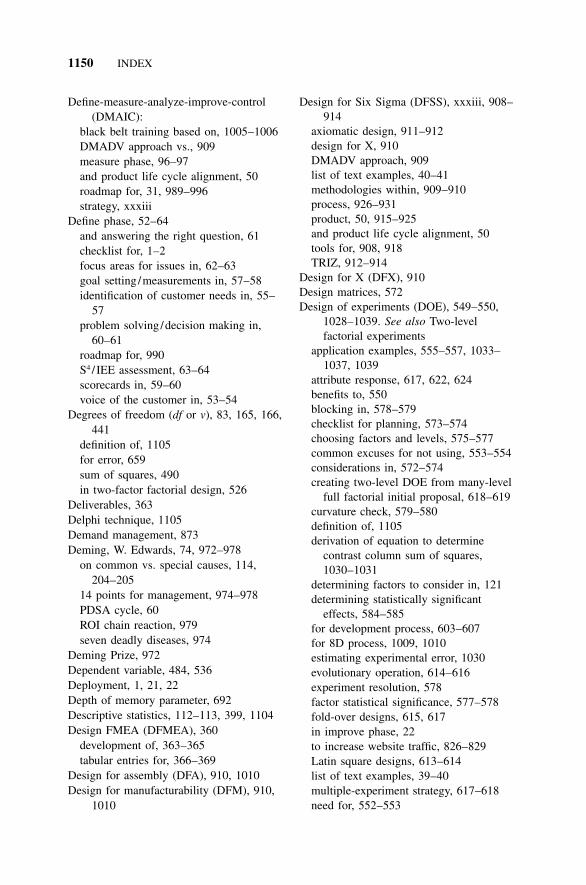
1150 INDEX

Define-measure-analyze-improve-control(DMAIC):

black belt training based on, 1005–1006DMADV approach vs., 909measure phase, 96–97and product life cycle alignment, 50roadmap for, 31, 989–996strategy, xxxiii

Define phase, 52–64and answering the right question, 61checklist for, 1–2focus areas for issues in, 62–63goal setting /measurements in, 57–58identification of customer needs in, 55–

57problem solving/decision making in,

60–61roadmap for, 990S4 / IEE assessment, 63–64scorecards in, 59–60voice of the customer in, 53–54

Degrees of freedom (df or v), 83, 165, 166,441

definition of, 1105for error, 659sum of squares, 490in two-factor factorial design, 526

Deliverables, 363Delphi technique, 1105Demand management, 873Deming, W. Edwards, 74, 972–978

on common vs. special causes, 114,204–205

14 points for management, 974–978PDSA cycle, 60ROI chain reaction, 979seven deadly diseases, 974

Deming Prize, 972Dependent variable, 484, 536Deployment, 1, 21, 22Depth of memory parameter, 692Descriptive statistics, 112–113, 399, 1104Design FMEA (DFMEA), 360

development of, 363–365tabular entries for, 366–369

Design for assembly (DFA), 910, 1010Design for manufacturability (DFM), 910,

1010

Design for Six Sigma (DFSS), xxxiii, 908–914

axiomatic design, 911–912design for X, 910DMADV approach, 909list of text examples, 40–41methodologies within, 909–910process, 926–931product, 50, 915–925and product life cycle alignment, 50tools for, 908, 918TRIZ, 912–914

Design for X (DFX), 910Design matrices, 572Design of experiments (DOE), 549–550,

1028–1039. See also Two-levelfactorial experiments

application examples, 555–557, 1033–1037, 1039

attribute response, 617, 622, 624benefits to, 550blocking in, 578–579checklist for planning, 573–574choosing factors and levels, 575–577common excuses for not using, 553–554considerations in, 572–574creating two-level DOE from many-level

full factorial initial proposal, 618–619curvature check, 579–580definition of, 1105derivation of equation to determine

contrast column sum of squares,1030–1031

determining factors to consider in, 121determining statistically significant

effects, 584–585for development process, 603–607for 8D process, 1009, 1010estimating experimental error, 1030evolutionary operation, 614–616experiment resolution, 578factor statistical significance, 577–578fold-over designs, 615, 617in improve phase, 22to increase website traffic, 826–829Latin square designs, 613–614list of text examples, 39–40multiple-experiment strategy, 617–618need for, 552–553

INDEX 1151

planning, 571–581probability plot in, 585with product development, 786–790QFD evaluation with, 794–800randomization in, 579reliability evaluations, 617resolution III, 619–622resolution V, 586–599robust, 630–642S4 / IEE assessments, 580, 607–609, 627sample size for continuous response

output DOE, 574–575sample size for mean factor effects,

1028–1030for service / transactional processes, 903settle-out time of stepper motor, 586–

599significance test for two-level

experiments, 103216-trial experiments, 599–603system DOE stress to fail test, 622–629and Table M design, 1038, 1039traditional experimentation vs., 551–552two-level design alternatives, 582–584two-level fractional experiment using

Tables M and N, 584two-level modeling equation format,

585–599Youden square designs, 614

Design of Experiments (Genichi Taguchi),973

Design parameters (DPs), 912Design requirements matrix (QFD), 350–

352Design verification plan / report, 1010Design wastes, 859Destructive testing, 307, 326–330. See also

Nonreplicable testingDetection evaluation criterion (FMEA),

368, 369, 375, 376Determination, coefficient of, see

Coefficient of determinationDevelopment:

of a bowling ball, 864–867product, see Product development

Development application examples:improving product development, 791–

794strategy for chemical product, 809–811

Development process(es):defining, 105–107DOE for, 603–607measurement / improvement of, 916–918

df, see Degrees of freedomDFA, see Design for assemblyDFM, see Design for manufacturabilityDFMEA, see Design FMEADFSS, see Design for Six SigmaDFX (design for X), 910Difference charts, 671Dimensional property, 19Direction of steepest ascent, 647, 666Discounted statements, 965Discrete data, 80, 1104. See also Attribute

dataDiscrete distribution, 1105Discrete flow manufacturing, 387Discrete random variable, 1105Discrete sample space, 142Discrimination:

of instruments, 318of a measurement system, 313, 1105

Discrimination ratio (d), 736, 1105Dispersion, 83Dispersion effects, 506, 636, 638, 639Dispersion graph, 485. See also Scatter

diagramsDistinct data categories, 1105Distributions, 148–166

applications for, 148–150, 169–171approximations, 169, 171, 428–431bell-shaped, 83bimodal, 416, 417, 1100binomial, 149, 153–156, 169, 230, 426–

428, 1100bivariate normal, 491child, 149chi-square, 163, 165, 456–457continuous, 1103cumulative frequency, 183definition of, 1105discrete, 1105double-sided t, 1044–1045exponential, 159–161F, 166, 167freak, 1107frequency, 183hazard rate for, 166–168

1152 INDEX

Distributions (continued )heavy-tailed, 199hypergeometric, 149, 157, 426–427, 432,

1108lognormal, 163, 164, 723, 756, 757,

766–768main, 1110multimodal, 1111multinomial, 169, 171nonnormal, process capability /

performance for, 290–292normal, 149–152, 190, 199, 427, 1112parent, 149Poisson, 149, 157–159, 169, 230, 427,

723–724, 734, 1113and probability paper plotting, 181of sample mean values, 400–401sampling, 149, 1117single-sided t, 1043skewed, 199, 248, 417t, 165, 166table forms for, 152tabulated probability, 163–167truncated, 417unimodal, 1122Weibull, 151–153, 722–723, 756–757,

1021–1022, 1123–1124Z, 268–269

DMADV, see Define-measure-analyze-design-verify

DMAIC, see Define-measure-analyze-improve-control strategy

DOA, see Dead on arrivalDocumentation. See also specific types

for 5-step measurement improvement,330

flowcharts for reduction of, 102for FMEAs, 363of processes, 104–105, 107

DOE, see Design of experimentsDOE collective response capability

assessment (DCRCA), 597–598, 1104Doers, people as, 958Domains (AD), 911Dominating participants (teams), 964Dot plots, 80–82Double-sided confidence intervals, 400,

403, 408, 411–413, 428

Double-sided confidence tests, 680, 1105Double-sided normal distribution, 151,

1042Double-sided t distributions, 1044–1045Downtime, 873, 874DPMO, see Defects per million

opportunitiesDPO (defects per total opportunities), 193DPs (design parameters), 912DPU, see Defects per unitDrift, measurement, 311Drill-down, 33

CTS tree diagram, 72, 73for process documentation, 107–108from roadmap, 36in Smarter Solutions project execution

roadmap, 1006of 30,000-foot-level KPOVs, 207

Drivers (interaction style), 959, 960Driving forces, 120DSO, see Days sales outstandingDummy activity, 950Dummy variables, see Indicator variables

Early-life failures, see Bathtub curveEase-of-resolution matrix, 122ECHIP, 663Economic Control of Quality of

Manufactured Product (Walter A.Shewhart), 973

EDA, see Exploratory data analysisEdison, Thomas, 967Education, statistical, 405. See also

Learning; TrainingEdwards, George D., 972Edwards Medal, 972Effect(s), 121, 122

best estimate factor, 557, 558confused, 93–94contrast column, 1103definition of, 1106factor, 1030interaction, 558–559magnitude of, 566, 567main, 1110mean, 387, 1028–1030statistically significant, in DOE, 584–585two-factor interaction, 558–559

INDEX 1153

Effectiveness:overall equipment, 874, 875Paynter charts for, 1007of teams, 957–966

Efficiency, 574definition of, 1106in manufacturing, 910

Efron, Bradley, 466, 4718D (8 disciplines), 61, 970, 1006–10118-trial two-level full / fractional factorial

designs, 575, 1064Eight laws of engineering system

development, 913Electromagnetic interference (EMI)

emissions, 772Elevate step (TOC), 889Emergency response action (ERA), 1007,

1009EMI (electromagnetic interference)

emissions, 772Employees:

involvement of, 972opinion survey effectiveness with, 815–

816S4 / IEE training agenda for, 1005–1006training agenda for, 1005–1006

Empowerment, 941–942Encouragement (for creativity), 969Energy transfer in the system, law of, 913Engineering applications of distributions,

169Engineering process control (EPC), 690,

692–702application examples, 690–691with EWMA, 692–701for process adjustment optimizing, 275

Engineering system development, eightlaws of, 913

Enthusiasts (interaction style), 959, 960Eo, see Activation energyEPC, see Engineering process controlEPE day (every part every day), 883Epsilon square relationship, 514–515Equality of variance, 506Equipment maintenance, 873Equipment variation (EV), 310–311, 317Equity valuation, 19ERA, see Emergency response action

Error(s):estimate of, 797, 1030experimental, 585, 1030, 1106, 1130internal estimate of, 572in KPIV levels, 708measurement, 90–92, 307, 326measurement system, 310, 1111NID(0, �2) assumption for, 492and process control, 220in project estimating, 947random, 678random sampling assumption about, 96reproducibility, 311risk of, 1029in simple linear regression, 487, 489standard, 658, 659, 1119standard deviation of, 1029sum of squares due to, 503–504type I, 60, 403–404, 1122type II, 60, 403–404, 1122type III, 60, 1122

Error-proofing, 708–709, 716Escape, 49, 731, 1106Escape point, 1009, 1010Estimate of error, 797, 1030EV, see Equipment variationEvery part every day (EPE day), 883Evolutionary operation (EVOP), 614–616,

1106EWMA, see Exponentially weighted

moving averageEWMA chart, 275, 691–692, 695Exact critical values (ANOM), 1053–1058Examples, 38–41. See also section titles

within table of contents for completelisting of text examples

Design for Six Sigma, 40–41design of experiments, 39–40generic process measurement and

improvement, 39testing products / reliability, 40

Excel, 43Executives:

CEO and embrace of Six Sigma, 48change and replacement of, 943and change management, 940–941communications between practitioners

and, 50

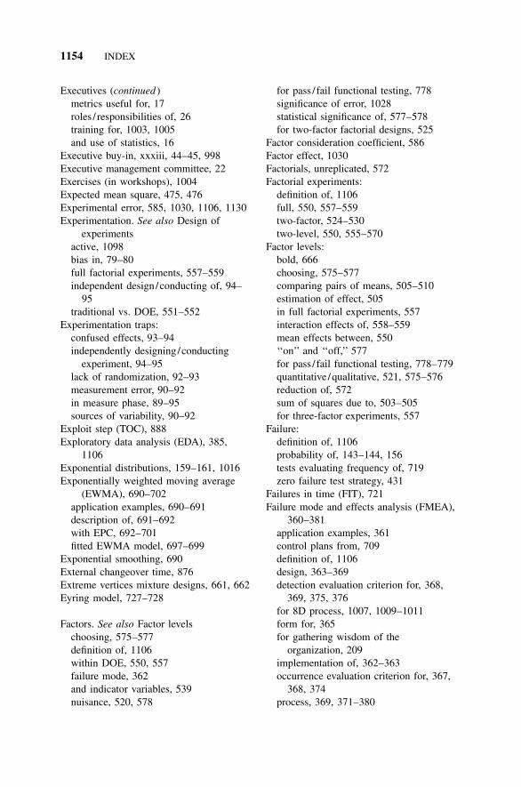
1154 INDEX

Executives (continued )metrics useful for, 17roles / responsibilities of, 26training for, 1003, 1005and use of statistics, 16

Executive buy-in, xxxiii, 44–45, 998Executive management committee, 22Exercises (in workshops), 1004Expected mean square, 475, 476Experimental error, 585, 1030, 1106, 1130Experimentation. See also Design of

experimentsactive, 1098bias in, 79–80full factorial experiments, 557–559independent design /conducting of, 94–

95traditional vs. DOE, 551–552

Experimentation traps:confused effects, 93–94independently designing/conducting

experiment, 94–95lack of randomization, 92–93measurement error, 90–92in measure phase, 89–95sources of variability, 90–92

Exploit step (TOC), 888Exploratory data analysis (EDA), 385,

1106Exponential distributions, 159–161, 1016Exponentially weighted moving average

(EWMA), 690–702application examples, 690–691description of, 691–692with EPC, 692–701fitted EWMA model, 697–699

Exponential smoothing, 690External changeover time, 876Extreme vertices mixture designs, 661, 662Eyring model, 727–728

Factors. See also Factor levelschoosing, 575–577definition of, 1106within DOE, 550, 557failure mode, 362and indicator variables, 539nuisance, 520, 578

for pass / fail functional testing, 778significance of error, 1028statistical significance of, 577–578for two-factor factorial designs, 525

Factor consideration coefficient, 586Factor effect, 1030Factorials, unreplicated, 572Factorial experiments:

definition of, 1106full, 550, 557–559two-factor, 524–530two-level, 550, 555–570

Factor levels:bold, 666choosing, 575–577comparing pairs of means, 505–510estimation of effect, 505in full factorial experiments, 557interaction effects of, 558–559mean effects between, 550‘‘on’’ and ‘‘off,’’ 577for pass / fail functional testing, 778–779quantitative /qualitative, 521, 575–576reduction of, 572sum of squares due to, 503–505for three-factor experiments, 557

Failure:definition of, 1106probability of, 143–144, 156tests evaluating frequency of, 719zero failure test strategy, 431

Failures in time (FIT), 721Failure mode and effects analysis (FMEA),

360–381application examples, 361control plans from, 709definition of, 1106design, 363–369detection evaluation criterion for, 368,

369, 375, 376for 8D process, 1007, 1009–1011form for, 365for gathering wisdom of the

organization, 209implementation of, 362–363occurrence evaluation criterion for, 367,

368, 374process, 369, 371–380

INDEX 1155

severity evaluation criterion for, 366,367, 371–373

team for, 362Failures per thousand hours (%/K), 721Failures per unit of time (ra), 733Failure rate(s), 733. See also Reliability

testing /assessmentaverage, 721confidence interval for evaluations of,

739–740converting, to Cpk, 298definition of, 1106hypothesis test of, 739–739intrinsic failure period, 168plotting, 230–231repairable system testing for changing,

747–752system, tests of, 734–735tracking chart for, 731with two-factor interactions, 552

Fault tree analysis, 1107Fault tree (FT), 124F distributions, 166, 167, 1046–1049Feedback:

for behavior reinforcement, 937–938team, 963

Feigenbaum, Armand V., 972–973Ferrell median regression line, 1023–1025Feuding team members, 96650-foot level, xxxii

control charts for, 207–208definition of, 1107for KPIV tracking, 709

Financial analysis, 953–955Firefighting, 20–21, 32–33

with customers, 48definition of, 1107high-level metrics for reduction of, 218–

219Fire prevention, 32–33

with customers, 48S4 / IEE roadmap for, 208statistics for, 64

‘‘Firms Air for Six Sigma Efficiency’’(Jones), 7

First-time yield, 154Fishbone diagrams, 121. See also Cause-

and-effect diagrams

Fisher, R. A., 165FIT (failures in time), 721Fitted EWMA model, 697–699Fitted value plots, 506Fitted values (residual analysis), 4935S method, 858, 872–8735-step measurement improvement process,

330–340accuracy (linearity), 332–333, 338–339example of, 335–340fixture study, 332, 337–338long-term stability, 334–335, 340machine variation, 331, 335–337repeatability and reproducibility, 333–

334, 339–340Five focusing steps (TOC), 8885 whys, 862, 863, 1008Fixed costs, 953Fixed-effects model:

definition of, 1107random effects model vs., 474statistical model for, 500two-factor factorial analysis of variance

for, 526Fixed-failure reliability testing, 734Fixed-length reliability testing, 734, 735Fixture variation study, 332, 337–338Floundering (teams), 964Flowcharts /flowcharting, 102–110

application examples, 103of changeover, 876defining process, 104–107description of, 103–104for 8D process, 1007focusing efforts after process

documentation, 107key process determination, 104–105project, 955S4 / IEE assessment, 107–108supply chain, 867–869

Flow (in lean), 858–859, 873, 877Flow kaizen, 861FMEA, see Failure mode and effects

analysisFold-over designs, 615, 617, 784, 1107Force-field analysis, 24, 119–121, 1010,

1011, 1107Ford Motor Company, 61

1156 INDEX

Forecasting, 873Forming stage (teams), 9584-trial two-level full / fractional factorial

designs, 575, 1062–106314 points for management (Deming), 50,

972, 974–978Fractional factorial experiments, 550

definition of, 11078-trial, 575, 1064factors with various resolutions in, 5784-trial, 575, 1062–1063pass / fail functional testing, 771–791percentage test coverage from, 774and problem definitions, 571in product development cycle, 787–790sample size for, 559, 1028saturated, 559–56116-trial, 575, 1065, 1068–107164-trial, 575, 1068–107132-trial, 575, 1066–1067two-factor interaction effects

confounding in contrast columns ofTables M resolution III, 1076–1080

two-factor interaction effectsconfounding in contrast columns ofTables M resolution IV, 1073–1075

two-factor interaction effectsconfounding in contrast columns ofTables M resolution V, 1072

Fraction nonconforming (p), 231, 235. Seealso p charts

Freak distributions, 1107Frequency distribution, 83–84, 183Friedman test, 530–531FRs, see Functional requirementsF statistic, 89F test, 447FT (fault tree), 124Full factorial experiments, 550, 557–559

and confused effects, 94creating two-level DOE from proposal

for, 618–619definition of, 11078-trial, 10644-trial, 1062–1063sample size for, 55916-trial, 106564-trial, 1068–107132-trial, 1066–1067

Functional benchmarking, 117Functional requirements (FRs), 909, 912Future state value stream map, 877, 878,

884–885Future value, 954

Gage, 1107Gage blocks, 307, 1107Gage linearity, 322–323Gage repeatability, 307Gage repeatability and reproducibility

(R&R), 307, 309, 312–314attribute study, 323–325definition of, 1107destructive testing study, 326–330essential characteristics for, 312example of, 318–322in 5-step measurement improvement

process, 333–334, 339–340relationships, 314–317variance components analysis vs., 482

Gage reproducibility, 307Gage R&R, see Gage repeatability and

reproducibilityGage R&R (GRR), 316, 317Galvin, Bob, 5Gamma function, 764, 1018, 1052Gantt charts, 948, 950, 1010Gap (between output and expectations), 35Gate-keeping, 964, 965Gaussian curve, 149GDT, see Geometric dimensioning and

tolerancingGeneral Electric (GE), 5–7, 936, 938General linear modeling (GLM), 1107General Motors, 61Generic benchmarking, 117Geometric dimensioning and tolerancing

(GDT), 1107–1108Geometric smoothing, 690Germaine, Jack, 5GE Work-Out, 968–987GLM (general linear modeling), 1107Goals:

in define phase, 57–58numerical, 978organizational, 17, 18SMART, 57stretch, 43, 58, 446team, 961

INDEX 1157

Go/no-go, 226, 426, 1108Goodness, analysis of, 607Goodness level, 12, 212Goodness-of-fit (�2) test, 456, 1108Goodness-of-fit (R2), 323Gosset, W. S., 165Graphic presentation. See also specific

typesin analyze phase, 385of gage R&R studies, 322in measure phase, 80–81for visualization of data, 391, 392

Green belts, 31roles / responsibilities of, 28as S4 / IEE practitioners, 28, 1000training for, 1004, 1006use of term, 31

Grieving, 944Ground rules (for teams), 962Group process, 962Group size, 1019, 1108Groupthink, 1108Growth, 19GRR, see Gage R&RGuiding coalition, forming, 940–941

Ha, see Alternative hypothesisHadamard matrix, 584Half-fraction factorial design, 587Half-normal probability plot, 585, 659,

1108Happenstance data, 485, 536Hard savings, 42, 1108Harmonization, law of, 913Hazard paper:

definition of, 1108for lognormal distributions, 1088for normal distributions, 1087for Weibull distribution, 1089

Hazard plots /plotting, 181–185nonrepairable device reliability testing,

757–762and probability plots, 176for Weibull distribution, 182, 184, 759,

761, 762Hazard rate (�), 166–168

definition of, 148, 1108of exponential distributions, 1016of Weibull distributions, 1018

Head count, 19Heavy-tailed distributions, 199‘‘Hidden factor,’’ 284Hidden factory, 20, 877

definition of, 1108process improvement and exposure of,

823–826Hierarchical decomposition, 911–912Hierarchy rule, 586High-level control charts, 208High-level process map, 35High-level supply chain map, 33High-temperature accelerated testing, 725–

727Histograms, 80–82

data grouping for, 176definition of, 1108for 8D process, 1007manual creation of, 1019–1021

Historical targets, 671Ho, see Null hypothesisHomogeneous Poisson process (HPP),

148–150, 168–169, 1108Hoshin, 1108House of quality, 349Hows, 349, 351–355How much area, 354, 355HPP, see Homogeneous Poisson ProcessHumanism, 861Hypergeometric distributions, 157

applications for, 149definition of, 1108equation for, 1015for pass / fail attribute response, 426–427,

432Hypothesis, see Alternative hypothesis;

Null hypothesisHypothesis tests / testing, 87–89, 399–404

about one population, total run time for,738

of attribute criterion, 427–428for correlation coefficient to equal zero,

486criteria alternatives, 410–411definition of, 1108–1109example of, 404–405of failure rate criterion, 739–739of mean criterion for continuous

response data, 408

1158 INDEX

Hypothesis tests / testing (continued )S4 / IEE assessment, 405selection tree for, 997single-factor analysis of variance, 502–

503type I / type II errors in, 403–404

IBM, 8ICA, see Interim containment actionI charts, see X chartsIdeal state value stream map, 877Identify step (TOC), 888IDs, see Interrelationship digraphsIEE, see Integrated Enterprise ExcellenceImplement stage (Work-Out), 987Improvement(s), 22

changing metrics to reflect, 32consolidation of, 942–943continuous, 3, 188, 860–861and day-to-day management, 32–33of development process, 916–918in employee opinion survey

effectiveness, 815–816identifying areas for, 75list of text examples, 39process, see Process improvementsfor processes with common cause

variability, 209–210for service processes, 137–139in sigma quality level, 12tracking, 46–48

Improvement plan (teams), 961Improve phase, 547–548. See also Design

of experimentschecklist for completion of, 54DOE tools in, 22proactive testing in, 22roadmap for, 993

I-MR charts, 226. See also XmR chartsIn control. See also Common causes;

Statistical stabilitydefinition of, 1109implications of, 248processes, 213, 215, 220, 222values, 223

Increasing ideality, law of, 913Increasing substance-field involvement, law

of, 913

Incubation (for creativity), 969Independence, 96, 493

across time, 693as design axiom, 912

Independency, lack of, 456Independent experimental design /

conducting, 94–95Independent (samples), 477Independent variable, 484, 489, 536, 550Indicator variables (dummy variables), 533,

539–542Indifference quality level (IQL), 211, 1109Individuals, recognizing contributions of,

1011Individual values (X), 226. See also X

chartsInductive reasoning, 405, 462Industrial engineering, 861Inferences:

attribute response, 426–435continuous response, 407–425

Inferential statistics, 399, 1109Information (as design axiom), 912Information board (EVOP), 614, 616Infrastructure building /management, 957Infrequent subgrouping/sampling, 12, 32,

208advantages of, 247for avoiding process capability /

performance confusion, 299definition of, 1109examples of, 208for high-level metrics, 218–219intents for, 208

Inherent process variation, 284, 357Injection-molding data:

analysis of means of, 513–514multi-vari chart of, 387–389plots of, 390–392variance components analysis of, 480–

481Inner array, 635, 1109Inputs, 10–11. See also Key process input

variablescontrollable, 10, 11in S4 / IEE strategy, 98uncontrollable, 10, 11variables in, 347

INDEX 1159

Input-process-output (IPO), 10Inspection plans, 171Inspections:

effectiveness of, 210visual, see Visual inspections

Instability, 220Institutionalizing change, 943Instructional material, licensing of, 1004Integrated Enterprise Excellence (IEE),

xxxi, 1109Integrity:

data, 306measurement systems, 307

Intensity function, 149, 168, 750–751,1109

Interaction(s):aliased, 583definition of, 1109of experimental factors, 572–573as product of factors, 586resolution III DOE, 619–622of row and column factor effects, 525seven-factor, 578styles of, on teams, 958–960in Taguchi test strategy, 632in two-factor ANOVA vs. randomized

block design, 526Interaction columns, 558, 559Interaction contrast columns, 565–568, 579Interaction effect(s), 558

statistical significance of, 585two-factor, 558–559

Interaction plot, 390, 392Intercept cells, 539, 541Interest / interest rates, 954Interim containment action (ICA), 1007–

1010Internal benchmarking, 117Internal changeover time, 876Internal rate of return (IRR), 955International Organization for

Standardization (ISO), 972Interrelationship digraphs (IDs), 24, 26,

123, 124, 1109Interviews, 349, 1007, 1011Intrinsic failure period, 168Invention, 913–914, 967Inventive problems, 913

Inventive thinking, 969–970Inventory (as TOC metric), 19, 46, 887,

888Inverse power law, 728Investment / inventory (as TOC metric), 19Iomega, 38IPO (input-process-output), 10IQL, see Indifference quality levelIRR (internal rate of return), 955Ishikawa, Kaoru, 121, 973Ishikawa diagrams, 121, 973. See also

Cause-and-effect diagramsIs / is not, 1008, 1010ISO 9000, xxxi, xxxii, 102, 972ISO 9000:2000, 29, 48, 982–983ISO (International Organization for

Standardization), 972

Japan, 972–974JIT, see Just-in-timeJuran, Joseph M., 74, 205, 973Just-in-time (JIT), 190, 858–859

k, see Characteristic life; Scale parameterKaizen, 860–861, 972Kanban, 876–877Kano diagram, 54KCA, see Knowledge-centered activityKey process input variables (KPIVs), 11,

12on cause-and-effect matrix, 356–357classification of, 72determining, 104–105driving KPOV, 46errors in, 70850-foot level, 207, 7095S method as, 872optimum levels for, 717on process maps, 103tracking, 46–47

Key process output variables (KPOVs), 10–12, 19–21

assessment of, 209classification of, 72determining, 104–105drill-down of, 207effect of process input variables on, 347KPIVs driving, 46

1160 INDEX

Key process output variables (KPOVs)(continued )

process improvement impact to, 25on process maps, 103tracking, 45–47traditional Six Sigma parameters vs., 45–

47variance components effect on, 475

Key system outputs, 52K factors, 414Knees:

probability plot, 761Weibull plot, 763

Knowledge-centered activity (KCA), 52–53, 971, 980, 1109

Knowledge management, 982KPIVs, see Key process input variablesKPOVs, see Key process output variablesKruskal-Wallis nonparametric test, 518–519Kurtosis calculation, 1026

�, see Hazard rateLack-of-fit, 181, 574, 1026, 1109Lack-of-fit tests, 666, 1026Lag, 693–694Lambda plot, 506, 1110Latin square designs, 613–614Laws of engineering system development,

913LCL, see Lower control limitLDL (lower decision lines), 511Leadership, quality, 979–980Leadership training, 1005Lead time, 860, 876, 1110Lean, 857–885

changeover reduction, 876definition of, 1110and demand management, 8735S method, 872–873and kanban, 876–877as term, 31and total productive maintenance, 873–

876value stream mapping, 877–885

Lean enterprise, 31Lean manufacturing, xxxii, xxxiii, 6, 29,

31, 857–858, 972, 999Lean metrics, 31, 860Lean process steps, 861–862Lean production, 31

Lean/Six Sigma projects, xxxiiLean thinking, 31, 939Lean tools, 68, 861Learning:

adult needs in, 1004organizational, 944–945student, 945

Learning disabilities, 51Learning organizations, 51, 207, 945Least squares, 489–490, 1110Lessons learned, 998, 1002, 1011

attributes of successful vs. lesssuccessful case studies, 49

Levels:coded, 1102definition of, 1110within DOE, 550goodness, 12, 212for new product development, 106of quality, see Quality levels

Level of the test, 403Levene’s test, 445, 447, 506Licensing:

of instructional material, 1004S4 / IEE, inquiries about, xii

Likert Scale, 815–816Linearity:

definition of, 322, 1110in 5-step measurement improvement

process, 332–333, 338–339as location metric, 312in measurement systems analysis, 309

Linearity graphs, 313Linear regression models, 489. See also

Simple linear regressionLoad leveling, 882, 883Location (in measurement systems), 312Location parameter (xo), 161, 1110Lockheed Martin, 7, 8, 938–939Logarithmic transformation, 635Logic flow map, 862Logic pass / fail response, 85, 771, 773. See

also ResponseLogistic regression, binary, 542–544Logit (transformation), 1110Lognormal distributions, 163, 164

applications for, 149hazard paper for, 1088for nonrepairable device testing, 723,

756, 757, 766–768

INDEX 1161

probability paper for, 1085Lognormal transformations, 506, 507Lombardi, Vince, 58Long-term capability, 260Long-term ppm nonconformance rates, 291Long-term process capability /performance,

267, 514–516Long-term stability:

in 5-step measurement improvementprocess, 334–335, 340

of measurement system, 334–335Long-term standard deviation, 261, 265,

515Long-term variability, 259–260, 297–298Loss function, 632–634, 1110Lot tolerance percent defective, see

Rejectable quality levelLower control limit (LCL), 114, 115, 130–

131below-zero, 231determining, 223

Lower decision lines (LDL), 511LTPD, see Rejectable quality level

�, see Mean; True meanMachine variation, 331, 335–337Main distribution, 1110Main effects:

confounding of, 560definition of, 1110statistical significance of, 585

Main effects plot, 390, 391Malcolm Baldrige assessment, xxxi, 29,

984–985Malcolm Baldrige National Quality Award,

5, 972, 984Mallows Cp statistic, 537, 1110Management. See also Executives

alignment of initiatives / strategies withS4 / IEE, 971–988

asking right questions by, 4change, 935–945commitment to business strategy by, 22and creativity, 967–970demand, 873Deming’s 14 points for, 974–978Deming’s seven deadly diseases, 974GE Work-Out, 968–987goal-setting by, 58ISO 9000:2000, 982–983

Malcolm Baldrige assessment, 984–985of nuisance factors, 520organization, 978–981project, 946–956quality, 981–982quality leadership in, 979–980quality philosophies /approaches in, 971–

972by results, 978S4 / IEE assessment, 987S4 / IEE training agenda for, 1005–1006Shingo Prize, 985–986for team effectiveness, 957–966top-rated people in, 972–973training agenda for, 1005–1006value stream, 877–878and wise use of statistical tools, 16

Managing Six Sigma (Breyfogle), xxxiiiMann-Whitney procedure, 518Manufactured door, 478, 479Manufacturing:

applications for, 895–900design FMEA for, 363efficiency in, 910lean, 857–858loss function in, 633measuring systems in, 306–307short-run charts in, 670

Manufacturing application examples. Seealso Development applicationexamples

AQL deception and alternative, 829–830AQL test assessment, 847–848automobile test—answering the right

question, 817–823process improvement and exposing the

hidden factory, 823–826QFD evaluation with DOE, 794–800qualification of capital equipment, 848–

851qualification of supplier’s production

process and ongoing certification,851–852

reliability and functional test of anassembly, 800–809

tracking/ improving change order times,813–815

tracking ongoing product compliance,811–813

1162 INDEX

Manufacturing processes:analysis techniques for, 205confirmation experiments for, 599and EVOP, 614experimental factors to consider for, 552problems with, 74–75, 205test strategy for, 553variance components within, 475

Manufacturing wastes, 859Mapping (AD), 911Marginal plot, 390, 391Market constraints, 888Maslow, Abraham, 861Master black belts, 31

roles / responsibilities of, 27training for, 1006

Material and information flow mapping,877. See also Value stream mapping

Matrices, QFD, 350Matrix diagrams, 125Maximum likelihood estimator (MLE):

definition of, 1110as a descriptive statistic, 113

Mean effects, 1028–1030Mean effects plot, 387Mean square, 475–476, 490, 1110Mean time between failures (MTBF), 240,

720, 722, 733, 1110Mean (x or �), 80, 82–83. See also x

chartsof binomial distribution, 1015bootstrapping and confidence interval

for, 467–470and central tendency, 84comparative tests of, 997comparing, of two continuous response

samples, 438–440confidence intervals on, 409–412definition of, 1110as a descriptive statistic, 112hypothesis test of, 502–503in Poisson distributions, 1016sample (x), 400–401, 407subgroup, XMR chart of, 245–247true (�), 158, 160, 407

Measures:effective use of, 297in project management, 948, 950–951for S4 / IEE projects, 96

Measurement(s). See also Measure phase;specific measurements

accuracy in, 309basic Six Sigma concept of, 13basic tools for, 111–112cascading, xxxii, 32–33choosing, 4converting DPMO or PPM to sigma

quality level units, 188–189in define phase, 57–58of development process, 916–918in gage R&R studies, 312list of text examples, 39measurement system analysis (measure

phase), 69precision in, 309process, 902–903for processes with common cause

variability, 209–210within S4 / IEE, 46Six Sigma, 188–203stability of, 311variability sources in, 90

Measurement drift, 311Measurement error, 307

for destructive tests, 326as experimentation trap, 90–92

Measurement systems. See alsoMeasurement systems analysis

definition of, 1111discrimination of, 1105and level of variability, 300purpose of, 312quality of, 307stability in, 312

Measurement system error, 310, 1111Measurement systems analysis (MSA), 69,

306–346, see Gage repeatability andreproducibility

application examples, 309–310attribute gage study, 323–325destructive testing gage study, 326–3305-step measurement improvement

process, 330–340gage R&R considerations, 312–314gage R&R example, 318–322gage R&R relationships, 314–317linearity, 322–323philosophy of, 308

INDEX 1163

preparation for, 317–318S4 / IEE assessment, 341for service / transactional processes, 902–

903sources of variability in, 90terminology related to, 310–311variability sources in 30,000-foot-level

metrics, 308–309Measurement tool-to-tool, 90Measurement variance, 308, 330Measure phase, 65–101. See also specific

topicsanalysis of variance output interpretation,

87–89attribute vs. continuous data response,

85–86baseline project, 67–68basic tools for, 111–112checklists for, 65–70common vs. special causes in, 74–75components to, 65consider lean tools, 68DMAIC, 96–97experimentation traps in, 89–95graphic presentations, 80–81hypothesis testing, 87–89improving a process that has defects

(example), 130–133improving service processes (example),

137–139measurement system analysis, 69plan project and metrics, 66reacting to data example, 75–79reducing total cycle time of processes

(example), 133–136roadmap for, 991S4 / IEE assessment, 97–99sample statistics, 81–84sampling considerations in, 96sampling in, 79–80variability in, 72, 74visual inspections, 86–87voice of the customer in, 71–73wisdom of the organization, 69–70

Median, 84confidence interval for, 471–472definition of, 1111as a descriptive statistic, 113of variable described by PDF, 177

Median charts, 236Median life, 759, 1017Median regression line, 1023–1025Median test, see Moods’ median testMeetings, team, 108, 961–962Metrics. See also specific metrics

for balanced scorecards, 59cascading, 29, 32–33controversial, in Six Sigma, 514–51650-foot level, xxxii. See also 50-foot levelguidelines for, 42lean, 31for operation activity orchestration, 980–

981plan project and metrics (measure

phase), 66satellite level, xxxii. See also Satellite

levelfor service / transactional processes, 902Six Sigma, 12–15, 188–20330,000-foot level, xxxii. See also

30,000-foot levelwithin TPM, 874wise address of, 24

Metrology, 307, 1111Micrometer calipers, 1111Micrometer readings, 85Micrometers, 307Mil, 1111Minimum (as descriptive statistic), 113Minitab, 43, 298, 311, 1004Mistake-proof /proofing, 708, 716Mixture experiments, 650–663

computer-generated, 661–665definition of, 1111extreme vertices, 661, 662with process variables, 656–661simplex lattice designs for exploring

whole simplex region, 652–657MLE, see Maximum likelihood estimatorModel bias, 574Model equations, 521Modeling equations, 585–599, 643–644Modified pre-control, 704–706Moe, Keith, xxxiMonetary issues:

communications as, 51guidelines for, 42in selling Six Sigma benefits, 44

1164 INDEX

Moods’ median test, 518–520Motivational forces, 936Motorola, 4–6, 267, 269Moving range (MR), 226–228, 678Moving range (MR) charts, 226, 227. See

also XmR chartsMR, see Moving range

see Average moving rangeMR,MR charts, see Moving range chartsMSA, see Measurement systems analysisMTBF, see Mean time between failuresMuda, 858Multicollinearity, 536, 664, 1111Multimodal distribution, 1111Multinomial distribution, 169, 171Multiple events, probability with, 142–143Multiple event relationships, 143–144Multiple-experiment strategy (DOE), 617–

618Multiple-hypothesis testing, 88Multiple regression, 489, 533–534

application examples, 533best subset analysis, 536–539description of, 534example of, 534–536

Multiple time censoring, 181, 182Multivariable testing (MVT), 550Multi-vari charts, 386–389, 1111Multi-vari study, 709Murder mystery, 11MVT (multivariable testing), 550

n, see Noise factors; Sample size�, see Degrees of freedomNatural characteristics (control charts), 220Natural process variation (NPV), 330Natural tolerances of a process, 225, 226,

1111Natural variables, 647–649ndc, see Number of distinct categoriesNegative reinforcement, 937Nested data, 1111Nested design, 341, 475–476Net costs, 955Net financial benefits, 955Net present value (NPV), 53, 954NGT, see Nominal group techniqueNHPP, see Nonhomogeneous Poisson

ProcessNID(0, �2) assumption, 492, 505

Nine M’s of quality, 973Noise, 10, 11, 21Noise factors (n), 107, 122Noise inputs variables, 10, 11, 209, 630Nomenclature (Six Sigma), 189Nominal chart, 671Nominal conditions, 552Nominal group technique (NGT), 119, 964,

1111Nominal value, 634, 671Nomogram, 682–683Nonconformance proportions, 458–460Nonconformance rates, 212, 213, 291Nonconformities per unit charts, see u

chartsNonconstant variance, 493Noncontrollable factors, 635Nondestructive testing, 307Nonhomogeneous Poisson process (NHPP):

uses of, 150with Weibull intensity, 148, 168, 747–

748, 1111Nonindependence, 692–693Nonlinear data plots, 761, 763–764Nonmanufacturing (transactional)

processes, 901–907applying DOE to, 561–570measurement / improvement, 902–903MSA issues in, 307probability plot for, 209–210S4 / IEE approach to, 867–872test strategy for, 55321-step integration of tools, 903–907

Nonnormal data, 291Nonnormal distributions:

process capability /performance for, 290–292

situations exhibiting, 199transformations for, 291

Nonparametric estimates, 400Friedman test, 530–531Kruskal-Wallis test, 518–519Mann-Whitney procedure, 518Moods’ median test, 518–520runs test for randomization, 420–421

Nonrepairable devices, 720–721, 1111–1112

Nonrepairable device reliability testing,722–723, 756–770

hazard plotting, 757–762

INDEX 1165

lognormal distribution, 766–768nonlinear data plots, 761, 763–764reduced sample size testing, 764–766repairable vs., 721–722S4 / IEE assessment, 768Weibull probability plotting, 757–759

Nonreplicable testing, 307, 1112. See alsoDestructive testing

Nonsignificant main effect terms, 584–585Nonstationary process, 1112Non-value-added activities, 63, 859Normal distributions, 150–152, 199

applications for, 149applied to Six Sigma, 12–14for approximation of binomial

distribution, 427bivariate, 491definition of, 1112double-sided, 151, 1042equation for, 1014hazard paper for, 1087probability paper for, 1084single-sided, 151, 1042standardized normal distribution

relationships for Z, 190Normality assessment:

residual analysis, 492statistical tolerancing, 417

Normalization of data, 291Normal probability density function (PDF),

84, 149, 150, 1014Normal transformations (Z value), 197–198Norming stage (teams), 958Notebook computer development, 923–924No trouble found (NTF), 553, 603, 923No-value-added activities, 107np charts, 214, 219, 235, 237–239NPV, see Net present valueNPV (natural process variation), 330NTF, see No trouble foundNuisance factors, 520, 578Null hypothesis (Ho), 87–88, 402–404

for comparing attribute data, 456for comparing means of two samples,

438for comparison test, 437definition of, 1112and risk types, 60, 409, 410

Number of days from customer-requesteddate, 19

Number of days from promise date, 19Number of distinct categories (ndc), 317,

329, 330Number of nonconforming items, 235. See

also np chartsNumber of nonconformities (c), 235Number of nonconformities charts, see c

charts

Objectives:organization, 978project, 946–947

Observation, process, 862Occurrence evaluation criterion (FMEA),

367, 368, 374OC curve, see Operating characteristic

curveOff-line conversation /confrontation, 963Off-page connector, symbol for, 104Ohno, Taiichi, 861One-at-a-time experiments, 99, 551–553,

619, 1112One-way analysis of variance, see Single-

factor analysis of varianceOne-way ANOM, 459–460Ongoing reliability test (ORT), 752–753On-page connector, symbol for, 104On-time delivery, 19Operating characteristic (OC) curve, 211–

212Operating expense (as TOC metric), 19,

887–888Operational quality planning, 981, 982Opinions, unquestioned acceptance of, 965Optical comparators, 1112Optimization, 51Ordinal, 1112Ordinate, 1112Organization(s):

average, 189change initiatives in, 935learning, 51, 207, 945management /quality leadership in, 978–

981test, 786–787value in, 967wisdom of, 69–70, 209world-class, 189

Organizational goals, 17, 18Organizational learning, 944–945

1166 INDEX

Organizational objectives, 978Organizational policy, 17, 47Organizational structure, 22Orientation (for creativity), 969Orming model, 957–958, 1112ORT, see Ongoing reliability testOrthogonal, 1112Orthogonal array, 613, 631Outer array, 635, 1112Outlier(s), 492, 493, 1112Out of control. See also Special causes

control plans for, 709definition of, 1112processes, 213, 215, 216, 219–221runs tests for, 227as special-cause problem, 243values, 223

Output(s), 10–12. See also Key processoutput variables

of analysis of variance, 87–89describing predictable output when no

specification exists, 284–290for fractional factorial experiments, 577as function of system, 886gage R&R, 318, 320–322from gage R&R analyses, 315–316key system, 52in S4 / IEE strategy, 98–99variables in, 347

Overall equipment effectiveness, 874, 875Overbearing participants (teams), 964Overproduction, 878

P, see Fraction nonconforming; Probability;Test performance ratio

Pacemaker process, 882, 883Pain, fear of, 936Paired comparisons, 127, 128Paired comparison testing, 443–445Parameter design, 96, 800Parametric estimates, 400Parent distribution, 149Pareto charts, 33, 116–117

application examples, 116construction procedure for, 117definition of, 1112for DPMO by failure type, 194for 8D process, 1007

for identifying areas for improvement,75

for service process improvement, 137,139

of solder defects, 131–133use of, 60

Pareto principle, 116, 1112Participation, team, 962Parts per million (ppm), 12–15, 721

calculating, from Z values, 272–274conversion between sigma and, 188–189,

299, 1090–1091conversion of Z variable to, 192

Parts per million per thousand hours (ppm/K), 721

Part-to-part variation (PV), 316–317Part variation (PV), 310, 317, 1112Pass / fail functional testing, 771–791

of an assembly (application example),800–809

applications of, 785–786approach for, 773–775assigning factors, 778automotive test example, 772–773for computer systems, 775–778concept of, 771–772definition of, 1112diagnostic search pattern strategy, 781–

785factor levels greater than 2, 778–779matrix coverage for, 1081product development management with

DOEs, 786–790S4 / IEE assessment, 790software interface test, 779–781

Pass / fail logic response, 771, 773Pass / fail response, see Attribute responsePassive analysis, 21, 22, 383, 1113. See

also Analyze phasePath of steepest ascent, 555, 647, 1113Payback period, 955Paynter chart, 1007, 1009, 1010, 1113PCA, see Permanent corrective actionp charts, 231–234

alternatives to, 237–239application examples, 232variables data vs., 283–284

PDCA (plan-do-check-act) cycle, 60

INDEX 1167

PDF, see Probability density functionPDPCs, see Process decision program

chartsPDSA cycle, see Plan-do-study-act cyclePercentage of population statement, 115,

142, 415–417Percentiles, confidence intervals for, 185%/K (failures per thousand hours), 721Percent of population, 413–414

axis describing, 180from CDF, 176confidence interval statements for, 185as function of standard deviation, 151,

152and PDF, 177probability plot for, 284–286and standard deviation in gage R&R

studies, 313Percent of process variation, 313Percent of tolerance, 313, 315Percent part tolerance, 322% R&R, 314–315, 1113Perceptual map, 55–56Perfection, 939Performance:

indices of, 47, 257–258output tracking for, 10process, 357, 1114. See also Process

performanceteam, 960in world-class vs. average organizations,

189Performance appraisal systems, 307Performing stage (teams), 958Permanent corrective action (PCA), 1007,

1009, 1010Personality tests, 959PERT, see Program evaluation and review

techniquePERT chart, 1010PERT-CPM chart, 950PERT-CPM project scheduling, 951PFMEA, see Process FMEAPhilosophies, management, 971–972Pigment paste, 476–478Plackett-Burnam designs, 574Plans /planning:

control, 709–716

DOEs, 571–581for measurement system studies, 317in project management, 946–949quality, 981–982for S4 / IEE implementation, 28–30sampling, see Sampling

Plan-do-check-act (PDCA) cycle, 60Plan-do-study-act (PDSA) cycle, 60–61,

1009Plan project and metrics (measure phase),

66Plan stage (Work-Out), 986Playing games with the numbers, 56, 282,

432–433, 1002Pleasure /pain principle, 936–398Plots. See also specific types

computer-generated, 1026for gage linearity, 324gage R&R, 319of injection-molding data, 390–392perceptual map, 55–56of two-factor interactions, 565

Plot of two variables, see Scatter diagramsPlot positions, 1082–1083Plotting:

of failure rates, 230–231manual estimation of best-fit probability

plot line, 1023–1026on probability paper, 1022–1023of three-component experiments, 651

P/NPV, 330Point estimate, 1113Poisson ANOM, 460–461Poisson distributions, 157–159

applications of, 149, 169for approximation of binomial

distribution, 427confidence factors for, 1060–1061control charts based on, 230definition of, 1113equation for, 1016for probabilities calculation, 212for repairable system testing, 723–724for system failure rate tests, 734yield in, 191Z variable in, 192

Poisson probability density function, 157–158

1168 INDEX

Poka-yoke, 374, 716, 972Policy constraints, 888Population(s):

comparing, with probability plot, 442–443

correlation coefficient of, 491definition of, 1113distribution of, see Distributionsestimating characteristics of, 399inferring properties of, 399percentage of, 414–417represented by random samples, 98variability within, 80

Positional variation, 358Positive attitude (for creativity), 969Positive reinforcement, 937–938Power of the test, 402, 404, 505Pp, 47, 257–260, 267–268

bootstrapping and confidence intervalfor, 466–470

confusion about, 299Ppk, 47, 257–260, 267–268

bootstrapping and confidence intervalfor, 466–470

confusion about, 299determining confidence interval for, 466

Ppm, see Parts per millionPpm/K (parts per million per thousand

hours), 721Practical significance, 400Practitioner, S4 / IEE, 28Precision:

components of, 311definition of, 310in measurement, 309, 1113Minitab vs. AIAG definitions for, 311and repeatability, 310

Precision-to-tolerance (P/T), 315, 330Pre-control charts, 703–707

application considerations, 706application examples, 703–704classical, 705description, 704modified, 705–706qualification procedure, 704S4 / IEE assessment, 706two-stage, 705

Predictable processes, 248. See also Incontrol

Prediction bands, 494Pre-launch control plans, 710Preparation (for creativity), 969Present value, 954Principle of abstraction, 914Prioritization:

of drill-down opportunities, 33of driving / restraining forces, 120of process input variables, 356–357

Prioritization matrices, 31, 125, 127, 128Proactive testing, 22, 1113Proactive testing phase, see Improve phaseProbability (P), 141–147, 399

Bayes’ theorem, 144–145in binomial distributions, 1015computer calculation of, 89and confidence intervals, 282confidence intervals for, see Confidence

intervalsdefinition of, 1113description of, 141–142hazard rate, 166–168in hypergeometric distributions, 1015multiple-event relationships, 143–144with multiple events, 142–143OC curve for, 212in Poisson distributions, 1016S4 / IEE assessment, 145–146test for correct choice of, 1025theorem of total probability, 144of type I errors, 403of type II errors, 403, 404

Probability density function (PDF), 83–84,183, 185

binomial, 154chi-square, 165definition of, 1114of exponential distributions, 160, 1016F, 166, 167in histogram shape, 176–177lognormal, 163, 164for nonrepairable device testing, 722–

723of normal distribution, 84, 149, 150,

1014of Poisson distributions, 157–158, 1016t, 166of Weibull distributions, 161, 162, 1017

INDEX 1169

Probability paper, 176, 177, 180–181definition of, 1114generic percent plot positions for, 1082–

1083lognormal, 768, 1085for normal distributions, 1084plotting positions on, 1022–1023Weibull, 768, 1021, 1086

Probability plots /plotting, 115, 175–187,405

application examples, 175–176applications examples, 181best estimate, 414–415comparing populations with, 442–443confidence intervals for, 185creation of, 183, 185DCRCA, 597, 598definition of, 1114description of, 176in DOE, 585example of, 177–180half-normal, 585, 1108hazard plots, 176, 181–185histograms vs., 81lognormal, 766–768manual estimation of best-fit probability

plot line, 1023–1026of mean contrast column effects, 1033–

1037, 1039nonlinear data on, 761normal, 178, 179for percentage of population, 284–286for percentage of the population

statements, 415–417positions on, 180–181and probability paper, 180–181for process capability /performance, 209–

210S4 / IEE assessment, 185–186theoretical concept of, 1021–1022Weibull, 757–759for Weibull distribution, 758–760

Probability points:of double-sided normal distribution,

1042of double-sided t distribution, 1044–

1045of single-sided normal distribution, 1042of single-sided t distribution, 1043

of variance ratio (F distribution), 1046–1049

Problems:chronic, 74, 75. See also Common

causescombinational, 551, 1102definition / redefinition of, 60, 61, 1006inventive, 913manufacturing process, 74–75organizational, 19–21sporadic, 74–75. See also Special causessubgroupings of, 63team, 963–966

Problem description, 1008Problem solving, 60–61, 1114. See also

CreativityProblem statement, 1008Process(es), 10–11

creativity as, 969–970with defects, improving, 130–133definition of, 1114development, see Development

process(es)documentation of, 107error-proof, 708–709in control (predictable), 213, 215, 220important responses from, 19–21inherent variation in, 357inputs /outputs of, 347instability in, 220measurement / improvement applications,

902–903mistake-proof, 708natural tolerances of, 1111nonstationary, 1112out of control (unpredictable), 213, 215,

216, 219–221reducing total cycle time of, 133–136reducing variability in, 98service, improving (example), 137–139stationary, 1119in statistical control, 213total variation in, 357tracking key system outputs as, 52view of organization as, 207

Process capability. See also Processcapability /performance

in control but not capable, 213, 215definition of, 357, 1114

1170 INDEX

Process capability (continued )for 8D process, 1007preliminary assessment of, 284

Process capability indices, 1114. See alsoCp; Cpk

Process capability /performance, 15, 254–305

application examples, 255–256assessment of indices, 275–278for attribute data, 283–284Box-Cox transformation, 292–298capability ratios, 269confidence interval for, 282–283confusion resulting from, 47Cp index, 265–267Cpk index, 265–267Cpm index, 269–270definitions related to, 257describing predictable output when no

specification exists, 284–290for 8D process, 1010implementation of measures, 297index computation methods, 270–275index needs, 279–282misunderstandings with indices of, 258–

259nonconformance rate studies for, 212,

213for nonnormal distribution, 290–292Pp index, 267–268Ppk index, 267–268probability plot for, 209–210S4 / IEE assessment, 299–300S4 / IEE difference in, 297–299short- and long-term, 514–516and short- vs. long-term variability, 259–

260single-factor analysis of variance for

determining, 516–518standard deviation calculation, 260–265at 30,000-foot level, 243–244variance components for determination

of, 479–480from XmR chart of subgroup means and

standard deviation, 290and Z distribution, 268–269

Process control charts, 213–217. See alsoControl charts

Process cycle time, 190–191Process decision program charts (PDPCs),

33, 62, 127, 129Process design (AD), 911, 912Process DFSS, 926–931

definition of, 91521-step integration of tools, 927–931

Process flow diagram (chart), 1010, 1011definition of, 1114for new product development, 106

Process FMEA (PFMEA), 360, 369–380development of, 369, 371tabular entries for, 371–380

Process improvement, 902–903brainstorming sessions for, 106DOE as part of, 608and exposing the hidden factory, 823–

826KPOV impact of, 25most effective activities for, 549strategies for, 11variability and, 72, 74

Process kaizen, 861Process management teams, 32Process maps, 103

for gathering wisdom of theorganization, 209

symbols associated with, 103–104Process mean charts, 214, 219, 222(x)Process observation, 862Process owner:

during project initiation stage, 35and project turnover meeting, 717

Process performance, 257–259, 357, 1114.See also Process capability /performance

Process simulation, 864, 884Process variables (PVs), 222, 656–661, 912Procurement process, 134–136Producer’s risk (�), 404, 408. See also

Alpha riskProducts. See also Product development

marketplace phenomena applying to, 53tracking ongoing compliance for, 811–

813Product design (AD), 911Product development, 3, 910

design for X, 910

INDEX 1171

failure rate tests during, 735fractional factorial experiments in cycle

of, 787–790improving, application example, 791–

794process for, 105–107strategy for chemical product, 809–811test strategy for, 553using DOEs with, 786–790

Product DFSS, 915–925development process measurement /

improvement, 916–918and DMAIC alignment, 50examples of, 923–92521-step integration of tools, 918–922

Production control plans, 710Production process, supplier’s, 851–852Product life cycle:

product DFSS and DMAIC alignmentwith, 50

and reliability testing /assessment, 719–721

Product manager, 105Profit, 19, 953Program evaluation and review technique

(PERT), 129, 950–953Projects:

baseline (measure phase), 67–68benefit determination for, 38classification of, 33completion of, 717–718guidelines for, 42–43identification subprocess for, 33, 34improvement in, 32initiation of, 33–36plan project and metrics (measure

phase), 66scope of, 19, 33, 62selection of, 1003in Six Sigma implementations, 5–6stretch goals for, 43target completion dates for, 43

Project benefit analysis, 36–38, 1002Project charter, 33, 35, 62, 947Project execution, 957Project execution roadmap, xxxiii, 6, 21,

33–36application of, 22–24

DMAIC roadmap addressed by, 36lean tools in, 31S4 / IEE DMAIC, 21, 989–996

Project flexibility matrix, 947Project management, 946–956

CPM/PERT example, 951–953financial analysis in, 953–955measures in, 948, 950–951planning in, 946–949S4 / IEE assessment, 955

Project manager, 951Project problem statement, 33Project team, 717Project turnover meeting, 717–718Proportion(s):

comparing, 456–458, 461conforming to specification, 284nonconformance, 458–460nonconforming (p) charts, 214, 219

Prototype control plans, 710P/T, see Precision-to-tolerancePull, pulled, or pulling (as a lean term), 6,

11, 29, 32, 45, 69, 207, 876, 943,981, 1003, 1114

Push, pushed, or pushing (as a lean term),5–6, 29, 207, 876, 943, 981, 1003,1114

PV, see Part-to-part variation; Part variationP value, 1114PVs, see Process variablesPyramid designs, 788, 790

Q1 and Q3, 113QFD, see Quality function deploymentQFD charts, 354–356QMS (quality management system), 972Qualification procedure (pre-control), 704Qualitative factor, 521, 575, 579, 1114Quality:

connotations of term, 3cost issues related to, 4four absolutes of, 972house of, see Quality function

deploymentlevel of, see Quality levelsnine M’s of, 973philosophies /approaches to, 971–973

Quality charting, 972

1172 INDEX

Quality circles, 972, 973Quality control, 973Quality function deployment (QFD), 52,

347, 349–356creating QFD chart, 354–356for customer needs, 55definition of, 1115DOE evaluation of, 794–800for 8D process, 1010, 1011matrix creation process for, 350–354as prioritization matrix, 127problems encountered in, 349uses of, 72

Quality improvement, 972Quality leadership, 979–980Quality levels, 4, 12

acceptable, 210–213goodness level, 12indifference, 211rejectable, 211sigma, 12–15. See also Sigma level

Quality management, 972Quality management and planning, 981–

982Quality management system (QMS), 972Quality Progress, 43Quantitative factor, 521, 575–576, 579,

1114Question(s):

answering the right, see Answering theright question

asking the right, see Asking the rightquestion

and brainstorming, 119Questionnaire (perceptual map), 55Quotas, 978

R, see Ranger, see Correlation coefficientR2, see Coefficient of determination;

Goodness-of-fita (failures per unit of time), 733Random causes, 204, 1115Random effects model. See also Variance

componentsdefinition of, 1115fixed effects model vs., 474, 500

Random error, 678Random experiments, 141–142, 153

Randomization, 89appropriateness of, 96in DOE, 579in fractional factorial experiments, 573lack of, 92–93runs test for, 420–421

Randomized block design, 520, 526Randomizing, 1115Random sampling:

assumption underlying, 96and experimental bias, 79–80population represented by, 98stratified, 399, 1120with /without replacement, 399

Random variables, 80of differing values, 230discrete, 1105normally distributed, 151

Range (R), 83. See also R chartsdefinition of, 1115factors for constructing control charts

for, 1059and variability, 84

Ranked sample values, 1115Ranking systems, 938Rare events, 239–242, 818Ratios, capability, 269Rational sampling, 217–219Rational subgrouping:

for control charts, 217–219, 249for process capability /performance

indices, 300Raytheon, 8R charts, 214, 219, 222, 678

for gage R&R studies, 316, 322, 327,328

unacceptable discrimination symptomsin, 313

Real daily operating time, 190Realistic tolerances, 716–717Real process cycle time, 190–191Reasoning, deductive vs. inductive, 405,

462Recognition, 43Reengineering, 6Reference books, 1003Reference tables, 1040–1091Reference value, 310, 312, 322, 1115

INDEX 1173

Regression:application examples, 485binary logistic, 542–544limitations of, 549multiple, 533–539purpose of, 489simple linear regression, 484–485, 487,

489–491stepwise, 536uses of, 549

Regression analysis. See also Simple linearregression

definition of, 1115determining factors to consider in, 121limitations of, 561–562for mixtures, 654

Rejectable quality level (RQL), 211Reject quality level (RQL), 681, 1115Relational block diagram, 363, 364Relational matrix, 127, 356Relationship matrix, 358–359Reliability:

definition of, 1115evaluation of, 617

Reliability growth, modeling of, 724Reliability testing /assessment, 719–732

accelerated, 719, 724–730of an assembly (example), 800–809DOE for, 617for failure times of sample components,

472of life data, 181list of text examples, 40nonrepairable device testing, 722–723.

See also Nonrepairable devicereliability testing

and product life cycle, 719–721repairable system testing, 723–724. See

also Repairable system reliabilitytesting

repairable vs. nonrepairable, 721–722S4 / IEE assessment, 730–732samples in, 149units in, 721

Reluctant participants (teams), 964–965Repairable system, 720–721, 1115Repairable system reliability testing, 733–

755

confidence interval for failure rateevaluations, 739–740

designing, 733–735design with test performance

considerations, 752–745hypothesis test of failure rate criterion,

738nonrepairable vs., 721–722ongoing reliability test plan, 752–753posttest assessments, 745–747reduced sample size testing, 741–742reliability testing /assessment, 723–724S4 / IEE assessment, 753–754sequential, 735–738for systems with changing failure rate,

747–752time-terminated reliability testing

confidence statement, 740total test time, 738–739

Repeatability, 90definition of, 310–311, 1115–1116as equipment variation, 317in 5-step measurement improvement

process, 333–334, 339–340gage, 307and precision, 310as precision component, 311as spread metric, 312

Repeated whys, 1008, 1011. See also 5whys

Repetition, 774Replication, 614, 1030, 1116Reproducibility, 90

definition of, 311, 1116in 5-step measurement improvement

process, 333–334, 339–340gage, 307as precision component, 311as spread metric, 312

Reproducibility error, 311Resampling, see BootstrappingResiduals, 489–490, 492

definition of, 1116and inconsistent variance, 506

Residual analysis, 492–493data transformations, 506–507fitted value plots, 506fitted values, 493and model adequacy, 505–506

1174 INDEX

Residual analysis (continued )normality assessment, 492for sources of variability reduction, 636–

639time sequence, 493

Residual error, 492, 1116. See alsoExperimental error

Resolution(s), 563, 570, 578, 582–583. Seealso Table M; Table N

choosing, 572, 619for common/special causes, 114–115of measurement systems, 313

Resolution III, 570, 583confounding in, 602–603definition of, 1116and fold-over, 615with interaction consideration, 619–620as screening experiment, 602with two-factor interaction assessment,

620–622two-factor interaction effects

confounding in contrast columns ofTable Ms fractional factorial design,1076–1080

Resolution IV, 570, 583definition of, 1116and fold-over, 615as screening experiment, 602two-factor interaction effects

confounding in contrast columns ofTable Ms fractional factorial design,1073–1075

Resolution V, 570, 583, 584, 586–599definition of, 1116two-factor interaction effects

confounding in contrast columns ofTable Ms fractional factorial design,1072

Resolution V�, 1116Resource constraints, 888Resources, project, 946–948Response(s), 19. See also Response surface

methodologycontinuous vs. attribute, 85definition of, 1116for histograms, 80logic pass / fail, 85perceptual map, 55from random samples, 80ranking by level of, 607, 608

Response surface methodology (RSM),643–666

Box-Behnken designs, 649, 651central composite design, 645–650computer-generated mixture designs /

analyses, 661–665definition of, 1116extreme vertices mixture designs, 661,

662for factor level identification, 618mixture designs, 650–663modeling equations, 643–644S4 / IEE assessment, 665–666simplex lattice designs for exploring

whole simplex region, 652–657Restraining forces, 120, 121Results, management by, 978Results orchestration (RO), 18, 19, 980,

981Return on investment (ROI), 954–955, 979

for black belt projects, 8–9for process changes, 107tracking of, 46

Revenue, 19Risk(s):

alpha, 1099beta, 1100consumer’s, 404and error, 60of error, 1029within hypothesis tests, 87–88producer’s, 404sample size and specifications for, 409sampling, 211

Risk analysis, 951Risk priority number (RPN), 362, 368,

375, 1116RO, see Results orchestrationRoadmaps, 33, 36, 861

DMAIC, 31for fire prevention, 208for FMEA entries, 363project execution, xxxiii. See also

Project execution roadmapS4 / IEE DMAIC, 21, 989–996S4 / IEE infrastructure, 30in Six Sigma benchmarking study, 1001–

1002for 21-step integration of tools, 21. See

also 21-step integration of tools

INDEX 1175

Robbins, Tony, 936Robust DOE, 630–642, 909

analyzing residuals for sources ofvariability reduction, 636–639

application examples, 631definition of, 1117for 8D process, 1010loss function, 632–634S4 / IEE assessment, 640strategy for, 635test strategies, 631–632

Robustness, 11, 437, 484, 505, 909, 1117ROI, see Return on investmentRoles and responsibilities:

in S4 / IEE infrastructure, 26–29, 31team, 961

Rolled throughput yield (RTY), 194–196,1117

Rollout (of Six Sigma), 998–999Rotatable experimental design, 645, 646,

649, 651, 1117Row factor effects, 525RPN, see Risk priority numberRQL, see Reject quality levelRQL (rejectable quality level), 211R&R, see Gage repeatability and

reproducibilityRSM, see Response surface methodologyRTY, see Rolled throughput yieldRun, 420, 1025, 1117Run charts, 113–114

application examples, 113definition of, 1117for 8D process, 1007

Run-in, 731–732, 1117Runs test, 221, 222, 227, 420–421

s, see Sample standard deviation�, see Standard deviations2, see Variance�2, see VarianceSafety factor, 99, 626Sales quoting process, lean in, 867–872Samples / sampling. See also specific topics

AQL, 210–213attribute, alternatives for, 432for CUSUM charting, 681–682definition of, 79, 1117forms of, 399infrequent, 208

for long-term view of process variability,209

in measure phase, 79–80, 96random, 79–80. See also Random

samplingrational, for control charts, 217–219in reliability tests, 149for S4 / IEE projects, 98sources of variability in, 90stratified random, 1120subgroup, 399systematic, 399

Sample mean :(x)of continuous response data, 407values of, 400–401

Sample size (n), 521alternative approach to, 413approximating limits for, 1025for attribute response, 427–430, 456and confidence interval, 84, 400continuous response, 437, 574–575definition of, 1117for full vs. fractional factorials, 559with hypergeometric distributions, 157for mean criterion test, 408–409for mean factor effects, 1028–1030in nonrepairable device testing, 757–758optimum number of cells for, 1019for pass / fail attribute response, 426with p charts, 231reduced, for attribute response testing,

439–432reduced, for nonrepairable device testing,

764–766reduced, for repairable system testing,

741–742Sample space, 142Sample standard deviation (s), 83, 222–

223, 407, 1119. See also s chartsSample statistics, 81–84Sampling distribution, 149, 1117Sampling plans (8D), 1007Sangster, Bill, xxxviiiSatellite level, xxxii, 968

in business strategy implementation, 17–19

capturing VOC at, 54and common-cause vs. special-cause

variability, 46control charts for, 206–207

1176 INDEX

Satellite level (continued )definition of, 1117in S4 / IEE strategy, 85730,000-foot-level metric alignment with,

35TOC measures as, 887, 889VOC at, 52

Saturated fractional factorial experiments,559–561

Savings:hard, 42–43, 1108soft, 42, 43, 49, 1119

Scale parameter (k), 161, 163. See alsoCharacteristic life

Scatter diagrams, 130, 485application examples, 130definition of, 1117for 8D process, 1007

s charts, 214, 219, 222–223Scientific approach (by teams), 962Scientific management, 861Scope, project, 19, 33, 62Scorecards:

balanced, 59–60, 889–890in define phase, 59–60importance of, 58

Screening design (DOE), 574, 583Screening experiment, 602, 1117Screen (in manufacturing), 748–752, 763,

1117SE, see Standard errorSearch patterns, pass / fail, 781–785Seder, Leonard, 386S.E.E., see Significant emotional eventSelection tree, 997Self-actualization, 861Self-assessment (for creativity), 969Self-confidence (for creativity), 969SE mean (standard error of mean), 113Senge, Peter, 51, 945Sensitivity, 1118Sequential testing, 432, 734–738, 1118Service application examples:

application of DOE to increase websitetraffic, 826–829

improving employee opinion surveyeffectiveness, 815–816

reduction of call center incoming waittime, 830–837

reduction of call center problem reports,842–846

reduction of call center response time tocalls, 837–842

tracking/ reducing customer paymenttime, 816–817

Service processes, 901–907experimental factors to consider for, 552improving, 137–139means of addressing, 1003measurement / improvement, 902–903MSA issues in, 307probability plot for, 209–21021-step integration of tools, 903–907variance components within, 475

Settle-out time of stepper motor, 586–599,683–684, 1033–1039

Setup procedure (pre-control), 7047 basic quality tools, 1117 Management and Planning tools (7MP

tools), 1117 Management tools (7M tools), 111Seven deadly diseases (Deming), 972, 974Seven-factor interaction, 578Severity evaluation criterion (FMEA), 366,

367, 371–373S4, see Smarter Six Sigma SolutionsS4 / IEE, xxxi–xxxiii. See also specific

topicsalignment of creativity with, 968alignment of management initiatives /

strategies with, 971–988applications of, see Application

examplesassessment of, 48–51and change management, 939–943day-to-day management using, 21–22integration of lean with, 857–885processes in, 10–11and quality leadership, 981Six Sigma and lean in, 857as Six Sigma/ lean integration, 31TPM and, 875traditional Six Sigma vs., 45–48training agenda for, 1005–1006

S4 / IEE practitioner, 28S4 (Smarter Six Sigma Solutions)

assessment, 1119

INDEX 1177

Shape parameter (b), Weibull distribution,161, 759

bathtub curve with, 167definition of, 1118, 1124estimate of, 765–766and percent failed at mean, 1062

Shewhart, Walter A., 60, 204, 972, 973Shewhart control charts, 1118. See also

Three-way control chartsShingo, Shigeo, 716, 876, 985Shingo Prize, xxxi, 985–986Short-run control charts, 669–670, 673–674Short-term capability, 260Short-term process capability /performance,

514–516Short-term standard deviation, 230, 262–

265, 515Short-term variability, 229, 230, 259–260,

278, 297–298Short-term wins, 942–943Sickafus, E. N., 970Sigma, 3–4, 1118Sigma level (sigma quality level), 4, 12–15

with 1.5� shift, 189clients’ use of, 1003conversion between ppm and, 188–189,

299, 1090–1091converting DPMO to units of, 188–189defect definition for, 47definition of, 1118in S4 / IEE, 46

Sigma limits, 692Signal-to-noise ratio, 614, 635, 973Significance. See also Statistical

significancedefinition of, 1118statistical vs. practical, 400

Significance test:for difference between means of two

samples, 438of regression coefficients, 490for two-level experiments, 1032

Significant emotional event (SEE), 943–944

Sign scores test, see Moods’ median testSimple, measurable, agreed to, reasonable,

and time-based (SMART) goals, 57Simple linear regression, 484–485, 487,

489–491

application examples, 493–496S4 / IEE assessment, 496

Simplex coordinate system, 651–652Simplex lattice designs, 652–657, 1118Simulation, 818Simulation, process, 864, 884Simultaneous engineering, 910Single-factor (one-way) analysis of

variance, 500–510adequacy of model, 505alternatives to, 518–520analysis of residuals, 506–507application examples, 501application steps, 501–502definition of, 1118determining process capability using,

516–518example of, 507–510hypothesis test, 502–503model parameter estimations, 504, 505S4 / IEE assessment, 521table calculations, 503–504unbalanced data, 505

Single-minute exchange of die (SMED),876

Single-sided confidence intervals, 400, 403,408, 411–412, 431

Single-sided confidence tests, 680–681,1118

Single-sided normal distribution, 151, 1042Single-sided t distributions, 1043SIPOC (suppliers, inputs, process, outputs,

and customers) diagram:in define phase, 63definition of, 1118as high-level process map, 103at project initiation, 33

SIT, see Structured inventive thinkingSix big losses (TPM), 873–874Six levels of cognition, xxxixSix Sigma, xxxi–xxxiii, 972

ASQ black belt certification test, 1011–1013

assessment of, 199–200assumptions, 199basic relationships, 189benchmarking study, see Six Sigma

benchmarking studychoosing provider for, 1002–1005

1178 INDEX

Six Sigma (continued )companyizing, 999controversial metrics /methods of, 514–

516converting DPMO or PPM to sigma

quality level units, 188–189definition of, 1118DPMO, 192–194experiences with, 7–10at General Electric, 5–7initiation /sustaining of, 207integrating strategies of, 29integration of lean with, 31, 857metrics associated with, 12–15, 188–203nomenclature, 189nontraditional applications of, 791–853origins of, 4–6process cycle time, 190–191processes in, 10–11rolled throughput yield, 194–196as S4 / IEE business strategy, 19–25S4 / IEE vs. traditional, 45–48selling benefits of, 44–45six-step approach to, 6standardized normal distribution

relationships for Z, 190as term, 3–4vs. total quality management (TQM),

48–49yield, 191yield calculation, 196–199yield relationships, 189–190Z variable equivalent, 192

Six Sigma benchmarking study, 16–17, 44,989, 998–1002

black belts, 999–1000company integration, 1000–1001duration of training, 1000project benefit analysis, 1002roadmap, 1001–1002rollout, 998–999

Six-step approach (Six Sigma), 616-trial experiment design, 575, 599–60316-trial two-level full / fractional factorial

designs, 106564-trial full / fractional factorial designs,

575, 1068–1071Skewed distribution, 199, 248, 417Skewness calculation, 1026

Slope, Weibull, see Shape parameter,Weibull distribution

Smarter Six Sigma Solutions (S4), xxxi,1118

Smarter Six Sigma Solutions (S4)assessment, 1119

Smarter Solutions, Inc., xii–xiii, xxxi–xxxiii, 36, 895, 915, 1005

SMART (simple, measurable, agreed to,reasonable, and time-based) goals, 57

SMED (single-minute exchange of die),876

Smith, Bill, 5Smoothing, geometric /exponential, 690Snapshots (QFD), 354SOD values, 362Soft savings, 42, 43, 49, 1119Soft skills, 29, 1119Software:

gage R&R, 315for generation of probability plots, 176lack of fit and plots generated by, 1026for mixture designs, 661–665for process charting, 105statistical, see Statistical softwarefor workshops, 41–42, 1004

Software interface test, 779–781SOP, see Standard operating procedureSpace (functional), 1119Spaghetti diagram, 862, 863Span time, 860, 1119Sparsity of effects principle, 572SPC, see Statistical process controlSpecial causes, 972. See also Sporadic

problemscommon causes vs., 46, 75–79, 204–205on control charts, 209, 213, 215–216satellite view for identification of, 206–

207Specifications:

creation of, 46definition of, 1119forcing, 300process outputs without, 284–290proportion conforming to, 284

Specification limits, 13, 76, 902Specification targets, 671Speed losses (TPM), 874Sponsor, roles / responsibilities of, 28

INDEX 1179

Sporadic problems, 74–75, 205, 1119. Seealso Special causes

Spread (in measurement systems), 312, 313Spreadsheets, 954, 955SQC, see Statistical quality controlSS, see Sum of squaresStability:

and confidence intervals, 466definition of, 311, 1119as location metric, 312of measurement system, 309, 312, 334–

335statistical, 312

Stakeholders:agreement of, in define phase, 62commitment levels of, 957definition of, 1119project problem statement agreement by,

33Stakeholder analysis, 957Standard deviation (� or s), 83. See also s

chartsfor attribute controls, 230of binomial distribution, 1015bootstrapping and confidence interval

for, 467–470calculation of, 260–265confidence interval for, 413–414, 467–

470definition of, 1119as descriptive statistic, 113of error, 1029estimates of, 674factors for constructing control charts

for, 1059in 5-step measurement improvement

process, 330long-term estimates of, 261, 265, 515mathematical determination of c4

constant, 1026–1027percent of population as function of,

151, 152in Poisson distributions, 1016pooled estimate for, 511, 512of a population (�), 80, 163, 1119for process capability /performance, 258,

259removing bias from, 1026–1027sample (s), 83, 222–223, 407, 1119

short-term, 230short-term estimates of, 262–265, 515and spread of sampling distribution, 401subgroup, XMR chart of, 245–247and variability, 84

Standard error of mean (SE mean), 113Standard error (SE), 536, 658, 659, 1119Standardized normal curve, area under,

151, 1040–1041Standardized normal distribution

relationships for Z (Six Sigma), 190Standardized variables control charts, see Z

chartsStandard operating procedure (SOP), 103,

107Stationary process, 1119Statistics, xxxviii. See also specific

statisticsdescriptive, 112–113, 399, 1104for fire prevention, 64inferential, 399, 1109in measure phase, 81–84Six Sigma, 6test, 402traditional deployment of, 15–16training and correct use of, 1006

Statistical control, 213, 230Statistical Methods for Testing

Development and Manufacturing(Breyfogle), 6

Statistical processes:Homogeneous Poisson, 168–169Nonhomogeneous Poisson, 168

Statistical process control (SPC), 669, 972charts used in, 669definition of, 1120for 8D process, 1007, 1010for process inputs, 716

Statistical quality control (SQC):definition of, 1120theory of, 204

Statistical significance, 400of DOE effects, 584–585of DOE factors, 577–578in factorial experiments, 558, 577–578of factors, 577–578

Statistical significance tests:control chart as, 248of stratifications, 400

1180 INDEX

Statistical significance tests (continued )for variances of two samples, 440–441

Statistical software, 15, 16, 43–44, 258for CUSUM analysis, 685–686equivalence of Table M design to DOE

from, 1038, 1039for estimates of distribution parameters,

291–292Minitab, 298multiple comparisons of means in, 529for regression, 490and short- vs. long-term variability, 298

Statistical stability, 311, 312. See also Incontrol

Statistical tolerancing, 417–420, 909–910Statisticians, 15–16Steepest ascent, 647, 666, 1113Steering committee, 940–941Steering team, 26, 27Stem-and-leaf diagram, 80, 1120Stepper motor, settle-out time of, 586–599,

683–684, 1033–1039Step stress testing, 768Stepwise regression, 536Stoplight control, 703. See also Pre-control

chartsStorming stage (teams), 958Strategic planning, xxxii, 889–890Strategic quality planning, 981, 982Stratification(s), 121, 220

statistical significance tests of, 400visualization of, 385

Stratified random sampling, 399, 1120Strengths, weaknesses, opportunities, and

threats (SWOT), 982Stress levels (accelerated testing), 724Stress signals, 944Stress tests, 724, 725, 1120Stress to fail test, system DOE, 622–629Stretch goals, 43, 58, 446Structured inventive thinking (SIT), 970,

1120Student learning, 945Student’s t-distribution, 165Styles, interaction, 958–960Subcauses, 122, 1120Subgroups /subgrouping:

breaking problems up into, 63

definition of, 1120–1121infrequent, 208process capability /performance metrics

from XmR chart of means /standarddeviation, 290

rational, for control charts, 217–219selection of, 242XMR chart of means /standard deviation,

245–247Subgroup sampling, 399Subjective probabilities, 127Subordinate step (TOC), 888–889Subprocesses, 33, 34, 36, 105, 982Sum of squares (SS), 490, 503–504

between-treatment, 1031for breaking down total variability, 515for contrast column, 1030–1031definition of, 1121of deviations above average, 503due to error, 503–504due to factor level, 503–505total corrected, 503in two-factor factorial design, 525

Supermarkets, 878, 882, 1120Supplier(s):

constraints related to, 888qualification of production process and

ongoing certification of, 851–852Supply chain:

flowchart of, 867–869improvements to, 873PDPC for, 33, 127, 129process decision program charts, 62

Supply chain map, 18, 33, 62, 867Surveys, 816

of customer needs, 55–56for determining ‘‘what’’ items, 349, 350for 8D process, 1007, 1010for process cycle time improvement, 133

Suspended judgment (for creativity), 969SWOT (strengths, weaknesses,

opportunities, and threats), 982Symbols:

list of, 1092–1097for process maps, 103–104for QFD cell strengths, 352for QFD correlations, 353–356value stream, 878–881

INDEX 1181

Synthesis (for creativity), 969Systems, 11

definition of, 1121pass / fail functional test for, 775–778problems assignable to, 205stress-to-fail test for, 622–629view of organization as, 207weakest link in, 886

Systematic sampling, 399System DOE stress to fail test, 622–629System inventive thinking, 970, 1120

Tables, reference, 1040–1091Table M:

avoidance of confounding using, 582–583

equivalence of DOE from statisticalsoftware to, 1038, 1039

example of use of, 583for multiple-experiment strategy, 617–

618resolution III fractional factorial designs,

two-factor interaction effectsconfounding in contrast columns,1076–1080

for resolution III or IV design with two-factor interactions, 602

resolution IV fractional factorial design,two-factor interaction effectsconfounding in contrast columns,1073–1075

resolution V fractional factorial design,two-factor interaction effectsconfounding in contrast columns,1072

two-level fractional experiment using,584

Table N:avoidance of confounding using, 582–

583for resolution III or IV design with two-

factor interactions, 602two-level fractional experiment using,

584Tabulated probability distributions, 163–

167Tactical quality planning, 981, 982Taguchi, Genichi, 630, 632, 973

Taguchi index, 269, 270Taguchi L9 orthogonal array, 613. See also

Latin square designsTaguchi method, 630

design alternatives in, 574in DOE, see Robust DOEparameter design, 574

Taguchi philosophy, 1121Takt time, 860, 878, 1121Target control charts, 670–673Target values (QFD), 354Taylor, Frederick W., 861, 972t distributions, 165, 166

double-sided, probability points of,1044–1045

single-sided, probability points of, 1043TDPU, see Total defects per unitTeam(s):

catapult exercises for, 42common problems with, 963–966effectiveness of, 957–9668D, 1007–1008FMEA, 362interaction styles, 958–960management, 980member feedback for, 963and Orming model, 957–958for process creation, 108process management, 32recognizing contributions of, 1011resources for, 28selection of, 35, 63steering, 26, 27successful, 959–962systematic improvement plans by, 979,

980visibility of, 36

Team-member-skill matrix, 947–949Technical importance, absolute, 352, 355Temporal variation, 358Tensile strength, 307, 1121Ten-step approach (Six Sigma), 6Terminal, symbol for, 104Test(s). See also specific tests

ASQ black belt certification, 1011–1013attribute response vs. continuous

response, 433comparison, 439–450, 455–464

1182 INDEX

Test(s) (continued )definition of, 1121double-sided, 403, 408effective strategies for, 99power of the, 402, 404single-sided, 403, 408unified strategy, 788–789using S4 / IEE strategy, 63–64

Test coverage:definition of, 1121pass / fail functional testing, 771, 773–

775, 1081Testing. See also specific topics

proactive, 22product, text examples for, 40

Test organizations, 786–787Test performance ratio (P), 742–745, 1121Test statistics, 402Texas Instruments, 42Theorem of total probability, 144Theoretical process cycle time, 190Theory of constraints (TOC), xxxii, 886–

891, 972for bottleneck improvement

opportunities, 33and development of strategic plans, 889–

890five focusing steps of, 888–889measures of, 887–888questions related to, 890–891as satellite-level metrics, 17, 19

Theory of inventive problem solving(TRIZ), 912–914, 970, 1122

Thermal cycling, 730Thinkers, people as, 95830,000-foot level, xxxii, 968

for avoiding process capability /performance confusion, 299

in business strategy implementation, 17–19

control charts for, 207–210, 242–245definition of, 1121and 5S method, 872and kaizen, 861for lean metrics, 860for output improvement tracking, 46and project improvements, 32in S4 / IEE strategy, 857use of term, 12

variability sources in, 308–309visual representation of, 35VOC at, 52, 71–72

32-trial two-level full / fractional factorialdesigns, 575, 1066–1067

Three-factor experiments, 557Three-level experiments, Taguchi, 631, 632Three-parameter Weibull model, 763–764,

1017Three-way (Shewhart) control charts, 204,

219, 247–248, 677–680applicability of, 240application examples, 677–678CUSUM charts vs., 681, 687development of, 204and EWMA charts, 690, 692format for, 219zones on, 220

Throughput (as TOC metric), 19, 887, 888,1122

Time (in project management), 946, 947Time-line chart, 1122Time-sequenced data, 284, 285Time sequence (residual analysis), 493Time series analysis, 692, 693Time-series charts, 206–207Time series plots, see Run chartsTime study, 861Time-terminated reliability testing, 740Time-value diagram, 862, 864–867, 1122Time value of money, 954, 955Titration, 307, 1122TOC, see Theory of constraintsTolerance(s):

analysis of, 316–317for bias, 312design of, 909–910extremes of, 800in five-part assembly example, 279–282natural, 225, 226, 1111nominal value of, 671percent of, 313, 315percent part, 322realistic, 716–717worst-case, 417, 419, 1124

Tolerancing, statistical, 417–420Total corrected sum of squares, 503Total defects per unit (TDPU), 196–197Total probability, theorem of, 144

INDEX 1183

Total process variation, 357Total productive maintenance (TPM), 873–

876Total quality control (TQC), 873, 973Total quality management (TQM), xxxi,

29, 48–49, 887, 972–973vs. Six Sigma, 48–49

Total variation (TV), 316–317Toyota, 716Toyota Production System (TPS), 861, 877,

985TPM, see Total productive maintenanceTPS, see Toyota Production SystemTQC, see Total quality controlTQM, see Total quality managementTrainers, experience of, 1004Training, 41–43

agenda for, 1005–1006basic format for, 1003black belt, 1000, 1003, 1004, 1006champion, 1005duration of, 1000green belt, 1004, 1006master black belt, 1006requirements for, 945when company develops Six Sigma on

its own, 998yellow belt, 1006

Training material, xiiTransactional processes, see

Nonmanufacturing processesTransformation(s):

Box-Cox, 291–298continuing (in company), 942–943data, 506–507logarithmic, 635for normalization of data, 291normal (Z value), 197–198to three-parameter Weibull model, 763–

764vision for, 941Z value, 673

Transition:from macro to micro, law of, 913management of, 943–944to super system, law of, 913

Treatment, see LevelsTree diagrams, 124–125

CTS, 73, 74

for customer requirement /processperformance, 72

for hypothesis test selection, 997Trend charts:

definition of, 1122for 8D process, 1007QFD, 354

Trial, 1122‘‘Tricks,’’ 970Trimmed mean (TrMean), 113TRIZ, see Theory of inventive problem

solvingTrMean (trimmed mean), 113True mean (�), 158, 160, 407Truncated distribution, 417Truncation time, 736, 737t test, 584, 1122Tukey’s multiple comparison tests, 529Turnover meeting, project, 717–718TV, see Total variation21-step integration of tools:

for manufacturing, 896–900process DFSS, 927–931product DFSS, 918–922roadmap for, 21, 896–900service / transactional applications, 903–

907Two-factor interaction effects, 558–559

confounding in contrast columns ofTable Ms resolution III fractionalfactorial design, 1076–1080

confounding in contrast columns ofTable Ms resolution IV fractionalfactorial design, 1073–1075

confounding in contrast columns ofTable Ms resolution V fractionalfactorial design, 1072

resolution III DOE with assessment of,620–622

Two-factor interactions:confounded, 563failure rate with, 552plots of, 565

Two-factor (two-way) analysis of variance,524–532

alternatives to, 530–531experimental design, 524–530S4 / IEE assessment, 531–532

1184 INDEX

Two-level experiments:8-trial, 10644-trial, 1062–1063significance test for, 103216-trial, 106564-trial, 1068–1071Taguchi, 631–63232-trial, 1066–1067

Two-level factorial experiments, 550, 555–570

contrast column sum of squares, 1030–1032

creating, from many-level initialproposals, 618–619

full factorial experiments, 557–559for nonmanufacturing process, 561–570pass / fail functional testing, 775response in, 643–644saturated two-level DOE, 559–561using Tables M and N, 584

Two-level modeling equation format, 585–599

Two-parameter Weibull model, 176, 1017,1018

Two-stage pre-control, 704–706Type I error, 60, 403–404, 1122. See also

Alpha riskType II error, 60, 403–404, 1122. See also

Beta riskType III error, 60, 1122

u charts, 214, 219, 236–239UCL, see Upper control limitUDL (upper decision lines), 511Unbalanced data, 505Unbalanced design, 505, 506Uncensored data, 176, 180, 1122Uncertainty (�):

acceptable amount of, 404, 408bootstrapping for, 465and confidence interval, 282and confidence interval statements, 80definition of, 1122and probability, 142

Uncontrollable (noise) inputs, 10, 11Uneven development of parts, law of, 913Unified structured inventive thinking

(USIT), 970, 1122

Unified test strategy, 788–789Uniform precision design, 645, 646, 1122Unimodal, 1122Unnatural patterns (control charts), 220Unpredictable processes, 248. See also Out

of controlUnreplicated factorials, 572Upper control limit (UCL), 114, 115, 130–

131, 223Upper decision lines (UDL), 511Urgency, establishing sense of, 940Usage, 1123USA Today, 7USIT, see Unified structured inventive

thinkingUtts, Jessica, 944

v, see Degrees of freedomValidation, 818, 1123Value, 939

in creativity, 967in lean, 858reference, 310

Value-added activities, 63, 107, 858, 859Value-added (VA) time, 1123Value analysis /engineering, 972Value stream, 858, 939Value stream manager, 877–878Value stream mapping, 877–885, 1123Variability, 3–4. See also Variance

componentsin ANOVA, 500. See also Analysis of

variancecauses of, 520common cause vs. special cause, 46, 75–

79, 209in continuous flow manufacturing, 387in discrete flow manufacturing, 387as experimentation trap, 90–92in gage R&R studies, 312and loss function, 633from measurement system, 307probability plot of, 209and process improvement, 72, 74residual analysis for sources of, 636–639short-term, 229, 230, 278short- vs. long-term, 259–260, 297–298in Six Sigma measurements, 515

INDEX 1185

sources of, 308–309, 341within subgroups, 242–243

Variability reduction, 10, 11, 98Variables:

blocking, 613class, 1102coded, 644, 647–649continuous, 484definition of, 1123dependent, 484, 536discrete random, 1105independent, 484, 489, 536, 550indicator (dummy), 539–542natural, 647–649noise input, 10, 11, 21, 209, 630process, 222, 656–661, 912random, see Random variables

Variables control charts, 1059Variable costs, 953Variable data, 219Variables data. See also Continuous data

definition of, 1123p charts and attribute control charts vs.,

283–284Variance (�2 or s2), 83. See also Variance

componentsin CCD, 645comparing, 440–441definition of, 83, 1123equality of, 506inconsistent, 506magnitude of, 166measurement, 308, 330nonconstant, 493

Variance components, 92, 474–483application examples, 474–475description of, 475–476determining process capability /

performance metrics using, 479–480gage R&R, 321for injection-molding data, 480–481of manufactured door, 478, 479negative estimates from, 476of pigment paste, 476–478for process capability /performance

analysis, 300S4 / IEE assessment, 481–482

Variance inflation factor (VIF), 536, 1123

Variance ratio, see F distributionVariation. See also Variability

appraiser, 317coefficient of, see Coefficient of

variationcycling, 358equipment, 317fixture, 332, 337–338inherent process, 357machine, 331natural process variation, 330natural vs. unnatural, 220part, 317part-to-part, 316–317percent of, 313positional, 358random vs. intermittent, 204ratio of explained vs. total, 491study of, see Control chartssubgroups and sources of, 218temporal, 358total, 316–317total process, 357within-system/equipment, 311

Variogram, 694–695, 697VA (value-added) time, 1123Verification, 727

for creativity, 969definition of, 1123in 8D, 1009

VIF, see Variance inflation factorVision (for change), 941–942Visual factory, 32, 860

creation of, 860definition of, 1123

Visual inspections, 86–87Visualization of data, 385–398

application examples, 386, 436–437box plots, 389–392multi-vari charts, 386–389S4 / IEE assessment, 391–392

Vital few, 824Voice of the customer (VOC):

in define phase, 53–54within DFSS process, 909difficulty in quantifying, 52for 8D process, 1011importance of, 52

1186 INDEX

Voice of the customer (VOC) (continued )in measure phase, 71–73in QFD implementation, 349

Wiggenhorn, Bill, 4–5Wanderlust, 966Waste, 19

attributes of, 859definition of, 1123identification of, 861from overproduction, 878prevention of, 858

WA (weighted average), 948Wear-out failures, see Bathtub curveWebsite traffic, applying DOE to increase,

826–829Weibull analysis (8D process), 1010Weibull distribution, 151–153, 761

applications for, 149CDF of, 1021definition of, 1123–1124equation for, 1017–1018hazard paper for, 1089hazard plot for, 182, 184NHPP with, 168for nonrepairable device testing, 722–

723, 756–766parameters in, 161probability paper for, 1086three-parameter, 161two-parameter, 161, 186

Weibull probability plotting:nonrepairable device reliability testing,

757–759repairable system testing, 747–748

Weibull slope, see Shape parameter,Weibull distribution

Weighted average (WA), 948Welch, Jack, 5, 6, 8Western Electric, 204, 692, 973Whats, 349–352, 354–356Why-why diagrams, 125, 126Wins, short-term, 942–943WIP, 857, 858, 877Wisdom of the organization, 69–70, 209Wisdom on the Green (Breyfogle), xxxiiiWithin-system variation, 311Work breakdown activity, 947–949

Work breakdown structure, 947, 948Workflow, 858–859, 883, 886Work-Out (GE), 968–987Workshops, black-belt, 41, 43–44, 1002,

1003–1005Work specialization, 972Work standards, 978World-class organizations, 189Worst-case tolerance, 417, 419, 605–607,

1124

x, see Mean, see Sample meanx

X and R charts, 222–226application examples, 223–224XmR charts vs., 229–230, 245–247and s charts, 222–223x

X charts, 226, 227charts, 214, 219, 222–226, 316x

X (individual values), 226XmR charts, 12, 226–229

as alternatives to c charts, 241, 242as alternatives to p charts, 237–238application examples, 227cascading, 32for gage study of destructive testing,

328, 329for identification of special-cause

conditions, 217for KPOV tracking, 46means /standard deviation from, 290process capability /performance metrics

from, 290for satellite-level metrics, 17of subgroup means /standard deviation,

245–247and R charts vs., 229–230x

XmR-R (between/within) chart, 658Xo, see Location parameterXs, see Key process input variables

Yellow belt, 1006Y � ƒ(x), 46Yield, 191

calculation of, 196–199first time, 154normalized, 198–199Poisson PDF for, 158

INDEX 1187

rolled throughput, 194–196Yield relationships (Six Sigma), 189–190Youden square designs, 614Ys, see Key process output variables

Z charts, 230–231, 239, 284, 673–674Z distribution, 268–269Zero failure test strategy, 431, 742, 744,

765–766Zero quality control (ZQC), 716ZmR charts, 674–675Z&MR charts, 238–239Zone charts, 677, 686–687

Zone tests, 221, 459ZQC (zero quality control), 716Z score, 239Z statistic, 152Z values, 268–269. See also Normal

transformationsin bootstrapping, 471calculating ppm from, 272–274normalized, 198–199for process capability /performance, 515,

516Z variable, 192Z variable equivalent, 192