Implementation and Evaluation of an AMR Framework for FDM Applications

Masaharu Matsumoto1*, Futoshi Mori1, Satoshi Ohshima1, Hideyuki Jitsumoto1, Takahiro Katagiri1, Kengo Nakajima1

1The University of Tokyo, Tokyo, Japan matsumoto@cc.u-tokyo.ac.jp

Abstract In order to execute various fin ite-difference method applications on large-scale parallel computers with a reasonable cost of computer resources, a framework using an adaptive mesh refinement (AMR) technique has been developed. AMR can realize h igh-resolution simulations while saving computer resources by generating and removing hierarchical grids dynamically. In the AMR framework, a dynamic domain decomposition (DDD) technique, as a dynamic load balancing method, is also implemented to correct the computational load imbalance between each process associated with parallelization. By performing a 3D AMR test simulat ion, it is confirmed that dynamic load balancing can be achieved and execution time can be reduced by introducing the DDD technique. Keywords: Adaptive Mesh Refinement, Dynamic Domain Decomposition, FDM Applications, AMR Framework

1 Introduction The demands of multi-scale and multi-physics simulations will be met with the advent of super

computer systems based on parallel processors. The need for efficient application codes suitable for such systems has emerged for scientists and engineers. Therefore, we have proposed an open -source infrastructure for development and execution of optimized and reliable simulat ion codes on large-scale parallel computers [1]. Th is in frast ructure is named “pp Open-HPC (ht tp :/ /ppopenhpc.cc.u -tokyo.ac.jp/),” where “pp” means “post-peta scale.” ppOpen-HPC consists of various types of lib raries that contribute to scientific computation and cover various types of procedures such as parallel I/O of data-sets, matrix fo rmation, linear solvers with practical and scalable preconditioners, visualization, adaptive mesh refinement, and dynamic load-balancing , in some specific types of computational models such as finite-element method (FEM), fin ite-difference method (FDM), fin ite-volume method (FVM), boundary-element method (BEM), and discrete-element method (DEM). This type of library

* Corresponding Author

Procedia Computer Science

Volume 29, 2014, Pages 936–946

ICCS 2014. 14th International Conference on Computational Science

936 Selection and peer-review under responsibility of the Scientific Programme Committee of ICCS 2014c© The Authors. Published by Elsevier B.V.

doi: 10.1016/j.procs.2014.05.084

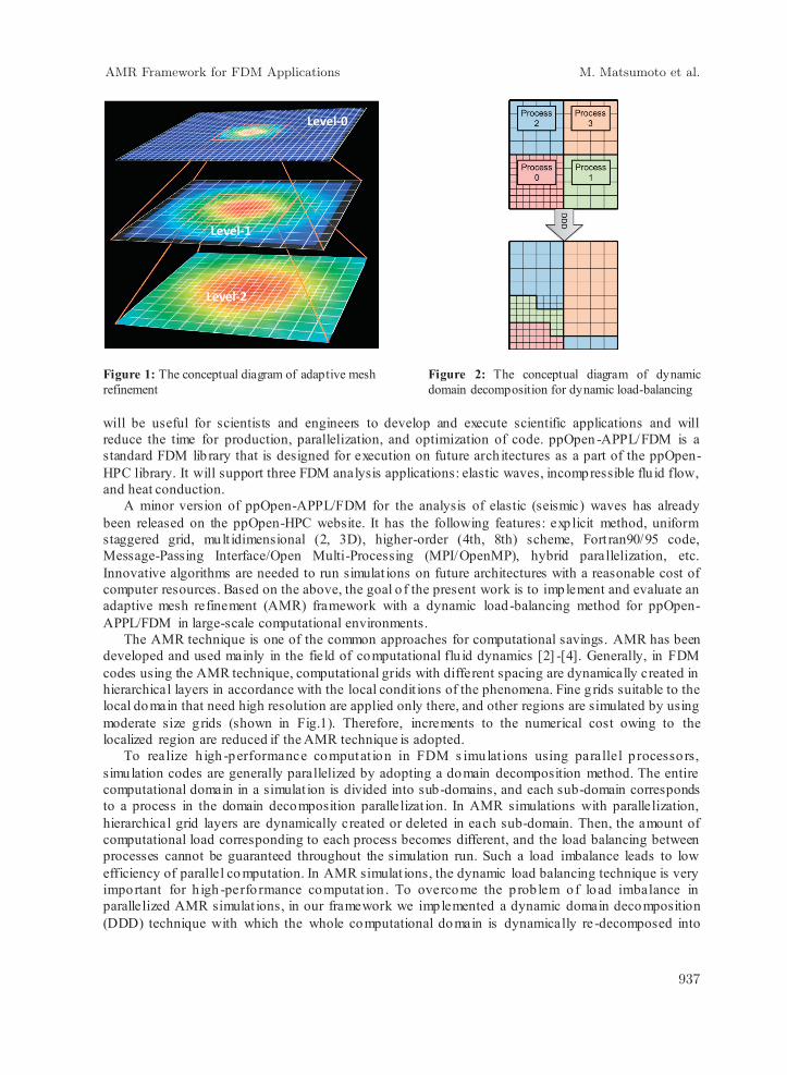
Figure 1: The conceptual diagram of adaptive mesh refinement

Figure 2: The conceptual diagram of dynamic domain decomposition for dynamic load-balancing

will be useful for scientists and engineers to develop and execute scientific applications and will reduce the time for production, parallelization, and optimization of code. ppOpen -APPL/FDM is a standard FDM lib rary that is designed for execution on future arch itectures as a part of the ppOpen-HPC library. It will support three FDM analysis applications: elastic waves, incompressible flu id flow, and heat conduction.

A minor version of ppOpen-APPL/FDM for the analysis of elastic (seismic) waves has already been released on the ppOpen-HPC website. It has the following features: exp licit method, uniform staggered grid, mult idimensional (2, 3D), higher-order (4th, 8th) scheme, Fort ran90/95 code, Message-Passing Interface/Open Multi-Processing (MPI/OpenMP), hybrid parallelization, etc. Innovative algorithms are needed to run simulat ions on future architectures with a reasonable cost of computer resources. Based on the above, the goal o f the present work is to implement and evaluate an adaptive mesh refinement (AMR) framework with a dynamic load-balancing method for ppOpen-APPL/FDM in large-scale computational environments.

The AMR technique is one of the common approaches for computational savings. AMR has been developed and used mainly in the field of computational flu id dynamics [2] -[4]. Generally, in FDM codes using the AMR technique, computational grids with different spacing are dynamically created in hierarchical layers in accordance with the local condit ions of the phenomena. Fine g rids suitable to the local domain that need high resolution are applied only there, and other regions are simulated by using moderate size g rids (shown in Fig.1). Therefore, increments to the numerical cost owing to the localized region are reduced if the AMR technique is adopted.

To realize h igh -performance computat ion in FDM s imulat ions using parallel p rocessors, simulation codes are generally parallelized by adopting a domain decomposition method. The entire computational domain in a simulat ion is divided into sub-domains, and each sub-domain corresponds to a process in the domain decomposition parallelizat ion. In AMR simulations with parallelization, hierarchical grid layers are dynamically created or deleted in each sub-domain. Then, the amount of computational load corresponding to each process becomes different, and the load balancing between processes cannot be guaranteed throughout the simulation run. Such a load imbalance leads to low efficiency of parallel co mputation. In AMR simulat ions, the dynamic load balancing technique is very important for h igh -performance computat ion . To overcome the p rob lem of load imbalance in parallelized AMR simulat ions, in our framework we implemented a dynamic domain decomposition(DDD) technique with which the whole computational domain is dynamically re -decomposed into

Level-0

Level-1

Level-2

AMR Framework for FDM Applications M. Matsumoto et al.

937

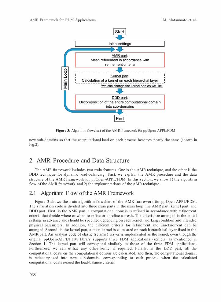
Figure 3: Algorithm flowchart of the AMR framework for ppOpen-APPL/FDM new sub-domains so that the computational load on each process becomes nearly the same (shown in Fig.2).

2 AMR Procedure and Data Structure The AMR framework includes two main features. One is the AMR technique, and the other is the

DDD technique for dynamic load-balancing. First, we exp lain the AMR procedure and the data structure of the AMR framework for ppOpen-APPL/FDM. In this section, we show 1) the algorithm flow of the AMR framework and 2) the implementations of the AMR technique.

2.1 Algorithm Flow of the AMR Framework Figure 3 shows the main algorithm flowchart of the AMR framework for ppOpen-APPL/FDM.

The simulat ion code is divided into three main parts in the main loop: the AMR part, kernel part, and DDD part. First, in the AMR part, a computational domain is refined in accordance with refinement criteria that decide where or when to refine or unrefine a mesh. The criteria are arranged in the initial settings in advance and should be specified depending on each kernel, working condition and intended physical parameters. In addition, the different criteria for refinement and unrefinement c an be arranged. Second, in the kernel part, a main kernel is calculated on each h ierarch ical layer fixed in the AMR part. An analysis code of elastic (seismic) waves is implemented as the kernel, even though the original ppOpen-APPL/FDM library supports three FDM applications (kernels) as mentioned in Section 1. The kernel part will correspond similarly to those of the three FDM applications. Furthermore, we can utilize any other kernel if required. Finally, in the DDD part, all the computational costs on the computational domain are calcu lated, and then, the computational domain is redecomposed into new sub-domains corresponding to each process when the calculated computational costs exceed the load-balance criteria.

AMR Framework for FDM Applications M. Matsumoto et al.

938

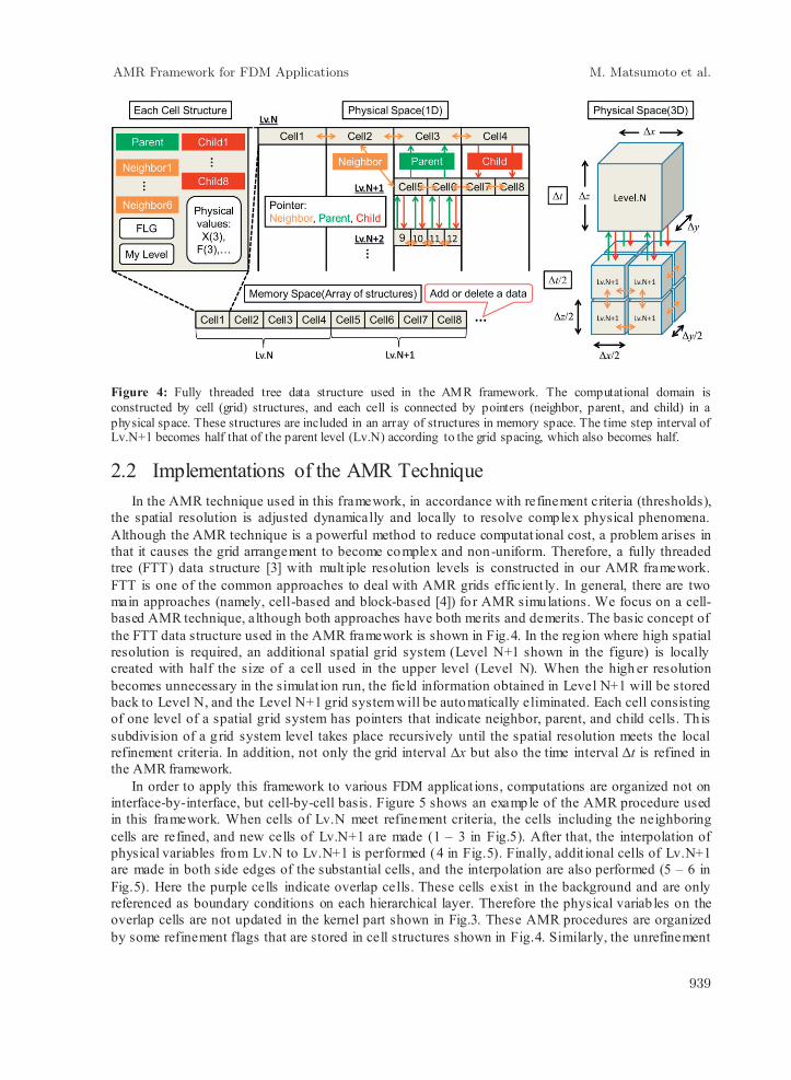
Figure 4: Fully threaded tree data structure used in the AMR framework. The computational domain is constructed by cell (grid) structures, and each cell is connected by pointers (neighbor, parent, and child) in a physical space. These structures are included in an array of structures in memory space. The time step interval of Lv.N+1 becomes half that of the parent level (Lv.N) according to the grid spacing, which also becomes half.

2.2 Implementations of the AMR Technique In the AMR technique used in this framework, in accordance with refinement criteria (thresholds),

the spatial resolution is adjusted dynamically and locally to resolve complex physical phenomena. Although the AMR technique is a powerful method to reduce computat ional cost, a problem arises inthat it causes the grid arrangement to become complex and non-uniform. Therefore, a fully threaded tree (FTT) data structure [3] with mult iple resolution levels is constructed in our AMR framework. FTT is one of the common approaches to deal with AMR grids efficient ly. In general, there are two main approaches (namely, cell-based and block-based [4]) fo r AMR simulations. We focus on a cell-based AMR technique, although both approaches have both merits and demerits. The basic concept of the FTT data structure used in the AMR framework is shown in Fig.4. In the reg ion where high spatial resolution is required, an additional spatial grid system (Level N+1 shown in the figure) is locally created with half the size of a cell used in the upper level (Level N). When the high er resolution becomes unnecessary in the simulat ion run, the field information obtained in Level N+1 will be stored back to Level N, and the Level N+1 grid system will be automatically eliminated. Each cell consisting of one level of a spatial grid system has pointers that indicate neighbor, parent, and child cells. Th is subdivision of a g rid system level takes place recursively until the spatial resolution meets the local refinement criteria. In addition, not only the grid interval ∆x but also the time interval ∆t is refined in the AMR framework.

In order to apply this framework to various FDM applicat ions, computations are organized not on interface-by-interface, but cell-by-cell basis. Figure 5 shows an example of the AMR procedure used in this framework. When cells of Lv.N meet refinement criteria, the cells including the neighboring cells are refined, and new cells of Lv.N+1 are made (1 – 3 in Fig.5). After that, the interpolation of physical variables from Lv.N to Lv.N+1 is performed (4 in Fig.5). Finally, addit ional cells of Lv.N+1 are made in both side edges of the substantial cells, and the interpolation are also performed (5 – 6 in Fig.5). Here the purple cells indicate overlap cells. These cells exist in the background and are only referenced as boundary conditions on each hierarchical layer. Therefore the physical variab les on the overlap cells are not updated in the kernel part shown in Fig.3. These AMR procedures are organized by some refinement flags that are stored in cell structures shown in Fig.4. Similarly, the unrefinement

AMR Framework for FDM Applications M. Matsumoto et al.

939

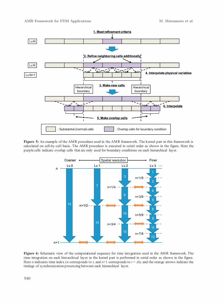
Figure 5: An example of the AMR procedure used in the AMR framework. The kernel part in this framework is calculated on cell-by-cell basis. The AMR procedure is executed in serial order as shown in the figure. Here the purple cells indicate overlap cells that are only used for boundary conditions on each hierarchical layer.

Figure 6: Schematic view of the computational sequence for time integration used in the AMR framework. The time integration on each hierarchical layer in the kernel part is performed in serial order as shown in the figure. Here n indicates time index (n corresponds to t, and n+1 corresponds to t + Δt), and the orange arrows indicate the timings of synchronization processing between each hierarchical layer.

AMR Framework for FDM Applications M. Matsumoto et al.

940

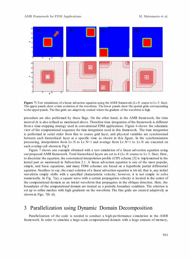
Figure 7: Test simulations of a linear advection equation using the AMR framework (Lv.0: coarse to Lv.3: fine). The upper panels show a time evolution of the waveform. The lower panels show the spatial grids corresponding to the upper panels. The fine grids are adaptively created where the gradient of the waveform is high. procedure are also performed by these flags. On the other hand, in the AMR framework, the time interval ∆t is also refined as mentioned above. Therefore time integration of the framework is different from a time-stepping strategy used in conventional FDM applications. Figure 6 shows the schematic view of the computational sequence for time integration used in this framework. The time integration is performed in serial order from fine to coarse grid layer, and physical variables are synchronized between each hierarchical layer at a specific t ime as shown in th is figure. In the synchronization processing, interpolation from Lv.N to Lv.N+1 and average from Lv.N+1 to Lv.N are executed on each overlap cell shown in Fig.5

Figure 7 shows one example obtained with a test simulat ion of a linear advection equation using our proposed AMR framework. Total hierarchical layers are set to 4 (Lv.0: coarse to Lv.3: fine). Here, to discretize the equation, the constrained interpolation profile (CIP) scheme [5] is implemented in the kernel part as mentioned in Subsection 2.1. A linear advection equation is one of the most popular, simple, and basic equations, and many FDM schemes are based on a hyperbolic partial d ifferential equation. Needless to say, the exact solution of a linear advection equation is triv ial, that is, any in itial waveform simply shifts with a specified characteristic velocity; however, it is not simple to solve numerically. In Fig. 7(a), a square wave with a certain propagation velocity is located in the center of the computational domain as an init ial waveform that propagates in the oblique direction. Here, the boundaries of the computational domain are treated as a periodic boundary condition. The criterion is set up to refine meshes with high gradients on the waveform. The fine grids are created adaptively as shown in Figs. 7(b–d).

3 Parallelization using Dynamic Domain Decomposition Parallelizat ion of the code is needed to conduct a h igh-performance s imulat ion in the AMR

framework. In order to simulate a large-scale computational domain with a large amount of memory,

AMR Framework for FDM Applications M. Matsumoto et al.

941

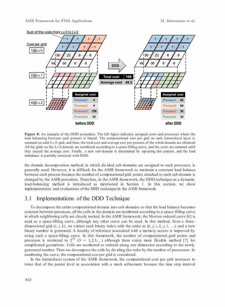
Figure 8: An example of the DDD procedure. The left figure indicates assigned costs and processes where the load balancing between each process is biased. The computational cost per grid on each hierarchical layer is summed on each Lv.0 grid, and then, the total cost and average cost per process of the whole domain are obtained. All the grids on the Lv.0 domain are numbered according to a space-filling curve, and the costs are summed until they exceed the average cost. Finally, a new sub-domain is determined by repeating this pattern, and the load imbalance is partially corrected with DDD. the domain decomposition method, in which div ided sub-domains are assigned to each processor, is generally used. However, it is difficult for the AMR framework to maintain a constant load balance between each process because the number of computational grid points attached to each sub-domain is changed by the AMR procedure. Therefore, in the AMR framework, the DDD technique as a dynamic load-balancing method is introduced as mentioned in Section 1. In this section, we show implementations and evaluations of the DDD technique in the AMR framework.

3.1 Implementations of the DDD Technique To decompose the entire computational domain into sub-domains so that the load balance becomes

constant between processes, all the cells in the domain are numbered according to a space-filling curve in which neighboring cells are closely ranked. In the AMR framework, the Morton ordered curve [6] is used as a space-filling curve, although any other curve can be used. In this method, from a three-dimensional grid (i, j, k), we extract each binary index with the order as (k , j, i, k , j, i, …), and a new binary number is generated. A locality of reference associated with a memory access is improved by using such a space-filling curve. In this framework, the number of computational grid points and processes is restricted to 23N (N = 1,2,3,…) although there exists more flexible method [7] for complicated geometries. Cells are numbered or ordered along one dimension according to the newly generated number. Then we decompose the cells by div iding the order by the number of processors. In numbering the curve, the computational cost per grid is considered.

In the hierarchical system of the AMR framework, the computational cost per grid increases to twice that of the parent level in association with a mesh refinement because the time step interval

AMR Framework for FDM Applications M. Matsumoto et al.

942

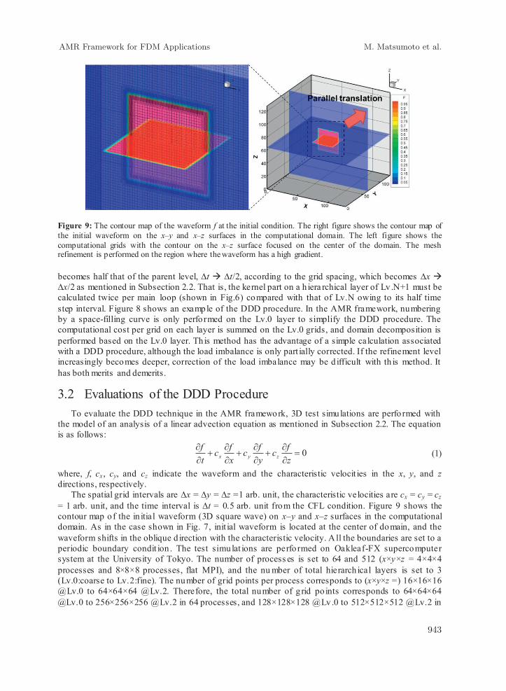
Figure 9: The contour map of the waveform f at the initial condition. The right figure shows the contour map of the initial waveform on the x–y and x–z surfaces in the computational domain. The left figure shows the computational grids with the contour on the x–z surface focused on the center of the domain. The mesh refinement is performed on the region where the waveform has a high gradient. becomes half that of the parent level, ∆t ∆t/2, according to the grid spacing, which becomes ∆x ∆x/2 as mentioned in Subsection 2.2. That is, the kernel part on a h iera rchical layer of Lv .N+1 must be calculated twice per main loop (shown in Fig.6) compared with that of Lv.N owing to its half time step interval. Figure 8 shows an example of the DDD procedure. In the AMR framework, numbering by a space-filling curve is only performed on the Lv.0 layer to simplify the DDD procedure. The computational cost per grid on each layer is summed on the Lv.0 grids, and domain decomposition is performed based on the Lv.0 layer. Th is method has the advantage of a simple calculation associated with a DDD procedure, although the load imbalance is only part ially corrected. If the refinement level increasingly becomes deeper, correction of the load imbalance may be d ifficult with th is method. It has both merits and demerits.

3.2 Evaluations of the DDD Procedure To evaluate the DDD technique in the AMR framework, 3D test simulations are performed with

the model of an analysis of a linear advection equation as mentioned in Subsection 2.2. The equation is as follows:

0zfc

yfc

xfc

tf

zyx (1)

where, f, cx , cy, and cz indicate the waveform and the characteristic velocit ies in the x, y, and z directions, respectively.

The spatial grid intervals are ∆x = ∆y = ∆z =1 arb. unit, the characteristic velocities are cx = cy = cz = 1 arb. unit, and the time interval is ∆t = 0.5 arb. unit from the CFL condition. Figure 9 shows the contour map of the in itial waveform (3D square wave) on x–y and x–z surfaces in the computational domain. As in the case shown in Fig. 7, init ial waveform is located at the center of domain, and the waveform shifts in the oblique d irection with the characteristic velocity. A ll the boundaries are set to a periodic boundary condit ion . The test simulat ions are performed on Oakleaf-FX supercomputer system at the University of Tokyo. The number of process es is set to 64 and 512 (x×y×z = 4×4×4 processes and 8×8×8 processes, flat MPI), and the nu mber of total hierarch ical layers is set to 3 (Lv.0:coarse to Lv.2:fine). The number of grid points per process corresponds to (x×y×z =) 16×16×16 @Lv.0 to 64×64×64 @Lv.2. Therefore, the total number of g rid po ints corresponds to 64×64×64 @Lv.0 to 256×256×256 @Lv.2 in 64 processes, and 128×128×128 @Lv.0 to 512×512×512 @Lv.2 in

AMR Framework for FDM Applications M. Matsumoto et al.

943

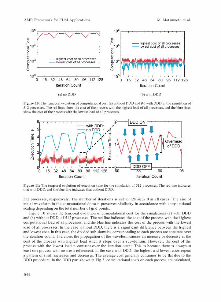
(a) no DDD (b) with DDD Figure 10: The temporal evolution of computational cost (a) without DDD and (b) with DDD in the simulation of 512 processes. The red lines show the cost of the process with the highest load of all processes, and the blue lines show the cost of the process with the lowest load of all processes.

Figure 11: The temporal evolution of execution time for the simulation of 512 processes. The red line indicates that with DDD, and the blue line indicates that without DDD. 512 processes, respectively. The number of iterations is set to 128 @Lv.0 in all cases. The size of initial waveform in the computational domain preserves similarity in accordance with computational scaling depending on the total number of grid points .

Figure 10 shows the temporal evolution of computational cost for the simulat ions (a) with DDD and (b) without DDD, of 512 processes. The red line indicates the cost of the process with the h ighest computational load of all processes, and the blue line indicates the cost of the process with the lowest load of all processes. In the case without DDD, there is a significant difference between the h ighest and lowest cost. In this case, the divided sub-domains corresponding to each process are constant over the iteration count. Therefore, the propagation of the waveform causes an increase or decrease in the cost of the process with highest load when it steps over a sub-domain. However, the cost of the process with the lowest load is constant over the iteration count. This is because there is always at least one process with no mesh refinement. In the case with DDD, the highest and lowest costs repeat a pattern of small increases and decreases. The average cost generally continues to be flat due to the DDD procedure. In the DDD part shown in Fig.3, computational costs on each process are calculated,

AMR Framework for FDM Applications M. Matsumoto et al.

944

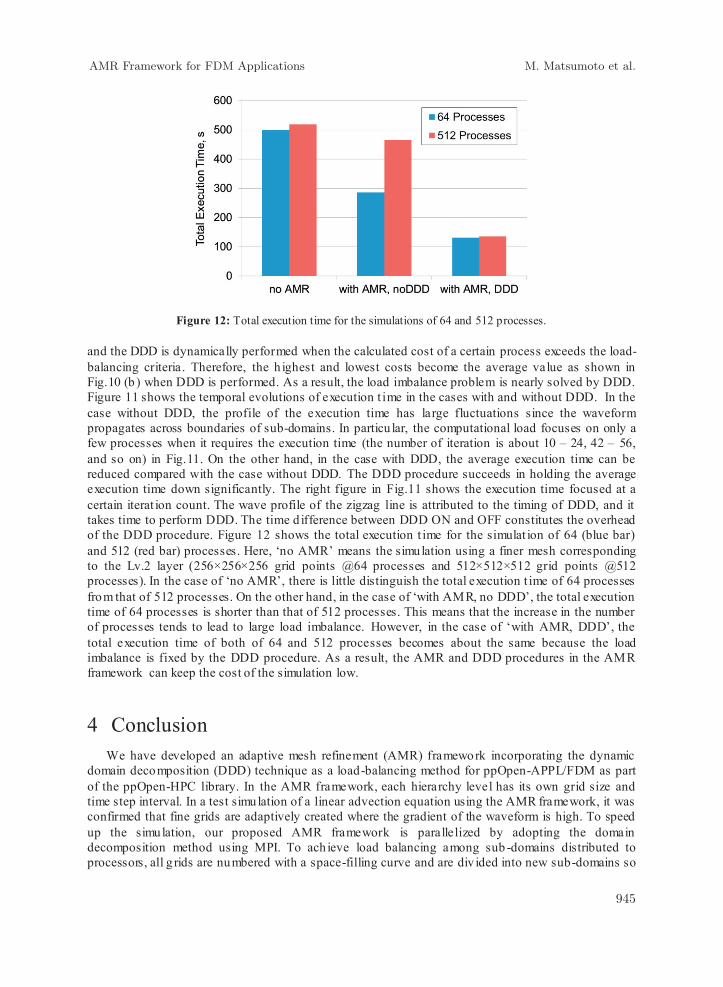
Figure 12: Total execution time for the simulations of 64 and 512 processes. and the DDD is dynamically performed when the calculated cost of a certain process exceeds the load-balancing criteria. Therefore, the h ighest and lowest costs become the average value as shown in Fig.10 (b ) when DDD is performed. As a result, the load imbalance problem is nearly solved by DDD. Figure 11 shows the temporal evolutions of execution t ime in the cases with and without DDD. In the case without DDD, the profile of the execution time has large fluctuations since the waveform propagates across boundaries of sub-domains. In particu lar, the computational load focuses on only a few processes when it requires the execution time (the number of iteration is about 10 – 24, 42 – 56, and so on) in Fig.11. On the other hand, in the case with DDD, the average execution time can be reduced compared with the case without DDD. The DDD procedure succeeds in holding the average execution time down significantly. The right figure in Fig.11 shows the execution time focused at a certain iterat ion count. The wave profile of the zigzag line is attributed to the timing of DDD, and it takes time to perform DDD. The time d ifference between DDD ON and OFF constitutes the overhead of the DDD procedure. Figure 12 shows the total execution t ime for the simulat ion of 64 (blue bar) and 512 (red bar) processes. Here, ‘no AMR’ means the simulation using a finer mesh corresponding to the Lv.2 layer (256×256×256 grid points @64 processes and 512×512×512 grid points @512 processes). In the case of ‘no AMR’, there is little distinguish the total execution t ime of 64 processes from that of 512 processes. On the other hand, in the case of ‘with AMR, no DDD’, the total execution time of 64 processes is shorter than that of 512 processes. This means that the increase in the number of processes tends to lead to large load imbalance. However, in the case of ‘with AMR, DDD’, the total execution time of both of 64 and 512 processes becomes about the same because the load imbalance is fixed by the DDD procedure. As a result, the AMR and DDD procedures in the AMR framework can keep the cost of the simulation low.

4 Conclusion We have developed an adaptive mesh refinement (AMR) framework incorporating the dynamic

domain decomposition (DDD) technique as a load-balancing method for ppOpen-APPL/FDM as part of the ppOpen-HPC library. In the AMR framework, each hierarchy level has its own grid size and time step interval. In a test simulation of a linear advection equation using the AMR framework, it was confirmed that fine grids are adaptively created where the gradient of the waveform is high. To speed up the simulation, our proposed AMR framework is parallelized by adopting the domain decomposition method using MPI. To ach ieve load balancing among sub -domains distributed to processors, all g rids are numbered with a space-filling curve and are div ided into new sub-domains so

AMR Framework for FDM Applications M. Matsumoto et al.

945

that the computational cost becomes nearly the same between each process. By performing a 3D test simulation, it can be confirmed that dynamic load balancing has been successfully achieved, and the execution time is considerably reduced compared with the conventional fixed decomp osition scheme.

Acknowledgement This work is funded by JST (Japan Science and Technology Agency)/CREST (Core Research for

Evolutional Science and Technology). The computation in the present study was performed with the Oakleaf-FX supercomputer system of Information Technology Center at the University of Tokyo.

References [1] Nakajima K. ppOpen-HPC: Open Source Infrastructure for Development and Execution of

Large-Scale Scientific Applications on Post-Peta-Scale Supercomputers with Automatic Tuning (AT). Proceedings of the ATIP/A*CRC Workshop on Accelerator Technologies for High -Performance Computing: Does Asia Lead the Way? 2012;ACM Digital Library.

[2] Berger MJ, Colella P. Local Adaptive Mesh Refinement fo r Shock Hydrodynamics. Journal of Computational Physics 1989;82:62–84.

[3] Khokhlov AM. Fully Threaded Tree Algorithms for Adaptive Refinement Fluid Dynamics Simulations. Journal of Computational Physics 1998;143:519–543.

[4] Stout QF, De Zeeuw DL, Gombosi TI, Groth CPT, Marshall HG, Powell KG. Adaptive Blocks: A High Performance Data Structure. Supercomputing '97 Proceedings of the 1997 ACM/IEEE conference on Supercomputing 1997:1-10.

[5] Yabe T, Xiao F, Utsumi T. The Constrained Interpolation Profile Method for Multiphase Analysis. Journal of Computational Physics 2001;169:556–593.

[6] Warren MS, Salmon JK. A Parallel Hashed Oct-Tree N-Body Algorithm. Supercomputing '93 Proceedings of the 1993 ACM/IEEE conference on Supercomputing 1993;12-21.

[7] Mitchell WF. A Refinement-Tree based Partitioning Method for Dynamic Load Balancing with Adaptively Refined Grids. Journal of Parallel and Distributed Computing 2007;67:417-429.

AMR Framework for FDM Applications M. Matsumoto et al.

946