Impacts on Market Integration in Wheat, Rice, and Pearl Millet

University of Illinois at Urbana-Champaign

From the SelectedWorks of Kathy Baylis

2013

The Food Corporation of India and the PublicDistribution System: Impacts on MarketIntegration in Wheat, Rice, and Pearl MilletMindy Mallory, University of Illinois at Urbana-ChampaignKathy Baylis, University of Illinois at Urbana-Champaign

Available at: http://works.bepress.com/kathy_baylis/45/

http://www.uiuc.edu/

http://works.bepress.com/kathy_baylis/

http://works.bepress.com/kathy_baylis/45/

Journal of Agribusiness 30, 2 (Fall 2012)

© Agricultural Economics Association of Georgia

Mindy Mallory and Kathy Baylis are assistant professors in the Department of Agricultural Economics at the

University of Illinois. We thank the conference participants at the 2012 NCCC-134 conference in St. Louis,

Mo., for their comments and suggestions. We also gratefully acknowledge funding from the ADM Institute for

the Prevention of Postharvest Loss. Any mistakes are our own.

Food Corporation of India and the Public Distribution

System: Impacts on Market Integration in Wheat, Rice, and

Pearl Millet

Mindy Mallory and Kathy Baylis

We examine the spatial integration of wheat, rice and pearl millet in the Indian states of

Bihar, Haryana, and Uttar Pradesh after the reforms of 2002 which liberalized inter-state

trade. Our data represent a large share of India’s cereal grains. The government regulates

markets for staple foods heavily; almost all grain is marketed through government

licensed markets that impose a price floor. This could discourage private investment in

storage capacity among farmers and traders, impacting market integration. We find little

evidence of market integration despite the 2002-03 reforms, and this fragmentation is

particularly notable for smaller, and less regulated crops.

Key words: India, infrastructure, market integration, multiple imputation, rice, wheat,

vector autoregression, vector error correction model

In this paper we examine the spatial integration of staple food commodity markets in

India. Food-grain crops are highly regulated in India, with floor prices for farmers,

government purchases and subsidized sales to consumers. State-specific regulations on

storage and transport further limit internal grain movement. In 2002 and 2003, India

reformed its domestic grains policies, with a particular eye to removing barriers to

interstate trade. In this paper we ask whether price signals are being transferred from one

market to another, which is a necessary condition for markets to operate efficiently.

Specifically, we use detailed market-level data to ask whether Indian grain markets are

spatially integrated after the imposition of these reforms.

While India has enjoyed rapid growth for the past twenty years, it still struggles with

development challenges, particularly around access to food. India hosts the world’s

second largest population, and although incomes have been rising, it faces large income

inequalities and one of the highest rates of child stunting in the world. Since India’s

independence in 1947, the government established a large social assistance program to

support the incomes of rural farmers while providing affordable food for its urban poor.

These goals are executed primarily through two institutions: The Food Corporation of

226 Fall 2012 Journal of Agribusiness

India (FCI) procures staple food crops from farmers, often at higher than market prices.

Then the Public Distribution System (PDS) sells to the poor through government-run Fair

Price Shops. This intervention comprises a large share of the market for staple crops. For

example, the FCI purchased 13% to 37% of the total wheat crop in India during 2005 to

2011 (U.S. Department of Agriculture Foreign Agricultural Service, 2012). As Indians

move from the countryside and subsistence agriculture to urban areas and nonagricultural

jobs, the transmission of price signals and product between producer and increasingly

distant consumer is more important than ever.

The government promises to purchase any grain that meets the standard of Fair

Average Quality at a stated Minimum Support Price (MSP), thus creating an effective

floor on the price of the grain. Since government buyers physically purchase the grain at

a price fixed throughout the year, the government stores much of the grain, leaving the

private sector with no incentive to invest in storage. Furthermore, the FCI does not

maintain adequate storage facilities to prevent losses during storage from moisture and

pests. Roughly 20% of cereal grains and oilseeds are lost postharvest due to a lack of

adequate storage facilities (Organization for Economic Co-operation and Development

(OECD), 2007).

In 2002 and 2003, India reformed the Stock Limits and Movement Restrictions on

Specified Foodstuffs. These reforms were intended to reduce the state-level restrictions

on grain storage and movement and create a more unified domestic market. At the same

time, the licensing requirement for dealers was also removed. Any dealer could now buy,

sell, store or transport any quantity of wheat, paddy/rice, coarse grains, pulses, or wheat

products without a license. Some state-specific restrictions persist, however, and when

combined with substantial federal market interventions and poor marketing infrastructure,

one might anticipate that price transmission among markets may continue to be limited.

In this paper we examine the spatial integration of wheat, rice and pearl millet markets

across the northern grain belt, specifically considering the states of Bihar, Haryana, Uttar

Pradesh and West Bengal India. Rice and wheat are the primary staple crops and while

pearl millet still faces MSPs; it has fewer state storage and transport restrictions since

pearl millet is perceived as being less crucial for food security.

Prices are obtained from AgMarkNet,1 the data portal of the Indian Ministry of

Agriculture. We use monthly local prices from 2005 to 2011 in the most active markets in

1 AgMarkNet is the website of the Indian Ministry of Agriculture http://agmarknet.nic.in/

Mallory and Baylis Market Integration in India 227

each primary producing state. We estimate a spatial cointegration model as proposed in

Ardeni (1989), Goodwin and Schroeder (1991), and Ardeni (1991) to determine the level

of integration among these markets.

We see three primary contributions of this study. First, to our knowledge, this is the

first paper to test whether Indian grains markets are spatially integrated after the

2002/2003 reforms. In this test, we use detailed spatial data of prices at multiple local

markets in the producing regions of India. Second, we use a relatively novel approach to

address the large fraction of missing observations in the data. We find little evidence that

markets are spatially integrated, and see substantial differences by states and crops.

Haryana has the most spatially integrated markets for rice and wheat, but not for pearl

millet. Thus, even when controlling for similar infrastructure within the same state, we do

not see integration of the smaller but less regulated crop. The crop with the most

integrated markets is rice, which is interesting since rice is also the most highly regulated

crop, particularly during this time period when India imposed a rice export ban. Our

findings raise the question as to whether the limited degree of integration we observe is in

fact an artifact of homogenous government policy instead of being indicative of active

arbitrage.

Background

The Indian government is highly involved in domestic agriculture. The Essential

Commodities Act (ECA) was established in 1955 and regulates commodity prices

through government purchases, licenses and permits which limit the movement,

distribution and disposal of commodities deemed essential such as cereals, pulses, edible

oilseeds, oilcakes, raw cotton, sugar, and jute (OECD, 2007). Similarly, the Agricultural

Produce Market Regulation Act (APMRA) requires that farm produce be sold only at

regulated markets through registered intermediaries. Until recently, capacity in food-

processing plants was limited and small-scale, low technology firms still dominate the

industry (Government of Canada, 2008).

In 1965, the Indian government established the Food Corporation of India (FCI) to

procure, store, and distribute food-grains at the national level, including handling and

distributing all grain imports. That same year, the Agricultural Price Commission was

established to set prices at a level that balanced producer and consumer interests (Ghosh,

2010). State zones were also introduced and the movement of grain out of surplus states

and districts was restricted. Part of the purpose of these restrictions was to lower local

prices in the producing states to facilitate government grain purchases which would then


be sold to the poor through the public distribution system (PDS) in consuming regions

(Radhakrishna and Indrakant, 1988). Along with being costly, the World Bank (1999)

found that these programs discouraged private trading in food grains and undermined

investment in India’s long- term food security.

Recent Reforms

Reforms in the domestic market occurred mainly during the 1990s and early 2000

period after trade liberalization. In the early 2000s, the ECA was amended to remove the

licensing requirement of dealers and restrictions on the storage and movement of food

grains, sugar, oilseeds and edible oils. Specifically, in 2002, the Removal of Licensing

Requirements, Stock Limits and Movement Restrictions on Specified Foodstuffs Order

was passed and amended in 2003 to allow any dealer to freely buy, sell, hold or trade any

quantity of food-grains and oilseeds without a license. The reform measures also

abolished selective credit controls used to regulate institutional credit to traders (Jha,

Srinivasan, and Ganesh Kumar 2010; OECD 2007). As a result of these reforms, state

traders no longer have a monopoly on trade. After 2003, the private sector was allowed to

establish parallel markets for the agricultural commodities under the Model Market Act

(Jayasuria, Kim, and Kumar 2007), and agricultural futures markets are now operating in

several commodities.

Continued Constraints to Grain Market Integration

Despite these reforms, substantial government intervention persists. Commodity

specific institutions continue to regulate markets through an array of measures including

minimum support prices, import subsidies, public procurement and distribution of food

grains. The Agricultural Produce Marketing Committee (APMC) in the states also

restricts the growth of agricultural marketing and does not allow cooperatives and private

parties to set up modern markets at will. Government institutions also control and

distribute inputs, develop infrastructure, and provide general services (OECD 2007).

Although the changes have reduced the barriers to internal trade to a large extent, certain

other restrictions continue to limit interstate trade. For example, traders are required to

own national and interstate permits, pay state-specific taxes for the sale of certain goods,

and suffer additional transactions costs (poor roads, extensive paperwork, multiple

checking, and clearance requirements) (Jha, Srinivasan, and Ganesh Kumar 2010).

The lack of infrastructure, including roads, power and storage can reduce agricultural

investment, price transmission and increase postharvest losses. The OECD (2007)


estimated post harvest losses for grains, fruits and vegetables to be 25% to 30%. But

private investment in storage is discouraged by fixed annual MSPs and the presence of

large government stocks. As of January 1, 2011, government grain stocks of 41 million

tonnes were estimated to be more than double the prescribed limit of 20 million tonnes,

which constrains price movement and spatial integration (Chand and Gulati, 2011).

Previous Literature

Previous work on the spatial integration of Indian feed-grain markets finds mixed results.

Palaskas and Harriss-White (1993) used the Engle and Granger (1987) method of

cointegration to test weekly prices of rice, potato and mustard collected from three

markets places in Burdwan district of West Bengal (India), and found cointegration for

most pairs. One concern about their approach is that results from the Engle and Granger

(1987) method of cointegration are very sensitive to the choice of a variable for

normalization (Ghosh, 2010). Their study was also limited by its use of a very short span

of data (weekly data for a period of less than three years).

Jha et al. (1997) study market integration using monthly data for 44 rice markets and

47 wheat markets for January 1980 to December 1990, again using the Engle-Granger

methodology. They concluded that food markets all over India are highly integrated

(Ghosh, 2003). In a later paper, however, the same authors find that there is a tendency to

hoard rice stocks, with the wholesalers holding more than optimal inventories (Jha and

Nagarajan, 1998). They also find evidence of substantial information asymmetries in the

grain markups (Jha et al., 1999). They suggest that government intervention and the

presence of a parallel controlled market create substantial information asymmetries.

Later work by Jhar, Murthy, and Sharma (2005) use the methodology from

Gonzalez-Rivera and Helfand (2001) and find that Indian grain markets are not

integrated. Specifically, the authors look at monthly prices from 55 rice markets from

1970 to 1999 and find significant regional fractionalization.

Ghosh (2003, 2010) uses the maximum likelihood methodology to test for

cointegration (Johansen, 1988), indicating whether grain markets are cointegrated within

and across the major producing states. He finds that for Uttar Pradesh all the prices are

pair-wise cointegrated, which indicates that the weak version of the law of one price

(LOP) holds in these markets. The cointegration results for the remaining three states,

Haryana, Rajastan and the Punjab indicate that the prices are not pair-wise cointegrated.

For rice, again, the evidence is mixed. For Orissa, he finds that regional rice markets are

integrated while, he finds no evidence for the LOP in rice markets in the states of Bihar,


Uttar Pradesh, and West Bengal. The results for interstate spatial integration of rice

markets represented by four market centers chosen from the four selected states reveal

that even though the markets were integrated, the law of one price was not in operation in

Haryana, Punjab, and Rajasthan. From cointegration tests, he finds that the law of one

price seems to hold for wheat markets in Bihar and UP, but not Haryana, Punjab, and

Rajasthan Ghosh concludes that food-grain markets are largely integrated, and therefore

government can let the private market have a larger role in grain trade, since price

transmission is largely existent.

In terms of the connection of domestic to international grain markets, again, the

evidence is mixed. Shekhar (2004) regresses domestic price on domestic production and

international price, and finds evidence of some international price transmission to

domestic markets, but not for the large domestic producing areas. Jayasuria, Kim, and

Kumar (2007) use panel unit root tests and find that after the reforms in 1994, rice prices

in India converge much more quickly to the international price. Naik and Jain (2002)

estimate the efficiency of future’s markets in India, and find that the markets are still in

their infancy, and are not yet efficient.

In this study, the methodology that we employ is similar to many of the studies

described above. Specifically, we use a vector error correction model and Johansen tests

for cointegration to test for the presence of a long-run equilibrium in Indian wheat, rice,

and pearl millet markets. Unlike previous work, we employ a novel method to deal with

missing data, and we use a different approach to group markets for analysis compared to

the studies described above. The studies described above did not discuss their strategies

for dealing with missing data. The authors of these studies likely employed list-wise

deletion for dates where missing data were present. Since we analyze a large number of

markets at once in this study, list-wise deletion would require us to throw away much

valuable information because list-wise deletion requires deleting all market observations

for a month if information for one month in even one market is missing. To retain the full

information available in the dataset we employ the method of multiple imputation to deal

with missing values.

Further, many of the studies above (aside from Gosh) tested for cointegration in pairs

of markets as a way of dealing with the dimensionality of the problem. Like imputation,

this method also minimizes the information lost by performing list-wise deletion.

However, markets that are integrated may exhibit more complicated dynamics and long

run relationships than can be captured by the pairwise model. For example, after testing

for cointegration between two pairs of markets it is possible to conclude that each pair is

not cointegrated, when, in fact, the four tested all together are cointegrated.


Data

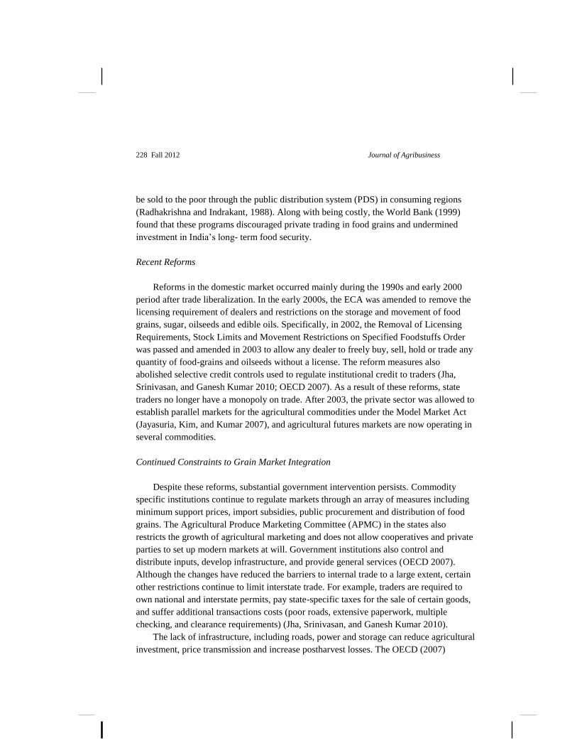
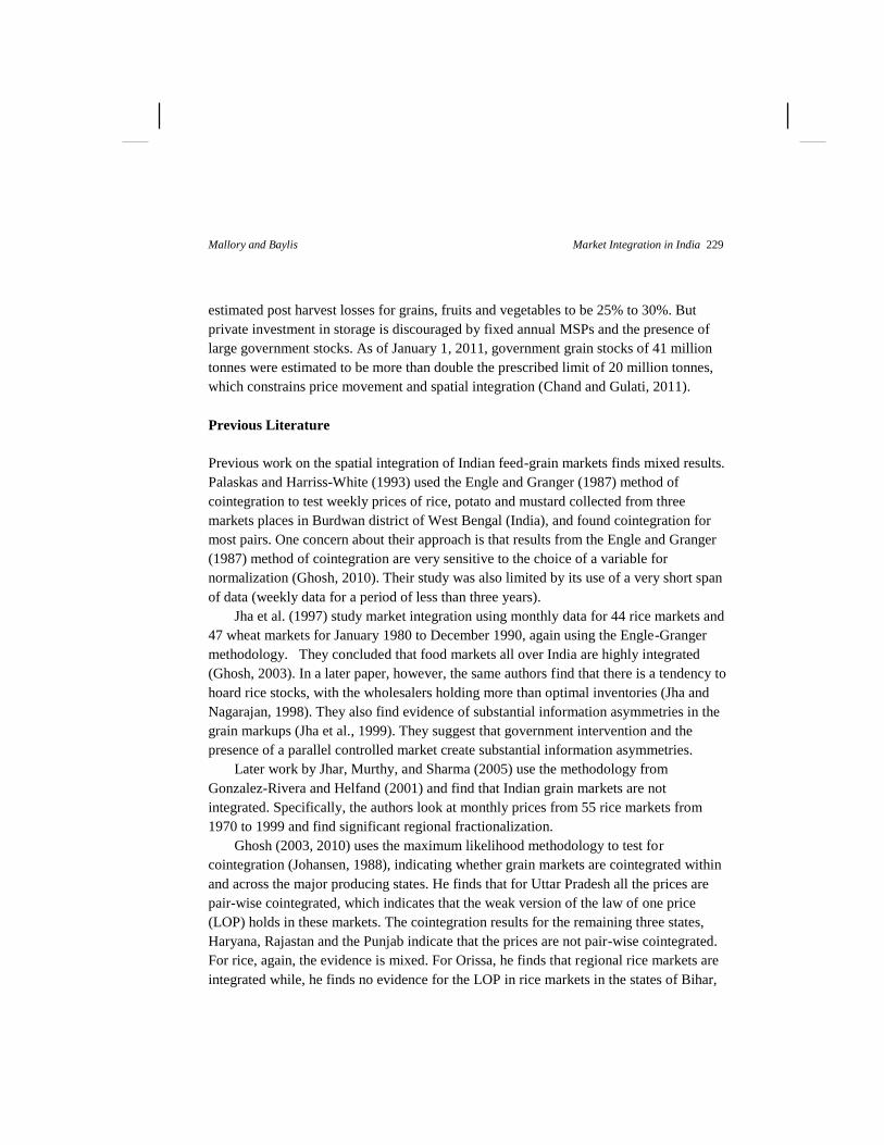
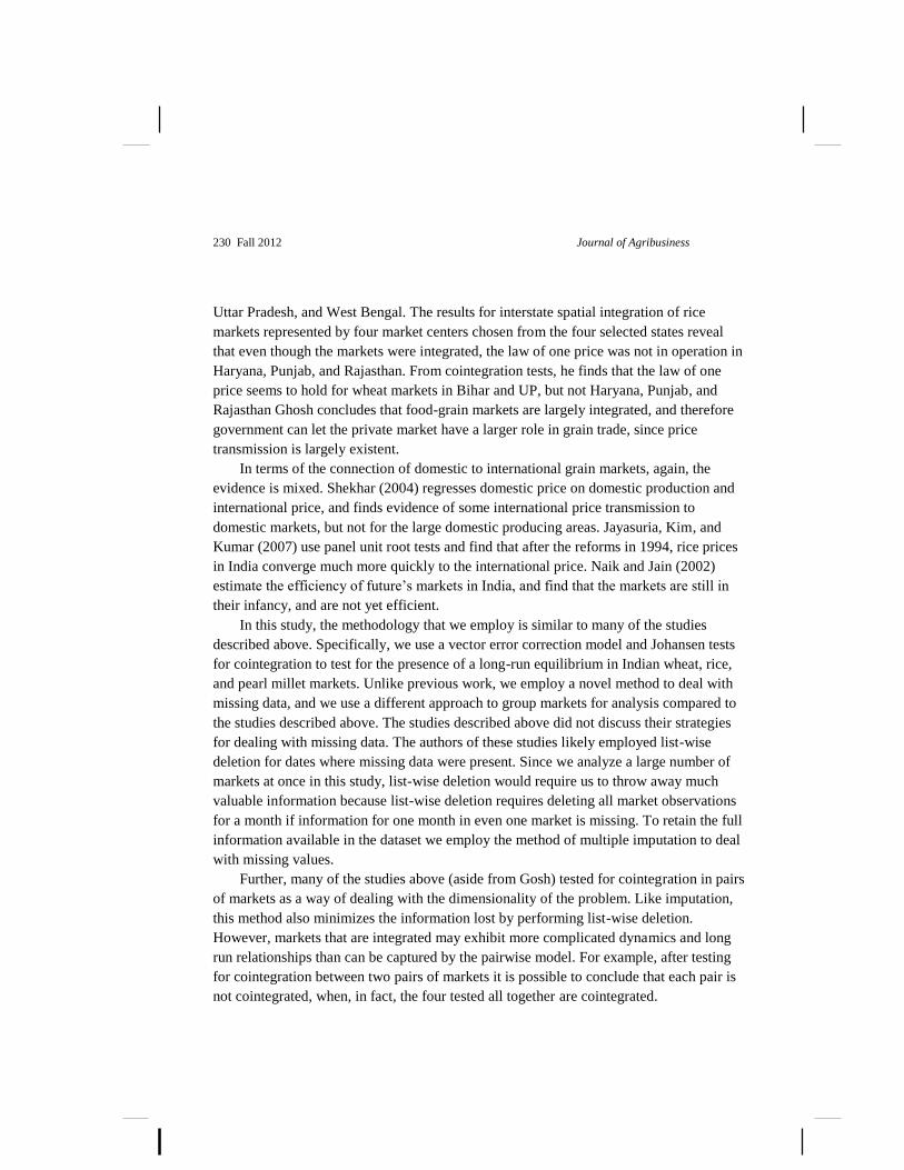
Each regulated market, or mandi, must report the minimum, maximum, and modal prices

to the Ministry of Agriculture on each day and for each crop that a transaction occurred.

The Ministry of Agriculture makes these data available to the public, and we obtained

data on wheat, rice, and pearl millet prices from the Indian Ministry of Agriculture’s

website. Our data set contains daily prices from 2005 through 2011. From the number of

missing observations, we observe that many mandis in our data set are not major markets

in the commodity of interest and contribute to the large number of missing daily price

data we observe in our data. We keep those markets where more than 50% of the

observations are not missing.

Figure 1. Mandi Locations by Commodity


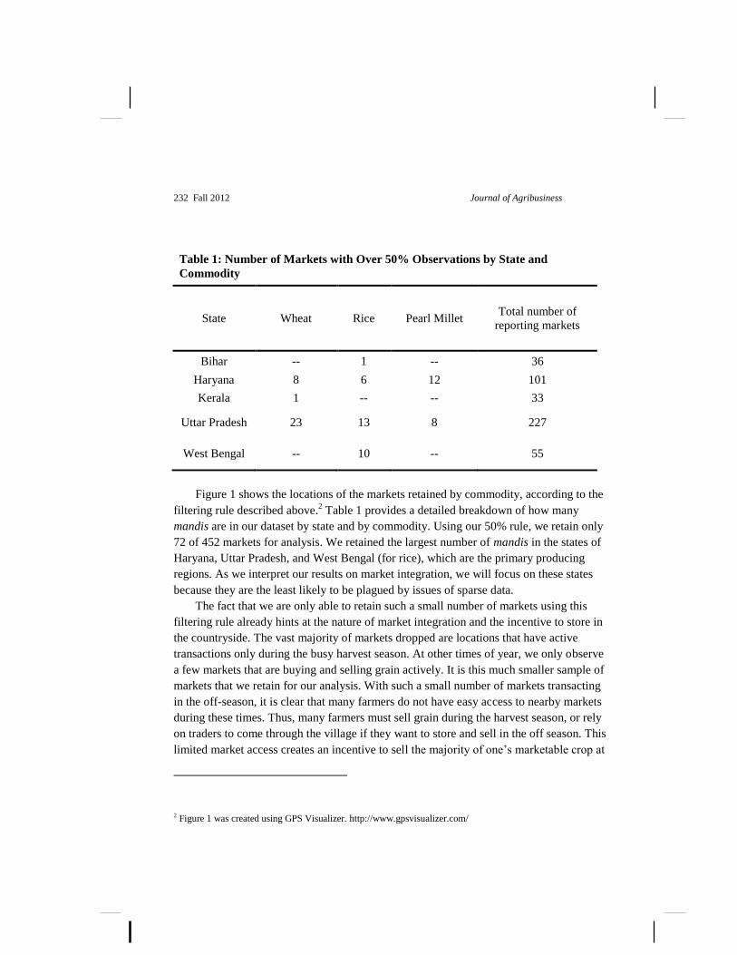
Table 1: Number of Markets with Over 50% Observations by State and

Commodity

State Wheat Rice Pearl Millet Total number of

reporting markets

Bihar -- 1 -- 36

Haryana 8 6 12 101

Kerala 1 -- -- 33

Uttar Pradesh 23 13 8 227

West Bengal -- 10 -- 55

Figure 1 shows the locations of the markets retained by commodity, according to the

filtering rule described above.2 Table 1 provides a detailed breakdown of how many

mandis are in our dataset by state and by commodity. Using our 50% rule, we retain only

72 of 452 markets for analysis. We retained the largest number of mandis in the states of

Haryana, Uttar Pradesh, and West Bengal (for rice), which are the primary producing

regions. As we interpret our results on market integration, we will focus on these states

because they are the least likely to be plagued by issues of sparse data.

The fact that we are only able to retain such a small number of markets using this

filtering rule already hints at the nature of market integration and the incentive to store in

the countryside. The vast majority of markets dropped are locations that have active

transactions only during the busy harvest season. At other times of year, we only observe

a few markets that are buying and selling grain actively. It is this much smaller sample of

markets that we retain for our analysis. With such a small number of markets transacting

in the off-season, it is clear that many farmers do not have easy access to nearby markets

during these times. Thus, many farmers must sell grain during the harvest season, or rely

on traders to come through the village if they want to store and sell in the off season. This

limited market access creates an incentive to sell the majority of one’s marketable crop at

2 Figure 1 was created using GPS Visualizer. http://www.gpsvisualizer.com/

http://www.gpsvisualizer.com/


harvest, when nearby markets are open. This incentive to sell at harvest-time also is

reinforced by credit practices that are common to rural Indian agriculture. Often farmers

take out small operating loans to pay for seed or other supplies needed to plant their

crops. At harvest these loans comes due, creating an extra need for cash at harvest-time

(Kumar, Turvey, and Kropp, 2012). The incentive to sell when one has access to a nearby

market, and the incentive to obtain cash to pay one’s debtors at harvest work together to

create a powerful incentive to sell most of one’s grain at harvest rather than storing any

marketable surplus for later sale.

We wondered if these more active markets are primarily located in larger urban

centers, which might have more nongovernment buyers. We use a cut-off population of

100,000 in the city where the mandi is located to define whether the market is in a city or

not. We find that the vast majority of markets with the most activity during the year are

located in cities in Uttar Pradesh, while except for Haryana wheat, in the other states

these markets tend to be in smaller centers.

Multiple Imputation

Even after culling multiple sparse markets, we are left with a considerable amount of

missing data in our retained set of markets. The most common method for dealing with

missing data in time-series applications is to simply delete the missing data and analyze

the remaining data. In our case, this is an unreasonable solution. Our dataset contains a

fairly wide panel of mandis observed over time. If we employ list-wise deletion, if a data

point is missing from just one mandi we would have to delete the entire row and discard

much valuable data.

The second most common method for dealing with missing data is to perform a

simple imputation of the data. In a time-series setting this is often accomplished by

linearly interpolating the observation using the two nearest observations (Friedman,

1962). However, simply imputing using the mean of the conditional distribution of the

data can greatly reduce the variance of the resulting sample and thereby affect inference

(King et al., 2001).

We employ the method of multiple imputation, which generates m completed

datasets making random draws from the conditional distribution over the missing data.

The method of multiple imputation was recently extended to the context of time-series

cross-section data (as is our dataset), which specifically allows for smooth time trends

and correlations across time and space to be considered in the imputation model

(Honaker and King, 2010).


The m completed datasets are the same for the observed data points, but the missing

data are replaced by draws from the posterior density and hence incorporate the relevant

level of uncertainty associated with those data points. Below we test for spatial market

integration on each of the m imputed datasets, and combine the results in such a way that

accounts for the uncertainty in the coefficient estimates both within and across imputed

datasets (Rubin, 1976).

To perform the multiple imputation algorithm, we employ the Amelia3 package

available for the R statistical software (Honaker, King, and Blackwell, 2011).4

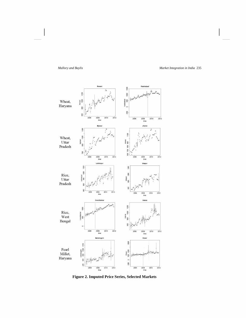
Figure 2 illustrates the imputed datasets for selected markets. Rather than providing

graphs of price series for all 95 price series, we demonstrate the range of missing

observations we face in this analysis by featuring markets representing the states and

commodities that we cover. Black dots correspond to observed prices, while the grey dots

represent the mean of the imputed data points and the grey vertical bars represent the

95% confidence interval over the imputed data. The apparent comovement of the prices

of wheat in Haryana in Figure 2 would suggest market integration is present, but the

empirical model that follows in a later section will allow us to formally test this

hypothesis.

3 http://cran.r-project.org/web/packages/Amelia/index.html 4 The nature of the reporting requirement results in a significant number of missing observations in the raw dataset. For example, if a mandi transacted wheat on only one day from 2005 to 2011, this market would show

up in our dataset, but every row except one would be missing. Since we are interested in measuring spatial

market integration we filter out those markets that are not major points of transaction in the following way.

First, we calculate a monthly median price to create a monthly time series for each market. Then we remove

markets for which more than 50% of the data are missing. Since the median is a measure of central tendency,

we may be introducing a degree of correlation among the variables, but given the sparse data, we felt that we should avoid the strong influence of outliers which would result from using the mean monthly price.

Alternatively, we could have used a point-based rule to create the monthly series. For example, we could have

chosen the price on the first Friday of every month. We used the monthly median for two reasons. First, since we are examining the nature of spatial market integration, we would rather err in the direction that makes us

more likely to conclude the markets are integrated. That way, if we conclude that the markets are not integrated,

it is less likely due to the way in which we constructed our dataset. Second, if data are sparse and we used a point-based rule, we would need to construct the series according to an algorithm that choose the first Thursday

if the first Friday was missing, the first Wednesday if the first Friday and first Thursday were missing, etc.

Markets which have sparse data will be more likely to produce observations for the month that are many days apart from the target date. Using the median monthly price minimizes this effect.

http://cran.r-project.org/web/packages/Amelia/index.html


Figure 2. Imputed Price Series, Selected Markets


Properties of the Data

We use the Augmented Dickey Fuller (ADF) test to determine the order of

integration of each (imputed) time series (Enders 2009). When we test for spatial market

integration below, we focus on the mandis at which a particular commodity is sold, by

state. That is, we group markets as indicated in Table 1 when we perform the test for

spatial integration. To enable that arrangement, each series in the group must be

integrated of the same order, while the ADF test is conducted on each series individually

and potentially may indicate a different degree of integration for each separate time

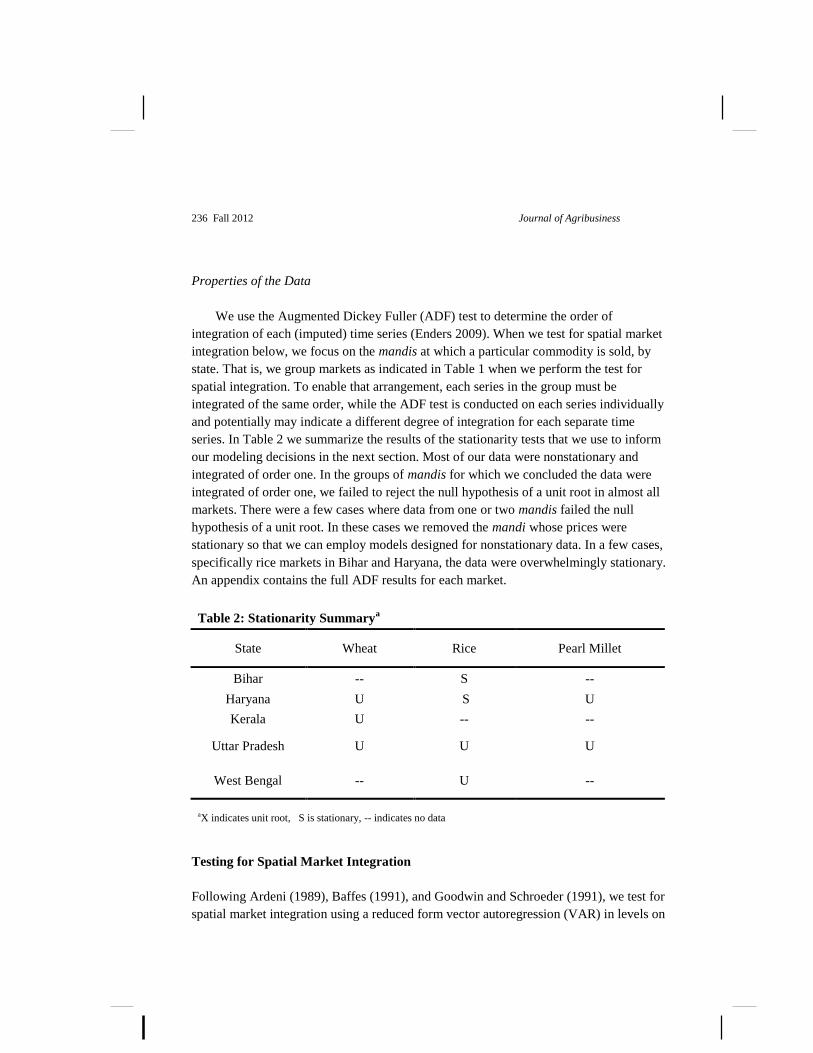
series. In Table 2 we summarize the results of the stationarity tests that we use to inform

our modeling decisions in the next section. Most of our data were nonstationary and

integrated of order one. In the groups of mandis for which we concluded the data were

integrated of order one, we failed to reject the null hypothesis of a unit root in almost all

markets. There were a few cases where data from one or two mandis failed the null

hypothesis of a unit root. In these cases we removed the mandi whose prices were

stationary so that we can employ models designed for nonstationary data. In a few cases,

specifically rice markets in Bihar and Haryana, the data were overwhelmingly stationary.

An appendix contains the full ADF results for each market.

Table 2: Stationarity Summarya

State Wheat Rice Pearl Millet

Bihar -- S --

Haryana U S U

Kerala U -- --

Uttar Pradesh U U U

West Bengal -- U --

aX indicates unit root, S is stationary, -- indicates no data

Testing for Spatial Market Integration

Following Ardeni (1989), Baffes (1991), and Goodwin and Schroeder (1991), we test for

spatial market integration using a reduced form vector autoregression (VAR) in levels on


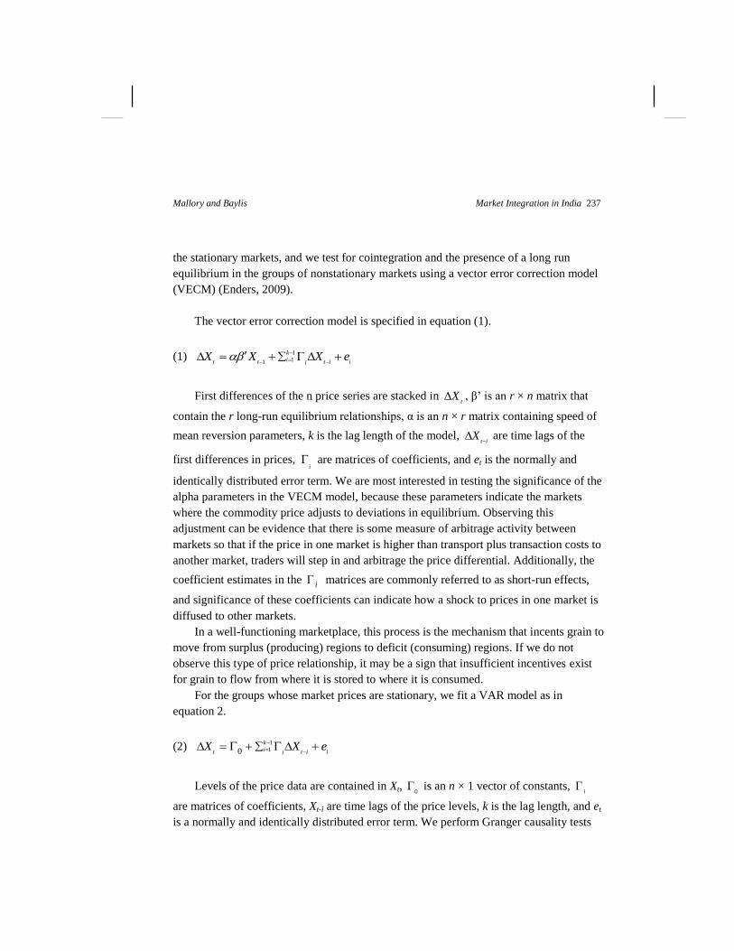
the stationary markets, and we test for cointegration and the presence of a long run

equilibrium in the groups of nonstationary markets using a vector error correction model

(VECM) (Enders, 2009).

The vector error correction model is specified in equation (1).

(1) 1

11

kit t t i ii

X X X e

First differences of the n price series are stacked in t

X , β’ is an r × n matrix that

contain the r long-run equilibrium relationships, α is an n × r matrix containing speed of

mean reversion parameters, k is the lag length of the model, t i

X

are time lags of the

first differences in prices, i are matrices of coefficients, and et is the normally and

identically distributed error term. We are most interested in testing the significance of the

alpha parameters in the VECM model, because these parameters indicate the markets

where the commodity price adjusts to deviations in equilibrium. Observing this

adjustment can be evidence that there is some measure of arbitrage activity between

markets so that if the price in one market is higher than transport plus transaction costs to

another market, traders will step in and arbitrage the price differential. Additionally, the

coefficient estimates in the i matrices are commonly referred to as short-run effects,

and significance of these coefficients can indicate how a shock to prices in one market is

diffused to other markets.

In a well-functioning marketplace, this process is the mechanism that incents grain to

move from surplus (producing) regions to deficit (consuming) regions. If we do not

observe this type of price relationship, it may be a sign that insufficient incentives exist

for grain to flow from where it is stored to where it is consumed.

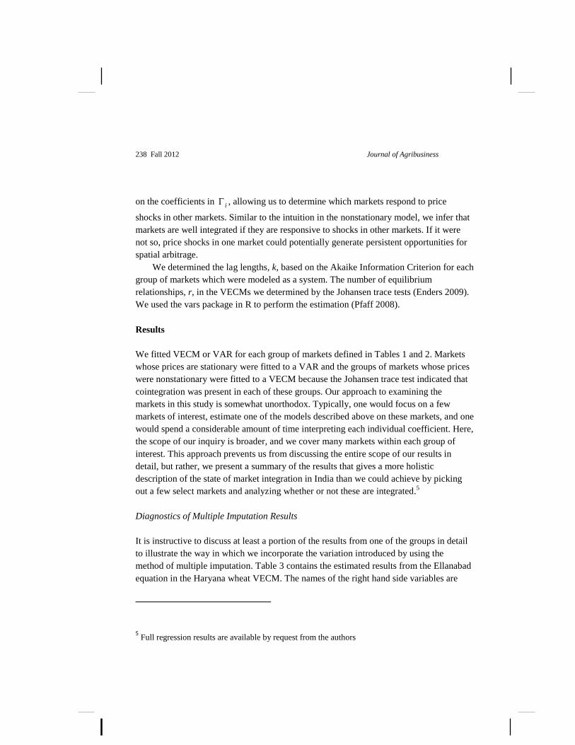
For the groups whose market prices are stationary, we fit a VAR model as in

equation 2.

(2) 1

10kit t i ii

X X e

Levels of the price data are contained in Xt, 0 is an n × 1 vector of constants,

i

are matrices of coefficients, Xt-i are time lags of the price levels, k is the lag length, and et

is a normally and identically distributed error term. We perform Granger causality tests


on the coefficients in i , allowing us to determine which markets respond to price

shocks in other markets. Similar to the intuition in the nonstationary model, we infer that

markets are well integrated if they are responsive to shocks in other markets. If it were

not so, price shocks in one market could potentially generate persistent opportunities for

spatial arbitrage.

We determined the lag lengths, k, based on the Akaike Information Criterion for each

group of markets which were modeled as a system. The number of equilibrium

relationships, r, in the VECMs we determined by the Johansen trace tests (Enders 2009).

We used the vars package in R to perform the estimation (Pfaff 2008).

Results

We fitted VECM or VAR for each group of markets defined in Tables 1 and 2. Markets

whose prices are stationary were fitted to a VAR and the groups of markets whose prices

were nonstationary were fitted to a VECM because the Johansen trace test indicated that

cointegration was present in each of these groups. Our approach to examining the

markets in this study is somewhat unorthodox. Typically, one would focus on a few

markets of interest, estimate one of the models described above on these markets, and one

would spend a considerable amount of time interpreting each individual coefficient. Here,

the scope of our inquiry is broader, and we cover many markets within each group of

interest. This approach prevents us from discussing the entire scope of our results in

detail, but rather, we present a summary of the results that gives a more holistic

description of the state of market integration in India than we could achieve by picking

out a few select markets and analyzing whether or not these are integrated.5

Diagnostics of Multiple Imputation Results

It is instructive to discuss at least a portion of the results from one of the groups in detail

to illustrate the way in which we incorporate the variation introduced by using the

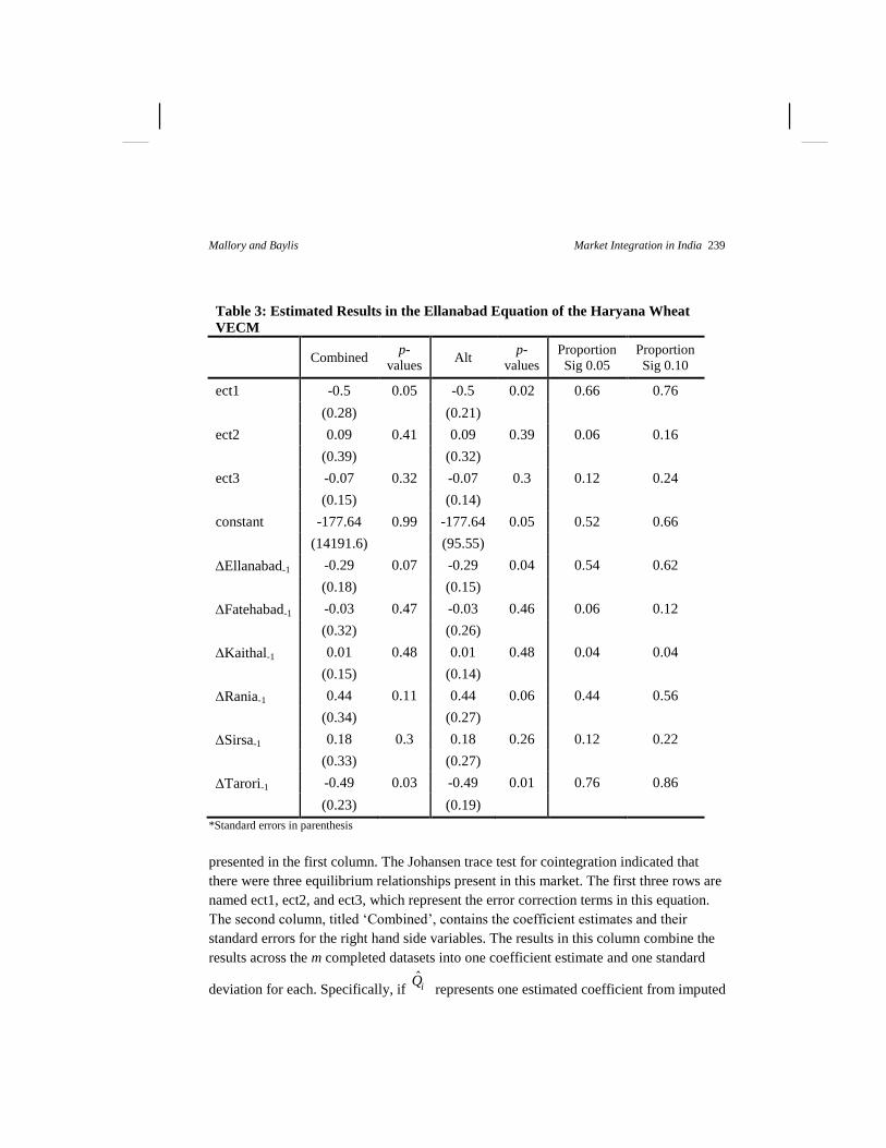
method of multiple imputation. Table 3 contains the estimated results from the Ellanabad

equation in the Haryana wheat VECM. The names of the right hand side variables are

5 Full regression results are available by request from the authors


Table 3: Estimated Results in the Ellanabad Equation of the Haryana Wheat

VECM

Combined p-

values Alt

p-

values

Proportion

Sig 0.05

Proportion

Sig 0.10

ect1 -0.5 0.05 -0.5 0.02 0.66 0.76

(0.28) (0.21)

ect2 0.09 0.41 0.09 0.39 0.06 0.16

(0.39) (0.32)

ect3 -0.07 0.32 -0.07 0.3 0.12 0.24

(0.15) (0.14)

constant -177.64 0.99 -177.64 0.05 0.52 0.66

(14191.6) (95.55)

Ellanabad-1 -0.29 0.07 -0.29 0.04 0.54 0.62

(0.18) (0.15)

Fatehabad-1 -0.03 0.47 -0.03 0.46 0.06 0.12

(0.32) (0.26)

Kaithal-1 0.01 0.48 0.01 0.48 0.04 0.04

(0.15) (0.14)

Rania-1 0.44 0.11 0.44 0.06 0.44 0.56

(0.34) (0.27)

Sirsa-1 0.18 0.3 0.18 0.26 0.12 0.22

(0.33) (0.27)

Tarori-1 -0.49 0.03 -0.49 0.01 0.76 0.86

(0.23) (0.19)

*Standard errors in parenthesis

presented in the first column. The Johansen trace test for cointegration indicated that

there were three equilibrium relationships present in this market. The first three rows are

named ect1, ect2, and ect3, which represent the error correction terms in this equation.

The second column, titled ‘Combined’, contains the coefficient estimates and their

standard errors for the right hand side variables. The results in this column combine the

results across the m completed datasets into one coefficient estimate and one standard

deviation for each. Specifically, if ˆ

iQ represents one estimated coefficient from imputed


dataset i from equation (1) or (2), then the coefficient estimate combined across the m

imputed datasets is simply the average of the coefficient estimates, 1ˆm

i iQ Q

.

Calculating the combined standard errors is a bit more complicated because one

needs to include both the within imputation and across imputation variation in this

measure. The inclusion of the imputation uncertainty is, in fact, the advantage of the

multiple imputation method in that it allows one to incorporate a reasonable amount of

uncertainty due to the missing data. If one ignored the uncertainty associated with the

missing values, one would over-reject the null hypothesis that the coefficient is zero. To

this end, the total variance of the coefficient estimate is given by 1

1 Bm

T U

,

where U is the average within imputation variance, or 1ˆmii UU , and B is the between

imputation variance, or 2

1

1

1

ˆmi i

B Q Qm

. More on the method of combining

results across multiple imputed datasets is found in Rubin (1976). The parameter

estimates presented in the column titled ‘Combined’ can be interpreted in the usual way.

The third column displays the p-values associated with the t-statistics obtained from

dividing the parameter estimate by the standard error in column 2. In this case, ect1 is

significant in the Ellanabad equation meaning that the price of wheat at Ellanabad

responds to a group shock to bring the prices back into equilibrium defined by ect1. The

only short run effect that is significantly different from zero in this equation is lagged

changes in the price of wheat at Tarori.

In the fourth and fifth columns of Table 4 we present the results without accounting

for the across-imputation variation. That is, the fourth and fifth columns calculate the

point estimates of the parameters in the same way, namely, 1ˆm

i iQ Q , but the variance

of the parameter estimate is obtained by T U . The results obtained by this method of

combining the results across the multiple imputed datasets puts a lower bound on the

standard deviation of the coefficient estimates and is quantitatively the same as if we

performed a single imputation that replaced the missing data with its conditional mean.

We felt it was important to put bounds on the estimates because one might be

concerned that our results were driven by the missing data, and the lack of evidence of

market integration in the groups of markets may be due to the fact that we inflated the

standard deviations of the coefficients when we accounted for the between imputation

uncertainty, B. Comparing the coefficient standard deviations in columns 2 with the

coefficient standard deviations in column 4, with an exception of the constant, one can


see that the standard deviations are only an average of 20% higher than these lower

bounds (ranging from 7% to 33%). This result is also apparent by examining the p-values

in columns 3 and 5. Only in the case of the constant term did the alternative methods of

combining the standard deviations across the multiple imputed datasets result in a drastic

reduction in the p-value.

In the sixth and seventh column we provide another diagnostic of the combination of

the results across multiple imputed datasets. Here we performed tests of significance of

for each of the imputed datasets. Then we counted the number of instances in which

the coefficient was significant, and report the proportion of such cases in columns 6 and

7. Roughly speaking, it appears that the combined results presented in columns 2 and 3

were significant at the 5-10% level if the proportion of imputed datasets in which the

coefficient was significant was roughly greater than half.

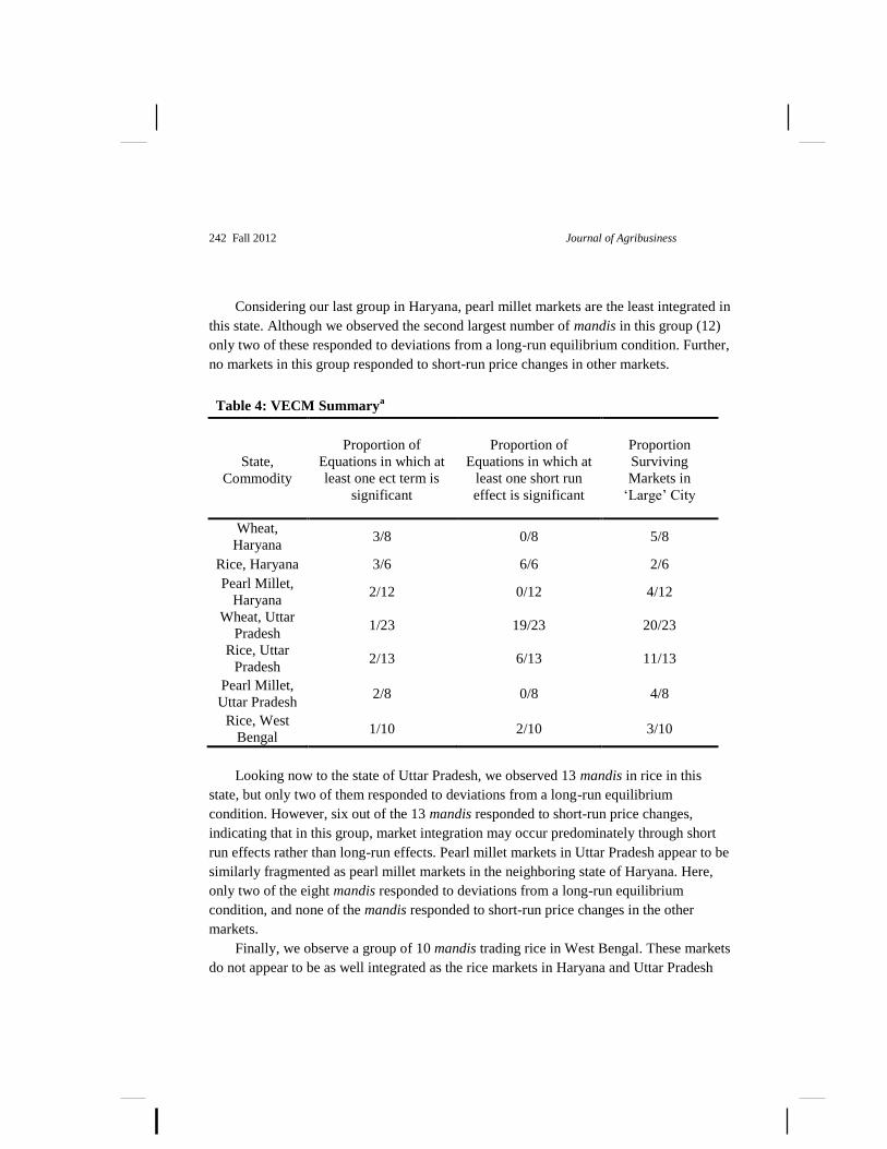
Main Results

The main results for the nonstationary data are found in Table 4. Here we present a

concise summary of the market integration results by displaying the proportion of mandis

in the group for which at least one of the error correction terms is significant in at least

one of the equations (in the first column) and the proportion of mandis in the group for

which at least one of the short run effects were significant in at least one of the equations.

That is, column 1 indicates the proportion of equations in which i

is significant in

equation i, and column 2 indicates the proportion of equations in which one of the ,i j

is

significant in equation i.

For example, row one contains the summary for the group of mandis in the state of

Haryana that report wheat sales in our dataset. In the first column, we report that in three

out of eight total mandis at least one of the error correction terms was significant. We

may conclude then, that prices in three of the eight mandis are integrated with one

another, while prices in five of the mandis where wheat is traded in Haryana do not

appear to adjust to maintain a long-run equilibrium with the other mandis. One can see in

the second column of row one that no short run effects were significant in any of the

mandis trading wheat in Haryana.

Even with a relatively low level of spatial integration, it appears that rice markets in

Haryana are the most integrated of the markets we consider. Three out of six respond to

deviations from long-run equilibrium, and all six mandis respond to at least one of the

short-run changes in one of the other markets.

i


Considering our last group in Haryana, pearl millet markets are the least integrated in

this state. Although we observed the second largest number of mandis in this group (12)

only two of these responded to deviations from a long-run equilibrium condition. Further,

no markets in this group responded to short-run price changes in other markets.

Table 4: VECM Summarya

State,

Commodity

Proportion of

Equations in which at

least one ect term is

significant

Proportion of

Equations in which at

least one short run

effect is significant

Proportion

Surviving

Markets in

‘Large’ City

Wheat,

Haryana 3/8 0/8 5/8

Rice, Haryana 3/6 6/6 2/6

Pearl Millet,

Haryana 2/12 0/12 4/12

Wheat, Uttar

Pradesh 1/23 19/23 20/23

Rice, Uttar

Pradesh 2/13 6/13 11/13

Pearl Millet,

Uttar Pradesh 2/8 0/8 4/8

Rice, West

Bengal 1/10 2/10 3/10

Looking now to the state of Uttar Pradesh, we observed 13 mandis in rice in this

state, but only two of them responded to deviations from a long-run equilibrium

condition. However, six out of the 13 mandis responded to short-run price changes,

indicating that in this group, market integration may occur predominately through short

run effects rather than long-run effects. Pearl millet markets in Uttar Pradesh appear to be

similarly fragmented as pearl millet markets in the neighboring state of Haryana. Here,

only two of the eight mandis responded to deviations from a long-run equilibrium

condition, and none of the mandis responded to short-run price changes in the other

markets.

Finally, we observe a group of 10 mandis trading rice in West Bengal. These markets

do not appear to be as well integrated as the rice markets in Haryana and Uttar Pradesh


with only one out of 10 responding to deviations from long-run equilibrium and two out

of 10 responding to short-run price changes in other mandis.

Discussion and Conclusions

In conclusion, despite using a sub sample of more active markets and median monthly

prices, both of which would tend to bias our results to finding integration, we observe

substantial fractionalization in grains markets in the producing states in India. We use a

novel method of data interpolation and unlike recent past market integration studies in

India, we find little evidence that grain markets are spatially integrated. We also observe

substantial differences in the degree of integration among states and crops. A lack of

observed spatial market integration can result from high and variable transportation costs

from one market to another, due to either poor physical or market information

infrastructure. Second, a lack of observed spatial market integration can also result from

limited storage near one market which will limit the ability of farmers or traders to take

advantage of post-harvest arbitrage opportunities. Third, we see a higher degree of spatial

integration in the wealthier states of Haryana and Uttar Pradesh, and less in the poorer

state of West Bengal. Thus, state-level differences clearly matter.

In our results, we see the highly regulated crops of wheat and rice have the highest

degree of spatial integration. Note that during this period, the federal government

instituted export bans on both crops and changed MSPs several points during the year, so

the price coordination may in part be a result of those national interventions, but more

research is needed to determine if this is the case.

This result is particularly notable in the case of the state of Haryana where physical

infrastructure is relatively good and markets are more modern. Even here however, we

see no evidence of market integration in pearl millet despite seeing some limited

evidence in wheat and rice. Thus, controlling for infrastructure, we observe the smaller,

less regulated market also being less integrated.

One might anticipate that those markets with more buyers are more likely to be

integrated. As a proxy for demand we consider which of our markets are in urban centers,

defined as having a population of more than 100,000. However, we see no strong

evidence that these markets are more likely to be spatially integrated. Markets in Uttar

Pradesh and Haryana for wheat tend to be located in urban centers, while the most

integrated markets are in Haryana for rice.


Second, we explored whether integrated markets were spatially clustered. However,

when we look at the location of these integrated markets, they do not appear to be

grouped more tightly than the markets where we see no evidence of integration.

A third alternative is the limited market integration we observe in wheat and rice prices is

driven by MSPs or by the rice export ban. In future work, we would like to formally test

these hypotheses. Second, we would like to test the effect of considering a smaller sample

of markets in each state affects our results, and how the degree of integration varies

across space within a state. We could limit our study to only those markets handling a

large volume to observe whether the lack of integration is only driven by thin markets.

In this paper, using comprehensive spatial integration techniques and appropriately

dealing with missing observations, we observe a significant lack of spatial market

integration in India. Thus, we argue that this finding raises the concern that farmers are

not able to benefit from arbitrage opportunities and may not receive appropriate price

signals. It is also clear that India’s market reforms of the early 2000s were insufficient to

develop a fully integrated, low-transaction cost grain market for her farmers.

References

AgMarkNet. (2012). http://agmarknet.nic.in/

Ardeni, P. (1989). “Does the law of one price really hold for commodity prices?” American Journal

of Agricultural Economics 71(3), 661-669.

Baffes, J. (1991). “Some further evidence on the law of one price: the law of one price still holds.”

American Journal of Agricultural Economics 73(4), 1264-1273.

Chand, R. and A. Gulati. (2011). “Managing food inflation in India: reforms and policy options.”

National Centre for Agricultural Economics and Policy Research, Policy Brief,

http://www.ncap.res.in/upload_files/policy_brief/pb35.pdf.

Enders, W. (2009). Applied Econometric Time Series.Wiley, 3rd Ed. ISBN-13:978-0470505397.

Engle, R. F., & Granger, C. W. (1987). “Co-integration and error correction: representation,

estimation, and testing.” Econometrica 55(1), 251-276.

Friedman, M. (1962). “The interpolation of time series by related series.” Journal of the American

Statistical Association 57(300), 729-757.

Ghosh, M. (2010). “Spatial price linkages in food grain markets in India.” Margin—The Journal of

Applied Economic Research 4(4), 495–516.

———. (2003). “Spatial integration of wheat markets in India: Evidence from cointegration tests.”

Oxford Development Studies 31(2), 159–71.

Goodwin, B., and Schroeder, T. (1991). “Cointegration tests and spatial price linkages in regional

cattle markets.” American Journal of Agricultural Economics 73(2), 452-464.


Gonzalez-Riera, G and S Helfand. (2001). “The extent, pattern and degree of market integration: a

multivariate approach for the Brazilian rice market.” American Journal of Agricultural

Economics 83(3), 576-92.

Government of Canada. (2008). “India agricultural policy review.” Agriculture and Agri-Food

Canada. (September) Ottawa: Agriculture and Agri-Food Canada.

Honaker, J. and G. King. (2010). “What to do about missing values in time series cross-section

data.” American Journal of Political Science 54(2), 561-581.

Honaker, J., G. King, M. Blackwell. (2011). “Amelia II: A program for missing data.” Journal of

Statistical Software 45(7), 1-47.

Jayasuriya, S. J.H. Kim and P. Kumar. (2007). “International and internal market integration in

Indian agriculture: a study of the Indian rice market.” Paper prepared for presentation at the

106th seminar of the European Association of Agricultural Economics, 25-27 October 2007,

Montpellier, France. http://purl.umn.edu/7935.

Jha, R., K. Murthy, H. Nagarajan and A. Seth. (1997). “Market integration in Indian agriculture.”

Economic Systems 21(3), 217-34.

Jha, R., K. Murthy, H. Nagarajan and A. Seth. (1999). “Components of the wholesale bid-ask

spread and the structure of grain markets: the case of rice in India.” Agricultural Economics 21,

173-189.

Jha, R., K. Murthy and A. Sharma. (2006). “Fragmentation of wholesale rice markets in India.”

Economic and Political Weekly 40(53) (Dec. 31, 2005 - Jan. 6, 2006), 5571-5577.

Jha, R. and H. K. Nagarajan. (1998). “Wholesaler stocks and hoarding in rice markets in india”

Economic and Political Weekly 33(41), 2658-2661.

Jha, S., P. V. Srinivasan and A. Ganesh-Kumar. (2010). “Achieving food security in a cost-

effective way: Implications of domestic deregulation and liberalized trade in India”. In A.

Ganesh-Kumar, D. Roy and A. Gulati (Eds.) Liberalizing Food Grains Markets: Experiences,

Impact and Lessons from South Asia, IFPRI-Oxford University Press, New Delhi.

Johansen, S. (1988). “Statistical analysis of cointegration vectors.” Journal of Economic Dynamics

and Control 12(2), 231-254.

King, G., J. Honaker, A. Joseph, and K. Scheve. (2001). ”Analyzing incomplete political science

data: an alternative algorithm for multiple imputation.” American Political Science Review

95(1), 49-69.

Kumar, C., Turvey, C., and Kropp, J. (2012).“Credit constraint impacts on farm households: survey

results from India and China.” Working Paper. Available at SSRN:

http://ssrn.com/abstract=2034487.

Naik, G. and S.K. Jain. (2002). “Indian agricultural commodity futures markets: a performance

survey.” Economic and Political Weekly 37(30) (Jul. 27 - Aug. 2, 2002), 3161-3173.

Organization for Economic Co-operation and Development (OECD). (2007). Agricultural Policies

in non-OECD Countries. OECD: Paris ISBN 978-92-64-03121-0.

Palaskas, T.B. and B. Harriss-White. (1993). “Testing market integration: New approach with case

material from the West Bengal food economy.” Journal of Development Studies 30(1), 1–57.


Pfaff, B. (2008). “VAR, SVAR and SVEC Models: Implementation within R Package vars.”

Journal of Statistical Software 27(4): 1-32. http://www.jstatsoft.org/v27/i04/.

Radhakrishna, R. and S. Indrakant. (1988). “Effects of rice market intervention policies in India:

the case of Andhra Pradesh.” in Evaluating Rice Market Intervention Policies, Some Asian

Examples, Manila: Asian Development Bank, 237-321.

Rubin, D.B. (1976). “Inference and missing data.” Biometrika 63, 581-592.

Sekhar, C.S.C. (2004). “Agricultural price volatility in international and indian markets.”

Economic and Political Weekly 39(43) (Oct. 23-29, 2004), 4729-4736.

Singh, S. (2012). “India grain and feed annual.” Report by the U.S. Department of Agriculture

Foreign Agricultural Service. Grain Report Number IN2026.

World Bank. (1999). India Food Grain Marketing Policies: Reforming to Meet Food Security

Needs, Vol. I and II, Report No. 18329” IN, April.

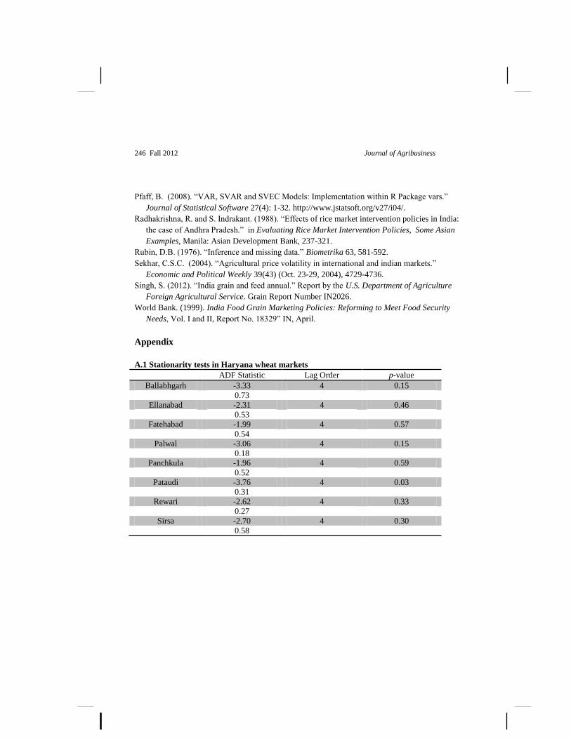
Appendix

A.1 Stationarity tests in Haryana wheat markets

ADF Statistic Lag Order p-value

Ballabhgarh -3.33 4 0.15

0.73

Ellanabad -2.31 4 0.46

0.53

Fatehabad -1.99 4 0.57

0.54

Palwal -3.06 4 0.15

0.18

Panchkula -1.96 4 0.59

0.52

Pataudi -3.76 4 0.03

0.31

Rewari -2.62 4 0.33

0.27

Sirsa -2.70 4 0.30

0.58


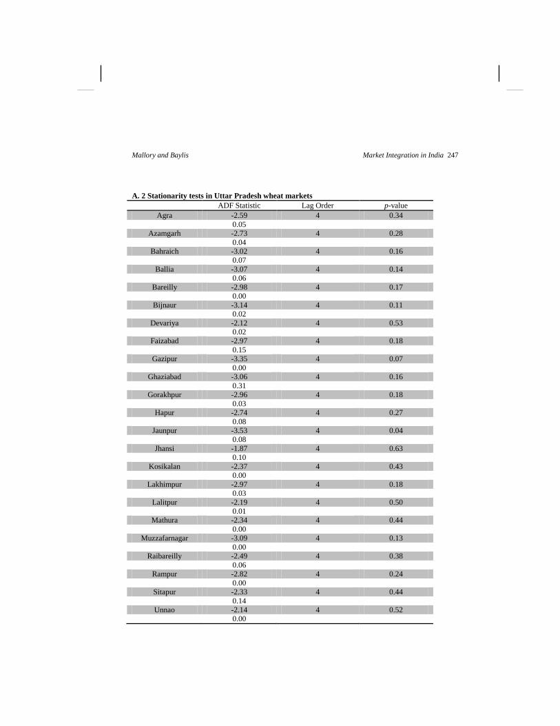
A. 2 Stationarity tests in Uttar Pradesh wheat markets


Agra -2.59 4 0.34

0.05

Azamgarh -2.73 4 0.28

0.04

Bahraich -3.02 4 0.16

0.07

Ballia -3.07 4 0.14

0.06

Bareilly -2.98 4 0.17

0.00

Bijnaur -3.14 4 0.11

0.02

Devariya -2.12 4 0.53

0.02

Faizabad -2.97 4 0.18

0.15

Gazipur -3.35 4 0.07

0.00

Ghaziabad -3.06 4 0.16

0.31

Gorakhpur -2.96 4 0.18

0.03

Hapur -2.74 4 0.27

0.08

Jaunpur -3.53 4 0.04

0.08

Jhansi -1.87 4 0.63

0.10

Kosikalan -2.37 4 0.43

0.00

Lakhimpur -2.97 4 0.18

0.03

Lalitpur -2.19 4 0.50

0.01

Mathura -2.34 4 0.44

0.00

Muzzafarnagar -3.09 4 0.13

0.00

Raibareilly -2.49 4 0.38

0.06

Rampur -2.82 4 0.24

0.00

Sitapur -2.33 4 0.44

0.14

Unnao -2.14 4 0.52

0.00


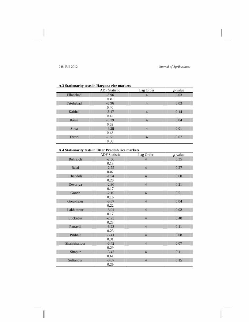
A.3 Stationarity tests in Haryana rice markets


Ellanabad -3.96 4 0.03

0.49


0.40

Kaithal -3.17 4 0.14

0.42

Rania -3.79 4 0.04

0.52

Sirsa -4.28 4 0.01

0.43

Tarori -3.51 4 0.07

0.38

A.4 Stationarity tests in Uttar Pradesh rice markets


Bahraich -2.56 4 0.35

0.13

Basti -2.75 4 0.27

0.07

Chandoli -1.94 4 0.60

0.20

Devariya -2.90 4 0.21

0.17

Gonda -2.16 4 0.51

0.16

Gorakhpur -3.67 4 0.04

0.22

Lakhimpur -3.94 4 0.02

0.17

Lucknow -2.23 4 0.48

0.23

Partaval -3.23 4 0.11

0.23

Pilibhit -3.41 4 0.08

0.31

Shahjahanpur -3.42 4 0.07

0.29

Sitapur -3.47 4 0.11

0.61

Sultanpur -3.07 4 0.15

0.29


A.5 Stationarity tests in West Bengal rice markets


Bethuadahari -1.27 4 0.86

0.26

Birbhum -1.72 4 0.69

0.31

Bishnupur -2.30 4 0.45

0.17

Bolpur -2.20 4 0.49

0.10

Coochbehar -2.12 4 0.53

0.35

Dinhata -1.39 4 0.76

0.81

Ghatal -2.13 4 0.52

0.28

Kalna -1.69 4 0.70

0.14

Katwa -2.72 4 0.28

0.31

Samsi -1.89 4 0.62

0.17


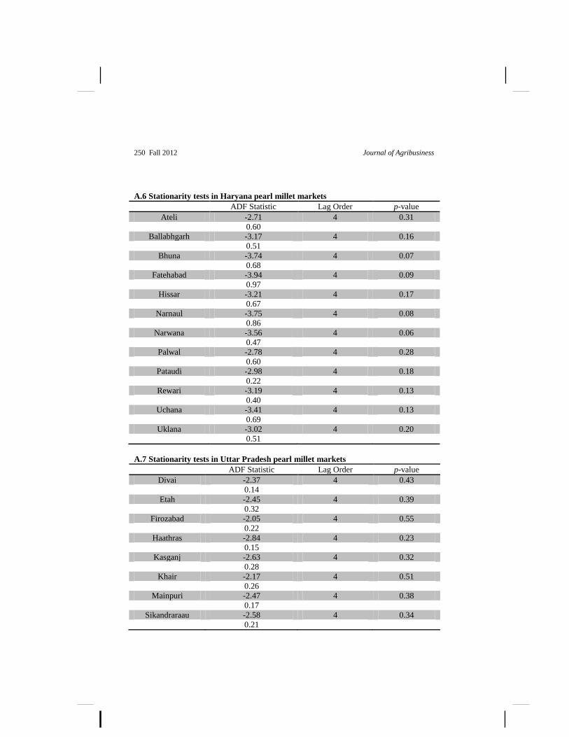
A.6 Stationarity tests in Haryana pearl millet markets


Ateli -2.71 4 0.31

0.60

Ballabhgarh -3.17 4 0.16

0.51

Bhuna -3.74 4 0.07

0.68


0.97

Hissar -3.21 4 0.17

0.67

Narnaul -3.75 4 0.08

0.86

Narwana -3.56 4 0.06

0.47

Palwal -2.78 4 0.28

0.60

Pataudi -2.98 4 0.18

0.22

Rewari -3.19 4 0.13

0.40

Uchana -3.41 4 0.13

0.69

Uklana -3.02 4 0.20

0.51

A.7 Stationarity tests in Uttar Pradesh pearl millet markets


Divai -2.37 4 0.43

0.14

Etah -2.45 4 0.39

0.32

Firozabad -2.05 4 0.55

0.22

Haathras -2.84 4 0.23

0.15

Kasganj -2.63 4 0.32

0.28

Khair -2.17 4 0.51

0.26

Mainpuri -2.47 4 0.38

0.17

Sikandraraau -2.58 4 0.34

0.21

Impacts on Market Integration in Wheat, Rice, and Pearl Millet

Documents

Transcript of Impacts on Market Integration in Wheat, Rice, and Pearl Millet