Biogeosciences, 5, 875–889, 2008www.biogeosciences.net/5/875/2008/© Author(s) 2008. This work is distributed underthe Creative Commons Attribution 3.0 License.

Biogeosciences

Impact of variable air-sea O2 and CO2 fluxes on atmosphericpotential oxygen (APO) and land-ocean carbon sink partitioning

C. D. Nevison1, N. M. Mahowald1,4, S. C. Doney2, I. D. Lima 2, and N. Cassar3

1National Center for Atmospheric Research, Boulder, Colorado, USA2Dept. of Marine Chemistry and Geochemistry, Woods Hole Oceanographic Institution, Woods Hole, MA, USA3Dept. of Geoscience, Princeton University, Princeton, NJ, USA4now at: Cornell University, Ithaca, NY, USA

Received: 4 July 2007 – Published in Biogeosciences Discuss.: 27 August 2007Revised: 7 April 2008 – Accepted: 7 April 2008 – Published: 2 June 2008

Abstract. A three dimensional, time-evolving field of at-mospheric potential oxygen (APO∼O2/N2+CO2) was esti-mated using surface O2, N2 and CO2 fluxes from the WHOIocean ecosystem model to force the MATCH atmospherictransport model. Land and fossil carbon fluxes were alsorun in MATCH and translated into O2 tracers using assumedO2:CO2 stoichiometries. The modeled seasonal cycles inAPO agree well with the observed cycles at 13 global moni-toring stations, with agreement helped by including oceanicCO2 in the APO calculation. The modeled latitudinal gradi-ent in APO is strongly influenced by seasonal rectifier effectsin atmospheric transport. An analysis of the APO-vs.-CO2mass-balance method for partitioning land and ocean carbonsinks was performed in the controlled context of the MATCHsimulation, in which the true surface carbon and oxygenfluxes were known exactly. This analysis suggests uncer-tainty of up to±0.2 PgC in the inferred sinks due to vari-ability associated with sparse atmospheric sampling. It alsoshows that interannual variability in oceanic O2 fluxes cancause large errors in the sink partitioning when the methodis applied over short timescales. However, when decadal orlonger averages are used, the variability in the oceanic O2flux is relatively small, allowing carbon sinks to be parti-tioned to within a standard deviation of 0.1 Pg C/yr of thetrue values, provided one has an accurate estimate of long-term mean O2 outgassing.

Correspondence to: C. D. Nevison(nevison@ucar.edu)

1 Introduction

Atmospheric O2/N2 measurements provide complementaryinformation about atmospheric CO2 due to the close couplingbetween oxygen and carbon fluxes during terrestrial photo-synthesis and respiration (Keeling et al., 1993). In contrast,oceanic O2 and CO2 fluxes are more or less decoupled, forreasons described below. The tracer atmospheric potentialoxygen (APO) exploits these differences to remove the ter-restrial contribution to changes in atmospheric O2/N2, thusallowing the oceanic contribution to be largely isolated. APOis defined as,

APO = O2/N2 +1.1

XO2

CO2, (1)

where 1.1 derives from the approximate – O2:CO2 molarratio of terrestrial photosynthesis and respiration (Severing-haus, 1995; Stephens et al., 1998; Keeling et al., 1998). TheparameterXO2=0.2098 is the mole fraction of O2 in dryair and converts from ppm O2 to per meg, the units usedfor O2/N2 (Keeling and Shertz, 1992). Oxygen and carbonfluxes are also closely coupled during fossil fuel combustion,but with a slightly larger – O2:CO2 molar ratio of∼1.4. Asa result, fossil fuel combustion exerts a small influence onAPO, since it yields changes in O2/N2 and CO2 that cancelout mostly but not completely in Eq. 1.

APO data have been used in at least three important carboncycle applications. First, the seasonal cycle in APO reflectsseasonal imbalances between photosynthetic new productionin the surface ocean, which occurs largely in spring and sum-mer, and the wintertime ventilation of deeper waters, whichare depleted in O2 due to remineralization. The amplitude ofthe seasonal cycle in APO has been used to infer the rate ofseasonal new production at the ocean basin or hemisphericscale (Bender et al., 1996; Balkanski et al., 1999; Najjar and

Published by Copernicus Publications on behalf of the European Geosciences Union.

876 C. D. Nevison et al.: Air-sea O2 flux variability and its impact on APO

Keeling, 2000), although temporal and spatial overlap be-tween new production and ventilation cause uncertainties inthe inferred rates (Nevison et al., 2005; Jin et al., 2007).

Second, the latitudinal gradient in APO in principle re-flects global-scale patterns of ocean biogeochemistry andocean circulation, with O2 uptake occurring primarily at highlatitudes and outgassing of both O2 and CO2 taking place inthe tropics. The ocean-induced patterns are superimposed onthe overall north-to-south increase in APO due to northernhemisphere-dominated fossil fuel combustion. Early atmo-spheric transport model simulations of the latitudinal gradi-ent in APO found a mismatch with observations, and sug-gested that the cause might be deficiencies in the physicsof the ocean carbon models used to force the simulations(Stephens et al., 1998). Later studies suggested that thediscrepancies might be attributed mainly to the atmospherictransport models (Gruber et al., 2001; Naegler et al., 2007).A further complication is that the observed APO gradient ap-pears to be evolving with time and displays significant inter-annual variability (Battle et al., 2006).

A third, critically important application of APO data is toconstrain the partitioning of anthropogenic CO2 uptake be-tween the ocean and the land biosphere, which together haveabsorbed more than half of the anthropogenic carbon put inthe atmosphere over the last half century (Battle et al., 2000;Bender et al., 2005; Manning and Keeling, 2006; referred tohereafter as MK06). This application involves solving a sys-tem with two equations and two unknowns, as derived fromthe mass balances for CO2 and O2/N2.

1CO2/1t = β(Ffuel − Fland − Focean) (2)

1(O2/N2)/1t = βγ (−αf Ffuel + αbioFland) + Zeff, (3)

whereβ=0.471 is the conversion from Pg C to ppm CO2,γ =1/XO2 is the ppm to per meg conversion factor describedabove,Zeff is an oceanic O2 outgassing term in per meg units,andαbio=1.1 andαf =1.4 are the – O2:CO2 molar ratios ofterrestrial respiration and photosynthesis and fossil fuel com-bustion. Ffuel is the release of fossil carbon to the atmo-sphere, which is known from industry data (Marland et al.,2002), whileFland andFocean, the two unknowns, are CO2uptake by land and ocean, defined here as positive when theyact as sinks for atmospheric CO2. Eqs. 2 and 3 can be com-bined according to the definition of APO in Eq. 1 to yield theAPO time derivative:

1(APO)/1t=βγ ((αbio−αf )Ffuel−αbioFocean)+Zeff (4)

One can solve forFland andFoceanusing either the systemof equations 2 and 3 or 2 and 4 based on the global rates ofchange of CO2 and O2/N2 or CO2 and APO, respectively,observed by global atmospheric monitoring networks.

The above method, originally presented as a vector dia-gram (Keeling et al., 1996), assumes that the O2:CO2 stoi-chiometries of fossil fuel combustion and terrestrial respira-tion and photosynthesis are known, but that oceanic O2 and

CO2 fluxes are decoupled. The vector method is often con-sidered the best way to monitor the partitioning of sinks foranthropogenic CO2 on a continual basis, allowing the detec-tion of trends or changes, e.g., the increased land sink of the1990s relative to the 1980s (Prentice et al., 2001). Alterna-tive methods for estimating ocean and land sinks are gener-ally more difficult to update quickly. Ocean inventory meth-ods, for example, require a large new set of ocean cruise data(e.g., Matsumoto and Gruber, 2005).

Despite the advantages of the APO vs. CO2 method, itsinherent uncertainties may be so large that it cannot con-strain the carbon sink partitioning to within better than∼±0.7 PgC/yr (LeQuere et al., 2003). This uncertainty rep-resents a substantial fraction of the mean total land and oceansinks, which are estimated at 1.9 and 1.2 PgC/yr, respec-tively, for 1990–2000 (MK06). Among the inherent un-certainties in the method are those associated with fossilfuel combustion inventories and the assumed – O2:CO2 stoi-chiometries of combustion and terrestrial photosynthesis andrespiration. However, the single largest uncertainty for esti-mating the ocean carbon sink is theZeff term associated withoceanic O2 fluxes (MK06).

Early applications of the vector method assumed that theatmosphere-ocean system for O2 was still essentially in equi-librium and thus that the net annual mean air-sea flux of O2was approximately zero (Keeling et al., 1993; 1996). Thisassumption was closely related to the reasons for the decou-pling of oceanic O2 and CO2 fluxes. First, O2 is far lesssoluble than CO2, with only 1% of the O2 in the ocean-atmosphere system partitioning into the ocean compared to98% for CO2. Second, the buffering effect of carbonatechemistry in seawater increases the air-sea CO2 equilibrationtime scale by an order of magnitude relative to that of O2.Third, fossil fuel combustion and deforestation have raisedatmospheric CO2 by ∼35% relative to preindustrial levels,thus providing the geochemical driving force for net globaloceanic CO2 uptake. In contrast, these processes have re-duced atmospheric O2/N2 by only∼240 per meg, or less than0.03% of the total O2 burden, since atmospheric monitoringof O2/N2 began in the late 1980s (MK06).

Although the assumption of a net zero annual oceanic O2flux initially seemed reasonable, it has long been knownthat natural interannual variability in oceanic O2 fluxes, due,e.g., to incomplete ventilation of O2-depleted thermoclinewaters in some years, followed by deep convection eventsin subsequent years, can create a non-zero net oceanic O2flux over a given year or even period of years (Keeling etal., 1993). Thus the vector method is generally applied tolonger, e.g., decadal averages, of APO and CO2 data withthe assumption that the interannual variability will averageto zero. In addition to natural interannual variability, re-cent studies have recognized that long-term ocean warm-ing may be inducing net O2 outgassing, with reinforcingfeedbacks associated with biology and ocean stratification(Sarmiento et al., 1998; Bopp et al., 2002; Plattner et al.,

Biogeosciences, 5, 875–889, 2008 www.biogeosciences.net/5/875/2008/

C. D. Nevison et al.: Air-sea O2 flux variability and its impact on APO 877

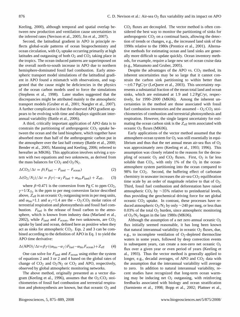
Table 1. Summary of surface fluxes used to drive MATCH simulations and the resulting tracers used to calculate APO.

Code Tracer Length of Simulation

WHOI Ocean Model FluxesW1 CO2 1979–2004W2 O2 1979–2004W3 N2 1979–2004W4 Thermal O2 1979–2004

Climatological Ocean FluxesC1 CO2 (Takahashi et al., 2002)∗ 1988–2004C2 O2 seasonal anomalies (GK01)∗ 1988–2004C3 N2 seasonal anomalies (GK01)∗ 1988–2004C4 O2 annual mean (Gruber et al., 2001) 1988–2004C5 N2 annual mean (Gloor et al., 2001) 1988–2004

Terrestrial FluxesL1 CASA GFED v.2 (Randerson et al., 2005; Van der Werf et al., 2006) 1997–2004L2 CASA Neutral Biosphere (Olsen and Randerson, 2002)∗ 1979–2004FF Fossil Fuel (Nevison et al., 2008) 1979–2004

Atmospheric Potential Oxygen (APO)∗∗ Inputs to Eq. 5∗∗

A1 WHOI W1,W2,W3,FFA2 WHOI thermal W1,W4,W3,FFA3 Seasonal climatology C1,C2,C3,FFA4 Annual climatology C1,C4,C5,FFA5 Composite climatology Sum of A3,A4

∗ Surface flux is cyclostationary (i.e., the same seasonal cycle is repeated each year).∗∗ The same code is used to refer to APOoc (calculated withoutFF ) and O2/Noc

2 (calculated from Eq. 6 withoutFF and COoc2 ).

2002). Both natural interannual variability and long-term netO2 outgassing are quantified based on empirical relationshipsbetween dissolved O2 and potential temperature extrapolatedto observed heat fluxes, although these relationships are notwell understood (Keeling and Garcia, 2002). MK06 estimatethe combined effects of these two processes on uncertaintyin ocean and land carbon sink partitioning at±0.5 Pg C/yr.

Here we present a model-based analysis of atmosphericAPO and CO2 focusing on interannual variability in oceanicO2 fluxes and their contribution to uncertainty in the APOvs. CO2 method for partitioning carbon sinks. To esti-mate oceanic O2, N2 and CO2 fluxes, we employ a process-based ocean ecosystem model coupled to a general circula-tion model, which represents an advance over the OCMIP-based (i.e., phosphate-restoring) ocean carbon models thatwere used predominantly in previous APO studies (Stephenset al., 1998; Naegler et al., 2007). The ocean fluxes are usedto force atmospheric transport model simulations that includefull interannual variability in the meteorological drivers. Wealso force the transport model with fossil and terrestrial CO2fluxes, which can be scaled to O2 based on assumed stoi-chiometries. Our simulation encompasses a complete set ofatmospheric tracers that can be used to evaluate uncertaintiesin the APO vs. CO2 method in a controlled model context inwhich the true surface CO2 and O2 fluxes are known exactly.We begin in Sect. 2 with a description of the atmospheric

tracer transport model (ATM) and ocean, land, and fossilfuel fluxes as well as the APO observations used to evaluatemodel results. We present a comparison of model vs. ob-served seasonal cycles and latitudinal gradients in Sects. 3.1and 3.2, respectively. In Sect. 3.3 we characterize the inter-annual variability in model APO and in Sect. 3.4 we analyzethe impact of interannual variability in oceanic O2 fluxes onthe APO vs. CO2 method for partitioning carbon sinks. Thissection also includes an analysis of errors in the method as-sociated with sparse sampling of the ATM at grid points cor-responding to APO monitoring stations. We conclude with asummary of our results in Sect. 4.

2 Methods

2.1 Atmospheric transport model

The Model of Atmospheric Transport and Chemistry(MATCH) (Rasch et al., 1997; Mahowald et al., 1997) wasused to simulate the atmospheric distribution of a rangeof surface O2, CO2 and N2 fluxes. The model was runat T62 horizontal resolution (about 1.9◦ latitude by longi-tude) with 28 vertical levels and a time step of 20 min us-ing archived 6 hourly winds for the years 1979–2004 fromthe National Center for Environmental Prediction (NCEP)

www.biogeosciences.net/5/875/2008/ Biogeosciences, 5, 875–889, 2008

878 C. D. Nevison et al.: Air-sea O2 flux variability and its impact on APO

reanalyses (Kalnay et al., 1996). The surface fluxes used toforce the simulations are described below and summarized inTable 1. See also Nevison et al. (2008) for additional details.

2.2 Air-sea fluxes of O2, CO2 and N2

Oceanic O2 and CO2 fluxes were obtained for 1979–2004from the WHOI-NCAR-UC Irvine ocean general circula-tion and marine ecosystem model (abbreviated here as theWHOI model). The ecosystem model includes a nutrient-phytoplankton-zooplankton-detritus (NPZD) food web withmulti-nutrient limitation (N, P, Si, Fe) and specific phyto-plankton functional groups (Doney et al., 1996; Moore et al.,2002, 2004). The general circulation model is the NCARocean model, which was run at 3.6◦ longitude resolution andvariable latitude resolution ranging from 0.6◦ near the equa-tor to 2.8◦ at mid-latitudes, and forced with historical daily-averaged NCEP reanalysis surface wind, heat flux, atmo-spheric temperature and humidity, and satellite data productsfrom 1979–2004 (Doney et al., 1998, 2007). With properhistorical forcing, the NCAR ocean model captures well themagnitude and phasing of upper ocean heat content interan-nual variability (Doney et al., 2007).

While O2 and CO2 fluxes were obtained prognosticallyfrom the WHOI model, N2 fluxes were diagnosed basedon the NCEP heat fluxes (Q) as FN2=Q(dSN2/dT )/Cp

(Keeling et al., 1998), wheredSN2/dT is the tempera-ture derivative of N2 solubility evaluated at the NCEPsea surface temperature. A similar equation was used toestimate the thermal component of the WHOI O2 flux:FO2 thermal=Q(dSO2/dT )/Cp, but with two modificationsrecommended by Jin et al. (2007), who optimized the for-mula based on comparisons to explicitly modeled thermal O2fluxes. First, the magnitude ofFO2 thermal was scaled downby a factor of 0.7 to account for incomplete thermal equili-bration of O2. Second, the flux was delayed for half a monthto account for non-instantaneous air-sea equilibration. Sim-ilar modifications may be needed forFN2, but were not ap-plied in the current study, since their appropriateness for N2has not yet been evaluated (X. Jin, personal communication).

In addition to the interannually-varying WHOI and NCEP-based fluxes, MATCH was also run from 1988–2004 with avariety of climatological oceanic CO2, O2, and N2 fluxes.These included the monthly sea surface CO2 flux clima-tology of Takahashi et al. (2002) (corrected to 10 m heightwindspeeds) and the monthly O2 and N2 flux anomaly cli-matology of Garcia and Keeling (2001) (hereafter referredto as GK01). The GK01 O2 fluxes are based on linearregressions that use ECMWF heat flux anomalies to spa-tially and temporally extrapolate historical dissolved O2 data.These empirical regressions reflect both biology and circula-tion and thermal-driven variations in oxygen flux. The N2flux anomalies are calculated from the same formula forFN2

above, but use climatological ECMWF values rather thaninterannually-varying NCEP data forQ. The monthly O2

and N2 flux anomalies have an annual mean of zero at allgridpoints and thus do not provide realistic spatial distribu-tions. To fill this gap, additional simulations were performedwith O2 and N2 fluxes from the annual-mean ocean inver-sions of Gruber et al. (2001) and Gloor et al. (2001). Theinversions are based on ocean inventory data and are subjectto ocean general circulation model biases but independent ofatmospheric transport influences.

2.3 Fossil fuel and land biosphere carbon fluxes

Fossil fuel carbon emissions were constructed from decadal1◦×1◦ maps (Andres et al., 1996; Brenkert, 1998) that wereinterpolated between decades based on the annual regionaltotals of (Marland et al., 2003). The carbon fluxes were runin MATCH from 1979-2004. The atmospheric O2 distribu-tions resulting from fossil fuel combustion were estimatedfrom MATCH CO2 multiplied by a mean fossil fuel O2:CO2stoichiometry of –1.4 (MK06).

Two versions of the CASA land biosphere model wereused for terrestrial CO2 fluxes. The first (L1 in Table 1)was the Global Fire Emissions Database (GFED v2) ver-sion of CASA, which incorporates satellite-based estimatesof burned area (Randerson et al., 2005; Van der Werf et al.,2006) and for which the biomass burning component of theemissions was optimized based on CO inversion results (Ka-sibhatla et al., manuscript in preparation). The second (L2)was a cyclostationary (i.e., the same seasonal cycle repeatedevery year) “neutral biosphere” version, run in MATCH from1979–2004, in which annual net ecosystem production wasassumed to be zero at each grid cell (Olsen and Randerson,2004). The L1 fluxes provide more realistic interannual vari-ability in atmospheric CO2 than the L2 fluxes, but are limitedto 1997–2004 (Nevison et al., 2008). At their original 1◦×1◦

resolution, the global mean L1 carbon flux was constrainedto equal zero over the 1997–2004 period, and the L2 flux hadan annual mean of zero every year. However, a small interpo-lation error in converting to the T62 MATCH grid resulted ina small net source of CO2 to the atmosphere of∼+0.1 PgC/yrfor both versions of the land flux over these respective peri-ods.

2.4 Model APO

Model atmospheric potential oxygen (APO) was calculatedsomewhat differently than observed APO (Eq. 1), since O2and N2 were run as separate tracers in MATCH. We usedequation 5, in which all individual O2, N2 and CO2 tracersare in ppm of dry air and APO is in per meg units (Stephenset al., 1998; Naegler et al., 2007).

Biogeosciences, 5, 875–889, 2008 www.biogeosciences.net/5/875/2008/

C. D. Nevison et al.: Air-sea O2 flux variability and its impact on APO 879

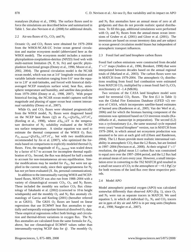
Fig. 1. Seasonal cycles of APOoc at 12 selected stations. Gray filled squares are fit to the Battle et al. (2006) observed climatological seasonalcycle; black solid line is APOoc from the WHOI-MATCH A1 simulation; black dotted line is the A3 seasonal climatology simulation; graysolid line is WHOI-MATCH COoc

2 from the C1 simulation, converted to per meg units; black dashed line is the A2 simulation, i.e., APOoc

calculated with WHOI thermal O2 rather than total Ooc2 . Mean seasonal cycles were calculated by detrending the MATCH results with a 3rd

order polynomial and taking the average of all Januaries, all Februaries, etc.(a) Alert, Canada (ALT),(b) Barrow, Alaska (BRW),(c) ColdBay, Alaska (CBA),(d) Sable Island, Nova Scotia (SBL),(e) La Jolla, CA (LJO),(f) Kumukahi, Hawaii (KUM),(g) Samoa (SMO),(h)Cape Grim, Tasmania (CGO),(i) Macquarie Island, Australia (MQA),(j) Palmer Station, Antarctica (PSA),(k) Syowa, Antarctica (SYO),(l) South Pole (SPO).

APO=1

XO2(Ooc

2 −1.4COFF2 )−

1

XN2Noc

2

+1.1

XO2(COoc

2 +COFF2 ) (5)

where the superscriptsoc andFF denote ocean and fossilfuel tracers, respectively.XO2 andXN2 are the fractions ofO2 and N2 in air (0.20946 and 0.78084, respectively). LandO2 and CO2 tracers could have been included in the first andthird right hand side terms of Eq. 5, respectively, but simplywould have canceled out, since we assumed that Oland

2 = –1.1 COland

2 . In practice, the COFF2 terms were important for

latitudinal gradients, but had little effect on seasonal or in-terannual variability. For some applications, the fossil termswere omitted to yield a quantity we refer to as APOoc, whichincludes only the oceanic tracers. To examine the conse-quences of neglecting COoc

2 in calculating APOoc, a thirdquantity, referred to here as O2/Noc

2 , was computed:

O2/N2oc

=1

XO2Ooc

2 −1

XN2Noc

2 (6)

2.5 Observed APO

For comparison to model results, we used observed seasonalcycles from Battle et al. (2006), who computed the 1996–2003 climatological cycles at 13 land-based atmosphericmonitoring stations, including both the SIO (Keeling et al.,1998) and Princeton (Bender et al., 2005) networks. Battleet al. also determined the latitudinal gradient in APO fromthe annual mean offsets of sinusoidal fits to the observed sea-sonal cycles at the land-based monitoring stations and fromadditional ship-based measurements in the Pacific Ocean.

3 Results and discussion

3.1 Seasonal cycles

The seasonal cycles in APO predicted by the WHOI-MATCH simulation (A1 in Table 1) generally agree well withthe observed cycles (Figs. 1–2). The model amplitude is cap-tured to within±10 to 20% at most stations and the agree-ment in phasing is excellent at all stations, except Palmer Sta-tion, Antarctica (PSA), where the model minimum is a month

www.biogeosciences.net/5/875/2008/ Biogeosciences, 5, 875–889, 2008

880 C. D. Nevison et al.: Air-sea O2 flux variability and its impact on APO

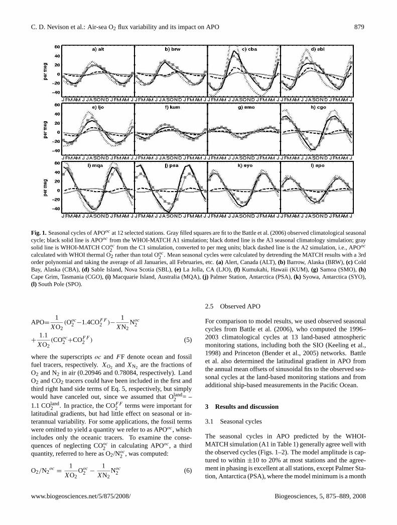
Fig. 2. Taylor diagrams summarizing the comparison of MATCH seasonal cycles to Battle et al. (2006) observations. The angleθ from thex-axis in the polar plot is the arccosine of the correlation coefficient R between the model and observed cycle, which reflects the agreementin shape and phasing. The value on the radial axis is the ratio of standard deviations:σmodel/σobs, which represents the match between theamplitude of the model and observed seasonal cycle (Taylor, 2001). Each symbol represents 1 of the 12 stations in Fig. 1, or a 13th station,Amsterdam Island, France (AMS). The 13 stations are sorted into 4 latitude bands according to the figure legend. The following MATCHsimulations are shown:(a) WHOI APOoc (A1) (b) WHOI O2/Noc

2 (A1, but COoc2 not included),(c) seasonal climatology APOoc (A3).

earlier than observed. Oceanic CO2, although sometimesneglected when calculating the APO seasonal cycle (e.g.,GK01; Blaine, 2005), appears to contribute in a small butnon-negligible manner to the amplitude agreement at somestations. Neglecting COoc

2 leads to a greater underestimateof the seasonal amplitude at the tropical SMO and KUM sta-tions, where the COoc

2 and Ooc2 seasonal cycles are in phase,

and a tendency to overestimate the seasonal amplitude at ex-tratropical southern stations, where COoc

2 opposes Ooc2 . In

comparison to A1, the A3 MATCH simulation with climato-logical ocean fluxes yields seasonal cycles in APO that agreeless well in shape and phasing with observations, and over-estimate the observed amplitude by 30–40% at most extrat-ropical stations and by nearly 100% at the Cold Bay, Alaska(CBA) station.

In general, thermal and biological O2 fluxes tend to rein-force each other over the seasonal cycle. In fall and win-ter, the increased solubility of cooling surface waters causesthermal ingassing, while the breakdown of the seasonal ther-mocline leads to biological uptake as deep waters depletedin O2 by microbial decomposition are ventilated (Keelinget al., 1993). Conversely, in spring and summer, warmingof surface waters tends to coincide with biological O2 out-gassing due to new production. However, comparison of theWHOI model A1 and A2 simulations suggests that net to-tal oceanic O2 fluxes do not always correlate well with ther-mal O2 fluxes (Fig. 1), as is assumed by the GK01 seasonalO2 climatology. At southern extratropical stations in particu-lar, thermal O2 fluxes are only moderately well correlated inshape and phasing (R=0.4–0.9) and only account for 10–15%of the amplitude of net O2 seasonal cycle, with the remain-der due to biology and circulation. At tropical and northernstations, the thermal O2 flux tends to correlate better and to

account for a larger (20–40%) share of the seasonal ampli-tude. In most regions of the ocean, Figs. 1–2 suggest that theexplicit modeling of ocean biology and circulation providedby the WHOI model yields superior results to the climatol-ogy. Similarly, the more sophisticated ocean ecosystem dy-namics of the WHOI model appears to yield more realisticseasonal cycles in APO than the P-restoring OCMIP oceanbiology parameterizations tested by Naegler et al. (2007).

A caveat on the above discussion is that the choice of at-mospheric transport model can influence the amplitude of themodel seasonal cycle in APO (Battle et al., 2006; Naegler etal., 2007), since many atmospheric transport models producea seasonal “rectifier” in APO (Stephens et al., 1998; Gruberet al., 2001; Blaine et al., 2005). The concept of seasonal rec-tification was first defined in atmospheric CO2 studies (Pear-man and Hyson, 1980; Keeling et al.,1989; Denning et al.,1995), and involves a covariation between seasonal variabil-ity in transport and surface fluxes that can yield annual-meansurface concentrations of an atmospheric tracer that are notzero, even when the annual mean surface flux of the tracer iszero.

Previous studies have found that ATMs with strong sea-sonal APO rectifiers, like TM3, tend to yield larger seasonalamplitudes in APO than weak rectifiers like TM2. Naegleret al. (2007) used the average of simulations with TM2 andTM3 as the best estimate of true APO, but Battle et al. (2006)suggested that TM3 may overestimate tracer concentrationsand thus seasonal amplitudes due to excessive vertical trap-ping in surface layers. This latter suggestion is supported bythe extreme overestimate of the seasonal amplitude at CBA inthe A3 simulation (Figs. 1–2). Transport model differencesmay explain the discrepancy between the results of GK01with TM2, which captures the amplitude of the observed

Biogeosciences, 5, 875–889, 2008 www.biogeosciences.net/5/875/2008/

C. D. Nevison et al.: Air-sea O2 flux variability and its impact on APO 881

O2/Noc2 cycle to within ±10% at most stations, and those

shown in Fig. 2c, in which the A3 simulation with the sameflux climatology tends to overestimate the observed APOseasonal cycle. Uncertainties associated with atmospherictransport are discussed further below in the context of latitu-dinal gradients.

3.2 Latitudinal gradient

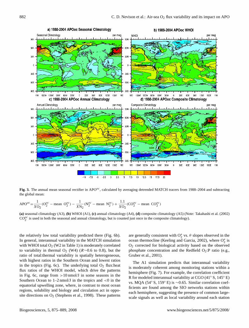
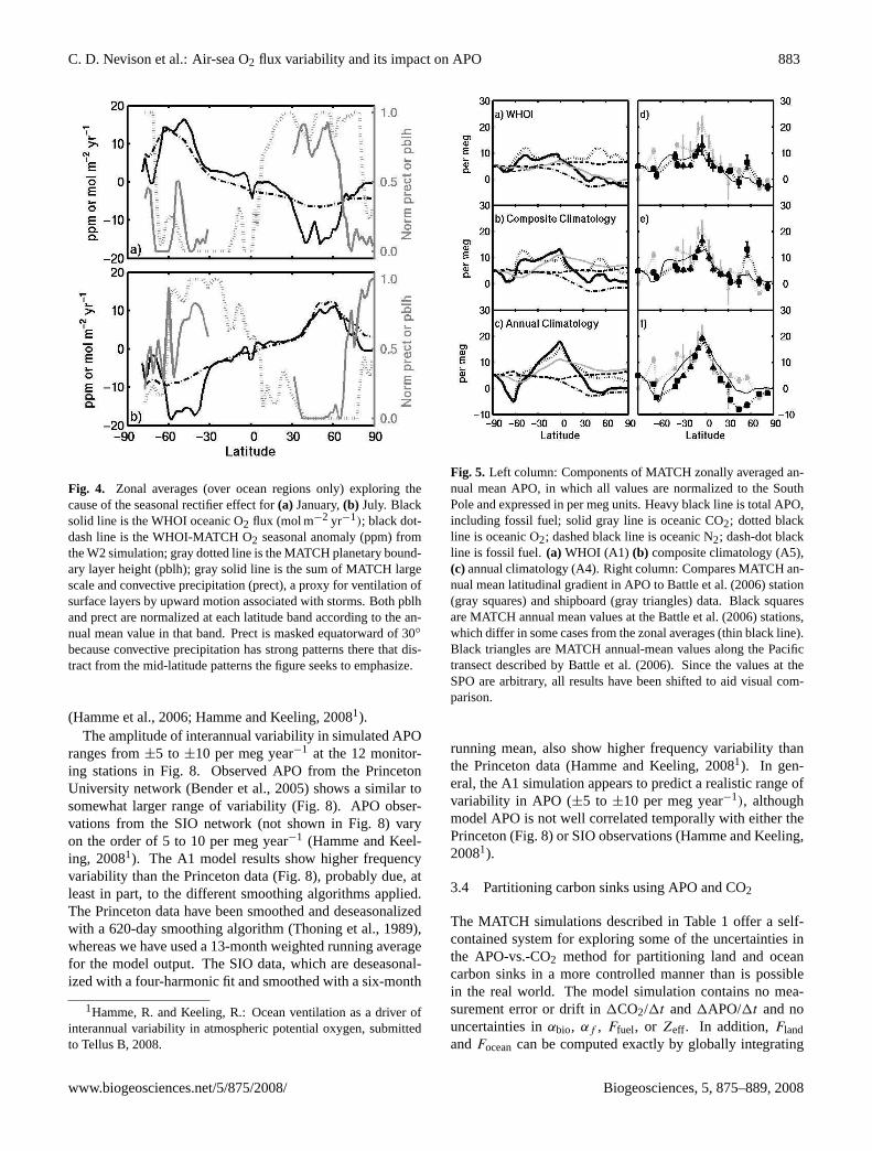
In the A3 simulation, in which climatological seasonal fluxanomalies have an annual mean of zero at all grid points forO2 and N2, MATCH predicts non-zero annual mean APOoc.Positive values of up to∼20 per meg are predicted overnorthern ocean regions centered around 45–60◦ N (encom-passing the CBA station) and up to∼10 per meg at compa-rable southern latitudes (Fig. 3a). Similar but weaker pat-terns appear in the A1 simulation with seasonally varyingWHOI fluxes (Fig. 3b). In contrast, the annual mean clima-tology simulation (A4) yields negative annual mean valuesof APOoc over the mid to high latitude oceans (Fig. 3c), con-sistent with the known patterns of net oceanic O2 uptake inthese regions. We also constructed a “composite” climatol-ogy (A5), as per Gruber et al. (2001) and Battle et al. (2006),by adding the results of MATCH simulations with the annualclimatology and the GK01 seasonal anomalies. The com-posite climatology yields an APOoc field similar to that ofthe WHOI model (Fig. 3d). The results shown in Fig. 3suggest that the MATCH transport model introduces a sea-sonal rectifier for simulations that include seasonally varyingoceanic O2 fluxes. Because the WHOI model itself predictsO2 uptake over the mid to high latitude oceans (not shown), itmust be that the atmospheric transport model, rather than theocean model, is responsible for the positive APOoc values inthe A1 results around 45–60◦ latitude (Fig. 3b).

The MATCH seasonal rectifier in APO is caused by at leasttwo interrelated mechanisms. First, the MATCH planetaryboundary layer is shallower in summer over the ocean than inwinter, due to increased convective heat release in wintertime(Fig. 4). Since positive sea-to-air O2 flux anomalies occurduring summer at mid to high latitudes, they are more likelyto be trapped near the surface, resulting in a net positive APOanomaly. Stephens et al. (1998) and Gruber et al. (2001)found a similar effect with the TM2 and GCTM transportmodels. A second, related mechanism also contributes to theMATCH rectifier effect. The sum of convective and large-scale precipitation, which is effectively a proxy for venti-lation of surface layers by upward motion associated withstorms, displays strong seasonal and hemispheric differences(Fig. 4). More storms occur over the ocean in the northernvs. the southern hemisphere and more storms occur in win-ter vs. summer in both hemispheres. Thus, negative winterO2 fluxes are more likely to be ventilated from the boundarylayer, especially in the northern hemisphere, helping to ex-plain the winter and summer pattern in both hemispheres aswell as the stronger seasonal difference in the north.

The “APO Transcom” intercomparison showed that themajority of nine transport models tested, using the GK01seasonal anomalies to produce the quantity referred to in thisstudy as O2/Noc

2 , yielded similar rectifier effects to those de-scribed above (Blaine, 2005). MATCH:NCEP fell amongthe strong rectifiers, but produced weaker annual mean val-ues than some of the other ATMs in that class. TM2 fellamong the weak rectifiers, especially when forced with the1986 ECMWF winds used by GK01.

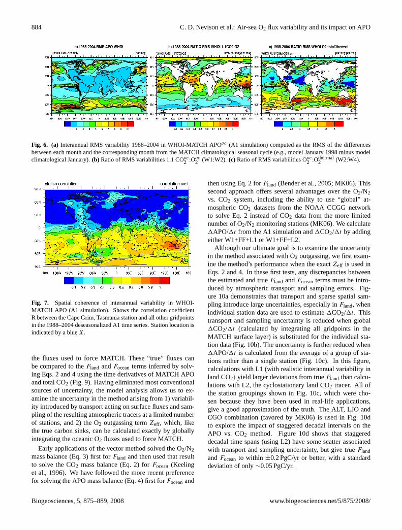
The MATCH seasonal rectifier is difficult to confirm ordisprove based on comparison with observed APO. The“equatorial bulge” in APO, a prominent feature of the obser-vations, is flattened in the A1 simulation by the strong mid tohigh latitude O2 maxima associated with the seasonal recti-fier (Fig. 5a,d). In contrast, the A4 simulation with the annualmean O2 flux climatology captures the “equatorial bulge”relatively well (Fig. 5c,f). There are no seasonal rectifier ef-fects in the A4 runs, since the O2 fluxes are uniform through-out the year and thus can not covary with transport. The com-posite climatology (A5) yields a rectifier-effect-dominatedlatitudinal gradient that resembles the A1 results but capturesthe equatorial bulge better, especially when model results aresubsampled in the tropical Pacific, where ship-based mea-surements are made, rather than zonally averaged (Fig. 5b,e).Battle et al. (2006) found similar results for TM3 simulationsusing the same composite climatology.

Aside from the equatorial bulge, both the A1 and A5simulations produce a south-to-north gradient that agreesreasonably well with observations (Fig. 5d,e). Both sim-ulations, particularly A5, overestimate the observed annualmean value at CBA, suggesting an exaggerated seasonal rec-tifier effect in that area of the North Pacific. However, the an-nual mean simulation (A4), which lacks a seasonal rectifier,substantially underestimates APO at midlatitudes relative tothe tropics, particularly in the northern hemisphere. Collec-tively, the above results suggest, in agreement with Naegleret al. (2007), that the APO seasonal rectifier probably existsto some degree in the real world, although both MATCH andTM3 may tend to exaggerate it. Overall, our results supportthe conclusion of Naegler et al. (2007) that evaluating oceanmodels (or flux climatologies) based on the latitudinal gradi-ent in APO is compromised by uncertainties in atmospherictransport models. The interannual variability and complexityof the observations further complicate the evaluation (Battleet al., 2006).

3.3 Interannual variability

A breakdown of APO from the WHOI-MATCH simulation(A1) into its components shows that oceanic O2 fluxes arethe main drivers of interannual variability in model APO(Fig. 6a,b). Most of the variability originates at mid tohigh latitudes, especially in the Southern Ocean (Fig. 6a).COoc

2 also contributes substantially to interannual variabil-ity in APO in the tropics, accounting for as much as half of

www.biogeosciences.net/5/875/2008/ Biogeosciences, 5, 875–889, 2008

882 C. D. Nevison et al.: Air-sea O2 flux variability and its impact on APO

Fig. 3. The annual mean seasonal rectifier in APOoc, calculated by averaging detrended MATCH tracers from 1988–2004 and subtractingthe global mean:

APOoc=

1

XO2(Ooc

2 − mean Ooc2 ) −

1

XN2(Noc

2 − mean Noc2 ) +

1.1

XO2(COoc

2 − mean COoc2 )

(a) seasonal climatology (A3),(b) WHOI (A1), (c) annual climatology (A4),(d) composite climatology (A5) (Note: Takahashi et al. (2002)COoc

2 is used in both the seasonal and annual climatology, but is counted just once in the composite climatology).

the relatively low total variability predicted there (Fig. 6b).In general, interannual variability in the MATCH simulationwith WHOI total O2 (W2 in Table 1) is moderately correlatedto variability in thermal O2 (W4) (R∼0.6 to 0.8), but theratio of total:thermal variability is spatially heterogeneous,with highest ratios in the Southern Ocean and lowest ratiosin the tropics (Fig. 6c). The underlying total O2 flux:heatflux ratios of the WHOI model, which drive the patternsin Fig. 6c, range from>10 nmol/J in some seasons in theSouthern Ocean to 1–2 nmol/J in the tropics and<0 in theequatorial upwelling zone, where, in contrast to most oceanregions, solubility and biology and circulation act in oppo-site directions on O2 (Stephens et al., 1998). These patterns

are generally consistent with O∗2 vs.θ slopes observed in theocean thermocline (Keeling and Garcia, 2002), where O∗

2 isO2 corrected for biological activity based on the observedphosphate concentration and the Redfield O2:P ratio (e.g.,Gruber et al., 2001).

The A1 simulation predicts that interannual variabilityis moderately coherent among monitoring stations within ahemisphere (Fig. 7). For example, the correlation coefficientR for modeled interannual variability at CGO (41◦ S, 145◦ E)vs. MQA (54◦ S, 159◦ E) is∼0.65. Similar correlation coef-ficients are found among the SIO networks stations withineach hemisphere, suggesting the presence of common large-scale signals as well as local variability around each station

Biogeosciences, 5, 875–889, 2008 www.biogeosciences.net/5/875/2008/

C. D. Nevison et al.: Air-sea O2 flux variability and its impact on APO 883

Fig. 4. Zonal averages (over ocean regions only) exploring thecause of the seasonal rectifier effect for(a) January,(b) July. Blacksolid line is the WHOI oceanic O2 flux (mol m−2 yr−1); black dot-dash line is the WHOI-MATCH O2 seasonal anomaly (ppm) fromthe W2 simulation; gray dotted line is the MATCH planetary bound-ary layer height (pblh); gray solid line is the sum of MATCH largescale and convective precipitation (prect), a proxy for ventilation ofsurface layers by upward motion associated with storms. Both pblhand prect are normalized at each latitude band according to the an-nual mean value in that band. Prect is masked equatorward of 30◦

because convective precipitation has strong patterns there that dis-tract from the mid-latitude patterns the figure seeks to emphasize.

(Hamme et al., 2006; Hamme and Keeling, 20081).The amplitude of interannual variability in simulated APO

ranges from±5 to ±10 per meg year−1 at the 12 monitor-ing stations in Fig. 8. Observed APO from the PrincetonUniversity network (Bender et al., 2005) shows a similar tosomewhat larger range of variability (Fig. 8). APO obser-vations from the SIO network (not shown in Fig. 8) varyon the order of 5 to 10 per meg year−1 (Hamme and Keel-ing, 20081). The A1 model results show higher frequencyvariability than the Princeton data (Fig. 8), probably due, atleast in part, to the different smoothing algorithms applied.The Princeton data have been smoothed and deseasonalizedwith a 620-day smoothing algorithm (Thoning et al., 1989),whereas we have used a 13-month weighted running averagefor the model output. The SIO data, which are deseasonal-ized with a four-harmonic fit and smoothed with a six-month

1Hamme, R. and Keeling, R.: Ocean ventilation as a driver ofinterannual variability in atmospheric potential oxygen, submittedto Tellus B, 2008.

Fig. 5. Left column: Components of MATCH zonally averaged an-nual mean APO, in which all values are normalized to the SouthPole and expressed in per meg units. Heavy black line is total APO,including fossil fuel; solid gray line is oceanic CO2; dotted blackline is oceanic O2; dashed black line is oceanic N2; dash-dot blackline is fossil fuel.(a) WHOI (A1) (b) composite climatology (A5),(c) annual climatology (A4). Right column: Compares MATCH an-nual mean latitudinal gradient in APO to Battle et al. (2006) station(gray squares) and shipboard (gray triangles) data. Black squaresare MATCH annual mean values at the Battle et al. (2006) stations,which differ in some cases from the zonal averages (thin black line).Black triangles are MATCH annual-mean values along the Pacifictransect described by Battle et al. (2006). Since the values at theSPO are arbitrary, all results have been shifted to aid visual com-parison.

running mean, also show higher frequency variability thanthe Princeton data (Hamme and Keeling, 20081). In gen-eral, the A1 simulation appears to predict a realistic range ofvariability in APO (±5 to ±10 per meg year−1), althoughmodel APO is not well correlated temporally with either thePrinceton (Fig. 8) or SIO observations (Hamme and Keeling,20081).

3.4 Partitioning carbon sinks using APO and CO2

The MATCH simulations described in Table 1 offer a self-contained system for exploring some of the uncertainties inthe APO-vs.-CO2 method for partitioning land and oceancarbon sinks in a more controlled manner than is possiblein the real world. The model simulation contains no mea-surement error or drift in1CO2/1t and1APO/1t and nouncertainties inαbio, αf , Ffuel, or Zeff. In addition,FlandandFoceancan be computed exactly by globally integrating

www.biogeosciences.net/5/875/2008/ Biogeosciences, 5, 875–889, 2008

884 C. D. Nevison et al.: Air-sea O2 flux variability and its impact on APO

Fig. 6. (a) Interannual RMS variability 1988–2004 in WHOI-MATCH APOoc (A1 simulation) computed as the RMS of the differencesbetween each month and the corresponding month from the MATCH climatological seasonal cycle (e.g., model January 1998 minus modelclimatological January).(b) Ratio of RMS variabilities 1.1 COoc

2 :Ooc2 (W1:W2). (c) Ratio of RMS variabilities Ooc

2 :Othermal2 (W2:W4).

Fig. 7. Spatial coherence of interannual variability in WHOI-MATCH APO (A1 simulation). Shows the correlation coefficientR between the Cape Grim, Tasmania station and all other gridpointsin the 1988–2004 deseasonalized A1 time series. Station location isindicated by a blueX.

the fluxes used to force MATCH. These “true” fluxes canbe compared to theFland andFoceanterms inferred by solv-ing Eqs. 2 and 4 using the time derivatives of MATCH APOand total CO2 (Fig. 9). Having eliminated most conventionalsources of uncertainty, the model analysis allows us to ex-amine the uncertainty in the method arising from 1) variabil-ity introduced by transport acting on surface fluxes and sam-pling of the resulting atmospheric tracers at a limited numberof stations, and 2) the O2 outgassing termZeff, which, likethe true carbon sinks, can be calculated exactly by globallyintegrating the oceanic O2 fluxes used to force MATCH.

Early applications of the vector method solved the O2/N2mass balance (Eq. 3) first forFland and then used that resultto solve the CO2 mass balance (Eq. 2) forFocean (Keelinget al., 1996). We have followed the more recent preferencefor solving the APO mass balance (Eq. 4) first forFoceanand

then using Eq. 2 forFland (Bender et al., 2005; MK06). Thissecond approach offers several advantages over the O2/N2vs. CO2 system, including the ability to use “global” at-mospheric CO2 datasets from the NOAA CCGG networkto solve Eq. 2 instead of CO2 data from the more limitednumber of O2/N2 monitoring stations (MK06). We calculate1APO/1t from the A1 simulation and1CO2/1t by addingeither W1+FF+L1 or W1+FF+L2.

Although our ultimate goal is to examine the uncertaintyin the method associated with O2 outgassing, we first exam-ine the method’s performance when the exactZeff is used inEqs. 2 and 4. In these first tests, any discrepancies betweenthe estimated and trueFland andFoceanterms must be intro-duced by atmospheric transport and sampling errors. Fig-ure 10a demonstrates that transport and sparse spatial sam-pling introduce large uncertainties, especially inFland, whenindividual station data are used to estimate1CO2/1t . Thistransport and sampling uncertainty is reduced when global1CO2/1t (calculated by integrating all gridpoints in theMATCH surface layer) is substituted for the individual sta-tion data (Fig. 10b). The uncertainty is further reduced when1APO/1t is calculated from the average of a group of sta-tions rather than a single station (Fig. 10c). In this figure,calculations with L1 (with realistic interannual variability inland CO2) yield larger deviations from trueFland than calcu-lations with L2, the cyclostationary land CO2 tracer. All ofthe station groupings shown in Fig. 10c, which were cho-sen because they have been used in real-life applications,give a good approximation of the truth. The ALT, LJO andCGO combination (favored by MK06) is used in Fig. 10dto explore the impact of staggered decadal intervals on theAPO vs. CO2 method. Figure 10d shows that staggereddecadal time spans (using L2) have some scatter associatedwith transport and sampling uncertainty, but give trueFlandandFoceanto within ±0.2 PgC/yr or better, with a standarddeviation of only∼0.05 PgC/yr.

Biogeosciences, 5, 875–889, 2008 www.biogeosciences.net/5/875/2008/

C. D. Nevison et al.: Air-sea O2 flux variability and its impact on APO 885

Fig. 8. Interannual variability in APO from the A1 WHOI-MATCHsimulation at the stations(a) to (l) defined in Fig. 1. Model APOis calculated from monthly mean output using Eq. 5. The seasonalcycle is removed with a 13-month weighted running average andinterannual variability in per meg year−1 is calculated as the timederivative of the deseasonalized time series. Observed interannualvariability from Bender et al. (2005) is shown (blue curve) at BRW,CGO, SMO, and SYO.

From the above results, we conclude that transport andsparse sampling introduce a small error of∼±0.2 PgC/yrinto the CO2 land and ocean sinks inferred using the APOvs. CO2 method. This error reflects uncertainty not onlyin the partitioning between land and ocean sinks, but also

Fig. 9. Vector diagram showing MATCH time derivatives1APO/1t (from A1 simulation) and1CO2/1t (from W1+FF+L1simulations) sampled at station Alert. The carbon sinksFland andFoceaninferred by solving Eqs. 4 and 2 are compared to the “ac-tual” surface fluxes used to force the MATCH simulation. The timederivative of the MATCH fossil fuel tracer1COFF

2 /1t (simulationFF ) is also compared to the actual surface fluxFfuel used to forceMATCH. The O2 outgassing term (Zeff) is computed as

Zeff = (1

XO2(f Ooc

2 ) −1

XN2(f Noc

2 ))/M ∗ 106/(βγαbio),

wheref Ooc2 and f Noc

2 are the globally integrated WHOI ocean

fluxes in moles/yr used to force MATCH,M=1.768×1020 is thetotal moles of dry air in the atmosphere, andβ, γ andαbio are con-version factors defined in the text that convert per meg to Pg C.Gray italic text denotes quantities known in the model simulationbut unknown in the real world. Unless labeled otherwise, all thesequantities are in PgC/yr, averaged over the 8 year interval 1997–2004. Note thatFland in the model is actually a small source ofcarbon and thus has a negative value in the diagram, sinceFlandandFoceanare defined as positive when they act as sinks.

in the absolute magnitude of the combined sinks (which isset by the differenceFfuel−1CO2/1t), since the transportand sampling uncertainty affects1CO2/1t . The analysisin Fig. 10 does not necessarily identify an optimal spatialsampling strategy, since the results may be influenced bytransport biases in the particular atmospheric transport model(MATCH) used here. It is possible, for example, that spu-rious seasonal rectifier effects for both APO, as discussedabove, and CO2 (Denning et al., 1995; Gurney et al., 2003)may bias the model uncertainty relative to the real world.

In the results discussed thus far, the trueZeff is known ex-actly and used to solve Eqs. 4 and 2. Figures 10c, 11 and 12investigate what happens in the more realistic case where theO2 outgassing term is not exactly known. Figure 10c showsthat ignoring O2 outgassing entirely leads to a clear underes-timate of the ocean carbon sinkFocean. This is true whether

www.biogeosciences.net/5/875/2008/ Biogeosciences, 5, 875–889, 2008

886 C. D. Nevison et al.: Air-sea O2 flux variability and its impact on APO

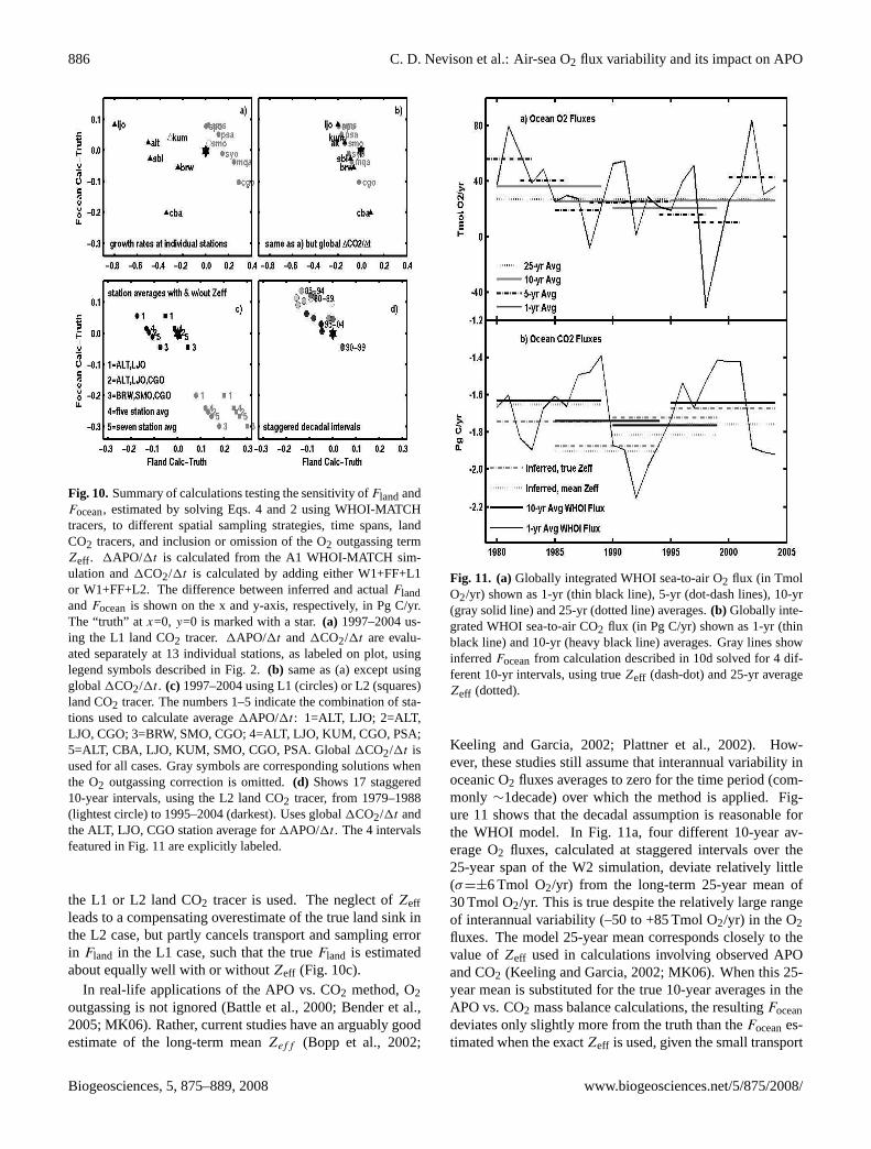
Fig. 10.Summary of calculations testing the sensitivity ofFlandandFocean, estimated by solving Eqs. 4 and 2 using WHOI-MATCHtracers, to different spatial sampling strategies, time spans, landCO2 tracers, and inclusion or omission of the O2 outgassing termZeff. 1APO/1t is calculated from the A1 WHOI-MATCH sim-ulation and1CO2/1t is calculated by adding either W1+FF+L1or W1+FF+L2. The difference between inferred and actualFlandandFoceanis shown on the x and y-axis, respectively, in Pg C/yr.The “truth” atx=0, y=0 is marked with a star.(a) 1997–2004 us-ing the L1 land CO2 tracer. 1APO/1t and1CO2/1t are evalu-ated separately at 13 individual stations, as labeled on plot, usinglegend symbols described in Fig. 2.(b) same as (a) except usingglobal1CO2/1t . (c) 1997–2004 using L1 (circles) or L2 (squares)land CO2 tracer. The numbers 1–5 indicate the combination of sta-tions used to calculate average1APO/1t : 1=ALT, LJO; 2=ALT,LJO, CGO; 3=BRW, SMO, CGO; 4=ALT, LJO, KUM, CGO, PSA;5=ALT, CBA, LJO, KUM, SMO, CGO, PSA. Global1CO2/1t isused for all cases. Gray symbols are corresponding solutions whenthe O2 outgassing correction is omitted.(d) Shows 17 staggered10-year intervals, using the L2 land CO2 tracer, from 1979–1988(lightest circle) to 1995–2004 (darkest). Uses global1CO2/1t andthe ALT, LJO, CGO station average for1APO/1t . The 4 intervalsfeatured in Fig. 11 are explicitly labeled.

the L1 or L2 land CO2 tracer is used. The neglect ofZeffleads to a compensating overestimate of the true land sink inthe L2 case, but partly cancels transport and sampling errorin Fland in the L1 case, such that the trueFland is estimatedabout equally well with or withoutZeff (Fig. 10c).

In real-life applications of the APO vs. CO2 method, O2outgassing is not ignored (Battle et al., 2000; Bender et al.,2005; MK06). Rather, current studies have an arguably goodestimate of the long-term meanZeff (Bopp et al., 2002;

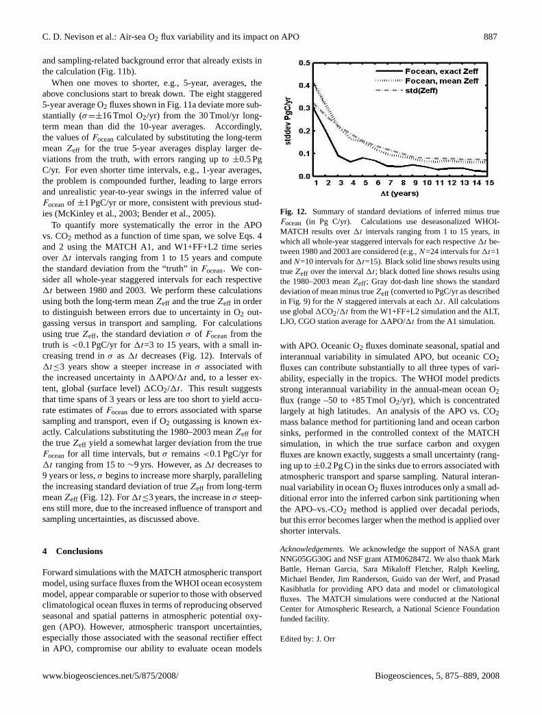
Fig. 11. (a)Globally integrated WHOI sea-to-air O2 flux (in TmolO2/yr) shown as 1-yr (thin black line), 5-yr (dot-dash lines), 10-yr(gray solid line) and 25-yr (dotted line) averages.(b) Globally inte-grated WHOI sea-to-air CO2 flux (in Pg C/yr) shown as 1-yr (thinblack line) and 10-yr (heavy black line) averages. Gray lines showinferredFoceanfrom calculation described in 10d solved for 4 dif-ferent 10-yr intervals, using trueZeff (dash-dot) and 25-yr averageZeff (dotted).

Keeling and Garcia, 2002; Plattner et al., 2002). How-ever, these studies still assume that interannual variability inoceanic O2 fluxes averages to zero for the time period (com-monly ∼1decade) over which the method is applied. Fig-ure 11 shows that the decadal assumption is reasonable forthe WHOI model. In Fig. 11a, four different 10-year av-erage O2 fluxes, calculated at staggered intervals over the25-year span of the W2 simulation, deviate relatively little(σ=±6 Tmol O2/yr) from the long-term 25-year mean of30 Tmol O2/yr. This is true despite the relatively large rangeof interannual variability (–50 to +85 Tmol O2/yr) in the O2fluxes. The model 25-year mean corresponds closely to thevalue ofZeff used in calculations involving observed APOand CO2 (Keeling and Garcia, 2002; MK06). When this 25-year mean is substituted for the true 10-year averages in theAPO vs. CO2 mass balance calculations, the resultingFoceandeviates only slightly more from the truth than theFoceanes-timated when the exactZeff is used, given the small transport

Biogeosciences, 5, 875–889, 2008 www.biogeosciences.net/5/875/2008/

C. D. Nevison et al.: Air-sea O2 flux variability and its impact on APO 887

and sampling-related background error that already exists inthe calculation (Fig. 11b).

When one moves to shorter, e.g., 5-year, averages, theabove conclusions start to break down. The eight staggered5-year average O2 fluxes shown in Fig. 11a deviate more sub-stantially (σ=±16 Tmol O2/yr) from the 30 Tmol/yr long-term mean than did the 10-year averages. Accordingly,the values ofFoceancalculated by substituting the long-termmeanZeff for the true 5-year averages display larger de-viations from the truth, with errors ranging up to±0.5 PgC/yr. For even shorter time intervals, e.g., 1-year averages,the problem is compounded further, leading to large errorsand unrealistic year-to-year swings in the inferred value ofFoceanof ±1 PgC/yr or more, consistent with previous stud-ies (McKinley et al., 2003; Bender et al., 2005).

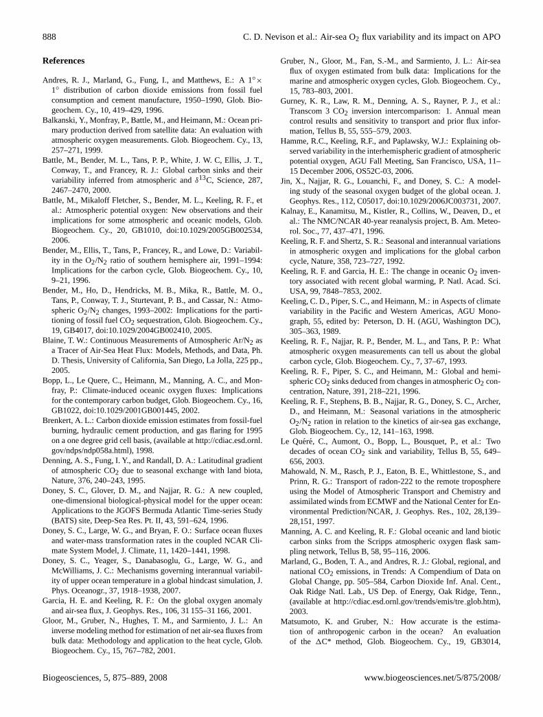
To quantify more systematically the error in the APOvs. CO2 method as a function of time span, we solve Eqs. 4and 2 using the MATCH A1, and W1+FF+L2 time seriesover 1t intervals ranging from 1 to 15 years and computethe standard deviation from the “truth” inFocean. We con-sider all whole-year staggered intervals for each respective1t between 1980 and 2003. We perform these calculationsusing both the long-term meanZeff and the trueZeff in orderto distinguish between errors due to uncertainty in O2 out-gassing versus in transport and sampling. For calculationsusing trueZeff, the standard deviationσ of Foceanfrom thetruth is <0.1 PgC/yr for1t=3 to 15 years, with a small in-creasing trend inσ as1t decreases (Fig. 12). Intervals of1t≤3 years show a steeper increase inσ associated withthe increased uncertainty in1APO/1t and, to a lesser ex-tent, global (surface level)1CO2/1t . This result suggeststhat time spans of 3 years or less are too short to yield accu-rate estimates ofFoceandue to errors associated with sparsesampling and transport, even if O2 outgassing is known ex-actly. Calculations substituting the 1980–2003 meanZeff forthe trueZeff yield a somewhat larger deviation from the trueFoceanfor all time intervals, butσ remains<0.1 PgC/yr for1t ranging from 15 to∼9 yrs. However, as1t decreases to9 years or less,σ begins to increase more sharply, parallelingthe increasing standard deviation of trueZeff from long-termmeanZeff (Fig. 12). For1t≤3 years, the increase inσ steep-ens still more, due to the increased influence of transport andsampling uncertainties, as discussed above.

4 Conclusions

Forward simulations with the MATCH atmospheric transportmodel, using surface fluxes from the WHOI ocean ecosystemmodel, appear comparable or superior to those with observedclimatological ocean fluxes in terms of reproducing observedseasonal and spatial patterns in atmospheric potential oxy-gen (APO). However, atmospheric transport uncertainties,especially those associated with the seasonal rectifier effectin APO, compromise our ability to evaluate ocean models

Fig. 12. Summary of standard deviations of inferred minus trueFocean (in Pg C/yr). Calculations use deseasonalized WHOI-MATCH results over1t intervals ranging from 1 to 15 years, inwhich all whole-year staggered intervals for each respective1t be-tween 1980 and 2003 are considered (e.g.,N=24 intervals for1t=1andN=10 intervals for1t=15). Black solid line shows results usingtrueZeff over the interval1t ; black dotted line shows results usingthe 1980–2003 meanZeff; Gray dot-dash line shows the standarddeviation of mean minus trueZeff (converted to PgC/yr as describedin Fig. 9) for theN staggered intervals at each1t . All calculationsuse global1CO2/1t from the W1+FF+L2 simulation and the ALT,LJO, CGO station average for1APO/1t from the A1 simulation.

with APO. Oceanic O2 fluxes dominate seasonal, spatial andinterannual variability in simulated APO, but oceanic CO2fluxes can contribute substantially to all three types of vari-ability, especially in the tropics. The WHOI model predictsstrong interannual variability in the annual-mean ocean O2flux (range –50 to +85 Tmol O2/yr), which is concentratedlargely at high latitudes. An analysis of the APO vs. CO2mass balance method for partitioning land and ocean carbonsinks, performed in the controlled context of the MATCHsimulation, in which the true surface carbon and oxygenfluxes are known exactly, suggests a small uncertainty (rang-ing up to±0.2 Pg C) in the sinks due to errors associated withatmospheric transport and sparse sampling. Natural interan-nual variability in ocean O2 fluxes introduces only a small ad-ditional error into the inferred carbon sink partitioning whenthe APO–vs.-CO2 method is applied over decadal periods,but this error becomes larger when the method is applied overshorter intervals.

Acknowledgements. We acknowledge the support of NASA grantNNG05GG30G and NSF grant ATM0628472. We also thank MarkBattle, Hernan Garcia, Sara Mikaloff Fletcher, Ralph Keeling,Michael Bender, Jim Randerson, Guido van der Werf, and PrasadKasibhatla for providing APO data and model or climatologicalfluxes. The MATCH simulations were conducted at the NationalCenter for Atmospheric Research, a National Science Foundationfunded facility.

Edited by: J. Orr

www.biogeosciences.net/5/875/2008/ Biogeosciences, 5, 875–889, 2008

888 C. D. Nevison et al.: Air-sea O2 flux variability and its impact on APO

References

Andres, R. J., Marland, G., Fung, I., and Matthews, E.: A 1◦×

1◦ distribution of carbon dioxide emissions from fossil fuelconsumption and cement manufacture, 1950–1990, Glob. Bio-geochem. Cy., 10, 419–429, 1996.

Balkanski, Y., Monfray, P., Battle, M., and Heimann, M.: Ocean pri-mary production derived from satellite data: An evaluation withatmospheric oxygen measurements. Glob. Biogeochem. Cy., 13,257–271, 1999.

Battle, M., Bender, M. L., Tans, P. P., White, J. W. C, Ellis, .J. T.,Conway, T., and Francey, R. J.: Global carbon sinks and theirvariability inferred from atmospheric andδ13C, Science, 287,2467–2470, 2000.

Battle, M., Mikaloff Fletcher, S., Bender, M. L., Keeling, R. F., etal.: Atmospheric potential oxygen: New observations and theirimplications for some atmospheric and oceanic models, Glob.Biogeochem. Cy., 20, GB1010, doi:10.1029/2005GB002534,2006.

Bender, M., Ellis, T., Tans, P., Francey, R., and Lowe, D.: Variabil-ity in the O2/N2 ratio of southern hemisphere air, 1991–1994:Implications for the carbon cycle, Glob. Biogeochem. Cy., 10,9–21, 1996.

Bender, M., Ho, D., Hendricks, M. B., Mika, R., Battle, M. O.,Tans, P., Conway, T. J., Sturtevant, P. B., and Cassar, N.: Atmo-spheric O2/N2 changes, 1993–2002: Implications for the parti-tioning of fossil fuel CO2 sequestration, Glob. Biogeochem. Cy.,19, GB4017, doi:10.1029/2004GB002410, 2005.

Blaine, T. W.: Continuous Measurements of Atmospheric Ar/N2 asa Tracer of Air-Sea Heat Flux: Models, Methods, and Data, Ph.D. Thesis, University of California, San Diego, La Jolla, 225 pp.,2005.

Bopp, L., Le Quere, C., Heimann, M., Manning, A. C., and Mon-fray, P.: Climate-induced oceanic oxygen fluxes: Implicationsfor the contemporary carbon budget, Glob. Biogeochem. Cy., 16,GB1022, doi:10.1029/2001GB001445, 2002.

Brenkert, A. L.: Carbon dioxide emission estimates from fossil-fuelburning, hydraulic cement production, and gas flaring for 1995on a one degree grid cell basis, (available at http://cdiac.esd.ornl.gov/ndps/ndp058a.html), 1998.

Denning, A. S., Fung, I. Y., and Randall, D. A.: Latitudinal gradientof atmospheric CO2 due to seasonal exchange with land biota,Nature, 376, 240–243, 1995.

Doney, S. C., Glover, D. M., and Najjar, R. G.: A new coupled,one-dimensional biological-physical model for the upper ocean:Applications to the JGOFS Bermuda Atlantic Time-series Study(BATS) site, Deep-Sea Res. Pt. II, 43, 591–624, 1996.

Doney, S. C., Large, W. G., and Bryan, F. O.: Surface ocean fluxesand water-mass transformation rates in the coupled NCAR Cli-mate System Model, J. Climate, 11, 1420–1441, 1998.

Doney, S. C., Yeager, S., Danabasoglu, G., Large, W. G., andMcWilliams, J. C.: Mechanisms governing interannual variabil-ity of upper ocean temperature in a global hindcast simulation, J.Phys. Oceanogr., 37, 1918–1938, 2007.

Garcia, H. E. and Keeling, R. F.: On the global oxygen anomalyand air-sea flux, J. Geophys. Res., 106, 31 155–31 166, 2001.

Gloor, M., Gruber, N., Hughes, T. M., and Sarmiento, J. L.: Aninverse modeling method for estimation of net air-sea fluxes frombulk data: Methodology and application to the heat cycle, Glob.Biogeochem. Cy., 15, 767–782, 2001.

Gruber, N., Gloor, M., Fan, S.-M., and Sarmiento, J. L.: Air-seaflux of oxygen estimated from bulk data: Implications for themarine and atmospheric oxygen cycles, Glob. Biogeochem. Cy.,15, 783–803, 2001.

Gurney, K. R., Law, R. M., Denning, A. S., Rayner, P. J., et al.:Transcom 3 CO2 inversion intercomparison: 1. Annual meancontrol results and sensitivity to transport and prior flux infor-mation, Tellus B, 55, 555–579, 2003.

Hamme, R.C., Keeling, R.F., and Paplawsky, W.J.: Explaining ob-served variability in the interhemispheric gradient of atmosphericpotential oxygen, AGU Fall Meeting, San Francisco, USA, 11–15 December 2006, OS52C-03, 2006.

Jin, X., Najjar, R. G., Louanchi, F., and Doney, S. C.: A model-ing study of the seasonal oxygen budget of the global ocean. J.Geophys. Res., 112, C05017, doi:10.1029/2006JC003731, 2007.

Kalnay, E., Kanamitsu, M., Kistler, R., Collins, W., Deaven, D., etal.: The NMC/NCAR 40-year reanalysis project, B. Am. Meteo-rol. Soc., 77, 437–471, 1996.

Keeling, R. F. and Shertz, S. R.: Seasonal and interannual variationsin atmospheric oxygen and implications for the global carboncycle, Nature, 358, 723–727, 1992.

Keeling, R. F. and Garcia, H. E.: The change in oceanic O2 inven-tory associated with recent global warming, P. Natl. Acad. Sci.USA, 99, 7848–7853, 2002.

Keeling, C. D., Piper, S. C., and Heimann, M.: in Aspects of climatevariability in the Pacific and Western Americas, AGU Mono-graph, 55, edited by: Peterson, D. H. (AGU, Washington DC),305–363, 1989.

Keeling, R. F., Najjar, R. P., Bender, M. L., and Tans, P. P.: Whatatmospheric oxygen measurements can tell us about the globalcarbon cycle, Glob. Biogeochem. Cy., 7, 37–67, 1993.

Keeling, R. F., Piper, S. C., and Heimann, M.: Global and hemi-spheric CO2 sinks deduced from changes in atmospheric O2 con-centration, Nature, 391, 218–221, 1996.

Keeling, R. F., Stephens, B. B., Najjar, R. G., Doney, S. C., Archer,D., and Heimann, M.: Seasonal variations in the atmosphericO2/N2 ration in relation to the kinetics of air-sea gas exchange,Glob. Biogeochem. Cy., 12, 141–163, 1998.

Le Quere, C., Aumont, O., Bopp, L., Bousquet, P., et al.: Twodecades of ocean CO2 sink and variability, Tellus B, 55, 649–656, 2003.

Mahowald, N. M., Rasch, P. J., Eaton, B. E., Whittlestone, S., andPrinn, R. G.: Transport of radon-222 to the remote troposphereusing the Model of Atmospheric Transport and Chemistry andassimilated winds from ECMWF and the National Center for En-vironmental Prediction/NCAR, J. Geophys. Res., 102, 28,139–28,151, 1997.

Manning, A. C. and Keeling, R. F.: Global oceanic and land bioticcarbon sinks from the Scripps atmospheric oxygen flask sam-pling network, Tellus B, 58, 95–116, 2006.

Marland, G., Boden, T. A., and Andres, R. J.: Global, regional, andnational CO2 emissions, in Trends: A Compendium of Data onGlobal Change, pp. 505–584, Carbon Dioxide Inf. Anal. Cent.,Oak Ridge Natl. Lab., US Dep. of Energy, Oak Ridge, Tenn.,(available at http://cdiac.esd.ornl.gov/trends/emis/treglob.htm),2003.

Matsumoto, K. and Gruber, N.: How accurate is the estima-tion of anthropogenic carbon in the ocean? An evaluationof the 1C* method, Glob. Biogeochem. Cy., 19, GB3014,

Biogeosciences, 5, 875–889, 2008 www.biogeosciences.net/5/875/2008/

C. D. Nevison et al.: Air-sea O2 flux variability and its impact on APO 889

doi:10.1029/2004GB002397, 2005.McKinley, G. A., Follows, M. J., Marshall, J., and Fan, S.M.: In-

terannual variability of air-sea O2 fluxes and the determinationof CO2 sinks using atmospheric O2/N2, Geophys. Res. Lett., 30,1101, doi:10.1029/2002GL016044, 2003.

Moore, J. K., Doney, S. C., Kleypas, J. C., Glover, D. M., and Fung,I.Y.: An intermediate complexity marine ecosystem model forthe global domain, Deep-Sea Res. Pt. II, 49, 403–462, 2002.

Moore, J. K., Doney, S. C., and Lindsay, K.: Upper oceanecosystem dynamics and iron cycling in a global three-dimensional model, Glob. Biogeochem. Cy., 18, GB4028,doi:10.1029/2004GB002220, 2004.

Naegler, T., Ciais, P., Orr, J. C., Aumont, O., and Roedenbeck, C.:On evaluating ocean models with atmospheric potential oxygen,Tellus, 59B, 138–156, 2007.

Najjar, R. G. and Keeling, R. F: Mean annual cycle of the air-seaoxygen flux: A global view, Glob. Biogeochem. Cy. 14(2), 573–584, 2000.

Nevison, C. D., Keeling, R. F., Weiss, R. F., Popp, B. N., Jin, X.,Fraser, P. J., Porter, L. W., and Hess, P. G.: Southern Ocean ven-tilation inferred from seasonal cycles of atmospheric N2O andO2/N2 at Cape Grim, Tasmania, Tellus, 57B, 218–229, 2005.

Nevison, C. D., Mahowald, N. M., Doney, S. C., Lima, I. D., vander Werf, G. R., Randerson, J. T., Baker, D. F., Kasibhatla, P.,and McKinley, G. A.: Contribution of ocean, fossil fuel, landbiosphere and biomass burning carbon fluxes to seasonal and in-terannual variability in atmospheric CO2, J. Geophys. Res., 113,G01010, doi:10.1029/2007JG000408, 2008.

Olsen, S. C. and Randerson, J. T.: Differences between sur-face and column atmospheric CO2 and implications forcarbon cycle research, J. Geophys. Res., 109, D02301,doi:10.1029/2003JD003968, 2004.

Pearman, G. I. and Hyson, P.: Activities of the Global Biosphereas Reflected in Atmospheric CO2 Records, J. Geophys. Res., 85,4457–4467, 1980.

Plattner, G. K., Joos, F., and Stocker, T. F.: Revision of the globalcarbon budget due to changing air-sea oxygen fluxes, Glob. Bio-geochem. Cy., 16, GB1096, doi:10.1029/2001GB001746, 2002.

Prentice, I. C., Farquhar, G. D., Fasham, M. J. R., Goulden, M. L.,Heimann, M., Jaramillo, V. J., Kheshgi, H. S., and Le Quere, C.:The carbon cycle and atmospheric carbon dioxide, in Climate

Change 2001: The Scientific Basis, Contribution of WorkingGroup I to the Third Assessment Report of the IntergovernmentalPanel on Climate Change, edited by: Houghton J. T., Ding, Y.,Griggs, D. J., et al., pp. 183–287, Cambridge Univ. Press, NewYork, 2001.

Randerson, J. T., van der Werf, G. R., Collatz, G. J., Giglio, L.,Still, C. J., Kasibhatla, P., Miller, J. B., White, J. W. C., De-Fries, R. S., and Kasischke, E. S.: Fire emissions from C3 and C4vegetation and their influence on interannual variability of atmo-spheric CO2 andδ13CO2, Glob. Biogeochem. Cy., 19, GB2019,doi:10.1029/2004GB002366, 2005.

Rasch, P. J., Mahowald, N. M., and Eaton, B. E.: Representationsof transport, convection, and the hydrologic cycle in chemicaltransport models: Implications for the modeling of short-livedand soluble species, J. Geophys. Res., 102, 28 127–28 138, 1997.

Sarmiento, J. L., Hughes, T. M. C., Stouffer, R. J., and Manabe, S.:Simulated response of the ocean carbon cycle to anthropogenicclimate warming, Nature, 393, 245–249, 1998.

Severinghaus, J. P.: Studies of the terrestrial O2 and carbon cyclesin sand dune gases and in Biosphere 2, Ph.D. thesis, ColumbiaUniversity, New York, 1995.

Stephens, B. B., Keeling, R. F., Heimann, M., Six, K. D., Murnane,R. and Caldeira, K.: Testing global ocean carbon cycle modelsusing measurements of atmospheric O2 and CO2 concentration,Glob. Biogeochem. Cy., 12, 213–230, 1998.

Takahashi, T., Poisson, A. Metzl, N., Tilbrook, B., Bates, N., andcoauthors: Global sea-air CO2 flux based on climatological sur-face oceanpCO2, and seasonal biological and temperature ef-fects, Deep-Sea Res. Pt. II, 49, 1601–1622, 2002.

Taylor, K. E.: Summarizing multiple aspects of model performancein a single diagram, J. Geophys. Res., 106, 7183–7192, 2001.

Thoning, K. W., Tans, P. P., and Komhyr, W. D.: Atmosphericcarbon dioxide at Mauna Loa Observatory: 2. Analysis of theNOAA GMCC data, 1974–1985, J. Geophys. Res., 94, 8549–8565, 1989.

Van der Werf, G. R., Randerson, J. T., Giglio, L., Collatz, G. J.,Kasibhatla, P. S., and Arellano, Jr., A. F.: Interannual variabilityin global biomass burning emissions from 1997 to 2004, Atmos.Chem. Phys., 6, 3423–3441, 2006,http://www.atmos-chem-phys.net/6/3423/2006/.

www.biogeosciences.net/5/875/2008/ Biogeosciences, 5, 875–889, 2008