IEEE 802.15.4 based Wireless monitoring of pH and temperature in a fish farm

M. López, J.M. Gómez, J. Sabater, A. Herms

Electronics Department, Sensors and Communications (SIC) Universitat de Barcelona (UB)

Barcelona, Spain manel.lopez@ub.edu

Abstract—In the last years the number of papers related to

wireless sensor networks has increased substantially. Most of them focus in raising issues as routing algorithms, network life-time, and more recently, Multiple Input Multiple Output wireless networks. In contrast with all those studies, we present a practical application of wireless networks: The sensing of the pH and temperature for a fish farm. The application requires two different kind of modules: the sensor itself and the wireless module. The sensor collect and transmit the information to a wireless module using a wired connection. Once the information reaches the wireless node, it is forwarded to the central unit through a wireless protocol. The central unit starts and manages the network, as well as stores all the received data. The sensor module includes an pH sensor based on a specially designed ISFET and a commercial temperature sensor. The wireless node collects the sensed data by means of an asynchronous wired serial polling communication. The use of this kind of protocol allows to connect a single master with multiple slaves. In our particular case, we have connected one master with four slaves using a transmission rate of 9600 b/s. The wireless transmission follows the standard IEEE 802.15.4, and implements the routing protocol based on the ZigBee standard. The number of nodes distributed in the fish farm has been limited to 30 while the maximum number of hops to 6. Moreover, between the MAC and the routing layer an energy management layer have been included. This layer reduces the power consumption of the wireless network using an RF activity duty cycle for the reception stage at the final end device of around 0.02%.

I. INTRODUCTION Wireless Sensor Networks (WSN) have had a large

increase in real applications during the last years. Its main advantage over other technologies is the actual economic development of its installation. Wireless sensor applications are not a real technology as a concept. The idea to implement an ad-hoc wireless network started at the beginning of the 70s [1]. The typical scenario was to set up a communication network in a battlefield, where no infrastructure is available. Since then, a large quantity of theoretical studies have carried out regarding the implementation, power consumption, routing algorithms, etc [2 – 4], but it was difficult to find real applications that solve a specifically case due to the high economical cost of the devices. Nowadays price is not an issue anymore.

Wired and wireless computer networks are composed of computers (data sources / sinks) and infrastructure (routers / repeaters) that forwards and delivers the information when

there is not a direct link (physical or logical) between two communication peers. In case of WSN this division is fuzzier, because routers can operate as data sources and/or sinks.

This paper shows a real application: the monitoring of a fish farm using pH and temperature sensors. Usually, those kind of tests require a very specialized and qualified staff, who should measure periodically the living conditions of the farm (pH, temperature, pKa,...) with a high accuracy. However, it is not feasible to perform these measurements manually with enough periodicity to detect immediate changes or predict possible events. The implementation of an ambient intelligence WSN makes it possible.

Although there are a lot of proprietary protocols in the literature, the current trend is to use standard protocols as IEEE 1451.5 or IEEE 802.15.4 [5, 6]. The last one defines two types of nodes: (i) end devices, also known as Reduced Functional Devices (RFD), which are responsible of sensing and data forwarding and (ii) router nodes or Fully Functional Devices (FFD), with a more complex communication protocol is able to route the information to/from the coordinator. Finally, one of these FFD will be the Network Coordinator (NC) that in addition to the router functionality is also responsible of the establishment and management of the network, and is well defined at the Zigbee standard [21]. From a general point of view, the communication goes from the end devices to the NC, which collects the data, whereas the control frames goes from the coordinator to the end devices.

One of the most important parts of every node is the supply system [7]. Due to the fact that these kinds of devices are battery operated, one of the major concerns must be the power consumption. The management of the power consumption is carried out either by the supply system or the microprocessor. In our case, an intermediate layer between MAC and routing layers has been introduced. This energy saving layer is based on a previous study published in [8] and has been adapted to work as an intermediate layer of the ZigBee stack.

.

II. SCENARIO Two different types of modules compose the designed

network. The instrumentation module is directly connected to the sensing system and will be introduced into the pool to measure the pH, the temperature and other relevant parameters. Due to the size of the pool several nodes must be

978-1-4244-5794-6/10/$26.00 ©2010 IEEE 575

distributed in order to estimate the distribution of those substances that might be critical for the different fish species. The wireless module transmits the information to the NC, which is attached to a central computer, where data is presented and analysed. The communication among the different instrumentation modules and the wireless module has been done using a polling serial wired connection. To comply with the conference paper formatting requirements is to use this document as a template and simply type your text into it.

A. Instrumentation Module The instrumentation module includes, in addition to the

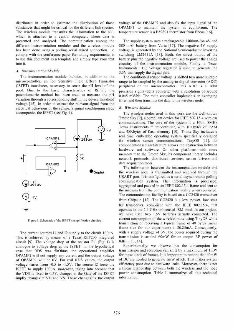
microcontroller, an Ion Sensitive Field Effect Transistor (ISFET) transducer, necessary to sense the pH level of the pool. Due to the basic characteristics of ISFET, the potentiometric method has been used to measure the pH variation through a corresponding shift in the device threshold voltage [15]. In order to extract the relevant signal from the electrical behaviour of the sensor, a signal conditioning stage accompanies the ISFET (see Fig. 1).

Figure 1. Schematic of the ISFET’s amplification circuitry.

The current sources I1 and I2 supply to the circuit 100uA. This is achieved by means of a Texas REF200 integrated circuit [9]. The voltage drop at the resistor R1 (Fig 1) is analogue to voltage drop at the ISFET. In the hypothetical case that RDS was 5kOhms, the operational amplifier OPAMP2 will not supply any current and the output voltage of OPAMP2 will be 0V. For real RDS values, the output voltage varies from -0.5 to -1.5V. The source I2 force the ISFET to supply 100uA, moreover, taking into account that the VDS is fixed to 0.5V, changes at the Gate of the ISFET impliy changes at VD and VS. These changes fix the output

voltage of the OPAMP2 and also fix the input signal of the OPAMP1 to maintain the system in equilibrium. The temperature sensor is a B59801 thermistor from Epcos [16].

The supply system uses a rechargeable Lithium-Ion 4V and

880 mAh battery from Varta [17]. The negative 4V supply voltage is generated by the National Semiconductor inverting switching LM2611A [18]. Both, the direct output of the battery plus the negative voltage are used to power the analog circuitry of the instrumentation module. Finally, a Texas Instruments LDO voltage regulator is used to generate the 3.3V that supply the digital part.

The conditioned sensor voltage is shifted to a more suitable range to be sampled by the analog-to-digital converter (ADC) peripheral of the microcontroller. This ADC is a 16bit precision sigma‑delta converter with a resolution of around 0.045 mV/bit. The main controller implements an averaging filter, and then transmits the data to the wireless node.

B. Wireless Module The wireless nodes used in this work are the well-known

Tmote Sky [9], a compliant device for IEEE 802.15.4 wireless communications. The core of the system is a 16bit, 8MHz Texas Instruments microcontroller, with 10Kbytes of RAM and 48Kbytes of flash memory [10]. Tmote Sky includes a real time, embedded operating system specifically designed for wireless sensor communications: TinyOS [11]. Its component-based architecture allows the abstraction between hardware and software. On other platforms with more memory than the Tmote Sky, its component library includes network protocols, distributed services, sensor drivers and data acquisition tools.

The information between the instrumentation module and the wireless node is transmitted and received through the USART port. It is configured as a serial asynchronous polling communication system. The information is processed, aggregated and packed in an IEEE 802.15.4 frame and sent to the medium from the communication facility when requested. The communication facility is based on a CC2420 transceiver from Chipcon [12]. The CC2420 is a low‑power, low‑cost RF‑transceiver, compliant with the IEEE 802.15.4, that operates in the 2.4 GHz unlicensed ISM band. In our project, we have used two 1.5V batteries serially connected. The current consumption of the wireless mote using TinyOS while transmitting or receiving a typical frame of 40 bytes (mean frame size for our experiment) is 20.85mA. Consequently, with a supply voltage of 3V, the power required during the transmission is around 60mW for an output RF power of 0dBm [13, 14].

Experimentally, we observe that the consumption for transmission and reception can shift by a maximum of 1mW for these kinds of frames. It is important to remark that 60mW of DC are needed to generate 1mW of RF. That makes system efficiency poor due to hardware leaks. Moreover, there is not a linear relationship between both the wireless and the node power consumption. Table I summarizes all this technical information.

576

TABLE I. DC POWER CONSUMPTION WS 2.4GHZ RF POWER

RF Power DC Power

0 dBm (1mW) ∼45 mW -5 dBm (0.32W) ∼36 mW

-10 dBm (0.1 mW) ∼30 mW

III. THE WIRELESS SENSOR NETWORK As stated before, the wireless node selected is a Tmote Sky

[9] running a real time embedded operating system: TinyOS. The OS includes libraries that implement the IEEE 802.15.4 Standard. Moreover, it is relatively easy to implement a network layer based on the ZigBee specification; the protocol that includes in its low level layers the IEEE 802.15.4. The ZigBee routing protocol used by the network layer is an AODV distance vector based routing algorithm [19], which is a reactive routing algorithm. Neither complicated routing tables are needed nor management of this routing table is considered, only a simple list of neighbours and some destinations previously located. In order to find any destination device, the source node searches the destination address in its routing table. If it is found, the datagram will be sent to the address specified by the routing table. When the route to the destination node is not known, the route discovery process starts. The source node broadcasts a route request to all its neighbours who proceed in the same manner. This process is repeated until the route request datagram arrives to the destination or message Time To Live (TTL) is reached. If the destination is reached, it sends its route reply via unicast transmission following the lowest cost path back to the source. When the source receives the reply, it will update its routing table for the destination address with the next hop in the path and the path cost, as well as each node in the path. Once a route has been established, all following transmissions for a given pair of nodes will follow the same path, if possible.

In our particular case, there is a sink node that collects all the information datagrams: The coordinator, forming a tree-like network topology. This node is located at the office of the fish farm and is directly attached to the mains supply. The other nodes are wired to the sensors in the pools, and therefore they will not be mobile.

In computer wireless networks, when authors talk about power consumption and routing algorithms do not take into consideration the fact that although the RF transceiver is not emitting, the reception is usually activated and then, the consumption associated to the RF stage is still quite high. To solve this problem, in WSN we have introduced a transparent link control layer that reduce the average power consumption of the wireless nodes minimizing its activity duty cycle in the RF part. As explained in a previous paper [8], low level “synchronization”, even in the milliseconds range is a good method to reduce idle listening. The wireless node remains in sleep mode for a period of time as close as possible to the desired response time, but slightly shorter. Once awake, it enables reception and after a while goes back to sleep again.

The duty cycle should be minimum since most of the energy is wasted when the RF transceiver is active. The best way to assure that a low-power, long battery-lifetime wireless node receives a request with a narrow, optimum receiver enabled window is to send a long burst of request from the source wireless node.

Figure 2. State Diagram of the Routing Algorithm developed software (for simplicity retries counter and route discovery counters are not shown)

The algorithm implemented works as follows: The initial

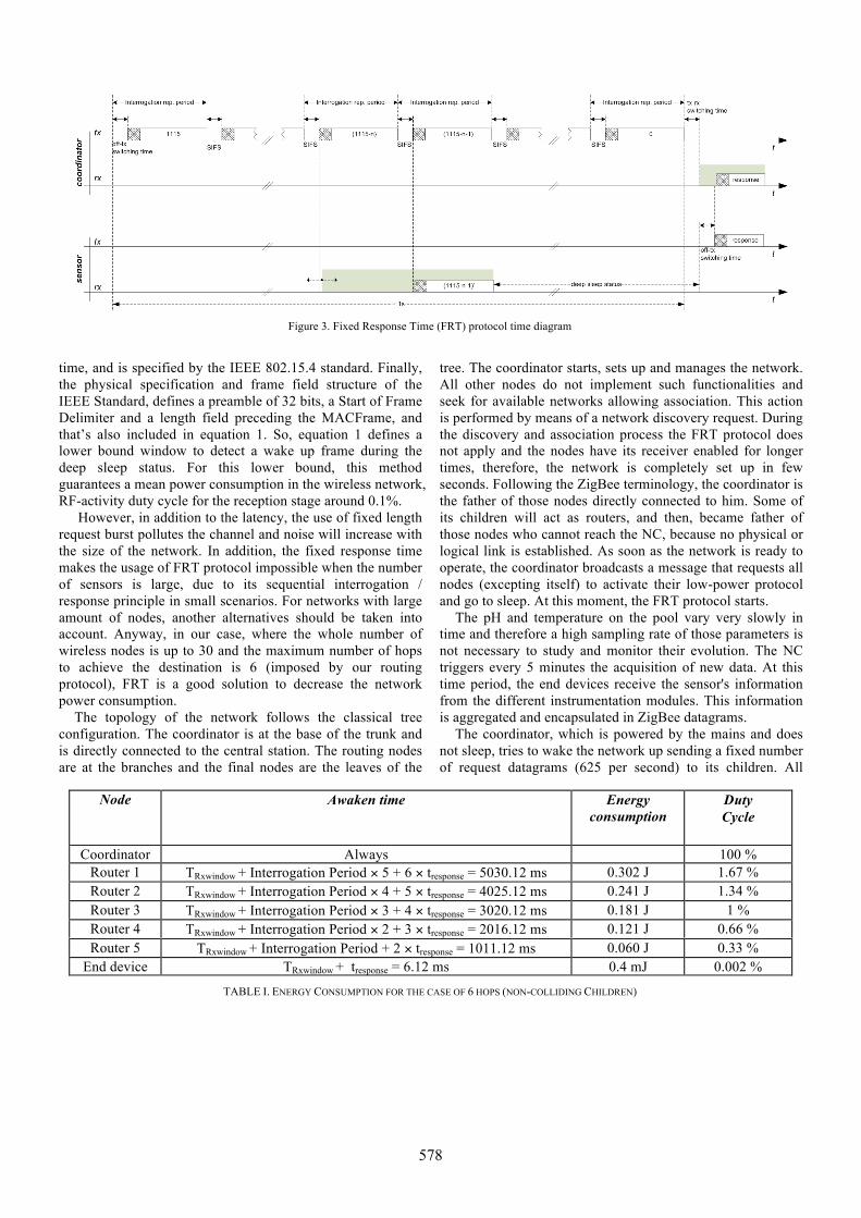
source node wakes its RF stage up and sends a fixed number of requests to the rest of wireless nodes, sequentially. The responses come just after the last request frame within a burst is transmitted. This concept was called Fixed Response Time (FRT) and was detailed explained at [8]. The timing diagram is shown in Fig. 3. The response frame is always located at the end of the burst request. In the example shown at figure 5, the receiver of the sensor is enabled just a few symbols after the preamble of the request in sent by the source node. Therefore, the receiver node is not able to receive the frame and continues listening until the destination address is checked. Broadcast datagrams are forwarded until the TTL expires. Considering the “typical frame” in our application and the IEEE 802.15.4 protocol constraint that specifies a minimum time within consecutive frames, a maximum number of 625 requests per second could be sent by the wireless node to wake up the next hop [6, 8].

The horizontal arrows symbolize that start of the reception window of the wireless node is not related to the source node activity and could be shifted in time since there is no real synchronization. To assure a successful reception, the receiver of the wireless node has to be enabled for a minimum time of:

€

tRXwindow = 2× SyncHeader+ length +MACFrame+ Inter framespacing (1) Where MACframe is the time spent in transmitting a

request frame; the inter-frame-spacing is the time gap between transmitted frames due to physical layer constraints and related to the maximum RX-to-TX and TX-to-RX turn around

577

time, and is specified by the IEEE 802.15.4 standard. Finally, the physical specification and frame field structure of the IEEE Standard, defines a preamble of 32 bits, a Start of Frame Delimiter and a length field preceding the MACFrame, and that’s also included in equation 1. So, equation 1 defines a lower bound window to detect a wake up frame during the deep sleep status. For this lower bound, this method guarantees a mean power consumption in the wireless network, RF-activity duty cycle for the reception stage around 0.1%.

However, in addition to the latency, the use of fixed length request burst pollutes the channel and noise will increase with the size of the network. In addition, the fixed response time makes the usage of FRT protocol impossible when the number of sensors is large, due to its sequential interrogation / response principle in small scenarios. For networks with large amount of nodes, another alternatives should be taken into account. Anyway, in our case, where the whole number of wireless nodes is up to 30 and the maximum number of hops to achieve the destination is 6 (imposed by our routing protocol), FRT is a good solution to decrease the network power consumption.

The topology of the network follows the classical tree configuration. The coordinator is at the base of the trunk and is directly connected to the central station. The routing nodes are at the branches and the final nodes are the leaves of the

tree. The coordinator starts, sets up and manages the network. All other nodes do not implement such functionalities and seek for available networks allowing association. This action is performed by means of a network discovery request. During the discovery and association process the FRT protocol does not apply and the nodes have its receiver enabled for longer times, therefore, the network is completely set up in few seconds. Following the ZigBee terminology, the coordinator is the father of those nodes directly connected to him. Some of its children will act as routers, and then, became father of those nodes who cannot reach the NC, because no physical or logical link is established. As soon as the network is ready to operate, the coordinator broadcasts a message that requests all nodes (excepting itself) to activate their low-power protocol and go to sleep. At this moment, the FRT protocol starts.

The pH and temperature on the pool vary very slowly in time and therefore a high sampling rate of those parameters is not necessary to study and monitor their evolution. The NC triggers every 5 minutes the acquisition of new data. At this time period, the end devices receive the sensor's information from the different instrumentation modules. This information is aggregated and encapsulated in ZigBee datagrams.

The coordinator, which is powered by the mains and does not sleep, tries to wake the network up sending a fixed number of request datagrams (625 per second) to its children. All

Figure 3. Fixed Response Time (FRT) protocol time diagram

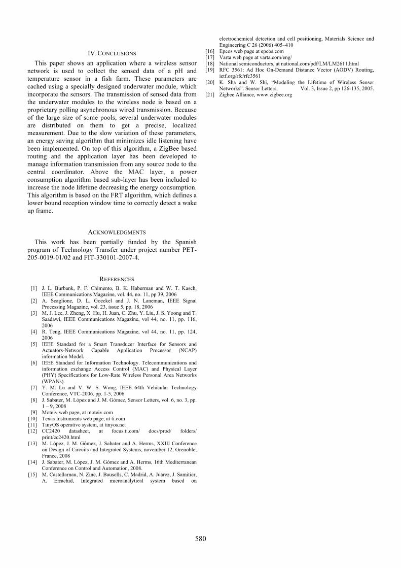
Node Awaken time

Energy consumption

Duty Cycle

Coordinator Always 100 %

Router 1 TRxwindow + Interrogation Period × 5 + 6 × tresponse = 5030.12 ms 0.302 J 1.67 % Router 2 TRxwindow + Interrogation Period × 4 + 5 × tresponse = 4025.12 ms 0.241 J 1.34 % Router 3 TRxwindow + Interrogation Period × 3 + 4 × tresponse = 3020.12 ms 0.181 J 1 % Router 4 TRxwindow + Interrogation Period × 2 + 3 × tresponse = 2016.12 ms 0.121 J 0.66 % Router 5 TRxwindow + Interrogation Period + 2 × tresponse = 1011.12 ms 0.060 J 0.33 %

End device TRxwindow + tresponse = 6.12 ms 0.4 mJ 0.002 %

TABLE I. ENERGY CONSUMPTION FOR THE CASE OF 6 HOPS (NON-COLLIDING CHILDREN)

578

other nodes wake up for a tRX window period larger than those defined at equation 1. In our particular case, and will detect RF transmission if they are in range. As soon as the complete frame has been received, the node will read the decreasing number of sequence that identifies each frame within the request and will return to sleep until the burst ends. Then, all the coordinator's neighbours will wake up and will resend this request to their children using the CSMA-CA protocol to avoid collisions, remaining in the reception stage until the datagrams from the end devices are received. The process will be repeated until all the end devices receive the data request. At this moment the network is ready to transmit the information, taking about 5 msec (see Fig. 4) to transmit the data between two nodes.

Figure 4. Wireless data transmission from end device (upper yellow line) to Network coordinator (lower green line). Middle blue line shows the router's data re-transmission

Table II shows the RF enabled time for each node within the network, taking into account the worst case routing analysis (6 hops) but non-colliding children. The power consumption in every stage and the duty cycle for every node is also shown. As can be observed, the end devices have a duty cycle of about 0.1%. The duty cycle of the intermediate routers can increase up to 1.8% (Table II). This increase of the power consumption for the routers is due to the particular application of the FRT algorithm.

Fig. 4 shows the transmission of the pH and temperature between three nodes of the network. As can be seen, the first node transmits the datagram (capture 1 at Fig. 4) to router 2. Due to the proximity between end device 1, router 2 and coordinator, on the other hand necessary to acquire the image with the oscilloscope, the datagram is received by both nodes (captures 2 and 3). When the MAC layer of the coordinator (always on) decodes the frame, discards it because the information packet is not for him. Router 2 decodes the frame and detects that the message must be forwarded to the coordinator. Capture 4 shows the transmission from router 2. This transmission is again detected by end device 1 (it is still on) and coordinator (captures 5 and 6), end device 1 discards the frame and switch the radio off, while the network coordinator process the data and send the pH and the temperature to a central processing unit (PC) for data handling.

Once the end device has sent the data frame, it will switch off the communication's transceiver to decrease the power consumption. Figure 5 shows the evolution of the current, supplied and acquired by an external Agilent N6705A source, in one of the end devices of the network. For this particular case we have chosen a tRXwindow of 128 mseconds and a tRXoff of 512 mseconds. These values are significantly higher than those presented at table II, that can be considered as an lower bound. As can be observed, the first step in figure 5 is the joining of the node to the network (a). Once the node is accepted, the NC sends the swich_radio_off frame to the whole network. At this period, it is possible to observe the evolution of the current consumption when the radio is switched on (tRXwindow ) and off (tRXoff ) (c). Capture (d) shows the reception of a frame at the fifth tRXwindow period and the subsequent transmission (d, e, f). Once completed the communications, the end device re-enter on the deep sleep state.

Figure 5. Evolution of the current consumption for end devices with the FRT protocol implemented. tRXwindow of 128 mseconds and tRXoff of 512 mseconds was chosen to design the sniffing window deep sleep state.

From the data extracted from table II, it is clear that those

nodes that are closer to the coordinator, higher hierarchical level in the tree, have a higher power consumption, since they have to remain listening while the message and reply propagates. A possible solution to solve this problem was presented by Sha and Shi at [20].

When the NC detects that a node does not respond, i.e. when a node has not forwarded its children information to its father for two processes of information request, the coordinator will withdraw the node from the routing table, the network will be woken up and will be reinitialized again. Similarly, when a new node wants be added to the the network, it will wait until a burst is received and then it will send join request to its emitter. The last node will send a message to the coordinator indicating the request. In this case, the coordinator will follow the same process explained above to optimize the network. In both cases, when the process ends, the network returns to its normal stage managed by the FRT protocol.

579

IV. CONCLUSIONS This paper shows an application where a wireless sensor

network is used to collect the sensed data of a pH and temperature sensor in a fish farm. These parameters are cached using a specially designed underwater module, which incorporate the sensors. The transmission of sensed data from the underwater modules to the wireless node is based on a proprietary polling asynchronous wired transmission. Because of the large size of some pools, several underwater modules are distributed on them to get a precise, localized measurement. Due to the slow variation of these parameters, an energy saving algorithm that minimizes idle listening have been implemented. On top of this algorithm, a ZigBee based routing and the application layer has been developed to manage information transmission from any source node to the central coordinator. Above the MAC layer, a power consumption algorithm based sub-layer has been included to increase the node lifetime decreasing the energy consumption. This algorithm is based on the FRT algorithm, which defines a lower bound reception window time to correctly detect a wake up frame.

ACKNOWLEDGMENTS This work has been partially funded by the Spanish

program of Technology Transfer under project number PET-205-0019-01/02 and FIT-330101-2007-4.

REFERENCES [1] J. L. Burbank, P. F. Chimento, B. K. Haberman and W. T. Kasch,

IEEE Communications Magazine, vol. 44, no. 11, pp 39, 2006 [2] A. Scaglione, D. L. Goeckel and J. N. Laneman, IEEE Signal

Processing Magazine, vol. 23, issue 5, pp. 18, 2006 [3] M. J. Lee, J. Zheng, X. Hu, H. Juan, C. Zhu, Y. Liu, J. S. Yoong and T.

Saadawi, IEEE Communications Magazine, vol 44, no. 11, pp. 116, 2006

[4] R. Teng, IEEE Communications Magazine, vol 44, no. 11, pp. 124, 2006

[5] IEEE Standard for a Smart Transducer Interface for Sensors and Actuators-Network Capable Application Processor (NCAP) information Model.

[6] IEEE Standard for Information Technology. Telecommunications and information exchange Access Control (MAC) and Physical Layer (PHY) Specifications for Low-Rate Wireless Personal Area Networks (WPANs).

[7] Y. M. Lu and V. W. S. Wong, IEEE 64th Vehicular Technology Conference, VTC-2006. pp. 1-5, 2006

[8] J. Sabater, M. López and J. M. Gómez, Sensor Letters, vol. 6, no. 3, pp. 1 – 9, 2008

[9] Moteiv web page, at moteiv.com [10] Texas Instruments web page, at ti.com [11] TinyOS operative system, at tinyos.net [12] CC2420 datasheet, at focus.ti.com/ docs/prod/ folders/

print/cc2420.html [13] M. López, J. M. Gómez, J. Sabater and A. Herms, XXIII Conference

on Design of Circuits and Integrated Systems, november 12, Grenoble, France, 2008

[14] J. Sabater, M. López, J. M. Gómez and A. Herms, 16th Mediterranean Conference on Control and Automation, 2008.

[15] M. Castellarnau, N. Zine, J. Bausells, C. Madrid, A. Juárez, J. Samitier, A. Errachid, Integrated microanalytical system based on

electrochemical detection and cell positioning, Materials Science and Engineering C 26 (2006) 405–410

[16] Epcos web page at epcos.com [17] Varta web page at varta.com/eng/ [18] National semiconductors, at national.com/pdf/LM/LM2611.html [19] RFC 3561: Ad Hoc On-Demand Distance Vector (AODV) Routing,

ietf.org/rfc/rfc3561 [20] K. Sha and W. Shi, “Modeling the Lifetime of Wireless Sensor

Networks”. Sensor Letters, Vol. 3, Issue 2, pp 126-135, 2005. [21] Zigbee Alliance, www.zigbee.org

580