Identifying Quality of Experience (QoE) in 3G/4G Radio ...

Identifying Quality of Experience (QoE) in 3G/4G RadioNetworks based on Quality of Service (QoS) Metrics

Vera Cristina da Silva Pedras

Thesis to obtain the Master of Science Degree in

Electrical and Computer Engineering

Supervisor(s): Prof. António José Castelo Branco RodriguesProf. Maria Paula Dos Santos Queluz RodriguesProf. Pedro Manuel de Almeida Carvalho Vieira

Examination Committee

Chairperson: Prof. José Eduardo Charters Ribeiro da Cunha SanguinoSupervisor: Prof. Maria Paula dos Santos Queluz Rodrigues

Member of the Committee: Prof. Pedro Joaquim Amaro Sebastião

November 2017

Dedicated to my family and friends...

iii

Acknowledgments

Firstly, I would like to thank my supervisors Professor Antonio Rodrigues, Professor Maria Paula Queluz

and Professor Pedro Vieira for all the support given during the development of this thesis .

I would like also to thank CELFINET for the provided resources and data, which were fundamental for

the development of this thesis. Thank you also to all my colleagues and friends in CELFINET, specially

thank you to engineer Marco Sousa for all the support and help during this process, as well as, to

engineer Andre Martins for the help in obtaining the needed resources and data.

To my family that always supported me, specially to my parents, who always showed interest in the

work that I was developing.

Finally, I would like to thank all my friends. A special acknowledgment to Ines Goncalves, Rita Costa,

Joao Vila de Brito, Ines Gil, Catarina Gaspar and Maria Monteiro for all the support and help through my

time in IST.

v

Resumo

Qualidade de Experiencia (QoE) e definida como a percepcao da qualidade de um servico por parte do

utilizador. A previsao e medida de QoE e importante no planeamento das redes, de modo a que esse

planeamento seja feito conforme as necessidades dos utilizadores. Diversos factores influenciam a

QoE, como a Qualidade de Servico (QoS) da rede, a expectativa do utilizador relativamente ao servico

e o tipo de aplicacao a ser usada. Diferentes utilizadores podem ter diferentes opinioes acerca da

usabilidade do mesmo servico, o que correspondera a uma QoE diferente.

Esta tese propoe dois novos modelos de previsao de QoE para chamadas de voz na 3a Geracao (3G)

e para navegacao na web na 4a Geracao, respectivamente. Para o desenvolvimento dos modelos foram

usadas tecnicas de machine learning, mais especificamente foi usado o algoritmo Support Vectors

Regression (SVR).

Os parametros de entrada de ambos os modelos sao medidas de QoS que podem ser obtidas por

exemplo atraves de drive tests. Os modelos mapeiam estes parametros numa unica medida de QoE, a

Mean Opinion Score (MOS).

O modelo desenvolvido para chamadas de voz estima a QoE atraves das seguintes metricas de

Radio Frequency (RF): RSCP, Ec/N0, SIR e SIR Target. O modelo apresentou uma estimativa de

QoE com um Root Mean Squared Error (RMSE) de 10.92% e correlacoes de Pearson e Spearman de

62.22% e 55.27%, respectivamente, em relacao a QoE medida (referencia).

O modelo QoE desenvolvido para navegacao na web em 4G usa como parametros de entrada as

seguintes metricas de QoS: RSRP, RSRQ, MCS, BLER e CQI. Para alem dos parametros QoS, este

modelo tambem usa como parametro de entrada o tamanho da pagina web que esta a ser acedida. O

modelo apresentou um desempenho que correspondeu a um RMSE de 9.79% e correlacoes de Pearson

e Spearman de 91.96% e 92.15%, respectivamente, sendo estas metricas determinadas atraves da

comparacao da estimativa feita pelo modelo e o valor de QoE medido, que e tomado como referencia.

Palavras-chave: LTE, UMTS, QoE, QoS, Navegacao na Web, Chamadas de Voz.

vii

Abstract

Quality of Experience (QoE) is defined as the perceived quality of a service by the user; its prediction and

measurement is important to network planning, in order to dimension it according to the users’ needs.

QoE is influenced by several factors, like the network Quality of Service (QoS), the users’ expectation

about the service and the type of application being used. Different users may have different opinions

regarding the usability of the same service, resulting in a different QoE.

This thesis proposes two novel QoE models for 3rd Generation (3G) voice calls and web browsing

in 4th Generation (4G), respectively. The models were developed using machine learning techniques,

more specifically the Support Vectors Regression (SVR) algorithm.

The models take as input QoS metrics that can be measured, for instance, in drive tests. The models

map these metrics in a single metric of QoE, the Mean Opinion Score (MOS).

The 3G voice calls QoE model performs an estimation of the perceived quality through the following

Radio Frequency (RF) metrics: RSCP, Ec/N0, SIR and SIR Target. This model estimates the QoE with a

Root Mean Squared Error (RMSE) of 10.92% and Pearson and Spearman Correlations of 62.22% and

55.27%, respectively, relatively to the measured QoE (reference).

The web browsing QoE model takes as input parameters the following 4G QoS metrics: RSRP,

RSRQ, MCS, BLER and CQI. The size of the web page being accessed is also an input parameter of

this model. The model performed an estimation of the perceived quality with a RMSE of 9.79% and

Pearson and Spearman Correlations of 91.96% and 92.15%, respectively, relatively to the measured

QoE (reference).

Keywords: LTE, UMTS, QoE, QoS, Web Browsing, Voice Calls.

ix

Contents

Acknowledgments . . . . . . . . . . . . . . . . . . . . . . . . . . . . . . . . . . . . . . . . . . . v

Resumo . . . . . . . . . . . . . . . . . . . . . . . . . . . . . . . . . . . . . . . . . . . . . . . . . vii

Abstract . . . . . . . . . . . . . . . . . . . . . . . . . . . . . . . . . . . . . . . . . . . . . . . . . ix

List of Tables . . . . . . . . . . . . . . . . . . . . . . . . . . . . . . . . . . . . . . . . . . . . . . xiii

List of Figures . . . . . . . . . . . . . . . . . . . . . . . . . . . . . . . . . . . . . . . . . . . . . xv

List of Symbols . . . . . . . . . . . . . . . . . . . . . . . . . . . . . . . . . . . . . . . . . . . . . xvii

Acronyms . . . . . . . . . . . . . . . . . . . . . . . . . . . . . . . . . . . . . . . . . . . . . . . . xix

1 Introduction 1

1.1 Motivation . . . . . . . . . . . . . . . . . . . . . . . . . . . . . . . . . . . . . . . . . . . . . 1

1.2 Objectives . . . . . . . . . . . . . . . . . . . . . . . . . . . . . . . . . . . . . . . . . . . . . 3

1.3 Contributions . . . . . . . . . . . . . . . . . . . . . . . . . . . . . . . . . . . . . . . . . . . 3

1.4 Thesis Outline . . . . . . . . . . . . . . . . . . . . . . . . . . . . . . . . . . . . . . . . . . 4

2 State of the Art 5

2.1 Universal Mobile Telecommunications System . . . . . . . . . . . . . . . . . . . . . . . . . 5

2.1.1 System Architecture . . . . . . . . . . . . . . . . . . . . . . . . . . . . . . . . . . . 6

2.1.2 Transport Channels . . . . . . . . . . . . . . . . . . . . . . . . . . . . . . . . . . . 7

2.1.3 Power Control . . . . . . . . . . . . . . . . . . . . . . . . . . . . . . . . . . . . . . 9

2.1.4 Handover . . . . . . . . . . . . . . . . . . . . . . . . . . . . . . . . . . . . . . . . . 9

2.1.5 QoS Differentiation . . . . . . . . . . . . . . . . . . . . . . . . . . . . . . . . . . . . 9

2.2 Long-Term Evolution . . . . . . . . . . . . . . . . . . . . . . . . . . . . . . . . . . . . . . . 10

2.2.1 System Architecture . . . . . . . . . . . . . . . . . . . . . . . . . . . . . . . . . . . 11

2.2.2 Transport Channels . . . . . . . . . . . . . . . . . . . . . . . . . . . . . . . . . . . 13

2.2.3 Transmission Modes . . . . . . . . . . . . . . . . . . . . . . . . . . . . . . . . . . . 13

2.3 QoE Models Classification . . . . . . . . . . . . . . . . . . . . . . . . . . . . . . . . . . . . 14

2.4 Service Specific Quality Models . . . . . . . . . . . . . . . . . . . . . . . . . . . . . . . . . 16

2.4.1 Voice Services Quality Models . . . . . . . . . . . . . . . . . . . . . . . . . . . . . 16

2.4.2 Video Services Quality Models . . . . . . . . . . . . . . . . . . . . . . . . . . . . . 17

2.4.3 Other Services Quality Models . . . . . . . . . . . . . . . . . . . . . . . . . . . . . 17

xi

3 Machine Learning Algorithms 19

3.1 Methodology . . . . . . . . . . . . . . . . . . . . . . . . . . . . . . . . . . . . . . . . . . . 19

3.1.1 Hypotheses Assessment . . . . . . . . . . . . . . . . . . . . . . . . . . . . . . . . 20

3.1.2 K-Fold Cross Validation Method . . . . . . . . . . . . . . . . . . . . . . . . . . . . 20

3.1.3 Overfitting and Underfitting Problems . . . . . . . . . . . . . . . . . . . . . . . . . 21

3.2 Multivariate Linear Regression . . . . . . . . . . . . . . . . . . . . . . . . . . . . . . . . . 22

3.2.1 Parameter Learning . . . . . . . . . . . . . . . . . . . . . . . . . . . . . . . . . . . 23

3.2.2 Regularized Linear Regression . . . . . . . . . . . . . . . . . . . . . . . . . . . . . 24

3.3 Support Vector Regression Algorithm . . . . . . . . . . . . . . . . . . . . . . . . . . . . . 24

3.3.1 Linear SVR . . . . . . . . . . . . . . . . . . . . . . . . . . . . . . . . . . . . . . . . 25

3.3.2 Non-linear SVR . . . . . . . . . . . . . . . . . . . . . . . . . . . . . . . . . . . . . . 25

4 QoE Model for 3G Voice Calls 29

4.1 QoE Model Parameters . . . . . . . . . . . . . . . . . . . . . . . . . . . . . . . . . . . . . 29

4.2 Model Development . . . . . . . . . . . . . . . . . . . . . . . . . . . . . . . . . . . . . . . 33

4.2.1 Multivariate Linear Regression Approach . . . . . . . . . . . . . . . . . . . . . . . 33

4.2.2 Support Vectors Regression Approach . . . . . . . . . . . . . . . . . . . . . . . . . 36

4.3 Model Selection and Results . . . . . . . . . . . . . . . . . . . . . . . . . . . . . . . . . . 37

4.4 QoE Monitoring . . . . . . . . . . . . . . . . . . . . . . . . . . . . . . . . . . . . . . . . . . 40

5 QoE Model for Web Browsing 43

5.1 QoE Model Parameters . . . . . . . . . . . . . . . . . . . . . . . . . . . . . . . . . . . . . 43

5.2 Model Development . . . . . . . . . . . . . . . . . . . . . . . . . . . . . . . . . . . . . . . 47

5.2.1 Multivariate Linear Regression Approach . . . . . . . . . . . . . . . . . . . . . . . 47

5.2.2 Support Vector Regression Approach . . . . . . . . . . . . . . . . . . . . . . . . . 49

5.3 Model Selection and Results . . . . . . . . . . . . . . . . . . . . . . . . . . . . . . . . . . 51

5.4 QoE Monitoring . . . . . . . . . . . . . . . . . . . . . . . . . . . . . . . . . . . . . . . . . . 53

6 Conclusions 57

6.1 Summary . . . . . . . . . . . . . . . . . . . . . . . . . . . . . . . . . . . . . . . . . . . . . 57

6.2 Future Work . . . . . . . . . . . . . . . . . . . . . . . . . . . . . . . . . . . . . . . . . . . . 58

References 59

xii

List of Tables

2.1 Peak rates that characterize each 3GPP release (adapted from [3]). . . . . . . . . . . . . 5

2.2 QoS differentiation classes (adapted from [3]). . . . . . . . . . . . . . . . . . . . . . . . . 10

2.3 Transmission Modes (adapted from [4]). . . . . . . . . . . . . . . . . . . . . . . . . . . . . 15

4.1 Correlation of the pre-selected features with the measured MOS for the voice model. . . . 32

4.2 Features Correlation for the voice model. . . . . . . . . . . . . . . . . . . . . . . . . . . . 32

4.3 Hypotheses considered for the voice calls model. . . . . . . . . . . . . . . . . . . . . . . . 33

4.4 RMSE and correlations for each hypothesis for the linear regression voice model. . . . . . 33

4.5 RMSE and correlations for each hypothesis of the SVR voice model. . . . . . . . . . . . . 37

4.6 RMSE and correlations for the two approaches of the voice model. . . . . . . . . . . . . . 38

5.1 Correlation of the pre-selected features with the measured MOS for the web browsing

model. . . . . . . . . . . . . . . . . . . . . . . . . . . . . . . . . . . . . . . . . . . . . . . . 45

5.2 Features Correlation of the web browsing model. . . . . . . . . . . . . . . . . . . . . . . . 46

5.3 Hypotheses considered for the web browsing model. . . . . . . . . . . . . . . . . . . . . . 47

5.4 RMSE and correlations for each hypothesis of the linear regression web browsing model. 48

5.5 RMSE and correlations for each hypothesis of the SVR web browsing model. . . . . . . . 50

5.6 RMSE and correlations for the two approaches of the web browsing model. . . . . . . . . 51

5.7 RMSE and correlations for the web browsing model without the web page size as feature. 52

xiii

List of Figures

1.1 The three dimensions of QoS. . . . . . . . . . . . . . . . . . . . . . . . . . . . . . . . . . . 2

2.1 UMTS architecture (adapted from [3]). . . . . . . . . . . . . . . . . . . . . . . . . . . . . . 7

2.2 Mapping of the transport channels onto the physical channels in UMTS (adapted from [3]). 8

2.3 Orthogonality between sub-carriers (adapted from [4]). . . . . . . . . . . . . . . . . . . . . 11

2.4 LTE architecture (adapted from [4]). . . . . . . . . . . . . . . . . . . . . . . . . . . . . . . 11

2.5 Mapping of the transport channels onto the physical channels in LTE (adapted from [4]). . 14

2.6 Illustration of typical objective QoE models. . . . . . . . . . . . . . . . . . . . . . . . . . . 16

3.1 K-fold method for K = 3. . . . . . . . . . . . . . . . . . . . . . . . . . . . . . . . . . . . . . 21

3.2 Examples of underfitting and overfitting. . . . . . . . . . . . . . . . . . . . . . . . . . . . . 21

3.3 Learning Curves for Underfit (a) and Overfit (b) cases. . . . . . . . . . . . . . . . . . . . . 22

3.4 Linear Regression Model Representation (adapted from [20]). . . . . . . . . . . . . . . . . 23

3.5 ε-insensitive Error Function. . . . . . . . . . . . . . . . . . . . . . . . . . . . . . . . . . . . 25

3.6 Representation of ξ, ξ∗ and ε (adapted from [21]). . . . . . . . . . . . . . . . . . . . . . . . 26

3.7 Application of ϕ(x) to a non-linear problem. . . . . . . . . . . . . . . . . . . . . . . . . . . 26

4.1 Examples of distributions with different skewness. . . . . . . . . . . . . . . . . . . . . . . 30

4.2 Examples of distributions with different kurtosis and equal standard deviations. . . . . . . 31

4.3 Learning Curves for the hypothesis 2 of the linear regression voice model. . . . . . . . . . 34

4.4 Relation between the predicted MOS and the measured MOS (a) and the residuals (b). . 35

4.5 Relation between each feature and the residuals. . . . . . . . . . . . . . . . . . . . . . . . 36

4.6 Normal Probability Plot. . . . . . . . . . . . . . . . . . . . . . . . . . . . . . . . . . . . . . 37

4.7 Learning Curves for the hypothesis 3 of the SVR voice model. . . . . . . . . . . . . . . . . 38

4.8 Relation between the measured MOS and the predicted MOS for the SVR model. . . . . 39

4.9 CDF of the measured MOS and of the SVR and Linear Regression (LR) predicted MOS

values. . . . . . . . . . . . . . . . . . . . . . . . . . . . . . . . . . . . . . . . . . . . . . . . 39

4.10 3G Voice Calls QoE Model representation. . . . . . . . . . . . . . . . . . . . . . . . . . . . 40

4.11 MOS estimated for 3G voice calls. . . . . . . . . . . . . . . . . . . . . . . . . . . . . . . . 41

5.1 Relation between the download time and the MOS. . . . . . . . . . . . . . . . . . . . . . . 44

5.2 Learning Curves for the hypothesis 6 of the linear regression web browsing model. . . . . 48

xv

5.3 Relation between the measured MOS and the predicted MOS for the linear regression

web browsing model. . . . . . . . . . . . . . . . . . . . . . . . . . . . . . . . . . . . . . . . 49

5.4 Learning curves of the selected hypothesis (H4) for the SVR web browsing model. . . . . 50

5.5 Relation between the measured MOS and the predicted MOS for the SVR web browsing

model. . . . . . . . . . . . . . . . . . . . . . . . . . . . . . . . . . . . . . . . . . . . . . . . 51

5.6 Web Browsing QoE Model representation. . . . . . . . . . . . . . . . . . . . . . . . . . . . 53

5.7 MOS estimated for web browsing a 1000 kBytes web page. . . . . . . . . . . . . . . . . . 54

5.8 MOS estimated for web browsing a 3100 kBytes web page. . . . . . . . . . . . . . . . . . 55

5.9 CDFs of the estimated MOS for web browsing 1000 kBytes and 3100 kBytes web pages. 55

xvi

List of Symbols

x Average of x.

θ Array with all linear regression coefficients.

L Matrix used for the regularized linear regression.

w Array with the weights of the support vectors.

X Matrix with the all x(i)j training examples.

x Array with all xj , j = 1, ..n features.

y Array with all y(i) training examples.

ε SVR hyperparameter that characterizes the ε-insensitive loss function.

y Estimation of y.

λ Linear regression regularization parameter.

BLER Mean value of BLER.

CQI Mean value of CQI.

RSCP Mean value of RSCP.

ρ SVR variable.

σ Standard Deviation (SD).

θj Linear regression coefficient j.

ξi Amount that the predictions exceeded the ε margin in SVR.

C, γ SVR hyperparameters.

d Web page download time in seconds.

f(·) SVR function.

hθ(·) Linear regression hypothesis.

xvii

J(·) Linear regression cost function.

Jreg(·) Regularized linear regression cost function.

K(·) Kernel function.

m Number of training examples.

n Number of input features.

RPearson Pearson correlation coefficient.

rmse Root Mean Squared Error.

Si Subsets of the data used in the K-Fold method, where i = 1, ..,K.

x(i)j ith training example of the jth feature.

xj Input feature j.

y Target value of the linear regression for a set of input features.

y(i) ith training example of y.

ymax Maximum value that y can take.

ymin Minimum value that y can take.

[SIR− SIRTarget]SD Standard Deviation of SIR − SIR Target.

BLER|kurt Kurtosis of BLER.

Ec/N0 |max Maximum value of Ec/N0.

MCS|flag MCS constant flag.

RSRP|min Minimum value of RSRP.

RSRQ|min Minimum value of RSRQ.

SIR|min Minimum value of SIR.

SIRTarget |max Maximum value of SIR Target.

SIRTarget |SD Standard Deviation of SIR Target.

xviii

Chapter 1

Introduction

This chapter presents the motivation behind the work developed for this thesis, as well as the established

objectives. Some contributions that resulted from the developed work are also presented. Finally, the

thesis outline is described.

1.1 Motivation

According to research results, for every costumer that complains about a certain provided service there

are 29 others who will not complain. In fact, 90% of the customers will simply leave the service once

they become unsatisfied [1]. For these and other reasons, it is very important for the operators to do

an estimation of the user satisfaction of a service, in order to adjust the service quality according to

the user’s needs. The user experience depends on several factors, some of them are network related

and others depend on the type of service being used, the end device features and the user expectation,

among others.

A network can be assessed objectively in terms of Quality of Service (QoS), which depends on

network parameters like throughput, packet loss, delay and jitter. This measurement is done in the

network side and does not take into account the type of service and the user characteristics. The

service quality may also be assessed at the application level - the so called application level QoS - with

parameters that are application specific; as an example, for a video streaming application the parameters

to be assessed may be the waiting time before the start of the video or the frequency of video stallings.

However, a good application QoS and network QoS does not necessarily mean that the end user

is satisfied with the provided service, since his satisfaction depends on other factors. Thus, in order to

measure the user satisfaction one needs to define the Quality of Experience (QoE), which takes into

account factors like expectation, requirements and perception of the end user, content type provided by

the service, user’s device features, network QoS and the context in which the user is using the service,

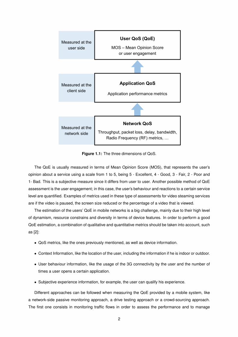
like the access type, movement (mobile or stationary) and location. The network QoS, the application

QoS and the user QoE are related, since the last one is dependent of the previous two and the second

one is dependent of the first. This relationship is represented in Figure 1.1.

1

Measured at the

user side

Measured at the

client side

Measured at the

network side

Network QoS

Throughput, packet loss, delay, bandwidth,

Radio Frequency (RF) metrics, …

User QoS (QoE)

MOS – Mean Opinion Score

or user engagement

Application QoS

Application performance metrics

Figure 1.1: The three dimensions of QoS.

The QoE is usually measured in terms of Mean Opinion Score (MOS), that represents the user’s

opinion about a service using a scale from 1 to 5, being 5 - Excellent, 4 - Good, 3 - Fair, 2 - Poor and

1- Bad. This is a subjective measure since it differs from user to user. Another possible method of QoE

assessment is the user engagement; in this case, the user’s behaviour and reactions to a certain service

level are quantified. Examples of metrics used in these type of assessments for video steaming services

are if the video is paused, the screen size reduced or the percentage of a video that is viewed.

The estimation of the users’ QoE in mobile networks is a big challenge, mainly due to their high level

of dynamism, resource constrains and diversity in terms of device features. In order to perform a good

QoE estimation, a combination of qualitative and quantitative metrics should be taken into account, such

as [2]:

• QoS metrics, like the ones previously mentioned, as well as device information.

• Context Information, like the location of the user, including the information if he is indoor or outdoor.

• User behaviour information, like the usage of the 3G connectivity by the user and the number of

times a user opens a certain application.

• Subjective experience information, for example, the user can qualify his experience.

Different approaches can be followed when measuring the QoE provided by a mobile system, like

a network-side passive monitoring approach, a drive testing approach or a crowd-sourcing approach.

The first one consists in monitoring traffic flows in order to assess the performance and to manage

2

the network; it is mostly a QoS oriented method. The drive testing method allows an in-field network

measurement, but it does not take into account the user context or his behaviour. Finally, the crowd-

sourcing method is performed by several end-users who assess their experience in real time.

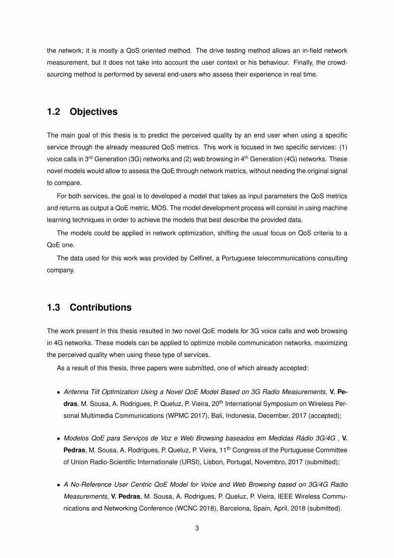
1.2 Objectives

The main goal of this thesis is to predict the perceived quality by an end user when using a specific

service through the already measured QoS metrics. This work is focused in two specific services: (1)

voice calls in 3rd Generation (3G) networks and (2) web browsing in 4th Generation (4G) networks. These

novel models would allow to assess the QoE through network metrics, without needing the original signal

to compare.

For both services, the goal is to developed a model that takes as input parameters the QoS metrics

and returns as output a QoE metric, MOS. The model development process will consist in using machine

learning techniques in order to achieve the models that best describe the provided data.

The models could be applied in network optimization, shifting the usual focus on QoS criteria to a

QoE one.

The data used for this work was provided by Celfinet, a Portuguese telecommunications consulting

company.

1.3 Contributions

The work present in this thesis resulted in two novel QoE models for 3G voice calls and web browsing

in 4G networks. These models can be applied to optimize mobile communication networks, maximizing

the perceived quality when using these type of services.

As a result of this thesis, three papers were submitted, one of which already accepted:

• Antenna Tilt Optimization Using a Novel QoE Model Based on 3G Radio Measurements, V. Pe-

dras, M. Sousa, A. Rodrigues, P. Queluz, P. Vieira, 20th International Symposium on Wireless Per-

sonal Multimedia Communications (WPMC 2017), Bali, Indonesia, December, 2017 (accepted);

• Modelos QoE para Servicos de Voz e Web Browsing baseados em Medidas Radio 3G/4G , V.

Pedras, M. Sousa, A. Rodrigues, P. Queluz, P. Vieira, 11th Congress of the Portuguese Committee

of Union Radio-Scientific Internationale (URSI), Lisbon, Portugal, Novembro, 2017 (submitted);

• A No-Reference User Centric QoE Model for Voice and Web Browsing based on 3G/4G Radio

Measurements, V. Pedras, M. Sousa, A. Rodrigues, P. Queluz, P. Vieira, IEEE Wireless Commu-

nications and Networking Conference (WCNC 2018), Barcelona, Spain, April, 2018 (submitted).

3

1.4 Thesis Outline

This thesis is organized in six chapters. The first chapter presents a brief introduction to the developed

work, presenting the motivation behind it. Chapter 2 presents the state of the art, which consists in an

overview of the 3G and 4G networks and an introduction to several models already developed, present

in the literature, that estimate the QoE of a specific service.

Chapter 3 introduces the methodology used for the development of the proposed models, as well as

the machine learning algorithms used in that process.

Chapter 4 describes all the process that resulted in the proposed model for QoE estimation in 3G

voice calls services. An assessment of the proposed model is also described in this chapter.

Chapter 5 presents all the steps that conducted to the development of the proposed model that

identifies the perceived quality of an end user when using a web browsing service in Long Term Evolution

(LTE). The results obtained with this model are also presented.

In chapter 6 some conclusions are drawn relatively to the proposed models. Future work is also

described in this chapter.

4

Chapter 2

State of the Art

This chapter presents an overview of the 3G and 4G networks. The important aspects of the wire-

less networks and the architecture of each technology are described, as well as the channels used to

transport the information. Some service specific QoE models are also presented in this chapter.

The information present in sections 2.1 and 2.2 was mainly based on the [3] and [4], respectively.

2.1 Universal Mobile Telecommunications System

The 3G systems use, as air interface, the Wideband Code Division Multiple Access (WCDMA) technol-

ogy, which is implemented by multiplying the user data with quasi-random bits (called chips) derived from

Code Division Multiple Access (CDMA) spreading codes. This technology supports Frequency Division

Duplex (FDD) as well as Time Division Duplex (TDD). FDD allows the use of 5 MHz carrier frequencies

for uplink and downlink respectively, while FDD uses a 5 MHz that is time-shared amid the uplink and

downlink. The WCDMA also supports variable user data rates, since the data rate can change from

frame to frame, and each frame has 10 ms of duration.

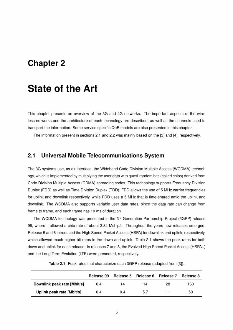
The WCDMA technology was presented in the 3rd Generation Partnership Project (3GPP) release

99, where it allowed a chip rate of about 3.84 Mchip/s. Throughout the years new releases emerged.

Release 5 and 6 introduced the High Speed Packet Access (HSPA) for downlink and uplink, respectively,

which allowed much higher bit rates in the down and uplink. Table 2.1 shows the peak rates for both

down and uplink for each release. In releases 7 and 8, the Evolved High Speed Packet Access (HSPA+)

and the Long Term Evolution (LTE) were presented, respectively.

Table 2.1: Peak rates that characterize each 3GPP release (adapted from [3]).

Release 99 Release 5 Release 6 Release 7 Release 8

Downlink peak rate [Mbit/s] 0.4 14 14 28 160

Uplink peak rate [Mbit/s] 0.4 0.4 5.7 11 50

5

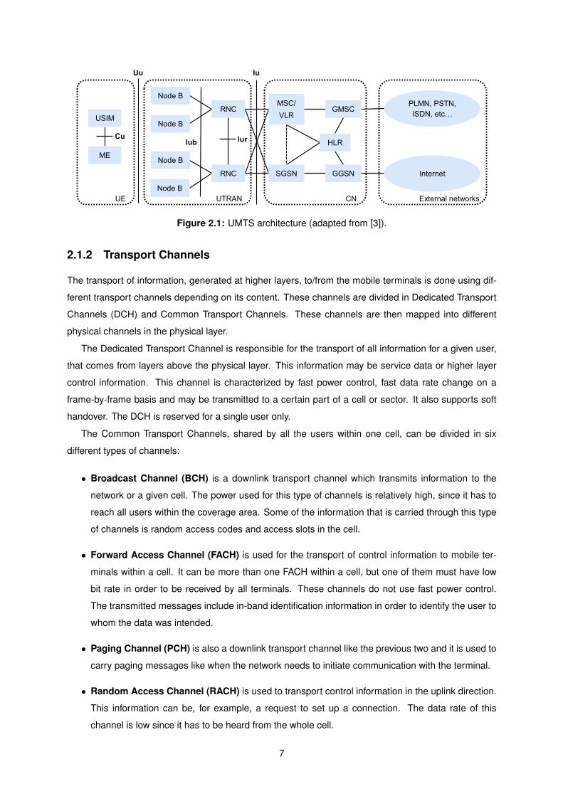
2.1.1 System Architecture

The high-level system architecture of Universal Mobile Telecommunication Services (UMTS) is divided

in three distinct components, the User Equipment (UE), the UMTS Terrestrial Radio Access Network

(UTRAN) and the Core Network (CN). The CN is connected with external networks which are divided

in two domains: the Circuit-Switched (CS) domain and the Packet-Switched (PS) domain. The UE

interfaces with the user and it is composed of the Mobile Equipment (ME), responsible for the radio

communications through the Uu interface, and the UMTS Subscriber Identity Module (USIM), which is

a smartcard that contains the subscriber identity number and handles the authentication. These two

components interact with each other over the Cu interface.

The UTRAN components are the Node Bs and the Radio Network Controllers (RNCs). One or more

Node Bs are connected with a RNC, over a Iub interface, forming a sub-network called Radio Network

Sub-system (RNS).

The Node B, also called Base Station (BS), interfaces with the UE over the Uu interface and is

responsible for all the processing associated with the air interface as well as the inner loop power control

(Fast Closed-Loop Power Control Procedure).

The RNC controls the radio resources of UTRAN and interfaces with CN over the Iu interface. Its

main functions are power control, admission control, channel allocation, radio resource control and

management and data multiplexing and demultiplexing [5]. One Node B is controlled by only one RNC,

the Controlling RNC (CRNC), but each RNC can control more than one Node B.

One mobile can be connected to more than one RNS; when this happens, the RNCs belonging to

each one of the RNSs have different functionalities. The Serving RNC (SRNC) is responsible for the

termination of the transport of user data over the Iu interface as well as all the associated signalling. The

SRNC also performs the handover decision and the outer loop power control. One UE can only have

one SRNC. The RNCs of the others RNSs connected to the UE are the Drift RNCs (DRNCs), which are

responsible for the routing of the user data to the SRNC over the Iur interface.

The CN is composed by the following network elements:

• Home Location Register (HLR), which stores the information related to the user’s service profile.

• Mobile Services Switching Centre (MSC)/Visitor Location Register (VLR), that serves the UE

for CS services.

• Gateway MSC (GMSC), which connects with the external networks in the CS domain.

• Serving General Packet Radio Service (GPRS) Support Node (SGSN), whose functionalities

are similar to MSC/VLR but is used for PS services.

• Gateway GPRS Support Node (GGSN), similar to GMSC, it is used for PS services.

Figure 2.1 shows the representation of the architecture featuring all the network elements previously

mentioned.

6

USIM

Cu

ME

Node B

Node B

Node B

Node B

RNC

RNC

lurlub

MSC/

VLR

SGSN

GMSC

GGSN

HLR

PLMN, PSTN,

ISDN, etc…

Internet

luUu

UE UTRAN CN External networks

Figure 2.1: UMTS architecture (adapted from [3]).

2.1.2 Transport Channels

The transport of information, generated at higher layers, to/from the mobile terminals is done using dif-

ferent transport channels depending on its content. These channels are divided in Dedicated Transport

Channels (DCH) and Common Transport Channels. These channels are then mapped into different

physical channels in the physical layer.

The Dedicated Transport Channel is responsible for the transport of all information for a given user,

that comes from layers above the physical layer. This information may be service data or higher layer

control information. This channel is characterized by fast power control, fast data rate change on a

frame-by-frame basis and may be transmitted to a certain part of a cell or sector. It also supports soft

handover. The DCH is reserved for a single user only.

The Common Transport Channels, shared by all the users within one cell, can be divided in six

different types of channels:

• Broadcast Channel (BCH) is a downlink transport channel which transmits information to the

network or a given cell. The power used for this type of channels is relatively high, since it has to

reach all users within the coverage area. Some of the information that is carried through this type

of channels is random access codes and access slots in the cell.

• Forward Access Channel (FACH) is used for the transport of control information to mobile ter-

minals within a cell. It can be more than one FACH within a cell, but one of them must have low

bit rate in order to be received by all terminals. These channels do not use fast power control.

The transmitted messages include in-band identification information in order to identify the user to

whom the data was intended.

• Paging Channel (PCH) is also a downlink transport channel like the previous two and it is used to

carry paging messages like when the network needs to initiate communication with the terminal.

• Random Access Channel (RACH) is used to transport control information in the uplink direction.

This information can be, for example, a request to set up a connection. The data rate of this

channel is low since it has to be heard from the whole cell.

7

• Uplink Common Packet Channel (CPCH) carries packet-based user information from the termi-

nal. The transmission of this channel may last several frames.

• Downlink Shared Channel (DSCH) is responsible for the transport of dedicated user data and/or

control information and may be shared by different users. This type of channels support fast power

control and variable bit rate on a frame-by-frame basis.

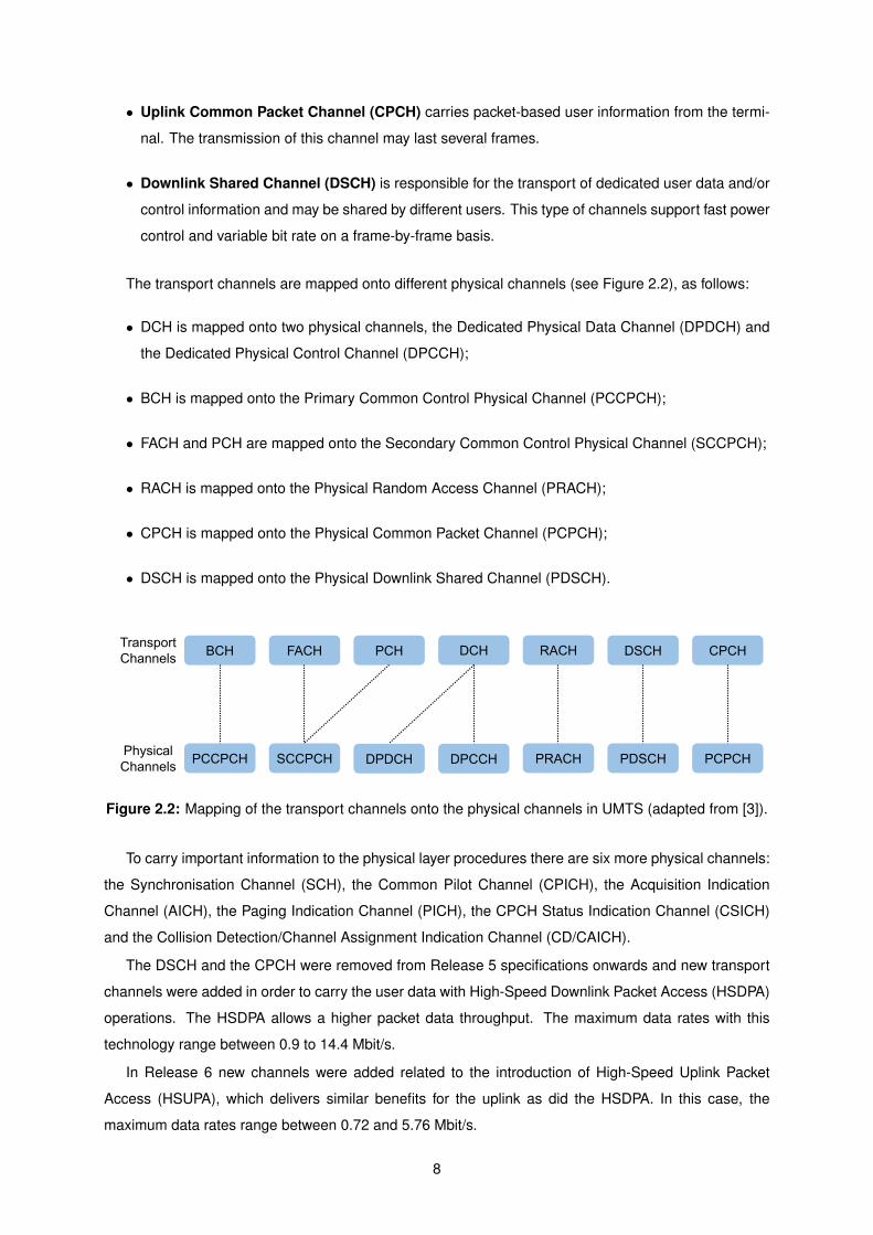
The transport channels are mapped onto different physical channels (see Figure 2.2), as follows:

• DCH is mapped onto two physical channels, the Dedicated Physical Data Channel (DPDCH) and

the Dedicated Physical Control Channel (DPCCH);

• BCH is mapped onto the Primary Common Control Physical Channel (PCCPCH);

• FACH and PCH are mapped onto the Secondary Common Control Physical Channel (SCCPCH);

• RACH is mapped onto the Physical Random Access Channel (PRACH);

• CPCH is mapped onto the Physical Common Packet Channel (PCPCH);

• DSCH is mapped onto the Physical Downlink Shared Channel (PDSCH).

DCHBCH FACH PCH RACH DSCH CPCH

DPCCHPCCPCH SCCPCH PRACHDPDCH PDSCH PCPCH

Transport

Channels

Physical

Channels

Figure 2.2: Mapping of the transport channels onto the physical channels in UMTS (adapted from [3]).

To carry important information to the physical layer procedures there are six more physical channels:

the Synchronisation Channel (SCH), the Common Pilot Channel (CPICH), the Acquisition Indication

Channel (AICH), the Paging Indication Channel (PICH), the CPCH Status Indication Channel (CSICH)

and the Collision Detection/Channel Assignment Indication Channel (CD/CAICH).

The DSCH and the CPCH were removed from Release 5 specifications onwards and new transport

channels were added in order to carry the user data with High-Speed Downlink Packet Access (HSDPA)

operations. The HSDPA allows a higher packet data throughput. The maximum data rates with this

technology range between 0.9 to 14.4 Mbit/s.

In Release 6 new channels were added related to the introduction of High-Speed Uplink Packet

Access (HSUPA), which delivers similar benefits for the uplink as did the HSDPA. In this case, the

maximum data rates range between 0.72 and 5.76 Mbit/s.

8

2.1.3 Power Control

The power control is a very important aspect in wireless systems, since each mobile station is in a

different location and consequently has different paths to the base station, which causes different signal

attenuation as well as different fading. Thus, each mobile station has a different transmission power

depending on its attenuation till the base station.

When a mobile begins a connection, the power is set, in a coarse way, by an open loop power control

mechanism. This mechanism consists in an estimation of path loss in the downlink, thus setting the initial

transmission power for the mobile station. This is a rough estimation since the path loss is significantly

different in the downlink and uplink, due to the difference between frequencies, in the WCDMA FDD

mode.

The power control is done using fast closed loop power control mechanism, which is implemented

in the uplink by estimating the received Signal-to-Interference Ratio (SIR) and comparing it to a target

SIR. The base station will then order the mobile station to change or maintain the transmission power,

according to the result of the SIR comparison. This control is executed at a high rate (1500 s-1) thus

being faster than the possible changes of path loss and fast fading.

The fast closed loop power control mechanism is also implemented in the downlink, to provide ad-

ditional power to the mobile stations at the cell edge, since these stations suffer a higher interference

from the other cells, and to decrease the fading effects. The target SIR, that is used to compare with the

received SIR, is adjusted by an outer loop power control mechanism. This adjustment is needed since

the minimum SIR for each mobile station depends on the mobile speed and on the multipath profile [3].

2.1.4 Handover

In 3G systems, different types of handover are used. The softer handover is one of them, which occurs

when a mobile station is in two adjacent sectors of a base station. In this scenario, the mobile and the

base station communicate through two different air interface channels, one for each sector. However,

there is only one power control loop active per connection. Another type of handover is the soft handover,

which occurs when the adjacent sectors belong to cells of different base stations. This type of handover

differs from the previous one since in this case two active power control loops are used per connection,

one for each base station. Other types of handover are the Inter-frequency hard handover that is used

to change the mobile WCDMA frequency carrier, the Inter-system hard handover which happens in the

transition of systems, for example from a WCDMA FDD to a WCDMA TDD system and the Inter-radio

access technology handover that allows a transition from services WCDMA to Global System for Mobile

Communications (GSM) without losing the connection with the mobile station.

2.1.5 QoS Differentiation

The different services provided by 3G networks have different requirements regarding to, e.g., delay

and bit rate. For this reason, QoS differentiation is typically used, which consists of prioritizing services

according to their needs.

9

The services are grouped into four different classes: conversational class, streaming class, inter-

active class and background class. The conversational class is characterized by low delay, low jitter

and symmetric traffic, and contains services such as Voice over IP (VoIP) and video conferencing. The

streaming class tolerates a little more delay than the Conversational class and includes services such

as video streaming and video on demand [3]. The interactive class does not require a low delay, but is

sensitive to the request response pattern of the end user; web browsing and network gaming are some

of the services belonging to this class. The background class does not have very strict requirements,

since the user does not expect data within a certain time [5]. Table 2.2 presents the characteristics of

each class together with an application example.

Table 2.2: QoS differentiation classes (adapted from [3]).

Classes Characteristics Applications

ConversationalLow delay (<400 ms)

No bufferingVoIP

StreamingModerate delay

Buffering allowedVideo streaming

InteractiveRequest response pattern

Buffering allowedWeb browsing

BackgroundPreserve payload content

No restraints on delaysE-mail

The QoS differentiation increases the network efficiency, especially when services with different delay

requirements are being used and the network load is high.

2.2 Long-Term Evolution

The LTE standard was introduced in Release 8 of 3GPP. This standard was developed to be exclusively

dedicated to packet-switched services. The LTE allows higher throughput and spectral efficiency as well

as lower latency and a more flexible channel bandwidth, relatively to UMTS. The peak data rate in this

standard in the downlink is 172.8 Mbit/s and 340 Mbit/s, using 2x2 and 4x4 Multiple-Input Multiple-Output

(MIMO), respectively. In the uplink, the peak data rate is 86.4 Mbit/s [4].

The used air interface is different for the downlink and the uplink, contrarily to the UMTS case which

uses a single air interface technology, the WCDMA. In LTE, the technologies used in the downlink

and in the uplink are the Orthogonal Frequency Division Multiple Access (OFDMA) and Single-Carrier

Frequency Division Multiple Access (SC-FDMA), respectively.

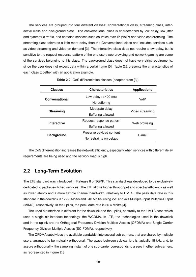
The OFDMA subdivides the available bandwidth into several sub-carriers, that are shared by multiple

users, arranged to be mutually orthogonal. The space between sub-carriers is typically 15 kHz and, to

assure orthogonality, the sampling instant of one sub-carrier corresponds to a zero in other sub-carriers,

as represented in Figure 2.3.

10

Sampling point for

sub-carrier

Zero value for other

sub-carriers

15 kHz

Figure 2.3: Orthogonality between sub-carriers (adapted from [4]).

The SC-FDMA also subdivides the available bandwidth into multiple sub-carriers, but each sub-

carrier is modulated with the same data.

Using these two multiple access technologies, the resource allocation is performed in the frequency

domain for both downlink and uplink, characterized by twelve sub-carriers of 15 kHz. However, the

resource allocation is done continuously for the uplink, since it is a single carrier transmission, and in

the downlink the resource blocks can be allocated from different parts of the spectrum.

2.2.1 System Architecture

The LTE architecture takes into account the exclusive PS services implementation characteristic of this

technology. Contrarily to the UMTS architecture, introduced in subsection 2.1.1, this technology is char-

acterized by a flat architecture, with less network nodes.

The evolution of the radio access is represented by LTE, through the Evolved-UTRAN (E-UTRAN). It

was accompanied by the evolution of non-radio aspects, designated by System Architecture Evolution

(SAE), which includes the Evolved Packet Core (EPC). The LTE architecture, or Evolved Packet System

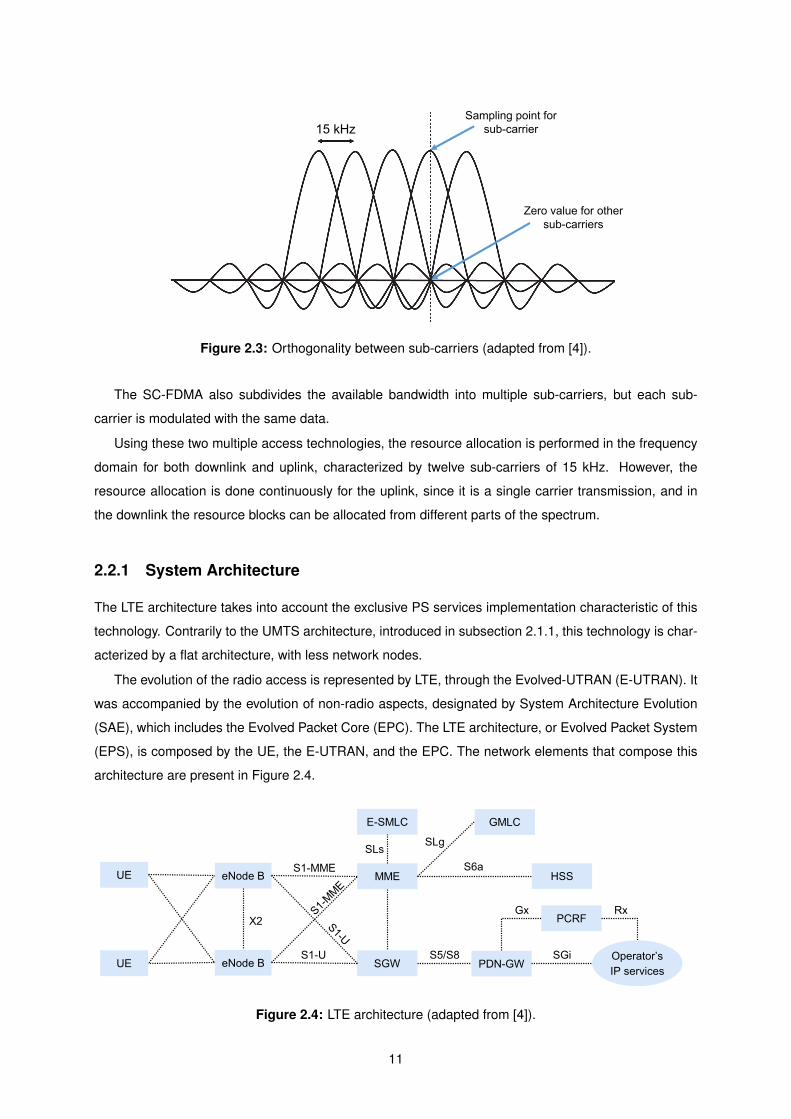
(EPS), is composed by the UE, the E-UTRAN, and the EPC. The network elements that compose this

architecture are present in Figure 2.4.

UE eNode B

MME

SGW

X2

UE eNode B HSS

GMLCE-SMLC

PDN-GWOperator’s

IP services

PCRF

S1-MME

S1-U

S6a

SLgSLs

S5/S8

Gx Rx

SGi

Figure 2.4: LTE architecture (adapted from [4]).

11

The eNodeBs are the only elements that compose the radio access network, as represented in

Figure 2.4, which justifies the denomination of flat architecture. The UMTS radio access network was

composed by the NodeBs and the RNCs, in LTE that does not happen, giving more importance to the

eNodeB, which are now responsible for the Radio Resource Management (RRM), data compression,

security and connectivity to the EPC, more specifically to the Mobility Management Entity (MME) and

the Serving Gateway (SGW). Additionally, the eNodeB is also responsible by the connectivity with the

UE.

The E-UTRAN architecture allows a better interaction between the radio access different layers pro-

tocols than the UTRAN, which conducts to a lower delay and an higher network efficiency.

The inter-connection between eNodeBs is done by X2 interface, used for handover purposes, for

instance. The connection with the EPC is done through the interface S1.

The core network (EPC) is responsible for the UE control and the establishment of bearers, which are

the paths used by the user traffic to connect with Packet Data Network (PDN) through the LTE transport

network. The EPC is composed by the following network elements:

• Mobility Management Entity (MME) - responsible by the transition between the access radio

network and the EPC. This node processes the signaling between the UE and the core network.

The main functions supported by the MME correspond to: functions related to bearer management;

functions related to connection management; and functions related to inter-working with other

networks.

• Evolved Serving Mobile Location Centre (E-SMLC) - manages the coordination and scheduling

of resources needed to estimate the UE location. Based on received estimations, it determines

the final location, as well as the UE speed, and achieved accuracy.

• Gateway Mobile Location Centre (GMLC) - consists of some functionalities that are required to

support LoCation Services (LCS). It requests and receives the final location estimates from MME,

after performing authorization.

• Home Subscriber Server (HSS) - data base with information about each mobile. It contains

information such as, the PDNs to which the user can connect to and the MME to which the user is

currently connected to.

• Serving Gateway (SGW) - responsible for keeping information regarding the bearers during the

UE’s iddle mode.

• PDN Gateway (PDN-GW) - connects the EPS with the PDN. It also allocates the Internet Protocol

(IP) addresses designated for the UE.

• Policy Control and Charging Rules Function (PCRF) - responsible for policy control decision-

making and controlling the flow-based charging functionalities.

The network elements mentioned are represented in Figure 2.4, as well as the interfaces that inter-

connect each one of them.

12

2.2.2 Transport Channels

The information generated at higher layers is transported through transport channels, which are charac-

terized by the way the information is transported and how it is coded. The defined transport channels in

LTE are the following:

• Broadcast Channel (BCH) - carries the basic system information used to configure and operate

the remain channels in the cell.

• Downlink Shared Channel (DL-SCH) - all user data is transported in this channel. This channel

also broadcasts the system information that is not transported by the BCH and transports paging

messages. The data is transmitted in Transport Blocks (TBs), for each Transmission Time Interval

(TTI) one TB is generated, where TTI is 1ms. For each UE, one or two TBs per subframe can

be transmitted, depending on the transmission mode. The next subsection has a more detailed

description regarding the transmission modes.

• Paging Channel (PCH) - downlink channel that transmits paging messages to the UE, which are

used to change the state from RRC IDLE to RRC CONNECTED (RRC - Radio Resource Control).

• Multicast Channel (MCH) - used to transport data regarding the Multimedia Broadcast and Multi-

cast Services (MBMS). This channel is only used in specific subframes designated by Multimedia

Broadcast Single Frequency Network (MBSFN).

• Uplink Shared Channel (UL-SCH) - responsible for the transport of UE data and control informa-

tion from the UE to the eNodeB.

• Random Access Channel (RACH) - used by the mobile devices for the random access to the

network.

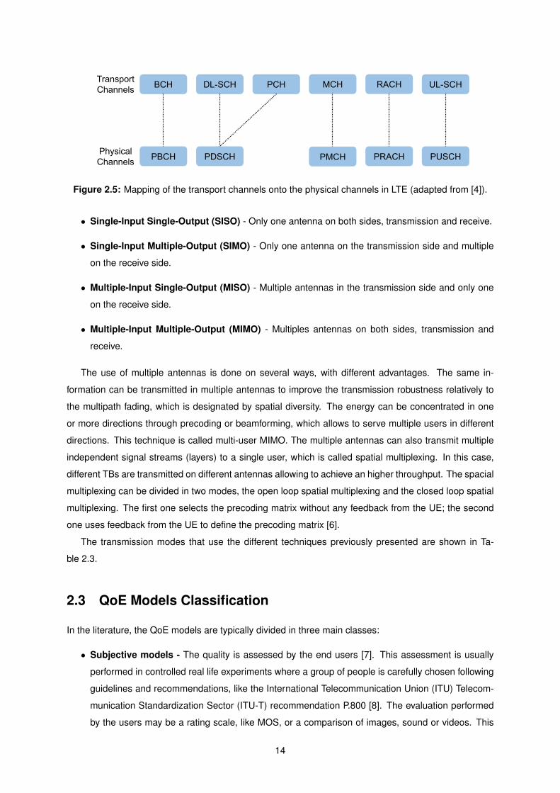
The mentioned transport channels are mapped into physical channels (Figure 2.5), as follows:

• BCH is mapped into Physical Broadcast Channel (PBCH);

• DL-SCH and PCH are mapped into Physical Downlink Shared Channel (PDSCH);

• MCH is mapped into Physical Multicast Channel (PMCH);

• RACH is mapped into Physical Random Access Channel (PRACH);

• UL-SCH is mapped into Physical Uplink Shared Channel (PUSCH).

2.2.3 Transmission Modes

The multi-antenna transmission mode scheme being used is configured by the transmission mode.

Therefore, in this subsection, the multiple antenna schemes are firstly introduced and then the trans-

mission modes are presented.

The various configurations of antennas used in the transmission and receive sides can be classified

as follows:

13

MCHBCH DL-SCH PCH RACH UL-SCH

PMCHPBCH PDSCH PRACH PUSCH

Transport

Channels

Physical

Channels

Figure 2.5: Mapping of the transport channels onto the physical channels in LTE (adapted from [4]).

• Single-Input Single-Output (SISO) - Only one antenna on both sides, transmission and receive.

• Single-Input Multiple-Output (SIMO) - Only one antenna on the transmission side and multiple

on the receive side.

• Multiple-Input Single-Output (MISO) - Multiple antennas in the transmission side and only one

on the receive side.

• Multiple-Input Multiple-Output (MIMO) - Multiples antennas on both sides, transmission and

receive.

The use of multiple antennas is done on several ways, with different advantages. The same in-

formation can be transmitted in multiple antennas to improve the transmission robustness relatively to

the multipath fading, which is designated by spatial diversity. The energy can be concentrated in one

or more directions through precoding or beamforming, which allows to serve multiple users in different

directions. This technique is called multi-user MIMO. The multiple antennas can also transmit multiple

independent signal streams (layers) to a single user, which is called spatial multiplexing. In this case,

different TBs are transmitted on different antennas allowing to achieve an higher throughput. The spacial

multiplexing can be divided in two modes, the open loop spatial multiplexing and the closed loop spatial

multiplexing. The first one selects the precoding matrix without any feedback from the UE; the second

one uses feedback from the UE to define the precoding matrix [6].

The transmission modes that use the different techniques previously presented are shown in Ta-

ble 2.3.

2.3 QoE Models Classification

In the literature, the QoE models are typically divided in three main classes:

• Subjective models - The quality is assessed by the end users [7]. This assessment is usually

performed in controlled real life experiments where a group of people is carefully chosen following

guidelines and recommendations, like the International Telecommunication Union (ITU) Telecom-

munication Standardization Sector (ITU-T) recommendation P.800 [8]. The evaluation performed

by the users may be a rating scale, like MOS, or a comparison of images, sound or videos. This

14

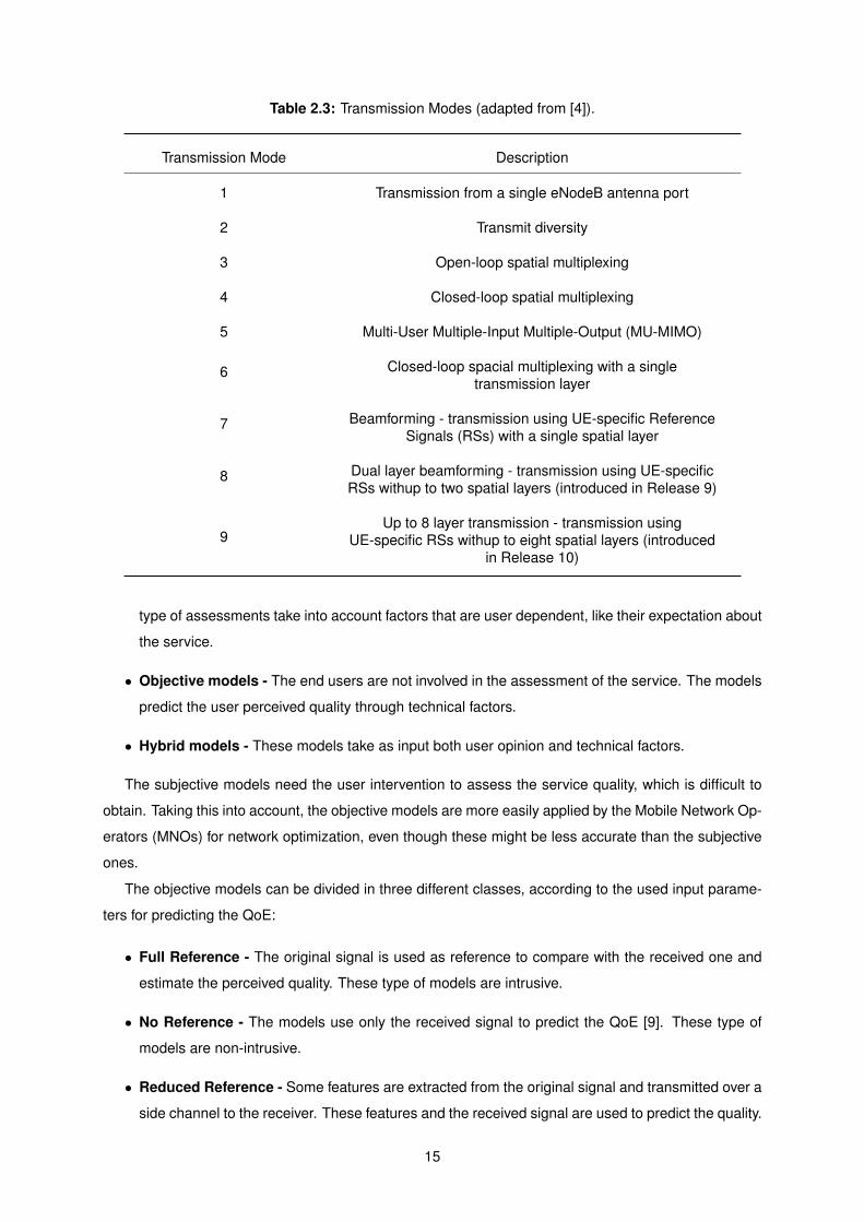
Table 2.3: Transmission Modes (adapted from [4]).

Transmission Mode Description

1 Transmission from a single eNodeB antenna port

2 Transmit diversity

3 Open-loop spatial multiplexing

4 Closed-loop spatial multiplexing

5 Multi-User Multiple-Input Multiple-Output (MU-MIMO)

6 Closed-loop spacial multiplexing with a singletransmission layer

7 Beamforming - transmission using UE-specific ReferenceSignals (RSs) with a single spatial layer

8 Dual layer beamforming - transmission using UE-specificRSs withup to two spatial layers (introduced in Release 9)

9Up to 8 layer transmission - transmission using

UE-specific RSs withup to eight spatial layers (introducedin Release 10)

type of assessments take into account factors that are user dependent, like their expectation about

the service.

• Objective models - The end users are not involved in the assessment of the service. The models

predict the user perceived quality through technical factors.

• Hybrid models - These models take as input both user opinion and technical factors.

The subjective models need the user intervention to assess the service quality, which is difficult to

obtain. Taking this into account, the objective models are more easily applied by the Mobile Network Op-

erators (MNOs) for network optimization, even though these might be less accurate than the subjective

ones.

The objective models can be divided in three different classes, according to the used input parame-

ters for predicting the QoE:

• Full Reference - The original signal is used as reference to compare with the received one and

estimate the perceived quality. These type of models are intrusive.

• No Reference - The models use only the received signal to predict the QoE [9]. These type of

models are non-intrusive.

• Reduced Reference - Some features are extracted from the original signal and transmitted over a

side channel to the receiver. These features and the received signal are used to predict the quality.

15

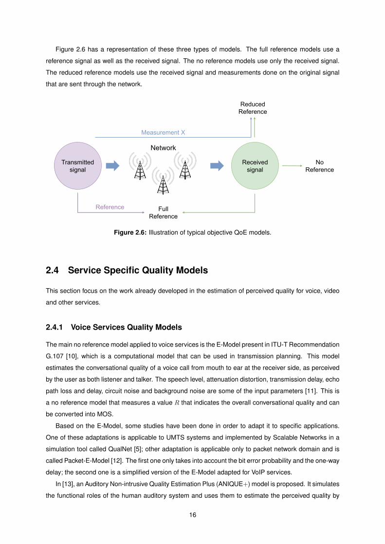
Figure 2.6 has a representation of these three types of models. The full reference models use a

reference signal as well as the received signal. The no reference models use only the received signal.

The reduced reference models use the received signal and measurements done on the original signal

that are sent through the network.

Transmitted

signal

Received

signal

Full

Reference

No

Reference

Measurement X

Reduced

Reference

Reference

Network

Figure 2.6: Illustration of typical objective QoE models.

2.4 Service Specific Quality Models

This section focus on the work already developed in the estimation of perceived quality for voice, video

and other services.

2.4.1 Voice Services Quality Models

The main no reference model applied to voice services is the E-Model present in ITU-T Recommendation

G.107 [10], which is a computational model that can be used in transmission planning. This model

estimates the conversational quality of a voice call from mouth to ear at the receiver side, as perceived

by the user as both listener and talker. The speech level, attenuation distortion, transmission delay, echo

path loss and delay, circuit noise and background noise are some of the input parameters [11]. This is

a no reference model that measures a value R that indicates the overall conversational quality and can

be converted into MOS.

Based on the E-Model, some studies have been done in order to adapt it to specific applications.

One of these adaptations is applicable to UMTS systems and implemented by Scalable Networks in a

simulation tool called QualNet [5]; other adaptation is applicable only to packet network domain and is

called Packet-E-Model [12]. The first one only takes into account the bit error probability and the one-way

delay; the second one is a simplified version of the E-Model adapted for VoIP services.

In [13], an Auditory Non-intrusive Quality Estimation Plus (ANIQUE+) model is proposed. It simulates

the functional roles of the human auditory system and uses them to estimate the perceived quality by

16

the end user.

In [14], the authors introduce a non-intrusive method to objectively assess the perceptual quality of

live VoIP calls. This model has the advantage of being implemented in voice calls in progress. The

method uses the VoIP packet streams that are copied from the network.

The models presented above are all no reference ones. In the case of the full reference models, ITU-

T presents in recommendation P.863 the Perceptual Objective Listening Quality Assessment (POLQA)

model, which estimates the quality of speech on the receiver side based on the original audio signal.

The received signal is compared with the original undistorted one which results in an estimation of the

mean perceived quality that a group of end-users would have.

2.4.2 Video Services Quality Models

In [15], a model to Hypertext Transfer Protocol (HTTP) video streaming services is introduced. This

model consists in three distinct steps. First, a relationship between the network QoS parameters and

the application QoS parameters is established; secondly the application QoS parameters are correlated

to the QoE values measured through MOS; finally, the combination of the previous two steps results in

a relationship between network QoS parameters and QoE. The network QoS parameters considered

are the round-trip time (RTT), the packet loss rate and the network bandwidth. These parameters are

converted in application level parameters in the second step, which are the following:

• Initial buffering time, that measures the period between the starting time of loading a video and the

starting time of playing it.

• Mean rebuffering duration, which is the average duration of a rebuffering event.

• Rebuffering frequency, which is the frequency of occurrence of the rebuffering events.

The study concluded that the RTT and the packet loss are the main factors that influence MOS.

In [16], the authors propose a model for video streaming of MPEG4 video sequences, which takes

into account the content being transmitted over wireless networks. This study considers three video con-

tent types, based on the temporal (movement) and spatial (edges, brightness) activities: Slight move-

ment (SM), Gentle walking (GW) and Rapid movement (RM). The video quality is estimated based on

the content type and network level parameter (packet error rate) and application level parameters (send

bitrate, frame rate). The results presented are very positive, having a correlation, between the predicted

and the reference QoE values, higher than 79% and a Root Mean Squared Error (RMSE) lower than 0.3

for all the three content types.

2.4.3 Other Services Quality Models

In addiction to the QoE models for voice and video services, it can be found in literature QoE models

applied to other services, like web browsing and File Transfer Protocol (FTP) services.

In [17], the authors propose a QoE model for web browsing that only takes into account the delay. It

is in agreement with the ITU-T Recomendation G.1031, which states that the delay is one of the most

17

important parameter in this type of services [18]. The results presented in this study [17] show that the

proposed model does a good estimation of the perceived quality by the end users when accessing a

web page of fixed size.

In [19], a QoE model for FTP services is presented. To predict the perceived quality, the model

considers the data rate, since it is the dominant factor affecting the QoE level .

18

Chapter 3

Machine Learning Algorithms

In this chapter the machine learning algorithms used to obtain the QoE models are introduced, as

well as the followed methodology . After a description of the used methodology, the multivariate linear

regression algorithm is presented, followed by the Support Vector Regression (SVR) algorithm. For each

algorithm, a description of the parameter learning algorithm is presented.

3.1 Methodology

The learning algorithms present in the next sections aim to predict an output y through a mathematical

expression that takes n parameters as input, called features, xj , j = 1, ..., n. These algorithms take as

input a training set (x(i)1 , x

(i)2 , ..., x

(i)n , y(i)), i = 1, ...,m composed by m training examples (x1, ..xn, y).

The development process for each learning algorithm follows the same methodology. The algorithms

are applied to different sets of features in order to form different hypotheses. The hypothesis with the

best performance is chosen as the final model.

To train and assess each hypothesis the data set is divided in three different subsets, as follows:

• 60% - Training set;

• 20% - Validation set;

• 20% - Test set.

The training set is the input of the learning algorithm and it is used to train each hypothesis. The

validation set is used to assess each hypothesis and to choose the best one. The test set is used to

determine the final performance of the model.

The next subsections describe the metrics used to assess each hypothesis and the method used

to tune the input parameters (hyperparameters) of the learning algorithms, the K-Fold Cross Validation

method. Finally, the overfitting and underfitting problems are also introduced.

19

3.1.1 Hypotheses Assessment

To assess the developed hypotheses, three metrics are considered: the Root Mean Squared Error

(RMSE), the Pearson Correlation and the Spearman Correlation.

The RMSE measures the square root of the average of the square of the differences between the

predicted and the original values. Expression (3.1) gives this metric, where y(i) and y(i) are the original

and predicted values of the ith set of parameters, respectively.

rmse =

√√√√ 1

m

m∑i=1

(y(i) − y(i))2 (3.1)

To simplify the results interpretation, the RMSE is converted to percentage. This conversion is done

by (3.2), where ymax and ymin are 5 and 1 respectively, since y is a value of MOS and its scale ranges

from 1 to 5.

RMSE[%] =rmse

ymax − ymin(3.2)

The Pearson Correlation measures the linear correlation between the predicted values and the orig-

inal ones. This metric is given by (3.3), where y(i) and y(i) are the original and predicted values of the

ith set of parameters. The y and ¯y represent the mean values of these metrics.

RPearson =

∑mi=1(y(i) − ¯y)(y(i) − y)√∑m

i=1(y(i) − ¯y)2√∑m

i=1(y(i) − y)2(3.3)

The Spearman Correlation measures the strength and direction of association between the original

and predicted values. The input parameters of this measurement are first ranked from 1 to N , being N

the total of samples of each parameter. After being ranked, (3.3) is applied to those rankings.

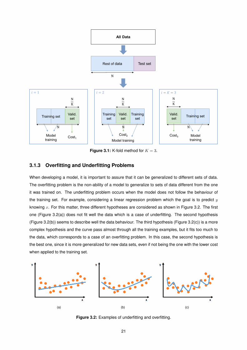
3.1.2 K-Fold Cross Validation Method

Before the learning algorithms are applied, it is necessary to tune their hyperparameters, which are the

parameters that are constants of the model’s equations. In order to choose the best hyperparameters,

the K-fold cross validation method is used.

The dataset is first randomly divided in different subsets. The test set is the same mentioned before.

The rest of the data is divided in K uniform subsets (Si, i = 1, ...,K). Then, a process of K iterations

is performed, where for each iteration one of the K subsets is considered as the validation set and the

remaining K − 1 subsets the training set. In each iteration, the training set is used to train the model

and the validation set is used to calculate the cost (it can be the RMSE). Finalized the K iterations,

the average cost of the validation sets is calculated. Figure 3.1 illustrates this method for K = 3. This

process is repeated for different combinations of the algorithm hyperparameters.

At the end, there is an average cost for each combination of the algorithm hyperparameters. The

combination with the lower cost is the chosen one.

20

All Data

Rest of data Test set

Valid.

set

Valid.

set

Valid.

set

N

K

Model

training

N

K

N

K

Cost1Cost2 Cost3

Model training

Model

training

𝑖 = 1 𝑖 = 2 𝑖 = 𝐾 = 3

N

Training setTraining

setTraining set

N NN

Training

set

Figure 3.1: K-fold method for K = 3.

3.1.3 Overfitting and Underfitting Problems

When developing a model, it is important to assure that it can be generalized to different sets of data.

The overfitting problem is the non-ability of a model to generalize to sets of data different from the one

it was trained on. The underfitting problem occurs when the model does not follow the behaviour of

the training set. For example, considering a linear regression problem which the goal is to predict y

knowing x. For this matter, three different hypotheses are considered as shown in Figure 3.2. The first

one (Figure 3.2(a)) does not fit well the data which is a case of underfitting. The second hypothesis

(Figure 3.2(b)) seems to describe well the data behaviour. The third hypothesis (Figure 3.2(c)) is a more

complex hypothesis and the curve pass almost through all the training examples, but it fits too much to

the data, which corresponds to a case of an overfitting problem. In this case, the second hypothesis is

the best one, since it is more generalized for new data sets, even if not being the one with the lower cost

when applied to the training set.

(a) (b) (c)

Figure 3.2: Examples of underfitting and overfitting.

21

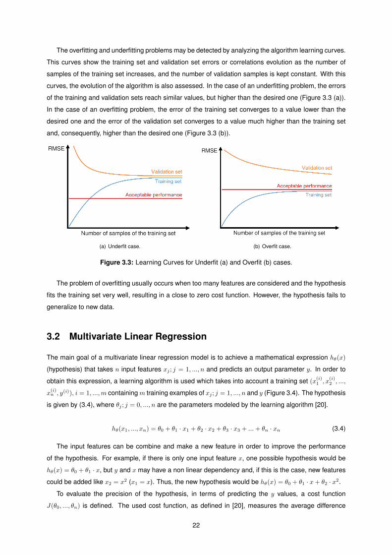
The overfitting and underfitting problems may be detected by analyzing the algorithm learning curves.

This curves show the training set and validation set errors or correlations evolution as the number of

samples of the training set increases, and the number of validation samples is kept constant. With this

curves, the evolution of the algorithm is also assessed. In the case of an underfitting problem, the errors

of the training and validation sets reach similar values, but higher than the desired one (Figure 3.3 (a)).

In the case of an overfitting problem, the error of the training set converges to a value lower than the

desired one and the error of the validation set converges to a value much higher than the training set

and, consequently, higher than the desired one (Figure 3.3 (b)).

(a) Underfit case. (b) Overfit case.

Figure 3.3: Learning Curves for Underfit (a) and Overfit (b) cases.

The problem of overfitting usually occurs when too many features are considered and the hypothesis

fits the training set very well, resulting in a close to zero cost function. However, the hypothesis fails to

generalize to new data.

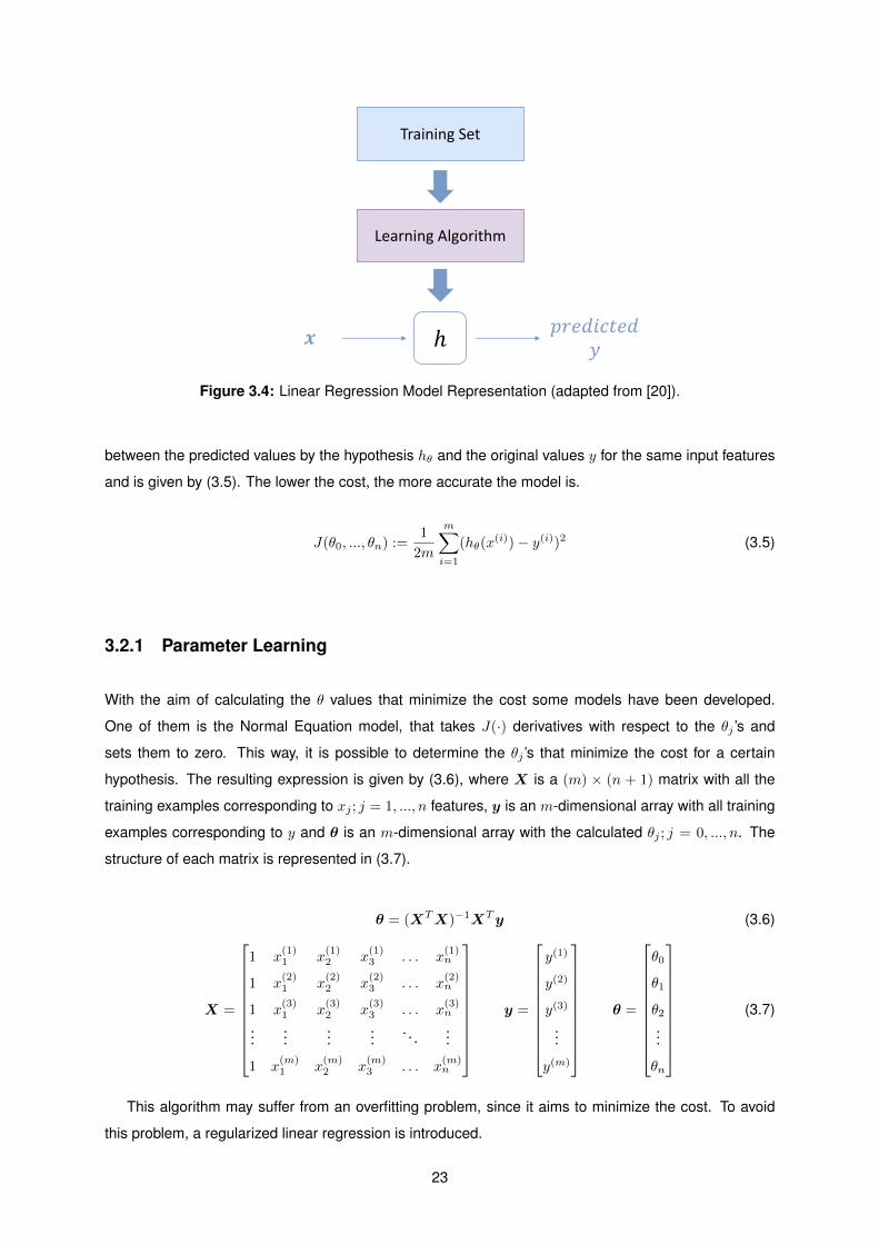
3.2 Multivariate Linear Regression

The main goal of a multivariate linear regression model is to achieve a mathematical expression hθ(x)

(hypothesis) that takes n input features xj ; j = 1, ..., n and predicts an output parameter y. In order to

obtain this expression, a learning algorithm is used which takes into account a training set (x(i)1 , x

(i)2 , ...,

x(i)n , y(i)), i = 1, ...,m containingm training examples of xj ; j = 1, ..., n and y (Figure 3.4). The hypothesis

is given by (3.4), where θj ; j = 0, ..., n are the parameters modeled by the learning algorithm [20].

hθ(x1, ..., xn) = θ0 + θ1 · x1 + θ2 · x2 + θ3 · x3 + ...+ θn · xn (3.4)

The input features can be combine and make a new feature in order to improve the performance

of the hypothesis. For example, if there is only one input feature x, one possible hypothesis would be

hθ(x) = θ0 + θ1 · x, but y and x may have a non linear dependency and, if this is the case, new features

could be added like x2 = x2 (x1 = x). Thus, the new hypothesis would be hθ(x) = θ0 + θ1 · x+ θ2 · x2.

To evaluate the precision of the hypothesis, in terms of predicting the y values, a cost function

J(θ0, ..., θn) is defined. The used cost function, as defined in [20], measures the average difference

22

Training Set

Learning Algorithm

ℎ𝒙𝑝𝑟𝑒𝑑𝑖𝑐𝑡𝑒𝑑

𝑦

Figure 3.4: Linear Regression Model Representation (adapted from [20]).

between the predicted values by the hypothesis hθ and the original values y for the same input features

and is given by (3.5). The lower the cost, the more accurate the model is.

J(θ0, ..., θn) :=1

2m

m∑i=1

(hθ(x(i))− y(i))2 (3.5)

3.2.1 Parameter Learning

With the aim of calculating the θ values that minimize the cost some models have been developed.

One of them is the Normal Equation model, that takes J(·) derivatives with respect to the θj ’s and

sets them to zero. This way, it is possible to determine the θj ’s that minimize the cost for a certain

hypothesis. The resulting expression is given by (3.6), where X is a (m) × (n + 1) matrix with all the

training examples corresponding to xj ; j = 1, ..., n features, y is an m-dimensional array with all training

examples corresponding to y and θ is an m-dimensional array with the calculated θj ; j = 0, ..., n. The

structure of each matrix is represented in (3.7).

θ = (XTX)−1XTy (3.6)

X =

1 x(1)1 x

(1)2 x

(1)3 . . . x

(1)n

1 x(2)1 x

(2)2 x

(2)3 . . . x

(2)n

1 x(3)1 x

(3)2 x

(3)3 . . . x

(3)n

......

......

. . ....

1 x(m)1 x

(m)2 x

(m)3 . . . x

(m)n

y =

y(1)

y(2)

y(3)

...

y(m)

θ =

θ0

θ1

θ2...

θn

(3.7)

This algorithm may suffer from an overfitting problem, since it aims to minimize the cost. To avoid

this problem, a regularized linear regression is introduced.

23

3.2.2 Regularized Linear Regression

To solve the overfitting problem, a penalty term, λ, is introduced in the cost function that is going to be

minimized in order to reduce the weight that each feature has on the final result. This penalty term, or

hyperparameter, can be applied to every feature or only to some features that are considered to be less

relevant.

Generally, it is possible to apply the regularization parameter to every feature and smooth the output

of the hypothesis in order to reduce the overfitting. Thus, the cost function presented in (3.5) is modified

to incorporate the regularization parameter, resulting in a new cost function equation, (3.8).

Jreg(θ0, .., θ4) =1

2m

m∑i=1

(hθ(x(i))− y(i))2 + λ

n∑j=1

θ2j (3.8)

The Normal Equation model can be adapted to include the regularization parameter and the expres-

sion representing the model is given by (3.9). The L is a (n + 1) × (n + 1) matrix similar to the identity

matrix but differs in the first value of the diagonal which is 0 in this case, as represented in (3.10).

θ = (XTX + λ ·L)−1XTy (3.9)

L =

0

1

1

. . .

1

(3.10)

The value of λ has to be chosen carefully: if λ is too high, the hypothesis will suffer from an un-

derfitting problem since it favours low weights and the hypothesis would tend to hθ(x) = θ0; if λ is too

low, there is no difference to the hypothesis without regularization and it can suffer from an overfitting

problem.

3.3 Support Vector Regression Algorithm

The SVR algorithm aims to achieve an optimized expression f(x) that predicts y given a set of n features

xj , j = 1, ..., n. The learning algorithm minimizes the ε-insensitive loss function shown in Figure 3.5;

this function is zero for errors that don’t exceed a tolerance margin [−ε; ε]. By taking this function as

reference, the algorithm will ignore errors less than ε.

The learning algorithm uses a training set (x(i)1 , x

(i)2 , ..., x

(i)n , y(i)), i = 1, ...,m, containing m training

examples of xj ; j = 1, ..., n and y, and optimizes a function f(x) that predicts the y value. It can be

applied to both linear and non-linear regressions problems. The following subsections describe the

algorithm for these two regression approaches.

24

Figure 3.5: ε-insensitive Loss Function.

3.3.1 Linear SVR

The linear SVR function to optimize is given by (3.11), where x ∈ Rn is an array with the features and

ρ ∈ R, w ∈ Rn are the parameters to be optimized.

f(x) = w · x− ρ (3.11)

On one hand, in order to obtain a function as flat as possible, avoiding overfitting problems, the

module of w has to be minimized. On the other hand, the deviation of the predictions has to be less

than ε. Taking into account that, in practice, the ε margin is difficult to ensure, larger deviations of the

predictions are tolerated which have also to be minimized. Therefore, the learning algorithm optimization

is given by:

minimize1

2‖w‖2 + C

m∑i=1

(ξi + ξ∗i )

subject to

y(i) −w · x(i) + ρ ≤ ε+ ξi

w · x(i) − ρ− y(i) ≤ ε+ ξ∗i

ξi, ξ∗i ≥ 0

,

(3.12)

where C is a constant greater than zero that balances the flatness of f and the predictions deviations

larger than ε. ξ, ξ∗ are the amount by which the predictions may exceed the ε margin. yi and xi corre-

spond to each training example. Figure 3.6 shows the representation of ξ, ξ∗ and ε.

3.3.2 Non-linear SVR

The main difference between the linear and the non-linear SVR algorithms is the introduction of the

Kernel function in the second one. The Kernel function introduces non-linearity to the data. This function

may be applied with support vectors (SV) that allow to transform the data into a multidimensional plane.

The function to be optimized in this case is given by:

f(x) = w ·K(x,SV )− ρ, (3.13)

25

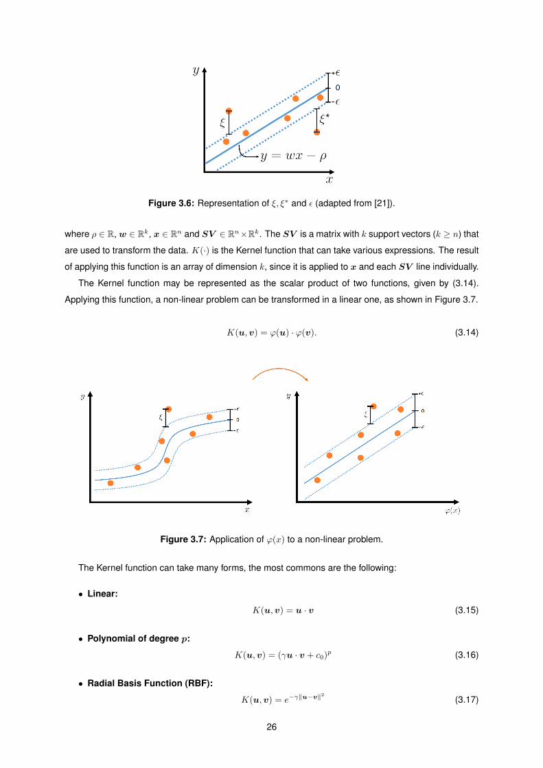
Figure 3.6: Representation of ξ, ξ∗ and ε (adapted from [21]).

where ρ ∈ R,w ∈ Rk, x ∈ Rn and SV ∈ Rn×Rk. The SV is a matrix with k support vectors (k ≥ n) that

are used to transform the data. K(·) is the Kernel function that can take various expressions. The result

of applying this function is an array of dimension k, since it is applied to x and each SV line individually.

The Kernel function may be represented as the scalar product of two functions, given by (3.14).

Applying this function, a non-linear problem can be transformed in a linear one, as shown in Figure 3.7.

K(u,v) = ϕ(u) · ϕ(v). (3.14)

Figure 3.7: Application of ϕ(x) to a non-linear problem.

The Kernel function can take many forms, the most commons are the following:

• Linear:

K(u,v) = u · v (3.15)

• Polynomial of degree p:

K(u,v) = (γu · v + c0)p (3.16)

• Radial Basis Function (RBF):

K(u,v) = e−γ‖u−v‖2

(3.17)

26

• Sigmoid:

K(u,v) = tanh(γu · v + c0) (3.18)

The choice of the Kernel function, and of its parameters, has to be done according to the problem

being analyzed.

27

Chapter 4

QoE Model for 3G Voice Calls

This chapter presents a new QoE model for 3G voice calls. An analysis of the available parameters was

firstly performed, followed by the selection of the most important ones. The model development process

consists in two different approaches, one linear and one non-linear. Finally the results of the proposed

model are presented.

4.1 QoE Model Parameters

The proposed QoE model was developed using Radio Frequency (RF) metrics obtained through drive-

testing in real mobile networks, which covered a suburban area. The data was collected using the Test

Mobile System (TEMS R©) [22], which is an active, end-to-end testing solution, used to verify, optimize

and troubleshoot Radio Access Network (RAN) services.

To evaluate the QoE, TEMS R© uses the POLQA [23]. The estimation of QoE performed by POLQA

only measures the effects of one-way speech distortion and noise, not taking into account other factors

like delay, sidetone and echo, which are related to the interaction between the end-users. Despite its

limitations, the algorithm performs with low error when compared to subjective tests in large groups of

people [23].

The RF parameters are measured in time series of about 5 seconds each. Each time series corre-

sponds to one MOS measurement. A total of 347 MOS measurements were collected, through 86 3G

phone calls. The network parameters measured in those time series are the following:

• SIR [dB] - ratio between the average received modulated carrier power and the average received

co-channel interference power.

• SIR Target [dB] - reference SIR set by the outer loop power control.

• Active Set (AS) Ec/N0 [dB] - AS best received chip energy to noise spectral density ratio.

• AS Received Signal Code Power (RSCP) [dBm] - AS best power measured in the CPICH.

• Received Signal Strength Indicator (RSSI) [dBm] - metric that takes into account the RSCP and

the received chip energy to interference level ratio (Ec/I0), given by:

29

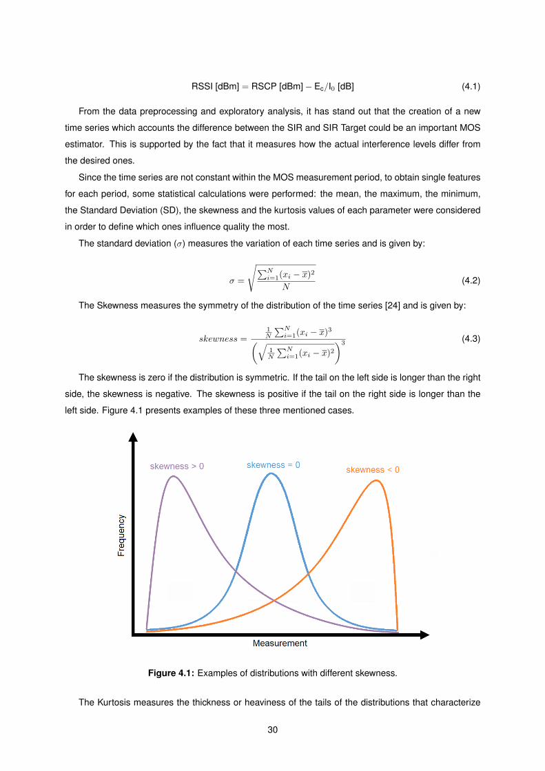
RSSI [dBm] = RSCP [dBm]− Ec/I0 [dB] (4.1)

From the data preprocessing and exploratory analysis, it has stand out that the creation of a new

time series which accounts the difference between the SIR and SIR Target could be an important MOS

estimator. This is supported by the fact that it measures how the actual interference levels differ from

the desired ones.

Since the time series are not constant within the MOS measurement period, to obtain single features

for each period, some statistical calculations were performed: the mean, the maximum, the minimum,

the Standard Deviation (SD), the skewness and the kurtosis values of each parameter were considered

in order to define which ones influence quality the most.

The standard deviation (σ) measures the variation of each time series and is given by:

σ =

√∑Ni=1(xi − x)2

N(4.2)

The Skewness measures the symmetry of the distribution of the time series [24] and is given by:

skewness =1N

∑Ni=1(xi − x)3(√

1N

∑Ni=1(xi − x)2

)3 (4.3)

The skewness is zero if the distribution is symmetric. If the tail on the left side is longer than the right

side, the skewness is negative. The skewness is positive if the tail on the right side is longer than the

left side. Figure 4.1 presents examples of these three mentioned cases.

Figure 4.1: Examples of distributions with different skewness.

The Kurtosis measures the thickness or heaviness of the tails of the distributions that characterize

30

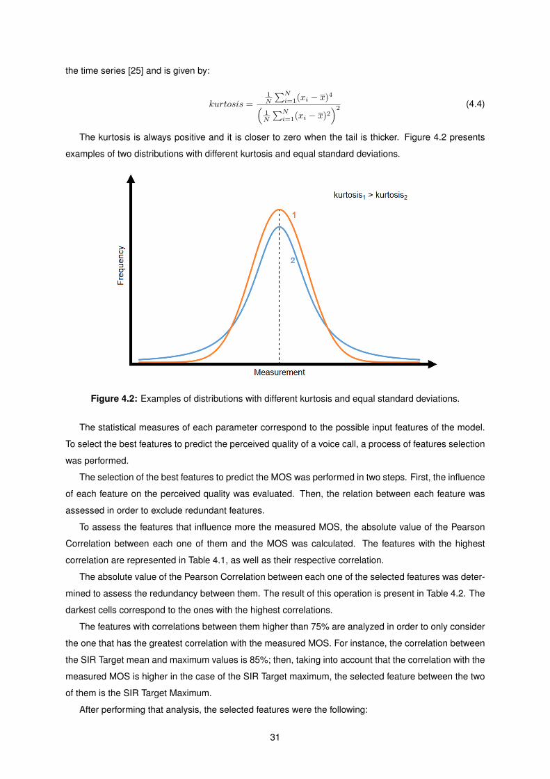
the time series [25] and is given by:

kurtosis =1N

∑Ni=1(xi − x)4(

1N

∑Ni=1(xi − x)2

)2 (4.4)

The kurtosis is always positive and it is closer to zero when the tail is thicker. Figure 4.2 presents

examples of two distributions with different kurtosis and equal standard deviations.

Figure 4.2: Examples of distributions with different kurtosis and equal standard deviations.

The statistical measures of each parameter correspond to the possible input features of the model.

To select the best features to predict the perceived quality of a voice call, a process of features selection

was performed.

The selection of the best features to predict the MOS was performed in two steps. First, the influence

of each feature on the perceived quality was evaluated. Then, the relation between each feature was

assessed in order to exclude redundant features.

To assess the features that influence more the measured MOS, the absolute value of the Pearson

Correlation between each one of them and the MOS was calculated. The features with the highest

correlation are represented in Table 4.1, as well as their respective correlation.

The absolute value of the Pearson Correlation between each one of the selected features was deter-

mined to assess the redundancy between them. The result of this operation is present in Table 4.2. The

darkest cells correspond to the ones with the highest correlations.

The features with correlations between them higher than 75% are analyzed in order to only consider

the one that has the greatest correlation with the measured MOS. For instance, the correlation between

the SIR Target mean and maximum values is 85%; then, taking into account that the correlation with the

measured MOS is higher in the case of the SIR Target maximum, the selected feature between the two

of them is the SIR Target Maximum.

After performing that analysis, the selected features were the following:

31

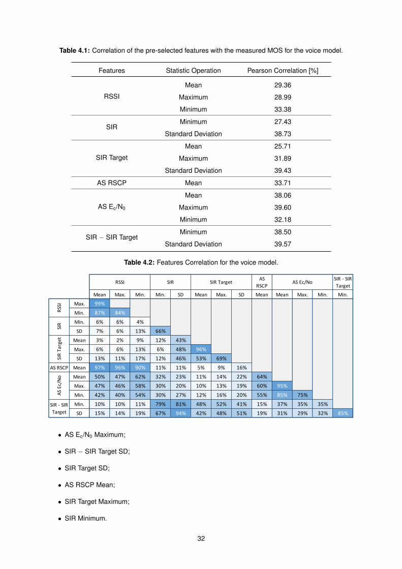
Table 4.1: Correlation of the pre-selected features with the measured MOS for the voice model.

Features Statistic Operation Pearson Correlation [%]

RSSI

Mean 29.36

Maximum 28.99

Minimum 33.38

SIRMinimum 27.43

Standard Deviation 38.73

SIR Target

Mean 25.71

Maximum 31.89


AS RSCP Mean 33.71

AS Ec/N0

Mean 38.06

Maximum 39.60

Minimum 32.18

SIR − SIR TargetMinimum 38.50


Table 4.2: Features Correlation for the voice model.

AS

RSCP

SIR - SIR

Target

Mean Max. Min. Min. SD Mean Max. SD Mean Mean Max. Min. Min.

Max. 99%

Min. 87% 84%

Min. 6% 6% 4%

SD 7% 6% 13% 66%

Mean 3% 2% 9% 12% 43%

Max. 6% 6% 13% 6% 48% 96%

SD 13% 11% 17% 12% 46% 53% 69%

AS RSCP Mean 97% 96% 90% 11% 11% 5% 9% 16%

Mean 50% 47% 62% 32% 23% 11% 14% 22% 64%

Max. 47% 46% 58% 30% 20% 10% 13% 19% 60% 95%

Min. 42% 40% 54% 30% 27% 12% 16% 20% 55% 85% 75%

Min. 10% 10% 11% 79% 81% 48% 52% 41% 15% 37% 35% 35%

SD 15% 14% 19% 67% 94% 42% 48% 51% 19% 31% 29% 32% 85%

SIR Target AS Ec/No

RSS

ISI

RSI

R T

arge

tA

S Ec

/No

SIR - SIR

Target

RSSI SIR

• AS Ec/N0 Maximum;

• SIR − SIR Target SD;

• SIR Target SD;

• AS RSCP Mean;

• SIR Target Maximum;

• SIR Minimum.

32

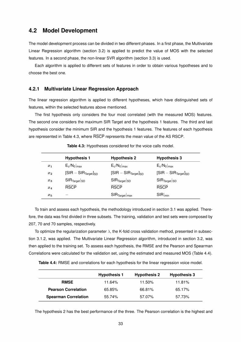
4.2 Model Development

The model development process can be divided in two different phases. In a first phase, the Multivariate

Linear Regression algorithm (section 3.2) is applied to predict the value of MOS with the selected

features. In a second phase, the non-linear SVR algorithm (section 3.3) is used.

Each algorithm is applied to different sets of features in order to obtain various hypotheses and to

choose the best one.

4.2.1 Multivariate Linear Regression Approach

The linear regression algorithm is applied to different hypotheses, which have distinguished sets of

features, within the selected features above mentioned.

The first hypothesis only considers the four most correlated (with the measured MOS) features.

The second one considers the maximum SIR Target and the hypothesis 1 features. The third and last

hypothesis consider the minimum SIR and the hypothesis 1 features. The features of each hypothesis

are represented in Table 4.3, where RSCP represents the mean value of the AS RSCP.

Table 4.3: Hypotheses considered for the voice calls model.

Hypothesis 1 Hypothesis 2 Hypothesis 3

x1 Ec/N0|max Ec/N0|max Ec/N0|max

x2 [SIR− SIRTarget]SD [SIR− SIRTarget]SD [SIR− SIRTarget]SD

x3 SIRTarget|SD SIRTarget|SD SIRTarget|SD

x4 RSCP RSCP RSCP

x5 − SIRTarget|max SIR|min

To train and assess each hypothesis, the methodology introduced in section 3.1 was applied. There-

fore, the data was first divided in three subsets. The training, validation and test sets were composed by

207, 70 and 70 samples, respectively.

To optimize the regularization parameter λ, the K-fold cross validation method, presented in subsec-

tion 3.1.2, was applied. The Multivariate Linear Regression algorithm, introduced in section 3.2, was

then applied to the training set. To assess each hypothesis, the RMSE and the Pearson and Spearman

Correlations were calculated for the validation set, using the estimated and measured MOS (Table 4.4).

Table 4.4: RMSE and correlations for each hypothesis for the linear regression voice model.


RMSE 11.64% 11.50% 11.81%

Pearson Correlation 65.85% 66.81% 65.17%

Spearman Correlation 55.74% 57.07% 57.73%

The hypothesis 2 has the best performance of the three. The Pearson correlation is the highest and

33

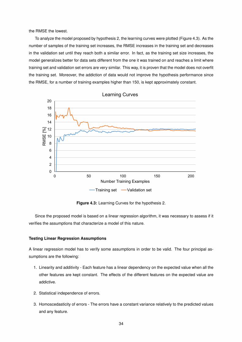
the RMSE the lowest.

To analyze the model proposed by hypothesis 2, the learning curves were plotted (Figure 4.3). As the

number of samples of the training set increases, the RMSE increases in the training set and decreases

in the validation set until they reach both a similar error. In fact, as the training set size increases, the

model generalizes better for data sets different from the one it was trained on and reaches a limit where

training set and validation set errors are very similar. This way, it is proven that the model does not overfit

the training set. Moreover, the addiction of data would not improve the hypothesis performance since

the RMSE, for a number of training examples higher than 150, is kept approximately constant.

0

2

4

6

8

10

12

14

16

18

20

0 50 100 150 200

RM

SE

[%

]

Number Training Examples

Learning Curves

Training set Validation set

Figure 4.3: Learning Curves for the hypothesis 2.

Since the proposed model is based on a linear regression algorithm, it was necessary to assess if it

verifies the assumptions that characterize a model of this nature.

Testing Linear Regression Assumptions

A linear regression model has to verify some assumptions in order to be valid. The four principal as-

sumptions are the following:

1. Linearity and additivity - Each feature has a linear dependency on the expected value when all the

other features are kept constant. The effects of the different features on the expected value are

addictive.

2. Statistical independence of errors.

3. Homoscedasticity of errors - The errors have a constant variance relatively to the predicted values

and any feature.

34

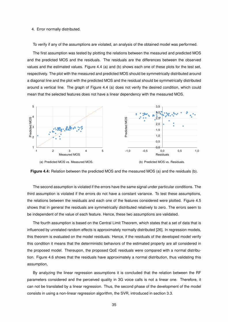
4. Error normally distributed.

To verify if any of the assumptions are violated, an analysis of the obtained model was performed.

The first assumption was tested by plotting the relations between the measured and predicted MOS

and the predicted MOS and the residuals. The residuals are the differences between the observed

values and the estimated values. Figure 4.4 (a) and (b) shows each one of these plots for the test set,

respectively. The plot with the measured and predicted MOS should be symmetrically distributed around

a diagonal line and the plot with the predicted MOS and the residual should be symmetrically distributed

around a vertical line. The graph of Figure 4.4 (a) does not verify the desired condition, which could

mean that the selected features does not have a linear dependency with the measured MOS.

1

2

3

4

5

1 2 3 4 5

Pre

dic

ted

MO

S

Measured MOS

(a) Predicted MOS vs. Measured MOS.

0,0

0,5

1,0

1,5

2,0

2,5

3,0

3,5

-1,0 -0,5 0,0 0,5 1,0

Pre

dic

ted

MO

S

Residuals

(b) Predicted MOS vs. Residuals.

Figure 4.4: Relation between the predicted MOS and the measured MOS (a) and the residuals (b).

The second assumption is violated if the errors have the same signal under particular conditions. The

third assumption is violated if the errors do not have a constant variance. To test these assumptions,

the relations between the residuals and each one of the features considered were plotted. Figure 4.5

shows that in general the residuals are symmetrically distributed relatively to zero. The errors seem to

be independent of the value of each feature. Hence, these two assumptions are validated.

The fourth assumption is based on the Central Limit Theorem, which states that a set of data that is

influenced by unrelated random effects is approximately normally distributed [26]. In regression models,

this theorem is evaluated on the model residuals. Hence, if the residuals of the developed model verify

this condition it means that the deterministic behaviors of the estimated property are all considered in

the proposed model. Thereupon, the proposed QoE residuals were compared with a normal distribu-

tion. Figure 4.6 shows that the residuals have approximately a normal distribution, thus validating this

assumption,

By analyzing the linear regression assumptions it is concluded that the relation between the RF

parameters considered and the perceived quality in 3G voice calls is not a linear one. Therefore, it

can not be translated by a linear regression. Thus, the second phase of the development of the model

consists in using a non-linear regression algorithm, the SVR, introduced in section 3.3.

35

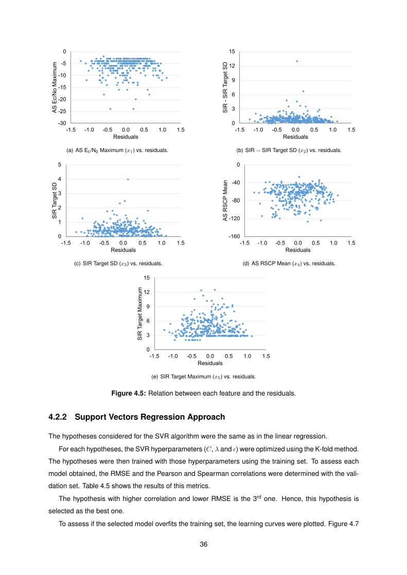
-30

-25

-20

-15

-10

-5

0

-1.5 -1.0 -0.5 0.0 0.5 1.0 1.5

AS

Ec/N

o M

axim

um

Residuals

(a) AS Ec/N0 Maximum (x1) vs. residuals.

0

3

6

9

12

15

-1.5 -1.0 -0.5 0.0 0.5 1.0 1.5

SIR

-S

IR T

arg

et

SD

Residuals

(b) SIR − SIR Target SD (x2) vs. residuals.

0

1

2

3

4

5

-1.5 -1.0 -0.5 0.0 0.5 1.0 1.5

SIR

Targ

et

SD

Residuals

(c) SIR Target SD (x3) vs. residuals.

-160

-120

-80

-40

0

-1.5 -1.0 -0.5 0.0 0.5 1.0 1.5

AS

RS

CP

Me

an

Residuals

(d) AS RSCP Mean (x4) vs. residuals.

0

3

6

9

12

15

-1.5 -1.0 -0.5 0.0 0.5 1.0 1.5

SIR

Ta

rge

t M

axim

um

Residuals

(e) SIR Target Maximum (x5) vs. residuals.

Figure 4.5: Relation between each feature and the residuals.

4.2.2 Support Vectors Regression Approach

The hypotheses considered for the SVR algorithm were the same as in the linear regression.

For each hypotheses, the SVR hyperparameters (C, λ and ε) were optimized using the K-fold method.

The hypotheses were then trained with those hyperparameters using the training set. To assess each

model obtained, the RMSE and the Pearson and Spearman correlations were determined with the vali-

dation set. Table 4.5 shows the results of this metrics.

The hypothesis with higher correlation and lower RMSE is the 3rd one. Hence, this hypothesis is

selected as the best one.

To assess if the selected model overfits the training set, the learning curves were plotted. Figure 4.7

36

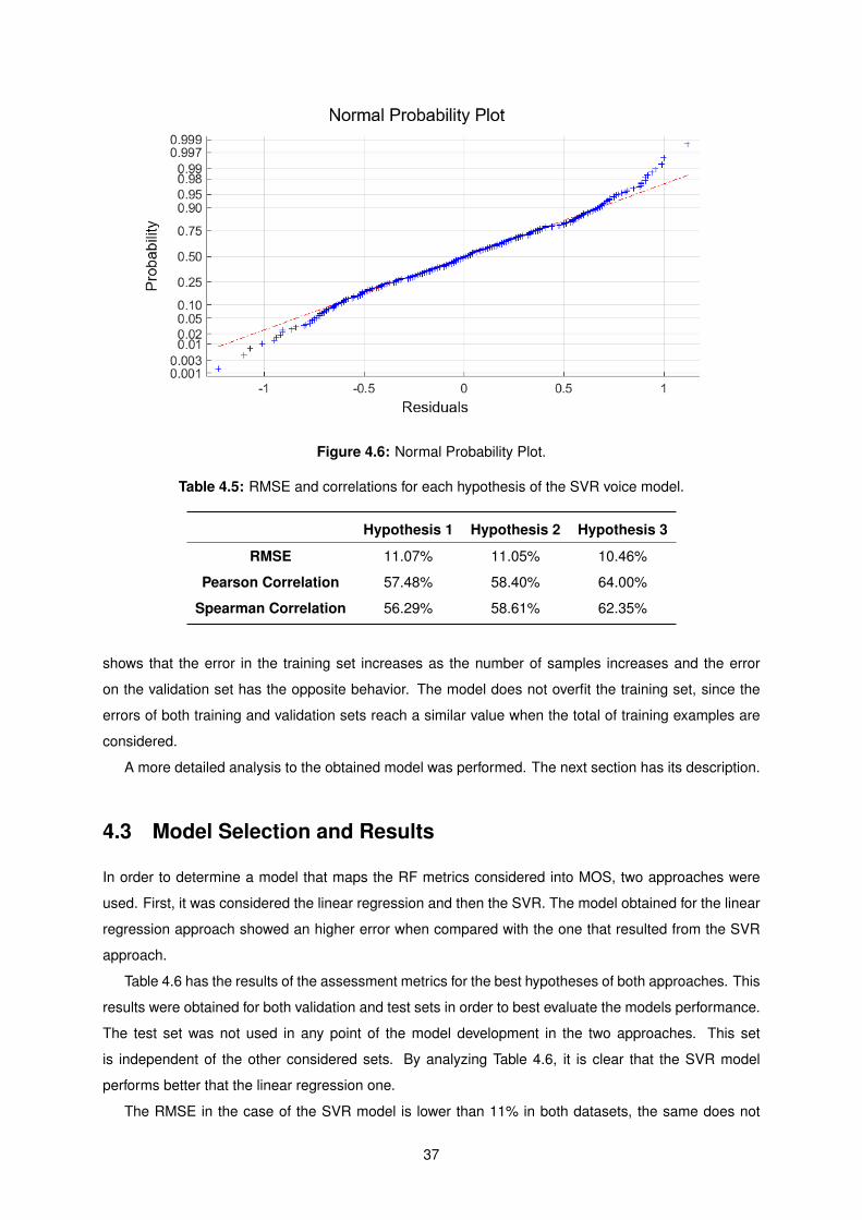
Figure 4.6: Normal Probability Plot.

Table 4.5: RMSE and correlations for each hypothesis of the SVR voice model.


RMSE 11.07% 11.05% 10.46%

Pearson Correlation 57.48% 58.40% 64.00%

Spearman Correlation 56.29% 58.61% 62.35%

shows that the error in the training set increases as the number of samples increases and the error

on the validation set has the opposite behavior. The model does not overfit the training set, since the

errors of both training and validation sets reach a similar value when the total of training examples are

considered.

A more detailed analysis to the obtained model was performed. The next section has its description.

4.3 Model Selection and Results

In order to determine a model that maps the RF metrics considered into MOS, two approaches were

used. First, it was considered the linear regression and then the SVR. The model obtained for the linear

regression approach showed an higher error when compared with the one that resulted from the SVR

approach.

Table 4.6 has the results of the assessment metrics for the best hypotheses of both approaches. This

results were obtained for both validation and test sets in order to best evaluate the models performance.

The test set was not used in any point of the model development in the two approaches. This set

is independent of the other considered sets. By analyzing Table 4.6, it is clear that the SVR model

performs better that the linear regression one.

The RMSE in the case of the SVR model is lower than 11% in both datasets, the same does not

37

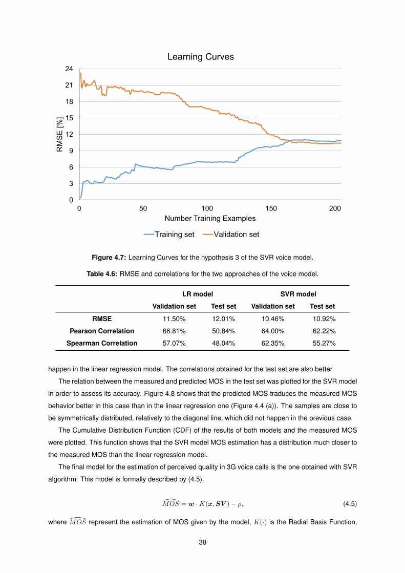
0

3

6

9

12

15

18

21

24

0 50 100 150 200

RM

SE

[%

]

Number Training Examples

Learning Curves


Figure 4.7: Learning Curves for the hypothesis 3 of the SVR voice model.

Table 4.6: RMSE and correlations for the two approaches of the voice model.

LR model SVR model

Validation set Test set Validation set Test set

RMSE 11.50% 12.01% 10.46% 10.92%

Pearson Correlation 66.81% 50.84% 64.00% 62.22%

Spearman Correlation 57.07% 48.04% 62.35% 55.27%

happen in the linear regression model. The correlations obtained for the test set are also better.

The relation between the measured and predicted MOS in the test set was plotted for the SVR model

in order to assess its accuracy. Figure 4.8 shows that the predicted MOS traduces the measured MOS

behavior better in this case than in the linear regression one (Figure 4.4 (a)). The samples are close to

be symmetrically distributed, relatively to the diagonal line, which did not happen in the previous case.

The Cumulative Distribution Function (CDF) of the results of both models and the measured MOS

were plotted. This function shows that the SVR model MOS estimation has a distribution much closer to

the measured MOS than the linear regression model.

The final model for the estimation of perceived quality in 3G voice calls is the one obtained with SVR

algorithm. This model is formally described by (4.5).

MOS = w ·K(x,SV )− ρ, (4.5)

where MOS represent the estimation of MOS given by the model, K(·) is the Radial Basis Function,

38

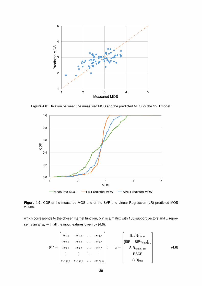
1

2

3

4

5

1 2 3 4 5

Pre

dic

ted

MO

S

Measured MOS

Figure 4.8: Relation between the measured MOS and the predicted MOS for the SVR model.

0.0

0.2

0.4

0.6

0.8

1.0

1 2 3 4 5

CD

F

MOS

Measured MOS LR Predicted MOS SVR Predicted MOS

Figure 4.9: CDF of the measured MOS and of the SVR and Linear Regression (LR) predicted MOSvalues.

which corresponds to the chosen Kernel function, SV is a matrix with 158 support vectors and x repre-

sents an array with all the input features given by (4.6).

SV =

sv1,1 sv1,2 . . . sv1,5

sv2,1 sv2,2 . . . sv2,5

sv3,1 sv3,2 . . . sv3,5...

.... . .

...

sv158,1 sv158,2 . . . sv158,5

; x =

Ec/N0|max

[SIR− SIRTarget]SD

SIRTarget|SD

RSCP

SIR|min

(4.6)

39

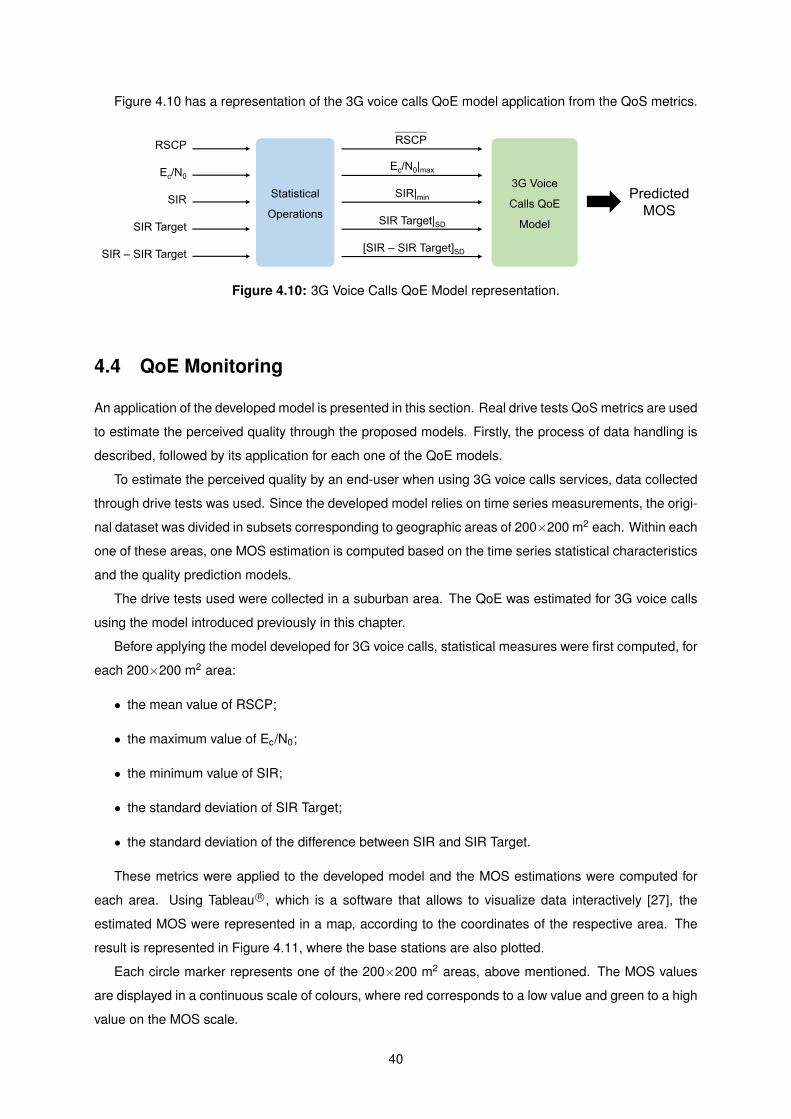
Figure 4.10 has a representation of the 3G voice calls QoE model application from the QoS metrics.

Ec/N0|max

SIR|min

SIR Target|SD

[SIR – SIR Target]SD

Statistical

Operations

RSCP

Ec/N0

SIR

SIR Target

SIR – SIR Target

RSCP

3G Voice

Calls QoE

Model

Predicted

MOS

Figure 4.10: 3G Voice Calls QoE Model representation.

4.4 QoE Monitoring

An application of the developed model is presented in this section. Real drive tests QoS metrics are used

to estimate the perceived quality through the proposed models. Firstly, the process of data handling is

described, followed by its application for each one of the QoE models.

To estimate the perceived quality by an end-user when using 3G voice calls services, data collected

through drive tests was used. Since the developed model relies on time series measurements, the origi-

nal dataset was divided in subsets corresponding to geographic areas of 200×200 m2 each. Within each

one of these areas, one MOS estimation is computed based on the time series statistical characteristics

and the quality prediction models.

The drive tests used were collected in a suburban area. The QoE was estimated for 3G voice calls

using the model introduced previously in this chapter.

Before applying the model developed for 3G voice calls, statistical measures were first computed, for

each 200×200 m2 area:

• the mean value of RSCP;

• the maximum value of Ec/N0;

• the minimum value of SIR;

• the standard deviation of SIR Target;

• the standard deviation of the difference between SIR and SIR Target.

These metrics were applied to the developed model and the MOS estimations were computed for

each area. Using Tableau R©, which is a software that allows to visualize data interactively [27], the

estimated MOS were represented in a map, according to the coordinates of the respective area. The

result is represented in Figure 4.11, where the base stations are also plotted.

Each circle marker represents one of the 200×200 m2 areas, above mentioned. The MOS values

are displayed in a continuous scale of colours, where red corresponds to a low value and green to a high

value on the MOS scale.

40

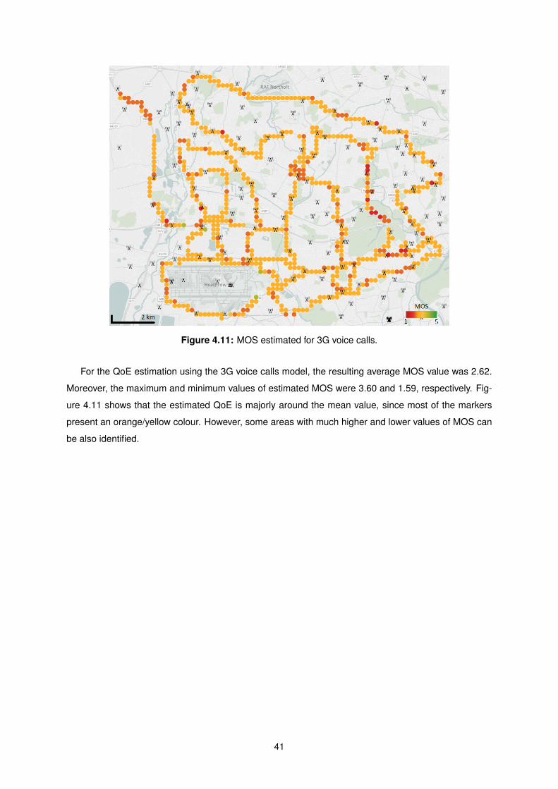
Figure 4.11: MOS estimated for 3G voice calls.

For the QoE estimation using the 3G voice calls model, the resulting average MOS value was 2.62.

Moreover, the maximum and minimum values of estimated MOS were 3.60 and 1.59, respectively. Fig-

ure 4.11 shows that the estimated QoE is majorly around the mean value, since most of the markers

present an orange/yellow colour. However, some areas with much higher and lower values of MOS can

be also identified.

41

Chapter 5

QoE Model for Web Browsing

This chapter presents a new QoE model for web browsing. First, the used model parameters are defined

followed by the description of the process implemented for the development of the model. Finally, the

selected model is presented together with the respective assessment results.

5.1 QoE Model Parameters

The Web Browsing QoE model proposed in this chapter was developed using RF metrics collected

through drive testing in real LTE networks. As in the voice model, the data was collected using TEMS R©.

To get the required ”ground truth” of MOS values, an existent objective model was used [17]. This

model takes into account the time that a web page takes to download, to estimate the QoE, using the

MOS scale. The results presented by the authors show that the model has a low error measuring the

perceived quality. The model proposed in [17] is given by (5.1), where d is the download time in seconds,

and its graphic representation is presented in Figure 5.1.

MOS = 5− 578

1 +(11.77 + 22.61

d

)2 (5.1)

Figure 5.1 shows that the QoE is very delay sensitive in this type of service. For download times

greater than 12 s, the MOS is lower than 2.

The network parameters, as in the voice model, are measured in time series, corresponding each

one to one MOS measurement. The selected parameters are the following:

• Reference Signals Received Power (RSRP) [dBm] - average power of resource elements that

carry cell specific reference signals over the entire bandwidth.

• Reference Signal Received Quality (RSRQ) [dB] - indicates the quality of the received reference

signal.

• RSSI [dBm] - total received wide-band power (measure in all symbols) including all interference

and thermal noise.

43

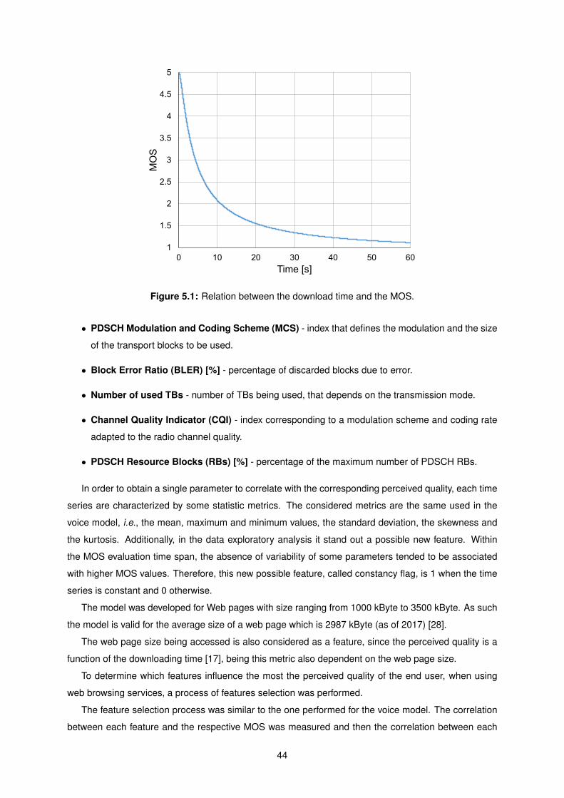
1

1.5

2

2.5

3

3.5

4

4.5

5

0 10 20 30 40 50 60

MO

S

Time [s]

Figure 5.1: Relation between the download time and the MOS.

• PDSCH Modulation and Coding Scheme (MCS) - index that defines the modulation and the size

of the transport blocks to be used.

• Block Error Ratio (BLER) [%] - percentage of discarded blocks due to error.

• Number of used TBs - number of TBs being used, that depends on the transmission mode.

• Channel Quality Indicator (CQI) - index corresponding to a modulation scheme and coding rate

adapted to the radio channel quality.

• PDSCH Resource Blocks (RBs) [%] - percentage of the maximum number of PDSCH RBs.

In order to obtain a single parameter to correlate with the corresponding perceived quality, each time

series are characterized by some statistic metrics. The considered metrics are the same used in the

voice model, i.e., the mean, maximum and minimum values, the standard deviation, the skewness and

the kurtosis. Additionally, in the data exploratory analysis it stand out a possible new feature. Within

the MOS evaluation time span, the absence of variability of some parameters tended to be associated

with higher MOS values. Therefore, this new possible feature, called constancy flag, is 1 when the time

series is constant and 0 otherwise.

The model was developed for Web pages with size ranging from 1000 kByte to 3500 kByte. As such

the model is valid for the average size of a web page which is 2987 kByte (as of 2017) [28].

The web page size being accessed is also considered as a feature, since the perceived quality is a

function of the downloading time [17], being this metric also dependent on the web page size.

To determine which features influence the most the perceived quality of the end user, when using

web browsing services, a process of features selection was performed.

The feature selection process was similar to the one performed for the voice model. The correlation

between each feature and the respective MOS was measured and then the correlation between each

44

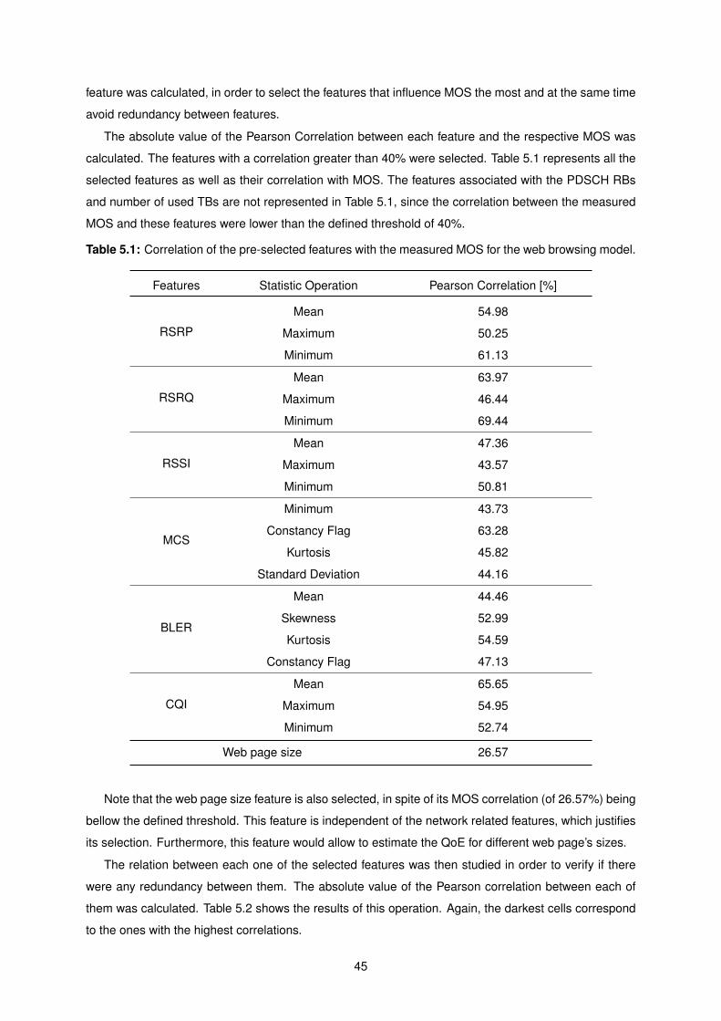
feature was calculated, in order to select the features that influence MOS the most and at the same time

avoid redundancy between features.

The absolute value of the Pearson Correlation between each feature and the respective MOS was

calculated. The features with a correlation greater than 40% were selected. Table 5.1 represents all the

selected features as well as their correlation with MOS. The features associated with the PDSCH RBs

and number of used TBs are not represented in Table 5.1, since the correlation between the measured

MOS and these features were lower than the defined threshold of 40%.

Table 5.1: Correlation of the pre-selected features with the measured MOS for the web browsing model.

Features Statistic Operation Pearson Correlation [%]

RSRP

Mean 54.98

Maximum 50.25

Minimum 61.13

RSRQ

Mean 63.97

Maximum 46.44

Minimum 69.44

RSSI

Mean 47.36

Maximum 43.57

Minimum 50.81

MCS

Minimum 43.73

Constancy Flag 63.28

Kurtosis 45.82


BLER

Mean 44.46

Skewness 52.99

Kurtosis 54.59

Constancy Flag 47.13

CQI

Mean 65.65

Maximum 54.95

Minimum 52.74

Web page size 26.57

Note that the web page size feature is also selected, in spite of its MOS correlation (of 26.57%) being

bellow the defined threshold. This feature is independent of the network related features, which justifies

its selection. Furthermore, this feature would allow to estimate the QoE for different web page’s sizes.

The relation between each one of the selected features was then studied in order to verify if there

were any redundancy between them. The absolute value of the Pearson correlation between each of

them was calculated. Table 5.2 shows the results of this operation. Again, the darkest cells correspond

to the ones with the highest correlations.

45

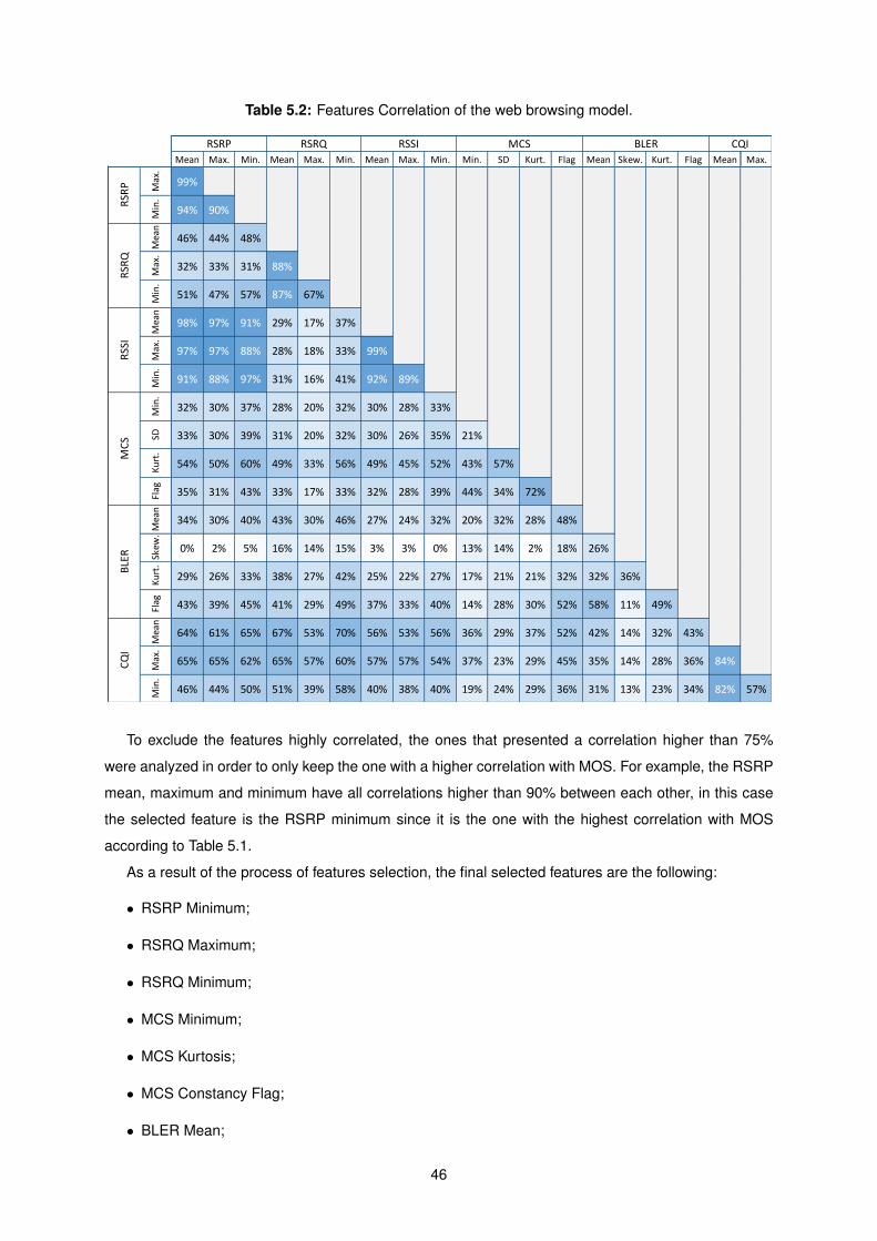
Table 5.2: Features Correlation of the web browsing model.

Mean Max. Min. Mean Max. Min. Mean Max. Min. Min. SD Kurt. Flag Mean Skew. Kurt. Flag MeanMax.

99%

Min.

94% 90%

Mean

46% 44% 48%

Max.

32% 33% 31% 88%

Min.

51% 47% 57% 87% 67%

Mean

98% 97% 91% 29% 17% 37%

Max.

97% 97% 88% 28% 18% 33% 99%

Min.

91% 88% 97% 31% 16% 41% 92% 89%

Min.

32% 30% 37% 28% 20% 32% 30% 28% 33%

SD 33% 30% 39% 31% 20% 32% 30% 26% 35% 21%

Kurt.

54% 50% 60% 49% 33% 56% 49% 45% 52% 43% 57%

Flag 35% 31% 43% 33% 17% 33% 32% 28% 39% 44% 34% 72%

Mean

34% 30% 40% 43% 30% 46% 27% 24% 32% 20% 32% 28% 48%

Skew

.

0% 2% 5% 16% 14% 15% 3% 3% 0% 13% 14% 2% 18% 26%

Kurt.

29% 26% 33% 38% 27% 42% 25% 22% 27% 17% 21% 21% 32% 32% 36%

Flag 43% 39% 45% 41% 29% 49% 37% 33% 40% 14% 28% 30% 52% 58% 11% 49%

Mean

64% 61% 65% 67% 53% 70% 56% 53% 56% 36% 29% 37% 52% 42% 14% 32% 43%

Max.

65% 65% 62% 65% 57% 60% 57% 57% 54% 37% 23% 29% 45% 35% 14% 28% 36% 84%

Min.

46% 44% 50% 51% 39% 58% 40% 38% 40% 19% 24% 29% 36% 31% 13% 23% 34% 82%

BLER CQI

CQI

RSRP RSRQ RSSI MCS

RSRP

RSRQ

RSSI

MCS

BLER

Max.

57%

CQICQI

To exclude the features highly correlated, the ones that presented a correlation higher than 75%

were analyzed in order to only keep the one with a higher correlation with MOS. For example, the RSRP

mean, maximum and minimum have all correlations higher than 90% between each other, in this case

the selected feature is the RSRP minimum since it is the one with the highest correlation with MOS

according to Table 5.1.

As a result of the process of features selection, the final selected features are the following:

• RSRP Minimum;

• RSRQ Maximum;

• RSRQ Minimum;

• MCS Minimum;

• MCS Kurtosis;

• MCS Constancy Flag;

• BLER Mean;

46

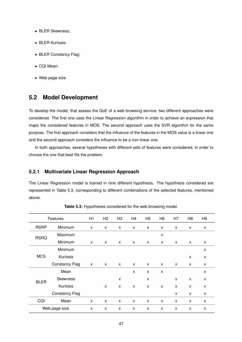
• BLER Skewness;

• BLER Kurtosis;

• BLER Constancy Flag;

• CQI Mean;

• Web page size.

5.2 Model Development

To develop the model, that assess the QoE of a web browsing service, two different approaches were

considered. The first one uses the Linear Regression algorithm in order to achieve an expression that

maps the considered features in MOS. The second approach uses the SVR algorithm for the same

purpose. The first approach considers that the influence of the features in the MOS value is a linear one

and the second approach considers the influence to be a non linear one.

In both approaches, several hypotheses with different sets of features were considered, in order to

choose the one that best fits the problem.

5.2.1 Multivariate Linear Regression Approach

The Linear Regression model is trained in nine different hypothesis. The hypothesis considered are

represented in Table 5.3, corresponding to different combinations of the selected features, mentioned

above.

Table 5.3: Hypotheses considered for the web browsing model.

Features H1 H2 H3 H4 H5 H6 H7 H8 H9

RSRP Minimum x x x x x x x x x

RSRQMaximum x

Minimum x x x x x x x x x

MCS

Minimum x

Kurtosis x x

Constancy Flag x x x x x x x x x

BLER

Mean x x x x

Skewness x x x x x

Kurtosis x x x x x x x x

Constancy Flag x x x

CQI Mean x x x x x x x x x

Web page size x x x x x x x x x

47

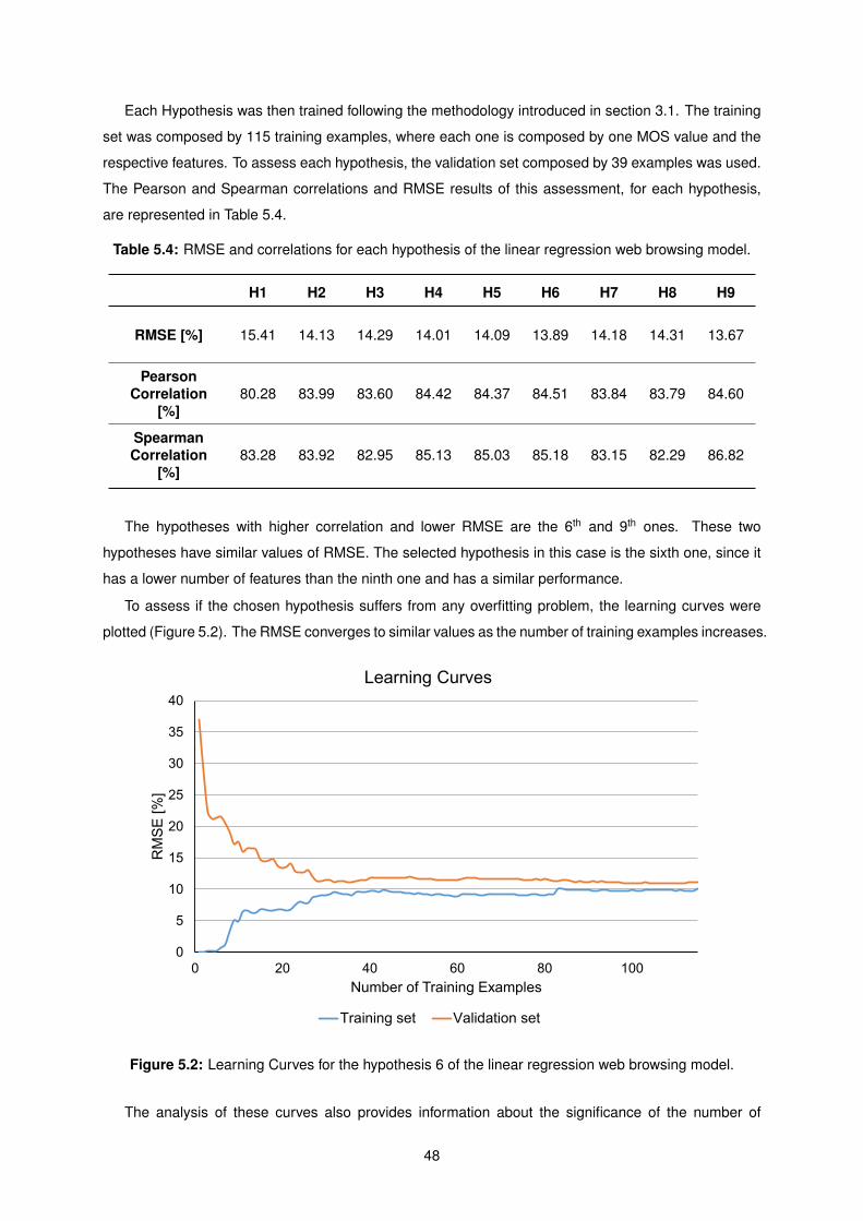
Each Hypothesis was then trained following the methodology introduced in section 3.1. The training

set was composed by 115 training examples, where each one is composed by one MOS value and the

respective features. To assess each hypothesis, the validation set composed by 39 examples was used.

The Pearson and Spearman correlations and RMSE results of this assessment, for each hypothesis,

are represented in Table 5.4.

Table 5.4: RMSE and correlations for each hypothesis of the linear regression web browsing model.

H1 H2 H3 H4 H5 H6 H7 H8 H9

RMSE [%] 15.41 14.13 14.29 14.01 14.09 13.89 14.18 14.31 13.67

PearsonCorrelation

[%]80.28 83.99 83.60 84.42 84.37 84.51 83.84 83.79 84.60

SpearmanCorrelation

[%]83.28 83.92 82.95 85.13 85.03 85.18 83.15 82.29 86.82

The hypotheses with higher correlation and lower RMSE are the 6th and 9th ones. These two

hypotheses have similar values of RMSE. The selected hypothesis in this case is the sixth one, since it

has a lower number of features than the ninth one and has a similar performance.

To assess if the chosen hypothesis suffers from any overfitting problem, the learning curves were

plotted (Figure 5.2). The RMSE converges to similar values as the number of training examples increases.

0

5

10

15

20

25

30

35

40

0 20 40 60 80 100

RM

SE

[%

]

Number of Training Examples

Learning Curves


Figure 5.2: Learning Curves for the hypothesis 6 of the linear regression web browsing model.

The analysis of these curves also provides information about the significance of the number of

48

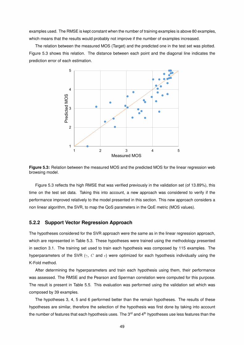
examples used. The RMSE is kept constant when the number of training examples is above 80 examples,

which means that the results would probably not improve if the number of examples increased.

The relation between the measured MOS (Target) and the predicted one in the test set was plotted.

Figure 5.3 shows this relation. The distance between each point and the diagonal line indicates the

prediction error of each estimation.

1

2

3

4

5

1 2 3 4 5

Pre

dic

ted

MO

S

Measured MOS

Figure 5.3: Relation between the measured MOS and the predicted MOS for the linear regression webbrowsing model.

Figure 5.3 reflects the high RMSE that was verified previously in the validation set (of 13.89%), this

time on the test set data. Taking this into account, a new approach was considered to verify if the

performance improved relatively to the model presented in this section. This new approach considers a

non linear algorithm, the SVR, to map the QoS parameters in the QoE metric (MOS values).

5.2.2 Support Vector Regression Approach

The hypotheses considered for the SVR approach were the same as in the linear regression approach,

which are represented in Table 5.3. These hypotheses were trained using the methodology presented

in section 3.1. The training set used to train each hypothesis was composed by 115 examples. The

hyperparameters of the SVR (γ, C and ε) were optimized for each hypothesis individually using the

K-Fold method.

After determining the hyperparameters and train each hypothesis using them, their performance

was assessed. The RMSE and the Pearson and Sperman correlation were computed for this purpose.

The result is present in Table 5.5. This evaluation was performed using the validation set which was

composed by 39 examples.

The hypotheses 3, 4, 5 and 6 performed better than the remain hypotheses. The results of these

hypotheses are similar, therefore the selection of the hypothesis was first done by taking into account

the number of features that each hypothesis uses. The 3rd and 4th hypotheses use less features than the

49

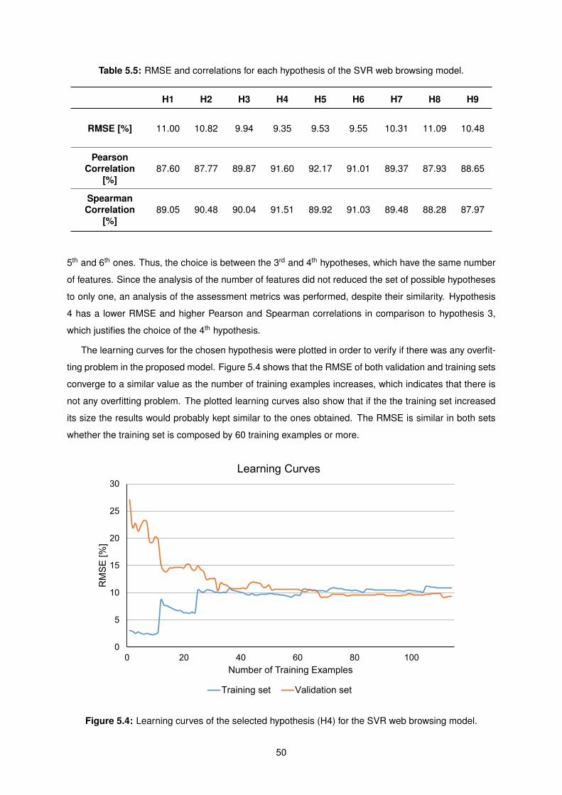
Table 5.5: RMSE and correlations for each hypothesis of the SVR web browsing model.

H1 H2 H3 H4 H5 H6 H7 H8 H9

RMSE [%] 11.00 10.82 9.94 9.35 9.53 9.55 10.31 11.09 10.48

PearsonCorrelation

[%]87.60 87.77 89.87 91.60 92.17 91.01 89.37 87.93 88.65

SpearmanCorrelation

[%]89.05 90.48 90.04 91.51 89.92 91.03 89.48 88.28 87.97

5th and 6th ones. Thus, the choice is between the 3rd and 4th hypotheses, which have the same number

of features. Since the analysis of the number of features did not reduced the set of possible hypotheses

to only one, an analysis of the assessment metrics was performed, despite their similarity. Hypothesis

4 has a lower RMSE and higher Pearson and Spearman correlations in comparison to hypothesis 3,

which justifies the choice of the 4th hypothesis.

The learning curves for the chosen hypothesis were plotted in order to verify if there was any overfit-

ting problem in the proposed model. Figure 5.4 shows that the RMSE of both validation and training sets

converge to a similar value as the number of training examples increases, which indicates that there is

not any overfitting problem. The plotted learning curves also show that if the the training set increased

its size the results would probably kept similar to the ones obtained. The RMSE is similar in both sets

whether the training set is composed by 60 training examples or more.

0

5

10

15

20

25

30

0 20 40 60 80 100

RM

SE

[%

]

Number of Training Examples

Learning Curves


Figure 5.4: Learning curves of the selected hypothesis (H4) for the SVR web browsing model.

50

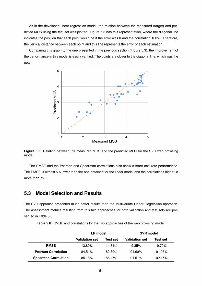
As in the developed linear regression model, the relation between the measured (target) and pre-

dicted MOS using the test set was plotted. Figure 5.5 has this representation, where the diagonal line

indicates the position that each point would be if the error was 0 and the correlation 100%. Therefore,

the vertical distance between each point and this line represents the error of each estimation.

Comparing this graph to the one presented in the previous section (Figure 5.3), the improvement of

the performance in this model is easily verified. The points are closer to the diagonal line, which was the

goal.

1

2

3

4

5

1 2 3 4 5

Pre

dic

ted

MO

S

Measured MOS

Figure 5.5: Relation between the measured MOS and the predicted MOS for the SVR web browsingmodel.

The RMSE and the Pearson and Spearman correlations also show a more accurate performance.

The RMSE is almost 5% lower than the one obtained for the linear model and the correlations higher in

more than 7%.

5.3 Model Selection and Results

The SVR approach presented much better results than the Multivariate Linear Regression approach.

The assessment metrics resulting from this two approaches for both validation and test sets are pre-

sented in Table 5.6.

Table 5.6: RMSE and correlations for the two approaches of the web browsing model.

LR model SVR model

Validation set Test set Validation set Test set

RMSE 13.89% 14.31% 9.35% 9.79%

Pearson Correlation 84.51% 82.89% 91.60% 91.96%

Spearman Correlation 85.18% 86.47% 91.51% 92.15%

51

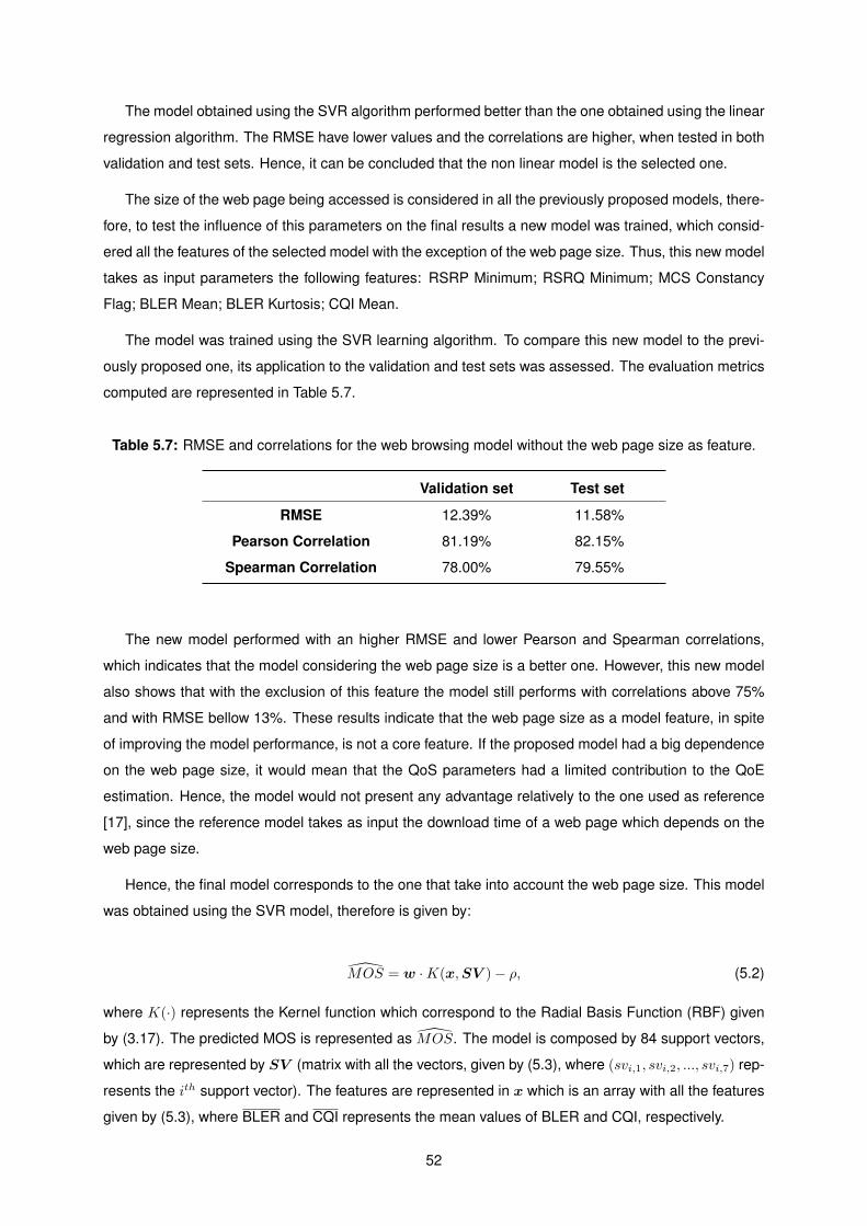
The model obtained using the SVR algorithm performed better than the one obtained using the linear

regression algorithm. The RMSE have lower values and the correlations are higher, when tested in both

validation and test sets. Hence, it can be concluded that the non linear model is the selected one.

The size of the web page being accessed is considered in all the previously proposed models, there-

fore, to test the influence of this parameters on the final results a new model was trained, which consid-

ered all the features of the selected model with the exception of the web page size. Thus, this new model

takes as input parameters the following features: RSRP Minimum; RSRQ Minimum; MCS Constancy

Flag; BLER Mean; BLER Kurtosis; CQI Mean.

The model was trained using the SVR learning algorithm. To compare this new model to the previ-

ously proposed one, its application to the validation and test sets was assessed. The evaluation metrics

computed are represented in Table 5.7.

Table 5.7: RMSE and correlations for the web browsing model without the web page size as feature.

Validation set Test set

RMSE 12.39% 11.58%

Pearson Correlation 81.19% 82.15%

Spearman Correlation 78.00% 79.55%

The new model performed with an higher RMSE and lower Pearson and Spearman correlations,

which indicates that the model considering the web page size is a better one. However, this new model

also shows that with the exclusion of this feature the model still performs with correlations above 75%

and with RMSE bellow 13%. These results indicate that the web page size as a model feature, in spite

of improving the model performance, is not a core feature. If the proposed model had a big dependence

on the web page size, it would mean that the QoS parameters had a limited contribution to the QoE

estimation. Hence, the model would not present any advantage relatively to the one used as reference

[17], since the reference model takes as input the download time of a web page which depends on the

web page size.

Hence, the final model corresponds to the one that take into account the web page size. This model

was obtained using the SVR model, therefore is given by:

MOS = w ·K(x,SV )− ρ, (5.2)

where K(·) represents the Kernel function which correspond to the Radial Basis Function (RBF) given

by (3.17). The predicted MOS is represented as MOS. The model is composed by 84 support vectors,

which are represented by SV (matrix with all the vectors, given by (5.3), where (svi,1, svi,2, ..., svi,7) rep-

resents the ith support vector). The features are represented in x which is an array with all the features

given by (5.3), where BLER and CQI represents the mean values of BLER and CQI, respectively.

52

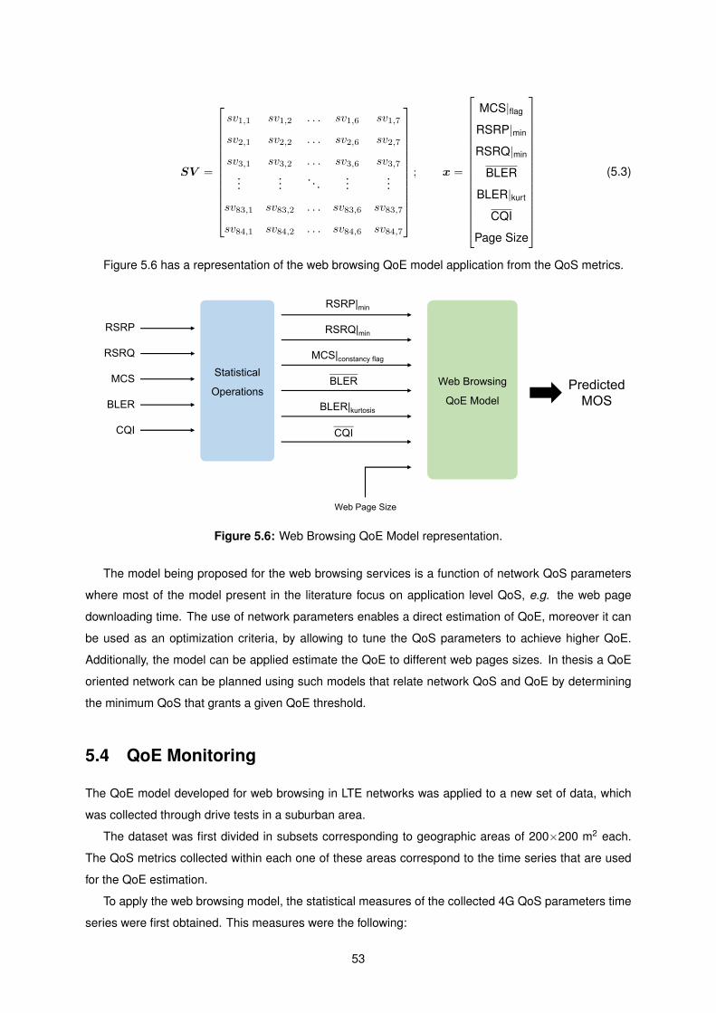
SV =

sv1,1 sv1,2 . . . sv1,6 sv1,7

sv2,1 sv2,2 . . . sv2,6 sv2,7

sv3,1 sv3,2 . . . sv3,6 sv3,7...

.... . .

......

sv83,1 sv83,2 . . . sv83,6 sv83,7

sv84,1 sv84,2 . . . sv84,6 sv84,7

; x =

MCS|flag

RSRP|min

RSRQ|min

BLER

BLER|kurt

CQI

Page Size

(5.3)

Figure 5.6 has a representation of the web browsing QoE model application from the QoS metrics.

RSRP|min

RSRQ|min

MCS|constancy flag

BLER|kurtosis

Statistical

Operations

RSRP

RSRQ

MCS

BLER

CQI

BLER Web Browsing

QoE Model

Predicted

MOS

CQI

Web Page Size

Figure 5.6: Web Browsing QoE Model representation.

The model being proposed for the web browsing services is a function of network QoS parameters

where most of the model present in the literature focus on application level QoS, e.g. the web page

downloading time. The use of network parameters enables a direct estimation of QoE, moreover it can

be used as an optimization criteria, by allowing to tune the QoS parameters to achieve higher QoE.

Additionally, the model can be applied estimate the QoE to different web pages sizes. In thesis a QoE

oriented network can be planned using such models that relate network QoS and QoE by determining

the minimum QoS that grants a given QoE threshold.

5.4 QoE Monitoring

The QoE model developed for web browsing in LTE networks was applied to a new set of data, which

was collected through drive tests in a suburban area.

The dataset was first divided in subsets corresponding to geographic areas of 200×200 m2 each.

The QoS metrics collected within each one of these areas correspond to the time series that are used

for the QoE estimation.

To apply the web browsing model, the statistical measures of the collected 4G QoS parameters time

series were first obtained. This measures were the following:

53

• the minimum value of RSRP;

• the minimum value of RSRQ;

• the constancy flag of MCS;

• the mean value of BLER;

• the kurtosis of BLER;

• the mean value of CQI.

To estimate the QoE two web pages sizes were considered, 1000 kBytes and 3100 kBytes, in order

to assess the influence that this feature has on the predicted quality. With the same network conditions

the perceived quality can be different, since the time to download a web page depends on its size.

Therefore, this two sizes were considered for the MOS estimation. The results presented in Figures

5.7 and 5.8 correspond to the QoE estimations for web pages of sizes 1000 kBytes and 3100 kBytes,

respectively. The circle markers represent each one of the 200×200 m2 areas, where one MOS value is

estimated. The MOS values are displayed in a scale of colours, being red a low value and green a good

value on the MOS scale.

Figure 5.7: MOS estimated for web browsing a 1000 kBytes web page.

The application of the web browsing QoE model resulted in areas with really good predicted MOS

and areas with low estimated MOS values. The maximum MOS values predicted were 4.91, in the case

with a web page size of 1000 kBytes, and 4.62, in the case with a web page size of 3100 kBytes. The

average MOS was 3.57 and 3.29 for web pages with sizes of 1000 kBytes and 3100 kBytes, respectively.

54

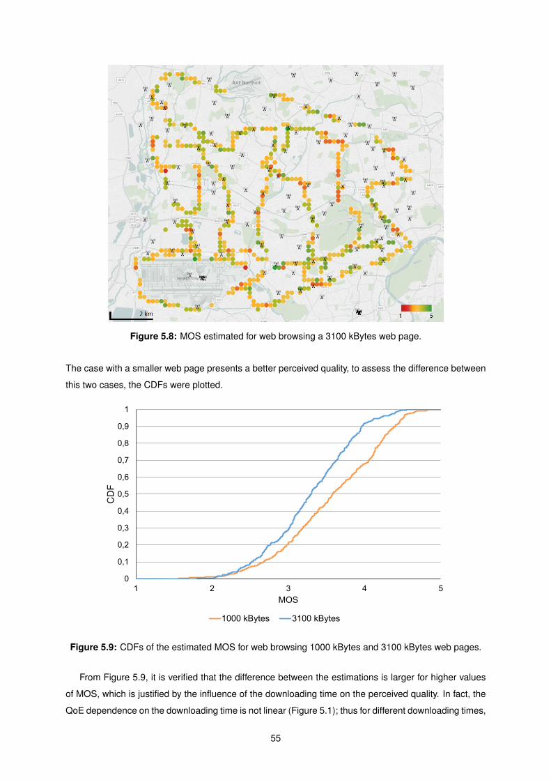
Figure 5.8: MOS estimated for web browsing a 3100 kBytes web page.

The case with a smaller web page presents a better perceived quality, to assess the difference between

this two cases, the CDFs were plotted.

0

0,1

0,2

0,3

0,4

0,5

0,6

0,7

0,8

0,9

1

1 2 3 4 5

CD

F

MOS

1000 kBytes 3100 kBytes

Figure 5.9: CDFs of the estimated MOS for web browsing 1000 kBytes and 3100 kBytes web pages.

From Figure 5.9, it is verified that the difference between the estimations is larger for higher values

of MOS, which is justified by the influence of the downloading time on the perceived quality. In fact, the

QoE dependence on the downloading time is not linear (Figure 5.1); thus for different downloading times,

55

an equal time increment will affect differently the perceived quality. Moreover, the same time variation

has an higher influence on the QoE for shorter downloading times than for larger ones.

56

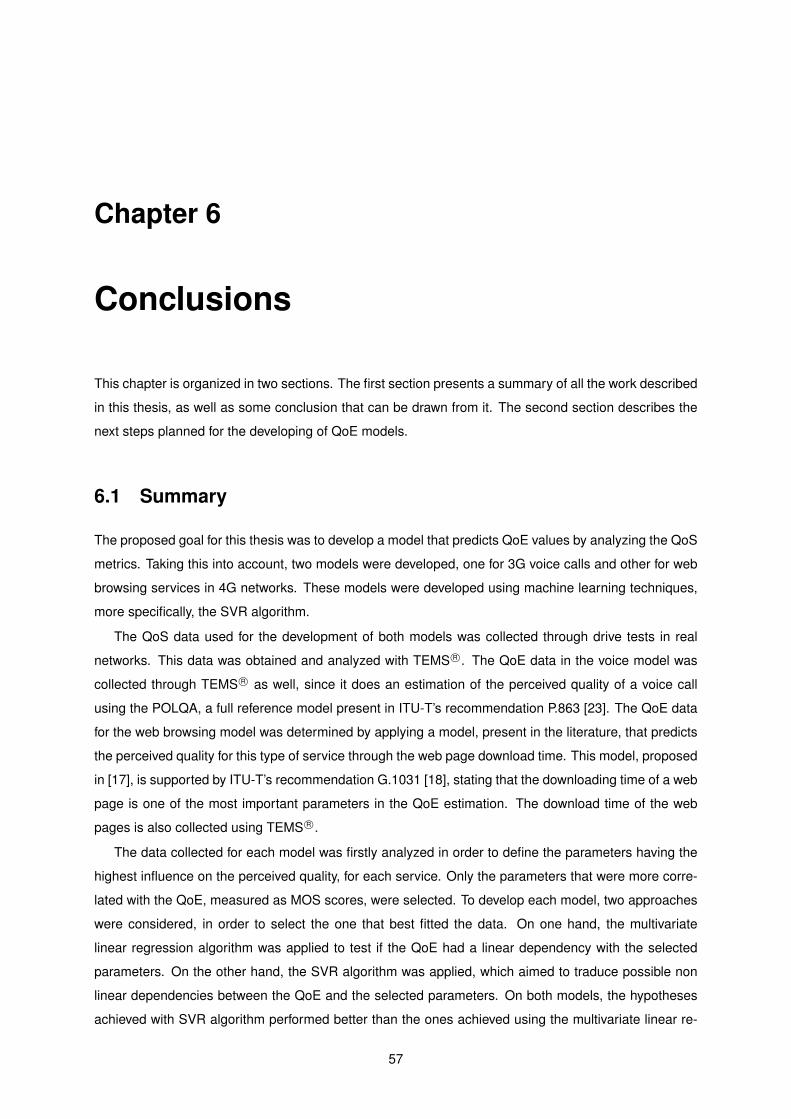
Chapter 6

Conclusions

This chapter is organized in two sections. The first section presents a summary of all the work described

in this thesis, as well as some conclusion that can be drawn from it. The second section describes the

next steps planned for the developing of QoE models.

6.1 Summary

The proposed goal for this thesis was to develop a model that predicts QoE values by analyzing the QoS

metrics. Taking this into account, two models were developed, one for 3G voice calls and other for web

browsing services in 4G networks. These models were developed using machine learning techniques,

more specifically, the SVR algorithm.

The QoS data used for the development of both models was collected through drive tests in real

networks. This data was obtained and analyzed with TEMS R©. The QoE data in the voice model was

collected through TEMS R© as well, since it does an estimation of the perceived quality of a voice call

using the POLQA, a full reference model present in ITU-T’s recommendation P.863 [23]. The QoE data

for the web browsing model was determined by applying a model, present in the literature, that predicts

the perceived quality for this type of service through the web page download time. This model, proposed

in [17], is supported by ITU-T’s recommendation G.1031 [18], stating that the downloading time of a web

page is one of the most important parameters in the QoE estimation. The download time of the web

pages is also collected using TEMS R©.

The data collected for each model was firstly analyzed in order to define the parameters having the

highest influence on the perceived quality, for each service. Only the parameters that were more corre-

lated with the QoE, measured as MOS scores, were selected. To develop each model, two approaches

were considered, in order to select the one that best fitted the data. On one hand, the multivariate

linear regression algorithm was applied to test if the QoE had a linear dependency with the selected

parameters. On the other hand, the SVR algorithm was applied, which aimed to traduce possible non

linear dependencies between the QoE and the selected parameters. On both models, the hypotheses

achieved with SVR algorithm performed better than the ones achieved using the multivariate linear re-

57

gression algorithm.

The proposed 3G voice calls QoE model performs an estimation of the perceived quality using sta-

tistical metrics of the following RF metrics: RSCP (in dBm); Ec/N0 (in dB); SIR (in dB); and SIR Target

(in dB). The model estimates the QoE with a Pearson correlation of 62.22%, a Spearman correlation of

55.27% and a RMSE of 10.92%; these metrics are all measured by comparing the estimated MOS with

the measured MOS values predicted by the full-reference POLQA model.

The obtained results for this model were positive; nonetheless, the model tends to struggle in

discerning the mid range of MOS values. The radio channel volatility, for instance, by multipath fading

phenomenon, adds variability in the RF metrics, which may be one of the reasons for the model

limitations. If the RF parameters were less prone to such variability, the contribution of each parameter

on the MOS estimation would be more easily accounted. Nevertheless, the use of RF metrics as input

parameters eases the application of the model for network planning or optimization, since this metrics

can be easily collected through drive testing.

The web browsing QoE model takes as input parameters different statistical metrics of the following

QoS measures: RSRP (in dBm); RSRQ (in dB); MCS; BLER (in %); and CQI. The web page size (in

kBytes) is also an input parameter required for the model. The model performs a MOS estimation with

a Pearson correlation of 91.96%, a Spearman correlation of 92.15% and a RMSE of 9.79%. This model

performed better than the one developed for the 3G voice calls services, with correlations higher than

90% and RMSE lower than 10%.

The introduction of the web page size as an input parameter aimed to allow the application of this

model for different web pages dimensions, for instance, an operator may assess the perceived quality

when web browsing a specific web page. The exclusive use of QoS network parameters, apart of the

web page size, allows to apply this model in network optimization, shifting from network centric QoS-

based optimization to user centric QoE-based optimization.

The main setback during the development of this work was related to the use of the TEMS R© tool. In

fact, it is a software that requires licenses and during the thesis development period the license check

failed, resulting in lost time, that could be more efficiently used in the analysis of the data. However,

this period, of about two weeks, was used to perform a more intense research relatively to the models

already developed, some of them being presented in section 2.4, and to learn more about the machine

learning techniques that would be needed in the next steps.

6.2 Future Work

This thesis proposes two QoE models for two types of services, respectively. For future work, new

models applied to different services can be developed, as well as to study the possibility of building a

general model, for each technology (3G and 4G), that estimates the QoE for all the available services.

This model would consider the features that influence the perceived quality the most in each service and

combine them in order to account all services requirements in terms of QoS and QoE. This would allow

to perform a QoE network optimization or planning without restricting it to only one service.

58

References

[1] NOKIA. Quality of Experience (QoE) of mobile services: Can it be measured and improved? White

Paper, 2004.

[2] V. A. Siris, K. Balampekos, and M. K. Marina. Mobile Quality of Experience: Recent Advances and

Challenges. The Sixth International Workshop on Information Quality and Quality of Service for

Pervasive Computing, pages 425–430, 2014.

[3] H. Holma and A. Toskala. WCDMA for UMTS - HSPA evolution and LTE. John Wiley && Sons, Ltd,

4th edition, 2007.

[4] S. Sesia, I. Toufik, and M. Baker. LTE - The UMTS Long Term Evolution: From Theory to Practice.

Wiley, 2011. ISBN 9780470978511.

[5] E. Puschita, A. E. I. Pastrav, C. Androne, and T. Palade. Enhanced QoS and QoE Support in

UMTS Cellular Architectures Based on Application Requirements and Core Network Capabilities.

International Journal on Advances in Internet Technology, 5(1 & 2):54–64, 2012.

[6] B. Schulz. LTE Transmission Modes and Beamforming. White Paper, 2015.

[7] D. Xenakis, N. I. Passas, L. F. Merakos, and C. V. Verikoukis. Handover decision for small cells:

Algorithms, lessons learned and simulation study. Computer Networks, 100:64–74, 2016.

[8] ITU-T. Methods for objective and subjective assessment of quality. Recommendation ITU-T P.800,

1998.

[9] M. Fiedler, T. Hossfeld, and P. Tran-Gia. A Generic Quantitative Relationship between Quality of

Experience and Quality of Service. IEEE Network Special Issue on Improving QoE for Network

Services, 2010.

[10] ITU-T. The E-model: a computational model for use in transmission planning. Recommendation

ITU-T G.107, 2011.

[11] ITU-T. Definition of categories of speech transmission quality. Recommendation ITU-T G.109,

1999.

[12] A. Meddahi and H. Afifi. ”Packet-E-Model”: E-Model for VoIP quality evaluation. Computer Networks

50, pages 2659–2675, 2006.

59

[13] D. Kim and A. Tarraf. ANIQUE+: A new american national standard for non-intrusive estimation of

narrowband speech quality. Bell Labs Technical Journal, 12(1):221–236, 2007.

[14] A. E. Conway. A Passive Method for Monitoring Voice-over-IP Call Quality with ITU-T Objective

Speech Quality Measurement Methods. 2002.

[15] R. K. P. Mok, E. W. W. Chan, and R. K. C. Chang. Measuring the Quality of Experience of HTTP

Video Streaming. 12th IFIP/IEEE 1M 2011: Mini Conference, pages 485–492, 2011.

[16] L. S. Asiya Khan and E. Ifeachor. Content Clustering Based Video Quality Prediction Model for

MPEG4 Video Streaming over Wireless Networks. IEEE ICC 2009 proceedings, 2009.

[17] P. Ameigeiras, J. J. Ramos-Munoz, J. Navarro-Ortiz, P. E. Mogensen, and J. M. Lopez-Soler. QoE

oriented cross-layer design of a resource allocation algorithm in beyond 3G systems. Computer

Communications, 33(5):571–582, 2010.

[18] ITU-T. QoE factors in web-browsing. Recommendation ITU-T G.1031, 2014.

[19] S. Thakolsri, S. Khan, E. G. Steinbach, and W. Kellerer. QoE-Driven Cross-Layer Optimization for

High Speed Downlink Packet Access. JCM, 4:669–680, 2009.

[20] A. Ng. Machine Learning course. https://www.coursera.org/learn/machine-

learning/home/welcome. Stanford University.

[21] A. J. Smola and B. Scholkopf. A tutorial on support vector regression. Statistics and Computing,

14(3):199–222, Aug 2004.

[22] Test Mobile System (TEMS). http://www.tems.com/products-for-radio-and-core-networks/radio-

network-engineering/ran-optimization-troubleshooting. Accessed: 2017-03-12.

[23] ITU-T. Perceptual objective listening quality assessment. Recommendation ITU-T P.863, 2014.

[24] J. Bai and S. Ng. Tests for skewness, kurtosis, and normality for time series data. Journal of

Business & Economic Statistics, 23(1):49–60, 2005.

[25] L. T. Decarlo. On the meaning and use of kurtosis. Psychological Methods, pages 292–307, 1997.

[26] S. L. Zabell. Alan turing and the central limit theorem. The American Mathematical Monthly, 102,

1995.

[27] Tableau. https://www.tableau.com/. Accessed: 2017-10-02.

[28] HTTP Archive. http://httparchive.org/compare.php?&r1=Nov%2015%202010&s1=All&r2=Jan%201

%202016&s2=All. Accessed: 2017-09-04.

60

Identifying Quality of Experience (QoE) in 3G/4G Radio ...

Documents

Transcript of Identifying Quality of Experience (QoE) in 3G/4G Radio ...