IDENTIFICATION-ROBUST SUBVECTOR INFERENCE

By

Donald W. K. Andrews

September 2017Updated September 2017

COWLES FOUNDATION DISCUSSION PAPER NO. 3005

COWLES FOUNDATION FOR RESEARCH IN ECONOMICS YALE UNIVERSITY

Box 208281 New Haven, Connecticut 06520-8281

http://cowles.yale.edu/

Identi�cation-Robust Subvector Inference

Donald W. K. Andrews

Cowles Foundation

Yale University

First Version: June 12, 2015

Revised: September 21, 2017�

Abstract

This paper introduces identi�cation-robust subvector tests and con�dence sets (CS�s) that have

asymptotic size equal to their nominal size and are asymptotically e¢ cient under strong identi�-

cation. Hence, inference is as good asymptotically as standard methods under standard regularity

conditions, but also is identi�cation robust. The results do not require special structure on the

models under consideration, or strong identi�cation of the nuisance parameters, as many existing

methods do.

We provide general results under high-level conditions that can be applied to moment condition,

likelihood, and minimum distance models, among others. We verify these conditions under primitive

conditions for moment condition models. In another paper, we do so for likelihood models.

The results build on the approach of Chaudhuri and Zivot (2011), who introduce a C(�)-type

Lagrange multiplier test and employ it in a Bonferroni subvector test. Here we consider two-step

tests and CS�s that employ a C(�)-type test in the second step. The two-step tests are closely related

to Bonferroni tests, but are not asymptotically conservative and achieve asymptotic e¢ ciency under

strong identi�cation.

Keywords: Asymptotics, con�dence set, identi�cation-robust, inference, instrumental variables,

moment condition, robust, test.

JEL Classi�cation Numbers: C10, C12.

�The author gratefully acknowledges the research support of the National Science Foundation via grant SES-1355504. The author thanks Koohyun Kwon for constructing the �gures and Jaewon Lee for a very careful proof-reading of the paper. The author thanks Isaiah Andrews, Angelo Melino, Charlie Saunders, and Katsumi Shimotsufor helpful comments.

1 Introduction

Existing identi�cation-robust subvector tests and con�dence sets (CS�s) have one or more of the

following drawbacks: (i) they are asymptotically conservative, such as projection and Bonferroni

methods; (ii) they are not asymptotically e¢ cient under strong identi�cation; (iii) they only apply if

nuisance parameters are strongly identi�ed; (iv) they only apply to models with special structure,

such as knowledge of the source of potential non-identi�cation; (v) they only apply to speci�c

models, such as the homoskedastic linear instrumental variables (IV) model; and/or (vi) they have

not been shown to have correct asymptotic size under primitive conditions. In particular, there

is no general identi�cation-robust subvector method in the literature that is asymptotically non-

conservative, is asymptotically e¢ cient under strong identi�cation, and has been shown to have

correct asymptotic size. (Further discussion of the literature is given below.)

This paper aims to �ll this gap in the literature. Under a set of high-level conditions, we pro-

vide a two-step Bonferroni-like method that is asymptotically non-conservative and asymptotically

e¢ cient under strong identi�cation. The method applies to what we call systems of equations (SE)

models, which include moment condition, likelihood, and minimum distance models, and versions

of these models that rely on preliminary n1=2-consistent estimators. In this paper, we verify the

high-level conditions in moment condition models with independent identically distributed (i.i.d.)

and time series observations. In Andrews (2017), we do likewise for likelihood models.

For a parameter � = (�01; �02)0 2 Rp; we consider nominal level � tests of H0 : �2 = �20 versus

H1 : �2 6= �20; where �1 is a nuisance parameter. A two-step test relies on a �rst-step identi�cation-

robust CS, CS1n; for �1 of level 1��1 for �1 < �; such as �1 = :005 and � = :05; as in a Bonferroni

test. This CS is augmented by an estimator set, b�1n; of �1 values that is designed to be such thatsome element of CS+1n := CS1n [ b�1n is necessarily close (within Op(n�1=2)) to the true value of �1under locally strongly-identi�ed sequences of distributions. This property is needed to obtain the

correct asymptotic level of the two-step test.1

The two-step test employs a C(�)-type identi�cation-robust second-step test that takes as given

a value of the nuisance parameter �1: Chaudhuri and Zivot (2011) introduce a Lagrange multiplier

(LM) test of this type for moment condition models. It is based on the (non-identi�cation-robust)

C(�) test of Neyman (1959) for likelihood models. I. Andrews (2017) also considers C(�)-type

tests. In the moment condition model, we consider C(�)-type identi�cation-robust Anderson-

Rubin (AR), LM, and conditional quasi-likelihood ratio (QLR) second-step tests. The C(�)-type

1For example, in the moment condition model, if CS1n is the (null-restricted) AR CS, then CS1n is empty withprobability bounded away from 0 as n ! 1 when the number of moments k exceeds the dimension of �1; which ittypically does, and hence, one cannot take b�1n = ?:

1

conditional QLR test considered here, which we refer to as C(�)-QLR1, is a C(�) version of a test

of Kleibergen (2005) and employs a rank statistic of the form in Robin and Smith (2000).

The second-step test uses a data-dependent signi�cance level, b�2n(�1); that lies between �2 :=���1 and �; such as �2 = :045 and � = :05; and depends on the given value of �1: This signi�cance

level is designed to equal �2 under weak identi�cation and transition to � under su¢ ciently strong

identi�cation. It is based on an identi�cation-category-selection statistic.

The two-step test rejects H0 if the second-step test given �1; with signi�cance level b�2n(�1);rejects the null hypothesis for all �1 2 CS+1n: The two-step CS for �2 is obtained by inverting

the two-step tests. Computation of the two-step test or CS is essentially the same as that of a

Bonferroni test or CS. Thus, in some scenarios, it can be easy to compute, but in other scenarios,

it can be di¢ cult to compute.

Di¤erent �rst-step CS�s can be employed. For moment condition models, the H0 : �2 = �20 null-

restricted AR CS is a good choice for power purposes because under the alternative, H1 : �2 6= �20;

this CS often is small and has low coverage probability (since it is based on the incorrect null

value �20): For moment condition models, the estimator set b�1n can be the set of solutions tothe generalized method of moments (GMM) criterion function �rst-order conditions (FOC�s) that

minimize, or nearly minimize, the GMM criterion function.

The second-step C(�) tests are based on the sample SE vector, such as the sample moment

vector, that has been orthogonalized with respect to (wrt) the sample Jacobian of the SE vector

wrt �1; which in turn has been transformed to be asymptotically independent of the sample SE

vector. Chaudhuri and Zivot (2011) recognize that a C(�)-type test is a good choice for the second-

step test in a Bonferroni procedure because it makes the test statistic less sensitive to �1 and closer

to being asymptotically similar, which is better for power against �2 6= �20: For the same reason,

C(�)-type tests are good for power in the two-step tests considered here. In fact, the C(�) nature

of the second-step tests is needed for the two-step tests to achieve an asymptotic oracle property

and asymptotic e¢ ciency under strong identi�cation.

The two-step subvector test does have some potential drawbacks. These include: (i) its asymp-

totic null rejection probabilities (NRP�s) may be less than � under weak identi�cation, (ii) it does

not have any asymptotic e¢ ciency properties under weak identi�cation, (iii) it is invariant to scale

reparameterizations of �; but not all reparameterizations, (iv) it requires some tuning parameters,

(v) in some scenarios it may be di¢ cult to compute, and (vi) it takes considerable e¤ort to verify

the high-level conditions using primitive conditions.

Now we provide a heuristic explanation of the asymptotic properties of the two-step test. First,

for locally-strongly-identi�ed sequences of distributions, the two-step test obtains asymptotic NRP�s

2

of � or less by exploiting properties of CS+1n and the second-step C(�) test. The true �1 value is

within Op(n�1=2) of CS+1n and the two-step test rejects H0 only if it rejects for all �1 2 CS+1n: Thus,

the test does not reject more often than the level � second-step C(�) test at some point that is

Op(n�1=2) from the true �1 value. By the properties of the second-step C(�) test, such a test has

asymptotic NRP � or less.

Second, for sequences of distributions that are not locally-strongly-identi�ed, the two-step test

obtains asymptotic NRP�s that are � or less by a Bonferroni argument. Speci�cally, the augmented

�rst step CS CS+1n (� CS1n) has con�dence level at least 1 � �1: By design, the second-step test

has signi�cance level b�2n(�1) = �2 wp!1 under such sequences when �1 is the true value. So, thestandard Bonferroni argument gives the asymptotic NRP to be �1 + �2 = � or less. To make the

transition between sequences of di¤erent types seamless, there are some sequences for which one

can obtain NRP�s of � or less using either the �rst or the second argument.

Given the asymptotic NRP results for certain sequences, we show that the asymptotic size of the

two-step test is less than or equal to � using the subsequence-type argument in Andrews, Cheng,

and Guggenberger (2011).

Next, we discuss why the asymptotic size of the two-step test is �; rather than less than �;

and why it is asymptotically e¢ cient under strong identi�cation. For globally-strongly-identi�ed

sequences, there exists a unique solution to the population system of equations. For such sequences,

the true �1 value is within Op(n�1=2) of CS+1n and all points in CS+1n are within Op(n

�1=2) of the

true �1 value. That is, the Hausdor¤ distance between the singleton set containing the true value

�1 and CS+1n is Op(n�1=2): For such sequences, by design, the data-dependent signi�cance levelb�2n(�1) satis�es b�2n(�1) = � for all �1 within Op(n�1=2) of the true �1 value wp!1. In this case,

by exploiting the properties of the second-step C(�) test, one gets an oracle asymptotic equivalence

property. Speci�cally, the two-step test is asymptotically equivalent to the nominal � oracle second-

step test that employs the true value of �1: This yields the asymptotic size of the two-step test to be

�; not less than �: It also yields asymptotic e¢ ciency of the two-step test under these sequences,

if the oracle second-step test is asymptotically e¢ cient. For example, in the moment condition

model, this holds for the second-step C(�)-LM and C(�)-QLR1 tests, but not the C(�)-AR test.

This paper considers subvector null hypotheses H0 : �2 = �20 and CS�s that concern �2: But, the

results apply to some linear and nonlinear functions of an unknown parameter. Suppose one has a

model indexed by 2 � � Rp and the null hypothesis of interest is H0 : r( ) = r0 for some known

function r(�) and vector r0 of dimension 1 � dr � p: If there exists a transformation q( ) 2 Rp�dr

such that ! t( ) := (q( )0; r( )0)0 is a one-to-one function from � to � := f� : � = t( ) for some

2 �g; then the results of the present paper can be applied with � = (�01; �02) = (q( )0; r( )0)0 and

3

the null hypothesis H0 : � = �20; where �20 = r0: For example, if r( ) = R2 for some full rank

dr � p matrix R2; then one can take t( ) = [R01 : R02]0 for any (p � dr) � p matrix R1 for which

[R01 : R02]0 2 Rp�p is nonsingular. This transformation method is employed below in a nonlinear IV

model that is used in some of the �nite-sample simulation results.

A second example, with a nonlinear transformation, arises with a stationary ARMA(1,1) model

Yi = Yi�1 1 + "i � 2"i�1; where the null hypothesis of interest concerns the impulse response

at horizon T : H0 : T = r0; where T := T�11 ( 1 � 2): In this case, � := t( ) := ( 1 � 2;

T�11 ( 1� 2)) is a one-to-one transformation that yields the transformed hypothesis of interest

to be H0 : �2 = �20 for �20 = r0: In this model, lack of identi�cation occurs when 1 = 2:

The paper provides some �nite-sample simulation results in two models. The �rst model is a het-

eroskedastic linear IV model with two right-hand side endogenous variables and �2 is the coe¢ cient

on one of them. The second model is a nonlinear (quadratic) IV model that is parametrized such

that �2 is the value of the structural function at a point of interest, or reparametrized such that �2

is the function�s derivative at the point of interest. For both models, we consider the two-step tests

based on the �rst-step AR CS and the second-step C(�)-AR, C(�)-LM, and C(�)-QLR1 tests, which

we denote by AR/AR, AR/LM, and AR/QLR1, respectively. We compare the power of these tests

with that of the (infeasible) oracle C(�)-QLR1 test, which takes the true value of �1 to be known,

and the projection (non-C(�)) QLR1 test, which is an existing identi�cation-robust subvector test

in the literature. In strong identi�cation scenarios, we also consider the (non-identi�cation-robust)

standard 2SLS t test.

In both models, under strong identi�cation, the AR/QLR1, AR/LM, and Oracle C(�)-QLR1

tests have essentially the same power. The 2SLS t test has equal power in the linear IV model to

these tests and somewhat higher power in the nonlinear IV model. The AR/AR and Proj-QLR1

tests have noticeably lower power. These results are broadly consistent with the asymptotic theory.

In both models, under weak identi�cation, the AR/QLR1 subvector test performs best in terms

of power among the feasible tests, not uniformly, but in an overall sense. It noticeably out-performs

the Proj-QLR1 test. The AR/LM test exhibits some quirky power behavior in some scenarios. Not

surprisingly, the Oracle C(�)-QLR1 test out-performs the feasible tests in scenarios where �1 is

weakly identi�ed. However, in the linear IV model with strongly identi�ed �1 and weakly identi�ed

�2; the AR/QLR1 test has equal power to the Oracle C(�)-QLR1 test.

Overall, the AR/QLR1 test is found easily to be the best two-step test in terms of power

in the over-identi�ed models considered here and its power is noticeably higher than that of the

Proj-QLR1 test. Given this, the remainder of the simulation results focus on the AR/QLR1 test.

The �nite-sample NRP�s of the AR/QLR1 test are simulated for a range of parameter con�gu-

4

rations and sample sizes. In the linear IV model, the maximum NRP�s (over the 25 identi�cation

scenarios considered) of the AR/QLR1 test are in [:049; :064] for (n; k) = (100; 4); (250; 4); (500; 4);

(100; 8); (250; 8); where k is the number of IV�s. In the nonlinear IV model, they are in [:040; :050]

for the structural function and [:039; :052] for its derivative for the same (n; k) values (with the

maximum NRP�s being over nine identi�cation scenarios).

We carry out extensive simulations to determine the sensitivity of the AR/QLR1 test to tun-

ing parameters. For some tuning parameters, there are theoretical reasons to expect little or no

sensitivity and this is borne out in the simulations. For �1; we �nd no sensitivity of the NRP�s in

both models (and both hypotheses in the nonlinear IV model) and some sensitivity of power. For a

constant, Krk; that appears in the rank statistic in the C(�)-QLR1 statistic, we �nd no sensitivity

of the NRP�s except some sensitivity in a couple of cases in the linear IV model. For power, we �nd

some sensitivity to Krk in both models, but not a lot. Overall, the base case values of �1 = :005

and Krk = 1 (which are used for the power comparisons and the NRP calculations in both models

and both hypotheses in the nonlinear model) perform well. These base case values also are used in

the simulations for likelihood models in Andrews (2017) and perform well there.

The remainder of the paper is organized as follows. Section 2 discusses subvector methods in

the literature. Section 3 introduces SE models, including the moment condition model. Section

4 introduces the two-step tests and CS�s for SE models. Section 5 provides asymptotic size and

strong-identi�cation asymptotic e¢ ciency results under high-level assumptions. Section 6 proves

the asymptotic results in Section 5.

The rest of the paper focuses on the moment condition model. Section 7 introduces the two-

step AR/AR, AR/LM, and AR/QLR1 tests and CS�s for the moment condition model. Section 8

provides primitive conditions under which these tests have correct asymptotic size and the latter

two are asymptotically e¢ cient in a GMM sense under strong identi�cation. The proofs of these

results utilize results in Andrews and Guggenberger (2017). Section 9 provides the �nite-sample

simulation results. The Supplemental Material (SM) to this paper generalizes the results in Section

8 from i.i.d. observations to strictly stationary strong mixing time series observations, proves the

results in Section 8, and provides some additional simulation results.

All limits are as n!1 unless stated otherwise.

2 Subvector Methods in the Literature

In this section, we discuss existing subvector methods in the literature. Widely used general

methods are the Bonferroni and Sche¤é projection methods, e.g., see Loh (1985), Berger and Boos

5

(1994), Cavanagh, Elliott, and Stock (1995), Campbell and Yogo (2006), Chaudhuri, Richardson,

Robins, and Zivot (2010), and Chaudhuri and Zivot (2011) for Bonferroni�s method, and Dufour

(1989) and Dufour and Jasiak (2001) for the projection method. These methods are asymptotically

conservative, i.e., their asymptotic size is less than their nominal level. The degree of conserva-

tiveness typically is larger for the projection method. It depends on the dimension of the nuisance

parameter and the shape of the power function of the joint test that is employed. A re�nement

of Bonferroni�s method that is not conservative, but is much more intensive computationally, is

provided by Cavanagh, Elliott, and Stock (1995). McCloskey (2011) also introduces a re�nement

of Bonferroni�s method.

When the nuisance parameters that appear under the null hypothesis are known to be strongly

identi�ed, one can obtain identi�cation-robust subvector tests by concentrating out these para-

meters or replacing them by n1=2-consistent asymptotically normal estimators. This method is

employed in Stock and Wright (2000), Kleibergen (2004, 2005), Guggenberger and Smith (2005),

Otsu (2006), Montiel Olea (2012), Guggenberger, Ramalho, and Smith (2013), I. Andrews and

Mikusheva (2015), and Andrews and Guggenberger (2015). This method yields non-conservative

inference asymptotically and is asymptotically e¢ cient under strong identi�cation of all of the para-

meters (for suitable tests). The drawback of this method, however, is that the nuisance parameters

cannot be weakly identi�ed.

Andrews and Cheng (2012, 2013a,b), Cheng (2015), Cox (2016), and Han and McCloskey (2016)

provide subvector tests with correct asymptotic size based on the asymptotic distributions of stan-

dard test statistics under the full range of possible identi�cation scenarios. These subvector methods

are not asymptotically conservative and are asymptotically e¢ cient under strong identi�cation of

all of the parameters (for suitable tests). However, they require one to have knowledge of the source

of the potential lack of identi�cation (e.g., which subvectors play the roles of �; �; and � in the

Andrews and Cheng (2012) notation) and require special structure of the model considered, such as

having a known correspondence between strongly-identi�ed reduced-form parameters and subsets

of the structural parameters of interest in the case of Cox (2016).

Elliott, Müller, and Watson (2015) develop nearly optimal subvector tests when a nuisance

parameter is present under the null hypothesis, which includes models with weak identi�cation, as

exempli�ed by their example of tests concerning the location of a change point when the magnitude

of the change point is moderate. Their tests are nearly optimal in the sense of nearly achieving

weighted average power for a given weight function.

Chen, Christensen, O�Hara, and Tamer (2016) provide subvector CS�s for the identi�ed set in

partially identi�ed models using Monte Carlo Markov chain methods in models where the parame-

6

ters of interest are functions of strongly-identi�ed reduced-form parameters.

For minimum distance models, I. Andrews and Mikusheva (2016a) provide subvector inference

using a geometric approach. This method has asymptotic size equal to its asymptotic nominal level

and may or may not be asymptotically e¢ cient under strong identi�cation depending upon the

model. For example, in the homoskedastic linear IV model, it does not yield asymptotic e¢ ciency

under strong identi�cation, but in other models it does.

I. Andrews (2017) constructs a two-step con�dence set for a parameter subvector in a GMM sce-

nario based on identi�cation-robust and standard (non-identifcation-robust) CS�s and an identi�ca-

tion-category selection method. The two-step CS yields the standard 1 � � CS with probability

that goes to one under strong identi�cation and the identi�cation-robust 1� � � CS otherwise.

The asymptotic theory for the method is based on high-level assumptions.

Chaudhuri (2016) extends the subvector Bonferroni test in Chaudhuri and Zivot (2011) to the

case of linear restrictions and provides a form of the C(�)-LM test that has some computational

advantages.

Two recent papers develop methods for subvector inference in moment inequality and/or equal-

ity models with partial identi�cation, see Bugni, Canay, and Shi (2016) and Kaido, Molinari, and

Stöye (2016). These methods focus on the special di¢ culties associated with moment inequalities,

but can be applied to the moment equality-type models considered in this paper. The proposed

methods are non-conservative asymptotically, but do not yield asymptotic e¢ ciency under strong

identi�cation.2

In the linear IV regression model with homoskedastic errors, subvector inference in which nui-

sance parameters are pro�led out and the �2 degrees of freedom are reduced accordingly is possible

using the Anderson-Rubin (AR) test, see Guggenberger, Kleibergen, Mavroeidis, and Chen (2012).

This method yields asymptotic e¢ ciency under strong identi�cation if the model is exactly identi-

�ed, but not if the model is over identi�ed. For related results, see Lee (2014). Kleibergen (2015)

also provides subvector methods for this model based on the likelihood ratio (LR) test.

3 System of Equations Model

Let fWi 2 Rm : i = 1; :::; ng denote the observations with distribution F and let � 2 � � Rp

be an unknown parameter. The observations may be independent or temporally dependent. We

partition � as � = (�01; �02)0 for �j 2 Rpj for j = 1; 2; where p1 + p2 = p: This paper is concerned

2For models with only moment equalities, the BCS test statistic reduces to the AR statistic or an AR-like statisticbased on a diagonal weight matrix. The KMS approach treats each moment equality as two inequalities and employsinf and sup statistics over the di¤erent inequalities.

7

with identi�cation-robust tests of the subvector null hypothesis

H0 : �2 = �20 versus H1 : �2 6= �20: (3.1)

Under H0 and H1; �1 is a nuisance parameter. The paper also considers CS�s for the subvector �2:

We consider a general class of models that we call SE models. These models depend on a sample

vector bgn(�) 2 Rk for �; whose population analogue, gF (�); satis�esgF (�) = 0

k (3.2)

when � is the true parameter value, where 0k := (0; :::; 0)0 2 Rk: The function gF (�) may or may notequal 0k for other values of � depending on whether � is identi�ed or not. SE models also depend

on a consistent estimator bn(�) of the asymptotic variance of bgn(�) (after suitable normalization).Examples of SE models include moment condition models with bgn(�) being a sample moment

vector: bgn(�) := n�1nXi=1

gi(�); where gi(�) := g(Wi; �): (3.3)

In moment condition models, gF (�) := EF g(Wi; �) = 0k when � is the true value and EF g(Wi; �)

may or may not equal 0k otherwise, depending on whether � is identi�ed.

Likelihood-based models, which we refer to as ML models, are SE models. For ML models, one

has a log-likelihood function (divided by n), bmn(�); and bgn(�) is the score function:bmn(�) := n�1

nXi=1

mi(�) and bgn(�) := @

@�bmn(�) = n�1

nXi=1

gi(�); where gi(�) :=@

@�mi(�); (3.4)

mi(�) is the log-likelihood function for the ith observation Wi (conditional on previous observa-

tions in time series settings), or mi(�) is the conditional log-likelihood function for Yi given some

covariates Xi when Wi := (Y 0i ; X0i)0: In i.i.d. scenarios, gi(�) := g(Wi; �) for some function g(�; �):

In ML models, gF (�) := EF (@=@�)mi(�) and k = p: Other models �t into the �sample average�SE

framework of (3.4) when mi(�) is a function, such as a least squares or quasi-log-likelihood function,

that di¤ers from a log-likelihood function.

Minimum distance models are SE models with bgn(�) taking the formbgn(�) := b�n � g(�) (3.5)

for some estimator b�n of a parameter � and some (known) k-vector of restrictions, g(�); on �: The8

restrictions on the true values �F and � under F are �F = g(�): In minimum distance models,

gF (�) := �F � g(�):In addition, moment condition, ML, and minimum distance models for which bgn(�) depends on a

preliminary n1=2-consistent estimator, say b n; also are SE models. In these cases, bgn(�) := bgn(�; b n):In the moment condition and ML models, for the case of i.i.d. observations, the estimator bn(�)

of the asymptotic variance of bgn(�) is given bybn(�) := n�1

nXi=1

(gi(�)� bgn(�))(gi(�)� bgn(�))0 2 Rk�k: (3.6)

With time series observations, bn(�) typically needs to be de�ned di¤erently to account for temporaldependence. For minimum distance models, bn(�) is a consistent estimator of the asymptoticvariance of b�n (after suitable normalization) and does not depend on �: In models with preliminaryestimators b n; bn(�) needs to be de�ned to take into account the e¤ect of b n on the asymptoticvariance of bgn(�):

The parameter space for � is � � Rp: Let �1 denote the null nuisance parameter space:

�1 := f�1 : � = (�01; �020)0 2 �g: (3.7)

The null parameter space for the pairs (�1; F ) is denoted by FSV ; where SV denotes subvector.

When the null hypothesis is true, i.e., �2 = �20; all such pairs satisfy gF (�1; �20) = 0k and have

�1 2 �1:When considering CS�s for �2; the parameter space for (�; F ) is denoted by F�;SV : In this case,

we make the dependence of FSV on the null hypothesis value �20 explicit: FSV = FSV (�20): Let�2� denote the set of possible true �2 parameter values. We assume that �2� � �2 := f�2 : 9�1such that (�01; �

02)0 2 �g: By de�nition,

F�;SV := f(�; F ) : � = (�01; �02)0 2 � such that (�1; F ) 2 FSV (�2) and �2 2 �2�g: (3.8)

In SE models, the sample Jacobian is

bGn(�) := [ bG1n(�) : bG2n(�)] 2 Rk�p; wherebGjn(�) := @

@�0jbgn(�) 2 Rk�pj for j = 1; 2: (3.9)

Let f��n : n � 1g be the sequence of true values of �: We write ��n = (�01�n; �02�n)

0; where

�1�n 2 Rp1 and �2�n 2 Rp2 :

9

For notational simplicity, when considering a test of H0 : �2 = �20; we write any function of

� that is evaluated at �2 = �20 as a function of �1 only. For example, gi(�1) denotes gi(�1; �20):

When considering a CS for �2; uniform asymptotic results require that we consider true values of

�2 that may depend on n; i.e., �2 = �2�n: In this case, we write any function of � that is evaluated

at �2 = �2�n as a function of �1 only.

The high-level results given in Section 5 below apply to the class of SE models. In this paper,

we verify the high-level conditions for three two-step subvector tests for moment condition models.

In Andrews (2017), we verify them for two two-step subvector tests for ML models.

4 Two-Step Subvector Tests and Con�dence Sets

This section provides a general de�nition of two-step tests of H0 : �2 = �20 with nominal level

� 2 (0; 1) for SE models. Two-step CS�s for �2 are obtained by inverting the tests. Section 7 belowprovides detailed descriptions of three two-step tests and CS�s in the moment condition model.

The �rst-step CS CS1n; estimator set b�1n; and second-step data-dependent signi�cance levelb�2n(�1) are as described in the Introduction. We de�neCS+1n = CS1n [ b�1n: (4.1)

We denote the second-step nominal level � identi�cation-robust C(�)-test for given �1 by �2n(�1; �);

where the test rejectsH0 : �2 = �20 when �2n(�1; �) > 0: That is, �2n(�1; �) is the di¤erence between

a test statistic and its (possibly data-dependent) critical value. We suppress the dependence of

�2n(�1; �) and b�2n(�1) on �20:The two-step subvector test with nominal level � is denoted by 'SV2n : It rejects H0 : �2 = �20 if

�2n(�1; b�2n(�1)) rejects H0 for all �1 2 CS+1n and it rejects H0 if CS+1n = ?: That is, the subvectortest rejects H0 : �2 = �20 if

'SV2n := inf�12CS+1n

�2n(�1; b�2n(�1)) > 0; (4.2)

where the inf over �1 2 ? is de�ned to equal 1:The nominal level � oracle subvector test of H0 : �2 = �20 is

�2n(�1�n; �); (4.3)

where �1�n is the true value of �1: This test is infeasible. Nevertheless, we show that the two-step test

10

is asymptotically equivalent to the oracle subvector test under most strongly-identi�ed sequences

of distributions� both null sequences and sequences that are contiguous to the null. Hence, the

two-step test inherits the same asymptotic local power properties as the oracle subvector test for

such sequences.

The subvector test described above is similar to the test of Chaudhuri and Zivot (2011), but

di¤ers in three ways. First, it employs an estimator set b�1n that guarantees that there is an elementof CS+1n that is close to the true nuisance parameter �1�n wp!1 under strongly-identi�ed sequences.Second, it employs a data-dependent second-step signi�cance level b�2n(�1) that guarantees that thenominal level of the second-step test �2n(�1; b�2n(�1)) equals � wp!1 under �1-strongly identi�edsequences. Third, it may di¤er in its choice of �rst-step CS and/or second-step test.

To de�ne the two-step CS for �2; we make the dependence of the components of the two-step test

on the null value �20 explicit and write: CS1n(�20); b�1n(�20); CS+1n(�20); b�2n(�1; �20); �2n(�1; �20; �);and 'SV2n (�20) for the quantities de�ned above. The two-step CS for �2 is

CSSV2n := f�2 2 �2 : 'SV2n (�2) � 0g; where �2 := f�2 : 9�1 such that (�01; �02)0 2 �g: (4.4)

5 Asymptotic Results under High-Level Conditions

The results in this section are based on high-level assumptions that are designed to apply to a

broad set of SE models. The results can be applied to a variety of �rst-step CS�s CS1n; estimator

sets b�1n; second-step tests �2n(�1; �); and second-step data-dependent signi�cance levels b�2n(�1):For �1 2 �1; let B(�1; r) denote a closed ball in �1 centered at �1 with radius r > 0: For

�1 2 Rp1 and A1 � Rp1 ; let

d(�1; A1) := inffjj�a � �1jj : �a 2 A1g and dH(�1; A1) := supfjj�a � �1jj : �a 2 A1g (5.1)

when A1 6= ?; and d(�1; A1) := dH(�1; A1) := 1 when A1 = ?: Note that dH(�1; A1) is the

Hausdor¤ distance between f�1g and A1:Let Fn denote the true distribution F when the sample size is n: Let �; �1; and �2 be de�ned as

above. That is, � 2 (0; 1); �1; �2 > 0; and �1 + �2 = �: Let df abbreviate �distribution function.�

When testing H0 : �2 = �20; let a null sequence be denoted by

S := f(��n; Fn) : (�1�n; Fn) 2 FSV ; �2�n = �20; n � 1g; (5.2)

where FSV is the null parameter space for (�1; F ): Let fmng denote a subsequence of fng: Let

11

Sm denote the subsequence of S determined by fmng; i.e., Sm := f(��mn ; Fmn) : (�1�mn ; Fmn) 2FSV ; �2�mn = �20; n � 1g: An alternative sequence SA := f(�A�n; FAn ) : n � 1g is a sequence forwhich �A�n = (�

A01�n; �

A02�n)

0 2 �; �A2�n 6= �20; and (3.2) holds with (�; F ) = (�A�n; FAn ); 8n � 1:

Given a null sequence S; we de�ne two alternative conditions on the components of the two-step

test, i.e., on CS1n; b�1n; �2n(�1; �); and b�2n(�1): For null sequences S for which Assumption B holds,we bound the asymptotic NRP�s of the subvector test by � using a Bonferroni (B) argument. For

sequences for which Assumption C holds, we bound the asymptotic NRP�s of the subvector test by

� using a Neyman C(�)-based (C) argument.

Assumption B. For the null sequence S;

(i) CS1n has asymptotic coverage probability 1� �1 or greater,(ii) �2n(�1�n; �2) has asymptotic NRP �2 or less, and

(iii) b�2n(�1�n) = �2 wp! 1:3

Assumption C. For the null sequence S;

(i) d(�1�n; CS+1n) = Op(n�1=2);

(ii) �2n(�1�n; �) has asymptotic NRP equal to �;

(iii) �2n(�1�n; �) has an asymptotic distribution whose df is continuous at 0;

(iv) �2n(�1; �) is nondecreasing in � on [�2; �] 8�1 2 �1; and(v) sup�12B(�1�n;K=n1=2) j�2n(�1; �)� �2n(�1�n; �)j = op(1) 8K 2 (0;1):

For a null subsequence Sm; we de�ne Assumptions B and C analogously with mn in place of n

throughout.

Depending on the second-step test �2n(�1; �); Assumption C is employed in scenarios in which �1

is (locally) strongly identi�ed given �20 (e.g., with the second-step C(�)-AR test), or in scenarios in

which � is (locally) strongly identi�ed (e.g., with the second-step C(�)-LM and C(�)-QLR1 tests).

Assumption B is employed in other scenarios and in some scenarios in which Assumption C is

employed.

Assumption B(i) requires that CS1n is an identi�cation-robust CS for �1 given the true value �20:

Assumptions B(ii) and C(ii) require that �2n(�1�n; �) is an identi�cation-robust test of H0 : �2 = �20

given the true value �1�n for � = �2 and �: Assumption B(iii) requires that the data-dependent

signi�cance level b�2n(�1�n) is small (i.e., equal to �2) wp!1 in the scenarios for which AssumptionB is applied.

Assumption C(i) requires that the true value �1�n is close to CS+1n in strongly-identi�ed scenar-

ios. Given the de�nition of d(�1; A1); Assumption C(i) requires that CS+1n is not empty wp!1. Note3More precisely, Assumptions B(i) and B(ii) mean that (i) lim infn!1 P��n;Fn(�1�n 2 CS1n) � 1 � �1 and (ii)

lim supn!1 P��n;Fn(�2n(�1�n; �2) > 0) � �2:

12

that d(�1�n; b�1n) = Op(n�1=2) is su¢ cient for Assumption C(i) and showing this is how Assump-

tion C(i) is veri�ed when CS1n is the AR CS. Assumptions C(iii) and C(iv) are mild conditions.

Assumption C(v) typically holds for a test statistic �2n(�1; �) only if it has been orthogonalized

wrt to �1 in the Neyman C(�)-type fashion.

The following assumption uses Assumptions B and C. Under this assumption the nominal level

� two-step subvector test speci�ed above has correct asymptotic level (CAL), i.e., its asymptotic

size equals � or less.

Assumption CAL. For any null sequence S and any subsequence fwng of fng; there exists asubsubsequence fmng such that Sm satis�es Assumption B or C.

Verifying Assumptions B and C for a selected subsequence fmng; as is required by Assump-tion CAL, is much easier than verifying it for an arbitrary sequence because one can choose the

subsequence to be one for which the limits of various population quantities of interest exist.

The sequential process of specifying CS1n; b�1n; �2n(�1; �); and b�2n(�1) such that Assump-tion CAL holds for selected subsequences fmng is as follows: (i) one selects CS1n and �2n(�1; �);(ii) given CS1n; one speci�es b�1n such that Assumption C(i) holds for a broad set of selectedsubsequences, (iii) given CS1n; b�1n; and �2n(�1; �); one determines as large a set of selected subse-quences such that Assumption C holds, and (iv) one applies Assumption B to all of the remaining

selected subsequences and one speci�es b�2n(�1) such that Assumption B(iii) holds for each of thesesubsequences. In step (i), the choice of CS1n does not depend on �2n(�1; �) and vice versa.

Under the next assumption, for a given null subsequence Sm; the subvector test is asymptotically

equivalent to the oracle subvector test and has asymptotic NRP equal to �: In consequence, the

test has asymptotic size � (not less than �) and is not asymptotically conservative.

Assumption OE. For some null sequence S that satis�es Assumption C,

(i) dH(�1�n; CS+1n) = Op(n

�1=2) and

(ii) b�2n(�1) = � 8�1 2 B(�1�n;K=n1=2) wp!1, 8K 2 (0;1)or, for some null subsequence Sm that satis�es Assumption C, the subsequence versions of OE(i)

and (ii) hold.

Note that OE abbreviates �oracle equivalence.�Assumption OE(i) guarantees that the �rst-

step CS for �1 shrinks to �1�n as n!1 and Assumption OE(ii) guarantees that the critical value

embodied in the 'SV2n test is �; not less than �; wp!1, for subsequences Sm that satisfy AssumptionOE. Whether Assumption OE(i) holds depends on the strength of identi�cation of �1; but not �2:

Assumption OE(i) holds if it holds both with CS1n in place of CS+1n and with b�1n in place of CS+1n:13

Assumptions B(iii) and OE(ii) are incompatible. Hence, sequences S or subsequences Sm that

satisfy one cannot satisfy the other.

Let AsySz denote the asymptotic size of the subvector test 'SV2n : That is,

AsySz := lim supn!1

sup(�1;F )2FSV

P�1;�20;F ('SV2n > 0): (5.3)

Let AsyNRP denote the asymptotic NRP of the subvector test 'SV2n under a sequence S or subse-

quence Sm: That is, for a sequence S;

AsyNRP := limn!1

P�1�n;�20;Fn('SV2n > 0); (5.4)

where (�1�n; Fn) 2 FSV ; provided this limit exists.When considering a CS for the subvector �2; we de�ne sequences S and subsequences Sm as in

(5.2), but with �20 replaced by some �2�n 2 �2� for n � 1: Given these de�nitions, Assumptions

B, C, CAL, and OE are de�ned for CS�s just as they are de�ned for tests. For a CS obtained by

inverting a subvector test 'SV2n = 'SV2n (�20) (of H0 : �2 = �20), asymptotic size is de�ned by

AsySz := 1� lim supn!1

sup�22�2�

sup(�1;F )2FSV (�2)

P�1;�2;F ('SV2n (�2) > 0): (5.5)

The asymptotic coverage probability of a CS under a sequence S; denoted by AsyCP; is

AsyCP := 1� limn!1

P�1�n;�2�n;Fn('SV2n (�2�n) > 0); (5.6)

where (�1�n; Fn) 2 FSV (�2�n) and �2�n 2 �2� for n � 1; provided this limit exists.The main result of the paper based on high-level conditions is the following.

Theorem 5.1 For the parameter space FSV ; the nominal level � two-step subvector test 'SV2n sat-

is�es

(a) AsySz � � under Assumption CAL,

(b) AsySz = � under Assumptions CAL and OE,

(c) AsyNRP = � for all null sequences S for which Assumption OE holds,

(d) for any null sequence S for which Assumption OE holds,

'SV2n = �2n(�1�n; �) + op(1) and limP��n;Fn('SV2n > 0) = limP��n;Fn(�2n(�1�n; �) > 0);

(e) for any alternative sequence SA that satis�es Assumption C(iii) and is contiguous to a null

sequence S that satis�es Assumption OE, 'SV2n = �2n(�1�n; �) + op(1) and limP�A�n;FAn ('SV2n > 0) =

limP�A�n;FAn (�2n(�1�n; �) > 0); and

14

(f) for the parameter space F�;SV ; the nominal level 1�� two-step subvector CS 'SV2n (�) satis�es(i) AsySz � 1�� under Assumption CAL, (ii) AsySz = 1�� under Assumptions CAL and OE,(iii) AsyCP = 1�� for all sequences S for which Assumption OE holds, (iv) for any sequence S forwhich Assumption OE holds, 'SV2n (�2�n) = �2n(�1�n; �2�n; �) + op(1) and limP��n;Fn('

SV2n (�2�n) >

0) = limP��n;Fn(�2n(�1�n; �2�n; �) > 0); and (v) for any alternative sequence SA that satis�es

Assumption C(iii) and is contiguous to a null sequence S that satis�es Assumption OE, 'SV2n (�2�n) =

�2n(�1�n; �2�n; �) + op(1) and limP�A�n;FAn ('SV2n (�2�n) > 0) = limP�A�n;FAn (�2n(�1�n; �2�n; �) > 0):

Comments: (i). In words, Theorem 5.1(a) states that the nominal level � subvector test 'SV2n has

correct asymptotic level � (i.e., its asymptotic size is � or less). Theorem 5.1(b) states that it has

asymptotic size equal to its nominal level �: Theorem 5.1(c) states that 'SV2n has AsyNRP equal to

its nominal level � for certain sequences S: Theorem 5.1(d) and (e) state that 'SV2n is asymptotically

equivalent to the oracle subvector test �2n(�1�n; �) under certain null and contiguous alternative

sequences, S and SA: Theorem 5.1(f) provides analogous results for two-step CS�s for �2:

(ii). Theorem 5.1(d) and (e) provide an asymptotic e¢ ciency result for the subvector test

'SV2n if the oracle test �2n(�1�n; �) is asymptotically equivalent to an asymptotically e¢ cient test

under the contiguous alternative sequence SA: More speci�cally, if �2 is strongly identi�ed given

�1 = �A1�n under SA; then the standard LM and Wald tests are asymptotically e¢ cient in a GMM

or ML sense (depending on the type of model considered), see Newey and West (1987) for GMM

models. Hence, if the oracle test �2n(�1�n; �) is asymptotically equivalent to these tests under SA;

then it inherits their asymptotic e¢ ciency properties.

(iii). Theorem 5.1(a) is established by showing that the two-step test has asymptotic NRP�s

equal to � or less for suitable sequences S (and subsequences Sm). To show this for a given sequence

S; one uses Assumption B or C depending on the strength of identi�cation local to (�1�n; �20):

Depending on the second-step test being considered, the �strength of identi�cation�may refer to

the strength of identi�cation of �1 (given �20) or �:

On the other hand, to verify Assumption OE(i) for some sequence S (or subsequence Sm)

one needs global strong identi�cation of �1 over �1: By the latter, we mean a global separation

between the value of a suitable population criterion function at �1�n and its value at �1 6= �1�n

(when �2 = �20): Hence, the results of Theorem 5.1(b) and (c) only hold if one has global strong

identi�cation of �1 over �1 in this sense for some sequence S (or subsequence Sm):

(iv). The results of Theorem 5.1(c)�(e) also apply to subsequences Sm and SAm:

(v). The proof of Theorem 5.1(f) is a minor variant of the proof of Theorem 5.1(a)�(e). The

only di¤erence is that �20 is replaced by �2�n; which can depend on n:

15

6 Proof of Theorem 5.1

Proof of Theorem 5.1. We prove part (a) �rst. We show below that for any null sequence S

and any subsequence fwng of fng; there exists a subsubsequence fmng such that, under Sm :=

f(��mn ; Fmn) : (�1�mn ; Fmn) 2 FSV ; �2�mn = �20; n � 1g; 'SV2mnsatis�es

lim supn!1

P��mn ;Fmn ('SV2mn

> 0) � �; (6.1)

where ��mn = (�01�mn

; �020)0:

To show AsySz � �; let S be a null sequence such that lim supn!1 P��nFn('SV2n > 0) =

lim supn!1 sup(�1;F )2FSV P�1;�20;F ('SV2n > 0) (:= AsySz); where ��n = (�01�n; �

020)

0: Such a sequence

always exists. Let fwn : n � 1g be a subsequence of fng such that limP��wnFwn ('SV2wn > 0) exists

and equals AsySz: Such a sequence always exists. By the result stated in the previous paragraph,

there exists a subsubsequence fmng of fwng such that (6.1) holds. Thus, we have

AsySz = limP��wn ;Fwn ('SV2wn > 0) = lim sup

n!1P��mn ;Fmn ('

SV2mn

> 0) � �; (6.2)

where the second equality holds because the limit of any subsequence of a convergent sequence is

the same as the limit of the original sequence.

Now we establish (6.1). By Assumption CAL, for any null sequence S and any subsequence

fwng of fng; there exists a subsubsequence fmng such that Sm satis�es Assumption B or C. First,suppose Assumption B holds. With n in place of mn for notational simplicity, we have

P��n;Fn('SV2n > 0)

:= P��n;Fn

inf

�12CS+1n�2n(�1; b�2n(�1)) > 0

!

� P��n;Fn

inf

�12CS+1n�2n(�1; b�2n(�1)) > 0; �1�n 2 CS1n

!+ P��n;Fn(�1�n =2 CS1n)

� P��n;Fn (�2n(�1�n; b�2n(�1�n)) > 0) + �1 + o(1)= P��n;Fn (�2n(�1�n; �2) > 0) + �1 + o(1)

� �2 + �1 + o(1)

= �+ o(1); (6.3)

where the second inequality holds using Assumption B(i) and the fact that CS1n � CS+1n by de�n-

ition, the second last equality holds by Assumption B(iii), the last inequality holds by Assumption

B(ii), and the last equality holds by the de�nition of �1 and �2: The inequalities in (6.3) are just

16

the standard inequalities in the Bonferroni argument. With mn in place of n; (6.3) establishes (6.1)

under Assumption B.

Second, suppose Assumption C holds. That is, for any null sequence S and any subsequence

fwng of fng; consider a subsubsequence fmng such that Assumption C holds under Sm: Let b�1mn

be an element of CS+1mnthat satis�es jjb�1mn��1�mn jj = Op(m

�1=2n ): Such a value b�1mn exists wp!1

by Assumption C(i). With n in place of mn for notational simplicity, we have

P��n;Fn('SV2n > 0) := P��n;Fn

inf

�12CS+1n�2n(�1; b�2n(�1)) > 0

!

� P��n;Fn

inf

�12CS+1n�2n(�1; �) > 0

!� P��n;Fn

��2n(

b�1n; �) > 0�+ o(1); (6.4)

where the �rst inequality holds by Assumption C(iv) and the second inequality holds becauseb�1n 2 CS+1n wp!1.Next, we show

�2mn(b�1mn ; �) = �2mn

(�1�mn ; �) + op(1): (6.5)

Again with n in place of mn for notational simplicity, we have: for all "; � > 0;

P��n;Fn

�j�2n(b�1n; �)� �2n(�1�n; �)j > "

�� P��n;Fn

�j�2n(b�1n; �)� �2n(�1�n; �)j > "; n1=2jjb�1n � �1�njj � K

�+P��n;Fn

�n1=2jjb�1n � �1�njj > K

�� P��n;Fn

sup

�12�1:n1=2jj�1��1�njj�Kj�2n(�1; �)� �2n(�1�n; �)j > "

!+ �

= o(1) + �; (6.6)

where the second inequality holds for K (= K�) su¢ ciently large and n su¢ ciently large using

the de�nition of b�1n and the equality holds by Assumption C(v). Since � > 0 is arbitrary, this

establishes (6.5).

Equation (6.5) and Assumption C(iii) imply that �2mn(b�1mn ; �) has the same asymptotic dis-

tribution as �2mn(�1�mn ; �) under Sm; which is absolutely continuous at 0: Hence,

limP��mn ;Fmn (�2mn(b�1mn ; �) > 0) = limP��mn ;Fmn (�2mn

(�1�mn ; �) > 0) = �; (6.7)

where the last equality holds by Assumption C(ii). This result and (6.4) (with mn in place of n)

17

establish (6.1) under Assumption C. This completes the proof of part (a) of Theorem 5.1.

Now we prove part (b). Given the result of part (a), it su¢ ces to show that there exists a

subsequence Sm under which limn!1 P��mn ;Fmn ('SV2mn

> 0) = �: We show below that for the

subsequence Sm speci�ed in Assumption OE we have

'SV2mn= �2mn

(�1�mn ; �) + op(1): (6.8)

This and Assumptions C(ii) and C(iii) give

limP��mn ;Fmn ('SV2mn

> 0) = limP��mn ;Fmn (�2mn(�1�mn ; �) > 0) = �: (6.9)

For part (b), it remains to show (6.8). For notational simplicity, we use n in place of mn

from here on. De�ne b�n := n1=2dH(�1�n; CS+1n): We have b�n = Op(1) by Assumption OE(i). Also,

CS+1n 6= ? wp!1 by Assumption OE(i). Given this, there is no loss in generality, and a gain insimplicity of the expressions, in assuming CS+1n 6= ? in the following calculations. By the de�nitionof dH ; �1 2 CS+1n implies jj�1 � �1�njj � dH(�1�n; CS

+1n) and n

1=2jj�1 � �1�njj � b�n: We use this inthe following: for all " > 0;

P��n;Fn(j'SV2n � �2n(�1�n; �)j > ")

= P��n;Fn

����� inf�12CS+1n

�2n(�1; �)� �2n(�1�n; �)����� > "

!

� P��n;Fn

sup

�12CS+1nj�2n(�1; �)� �2n(�1�n; �)j > "

!(6.10)

� P��n;Fn

sup

�12�1:n1=2jj�1��1�njj�b�n j�2n(�1; �)� �2n(�1�n; �)j > "

!

� P��n;Fn

sup

�12�1:n1=2jj�1��1�njj�Kj�2n(�1; �)� �2n(�1�n; �)j > "; b�n � K

!+ P��n;Fn(

b�n > K)

� o(1) + �;

where the equality holds wp!1 because b�2n(�1) = � 8�1 2 CS+1n wp!1 by Assumption OE(ii), thesecond inequality holds because �1 2 CS+1n implies n

1=2jj�1 � �1�njj � b�n; and the last inequalityholds for K (= K�) su¢ ciently large and n su¢ ciently large by Assumption C(v) and becauseb�n = Op(1): Since � > 0 is arbitrary, (6.10) implies (6.8), which completes the proof of part (b).

Next, we prove parts (c) and (d). For any null sequence S that satis�es Assumption OE, (1)

the �rst result of part (d) holds by the proof of (6.8), and (2) part (c) and the second result of part

(d) hold by the same argument as for (6.7) using Assumption C(iii).

18

Now, we prove part (e). Let SA be as in part (e). By the de�nition of contiguity, any sequence

of events whose probabilities converge to zero under S also converge to zero under SA: Hence,

Assumptions OE(i), OE(ii), and C(v) also hold under SA: (For Assumption OE(i), this uses the

fact thatXn = Op(1) if and only if P (jXnj > Kn)! 0 for all sequences of �nite constantsKn !1:)Given this, the �rst result of part (e) holds by the proof of (6.8) and the second result of part (e)

holds by the same argument as for (6.7).

The proof of part (f) is the same as the proof of parts (a)�(e) with some minor changes.

Throughout the proof, �20 is replaced by �2�n 2 �2�; the sequences S (and subsequences Sm)

considered are null sequences (and subsequences) for null hypotheses that may depend on n (i.e.,

H0 : �2 = �2�n); the quantities FSV ; 'SV2n ; �2n(�1; �); b�2n(�1); and CS+1n are taken to be functionsof �2�n rather than �20; and the expression lim supn!1 sup(�1;F )2FSV P�1;�20;F ('

SV2n > 0) in the

paragraph following (6.1), which is the asymptotic size of the test 'SV2n ; see (5.3), is replaced by

lim supn!1 sup�22�2� sup(�1;F )2FSV (�2) P�1;�2;F ('SV2n (�2) > 0); which is one minus the asymptotic

size of the CS based on 'SV2n (�); see (5.5). �

7 Two-Step Tests in the Moment Condition Model

In this section, we describe in detail three two-step tests for the moment condition model.

We consider a �rst-step AR CS for �1; an estimator set b�1n based on solutions to GMM FOC�s,

data-dependent signi�cance levels b�2n(�1); and second step C(�)-AR, C(�)-LM, and C(�)-QLR1tests.

Given the de�nition of two-step CS�s for �2 in (4.4), this section implicitly also provides detailed

descriptions of three two-step CS�s for the moment condition model.

7.1 Speci�cation of the First-Step CS

For the �rst-step CS for �1; CS1n; we consider the (null-restricted) AR CS. Other CS�s could

be used, but the AR CS has power advantages, as noted in the Introduction.

The nominal 1� � (null-restricted) AR CS for �1 is

CSAR1n := f�1 2 �1 : ARn(�1; �20) � �2k(1� �)g; where ARn(�) := nbgn(�)0b�1n (�)bgn(�) (7.1)

and �2k(1� �) denotes the 1� � quantile of the �2k distribution for some � 2 (0; 1):

19

7.2 Speci�cation of the Estimator Set

Let bQn(�) denote the GMM criterion function

bQn(�) := bgn(�)0cW1nbgn(�); (7.2)

where cW1n is a symmetric, positive semi-de�nite, possibly data-dependent, k � k weight matrix

that does not depend on �1 (but may depend on the null value �20): When bgn(�) is of the formbgn(�) := n�1Pni=1 Ziui(�) for some k vector of instruments and some scalar ui(�); e.g., as in

Stock and Wright (2000), one can take cW1n = (n�1Pn

i=1 ZiZ0i)�1: This choice yields invariance to

nonsingular transformations of Zi: Or, one can take cW1n to be the usual �rst-step or second-step

GMM weight matrix used to compute the two-step GMM estimator. (The usual �rst-step GMM

weight matrix is just cW1n = Ik:)

The leading choice for the estimator set b�1n to be used in the moment condition model isb�1n := f�1 2 �1 : bG1n(�1)0cW1nbgn(�1) = 0p1 & bQn(�1) � inf

�12�1bQn(�1) + cng (7.3)

for some positive constants fcn : n � 1g for which cn ! 0; where bG1n(�1) is de�ned in (3.9). Thechoice of the constants fcng depends on the choice of the criterion function bQn(�): When bQn(�) isa GMM criterion function, we require ncn !1; e.g., cn = log(n)=n:

We de�ne b�1n as in (7.3) because we can show that, under suitable assumptions, there exists an1=2-consistent solution to the FOC�s of the GMM criterion function that minimizes the criterion

function bQn(�1) up to cn: One could omit the minimization condition in (7.3). But, this conditionmakes b�1n smaller, which is desirable for power purposes because it allows one to exclude localminima, local and global maxima, and in�ection points from b�1n:7.3 Speci�cation of the Second-Step Signi�cance Level

For use with the second-step C(�)-AR test, we employ the following identi�cation-category-

selection statistic (ICS):

ICS1n(�) := �1=2min

�b�1n(�) bG1n(�)0b�1n (�) bG1n(�)b�1n(�)� ; (7.4)

20

where bG1n(�) is de�ned in (3.9), bn(�) is de�ned in (3.6), andb�jn(�) := Diagfb��1j1n(�); :::; b��1jpjn(�)g 2 Rpj�pj ;b�2jsn(�) := n�1

nXi=1

�jjGjsi(�)jj � jj bGjjjsn(�)�2 ; (7.5)

Gjsi(�) :=@

@�jsgi(�) 2 Rk; �j = (�j1; :::; �jpj )0; and jj bGjjjsn(�) := n�1

nXi=1

jjGjsi(�)jj

for s = 1; :::; pj and j = 1; 2:

For use with the second-step C(�)-LM and C(�)-QLR1 tests, we employ the following ICS

statistic:

ICS�n(�) := �1=2min

�b�n(�) bGn(�)0b�1n (�) bGn(�)b�n(�)� ; whereb�n(�) := Diagfb�1n(�); b�2n(�)g 2 Rp�p (7.6)

and bGn(�) is de�ned in (3.9).The matrices b�1n(�) and b�2n(�) that appear in the de�nitions of ICS1n(�) and ICS�n(�) ensure

that these statistics are invariant to rescaling of the parameters �js for s = 1; :::; pj and j = 1; 2:

The statistic ICS1n(�) is an estimator of the smallest singular value of �1=2F (�)EFG1i(�)�1F (�);

where EFG1i(�) is the expected Jacobian of the moment functions wrt �1; F (�) denotes the

variance matrix of n1=2bgn(�); and �jF (�) denotes the diagonal matrix containing the reciprocalsof the standard deviations of jjGjsi(�)jj for s = 1; :::; pj and j = 1; 2: Analogously, the statistic

ICS�n(�) is an estimator of the smallest singular value of �1=2F (�)EFGi(�)�F (�); where EFGi(�) is

the expected Jacobian of the moment functions wrt � and �F (�) := Diagf�1F (�);�2F (�)g 2 Rp�p:We let4

ICSn(�1) :=

8<: ICS1n(�1) for the 2nd-step C(�)-AR test

ICS�n(�1) for the 2nd-step C(�)-LM and C(�)-QLR1 tests.(7.7)

The ICSn(�) statistic is di¤erent from, but related to, the ICS statistic employed in Andrews

and Cheng (2012, 2013, 2014). The latter is a Wald statistic based on an estimator of a parameter

that determines the strength of identi�cation. In the models considered in this paper, no such

parameter need exist.

4The second-step C(�)-AR test does not rely on bG2n(�1); whereas the second-step C(�)-LM and C(�)-QLR1 testsdo. In consequence, it turns out that for the latter tests local strong identi�cation of the whole vector � is required forsequences to satisfy Assumption C. For the second-step C(�)-AR test only local strong identi�cation of �1 given thetrue value of �2 is required for sequences to satisfy Assumption C. These di¤erences lead to the di¤erent de�nitionsof the ICSn(�) statistic in (7.7) for the di¤erent second-step tests.

21

Given ICSn(�1); we de�ne the data-dependent signi�cance level b�2n(�1) as follows:

b�2n(�1) :=8>>><>>>:

�2 if ICSn(�1) � KL

�2 + s�ICSn(�1)�KL

KU�KL

��1 if ICSn(�1) 2 (KL;KU ]

� if ICSn(�1) > KU ;

(7.8)

where s(�) is a strictly increasing continuous function on [0; 1] with s(0) = 0 and s(1) = 1 and

0 < KL � KU <1: For example, s(x) = x1(0 < x < 1) + 1(x � 1):In some scenarios it may be advantageous to use an ICS statistic that di¤ers from the ones

de�ned in (7.4)�(7.7). For example, for models that fall into the framework considered in Andrews

and Cheng (2012, 2013, 2014), one could use the ICS statistics in those papers. One could also

consider the ICS statistic in I. Andrews (2017).

7.4 Speci�cation of the Second-Step Test

Next, we specify three second-step C(�)-type tests for moment condition models. They follow

the form of Chaudhuri and Zivot�s (2011) C(�)-LM test. The latter extends, from likelihood models

to moment condition models, the C(�) tests of Neyman (1959), Moran (1970), and Bera and Bilias

(2001, eqn. (3.24)). For related results and extensions, see Smith (1987) and I. Andrews (2017).

Following Kleibergen (2005), let bDjn(�) be the sample Jacobian of the moment functions wrt �jadjusted to be asymptotically independent of the sample moments bgn(�) for j = 1; 2: By de�nition,for j = 1; 2;

bDjn(�) := [ bDj1n(�) : � � � : bDjpjn(�)]; where, for s = 1; :::; pj ;bDjsn(�) := bGjsn(�)� b�jsn(�)b�1n (�)bgn(�) 2 Rk;bGjsn(�) := @

@�jsbgn(�) 2 Rk; �j := (�j1; :::; �jpj )0 2 Rpj ; and

b�jsn(�) := n�1nPi=1

�@

@�jsgi(�)� bGjsn(�)� gi(�)0 2 Rk�k: (7.9)

Given a matrix A; let PA and MA denote the projection matrices onto the column space of A

and the space orthogonal to the column space of A; respectively.

7.4.1 C(�)-AR Test

The second-step C(�)-AR test is a quadratic form in the residuals from the projection of the

sample moments onto the space spanned by the random k� p1 matrix b�1=2n (�) bD1n(�): This yieldsa statistic whose power is directed towards violations of H0 : �2 = �20: To obtain the desired �2k�p1

22

asymptotic distribution of this statistic, we need b�1=2n (�) bD1n(�) to have full rank p1 a.s. asymp-totically. Andrews and Guggenberger (2017) (AG1) provides a fairly general, but complicated, set

of conditions under which this holds.

Here we take a di¤erent approach that yields a �2k�p1 asymptotic distribution under very

simple and general conditions. Rather than projecting onto b�1=2n (�) bD1n(�); we project ontob�1=2n (�) bD1n(�) + an�1=2�1; where �1 is a k � p1 matrix of independent standard normal ran-

dom variables that are independent of all of the statistics considered, such as bgn(�); bGn(�); andbn(�); and a is a small positive constant. This small random perturbation an�1=2�1 guarantees

that the space spanned by b�1=2n (�) bD1n(�)+an�1=2�1 has dimension p1 a.s. asymptotically. Understrong and semi-strong identi�cation this perturbation has no e¤ect asymptotically and very little

e¤ect in �nite samples for a small. Under weak identi�cation it has a small, but non-negligible,

asymptotic e¤ect. Note that all of the results given below still hold if one takes a = 0 provided one

restricts the parameter space for the distributions F as in AG1 (see F0 in AG1).For given �1 2 �1; the nominal � second-step C(�)-AR test rejects H0 : �2 = �20 when

�AR2n (�1; �) := AR2n(�1; �20)� �2k�p1(1� �) > 0; where

AR2n(�) := negn(�)0cM1n(�)egn(�); egn(�) := b�1=2n (�)bgn(�);cM1n(�) := Ik � Pb�1=2n (�) bD1n(�)+an�1=2�1 ; (7.10)

�2k�p1(1 � �) denotes the 1 � � quantile of the �2k�p1 distribution for some � 2 (0; 1); bgn(�) andbn(�) are de�ned in (3.3) and (3.6), and bD1n(�) is de�ned in (7.9).7.4.2 C(�)-LM Test

The de�nition of the C(�)-LM test in Chaudhuri and Zivot (2011) involves projection of egn(�)onto Mb�1=2n (�) bD1n(�)b�1=2n (�) bD2n(�): To obtain the desired �2p2 asymptotic null distribution of thisstatistic when � equals the true value (�1�n; �20); one needs this matrix to have full rank p2 a.s. as-

ymptotically. This can be violated under weak identi�cation. For example, if bD2n (= bD2n(�1�n; �20))has rank less than p2 with positive probability for all n; then it is violated. Another example occurs

when bD2n and bD1n individually display strong identi�cation, but jointly display weak identi�ca-tion.5 In cases like these, projection onto Mb�1=2n (�) bD1n(�)b�1=2n (�) bD2n(�) does not lead to thedesired �2p2 asymptotic distribution of the C(�)-LM statistic.

We introduce a modi�ed C(�)-LM statistic that behaves like a C(�)-LM statistic under strong

5That is, bD2n and bD1n have asymptotic distributions (after suitable normalizations) with positive smallest singularvalues a.s., but [ bD1n : bD2n] has an asymptotic distribution whose smallest singular value is zero.

23

identi�cation of �; but has an asymptotic �2p2 null distribution regardless of the strength of iden-

ti�cation of �: First, we replace b�1=2n (�) bD2n(�) by b�1=2n (�) bD2n(�) + an�1=2�2; which has a smallrandom perturbation that guarantees that the k � p2 matrix has full column rank p2 a.s. asymp-

totically. Second, we employ cM1n(�) (de�ned in (7.10)), rather than Mb�1=2n (�) bD1n(�), which utilizesa small random perturbation to b�1=2n (�) bD1n(�): Third, under weak identi�cation we project ontob�1=2n (�) bD2n(�)+an�1=2�2; rather than onto cM1n(�)(b�1=2n (�) bD2n(�)+an�1=2�2) because this cir-cumvents the potential problem (described in the previous paragraph) that b�1=2n (�) bD2n(�) andb�1=2n (�) bD1n(�)might be collinear asymptotically. In particular, we use a data-dependent smoothedindicator function, WIn(�); that equals one under weak identi�cation and equals zero under strong

enough identi�cation of �: We employ cM1n(�) when WIn(�) = 1 and Ik when WIn(�) = 0:

We de�ne

WIn(�) := 1� s�ICS�n(�)�K�

L

K�U �K�

L

�; (7.11)

where ICS�n(�) and s(�) are de�ned in (7.6) and (7.8), respectively, and K�L and K

�U are tuning

parameters that satisfy 0 � K�L < K�

U < KL � KU <1: As de�ned, WIn(�) = 1 if ICS�n(�) � K�L

and WIn(�) = 0 if ICS�n(�) � K�U :

We project egn(�) onto the space spanned byDy2n(�) := (cM1n(�) +WIn(�) bP1n(�))(b�1=2n (�) bD2n(�) + an�1=2�2); wherebP1n(�) := Pb�1=2n (�) bD1n(�)+an�1=2�1

�= Ik � cM1n(�)

�: (7.12)

For given �1 2 �1; the nominal level � second-step C(�)-LM test rejects H0 : �2 = �20 when

�LM2n (�1; �) := LM2n(�1; �20)� �2p2(1� �) > 0; where

LM2n(�) := negn(�)0PDy2n(�)

egn(�); (7.13)

�2 is a k� p2 matrix of independent standard normal random variables that are independent of all

statistics considered, such as bgn(�); bGn(�); bn(�); and �1; and a is a small positive constant.The second-step C(�)-LM test reduces to the C(�)-LM test in Chaudhuri and Zivot (2011)

when WIn(�) := 0 and a = 0: We provide correct asymptotic size results both for the case where

WIn(�) is de�ned in (7.11) and for the case where WIn(�) := 0: But, the latter case requires a

more restrictive parameter space, see (8.12) below.

24

7.4.3 C(�)-QLR1 Test

Next, we consider a C(�) version of Kleibergen�s (2005, Sec. 5.1) nonlinear CLR test. This test

employs a rank statistic, rk2n(�); that is suitable for testing the hypothesis rank(EFG2i) � p2 � 1against rank(EFG2i) = p2; where rank(A) denotes the rank of a matrix A: For this we use the

rank statistic of Robin and Smith (2000). The second-step C(�)-QLR1 test statistic is

QLR12n(�) :=1

2

�ARy2n(�)� rk2n(�) +

q(ARy2n(�)� rk2n(�))2 + 4LM2n(�) � rk2n(�)

�; where

ARy2n(�) := negn(�)0 �cM1n(�) +WIn(�) bP1n(�)� egn(�); (7.14)

LM2n(�) is the second-step C(�)-LM test statistic de�ned in (7.13), and bP1n(�) is de�ned in (7.12).Given the C(�) de�nition of LM2n(�); the C(�)-QLR1 statistic, QLR12n(�); is de�ned with the

modi�ed C(�)-AR statistic, ARy2n(�); rather than the AR2n(�) statistic de�ned in (7.10).

The Robin and Smith (2000)-type rank statistic that we consider is

rk2n(�) := �min(Krknb�2n(�) bD2n(�)0b�1n (�) bD2n(�)b�2n(�)); (7.15)

where b�2n(�) is de�ned in (7.5) and Krk > 0 is a constant. The matrix b�2n(�) that appears inthe de�nition of rk2n(�) ensures that rk2n(�) is invariant to rescaling of the parameters �2s for

s = 1; :::; p2: This is a useful feature because one does not want this statistic to vary when one

changes the unit of measurement of a parameter.

The C(�)-QLR1 test uses a conditional critical value that depends on the rank statistic and

WIn(�): For �xed 0 � r <1 and w 2 f0; 1g; let cQLR1(1� �; r; w) denote the 1� � quantile of thedistribution of

QLR1(r; w) :=1

2

��2p2 + �

2k�p+wp1 � r +

q(�2p2 + �

2k�p+wp1 � r)

2 + 4�2p2r�; (7.16)

where �2p2 and �2k�p+wp1 are independent chi-square random variables with p2 and k � p + wp1

degrees of freedom, respectively. For a nominal level � test, the C(�)-QLR1 critical value is

cQLR1(1� �; rk2n(�);WIyn(�)); where WIyn(�) := 1(WIn(�) > 0): (7.17)

As de�ned, the critical value depends on a �2k�p2 distribution when WIn(�) > 0 (i.e., ICS�n(�) <

K�U ) and a �

2k�p distribution when WIn(�) = 0: It can be shown that when rk2n(�)!p 1 (which

holds under strong identi�cation of �2); cQLR1(1 � �; rk2n(�);WIyn(�)) !p �2p2(1 � �) whether

WIyn(�) = 0 or 1 for any n � 1: Thus, the value of WIyn(�) is asymptotically irrelevant in this case.

25

Given �1 2 �1; the nominal level � second-step C(�)-QLR1 test rejects H0 : �2 = �20 when

�QLR12n (�1; �) := QLR12n(�1; �20)� cQLR1(1� �; rk2n(�1; �20);WIyn(�1; �20)) > 0: (7.18)

8 Asymptotic Results under Primitive Conditions in the

Moment Condition Model

In this section, we provide asymptotic results under primitive conditions for three subvector tests

AR/AR, AR/LM, and AR/CQLR1 (and corresponding CS�s) for the moment condition model in

(3.3). All three tests use the �rst-step AR CS de�ned in (7.1) and the estimator set b�1n de�nedin (7.3). The results are obtained by verifying the assumptions of Theorem 5.1. Here we consider

the case where the observations fWi : i = 1; 2; :::g are i.i.d. under any distribution F:

8.1 Parameter Space De�nitions

8.1.1 Notation

The moment functions gi(�) are de�ned on �: The parameter space � is assumed to be an open

subset of Rp: Given �; �1 is de�ned in (3.7). The parameter space �1 is employed in the de�nitions

of CS1n and b�1n: Given that � is open, �1 is open. The true value of the nuisance parameter �1

is assumed to lie in a set �1� that satis�es �1� is bounded and B(�1�; ") � �1 for some " > 0;

where B(�1�; ") denotes the union of closed balls in Rp1 with radius " centered at points in �1�:

This implies that the true value of �1 cannot be on the boundary of the optimization set �1:6

When considering CS�s for �2; we assume that � is open and the true parameter � lies in a

set �� that is bounded and satis�es B(��; ") � � for some " > 0: In the CS case, we de�ne

�1� := f�1 : 9�2 such that (�01; �02)0 2 ��g and �2� := f�2 : 9�1 such that (�01; �02)0 2 ��g:The variance matrix of the moments is denoted by

F (�) := EF (gi(�)� EF gi(�))(gi(�)� EF gi(�))0: (8.1)

Let �j = (�j1; :::; �jpj )0 for j = 1; 2: When the following derivatives exist, we de�ne

�ji := maxs;u�pj

sup�12�1

@2

@�js@�jugi(�1; �20)

for j = 1; 2 and�12i := max

s�p1;u�p2sup�12�1

@2

@�1s@�2ugi(�1; �20)

: (8.2)

6 If this condition is violated, the possible e¤ect is small. Speci�cally, asymptotic NRP�s are still � + �1 or lessand, hence, the distortion is at most �1; such as �1 = :005:

26

We let ��jn = ��jn(��n) for ��n = (�01�n; �

020)

0: Here, ��jn(�) denotes the smallest singular value of

�1=2Fn

(�)EFn bGjn(�)�jFn(�); where�jF (�) := DiagfV ar�1=2F (jjGj1i(�)jj); :::; V ar�1=2F (jjGjpji(�)jj)g (8.3)

and Gji(�) = (Gj1i(�); :::; Gjpji(�)) 2 Rk�pj is de�ned in (7.5) for j = 1; 2: We let ��n = ��n (��n);

where ��n (�) denotes the smallest singular value of

�1=2Fn

(�)EFn bGn(�)�Fn(�); and �F (�) := Diagf�1F (�);�2F (�)g 2 Rp�p: (8.4)

De�ne

rjF (�) := rank(�1=2F (�)EF bGjn(�)) for j = 1; 2: (8.5)

A compact singular value decomposition (SVD) of �1=2F (�)EF bGjn(�) is�1=2F (�)EF bGjn(�) = C�jF (�)��jF (�)B�jF (�)

0 for j = 1; 2; (8.6)

where C�jF (�) 2 Rk�rjF (�); ��jF (�) 2 RrjF (�)�rjF (�); B�jF (�) 2 Rpj�rjF (�); the columns of C�jF (�)are orthonormal, the columns of B�jF (�) are orthonormal, and ��jF (�) is the diagonal matrix with

the positive singular values of �1=2F (�)EF bGjn(�) on its diagonal in non-increasing order.7 De�neC�F (�) := [C�1F (�) : C�2F (�)] 2 Rk�(r1F (�)+r2F (�)): (8.7)

8.1.2 AR/AR Subvector Test

For the AR/AR subvector test, we assume that gi(�1) is twice continuously di¤erentiable in �1

on �1 for all sample realizations. For this test, the null parameter space for the true (�1; F ) is

FAR=AR := f(�1; F ) : EF gi(�1) = 0k; �1 2 �1�; fWi : i � 1g are i.i.d. under F;

EF jjgi(�1)jj2+ �M; EF jjvec(G1i(�1))jj2+ �M; EF �21i �M;

�min(F (�1)) � �; V arF (jjG1si(�1)jj) � � 8s = 1; :::; p1g (8.8)

for some ; � > 0 and M <1:The second last condition in FAR=AR bounds �min(F (�1)) away from zero. This is not restric-

tive in most moment condition models, but it is restrictive in likelihood scenarios because under

7A compact SVD can be obtained from any SVD by deleting the non-essential rows and columns of the matricesin the SVD as in (8.6), e.g., see Demmel (2000).

27

weak identi�cation the Jacobian is close to being singular and this implies that the variance matrix

F (�1) also is close to being singular (by the information matrix equality).

The last condition in FAR=AR is not restrictive. For example, in the linear IV model with

multiple right-hand side (rhs) endogenous variables, G1si = ZiX1si; where Zi is an IV vector and

X1si is the sth rhs endogenous variable whose coe¢ cient is not speci�ed by the null hypothesis. In

this case, this condition is quite mild.

If cW1n 6= Ik; then some conditions that control the behavior of cW1n typically need to be added

to the de�nition of FAR=AR in order to verify the condition on cW1n in Theorem 8.1 below. For

example, if cW1n = (n�1Pn

i=1 ZiZ0i)�1; then the following conditions are added to the de�nition of

FAR=AR: �min(EFZiZ 0i) � � and EF jjZijj2+ �M:

For the AR/AR CS, the parameter space for the true (�; F ) is

F�;AR=AR := f(�; F ) : � = (�01; �02)0 2 � such that (�1; F ) 2 FAR=AR(�2) and �2 2 �2�g;

(8.9)

where FAR=AR(�20) denotes FAR=AR with its dependence on the null value �20 made explicit.

8.1.3 AR/LM and AR/QLR1 Subvector Tests

For the AR/LM and AR/QLR1 subvector tests, we assume that gi(�1) is twice continuously

di¤erentiable in �1 on �1; gi(�1; �2) is di¤erentiable in �2 at �20 8�1 2 �1; and (@=@�02)gi(�1; �20) isdi¤erentiable in �1 8�1 2 �1 for all sample realizations. A su¢ cient condition for these conditionsis gi(�) is twice continuously di¤erentiable in � at (�01; �

020)

0 8�1 2 �1 for all sample realizations.For the AR/LM and AR/QLR1 subvector tests, the null parameter space for the true (�1; F ) is

FAR=LM;QLR1 := f(�1; F ) 2 FAR=AR : EF jjvec(G2i(�1))jj2+ �M; EF �22i �M; EF �12i �M;

V arF (jjG2si(�1)jj) � � 8s = 1; :::; p2g (8.10)

for ; � > 0 and M <1 as in the de�nition of FAR=AR:For the AR/LM and AR/QLR1 CS�s, the parameter space for the true (�; F ) is

F�;AR=LM;QLR1 := f(�; F ) : � = (�01; �02)0 2 � such that (�1; F ) 2 FAR=LM;QLR1(�2) and �2 2 �2�g;

(8.11)

where FAR=LM;QLR1(�20) denotes FAR=LM;QLR1 with its dependence on the null value �20 madeexplicit.

28

Next, we de�ne the null parameter space for the AR/LM and AR/QLR1 subvector tests if

one de�nes the LM2n(�) and ARy2n(�) statistics and C(�)-QLR1 critical value with WIn(�) := 0;

which yields pure C(�)-LM and C(�)-QLR1 tests. In this case, FAR=LM;QLR1 needs to include theadditional condition

�min(C�F (�1)0C�F (�1)) � � (8.12)

for � > 0 as above in FAR=LM;QLR1:8 This condition is used to guarantee that the asymptoticdistribution of the matrix in the projection in the LM2n(�) statistic (see (7.13)) has full column

rank p2 a.s. It allows the rank of �1=2F (�1)EF bGjn(�1) to take any value in f0; :::; pjg for j = 1; 2:

But, it precludes the column spaces of �1=2F (�1)EF bG1n(�1) and �1=2F (�1)EF bG2n(�1) from being

too similar, which is restrictive. The condition in (8.12) is not redundant.9

8.2 Asymptotic Results

8.2.1 AR/AR Subvector Test

Next, we provide asymptotic size results for the two-step AR/AR subvector test, denoted by

'AR=AR2n ; and the corresponding two-step AR/AR CS. Here, null sequences S are de�ned as in (5.2),

but with the generic parameter space FSV replaced by FAR=AR; de�ned in (8.8).For null sequences S that satisfy the following strong identi�cation (SI) assumption, the 'AR=AR2n

test has asymptotic NRP equal to �: For other sequences, its asymptotic NRP�s may be less than

�: The (smallest singular) value ��1n is de�ned in (8.3) above.

Assumption SI. For the null sequence S and some r > 2; (i) lim infn!1 inf�1 =2B(�1�n;") jjEFngi(�1)jj> 0 for all " > 0; (ii) lim infn!1 ��1n > KU (for KU > 0 as in the de�nition of b�2n(�1) in (7.8)),(iii) lim supn!1EFn sup�12�1 jjgi(�1)jjr < 1; (iv) lim supn!1EFn sup�12�1 jjG1i(�1)jjr < 1; (v)�1 is convex and bounded, and (vi) lim infn!1 inf�12�1 �min(Fn(�1)) > 0:

Assumptions SI(i) and SI(ii) are global and local strong-identi�cation assumptions, respectively,

on �1 at f�1�n : n � 1g given �20: Assumptions SI(iv) and (v) can be replaced by the Lipschitzcondition: jjgi(�a)�gi(�b)jj � B1ijj�a��bjj 8�a; �b 2 �1 for some random variable B1i that satis�eslim supn!1EFnB

r1i <1 for some r > 2 and �1 is bounded.

We use the following condition on cW1n; which appears in (7.2) and (7.3).

Assumption W. For the null sequence S; (i) cW1n is symmetric and positive semide�nite (psd)

and (ii) cW1n !p W11 for some nonrandom nonsingular k � k matrix W11:

8This condition does not depend on the particular choice of matrix C�F (�1) (which is not uniquely de�ned).9For example, it is violated (in the unlikely case) when bG1n(�1) = bG2n(�1) because C�1F (�1) = C�2F (�1) and

�min(C�F (�1)0C�F (�1)) = 0:

29

Theorem 8.1 Suppose bgn(�1) are the moment functions de�ned in (3.3), bD1n(�) is de�ned in(7.9), and cM1n(�1) is de�ned in (7.10) with a > 0: Suppose CS1n is the �rst-step AR CS CSAR1n ;

�2n(�1; �) is the second-step C(�)-AR test �AR2n (�1; �); and b�2n(�1) is de�ned in (7.4)�(7.8). Suppose

gi(�) is a function on � for all i � 1; � is an open subset of Rp; gi(�1) (:= gi(�1; �20)) is twice

continuously di¤erentiable in �1 on �1 for all sample realizations for �1 de�ned in (3.7), �1� in

FAR=AR is bounded, B(�1�; ") � �1 for some " > 0; p1 < k; and the positive constants fcn : n � 1gin (7.3) satisfy cn ! 0 and ncn ! 1: Suppose for every subsequence fwng of fng there exists asubsubsequence fmng such that the null subsequence Sm in FAR=AR satis�es Assumption W. Then,the two-step AR/AR subvector test, 'AR=AR2n ; satis�es

(a) AsySz � � for the null parameter space FAR=AR;(b) AsyNRP = � for all null sequences S in FAR=AR that satisfy Assumption SI,(c) AsySz = � provided some null sequence S in FAR=AR satis�es Assumption SI,(d) for any null sequence S in FAR=AR that satis�es Assumption SI, '

AR=AR2n = �AR2n (��n; �) +

op(1) and limP��n;Fn('AR=AR2n > 0) = limP��n;Fn(�

AR2n (��n; �) > 0);

(e) for any alternative sequence SA = f(�A�n; FAn ) : n � 1g that satis�es Assumption C(iii) andis contiguous to a null sequence S that satis�es Assumption OE, 'AR=AR2n = �AR2n (��n; �) + op(1)

and limP�A�n;FAn ('AR=AR2n > 0) = limP�A�n;FAn (�

AR2n (��n; �) > 0); and

(f) under the assumptions stated in the Theorem before part (a), plus �� is bounded and satis�es

B(��; ") � � for some " > 0; the two-step AR/AR CS satis�es (i) AsySz � 1�� for the parameterspace F�;AR=AR; (ii) AsyCP = 1� � for all sequences S in F�;AR=AR that satisfy Assumption SI;(iii) AsySz = 1 � � provided some sequence S in F�;AR=AR satis�es Assumption SI; (iv) for

any sequence S in F�;AR=AR that satis�es Assumption SI; 'AR=AR2n (�2�n) = �AR2n (��n; �) + op(1)

and limP��n;Fn('AR=AR2n (�2�n) > 0) = limP��n;Fn(�

AR2n (��n; �) > 0); and (v) for any alternative

sequence SA that satis�es Assumption C(iii) and is contiguous to a null sequence S that satis�es

Assumption OE, 'AR=AR2n (�2�n) = �AR2n (��n; �) + op(1) and limP�A�n;FAn ('AR=AR2n (�2�n) > 0) = lim

P�A�n;FAn (�AR2n (��n; �) > 0):

Comments: (i). In Theorem 8.1(c), the existence of a null sequence S that satis�es Assumption

SI is not restrictive because the latter imposes standard strong-identi�cation regularity conditions.

(ii). Theorem 8.1(d) and (e) show that, under global strong identi�cation, 'AR=AR2n is asymp-

totically equivalent to the oracle second-step C(�)-AR test �AR2n (�1�n; �) under the null hypothesis

and contiguous local alternatives. When there are no over-identifying restrictions, i.e., k = p; the

latter test is asymptotically e¢ cient in a GMM sense, e.g., as de�ned in Newey and West (1987),

under global strong identi�cation. Hence, the two-step 'AR=AR2n test is as well (when k = p):

(iii). The proof of Theorem 8.1 in the SM employs Theorem 5.1. In the proof, we show that

30

sequences S for which limn!1 ��1n < KL (and some other conditions hold) satisfy Assumption B of

Section 5. We show that sequences S for which limn!1 ��1n > 0 (and some other conditions hold)

satisfy Assumption C of Section 5. In addition, we show that sequences S that satisfy Assumption

SI (and some other conditions) satisfy Assumption OE of Section 5.

8.2.2 AR/LM and AR/QLR1 Subvector Tests

Next, we provide asymptotic size results for the two-step AR/LM and AR/QLR1 subvector

tests, denoted by 'AR=LM2n and 'AR=QLR12n ; respectively, with the parameter space FAR=LM;QLR1;and the corresponding CS�s. For these two-step tests, asymptotic NRP�s that necessarily equal �;

not � or less, are achieved for sequences S for which lim infn!1 ��n > KU (as well as global strong

identi�cation of �1 given �20): This condition requires local strong identi�cation of �; rather than

local strong identi�cation of �1 given �20: It is needed because these tests rely on the projection ofb�1=2nbD2n onto the space orthogonal to b�1=2n

bD1n; which yields a matrix with full column rank p2wp!1 only if b�1=2n [ bD1n : bD2n] has full column rank p wp!1.Assumption SI2. Assumption SI holds with ��n in place of �

�1n in part (ii).

Theorem 8.2 Suppose the statistics and conditions are as in Theorem 8.1 except that �2n(�1; �)

is the second-step C(�)-LM test �LM2n (�1; �) or C(�)-QLR1 test �QLR12n (�1; �) with WIn(�) de�ned

as in (7.11), b�2n(�1) is de�ned accordingly in (7.6)�(7.8), the parameter space FAR=AR is replacedby the parameter space FAR=LM;QLR1; and the condition p1 < k is replaced by p2 � 1 for the

C(�)-LM test and by p2 � 1 and p � k for the C(�)-QLR1 test. In addition, suppose gi(�1; �2) is

di¤erentiable in �2 at �20 8�1 2 �1 and (@=@�02)gi(�1; �20) is di¤erentiable in �1 8�1 2 �1 for allsample realizations. Then, the two-step AR/LM and AR/QLR1 subvector tests satisfy

(a) AsySz � � for the null parameter space FAR=LM;QLR1;(b) AsyNRP = � for all null sequences S in FAR=LM;QLR1 that satisfy Assumption SI2,(c) AsySz = � provided some null sequence S in FAR=LM;QLR1 satis�es Assumption SI2,(d) for any null sequence S in FAR=LM;QLR1 that satis�es Assumption SI2, 'AR=LM2n =

�LM2n (��n; �) + op(1); limP��n;Fn('AR=LM2n > 0) = limP��n;Fn(�

LM2n (��n; �) > 0); and analogous

results hold for 'AR=QLR12n and �QLR12n (�1�n; �);

(e) for any alternative sequence SA = f(�A�n; FAn ) : n � 1g that satis�es Assumption C(iii) andis contiguous to a null sequence S that satis�es Assumption OE, 'AR=LM2n = �LM2n (��n; �) + op(1);

limP�A�n;FAn ('AR=LM2n > 0) = limP�A�n;FAn (�

LM2n (��n; �) > 0) and analogous results hold for '

AR=QLR12n

and �QLR12n (�1�n; �); and

(f) under the assumptions stated before part (a) of the Theorem, plus �� is bounded and satis�es

31

B(��; ") � � for some " > 0; the two-step AR/LM and AR/QLR1 CS�s satisfy (i) AsySz � 1��for the parameter space F�;AR=LM;QLR1; (ii) AsyCP = 1�� for all sequences S in F�;AR=LM;QLR1that satisfy Assumption SI2; (iii) AsySz = 1 � � provided some sequence S in F�;AR=LM;QLR1satis�es Assumption SI2; (iv) for any sequence S in F�;AR=LM;QLR1 that satis�es Assumption SI2;'AR=LM2n (�2�n) = �LM2n (��n; �) + op(1); limP��n;Fn('

AR=LM2n (�2�n) > 0) = limP��n;Fn(�

LM2n (��n; �) >

0); and analogous results for 'AR=QLR12n (�2�n) and �QLR12n (��n; �); and (v) for any alternative se-

quence SA that satis�es Assumption C(iii) and is contiguous to a null sequence S that satis-

�es Assumption OE, 'AR=LM2n (�2�n) = �LM2n (��n; �) + op(1); limP�A�n;FAn ('AR=LM2n (�2�n) > 0) =

limP�A�n;FAn (�LM2n (��n; �) > 0); and analogous results hold for '

AR=QLR12n (�2�n) and �

QLR12n (��n; �):

Comments: (i). Theorem 8.2(d) and (e) show that, under global strong identi�cation, 'AR=LM2n

and 'AR=QLR12n are asymptotically equivalent to the oracle second-step C(�)-LM test �LM2n (�1�n; �)

and the oracle second-step C(�)-QLR1 test �QLR12n (�1�n; �); respectively, under the null hypothesis

and contiguous local alternatives. The latter tests are asymptotically e¢ cient in a GMM sense,

e.g., as de�ned in Newey and West (1987), under global strong identi�cation when k � p: Hence,

the two-step 'AR=LM2n and 'AR=QLR12n tests are as well.

(ii). The proof of Theorem 8.2 in the SM employs Theorem 5.1. In the proof, we show that

sequences S for which limn!1 ��n < KL (and some other conditions hold) satisfy Assumption B of

Section 5. We show that sequences S for which limn!1 ��n > K�U (and some other conditions hold)

satisfy Assumption C of Section 5, where K�U < KL by assumption. We also show that sequences

S that satisfy Assumption SI2 (and some other conditions) satisfy Assumption OE of Section 5.

(iii). The results of Theorem 8.2 also hold when WIn(�) := 0; which yields pure C(�)-LM and

C(�)-QLR1 tests, provided FAR=LM;QLR1 in (8.10) is de�ned to include the condition in (8.12).(This result is proved in the SM.)

(iv) Time series versions of Theorems 8.1 and 8.2 are given in the SM.

9 Finite-Sample Simulations

9.1 Heteroskedastic Linear IV Model

9.1.1 Simulation Set-up

In this section, we consider a heteroskedastic linear IV model with two rhs endogenous vari-

ables. We consider tests concerning the coe¢ cient on the second rhs endogenous variable Y2i: The

coe¢ cient on the �rst rhs endogenous variable is a nuisance parameter. The model and sample

32

moment vector are

Yi = Y1i�1 + Y2i�2 + Ui;

Yji = Z 0i(�j=n1=2) + Vji for j = 1; 2; and

gi(�) := (Yi � Y1i�1 � Y2i�2)Zi; (9.1)

where (Ui; V1i; V2i)0 = ((jjZijj=k1=2)"Ui; (jjZijj=k1=2)"1i; (jjZijj=k1=2)"2i)0; ("Ui; "1i; "2i)0 � i.i.d.

N(0k; V ) for V 2 R3�3 with Vjj = 1 8j � 3; V1j = :8 for j = 2; 3; and V23 = :3; Zi � i.i.d.

N(0k; Ik) independent of ("Ui; "1i; "2i)0; �1 = jj�1jj1k=k1=2 for some jj�1jj; �2 = jj�2jj��2=k1=2 for��2 = (1

k=20;�1k=20)0 and some jj�2jj; and k is an even number. The coe¢ cient vectors �j=n1=2 onZi in the reduced-form equations are scaled by n�1=2: This is innocuous to the �nite-sample results.

It is done only to facilitate the assessment of the e¤ect of n on power. If the asymptotic results are

accurate, power should not be sensitive to n with this rescaling. Similarly, the �j vectors are scaled

by k�1=2 to ensure that the expected concentration parameter E�0jZiZ0i�j=n = jj�j jj2=n does not

depend on k; which facilitates the assessment of the e¤ect of k on power.

The hypotheses are H0 : �2 = �20 and H1 : �2 6= �20: The NRP�s and power of the tests

considered are invariant wrt �1 and equivariant wrt �2: In consequence, without loss of generality,

we take �1 = 0 and �20 = 0:

The tests considered include the two-step AR/AR, AR/LM, and AR/QLR1 tests de�ned in

Section 7. We also consider (i) the Oracle C(�)-QLR1 test, which is the infeasible C(�)-QLR1 test

�QLR12n (�1; �) (de�ned in (7.18)) evaluated at the true value of �1; and (ii) the projection (non-C(�))

conditional QLR1 test, which is denoted by Proj-QLR1.10 The Oracle C(�)-QLR1 test is used to

assess the e¤ect of not knowing �1 on the power of the two-step AR/QLR1 test. The (non-C(�))

Proj-QLR1 test is considered because it is the existing test in the literature that is closest to the

AR/QLR1 two-step test. We do not report results for the Oracle C(�)-AR, Oracle C(�)-LM, Proj-

AR, or Proj-LM tests because they have lower power than the corresponding QLR1 tests. For

the case of strong identi�cation, we also consider the two-stage least-squares (2SLS) test.11 The

nominal size of the tests is .05.

For NRP�s and power, we consider four identi�cation cases: (i) jj�1jj = jj�2jj = 40 (strong

10The (non-C(�)) QLR1 test statistic is QLR12n(�) (de�ned in (7.14)) with ARn(�) (de�ned in (7.1)) in placeof ARy2n(�); with LM2n(�) (de�ned in (7.13)) de�ned using the weight matrix Pb�1=2n (�)( bD1n(�): bD2n(�))

in place of

PDy2n(�)

; and with rk2n(�) (de�ned in (7.15)) de�ned with [ bD1n(�) : bD2n(�)] and [b�1n(�) : b�2n(�)] in place of bD2n(�)

and b�2n(�); respectively. Its conditional critical value is given by the 1� � quantile of QLR1(r; 0) de�ned in (7.16))with p in place of p2 and evaluated at r = rk2n(�): The (non-C(�)) Proj-QLR1 test rejects H0 only if it rejects H0

when evaluated at � = (�01; �020)

0 for all �1 2 R:11The 2SLS test is not considered in the other cases, because it is not identi�cation robust and, hence, over-rejects

in these cases.

33

identi�cation of �1 and �2); (ii) jj�1jj = jj�2jj = 4 (weak identi�cation of �1 and �2); (iii) jj�1jj = 4and jj�2jj = 40; and (iv) jj�1jj = 40 and jj�2jj = 4: For each case, we consider power for �2 2 [�B;B]for B chosen suitably.

The results are for sample size n = 250 and k = 4 IV�s, except in Table III. For the two-step

tests, we use �1 = :005 for �rst-step CS, KL = KU = :05 for second-step signi�cance level, and

Krk = 1 for the QLR1 rank statistic. These are referred to as the base case values. A sensitivity

analysis of the results to these choices is provided in Table II. The data-dependent critical values

are taken from a look-up table that was simulated using 500; 000 simulation repetitions. The

number of simulations employed for the rejection probabilities is 10; 000; except in Table I, which

employs 25; 000 repetitions for the NRP�s. The grid used for the �rst-step CI values of �1 is [�3; 3]with a grid width of :1: In the tables, the base case values of n; k; and the tuning parameters is

indicated by bold face. In the �gures, the power of the Oracle C(�)-QLR1 and 2SLS tests are

NRP-corrected because they over-reject somewhat in �nite samples. The power for the other tests

are not NRP-corrected because they do not over-reject.

9.1.2 Simulation Results

Figures 1 and 2 provide �nite-sample power curves for identi�cation cases (i)�(iv). In Figure 1

with strong identi�cation (top), the power curves for the AR/LM (yellow), AR/QLR1 (blue), and

Oracle C(�)-QLR1 (red) tests are high and are on top of each other. The 2SLS power curve (circles)

is quite similar, but with somewhat lower power for negative �2 values and somewhat higher power

for positive �2 values. The Proj-QLR1 (black) and AR/AR (green) tests have noticeably lower

power than the other tests.

In Figure 1 with weak identi�cation (bottom), the AR/AR and AR/QLR1 tests have equal

power and have the highest power of the feasible tests. The AR/LM test has the lowest power of

all of the tests for negative �2 values, while the Proj-QLR1 has the lowest power for positive �2

values. The Oracle C(�)-QLR1 test has noticeably higher power than any of the feasible tests.

This is not surprising, because weak identi�cation of �1 implies that knowledge of the true value

of �1 is quite valuable. Note that the scales of the �2 axes in the two graphs in Figure 1 are quite

di¤erent. This re�ects the di¤ering amounts of information available about �2 in these two cases.

In Figure 2 top, the AR/QLR1 and Oracle C(�)-QLR1 tests have equal power� due to the

strong identi�cation of �1: The AR/AR test has similar power, but its power is lower for negative

�2 values where the power curves are steep. The AR/LM test has poor (quirky) power for negative

�2 values, but the highest power of all of the tests for positive �2 values. The Proj-QLR1 test has

the lowest power of all of the tests except for the AR/LM test for some of the negative �2 values.

34

−0.2 −0.1 0.0 0.1 0.2θ2

●●●●●●●●●●●●●●●●●●●●●●●●●●●●●●●●●●●●●●●●●●●●●●●●●●●●●●●●●●●

●●

●●

●●

●

●

●

●

●

●

●

●

●

●

●

●

●

●

●

●

●

●

●

●●

●●

●●

●●●●●●●●●●●●●●●●

●●

●●

●●

●●

●●

●

●

●

●

●

●

●

●

●

●

●

●

●

●●

●●

●●

●●

●●

●●

●●

●●●●●●●●●●●●●●●●●●●●●●●●●●●●●●●●●●●●●●●●●●●●●●●●●●●●●●●●●●

0.05

0.40

0.80

●

AR/ARAR/LMAR/QLR1Proj−QLR1Oracle C(α)−QLR12SLS t

−4 −2 0 2 4θ2

0.05

0.40

0.80

AR/ARAR/LMAR/QLR1Proj−QLR1Oracle C(α)−QLR1

Figure 1. Heteroskedastic Linear IV: Power for n=250, k=4 with(||π1||,||π2||)=(40,40) (top) and (||π1||,||π2||)=(4,4) (bottom)

−3 −2 −1 0 1 2 3θ2

0.05

0.40

0.80

AR/ARAR/LMAR/QLR1Proj−QLR1Oracle C(α)−QLR1

−0.6 −0.4 −0.2 0.0 0.2 0.4 0.6θ2

0.05

0.40

0.80

AR/ARAR/LMAR/QLR1Proj−QLR1Oracle C(α)−QLR1

Figure 2. Heteroskedastic Linear IV: Power for n=250, k=4 with (||π1||,||π2||)=(40,4) (top) and (||π1||,||π2||)=(4,40) (bottom)

In Figure 2 bottom, the Oracle C(�)-QLR1 test has the highest power by a substantial margin.

This is because �1 is weakly identi�ed in this case. The ranking of the other tests� power has

the interesting feature that it is reversed between �2 values where power is � :80 and � :80: In

the former case, the ranking from highest to lowest power is AR/LM, AR/QLR1, AR/AR, and

Proj-QLR1. In the latter case, it is the reverse.

In conclusion, the two-step AR/QLR1 subvector test performs the best in terms of power

among the feasible tests in Figures 1 and 2. It noticeably out-performs the Proj-QLR1 test. We

now investigate its NRP�s and the sensitivity of its NRP�s and power to the tuning parameters.

Table I provides NRP�s for the nominal :05 AR/QLR1 test for n = 100; 250 and jj�1jj; jj�2jj 2f40; 20; 12; 4; 0g: The results show that the NRP�s vary between :000 and :052 over these cases. TheNRP�s are in [:043; :052] for jj�1jj � 12 and all jj�2jj values. They are in [:000; :039] for jj�1jj � 4and all jj�2jj values. Hence, the �nite-sample size of the AR/QLR1 test is close to its nominal sizeand it under-rejects the null noticeably only for jj�1jj � 4:

TABLE I. NRP�s of the Nominal :05 AR/QLR1 Test for k = 4; N = 100 and 250; and Base

Case Tuning Parameters in the Heteroskedastic Linear Instrumental Variables Model

n = 100 n = 250

jj�2jj : 40 20 12 4 0 40 20 12 4 0

40 .046 .045 .046 .048 .052 .049 .049 .049 .047 .046

20 .045 .044 .044 .046 .050 .049 .049 .049 .046 .045

jj�1jj 12 .044 .043 .043 .044 .049 .048 .048 .048 .044 .044

4 .025 .025 .025 .029 .039 .033 .032 .030 .030 .037

0 .000 .001 .001 .001 .001 .000 .000 .000 .001 .001

Table II investigates the sensitivity of the NRP and power of the nominal :05 AR/QLR1 test

to the tuning parameters �1; KL (= KU ); Krk; K�L; and a for identi�cation cases (i)�(iv) and �ve

values of �2 including the null value zero, two negative values, and two positive values, which are

chosen (di¤erently in di¤erent scenarios) to yield power around :80 and :50 (when the identi�cation

strength is su¢ cient to yield such power).

In Table II, for changes in �1 (where 1��1 is the �rst-step CI nominal level), there is very littlesensitivity of the NRP�s. There is some sensitivity of power for some �2 values in cases (ii)�(iv)

with power decreasing as �1 is increased from its base case value of :005 and power being relatively

insensitive to reductions of �1 from its base case value. The base case value works well in an overall

sense. For KL; K�L; and a; there is very little or no sensitivity of NRP�s or power. For Krk; in case

(i), there is no sensitivity of NRP�s or power; for case (ii), there is a little sensitivity of NRP�s, a

35

noticeable drop in power for �2 = �1:05 as Krk increased from its base case value to the largest

Krk value, and little sensitivity in power for other �2 values. For Krk; in case (iii), there is no

sensitivity of NRP�s or power except for �2 = �:45; where power drops noticeably for the smallestKrk value; and in case (iv), there is no sensitivity of NRP�s, but sensitivity of power with power

generally increasing in Krk and power at the base case Krk value being in the middle of the range.

TABLE II. Sensitivity of NRP and Power of the Nominal :05 AR/QLR1 Test to the Tuning

Parameters �1; KL; Krk; K�L; and a for (jj�1jj; jj�2jj) = (40; 40); (4; 4); (40; 4); and (4; 40) and for

Five Values of �2 in the Heteroskedastic Linear Instrumental Variables Model

Tuning (jj�1jj; jj�2jj) = (40; 40) (jj�1jj; jj�2jj) = (4; 4)Parameter �2 : .00 -.082 -.059 .064 .094 .00 -1.05 -.575 2.00 3.75

.0010 .050 .804 .510 .501 .799 .031 .663 .406 .314 .417

.0025 .050 .804 .510 .501 .799 .031 .660 .402 .309 .410

�1 .0050 .050 .804 .511 .501 .799 .030 .654 .398 .299 .401

.0100 .050 .804 .511 .502 .799 .029 .638 .385 .280 .380

.0150 .050 .805 .512 .502 .800 .028 .619 .372 .258 .360

.01 .050 .804 .511 .501 .799 .032 .666 .409 .317 .420

KL .05 .050 .804 .511 .501 .799 .030 .654 .398 .299 .401

.10 .050 .804 .511 .501 .799 .029 .651 .397 .299 .401

.25 .051 .799 .503 .483 .780 .039 .657 .412 .299 .400

.50 .050 .805 .510 .498 .797 .036 .659 .405 .299 .401

Krk 1.0 .050 .804 .511 .501 .799 .030 .654 .398 .299 .401

2.0 .050 .803 .510 .500 .799 .027 .633 .393 .301 .403

4.0 .050 .803 .510 .501 .798 .028 .593 .397 .305 .404

.001 .050 .804 .511 .501 .799 .031 .654 .398 .299 .401

K�L .005 .050 .804 .511 .501 .799 .030 .654 .398 .299 .401

.010 .050 .804 .511 .501 .799 .030 .653 .397 .299 .401

.00 .050 .804 .511 .501 .799 .030 .654 .398 .299 .401

a 10�6 .050 .804 .511 .501 .799 .030 .654 .398 .299 .401

.01 .050 .804 .511 .501 .799 .030 .652 .393 .300 .401

36

TABLE II. (cont.)

Tuning (jj�1jj; jj�2jj) = (40; 4) (jj�1jj; jj�2jj) = (4; 40)Parameter �2 : .00 -.59 -.45 1.65 4.00 .00 -.250 -.085 .095 .290

.0010 .047 .803 .504 .412 .599 .033 .804 .497 .493 .806

.0025 .047 .803 .505 .408 .595 .035 .802 .502 .500 .806

�1 .0050 .047 .803 .505 .403 .586 .035 .800 .503 .502 .802

.0100 .047 .804 .505 .392 .567 .034 .791 .494 .489 .793

.0150 .047 .804 .505 .382 .547 .033 .781 .481 .476 .783

.01 .047 .803 .505 .413 .602 .037 .811 .517 .517 .814

KL .05 .047 .803 .505 .403 .586 .035 .800 .503 .502 .802

.10 .045 .803 .504 .394 .586 .034 .799 .500 .500 .802

.25 .050 .769 .458 .401 .586 .033 .766 .471 .469 .774

.50 .047 .794 .489 .402 .586 .034 .780 .485 .480 .784

Krk 1.0 .047 .803 .505 .403 .586 .035 .800 .503 .502 .802

2.0 .049 .799 .512 .405 .587 .036 .811 .528 .530 .818

4.0 .048 .793 .510 .410 .588 .038 .815 .541 .543 .828

.001 .047 .803 .505 .403 .586 .035 .800 .503 .502 .802

K�L .005 .047 .803 .505 .403 .586 .035 .800 .503 .502 .802

.010 .047 .803 .505 .403 .586 .035 .800 .503 .502 .802

0 .047 .803 .505 .403 .586 .035 .800 .503 .502 .802

a 10�6 .047 .803 .505 .403 .586 .035 .800 .503 .502 .802

.01 .047 .803 .505 .403 .586 .035 .798 .502 .500 .801

Overall, the base case value of Krk performs well.

Table III investigates the sensitivity of the NRP and power of the nominal .05 AR/QLR1 test

to the sample size n 2 f50; 100; 250; 500; 1000g and the number of IV�s k 2 f4; 8; 12g: In Table III,the NRP�s are insensitive to n for n � 100 and slightly lower for n = 50: The NRP�s are close

to :05 in cases (i) and (iii), which both have jj�1jj = 40; and less than :05 in the other two cases,uniformly across n: In Table III, power increases from n = 50 to 100 and in some cases to 200 (even

with the n�1=2 scaling of the coe¢ cients on Zi): Power is stable for larger values of n:

In Table III, the NRP�s vary with k; but there are no clear patterns. NRP�s increase with k in

37

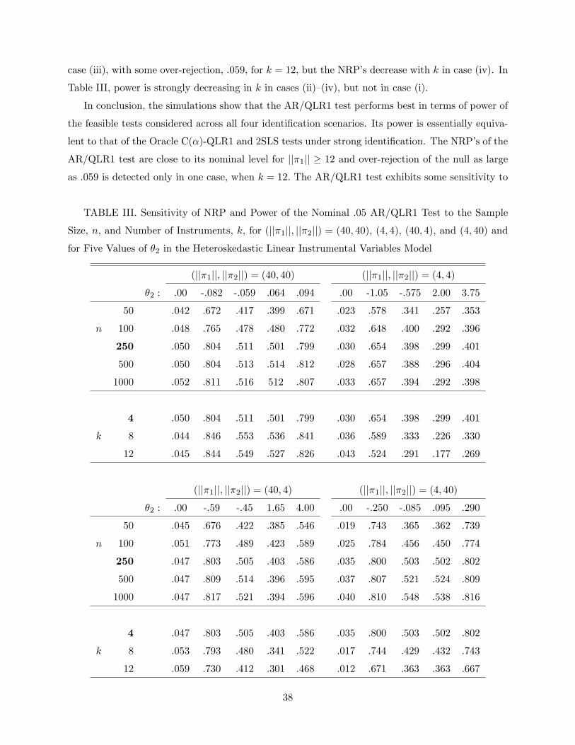
case (iii), with some over-rejection, :059; for k = 12; but the NRP�s decrease with k in case (iv). In

Table III, power is strongly decreasing in k in cases (ii)�(iv), but not in case (i).

In conclusion, the simulations show that the AR/QLR1 test performs best in terms of power of

the feasible tests considered across all four identi�cation scenarios. Its power is essentially equiva-

lent to that of the Oracle C(�)-QLR1 and 2SLS tests under strong identi�cation. The NRP�s of the

AR/QLR1 test are close to its nominal level for jj�1jj � 12 and over-rejection of the null as largeas :059 is detected only in one case, when k = 12: The AR/QLR1 test exhibits some sensitivity to

TABLE III. Sensitivity of NRP and Power of the Nominal :05 AR/QLR1 Test to the Sample

Size, n; and Number of Instruments, k; for (jj�1jj; jj�2jj) = (40; 40); (4; 4); (40; 4); and (4; 40) andfor Five Values of �2 in the Heteroskedastic Linear Instrumental Variables Model

(jj�1jj; jj�2jj) = (40; 40) (jj�1jj; jj�2jj) = (4; 4)�2 : .00 -.082 -.059 .064 .094 .00 -1.05 -.575 2.00 3.75

50 .042 .672 .417 .399 .671 .023 .578 .341 .257 .353

n 100 .048 .765 .478 .480 .772 .032 .648 .400 .292 .396

250 .050 .804 .511 .501 .799 .030 .654 .398 .299 .401

500 .050 .804 .513 .514 .812 .028 .657 .388 .296 .404

1000 .052 .811 .516 512 .807 .033 .657 .394 .292 .398

4 .050 .804 .511 .501 .799 .030 .654 .398 .299 .401

k 8 .044 .846 .553 .536 .841 .036 .589 .333 .226 .330

12 .045 .844 .549 .527 .826 .043 .524 .291 .177 .269

(jj�1jj; jj�2jj) = (40; 4) (jj�1jj; jj�2jj) = (4; 40)�2 : .00 -.59 -.45 1.65 4.00 .00 -.250 -.085 .095 .290

50 .045 .676 .422 .385 .546 .019 .743 .365 .362 .739

n 100 .051 .773 .489 .423 .589 .025 .784 .456 .450 .774

250 .047 .803 .505 .403 .586 .035 .800 .503 .502 .802

500 .047 .809 .514 .396 .595 .037 .807 .521 .524 .809

1000 .047 .817 .521 .394 .596 .040 .810 .548 .538 .816

4 .047 .803 .505 .403 .586 .035 .800 .503 .502 .802

k 8 .053 .793 .480 .341 .522 .017 .744 .429 .432 .743

12 .059 .730 .412 .301 .468 .012 .671 .363 .363 .667

38

the choice of Krk; a little sensitivity to the choice of �1; but little or no sensitivity to the choices

of KL; K�L; and a: Even for sample sizes as small as 50; the AR/QLR1 test has NRP�s less than its

nominal level. However, its power at this small a sample size is below what the asymptotic results

suggest. Overall, the AR/QLR1 test seems to perform quite well in this model for the parameter

scenarios considered.

9.2 Nonlinear IV Model

9.2.1 Simulation Set-up

Next, we consider an IV model with one rhs endogenous variable that enters nonlinearly:

Yi = Y1i 1 + Y21i 2 + Ui;

Y1i = Z 01i(�=n1=2) + Vi; (9.2)

where (Ui; Vi) � i.i.d. N(0; V ) for V 2 R2�2 with Vjj = 1 for j = 1; 2 and V12 = :8; Zi =

(Z 01i; Z02i)0 2 Rk; Z1i = (Z11i; :::; Z1(k=2)i)

0 � i.i.d. N(0k=2; Ik=2) independent of (Ui; Vi); Z2i =

(Z211i; :::; Z21(k=2)i)

0 2 Rk=2; and � = jj�jj1k=k1=2: The errors are homoskedastic. The coe¢ cientvector �=n1=2 on Zi in the reduced-form equation is scaled by n�1=2 and � is scaled by k�1=2 for

the same reasons as in Section 9.1.

We consider hypotheses concerning the value and derivative of the quadratic structural function

y1 1+y21 2 at the point y1 = 2: For the function value, we set �1 := y1 1 and �2 := y1 1+y

21 2 and

test H0 : �2 = �20: That is, we transform the parameters from ( 1; 2) to (�1; �2) and the structural

equation to Yi = Y �1i�1+Y�2i�2+Ui; where Y

�1i := Y1i=y1�Y 21i=y21 and Y �2i := Y 21i=y

21: For the function

derivative, we set �1 := 1 and �2 := 1+2y1 2; test H0 : �2 = �20; and the transformed structural

equation has Y �1i := Y1i � Y 21i=(2y1) and Y �2i := Y 21i=(2y1): In both cases, the moment vector is

gi(�) := (Yi � Y �1i�1 � Y �2i�2)Zi; (9.3)

but with di¤erent de�nitions of (Y �1i; Y�2i): The NRP�s and power of the tests considered are invariant

wrt �1 and equivariant wrt �2: In consequence, without loss of generality, we take the true value of

�1 to be zero, the null value �20 to be zero, and test the hypotheses H0 : �2 = 0 versus H1 : �2 6= 0:12

The same tests, base case tuning parameters, and simulation repetition numbers are used as for

the linear IV model. As above, � = :05: Figures 3 and 4 are for n = 500 and k = 4:

For NRP�s and power, we consider two identi�cation cases: (i) jj�jj = 50 (strong identi�cation)12The hypothesis H0 : �2 = 0 is obtained by replacing Yi by Yi � Y �

2i�20 and �2 by �2 � �20:

39

and (ii) jj�jj = 4 (weak identi�cation). For each case, we consider power for �2 2 [�B;B] for Bchosen suitably.

9.2.2 Simulation Results

Figures 3 and 4 provide �nite-sample power curves for identi�cation cases (i) and (ii) for the

hypotheses that concern the value and derivative of the structural function, respectively.

In Figure 3 for strong identi�cation (top), the AR/LM, AR/QLR1, and 2SLS tests have equal

and highest power for negative �2 values. The power of the Oracle C(�)-QLR1 test is similar, but

slightly lower for some negative �2 values. For positive �2 values, the 2SLS test clearly has the

highest power, while the AR/LM, AR/QLR1, and Oracle C(�)-QLR1 have equal, but lower power

than 2SLS. Note that the power curves of the tests are not symmetric about �2 = 0 (including 2SLS,

but to a lesser extent than the other tests). This indicates that the values of n and jj�jj are notsu¢ ciently large for the strong-identi�cation normal approximation to be highly accurate (although

this does not cause over-rejection under H0): The power curves of the AR/AR and Proj-QLR1 tests

are noticeably below those of the other tests, as is expected in this case.

In Figure 3 for weak identi�cation (bottom), the Oracle C(�)-QLR1 test has the highest power

for all �2 values. The AR/QLR1 test has equal power to it for negative �2 values, but noticeably

lower power for positive �2 values. The AR/LM test has quirky, low power for some negative �2

values, but relatively high power for positive �2 values. The AR/AR test has somewhat lower power

than the AR/QLR1 test. The Proj-QLR1 has noticeably lower power than the AR/QLR1 test for

all �2 values.

Figure 4 for the derivative of the structural function is quite similar to Figure 3. This is due to

the similarity of the transformed parameters �1 and �2 in these two cases.

Table IV provides NRP�s for the nominal .05 AR/QLR1 test for a range of values of jj�jj;n; and k with homoskedastic errors, and in one case heteroskedastic errors (with the same form

of heteroskedasticity as in (9.1) for the linear IV model). The table shows that the NRP�s vary

between :007 and :050 over these cases. The lowest NRP�s occur for jj�jj = 0: In the base case

scenario, n = 500 and k = 4; the NRP�s are in [:038; :042] for jj�jj � 4:The SM provides tables that are analogous to Tables II and III, which concern sensitivity of the

AR/QLR1 test to the tuning parameters, as well as to n and k; but for the nonlinear IV model with

hypotheses concerning the structural function and its derivative. Broadly speaking, the results are

similar to those in Tables II and III.

Overall, the AR/QLR1 test performs well in terms of NRP�s and power in the nonlinear IV

model for the parameter scenarios considered.

40

−0.1 0.0 0.1 0.2θ2

●●●●●●●●●●●●●●●●●●●●●●●●

●●

●●

●●

●●

●●

●●

●●

●●

●●

●●

●●

●●

●●

●●

●●

●●

●●

●●

●●

●●

●●●●●●●●●●●●●●●●●●●●●●●●●●●●●●●

●●●

●●

●●

●●

●●

●●

●●

●●

●●

●●

●●

●●

●●

●●

●●

●●

●●

●●

●●

●●

●●

●●●●●●●●●●●●●●●●●●●●●●●●●●●●●●●●●●●●●●●●●●●●●●●●●●●●●●●●●●●●●●●

0.05

0.40

0.80

●

AR/ARAR/LMAR/QLR1Proj−QLR1Oracle C(α)−QLR12SLS t

0 5 10θ2

0.05

0.40

0.80

AR/ARAR/LMAR/QLR1Proj−QLR1Oracle C(α)−QLR1

Figure 3. Nonlinear IV Model, Structural Function: Power for n=500, k=4,||π||=50 (top) and ||π||=4 (bottom)

−0.1 0.0 0.1 0.2θ2

●●●●●●●●●●●●●●●●●●●●●●●●●●●●●●●●●●●●●●●●

●●

●●

●●

●

●

●

●

●

●

●

●

●

●

●

●

●

●

●

●

●

●●

●●

●●

●●

●●●●●●●●●●●●●●●●●

●●

●●

●●

●●

●

●

●

●

●

●

●

●

●

●

●

●●

●●

●●

●●

●●

●●

●●

●●

●●●●●●●●●●●●●●●●●●●●●●●●●●●●●●●●●●●●●●●●●●●●●●●●●●●●●●●●●●●●●●●●●●●●●●●●●●●●●●

0.05

0.40

0.80

●

AR/ARAR/LMAR/QLR1Proj−QLR1Oracle C(α)−QLR12SLS t

0 5 10θ2

0.05

0.40

0.80

AR/ARAR/LMAR/QLR1Proj−QLR1Oracle C(α)−QLR1

Figure 4. Nonlinear IV Model, Derivative of Structural Function: Power forn=500, k=4, ||π||=50 (top) and ||π||=4 (bottom)

TABLE IV. NRP�s of the Nominal :05 AR/QLR1 Test for Base Case Tuning Parameters for

Inference on the Structural Function at y1 = 2 in the Nonlinear Instrumental Variables Model

k n Errors jj�jj : 100 75 50 35 20 14 8 4 0

4 50 Homoskedastic .032 .031 .026 .021 .018 .019 .019 .018 .009

4 100 Homoskedastic .040 .039 .036 .033 .033 .033 .032 .027 .017

4 250 Homoskedastic .041 .041 .041 .040 .039 .039 .038 .035 .024

4 500 Homoskedastic .042 .043 .045 .044 .043 .042 .039 .038 .026

8 100 Homoskedastic .050 .050 .046 .043 .044 .043 .041 .035 .025

8 250 Homoskedastic .043 .043 .044 .044 .045 .044 .042 .039 .035

4 250 Heteroskedastic .032 .030 .027 .025 .021 .018 .013 .009 .007

41

References

Andrews, D. W. K. (2017): �Identi�cation-Robust Subvector Inference for Likelihood-Based Mod-

els,�manuscript in preparation, Cowles Foundation, Yale University.

Andrews, D. W. K., and X. Cheng (2012): �Estimation and Inference with Weak, Semi-strong, and

Strong Identi�cation,�Econometrica, 80, 2153�2211. Supplemental Material is available at

Econometrica Supplemental Material , 80, http://www.econometricsociety.org/ecta/Supmat

/9456_miscellaneous.pdf.

� � � (2013): �Maximum Likelihood Estimation and Uniform Inference with Sporadic Identi-

�cation Failure,� Journal of Econometrics, 173, 36�56. Supplemental Material is available

with Cowles Foundation Discussion Paper No. 1824R, 2011, Yale University.

� � � (2014): �GMM Estimation and Uniform Subvector Inference with Possible Identi�cation

Failure,�Econometric Theory, 30, 287�333.

Andrews, D. W. K., X. Cheng, and P. Guggenberger (2011): �Generic Results for Establishing

the Asymptotic Size of Con�dence Sets and Tests,�Cowles Foundation Discussion Paper No.

1813, Yale University.

Andrews, D. W. K., and P. Guggenberger (2015): �Identi�cation- and Singularity-Robust Infer-

ence for Moment Condition Models,�Cowles Foundation Discussion Paper No. 1978, Yale

University, revised 2017.

� � � (2017): �Asymptotic Size of Kleibergen�s LM and Conditional LR Tests for Moment

Condition Models,�Econometric Theory, 33, forthcoming. Earlier version available as Cowles

Foundation Discussion Paper No. 1977, Yale University.

Andrews, I. (2017): �Valid Two-Step Identi�cation-Robust Con�dence Sets for GMM,�Review of

Economics and Statistics, forthcoming.

Andrews, I., and A. Mikusheva (2015): �Maximum Likelihood Inference in Weakly Identi�ed

Dynamic Stochastic General Equilibrium Models,�Quantitative Economics, 6, 123�152.

� � � (2016a): �A Geometric Approach to Nonlinear Econometric Models,�Econometrica, 84,

1249�1264.

� � � (2016b): �Conditional Inference with a Functional Nuisance Parameter,�Econometrica,

84, 1571�1612.

42

Bera, A. K., and Y. Bilias (2001): �Rao�s Score, Neyman�s C(�) and Silvey�s LM Tests: An

Essay on Historical Developments and Some New Results,� Journal of Statistical Inference

and Planning, 97, 9�44.

Berger, R. L., and D. D. Boos (1994): �P Values Maximized over a Con�dence Set for the Nuisance

Parameter,�Journal of the American Statistical Association, 89, 1012�1016.

Bugni, F. A., I. A. Canay, and X. Shi (2016): �Inference for Subvectors and Other Functions

of Partially Identi�ed Parameters in Moment Inequality Models,� unpublished manuscript,

Department of Economics, University of Wisconsin, Madison.

Campbell, J. Y., and M. Yogo (2006): �E¢ cient Tests of Stock Return Predictability,�Journal of

Financial Economics, 81, 27�60.

Cavanagh, C. L., G. Elliott, and J. H. Stock (1995): �Inference in Models with Nearly Integrated

Regressors,�Econometric Theory, 11, 1131�1147.

Chaudhuri, S. (2016): �Improved Projection GMM-LM Tests for Linear Restrictions,�unpublished

manuscript, Department of Economics, University of Montreal.

Chaudhuri, S., T. Richardson, J. Robins, and E. Zivot (2010): �A New Projection-Type Split-

Sample Score Test in Linear Instrumental Variables Regression,�Econometric Theory, 26,

1820�1837.

Chaudhuri, S., and E. Zivot (2011): �A New Method of Projection-Based Inference in GMM with

Weakly Identi�ed Nuisance Parameters,�Journal of Econometrics, 164, 239�251.

Chen, X., T. M. Christensen, K. O�Hara, and E. Tamer (2016): �Monte Carlo Markov Chain

Con�dence Sets for Identi�ed Sets,�Cowles Foundation Discussion Paper No. 2017R, Yale

University.

Cheng, X. (2015): �Robust Inference in Nonlinear Models with Mixed Identi�cation Strength,�

Journal of Econometrics, 189, 207�228.

Cox, G. (2016): �Robust Inference in a Class of Generically Identi�ed Models with an Application

to Factor Models,�unpublished manuscript, Department of Economics, Yale University.

Demmel, J. (1980): �Singular Value Decomposition,�in Z. Bai, J. Demmel, J. Dongarra, A. Ruhe,

and H. van der Vorst (eds.) Templates for the Solution of Algebraic Eigenvalue Problems: A

Practical Guide. Philadelphia: SIAM.

43

Dufour, J.-M. (1989): �Nonlinear Hypotheses, Inequality Restrictions, and Non-Nested Hypothe-

ses: Exact Simultaneous Tests in Linear Regressions,�Econometrica, 57, 335�355.

Dufour, J.-M., and J. Jasiak (2001): �Finite Sample Limited Information Inference Methods

for Structural Equations and Structural Models with Generated Regressors,� International

Economic Review, 42, 815�843.

Elliott, G., U. K. Müller, and M. W. Watson (2015): �Nearly Optimal Tests When a Nuisance

Parameter Is Present under the Null Hypothesis,�Econometrica, 83, 771�811.

Guggenberger, P., F. Kleibergen, S. Mavroeidis, and L. Chen (2012): �On the Asymptotic Sizes

of Subset Anderson-Rubin and Lagrange Multiplier Tests in Linear Instrumental Variables

Regression,�Econometrica, 80, 2649�2666.

Guggenberger, P., J. J. S. Ramalho, and R. J. Smith (2012): �GEL Statistics Under Weak Iden-

ti�cation,�Journal of Econometrics, 170, 331�349.

Guggenberger, P., and R. J. Smith (2005): �Generalized Empirical Likelihood Estimators and

Tests Under Partial, Weak and Strong Identi�cation,�Econometric Theory, 21, 667�709.

Han, S., and A. McCloskey (2016): �Estimation and Inference with a (Nearly) Singular Jacobian,�

unpublished manuscript, Department of Economics, University of Texas, Austin.

Kaido, H., F. Molinari, and J. Stöye (2016): �Con�dence Intervals for Projections of Partially

Identi�ed Parameters,�unpublished manuscript, Department of Economics, Boston Univer-

sity.

Kleibergen, F. (2004): �Testing Subsets of Structural Parameters in the Instrumental Variables

Regression Model,�Review of Economics and Statistics, 86, 418�423.

� � � (2005): �Testing Parameters in GMM Without Assuming That They Are Identi�ed,�

Econometrica, 73, 1103�1123.

� � � (2015): �E¢ cient Size Correct Subset Inference in Linear Instrumental Variables Regres-

sion,�unpublished manuscript, Amsterdam School of Economics, University of Amsterdam.

Lee, J. (2014): �Asymptotic Sizes of Subset Anderson-Rubin Tests with Weakly Identi�ed Nui-

sance Parameters and General Covariance Structure,�unpublished manuscript, Department

of Economics, M.I.T.

44

Loh, W.-Y. (1985): �A New Method for Testing Separate Families of Hypotheses,�Journal of the

American Statistical Association, 80, 362�368.

McCloskey, A. (2011): �Bonferroni-Based Size-Correction for Nonstandard Testing Problems,�

unpublished manuscript, Department of Economics, Brown University.

Montiel Olea, J. L. (2012): �E¢ cient Conditionally Similar-on-the-Boundary Tests,�unpublished

manuscript, Department of Economics, New York University.

Moran, P. A. P. (1979): �On Asymptotically Optimal Tests of Composite Hypotheses,� Bio-

metrika, 57, 47�55.

Newey, W. K., and K. West (1987): �Hypothesis Testing with E¢ cient Method of Moments

Estimation,�International Economic Review, 28, 777�787.

Neyman, J. (1959): �Optimal Asymptotic Test of Composite Statistical Hypothesis,� in U.

Grenander (ed.) Probability and Statistics, The Harold Cramér Volume. Uppsala: Almqvist

and Wiksell, pp. 313�334.

Otsu, T. (2006): �Generalized Empirical Likelihood Inference for Nonlinear and Time Series

Models Under Weak Identi�cation,�Econometric Theory, 22, 513�527.

Robin, J.-M., and R. J. Smith (2000): �Tests of Rank,�Econometric Theory, 16, 151�175.

Smith, R. J. (1987): �Alternative Asymptotically Optimal Tests and Their Application to Dy-

namic Speci�cation,�Review of Economic Studies, 54, 665�680.

Stock, J. H., and J. H. Wright (2000): �GMM with Weak Identi�cation,� Econometrica, 68,

1055�1096.

45