Identification of a Drinking

Water Softening Model using

Machine Learning

J.N. Jenden January 2020

Faculty of Electrical Engineering, Mathematics and Computer Science (EEMCS)

Graduation committee: Prof.dr. H.J. Zwart (UT) Dr. C. Brune (UT) Prof.dr. A.A. Stoorvogel (UT) Ir. E.H.B. Visser (Witteveen+Bos) Control Theory Department of Systems and Control Faculty of Electrical Engineering, Mathematics and Computer Science University of Twente P.O. Box 217 7500 AE Enschede The Netherlands

M.Sc. THESIS

Company: Witteveen+Bos Deventer, the Netherlands

Contents

Table of contents . . . . . . . . . . . . . . . . . . . . . . . . . . . . . . . . . . . . . . . . . . . . . . . iiList of figures . . . . . . . . . . . . . . . . . . . . . . . . . . . . . . . . . . . . . . . . . . . . . . . . . iiiAbstract . . . . . . . . . . . . . . . . . . . . . . . . . . . . . . . . . . . . . . . . . . . . . . . . . . . . ivAcknowledgements . . . . . . . . . . . . . . . . . . . . . . . . . . . . . . . . . . . . . . . . . . . . . vAcronyms and Term Dictionary . . . . . . . . . . . . . . . . . . . . . . . . . . . . . . . . . . . . . . viChapter 1: Introduction . . . . . . . . . . . . . . . . . . . . . . . . . . . . . . . . . . . . . . . . . . . 1

Softening Treatment Process . . . . . . . . . . . . . . . . . . . . . . . . . . . . . . . . . . . . . 1Hard Water . . . . . . . . . . . . . . . . . . . . . . . . . . . . . . . . . . . . . . . . . . . . . . . 1What is Machine Learning? . . . . . . . . . . . . . . . . . . . . . . . . . . . . . . . . . . . . . 2Train, Validation and Test Data . . . . . . . . . . . . . . . . . . . . . . . . . . . . . . . . . . . 2Previous Research . . . . . . . . . . . . . . . . . . . . . . . . . . . . . . . . . . . . . . . . . . . 2Aim of the Report . . . . . . . . . . . . . . . . . . . . . . . . . . . . . . . . . . . . . . . . . . . 3Report Layout . . . . . . . . . . . . . . . . . . . . . . . . . . . . . . . . . . . . . . . . . . . . . 3

Chapter 2: Background Information . . . . . . . . . . . . . . . . . . . . . . . . . . . . . . . . . . . . 6Softening Process Configuration . . . . . . . . . . . . . . . . . . . . . . . . . . . . . . . . . . 6Pellet Softening Reactor . . . . . . . . . . . . . . . . . . . . . . . . . . . . . . . . . . . . . . . 6Control Actions in the Softening Treatment Step . . . . . . . . . . . . . . . . . . . . . . . . . 7pH as a Control Variable . . . . . . . . . . . . . . . . . . . . . . . . . . . . . . . . . . . . . . . 8

Chapter 3: Data Pre-Processing and Data Analysis . . . . . . . . . . . . . . . . . . . . . . . . . . . 9Time Series . . . . . . . . . . . . . . . . . . . . . . . . . . . . . . . . . . . . . . . . . . . . . . . 9Normalising the Data . . . . . . . . . . . . . . . . . . . . . . . . . . . . . . . . . . . . . . . . . 9Removing Corrupted Data . . . . . . . . . . . . . . . . . . . . . . . . . . . . . . . . . . . . . . 9Pearson’s Correlation Coefficient . . . . . . . . . . . . . . . . . . . . . . . . . . . . . . . . . . 10Autocorrelation . . . . . . . . . . . . . . . . . . . . . . . . . . . . . . . . . . . . . . . . . . . . 10

Chapter 4: Machine Learning . . . . . . . . . . . . . . . . . . . . . . . . . . . . . . . . . . . . . . . . 11Supervised Learning . . . . . . . . . . . . . . . . . . . . . . . . . . . . . . . . . . . . . . . . . 11Train-Validation-Test Data Splitting Method . . . . . . . . . . . . . . . . . . . . . . . . . . . 11Walk-forward Data Splitting Method . . . . . . . . . . . . . . . . . . . . . . . . . . . . . . . . 12Hyperparameters and Hyperparameter Grid Searches . . . . . . . . . . . . . . . . . . . . . . 12Overfitting and Underfitting . . . . . . . . . . . . . . . . . . . . . . . . . . . . . . . . . . . . . 13Evaluation Metrics . . . . . . . . . . . . . . . . . . . . . . . . . . . . . . . . . . . . . . . . . . . 13

Chapter 5: Neural Networks and XGBoost . . . . . . . . . . . . . . . . . . . . . . . . . . . . . . . . 15Neural Networks . . . . . . . . . . . . . . . . . . . . . . . . . . . . . . . . . . . . . . . . . . . . 15Recurrent Neural Networks (RNNs) . . . . . . . . . . . . . . . . . . . . . . . . . . . . . . . . . 15Memory Cells . . . . . . . . . . . . . . . . . . . . . . . . . . . . . . . . . . . . . . . . . . . . . . 16Standard Time Series NN Structure . . . . . . . . . . . . . . . . . . . . . . . . . . . . . . . . . 17LSTM Cells . . . . . . . . . . . . . . . . . . . . . . . . . . . . . . . . . . . . . . . . . . . . . . . 17Regularisation using a Dropout Layer . . . . . . . . . . . . . . . . . . . . . . . . . . . . . . . 18Gradient Descent . . . . . . . . . . . . . . . . . . . . . . . . . . . . . . . . . . . . . . . . . . . 19

i

Introduction to Decision Trees . . . . . . . . . . . . . . . . . . . . . . . . . . . . . . . . . . . 20Difference between Classification and Regression Trees . . . . . . . . . . . . . . . . . . . . . 20Introduction to XGBoost . . . . . . . . . . . . . . . . . . . . . . . . . . . . . . . . . . . . . . . 20Feature Importance . . . . . . . . . . . . . . . . . . . . . . . . . . . . . . . . . . . . . . . . . . 21XGBoost and RNN Model Prediction Horizons . . . . . . . . . . . . . . . . . . . . . . . . . . 21

Chapter 6: Methods . . . . . . . . . . . . . . . . . . . . . . . . . . . . . . . . . . . . . . . . . . . . . 22Identification of Inputs and Outputs . . . . . . . . . . . . . . . . . . . . . . . . . . . . . . . . 22Data Collection . . . . . . . . . . . . . . . . . . . . . . . . . . . . . . . . . . . . . . . . . . . . 23Data Pre-Processing and Data Analysis . . . . . . . . . . . . . . . . . . . . . . . . . . . . . . . 23Prediction . . . . . . . . . . . . . . . . . . . . . . . . . . . . . . . . . . . . . . . . . . . . . . . . 29

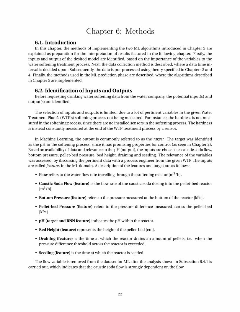
Chapter 7: Machine Learning Results . . . . . . . . . . . . . . . . . . . . . . . . . . . . . . . . . . . 30RNN Train-Validation-Test Model . . . . . . . . . . . . . . . . . . . . . . . . . . . . . . . . . . 30RNN Walk-Forward Models . . . . . . . . . . . . . . . . . . . . . . . . . . . . . . . . . . . . . 31XGBoost Train-Validation-Test Model . . . . . . . . . . . . . . . . . . . . . . . . . . . . . . . 35XGBoost Walk-Forward Models . . . . . . . . . . . . . . . . . . . . . . . . . . . . . . . . . . . 36

Chapter 8: Discussion and Conclusions . . . . . . . . . . . . . . . . . . . . . . . . . . . . . . . . . 37Chapter 9: Recommendations . . . . . . . . . . . . . . . . . . . . . . . . . . . . . . . . . . . . . . . 40Bibliography . . . . . . . . . . . . . . . . . . . . . . . . . . . . . . . . . . . . . . . . . . . . . . . . . 42Appendix A: Drinking WTP Example and Softening Process Background Information . . . . . . 44

Example WTP . . . . . . . . . . . . . . . . . . . . . . . . . . . . . . . . . . . . . . . . . . . . . 44Water Flux . . . . . . . . . . . . . . . . . . . . . . . . . . . . . . . . . . . . . . . . . . . . . . . 44Water Hardness Chemistry . . . . . . . . . . . . . . . . . . . . . . . . . . . . . . . . . . . . . . 45Bypass . . . . . . . . . . . . . . . . . . . . . . . . . . . . . . . . . . . . . . . . . . . . . . . . . . 45Calcium Carbonate Crystallisation Reaction . . . . . . . . . . . . . . . . . . . . . . . . . . . 46

Appendix B: Data Analysis . . . . . . . . . . . . . . . . . . . . . . . . . . . . . . . . . . . . . . . . . 47Pearson’s Correlation Coefficient Matrix . . . . . . . . . . . . . . . . . . . . . . . . . . . . . . 47Box Plot . . . . . . . . . . . . . . . . . . . . . . . . . . . . . . . . . . . . . . . . . . . . . . . . . 47

Appendix C: Machine Learning . . . . . . . . . . . . . . . . . . . . . . . . . . . . . . . . . . . . . . 50Python vs Matlab®: Machine Learning and Control Theory Implementation . . . . . . . . 50RMSProp Optimisation . . . . . . . . . . . . . . . . . . . . . . . . . . . . . . . . . . . . . . . . 50Derivation of Backpropagation Equations . . . . . . . . . . . . . . . . . . . . . . . . . . . . . 51The Backpropagation Algorithm . . . . . . . . . . . . . . . . . . . . . . . . . . . . . . . . . . 53Logistic Activation Function . . . . . . . . . . . . . . . . . . . . . . . . . . . . . . . . . . . . . 54

Appendix D: eXtreme Gradient Boost (XGBoost) . . . . . . . . . . . . . . . . . . . . . . . . . . . . 55Regularisation Learning Objective . . . . . . . . . . . . . . . . . . . . . . . . . . . . . . . . . 55Gradient Tree Boosting . . . . . . . . . . . . . . . . . . . . . . . . . . . . . . . . . . . . . . . . 56

Appendix E: XGBoost and RNN Implementation . . . . . . . . . . . . . . . . . . . . . . . . . . . . 57XGBoost Results . . . . . . . . . . . . . . . . . . . . . . . . . . . . . . . . . . . . . . . . . . . . 57RNN Results (F=24[hr]) . . . . . . . . . . . . . . . . . . . . . . . . . . . . . . . . . . . . . . . . 61XGBoost Hyperparameter Selection . . . . . . . . . . . . . . . . . . . . . . . . . . . . . . . . 63RNN Hyperparameter Selection . . . . . . . . . . . . . . . . . . . . . . . . . . . . . . . . . . . 64RNN Walk-Forward Training (F=1[min]) . . . . . . . . . . . . . . . . . . . . . . . . . . . . . . 64RNN Train-Validation-Test Training (F=1[min]) . . . . . . . . . . . . . . . . . . . . . . . . . . 65RNN Walk-Forward Training (F=24 [hr]) . . . . . . . . . . . . . . . . . . . . . . . . . . . . . . 66RNN Walk-Forward Training (F=4 [hr]) . . . . . . . . . . . . . . . . . . . . . . . . . . . . . . . 68XGBoost Train-Validation-Test Training . . . . . . . . . . . . . . . . . . . . . . . . . . . . . . 69XGBoost Walk-Forward Training . . . . . . . . . . . . . . . . . . . . . . . . . . . . . . . . . . 70

ii

List of Figures

1 Softening treatment process diagram . . . . . . . . . . . . . . . . . . . . . . . . . . . . . . . 12 Water Treatment Plant (WTP) standard set-up . . . . . . . . . . . . . . . . . . . . . . . . . . 63 Typical pellet softening fluidised bed reactor . . . . . . . . . . . . . . . . . . . . . . . . . . . 74 Supervised learning example . . . . . . . . . . . . . . . . . . . . . . . . . . . . . . . . . . . . 115 Train-validation-test data split . . . . . . . . . . . . . . . . . . . . . . . . . . . . . . . . . . . . 126 Walk-forward . . . . . . . . . . . . . . . . . . . . . . . . . . . . . . . . . . . . . . . . . . . . . . 127 Simple network . . . . . . . . . . . . . . . . . . . . . . . . . . . . . . . . . . . . . . . . . . . . 158 Recurrent Neural Network (RNN) over time . . . . . . . . . . . . . . . . . . . . . . . . . . . . 159 Memory cell . . . . . . . . . . . . . . . . . . . . . . . . . . . . . . . . . . . . . . . . . . . . . . 1610 Example RNN structure . . . . . . . . . . . . . . . . . . . . . . . . . . . . . . . . . . . . . . . . 1711 LSTM . . . . . . . . . . . . . . . . . . . . . . . . . . . . . . . . . . . . . . . . . . . . . . . . . . 1712 Dropout layer . . . . . . . . . . . . . . . . . . . . . . . . . . . . . . . . . . . . . . . . . . . . . 1813 Gradient descent . . . . . . . . . . . . . . . . . . . . . . . . . . . . . . . . . . . . . . . . . . . . 1914 Regression tree example . . . . . . . . . . . . . . . . . . . . . . . . . . . . . . . . . . . . . . . 2015 Gradient boosting . . . . . . . . . . . . . . . . . . . . . . . . . . . . . . . . . . . . . . . . . . . 2116 XGBoost and RNN model features and targets . . . . . . . . . . . . . . . . . . . . . . . . . . 2117 Data interpolation method . . . . . . . . . . . . . . . . . . . . . . . . . . . . . . . . . . . . . . 2318 Caustic soda dosage flow rate and flow rate . . . . . . . . . . . . . . . . . . . . . . . . . . . . 2419 pH autocorrelation . . . . . . . . . . . . . . . . . . . . . . . . . . . . . . . . . . . . . . . . . . 2620 Mean pH over one day . . . . . . . . . . . . . . . . . . . . . . . . . . . . . . . . . . . . . . . . 2721 pH box plot over hours. . . . . . . . . . . . . . . . . . . . . . . . . . . . . . . . . . . . . . . . . 2722 A month of data from a drinking water reactor . . . . . . . . . . . . . . . . . . . . . . . . . . 2824 RNN train-validation-test model prediction . . . . . . . . . . . . . . . . . . . . . . . . . . . . 3025 The first twp RNN walk-forward models . . . . . . . . . . . . . . . . . . . . . . . . . . . . . . 3126 The last four RNN walk-forward models . . . . . . . . . . . . . . . . . . . . . . . . . . . . . . 3228 Walk-forward forecasting RNN model predictions . . . . . . . . . . . . . . . . . . . . . . . . 3429 XGBoost train-validation-test split model prediction . . . . . . . . . . . . . . . . . . . . . . 3530 Feature Importance Train-Validation-Test XGBoost Model . . . . . . . . . . . . . . . . . . . 3531 Weesperkarspel Water Treatment Plant (WTP) . . . . . . . . . . . . . . . . . . . . . . . . . . 4432 Water flux . . . . . . . . . . . . . . . . . . . . . . . . . . . . . . . . . . . . . . . . . . . . . . . . 4533 Boxplot . . . . . . . . . . . . . . . . . . . . . . . . . . . . . . . . . . . . . . . . . . . . . . . . . 4734 Hourly mean of data features and the seeding and draining per hour . . . . . . . . . . . . . 4935 Logistic Activation Function . . . . . . . . . . . . . . . . . . . . . . . . . . . . . . . . . . . . . 5436 Tree ensemble model example . . . . . . . . . . . . . . . . . . . . . . . . . . . . . . . . . . . 5537 First four XGBoost walk-forward split model predictions . . . . . . . . . . . . . . . . . . . . 5838 Last three XGBoost walk-forward model predictions . . . . . . . . . . . . . . . . . . . . . . . 5939 Feature importance of XGBoost models 0 to 3 . . . . . . . . . . . . . . . . . . . . . . . . . . . 6040 Feature importance of XGBoost models 4, 5 and 6 . . . . . . . . . . . . . . . . . . . . . . . . 6141 Walk-forward forecasting RNN model predictions . . . . . . . . . . . . . . . . . . . . . . . . 62

iii

Abstract

This report identifies Machine Learning (ML) models of the water softening treatment process in aWater Treatment Plant (WTP), using two different ML algorithms applied on time series data: eXtremeGradient Boost (XGBoost) and Recurrent Neural Networks (RNNs). In addition, a control method for thedraining of pellets in the softening reactor is explored based on collected softening treatment data andthe resulting ML models. In particular, the pH is identified as a potential variable for the control of pelletdraining within a softening reactor. The pH forecasts produced by ML models are able to predict thefuture behaviour of the pH and potentially anticipate when the pellets should be drained.

For implementation of the ML algorithms, the inputs and outputs of the ML models are first identi-fied. Wherein, the pH within the softening reactor is selected as the output, due to its potential controlproperties. Subsequently, water softening treatment data is collected from a water company residing inthe Netherlands. After collection, the data is pre-processed and analysed to be able to better interpretthe ML results and to improve the performance of the ML models trained. During pre-processing, theimplementation of two ML data splitting methods, walk-forward and train-validation-test, is carried out.The performance of the models is gauged using two different evaluation metrics: Mean Squared Error(MSE) and R-squared. Lastly, predictions are carried out using the trained ML models for a set of forecasthorizon lengths.

Comparing the XGBoost and RNN pH predictions, the RNN performs in general better than the XG-Boost method, where the RNN model with a train-validation-test split, has a MSE value of 0.0004 (4 d.p.)and an R-squared value of 0.9007 (4 d.p.). Extending the forecast horizon to four hours for the RNN walk-forward model yielded MSE values below 0.01, but only negative R-squared values. Thereby, suggestingthat the prediction is relatively close to the actual data points, but does not follow the shape of the actualdata points well.

The evaluation metric results suggest that it is possible to create a good performing model using theRNN method for a forecast horizon length equal to one minute. Alternatively, this model is heavily de-pendent on the current pH value and therefore is deemed to be not a good predictor of the pH. Increasingthe horizon length leads to only slightly lower MSE values, but the R-squared values are in general nega-tive, indicating a poor fit.

Keywords: Machine Learning (ML), water softening treatment, Water Treatment Plant (WTP), timeseries, eXtreme Gradient Boost (XGBoost), Recurrent Neural Network (RNN), pH, control, pellet drain-ing, softening reactor, forecast, inputs, outputs, pre-process, data splitting method, walk-forward, train-validation-test, evaluation metric, Mean Squared Error (MSE), R-squared, prediction, forecast horizon

iv

Acknowledgements

This thesis report is the final product of a team effort. I would like to express my gratitude to a num-ber of people that helped me reach this final stage of publication.

Firstly and most importantly, I would like to thank ir. Erwin Visser, my supervisor at Witteveen+Bos(W+B), for formulating such an interesting topic for my thesis and allowing me to carry out my researchat W+B. Furthermore, his technical insights on the water softening treatment system were incrediblyuseful and helped me better understand the system during our weekly meetings. Additionally, I wouldlike to thank the whole of the Process Automation team at W+B for their support during my entire thesis.Particularly Ko Roebers and Eddy Janssen, for bringing me in contact with a water company.

Secondly, I would like to send a special thanks to Prof. Hans Zwart, my supervisor from the Universityof Twente, who gave me technical nuggets of information during my research and helped me shape myfinal report.

Next, I would like to thank my fellow Systems and Control class mate Anne Steenbeek for his wisdomand advice about the machine learning implementation part of my research. In addition, I want to thankAkhyar Sadad for explaining his machine learning implementation in Python.

Finally, I would like to thank my colleagues Eleftheria Chiou and Shanti Bruyn for their technical in-put.

v

Acronyms and Term Dictionary

Acronym

CPU Central Processing Unit

IQR Interquartile Range

LSTM Long Short-Term Memory

ML Machine Learning

MPC Model Predictive Control

MSE Mean Squared Error

NN Neural Network

PHREEQC pH-Redox-Equilibrium Calculations

RAM Random Access Memory

RMSProp Root Mean Square Propagation

RNN Recurrent Neural Network

WTP Water Treatment Plant

WWTP Wastewater Treatment Plant

XGBoost eXtreme Gradient Boost

vi

Term Definition

Activation function a function, that transforms the summed weighted input from the neuron into the output

Backend the computing task that is performed in the background. The user is not able to observe thistask being carried out

Backpropagation an algorithm used during the training of a Recurrent Neural Network (RNN) model

Break through the act of the grains in the pellet softening reactor being flushed out of the softening reactorto the following stage of the Water Treatment Plant (WTP)

Corrupted data data containing blanks, NaNs, null-values or other placeholders

Crystallisation rate the rate at which a solid forms, where the atoms are organised into a crystal structure

Dissolution the action of becoming incorporated into a liquid, resulting in a solution

Effluent the water exiting a softening treatment reactor

Ensemble Learning building a model based on an array of other models [6]

Eutrophication the phenomenon of an excessive richness of nutrients in a body of water, causing a surge ofplant growth

Feature a measurable property of a system. Although, the target of the machine learning algorithmis not considered a feature

Frontend the graphical user interface provided to the user when operating software

Horizon span the array of forecast time steps of a particular model

Hyperparameter a parameter of a learning algorithm and external to the model

Influent the water entering a softening treatment reactor

Ion an atom or a molecule that possesses a positive or negative charge

Learner variable a variable that is used during the training of a machine learning model

Linear regression the calculation of a function that minimises the distance between the fitted line and all of thedata points. The line is often referred to as the regression line

Lookback the number of past time steps used to make a model prediction

Misclassify the act of a result being wrongly classified

Model performance indicator a statistical measure of the performance of the model against the test set. This term is also oftenreferred to as an evaluation metric

Model Predictive Control (MPC) a method of system control, which seeks to control a process while satisfying a set ofconstraints

Overfitting learning the detail and noise of the training data to the extent that it negatively impacts theperformance of the model on new data [12]

Predictor a variable employed as an input in order to determine the target numeric valuein the data

Redox reaction a reaction where a transfer of electrons is involved

Regularisation the process of adding information in order to prevent overfitting

Response variable the target (output) of a decision tree

Supervised learning the process of feeding a machine learning algorithm with example input-output training datapairs

Target the output for a machine learning model

Water treatment act or process of making water more useful or potable [20]

Window of data a number of rows extracted from the original dataset

vii

Chapter 1: Introduction1.1. Water Treatment Plant (WTP)The purpose of a Water Treatment Plant (WTP) is to remove particles and organisms that cause dis-

eases, protect the public’s welfare and provide clean drinkable water for the environment, people andliving organisms [20]. As of 2016, there are ten different drinking water companies in the Netherlands,employing 4,856 workers. A total 1,095 million m3 of drinking water was produced in the Netherlands in2016 [23]. An overview of an example WTP can be found in Appendix A.

1.1.1. Softening Treatment Process

Figure 1: Softening treatment process diagram.

Once the water has been pre-treated, it undergoes softening in theWTP. A popular softening process set-up is displayed in Figure 1. The rawwater enters the process and flowsthrough to the pellet-softening reactor.The softened water then exits the re-actor at the top and is subsequentlymixed with the bypassed water. Finally,the water is dosed with a form of acidto ensure that the pH reduces. A largepH value kills the bacteria in the down-stream biofilters. In addition, the acidcounteracts the chemical reactions in-volving caustic soda. These reactionscan potentially negatively impact thedownstream WTP equipment. The by-pass (described in Appendix A) and rawwater flow are controlled using valves.

1.1.2. Hard WaterMagnesium and calcium ions are dissolved when water comes into contact with rocks and minerals.

The hardness of the water is the total amount of dissolved metal ions in the water. In practice, the hard-ness is determined by adding the concentration of calcium and magnesium ions in the water, since theyare generally the most abundant in the influent. Hard water can cause the following problems [1]:

• Decreasing the calcium concentration in water gives rise to a higher pH value in the distributedwater, leading to a decrease in the dissolution of copper and lead in the distribution system. Inges-tion of large quantities of dissolved copper and lead has negative effects on the public’s health.

• A higher detergent dosage for washing is required for harder water. This increases the concen-tration of phosphate in wastewater and contributing to the eutrophication effect. Furthermore, agreater usage of detergent increases the average household costs.

• Hard water causes scale buildup in heating equipment and appliances, causing an increase in en-ergy consumption and equipment defects.

• Hard water tastes worse than soft water.

• The damaging or staining of clothing during a wash is often caused by hard water.

1

1.2. Machine Learning

1.2.1. What is Machine Learning?Machine Learning (ML) is the science of programming computers using algorithms, so they can learn

from data [6]. The algorithms develop models, which are able to perform a specific task, relying only oninference and patterns. A more formal definition is as follows:

A computer program is said to learn from experience E with re-spect to some task T and some performance measure P, if itsperformance on T, as measured by P, improves with experienceE.

ML has been frequently used to solve various real-life problems in recent years. One example is pre-dicting the stock market, where stakeholders frequently want to predict future trends of the stock prices.Implementing a ML algorithm using past stock data allows you to generate a model that can predict thefuture trajectory of the stock price.

1.2.2. Train, Validation and Test DataA dataset is often for ML partitioned into: train, validation and test datasets. The train partition is

used for training during the implementation of the ML algorithm. The validation data is used to evalu-ate the model during training and allows you to effectively tune the hyperparameters. A hyperparameteris a parameter of a learning algorithm and external to the model. Therefore, hyperparameters remainconstant during the training of a ML model. Checking the model against the validation data allows youto identify if the model is overfitting (explained in Section 4.6) on the training dataset. The test partitionconsists of the data used to determine the final performance of the created model.

1.3. Previous ResearchIn K.M. van Schagen’s research paper, Model-Based Control of Drinking-Water Treatment Plants (pub-

lished in 2009) [4], the softening process in the Weesperkarspel WTP is evaluated. K.M. van Schagen pro-poses controlling the pellet-bed height using a Model Prediction Controller (MPC). The MPC determinesthe seeding material dosage and pellet discharge, to maintain the optimal pellet diameter and maximumbed height under variable flow in the reactor and corresponding temperature.

Stimela is a modelling environment for drinking water treatment processes (including the water soft-ening process) in Matlab®/Simulink® [24]. Stimela was developed by DHV Water BV and Delft Univer-sity of Technology. The Stimela models calculate changes of water quality parameters, such as pH, pelletdiameter and pellet-bed height.

PHREEQC (pH-Redox-Equilibrium Calculations) is a model that was developed by Uninited StatesGeological Survey (USGS) to calculate the groundwater chemistry [10]. PHREEQC is comprised of all therelevant chemical balance equations for water chemistry, such as acid-base and redox (reduction/oxi-dation) reactions. The PHREEQC (in combination with a model of the calcium carbonate crystallisationrate) simulates a pellet softening reactor [5].

A. Sadad published a research paper in 2019 [9], about a general step-by-step method of applying MLanalysis on a time-series dataset. One example case featuring in the research is a Wastewater TreatmentPlant (WWTP) system, where an accurate ML model was developed using Recurrent Neural Networks(RNNs) and the XGBoost algorithm (see Chapter 5). Both of the ML algorithms were implemented inPython. In this research, an adapted version of A. Sadad’s implementation is employed. This research

2

firstly seeks to verify the step-by-step method proposed by A. Sadad and secondly, to adapt the imple-mentation to be able to forecast further into the future.

There are no research publications about applying ML on the drinking water treatment softeningprocess. One purpose of this research, is to investigate if it is possible to apply ML on a drinking watertreatment softening process and generate an accurate model of the process.

1.4. Aim of the ReportThe aim of the research is as follows:

Develop a control strategy that efficiently controls the seedingand draining of the softening reactor based on the pH, using amodel developed through ML.

Moreover, this research seeks to answer the following questions:

1. Is it possible to develop a model of the softening treatment process of a WTP using ML?

2. Is the data provided for this research sufficient to develop a model using ML?

3. Can the seeding and draining control be improved by developing a control strategy using the pro-duced ML model?

1.5. Report LayoutThe report is organised as follows:

• Chapter 1. Introduction: In this chapter, an introduction to the problem and background infor-mation about ML and WTPs are given. In particular, this chapter briefly describes: the softeningtreatment process within a WTP, the problems associated with hard water, a definition of ML andthe different partitions of the dataset used for ML implementation. Finally, the relevant previousresearch is identified and an aim of the report is defined.

• Chapter 2. Background Information: In this chapter, further background information about thesoftening process in a WTP is presented. Beginning with a description of a typical softening pro-cess configuration, explaining the role of reserve softening reactors in the softening process. Next,the main features of a pellet softening reactor are described, including the standard WTP pelletdischarge action. Furthermore, the key control actions that take place in the softening processare described, including caustic soda dosing in the softening reactor. Lastly, the properties of thepH are described and its potential for use as a draining control variable in the softening process isexplained.

• Chapter 3. Data Pre-Processing and Data Analysis: Firstly, this chapter describes time series data,the Z-score normalisation method and the applicability of normalising the data used for ML. Af-terwards, methods of removing erroneous values from the dataset are explored, where erroneousrows and columns can be removed or interpolation applied. Finally, Pearson’s correlation coeffi-cient and the autocorrelation are mathematically described.

• Chapter 4. Machine Learning: In this chapter, ML principles are described, where the conceptof supervised learning is introduced and two techniques used to split data before applying MLalgorithms are introduced: walk-forward and train-validation-test data splitting. Next, the roleof hyperparameters is explained, along with examples of hyperparameters featuring in a NeuralNetwork (NN) and the use of implementing a hyperparameter grid search. Lastly, two so-calledevaluation metrics are introduced with an explanation of how they can be interpreted.

3

• Chapter 5. Neural Networks and XGBoost: In this chapter, the ML theory is studied in more depthby exploring two prominent ML algorithms used for time series problems: NNs and eXtreme Gra-dient Boost (XGBoost). Firstly, the NNs section introduces the main components of a NN and howthe NN parameters update during training, using samples from a dataset via the gradient descentalgorithm. Subsequently, the notion of a RNN is introduced, where past outputs are incorporatedinto the NN. This concept is expanded on, by describing the function of a Long Short-Term Mem-ory (LSTM) cell, where past outputs are selectively retained based on a mathematical algorithm.Thereafter, the purpose of regularisation is explained and a pertinent NN regularisation technique(the dropout layer) is described. Then, a typical RNN structure is described. In the beginning ofthe XGBoost section: decision trees are introduced, a distinction between classification and re-gression trees is shown and a relevant example is depicted. Afterwards, the XGBoost algorithm issummarised with its associated feature importance score. The chapter is brought to a conclusion,by comparing the prediction horizons of the XGBoost and RNN models, giving an indication oftheir predictive qualities.

• Chapter 6. Methods: In this chapter, the methods used to apply the ML algorithms featured inChapter 5 are explained, which leads to the results shown in Chapter 7. Firstly, the inputs and out-puts of the proposed model are identified, using knowledge of the softening process introduced inChapters 1 and 2. Thereafter, the data is collected from the given water company, taking into ac-count data interpolation and deciding upon a suitable data time interval. Next, the delivered datais pre-processed and analysed using techniques described in Chapters 3 and 4, as preparation forthe ML algorithms. Finally, the ML prediction phase methods are explained, making use of the the-ory of the ML algorithms introduced in Chapter 5. Including an explanation of the hyperparameterselection for the ML algorithms.

• Chapter 7. Machine Learning Results: In this chapter, the ML results generated using the methodsfrom Chapter 6 are analysed. In particular, the evaluation metrics described in Chapter 4 are usedto assess the performance of the different generated models.

• Chapter 8. Discussion and Conclusions: In this chapter, the results of Chapter 7 are discussed andconclusions are drawn based on the results. The conclusion seeks to answer the questions posedin the Aim of the Report Section (Section 1.4).

• Chapter 9. Recommendations: In this chapter, recommendations are given for further analysis,including tips for improving the performance of a model generated using the ML algorithms andthe practical implications associated.

• Appendices: The appendices provide supplementary information to the reader. Appendix A de-scribes an example WTP, as well as the pre-treatment process. In addition, the description outlineswhere the softening process is positioned in the softening treatment process. In the remainder ofAppendix A, the dynamics of water flux in the softening reactor, water hardness chemistry, bypasscomponent in the softening treatment process and calcium carbonate crystallisation reaction areexplained. In Appendix B, the Pearson’s correlation coefficient matrix for the dataset used in thisresearch is shown and a brief description of the main features of a box plot are given. Moreover,a figure of the hourly mean of the variables in the dataset is displayed. In Appendix C, the prosand cons of using Python and Matlab® for ML and control theory implementation are consid-ered. Furthermore, a modified version of the gradient descent algorithm (RMSProp Optimisation)is considered, along with a detailed derivation of the backpropagation algorithm, a summary ofthe steps taken in the backpropagation algorithm and the logistic activation function. In AppendixD, the XGBoost ML algorithm is described. In Appendix E, additional results of the XGBoost and

4

RNN algorithms are depicted. In addition, the hyperparameter choices for each ML algorithm aredescribed and the Python training logs are given.

5

Chapter 2: Background Information2.1. IntroductionIn this chapter, the softening process in a Water Treatment Plant (WTP) is described in greater detail.

An example softening process configuration is introduced, demonstrating the function of reserve soft-ening reactors. A typical pellet softening reactor and the general softening processes are described, suchas the draining of the pellets. Information is provided about the control actions and behaviour present inthe process, which seeks to aid the analysis of the dataset and provide more insight into potential controlstrategy improvements. Finally, the properties of the pH are explained, along with reasoning as to whythe pH could be used as a control variable within the system.

2.2. Softening Process Configuration

Figure 2: Water Treatment Plant (WTP) standardconfiguration. The green circles represent the activepellet-softening reactors and the orange the reservereactors.

A typical WTP reactor configuration is shownin Figure 2. In this example the reactors are splitinto groups of three, consisting of two active re-actors (shown in green) and one reserve reactor(shown in orange). The active reactors are con-sistently used in the process, unless the reactorneeds to be switched off. For instance, a reactormay need to be unclogged or components withinthe reactor replaced. Once an active reactor isswitched off, the influent water is redirected tothe reserve reactor, thereby giving continuity tothe process. The reserve reactors also give flex-ibility to changes in effluent demand. If the ef-fluent demand increases, the reserve reactors areswitched on, thus increasing the softening capac-ity. Simultaneously, the influent flow is increasedby pumping more water from the raw water col-lection points. Having multiple groups of reac-tors, allows maintenance to be carried out on onegroup, while the other groups can continue soft-ening the influent.

2.3. Pellet Softening ReactorThe cylindrical pellet softening reactors used at one of the WTPs of Waternet have a diameter of 2.6

meters and a height of 6 meters. These reactors have a capacity of approximately 4800 m3/h [10]. Figure3 displays an image of a typical pellet softening reactor.

During the pellet softening process, water is pumped in an upward direction in the reactor. The hardwater is supplied to the reactor via the pipe labeled A in Figure 3 and the reactor is filled with seedingmaterial. Calcium carbonate crystallisation takes place on the surface of the seeding material, leadingto a variation of pellet sizes being deposited in layers on the circular plate. More specifically, the heavierlarger pellets form the bottom layer of the bed and the smaller pellets accumulate on top. The flow ofwater through the reactor, causes the majority of the pellets to swirl around above the circular plate intheir associated layers. Dosing heads span the width of the circular plate, allowing the supplied water atthe bottom of the reactor to pass through. Caustic soda is fed into the reactor via the pipe labeled B. Thecaustic soda is required for the calcium carbonate crystallisation process that takes place on the surface

6

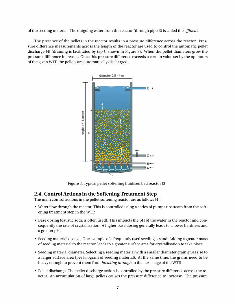
of the seeding material. The outgoing water from the reactor (through pipe E) is called the effluent.

The presence of the pellets in the reactor results in a pressure difference across the reactor. Pres-sure difference measurements across the length of the reactor are used to control the automatic pelletdischarge [4] (draining is facilitated by tap C shown in Figure 3). When the pellet diameters grow thepressure difference increases. Once this pressure difference exceeds a certain value set by the operatorsof the given WTP, the pellets are automatically discharged.

Figure 3: Typical pellet softening fluidised bed reactor [3].

2.4. Control Actions in the Softening Treatment StepThe main control actions in the pellet softening reactor are as follows [4]:

• Water flow through the reactor. This is controlled using a series of pumps upstream from the soft-ening treatment step in the WTP.

• Base dosing (caustic soda is often used). This impacts the pH of the water in the reactor and con-sequently the rate of crystallisation. A higher base dosing generally leads to a lower hardness anda greater pH.

• Seeding material dosage. One example of a frequently used seeding is sand. Adding a greater massof seeding material to the reactor, leads to a greater surface area for crystallisation to take place.

• Seeding material diameter. Selecting a seeding material with a smaller diameter grain gives rise toa larger surface area (per kilogram of seeding material). At the same time, the grains need to beheavy enough to prevent them from breaking through to the next stage of the WTP.

• Pellet discharge. The pellet discharge action is controlled by the pressure difference across the re-actor. An accumulation of large pellets causes the pressure difference to increase. The pressure

7

difference threshold value can be adjusted by the operator at a certain WTP. Increasing the thresh-old value leads to a lower discharge rate. Thereby, leading to an increase in the size of the pelletsin the pellet-bed and consequently less surface area for crystallisation to occur. Moreover, it cancause blockages in the reactor, due to a decrease in the porosity of the pellet-bed. Conversely, de-creasing the threshold value increases the frequency of discharges, generally leading to pellets witha lower diameter in the bed. An increase in discharges, requires more seeding material to be addedto the reactor, therefore leading to higher softening treatment costs.

2.5. pH as a Control VariableThe pH describes the acidity or alkalinity of a solution and common values range from 0 to 14, where

7 indicates neutrality of the solution (at 25C). Values less than 7 (at 25C and a certain salinity) impliesan acid solution and greater than 7 (at 25C and a certain salinity) an alkaline solution. More formally,the pH is the decadic logarithm (logarithm with base 10) of the reciprocal of the hydrogen activity in a so-lution, where the hydrogen ion activity is denoted as aH+ and is described by the following mathematicalformula:

pH =−log10(aH+) = log10(1

aH+).

Once the pellets tend to saturation, less calcium carbonate is able to crystallise onto the pellets. Lead-ing to surplus caustic soda in the reactor and an increase in pH. Consequently, the effluent becomesharder, due to less metal ions being removed from the water. Therefore, an increase in pH gives a goodindication of when the pellets should have been drained.

A high pH in the reactor could kill the bacteria in the downstream biofilters, if the acid dosing down-stream from the softening reactor is not able to lower the pH sufficiently. The biofilters are required toeliminate dissolved organic compounds in the water. Moreover, reactions involving caustic soda down-stream from the reactor could occur, if the pH is too high after the acid dosing step.

8

Chapter 3: Data Pre-Processing and Data Analysis

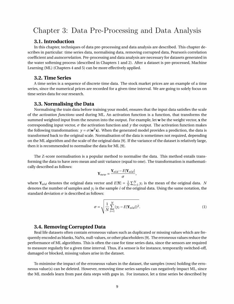
3.1. IntroductionIn this chapter, techniques of data pre-processing and data analysis are described. This chapter de-

scribes in particular: time series data, normalising data, removing corrupted data, Pearson’s correlationcoefficient and autocorrelation. Pre-processing and data analysis are necessary for datasets generated inthe water softening process (described in Chapters 1 and 2). After a dataset is pre-processed, MachineLearning (ML) (Chapters 4 and 5) can be more effectively applied.

3.2. Time SeriesA time series is a sequence of discrete time data. The stock market prices are an example of a time

series, since the numerical prices are recorded for a given time interval. We are going to solely focus ontime series data for our research.

3.3. Normalising the DataNormalising the train data before training your model, ensures that the input data satisfies the scale

of the activation functions used during ML. An activation function is a function, that transforms thesummed weighted input from the neuron into the output. For example, let w be the weight vector, x thecorresponding input vector, σ the activation function and y the output. The activation function makesthe following transformation: y = σ(wTx). When the generated model provides a prediction, the data istransformed back to the original scale. Normalisation of the data is sometimes not required, dependingon the ML algorithm and the scale of the original data [9]. If the variance of the dataset is relatively large,then it is recommended to normalise the data for ML [9].

The Z-score normalisation is a popular method to normalise the data. This method entails trans-forming the data to have zero mean and unit variance (equal to one). The transformation is mathemati-cally described as follows:

Ynew = Yol d −E [Yol d ]

σ,

where Yol d denotes the original data vector and E [Y] = 1N

∑Ni=1 yi is the mean of the original data. N

denotes the number of samples and yi is the sample i of the original data. Using the same notation, thestandard deviation σ is described as follows:

σ=√√√√ 1

N

N∑i=1

(yi −E [Yol d ])2. (1)

3.4. Removing Corrupted DataReal life datasets often contain erroneous values such as duplicated or missing values which are fre-

quently encoded as blanks, NaNs, null-values, or other placeholders [9]. The erroneous values reduce theperformance of ML algorithms. This is often the case for time series data, since the sensors are requiredto measure regularly for a given time interval. Thus, if a sensor is for instance, temporarily switched-off,damaged or blocked, missing values arise in the dataset.

To minimise the impact of the erroneous values in the dataset, the samples (rows) holding the erro-neous value(s) can be deleted. However, removing time series samples can negatively impact ML, sincethe ML models learn from past data steps with gaps in. For instance, let a time series be described by

9

yt = αyt−1 +βut , where y is the output, u the input and t the present time step. If time step t − 1 isremoved from the dataset, then the previous time step t −2 is used instead (if it is not also removed fromthe dataset), i.e. the equation becomes yt = αyt−2 +βut . Therefore, the value yt−1 is skipped, leadingto a gap in the information fed into the ML algorithms. In addition, if the number of corrupted sam-ples is relatively large, it is generally better to find a way to save as many samples as possible, becausethe data could hold important information about the system. Data samples can be saved by replacingthe erroneous values with interpolated values. Interpolation means estimating data values based onknown sequential-data. Another technique, is to set the missing values to a constant number, such as0 or a large negative value, depending on the dataset. The idea is that the ML algorithm will ignore theirregular values (outliers) when training the model. All of the methods explained should be taken intoconsideration when cleaning a particular dataset. One method is likely to perform better than the restfor a given dataset and can often be deduced from knowledge about the system.

3.5. Pearson’s Correlation CoefficientThe Pearson’s correlation coefficient measures the degree of correlation between two variables. The

coefficient (denoted ρ) satisfies −1 ≤ ρ ≤ 1, where 1 indicates strong positive correlation and −1 strongnegative correlation. If magnitude of the coefficient is relatively low, then the correlation is consideredweak between the two variables. A value of 0 indicates that there is no correlation whatsoever. Pearson’scorrelation coefficient is described by the following formula:

ρX,Y = cov(X,Y)

σXσY,

where ρX,Y signifies the Pearson’s correlation coefficient between vectors X and Y, cov(X,Y) = 1N

∑Ni=1(xi −

E [X])(yi −E [Y]) is the covariance between X and Y. N symbolises the number of samples, the vector pair(X,Y) takes on values (xi , yi ) and E [X] (E [Y]) is the expected value (mean) of X (Y). Furthermore, σX andσY represent the standard deviation of X and Y respectively and are calculated as described in equation(1).

3.6. AutocorrelationAutocorrelation is the degree of similarity between a given time series and a lagged version of itself

over successive time intervals [18]. It can be likened to calculating the correlation between two differenttime series, except autocorrelation employs the same time series twice, i.e. a lagged version and anoriginal. The autocorrelation is defined as follows:

ρτ =∑N−τ

t=τ+1(xt−τ−E [X])(xt − [X])∑Nt=1(xt −E [X])2

,

where τ (∈N\0) is the lag and xt is a sample of vector X. E [X] the mean of vector X and N the numberof samples of the variable.

10

Chapter 4: Machine Learning4.1. IntroductionIn this chapter, key basic Machine Learning (ML) principles are explained. These explanations en-

compass: overfitting and underfitting, hyperparameters, supervised learning, two data splitting tech-niques and ML evaluation metrics. The resulting pre-processed data (described in Chapter 3), needs tobe partitioned before applying ML algorithms. Afterwards, so-called hyperparameters can be tacticallyselected for the given ML algorithm. Finally, the resulting ML model requires a performance evaluationusing evaluation metrics. In the ML research domain, a feature refers to an input of the ML model andthe target is the output.

4.2. Supervised Learning

Figure 4: Supervised learning spam identification example. Takenfrom [26].

Supervised learning is whenyou feed your ML algorithm withexample input-output training datapairs. The ML algorithm then gen-erates a function (model) that isable to map the input to the out-put, i.e. Y = f (X), where Y is theoutput, f a function and X the in-put. On the other hand, unsu-pervised learning is when the ex-ample data fed into the algorithmdoes not include a correspondingoutput (only input training data),that it can learn from. Therefore,unsupervised learning learns onlyfrom the input X and the corre-sponding output Y is unknown.In this research, only supervisedlearning algorithms are implemented, because time series forecasting ML models use supervised learn-ing.

An example of supervised learning is illustrated in Figure 4. In this example, the aim is to differentiatebetween the spam emails and the emails that do not contain spam. The computer is able to learn fromprevious emails with a corresponding email label, not spam or spam. The spam labels are considered tobe the output Y. Implementing ML via the computer, generates the function f and can be subsequentlyused to classify new emails, where input X consists of the email features and the corresponding outputsconsist of a prediction of the spam label.

Two possible data splitting methods for supervised ML are: train-validation-test and walk-forward.The train-validation-test is the most commonly used data splitting method amongst data scientists. Thewalk-forward method was originally designed by the financial trading industry and is these days fre-quently applied on a variety of time series datasets.

4.2.1. Train-Validation-Test Data Splitting MethodFor the train-validation-test data splitting method, the dataset is partitioned into a train-validation-

test data split (as illustrated in Figure 5). The train partition is used for training during the implementa-

11

tion of the ML algorithm. The validation data is used to evaluate the model during training and allowsyou to effectively tune the hyperparameters (explained in Section 4.3.). Checking the model against thevalidation data allows you to identify if the model is overfitting on the training dataset. The test partitionconsists of the data used to determine the final performance of the created ML model.

Figure 5: Train-validation-test data split.

A data split of 80% train data and 20% test data isoften selected as a starting point, where a partition ofvalidation data is not considered a necessity. An ad-justment of the data split could be deemed necessarybased on the amount of data available. For instance, ifthere is a large quantity of data available, then a higherpercentage can be allocated to the training dataset, since there is considered to be enough test data.

4.2.2. Walk-forward Data Splitting Method

Figure 6: Walk-forward.

The walk-forward validationstrategy is used exclusively fortime series data analysis. For thisstrategy, the data is split into win-dows. Each window has the sametrain-test data split. The train datacontains the features (inputs) andtarget (output) for a given time pe-riod. The test data holds the targetdata (outputs) for a time periodfollowing the respective train datatime period. The following win-dow is the same length and shiftedin time by the length of the testset. This data splitting techniqueis illustrated in Figure 6. A modelis generated for each set of win-dowed data. The respective model gives a prediction based on the training data and this can be com-pared against the test data to measure the performance of the model.

Applying the walk-forward validation strategy is useful to validate whether the hyperparameters needto be adjusted to improve the performance of the ML algorithm, since the computation times to gener-ate a model can be considerably lower than the computation times of the train-validation-test method,depending on the length of the window selected. Moreover, the water softening treatment methods canvary in a Water Treatment Plant (WTP) over the course of time, thus the walk-forward validation strategyis able to cope better with these changes by training the given model on only the most recent window ofdata. For example, the caustic soda dosing method could be altered for a certain WTP.

4.3. Hyperparameters and Hyperparameter Grid SearchesA hyperparameter is a parameter of a learning algorithm and external to the model [6]. The hyperpa-

rameters are fixed during training of the ML model. A few examples of hyperparameters are: the numberof layers in a NN, the amount of neurons in a layer, the type of activation function used in each layer andthe learning rate.

12

The enormous size of potential hyperparameter combinations to train your NN can become over-whelming. To mitigate this problem, it is helpful to use a hyperparameter grid search. This methoditerates through a set of hyperparameter combinations and calculates the optimum combination basedon evaluation metrics (explained in Section 4.5). Thus, sparing the user from having to manually inputnew hyperparameters and noting the evaluation metrics at the end of each ML training run. Naturally,there are an infinite number of combinations and the search can only analyse a small portion, due to thecomputation times.

4.4. Overfitting and UnderfittingOverfitting occurs when a model is generated via Machine Learning (ML) and the resulting model

models the training data too closely. In other words, “overfitting happens when a model learns the detailand noise of the training data to the extent that it negatively impacts the performance of the model onnew data" (J. Brownlee, 2016) [12]. Thus, the noise or random fluctuations of the training set are learntas concepts by the model. The resulting model is then not able to generalise as well and therefore is notas effective at dealing with new data.

Overfitting can be reduced by increasing the amount of training data, applying regularisation tech-niques to the ML algorithms or by reducing the size of the neural network.

Underfitting occurs when a model is unable to model the training data nor generalise to new data.A model is said to generalise well to new data, when it is able to make an relatively accurate predictionbased on the new data as input. In terms of the two evaluation metrics introduced in Section 4.5, theMSE would be relatively low and the R-squared value close to a positive value of one.

4.5. Evaluation MetricsOnce a model has been created by implementing ML on the training data, a prediction is made us-

ing the model. This prediction is then compared against the test data for an indication of model per-formance. To be able to effectively determine the performance, it is helpful to use a model evaluationmetric. Two popular evaluation metrics, R-squared and Mean Squared Error (MSE), are described in Sub-sections 4.5.1. and 4.5.2. respectively.

It is more effective to use multiple indicators in conjunction, since a single indicator is unable to givea full explanation of the model performance, due to each individual indicator having its pros and cons(Krause et al., 2015) [16].

4.5.1. R-squaredR-squared, also known as coefficient of determination is a statistical measure of the distance between

the data and the regression predictions. In other words, the R-squared metric measures the proportion ofvariance of the actual data points that is described by a model prediction. The mathematical definitionis [9]:

R2 ≡ 1− SSr es

SStot,

where SStot =∑i (yi −E [Y])2 is the total sum of squares (variance multiplied by the number of data points

in the dataset) and Y is the vector of data points yi (with i ∈N\0). E [Y] = 1N

∑Ni=1 yi denotes the mean

of the dataset, where N (∈N\0) is the number of data points in the dataset. SSr es = ∑i (yi − fi )2 ( fi is a

given predicted value) represents the residual sum of squares.

13

If R2 = 1, the regression prediction fits the actual data points perfectly. On the other hand, R2 = 0implies that none of the variability of the data points is explained by the prediction around the meanof the data points. Thus, the ultimate aim is to minimise SSr es . A value outside the range 0 to 1 occurswhen the model fits the data worse than the mean horizontal hyperplane (mean for each dimension).This could indicate that the model is not an appropriate fit for the data.

4.5.2. Mean Squared Error (MSE)The MSE measures the average of the errors squared, where the error is the difference between the

actual data point and the data point generated by the model. As a mathematical function, the MSE isrepresented as follows:

MSE = 1

N

N∑i=1

(yi − fi )2,

where N is the number of predictions, yi the actual data point at index i (∈ 1, ..., N ) and fi the predicteddata point at index i .

One criticism of MSE, is that the outliers are heavily weighted. On the other hand, MSE is widelyrecognised as one of the best error functions.

14

Chapter 5: Neural Networks and XGBoost

5.1. IntroductionIn this chapter, Neural Networks (NNs) and the eXtreme Gradient Boost (XGBoost) algorithm are de-

scribed. NNs and XGBoost algorithms are often used for Machine Learning (ML) using time series data,since they are able to incorporate relations between past and current time steps in the resulting model.For improved results, the dataset should be pre-processed using techniques described in Chapter 3 andsplit employing the two splitting techniques in Chapter 4. A resulting NN (or XGBoost) model can beevaluated using the evaluation metrics described in Section 4.6. If the evaluation metrics results are notsatisfactory, adjusting the NN (or XGBoost) hyperparameters (described in Chapter 4) can lead to an im-proved NN (or XGBoost) model. Subsections 5.2.1, 5.2.2, 5.2.3.1 and 5.2.3.2 are largely based on Chapters11 and 14 from Hands-On Machine Learning with Scikit-Learn & TensorFlow, published by A. Géron in2017 [6].

5.2. Neural Networks

Figure 7: Simple network.

NNs are comprised of layers of neurons withweights interlinking them. A simple NN structurecan be observed in Figure 7. The orange circlessymbolise the bias neurons, the blue circles repre-sent the hidden neurons, the green circles the in-put neurons and the purple circles denote the out-put neurons. The symbol a3

1 denotes the activa-tion function of the first neuron in the third layer.There is one hidden layer in this example. TheNN in Figure 7 is a feedforward network, since theconnections are in a forward direction, i.e. in thedirection of the output. The bias (orange circlesin Figure 7) neurons are not dependent on previ-ous layers. The purpose of the bias is to create adesired shift in the activation function of a givenlayer and ultimately generate a better performingmodel. In this research, a more sophisticated NN, Recurrent Neural Network (RNN), is employed.

5.2.1. Recurrent Neural Networks (RNNs)

Figure 8: RNN over time.

A recurrent network is almost iden-tical to a feedforward network, except ithas also connections in a backwards di-rection. The diagram of a RNN mappedagainst a time axis can be seen in Figure8.

For the example feedforward casefor a single neuron and a single in-stance, the output is described as

y (t ) =φ(

xT(t ) ·w x +b

),

whereφ represents the given activation function, w x the weight for the input x and b is the bias constant.

15

In comparison the RNN output for a single neuron and single time instance is given by

y (t ) =φ(

xT(t ) ·w x + y T

(t−1) ·w y +b),

where y (t−1) symbolises the output of the previous time step and w y is the corresponding weight. Thetraining data is split into batches and each batch is referred to as a mini-batch. This formula can be ex-tended to accommodate multiple recurrent neurons for all instances in a mini-batch, using a vectorisedform of the previous equation [6]

Y (t ) =φ(

X (t ) ·W x +Y (t−1) ·W y +b).

• Y (t ) is a m ×nneur ons matrix containing the layer’s outputs at time step t for each instance in themini-batch, where m is the number of instances in the mini-batch and nneur ons the number ofneurons in the layer.

• X (t ) is a m×ni nput s matrix containing the inputs for all instances, where ni nput s denotes the num-ber of inputs.

• W x is a ni nput s ×nneur ons matrix containing the connection weights for the inputs of the currenttime step.

• W y is a nneur ons ×nneur ons matrix containing the connection weights for the outputs of the previ-ous time step.

• b is a vector of size nneur ons containing each neuron’s bias term.

Notice that Y (t ) depends on X (t ) and Y (t−1), which in turn is dependant on X (t−1) and Y (t−2), which isdependant on X (t−2) and Y (t−3) and so forth. Therefore, Y (t ) is a function of all inputs from time t = 0,i.e. X (0), X (1), X (2), X (3), ..., X (t ). At t = 0 it is assumed that there are no previous outputs and are taken tobe zeros.

5.2.2. Memory Cells

Figure 9: Memory cell.

The accumulation of outputs at arecurrent neuron from the previoustime steps, can be likened to storingmemories. A component of a NN thatpreserves some state across time stepsis called a memory cell.

Mathematically, a cell’s state is rep-resented as h(t ) = f (h(t−1), x (t )) [6].Thus, depending on the input vector ofthe current time step and the memorystate of the previous time step. The vec-tor h stands for "hidden". As a result,the output at time step t , denoted by y (t ) = z(h(t−1), x (t )), is a function of the previous memory state andthe current inputs. A diagram representation of a memory cell is shown in Figure 9. The left hand sideimage displays a memory cell. The right hand side shows the pattern of a memory cell over time.

16

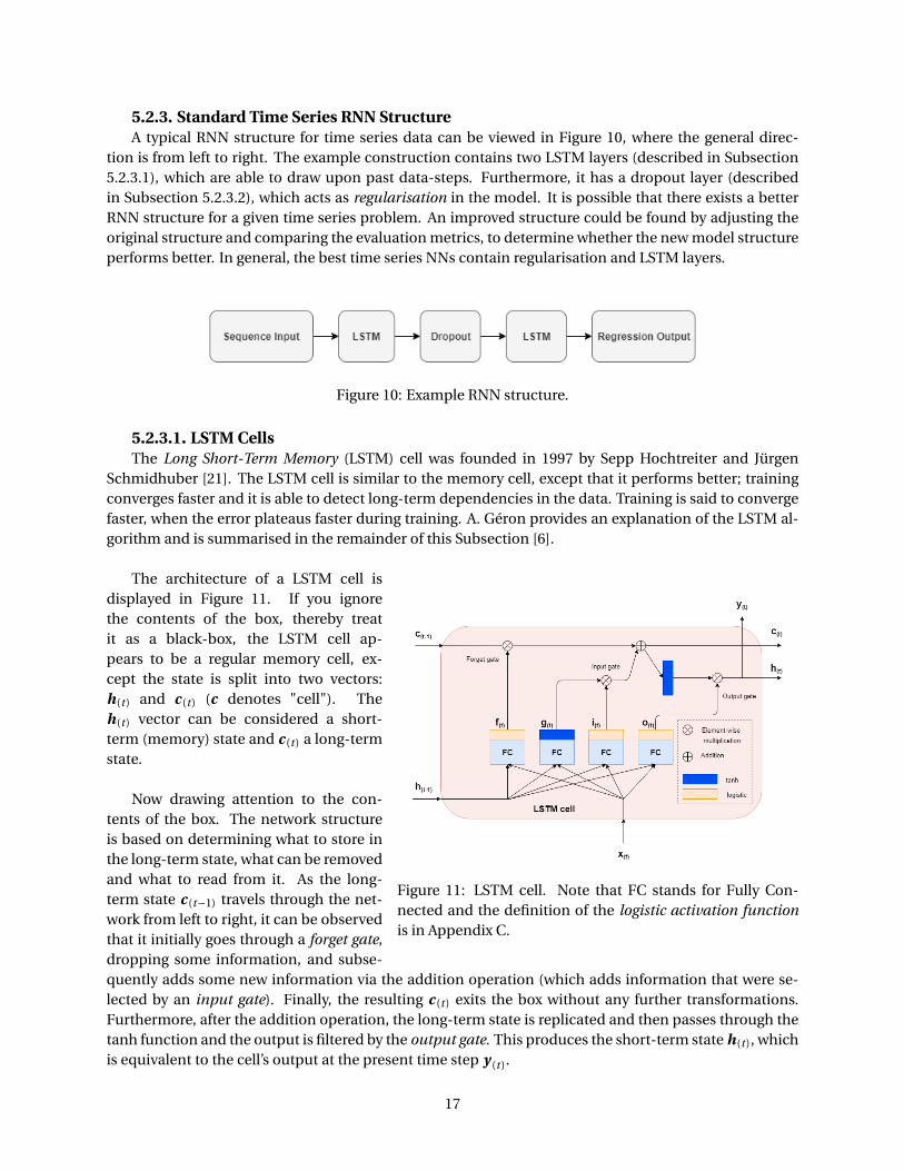
5.2.3. Standard Time Series RNN StructureA typical RNN structure for time series data can be viewed in Figure 10, where the general direc-

tion is from left to right. The example construction contains two LSTM layers (described in Subsection5.2.3.1), which are able to draw upon past data-steps. Furthermore, it has a dropout layer (describedin Subsection 5.2.3.2), which acts as regularisation in the model. It is possible that there exists a betterRNN structure for a given time series problem. An improved structure could be found by adjusting theoriginal structure and comparing the evaluation metrics, to determine whether the new model structureperforms better. In general, the best time series NNs contain regularisation and LSTM layers.

Figure 10: Example RNN structure.

5.2.3.1. LSTM CellsThe Long Short-Term Memory (LSTM) cell was founded in 1997 by Sepp Hochtreiter and Jürgen

Schmidhuber [21]. The LSTM cell is similar to the memory cell, except that it performs better; trainingconverges faster and it is able to detect long-term dependencies in the data. Training is said to convergefaster, when the error plateaus faster during training. A. Géron provides an explanation of the LSTM al-gorithm and is summarised in the remainder of this Subsection [6].

Figure 11: LSTM cell. Note that FC stands for Fully Con-nected and the definition of the logistic activation functionis in Appendix C.

The architecture of a LSTM cell isdisplayed in Figure 11. If you ignorethe contents of the box, thereby treatit as a black-box, the LSTM cell ap-pears to be a regular memory cell, ex-cept the state is split into two vectors:h(t ) and c (t ) (c denotes "cell"). Theh(t ) vector can be considered a short-term (memory) state and c (t ) a long-termstate.

Now drawing attention to the con-tents of the box. The network structureis based on determining what to store inthe long-term state, what can be removedand what to read from it. As the long-term state c (t−1) travels through the net-work from left to right, it can be observedthat it initially goes through a forget gate,dropping some information, and subse-quently adds some new information via the addition operation (which adds information that were se-lected by an input gate). Finally, the resulting c (t ) exits the box without any further transformations.Furthermore, after the addition operation, the long-term state is replicated and then passes through thetanh function and the output is filtered by the output gate. This produces the short-term state h(t ), whichis equivalent to the cell’s output at the present time step y (t ).

17

The next step is explaining the origin of the new memories and how the gates function. Firstly, cur-rent input vector x (t ) and the previous short-term state h(t−1) are fed to four different fully connectedlayers. Each fully connected layer has its own function:

• The main layer outputs vector g (t ). It analyses the current inputs x (t ) and the previous short-termstate h(t−1). In a standard memory cell (as described in Subsection 5.2.2), there exist no otherneuron layers and its output goes straight out to y (t ) and h(t ). In contrast, in an LSTM cell thislayer’s output is instead partly stored in the long-term state.

• The remaining three neuron layers are so-called gate controllers. There outputs range from 0 to 1,since they make use of the logistic activation function (see Appendix C for the definition). Noticethat their outputs are fed to element-wise multiplication operations. Therefore, if they output 0s,the gate is closed and 1s as output, opens the gate. In more detail:

– The forget gate (controlled by f (t )) controls which time steps of the long-term state should beremoved.

– The input gate (controlled by i (t )) controls which time steps of g (t ) should be added to thelong-term state.

– The output gate (controlled by o(t )) controls which time steps of the long-term state shouldbe read and added to the output at the current time step (for both y (t ) and h(t )).

In summary, a LSTM cell is able to learn to recognise an important input (that is the role of the inputgate), store it in the long-term state, learn to preserve it for as long as it is necessary (that is the role of theforget gate) and learn to extract it whenever it is required. This explains why LSTM are very successful incapturing long-term patterns in time series.

5.2.3.2. Regularisation using a Dropout Layer

Figure 12: Dropout layer.

Regularisation is implemented to reduce overfit-ting. A frequently used regularisation technique fordeep (many layered) NNs is dropout. It was proposedby G. E. Hinton in 2012 and subsequently a paper waspublished giving greater detail by Nitish Srivastava etal. in 2014 [22].

At every training step, every neuron (includingthe input neurons, but excluding the output neu-rons) has probability p of being briefly "droppedout". In other words, it will be completely ignoredduring the current training step, but has the poten-tial to be active during the next step. This algorithm isshown in Figure 12. Note that the green circles repre-sent the input neurons, the blue circles represent thehidden layer neurons and the orange circles symbol-ise the bias neurons. A cross in the neurons indicatesthat the neuron is not active for that time step. Thehyperparameter p is called the dropout rate and is usually set to 50%. The neurons are not dropped oncethe training is finished. The purpose of this method is to reduce the co-dependencies in the network,

18

thus reducing overfitting.

5.2.4. Gradient Descent

Figure 13: Gradient descent.

The gradient descent algorithm isa frequently used method to updatethe weights of the network. Generally,it is a iterative optimisation algorithmfor finding the minimum of a function.The algorithm adjusts the weight with astep proportional to the negative gradi-ent of the cost function at a given itera-tion. A diagram of a visual representa-tion of gradient descent is depicted inFigure 13. The vector of the networkweights is updated using the followingformula:

w (i ) = w (i−1) −η∇C (w (i−1)), (2)

where i is the current time step and η isthe learning rate hyperparameter. The∇C (w (i−1)) part of the second term can be determined using backpropagation (see Appendix SectionC.3. for more information). A faster gradient optimiser is RMSProp and is explained in Appendix SectionC.2.

There are two different algorithms that can be used to apply Gradient Descent on our training data:Stochastic Gradient Descent and Batch Gradient Descent. The Stochastic Gradient Descent algorithmuses equation (2) to update the weights of the network and the gradient for every training sample. Onthe other hand, the Batch Gradient Descent algorithm updates the weights only when all the trainingsamples have been fed into the network, therefore using formula (2) only once.

19

5.3. XGBoost

5.3.1. Introduction to Decision TreesA decision tree is defined by R. S. Brid (2018) as follows [15]:

A decision tree is a decision support tool that uses a tree-likegraph or model of decisions and their possible consequences,including chance event outcomes, resource costs, and utility.It is one way to display an algorithm that only contains condi-tional control statements.

5.3.2. Difference between Classification and Regression Trees

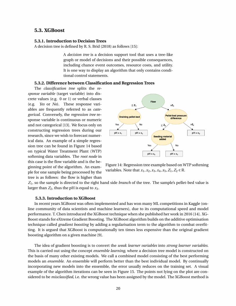
Figure 14: Regression tree example based on WTP softeningvariables. Note that x1, x2, x3, x4, x5, Z1, Z2 ∈R.

The classification tree splits the re-sponse variable (target variable) into dis-crete values (e.g. 0 or 1) or verbal classes(e.g. Yes or No). These response vari-ables are frequently referred to as cate-gorical. Conversely, the regression tree re-sponse variable is continuous or numericand not categorical [13]. We focus only onconstructing regression trees during ourresearch, since we wish to forecast numer-ical data. An example of a simple regres-sion tree can be found in Figure 14 basedon typical Water Treatment Plant (WTP)softening data variables. The root node inthis case is the flow variable and is the be-ginning point of the algorithm. An exam-ple for one sample being processed by thetree is as follows: the flow is higher thanZ1, so the sample is directed to the right hand side branch of the tree. The sample’s pellet-bed value islarger than Z2, thus the pH is equal to x3.

5.3.3. Introduction to XGBoostIn recent years XGBoost was often implemented and has won many ML competitions in Kaggle (on-

line community of data scientists and machine learners), due to its computational speed and modelperformance. T. Chen introduced the XGBoost technique when she published her work in 2016 [14]. XG-Boost stands for eXtreme Gradient Boosting. The XGBoost algorithm builds on the additive optimisationtechnique called gradient boosting by adding a regularisation term to the algorithm to combat overfit-ting. It is argued that XGBoost is computationally ten times less expensive than the original gradientboosting algorithm on a given machine [9].

The idea of gradient boosting is to convert the weak learner variables into strong learner variables.This is carried out using the concept ensemble learning, where a decision tree model is constructed onthe basis of many other existing models. We call a combined model consisting of the best performingmodels an ensemble. An ensemble will perform better than the best individual model. By continuallyincorporating new models into the ensemble, the error usually reduces on the training set. A visualexample of the algorithm iterations can be seen in Figure 15. The points not lying on the plot are con-sidered to be misclassified, i.e. the wrong value has been assigned by the model. The XGBoost method is

20

described in more detail in Appendix D.

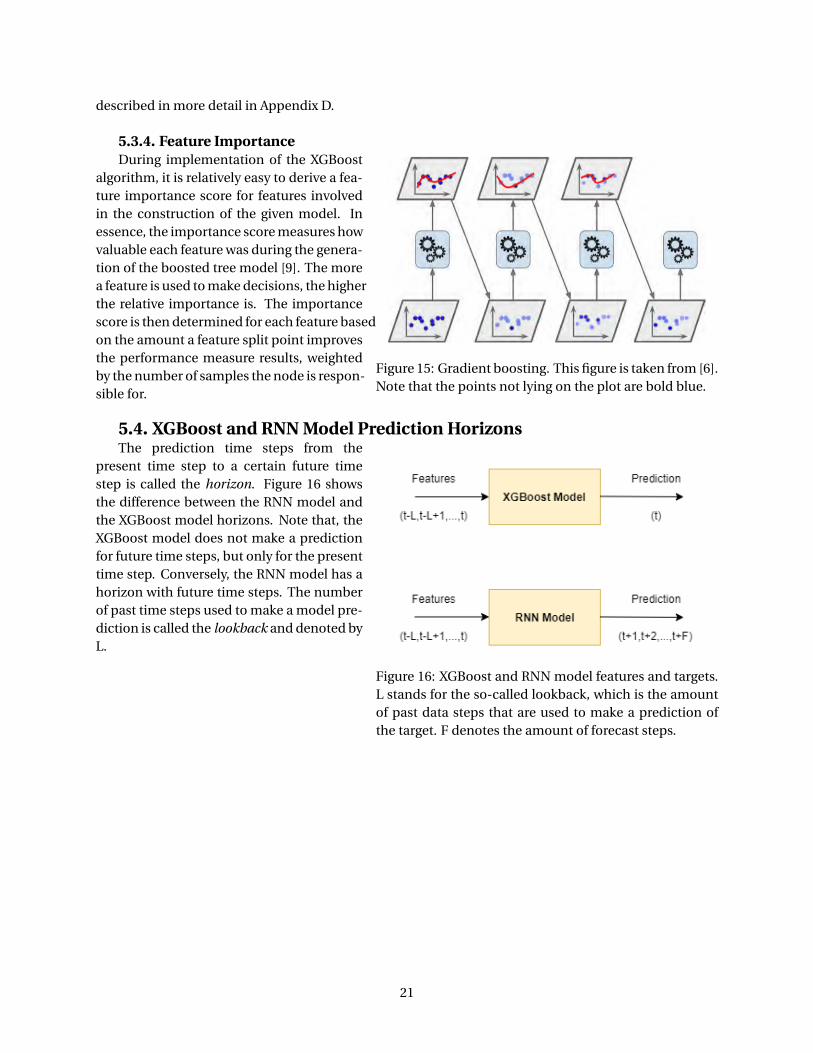
Figure 15: Gradient boosting. This figure is taken from [6].Note that the points not lying on the plot are bold blue.

5.3.4. Feature ImportanceDuring implementation of the XGBoost

algorithm, it is relatively easy to derive a fea-ture importance score for features involvedin the construction of the given model. Inessence, the importance score measures howvaluable each feature was during the genera-tion of the boosted tree model [9]. The morea feature is used to make decisions, the higherthe relative importance is. The importancescore is then determined for each feature basedon the amount a feature split point improvesthe performance measure results, weightedby the number of samples the node is respon-sible for.

5.4. XGBoost and RNN Model Prediction Horizons

Figure 16: XGBoost and RNN model features and targets.L stands for the so-called lookback, which is the amountof past data steps that are used to make a prediction ofthe target. F denotes the amount of forecast steps.

The prediction time steps from thepresent time step to a certain future timestep is called the horizon. Figure 16 showsthe difference between the RNN model andthe XGBoost model horizons. Note that, theXGBoost model does not make a predictionfor future time steps, but only for the presenttime step. Conversely, the RNN model has ahorizon with future time steps. The numberof past time steps used to make a model pre-diction is called the lookback and denoted byL.

21

Chapter 6: Methods

6.1. IntroductionIn this chapter, the methods of implementing the two ML algorithms introduced in Chapter 5 are

explained as preparation for the interpretation of results featured in the following chapter. Firstly, theinputs and output of the desired model are identified, based on the importance of the variables to thewater softening treatment process. Next, the data collection method is described, where a data time in-terval is decided upon. Subsequently, the data is pre-processed using theory specified in Chapters 3 and4. Finally, the methods used in the ML prediction phase are described, where the algorithms describedin Chapter 5 are implemented.

6.2. Identification of Inputs and OutputsBefore requesting drinking water softening data from the water company, the potential input(s) and

output(s) are identified.

The selection of inputs and outputs is limited, due to a lot of pertinent variables in the given WaterTreatment Plant’s (WTP’s) softening process not being measured. For instance, the hardness is not mea-sured in the softening process, since there are no installed sensors in the softening process. The hardnessis instead constantly measured at the end of the WTP treatment process by a sensor.

In Machine Learning, the output is commonly referred to as the target. The target was identifiedas the pH in the softening process, since it has promising properties for control (as seen in Chapter 2).Based on availability of data and relevance to the pH (output), the inputs are chosen as: caustic soda flow,bottom pressure, pellet-bed pressure, bed height, draining and seeding. The relevance of the variableswas assessed, by discussing the pertinent data with a process engineer from the given WTP. The inputsare called features in the ML domain. A description of the features and target are as follows:

• Flow refers to the water flow rate travelling through the softening reactor [m3/h].

• Caustic Soda Flow (feature) is the flow rate of the caustic soda dosing into the pellet-bed reactor[m3/h].

• Bottom Pressure (feature) refers to the pressure measured at the bottom of the reactor [kPa].

• Pellet-bed Pressure (feature) refers to the pressure difference measured across the pellet-bed[kPa].

• pH (target and RNN feature) indicates the pH within the reactor.

• Bed Height (feature) represents the height of the pellet-bed [cm].

• Draining (feature) is the time at which the reactor drains an amount of pellets, i.e. when thepressure difference threshold across the reactor is exceeded.

• Seeding (feature) is the time at which the reactor is seeded.

The flow variable is removed from the dataset for ML after the analysis shown in Subsection 6.4.1 iscarried out, which indicates that the caustic soda flow is strongly dependent on the flow.

22

6.3. Data Collection

6.3.1. Data Storage

Figure 17: Data interpolation method. The redpoints denote the recorded data points and thegreen the disregarded data readings.

The data is recorded live in the water com-pany’s system, using an interpolation method. Itis possible to extract data from the system byspecifying a time interval. This data is then sub-sequently transferred to an Excel document. Nat-urally, a smaller time interval for a requestedperiod of time leads to more data points, thuscosting more computation time to upload thedata.

In order to reduce the amount of saved dataon the water company’s storage drives, interpola-tion is applied on the live data readings before be-ing saved. The system adopted by the water com-pany, records a value when it falls outside bound-aries set by the WTP operator. For example, an operator may set the boundaries to 2% of the previouslyrecorded value. Once a value falls outside the boundaries and is therefore recorded, interpolation isapplied between the current recorded value and the previous one. This method of interpolation usingboundaries can be viewed in Figure 17.

6.3.2. Time Interval SelectionFirstly, a day’s worth of data with a time interval of one second is analysed, to ascertain which time

interval would be appropriate to use for ML implementation. The time interval of one second seemsto be unnecessarily low, because the data is interpolated (based on the method described in Subsection6.3.1). Therefore, there is not a large loss of data information if a slightly larger time interval is selected.Deciding upon a one minute time interval, provides satisfactory retention of data information and lowcomputation times.

Once the time interval, inputs and output are selected, a year’s data is extracted from the systemfor ML implementation. A year’s data provides enough information about the patterns of the softeningprocess to train a ML model, since the seasons are not a large contributor to the dynamics of the watersoftening treatment process. For example, one of the most influential seasonal variables is the watertemperature. The water temperature remains relatively constant throughout the whole of the WTP, dueto there being always a large volume of water within the WTP at a given moment. Moreover, the WTP isinsulated, so that the outside temperature does not have a substantial impact on the temperature insidethe WTP. Typically, the temperature of the water in the WTP is largely determined by the temperature ofthe water at the source (collection point). On average the temperature is around 14C throughout theyear for the given WTP and is often two degrees higher or lower if the average is taken in the summer orwinter respectively.

6.4. Data Pre-Processing and Data AnalysisThe pre-processing and analysis in this section is conducted using the Python packages: NumPy,

Pandas and StatsModels.

23

6.4.1. Erroneous Values and Variable DependenciesLooking at Figure 22 on page 28, it is clear that the sensors are not recording sensible values (or are

turned off) for irregular time intervals. For instance on 2 February, all the readings displayed in Figure22 drop to zero, apart from pH, which instead falls in value considerably. The drop in the pH, could beexplained by no caustic soda being dosed, which typically increases the pH. During these periods, it isalso notable that no draining and seeding actions are recorded. This could be due to the reactor beingswitched off. For our machine learning algorithms, the corrupted data readings are removed from thedataset, since it does not describe the operational behaviour within the reactor. Removal of this uninter-esting data, leads to retention of approximately two thirds of the data. The number of retained samplesis considered sufficient to feed into the ML algorithms. The irregular time periods of corrupted readingsspan days. Thus, interpolating within these irregular time periods would not give an accurate represen-tation of the actual values.

Figure 18: Caustic soda dosage flow rate and flow rate. The red plot isthe flow and the blue is the caustic soda flow. The time axis increases inincrements of 12 hours.

After removing the datawith the corrupted sensorreadings, we calculated thePearson’s correlation coeffi-cient matrix for 2018 (seen inTable 7 in Appendix B) to un-derstand the relationship ofthe variables with each other.It can be observed in Table7 that there is strong cor-relation between the caus-tic soda dosing and the flow.This is due to the causticsoda flow being controlledby the flow in the given WTP.Moreover, Figure 18 displays the caustic soda flow on the same plot as the flow over a few days in Febru-ary. By observing Figure 18, it is evident that the caustic soda flow is strongly dependent on the flow.Hence, the water flow in the softening reactor is not included as a feature during ML training. Further-more, caustic soda flow is retained, due to the variable having a greater impact on the pH in the softeningreactor.

6.4.2. Feature RangesThe minimums and maximums of the dataset after the erroneous are removed can be seen in Table 1.

This suggests that the resulting ML model may only be able to give accurate outputs for inputs (features)within these boundaries, since the model is trained using a dataset that stays within these values.

24

Feature Minimum Maximum

Flow 200.6 502.9Caustic Soda Flow 30 95.7Bottom Pressure 5.1 25.5Pellet-bed Pressure 11.3 35.6pH 7.6 9.4Bed Height 298.9 401.6

Table 1: Minimums and maximums of features to one decimal place.

6.4.3. NormalisationNormalisation is applied to the train dataset, using the method explained in Section 3.3 and is only

applied on the dataset used for the RNN ML algorithm, since the algorithm makes use of activationfunctions. Conversely, the XGBoost algorithm does not use activation functions and is based on decisiontrees. Therefore, normalisation of the dataset for the XGBoost algorithm is generally considered unnec-essary [9].

6.4.4. Data SplittingThe data splits for ML algorithms are shown in Table 2. Note that, all the algorithm methods con-

sisted of a 90% train and a 10% test data split, except for the train-validation-test RNN algorithm method.Based on the reasonably high number of samples available from the collected data, only 10% test data isrequired to evaluate the resulting models. Although, for the RNN Train-Validation-Test method, a 65%train, 30% validation and 5% test data split is picked, so that the hyperparameters can be altered duringtraining to improve the model, based on the evaluation metrics of the validation data. This prevents over-fitting on the test dataset, since the hyperparameters are adjusted on the basis of the validation datasetevaluation metric results, instead of on the basis of the test dataset evaluation metric results.

Data Splitting Method XGBoost RNN

Walk-Forward 90% train, 10% test 90% train, 10% testTrain-Validation-Test 90% train, 10% test 65% train, 30% validation, 5 % test

Table 2: Data splits for both algorithms: XGBoost and RNN.

6.4.5. Evaluation Metric SelectionThe two evaluation metrics described in Section 4.6 (MSE and R-squared) are used in conjunction.

Analysing the MSE evaluation metric gives insight into the accumulated error of the actual data pointscompared against the predicted data points. The R-squared provides information about the fit of theprediction relative to the actual data points.

6.4.6. Output Variable AnalysisBefore the prediction, the pH within the softening reactor is analysed. An analysis of the pH is neces-

sary to understand the prediction outputs generated in the following prediction phase (discussed in thefollowing section).

Draining of the pellets in the reactor is often shortly followed by seeding of the reactor (as seen inFigure 22 on page 28). Sometimes during these actions, the pressure difference across the pellet-bed in-creases drastically, since the pellet-bed has been disturbed. Furthermore, draining and seeding actions

25

appear to lead to an immediate decrease in pH, because the saturated pellets are drained and replen-ished with new sand. This increases the surface area, in which crystallisation of sodium carbonate takesplace. Thereby, using up more caustic soda (with typically a pH of about 12).

The autocorrelation plot in Figure 19 of the pH in February 2018, shows that there is a relativelystrong correlation with past time steps of data. Looking at the figure of three days worth of lags, it isevident that the autocorrelation has daily periodicity, where the x-axis consists of the number of minutelags. The daily periodicity can be explained by the draining actions in general occurring at approximatelythe same time of day for most days. This suggests that including past pH readings as a feature would im-prove the model produced through ML.

(a) Autocorrelation of the pH in February2018.

(b) Autocorrelation of the pH in February, dis-playing the three days worth of lags.

Figure 19: The light blue area represents the area bounded by the 95% confidence intervals, where thestandard deviation is calculated using Bartlett’s formula. The x-axis consists of the number of minutelags.

In Figure 20a the mean pH is taken over the period of a day, where time zero is the first time stepafter the draining action. This is calculated by compiling the instances of 24 hours of data after drainingand taking the mean over all the samples for each time step in the 24 hours of compiled instances. In thefirst couple of hours after the draining action, the mean pH plummets, largely due to the sand seedingbeing added to the reactor. The plot then gradually continues to decrease until approximately 18 hoursafter the draining action. At about 22 hours, the pH increases significantly, since the pellets become sat-urated. Figure 20b depicts the mean pH bounded by the maximum and the minimum over the periodof a day. The maximum and minimum are calculated for each time step, using once again the compiled24 hours of data after a draining action. Furthermore, Figure 20b demonstrates the expected boundariesfor a realistic pH prediction, i.e. to stay within the minimum and maximum boundaries over the courseof the subsequent 24 hours after a draining action.

26

(a) Mean pH over one day. Time zero is thefirst time step after the draining action.

(b) Mean pH over one day bounded by themaximum and minimum pH. Time zero is thefirst time step after a draining action.

Figure 20

The box plot of the pH over the length of 24 hours is shown in Figure 21. Information about thekey characteristics of a box plot can be found in Appendix B. It is clear that the pH peaks at about 9:00,since the majority of the draining actions occur at this time (see Figure 34 in Appendix B). Draining andseeding is commonly carried out during working hours, so that operators can oversee the actions andintervene if necessary. The IQR (Interquartile Range) is relatively large at 9:00, thus indicating that thepH readings are more skewed at this time. This could be the result of differing draining amounts. Thedraining action generally drains less than one percent of the pellet-bed in variable amounts. The outliersare the points below or above the bar at a corresponding hour in a box plot. There are many outliers inthe following hours after 9:00, which is possibly due to draining actions sometimes occurring at othermoments in the day or an increase in the flow rate, leading to a higher caustic soda dosage.

Figure 21: pH box plot over hours.

The maximum pH value is 9.4 and the minimum is 7.6, as observed in Table 1. Implying that an ex-pected prediction should stay within these minimum and maximum boundaries.

27

Figure 22: A month of data graphed. The vertical yellow spotted-dashed lines represent a draining actionand the vertical black dashed lines represent a seeding action.

28

6.5. Prediction

6.5.1. ML ImplementationA. Sadad published his thesis about using a general ML framework for time series data [9]. For imple-

mentation of the RNN algorithm, the Python code (using Tensor Flow as backend and Keras as frontend)from A. Sadad has been adapted to give a greater horizon span (forecast length) and to use past data stepsof the target (pH) as a feature.

Colaborative (subsidiary of Google) was used to execute the Python code, due to its free-of-chargeGPU 12GB-RAM, which is significantly faster than the CPU RAM in a standard PC.

6.5.2. Hyperparameter SelectionThe RNN structure adopted is as seen in Figure 10 on page 21, with seven features (inputs). The

hyperparameter, lookback, refers to the amount of past time steps that are used in a ML algorithm (seeSection 5.4). For the RNN implementation, a lookback of 180 minutes was set, based on a balance be-tween computation time and evaluation metric performance. The other hyperparameter choices can befound in Appendix E for the walk-forward and train-validation-test model training.

Training is applied for the forecast lengths: F=1[min], 4[hr] and 24[hr]. This set of forecast lengthsis selected to sufficiently test the limits of the RNN algorithm, i.e. the amount the evaluation metricsdecline in performance as the forecast length is increased.

XGBoost is only able to make a prediction of the present target value based on present and past fea-ture values (as seen in Figure 16). A lookback of 60 minutes (60 past data steps) was selected, based ona compromise between accuracy and computation times. The remaining value choices can be seen inAppendix E and were selected based on the Wastewater Treatment Plant (WWTP) XGBoost implementa-tion by A. Sadad.

6.5.3. Supervised LearningThe predictions are made using the supervised learning training technique (described in Section 4.2)

for both ML algorithms.

29

Chapter 7: Machine Learning Results

7.1. IntroductionIn this chapter, the results of implemented Machine Learning (ML) algorithms, Recurrent Neural

Networks (RNNs) and eXtreme Gradient Boost (XGBoost), are analysed using the evaluation metrics (de-fined in Chapter 3). The ML algorithms make use of the pre-processed data from Chapter 6. Based onthe results, comparisons are drawn between the derived models from both of the data splitting methods:walk-forward and train-validation-test. The pH is selected as the target (output), therefore all the resultsin this chapter feature the pH as the output.

7.2. RNN Results

7.2.1. RNN Train-Validation-Test Model

Figure 23: The last three hours of the RNN train-validation-testmodel prediction.

Figure 24 depicts the predictionof the train-validation-test data splitmodel, where the forecast horizon con-sists of one time step (i.e. F=1[min],where F is defined in Section 5.4) andFigure 23 displays the last three hoursof the prediction. Clearly, the predic-tion lags marginally behind the fluctua-tions of the actual data points. The pre-diction follows the pattern of the testdata closely and is also able to followsharp peaks. Training the model, givesa corresponding MSE equal to 0.0004 (4d.p.) and an R-squared value of 0.9007(4 d.p.). The relative MSE is equal to0.0045% and is calculated by dividing the MSE value by the mean pH across the whole dataset usedfor ML and multiplying by 100.

Figure 24: RNN train-validation-test model (with F=1[min]) prediction.

30

7.2.2. RNN Walk-Forward Models

Model MSE Relative MSE R-squared

0 0.0013 0.0148% 0.63731 0.0009 0.0102% 0.88012 0.0016 0.0182% 0.72693 0.0005 0.0057% 0.86384 0.0017 0.0193% 0.30005 0.0011 0.0125% 0.7678

Table 3: Evaluation metrics for the walk-forward RNN mod-els to 4 decimal places.

Setting the prediction one time stepinto the future (i.e. F=1[min], where Fis defined in Section 5.4), gives the re-sults in Figures 25 and 26. For more de-tail, the first three hours of models 0 and4 are plotted in Figure 27. The predic-tion lags slightly behind the pattern ofthe actual data points. The gaps in dataplots are a result of removing the cor-rupted data values. It can be deduced thatthe predictions follow the real data well,although model 4 appears to be slightlymore shifted above the real data and con-sequently have a lower R-squared value (as seen in Table 3). In general, the predictions follow the patternof the test data relatively closely, including the sharp peaks. For instance model 0 predicts a sharp peakon 25 October in the morning, which exceeds a pH of 9.

Figure 25: The first two RNN walk-forward models (with F=1[min]).

31

Figure 26: The last four RNN walk-forward models.

32

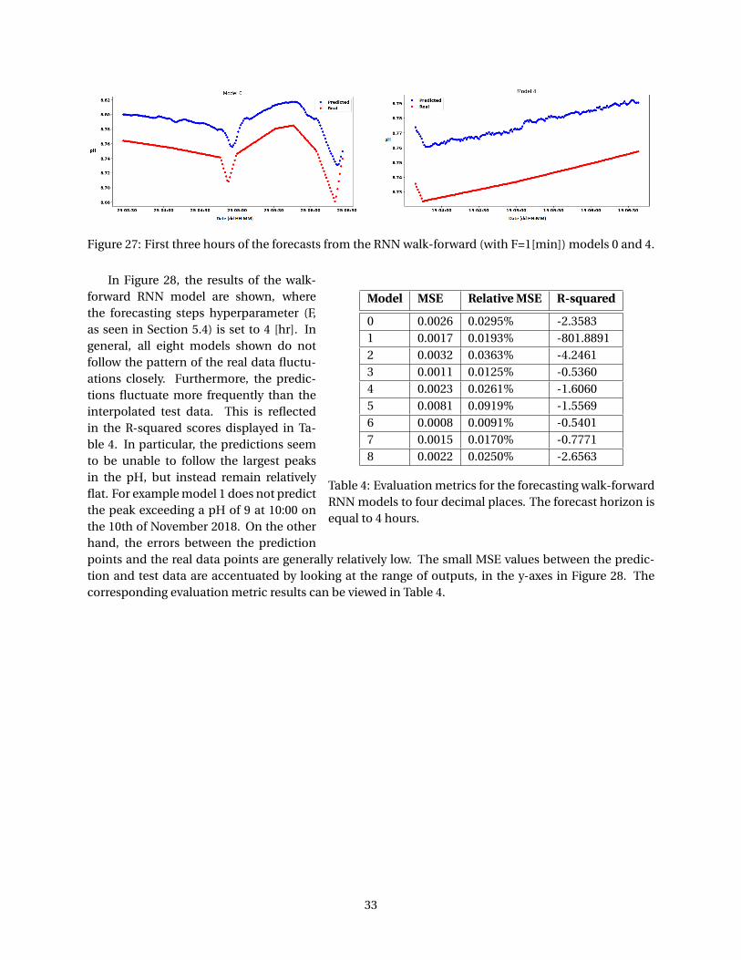
Figure 27: First three hours of the forecasts from the RNN walk-forward (with F=1[min]) models 0 and 4.

Model MSE Relative MSE R-squared

0 0.0026 0.0295% -2.35831 0.0017 0.0193% -801.88912 0.0032 0.0363% -4.24613 0.0011 0.0125% -0.53604 0.0023 0.0261% -1.60605 0.0081 0.0919% -1.55696 0.0008 0.0091% -0.54017 0.0015 0.0170% -0.77718 0.0022 0.0250% -2.6563

Table 4: Evaluation metrics for the forecasting walk-forwardRNN models to four decimal places. The forecast horizon isequal to 4 hours.

In Figure 28, the results of the walk-forward RNN model are shown, wherethe forecasting steps hyperparameter (F,as seen in Section 5.4) is set to 4 [hr]. Ingeneral, all eight models shown do notfollow the pattern of the real data fluctu-ations closely. Furthermore, the predic-tions fluctuate more frequently than theinterpolated test data. This is reflectedin the R-squared scores displayed in Ta-ble 4. In particular, the predictions seemto be unable to follow the largest peaksin the pH, but instead remain relativelyflat. For example model 1 does not predictthe peak exceeding a pH of 9 at 10:00 onthe 10th of November 2018. On the otherhand, the errors between the predictionpoints and the real data points are generally relatively low. The small MSE values between the predic-tion and test data are accentuated by looking at the range of outputs, in the y-axes in Figure 28. Thecorresponding evaluation metric results can be viewed in Table 4.

33

Figure 28: Walk-forward forecasting RNN model predictions, where F=4 [hr].

34

7.3. XGBoost Results

7.3.1. XGBoost Train-Validation-Test ModelThe trained train-validation-test XGBoost model is displayed in Figure 29 and has a MSE value equal

to 0.0057 (4 d.p.) and an R-squared value of -0.1871 (4 d.p.). In addition the relative MSE is equal to0.0647%, which is calculated by dividing the MSE by the mean pH of the dataset (≈ 8.8097) and multiply-ing by a hundred. The predicted data as a whole does not follow the test data closely.

Figure 30 depicts the feature importance of the XGBoost train-validation-test model. The featuresfor the present time step, pellet-bed pressure, draining and seeding, have the greatest impact on theresulting model. The most prominent past time steps from the most influential features, appear to beone, two, 58 and 59. For example, the ’bottom_press_59’ represents the pressure at the bottom of thesoftening reactor 59 minutes ago and scores as the fourth most influential feature.

Figure 29: XGBoost train-validation-test split model prediction.

Figure 30: The feature importance of the train-validation-test XGBoost model. The ’pellet_bed_press’refers to the pellet-bed pressure difference feature for the present time step. An appended underscorefollowed by a number, denotes the past time step in minutes for that particular feature.

35

7.3.2. XGBoost Walk-Forward Models

Model MSE Relative MSE R-squared

0 0.0176 0.1998% -3.81381 0.0040 0.0454% -0.28052 0.0049 0.0556% -0.23893 0.0086 0.0976% -0.50574 0.0276 0.3133% -4.76295 0.0127 0.1442% -7.47276 0.0043 0.0488% -0.3530

Table 5: Evaluation metrics for the walk-forward XGBoost models to 4decimal places.

The XGBoost walk-forwardevaluation metric results aredisplayed in Table 5. Allthe R-squared values are neg-ative, suggesting that the mod-els do not fit the actual dataclosely. Alternatively, theMSE values are relatively lowwith respect to the pH scale,indicating a low error. Thisis confirmed by observing therelative MSE metric. Theremaining walk-forward XG-Boost results can be found inAppendix E.

36

Chapter 8: Discussion and Conclusions8.1. DiscussionComparing all the models displayed in Chapter 7 based on their evaluation metrics and output plots,

it is evident that the Recurrent Neural Network (RNN) train-validation-test model (with F=1[min]) per-forms the best, since its R-squared value is the largest (positive value) and its MSE value is the lowest(joint lowest with model 0 of the RNN walk-forward method). This could be the result of the modellearning from a larger train dataset than the models produced using the walk-forward data split. Fur-thermore, looking at Figure 24, it is clear that the predictions closely follow the sharp peaks. This impliesthat the model can accurately model the behaviour of the pH when a draining action takes place. Con-versely, a model with a forecasting horizon length of one minute is extremely limiting in practice, since aprocess engineer at a Water Treatment Plant (WTP) has only one minute to respond to changes based onthe prediction. In addition, observing the walk-forward RNN and train-validation-test RNN results (withF=1[min]) more closely (see Figure 23 and Figure 27), it can be noted that the prediction lags slightlybehind the real data points. This may be caused by the model heavily relying on the present pH value topredict the next time step. Thus, the lag implies that the model is unable to predict the fluctuations atall, since it responds too late.

Clearly, the walk-forward forecasting RNN model (with F=4[hr]) is unable to fit the real data pointsclosely, by looking at Figure 28 and the R-squared results in Table 4. This could be due to the real databeing interpolated, thereby giving it a flat profile, whereas the predictions exhibit frequent fluctuations.Conversely, the relative MSE remains under 0.1% for all of the walk-forward models produced (see Table4). Therefore, indicating that the relative error between the predictions and the real data points is low.Increasing the forecasting horizon from a length of four hours to a length of 24 hours, gives in generalslightly worse MSE results (see Table 8) and similarly negative R-squared values. These results are con-firmed by looking at Figure 41 on page 62. Therefore, an increase of the forecast horizon from four to 24hours does not seem to drastically worsen the results.

In Table 4, the extremely negative R-squared value for the RNN walk-forward model 1 can be justifiedby referring to Subsection 4.5.1. Extremely negative R-squared values are caused by significantly largerSSr es values than SStot values, i.e. the actual prediction performs significantly worse than the mean as aprediction. This is reinforced by inspecting the prediction displayed in Figure 28.

The poorer results of the XGBoost models, could be attributed to the model not incorporating pastpH data as a feature or the model having a lookback of only 60 minutes (compared to a RNN lookback of180 minutes). In particular, the R-squared values for the train-validation-test and walk-forward modelsare all negative (see Section 7.3), hence implying that the prediction values do not fit the real data pointswell. Moreover, although the relative MSE values for all the XGBoost models are low (less than 1%), theyare in general not lower than the values derived from the RNN models.

8.2. ConclusionsIn this section, the research questions posed in Section 1.4 are answered, making use of the results pre-sented in Chapter 7.

8.2.1. Is it possible to develop a model of the softening treatment process of a WTP usingMachine Learning (ML)?

The results featured in Chapter 7 suggest that an accurate model of the softening treatment processof a WTP can be constructed using the RNN ML algorithm (with F=1[min]), based on the evaluation met-

37

rics. Moreover, all of the model predictions are considered feasible in the water softening reactor, sincethey stay within the maximum pH (9.4) and minimum pH (7.6) of the dataset used to train the model. Onthe other hand, the model is considerably limited, since it is only capable of predicting one minute intothe future and is heavily influenced by the pH value at the present time step. Thus, the model does notdisplay predictive qualities, since the fluctuations lag behind the actual data points. In addition, whenthe forecast horizon length is further increased (e.g. F=10[min] or 10 time steps), the resulting modelR-squared values are substantially worse, due to more fluctuations in the prediction than in the actualdata. Although, the MSE values remain relatively low. This may be caused by the actual data being inter-polated according to the method presented in Subsection 6.3.1.

8.2.2. Is the data provided for this research sufficient to develop a model using ML?It can be concluded that the data provided is insufficient to generate a good performing RNN model.

In spite of the RNN models (with F=1[min]) producing excellent evaluation metric results, the modelsare heavily reliant on the present pH value. Thus, the model outputs a lagged version of the actual data.Increasing the horizon length beyond one time step generally leads to a worse R-squared value. Forinstance, the four hour walk-forward RNN forecasts have negative R-squared values (see Table 4) andgenerally do not fit the trends of the actual data (see Figure 28). This suggests that the interpolated datadoes not provide the amount of detail required to generate a model that fits the actual data closely for alarge forecast horizon. On the other hand, the MSE values remain relatively low with respect to the pHscale.

In general, the XGBoost models have low MSE values, but negative R-squared values, thereby indi-cating that the predictions do not fit the test data well. This could be due to a lack of data to learn from,interpolation of the actual data or an absence of the incorporation of past pH values as a feature in themodel.

The data does not show the behaviour for instances when no draining occurs during the day, there-fore the model is conditioned to expect a daily draining action. For instance, regardless of the input, themodel might output a peak in the pH, which would correspond to a draining action, even if no drainingoccurs on that particular day. Whereas, when there is no draining action, you would expect the pH tocontinue to increase, since the pellets in the reactor are saturated, causing a decrease in the crystallisa-tion rate in the softening reactor.

The models are generated based on feature data contained within the maximum and minimumboundaries seen in Table 1. Therefore, the model may not be able to effectively predict for feature dataoutside these boundaries. This could be limiting, when extreme feature values (outside the boundaries)appear in the system, since the model might not be able to predict a realistic value for the pH in the soft-ening reactor.

8.2.3. Can the seeding and draining control be improved by developing a control strategyusing the produced ML model?

Based on RNN model predictive capabilities, it may be possible to predict when the pH is going torapidly increase and therefore in advance carry out a draining action. The XGBoost model is incapableof forecasting, thus this control method can only be implemented using a RNN model. Furthermore, itis advisable to set the forecasting horizon to about a couple of hours or greater (e.g. 4 hours), so that thepeak in pH can be on time anticipated and a draining action carried out in advance. Implementing thiscontrol method would have a stabilising effect on the pH softening treatment, i.e. the method shouldremove sharp peaks in the pH. In addition, the control implementation should lead to a more efficient

38

process, since the pellets are drained before the crystallisation rate declines significantly. Therefore, in-creasing the average of the crystallisation rate within the softening reactor.

The RNN walk-forward model predictions, with a prediction horizon equal to four hours (results seenin Figure 28), do not fit the test data particularly well. Moreover, the predictions do not appear to predictthe sharp peaks in the pH value. Therefore, the model is regarded as unsatisfactory to use for the sug-gested control strategy implementation.

39

Chapter 9: RecommendationsIn this chapter, potential further work is outlined, which could improve the performance of the Ma-

chine Learning (ML) model (based on the evaluation metrics). In addition, suggestions for implementingthe draining and seeding control strategy (described in Subsection 8.2.3) are explored.

9.1. Machine Learning (ML) RecommendationsIt might yield better results if you split the data into subsets that span from slightly after a draining

action until slightly before the next draining action. These subsets will differ in size, because the drainingactions do not occur at a set time every day. The ML algorithms should be adapted to learn from subsetsof data of differing lengths. The implementation using subsets, could have the effect of removing theimpact of the daily draining control action on the resulting ML model, since the dataset does not containdata around the time of draining.

Using a softening reactor experiment setup, allows you to collect data for when no draining actionoccurs for a certain period of time or irregular draining times. For instance, a draining action could havea probability of 75 % of occurring on a given day at a random time within WTP operating hours. A drain-ing action occurring during operation hours, ensures that the draining action is supervised. If there is adefect during the draining action or afterwards, the operators are able to oversee and intervene if neces-sary. Experimentation could be carried out in a reserve softening reactor. Collecting data with irregularand infrequent draining, prevents the model from being conditioned to expect a draining action andallows the ML model to learn from data with more information, i.e. data that includes behaviour whena draining action does not take place on a certain day. Furthermore, using the experiment setup givesthe opportunity to collect data for extreme influents. For example, an extreme influent could exhibit ex-tremely low or high pH values, where the influent is the water entering the softening reactor.

Due to computation times, it is not feasible to update the model every time step (one minute), sinceit takes longer than one minute to train the model. Although, it is possible to approximate computationtimes of training a ML XGBoost or a RNN (depending on the algorithm selected) model and thereforedecide upon a regular model update that does not conflict with the computation time. The computa-tion time can be reduced by using a GPU to run the ML implementation. Regular updating of the modelallows the new model to incorporate more recent data trends, since there are often changes in the op-erations carried out at a WTP, that lead to different trends in the data. For instance, the water collectionpoint (source) could be switched to another.

It is recommended to implement the best performing model from this research on another softeningreactor using data with the same time interval. The model will work only if the features and the target arekept the same, with the same corresponding units as the dataset used to train the ML model. Anotherreactor from the same WTP, where the softening reactor has the same specifications and the influentcomes from the same collection point (source), should perform accurately. If the model does indeedperform well, then it is possible to implement the model at other WTPs, thereby testing the generality ofthe model. Although, if this is unsuccessful, another ML model with the correct data can be trained forthe respective softening reactor. Each WTP has a unique set of sensors installed, resulting in a unique setof variables featuring in the dataset for each WTP. Therefore, the features and target(s) should be modi-fied accordingly.

A hyperparameter grid search could lead to a model of greater accuracy, where multiple possible hy-perparameter permutations can be tested and compared using the ML evaluation metrics. Naturally,

40

the more permutations that are tested, the higher the computation time. This implementation was notapplied for this research, since it was deemed too time consuming to program the grid search in Pythongiven the deadline for this research.

Multiple output variables (targets) may be desired from the ML model. For example, a control methodwithin the WTP could require multiple inputs (outputs from the ML model). It is possible to train a mul-tivariate output model by adapting the Python implementation.

It may be possible to obtain data that is not interpolated, thus providing more information about thedynamics of the system. WTPs often have access to systems that take live readings from certain sensors.Training on data that is not interpolated should lead to a more accurate ML model, since it learns frommore ‘informative’ data.

ML could possibly train a better performing softening treatment model, if the ML algorithm uses alarger train dataset. More data can be obtained by retrieving data further into the past from the samesoftening reactor or making the time interval of the extracted data smaller. For example, some WTPshave access to three years (backtracking from the present time) of stored data. Furthermore, a betterperforming model could result from data that contains less corrupted values, because less data wouldbe removed (or interpolated) and the resulting dataset would have greater continuity with respect to thedata time steps. Data with less corrupted values could be obtained from a different softening reactor.

A sensor measuring hardness could be installed in the softening reactor. Subsequently, these read-ings could be used as a feature for training of the ML model. This would probably yield a more accurateML model, due to the algorithm having a larger dataset to learn from. Conversely, after the installation ofthe sensor, it takes time to accumulate data readings, thus initially the feature would not provide muchinformation. Moreover, a sensor can be costly and the WTP would probably be reluctant to pay for a newsensor. Furthermore, there are often many softening reactors in a WTP, thus many sensors would needto be purchased to standardise all the softening reactors in the whole WTP.

9.2. Draining and Seeding Control RecommendationsA softening reactor experiment setup offers the chance to implement the control strategy proposed in

Subsection 8.2.3. The running costs can be compared, for the following scenarios: the softening processwith the implementation of the proposed control strategy and the softening process with the originalcontrol strategy. Note that this control method can only be acceptably implemented, if a forecastingmodel with a forecast horizon of at least two hours and satisfactory evaluation metric values can be gen-erated.

It is hard to implement MPC (Model Predictive Control) to control the draining and seeding actionswithin a softening reactor, since a MPC cost function can not be easily formulated. This is due to thepellet softening reactor requiring a draining action each day within working hours, thus the amount ofdraining and seeding control actions can not be reduced without potential consequences. For instance,if a draining action is skipped on a certain day, then the reactor could become clogged leading to the pro-cess coming to a halt and costing most probably more than draining the pellets using the MPC method.

41

Bibliography

[1] J. C. Van Dijk, J. Q. J. C. Verberk and P.J. De Moel (2018). Drinking Water: Principles and Practices.World Scientific Publishing Co Pte Ltd.

[2] A. W. C. van der Helm, O. J. I. Kramer, J. F. M. Hooft and P. J. Moel (2015). Plant wide chemical wa-ter stability modeling with PHREEQC for drinking water treatment. International Water Conference:New Developments in IT & Water, Rotterdam, The Netherlands.

[3] L. Rietveld (2015). Softening. Drinking water treatment, Delft University of Technology.

[4] K.M. van Schagen (2009). Model-Based Control of Drinking-water Treatment Plants. Drinking watertreatment, Delft University of Technology.

[5] E. Chiou (2018). An improved model of CaCO3 crystallization. Drinking water treatment, Delft Uni-versity of Technology.

[6] A. Géron (2017). Hands-On Machine Learning with Scikit-Learn and TensorFlow: Cocepts, Tools, andTechniques to Build Intelligent Systems. O’Reilly Media, Inc., 1005 Gravenstein Highway North, Se-bastopol, CA 95472.

[7] C. M. Bishop (2006). Pattern Recognition and Machine Learning. Springer Science+Business Media,LLC, 233 Spring Street, New York, NY 10013, USA.

[8] M. Nielsen (2013). Neural Networks and Deep Learning. Ebook available (06/09/2019) via:https://github.com/antonvladyka/neuralnetworksanddeeplearning.com.pdf.‘

[9] A. Sadad (2019). Reusable Machine Learning Framework for Predicting Future System Performance: AComparison Study of Validation Strategy on WWTP Time Series Data. Department of Electrical Engi-neering, Mathematics and Computer Science (EEMCS), University of Twente.

[10] L. van den Hout (2013). Modellering van de hardheidsreductie. Hogeschool Utrecht, Institute for LifeSciences and Chemistry and Waternet, Sector Drinkwater, Afdeling Productie Team Waterkwaliteiten Procesondersteuning.

[11] M. A. Jobse (2013). Modellering van de fluïdisatie bij korrelreactoren. Thesis, Hogeschool Utrecht,Institute for Life Science and Chemistry.

[12] J. Brownlee (2016). Overfitting and Underfitting With Machine Learn-ing Algorithms. Article is available (12/09/2019) via the following link:https://machinelearningmastery.com/overfitting-and-underfitting-with-machine-learning-algorithms/.

42

[13] G. P. Pulipaka (2016). An essential guide to classification and regression trees in R Lan-guage. Article is available (12/09/2019) via the following link: https://medium.com/@gp_pulipaka/an-essential-guide-to-classification-and-regression-trees-in-r-language-4ced657d176b.

[14] T. Chen and C. Guestrin (2016). XGBoost: A Scalable Tree Boosting System. University of Washington.

[15] R. S. Brid (2018). Introduction to Decision Trees. GreyAtom School. Article is available (16/09/2019)via the following link: https://medium.com/greyatom/decision-trees-a-simple-way-to-visualize-a-decision-dc506a403aeb

[16] P. Krause, D. P. Boyle and F. Bäse (2005). Comparison of different efficiency criteria for hydrologicalmodel assessment. Adv. Geosci. 5, 89-97. University of Washington.

[17] X. Yuan (2009). Model Validation and New Water Control Strategies in Drinking Water TreatmentPlant Wim Mensink. Department of Water Management, Sanitary Engineering Section, Faculty ofCivil Engineering and Geosciences, Delft University of Technology.

[18] T. Smith (2019). Autocorrelation. Article is available (30/09/2019) via the following link:https://www.investopedia.com/terms/a/autocorrelation.asp. Investopedia.

[19] M. A. Jobse (2013). Modellering van de fluïdisatie bij korrelreactoren. Thesis, Hogeschool Utrecht,Institute for Life Science and Chemistry.

[20] E. Dizdar, A. Dizdar, C. Dizdar and A. Downey (2014). PURE-H2O Implementation of ECVET forQualification Design in Drinking Water Treatment Plants and Sanitation for Pure Drinkable Water.Orkon International Engineering Training Consulting Co. Inc.

[21] S. Hochreiter and J. Schmidhuber (1997). Long Short-Term Memory, Neural Computation vol. 9:1735-1780 pg. Faculty of Computer Science, Technical University of Munich and IDSIA.

[22] N. Srivastava, G Hinton, A. Krizhevsky, I. Sutskever and R. Salakhutdinov (2014). Dropout: A Sim-ple Way to Prevent Neural Networks from Overfitting, Journal of Machine Learning Reserach vol. 15:1929-1958. Department of Computer Science, University of Toronto.

[23] Dutch Drinking Water Statistics 2017: From source to tap. Vewin, Association of Dutch water com-panies.

[24] A. W. C. van der Helm and L. C. Rietveld (2002). Modelling of drinking water treatment processeswithin the Stimela environment, Water Science & Technology Water Supply. DHV Water BV and DelftUniversity of Technology.

[25] M. Galarnyk (2018). Understanding Boxplots. Article is available (18/10/2019) via the following link:https://towardsdatascience.com/understanding-boxplots-5e2df7bcbd51.

[26] A. Sivalingam (2019). What is machine learning ?. Article is available (29/11/2019) via the followinglink: https://medium.com/swlh/what-is-machine-learning-9b569ff7858a.

[27] S. Sharma (2017). Activation Functions in Neural Networks. Article is available (03/12/2019) via thefollowing link: https://towardsdatascience.com/activation-functions-neural-networks-1cbd9f8d91d6.

43

Appendix A: Drinking WTP Example and SofteningProcess Background Information

A.1. Example WTPIn Figure 31, a diagram of a drinking water treatment process is presented. The water is pre-treated

at Loenderveen before reaching the Water Treatment Plant (WTP). The raw water is predominantly seep-age water from the Buthune polder, sometimes blended with Amsterdam-Rhine Canal water. The rawwater is coagulated with ferric chloride (FeCl3) and flocs are removed in horizontal settling tanks. Result-ing in the removal of phosphate, suspended solids, heavy metals and Natural Organic Matter (NOM) [4].Afterwards, sedimentation, nitrification of ammonium and biodegradation take place in a lake-waterreservoir of 130 hectares. The retention time of the reservoir is approximately 100 days. The left overammonium, suspended solids and algae are removed using rapid sand filtration. The resulting water isthen transported more than 10 kilometers to the Weesperkarspel WTP.

At the drinking WTP Weesperkarspel, the first process applied is ozonation for disinfection and oxi-dation of micro pollutants and NOM. Resulting in an increase in the biodegradability of organic matter.Subsequently, softening pellet reactors are used to reduce the hardness of the water and then biologicalactivated carbon (BAC) filters are used to remove organic matter and organic micro pollutants. Finally,the water passes through a slow sand filter for extra nutrient and suspended solid removal. The water isthen stored in a clear water reservoir ready for distribution.

Figure 31: Diagram of the pre-treatment processes at Loenderveen and drinking water treatment atWeesperkarspel Water Treatment Plant (WTP) of Waternet [2]

A.2. Water FluxThe distribution of the particles in the reactor is dependent on the flow rate. A higher flow rate cor-

responds to a greater water flux in the reactor. We refer to the speed of the water travelling through thepellet-bed as water flux.

44

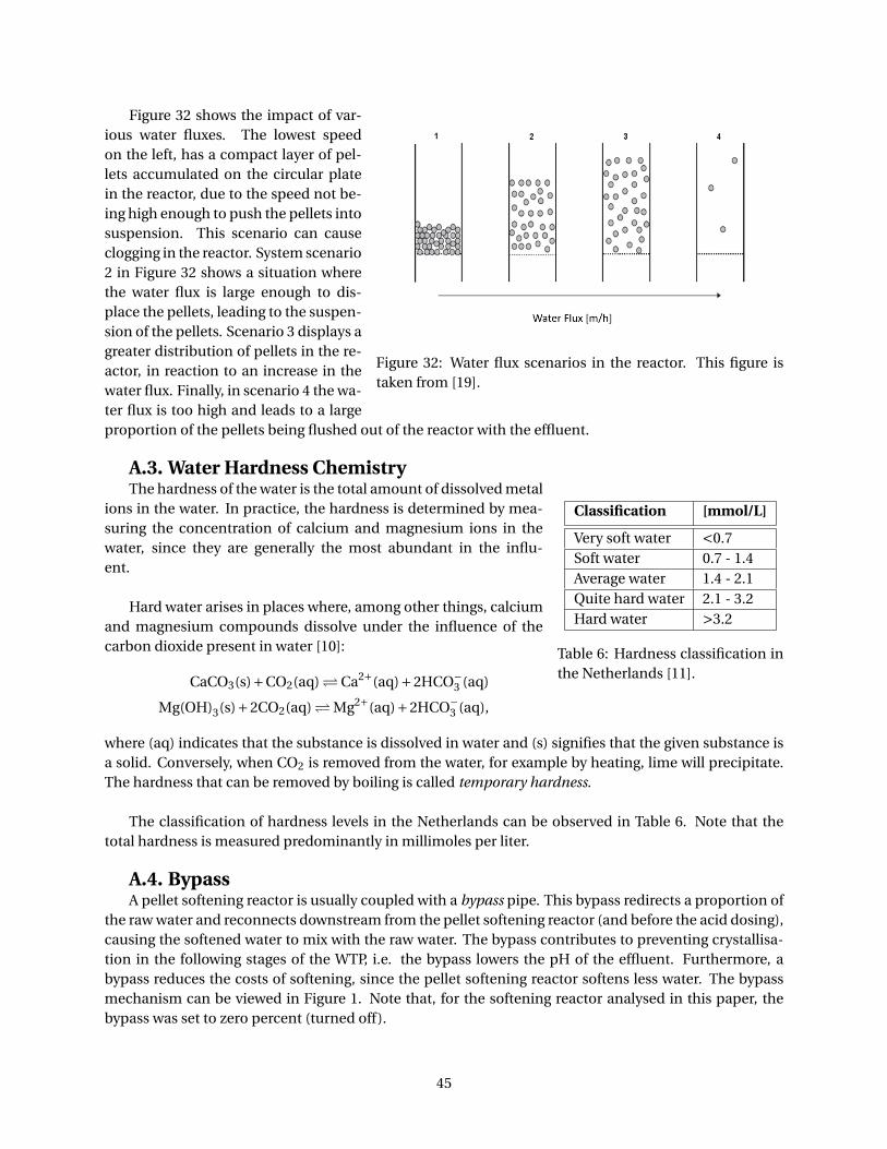
Figure 32: Water flux scenarios in the reactor. This figure istaken from [19].

Figure 32 shows the impact of var-ious water fluxes. The lowest speedon the left, has a compact layer of pel-lets accumulated on the circular platein the reactor, due to the speed not be-ing high enough to push the pellets intosuspension. This scenario can causeclogging in the reactor. System scenario2 in Figure 32 shows a situation wherethe water flux is large enough to dis-place the pellets, leading to the suspen-sion of the pellets. Scenario 3 displays agreater distribution of pellets in the re-actor, in reaction to an increase in thewater flux. Finally, in scenario 4 the wa-ter flux is too high and leads to a largeproportion of the pellets being flushed out of the reactor with the effluent.

A.3. Water Hardness Chemistry

Classification [mmol/L]

Very soft water <0.7Soft water 0.7 - 1.4Average water 1.4 - 2.1Quite hard water 2.1 - 3.2Hard water >3.2

Table 6: Hardness classification inthe Netherlands [11].

The hardness of the water is the total amount of dissolved metalions in the water. In practice, the hardness is determined by mea-suring the concentration of calcium and magnesium ions in thewater, since they are generally the most abundant in the influ-ent.

Hard water arises in places where, among other things, calciumand magnesium compounds dissolve under the influence of thecarbon dioxide present in water [10]:

CaCO3(s)+CO2(aq)Ca2+(aq)+2HCO−3 (aq)

Mg(OH)3(s)+2CO2(aq)Mg2+(aq)+2HCO−3 (aq),

where (aq) indicates that the substance is dissolved in water and (s) signifies that the given substance isa solid. Conversely, when CO2 is removed from the water, for example by heating, lime will precipitate.The hardness that can be removed by boiling is called temporary hardness.

The classification of hardness levels in the Netherlands can be observed in Table 6. Note that thetotal hardness is measured predominantly in millimoles per liter.

A.4. BypassA pellet softening reactor is usually coupled with a bypass pipe. This bypass redirects a proportion of

the raw water and reconnects downstream from the pellet softening reactor (and before the acid dosing),causing the softened water to mix with the raw water. The bypass contributes to preventing crystallisa-tion in the following stages of the WTP, i.e. the bypass lowers the pH of the effluent. Furthermore, abypass reduces the costs of softening, since the pellet softening reactor softens less water. The bypassmechanism can be viewed in Figure 1. Note that, for the softening reactor analysed in this paper, thebypass was set to zero percent (turned off).

45

A.5. Calcium Carbonate Crystallisation ReactionCalcium carbonate is one of the most broadly studied minerals and is investigated in studies in-

volving geological, chemical and biological processes. The calcium carbonate crystallisation reaction isdescribed by the following chemical equation:

Ca2++CO2−3 CaCO3(s).

This reaction often takes place on the softening pellets in a softening reactor of a WTP.

46

Appendix B: Data Analysis

B.1. Pearson’s Correlation Coefficient MatrixThe Pearson’s correlation coefficient matrix of the relevant variables of the drinking Water Treatment

Plant (WTP) softening reactor used in this research is displayed in Table 7. The second highest correla-tion coefficient magnitude is between the bed height and the caustic soda flow, since caustic soda is usedto facilitate crystallisation and crystallisation leads to thicker pellets in the reactor. Thick pellets weighmore and sink to a lower height in the reactor and consequently resulting in a higher bed height reading.

B.2. Box Plot

Figure 33: Boxplot. This image is taken from [25].

A boxplot is a visual rep-resentation of how the datais skewed. The graphic con-sists of (from left to right):"minimum", first quartile (Q1),median, third quartile (Q3)and the "maximum". Theoutliers are also shown in aboxplot. An example box-plot can be viewed in Figure33.

47

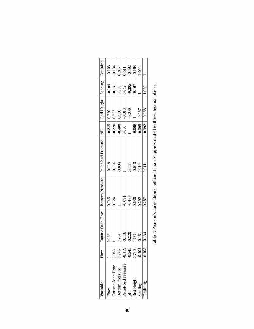
Vari

able

Flow

Cau

stic

Sod

aFl

owB

ott

om

Pre

ssu

reP

elle

t-b

edP

ress

ure

pH

Bed

Hei

ght

Seed

ing

Dra

inin

g

Flow

10.

983

0.74

5-0

.119

-0.2

450.

730

-0.1

04-0

.108

Cau

stic

Sod

aFl

ow0.

983

10.

724

-0.1

16-0

.220

0.73

7-0

.131

-0.1

34B

ott

om

Pre

ssu

re0.

745

0.72

41

-0.0

94-0

.488

0.53

00.

292

0.28

7P

elle

t-b

edP

ress

ure

-0.1

19-0

.116

-0.0

941

0.00

3-0

.013

0.04

20.

041

pH

-0.2

45-0

.220

-0.4

880.

003

1-0

.066

-0.3

95-0

.392

Bed

Hei

ght

0.73

00.

737

0.53

0-0

.013

-0.0

661

-0.1

67-0

.168

Seed

ing

-0.1

04-0

.131

0.29

20.

042

-0.3

95-0

.167

11.

000

Dra

inin

g-0

.108

-0.1

340.

287

0.04

1-0

.392

-0.1

681.

000

1

Tab

le7:

Pear

son’

sco

rrel

atio

nco

effi

cien

tmat

rix

app

roxi

mat

edto

thre

ed

ecim

alp

lace

s.

48

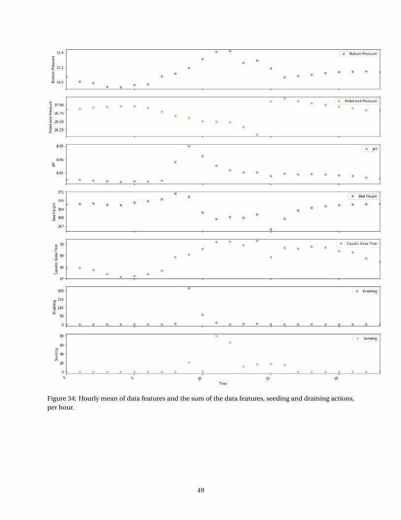
Figure 34: Hourly mean of data features and the sum of the data features, seeding and draining actions,per hour.

49

Appendix C: Machine Learning

C.1. Python vs Matlab®: Machine Learning and Control Theory Imple-mentation

Before carrying out the analysis on the dataset used in this research, a particular software packagewas chosen to conduct the analysis. The choice was slimmed down to two candidates: Matlab® andPython. Eventually, Python was selected on the basis of the following comparisons between the twosoftware packages:

• It is possible to obtain free extra RAM (memory) using Python in Colaborative. Using Matlab®, youare restricted to using the graphics card in your PC or your CPU, which can be considerably slower.

• There are more help forums for Python machine learning. For instance, Kaggle has many examplesof machine learning algorithms being implemented using Python code. Matlab® on the otherhand, has less information via online forums, due to it being less frequently used.

• Matlab® does not react as quickly to new machine learning developments as Python and thus thefunctionality of the machine learning toolboxes can be limiting. For instance, there is no Matlab®function for the XGBoost algorithm.

• Colaborative (provided by Google) is free to use, although you need to upload your dataset toGoogle Drive in order to use Colaborative. Some businesses may find this problematic, due todata confidentiality. Conversely, Matlab® requires you to pay for a subscription licence.

• Matlab® has a useful control theory toolbox called Simulink®. This allows you to effectively sim-ulate and control theoretical systems using visual block diagrams. Although Python has a recentlydeveloped (in 2018) a new package SimuPy that is relatively similar to Simulink®, Simulink® is stillregarded generally speaking to be the best amongst Systems and Control engineers. However, forthis research Python is considered satisfactory to carry out the control methods, since the methodsare not particularly complicated.

C.2. RMSProp OptimisationRMSProp optimisation is often chosen over the standard gradient descent optimisation method,

since it takes a more direct route to the optimum [6]. The standard Gradient Descent method, beginsby going speedily down the steepest slope and then slowly down to the bottom of the valley. The RM-SProp on the other hand, is able to prevent this, by scaling down the speed going down the steepest slopeand taking a different route, that is more direct to the optimum point (bottom of the valley). RMSPropoptimisation algorithm can be described by the following two equations:

s(i ) ←−βs(i−1) + (1−β)∇wC (w (i−1))⊗∇wC (w (i−1)) (3)

w (i ) ←− w (i−1) −η∇wC (w (i−1))®√

s(i ) +ε, (4)

where β represents the decay rate (often set to 0.9), w the weight vector, ⊗ symbolises the element-wisemultiplication operation, ® the element-wise division operation, η is the learning rate, ε is a smoothingterm to avoid division by zero (often set to 10−10) and i denotes the time step. In addition, ∇wC (w (i )) isthe partial derivative of C with respect to w for the time step i .

50

C.3. Derivation of Backpropagation EquationsWe can denote the weights of the Neural Network (NN) as w l

j k using notation proposed by M. Nielsen[8], where the indices indicate that the weight connects the k-th neuron in the (l-1)-th layer of the NNto the j -th neuron in the l-th layer [8]. Similar notation is employed for the bias bl

j ; symbolising the j -th

neuron in the l-th layer. Likewise, we express the activation as alj and is described as follows:

alj = h

(∑w l

j k al−1k +bl

j

), (5)

where the sum is over all neurons k in the (l-1)-th layer and h represents the activation function, whichacts as a hyperparameter.

For simplicity, equation (5) can be rewritten in matrix form as follows:

al = h(w l al−1 +bl

).

Let z l ≡ w l al−1 +bl and we refer to z l as the weighted input to the neurons in layer l .

In order to update our weights when carrying out training, we need to define a cost function C . Apopular choice is the Mean Squared Error (MSE) cost function:

C = 1

2N

∑x||y(x)−aL(x)||2,

where N is the total number of training samples, the sum is over the training samples x, y(x) signifiesthe target output and L is the number of layers in the network and aL(x) represents the vector of activa-tion outputs from the network and dependant on the input x. The aim is to minimise the cost functionoutput (error) when evaluating the model using the test data.

We have assumed that C = 1n

∑x Cx with cost function Cx for an individual training sample. There-

fore, for the MSE cost function Cx = 12 ||y(x)− aL(x)||2. Let us suppose that the training sample is fixed

and we drop the x subscript from the cost function. Thus, writing Cx as C .

Backpropagation in simple terms is about how changing the weights and biases in a network changesthe cost function. Meaning mathematically that the partial derivatives, ∂C

∂w lj k

and ∂C∂bl

j

, need to be com-

puted. M. Nielsen [8] explains a four-step technique to calculate the backpropagation and is explainedin the remainder of this Subsection.

Firstly, we define the error δlj of neuron j in layer l by

δlj ≡

∂C

∂z lj

, (6)

where z lj =

∑k=1 w l

j k al−1k +bl

j . Using the chain rule, equation (6) for the output layer is described as

δLj =

∑k

∂C

∂aLk

∂aLk

∂zLj

, (7)

51

where the sum is taken over all k neurons in the output layer. The output activation aLk of the k-th neuron

is only dependent on the weighted input zLj for the j -th neuron when k = j . Thus, the terms in equation

(7) disappear when k 6= j and results in the following simplified expression

δLj ≡

∂C

∂aLj

∂aLj

∂zLj

. (8)

Now, using equation (5) the second term in the product can written as h′(zLj ). This gives

δLj =

∂C

∂aLj

h′(zLj ). (9)

For our MSE cost function C = 12

∑j (y j −aL

j )2, the partial derivative is ∂C∂aL

j= (aL

j − y j ). Similarly as before,

we denote the vector of errors associated with layer l as δl . Writing equation (9) in matrix form using theMSE cost function gives

δL = (aL − y) ·h′(zL), (10)

where · symbolises the inner product.

Secondly, δlj = ∂C

∂z lj

is rewritten in terms of δl+1k = ∂C

∂z l+1k

. This is achieved using the chain rule,

δlj =

∂C

∂z lj

=∑k

∂C

∂z l+1k

∂z l+1k

∂z lj

=∑k

∂z l+1k

∂z lj

δl+1k , (11)

where the terms are interchanged. The first term in the resulting equation is further mathematicallymanipulated as follows

z l+1k =∑

jw l+1

k j alj +bl+1

k =∑j

w l+1k j h(z l

j )+bl+1k .

Taking the partial derivative, leads to∂z l+1

k

∂z lj

= w l+1k j h′(z l

j ).

Substituting back into equation (11), yields the vector equation for the error δl in terms of the error inthe next layer δl+1:

δl = ((w l+1)Tδl+1) ·h′(zL). (12)

Here, (w l+1)T is the transpose of the weight matrix w l+1 for the (l+1)-th layer. Combining the two equa-tions (10) and (12) it is possible to determine the error δl for any layer in the network, i.e. beginning withδL and working your way back calculating subsequently δL−1, δL−2, etc. Thus, backpropagating throughthe network.

Thirdly, ∂C∂bl

j

δlj is derived using, once again, the chain rule:

∂C

∂blj

=∑k

∂z lk

∂blj

∂C

∂z lk

= ∂C

∂z lj

= δlj , (13)

where z lj =

∑k w l

j k al−1k +bl

j . Using the vector notation, equation (13) can be described as

∂C

∂bl= δl .

52

Lastly, the rate of change of the cost with respect to any weight in the network is calculated via thefollowing formula:

∂C

∂w lj k

= al−1k δl

j . (14)

The corresponding vector form for equation (14) is:

∂C

∂w l= al−1δl , (15)

where the derivation is calculated in a similar way as the above equations, i.e. using the chain rule. Aninteresting side-effect of equation (15) is that when al−1 is small (al−1 ≈ 0), the gradient term ∂C

∂w l willalso be small. This causes the weights to learn slowly, i.e. they do not change significantly during gradi-ent descent implementation.

C.4. The Backpropagation AlgorithmThe backpropagation equations derived in the previous section, make it possible to compute the

gradient of the cost function, which is often used in gradient descent (described in Subsection 5.2.2) forthe learning of a NN. The steps of the algorithm used to derive the gradient of the cost function, are asfollows:

1. Input x: Compute activation a1 for the input layer.

2. Feedforward: For each l = 2,3, ...,L calculate z l = w l al−1 +bl and al = h(z l ).

3. Output error δL : Calculate the vector δL = ∂C∂aL h′(zL)

4. Backpropagation of the error: For each l = L−1,L−2, ...,2 calculate δl = ((w l+1)Tδl+1) ·h′(zL).

5. Output: Finally, the gradient of the cost function is calculated using ∂C∂w l

j k

= al−1k δl

j and ∂C∂bl

j

= δlj .

53

C.5. Logistic Activation Function

Figure 35: Logistic Activation Function. This image is takenfrom [27].

The logistic activation function is asfollows:

σ(z) = 1

1+e−z ,

where z symbolises the input.

54

Appendix D: eXtreme Gradient Boost (XGBoost)

D.1. Regularisation Learning Objective

Figure 36: Example of a tree ensemble model, consisting of twodecision trees. The red weights are the weights correspondingto a particular input x1.

For a given dataset with n sam-ples and m features (inputs) D =(xi , yi ) (|D| = n, xi ∈ Rm , yi ∈ R), a treeensemble model uses K additive func-tions to predict the output. The predic-tion is described as follows:

yi =φ(x i ) =K∑

k=1fk (x i ), fk ∈F ,

where F = f (x) = wq(x) (q : Rm −→T, w ∈ RT ) is the space of regressiontrees, q denotes the structure of eachtree which maps a sample to the corre-sponding leaf index (includes the treedecision rules), T is the number ofleaves in the tree and fk correspondsto an independent tree structure q andleaf weights w . Unlike decision trees(or classification trees), each regressiontree contains a continuous score oneach of the leaves and is represented aswi for the i -th leaf. An example tree en-semble model is featured in Figure 36.In this example, the function φ for anexample input x1 is equal to:

φ(x1) = f1(x1)+ f2(x1) = 0.3+0.9 = 1.2,

where f1 corresponds to the first deci-sion tree and f2 to the second.

In order to learn the set of functions used in the model, we minimise the following regularised objec-tive function:

L (φ) =∑i

l (yi , yi )+∑kΩ( fk ), (16)

where Ω(w) = γT + 12λ||w ||2 and l is a differential convex (i.e. ∀yi , yi ∈ X ,∀t ∈ [0,1] : l (t yi + (1− t )yi ) ≤

t l (yi )+(1− t )l (yi ), where X is a convex set in a real vector space and a convex set is a set of points, whereevery point on a line segment joining any two points within the set, lies within the set) loss functioncalculating the difference between the prediction yi and the target yi . The second term Ω penalisesthe complexity of the model (the regression tree functions) and is considered a regularisation term thatsmooths the final learnt weights to avoid overfitting. A desired side-effect is that the regularised objectivewill tend to select a model employing simple functions and functions that can more accurately predictthe target of new data. If the regularisation parameter λ is set to zero, the objective transforms back tothe standard gradient tree boosting loss function.

55

D.2. Gradient Tree BoostingThe tree ensemble model described by equation (16) cannot be optimised by implementing the tra-

ditional methods in the Euclidean space, since the model employs functions as parameters. It is insteadtrained by applying addition. Let y (t )

i be the prediction of the i -th instance at the t-th iteration. We addft and minimise the resulting objective function:

L (t ) =n∑

i=1l (y (t−1)

i + ft (x i ), yi )+Ω( ft ).

Therefore, the optimal ft that most improves the model (seen in equation (16)) is added to the predictionin the loss function. The function ft has T leaves. For a speedier optimisation the objective function canbe written as follows using Taylor’s series:

L (t ) 'n∑

i=1

[l (y (t−1)

i , yi )+ gi ft (x i )+ 1

2hi f 2

t (x i )]+Ω( ft ),

where gi = ∂l (yi ,y (t−1)i )

∂y (t−1)i

and hi = ∂2l (yi ,y (t−1)i )

∂y (t−1)i

2are respectively the first and second order partial derivatives of

the loss function with respect to y (t−1)i . We proceed by removing the loss function, resulting in:

L (t ) =n∑

i=1

[gi ft (x i )+ 1

2hi f 2

t (x i )]+Ω( ft ). (17)

We define I j = i | q(x i ) = j as the instance set of leaf j and rewrite equation (17), using the fact thatf (x) = wq(x) and by expandingΩ, as follows:

L (t ) =n∑

i=1

[gi ft (x i )+ 1

2hi f 2

t (x i )]+γT + 1

2λ

T∑j=1

w2j =

n∑i=1

gi wq(xi ) + 1

2

n∑i=1

hi (wq(xi ))2 + 1

2λ

T∑j=1

w2j +γT

= ∑i∈I j

gi

T∑j=1

w j + 1

2

∑i∈I j

hi

T∑j=1

w2j +

λ

2

T∑j=1

w2j +γT =

T∑j=1

[(∑

i∈I j

gi )w j + 1

2(∑

i∈I j

hi +λ)w2j

]+γT.

For a fixed structure q(x), the optimal weight w∗j can be derived by taking the derivative with respect to

the weight and rearranging, giving:

w∗j =−

∑i∈I j

gi∑i∈I j

hi +λ,

The corresponding optimal objective value is then:

L (t )(q) =−1

2

T∑j=1

(∑

i∈I jgi )2∑

i∈I jhi +λ

+γT. (18)

Subsequently, equation (18) can be used as a scoring function to measure the quality of a tree structureq . The score is similar to the impurity scores used to evaluate a decision tree (such as the impurity scorecalculated using the so-called entropy function), but instead applies for a wider range of objective func-tions. In most cases, it is computationally too expensive to find the optimal for every tree structure q . Toavoid evaluating every possible q structure, the greedy algorithm is implemented. Briefly, the algorithmbegins at a single leaf and iteratively adds branches to the tree [14].

56

Appendix E: XGBoost and RNN Implementation

E.1. XGBoost ResultsFigures 37 and 38 display the resulting model predictions using the walk-forward data split method.

Clearly, the predictions do not follow the pattern of the real data closely. This is confirmed in Table 5,where the R-squared evaluation metric values are negative. It is also evident, that the models are notable to predict the pH values in the region of a draining action, since the predictions generally do notspike significantly in value. On the other hand, the MSE evaluation metric values are relatively low.

The feature importance for model 4 is depicted in Figure 40. Clearly, the feature ’pellet_bed_press’,denoting the pellet-bed pressure feature for the present time step, is by a long way the most important,followed by the present time step seeding, bed height, bottom pressure and draining features in impor-tance. The most influential past data steps appear to be one, two, 58 and 59, where for instance a pasttime step of one indicates a measurement taken one minute ago.

57

Figure 37: First four XGBoost walk-forward split model predictions on the same plot as the test data. Thetest data spans three days in total.

58

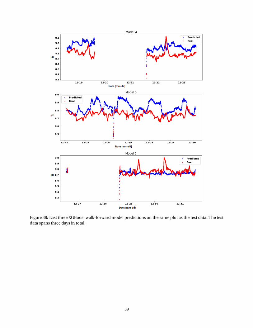
Figure 38: Last three XGBoost walk-forward model predictions on the same plot as the test data. The testdata spans three days in total.

59

Figure 39: Feature importance of XGBoost models 0 to 3.

60

Figure 40: Feature importance of XGBoost models 4, 5 and 6.

E.2. RNN Results (F=24[hr])

Model MSE Relative MSE R-squared

0 0.0120 0.1362% -6.23751 0.0100 0.1135% -0.18602 0.0035 0.0397% -0.49683 0.0020 0.0227% -0.17084 0.0030 0.0341% -0.08435 0.0019 0.0216% -0.16936 0.0031 0.0352% -0.29077 0.0026 0.0295% -0.11878 0.0038 0.0431% -0.7773

Table 8: Evaluation metrics for the forecasting walk-forward RNN models to four decimal places. Theforecast horizon is equal to 24 hours.

61

Figure 41: Walk-forward forecasting RNN model predictions, where F=24 [hr].

62

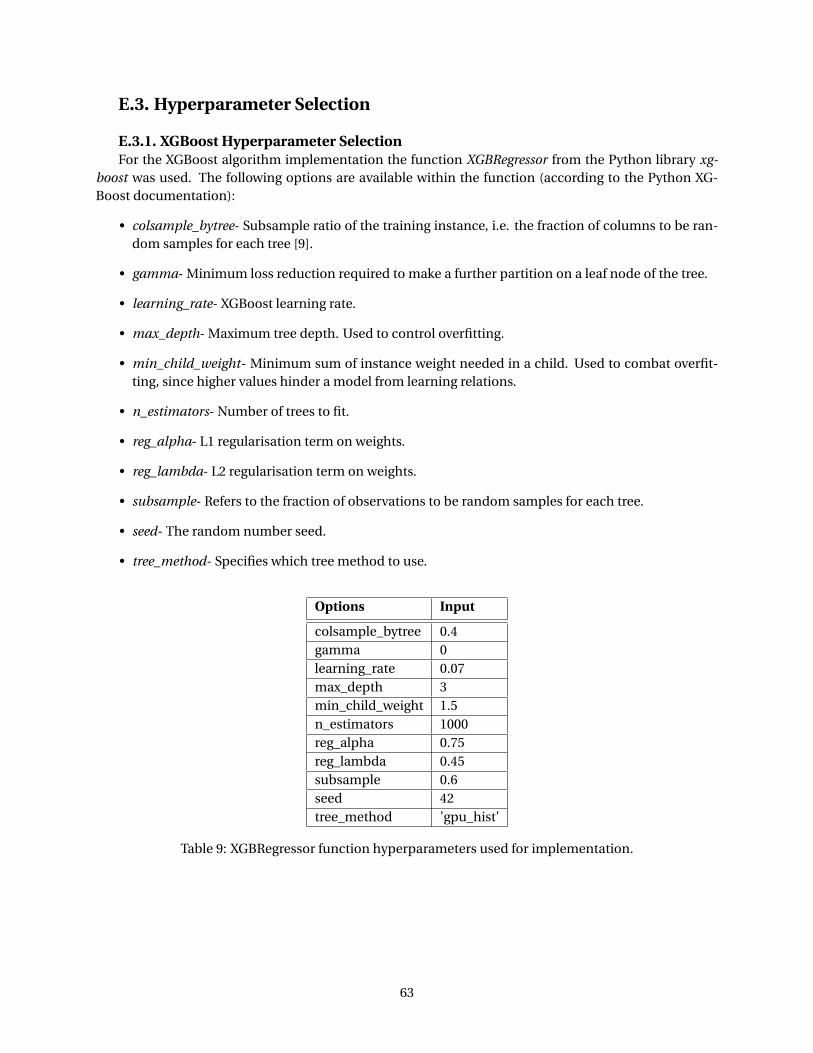
E.3. Hyperparameter Selection

E.3.1. XGBoost Hyperparameter SelectionFor the XGBoost algorithm implementation the function XGBRegressor from the Python library xg-

boost was used. The following options are available within the function (according to the Python XG-Boost documentation):

• colsample_bytree- Subsample ratio of the training instance, i.e. the fraction of columns to be ran-dom samples for each tree [9].

• gamma- Minimum loss reduction required to make a further partition on a leaf node of the tree.

• learning_rate- XGBoost learning rate.

• max_depth- Maximum tree depth. Used to control overfitting.

• min_child_weight- Minimum sum of instance weight needed in a child. Used to combat overfit-ting, since higher values hinder a model from learning relations.

• n_estimators- Number of trees to fit.

• reg_alpha- L1 regularisation term on weights.

• reg_lambda- L2 regularisation term on weights.

• subsample- Refers to the fraction of observations to be random samples for each tree.

• seed- The random number seed.

• tree_method- Specifies which tree method to use.

Options Input

colsample_bytree 0.4gamma 0learning_rate 0.07max_depth 3min_child_weight 1.5n_estimators 1000reg_alpha 0.75reg_lambda 0.45subsample 0.6seed 42tree_method ’gpu_hist’

Table 9: XGBRegressor function hyperparameters used for implementation.

63

E.3.2. RNN Hyperparameter SelectionThe RNN structure adopted is as seen in Figure 10, with seven features (inputs). The first LSTM from

left to right is comprised of 64 neurons and the second 32 neurons. The dropout probability is set to 0.2.The amount of neurons and dropout probability are derived from A. Sadad’s thesis for the WastewaterTreatment Plant (WWTP). Deviating these hyperparameters did not seem to give improved results. Theregression output is the pH in the softening reactor and the Mean Squared Error (MSE) function waschosen for model training (see the backpropagation algorithm, in appendix C for more insight). Further-more, when training the RMSProp optimiser (described in appendix C) was used.

E.4. Model Training Logs

E.4.1. RNN Walk-Forward Training (F=1[min])Three epochs and a batch size of 256 were used for training of the model, using the Batch Gradient

Descent method (explained in chapter 5).

The Python log during training of the RNN walk-forward models (with F=1 [min]) is as follows:

Number of models for walkforward validation: 6Training on index 189569:249569, Testing on index 249569:253889Epoch 1/3- 7s - loss: 2.5074 - mean_squared_error: 2.5074Epoch 2/3- 5s - loss: 0.0034 - mean_squared_error: 0.0034Epoch 3/3- 5s - loss: 0.0018 - mean_squared_error: 0.0018MSE 0.0013159741401491626R2 0.6372750930392224

Training on index 193889:253889, Testing on index 253889:258209Epoch 1/3- 7s - loss: 2.6694 - mean_squared_error: 2.6694Epoch 2/3- 5s - loss: 0.0031 - mean_squared_error: 0.0031Epoch 3/3- 5s - loss: 0.0016 - mean_squared_error: 0.0016MSE 0.0009467924775900951R2 0.8800728418928929

Training on index 198209:258209, Testing on index 258209:262529Epoch 1/3- 7s - loss: 2.1012 - mean_squared_error: 2.1012Epoch 2/3- 5s - loss: 0.0032 - mean_squared_error: 0.0032Epoch 3/3- 5s - loss: 0.0017 - mean_squared_error: 0.0017MSE 0.0015642625093958199R2 0.7268537541438583

64

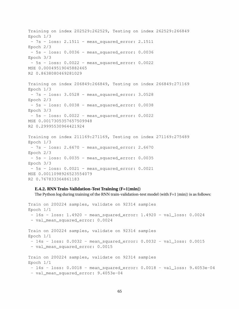
Training on index 202529:262529, Testing on index 262529:266849Epoch 1/3- 7s - loss: 2.1511 - mean_squared_error: 2.1511Epoch 2/3- 5s - loss: 0.0036 - mean_squared_error: 0.0036Epoch 3/3- 5s - loss: 0.0022 - mean_squared_error: 0.0022MSE 0.00049519045882465R2 0.8638080469281029

Training on index 206849:266849, Testing on index 266849:271169Epoch 1/3- 7s - loss: 3.0528 - mean_squared_error: 3.0528Epoch 2/3- 5s - loss: 0.0038 - mean_squared_error: 0.0038Epoch 3/3- 5s - loss: 0.0022 - mean_squared_error: 0.0022MSE 0.0017305357657509948R2 0.29995530964421924

Training on index 211169:271169, Testing on index 271169:275489Epoch 1/3- 7s - loss: 2.6670 - mean_squared_error: 2.6670Epoch 2/3- 5s - loss: 0.0035 - mean_squared_error: 0.0035Epoch 3/3- 5s - loss: 0.0021 - mean_squared_error: 0.0021MSE 0.0011098926523554079R2 0.767833364861183

E.4.2. RNN Train-Validation-Test Training (F=1[min])The Python log during training of the RNN train-validation-test model (with F=1 [min]) is as follows:

Train on 200224 samples, validate on 92314 samplesEpoch 1/1- 16s - loss: 1.4920 - mean_squared_error: 1.4920 - val_loss: 0.0024- val_mean_squared_error: 0.0024

Train on 200224 samples, validate on 92314 samplesEpoch 1/1- 14s - loss: 0.0032 - mean_squared_error: 0.0032 - val_loss: 0.0015- val_mean_squared_error: 0.0015

Train on 200224 samples, validate on 92314 samplesEpoch 1/1- 14s - loss: 0.0018 - mean_squared_error: 0.0018 - val_loss: 9.4053e-04- val_mean_squared_error: 9.4053e-04

65

MSE 0.00044540128569551184R2 0.9006795730436753

E.4.3. RNN Walk-Forward Training (F=24 [hr])The Python log during training of the RNN walk-forward models (with F=24 [hr]) is as follows:

Number of models for walkforward validation: 9Training on index 200699:260699, Testing on index 260699:262139Epoch 1/3- 8s - loss: 25.4802 - mean_squared_error: 25.4802Epoch 2/3- 6s - loss: 0.0743 - mean_squared_error: 0.0743Epoch 3/3- 6s - loss: 0.0084 - mean_squared_error: 0.0084MSE 0.01203079266193375R2 -6.237542567644389

Training on index 202139:262139, Testing on index 262139:263579Epoch 1/3- 8s - loss: 25.7666 - mean_squared_error: 25.7666Epoch 2/3- 6s - loss: 0.0786 - mean_squared_error: 0.0786Epoch 3/3- 6s - loss: 0.0084 - mean_squared_error: 0.0084MSE 0.009982301908486433R2 -0.18603822796927627

Training on index 203579:263579, Testing on index 263579:265019Epoch 1/3- 8s - loss: 25.6982 - mean_squared_error: 25.6982Epoch 2/3- 6s - loss: 0.0777 - mean_squared_error: 0.0777Epoch 3/3- 6s - loss: 0.0083 - mean_squared_error: 0.0083MSE 0.003514358208861444R2 -0.496832759297005

Training on index 205019:265019, Testing on index 265019:266459Epoch 1/3- 9s - loss: 25.5791 - mean_squared_error: 25.5791Epoch 2/3- 6s - loss: 0.0761 - mean_squared_error: 0.0761Epoch 3/3- 6s - loss: 0.0081 - mean_squared_error: 0.0081MSE 0.0019810804050362347R2 -0.1708376011249737

Training on index 206459:266459, Testing on index 266459:267899

66

Epoch 1/3- 9s - loss: 25.6876 - mean_squared_error: 25.6876Epoch 2/3- 6s - loss: 0.0764 - mean_squared_error: 0.0764Epoch 3/3- 6s - loss: 0.0079 - mean_squared_error: 0.0079MSE 0.003047756802827608R2 -0.08428679237062675

Training on index 207899:267899, Testing on index 267899:269339Epoch 1/3- 9s - loss: 25.6174 - mean_squared_error: 25.6174Epoch 2/3- 6s - loss: 0.0761 - mean_squared_error: 0.0761Epoch 3/3- 6s - loss: 0.0078 - mean_squared_error: 0.0078MSE 0.0018545439072492323R2 -0.16927476280236786

Training on index 209339:269339, Testing on index 269339:270779Epoch 1/3- 9s - loss: 25.5759 - mean_squared_error: 25.5759Epoch 2/3- 6s - loss: 0.0752 - mean_squared_error: 0.0752Epoch 3/3- 6s - loss: 0.0078 - mean_squared_error: 0.0078MSE 0.0031274762687713872R2 -0.2907473882620255

Training on index 210779:270779, Testing on index 270779:272219Epoch 1/3- 9s - loss: 25.5906 - mean_squared_error: 25.5906Epoch 2/3- 6s - loss: 0.0761 - mean_squared_error: 0.0761Epoch 3/3- 6s - loss: 0.0077 - mean_squared_error: 0.0077MSE 0.0026181155149427268R2 -0.11874536027543758

Training on index 212219:272219, Testing on index 272219:273659Epoch 1/3- 9s - loss: 25.7260 - mean_squared_error: 25.7260Epoch 2/3- 6s - loss: 0.0786 - mean_squared_error: 0.0786Epoch 3/3- 6s - loss: 0.0076 - mean_squared_error: 0.0076MSE 0.00377561454611042R2 -0.7773242802171785.

67

E.4.4. RNN Walk-Forward Training (F=4 [hr])The Python log during training of the RNN walk-forward models (with F=4 [hr]) for the first nine

models is as follows:

Training on index 202979:262979, Testing on index 262979:263219Epoch 1/3- 6s - loss: 25.2531 - mean_squared_error: 25.2531Epoch 2/3- 5s - loss: 0.0879 - mean_squared_error: 0.0879Epoch 3/3- 5s - loss: 0.0085 - mean_squared_error: 0.0085MSE 0.0025936636032497518R2 -2.358257007307579

Training on index 203219:263219, Testing on index 263219:263459Epoch 1/3- 6s - loss: 25.5175 - mean_squared_error: 25.5175Epoch 2/3- 5s - loss: 0.0967 - mean_squared_error: 0.0967Epoch 3/3- 5s - loss: 0.0084 - mean_squared_error: 0.0084MSE 0.0016546123607099616R2 -801.8891442934232

Training on index 203459:263459, Testing on index 263459:263699Epoch 1/3- 6s - loss: 25.3872 - mean_squared_error: 25.3872Epoch 2/3- 5s - loss: 0.0890 - mean_squared_error: 0.0890Epoch 3/3- 5s - loss: 0.0084 - mean_squared_error: 0.0084MSE 0.003222422027738503R2 -4.24612932990162

Training on index 203699:263699, Testing on index 263699:263939Epoch 1/3- 6s - loss: 25.5995 - mean_squared_error: 25.5995Epoch 2/3- 5s - loss: 0.0926 - mean_squared_error: 0.0926Epoch 3/3- 5s - loss: 0.0084 - mean_squared_error: 0.0084MSE 0.0011201554964107648R2 -0.5359855698656777

Training on index 203939:263939, Testing on index 263939:264179Epoch 1/3- 6s - loss: 25.3692 - mean_squared_error: 25.3692Epoch 2/3

68

- 5s - loss: 0.0880 - mean_squared_error: 0.0880Epoch 3/3- 5s - loss: 0.0084 - mean_squared_error: 0.0084MSE 0.0022737514387699775R2 -1.6060138628962237

Training on index 204179:264179, Testing on index 264179:264419Epoch 1/3- 6s - loss: 25.4679 - mean_squared_error: 25.4679Epoch 2/3- 5s - loss: 0.0916 - mean_squared_error: 0.0916Epoch 3/3- 5s - loss: 0.0083 - mean_squared_error: 0.0083MSE 0.008136325113143054R2 -1.5568766810367651

Training on index 204419:264419, Testing on index 264419:264659Epoch 1/3- 7s - loss: 25.6191 - mean_squared_error: 25.6191Epoch 2/3- 5s - loss: 0.0929 - mean_squared_error: 0.0929Epoch 3/3- 5s - loss: 0.0083 - mean_squared_error: 0.0083MSE 0.0007989311898692601R2 -0.5401342870579247

Training on index 204659:264659, Testing on index 264659:264899Epoch 1/3- 7s - loss: 25.2936 - mean_squared_error: 25.2936Epoch 2/3- 5s - loss: 0.0885 - mean_squared_error: 0.0885Epoch 3/3- 5s - loss: 0.0083 - mean_squared_error: 0.0083MSE 0.001480038286005462R2 -0.7771419745709061

Training on index 204899:264899, Testing on index 264899:265139Epoch 1/3- 7s - loss: 25.2056 - mean_squared_error: 25.2056Epoch 2/3- 5s - loss: 0.0867 - mean_squared_error: 0.0867Epoch 3/3- 5s - loss: 0.0083 - mean_squared_error: 0.0083MSE 0.0022336121114487164R2 -2.65633232488729

E.4.5. XGBoost Train-Validation-Test TrainingThe Python log during training of the XGBoost Train-Validation-Test model is as follows:

69

Training on index 0:292898, Testing on index 292898:308314MSE 0.005656752010293507R2 -0.18710613171327273.

E.4.6. XGBoost Walk-Forward TrainingThe Python log during training of the XGBoost walk-forward models is as follows:

Number of models for walkforward validation: 7Training on index 217482:277482, Testing on index 277482:281802MSE 0.017627705529895576R2 -3.8138070276619054

Training on index 221802:281802, Testing on index 281802:286122MSE 0.0040437185770498575R2 -0.2805481716503393

Training on index 226122:286122, Testing on index 286122:290442MSE 0.004901782404743926R2 -0.23885435514421127

Training on index 230442:290442, Testing on index 290442:294762MSE 0.008562428893266845R2 -0.5057377146450821

Training on index 234762:294762, Testing on index 294762:299082MSE 0.02763251097375469R2 -4.7628726770061425

Training on index 239082:299082, Testing on index 299082:303402MSE 0.012681836268440192R2 -7.472719909357579

Training on index 243402:303402, Testing on index 303402:307722MSE 0.004293264937667505R2 -0.35304925162849266.

70